probit and logit models - indira gandhi institute of ... · probit and logit models abhilasha,...

Probit and Logit Models

Abhilasha, Prerna, Sharada, Shreya

April 19, 2013

Abhilasha, Prerna, Sharada, Shreya Probit and Logit Models

Motivation

I In the linear regression model, the dependent variable isquantitative. We discuss a model wherein the regressand isqualitative in nature.

I In a model where Y is quantitative the objective is toestimate its expected value given the value of the regressorswhereas when Y is qualitative the objective is to find theprobability of occurrence of an event. For ex: A studentgetting admission in IGIDR

I Qualitative response regression models are also known asProbability Models.


Introduction

I We study the impact of variables such as GRE, GPA andprestige of an undergraduate institute on admission intograduate school.

I Thus the response variable ’Admit’ is a binary variable takingtwo values, 1 for admission and 0 otherwise.

I There are 3 ways to develop a probability model for a binaryresponse variable:

1. Linear Probability Model2. The Logit Model3. The Probit Model

I We will elucidate on the Logit and Probit models.


Probit and Logit Model

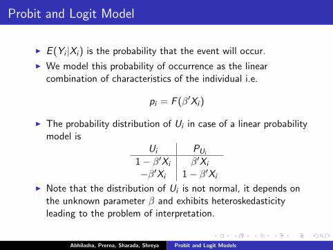
I E (Yi |Xi ) is the probability that the event will occur.

I We model this probability of occurrence as the linearcombination of characteristics of the individual i.e.

pi = F (β′Xi )

I The probability distribution of Ui in case of a linear probabilitymodel is

Ui PUi

1− β′Xi β′Xi

−β′Xi 1− β′Xi

I Note that the distribution of Ui is not normal, it depends onthe unknown parameter β and exhibits heteroskedasticityleading to the problem of interpretation.


Probit and Logit Functions

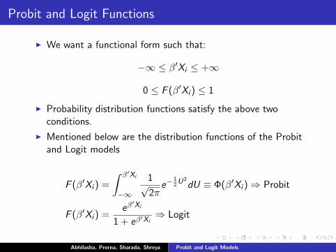
I We want a functional form such that:

−∞ ≤ β′Xi ≤ +∞

0 ≤ F (β′Xi ) ≤ 1

I Probability distribution functions satisfy the above twoconditions.

I Mentioned below are the distribution functions of the Probitand Logit models

F (β′Xi ) =

∫ β′Xi

−∞

1√2π

e−12U2dU ≡ Φ(β′Xi )⇒ Probit

F (β′Xi ) =eβ′Xi

1 + eβ′Xi⇒ Logit


Latent Variable

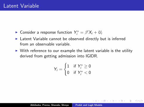
I Consider a response function Y ∗i = β′Xi + Ui

I Latent Variable cannot be observed directly but is inferredfrom an observable variable.

I With reference to our example the latent variable is the utilityderived from getting admission into IGIDR.

Yi =

{1 if Y ∗i ≥ 0

0 if Y ∗i < 0


Odds Ratio

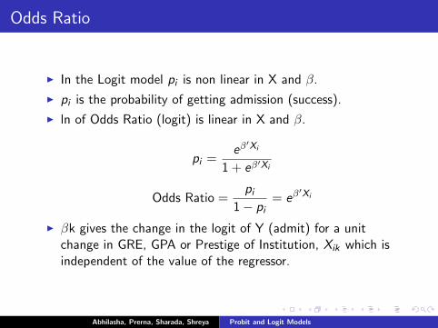
I In the Logit model pi is non linear in X and β.

I pi is the probability of getting admission (success).

I ln of Odds Ratio (logit) is linear in X and β.

pi =eβ′Xi

1 + eβ′Xi

Odds Ratio =pi

1− pi= eβ

′Xi

I βk gives the change in the logit of Y (admit) for a unitchange in GRE, GPA or Prestige of Institution, Xik which isindependent of the value of the regressor.


Marginal Effects

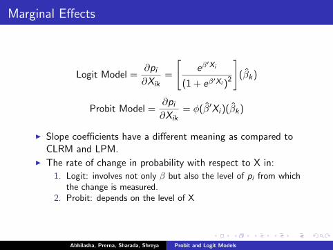
Logit Model =∂pi∂Xik

=

[eβ′Xi

(1 + eβ′Xi )2

](β̂k)

Probit Model =∂pi∂Xik

= φ(β̂′Xi )(β̂k)

I Slope coefficients have a different meaning as compared toCLRM and LPM.

I The rate of change in probability with respect to X in:

1. Logit: involves not only β but also the level of pi from whichthe change is measured.

2. Probit: depends on the level of X


Estimation

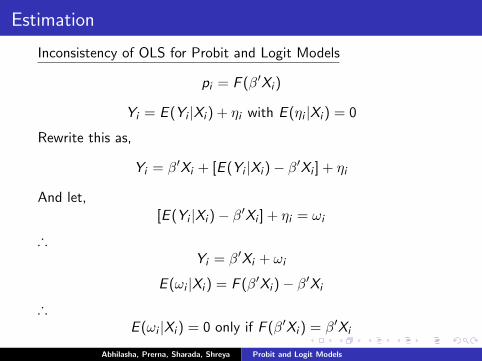
Inconsistency of OLS for Probit and Logit Models

pi = F (β′Xi )

Yi = E (Yi |Xi ) + ηi with E (ηi |Xi ) = 0

Rewrite this as,

Yi = β′Xi + [E (Yi |Xi )− β′Xi ] + ηi

And let,[E (Yi |Xi )− β′Xi ] + ηi = ωi

∴Yi = β′Xi + ωi

E (ωi |Xi ) = F (β′Xi )− β′Xi

∴E (ωi |Xi ) = 0 only if F (β′Xi ) = β′Xi


Estimation

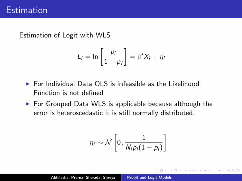
Estimation of Logit with WLS

Li = ln

[pi

1− pi

]= β′Xi + ηi

I For Individual Data OLS is infeasible as the LikelihoodFunction is not defined

I For Grouped Data WLS is applicable because although theerror is heteroscedastic it is still normally distributed.

ηi ∼ N[

0,1

Nipi (1− pi )

]


Estimation

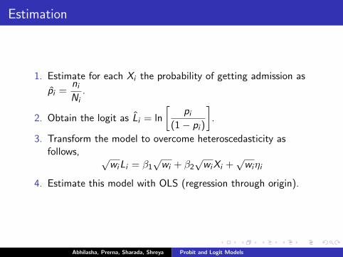
1. Estimate for each Xi the probability of getting admission as

p̂i =niNi

.

2. Obtain the logit as L̂i = ln

[pi

(1− pi )

].

3. Transform the model to overcome heteroscedasticity asfollows, √

wiLi = β1√wi + β2

√wiXi +

√wiηi

4. Estimate this model with OLS (regression through origin).


Non Linear Least Squares

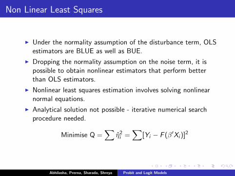
I Under the normality assumption of the disturbance term, OLSestimators are BLUE as well as BUE.

I Dropping the normality assumption on the noise term, it ispossible to obtain nonlinear estimators that perform betterthan OLS estimators.

I Nonlinear least squares estimation involves solving nonlinearnormal equations.

I Analytical solution not possible - iterative numerical searchprocedure needed.

Minimise Q =∑

η̂2i =∑

[Yi − F (β′Xi )]2


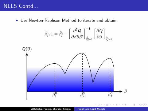
NLLS Contd...

I Use Newton-Raphson Method to iterate and obtain:

β̂j+1 = β̂j −[∂2Q

∂β∂β′

]−1β̂j−1

[∂Q

∂β

]β̂j−1

β

Q(0)

β01 β02 β03


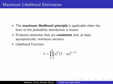
Maximum Likelihood Estimation

I The maximum likelihood principle is applicable when theform of the probability distribution is known.

I Produces estimates that are consistent and, at leastasymptotically, minimum variance.

I Likelihood Function

L =n∏

i=1

pYii (1− pi )

1−Yi


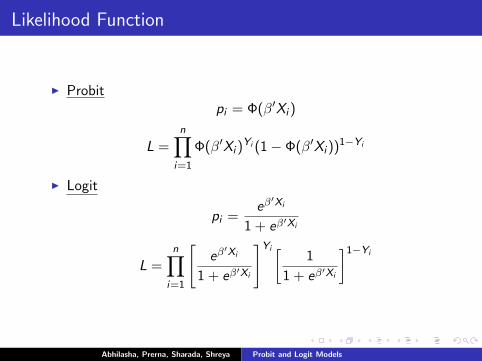
Likelihood Function

I Probitpi = Φ(β′Xi )

L =n∏

i=1

Φ(β′Xi )Yi (1− Φ(β′Xi ))1−Yi

I Logit

pi =eβ′Xi

1 + eβ′Xi

L =n∏

i=1

[eβ′Xi

1 + eβ′Xi

]Yi[1

1 + eβ′Xi

]1−Yi


Maximum Likelihood Contd...

I As with nonlinear estimation closed form solution is difficult

I Iterative procedures (Newton Raphson) must be used (replaceQ with log L).

I Convergence to global maximum is ensured as Log function isglobally concave

β

L(0)

β0


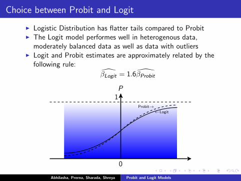
Choice between Probit and Logit

I Logistic Distribution has flatter tails compared to ProbitI The Logit model performes well in heterogenous data,

moderately balanced data as well as data with outliersI Logit and Probit estimates are approximately related by the

following rule:

β̂Logit = 1.6β̂Probit

P

0

1Probit→

←Logit


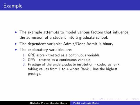
Example

I The example attempts to model various factors that influencethe admission of a student into a graduate school.

I The dependent variable; Admit/Dont Admit is binary.I The explanatory variables are:

1. GRE score - treated as a continuous variable2. GPA - treated as a continuous variable3. Prestige of the undergraduate institution - coded as rank,

taking values from 1 to 4 where Rank 1 has the highestprestige.


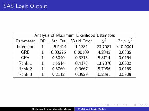
SAS Logit Output

Analysis of Maximum Likelihood Estimates

Parameter DF Std Est Wald Error χ2 Pr > χ2

Intercept 1 −5.5414 1.1381 23.7081 < 0.0001GRE 1 0.00226 0.00109 4.2842 0.0385GPA 1 0.8040 0.3318 5.8714 0.0154

Rank 1 1 1.5514 0.4178 13.7870 0.0002Rank 2 1 0.8760 0.3667 5.7056 0.0165Rank 3 1 0.2112 0.3929 0.2891 0.5908


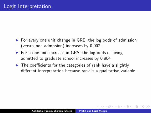
Logit Interpretation

I For every one unit change in GRE, the log odds of admission(versus non-admission) increases by 0.002.

I For a one unit increase in GPA, the log odds of beingadmitted to graduate school increases by 0.804

I The coefficients for the categories of rank have a slightlydifferent interpretation because rank is a qualitative variable.


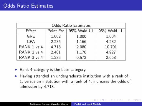
Odds Ratio Estimates

Odds Ratio Estimates

Effect Point Est 95% Wald UL 95% Wald LL

GRE 1.002 1.000 1.004GPA 2.235 1.166 4.282

RANK 1 vs 4 4.718 2.080 10.701RANK 2 vs 4 2.401 1.170 4.927RANK 3 vs 4 1.235 0.572 2.668

I Rank 4 category is the base category.

I Having attended an undergraduate institution with a rank of1, versus an institution with a rank of 4, increases the odds ofadmission by 4.718.


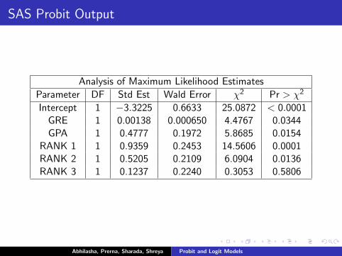
SAS Probit Output

Analysis of Maximum Likelihood Estimates

Parameter DF Std Est Wald Error χ2 Pr > χ2

Intercept 1 −3.3225 0.6633 25.0872 < 0.0001GRE 1 0.00138 0.000650 4.4767 0.0344GPA 1 0.4777 0.1972 5.8685 0.0154

RANK 1 1 0.9359 0.2453 14.5606 0.0001RANK 2 1 0.5205 0.2109 6.0904 0.0136RANK 3 1 0.1237 0.2240 0.3053 0.5806


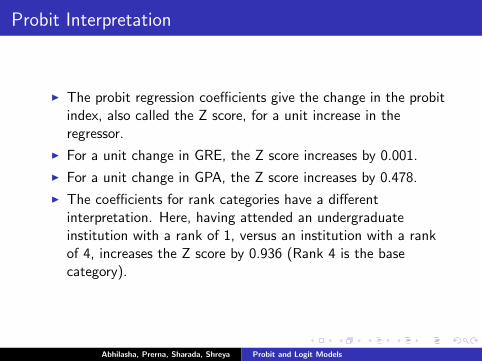
Probit Interpretation

I The probit regression coefficients give the change in the probitindex, also called the Z score, for a unit increase in theregressor.

I For a unit change in GRE, the Z score increases by 0.001.

I For a unit change in GPA, the Z score increases by 0.478.

I The coefficients for rank categories have a differentinterpretation. Here, having attended an undergraduateinstitution with a rank of 1, versus an institution with a rankof 4, increases the Z score by 0.936 (Rank 4 is the basecategory).


THANK YOU


probit and logit models - indira gandhi institute of ... · probit and logit models abhilasha,...

Documents