QEDQueen’s Economics Department Working Paper No. 514

Convenient Specification Tests for Logit and Probit Models

Russell DavidsonQueen’s University

James G. MacKinnonQueen’s University

Department of EconomicsQueen’s University

94 University AvenueKingston, Ontario, Canada

K7L 3N6

11-1982

Convenient Specification Testsfor Logit and Probit Models

Russell Davidson

and

James G. MacKinnon

Department of EconomicsQueen’s University

Kingston, Ontario, CanadaK7L 3N6

Abstract

We propose several Lagrange multiplier tests of logit and probit models, which may beinexpensively computed by means of artificial linear regressions. These may be used totest for various forms of model inadequacy, including the omission of specified variablesand heteroskedasticity of known form. We perform a number of sampling experimentsin which we compare the small-sample properties of these tests and of likelihood ratiotests. One of the LM tests turns out to have better small-sample properties than anyof the others. We then investigate the power of the tests against local alternatives.Finally, we conduct a further series of sampling experiments to compare the power ofvarious tests.

We are greatly indebted to Alison Morgan for research assistance beyond the call of duty.

This research was supported, in part, by grants from the Social Sciences and Humanities

Research Council of Canada and the School of Graduate Studies and Research of Queen’s

University. This paper was published in the Journal of Econometrics, 25, 1984, 241–262. The

references have been updated.

November, 1982

1. Introduction

The logit and probit models, together with their multi-response and multivariate gener-alizations, are now widely used in applied econometric work. Such models are typicallyestimated by maximum likelihood methods which require the numerical maximizationof a loglikelihood function. Since this is usually much more expensive than, say, cal-culating ordinary least squares estimates for a linear regression model, investigatorsoften display a natural reluctance to test the specification of the model as thoroughlyas would normally be done in the regression case. There is thus a clear need for speci-fication tests of logit and probit models which are easy to understand and inexpensiveto compute.

In this context, it seems natural to investigate the use of Lagrange multiplier, or score,tests, because they require only estimates under the null hypothesis, and they canoften be computed by means of artificial linear regressions. The literature on LMtests for logit and probit models is, however, remarkably limited. The recent surveyof qualitative response models by Amemiya (1981) does not mention LM tests at all,and the survey of LM tests by Engle (1982) describes only one such test for logit andprobit models, which appears to be new.

In this paper, we discuss several varieties of LM test for logit and probit models, eachof which may be computed by means of an artificial linear regression. For a givenalternative hypothesis, there turn out to be two different artificial linear regressionswhich generate five different, but asymptotically equivalent, test statistics. Theseprocedures may be used to test both for omitted variables, which was the case examinedby Engle (1982), and for heteroskedasticity of known form. The latter is a seriousproblem in the case of logit and probit models, because it renders parameter estimatesinconsistent.

We perform two sets of sampling experiments. In the first set, we examine the perfor-mance of six tests under the null: the five LM or pseudo-LM tests referred to above,and the Likelihood Ratio test. We find that one of the LM tests outperforms theother tests, in the sense that the small-sample distribution of the test statistic underthe null more closely approximates the asymptotic distribution. Thus use of this testrather than any of the others will generally result in Type I error being known moreaccurately. We also find that different asymptotically equivalent tests based on thesame artificial regression may behave very differently in small samples.

In the second set of sampling experiments, we investigate the power of two LM testsand the LR test. We compare the power of the tests both at fixed critical valuesand at estimated critical values based on the previous experiments, so as to controlthe level of Type I error. We also examine how closely the distributions of the testsapproximate their asymptotic distributions under local alternatives, which is all thatasymptotic theory has to tell us about the power of these tests. The approximationturns out to be quite poor in many cases.

–1–

2. LM Tests for Logit and Probit Models

The tests we shall develop are applicable to a fairly wide class of binary choice mod-els, of which the logit and probit models are by far the most commonly encounteredvarieties. In models of this class, the dependent variable can take on only two values,which it is convenient to denote by 0 and 1. The probability that yt, the tth observa-tion on the dependent variable, is equal to 1 is given by F

(xt(β)

). F is an increasing

function of xt which has the properties that F (−∞) = 0 and F (∞) = 1. xt is apossibly nonlinear function, which depends on Xt a row vector of exogenous variables,and β, a column vector of parameters to be estimated. In the commonly encounteredlinear case, xt(β) = Xtβ.

The only difference between the logit and probit models is that they employ differentfunctions for F . In the case of the probit model,

F(xt(β)

)= Φ

(xt(β)

), (1)

where Φ denotes the cumulative distribution function of the standard normal distri-bution. In the case of the logit model,

F(xt(β)

)=

exp(xt(β)

)

1 + exp(xt(β)

)

=1

1 + exp(−xt(β)

) .(2)

Note that, for both (1) and (2), F (−z) = 1 − F (z), a convenient property of whichwe shall make use below. Other binary choice models use other functions in place of(1) and (2); see Amemiya (1981). Provided the functions also have this symmetryproperty, everything we say below will apply to them as well.

We shall denote by `t(β; yt) the contribution to the loglikelihood function made bythe tth observation. It is easy to see that

`t(β; 1) = logF(xt(β)

), and

`t(β; 0) = logF(−xt(β)

).

(3)

Thus the loglikelihood function is

`(β;y) =n∑t=1

`t(β; yt). (4)

In the linear case, this function is globally concave for both the logit and probit models,except in pathological cases where it is unbounded; see Amemiya (1981). Thus MLestimates may be found in a straightforward fashion by maximizing it.

–2–

We shall denote the gradient of (4) with respect to β by the row vector g(β;y). Itsith component is

gt(β;y) =n∑t=1

Gti(β; yt),

where

Gti(β; yt) =(

yt

F(xt(β)

) +yt − 1

F(−xt(β)

))f(xt(β)

)Xti(β). (5)

Here Xti(β) denotes the derivative of xt(β) with respect to βi; in the linear case, thiswill simply be equal to Xti. f(z) denotes the first derivative of F (z), and we have madeuse of the fact that f(z) = f(−z). For the probit mode, f(z) = φ(z), the standardnormal density. For the logit model,

f(z) =exp(−z)(

1 + exp(−z))2 . (6)

The ML estimates β must of course satisfy the first-order conditions

g(β;y) = 0. (7)

The variance-covariance matrix of β may be consistently estimated in at least threedifferent ways. We define the information matrix, I(β), as the matrix whose ij th

element isE

(gi(β;y)gj(β;y)

). (8)

This may of course be consistently estimated by minus the Hessian, evaluated at β,but this estimator turns out to be inconvenient in this context.1 A more convenientestimator is

IOPG = G>(β)G(β), (9)

where G(β) is the matrix with typical element Gti(β; yt). The use of the “outer prod-uct of the gradient” estimator IOPG for estimation and inference has been advocatedby Berndt, Hall, Hall, and Hausman (1974). The third way to estimate I(β) is simplyto use I(β). It is easily derived that a typical element of I(β) is

Iij =n∑t=1

f2(xt(β)

)Xti(β)Xtj(β)

F(xt(β)

)F

(−xt(β)) . (10)

Notice that (10) depends on y only through β. This is not true for the other twoestimators of the information matrix.

1 Strictly speaking, it is of course I ≡ n−1I which is consistently estimated by minus1/n times the Hessian. Here and elsewhere, we ignore this distinction when it is notimportant to the argument.

–3–

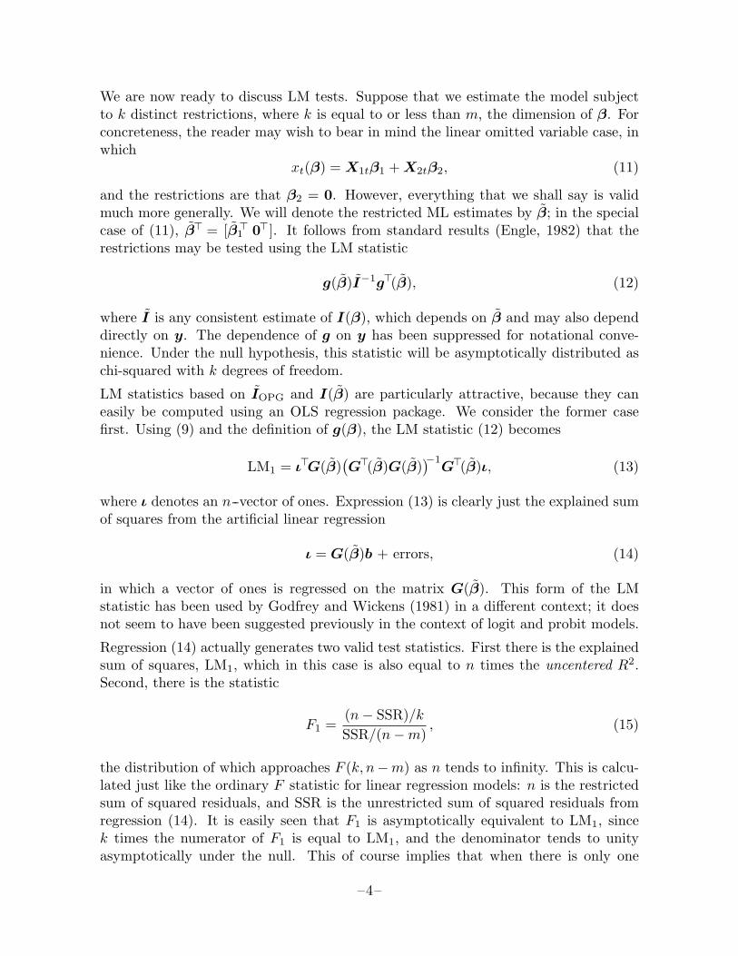
We are now ready to discuss LM tests. Suppose that we estimate the model subjectto k distinct restrictions, where k is equal to or less than m, the dimension of β. Forconcreteness, the reader may wish to bear in mind the linear omitted variable case, inwhich

xt(β) = X1tβ1 +X2tβ2, (11)

and the restrictions are that β2 = 0. However, everything that we shall say is validmuch more generally. We will denote the restricted ML estimates by β; in the specialcase of (11), β> = [β1

> 0>]. It follows from standard results (Engle, 1982) that therestrictions may be tested using the LM statistic

g(β)I−1g>(β), (12)

where I is any consistent estimate of I(β), which depends on β and may also dependdirectly on y. The dependence of g on y has been suppressed for notational conve-nience. Under the null hypothesis, this statistic will be asymptotically distributed aschi-squared with k degrees of freedom.

LM statistics based on IOPG and I(β) are particularly attractive, because they caneasily be computed using an OLS regression package. We consider the former casefirst. Using (9) and the definition of g(β), the LM statistic (12) becomes

LM1 = ι>G(β)(G>(β)G(β)

)−1G>(β)ι, (13)

where ι denotes an n--vector of ones. Expression (13) is clearly just the explained sumof squares from the artificial linear regression

ι = G(β)b + errors, (14)

in which a vector of ones is regressed on the matrix G(β). This form of the LMstatistic has been used by Godfrey and Wickens (1981) in a different context; it doesnot seem to have been suggested previously in the context of logit and probit models.

Regression (14) actually generates two valid test statistics. First there is the explainedsum of squares, LM1, which in this case is also equal to n times the uncentered R2.Second, there is the statistic

F1 =(n− SSR)/kSSR/(n−m)

, (15)

the distribution of which approaches F (k, n−m) as n tends to infinity. This is calcu-lated just like the ordinary F statistic for linear regression models: n is the restrictedsum of squared residuals, and SSR is the unrestricted sum of squared residuals fromregression (14). It is easily seen that F1 is asymptotically equivalent to LM1, sincek times the numerator of F1 is equal to LM1, and the denominator tends to unityasymptotically under the null. This of course implies that when there is only one

–4–

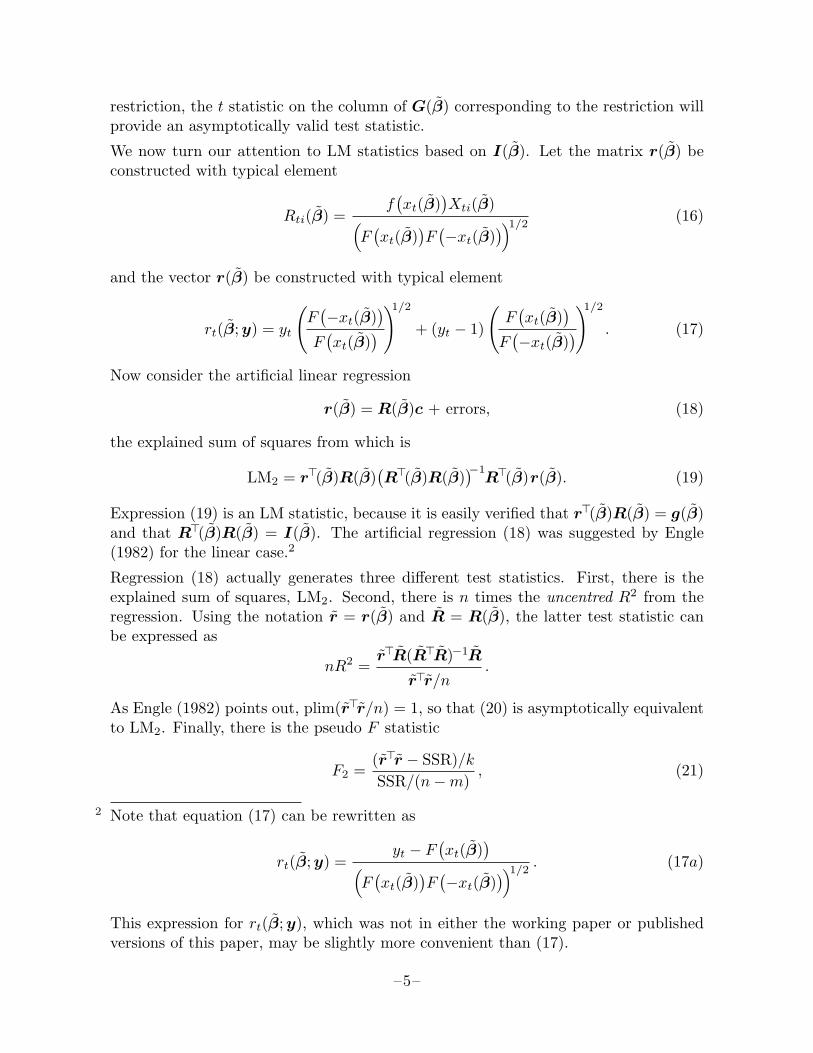
restriction, the t statistic on the column of G(β) corresponding to the restriction willprovide an asymptotically valid test statistic.

We now turn our attention to LM statistics based on I(β). Let the matrix r(β) beconstructed with typical element

Rti(β) =f(xt(β)

)Xti(β)

(F

(xt(β)

)F

(−xt(β)))1/2

(16)

and the vector r(β) be constructed with typical element

rt(β;y) = yt

(F

(−xt(β))

F(xt(β)

))1/2

+ (yt − 1)

(F

(xt(β)

)

F(−xt(β)

))1/2

. (17)

Now consider the artificial linear regression

r(β) = R(β)c + errors, (18)

the explained sum of squares from which is

LM2 = r>(β)R(β)(R>(β)R(β)

)−1R>(β)r(β). (19)

Expression (19) is an LM statistic, because it is easily verified that r>(β)R(β) = g(β)and that R>(β)R(β) = I(β). The artificial regression (18) was suggested by Engle(1982) for the linear case.2

Regression (18) actually generates three different test statistics. First, there is theexplained sum of squares, LM2. Second, there is n times the uncentred R2 from theregression. Using the notation r = r(β) and R = R(β), the latter test statistic canbe expressed as

nR2 =r>R(R>R)−1R

r>r/n.

As Engle (1982) points out, plim(r>r/n) = 1, so that (20) is asymptotically equivalentto LM2. Finally, there is the pseudo F statistic

F2 =(r>r − SSR)/kSSR/(n−m)

, (21)

2 Note that equation (17) can be rewritten as

rt(β;y) =yt − F

(xt(β)

)(F

(xt(β)

)F

(−xt(β)))1/2

. (17a)

This expression for rt(β;y), which was not in either the working paper or publishedversions of this paper, may be slightly more convenient than (17).

–5–

which is analogous to F1 in every respect: k times the numerator is equal to LM2, andthe denominator tends to unity asymptotically, under the null. Once again, the factthat F2 is valid implies that when there is only one restriction, the t statistic on thecolumn of R corresponding to the restriction will also be an asymptotically valid teststatistic.

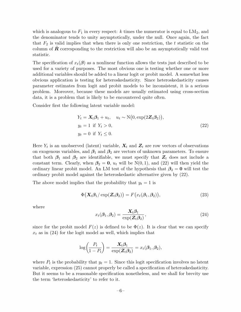
The specification of xt(β) as a nonlinear function allows the tests just described to beused for a variety of purposes. The most obvious one is testing whether one or moreadditional variables should be added to a linear logit or probit model. A somewhat lessobvious application is testing for heteroskedasticity. Since heteroskedasticity causesparameter estimates from logit and probit models to be inconsistent, it is a seriousproblem. Moreover, because these models are usually estimated using cross-sectiondata, it is a problem that is likely to be encountered quite often.

Consider first the following latent variable model:

Yt = Xtβ1 + ut, ut ∼ N(0, exp(2Ztβ2)

),

yt = 1 if Yt > 0,

yt = 0 if Yt ≤ 0.

(22)

Here Yt is an unobserved (latent) variable, Xt and Zt are row vectors of observationson exogenous variables, and β1 and β2 are vectors of unknown parameters. To ensurethat both β1 and β2 are identifiable, we must specify that Zt does not include aconstant term. Clearly, when β2 = 0, ut will be N(0, 1), and (22) will then yield theordinary linear probit model. An LM test of the hypothesis that β2 = 0 will test theordinary probit model against the heteroskedastic alternative given by (22).

The above model implies that the probability that yt = 1 is

Φ(Xtβ1/ exp(Ztβ2)

)= F

(xt(β1,β2)

), (23)

where

xt(β1,β2) =Xtβ1

exp(Ztβ2), (24)

since for the probit model F (z) is defined to be Φ(z). It is clear that we can specifyxt as in (24) for the logit model as well, which implies that

log(

Pt1− Pt

)=

Xtβ1

exp(Ztβ2)= xt(β1,β2),

where Pt is the probability that yt = 1. Since this logit specification involves no latentvariable, expression (25) cannot properly be called a specification of heteroskedasticity.But it seems to be a reasonable specification nonetheless, and we shall for brevity usethe term ‘heteroskedasticity’ to refer to it.

–6–

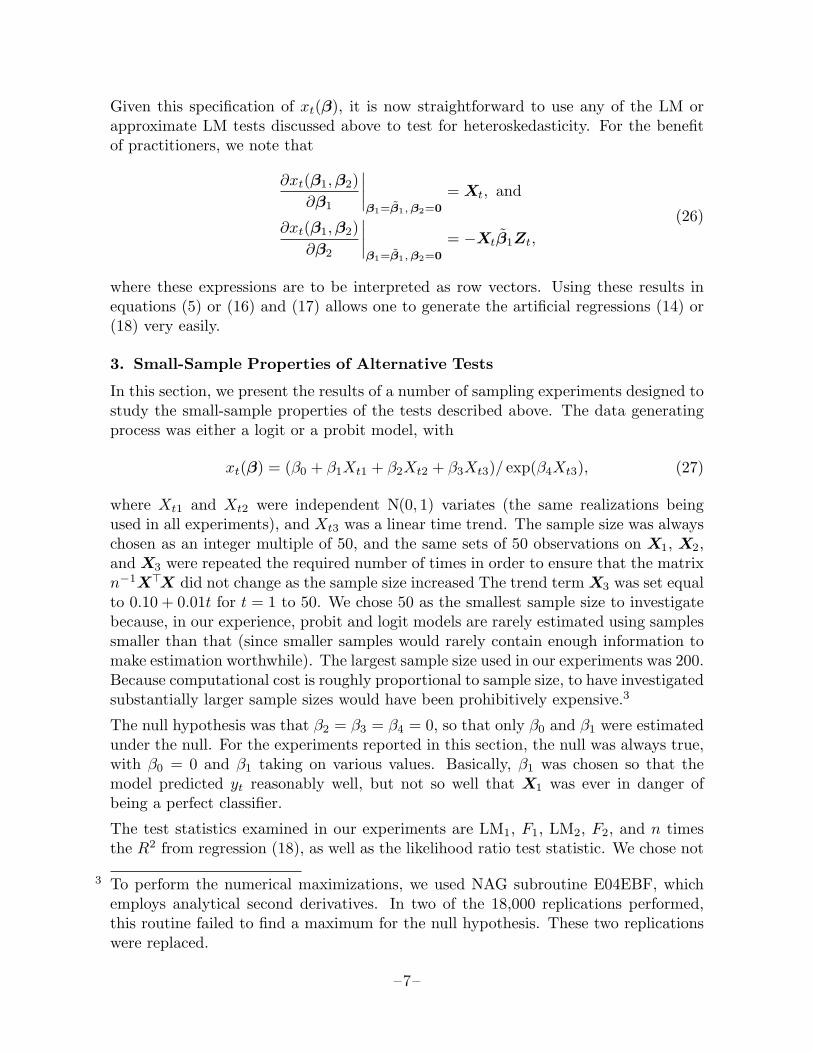
Given this specification of xt(β), it is now straightforward to use any of the LM orapproximate LM tests discussed above to test for heteroskedasticity. For the benefitof practitioners, we note that

∂xt(β1,β2)∂β1

∣∣∣∣β1=β1,β2=0

= Xt, and

∂xt(β1,β2)∂β2

∣∣∣∣β1=β1,β2=0

= −Xtβ1Zt,

(26)

where these expressions are to be interpreted as row vectors. Using these results inequations (5) or (16) and (17) allows one to generate the artificial regressions (14) or(18) very easily.

3. Small-Sample Properties of Alternative Tests

In this section, we present the results of a number of sampling experiments designed tostudy the small-sample properties of the tests described above. The data generatingprocess was either a logit or a probit model, with

xt(β) = (β0 + β1Xt1 + β2Xt2 + β3Xt3)/ exp(β4Xt3), (27)

where Xt1 and Xt2 were independent N(0, 1) variates (the same realizations beingused in all experiments), and Xt3 was a linear time trend. The sample size was alwayschosen as an integer multiple of 50, and the same sets of 50 observations on X1, X2,and X3 were repeated the required number of times in order to ensure that the matrixn−1X>X did not change as the sample size increased The trend term X3 was set equalto 0.10 + 0.01t for t = 1 to 50. We chose 50 as the smallest sample size to investigatebecause, in our experience, probit and logit models are rarely estimated using samplessmaller than that (since smaller samples would rarely contain enough information tomake estimation worthwhile). The largest sample size used in our experiments was 200.Because computational cost is roughly proportional to sample size, to have investigatedsubstantially larger sample sizes would have been prohibitively expensive.3

The null hypothesis was that β2 = β3 = β4 = 0, so that only β0 and β1 were estimatedunder the null. For the experiments reported in this section, the null was always true,with β0 = 0 and β1 taking on various values. Basically, β1 was chosen so that themodel predicted yt reasonably well, but not so well that X1 was ever in danger ofbeing a perfect classifier.

The test statistics examined in our experiments are LM1, F1, LM2, F2, and n timesthe R2 from regression (18), as well as the likelihood ratio test statistic. We chose not

3 To perform the numerical maximizations, we used NAG subroutine E04EBF, whichemploys analytical second derivatives. In two of the 18,000 replications performed,this routine failed to find a maximum for the null hypothesis. These two replicationswere replaced.

–7–

to examine Wald test statistics because they are clearly unattractive in this context.Estimation of the null will here be easier than estimation of the alternative, and manyinvestigators will wish to avoid the latter entirely by using one of the LM-type tests.If estimation of the alternative is undertaken, estimates under the null will normallyalready be available, so that calculation of the LR statistic will then be trivial, mucheasier than calculation of a Wald statistic. Moreover, just as there are several LM-typetests, so too are there several Wald-type tests, and attempting to deal with them allwould have made reporting the experimental results quite difficult.

The results of eight experiments are presented in Tables 1 through 3. The hypothesesthat β2, β3, and β4 were zero were each tested separately. Since the resulting teststatistics have only one degree of freedom, we transformed them into test statisticswhich would be asymptotically N(0, 1) under the null. This was done by taking theirsquare roots and multiplying by minus one if the coefficient of the test regressor inthe artificial regression (14) or (18) was negative, or, in the case of the LR test, if theunrestricted coefficient estimate was negative.

All of the test statistics turned out to have means acceptably close to zero; thus we donot report this information. On the other hand, the standard deviations of the varioustest statistics differed dramatically, and these are therefore presented in Table 1. Inthis table, ‘Hyp.’ indicates which coefficient is being tested, and ‘Exp.’ indicates thesample size (50, 100, or 200), whether the logit or probit model was used, and thevalue of β1. The numbers under ‘Std. Dev.’ are the observed standard deviations ofthe various test statistics in 1000 replications, and the numbers in brackets followingthese are asymptotic t statistics for the hypothesis that the true standard deviation isunity.4

Several features of Table 1 are striking. The only test statistic which ever has anestimated standard deviation of less than one, and the only test statistic for which thehypothesis that the standard deviation is unity cannot be rejected most of the time,is LM2. Of particular interest is the performance of F2 and nR2, which are basedon exactly the same artificial regression as LM2; the latter is n times the R2 fromregression (18). Nevertheless, they always have larger standard deviations than LM2,often so large that they will clearly yield highly unreliable inferences. There seems tobe an explanation for this. Note that

nR2 =n

r>rLM2, (28)

the first factor here being a random variable with a plim of unity. Unless there issubstantial negative covariance between this factor and LM2, nR2 will have greatervariance than LM2, which is exactly what we find in Table 1. Similarly, F2 is related

4 This t statistic is (s − 1)(2N)1/2, where s is the standard deviation, and N is thenumber of replications. Since N is always 1000, the normal approximation on whichthis statistic is based should be quite accurate.

–8–

to LM2 by the equation

kF2 =n−m

r>r − LM2LM2. (29)

Since r>r is Op(n) while LM2 is Op(1), under the null hypothesis, the first factor in(29) will tend to be very similar to the first factor in (28), so that kF2 and nR2 can beexpected to be very close. Indeed, Table 1 shows that the standard errors of F2 andnR2 are always extremely similar, much more so than those of any of the other teststatistics.

It seems clear from Table 1 that we would always wish to use LM2 rather than thepseudo-LM statistics F2 and nR2 based on the same artificial regression. The choicebetween LM1 and F1 is not so clearcut, since the standard deviations of those twostatistics tend to be very similar. However, close examination of Table 1 shows thatthe standard deviation of F1 always exceeds that of LM1, which is in turn alwaysgreater than unity, so that LM1 clearly dominates F1. This then leaves three teststatistics which are worth examining more closely: LR, LM1, and LM2. Detailedresults for these three statistics are presented in Tables 2 and 3. Here ‘Rep.’ and‘Nobs.’ indicate the number of replications and the sample size, respectively. Besidesthe standard errors, we report here the proportion of the time that the test statisticsexceeded 2.576, 1.960, and 1.645 (the 0.01, 0.05, and 0.10 critical values of the standardnormal distribution) under ‘0.01 tail’, ‘0.05 tail’, and ‘0.10 tail’, respectively. Theseare followed by estimated asymptotic absolute t statistics for the hypotheses that theseproportions are 0.01, 0.05, and 0.10.5 Finally, under ‘0.05 crit.’ we report estimatedcritical values for tests with a size of 0.05, together with estimated 95% confidenceintervals on these estimates.6

Tables 2 and 3 are largely self-explanatory. It is evident that LM2 is much the bestbehaved of the three test statistics in almost all cases, followed at some distance byLR, and at a long distance by LM1. This last always rejects the null hypothesis moreoften than it should, sometimes rejecting more than 10% of the time at a nominal 1%level. The performance of all the test statistics tend to improve as the sample sizeincreases, and tends to worsen when β1 is increased. Tests of β2 = 0 and β3 = 0 tendto be better behaved than tests of β4 = 0, perhaps because of the greater nonlinearityinvolved in the heteroskedastic alternative.

The poor performance of LM1 relative to LM2 is not entirely unexpected. As we showin the Appendix, the random variable towards which all of the LM test statistics tendasymptotically, LM0, depends on y only through the gradient; the information matrix

5 This t statistic is equal to (p−p)/(p(1−p)/N)1/2, where p is the observed proportionand p is the expected proportion if the test statistic were really N(0, 1). Use of thenormal approximation to the binomial is justified by the fact that N is always 1000.

6 Note that these confidence bounds, which are based on non-parametric inference, arenot symmetric around the estimate. For details on their calculation, see Mood andGraybill (1963, 406–409).

–9–

does not depend on y at all. LM2 differs from LM0 only because the former uses I(β)while the latter uses I(β0), where β0 is the true parameter vector. Note that, sinceβ is an ML estimate, I(β) is asymptotically efficient for I(β0). In contrast, LM1 usesIOPG, which does depend directly on y and must therefore be a less efficient estimatorthan I(β). Since the asymptotic distribution of LM0 depends on I(β0) being non-random, we would expect that LM2, which uses a relatively efficient estimate of I(β0),should more closely approximate the distribution of LM0 than does LM1. For a similarargument, see Davidson and MacKinnon (1983).

The results of these experiments are thus quite definite. One is least likely to makea Type I error if one uses LM2. Indeed, except for tests of β4 = 0, where it tends toreject the null less often than it should, LM2 seems to have a small-sample distributionthat is remarkably close to its asymptotic one. The likelihood ratio test is less reliablethan LM2, but it is still reasonably well behaved. However, LM1, F1, F2, and nR2 areoften very badly behaved; they may reject a true null hypothesis much too often.

4. Power of the Tests

In this section, we investigate the power of the tests dealt with previously. In orderto do so, we first investigate the asymptotic distribution of the LM test statistic whenthe null hypothesis is false, but the data generating process, or DGP, is assumed tobe ‘close’ to the null. On the basis of this asymptotic distribution, which is of coursethe same for all the LM and pseudo-LM tests and for the LR test, we know what thepower of the tests should be asymptotically. We can then see how this compares withthe actual power of the tests in small samples.

The parameter vector β may be partitioned into two column vectors, β1 and β2, oflengths m − k and k, respectively. The ‘true’ value of β1 is β0

1 , and the ‘true’ valueof β2 is 0, where the meaning of ‘true’ should become clear in a moment. Thus β0 isthe vector whose first m − k elements are β0

1 and whose last k elements are 0. Theinformation matrix from a sample of size n is defined by

I ≡ bI ≡ E0

(g>(β0;y)g(β0;y)

), (30)

where the expectation in (30) is taken assuming that β = β0, and I represents theaverage information contained in one observation.

The DGP is characterized by the loglikelihood function

n∑t=1

`t(at,β0; yt), (31)

where`t(at,β0; 1) = log

(F

(xt(β0)

)+ at

),

`t(at,β0; 0) = log(F

(−xt(β0))− at

).

(32)

–10–

The numbers at have the properties that

0 ≤ F (xt(β0)

)+ at ≤ 1 (33)

and

n−1/2n∑t=1

at = Op(1). (34)

Each individual at therefore becomes small like n−1/2 as n becomes large, so that theDGP approaches the null hypothesis in large samples.

This characterization of the DGP is unrelated to the alternative hypothesis againstwhich the LM test is constructed. The standard case where the DGP is a special caseof the alternative hypothesis is easily accommodated, however. Suppose that, for somescalar α of order n−1/2, the probability that yt = 1 is F

(xt(β0

1 , αβ02)

), which is nested

in the parametric family F(xt(β1,β2)

). This parametric family clearly includes the

null at β1 = β01 , α = 0. Then the at, being of order n−1/2, can to that order be

approximated by

α

k∑

j=1

β02j f

(xt(β0

1 , 0))Xtj(β0

1 , 0), (35)

where Xtj(β01 ,β2) denotes the derivative of xt with respect to the j th element of β2.

If the at were defined by (35), then the results of our analysis below would correspondwith standard results for the case where the DGP is embedded within the alternativehypothesis.

Now define the 1×m vector

Λ ≡ n−1/2n∑t=1

at(Gt(β0; 1)−Gt(β0; 0)

), (36)

where, as before, Gt(β0; yt) is the contribution to the gradient g(β0;y) made by thetth observation. From (5), we see that

Gt(β0; 1) =f(xt(β0)

)

F(xt(β0)

)Xt(β0),

Gt(β0; 0) =−f(

xt(β0))

F(−xt(β0)

)Xt(β0),

(37)

where Xt(β0) (a row vector of length m) is the gradient of xt evaluated at β0.

The vector Λ and the information matrix I may be partitioned according to thedistinction between β1 and β2 as follows:

Λ = [Λ1 Λ2] I =[I11 I12

I21 I22

].

–11–

It is shown in the Appendix that the asymptotic distribution of all the LM statisticsis non-central chi-squared, with non-centrality parameter

n(Λ2 −Λ1I

−111 I12

)(I−1)22

(Λ2>− I21I

−111 Λ1

>). (38)

Here I−111 denotes the inverse of I11, while (I−1)22 denotes the 2-2 block of I−1. It is

easily derived that(I−1)22 =

(I22 − I21I

−111 I12

)−1. (39)

Now define the matrix R as the matrix with typical element Rti(β0), where the latterwas defined in (16), and partition it as [R1 R2]. In addition, define the n× 1 columnvector r0 by the equation

r0t = at

(F

(xt(β0)

)F

(−xt(β0)))−1/2

. (40)

Clearly, I = R>R, and Λ = n1/2r0>R. In addition, make the definition

M1 ≡ I−R1(R1>R1)−1R1

>. (41)

Then it is evident thatIij = R1

>Rj for i, j = 1, 2, (42)

and that(I−1)22 = (R2

>M1R2)−1; (43)

this result follows immediately from (39). Making use of these results, we can reduceexpression (38) for the non-centrality parameter to

r0>M1R2(R2

>M1R2)−1R2>M1r0. (44)

This expression may readily be computed by means of artificial linear regressions.

The results we have just derived are strictly valid only in the limit, as the sample sizetends to infinity and the DGP tends to the null hypothesis. If they are to be useful,these results should be approximately valid when the sample size is moderate and theDGP is some distance from the null. To see whether this is in fact the case, andto compare the power of alternative tests, we conducted a further series of samplingexperiments, similar to the ones reported on in Section 3; the results are presented inTables 4 and 5.

In these experiments, xt(β) was given by (27), and one of β2, β3, or β4 was alwaysnon-zero; which one, and its value, are indicated under ‘Alt.’ in the tables. Withtwo exceptions, the value of the non-zero parameter was chosen so that when thehypothesis being tested (indicated under ‘Hyp.’) was the alternative which generatedthe data, λ, the square root of the noncentrality parameter, would be 1.96. The valueof λ is shown under ‘Root NCP’ in the tables. Setting λ = 1.96 ensures that the power

–12–

of a test at the 0.05 level should be approximately 0.5, since if the test statistic weredistributed as N(λ, 1), it should be greater than 1.96 half the time (in addition, ofcourse, it would be less than −1.96 a very small fraction of the time). The design ofour experiments was such that λ was always very small when the alternative whichgenerated the data was not also the hypothesis under test; for the most part, therefore,we report results only for the case where they were the same.

According to the asymptotic theory, each of the test statistics should be N(λ, 1); recallthat they have been transformed so that they are asymptotically standard normal.We therefore report the means and standard deviations of the statistics, together witht statistics for the hypotheses that the mean is λ and the standard deviation is one;the t statistics are asymptotic in the latter case. It is evident from the tables that theasymptotic approximation is somewhat deficient. The mean is often significantly toosmall for LM2, and it is sometimes significantly different from λ (but not always toosmall) for LR and LM1. The standard deviation is often significantly different fromunity, tending to be too small for LM2. Power using the asymptotic critical value of1.96 is shown under ‘Power (A)’. When the mean is less than λ, power suffers. Inconsequence, LM2 always has less power using a critical value of 1.96 than either ofthe other test statistics;

Such a comparison is not fair, however, because LM2 was also less likely to rejectthe null when it was true. A more reasonable comparison is to use different criticalvalues for each of the test statistics, based on the estimated 0.05 critical values fromthe experiments reported on in Section 3. Test powers at these estimated criticalvalues are shown under ‘Power (E)’, and the estimated critical values under ‘Est.’.The performance of all three tests is now quite similar, with LM1 and LR tending todo slightly better than LM2 in most cases. However, LM1 has quite low power whentesting the hypothesis that β4 = 0. The reason for this appears to be that the standarddeviation of LM1, although greater than one, is substantially less than it was whenthe null was true, so that the estimated critical values are too conservative.

By and large, the asymptotic results do not appear to be seriously misleading when thealternative which generated the data is β2 6= 0 or β3 6= 0, but when β4 6= 0, they canbe misleading. In almost all cases when β4 6= 0, the actual mean of the test statisticis far less than λ. This discrepancy diminishes as the sample size is increased, and itdiminishes even more strikingly when the value of λ is halved to 0.98; see Table 4. Theeffect of each of these changes is to reduce the value of β4, so that the DGP is closer tothe null hypothesis. This suggests that the poor performance of the asymptotic theoryin this case is due to the nonlinearity of xt(β) with respect to β4.

The results of this section do not provide any clearcut guidance on the choice of tests.The fine performance of LM2 under the null does not carry over to the alternative,although on a size-corrected basis it is rarely much less powerful than the other tests.The LR test generally performs quite well, and it would seem to be preferable to LM1

because of its better performance against β4 6= 0 and under the null. Unfortunately,the LR test is expensive. In our experiments, calculating the three LR test statistics

–13–

took more than ten times as much computer time as calculating both LM1 and LM2

for all three alternatives.

5. Conclusion

In this paper, we have discussed two forms of the LM test for logit and probit models.These were derived in the context of general nonlinear binary choice models. Theymay be used to test for both omitted variables and heteroskedasticity, among otherthings. In a series of sampling experiments, we compared these two forms of the LMtest, along with several pseudo-LM tests based on the same artificial regressions, aswell as the likelihood ratio test. We found that LM2 tends to be the most reliable testunder the null, but not the most powerful. We also found that pseudo-LM tests maybehave very differently from genuine LM tests that are based on the same artificialregression.

Appendix

In this appendix, we show that, under local alternatives as specified by equations (31)to (34) in the text, both LM1 and LM2 tend asymptotically to the same random vari-able, LM0. We then work out the asymptotic distribution of LM0. Our specificationof local alternatives is more general, and our results more explicit, than the treatmentsin standard references such as Engle (1982).

We first derive an expression for β = [β1> β2

>]>, the vector of constrained parameterestimates. β1 is defined by the likelihood equations

g1(β1,0;y) =n∑t=1

Gt1(β1,0; yt) = 0, (A1)

where g1 and Gt1 denote the gradients of ` and `t with respect to β1 only. Taylorexpansion of these likelihood equations yields

0 = n−1/2n∑t=1

Gt1(β0; yt) + n1/2(β1 − β01)>

(1−n

n∑t=1

Ht11(β0; yt))

+Op(n−1/2), (A2)

where Ht is the contribution from the tth observation to the Hessian of the loglikeli-hood, and Ht11 is the block corresponding to β1.

We must show that the Taylor expansion in (A2) is valid. First of all, we note thatE

(Gt1(β0; yt)

)= Op(n−1/2). This follows from the facts that E0

(Gt1(β0; yt)

)= 0 and

that the difference between the likelihoods used in calculating these two expectations(namely, at) is Op(n−1/2). The law of large numbers allows us to conclude that

1−n

n∑t=1

Gt1(β0; yt))

= Op(n−1/2).

–14–

Similarly,E

(Ht(β0; yt)

)= E0

(Ht(β0; yt)

)+Op(n−1/2). (A3)

Thus, from the central limit theorem and the standard result (the information matrixequality) which tells us that

E0(−Ht) = E0(Gt>Gt),

we may deduce that

1−n

n∑t=1

Ht(β0; yt) = 1−n

E0

( n∑t=1

Ht(β0; yt))

+Op(n−1/2)

= −I +Op(n−1/2).

(A4)

Consequently,1−n

n∑t=1

Ht11(β0; yt) = −I11 +Op(n−1/2).

This is therefore not only Op(1) but also bounded away from zero, since asymptoticidentifiability requires that I be strictly positive definite. From (A2), then, β1−β0

1 =Op(n−1), and the Taylor expansion is justified. In fact,

n1/2(β1 − β01) = I−1

11

(n−1/2

n∑t=1

G>t1(β0; yt))

+Op(n−1/2). (A5)

The LM statistic in any of its various forms may be written as

g2(β;y)(I−1∗ )22 g2

>(β;y), (A6)

where nI−1∗ is some estimator, consistent if β = β0, of n times the inverse of the

information matrix. The choice of this estimator does not affect the fact that, underlocal alternatives, nI−1

∗ is asymptotically non-stochastic and equal to I−1, because thelikelihood differences at introduce only terms of order n−1/2.

By (A4) and (A5),

n−1/2g2(β;y) = n−1/2n∑t=1

Gt2(β; yt)

= n−1/2n∑t=1

Gt2(β0; yt)

+ n1/2(β1 − β01)>

(1−n

n∑t=1

Ht12(β0; yt))

+Op(n−1/2)

= n−1/2(g(β0;y)[−I−1

11 I12

Ik

]+Op(n−1/2),

(A7)

–15–

where Ik is the k × k identity matrix. Thus the LM statistic (A6) is equal to

1−ng(β0;y)

[−I−111 I12

Ik

](I−1)22

[−I12I−111 Ik

]g>(β0;y) +Op(n−1/2). (A8)

The asymptotic term in (A8) is the random variable called LM0 in the text; is evidentthat LM0 depends on y only through the gradient g(β0;y).

The expectation of n−1/2g(β0;y) is easily calculated. It is

E(n−1/2g(β0;y)

)= n−1/2

n∑t=1

at(Gt(β0; 1)−Gt(β0; 0)

)= Λ. (A9)

The equality here follows from the definition of Λ in (36) and from the fact thatE0

(g(β0;y)

)= 0. By the argument used to derive (A4), it is evident that

Var(g(β0;y)

)= E

(1−ng>(β0;y)

(g(β0;y)−Λ))

= I +Op(n−1/2). (A10)

It is now straightforward to compute that

Var(n−1/2g(β0;y)

[−I−111 I12

Ik

])=

((I−1)22

)−1 +Op(n−1/2). (A11)

Now let the random vector on the left-hand side of equation (A11) be denoted by x>.By a central limit theorem applied to the vector n−1/2g(β0;y), x is asymptoticallynormal. Its mean is

µ ≡ [−I21I−111 Ik

]Λ>,

and its covariance matrix is((I−1)22

)−1, which we shall call A. Then it is immediatefrom (A8) that, if one ignores terms not of leading order, LM0 is equal to x>A−1x.

It is a standard result that, if x is distributed as N(µ,A), then the statistic x>A−1xhas the noncentral chi-squared distribution, with number of degrees of freedom equalto the rank of A and non-centrality parameter µ>A−1µ; see, for example, Hogg andCraig (1978, p. 413). In this case, the rank of A is k (the dimension of β2), and thenon-centrality parameter is

(Λ2 −Λ1I

−111 I12

)(I−1)22

(Λ2>− I21I

−111 Λ1

>), (A12)

which is equivalent to expression (38) in the text.

Although this calculation is strictly for the LM statistic, a similar calculation showsthat (A12) gives the non-centrality parameter for the LR statistic as well.

–16–

References

Amemiya, Takeshi (1981). “Qualitative response models: A survey,” Journal ofEconomic Literature, 19, 1483–1536.

Berndt, Ernst R., Bronwyn H. Hall, Robert E. Hall, and Jerry A. Hausman (1974).“Estimation and inference in nonlinear structural models,” Annals of Economicand Social Measurement, 3, 653–665.

Davidson, Russell, and James G. MacKinnon (1983). “Small sample propertiesof alternative forms of the Lagrange multiplier test,” Economics Letters, 12,269–275.

Engle, Robert F. (1982). “Wald, likelihood ratio and Lagrange multiplier testsin econometrics,” in Z. Griliches and M. Intriligator, eds., Handbook ofEconometrics, North-Holland, Amsterdam.

Godfrey, Leslie G., and Michael R. Wickens (1981). “Testing linear and log-linearregressions for functional form,” Review of Economic Studies, 48, 487–496.

Hogg, Robert V., and Allen T. Craig (1978). Introduction to MathematicalStatistics, 4th edition, Macmillan, New York.

Mood, Alexander M., and Franklin A. Graybill (1963). Introduction to the Theoryof Statistics, 2nd edition, McGraw-Hill, New York.

–17–

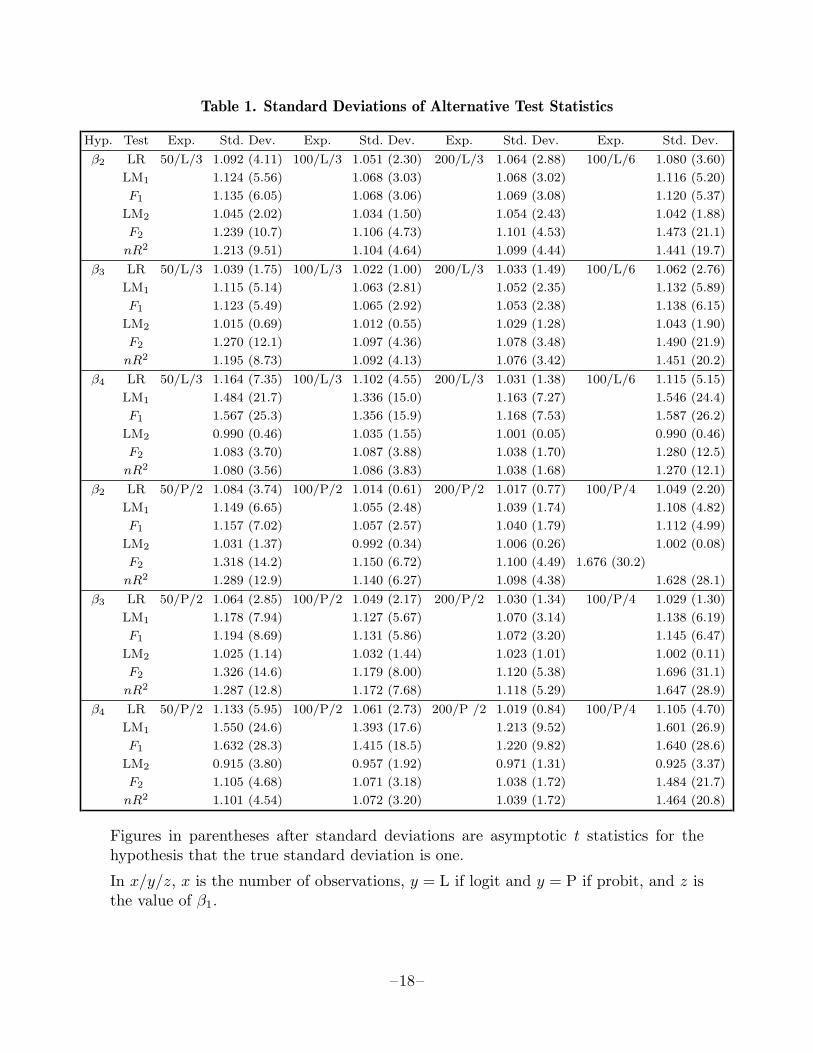
Table 1. Standard Deviations of Alternative Test Statistics

Hyp. Test Exp. Std. Dev. Exp. Std. Dev. Exp. Std. Dev. Exp. Std. Dev.

β2 LR 50/L/3 1.092 (4.11) 100/L/3 1.051 (2.30) 200/L/3 1.064 (2.88) 100/L/6 1.080 (3.60)

LM1 1.124 (5.56) 1.068 (3.03) 1.068 (3.02) 1.116 (5.20)

F1 1.135 (6.05) 1.068 (3.06) 1.069 (3.08) 1.120 (5.37)

LM2 1.045 (2.02) 1.034 (1.50) 1.054 (2.43) 1.042 (1.88)

F2 1.239 (10.7) 1.106 (4.73) 1.101 (4.53) 1.473 (21.1)

nR2 1.213 (9.51) 1.104 (4.64) 1.099 (4.44) 1.441 (19.7)

β3 LR 50/L/3 1.039 (1.75) 100/L/3 1.022 (1.00) 200/L/3 1.033 (1.49) 100/L/6 1.062 (2.76)

LM1 1.115 (5.14) 1.063 (2.81) 1.052 (2.35) 1.132 (5.89)

F1 1.123 (5.49) 1.065 (2.92) 1.053 (2.38) 1.138 (6.15)

LM2 1.015 (0.69) 1.012 (0.55) 1.029 (1.28) 1.043 (1.90)

F2 1.270 (12.1) 1.097 (4.36) 1.078 (3.48) 1.490 (21.9)

nR2 1.195 (8.73) 1.092 (4.13) 1.076 (3.42) 1.451 (20.2)

β4 LR 50/L/3 1.164 (7.35) 100/L/3 1.102 (4.55) 200/L/3 1.031 (1.38) 100/L/6 1.115 (5.15)

LM1 1.484 (21.7) 1.336 (15.0) 1.163 (7.27) 1.546 (24.4)

F1 1.567 (25.3) 1.356 (15.9) 1.168 (7.53) 1.587 (26.2)

LM2 0.990 (0.46) 1.035 (1.55) 1.001 (0.05) 0.990 (0.46)

F2 1.083 (3.70) 1.087 (3.88) 1.038 (1.70) 1.280 (12.5)

nR2 1.080 (3.56) 1.086 (3.83) 1.038 (1.68) 1.270 (12.1)

β2 LR 50/P/2 1.084 (3.74) 100/P/2 1.014 (0.61) 200/P/2 1.017 (0.77) 100/P/4 1.049 (2.20)

LM1 1.149 (6.65) 1.055 (2.48) 1.039 (1.74) 1.108 (4.82)

F1 1.157 (7.02) 1.057 (2.57) 1.040 (1.79) 1.112 (4.99)

LM2 1.031 (1.37) 0.992 (0.34) 1.006 (0.26) 1.002 (0.08)

F2 1.318 (14.2) 1.150 (6.72) 1.100 (4.49) 1.676 (30.2)

nR2 1.289 (12.9) 1.140 (6.27) 1.098 (4.38) 1.628 (28.1)

β3 LR 50/P/2 1.064 (2.85) 100/P/2 1.049 (2.17) 200/P/2 1.030 (1.34) 100/P/4 1.029 (1.30)

LM1 1.178 (7.94) 1.127 (5.67) 1.070 (3.14) 1.138 (6.19)

F1 1.194 (8.69) 1.131 (5.86) 1.072 (3.20) 1.145 (6.47)

LM2 1.025 (1.14) 1.032 (1.44) 1.023 (1.01) 1.002 (0.11)

F2 1.326 (14.6) 1.179 (8.00) 1.120 (5.38) 1.696 (31.1)

nR2 1.287 (12.8) 1.172 (7.68) 1.118 (5.29) 1.647 (28.9)

β4 LR 50/P/2 1.133 (5.95) 100/P/2 1.061 (2.73) 200/P /2 1.019 (0.84) 100/P/4 1.105 (4.70)

LM1 1.550 (24.6) 1.393 (17.6) 1.213 (9.52) 1.601 (26.9)

F1 1.632 (28.3) 1.415 (18.5) 1.220 (9.82) 1.640 (28.6)

LM2 0.915 (3.80) 0.957 (1.92) 0.971 (1.31) 0.925 (3.37)

F2 1.105 (4.68) 1.071 (3.18) 1.038 (1.72) 1.484 (21.7)

nR2 1.101 (4.54) 1.072 (3.20) 1.039 (1.72) 1.464 (20.8)

Figures in parentheses after standard deviations are asymptotic t statistics for thehypothesis that the true standard deviation is one.

In x/y/z, x is the number of observations, y = L if logit and y = P if probit, and z isthe value of β1.

–18–

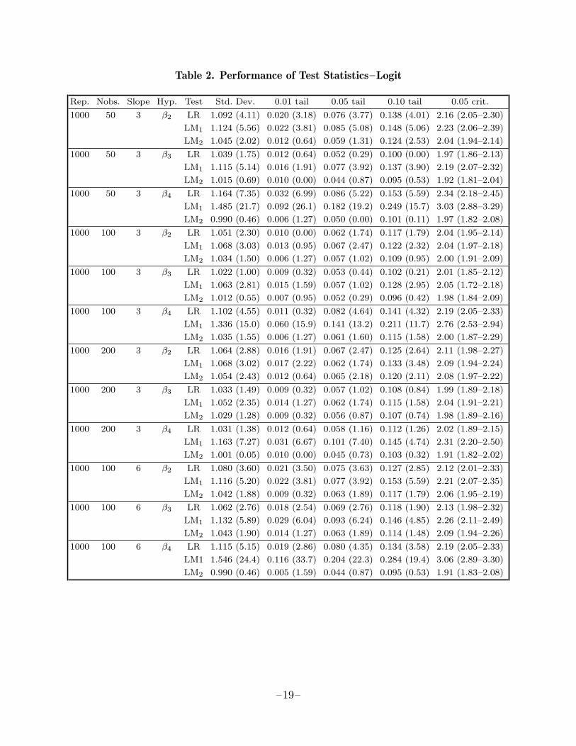
Table 2. Performance of Test Statistics–Logit

Rep. Nobs. Slope Hyp. Test Std. Dev. 0.01 tail 0.05 tail 0.10 tail 0.05 crit.

1000 50 3 β2 LR 1.092 (4.11) 0.020 (3.18) 0.076 (3.77) 0.138 (4.01) 2.16 (2.05–2.30)

LM1 1.124 (5.56) 0.022 (3.81) 0.085 (5.08) 0.148 (5.06) 2.23 (2.06–2.39)

LM2 1.045 (2.02) 0.012 (0.64) 0.059 (1.31) 0.124 (2.53) 2.04 (1.94–2.14)

1000 50 3 β3 LR 1.039 (1.75) 0.012 (0.64) 0.052 (0.29) 0.100 (0.00) 1.97 (1.86–2.13)

LM1 1.115 (5.14) 0.016 (1.91) 0.077 (3.92) 0.137 (3.90) 2.19 (2.07–2.32)

LM2 1.015 (0.69) 0.010 (0.00) 0.044 (0.87) 0.095 (0.53) 1.92 (1.81–2.04)

1000 50 3 β4 LR 1.164 (7.35) 0.032 (6.99) 0.086 (5.22) 0.153 (5.59) 2.34 (2.18–2.45)

LM1 1.485 (21.7) 0.092 (26.1) 0.182 (19.2) 0.249 (15.7) 3.03 (2.88–3.29)

LM2 0.990 (0.46) 0.006 (1.27) 0.050 (0.00) 0.101 (0.11) 1.97 (1.82–2.08)

1000 100 3 β2 LR 1.051 (2.30) 0.010 (0.00) 0.062 (1.74) 0.117 (1.79) 2.04 (1.95–2.14)

LM1 1.068 (3.03) 0.013 (0.95) 0.067 (2.47) 0.122 (2.32) 2.04 (1.97–2.18)

LM2 1.034 (1.50) 0.006 (1.27) 0.057 (1.02) 0.109 (0.95) 2.00 (1.91–2.09)

1000 100 3 β3 LR 1.022 (1.00) 0.009 (0.32) 0.053 (0.44) 0.102 (0.21) 2.01 (1.85–2.12)

LM1 1.063 (2.81) 0.015 (1.59) 0.057 (1.02) 0.128 (2.95) 2.05 (1.72–2.18)

LM2 1.012 (0.55) 0.007 (0.95) 0.052 (0.29) 0.096 (0.42) 1.98 (1.84–2.09)

1000 100 3 β4 LR 1.102 (4.55) 0.011 (0.32) 0.082 (4.64) 0.141 (4.32) 2.19 (2.05–2.33)

LM1 1.336 (15.0) 0.060 (15.9) 0.141 (13.2) 0.211 (11.7) 2.76 (2.53–2.94)

LM2 1.035 (1.55) 0.006 (1.27) 0.061 (1.60) 0.115 (1.58) 2.00 (1.87–2.29)

1000 200 3 β2 LR 1.064 (2.88) 0.016 (1.91) 0.067 (2.47) 0.125 (2.64) 2.11 (1.98–2.27)

LM1 1.068 (3.02) 0.017 (2.22) 0.062 (1.74) 0.133 (3.48) 2.09 (1.94–2.24)

LM2 1.054 (2.43) 0.012 (0.64) 0.065 (2.18) 0.120 (2.11) 2.08 (1.97–2.22)

1000 200 3 β3 LR 1.033 (1.49) 0.009 (0.32) 0.057 (1.02) 0.108 (0.84) 1.99 (1.89–2.18)

LM1 1.052 (2.35) 0.014 (1.27) 0.062 (1.74) 0.115 (1.58) 2.04 (1.91–2.21)

LM2 1.029 (1.28) 0.009 (0.32) 0.056 (0.87) 0.107 (0.74) 1.98 (1.89–2.16)

1000 200 3 β4 LR 1.031 (1.38) 0.012 (0.64) 0.058 (1.16) 0.112 (1.26) 2.02 (1.89–2.15)

LM1 1.163 (7.27) 0.031 (6.67) 0.101 (7.40) 0.145 (4.74) 2.31 (2.20–2.50)

LM2 1.001 (0.05) 0.010 (0.00) 0.045 (0.73) 0.103 (0.32) 1.91 (1.82–2.02)

1000 100 6 β2 LR 1.080 (3.60) 0.021 (3.50) 0.075 (3.63) 0.127 (2.85) 2.12 (2.01–2.33)

LM1 1.116 (5.20) 0.022 (3.81) 0.077 (3.92) 0.153 (5.59) 2.21 (2.07–2.35)

LM2 1.042 (1.88) 0.009 (0.32) 0.063 (1.89) 0.117 (1.79) 2.06 (1.95–2.19)

1000 100 6 β3 LR 1.062 (2.76) 0.018 (2.54) 0.069 (2.76) 0.118 (1.90) 2.13 (1.98–2.32)

LM1 1.132 (5.89) 0.029 (6.04) 0.093 (6.24) 0.146 (4.85) 2.26 (2.11–2.49)

LM2 1.043 (1.90) 0.014 (1.27) 0.063 (1.89) 0.114 (1.48) 2.09 (1.94–2.26)

1000 100 6 β4 LR 1.115 (5.15) 0.019 (2.86) 0.080 (4.35) 0.134 (3.58) 2.19 (2.05–2.33)

LM1 1.546 (24.4) 0.116 (33.7) 0.204 (22.3) 0.284 (19.4) 3.06 (2.89–3.30)

LM2 0.990 (0.46) 0.005 (1.59) 0.044 (0.87) 0.095 (0.53) 1.91 (1.83–2.08)

–19–

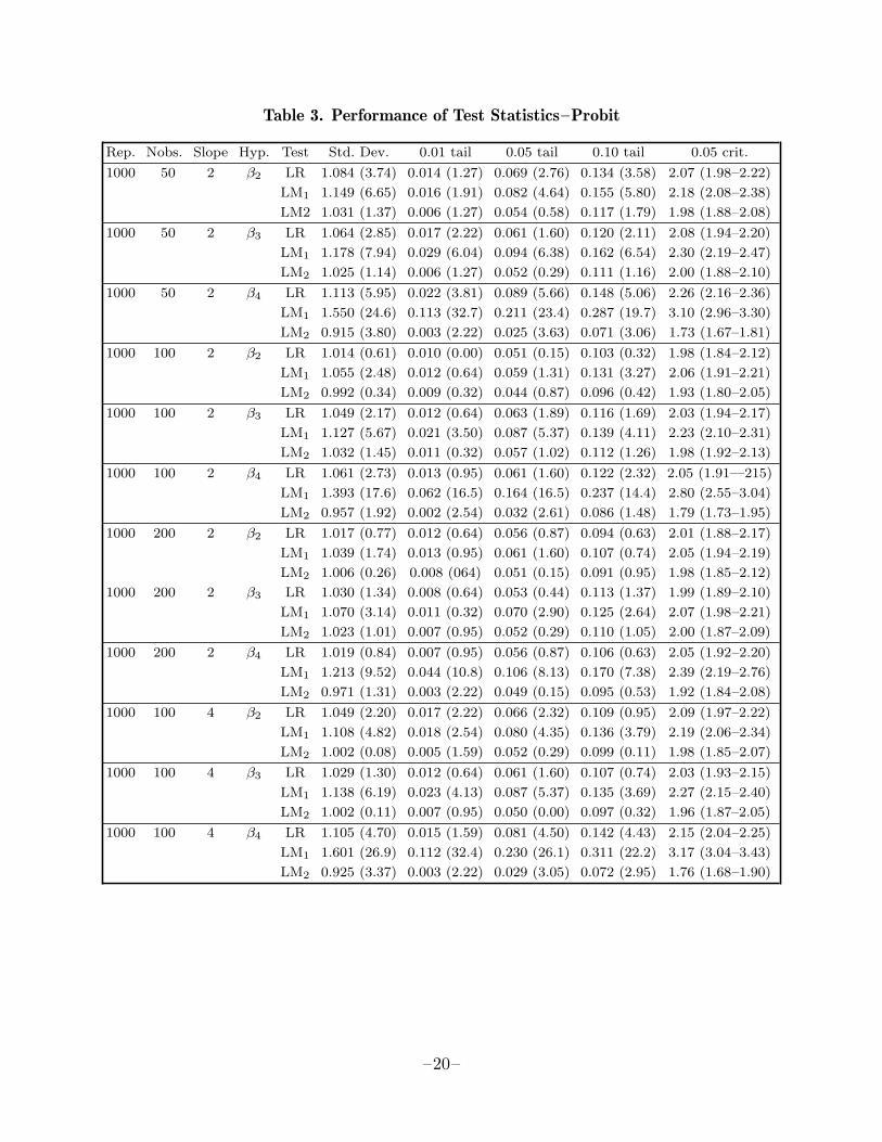
Table 3. Performance of Test Statistics–Probit

Rep. Nobs. Slope Hyp. Test Std. Dev. 0.01 tail 0.05 tail 0.10 tail 0.05 crit.

1000 50 2 β2 LR 1.084 (3.74) 0.014 (1.27) 0.069 (2.76) 0.134 (3.58) 2.07 (1.98–2.22)

LM1 1.149 (6.65) 0.016 (1.91) 0.082 (4.64) 0.155 (5.80) 2.18 (2.08–2.38)

LM2 1.031 (1.37) 0.006 (1.27) 0.054 (0.58) 0.117 (1.79) 1.98 (1.88–2.08)

1000 50 2 β3 LR 1.064 (2.85) 0.017 (2.22) 0.061 (1.60) 0.120 (2.11) 2.08 (1.94–2.20)

LM1 1.178 (7.94) 0.029 (6.04) 0.094 (6.38) 0.162 (6.54) 2.30 (2.19–2.47)

LM2 1.025 (1.14) 0.006 (1.27) 0.052 (0.29) 0.111 (1.16) 2.00 (1.88–2.10)

1000 50 2 β4 LR 1.113 (5.95) 0.022 (3.81) 0.089 (5.66) 0.148 (5.06) 2.26 (2.16–2.36)

LM1 1.550 (24.6) 0.113 (32.7) 0.211 (23.4) 0.287 (19.7) 3.10 (2.96–3.30)

LM2 0.915 (3.80) 0.003 (2.22) 0.025 (3.63) 0.071 (3.06) 1.73 (1.67–1.81)

1000 100 2 β2 LR 1.014 (0.61) 0.010 (0.00) 0.051 (0.15) 0.103 (0.32) 1.98 (1.84–2.12)

LM1 1.055 (2.48) 0.012 (0.64) 0.059 (1.31) 0.131 (3.27) 2.06 (1.91–2.21)

LM2 0.992 (0.34) 0.009 (0.32) 0.044 (0.87) 0.096 (0.42) 1.93 (1.80–2.05)

1000 100 2 β3 LR 1.049 (2.17) 0.012 (0.64) 0.063 (1.89) 0.116 (1.69) 2.03 (1.94–2.17)

LM1 1.127 (5.67) 0.021 (3.50) 0.087 (5.37) 0.139 (4.11) 2.23 (2.10–2.31)

LM2 1.032 (1.45) 0.011 (0.32) 0.057 (1.02) 0.112 (1.26) 1.98 (1.92–2.13)

1000 100 2 β4 LR 1.061 (2.73) 0.013 (0.95) 0.061 (1.60) 0.122 (2.32) 2.05 (1.91—215)

LM1 1.393 (17.6) 0.062 (16.5) 0.164 (16.5) 0.237 (14.4) 2.80 (2.55–3.04)

LM2 0.957 (1.92) 0.002 (2.54) 0.032 (2.61) 0.086 (1.48) 1.79 (1.73–1.95)

1000 200 2 β2 LR 1.017 (0.77) 0.012 (0.64) 0.056 (0.87) 0.094 (0.63) 2.01 (1.88–2.17)

LM1 1.039 (1.74) 0.013 (0.95) 0.061 (1.60) 0.107 (0.74) 2.05 (1.94–2.19)

LM2 1.006 (0.26) 0.008 (064) 0.051 (0.15) 0.091 (0.95) 1.98 (1.85–2.12)

1000 200 2 β3 LR 1.030 (1.34) 0.008 (0.64) 0.053 (0.44) 0.113 (1.37) 1.99 (1.89–2.10)

LM1 1.070 (3.14) 0.011 (0.32) 0.070 (2.90) 0.125 (2.64) 2.07 (1.98–2.21)

LM2 1.023 (1.01) 0.007 (0.95) 0.052 (0.29) 0.110 (1.05) 2.00 (1.87–2.09)

1000 200 2 β4 LR 1.019 (0.84) 0.007 (0.95) 0.056 (0.87) 0.106 (0.63) 2.05 (1.92–2.20)

LM1 1.213 (9.52) 0.044 (10.8) 0.106 (8.13) 0.170 (7.38) 2.39 (2.19–2.76)

LM2 0.971 (1.31) 0.003 (2.22) 0.049 (0.15) 0.095 (0.53) 1.92 (1.84–2.08)

1000 100 4 β2 LR 1.049 (2.20) 0.017 (2.22) 0.066 (2.32) 0.109 (0.95) 2.09 (1.97–2.22)

LM1 1.108 (4.82) 0.018 (2.54) 0.080 (4.35) 0.136 (3.79) 2.19 (2.06–2.34)

LM2 1.002 (0.08) 0.005 (1.59) 0.052 (0.29) 0.099 (0.11) 1.98 (1.85–2.07)

1000 100 4 β3 LR 1.029 (1.30) 0.012 (0.64) 0.061 (1.60) 0.107 (0.74) 2.03 (1.93–2.15)

LM1 1.138 (6.19) 0.023 (4.13) 0.087 (5.37) 0.135 (3.69) 2.27 (2.15–2.40)

LM2 1.002 (0.11) 0.007 (0.95) 0.050 (0.00) 0.097 (0.32) 1.96 (1.87–2.05)

1000 100 4 β4 LR 1.105 (4.70) 0.015 (1.59) 0.081 (4.50) 0.142 (4.43) 2.15 (2.04–2.25)

LM1 1.601 (26.9) 0.112 (32.4) 0.230 (26.1) 0.311 (22.2) 3.17 (3.04–3.43)

LM2 0.925 (3.37) 0.003 (2.22) 0.029 (3.05) 0.072 (2.95) 1.76 (1.68–1.90)

–20–

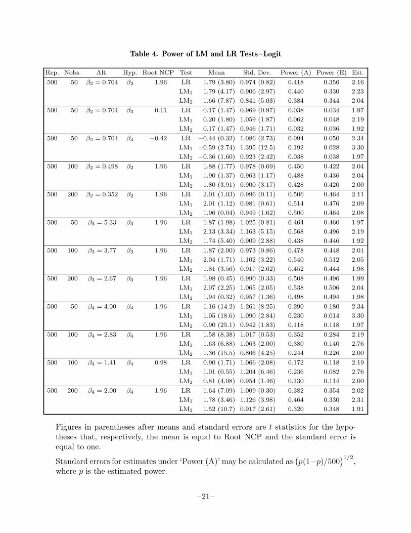
Table 4. Power of LM and LR Tests–Logit

Rep. Nobs. Alt. Hyp. Root NCP Test Mean Std. Dev. Power (A) Power (E) Est.

500 50 β2 = 0.704 β2 1.96 LR 1.79 (3.80) 0.974 (0.82) 0.418 0.356 2.16

LM1 1.79 (4.17) 0.906 (2.97) 0.440 0.330 2.23

LM2 1.66 (7.87) 0.841 (5.03) 0.384 0.344 2.04

500 50 β2 = 0.704 β3 0.11 LR 0.17 (1.47) 0.969 (0.97) 0.038 0.034 1.97

LM1 0.20 (1.80) 1.059 (1.87) 0.062 0.048 2.19

LM2 0.17 (1.47) 0.946 (1.71) 0.032 0.036 1.92

500 50 β2 = 0.704 β4 −0.42 LR −0.44 (0.32) 1.086 (2.73) 0.094 0.050 2.34

LM1 −0.59 (2.74) 1.395 (12.5) 0.192 0.028 3.30

LM2 −0.36 (1.60) 0.923 (2.42) 0.038 0.038 1.97

500 100 β2 = 0.498 β2 1.96 LR 1.88 (1.77) 0.978 (0.69) 0.450 0.422 2.04

LM1 1.90 (1.37) 0.963 (1.17) 0.488 0.436 2.04

LM2 1.80 (3.91) 0.900 (3.17) 0.428 0.420 2.00

500 200 β2 = 0.352 β2 1.96 LR 2.01 (1.03) 0.996 (0.11) 0.506 0.464 2.11

LM1 2.01 (1.12) 0.981 (0.61) 0.514 0.476 2.09

LM2 1.96 (0.04) 0.949 (1.62) 0.500 0.464 2.08

500 50 β3 = 5.33 β3 1.96 LR 1.87 (1.98) 1.025 (0.81) 0.464 0.460 1.97

LM1 2.13 (3.34) 1.163 (5.15) 0.568 0.496 2.19

LM2 1.74 (5.40) 0.909 (2.88) 0.438 0.446 1.92

500 100 β3 = 3.77 β3 1.96 LR 1.87 (2.00) 0.973 (0.86) 0.478 0.448 2.01

LM1 2.04 (1.71) 1.102 (3.22) 0.540 0.512 2.05

LM2 1.81 (3.56) 0.917 (2.62) 0.452 0.444 1.98

500 200 β3 = 2.67 β3 1.96 LR 1.98 (0.45) 0.990 (0.33) 0.508 0.496 1.99

LM1 2.07 (2.25) 1.065 (2.05) 0.538 0.506 2.04

LM2 1.94 (0.32) 0.957 (1.36) 0.498 0.494 1.98

500 50 β4 = 4.00 β4 1.96 LR 1.16 (14.2) 1.261 (8.25) 0.290 0.180 2.34

LM1 1.05 (18.6) 1.090 (2.84) 0.230 0.014 3.30

LM2 0.90 (25.1) 0.942 (1.83) 0.118 0.118 1.97

500 100 β4 = 2.83 β4 1.96 LR 1.58 (8.38) 1.017 (0.53) 0.352 0.284 2.19

LM1 1.63 (6.88) 1.063 (2.00) 0.380 0.140 2.76

LM2 1.36 (15.5) 0.866 (4.25) 0.244 0.226 2.00

500 100 β4 = 1.41 β4 0.98 LR 0.90 (1.71) 1.066 (2.08) 0.172 0.118 2.19

LM1 1.01 (0.55) 1.204 (6.46) 0.236 0.082 2.76

LM2 0.81 (4.08) 0.954 (1.46) 0.130 0.114 2.00

500 200 β4 = 2.00 β4 1.96 LR 1.64 (7.09) 1.009 (0.30) 0.382 0.354 2.02

LM1 1.78 (3.46) 1.126 (3.98) 0.464 0.330 2.31

LM2 1.52 (10.7) 0.917 (2.61) 0.320 0.348 1.91

Figures in parentheses after means and standard errors are t statistics for the hypo-theses that, respectively, the mean is equal to Root NCP and the standard error isequal to one.

Standard errors for estimates under ‘Power (A)’ may be calculated as(p(1−p)/500

)1/2,where p is the estimated power.

–21–

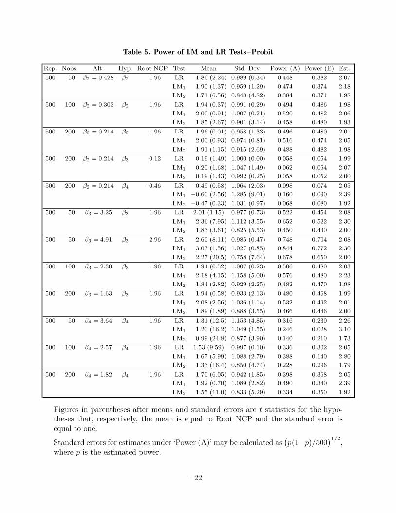
Table 5. Power of LM and LR Tests–Probit

Rep. Nobs. Alt. Hyp. Root NCP Test Mean Std. Dev. Power (A) Power (E) Est.

500 50 β2 = 0.428 β2 1.96 LR 1.86 (2.24) 0.989 (0.34) 0.448 0.382 2.07

LM1 1.90 (1.37) 0.959 (1.29) 0.474 0.374 2.18

LM2 1.71 (6.56) 0.848 (4.82) 0.384 0.374 1.98

500 100 β2 = 0.303 β2 1.96 LR 1.94 (0.37) 0.991 (0.29) 0.494 0.486 1.98

LM1 2.00 (0.91) 1.007 (0.21) 0.520 0.482 2.06

LM2 1.85 (2.67) 0.901 (3.14) 0.458 0.480 1.93

500 200 β2 = 0.214 β2 1.96 LR 1.96 (0.01) 0.958 (1.33) 0.496 0.480 2.01

LM1 2.00 (0.93) 0.974 (0.81) 0.516 0.474 2.05

LM2 1.91 (1.15) 0.915 (2.69) 0.488 0.482 1.98

500 200 β2 = 0.214 β3 0.12 LR 0.19 (1.49) 1.000 (0.00) 0.058 0.054 1.99

LM1 0.20 (1.68) 1.047 (1.49) 0.062 0.054 2.07

LM2 0.19 (1.43) 0.992 (0.25) 0.058 0.052 2.00

500 200 β2 = 0.214 β4 −0.46 LR −0.49 (0.58) 1.064 (2.03) 0.098 0.074 2.05

LM1 −0.60 (2.56) 1.285 (9.01) 0.160 0.090 2.39

LM2 −0.47 (0.33) 1.031 (0.97) 0.068 0.080 1.92

500 50 β3 = 3.25 β3 1.96 LR 2.01 (1.15) 0.977 (0.73) 0.522 0.454 2.08

LM1 2.36 (7.95) 1.112 (3.55) 0.652 0.522 2.30

LM2 1.83 (3.61) 0.825 (5.53) 0.450 0.430 2.00

500 50 β3 = 4.91 β3 2.96 LR 2.60 (8.11) 0.985 (0.47) 0.748 0.704 2.08

LM1 3.03 (1.56) 1.027 (0.85) 0.844 0.772 2.30

LM2 2.27 (20.5) 0.758 (7.64) 0.678 0.650 2.00

500 100 β3 = 2.30 β3 1.96 LR 1.94 (0.52) 1.007 (0.23) 0.506 0.480 2.03

LM1 2.18 (4.15) 1.158 (5.00) 0.576 0.480 2.23

LM2 1.84 (2.82) 0.929 (2.25) 0.482 0.470 1.98

500 200 β3 = 1.63 β3 1.96 LR 1.94 (0.58) 0.933 (2.13) 0.480 0.468 1.99

LM1 2.08 (2.56) 1.036 (1.14) 0.532 0.492 2.01

LM2 1.89 (1.89) 0.888 (3.55) 0.466 0.446 2.00

500 50 β4 = 3.64 β4 1.96 LR 1.31 (12.5) 1.153 (4.85) 0.316 0.230 2.26

LM1 1.20 (16.2) 1.049 (1.55) 0.246 0.028 3.10

LM2 0.99 (24.8) 0.877 (3.90) 0.140 0.210 1.73

500 100 β4 = 2.57 β4 1.96 LR 1.53 (9.59) 0.997 (0.10) 0.336 0.302 2.05

LM1 1.67 (5.99) 1.088 (2.79) 0.388 0.140 2.80

LM2 1.33 (16.4) 0.850 (4.74) 0.228 0.296 1.79

500 200 β4 = 1.82 β4 1.96 LR 1.70 (6.05) 0.942 (1.85) 0.398 0.368 2.05

LM1 1.92 (0.70) 1.089 (2.82) 0.490 0.340 2.39

LM2 1.55 (11.0) 0.833 (5.29) 0.334 0.350 1.92

Figures in parentheses after means and standard errors are t statistics for the hypo-theses that, respectively, the mean is equal to Root NCP and the standard error isequal to one.

Standard errors for estimates under ‘Power (A)’ may be calculated as(p(1−p)/500

)1/2,where p is the estimated power.

–22–