polo2: a user's guide to multiple probit or logit analysis

8/8/2019 POLO2: a user's guide to multiple Probit Or LOgit analysis

http://slidepdf.com/reader/full/polo2-a-users-guide-to-multiple-probit-or-logit-analysis 1/43

United StatesDepartment of Agriculture

Forest Service

Pacific SouthwestForest and RangeExperiment Station

General Technical

Report PSW- 55

a user's guide to mult iple Probit Or LOgit analysis

Robert M. Russell, N. E. Savin, Jacqueline L. Robertson



Authors:

ROBERT M. RUSSELL has been a computer programmer at the Station since 1965.

He was graduated from Graceland College in 1953, and holds a B.S. degree (1956) in

mathematics from the University of Michigan. N. E. SAVIN earned a B.A. degree(1956) in economics and M.A. (1960) and Ph.D. (1969) degrees in economic statistics

at the University of California, Berkeley. Since 1976, he has been a fellow and lecturer

with the Faculty of Economics and Politics at Trinity College, Cambridge University,

England. JACQUELINE L. ROBERTSON is a research entomologist assigned to the

Station's insecticide evaluation research unit, at Berkeley, California. She earned a

B.A. degree (1969) in zoology, and a Ph.D. degree (1973) in entomology at the

University of California, Berkeley. She has been a member of the Station's research

staff since 1966.

Acknowledgments:

We thank Benjamin Spada and Dr. Michael I. Haverty, Pacific Southwest Forest

and Range Experiment Station, U.S. Department of Agriculture, Berkeley,

California, for their support of the development of POL02.

Publisher:

Pacific Southwest Forest and Range Experiment StationP.O. Box 245, Berkeley, California 94701

September 1981



1

2

3

4

5

67

POLO2:a user's guide to multiple Probit Or LOgit analysis

Robert M. Russell, N. E. Savin, Jacqueline L. Robertson

CONTENTS Introduction .....................................................................................................1 1. General Statistical Features ................... ........... .......... ........... ........... ........ 12. Data Input Format .....................................................................................2

2.1 Starter Cards ...........................................................................................22.2 Title Card ................................................................................................22.3 Control Card ...........................................................................................32.4 Transformation Card ...............................................................................4

2.4.1 Reverse Polish Notation .................................................................42.4.2 Operators ........................................................................................42.4.3 Operands ........................................................................................42.4.4 Examples ........................................................................................4

2.5 Parameter Label Card .............................................................................5

2.6 Starting Values of the Parameters Card ..................................................52.7 Format Card ............................................................................................52.8 Data Cards ...............................................................................................52.9 End Card .................................................................................................6

3. Limitations ..................................................................................................6 4. Data Output Examples ...............................................................................6

4.1 Toxicity of Pyrethrum Spray and Film ...................................................64.1. Models ...........................................................................................64.1. Hypotheses .....................................................................................64.1. Analyses Required .........................................................................74.1. Input ...............................................................................................74.1. Output ............................................................................................94.1. Hypotheses Testing ......................................................................19 4.1. Comparison with Published Calculations ....................................19

4.2 Vaso-Constriction .................................................................................19 4.2.1 Models, Hypothesis, and Analyses Required ...............................19 4.2.2 Input .............................................................................................19 4.2.3 Output ..........................................................................................204.2.4 Hypothesis Testing .......................................................................21

4.3 Body Weight as a Variable: Higher Order Terms .................................254.3.1 Models and Hypothesis ................................................................254.3.2 Input .............................................................................................254.3.3 Output ..........................................................................................26



4.4 Body Weight as a Variable: PROPORTIONAL Option .....................294.4.1 Models and Hypotheses ..............................................................294.4.2 Input ...........................................................................................294.4.3 Output .........................................................................................30 4.4.4 Hypothesis Testing .....................................................................30

4.5 Body Weight as a Variable: BASIC Option ........................................30 4.5.1 Input ...........................................................................................334.5.2 Output .........................................................................................33

5. Error Messages .......................................................................................36 6. References ................................................................................................37



Many studies involving quantal response include

more than one explanatory variable. The variables

in an insecticide bioassay, for example, might be the dose

of the chemical as well as the body weight of the test

subjects. POLO2 is a computer program developed toanalyze binary quantal response models with one to nine

explanatory variables. Such models are of interest in

insecticide research as well as in other subject areas. For examples of other applications, texts such as those by

Domencich and McFadden (1975) and Maddala (1977)

should be consulted.

For models in which only one explanatory variable (inaddition to the constant) is present, another program,

POLO (Russell and others 1977, Savin and others 1977,

Robertson and others 1980) is available. However, the

statistical inferences drawn from this simple model may be

misleading if relevant explanatory variables have been

omitted. A more satisfactory approach is to begin theanalysis with a general model which includes all the

explanatory variables suspected as important in explainingthe response of the individual. One may then test whether

certain variables can be omitted from the model. The

necessary calculations for carrying out these tests are performed by POLO2. If the extra variables are not

significant in the multiple regression, a simple regression

model may be appropriate.

The statistical documentation of POLO2, descriptions

of its statistical features, and examples of its applicationare described in articles by Robertson and others

(1981 a, b), and Savin and others (1981).

The POLO2 program is available upon request to:

Director Pacific Southwest Forest and Range Experiment Station P.O. Box 245 Berkeley, California 94701 Attention: Computer Services Librarian

A magnetic tape with format specifications should be sent

with the request. The program is currently operational on

the Univac 1100 Series, but can be modified for use with

other large scientific computers. The program is not

suitable for adaptation to programmable desk calculators.

This guide was prepared to assist users of the POLO2

program. Selected statistical features of the program aredescribed by means of a series of examples chosen from our

work and that of others. A comprehensive description of

all possible situations or experiments amenable tomultivariate analyses is beyond the scope of this guide. For

experiments more complex than those described here, a

statistician or programmer, or both, should be consulted

regarding the appropriate use of POLO2.

1. GENERAL STATISTICAL

FEATURES

Consider a sample of I individuals indexed by i = 1,...,I.

For individual i there is an observed J x 1 vector si´ =

(s1i,.... ,sJi) of individual characteristics. In a binary

quantal response model the individual has two responsesor choices. These can be denoted by defining the binomial

variable

f i = 1 if the first response occurs

(if alternative 1 is chosen),

f i = 0 if the second response occurs

(if alternative 2 is chosen).

For example, in a bioassay of toxicants the individuals are

insects and the possible responses are dead or alive. The

measured characteristics may include the dose of the

toxicant, the insect's weight and its age.The probability (P) that f i = 1 is

Pi = F( β zi)



where F is a cumulative distribution function (CDF) of-fit are routinely calculated. One is the prediction success

mapping points on the real line into the unit interval, table (Domencich and McFadden 1975), which compares

β = ( β 1, ... , β K ) is a K x 1 vector of unknown parameters, the results predicted by the multiple regression model withzki = zk (si) is a numerical function of s i, and zi´= (z1i,...,zKi) the results actually observed. The other goodness-of-fit

is K x 1 vector of these numerical functions. If, for instance, indicator is the calculation of the likelihood ratio statistic

weight is one of the measured characteristics, then the for testing the hypothesis that all coefficients in the

function zki may be the weight itself, the logarithm of the regression are equal to zero. Finally, a general method for weight or the square of the weight. transformation of variables is included.

For the probit model

Pi = F( β zi) = Φ ( β zi)

where Φ is the standard normal CDF. For the logit model

2. DATA INPUT FORMATPi = F( β zi) = 1 /[1 + e ´-β´zi].

POLO2 estimates both models by the maximum likelihood(ML) method with grouped as well as ungrouped data. 2.1 Starter Cards

The ML procedure can be applied to the probability

function Pi = F( β zi) where F is any CDF. Since f i is a Every POLO2 run starts with five cards that call the binomial variable, the log of the probability of observing a program from a tape ( fig. 1).These cards reflect the currentgiven sample is

Univac 1100 implementation and would be completelydifferent if POLO2 were modified to run on a differentI computer. All of the remaining input described in sections

L = ∑[f i logPi + (1− f i ) log(1− Pi )]2.2-2.9 would be the same on any computer.

i=1

where L is referred to as the log likelihood function. TheML method selects as an estimate of β that vector which

maximizes L. In other words, the ML estimator for β maximizes the calculated probability of observing thegiven sample.

When the data are grouped there are repeated

observations for each vector of values of the explanatoryvariables. With grouped data, we change the notation as

Figure 1.

follows. Now let I denote the number of groups andi=1,...,I denote the levels (zi, si) of the explanatory Cards 2-5 must be punched as shown. In card 1, thevariables. Let ni denote the number of observations at level user's identification and account number should be placedi and r i denote the number of times that the first response in columns 10-21. Column 24 is the time limit in minutes;occurs. The log likelihood function for grouped data is the page limit is listed in columns 26-28. Both time andthen page limits may be changed to meet particular needs.

I

L = ∑[r i log Pi − (n i − r i ) log(1− Pi )]2.2 Title Card i=1

Again, the ML method selects the vector that maximizes Each data set begins with a title card that has an equalthe log likelihood function L as an estimate of β . For sign (=) punched in column 1. Anything desired may befurther discussion of the estimation of probit and logit placed in columns 2-80 ( fig. 2). This card is useful in

models with several explanatory variables, see Finney documenting the data, the model, the procedures used for (1971) and Domencich and McFadden (1975). the analysis, or equivalent information. The information is

The maximum of the log likelihood is reported to reprinted at the top of every page of the output. Only one

facilitate hypothesis testing. Two indicators of goodness- title card per data set may be used.

Figure 2.

2



2.3 Control Card

The information on this card controls the operation of the

program. All items are integers, separated by commas

( fig. 3). These numbers need not occur in fixed fields

(specific columns on a card). Extra spaces may be inserted

before or after the commas as desired ( fig. 4). Twelveintegers must be present. These are, from left to right:

Internal program

Position designation Explanation

1 NVAR Number of regression coefficients in the model,including the constant term, but not including

natural response.

2 NV Number of variables to be read from a data card.

This number corresponds to the number of F'sand I's on the Format Card ( sec. 2.7 ). Normally,

NV=NVAR-1 because the data do not include aconstant 1 for the constant term. NV may differ

from NVAR-1 when transformations are used

in the analysis.

3 LOGIT

LOGIT=0 if the probit model is to be used;LOGIT=1 if the logit model is desired.

4 KONTROL One of the explanatory variables (for example,dose) will be zero, for the group when a control

group is used. KONTROL is the index of that

parameter within the sequence of parameters

used, with 2 ≤ KONTROL ≤ NVAR. This limit

indicates that any parameter except the constant

term may have a control group.

5 ITRAN ITRAN=1 if variables are transformed and a

transformation card will be read. ITRAN=0 if

the variables are to be analyzed as is and there

will be no transformation card.

6 ISTARV ISTAR V=1 if starting values of the parametersare to be input; ISTARV=0 if they will be

calculated automatically. The ISTARV=1option should be used only if the automatic

method fails.

7 IECHO IECHO=1 if all data are to be printed back for

error checking. If the data have beenscrupulously checked, the IECHO=0 option may

be used and the data will not be printed back in

their entirety. A sample of the data set will be

printed instead.

8 NPARN NPARN=0 if natural response, such as that

which occurs without the presence of an insecticide, is present and is to be calculated as a

parameter. If natural response is not a para-

meter, NPARN=1.

9 IGROUP IGROUP=0 if there is only one test subject per

data card; IGROUP=1 if there is more than one(that is, if the data are grouped).

10 NPLL Number of parallel groups in the data (see sec.

4.1 for an example). NPLL=0 is read as if it were NPLL=1; in other words, a single data set would

compose a group parallel to itself.

11 KERNEL When a restricted model is to be computed, some

variables will be omitted from the model and the

regression will be rerun. The KERNEL control

instructs the program how may variables to

retain. Variables 1 through KERNEL are

retained, where 2 ≤ KERNEL ≤ NVAR; vari

ables KERNEL+1 through NVAR are dropped. Note that variables can be rearranged as desired

through the use of transformation or the "T"

editing control on the format card ( sec. 2.7 ).

When a restricted model is not desired,KERNEL=0.

12 NITER This integer specifies the number of iterations to be done in search of the maximum log

likelihood. When NITER=0, the program

chooses a suitable value. If starting values are

input (ISTARV=1), NITER=0 will be inter preted as no iterations and starting values

become the final values. Unless the final values

are known and can be used as the starting values,

NITER=50 should achieve maximization.

Figure 3

Control card specifying three regression coefficients,

two variables to be read from a data card, probit model to

be used, no controls, a transformation card to be read, andstarting ameters alculated

automatically. Data will be printed back, natural response

is not a parameter, there is one subject per data card, no

parallel groups, no restricted model will be calculated, and

the program will select the number of iterations to be done

to find the maximum values of the likelihood function.

par theof values c beto

Figure 4

Control card specifying three regression coefficients,

two variables to be read from each data card, and the logit

model to be used. The second variable defines a controlgroup, a transformation card to be read, starting values of

the parameters will be calculated automatically, data willnot be printed back, natural response is not a parameter,

data are grouped with more than one individual per card,and there are no parallel groups. A restricted model with

the first and second variables will be calculated, and the program will select the number of iterations to be done to

find the maximum value of the likelihood function. All

integers will be read as intended because each is separated

from the next by a comma, despite the presence or absence

of a blank space.

3



2.4 Transformation Card

This card contains a series of symbols written in Reverse

"Polish" Notation (RPN) (see sec. 2.4.1) which defines one

or more transformations of the variables. This option is

indicated by ITRAN=1 on the control card ( sec. 2.3). If

ITRAN=0 on the control card, the program will not read atransformation card.

2.4.1 Reverse Polish NotationReverse Polish Notation is widely used in computer

science and in Hewlett-Packard calculators. It is an

efficient and concise method for presenting a series of arithmetic calculations without using parentheses. The

calculations are listed in a form that can be acted on

directed by a computer and can be readily understood by

the user.The central concept of RPN is a "stack" of operands

(numbers). The "stack" is likened to a stack of cafeteria

trays. We specify that a tray can only be removed from the

top of the stack; likewise, a tray can only be put back in the

stack at the top. Reverse Polish Notation prescribes allcalculations in a stack of operands. An addition operation,

for example, calls the top two operands from the stack (reducing the height by two), adds them together, and

places the sum back on the stack. Subtraction,

multiplication, and division also take two operands from

the stack and return one. Simple functions like logarithms

and square roots take one operand and return one.How do numbers get into the stack? Reverse Polish

Notation consists of a string of symbols (the operators) and

the operands. The string is read from left to right. When an

operand is encountered, it is placed on the stack. When anoperator is encountered, the necessary operands are

removed, and the result is returned to the stack. At the endof the scan, only one number, the final result, remains.To write an RPN string, any algebraic formula should

first be rewritten in linear form.

a + bFor example, is rewritten (a + b)/c.

c

The operands are written in the order in which they appear

in the linear equation. The operators are interspersed in thestring in the order in which the stack operates, that is,

ab+c/. No parentheses are used. When this string is

scanned, the following operations occur: (1) a is put on the

stack, (2) b is put on the stack, (3) + takes the top two stack items (a,b) and places their sum back on the stack, (4) c is

put on the stack, (5) / takes the top stack item (c), divides it

into the next item (a+b), and places this result back on the

stack. In cases where the subtraction operator in an

algebraic formula only uses one operand (for example,-a+b), a single-operand negative operator such as N can be

used. The string is then written aNb+.

Once a string has been scanned, a means must exist to begin another stack for another transformation. This is

achieved by an operator =, which disposes of the final

4

result. For example (a+b) / c=d becomes the string ab+c / d=.

The operator = takes two items from the stack and returns

none; the result is stored and the stack is empty.

2.4.2 OperatorsThe operators used in POLO2 are:

Number of Number of

Operator operands results Operation

+ 2 1 addition

- 2 1 subtraction

* 2 1 multiplication/ 2 1 division

N 1 1 negation

E 1 1 exponentiation (10x)

L 1 1 logarithm (base 10)

S 1 1 square root= 2 0 store result

2.4.3 OperandsThe operands are taken from an array of values of the

variables, that is, x1, x2, x3, ... ,xn. These variables are

simply expressed with the subscripts (1,2,3,...,n); thesubscripts are the operands in the RPN string. The symbols

in the string are punched one per column, with no

intervening blanks. If several new variables are formed bytransformations, their RPN strings follow one after

another on the card. The first blank terminates the

transformations.

The transformations use x1, x2, x3,...,xn, to form new

variables that must replace them in the same array. To

avoid confusion, the x array is copied into another array, y.

A transformation then uses operands from x and stores the

result in y. Finally, the y is copied back into x and thetransformations are done.

The first NPLL numbers in the x array are dummies, or

the constant term (1.0) if NPLL=1. Transformations,therefore, are done on x2, x3,...,xn, and not on the

constant term or the dummy variables.

2.4.4 ExamplesSeveral examples of transformations from algebraic

notation to RPN are the following:

Algebraic Notation RPN

log(x2/ x3) = y2 23/ L2 =

(x2+x3)(x4+x5) = y5 23+45+*5=

(x2)2

+2x2x3+(x3)2

= y2 22*23*+23*+33*+2 =(x2)

2 = y2 (x2)4 = y3 22*2 = 22*22**3 =

-x3+(x3)2-x2x4 = y2 3N33*24*-S+2 =

x2(10x3+ 10x4) = y2 23E4E+*2 =

For another example, let the variables in a data set be x1,

x2, x3, and x4; x1 is the constant term. We require thetransformations y2 = log(x2/x3), y3 = log(x3), y5 = (x2)

2, and

y6 = x2x3; x4 is left unchanged. The RPN strings are 23/L2=,

3L3=, 22*5=, and 23*6=. The appropriate transformation

card for this series is shown in figure 5.



Figure 5.

2.5 Parameter Label Card

This card contains the descriptive labels for all NVAR

parameters. These labels are used on the printout. The parameters include the constant term or dummy variables,other explanatory variables, and natural response, if it is

present. Labels apply to the explanatory variables after any

transformations. Each label is 8 characters long. Usecolumns 1-8 for the first label, columns 9-16 for the second,

and so on ( fig. 6 ). If a label does not fill the 8 spaces, begin

the label in the leftmost space available (columns 1, 9, 17,

15, 33, and so on).

Figure 6.

2.6 Starting Values of the ParametersCard

This card is used only under special circumstances, such

as quickly confirming calculations in previously publishedexperiments. If this card is to be used, ISTARV=1 on the

control card ( sec. 2.3). The parameters are punched in

10F8.6 format (up to 10 fields of 8 columns each); in each

field there is a number with six digits to the right of the

decimal point and two to the left. The decimal point neednot be punched. The parameters on this card are the same

in number and order as on the label card ( fig. 6, 7 ).

Figure 7.

In this example, the constant is 3.4674, β 1 is 6.6292, and

β 2 is 5.8842. All POLO2 calculations will be done on the

basis of these parameter values if ISTARV=1 and NITER=0on the control card ( sec. 2.3).

2.7 Format Card

This card contains a standard FORTRAN format

statement with parentheses but without "FORMAT" punched on the card ( fig. 8). This statement instructs the

program how to read the data from each card. A variable

occupies specific columns—a field—on each data card; this

area is specified by "F" followed by a number giving the

field width. After that number is a decimal point and

another number telling where the decimal point is located,if it is not punched on the data cards. For example, "F7.2"

means that the data item requires a 7-column field; a

decimal point occurs between columns 5 and 6. "F7.0"

means whole numbers. When a decimal point is actually punched on a data card, the computer ignores what the

format card might say about its location. (For moreinformation, see any FORTRAN textbook.)

Besides the variables, the other items on a data card,such as the group number (K), number of subjects (N), and

number of subjects responding (M) must be specified on

the format card in "I" (integer) format. Formal editingcontrols "X" and "T" may be used to skip extraneous

columns on a data card or to go to a particular column. For

example, "3X" skips 3 columns and "16T resets the format

scan to column 16 regardless of where the scan was

previously. All steps in the format statement are separated by commas, and the statement is enclosed in parentheses.

Figure 8.

Format card instructing program to skip the first 10columns of each data card, read the first variable within the

next 4 columns assuming 2 decimal places, read the second

variable within the next 5 columns assuming 1 decimal

place, then go to column 24 and read a single integer, M(M=1 for response; M=0 for no response).

2.8 Data Cards

Punch one card per subject or per group of subjects

grouped at identical values of one of the independent

variables. All individuals treated with the same dose of aninsecticide, for example, might be grouped on a single card,

or each might have its own data card. Values of the NV

variables are punched, followed by N (the number of subjects) and M (the number responding). If there is only

one subject per card (IGROUP=0) (see sec. 2.3), N should

be omitted.

If parallel groups are being compared (NPLL > 1), the

data card must also contain the group number K (K = 1, 2, 3, . . .,NPLL) punched before the variables. In

summary, a data card contains K,x1,x2,x3,...,x NV,N,M

with K omitted when NPLL = 0 or 1, and N omitted if IGROUP=0.

Figures illustrating these alternatives will be provided in

the examples to follow. If data have already been punched, but are to be used in a different order, the order may be

altered in the format card by use of the "T" format editing

control. This control will permit the scan to jump

backwards, as necessary.

5



2.9 END Card

To indicate the end of a problem if more problems are to

follow in the same job, "END" should be punched in

columns 1-3 ( fig. 9). If only one problem is analyzed, this

card is not necessary.

3. LIMITATIONS

No more than 3000 test subjects may be included in asingle analysis. This counts all subjects in grouped data.

Including the constant term(s), no more than nine

explanatory variables may be used.

4. DATA OUTPUT EXAMPLES

Examples illustrating POLO2 data output and uses of

the program's special features for hypotheses testing

follow. Each problem is presented in its entirety, from data

input through hypotheses testing, with statistics from the

output.

4.1 Toxicity of Pyrethrum Spray and Film

Data from experiments of Tattersfield and Potter (1943)

are used by Finney (1971, p. 162-169) to illustrate the

calculations for fitting parallel probit planes. Insects(Tribolium castaneum) were exposed to pyrethrum, a

botanical insecticide, either as a direct spray or as a filmdeposited on a glass disc. We use these data to illustrate

multivariate analysis of grouped data, use of dummy

variables, use of transformations, the likelihood ratio test

for parallelism of probit planes, and the likelihood ratiotest for equality of the planes.

4.1.1 ModelsThe probit model expressing the lethal effect of

pyrethrum spray is

ys = αs + β s1x1 + β 2sx2 [1]

where ys is the probit of percent mortality, x1 is the

concentration of pyrethrum in mg/ ml, and x2 is the weight

(deposit) in mg/ cm2. The regression coefficients are αs for

the constant, β 1s for spray concentration, and β 2s for

weight. Similarly, the model for the lethal effect of

pyrethrum film is

yf = αf + β if x1 + β 2f x2 [2]

6

where yf is the probit of percent mortality, x1 is

concentration, and x2 is weight. The regression coefficients

are αf for the constant, β 1f for concentration, and β 2f for weight (deposit) of pyrethrum in the film.

4.1.2 HypothesesThe likelihood ratio (LR) procedure will be used to test

three hypotheses. These hypotheses are that the spray and

film planes are parallel, that the planes are equal given theassumption that the planes are parallel, and that the planesare equal with no assumption of parallelism.

The LR test compares two values of the logarithm of the

likelihood function. The first is the maximum value of thelog likelihood when it is maximized unrestrictedly. The

second is the maximum value when it is maximized subject

to the restrictions imposed by the hypothesis being tested.

The unrestricted maximum of the log likelihood is denoted by L(Ω) and the restricted maximum by L(ω).

The hypothesis of parallelism is H:(P): β 1s = β 1f , β 2s = β 2f .

Let Ls and Lf denote the maximum value of the log

likelihood for models [1] and [2], respectively. The value

L(Ω) is the sum of Ls and Lf .

(i) Ls: = ML estimation of [1].

Lf : = ML estimation of [2].

L(Ω) = Ls + Lf .

The model with the restrictions imposed is

y = αsxs + αf xf + β x1 + β 2x2 [3]

In this restricted model, dummy variables are used. The

dummy variables xs and xf are defined as follows:

xs = 1 for spray; xf = 1 for film;

xs = 0 for film; xf = 0 for spray;

The value L(ω) is obtained by estimating [3] by ML.

(ii) L(ω): ML estimation of [3].

When H is true, asymptotically,

LR = 2[L(Ω) - L(ω)] ~ χ 2 (2).

In other words, for large samples the LR test statistic has

approximately a chi-square distribution with 2 degrees of freedom (df). The df is the number of restrictions imposed

by the hypothesis, which in this situation equals the

number of parameters constrained to be the same. The LR

test accepts H(P) at significance level α if

LR ≤ χ α 2 (n)

where χ 2(n) denotes the upper significance point of a chi-

square distribution with n df.

The hypothesis of equality given parallelism is H(E|P):

αs = αf . Now the unrestricted model is [3] and the restrictedmodel is

y = α + β 1x1 + β 2x2 [4]



In this model the coefficients for spray and film are

restricted to be the same. The required maximum log

likelihoods are L(Ω) and L(ω).

(i) L(Ω): ML estimation of [3].


When H(E|P) is true, asymptotically,

LR = 2[L(Ω) ~ L(ω)] ~ χ 2 (1).

The hypothesis H(E| P) is accepted at significance level α if

LR ≤ χ 2 (1).

Once H(P) is accepted we may wish to test H(E|P). Note the

H(E|P) assumes that H(P) is true. Of course, H(P) can be

accepted even if it is false. This is the well known Type IIerror of hypothesis testing.

The hypothesis of equality is H(E): αs = αf , β 1s =, β 1f , β 2s=

β 2f . Here the unrestricted model consists of [1] and [2] and

the restricted model is [4]. The required maximum log

likelihoods are L(Ω) and L(ω).

(i) L(Ω) = LS + Lf : ML estimation of [1] and [2].


When H(E) is true, asymptotically,

LR = 2[L(Ω) - L(ω)]~χ 2

(3).

The hypothesis H(E) is accepted if

LR ≤ χ 2 (3).

4.1.3 Analyses RequiredThe data must be analyzed for models [1]-[4] to perform

the statistical tests described in section 4.1.2. In addition,

model [3] including natural response as a parameter, which

is referred to as model [5], will be analyzed. The estimationof [5] permits a direct comparison with Finney's (1971)

calculations. A total of five analyses, therefore, are

provided in this example.

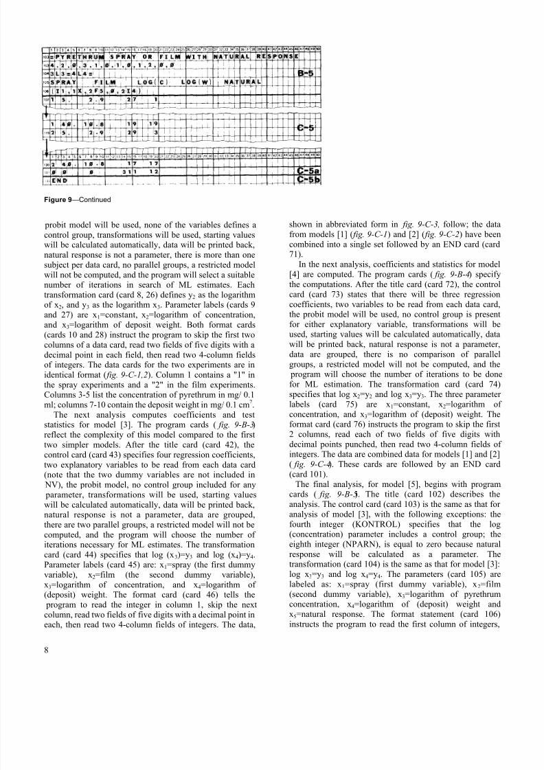
4.1.4 InputThe input for these analyses consists of 132 cards ( fig. 9).

The starter cards ( fig. 9-A) are followed by the first set of

program cards ( fig. 9-B-1) for the pyrethrum sprayapplication (model [1]). The data cards are next ( fig . 9-C-1); an "END" card indicates that another problemfollows. The next problem, pyrethrum film (model [2]),

begins with its program cards ( fig. 9-B-2), followed by the

data and an END card ( fig. 9-C-2).Except for the title cards (cards 6 and 24), the program

cards for the first two data sets are identical. Each control

card (cards 7 and 25) specifies three regression coefficients,

and two variables to be read from each data card. The

7



Figure 9—Continued

probit model will be used, none of the variables defines a

control group, transformations will be used, starting valueswill be calculated automatically, data will be printed back,

natural response is not a parameter, there is more than one

subject per data card, no parallel groups, a restricted modelwill not be computed, and the program will select a suitablenumber of iterations in search of ML estimates. Each

transformation card (card 8, 26) defines y2 as the logarithmof x2, and y3 as the logarithm x3. Parameter labels (cards 9

and 27) are x1=constant, x2=logarithm of concentration,

and x3=logarithm of deposit weight. Both format cards

(cards 10 and 28) instruct the program to skip the first two

columns of a data card, read two fields of five digits with a

decimal point in each field, then read two 4-column fieldsof integers. The data cards for the two experiments are in

identical format ( fig. 9-C-1,2). Column 1 contains a "1" in

the spray experiments and a "2" in the film experiments.

Columns 3-5 list the concentration of pyrethrum in mg/ 0.1ml; columns 7-10 contain the deposit weight in mg/ 0.1 cm2.

The next analysis computes coefficients and teststatistics for model [3]. The program cards ( fig. 9-B-3)

reflect the complexity of this model compared to the first

two simpler models. After the title card (card 42), the

control card (card 43) specifies four regression coefficients,

two explanatory variables to be read from each data card(note that the two dummy variables are not included in

NV), the probit model, no control group included for any

parameter, transformations will be used, starting values

will be calculated automatically, data will be printed back,natural response is not a parameter, data are grouped,

there are two parallel groups, a restricted model will not be

computed, and the program will choose the number of iterations necessary for ML estimates. The transformation

card (card 44) specifies that log (x3)=y3 and log (x4)=y4.

Parameter labels (card 45) are: x1=spray (the first dummy

variable), x2=film (the second dummy variable),

x3=logarithm of concentration, and x4=logarithm of (deposit) weight. The format card (card 46) tells the

program to read the integer in column 1, skip the next

column, read two fields of five digits with a decimal point ineach, then read two 4-column fields of integers. The data,

8

shown in abbreviated form in fig. 9-C-3, follow; the data

from models [1] ( fig. 9-C-1) and [2] ( fig. 9-C-2) have been

combined into a single set followed by an END card (card71).

In the next analysis, coefficients and statistics for model[4] are computed. The program cards ( fig. 9-B-4) specify

the computations. After the title card (card 72), the control

card (card 73) states that there will be three regression

coefficients, two variables to be read from each data card,the probit model will be used, no control group is present

for either explanatory variable, transformations will beused, starting values will be calculated automatically, data

will be printed back, natural response is not a parameter,

data are grouped, there is no comparison of parallel

groups, a restricted model will not be computed, and the program will choose the number of iterations to be done

for ML estimation. The transformation card (card 74)

specifies that log x2=y2 and log x3=y3. The three parameter labels (card 75) are x1=constant, x2=logarithm of

concentration, and x3=logarithm of (deposit) weight. Theformat card (card 76) instructs the program to skip the first

2 columns, read each of two fields of five digits with

decimal points punched, then read two 4-column fields of integers. The data are combined data for models [1] and [2]

( fig. 9-C-4). These cards are followed by an END card

(card 101).

The final analysis, for model [5], begins with programcards ( fig. 9-B-5). The title (card 102) describes the

analysis. The control card (card 103) is the same as that for

analysis of model [3], with the following exceptions: the

fourth integer (KONTROL) specifies that the log

(concentration) parameter includes a control group; theeighth integer (NPARN), is equal to zero because natural

response will be calculated as a parameter. Thetransformation (card 104) is the same as that for model [3]:

log x3=y3 and log x4=y4. The parameters (card 105) are

labeled as: x1=spray (first dummy variable), x2=film

(second dummy variable), x3=logarithm of pyrethrumconcentration, x4=logarithm of (deposit) weight and

x5=natural response. The format statement (card 106)

instructs the program to read the first column of integers,



skip the next column, read two 5-digit fields each of which

includes a decimal point, then read two 4-column fields of

integers. The data cards ( fig. 9-C-5) are followed by thenatural response data card ( fig. 9-C-5a), then the END card

( fig. 9-C-5b).

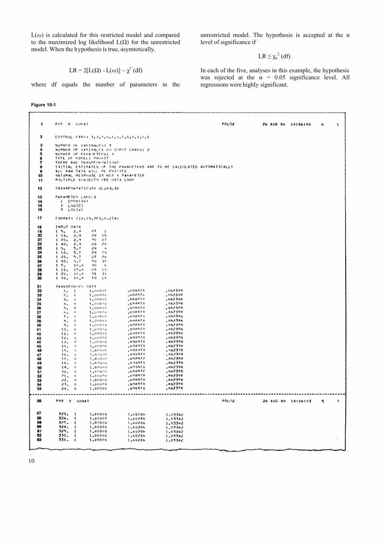
4.1.5 OutputThe output for the five analyses is shown in figure 10.

Except where noted, each analysis is shown in its entirety.The title of the analysis is printed as the first line on each

page ( fig. 10-1, lines 1 and 56; fig. 10-2, lines 94 and 149; fig.

10-3, lines 184, 239, 297; fig. 10-4, lines 324, 378, and 435; fig. 10-5, lines 459, 514, and 573). Next, each control card is

listed ( fig. 10-1, line 2; fig. 10-2, line 95; fig . 10-3, line 185; fig. 10-4, line 325; fig. 10-5, line 460). The subsequent

section of the printout describes the specifications of the

analysis and reflects the information on the control card( fig. 10-1, lines 3-11; fig. 10-2, lines 96-104; fig. 10-3, lines

186-195; fig. 10-4, lines 326-334; fig. 10-5, lines 461-471).

Transformations are reproduced in RPN, just as they

were punched on the transformation card ( fig. 10-1, line 12;

fig. 10-2, line 105; fig. 10-3, line 196; fig. 10-4, line 335; fig.10-5, line 472). Parameter labels are reproduced next ( fig.

10-1, lines 13-16; fig. 10-2, lines 106-109; fig . 10-3, lines 197-

201; fig. 10-4, lines 336-339; fig. 10-5, lines 473-478),followed by the format statement ( fig. 10-1, line 17; fig. 10-

2, line 110; fig. 10-3, line 202; fig. 10-4, line 340; fig. 10-5,

line 479).In the next section, input data are listed as punched on the

data cards ( fig. 10-1, lines 18-30; fig. 10-2, lines 111-123;

fig. 10-3, lines 203-227; fig. 10-4, lines 341-363; fig. 10-5,

lines 480-505). The transformed data are listed after the

data input. For the purposes of computation of the prediction success table and other statistics, grouped data

are now listed as individual cases. This section of the

output has been abbreviated in the figure ( fig. 10-1, lines31-65; fig. 10-2, lines 124-155; fig. 10-3, lines 228-292; fig.

10-4, lines 364-429; fig. 10-5, lines 506-570). At the end of

the transformed data, the total number of cases

(observations plus controls) is summarized ( fig. 10-1, line66; fig. 10-2, line 156; fig. 10-3, line 293; fig. 10-4, line 430;

fig. 10-5, line 571). Proportional control mortality is also

printed ( fig. 10-5, line 572).

Initial estimates of the parameters that were computed

by the program are printed ( fig. 10-1, lines 67-68; fig. 10-2,

lines 157-158; fig. 10-3, lines 294-295; fig. 10-4, lines 431-

432; fig. 10-5, lines 574-577), followed by the initial value of

the log likelihood ( fig. 10-1, line 69; fig. 10-2, line 159; fig.

10-3, line 296; fig. 10-4, line 433; fig. 10-5, line 578). The program begins with logit iterations that are

computationally simpler, then switches to probitcalculations. The number of iterations of each type are

listed ( fig. 10-1, lines 70-71; fig. 10-2, lines 160-161; fig. 10-

3, lines 298-299; fig. 10-4, lines 434, 436; fig. 10-5, lines 579-

580) preceding the final value of the log likelihood ( fig. 10-

1, line 72; fig. 10-2, line 162; fig. 10-3, line 300; fig. 10-4, line

437; fig. 10-5, line 581).

Parameter values, their standard errors, and their t-

ratios (parameter values divided by its standard error) are

then presented ( fig. 10-1, lines 73-76; fig. 10-2, lines 163-166; fig. 10-3, lines 301-305; fig. 10-4, lines 438-441; fig. 10-

5, lines 582-587). The t-ratios are used to test the

significance of each parameter in the regression. Thehypothesis that a regression coefficient is zero is rejected at

the α = 0.05 significance level when the absolute values of

the t-ratio is greater than t = 1.96, that is, the upper α =0.05significance point of a t distribution with ∞ df. All

parameters in each of the five analyses were significant inthis example. These statistics are followed by the

covariance matrix for the analysis ( fig. 10-1, lines 77-81;

fig. 10-2, lines 167-171; fig. 10-3, lines 306-311; fig. 10-4,lines 442-446; fig. 10-5, lines 588-594).

A prediction success table ( fig. 10-1, lines 82-91; fig. 10-

2, lines 172-181; fig. 10-3, lines 312-321; fig. 10-4, lines 447-

456; fig. 10-5, lines 595-604) lists the number of individualtest subjects that were predicted to be alive and were

actually alive, predicted to be alive but were actually dead,

predicted to be dead and were actually dead, and predicted

to be dead but were actually alive. The numbers are

calculated by using maximum probability as a criterion(Domencich and McFadden 1975). The percent correct

prediction, rounded to the nearest percent, is calculated as

the number predicted correctly (that is, alive when predicted alive, or dead when predicted dead) divided by

the total number predicted in that category, times 100. In

the pyrethrum spray experiment ( fig. 10-1), for example,

89 individuals were correctly forecast as alive, but 26 otherswere dead when they had been predicted to be alive. The

correct percent alive is

89

89 + 26x100,

which is 77 percent ( fig. 10-1, line 90). The overall percentcorrect (OPC) equals the total number correctly predicted

divided by the total number of observations, times 100,

rounded to the nearest percent. In the pyrethrum spray

example, OPC equals

89 + 195

333x100,

or 85 percent ( fig. 10-1, line 91). On the basis of randomchoice, the correct choice should be selected for about 50

percent of the observations. In the five analyses, OPC

values indicate reliable prediction by the models used, since

all were greater than 80 percent.The last portion of the output tests the significance of the

regression coefficients in each regression ( fig. 10-1, lines

92-93; fig. 10-2, lines 182-183; fig. 10-3, lines 322-323; fig.

10-4, lines 457-458; fig. 10-5, lines 605-606). The hypothesis

tested is that all the regression coefficients equal zero. Thishypothesis implies that the probability of death is 0.5 at all

spray concentrations and film deposits. The log likelihood

9



L(ω) is calculated for this restricted model and compared

to the maximized log likelihood L(Ω) for the unrestricted

model. When the hypothesis is true, asymtotically,

LR = 2[L(Ω) - L(ω)] ~ χ 2 (df)

where df equals the number of parameters in the

Figure 10-1

unrestricted model. The hypothesis is accepted at the α level of significance if

LR ≤ χ α 2 (df).

In each of the five, analyses in this example, the hypothesiswas rejected at the α = 0.05 significance level. All

regressions were highly significant.

10



Figure 10-1—Continued

Figure 10-2

11




12



Figure 10-3

13




14



Figure 10-4

15




Figure 10-5

16




17




18



4.1.6 Hypotheses TestingThe maximized log likelihood values needed to test the

hypotheses outlined in section 4.1.2 are:

Model L Source

[1] -101.3851 fig. 10-1, line 72

[2] -122.4908 fig. 10-2, line 162

[3] -225.1918 fig. 10-3, line 300

[4] -225.8631 fig. 10-4, line 437

The LR tests of the three hypotheses are the following:(1) Hypothesis H(P) of parallelism.

L(Ω) = -101.3851 + -122.4908

= -223.8759,L(Ω) = -225.1918,

LR = 2[L(Ω) - L(ω)] = 2[-223.8959 + 225.1918]

= 2[l.3159] = 2.6318.

The hypothesis H(P) is accepted, at significance level α =

0.05 if

LR ≤ χ 2.05(2) = 5.99.

Since 2.6318 < 5.99, we accept H(P).

(2) Hypothesis H(E|P) of equality given parallelism.

L(Ω) = -225.1918,

L(ω) = -225.8631,

LR = 2[L(Ω) - L(ω)] = 2[-225.1918 + 225.8631]= 2[0.6713] = 1.3426.

The hypothesis H(E|P) is accepted at level α = 0.05 if

LR ≤χ 2.05(1)=3.84.

Since 1.3426 < 3.84, we accept H(E| P).

(3) Hypothesis H(E) of equality.

L(Ω) = -223.8759,

L(ω) = -225.8631,LR = 2[L(Ω) - L(ω)] = 2[-223.8759 + 225.8631]= 2[1.9872] = 3.9744.

The hypothesis H(E) is accepted at level α = 0.05 if

LR ≤ χ 2.05(3) = 7.81.

We also accept this hypothesis since 3.9744 < 7.81.

4.1.7 Comparison with Published CalculationsThe analyses of models [1]-[4] cannot be compared

directly with those described by Finney. The parameter values for model [5] confirm those of Finney's equations

(8.27) and (8.28) (Finney 1971, p. 169).

4.2 Vaso-Constriction

Finney (1971, p. 183-190) describes a series of

measurements of the volume of air inspired by humansubjects, their rate of inspiration, and whether or not a

vaso-constriction reflex occurred in the skin of their

fingers. These experiments were reported originally by

Gilliatt (1947). A feature of this example is that the data are

ungrouped. We use the example to illustrate the analysis of

ungrouped data, the likelihood ratio test for equalregression coefficients, and the use of transformations.

4.2.1 Models, Hypothesis, and Analyses RequiredThe model expressing the probability of the vaso-

constriction reflex is

Y=α+ β 1x1 + β 2x2 [1]

where y is the probit or logit of the probability, α is the

constant term, x1 is the logarithm volume of air inspired in

liters, x2 is the logarithm of rate of inspiration in liters per

second, β 1 is the regression coefficient for volume, and β 2 is

the regression coefficient for rate.The hypothesis is H: β 1= β 2 which states that the

regression coefficients for rate and volume of air inspired

are the same. The unrestricted model is [1] and therestricted model is

Y = α + β (xl+x2) = α + β x [2]

The required maximum log likelihoods are L(Ω) and L(ω).(i) L(Ω): ML estimation of [1].


When the hypothesis H is true, asymptotically,

LR = 2[L(Ω) - L(ω)] ~ χ 2 (1)

so that the hypothesis H is accepted at the α level of

significance if

LR ≤ χ α 2 (1).

4.2.2 InputThe input for analyses of the two required models

consists of 97 cards ( fig. 11). After the starter cards ( fig. 11-

A), program cards specify the analysis of model [1] ( fig. 11-

B-1). The title card (card 6) cites the source of the data; the

control card (card 7) specifies three regression coefficients,two variables to be read from each data card, the probit

model to be used, none of the explanatory variables

contains a control group, transformations will be used,

starting values of the parameters will be calculated

automatically, data will be printed back, natural responseis not a parameter, there is one subject per data card, there

are no parallel groups, a restricted model will not be

computed, and the program will select a suitable number of

iterations in serach of an ML estimate. The transformationcard (card 8) defines y2 as the logarithm of x2, and y3 as the

logarithm of x3. The three parameters (card 9) are labeled

constant (x1), volume (x2), and rate (x3). The formatstatement (card 10) instructs the program to read a 5-

column field including a decimal point (volume), and a 6-

column field including a decimal point (rate), and finally, a

single column of integers (l=constricted, 0=not

constricted). The data, consisting of 39 individual records,

19



term. The

130-138). Each

lines 12 and

in both raw and

follows ( fig. 11-C-1). After the END card (card 51), the

input for analysis of model [2] follows.

The program cards for model [2] ( fig. 11-B-2) begin witha descriptive title (card 52); the control card (card 53)

differs from that for model [1] only in the NVAR position

(integer 1). In this analysis, there are only two regression

coefficients n addition to the stant

transformations are also different (card 54). The variable

y2=x is defined as the sum of the logarithm of x2 and thelogarithm of x3. The two parameter labels are "constant"

and "combine" (card 55). The format statement (card 56)and the data ( fig. 11-C-2) are identical to that in the

analysis of model [1].

4.2.3 OutputThe analyses, in their entirety, are shown in figure 12.

Titles for the analyses are reprinted at the top of each page

( fig. 12, lines 1, 57, 110, 128, 184, and 235). Integers from

the control cards ( fig. 12, lines 2 and 129) begin each printout, followed by specification statements for each

analysis fig. , es 11 and

transformation card is reproduced ( fig. 12,139), after which the parameter labels are stated ( fig. 12,

lines 13-16; lines 140-142). Format statements ( fig. 12, lines

17 and 143) precede listings of data

transformed versions ( fig. 12, lines 18-56 and 58-98, lines

144-183 and 185-224). From left to right, the columns in thetransformed data listing are chronological number of the

individual, its response, sample size (=1 is all cases),

logarithm (base 10) of volume, and logarithm (base 10) of

i con

( 12 lin 3-

20



rate. The summary of total observations concludes the

descriptive portion of each printout ( fig. 12, lines 99 and

225.

Initial parameter estimates, starting ML values, and

iteration statements ( fig. 12, lines 100-104; lines 226-230)

begin the statistical portion of each printout. The final ML

estimate follows ( fig. 12, lines 105 and 231); parameter

values, their standard errors, and t-ratios ( fig. 12, lines 106-

109; lines 232-234) are printed next. The covariance matrixand prediction success table follow ( fig. 12, lines 111-125;

lines 236-249). Note that the program's automatic dead-

alive category labels are not appropriate for this

experiment; labels such as constricted and not constricted

would be more appropriate. The LR test for significance of

the model coefficients ends each analysis ( fig. 12, lines 126-

127; lines 250-251).

The t-ratios of the parameters for both models indicate

that each parameter is significant in the regression. The

Figure 12

OPC values indicate that each model is a good predictor of

observed results, and the LR tests indicate that both

regressions are highly significant (α = 0.05).

4.2.4 Hypothesis TestingThe maximum log likelihoods needed to test the

hypothesis H: β 1=: β 2 are:

Model L Source

[1] -14.6608 fig. 12, line 105

[2] -14.7746 fig. 12, line 231

In this example

L(Ω) = -14.6608,

L(ω) = -14.7746,

LR = 2[L(Ω) - L(ω)] = 2[0.1138] = 0.2276.

For a test at the 0.05 significance levels, the χ 2 critical value

is 3.84. Hence we accept the hypothesis H.

21




22




23



4.3 Body Weight as a Variable: Higher Order Terms

Robertson and others (1981) described a series of

experiments designed to test the hypothesis that the

response of an insect (Choristoneura occidentalisFreeman) is proportional to its body weight. Three

chemicals, including mexacarbate, were used. We use data

for tests with mexacarbate to illustrate the use of individual

data to test the significance of a higher order term in a

polynomial model. This example demonstrates the use of the restricted model option of POLO2 (see section 2.3).

Briefly, each insect in this experiment was selected at

random from a laboratory colony, weighed, and treated

with 1 µl of mexacarbate dissolved in acetone. Mortalitywas tallied after 7 days. Individual records for 253 insects

were kept. Because a printback of all the data is too

voluminous for this report, we use the program option of IECHO=0 (see section 2.3).

4.3.1 Models and HypothesisThe polynomial model is

y = δ0 + δ1x1 + δ2x2 + δ3z

where y is the probit or logit of response, x, is the logarithm

of dose (in µg), x2 is the logarithm of body weight (in mg),and z is the square of the logarithm of body weight (z=x2

2).

The regression coefficients are δ0 for the constant, δ1 for log

dose, δ2 for log weight, and δ3 for the square of log weight.The hypothesis is H: δ3=0, that is, the coefficient of the

higher order term in weight equals zero. The unrestricted

model is [1] and the restricted model is

Y = δ0 + δ1x1 + δ2x2 [2]

The required maximum log likelihoods are L(Ω) and L(ω).



When H is true, asymptotically,

LR = 2[L(Ω) - L(ω)] ~ χ 2 (1),

so that H is accepted at level α if

LR ≤ χ 2 (1).

The program will automatically conduct an LR test ofH: δ3=0.

4.3.2 InputThe input for this analysis consists of 263 cards ( fig . 13).

The program cards ( fig. 13-B) follow the usual starter cards( fig. 13-A). Following the title (card 6), the control card

specifies four regression coefficients, two variables to be

read from each data card, the probit model is to be used,the second parameter (log (D)) contains a control group,

transformations will be used, starting values will be

calculated automatically, data printback will be

suppressed, natural response is a parameter, there is one

subject per data card, there are no parallel groups, arestricted model retaining three variables will be

computed, and the program will choose the number of

iterations for M L estimates. The transformations defined

(card 8) are: y2 equals the logarithm of x2, y3 equals thelogarithm of x3, and y4 equals the square of the logarithm

of x3. Parameters are x1="constant," x2="logarithm ofdose," x3="logarithm of weight," x4="(logarithm of

weight)2," and x5="natural response." Suggestive labels

appear on card 9.

The germane information on each data card (card 11-

263, fig. 13-C ) is listed in columns 12-14 (dose), 17-19(weight), and 24 (dead or alive). The format statement

(card 10), therefore, instructs the program to skip the first10 columns, read a 4-column field with two digits to the

right of the decimal point, read a 5-column field with onedigit to the right of the decimal point, then go to column 24

to read an integer. No END card is needed after the data

assuming that no other analysis follows.

Figure 13

25



4.3.3 Outpu t

The title is repeated at the top of each page of the printout ( fig. 14, lines 1, 56, and 101). The initial portions

of the analysis demonstrate the same features noted in

previous examples: the control card listing ( fig . 14, line 2) isfollowed by specification statements ( fig . 14, lines 3-12),

the transformation statement ( fig. 14, line 13), parameter

labels ( fig . 14, lines 14-19), and the format statement ( fig.14, line 20). Because the data printback option was not

used (IECHO=0), the program prints only the first 20 data

cards in raw and transformed versions ( fig. 14, lines 21-55

and 57-65). This permits the user to check a sample to

assure that the data are being transformed correctly. Theobservations summary ( fig . 14, line 66) is followed by the

proportional mortality observed in the controls ( fig . 14,

line 67).

The statistical portion of the printout begins with initial parameter estimates ( fig . 14, line 68-71), the initial log

likelihood values ( fig . 14, line 72), iterations totals ( fig . 14,

lines 73-74) and the final log likelihood value ( fig . 14, line75). These precede the table of parameter values, their

standard errors, and t-ratios ( fig . 14, lines 76-81). In thisexample, the only parameter with a significant t-ratio is

log(D); the values of the ratios for all other parameters fall

below the critical t = 1.96 tabular value. The covariancematrix ( fig . 14, lines 82-88) and prediction success table

( fig . 14, lines 89-98) follow. The OPC indicates good

Figure 14

prediction success. Finally, the significance of the ful

model is tested ( fig . 14, lines 99-100).

The restricted model [2] is computed next, with the (logW)2 parameter omitted ( fig . 14, line 102). The initial

estimates of the parameters that are retained are listed ( fig .

14, lines 103-104), followed by the initial log likelihood

value ( fig . 14, line 105) and the iteration summary ( fig . 14,lines 106-107). The final log likelihood value ( fig . 14, line

108) and parameter estimates with their standard errorsand t-ratios ( fig . 14, lines 109-113) follow. In the restricted

model, the t-ratios of all the parameters except naturalresponse are now significant; this contasts with the lack of

significance of all parameters expect dose in model [1]. The

next portion of the printout is the usual presentation of thecovariance matrix ( fig . 14, lines 114-119), followed by the

prediction success table ( fig . 14, lines 120-129) and LR test

of the hypothesis that the regression coefficients of the

restricted model equal zero ( fig . 14, lines 130-131). Thehypothesis is rejected. Finally, the LR test of the hypothesis

H: δ3=0, which was outlined in section 4.3.1, is presented

( fig . 14, lines 132-133).The maximum log likelihood for the

unrestricted model, the model including (log weight)2, is

L(Ω) = -93.6792 and for the restricted model, the oneexcluding (log weight)2, is L(ω) = -94.9086. Since LR =

2[L(Ω) - L(ω)] = 2(1.2294) = 2.4589 < 3.84, the hypothesis

H is accepted at the 0.05 significance level. Consequently,we conclude that (log weight)2 is not a relevant

explanatory variable in the regression.

26




27




28



4.4 Body Weight as a Variable:PROPORTIONAL Option

Dosage estimates are the primary objective of many

toxicological investigations. The topical application

technique described by Savin and others (1977), for

example, is used to obtain precise estimates of the amountsof chemicals necessary to affect 50 or 90 percent of test

subjects. The quality of chemical applied is known, as is the

weight of test subjects. In the previous example, we testedthe significance of a higher order term in a polynominal

model. On the basis of an LR test, we conclude that the

higher order term was not relevant. The PROPOR-

TIONAL option permits the user to test the hypothesis thatthe response of test subjects is proportional to their body

weight. If the hypothesis of proportionality is correct, LD50

and LD90 estimates at weights chosen by the investigator

can be calculated.

4.4.1 Models and HypothesesWe now consider the model

y = δ0 + δ1x1 + δ2x2

Where y = the probit or logit of the response, x1 = logarithmof the dose (log D), and x2 = logarithm of the weight (log

W). Let δ0= β 0, δ1= β 2, and β 2=δ1 +δ2. Then the model [1] can

be rewritten as

y = β 0 + β 1 log (D/ W) + β 2 log W.

The hypothesis of proportionality is H: β 2=0 (Robertson

and others 1981). The unrestricted model is [1] and therestricted model is

y = β 0 + β 1 log (D/W)

The required maximum log likelihoods are L(Ω) and L(ω).



When the hypothesis H is true, asymptotically,

LR = 2[L(Ω) - L(ω)] ~ χ 2

(1)

so that the hypothesis H is accepted at the α significance

level if

LR ≤ χ 2(1).

The necessary calculations are automatically performedwhen the PROPORTIONAL option is chosen. Note that

the hypothesis can also be tested using the t-ratio for β 2. If

the hypothesis is accepted, the user may obtain LD50 and

LD90 estimates for any body weight desired with themethod described by Savin and others (1981). If the hypo-

thesis is rejected, the BASIC option ( sec. 4.5) should beused.

4.4.2 InputThe input ( fig. 15) may begin with the usual starter cards

( fig. 15-A) unless the PROPORTIONAL option is used

after another analysis (except another PROPORTIONAL

option set or the BASIC option—no other analysis may

follow the use of either). In this example, input begins with

the program cards ( fig. 15-B).The program card must have PROPORTIONAL in

some position from columns 2-80 (card 6). The controlcard (card 7) must have NVAR=3 and KERNEL=2 so that

the proportionality hypothesis will be tested. If the LR test

of proportionality is not needed, NVAR=2 and

KERNEL=0 may be specified; however, we suggest that theLR test be performed unless there is ample evidence that

proportional response can be assumed. NPLL must be zero

in either case, but other integers on the control card may

vary as needed.

In this example, the transformations specified (card 8)

are y2 = log (x2/x3) and y3 = log x3. If the LR test of proportionality is not requested and NVAR=2

KERNEL=0 are present on the control card, thetransformation y2 = log(x2/x3) alone- should be used.

Parameters are: constant, log dose divided by log weight,

Figure 1529



log weight, and natural response. Card 9 has labels

suggestive of these names. The format card (card 10)

instructs the program to read dose ( fig. 15-C , columns 11-14), weight ( fig. 15-C , columns 15-19), and response ( fig .

15-C , column 24) from the data cards. The data cards are

followed by an END card (card 264).

If the proportionality hypothesis is accepted, weightsspecified by the user may be placed behind the END card

to obtain LD50 and LD90 estimates. One weight can be punched on each card in free field format.

4.4.3 OutputThe output follows the usual pattern until the last

portion. Titles appear at the top of each page ( fig. 16 , lines1, 56 and 96). The descriptive section lists specification

statements ( fig. 16 , line 3-12), transformation statement

( fig. 16 , line 13), parameter labels ( fig. 16 , lines 14-18),format statement ( fig. 16 , line 19), abbreviated raw and

transformed data listing ( fig. 16 , lines 20-55 and 57-64), the

observation summary ( fig. 16 , line 65), and the natural

mortality statement ( fig. 16 , line 66).

The statistical portion of the printout begins, as usual,with the initial parameter estimates ( fig. 16 , lines 67-68),

starting log likelihood value ( fig. 16 , line 69), and the

iteration summary ( fig. 16 , lines 70-71) preceding the finallog likelihood value ( fig. 16 , line 72). Parameter values and

statistics ( fig. 16 , lines 73-77), covariance matrix ( fig. 16 ,

lines 78-83), prediction success table with OPC ( fig. 16 ,lines 84-93) and test of significance of coefficients in the full

model [2] follow ( fig. 16 , lines 94-95). The statistics and LR

Figure 16

test for the restricted model [3] are printed next ( fig. 16,

lines 97-124).

4.4.4 Hypothesis TestingThe LR statistic is

LR = 2[L(Ω) - L(ω)] = 2[-94.9086 + 99.4884]

= 2[4.5788] = 9.1596.

The hypothesis of proportionality is rejected at the 0.05

significance level because the χ 2 critical value is 3.84. Notethat the hypothesis is also rejected by the t-test because the

t-ratio for β 2 is -2.92. The calculations in the last section of

the printout are statistics based on average weight; theseshould be disregarded unless the proportionality

hypothesis was accepted (see sec. 4.5.2 for an explanation

of the printout).

4.5 Body Weight as a Variable: BASIC Option

The BASIC option estimates lethal doses D in the

equation

y = β 0+ β 1(log D)+ β 2(log W)

when β 1 ≠ β 2. This model is appropriate when the

proportionality hypothesis has been rejected, as in the

previous example ( sec. 4.4). Calculations are described by

Savin and others (1981).

30




31




32



4.5.1 InputThe input ( fig. 17 ) begins with the usual starter cards

( fig. 17-A) unless the BASIC option follows another

analysis (except another BASIC or PROPORTIONAL

set). In that case, input would begin with the program cards( fig. 17-B). The program cards must have:

1. BASIC is some position on the title card (card 6).2. A control card (card 7) with NVAR=3, NPLL=0, and

KERNEL=0. The basic model is limited to three

regression coefficients (NVAR), no parallel groups,

and no test of a restricted model. The other integersmay vary, as required.

In this example, the transformation card (card 8) states

that y2=log x2 and y3=log x3. The parameters (card 9) are

labeled: "constant," "log(D)," and "log(W)." Naturalresponse is a parameter is this example, but need not be

present in each use of the BASIC option. The format

statement (card 10) instructs the program to read only dose

( fig. 17-C , columns 11-14), body weight ( fig. 17-C , columns

15-19), and response ( fig. 17-C , column 24). The data are

followed by an END card ( fig. 17-D, card 264) and weightcards ( fig. 17-D, cards 265-269).

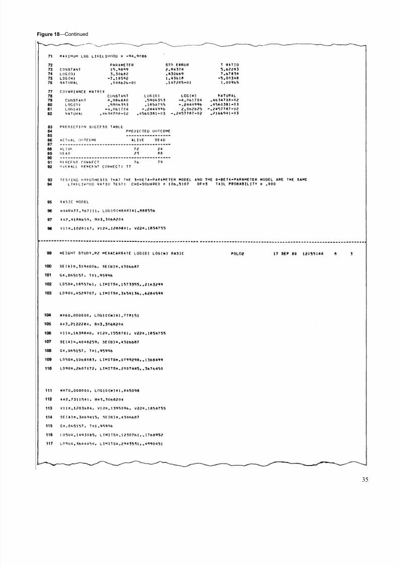
4.5.2 OutputThe BASIC output follows the usual pattern until the

last section. Title repetition on each page ( fig. 18, lines 1,56, 99, and 125), control card listing ( fig. 18, line 2),

specification statements ( fig. 18, lines 3-11), transfor-

mation listing ( fig. 18, line 12), parameter labels ( fig. 18,

lines 13-17), format statement listing ( fig. 16 , line 18), an

abbreviated raw and transformed data listing ( fig. 18, lines

19-55 and 57-63), observations summary ( fig. 18, line 64),and natural response statement ( fig. 18, line 65) form the

descriptive portion of the output.

The statistical portion contains the usual initial

parameter estimates ( fig. 18, lines 66-67), initial loglikelihood value ( fig. 18, line 68), iteration summary ( fig.

18, lines 69-70) final log likelihood value ( fig. 18, line 71), parameter values and statistics ( fig. 18, lines 72-76),

covariance matrix ( fig. 18, lines 77-82), prediction successtable ( fig. 18, lines 83-92), and LR test of the full model ( fig.

18, lines 93-94).

Statistics for the model using average weight of the testsubjects as the value of W follows ( fig. 18, lines 95-98 and

100-102). The terminology of these statistics is as follows.

WBAR is average weight, and LOGIO (WBAR) is the

logarithm of WBAR to the base 10 ( fig. 18, line 96). The parameters are called "A" and "B"; A is the intercept of the

line calculated at WBAR, and B is the slope of the line ( fig.18, line 97). The variances and covariances of the

parameters are listed next ( fig. 18, line 98), followed by the

standard errors of intercept and slope ( fig. 18, line 100).Values of g and t , used to calculate confidence limits

(Finney 1971) for point estimates on a probit or logit line,

appear next ( fig. 16 , line 101). Finally, values of the lethaldose necessary for 50 and 90 percent mortality at WBAR,

together with their 95 percent confidence limits, are printed

( fig. 18, lines 101-102). Next, statistics for each weight

specified on the weight cards ( fig. 17-D, cards 265-269) are

printed ( fig. 18, lines 104-124 and 126-139).

Figure 17.

33



Figure 18

34




35




5. ERROR MESSAGES

Error messages clearly indicate mistakes in the input.

For example:

Message Reason

CONTROL CARD: One of the integers is missing from

4,4,0,2,1,0,0,0,0,3,0 the control card.

THERE SHOULD BE 12

NUMBERS, NOT 11

FORMAT: The parenthesis preceding T24

(10x,F4.2,F5.I(T24,I1) should have been a comma.

36

ILLEGAL FORMAT

CHARACTERS WERE

ACCEPTED AS BLANKS

TRANSFORMATIONS: An extra "3" was punched ("33"

L2=3L3=3L33L3*4= should be "3"), so an extra x3 was

STACK MUST BE EMPTY AT put into the sta ck. The sta ck,END OF POLISH STRING therefore, was not empty at the end

of the scan. See section 2.4.1.

CONTROL CARD: The 3 belon ged in the KERN EL

4,4,0,2,1,0,0,0,0,3,0,0 column, not in the NPLL column.

THERE ARE NOW

16750372454

PARALLEL GROUPS,

EXCEEDING 3

Along with the error message, the user will receive a

message guaranteed to catch the eye.



6. REFERENCES

Domencich, T.A.; McFadden, D. Urban travel demand. New York:

American Elsevier Co.; 1975. 215 p.

Finney, D. J. Probit analysis. 3d ed. London: Cambridge University

Press; 1971. 333 p.Gilliatt, R. M. Vaso-constriction in the finger following deep inspiration.

J. Physiol. 107:76-88; 1947.

Maddala, G. S. Econometrics. New York: McGraw-Hill Book Co.; 1977.

516 p.

Robertson, Jacqueline L.; Russell, Robert M.; Savin, N. E. POLO: a

user's guide to Probit or Logit analysis. Gen. Tech. Rep. PSW-38.

Berkeley, CA : Pacific Southwest Forest and Range Experiment

Station, Forest Service, U.S. Department of Agriculture; 1980. 15 p.

Robertson, Jacqueline L.; Russell, Robert M.; Savin, N. E. POLO2: a

new computer program for multiple probit or logit analysis. Bull.

Entomol. Soc. Amer. (In press.) 1981.

Robertson, Jacqueline L.; Savin, N. E.; Russell, Robert M. Weight as a

variable in the response of the western spruce budworm to insecticides.

J. Econ. Entomol. (In press.) 1981.

Russell, Robert M.; Robertson, Jacqueline L.; Savin, N. E. POLO: a new

computer program for probit analysis. Bull. Entomol. Soc. Amer.

23(3):209-213; 1977 September.

Savin, N. E.; Robertson, Jacqueline L.; Russell, Robert M. A critical

evaluation of bioassay in insecticide research: likelihood ratio tests to

dose-mortality regression. Bull. Entomol. Soc. Amer. 23(4):257-266;

1977 December.

Savin, N. E.; Robertson, Jacqueline L.: Russell, Robert M. Effect of

insect weight on lethal dose estimates for the western spruce budworm.

J. Econ. Entomol. (In press.) 1981.

Tattersfield, F.; Potter, C. Biological methods of determining the

insecticidal values of pyrethrum preparations (particularly extracts in

heavy oil). Ann. Appl. Biol. 30:259-279: 1943.

37



The Forest Service of the U.S. Department of Agriculture

. . . Conducts forest and range research at more than 75 locations from Puerto Rico toAlaska and Hawaii.

. . . Participates with all State forestry agencies in cooperative programs to protect and

improve the Nation's 395 million acres of State, local, and private forest lands.

. . . Manages and protects the 187-million-acre National Forest System for sustainedyield of its many products and services.

The Pacific Southwest Forest and Range Experiment Station. . . Represents the research branch of the Forest Service in California, Hawaii, and the

western Pacific.

GPO 793-057/40



Russell, Robert M.; Savin, N.E.; Robertson, Jacqueline L. POLO2: a user's guide to

multiple Probit Or LOgit analysis. Gen. Tech. Rep. PSW-55. Berkeley, CA: Pacific

Southwest Forest and Range Experiment Station, Forest Service, U.S. Departmentof Agriculture; 1981. 37 p.

This guide provides instructions for the use of POLO2, a computer program for

multivariate probit or logic analysis of quantal response data. As many as 3000 test

subjects may be included in a single analysis. Including the constant term, up to nineexplanatory variables may be used. Examples illustrating input, output, and uses of

the program's special features for hypothesis testing are included.

Retrieval terms: multiple probit analysis, multiple logit analysis, multivariate analysis

polo2: a user's guide to multiple probit or logit analysis

Documents