comparing logit and probit coefficients across groups

Using Heterogeneous Choice Models

To Compare Logit and Probit Coefficients Across Groups

Revised March 2009*

Richard Williams, [email protected]

* A final version of this paper appears in Sociological Methods and Research, May 2009,

Volume 37 Number 4, pp. 531-559.

mailto:[email protected]

About the Author Richard Williams is Associate Professor and a former Chairman of the Department of Sociology

at the University of Notre Dame. His teaching and research interests include Methods and

Statistics, Demography, and Urban Sociology. His work has appeared in the American

Sociological Review, Social Problems, Demography, Sociology of Education, Journal of Urban

Affairs, Cityscape, Journal of Marriage and the Family, The Stata Journal, and Sociological

Methods and Research. His current research, which has been funded by grants from the

Department of Housing and Urban Development and the National Science Foundation, focuses

on the causes and consequences of inequality in American home ownership.

User-written software

The Stata oglm command used in this paper was written by the author. Users of Stata 9 or higher

with Internet access can install the program by starting Stata and then giving the command

ssc install oglm. Those without Stata 9 can achieve similar results with SPSS‟s PLUM

routine.

Acknowledgements

The author thanks Sarah Mustillo, Dan Powers, Richard Campbell, William Greene, J. Scott

Long, Michael Lacy, Brian Miller and three anonymous reviewers for their helpful comments on

earlier versions of the manuscript. He also thanks Joseph Hilbe, Rory Wolfe and Jeff Pitblado

for their input on developing the oglm program. Also thanks to Roy Wada and Ben Jann, whose

user-written Stata routines outreg2 and estout greatly simplified the preparation of many of the

tables in this paper.

Using Heterogeneous Choice Models to Compare Logit & Probit Coefficients Across Groups – Page 1



Revised March 2009

Abstract

Allison (1999) notes that comparisons of logit and probit coefficients across groups can be

invalid and misleading. He proposes a procedure by which these problems can be corrected, and

argues that “routine use [of this method] seems advisable” and that “it is hard to see how [the

method] can be improved.” We argue that, as originally proposed, this method can have serious

problems and should not be applied on a routine basis. However, we also show that the model

used by Allison is part of a larger class of models variously known as heterogeneous choice or

location-scale models. We illustrate that there are several advantages to turning to this broader

and more flexible class of models. Dependent variables can be ordinal in addition to binary,

sources of heterogeneity can be better modeled and controlled for, and insights can be gained

into the effects of group characteristics on outcomes that would be missed by other methods.




Revised March 2009

I Introduction

Allison (1999) argues that we are often interested in comparing how the effects of variables

differ across groups (e.g. is the effect of education on income greater for men than it is for

women?). HOWEVER, when doing logistic regression, there is a potential pitfall in cross-group

comparisons that, Allison claims, has largely gone unnoticed. Unlike linear regression

coefficients, coefficients in binary regression models are confounded with residual variation

(unobserved heterogeneity). Differences in the degree of residual variation across groups can

produce apparent differences in slope coefficients that are not indicative of true differences. He

proposes a procedure by which these problems can be corrected, and argues that “routine use [of

this method] seems advisable” and that “it is hard to see how [the method] can be improved.”

In this paper, we argue that heterogeneous choice (also known as location scale) models provide

a superior means for dealing with the problems Allison presents. We show that Allison‟s

solution actually involves a special case of these models, the heteroskedastic logit model. While

this more limited method works well in some situations, in other cases it can produce biased and

inefficient estimates and can lead researchers to either overstate or understate the statistical and

substantive significance of the differences that are found. With heterogeneous choice models,

the determinants of heteroskedasticity can be better modeled, dependent variables can be ordinal

in addition to binary, and widely available commercial software can be used.


II The problem with comparing logit and probit coefficients across groups, and

Allison’s proposed solution

Allison illustrates his concerns via the analysis of a data set of 301 male and 177 female

biochemists (for a detailed description of the data, set Long, Allison and McGinnis 1993; the

description provided here is adapted from Allison‟s 1999 paper). These scientists were assistant

professors at graduate universities at some point in their careers. Allison uses logistic

regressions to predict the probability of promotion to associate professor. The units of analysis

are person-years rather than persons, with 1,741 person-years for men and 1,056 person-years for

women1.

In his analysis, the dependent variable is coded 1 if the scientist was promoted to associate

professor in that person-year, 0 otherwise. (After promotion no additional person-years are added

for that case.) Duration is the number of years since the beginning of the assistant professorship,

undergraduate selectivity is a measure of the selectivity of the colleges where scientists received

their bachelor‟s degrees, number of articles is the cumulative number of articles published by the

end of each person-year, and job prestige is a measure of prestige of the department in which

scientists were employed. His results are reprinted in Table 1.

Table 1 About Here

As Table 1 shows, the effect of number of articles on promotion is about twice as great for males

as it is females. If accurate, this difference suggests that men get a greater payoff from their

published work than do females, “a conclusion that many would find troubling” (Allison 1999, p.

186).


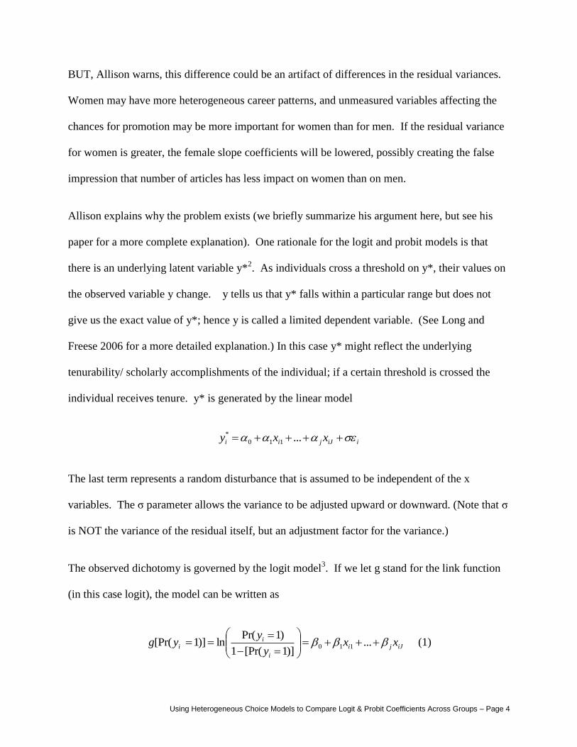
BUT, Allison warns, this difference could be an artifact of differences in the residual variances.

Women may have more heterogeneous career patterns, and unmeasured variables affecting the

chances for promotion may be more important for women than for men. If the residual variance

for women is greater, the female slope coefficients will be lowered, possibly creating the false

impression that number of articles has less impact on women than on men.

Allison explains why the problem exists (we briefly summarize his argument here, but see his

paper for a more complete explanation). One rationale for the logit and probit models is that

there is an underlying latent variable y*2. As individuals cross a threshold on y*, their values on

the observed variable y change. y tells us that y* falls within a particular range but does not

give us the exact value of y*; hence y is called a limited dependent variable. (See Long and

Freese 2006 for a more detailed explanation.) In this case y* might reflect the underlying

tenurability/ scholarly accomplishments of the individual; if a certain threshold is crossed the

individual receives tenure. y* is generated by the linear model

iiJjii xxy ...110

*

The last term represents a random disturbance that is assumed to be independent of the x

variables. The ζ parameter allows the variance to be adjusted upward or downward. (Note that ζ

is NOT the variance of the residual itself, but an adjustment factor for the variance.)

The observed dichotomy is governed by the logit model3. If we let g stand for the link function

(in this case logit), the model can be written as

iJji

i

ii xx

y

yyg

...

)]1[Pr(1

)1Pr(ln)]1[Pr( 110 (1)


Note that, in a logistic regression, what we actually estimate are the βs rather than the αs. As

Allison (1999, citing Amemiya 1985:269) notes, the αs and the βs are related this way:

Jjjj ,,1/ (2)

As the above equations imply, we cannot actually estimate the αs and ζ separately; all we can

estimate are their ratios, the βs.

A problem arises when residual variances differ across groups. Two groups could have identical

values on the αs – but if their residual variances differ, their βs will differ as well. Similarly, the

α values could be larger in one group; but if the residual variance is also greater for that group,

the β values for the two groups could be equal. It is even possible for the α values to be larger

for one group, but if its residual variance is large enough its βs could be smaller than the other

group‟s.

To further clarify, we can think of this as being very similar to the well-known problems with

comparing standardized OLS regression coefficients across groups (Duncan 1968). In OLS,

variables are often standardized by rescaling them to have a variance of one and a mean of zero.

If variances differ across groups, the standardization will also differ across groups, making

coefficients non-comparable. For example, the non-standardized effects of education can be

compared across groups in OLS regression, because education is measured the same way in both

groups. But, if the variance of education differs across groups, the standardized coefficients will

not be comparable because education will get rescaled differently in the two groups.

Although less obvious, the same problem exists in probit and logit models. As Long and Freese

(2006, p. 134) note,


In the [Linear Regression Model], Var(ε) can be estimated because y is observed.

For the [Binary Regression Model], the value of Var(ε) must be assumed because

the dependent variable is unobserved. The model is unidentified unless an

assumption is made about the variance of the errors. For probit, we assume

Var(ε) = 1… In the logit model, the variance is set to π2/3…

So, in logit and probit models, coefficients are inherently standardized. Rather than

standardizing by rescaling all variables to have a variance of one, as in OLS, the standardization

is accomplished by scaling the variables and residuals so that the residual variances are either

one (as in probit) or π2/3 (as in logit). If residual variances differ across groups, the

standardization will also differ, making comparisons of coefficients across groups inappropriate.

In order to deal with this problem, Allison says we first need to determine if residual variances

differ across groups; and if they do, we have to adjust the slope coefficients to reflect those

differences. His procedure is as follows.

Step 1 (Shown in Table 1 above): Separate logistic regression models are estimated for

each group (which are numbered 0 and 1). This allows the coefficients for all variables to differ

across groups. The log likelihoods from the two separate models are added together4.

Step 2: A model (without interaction terms) is estimated for the entire sample. A dummy

variable for group membership is included. This constrains all coefficients (except the

intercepts) to be the same for both groups5.


Step 3 (shown in the first half of Table 2 below): A parameter called δ is added to the

model from Step 26. Let Gi = 0 for men (group 0) and 1 for women (group 1). The underlying

model (Allison 1999:192) then becomes

1

10

*

j

iiijjii xGy (3)

δ is implicit in the above model because the scaling factor ζ is a function of δ:

i

iG

1

1 (4)

Equivalently, the formula for δ is

1

11

Group

Group

(5)

Once this is done, ζGroup 0 is fixed at 1 while ζGroup 1 is free to vary. δ, then, is an estimate of how

much the disturbance standard deviation differs by group. So, for example, a δ of 1 would

indicate that the disturbance variance of group 0 is 100% higher (i.e. double) the disturbance

variance of group 1. A δ of -.5 indicates that the disturbance variance for group 0 is only half as

large as the variance for group 1. A δ of 0 means that there are no differences in residual

variation across groups. By including δ in the model, the differences in residual variation that

distort cross-group comparisons are presumably controlled for. Note that this model continues to

be estimated under the assumption that the underlying αs for both groups are equal.

Step 4: A series of hypotheses are then tested; and based on these results, additional

models may be estimated7.


o First tested is the null hypothesis that the α coefficients are the same but the

residual variances differ (i.e. δ = 0). This involves a chi-square contrast between

the models from steps 2 and 3. Note that this test is done under the assumption

that the underlying αs for both groups are equal. As we will see, this is a critical

and potentially problematic assumption.

o Second, if the residual variances are found to differ, a global test is done of

whether any αs differ across groups. This involves a chi-square contrast between

the models of Step 3 and Step 1. A significant chi-square value supposedly

indicates that at least one coefficient differs across groups, even after controlling

for differences in residual variation.

o Third, if it is found that at least one coefficient differs across groups, additional

models can be estimated to identify the specific variables whose effects differ.

This is done by adding interaction terms to the model from Step 3 and doing a

chi-square contrast with the Step 3 model. (This is shown in the second half of

Table 2 below.) In order to conduct these tests, however, at least one set of

coefficients must be assumed to be equal across groups. A model with all possible

group interactions and a parameter for differences in residual variation would not

be identified. Again, we will see that this is a critical and potentially problematic

assumption.

The results from this procedure are presented in Table 2.

Table 2 About Here


According to Allison, the estimated δ coefficient value of –.26 in the “All coefficients equal”

model tells us that the standard deviation of the disturbance variance for men (group 0) is 26

percent lower than the standard deviation for women. A likelihood ratio chi-square contrast with

the non-heteroskedastic logit model from Step 2 shows that the estimate of δ is statistically

significant (LR chi-square = 4.50 with 1 d.f.).

With differences in residual variation taken into account, the interaction term for Articles *

Female is NOT statistically significant, i.e. as the final columns of Table 2 show there is no

statistically significant difference in the effects of number of articles on men as opposed to

women. Allison therefore concludes “The apparent difference in the coefficients for article

counts in Table 1 does not necessarily reflect a real difference in causal effects. It can be readily

explained by differences in the degree of residual variation between men and women.” He

further argues that “routine use [of this method] seems advisable” and that “it is hard to see how

[the method] can be improved.”

III Heteroskedastic Logit & Heterogeneous Choice Models

Allison has illustrated a critical problem that researchers need to be aware of8. In assessing his

proposed solution, it is useful to realize that his approach involves (but is not limited to) a re-

parameterization of the heteroskedastic logit model. The heteroskedastic logit model, in turn, is

part of a larger class of models that is variously known as location-scale models (McCullagh &

Nelder 1989) and heterogeneous choice models (Alvarez & Brehm, 1995; Keele & Park, 2006).

Because the term “heterogenous choice” has recently become popular in the social sciences

literature, we will use it throughout the rest of this paper, but readers should remember that the


terms “heterogeneous choice” and “location-scale” are interchangeable and that other authors

prefer the latter.

With heterogeneous choice models, the dependent variable can be ordinal or binary. For a

binary dependent variable, the model (Keele & Park, 2006) can be written as

i

i

i

i

i

ii

xg

xg

z

xgy

))exp(ln()exp()1Pr( (6)

In the above formula,

g stands for the link function (in this case logit; probit is also commonly used, and other

options are possible, such as the complementary log-log, log-log and cauchit).

x is a vector of values for the ith observation. The x‟s are the explanatory variables and

are said to be the determinants of the choice, or outcome.

z is a vector of values for the ith observation. The z‟s can define groups with different

error variances in the underlying latent variable, e.g. the z‟s might include dummy variables for

gender or race. But, the z‟s can also include continuous variables that are related to the error

variances, e.g. as income increases, the error variances may increase. The z‟s and x‟s need not

include any of the same variables, although they can.

β and γ are vectors of coefficients. They show how the x‟s affect the choice and the z‟s

affect the variance (or more specifically, the log of ζ)9.


The numerator in the above formula is referred to as the choice equation, while the

denominator is the variance equation. These are also referred to as the location and scale

equations. Also, the choice equation includes a constant term but the variance equation does not.

Allison‟s model is a special case of the above, where there is a single dichotomous variable in

the variance equation, i.e. the dichotomy indicating group membership. This variable appears in

both the choice and variance equations. In addition, rather than estimating ζ, Allison estimates a

function of ζ that he calls δ.

This equivalence can be illustrated through a re-analysis of the Biochemist data10

. First, we used

Allison‟s Stata program, which was included in the appendix of his article11

. The results are

virtually identical to those published in Table 2 of his paper12

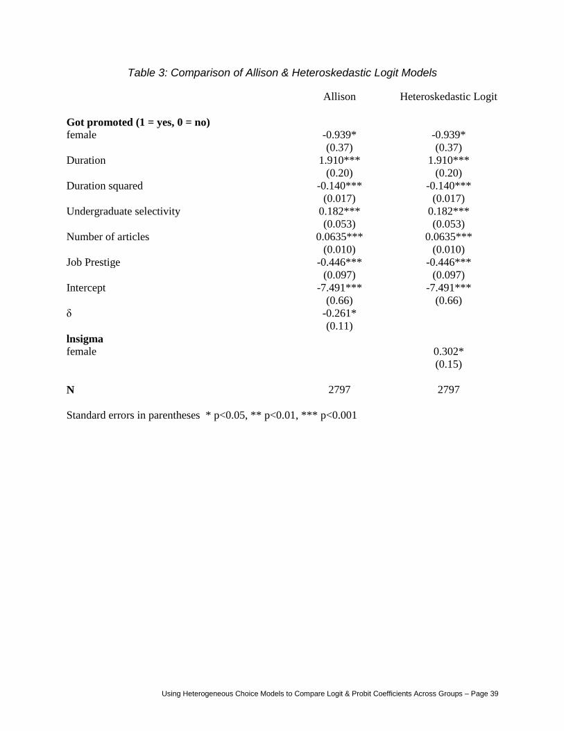
. We then estimated a

heteroskedastic logit model using oglm (Ordinal Generalized Linear Models), a Stata 9 routine

written by Williams (2006b). Table 3 shows the results.

Table 3 About Here

For both models, a Wald test of the hypothesis that the coefficients for the choice coefficients all

equaled zero yielded a chi-square value of 181.39 with 6 degrees of freedom. The differences

between the models are trivial. Allison‟s model includes a parameter for δ while oglm includes a

parameter for the variance. These are simply two equivalent ways of parameterizing the same

concept. 13

In the heteroskedastic logit model, the variance scaling factor for each case is

.3022305)*exp( ii female (7)


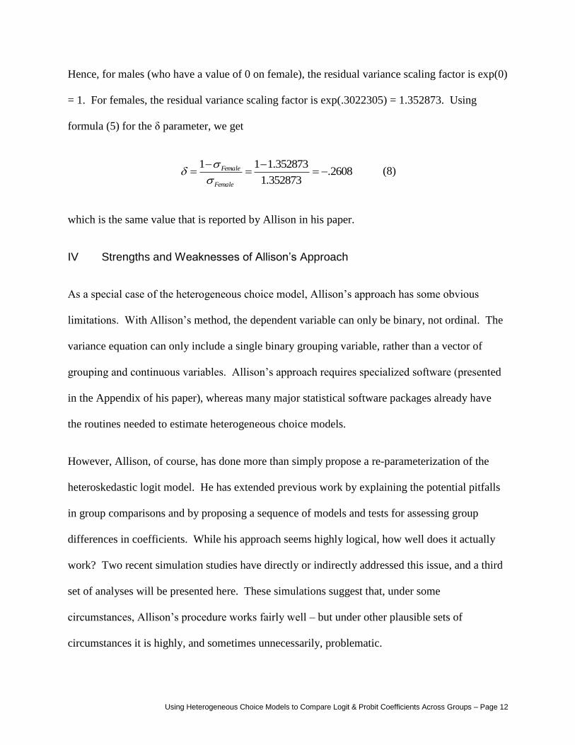
Hence, for males (who have a value of 0 on female), the residual variance scaling factor is exp(0)

= 1. For females, the residual variance scaling factor is exp(.3022305) = 1.352873. Using

formula (5) for the δ parameter, we get

2608.1.352873

1.35287311

Female

Female

(8)

which is the same value that is reported by Allison in his paper.

IV Strengths and Weaknesses of Allison’s Approach

As a special case of the heterogeneous choice model, Allison‟s approach has some obvious

limitations. With Allison‟s method, the dependent variable can only be binary, not ordinal. The

variance equation can only include a single binary grouping variable, rather than a vector of

grouping and continuous variables. Allison‟s approach requires specialized software (presented

in the Appendix of his paper), whereas many major statistical software packages already have

the routines needed to estimate heterogeneous choice models.

However, Allison, of course, has done more than simply propose a re-parameterization of the

heteroskedastic logit model. He has extended previous work by explaining the potential pitfalls

in group comparisons and by proposing a sequence of models and tests for assessing group

differences in coefficients. While his approach seems highly logical, how well does it actually

work? Two recent simulation studies have directly or indirectly addressed this issue, and a third

set of analyses will be presented here. These simulations suggest that, under some

circumstances, Allison‟s procedure works fairly well – but under other plausible sets of

circumstances it is highly, and sometimes unnecessarily, problematic.


Hoetker (2004) did a series of simulations where he examined the problems raised by Allison

and how well Allison‟s method addressed them. He found (p. 17) that “in the presence of even

fairly small differences in residual variation, naive comparisons of coefficients can indicate

differences where none exist, hide differences that do exist, and even show differences in the

opposite direction of what actually exists.” At least in the simulations he ran, he found that

Allison‟s method accurately detected differences in residual variation and false differences in

coefficients, and that it also accurately detected true differences in coefficients.

While Hoetker does raise some concerns14

, overall his simulations would seem to provide

powerful support for Allison‟s method. A closer examination reveals, however, that almost all

of his simulations assumed that (a) there really were differences in residual variation across

groups, and (b) the effects of heteroskedasticity were captured by a single grouping variable. In

other words, they showed that Allison‟s method worked well when the model was correctly

specified. Allison‟s assumptions, however, that there are differences in residual variation, and

that only one grouping variable is needed to capture these differences, may be highly

problematic in practice.

Keele and Park (2006) do not specifically discuss Allison‟s paper, but they do look at the closely

related case of the heteroskedastic probit model. Their analysis was motivated by the

observation (p. 4) that

While heterogenous choice models can be used for either “curing” probit models

with unequal error variances or for testing hypotheses about heterogenous

choices, there is little evidence, analytical or empirical, about how well these

models perform at either task.


To assess the performance of heteroskedastic probit models, Keele and Park use both Monte

Carlo simulations where true parameter values are known, and a re-analysis of the Alvarez and

Brehm (1995) data on abortion attitudes. They find that

Even under ideal conditions, i.e. when the model is correctly specified, estimates from

the heteroskedastic probit model are problematic. Researchers are more likely to conclude that a

parameter is statistically significant when it is not. Alvarez and Brehm (1995) found 22

significant coefficients in their analysis of abortion attitudes; when Keele and Park used

bootstrapped errors, they found that only 13 of the coefficients were significant. Keele & Park

conclude (p. 26) that “the standard errors from heteroskedastic probit models should not be relied

upon. The standard errors from these models are overly optimistic and can lead to incorrect

inferences.”15

Keele and Park also found that the heteroskedastic probit model had even worse

problems when the model was mis-specified. When a relevant variable was excluded from the

variance equation, parameter estimates were actually more biased than when the unequal

variances were ignored altogether. They concluded (p. 27) that

If researchers are only interested in the parameters from the choice model, but

suspect heteroskedasticity, these models may not be the best alternative. If the

error variance differs across well defined groups, specification of the variance

model should be relatively easy. But if the source of the heteroskedasticity is less

clear and harder to specify, it is better to estimate a standard probit and ignore

the heteroskedasticity than poorly specify a heteroskedastic model. [emphasis

added]


To review, Hoetker did simulations where the model was correctly specified and argued that

under those conditions Allison‟s procedure worked fairly well. However, Keele and Park

showed that, even with correct model specification, the standard errors of heteroskedastic probit

models can be biased, and they further showed that serious biases can occur when relevant

variables are omitted from the variance equation. A procedure, such as Allison‟s, that only

allows for a single dichotomous variable in the variance equation would presumably make

omitted variable bias more likely in many situations.

We now consider how well Allison‟s method works under a third plausible set of conditions:

effects of one or more variables differ across populations, but residual variances are the same

across groups and no adjustment for heteroskedasticity is needed. Under these conditions,

Allison‟s method (or any other method with a similar goal) should ideally indicate that

conventional methods for group comparisons using interaction effects are not problematic.

Conversely, the method should NOT lead the researcher to make adjustments that make things

worse rather than better (although as we will see, this is exactly what happens).

Therefore, in these simulations16

, we allowed the effects of independent variables to differ across

populations while the residual variances did not. In equation form, the models for these

simulations can be written as

iiii

iiii

xxcy

xxy

21

*

21

*

*2*1:1 Group

1:0 Group (9)

where the variances of the residuals and the X‟s are identical across groups, and c is a constant

that was varied between .5 and 3.0. Specifically,


we created two groups (numbered 0 and 1) with equal residual variances, i.e. δ = 0.

There was a dichotomous dependent variable Y, and two independent normally

distributed variables, X1 and X2.

X1 and X2 were sampled from hypothetical populations where their variances were 1

and their correlations were 0.

For group 0, the X1 and X2 α coefficients always equaled 1. For group 1, the α for X2

always equaled 2, i.e. was twice as large in group 1 as it was in group 0. The constants

were always fixed at 1 for both groups.

We varied the value for α1 in group 1, starting it at .5 and increasing it gradually to 3.0,

i.e. α1 was sometimes smaller in group 1 than in group 0, and sometimes larger17

.

Each simulation involved 1,000 cases, with 500 members in each group.

For each simulation, we tested (a) the hypothesis that the residual variances were equal,

i.e. δ = 0, and (b) the hypothesis that one or more coefficients still differed across groups

even after allowing for differences in residual variation.

We also estimated a model in which an interaction term was added, allowing the effect of

X2 to differ across groups.

The results of these simulations are presented in Table 4. When viewing these results, keep in

mind that the true conditions are (a) the residual variances do not differ across groups and δ = 0

(b) the coefficients do differ, and (c) the interaction term for X2 is equal to 1. Ideally the results

from the simulations would reflect this.


Table 4 About Here

These results indicate that there are a number of problems with the heteroskedastic logit model

and Allison‟s sequence of tests under the conditions simulated here.

First, in every simulation, the hypothesis of equal residual variances is falsely rejected the vast

majority of the time. Why does this occur? Recall, as Allison pointed out, that the test is done

under the assumption that the α coefficients are the same across groups. This assumption, of

course, is the very thing we eventually want to test. Because the assumption is not true in these

simulations, and because the coefficients are constrained to be equal across groups, the only way

to adjust for differences across groups is by allowing the residual variances to differ. As the

average value of δ indicates, as the simulated value of α1 in group 1 gets larger and larger, δ gets

bigger and bigger. That is, the larger the true difference is between the coefficients in the true

groups, the larger the estimate of δ is to compensate for these differences.

Therefore, the test for equality of residual variances is not very informative, and indeed it really

doesn‟t test what it claims to. A significant test statistic could indicate that residual variances

differ across groups, but it could just as easily indicate that coefficients differ across groups.

Second, the sequence in which hypotheses are tested can affect the conclusions reached. In

Allison‟s example, he first added the δ parameter to his model, noted that it was significant, and

then added the interaction term for gender and articles, which he concluded was insignificant.

However, as Table 2 shows, the δ term also becomes insignificant once the interaction term is

entered. If instead the interaction term for articles is added first, it is significant, and the δ term is

insignificant when it is next added to the model. In other words, the sequence of models gives


preference to the hypothesis of different residual variances over the hypothesis of differing

coefficients, even though (as noted above) the test used cannot distinguish between the two.

Third, Table 4 shows that, when α1 in group 1 is smaller than α1 in group 0, the hypothesis that

the coefficients are equal is usually rejected. This makes sense, since it is highly implausible that

differences in residual variation could account for a situation in which some coefficients were

larger in one group while others were smaller. However, in the next several simulations, as α1

increases, we become increasingly less likely to correctly reject the hypothesis that the

coefficients are equal.

Again, why does this happen? Because in the model that includes δ, true differences in

coefficients are falsely attributed to differences in residual variation. Hence, when the model

that contains δ is contrasted with the model that allows all coefficients to differ across groups,

the differences in coefficients appear to be smaller than they really are, and the statistical

significance of the difference is understated. Allison noted that his procedure would have

problems when the coefficients for one group all differed by a scale factor from the other group –

a situation simulated here when α1 is 2 for group 1 – but as these simulations show, the test for

equal coefficients can have problems under a much broader range of conditions.

The last few columns of Table 4 show what happens when an interaction term is added that

allows the effect of X2 to differ across groups. Recall that tests for interactions must be done

under the assumption that at least one X (in this case X1) has the same effect in both groups. In

only one of these simulations is that assumption true. In that case – where α1 = 1 in both groups

– the interaction term is estimated almost perfectly (average estimated value is 1.063, compared

to the true value of 1.0). When α1 is smaller in group 1, the value of the interaction term is


actually overestimated. As α1 gets greater and greater than 1, the estimated value of the

interaction gets smaller and smaller; indeed it eventually goes negative.

Again, this occurs because the model is estimated under the false assumption that the effect of

X1 is the same in both groups. As a result, the inclusion of the δ parameter erroneously causes

some of the true differences in coefficients to be attributed to differences in residual variation.

When the αs all happen to be larger in one group than the other, the result is a downward bias in

the estimated interaction term. It is not hard to think of situations where this could occur, e.g.

men might benefit more from their education and job experience than women do.

To sum up: Allison‟s procedure requires critical assumptions at two points, and when these

assumptions are incorrect the results can be highly misleading. The test of equal residual

variances requires the assumption that the coefficients are the same in both groups. When this

assumption is wrong, differences in coefficients are erroneously attributed to differences in

residual variance. The test of equal residual variances therefore isn‟t very meaningful, and it

requires that we assume the very thing we eventually want to prove or disprove. The erroneous

inclusion of the δ parameter further biases subsequent tests of whether coefficients differ across

groups. The procedure also requires that, if we want to test whether specific coefficients differ

across groups, we must assume that at least one coefficient is the same in both populations.

When this assumption is correct, the estimates of across-group differences in the other

coefficients are good, but when the assumption is wrong the estimates of other coefficients are

biased upward or downward. In particular, when the coefficients are all larger in one group than

the other, there is a downward bias in the estimated differences across groups.


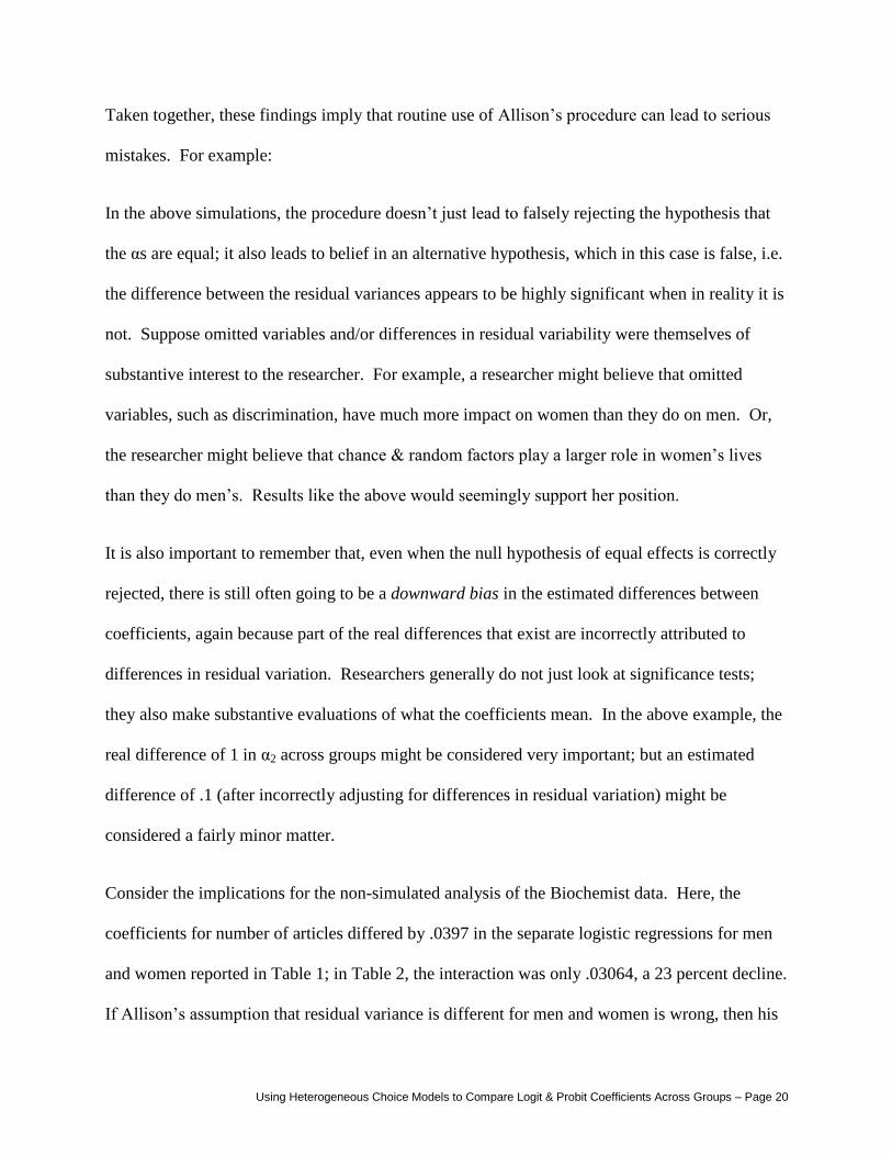
Taken together, these findings imply that routine use of Allison‟s procedure can lead to serious

mistakes. For example:

In the above simulations, the procedure doesn‟t just lead to falsely rejecting the hypothesis that

the αs are equal; it also leads to belief in an alternative hypothesis, which in this case is false, i.e.

the difference between the residual variances appears to be highly significant when in reality it is

not. Suppose omitted variables and/or differences in residual variability were themselves of

substantive interest to the researcher. For example, a researcher might believe that omitted

variables, such as discrimination, have much more impact on women than they do on men. Or,

the researcher might believe that chance & random factors play a larger role in women‟s lives

than they do men‟s. Results like the above would seemingly support her position.

It is also important to remember that, even when the null hypothesis of equal effects is correctly

rejected, there is still often going to be a downward bias in the estimated differences between

coefficients, again because part of the real differences that exist are incorrectly attributed to

differences in residual variation. Researchers generally do not just look at significance tests;

they also make substantive evaluations of what the coefficients mean. In the above example, the

real difference of 1 in α2 across groups might be considered very important; but an estimated

difference of .1 (after incorrectly adjusting for differences in residual variation) might be

considered a fairly minor matter.

Consider the implications for the non-simulated analysis of the Biochemist data. Here, the

coefficients for number of articles differed by .0397 in the separate logistic regressions for men

and women reported in Table 1; in Table 2, the interaction was only .03064, a 23 percent decline.

If Allison‟s assumption that residual variance is different for men and women is wrong, then his


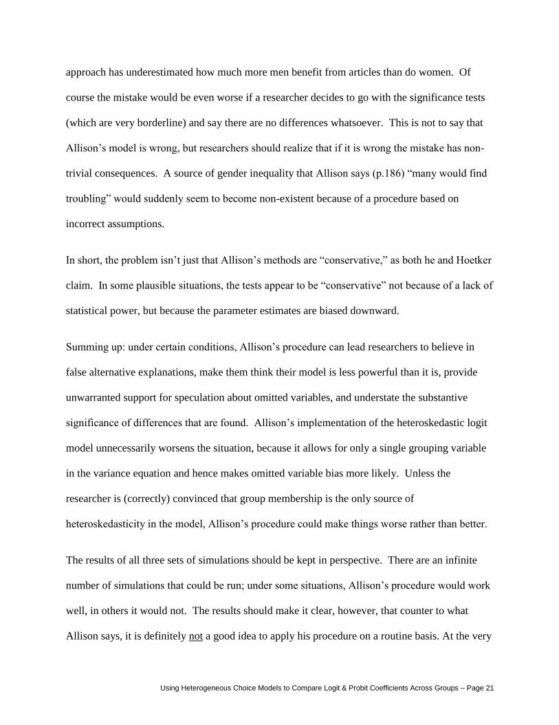
approach has underestimated how much more men benefit from articles than do women. Of

course the mistake would be even worse if a researcher decides to go with the significance tests

(which are very borderline) and say there are no differences whatsoever. This is not to say that

Allison‟s model is wrong, but researchers should realize that if it is wrong the mistake has non-

trivial consequences. A source of gender inequality that Allison says (p.186) “many would find

troubling” would suddenly seem to become non-existent because of a procedure based on

incorrect assumptions.

In short, the problem isn‟t just that Allison‟s methods are “conservative,” as both he and Hoetker

claim. In some plausible situations, the tests appear to be “conservative” not because of a lack of

statistical power, but because the parameter estimates are biased downward.

Summing up: under certain conditions, Allison‟s procedure can lead researchers to believe in

false alternative explanations, make them think their model is less powerful than it is, provide

unwarranted support for speculation about omitted variables, and understate the substantive

significance of differences that are found. Allison‟s implementation of the heteroskedastic logit

model unnecessarily worsens the situation, because it allows for only a single grouping variable

in the variance equation and hence makes omitted variable bias more likely. Unless the

researcher is (correctly) convinced that group membership is the only source of

heteroskedasticity in the model, Allison‟s procedure could make things worse rather than better.

The results of all three sets of simulations should be kept in perspective. There are an infinite

number of simulations that could be run; under some situations, Allison‟s procedure would work

well, in others it would not. The results should make it clear, however, that counter to what

Allison says, it is definitely not a good idea to apply his procedure on a routine basis. At the very


least, researchers need to be aware of its limitations, and realize that procedures that make some

mistakes less likely can also make perhaps-equally serious mistakes more likely. Further,

researchers should also be aware that superior alternatives are often available.

V A Superior Alternative: Heterogeneous Choice Models

As noted before, the heteroskedastic logit model, with a single dichotomous variable in the

variance equation, is a special case of the larger class of models that are variously known as

location-scale models and heterogeneous choice models. These models allow for ordinal

dependent variables and a much more flexible specification of the variance equation. Turning to

this larger class of models offers several ways to improve on Allison‟s approach and hopefully

overcome its most significant weaknesses.

We begin with an example that will illustrate many of our points. Long and Freese (2006)

present data from the 1977/1989 General Social Survey. Respondents are asked to evaluate the

following statement: “A working mother can establish just as warm and secure a relationship

with her child as a mother who does not work.” Responses were coded as 1 = Strongly Disagree

(1SD), 2 = Disagree (2D), 3 = Agree (3A), and 4 = Strongly Agree (4SA). Explanatory variables

are yr89 (survey year; 0 = 1977, 1 = 1989), male (0 = female, 1 = male), white (0 = nonwhite, 1

= white), age (measured in years), ed (years of education), and prst (occupational prestige scale).

Table 5 About Here

In Table 5, we present a series of models for these data, all estimated with the oglm (Williams

2006b) routine in Stata. Model 1 is an ordered logit model, with no controls for


heteroskedasticity. As Williams (2006a) notes, the results from Model 1 are relatively

straightforward, intuitive and easy to interpret. People tended to be more supportive of working

mothers in 1989 than in 1977. Males, whites and older people tended to be less supportive of

working mothers, while better educated people and people with higher occupational prestige

were more supportive. Model 2 further shows that none of the gender interactions terms are

statistically significant.

But, while the results may be straightforward, intuitive, and easy to interpret, are they correct?

Are the assumptions of the ordered logit model met? To answer this question, we first need to

clarify what the assumptions of the ordered logit model are. As Williams (2006a) notes, the

ordered logit model can be written as follows:

1M ..., 2, , 1 j ,)][exp(1

)exp()()(

ij

ij

iX

XXgjYP (10)

where M is the number of categories of the ordinal dependent variable (in this case 4). A key

assumption of the model is that, while the thresholds differ across values of j, the βs do not. This

is referred to as the parallel lines assumption. One of the key advantages of the ordered logit

model is that there are well-established tests for whether the parallel lines assumption is violated;

and as Long and Freese (2006) point out, if the parallel lines assumption is violated, alternative

methods for ordinal regression should be considered. Both Long and Freese (2006) and

Williams (2006a) find that the assumptions of the ordered logit model are indeed violated with

these data. In particular, a Brant test (Brant 1990; Long and Freese 2006) reveals that the

variables yr89 and male do not meet the parallel lines assumption. While this in and of itself

does not necessarily mean that a heterogeneous choice model is called for, oglm‟s stepwise


selection procedure also identifies yr89 and male as statistically significant variables for

inclusion in the variance equation. This implies that residual variability in attitudes toward

working mothers differed by year and by gender, both of which are substantively plausible.

Model 3 therefore is a heterogeneous choice model, allowing for heteroskedasticity for both year

and gender. The negative coefficients for these variables in the variance equation tell us that,

after controlling for other variables, the residual variability in attitudes towards working mothers

declined across time, and that there was less residual variability in men‟s attitudes than there was

for women. The addition of the two heteroskedasticity parameters improves the model fit

significantly (29.3 chi-square with only 2 d.f.). The values of the BIC statistics (Raftery, 1995)

also favor the heterogeneous choice model.

Contingent on the thresholds being the same for both men and women, we can further test

whether any of the coefficients for the choice equation differ by gender. Model 4 adds

interaction terms for gender to Model 3. As was the case with the ordered logit model, none of

the interaction terms for gender are significant. Further, the chi-square contrast between the two

models is 7.04 with 5 d.f., which is also insignificant.

In this case, the interaction effects involving group membership are not significant. Nonetheless,

the heterogeneous choice model yields important insights into the effects of gender and year that

would be overlooked in a mis-specified ordered logit model. An examination of marginal effects

helps to clarify what the substantive differences are between the two models. With marginal

effects, all variables except one are set equal to their means, and we see how changes in the

remaining variables affect the probability of each possible outcome occurring. For a

dichotomous explanatory variable, we measure the effect as the variable changes from 0 to 1.


For continuous variables, the instantaneous rate of change is measured. (See Long and Freese

2006 for a more detailed discussion of marginal effects in categorical models.) Table 6 presents

the marginal effects for the ordered logit and heterogeneous choice models that did not include

the insignificant interaction terms (models 1 and 3 from Table 5)18

. The table illustrates

important differences and similarities for the two models.

Table 6 About Here

Let us begin by noting the similarities. The marginal effects for white, age, ed and prst are very

similar in both models and for all outcomes. These are the four variables that were not included

in the variance equation of the heterogeneous choice model. It is not surprising that both models

therefore largely agree on the effects of these four variables.

The story is very different for the variables yr89 and male. Both models agree that there was a

shift toward more positive attitudes between 1977 and 1989, but they describe that shift

differently. The ordered logit model provides the smallest estimate of the decline in strong

disagreement (4.99% as opposed to 7.86%) and the largest estimate of the increase in strong

agreement (7.35% versus a little over 4%). That is, the heterogeneous choice model says that the

main reason attitudes became more favorable across time was because people shifted from

extremely negative positions to more moderate positions; there was only a fairly small increase

in people strongly agreeing that women should work. The ordered logit model, on the other

hand, understates how much people moved from an extremely negative position and overstates

how much they became extremely positive.


The models also provide different pictures of the effect of gender on attitudes. The ordered logit

model provides a much larger estimate of how much men strongly disagree with a mother

working (7.46% versus 3.55%). However, it also provides the smallest estimates of how much

less likely men are to strongly agree that a woman should work. Again, the ordered logit model

is creating a misleading image of why men were less supportive of working mothers; it isn‟t so

much that men were extremely negative in their attitudes, it is more a matter of them being less

likely than women to be extremely supportive.

The advantages of the heterogeneous choice model can now be summarized as follows:

Even when coefficients do not differ across groups, as in our example, heterogeneous

choice models can yield insights into the effects of group characteristics that would be

overlooked in mis-specified models. That is, the estimated effects of group characteristics (as

well as other variables) can differ once heterogeneity is taken into account.

There is no need to limit the variance equation to a single dichotomous grouping variable.

Multiple grouping variables can be used. Indeed, the variables in the variance equation need not

even be a subset of the variables in the choice equation. This hopefully reduces or even

eliminates problems caused by specification error in the variance equation.

Note further that, while we have primarily focused on group differences in residual

variances, group differences are only one possible source of heteroskedasticity. For example,

heteroskedasticity can be a concern with continuous variables like income, where it may be

unreasonable to assume that errors are the same in magnitude no matter how large the value of

the independent variable is. Unfortunately, unlike OLS, uncorrected heteroskedasticity in a

model with dichotomous or ordinal dependent variables results in biased parameter estimates


(Yatchew & Griliches 1985; Greene 2003; Keele & Park, 2006), for reasons similar to those as

already described for group differences, e.g. if the residual variances differ by income, then the

standardization of coefficients will also differ by income. Therefore, researchers who are

concerned about biased parameter estimates should not confine themselves to the special case of

group differences in residual variances; they should worry about any source of heteroskedasticity

and its possible biasing effects. Indeed, in the Biochemist data, the only variable that enters into

the variance equation using oglm‟s stepwise selection procedure is number of articles. This is

not surprising: there may be little residual variability among those with few articles (with most

getting denied tenure) but there may be much more variability among those with more articles

(having many articles may be a necessary but not sufficient condition for tenure). Hence, while

heteroskedasticity may be a problem with these data, it may not be for the reasons originally

thought19

. Heterogeneous choice models can easily incorporate continuous variables in the

variance equation.

The variance may itself be of substantive interest. The variance equation makes it

possible to examine the determinants of variability. Alvarez and Brehm (1995), for example,

argued that individuals whose core values are in conflict will have a harder time making a

decision about abortion and will hence have greater variability/error variances in their responses.

In the case of the Biochemist data, we might be interested in whether gender, number of articles

or other factors affect the variability in careers.

Heteroskedastic logit and and probit models only work with dichotomous dependent

variables. Heterogeneous choice models also allow for ordinal dependent variables. There are

several advantages to using ordinal variables when possible.


o As Keele and Park (2006) note, ordinal variables contain more information and

models using them are much less prone to problems than are models with

dichotomous dependent variables. Based on their Monte Carlo simulations, they

concluded that, unlike the heteroskedastic probit model, when the model was

correctly specified, “The heteroskedastic ordered probit model can be given a

clean bill of health, as both the level of overconfidence and coverage rates are

close to ideal.” (However, even for a heteroskedastic ordered probit model, they

stressed the importance of the model being correctly specified; a mis-specified

model, e.g. a variance equation with omitted variables might be worse than a

model that made no correction at all for heteroskedasticity.)

o There are well-established diagnostic procedures that can indicate when the

assumptions of the ordered logit model are violated. Based on these diagnostics,

researchers can examine whether a heterogeneous choice model (or some other

ordinal regression model) is more appropriate for the data.

o Also, as our example showed, with ordinal variables (that have three or more

categories) it is not necessary to make the questionable assumption that at least

one coefficient is the same across groups; the multiple cutpoints make it possible

to identify the model and allow coefficients to differ across groups. It is,

however, necessary to make the assumption that the cutpoints are the same for

both groups. This is a less questionable assumption, in that it implies that both

groups interpret the question the same way20

.


The specialized programs that Allison wrote are no longer necessary because today major

software packages include routines for estimating heterogeneous choice models. For example,

SPSS has PLUM (Norusis, 2005) while Stata has the free user-written routine oglm (Williams,

2006b)21

. Routines like PLUM and oglm make it easy to estimate a broad range of models,

choose different link functions that may be more appropriate for the data (e.g. probit, cauchit)22

,

and compute other quantities of interest such as the predicted probabilities for each case that are

implied by the model. With oglm it is also possible to do stepwise selection of variables in either

the choice or variance equations, easily estimate a sequence of nested models, and do survey data

analysis of data sets with complicated sampling schemes.

VII Conclusions

Allison (1999) has alerted researchers to an important problem that has gone unnoticed by many.

Unfortunately, under plausible conditions, his procedure can produce biased and inefficient

estimates, and may be worse than doing nothing at all. Luckily, heterogeneous choice models

provide a powerful, and often more appropriate, way for addressing these issues. Dependent

variables can be ordinal or binary, sources of heterogeneity can be better modeled and controlled

for, and insights can be gained into the effects of group characteristics on outcomes that would

be missed by other methods.

At the same time, researchers need to realize that even with these methods, mis-specified models

can be problematic. As Keele and Park (2006) show, ordinal models can also produce

misleading results when the variance equation is mis-specified. The greater flexibility of

heterogeneous choice models (which allow multiple variables in the variance equation) make

omitted variable bias less likely, but it is still up to researchers to think through their models


carefully. The inclusion of extraneous variables in the variance equation could still potentially

distort estimates of group differences. Again, this seems less likely with a well thought-out

model involving multiple variables, but it could still happen. Researchers should therefore

estimate models both with and without controls for heteroskedasticity, and consider whether

model mis-specification could be the cause of any seemingly-major differences in conclusions.

As part of this process, researchers may wish to vary the sequence in which they estimate nested

models. As noted before, it can be difficult to distinguish between group differences that are due

to differences in residual variation and differences that are due to real differences in effects; the

sequence of models should therefore not automatically give preference to one possibility over the

other. If the sequence of models does affect the conclusions reached, i.e. if the final model

differs depending on whether heteroskedasticity or interaction effects are tested first, researchers

should at least acknowledge this in their discussion if not rethink their models altogether.

In short, comparisons of logit and probit coefficients across groups pose challenges to

researchers. However, well thought out models, modern statistical software, and the methods

described here can make those challenges manageable.


End Notes

1 Citing Allison (1982), Allison (1999:187) points out that “the likelihood function for this sort

of data factors in such a way that the multiple observations per person are effectively

independent. Hence, it is entirely appropriate to use ordinary logistic regression without any

correction for dependence.”

2 Allison (1999, pp. 190-191) also offers an alternative rationale that does not rely on the idea of

an underlying y*.

3 Other link functions, e.g. probit, can also be used.

4 This is equivalent to running a pooled model with a dummy variable for group membership and

group membership interaction terms for all variables. Which method is used is purely a matter

of personal preference.

5 Allison does not show this model in his paper but its log-likelihood is -838.53.

6 This model cannot be estimated via conventional logistic regression routines. Allison (1999)

provides the necessary computer code in the appendix to his paper.

7 As Allison (1999:195) notes, these tests should ideally be done “with some sort of correction

for multiple comparisons”, e.g. Bonferroni adjustments.

8 As of March 2009, the Social Science Citation Index lists Allison‟s paper as having been cited

67 times, perhaps suggesting that it has been influential but that many are still not aware of the

important issues it raises.

9 Estimating the log of ζ guarantees that ζ itself will always have a positive value.

10 We thank J. Scott Long for graciously making the data available to us.


11

Hoetker (2004) has written a program called complogit that automates the estimation of the

entire sequence of models and tests proposed by Allison. This same sequence can also be easily

estimated via oglm.

12 Although not mentioned in his paper, Allison restricted his sample to those person-years where

duration was 10 years or less. We make the same restriction in our analysis.

13 oglm is an ordinal regression program and as such actually reports cut-points rather than

constants or intercepts. In the case of a dichotomous dependent variable, the cut-point reported

by oglm equals the negative of the constant reported by Allison‟s procedure. This adjustment

has been made in the table.

14 Hoetker notes that smaller samples are much less powerful at detecting true differences in

coefficients. He also notes (p. 11) that a 40% difference in the scale of residual variation caused

conventional tests to falsely indicate a difference in the true effect of a covariate in 681 of 1000

cases. To overcome what he sees as some of Allison‟s limitations, he proposes alternative

approaches that avoid the assumption of equal residual variation entirely.

15 An implication of this is that bootstrapping can be used to obtain more accurate standard

errors. However, this can be computationally intensive and time-consuming. Keele and Park

(2006, p. 25) used “a nonparametric random-X bootstrap with 1000 bootstrap resamples to

calculate the standard errors and confidence intervals.”

16 The simulations were done in Stata 9.1. The code for the simulations is available on request.

17 Values lower than .5 produced highly volatile estimates that varied greatly from one

simulation to the next. This probably reflects the extreme implausibility of the heteroskedastic

logit model when some coefficients are much larger in one group while others are much smaller.


18

Marginal effects were estimated using Williams‟ (2007) mfx2 command. We used the default

options that cause the binary explanatory variables to be treated as discrete (rather than

continuous) and that set the explanatory variables to their means when calculating marginal

effects.

19 Stepwise selection procedures are often criticized as a model-building device because they are

atheoretical and can capitalize on chance. However, as our examples illustrate, they can be

useful as a means for identifying problems with a model, such as heteroskedasticity. It can also

be useful to see whether a stepwise procedure produces the same model that the researcher‟s

theory does. In this example, a stepwise procedure produces a theoretically plausible alternative

to Allison‟s model that fits the data better, an alternative that might otherwise be overlooked.

20 Nonetheless, researchers should realize that the assumption may be wrong in some cases; for

example, Lindeboom & Doorslaer (2004) note (p. 1084) that sometimes “sub-groups of a

population use systematically different threshold levels when assessing their health, despite

having the same level of „true‟ health. These differences may be influenced by, among other

things, age, sex, education, language and personal experience of illness. It means that different

groups appear to „speak different languages‟ and to use different reference points when they are

responding to the same question.” Of course, any procedure can have problems if different

groups interpret and answer questions differently.

21 SPSS PLUM uses the location-scale terminology for its models, while oglm lets the user

choose whichever terminology they prefer.

22 oglm allows for the logit, probit, complementary log-log, log-log and Cauchit links. SPSS

PLUM allows for the same links but uses different names for some of them. Norusis (2005) and

the help file for oglm provide brief discussions of when different links are appropriate.


References

Allison, Paul. 1999. “Comparing Logit and Probit Coefficients Across Groups.” Sociological

Methods and Research 28(2): 186-208.

Allison, Paul. 1982. “Discrete-Time Methods for the Analysis of Event Histories.” Pp. 61-98 in

Sociological Methodology 1982, edited by Samuel Leinhardt. San Francisco: Jossey-

Bass.

Alvarez, R. Michael and John Brehm. 1995. “American Ambivalence Towards Abortion

Policy: Development of a Heteroskedastic Probit Model of Competing Values.”

American Journal of Political Science 39:1055-1082.

Amemiya, Takeshi. 1985. Advanced Econometrics. Cambridge, MA: Harvard University Press.

Brant, Rollin. 1990. “Assessing Proportionality in the Proportional Odds Model for Ordinal

Logistic Regression.” Biometrics 46(4): 1171-1178.

Duncan, Otis Dudley. 1975. Introduction to Structural Equation Models. Academic Press: New

York.

Greene, William. 2003. Econometric Analysis. Fifth Edition. Upper Saddle River, New Jersey:

Prentice Hall.

Hoetker, Glenn. 2004. “Confounded Coefficients: Extending Recent Advances in the Accurate

Comparison of Logit and Probit Coefficients Across Groups.” Working Paper, October

22, 2004. Retrieved March 21, 2006

(http://www.business.uiuc.edu/ghoetker/documents/Hoetker_comp_logit.pdf )

Keele, Luke and David K. Park. 2006. “Difficult Choices: An Evaluation of Heterogeneous

Choice Models.” Working Paper, March 3, 2006. Retrieved March 21, 2006

(http://www.nd.edu/~rwilliam/oglm/ljk-021706.pdf )

http://www.business.uiuc.edu/ghoetker/documents/Hoetker_comp_logit.pdf

http://www.nd.edu/~rwilliam/oglm/ljk-021706.pdf


Lindeboom, Maarten and Eddy van Doorslaer. 2004. “Cut-point shift and index shift in self-

reported health.” Journal of Health Economics 23: 1083–1099

Long, J. Scott. 1997. Regression Models for Categorical and Limited Dependent Variables.

Thousand Oaks, CA: Sage Publications.

Long, J. Scott, Paul D. Allison, and Robert McGinnis. 1993. “Rank Advancement in Academic

Careers: Sex Differences and the Effects of Productivity.” American Sociological Review

58:703-722.

Long, J. Scott and Jeremy Freese. 2006. Regression Models for Categorical Dependent

Variables Using Stata, Second Edition. College Station, Texas: Stata Press.

McCullagh, P. and J.A. Nelder. 1989. Generalized Linear Models. Second Edition. New York:

Chapman and Hall.

Norusis, Marija. 2005. SPSS 13.0 Advanced Statistical Procedures Companion. Upper Saddle

River, New Jersey: Prentice Hall.

Raftery, Adrian E. 1995. “Bayesian Model Selection in Social Research.” Sociological

Methodology 25: 111-163.

Williams, Richard. 2006a. “Generalized Ordered Logit/ Partial Proportional Odds Models for

Ordinal Dependent Variables.” The Stata Journal 6(1):58-82. A pre-publication version

is available at http://www.nd.edu/~rwilliam/gologit2/gologit2.pdf .

Williams, Richard. 2006b. “OGLM: Stata Module to Estimate Ordinal Generalized Linear

Models.” http://econpapers.repec.org/software/bocbocode/s453402.htm .

Williams, Richard. 2007. “MFX2: Stata module to enhance mfx command for obtaining

marginal effects or elasticities after estimation.”

http://econpapers.repec.org/software/bocbocode/s456726.htm

http://www.nd.edu/~rwilliam/gologit2/gologit2.pdf




Yatchew, A. and Z. Griliches. 1985. “Specification Error in Probit Models.” Review of

Economics and Statistics 67(1):134-139.


Table 1: Results of Logit Regressions Predicting Promotion to Associate Professor for Male and Female Biochemists Men Women Ratio of

Coefficients

Chi-Square

for Difference Variable Coefficient SE Coefficient SE

Intercept -7.6802*** .6814 -5.8420*** .8659 .76 2.78

Duration 1.9089*** .2141 1.4078*** .2573 .74 2.24

Duration

squared -0.1432*** .0186 -0.0956*** .0219 .67 2.74

Undergraduate

selectivity 0.2158*** .0614 0.0551 .0717 .25 2.90

Number of

articles 0.0737*** .0116 0.0340** .0126 .46 5.37*

Job prestige -0.4312*** .1088 -0.3708* .1560 .86 0.10

Log

likelihood -526.54 -306.19

*p < .05, **p < .01, *** p < .001

Reprinted from Allison (1999, p. 188)


Table 2: Logit Regressions Predicting Promotion to Associate Professor for Male and Female Biochemists, Disturbance Variances Unconstrained

All Coefficients Equal

Articles

Coefficient Unconstrained

Variable Coefficient SE Coefficient SE

Intercept -7.4913*** .6845 -7.3655*** .6818

Female -0.93918** .3624 -0.37819 .4833

Duration 1.9097*** .2147 1.8384*** .2143

Duration squared -0.13970*** .0173 -0.13429*** .01749

Undergraduate

selectivity

0.18195** .0615 0.16997*** .04959

Number of articles 0.06354*** .0117 0.07199*** .01079

Job prestige -0.4460*** .1098 -0.42046*** .09007

δ -0.26084* .1116 -0.16262 .1505

Articles x Female -0.03064 .0173

Log likelihood -836.28 -835.13

*p < .05, **p < .01, *** p < .001

Reprinted from Allison (1999, p. 195)


Table 3: Comparison of Allison & Heteroskedastic Logit Models

Allison Heteroskedastic Logit

Got promoted (1 = yes, 0 = no)

female -0.939* -0.939*

(0.37) (0.37)

Duration 1.910*** 1.910***

(0.20) (0.20)

Duration squared -0.140*** -0.140***

(0.017) (0.017)

Undergraduate selectivity 0.182*** 0.182***

(0.053) (0.053)

Number of articles 0.0635*** 0.0635***

(0.010) (0.010)

Job Prestige -0.446*** -0.446***

(0.097) (0.097)

Intercept -7.491*** -7.491***

(0.66) (0.66)

δ -0.261*

(0.11)

lnsigma

female 0.302*

(0.15)

N 2797 2797

Standard errors in parentheses * p<0.05, ** p<0.01, *** p<0.001


Table 4: Simulations where residual variances are equal across groups but the coefficients are not*

αs:

varies

2

1

1

1

1

2

0

2

0

1

Test of residual variances differ

across groups, while αs are

assumed to be the same

% of time LR

test correctly

rejects hyp of

equal

coefficients

across groups

Effect of X2 allowed

to differ across groups

Average

estimated

value of δ

% of times LR test

falsely rejects hyp of

equal residual

variances

Average

estimated

value of

δ

Average

estimated

value of

X2

interaction

term

50.01

1 0.591 82.4% 99.9% -0.491 3.346

75.01

1 0.608 87.5% 98.9% -0.238 1.798

00.11

1 0.649 92.3% 90.7% 0.016 1.063

25.11

1 0.718 95.5% 67.7% 0.271 0.638

50.11

1 0.802 98.4% 35.5% 0.522 0.359

75.11

1 0.908 99.6% 11.6% 0.782 0.157

0.21

1 1.023 100.0% 5.1% 1.029 0.012

25.21

1 1.151 100.0% 9.7% 1.277 -0.102

50.21

1 1.303 100.0% 21.5% 1.539 -0.195

75.21

1 1.460 100.0% 40.3% 1.795 -0.271

00.31

1 1.631 100.0% 59.8% 2.054 -0.333

* By construction, in every simulation the true value of δ is 0, the hypothesis of equal residual

variances is true, the hypothesis of equal coefficients is false, and the true value of the X2

interaction term is 1.


Table 5: Ordered Logit & Heterogeneous Choice Models for the Working Mothers’ Data

(1) (2) (3) (4)

Equation/ Variable

Ordered Logit Ordered Logit + Gender

Interactions

Heterogeneous Choice

Heterogeneous Choice + Gender

Interactions

Choice yr89 0.524

*** 0.483

*** 0.453

*** 0.413

***

(6.56) (4.39) (6.60) (4.10)

male -0.733***

-0.431 -0.635***

-0.418

(-9.34) (-0.93) (-9.10) (-1.04)

white -0.391***

-0.564***

-0.309**

-0.496***

(-3.30) (-3.57) (-3.01) (-3.42)

age -0.0217***

-0.0212***

-0.0186***

-0.0184***

(-8.78) (-6.22) (-8.56) (-5.82)

ed 0.0672***

0.0979***

0.0536***

0.0831***

(4.20) (3.77) (3.94) (3.46)

prst 0.00607 0.00617 0.00529 0.00530

(1.84) (1.26) (1.90) (1.19)

male*yr89 0.0818 0.0689

(0.51) (0.51)

male*white 0.392 0.371

(1.64) (1.82)

male*age -0.000144 0.000110

(-0.03) (0.03)

male*ed -0.0499 -0.0437

(-1.52) (-1.52)

male*prst -0.00155 -0.00105

(-0.23) (-0.18)

Thresholds Cutpoint 1 -2.465

*** -2.237

*** -2.151

*** -1.959

***

(-10.32) (-6.38) (-10.18) (-6.02)

Cutpoint 2 -0.631**

-0.404 -0.570**

-0.382

(-2.70) (-1.16) (-2.86) (-1.20)

Cutpoint 3 1.262***

1.497***

1.067***

1.259***

(5.39) (4.30) (5.27) (3.90)

Variance yr89 -0.149

** -0.147

**

(-3.24) (-3.21)

male -0.191***

-0.194***

(-4.26) (-4.34)

N 2293 2293 2293 2293

pseudo R2 0.050 0.051 0.055 0.056

Model χ2

301.7 308.2 331.0 338.1

Model d.f. 6 11 8 13

BIC 5759.5 5791.6 5745.6 5777.2 t statistics in parentheses * p < 0.05, ** p < 0.01, *** p < 0.001


Table 6: Marginal Effects for the ordered logit and heterogeneous choice models without gender interactions

COEFFICIENT Ordered Logit Heterogeneous Choice

Strongly Disagree

yr89 -0.0499*** -0.0786***

male 0.0746*** 0.0355***

white 0.0345*** 0.0319***

age 0.00214*** 0.00213***

ed -0.00664*** -0.00613***

prst -0.000600 -0.000605

Disagree

yr89 -0.0775*** -0.0618***

male 0.105*** 0.137***

white 0.0594*** 0.0543***

age 0.00319*** 0.00318***

ed -0.00990*** -0.00916***

prst -0.000895 -0.000904

Agree

yr89 0.0539*** 0.0995***

male -0.0814*** -0.0344***

white -0.0356*** -0.0333***

age -0.00241*** -0.00240***

ed 0.00746*** 0.00691***

prst 0.000675 0.000682

Strongly Agree

yr89 0.0735*** 0.0409***

male -0.0979*** -0.138***

white -0.0583*** -0.0529***

age -0.00293*** -0.00291***

ed 0.00908*** 0.00839***

prst 0.000821 0.000828

* p < 0.05, ** p < 0.01, *** p < 0.001


Appendix: Stata Code The following code replicates parts of the analysis in this paper. The user-written oglm and

mfx2 commands must be installed; from within Stata type help findit. For more

information, see the author‟s web page at http://www.nd.edu/~rwilliam/oglm/index.html.

Stata Code for Tables 1 & 2:

* Step 1. Unconstrained models, all coefficients can differ by gender.

use "http://www.indiana.edu/~jslsoc/stata/spex_data/tenure01.dta", clear

* Allison limited the sample to the first 10 years untenured

keep if pdasample

* Males Only

oglm tenure year yearsq select articles prestige if male, store(step1male)

* Females Only

oglm tenure year yearsq select articles prestige if female, store(step1fem)

* Equivalent pooled model, using interactions.

oglm tenure year yearsq select articles prestige f_year f_yearsq f_select f_articles

f_prestige female, store(step1)

* Step 2. Pooled model; only the intercepts differ by gender.

* Allison refers to this model but does not present it in the paper.

oglm tenure year yearsq select articles prestige female, store(step2)

* Step 3. Residual variances allowed to differ by gender.

* Allison’s model is actually a special case of a heterogeneous

* choice model, and it is easy to compute Allison’s delta using oglm.

* Compare these results with the first half of Allison’s Table 2.

oglm tenure female year yearsq select articles prestige , het(female) store(step3)

* Compute delta

display (1 - exp(.3022305))/ exp(.3022305)

* Step 4A. Test that the Alphas are = but residual variances differ.

lrtest step2 step3, stats

* Step 4B. Test whether any Alphas differ across groups given that

* residual variances differ.

lrtest step1 step3, stats

* Step 4C. Test whether the effect of articles differs across groups.

* First have to estimate the model with the interaction term added.

* Compare this with the second half of Allison’s Table 2.

oglm tenure female year yearsq select articles prestige f_articles, het(female)

store(step4c)

* Compute delta

display (1 - exp(.1774193))/ exp(.1774193)

* Now do the formal test of the female*articles interaction term.

lrtest step3 step4c, stats

http://www.nd.edu/~rwilliam/oglm/index.html


Stata Code for Tables 5 & 6:

use "http://www.indiana.edu/~jslsoc/stata/spex_data/ordwarm2.dta", clear

* Compute interaction terms

gen male89 = male*yr89

gen malewhit = male*white

gen maleage = male*age

gen maleed = male*ed

gen maleprst = male*prst

* Model 1, Table 5

oglm warm yr89 male white age ed prst

mfx2, stub(m1) nolog

* Model 2, Table 5

oglm warm yr89 male white age ed prst male89 malewhit maleage maleed maleprst


* Model 3, Table 5 nolog

oglm warm yr89 male white age ed prst, het(yr89 male)


* Alternative coding for Model 3, Table 5

* using stepwise regression for the variance equation

sw, pe(.05) lr: oglm warm yr89 male white age ed prst, eq2( yr89 male white age ed

prst) flip

* Model 4, Table 5

oglm warm yr89 male white age ed prst male89 malewhit maleage maleed maleprst, het(yr89 male)


comparing logit and probit coefficients across groups

Documents