UNDERSTANDING THE WORLD WOOL MARKET:TRADE, PRODUCTIVITY AND GROWER INCOMES

PART I: INTRODUCTION*

by

George Verikios

Economics ProgramSchool of Economics and Commerce

The University of Western Australia

* This is the front matter and Chapter 1 of my PhD thesisUnderstanding the World Wool Market: Trade, Productivity and Grower Incomes,UWA, 2006. The full thesis is available as Discussion Papers06.19 to 06.24. The thesis is formatted for two-sided printingand is best viewed in this format.

DISCUSSION PAPER 06.19

ii

ABSTRACT

The core objective of this thesis is summarised by its

title: “Understanding the World Wool Market: Trade, Productivity and Grower

Incomes”. Thus, we wish to aid understanding of the economic

mechanisms by which the world wool market operates. In doing

so, we analyse two issues – trade and productivity – and

their effect on, inter alia, grower incomes. To achieve the

objective, we develop a novel analytical framework, or model.

The model combines two long and rich modelling traditions:

the partial-equilibrium commodity-specific approach and the

computable-general-equilibrium approach. The result is a

model that represents the world wool market in detail,

tracking the production of greasy wool through five off-farm

production stages ending in the production of wool garments.

Capturing the multistage nature of the wool production system

is a key pillar in this part of the model. At the same time,

the rest of the economy, or nonwool economy, is represented

through six representative agents: nonwool producers, capital

creators, households, exporters, governments and importers.

i

The model is first applied to analysing the relationship

between productivity changes and grower incomes. Here, we

examine the relationship between grower incomes and on- and

off-farm productivity changes. The analysis indicates that

the nature of the assumed supply shift from research is

crucial in estimating returns to wool growers from

productivity improvements. Assuming a degree of research

leakage to foreign producers, a pivotal supply shift (whereby

each supply price decreases equiproportionately) will reduce

quasi-rents to Australian wool producers for both on- and

off-farm research, in both the short and long run; the losses

are largest from on-farm research. Again assuming a degree

of research leakage to foreign producers, a parallel supply

shift (an equal absolute decrease in each supply price) will

increase quasi-rents to Australian wool producers for both

on- and off-farm research, in both the short and long run;

the gains are largest from on-farm research.

The model is then applied to analysing the economic

effects of wool tariff changes. Changes in recent wool

tariffs (i.e., between 1997 and 2005) are found to cause

positive welfare effects for most regions. Nevertheless,

ii

sensitivity analysis shows that the estimated welfare gains

are robust only for three regions: Italy, the United Kingdom

and China. The welfare gains for Italy and China, 0.09% for

both regions, are significant given the small relative size

of the wool industries in these regions. The results

indicate that Italy and China are the biggest winners from

changes in recent wool tariffs.

For the removal of current (2005) wool tariffs, China

and the United Kingdom are estimated to be the only winners;

but the welfare gain is robust only for China. The estimated

welfare gain for China is 0.1% of real income; this is a

significant welfare gain. For three losing regions – Italy,

Germany and Japan – the results are robust and we can be

highly confident that these regions are the largest losers

from the complete removal of 2005 wool tariffs. In both wool

tariff liberalisation scenarios, regions whose exports are

skewed towards wool textiles and garments gain the most as it

is these wool products that have the highest initial tariff

rates.

The overall finding of this work is that a sophisticated

analytical framework is necessary for analysing productivity

iii

and trade issues in the world wool market. Only a model of

this kind can appropriately handle the degree of complexity

of interactions between members (domestic and foreign) of the

multistage wool production system. Further, including the

nonwool economy in the analytical framework allows us to

capture the indirect effects of changes in the world wool

market and also the effects on the nonwool economy itself.

TABLE OF CONTENTS

ABSTRACT i

TABLE OF CONTENTS

iii

ACKNOWLEDGEMENTS

xiii

CHAPTER 1 INTRODUCTION 11.1 Preamble 11.2 Background 21.2.1 The world wool market 21.2.2 The Australian wool industry 61.3 The nature of the wool production system 81.4 Methodology 131.4.1 The partial-equilibrium commodity-specific modelling approach 13

iv

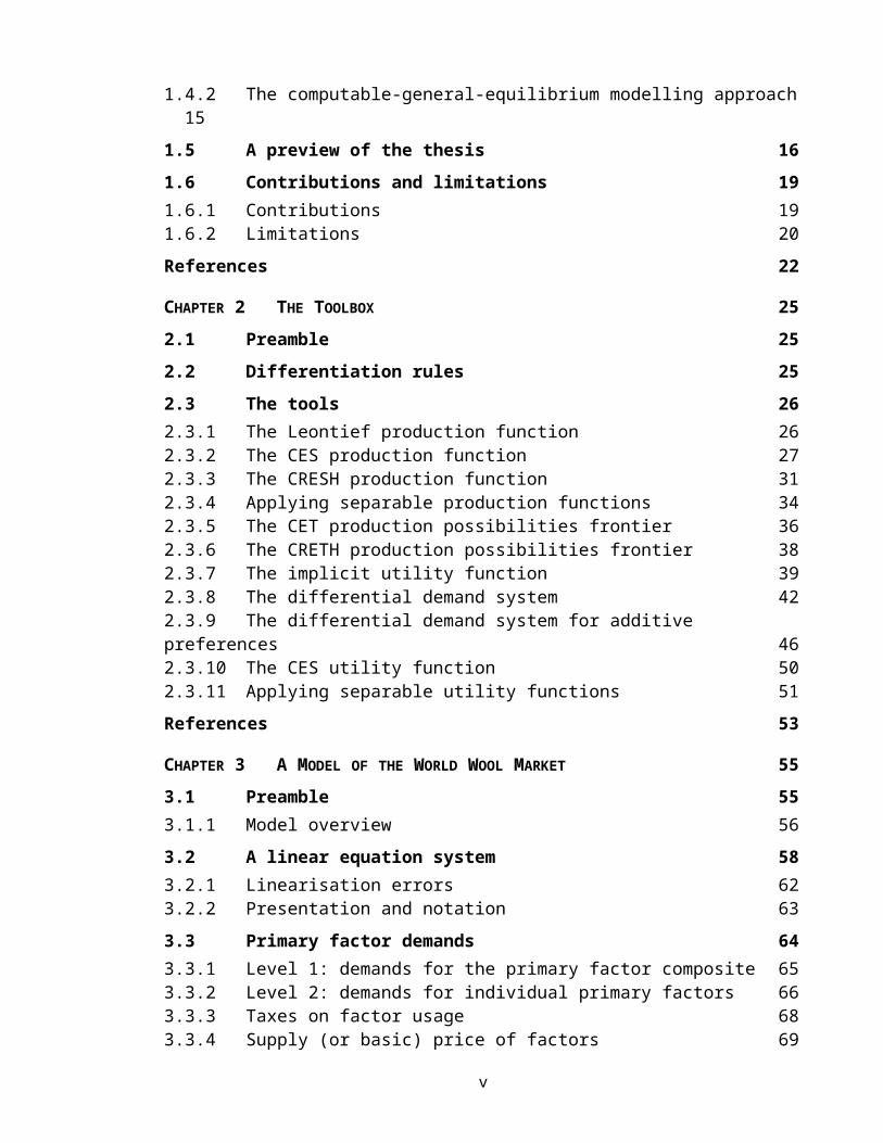
1.4.2 The computable-general-equilibrium modelling approach15

1.5 A preview of the thesis 161.6 Contributions and limitations 191.6.1 Contributions 191.6.2 Limitations 20References 22

CHAPTER 2 THE TOOLBOX 252.1 Preamble 252.2 Differentiation rules 252.3 The tools 262.3.1 The Leontief production function 262.3.2 The CES production function 272.3.3 The CRESH production function 312.3.4 Applying separable production functions 342.3.5 The CET production possibilities frontier 362.3.6 The CRETH production possibilities frontier 382.3.7 The implicit utility function 392.3.8 The differential demand system 422.3.9 The differential demand system for additive preferences 462.3.10 The CES utility function 502.3.11 Applying separable utility functions 51References 53

CHAPTER 3 A MODEL OF THE WORLD WOOL MARKET 553.1 Preamble 553.1.1 Model overview 563.2 A linear equation system 583.2.1 Linearisation errors 623.2.2 Presentation and notation 633.3 Primary factor demands 643.3.1 Level 1: demands for the primary factor composite 653.3.2 Level 2: demands for individual primary factors 663.3.3 Taxes on factor usage 683.3.4 Supply (or basic) price of factors 69

v

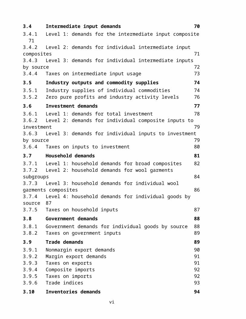
3.4 Intermediate input demands 703.4.1 Level 1: demands for the intermediate input composite71

3.4.2 Level 2: demands for individual intermediate input composites 713.4.3 Level 3: demands for individual intermediate inputs by source 723.4.4 Taxes on intermediate input usage 733.5 Industry outputs and commodity supplies 743.5.1 Industry supplies of individual commodities 743.5.2 Zero pure profits and industry activity levels 763.6 Investment demands 773.6.1 Level 1: demands for total investment 783.6.2 Level 2: demands for individual composite inputs to investment 793.6.3 Level 3: demands for individual inputs to investment by source 793.6.4 Taxes on inputs to investment 803.7 Household demands 813.7.1 Level 1: household demands for broad composites 823.7.2 Level 2: household demands for wool garments subgroups 843.7.3 Level 3: household demands for individual wool garments composites 863.7.4 Level 4: household demands for individual goods by source 873.7.5 Taxes on household inputs 873.8 Government demands 883.8.1 Government demands for individual goods by source 883.8.2 Taxes on government inputs 893.9 Trade demands 893.9.1 Nonmargin export demands 903.9.2 Margin export demands 913.9.3 Taxes on exports 913.9.4 Composite imports 923.9.5 Taxes on imports 923.9.6 Trade indices 933.10 Inventories demands 94

vi

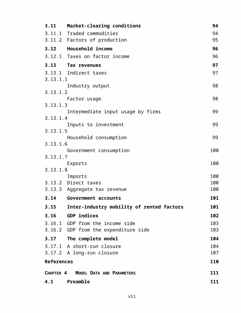
3.11 Market-clearing conditions 943.11.1 Traded commodities 943.11.2 Factors of production 953.12 Household income 963.12.1 Taxes on factor income 963.13 Tax revenues 973.13.1 Indirect taxes 973.13.1.1

Industry output 983.13.1.2

Factor usage 983.13.1.3

Intermediate input usage by firms 993.13.1.4

Inputs to investment 993.13.1.5

Household consumption 993.13.1.6

Government consumption 1003.13.1.7

Exports 1003.13.1.8

Imports 1003.13.2 Direct taxes 1003.13.3 Aggregate tax revenue 1003.14 Government accounts 1013.15 Inter-industry mobility of rented factors 1013.16 GDP indices 1023.16.1 GDP from the income side 1033.16.2 GDP from the expenditure side 1033.17 The complete model 1043.17.1 A short-run closure 1043.17.2 A long-run closure 107References 110

CHAPTER 4 MODEL DATA AND PARAMETERS 1114.1 Preamble 111

vii

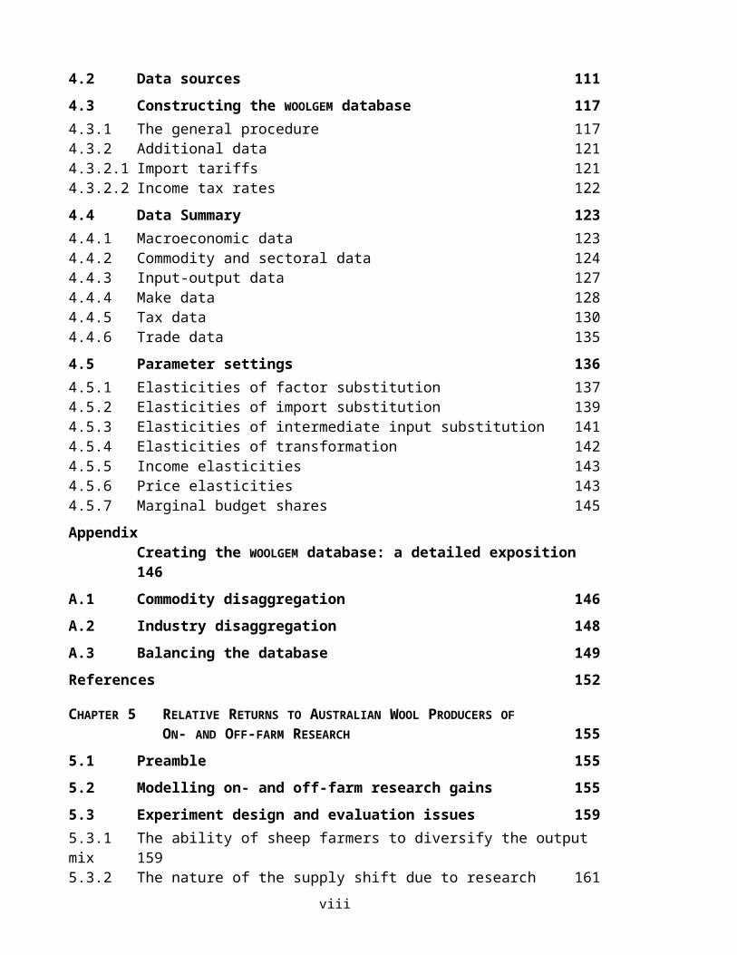
4.2 Data sources 1114.3 Constructing the WOOLGEM database 1174.3.1 The general procedure 1174.3.2 Additional data 1214.3.2.1 Import tariffs 1214.3.2.2 Income tax rates 1224.4 Data Summary 1234.4.1 Macroeconomic data 1234.4.2 Commodity and sectoral data 1244.4.3 Input-output data 1274.4.4 Make data 1284.4.5 Tax data 1304.4.6 Trade data 1354.5 Parameter settings 1364.5.1 Elasticities of factor substitution 1374.5.2 Elasticities of import substitution 1394.5.3 Elasticities of intermediate input substitution 1414.5.4 Elasticities of transformation 1424.5.5 Income elasticities 1434.5.6 Price elasticities 1434.5.7 Marginal budget shares 145Appendix

Creating the WOOLGEM database: a detailed exposition146

A.1 Commodity disaggregation 146A.2 Industry disaggregation 148A.3 Balancing the database 149References 152

CHAPTER 5 RELATIVE RETURNS TO AUSTRALIAN WOOL PRODUCERS OFON- AND OFF-FARM RESEARCH 155

5.1 Preamble 1555.2 Modelling on- and off-farm research gains 1555.3 Experiment design and evaluation issues 1595.3.1 The ability of sheep farmers to diversify the output mix 1595.3.2 The nature of the supply shift due to research 161

viii

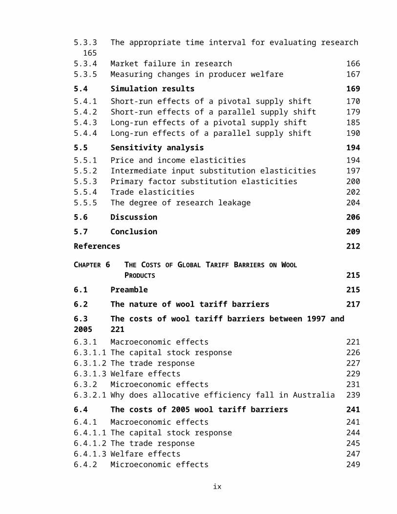
5.3.3 The appropriate time interval for evaluating research165

5.3.4 Market failure in research 1665.3.5 Measuring changes in producer welfare 1675.4 Simulation results 1695.4.1 Short-run effects of a pivotal supply shift 1705.4.2 Short-run effects of a parallel supply shift 1795.4.3 Long-run effects of a pivotal supply shift 1855.4.4 Long-run effects of a parallel supply shift 1905.5 Sensitivity analysis 1945.5.1 Price and income elasticities 1945.5.2 Intermediate input substitution elasticities 1975.5.3 Primary factor substitution elasticities 2005.5.4 Trade elasticities 2025.5.5 The degree of research leakage 2045.6 Discussion 2065.7 Conclusion 209References 212

CHAPTER 6 THE COSTS OF GLOBAL TARIFF BARRIERS ON WOOL PRODUCTS 215

6.1 Preamble 2156.2 The nature of wool tariff barriers 2176.3 The costs of wool tariff barriers between 1997 and 2005 2216.3.1 Macroeconomic effects 2216.3.1.1 The capital stock response 2266.3.1.2 The trade response 2276.3.1.3 Welfare effects 2296.3.2 Microeconomic effects 2316.3.2.1 Why does allocative efficiency fall in Australia 2396.4 The costs of 2005 wool tariff barriers 2416.4.1 Macroeconomic effects 2416.4.1.1 The capital stock response 2446.4.1.2 The trade response 2456.4.1.3 Welfare effects 2476.4.2 Microeconomic effects 249

ix

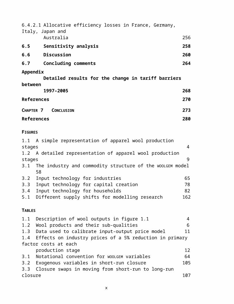
6.4.2.1 Allocative efficiency losses in France, Germany, Italy, Japan and

Australia 2566.5 Sensitivity analysis 2586.6 Discussion 2606.7 Concluding comments 264Appendix

Detailed results for the change in tariff barriers between

1997–2005 268References 270

CHAPTER 7 CONCLUSION 273References 280

FIGURES1.1 A simple representation of apparel wool production stages 41.2 A detailed representation of apparel wool production stages 93.1 The industry and commodity structure of the WOOLGEM model

583.2 Input technology for industries 653.3 Input technology for capital creation 783.4 Input technology for households 825.1 Different supply shifts for modelling research 162

TABLES1.1 Description of wool outputs in figure 1.1 41.2 Wool products and their sub-qualities 61.3 Data used to calibrate input-output price model 111.4 Effects on industry prices of a 5% reduction in primary factor costs at each

production stage 123.1 Notational convention for WOOLGEM variables 643.2 Exogenous variables in short-run closure 1053.3 Closure swaps in moving from short-run to long-run closure 107

x

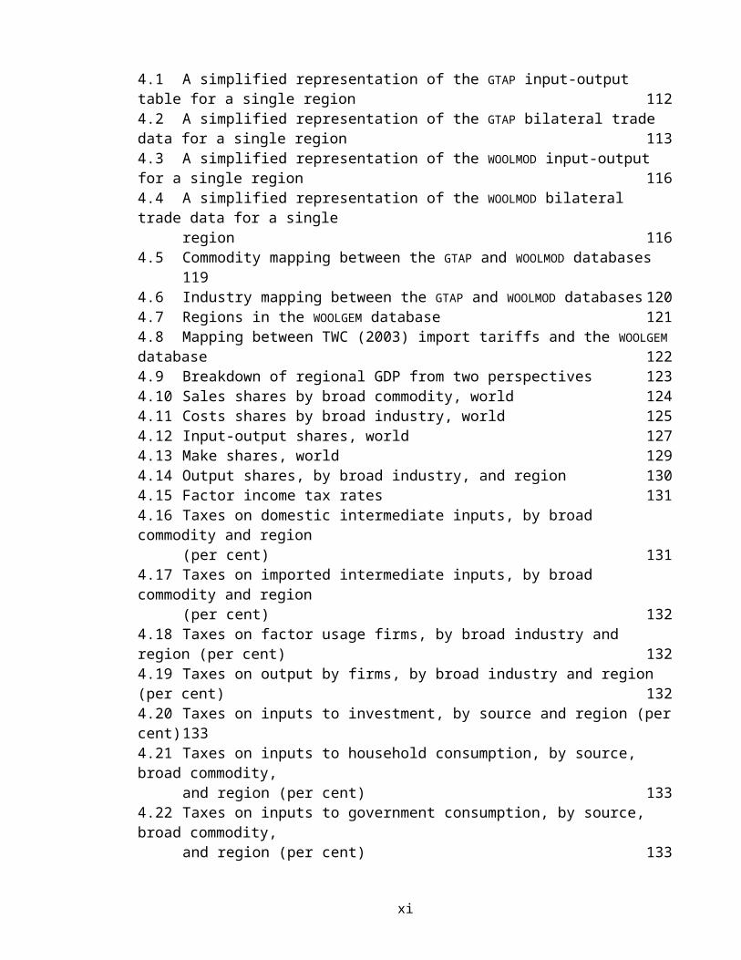
4.1 A simplified representation of the GTAP input-output table for a single region 1124.2 A simplified representation of the GTAP bilateral trade data for a single region 1134.3 A simplified representation of the WOOLMOD input-output for a single region 1164.4 A simplified representation of the WOOLMOD bilateral trade data for a single

region 1164.5 Commodity mapping between the GTAP and WOOLMOD databases

1194.6 Industry mapping between the GTAP and WOOLMOD databases 1204.7 Regions in the WOOLGEM database 1214.8 Mapping between TWC (2003) import tariffs and the WOOLGEMdatabase 1224.9 Breakdown of regional GDP from two perspectives 1234.10 Sales shares by broad commodity, world 1244.11 Costs shares by broad industry, world 1254.12 Input-output shares, world 1274.13 Make shares, world 1294.14 Output shares, by broad industry, and region 1304.15 Factor income tax rates 1314.16 Taxes on domestic intermediate inputs, by broad commodity and region

(per cent) 1314.17 Taxes on imported intermediate inputs, by broad commodity and region

(per cent) 1324.18 Taxes on factor usage firms, by broad industry and region (per cent) 1324.19 Taxes on output by firms, by broad industry and region (per cent) 1324.20 Taxes on inputs to investment, by source and region (percent)1334.21 Taxes on inputs to household consumption, by source, broad commodity,

and region (per cent) 1334.22 Taxes on inputs to government consumption, by source, broad commodity,

and region (per cent) 133

xi

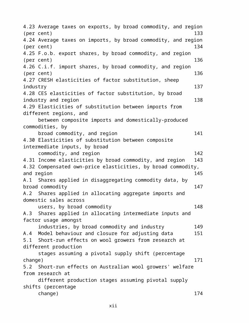
4.23 Average taxes on exports, by broad commodity, and region(per cent) 1334.24 Average taxes on imports, by broad commodity, and region(per cent) 1344.25 F.o.b. export shares, by broad commodity, and region (per cent) 1364.26 C.i.f. import shares, by broad commodity, and region (per cent) 1364.27 CRESH elasticities of factor substitution, sheep industry 1374.28 CES elasticities of factor substitution, by broad industry and region 1384.29 Elasticities of substitution between imports from different regions, and

between composite imports and domestically-produced commodities, by

broad commodity, and region 1414.30 Elasticities of substitution between composite intermediate inputs, by broad

commodity, and region 1424.31 Income elasticities by broad commodity, and region 1434.32 Compensated own-price elasticities, by broad commodity, and region 145A.1 Shares applied in disaggregating commodity data, by broad commodity 147A.2 Shares applied in allocating aggregate imports and domestic sales across

users, by broad commodity 148A.3 Shares applied in allocating intermediate inputs and factor usage amongst

industries, by broad commodity and industry 149A.4 Model behaviour and closure for adjusting data 1515.1 Short-run effects on wool growers from research at different production

stages assuming a pivotal supply shift (percentage change) 1715.2 Short-run effects on Australian wool growers' welfare from research at

different production stages assuming pivotal supply shifts (percentage

change) 174

xii

5.3 Short-run effects on wool growers from research at different production

stages assuming a parallel supply shift (percentage change) 1805.4 Short-run effects on Australian wool growers' welfare from research at

different production stages assuming parallel supply shifts (percentage

change) 1825.5 Long-run effects on wool growers from research at different production

stages assuming a pivotal supply shift (percentage change) 1875.6 Long-run effects on Australian wool growers' welfare from research at

different production stages assuming pivotal supply shifts (percentage

change) 1885.7 Long-run effects on wool growers from research at different production

stages assuming a parallel supply shift (percentage change) 1915.8 Long-run effects on Australian wool growers' welfare from research at

different production stages assuming parallel supply shifts (percentage

change) 1925.9 Comparison of Australian wool growers' welfare from research and

standard deviation from variations in price and income elasticities

(percentage change) 1955.10 Effects on global output of wool garments from research at different

production stages assuming pivotal and parallel supply shifts (percentage

change) 1975.11 Comparison of Australian wool growers' welfare from research and

sensitivity to variations in wool/nonwool input

xiii

substitution (percentage change) 199

5.12 Comparison of Australian wool growers' welfare from research and

sensitivity to variations in primary factor substitution(percentage change) 2015.13 Comparison of Australian wool growers' welfare from research and

sensitivity to variations in trade elasticities (percentage change) 2035.14 Comparison of Australian wool growers' welfare from research and

sensitivity to variations in research leakage (percentage change) 2055.15 Range of effects on Australian wool growers' welfare from research at

different production stages assuming pivotal and parallel supply shifts

(percentage change) 2075.16 Standard deviations for Australian wool growers' welfarefrom research at

different production stages assuming parallel supply shifts in the long run

(percentage change) 2096.1 Average import tax rates in model database representing 1997 wool tariff

barriers (per cent) 2186.2 Percentage change in average import tax rates, 1997–2005

2196.3 Average import tax rates, 1997 and 2005 (per cent) 2206.4 macroeconomic effects of changes in wool tariff barriers, 1997–2005

(percentage change) 2226.5 Effects on regional capital stocks and relative primary factor prices of

changes in wool tariff barriers, 1997–2005 (percentage change) 2266.6 Regional trade effects of changes in wool tariff barriers, 1997–2005

(percentage change) 228

xiv

6.7 Regional welfare effects due to changes in wool tariff barriers, 1997–2005

(percentage change) 2306.8 Changes in import tariffs, export barriers and relative primary factor prices

due to changes in tariff barriers, 1997–2005 (percentagechange) 2316.9 Selected industry and commodity effects of changes in tariff barriers,

1997–2005 (percentage change) 2336.10 Industry and commodity allocative efficiency effects in Australia due to

changes in tariff barriers, 1997–2005 (percentage change) 2406.11 Macroeconomic effects of the complete removal of 2005 wool tariff

barriers (percentage change) 2416.12 Effects on regional capital stocks and relative primary factor prices of the

complete removal of 2005 wool tariff barriers (percentage change) 2446.13 Regional trade effects of the complete removal of 2005 wool tariffs

(percentage change) 2466.14 Regional welfare effects of the complete removal of 2005wool tariffs

(percentage change) 2486.15 2005 wool import and export tariff barriers (per cent)

2506.16 Selected industry and commodity effects due to the complete removal of

2005 wool tariff barriers (percentage change) 2526.17 Export effects on European regions due to the complete removal of 2005

wool tariff barriers (percentage change) 2556.18 Industry and commodity allocative efficiency effects of the complete

removal of 2005 wool tariff barriers (percentage change)256

xv

6.19 Mean and standard deviation of regional welfare with respect to various

model parameters (percentage change) 2596.20 Various regional effects of wool tariff liberalisation scenarios

(percentage change) 261A.1 Industry output (percentage change) 269

ACKNOWLEDGEMENTS

xvi

This work was completed while I was employed as a full-

time Research Fellow in the Economic Research Centre of the

Economics Program at The University of Western Australia. I

was employed as part of the project Economic Aspects of Wool in

Western Australia, jointly financed by the Australian Research

Council and the Department of Agriculture Western Australia

under a Linkage Project grant, with Professor Kenneth

Clements as the chief investigator. This thesis includes a

nontrivial subset of the work I undertook while employed on

the project. In completing this research I have a number of

people to thank.

First and foremost my supervisor, Professor Clements,

who allowed me to undertake a doctoral thesis while employed

full-time on the abovementioned project. I thank him for the

generosity and trust he showed in taking this decision. In

completing my doctoral thesis, Professor Clements provided me

with liberal access to his vast experience in applied

economics and doctoral supervision. The guidance,

encouragement and support he provided ensured the thesis

proceeded to a timely and quality outcome. For this too, I

xvii

thank him. I also thank Professor Clements for his keen

sense of humour, which ensured that our regular meetings were

both valuable and enjoyable.

Second, the Department of Agriculture Western Australia.

Officers of the Department, John Stanton and Nazrul Islam,

provided data that formed an important starting point for the

data underlying this work. They also provided general

background on the world wool market which aided the

development of the model theory.

Third, participants and discussants of various seminars

and conferences who provided useful feedback on this work,

whether in preliminary or final form. These include: the

Centre of Policy Studies at Monash University, particularly

Professor Peter Dixon and Dr Mark Horridge; the 2004 PhD

Conference in Economics and Business held at The Australian National

University, particularly Professor Rodney Tyers; and the

Economics Program and the School of Agricultural and Resource

Economics at The University of Western Australia.

Fourth, special thanks go to a number of people who

generously gave their time in discussing this work and/or in

providing comments on early drafts. They include: Professor

xviii

John Freebairn of The University of Melbourne; Professor

Michael Wohlgenant of North Carolina State University;

Professor Robert Lindner of the School of Agricultural and

Resource Economics at The University of Western Australia,

and Chris Wilcox of The Woolmark Company.

My final thanks go to my wife, Joanne, who willingly

moved from Melbourne to Perth so that I could take up the

Research Fellow position at The University of Western

Australia. Her support and sense of humour have

significantly contributed to the completion of the thesis.

xix

CHAPTER 1

INTRODUCTION

1.1 Preamble

The core objective of this thesis is to aid

understanding of the economic mechanisms by which the world

wool market operates. We do this by constructing an

analytical framework, or model, that encompasses the most

important characteristics of the world wool market: the

extreme multistage nature of the wool production system, the

highly heterogeneous nature of wool products, and the

significant trade in wool products. These characteristics

are introduced in Section 1.2; this section also provides a

description of the general profile of the Australian wool

industry. We then explore the nature of the wool production

system and demonstrate the significant ‘economic distance’

between members of the wool production system (Section 1.3).

Besides capturing wool-specific aspects of the world wool

market in the model, it also desirable to allow for feedback

effects from the wool economy to the nonwool economy and back

1

to the wool economy. Therefore, we model the wool economy as

a fully integrated part of the wider economy by applying the

computable-general-equilibrium (CGE) approach. Section 1.4

discusses the two modelling approaches – commodity-specific

and CGE – that are synthesised to create the model; it also

discusses recent wool models and compares them to the model

constructed here. We then provide a preview of the thesis

(Section 1.5) and discuss the contributions and limitations

of the thesis (Section 1.6).

1.2 Background

1.2.1 The world wool market

Wool, cotton and man-made fibres account for around 98%

of world fibre use.1 Amongst these three fibres, man-made

fibres hold the dominant position accounting for around 60%

of world fibre use; cotton accounts for around 36% and wool

around 2% (TWC 2004). Wool’s small share of world fibre use

belies the concentration of wool production, exporting,

importing and processing, amongst a few but different

countries/regions.

1 All data discussed in this subsection refers to quantities and either2003 or 2004.

2

In terms of primary production, Australia is the world’s

largest wool producer accounting for one-quarter of world

wool output; China and New Zealand are the next most

important producers at 16% and 11% each (TWC 2004). In terms

of apparel wool, Australia’s importance is even greater with

it supplying around half of such wool (AWIL 2006).

Similarly, nearly two-thirds of wool exports are supplied by

three countries alone: Australia, 40%; New Zealand, 19%; the

United Kingdom (UK), 5% (TWC 2004). Wool imports are

somewhat less concentrated: China is the dominant importer

(27%),2 followed by Italy (10%), India and the UK (8% each),

and France and Germany (5% each).

At the spinning (or yarn) and weaving (or fabric)

production stages, the use of wool is concentrated in the Far

East (mainly China) at 30%, Western Europe (mainly Italy and

the UK) at 21%, and the Indian subcontinent (mainly India and

Pakistan) at 14%. At the garment-manufacturing stage, the

regional concentration is similar but Western Europe is less

important (16%) and the Indian subcontinent more important

(15%). The consumption of wool at the retail stage (in the

2 This includes Hong Kong and Macau.

3

form of apparel, carpets, etc.) is distributed differently

again. Here, Western Europe (mainly UK, Italy and Germany)

and the Far East (mainly China and Japan) are equally

important at 26% each, and North America (mainly the United

States) less important at 13% (TWC 2004).

The above discussion has hinted at four broad stages of

production through which apparel wool passes; the left-hand

side of figure 1.1 summarises this structure. This

structure, though highly simplified, captures the multistage

nature of the wool production system. But the outputs of

each of the four production stages can be further

disaggregated to provide a more realistic structure of the

wool production system that underlies the world wool market.

Raw wool produced at stage 1 can be disaggregated into

greasy, scoured, carbonised, carded and combed wool. Wool

yarn produced at stage 2 can be divided into worsted and

woollen yarn, and similarly for wool fabrics produced at

stage 3 and wool garments produced at stage 4. Table 1.1

provides a short description of each of these outputs.

The wool production system begins with the production of

greasy wool, which is removed from the sheep’s back by

4

shearing. Greasy wool is then washed (scoured) to remove

extraneous matter, giving scoured wool. Some scoured wools

are then carbonised to remove vegetable matter and then

carded; other scoured wools bypass the carbonising process

and are carded directly and then combed (the carding and

combing processes prepare wool for the spinning process). At

this point, wools now enter the spinning process where yarns

are produced. In general, two types of yarns can be

distinguished: worsted and woollen. Worsted yarns are

produced from combed wools; woollen yarns are produced from

carded wools. The distinction between worsted and woollen

yarns is maintained through the weaving process where fabrics

are produced and the manufacturing process where garments are

produced.

5

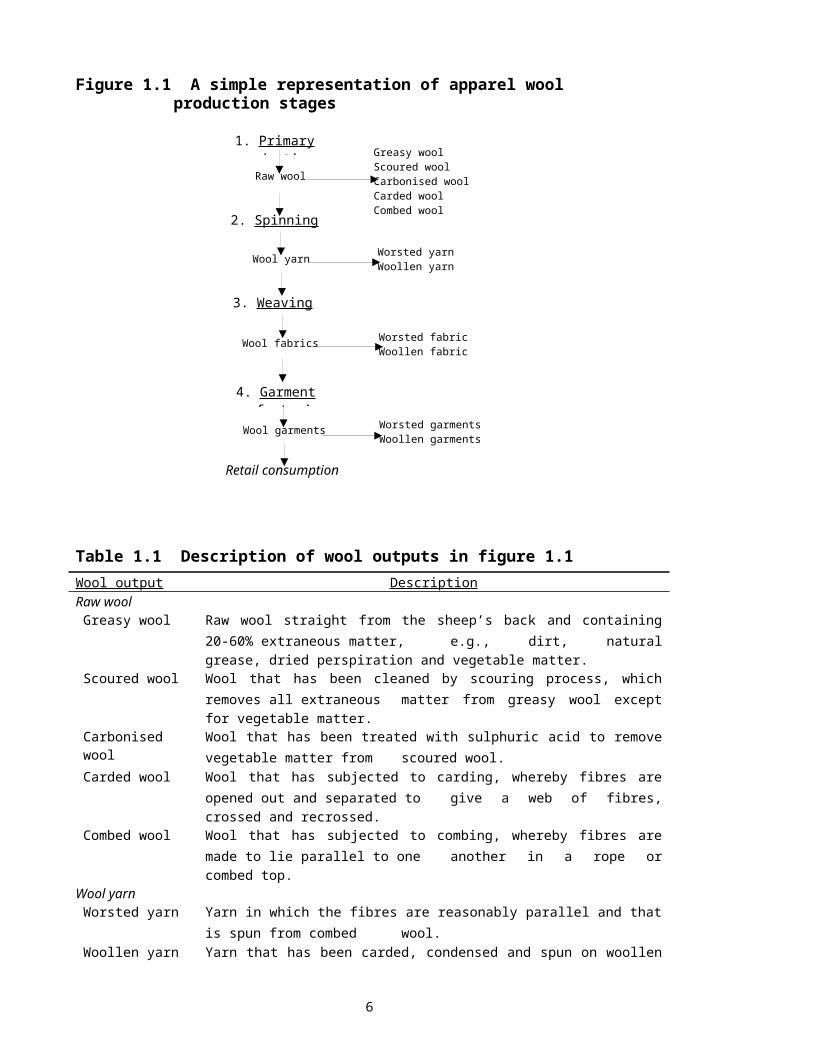
Figure 1.1 A simple representation of apparel wool production stages

Table 1.1 Description of wool outputs in figure 1.1Wool output DescriptionRaw woolGreasy wool Raw wool straight from the sheep’s back and containing

20-60% extraneous matter, e.g., dirt, naturalgrease, dried perspiration and vegetable matter.

Scoured wool Wool that has been cleaned by scouring process, whichremoves all extraneous matter from greasy wool exceptfor vegetable matter.

Carbonised wool

Wool that has been treated with sulphuric acid to removevegetable matter from scoured wool.

Carded wool Wool that has subjected to carding, whereby fibres areopened out and separated to give a web of fibres,crossed and recrossed.

Combed wool Wool that has subjected to combing, whereby fibres aremade to lie parallel to one another in a rope orcombed top.

Wool yarnWorsted yarn Yarn in which the fibres are reasonably parallel and that

is spun from combed wool.Woollen yarn Yarn that has been carded, condensed and spun on woollen

1. Primaryproduction

Raw wool

2. Spinning

Wool yarn

3. Weaving

Wool fabrics

4. Garmentmanufacturing

Wool garments

Retail consumption

Greasy woolScoured woolCarbonised woolCarded woolCombed wool

Worsted yarnWoollen yarn

Worsted fabricWoollen fabric

Worsted garmentsWoollen garments

6

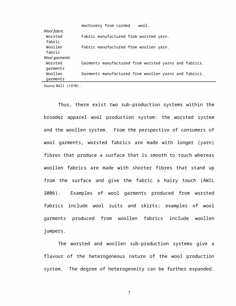
machinery from carded wool.Wool fabricWorsted fabric

Fabric manufactured from worsted yarn.

Woollen fabric

Fabric manufactured from woollen yarn.

Wool garmentsWorsted garments

Garments manufactured from worsted yarns and fabrics.

Woollen garments

Garments manufactured from woollen yarns and fabrics.

Source: Bell (1970).

Thus, there exist two sub-production systems within the

broader apparel wool production system: the worsted system

and the woollen system. From the perspective of consumers of

wool garments, worsted fabrics are made with longer (yarn)

fibres that produce a surface that is smooth to touch whereas

woollen fabrics are made with shorter fibres that stand up

from the surface and give the fabric a hairy touch (AWIL

2006). Examples of wool garments produced from worsted

fabrics include wool suits and skirts; examples of wool

garments produced from woollen fabrics include woollen

jumpers.

The worsted and woollen sub-production systems give a

flavour of the heterogeneous nature of the wool production

system. The degree of heterogeneity can be further expanded.

7

Raw wool (greasy, scoured, etc.) is commonly distinguished by

hauteur (or length) and diameter. Hauteur is quoted in

millimetres (mm); diameter is quoted in microns, or

millionths of a metre, (μm). The properties, or qualities,

of hauteur and diameter determine the type of processing and

the range of products that can be made from a given batch of

wool. Consequently, the qualities determine the relative

price of different wools by reflecting the relative value of

the end-use products that they enter. In general, finer

wools fetch higher prices. Finer wool (<20 μm) is used for

producing lightweight fabrics and garments. Broader wool is

processed into nonapparel, e.g., blankets, upholstery and

carpets. Longer fibres (>56 mm) enter the worsted system and

are used for making suiting and lightweight knitwear.

Shorter fibres (<56 mm) enter the woollen system and are used

for making bulky fabrics such as tweeds, felts, flannels and

knitwear (Kopke et al. 2004). Table 1.2 summarises the wool

sub-qualities as they apply to wool products identified in

figure 1.1. In this work, these sub-qualities are used to

represent a highly detailed wool production system.

8

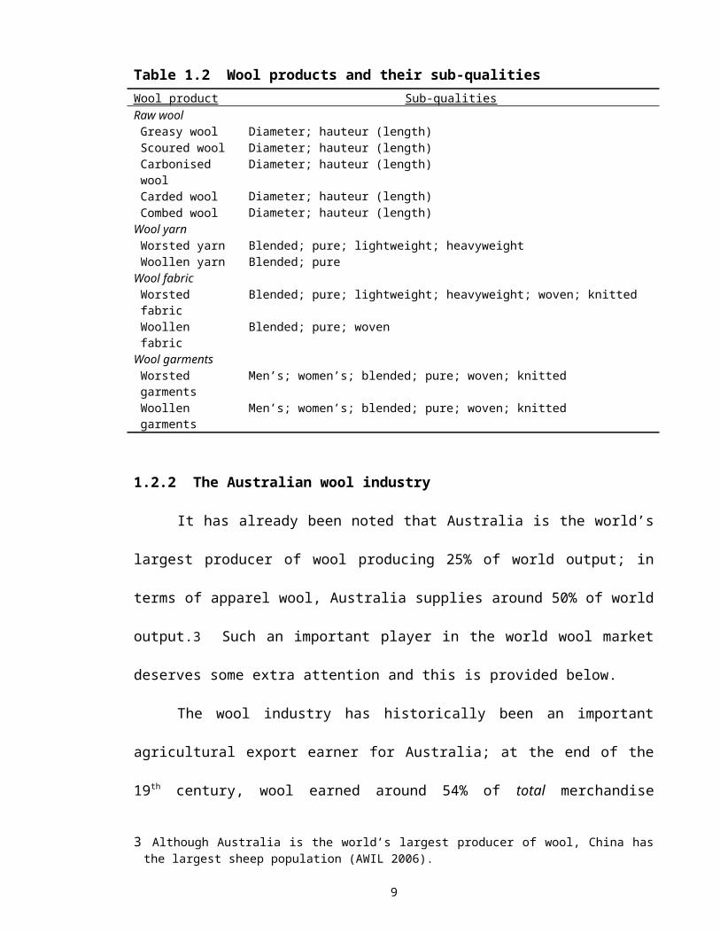
Table 1.2 Wool products and their sub-qualitiesWool product Sub-qualitiesRaw woolGreasy wool Diameter; hauteur (length)Scoured wool Diameter; hauteur (length)Carbonised wool

Diameter; hauteur (length)

Carded wool Diameter; hauteur (length)Combed wool Diameter; hauteur (length)

Wool yarnWorsted yarn Blended; pure; lightweight; heavyweightWoollen yarn Blended; pure

Wool fabricWorsted fabric

Blended; pure; lightweight; heavyweight; woven; knitted

Woollen fabric

Blended; pure; woven

Wool garmentsWorsted garments

Men’s; women’s; blended; pure; woven; knitted

Woollen garments

Men’s; women’s; blended; pure; woven; knitted

1.2.2 The Australian wool industry

It has already been noted that Australia is the world’s

largest producer of wool producing 25% of world output; in

terms of apparel wool, Australia supplies around 50% of world

output.3 Such an important player in the world wool market

deserves some extra attention and this is provided below.

The wool industry has historically been an important

agricultural export earner for Australia; at the end of the

19th century, wool earned around 54% of total merchandise

3 Although Australia is the world’s largest producer of wool, China hasthe largest sheep population (AWIL 2006).

9

exports (Boehm 1979).4 But the relative importance of wool

exports has been on a secular downward trend since that time;

in 2004-05 wool accounted for only 2.5% of Australia’s total

commodity (agricultural and mining) exports, and only 8.3% of

Australia’s agricultural exports, ranking fourth behind beef,

wheat and wine. In dollar terms, wool exports were valued at

$2.5 billion in 2004-05 (AWIL 2006).

The declining relative importance of wool export

earnings, over the last 100 years or so, reflects the huge

growth in other commodity exports (particularly mining), but

also, more recently, declining sheep numbers and wool

production; in 1989, the sheep flock was around 170 million

whereas in 2004-05 it had fallen to around 107 million (AWIL

2006; CIE 2002). The decline in sheep numbers over this

period reflects lower wool prices that, in turn, reflect

lower wool demand. At the same time, incomes for wool-

producing farms have fallen in concert with wool prices.

This has encouraged wool producers to diversify their

production by producing less wool and more crops and

livestock. Consequently, in 2002 only about one-third of the

4 This is an average for the period 1881–90.

10

45 000 sheep- and wool-producing farms in Australia derived a

significant proportion of their income from sheep and wool,

whereas the remainder were mixed livestock-crops and sheep-

beef producers (CIE 2002).

In 2003, the Australian flock was mainly composed of

Merino sheep (85%); Merino sheep are bred primarily for their

wool. In the same year, 73% of the total wool produced in

Australia was produced by less than 40% of wool-producing

farms. This reflects a degree of concentration in Australian

wool production. It is expected that the amount of wool

produced in 2005-06 will fall by 1.7% reflecting low wool

prices relative to lamb and alternative farm uses. Since

1993-94 there has been a significant increase in the 19 μm

profile of the Australian clip, from 9% to 32% (AWIL 2006).

This has contributed to Australia’s reputation as the world’s

leading producer of quality fine apparel wool (DAWA 1999).

Over the second half of the 20th century, the Australian

wool industry has oscillated from almost zero government

intervention in the 1960s to a number of failed price support

schemes in the 1970s and 1980s, and (again) back to almost

zero government intervention at the end of the 20th century.

11

The most well-known of the failed price support schemes

commenced in 1974 and was eventually known as the ‘Reserve

Price Scheme’ (RPS). The RPS established a firm floor price

and was backed by a compulsory levy of 5% of the gross

proceeds from the sale of shorn wool. The scheme appeared to

stabilise Australian dollar prices over the period 1974–87.

Up to 1987 the (nominal) floor price was increased annually

by 5-7%, but during the two-year period 1987–1988 it was

increased by 70%. This was followed by a 19% increase in

production in 1989-90 to record levels. The RPS eventually

collapsed and was abandoned in 1991. By this time, 4.75

million bales of wool (about one average wool clip) had been

amassed under the scheme due to the failure to reduce the

reserve price after 1988. Nine years after the scheme was

abandoned, a million bales of wool remained in the stockpile.

One legacy of the RPS is the return, at the beginning of the

21st century, to the minimal (government) intervention

environment of the 1950s (Richardson 2001).

1.3 The nature of the wool production system

12

Applying some of the wool sub-qualities to the wool

production system presented in figure 1.1, we can develop a

more realistic representation of the wool production system;

this is presented in figure 1.2 with arrows indicating the

flows of outputs and inputs at each production stage. Six

production stages are distinguished: primary production

(producing greasy wool), scouring (producing scoured wool),

carding/combing (producing carbonised wool, worsted tops, and

noils), spinning (producing yarns), weaving (producing

fabrics), and manufacturing (producing garments). Figure 1.2

also includes the use of nonwool inputs, such as synthetic

textiles (used to produce blended wool yarns), and factors of

production.

13

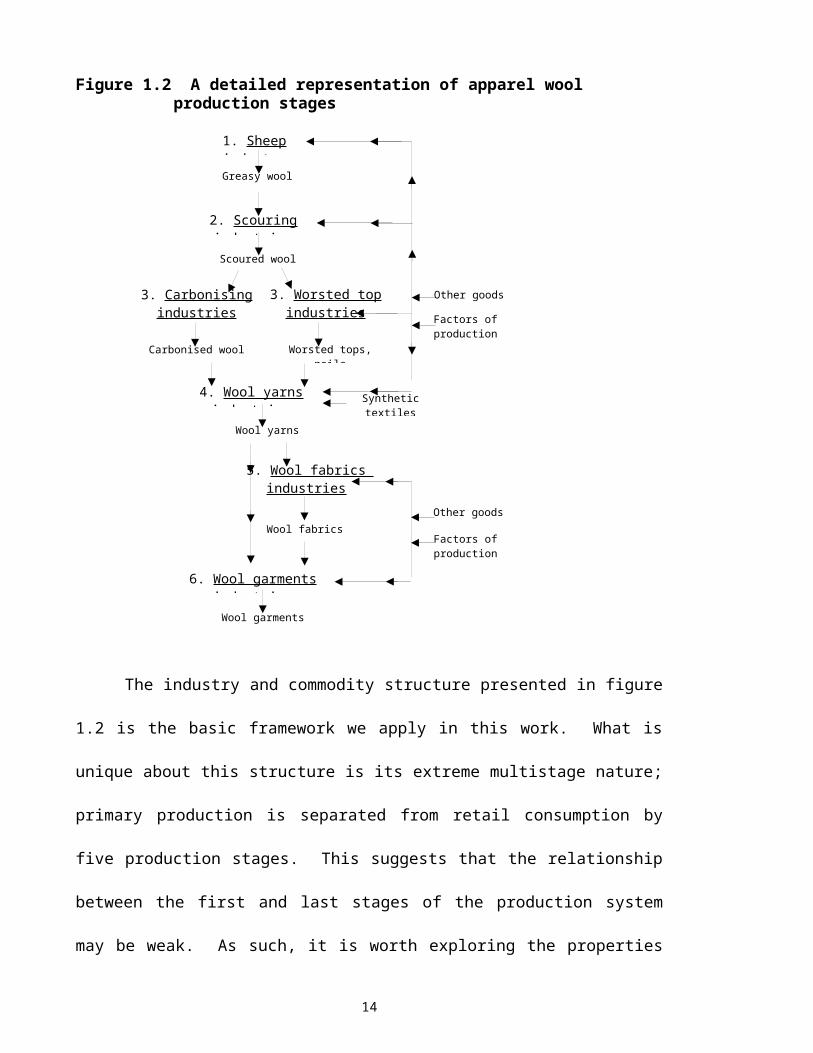
Figure 1.2 A detailed representation of apparel wool production stages

The industry and commodity structure presented in figure

1.2 is the basic framework we apply in this work. What is

unique about this structure is its extreme multistage nature;

primary production is separated from retail consumption by

five production stages. This suggests that the relationship

between the first and last stages of the production system

may be weak. As such, it is worth exploring the properties

Carbonised wool Worsted tops,noils

6. Wool garmentsindustriesWool garments

Factors of production

Other goods

4. Wool yarnsindustries

Wool yarns

5. Wool fabrics industries

Wool fabrics

Synthetictextiles

Scoured wool

3. Carbonisingindustries

3. Worsted topindustries Factors of

production

Other goods

2. Scouringindustries

Greasy wool

1. Sheepindustry

14

of the system using a simple input-output price model, one

that implicitly assumes no substitution and fixes the prices

of goods not produced within the system.

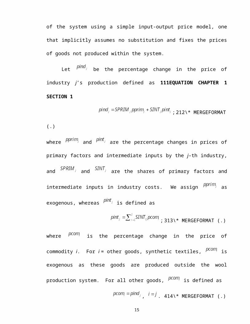
Let be the percentage change in the price of

industry j’s production defined as 111EQUATION CHAPTER 1

SECTION 1

;212\* MERGEFORMAT

(.)

where and are the percentage changes in prices of

primary factors and intermediate inputs by the j-th industry,

and and are the shares of primary factors and

intermediate inputs in industry costs. We assign as

exogenous, whereas is defined as

; 313\* MERGEFORMAT (.)

where is the percentage change in the price of

commodity i. For i = other goods, synthetic textiles, is

exogenous as these goods are produced outside the wool

production system. For all other goods, is defined as

, . 414\* MERGEFORMAT (.)

15

We calibrate the model by using the data presented in

table 1.3, which is an aggregated form of the data used in

this study (see Chapter 4). The data show a number of

interesting trends as wool moves through the production

system. First, the importance of primary factors (row 1) is

low and intermediate inputs (row 2) high in the production

costs of early-stage processing industries (scoured wool,

column 2; carbonised wool, column 3; worsted top, column 4).

As wool moves to late-stage processing industries (yarn,

column 5; fabric, column 6; garments, column 7) primary

factors become more important and intermediate inputs less

important. Second, the importance of other goods (row 11) is

low and wool inputs (rows 3–9) high in the intermediate input

costs of early-stage processing industries. But the

importance of other goods as an intermediate input is much

greater in late-stage processing industries, so much so that

it is more important than wool inputs in garment production.

Third, the input-output table (table 1.3) shows a recursive

pattern. That is, if represents the input-output

16

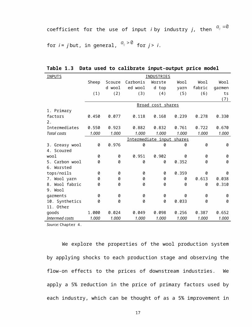
coefficient for the use of input i by industry j, then

for i = j but, in general, for j > i.

Table 1.3 Data used to calibrate input-output price modelINPUTS INDUSTRIES

Sheep

(1)

Scoured wool

(2)

Carbonised wool

(3)

Worsted top(4)

Woolyarn(5)

Woolfabric

(6)

Woolgarmen

ts(7)

Broad cost shares1. Primary factors 0.450 0.077 0.118 0.168 0.239 0.278 0.3302. Intermediates 0.550 0.923 0.882 0.832 0.761 0.722 0.670Total costs 1.000 1.000 1.000 1.000 1.000 1.000 1.000

Intermediate input shares3. Greasy wool 0 0.976 0 0 0 0 04. Scoured wool 0 0 0.951 0.902 0 0 05. Carbon wool 0 0 0 0 0.352 0 06. Worsted tops/noils 0 0 0 0 0.359 0 07. Wool yarn 0 0 0 0 0 0.613 0.0388. Wool fabric 0 0 0 0 0 0 0.3109. Wool garments 0 0 0 0 0 0 010. Synthetics 0 0 0 0 0.033 0 011. Other goods 1.000 0.024 0.049 0.098 0.256 0.387 0.652Intermed costs 1.000 1.000 1.000 1.000 1.000 1.000 1.000Source: Chapter 4.

We explore the properties of the wool production system

by applying shocks to each production stage and observing the

flow-on effects to the prices of downstream industries. We

apply a 5% reduction in the price of primary factors used by

each industry, which can be thought of as a 5% improvement in

17

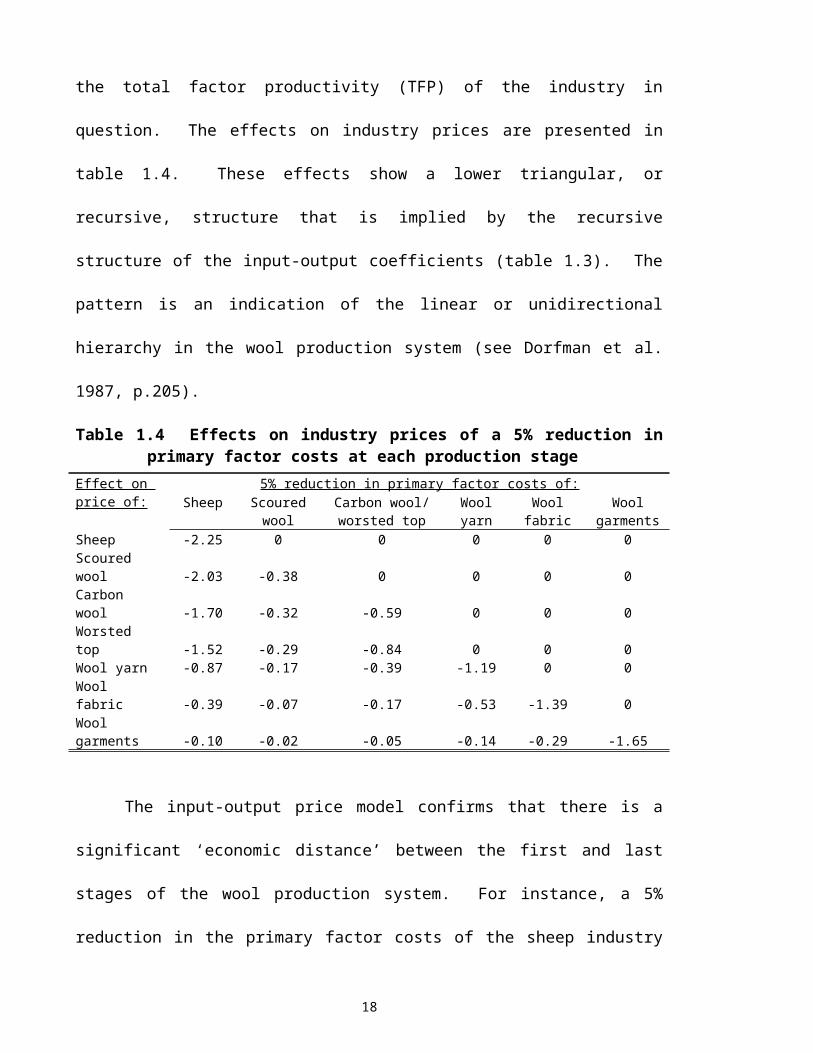
the total factor productivity (TFP) of the industry in

question. The effects on industry prices are presented in

table 1.4. These effects show a lower triangular, or

recursive, structure that is implied by the recursive

structure of the input-output coefficients (table 1.3). The

pattern is an indication of the linear or unidirectional

hierarchy in the wool production system (see Dorfman et al.

1987, p.205).

Table 1.4 Effects on industry prices of a 5% reduction inprimary factor costs at each production stage

Effect on price of:

5% reduction in primary factor costs of:Sheep Scoured

woolCarbon wool/worsted top

Woolyarn

Woolfabric

Woolgarments

Sheep -2.25 0 0 0 0 0Scoured wool -2.03 -0.38 0 0 0 0Carbon wool -1.70 -0.32 -0.59 0 0 0Worsted top -1.52 -0.29 -0.84 0 0 0Wool yarn -0.87 -0.17 -0.39 -1.19 0 0Wool fabric -0.39 -0.07 -0.17 -0.53 -1.39 0Wool garments -0.10 -0.02 -0.05 -0.14 -0.29 -1.65

The input-output price model confirms that there is a

significant ‘economic distance’ between the first and last

stages of the wool production system. For instance, a 5%

reduction in the primary factor costs of the sheep industry

18

leads to only a 0.1% reduction in the price of wool garments.

This reflects the decreasing importance of wool inputs at

each successive production stage as wool moves from on-farm

production to early-stage wool processing to late-stage

processing. In contrast, there is less economic distance

between the sheep industry and the early-stage processing

industries, e.g., a 5% TFP improvement in the sheep industry

leads to a 2% fall in the price of scoured wool, a 1.7% fall

in the price of carbonised wool and a 1.5% fall in the price

of worsted top industry. Further, the links between the

late-stage processing industries are also weak. Thus, a 5%

reduction in the primary factor costs of the wool fabric

industry leads to only a 0.3% reduction in the price of wool

garments. This reflects the minority share of total costs

that wool inputs (yarns and fabrics) comprise in garment

production (35%).

The model demonstrates the general weakness of the

economic links between early- and late-stage members of the

wool production system. If substitution between inputs were

allowed in the model, then the links would be stronger;

industries could then exploit lower input prices by

19

substituting cheaper inputs for more expensive inputs.

Regardless, allowing substitution would not change the

general result unless the degree of substitution was

infinite. The general result serves to illustrate an

important property of the wool production system that

surfaces prominently in the productivity experiments

performed in Chapter 5.

1.4 Methodology

The model developed here represents the synthesis of two

modelling traditions: (i) the partial-equilibrium commodity-

specific approach, and (ii) the computable-general-

equilibrium (CGE) approach.

1.4.1 The partial-equilibrium commodity-specific modelling

approach

Commodity-specific models have a long and rich history

that began in the 1960s. They do not constitute a unique

research stream but consist of an amalgam of work from

agricultural economics, energy economics, mineral economics,

marine economics, commodity futures and financial economics.

20

These models feature varied methodologies, consisting of

econometrics, mathematical programming, input-output

analysis, and systems simulation theory and methods (Guvenen

et al. 1991).

In the aggregate, models of agricultural commodities

vary widely but they all contain a number of common

characteristics; inelastic demand, slow growth in total

demand, competitive market structure, significant

technological change, and the tendency of resources to become

specific to the agricultural sector. For individual

agricultural commodities the aggregate modelling approach is

modified to account for additional characteristics that are

unique to the commodity in question (Guvenen et al. 1991).

The work presented here contains characteristics common to

all agricultural models (inelastic demand, competitive market

structure, sector-specific resources) and additional

characteristics that are unique to wool (the multistage

nature of the wool production system, heterogeneous treatment

of wool products). There are many commodity-specific models

of wool. Recent examples include Mullen et al. (1989),

21

Connolly (1992), Tulpule et al. (1992), Layman (1999) and

Verikios (2004).

Mullen et al. (1989) construct an equilibrium

displacement model of the world wool top industry, which uses

wool and nonwool inputs to produce wool top. Wool inputs are

distinguished between Australian and foreign supply.

Connolly (1992) constructs an econometrically-estimated

partial-equilibrium model of the world wool market and

distinguishes between apparel and carpet wool. There are

seven demand regions and five supply regions. The wool

production system is depicted via three stages: raw wool

production, textile production, and end-use products. Wool

products from different regions are treated as differentiated

products. The model by Tulpule et al. (1992) is also

econometrically estimated and partial equilibrium. It

represents the wool production system via four production

stages: wool top, yarn, fabric, and garments. Wool inputs to

top production are distinguished between Australian and

foreign supply. At each production stage, wool products are

assumed to be differentiated on the basis of four categories

of wool content: pure wool, wool rich, wool poor, and

22

nonwool; but there is no geographic differentiation of these

products.

Layman (1999) represents a significant advance on the

models already discussed. Similar to Mullen et al. (1989),

it is an equilibrium displacement model, albeit a very large

one. It depicts seven production stages: a sheep industry,

scouring industries, carding/combing industries, yarn

industries, fabric industries, wholesale garment industries

and retail garment industries. It differentiates wool

products by both quality (diameter, hauteur, worsted,

woollen, woven, knitted, pure, blended, etc.) and place of

production. Thus, 10 regions of the world are distinguished

and international trade occurs in all wool products except

retail garments. The degree of industry and commodity detail

in Layman (1999) is unprecedented. Verikios (2004) uses the

database of Layman (1999) to construct a model of the world

wool market with an almost identical degree of industry and

commodity detail. It departs from Layman (1999) by adjusting

the benchmark data for discrepancies, using more flexible

functional forms to represent demand and supply for all

23

inputs and outputs, and updating all parameter values using a

literature search and wool experts’ advice.

1.4.2 The computable-general-equilibrium modelling approach

The defining characteristic of CGE models is a

comprehensive representation of the economy, i.e., as a

complete system of interdependent components – industries,

households, investors, governments, importers and exporters

(Dixon et al. 1992). These can be single region models,

e.g., Dixon et al. (1982), or multi-region models, e.g.,

Hertel (1997). It is not unheard of to incorporate the

characteristics of commodity-specific models within a CGE

framework, but it is uncommon. The most prominent examples

of such a synthesis are the linking of input-output models of

the energy sector with macroeconomic models (e.g., Hudson and

Jorgenson 1974). Synthesised energy-market models allow for

feedback effects, from the energy sector to the rest of the

economy and back to the energy sector, to inform the analysis

of energy-specific issues. A more recent example of such a

synthesis is Trela and Whalley (1990), who construct a CGE

model of textile and apparel markets with 14 specific textile

24

and apparel categories and one composite other good, and 37

regions trading regions. In terms of wool, the only example

of a wool CGE model (that we are aware of) is CIE (2002),

where GTAP, a multi-region CGE model (Hertel 1997), is

disaggregated to distinguish raw wool, wool textile and wool

garments sectors. The main drawback of such a model is the

homogeneous representation of wool products.

In developing a synthesised wool model, we take a

similar approach to Trela and Whalley (1990). Thus, we

distinguish 54 individual wool products and two nonwool

products (synthetic textiles and one composite other good).

But our approach goes further, by distinguishing 42

individual wool products industries and a separate composite

other industries sector.5 The wool products industries in

each region are linked with the other industries sector

through domestic factor markets, domestic and international

markets for intermediate inputs, and domestic and

international markets for household goods. This completes

and complements the commodity-specific aspects of the model.

This also constrains the behaviour of the wool economy in

5 See Chapter 4 for a complete listing of model industries andcommodities.

25

individual regions to assumptions about macroeconomic

behaviour, such as a balance of trade constraint, and

household and government consumption constraints. All of

this is done at minimum computational cost, by representing

nonwool industries and commodities as a single composite

industry and commodity. This model builds on the work of

Verikios (2004).

26

1.5 A preview of the thesis

The thesis consists of six chapters. Chapter 2 presents

a number of ‘tools’ that are applied in constructing the

model. The tools consist of functional forms used to develop

the theoretical structure of the model. The linearised

versions of the functional forms are derived from their

nonlinear forms. In doing so, many of the assumptions

underlying the functional forms, and their properties, are

identified. Chapter 3 applies the linearised versions of the

functional forms to develop the theoretical structure of the

model. This is done by documenting the equations, variables

and coefficients of the model. We also develop two

alternative model closures: a short-run and long-run closure.

Chapter 4 is concerned with the model database and parameter

values. As such, it does three things: (i) it describes the

sources and methods used to construct the model database;

(ii) it summarises the resulting database to aid in the

interpretation of simulation results; (iii) it describes the

sources and rationale underlying the parameters used to

calibrate the behavioural equations of the model.

27

Chapters 5 and 6 apply the model to issues of interest

to scholars, wool industry analysts and policy makers. The

model is first applied to analysing the relationship between

on- and off-farm productivity changes and grower incomes

(Chapter 5). The analysis is conducted under short- and

long-run assumptions, and under alternative assumptions

regarding the degree of productivity spill-over to foreign

competitors. Our results show that the estimated research

gains for Australian wool producers depend crucially on the

nature of the assumed research-induced supply shift, i.e.,

pivotal or parallel. Pivotal supply shifts lead to losses

for on- and off-farm research, in both short- and long-run

environments. Parallel supply shifts lead to gains for on-

and off-farm research, in both short- and long-run

environments. Extensive sensitivity analysis confirms that

the assumed nature of the supply shift is the important

determinant of the sign of the welfare effects from research.

Following the argument made by Rose (1980) in favour of

using a parallel supply shift as the best approximation, we

focus on the estimates generated from parallel supply shifts.

We find that on-farm research is to be preferred to all other

28

forms of research; on-farm research gives the largest welfare

gain to Australian wool producers and off-farm research ranks

second. Our results indicate that, in general, off-farm

research that is ‘close’ to the wool producer provides larger

benefits than off-farm research that is ‘distant’. Extensive

sensitivity analysis indicates that certain assumptions do

affect the estimated welfare gains from research. None of

these assumptions are found to alter the ranking of benefits

from on- and off-farm research.

The model is then applied to analysing the economic

effects of global wool tariff changes (Chapter 6). We

analyse the effects of recent (i.e., between 1997 and 2005)

and current (2005) tariffs on wool products. Sensitivity

analysis is undertaken to test the robustness of the results

with respect to variations in parameter values.

The results provide an indication of the degree of

discrimination imposed by wool tariffs. Recent (1997–2005)

wool tariffs lead to positive welfare effects for most

regions. Nevertheless, sensitivity analysis shows that the

estimated welfare gains are robust only for three regions:

Italy, the UK and China. The welfare gains for Italy and

29

China are significant given the small relative size of the

wool industries in these regions. Tariff barriers on wool

textiles and garments fall significantly over 1997–2005 and

the pattern of both China’s and Italy’s exports are more

skewed towards these goods than in other regions.

For the removal of 2005 wool tariffs, China and the UK

are estimated to be the only winners; but the welfare gain is

only robust for China. The reason for China’s gain from 2005

wool tariffs is similar to the reason for its gain from 1997–

2005 tariff changes; its exports are skewed towards wool

products that have the highest tariff rates in 2005 (i.e.,

wool fabrics and garments) and their removal benefits China

more than any other region. The result is an allocative

efficiency improvement and increase in the use of capital due

to a rise in the demand for primary factors that reduces the

relative price of capital.

Underlying the welfare effects of recent and current

wool tariffs are the effects on individual industries in each

region. The results indicate that the nature of both recent

and current wool tariffs severely distort the size of wool

industries in different regions. For recent wool tariffs,

30

the changes in the output of wool commodities are extreme

reflecting the discriminatory nature of the tariffs. The

results indicate a relocation of wool garments production

away from France, Germany and Italy, largely to China and the

ROW region. For 2005 wool tariffs, production effects on

wool processing follow a general pattern: large reductions in

most regions and large expansions in China. There is also a

major relocation of wool garments industries away from

France, Germany and Italy to the UK, China and the ROW

region.

1.6 Contributions and limitations

Any piece of large-scale research is expected to make

some contribution to existing knowledge while at the same

having some limitations. This thesis is no different.

1.6.1 Contributions

The main contribution of this research is the

development of a sophisticated and novel analytical framework

for analysing the world wool market. This framework combines

the advantages of commodity-specific and CGE modelling. The

31

model is rich enough in commodity and industry detail to

realistically represent all of the special characteristics of

the world wool market and its submarkets (i.e., the

multistage nature of the production system, the heterogeneous

nature of wool products); it is also rich enough in nonwool

economy detail to represent each region as complete system of

interdependent components (i.e., distinguishing nonwool

industries, households, investors, governments, importers and

exporters). Within such a setting, it is possible to analyse

both wool-specific and economy-wide issues and to capture the

direct and indirect effects of such issues. The development

of such a model represents a significant advance on previous

models in this area.

The applications of the model in this thesis also

represent a contribution to knowledge. The relationship

between on- and off-farm productivity changes and wool

growers’ welfare has been thoroughly examined by previous

studies using a variety of models (see Freebairn et al. 1982;

Alston and Scobie 1983; Holloway 1989; Mullen et al. 1989).

Studies addressing this issues have suffered from two

limitations: failure to represent the extreme multistage

32

nature of the wool production system, and treating wool

products as homogeneous. These limitations are addressed by

the application of the model developed here.

Analysis of the economic effects of global wool tariffs

is unprecedented in the literature. Here we apply our model

to analysing the effects of recent (i.e., between 1997 and

2005) and current (2005) tariffs on wool products. The

estimates represent a first pass at establishing which

industries and regions gain or lose from recent and current

wool tariffs.

1.6.2 Limitations

The main limitation of the work is the age of the

benchmark data (1997). The wool economy has not stood still

1997 and, as such, to the extent that changes have occurred,

the database deviates from the present nature of the wool

economy. Nevertheless, we have minimised the influence of

this limitation by addressing issues that we have judged not

to be unduly affected by the changes that have occurred in

the wool economy since 1997. Any future applications of the

33

model would need to keep in mind this limitation and how it

might influence the results.

Another, but less important, limitation is the

comparative-static nature of the model, i.e., the model tells

us the difference between the initial and new equilibrium and

there is no information on how the economy changes over time.

Where information on the economy’s trajectory through time is

of interest, an intertemporal framework would be required. A

major advantage of an intertemporal framework is the explicit

consideration of expectations, especially firms’ investment

responses to a policy shock, such as tariff liberalisation.

Such responses will vary depending on whether it is assumed

that changes in tariffs are announced or unannounced (Dixon

et al. 1992). Thus, as the model is comparative-static it

ignores the issue of announcement effects that could be

important in the analysis of wool tariff changes in Chapter

6.

34

References

Alston, J.M. and Scobie, G.M. 1983, ‘Distribution of research

gains in multistage production systems: comment’, American

Journal of Agricultural Economics, vol. 65, no. 2, pp. 353–6.

AWIL (Australian Wool Innovation Limited) 2006, Wool Facts,

AWIL, Sydney.

Bell, H.S. 1970, Wool: An Introduction to Wool Production and Marketing,

Pitman, London.

Boehm, E.A. 1979, Twentieth Century Economic Development in Australia,

2nd edn, Longman Chesire, Melbourne.

CIE (Centre for International Economics) 2002, Prospects for

Further Wool Processing in Australia, CIE, Canberra.

Connolly, G.P. 1992, World Wool Trade Model, ABARE Research

Report 92.12, AGPS, Canberra.

DAWA (Department of Agriculture Western Australia) 1999, Trade

and Investment Opportunities in the Western Australian Wool Industry, DAWA,

Perth.

Dixon, P.B., Parmenter, B.R., Powell, A.A. and Wilcoxen, P.J.

1992, Notes and Problems in Applied General Equilibrium Economics,

North-Holland, Amsterdam.

35

——, ——, Sutton, J. and Vincent, D.P. 1982, ORANI: A Multisectoral

Model of the Australian Economy, North-Holland, Amsterdam.

Dorfman, R., Samuelson, P.A. and Solow, R.M. 1987 (1958),

Linear Programming and Economic Analysis, Dover Publications, New

York.

Freebairn, J.W., Davis, J.S. and Edwards, G.W. 1982,

‘Distribution of research gains in multistage production

systems’, American Journal of Agricultural Economics, vol. 64, no.

1, pp. 39–46.

Guvenen, O., Labys, W. and Lesourd, J.B. (eds.) 1991,

International Commodity Market Models: Advances in Methodology and

Applications, Chapman and Hall, London.

Hertel, T.W. (ed.) 1997, Global Trade Analysis: Modeling and

Applications, Cambridge University Press, Cambridge.

Holloway, G.J. 1989, ‘Distribution of research gains in

multistage production systems: further results’, American

Journal of Agricultural Economics, vol. 71, no. 2, pp. 338–43.

Hudson, E.A. and Jorgenson, D.W. 1974, ‘U.S. energy policy

and economic growth, 1975-2000’, Bell Journal of Economics, vol.

5, no. 1, pp. 461–514.

36

Kopke, E., Stanton, J. and Islam, N. 2004, Compiling data for

a world wool model, Presented at 48th Annual Conference of

the Australian Agricultural and Resource Economics Society,

Melbourne, Australia, 11-13 February.

Mullen, J.D., Alston, J.M. and Wohlgenant, M.K. 1989, ‘The

impact of farm and processing research on the Australian

wool industry’, Australian Journal of Agricultural Economics, vol. 33,

no. 1, pp. 32–47.

Richardson, B, 2001, ‘The politics and economics of wool

marketing, 1950–2000’, Australian Journal of Agricultural and Resource

Economics, vol. 45, no. 1, pp. 95–115.

Rose, RN. 1980, ‘Supply shifts and research benefits:

comment’, American Journal of Agricultural Economics, vol. 62, no.

4, pp. 834–37.

TWC (The Woolmark Company) 2004, Wool Fact File 2003/2004, TWC.

Trela, I. and Whalley, J. 1990, ‘Global effects of developed

country trade restrictions on textiles and apparel’, The

Economic Journal, vol. 100, no. 403, pp. 1190–1205.

Tulpule, V., Johnston, B. and Foster, M. 1992, TEXTABARE: A

Model for Assessing the Benefits of Wool Textile Research, ABARE Research

Report 92.6, AGPS, Canberra.

37

Verikios, G. 2004, ‘A model of the world wool market’,

Discussion Paper 04.24, Economics Program, The University of

Western Australia.

38