u.s. income comparisons with regional price parity

U.S. Income Comparisons with

Regional Price Parity Adjustments

John A. Bishop

Department of Economics

East Carolina University

Greenville, NC 27858

Email: [email protected]

Jonathan M. Lee





Lester A. Zeager





(for correspondence and/or offprints)

Keywords: regional price parities, poverty, inequality, tax progressivity, agglomeration, United

States

JEL Classification: D31 ∙ I32

September 1, 2016

mailto:[email protected]



1

Abstract

Using official regional prices parities (RPPs) recently released by the U.S. Bureau of

Economic Analysis, we investigate how RPP adjustments affect the entire distribution of U.S.

family incomes, poverty, inequality, tax progressivity, and metro-size agglomeration premiums.

Mean family income and poverty rates are hardly affected, but incomes fall in top quintiles and

rise in lower quintiles. We find meaningful effects on poverty’s spatial distribution: differences

in poverty for metro and non-metro areas vanish and poverty rates converge in all regions except

the Midwest. Poverty rates for Census divisions do not converge. We also find that high-income

families live in high-price areas, which influences both inequality and effective tax progressivity.

RPP adjustment raises effective federal tax progressivity by more than 25 percent, equivalent to

a $2,500 cash transfer. When we control for the characteristics of the family head, the income

(agglomeration) premiums for major metropolitan areas largely disappear.

Abbreviations:

ACCRA: American Chambers of Commerce Researchers Association

ACS: American Community Survey

BEA: Bureau of Economic Analysis

BLS: Bureau of Labor Statistics

CPI: Consumer Price Index

CPS: Current Population Survey

FMR: Fair Market Rent

NAS: National Academy of Sciences

PPP: Purchasing Power Parity

RPP: Regional Price Parity

SMSA: Standard Metropolitan Statistical Area

2

U.S. Income Comparisons with

Regional Price Parity Adjustments

“National and international statistical systems are strangely reticent on differences in price

levels within countries. Nations as diverse as India and the United States publish inflation rates

for different areas, but provide nothing that allows comparison across places at a point in time."

(Deaton and Dupriez , 2011, 1)

“For the first time, Americans looking to move or take a job anywhere in the country can

compare inflation-adjusted incomes across the states and metropolitan areas to better understand

how their personal income may be affected by a job change or move…” (U.S. Secretary of

Commerce Penny Pritzker April 24, 2014 press release).

1 Introduction

Income comparisons across families involve a series of choices that can substantially

influence the results: the choice of income concept and the methods for valuing various in-kind

transfers, adjustments for family size and composition, and adjustments for differences in prices

and other living costs.1 Much has been written on income concepts and methods for valuing in-

kind transfers; see Armour, et al. (2013; 2014) for recent thinking on these issues. There are also

different ways to adjust for family size and composition by using equivalence scales (Orshansky

1963; OECD 1982, 2008; Hagenaars et al. 1994, Bishop et al., 2014) or by comparing families

1 We minimize references to the “cost of living,” as it is often taken to include the value of

amenities, which are not captured by the regional price parities we employ.

3

of similar composition. Relatively little has been done about regional price adjustments,

however, because the requisite data are simply not available in many countries.

Deaton and Dupriez (2011, 4) surmised that “the lack of these [spatial price] indexes

more likely reflects the difficulty and cost of producing them,” rather than a lack of usefulness

for policy purposes. The National Academy of Sciences’ (NAS) Panel on Poverty and Family

Assistance points out the need to correct for regional cost of living differences when measuring

poverty (Citro and Michael 1995). In addition, numerous authors have noted the importance of

adjusting for regional variation in prices when quantifying the public policy effects on inequality,

tax progressivity, and urban agglomeration premiums (see, for example, Albuoy 2009; Glaeser

and Resseger 2010; Combes et al. 2008; Timmins 2006).

In April 2014 the Bureau of Economic Analysis (BEA) released new, official regional

price parities (RPPs) for the U.S., making it possible to more accurately adjust any variables of

interest for regional price variation. This paper adjusts the 2013 U.S. Current Population Survey

(CPS) family money incomes (from 2012) for local prices, using the BEA RPPs for the 381 U.S.

standard metropolitan statistical areas (SMSAs) and the 50 state-level non-metro RPPs. We then

compare mean family incomes, poverty rates, and Gini coefficients – adjusted and unadjusted for

local prices – being careful to compare the latter to the official unadjusted (benchmark) estimates

published by the U.S. Census. Our unadjusted estimates closely match the official figures in the

Census publications for each of these covariates. After adjusting for regional price differences,

we find little effect on either the overall U.S. mean family income or poverty rate. Overall

inequality declines slightly, with the Gini falling from 0.450 to 0.443.

However, these overall comparisons of income, poverty and inequality mask important

heterogeneity within income quintiles and across SMSAs, Census regions and Census divisions.

4

In the entire distribution of family incomes, the top quintile incomes fall and lower incomes rise

after RPP adjustments. Likewise, the substantial gap between the metro and non-metro poverty

rates (2.3 percentage points) is eliminated by adjusting for RPPs. We find convergence of metro

and non-metro average incomes after adjusting for price differences faced by families. Also, we

observe strongly converging mean incomes for Census regions and divisions, converging poverty

rates for the Northeast, South, and West, but no divergence or convergence in either inequality or

poverty rates by division.2 Unfortunately, the analysis cannot be applied at the state level as the

CPS fails to sample all states.

Next, we turn to the interrelated issues of income inequality, vertical equity, and tax

progressivity. Following the thinking of Albuoy (2009), if high-income families cluster in areas

with relatively higher prices, then inequality measures are likely biased upwards, and conversely,

measures of tax progressivity will be biased downwards. Our results support this positive sorting

hypothesis, as Gini coefficients for all the SMSA, region, and division classifications fall when

we adjust for local price differences. Furthermore, taking into account that high-income families

tend to live in high-price regions, the effective federal tax progressivity increases by 25 percent.

This increase in progressivity is primarily driven by families in the largest metropolitan areas –

cities with more than 2.5 million people – who pay a disproportionate share of total income

taxes.3

2 There are earlier studies of the impact of living cost adjustments on U.S. poverty: Short, et al.

(1999), Nelson and Short (2003), Nelson (2004), Dalaker (2005), Jolliffe (2006), Beth Curran, et

al. (2006), Renwick (2009), and Early and Olsen (2012). These studies compare poverty rates

across the four Census regions, 50 U.S. states, or 98 central cities, but do not use the official

BEA RPPs.

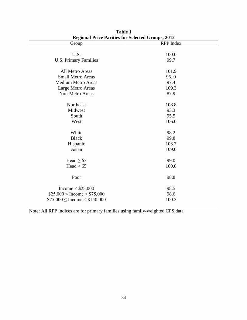
3 Table 1 shows that the average RPPs in non-metro and smaller metropolitan areas are all less

than 100. Thus, families in these areas benefit, on average, from the fact that the tax code does

not adjust for price differences.

5

Finally, we investigate metro-size agglomeration economies to distinguish between

higher costs (price differences) and benefits (agglomeration) of living in a major metropolitan

area. Families are divided into large, medium, and small metro dwellers; all non-metro families

form the comparison group. After adjusting for the RPPs and controlling for the family head’s

characteristics, the higher family incomes found in major metropolitan areas largely, but not

completely, disappear.

The rest of the paper proceeds as follows. Section 2 reviews the BEA procedures for

generating the new RPP measures and presents the resulting regional price differences. Section

3 explores how RPP adjustments affect mean income, poverty, and income inequality in Census

regions and divisions, as well as the quantile functions for the entire U.S. Section 4 investigates

the effects of RPP adjustments for federal income tax progressivity among U.S. primary families.

Section 5 examines the effect of RPP adjustments on urban agglomeration premiums. Section 6

presents our conclusions.

2 Background and Data

This research is closely related to the international studies examining the impact of

purchasing power parity (PPP) adjustments on global poverty and inequality. As Deaton and

Dupriez (2011, 1) point out, “… for the same reasons that we expect price levels to be lower in

poor countries—the Balassa-Samuelson theorem—we would expect prices to be lower in poorer

areas within countries, at least if people are not completely mobile across space.” In applications

to poorer countries, such as India and Brazil, they focus on spatial variation in food prices, where

the rural advantage appears to diminish as countries become richer. In the richest countries, such

as the U.S., the rural advantage is mainly due to lower housing and fuel prices (Aten, Figueroa,

6

and Martin, 2011). When discussing price-level differences in relation to living costs, it is also

important to keep in mind that both amenities and prices vary across space, so areas with high

prices must also have compensating amenities in equilibrium (Roback, 1982).

Comparing living standards across regions in the U.S., however, is much less

complicated than international comparisons using PPPs. In the global comparisons, the wider

variation in consumption patterns among countries makes it harder to estimate relative prices.

Deaton (2016, 1226) captures the dilemma,

On the one hand, we need to compare like with like, using only goods and

services that are close to identical in different countries. On the other hand, we

also wish to capture what people actually spend, so that we want to use goods and

services that are widely consumed and representative of actual purchases. These

two requirements often stand in sharp opposition; in the extreme case where

consumption bundles have nothing in common, there is no basis for comparisons

of living standards.

Deaton (2010) concludes that comparisons are more meaningful for broadly similar countries

and, we add, still more so for regions within the same country.

As background for our analysis, we review some important steps leading to the

appearance of the official RPP indices. Three Budgets for an Urban Family of Four Persons

(U.S. Department of Labor 1979) was an early attempt by the BLS to measure regional living

costs. This measure was estimated for 25 metropolitan areas and for the non-metro areas of the

four Census regions. Bishop, Formby, and Thistle (1992; 1994) used this series to study regional

income convergence in the U.S. and to create regional living cost indices for 1969 and 1979.

Unfortunately, the series was discontinued in the early 1980s.

7

Another important study, Measuring Poverty: A New Approach (Citro and Michael,

1995) by the NAS Panel on Poverty and Family Assistance, dealt with all the issues listed in the

first paragraph of this paper, including variation in prices across regions. It recommended using

housing price indices to approximate regional price levels. As Deaton and Dupriez (2011, 4)

note, “This proposal generated a substantial subsequent research effort within federal statistical

agencies, see for example Short, Garner, Johnson, and Doyle (1999), Renwick (2011), Short

(2011), and Aten, Figueroa and Martin (2011),” the last of these being the primary source for

understanding the RPPs used in our analysis.

To give a sense of the findings from using housing price adjustments, we focus on an

important contribution to this literature. Jolliffe (2006) matched CPS data with a spatial price

index created by the Census Bureau, using Fair Market Rent (FMR) data, and adjusted poverty

measures for differences in metro and non-metro housing costs. He found that the adjustments

reversed the poverty profiles of the metro and non-metro areas, rendering the incidence, depth,

and severity of poverty greater in the metro areas than in the non-metro areas for 1991-2002.4

The limitation of this study is that the FMR data captures only differences in housing prices –

though housing costs are the single most important component in household budgets.5 In our

paper, we will repeat the comparison using a broader measure of price variation.

The NAS panel suggested adjusting for regional price differences using housing price

indices as a first step, primarily because these indices were readily available at the time of the

4 A later study by Early and Olsen (2012), which uses a price index that captures variation in all

prices (not just housing prices), finds little difference in poverty rates across metropolitan status.

5 Another study along these lines, Nelson and Short (2003), explores the impact of housing price

adjustments on poverty rates by state, and provides rough estimates of their impact on federal

government transfers to the poor by state.

8

report and “good data” on all other budget items was not readily available (Citro and Michael,

1995). Moving forward, the NAS panel also called for the development of more encompassing

geographic price parities for all household goods and services. In the past, researchers interested

in regional purchasing power differences for all goods and services have typically relied on the

American Chambers of Commerce Researchers Association’s (ACCRA) metropolitan area

indices. The ACCRA indices are only available for the metropolitan areas, and the housing

component of ACCRA has been criticized for failing to adjust for quality differences in

locational housing stock (Carrillo, et al., 2014).

In an important recent development, the BEA and the U.S. Census Bureau, in

collaboration with the Bureau of Labor Statistics (BLS), released the first official RPPs for all

the 381 U.S. metropolitan areas and state-level, non-metropolitan areas. Around the same time,

Carrillo, et al. (2014) published unofficial price indices covering all produced goods and services

in all areas of the U.S. (metro and non-metro) that extend back to 1982.6 The data released by

the BEA allow us to address each of the aforementioned shortcomings with earlier attempts to

control for regional differences in prices.

2.1 The New Regional Price Parities

This section gives an overview of the construction of the new RPP indices. Aten, et al.

(2011) and Aten and Figueroa (2014) give a detailed overview of the BEA’s newly constructed

RPPs. Except where otherwise noted, our discussion relies heavily on their documentation. We

6 Their paper notes that, at the time, the BEA had “exploratory” RPP indices that were not yet

publically available.

9

then summarize the RPP data across metropolitan and non-metropolitan areas, Census regions,

and divisions using the combined BEA and CPS datasets.

Beginning in 2003-2004, the BEA estimated U.S. regional price parities for the 38

metropolitan and urban areas that the BLS uses to generate the CPI, which contained about 87

percent of the U.S. population at that time. The procedure was based on the price information in

the CPI (covering hundreds of consumer goods and services) and used hedonic methods to adjust

for differences in product characteristics (type of outlet selling a good or service, packaging, etc.)

for the 75 most important item categories, representing about 85 percent of all expenditures. For

the remaining categories, a method roughly equivalent to a weighted geometric mean of prices in

each item category generated relative price levels. The estimation results were then checked for

outliers using methods similar to those developed for comparing relative prices across countries

in the Income Comparison Project.

The BEA extended the analysis beyond areas covered by the CPI in 2005-06, using

housing data from the American Community Survey (ACS). Housing is the key factor in the

cost of living; rents and owners’ equivalent rents are the most important consumer expenditure

category by far, accounting for 30 percent of the total. Once again, hedonic regression methods

allow adjustments for differences in housing characteristics (the number of rooms and bedrooms;

the age and type of housing unit). For all remaining goods and services, price levels for non-CPI

areas are equated to the average for that region (e.g., the Midwest). The BEA released its official

real, per capita incomes for states and metropolitan statistical areas in April 2014, adjusted with

RPPs, i.e., percent differences in regional average prices from the national average (Aten and

Figueroa, 2014).

10

2.2 U.S. Price Level Differences

By construction, the national average price level is 100 and the RPPs for comparison

areas are expressed as percentages of the national average. Thus, the ratio RPP/100 gives the

relative price level for a comparison area. In 2012 the metro areas with the highest RPPs were

Honolulu, Hawaii (122.9), New York, New York and Newark-Jersey City, New Jersey (122.2),

San Jose-Sunnyvale-Santa Clara, California (122), Bridgeport-Stamford-Norwalk, Connecticut

(121.5), and Santa Cruz-Watsonville, California (121.4). Danville, Illinois (79.4), Jefferson City,

Missouri (80.8), Jackson, Tennessee (81.5), and Jonesboro, Arkansas (81.7) had the lowest metro

RPPs. The weighted-average price level in Honolulu is about 23 percent higher (122.9/100) than

the national average, and the relative price level in the District of Columbia is approximately 47

percent higher than in Jackson, Tennessee or in Jonesboro, Arkansas (120.4/81.5 = 1.477). Aten,

et al. (2011) note that price levels vary more across regions for services than goods, and services

account for two-thirds of consumer expenditures. Among expenditure categories, housing rents

vary the most and transportation costs (e.g., new and used vehicle purchases) vary the least.

Table 1 presents the new RPP indices by metro status, region, race, age, and family

income, estimated with 2012 BEA metro-level and state-level non-metro RPP indices and the

2013 CPS data (2012 incomes). The mean RPP for primary families is slightly less than 100

(99.7). The RPP index varies by metro status (non-metro areas are the least expensive locations

with an RPP of 87.9 on average) and size (from 95.0, on average, for small metro areas to 109.3

for large metro areas). The Northeast is the highest RPP region (108.8), followed by the West

(106.0). The Midwest (93.3), not the traditionally poor South (95.5), has the lowest price level

among regions. The comparisons by race show that Asians live in more expensive areas (109.0)

than whites (98.2), an 11 percent difference. Hispanics (103.7) also live is areas slightly more

11

expensive than whites. RPPs vary little by the age of the family head, but increase with income

– from 98.5 for families with incomes below $25,000 to 104.1 for families with incomes above

$150,000. The families identified by the U.S. Census as “poor” face price levels (98.8) that are

slightly below the U.S. average.

[place Table 1 about here]

2.3 Comparisons with U.S. Census Figures—Family Money Income

As a check on our data, we attempt to “match” the means, poverty rates, and Gini

coefficients, constructed from the CPS microdata, to those published by the U.S. Census. The

attempt to match the published figures reveals the degree to which the top-coding of incomes in

the public-use CPS files affects our findings. We make comparisons with family money income,

the standard used in the published U.S. Census figures, which we construct from the March 2013

CPS data. These figures provide the benchmark for assessing the effects of the RPP adjustments.

Census money income includes wages and salaries, self-employment income, dividends, rent,

interest, cash transfers (Social Security and Unemployment Insurance), and other cash income,

but it excludes the market value of in-kind transfers, the earned income tax credit, and all taxes.

In spite of its shortcomings, Census money income is the basis for the most frequently cited U.S.

poverty and inequality statistics.7

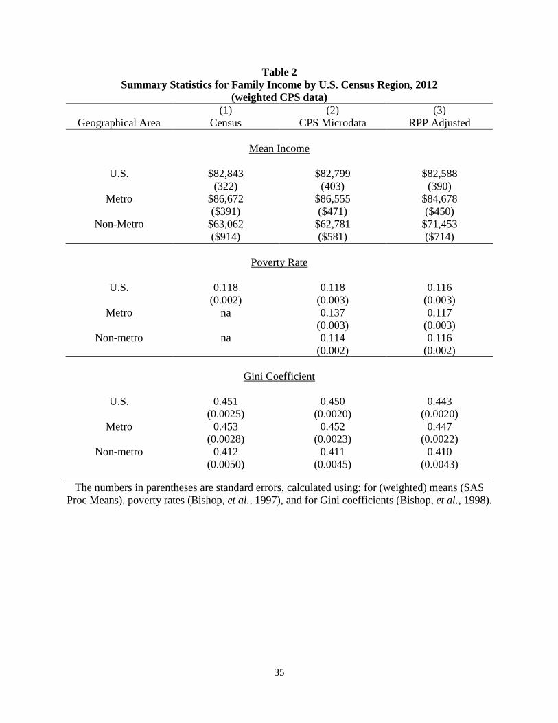
Table 2 reports the mean family money income, the percentage of families receiving

incomes below the official poverty level (with standard errors calculated as in Bishop, et al.,

7 We replicated much of the analysis with household adult equivalent comprehensive income

(including taxes and in-kind transfers, such as food stamps) and obtained essentially the same

results as reported in Tables 1-5 below. See Bishop, Formby and Zheng (1999) for a definition

of adult equivalent comprehensive income.

12

1997),8 and Gini ratios for family money income (with standard errors calculated as in Bishop, et

al., 1998) in the U.S. overall, in metro areas, and in non-metro areas, respectively. The figures in

column 1, labeled “Census,” are taken from the P-60 Series, “Income and Poverty in the United

States, 2013,” Document FINC-01, “Selected Characteristics of Families by Total Money

Income, 2012”, as well as the regional poverty statistics obtained from the U.S. Census Bureau’s

“Table-Creator” website. Columns 2 and 3 in Table 2 are generated by the authors. Column 2,

labeled “Microdata,” presents statistics calculated from the March 2013 Annual Demographic

File, based on data for 2012 family money incomes. Column 3, labeled “RPP-Adjusted,” reports

statistics generated by combining the CPS microdata with the BEA RPP adjustments.


As Table 2 shows, our estimate of the overall mean U.S. family money income is within

$50 of the published figure. Our estimate of the U.S. family income Gini is within 0.001 of the

published Census figure and our U.S. family poverty rate matches the published Census figure

exactly. As expected, RPP adjustment has little effect on the overall U.S. mean income, while

the overall U.S. poverty rate declines from 11.8 to 11.6 – which we anticipated from Table 1,

because poor families have RPPs slightly less than 100 on average. The U.S. family income

Gini declines from 0.450 to 0.443.

8 Joliffe (2003) notes that the standard errors produced by this method (see footnote 3) may

underestimate the headcount poverty rate standard errors when surveys follow complex multi-

stage sampling procedures. However, Jolliffe (2005) also notes that the primary sampling units

and strata used by the Census Bureau for CPS sampling are not publicly available. He devises a

method to replicate the CPS sampling design by treating regions as strata and sorting the data by

family income, with families separated into rank order groups of 4 that then serve as the primary

sampling units. We estimated some standard errors using this method as a robustness check, but

did not find any meaningful difference in statistical inferences for the poverty rates from our

standard error estimation using CPS family weights.

13

Turning to SMSA status, we find that we can again match mean incomes and Gini

coefficient quite well (poverty rates by SMSA status are not published). Here the effect of RPP

adjustments is more dramatic; the gap between metro and non-metro incomes falls from $23,610

to $13,225 after RPP adjustments. While the metro poverty rate is barely changed (11.4 to 11.6),

the non-metro poverty rate falls by a full two percentage points (13.7 to 11.7), which eliminates

the disparity in poverty rates between the metro and non-metro areas.9 Notice that this finding

contrasts with Jolliffe (2006), who reports a reversal in the metro and non-metro rankings after

adjusting for differences in housing prices, but matches with Early and Olsen (2012), who find

little difference in poverty rates by metropolitan status. The latter study applies a broader price

measure than Jolliffe (2006), as we do. The discrepancy is probably due to greater variation in

housing prices (a regionally nontraded good) than in other prices, so that adjusting incomes by

housing prices leads to excessive compensation for price differences between metro and non-

metro areas.

2.4 Comparison to Census Supplemental Poverty Rates

In the previous section we saw a dramatic decline in the gap between metro and non-

metro average incomes and poverty rates with RPP adjustments. In this section we investigate

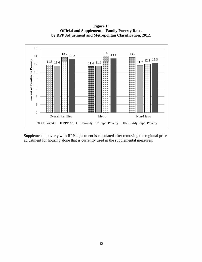
alternative definitions of poverty by metro status. Figure 1 reports family poverty rates based on

the U.S. Census Bureau’s official method (family money income), Supplemental Poverty method

(with local housing cost adjustments), and official and Supplemental Poverty measures with RPP

9 Although not reported in Table 2, we also made similar adjustments in family poverty rates for

racial minorities. Recall from Table 1 that the RPPs for Asians and Hispanics are above the U.S.

average. RPP adjustments increase the Hispanic poverty rate from 23.4 percent to 24.3 percent

and the Asian poverty rate from 9.3 percent to 10.3 percent.

14

adjustments.10 Supplemental Poverty rates are published in Short (2013). They involve a more

comprehensive measure of family income that includes subsidies and transfers, assume a three-

parameter equivalence scale that varies with the number of adults and children in the family, and

adjust poverty thresholds for differences in food, clothing, and utility costs (all linked to housing

ownership status), as well as regional differences in the cost of shelter (Short 2013).

[place Figures 1 and 2 about here]

Consider Figure 1, where Census family poverty rate without adjustment is 11.4 percent

for metro regions and 13.7 for non-metro regions. The RPP adjustments reduce the gap between

the metro and non-metro poverty rates for families from 2.3 percentage points to a negligible 0.1

percentage point. Short’s method goes somewhat farther in that the non-metro poverty rate (12.1

percent) is lower than the metro poverty rate (14.0 percent). However, when the supplemental

poverty rates are adjusted by the more comprehensive BEA RPPs, rather than simply adjusting

for regional differences in housing costs, the metro (13.4 percent) and non-metro (12.3 percent)

poverty gap is reduced to 1.1 percentage points. Therefore, we infer that a significant portion

(roughly 42%) of the metro/non-metro poverty gap associated with the Supplemental Poverty

measures is actually due to the aforementioned excessive compensation for price differences

between metro and non-metro areas when the price parities only adjust for housing costs.

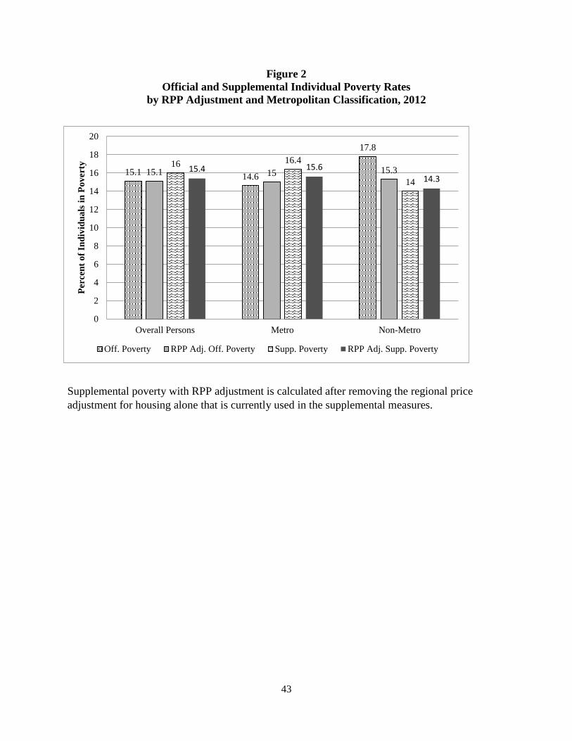
Short presents her results in terms of individuals; we re-estimated the supplemental

poverty rate for families in Figure 1. Figure 2 shows the same results for individuals in families,

not simply families. With individuals as the income recipient unit, RPP adjustment reduces non-

10 The Census poverty rates and Supplemental poverty rates are published in the P-60 Series,

“Income and Poverty in the United States, 2013,” Document FINC-01, “Selected Characteristics

of Families by Total Money Income, 2012.” Supplemental poverty with RPP adjustment is

calculated after removing the regional price adjustment for housing alone that is currently used in

the supplemental measures.

15

metro Census poverty rates from 17.8 percent to 15.3 percent, and raises the metro poverty rates

slightly (14.6 percent to 15.0 percent). Likewise, supplemental poverty rates are lower for non-

metro regions (14.0 percent and 16.4 percent). In sum, by comparing the Supplemental Poverty

rates by both families and individuals, we confirm the finding of Table 2 that local price

adjustment has a significant impact on non-metro poverty rates.

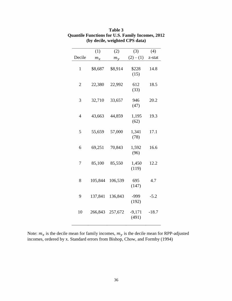
2.5 RPP Adjustments to the U.S. Quantile Function

RPP adjustments raise incomes in some areas and lower incomes in other areas, so it is

no surprise that they do not alter average family income for the entire U.S. (see Table 2). Here

we go beyond the mean by examining the entire pre- and post-RPP-adjusted income distribution.

Table 3 reports the decile conditional means before and after RPP adjustment, while maintaining

throughout the pre-adjustment income ordering.11

The results in Table 3 are illuminating. The lowest eight deciles all gain income from

RPP adjustment, while the losses are concentrated in the top two deciles. The biggest gain is in

the sixth decile ($1,592) and the largest loss is in the top decile ($9,171). This result is perhaps

not surprising, given that the highest income families tend to live in the areas with the highest

prices.


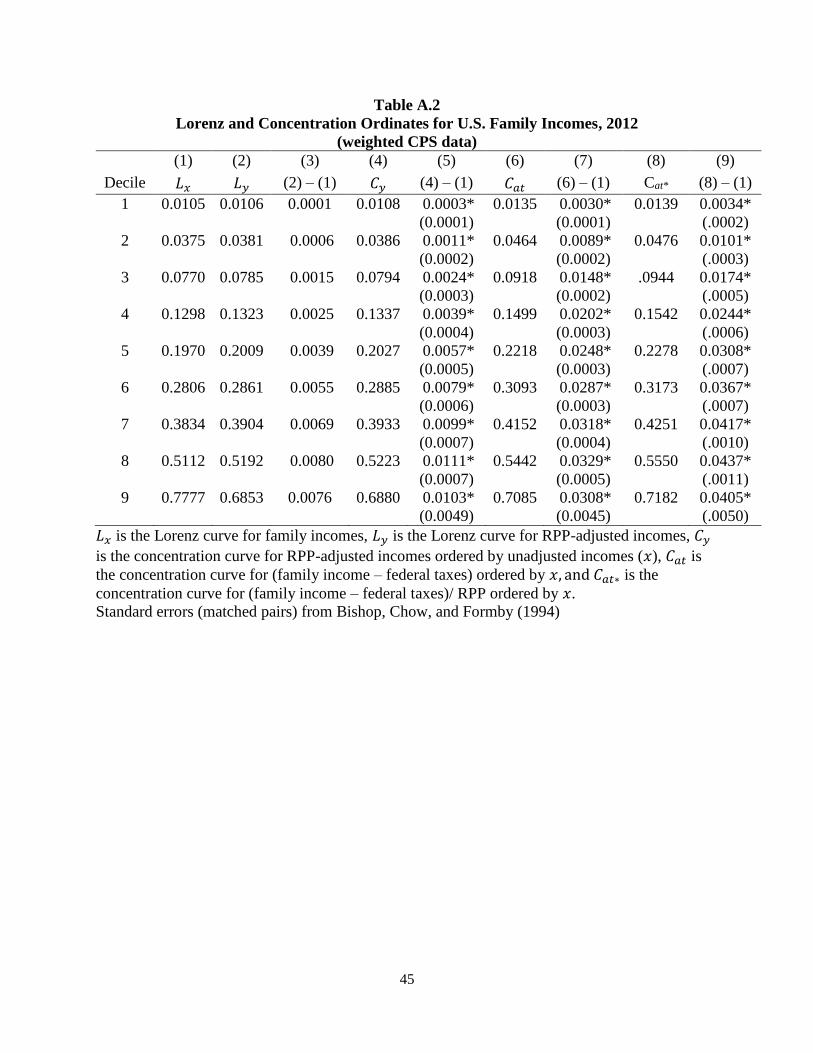
11 Appendix Table A.2, columns 1 and 2, give the family money income Lorenz and

concentration ordinates by decile, before and after RPP adjustment.

16

3. RPP Adjustments of Incomes and Poverty Rates U.S. Region and Division

U.S. Census Bureau partitions the country into four major regions and nine divisions,

each defined by groupings of states. Table A.1 in the appendix gives the assignment of states to

these regions and divisions. The Northeast, Midwest, and West contain two divisions each while

the South contains three divisions. Divisions can have as few as three states (Middle Atlantic) or

as many as nine (South Atlantic).

We have already shown in Table 2 that RPP adjustment has small effects on the overall

mean income, poverty rate, and Gini coefficient, but that meaningful effects emerge between the

metro and non-metro areas. To expand our geographical analysis of RPP adjustment, this section

makes comparisons among the Northeast, South, Midwest and West regions and the nine Census

divisions. We focus on these geographical groupings because the CPS is not representative at

the level of individual U.S. states.

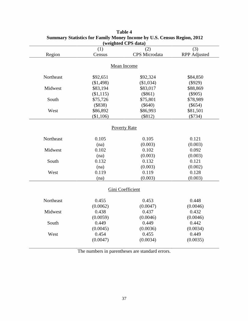
3.1 RPP Adjustments by Census Regions

Table 4 is structured like Table 2 above, where we compare our estimates of mean

income, poverty, and inequality to those reported by the U.S. Census Bureau, but it focuses on

the four Census regions. Our estimates for regional mean income (column 2) are very close to

those published by the Census (column 1), our poverty rates match exactly, and our Gini

coefficient estimates deviate by no more than 0.002.


Adjusting for RPPs (column 3) results in a convergence in income levels among the

regions and the emergence of the Midwest as the region with the highest income. Before RPP

17

adjustments, the difference in mean incomes between the Northeast and South is $16,925; after

adjustments, the gap between the highest (Midwest) and lowest (South) regions falls to $9,880.

Poverty rates are also affected by RPP adjustments. Before the adjustments, the

Northeast and Midwest have similar poverty rates (10.5 and 10.2) but after the adjustment the

increase in poverty in the Northeast and the decline in poverty in the Midwest widens the gap to

2.9 percentage points. Southern poverty falls by 1.1 percentage points and Western poverty rises

by 0.9. In sum, regional poverty rates largely converge – with the exception of the low-poverty

Midwest region.

The bottom of Table 4 reports the regional Gini coefficients. The reductions in these

coefficients are slightly smaller than the 0.008 reduction in the overall U.S. Gini (given in Table

2). It appears that within each region, higher-income families live in higher-price areas. Table 4

shows that we find no change in the regional inequality rankings after the RPP adjustments.

We also examine the complete income distributions for the four regions (in a manner

similar to Table 3, but not shown in Table 4) and find that in the Midwest and South, incomes

increase in all deciles with RPP adjustment, whereas in the West and Northeast, incomes in all

deciles decrease. Our key finding using 2012 data and the new RPPs is the divergence of the

Midwest, especially below the median income, from other US regions. This is in contrast to

earlier studies using BEA’s Three Budgets for an Urban Family that find convergence of

Southern incomes to the rest of the nation.

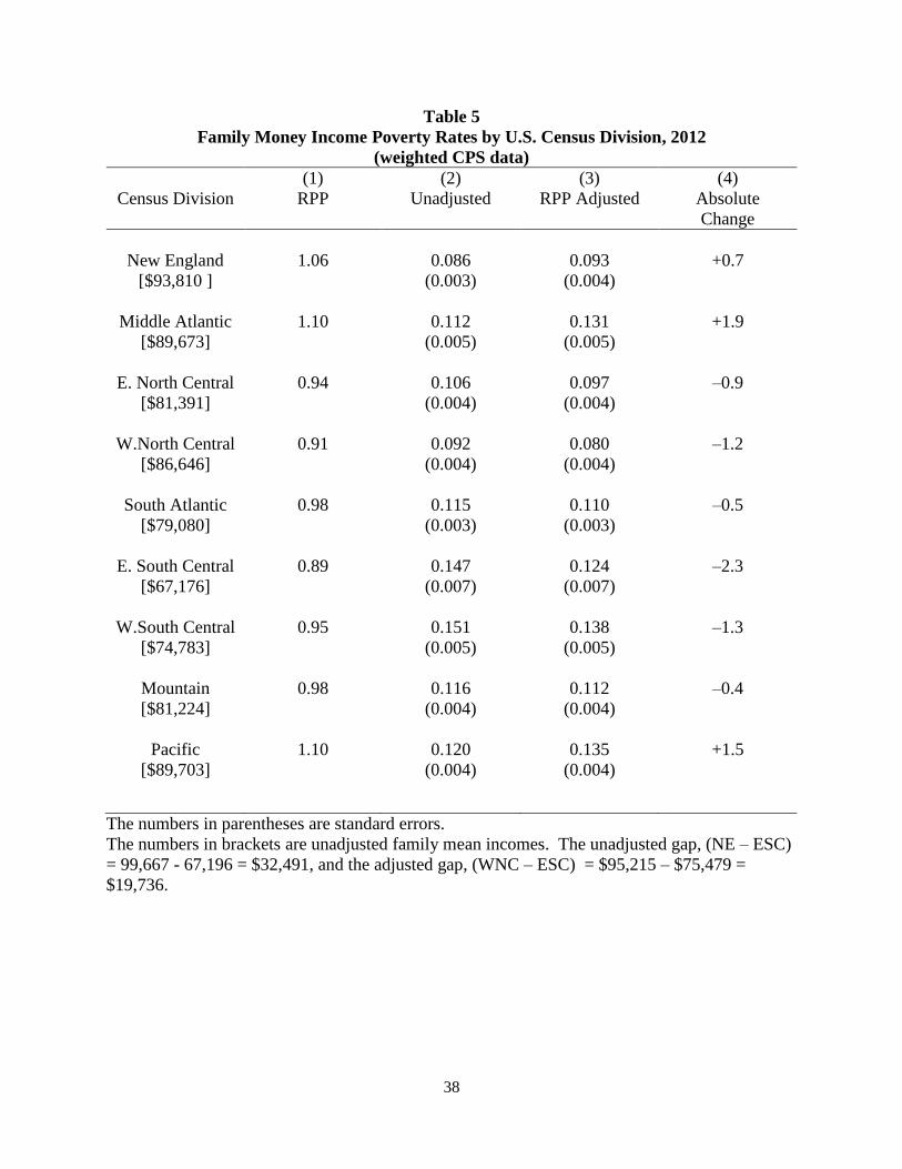
3.2 Census Divisions and RPP Adjustments

Table 5 shows the unadjusted mean incomes [in brackets], official RPP indices, and

poverty rates for the nine Census divisions before and after RPP adjustments. The RPP index

18

varies substantially among the Census divisions, from a high of 110.0 in the Middle Atlantic and

Pacific divisions to a low of 89.0 in the East South Central division, a 24 percent difference. The

effect of this discrepancy in RPPs is immediately apparent when we compare the mean incomes.

Unadjusted for RPPs, we find the largest gap between the New England and East South Central

divisions, $32,491 (= $99,667 – $67,196); after RPP adjustment, the largest gap, the West North

Central and the East South Central, falls to $19,736 ($95,215 – $75,479). Clearly, mean incomes

in the divisions are converging with RPP adjustments.


Turning to the poverty comparisons, column 4 of Table 5 gives the percentage point

changes in poverty rates between columns 2 and 3. The East South Central, West South Central

and West North Central divisions have the greatest percentage point reductions, while the largest

increases in poverty occur in the Mid-Atlantic and Pacific divisions. No division shows less than

a 0.5 percentage point change in poverty due to the RPP adjustments. It is also noteworthy that,

while RPP adjustments eliminate the metro vs. non-metro difference in poverty rates (see Table

2), the same adjustments reduce the dispersion in poverty rates across the Census divisions only

slightly. The limited convergence in poverty rates across divisions can be understood by noting

that the West North Central division is a low-cost, low-poverty area while the Pacific division is

a high-cost, high-poverty area. Before the RPP adjustments, the New England and West North

Central divisions have the lowest poverty rates; after the adjustments, the West North Central

division has a poverty rate 1.3 percentage points lower than New England.

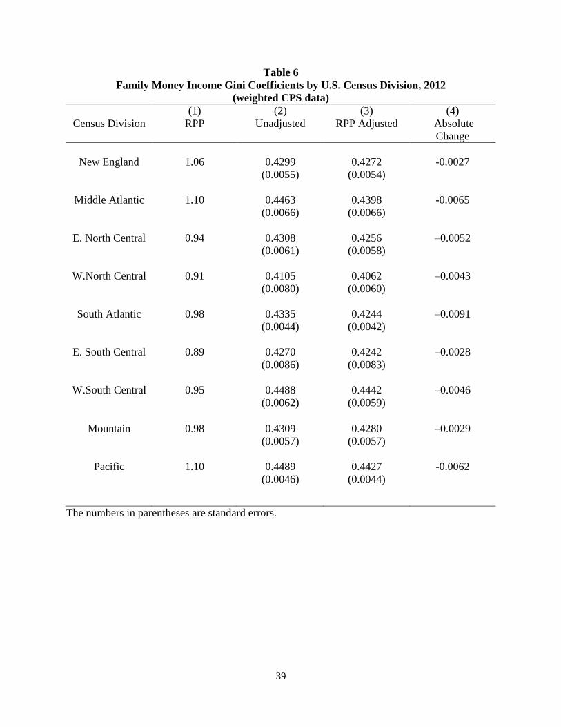
Table 6 is similar to Table 5, but examines changes in the divisional Gini coefficients

after RPP adjustments. All divisions show small reductions in inequality after the adjustments,

the largest reduction being in the South Atlantic (0.0091) – which is similar to the decline in the

19

overall U.S. Gini coefficient (0.008). Yet the gap between the most and the least equal divisions

does not change (0.038), suggesting no convergence in divisional inequality due to the RPP

adjustments.


In summary, we find strong convergence in mean incomes for the divisions. We also

find meaningful changes in divisional poverty rates, but neither divergence nor convergence in

divisional income inequality. Finally, we look at the complete income distributions for the nine

Census divisions (not reported in any table). One case of particular interest is the South Atlantic

Division, a very diverse region that encompasses low-price southern states and several high-price

cities, such as Washington, DC. Here we find that deciles 1-8 gain income after RPP adjustment,

decile 9 is not significantly different after RPP adjustment, and the top decile shows a significant

income reduction after RPP, which mirrors our finding for the entire U.S. distribution. Changes

in all the other deciles, in all other divisions, mimic the changes in their mean incomes.

4. Inequality, Vertical Equity, and Tax Progressivity

In sections 2 and 3 above we showed that the effect of RPP adjustment is to reduce

income inequality. This is explained by our finding that high-income families tend to live in

high-price areas. Albouy (2009, 656) notes that ignoring prices differences leads to an unequal

burden of federal taxes because a worker, “moving from a low-wage city to a typical high-wage

city sees her average tax rate rise from 14.8 percent to 19.2 percent, paying 27 percent more in

federal taxes.” All of this suggests that without RPP adjustments, we may understate actual

federal tax progressivity.

20

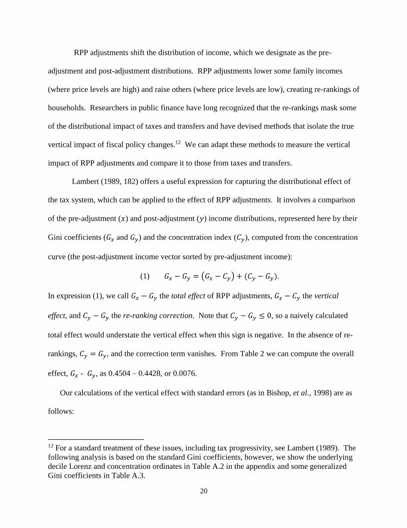
RPP adjustments shift the distribution of income, which we designate as the pre-

adjustment and post-adjustment distributions. RPP adjustments lower some family incomes

(where price levels are high) and raise others (where price levels are low), creating re-rankings of

households. Researchers in public finance have long recognized that the re-rankings mask some

of the distributional impact of taxes and transfers and have devised methods that isolate the true

vertical impact of fiscal policy changes.12 We can adapt these methods to measure the vertical

impact of RPP adjustments and compare it to those from taxes and transfers.

Lambert (1989, 182) offers a useful expression for capturing the distributional effect of

the tax system, which can be applied to the effect of RPP adjustments. It involves a comparison

of the pre-adjustment (𝑥) and post-adjustment (𝑦) income distributions, represented here by their

Gini coefficients (𝐺𝑥 and 𝐺𝑦) and the concentration index (𝐶𝑦), computed from the concentration

curve (the post-adjustment income vector sorted by pre-adjustment income):

(1) 𝐺𝑥 − 𝐺𝑦 = (𝐺𝑥 − 𝐶𝑦) + (𝐶𝑦 − 𝐺𝑦).

In expression (1), we call 𝐺𝑥 − 𝐺𝑦 the total effect of RPP adjustments, 𝐺𝑥 − 𝐶𝑦 the vertical

effect, and 𝐶𝑦 − 𝐺𝑦 the re-ranking correction. Note that 𝐶𝑦 − 𝐺𝑦 ≤ 0, so a naively calculated

total effect would understate the vertical effect when this sign is negative. In the absence of re-

rankings, 𝐶𝑦 = 𝐺𝑦, and the correction term vanishes. From Table 2 we can compute the overall

effect, 𝐺𝑥 - 𝐺𝑦, as 0.4504 – 0.4428, or 0.0076.

Our calculations of the vertical effect with standard errors (as in Bishop, et al., 1998) are as

follows:

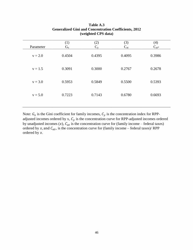
12 For a standard treatment of these issues, including tax progressivity, see Lambert (1989). The

following analysis is based on the standard Gini coefficients, however, we show the underlying

decile Lorenz and concentration ordinates in Table A.2 in the appendix and some generalized

Gini coefficients in Table A.3.

21

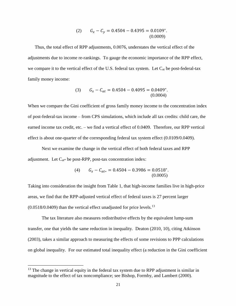
(2) 𝐺𝑥 − 𝐶𝑦 = 0.4504 − 0.4395 = 0.0109∗.

(0.0009)

Thus, the total effect of RPP adjustments, 0.0076, understates the vertical effect of the

adjustments due to income re-rankings. To gauge the economic importance of the RPP effect,

we compare it to the vertical effect of the U.S. federal tax system. Let Cat be post-federal-tax

family money income:

(3) 𝐺𝑥 − 𝐶𝑎𝑡 = 0.4504 − 0.4095 = 0.0409∗.

(0.0004)

When we compare the Gini coefficient of gross family money income to the concentration index

of post-federal-tax income – from CPS simulations, which include all tax credits: child care, the

earned income tax credit, etc. – we find a vertical effect of 0.0409. Therefore, our RPP vertical

effect is about one-quarter of the corresponding federal tax system effect (0.0109/0.0409).

Next we examine the change in the vertical effect of both federal taxes and RPP

adjustment. Let Cat* be post-RPP, post-tax concentration index:

(4) 𝐺𝑥 − 𝐶𝑎𝑡∗ = 0.4504 − 0.3986 = 0.0518∗.

(0.0005)

Taking into consideration the insight from Table 1, that high-income families live in high-price

areas, we find that the RPP-adjusted vertical effect of federal taxes is 27 percent larger

(0.0518/0.0409) than the vertical effect unadjusted for price levels.13

The tax literature also measures redistributive effects by the equivalent lump-sum

transfer, one that yields the same reduction in inequality. Deaton (2010, 10), citing Atkinson

(2003), takes a similar approach to measuring the effects of some revisions to PPP calculations

on global inequality. For our estimated total inequality effect (a reduction in the Gini coefficient

13 The change in vertical equity in the federal tax system due to RPP adjustment is similar in

magnitude to the effect of tax noncompliance; see Bishop, Formby, and Lambert (2000).

22

by 0.0079), the equivalent lump-sum transfer is approximately $1,500 for each primary family in

the United States, while the pure vertical effect (a reduction in the Gini coefficient by 0.0109) is

equivalent to approximately $2,000. To reduce the after-tax Gini in a manner equivalent to the

unadjusted tax effect would require a lump-sum transfer of $8,500. To reach the RPP-adjusted

tax effect would require an additional $2,500, or $11,000 in total. Thus, we conclude that the

effect of adjusting for price level changes on measured vertical equity is substantial.

5. Regional Price Parities, Metro Size, and Agglomeration Premiums

The theory of agglomeration economies suggests that greater urban population density

may raise worker productivity, and these productivity gains should be reflected in both nominal

earnings and rents (e.g., Glaeser and Gottlieb, 2009; Puga, 2010). Yet, neo-classical economic

theory suggests that there should be no differences in equilibrium real wages by location, unless

locations also vary in amenities (Rosen, 1979; Roback, 1982); otherwise, labor migration would

equalize real wages. Still, more recent studies of household sorting suggest that the transactions

costs associated with migration are considerable; see, e.g., Bayer, et al., (2009), which finds that

the vast majority of U.S. households reside in the same region as the head’s birth region. In the

presence of sorting frictions, real wage differences by location can reflect worker heterogeneity,

e.g., equilibrium differences in innate human capital. For those who assume that real wages are

unaffected by city size, nominal earnings premiums that increase with population density can be

interpreted as evidence of agglomeration economies (e.g., Glaeser and Mare, 2001; Glaeser and

Gottlieb, 2009; Glaeser and Resseger, 2010; Puga, 2010), even more so if controls for amenities

(temperature) do not alter the results.

23

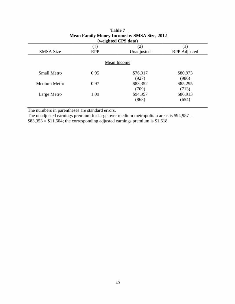
Before beginning the formal analysis we consider Table 7, which compares the

unconditional, unadjusted family income means by metro size to the unconditional, RPP-

adjusted means. Table 7 considers three size classifications: metro areas between 100,000 and

500,000 persons (Small), metro areas between 500,000 and 2.5 million persons (Medium), and

metro areas with more than 2.5 million persons (Large). We can see the potential effect of RPP

adjustment by noting that the difference in means between Large and Medium SMSAs falls from

$11,604 to $1,618 after correcting for the price differences.


Empirical analyses of the relationship between population size and nominal incomes –

the agglomeration premium – are complicated by the possibility of omitted variable bias due to

either unobserved innate worker productivity characteristics or amenity levels or both (see, e.g.,

Roback (1982) and Combes, Duranton, et al., (2008)).14 Endogenous sorting of the high-skilled

workers into larger cities should result in higher real incomes in those locations; however, higher

amenity levels in large cities should lower workers’ real incomes. As the two unobserved factors

move in opposite directions, analyzing the net effect of population density on real family income

(using better measures of local prices) sheds light on which effect – the unobserved productivity

sorting or amenities – dominates. Here is where the RPPs from the BEA can improve upon the

ACCRA data used in previous studies.

The following OLS specification is used to formally test for agglomeration benefits:

(5) cjcjcj MSFCIncome ,, **ln

14 Note that if worker productivity increases as a result of individuals collocating in densely

populated regions (agglomeration) and migration is costless, equilibrium real wages should not

vary by population density (Glaeser and Resseger, 2010).

24

where the log of money income of family j in geographical location c is a function of a vector of

family characteristics, FCj, that includes the number of children and characteristics of the family

head (age, sex, race, education, and previous years of full- and part-time experience). Equation

(5) also includes a vector of indicator variables, MSc, for metro size (Small, Medium and Large)

of location c. As such, the estimated vector of coefficients on metropolitan size, Γ, contains the

key coefficients of interest, measuring the capitalization of agglomeration benefits into family

income relative to the omitted non-metropolitan areas.

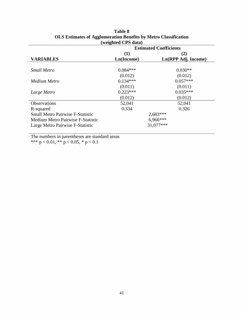
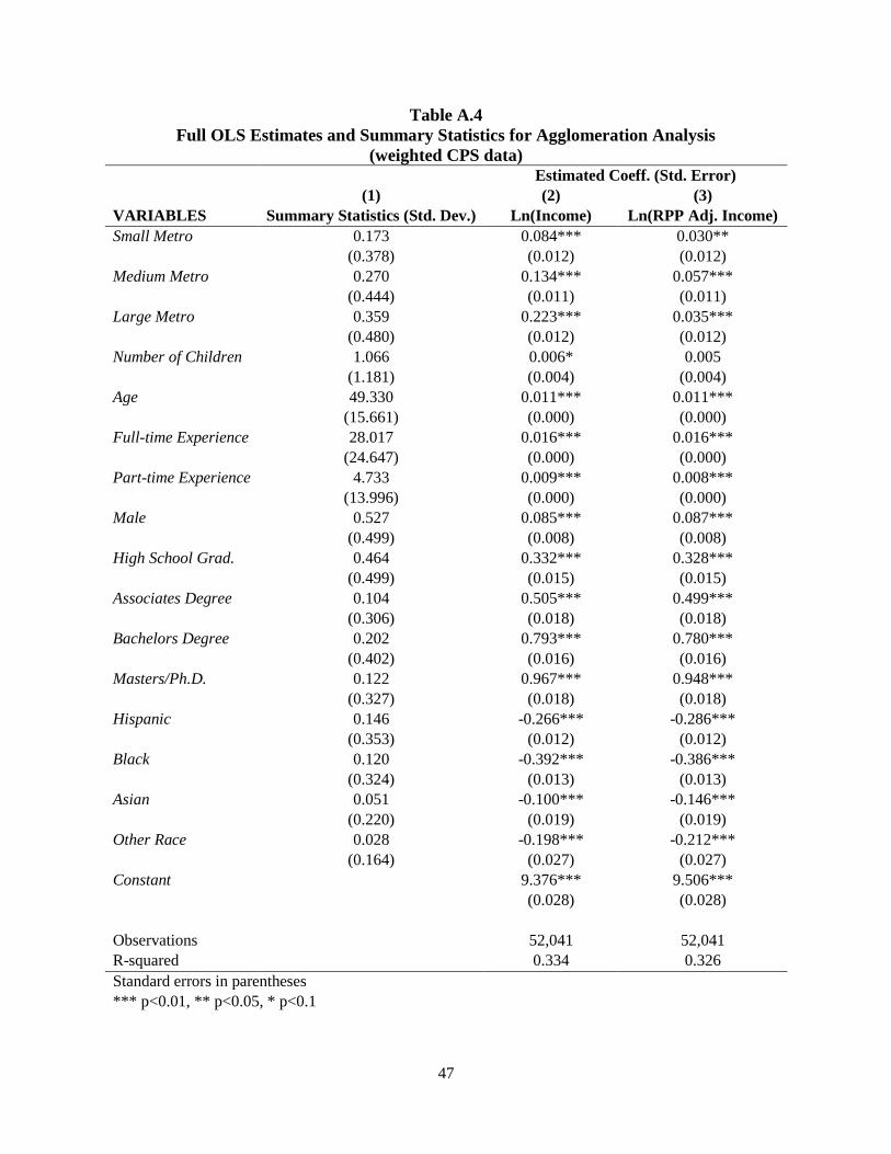
Results from the estimation of equation (5) are presented in Table 8 for the vector of

coefficients measuring metropolitan density effects.15 Column 1 of Table 8 presents results for

the nominal earnings equation, and indicates that families in the smallest metropolitan areas earn

8.8% (95% confidence interval of 6.2% to 11.3%) more than their non-metropolitan counterparts

annually. Likewise, families living in the Middle and Large metropolitan areas earn 14.3% (95%

confidence interval of 11.9% to 16.8%) and 25.0% (95% confidence interval of 22.1% to 27.9%)

annual income premiums relative to non-metropolitan families, respectively. In other words, a

non-metropolitan family moving to Reno, NV, Pittsburgh, PA, and Chicago, IL metropolitan

statistical areas could expect an 8.8%, 14.3%, and 25.0% increase in average family income,

respectively.


These results are largely consistent with the presence of agglomeration benefits that are

capitalized into family incomes. Specifically, families in all metropolitan areas are estimated to

have significantly higher incomes than non-metropolitan families and these earnings differentials

15 The full set of results, along with summary statistics from the estimation of equation (5), are

provided in Appendix Table A.4.

25

increase with metropolitan population density. Further, formal F-tests reject the null hypothesis

of homogeneous earnings differentials across each of the sequential metropolitan size categories

at the 1% level, suggesting that the estimated income differentials by metropolitan size are

significantly different from one another.

Column 2 of Table 8 reports results from a similar specification using the log of real,

RPP-adjusted family income as the dependent variable in equation (5). Interestingly, a larger

metropolitan location has a positive and statistically significant impact on real income across all

metropolitan population density classifications. Families in Metro 1 areas are estimated to have

3.0% higher real incomes (95% confidence interval of 0.7% to 5.5%) and the families in Metro 2

areas earn 5.9% more on average (95% confidence interval of 3.6% to 8.2%) than the non-metro

families. These results are consistent with a positive sorting equilibrium, where the workers with

higher unobserved productivity levels choose to live in the more densely populated areas. In the

neo-classical paradigm, these results could be driven by more disamenities in densely populated

metropolitan areas. F-tests also reject the null hypothesis of homogenous metropolitan effects

for Metro 1 and Metro 2 groups at the 5% level.

Interestingly, however, the real earnings premium in the largest metropolitan

classification is estimated to be 3.6% (roughly 2 percentage points less than the Medium

premium), and formal F-tests also reject the null hypothesis of homogenous metropolitan size

effects for the comparison of Medium and Large groups.16 In terms of real income potential, a

non-metropolitan family is likely to experience the largest gains in average earnings by moving

to a medium-sized city like Pittsburgh, PA, rather than a small city like Reno, NV, or a large city

16 F-tests for the equality of the coefficients on Metro 1 and Metro 3 fail to reject the null

hypothesis that these coefficients are statistically indistinguishable at any conventional level of

significance.

26

like Chicago, IL. Overall, these results could be explained by a worker sorting process that is

non-linear in terms of unobserved productivity, or the results may simply reflect a large increase

in amenities when moving from Medium to Large metropolitan areas, which dampens the

productivity effect.

Nonetheless, across all metropolitan classifications the endogenous, productivity-sorting

effect appears to dominate any effects of increased amenities available to the metro families but

not to the non-metro families. Comparing the point estimates across columns 1 and 2 in Table 8,

we find that between 15.7% and 42.5% of the metro agglomeration estimated benefits in column

1 actually reflect endogenous sorting of workers with heterogeneous, unobserved productivity

characteristics. Glaeser and Resseger (2010) and Combes et. al., (2008) estimate that roughly

30% – 50% of the observed worker productivity premium associated with greater population

density can be attributed to endogenous sorting, and our results are similar in magnitude.

Stacking the data and simultaneously estimating the nominal and real income equations

in a fully nested model enables us to formally test the equality of coefficients for each pairwise

metro-size comparison across columns 1 and 2. These pairwise F-test statistics for each variable

are reported in the last three rows of Table 8 and reveal that the estimated agglomeration effects

from column 1 are significantly larger, statistically, than the productivity effects on real income

from column 2 at the 1% level. Thus, there remains a statistically significant income differential

attributable to agglomeration economies that is increasing with population density and cannot be

completely explained by unobserved productivity and amenity confounders. With that stated, it

is still the case that the majority of the metro-size family income premium disappears after

making RPP adjustments.

27

6. Conclusion

Calls to incorporate spatial price indices in public policy analysis have come from such

notables as Nobel Prize winner Angus Deaton and the prestigious National Academy of Sciences

Panel on Poverty and Family Assistance. Until recently, responses to this call have used housing

price indices, the only data available, to adjust incomes for prices. Fortunately, the U.S. Bureau

Economic Analysis recently released the first official, regional price parities (RPPs) for all the

metro and non-metro areas in the U.S., which cover all the goods and services included in the

computation of the CPI. We examine the impact of the new, broader price measures on the

overall U.S. income distribution, poverty rates, income inequality, vertical equity, tax

progressivity, and urban agglomeration premiums.

As the RPPs reveal, among all family expenditures, housing displays the greatest

geographical price variation (Aten, et al., 2011). Thus, using housing prices to adjust for all

prices exaggerates regional differences in prices and leads to an overcorrection. For example,

Jolliffe (2006) uses housing prices to adjust the metro and non-metro poverty rates and finds a

reversal of the rankings, whereas we find mere convergence in poverty rates between the metro

and non-metro areas. In the same vein, we find convergence in poverty rates among Census

regions, except for the Midwest, after RPP adjustment, but not among the smaller Census

divisions.

We also demonstrate that adjustments for geographical price variation have important

implications for inequality measurement and the related literature on income tax progressivity.

Using methods from these fields to carefully measure the effect of RPP adjustments, inequality

(in terms of the Gini coefficient) falls by an amount equivalent to a $1,500 cash transfer to each

U.S. primary family. Correcting for price level disparities increases effective tax by more than

28

25 percent, or the equivalent of a $2,500 per family cash transfer. These effects occur because

high-income families tend to live in high-price areas.

Finally, we explore the effects of RPP adjustment on the lively topic of urban

agglomeration premiums. Here the literature relies on ACCRA data, which does not adjust

housing prices for quality differences. After adjusting for RPPs and controlling for the family

head’s characteristics, we find that the higher family incomes found in major U.S. metropolitan

areas largely, but not completely, disappear. Clearly, there is more to be done here than we can

fit within the scope of this paper, but our results suggest that further investigation could sharpen

our understanding of the variation in wages and incomes across cities.

References

Albuoy, D.: The Unequal Geographic Burden of Federal Taxation. Journal of Political Economy.

117(4), 635-667 (2009)

Armour, P., Burkhauser, R.V., Larrimore, J.: Deconstructing Income and Income Inequality

Measures: A Crosswalk from Market Income to Comprehensive Income. American

Economic Review. 103(3), 173-177 (2013)

Armour, P., Burkhauser, R.V., Larrimore, J.: Levels and Trends in U.S. Income and its

Distribution: A Crosswalk from Market Income towards a Comprehensive Haig-Simons

Income Approach. Southern Economic Journal. 81(2), 271-293 (2014)

Aten, B.H., Figueroa, E.B., Martin, T.M.: Regional Price Parities by Expenditure Class for 2005-

2009. Survey of Current Business. 91(May), 73–87 (2011)

Aten, B.H., Figueroa, E.B.: Real Personal Income and Regional Price Parities for States and

Metropolitan Areas 2008-2012. Survey of Current Business. 94(June): 1–9 (2014)

29

Atkinson, A.B., Income Inequality in OECD Countries: Data and Explanations. CESifo

Economic Studies. 49(4): 479-513 (2003)

Bayer, P., Keohane, N., Timmins, C.: Migration and Hedonic Valuation: The Case of Air

Quality. Journal of Environmental Economics and Management. 58(1): 1-14 (2009)

Beth Curran, L., Wolman, H., Hill, E.W., and Furdell, K.: Economic Well-being and Where We

Live: Accounting for Geographical Cost-of-Living Differences in the US. Urban Studies.

43(13): 2443-2466 (2006)

Bishop, J.A., Chow, K.V., Formby, J.P.: Testing for Marginal Changes in Income Distributions

with Lorenz and Concentration Curves. 35(2): 479-488 (1994)

Bishop, J.A., Formby, J.P., Lambert, P.: Redistribution Through the Income Tax: The Vertical

and Horizontal Effects of Noncompliance and Tax Evasion. Public Finance Review.

28(4): 335-350. (2000)

Bishop, J.A., Formby, J.P., Thistle, P.D.: Convergence of the South and Non-South Income

Distributions 1969-1979. American Economic Review. 82(1): 262-272 (1992)

Bishop, J.A., Formby, J.P., Thistle, P.D.: Convergence and Divergence of Regional Income

Distributions and Welfare. Review of Economics and Statistics. 76(1): 228-235 (1994).

Bishop, J.A., Formby, J.P., Zheng, B.: Statistical Inference and the Sen Index of Poverty.

International Economic Review. 38(2): 381-387 (1997)

Bishop, J.A., Formby, J.P. and Zheng. B.: Inference Tests for Gini-Based Tax Progressivity

Indexes. Journal of Business and Economic Statistics 16(3): 322-330 (1998)

Bishop, J.A., Formby, J.P., Zheng, B.: Distribution Sensitive Measures of Poverty in the United

States. Review of Social Economy. 57(3): 306-343 (1999)

30

Bishop, J. A., Grodner, A., Liu, H., and Ahamdanech-Zarco, I.: Subjective poverty equivalence

scales for Euro Zone countries. Journal of Economic Inequality. 12(2): 265-278 (2014)

Carrillo, P.E., Early, D.W., Olsen, E.O.: A Panel of Interarea Price Indices for All Areas of the

United States 1982-2012. Journal of Housing Economics. 26(Dec.), 81-93 (2014)

Citro, C.F. and Michael, R.T. (ed.): Measuring Poverty: A New Approach. National Academy

Press, Washington, DC (1995)

Combes, P.-P., et al.: Spatial Wage Disparities: Sorting Matters! Journal of Urban Economics

63(2): 723-742 (2008)

Dalaker, J.: Alternative Poverty Estimates in the United States: 2003. Current Population

Reports, June, 1-22 (2005)

Deaton, A., Measuring and Understanding Behavior, Welfare, and Poverty. American Economic

Review. 106(6): 1221-1243 (2016)

Deaton, A., Price Indexes, Inequality, and the Measurement of World Poverty. American

Economic Review. 100(1): 3-34 (2010)

Deaton, A. and Dupriez, O.: Spatial Price Differences Within Large Countries. Unpublished

Paper, June (2011)

Early, D.W. and Olsen, E.O.: Geographical Price Variation, Housing Assistance and Poverty, In

Jefferson P.M. (ed.) The Oxford Handbook of the Economics of Poverty, pp. 380-424.

Oxford University Press, Oxford (2012)

Glaeser, E.L. and Gottlieb, J.D.: The Wealth of Cities: Agglomeration Economies and Spatial

Equilibrium in the United States, Journal of Economic Literature. 47(4): 983-1028 (2009)

Glaeser, E.L. and Mare, D. C.: Cities and Skills, Journal of Labor Economics. 19(2): 316-

342 (2001)

31

Glaeser, E.L. and Resseger, M.G.: The Complementarity Between Cities and Skills. Journal of

Regional Science 50(1): 221-244 (2010)

Jolliffe, D.: On the Relative Well-Being of the Nonmetropolitan Poor: An Examination of

Alternative Definitions of Poverty during the 1990s. Southern Economic Journal. 70(2),

295-311 (2003)

Jolliffe, D., Gundersen, C., Tiehen, L., Winicki, J.: Food Stamp Benefits and Child Poverty.

American Journal of Agricultural Economics. 87(3), 569-581 (2005)

Jolliffe, D.: Poverty, Prices, and Place: How Sensitive is the Spatial Distribution of Poverty to

Cost of Living Adjustments. Economic Inquiry. 44(2), 296-310 (2006)

Hagenaars, A., de Vos, K., Zaidi, M.A.: Poverty Statistics in the Late 1980s: Research Based on

Micro-data. Office for Official Publications of the European Communities, Luxembourg,

(1994)

Lambert, P.J.: The Distribution and Redistribution of Income – A Mathematical Analysis. Basil

Blackwell, Oxford (1989)

Nelson, C.: Geographic Adjustments in Poverty Thresholds.

http://citeseerx.ist.psu.edu/viewdoc/download?rep=rep1&type=pdf&doi=10.1.1.207.4251

Cited 26 May 2004 (2004)

Nelson, C. and Short, K.: The Distributional Implications of Geographic Adjustment of Poverty

Thresholds. https://www.census.gov/hhes/povmeas/publications/povthres/geopaper.pdf

Cited 8 December 2003 (2003)

Organization for Economic Co-operation and Development: The OECD List of Social Indicators.

Paris (1982)

http://citeseerx.ist.psu.edu/viewdoc/download?rep=rep1&type=pdf&doi=10.1.1.207.4251

https://www.census.gov/hhes/povmeas/publications/povthres/geopaper.pdf

32

Organization for Economic Co-operation and Development: Growing Unequal? Income

Distribution and Poverty in OECD Countries. Paris (2008)

Orshansky, M.: Children of the Poor. Social Security Bulletin 26(July), 3-13 (1963)

Puga, D.: The Magnitude and Causes of Agglomeration Economies, Journal of Regional Science

50(1): 203-219 (2010)

Pritzker, P., U.S. Department of Commerce,

http://www.bea.gov/newsreleases/regional/rpp/rpp_newsrelease.htm Cited 24 April 2014

(2014)

Renwick, T.: Geographic Adjustments of Supplemental Poverty Measure Thresholds: Using the

American Community Survey Five Year Data on Housing Costs, U.S. Census Bureau,

Working Paper (2011)

Renwick, T.: Alternative Geographic Adjustments of U.S. Poverty Thresholds: Impact on State

Poverty Rates. https://www.census.gov/hhes/povmeas/publications/povthres/Geo-Adj-

Pov-Thld8.pdf Cited August 2009 (2009)

Roback, J.: Wages, Rents, and the Quality of Life. The Journal of Political Economy: 1257-1278

(1982)

Rosen, S.: Wages-based Indexes of Urban Quality of Life. In Mieszkowski, P., Straszheim, M.

(ed.) Current Issues in Urban Economics pp. 74-104. Johns Hopkins University Press,

Baltimore (1979)

Short, K.: The Research Supplemental Poverty Measure: 2012, P60-247 (2013).

Short, K.: Who is Poor? A New Look With the Supplemental Poverty Measures, Washington,

DC. U.S. Census Bureau, SEHSD Working Paper 2010-15, (2011).

http://www.bea.gov/newsreleases/regional/rpp/rpp_newsrelease.htm

https://www.census.gov/hhes/povmeas/publications/povthres/Geo-Adj-Pov-Thld8.pdf

https://www.census.gov/hhes/povmeas/publications/povthres/Geo-Adj-Pov-Thld8.pdf

33

Short, K., Garner, T., Johnson, D., Doyle, P.: Experimental Poverty Estimates, 1990-1997.

Current Population Reports: Consumer Income, June, P60-205 (1999)

Timmins, C.: Estimating Spatial Differences in the Brazilian Cost of Living with Household

Location Choices. Journal of Development Economics. 80(1), 59-83 (2006)

U.S. Department of Labor: Bureau of Labor Statistics: Three Budgets for an Urban Family of

Four Persons. U.S. Government Printing Office, Washington, D.C. (1979)

34

Table 1

Regional Price Parities for Selected Groups, 2012

Group RPP Index

U.S. 100.0

U.S. Primary Families 99.7

All Metro Areas 101.9

Small Metro Areas 95. 0

Medium Metro Areas 97.4

Large Metro Areas 109.3

Non-Metro Areas 87.9

Northeast 108.8

Midwest 93.3

South 95.5

West 106.0

White 98.2

Black 99.8

Hispanic 103.7

Asian 109.0

Head ≥ 65 99.0

Head < 65 100.0

Poor 98.8

Income < $25,000 98.5

$25,000 ≤ Income < $75,000 98.6

$75,000 ≤ Income < $150,000 100.3

Note: All RPP indices are for primary families using family-weighted CPS data

35

Table 2

Summary Statistics for Family Income by U.S. Census Region, 2012

(weighted CPS data)

(1) (2) (3)

Geographical Area Census CPS Microdata RPP Adjusted

Mean Income

U.S. $82,843 $82,799 $82,588

(322) (403) (390)

Metro $86,672 $86,555 $84,678

($391) ($471) ($450)

Non-Metro $63,062 $62,781 $71,453

($914) ($581) ($714)

Poverty Rate

U.S. 0.118 0.118 0.116

(0.002) (0.003) (0.003)

Metro na 0.137 0.117

(0.003) (0.003)

Non-metro na 0.114 0.116

(0.002) (0.002)

Gini Coefficient

U.S. 0.451 0.450 0.443

(0.0025) (0.0020) (0.0020)

Metro 0.453 0.452 0.447

(0.0028) (0.0023) (0.0022)

Non-metro 0.412 0.411 0.410

(0.0050) (0.0045) (0.0043)

The numbers in parentheses are standard errors, calculated using: for (weighted) means (SAS

Proc Means), poverty rates (Bishop, et al., 1997), and for Gini coefficients (Bishop, et al., 1998).

36

Table 3

Quantile Functions for U.S. Family Incomes, 2012

(by decile, weighted CPS data)

(1) (2) (3) (4)

Decile 𝑚𝑥 𝑚𝑦 (2) – (1) z-stat

1

$8,687

$8,914

$228

14.8

(15)

2 22,380 22,992 612 18.5

(33)

3 32,710 33,657 946 20.2

(47)

4 43,663 44,859 1,195

(62)

19.3

5 55,659 57,000 1,341

(78)

17.1

6 69,251 70,843 1,592

(96)

16.6

7 85,100 85,550 1,450

(119)

12.2

8 105,844 106,539 695 4.7

(147)

9 137,841 136,843 -999 -5.2

(192)

10 266,843 257,672 -9,171

(491)

-18.7

Note: 𝑚𝑥 is the decile mean for family incomes, 𝑚𝑦 is the decile mean for RPP-adjusted

incomes, ordered by x. Standard errors from Bishop, Chow, and Formby (1994)

37

Table 4

Summary Statistics for Family Money Income by U.S. Census Region, 2012

(weighted CPS data)

(1) (2) (3)

Region Census CPS Microdata RPP Adjusted

Mean Income

Northeast $92,651 $92,324 $84,850

($1,498) ($1,034) ($929)

Midwest $83,194 $83,017 $88,869

($1,115) ($861) ($905)

South $75,726 $75,801 $78,989

($838) ($640) ($654)

West $86,892 $86,993 $81,501

($1,106) ($812) ($734)

Poverty Rate

Northeast 0.105 0.105 0.121

(na) (0.003) (0.003)

Midwest 0.102 0.102 0.092

(na) (0.003) (0.003)

South 0.132 0.132 0.121

(na) (0.003) (0.002)

West 0.119 0.119 0.128

(na) (0.003) (0.003)

Gini Coefficient

Northeast 0.455 0.453 0.448

(0.0062) (0.0047) (0.0046)

Midwest 0.438 0.437 0.432

(0.0059) (0.0046) (0.0046)

South 0.449 0.449 0.442

(0.0045) (0.0036) (0.0034)

West 0.454 0.455 0.449

(0.0047) (0.0034) (0.0035)

The numbers in parentheses are standard errors.

38

Table 5

Family Money Income Poverty Rates by U.S. Census Division, 2012

(weighted CPS data)

(1) (2) (3) (4)

Census Division RPP Unadjusted RPP Adjusted Absolute

Change

New England 1.06 0.086 0.093 +0.7

[$93,810 ] (0.003) (0.004)

Middle Atlantic 1.10 0.112 0.131 +1.9

[$89,673] (0.005) (0.005)

E. North Central 0.94 0.106 0.097 –0.9

[$81,391] (0.004) (0.004)

W.North Central 0.91 0.092 0.080 –1.2

[$86,646] (0.004) (0.004)

South Atlantic 0.98 0.115 0.110 –0.5

[$79,080] (0.003) (0.003)

E. South Central 0.89 0.147 0.124 –2.3

[$67,176] (0.007) (0.007)

W.South Central 0.95 0.151 0.138 –1.3

[$74,783] (0.005) (0.005)

Mountain 0.98 0.116 0.112 –0.4

[$81,224] (0.004) (0.004)

Pacific 1.10 0.120 0.135 +1.5

[$89,703] (0.004) (0.004)


The numbers in brackets are unadjusted family mean incomes. The unadjusted gap, (NE – ESC)

= 99,667 - 67,196 = $32,491, and the adjusted gap, (WNC – ESC) = $95,215 – $75,479 =

$19,736.

39

Table 6

Family Money Income Gini Coefficients by U.S. Census Division, 2012

(weighted CPS data)

(1) (2) (3) (4)

Census Division RPP Unadjusted RPP Adjusted Absolute

Change

New England 1.06 0.4299 0.4272 -0.0027

(0.0055) (0.0054)

Middle Atlantic 1.10 0.4463 0.4398 -0.0065

(0.0066) (0.0066)

E. North Central 0.94 0.4308 0.4256 –0.0052

(0.0061) (0.0058)

W.North Central 0.91 0.4105 0.4062 –0.0043

(0.0080) (0.0060)

South Atlantic 0.98 0.4335 0.4244 –0.0091

(0.0044) (0.0042)

E. South Central 0.89 0.4270 0.4242 –0.0028

(0.0086) (0.0083)

W.South Central 0.95 0.4488 0.4442 –0.0046

(0.0062) (0.0059)

Mountain 0.98 0.4309 0.4280 –0.0029

(0.0057) (0.0057)

Pacific 1.10 0.4489 0.4427 -0.0062

(0.0046) (0.0044)


40

Table 7

Mean Family Money Income by SMSA Size, 2012

(weighted CPS data)

(1) (2) (3)

SMSA Size RPP Unadjusted RPP Adjusted

Mean Income

Small Metro 0.95 $76,917 $80,973

(927) (986)

Medium Metro 0.97 $83,352 $85,295

(709) (713)

Large Metro 1.09 $94,957 $86,913

(868) (654)


The unadjusted earnings premium for large over medium metropolitan areas is $94,957 –

$83,353 = $11,604; the corresponding adjusted earnings premium is $1,618.

41

Table 8

OLS Estimates of Agglomeration Benefits by Metro Classification

(weighted CPS data)

Estimated Coefficients

(1) (2)

VARIABLES Ln(Income) Ln(RPP Adj. Income)

Small Metro 0.084*** 0.030**

(0.012) (0.012)

Medium Metro 0.134*** 0.057***

(0.011) (0.011)

Large Metro 0.223*** 0.035***

(0.012) (0.012)

Observations 52,041 52,041

R-squared 0.334 0.326

Small Metro Pairwise F-Statistic 2,683***

Medium Metro Pairwise F-Statistic 6,966***

Large Metro Pairwise F-Statistic 31,077***

The numbers in parentheses are standard areas

*** p < 0.01, ** p < 0.05, * p < 0.1

42

11.811.4

13.7

11.6 11.6 11.7

13.7 14

12.1

13.2 13.4

12.3

0

2

4

6

8

10

12

14

16

Overall Families Metro Non-Metro

Per

cen

t o

f F

am

ilie

s in

Po

ver

ty

Off. Poverty RPP Adj. Off. Poverty Supp. Poverty RPP Adj. Supp. Poverty

Figure 1:

Official and Supplemental Family Poverty Rates

by RPP Adjustment and Metropolitan Classification, 2012.

Supplemental poverty with RPP adjustment is calculated after removing the regional price

adjustment for housing alone that is currently used in the supplemental measures.

43

15.114.6

17.8

15.1 15 15.316 16.4

14

15.4 15.6

14.3

0

2

4

6

8

10

12

14

16

18

20

Overall Persons Metro Non-Metro

Percen

t o

f In

div

idu

als

in

Po

verty

Off. Poverty RPP Adj. Off. Poverty Supp. Poverty RPP Adj. Supp. Poverty

Figure 2

Official and Supplemental Individual Poverty Rates

by RPP Adjustment and Metropolitan Classification, 2012

Supplemental poverty with RPP adjustment is calculated after removing the regional price

adjustment for housing alone that is currently used in the supplemental measures.

44

Appendix

Table A.1

Census Bureau Regions and Divisions

Region 1 – Northeast [RPP = 106.8]

Division 1 – New England (NE): Connecticut, Maine, Massachusetts, New Hampshire, Rhode

Island, Vermont [RPP =

Division 2 – Middle Atlantic (MA): New Jersey, New York, Pennsylvania

Region 2 – Midwest

Division 3 – East North Central (ENC): Indiana, Illinois, Michigan, Ohio, Wisconsin

Division 4 – West North Central (WNC): Iowa, Kansas, Minnesota, Missouri, Nebraska,

North Dakota, South Dakota

Region 3 – South

Division 5 – South Atlantic (SA): Delaware, District of Columbia, Florida, Georgia,

Maryland, North Carolina, South Carolina, Virginia, West Virginia

Division 6 – East South Central (ESC): Alabama, Kentucky, Mississippi, Tennessee

Division 7 – West South Central (WSC): Arkansas, Louisiana, Oklahoma, Texas

Region 4 – West

Division 8 – Mountain (MTN): Arizona, Colorado, Idaho, New Mexico, Montana, Utah,

Nevada, Wyoming

Division 9 – Pacific (PAC): Alaska, California, Hawaii, Oregon, Washington

45

Table A.2

Lorenz and Concentration Ordinates for U.S. Family Incomes, 2012

(weighted CPS data)

(1) (2) (3) (4) (5) (6) (7) (8) (9)

Decile 𝐿𝑥 𝐿𝑦 (2) – (1) 𝐶𝑦 (4) – (1) 𝐶𝑎𝑡 (6) – (1) Cat* (8) – (1)

1 0.0105 0.0106 0.0001 0.0108 0.0003* 0.0135 0.0030* 0.0139 0.0034*

(0.0001) (0.0001) (.0002)

2 0.0375 0.0381 0.0006 0.0386 0.0011* 0.0464 0.0089* 0.0476 0.0101*

(0.0002) (0.0002) (.0003)

3 0.0770 0.0785 0.0015 0.0794 0.0024* 0.0918 0.0148* .0944 0.0174*

(0.0003) (0.0002) (.0005)

4 0.1298 0.1323 0.0025 0.1337 0.0039* 0.1499 0.0202* 0.1542 0.0244*

(0.0004) (0.0003) (.0006)

5 0.1970 0.2009 0.0039 0.2027 0.0057* 0.2218 0.0248* 0.2278 0.0308*

(0.0005) (0.0003) (.0007)

6 0.2806 0.2861 0.0055 0.2885 0.0079* 0.3093 0.0287* 0.3173 0.0367*

(0.0006) (0.0003) (.0007)

7 0.3834 0.3904 0.0069 0.3933 0.0099* 0.4152 0.0318* 0.4251 0.0417*

(0.0007) (0.0004) (.0010)

8 0.5112 0.5192 0.0080 0.5223 0.0111* 0.5442 0.0329* 0.5550 0.0437*

(0.0007) (0.0005) (.0011)

9 0.7777 0.6853 0.0076 0.6880 0.0103* 0.7085 0.0308* 0.7182 0.0405*

(0.0049) (0.0045) (.0050)

𝐿𝑥 is the Lorenz curve for family incomes, 𝐿𝑦 is the Lorenz curve for RPP-adjusted incomes, 𝐶𝑦

is the concentration curve for RPP-adjusted incomes ordered by unadjusted incomes (𝑥), 𝐶𝑎𝑡 is

the concentration curve for (family income – federal taxes) ordered by 𝑥, and 𝐶𝑎𝑡∗ is the

concentration curve for (family income – federal taxes)/ RPP ordered by 𝑥.

Standard errors (matched pairs) from Bishop, Chow, and Formby (1994)

46

Table A.3

Generalized Gini and Concentration Coefficients, 2012

(weighted CPS data)

(1) (2) (3) (4)

Parameter Gx Cy Cat Cat*

v = 2.0

0.4504

0.4395

0.4095

0.3986

v = 1.5 0.3091 0.3000 0.2767 0.2678

v = 3.0 0.5953 0.5849 0.5500 0.5393

v = 5.0 0.7223 0.7143 0.6780 0.6693

Note: 𝐺𝑥 is the Gini coefficient for family incomes, 𝐶𝑦 is the concentration index for RPP-

adjusted incomes ordered by x, 𝐶𝑦 is the concentration curve for RPP-adjusted incomes ordered

by unadjusted incomes (𝑥), 𝐶𝑎𝑡 is the concentration curve for (family income – federal taxes)

ordered by 𝑥, and 𝐶𝑎𝑡∗ is the concentration curve for (family income – federal taxes)/ RPP

ordered by 𝑥.

47

Table A.4

Full OLS Estimates and Summary Statistics for Agglomeration Analysis

(weighted CPS data)

Estimated Coeff. (Std. Error)

(1) (2) (3)

VARIABLES Summary Statistics (Std. Dev.) Ln(Income) Ln(RPP Adj. Income)

Small Metro 0.173 0.084*** 0.030**

(0.378) (0.012) (0.012)

Medium Metro 0.270 0.134*** 0.057***

(0.444) (0.011) (0.011)

Large Metro 0.359 0.223*** 0.035***

(0.480) (0.012) (0.012)

Number of Children 1.066 0.006* 0.005

(1.181) (0.004) (0.004)

Age 49.330 0.011*** 0.011***

(15.661) (0.000) (0.000)

Full-time Experience 28.017 0.016*** 0.016***

(24.647) (0.000) (0.000)

Part-time Experience 4.733 0.009*** 0.008***

(13.996) (0.000) (0.000)

Male 0.527 0.085*** 0.087***

(0.499) (0.008) (0.008)

High School Grad. 0.464 0.332*** 0.328***

(0.499) (0.015) (0.015)

Associates Degree 0.104 0.505*** 0.499***

(0.306) (0.018) (0.018)

Bachelors Degree 0.202 0.793*** 0.780***

(0.402) (0.016) (0.016)

Masters/Ph.D. 0.122 0.967*** 0.948***

(0.327) (0.018) (0.018)

Hispanic 0.146 -0.266*** -0.286***

(0.353) (0.012) (0.012)

Black 0.120 -0.392*** -0.386***

(0.324) (0.013) (0.013)

Asian 0.051 -0.100*** -0.146***

(0.220) (0.019) (0.019)

Other Race 0.028 -0.198*** -0.212***

(0.164) (0.027) (0.027)

Constant 9.376*** 9.506***

(0.028) (0.028)

Observations 52,041 52,041

R-squared 0.334 0.326

Standard errors in parentheses

*** p<0.01, ** p<0.05, * p<0.1

u.s. income comparisons with regional price parity

Documents