NONLINEAR PPP UNDER THE GOLD STANDARD *

Ivan Payá and David A. Peel **

WP-AD 2004-24

Corresponding author: Ivan Payá, Departamento Fundamentos Análisis Económico, University of Alicante, 03080 Alicante, Spain. E-mail address: ivanpaya@merlin.fae.ua.es Tel.: +34 965903614 Editor: Instituto Valenciano de Investigaciones Económicas, S.A. Primera Edición Junio 2004. Depósito Legal: V-3009-2004 IVIE working papers offer in advance the results of economic research under way in order to encourage a discussion process before sending them to scientific journals for their final publication.

* The authors are grateful to participants of the Understanding Evolving Macroeconomy Annual Conference, University College Oxford 15-16 September 2003. Ivan Paya acknowledges financial support of Instituto Valenciano Investigaciones Economicas (IVIE). ** I. Payá: Departamento Fundamento Análisis Económico, University of Alicante, 03080 Alicante, Spain E-mail address: ivanpaya@merlin.fae.ua.es Tel.: +34 965903614. Fax: +34 965903898. D. A. Peel: Lancaster University Management School, Lancaster, LA1 4YX, UK, United Kingdom

NONLINEAR PPP UNDER THE GOLD STANDARD

Ivan Payá and David A. Peel

ABSTRACT

Hegwood and Papell (2002) conclude on the basis of analysis in a linear framework

that long-run purchasing power parity (PPP)\ does not hold for sixteen real exchange rate

series, analyzed in Diebold, Husted, and Rush (1991) for the period 1792-1913, under the

Gold Standard. Rather, purchasing power parity deviations are mean-reverting to a changing

equilibrium -a quasi PPP (QPPP) theory. We analyze the real exchange rate adjustment

mechanism for their data set assuming a nonlinear adjustment process allowing for both a

constant and a mean shifting equilibrium. Our results confirm that real exchange rates at that

time were stationary, symmetric, nonlinear processes that revert to a non-constant equilibrium

rate. Speeds of adjustment were much quicker when breaks were allowed.

Key Words: Purchasing Power Parity, ESTAR, Bootstrapping. JEL classification: F31, C15, C22, C51

3

1. Introduction

Recent theoretical analysis of purchasing power deviations (see, e.g., Dumas 1992; Sercu,

Uppal, and VanHull 1995; and O’Connell and Wei 1997) demonstrates how transactions

costs or the sunk costs of international arbitrage induce nonlinear adjustment of the real

exchange rate to purchasing power parity (PPP). While globally mean-reverting this

nonlinear process has the important property of exhibiting near unit root behavior for

small deviations from PPP since small deviations from PPP are left uncorrected if they are

not large enough to cover the transactions costs or the sunk costs of international arbitrage.

A parametric nonlinear model, suggested by the theoretical literature, that capture the

nonlinear adjustment process in aggregate data is the exponential smooth transition

autoregression model (ESTAR) of Ozaki (1985). A smooth rather than discrete adjustment

mechanism is motivated by the theoretical analysis of Dumas (1992). Also, as postulated

by Terasvirta (1994) and demonstrated theoretically by Berka (2002), in aggregate data,

regime changes may be smooth rather than discrete given that heterogeneous agents do not

act simultaneously even if they make dichotomous decisions.1 Recent empirical work (e.g.,

Michael, Nobay, and Peel 1997; Taylor, Peel, and Sarno 2001; Peel and Venetis 2002) has

reported empirical results that suggest that the ESTAR model provides a parsimonious fit

into a variety of data sets, particular for monthly data for the interwar and postwar

floating period as well as for annual data spanning two hundred years, as reported in

Lothian and Taylor (1996). In addition, nonlinear impulse response functions derived from

the ESTAR models show that while the speed of adjustment for small shocks around

equilibrium will be highly persistent, larger shocks mean-revert much faster than the

“glacial rates” previously reported for linear models (Rogoff 1996). In this respect, the

ESTAR models provide some solution to the PPP puzzle outlined in Rogoff (1996).2

The ESTAR model can also provide an explanation of why PPP deviations analyzed

4

from a linear perspective appear to be described by either a non-stationary integrated I(1)

process, or alternatively, described by fractional processes (see, e.g., Diebold, Husted, and

Rush 1991). Taylor, Peel, and Sarno (2001), and Pippenger and Goering (1993) show that

the Dickey-Fuller tests have low power against data simulated from an ESTAR model.

Michael, Nobay, and Peel (1997) and Byers and Peel (2003) show that data that is

generated from an ESTAR process can appear to exhibit the fractional property. That this

would be the case was an early conjecture by Acosta and Granger (1995). Given that the

ESTAR model has a theoretical rationale while the fractional process is a relatively

nonintuitive one, the fractional property might reasonably be interpreted as a misleading

linear property of PPP deviations (Granger and Terasvirta 1999).

While the empirical work employing ESTAR models provides some explanation of the

glacially slow adjustment speeds obtained in linear models, there is one aspect of the

empirical work that is worthy of further attention. A second way of explaining the Rogoff

puzzle, raised by Rogoff himself,3 is to relax the assumption that the equilibrium real

exchange rate is a constant (see, e.g., Canzoneri, Cumby, and Diba 1996; and Chinn and

Johnston 1996). Theoretical models, such as that of Balassa (1964) and Samuelson (1964),

imply a non-constant equilibrium in the real exchange rate if real productivity growth rates

differ between countries.4 Nonlinear models that incorporate proxies for these effects are

found to parsimoniously fit post-Bretton Woods data for the main real exchange rates (see

Venetis, Paya, and Peel 2002; and Paya, Venetis, and Peel 2003). Naturally, models that

ignore this effect may generate misleading speeds of PPP adjustment to shocks. In this

regard, the empirical results of Hegwood and Papell (2002) for the Gold Standard period

are particularly interesting. Balassa-Samuelson effects are one of the major arguments for

the numerous equilibrium mean shifts found in Hegwood and Papell (2002) for the real

exchange rates in the sixteen real exchange rate series analyzed in Diebold, Husted, and

5

Rush (1991) for the period 1792-1913 under the Gold Standard. Hegwood and Papell

(2002) assume linear adjustment around an occasionally changing equilibrium determined

on the basis of the Bai-Perron (1998) test for multiple structural breaks. They report that

quick mean reversion around an occasionally changing mean provides a more reasonable

representation of the data than does fractional integration - originally reported by Diebold,

Husted, and Rush (1991) for their data set. They conclude that long-run PPP (LRPPP)

does not hold but instead it is quasi-PPP (QPPP) theory-the one supported by their

analysis of the data. They also state that the slow convergence of LRPPP is due to the

unaccounted mean shifts in the equilibrium rate and that a reduction of more than 50% is

achieved in the half-lives of shocks when those shifts are included in the model.

These results are potentially important and provide motivation for our study.

Hegwood and Papell (2002) only consider the impacts of structural breaks in the context of

linear adjustment. In this article, we further examine the real exchange rate adjustment

mechanism in the nineteenth and early twentieth centuries under the Gold Standard by

employing an ESTAR framework that allows for both a constant and structural breaks in

the equilibrium real rate. Because the gold standard era was “a high point of international

cooperation” (Diebold, Husted, and Rush 1991, p. 1254) and it was a symmetric

arrangement (both parts were committed to maintain parities), the symmetric nonlinear

ESTAR model is an appropriate model of real exchange rate behavior at that time. We

find that ESTAR models incorporating the structural breaks employed by Hegwood and

Papell provide a parsimonious explanation of the data. We determine the significance of

the structural breaks via bootstrap and Monte Carlo analysis. We then investigate the

speeds of adjustment obtained from nonlinear impulse response functions in these models

and compare them to the estimated models that exclude structural breaks. Our results

provide further support, on a new data set, for the hypothesis that real exchange rates are

6

stationary, symmetric, nonlinear processes that reverted in this time period to a changing

equilibrium real rate. The half-life of shocks implied by the nonlinear impulse response

functions were found to be dramatically faster than those obtained in models that do not

include the breaks. Clearly, our results support those of Hegwood and Papell (2002).

The rest of the article is organized as follows. In section 2, we discuss the ESTAR

model considered in our empirical applications and report empirical estimates of ESTAR

models where the real exchange rate long run path is modelled both as a variable or a

constant. Section 3 presents the Monte Carlo simulation exercise for the confidence interval

of the statistics. Section 4 presents the results of the estimated impulse response functions

for the nonlinear models. Finally, section 5 summarizes our main conclusions.

2. Nonlinear PPP

We analyze properties of a set of currencies (Dollar, Pound, Deutsche Mark, French franc,

Belgian franc, and Swedish krona) spanning the period 1792-1913. We use the same data

set as in Diebold, Husted, and Rush (1991) and Hegwood and Papell (2002).5 This data

set includes ten real exchange rates using wholesale price index (WPI) as the deflator of

the nominal exchange rate, and six real exchange rates that use the consumer price index

(CPI) as deflator. We normalize all the real rates so that the first observation is set equal

to zero. Hegwood and Papell (2002) could not reject the null of a unit root on the basis of

the Augmented Dickey Fuller (ADF) tests for 11 out of the 16 series. Six additional series

reject the null of unit root when they apply the Perron-Vogelsang (1992) test for unit root

while allowing a single mean shift in the data. The five remaining real exchange rates

reject the unit root test in favor of a fractionally integrated alternative as reported in

Diebold, Husted, and Rush (1991). These results are all consistent with the possibility that

7

the real exchange rate followed an ESTAR process as noted in the previous section.6

We assume the true data generating process for the purchasing power parity

deviations (yt) modified for structural breaks has the simple form of ESTAR model

reported in Taylor, Peel, and Sarno (2001) and Paya, Venetis, and Peel (2003):

yt = α+ d1 + d2 + ...+ dn + eγ(yt−1−α−d1−d2−...−dn)2(

n

i=1

(βiyt−i − α− d1 − d2 − ...− dn) + ut,

(1)

where yt is the real exchange rate (yt = st − pt + p∗t ), st is the logarithm of the spot

exchange rate, pt is the logarithm of the domestic price level and p∗t the logarithm of the

foreign price level. α is the constant equilibrium level of the real exchange rate, γ is a

positive constant -the speed of adjustment, βi are constants, d1...dn are dummies for shifts

in the equilibrium rate, and ut is a random disturbance term.7

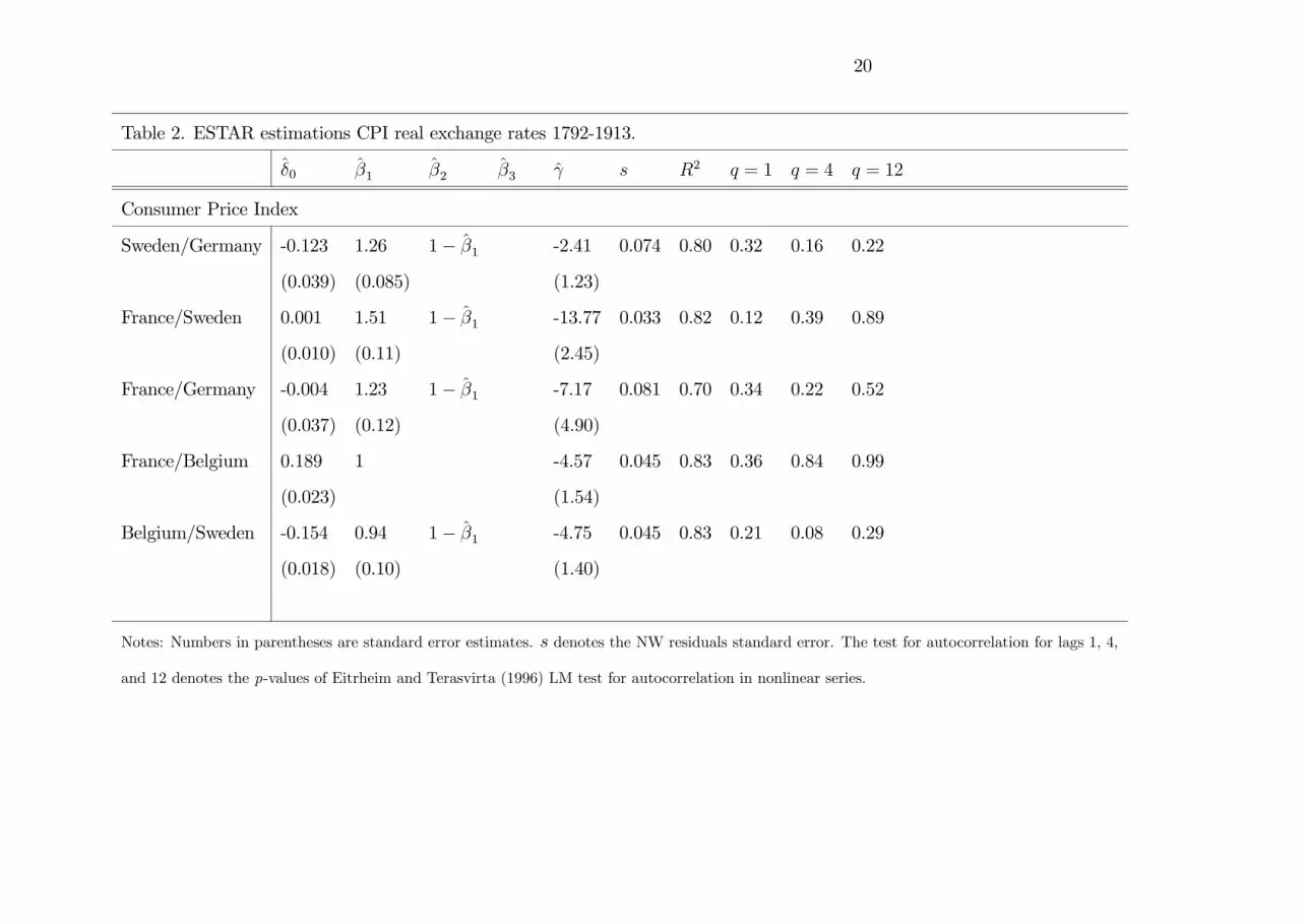
The first model we estimate is the simple ESTAR model for the real exchange rate

with a constant equilibrium (d1...dn are set to zero). Tables 1 and 2 present the results of

the estimations for WPI and CPI real rates, respectively. The speed of adjustment

parameter is significant in all cases except for the Belgium/U.S. and Belgium/Germany

WPI rates and the Belgium/Germany CPI rate. The autoregressive structure of the

ESTAR model (the βi) varies from an AR(1) to an AR(3).8 Given the significance of γ and

that in all cases we cannot reject that the sum of the autoregressive terms adds up to one,

we impose this constraint in all estimations.9

Hegwood and Papell (2002), on the basis of the Bai and Perron (1998) test for

multiple mean shifts, provide evidence that the real exchange rates do not exhibit a

constant conditional mean for the whole sample, but, instead, they follow a mean reversion

process to a changing mean. We include the same dummies that they found significant in

the equilibrium process of the real exchange rates.10 Tables 3 and 4 present the results for

19

Table 1. ESTAR estimations WPI real exchange rates 1792-1973

δ̂0 β̂1 β̂2 β̂3 γ̂ s R2 q = 1 q = 4 q = 12

Wholesale Price Index

US/UK -0.076 1.28 1− β̂1 -3.12 0.075 0.71 0.70 0.89 0.69

(0.019) (0.13) (0.90)

US/Germany -0.033 1.09 1− β̂1 -2.52 0.095 0.65 0.72 0.32 0.37

(0.031) (0.08) (0.71)

Germany/UK -0.21 1.25 -0.56 1− β̂1 − β̂2 -1.52 0.076 0.80 0.42 0.80 0.75

(0.039) (0.09) (0.16) (0.68)

France/UK 0.008 1.14 1− β̂1 -11.86 0.057 0.57 0.95 0.40 0.75

(0.014) (0.10) (1.03)

France/US -0.141 1.03 1− β̂1 -7.42 0.060 0.70 0.93 0.80 0.93

(0.017) (0.10) (1.86)

France/Germany 0.186 1.23 0.48 1− β̂1 − β̂2 -2.55 0.051 0.89 0.16 0.26 0.55

(0.027) (0.06) (0.096) (0.98)

Belgium/UK 0.262 1 -2.49 0.042 0.88 0.16 0.30 0.49

(0.026) (0.95)

Belgium/France 0.197 1 -2.98 0.047 0.87 0.31 0.31 0.22

(0.019) (0.94)

Notes: Numbers in parentheses are the Newey-West (1987) (NW) standard error estimates. s denotes residuals standard error. The test for

autocorrelation for lags 1, 4, and 12 denotes the p-values of Eitrheim and Terasvirta (1996) LM test for autocorrelation in nonlinear series.

20

Table 2. ESTAR estimations CPI real exchange rates 1792-1913.

δ̂0 β̂1 β̂2 β̂3 γ̂ s R2 q = 1 q = 4 q = 12

Consumer Price Index

Sweden/Germany -0.123 1.26 1− β̂1 -2.41 0.074 0.80 0.32 0.16 0.22

(0.039) (0.085) (1.23)

France/Sweden 0.001 1.51 1− β̂1 -13.77 0.033 0.82 0.12 0.39 0.89

(0.010) (0.11) (2.45)

France/Germany -0.004 1.23 1− β̂1 -7.17 0.081 0.70 0.34 0.22 0.52

(0.037) (0.12) (4.90)

France/Belgium 0.189 1 -4.57 0.045 0.83 0.36 0.84 0.99

(0.023) (1.54)

Belgium/Sweden -0.154 0.94 1− β̂1 -4.75 0.045 0.83 0.21 0.08 0.29

(0.018) (0.10) (1.40)

Notes: Numbers in parentheses are standard error estimates. s denotes the NW residuals standard error. The test for autocorrelation for lags 1, 4,

and 12 denotes the p-values of Eitrheim and Terasvirta (1996) LM test for autocorrelation in nonlinear series.

jteschen

22

Table 4. ESTAR estimations CPI real exchange rates 1792-1913 with dummies.

δ̂0 δ̂1 δ̂2 δ̂3 δ̂4 δ̂5 β̂1 β̂2 γ̂ s R2 q=1 q=4 q=12 F

Consumer Price Index

Sweden/ -0.278 0.312 0.173 1.43 1− β̂1 -17.41 0.060 0.88 0.28 0.15 0.00 22.8

Germany (0.017) (0.028) (0.028) (0.13) (4.69)

France/ 0.000 -0.023 0.015 1.50 1− β̂1 -21.18 0.033 0.82 0.11 0.35 0.91 0.93

Sweden (0.007) (0.012) (0.008) (0.11) (4.35)

France/ -0.030 0.241 0.048 1.31 -0.62 -7.63 0.074 0.75 0.10 0.23 0.62 3.88

Germany (0.033) (0.064) (0.025) (0.09) (0.13) (4.25)

France/ 0.197 -0.015 1 -5.20 0.046 0.85 0.27 0.71 0.99

Belgium (0.024) (0.007) (2.11)

Belgium/ -0.273 0.264 0.180 0.078 1.16 1− β̂1 -255 0.037 0.89 0.30 0.67 0.59 13.16

Sweden (0.009) (0.011) (0.011) (0.012) (0.12) (71.8)

Belgium/ -0.732 0.604 0.453 0.192 0.073 0.026 1.39 1− β̂1 -19.88 0.062 0.93 0.51 0.63 0.99 7.96

Germany (0.015) (0.017) (0.033) (0.040) (0.029) (0.022) (0.12) (5.67)

Notes: Numbers in parentheses are standard error estimates. s denotes the residuals standard error. The test for autocorrelation denotes the

p-values of Eitrheim and Terasvirta (1996) LM test. The β̂3 coefficient in the France/Germany rates equals 1− β̂1 − β̂2.

8

the estimation of the ESTAR model with changing equilibrium rates. Some of the initial

dummies appeared to be insignificant when the real rates are allowed to follow a nonlinear

mean-reverting process. We then removed the dummies that were insignificant in the new

estimations.11 The last column of Tables 3 and 4 display the F -test for the joint

significance of all remaining dummies. In all cases, we can reject the null that all dummies

were insignificant when taken all together, except in the case of the France/Sweden CPI

real exchange rate. However, the residuals do exhibit significant non-normality, and, in this

case, the distribution of the statistics could follow non-classical forms within a nonlinear

framework. Consequently, we employ a bootstrap method in order to obtain appropriate

test statistics.

3. Robustness Analysis

Our null hypothesis is that the dummy variables for breaks have zero coefficients.

Accordingly we simulate an “artificial” series for yt (yt), given the estimates of α and γ

obtained in Tables 3 and 4, with the coefficients on the dummy variables for structural

breaks set to zero. The residuals ub are obtained from bootstrapping, with replacement,

the estimated residuals obtained from the ESTAR models reported in those Tables which

include the dummies.12 The resulting “artificial” series are given by

yt = a+ eγ(yt−1−a)2(yt−1 − a) + ub, (2)

We then estimate the nonlinear ESTAR model including the pertinent dummies in each

case, and we repeat this experiment 10,000 times. The distribution of the t-statistics are

computed as well as the distribution of the F -test for each real exchange rate. Tables 5 and

6 present the 90% and 95% confidence interval for the t-statistics of each dummy and the

23

Table 5. Bootstrap confidence interval for t-stat and F -stat for dummies

Wholesale Price Index D1 D2 D3 F

US/UK 90% (-3.2,3.1)

95% (-4.4,4.0)*

US/Germany 90% (-2.8,2.8) (-2.5,2.5) (-2.36,2.1) 3.34

95% (-3.5,3.4)* (-3.2,3.2)* (-3.0,2.6)* 4.41*

Germany/UK 90% (-3.9,4.0) (-3.45,3.40) (-3.10,3.15)* 2.84

95% (-4.9,5.0) (-4.35,4.25)* (-3.90,4.0) 3.60*

US/France 90% (-3.10,3.35)* (-3.30,3.05) (-2.85,2.45) 3.60

95% (-4.05,4.80) (-4.40,4.15) (-4.20,3.15)* 6.00*

France/UK 90% (-2.24,2.36) (-1.88,2.10)* (-2.01,1.98)* 3.96

95% (-3.01,3.08)* (-2.34,2.56) (-2.75,2.69) 5.02*

France/Germany 90% (-3.25,2.65) (-2.85,2.65) (-2.60,2.25) 3.45

95% (-4.25,3.25)* (-3.80,3.45)* (-3.35,3.00)* 4.70*

Belgium/UK 90% (-2.46,2.36) (-2.3,2.1) (-2.2,2.1) 4.55

95% (-3.02,2.92)* (-2.9,2.7)* (-2.8,2.6)* 5.55*

Belgium/US 90% (-2.65,2.55) (-2.55,2.40) 3.71

95% (-3.32,3.22)* (-2.95,3.00)* 4.75*

Belgium/Germany 90% (-2.48,2.18)

95% (-3.22,3.02)*

Belgium/France 90% (-1.60,1.60)

95% (-1.94,1.92)*

24

Table 6. Bootstrap confidence interval for t-stat and F -stat for dummies

Consumer Price Index D1 D2 D3 D4 D5 F

Sweden/Germany 90% (-2.28,2.91) (-2.40,2.40) 3.25

95% (-2.86,3.72)* (-3.00,3.05)* 4.25*

France/Sweden 90% (-2.60,2.55) (-2.20,2.12) 3.24

95% (-3.30,3.20) (-2.66,2.70) 4.32

France/Germany 90% (-2.40,2.38) (-2.35,2.35) 5.25

95% (-3.10,3.02)* (-3.25,3.05) 7.40

France/Belgium 90% (-3.15,3.15)

95% (-4.15,4.01)

Belgium/Sweden 90% (-2.10,2.10) (-2.05,2.10) (-2.04,2.05) 3.60

95% (-2.60,2.65)* (-2.60,2.70)* (-2.60,2.70)* 4.55*

Belgium/Germany 90% (-2.80,2.95) (-3.00,2.80) (-2.95,2.70) (-2.80,2.55)* (-2.55,2.45) 2.50

95% (-3.46,3.78)* (-3.84,3.60)* (-3.60,3.30)* (-3.45,3.20) (-3.20,3.00) 3.12*

9

F -test. On the basis of the F -statistics obtained in the nonlinear estimation and the

critical values from the bootstrap, we can reject the null of joint non-significance of the

dummies in all cases except for the France/Sweden and France/Germany CPI real rates.

With regard to the particular dummy variables, some of them cannot be considered

significant within this framework.13 Hegwood and Papell (2002) provide some historical

support for some of the dummies they found significant in their study. Our results support

the significance of most of those dummies: the 1864 dummy in the U.S. real exchange rate

coinciding with the American Civil War, the 1866 dummy in the German real exchange

rates coinciding with the dissolution of the German Confederation, and the dummies of the

forties when there was “widespread protest, rebellion, and revolution in Europe” (Cook

and Stevenson 1998, p.460).

4. Nonlinear Half-Lives of Shocks

In this section we compare the speed of mean reversion of the nonlinear model of real

exchange rates with constant equilibrium as well as shifting equilibrium comparing with

the speed of mean reversion of the linear model as in Hegwood and Papell (2002). To

calculate the half-lives of PPP deviations within the nonlinear framework we must take

into account that a number of properties of the impulse response functions of linear models

do not carry over to the nonlinear models.14 Koop, Pesaran, and Potter (1996) introduced

the Generalized Impulse Response Function (GIRF) for nonlinear models. The GIRF is

defined as the average difference between two realizations of the stochastic process {yt+h}which start with identical histories up to time t− 1 (initial conditions). The firstrealization is hit by a shock at time t while the other one is not:

10

GIRFh(h, δ,ωt−1) = E(yt+h|ut = δ,ωt−1)−E(yt+h|ut = 0,ωt−1), (3)

where h = 1, 2, .., denotes horizon, ut = δ is an arbitrary shock occurring at time t, and

ωt−1 defines the history set of yt.

Given that δ and ωt−1 are single realizations of random variables, Equation 3 is

considered to be a random variable. In order to obtain sample estimates of Equation 3, we

average out the effect of all histories ωt−1 that consist of every set (yt−1, ..., yt−p) for

t ≥ p+ 1 where p is the autoregressive lag length, and we also average out the effect offuture shocks ut+h.15 We set δ = 5%, 10%, 20%, 30%, and 40%. The different values of δs

would allow us to compare the persistence of very large and small shocks. As in Taylor,

Peel, and Sarno (2001) and in Paya, Venetis, and Peel (2003), Tables 7 and 8 report the

half-lives of shocks, that is, the time needed for GIRFh < 12δ.16 The last columns of both

Table 7 and Table 8 correspond to the speeds of adjustment found in the linear models of

Hegwood and Papell. For the nonlinear models with constant equilibrium, Table 7, the

half-life of the shocks decreases significantly for shocks of around 30%, or even 40% in some

cases. However, compared with the linear case, even with the smallest shock of 5% the

speed of mean reversion is faster in the ESTAR model. When the equilibrium is allowed to

change over time, Table 8, the “arbitrage band” in the nonlinear model, seems to lie

around 20% or even 10%. In this case, ten out of the sixteen real exchange rates need a

shock of 20% to achieve faster adjustment than the linear case.

5. Conclusions

Hegwood and Papell (2002) analyzed PPP adjustment under the Gold Standard. They

novelly allowed for structural breaks in the equilibrium real exchange rate and suggested

25

Table 7. Estimated half-lives shocks in months for annual model

γ̂ Shock 5% 10% 20% 30% 40% Linear

Real rate WPI

US/UK -3.12 5 4 3 2 2 4.04

US/Germany -2.52 4 4 4 3 2 3.24

Germany/UK -1.52 6 6 5 2 2 5.72

France/UK -11.8 5 4 3 1 0 3.22

France/US -7.42 3 3 2 1 0 7.85

France/Germany -2.89 5 4 4 2 1 5.77

Belgium/UK -2.49 7 7 7 6 4 9.24

Belgium/France -2.98 5 5 5 4 2 9.66

Real rate CPI

Sweden/Germany -2.41 5 5 5 4 3 5.99

France/Sweden -13.7 4 4 2 1 0 5.24

France/Germany -7.17 3 3 2 2 2 4.08

France/Belgium -4.53 5 5 4 3 3 7.31

Belgium/Sweden -4.75 5 4 3 1 0 7.40

26

Table 8. Estimated half-lives shocks in months for annual model with dummies

γ̂ Shock 5% 10% 20% 30% 40% Linear

Real rate WPI

US/UK -4.28 5 4 3 2 1 2.51

US/Germany -4.43 3 3 3 2 1 1.24

Germany/UK -8.50 3 3 2 1 0 1.25

France/UK -30.7 3 2 0 0 0 1.42

France/US -34.1 2 2 0 0 0 2.54

France/Germany -27.5 2 2 1 0 0 1.42

Belgium/UK -186 1 0 0 0 0 0.83

Belgium/US -0.88 6 5 4 3 2 1.68

Belgium/Germany -8.96 4 4 3 2 1 1.26

Belgium/France -56.9 1 0 0 0 0 1.43

Real rate CPI

Sweden/Germany -17.4 3 2 1 0 0 1.13

France/Germany -7.63 2 1 1 1 0 1.13

Belgium/Sweden -255 1 0 0 0 0 0.61

Belgium/Germany -20 2 2 1 0 0 1.07

11

that relatively quick linear adjustment to an occasionally changing mean provides a more

reasonable representation of the data than does the fractional process, with its long

memory property, for their data set - the latter originally reported by Diebold, Husted, and

Rush (1991) .

In this article we have shown that the theoretically well-motivated nonlinear ESTAR

process, embodying structural breaks in the equilibrium real rate, provides a parsimonious

explanation of the data set.

As conjectured by Rogoff (1996), and supported by our analysis and that of Hegwood

and Papell (2002), allowance for a changing real equilibrium can have dramatic

implications for the estimates of PPP adjustment speeds. On the basis of these results

empirical work exploring this possibility in postwar data may help solve the Rogoff puzzle.

12

References

Acosta, Aparicio F.M. , and Clive W.J. Granger. 1995. A linearity test for near-unit root

time series. Discussion paper no. 95-12, University of California San Diego, San Diego, CA.

Bai, Jushan, and Pierre Perron. 1998. Estimation and testing linear models with mulitple

structural changes. Econometrica 66: 47-78.

Balassa, Bela. 1964. The purchasing-power parity doctrine: A reappraisal. Journal of

Political Economy 72: 584-96.

Berka, Martin. 2002. General equilibrium model of arbitrage trade and real exchange rate

persistence. Unpublished paper, University of British Columbia.

Byers, David, and David A. Peel. 2003. A nonlinear time series with misleading linear

properties. Applied Economics Letters 10: 47-51.

Canzoneri, Matthew B., Robert E. Cumby, and Behzad T. Diba. 1996. Relative labor

productivity and the real exchange rate in the long run: Evidence for a panel of OECD

countries. Journal of International Economics 47: 245-66.

Chinn, Menzie, and Louis Johnston. 1996. Real exchange levels, productivity and demand

shocks: Evidence from a panel of 14 countries. NBER Working Paper No. 5709.

Cook, Chris, and John Stevenson. 1998. Longman handbook of modern European history

1763-1997, 3rd edition. New York: Addison Wesley Longman.

Diebold, Francis X., Steven Husted, and Mark Rush. 1991. Real exchange rates under the

gold standard. Journal of Political Economy 99: 1252-71.

Dumas, Bernard. 1992. Dynamic equilibrium and the real exchange rate in a spatially

separated world. Review of Financial Studies 5: 153-80.

Eitrheim, Oyvind, and Timo Terasvirta. 1996. Testing the adequacy of smooth transition

autoregressive models. Journal of Econometrics 74: 59-75.

Froot, Kenneth A., and Kenneth Rogoff. 1995. Perspectives on PPP and long-run real

13

exchange rates. In Handbook of International Economics, Volume 3, edited by G.M.

Grossman and K. Rogoff. Amsterdam: North-Holland.

Granger, Clive W.J., and Timo Terasvirta. 1999. Ocasional structural breaks and long

memory. Discussion Paper 98-03, University of California San Diego, San Diego, CA.

Hegwood, Natalie D., and David H. Papell. 2002. Purchasing power parity under the Gold

Standard. Southern Economic Journal 69: 72-91.

Koop, Gary, Hashem Pesaran, and Simon M. Potter. 1996. Impulse response analysis in

nonlinear multivariate models. Journal of Econometrics 74: 119-47.

Lothian, James R., and Mark P. Taylor. 1996. Real exchange rate behavior: The recent

float from the perspective of the past two centuries. Journal of Political Economy 104:

488-507.

Michael, Panos, Robert Nobay, and David A. Peel. 1997. Transactions costs and nonlinear

adjustment in real exchange rates: an empirical investigation. Journal of Political

Economy 105: 862-79.

Newey, Whitney, and Kenneth West. 1987. A simple positive semi-definite,

heteroscedasticity and autocorrelation consistent covariance matrix. Econometrica 55:

703-8.

O’Connell, Paul, and Shang-Jin Wei. 1997. The bigger they are, the harder they fall: How

price differences between U.S. cities are arbitraged. Discussion Paper, Department of

Economics, Harvard University.

Ozaki, Tohru. 1985. Nonlinear time series models and dynamical systems. In Handbook of

Statistics V pp. 25-83. E.J. Hannan, P.R. Krishnaiah, and M.M. Rao, Amsterdam:

Elsevier.

Paya, Ivan, and David A. Peel. 2003. Temporal aggregation of an ESTAR process: Some

implications for PPP adjustments. Unpublished paper, Cardiff Business School.

14

Paya, Ivan, Ioannis A. Venetis, and David A. Peel. 2003. Further evidence on PPP

adjusment speeds: The case of effective real exchange rates and the EMS. Oxford Bulletin

of Economics and Statistics 65: 421-38.

Peel, David A., and Ioannis A. Venetis. 2002. Purchasing power parity over two centuries:

trends and non-linearity. Applied Economics 35: 609-17.

Perron, Pierre, and Timothy J. Vogelsang. 1992. Nonstationarity and level shifts with an

application to purchasing power parity. Journal of Business and Economic Statistics 10:

301-20.

Pippenger, Michael K., and Gregory Goering. 1993. A note on the empirical power of unit

root tests under threshold processes. Oxford Bulletin of Economics and Statistics 55:

473-81.

Rogoff, Kenneth. 1996. The purchasing power parity puzzle. Journal of Economic

Literature 34: 647-68

Samuelson, Paul. 1964. Theoretical notes on trade problems. Review of Economics and

Statistics 46: 145-54.

Sercu, Piet, Raman Uppal, and C. Van Hull. 1995. The exchange rate in the presence of

transactions costs: Implications for tests of purchasing power parity. Journal of Finance

50: 1309-19.

Taylor, Alan M. 2001. Potential pitfalls for the purchasing power parity puzzle? Sampling

and specification biases in mean-reversion tests of the taw of one price. Econometrica 69:

473-98.

Taylor, Mark P., David A. Peel, and Lucio Sarno. 2001. Nonlinear mean-reversion in real

exchange rates: Toward a solution to the purchasing power parity puzzles. International

Economic Review 42: 1015-42.

Terasvirta, Timo. 1994. Specification, estimation and evaluation of smooth transition

15

autoregressive models. Journal of the American Statistical Association 89: 208—18.

Tse, Yi. 2001. Index arbitrage with heterogeneous investors: A smooth transition error

correction analysis. Journal of Banking and Finance 25: 1829-55.

Venetis, Ioannis A., Ivan Paya, and David A. Peel. 2002. Do real exchange rate ‘mean

revert’ to productivity? A nonlinear approach. Unpublished paper, Cardiff Business School.

16

Notes1Even in high frequency asset markets the idea of heteregeneous traders facing different

capital constraints or percieved risk of arbitrage has been employed to rationalise employment

of the ESTAR model. See, for example, Tse (2001) for arbitrage between stock and index

futures.

2Namely, how to reconcile the enormous short run volatility of real exchange rates with

the extremely slow rate at which shocks appear to damp out-in linear models, around 3-5

years, seemingly far too long to be explained by nominal rigidities.

3He suggests for instance that the sustained Post Bretton Woods war appreciation of

Japan’s real exchange rate against the Dollar is consistent with the Balassa-Samuelson (BS)

effects, in fact, he calls it the “canonical” example of BS effects.

4We know from the analysis of Taylor (2001) that if the true data generation process is

nonlinear then the use of the linear models can severely underestimate the speed of adjust-

ment particularly if the low frequency data is temporally aggregated.

5We thank Hegwood and Papell for kindly proving us with the data.

6A key property of some ESTAR models (also shared by some Threshold models) is that

data simulated from them, although globally mean reverting, can appear to exhibit a unit

root. As a consequence, the test proposed in Froot and Rogoff (1995), namely, that we

impose unit coefficients and test directly, employing unit root tests, whether PPP deviations

are mean reverting, can have low power if the true data generating process is nonlinear.

7We note in this article, as pointed out by a referee, we test for nonlinear mean reversion

while assuming that PPP holds. In this article, it is assumed that there is reversion to a

changing mean, and what is being tested is the form of the reversion. As a consequence,

the standard errors reported for the ESTAR have classical values. There is a common

misconception that research on nonlinear adjustment to PPP tests a unit root null against

a nonlinear mean-reverting alternative.

17

8This variation is not surprising if we assume that the true data generating process (DGP)

of the real exchange rate is generated at a higher frequency, that is, monthly. In that case,

Paya and Peel (2003) show that temporal aggregation of the true monthly DGP into, for

instance, annual data induces additional autoregressive terms in the ESTAR model.

9We observe from Equation 1 that whenn

i=1

βi = 1 if γ = 0, PPP deviations follow a

unit root. As a consequence of this point there is perhaps a conception that research on

nonlinear adjustment to PPP tests, in general, a unit root null against a nonlinear mean

reverting alternative. This need not be the case. Given the results reported previously, we

assume, as noted above, that PPP holds and test for the form of reversion.

10See Hegwood and Papell (2002) for an explanation of potential causes of the different

breaks. We recognise that the breaks were obtained from estimates of a linear structure.

Our Monte Carlo evidence suggests the breaks are in the majority significant.

11In particular, for the WPI rates we removed the third dummy of the Beligium/Germany,

third dummy in the Belgium/US, fourth dummy in the France/UK, and the fourth dummy in

the US/Germany rate. For the CPI rates, we removed the first dummy of the France/Sweden

rate and the third dummy of the Sweden/Germany rate.

12The bootstrapped residuals were centered on zero and scaled. The scaling factor is

(n/n-k)^0.5.

13In particular, the first dummy of the Germany/UKWPI rate, second dummy France/US

WPI rate, second dummy France/UK WPI rate, second dummy France/Germany CPI rate,

fifth dummy Belgium/Germany rate, and both dummies of the France/Sweden CPI rate.

14In particular, impulse responses produced by nonlinear models are (i) history dependent,

so they depend on initial conditions, (ii) they are dependent on the size and sign of the

current shock, and (iii) they depend on the future shocks as well. That is, nonlinear impulse

responses critically depend on the “past, present, and the future”.

18

15For each available history, we use 300 repetitions (500 repetitions found similar result) to

average out future shocks where future shocks are drawn with replacement from the models’

residuals and then we average the result across all histories. We set to max{h} = 48.16The France/Sweden and France/Belgium CPI exchange rates have not been included in

Table 8 because the dummy variables were not jointly significant according to the bootstrap

confidence interval presented in Table 6. In the case of the France/Germany CPI rate we

include the dummy that appears significant under the bootstrap confidence interval.