Economics of Planning 36: 201–221, 2003.© 2004 Kluwer Academic Publishers. Printed in the Netherlands.

201

Purchasing Power Parity in Three TransitionEconomies

DAVID BARLOWNewcastle University Business School, University of Newcastle upon Tyne, NE1 7RU, Newcastle,UK (E-mail: david.barlow@ncl.ac.uk)

Received 21 March 2003; accepted in revised form 12 November 2003

Abstract. This paper uses cointegration analysis on monthly data over April 1994–December 2000to test the relevance theory of Purchasing Power Parity (PPP) for two advanced transition economies(Poland and the Czech Republic) and one lagging transition economy (Romania). PPP is not rejectedbetween the lagging reformer and developed market economies, but is rejected between the advancedreformers and the developed economies. However, PPP is not rejected between the two advancedtransition economies, though it is rejected between the lagging and advanced transition economies.The evolution of the real exchange rates over 1994–2000 suggest that a significant explanation forthese findings is the central role of the exchange rate in the disinflation strategies of Poland and theCzech Republic in the early part of this period, in contrast to the managed float followed by Romaniathroughout the period.

JEL classifications: E31, F31, P24.

Key words: disinflation, real exchange rate, transition

1. Introduction

In the strictest form of the theory of purchasing power parity (PPP), exchangerates and relative prices are expected to move together so that the prices of goodsin different countries are equal when expressed in a common currency. Thus theequilibrium real exchange rate is predicted to be constant. The well documentedappreciation of real exchange rates of transition economies over the 1990s wouldseem to be a rejection of this theory. Halpern and Wyplosz (1997) argue that the realappreciation could be a consequence of changes in the relative prices of traded andnon-traded goods due to shifts in demand and rising productivity brought about by‘deep’ restructuring. However, the real appreciation of exchange rates of transitioneconomies could also be due to nominal shocks, such as fiscal and monetary policy.Orlowski (2000) provides evidence of a significant role for monetary policy in theappreciation of the real exchange rates of transition economies. Brada (1998) ar-gues that the real exchanges rates of countries undergoing different types of shocksshould display different patterns of behaviour over time. One possible implicationof this argument is that the theory of PPP may hold between the currencies of two

202

countries experiencing similar transition shocks even though the real exchange ratefor each country against non-transition economies is appreciating.

A number of papers have attempted to measure the contributions of variousfactors that might have affected the equilibrium real exchange rate of transitioneconomies.1 It is, however, possible that evidence for appreciation of the equilib-rium real exchange rates is spurious if the real appreciation is simply a correction toan undervalued exchange rate. For the transition economies this is a very real pos-sibility, since each began the transition with a large devaluation of their currency.2

Furthermore attempts to model changes in the equilibrium real exchange rate maybe thwarted by inadequate data.3 An additional complicating factor is that in anumber of the transition countries the exchange rate has been used in the dis-inflation strategy. In these cases, the authorities have tried to engineer rates ofdevaluation less than the inflation differential, and inevitably the real exchangerate has appreciated.

This paper does not seek to model the real appreciation but rather it looks forevidence that there is a common pattern to the real appreciation in two advancedtransition economies, namely Poland and the Czech Republic, which is not com-mon to a less advanced transition economy (Romania). Firstly, the real exchangerates against major trading partners are tested for stationarity using an ADF testand a cointegrating test of the theory of PPP. The real exchange rates for both thePolish Zloty and the Czech Koruna are found to be non-stationary and appear to beappreciating. In contrast, there is no evidence of real appreciation for the RomanianLeu. The theory of PPP is then tested for the Zloty against the Koruna, in thiscase the theory cannot be rejected. However, PPP is rejected for both the Zlotyagainst the Leu, and for the Koruna against the Leu. The time profiles of the realexchange rates against the major currencies suggest that exchange managementplayed significant part in the behaviour appreciation of the three currencies.

The paper is organized as follows: Section 2 reviews the theory of PPP andapplications to transition economies. Section 3 reviews exchange rate and monetarydevelopments in Poland, the Czech Republic and Romania. Section 4 discussesthe data. Section 5 outlines the empirical methodology. Section 6 presents resultsempirical results of testing the theory PPP between the transition economies andthe major economies, and between each other. Section 7 concludes.

2. Theories of the real exchange rate

The most well known theory of the real exchange rate is PPP. This theory assumesthat in the absence of transport costs and other impediments to trade (such astariffs and quotas) the prices of a good in different countries should be equal whenexpressed in a common currency. Thus, if we denote the exchange rate (expressedas units of domestic currency required to buy one unit of foreign currency) as E,and use Pd and Pv to denote the domestic and foreign prices respectively, then

Pd = E × Pv (1)

203

Alternatively this may be written as

E

(Pv

Pd

)= 1 (2)

where E(Pv/Pd) is the real exchange rate (denoted RER). More generally the realexchange rate can be regarded as a constant (K) to allow for a wedge between theprices of goods produced in different countries due to transport costs and tariffs.4

In this case PPP requires that the domestic prices of goods move in line with theforeign price converted into the domestic currency. It is also recognized that in theshort run PPP may not hold due to information problems and adjustment costs. Butin the long run it would be expected that PPP does hold, and that therefore in thelong run the real exchange rate is constant.

Clearly this theory assumes that the goods in question are traded internation-ally, the existence of goods that are not internationally traded presents a problem,especially when applying the theory to a price index that is aggregated over bothtradeable and non-tradeable goods and services. Assuming that the prices of trade-able goods are set in the world market, but that the prices of non-traded goods canbe set domestically, then the real exchange rate can be thought of as the price oftraded goods (Pt) relative to non-traded goods prices (Pn).

RER = Pt

Pn= K (3)

Halpern and Wyplosz (1997) argue that the real appreciation observed in thetransition economies could be due to a rise in the relative price of non-tradeablesas a consequence of the transition.5 Balazs (2002), de Broeck and Slok (2001) andHalpern and Wyplosz (2001) present evidence that real exchange rate movementscan be explained by productivity changes. A number of empirical studies reportthat the initial undervaluation of the currencies explains a large part of the realappreciation.6 However, there are also other reasons for the currencies to haveappreciated in real terms. Desai (1998) argues that the real appreciation could beexplained by stabilization policies under which the nominal rate of depreciationis maintained below the rate of price inflation, Orlowski (2000) offers supportingevidence for this argument. According to Liargovas (1999) Foreign Direct Invest-ment is a significant cause in the real appreciation of both the Polish and the Czechcurrencies. Dibooglu and Kutan (2001) argue that nominal shocks have dominatedmovements of the Polish real exchange rate, whilst Begg (1998) argues that thereis little evidence for productivity growth causing the Czech currency to appreciatein real terms.

From the above discussion it becomes clear that whether or not PPP is found tohold can depend upon the choice of countries on which PPP is tested. In the caseof transition economies PPP may not hold when the trading partner is defined tobe a developed market economy, but PPP may hold between transition economiesthat are going through similar experiences, such as stabilization policies. There

204

have been few tests of the theory of PPP using cointegration analysis performed ontransition economies. Largely this reflects the short time period since the transitionbegan.7 Choudhry (1998) reports little support for strict PPP between a sample offour transition economies (Poland, Russia, Romania and Slovenia) and the USA,a similar finding applies between the four transition economies.8 Christev andNoorbakhsh (2000) also report that PPP does not hold for transition economies. Incontrast, Barlow and Radulescu (2002) find strongly supportive evidence of strictPPP for Romania against the USA.

3. Exchange rates, transition and stabilization

Both the Czech Republic and Poland are regarded as being at the forefront ofthe transition. Poland started the rapid transformation of its economy in 1990, theCzech Republic soon followed the Polish lead. It should be noted that the two eco-nomies started from very different positions. Though the former Czechoslavakiaended the communist era considerably wealthier than Poland, it was also consid-erably less reformed. Czechoslavakia maintained the classical Soviet style eco-nomy right up to the demise of communism. In contrast, throughout the 1980sPoland had experimented with some reform,9 and a significant private sector ex-isted throughout the communist era, especially in agriculture which had not beenfully collectivized. Poland recovered from the transition recession faster than anyother country, but the Czech Republic soon recovered too.10 In the mid-1990s bothachieved impressive growth rates. However, whilst Poland continued to grow, theCzech Republic went into recession in 1997 following a financial crisis and onlybegan to recover in 1999/2000.

To represent lagging transition countries Romania is chosen. The liberalizationindices published annually by the EBRD show reform in Romania to be consider-ably behind that of Poland and the Czech Republic. For example, an unweightedsummation of the indices gives an annual average over 1991–1999 of 25.06 and24.82 for the Czech Republic and Poland respectively, but only 17.9 for Romania.11

Romania ended the communist era in a far worse position than either Poland orCzechoslavakia. The state had maintained rigid control over an economy, whichhad become increasingly impoverished and backward as production became gearedto the repayment of foreign debt.

Following the initial devaluation of their currencies at the start of the transitionboth the Czech and Polish authorities attempted to peg their currencies. However,Poland’s high inflation early in the 1990s soon forced the adoption of a crawlingpeg. Over 1994 the crawl was gradually reduced. In May 1995 the regime switchedto a managed float within gliding bands. Following a revaluation in December1995, the exchange rate stayed with the bands until capital outflows following theEast Asian crisis forced a depreciation. Through 1999 the band was widened andin April 2000 the Zloty was allowed to float.12

The Czech Koruna was initially pegged within bands to a central rate of 28Koruny to the Dollar, but in May 1995 the Koruna was fixed to a basket consisting

205

of 65% German Marks and 35% US Dollars. In February 1996 the bands werewidened, and with the onset of the financial crisis in 1997, the Koruna was al-lowed to float in May of that year. Initially the floating Koruna depreciated by 10%compared with the previous central rate, but then partially recovered.13 In contrastto the Czech Republic and Poland, throughout the transition period Romania hasoperated a managed floating exchange rate arrangement following the devaluationat the start of transition. Until 1997 official intervention in the market lead to therationing of foreign currency, but since then the regime has been considerably moreliberal and foreign currency rationing has ended.

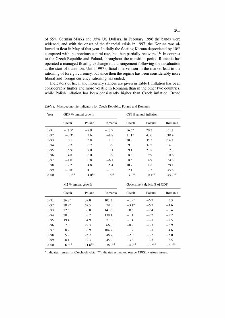
Indicators of fiscal and monetary stances are given in Table I. Inflation has beenconsiderably higher and more volatile in Romania than in the other two countries,while Polish inflation has been consistently higher than Czech inflation. Broad

Table I. Macroeconomic indicators for Czech Republic, Poland and Romania

Year GDP % annual growth CPI % annual inflation

Czech Poland Romania Czech Poland Romania

1991 −11.5∗ −7.0 −12.9 56.6∗ 70.3 161.1

1992 −3.3∗ 2.6 −8.8 11.1∗ 43.0 210.4

1993 0.1 3.8 1.5 20.8 35.3 256.1

1994 2.2 5.2 3.9 9.9 32.2 136.7

1995 5.9 7.0 7.1 9.1 27.8 32.3

1996 4.8 6.0 3.9 8.8 19.9 38.8

1997 −1.0 6.8 −6.1 8.5 14.9 154.8

1998 −2.2 4.8 −5.4 10.7 11.8 59.1

1999 −0.8 4.1 −3.2 2.1 7.3 45.8

2000 3.1∗∗ 4.0∗∗ 1.6∗∗ 3.9∗∗ 10.1∗∗ 45.7∗∗

M2 % annual growth Government deficit % of GDP

Czech Poland Romania Czech Poland Romania

1991 26.8∗ 37.0 101.2 −1.9∗ −6.7 3.3

1992 20.7∗ 57.5 79.6 −3.1∗ −6.7 −4.6

1993 22.5 36.0 141.0 0.5 −2.4 −0.4

1994 20.8 38.2 138.1 −1.1 −2.2 −2.2

1995 19.4 34.9 71.6 −1.4 −3.1 −2.5

1996 7.8 29.3 66.0 −0.9 −3.3 −3.9

1997 8.7 30.9 104.9 −1.7 −3.1 −4.6

1998 5.2 25.2 48.9 −2.0 −3.2 −5.0

1999 8.1 19.3 45.0 −3.3 −3.7 −3.5

2000 6.6∗∗ 11.8∗∗ 38.0∗∗ −4.9∗∗ −3.2∗∗ −3.7∗∗

∗Indicates figures for Czechoslavakia; **indicates estimates, source EBRD, various issues.

206

money growth displays a similar pattern across the countries to inflation. Until 1999the Czech Republic achieved small government deficits relative to GDP, though thefiscal position worsened following the crisis of 1997. The Polish government deficithas been gradually falling. The Romanian deficit has also been falling in the latteryears. Thus it can be argued that Romania lags behind the Czech Republic andPoland not only on reform but on stabilization too.

4. Data

The exchange rates used in this analysis are a geometric average of the rates againstthe US Dollar and German Mark (DM),14 the exchange rates are defined as thenumber of units of the domestic currency required to buy one unit of foreigncurrency. Similarly the foreign price series is the geometric average of the USand German price series. The price series used are consumer price indices.15 Theexchange rates against the DM are calculated from the Dollar rate and the rateof the DM against the Dollar. The foreign price level is denoted by Pf, while Ecand Pc denote the nominal exchange rate and price level for the Czech Republic,Ep and Pp denote the same for Poland, and Ero and Pro indicate the same forRomania. Epc denotes the number of Zloties required to buy one Koruna, Eprodenotes the number of Zloties required to by one Leu and Ecro is the numberof Koruna needed to by one Leu, these are calculated from the respective Dollarexchange rates. All data are taken from International Financial Statistics, and aremeasured in logarithms.

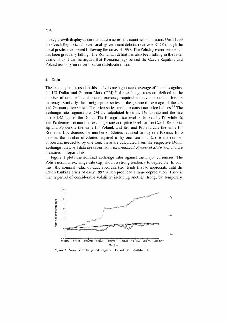
Figure 1 plots the nominal exchange rates against the major currencies. ThePolish nominal exchange rate (Ep) shows a strong tendency to depreciate. In con-trast, the nominal value of Czech Koruna (Ec) tends first to appreciate until theCzech banking crisis of early 1997 which produced a large depreciation. There isthen a period of considerable volatility, including another strong, but temporary,

Figure 1. Nominal exchange rates against Dollar/D.M, 1994M4 = 1.

207

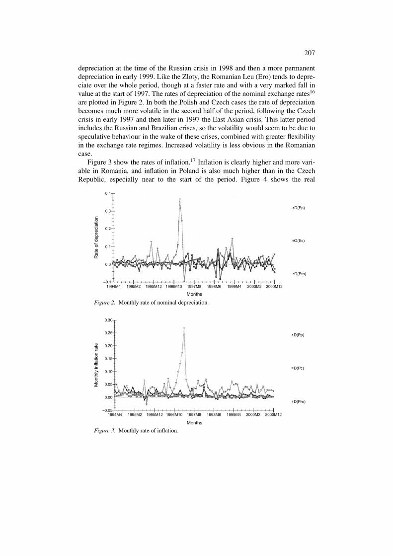
depreciation at the time of the Russian crisis in 1998 and then a more permanentdepreciation in early 1999. Like the Zloty, the Romanian Leu (Ero) tends to depre-ciate over the whole period, though at a faster rate and with a very marked fall invalue at the start of 1997. The rates of depreciation of the nominal exchange rates16

are plotted in Figure 2. In both the Polish and Czech cases the rate of depreciationbecomes much more volatile in the second half of the period, following the Czechcrisis in early 1997 and then later in 1997 the East Asian crisis. This latter periodincludes the Russian and Brazilian crises, so the volatility would seem to be due tospeculative behaviour in the wake of these crises, combined with greater flexibilityin the exchange rate regimes. Increased volatility is less obvious in the Romaniancase.

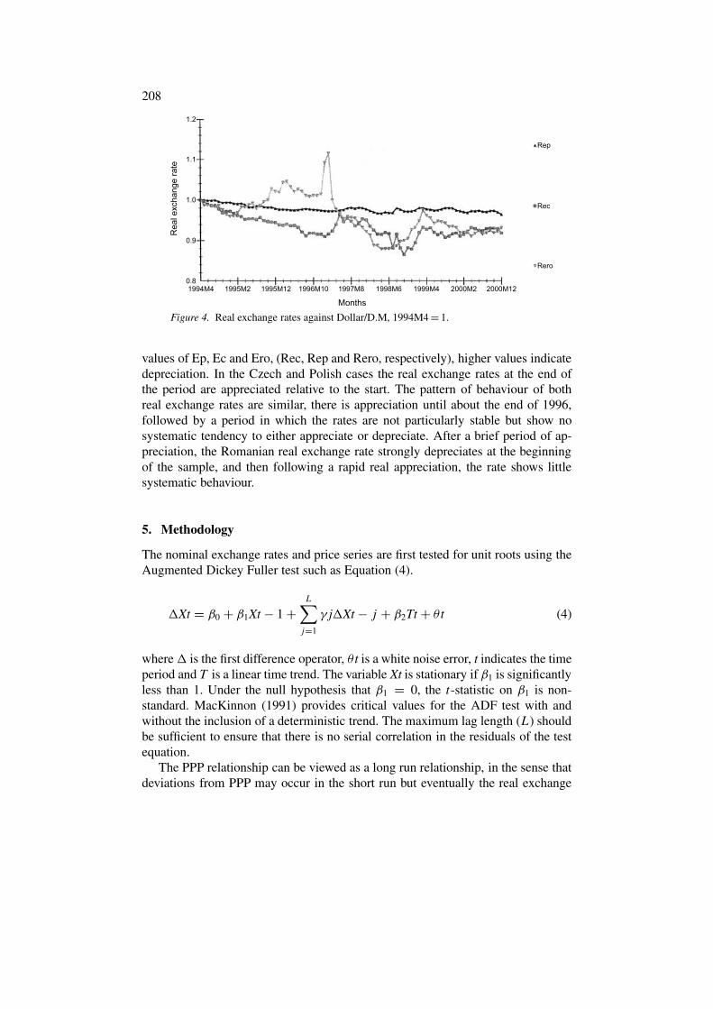
Figure 3 show the rates of inflation.17 Inflation is clearly higher and more vari-able in Romania, and inflation in Poland is also much higher than in the CzechRepublic, especially near to the start of the period. Figure 4 shows the real

Figure 2. Monthly rate of nominal depreciation.

Figure 3. Monthly rate of inflation.

208

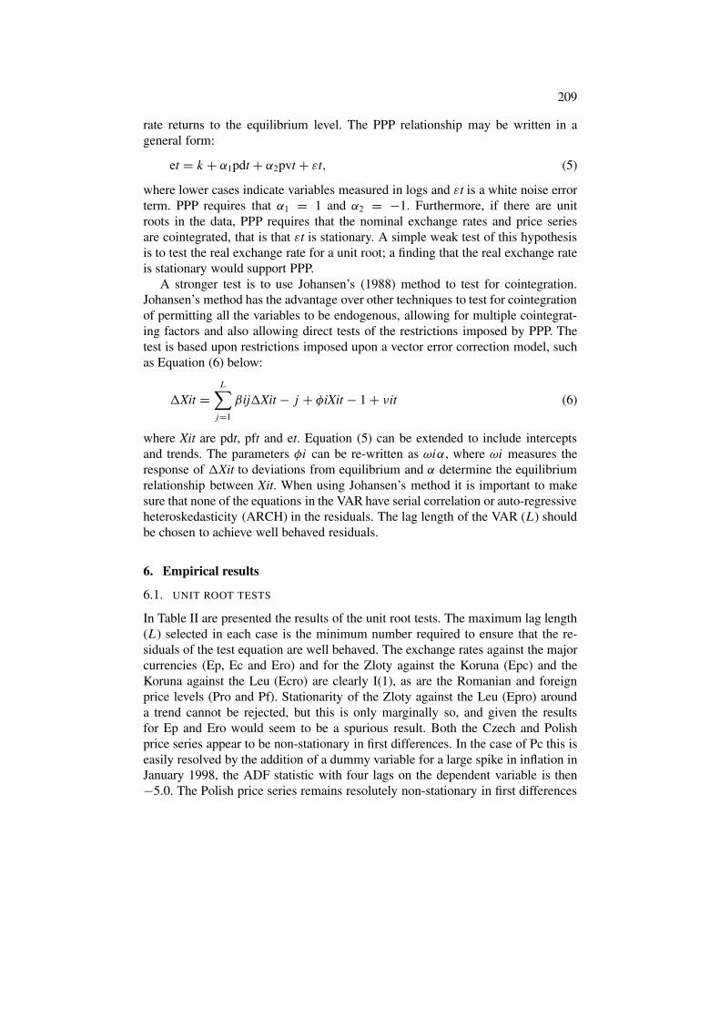
Figure 4. Real exchange rates against Dollar/D.M, 1994M4 = 1.

values of Ep, Ec and Ero, (Rec, Rep and Rero, respectively), higher values indicatedepreciation. In the Czech and Polish cases the real exchange rates at the end ofthe period are appreciated relative to the start. The pattern of behaviour of bothreal exchange rates are similar, there is appreciation until about the end of 1996,followed by a period in which the rates are not particularly stable but show nosystematic tendency to either appreciate or depreciate. After a brief period of ap-preciation, the Romanian real exchange rate strongly depreciates at the beginningof the sample, and then following a rapid real appreciation, the rate shows littlesystematic behaviour.

5. Methodology

The nominal exchange rates and price series are first tested for unit roots using theAugmented Dickey Fuller test such as Equation (4).

�Xt = β0 + β1Xt − 1 +L∑

j=1

γ j�Xt − j + β2Tt + θ t (4)

where � is the first difference operator, θ t is a white noise error, t indicates the timeperiod and T is a linear time trend. The variable Xt is stationary if β1 is significantlyless than 1. Under the null hypothesis that β1 = 0, the t-statistic on β1 is non-standard. MacKinnon (1991) provides critical values for the ADF test with andwithout the inclusion of a deterministic trend. The maximum lag length (L) shouldbe sufficient to ensure that there is no serial correlation in the residuals of the testequation.

The PPP relationship can be viewed as a long run relationship, in the sense thatdeviations from PPP may occur in the short run but eventually the real exchange

209

rate returns to the equilibrium level. The PPP relationship may be written in ageneral form:

et = k + α1pdt + α2pvt + εt, (5)

where lower cases indicate variables measured in logs and εt is a white noise errorterm. PPP requires that α1 = 1 and α2 = −1. Furthermore, if there are unitroots in the data, PPP requires that the nominal exchange rates and price seriesare cointegrated, that is that εt is stationary. A simple weak test of this hypothesisis to test the real exchange rate for a unit root; a finding that the real exchange rateis stationary would support PPP.

A stronger test is to use Johansen’s (1988) method to test for cointegration.Johansen’s method has the advantage over other techniques to test for cointegrationof permitting all the variables to be endogenous, allowing for multiple cointegrat-ing factors and also allowing direct tests of the restrictions imposed by PPP. Thetest is based upon restrictions imposed upon a vector error correction model, suchas Equation (6) below:

�Xit =L∑

j=1

βij�Xit − j + φiXit − 1 + νit (6)

where Xit are pdt, pft and et. Equation (5) can be extended to include interceptsand trends. The parameters φi can be re-written as ωiα, where ωi measures theresponse of �Xit to deviations from equilibrium and α determine the equilibriumrelationship between Xit. When using Johansen’s method it is important to makesure that none of the equations in the VAR have serial correlation or auto-regressiveheteroskedasticity (ARCH) in the residuals. The lag length of the VAR (L) shouldbe chosen to achieve well behaved residuals.

6. Empirical results

6.1. UNIT ROOT TESTS

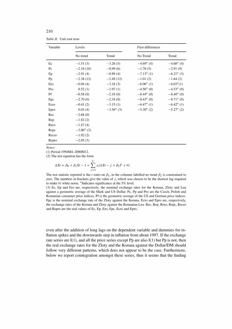
In Table II are presented the results of the unit root tests. The maximum lag length(L) selected in each case is the minimum number required to ensure that the re-siduals of the test equation are well behaved. The exchange rates against the majorcurrencies (Ep, Ec and Ero) and for the Zloty against the Koruna (Epc) and theKoruna against the Leu (Ecro) are clearly I(1), as are the Romanian and foreignprice levels (Pro and Pf). Stationarity of the Zloty against the Leu (Epro) arounda trend cannot be rejected, but this is only marginally so, and given the resultsfor Ep and Ero would seem to be a spurious result. Both the Czech and Polishprice series appear to be non-stationary in first differences. In the case of Pc this iseasily resolved by the addition of a dummy variable for a large spike in inflation inJanuary 1998, the ADF statistic with four lags on the dependent variable is then−5.0. The Polish price series remains resolutely non-stationary in first differences

210

Table II. Unit root tests

Variable Levels First differences

No trend Trend No Trend Trend

Ec −1.51 (3) −3.26 (5) −4.69∗ (4) −4.68∗ (4)

Pc −2.16 (10) −0.99 (6) −1.78 (5) −2.91 (9)

Ep −2.91 (4) −0.89 (4) −7.13∗ (1) −6.21∗ (3)

Pp −2.38 (12) −2.49 (12) −1.01 (2) −1.64 (2)

Ero −0.04 (4) −3.16 (3) −6.06∗ (1) −6.03∗(1)

Pro 0.52 (1) −1.97 (1) −4.56∗ (0) −4.53∗ (0)

Pf −0.58 (0) −2.18 (0) −8.44∗ (0) −8.40∗ (0)

Epc −2.70 (0) −2.34 (0) −8.43∗ (0) −8.71∗ (0)

Ecro −0.41 (2) −3.15 (1) −6.47∗ (1) −6.42∗ (1)

Epro 0.03 (4) −3.56∗ (3) −5.30∗ (2) −5.27∗ (2)

Rec −2.68 (0)

Rep −1.82 (2)

Rero −1.47 (4)

Repc −3.06∗ (2)

Recro −1.92 (2)

Repro −2.05 (3)

Notes:(1) Period 1994M4–2000M12.(2) The test equation has the form

�Xt = β0 + β1Xt − 1 +L∑

j=1

γ j�Xt − j + β2T + θ t.

The test statistic reported is the t-ratio on β1, in the columns labelled no trend β2 is constrained tozero. The numbers in brackets give the value of j , which was chosen to be the shortest lag requiredto make θt white noise. ∗Indicates significance at the 5% level.(3) Ec, Ep and Ero are, respectively, the nominal exchange rates for the Koruna, Zloty and Leuagainst a geometric average of the Mark and US Dollar. Pc, Pp and Pro are the Czech, Polish andRomanian consumer price indices, Pf is the geometric average of the US and German price indices.Epc is the nominal exchange rate of the Zloty against the Koruna. Ecro and Epro are, respectively,the exchange rates of the Koruna and Zloty against the Romanian Leu. Rec, Rep, Rero, Repc, Recroand Repro are the real values of Ec, Ep, Ero, Epc, Ecro and Epro.

even after the addition of long lags on the dependent variable and dummies for in-flation spikes and the downwards step in inflation from about 1997. If the exchangerate series are I(1), and all the price series except Pp are also I(1) but Pp is not, thenthe real exchange rates for the Zloty and the Koruna against the Dollar/DM shouldfollow very different patterns, which does not appear to be the case. Furthermore,below we report cointegration amongst these series, thus it seems that the finding

211

of a different order of integration between Pp and the other series is spurious.18

On the basis of the evidence of Table II, it is concluded that the nominal exchangerates and the price series are all I(1).

Table II also shows that the real exchange rates for Poland, the Czech Re-public and Romania (Rep, Rec and Rero, respectively) are non-stationary whenthe exchange rate is the weighted average of the rate against the Dollar and DM.The real exchange rates for the Zloty and the Koruna against the Leu, Repro andRecro, are also found to be non-stationary. In contrast, the real exchange rate ofthe Zloty against the Koruna (Repc) is found to be stationary, implying a constantequilibrium rate.19

6.2. JOHANSEN TEST OF PPP BETWEEN TRANSITION ECONOMIES

AND MAJOR ECONOMIES

In Tables III–V are reported the results of testing for PPP against the developedcountries using Johansen’s method. It does not prove possible to remove serialcorrelation and ARCH simply by varying the lag length of the VAR, it is alsonecessary to add dummy variables to obtain well behaved residuals in the VAR.20

The dummies correspond to residuals in the individual error correction equations

Table III. Johansen test of PPP for the Zloty against Dollar/Mark

Null Alternative Statistic

Maximal eigenvalue test

r = 0 r = 1 45.16∗r � 1 r = 2 5.23

Trace test

r = 0 r � 1 50.39∗r � 1 r = 2 5.23

Estimated cointegrating vector normalized on Ep.Ep =−19.83 + 0.43 Pp + 5.53 Pf.Test that the coefficients on Pp = 1 and on Pf =−1, χ2(2)= 28.43∗.Notes:(1) Period 1994M4–2000M12.(2) Maximum lag in VAR = 12.(3) Ep, Pp and Pf are included in the cointegrating vector with Pf treatedas exogenous. D957, D977, D981, D988, D989, D992 are included in theVAR as I(0) variables. The constant is restricted to the cointegrating vectorand there are no trends included. ∗Indicates significant at the 5% level.(4) r is the number of cointegrating vectors. Ep is the geometric average ofthe nominal exchange rate of the Zloty against of the Mark and US Dollar.Pp is the Polish consumer price level, and Pf is the geometric average ofthe US and German consumer prices.

212

Table IV. Johansen test of PPP for the Koruna against Dollar/Mark

Null Alternative Statistic

Maximal eigenvalue test

r = 0 r = 1 28.37∗r � 1 r = 2 9.21

Trace test

r = 0 r � 1 37.58∗r � 1 r = 2 9.21

Estimated cointegrating vector normalized on Ec.Ec = −26.17–3.26 Pc + 10.04 Pf.Test that the coefficients on Pc = 1 and on Pf =−1, χ2(2) = 11.33∗.Notes:(1) Period 1994M4–2000M12.(2) Maximum lag length in VAR = 7.(3) Ec, Pc and Pf are included in the cointegrating vector with Pf treatedas exogenous. D949, D981, D988, D989 are included in the VAR as I(0)variables. The constant is restricted to the cointegrating vector and thereare no trends included. ∗Indicates significant at the 5% level.(4) r is the number of cointegrating vectors. Ec is the geometric average ofthe nominal exchange rate of the Koruna against the Mark and US Dollar.Pc is the Czech consumer price index, and Pf is the geometric average ofthe US and German consumer price indices.

that lie outside of the 5% level error bounds, but are only added if their additionis necessary to remove serial correlation or ARCH from the residuals. In the caseof the exchange rate equation the dummies often correspond to emerging marketcrises, but in the case of the price level equation it is not easy to explain the need forthe dummies. The VARs include an intercept which is restricted to the cointegratingvector and no trends. When the foreign price level is defined as the average of theGerman and US prices, then pf is treated as exogenous, as it would seem unlikelythat Ep, Ec, Pp, Pc, Ero or Pro would ‘cause’ German or US prices.

For the Zloty a maximum VAR lag length of 12 is found necessary (Table III).21

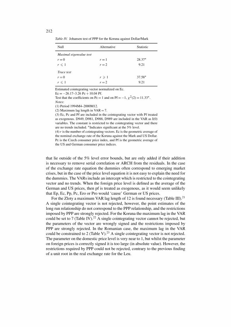
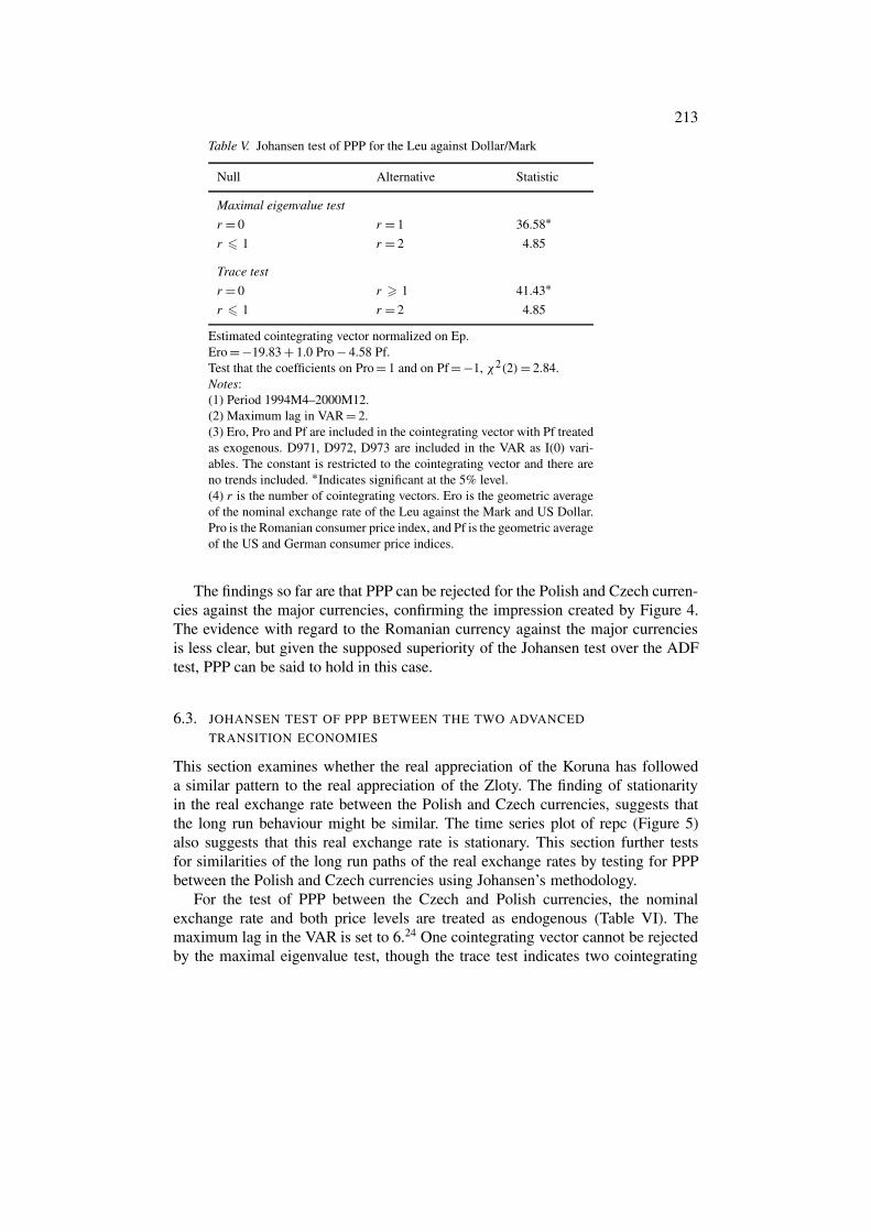
A single cointegrating vector is not rejected, however, the point estimates of thelong run relationship do not correspond to the PPP relationship, and the restrictionsimposed by PPP are strongly rejected. For the Koruna the maximum lag in the VARcould be set to 7 (Table IV).22 A single cointegrating vector cannot be rejected, butthe parameters of the vector are wrongly signed and the restrictions imposed byPPP are strongly rejected. In the Romanian case, the maximum lag in the VARcould be constrained to 2 (Table V).23 A single cointegrating vector is not rejected.The parameter on the domestic price level is very near to 1, but whilst the parameteron foreign prices is correctly signed it is too large (in absolute value). However, therestrictions required by PPP could not be rejected, contrary to the previous findingof a unit root in the real exchange rate for the Leu.

213

Table V. Johansen test of PPP for the Leu against Dollar/Mark

Null Alternative Statistic

Maximal eigenvalue test

r = 0 r = 1 36.58∗r � 1 r = 2 4.85

Trace test

r = 0 r � 1 41.43∗r � 1 r = 2 4.85

Estimated cointegrating vector normalized on Ep.Ero =−19.83 + 1.0 Pro − 4.58 Pf.Test that the coefficients on Pro = 1 and on Pf =−1, χ2(2) = 2.84.Notes:(1) Period 1994M4–2000M12.(2) Maximum lag in VAR = 2.(3) Ero, Pro and Pf are included in the cointegrating vector with Pf treatedas exogenous. D971, D972, D973 are included in the VAR as I(0) vari-ables. The constant is restricted to the cointegrating vector and there areno trends included. ∗Indicates significant at the 5% level.(4) r is the number of cointegrating vectors. Ero is the geometric averageof the nominal exchange rate of the Leu against the Mark and US Dollar.Pro is the Romanian consumer price index, and Pf is the geometric averageof the US and German consumer price indices.

The findings so far are that PPP can be rejected for the Polish and Czech curren-cies against the major currencies, confirming the impression created by Figure 4.The evidence with regard to the Romanian currency against the major currenciesis less clear, but given the supposed superiority of the Johansen test over the ADFtest, PPP can be said to hold in this case.

6.3. JOHANSEN TEST OF PPP BETWEEN THE TWO ADVANCED

TRANSITION ECONOMIES

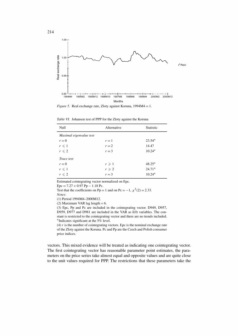
This section examines whether the real appreciation of the Koruna has followeda similar pattern to the real appreciation of the Zloty. The finding of stationarityin the real exchange rate between the Polish and Czech currencies, suggests thatthe long run behaviour might be similar. The time series plot of repc (Figure 5)also suggests that this real exchange rate is stationary. This section further testsfor similarities of the long run paths of the real exchange rates by testing for PPPbetween the Polish and Czech currencies using Johansen’s methodology.

For the test of PPP between the Czech and Polish currencies, the nominalexchange rate and both price levels are treated as endogenous (Table VI). Themaximum lag in the VAR is set to 6.24 One cointegrating vector cannot be rejectedby the maximal eigenvalue test, though the trace test indicates two cointegrating

214

Figure 5. Real exchange rate, Zloty against Koruna, 1994M4 = 1.

Table VI. Johansen test of PPP for the Zloty against the Koruna

Null Alternative Statistic

Maximal eigenvalue test

r = 0 r = 1 23.54∗r � 1 r = 2 14.47

r � 2 r = 3 10.24∗

Trace test

r = 0 r � 1 48.25∗r � 1 r � 2 24.71∗r � 2 r = 3 10.24∗

Estimated cointegrating vector normalized on Epc.Epc = 7.27 + 0.97 Pp − 1.18 Pc.Test that the coefficients on Pp = 1 and on Pc = −1, χ2(2)= 2.33.Notes:(1) Period 1994M4–2000M12.(2) Maximum VAR lag length = 6.(3) Epc, Pp and Pc are included in the cointegrating vector. D949, D957,D959, D977 and D981 are included in the VAR as I(0) variables. The con-stant is restricted to the cointegrating vector and there are no trends included.∗Indicates significant at the 5% level.(4) r is the number of cointegrating vectors. Epc is the nominal exchange rateof the Zloty against the Koruna. Pc and Pp are the Czech and Polish consumerprice indices.

vectors. This mixed evidence will be treated as indicating one cointegrating vector.The first cointegrating vector has reasonable parameter point estimates, the para-meters on the price series take almost equal and opposite values and are quite closeto the unit values required for PPP. The restrictions that these parameters take the

215

values required by PPP cannot be rejected at the 5% level. Thus the balance ofevidence suggests that PPP does hold between the Polish and Czech currencies.

6.4. JOHANSEN TEST OF PPP BETWEEN THE ADVANCED REFORMERS

AND THE LAGGING REFORMER

PPP appears to hold between the two advanced transition economies, but doesit hold between them and the less stable and less advanced transition economy.Certainly the evidence of stationarity of the Romanian real exchange rate againstmajor currencies would suggest that the real exchange rate for this currency againstthe Zloty and Koruna is unlikely to be stationary. This evidence is supported by thenon-stationarity of the real exchange rates of the Koruna and the Zloty against theLeu reported in Table II.

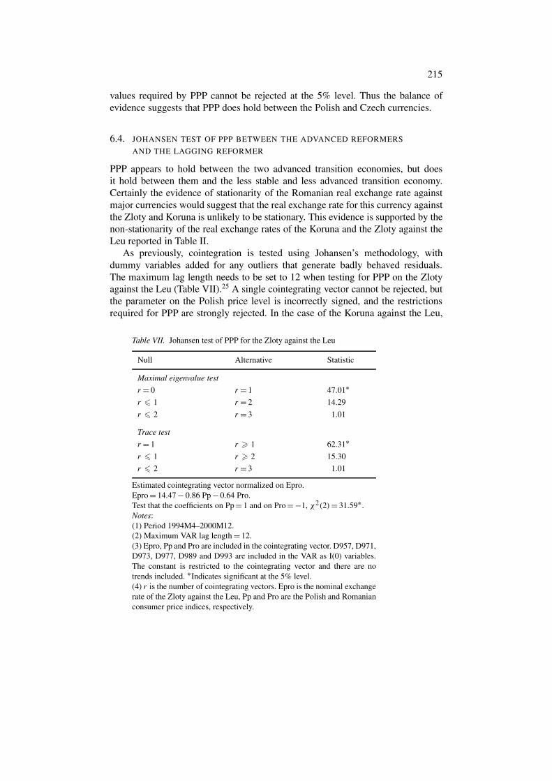
As previously, cointegration is tested using Johansen’s methodology, withdummy variables added for any outliers that generate badly behaved residuals.The maximum lag length needs to be set to 12 when testing for PPP on the Zlotyagainst the Leu (Table VII).25 A single cointegrating vector cannot be rejected, butthe parameter on the Polish price level is incorrectly signed, and the restrictionsrequired for PPP are strongly rejected. In the case of the Koruna against the Leu,

Table VII. Johansen test of PPP for the Zloty against the Leu

Null Alternative Statistic

Maximal eigenvalue test

r = 0 r = 1 47.01∗r � 1 r = 2 14.29

r � 2 r = 3 1.01

Trace test

r = 1 r � 1 62.31∗r � 1 r � 2 15.30

r � 2 r = 3 1.01

Estimated cointegrating vector normalized on Epro.Epro = 14.47 − 0.86 Pp − 0.64 Pro.Test that the coefficients on Pp = 1 and on Pro = −1, χ2(2)= 31.59∗.Notes:(1) Period 1994M4–2000M12.(2) Maximum VAR lag length = 12.(3) Epro, Pp and Pro are included in the cointegrating vector. D957, D971,D973, D977, D989 and D993 are included in the VAR as I(0) variables.The constant is restricted to the cointegrating vector and there are notrends included. ∗Indicates significant at the 5% level.(4) r is the number of cointegrating vectors. Epro is the nominal exchangerate of the Zloty against the Leu, Pp and Pro are the Polish and Romanianconsumer price indices, respectively.

216

Table VIII. Johansen test of PPP for the Koruna against the Leu

Null Alternative Statistic

Maximal eigenvalue test

r = 0 r = 1 51.55∗r � 1 r = 2 15.97∗r � 2 r = 3 12.14∗

Trace test

r = 0 r � 1 79.67∗r � 1 r = 2 28.11∗r � 2 r = 3 12.14∗

Estimated cointegrating vector normalized on Ep.Ecro = 29.94 − 2.87 Pc − 0.32 Pro.Test that the coefficients on Pc = 1 and on Pro = −1, χ2(2)= 19.58∗.Notes:(1) Period 1994M4–2000M12.(2) Maximum lag length = 9.(3) Ecro, Pc and Pro are included in the cointegrating vector. D961, D971,D972, D981 are included in the VAR as I(0) variables. The constant isrestricted to the cointegrating vector and there are no trends included.∗Indicates significant at the 5% level.(4) r is the number of cointegrating vectors. Ecro is the nominal exchangerate of the Koruna against the Leu, Pc and Pro are the consumer priceindices for the Czech Republic and Romania, respectively.

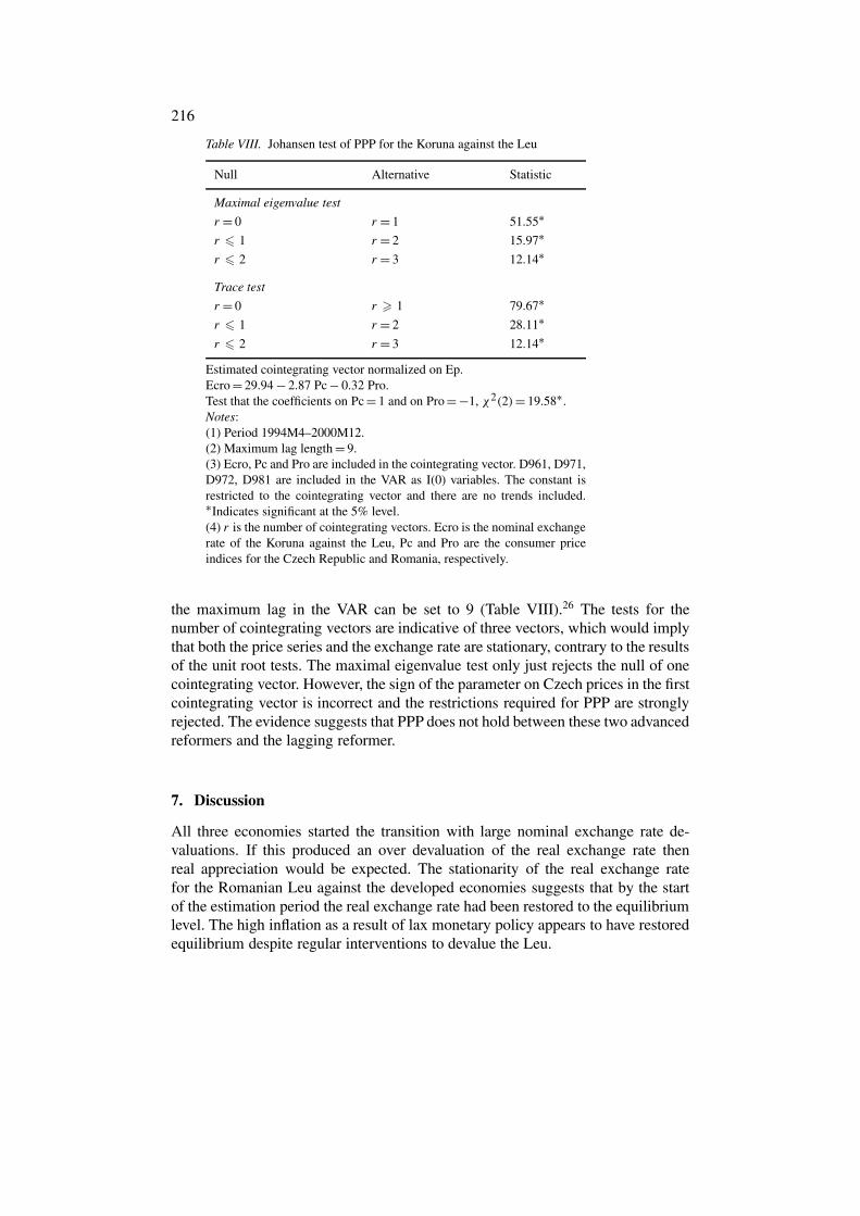
the maximum lag in the VAR can be set to 9 (Table VIII).26 The tests for thenumber of cointegrating vectors are indicative of three vectors, which would implythat both the price series and the exchange rate are stationary, contrary to the resultsof the unit root tests. The maximal eigenvalue test only just rejects the null of onecointegrating vector. However, the sign of the parameter on Czech prices in the firstcointegrating vector is incorrect and the restrictions required for PPP are stronglyrejected. The evidence suggests that PPP does not hold between these two advancedreformers and the lagging reformer.

7. Discussion

All three economies started the transition with large nominal exchange rate de-valuations. If this produced an over devaluation of the real exchange rate thenreal appreciation would be expected. The stationarity of the real exchange ratefor the Romanian Leu against the developed economies suggests that by the startof the estimation period the real exchange rate had been restored to the equilibriumlevel. The high inflation as a result of lax monetary policy appears to have restoredequilibrium despite regular interventions to devalue the Leu.

217

Both the Polish and the Czech currencies would also have been expected torequire real appreciation to correct for excessive nominal devaluation. This correc-tion appears to have been slower than in the Romanian case. Figure 4 shows thatin the period to 1996/1997 the Polish and Czech currencies were appreciating inreal terms, after which the real exchange rates do not appear to be systematicallyappreciating or depreciating. One cause of the longer time taken to achieve equi-librium could be an appreciation of the equilibrium real rate due to productivitygains in the traded goods sector. But if this were the only reason it is not clear whythe real appreciation should follow similar timings in both countries. Changes inthe role of the exchange rate in the disinflation strategy offer a plausible reasonfor this, though the Balassa–Samuleson effect cannot be excluded. The tightermonetary policy may have acted to slow down the correction to the real exchangerate by limiting the extent of inflation. Over the period in which the real exchangerate had been appreciating, both countries had followed an exchange rate baseddisinflation strategy. The Czech currency had been fixed within bands until May1997, inflation over this period was in the range of 9 or 10%. The Zloty wasmanaged in an adjustable peg arrangement, with until 1997, a rate of crawl that wasconsiderably below the inflation rate differential (OECD 1999). Since May 1997the Czech exchange rate regime has been a managed float. From 1997 to 2000,the rate of crawl of the Zloty was approximately equal to the rate of inflation, asthe Polish authorities reduced the emphasis on the exchange rate in the disinflationstrategy (see OECD 1999, 2001), and from mid-2000 the Zloty has been floating.Under these latter arrangements both nominal exchange rates were permitted toadjust to inflation differentials, and these adjustments appear to have stopped thereal appreciation.

The suggestion that productivity changes might not be the most important causeof the real appreciation seems to contradict some other results. However, Balazs(2002) argues that exchange rate management has caused an appreciation of thereal exchange rate in excess of that warranted by productivity changes when theconsumer price index is used. The results reported here could be reconciled withthe findings of Halpern and Wyplosz (2001) and de Broeck and Slok (2001) ifthe direction of causality is as proposed by Grafe and Wyplosz (1999), who arguethat real appreciation raises productivity by squeezing labour out of less efficientsectors.

8. Conclusion

Evidence has been presented that the currencies of Poland and the Czech Republichave not been stationary in real terms against developed economies, and appearto be appreciating, but that against each other they have been stationary in realterms. In contrast, the real exchange rates of the Polish and Czech currenciesagainst the Romanian currency, as an example of a lagging reformer, have not beenstationary. In other words, PPP holds between the currencies of the two advanced

218

transition currencies, but does not hold for the advanced transition countries againstdeveloped market economies or for the advanced transition economies against thelagging reformer.

The real appreciation of the Czech and Polish currencies against the major cur-rencies ended at about the same time that the exchange rate became less centralto the disinflation. Once the exchange rates of Poland and the Czech Republicwere able to devalue/depreciate in line with price differentials, then the real ap-preciation stopped. The Romanian currency is not observed to have appreciatedin real terms over the sample period because the managed floating exchange rateregime permitted the authorities to limit any tendency for real appreciation. Thisevidence supports Desai’s (1998) and Orlowski’s (2000) arguments that exchangerate based disinflation strategies have been a major source of the real appreciationof the currencies of transition economies.

Acknowledgements

The author wishes to thank Roxana Radulescu and Hugh Metcalf of NewcastleUniversity for helpful comments.

Notes

1. See also the papers by Brada; Desai; Begg; Drabek and Brada; and Szpary and Jakab in a symposiumpublished in the Journal of Comparative Economics in 1998, and also Kemme and Teng (1988) and Liargovas(1999).

2. The black market premium that existed at the end of the communist era could have guided the scale ofthe required devaluation, but it was always likely that mistakes would occur. According to Nuti (1991), atthe start of the transition, the US Dollar rose to between four and five times its PPP value in Poland andCzechoslavakia.

3. For example, Brada (1998) argues that Begg’s (1998) failure to find a significant role for productivity changescould be due to the mismeasurement of aggregate output.

4. In addition, the constant allows for differences in the base years of aggregate price series.5. Halpern and Wyplosz (1997) list a number of consequences of the transition that could produce such a change

in relative prices. Firstly, rising incomes could raise demand for services faster than demand for goods,services are dominated far more by non-tradeables than are goods and so the relative price of tradeablesfalls. Secondly, since the service sector had been repressed under socialism the expansion of services overthe transition would create a real appreciation. Third, deep restructuring may raise productivity in the tradedsector relative to productivity in the non-traded sector, thus causing the prices of traded goods to fall relativeto the price of non-traded goods, such as in the Balassa (1964) and Samuleson (1964) effect. Fourth, foreigndirect investment tends to produce a real appreciation, though Liargovas (1999) points out that FDI to thenon-tradeables sector could produce a real depreciation of the currency. Fifth, improvements in the qualityof traded goods would improve the terms of trade.

6. Halpern and Wyplosz (1997), Begg, Halpern and Wyplosz (1999) and Krajnyak and Zettelmeyer (1998)estimate equilibrium dollar wage equations to show that in many transition economies actual dollar wageshave been increasing towards the equilibrium level. These studies also show that the equilibrium dollar wagehas been appreciating in the advanced reformers but not in the lagging reformers.

7. The problem is not so much a shortage of observations, but rather the long period usually required forPPP to take effect. Rogoff (1996) reports that it can take up to 5 years for one-half of the deviation of theexchange rate from the PPP level to be closed. Thus care should be taken in the interpretation of negativeresults. However, a finding in support of a cointegrating vector corresponding to a PPP relationship is strongevidence in favour of the theory.

219

8. Unlike this paper, Choudhry utilizes fractional cointegration tests. Choudhry also tests for relative purchasingpower parity, that PPP holds in first differences, some favourable evidence for relative PPP, both between thetransition economies and the US, and amongst the transition economies, is found.

9. A consequence of these differences in the extent of pre-transition reform is that Poland started the transitionwith a considerably higher level of repressed inflation than did Czechoslavakia, as the latter had not grantedthe sort of inflationary pay rises the former had given. Consequently inflation in Poland at the start of thetransition was worse than in Czechoslavakia.

10. A complicating factor in the Czech case is the dissolution of the Czechoslovak Federal Republic in January1993 and the collapse of the Monetary Union between the Czech and Slovak Republics in February 1993.

11. The EBRD reports indices for eight aspects of reform. The values range from 1 to 4+, the former indicatingalmost no reform, the latter indicating standards similar to a developed market economy. For the purposesof calculating the average, a score with a ‘+’ is treated as being 0.3 above the number, for example, 4+becomes 4.3, and a score with a ‘−’ is treated as 0.3 below, for example, 4− is 3.7.

12. Kemme and Teng (1988) provide an excellent overview of developments concerning the exchange rate forthe Zloty.

13. Developments concerning the exchange rate for the Koruna are outlined by Begg (1998).14. Germany is chosen at the representative of trade with the EU and the US is representative of all other trade

partners.15. Arguably wholesale price indices are a more appropriate index to use when testing PPP than consumer price

indices, since services make up a large share of the latter. However, wholesale price indices are not availablefor a sufficiently long period on a monthly basis to permit the analysis used in this study.

16. Calculated as the first difference of the log of the nominal exchange rate and denoted by D(Ep), D(Ec) andD(Ero) for the depreciations of the Zloty, Koruna and Leu, respectively.

17. Calculated as the first difference of the log of the price level and denoted by D(Pp), D(Pc) and D(Pro) forPolish, Czech and Romanian inflation, respectively.

18. If the domestic price series and the nominal exchange rates are combined to give a price series measured inthe foreign currency, then for both Poland and the Czech Republic the redefined price series are I(1). A 2ndorder ADF test yields −1.52 on (Pp − Ep) and a first order ADF test yields −7.27 on �(Pp − Ep). A firstorder ADF yields for −2.25 for (Pc − Ec) and −6.67 for �(Pc − Ec). This suggests that the domestic priceindices are themselves I(1).

19. Since stationarity around a trend would imply that the equilibrium real exchange rate is not constant, onlythe results for the non-trended case are reported.

20. The dummy variables take the value 1 in the month indicated and zero otherwise.21. The dummies included in the VAR are for large depreciations at the time of the Russian crisis in August 1998

(D988) and the month following the Brazilian crisis in January 1999 (D992), for a recovery in the exchangerate in the month following the Russian crisis (D989) and for inflation outliers in July 1995 (D957), July1997 (D977) and January 1998 (D981).

22. The dummies included are for large depreciations at the time of the Russian crisis D988, plus D989 whichpicks up a large nominal appreciation in September 1998 following the depreciation caused by the Russiancrisis. Whilst the depreciation at the time of the Czech crisis of 1997 is badly underpredicted, it does notproduce a residual that lies outside the 5% bounds. A dummy for the crisis taking the value 1 in the monthof the largest residual (May 1997) is significant in the exchange rate equation but it induces serial correlationin the residuals. For these reasons the dummy is excluded. In addition, unlike the other emerging marketcrises the Czech crisis is endogenous as it produced a correction to an exchange rate that had been rapidlyappreciating in real terms prior to the crisis (see Figure 4). In addition, there are dummies for inflation outliersin January 1998 (D981) and September 1994 (D949).

23. Dummy variables are required for January, February and March of 1997 (D971, D972 and D973). Theseare for the rapid depreciation in the first 2 months of 1997, due to the ending of currency rationing, andfor extra inflationary pressure in March 1997, due to heavy capital inflows following the resumption of thestabilization program. Notably, dummy variables are not required for the emerging markets and Russianfinancial crises, confirming the impression created by Figure 2, that the volatility of the nominal exchangerate was no different in the latter part of the sample than in the early part.

24. Dummies included are D949, D957, D977, D981, and in addition a dummy for a Polish inflation outlier inSeptember 1995 (D959). Curiously this movement in inflation is not significantly underpredicted when theforeign country is defined to be the composite of Germany and the USA. Clearly movements in Pf or Ep arebetter predictors of Polish inflation in this month.

220

25. Dummy variables are again required for inflation outliers in July 1995 and July 1997. In addition, dummyvariables are needed for the month immediately after the breaking of the Russian financial crises and 2months after the Brazilian crisis (March 1999, D993). Dummy variables are also required for January 1997(D971), and March 1997 (D973).

26. The dummy variables required are for inflation outliers in January 1996 and January 1998, and also forJanuary 1997 and February 1997 (D971 and D972).

References

Balassa, B. (1964), ‘The purchasing power parity doctrine: a reappraisal’, Journal of PoliticalEconomy 72, 584–596.

Balazs, E. (2002), ‘Investigating the Balassa–Samuleson hypothesis, do we understand what we see?A panel study’, Economics of Transition 10(2), 273–309.

Barlow, D. and Radulescu, R. (2002), ‘Purchasing power parity in the transition: the case of theRomanian Leu against the dollar’, Post-Communist Economies 14(1), 123–135.

Begg, D. (1998), ‘Pegging out: lessons from the Czech exchange rate crisis’, Journal of ComparativeEconomics 26(4), 669–690.

Begg, D., Halpern, L. and Wyplosz, C. (1999), Monetary and Exchange Rate Policies, EMU andCentral and Eastern Europe. Forum Report of the Economic Policy Initiative, New York, Centrefor Economic Policy Research.

Brada, C.J. (1998), ‘Introduction: exchange rates, capital flows, and commercial policies in transitioneconomies’, Journal of Comparative Economics 26(4), 613–620.

de Broeck, M. and Slok, T. (2001), ‘Interpreting real exchange rate movements in transitioncountries’, International Monetary Fund, Working Paper WP/01/56.

Choudhry, T. (1998), ‘Purchasing power parity in high inflation eastern European countries: evid-ence from fractional and Harris-Inder cointegration tests’, Journal of Macroeconomics 21(2),293–308.

Christev, A. and Noorbakhsk, A. (2000), ‘Long run purchasing power parity, prices and exchangerates in transition, the case of six central and east European countries’, Global Finance Journal11, 87–108.

Desai, P. (1998), ‘Macroeconomic fragility and exchange rate vulnerability: a cautionary record oftransition economies’, Journal of Comparative Economics 26(4), 621–641.

Dibooglu, S. and Kutan, M.A. (2001), ‘Sources of real exchange rate fluctuations in trans-ition economies: the case of Poland and Hungary’, Journal of Comparative Economics 29,257–275.

Drabek, Z. and Brada, C.J. (1998), ‘Exchange rate regimes and the stability of trade policy intransition economies’, Journal of Comparative Economics 26(4), 642–668.

European Bank for Reconstruction and Development, Transition Report, various issues.Grafe, C. and Wyplosz, C. (1999), ‘A model of real exchange rate determination in transition econo-

mies’ in M. Blejer and M. Skreb (eds), Balance of Payments, Exchange Rates and Competitive-ness in Transition Economies, pp. 159–184, Boston, Kluwer Academic Press.

Halpern, L. and Wyplosz, C. (1997), ‘Equilibrium exchange rates in transition economies’, IMF StaffPapers 44(4), 430–461.

Halpern, L. and Wyplosz, C. (2001), ‘Economic transformation and real exchange rates in the 2000s;The Balassa Samuleson connection’, United Nations Economic Council for Europe, EconomicSurvey of Europe.

Johansen, S. (1988), ‘Statistical analysis of co-integration vectors’, Journal of Economic Dynamicsand Control 12, 231–254.

Kemme, M.D. and Teng, W. (1988), ‘Determinants of the real exchange rate, misalignment andimplications for growth in Poland’, Economic Systems 24(2), 171–205.

221

Krajnyak, K. and Zettelmeyer, J. (1998), ‘Competitiveness in transition economies: what scope forreal appreciation’, International Monetary Fund, Staff Papers 45(2), 309–362.

Liargovas, P. (1999), ‘An assessment of real exchange rate movements in the transition economies ofcentral and eastern Europe’, Post-Communist Economies 11(3), 299–318.

MacKinnon, G.J. ‘Critical values for co-integration tests’ in R.F. Engle and C.W.J. Granger (eds),Long Run Economic Relationships, Oxford, Oxford University Press.

Nuti, D.M. (1991), ‘Inflation, interest and exchange rates in the transition’, Economical Transition4(1), 137–158, 1996.

Organisation for Economic Cooperation and Development (1999), OECD Economic Surveys:Poland, Paris, OECD.

Organisation for Economic Cooperation and Development (2001), OECD Economic Surveys:Poland, Paris, OECD.

Orlowski, T.L. (2000), ‘Monetary policy regimes and real exchange rate rates in central Europe’stransition economies’, Economic Systems 24(2), 145–166.

Rogoff, K. (1996), ‘The purchasing power parity puzzle’, Journal of Economic Literature 34,647–668.

Samuleson, A.P. (1964), ‘Theoretical notes on trade problems’, Review of Economics and Statistics46, 145–154.

Szarpy, G. and Jakab, M.Z. (1998), ‘Exchange rate policy in transition economies: the case ofHungary’, Journal of Comparative Economics 26(4), 691–717.