Masthead LogoFordham University

DigitalResearch@Fordham

CRIF Seminar series Frank J. Petrilli Center for Research in InternationalFinance

Spring 2004

The Purchasing Power Parity DebateAlan M. TaylorUniversity of California, Davis

Mark P. TaylorUniversity of Warwick

Follow this and additional works at: https://fordham.bepress.com/crif_seminar_series

Part of the Finance and Financial Management Commons

This Article is brought to you for free and open access by the Frank J. Petrilli Center for Research in International Finance atDigitalResearch@Fordham. It has been accepted for inclusion in CRIF Seminar series by an authorized administrator of DigitalResearch@Fordham.For more information, please contact considine@fordham.edu.

Recommended CitationTaylor, Alan M. and Taylor, Mark P., "The Purchasing Power Parity Debate" (2004). CRIF Seminar series. 24.https://fordham.bepress.com/crif_seminar_series/24

1

The Purchasing Power Parity Debate

Alan M. Taylor

University of California, Davis; National Bureau for Economic Research;

and Centre for Economic Policy Research

Mark P. Taylor

University of Warwick and

Centre for Economic Policy Research

Prepared for Journal of Economic Perspectives Draft: comments welcome, please do not cite

2

The term purchasing power parity was apparently introduced into economic discourse

less than a century ago (Cassel, 1918), although the concept itself has a very much longer

history in economics, dating back several centuries. While the concept of PPP appears to

be implicit in the writings of several of the classical economists, however, it appears to

have largely lain dormant for many years until it was re-introduced into the international

policy debate concerning the appropriate level for nominal exchange rates among the

major industrialized countries after the large-scale inflations during and after World War

One. In the ensuing period, the idea of PPP appears to have become embedded in the way

many international economists think about the world. Writing over a quarter of a century

ago, for example, Dornbusch and Krugman (1976) noted that “Under the skin of any

international economist lies a deep-seated belief in some variant of the PPP theory of the

exchange rate.” And twenty years later, Rogoff (1996) expressed much the same

sentiment: “While few empirically literate economists take PPP seriously as a short-term

proposition, most instinctively believe in some variant of purchasing power parity as an

anchor for long-run real exchange rates.”

Despite the strongly intuitive appeal of PPP, however, the concept has, since the

early 1970s, been the subject of an ongoing and lively debate in economics and some of

the central problems which the profession has analyzed in this connexion over the past

three decades have only recently been resolved, while others still remain on the research

agenda and still other puzzles have only recently come onto the agenda. In this paper, we

provide a highly personalized view of the PPP debate.

In Section 3 we provide a guide to the PPP debate over the past three decades, while

in Section 4 we discuss more recent work on nonlinearities in real exchange rates and, in

3

Section 5, highlight two issues which we see as important puzzles on the frontier of

research. In the next two sections, however, we lay the groundwork for our discussion by

setting out the basic arguments for whether or not PPP should hold and presenting some

simple but nevertheless, in our view, compelling evidence as to whether PPP does in fact

hold to a first approximation over various time periods and time horizons.

1. Why should PPP hold at all?

Advocates of PPP have generally based their view either on arguments relating to

international asset market equilibrium or—more frequently—on arguments relating to

international goods arbitrage.

The argument for PPP based on international goods arbitrage is straightforward

and is related to the so-called Law of One Price. According to the Law of One Price, the

price of an internationally traded good should be the same anywhere in the world once

that price is expressed in a common currency—otherwise people could make a riskless

profit by shipping the goods from locations where the price is low to locations where the

price is high. If the same goods enter each country’s market basket used to construct the

aggregate price level—and with the same weight—then the Law of One Price implies

that absolute PPP should hold between the two countries concerned.

Possible objections to this line of reasoning are immediate. For example, the

presence of transactions costs in arbitrage—perhaps arising from tariffs and duties,

transport costs and nontariff barriers—would induce a violation of the Law of One Price

and this is an issue we shall discuss later. In addition, as the “new trade theory” attests,

different countries tend to produce goods that are differentiated rather than perfectly

4

substitutable. And it also clear both that not all goods are traded and that the weight

attached to similar goods in aggregate price indices will differ across countries. These

objections notwithstanding, however, it is often asserted that PPP will hold to a close

approximation because of at least the possibility of international goods arbitrage. Indeed,

as we shall see, a recent literature has attempted to allow for imperfections of this kind in

testing for PPP.

The other, less frequently advanced justification for belief in PPP is based on the

notion of asset market equilibrium, although the precise mechanism by which PPP is

supposed to occur as a result of this equilibrium is often left somewhat obscure. This kind

of argument was adopted, for example, by early proponents of the monetary approach to

the exchange rate (e.g., Frenkel, 1976), which emerged in the early 1970s as the then

dominant theory of exchange rate determination and which was based on an assumption

that PPP held at all times, or continuously. Advocates of the monetary approach argued

that since the exchange rate is the relative price of two monies, that relative price should

be determined by the relative balance of supply and demand in the respective money

markets. Exactly how percentage changes in relative money supplies are translated, other

things equal, into exactly matching exchange rate movements is not immediately

obvious, however, unless one resorts to an argument based on goods arbitrage: changes in

the relative money supply affect relative prices including relative traded goods prices

which then leads to international goods arbitrage.

In sum, our view is that insofar as PPP is expected to hold at all, arguments based

on international goods arbitrage appear to be more logically consistent than arguments

based on asset market equilibrium. It is likely, however, that there are important

5

deviations from the Law of One Price because of product differentiation and various

transactions cost in international arbitrage, and many a slip between the Law of One Price

and PPP because of various index number issues. Hence, we should not expect PPP to

hold perfectly. Given that the Law of One Price is more likely to be a better

approximation for goods which are traded internationally, however, we should perhaps

expect PPP to be a better approximation if we compare national price levels based on

indices containing a higher proportion of traded goods—such as producer price indices

which tend to contain the prices of more manufactured tradables than do consumer price

indices, which tend to reflect the prices of relatively more nontradables, such as many

services.

2. So does PPP hold? The long and the short of it

Absolute purchasing power parity (PPP) holds when the nominal foreign exchange rate

between two currencies is such that the purchasing power of a unit of currency is exactly

the same in the foreign economy as in the domestic economy, once it is converted into

foreign currency at that rate. Equivalently, absolute PPP implies that the nominal

exchange rate between two currencies is equal to the ratio of national price levels.

Relative PPP holds when the percentage change in the exchange rate over a given period

just offsets the difference in inflation rates in the countries concerned over the same

period, so that the purchasing power of a unit of the domestic currency in the domestic

economy relative to its purchasing power in the foreign economy when converted at the

going exchange rate is the same at the end of the period as at the beginning of the period.

6

So does PPP hold in either its relative or its absolute versions? To get a feel for

whether PPP is even a moderately good approximation to the real world, let’s analyse

some real-world data. Take a look at Figure 1. In the top panel of Figure 1 we have

plotted data on the U.S. and U.K. consumer price indices (CPIs) in dollar terms (i.e., after

multiplying the U.K. CPI by the number of U.S. dollars exchanging for one U.K. pound

at that point in time), over the period 1820–2001. In the bottom panel of the figure we

have done the same thing with producer price indices, using data for a slightly longer

period 1791–2001.1 We have (arbitrarily) normalised each of the series to be equal to

zero in 1900. Although we do not know, a priori, whether or not absolute PPP happened

to hold at any particular point in time over the sample period, it must nevertheless be true

that if absolute PPP had held continuously over these long historical periods, the two

lines in each graph should be perfectly correlated. At least three points are worth raising

from a consideration of these graphs. First, it is clear that absolute PPP did not hold

perfectly and continuously: the correlation between the two lines is less than perfect in

both cases. Second, however, it is equally clear that the national price levels of the two

countries, expressed in a common currency, did tend to move together over these long

periods in the sense that the deviation between the two lines does not get bigger over

time. Third, it is clear that the correlation between the two national price levels is much

greater when we use producer prices than when we use consumer prices.

Now take a look at Figure 2. In the former we have plotted several graphs using

data for a large number of countries over the period 1970-1998.2 Consider first the two

1 See Lothian and Taylor (1996, 2003) for a guide to the sources for these data series. 2 The scatter plots are based on data from the International Monetary Fund's International Financial Statistics database over the period 1970–1998 (data was not available after

7

graphs in the top row of Figure 2. For each country we calculated the 1-year inflation rate

in each of the 29 years and subtracted the 1-year U.S. inflation rate in the same years to

obtain a measure of relative inflation (using consumer price indices for the first column

and producer price indices for the second column). We then calculated the percentage

change in the dollar exchange rate for each year and finally we plotted relative annual

inflation against exchange rate depreciation for each of the 29 years for each of the

countries. If relative PPP held perfectly, then each of the scatter points would lie on a 45o

ray through the origin. In the second row we have carried out a similar exercise, except

we have taken averages: we have plotted 29-year annualised average relative inflation

against the average annual depreciation of the currency against the US dollar over the

whole period (just one scatter point for each country).

So what does Figure 2 tell us about relative PPP? In some ways, it sends similar

messages to those emanating from Figure 1. For small differences in annual inflation

between the U.S. and the country concerned, the correlation between relative inflation

and depreciation in each of the years seems low, and for the postwar data this is true

whether we use the PPI or the CPI to measure relative inflation. Thus, relative PPP

1998 for some countries). The series extracted were the exchange rate of the national currency against the US dollar and both the consumer and producer price indices where available. The sample included data on consumer price indices for 20 industrialized countries and 26 developing countries: the USA, Austria, Belgium, Canada, Denmark, Finland, France, Germany, Greece, Israel, Italy, Japan, the Netherlands, Norway, Portugal, South Africa, Spain, Sweden, Switzerland, the UK, Argentina, Chile, Colombia, Dominican Republic, Ecuador, Egypt, El Salvador, Ghana, Guatemala, Honduras, India, Indonesia, Jamaica, South Korea, Malaysia, Mexico, Myanmar, Pakistan, Paraguay, Peru, Philippines, Sri Lanka, Sudan, Thailand, Turkey and Venezuela. The corresponding list of countries for which producer price indices was available excludes Belgium, France, Italy, Norway, Portugal, and Sweden but adds Ireland to include fourteen industrialized countries, and includes twelve developing

8

certainly does not appear to hold perfectly and continuously in the short run. When we

take 29-year averages, however, the scatter plots tend to collapse onto the 45o ray.3 Thus,

there is again some evidence that PPP—this time relative PPP—tends to hold in a long-

run sense while it does not seem a good approximation for low relative inflation countries

in the short run. Also, as we take the longer-run averages, the degree of correlation

between relative inflation and exchange rate depreciation again seems even higher when

using PPIs than when using CPIs. Another aspect of relative PPP apparent from Figure 2

is that, even at the 1-year horizon, it appears to hold more closely for countries

experiencing relatively high inflation.

So the conclusions emerging from our informal eyeballing of Figures 1 and 2

seem to be the following. Neither absolute nor relative PPP appear to hold closely in the

short-run, although both appear to hold reasonably well as a long-run average and when

there are large movements in relative prices and both appear to hold better between

producer price indices than between consumer price indices. That’s the long and the short

of it. On our reading of the literature, moreover, these conclusions are in fact broadly in

line with the current consensus view on PPP. So where does all the controversy arise?

3. The PPP debate: A tour d’horizon of the past three decades

a) The rise and fall of continuous PPP

Empirically, the PPP debate has generally been conducted in terms of an analysis of the

log-levels of prices and exchange rates. Let ts denote the logarithm of the market

countries: Brazil, Chile, Colombia, Costa Rica, Egypt, El Salvador, India, Korea, Mexico, Pakistan, Philippines and Thailand.

9

exchange rate at time t (the domestic price of foreign currency) and let tp and *tp denote

the logarithms of the domestic and foreign price level respectively. Now because tp and

*tp are indices designed to measure price levels relative to an arbitrary base period within

each country, rather than relative to the price level in a foreign country, we need to adjust

them in order to pin down the PPP exchange rate — i.e., the rate at which absolute PPP

holds. If we could find a point in time — at the end of period τ, say — when the nominal

exchange rate was such that absolute PPP held on our above definition, then we could

define this adjustment factor, PPPq say, as:

q PPP ≡sτ − pτ + pτ* . (1)

If absolute PPP held continuously then the nominal exchange rate scaled by this same

adjustment factor, )( PPPt qs − , should be equal to relative prices, )( *tt pp − , in any

period t. In theoretical discussions, PPPq can be defined as a parameter and it is often in

fact normalized to zero. Empirically, however, PPPq is difficult to measure reliably and it

is for this reason that empirical researchers have usually tested necessary rather than

sufficient conditions for absolute PPP to hold, as we shall see presently.

Given the dominance of the monetary approach to the exchange rate in the early

1970s (Taylor, 1995; Frankel and Rose, 1995) and its central assumption of continuous

PPP, it is hardly surprising that a wave of empirical studies on PPP appeared around this

time, as well as on the monetary approach to the exchange rate more generally (see e.g.,

Frenkel and Johnson, 1978). One did not, however, have to be an econometrician to

witness the “collapse of purchasing power parity” (Frenkel, 1981) in the early years of

3 This effect is only slightly less marked if we take averages over shorter periods of ten

10

the new floating rate regime: nominal exchange rates were patently far more volatile than

relative national price levels, thereby ruling out continuous PPP. The tenacity with which

economists clung to some form of PPP is evidenced, however, by the rise in popularity at

this time of overshooting exchange rate models (Dornbusch, 1976), in which PPP is

retained as a long-run equilibrium while allowing for significant short-run deviations due

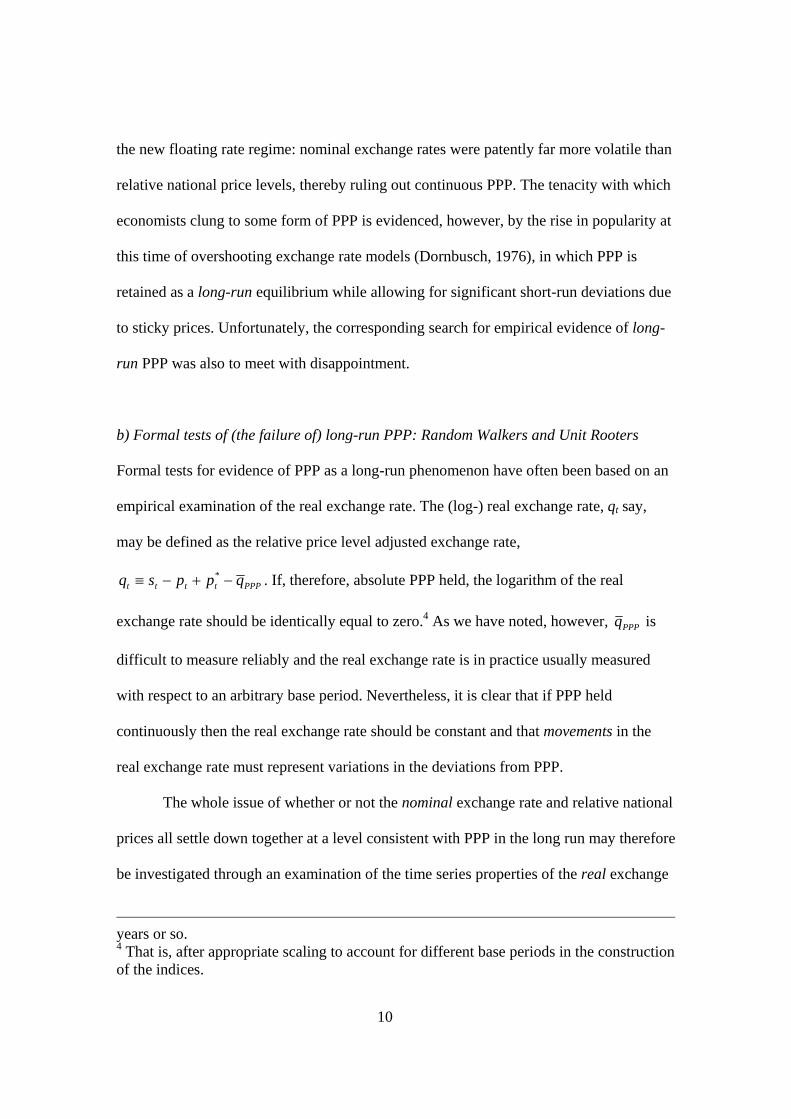
to sticky prices. Unfortunately, the corresponding search for empirical evidence of long-

run PPP was also to meet with disappointment.

b) Formal tests of (the failure of) long-run PPP: Random Walkers and Unit Rooters

Formal tests for evidence of PPP as a long-run phenomenon have often been based on an

empirical examination of the real exchange rate. The (log-) real exchange rate, qt say,

may be defined as the relative price level adjusted exchange rate,

PPPtttt qppsq −+−≡ * . If, therefore, absolute PPP held, the logarithm of the real

exchange rate should be identically equal to zero.4 As we have noted, however, PPPq is

difficult to measure reliably and the real exchange rate is in practice usually measured

with respect to an arbitrary base period. Nevertheless, it is clear that if PPP held

continuously then the real exchange rate should be constant and that movements in the

real exchange rate must represent variations in the deviations from PPP.

The whole issue of whether or not the nominal exchange rate and relative national

prices all settle down together at a level consistent with PPP in the long run may therefore

be investigated through an examination of the time series properties of the real exchange

years or so. 4 That is, after appropriate scaling to account for different base periods in the construction of the indices.

11

rate. This is because, for the real exchange rate to settle down at any level whatsoever, it

must display reversion towards its own mean. Hence, a necessary condition for long-run

absolute PPP to hold is that the real exchange rate be mean reverting, although this is not

a sufficient condition since it may be reverting towards a mean not equal to the PPP real

exchange rate PPPq .5

Early studies by Roll (1979) and Adler and Lehmann (1983) tested the null

hypothesis that the real exchange rate in fact follows a random walk—the archetypal

non–mean reverting time series process in which real exchange rate changes in each

period are purely random. In neither study could the random walk or non–mean reversion

hypothesis be rejected. In the late 1980s, following Engle and Granger’s (1987) seminal

paper, a more sophisticated econometric literature on long-run PPP developed, at the core

of which was the concept of a unit root process. If a time series on an economic variable

is a realisation of a unit-root process, then while changes in the variable may be to some

extent predictable, the variable may still never settle down at any one particular level,

even in the very long run. Tests for unit roots in real exchange rates thus seemed ideally

5 It is sometimes asserted that by specifying an arbitrary base period, researchers are implicitly testing for relative rather than absolute PPP. In tests of short-run PPP, we would agree with this view: clearly, if 0~* ≡−+−≡ qppsq tttt at all times, where q~ is an arbitrary constant, then we must have 0* ≡∆+∆−∆ ttt pps , which is a statement of relative PPP. Since relative PPP is a necessary but not a sufficient condition for absolute PPP, our discussion of necessary and sufficient conditions in the text is consistent with this view. In tests of long-run PPP, however, the issue is slightly more subtle. Suppose, for example, we knew that ttttt uqppsq +−+−≡ ~* , where all of the variables, including the term ut, were first-difference stationary: a researcher finding this would conclude that long-run absolute PPP was rejected since there is no mean reversion in the real exchange rate. However, after first-differencing we have

ttttt uppsq ∆+∆+∆−∆≡∆ * and, since all variables are now stationary, this implies that depreciation of the nominal exchange rate will exactly reflect movements in relative

12

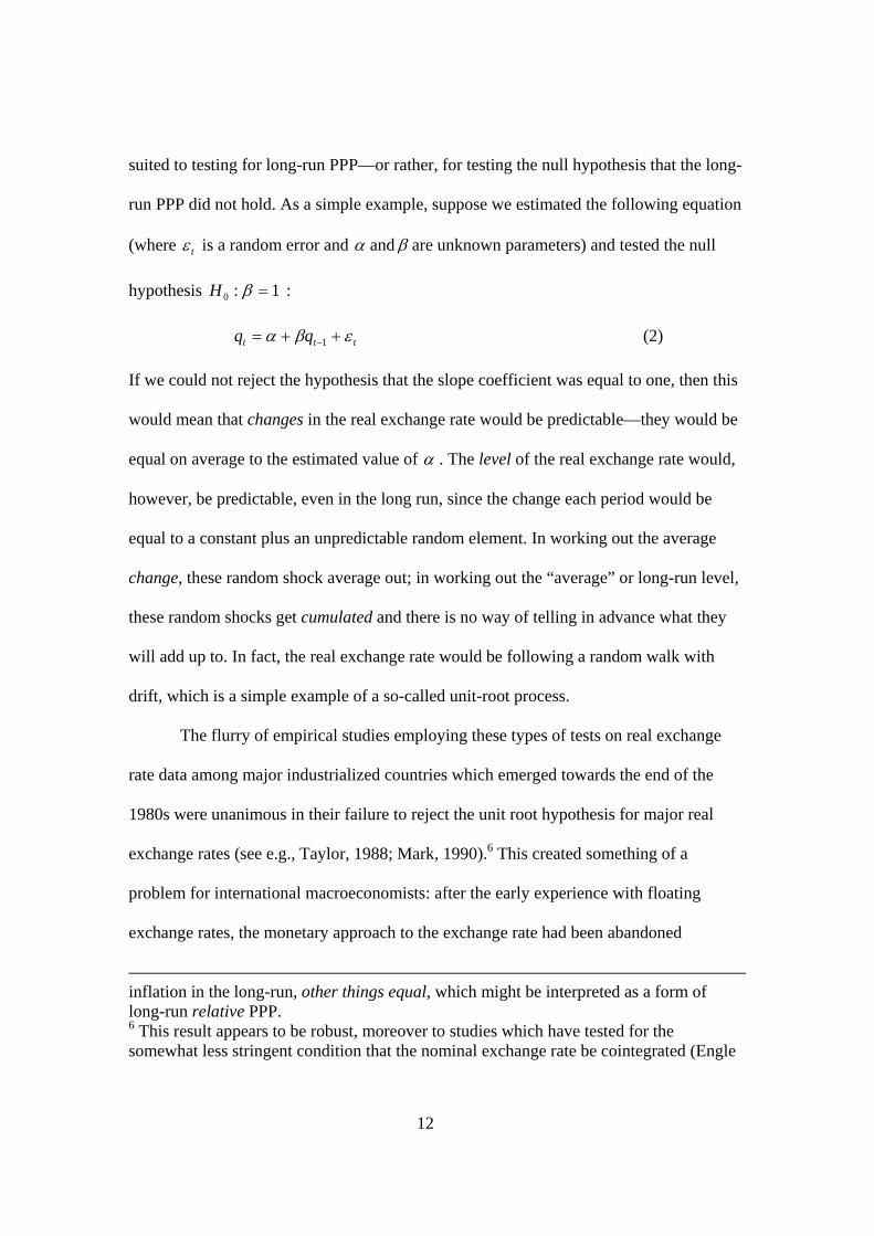
suited to testing for long-run PPP—or rather, for testing the null hypothesis that the long-

run PPP did not hold. As a simple example, suppose we estimated the following equation

(where tε is a random error and α and β are unknown parameters) and tested the null

hypothesis 1:0 =βH :

ttt qq εβα ++= −1 (2)

If we could not reject the hypothesis that the slope coefficient was equal to one, then this

would mean that changes in the real exchange rate would be predictable—they would be

equal on average to the estimated value of α . The level of the real exchange rate would,

however, be predictable, even in the long run, since the change each period would be

equal to a constant plus an unpredictable random element. In working out the average

change, these random shock average out; in working out the “average” or long-run level,

these random shocks get cumulated and there is no way of telling in advance what they

will add up to. In fact, the real exchange rate would be following a random walk with

drift, which is a simple example of a so-called unit-root process.

The flurry of empirical studies employing these types of tests on real exchange

rate data among major industrialized countries which emerged towards the end of the

1980s were unanimous in their failure to reject the unit root hypothesis for major real

exchange rates (see e.g., Taylor, 1988; Mark, 1990).6 This created something of a

problem for international macroeconomists: after the early experience with floating

exchange rates, the monetary approach to the exchange rate had been abandoned

inflation in the long-run, other things equal, which might be interpreted as a form of long-run relative PPP. 6 This result appears to be robust, moreover to studies which have tested for the somewhat less stringent condition that the nominal exchange rate be cointegrated (Engle

13

although there was still a consensus belief in long-run PPP coupled with overshooting

exchange rate models; now the data appeared to be telling us that even long-run PPP was

a chimera. This led some economists to posit theoretical models to explain why the real

exchange rate could in fact be non-mean reverting (e.g., Stockman, 1987). Others refused

to take the empirical evidence at face value and were prompted to question the empirical

methodology used to produce this evidence.

In particular, Frankel (1986, 1990) noted that while a researcher may not be able

to reject the null hypothesis of a random walk real exchange rate at a given significance

level, it does not mean that she has to accept it, especially if—as Frankel argues—it

seems unreasonable to do so. To draw an analogy, if someone comes into a room

carrying a cup of coffee, you cannot immediately reject the hypothesis that they are going

to throw it over you, but it would be classed as schizophrenic behavior to duck under the

table every time someone came back from Starbuck's! Furthermore, Frankel was the first

economist to point out that the tests typically employed to examine the long-run stability

of the real exchange, if based on data covering just fifteen years or so, may have very low

power to reject the null hypothesis of a unit root even if it is indeed false. The latter point

was further taken up and examined by other authors (Froot and Rogoff, 1995; Lothian

and Taylor, 1996, 1997). The argument is that if the real exchange rate is in fact stable in

the sense that it tends to revert towards its mean over long periods of time, then

examination of just one real exchange rate over a relatively short period may not yield

enough information to be able to detect slow mean reversion towards PPP. Moreover,

increasing the sample size by increasing the frequency of observation—moving from,

and Granger, 1987) with domestic and foreign prices—see e.g Taylor (1988); Taylor and

14

say, quarterly to monthly data—won’t help because increasing the amount of detail

concerning short-run movements can only give you more information about short-run

behaviour rather than about long-run equilibrium and will therefore not increase the

power of tests for non-mean-reversion (Shiller and Perron, 1985). If you want to get more

information about the long-run behaviour of a particular real exchange rate, you really

need to get more data in terms of years—in other words you need to increase the span of

the data.

On the basis of Monte Carlo evidence calibrated on a speed of real exchange rate

adjustment of about 11% per annum (from Lothian and Taylor’s 1996 study, discussed

below), Lothian and Taylor (1997) and Sarno and Taylor (2002a) show that the

probability of rejecting at the five percent level the null hypothesis of a random walk real

exchange rate, when in fact the real rate is mean reverting, is extremely low —

somewhere between about five and eight percent — when using standard tests and a data

span of about fifteen years, corresponding to the early long-run PPP studies of the late

1980s. Moreover, even with the benefit of the additional ten to fifteen years or so of data

which is now available, the power of the test increases by only a couple of percentage

points, and even with a century of data there would be less than an even chance of

correctly rejecting the unit-root hypothesis.

A logical next phase of the analysis of long-run real exchange rates therefore

involved testing for mean reversion using long spans of data in order to increase the

power of the tests. Using annual data from 1869 to 1984 for the dollar-sterling real

McMahon (1988).

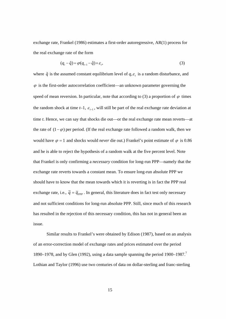
15

exchange rate, Frankel (1986) estimates a first-order autoregressive, AR(1) process for

the real exchange rate of the form

(qt − ˜ q ) =ϕ(qt−1 − ˜ q )+ε t , (3)

where ˜ q is the assumed constant equilibrium level of q, tε is a random disturbance, and

ϕ is the first-order autocorrelation coefficient—an unknown parameter governing the

speed of mean reversion. In particular, note that according to (3) a proportion of ϕ times

the random shock at time t–1, 1−tε , will still be part of the real exchange rate deviation at

time t. Hence, we can say that shocks die out—or the real exchange rate mean reverts—at

the rate of )1( ϕ− per period. (If the real exchange rate followed a random walk, then we

would have 1=ϕ and shocks would never die out.) Frankel’s point estimate of ϕ is 0.86

and he is able to reject the hypothesis of a random walk at the five percent level. Note

that Frankel is only confirming a necessary condition for long-run PPP—namely that the

exchange rate reverts towards a constant mean. To ensure long-run absolute PPP we

should have to know that the mean towards which it is reverting is in fact the PPP real

exchange rate, i.e., PPPqq =~ . In general, this literature does in fact test only necessary

and not sufficient conditions for long-run absolute PPP. Still, since much of this research

has resulted in the rejection of this necessary condition, this has not in general been an

issue.

Similar results to Frankel’s were obtained by Edison (1987), based on an analysis

of an error-correction model of exchange rates and prices estimated over the period

1890–1978, and by Glen (1992), using a data sample spanning the period 1900–1987.7

Lothian and Taylor (1996) use two centuries of data on dollar-sterling and franc-sterling

16

real exchange rates, reject the random-walk hypothesis and find point estimates of ϕ of

0.89 for dollar-sterling and of 0.76 for franc-sterling. Moreover, they are unable to detect

any significant evidence of a structural break between the pre– and post–Bretton Woods

period. Taylor (2002) extends the long-run analysis to a set of 20 countries over the

1870–1996 period and also finds support for PPP and stable coefficients; he found that

although the forcing term in (3) does appear to vary widely across monetary regimes, the

convergence speed does not. Effectively, studies such as these provide the formal

counterpart to the informal evidence of long-run relative PPP that we obtained by

eyeballing Figure 1.

Nevertheless, long-span studies have been subject to some criticism in the

literature. One criticism relates to the fact that, because of the very long data spans

involved, various exchange rate regimes are typically spanned. Also, over long periods of

time, real factors may have generated structural breaks or shifts in the equilibrium real

exchange rate. In order to provide a convincing test of real exchange rate stability during

the post–Bretton Woods period, it is therefore necessary to devise a test using data for the

more recent period alone. One way in which researchers have attempted to do this

corresponds roughly to the approach we adopted in Figure 2 of using data for a number of

countries but keeping the span fairly short. The rationale for this approach is that by

increasing the amount of information employed in the tests across exchange rates, the

power of the test should be increased.

Abuaf and Jorion (1990) examine a system of ten first-order autoregressive

regressions for real dollar exchange rates over the period 1973–87, where the first-order

7 See also Lothian (1990) and Taylor (2002).

17

autocorrelation coefficient is constrained to be the same in every case, and taking account

of contemporaneous correlations among the disturbances. Effectively they estimate

equation (3) for each of their ten exchange rates using the method of seemingly unrelated

regressions and with ϕ constrained to be the same for each real exchange rate. Their

results indicate a marginal rejection of the null hypothesis of joint non-mean reversion at

conventional significance levels and they interpret this as evidence in favor of long-run

PPP.

Following the Abuaf-Jorion study, an academic cottage industry sprung up in the

1990s involving the application of panel unit root tests to real exchange rate data for the

post–Bretton Woods period and in a number of these studies the authors claimed to

provide evidence supporting long-run PPP. Taylor and Sarno (1998), however, pointed

out an important flaw in this literature, which is this. The tests typically applied by

researchers in panel-data studies of long-run PPP test the null hypothesis that none of the

real exchange rates under consideration are mean reverting. If this null hypothesis is

rejected, then the most that can be inferred is that at least one of the rates is mean

reverting. However, researchers tended to draw a much stronger inference from a

rejection of the joint null hypothesis — namely that all of the real exchange rates were

mean reverting; this inference is not valid.

c) Rogoff’s Puzzle

In his 1996 paper in the Journal of Economic Literature, Rogoff (1996) set out an

empirical puzzle relating to the apparently slow speed of adjustment of real exchange

18

rates that provided a further spur to empirical work in this area.8 Rogoff starts by noting

an apparent consensus in the estimated speed of mean reversion of real exchange rates in

the long-span and panel unit root studies. As we noted above, this speed is related to the

estimated coefficient in the autoregressive process (3): a proportion of ϕ of any shock

will still remain after one period, 2ϕ of it remains after two periods, 3ϕ remains after

three periods, and in general, nϕ of the shock will remain after n periods. How many

periods will it take for the effect of the shock to disappear completely? Because the effect

of the shock will die out asymptotically (assuming ϕ is less than one), this is not a

meaningful question since nϕ never exactly reaches zero (even though it gets

infinitesimally close). Instead, we can get a feel for how fast the real exchange rate mean

reverts by asking how long it would take for the effect of a shock to die out by exactly

fifty percent—in other words, we can compute the half-life of shocks to the real exchange

rate.

Based on a reading of the panel unit root and long-span investigations of long-run

PPP, Rogoff notes a high degree of consensus concerning the estimated half-lives of

adjustment: they mostly tend to fall into the range of three to five years. Arguing that real

shocks to tastes and technology cannot account for the major part of the observed high

volatility in real exchange rates, Rogoff then suggests that the persistence in the real

exchange (i.e., its slow speed of adjustment) must be due largely to the persistence in

8 Note, however, that Rogoff’s starting point is to assume that we can take at face value the results of the literature on long-run PPP using long spans of data or panel unit root tests. As we have noted above, each of these strands of the literature have been subject to various criticisms and—in our view—the critique of the panel unit root studies discussed in the previous section is particularly devastating. If we take just the results of the long-span studies as moderately reliable, however, then Rogoff’s analysis still goes through.

19

nominal variables such as nominal wages and prices. But nominal variables would be

expected to adjust much faster than a half-life of three to five years would suggest: “The

purchasing power parity puzzle then is this: How can one reconcile the enormous short-

term volatility of real exchange rates with the extremely slow rate at which shocks appear

to damp out?” (Rogoff, 1996).

d) So where does that leave us?

Our tour d’horizon of the PPP debate thus far gives an overview of the main flashpoints

from the 1970s to the turn of the century. The focus over most of this period on linear

models and relative PPP has generally resulted in very weak evidence in favor of PPP. In

particular, while the hypothesis of a unit root in the real exchange rate has been rejected

in favour of long-run PPP using linear models, this evidence has been questioned. The

long-span studies raise the issue of possible regime shifts and whether the recent

evidence may be swamped by previous and perhaps less relevant history. The panel-data

studies raise the issue of whether the hypothesis of non-mean reversion is being rejected

because of just a few mean-reverting real exchange rates within the panel. Following

Taylor, Peel, and Sarno (2001), we see the puzzling lack of evidence for long-run PPP for

the post–Bretton Woods period as the first PPP puzzle. In addition, even if we take the

long-span studies or the panel-data studies at face value, the implied speeds of mean-

reversion of the real exchange rate seem far too slow; again following Taylor, Peel and

Sarno (2001), we term this the second PPP puzzle.

20

In our view, the key to resolving the twin PPP puzzles lies in allowing for

nonlinear dynamics in real exchange rate adjustment, an approach that may be motivated

by transaction costs or other macro- or microeconomic features.

4. Nonlinearity and all that

In a linear framework, the adjustment speed of PPP deviations is assumed to be uniform

at all times and, in particular, for all sizes of deviation, and implicitly the econometric

problem is reduced to the estimation of a single parameter—the half-life. Whilst this

framework is very convenient, there are compelling theoretical reasons to doubt its

underlying assumptions and, in recent years, a massing of empirical evidence has

reinforced these doubts.

One way of thinking about this is to look again at the simple AR(1) model for the

real exchange rate, equation (3). As we have noted, the speed of mean reversion of tq in

such a model is a constant )1( ϕ− per period. Suppose, however, that the slope coefficient

in equation (3) were not constant but varied with the size of the deviation from PPP—i.e.,

with the size of tq . As argued below, we might for example expect that the speed of

adjustment to increase as tq —the deviation from PPP—rose in absolute value. How

could we detect this nonlinearity? Well, we could plot the change in the real exchange

rate against the level of the real exchange rate and fit a line of best fit to the scatter. If

changes in the exchange rate are small when the level of the real exchange rate is low, but

tend to grow in absolute value as the level of the absolute level of the real exchange rate

increases, then this line of best fit through the scatter should be nonlinear, with a negative

slope for large values of the real exchange rate, and a flatter slope for small values of the

21

exchange rate. This line can in fact be fitted by so-called nonparametric regression—

effectively this involves drawing a line of best fit through the scatter while keeping it

suitably rigid and smooth. Figure 3 shows the nonparametric regression lines of tq∆ onto

1−tq , with the real exchange rate constructed using the same long-span American and

British data as used in Figure 1. It is quite striking that these figures reveal a distinct

“lazy-S” shape, such that the slope is indeed fairly flat (i.e., close to zero) for small

values of the real exchange rate but increases in absolute value as the real exchange rate

increases in absolute value. Thus, it seems that large deviations from parity induce a more

rapid speed of adjustment, while small deviations are highly persistent and elicit little or

no adjustment. Put another, way, the figures suggest that the real exchange rate is close to

a random walk or unit root process for small deviations from PPP but becomes

increasingly mean-reverting for larger deviations from PPP.

This empirical regularity, once it was stumbled upon, led researchers to introduce

richer nonlinear dynamics models into the PPP debate, where the chief innovation

consists of allowing the model dynamics to vary—discretely or smoothly —as a function

of the size of deviations. A seemingly straightforward refinement, this adaptation of the

modeling strategy has delivered striking results and has strongly challenged long-held

beliefs about the two PPP puzzles.9 Such insights found expression in the theoretical

9 At a theoretical level, the nonlinear approach has ancient and distinguished antecedents. Laying out the price-specie-flow theory—the precursor of the monetary approach to the exchange rate—David Hume (1752) remarked that the prices of goods in different locations would be equalized by arbitrage much as “all water, wherever it communicates, remains always at a level.” But Hume went on to qualify his argument, noting that where markets are separated “by any material of physical impediment…there may, in such a case, be a very great inequality of money.” In the subsequent two and half centuries, Hume’s caveat has received occasional, but largely superficial, attention. Cassel (1918) acknowledged the point and moved on. Heckscher (1916) takes credit for expanding the

22

literature starting in the late 1980s when models of exchange rates started to incorporate

transaction costs.10 In the various models proposed, costs might take the form of the

stylized “iceberg” shipping costs (“iceberg” because some of the goods effectively

disappear when they are shipped and the transaction cost may also be proportional to the

distance shipped), fixed costs of trading operations or of shipments, or time lags for the

delivery of goods from one location to another. However, the qualitative effect of such

frictions is similar in all of the proposed models: the lack of arbitrage arising from

transactions costs creates a “band of inaction” within which price dynamics in the two

locations are essentially disconnected.

Other, less formal arguments for the presence of nonlinearities in real exchange

rate adjustment have also been advanced. Kilian and Taylor (2003), for example, suggest

that nonlinearity may arise from the heterogeneity of opinion in the foreign exchange

market concerning the appropriate equilibrium level of the nominal exchange rate: as the

nominal rate takes on more extreme values, a greater degree of consensus develops

concerning the appropriate direction of exchange rate moves, and traders act accordingly.

Taylor (2004) argues that exchange rate nonlinearity may also arise from the intervention

operations of the authorities. By operating as a co-ordinating device in the market,

intervention is more likely to be effective when the nominal—and hence the real—

exchange rate has been driven a long distance away from its PPP or fundamental

idea further and recognizing that goods arbitrage between two locations would only operate once price differentials exceeded a certain threshold equal to the cost of transporting the goods, what he called the “commodity points.” 10 See Benninga and Protopapadakis (1988); Williams and Wright (1991); Dumas (1992); Sercu, Uppal, and van Hulle (1992); Coleman (1995); Prakash (1996); O’Connell and Wei (2002).

23

equilibrium, so that the return towards equilibrium is more likely the greater is the

deviation.

In terms of the empirical work on mean reversion in the real exchange rate, the

influence of nonlinearity can be most simply and directly examined through the

estimation of autoregressive models similar in form to (3) but involving a time-varying

autoregressive parameter. This means that the speed of mean-reversion of the real

exchange rate in the wake of a shock can vary over time. For example, transactions costs

of arbitrage may lead to changes in the real exchange rate being purely random until a

threshold equal to the transactions cost is breached, when arbitrage takes place and the

real exchange rate mean reverts back towards the band through the influence of goods

arbitrage (although the return is not instantaneous because of shipping time, increasing

marginal costs, or other frictions). Not surprisingly, this kind of model is known as

threshold autoregressive (TAR). Estimation is usually via a grid search on the thresholds,

and the various restrictions can, of course, be tested, although inference is nonstandard

since some parameters are not identified under the common null hypothesis of a linear

autoregressive model. Prakash and Taylor (1996) constructed a theoretical arbitrage

model with transaction costs and studied the classical gold standard using such a

framework applied to daily data from 1879 to 1913, and found exchange-rate adjustment

consistent with the predicted TAR model. The threshold estimates so extracted could then

be treated as “revealed gold points” implied by the adjustment dynamics. Extending the

principle to other commodities and to aggregate price indices, Obstfeld and Taylor (1997)

modeled price adjustment in various international cities in the post-1973 period and also

found significant nonlinearities. The implied transaction cost bands and adjustment

24

speeds were also found to be of a reasonable size (consistent with direct shipping cost

measures) and to vary systematically with impediments such as distance, tariffs, quotas,

and exchange-rate volatility, offering further support for a transaction-cost approach.11

Similar TAR results are also reported by Sarno, Taylor, and Chowdhury (2004) using

disaggregated data across a broad range of goods among the G7 countries.

While the discretely adjusting TAR framework seems intuitively appropriate for

studies of the Law of One Price, where the transactions costs for a particular class of

goods may be reasonably well defined, given that PPP relates to aggregate indices of the

prices of many goods with differing thresholds, however, it seems reasonable to suppose

that adjustment of the real exchange rate will less be discrete, displaying a smoothly

increasing tendency towards mean reversion as the deviation from PPP increases. In fact,

econometric models capturing this kind of smooth nonlinear adjustment are well

developed.12 Using models of this kind, and data on real dollar exchange rates among the

G5 countries, Taylor, Peel, and Sarno (2001) are able to reject the hypothesis of a unit

root in the real exchange rate against a nonlinearly mean-reverting alternative using data

just for the post–Bretton Woods period—thus apparently resolving the first PPP puzzle

data—and also go some way towards resolving the second PPP puzzle: even for modest

real exchange shocks in the 1 to 5 percent range, the half-life of decay is estimated at

11 Zussman (2003) uses a TAR model with the postwar Penn World Table data to show nonlinear adjustment speeds for a very wide sample of countries. 12 The smoothly adjusting extension of the TAR model is the aptly-named smooth-transition autoregressive (STAR) model (Granger and Teräsvirta, 1992), of which the exponential STAR or ESTAR formulation has proved most successful in the application to real exchange rates (see e.g. Sarno and Taylor, 2002 for a text book exposition). The ESTAR model can thus be thought of as analogous to a TAR but with an infinite number of regimes and a continuously varying and bounded adjustment speed. Like the TAR, it is

25

under 3 years while for larger shocks it is estimated to be much smaller.13 These results

are corroborated by Kilian and Taylor (2003).14, 15

In sum, the nonlinear approach to real exchange rate modeling can promise—for

some, may have already delivered—an effective resolution of the PPP puzzles.

Simulations show that if the true data are generated by a nonlinear process and an AR

model is naïvely estimated then the misspecification will cause a serious downward bias

in the convergence speed. As a result, inference on the global stationarity of the process

can be seriously compromised. Standard unit root tests, already weak in power, are

further enfeebled in this setting, and half-lives can be dramatically exaggerated, and

especially so if any temporal aggregation occurs in the data, as is likely in practice

(Taylor, 2001; Taylor, Peel, and Sarno, 2001).

Moreover, the transactions-cost approach to real exchange rates is rapidly

transforming not only perceptions of the PPP puzzles but, more importantly, is generating

influential intellectual spillovers into current research flourishing at the nexus of the two

fields of international trade and international macroeconomics. The study of international

fairly simple to implement, using nonlinear least squares estimation, albeit with some related issues of nonstandard inference. 13 In nonlinear models, the speed of mean reversion depends upon the size of the initial shock, since large shocks will tend to mean revert much faster. See Granger and Teräsvirta (1992) and Taylor, Peel and Sarno (2001) for a discussion of some of the technical issues raised in this connexion. 14 Kilian and Taylor (2003) also suggest and provide some evidence to support the proposition that nonlinearity may also account for another puzzle in exchange rate economics—namely the difficulty of beating a random walk in out-of-sample forecasts of the nominal exchange rate. 15 Michael, Nobay and Peel (1997) also successfully applied the ESTAR model to the Lothian-Taylor (1996) data, while Taylor and Peel (2000) show that, for dollar-sterling and dollar-mark over the Bretton Woods period, deviations of the nominal exchange rate from a long-run equilibrium corresponding to a long-run version of the monetary

26

trade has currently been enlivened by a new focus on the role of physical and other

barriers, such as distance, remoteness, borders, or various policies. The maturing of the

gravity model as a theoretical and empirical tool has sharpened this discussion and closer

empirical attention to the underlying determinants of shipping costs has raised our

awareness of the central role of frictions in determining trade patterns and volumes.16 As

further validation, international macroeconomists are also now making explicit the role of

these trading frictions in new models from the New Open Economy Macroeconomics

school, where such refinements may yet help us solve some, if not all, of the major

puzzles in the field (Obstfeld and Rogoff, 2001). Recent research indicates the great

promise of this approach in empirical applications.17 Frictionless trade and

macroeconomic models may have been destined to lose ground anyway, but the recent

findings of the PPP literature are hastening their retreat.

5. Remaining Puzzles

Practitioners have been fretting about two problems more than any others in the recent

past, the so-called PPP puzzles, but recent findings show these to be less of a puzzle than

was originally thought. Still, the field is by no means in a tranquil state of agreement or

lacking in other problems worthy of study.

To conclude we highlight two such research frontiers—areas that occupy, in some

sense, a more sparsely settled region of the intellectual terrain not invaded by the crowds

approach to the exchange rate (i.e., an equilibrium based on relative monetary velocity) may also be modelled as an ESTAR process. 16 See, for example, Anderson and van Wincoop (2003ab); Eaton and Kortum (2002); Hummels (1999, 2001ab); Redding and Venables (2001).

27

of recent PPP puzzlers. Whilst the puzzlers concentrated on medium-term dynamics,

some quite different and contentious questions remain wide open in the other, more

extreme parts of the frequency spectrum: over the very short run of months, weeks, and

days; and over the very long run of decades and centuries.

To clarify, we may return to the basic real exchange rate model (3). Empirical

work has to grapple with three key components of the model: the reversion speed

ρ =1−ϕ ; the volatility of the disturbance term σε ; and the long-run, or equilibrium, level

of the real exchange rate ˜ q t , which we now allow to be possibly time varying (hence the

subscript t). In the heyday of the PPP puzzlers the debate was all about ρ . In the future,

we expect to see more attention given to disturbances σε and long-run levels ˜ q t . If you

will, questions about the real exchange rate are likely to shift—from not so much “how

fast is it reverting?” to more of “what is it reverting to?” and “how did it deviate in the

first place?”

At the higher frequencies, even if the speeds of reversion and half-lives can be

brought more into line with our priors, the volatilities present in the data still cause

considerable mystification, at least under floating-rate regimes. Several striking gross

features of the data stand out. Real and nominal exchange rates tend to move hand in

hand at the higher frequencies, with considerable deviations from Law of One Price for

traded goods (Flood and Rose, 1995; Engel, 1999). Moreover, real and nominal exchange

rate volatilities are correlated almost one for one across different monetary regime types

over a wide swathe of historical experience (Taylor, 2002). Given these patterns, and

even just the extent and frequency of the shocks, strict adherence to money-neutral,

17 See, for example, Betts and Kehoe (2001); Bergin and Glick (2003); Ghironi and

28

flexible price models, and purely real disturbances has generally proven to be a

disappointing empirical strategy.

To consider an illustrative case, in the time dimension it is hard to imagine that,

say, the real shocks to the Argentine economy were small in the 1960s, say, then

suddenly became several times larger during the 1980s hyperinflations, then shrank again

in the 1990s currency-board epoch, only to mysteriously reappear in late 2001. And in

cross section, the real shocks would have to vary systematically across countries in a way

that, just coincidentally, happened to match the data in each one—which is rather

implausible. In contrast, we know that to a first approximation Argentina’s turbulent

monetary history matches the observed volatilities very closely indeed. Observations

such as these bring price stickiness and money nonneutrality to the fore, although even

here models can still have a hard time matching the data.

Various strands in the literature seek to solve this puzzle, where a common theme

now recognizes the important role of frictions in trade, not just for generating no-

arbitrage bands for traded goods, but for delineating traded from nontraded varieties. If

the nontraded share of the economy is then sufficiently large, new pathways from real or

monetary fundamentals to real exchange rate disturbances can emerge. For example, it is

well known that a simple monetary model with sticky nontraded goods prices leverages

small money shocks into large exchange rate shocks. Or consider a New Open Economy

Macroeconomics setting (Obstfeld and Rogoff, 2000; Hau, 2000, 2002). When the

nontraded share rises, the economy is less “open” and the flexible-price Law of One Price

Melitz (2003).

29

assumption applies to a smaller fraction of goods (here, imported varieties), implying a

larger role for overshooting and other sources of exchange rate volatility.

Economies may be more closed than we once thought, with very high nontraded

shares once all sectors of activity are considered, e.g., retailing, wholesaling and

distribution (Obstfeld, 2001; Obstfeld and Rogoff 2001; Burstein, Neves, and Rebelo,

2003). This insight is now being developed and applied in a number of ways and can

generate quite high levels of volatility from small monetary shocks.18 Future research

might pursue this avenue further. Successful models need to finesse the challenge of

allowing the pass-through of monetary shocks to be large enough to match developing

country volatilities without being so large as to produce excessive volatility when applied

in a developed country setting without ad hoc reparameterization. One suspects that other

omitted factors such as volatile risk premia and peso problems could be extremely

important in some cases, e.g., emerging-market crises, and this will need careful

integration into the modelling strategy.

Turning now to puzzles at the other end of the frequency spectrum, what new can

be said about the equilibrium level of the real exchange rate? Here, researchers have been

reexamining traditional mechanisms built around some key real fundamentals, models

that seem uncontroversial in theory but have often proven difficult to validate in practice.

Some suggestive results have appeared that are consistent with the general intuition we

have gleaned from our benchmark open-economy macroeconomic models. We might

18 For example, Burstein, Eichenbaum, and Rebelo (2003) combine nontraded price stickiness with a nontraded share well above 0.5. This setup yields a large devaluation response of an emerging-market country even for a small monetary shock (e.g., as in Argentina 2001–02).

30

expect continued work here to pin down these relationships and to confront some new

puzzles that have been thrown up along the way.

One of the textbook explanations for changes in the level of the real exchange rate

focuses on the net international asset position. Consider a small, open economy in long-

run equilibrium. Now impose a shock in the form of an increase in the external debt. The

country must run a trade surplus in the future to service the interest payments due. To

encourage foreign consumers to import more, and to encourage its own consumers to

import less, the country’s relative price level must fall in equilibrium.19

Is this logic borne out by the data? Lane and Milesi-Ferreti (2002) show that it is.

Controlling for other factors and allowing for real return differentials across countries,

they find that countries with a larger positive net asset position have more positive trade

balances and stronger real exchange rates. The result has wider implications for the study

of shorter-run real exchange rate dynamics. If shifts in ˜ q t arise due to changes in net

wealth, and if these shifts are not appropriately controlled for in equation (3), spurious

results will follow, not least an omitted-variable bias in ρ . Mismeasurement of ˜ q t will

make q appear to deviate too much or for too long, making the PPP puzzles look worse

than they actually are.

Going beyond the differentiation of just home and foreign goods, we might again

turn to the role played by traded versus nontraded goods by invoking the venerable

Harrod-Balassa-Samuelson (HBS) story.20 In that account, rich countries grow rich by

19 The example supposes differentiated goods at home and abroad, but the logic holds in a wide range of models. This kind of effect is most clearly seen in exchange rate models allowing for differentiation between domestic and foreign assets, such as the portfolio balance model—see Taylor (1995) and Sarno and Taylor (2002b). 20 Harrod (1933), Balassa (1964), Samuleson (1964).

31

advancing the productivity in traded “modern” sectors (think manufacturing). Meantime,

all nontraded “traditional” sectors, in rich and poor countries alike, remain in

technological stasis (think haircuts). Suppose the Law of One Price holds among traded

goods and we live in a Ricardian world where labor is mobile intersectorally but not

internationally. As productivity in the modern sector rises, wage levels rise, so prices of

nontraded goods will have to rise (as there has been no rise in productivity in that sector).

If we measure the overall price index as a weighted average of traded and nontraded

goods prices, relatively rich countries will tend to have “overvalued” currencies.

It is clear that, after languishing for some years in relative obscurity, the HBS

story is attracting renewed interest, for various reasons. Over time, researchers have had

greater and greater success in confirming the HBS effect, making it a more relevant issue.

For example, early studies such as Officer (1982) found little support in the data from the

1950s to the early 1970s. But newer research dealing with later periods has often found

support for this hypothesis and it is now textbook material.21 Why have more recent

studies provided stronger evidence of the HBS effect? At some level, we can simply call

upon the same kinds of explanations given for the progress towards a resolution of the

PPP puzzle: more data, of longer span, for a wider sample of countries, coupled with

more powerful univariate and panel econometric techniques, has allowed researchers to

take a once-fuzzy relationship in the data and make it tight.

Yet there could be more to the rising prominence of the HBS effect than simply

advances in statistical prowess alone. Recent work suggests that the magnitude of this

21 See, inter alia, Hsieh (1982); Marston (1990); Micossi and Milesi-Ferreti (1994); De Gregorio, Giovannini, and Wolf (1994); De Gregorio and Wolf (1994); Chinn and

32

effect, and even its very existence, has been variable over time—certainly in the postwar

period, and perhaps going back several centuries (Bergin, Glick, and Taylor, 2003). As

the simple parameter estimates in Figure 4 show, the cross-country relationship between

price levels (real exchange rates) and income per capita has been intensifying since 1950;

once very close to zero, and statistically insignificant, the elasticity is now over one

half.22 The increase in the slope has been virtually monotonic. Hence, the nature of the

HBS effect appears not to have been a “universal constant” even in recent times.

Why was this so and why does it matter? One could appeal to the textbook model.

Perhaps the nontraded share has increased over time to generate results? This appears

implausible, given the magnitudes involved, and fits poorly with longer run patterns.

Perhaps the productivity advances of traded and nontraded goods have differed at various

times? This may better help us explain the data, but over long time frames begs the

question of which goods are traded and why. Bergin, Glick, and Taylor (2003) advance

another hypothesis: that trade costs determine tradability patterns, allowing a rich variety

of possible productivity shocks to eventually give rise to an endogenous HBS effect.

Once again, low-frequency movements in the equilibrium level of q have a

bearing on all analyses of exchange rate dynamics. Getting the trend wrong implies

spurious dynamic regressions and biased half-lives and other estimates. Bergin, Glick,

and Taylor (2003), Lothian and Taylor (2000; 2003) and Taylor (2002) all find that an

Johnston (1996); Ito, Isard, and Symansky (1999); Chinn (2000); Zussman (2001); Papell (2003). 22 The null of a zero slope can be rejected beginning in the early 1960s—when Balassa and Samuelson wrote their seminal papers, albeit with no knowledge of these hypothesis tests.

33

allowance for such long run trends can make a material difference in resolving the old

PPP puzzles.23

The equilibrium real exchange rate could shift for a number of reasons over the

very long run: wealth effects, productivity effects, and other forces could all be

important. Evidence on the role played by net asset positions warrants further research.

The stylized facts about the HBS effect also demand an explanation, but one that is

consistent with our broader accounts of macroeconomic growth and economic history.

Models that allow for a time-varying equilibrium real exchange rate, and permit an

exploration of its causes and consequences, are likely to be a busy area for future

research.

6. Concluding comments The PPP debate is an example of the liveliness of economic debate more generally.

Investigations have been based as much on strong economic intuition as on underlying

economic theory. Conjectures have been revised and amended in the light of the

empirical evidence, and empirical methodology itself has been questioned, revised and

improved as the profession has striven to provide hypotheses which are at once internally

consistent, strongly intuitive, and well supported by the data. This research endeavor,

moreover, is of strong practical value to the real world concerning the self-equilibrating

nature of the international macroeconomic system.

23 Taylor (2002) finds relatively low half-lives in a 20-country panel when an allowance is made for long run trends. Allowing for nonlinear time trends, Lothian and Taylor (2000) suggest that the half-life of deviations from PPP for the U.S.-U.K. exchange rate may in fact be as low as two and a half years. Lothian and Taylor (2003) show that the HBS effect may account for about a third of the variation in this real exchange rate.

34

The main upshot of the PPP debate may, on our reading, be reduced to the

following. The real exchange rate does appear to be mean reverting over sufficiently long

periods of time, although its speed of mean reversion may vary with the size of the

deviation from equilibrium. Thus, real exchange rates appear to display behavior that is at

least consistent with long-run PPP. There is, however, some emerging evidence that the

equilibrium real exchange rate may itself shift over time, although the degree of variation

in the equilibrium may be quite small when compared to the degree of variation in

national price levels over long periods. Movements in the equilibrium could arise because

of Harrod-Balassa-Samuelson, aggregate wealth effects, or other causes. Whether such

shifts in the equilibrium are economically important as well as statistically significant

remains to be seen.

Overall, our interpretation of the consensus view of the PPP debate — that short-

run PPP does not hold, that long-run PPP may hold in the sense that there is significant

mean reversion of the real exchange rate, although there may be factors impinging on the

equilibrium real exchange rate through time — is highly reminiscent of the consensus

view that held sway in the period before the 1970s. In that sense, this paper may be taken

as evidence of mean reversion in economic thought.

35

References Abuaf, Niso and Philippe Jorion. 1990. “Purchasing Power Parity in the Long Run.”

Journal of Finanace, 45:1, pp. 157–74. Adler, Michael and Bruce Lehmann. 1983. “Deviations from Purchasing Power Parity

in the Long Run.” Journal of Finance, 38:5, pp. 1471-87. Anderson, James E. and Eric van Wincoop. 2003a. “Gravity with Gravitas: A

Solution to the Border Puzzle.” American Economic Review, 93:1, pp. 170–92. Anderson, James E. and Eric van Wincoop. 2003b. “Trade Costs.” Boston University. Balassa, Bela. 1964. “The Purchasing-Power Parity Doctrine: A Reappraisal.” Journal of

Political Economy, 72, pp. 584–96. Benninga, Simon and Aris A. Protopapadakis. 1988. “The Equilibrium Pricing of

Exchange Rates and Assets When Trade Takes Time.” Journal of International Economics, 7, pp. 129–49.

Bergin, Paul R. and Reuven Glick. 2003. “Endogenous Nontradability and Macroeconomic Implications.” Working Paper Series no. 9739, National Bureau of Economic Research (June).

Bergin, Paul R., Reuven Glick, and Alan M. Taylor. 2003. “Productivity, Tradability, and The Great Divergence.” Photocopy, UC Davis (November).

Betts, Caroline M. and Timothy J. Kehoe. 2001. “Tradability of Goods and Real Exchange Rate Fluctuations.” University of Southern California.

Burstein, Ariel, João Neves, and Sergio Rebelo. 2003. “Distribution Costs and Real Exchange Rate Dynamics.” Journal of Monetary Economics, 00, pp. 000–000.

Burstein, Ariel, Martin Eichenbaum, and Sergio Rebelo. 2003. Large Devaluations and the Real Exchange Rate. Photocopy, Northwestern University (September).

Cassel, Gustav. 1918. “Abnormal Deviations in International Exchanges.” Economic Journal, 28, pp. 413–15.

Cassel, Gustav. 1922. Money and Foreign Exchange After 1914. New York: Macmillan. Chinn, Menzie D. 2000. “The Usual Suspects? Productivity and Demand Shocks and

Asia-Pacific Real Exchange Rates.” Review of International Economics, 8, pp. 20–43.

Chinn, Menzie D. and Louis Johnston. 1996. “Real Exchange Rate Levels, Productivity and Demand Shocks.” Working Paper Series no. 5709, National Bureau of Economic Research (August).

Coleman, Andrew M. G. 1995. “Arbitrage, Storage, and the ‘Law of One Price’: New Theory for the Time Series Analysis of an Old Problem.” Princeton, N.J.

Davutyan, Nurhan and John Pippenger. 1990. “Testing Purchasing Power Parity: Some Evidence of the Effects of Transaction Costs.” Econometric Reviews, 9, pp. 211–40.

De Grauwe, Paul, Marc Janssens, and Hilde Leliaert. 1985. “Real Exchange-Rate Variability from 1920 to 1926 and 1973 to 1982.” Princeton Studies in International Finance, 56.

De Gregorio, Jose, Alberto Giovannini, and Holger C. Wolf. 1994. “International Evidence on Tradable and Nontradables Inflation.” European Economic Review 38, pp. 1225–44.

36

De Gregorio, Jose and Holger C. Wolf. 1994. “Terms of Trade, Productivity, and the Real Exchange Rate.” Working Paper Series no. 4807, National Bureau of Economic Research (July).

Dornbusch, Rudiger. 1976. “Expectations and Exchange Rate Dynamics.” Journal of Political Economy, 84:6, pp. 1161–76.

Dornbusch, Rudiger and Paul Krugman. 1976. “Flexible Exchange Rates in the Short Run.” Brookings Papers on Economic Activity, 3, pp. 537–75.

Dumas, Bernard. 1992. “Dynamic Equilibrium and the Real Exchange Rate in a Spatially Separated World.” Review of Financial Studies, 5, pp. 153–80.

Eaton, Jonathan and Samuel Kortum. 2002. “Technology, Geography, and Trade.” Econometrica, 70:5, pp. 1741–79.

Edison, Hali J. 1987. “Purchasing Power Parity in the Long Run: A Test of the Dollar/Pound Exchange Rate, 1890–1978.” Journal of Money, Credit and Banking, 19:3, pp. 376–87.

Engel, Charles. 1999. “Accounting for U.S. Real Exchange Rate Changes.” Journal of Political Economy, 107:3, pp. 507–38.

Engle, Robert and Clive W. J. Granger. 1987. “Co-integration and Error Correction: Representation, Estimation and Testing.” Econometrica, 55:2, pp. 251–76.

Flood, Robert P. and Andrew K. Rose. 1995. “Fixing Exchange Rates: A Virtual Quest for Fundamentals.” Journal of Monetary Economics, 36:1, pp. 3–37.

Frankel, Jeffrey A. 1986. “International Capital Mobility and Crowding-out in the U.S. Economy: Imperfect Integration of Financial Markets or of Goods Markets?,” in How Open is the U.S. Economy? R. W. Hafer ed. Lexington, Mass.: Lexington Books, pp. 33–67.

Frankel, Jeffrey A. 1990. “Zen and the Art of Modern Macroeconomics: A Commentary,” in Monetary Policy for a Volatile Global Economy. William S. Haraf and Thomas D. Willett eds. Washington, D.C.: AEI Press, pp. 117–23.

Frankel, Jeffrey A. and Andrew K. Rose. 1995. “Empirical research on Nominal Exchange Rates,” in Handbook of International Economics, Volume 3. G. Grossman and K. Rogoff eds. Amsterdam, New York and Oxford: Elsevier, North-Holland.

Frankel, Jeffrey A. and Andrew K. Rose. 1996. “A Panel Project on Purchasing Power Parity: Mean Reversion Within and Between Countries.” Journal of International Economics, 40:1–2, pp. 209–24.

Frenkel , Jacob A. 1976. “A Monetary Approach to the Exchange Rate: Doctrinal Aspects and Empirical Evidence.” Scandinavian Journal of Economics, 78, pp. 200–24.

Frenkel, Jacob A. 1981. “The Collapse of Purchasing Power Parity During the 1970s.” European Economic Review, 16, pp. 145–65.

Frenkel, Jacob A. and Harry G. Johnson. 1976. The Monetary Approach to the Balance of Payments. London: Allen & Unwin.

Froot, Kenneth A. and Kenneth Rogoff. 1995. “Perspectives on PPP and Long-Run Real Exchange Rates,” in Handbook of International Economics. Gene Grossman and Kenneth Rogoff eds. Amsterdam: North Holland, pp. 1647-88.

Glen, Jack D. 1992. “Real Exchange Rates in the Short, Medium, and Long Run.” Journal of International Economics, 33:1–2, pp. 147–66.

37

Granger, Clive W. J. and Timo Teräsvirta. 1993. Modelling Nonlinear Economic Relationships. Oxford: Oxford University Press.

Harrod, Roy. 1933. International Economics. London: Nisbet and Cambridge University Press.

Hau, Harald. 2000. “Exchange Rate Determination under Factor Price Rigidities.” Journal of International Economics 50:2, pp. 421–47.

Hau, Harald. 2002. “Real Exchange Rate Volatility and Economic Openness: Theory and Evidence.” Journal of Money, Credit and Banking 34:3, pp. 611–30

Heckscher, Eli F. 1916. “Växelkurens grundval vid pappersmynfot.” Economisk Tidskrift, 18, pp. 309–12.

Hsieh, David. 1982. “The Determination of the Real Exchange Rate: The Productivity Approach.” Journal of International Economics, 12, pp. 355–62.

Hume, David. 1742–52 [1987]. Essays, Moral, Political, and Literary. Indianapolis, Ind.: The Liberty Fund.

Hummels, David. 1999. “Have International Transportation Costs Declined?” University of Chicago.

Hummels, David. 2001a. “Time as a Trade Barrier.” Purdue University. Hummels, David. 2001b. “Toward a Geography of Trade Costs.” Purdue University. Imbs, Jean, Haroon Mumtaz, Morten Ravn and Helene Rey. 2002. “PPP Strikes

Back: Aggregation and the Real Exchange Rate.” Working Paper Series no. 9372, National Bureau of Economic Research (December).

Ito, Takatoshi, Peter Isard, and Steven Symansky. 1999. “Economic Growth and Real Exchange Rate: An Overview of the Balassa-Samuelson Hypothesis in Asia.” In Changes in Exchange Rates in Rapidly Developing Countries: Theory, Practice, and Policy Issues, edited by Takatoshi Ito and Anne O. Krueger. Chicago: University of Chicago Press.

Kilian, Lutz and Mark P. Taylor. 2003. “Why Is It So Difficult to Beat the Random Walk Forecast of Exchange Rates?” Journal of International Economics, 60:1, pp. 85-107.

Lothian, James R. 1990. “A Century plus of Japanese Exchange Rate Behavior.'' Japan and the World Economy, 2, pp. 47-50.

Lothian, James R. and Mark P. Taylor. 1996. “Real Exchange Rate Behavior: The Recent Float From the Perspective of the Past Two Centuries.” Journal of Political Economy, 104:3, pp. 488–509.

Lothian, James R. and Mark P. Taylor. 1997. “Real Exchange Rate Behavior: The Problem of Power and Sample Size.” Journal of International Money and Finance, 16:6, pp. 945–54.

Lothian, James R. and Mark P. Taylor. 2003. “Real Exchange Rates Over the Past Two Centuries: How Important is the Harrod-Balassa-Samuelson Effect?” Warwick University.

Marston, Richard C. 1990. “Systematic Movements in Real Exchange Rates in the G-5: Evidence on the Integration of Internal and External Markets.” Journal of Banking and Finance, 14, pp. 1023–44.

38

Micossi, Stefano and Gian Maria Milesi-Ferretti. 1994. “Real Exchange Rates and the Prices of Nontradable Goods.” Working Papers no. 94/19, International Monetary Fund.

Michael, Panos, A. Robert Nobay and David A. Peel. 1997. “Transaction Costs and Nonlinear Adjustment in Real Exchange Rates: An Empirical Investigation.” Journal of Political Economy, 105:4, pp. 862–79.

O’Connell, Paul G. J. and Shang-Jin Wei. 2002. ““The Bigger They Are, The Harder They Fall”: Retail Price Differences Across U.S. Cities.” Journal of International Economics, 56:1, pp. 21–53.

Obstfeld, Maurice. 2001. “International Macroeconomics: Beyond the Mundell-Fleming Model” IMF Staff Papers, 47 (Special Issue), pp. 1–39.

Obstfeld, Maurice and Kenneth Rogoff. 2001. “The Six Major Puzzles in International Macroeconomics: Is There a Common Cause?,” in NBER Macroeconomics Annual 2000. Ben S. Bernanke and Kenneth Rogoff eds.

Obstfeld, Maurice and Alan M. Taylor. 1997. “Nonlinear Aspects of Goods-Market Arbitrage and Adjustment: Heckscher’s Commodity Points Revisited.” Journal of the Japanese and International Economies, 11:4, pp. 441–79.

Officer, Lawrence H. 1982. Purchasing Power Parity and Exchange Rates: Theory, Evidence and Relevance. Greenwich, Conn.: JAI Press.

Papell, David H. 1997. “Searching for Stationarity: Purchasing Power Parity Under the Current Float.” Journal of International Economics, 43:3–4, pp. 313–32.

Papell, David H. 2003. “Long Run Purchasing Power Parity: Cassel or Balassa-Samuelson?” Photocopy (June). University of Houston.

Prakash, Gauri and Alan M. Taylor. 1997. “Measuring Market Integration: A Model of Arbitrage with an Econometric Application to the Gold Standard, 1880–1913.” Working Paper Series no. 6073, National Bureau of Economic Research (June).

Rogoff, Kenneth. 1996. “The Purchasing Power Parity Puzzle.” Journal of Economic Literature, 34:2, pp. 647–68.

Roll, Richard. 1979. “Violations of Purchasing Power Parity and their Implications for Efficient International Commodity Markets,” in International Finance and Trade, Vol. 1. M. Sarnat and G.P. Szego eds. Cambridge MA: Ballinger.

Redding, Stephen and Anthony J. Venables. 2001. “Economic Geography and International Inequality.” London School of Economics.

Samuelson, Paul A. 1964. “Theoretical Notes on Trade Problems.” Review of Economics and Statistics, 46, pp. 145–54.

Sarno, Lucio and Mark P. Taylor. 2002a. “Purchasing Power Parity and the Real Exchange Rate.” International Monetary Fund Staff Papers, 49:1, pp. 65-105.

Sarno, Lucio and Mark P. Taylor. 2002b. The Economics of Exchange Rates. Cambridge and New York: Cambridge University Press.

Sarno, Lucio, Ibrahim Chowdhury and Mark P. Taylor. 2004. “Non-Linear Dynamics in Deviations from the Law of One Price: A Broad-Based Empirical Study.” Centre for Economic Policy Research Discussion Paper 3377, forthcoming Journal of International Money and Finance.

Sercu, Piet, Raman Uppal, and Cynthia Van Hulle. 1995. “The Exchange Rate in the Presence of Transaction Costs: Implications for Tests of Purchasing Power Parity.” Journal of Finance, 50, pp. 1309–19.

39

Shiller, Robert J. and Pierre Perron. 1985. “Testing the Random Walk Hypothesis: Power Versus Frequency of Observation.” Economics Letters, 18:4, pp. 381–86.

Stockman, Alan C. 1987. “The Equilibrium Approach to Exchange Rates.” Federal Reserve Bank of Richmond Economic Review, 73:2, pp. 12–30.

Taylor, Alan M. 2001. “Potential Pitfalls for the Purchasing-Power Parity Puzzle? Sampling and Specification Biases in Mean-Reversion Tests of the Law of One Price.” Econometrica, 69:2, pp. 473–98.

Taylor, Alan M. 2002. “A Century of Purchasing Power Parity.” Review of Economics and Statistics, 84:1, pp. 139–50.

Taylor, Mark P. 1988. “An Empirical Examination of Long-Run Purchasing Power Parity Using Cointegration Techniques.” Applied Economics, 20:10, pp. 1369-81.

Taylor, Mark P. 1995. “The Economics of Exchange Rates.” Journal of Economic Literature, 33:1, pp. 13–47.

Taylor, Mark P. 2004. “Is Official Exchange Rate Intervention Effective?” Centre for Economic Policy Research Discussion Paper 3758, forthcoming Economica.

Taylor, Mark P. and Patrick C. McMahon. 1988. “Long-Run Purchasing Power Parity in the 1920s.” European Economic Review, 32:1, pp. 179–97.

Taylor, Mark P., David A. Peel and Lucio Sarno. 2001. “Nonlinear Mean-Reversion in Real Exchange Rates: Towards a Solution to the Purchasing Power Parity Puzzles.” International Economic Review, 42, pp. 1015–42.

Taylor, Mark P. and Lucio Sarno. 1998. “The Behavior of Real Exchange Rates During the Post-Bretton Woods Period.” Journal of International Economics, 46:2, pp. 281–312.

Williams, Jeffrey C. and Brian D. Wright. 1991. Storage and Commodity Markets. Cambridge: Cambridge University Press.

Zussman, Asaf. 2001. “Real Exchange Rate Behavior in a Convergence Club.” Stanford University.

Zussman, Asaf. 2003. “The Limits of Arbitrage: Trading Frictions and Deviations from Purchasing Power Parity.” Stanford University.

US and UK PPIs in Dollar Terms (log scale, 1900=0), 1820-2001

-0.50

0.51

1.52

2.53

1791

1803

1815

1827

1839

1851

1863

1875

1887

1899

1911

1923

1935

1947

1959

1971

1983

1995

PPIUK PPIUS

US and UK CPIs in Dollar Terms (log scale, 1900=0), 1820-2001

-0.50

0.51

1.52

2.53

3.5

1820

1830

1840

1850

1860

1870

1880

1890

1900

1910

1920

1930

1940

1950

1960

1970

1980

1990

2000

CPIUS CPIUK

Figure 1Dollar-Sterling PPP Over Two Centuries

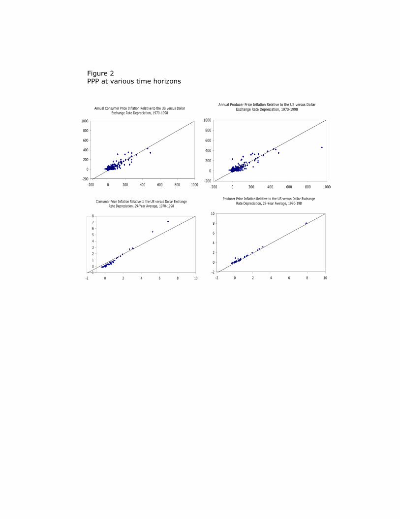
Figure 2PPP at various time horizons

Annual Consumer Price Inflation Relative to the US versus Dollar Exchange Rate Depreciation, 1970-1998

-200

0

200

400

600

800

1000

-200 0 200 400 600 800 1000

Annual Producer Price Inflation Relative to the US versus Dollar Exchange Rate Depreciation, 1970-1998

-200

0

200

400

600

800

1000

-200 0 200 400 600 800 1000

Consumer Price Inflation Relative to the US versus Dollar Exchange Rate Depreciation, 29-Year Average, 1970-1998

-1

0

1

2

3

4

5

6

7

8

-2 0 2 4 6 8 10

Producer Price Inflation Relative to the US versus Dollar Exchange Rate Depreciation, 29-Year Average, 1970-198

-2

0

2

4

6

8

10

-2 0 2 4 6 8 10

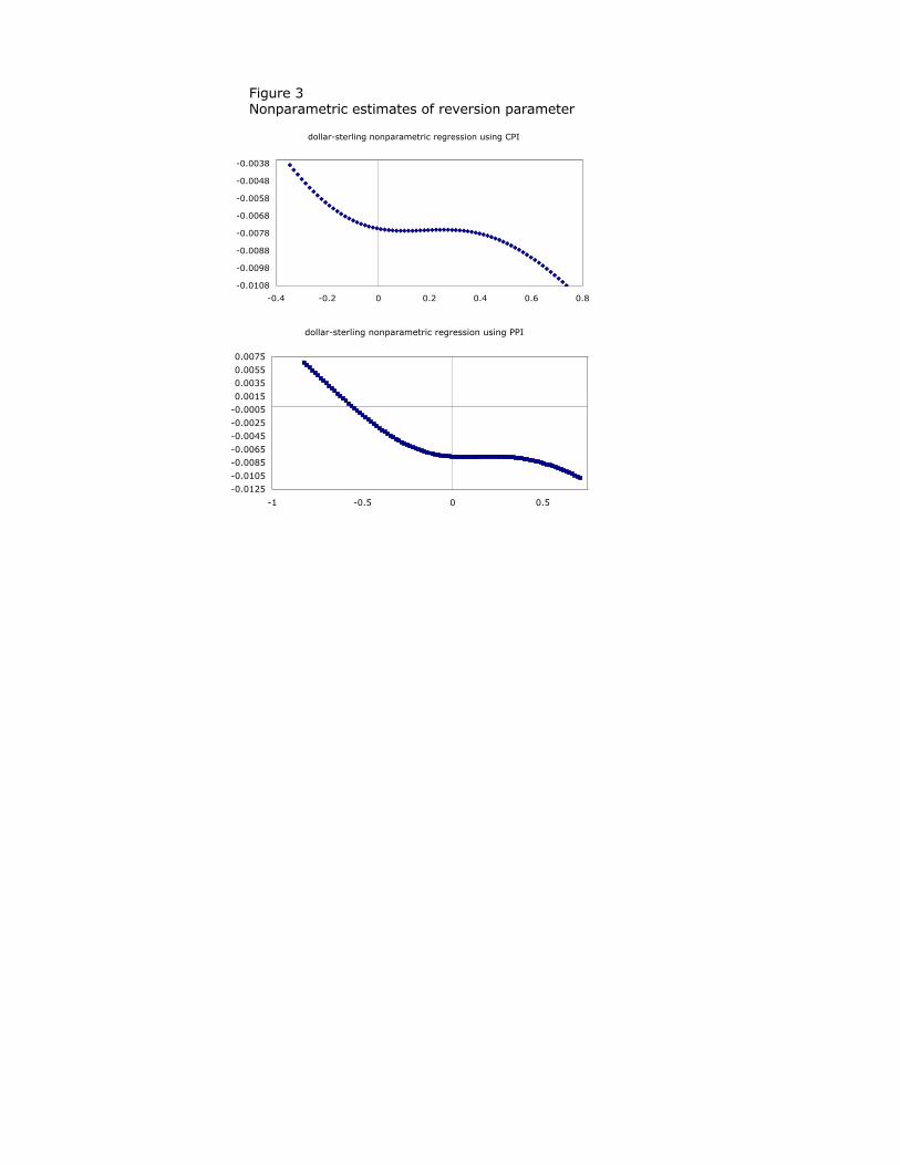
dollar-sterling nonparametric regression using CPI

-0.0108

-0.0098

-0.0088

-0.0078

-0.0068

-0.0058

-0.0048

-0.0038

-0.4 -0.2 0 0.2 0.4 0.6 0.8

dollar-sterling nonparametric regression using PPI

-0.0125

-0.0105

-0.0085

-0.0065

-0.0045

-0.0025

-0.0005

0.0015

0.0035

0.0055

0.0075

-1 -0.5 0 0.5

Figure 3Nonparametric estimates of reversion parameter

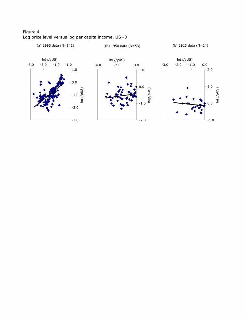
Figure 4Log price level versus log per capita income, US=0

(a) 1995 data (N=142)

-3.0

-2.0

-1.0

0.0

1.0

-5.0 -3.0 -1.0 1.0

ln(y/yUS)

ln(p

/pU

S)

(b) 1913 data (N=24)

-1.0

0.0

1.0

2.0

-3.0 -2.0 -1.0 0.0

ln(y/yUS)

ln(p

/pU

S)

(b) 1950 data (N=53)

-2.0

-1.0

0.0

1.0

-4.0 -2.0 0.0

ln(y/yUS)

ln(p

/pU

S)