UNINTENDED FEEDBACKS: IMPLICATIONS AND

APPLICATIONS FOR CONSERVATION

CECILIA LARROSA

(MSc, Imperial College London)

A THESIS SUBMITTED

FOR THE DEGREE OF DOCTOR OF PHILOSOPHY

DEPARTMENT OF BIOLOGICAL SCIENCES

NATIONAL UNIVERSITY OF SINGAPORE

DEPARTMENT OF LIFE SCIENCES

IMPERIAL COLLEGE LONDON

2017

Supervisors:Professor E.J. Milner-Gulland

Assistant Professor L. Roman Carrasco

Examiners:Assistant Professor Chisholm, Ryan AlistarDr Kaveh Madani, Imperial College London

Associate Professor James Watson, University of Queensland

- 2 -

Declaration of Originality

I hereby declare that this thesis is my original work and it has beenwritten by me in its entirety, I have duly acknowledged all the sources ofinformation which have been used in the thesis.This thesis has also not been submitted for any degree in any universitypreviously.

Copyright Declaration

‘The copyright of this thesis rests with the author and is made availableunder a Creative Commons Attribution Non-Commercial No Derivativeslicence. Researchers are free to copy, distribute or transmit the thesison the condition that they attribute it, that they do not use it forcommercial purposes and that they do not alter, transform or build uponit. For any reuse or redistribution, researchers must make clear to othersthe licence terms of this work’

- 3 -

Summary

Human reactions to conservation interventions can trigger unintended

feedbacks resulting in poor conservation outcomes. Understanding

unintended feedbacks is a necessary first step toward the diagnosis and

solution of environmental problems, but existing anecdotal evidence

cannot support decision-making. The aim of this PhD is to improve our

understanding of the role these unintended feedbacks play in

conservation science, and provide recommendations for incorporating

them into practice.

In chapter two, I analyse the implications these unintended feedbacks

have for conservation from a social-ecological systems perspective. I

present a conceptual framework that provides a theoretical

understanding of how conservation interventions can trigger unintended

feedbacks, and create a typology of unintended feedbacks that show

how unintended feedbacks undermine conservation efforts. I use the

typology to reflect on how best to plan for and mitigate unintended

feedbacks in conservation practice, and provide concrete

recommendations for future work.

Focusing on large-scale potential economic feedbacks based on

recommendations from chapter two, chapter three is an exploration of

potential unintended feedback effects of setting aside agricultural land

for conservation, and an assessment of their application in systematic

conservation planning to the Brazilian Atlantic Forest case study.

Results show that there is considerable potential for modelling land

- 4 -

market feedbacks from conservation interventions using techniques

from other fields, such as land economics. However, I found two main

limitations for large-scale empirical applications: data availability, and

small effects on global markets. For the Brazilian Atlantic Forest,

feedback effects derived from informational rent capture were the most

relevant to the case study.

Widely used tools for conservation planning could produce misleading

recommendations if feedbacks are ignored. For example, in systematic

conservation planning, effectiveness depends partly on accounting for

natural and anthropogenic dynamics. Some dynamic conservation

planning approaches exist, but they need to be further developed, and

assessed against static approaches. In chapter four I examine the

impact of accounting for both economic and environmental feedbacks

into spatial planning for a set-aside programme in the Brazilian Atlantic

Forest. I model changes in forest connectivity and land opportunity costs

to evaluate the cost-effectiveness of the set-aside programme based on

spatial static and discrete dynamic conservation planning. Results show

that cost-effectiveness improvement for the dynamic approach was

relatively small, but varied widely with biogeographical region. However,

the proposed dynamic framework not only improved overall cost-

effectiveness, but increased informational rent capture, in so doing also

involving more municipalities in the programme.

In chapter five I apply the model developed in chapter four to multiple

policy relevant targets of Atlantic Forest restoration and provide

- 5 -

recommendations for prioritising areas. In a reality of multiple targets and

objectives, the resulting map provides a starting point for priority

restoration areas based on three important considerations; potential to

improve forest connectivity, cost effectiveness, and potential to

incentivise participation through informational rent. However, the

assessment found that the cost of payment per year of set-asides for

meeting varying reforestation targets ranged between 15% and 133% of

Brazil’s annual expenditure on agricultural subsidies, making the

implementation of some of these targets highly unlikely.

This thesis identifies an urgent needed for the collection of evidence in

a structured way in order to understand the mechanisms by which

human decision-making feeds through to conservation outcomes at

different scales. Socio-economic data availability, a mismatch in scale

between data availability and prioritisation grain, and economic model

complexity present the main limitations to accounting for these

feedbacks in spatial conservation planning. Even though a dynamic

approach to spatial conservation planning does entail higher

computational requirements and transactions costs, I find the potential

benefits in terms of increased cost-effectiveness could offset these

costs. Most importantly, the analysis shows that a dynamic approach

can help decision-makers maximise the existence of informational rents

by prioritising areas with higher informational rent capture and still result

in a lower overall intervention cost. Accounting for environmental and

economic feedbacks can be a valuable tool for more evenly distributed

interventions that provide higher incentives for participation without

- 6 -

increasing intervention cost.

People adapt and respond to conservation interventions, and their

actions feed through into changes in the conservation situation itself; this

fact is something that conservationists rely on for their impact. However,

these same responses are being overlooked when they affect outcomes

indirectly through unintended feedbacks. The research undertaken for

this PhD advances knowledge on the role feedbacks play in both applied

conservation and conservation science. Showing from theory to practice

how studying and managing unintended feedbacks can improve

conservation by providing insight into the realm of possible outcomes

from planned conservation interventions.

- 7 -

Acknowledgements

It is nice, after an incredibly hectic period of time, to be able to stop and

acknowledge what an amazing self-discovery journey this PhD has

been, and the people that shared this journey with me. I would like to

thank both the National University of Singapore and Imperial College for

giving me this opportunity.

I am profoundly thankful to my supervisors, Prof. Milner-Gulland and Dr

Carrasco. You’ve been great teachers, professionally and personally.

You are both kind, caring people, and I am glad I’ve had the chance to

be your student. Despite some hard times, I always felt your trust, and

that was great fuel to keep me going. Thank you, EJ. Thank you, Roman.

I would also like to acknowledge Dr Katrina Brandon, for encouraging

and inspiring me, back then in Argentina, to pursue this dream of mine

of studying for a PhD abroad. Her support and friendship were crucial in

materialising what then seemed like a very long shot.

Living in Singapore for a year and a half, away from my husband, would

not have been the amazing experience it was without my S14 friends. I

just want to mention specially Deepthi and Francesca, thank you guys

for being there, and above all, for all the shared laughs!

Some other friends I had the joy of having near me, Sarah, Chewy, Ro,

Checha, Jeremy, Diego… thank you for caring for me, and always

cheering me up, this PhD experience is as much mine as yours.

Chewy, my dear “twin PhD-sister”, all the joys and woes of this Joint PhD

programme we’ve shared! I am so happy we did this together, and I had

- 8 -

you there every step of the way. Thank you for your calmness, honesty

and friendship.

My PhD mates at ICCS, Belle, Emilie, Sam E, Juliet, thank you, girls for

all those talks, tips, and advice. It was really nice feeling you were

cheering for me right up to the end.

I did not have the luck of having my family living in the same continent

at any point in the PhD. But do not doubt it, without their love and

support, I would not be where I am today. Mum, Dad, my dearest sisters

Belu, Isa, Cani; Facu, Gon and all the rest. Thank you. Always. Gracias

Totales.

But of course, my anchor, my bellows, my greatest fan. Rafa, thank you

for supporting me, believing in me, and taking care of me every step of

the way. It was your caring, patient, tender partnership that got me

through the hard times.

As I was saying… it’s been an incredible ride!

- 9 -

Table of Contents

Declaration of Originality ....................................................................... - 2 -

Copyright Declaration............................................................................. - 2 -

Summary................................................................................................ - 3 -

Acknowledgements................................................................................ - 7 -

Table of Contents ................................................................................... - 9 -

List of Tables ........................................................................................ - 11 -

List of Figures ....................................................................................... - 12 -

List of Acronyms................................................................................... - 14 -

Chapter 1: Introduction ........................................................................ - 16 -1. Context and problem statement ............................................................. - 17 -2. The Brazilian Atlantic Forest.................................................................... - 21 -1.3 Aims and objectives.............................................................................. - 28 -1.4 Thesis outline ....................................................................................... - 32 -

Chapter 2: Unintended feedbacks: challenges and opportunities forimproving conservation effectiveness................................................... - 35 -1. Actions lead to reactions......................................................................... - 36 -3. Building an understanding: an SES perspective ........................................ - 41 -4. A typology of unintended feedbacks ....................................................... - 47 -5. Implications for applied conservation ..................................................... - 50 -6. Implications for future work in conservation science ............................... - 53 -7. Conclusion.............................................................................................. - 59 -

Chapter 3: An empirical assessment of economic mechanisms forunintended feedback effects of agricultural set-asides in conservation. - 60 -1. Introduction ........................................................................................... - 61 -2. Mechanisms for feedback effects ............................................................ - 65 -3. The case study........................................................................................ - 79 -4. Evaluating approaches to modelling land market feedbacks for the BAF .. - 83 -5. Discussion .............................................................................................. - 90 -6. Conclusion.............................................................................................. - 95 -

Chapter 4: Spatial conservation planning accounting for environmental andeconomic feedbacks ............................................................................. - 96 -1. Introduction ........................................................................................... - 97 -2. Methods .............................................................................................. - 102 -3. Results ................................................................................................. - 130 -4. Discussion ............................................................................................ - 152 -

- 10 -

5. Conclusion............................................................................................ - 161 -

Chapter 5: Restoring the Brazilian Atlantic Forest: understanding the role ofmultiple restoration targets and prioritisation approaches ................. - 162 -1. Introduction ......................................................................................... - 163 -2. Methods .............................................................................................. - 168 -3. Results ................................................................................................. - 176 -4. Discussion ............................................................................................ - 198 -5. Conclusion............................................................................................ - 206 -

Chapter 6: Discussion ......................................................................... - 207 -6.1 Overview............................................................................................ - 208 -6.2 Empirical evidence.............................................................................. - 208 -6.3 Static vs. Dynamic approach to conservation planning......................... - 211 -6.4 Spatial and temporal interactions between feedbacks......................... - 214 -6.5 Conclusion.......................................................................................... - 215 -

Bibliography....................................................................................... - 217 -

Supplementary Materials ................................................................... - 245 -Annex 1: Tables........................................................................................ - 246 -Annex 2: Figures....................................................................................... - 269 -Annex 3: Example of GTAP-VonThunen coupled model ............................. - 271 -Annex 4: Ensuring a robust Marxan analysis.............................................. - 274 -Annex 5: Detailed description of results for chapter 4 ............................... - 280 -

- 11 -

List of Tables

Table 2.1. Properties of social-ecological systems as complexadaptive systems

Table 2.2. Examples for the operationalization of the typology ofunintended feedbacks

Table 2.3. Questions for future work on unintended feedbacks ofconservation, and recommended next steps

Table 3.1 Situations that lead to market failure

Table 3.2 Modelling feedbacks in the Brazilian Atlantic Forest

Table 4.1. Policy target for the restoration of the Brazilian AtlanticForest

Table 4.2. Datasets included in the analysis and their treatment

Table 4.3. Comparison of results at Brazilian Atlantic Forest level

Table 4.4. Comparison of total cost, forest connectivity increment andinformational rent capture for static and dynamic prioritisationapproaches by biogeographical subregion

Table 4.5. Number of municipalities included in solution for differentprioritisation approaches by biogeographical region

Table 4.6. Summary of the effect of explanatory variables ondifferences between approaches

Table 4.7. Summary of possible relationships between explanatoryand dependent variables

Table 5.1. Summary of key concepts relating to methods developed inchapter 4

Table 5.2. Comparison of forest restoration targets

Table 5.3. Comparison of total costs and benefits of prioritisationsolutions

Table 5.4. Comparison of informational rent capture

Table 5.5. Summary of significant effects of restoration target andprioritisation approach on prioritisation outcomes

- 12 -

List of Figures

Figure 1.1 Map of Brazil: population, Atlantic Forest andbiogeographical subregions

Figure 2.1. Theoretical framework for understanding unintendedfeedbacks from conservation interventions adapted from theSocial-ecological System (SES) Framework

Figure 3.1 Market model showing the mechanism for a feedback ofincreased demand for land

Figure 3.2 Market model showing the mechanism for a feedback ofdecreased supply of commodities

Figure 3.3 Market model showing the mechanism for a feedback dueto increased amenity value

Figure 3.4 Market model for informational rent extraction

Figure 3.5 Feedback of agricultural set-aside payments on opportunitycost of land

Figure 3.6 Forgone global production of Coffee, Oranges andSugarcane for productive land set-aside in the Federative unitswith the highest production of the mentioned commodities

Figure 4.1 Methodological framework for restoration prioritisationapproaches

Figure 4.2 Time scale schedule for the static and dynamic spatialprioritisation approaches

Figure 4.3 Visual aid for understanding the calculation of informationalrent at municipality level

Figure 4.4 Distribution of differences between static and dynamicsolutions

Figure 4.5 Percentage difference between static and dynamicsolutions, by biogeographical region, through time

Figure 4.6 Aggregate results through time at the Brazilian AtlanticForest level

Figure 4.7 Municipalities included as part of a prioritisation solution

Figure 4.8 Map of feedback effects on opportunity cost of land,informational rent capture and forest connectivity

- 13 -

Figure 5.1 Changes in cost effectiveness and proportional forestconnectivity increment with restoration target bybiogeographical subregion

Figure 5.2 Map of prioritisation concordance by biogeographicalsubregion

Figure 5.3 Prioritisation concordance by biogeographical subregion

Figure 5.4 Changes in spatial configuration of solutions

Figure 5.5 Absolute difference in percent selection frequency bybiogeographical subregion

Figure 5.6 Variation in differences between static and dynamicsolutions across restoration targets

Figure 5.7 Differences between approaches in cost effectiveness andproportional forest increment

Figure 5.8 Distribution of informational rent capture at municipalitylevel for all approaches and restoration targets

- 14 -

List of Acronyms

AFRP Atlantic Forest Restoration Pact

AIC Akaike Information Criterion

ANEC National Association of Cereal Exporters

ARC Advanced Research Computing

BAF Brazilian Atlantic Forest

BR Biogeographical Subregion

CBD Convention on Biological Diversity

FAO Food and Agriculture Organization of the United Nations

FAOSTAT Food and Agriculture Organization of the United Nations -Statistics

GAMS Generalised Algebraic Modelling System

GDP Gross Domestic Product

GLS Generalised Least Squares

GTAP Global Trade Analytic Project

IBGE Brazilian Institute of Geography and Statistics

IEG Informa Economics Group

IFNP Informa Economics Brazil- Consultancy

INPE National Institute for Space and Research

InVEST Integrated Valuation of Ecosystem Services and Trade-offs

IUCN International Union for Conservation of Nature

NGO Non-Governmental Organisation

PES Payment for Ecosystem Services

SES Social-ecological System

SESF Social-Ecological Systems Framework

SESMAD Social-Ecological Systems Meta-Analysis Database

SIDRA IBGE Automatic Recovery System

- 15 -

SM Supplementary Materials

UNESCO United Nations Educational, Scientific and CulturalOrganization

USA The United States of America

USD United States Dollar

- 16 -

Chapter 1: Introduction

- 17 -

1. Context and problem statement

Planning conservation in a complex world

One of the central challenges faced by society is understanding and

managing complex interactions between humans and nature (Hull et al.

2015b). Even though historically conservation interventions seemed to

be at odds with other societal needs, there are multiple examples of

positive unintended consequences of conservation interventions on

people (Miller et al. 2012). However, the complex interaction between

humans and nature, when aggregated, has the potential to undermine

outcomes of planned conservation interventions, and even do more

harm than good (Polasky 2006; Jack et al. 2008). An unintended

consequence can have knock-on effects that ultimately have a feedback

effect on the intended conservation outcome.

Feedbacks play a central role in determining the outcomes of human-

nature interactions, and recent studies have started exploring methods

for monitoring and modelling feedbacks in the context of Coupled Human

and Natural Systems (Carter et al. 2014; Mayer et al. 2014; Spies et al.

2014). In conservation, evidence of perverse outcomes of conservation

interventions due to feedback effects comes mostly from theoretical

models, or is of an anecdotal nature (Armsworth et al. 2006; Polasky

2006; Spiteri & Nepalz 2006) (see chapter 2 for multiple examples).

However, this evidence is enough to highlight the need to understand

the role these feedbacks have in determining conservation effectiveness

and success (Damania et al. 2005; Lambin & Meyfroidt 2010).

- 18 -

Conservation faces the challenge of preserving biodiversity and

ecosystem functions with limited access to resources (Balvanera et al.

2001; West et al. 2014). Overcoming this challenge requires transparent

assessments and cost-effective approaches to support decision making

(Ferraro & Pattanayak 2006; Laycock et al. 2013). Systematic

conservation planning is a process of identifying, prioritising and

managing conservation resources and actions to protect biodiversity and

ecosystem services (Margules & Pressey 2000a; Sarkar et al. 2006).

This approach has been widely applied in various forms, and in the past

30 years has grown to be the most important paradigm for identifying

conservation priorities and investments (Kukkala & Moilanen 2013; Boyd

et al. 2015; McIntosh et al. 2016).

Despite the benefits brought by systematic conservation planning,

various weaknesses have been identified (Ban et al. 2013; Guerrero et

al. 2013a). A key limitation of this approach is that the process and

products of systematic conservation planning tend to be static, the

underlying assumption being that time (and the conservation

intervention itself) do not affect the features being preserved or their

context beyond the intended outcome, such as other land uses (Loyola

et al. 2013; Jones et al. 2016). However, these assumptions generally

do not hold. The number of studies accounting for environmental

dynamics in spatial conservation planning is steadily growing (Faleiro et

al. 2013; Loyola et al. 2013; Tambosi & Metzger 2015; Uezu & Metzger

2016). Accounting for social dynamics, on the other hand, has been

confined to incorporating land market feedbacks within the context of the

- 19 -

optimal reserve selection problem (Dissanayake & Önal 2011; Butsic et

al. 2013). This lack of inclusion of sufficient consideration of social

processes and feedbacks of the system for which the planning is

designed can contribute substantially to programme failure (Ban et al.

2013).

Limited resources: conservation and the competition for land

With increasing global population and per capita consumption, meeting

global demand for food and other natural resources whilst protecting the

environment is a major challenge (West et al. 2014). With crop demands

projected to increase by 100 – 110% from 2005 levels by 2050 (Tilman

et al. 2011), there is an urgent need to better manage agricultural land-

use change to reduce the loss of habitat and ecosystem functions, whilst

meeting a rising demand for resources (Godfray et al. 2010). However,

reconciling development and conservation does not involve simple

trade-offs. Conservation interventions that impact land use at large-

scales have the potential of becoming a market force locally and globally.

Large conservation land purchases act as a competitor in the market

having an effect on agricultural land and food prices (Schleupner &

Schneider 2010; Bakker et al. 2015), and policies that change land use

can have an effect on the price of commodities (Jantke & Schneider

2011; Villoria et al. 2013). Approaches that aim to find solutions that

reconcile conservation and development need thus to account for the

- 20 -

role large-scale conservation plays in related markets to have a chance

of being successful.

Fragmentation and the preservation of biodiversity and ecosystem

services

Widespread conversion of forest to agriculture and related infrastructure

has left heavily degraded biomes across the world; 70% of the remaining

global forest is within 1 km of the forest’s edge, exposed to the effects of

fragmentation (Haddad et al. 2015). Fragmentation, the division of

habitat into smaller and more isolated fragments separated by a matrix

of the human-modified landscape, leads to long-term changes in the

structure and function of the remaining fragments (Fischer &

Lindenmayer 2007). Despite disagreement on the extent to which

fragmentation itself is detrimental for biodiversity conservation (Didham

et al. 2012; Fahrig 2013), a recent study found that habitat fragmentation

reduces biodiversity by 13 to 75% and undermines key ecosystem

functions by decreasing biomass and altering nutrient cycles (Haddad et

al. 2015). The detrimental effects of fragmentation together with the

changes in phenology, species composition and range shifts produced

by climate change are likely to result in exacerbated biodiversity decline

and extinction in the near future (Watson et al. 2013).

The best approach to preserving biodiversity and ecosystem function in

fragmented landscapes appears to be strategic: preserve key forest

remnants (Ekroos et al. 2014; Melo et al. 2013), and at the same time

- 21 -

determine where and how vegetation can be restored in order to facilitate

connectivity between preserved remnants (Chazdon 2008; Howe 2014).

This strategic approach is best undertaken through the use of systematic

conservation planning. However, a systematic conservation planning

approach that ignores dynamics and feedbacks is likely to be particularly

misleading when applied to fragmented landscapes where restoration of

ecological function and conservation of biodiversity require the setting

aside of land currently in other productive uses. This is because these

are the landscapes in which the trade-offs between different land-uses

are likely to be most acute, and changes in land use in one location will

potentially have knock-on effects at the landscape scale.

2. The Brazilian Atlantic Forest

Ecological importance

The Atlantic Forest originally covered approximately 150 million

hectares, extending over a latitudinal range of around 29 degrees across

Brazil, Paraguay and Argentina (Ribeiro et al. 2009). This biome of

evergreen and seasonally-dry forests hosts thousands of endemic

species, from more than 8000 plant species to more than 650 vertebrate

species (Tabarelli et al. 2010). The Brazilian Atlantic Forest (BAF) is

regarded as the oldest Brazilian forest (Rizzini 1997), composed of five

main types of forests produced by differentiation related to combinations

of temperature and rainfall ranges (Oliveira- Filho & Fontes 2000;

Scudeller et al. 2001). Endemic species are clustered in eight

- 22 -

biogeographical subregions, five of which are widely recognized centres

of species endemism (da Silva & Casteleti 2003). This complex biome

hosts plant species diversity per unit area higher than that of the majority

of the Amazon forest, which underpins the inclusion of some reserves in

this biome in the United Nations Organisation for Education’s (UNESCO)

list of World Natural Heritage Sites (Joly et al. 2014b).

Due to the presence of exceptional biodiversity and extreme land cover

disturbance, this biome has been recognised as a key global biodiversity

hotspot for more than a decade (Mittermier et al. 2004). It has also been

referred to as the “hottest hotspot” (Laurance 2009), “shrinking hotspot”

(Cezar Ribeiro et al. 2011), and “top hotspot” (Eisenlohr et al. 2013). The

latest estimate of remaining natural intact vegetation in the Atlantic

Forest is 3.5% of its original extent (Sloan et al. 2014), 11-16% for the

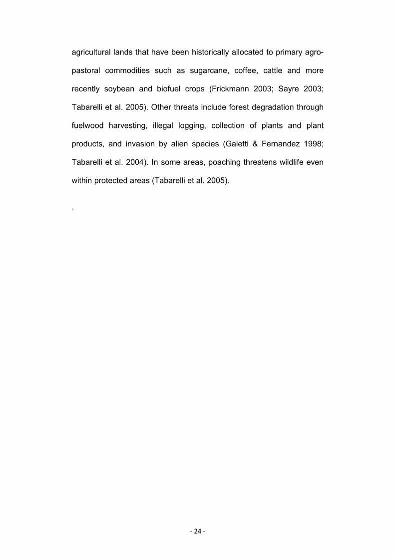
BAF (Ribeiro et al. 2009). The remaining forest in the BAF is a highly

fragmented landscape that spans across the Brazilian Atlantic coast

(figure 1.1). Banks-Leite et al. (2014) estimated that over 88% of the BAF

has less than 30% forest cover using 200-ha landscape units. Forest

fragmentation is a major cause of forest species loss within isolated

forest remnants (Cardoso da Silva & Tabarelli 2000; Cullen et al. 2016),

and a strong positive relationship has been found between the number

of animal and plant species and forest fragment area (Chiarello 1999;

Tabarelli et al. 1999).

- 23 -

Social importance

Over 125 million people (~70% of the Brazilian population) live along the

Brazilian Atlantic coast, and the BAF provides a series of ecosystem

services that contribute to their well-being (figure 1.1). Reservoirs in the

BAF produce 62% of Brazil’s electric power production, as well as

providing drinking water for the 125million inhabitants (Joly et al. 2014b).

Traditional and local people still rely on many native species fruits as a

food source, as well as raw materials such as fibres and oils (Apel et al.

2006; Satyanarayana et al. 2007). For example, fast growing demand

for an Amazonian berry has led to an increase in production of native

Jucara berry pulp in the BAF, from 5 tons in 2010 to 97.76 tons in 2011

(Trevisan et al. 2015). In terms of agriculture-related services, the BAF

hosts approximately 60 species of long-distance pollinator bees, though

the service they provide is at risk due to habitat loss, exotic species and

climate change (Giannini et al. 2012)

Main threats

Habitat loss, the main threat in the BAF, is stratified by altitude (Tabarelli

et al. 2010). At elevations greater than 1600 metres above sea level,

40% of all forest still persist, though these areas represent less than 1%

of the entire BAF. However, massive forest conversion into croplands,

abandoned pastures, real estate properties and urban areas has

occurred primarily across low to intermediate elevations (Tabarelli et al.

2010; Scarano & Ceotto 2015). Intermediate elevations are mostly

- 24 -

agricultural lands that have been historically allocated to primary agro-

pastoral commodities such as sugarcane, coffee, cattle and more

recently soybean and biofuel crops (Frickmann 2003; Sayre 2003;

Tabarelli et al. 2005). Other threats include forest degradation through

fuelwood harvesting, illegal logging, collection of plants and plant

products, and invasion by alien species (Galetti & Fernandez 1998;

Tabarelli et al. 2004). In some areas, poaching threatens wildlife even

within protected areas (Tabarelli et al. 2005).

.

- 25 -

Figure 1.1 Map of Brazil: population, Atlantic Forest cover for 2012,and biogeographical subregions. Sources: AmerPop 2015, SOSMataAtlantica 2012, Casteletti & Silva 2003.

- 26 -

Conservation efforts

Within the last four decades, over 700 protected areas have been

created in the BAF (Sayre 2003). However, these represent only 9% of

the remaining forest (Joly et al. 2014b), and protected areas with strict

protection (IUCN categories I and II) encompass only 1.7% (Ribeiro et

al. 2009). 75% of all protected areas are smaller than 10,000 ha, too

small to ensure long-term species persistence, and almost 80% of all

remaining forest cover is farther than 10 km from the nearest protected

area (Ribeiro et al. 2009; Tabarelli et al. 2010). Only 1% of the

threatened plant species and 15% of the threatened animal species

occur inside protected areas (Scarano & Ceotto 2015). Improving the

protected areas system and protecting large existing forest remnants in

the BAF is crucial; however, large-scale forest restoration is necessary

to ensure that biodiversity-derived ecological functions are provided

across the biome (Banks-Leite et al. 2014b).

The potential for forest restoration

Restoration has been practised in the BAF for the past 30 years, but with

small scale, isolated projects, no major changes in forest cover have

been observed (Rodrigues et al. 2009). To become an effective and

widespread means of conserving the Atlantic Forest, restoration

initiatives still have big challenges to overcome, such as reducing costs,

conforming to socio-political issues, scaling up restoration projects and

planning restoration actions at landscape-level (Rodrigues et al. 2009;

- 27 -

Melo et al. 2013b). The Atlantic Forest Restoration Pact (AFRP) was

created to address this need in 2009, one of the most ambitious multi-

sectoral coalitions set up for restoration, with more than 260 institutions

involved (Pinto et al. 2014). The AFRP was launched in 2009, with the

goal of restoring 15 million ha of the Brazilian Atlantic Forest by 2050

through the promotion of biodiversity conservation, jobs and income

generation, ecosystem services maintenance and provisioning, and by

supporting farmers to comply with the Forest Code across the biome

(Brancalion et al. 2012; Pinto et al. 2014). It is estimated that the cost of

actively restoring 15 million hectares including seedlings, replanting and

monitoring for two years– but excluding acquisition costs– ranges

between 49,000 and 77,000 mill. $ (c. $3,315-5,216/ha; Calmon et al.

2009).

It can be unrealistic to restore such large amounts of forest through land

acquisition, especially considering the fragmented nature of the BAF,

which would involve several small purchases to maximize forest

connectivity. Ecological set-asides on private land are a promising

strategy to preserve biodiversity and ecosystem services across

farmlands (Dobson et al. 2006), enabling their benefits to reach people

more widely (Gardner et al. 2009). Setting aside private land for

conservation nonetheless, comes with financial costs to the landowner.

In the BAF, the median yearly gross profit per hectare of agricultural land

is USD $467 (interquartile range $199 to $868), which is more than the

Brazilian minimum wage (Banks-Leite et al. 2014b). Payment for

ecosystem services (PES) schemes provide a mechanism to incentivize

- 28 -

landowner participation on set-asides (Milder et al. 2010). Brancalion et

al. (2012) provide a detailed analysis of a ‘‘basket of opportunities’’ to

incentivise forest restoration that includes PES, as well as other

opportunities such as crop production in agro-successional restoration

schemes and exploitation of timber and non-timber forest products in

restored areas. In general in Latin America, there’s been increasing

implementation of policies devoted to payments for ecosystem services

(Balvanera et al. 2012; Melo et al. 2013). In Brazil, there is a national

PES scheme, in which watershed committees established by law charge

for the use of water within a watershed and return part of this fee through

PES to landowners who implement forest restoration projects. For

instance, in Minas Gerais, this PES scheme increased native forest

cover by 60% in a targeted sub-watershed (Richards et al. 2015).

Research suggests that developing and promoting non-timber forest

products integrated into agroforestry systems on family farms in Brazil

could not only reduce deforestation pressures but also actively stimulate

reforestation (Souza et al. 2010; Trevisan et al. 2015). These

characteristics make PES-linked restoration initiatives based on

agricultural set-asides a realistic approach to large-scale restoration of

the BAF.

1.3 Aims and objectives

The aim of this thesis is to explore the importance of feedback effects of

conservation interventions and the ways they can be included in

- 29 -

conservation planning for real-life conservation problems. I use the

Brazilian Atlantic Forest as a case study because it presents the

opportunity to assess multiple feedbacks within the extremely relevant

scenario of a highly fragmented threatened biome in direct competition

with agriculture for available land, where there is high-level commitment

to a large-scale forest restoration intervention.

The following objectives were designed to address the aims of the thesis:

(1) Explore the role that unintended feedbacks play in conservation

outcomes. Sub-objectives are:

a. to develop a theoretical framework for understanding how

conservation interventions can trigger unintended

feedbacks and provide a new typology of unintended

feedbacks to guide the collection and organisation of

evidence.

b. to assess existing evidence for unintended feedbacks in

conservation.

c. to identify how best to plan for and mitigate unintended

feedbacks in conservation practice.

- 30 -

(2) Explore underlying mechanisms that have the potential to

undermine the cost-effectiveness of conservation programmes by

increasing the price of agricultural land, and assess their

applicability to a real-life case study. Sub-objectives are:

a. To review economic mechanisms within the context of

unintended feedback effects of conservation interventions

based on land use change.

b. To assess existing methods and data requirement for

mechanisms identified in 2.a.

c. To empirically assess the modelling of these mechanisms

for the Brazilian Atlantic Forest.

(3) Develop and test a methodological framework to prioritise a large-

scale set aside programme that enables accounting for both

environmental and social feedbacks simultaneously. Sub-

objectives are:

a. To develop a methodology for a spatial conservation

planning approach that includes both environmental and

economic dynamics.

b. To compare prioritisation outcomes for both a static and a

discrete dynamic prioritisation approach and evaluate the

trade-offs between them.

c. To assess the degree to which ecological and economic

characteristics of prioritisation units affect the best

prioritisation approach for that unit.

- 31 -

d. To characterise the role informational rent capture plays in

a large-scale prioritisation within the context of both a static

and a discrete dynamic prioritisation approach.

(4) Explore the relative effects of different conservation targets and

prioritisation approaches on the outcome of a conservation prioritisation.

Provide recommendations for restoring the Brazilian Atlantic Forest.

Sub-objectives are:

a. To identify priority areas for natural restoration in the BAF

that are robust to diverse targets and approaches.

b. To compare costs and benefits of meeting three different

forest restoration targets that are currently policy-relevant

to the BAF and have the potential to be implemented.

c. To assess the effect of increasing target area on the

difference in prioritisation outcomes for both static and

discrete dynamic prioritisation approaches.

d. To provide recommendations regarding prioritisation

approach choice in the context of diverse targets for the

BAF.

- 32 -

1.4 Thesis outline

Chapter 2: Unintended feedbacks: challenges and opportunities for

improving conservation effectiveness

In this chapter, I examine the role unintended feedbacks play in

conservation outcomes and the need for better evidence on their

prevalence and types in different circumstances. I develop a framework

for understanding unintended feedbacks and provide a typology based

on an existing social-ecological system approach that facilitates the

systematic collation of evidence. Approaches to planning for and

mitigating unintended feedbacks in conservation practice are discussed

to provide recommendations for management and future research. Gaps

identified in this chapter were used to guide research for the rest of this

PhD.

This work has been published as

Larrosa, C., Carrasco, L.R. & Milner-Gulland, E.J. (2016). Unintended

feedbacks: challenges and opportunities for improving conservation

effectiveness. Conserv. Lett., 9, 316-326.

Chapter 3: An empirical assessment of economic mechanisms for

unintended feedback effects of agricultural set-asides in conservation.

In this chapter, I explore economic mechanisms that underpin potential

unintended feedback effects of conservation interventions that are

based on changing land cover. I present the theory behind both classical

- 33 -

market and market failure mechanisms, and explore approaches that

could be used to model these feedbacks. This understanding is then

applied to a real-life case study, the large-scale restoration of the

Brazilian Atlantic Forest (BAF) through payments to set-aside

agricultural land. I describe the socio-economic context of the case

study, identify the mechanisms that may cause feedbacks in this system,

and assess the potential for modelling them. The analyses in this chapter

inform the choice of feedback effect (informational rent) modelled in

chapters 4 and 5.

Chapter 4: Spatial conservation planning accounting for environmental

and economic feedbacks

Chapter 2 shows a gap in the literature for dynamic conservation

planning approaches that account for both ecological and socio-

economic dynamics. Focusing on a farmland set-aside restoration

programme for the Brazilian Atlantic Forest, and based on results from

chapter three, in chapter four I propose and test a methodological

framework to prioritise a large-scale set-aside programme that enables

accounting for both environmental and social feedbacks simultaneously.

I model an environmental feedback that accounts for changes in forest

connectivity, and an economic feedback that accounts for changes in the

opportunity cost of farmland promoted by informational rent capture. I

compare prioritisation outcomes for a static approach with the proposed

discrete dynamic approach, and explore the trade-offs between

- 34 -

approaches. I assess the role that informational rent capture plays for

spatial conservation planning at large scales, and discuss the

implications of the results for conservation planning in the BAF.

Chapter 5: Restoring the Brazilian Atlantic Forest: understanding the role

of multiple restoration targets and prioritisation approaches

This chapter is centred on the application of the understanding and

methods developed in chapters two, three and four, to provide insights

and recommendations for restoring the Brazilian Atlantic Forest. I apply

a spatial conservation planning to the case study in the context of

compliance with the Brazilian Forest Code. Using three qualitatively and

quantitatively different restoration targets which have been proposed for

the BAF, I compare prioritisation solutions for both the static and

dynamic approaches defined in chapter three, assessing informational

rent capture as an economic incentive for restoration. I discuss how likely

it is that these targets are implemented, and how my results could work

in conjunction with existing initiatives.

Chapter 6: Discussion

This chapter provides a synthesis of research findings, key implications

for conservation management and science, policy recommendations,

and directions for future research.

- 35 -

Chapter 2: Unintended feedbacks: challenges and

opportunities for improving conservation effectiveness

- 36 -

1. Actions lead to reactions

Unintended effects of planned conservation interventions can have

knock-on effects that result in perverse outcomes. For example, the

threatened Javan hawk eagle was declared a National Rare/Precious

Animal to promote public attention for its conservation, but this attention

also increased trade demand for the species (Nijman et al. 2009).

Potential land use restrictions under the Endangered Species Act

resulted in pre-emptive timber harvesting, which destroyed an area of

habitat that could have supported half the 129 colonies needed to meet

the red-cockaded woodpecker’s conservation target (Lueck & Michael

2003). In Indonesia, increased income from seaweed farming, promoted

as a conservation tool to reduce pressure on fisheries, was invested in

capital improvement of fisheries businesses, potentially increasing

pressure on fisheries (Sievanen et al. 2005).

Conservation science needs to be able to predict and design for human

reactions to interventions, and the range and extremes of possible

outcomes (St John et al. 2013). Understanding the feedback loops that

constitute the unintended knock-on effects of conservation interventions

is a key element in achieving this goal. An unintended feedback exists

when reactions to an intervention have an effect on the intended

outcomes directly or indirectly, as illustrated in the examples above.

Unintended feedbacks include both human reactions to interventions

and ecosystem dynamics. There are multiple examples of perverse

outcomes in natural resource management, such as management

suppressing natural disturbance regimes or altering slowly changing

- 37 -

ecological variables, leading to unintended detrimental changes in soils,

hydrology and biodiversity (Holling & Meffe 1996). However, the

unintended feedbacks of conservation interventions modulated through

human decision-making are poorly studied, and are likely to be

significant determinants of conservation outcomes (Milner-Gulland

2012). Here we highlight the role unintended feedbacks play in

conservation outcomes, and the need for better evidence on their

prevalence and types in different circumstances. In order to guide the

collection and organisation of evidence, so that a strong empirical

underpinning can be built for future research, we develop a new

framework for understanding unintended feedbacks. First, we modify an

existing social-ecological system (SES) approach to provide a

theoretical understanding of how conservation interventions can trigger

unintended feedbacks. Then, we present a new typology of unintended

feedbacks, drawing on a wide range of conservation examples that show

how unintended feedbacks undermine conservation efforts. Finally, we

use the typology to reflect on how best to plan for and mitigate

unintended feedbacks in conservation practice, and discuss implications

for future work.

- 38 -

2. Undermining conservation efforts: how much do we know?

It has been recognized that unintended feedbacks can render

conservation interventions inefficient and ineffective (Polasky 2006).

However, there is still a relatively simplistic narrative regarding how

people will react when planning conservation interventions (St John et

al. 2013). For example, a lack of success in the alternative livelihoods

approach is linked to its three simplistic assumptions of substitution,

homogeneous community and impact scalability (Wright et al. 2016).

Even with the use of project design tools like Miradi (Miradi 2007), which

make the theory of change underlying the chosen intervention explicit,

the indirect consequences of people's reactions to conservation can still

remain unaccounted for. With conservation interventions increasingly

centred on changing human behaviour, understanding how these

interventions alter the incentives and actions of the people causing

biodiversity loss, and their knock-on effects, is of great relevance to the

design and evaluation of such interventions.

The literature on unintended consequences of conservation

interventions on people (Cernea & Schmidt-Soltau 2006) or non-target

species (Harihar et al. 2011) is large, however, cases documenting how

unintended consequences feed back to result in undermined

conservation goals are uncommon and mostly anecdotal. Examples of

potential unintended feedbacks mediated through human decisions

include integrated conservation and development projects enhancing

the profitability of existing environmentally harmful activities such as land

- 39 -

clearance (Jack et al. 2008), promoting development of new enterprises

that may impact other ecosystem components (Spiteri & Nepalz 2006),

or leading to positive net migration (Oates 1995). Widely used market-

based approaches such as payments for ecosystem services (PES)

bring into play spatial and temporal scales that can differ from the target

system, broadening the scope of potential effects of feedbacks. For

example, protection of forests from exploitation under Reducing

Emissions from Deforestation and Forest Degradation initiatives can

lead to displacement of exploitation to distant areas (Angelsen 2007a).

Studies addressing real-world unintended feedbacks in conservation are

scarce, but modelling has been used to explore how interventions can

backfire. Damania et al. (2005) used a household utility model to show

how an alternative livelihoods approach to alter hunting behaviour could

increase mortality of the most vulnerable species. Other modelling

studies have shown how land market feedbacks lead to highly cost

ineffective conservation planning (Jantke & Schneider 2011), or that

buying land for conservation can sometimes condemn more species

than it saves (Armsworth et al. 2006). Land purchase for conservation

can increase the price of non-developed land, for example by reducing

the stock of land for development, raising the prospect of future

conservation land purchase, or increasing the amenity value of

neighbouring land. This can then displace development, potentially to

other biologically sensitive areas, or limit the amount of land that can be

purchased for a given conservation budget.

- 40 -

Reviews of unintended feedbacks are also few and scattered. A review

examining the extent to which the peer-reviewed literature addressed

feedbacks between conservation interventions and SESs found most

articles focused either on the effect of conservation on people, or of

people on the environment, with few studies empirically addressing both

the social dynamics resulting from conservation initiatives and

subsequent environmental effects (Miller et al. 2012). There is a lot more

focus on feedbacks in the resilience and SESs literature (Gunderson &

Holling 2002). This literature is based on a systems thinking approach

that explicitly considers the interaction between the social and ecological

components of a system, facilitating interdisciplinary analysis of human–

nature dynamics (Glaser et al. 2008). Within the last decade, significant

progress has been made with respect to interdisciplinary investigation

and modelling of coupled SESs (Baur & Binder 2013).

Recently, the importance of explicitly accounting for feedbacks to better

manage complex systems has been highlighted with a Special Feature

published in Ecology and Society (Hull et al. 2015a). From a coupled

human and natural systems perspective, the articles in this issue identify

feedbacks that stabilize and destabilize systems across agricultural,

forest, and urban landscapes. Emerging themes include multilevel

feedbacks, time lags, and surprises as a result of feedbacks.

- 41 -

3. Building an understanding: an SES perspective

Systems thinking is especially attuned to explaining side effects and

perverse outcomes due to its emphasis on feedback loops, and it has

been recommended as a theoretical approach to underpin behavioural

change policy design (Lucas et al. 2008). Systems dynamics modelling

has been applied to manage and avoid unintended consequences and

their feedbacks in designing hazards management and disaster relief

policy (Gillespie et al. 2004). For example forest fire management

(Collins et al. 2013), emergency resource coordination (Wang et al.

2012), and efficient positioning of relief services (Widener et al. 2015).

Clearly articulated with systems thinking theory, the SES literature is

where most of the work on human-natural systems has been done,

providing a strong grounding for work on unintended feedbacks.

An SES is a complex, adaptive system consisting of a bio-geophysical

unit and its associated social actors and institutions, with boundaries that

delimit a particular ecosystem and its problem context (Glaser et al.

2012). As complex systems, SESs present inherent properties such as

nonlinearity, emergence and self-organization, path dependence, and

positive/negative feedback loops (definitions in Table 2.1; Becker 2012).

These properties are relevant to the analysis and planning of

conservation interventions because they provide a framework for

understanding and describing SES behaviour. Given the increasing

spatial tele connectedness of social actors and institutions through

international trade, information technologies and travel, the spatial

- 42 -

boundaries of the SES can encompass multiple countries or represent a

global system.

In systems thinking, a feedback loop exists when results from some

action travel through the system and eventually return in some form to

the original action, potentially influencing future actions. In a “negative or

balancing” feedback the initial change to a system causes a change in

the opposite direction, dampening the effect; in a “positive or reinforcing”

feedback the initial change to a system causes more change in the same

direction, amplifying the effect (Chin et al. 2014). For example, a

reinforcing feedback loop between fragmentation processes (fire,

logging) and landscape pattern (connectivity, patch characteristics, and

edge effects) significantly accelerated the effect of deforestation on

biodiversity in the Brazilian Amazon (Cumming et al. 2012).

There are several frameworks to analyse environmental problems in the

context of SESs. We take as our starting point the SES Framework

(SESF), developed by Ostrom (2009) as a diagnostic tool for

understanding the sustainability of complex SESs. Binder et al. (2013)

reviewed 10 SES frameworks that were explicitly designed for

application by both researchers and practitioners (SM Table 1). Ostrom’s

framework is the only one of these that conceptualizes the bi-directional

interaction between the social and ecological systems, and treats both

systems in almost equal depth (Binder et al. 2013). The SESF is also

relevant to a wide range of natural resource issues, has been

increasingly applied in conservation, and enables the visualization of the

- 43 -

system’s structure with varying degrees of complexity. The extent to

which the theories underlying different SES frameworks would lead to

similar or diverging results would still require exploration.

Ostrom’s SESF (figure 2.1) has a nested structure where actors use and

provide for the maintenance of resource units, within a resource system,

according to rules and procedures determined by a governance system,

in the context of related ecological systems and broader social, political

and economic settings (McGinnis & Ostrom 2014). The framework

enables analyses of how attributes of the four core subsystems both

affect and are affected by interactions and outcomes via feedbacks at a

particular time and place (Ostrom 2007). These subsystems are: (i)

resource systems (e.g., protected area, lake); (ii) resource units (e.g.,

trees, amount and flow of water); (iii) governance systems (e.g., the

specific rules related to the use of the protected area or lake, and their

implementation); and (iv) actors (e.g. resource users, managers;

figure.1.1).

Although the fact that conservation acts on complex SESs is well

accepted, the consequences of considering the conservation

intervention itself as embedded in the system are less well appreciated.

The moment a conservation action or policy is mooted, it becomes part

of the SES, redefining it, affecting all four subsystems directly or

indirectly (figure 2.1). The triggered reactions to the conservation

intervention flow through the SES and in turn affect the intended

outcomes, forming feedback loops. It is via these interactions that

- 44 -

reactions have the potential to undermine conservation outcomes or

generate policy resistant systems (Sterman 2000).

As it becomes a part of the SES, the conservation intervention can alter

both the system's structure and/or the dynamics of the processes within

it. These dynamics include economic processes at the system scale,

such as land market feedbacks (Armsworth et al. 2006) or behavioural

changes at the scale of the individual or community, such as are

explored in psychology and decision science (Gintis 2007). For example,

some PES schemes have increased inequity through processes such as

marginalisation, elite capture of benefits and increased vulnerability of

some groups, resulting in reduced project legitimacy, non-participation,

corruption and even active resistance (Pascual et al. 2014). These types

of processes at a smaller scale can drive feedbacks at the system scale.

- 45 -

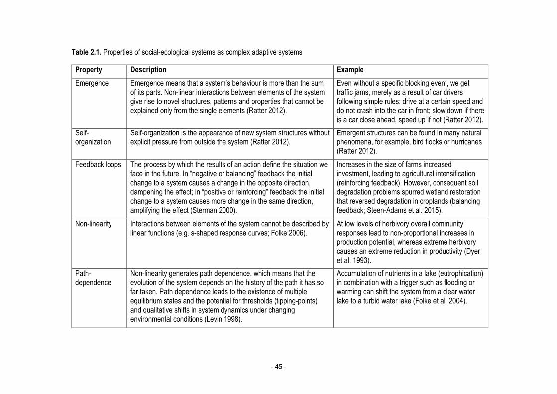
Table 2.1. Properties of social-ecological systems as complex adaptive systems

Property Description ExampleEmergence Emergence means that a system’s behaviour is more than the sum

of its parts. Non-linear interactions between elements of the systemgive rise to novel structures, patterns and properties that cannot beexplained only from the single elements (Ratter 2012).

Even without a specific blocking event, we gettraffic jams, merely as a result of car driversfollowing simple rules: drive at a certain speed anddo not crash into the car in front; slow down if thereis a car close ahead, speed up if not (Ratter 2012).

Self-organization

Self-organization is the appearance of new system structures withoutexplicit pressure from outside the system (Ratter 2012).

Emergent structures can be found in many naturalphenomena, for example, bird flocks or hurricanes(Ratter 2012).

Feedback loops The process by which the results of an action define the situation weface in the future. In “negative or balancing” feedback the initialchange to a system causes a change in the opposite direction,dampening the effect; in “positive or reinforcing” feedback the initialchange to a system causes more change in the same direction,amplifying the effect (Sterman 2000).

Increases in the size of farms increasedinvestment, leading to agricultural intensification(reinforcing feedback). However, consequent soildegradation problems spurred wetland restorationthat reversed degradation in croplands (balancingfeedback; Steen-Adams et al. 2015).

Non-linearity Interactions between elements of the system cannot be described bylinear functions (e.g. s-shaped response curves; Folke 2006).

At low levels of herbivory overall communityresponses lead to non-proportional increases inproduction potential, whereas extreme herbivorycauses an extreme reduction in productivity (Dyeret al. 1993).

Path-dependence

Non-linearity generates path dependence, which means that theevolution of the system depends on the history of the path it has sofar taken. Path dependence leads to the existence of multipleequilibrium states and the potential for thresholds (tipping-points)and qualitative shifts in system dynamics under changingenvironmental conditions (Levin 1998).

Accumulation of nutrients in a lake (eutrophication)in combination with a trigger such as flooding orwarming can shift the system from a clear waterlake to a turbid water lake (Folke et al. 2004).

- 46 -

Figure 2.1. Theoretical framework for understanding unintendedfeedbacks from conservation interventions adapted from the Social-ecological System (SES) Framework (McGinnis & Ostrom 2014). Inblack the SES Framework: solid ovals denote core subsystems and fullarrows denote direct links between subsystems. Core subsystemsinteract to produce outcomes that have feedback effects denoted bydashed arrows. In blue a modification to the SES Framework: theconservation intervention becomes part of the system jointly affectingand affected by interactions and outcomes. The dotted-and-dashed lineindicates the boundary of SES; exogenous social, economic and politicalsettings or related ecosystems can affect any element of the SES.

- 47 -

4. A typology of unintended feedbacks

Schoon and Cox (2012) introduced a framework to analyse disturbance-

response dyads in an SES that accounts for both structure and flow,

based on the SESF. We use their work as a basis for creating a typology

of unintended feedbacks, whereby disturbance to the structure or flow of

an SES, caused by a conservation intervention, triggers unintended

feedbacks.

We define an unintended feedback as a feedback triggered by a

conservation intervention, which was not built into intervention design,

and that has an effect on conservation outcomes. It can consist of

multiple reinforcing or balancing loops, and the net effect can either

undermine or enhance conservation outcomes. Here we focus on

feedbacks that undermine conservation outcomes because they are of

greater concern to implementers. Three types of unintended feedback

are identified: (1) Flow (relating to a change in a parameter within the

SES), (2) Deletion, and (3) Addition (both relating to a change in SES

structure).

(1) Flow unintended feedbacks are due to the enhancement or

dampening of pre-existing feedback loops within the SES, caused by the

conservation intervention. For example, in the USA, land use restrictions

imposed on Federal forest concessions by the Endangered Species Act

reduced lumber supply. This increased its price, thereby promoting

logging in private forests within that region (Murray & Wear 1998;

Polasky 2006). Another study showed that, depending on the structure

- 48 -

of demand for bushmeat, a reduction in supply caused by enforcement

of anti-poaching laws could lead to an increase in prices inducing others

to enter the market and increase hunting levels (Wilkie & Godoy 2001).

(2) Deletion unintended feedbacks occur when pre-existing feedback

loops within the SES are lost due to the conservation intervention. For

example, in Kenya, impoundment by the government of an area along

the Turkwel River curtailed traditional management of this area. The loss

of this institutional structure led to increased forest degradation (Stave

et al. 2001).

(3) Addition unintended feedbacks occur when interventions add

components to the SES network structure. Most conservation

interventions add actors, institutional structures or links, either human or

natural. For example, new legislation aimed at creating incentives for

biodiversity conservation in Mexico allowed landowners to benefit

directly from wildlife exploitation through the creation of wildlife

conservation units. However, in some regions, these new structures led

to investment in practices that reduced native biodiversity in the long

term, such as fencing and cultivation of exotic grasslands (Sisk et al.

2007). Re-introducing wild dogs generated negative attitudes and

persecution of existing wild dog populations in South Africa due to

perceived and real threats of predation on livestock, despite a

compensation scheme being in place (Gusset et al. 2007).

Multiple feedback loops can interact to undermine an outcome. For

example, Österblom et al. (2011) identified three unintended partial

- 49 -

feedback loops that explained in part the European Common Fisheries

Policy’s failure to deliver on its social and ecological goals despite

continuous efforts. Additionally, a single intervention can produce

different types of unintended feedbacks. For example, the establishment

of protected areas can trigger a flow unintended feedback; increases in

land allocated to protected areas could increase the prices of agricultural

commodities due to foregone agricultural production, which can result in

highly cost ineffective conservation (Jantke & Schneider 2011). The

establishment of a protected area can also trigger a deletion unintended

feedback: the imposition of external conservation rules brought by

Ranomafana National Park in Madagascar resulted in a change of social

norms concerning accepted behaviour when harvesting pandans

(Pandanus spp.) that led to unsustainable use in the villages surrounding

the park (Jones et al. 2008). The establishment of a protected area can

trigger an addition unintended feedback as well: Tarangire National

Park, in Tanzania, is a source of added risk for household decision

makers, some of whom pursued aggressive land conversion in

anticipation of park expansion (Baird et al. 2009).

- 50 -

5. Implications for applied conservation

The prevalence and potentially disastrous effects of unintended

feedbacks highlights the need to consider them more fully as important

elements of conservation intervention design. By representing the way

in which a conservation intervention alters an SES as three easily

identifiable disturbances, the typology presented here facilitates a

diagnostic approach to analysing how unintended feedbacks affect

outcomes.

A priori identification of potential unintended feedbacks can improve

conservation practice by enabling the consideration of complex

relationships. In Tarangire National Park, consideration of SES

dynamics suggested that greater security of land tenure would be a

better approach to forestalling pre-emptive land conversion in

anticipation of park expansion than the proposed increase in land use

restrictions (Baird et al. 2009). Applying the typology of unintended

feedbacks within results chains during the conservation intervention

design process could highlight potential unintended feedbacks,

substantially improving the utility of project design tools such as Miradi

(Miradi 2007).

Evaluating the possible perverse outcomes of policy interventions is

often highlighted as an important step in guidelines for policy design (e.g.

Hallsworth et al. 2011). For example, to avoid feedbacks from negative

impacts on equity, it has been suggested that policy development

processes use standard assessment tools (such as Impact

- 51 -

Assessments), on top of which additional criteria can be addressed

(such as social or environmental justice; Brooks et al. 2006). Guidelines

for selecting models and developing interventions from the policy design

field could be adapted in future to inform conservation intervention

design within the context of unintended feedbacks.

An incomplete understanding of an SES and its history is not the only

cause of unintended feedbacks. Prediction of human behaviour, and

knowledge of system behaviour can provide an idea of the range of

conservation outcomes and intervention can produce. However,

unintended behaviour within an SES can also be due to emergent

properties that, so far, cannot be predicted (Ratter 2012). An adaptive

management approach that monitors feedback structure and behaviour

could improve the early detection of emerging properties of an SES.

Recently, Mayer et al. (2014) proposed the use of specific indicators that

give insight into the structure and behaviour of feedbacks, such as

Shannon entropy and Fisher information, as monitoring tools for

sustainable management.

Evaluations of conservation impact need to understand the mechanisms

by which conservation interventions have impact, including both directly

on the target and indirectly on other components of the ecosystem via

changes in human behaviour. A posteriori consideration of potential

feedbacks operating in an SES can help identify the true drivers of

observed patterns. For example, the change at national scale from net

deforestation to net reforestation that took place in Vietnam was a

- 52 -

consequence of two separate forces: endogenous socio-ecological

feedbacks, such as local resource depletion, explained a slowing down

of deforestation and stabilization of forest cover. However, it was

exogenous socio-economic factors, such as global trade, that better

accounted for reforestation. Neither process represented a planned

response to ecosystem degradation (Lambin & Meyfroidt 2010).

- 53 -

6. Implications for future work in conservation science

The current anecdotal and scattered evidence is not enough to support

general principles for conservation decision-making that minimize

unintended feedbacks. It is difficult to say at present under which

circumstances unintended feedbacks may be most significant for

conservation outcomes, or which mechanisms of human behaviour

underlie them. The type of conservation intervention, and the complexity

of the SES, may play a crucial role. For example, it is expected that

indirect approaches, such as alternative livelihoods, may increase the

likelihood of promoting unintended feedbacks due to the higher number

of actors and links comprising the system. However, there is not enough

evidence to substantiate this statement because currently the literature

is inadequate to support a systematic review. Studies of the correlates

of conservation success have encountered similar limitations (Brooks et

al., 2012). There is a need to establish comparative databases to collate

case studies for analysis, in order to describe unintended feedbacks,

their drivers and underlying mechanisms (Table 2.2). The typology

presented could provide a framework for this task. Data collection efforts

are underway to gather examples of SESs, which could inform this

analysis, for example the social-ecological systems meta-analysis

database (SESMAD) project, which aims to enable analysis of case

studies of a diversity of SESs by collating them in a comparable format

(Cox 2015).

- 54 -

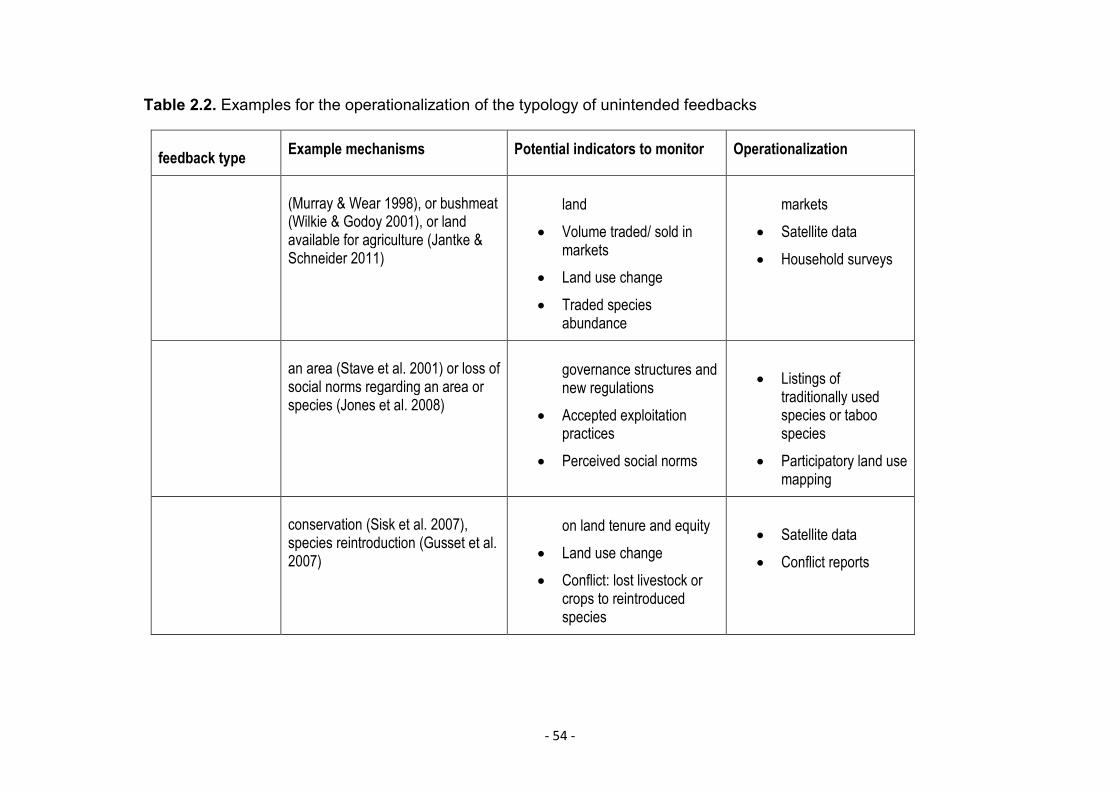
Table 2.2. Examples for the operationalization of the typology of unintended feedbacks

Unintendedfeedback type Example mechanisms Potential indicators to monitor Operationalization

Flow Reduction in supply of lumber(Murray & Wear 1998), or bushmeat(Wilkie & Godoy 2001), or landavailable for agriculture (Jantke &Schneider 2011)

x Price of lumber/ bushmeat/land

x Volume traded/ sold inmarkets

x Land use changex Traded species

abundance

x Surveys in keymarkets

x Satellite datax Household surveys

Deletion Loss of traditional management overan area (Stave et al. 2001) or loss ofsocial norms regarding an area orspecies (Jones et al. 2008)

x Overlap between existinggovernance structures andnew regulations

x Accepted exploitationpractices

x Perceived social norms

x Household surveysx Listings of

traditionally usedspecies or taboospecies

x Participatory land usemapping

Addition Creating economic incentives forconservation (Sisk et al. 2007),species reintroduction (Gusset et al.2007)

x Impact of new regulationon land tenure and equity

x Land use changex Conflict: lost livestock or

crops to reintroducedspecies

x Household surveysx Satellite datax Conflict reports

- 55 -

The literature on behavioural change based policy can shed light on

which aspects of an intervention need to be considered when analysing

evidence of unintended feedbacks. Darnton's (2008) review of

behavioural change found that three elements determine whether a

policy intervention has negative impacts on equity or not: (1) what factors

of a behavioural model are targeted by an intervention, (2) the way in

which those factors are targeted, and (3) the theory of change underlying

the intervention. Given that interventions that have negative impacts on

equity can result in unintended feedbacks such as corruption or

sabotage (Pascual et al. 2014), these same elements could prove to be

important intervention characteristics within the context of unintended

feedbacks.

Feedbacks that enhance conservation outcomes are also possible, and

present opportunities to magnify or extend conservation effectiveness

by harnessing synergies within the system. Similarly, there is a need to

collect case studies in order to start exploring the circumstances and

mechanisms that enable this type of feedback. Additionally, focusing on

finding and studying examples in which unintended feedbacks were

overcome and managed could provide invaluable insight.

Currently, policy support tools widely used to explore the potential

impact of different interventions at large scales are based on static

models that cannot account for unintended feedbacks. InVEST (Nelson

et al. 2009), for example, ranks relative biodiversity and ecosystem

services outputs under different scenarios; the tool currently focuses on

- 56 -

developing relatively simple models to meet demand from decision-

makers (Ruckelshaus et al. 2015). Under some circumstances

incorporating unintended feedbacks might not have a large effect on

model predictions (Zvoleff & An 2014a), but this will depend on the

system (Armsworth et al. 2006). Mechanisms by which unintended

feedbacks occur could be incorporated into these models to assess the

robustness of their predictions; however, there will be a trade-off

between model complexity and the gain in predictive power given the

likely high uncertainties in developing and parameterizing a dynamic

systems model. This trade-off needs to be explored urgently to elucidate

when more complex models are necessary to avoid misleading

recommendations from such tools, or when simpler models give robust

results (Table 2.3).

- 57 -

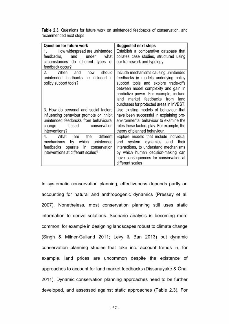
Table 2.3. Questions for future work on unintended feedbacks of conservation, andrecommended next steps

Question for future work Suggested next steps1. How widespread are unintendedfeedbacks, and under whatcircumstances do different types offeedback occur?

Establish a comparative database thatcollates case studies, structured usingour framework and typology.

2. When and how shouldunintended feedbacks be included inpolicy support tools?

Include mechanisms causing unintendedfeedbacks in models underlying policysupport tools and explore trade-offsbetween model complexity and gain inpredictive power. For example, includeland market feedbacks from landpurchases for protected areas in InVEST.

3. How do personal and social factorsinfluencing behaviour promote or inhibitunintended feedbacks from behaviouralchange based conservationinterventions?

Use existing models of behaviour thathave been successful in explaining pro-environmental behaviour to examine theroles these factors play. For example, thetheory of planned behaviour.

4. What are the differentmechanisms by which unintendedfeedbacks operate in conservationinterventions at different scales?

Explore models that include individualand system dynamics and theirinteractions, to understand mechanismsby which human decision-making canhave consequences for conservation atdifferent scales

In systematic conservation planning, effectiveness depends partly on

accounting for natural and anthropogenic dynamics (Pressey et al.

2007). Nonetheless, most conservation planning still uses static

information to derive solutions. Scenario analysis is becoming more

common, for example in designing landscapes robust to climate change

(Singh & Milner-Gulland 2011; Levy & Ban 2013) but dynamic

conservation planning studies that take into account trends in, for

example, land prices are uncommon despite the existence of

approaches to account for land market feedbacks (Dissanayake & Önal

2011). Dynamic conservation planning approaches need to be further

developed, and assessed against static approaches (Table 2.3). For

- 58 -

instance, empirical data have been used to suggest that reserve

selection could be improved by accounting for land market feedbacks

which vary across landscapes (Butsic et al. 2013).

Ultimately, conservation outcomes derive from human decision-making.

Much work has been done using behavioural theory to explore

conservation outcomes. Tools at the individual or household level

include bio-economic models based on rational choice (e.g. Stephens et

al., 2012) and social-psychological models based on the theory of

planned behaviour (e.g. Williams et al., 2012). SESs have emergent

properties that make responses to interventions different than the sum

of individual responses. It is important to understand the ways in which

system behaviour emerges from the collection of many individual

decisions, and how individual- and system-level dynamics interact

(Ratter 2012). Agent-based models can capture these properties

(Rounsevell et al. 2012), but also need to include institutional dynamics

and external trends. Advanced tools for modelling complex adaptive

systems can be applied to SES structure analysis, such as network

topology (Janssen et al. 2006). Social network theory has been applied

within the context of social movement theory to explain how

environmental social movements develop (Ernstson 2013). These tools

applied to the study of SES properties such as emergent behaviour and

self-organisation can start to unveil the mechanisms by which human

decision-making could have consequences for conservation (Table 2.3).

- 59 -

7. Conclusion

There is plenty of anecdotal evidence that understanding unintended

feedbacks is vital for effective interventions to combat biodiversity loss.

The recent interest in the central role of feedbacks in managing complex

systems (Hull et al. 2015a) provides the right arena where a literature on

unintended feedbacks could flourish. The fact that people adapt and

respond to conservation interventions, and that their actions feed

through into changes in the conservation situation itself, is something

that conservationists rely on for their impact. However, these same

responses are being overlooked when they affect outcomes indirectly

through unintended feedbacks. There is an urgent need to collect

evidence to understand the mechanisms by which human decision-

making feeds through to conservation outcomes at different scales.

- 60 -

Chapter 3: An empirical assessment of economic

mechanisms for unintended feedback effects of

agricultural set-asides in conservation.

- 61 -

1. Introduction

In Chapter 2, I presented a typology of unintended feedback effects that

may impact the success of conservation interventions. I also highlighted

the lack of empirical analysis of the prevalence and magnitude of these

effects within the conservation literature, with the evidence instead

largely consisting of anecdotes. The lack of evidence precludes

systematic review and general statements about the likelihood of such

feedbacks occurring for a given intervention type or context. Some

quantitative empirical studies have been done in a few locations,

however, these are based on predictive modelling rather than actual

evidence of feedbacks. For example, in Brazil, statistical analyses at

county level found that policies intending to spare land through soy yield

improvements could actually lead to an agricultural land expansion in

the absence of strong regulation (Garrett et al. 2013). Yield

improvements in oil palm could lead to sparing of temperate agricultural

land, but increased deforestation in the tropics (Carrasco et al. 2014).

These unintended feedback effects are based onmechanisms explained

by market dynamics; given the realistic assumption that demand for

these basic commodities is inelastic, increased yields are not matched

by equivalent price drops, and therefore mostly increase rents from land,

increasing producers’ incentives to expand their production over time.

Market mechanisms such as these play a crucial role in determining

conservation success and cost-effectiveness, and ignoring them can

jeopardise conservation at local and international scales (Seidl et al.

2001; Armsworth et al. 2006; Wilson et al. 2006).

- 62 -

A large component of conservation science research revolves around

understanding incentives that promote sustainable changes in human

behaviour (Spiteri & Nepalz 2006; Gibbons et al. 2011; Armsworth et al.

2012; Bryan 2013). Incentive-based interventions change the economic

incentives of private actors, leaving the decision on whether and how

much to change behaviour to them (Jack et al. 2008). The literature on

these mechanisms is vast in policy design and implementation (Oates et

al. 1989; Jaffe et al. 2003; de Vries & Hanley 2016), and lessons from

this field can be applied to incentive-based conservation interventions

such as payments for ecosystem services (Jack et al. 2008). However,

altering behaviour via economic incentives has the potential to trigger

feedbacks of various kinds that can undermine conservation outcomes.

Market-based mechanisms that explain feedback effects have been

mostly studied in the context of conservation planning and reserve

selection (Armsworth et al. 2006; Dissanayake & Önal 2011; Zvoleff &

An 2014b). In a seminal paper, Armsworth et al. (2006) used a simple

land market equilibriummodel to show how conservation land purchases

could result in increased biodiversity loss due to reduced availability of

land, increases in land prices and displacement of development.

However, studies in which these mechanisms have been modelled

empirically in a spatially explicit way are few (Walker 2012a; Butsic et al.

2013), and biased towards developed regions of the globe (Armsworth

2014). An assessment of the applicability of existing methods of

modelling market-based mechanisms to empirical case studies could

- 63 -

better inform understanding of knowledge gaps and drive future work in

this area.

Certain situations cause market failure, resulting in inefficient allocation

of goods and services (Mas-Colell et al. 1995). To identify when and how

governments should intervene to correct the inefficiency, a framework

was developed to characterise situations which may predispose markets

to failure (Zerbe Jr & McCurdy 2000). These situations include the

provision of public goods, perpetuation of inequality, and externalities,

situations extremely common in the type of problems conservation

addresses (Hardin 1968; Marris 2009; Kemkes et al. 2010; Pascual et

al. 2014). Despite the relevance market failure seems to have for

conservation issues, few studies have looked at these mechanisms in

the context of potential feedback effects of conservation interventions.

For example, a market failure situation called information failure has

been shown to undermine conservation project cost-effectiveness due

to informational rent capture (Ferraro 2008; Harvey 2010). Informational

rent capture has been modelled for optimal design of carbon contracts

(Mason & Plantinga 2013), but its potential for feedback effects and

implications for conservation have not been assessed (but see chapter

4). If incentive-based conservation is to plan and manage for unintended

feedbacks, the potential for market failure needs to be considered.

Accounting for system dynamics is key to effective conservation

planning (Pressey et al. 2007), but to empirically model these dynamics

the mechanisms underlying the feedback effects of incentive-based

- 64 -

conservation need to be understood. The aim of this chapter is therefore

to explore economic mechanisms that have the potential to undermine

the cost-effectiveness of conservation programmes by increasing the

price of agricultural land, and provide guidance in approaching their

modelling. In the first section, I review the underlying mechanisms that

have the potential to undermine the cost-effectiveness of conservation

programmes by increasing the price of agricultural land. I review various

types of market feedbacks that may take place, based both on classical

market mechanisms of change in demand and supply, and on market

failures due to unpriced externalities. Examples of existing methods for

modelling and data requirement are indicated for the identified

mechanisms. In the second section, I describe the socio-economic

context of a specific case study, the large-scale restoration of the

Brazilian Atlantic Forest through payments to set-aside agricultural land.

In the third section, I assess the potential for modelling various

mechanisms for feedback effects within the context of the case study,

providing an example of how to empirically approach the modelling of

these feedbacks.

- 65 -

2. Mechanisms for feedback effects

2.1 Based on classical market behaviour

Land markets potentially undermine conservation goals through

feedbacks that change the market value of land (Armsworth et al. 2006;

Polasky 2006). Market behaviour can be studied using mechanistic

models such as general and partial equilibrium models, based on

equilibrium theory (Dumas 1993). Equilibrium theory describes

characteristics of an economic system in equilibrium, and its underlying

assumptions are (1) perfect competition, and (2) perfect divisibility of all

resources and products (Scitovsky 1954).

Most commonly market behaviour has been studied via partial

equilibrium models, however, general equilibrium models now play an

important role in many fields of economics due to technological

advances which provide the necessary computing power (Nicholson &

Westhoff 2009). Partial equilibrium models limit the scope of the effects

of the intervention to one section of the market, and so are applicable

when the effects of the intervention in the economy as a whole are so

small they can be ignored (Mas-Colell et al. 1995). General equilibrium

models consider the economy as a whole and are applicable when

multiple sectors are interdependent (Mas-Colell et al. 1995). Within this

context, Butsic et al. (2013) grouped land market feedbacks by whether

they had equilibrium effects, or partial equilibrium effects. Both

equilibrium and partial equilibrium feedbacks can increase the market

- 66 -

value of land and thereby heighten development risk in the area, which

can potentially undermine conservation goals.

Feedback from increased demand for land

When large areas are set-aside for conservation, either through

purchase, easements or other measures that take the land out of

circulation, supply and demand in local markets will be affected. An

increase in demand for land by conservation groups shifts the demand

curve outward, which results in additional land being traded in the

market, and at a higher price (figure 3.1, Armsworth et al. 2006). For

example, environmental land purchases by the Dutch government had

the effect of increasing prices on the land market (Jongeneel et al. 2012),

and increasing competition for land between conservationists and

farmers (Bakker et al. 2015).

In conservation, land market feedbacks have been studied by estimating

the price elasticity of land supply and land rents, mostly in data-rich

geographical areas such as Europe (Jantke & Schneider 2011; Toth et

al. 2011). To calculate these feedbacks, the economic data required

might not be available at a useful resolution for many developing

countries. These include time series data on land cost or land rent, and

data on the elasticity of supply and demand that can be estimated with

data on the amount of land sold per year (Eickhout et al. 2009; Barr et

al. 2011).

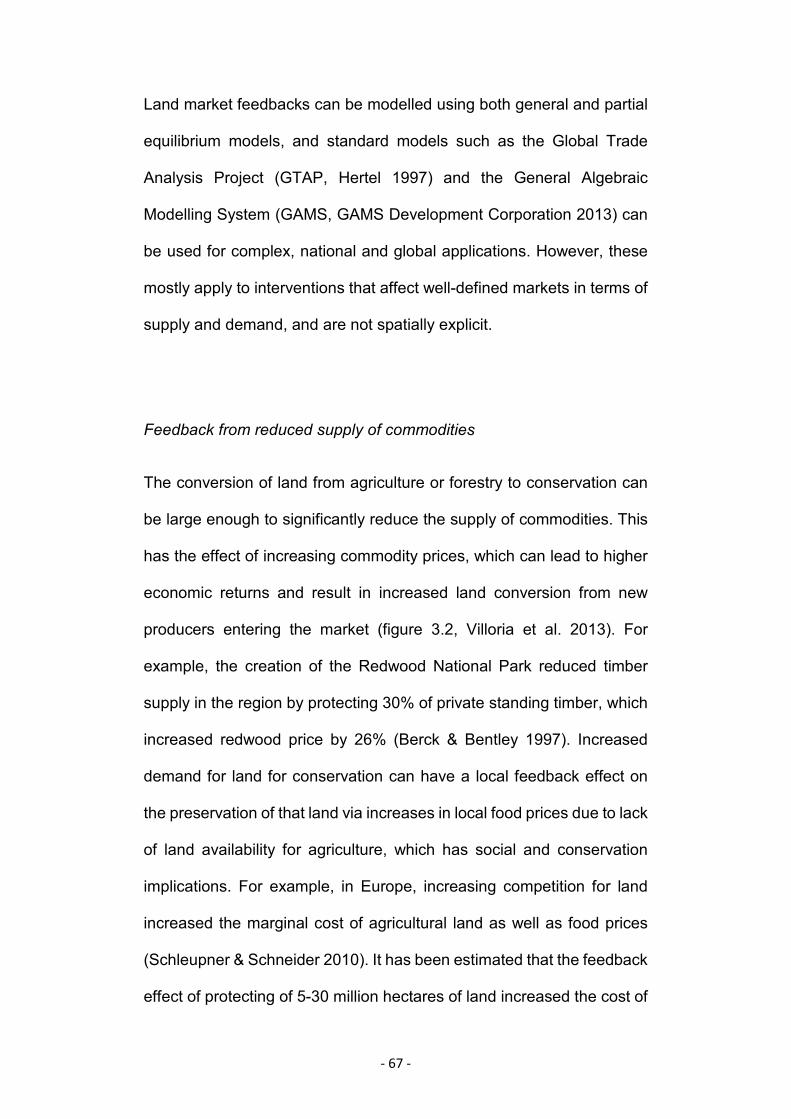
- 67 -

Land market feedbacks can be modelled using both general and partial

equilibrium models, and standard models such as the Global Trade

Analysis Project (GTAP, Hertel 1997) and the General Algebraic

Modelling System (GAMS, GAMS Development Corporation 2013) can

be used for complex, national and global applications. However, these

mostly apply to interventions that affect well-defined markets in terms of

supply and demand, and are not spatially explicit.

Feedback from reduced supply of commodities

The conversion of land from agriculture or forestry to conservation can

be large enough to significantly reduce the supply of commodities. This

has the effect of increasing commodity prices, which can lead to higher

economic returns and result in increased land conversion from new

producers entering the market (figure 3.2, Villoria et al. 2013). For

example, the creation of the Redwood National Park reduced timber

supply in the region by protecting 30% of private standing timber, which

increased redwood price by 26% (Berck & Bentley 1997). Increased

demand for land for conservation can have a local feedback effect on

the preservation of that land via increases in local food prices due to lack

of land availability for agriculture, which has social and conservation

implications. For example, in Europe, increasing competition for land

increased the marginal cost of agricultural land as well as food prices

(Schleupner & Schneider 2010). It has been estimated that the feedback

effect of protecting of 5-30 million hectares of land increased the cost of

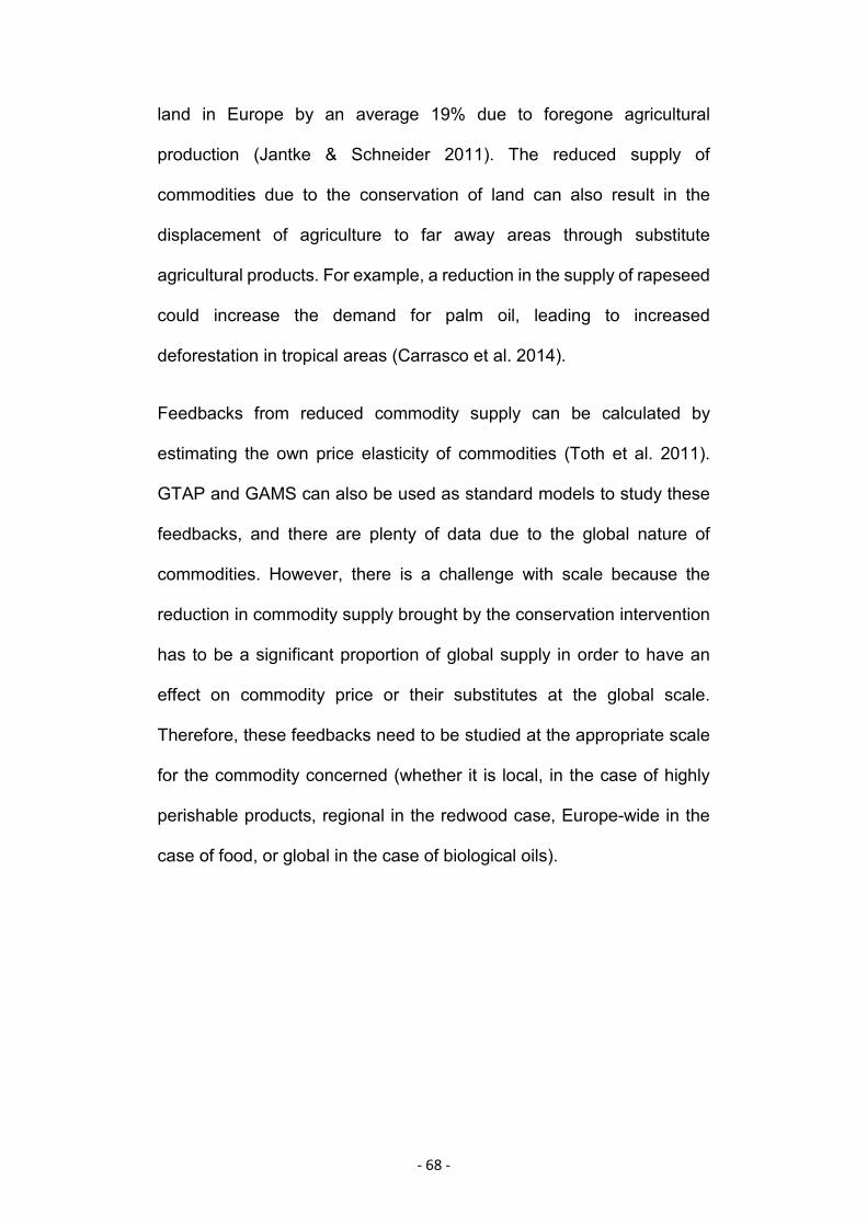
- 68 -

land in Europe by an average 19% due to foregone agricultural

production (Jantke & Schneider 2011). The reduced supply of

commodities due to the conservation of land can also result in the

displacement of agriculture to far away areas through substitute

agricultural products. For example, a reduction in the supply of rapeseed

could increase the demand for palm oil, leading to increased

deforestation in tropical areas (Carrasco et al. 2014).

Feedbacks from reduced commodity supply can be calculated by

estimating the own price elasticity of commodities (Toth et al. 2011).

GTAP and GAMS can also be used as standard models to study these

feedbacks, and there are plenty of data due to the global nature of

commodities. However, there is a challenge with scale because the

reduction in commodity supply brought by the conservation intervention

has to be a significant proportion of global supply in order to have an

effect on commodity price or their substitutes at the global scale.

Therefore, these feedbacks need to be studied at the appropriate scale

for the commodity concerned (whether it is local, in the case of highly

perishable products, regional in the redwood case, Europe-wide in the

case of food, or global in the case of biological oils).

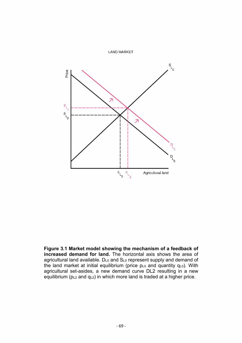
- 69 -

Figure 3.1 Market model showing the mechanism of a feedback ofincreased demand for land. The horizontal axis shows the area ofagricultural land available. DL0 and SL0 represent supply and demand ofthe land market at initial equilibrium (price pL0 and quantity qL0). Withagricultural set-asides, a new demand curve DL2 resulting in a newequilibrium (pL2 and qL2) in which more land is traded at a higher price.

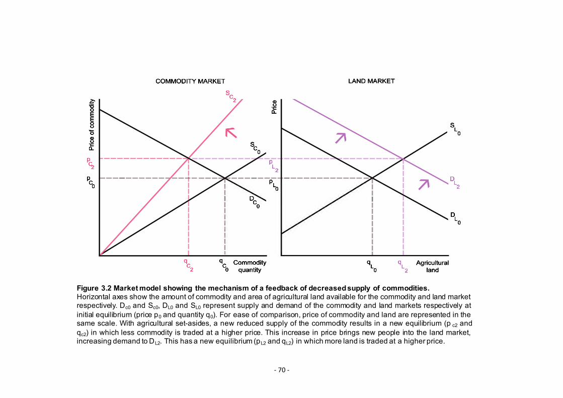
- 70 -

Figure 3.2 Marketmodel showing the mechanism of a feedback of decreasedsupply of commodities.Horizontal axes show the amount of commodity and area of agricultural land available for the commodity and land marketrespectively. Dc0 and Sc0, DL0 and SL0 represent supply and demand of the commodity and land markets respectively atinitial equilibrium (price p0 and quantity q0). For ease of comparison, price of commodity and land are represented in thesame scale. With agricultural set-asides, a new reduced supply of the commodity results in a new equilibrium (p c2 andqc2) in which less commodity is traded at a higher price. This increase in price brings new people into the land market,increasing demand to DL2. This has a new equilibrium (pL2 and qL2) in whichmore land is traded at a higher price.

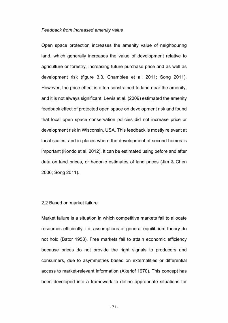
- 71 -

Feedback from increased amenity value

Open space protection increases the amenity value of neighbouring

land, which generally increases the value of development relative to

agriculture or forestry, increasing future purchase price and as well as

development risk (figure 3.3, Chamblee et al. 2011; Song 2011).

However, the price effect is often constrained to land near the amenity,

and it is not always significant. Lewis et al. (2009) estimated the amenity

feedback effect of protected open space on development risk and found

that local open space conservation policies did not increase price or

development risk in Wisconsin, USA. This feedback is mostly relevant at

local scales, and in places where the development of second homes is

important (Kondo et al. 2012). It can be estimated using before and after

data on land prices, or hedonic estimates of land prices (Jim & Chen

2006; Song 2011).

2.2 Based on market failure

Market failure is a situation in which competitive markets fail to allocate

resources efficiently, i.e. assumptions of general equilibrium theory do

not hold (Bator 1958). Free markets fail to attain economic efficiency

because prices do not provide the right signals to producers and

consumers, due to asymmetries based on externalities or differential

access to market-relevant information (Akerlof 1970). This concept has

been developed into a framework to define appropriate situations for

- 72 -

government intervention and determine the type and scope of

intervention (Zerbe Jr & McCurdy 2000).

Economists have identified situations that lead to market failure, and

most of them have been studied directly or indirectly in the context of

conservation, especially within the payment for ecosystems services

(PES) context (table 3.1). However, evidence of how market failure

situations can lead to a feedback effect of conservation interventions on

the value of land proved hard to find. Here, I focus on information failure

due to its proven effect on reducing environmental and conservation

schemes’ cost-effectiveness (Latacz-Lohmann & Schilizzi 2005; Harvey

2010; Mason & Plantinga 2013).

Informational rent capture

Information failure takes place when there is an incentive for one of the

parties in a market transaction to hide information or actions. There are

two main types of information asymmetry, hidden information and hidden

actions, which result in adverse selection and moral hazard, respectively

(Mas-Colell et al. 1995). Adverse selection happens when those with the

higher level of information are better able to make choices that benefit

them, while moral hazard is when the incentive is to conceal or mislead

others in order to benefit from the market. In terms of land markets, a

good way to think about the issue is within the principal-agent framework

(Laffont & Tirole 1993; Salanie 2005). In a transaction between a

landowner (agent) and an institution or regulator (principal), it is usually

assumed that the landowners are better informed about their costs than

- 73 -

the institutions, in the context of environmental and agricultural policy

(Wu et al. 2001; Bartolini et al. 2012). In moral hazard, the institution

cannot observe landowners’ actions, and those actions affect the

probability distribution of the outcome in a way that is costly to the

institution (Hölmstrom 1979). For example, an agro-environmental

scheme requires landowners to meet a given water quality target for a

neighbouring water body. However, the un-observability of fertilizer use

by landowners may provide an incentive to maximise private profit,

compromising the probability of meeting the target. The water target is

shared by a collective of contracted landowners, and the additional

presence of stochastic influences, such as rainfall, prevents the

regulator inferring a direct relationship between behaviour and water

quality (Harvey 2010). Therefore, the collective incentive provides a

temptation to free ride at the individual level.

In adverse selection, landowners have hidden characteristics, e.g. land

quality, that affect their cost of complying with the contract, and the

regulator cannot observe them (Akerlof 1970). For example, in the

context of conservation contracting, landowners (agents) know better

than the programme administrator (principal) about how participation (in

conservation actions) affect their production plans and profit (Latacz-

Lohmann & Schilizzi 2005). In this circumstance, there is an economic

incentive to hide the real cost of participation in the expectation of

extracting surplus rent, informational rent capture (figure 3.4). Capture

of informational rent is a concern because it leads to reduced cost-

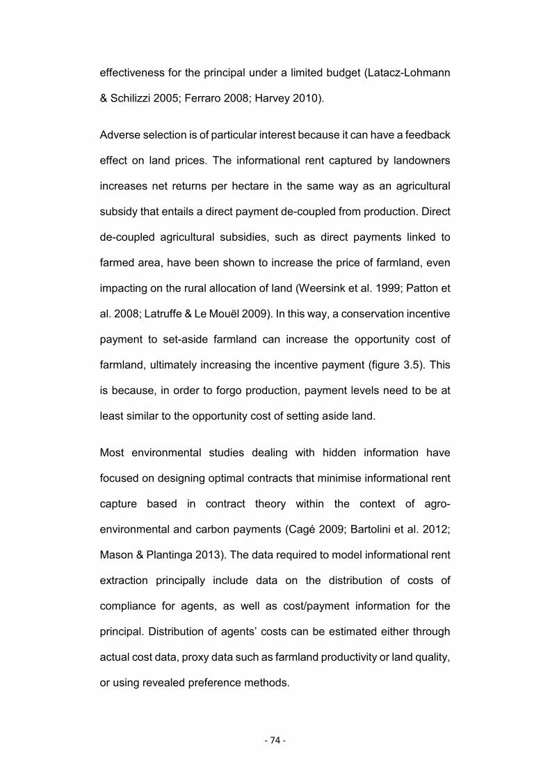
- 74 -

effectiveness for the principal under a limited budget (Latacz-Lohmann

& Schilizzi 2005; Ferraro 2008; Harvey 2010).

Adverse selection is of particular interest because it can have a feedback

effect on land prices. The informational rent captured by landowners

increases net returns per hectare in the same way as an agricultural

subsidy that entails a direct payment de-coupled from production. Direct

de-coupled agricultural subsidies, such as direct payments linked to

farmed area, have been shown to increase the price of farmland, even

impacting on the rural allocation of land (Weersink et al. 1999; Patton et

al. 2008; Latruffe & Le Mouël 2009). In this way, a conservation incentive

payment to set-aside farmland can increase the opportunity cost of

farmland, ultimately increasing the incentive payment (figure 3.5). This

is because, in order to forgo production, payment levels need to be at

least similar to the opportunity cost of setting aside land.

Most environmental studies dealing with hidden information have

focused on designing optimal contracts that minimise informational rent

capture based in contract theory within the context of agro-

environmental and carbon payments (Cagé 2009; Bartolini et al. 2012;

Mason & Plantinga 2013). The data required to model informational rent

extraction principally include data on the distribution of costs of

compliance for agents, as well as cost/payment information for the

principal. Distribution of agents’ costs can be estimated either through

actual cost data, proxy data such as farmland productivity or land quality,

or using revealed preference methods.

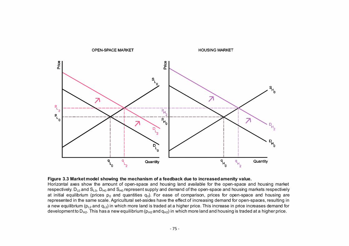
- 75 -

Figure 3.3 Marketmodel showing the mechanism of a feedback due to increasedamenity value.Horizontal axes show the amount of open-space and housing land available for the open-space and housing marketrespectively. DL0 and SL0, DH0 and SH0 represent supply and demand of the open-space and housing markets respectivelyat initial equilibrium (prices p0 and quantities q0). For ease of comparison, prices for open-space and housing arerepresented in the same scale. Agricultural set-asides have the effect of increasing demand for open-spaces, resulting ina new equilibrium (pL2 and qL2) in which more land is traded at a higher price. This increase in price increases demand fordevelopment to DH2. This has a new equilibrium (pH2and qH2) in whichmore land and housing is traded at a higher price.

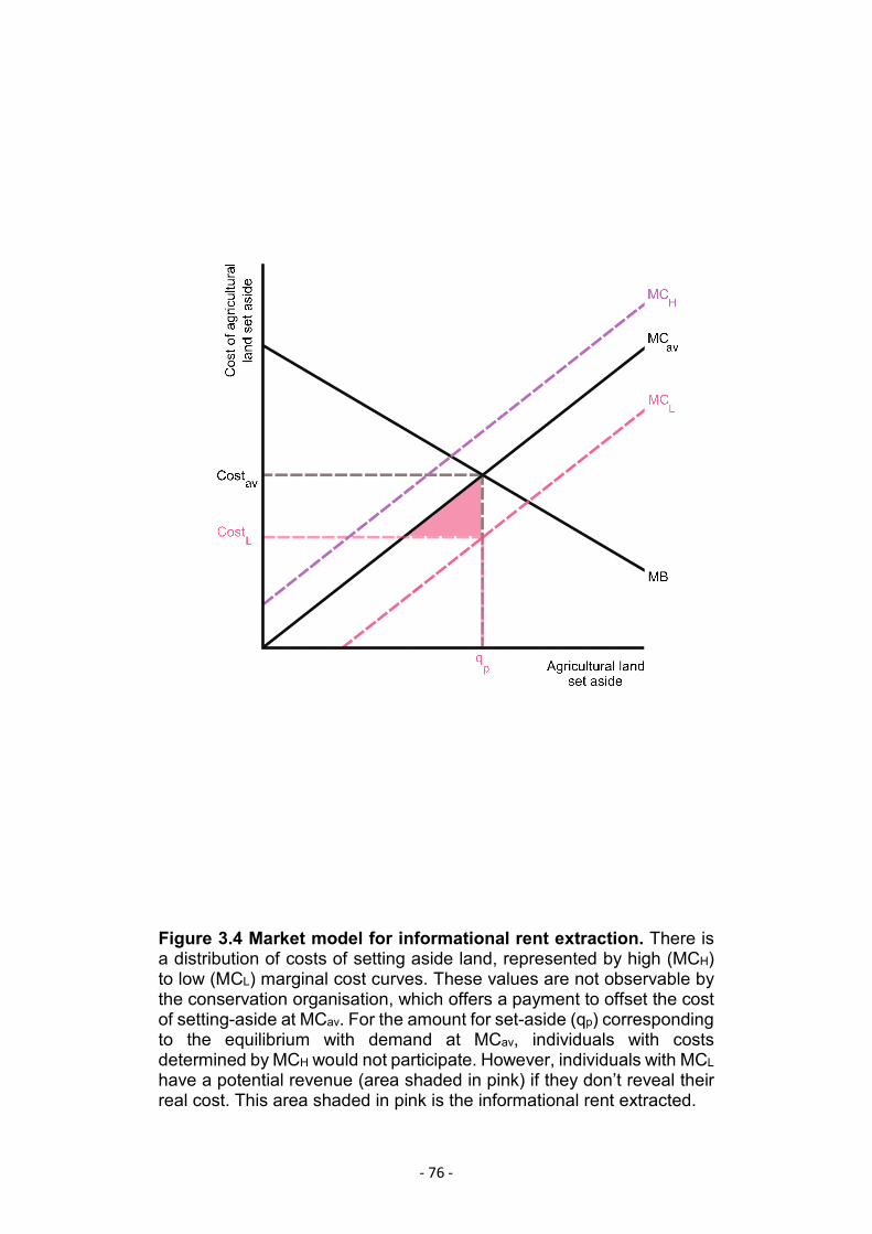
- 76 -

Figure 3.4 Market model for informational rent extraction. There isa distribution of costs of setting aside land, represented by high (MCH)to low (MCL) marginal cost curves. These values are not observable bythe conservation organisation, which offers a payment to offset the costof setting-aside at MCav. For the amount for set-aside (qp) correspondingto the equilibrium with demand at MCav, individuals with costsdetermined by MCH would not participate. However, individuals with MCLhave a potential revenue (area shaded in pink) if they don’t reveal theirreal cost. This area shaded in pink is the informational rent extracted.

- 77 -

Table 3.1 Situations that lead to market failure. These are situations in which the allocation of goods and servicesby markets is not efficient, and can occur simultaneously. The presence of any one of these situations leads to marketfailure.

Market Failure Description Examples Studies in conservation

Productive andallocativeinefficiency

Failure to produce and allocate scarceresources in the most efficient way

Moments of food shortage,disease outbreaks andvaccines

In general, ecological– economic approaches towards biodiversity are based on the idea of scarcity(Baumgärtner et al. 2006)

Monopoly powerFailure to control abuses of monopolisticpower Monopoly of services

Development of eco-tourism in the context of state's monopoly over access to forests in South India(Münster & Münster 2012)

Missing marketsFailure to form, resulting in a failure to meet aneed or want Public goods

In villages around protected areas, markets for certain resources, e.g. fuelwood, will fail to form if thetransaction costs of getting resource products to distant markets outweigh the benefits (Muller & Albers2004)

Incompletemarkets Failure to produce merit goods Education, Healthcare

About 90% of the finances for land-related PES projects in 2009 were created by command, based onincomplete markets (Vatn 2015)

De-merit goodsFailure to control the production of goods thathave less merit than consumers perceive Cigarettes, alcohol -

Negativeexternalities

Failure to take into account cost of an actionon third parties. Pollution

Ecotourism can have external costs on the resources it intends to protect, for example, in a survey ofUnited States National Park superintendents studying the adverse impacts associated with tourists,84.1% reported negative impacts of visitors on native flora and fauna (Wang & Miko 1997)

Property rightsFailure to assign property rights, which maylimit the ability of markets to form Common property

PES to provide alternatives to logging in Indonesia would not work because communities would not beable to enforce a PES agreement due to weak property rights (Engel & Palmer 2008)

Informationfailure

Failure to provide enough informationbecause there is an incentive to hideinformation

Cost of pollutionabatement

In contractual relationships involving PES, conservation buyers know less than landowners know aboutthe costs of contractual compliance. This enables landowners to extract informational rents fromconservation buyers by using their private information as a source of market power. This rent captureneeds to be minimised to improve conservation cost-effectiveness (Ferraro 2008)

Unstablemarkets Volatile markets fail to reach equilibrium

Certain agriculturalmarkets, foreignexchange, credit markets

Young markets with new instruments are unstable making prices volatile, such as carbon markets.These conditions have seen the development of subprime carbon, contracts with high risks of not beingfulfilled in terms of greenhouse gas emission reductions. This can have consequences for food securitywhen these contracts are bundled with other agricultural and non-agricultural contracts into commodityindex funds (Mol 2012)

Inequality Failure to limit the gap between earners Perpetuation of pay-gaps

International PES will entail a net upward redistribution of wealth from poorer to wealthier classes andfrom rural regions to distant centres of capital accumulation, mainly in the global North. This is becausethe market model, in which profit incentives depend upon differential opportunity costs (Mcafee 2012)

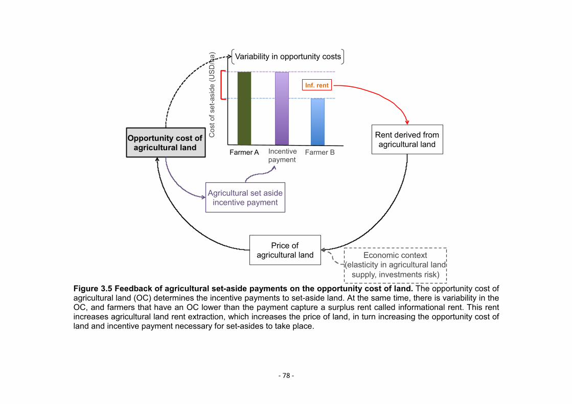
- 78 -

Figure 3.5 Feedback of agricultural set-aside payments on the opportunity cost of land. The opportunity cost ofagricultural land (OC) determines the incentive payments to set-aside land. At the same time, there is variability in theOC, and farmers that have an OC lower than the payment capture a surplus rent called informational rent. This rentincreases agricultural land rent extraction, which increases the price of land, in turn increasing the opportunity cost ofland and incentive payment necessary for set-asides to take place.

Rent derived fromagricultural land

Opportunity cost ofagricultural land

Price ofagricultural land Economic context

(elasticity in agricultural landsupply, investments risk)

Inf. rent

Costofset-aside(USD/ha)

Incentivepayment

Farmer BFarmer A

Variability in opportunity costs

Agricultural set asideincentive payment

- 79 -

3. The case study

3.1 Socio-economic context

Country Profile

Brazil has chosen a development path that heavily relies on agriculture

for economic growth (Barros 2009). Agricultural production accounts for

6% of Brazil’s gross domestic product (GDP) (SM table 2), while the

entire agribusiness sector contributes to approximately 25% of the

country’s GDP (Martinelli et al. 2010). Fifteen percent of employment is

taken up by this sector (SM table 2), and in 2016 the country’s total credit

to agriculture was ~$7,000 million USD (broad definition which includes

Forestry and Fishing, FAOSTAT), the third-highest volume in credit to

agriculture (FAO 2015).

National policies to support agriculture include macro economic

adjustments, price supports and other fiscal incentives, favourable

agricultural trade policies, and investments in research and

development. These have transformed Brazil into a powerhouse of food,

fibre and biofuel production (Barros 2009; Martinelli et al. 2010). Brazil

is the second largest food exporter (~$60,000 million USD, SM table 2),

and among the top 15 food producing countries based on net per capita

production value (FAOSTAT, FAO 2015). The country is a leading

producer and exporter of soybean, sugar, coffee, oranges, poultry, beef,

and ethanol, but is also one of the world top 10 exporters of forest

products (~$7,500 million USD in 2012, FAOSTAT, FAO 2015) (SM

table 3). Even though it is decreasing its emissions, Brazil is the third

- 80 -

largest greenhouse gas emitter in agriculture (~450 Mt CO2eq in 2012),

and the second in land use total emissions (~800 Mt CO2eq in 2012,

FAO 2015).

The success of the agricultural sector has been associated with

widespread destruction of Brazilian ecosystems, especially the Cerrado

and the Brazilian Amazon rainforest in the past decades (Cumming et

al. 2012; Walker 2012b; Rada 2013). From the year 2000, Brazil has

seen increasing intensification and commoditization of agriculture,

resulting in a decrease of ~40% in greenhouse gas emissions since

2005 and de-coupling of deforestation and agriculture (Lapola et al.

2014). For example, since the soy moratorium in 2006, only 1% of soy

expansion in the Amazon resulted in deforestation (Gibbs et al. 2015).

However, these changes in the land-use system reinforce the long-

established inequality in land ownership, contributing to rural–urban

migration that ultimately fuels the haphazard expansion of urban areas

(Lapola et al. 2014). Brazil’s status as one of the world’s most inequitable

countries in terms of income and land distribution is reinforced by this

pattern of agricultural growth, putting the sustainability of the country's

development at risk (Ocampo 2004; Martinelli et al. 2010).

Agricultural land market

The agricultural land market in Brazil has some unique characteristics,

such as low liquidity, but returns from agricultural production remain a

- 81 -

key factor in market price dynamics is (Sauer & Pereira Leite 2011).

However, other factors like yield potential, soil type, rainfall pattern and

distance from markets can influence the land market (Cavailh & Thomas

2013; Choumert & Phélinas 2015). Poor logistics infrastructure - 53% of

the national transport is based on trucks (ANEC 2012) - and the massive

average distance to ports (>1000 km) make the distance to infrastructure

an important determinant of agricultural rent (Wohlenberg 2014).

In Brazil, land markets have become very dynamic in recent years due

to the growth of agribusiness, attracting the interest of investors given

the large amount of land available for agricultural expansion (Sauer &

Pereira Leite 2012; Brewer 2015). The less developed areas of the

country, known as the agricultural frontiers, where land prices are lower

compared to traditional areas, attract the attention of investors because

by occupying marginal areas before investments in infrastructure and

transportation have occurred, there is a greater future appreciation

potential (Wohlenberg 2014). However, this variability in the elasticity of

supply of agricultural land renders typical farmland market equilibrium

analyses, which consider only factors on the demand side and make the

implicit assumption that the stock of land is constant, inapplicable

(Rezende 2002; Sauer & Pereira Leite 2012). In less occupied regions

an increase in demand for land may lead to a negative impact on land

prices because of the higher elasticity of the land supply and the

possibility of converting lands and pastures into agricultural areas,

whereas in the developed areas the relationship is positive, since land

supply is almost inelastic (Barr et al. 2011; Ferro 2012).

- 82 -

The wider economic context also has an effect on agricultural land

prices, modifying price signals. For example, in Brazil in the 1970s the

increase in the price of agricultural land was much higher than the

increase in the price of leasing land, suggesting that the benefits of land

tenure as an asset were higher than the benefits derived from

agricultural production (Ferro & Castro 2013). Speculation is an

important factor in the agricultural frontier region, different from that

observed in other regions, highlighting the strong interest of investor

groups interested in the potential of land appreciation in that region

(Ferro 2012). Wohlenberg (2014) observed that in Brazil, areas far from

end markets are exposed to greater changes in land prices and those

same areas are more susceptible to price cycles.

3.2 Forest restoration in the context of agricultural land markets

For restoration to be a successful conservation measure in the BAF,

regional level spatial conservation planning is a necessary step (Calmon

et al. 2009; Rodrigues et al. 2009). Furthermore, accounting for the

dynamics of the system, both environmental and economic, could

potentially have major impacts on spatial prioritisation outputs

(Armsworth et al. 2006; Butsic et al. 2013; Crouzeilles et al. 2015;

Goulart et al. 2015). In the following section, I assess the application of

market feedbackmodels within a spatial planning approach to prioritising

areas for forest restoration via agricultural set-asides in the BAF.

- 83 -

4. Evaluating approaches to modelling land market feedbacks for

the BAF

The BAF overlaps with 17 federative units (or states, UF) that extend

across a massive 3.4 million sq. km (40% of Brazil; SM table 5, figure

1.1 in Chapter 1). Some of these states overlap with the Cerrado biome,

and are considered part of the agricultural frontier (Rada 2013), and

others have well-developed infrastructure and farmland, for example,

Sao Paulo produces 60% of Brazil’s sugarcane production (SM table 4).

Consequently, the land market will have local, as well as regional

characteristics. Commodity production is localised for sugar cane and

oranges, with Sao Paulo generating >60% of national production.

However, for other commodities such as soybean, chicken and beef,

production is more evenly distributed between multiple states.

Therefore, defining the relevant scale for modelling market feedbacks in

the BAF is a crucial challenge. I excluded feedbacks from increased

amenity value because they were not relevant across for the case study

due to their local effects.

Feedback from increased demand for land

Large-scale restoration initiatives can become one more major

competitor for land, an increasingly scarce resource due to a larger,

more affluent human population (Smith et al. 2010). In the BAF, a large-

scale increase in the demand for agricultural land from the conservation

sector could, in theory, have a feedback effect on agricultural land price

- 84 -

(Table 3.2). Modelling the market for agricultural land can be

approached with a simple partial equilibrium model, where commonly

supply is assumed to be inelastic (Hertel 2010). However, in the BAF

this assumption does not hold (Ferro & Castro 2013), as geographical

location has a potentially strong effect on model parameters that shape

supply and demand (Wohlenberg 2014). For the spatial prioritisation to

be meaningful for ecological restoration, land markets would need to be

modelled at least at the municipality level, but the data required for local

land market modelling are not available for the BAF.

Feedback from reduced supply in commodity

Large-scale restoration could also result in agricultural production loss,

which given the role of the BAF in the global production of sugarcane,

coffee and oranges (SM table 3), could move the price of these

commodities, having an effect on the price of land for their production

(Table 3.2).

Modelling this feedback in a spatially explicit way could be done by

coupling a spatially explicit land rent model, for example, a von Thünen

model, with a global general/partial equilibrium trade model (either

GTAP or GAMS). The von Thünen model is a model of land use that

illustrates the trade-off between land values and the distance from points

of attraction, e.g. markets, in which land is allocated to the use that yields

the highest rents, and the rents of various land uses are determined by

location (von Thünen 1966). In conservation, this model has been used

- 85 -

to analyse forest cover change by considering a simple model where

land has two uses: agriculture and forest (Angelsen 2007b). The von

Thünen together with the incentive payment, determines which areas

are set-aside defining whether or not there is a decrease in the

production of commodities. The decrease in the supply of the commodity

feeds into the global general/partial equilibrium trade model, which as a

consequence finds a new price for the commodity. This new price is the

input for the von Thünen model to find the new demand for land (see

supplementary materials for a case study). However, for the feedback to

be significant, changes in the supply of the commodity have to be large

enough.

In the BAF case study, there are three commodities that could potentially

move global commodity prices, sugarcane, coffee and oranges (SM

table 3). Sugarcane and oranges are mostly produced in Sao Paulo, and

coffee in Minas Gerais (SM table 3). Figure 3.6 shows, for each

commodity, what percentage of global production is affected as a

function of the area set-aside within the major producing states. Even if

half of the existing area of each of the commodities within those states

were withdrawn from production, which is an unrealistically high target,

global supply would be affected by no more than 8%. This forgone

agricultural production might not be enough to move global commodity

price. Consequently, modelling this feedback in a spatially explicit way

might not translate into important effects on the price of land. The effect

of different set-aside amounts on global trade could be tested in

- 86 -

standardised models like GTAP, and based on results a decision could

be made whether to model the full coupled system or not.

Feedback from informational rent capture

Given the extent of the BAF, and the fact that landowners know the costs

of setting aside their agricultural land better than the agencies that will

be implementing the restoration project, informational rent capture is

practically unavoidable, producing a potentially significant feedback on

the price of land (Table 3.2). Informational rent capture models are

available in the contract theory literature (e.g. Corbett & Tang 1999;

Laffont & Martimort 2009). The biggest limitation for modelling these

feedbacks is access to data that enables the estimation of the variability

in the cost of setting aside agricultural land at a resolution that is

meaningful for the restoration programme, ecologically and

institutionally. This means enough samples of the cost of setting aside

land at, for example, the county level, allowing for the estimation of the

distribution of costs at the county level. This grain then could be

matched with ecological data without losing too much information on the

feature to be preserved. Proxies for the opportunity cost of agricultural

land can be used to estimate set-aside costs, including the price of

agricultural land and agricultural land rent estimates from production.

Informa Economics IEG FNP (http://www.informaecon-

fnp.com/english/aboutus) is the Brazilian division of the Informa

Economics group, and it operates in consulting and agribusiness

- 87 -

information. This organisation owns a 25-year database of bi-monthly

surveys of prices for agricultural properties bought/sold for the whole of

Brazil. These results in multiple observations of the cost of land for every

two-month period that are classified by land type, which are aggregated

into regions that are homogeneous in term of land price determinants

(e.g. access to markets, land use type, and climatic variables.). These

regions vary in size but are comparable to the meso-region scale in

Brazil (small groups of municipalities, for more details on the data, see

Chapter 4). This unique dataset meets all requirements to model

informational rent capture.

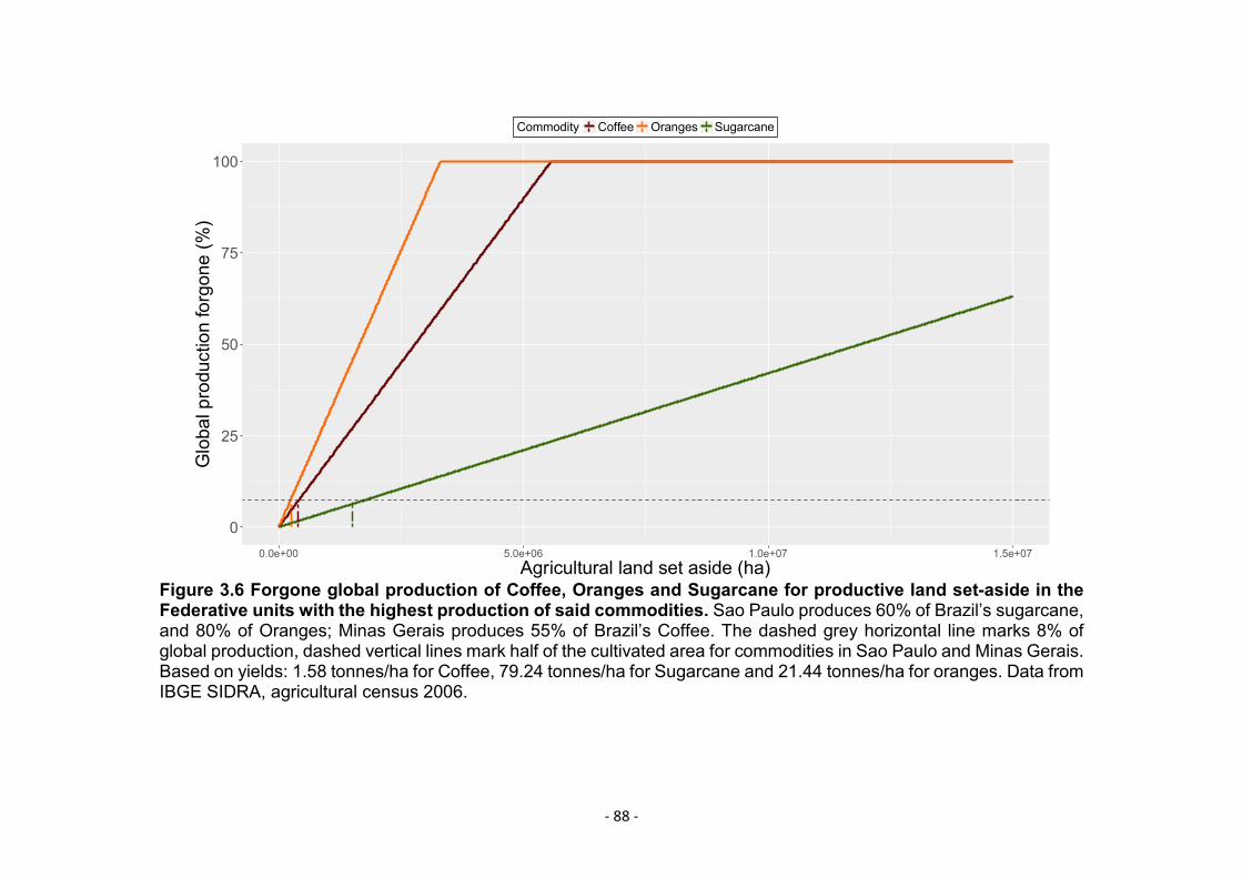
- 88 -

Figure 3.6 Forgone global production of Coffee, Oranges and Sugarcane for productive land set-aside in theFederative units with the highest production of said commodities. Sao Paulo produces 60% of Brazil’s sugarcane,and 80% of Oranges; Minas Gerais produces 55% of Brazil’s Coffee. The dashed grey horizontal line marks 8% ofglobal production, dashed vertical lines mark half of the cultivated area for commodities in Sao Paulo and Minas Gerais.Based on yields: 1.58 tonnes/ha for Coffee, 79.24 tonnes/ha for Sugarcane and 21.44 tonnes/ha for oranges. Data fromIBGE SIDRA, agricultural census 2006.

0

25

50

75

100

0.0e+00 5.0e+06 1.0e+07 1.5e+07Agricultural land set aside (ha)

Globalproductionforgone(%)

Commodity Coffee Oranges Sugarcane

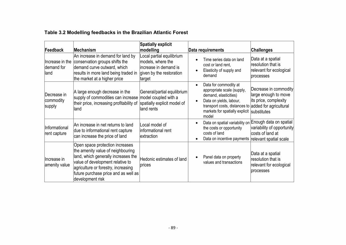
- 89 -

Table 3.2 Modelling feedbacks in the Brazilian Atlantic Forest

Feedback MechanismSpatially explicitmodelling Data requirements Challenges

Increase in thedemand forland

An increase in demand for land byconservation groups shifts thedemand curve outward, whichresults in more land being traded inthe market at a higher price

Local partial equilibriummodels, where theincrease in demand isgiven by the restorationtarget

x Time series data on landcost or land rent,

x Elasticity of supply anddemand

Data at a spatialresolution that isrelevant for ecologicalprocesses

Decrease incommoditysupply

A large enough decrease in thesupply of commodities can increasetheir price, increasing profitability ofland

General/partial equilibriummodel coupled with aspatially explicit model ofland rents

x Data for commodity atappropriate scale (supply,demand, elasticities)

x Data on yields, labour,transport costs, distances tomarkets for spatially explicitmodel

Decrease in commoditylarge enough to moveits price, complexityadded for agriculturalsubstitutes

Informationalrent capture

An increase in net returns to landdue to informational rent capturecan increase the price of land

Local model ofinformational rentextraction

x Data on spatial variability onthe costs or opportunitycosts of land

x Data on incentive payments

Enough data on spatialvariability of opportunitycosts of land atrelevant spatial scale

Increase inamenity value

Open space protection increasesthe amenity value of neighbouringland, which generally increases thevalue of development relative toagriculture or forestry, increasingfuture purchase price and as well asdevelopment risk

Hedonic estimates of landprices

x Panel data on propertyvalues and transactions

Data at a spatialresolution that isrelevant for ecologicalprocesses

- 90 -

5. Discussion

Understanding the unintended consequences of conservation

interventions via market mechanisms have been highlighted as crucial

for conservation cost-effectiveness for at least 10 years (Armsworth et

al. 2006; Polasky 2006). A few studies have addressed this need using

theoretical frameworks to show land market feedback effects of reserve

establishment in conservation planning (Armsworth et al. 2006;

Dissanayake & Önal 2011; Zvoleff & An 2014b). However, only a few

empirical applications have studied market feedbacks in conservation,

and they are at local scales, or at large scale but not in a spatially explicit

way (Walker 2012b; Butsic et al. 2013). In other fields, however, such as

land economics, these assessments are commonplace, and modelling

and data analysis approaches are well established (Quigley & Rosenthal

2005; van Meijl et al. 2006). Therefore, there is considerable potential

for modelling land market feedbacks and their potential effects on

conservation. In this chapter, I took a case study area, the BAF, as an

example of an area where large-scale conservation-focused land use

change is planned, in the form of a forest restoration programme. I

assessed the degree to which different land market feedbacks are likely

for this area, and how these might be modelled.

This assessment found two main limitations for large-scale empirical

applications: firstly, modelling land market feedbacks requires spatially

explicit data on land markets at a spatial and temporal resolution that is

not easily available, particularly for the more remote, developing country

regions where conservation effort is often focussed. Secondly, even for

- 91 -

countries such as Brazil, that are leading agricultural exporters, moving

land into conservation might not have a large enough impact on global

commodity price to cause a feedback via forgone agricultural production.

If production is mainly for local consumption, a model of the local market

could show strong feedback effects of forgone agriculture. However,

most commodities are globally traded so a reduction in local supply could

be easily met with supply from markets outside the local production,

negating an effect on price. Consequently, modelling the feedbacks of

forgone agriculture is unlikely to show an effect.

Increasingly, conservation organisations are moving towards cost-

effective conservation, which has led to the adoption of systematic

conservation planning approaches across the globe and multiple spatial

conservation plans even for the same regions (McIntosh et al. 2016).

Large-scale spatial prioritisations need a spatial unit that will reflect the

ecological process being preserved (Margules & Pressey 2000b).

However, the spatial grain over which socio-economic data are available

is often much coarser than the spatial grain that the prioritisation needs

to respond to on the conservation side, whether for ecological or

institutional reasons (Armsworth 2014). This mismatch between the

scale at which socio-economic data are available and the scale at which

priorities have to be set from the ecology perspective, is an obstacle to

accounting for market dynamics in spatial planning. Finding ways of

bridging this mismatch, such as using simulations that bring the datasets

into the same spatio-temporal resolution, are key to the integration of

market dynamics in spatial conservation planning.

- 92 -

In the BAF case study, three of the proposed feedbacks on the price of

land have the potential to be significant; these are informational rents,

feedbacks on land prices, and feedbacks through prices of foregone

agricultural production. Given the spatial scale covered in restoring the

BAF, informational rent capture has the potential to be quite large,

potentially having a significant effect on project cost-effectiveness. Due

to the limited amount of exploration, this topic has had in conservation

planning, modelling this feedback could provide new insight into the role

of this type of market failure in determining priorities for conservation.

Additionally, a comparative empirical assessment of the relative

importance of feedbacks via the price of land could also prove important.

In some particularly developed states, such as Sao Paulo, all four

feedbacks (including the fourth feedback, amenity value) have the

potential to be important, and being the richest state, it has high-

resolution socio-economic data available.

Payment for ecosystems services, in this case, to set-aside agricultural

land, are a conservation intervention centred on providing an economic

incentive for changing behaviour (Wunder 2006; Daily & Matson 2008).

As such, this incentive will interact with other economic incentives within

the political context (Jack et al. 2008). Incentive-based mechanisms

include charges (such as taxes, user fees, and deposit–refund systems),

subsidies, tradable permits (including markets for pollution reduction and

tradable development rights), and market friction reduction (e.g., liability

rules and information programs) (Jaffe et al. 2003). Interactions between

mechanisms instituted for conservation and those instituted for other

- 93 -

reasons and by other sectors could amplify or reduce the effect of

conservation-induced market feedbacks. For example, a PES that

reduces farmland area competes directly with land-linked direct

subsidies for agriculture, trading off one incentive for another (Latruffe &

Le Mouël 2009). However, PES schemes can increase the average yield

of farmland by pushing out of production the least productive areas

(Angelsen 2010). Consequently, in countries (such as Brazil) where

taxes to agricultural land are based on the number of hectares under

agricultural use, conservation-motivated PES schemes could have a

larger impact on the price of land because they reduce property tax, but

increase average yield. Therefore, there is a key research need in

understanding the interactions between conservation-motivated

incentive mechanisms and incentive mechanisms that are already in

place to address priorities in other parts of the economy. This has not

been traditionally researched in conservation science, although there is

increasing focus on navigating trade-offs between different conservation

targets at the global level, as well as trade-offs between provision of

different ecosystem services at the landscape level (e.g. (Seppelt et al.

2011; Lester et al. 2013; Castro et al. 2014)).

A serious potential feedback effect of protecting land is displacement of

exploitation to distant areas (Angelsen 2007a). A key challenge for large-

scale restoration initiatives is avoiding displacement of land uses, or

leakage, which can result in loss of biodiversity in distant parts of the

same country, or different countries (Schwarze et al. 2002; Melo et al.

2013b). This is beyond the scope of this chapter, but it something that is

- 94 -

important to bear in mind for future research; general equilibrium and

partial equilibrium models could be of use in predicting the potential for

leakage at different scales (Carrasco et al. 2014).

In Brazil, the economic focus on agriculture for development poses a

further challenge to integrating large scale restoration and increased

agricultural production, at the national level (Alves-Pinto et al. 2017).

Restoration in areas with high cattle productivity in the BAF has been

shown to increase the risk of cattle ranching displacement to other

biomes (Latawiec et al. 2015). Even restricting deforestation in the BAF,

which results in little loss of national GDP, has disproportionate impact

on the agricultural and food sector because of the high importance of the

BAF area for agricultural production (de Souza Rodrigues Cabral &

Gurge 2014). However, the BAF presents a unique opportunity for large-

scale restoration due to its high potential for improved agricultural

efficiency (Joly et al. 2014a). For example, even though Brazil is among

the biggest beef producers worldwide (FAOSTAT, 2015), cattle ranching

is based on an extensive system with a stocking rate that is

approximately 33% of its sustainable potential (Strassburg et al. 2014a).

It has been suggested that combined efforts to promote sustainable

intensification, accompanied by other strategies such as diversification

of activities and PES for restoration, could result in tropical forest

restoration without risking perverse outcomes for food production and

development in Brazil (Brancalion et al. 2012; Pinto et al. 2014; Alves-

Pinto et al. 2017).

- 95 -

6. Conclusion

Large-scale restoration projects can trigger multiple economic feedback

effects that can potentially undermine the overall outcome. However,

socio-economic data availability, a mismatch in scale between data

availability and prioritisation grain, and economic model complexity

present restrictions to accounting for these feedbacks in spatial

conservation planning. The BAF presents a unique opportunity in terms

of scale and policy relevance for accounting for economic feedbacks,

and I identify an informational rent capture feedback as the most relevant

and potentially informative to model. This chapter provides valuable

insight into accounting for economic dynamics in a real-life case study;

the remaining outstanding questions could provide guidance for future

work.

- 96 -

Chapter 4: Spatial conservation planning accounting for

environmental and economic feedbacks

- 97 -

1. Introduction

In order to design cost-effective interventions, conservation planners

need to consider both social and ecological dynamics throughout the

planning process. In systematic conservation planning, effectiveness

depends partly on accounting for natural and anthropogenic dynamics

(Pressey et al. 2007). Nonetheless, many organisations do not go

beyond mapping to identify priority areas when undertaking conservation

planning (McIntosh et al. 2016), either based on primary data or models,

which cannot account for feedbacks caused by the planned intervention.

The most widely used tools for spatial conservation planning still use

static approaches to derive priority solutions (Larrosa et al. 2016),

including Marxan (Ball et al. 2009), which is unable to easily integrate

stochastic or temporally dynamic data (Ardron et al. 2010).

Ecosystem dynamics have been included in conservation planning using

dynamic optimization methods for natural resource management

problems and restoration (Wilson et al. 2011; Williams & Johnson 2013).

Modelling of vegetation succession dynamics has been done with the

conservation planning software “Marxan with Zones” to incorporate

ecological dynamics in decision-making (Levin et al. 2013). The impact

of social processes on conservation planning outcomes has been

demonstrated by incorporating development risk (Costello & Polasky

2004) and market feedbacks (Wu et al. 2001, Butsic et al. 2013, Duke et

al. 2013) into reserve selection. Armsworth et al. (2006) showed using a

theoretical model that buying land to protect it could lead to an increased

probability of habitat conversion elsewhere in the landscape and result

- 98 -

in overall biodiversity losses. This is because the act of buying land

increases its market price and accelerates its development. Land market

feedbacks triggered by the conservation purchases themselves could,

therefore, lead to undermined and even perverse outcomes. Some

studies have shown that dynamic conservation planning improves

project cost-effectiveness (Tambosi 2014), whilst in others, the benefits

were not so clear (Butsic et al. 2013). However, the joint effect of land

market feedbacks together with ecosystem dynamics has yet to be

empirically assessed in conservation planning.

Ecological set-asides on private land are a promising strategy to

preserve biodiversity and ecosystem services across farming

landscapes, especially where large numbers of small purchases are

required (Dobson et al. 2006). Setting aside private land for conservation

nonetheless comes with financial costs to the landowner, and in order to

forgo production, incentive payments need to be at least similar to the

opportunity cost of setting aside land. As shown in chapter 3,

conservation interventions that promote land cover changes can have

an effect on land prices via market feedbacks due to changes in the

supply and demand for land and agricultural commodities. These

changes in land price could lead to larger incentive payments in the

future, increasing the overall cost of the program, or affecting ecological

outcomes when the budget is limited.

Another mechanism by which feedback effects of a set-aside program

can increase the price of land is through the capture of informational rent.

- 99 -

After owning land for a length of time, landowners form a better idea of

the cost of setting aside land than conservation agents. This is called

asymmetric information, and it is a type of market failure mechanism,

meaning that market prices do not provide the proper signals for the

efficient allocation of resources (Akerlof 1970). Landholders in such

circumstances can use their private information as a source of market

power to extract informational rent from conservation agents (Ferraro

2008). For example, consider a program where farmers receive a

payment to set-aside land for biodiversity: if the payment value is higher

than the opportunity cost of the area to be set-aside, there is an

informational rent captured by the farmers. By increasing net returns per

hectare, the programme therefore indirectly increases the price of

farmland (chapter 3).

Informational rent capture has been discussed in the conservation

literature as something to be avoided or minimized in order to increase

the effectiveness of incentive-based conservation interventions (Ferraro

2008; Ulber et al. 2011; Mason & Plantinga 2013). Reducing

informational rent capture is an important task for buyers of

environmental services who wish to maximize the services obtained

from their limited budgets. One way of reducing informational rent

capture is by obtaining information on observable landowner attributes

that are correlated with opportunity costs, which can be costly and still

be inaccurate (Ferraro 2008). Another way of reducing informational rent

include revelation mechanisms, which entail designing contracting

systems to induce landowners to reveal their hidden information, and are

- 100 -

increasingly used for payment for ecosystem services (PES) contract

design. They tend to increase programme cost-effectiveness, but the

amount by which they do so depends on a number of things, such as

how much information on potential conservation benefits and timeline is

revealed to landowners, the auction pricing rule, and whether it is a static

(one bidding period) or dynamic (multiple bidding periods) market setting

(de Vries & Hanley 2016). Additionally, achieving fairness in PES

through auctions has been shown to be very challenging (Narloch et al.

2013). Costs of reducing that information gap through either mechanism

will increase with programme scale, and might even not be feasible for

large-scale programs. Reducing the information gap for increased cost-

effectiveness might not be beneficial at large scales due to the

associated costs, or when issues of fairness are considered. Within this

context, the role informational rent capture plays at large spatial scales

in spatial conservation planning is particularly relevant, and has yet to

be assessed.

There is a gap in the conservation planning literature on accounting

simultaneously for social and environmental system dynamics when

prioritising for a conservation intervention. Additionally, there is a need

to evaluate empirically the economic dynamics triggered by conservation

interventions at large scales. The aim of this chapter is to address these

gaps focusing on a farmland set aside restoration programme for the

Brazilian Atlantic Forest. I propose the first, to the best of my knowledge,

methodological framework to prioritise a large-scale set aside

programme that enables accounting for both environmental and social

- 101 -

feedbacks simultaneously. The environmental feedback modelled

accounts for changes in forest connectivity using forest increment

experiments, and the economic feedback modelled accounts for

changes in the opportunity cost of farmland promoted by informational

rent capture. I evaluate the trade-offs between a static and a discrete

dynamic prioritisation approach by comparing their outputs for the same

case study. I characterise the role informational rents play in a large-

scale prioritisation, and examine how both approaches affect it. Finally,

I assess the degree to which ecological and economic characteristics of

a prioritisation unit influence which is the best prioritisation approach for

different metrics.

- 102 -

2. Methods

2.1 Case Study

The Brazilian Atlantic forest (BAF) is a key global biodiversity hotspot

due to its exceptional biodiversity and extreme land cover disturbance

(Mittermier et al. 2004). It is a highly fragmented landscape that spans 8

biogeographical subregions of the Brazilian Atlantic Coast: Brejos

Nordestinos, Pernambuco, Diamantina, Bahia, Serra do Mar, Sao

Francisco, the Interior Forests (Florestas de Interior), and the Brazilian

Pines Forests (Florestas de Araucaria). Over 125 million people (or 70%

of the Brazilian population) live along the Brazilian Atlantic coast, and

the main threats to the biome are timber exploitation and agricultural

expansion (Saatchi et al. 2001).

Forest fragmentation in the BAF is a major cause of forest species losses

within the isolated forest remnants (Cardoso da Silva & Tabarelli 2000).

Restoration efforts have been underway for the past 30 years, but

scaling up restoration projects and planning restoration actions at the

landscape level remains a major challenge (Rodrigues et al. 2009; Melo

et al. 2013b). Landscape level forest connectivity regulates species level

biodiversity, wildlife movement, seed dispersal and ecological factors,

and so increasing it is an important target for biodiversity conservation

strategies (Shanthala Devi et al. 2013). Preserving large existing

remnants is crucial, as they provide a refuge to many species, however,

there is also an urgent need for restoration to ensure that biodiversity-

derived ecological functions are provided across the BAF (Banks-Leite

- 103 -

et al. 2014b). In this chapter, I focus on ecological set-asides of private

land across farmlands as a strategy for the restoration of the BAF.

Although there are potentially many different costs associated with

restoration, I considered only incentive payment costs. I centred on

natural restoration, excluding active restoration costs because the

incentive payment is the central cost affected by economic feedback

effects (chapter 3).

Under the Convention on Biological Diversity's Aichi Targets, Brazil has

set a target for the “…restoration of at least 15% of degraded

ecosystems, prioritizing the most degraded biomes, hydrographic

regions and ecoregions…” by 2020 (National Target 15, www.cbd.int). I

used this as the policy target for forest restoration, under the

interpretation that the BAF is a heavily degraded biome and 15% of the

remaining biome needs to be restored. I calculated the restoration target

as of 15% of existing forest in each municipality for all the BAF, which

amounts to restoring a total of 2.68 million hectares (M ha) (table 4.1).

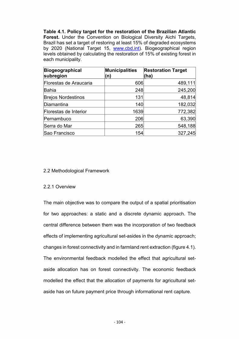
- 104 -

Table 4.1. Policy target for the restoration of the Brazilian AtlanticForest. Under the Convention on Biological Diversity Aichi Targets,Brazil has set a target of restoring at least 15% of degraded ecosystemsby 2020 (National Target 15, www.cbd.int). Biogeographical regionlevels obtained by calculating the restoration of 15% of existing forest ineach municipality.

Biogeographicalsubregion

Municipalities(n)

Restoration Target(ha)

Florestas de Araucaria 606 489,111Bahia 248 245,200Brejos Nordestinos 131 48,814Diamantina 140 182,032Florestas de Interior 1639 772,382Pernambuco 206 63,390Serra do Mar 265 548,188Sao Francisco 154 327,245

2.2 Methodological Framework

2.2.1 Overview

The main objective was to compare the output of a spatial prioritisation

for two approaches: a static and a discrete dynamic approach. The

central difference between them was the incorporation of two feedback

effects of implementing agricultural set-asides in the dynamic approach;

changes in forest connectivity and in farmland rent extraction (figure 4.1).

The environmental feedback modelled the effect that agricultural set-

aside allocation has on forest connectivity. The economic feedback

modelled the effect that the allocation of payments for agricultural set-

aside has on future payment price through informational rent capture.

- 105 -

The main implementation difference between the two approaches was

in the temporal scale (figure 4.2). The static approach entails one spatial

prioritisation event, and the sequential allocation of set-asides in three

time-steps. From now on the “dynamic approach” refers to a discrete

time step-wise approach to the spatial planning exercise, which includes

three spatial prioritisation events, one at each time step (for more details

see the “Temporal Scale” section below).

Figure 4.2. Time scale schedule for the static and dynamic spatialprioritisation approaches. The prioritisation is run using Marxan. R=farmland rent extraction ($/ha), forest connectivity increment (ha)

STATIC

Time

1.Calculate R2.Calculate dIIC3.Run prioritization4.Set aside allocation

ts=1 ts=2

1.Update R2.Update dIIC3.Run prioritization4.Set aside allocation

ts=3

1.Update R2.Update dIIC3.Run prioritization4.Set aside allocation

DYNAMIC

- 106 -

The spatial conservation planning exercise was set to meet two

conservation targets, a restoration and a forest connectivity target, at the

minimum possible cost. It involved four steps: (1) calculation of base

metrics from data, (2) calculation of prioritisation inputs, (3) spatial

prioritisation, and (4) solution assessment and implementation (figure

4.1). For the dynamic approach, there was a fifth step at each time step:

updating prioritisation input variables (figures 4.1 & 4. 2).

2.2.2 Scales, Units and Variables

Temporal scales

The static approach entailed one spatial conservation planning exercise

at time step one, that involved the four steps above mentioned (figures

4.1 & 4.2). Following the prioritisation solution, total set-aside allocation

is divided into three equal parts, and implemented one part at each time

step within a nine-year period. This is a meaningful time horizon both for

forest regeneration (Metzger et al. 2009) and program commitment

(Banks-Leite, pers. comm.).

The dynamic approach was discrete, where time moved forward in

steps. One time step represented three years, over a period of nine

years. In the first time step, I ran a spatial conservation planning exercise

in which municipalities were prioritised to be part of the set-aside

programme for the whole nine-year period, and the restoration target for

that time step was one-third of the total restoration target. For the second

- 107 -

and third time steps, the same process was repeated with updated

prioritisation inputs, the only difference being the time for which

municipalities could be part of the programme (six and three years

respectively). At each time step, the approach entailed one spatial

conservation planning exercise that involved the four steps above

mentioned (figures 4.1 & 4.2).

Spatial scales

There were three spatial scales of relevance to the study: municipality,

biogeographical subregion (BR) level, and whole biome (BAF) level.

Approximately 3,400 municipalities were included in the analysis,

covering an area of 212M ha. Municipalities were grouped by the 8

biogeographical subregions that span the BAF, which were analysed

separately to ensure all subregions are represented in the priority areas,

thereby maximizing beta diversity for the whole Atlantic Forest biome

(after Tambosi et al. 2014).

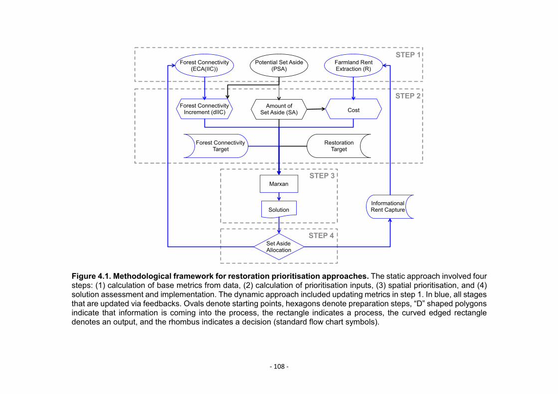
- 108 -

Figure 4.1. Methodological framework for restoration prioritisation approaches. The static approach involved foursteps: (1) calculation of base metrics from data, (2) calculation of prioritisation inputs, (3) spatial prioritisation, and (4)solution assessment and implementation. The dynamic approach included updating metrics in step 1. In blue, all stagesthat are updated via feedbacks. Ovals denote starting points, hexagons denote preparation steps, “D” shaped polygonsindicate that information is coming into the process, the rectangle indicates a process, the curved edged rectangledenotes an output, and the rhombus indicates a decision (standard flow chart symbols).

STEP 1

Forest ConnectivityTarget

RestorationTarget

STEP 2

Forest Connectivity(ECA(IIC))

Forest ConnectivityIncrement (dIIC)

Farmland RentExtraction (R)

Cost

Potential Set Aside(PSA)

Amount ofSet Aside (SA)

Marxan

Solution

Set AsideAllocation

STEP 3

STEP 4

InformationalRent Capture

- 109 -

Units

The unit of analysis was a municipality because it is meaningful in policy

terms, and a good compromise between the ecological and social data

available (table 4.2). All municipalities that had at least 10 ha of forest

within them were included in the analysis.

Instead of using the municipality boundary as a hard limit for forest

connectivity, I calculated a one-kilometre buffer around the municipality’s

boundary and included all forest patches that fell within this buffer in the

calculation of forest connectivity. This was done to include information

about the municipality’s immediately neighbouring forest, as well as

avoiding problems in forest connectivity metrics created by the artificial

limits of municipalities’ boundaries.

For all forest patches, I delimited a one-kilometre buffer area where set-

asides could occur; meaning that in the forest increment experiments

new forest patches could only be created in this potential set-aside area

(PSA). This radius is considered a relevant landscape context for bird

species occurrence in the BAF (Boscolo & Metzger 2011), and provides

a good threshold distance for the establishment of early succession

woody species and natural regeneration (Scervino & Torezan 2015).

Land classes that cannot regenerate into forest, such as urban areas,

dunes, flood lands and large water bodies were excluded from the PSA.

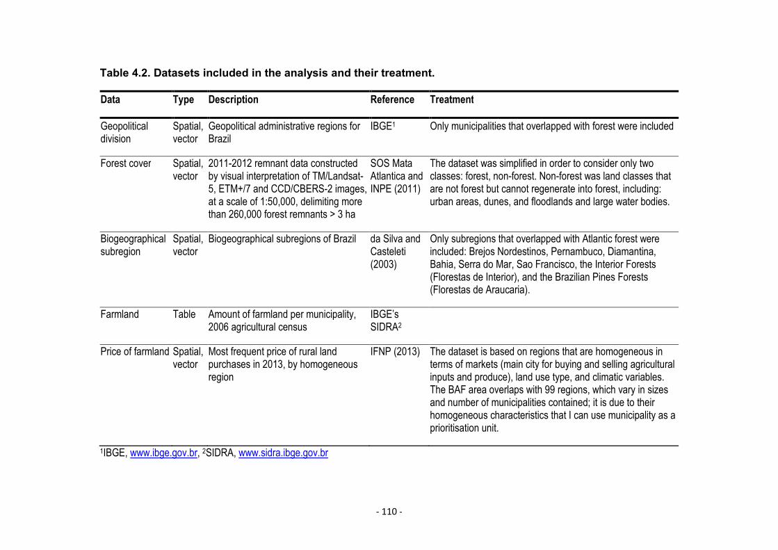
- 110 -

Table 4.2. Datasets included in the analysis and their treatment.

Data Type Description Reference Treatment

Geopoliticaldivision

Spatial,vector

Geopolitical administrative regions forBrazil

IBGE1 Only municipalities that overlapped with forest were included

Forest cover Spatial,vector

2011-2012 remnant data constructedby visual interpretation of TM/Landsat-5, ETM+/7 and CCD/CBERS-2 images,at a scale of 1:50,000, delimiting morethan 260,000 forest remnants > 3 ha

SOS MataAtlantica andINPE (2011)

The dataset was simplified in order to consider only twoclasses: forest, non-forest. Non-forest was land classes thatare not forest but cannot regenerate into forest, including:urban areas, dunes, and floodlands and large water bodies.

Biogeographicalsubregion

Spatial,vector

Biogeographical subregions of Brazil da Silva andCasteleti(2003)

Only subregions that overlapped with Atlantic forest wereincluded: Brejos Nordestinos, Pernambuco, Diamantina,Bahia, Serra do Mar, Sao Francisco, the Interior Forests(Florestas de Interior), and the Brazilian Pines Forests(Florestas de Araucaria).

Farmland Table Amount of farmland per municipality,2006 agricultural census

IBGE’sSIDRA2

Price of farmland Spatial,vector

Most frequent price of rural landpurchases in 2013, by homogeneousregion

IFNP (2013) The dataset is based on regions that are homogeneous interms of markets (main city for buying and selling agriculturalinputs and produce), land use type, and climatic variables.The BAF area overlaps with 99 regions, which vary in sizesand number of municipalities contained; it is due to theirhomogeneous characteristics that I can use municipality as aprioritisation unit.

1IBGE, www.ibge.gov.br, 2SIDRA, www.sidra.ibge.gov.br

- 111 -

Within municipalities, I defined Forest Landscape (FL) as the area of

existing forest plus its corresponding PSA. Defining landscapes for

restoration is a controversial issue. Studies in the BAF region have used

a range of landscape sizes that vary from 10 to 10,000 hectares to define

landscapes for forest dwelling species (Tambosi et al. 2014).

Approximately 87% of FL areas fell within this size interval.

Variables

The variables used to evaluate restoration priorities, calculated in step 2

(figure 4.1), were forest connectivity increment (dIIC, ha), cost (USD,

from now on $) and contribution to the restoration target (amount of set-

aside (SA), ha) at the municipality level. I used dIIC to assess set-asides

that resulted in the largest increases in forest connectivity in the long

term, given that passive restoration is not an instant process of forest

restoration. Target achievement was assessed at the biogeographical

subregion level.

Variables used to compare approaches (static vs. dynamic) were cost

($), forest connectivity increment (ha), informational rent capture ($), set-

aside cost-effectiveness (ha/$), forest connectivity increment cost-

effectiveness (ha/$), and proportional informational rent capture

(proportion of each $ spent that is captured as informational rent). These

variables were compared for the whole BAF, as well as subregion and

municipality levels (variables were divided by hectares set-aside for

comparability), and across time (variables were divided by years in

programme for comparability).

- 112 -

2.2.3 Data and software

Data

The datasets that form the basis for this analysis are forest cover,

geopolitical divisions, biogeographical subregions (BRs), farmland

availability and price of farmland (table 4.2).

Forest cover was based on the BAF 2011-2012 remnant data

constructed by visual interpretation of TM/Landsat-5, ETM+/7 and

CCD/CBERS-2 images, at a scale of 1:50,000, delimiting more than

260,000 forest remnants > 3 ha (SOS Mata Atlantica & INPE 2011). The

dataset was simplified in order to consider only two classes: forest, non-

forest. Non-forest included land classes that are not forest but cannot

regenerate into forest, including urban areas, dunes, and flood lands and

large water bodies.

Land price was based on the 2013 yearbook of the purchase price of

rural land (IFNP 2013). A survey of prices for properties bought/sold is

the central land price data. The structure of the dataset is based on

regions and land types. The country was divided into 133 regions that

are homogeneous considering markets (main city for buying and selling

agricultural inputs and produce), land use type, and climatic variables.

For each region, main “land types” were identified using a classification

based on land use type, distance to market, soil type, climatic variables,

level of agricultural intensification, mechanization possibilities, distance

to rivers, elevation and slope, current and past vegetation, and other

variables that affect land prices in each specific region. There are over

- 113 -

1000 land types for Brazil, each with their land price. For each region

and land type, the most frequent purchase value is published in R$/ha

(reais per hectare) and USD/ha. The BAF area overlaps with 99 regions,

which vary in sizes and number of municipalities contained; it is due to

the regions' homogeneous characteristics that I can use municipality as

the prioritisation unit. For the analysis, the original dataset land-types

were re-classified into two categories: farmland (included pasture and

agricultural land types) and other (land that cannot be set-aside for

restoration because it would not regenerate into forest, including forest

itself, and ecosystems that are not forest, such as Cerrado and

Caatinga).

The geopolitical administrative regions (2013) spatial dataset was

obtained from the Brazilian Institute of Geography and Statistics (IBGE,

www.ibge.gov.br) in January 2015. Farmland availability per municipality

was obtained from Brazil’s 2006 agricultural census at IBGE’s Automatic

Recovery System (SIDRA, www.sidra.ibge.gov.br) in May 2015.

Farmland included the area of crops, pasture and agroforestry.

Biogeographical subregions (BR) data were obtained from da Silva and

Casteleti (2003).

Software

The central software used in this analysis was R 3.2.1 (R Core Team

2016), used for data manipulation, modelling, figure creation and from

which other software were called to run. ArcGIS 10 (Esri 2011) and

Python 3.5.2 (https://www.python.org) were used for data visualization,

- 114 -

data manipulation and figure creation. Conefor Sensinode 2.5.8

command line version (Saura & Torné 2009) was used for forest

connectivity calculation, and MARXAN (Ball et al. 2009) was used for

spatial prioritisation planning.

2.2.4 Spatial conservation planning exercise (figure 4.1)

2.2.4 Step 1: Calculation of base metrics

Potential set-aside (PSA)

Potential set-aside (PSA) is the area of the forest landscape (FL) that is

available for regeneration, and it is calculated as FL area minus forest

area for each municipality.

Forest connectivity (ECA(IIC))

I used a graph theory approach to evaluate landscape connectivity, due

to its simplicity of representation, robustness, predictive power, and high

potential to incorporate connectivity functional attributes (Urban & Keitt

2001). The integral index of connectivity (IIC, Pascual-Hortal and Saura

2006) is recommended as the best binary index for the type of

connectivity analysis performed, presenting consistent and robust

behaviour for analysing landscape changes (Saura & Pascual-Hortal

2007). IIC has been applied in many conservation planning case studies

(Saura et al. 2011a), as well as for landscape monitoring purposes

(Rappaport et al. 2015a), due to its suitability for evaluating the impact

of spatial changes on functional landscape connectivity.

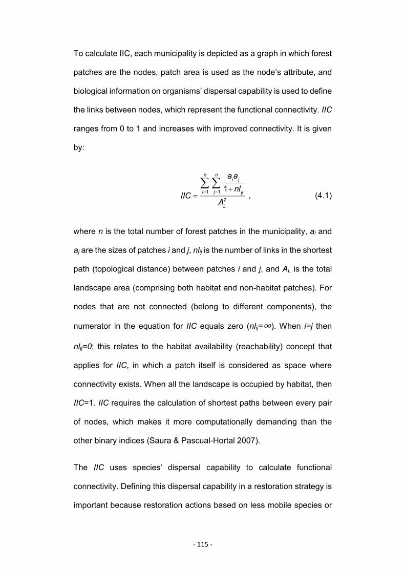
- 115 -

To calculate IIC, each municipality is depicted as a graph in which forest

patches are the nodes, patch area is used as the node’s attribute, and

biological information on organisms’ dispersal capability is used to define

the links between nodes, which represent the functional connectivity. IIC

ranges from 0 to 1 and increases with improved connectivity. It is given

by:

, (4.1)

where n is the total number of forest patches in the municipality, ai and

aj are the sizes of patches i and j, nlij is the number of links in the shortest

path (topological distance) between patches i and j, and AL is the total

landscape area (comprising both habitat and non-habitat patches). For

nodes that are not connected (belong to different components), the

numerator in the equation for IIC equals zero (nlij=∞). When i=j then

nlij=0; this relates to the habitat availability (reachability) concept that

applies for IIC, in which a patch itself is considered as space where

connectivity exists. When all the landscape is occupied by habitat, then

IIC=1. IIC requires the calculation of shortest paths between every pair

of nodes, which makes it more computationally demanding than the

other binary indices (Saura & Pascual-Hortal 2007).

The IIC uses species' dispersal capability to calculate functional

connectivity. Defining this dispersal capability in a restoration strategy is

important because restoration actions based on less mobile species or

IIC =

aiaj1+ nlijj=1

n

Âi=1

n

ÂAL2

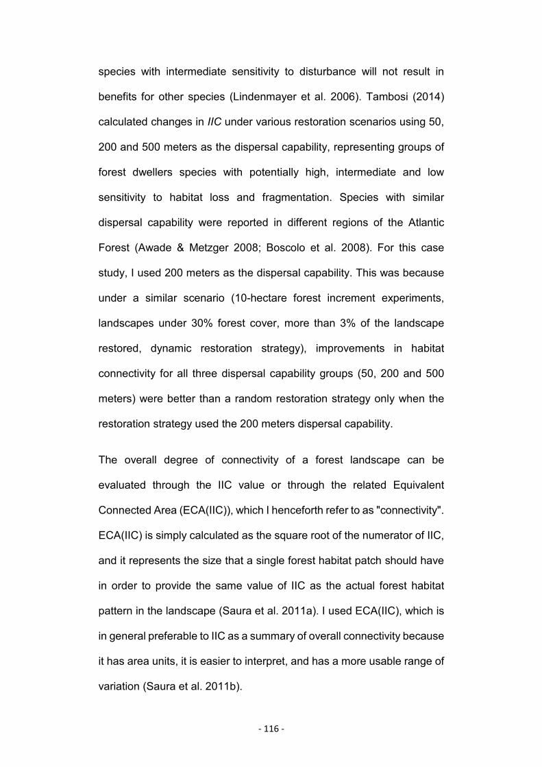
- 116 -

species with intermediate sensitivity to disturbance will not result in

benefits for other species (Lindenmayer et al. 2006). Tambosi (2014)

calculated changes in IIC under various restoration scenarios using 50,

200 and 500 meters as the dispersal capability, representing groups of

forest dwellers species with potentially high, intermediate and low

sensitivity to habitat loss and fragmentation. Species with similar

dispersal capability were reported in different regions of the Atlantic

Forest (Awade & Metzger 2008; Boscolo et al. 2008). For this case

study, I used 200 meters as the dispersal capability. This was because

under a similar scenario (10-hectare forest increment experiments,

landscapes under 30% forest cover, more than 3% of the landscape

restored, dynamic restoration strategy), improvements in habitat

connectivity for all three dispersal capability groups (50, 200 and 500

meters) were better than a random restoration strategy only when the

restoration strategy used the 200 meters dispersal capability.

The overall degree of connectivity of a forest landscape can be

evaluated through the IIC value or through the related Equivalent

Connected Area (ECA(IIC)), which I henceforth refer to as "connectivity".

ECA(IIC) is simply calculated as the square root of the numerator of IIC,

and it represents the size that a single forest habitat patch should have

in order to provide the same value of IIC as the actual forest habitat

pattern in the landscape (Saura et al. 2011a). I used ECA(IIC), which is

in general preferable to IIC as a summary of overall connectivity because

it has area units, it is easier to interpret, and has a more usable range of

variation (Saura et al. 2011b).

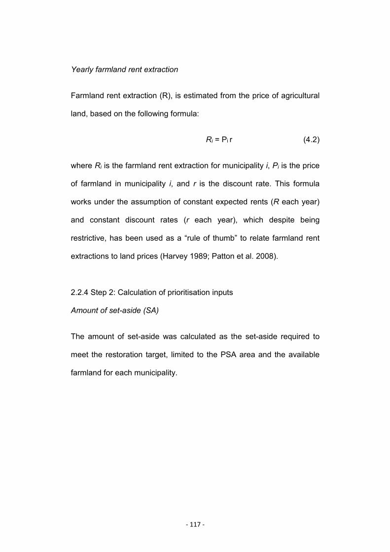
- 117 -

Yearly farmland rent extraction

Farmland rent extraction (R), is estimated from the price of agricultural

land, based on the following formula:

Ri = Pi r (4.2)

where Ri is the farmland rent extraction for municipality i, Pi is the price

of farmland in municipality i, and r is the discount rate. This formula

works under the assumption of constant expected rents (R each year)

and constant discount rates (r each year), which despite being

restrictive, has been used as a “rule of thumb” to relate farmland rent

extractions to land prices (Harvey 1989; Patton et al. 2008).

2.2.4 Step 2: Calculation of prioritisation inputs

Amount of set-aside (SA)

The amount of set-aside was calculated as the set-aside required to

meet the restoration target, limited to the PSA area and the available

farmland for each municipality.

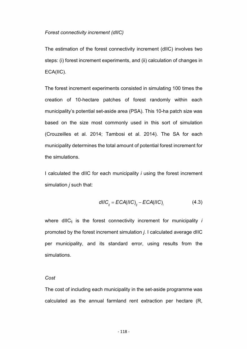
- 118 -

Forest connectivity increment (dIIC)

The estimation of the forest connectivity increment (dIIC) involves two

steps: (i) forest increment experiments, and (ii) calculation of changes in

ECA(IIC).

The forest increment experiments consisted in simulating 100 times the

creation of 10-hectare patches of forest randomly within each

municipality’s potential set-aside area (PSA). This 10-ha patch size was

based on the size most commonly used in this sort of simulation

(Crouzeilles et al. 2014; Tambosi et al. 2014). The SA for each

municipality determines the total amount of potential forest increment for

the simulations.

I calculated the dIIC for each municipality i using the forest increment

simulation j such that:

(4.3)

where dIICij is the forest connectivity increment for municipality i

promoted by the forest increment simulation j. I calculated average dIIC

per municipality, and its standard error, using results from the

simulations.

Cost

The cost of including each municipality in the set-aside programme was

calculated as the annual farmland rent extraction per hectare (R,

dIICij = ECA(IIC)ij -ECA(IIC)i

- 119 -

equation 4.2), multiplied by the set-aside area (SA) for each municipality

and the number of years within the programme.

Restoration Target

The restoration target in number of hectares was calculated as 15% of

the existing forest over all the BAF, which amounts to restoring a total of

2.68 million hectares. This was based on Brazil’s Convention on

Biological Diversity's Aichi Target of restoring at least 15% of degraded

ecosystems by 2020 (National Target 15, www.cbd.int).

Forest Connectivity Target

This target was set as a proxy for maximizing forest connectivity gains

for the restoration target. For each BR I calculated the total potential

forest connectivity increment for the restoration target, and set the forest

connectivity target to 90% of that total. The sensitivity of results to

different targets (80%, 90%, 100%) was tested as part of the sensitivity

analysis (supplementary materials, Annex 4); the results did not differ

substantially.

2.2.4 Step 3: Spatial prioritisation

Marxan (Ball et al. 2009) is a popular conservation planning software

with over 4200 active users from more than 180 countries (McIntosh et

al. 2016). It solves a form of the reserve selection problem whereby

planning units are selected to meet targets for a minimum total cost.

Marxan uses simulated annealing to find optimal solutions to the reserve

- 120 -

selection type of problem. Simulated annealing is a probabilistic search

heuristic commonly used to optimise functions that are hard to optimise

with deterministic methods for two reasons: (1) it avoids an accumulation

of disadvantageous steps in the optimisation process; and (2) it avoids

being trapped in local optima (Maucher et al. 2011).

I used Marxan to find solutions to the problem: which municipalities do

we need to include in a set-aside programme to minimise total

programme cost subject to meeting all conservation targets, both

restoration and forest connectivity targets? Specifically, the problem that

Marxan solved was:

, (4.4)

subject to the constraint that both conservation targets (Tj) were met as

follows

(4.5)

where mk is the total number of municipalities in a given subregion k, cik

is the farmland rent extraction in municipality i in subregion k, xik is the

binary decision variable indicating whether municipality i is selected (xik

= 1) or not (xik = 0) for the solution group in subregion k, and Aijk is the

contribution of municipality i to the target j in subregion k. Units for Aijk

are in hectares for both restoration and connectivity targets.

minimiseikc ikx

ik=1

mk

Â

ijkA ikx %ik=1

mk

 jkT " jk

- 121 -

I set Marxan to find 1000 solutions to the objective function, with 95% as

the proportion of the target a conservation feature must reach for it to be

reported as met. Because simulated annealing is a local search

heuristic, for which the search could terminate at a local, rather than

global, optimum, the algorithm has to be repeated from different starting

solutions (Dowsland & Thompson 2012). Algorithm calibration and

sensitivity analyses were run to get robust results following the Good

Practices Handbook (Ardron et al. 2010). For details on this process see

supplementary materials (SM Annex 4).

Marxan has two spatial output files, the “best” solution and the “summed”

solution. The “best” solution is the solution with the best score amongst

all runs. The “summed” solution shows the selection frequency for each

municipality. It is good practice to use both solutions when interpreting

results and refining the algorithm (Ardron et al. 2010). I ran the complete

analysis using the best solution and found that results were not robust

enough for this type of comparative analysis with sequential

prioritisations. Following the logic behind the summed solution, I created

a “robust” solution, from now on referred to simply as “solution”, which I

used for the comparative analysis. This solution included municipalities

with the highest selection frequency decreasingly until both conservation

targets were met, using the summed solutions file.

- 122 -

2.2.4 Step 4: Solution assessment and implementation

For all solutions, target achievement was assessed at the

biogeographical subregion (BR) level. For the static approach,

implementation of set-asides was done in three time-steps to match the

dynamic’s approach schedule for ease of comparison.

2.2.5 Modelling feedbacks

2.2.2.5.1 Basic principles

A static prioritisation approach assumes that the sequential allocation of

set-asides does not affect the prioritisation outcome itself. However, the

location and amount of set-aside allocation at any time-step has

environmental and economic feedback effects. The implementation of

set-asides has an effect on the prioritisation variables themselves in the

future (figure 4.1). This is modelled in the dynamic prioritisation approach

by updating both forest connectivity and farmland rent extraction before

re-prioritising at 3 time-steps (figure 4.2).

For the environmental feedback, I assumed that agricultural set-asides

regenerated into forest, increasing the forest connectivity metric in the

subsequent time step (figure 4.1). Taking into account the connectivity

value added by the set-aside could result in different prioritisation

outcomes.

The economic feedback modelled the effect that the allocation of

payments for agricultural set-aside can have on future payment price.

This feedback is caused by the informational rent capture derived from

- 123 -

an asymmetry in the information on the opportunity cost of farmland

between landowners and the organization making the payments

(chapter 3). Given that the set-aside program is run at such a large scale,

I assumed a simplification in payment structure, where a single level of

payment is offered to set-aside farmland for each municipality, set at the

average rent extracted from farmland in that municipality (which from

now on I refer to as the opportunity cost of setting aside farmland).

Wherever the opportunity cost of farmland is lower than the offered set-

aside payment, additional rent is captured that increases average net

returns per farmland hectare. Assuming that the set-aside payment has

to at least match rent extraction as a condition for farmers to join the

program, increases in net returns generated by the set-aside program

could result in increases in set-aside payment in the future (figure 4.1).

Taking into account increases in set-aside payments due to set-aside

allocation could result in different prioritisation outcomes.

2.2.5.2 Environmental Feedback

Forest connectivity increment (dIIC) update

The allocation of farmland set-asides modifies forest configuration in the

future. I updated dIIC by re calculating ECA(IIC) and dIIC at each time

step with the new forest cover values. Because these metrics are based

on simulations, the mean value was employed, with the attached error.

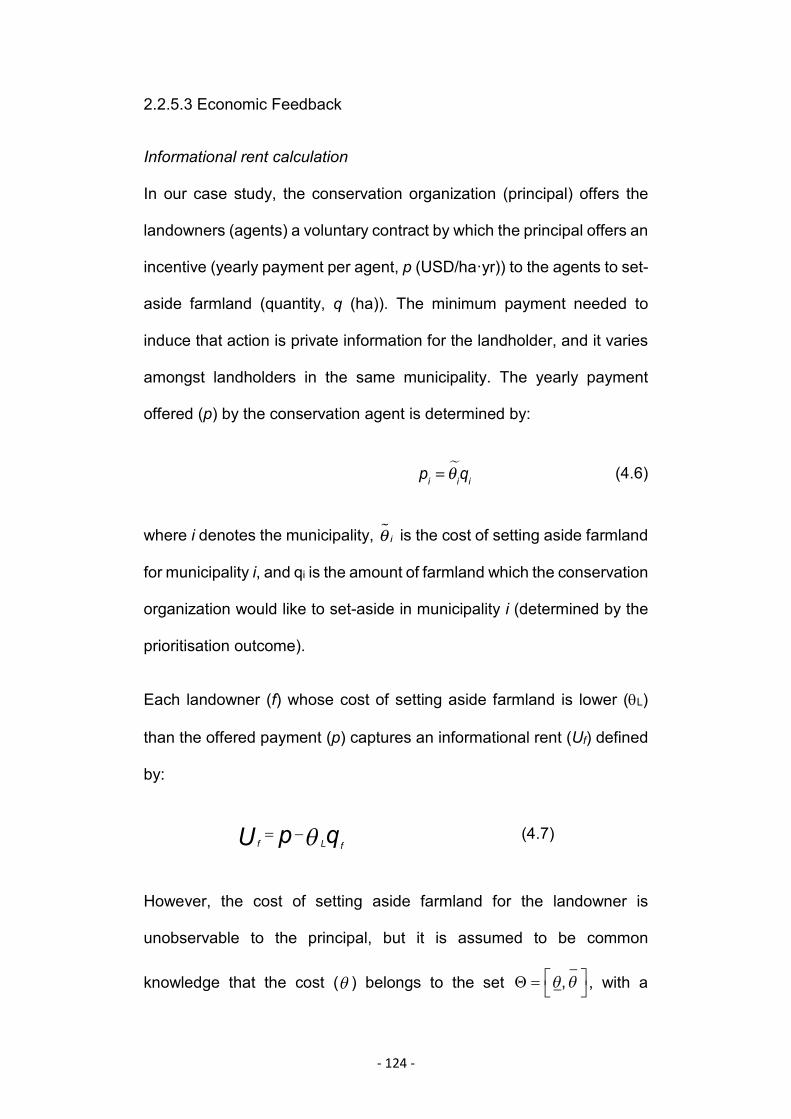
- 124 -

2.2.5.3 Economic Feedback

Informational rent calculation

In our case study, the conservation organization (principal) offers the

landowners (agents) a voluntary contract by which the principal offers an

incentive (yearly payment per agent, p (USD/ha·yr)) to the agents to set-

aside farmland (quantity, q (ha)). The minimum payment needed to

induce that action is private information for the landholder, and it varies

amongst landholders in the same municipality. The yearly payment

offered (p) by the conservation agent is determined by:

(4.6)

where i denotes the municipality, is the cost of setting aside farmland

for municipality i, and qi is the amount of farmland which the conservation

organization would like to set-aside in municipality i (determined by the

prioritisation outcome).

Each landowner (f) whose cost of setting aside farmland is lower (TL)

than the offered payment (p) captures an informational rent (Uf) defined

by:

fU = p - Lq fq (4.7)

However, the cost of setting aside farmland for the landowner is

unobservable to the principal, but it is assumed to be common

knowledge that the cost ( ) belongs to the set , with aq Q = q,qÈÎ

˘˚

- 125 -

cumulative distribution function and a density function on

. The total informational rent captured by landowners in a given

municipality depends on the distribution of opportunity costs for

that municipality. I used the estimated farmland rent extractions (R) and

created frequency histograms to estimate the probability distribution of

opportunity costs for each municipality (figure 4.3). Histogram bin

width is critical because it can change the shape of the probability

distribution. I tested three methods to calculate bin width: Sturges rule,

Friedman-Diaconis rule and Hideaki Shimazaki methodology. The effect

of bin width division method on yearly informational rent per hectare

showed no consistent bias; no method resulted in consistently

higher/lower informational rents across municipalities. I chose the

Friedman-Diaconis rule as it generated no “combed” histograms, and

created a histogram for each municipality i. For each histogram, I

calculated the mean cost ( i), mid-bin cost for bin j ( ) and probability

for the mid-bin cost for bin j ( ij). The total informational rent capture (U)

for municipality i is given by:

(4.8)

where i denotes the municipality, is the mean opportunity cost of

farmland for municipality i, and are the opportunity cost value and

its probability for bin j in municipality i respectively, and qi is the amount

F(q ) f (q)

q,qÈÎ ˘̊

F(q )

F(q )

q ij

n

q ij n ij

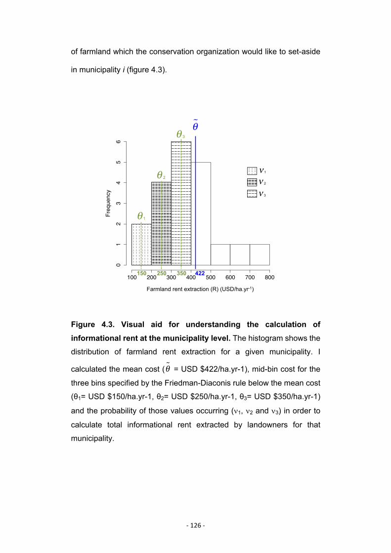
-126-

of farmland which the conservation organization would like to set-aside

in municipality i (figure 4.3).

Figure 4.3. Visual aid for understanding the calculation of informational rent at the municipality level. The histogram shows the

distribution of farmland rent extraction for a given municipality. I

calculated the mean cost ( = USD $422/ha.yr-1), mid-bin cost for the

three bins specified by the Friedman-Diaconis rule below the mean cost

(θ1= USD $150/ha.yr-1, θ2= USD $250/ha.yr-1, θ3= USD $350/ha.yr-1)

and the probability of those values occurring (n1, n2 and n3) in order to

calculate total informational rent extracted by landowners for that

municipality.

Histogram of fnpData.subset

fnpData.subset

Frequency

100 200 300 400 500 600 700 800

01

23

45

6

Farmland rent extraction (R) (USD/ha.yr-1)

θ!

3θ

2θ

1θ

422 150 250 350

1ν 2ν 3ν

θ!

- 127 -

Farmland rent extraction update

The sum of the estimated yearly informational rent extraction per

municipality determines the increase in economic rent derived from

farmland for said municipality. However, the new opportunity cost

( ) on which to estimate payment (pi) for municipality i in the following

time step is defined as:

(4.9)

where i denotes the municipality, (t+1) denotes the subsequent time

step, is the mean farmland rent extraction for municipality i at time

step t, Ui,t is the total informational rent accrued for municipality i at time

step t, and qi,t is the total amount of farmland set-aside for municipality i

at time step t. For the calculation of Ui,t the temporal assumption is that

landowners at the lower bound of become part of the set-aside

programme first, and as time step increase landowners with increasing

set-aside cost get involved.

2.2.6 Modelling validation

Model validation and verification were an integral part of model

development to ensure an accurate representation of the real system.

There are four main areas of assessment for model validation and

F(q )

- 128 -

verification (Sargent 2013): (1) data validity, (2) conceptual model

validation, (3) computerised model verification, and (4) operational

validity. Data validity was ensured by choosing best available data, data

examination for spatial consistency across relevant datasets, and

sensitivity analysis for important data transformation (for example,

generating opportunity cost histograms). Conceptual model validation

included face validation, structured walkthroughs (both supervisors, as

well as experts for the BAF system Dr Tambosi, Dr Igari, and Dr Banks-

Leite), model internal validity checks and parameter variability-sensitivity

checks (for example, this process identified Marxan’s “best solution” as

a weak step in the model, which lead to the use of the “robust solution”,

see page 119). Computerised model verification also included internal

validity checks, as well as output relationship correctness and

operational graphics (visually display results through time). Operational

validation was limited by the availability of data or results from other

studies comparing static and dynamic approaches (not found).

2.3 Regression model

Linear models were fitted to explore the effect of municipality

characteristics on the difference in results between static and dynamic

solutions. Different models were fitted for 6 response variables:

difference in opportunity cost per hectare, difference in informational rent

capture per hectare, difference in forest connectivity increment,

difference in set-aside cost-effectiveness, difference in forest

connectivity increment cost-effectiveness, and differences in the

- 129 -

proportion of each dollar spent that is captured as informational rent. All

response variables were defined as differences in which negative

difference values mean that the dynamic solution has larger values than

the static solution, and positive difference values mean the opposite.

Explanatory variables included municipality size (ha), forest area (ha),

farmland area (ha), landscape area (ha), potential set-aside area (ha),

forest connectivity (ha), farmland average opportunity cost ($/ha), and

variation in opportunity cost of farmland measured by its standard

deviation ($/ha). Models were checked for multi-collinearity, and

municipality size (ha), forest area (ha), and landscape area (ha) were

excluded from all models as a result.

I expected spatial dependence in observations, and model fit

assessment showed heterogeneity of variance between regions.

Generalised least squares (GLS) models were selected in order to

account for variance structure as a function of the biogeographical

subregion. GLS are specifically weighted regressions in which a direct

marginal variance–covariance spatial structure of the responses can be

specified (Zuur et al. 2009). Model fit was assessed using residual plots

as recommended by Pinheiro and Bates (2000). For each dependent

variable, GLS model optimal residual variance structure was selected

using Akaike's Information Criterion (AIC), which takes into account both

goodness of fit and model complexity.

- 130 -

3. Results

3.1 Differences in costs and benefits

The total cost of meeting the restoration target was $3,553 million (mill.

$) for the dynamic solution over the whole 9-year period (table 4.3). The

static estimation of the total cost was 3,480 mill. $ over the same period

of time. However, this did not account for the feedback on the opportunity

cost of land due to informational rent capture. When accounting for this

feedback, the total cost of the static approach was 3,797 mill. $ (table

4.3). This meant that for the static solution the programme either run out

of money and failed to fulfil the policy target, or found funds to cover the

317mill. $ deficit. In order to make results readily comparable, I assumed

the second scenario for the rest of the chapter. For a detailed description

of all results see supplementary materials Annex 5.

As expected, the total cost of meeting the government's reforestation

policy target was cheaper for the dynamic solution than the static

solution. This is because farmland opportunity costs increase over time

due the economic feedback, and in the dynamic approach cost was

updated at each time step, allowing the inclusion of the most cost-

effective municipalities every time. However, differences between

approaches were small in proportional terms at the BAF level. For each

hectare of land that was set-aside, the dynamic approach cost 6.4% less

and enabled the capture of 33.6% more informational rent than the static

approach. For each dollar spent in setting aside farmland, the dynamic

solution was 6.9% more cost effective than the static solution, and the

- 131 -

proportion of a dollar captured in informational rent was 42.7% higher

than the static solution (table 4.3).

Accounting for the forest connectivity feedback did not, however, result

in a higher forest connectivity increment for the dynamic solution, which

was unexpected. At the BAF level, for each hectare of land that was set-

aside, the dynamic solution had an increase in forest connectivity that

was 4.4% smaller than the static solution. For each dollar spent the

dynamic solution was 2.2% less cost-effective in forest connectivity

terms than the static solution, though the difference was not significant

(table 4.3). Two methodological considerations explained these results,

both at BAF and BR levels. Firstly, due to the size of BRs, forest

connectivity cannot be assessed using the same methods for the whole

BR as a unit, so when comparing forest connectivity at BR level I used

summed dIIC. Summed forest connectivity increment did not account for

the improvement in forest connectivity for the BR as a unit, only how

much forest connectivity increased at the municipality level, aggregated.

Secondly, there is a non-linear relationship between forest cover and

forest connectivity, by which the same increment in forest cover results

in larger connectivity increment the larger the base forest cover is

(Rappaport et al. 2015a). The static approach resulted in a sequential

set-aside allocation in which the same municipalities received set-aside

allocations over time. Given the way the forest connectivity feedback

was defined, forest cover increased at each time step, consequently,

forest connectivity increment for the same set-aside amount increased

over time.

- 132 -

Table 4.3. Comparison of results at Brazilian Atlantic Forest level. Cost, forest connectivity increment andinformational rent capture for static and dynamic prioritisation approaches for all time steps. The difference results fromsubtracting dynamic from static results, negative % indicates the dynamic value is highest. For % differences, the staticresults are taken as 100%. M ha: million hectares, mill. $: million USD.

Variable Units

Time Step 1 Time Step 2 Time Step 3 TotalStatic Dynam. Diff.

(%)Static Dynam. Diff.

(%)Static Dynam. Diff.

(%)Static Dynam. Diff.

(%)value value value value value value value valueStandardised setaside M ha 0.89 0.89 0.00 0.89 0.89 0.00 0.89 0.89 0.00 2.68 2.68 0.00Cost mill.$ 1,756.79 1,703.13 3.10 1,335.6 1,185.64 11.20 704.7 658.40 6.603,797.1 3,553.46 6.40Informational Rent mill.$ 739.63 756.00 -2.20 221.55 348.32 -57.20 1.85 177.99 -9,526.90 963.04 1,286.45 -33.60Forest connectivity increment M ha 0.19 0.24 -27.80 0.26 0.22 14.70 0.30 0.25 15.50 0.74 0.71 4.40Cost/ha usd/ha 1,969.23 1,909.08 3.10 1,497.1 1,329.02 11.20 789.9 738.02 6.601,418.7 1,327.72 6.40Informational Rent/ha usd/ha 829.06 847.42 -2.20 248.34 390.44 -57.20 2.07 199.51 -9,526.90 359.83 480.67 -33.60Forest connectivity incr./ha ha/ha 0.21 0.27 -27.80 0.29 0.25 14.70 0.33 0.28 15.50 0.28 0.26 4.40Setaside cost effectiveness ha/usd 0.00 0.00 -3.20 0.00 0.00 -12.60 0.00 0.00 -7.00 0.00 0.00 -6.90Informational Rent/cost usd/usd 0.42 0.44 -5.40 0.17 0.29 -77.10 0.00 0.27 -10,203.9 0.25 0.36 -42.70Forest connectivity cost-eff. ha/usd 0.00 0.00 -31.80 0.00 0.00 4.00 0.00 0.00 9.50 0.00 0.00 -2.20Yearly cost mill.$/yr 195.20 189.24 3.10 222.59 197.61 11.20 234.9 219.47 6.60 421.90 394.83 6.40Yearly Informational Rent mill.$/yr 82.18 84.00 -2.20 36.92 58.05 -57.20 0.62 59.33 -9,526.90 107.00 142.94 -33.60Yearly Forest connectivity incr. M ha/yr 0.02 0.03 -27.80 0.04 0.04 14.70 0.10 0.08 15.50 0.08 0.08 4.40Yearly cost/ha usd/ha/yr 218.80 212.12 3.10 249.51 221.50 11.20 263.3 246.01 6.60 157.64 147.52 6.40Yearly Informational Rent/ha usd/ha/yr 92.12 94.16 -2.20 41.39 65.07 -57.20 0.69 66.50 -9,526.90 39.98 53.41 -33.60Yearly Forest connectivityincr./ha ha/ha/yr 0.02 0.03 -27.80 0.05 0.04 14.70 0.11 0.09 15.50 0.03 0.03 4.40Yearly setaside cost-eff. ha/usd/yr 0.00 0.00 -3.20 0.00 0.00 -12.60 0.00 0.00 -7.00 0.00 0.00 -6.90Yearly Informational Rent/cost usd/usd/yr 0.05 0.05 -5.40 0.03 0.05 -77.10 0.00 0.09 -10,203.9 0.03 0.04 -42.70Yearly forest connectivity cost-effectiveness ha/usd/yr 0.00 0.00 -31.80 0.00 0.00 4.00 0.00 0.00 9.50 0.00 0.00 -2.20

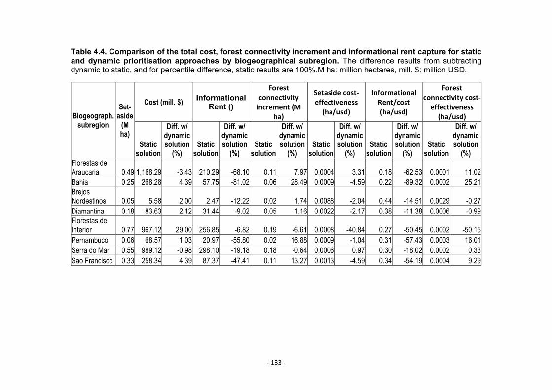
- 133 -

Table 4.4. Comparison of the total cost, forest connectivity increment and informational rent capture for staticand dynamic prioritisation approaches by biogeographical subregion. The difference results from subtractingdynamic to static, and for percentile difference, static results are 100%.M ha: million hectares, mill. $: million USD.

Biogeograph.subregion

Set-aside

(Mha)

Cost (mill. $) InformationalRent ()

Forestconnectivityincrement (M

ha)

Setaside cost-effectiveness(ha/usd)

InformationalRent/cost(ha/usd)

Forestconnectivity cost-effectiveness(ha/usd)

Staticsolution

Diff. w/dynamicsolution

(%)Static

solution

Diff. w/dynamicsolution

(%)Static

solution

Diff. w/dynamicsolution

(%)Static

solution

Diff. w/dynamicsolution

(%)Static

solution

Diff. w/dynamicsolution

(%)Static

solution

Diff. w/dynamicsolution

(%)Florestas deAraucaria 0.49 1,168.29 -3.43 210.29 -68.10 0.11 7.97 0.0004 3.31 0.18 -62.53 0.0001 11.02Bahia 0.25 268.28 4.39 57.75 -81.02 0.06 28.49 0.0009 -4.59 0.22 -89.32 0.0002 25.21BrejosNordestinos 0.05 5.58 2.00 2.47 -12.22 0.02 1.74 0.0088 -2.04 0.44 -14.51 0.0029 -0.27Diamantina 0.18 83.63 2.12 31.44 -9.02 0.05 1.16 0.0022 -2.17 0.38 -11.38 0.0006 -0.99Florestas deInterior 0.77 967.12 29.00 256.85 -6.82 0.19 -6.61 0.0008 -40.84 0.27 -50.45 0.0002 -50.15Pernambuco 0.06 68.57 1.03 20.97 -55.80 0.02 16.88 0.0009 -1.04 0.31 -57.43 0.0003 16.01Serra do Mar 0.55 989.12 -0.98 298.10 -19.18 0.18 -0.64 0.0006 0.97 0.30 -18.02 0.0002 0.33Sao Francisco 0.33 258.34 4.39 87.37 -47.41 0.11 13.27 0.0013 -4.59 0.34 -54.19 0.0004 9.29

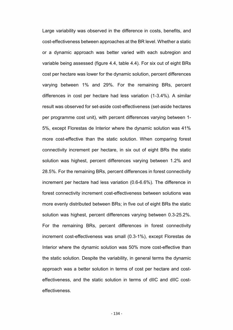
- 134 -

Large variability was observed in the difference in costs, benefits, and

cost-effectiveness between approaches at the BR level. Whether a static

or a dynamic approach was better varied with each subregion and

variable being assessed (figure 4.4, table 4.4). For six out of eight BRs

cost per hectare was lower for the dynamic solution, percent differences

varying between 1% and 29%. For the remaining BRs, percent

differences in cost per hectare had less variation (1-3.4%). A similar

result was observed for set-aside cost-effectiveness (set-aside hectares

per programme cost unit), with percent differences varying between 1-

5%, except Florestas de Interior where the dynamic solution was 41%

more cost-effective than the static solution. When comparing forest

connectivity increment per hectare, in six out of eight BRs the static

solution was highest, percent differences varying between 1.2% and

28.5%. For the remaining BRs, percent differences in forest connectivity

increment per hectare had less variation (0.6-6.6%). The difference in

forest connectivity increment cost-effectiveness between solutions was

more evenly distributed between BRs; in five out of eight BRs the static

solution was highest, percent differences varying between 0.3-25.2%.

For the remaining BRs, percent differences in forest connectivity

increment cost-effectiveness was small (0.3-1%), except Florestas de

Interior where the dynamic solution was 50% more cost-effective than

the static solution. Despite the variability, in general terms the dynamic

approach was a better solution in terms of cost per hectare and cost-

effectiveness, and the static solution in terms of dIIC and dIIC cost-

effectiveness.

- 135 -

Figure 4.4. Distribution of differences between static and dynamic solution results. Boxplots show min, max,median and interquartile range for municipality level observations, diamonds show the value of the variable atbiogeographical region level. In blue are the negative differences, where the dynamic solution is larger than the staticsolution. In red the positive values. Biogeographical regions: Florestas de Araucaria (Ar), Bahia (Ba), Brejos Nordestinos(BN), Diamantina (Di), Florestas de Interior (FdI), Pernambuco (Per), Serra do Mar (SdM), and Sao Francisco (SF).

●●●●●●●●

●●●●●●●●●●●●●●●●●●●●●●●●

●●●●●●●●●●●●●●●●

●●●●●●●●●●●●●●●●

●●●●●●●●●●●●●●●●●●●●●●●●●●●●●●●●

●●●●●●●● ●●●●●●●●

●●●●●●●●

●●●●●●●●●●●●●●●●

●●●●●●●●●●●●●●●●●●●●●●●●

●●●●●●●●●●●●●●●●

●●●●●●●●

●●●●●●●●●●●●●●●●●●●●●●●●●●●●●●●●

●●●●●●●●

●●●●●●●●

●●●●●●●●

●●●●●●●●●●●●●●●●●●●●●●●●●●●●●●●●●●●●●●●●

●●●●●●●●

●●●●●●●●

●●●●●●●●

●●●●●●●●

●●●●●●●●

●●●●●●●●●●●●●●●●

●●●●●●●●

●●●●●●●●●●●●●●●●

●●●●●●●●●●●●●●●●

●●●●●●●●

●●●●●●●●

●●●●●●●●●●●●●●●●●●●●●●●●

●●●●●●●●

●●●●●●●●

●●●●●●●●

●●●●●●●● ●●●●●●●●

●●●●●●●●●●●●●●●●●●●●●●●●●●●●●●●●●●●●●●●●●●●●●●●●

●●●●●●●●●●●●●●●●

●●●●●●●●

●●●●●●●●●●●●●●●●●●●●●●●●●●●●●●●●

●●●●●●●●

●●●●●●●●●●●●●●●●●●●●●●●●●●●●●●●●●●●●●●●●●●●●●●●●●●●●●●●● ●●●●●●●●●●●●●●●●●●●●●●●●●●●●●●●●●●●●●●●●

●●●●●●●●●●●●●●●●●●●●●●●●

●●●●●●●●●●●●●●●●

●●●●●●●●

●●●●●●●●

●●●●●●●●

●●●●●●●●●●●●●●●●●●●●●●●●●●●●●●●●

●●●●●●●●

●●●●●●●●

●●●●●●●●

●●●●●●●●●●●●●●●●●●●●●●●●●●●●●●●●●●●●●●●●●●●●●●●●

●●●●●●●●

●●●●●●●●●●●●●●●●●●●●●●●●

●●●●●●●●●●●●●●●●

●●●●●●●●●●●●●●●●●●●●●●●●●●●●●●●●

●●●●●●●●●●●●●●●●

●●●●●●●●

●●●●●●●●

●●●●●●●●

●●●●●●●●●●●●●●●●

●●●●●●●●

●●●●●●●●

●●●●●●●●

●●●●●●●●

●●●●●●●●

●●●●●●●●

●●●●●●●●●●●●●●●●●●●●●●●●●●●●●●●●●●●●●●●●●●●●●●●●

Cost(usd/ha)

Informational Rent(usd/ha)

Forest connectivity change(proportion of ha setaside)

Setaside Cost−effectiveness(ha/usd)

Informational Rent(proportion of usd spent)

dIIC Cost−effectiveness(ha/usd)

−5000

−2500

0

2500

−4000

−3000

−2000

−1000

0

−1.5

−1.0

−0.5

0.0

0.5

−0.0100

−0.0075

−0.0050

−0.0025

0.0000

−1.0

−0.5

0.0

−0.003

−0.002

−0.001

0.000

Ar Ba BN Di FdI PerSdM SF Ar Ba BN Di FdI PerSdM SF Ar Ba BN Di FdI PerSdM SF

Ar Ba BN Di FdI PerSdM SF Ar Ba BN Di FdI PerSdM SF Ar Ba BN Di FdI PerSdM SFBiogeographical region

Differencebetweensolutions

Largest variablevalue at BR levelDynamicStatic

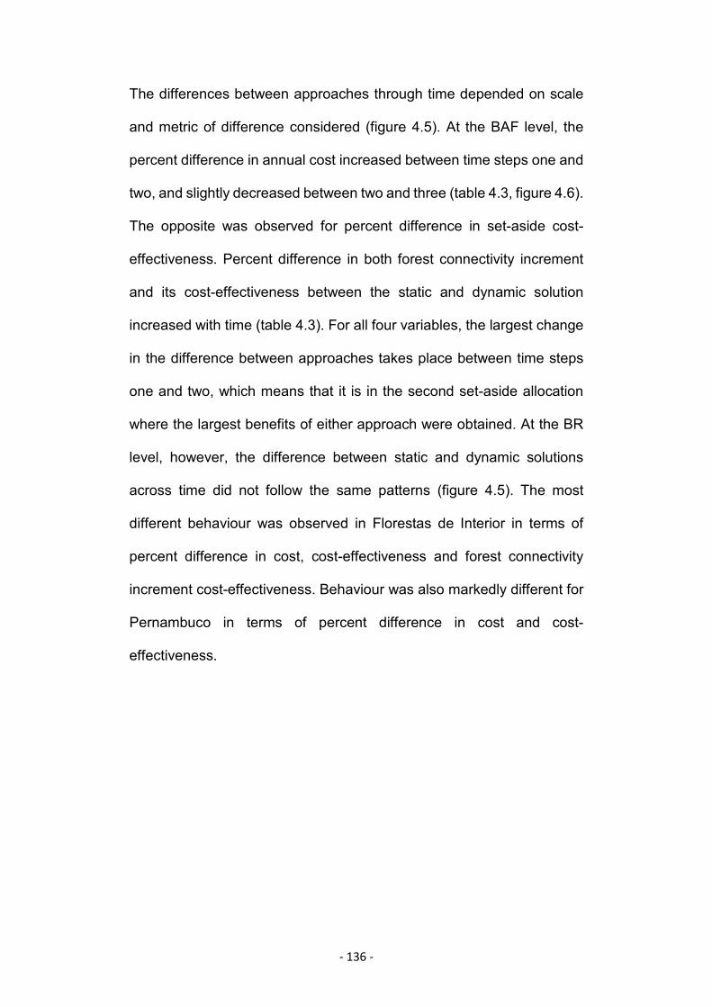
- 136 -

The differences between approaches through time depended on scale

and metric of difference considered (figure 4.5). At the BAF level, the

percent difference in annual cost increased between time steps one and

two, and slightly decreased between two and three (table 4.3, figure 4.6).

The opposite was observed for percent difference in set-aside cost-

effectiveness. Percent difference in both forest connectivity increment

and its cost-effectiveness between the static and dynamic solution

increased with time (table 4.3). For all four variables, the largest change

in the difference between approaches takes place between time steps

one and two, which means that it is in the second set-aside allocation

where the largest benefits of either approach were obtained. At the BR

level, however, the difference between static and dynamic solutions

across time did not follow the same patterns (figure 4.5). The most

different behaviour was observed in Florestas de Interior in terms of

percent difference in cost, cost-effectiveness and forest connectivity

increment cost-effectiveness. Behaviour was also markedly different for

Pernambuco in terms of percent difference in cost and cost-

effectiveness.

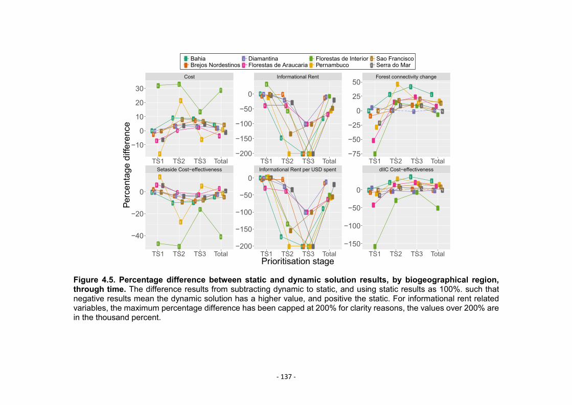
- 137 -

Figure 4.5. Percentage difference between static and dynamic solution results, by biogeographical region,through time. The difference results from subtracting dynamic to static, and using static results as 100%. such thatnegative results mean the dynamic solution has a higher value, and positive the static. For informational rent relatedvariables, the maximum percentage difference has been capped at 200% for clarity reasons, the values over 200% arein the thousand percent.

Cost Informational Rent Forest connectivity change

Setaside Cost−effectiveness Informational Rent per USD spent dIIC Cost−effectiveness

−10

0

10

20

30

−200

−150

−100

−50

0

−75

−50

−25

0

25

50

−40

−20

0

−200

−150

−100

−50

0

−150

−100

−50

0

TS1 TS2 TS3 Total TS1 TS2 TS3 Total TS1 TS2 TS3 Total

TS1 TS2 TS3 Total TS1 TS2 TS3 Total TS1 TS2 TS3 TotalPrioritisation stage

Percentagedifference

BahiaBrejos Nordestinos

DiamantinaFlorestas de Araucaria

Florestas de InteriorPernambuco

Sao FranciscoSerra do Mar

- 138 -

Figure 4.6. Aggregate results through time at the Brazilian AtlanticForest level. TS represents each time step 1, 2, and 3 respectively.

Florestas de Interior was an exception for differences between

approaches in cost-effectiveness and dIIC cost-effectiveness, as well as

their behaviour over time. This BR was the largest in terms of area and

number of municipalities included (table 4.5), almost 3 times the second

largest (Florestas de Araucaria). It was also the only BR for which the

static approach included more municipalities in its solution than the

dynamic approach. These facts suggest a higher number of highly cost-

effective municipalities in this BR, and given that the proportion of

municipalities included in the solutions was small (5%), this could explain

the large differences in cost-effectiveness between dynamic and static

approaches.

●

●

●

●

●

● ●●

●

●

●

●

●

●

●

●

●

●

● ●

●●

●

●

●●

●

●

●

●●

●

● ●

●

●

Cost(Musd/yr)

Informational Rent(Musd/yr)

Forest connectivity change(Mha/yr)

Setaside Cost−effectiveness(ha/usd/yr)

Informational Rent(proportion of usd spent/yr)

dIIC Cost−effectiveness(ha/usd/yr)

190

200

210

220

230

0

20

40

60

80

0.02

0.04

0.06

0.08

0.10

1e−04

2e−04

3e−04

4e−04

0.000

0.025

0.050

0.075

5e−05

1e−04

TS1 TS2 TS3 TS1 TS2 TS3 TS1 TS2 TS3

TS1 TS2 TS3 TS1 TS2 TS3 TS1 TS2 TS3Prioritisation stage

Variablevalue

●

●

dynamicstatic

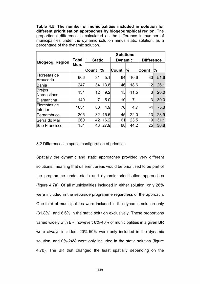
- 139 -

Table 4.5. The number of municipalities included in solution fordifferent prioritisation approaches by biogeographical region. Theproportional difference is calculated as the difference in number ofmunicipalities under the dynamic solution minus static solution, as apercentage of the dynamic solution.

Biogeog. Region TotalMun.

SolutionsStatic Dynamic Difference

Count % Count % Count %Florestas deAraucaria 606 31 5.1 64 10.6 33 51.6

Bahia 247 34 13.8 46 18.6 12 26.1BrejosNordestinos 131 12 9.2 15 11.5 3 20.0

Diamantina 140 7 5.0 10 7.1 3 30.0Florestas deInterior 1634 80 4.9 76 4.7 -4 -5.3

Pernambuco 205 32 15.6 45 22.0 13 28.9Serra do Mar 260 42 16.2 61 23.5 19 31.1Sao Francisco 154 43 27.9 68 44.2 25 36.8

3.2 Differences in spatial configuration of priorities

Spatially the dynamic and static approaches provided very different

solutions, meaning that different areas would be prioritised to be part of

the programme under static and dynamic prioritisation approaches

(figure 4.7a). Of all municipalities included in either solution, only 26%

were included in the set-aside programme regardless of the approach.

One-third of municipalities were included in the dynamic solution only

(31.8%), and 6.6% in the static solution exclusively. These proportions

varied widely with BR, however: 6%-40% of municipalities in a given BR

were always included, 20%-50% were only included in the dynamic

solution, and 0%-24% were only included in the static solution (figure

4.7b). The BR that changed the least spatially depending on the

- 140 -

prioritisation approach was Serra do Mar, and the one that changed the

most was Bahia. For Serra do Mar then, the approach did not make a

big difference in terms of which municipalities are included in the

programme, but for Bahia it did.

The number of municipalities included in the dynamic solution was

higher than the static solution, with the static solution including 20-50%

fewer municipalities than the dynamic solution depending on the BR (5%

more in Florestas de Interior, table 4.5). This difference in the number of

municipalities included between solutions was not explained by the size

of the BR (in terms of the number of municipalities) (SM figure 2). By

including more municipalities in the programme, the dynamic approach

could reach a wider group of landowners. Despite the larger forest

connectivity increment of the static solution at both BAF level and BR

level for most BRs, the number of municipalities in which forest

connectivity increment per hectare was largest for the dynamic solution

was similar to the number under the static solution (figure 4.8.c).

Furthermore, when the dynamic solution resulted in larger forest

connectivity increments the difference between approaches was highest

(figure 4.8c, the number of “+” signs). So if the objective of a prioritisation

were to increase forest connectivity more evenly and widely, the dynamic

approach would be a better option regardless of cost considerations.

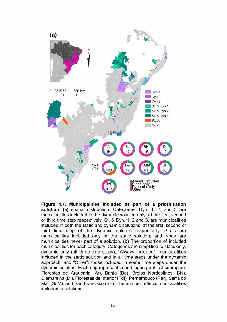
- 141 -

Figure 4.7. Municipalities included as part of a prioritisationsolution: (a) spatial distribution. Categories: Dyn. 1, 2, and 3 aremunicipalities included in the dynamic solution only, at the first, secondor third time step respectively; St. & Dyn. 1, 2 and 3, are municipalitiesincluded in both the static and dynamic solutions, at the first, second orthird time step of the dynamic solution respectively; Static aremunicipalities included only in the static solution; and None aremunicipalities never part of a solution. (b) The proportion of includedmunicipalities for each category. Categories are simplified to static only,dynamic only (all three-time steps), “Always included”: municipalitiesincluded in the static solution and in all time steps under the dynamicapproach, and “Other”: those included in some time steps under thedynamic solution. Each ring represents one biogeographical subregion:Florestas de Araucaria (Ar), Bahia (Ba), Brejos Nordestinos (BN),Diamantina (Di), Florestas de Interior (FdI), Pernambuco (Per), Serra doMar (SdM), and Sao Francisco (SF). The number reflects municipalitiesincluded in solutions.

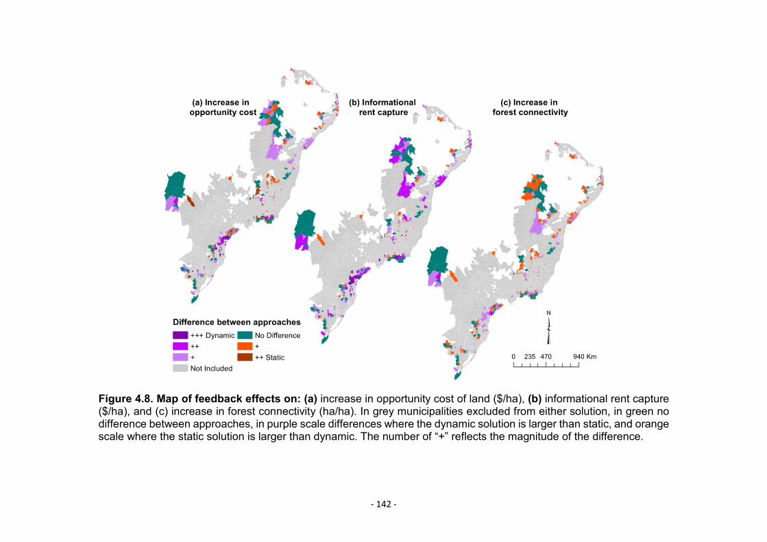
- 142 -

Figure 4.8. Map of feedback effects on: (a) increase in opportunity cost of land ($/ha), (b) informational rent capture($/ha), and (c) increase in forest connectivity (ha/ha). In grey municipalities excluded from either solution, in green nodifference between approaches, in purple scale differences where the dynamic solution is larger than static, and orangescale where the static solution is larger than dynamic. The number of “+” reflects the magnitude of the difference.

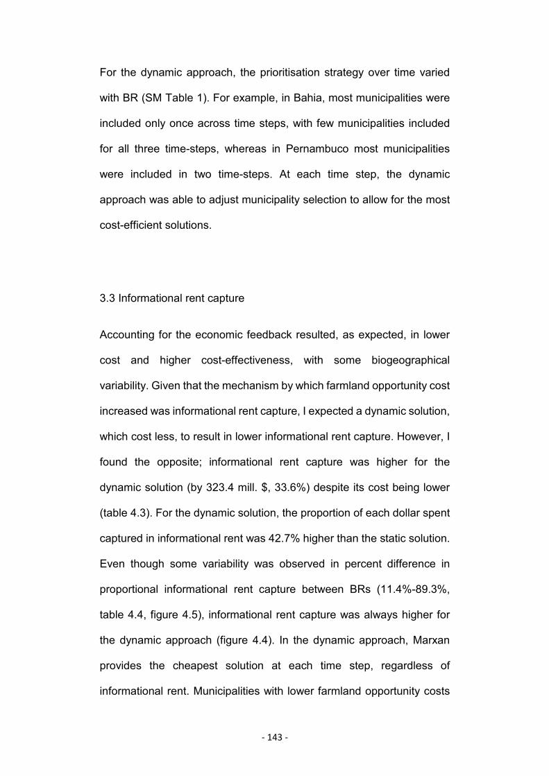
- 143 -

For the dynamic approach, the prioritisation strategy over time varied

with BR (SM Table 1). For example, in Bahia, most municipalities were

included only once across time steps, with few municipalities included

for all three time-steps, whereas in Pernambuco most municipalities

were included in two time-steps. At each time step, the dynamic

approach was able to adjust municipality selection to allow for the most

cost-efficient solutions.

3.3 Informational rent capture

Accounting for the economic feedback resulted, as expected, in lower

cost and higher cost-effectiveness, with some biogeographical

variability. Given that the mechanism by which farmland opportunity cost

increased was informational rent capture, I expected a dynamic solution,

which cost less, to result in lower informational rent capture. However, I

found the opposite; informational rent capture was higher for the

dynamic solution (by 323.4 mill. $, 33.6%) despite its cost being lower

(table 4.3). For the dynamic solution, the proportion of each dollar spent

captured in informational rent was 42.7% higher than the static solution.

Even though some variability was observed in percent difference in

proportional informational rent capture between BRs (11.4%-89.3%,

table 4.4, figure 4.5), informational rent capture was always higher for

the dynamic approach (figure 4.4). In the dynamic approach, Marxan

provides the cheapest solution at each time step, regardless of

informational rent. Municipalities with lower farmland opportunity costs

- 144 -

are prioritised over municipalities with higher opportunity costs, even if

the former entail higher informational rent capture than the latter. In this

way, the dynamic solution has a lower cost and captures more

informational rent.

Annual informational rent capture was highest for the dynamic solution

at all time steps, and decreased with time for both solutions (figure 4.6).

The difference between approaches in annual informational rent capture

increased with time both in absolute (figure 4.6) and percent (figure 4.5)

values. This behaviour was explained by a combination of factors. At the

municipality level, informational rent capture decreased over time

because there is only a limited number of hectares with farmland

opportunity cost lower than the incentive payment, and hectares with the

lowest opportunity cost were set-aside first. So, for the same

municipality, informational rent captured in the first set-aside allocation

was higher than the one captured in the second set-aside allocation, and

so on. Because in the static approach the same municipalities receive a

set-aside allocation at all time steps, informational rent capture for this

approach decreased over time. However, in the dynamic approach this

was not the case, and the difference between approaches, therefore,

increased over time.

There were more municipalities for which informational rent capture per

hectare was higher in the dynamic solution, and the differences reached

higher values (figure 4.8.b). Even in municipalities where the increase in

opportunity cost was larger for the static approach, informational rent

- 145 -

capture was higher for the dynamic approach. This suggests that in the

dynamic approach not only do a wider range of landowners have an

incentive to participate in the programme due to informational rent

capture, but that those incentives are also higher.

3.4 Predicting the best approach

Models of the effect of municipality characteristics on the difference

between solutions showed that biogeographical subregion explained

most of the differences, suggesting that whether to use a dynamic or

static approach is region-dependent (table 4.6). The second variable that

explained most differences was variability of farmland opportunity cost,

with mostly small effects on dependent variables. Potential set-aside

(PSA) had very small effects on most dependent variables. Area of

farmland and forest connectivity were the least important variables in

explaining differences between approaches, with very small effects on

most dependent variables. For the detailed GLS tables for all models

see SM Table 6.

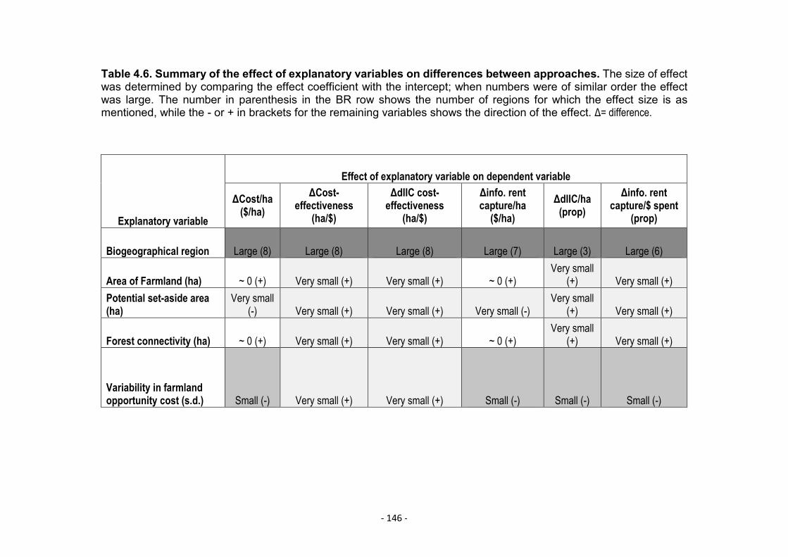
- 146 -

Table 4.6. Summary of the effect of explanatory variables on differences between approaches. The size of effectwas determined by comparing the effect coefficient with the intercept; when numbers were of similar order the effectwas large. The number in parenthesis in the BR row shows the number of regions for which the effect size is asmentioned, while the - or + in brackets for the remaining variables shows the direction of the effect. Δ= difference.

Explanatory variable

Effect of explanatory variable on dependent variable

ΔCost/ha ($/ha)

ΔCost-effectiveness

(ha/$)

ΔdIIC cost-effectiveness

(ha/$)

Δinfo. rent capture/ha

($/ha)ΔdIIC/ha

(prop)Δinfo. rent

capture/$ spent(prop)

Biogeographical region Large (8) Large (8) Large (8) Large (7) Large (3) Large (6)

Area of Farmland (ha) ~ 0 (+) Very small (+) Very small (+) ~ 0 (+)Very small

(+) Very small (+)Potential set-aside area(ha)

Very small(-) Very small (+) Very small (+) Very small (-)

Very small(+) Very small (+)

Forest connectivity (ha) ~ 0 (+) Very small (+) Very small (+) ~ 0 (+)Very small

(+) Very small (+)

Variability in farmlandopportunity cost (s.d.) Small (-) Very small (+) Very small (+) Small (-) Small (-) Small (-)

- 147 -

What the direction of the effect of explanatory variables means for each

dependent variable is not intuitive due to the nature of the dependent

variables, which are differences that have both negative and positive

values. This will depend on whether the value of the intercept for each

BR is positive (value of the variable for the static solution is higher than

the dynamic solution) or negative (the opposite). Table 4.7 explains what

the direction of the effect of explanatory variables means under different

BR intercept conditions. Most commonly, across BRs, increasing

farmland area and forest connectivity had the effect of increasing the

difference between approaches on all response variables except cost

effectiveness (table4.7). This means that even though the dynamic

approach is best in terms of cost/ha, informational rent capture/ha, forest

connectivity/ha, informational rent/$ and forest connectivity cost-

effectiveness, for regions with small farmland area and forest

connectivity the difference between approaches might not be enough to

offset the transaction cost of implementing the dynamic approach (which

requires three implementations rather than one). PSA and variability in

farmland opportunity cost had the effect of increasing the difference

between approaches in cost-effectiveness (table 4.7), meaning that

even though the dynamic approach was more cost-effective than the

static approach always, for regions with small PSA and variability in

farmland opportunity cost the difference between approaches might not

be. However, increasing PSA and variability in farmland opportunity cost

would increase that difference, making the dynamic approach more

desirable. Large PSA values reflect areas of high forest cover and high

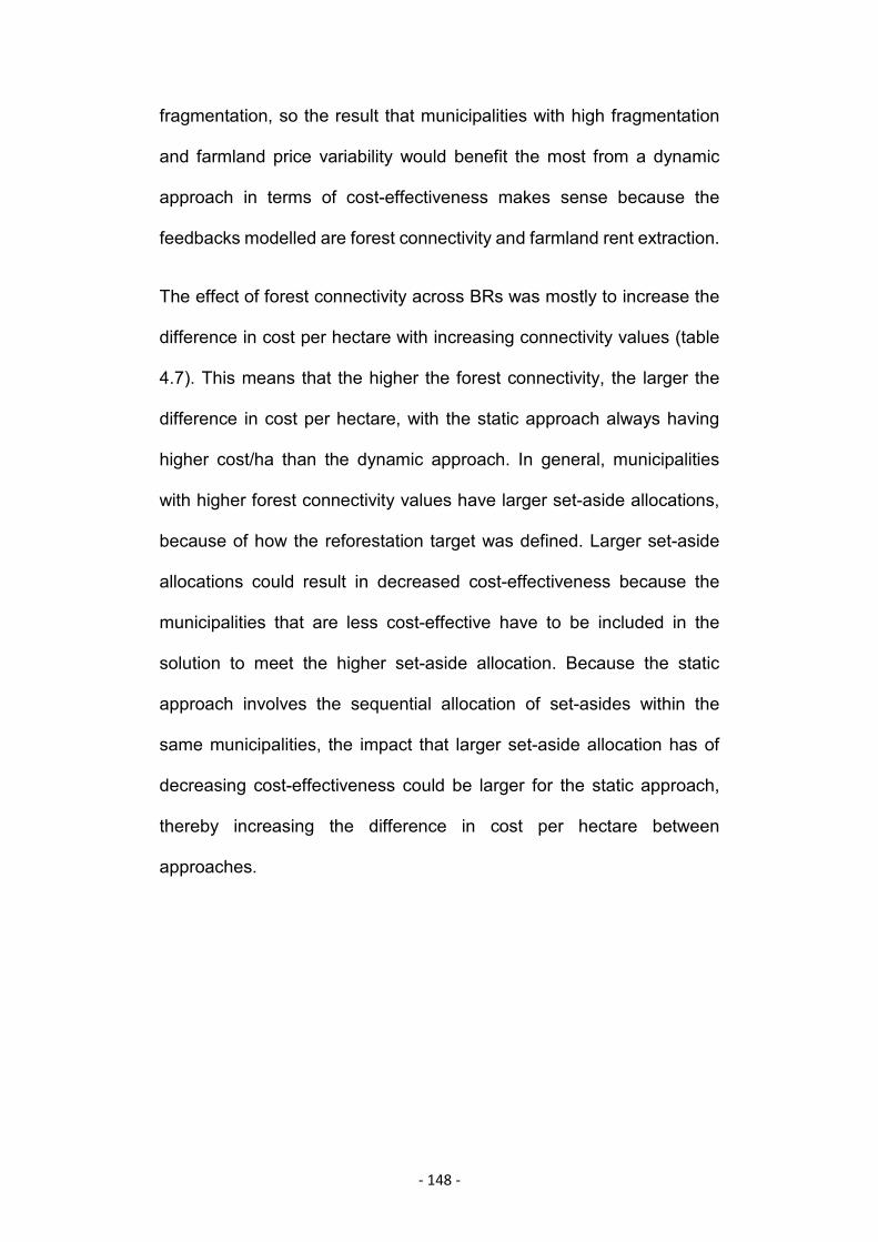
- 148 -

fragmentation, so the result that municipalities with high fragmentation

and farmland price variability would benefit the most from a dynamic

approach in terms of cost-effectiveness makes sense because the

feedbacks modelled are forest connectivity and farmland rent extraction.

The effect of forest connectivity across BRs was mostly to increase the

difference in cost per hectare with increasing connectivity values (table

4.7). This means that the higher the forest connectivity, the larger the

difference in cost per hectare, with the static approach always having

higher cost/ha than the dynamic approach. In general, municipalities

with higher forest connectivity values have larger set-aside allocations,

because of how the reforestation target was defined. Larger set-aside

allocations could result in decreased cost-effectiveness because the

municipalities that are less cost-effective have to be included in the

solution to meet the higher set-aside allocation. Because the static

approach involves the sequential allocation of set-asides within the

same municipalities, the impact that larger set-aside allocation has of

decreasing cost-effectiveness could be larger for the static approach,

thereby increasing the difference in cost per hectare between

approaches.

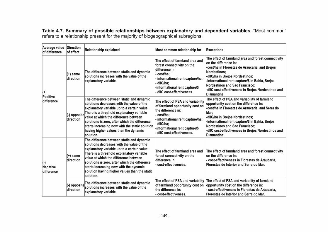
- 149 -

Table 4.7. Summary of possible relationships between explanatory and dependent variables. “Most common”refers to a relationship present for the majority of biogeographical subregions.

Average valueof difference

Directionof effect Relationship explained Most common relationship for Exceptions

(+)Positivedifference

(+) samedirection

The difference between static and dynamicsolutions increases with the value of theexplanatory variable.

The effect of farmland area andforest connectivity on thedifference in:- cost/ha;- informational rent capture/ha;- dIIC/ha;-informational rent capture/$- dIIC cost-effectiveness.

The effect of farmland area and forest connectivityon the difference in:-cost/ha in Florestas de Araucaria, and BrejosNordestinos;-dIIC/ha in Brejos Nordestinos;-informational rent capture/$ in Bahia, BrejosNordestinos and Sao Francisco;-dIIC cost-effectiveness in Brejos Nordestinos andDiamantina.

(-) oppositedirection

The difference between static and dynamicsolutions decreases with the value of theexplanatory variable up to a certain value.There is a threshold explanatory variablevalue at which the difference betweensolutions is zero, after which the differencestarts increasing now with the static solutionhaving higher values than the dynamicsolution.

The effect of PSA and variabilityof farmland opportunity cost onthe difference in:- cost/ha;- informational rent capture/ha;- dIIC/ha;-informational rent capture/$- dIIC cost-effectiveness.

The effect of PSA and variability of farmlandopportunity cost on the difference in:-cost/ha in Florestas de Araucaria, and Serra doMar;-dIIC/ha in Brejos Nordestinos;-informational rent capture/$ in Bahia, BrejosNordestinos and Sao Francisco;-dIIC cost-effectiveness in Brejos Nordestinos andDiamantina.

(-)Negativedifference

(+) samedirection

The difference between static and dynamicsolutions decreases with the value of theexplanatory variable up to a certain value.There is a threshold explanatory variablevalue at which the difference betweensolutions is zero, after which the differencestarts increasing now with the dynamicsolution having higher values than the staticsolution.

The effect of farmland area andforest connectivity on thedifference in:- cost-effectiveness.

The effect of farmland area and forest connectivityon the difference in:- cost-effectiveness in Florestas de Araucaria,Florestas de Interior and Serra do Mar.

(-) oppositedirection

The difference between static and dynamicsolutions increases with the value of theexplanatory variable.

The effect of PSA and variabilityof farmland opportunity cost onthe difference in:- cost-effectiveness.

The effect of PSA and variability of farmlandopportunity cost on the difference in:- cost-effectiveness in Florestas de Araucaria,Florestas de Interior and Serra do Mar.

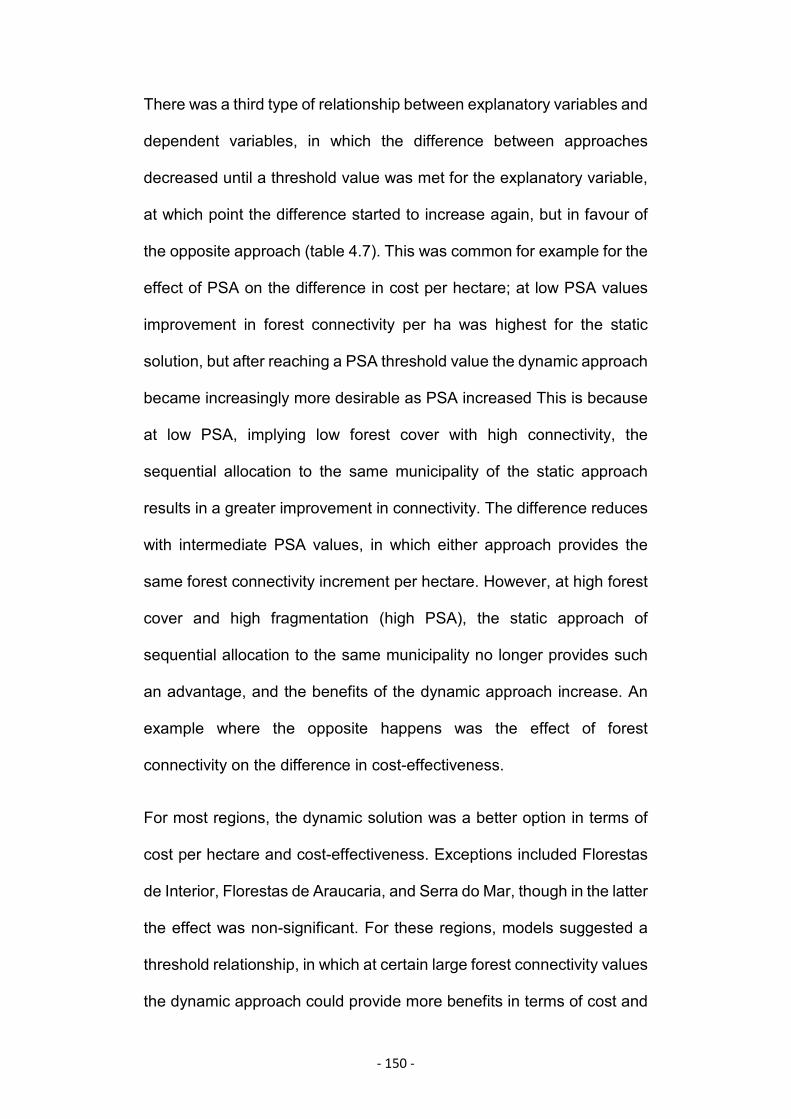
- 150 -

There was a third type of relationship between explanatory variables and

dependent variables, in which the difference between approaches

decreased until a threshold value was met for the explanatory variable,

at which point the difference started to increase again, but in favour of

the opposite approach (table 4.7). This was common for example for the

effect of PSA on the difference in cost per hectare; at low PSA values

improvement in forest connectivity per ha was highest for the static

solution, but after reaching a PSA threshold value the dynamic approach

became increasingly more desirable as PSA increased This is because

at low PSA, implying low forest cover with high connectivity, the

sequential allocation to the same municipality of the static approach

results in a greater improvement in connectivity. The difference reduces

with intermediate PSA values, in which either approach provides the

same forest connectivity increment per hectare. However, at high forest

cover and high fragmentation (high PSA), the static approach of

sequential allocation to the same municipality no longer provides such

an advantage, and the benefits of the dynamic approach increase. An

example where the opposite happens was the effect of forest

connectivity on the difference in cost-effectiveness.

For most regions, the dynamic solution was a better option in terms of

cost per hectare and cost-effectiveness. Exceptions included Florestas

de Interior, Florestas de Araucaria, and Serra do Mar, though in the latter

the effect was non-significant. For these regions, models suggested a

threshold relationship, in which at certain large forest connectivity values

the dynamic approach could provide more benefits in terms of cost and

- 151 -

cost-effectiveness. This explained why prioritisation results show that

the dynamic approach for Florestas de Interior provided high benefits

compared to the static approach. Interestingly, these three regions

presented the highest variability in cost per hectare, and the lowest

variability in set-aside cost-effectiveness (figure 4.4).

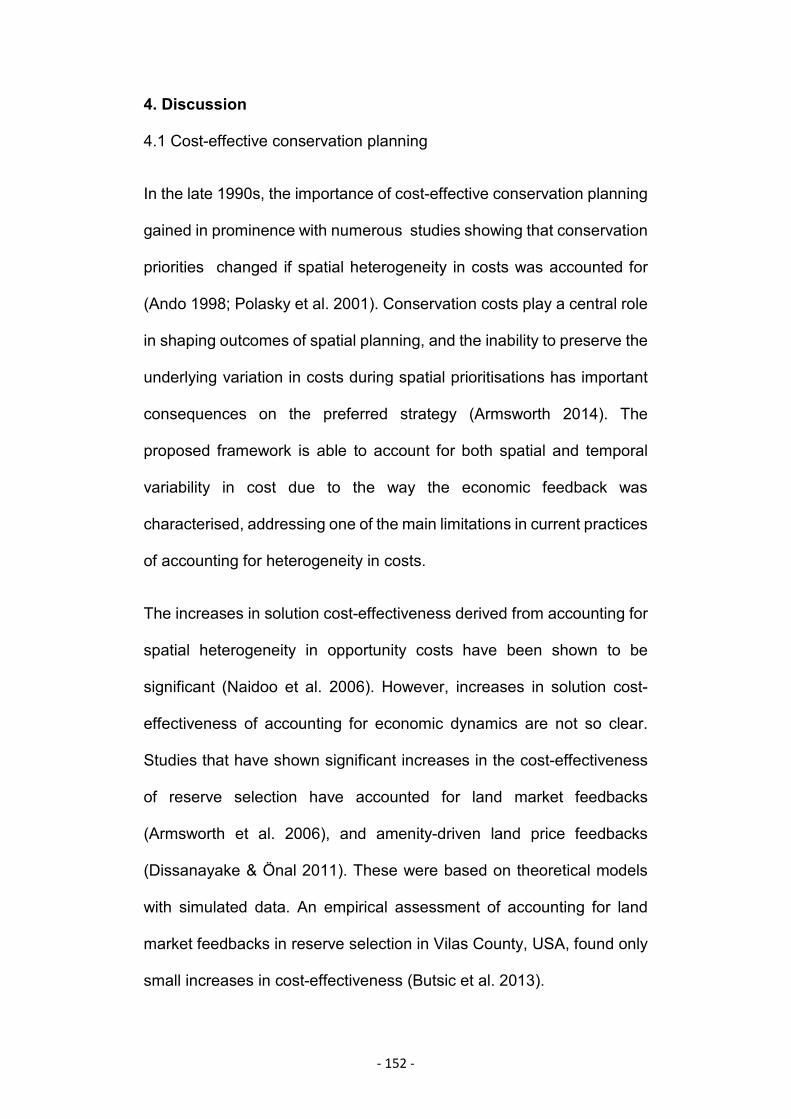
- 152 -

4. Discussion

4.1 Cost-effective conservation planning

In the late 1990s, the importance of cost-effective conservation planning

gained in prominence with numerous studies showing that conservation

priorities changed if spatial heterogeneity in costs was accounted for

(Ando 1998; Polasky et al. 2001). Conservation costs play a central role

in shaping outcomes of spatial planning, and the inability to preserve the

underlying variation in costs during spatial prioritisations has important

consequences on the preferred strategy (Armsworth 2014). The

proposed framework is able to account for both spatial and temporal

variability in cost due to the way the economic feedback was

characterised, addressing one of the main limitations in current practices

of accounting for heterogeneity in costs.

The increases in solution cost-effectiveness derived from accounting for

spatial heterogeneity in opportunity costs have been shown to be

significant (Naidoo et al. 2006). However, increases in solution cost-

effectiveness of accounting for economic dynamics are not so clear.

Studies that have shown significant increases in the cost-effectiveness

of reserve selection have accounted for land market feedbacks

(Armsworth et al. 2006), and amenity-driven land price feedbacks

(Dissanayake & Önal 2011). These were based on theoretical models

with simulated data. An empirical assessment of accounting for land

market feedbacks in reserve selection in Vilas County, USA, found only

small increases in cost-effectiveness (Butsic et al. 2013).

- 153 -

Studies accounting for economic feedbacks in spatial conservation

outcomes all found that the extent to which accounting for the feedback

improved cost-effectiveness depended on system and location

characteristics (Armsworth et al. 2006; Dissanayake & Önal 2011; Butsic

et al. 2013). In this study, cost-effectiveness improvement for the

dynamic approach also varied widely with biogeographical subregion,

and the subregion was the variable that explained most of the difference

in cost-effectiveness in the regression analyses. However, I found that

the dynamic approach would be more desirable when the feedback

effect is strong and there are alternative planning units that, once

chosen, allow escaping the deleterious effect of the feedback. If the

feedback is small and there are no other “low hanging fruits” in terms of

planning units, then there will be little gains to be obtained from the

dynamic approach. More case studies are needed to generalise these

findings, and better understand the circumstances under which a

dynamic approach yields more benefits than a static approach, including

different geographical regions, reforestation targets and conservation

interventions.

4.2 The role of informational rent capture

Most literature on informational rent in conservation focuses on the need

to minimise its capture to improve cost-effectiveness (Ferraro 2008;

White & Hanley 2016). Several studies have used contract theory to

show how auctions help reveal hidden costs and avoid adverse

- 154 -

selection, especially in the context of agri-environmental policies

(Latacz-Lohmann & Schilizzi 2005). However, the prospect of

informational rent capture acts as an economic incentive for programme

participation which can be used to improve resource use efficiency

(Scheufele & Bennett 2017). The dynamic framework proposed in this

study not only improved overall cost-effectiveness, but increased

informational rent capture, in so doing also involving more municipalities

in the programme. Given that asymmetric information is bound to exist,

especially at large scales, the dynamic framework can be a valuable new

tool to get informational rent capture working for conservation instead of

attempting to minimise it.

Conservation on private lands plays a crucial role in the conservation of

biodiversity in highly fragmented areas (Paloniemi & Tikka 2008).

Traditional regulation has not provided a complete solution due to the

large numbers of private landowners and the hidden nature of their

activities, which has led to an increasing emphasis on offering financial

incentives for conservation (Stern 2006). Conservation payments can

either aim to offset costs, or aim to change behaviour, or do both (Vatn

2010; Muradian & Rival 2012). Using the proposed dynamic

prioritisation, the set-aside programme moves away from being only an

offset payment to including an incentive to change behaviour as well by

increasing and optimising informational rent capture without increasing

the cost of the programme. The fact that more informational rent is

captured, and in a more even way across municipalities, could be an

- 155 -

invaluable benefit of the dynamic approach in regions where there is low

willingness to join this type of programme.

Real and perceived equity pay a crucial role in conservation payment

success by increasing the probability of self-enforcement because

people perceive the restrictions as fair (White et al. 2012). Increases in

equity are typically believed to come at the cost of financially optimal

conservation solutions, but the degree of equity in an intervention can

affect social and ecological outcomes in myriad ways (Pascual et al.

2010). Optimisation studies in the PES literature and spatial planning

literature have begun to incorporate dimensions of equity (Halpern et al.

2013; Narloch et al. 2013). Equity has multiple dimensions: procedural

legitimacy (i.e., the degree of participation in decision-making); the

distribution of costs and benefits of conservation; and the recognition of

stakeholder rights, norms and values (Pascual et al. 2014). Two

potential issues with this large scale set-aside payment programme

could be the distribution of costs (land-use restrictions) and benefits

(economic incentive) of the programme. The payment in the programme

aims to offset the cost, but it also provides an economic incentive when

informational rent is captured. The dynamic solution provides a more

equitable outcome than the static solution without any loss in cost-

effectiveness, in terms of both cost and benefit distributions, because

more municipalities are included in the solution. The fact that a wider

group of landowners is included in the programme with the dynamic

solution may also play a role in increasing perceived fairness, which

- 156 -

added to the increase in equity may significantly increase the probability

of success (Pascual et al. 2014).

4.3 Trade-off assessment

Running the static prioritisation has computational and data

requirements that are not hard to meet. Most of the data are free to

access, except for the cost of farmland that needs to be purchased.

Marxan is freely available, widely used in conservation prioritisations,

and does not require highly trained specialists or an exceptionally

powerful computer to run. However, the dynamic approach involves high

skills, informatics and time requirements. For this analysis, Python, R

and Linux coding skills were necessary, as well as access to high-

performance computing. Time requirements were also high,

approximately three months of running computing time to generate

results exclusive to the dynamic approach. The main limiting

computational step was the calculation of the forest connectivity metric

(ECA(IIC)), which requires metrics for patch area and distance between

patches for all forest patches within a municipality (see pages 112-114),

and municipalities had up to 20,000 forest patches. This index was

calculated for each forest simulation (100), for each municipality (3,500),

and for each time step (3), resulting in it being calculated over one million

times.

Increasing model complexity increases uncertainty and reduces model

predictability. Uncertainty increases with model complexity due to the

- 157 -

testing of all hypotheses upon which these models are based (Bradshaw

& Borchers 2000), as well as uncertainty propagation of multiple model

parameters. In this way, the dynamic solution could have higher

uncertainty levels. Quantifying and accounting for uncertainty in outputs

for both solutions is needed to communicate the reliability of results to

decision-makers, and avoid suboptimal allocation of management

actions (Langford et al. 2009). This could be achieved by exploring the

consequences of using different parameters through the use of

sensitivity analyses, scenario planning, and simulation modelling,

facilitating integrated modelling (Álvarez-Romero et al. 2015).

Both increased uncertainty and computational requirements need to be

considered when deciding on the optimal approach for a given

biogeographical region. For example, if I consider the effect of

accounting for environmental and economic feedbacks on cost and cost-

effectiveness, it is crucial to assess the reduction in total cost against the

increase in cost that the dynamic approach entails. The 0.7 mill. $

reduction in cost for Pernambuco might not be enough to offset the

increase in cost brought by the increased technical and computing

requirements of the dynamic approach, as well as the administrative

costs of repeating the prioritisation at regular intervals. However, a larger

reduction, such as the 280.4 mill. $ reduction for Florestas de Interior,

might make the dynamic approach more cost-effective.

In this study, only incentive payment costs were considered in the

prioritisation. These estimates based on farmland cost data were based

- 158 -

on the best available data (see pages 87-88 for detailed description).

However, there are transaction costs associated with the set-aside

programme, which include the operation, maintenance, and

administration of the programme (Zheng et al. 2013). Acquisition costs

and transaction costs do not necessarily reflect each other, and

accounting for both of them can affect prioritisation output (Armsworth

2014). However, to account for spatial heterogeneity in transaction

costs, data on what these costs entail are necessary, which were not

available at the time of analysis.

4.4 Implications for conservation and decision-making

Ignoring the economic feedback resulted in the static approach costing

$317 mill. more than the static cost estimation of meeting the restoration

target. This extra cost is large enough that the restoration target would

not be met over the nine-year period. Nowadays, rigorous planning

methods are especially needed given that collaborative conservation

action is on the rise and global financial crises restrict conservation

investments (Mazor et al. 2014). Simply applying the economic feedback

to the static solution can provide an estimation of how short the budget

will fall, improving budget estimation.

In the move towards cost-efficient conservation planning, a large body

of literature has been developed to make conservation as efficient as

possible at meeting stated goals (Naidoo et al. 2006; Klein et al. 2008;

Nelson et al. 2009). The most common focus has been on the

opportunity cost of land (for a review see Armsworth 2014). However,

- 159 -

this study shows that focusing on informational rents could potentially

increase benefits in terms of programme participation, equity and

potentially perceived fairness, without compromising cost-effectiveness.

Finding new ways of using informational rents in systematic

conservation planning is an important next step in improving

conservation success.

4.5 Recommendations for future work

In this case study, I chose Marxan as the prioritisation tool due to its

widespread use in spatial conservation planning. Marxan is based on a

minimisation optimisation problem, and in doing so it minimises the cost

of meeting targets (Ball et al. 2009). This results in an inclusion criterion

that does not necessarily include the municipalities with the highest

forest connectivity increment per hectare. An optimisation that minimises

cost whilst maximising forest connectivity increase subject to the

restoration target would maximise the benefits of accounting for the

environmental feedback. ConsNet (Ciarleglio et al. 2009) is a

conservation planning software that uses a multi-criteria analysis

approach with a meta-heuristic algorithm and could allow these types of

objectives, but has not been so widely implemented.

Sequential assessment of benefits and costs tends to be suboptimal in

reserve allocation (Duke et al. 2013). The timing of allocation can be

critical in terms of biodiversity protection in reserve selection problems

(Costello & Polasky 2004). Dynamic optimisation methods solve the

general management problem that involves a temporal sequence of

- 160 -

decisions, where the action at each decision point may differ depending

on time and/or system state (Possingham 1997). They have been

applied in natural resource management problems, and ways to deal

with uncertainty in the optimisation have been suggested (Williams &

Johnson 2013). Using a smaller, and therefore more computationally

tractable, case study, for example a biogeographical subregion, a

dynamic optimisation method based on a continuous informational rent

approach could be used to test differences in outputs.

Our study only modelled two feedbacks, chosen because they are

relevant to the scale and circumstances of the BAF (chapter 3).

However, complex dynamics are at play at multiple temporal and spatial

scales in any conservation intervention (Guerrero et al. 2013b)

Environmental dynamics are changing with climate change in both

terrestrial and marine ecosystems (Doney et al. 2012; Garcia et al.

2014). As shown in chapter 3, multiple economic feedback effects act at

the same time at different levels. For example, payments for ecosystem

services influence local land and labour markets (Wunder 2006), are

affected by trends in agricultural productivity (Phelps et al. 2013) and

increase landowners' perceptions of the value of fallow land (Rico

García-Amado et al. 2013) leading to unpredictable outcomes in terms

of conservation cost (Curran et al. 2016). A better understanding of

which feedbacks are most relevant under various circumstances is

needed in order to address the challenge of accounting for system

dynamics in conservation planning.

- 161 -

5. Conclusion

Accounting for environmental and social dynamics of the systems to be

intervened in is crucial if conservation planners are to provide more

realistic conservation recommendations. The methodology developed in

this chapter is the first attempt to account for both environmental and

economic dynamics in spatial conservation planning.

Evidence from this chapter is not conclusive in terms of which is the best

approach. Prioritisation outcomes were significantly different depending

on the geographical area, and in terms of the number of farms involved

in the scheme and the degree of informational rent capture. However,

differences were proportionally small in terms of cost-effectiveness, and

the geographical area mostly determined which approach was best.

A dynamic approach to spatial conservation planning does entail higher

computational requirements and transactions costs, but the potential

benefits in terms of increased cost-effectiveness could offset them. Most

importantly, the dynamic approach makes the most of the economic

incentive for participation from informational rents, and still has a similar

or lower overall cost. These results could potentially re-define the way in

which conservation projects manage informational rent extraction, away

from minimisation and towards exploiting the opportunities that it

provides. There is still much work to do in dynamic systematic

conservation planning, but these results already show an important

benefit in terms of understanding, and then working with, the feedbacks

that inevitably accompany large-scale conservation interventions.

- 162 -

Chapter 5: Restoring the Brazilian Atlantic Forest:

understanding the role of multiple restoration targets

and prioritisation approaches

- 163 -

1. Introduction

The level of threat facing the Brazilian Atlantic Forest (BAF), and the

importance of its restoration for the preservation of its biodiversity and

ecosystem services, have been highlighted by numerous studies (for a

recent overview see Eisenlohr et al. 2015). Despite a multitude of small-

scale forest restoration initiatives in the BAF since the 2000s, there has

been no significant expansion of native forests (Pinto et al. 2014). For

restoration to become an effective means of conserving the BAF,

challenges include reducing costs, planning restoration actions at the

landscape level, and addressing socio-political issues (Rodrigues et al.

2009; Melo et al. 2013b).

Systematic conservation planning is an area of conservation specifically

focused on optimizing conservation outcomes cost-effectively;

thousands of systematic conservation plans have been developed

around the globe (McIntosh et al. 2016). It involves a systematic

structured approach to the selection of areas for conservation action

(including preservation, restoration and management), using limited

resources to achieve clear conservation goals in the face of competing

land uses, and with outcomes open to critical review (Margules &

Pressey 2000a; Kukkala & Moilanen 2013). A critical element of

systematic conservation planning is spatial prioritisation, and various

software have been built for this purpose (e.g. Marxan (Ball et al. 2009),

C-Plan (Pressey et al. 2009) and Zonation (Lehtomäki & Moilanen

2013)). The application of a systematic conservation planning approach

at the landscape level for the BAF would, in theory, help solve two of the

- 164 -

main challenges to restoring it (landscape-level planning and cost-

effectiveness).

A few studies have applied a systematic conservation planning approach

to set priorities for restoration at the BAF level. Most of the conservation

planning exercises carried out for the BAF produce priorities based on

ecological features, with only some of them including social or cost data.

Some studies use complex ecological techniques such as ecological

niche modelling (Lemes & Loyola 2013) and habitat removal

experiments (Tambosi et al. 2014) to set priorities, but exclude socio-

economic data from their analyses. The Atlantic Forest Restoration Pact

(AFRP, see chapter 1) prioritised areas for restoration based on an

assessment of deforested lands protected by the Brazilian Forest Code,

as well as extensive, low-productivity pasturelands with few cattle

(Calmon et al. 2011). The AFRP’s prioritisation criteria were mainly

socio-economic, but they additionally produced thematic maps that can

be overlaid to guide restoration efforts depending on the funder’s

objective (Brancalion et al. 2013b). More recently, two BAF-level spatial

conservation planning approaches included both ecosystem and

economic criteria in prioritising areas for restoration. In 2014 using data

from a large field study surveying mammals, amphibians and birds,

restoration priorities were identified in terms of community integrity and

phylogenetic integrity, and cost of agricultural set-asides (Banks-Leite et

al. 2014b). In 2015, priorities for restoration were identified in terms of

expected post-restoration habitat availability per USD for two mammal

species with widely different dispersal abilities and habitat patch

- 165 -

requirements (Crouzeilles et al. 2015). All of these prioritisations had

very different objectives when setting priorities to restore the BAF,

resulting in restoration targets that ranged between 424,000 ha and 15

million hectares for the whole biome. However, to build one consistent

approach to restoring the BAF, priority areas need to be identified in the

context of diverse targets.

Important assumptions underlie the systematic conservation planning

approach, one of them being that environmental and economic

conditions remain static over time (Meir et al. 2004). However,

commonly these assumptions do not hold, which can lead to reduced

cost-effectiveness of conservation programmes or even to misleading

recommendations (chapter 2). Studies that account directly or indirectly

for ecosystem dynamics when prioritising areas for conservation in the

Atlantic Forest, rather than taking a static approach, include those using

climate models to predict the effect of climate change on species

distributions (Loyola et al. 2012; Faleiro et al. 2013) and habitat

availability improvement triggered by the restoration itself (Crouzeilles et

al. 2015; Rappaport et al. 2015b; Tambosi & Metzger 2015). Most

recently, temporal dynamics were included in an assessment of priorities

for restoration at a site in the BAF accounting for the time-lagged

response of bird functional-group richness to fragmentation (Uezu &

Metzger 2016). However, no studies were found that included economic

dynamics into conservation planning exercises in the BAF, and in fact,

both economic and ecological dynamics are rarely included in

systematic conservation planning (chapter 3).

- 166 -

Roughly 53% of Brazil’s native vegetation occurs on private properties,

and in order to comply with the new Forest Code (FC) (National Law No.

12.651/2012), Brazilian landowners need to collectively restore ~6.2

million hectares within the Atlantic Forest hotspot (Soares-Filho et al.

2014). The FC provides a legal framework for control and incentives for

the protection of forest, promoting mechanisms and policies to support

forest restoration (Brancalion et al. 2016). However, the history of the

FC showed that the implementation of restoration on farmlands is

challenging to enforce (Alves-Pinto et al. 2017). Using multiple

correspondence analyses, Trevisan et al. (2016) identified three types

of farmers in Santa Catarina: those who understood the FC and its

ecological impacts and were willing to comply; those who understood

the ecological benefits of restoration but were unwilling to comply; and

those with little knowledge of benefits or interest in compliance.

Compliance comes at a cost for landowners, and as for any type of

conservation on private lands, an incentive is needed (Stern 2006;

Latawiec et al. 2015). Payment for ecosystem services (PES) schemes

in Brazil have been growing for the last 10 years (Richards et al. 2015),

and PES has been put forward as one of many mechanisms for making

restoration in the BAF economically sustainable (Brancalion et al. 2012;

Lopes et al. 2013; Soares-filho et al. 2014; Trevisan et al. 2016). If the

groups of landowners with no interest or willingness to comply are to be

part of a PES programme to restore the BAF, incentive payments need

to do more than offset the cost of restoration, they need to provide an

economic incentive to change behaviour (Vatn 2010; de Rezende et al.

- 167 -

2015). Ways to provide this type of incentive in the most cost-effective

way, and to structure these incentives into priority-setting for to BAF

restoration are still missing.

Considering setting aside agricultural land as the minimum level of

action to allow for natural regeneration (Strassburg et al. 2016), I applied

a spatial conservation planning approach to prioritising natural

restoration on farmland in the BAF. In the context of diverse restoration

targets, I compared prioritisation solutions for both the static and

dynamic approaches defined in chapter four, assessing informational

rent capture as an economic incentive for restoration for all solutions.

Specifically, the objectives of this chapter were to: (1) identify priority

areas for natural restoration in the BAF that are robust to diverse targets

and approaches; (2) compare costs and benefits for each of the chosen

targets; (3) assess the effect of changing targets on the difference in

outputs between static and dynamic approaches; and (4) provide

recommendations regarding the choice of prioritisation approach in the

context of diverse targets for the BAF.

- 168 -

2. Methods

2.1 Methodological framework

Methods were based on the framework developed in chapter 4. To

assess the robustness of the allocation to different targets, the

framework was applied at the biogeographical subregion level for the

BAF, for three different restoration targets (low, medium, high). To

improve readability of this chapter, table 5.1 summarises some key

definitions from chapter 4.

The spatial conservation planning exercise involved four steps: (1)

calculation of base metrics from data, (2) calculation of prioritisation

inputs, (3) spatial prioritisation, and (4) solution assessment and

implementation (figure 4.1, chapter 4).

2.2 Data and software

The same data that were used in chapter 4 I used for this analysis (table

4.1, chapter 4). Additionally, values of gross domestic product (GDP)

were obtained from the United Nations Statistics Division

(http://unstats.un.org/unsd/snaama/selectionbasicFast.asp), and

agricultural subsidies were obtained from the Brazilian Ministry of

Finances (http://www.orcamentofederal.gov.br), both for the year 2015.

Software used for analyses include R 3.2.1 (R Core Team 2016), ArcGIS

10 (Esri 2011), Conefor Sensinode 2.5.8 command line version (Saura

& Torné 2009), and MARXAN (Ball et al. 2009). The University of Oxford

- 169 -

Advanced Research Computing (ARC) facility was used to carry out this

work.

2.3 Model validation

Model validation and verification include the same methods used for the

model in Chapter Four. Additionally, operational validity was subjectively

assessed by comparison with other studies other studies that produced

priorities for forest restoration in the BAF, with restoration targets within

the range used in this chapter.

2.4 Restoration Targets

I chose three different restoration targets, all of which are based on

stated objectives for restoring the BAF. The targets vary in terms of the

number of hectares restored and the rationale behind the target. At the

BAF level, the number of hectares to be restored quantitatively increases

from target one to three. At the BR level however, this is not always the

case due to the qualitative definition of targets (see below and Table

5.2).

Target 1: Low target

This target is based on Brazil’s international commitment to the

Convention on Biological Diversity (CBD) Aichi targets. Under National

Target 15, Brazil has set a target of restoring at least 15% of degraded

- 170 -

ecosystems by 2020 (www.cbd.int). By calculating the restoration of

15% of existing forest in each biogeographical subregion, target one

amounts to restoring a total of 2.7 million hectares (M ha; table 5.2). This

target is the same target used in Chapter four, and results based on this

target derive from the analysis done for that chapter.

Target two: Medium target

Using data from a large field study in the BAF surveying mammals,

amphibians and birds, it was suggested that to maintain biodiversity both

in terms of community integrity and phylogenetic integrity, a minimum of

30% of forest cover is required across the BAF (Banks-Leite et al.

2014b). By calculating the restoration needed to bring each forest

landscape (FL; see Table 5.1) to 30% forest cover for every municipality,

target two amounts to restoring a total of 10.6M ha (table 5.2). This

amount was estimated by calculating 30% of each forest landscape for

all municipalities, and subtracting existing forest to that value. Some

municipalities’ FL forest cover was higher than 30%, and these were

excluded from restoration allocations.

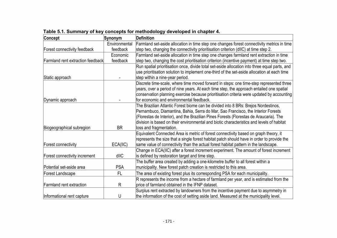
- 171 -

Table 5.1. Summary of key concepts for methodology developed in chapter 4.Concept Synonym Definition

Forest connectivity feedbackEnvironmental

feedbackFarmland set-aside allocation in time step one changes forest connectivity metrics in timestep two, changing the connectivity prioritisation criterion (dIIC) at time step 2.

Farmland rent extraction feedbackEconomicfeedback

Farmland set-aside allocation in time step one changes farmland rent extraction in timestep two, changing the cost prioritisation criterion (incentive payment) at time step two.

Static approach -

Run spatial prioritisation once, divide total set-aside allocation into three equal parts, anduse prioritisation solution to implement one-third of the set-aside allocation at each timestep within a nine-year period.

Dynamic approach -

Discrete time-scale, where time moved forward in steps: one time-step represented threeyears, over a period of nine years. At each time step, the approach entailed one spatialconservation planning exercise because prioritisation criteria were updated by accountingfor economic and environmental feedback.

Biogeographical subregion BR

The Brazilian Atlantic Forest biome can be divided into 8 BRs: Brejos Nordestinos,Pernambuco, Diamantina, Bahia, Serra do Mar, Sao Francisco, the Interior Forests(Florestas de Interior), and the Brazilian Pines Forests (Florestas de Araucaria). Thedivision is based on their environmental and biotic characteristics and levels of habitatloss and fragmentation.

Forest connectivity ECA(IIC)

Equivalent Connected Area is metric of forest connectivity based on graph theory, itrepresents the size that a single forest habitat patch should have in order to provide thesame value of connectivity than the actual forest habitat pattern in the landscape.

Forest connectivity increment dIICChange in ECA(IIC) after a forest increment experiment. The amount of forest incrementis defined by restoration target and time step.

Potential set-aside area PSAThe buffer area created by adding a one-kilometre buffer to all forest within amunicipality. New forest patch creation is restricted to this area.

Forest Landscape FL The area of existing forest plus its corresponding PSA for each municipality.

Farmland rent extraction RR represents the income from a hectare of farmland per year, and is estimated from theprice of farmland obtained in the IFNP dataset.

Informational rent capture USurplus rent extracted by landowners from the incentive payment due to asymmetry inthe information of the cost of setting aside land. Measured at the municipality level.

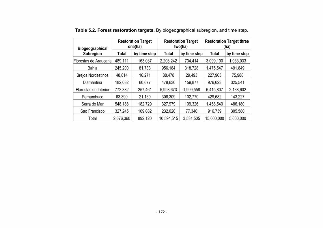
- 172 -

Table 5.2. Forest restoration targets. By biogeographical subregion, and time step.

BiogeographicalSubregion

Restoration Targetone(ha)

Restoration Targettwo(ha)

Restoration Target three(ha)

Total by time step Total by time step Total by time stepFlorestas de Araucaria 489,111 163,037 2,203,242 734,414 3,099,100 1,033,033

Bahia 245,200 81,733 956,184 318,728 1,475,547 491,849Brejos Nordestinos 48,814 16,271 88,478 29,493 227,963 75,988

Diamantina 182,032 60,677 479,630 159,877 976,623 325,541Florestas de Interior 772,382 257,461 5,998,673 1,999,558 6,415,807 2,138,602

Pernambuco 63,390 21,130 308,309 102,770 429,682 143,227Serra do Mar 548,188 182,729 327,979 109,326 1,458,540 486,180

Sao Francisco 327,245 109,082 232,020 77,340 916,739 305,580Total 2,676,360 892,120 10,594,515 3,531,505 15,000,000 5,000,000

- 173 -

Target three: High target

In 2009, a group of NGOs, private companies, governments, and

research institutions launched one of the most ambitious ecological

restoration programs in the world – the Atlantic Forest (Mata Atlântica)

Restoration Pact (AFRP). The program has more than 260 members

and has a mission to restore 15M ha of the forest by 2050 using native

species (Brancalion et al. 2012). I used their mission target as target

three, and the 15M ha were distributed proportionally to the total FL

across biogeographical subregions (table 5.2). I tested other ways of

distributing the 15M ha, such as proportional to existing forest and

potential set-aside area (PSA): the resultant allocations were similar

except the chosen allocation gave more weight to highly fragmented

areas.

2.5 Variables

Spatial configuration

One of Marxan’s outputs provides selection frequency for each

municipality. The selection frequency shows how many times out of a

thousand Marxan runs the municipality was included as part of a

solution. For each restoration target and approach, I chose only

solutions that met both restoration and connectivity targets, and

calculated the percent selection frequency for each municipality. Percent

selection frequency represented the probability of a municipality being

included as part of the spatial prioritisation solution, as a percentage. I

- 174 -

used this as a basis for the calculation of two variables: (1) concordance

score and (2) difference in percent selection frequency (dSF).

(1) Concordance score: the minimum percent selection frequency

common to all target and approach combinations for each municipality.

This score represents the minimum probability of a municipality being

included in a solution for all restoration targets and approaches.

(2) Difference in percent selection frequency (dSF): simply the difference

in percent selection frequency for each municipality between the static

and dynamic approaches for each restoration target individually. This

variable represents how much the probability of a municipality being

included in the solution changed with prioritisation approach, rather than

the target. A -100 score shows municipalities always included in the

dynamic solution and never in the static, a 100 score shows

municipalities always included in the static solution and never in the

dynamic one, and values close to zero show municipalities whose

probabilities of being included in the solution did not change significantly

with prioritisation approach.

Costs and Benefits

Solutions for the 3 restoration targets under both static and dynamic

approaches were compared spatially and through time on the basis of

cost (USD, $), cost-effectiveness (ha/USD), forest connectivity

increment (ha), informational rent capture (USD, $) and proportional

- 175 -

informational rent capture (informational rent capture as a proportion of

USD spent). Temporal comparisons were on a per year basis, and

regional comparisons on a per hectare basis (cf Armsworth 2014).

2.6 Testing importance of restoration target and prioritisation approach

Linear models were fitted to test the effect of restoration target and

prioritisation approach on the solution obtained. Different models were

fitted for 3 response variables: cost-effectiveness, connectivity (dIIC/ha),

and proportional informational rent capture (see table 5.1 and chapter

4). Models were fitted for each BR individually because the objective was

to understand the relative importance of restoration target and

prioritisation approach for each BR independently.

Two-way ANOVAs were fitted using the lm() function in R, and model fit

was assessed using residual plots as recommended by Pinheiro and

Bates (2000). Box-cox transformations were applied to the response

variables to solve non-linearity issues (Box & Cox 1964; Kato 2012).

- 176 -

3. Results

3.1 Costs and benefits of meeting restoration targets

The total cost of achieving restoration targets via a payment scheme was

approximately 3,553-3,797 million USD (mill. $) for restoration target

one, 20,400- 20,640 mill. $ for restoration target two, and 30,010-30,358

mill. $ for restoration target three (table 5.3). These costs represented

half of the cost of purchasing farmland for the same solutions: 7,400,

40,900 and 60,100 mill. $ for targets one, two and three respectively.

The dynamic solution was 243-347 mill. $ cheaper than the static

solution depending on the restoration target.

Cost-effectiveness, the number of hectares set-aside per USD spent,

increased at each time step in the dynamic prioritisation, but decreased

with the number of hectares to be restored (SM Table 8). Cost-

effectiveness for the dynamic solution under targets two and three were

31% and 34% lower than target one respectively (SM Table 8). The cost-

effectiveness difference between targets was slightly smaller for the

static approach, but followed the same trend (SM Table 8). This

decrease in cost-effectiveness could be expected because the Marxan’s

solution includes municipalities in decreasing order of cost-

effectiveness, so a larger target meant decreased overall cost-

effectiveness.

The restoration targets defined forest cover benefits, and the total forest

connectivity increment promoted by those targets defined forest

connectivity benefits (dIIC, table 5.3). Total dIIC ranged between 0.71-

- 177 -

0.74, 2.22-2.37, and 3.16-3.42 million hectares (M ha) for restoration

targets one, two and three respectively; the lower value of the range

belonged to the dynamic solutions (table 5.3). Forest connectivity

increment per restored hectare (dIIC/ha) had a similar behaviour to cost-

effectiveness at the BAF level; decreasing with restoration target. For

the dynamic approach, dIIC/ha decreased by 21% between targets one

and two, but the difference between targets two and three were close to

0% (SM Table 8). The difference in dIIC/ha between targets was slightly

smaller for the static approach, but followed the same trend. This

decrease in dIIC/ha was explained by the same mechanism that

explains decreasing cost-effectiveness. However, the fact the

magnitude of the difference decreased with restoration target could be

explained by the logarithmic-type relationship between forest cover and

dIIC. This relationship seems to have decreasing marginal returns that

are hit at ~10M ha (target two). The increase in forest connectivity

promoted by a set number of hectares at lower forest cover values is

smaller than the one promoted by the same amount at higher forest

cover values. In target one dIIC/ha reached higher values and larger

differences between approaches, but with increasing target, dIIC/ha and

its differences between approaches became much smaller.

At the BR level, the same BAF level trends in cost per hectare (SM

Figure 3) and cost-effectiveness (figure 5.1a) across targets were

observed for most subregions. The largest drop in cost-effectiveness

was observed between targets one and two for most regions (figure

5.1a). The most common trend for dIIC/ha was decreasing dIIC/ha with

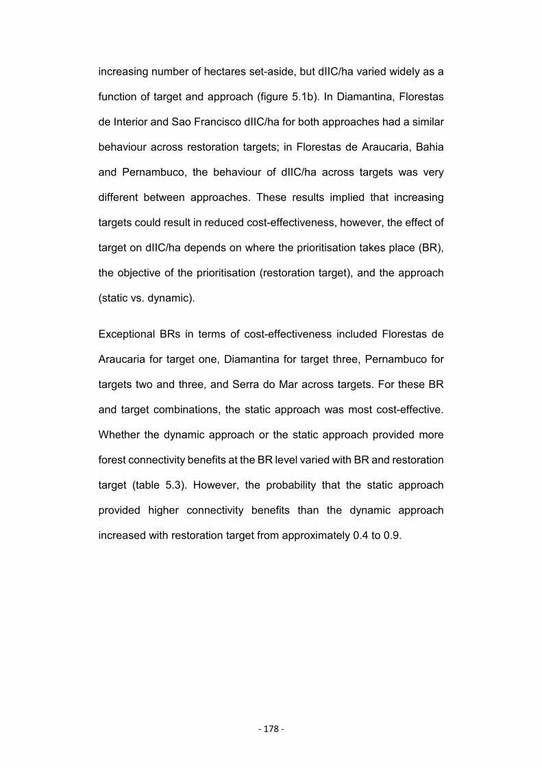
- 178 -

increasing number of hectares set-aside, but dIIC/ha varied widely as a

function of target and approach (figure 5.1b). In Diamantina, Florestas

de Interior and Sao Francisco dIIC/ha for both approaches had a similar

behaviour across restoration targets; in Florestas de Araucaria, Bahia

and Pernambuco, the behaviour of dIIC/ha across targets was very

different between approaches. These results implied that increasing

targets could result in reduced cost-effectiveness, however, the effect of

target on dIIC/ha depends on where the prioritisation takes place (BR),

the objective of the prioritisation (restoration target), and the approach

(static vs. dynamic).

Exceptional BRs in terms of cost-effectiveness included Florestas de

Araucaria for target one, Diamantina for target three, Pernambuco for

targets two and three, and Serra do Mar across targets. For these BR

and target combinations, the static approach was most cost-effective.

Whether the dynamic approach or the static approach provided more

forest connectivity benefits at the BR level varied with BR and restoration

target (table 5.3). However, the probability that the static approach

provided higher connectivity benefits than the dynamic approach

increased with restoration target from approximately 0.4 to 0.9.

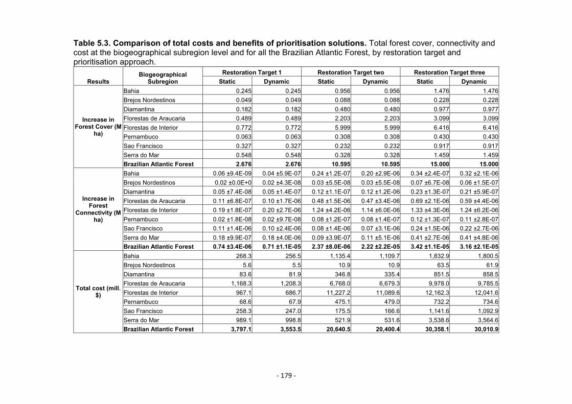
- 179 -

Table 5.3. Comparison of total costs and benefits of prioritisation solutions. Total forest cover, connectivity andcost at the biogeographical subregion level and for all the Brazilian Atlantic Forest, by restoration target andprioritisation approach.

ResultsBiogeographicalSubregion

Restoration Target 1 Restoration Target two Restoration Target threeStatic Dynamic Static Dynamic Static Dynamic

Increase inForest Cover (M

ha)

Bahia 0.245 0.245 0.956 0.956 1.476 1.476Brejos Nordestinos 0.049 0.049 0.088 0.088 0.228 0.228Diamantina 0.182 0.182 0.480 0.480 0.977 0.977Florestas de Araucaria 0.489 0.489 2.203 2.203 3.099 3.099Florestas de Interior 0.772 0.772 5.999 5.999 6.416 6.416Pernambuco 0.063 0.063 0.308 0.308 0.430 0.430Sao Francisco 0.327 0.327 0.232 0.232 0.917 0.917Serra do Mar 0.548 0.548 0.328 0.328 1.459 1.459Brazilian Atlantic Forest 2.676 2.676 10.595 10.595 15.000 15.000

Increase inForest

Connectivity (Mha)

Bahia 0.06 ±9.4E-09 0.04 ±5.9E-07 0.24 ±1.2E-07 0.20 ±2.9E-06 0.34 ±2.4E-07 0.32 ±2.1E-06Brejos Nordestinos 0.02 ±0.0E+0 0.02 ±4.3E-08 0.03 ±5.5E-08 0.03 ±5.5E-08 0.07 ±6.7E-08 0.06 ±1.5E-07Diamantina 0.05 ±7.4E-08 0.05 ±1.4E-07 0.12 ±1.1E-07 0.12 ±1.2E-06 0.23 ±1.3E-07 0.21 ±5.9E-07Florestas de Araucaria 0.11 ±6.8E-07 0.10 ±1.7E-06 0.48 ±1.5E-06 0.47 ±3.4E-06 0.69 ±2.1E-06 0.59 ±4.4E-06Florestas de Interior 0.19 ±1.8E-07 0.20 ±2.7E-06 1.24 ±4.2E-06 1.14 ±6.0E-06 1.33 ±4.3E-06 1.24 ±6.2E-06Pernambuco 0.02 ±1.8E-08 0.02 ±9.7E-08 0.08 ±1.2E-07 0.08 ±1.4E-07 0.12 ±1.3E-07 0.11 ±2.8E-07Sao Francisco 0.11 ±1.4E-06 0.10 ±2.4E-06 0.08 ±1.4E-06 0.07 ±3.1E-06 0.24 ±1.5E-06 0.22 ±2.7E-06Serra do Mar 0.18 ±9.9E-07 0.18 ±4.0E-06 0.09 ±3.9E-07 0.11 ±5.1E-06 0.41 ±2.7E-06 0.41 ±4.8E-06Brazilian Atlantic Forest 0.74 ±3.4E-06 0.71 ±1.1E-05 2.37 ±8.0E-06 2.22 ±2.2E-05 3.42 ±1.1E-05 3.16 ±2.1E-05

Total cost (mill.$)

Bahia 268.3 256.5 1,135.4 1,109.7 1,832.9 1,800.5Brejos Nordestinos 5.6 5.5 10.9 10.9 63.5 61.9Diamantina 83.6 81.9 346.8 335.4 851.5 858.5Florestas de Araucaria 1,168.3 1,208.3 6,768.0 6,679.3 9,978.0 9,785.5Florestas de Interior 967.1 686.7 11,227.2 11,089.6 12,162.3 12,041.6Pernambuco 68.6 67.9 475.1 479.0 732.2 734.6Sao Francisco 258.3 247.0 175.5 166.6 1,141.6 1,092.9Serra do Mar 989.1 998.8 521.9 531.6 3,538.6 3,564.6Brazilian Atlantic Forest 3,797.1 3,553.5 20,640.5 20,400.4 30,358.1 30,010.9

- 180 -

Figure 5.1. Changes in cost effectiveness and proportional forestincrement. (a) Cost effectiveness and (B) forest connectivity incrementfor all prioritisation solutions by biogeographical subregions.

Florestas de Araucaria Bahia Brejos Nordestinos Diamantina

Florestas de Interior Pernambuco Serra do Mar Sao Francisco

3.25e−04

3.50e−04

3.75e−04

4.00e−04

8.0e−04

8.5e−04

9.0e−04

9.5e−04

4e−03

5e−03

6e−03

7e−03

8e−03

9e−03

1.25e−03

1.50e−03

1.75e−03

2.00e−03

2.25e−03

6e−04

8e−04

1e−03

6e−04

7e−04

8e−04

9e−04

4.0e−04

4.5e−04

5.0e−04

5.5e−04

6.0e−04

8.0e−04

1.0e−03

1.2e−03

1.4e−03

T1 T2 T3 T1 T2 T3 T1 T2 T3 T1 T2 T3

T1 T2 T3 T1 T2 T3 T1 T2 T3 T1 T2 T3Restoration Target

Costeffectiveness(ha/usd)

SolutionDynamicStatic

(A) Cost effectiveness

Florestas de Araucaria Bahia Brejos Nordestinos Diamantina

Florestas de Interior Pernambuco Serra do Mar Sao Francisco

0.20

0.25

0.30

0.35

0.20

0.25

0.30

0.35

T1 T2 T3 T1 T2 T3 T1 T2 T3 T1 T2 T3Restoration Target

Forestconnectivityincrementpersetasidehectare(proportion)

SolutionDynamicStatic

(B) Forest connectivity change

- 181 -

3.2 Spatial prioritisation agreement

All BRs had high concordance areas, meaning groups of municipalities

with concordance scores of 50% or higher, except for Pernambuco

(figure 5.2). However, the proportion of BRs with municipalities with high

concordance scores varied widely, with Bahia having the smallest and

Florestas de Araucaria the largest. The highest concordance scores (75-

100%) were found in Serra do Mar, Brejos Nordestinos and Diamantina

(figures 5.2 & 5.3).

There were five BRs with a high proportion of 0% concordance scores:

Florestas de Araucaria, Florestas de Interior, Brejos Nordestinos,

Diamantina, and Serra do Mar (figure 5.3). For each of these BRs, of all

municipalities included in any given solution, more than 75% had at least

one solution for which the municipality had not been included. However,

the concordance score was created to look at strong agreement, not lack

of it, so a 0% score simply suggests no agreement in the solution across

approach/target combinations, but not the degree of disagreement.

Studies looking at congruence among spatial prioritisation for different

taxonomic groups in Brazil have also found low congruence across large

areas (Sobral et al. 2012).

Three groups of BRs could be identified based on distribution of

concordance scores different to zero: (1) low, (3) intermediate, and (3)

high. These groups were defined on the basis of score value and

representation. Pernambuco had the lowest concordance, never

reaching concordance scores higher than 10% (figure 5.3). The

- 182 -

“intermediate concordance” group included Florestas de Interior,

Florestas de Araucaria, Brejos Nordestinos, Diamantina, and Serra do

Mar. Scores varied widely for these BRs, but not one score category was

representative of more than 8% of the BR (excluding 0% category).

Bahia also belonged to the intermediate concordance group, with one-

third of it having scored 30% or lower. Finally, Sao Francisco was the

only BR in the high concordance category, because one-quarter of it had

concordance scores between 30-75%. The majority of BRs (6 out of

eight) had intermediate concordance scores, highlighting Pernambuco

and Sao Francisco as BRs where the choice of approach/target

combination had a high and low impact on the spatial solution,

respectively.

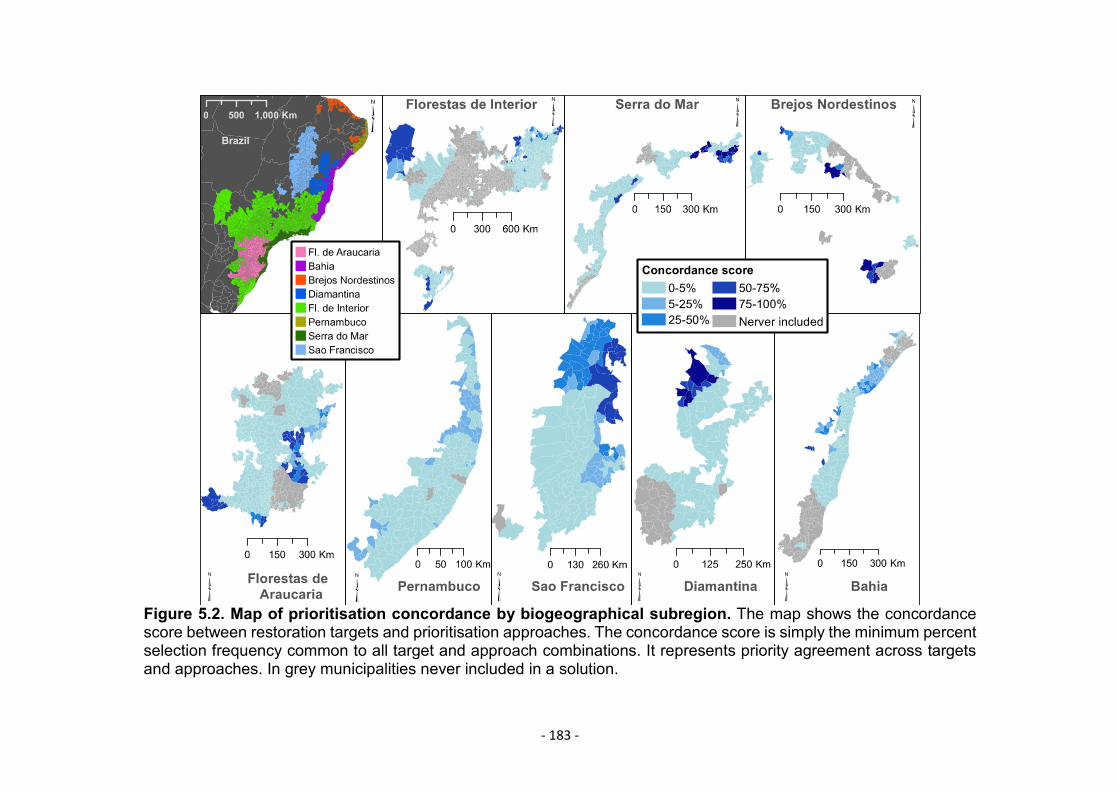
- 183 -

Figure 5.2. Map of prioritisation concordance by biogeographical subregion. The map shows the concordancescore between restoration targets and prioritisation approaches. The concordance score is simply the minimum percentselection frequency common to all target and approach combinations. It represents priority agreement across targetsand approaches. In grey municipalities never included in a solution.

- 184 -

Figure 5.3. Prioritisation concordance by biogeographical subregion. The proportion of each biogeographicalregion that have different concordance scores. The concordance score is simply the minimum percentage selectionfrequency common to all target and approach combinations, representing agreement across targets and approaches.Proportions were calculated in terms of number of municipalities.

Florestas de Araucaria Bahia Brejos Nordestinos Diamantina

Florestas de Interior Pernambuco Serra do Mar Sao Francisco0.00

0.25

0.50

0.75

0.00

0.25

0.50

0.75

0% 0−10%

10−30%

30−50%

50−75%

75−100%

0% 0−10%

10−30%

30−50%

50−75%

75−100%

0% 0−10%

10−30%

30−50%

50−75%

75−100%

0% 0−10%

10−30%

30−50%

50−75%

75−100%

Concordance score

Proportionofbiogeographicalsubregion

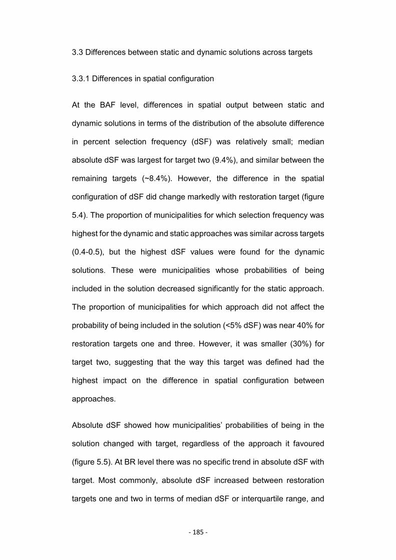
- 185 -

3.3 Differences between static and dynamic solutions across targets

3.3.1 Differences in spatial configuration

At the BAF level, differences in spatial output between static and

dynamic solutions in terms of the distribution of the absolute difference

in percent selection frequency (dSF) was relatively small; median

absolute dSF was largest for target two (9.4%), and similar between the

remaining targets (~8.4%). However, the difference in the spatial

configuration of dSF did change markedly with restoration target (figure

5.4). The proportion of municipalities for which selection frequency was

highest for the dynamic and static approaches was similar across targets

(0.4-0.5), but the highest dSF values were found for the dynamic

solutions. These were municipalities whose probabilities of being

included in the solution decreased significantly for the static approach.

The proportion of municipalities for which approach did not affect the

probability of being included in the solution (<5% dSF) was near 40% for

restoration targets one and three. However, it was smaller (30%) for

target two, suggesting that the way this target was defined had the

highest impact on the difference in spatial configuration between

approaches.

Absolute dSF showed how municipalities’ probabilities of being in the

solution changed with target, regardless of the approach it favoured

(figure 5.5). At BR level there was no specific trend in absolute dSF with

target. Most commonly, absolute dSF increased between restoration

targets one and two in terms of median dSF or interquartile range, and

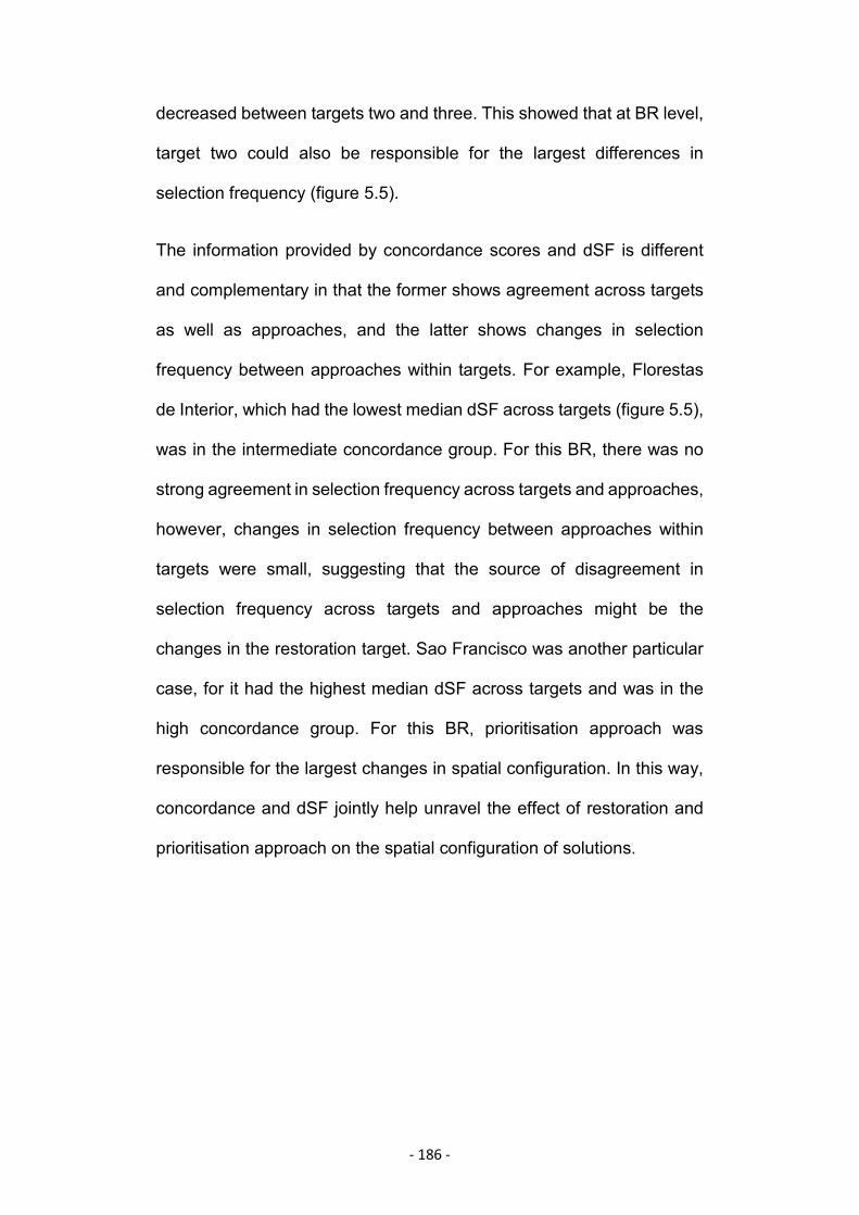
- 186 -

decreased between targets two and three. This showed that at BR level,

target two could also be responsible for the largest differences in

selection frequency (figure 5.5).

The information provided by concordance scores and dSF is different

and complementary in that the former shows agreement across targets

as well as approaches, and the latter shows changes in selection

frequency between approaches within targets. For example, Florestas

de Interior, which had the lowest median dSF across targets (figure 5.5),

was in the intermediate concordance group. For this BR, there was no

strong agreement in selection frequency across targets and approaches,

however, changes in selection frequency between approaches within

targets were small, suggesting that the source of disagreement in

selection frequency across targets and approaches might be the

changes in the restoration target. Sao Francisco was another particular

case, for it had the highest median dSF across targets and was in the

high concordance group. For this BR, prioritisation approach was

responsible for the largest changes in spatial configuration. In this way,

concordance and dSF jointly help unravel the effect of restoration and

prioritisation approach on the spatial configuration of solutions.

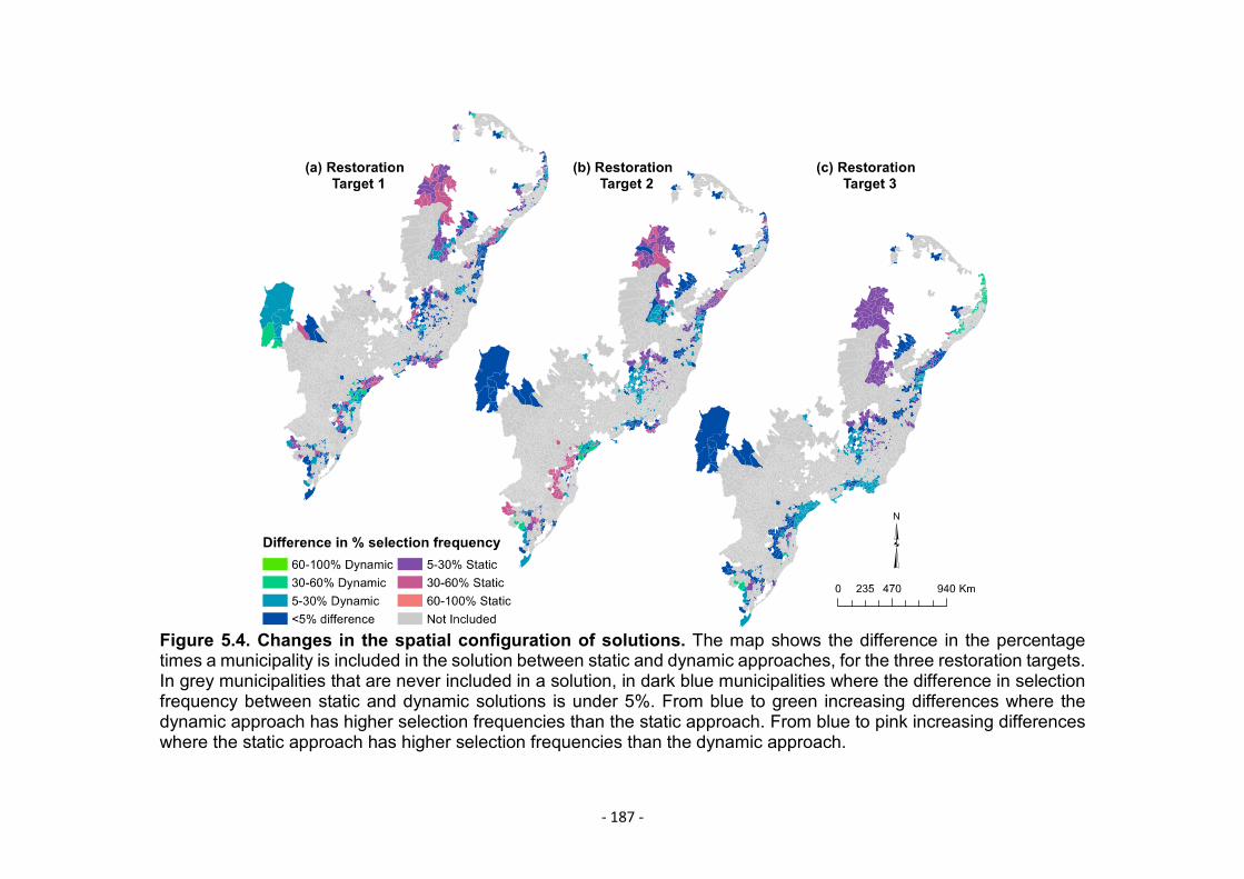
- 187 -

Figure 5.4. Changes in the spatial configuration of solutions. The map shows the difference in the percentagetimes a municipality is included in the solution between static and dynamic approaches, for the three restoration targets.In grey municipalities that are never included in a solution, in dark blue municipalities where the difference in selectionfrequency between static and dynamic solutions is under 5%. From blue to green increasing differences where thedynamic approach has higher selection frequencies than the static approach. From blue to pink increasing differenceswhere the static approach has higher selection frequencies than the dynamic approach.

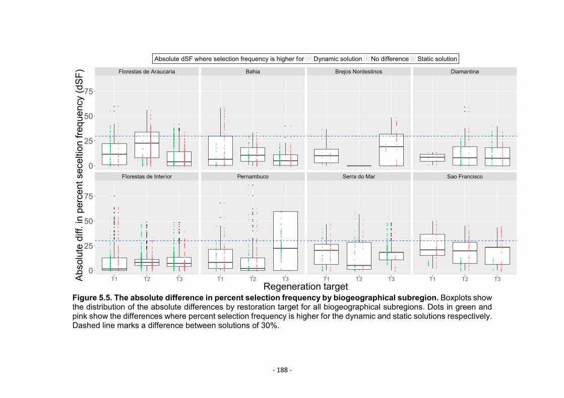
- 188 -

Figure 5.5. The absolute difference in percent selection frequency by biogeographical subregion. Boxplots showthe distribution of the absolute differences by restoration target for all biogeographical subregions. Dots in green andpink show the differences where percent selection frequency is higher for the dynamic and static solutions respectively.Dashed line marks a difference between solutions of 30%.

●

●

●

●

●●●●●●●●●

●

●●●●●●●●●●●●●●●●●●●●●●●●●●●●●●●●●●●●●●●●●●●●●●●●●●●●●●●●●●●●●●●●●●●●●●●●●●●●●●●●● ●●●

●●●●●●●●●●●●●

●

●●●

●

●●●

●

●●●

●●●●●●

●

●

●

●

●

●●●

●

●●●

●

●●

●

●●●

●

●

●

●●●●

●

●●●

●

●

●

●

●

●●

●

●

●●●

●

●●●●

●●

●

●

●

●●●

●

●

●

●

●

●

●

● ●

●

●

●

●

●

●

●

●

●

●

●

●

●

●

●●●●●

●

●

●

●

●

●●●

●●

●

●

●

●

●

●

●

●●●

●●

●

●

●

●

●

●

●

●

●

●

●●●●

●

●●●

●● ●●

●

●●●●●●●●

●

●

●●

●

●

●

●

●

●

●

●

●●●

●

●

●

●

●●

●

●●

●

●

●

●●

●

●●

●

●

●

●

●

●●

●

●●

●

●

●

●

●

●

●

●

●

●

●

●

●

●

●

●

●

●

●

●

●

●

●

●

●

●

●●

●

●

●●●●

●

●

●

●●

●

●

●●

●

●

●

●●

●

●

●●●●

●

●

●

●

●●●

●

●●●

●

●

●

●

●●●●

●

●

●

●

●

●

●

●

●

●

●

●

●

●●●

●

●

●●

●●●

●

●

●

●

●

●

●

●●

●

●

●

●●

●

●●

●

●●

●

●

●

●

●●

●

●

●●

●●●

●●

●

●

●●●

●●●

●●

●

●●●●●●●●●●●●●●●●●●●●●●●●●

●●●●●●●●●●●●●●●●●●●●●● ● ●● ●●●●

●● ●

●

●●●●●●●

●

●●

●

●●●

●

●

●

●● ●● ●●

●

●

●

●●●● ●●

●●

●

●

●● ●●● ●●

●

●

●●●●

●●

●

●

●●

●

●

●

●●●●● ●●●

●

●●●

●

●●●●●●

●

●

●

●

●

●●

●●

●

●

●

●

●

●

●●

●

●●●●

●

●

●

●

●

●

●

●●

●

●

●

●

●

●●

●●

●●

●

●

●

●

●

●

●

●

●

●

●

●●

●

●

●

●● ●

●

●

●●

●

●

●

●

●

●●●

●

●●●●

● ●●

●

●

●

●

●

●

●●

●

●

●

●

●

●

●

●

●

●

●

●

●

●●●●

●

●●

●●

●

●

●●

●

●

●●●●

●

● ●

● ●●

● ●●

●●

●●●

●

●●

●

●

●●

●

●●●●

●

●●

●●

●

● ●●

●

●●

●

●

●●

●

●●

●●

●

●●

●

●

●●

●●●●

●●

●

●

●

●●

●●●●●●

●

●●●

●

●

●

●●

●●

●●

●

●

●●

● ●●●

●

●

●●●●

● ●●

●

●

●

●

●●●

●

●

●●●●

●

●●

●

●

●

●

●

●

●

●

●

●●

●

●

●

●

●●

●●

●

●

●

●●

●●●

●

●●●

●●

●●

●●

●●

●

●●

●

●

●●●

●

●

●

●

●●

● ●●●●●●●● ● ●●●●●●●● ●●●●●●● ●●●●●●●●●●●●●●●●●●●●●●●●●●●●●●●●●●●●●●●●●●●●●●●●●●●●●●●●●●●●●●●●●●●●●●●●●●●●●●●●●●●●●●●●●●●●●●●●●●●●●●●●●●●●●●

●

●

●●

●

●

●

●●●●●●●●●● ●●●●●●●●●●●●●●●●●●●●●●●●●●●●●●●●

●●●●●●●●●●●●●●●●●●●●●●●

●●●

●●●●●●●●●

●●●●●●●●●●●●●●●●●●●●●●●●

●●

●

●

●●

●

●●

●

●

●

●

●

●

●

●●

●●

●●●

●●●

●●●●

●

●

●

●

●●

●

●

●

●●

●

●

●●

●

●

●

●

●

●

●●●

●

●●

●

●●

●

●●

●

● ●●● ●●

●

●●

●

●

●

●●●●

●

●

●

●

●●

●●●

●

●

●

●

●

●

●

●●●

●

●

●●

●

●

●

●

●●

●

●

●

●●●●●●

●●

●●●●●

●●●●●●●●● ●●●● ●●●

●●

●

●

●

●

●

●

●

●●

●●●

●

●

●●

●

●●●

●

●

●

●●

●

●

●

●

●

●

●●

●

●

●●

●

●

●

●

●

●

●

●

●

●

●

●

●

●

●

●●

●●●●●

●●

●

●●

●

●●●

●

●●

●

●

●

●●●●

●●●

● ●●●

●

●● ●●

●● ●●

●

●

●

●

●

●●

●

●

●

●

●

●

●●

●● ●

●

●

●

●

●● ● ●●●●●●●●●●●●●●●●●

●

●

●

●

●

●●●● ●

●

●●●●●

●

●

●●●●●●●●●●●●●●●● ●●●●●●● ●

●

●●●●● ●●

●●●

●

●

●●

●

●

●

●

●●

●

●

●●

●

●

●●●●●

●

●

●

●

●

●

●

●●●●●●●

●

●●

●●●●

●

●●

● ●●●●●●●● ●●●●

●

●

●

●●

●● ●●●●●●●●●●●●

●●●●●

●

●

●

●

●

●

●

●

●

●

●

●

●

●

●

●

●●

●●

●

●

●●

●

●

● ●●

●

●

●●●

●

●

●

●

●

●

●

●

●●

●

●

●

●

●

●

●●

●

●

●

●

●

●

●

●

●

●

●●

●

●

●●●●●●●●●●●●●● ●●●● ●

●

●

●

●

●

●

●●

●

●

●

●

●

●

●

●

●

●●

●

●

●

●

●

●

●●●

●

●●

●

●

●

●

●

●

●

●

●

●

●

●

●

●

●

●

●

●

● ●

●

●

●

●●●

●

●

●●

●

●●

●

●

●

●

●

●●

●

●

●●●●●●● ●●●●● ●●●●●●●●●●●●●●●●●●●●●●

●

●

●

●●●●●●●●●●

●●●●●●●●●●

●●●●●

●●

●

●

●

●

●

●

●●●●●

●

●

●

●

●

●●

●

●●

●

●

●●

●●

●

●

●

●

●

●

●

●

●●●●●●●●

●

●

●

●●●●

●

●●

●

●

●

●

●

●●

●●●

●●●●●●●●●●●●●●●●●●●●●●●●●●●●●●●●●●●●●●●●●●●●●●●●●●●●●●●●●●●●●●●●●●●●●●●●●●●●●●●●●●●●●●●●●●●●●●●●●●●●●●●●●●●●●●●●●●●●●●●●●●●●●●●●●●●●●●●●●●●●●●●●●●●●●●●●●●●●●●●●●●●●●●●●●●●●●● ●●●●●●●●●●●●

●●●●●●●●●●●●●●●●●●●●●●●●●●●●●●●●●●●●●●

●●●●●●●●

●●●●●●●●●●

●●●●●

●●●●●●●●●●

●●

●●●●

●●●

● ●●

●

●

●●

●●●●●●●●

●

●

●●

●● ●

●

●

●●

●

●

●

●●

●

●

●

●●

●

●

●●

●●●

●●

●

●●

●●

●●

●

●●

● ●

●

●

●

●

●●

● ●

●

●

●

●●●

●

●

●

●●

●●

●

●●●

● ●●

●●●

●

●

●

●●●●●

●●

●●

●

●●

●

●

●●

●

●●

●●

●●●

●

●

●

●

●

●

●●● ●

●

●●●

●●

●●●

●

●●

●

●

●

●●

●

●

●

●

●●●

●●

●●

●

●●

●

●

●●●

●

●●●

●

●●

●

●●●●

●●●

●

●

●

●●

●

●

●●

●●

●●

●●

●

●

●●

● ●●

●●●

●

●

●

●

●

●●●

●

●

●●

●

●

●

●●●

●●

●

●●●

●●●

●

●

●●●

●

●●●

●●

●

●

●

●

●

●

●●●

●

●

●

●●

●●

●

●

●

●

●

●●●●●

●

●

●●

●●

●● ●

●

●

●

●

●●

●

●

●●

●●●●●●

●

●

●

●

●

●

●

●

● ●●

●

●●●

●

●●●●●

●

● ●

●●

●●●

●●●●

●

●●●

●

● ●

●●●●●●

●●

●

●●

●

●

●

●

●

●

●●

●

●●

●●

●●●●●●●

●●

●●●

●

●●

●●●●

●

●●●

●

●● ●●

●

●

●

●●

●●

●●

●

●

●●

●●●●

●●

●●● ●● ●●

●

●

●

●●●

●●

●●●

●

●●

●

●

●

●

●

●

●

●

●

●

●

●

●

●●

●

●

●●●

●●●

●●

●

●●

●●

●●●

●

●

●●

●●

●

●

●

●●

●

●

●

●

●●

●

●

●●●

●

●

●

●

●

●

●

●

●

●●

●

●

●●

●

●

●●

●

●

●●●

●

●

●●

●

●●

●●

●●

●

●●

●

● ●

●●

●●

●

●

●●

●

●

●

●

●

●

●

●

●

●●

●

●●●

●

●

●

●

●

●●●

●

●

●

●

●●

●●●

●

●●

●●●

●

●●●●●●●●●●●●●●●●●●

●●

●●●●

●

●●

●

●●

●

●

●●

●●●●●●●●

●●

●●

●● ●

●●

●●

●

●

●

●

●

●

●

●

●●

●●●●

●●

●

●●

●

●●

●

●

●●

●

●

●

●

●●

●●

●

●●

●

●

●

●●●

●●

●

●

●

●●

●●

●●●

●

● ●●

●

●●

● ●●

●●●●●

●

●●

●

●

●

●

●

●

●

●

●

●

●●● ●●

●

●

●

●

●

●

● ●●

●●●●●

●●●

●

●

●

●

●

●

●

●

●

●

●●●

●

●

●●●

●●

●

●

●

●●

●

●

●●

●

●●

●

●

●

●●

●

●●●

●

●●●

●

●

●

●●

●

●

●

●

●●

●

●

●●

●

●

●●

●●

●

●

●●

●●

●●

●

●

●●

●

●

●

●●

●

●

●●

●

●

●

●

●

●●

●

●●

●

●

●●●●●

●

●●●● ●

●

●

●●

●●

●

●●●

●

●●

●

●

●

●

●

●

● ●●●●

●

●

●

●●●

●●

●●●

●

●

●● ●●●●

●●●

●●●

●

●

●

●

●

●

●

●

●●

●

●

●●●

●●

●●●

●

●

●

●●●

●●●

●

●

●●

●

●●

●

●

●

●

●●●

●●●

●●

● ●

●

●

●

●●●

●

●●

●●

●

●

●

●

●

●

●●

●●

●●

●●

●

● ●

●

●

●●●●

●

●

●●

●●

●●●

●

●

●● ●

●

●●

●

●

●●●

●●

●

●

●

●●●

●

●

●

●

●

●

●

●●●

●●

●

●●

●

●●

●

●

●

●

●●

●

●

●

●●●

●

●●

●

●

●●

●

●●

●

●

●

●●●

●●●●

●

●

●●●●●●

●

●

●

●

●

●

●

●

●●

●

●

●●

●

●

●

●

●

●

●●●

●

●●

●

●

●

●

●

●

●●

●

●

● ●

●

●●

●●

●

●●●●

●●

●

●●

●

●

●

●●

●

●

●●

●●

●

●

●

●

●

●

●

●

●

●●

●

●●●

●

●

●

●

●

●●

●

●

●●

●

●●

●●●

●

●●

●●●

●

●●●●●●●●●●●●●●●●●●●●●●

●

●

●

●

●

●

●

●

●

●●

●

●

●

●

●

●

●●●●●●●●●●●●●●●●●●●●●●●●●● ●●●●●●●●●●●●

●●●●●●●●●●●●●●●●●●●●●●●●●●●

●●●●●●●●●●●●●●

●●●●●●●●

●

●

●●●●●

●

●

●●

●

●

●

●

●●●

●

●

●●●●

●

●●

●

●

●

●

●

●

●

●

●

●

●

●

●

● ●

●●

●

●●

●

●●

●●

●

●

●

●

●●

●

●

●

●

●

●

●

●

●

●

●

●

●

●

●

●

● ●

●

●

●

●

●

●

●

●●

●

●

●

●

●●●

●

●●

●

●

●●●●●●

●

●

●

●

●● ●

●

●●

●

●●●●●●● ●●

●

●●●●●● ●●

●

●●●●●●●●●●●●●●●●●●●●●●●●●●●●●●●●●●●●●●●●●●●●●●●●

●

●

●●

●

●

●

●

●●●

●

●●

●

●●

●

●

●

●

●

●

●

●

●

●●●●

●

●

●

●

●

●

●

●

●●

●

●

●

●●

●

●

●

●

●

●

●

●●

●

●

●●

●●

●

●

●

●

●●

●●●

●

●

●

●

●

●●

●●

●

●●

●

●●●

●

●●

●

●

●●●●●●●●

●

●●●●●●●

●

●●●●●●●●●●●●●●●●●●●●

●●●●●●●●●●●●●●●●●●●●●●●●●●●●●●●●●●●●●●●●●●●●●●●●●●●●●●●●●●●●●●●●●●●●●●●●●●●●

●

●

●

●●

●

●

●

●●

●

●

●

●●●

●

●

●

●●●●●

●

●

●●●●●●●●●●●●●●●●●●●●●●●●●●●●● ●●●

●●

●●●●●●●●●●●●●●●●●●●●●●●●●●●●●●●●●●●●●●●●●●●●●●

●

●●●

●

●●

●●●●●●●

●●● ●●

●

●

●

●

●

●

●

●

●●

●

●

●●

●

●●●●●●

●

●

●

●

●

●

●

●

●

●

●

●

●

●

●

●

●

●●

●

●

●●

●●●

●

●●●●●●●●

●

●●

●

●●

●

●●●

●

●●●

●

●

●●●●

●

●

●

●

●

●

●●●●

●

●

●●

●

●

●

●

●

●

●

●

●

●●

●

●

●

●

●●

●

●

●

●

●

●

●●

●

●

●

●

●

●

●

●

●

●

●●

●

●

●

●

●

●●

●

●

●

●

●

●●●

●

●

●

●

●●●

●

●●●●●●●●●●●●●●●●●●●●●●●●●●●●●●●●●●●●●●●●●●●●●●●●●●●●

●●●●●●●●●●●●●●●●●●●●●●●●●●●●●●●●●●●●●●●●

●●●●●●●●●●●●●●●

●●●●●●●●●●●●●●●●●●●●●●●●●●●●●●

●●●●●●●●●●●●●●●●●●●●●●●●

●●

●

●●●

●

●● ●

●●

●●

●●

●

●

●

●

●

●●

●

●

●

● ●

●

●

●

●

●●

●●

●

●

●

●

●

●●●●

●

●

●

●

●

●

●

●●●●●●●●

●

●●●●

●

●

●●●

●●●●●●●●●●●

●

●

●

●

●●

●

●

●

●●

●

●

●

●

●

●

●

●

●

●

●

●●

●

●

●●

●●

●

●

●●

●

●

●

●

●●

●

●

●

●●

●

●●

●

●

●

●

●

●●

●●●●●●●●●●●●●●●●●●●●●●●●●●●●●●●●●●●●●●●●●●●●●●●●●●●●●●●●●●●●

●●●●●●●●●●●●●●●●●●●●●●●●●●●●

Florestas de Araucaria Bahia Brejos Nordestinos Diamantina

Florestas de Interior Pernambuco Serra do Mar Sao Francisco

0

25

50

75

0

25

50

75

T1 T2 T3 T1 T2 T3 T1 T2 T3 T1 T2 T3Regeneration target

Absolutediff.inpercentseceltionfrequency(dSF)

Absolute dSF where selection frequency is higher for ● ● ●Dynamic solution No difference Static solution

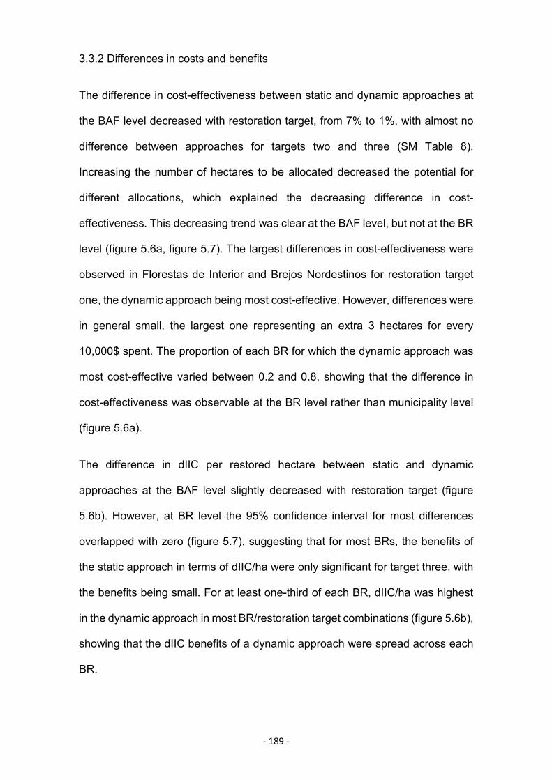
- 189 -

3.3.2 Differences in costs and benefits

The difference in cost-effectiveness between static and dynamic approaches at

the BAF level decreased with restoration target, from 7% to 1%, with almost no

difference between approaches for targets two and three (SM Table 8).

Increasing the number of hectares to be allocated decreased the potential for

different allocations, which explained the decreasing difference in cost-

effectiveness. This decreasing trend was clear at the BAF level, but not at the BR

level (figure 5.6a, figure 5.7). The largest differences in cost-effectiveness were

observed in Florestas de Interior and Brejos Nordestinos for restoration target

one, the dynamic approach being most cost-effective. However, differences were

in general small, the largest one representing an extra 3 hectares for every

10,000$ spent. The proportion of each BR for which the dynamic approach was

most cost-effective varied between 0.2 and 0.8, showing that the difference in

cost-effectiveness was observable at the BR level rather than municipality level

(figure 5.6a).

The difference in dIIC per restored hectare between static and dynamic

approaches at the BAF level slightly decreased with restoration target (figure

5.6b). However, at BR level the 95% confidence interval for most differences

overlapped with zero (figure 5.7), suggesting that for most BRs, the benefits of

the static approach in terms of dIIC/ha were only significant for target three, with

the benefits being small. For at least one-third of each BR, dIIC/ha was highest

in the dynamic approach in most BR/restoration target combinations (figure 5.6b),

showing that the dIIC benefits of a dynamic approach were spread across each

BR.

- 190 -

3.4 Informational rent capture

BRs with higher median informational rent capture are expected to have a higher

incentive to join the set-aside programme than for BRs with lower values.

Informational rent capture was always highest for the dynamic approach, whether

measured as a total, per hectare or as a proportion of each USD spent (Table

5.4). This was true for all biogeographical subregions and across all restoration

targets, with the exception of Brejos Nordestinos for target two where static and

dynamic solutions were identical. This was expected given the results from

chapter 4.

Informational rent capture per hectare at the BAF level increased with the

restoration target for both static and dynamic approaches in similar proportions;

capture per hectare for targets two and three was ~25% and ~40% higher than

for target one respectively (SM Table 8). At the BR level this increase with

restoration target was not so clear; for example, see Florestas de Interior between

targets two and three (figure 5.8). Higher capture per hectare was not only due

to the dynamic approach reaching higher values at the municipality level, but also

to the increased number of municipalities capturing informational rent (figure 5.8).

Subregions with the highest median informational rent capture per hectare were

Florestas de Araucaria, Serra do Mar, and Sao Francisco for target three, and

the one with the lowest was Brejos Nordestinos for targets one and two (figure

5.8).

At the BAF level, the difference in informational rent capture between static and

dynamic approaches decreased as a function of restoration target (as a

proportion of total area, figure 5.8c). However, this was not true at BR level for all

regions. In most cases, for at least half of each BR informational rent capture was

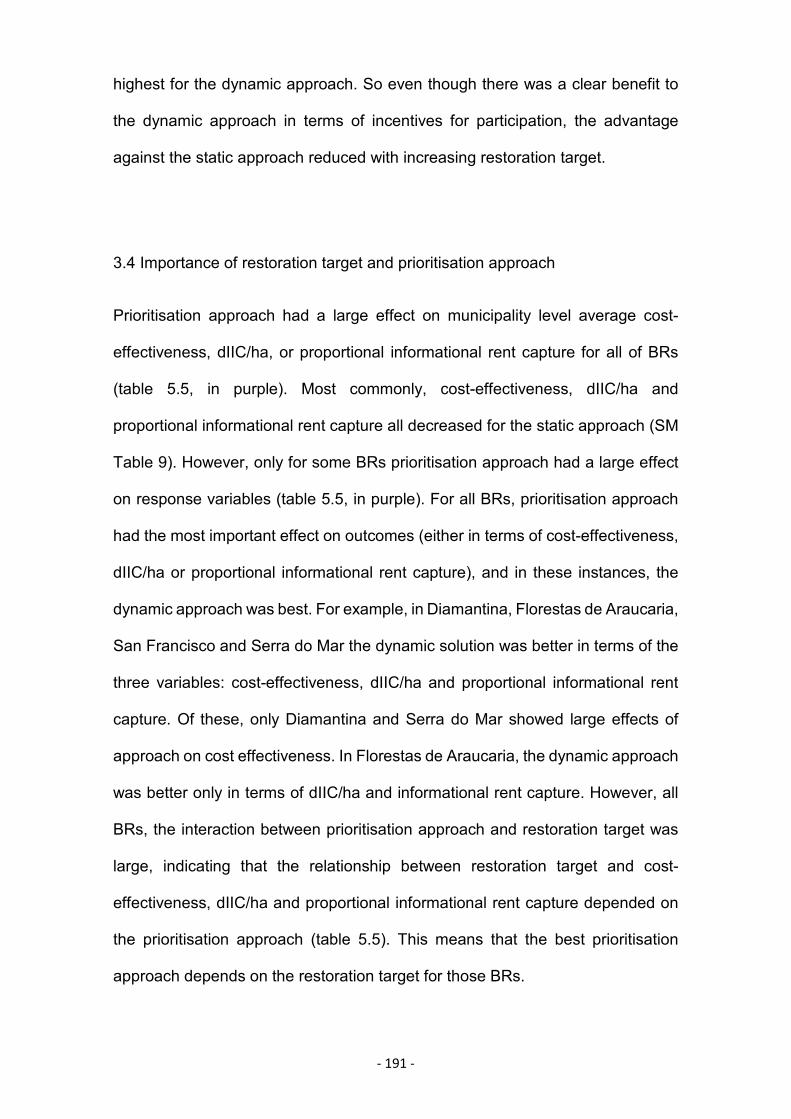
- 191 -

highest for the dynamic approach. So even though there was a clear benefit to

the dynamic approach in terms of incentives for participation, the advantage

against the static approach reduced with increasing restoration target.

3.4 Importance of restoration target and prioritisation approach

Prioritisation approach had a large effect on municipality level average cost-

effectiveness, dIIC/ha, or proportional informational rent capture for all of BRs

(table 5.5, in purple). Most commonly, cost-effectiveness, dIIC/ha and

proportional informational rent capture all decreased for the static approach (SM

Table 9). However, only for some BRs prioritisation approach had a large effect

on response variables (table 5.5, in purple). For all BRs, prioritisation approach

had the most important effect on outcomes (either in terms of cost-effectiveness,

dIIC/ha or proportional informational rent capture), and in these instances, the

dynamic approach was best. For example, in Diamantina, Florestas de Araucaria,

San Francisco and Serra do Mar the dynamic solution was better in terms of the

three variables: cost-effectiveness, dIIC/ha and proportional informational rent

capture. Of these, only Diamantina and Serra do Mar showed large effects of

approach on cost effectiveness. In Florestas de Araucaria, the dynamic approach

was better only in terms of dIIC/ha and informational rent capture. However, all

BRs, the interaction between prioritisation approach and restoration target was

large, indicating that the relationship between restoration target and cost-

effectiveness, dIIC/ha and proportional informational rent capture depended on

the prioritisation approach (table 5.5). This means that the best prioritisation

approach depends on the restoration target for those BRs.

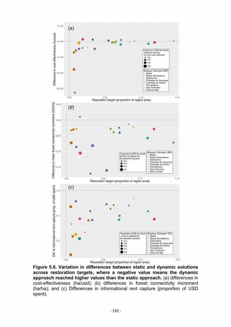
- 192 -

Figure 5.6. Variation in differences between static and dynamic solutionsacross restoration targets, where a negative value means the dynamicapproach reached higher values than the static approach. (a) differences incost-effectiveness (ha/usd); (b) differences in forest connectivity increment(ha/ha); and (c) Differences in informational rent capture (proportion of USDspent).

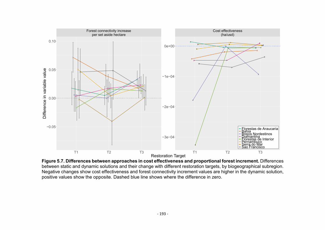
- 193 -

Figure 5.7. Differences between approaches in cost effectiveness and proportional forest increment.Differencesbetween static and dynamic solutions and their change with different restoration targets, by biogeographical subregion.Negative changes show cost effectiveness and forest connectivity increment values are higher in the dynamic solution,positive values show the opposite. Dashed blue line shows where the difference in zero.

Forest connectivity increaseper set aside hectare

Cost effectiveness(ha/usd)

−0.05

0.00

0.05

0.10

−3e−04

−2e−04

−1e−04

0e+00

T1 T2 T3 T1 T2 T3Restoration Target

Differenceinvariablevalue

Florestas de AraucariaBahiaBrejos NordestinosDiamantinaFlorestas de InteriorPernambucoSerra do MarSao Francisco

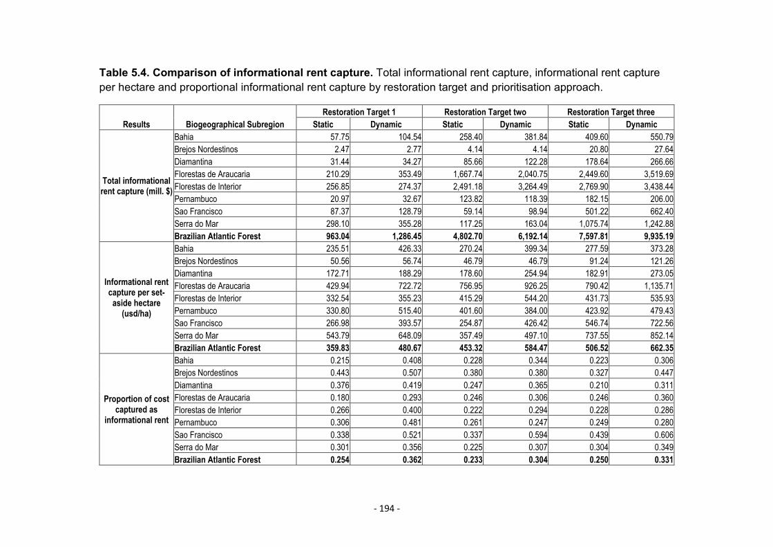
- 194 -

Table 5.4. Comparison of informational rent capture. Total informational rent capture, informational rent captureper hectare and proportional informational rent capture by restoration target and prioritisation approach.

Results Biogeographical SubregionRestoration Target 1 Restoration Target two Restoration Target three

Static Dynamic Static Dynamic Static Dynamic

Total informationalrent capture (mill. $)

Bahia 57.75 104.54 258.40 381.84 409.60 550.79Brejos Nordestinos 2.47 2.77 4.14 4.14 20.80 27.64Diamantina 31.44 34.27 85.66 122.28 178.64 266.66Florestas de Araucaria 210.29 353.49 1,667.74 2,040.75 2,449.60 3,519.69Florestas de Interior 256.85 274.37 2,491.18 3,264.49 2,769.90 3,438.44Pernambuco 20.97 32.67 123.82 118.39 182.15 206.00Sao Francisco 87.37 128.79 59.14 98.94 501.22 662.40Serra do Mar 298.10 355.28 117.25 163.04 1,075.74 1,242.88Brazilian Atlantic Forest 963.04 1,286.45 4,802.70 6,192.14 7,597.81 9,935.19

Informational rentcapture per set-

aside hectare(usd/ha)

Bahia 235.51 426.33 270.24 399.34 277.59 373.28Brejos Nordestinos 50.56 56.74 46.79 46.79 91.24 121.26Diamantina 172.71 188.29 178.60 254.94 182.91 273.05Florestas de Araucaria 429.94 722.72 756.95 926.25 790.42 1,135.71Florestas de Interior 332.54 355.23 415.29 544.20 431.73 535.93Pernambuco 330.80 515.40 401.60 384.00 423.92 479.43Sao Francisco 266.98 393.57 254.87 426.42 546.74 722.56Serra do Mar 543.79 648.09 357.49 497.10 737.55 852.14Brazilian Atlantic Forest 359.83 480.67 453.32 584.47 506.52 662.35

Proportion of costcaptured as

informational rent

Bahia 0.215 0.408 0.228 0.344 0.223 0.306Brejos Nordestinos 0.443 0.507 0.380 0.380 0.327 0.447Diamantina 0.376 0.419 0.247 0.365 0.210 0.311Florestas de Araucaria 0.180 0.293 0.246 0.306 0.246 0.360Florestas de Interior 0.266 0.400 0.222 0.294 0.228 0.286Pernambuco 0.306 0.481 0.261 0.247 0.249 0.280Sao Francisco 0.338 0.521 0.337 0.594 0.439 0.606Serra do Mar 0.301 0.356 0.225 0.307 0.304 0.349Brazilian Atlantic Forest 0.254 0.362 0.233 0.304 0.250 0.331

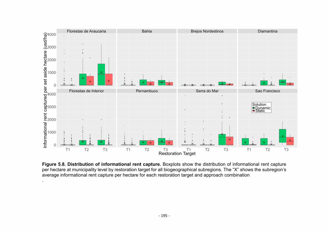
- 195 -

Figure 5.8. Distribution of informational rent capture. Boxplots show the distribution of informational rent captureper hectare at municipality level by restoration target for all biogeographical subregions. The “X” shows the subregion’saverage informational rent capture per hectare for each restoration target and approach combination.

●

●

●●

●●

●●

●

●●●

●

●

●●●●

●

●●

●●

●●●●

●

●

●●●

●

●

●●●●

●

●●●

●

●●●

●

●

●

●●●●

●

●

●

●

●

●

●

●

●

●●

●●●●●●●●●●●●●●●●●●●●●●●●●●●●●●●

●

●

●

●

●

●

●

●●●●

●

●

●

●

●●●●●●●●●●●●●●●●●●●●●●●●●●●●●●●●●●●●●●●●●●●●●●●●●●●●●●●●●●●●

●●●●●●●●●●●

●●●

●

●

●

●

●●

●●●

●

●

●

●●●

●●

●

●●

●●●

●

●

●

●

●

●

●

●

●

●

●●

●●●●

●

●●●

●

●●●●●●●●●●●●●●●●●●●●●●●●●●●●●●

●●●●●●●●●●●●●●●●●● ●●●●●●●

●●●●● ●●●●●●●●●●●●●●●● ●●●●●●●●●●●

●●●●●●●●●●●●●●●

●●●●●●●

●●

●●●●●●

●

●●●●●●

●

●●●●●●●●●●●●●●●

●●

●

●●

●●

●

●

●

●

●

●

●

●●

●

●●

●

●

●●

●

●

●

●

●

●

●

●

●

●●

●

●●

●●

●

●●

●

●●

●

●

●

●

●

●

●●●●●

●

●

●

●

●

●●

●

●

●●

●●

●

●

●●●●

●●●

●

●

●●

●

●

●

●

●

●●●

●●●

●

●

●

●

●

●

●

●●●

●

●

●

●

●

●

●

●

●

●●

●

●

●●

●

●

●●

●

●●

●●●●●●

●●●●●●●●●●●●●●●●●●●

●●●●●●

●●

●●●●●●

●

●●●●●●●●●●●●●●●●

●

●●●●●●●●

●

●●●●●●●●●●●●●●●●●●●●●●●●●●●●●●

●

●●

●●●

●

●

●●●●●●●●●●●●●●●

●

●●

●

●●●●●●●●●●●●●●●●●●●●●

●

●●●●●●●●●●●●●●●●●●●●●●●●●●

●

●●●●●●●●●●●●●●●●●●●●●●●●

●●●●●●

●●●●●●●●●●

●

●●

●

●●●

●

●

●

●●

●●

●●

●●●●

●

●

●

●

●

●

●

●

●

●

●

●

●

●●

●●●●●●●●

●●●●●●

●●●

●

●●

●●●●●

●

●●●

●●

●

●●●

●●

●

●●●●●

●●

●

●●●●●

●●

●

●

●●

●●

●●●●

●

●●●

●

●●●

●●●

●●●●●

●

●

●

●

●

●●●

●

●

●●●●

●

●

●●

●●

●

●

●

●

●

●

●

●

●

●

●

●●

●

●

●

●

●●

●

●

●●

●

●●●

●●●

●

●●●

●●

●●●

●

●●●●

●

●

●

●●●●●

●●●

●●●

●●●

●

●

●●●

●●

●●

●

●

●

●

●

●●

●

●

●

●

●

●●

●

●●

●

●

●●

●●

●●●

●

●●●●

●

●

●●●

●

●

●●●

●

●

●

●●●●●●

●●

●

●

●●●●●

●

●●●●●●●●●●●●●●

●●

●●

●

●

●

●

●●●

●

●

●

●

●

●●

●

●

●

●●

●

●●

●

●●●

●

●

●

●●●●●●●●●●●●●●●●●●●●●●●●●●●●●●●●●●●●●●●●●●●●

●●●

●

●

●●●●●●

●

●

●

●●

●●●

●●●●●●

●●

●●

●

●

●

●●●●●●

●●

●●●●●●●●●

●

●

●

●

●●●●●●●●●●●●●●●●●

●

●

●●●

●

●

●

●

●

●●

●

●●●●●●

●

●

●●●●●●●●●●●●●●

●

●●●

●

●●●●●●●●●●●●

●

●

●

●●●●●●●●●●●●

●●●●●●

●●●●●●●●●●

●

●

●●

●

●

●

●

●

●

●

●

●

●●

●●

●●

●●

●●

●●

●

●

●

●

●

●

●

●

●

●

●

●

●

●●

●●●●●●●●

●●●●●●

●●●

●

●●

●●●●●

●

●●

●●

●

●●●

●●

●

●●●●●

●●

●

●●●●●

●

●

●

●

●●

●●

●●●●

●

●●●

●

●●●

●●●

●●●●●

●

●

●

●

●

●●●

●

●

●●●●

●●●

●●

●

●

●

●

●

●

●

●

●

●●

●

●

●●

●

●

●

●

●

●

●

●

●

●●

●

●●●

●●●

●

●●●

●

●●●

●

●●●●

●

●

●

●●●●●

●●●

●●●

●●●

●

●

●●●

●

●

●

●●

●

●

●

●

●

●●

●

●

●

●

●

●●

●

●

●

●

●●

●●

●●●

●

●●●●

●

●

●●●

●

●

●●●

●

●

●

●●●●●●

●●

●

●

●●●●●

●

●●●●●●●●●●●●●●●

●●

●●

●

●

●

●

●●●

●

●

●

●

●

●●

●

●

●

●●

●

●●

●

●●●

●

●

●

●●●●●●●●●●●●●●●●●●●●●●●●●●●●●●●●●●●●●●●●

●●●

●

●

●●●●●●

●

●

●

●●

●●●

●●●●●●

●

●

●

●

●

●

●●

●●

●

●●●●

●

●

●

●

●

●●●

●

●

●●●

●

●

●

●

●●●●

●●●●

●

●●

●

●

●●

●

●

●●●●●●●

●

●●●

●

●●●●

●

●●

●●●●

●

●●●●

●

●

●

●

●

●●●●●

●

●●●

●

●●

●

●●●●●

●

●

●

●●

●

●

●

●

●

●

●●

●

●

●●●●●

●

●●

●●

●●

●

●

●

●

●

●●●●

●

●

●

●●●●●●●

●

●●●

●

●●●●●●●

●

●●●●

●●●●●●●●●●●●●●●●●●

●●●●●●●●

●●●●●●●●●

●

●●●

●

●●

●

●

●●●

●

●

●●●●●●●●●●●●●●●●●●●●●

●●●●

●

●

●●

●

●●●

●

●●●●

●

●

●

●

●

●●

●

●

●

●●

●

●

●

●●●

●●●

●●●●

●

●

●

●

●

●

●

●●

●●●●●●●●●●●●●●●●●●●●●●●

●●●●●●●●●●●●●●●●●●●●●●●●●●●●●●●●

●●

●

●

●

●●●

●

●●●

●

●●●●●●

●

●

●

●●●●●●●●●

●

●●

●

●●●●●●

Florestas de Araucaria Bahia Brejos Nordestinos Diamantina

Florestas de Interior Pernambuco Serra do Mar Sao Francisco0

1000

2000

3000

4000

0

1000

2000

3000

4000

T1 T2 T3 T1 T2 T3 T1 T2 T3 T1 T2 T3Restoration Target

Informationalrentcapturedpersetasidehectare(usd/ha)

SolutionDynamicStatic

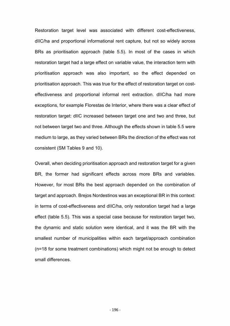
- 196 -

Restoration target level was associated with different cost-effectiveness,

dIIC/ha and proportional informational rent capture, but not so widely across

BRs as prioritisation approach (table 5.5). In most of the cases in which

restoration target had a large effect on variable value, the interaction term with

prioritisation approach was also important, so the effect depended on

prioritisation approach. This was true for the effect of restoration target on cost-

effectiveness and proportional informal rent extraction. dIIC/ha had more

exceptions, for example Florestas de Interior, where there was a clear effect of

restoration target: dIIC increased between target one and two and three, but

not between target two and three. Although the effects shown in table 5.5 were

medium to large, as they varied between BRs the direction of the effect was not

consistent (SM Tables 9 and 10).

Overall, when deciding prioritisation approach and restoration target for a given

BR, the former had significant effects across more BRs and variables.

However, for most BRs the best approach depended on the combination of

target and approach. Brejos Nordestinos was an exceptional BR in this context:

in terms of cost-effectiveness and dIIC/ha, only restoration target had a large

effect (table 5.5). This was a special case because for restoration target two,

the dynamic and static solution were identical, and it was the BR with the

smallest number of municipalities within each target/approach combination

(n=18 for some treatment combinations) which might not be enough to detect

small differences.

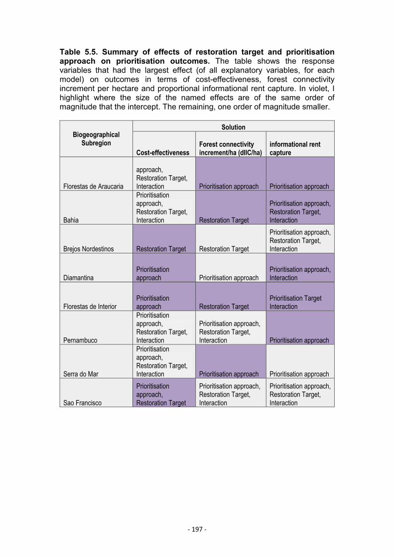
- 197 -

Table 5.5. Summary of effects of restoration target and prioritisationapproach on prioritisation outcomes. The table shows the responsevariables that had the largest effect (of all explanatory variables, for eachmodel) on outcomes in terms of cost-effectiveness, forest connectivityincrement per hectare and proportional informational rent capture. In violet, Ihighlight where the size of the named effects are of the same order ofmagnitude that the intercept. The remaining, one order of magnitude smaller.

BiogeographicalSubregion

Solution

Cost-effectivenessForest connectivityincrement/ha (dIIC/ha)

Proportionalinformational rentcapture

Florestas de Araucaria

Prioritisationapproach,Restoration Target,Interaction Prioritisation approach Prioritisation approach

Bahia

Prioritisationapproach,Restoration Target,Interaction Restoration Target

Prioritisation approach,Restoration Target,Interaction

Brejos Nordestinos Restoration Target Restoration Target

Prioritisation approach,Restoration Target,Interaction

DiamantinaPrioritisationapproach Prioritisation approach

Prioritisation approach,Interaction

Florestas de InteriorPrioritisationapproach Restoration Target

Prioritisation TargetInteraction

Pernambuco

Prioritisationapproach,Restoration Target,Interaction

Prioritisation approach,Restoration Target,Interaction Prioritisation approach

Serra do Mar

Prioritisationapproach,Restoration Target,Interaction Prioritisation approach Prioritisation approach

Sao Francisco

Prioritisationapproach,Restoration Target

Prioritisation approach,Restoration Target,Interaction

Prioritisation approach,Restoration Target,Interaction

- 198 -

4. Discussion

4.1 Priority areas for natural restoration in the BAF

Over the last 5 years, four regional-scale plans for restoration priority areas

have been developed for the BAF (Calmon et al. 2011; Banks-Leite et al.

2014b; Tambosi et al. 2014; Crouzeilles et al. 2015). Even though a variety of

perspectives and approaches to restoring the BAF can encourage open debate

(Stewart & Possingham 2005), these initiatives involve publishing different

outcomes, which can create policy confusion (Mace 2000; Brooks et al. 2006b).

Without a clear message to decision-makers, opportunities to catalyse efforts

to restore the BAF could be lost. This study is another effort to provide a plan

of priorities to restore the BAF, however, by looking for agreement between two

prioritisation approaches and three different targets, it provides information on

areas that have a high probability of being priority areas regardless of target

and approach. In the midst of multiple targets and objectives, our map provides

a starting point for priority restoration areas based on three important

considerations; potential to improve forest connectivity, cost effectiveness, and

potential to incentivise participation through informational rent.

This study identified all BRs (except Pernambuco) as having some areas of

high concordance, and Sao Francisco had the most extensive areas of

concordance. Priority areas of high concordance within each BR were not the

same as the priority areas highlighted by the other four regional-scale plans for

restoration priority areas developed for the BAF, probably because they were

generally prioritising on static ecological criteria. However, there was overlap

between areas with concordance, even if low, and some of the other priority

- 199 -

areas. The AFRP’s prioritisation mapped 17M ha of illegally deforested land

according to forest code, and most of their priority areas were in Florestas de

Interior and Florestas de Araucaria (Calmon et al., 2011). These BRs had

intermediate concordance scores, but the areas prioritised by the AFRP did

overlap with low concordance areas. Tambosi et al. (2014) ranked landscapes

for restoration considering habitat amount and connectivity, identifying

landscapes within Serra do Mar and Bahia as restoration priorities. Very similar

areas had >25% concordance scores for those BRs in this study. Banks-Leite

et al. (2014) prioritised landscapes in terms of community integrity and

economic costs and most priority areas fell within Diamantina, Bahia, Florestas

de Interior, Florestas de Araucaria and Serra do Mar. All of those BRs had high

concordance scores areas that overlapped loosely with their priority

landscapes. Finally, Crouzeilles et al. (2015) prioritised areas for restoration

incorporating the ecological value of habitat patch, while also considering BR

representation and cost-effectiveness. Most of their priority areas fell in

Florestas de Interior and Florestas de Araucaria, and the ones in the latter

overlapped with the areas of high concordance scores in this study. This study

complements previous studies as none of them considered ecologic and

economic feedback effects, as well as multiple restoration objectives.

Additionally, by providing results at both low and high resolutions, for socially

meaningful units (BRs and municipalities), this study facilitates top-down

implementation considerations, as well as providing enough flexibility to

consider local context as restoration is not tied to specific locations beyond

municipality level.

- 200 -

4.2 Feasibility of costs of meeting targets

Of the four above-mentioned previous studies, only two included direct cost

considerations with very different cost estimates. The cost of purchasing land

for restoration to improve habitat availability for two species, ensuring 20%

forest cover within each BR, was estimated by Crouzeilles et al. (2015) as

$17,500-$20,500 million ($1,534-$1,597 per hectare). The cost of payments to

set-aside agricultural land for restoration to reach a restoration target of 30%

forest cover in priority landscapes was estimated by Banks-Leite et al. (2014)

at $56.3 million per year (range $25.7 million to $91.6 million), based on the

average PES values across the biome, equivalent to $132.73 per hectare per

year. In our study, the cost of agricultural set-asides for restoration was

approximately $147.5, $214, and $222.3 per hectare per year for targets one,

two and three respectively. These estimates are within the range of PES in

Brazil used in Banks-Leite et al. (2014), the increasing cost per hectare being

explained by the decrease in the cost-effectiveness of the solution as the

amount of restoration required increased. However, our estimates of the cost

of purchasing the set-asides were much higher than the estimates of

Crouzeilles et al. (2015); $2,765/ha, $3,860/ha and $4,007/ha for targets one,

two and three respectively. Crouzeilles et al. (2015) had most of their priority

areas in Florestas de interior and Florestas de Araucaria, which are cheaper

and less degraded than the rest of BAF. Because I forced priority areas in all

BRs by analysing each separately, it could be expected our estimates to be

higher.

- 201 -

Estimates of total cost per year for targets 1 2 and 3 were $394.8-$422 mill.,

$2267-$2293 mill., and $3335-$3373 mill. respectively. The feasibility of these

targets being implemented can be assessed by comparison with yearly

subsidies for agriculture, one of the most important economic sectors in the

BAF region (Soares-filho et al. 2014). Comparatively, the cost of payment per

year of set-asides for target one is 15-17% of Brazil’s annual expenditure on

agricultural subsidies, which makes it achievable. However, costs for targets

two and three respectively represent 89-90% and 130-133% of annual

agricultural subsidies, which makes their implementation highly unlikely.

Furthermore, cost estimates only involve the cost of the payment the farmer

would receive. There are additional costs that cannot be ignored, such as

hidden natural regeneration costs and transaction costs. Although most areas

would follow natural regeneration simply by ceasing the drivers of disturbance

(Melo et al. 2013b), passive restoration in abandoned pastures does have

some financial costs, e.g. establishing fences (Zahawi et al. 2014), and these

costs can reach USD $ 850 – 1200 per ha in the Atlantic Forest (Alves-Pinto et

al. 2017). It has also been estimated that 20% of the area considered for

restoration would require active reforestation practices, with associated costs

of up to $5000/ha during the first 3 years (Melo et al. 2013b). This means that

during the first years of implementation there would be additional costs related

to regeneration if restoration were to be successful.

A clear understanding of transaction costs is needed before concluding whether

a PES programme is cost-effective or not. However, PES transaction costs are

poorly understood both at small and large scales (Wunder et al. 2008), in

- 202 -

general and specifically for the BAF (Finney 2015). Costa Rica’s Fonafifo,

which operates at scale, reported transaction costs of 19 to 25% of total project

costs (Wunder 2007). In the BAF, grey literature on one case shows a

transaction cost of 21% of total project cost, compared with incentive payments

of 23% (Finney 2015). Estimating a transaction cost similar to payment cost

would bring the cost of meeting target one to ~$800 mill. per year; ~0.045% of

Brazil’s GDP for 2015. This, however, is a high transaction cost estimate,

because 55% of transaction costs in the mentioned case study consist of

general assessment, property mapping and monitoring, things that are already

under way in the BAF (Banks-Leite et al. 2014a).

4.3 Static vs. Dynamic approaches and the importance of the restoration target

This chapter advances understanding on the effects of employing a dynamic

approach to prioritisation on outcomes, by also evaluating the role of the target

set for restoration. There was a trend of decreasing cost-effectiveness with

increasing restoration target (in terms of hectares set-aside), which is a relevant

trade-off for decision-making. Similar to chapter 4, the cost-effectiveness

benefits of a dynamic approach were geographically variable, and restoration

target played an important role in determining these benefits in interaction with

BR. The fact that target definition is crucial in defining spatial conservation

planning priorities was not a surprise (Margules & Pressey 2000b; Kukkala &

Moilanen 2013); other studies have found priority areas vary widely with

different targets based on taxonomic, phylogenetic and functional diversity for

mammals and birds occurring in Brazil (Sobral et al. 2012).

- 203 -

4.4 Informational rent as a cost-effective incentive to set-aside farmland

As a consequence of the Forest Code, landholders have collectively accrued a

large “environmental debt” in the BAF, which are hectares that have to be

reforested by law (Soares-Filho et al. 2014). However, due to the lost

opportunity costs of land, and lack of enforcement, achieving compliance

remains a challenge (Latawiec et al. 2015; Alves-Pinto et al. 2017). It has been

suggested that to achieve compliance, restoration needs to be an economically

sustainable activity in the BAF, and several mechanisms have been put forward

(Brancalion et al. 2012; Lopes et al. 2013; Soares-filho et al. 2014; Trevisan et

al. 2016). These include agricultural intensification to offset the lost farmland,

diversification by sustainably exploiting restored forest, and implementing

payments for ecosystems services for carbon and water (Brancalion et al. 2012;

Strassburg et al. 2014b; Alves-Pinto et al. 2017). These are all key steps in

long-term compliance, but require longer time-lines and high investment. In

chapter 4, I proposed the use of informational rent extraction as a fast, cost-

effective way of incentivising landholders to comply, that complements the

other longer-term mechanisms. The priority areas resulting from this analysis

already optimise the use of the existing potential informational rent capture,

proving a valuable addition to existing cost-based prioritisations.

Large-scale restoration can act as another factor in the demand for agricultural

land, and one of the main challenges in the BAF is integrating large-scale

restoration and increasing demand for food production, avoiding displacement

to other biomes (Latawiec et al. 2015). The BAF presents a huge opportunity

- 204 -

for establishing forest restoration as an economically viable practice due to its

large potential for agricultural productivity improvement (Joly et al. 2010;

Strassburg et al. 2014a). Using informational rent capture as an incentive for

restoration at large scales would complement the goal of improving productivity,

as in order to make the largest informational rent capture the lowest productivity

land needs to be set-aside. If complementary activities are implemented to

increase the productivity of lands currently under agriculture, tropical forest

restoration could be supported without risking perverse outcomes for food

production (Brancalion et al. 2012).

4.5 Future work

The BAF is thought to be particularly vulnerable to climate change both socially

and in biodiversity terms (Bellard et al. 2014; Scarano & Ceotto 2015). Including

climate change and its impact on biodiversity and agricultural yields is a crucial

next step in setting priorities for restoration.

The implementation crisis in conservation planning is one of conservation's

greatest challenges (Biggs et al. 2011). Many conservation planning

approaches continue to emphasize ecological over social considerations

(Knight et al. 2006), and translating assessments into conservation actions

remains a challenge (Knight et al. 2013). The BAF presents a great opportunity

to bridge this planning-implementation gap due to the existence of the AFRP.

Core to the planning–implementation gap is the failure to achieve the necessary

shared vision and collaboration among typically diverse stakeholder groups

(Biggs et al. 2011), which is particularly hard to achieve at large scales.

However, the AFRP, funded 7 years ago, is currently a coalition of 260+

- 205 -

stakeholders across the BAF, including governmental agencies, the private

sector, NGOs and research institutions (Pinto et al. 2014). This provides a

unique opportunity for success, if collaboration is possible. Even though the

AFRP has their own priority areas for restoration (Calmon et al. 2011), they also

work with thematic maps that can be overlaid to their priorities, which include

(a) eligible areas for carbon restoration projects under the Verified Carbon

Standard; (b) key areas for urban water supply; and (c) priority areas for

improving landscape connectivity (Brancalion et al. 2013a). Our approach

would add information on incentives for setting aside land to their priorities, and

could usefully be integrated into their existing prioritisations.

- 206 -

5. Conclusion

Priority areas for natural regeneration of forests in the BAF vary widely, but

agreement was found between existing assessments and this study’s results.

These areas of consistent priority are a good starting point for decision making

to restore the BAF. Our results suggested that the costs of meeting targets 2

(scientifically suggested target for ecological integrity) and 3 (AFRP target) are

too high for realistic implementation, but that implementing target 1 (the

government's 15% set-aside CBD target) at the BR level would be realistic. Our

estimates of cost are, however, very different to other estimates for same

targets, as shown in the discussion.

This chapter suggests that definition of the target to be met in prioritisations is

as important as regional characteristics in determining whether a static or a

dynamic approach is best. Exploring the implications of different targets for the

outcome of prioritisations is not often done, but this work highlights the

importance of recognising that different target specifications can lead to very

different outcomes on the ground.

- 207 -

Chapter 6: Discussion

- 208 -

6.1 Overview

In assessing the role of unintended feedback effects of conservation

interventions in conservation science and practice, three cross-cutting themes

emerged. For conservation to be able to plan for and manage unintended

feedback effects, these themes need to be addressed. The first theme is the

need for collection of real-world evidence of feedback effects; the second

theme concerns understanding when a dynamic approach to conservation

planning outperforms a simple static approach, and the third theme is

assessing the spatial and temporal interactions of unintended feedbacks. This

thesis advanced knowledge on each of these themes working with the empirical

case study of the BAF, and in the next sections, I discuss each of them in turn.

6.2 Empirical evidence

Conservation science, defined as the interdisciplinary field that explicitly

recognizes the tight coupling of social and natural systems, is a relatively new

discipline (Kareiva & Marvier 2012). It is not surprising then that many important

questions in the field initially find that the literature can be of anecdotal nature

and cannot support systematic reviews. Similar issues were faced by

researchers studying the shifting baseline syndrome (Papworth et al. 2009) and

determinants of conservation success (Brooks et al. 2012). In chapter two I

found that the current state of the literature that provides evidence on

unintended feedback effects of conservation interventions is not enough to

support a systematic review and provide generalisations on minimising their

effects. To understand drivers, mechanisms and circumstances that enhance

- 209 -

or dampen unintended feedbacks, there is a need to establish comparative

databases to collate case studies that provide an evidence base (Sutherland et

al. 2004). Additionally, focusing on finding and studying examples in which

unintended feedbacks were overcome and managed could provide invaluable

insight. Such an initiative could work with existing similar efforts in the SES

framework. For example, the social-ecological systems meta-analysis

database, an on-going effort to collate examples of SESs, could facilitate such

an enterprise (Cox 2015). A posteriori empirical evidence could be collected

from evaluations of conservation impact that, by considering feedbacks

operating in an SES, could help identify the true drivers of observed patterns

(Lambin & Meyfroidt 2010).

Interdisciplinary empirical approaches present challenges across conservation

sectors. Most of the work on coupled social and ecological systems has been

theoretical (Liu et al. 2007). Results from Chapters three and four provide

evidence on the importance of empirical models. Despite numerous studies

addressing market feedback effects of reserve allocation, few of them were

based on empirical data (chapter 3). Additionally, results varied somewhat

between theoretical approaches and those based on real-life case studies.

Theoretical approaches tended to find larger differences in the cost-

effectiveness of reserve allocation between static and dynamic approaches

(Armsworth et al. 2006; Dissanayake & Önal 2011; Zvoleff & An 2014b), and

empirical case studies had more conservative results (Walker 2012b; Butsic et

al. 2013). Results from chapter four are aligned with the other empirical studies

in that differences in cost-effectiveness between approaches were small.

However, modelling the feedback effect caused by informational rent capture

- 210 -

in chapter four lead to important and unexpected results: that informational rent

capture can be maximised to provide incentives for conservation without losing

project cost-effectiveness. These results highlight the importance of real-life

case studies, as a key factor in unravelling the true nature of the feedback

effects that are likely to be encountered in the real world.

The challenges of interdisciplinary models include the integration and scaling

of data to make them compatible on input (Dumanski et al. 1998). I found this

was also the case for modelling both environmental and economic feedbacks

of conservation interventions based on empirical case studies (chapter 3). In

addition, I found that modelling land market feedbacks requires temporal series

of spatially explicit data on land markets (chapter 3) which are commonly

available at a much coarser spatial grain that the prioritisation needs to respond

to on the conservation side (Armsworth 2014). Reconciling this mismatch

between the scale at which socio-economic data are available for modelling,

and the scale at which priorities need to be set (for ecological or institutional

reasons) is the first obstacle to modelling market feedbacks in empirical spatial

planning prioritisations. Using simulations, the approach selected for this work,

is time and data hungry, but provide a statistically robust way of reconciling the

data’s spatio-temporal resolution.

- 211 -

6.3 Static vs. Dynamic approach to conservation planning

In chapters two and four, I identified the need to understand under which

circumstances accounting for feedback effects was key for conservation

success, and when a static approach would be good enough. Several tools

have been developed to explore the potential impacts of conservation

interventions and support decision-making, such as InVEST and Marxan (Ball

et al. 2009; Nelson et al. 2009). These are widely used, and even though

mechanisms for feedback effects could be included in their analyses, this would

be a substantial addition to complexity, both in terms of data requirements,

technical capacity for analysis and computing speed. There is, therefore, a

trade-off that needs to be assessed before investing in making these tools more

realistically dynamic. This assessment is required for a range of case studies,

and through conceptual modelling of when feedbacks are most likely to be

severe, backed up by a systematic review of evidence (once it becomes

available). This research agenda would then enable conservation scientists and

managers to find the balance between too many recommendations, which can

create policy confusion (Mace 2000; Brooks et al. 2006b), and provide

misleading recommendations from static tools.

Chapter four aimed to address this trade-off for the first time by comparing

prioritisation solutions for a static and a dynamic approach in circumstances

where there is both an ecological and an economic feedback as a result of

conservation intervention. In this case, the intervention is set-aside of private

agricultural land for forest restoration and the feedbacks are changes in forest

connectivity as a result of set-aside placement, and changes in the opportunity

cost of land set-aside as a result of informational rent capture by landowners.

- 212 -

Results showed a clear trade-off between approaches in terms of the resources

required to generate a prioritisation based on modelling the system using a

static or dynamic approach and potential improvements in the cost-

effectiveness of the prioritisation. However, the outcome of the trade-off, i.e.

which approach was more desirable, varied widely with the region. In chapter

five I showed that the outcome of this trade-off also varied for different

conservation targets. This provides a challenge to conservation planners, and

suggests that more case studies that vary in terms of targets and geographical

regions are needed to provide general principles on the optimal approach, as

well as considering other types of feedback.

Two factors need to be included in the trade-off analysis in addition to cost-

effectiveness considerations. The first factor is uncertainty; increases in

uncertainty due to model complexity need to be quantified and included in the

trade-off assessments. The second factor is consideration of the wider socio-

ecological context. Results from chapter four showed that the dynamic

prioritisation approach resulted in higher informational rent capture, increasing

incentives for conservation without decreasing programme cost-effectiveness,

thereby potentially enhancing the probability of success in terms of increased

participation in the programme by landowners (Scheufele & Bennett 2017). The

wider range of areas included in the dynamic prioritisation may also increase

the equity and perceived fairness of the programme (Pascual et al. 2014).

These considerations could prove more important advantages over the static

approach than reductions in cost-effectiveness under certain circumstances.

For example, in the BAF case study, where a large portion of a restoration

target could be achieved by compliance with an existing law (chapter 5), the

- 213 -

incentive for compliance provided by the dynamic approach may be most

desirable even if there were no differences in cost-effectiveness between static

and dynamic approaches.

The question then is whether the potential increase in transactions costs

engendered by the dynamic approach is worthwhile. It is worth noting that the

capacity, computational and time costs of implementing dynamic prioritisation

approaches are likely to diminish relatively rapidly once the approach becomes

widespread and accepted; as experience, frameworks and tools accumulate

subsequent prioritisations will be less arduous. This is evidenced for example

in the massive increase in the use of Marxan, and then the more sophisticated

Marxan with zones, and then Zonation, in conservation planning both by

practitioners and researchers over the last decade (McIntosh et al. 2016).

Therefore, to a great extent the adoption of more complex methods, when they

would make a substantive difference to outcomes, depends on the will to make

this change, rather than analytical or budgetary limitations, particularly when

conservation programmes are large and expensive, such as in the BAF. My

crude comparison of the relative cost of dynamic rather than static analysis,

compared to the cost-saving power of its implementation, suggested the cost

savings over the whole BAF set-aside areas were an order of magnitude larger

than the cost of implementing the approach.

There are benefits to models such as the one developed in this thesis beyond

answering academic questions. The first benefit is providing broad insight,

when results are not obvious beforehand. The two main insights from this

model, representing a valuable contribution to knowledge, are that: (1) adding

- 214 -

complexity does not necessarily mean improved project cost-effectiveness, but

results are significantly different in terms of geographic areas selected for

prioritisation, number of farms included in the scheme, and the degree of

informational rent capture, and this needs to be further explored; (2)

implementing these models on a real case study sheds light on the system and

lead to unexpected insights, such as the potential benefit of using informational

rent capture in favour of conservation projects. A second benefit is to provide

specific quantitative guidance at a scale and reliability useful for policy-making.

This was achieved by implementing the model to a real case study (restoring

the BAF). The approach implemented to chapter 5 was intended to identify

spatial priorities that are robust, and by assessing selection frequency and

concordance across approaches and targets, the outputs are reliable enough

for decision-making. At least as reliable as (or more) than currently used

prioritisations based on limited social data and/or narrow ecological targets (see

pages 162-163 for a summary of existing approaches).

6.4 Spatial and temporal interactions between feedbacks

In chapters four and five, I showed how complex feedbacks can be when

accounting for spatial variation. For either the environmental or economic

feedback, region and its interaction with target explained most of the

differences in results. Very few generalisations could be drawn from these

results in terms of whether the static or dynamic approaches were most

desirable for a given planning unit. For any given conservation intervention

complex dynamics are at play at multiple temporal and spatial scales (Guerrero

- 215 -

et al. 2013b). Other dynamics including the effects of climate change (Doney et

al. 2012; Garcia et al. 2014) or trends in agricultural productivity (Phelps et al.

2013) could be more or less important than the modelled feedbacks in

determining conservation outcome. There is a need, therefore, to start

addressing multiple feedback effects and their relative importance in

conservation outcomes. The SES framework (Ostrom 2007) and systems

dynamics modelling (Sterman 2000) approaches have vast literature with case

studies that consider multiple feedbacks simultaneously, providing a good

starting point. Chapter three identified Sao Paulo state as a region where all

four economic feedbacks have the potential to be important in terms of moving

the price of agricultural land. This is also a data-rich state, which presents a

unique opportunity for a comparative empirical assessment of the relative

importance of feedbacks via the price of land in the developing world.

6.5 Conclusion

Conservationists rely on the fact that people adapt their behaviour based on

changes in incentives. However, this same fact is being overlooked when

unintended changes in incentives occur as a result of conservation

interventions. This thesis found an urgent need to collect evidence to

understand mechanisms for unintended feedback effects at multiple scales.

Large-scale conservation interventions have the potential to trigger economic

feedbacks with significant socio-economic consequences. However, socio-

economic data availability, a mismatch in scale between data availability and

prioritisation grain, and economic model complexity present restrictions to

- 216 -

accounting for these feedbacks in spatial conservation planning. A dynamic

approach to spatial conservation planning does entail higher computational

requirements and transactions costs, but the potential benefits in terms of

increased cost-effectiveness could offset them. Particularly, the dynamic

approach makes the most of the economic incentive for participation from

informational rents, and still has a lower overall cost.

The restoration of the BAF presented a unique opportunity, in terms of the scale

of conservation intervention and policy relevance, for accounting for economic

and configuration feedbacks in conservation planning. The dynamic approach,

by using informational rent capture to map and optimise incentives for

restoration provides a new tool for compliance with the Forest Code.

There is still much work to do for conservation to be able to plan for and manage

unintended feedbacks, but these results already show the importance of

modelling feedbacks in real-world case studies, and identifies avenues for

future research.

- 217 -

Bibliography

- 218 -

Akerlof, G.A. (1970). The Market for “Lemons”: Quality Uncertainty and theMarket Mechanism. Q. J. Econ., 84, 488.

Álvarez-Romero, J.G., Pressey, R.L., Ban, N.C. & Brodie, J. (2015).Advancing land-sea conservation planning: Integrating modelling ofcatchments, land-use change, and river plumes to prioritise catchmentmanagement and protection. PLoS One, 10, 1–26.

Alves-Pinto, H.N., Latawiec, A.E., Strassburg, B.B.N., Barros, F.S.M.,Sansevero, J.B.B., Iribarrem, A., Crouzeilles, R., Lemgruber, L., C.Rangel, M. & Silva, A.C.P. (2017). Reconciling rural development andecological restoration: Strategies and policy recommendations for theBrazilian Atlantic Forest. Land use policy, 60, 419–426.

Ando, a. (1998). Species Distributions, Land Values, and EfficientConservation. Science (80-. )., 279, 2126–2128.

ANEC. (2012). Estudo de Logistica e Custos com Fretes e Receita final doProdutor.

Angelsen, A. (2007a). Forest Cover Change in Space and Time : Combining the von Thünen and Forest Transition.World Bank Policy Res. Work.Pap.World Bank Publications.

Angelsen, A. (2007b). Forest cover change in space and time: combining thevon Thünen and forest transition theories ( No. 4117). Policy ResearchWorking Paper.

Angelsen, A. (2010). Policies for reduced deforestation and their impact onagricultural production. Proc. Natl. Acad. Sci. U. S. A., 107, 19639–44.

Apel, M.A., Lima, M.E.L., Souza, A., Cordeiro, I., Young, M.C.M., Sobral,M.E.G., Suffredini, I.B. & Moreno, P.R.H. (2006). Screening of thebiological activity from essential oils of native species from the AtlanticRain Forest (São Paulo - Brazil). Pharmacologyonline, 3, 376.

Ardron, J.A., Possingham, H.P. & Klein, C.J. (2010). Marxan Good PracticesHandbook, Version 2. Pacific Mar. Anal. Res. Assoc., 165.

Armsworth, P.R. (2014). Inclusion of costs in conservation planning dependson limited datasets and hopeful assumptions. Ann. N. Y. Acad. Sci., 1–16.

Armsworth, P.R., Acs, S., Dallimer, M., Gaston, K.J., Hanley, N. & Wilson, P.(2012). The cost of policy simplification in conservation incentiveprograms. Ecol. Lett., 15, 406–414.

Armsworth, P.R., Daily, G.C., Kareiva, P. & Sanchirico, J.N. (2006). Landmarket feedbacks can undermine biodiversity conservation. Proc. Natl.Acad. Sci. U. S. A., 103, 5403–8.

- 219 -

Awade, M. & Metzger, J.P. (2008). Using gap-crossing capacity to evaluatefunctional connectivity of two Atlantic rainforest birds and their responseto fragmentation. Austral Ecol., 33, 863–871.

Baird, T.D., Leslie, P.W. & McCabe, J.T. (2009). The effect of wildlifeconservation on local perceptions of risk and behavioral response. Hum.Ecol., 37, 463–474.

Bakker, M., Alam, S.J., van Dijk, J., Rounsevell, M., Spek, T. & van den Brink,A. (2015). The feasibility of implementing an ecological network in TheNetherlands under conditions of global change. Landsc. Ecol., 30, 791–804.

Ball, I.R., Possingham, H.P. & Watts, M.E. (2009). Marxan and Relatives : Software for Spatial Conservation Prioritization. In: Spat. Conserv.Prioritization Quant. Methods Comput. Tools (eds. Moilanen, A., Wilson,K.A. & Possingham, H.). Oxford University Press, Oxford, pp. 185–195.

Balvanera, P., Daily, G.C., Ehrlich, P.R., Ricketts, T.H., Bailey, S.A., Kark, C.& Pereira, H. (2001). Conserving biodiversity and ecosystem services.Science (80-. ).

Balvanera, P., Uriarte, M., Almeida-Le??ero, L., Altesor, A., DeClerck, F.,Gardner, T., Hall, J., Lara, A., Laterra, P., Pe??a-Claros, M., Silva Matos,D.M., Vogl, A.L., Romero-Duque, L.P., Arreola, L.F., Caro-Borrero,??ngela Piedad, Gallego, F., Jain, M., Little, C., de Oliveira Xavier, R.,Paruelo, J.M., Peinado, J.E., Poorter, L., Ascarrunz, N., Correa, F.,Cunha-Santino, M.B., Hern??ndez-S??nchez, A.P. & Vallejos, M. (2012).Ecosystem services research in Latin America: The state of the art.Ecosyst. Serv.

Ban, N.C., Mills, M., Tam, J., Hicks, C.C., Klain, S., Stoeckl, N., Bottrill, M.C.,Levine, J., Pressey, R.L., Satterfield, T. & Chan, K.M. a. (2013). A social-ecological approach to conservation planning: Embedding socialconsiderations. Front. Ecol. Environ., 11, 194–202.

Banks-Leite, C., Pardini, R., Tambosi, L.R., Pearse, W.D., Bueno, A.A.,Bruscagin, R.T., Condez, T.H., Dixo, M., Igari, A.T., Martensen, A.C. &Metzger, J.P. (2014a). Response to Comment on “Using ecologicalthresholds to evaluate the costs and benefits of set-asides in abiodiversity hotspot.” Science (80-. )., 345, 1041–1045.

Banks-Leite, C., Pardini, R., Tambosi, L.R., Pearse, W.D., Bueno, a. a.,Bruscagin, R.T., Condez, T.H., Dixo, M., Igari, a. T., Martensen, a. C. &Metzger, J.P. (2014b). Using ecological thresholds to evaluate the costsand benefits of set-asides in a biodiversity hotspot. Science (80-. )., 345,1041–1045.

Barr, K.J., Babcock, B. a., Carriquiry, M. a., Nassar, A.M. & Harfuch, L.(2011). Agricultural land elasticities in the United States and Brazil. Appl.Econ. Perspect. Policy, 33, 449–462.

- 220 -

Barros, G. (2009). Brazil: The Challenges in Becoming an AgriculturalSuperpower. In: Brazil As An Econ. Superpower? Underst. Brazil’sChang. Role Glob. Econ. pp. 81–109.

Bartolini, F., Gallerani, V., Raggi, M. & Viaggi, D. (2012). Modelling theLinkages between Cross-Compliance and Agri-Environmental SchemesUnder Asymmetric Information. J. Agric. Econ., 63, 310–330.

Bator, F.M. (1958). The Anatomy of Market Failure. Q. J. Econ., 72, 351–379.

Baumgärtner, S., Becker, C., Faber, M. & Manstetten, R. (2006). Relative andabsolute scarcity of nature. Assessing the roles of economics andecology for biodiversity conservation. Ecol. Econ., 59, 487–498.

Baur, I. & Binder, C. (2013). Adapting to Socioeconomic Developments byChanging Rules in the Governance of Common Property Pastures in theSwiss Alps. Ecol. Soc., 18.

Becker, E. (2012). Social-ecological systems as epistemic objects. In: Human-nature Interact. Anthr. potential Soc. Syst. Anal. (eds. Glaser, M., Krause,G., Ratter, W.B.M. & Welp, M.). Routledge, London.

Bellard, C., Leclerc, C., Leroy, B., Bakkenes, M., Veloz, S., Thuiller, W. &Courchamp, F. (2014). Vulnerability of biodiversity hotspots to globalchange. Glob. Ecol. Biogeogr., n/a-n/a.

Berck, P. & Bentley, W.R. (1997). Hotelling’s Theory, Enhancement, and theTaking of the Redwood National Park. Agric. Econ., 79, 287–298.

Biggs, D., Abel, N., Knight, A.T., Leitch, A., Langston, A. & Ban, N.C. (2011).The implementation crisis in conservation planning: Could “mentalmodels” help? Conserv. Lett.

Binder, C., Hinkel, J., Bots, P.W.G. & Pahl-Wostl, C. (2013). Comparison offrameworks for analyzing social-ecological systems. Ecol. Soc., 18, 26.

Boscolo, D., Candia-Gallardo, C., Awade, M. & Metzger, J.P. (2008).Importance of interhabitat gaps and stepping-stones for lesserwoodcreepers (Xiphorhynchus fuscus) in the Atlantic forest, Brazil.Biotropica, 40, 273–276.

Boscolo, D. & Metzger, J.P. (2011). Isolation determines patterns of speciespresence in highly fragmented landscapes. Ecography (Cop.)., 34, 1018–1029.

Box, G.E.P. & Cox, D.R. (1964). An analysis of transformations. J. R. Stat.Soc. Ser. B (Methodological, 211–252.

Boyd, J., Epanchin-Niell, R. & Siikamäki, J. (2015). Conservation planning: Areview of return on investment analysis. Rev. Environ. Econ. Policy, 9,23–42.

- 221 -

Bradshaw, G.A. & Borchers, J.G. (2000). Uncertainty as information:Narrowing the science-policy gap. Ecol. Soc.

Brancalion, P.H.S., Garcia, L.C., Loyola, R., Rodrigues, R.R., Pillar, V.D. &Lewinsohn, T.M. (2016). Natureza & Conservação A critical analysis ofthe Native Vegetation Protection Law of Brazil ( 2012 ): updates andongoing initiatives. Nat. Conserv., 14, 1–15.

Brancalion, P.H.S., Melo, F.P.L., Tabarelli, M. & Rodrigues, R.R. (2013a).Biodiversity persistence in highly humanmodified tropical landscapesdepends on ecological restoration. Trop. Conserv. Sci., 6, 705–710.

Brancalion, P.H.S., Viani, R.A.G., Strassburg, B.B.N. & Rodrigues, R.R.(2012). Finding the money for tropical forest restoration. Unasylva, 63,41–50.

Brancalion, P.H.S., Viani, R. a. G., Calmon, M., Carrascosa, H. & Rodrigues,R.R. (2013b). How to Organize a Large-Scale Ecological RestorationProgram? The Framework Developed by the Atlantic Forest RestorationPact in Brazil. J. Sustain. For., 32, 728–744.

Brewer, B.E. (2015). Information cascades in the brazilian farmland market.

Brooks, J.S., Waylen, K. a & Borgerhoff Mulder, M. (2012). How nationalcontext, project design, and local community characteristics influencesuccess in community-based conservation projects. Proc. Natl. Acad. Sci.U. S. A., 109, 21265–70.

Brooks, M., Darnton, A., Elster-Jones, J. & Lucas, K. (2006a). Promoting Pro-Environmental Behaviour: Existing Evidence to Inform Better Policy-Making Chapter 2: Policy Instruments. London.

Brooks, T.M., Mittermeier, R.A., da Fonseca, G.A.B., Gerlach, J., Hoffmann,M., Lamoreux, J.F., Mittermeier, C.G., Pilgrim, J.D. & Rodrigues, A.S.L.(2006b). Global biodiversity conservation priorities. Science, 313, 58–61.

Bryan, B. a. (2013). Incentives, land use, and ecosystem services:Synthesizing complex linkages. Environ. Sci. Policy, 27, 124–134.

Butsic, V., Lewis, D.J. & Radeloff, V.C. (2013). Reserve selection with landmarket feedbacks. J. Environ. Manage., 114, 276–84.

Cagé, J. (2009). Asymmetric Information, Rent Extraction and Aid Efficiency,33, 0–45.

Calmon, M., Brancalion, P.H.S., Paese, A., Aronson, J., Castro, P., da Silva,S.C. & Rodrigues, R.R. (2011). Emerging Threats and Opportunities forLarge-Scale Ecological Restoration in the Atlantic Forest of Brazil.Restor. Ecol., 19, 154–158.

Calmon, M., Lino, C.F., Nave, A.G., Pinto, L.P. & Rodrigues, R.R. (2009).Pacto pela restauracao da Mata Atlantica: um movimento pela

- 222 -

restauracao da floresta. O valor das florestas. LERF/ESALQ, Sao Paulo,Brasil.

Cardoso da Silva, J.M. & Tabarelli, M. (2000). Tree species impoverishmentand the future flora of the Atlantic forest of northeast Brazil. Nature, 404,72–4.

Carrasco, L.R., Larrosa, C., Milner-Gulland, E.J. & Edwards, D.P. (2014). Adouble-edged sword for tropical forests. Science (80-. )., 346, 38–40.

Carter, S.K., Keuler, N.S., Pidgeon, A.M. & Radeloff, V.C. (2014). Evaluatingthe influence of conservation plans on land protection actions inWisconsin, USA. Biol Conserv, 178.

Castro, A.J., Verburg, P.H., Martín-López, B., Garcia-Llorente, M., Cabello, J.,Vaughn, C.C. & López, E. (2014). Ecosystem service trade-offs fromsupply to social demand: A landscape-scale spatial analysis. Landsc.Urban Plan., 132, 102–110.

Cavailh, J. & Thomas, I. (2013). Are Agricultural and Developable Land PricesGoverned by the Same Spatial Rules ? The Case of Belgium, 61, 439–463.

Cernea, M.M. & Schmidt-Soltau, K. (2006). Poverty Risks and National Parks:Policy Issues in Conservation and Resettlement.World Dev., 34, 1808–1830.

Cezar Ribeiro, M., Camargo Martensen, A., Paul Metzger, J., Tabarelli, M.,Scarano, F., Fortin, M.-J., Ribeiro, M., Martensen, A., Metzger, J.,Tabarelli, M., Fortin, M., Zachos, F., Habel, J. & Hotspots, B. (2011). TheBrazilian Atlantic Forest: A Shrinking Biodiversity Hotspot. In: Biodivers.Hotspots. pp. 405–434.

Chamblee, J.J.F., Colwell, P.F.P.P.F., Dehring, C.A. & Depken, C.A. (2011).The Effect of Conservation Activity on Surrounding Land Prices. LandEcon., 87, 453–472.

Chazdon, R.L. (2008). Beyond deforestation: Restoring forests andecosystem services on degraded lands. Science (80-. )., 320, 1458–1460.

Chiarello, A. (1999). Effects of fragmentation of the Atlantic forest on mammalcommunities in south-eastern Brazil. Biol. Conserv., 89.

Chin, A., Florsheim, J.L., Wohl, E. & Collins, B.D. (2014). Feedbacks inhuman-landscape systems. Environ. Manage., 53, 28–41.

Choumert, J. & Phélinas, P. (2015). Determinants of agricultural land valuesin Argentina. Ecol. Econ., 110, 134–140.

Ciarleglio, M., Wesley Barnes, J. & Sarkar, S. (2009). ConsNet: New softwarefor the selection of conservation area networks with spatial and multi-

- 223 -

criteria analyses. Ecography (Cop.)., 32, 205–209.

Collins, R.D., de Neufville, R., Claro, J., Oliveira, T. & Pacheco, A.P. (2013).Forest fire management to avoid unintended consequences: A casestudy of Portugal using system dynamics. J. Environ. Manage., 130, 1–9.

Corbett, C.J. & Tang, C.S. (1999). Designing Supply Contracts: Contract Typeand Information Asymmetry. In: Quant. Model. Supply Chain Manag.(eds. Tayur, S., Ganeshan, R. & Magazine, M.). Springer US, Boston,MA, pp. 269–297.

Costello, C. & Polasky, S. (2004). Dynamic reserve site selection. Resour.Energy Econ., 26, 157–174.

Cox, M. (2015). Understanding large social-ecological systems : introducing the SESMAD project, 8, 1–7.

Crawley, M.J. (2007). The R Book. R B. John Wiley and Sons.

Crouzeilles, R., Beyer, H.L., Mills, M., Grelle, C.E. V. & Possingham, H.P.(2015). Incorporating habitat availability into systematic planning forrestoration: a species-specific approach for Atlantic Forest mammals.Divers. Distrib., n/a-n/a.

Crouzeilles, R., Prevedello, J.A., Figueiredo, M. de S.L., Lorini, M.L. & Grelle,C.E.V. (2014). The effects of the number, size and isolation of patchesalong a gradient of native vegetation cover: how can we incrementhabitat availability? Landsc. Ecol., 29, 479–489.

Cullen, L., Stanton, J.C., Lima, F., Uezu, A., Perilli, M.L.L. & Akçakaya, H.R.(2016). Implications of Fine-Grained Habitat Fragmentation and RoadMortality for Jaguar Conservation in the Atlantic Forest, Brazil. PLoSOne, 11, e0167372.

Cumming, G.S., Southworth, J., Rondon, X.J. & Marsik, M. (2012). Spatialcomplexity in fragmenting Amazonian rainforests: Do feedbacks fromedge effects push forests towards an ecological threshold? Ecol.Complex., 11, 67–74.

Curran, M., Kiteme, B., Wünscher, T., Koellner, T. & Hellweg, S. (2016). Paythe farmer, Or buy the land?-Cost-effectiveness of payments forecosystem services versus land purchases or easements in CentralKenya. Ecol. Econ., 127, 59–67.

Daily, G.C. & Matson, P.A. (2008). Ecosystem Services: From Theory toImplementation. Proc. Natl. Acad. Sci., 105, 9455–9456.

Damania, R., Milner-Gulland, E.J. & Crookes, D.J. (2005). A bioeconomicanalysis of bushmeat hunting. Proc. Biol. Sci., 272, 259–66.

Darnton, A. (2008). GSR Behaviour Change Knowledge Review - ReferenceReport: An Overvie of behaviour change models and their uses.

- 224 -

Didham, R.K., Kapos, V. & Ewers, R.M. (2012). Rethinking the conceptualfoundations of habitat fragmentation research. Oikos, 121, 161–170.

Dissanayake, S.T.M. & Önal, H. (2011). Amenity driven price effects andconservation reserve site selection: A dynamic linear integerprogramming approach. Ecol. Econ., 70, 2225–2235.

Dobson, A., Lodge, D., Alder, J., Cumming, G.S., Keymer, J., McGlade, J.,Mooney, H., Rusak, J. a., Sala, O., Wolters, V., Wall, D., Winfree, R. &Xenopoulos, M. a. (2006). Habitat loss, trophic collapse, and the declineof ecosystem services. Ecology, 87, 1915–1924.

Doney, S.C., Ruckelshaus, M., Emmett Duffy, J., Barry, J.P., Chan, F.,English, C.A., Galindo, H.M., Grebmeier, J.M., Hollowed, A.B., Knowlton,N., Polovina, J., Rabalais, N.N., Sydeman, W.J. & Talley, L.D. (2012).Climate Change Impacts on Marine Ecosystems. Ann. Rev. Mar. Sci., 4,11–37.

Dowsland, K.A. & Thompson, J.M. (2012). Simulated Annealing. In: Handb.Nat. Comput. pp. 1623–1655.

Duke, J.M., Dundas, S.J. & Messer, K.D. (2013). Cost-effective conservationplanning: lessons from economics. J. Environ. Manage., 125, 126–33.

Dumanski, J., Pettapiece, W.W. & McGregor, R.J. (1998). Relevance of scaledependent approaches for integrating biophysical and socio-economicinformation and development of agroecological indicators. In: Soil WaterQual. Differ. Scales Proc. Work. ``Soil Water Qual. Differ. Scales’’ held 7--9 August 1996, Wageningen, Netherlands (eds. Finke, P.A., Bouma, J. &Hoosbeek, M.R.). Springer Netherlands, Dordrecht, pp. 13–22.

Dumas, B. (1993). Partial- Vs. General-Equilibrium Models of the InternationalCapital Market. Natl. Bur. Econ. Res. Work. Pap. Ser., No. 4446.

Dyer, M.I., Turner, C.L. & Seastedt, T.R. (1993). Herbivory and itsconsequences. Ecol. Appl., 3, 10–16.

Eickhout, B., Meijl, H. van, Tabeau, A., Stehfest, E., Van Meijl, H., Tabeau, A.& Stehfest, E. (2009). The Impact of Environmental and ClimateConstraints on Global Food Supply. Econ. Anal. L. Use Glob. Clim.Chang. Policy, 206–234.

Eisenlohr, P. V., Alves, L.F., Bernacci, L.C., Padgurschi, M.C.G., Torres, R.B.,Prata, E.M.B., dos Santos, F.A.M., Assis, M.A., Ramos, E., Rochelle,A.L.C., Martins, F.R., Campos, M.C.R., Pedroni, F., Sanchez, M.,Pereira, L.S., Vieira, S.A., Gomes, J.A.M.A., Tamashiro, J.Y., Scaranello,M.A.S., Caron, C.J. & Joly, C.A. (2013). Disturbances, elevation,topography and spatial proximity drive vegetation patterns along analtitudinal gradient of a top biodiversity hotspot. Biodivers. Conserv., 22,2767–2783.

Eisenlohr, P. V., de Oliveira-Filho, A.T. & Prado, J. (2015). The Brazilian

- 225 -

Atlantic Forest: new findings, challenges and prospects in a shrinkinghotspot. Biodivers. Conserv., 24, 2129–2133.

Ekroos, J., Olsson, O., Rundlöf, M., Wätzold, F. & Smith, H.G. (2014).Optimizing agri-environment schemes for biodiversity, ecosystemservices or both? Biol. Conserv., 172, 65–71.

Engel, S. & Palmer, C. (2008). Payments for environmental services as analternative to logging under weak property rights: The case of Indonesia.Ecol. Econ., 65, 799–809.

Ernstson, H. (2013). The social production of ecosystem services: Aframework for studying environmental justice and ecological complexity inurbanized landscapes. Landsc. Urban Plan., 109, 7–17.

Esri. (2011). ArcGIS Desktop: Release 10. Redlands CA.

Fahrig, L. (2013). Rethinking patch size and isolation effects: The habitatamount hypothesis. J. Biogeogr., 40, 1649–1663.

Faleiro, F. V., Machado, R.B. & Loyola, R.D. (2013). Defining spatialconservation priorities in the face of land-use and climate change. Biol.Conserv., 158, 248–257.

FAO. (2015). FAO Statistical Pocketbook 2015. Food Agric. Organ. UnitedNations.

FAO United Nations Food and Agriculture Organization. (2015). FAOSTAT[WWW Document]. 2016. URL http://faostat.fao.org/

Ferraro, P.J. (2008). Asymmetric information and contract design forpayments for environmental services. Ecol. Econ., 65, 810–821.

Ferraro, P.J. & Pattanayak, S.K. (2006). Money for nothing? A call forempirical evaluation of biodiversity conservation investments. PLoS Biol.

Ferro, A.B. (2012). Aline barrozo ferro comportamento dos preços de terrasem região de fronteira agrícola e em áreas tradicionais.

Ferro, a B. & Castro, E.R. (2013). Determinantes dos preços de terras noBrasil: uma análise de região de fronteira agrícola e áreas tradicionais.Rev. Econ. e Sociol. Rural, 51, 591–610.

Finney, C. (2015). Conservation economics. Comment on “Using ecologicalthresholds to evaluate the costs and benefits of set-asides in abiodiversity hotspot”. Science, 347, 731.

Fischer, J. & Lindenmayer, D.B. (2007). Landscape modification and habitatfragmentation: a synthesis. Glob. Ecol. Biogeogr., 15, 55–66.

Folke, C. (2006). Resilience: The emergence of a perspective for social–ecological systems analyses. Glob. Environ. Chang., 16, 253–267.

- 226 -

Folke, C., Carpenter, S., Walker, B., Scheffer, M., Elmqvist, T., Gunderson, L.& Holling, C.S. (2004). Regime Shifts , Resilience , in EcosystemManagement. Annu. Rev. Ecol. Evol. Syst., 35, 557–581.

Frickmann, C.E. (2003). Socioeconomic causes of deforestation in the AtlanticForest of Brazil. In: Atl. For. South Am. Biodivers. status, Threat. outlook.pp. 103–117.

Galetti, M. & Fernandez, J.C. (1998). Palm heart harvesting in the Brazilianatlantic forest: Changes in industry structure and the illegal trade. J. Appl.Ecol., 35, 294–301.

Game, E.T., Grantham, H.S., Grantham, H.S., Klein, C., Klein, C., Nicolson,D., Nicolson, D., Watts, M., Watts, M., Decision, A.E., Decision, A.E.,Facility, A., Facility, A., Centre, T.E., Centre, T.E., Lucia, S., Lucia, S.,Analysis, P.M., Analysis, P.M., Columbia, B. & Columbia, B. (2008).Marxan User Manual: For Marxan. Analysis, 127.

GAMS Development Corporation. (2013). General Algebraic Modeling System(GAMS) Release 24.2.1.

Garcia, R.A., Cabeza, M., Rahbek, C. & Araújo, M.B. (2014). MultipleDimensions of Climate Change and Their Implications for Biodiversity.Science (80-. )., 344, 1247579–1247579.

Gardner, T.A., Barlow, J., Chazdon, R., Ewers, R.M., Harvey, C. a., Peres, C.a. & Sodhi, N.S. (2009). Prospects for tropical forest biodiversity in ahuman-modified world. Ecol. Lett., 12, 561–582.

Garrett, R.D., Lambin, E.F. & Naylor, R.L. (2013). Land institutions and supplychain configurations as determinants of soybean planted area and yieldsin Brazil. Land use policy, 31, 385–396.

Giannini, T.C., Acosta, A.L., Garófalo, C.A., Saraiva, A.M., Alves-dos-Santos,I. & Imperatriz-Fonseca, V.L. (2012). Pollination services at risk: Beehabitats will decrease owing to climate change in Brazil. Ecol. Modell.,244, 127–131.

Gibbons, J.M., Nicholson, E., Milner-Gulland, E.J. & Jones, J.P.G. (2011).Should payments for biodiversity conservation be based on action orresults? J. Appl. Ecol., 48, 1218–1226.

Gibbs, H.K., Rausch, L., Munger, J., Schelly, I., Morton, D.C., Noojipady, P.,Barreto, P., Micol, L., Walker, N.F., Gibbs, B.H.K., Rausch, L., Munger,J., Schelly, I., Morton, D.C., Noojipady, P., Barreto, P., Micol, L., Walker,N.F., Amazon, B. & Cerrado, E. (2015). Brazil’s Soy Moratorium. Sci. -Policy Forum Environ. Dev., 347, 377–378.

Gillespie, D.F., Robards, K.J. & Cho, S. (2004). Designing Safe Systems:Using System Dynamics to Understand Complexity. Nat. Hazards Rev.,5, 82–88.

- 227 -

Gintis, H. (2007). A framework for the unification of the behavioral sciences.Behav. Brain Sci., 30, 1-16-61.

Glaser, M., Krause, G., Ratter, B. & Welp, M. (2008). Human-NatureInteractions in the Anthropocene. GAIA, 17, 77–80.

Glaser, M., Krause, G., Ratter, B. & Welp, M. (2012). New approaches to theanalysis of human-nature relations. In: Human-Nature Interact. Anthr.potential Soc. Syst. Anal. (eds. Glaser, M., Krause, G., Ratter, B.M.W. &Welp, M.). Routledge studies in environment, culture and society,Abingdon, pp. 3–12.

Godfray, H.C.J., Beddington, J.R., Crute, I.R., Haddad, L., Lawrence, D.,Muir, J.F., Pretty, J., Robinson, S., Thomas, S.M. & Toulmin, C. (2010).Food Security: The Challenge of Feeding 9 Billion People. Science (80-.)., 327, 812–818.

Goulart, F., Takahashi, F.S.C., Rodrigues, M., Machado, R.B. & Soares-Filho,B. (2015). Where matrix quality most matters? Using connectivity modelsto assess effectiveness of matrix conversion in the Atlantic Forest. Nat.Conserv., 13, 1–7.

Guerrero, A.M., McAllister, R.R.J., Corcoran, J. & Wilson, K.A. (2013a). ScaleMismatches, Conservation Planning, and the Value of Social-NetworkAnalyses. Conserv. Biol., 27, 35–44.

Guerrero, A.M., McAllister, R.R.J., Corcoran, J. & Wilson, K. a. (2013b). Scalemismatches, conservation planning, and the value of social-networkanalyses. Conserv. Biol., 27, 35–44.

Gunderson, L.H. & Holling, C.S. (eds.). (2002). Panarchy: understandingtransformations in human and natural systems. Island Press, WashingtonDC.

Gusset, M., Maddock, A.H., Gunther, G.J., Szykman, M., Slotow, R., Walters,M. & Somers, M.J. (2007). Conflicting human interests over the re-introduction of endangered wild dogs in South Africa. Biodivers.Conserv., 17, 83–101.

Haddad, N.M., Brudvig, L. a., Clobert, J., Davies, K.F., Gonzalez, A., Holt,R.D., Lovejoy, T.E., Sexton, J.O., Austin, M.P., Collins, C.D., Cook, W.M.,Damschen, E.I., Ewers, R.M., Foster, B.L., Jenkins, C.N., King, a. J.,Laurance, W.F., Levey, D.J., Margules, C.R., Melbourne, B. a., Nicholls,a. O., Orrock, J.L., Song, D.-X. & Townshend, J.R. (2015). Habitatfragmentation and its lasting impact on Earth’s ecosystems. Sci. Adv., 1,1–9.

Hallsworth, M., Parker, S. & Rutter, J. (2011). Policy Making in the RealWorld: Evidence and Analysis. London.

Halpern, B.S., Klein, C.J., Brown, C.J., Beger, M., Grantham, H.S.,Mangubhai, S., Ruckelshaus, M., Tulloch, V.J., Watts, M., White, C. &

- 228 -

Possingham, H.P. (2013). Achieving the triple bottom line in the face ofinherent trade-offs among social equity, economic return, andconservation. Proc. Natl. Acad. Sci. U. S. A., 110, 6229–34.

Hardin, G. (1968). The tragedy of commons. Science (80-. )., 162, 1243–1248.

Harihar, A., Pandav, B. & Goyal, S.P. (2011). Responses of leopard Pantherapardus to the recovery of a tiger Panthera tigris population. J. Appl. Ecol.,48, 806–814.

Harvey, D. (1989). The economics of the farmland market. In: Pap. Present.to Agric. Econ. Soc. Conf. Agric. Mark. p. 17.

Harvey, S. (2010). Designing Agri-environmental Policy for CatchmentManagement with Hidden and Limited Information : A Case Study of Dryland Salinity Abatement in the Lake Warden Catchment WesternAustralia September 2010.

Hertel, T. (1997a). Global Trade Analysis: Modeling and Applications.Cambridge University Press, Massachutes.

Hertel, T. (2010). The Global Supply and Demand for Agricultural Land in2050: A Perfect Storm in the Making? AAEA Presidential Address. Cent.Glob. Trade Anal. Dep. Agric. Econ. Purdue Univ. GTAP Work. Pap.2010.

Hertel, T.W. (ed.). (1997b). Global Trade Analysis: Modeling and Applications.Cambridge University Press, Cambridge, UK.

Holling, C.S. & Meffe, G.K. (1996). Command and control and the pathologyof natural resource management. Conserv. Biol., 10, 328–337.

Hölmstrom, B. (1979). Moral hazard and observability. Bell J. Econ., 10, , 74–91.

Howe, H.F. (2014). Diversity Storage: Implications for tropical conservationand restoration. Glob. Ecol. Conserv., 2, 349–358.

Hull, V., Tuanmu, M. & Liu, J. (2015a). Synthesis of human-nature feedbacks,20.

Hull, V., Tuanmu, M., Liu, J. & Lags, T. (2015b). Synthesis of human-naturefeedbacks. Ecol. Soc., 20, 17.

IBGE. (2016). Sistems IBGE de recuperacion automatica (SIDRA) [WWWDocument]. Agric. Census 2006. URLhttps://sidra.ibge.gov.br/pesquisa/censo-agropecuario/censo-agropecuario-2006/segunda-apuracao

IFNP. (2013). Analise do mercado de terras. Sao Paulo, Brasil.

- 229 -

Jack, B.K., Kousky, C. & Sims, K.R.E. (2008). Designing payments forecosystem services: Lessons from previous experience with incentive-based mechanisms. Proc. Natl. Acad. Sci. U. S. A., 105, 9465–70.

Jaffe, A.B., Newell, R.G. & Stavins, R.N. (2003). Handbook of EnvironmentalEconomics. In: Handb. Environ. Econ. pp. 461–516.

Janssen, M., Bodin, O. & Anderies, J. (2006). Toward a network perspectiveof the study of resilience in social-ecological systems. Ecol. Soc., 11, 15.

Jantke, K. & Schneider, U. a. (2011). Integrating land market feedbacks intoconservation llanning—a mathematical programming approach. Environ.Model. Assess., 16, 227–238.

Jim, C.Y. & Chen, W.Y. (2006). Impacts of urban environmental elements onresidential housing prices in Guangzhou (China). Landsc. Urban Plan.,78, 422–434.

Joly, C.A., Metzger, J.P. & Tabarelli, M. (2014a). Experiences from theBrazilian Atlantic Forest: ecological findings and conservation initiatives.New Phytol., 204, 459–73.

Joly, C.A., Metzger, J.P., Tabarelli, M., Joly, C.A., Joly, C.A., Metzger, J.P. &Tabarelli, M. (2014b). Experiences from the Brazilian Atlantic Forest : ecological findings and conservation initiatives Tansley reviewExperiences from the Brazilian Atlantic Forest : ecological findings and conservation initiatives, 459–473.

Joly, C.A., Rodrigues, R.R., Metzger, J.P., Haddad, C.F.B., Verdade, L.M.,Oliveira, M.C. & Bolzani, V.S. (2010). Biodiversity conservation research,training, and policy in São Paulo. Science (80-. )., 328, 1358–1359.

Jones, J.P.G., Andriamarovololona, M.M. & Hockley, N. (2008). Theimportance of taboos and social norms to conservation in Madagascar.Conserv. Biol., 22, 976–86.

Jones, K.R., Watson, J.E.M., Possingham, H.P. & Klein, C.J. (2016).Incorporating climate change into spatial conservation prioritisation: Areview. Biol. Conserv.

Jongeneel, R., Polman, N. & Slangen, L. (2012). Cost-benefit analysis of theDutch nature policy: Transaction costs and land market impacts. Landuse policy, 29, 827–836.

Kareiva, P. & Marvier, M. (2012). What Is Conservation Science? Bioscience,62, 962–969.

Kato, K. (2012). Estimation in functional linear quantile regression. Ann. Stat.,40, 3108–3136.

Kemkes, R.J., Farley, J. & Koliba, C.J. (2010). Determining when paymentsare an effective policy approach to ecosystem service provision. Ecol.

- 230 -

Econ., 69, 2069–2074.

Klein, C.J., Chan, A., Kircher, L., Cundiff, A., Hrovat, Y., Gardner, N., Kendall,B.E., Scholz, A. & Airame, S. (2008). Striking a balance betweenbiodiversity conservation and socioeconomic viability in marine protectedarea design. Conserv. Biol., 22, 691–700.

Knight, A.T., Cowling, R.M. & Campbell, B.M. (2006). An Operational Modelfor Implementing Conservation Action. Conserv. Biol., 20, 408–419.

Knight, A.T., Rodrigues, A.S.L., Strange, N., Tew, T. & Wilson, K.A. (2013).Designing effective solutions to conservation planning problems.

Kondo, M.C., Rivera, R. & Rullman, S. (2012). Protecting the idyll but not theenvironment: Second homes, amenity migration and rural exclusion inWashington State. Landsc. Urban Plan., 106, 174–182.

Kukkala, A.S. & Moilanen, A. (2013). Core concepts of spatial prioritisation insystematic conservation planning. Biol. Rev. Camb. Philos. Soc., 88,443–64.

Laffont, J.-J. & Martimort, D. (2009). The Theory of Incentives. Princ. Model.

Laffont, J.-J. & Tirole, J. (1993). A Theory of Incentives in Procurement andRegulation. MIT Press, Cambridge,MA.

Lambin, E.F. & Meyfroidt, P. (2010). Land use transitions: Socio-ecologicalfeedback versus socio-economic change. Land use policy, 27, 108–118.

Langford, W.T., Gordon, A. & Bastin, L. (2009). When do conservationplanning methods deliver? Quantifying the consequences of uncertainty.Ecol. Inform., 4, 123–135.

Lapola, D.M., Martinelli, L. a., Peres, C. a., Ometto, J.P.H.B., Ferreira, M.E.,Nobre, C. a., Aguiar, A.P.D., Bustamante, M.M.C., Cardoso, M.F., Costa,M.H., Joly, C. a., Leite, C.C., Moutinho, P., Sampaio, G., Strassburg,B.B.N. & Vieira, I.C.G. (2014). Pervasive transition of the Brazilian land-use system. Nat. Clim. Chang., 4, 27–35.

Larrosa, C., Carrasco, L.R. & Milner-Gulland, E.J. (2016). UnintendedFeedbacks: Challenges and Opportunities for Improving ConservationEffectiveness. Conserv. Lett., Early view, 1–11.

Latacz-Lohmann, U. & Schilizzi, S. (2005). Auctions for ConservationContracts: A Review of the Theoretical and Empirical Literature. Rep. toScottish Exec. Environ. Rural Aff. Dep. (Project No UKL/001/05).

Latawiec, A.E., Strassburg, B.B.N., Brancalion, P.H.S., Rodrigues, R.R. &Gardner, T. (2015). Creating space for large-scale restoration in tropicalagricultural landscapes. Front. Ecol. Environ., 13, 211–218.

Latruffe, L. & Le Mouël, C. (2009). Capitalization of government support in

- 231 -

agricultural land prices: What do we know? J. Econ. Surv., 23, 659–691.

Laurance, W.F. (2009). Conserving the hottest of the hotspots. Biol. Conserv.,142, 1137.

Laycock, H.F., Moran, D., Raffaelli, D.G. & White, P.C.L. (2013). Biologicaland operational determinants of the effectiveness and efficiency ofbiodiversity conservation programs.Wildl Res, 40.

Lehtomäki, J. & Moilanen, A. (2013). Methods and workflow for spatialconservation prioritization using Zonation. Env. Model Softw, 47.

Lemes, P. & Loyola, R.D. (2013). Accommodating species climate-forceddispersal and uncertainties in spatial conservation planning. PLoS One,8, e54323.

Lester, S.E., Costello, C., Halpern, B.S., Gaines, S.D., White, C. & Barth, J.A.(2013). Evaluating tradeoffs among ecosystem services to inform marinespatial planning. Mar. Policy, 38, 80–89.

Levin, N., Watson, J.E.M., Joseph, L.N., Grantham, H.S., Hadar, L., Apel, N.,Perevolotsky, A., DeMalach, N., Possingham, H.P. & Kark, S. (2013). Aframework for systematic conservation planning and management ofMediterranean landscapes. Biol. Conserv., 158, 371–383.

Levin, S. (1998). Ecosystems and the biosphere as complex adaptivesystems. Ecosystems, 1, 431–436.

Levy, J.S. & Ban, N.C. (2013). A method for incorporating climate changemodelling into marine conservation planning: An Indo-west Pacificexample. Mar. Policy, 38, 16–24.

Lewis, D.J., Provencher, B. & Butsic, V. (2009). The dynamic effects of open-space conservation policies on residential development density. J.Environ. Econ. Manage., 57, 239–252.

Lindenmayer, D.B., Franklin, J.F. & Fischer, J. (2006). General managementprinciples and a checklist of strategies to guide forest biodiversityconservation. Biol. Conserv., 131, 433–445.

Liu, J., Dietz, T., Carpenter, S.R., Alberti, M., Folke, C., Moran, E., Pell, A.N.,Deadman, P., Kratz, T., Lubchenco, J., Ostrom, E., Ouyang, Z.,Provencher, W., Redman, C.L., Schneider, S.H. & Taylor, W.W. (2007).Complexity of coupled human and natural systems. Science, 317, 1513–1516.

Lopes, R. de M.F., Freitas, V.L. de O. & Barbosa, P.M.M. (2013). Estrutura docomponente arbóreo em áreas de cerrado no município de São Tomédas Letras, MG. Rev. Árvore, 37, 801–813.

Loyola, R.D., Lemes, P., Nabout, J.C., Trindade-Filho, J., Sagnori, M.D.,Dobrovolski, R. & Diniz-Filho, J.A.F. (2012). A straightforward conceptual

- 232 -

approach for evaluating spatial conservation priorities under climatechange. Biodivers. Conserv., 22, 483–495.

Loyola, R.D., Lemes, P., Nabout, J.C., Trindade-Filho, J., Sagnori, M.D.,Dobrovolski, R. & Diniz-Filho, J.A.F. (2013). A straightforward conceptualapproach for evaluating spatial conservation priorities under climatechange. Biodivers. Conserv., 22, 483–495.

Lucas, K., Brooks, M., Darnton, A. & Jones, J.E. (2008). Promoting pro-environmental behaviour : existing evidence and policy implications. Environ. Sci. Policy, 11, 456–466.

Lueck, D. & Michael, J. (2003). Preemptive habitat destruction under theEndangered Species Act. J. Law Econ., 46, 27–60.

Mace, G.M. (2000). It’s time to work together and stop duplicatingconservation efforts... Nature, 405, 393.

Margules, C.R. & Pressey, R.L. (2000a). Systematic conservation planning.Nature, 405, 243–53.

Margules, C.R. & Pressey, R.L. (2000b). Systematic conservation planning.Nature, 405.

Marris, E. (2009). Biodiversity: Putting a price on nature. Nature, 462, 270–271.

Martinelli, L. a, Naylor, R., Vitousek, P.M. & Moutinho, P. (2010). Agriculturein Brazil: impacts, costs, and opportunities for a sustainable future. Curr.Opin. Environ. Sustain., 2, 431–438.

Mas-Colell, A., Whinston, M.D. & Green, J.R. (1995). Microeconomic theory.Can. J. Econ.

Mason, C.F. & Plantinga, A.J. (2013). The additionality problem with offsets:Optimal contracts for carbon sequestration in forests. J. Environ. Econ.Manage., 66, 1–14.

Maucher, M., Schöning, U. & Kestler, H. a. (2011). Search heuristics and theinfluence of non-perfect randomness: Examining Genetic Algorithms andSimulated Annealing. Comput. Stat., 26, 303–319.

Mayer, A.L., Donovan, R.P. & Pawlowski, C.W. (2014). Information andentropy theory for the sustainability of coupled human and naturalsystems. Ecol. Soc., 19, 11.

Mazor, T., Giakoumi, S., Kark, S. & Possingham, H.P. (2014). Large-scaleconservation planning in a multinational marine environment: Costmatters. Ecol. Appl., 24, 1115–1130.

Mcafee, K. (2012). The Contradictory Logic of Global Ecosystem ServicesMarkets. Dev. Change, 43, 105–131.

- 233 -

McGinnis, M.D. & Ostrom, E. (2014). Social-ecological system framework:initial changes and continuing challenges. Ecol. Soc., 19, 30.

McIntosh, E.J., McKinnon, M.C., Pressey, R.L. & Grenyer, R. (2016). What isthe extent and distribution of evidence on effectiveness of systematicconservation planning around the globe? A systematic map protocol.Environ. Evid., 5, 15.

van Meijl, H., van Rheenen, T., Tabeau, A. & Eickhout, B. (2006). The impactof different policy environments on agricultural land use in Europe. Agric.Ecosyst. Environ., 114, 21–38.

Meir, E., Andelman, S. & Possingham, H.P. (2004). Does conservationplanning matter in a dynamic and uncertain world? Ecol. Lett., 7, 615–622.

Melo, F.P., Arroyo-Rodríguez, V., Fahrig, L., Martínez-Ramos, M. & Tabarelli,M. (2013a). On the hope for biodiversity-friendly tropical landscapes.Trends Ecol. Evol., 28, 462–468.

Melo, F.P.L., Pinto, S.R.R., Brancalion, P.H.S., Castro, P.S., Rodrigues, R.R.,Aronson, J. & Tabarelli, M. (2013b). Priority setting for scaling-up tropicalforest restoration projects: Early lessons from the Atlantic ForestRestoration Pact. Environ. Sci. Policy, 33, 395–404.

Metzger, J.P., Martensen, A.C., Dixo, M., Bernacci, L.C., Ribeiro, M.C.,Teixeira, A.M.G. & Pardini, R. (2009). Time-lag in biological responses tolandscape changes in a highly dynamic Atlantic forest region. Biol.Conserv., 142, 1166–1177.

Milder, J.C., Scherr, S.J. & Bracer, C. (2010). Trends and Future Potential ofPayment for Ecosystem Services to, 15.

Miller, B.W., Caplow, S.C. & Leslie, P.W. (2012). Feedbacks betweenconservation and social-ecological systems. Conserv. Biol., 26, 218–27.

Milner-Gulland, E.J. (2012). Interactions between human behaviour andecological systems. Philos. Trans. R. Soc. Lond. B. Biol. Sci., 367, 270–8.

Miradi. (2007). Miradi [WWW Document]. URL https://miradi.org/

Mittermier, R.A., Gil, P.R., Hoffmann, M., Pilgrim, J., Brooks, T., Mittermeier,C.G. & Da Fonseca, G.A.B. (eds.). (2004). Hotspots revisited. CEMEX,SA de CV.

Mol, A.P.J. (2012). Carbon flows, financial markets and climate changemitigation. Environ. Dev., 1, 10–24.

Muller, J. & Albers, H.J. (2004). Enforcement, payments, and developmentprojects near protected areas: How the market setting determines whatworks where. Resour. Energy Econ., 26, 185–204.

- 234 -

Münster, D. & Münster, U. (2012). Consuming the Forest in an Environment ofCrisis: Nature Tourism, Forest Conservation and Neoliberal Agriculture inSouth India. Dev. Change, 43, 205–227.

Muradian, R. & Rival, L. (2012). Between markets and hierarchies: Thechallenge of governing ecosystem services. Ecosyst. Serv., 1, 93–100.

Murray, B. & Wear, D. (1998). Federal timber restrictions and interregionalarbitrage in U. S. lumber. Land Econ., 74, 76–91.

Naidoo, R., Balmford, A., Ferraro, P.J., Polasky, S., Ricketts, T.H. & Rouget,M. (2006). Integrating economic costs into conservation planning. TrendsEcol Evol, 21.

Narayana, B., Aguiar, A. & McDougall, R. (2012). Global Trade, Assistance,and Production: The GTAP 8 Data Base.

Narloch, U., Pascual, U. & Drucker, A.G. (2013). How to achieve fairness inpayments for ecosystem services? Insights from agrobiodiversityconservation auctions. Land use policy, 35, 107–118.

Nelson, E., Mendoza, G., Regetz, J., Polasky, S., Tallis, H., Cameron, Dr.,Chan, K.M., Daily, G.C., Goldstein, J., Kareiva, P.M., Lonsdorf, E.,Naidoo, R., Ricketts, T.H. & Shaw, Mr. (2009). Modeling multipleecosystem services, biodiversity conservation, commodity production,and tradeoffs at landscape scales. Front. Ecol. Environ., 7, 4–11.

Nicholson, W. & Westhoff, F. (2009). General Equilibrium Models: Improvingthe Microeconomics Classroom. J. Econ. Educ., 40, 297–314.

Nijman, V., Shepherd, C.R. & van Balen, S. (2009). Declaration of the Javanhawk eagle Spizaetus bartelsi as Indonesia’s National Rare Animalimpedes conservation of the species. Oryx, 43, 122.

Oates, J.F. (1995). The dangers of conservation by rural development – acase-study from the forests of Nigeria. Oryx, 29, 115.

Oates, W.E., Portney, P.R., Mcgartland, A.M., Oates, B.W.E., Portney, P.R. &Mcgartland, A.M. (1989). The Net Benefits of Incentive-based Regulation:A case study of environmental standard setting. Am. Econ. Rev., 79,1233–1242.

Ocampo, J.A. (2004). Latin America’s Growth and Equity Frustrations DuringStructural Reforms. J. Econ. Perspect., 18.

Oliveira‐Filho, A. & Fontes, M. (2000). Patterns of Floristic Differentiationamong Atlantic Forests in Southeastern Brazil and the Influence ofClimate. Biotropica, 32, 793–810.

Österblom, H., Sissenwine, M., Symes, D., Kadin, M., Daw, T. & Folke, C.(2011). Incentives, social–ecological feedbacks and European fisheries.Mar. Policy, 35, 568–574.

- 235 -

Ostrom, E. (2007). A diagnostic approach for going beyond panaceas. Proc.Natl. Acad. Sci. U. S. A., 104, 15181–7.

Ostrom, E. (2009). A general framework for analyzing sustainability of social-ecological systems. Science, 325, 419–22.

Paloniemi, R. & Tikka, P.M. (2008). Ecological and social aspects ofbiodiversity conservation on private lands. Environ. Sci. Policy, 11, 336–346.

Papworth, S.K., Rist, J., Coad, L. & Milner-Gulland, E.J. (2009). Evidence forshifting baseline syndrome in conservation. Conserv. Lett.

Pascual-Hortal, L. & Saura, S. (2006). Comparison and development of newgraph-based landscape connectivity indices: Towards the priorization ofhabitat patches and corridors for conservation. Landsc. Ecol., 21, 959–967.

Pascual, U., Muradian, R., Rodríguez, L.C. & Duraiappah, A. (2010).Exploring the links between equity and efficiency in payments forenvironmental services: A conceptual approach. Ecol. Econ., 69, 1237–1244.

Pascual, U., Phelps, J., Garmendia, E., Brown, K., Corbera, E., Martin, a.,Gomez-Baggethun, E. & Muradian, R. (2014). Social Equity Matters inPayments for Ecosystem Services. Bioscience, 64, 1027–1036.

Patton, M., Kostov, P., McErlean, S. & Moss, J. (2008). Assessing theinfluence of direct payments on the rental value of agricultural land. FoodPolicy, 33, 397–405.

Phelps, J., Carrasco, L.R., Webb, E.L., Koh, L.P. & Pascual, U. (2013).Agricultural intensification escalates future conservation costs. Proc. Natl.Acad. Sci. U. S. A., 110, 7601–6.

Pinheiro, J.C. & Bates, D.M. (2000). Mixed-Effects Models in S and S-Plus.Springer Sci. Bus. Media.

Pinto, S., Melo, F., Tabarelli, M., Padovesi, A., Mesquita, C., de MattosScaramuzza, C., Castro, P., Carrascosa, H., Calmon, M., Rodrigues, R.,César, R. & Brancalion, P. (2014). Governing and Delivering a Biome-Wide Restoration Initiative: The Case of Atlantic Forest Restoration Pactin Brazil. Forests, 5, 2212–2229.

Polasky, S. (2006). You can’t always get what you want: Conservationplanning with feedback effects. Proc. Natl. Acad. …, 103, 5245–5246.

Polasky, S., Camm, J.D. & Garber-Yonts, B. (2001). Selecting biologicalreserves cost-effectively: An application to terrestrial vertebrateconservation in Oregon. Land Econ., 77, 68–78.

Possingham, H.P. (1997). State-Dependent Decision Analysis for

- 236 -

Conservation Biology. In: Ecol. Basis Conserv. Heterog. Ecosyst.Biodivers. (eds. Pickett, S.T.A., Ostfeld, R.S., Shachak, M. & Likens,G.E.). Springer US, Boston, MA, pp. 298–304.

Pressey, R.L., Cabeza, M., Watts, M.E., Cowling, R.M. & Wilson, K. a. (2007).Conservation planning in a changing world. Trends Ecol. Evol., 22, 583–92.

Pressey, R.L., Watts, M.E., Barrett, T.W. & Ridges, M.J. (2009). The C-planconservation planning system: origins, applications, and possible futures.

Quigley, J.M. & Rosenthal, L.A. (2005). The Effects of Land Use Regulationon the Price of Housing: What Do We Know? What Can We Learn?Cityscape, 8, 69–137.

R Core Team. (2016). R: A language and environment for statisticalcomputing.

Rada, N. (2013). Assessing Brazil’s Cerrado agricultural miracle. Food Policy,38, 146–155.

Rappaport, D.I., Tambosi, L.R. & Metzger, J.P. (2015a). A landscape triageapproach: Combining spatial and temporal dynamics to prioritizerestoration and conservation. J. Appl. Ecol., 52, 590–601.

Rappaport, D.I., Tambosi, L.R. & Metzger, J.P. (2015b). A landscape triageapproach: Combining spatial and temporal dynamics to prioritizerestoration and conservation. Press.

Ratter, B. (2012). Complexity and emergence: key concepts in non-lineardynamic systems. In: Human-Nature Interact. Anthr. potential Soc. Syst.Anal. (eds. Glaser, M., Krause, G., Ratter, B.M.W. & Welp, M.).Routledge studies in environment, culture and society, Abingdon, pp. 90–104.

de Rezende, C.L., Uezu, A., Scarano, F.R. & Araujo, D.S.D. (2015). AtlanticForest spontaneous regeneration at landscape scale. Biodivers. Conserv.

Rezende, G.C. (2002). Ocupação agrícola e estrutura agrária no cerrado: opapel do preço da terra, dos recursos naturais e da tecnologia. Brasilia.

Ribeiro, M.C., Metzger, J.P., Martensen, A.C., Ponzoni, F.J. & Hirota, M.M.(2009). The Brazilian Atlantic Forest: How much is left, and how is theremaining forest distributed? Implications for conservation. Biol.Conserv., 142, 1141–1153.

Richards, R.C., Rerolle, J., Aronson, J., Henrique, P., Gonçalves, H. &Brancalion, P.H.S. (2015). Governing a pioneer program on payment forwatershed services : Stakeholder involvement , legal frameworks and early lessons from the Atlantic forest of Brazil. Ecosyst. Serv., 16, 23–32.

Rico García-Amado, L., Ruiz Pérez, M. & Barrasa García, S. (2013).

- 237 -

Motivation for conservation: Assessing integrated conservation anddevelopment projects and payments for environmental services in lasepultura biosphere reserve, mexico, chiapas. Ecol. Econ., 89, 92–100.

Rizzini, C.T. (1997). Tratado de fitogeografia do Brasil : aspectos ecologicos, sociológicos e florísticos. Ambito Cultural, Rio de Janeiro.

Rodrigues, R.R., Lima, R.A.F., Gandolfi, S. & Nave, A.G. (2009). On therestoration of high diversity forests: 30 years of experience in theBrazilian Atlantic Forest. Biol. Conserv., 142, 1242–1251.

Rounsevell, M.D. a, Robinson, D.T. & Murray-Rust, D. (2012). From actors toagents in socio-ecological systems models. Philos. Trans. R. Soc. Lond.B. Biol. Sci., 367, 259–69.

Ruckelshaus, M., McKenzie, E., Tallis, H., Guerry, A., Daily, G., Kareiva, P.,Polasky, S., Ricketts, T., Bhagabati, N., Wood, S.A. & Bernhardt, J.(2015). Notes from the field: Lessons learned from using ecosystemservice approaches to inform real-world decisions. Ecol. Econ., 115, 11–21.

Saatchi, S., Agosti, D., Alger, K., Delabie, J. & Musinsky, J. (2001). ExaminingFragmentation and Loss of Primary Forest in the Southern BahianAtlantic Forest of Brazil with Radar Imagery. Conserv. Biol., 15, 867–875.

Salanie, B. (2005). The Economics of Contracts: A Primer. 2nd Edn. MITPress, Cambridge, MA.

Sargent, R. (2013). Verification and validation of simulation models. J. Simul.,7, 12–24.

Sarkar, S., Pressey, R.L., Faith, D.P., Margules, C.R., Fuller, T. & Stoms,D.M. (2006). Biodiversity conservation planning tools: present status andchallenges for the future. Annu Rev Env. Resour, 31.

Satyanarayana, K.G., Guimarães, J.L. & Wypych, F. (2007). Studies onlignocellulosic fibers of Brazil. Part I: Source, production, morphology,properties and applications. Compos. Part A Appl. Sci. Manuf., 38, 1694–1709.

Sauer, S. & Pereira Leite, S. (2011). Agrarian structure, foreign landownership, and land value in Brazil. In: Glob. L. Grabbing. p. 35.

Sauer, S. & Pereira Leite, S. (2012). Agrarian structure, foreign investment inland, and land prices in Brazil. J. Peasant Stud., 39, 873–898.

Saura, S., Estreguil, C., Mouton, C. & Rodr??guez-Freire, M. (2011a).Network analysis to assess landscape connectivity trends: Application toEuropean forests (1990-2000). Ecol. Indic., 11, 407–416.

Saura, S. & Pascual-Hortal, L. (2007). A new habitat availability index tointegrate connectivity in landscape conservation planning: Comparison

- 238 -

with existing indices and application to a case study. Landsc. UrbanPlan., 83, 91–103.

Saura, S. & Torné, J. (2009). Conefor Sensinode 2.2: A software package forquantifying the importance of habitat patches for landscape connectivity.Environ. Model. Softw., 24, 135–139.

Saura, S., Vogt, P., Vel??zquez, J., Hernando, A. & Tejera, R. (2011b). Keystructural forest connectors can be identified by combining landscapespatial pattern and network analyses. For. Ecol. Manage., 262, 150–160.

Sayre, D. (2003). The Atlantic Forest of South America: Biodiversity Status,Threats, and Outlook. Electron. Green J., 1.

Scarano, F.R. & Ceotto, P. (2015). Brazilian Atlantic forest: impact,vulnerability, and adaptation to climate change. Biodivers. Conserv., 24,2319–2331.

Scervino, R.P. & Torezan, J.M.D. (2015). Factors affecting the genesis ofvegetation patches in anthropogenic pastures in the Atlantic forestdomain in Brazil. Plant Ecol. Divers., 1–8.

Scheufele, G. & Bennett, J. (2017). Can payments for ecosystem servicesschemes mimic markets? Ecosyst. Serv., 23, 30–37.

Schleupner, C. & Schneider, U.A. (2010). Effects of bioenergy policies andtargets on European wetland restoration options. Environ. Sci. Policy, 13,721–732.

Schoon, M.L. & Cox, M.E. (2012). Understanding disturbances and responsesin social-ecological systems. Soc. Nat. Resour., 25, 141–155.

Schwarze, R., Niles, J.O. & Olander, J. (2002). Understanding and managingleakage in forest-based greenhouse-gas-mitigation projects. Philos.Trans. A. Math. Phys. Eng. Sci., 360, 1685–1703.

Scitovsky, T. (1954). Two concepts of external economies. J. Polit. Econ., 62,143–151.

Scudeller, V.V., Martins, F.R. & Shepherd, G.J. (2001). Distribution andabundance of arboreal species in the atlantic ombrophilous dense forestin Southeastern Brazil. Plant Ecol., 152, 185–199.

Seidl, A.F., De Silva, J.D.S.V. & Moraes, A.S. (2001). Cattle ranching anddeforestation in the Brazilian Pantanal. Ecol. Econ.

Seppelt, R., Dormann, C.F., Eppink, F. V., Lautenbach, S. & Schmidt, S.(2011). A quantitative review of ecosystem service studies: approaches,shortcomings and the road ahead. J. Appl. Ecol., 48, 630–636.

Shanthala Devi, B.S., Murthy, M.S.R., Debnath, B. & Jha, C.S. (2013). Forestpatch connectivity diagnostics and prioritization using graph theory. Ecol.

- 239 -

Modell., 251, 279–287.

Sievanen, L., Crawford, B., Pollnac, R. & Lowe, C. (2005). Weeding throughassumptions of livelihood approaches in ICM: Seaweed farming in thePhilippines and Indonesia. Ocean Coast. Manag., 48, 297–313.

da Silva, J. & Casteleti, C. (2003). Status of the biodiversity of the AtlanticForest of Brazil. In: Atl. For. South Am. Biodivers. Status, Threat. Outlook(eds. Galindo-Leal, C. & Camara, I.). CABS and Island Press,Washington, pp. 43–59.

Singh, N.J. & Milner-Gulland, E.J. (2011). Conserving a moving target:planning protection for a migratory species as its distribution changes. J.Appl. Ecol., 48, 35–46.

Sisk, T., Castellanos, A.E. & Koch, W. (2007). Ecological impacts of wildlifeconservation units policy in Mexico. Front. Ecol. Environ., 5, 209–212.

Sloan, S., Jenkins, C.N., Joppa, L.N., Gaveau, D.L. a. & Laurance, W.F.(2014). Remaining natural vegetation in the global biodiversity hotspots.Biol. Conserv., 177, 12–24.

Smith, P., Gregory, P.J., Van Vuuren, D., Obersteiner, M., Havlík, P.,Rounsevell, M., Woods, J., Stehfest, E. & Bellarby, J. (2010). Competitionfor land. Phil Trans R Soc, 365, 2941–2957.

Soares-Filho, B., Rajão, R. & Macedo, M. (2014). Cracking Brazil’s ForestCode. Science (80-. )., 363–364.

Soares-filho, B., Rajão, R., Macedo, M., Carneiro, A., Costa, W., Coe, M.,Rodrigues, H. & Alencar, A. (2014). Cracking Brazil ’ s Forest Code.Science (80-. )., 344, 363–364.

Sobral, F.L., Jardim, L., Lemes, P., Machado, N., Loyola, R. & Cianciaruso,M. V. (2012). Spatial conservation priorities for top predators revealmismatches among taxonomic, phylogenetic and functional diversity. Nat.e Conserv., 12, 150–155.

Song, Y. (2011). Preservation backfired? Open space acquisition and itsimpacts on land markets. In: Growth Manag. Public L. Acquis. Balanc.Conserv. Dev. (eds. Chapin, T.S. & Coutts, C.). Ashgate Publishing Ltd,Farnham, England, pp. 101–116.

SOS Mata Atlantica & INPE. (2011). Atlas dos remanescentes florestais daMata Atlantica – Perıodo de 2011-2012. Sao Paulo, Brasil.

Souza, H.N., Cardoso, I.M., Fernandes, J.M., Garcia, F.C.P., Bonfim, V.R.,Santos, A.C., Carvalho, A.F. & Mendonça, E.S. (2010). Selection ofnative trees for intercropping with coffee in the Atlantic Rainforest biome.Agrofor. Syst., 80, 1–16.

de Souza Rodrigues Cabral, C. & Gurge, A.C. (2014). Analise economica da

- 240 -

limitacao do desmatamento no brasil utilizando um modelo de equilibriogeral computavel.

Spies, T.A., White, E.M., Kline, J.D., Fischer, A.P., Ager, A., Bailey, J., Bolte,J. & Koch, J. (2014). Examining fire-prone forest landscapes as coupledhuman and natural systems, 19.

Spiteri, A. & Nepalz, S.K. (2006). Incentive-based conservation programs indeveloping countries: a review of some key issues and suggestions forimprovements. Environ. Manage., 37, 1–14.

St John, F.A. V, Keane, A.M. & Milner-Gulland, E.J. (2013). Effectiveconservation depends upon understanding human behaviour. In: KeyTop. Conserv. Biol. 2. pp. 344–361.

Stave, J., Oba, G. & Stenseth, N.C.C. (2001). Temporal changes in woody-plant use and the ekwar indigenous tree management system along theTurkwel River, Kenya. Environ. Conserv., 28, 150–159.

Stephens, E.C., Nicholson, C.F., Brown, D.R., Parsons, D., Barrett, C.B.,Lehmann, J., Mbugua, D., Ngoze, S., Pell, A.N. & Riha, S.J. (2012).Modeling the impact of natural resource-based poverty traps on foodsecurity in Kenya: The Crops, Livestock and Soils in SmallholderEconomic Systems (CLASSES) model. Food Secur., 4, 423–439.

Sterman, J.D. (2000). Business dynamics: systems thinking and modeling fora complex world. The McGraw-Hill Companies, Inc, USA.

Stern, S. (2006). Encouraging Conservation on Private Lands: A BehavioralAnalysis of Financial Incentives. Ariz. L. Rev.

Stewart, R.R. & Possingham, H.P. (2005). Efficiency, costs and trade-offs inmarine reserve system design. Environ. Model. Assess., 10, 203–213.

Strassburg, B.B.N., Barros, F.S.M., Crouzeilles, R., Iribarrem, A., Santos, J.S.dos, Silva, D., Sansevero, J.B.B., Alves-Pinto, H.N., Feltran-Barbieri, R. &Latawiec, A.E. (2016). The role of natural regeneration to ecosystemservices provision and habitat availability: a case study in the BrazilianAtlantic Forest. Biotropica, 48, 890–899.

Strassburg, B.B.N., Latawiec, A.E., Barioni, L.G., Nobre, C.A., da Silva, V.P.,Valentim, J.F., Vianna, M. & Assad, E.D. (2014a). When enough shouldbe enough: Improving the use of current agricultural lands could meetproduction demands and spare natural habitats in Brazil. Glob. Environ.Chang., 28, 84–97.

Strassburg, B.B.N., Latawiec, A.E., Creed, A., Nguyen, N., Sunnenberg, G.,Miles, L., Lovett, A., Joppa, L., Ashton, R., Scharlemann, J.P.W.,Cronenberger, F. & Iribarren, A. (2014b). Biophysical suitability,economic pressure and land-cover change: a global probabilisticapproach and insights for REDD+. Sustain. Sci., 9, 129–141.

- 241 -

Sutherland, W.J., Pullin, A.S., Dolman, P.M. & Knight, T.M. (2004). The needfor evidence-based conservation. Trends Ecol. Evol., 19, 305–308.

Tabarelli, M., Aguiar, A.V., Ribeiro, M.C., Metzger, J.P. & Peres, C. a. (2010).Prospects for biodiversity conservation in the Atlantic Forest: Lessonsfrom aging human-modified landscapes. Biol. Conserv., 143, 2328–2340.

Tabarelli, M., Cardoso Da Silva, J.M. & Gascon, C. (2004). Forestfragmentation, synergisms and the impoverishment of neotropical forests.Biodivers. Conserv., 13, 1419–1425.

Tabarelli, M., Mantovani, W. & Peres, C. (1999). Effects of habitatfragmentation on plant guild structure in the montane Atlantic forest ofsoutheastern Brasil. Biol. Conserv., 91.

Tabarelli, M., Pinto, L.P., Silva, J.M.C., Hirota, M. & BEDE, L. (2005).Challenges and Opportunities for Biodiversity Conservation in theBrazilian Atlantic Forest. Conserv. Biol., 19, 695–700.

Tambosi, L.R. (2014). Spatial strategies to optimize restoration efforts basedon landscape ecology theory.

Tambosi, L.R., Martensen, A.C., Ribeiro, M.C. & Metzger, J.P. (2014). AFramework to Optimize Biodiversity Restoration Efforts Based on HabitatAmount and Landscape Connectivity. Restor. Ecol., 22, 169–177.

Tambosi, L.R. & Metzger, J.P. (2015). Optimizing landscape restoration usinga dynamic spatially explicit approach.

von Thünen, J.H. (1966). The Isolated State. Pergamon, New York.

Toth, S.F., Haight, R.G. & Rogers, L.W. (2011). Dynamic Reserve Selection:Optimal Land Retention with Land-Price Feedbacks. Oper. Res., 59,1059–1078.

Trevisan, A.C.D., Fantini, A.C., Schmitt-Filho, A.L. & Farley, J. (2015). Marketfor Amazonian Açaí ( Euterpe oleraceae ) Stimulates Pulp Productionfrom Atlantic Forest Juçara Berries ( Euterpe edulis ). Agroecol. Sustain.Food Syst., 39, 762–781.

Trevisan, A.C.D., Schmitt-Filho, A.L., Farley, J., Fantini, A.C. & Longo, C.(2016). Farmer perceptions, policy and reforestation in Santa Catarina,Brazil Trevisan, A.C.D. Ecol. Econ., 130, 51–100.

Uezu, A. & Metzger, J.P. (2016). Time-lag in responses of birds to Atlanticforest fragmentation: Restoration opportunity and urgency. PLoS One,11, 1–16.

Ulber, L., Klimek, S., Steinmann, H.-H., Isselstein, J. & Groth, M. (2011).Implementing and evaluating the effectiveness of a payment scheme forenvironmental services from agricultural land. Environ. Conserv., 38,464–472.

- 242 -

Urban, D. & Keitt, T. (2001). Landscape connectivity: A graph-theoreticperspective. Ecology, 82, 1205–1218.

Vatn, A. (2010). An institutional analysis of payments for environmentalservices. Ecol. Econ., 69, 1245–1252.

Vatn, A. (2015). Markets in environmental governance. From theory topractice. Ecol. Econ., 117, 225–233.

Villoria, N.B., Golub, a., Byerlee, D. & Stevenson, J. (2013). Will YieldImprovements on the Forest Frontier Reduce Greenhouse GasEmissions? A Global Analysis of Oil Palm. Am. J. Agric. Econ., 95, 1301–1308.

de Vries, F.P. & Hanley, N. (2016). Incentive-Based Policy Design forPollution Control and Biodiversity Conservation: A Review. Environ.Resour. Econ., 63, 687–702.

Walker, R. (2012a). The scale of forest transition: Amazonia and the Atlanticforests of Brazil. Appl. Geogr., 32, 12–20.

Walker, R. (2012b). The scale of forest transition: Amazonia and the Atlanticforests of Brazil. Appl. Geogr., 32, 12–20.

Walmsley, T.L., Aguiar, A.H. & Narayanan, B. (2012). Introduction to theGlobal Trade Analysis Project and the GTAP Data Base ( No. 67). GTAPWorking Paper.

Wang, C.-Y. & Miko, P.S. (1997). Environmental impacts of tourism on USnational parks. J. Travel Res., 35, 31–37.

Wang, X., Wang, Q. & Chen, M. (2012). System Dynamics Model ofUnconventional Emergency Resource Coordination System. 2012 FifthInt. Jt. Conf. Comput. Sci. Optim., 271–275.

Watson, J.E.M., Iwamura, T. & Butt, N. (2013). Mapping vulnerability andconservation adaptation strategies under climate change. Nat. Clim.Chang., 3, 989–994.

Waylen, K., Fischer, A., McGowan, P., Thirgood, S. & Milner-Gulland, E.(2010). The effect of local cultural context on community-basedconservation interventions: evaluating ecological, economic, attitudinal,and behavioural outcomes. Syst. ….

Weersink, A., Clark, S., Turvey, C.G. & Sarker, R. (1999). The Effect ofAgricultural Policy on Farmland Values. Land Econ., 75, 425–439.

West, P.C., Gerber, J.S., Engstrom, P.M., Mueller, N.D., Brauman, K. a.,Carlson, K.M., Cassidy, E.S., Johnston, M., MacDonald, G.K., Ray, D.K.& Siebert, S. (2014). Leverage points for improving global food securityand the environment. Science (80-. )., 345, 325–328.

- 243 -

White, B. & Hanley, N. (2016). Should We Pay for Ecosystem ServiceOutputs, Inputs or Both? Environ. Resour. Econ., 63, 765–787.

White, C., Costello, C., Kendall, B.E. & Brown, C.J. (2012). The value ofcoordinated management of interacting ecosystem services. Ecol. Lett.,15, 509–519.

Widener, M.J., Horner, M.W. & Ma, K. (2015). Positioning Disaster ReliefTeams Given Dynamic Service Demand: A Hybrid Agent-Based andSpatial Optimization Approach. Trans. GIS, 19, 279–295.

Wilkie, D. & Godoy, R. (2001). Income and price elasticities of bushmeatdemand in lowland amerindian societies. Conserv. Biol., 15, 761–769.

Williams, B.K. & Johnson, F.A. (2013). Confronting dynamics and uncertaintyin optimal decision making for conservation. Environ. Res. Lett., 8,25004.

Williams, S.J., Jones, J.P.G., Clubbe, C. & Gibbons, J.M. (2012). Trainingprogrammes can change behaviour and encourage the cultivation ofover-harvested plant species. PLoS One, 7, e33012.

Wilson, K.A., McBride, M.F., Bode, M. & Possingham, H.P. (2006). Prioritizingglobal conservation efforts. Nature, 440, 337–40.

Wilson, K. a., Lulow, M., Burger, J., Fang, Y.C., Andersen, C., Olson, D.,O&apos;Connell, M. & Mcbride, M.F. (2011). Optimal restoration:Accounting for space, time and uncertainty. J. Appl. Ecol., 48, 715–725.

Wohlenberg, E. (2014). Brazil farmland price volatility in distinct productionregions.

Wright, J., Hill, Ni., Roe, D., Rowcliffe, M., Kumpel, N., Day, M., Booker, F. &Milner-Gulland, E.J. (2016). Reframing the concept of “alternativelivelihoods.” Conserv. Biol., 30, 7–13.

Wu, J., Zilberman, D. & Babcock, B. a. (2001). Environmental andDistributional Impacts of Conservation Targeting Strategies. J. Environ.Econ. Manage., 41, 333–350.

Wunder, S. (2006). Are direct payments for environmental services spellingdoom for sustainable forest management in the tropics? Ecol. Soc., 11.

Wunder, S. (2007). The efficiency of payments for environmental services intropical conservation: Essays. Conserv. Biol., 21, 48–58.

Wunder, S., Engel, S. & Pagiola, S. (2008). Taking stock: A comparativeanalysis of payments for environmental services programs in developedand developing countries. Ecol. Econ., 65, 834–852.

Zahawi, R.A., Reid, J.L. & Holl, K.D. (2014). Hidden Costs of PassiveRestoration. Restor. Ecol., 22, 284–287.

- 244 -

Zerbe Jr, R.O. & McCurdy, H. (2000). The End of Market Failure. Regulation,23, 10.

Zheng, H., Robinson, B.E., Liang, Y.-C., Polasky, S., Ma, D.-C., Wang, F.-C.,Ruckelshaus, M., Ouyang, Z.-Y. & Daily, G.C. (2013). Benefits, costs,and livelihood implications of a regional payment for ecosystem serviceprogram. Proc. Natl. Acad. Sci. U. S. A., 110, 16681–16686.

Zuur, A., Ieno, E., Walker, N., Saveliev, A. & Smith, G. (2009). Mixed effectsmodels and extensions in ecology with R. Springer.

Zvoleff, A. & An, L. (2014a). The effect of reciprocal connections betweendemographic decision making and land use on decadal dynamics ofpopulation and land-use change. Ecol. Soc., 19.

Zvoleff, A. & An, L. (2014b). Analyzing Human-Landscape Interactions: ToolsThat Integrate. Environ. Manage., 53, 94–111.

- 245 -

Supplementary Materials

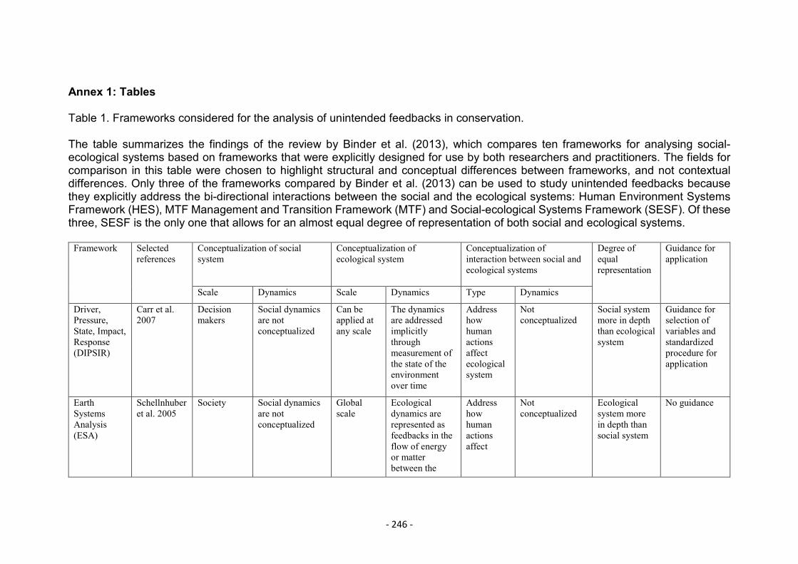
- 246 -

Annex 1: Tables

Table 1. Frameworks considered for the analysis of unintended feedbacks in conservation.

The table summarizes the findings of the review by Binder et al. (2013), which compares ten frameworks for analysing social-ecological systems based on frameworks that were explicitly designed for use by both researchers and practitioners. The fields forcomparison in this table were chosen to highlight structural and conceptual differences between frameworks, and not contextualdifferences. Only three of the frameworks compared by Binder et al. (2013) can be used to study unintended feedbacks becausethey explicitly address the bi-directional interactions between the social and the ecological systems: Human Environment SystemsFramework (HES), MTF Management and Transition Framework (MTF) and Social-ecological Systems Framework (SESF). Of thesethree, SESF is the only one that allows for an almost equal degree of representation of both social and ecological systems.

Framework Selectedreferences

Conceptualization of socialsystem

Conceptualization ofecological system

Conceptualization ofinteraction between social andecological systems

Degree ofequalrepresentation

Guidance forapplication

Scale Dynamics Scale Dynamics Type Dynamics

Driver,Pressure,State, Impact,Response(DIPSIR)

Carr et al.2007

Decisionmakers

Social dynamicsare notconceptualized

Can beapplied atany scale

The dynamicsare addressedimplicitlythroughmeasurement ofthe state of theenvironmentover time

Addresshowhumanactionsaffectecologicalsystem

Notconceptualized

Social systemmore in depththan ecologicalsystem

Guidance forselection ofvariables andstandardizedprocedure forapplication

EarthSystemsAnalysis(ESA)

Schellnhuberet al. 2005

Society Social dynamicsare notconceptualized

Globalscale

Ecologicaldynamics arerepresented asfeedbacks in theflow of energyor matterbetween the

Addresshowhumanactionsaffect

Notconceptualized

Ecologicalsystem morein depth thansocial system

No guidance

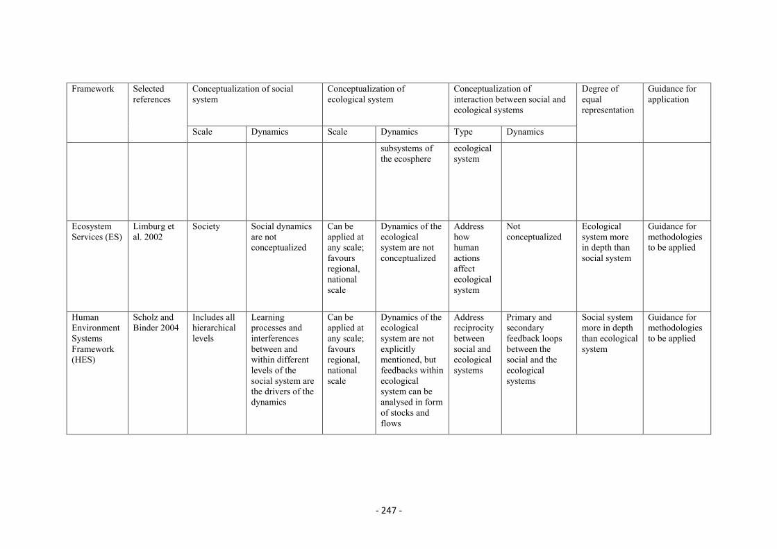
- 247 -

Framework Selectedreferences

Conceptualization of socialsystem

Conceptualization ofecological system

Conceptualization ofinteraction between social andecological systems

Degree ofequalrepresentation

Guidance forapplication

Scale Dynamics Scale Dynamics Type Dynamics

subsystems ofthe ecosphere

ecologicalsystem

EcosystemServices (ES)

Limburg etal. 2002

Society Social dynamicsare notconceptualized

Can beapplied atany scale;favoursregional,nationalscale

Dynamics of theecologicalsystem are notconceptualized

Addresshowhumanactionsaffectecologicalsystem

Notconceptualized

Ecologicalsystem morein depth thansocial system

Guidance formethodologiesto be applied

HumanEnvironmentSystemsFramework(HES)

Scholz andBinder 2004

Includes allhierarchicallevels

Learningprocesses andinterferencesbetween andwithin differentlevels of thesocial system arethe drivers of thedynamics

Can beapplied atany scale;favoursregional,nationalscale

Dynamics of theecologicalsystem are notexplicitlymentioned, butfeedbacks withinecologicalsystem can beanalysed in formof stocks andflows

Addressreciprocitybetweensocial andecologicalsystems

Primary andsecondaryfeedback loopsbetween thesocial and theecologicalsystems

Social systemmore in depththan ecologicalsystem

Guidance formethodologiesto be applied

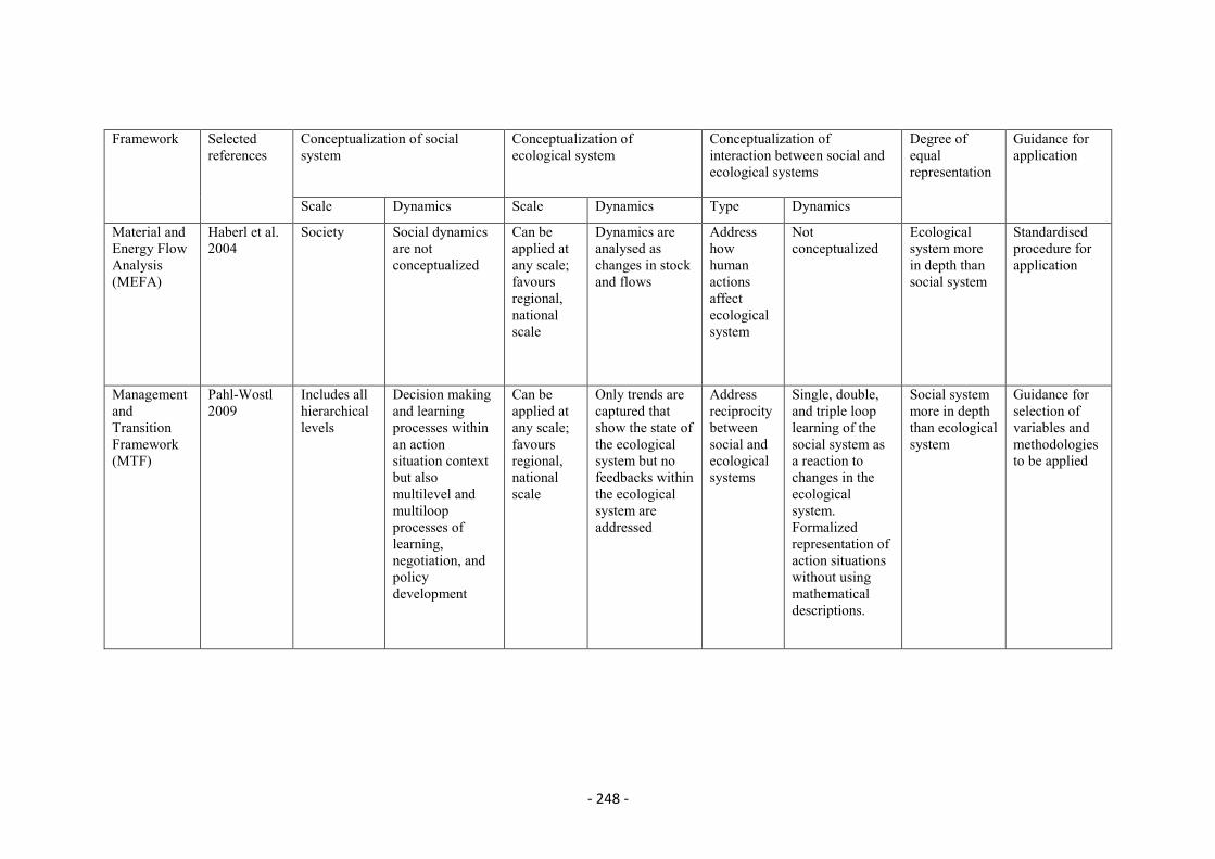
- 248 -

Framework Selectedreferences

Conceptualization of socialsystem

Conceptualization ofecological system

Conceptualization ofinteraction between social andecological systems

Degree ofequalrepresentation

Guidance forapplication

Scale Dynamics Scale Dynamics Type Dynamics

Material andEnergy FlowAnalysis(MEFA)

Haberl et al.2004

Society Social dynamicsare notconceptualized

Can beapplied atany scale;favoursregional,nationalscale

Dynamics areanalysed aschanges in stockand flows

Addresshowhumanactionsaffectecologicalsystem

Notconceptualized

Ecologicalsystem morein depth thansocial system

Standardisedprocedure forapplication

ManagementandTransitionFramework(MTF)

Pahl-Wostl2009

Includes allhierarchicallevels

Decision makingand learningprocesses withinan actionsituation contextbut alsomultilevel andmultiloopprocesses oflearning,negotiation, andpolicydevelopment

Can beapplied atany scale;favoursregional,nationalscale

Only trends arecaptured thatshow the state ofthe ecologicalsystem but nofeedbacks withinthe ecologicalsystem areaddressed

Addressreciprocitybetweensocial andecologicalsystems

Single, double,and triple looplearning of thesocial system asa reaction tochanges in theecologicalsystem.Formalizedrepresentation ofaction situationswithout usingmathematicaldescriptions.

Social systemmore in depththan ecologicalsystem

Guidance forselection ofvariables andmethodologiesto be applied

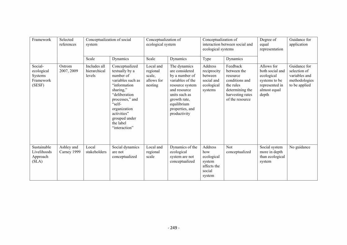
- 249 -

Framework Selectedreferences

Conceptualization of socialsystem

Conceptualization ofecological system

Conceptualization ofinteraction between social andecological systems

Degree ofequalrepresentation

Guidance forapplication

Scale Dynamics Scale Dynamics Type Dynamics

Social-ecologicalSystemsFramework(SESF)

Ostrom2007, 2009

Includes allhierarchicallevels

Conceptualizedtextually by anumber ofvariables such as“informationsharing,”“deliberationprocesses,” and“self-organizationactivities”grouped underthe label“interaction”

Local andregionalscale,allows fornesting

The dynamicsare consideredby a number ofvariables of theresource systemand resourceunits such asgrowth rate,equilibriumproperties, andproductivity

Addressreciprocitybetweensocial andecologicalsystems

Feedbackbetween theresourceconditions andthe rulesdetermining theharvesting ratesof the resource

Allows forboth social andecologicalsystems to berepresented inalmost equaldepth

Guidance forselection ofvariables andmethodologiesto be applied

SustainableLivelihoodsApproach(SLA)

Ashley andCarney 1999

Localstakeholders

Social dynamicsare notconceptualized

Local andregionalscale

Dynamics of theecologicalsystem are notconceptualized

Addresshowecologicalsystemaffects thesocialsystem

Notconceptualized

Social systemmore in depththan ecologicalsystem

No guidance

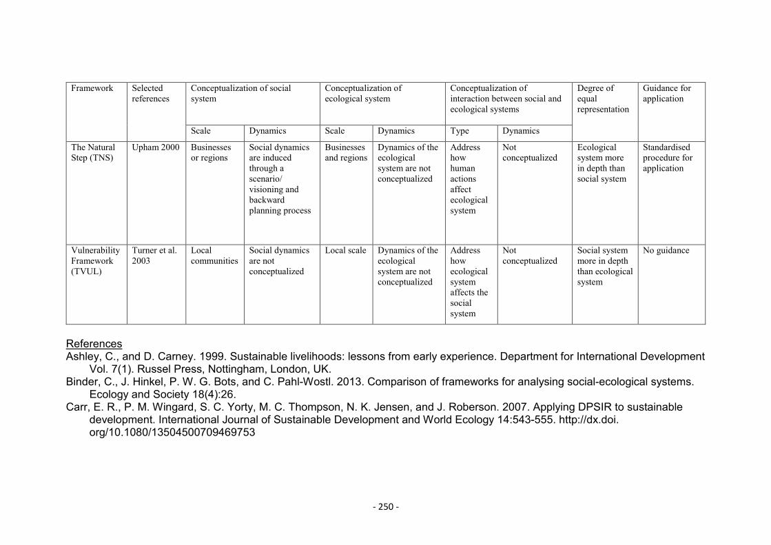
- 250 -

Framework Selectedreferences

Conceptualization of socialsystem

Conceptualization ofecological system

Conceptualization ofinteraction between social andecological systems

Degree ofequalrepresentation

Guidance forapplication

Scale Dynamics Scale Dynamics Type Dynamics

The NaturalStep (TNS)

Upham 2000 Businessesor regions

Social dynamicsare inducedthrough ascenario/visioning andbackwardplanning process

Businessesand regions

Dynamics of theecologicalsystem are notconceptualized

Addresshowhumanactionsaffectecologicalsystem

Notconceptualized

Ecologicalsystem morein depth thansocial system

Standardisedprocedure forapplication

VulnerabilityFramework(TVUL)

Turner et al.2003

Localcommunities

Social dynamicsare notconceptualized

Local scale Dynamics of theecologicalsystem are notconceptualized

Addresshowecologicalsystemaffects thesocialsystem

Notconceptualized

Social systemmore in depththan ecologicalsystem

No guidance

ReferencesAshley, C., and D. Carney. 1999. Sustainable livelihoods: lessons from early experience. Department for International Development

Vol. 7(1). Russel Press, Nottingham, London, UK.Binder, C., J. Hinkel, P. W. G. Bots, and C. Pahl-Wostl. 2013. Comparison of frameworks for analysing social-ecological systems.

Ecology and Society 18(4):26.Carr, E. R., P. M. Wingard, S. C. Yorty, M. C. Thompson, N. K. Jensen, and J. Roberson. 2007. Applying DPSIR to sustainable

development. International Journal of Sustainable Development and World Ecology 14:543-555. http://dx.doi.org/10.1080/13504500709469753

- 251 -

Haberl, H., M. Fischer-Kowalski, F. Krausmann, H. Weisz, and V. Winiwarter. 2004. Progress towards sustainability? What theconceptual framework of material and energy flow accounting (MEFA) can offer. Land Use Policy 21:199-213.http://dx.doi.org/10.1016/j.landusepol.2003.10.013

Limburg, K. E., R. V. O’Neill, R. Costanza, and S. Farber. 2002. Complex systems and valuation. Ecological Economics 41:409-420. http://dx.doi.org/10.1016/S0921-8009(02)00090-3

Ostrom, E. 2007. A diagnostic approach for going beyond panaceas. Proceedings of the National Academy of Sciences of theUnited States of America 104:15181-15187. http://dx. doi.org/10.1073/pnas.0702288104

Ostrom, E. 2009. A general framework for analysing sustainability of social-ecological systems. Science 325:419-422.http://dx.doi.org/10.1126/science.1172133

Pahl-Wostl, C. 2009. A conceptual framework for analysing adaptive capacity and multi-level learning processes in resourcegovernance regimes. Global Environmental Change 19:354-365. http://dx.doi.org/10.1016/j.gloenvcha.2009.06.001

Schellnhuber, H.-J., P. J. Crutzen, W. C. Clark, and J. Hunt. 2005. Earth system analysis for sustainability. Environment: Scienceand Policy for Sustainable Development 47(8):10-25. http://dx.doi.org/10.3200/ENVT.47.8.10-25

Scholz, R. W., and C. R. Binder. 2004. Principles of human- environment systems research. Pages 791-796 in C. Pahl, S. Schmidt,and T. Jakeman, editors. iEMSs 2004 International Congress: Complexity and Integrated Resources Management.International Environmental Modelling and Software Society, Osnabrueck, Germany.

Turner, B. L., P. Matson, J. J. McCarthy, R. W. Corell, L. Christensen, N. Eckley, G. Hovelsrud-Broda, J. X. Kasperson, R. E.Kasperson, A. Luers, M. L. Martello, S. Mathiesen, R. Naylor, C. Polsky, A. Pulsipher, A. Schiller, H. Selin, and N. Tyler.2003b. Illustrating the coupled human-environment system for vulnerability analysis: three case studies. Proceedings of theNational Academy of Sciences 100 (14):8080-8085. http://dx.doi.org/10.1073/pnas.1231334100

Upham, P. 2000. An assessment of the natural step theory of sustainability. Journal of Cleaner Production 8:445-454.http://dx.doi.org/10.1016/S0959-6526(00)00012-3

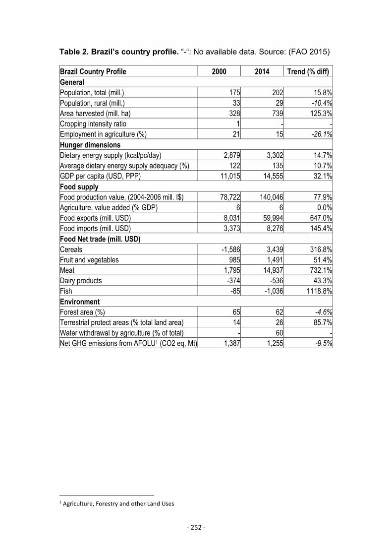
- 252 -

Table 2. Brazil’s country profile. “-“: No available data. Source: (FAO 2015)

Brazil Country Profile 2000 2014 Trend (% diff)GeneralPopulation, total (mill.) 175 202 15.8%Population, rural (mill.) 33 29 -10.4%Area harvested (mill. ha) 328 739 125.3%Cropping intensity ratio 1 - -Employment in agriculture (%) 21 15 -26.1%Hunger dimensionsDietary energy supply (kcal/pc/day) 2,879 3,302 14.7%Average dietary energy supply adequacy (%) 122 135 10.7%GDP per capita (USD, PPP) 11,015 14,555 32.1%Food supplyFood production value, (2004-2006 mill. I$) 78,722 140,046 77.9%Agriculture, value added (% GDP) 6 6 0.0%Food exports (mill. USD) 8,031 59,994 647.0%Food imports (mill. USD) 3,373 8,276 145.4%Food Net trade (mill. USD)Cereals -1,586 3,439 316.8%Fruit and vegetables 985 1,491 51.4%Meat 1,795 14,937 732.1%Dairy products -374 -536 43.3%Fish -85 -1,036 1118.8%EnvironmentForest area (%) 65 62 -4.6%Terrestrial protect areas (% total land area) 14 26 85.7%Water withdrawal by agriculture (% of total) - 60 -Net GHG emissions from AFOLU1 (CO2 eq, Mt) 1,387 1,255 -9.5%

1 Agriculture, Forestry and other Land Uses

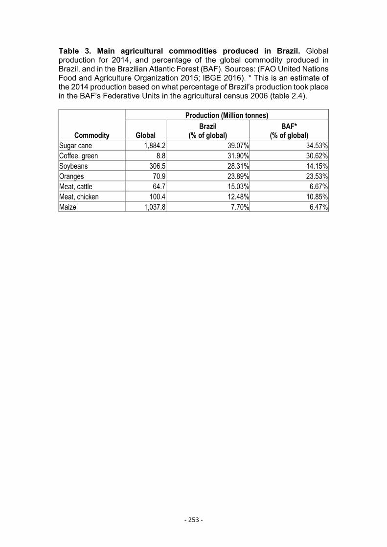
- 253 -

Table 3. Main agricultural commodities produced in Brazil. Globalproduction for 2014, and percentage of the global commodity produced inBrazil, and in the Brazilian Atlantic Forest (BAF). Sources: (FAO United NationsFood and Agriculture Organization 2015; IBGE 2016). * This is an estimate ofthe 2014 production based on what percentage of Brazil’s production took placein the BAF’s Federative Units in the agricultural census 2006 (table 2.4).

Commodity

Production (Million tonnes)

GlobalBrazil

(% of global)BAF*

(% of global)Sugar cane 1,884.2 39.07% 34.53%Coffee, green 8.8 31.90% 30.62%Soybeans 306.5 28.31% 14.15%Oranges 70.9 23.89% 23.53%Meat, cattle 64.7 15.03% 6.67%Meat, chicken 100.4 12.48% 10.85%Maize 1,037.8 7.70% 6.47%

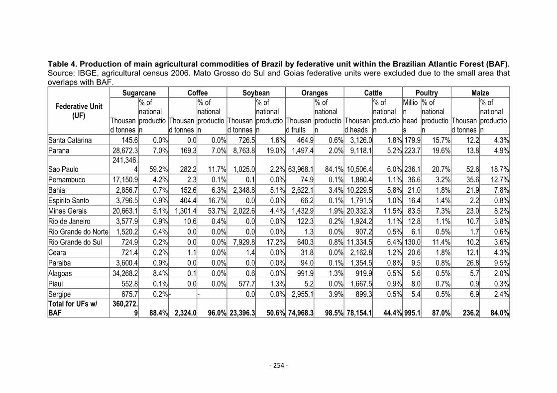
- 254 -

Table 4. Production of main agricultural commodities of Brazil by federative unit within the Brazilian Atlantic Forest (BAF).Source: IBGE, agricultural census 2006. Mato Grosso do Sul and Goias federative units were excluded due to the small area thatoverlaps with BAF.

Federative Unit(UF)

Sugarcane Coffee Soybean Oranges Cattle Poultry Maize

Thousand tonnes

% ofnationalproduction

Thousand tonnes

% ofnationalproduction

Thousand tonnes

% ofnationalproduction

Thousand fruits

% ofnationalproduction

Thousand heads

% ofnationalproduction

Millionheads

% ofnationalproduction

Thousand tonnes

% ofnationalproduction

Santa Catarina 145.6 0.0% 0.0 0.0% 726.5 1.6% 464.9 0.6% 3,126.0 1.8% 179.9 15.7% 12.2 4.3%Parana 28,672.3 7.0% 169.3 7.0% 8,763.8 19.0% 1,497.4 2.0% 9,118.1 5.2% 223.7 19.6% 13.8 4.9%

Sao Paulo241,346.

4 59.2% 282.2 11.7% 1,025.0 2.2% 63,968.1 84.1% 10,506.4 6.0% 236.1 20.7% 52.6 18.7%Pernambuco 17,150.9 4.2% 2.3 0.1% 0.1 0.0% 74.9 0.1% 1,880.4 1.1% 36.6 3.2% 35.6 12.7%Bahia 2,856.7 0.7% 152.6 6.3% 2,348.8 5.1% 2,622.1 3.4% 10,229.5 5.8% 21.0 1.8% 21.9 7.8%Espirito Santo 3,796.5 0.9% 404.4 16.7% 0.0 0.0% 66.2 0.1% 1,791.5 1.0% 16.4 1.4% 2.2 0.8%Minas Gerais 20,663.1 5.1% 1,301.4 53.7% 2,022.6 4.4% 1,432.9 1.9% 20,332.3 11.5% 83.5 7.3% 23.0 8.2%Rio de Janeiro 3,577.9 0.9% 10.6 0.4% 0.0 0.0% 122.3 0.2% 1,924.2 1.1% 12.8 1.1% 10.7 3.8%Rio Grande do Norte 1,520.2 0.4% 0.0 0.0% 0.0 0.0% 1.3 0.0% 907.2 0.5% 6.1 0.5% 1.7 0.6%Rio Grande do Sul 724.9 0.2% 0.0 0.0% 7,929.8 17.2% 640.3 0.8% 11,334.5 6.4% 130.0 11.4% 10.2 3.6%Ceara 721.4 0.2% 1.1 0.0% 1.4 0.0% 31.8 0.0% 2,162.8 1.2% 20.6 1.8% 12.1 4.3%Paraiba 3,600.4 0.9% 0.0 0.0% 0.0 0.0% 94.0 0.1% 1,354.5 0.8% 9.5 0.8% 26.8 9.5%Alagoas 34,268.2 8.4% 0.1 0.0% 0.6 0.0% 991.9 1.3% 919.9 0.5% 5.6 0.5% 5.7 2.0%Piaui 552.8 0.1% 0.0 0.0% 577.7 1.3% 5.2 0.0% 1,667.5 0.9% 8.0 0.7% 0.9 0.3%Sergipe 675.7 0.2%- - 0.0 0.0% 2,955.1 3.9% 899.3 0.5% 5.4 0.5% 6.9 2.4%Total for UFs w/BAF

360,272.9 88.4% 2,324.0 96.0% 23,396.3 50.6% 74,968.3 98.5% 78,154.1 44.4% 995.1 87.0% 236.2 84.0%

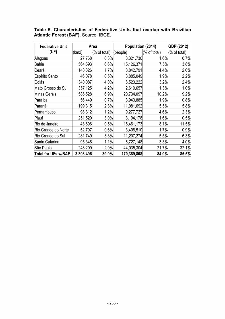
- 255 -

Table 5. Characteristics of Federative Units that overlap with BrazilianAtlantic Forest (BAF). Source: IBGE.

Federative Unit(UF)

Area Population (2014) GDP (2012)(km2) (% of total) (people) (% of total) (% of total)

Alagoas 27,768 0.3% 3,321,730 1.6% 0.7%Bahia 564,693 6.6% 15,126,371 7.5% 3.8%Ceará 148,826 1.7% 8,842,791 4.4% 2.0%Espírito Santo 46,078 0.5% 3,885,049 1.9% 2.2%Goiás 340,087 4.0% 6,523,222 3.2% 2.4%Mato Grosso do Sul 357,125 4.2% 2,619,657 1.3% 1.0%Minas Gerais 586,528 6.9% 20,734,097 10.2% 9.2%Paraíba 56,440 0.7% 3,943,885 1.9% 0.8%Paraná 199,315 2.3% 11,081,692 5.5% 5.8%Pernambuco 98,312 1.2% 9,277,727 4.6% 2.3%Piauí 251,529 3.0% 3,194,178 1.6% 0.5%Rio de Janeiro 43,696 0.5% 16,461,173 8.1% 11.5%Rio Grande do Norte 52,797 0.6% 3,408,510 1.7% 0.9%Rio Grande do Sul 281,749 3.3% 11,207,274 5.5% 6.3%Santa Catarina 95,346 1.1% 6,727,148 3.3% 4.0%São Paulo 248,209 2.9% 44,035,304 21.7% 32.1%Total for UFs w/BAF 3,398,496 39.9% 170,389,808 84.0% 85.5%

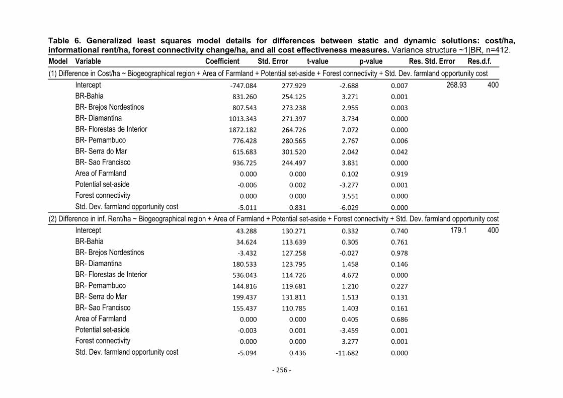
- 256 -

Table 6. Generalized least squares model details for differences between static and dynamic solutions: cost/ha,informational rent/ha, forest connectivity change/ha, and all cost effectiveness measures. Variance structure ~1|BR, n=412.Model Variable Coefficient Std. Error t-value p-value Res. Std. Error Res.d.f.(1) Difference in Cost/ha ~ Biogeographical region + Area of Farmland + Potential set-aside + Forest connectivity + Std. Dev. farmland opportunity cost

Intercept -747.084 277.929 -2.688 0.007 268.93 400BR-Bahia 831.260 254.125 3.271 0.001BR- Brejos Nordestinos 807.543 273.238 2.955 0.003BR- Diamantina 1013.343 271.397 3.734 0.000BR- Florestas de Interior 1872.182 264.726 7.072 0.000BR- Pernambuco 776.428 280.565 2.767 0.006BR- Serra do Mar 615.683 301.520 2.042 0.042BR- Sao Francisco 936.725 244.497 3.831 0.000Area of Farmland 0.000 0.000 0.102 0.919Potential set-aside -0.006 0.002 -3.277 0.001Forest connectivity 0.000 0.000 3.551 0.000Std. Dev. farmland opportunity cost -5.011 0.831 -6.029 0.000

(2) Difference in inf. Rent/ha ~ Biogeographical region + Area of Farmland + Potential set-aside + Forest connectivity + Std. Dev. farmland opportunity costIntercept 43.288 130.271 0.332 0.740 179.1 400BR-Bahia 34.624 113.639 0.305 0.761BR- Brejos Nordestinos -3.432 127.258 -0.027 0.978BR- Diamantina 180.533 123.795 1.458 0.146BR- Florestas de Interior 536.043 114.726 4.672 0.000BR- Pernambuco 144.816 119.681 1.210 0.227BR- Serra do Mar 199.437 131.811 1.513 0.131BR- Sao Francisco 155.437 110.785 1.403 0.161Area of Farmland 0.000 0.000 0.405 0.686Potential set-aside -0.003 0.001 -3.459 0.001Forest connectivity 0.000 0.000 3.277 0.001Std. Dev. farmland opportunity cost -5.094 0.436 -11.682 0.000

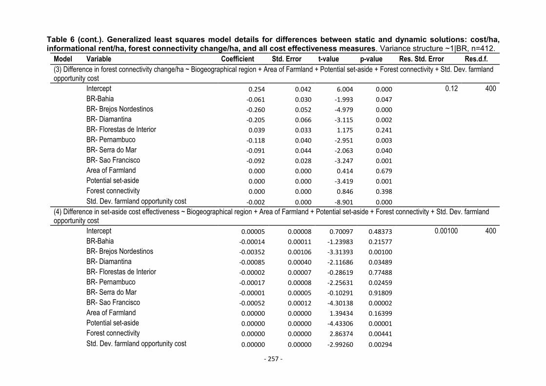
- 257 -

Table 6 (cont.). Generalized least squares model details for differences between static and dynamic solutions: cost/ha,informational rent/ha, forest connectivity change/ha, and all cost effectiveness measures. Variance structure ~1|BR, n=412.

Model Variable Coefficient Std. Error t-value p-value Res. Std. Error Res.d.f.(3) Difference in forest connectivity change/ha ~ Biogeographical region + Area of Farmland + Potential set-aside + Forest connectivity + Std. Dev. farmlandopportunity cost

Intercept 0.254 0.042 6.004 0.000 0.12 400BR-Bahia -0.061 0.030 -1.993 0.047BR- Brejos Nordestinos -0.260 0.052 -4.979 0.000BR- Diamantina -0.205 0.066 -3.115 0.002BR- Florestas de Interior 0.039 0.033 1.175 0.241BR- Pernambuco -0.118 0.040 -2.951 0.003BR- Serra do Mar -0.091 0.044 -2.063 0.040BR- Sao Francisco -0.092 0.028 -3.247 0.001Area of Farmland 0.000 0.000 0.414 0.679Potential set-aside 0.000 0.000 -3.419 0.001Forest connectivity 0.000 0.000 0.846 0.398Std. Dev. farmland opportunity cost -0.002 0.000 -8.901 0.000

(4) Difference in set-aside cost effectiveness ~ Biogeographical region + Area of Farmland + Potential set-aside + Forest connectivity + Std. Dev. farmlandopportunity cost

Intercept 0.00005 0.00008 0.70097 0.48373 0.00100 400BR-Bahia -0.00014 0.00011 -1.23983 0.21577BR- Brejos Nordestinos -0.00352 0.00106 -3.31393 0.00100BR- Diamantina -0.00085 0.00040 -2.11686 0.03489BR- Florestas de Interior -0.00002 0.00007 -0.28619 0.77488BR- Pernambuco -0.00017 0.00008 -2.25631 0.02459BR- Serra do Mar -0.00001 0.00005 -0.10291 0.91809BR- Sao Francisco -0.00052 0.00012 -4.30138 0.00002Area of Farmland 0.00000 0.00000 1.39434 0.16399Potential set-aside 0.00000 0.00000 -4.43306 0.00001Forest connectivity 0.00000 0.00000 2.86374 0.00441Std. Dev. farmland opportunity cost 0.00000 0.00000 -2.99260 0.00294

- 258 -

Table 6 (cont.). Generalized least squares model details for differences between static and dynamic solutions: cost/ha,informational rent/ha, forest connectivity change/ha, and all cost effectiveness measures. Variance structure ~1|BR, n=412.

Model Variable Coefficient Std. Error t-value p-value Res. Std. Error Res.d.f.(5) Difference in inf. Rent/$ ~ Biogeographical region + Area of Farmland + Potential set-aside + Forest connectivity + Std. Dev. farmland opportunity cost

Intercept 0.1989 0.0704 2.8235 0.0050 0.3800 400BR-Bahia -0.2630 0.0642 -4.0935 0.0001BR- Brejos Nordestinos -0.3767 0.0876 -4.3013 0.0000BR- Diamantina -0.1939 0.1015 -1.9103 0.0568BR- Florestas de Interior 0.0006 0.0553 0.0106 0.9915BR- Pernambuco -0.1738 0.0589 -2.9499 0.0034BR- Serra do Mar -0.0149 0.0510 -0.2924 0.7701BR- Sao Francisco -0.3630 0.0668 -5.4308 0.0000Area of Farmland 0.0000 0.0000 0.8107 0.4180Potential set-aside 0.0000 0.0000 -3.8318 0.0001Forest connectivity 0.0000 0.0000 3.9496 0.0001Std. Dev. farmland opportunity cost -0.0025 0.0003 -8.2614 0.0000

(6) Difference in forest connectivity change cost effectiveness ~ Biogeographical region + Area of Farmland + Potential set-aside + Forest connectivity + Std.Dev. farmland opportunity cost

Intercept 0.00007 0.00002 4.74829 0.00000 0.00020 400BR-Bahia -0.00001 0.00002 -0.63167 0.52796BR- Brejos Nordestinos -0.00073 0.00030 -2.42158 0.01590BR- Diamantina -0.00032 0.00013 -2.39626 0.01702BR- Florestas de Interior -0.00002 0.00002 -1.44945 0.14800BR- Pernambuco -0.00004 0.00002 -1.77339 0.07692BR- Serra do Mar -0.00002 0.00001 -1.84439 0.06587BR- Sao Francisco -0.00007 0.00002 -3.18464 0.00156Area of Farmland 0.00000 0.00000 0.69939 0.48472Potential set-aside 0.00000 0.00000 -2.04142 0.04186Forest connectivity 0.00000 0.00000 0.26147 0.79386Std. Dev. farmland opportunity cost 0.00000 0.00000 -6.94882 0.00000

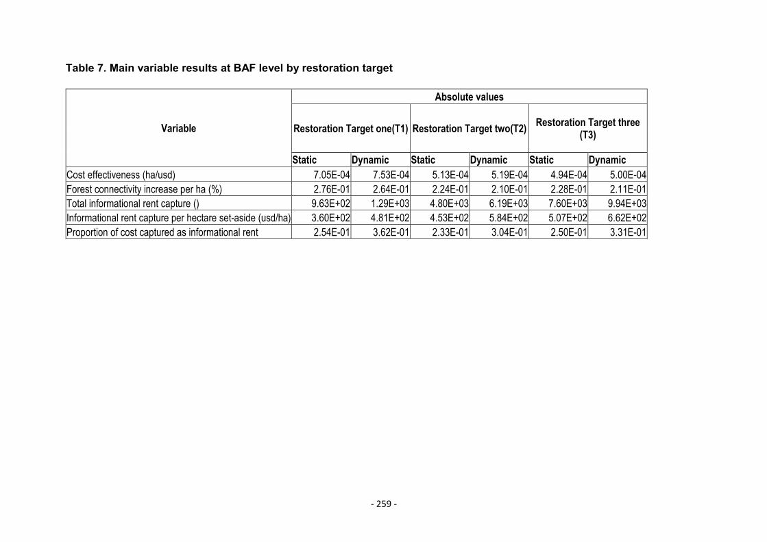
- 259 -

Table 7. Main variable results at BAF level by restoration target

Variable

Absolute values

Restoration Target one(T1) Restoration Target two(T2) Restoration Target three(T3)

Static Dynamic Static Dynamic Static DynamicCost effectiveness (ha/usd) 7.05E-04 7.53E-04 5.13E-04 5.19E-04 4.94E-04 5.00E-04Forest connectivity increase per ha (%) 2.76E-01 2.64E-01 2.24E-01 2.10E-01 2.28E-01 2.11E-01Total informational rent capture () 9.63E+02 1.29E+03 4.80E+03 6.19E+03 7.60E+03 9.94E+03Informational rent capture per hectare set-aside (usd/ha) 3.60E+02 4.81E+02 4.53E+02 5.84E+02 5.07E+02 6.62E+02Proportion of cost captured as informational rent 2.54E-01 3.62E-01 2.33E-01 3.04E-01 2.50E-01 3.31E-01

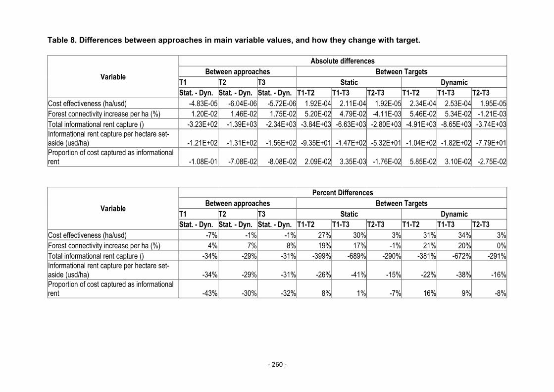
- 260 -

Table 8. Differences between approaches in main variable values, and how they change with target.

Variable

Absolute differencesBetween approaches Between Targets

T1 T2 T3 Static DynamicStat. - Dyn. Stat. - Dyn. Stat. - Dyn. T1-T2 T1-T3 T2-T3 T1-T2 T1-T3 T2-T3

Cost effectiveness (ha/usd) -4.83E-05 -6.04E-06 -5.72E-06 1.92E-04 2.11E-04 1.92E-05 2.34E-04 2.53E-04 1.95E-05Forest connectivity increase per ha (%) 1.20E-02 1.46E-02 1.75E-02 5.20E-02 4.79E-02 -4.11E-03 5.46E-02 5.34E-02 -1.21E-03Total informational rent capture () -3.23E+02 -1.39E+03 -2.34E+03 -3.84E+03 -6.63E+03 -2.80E+03 -4.91E+03 -8.65E+03 -3.74E+03Informational rent capture per hectare set-aside (usd/ha) -1.21E+02 -1.31E+02 -1.56E+02 -9.35E+01 -1.47E+02 -5.32E+01 -1.04E+02 -1.82E+02 -7.79E+01Proportion of cost captured as informationalrent -1.08E-01 -7.08E-02 -8.08E-02 2.09E-02 3.35E-03 -1.76E-02 5.85E-02 3.10E-02 -2.75E-02

Variable

Percent DifferencesBetween approaches Between Targets

T1 T2 T3 Static DynamicStat. - Dyn. Stat. - Dyn. Stat. - Dyn. T1-T2 T1-T3 T2-T3 T1-T2 T1-T3 T2-T3

Cost effectiveness (ha/usd) -7% -1% -1% 27% 30% 3% 31% 34% 3%Forest connectivity increase per ha (%) 4% 7% 8% 19% 17% -1% 21% 20% 0%Total informational rent capture () -34% -29% -31% -399% -689% -290% -381% -672% -291%Informational rent capture per hectare set-aside (usd/ha) -34% -29% -31% -26% -41% -15% -22% -38% -16%Proportion of cost captured as informationalrent -43% -30% -32% 8% 1% -7% 16% 9% -8%

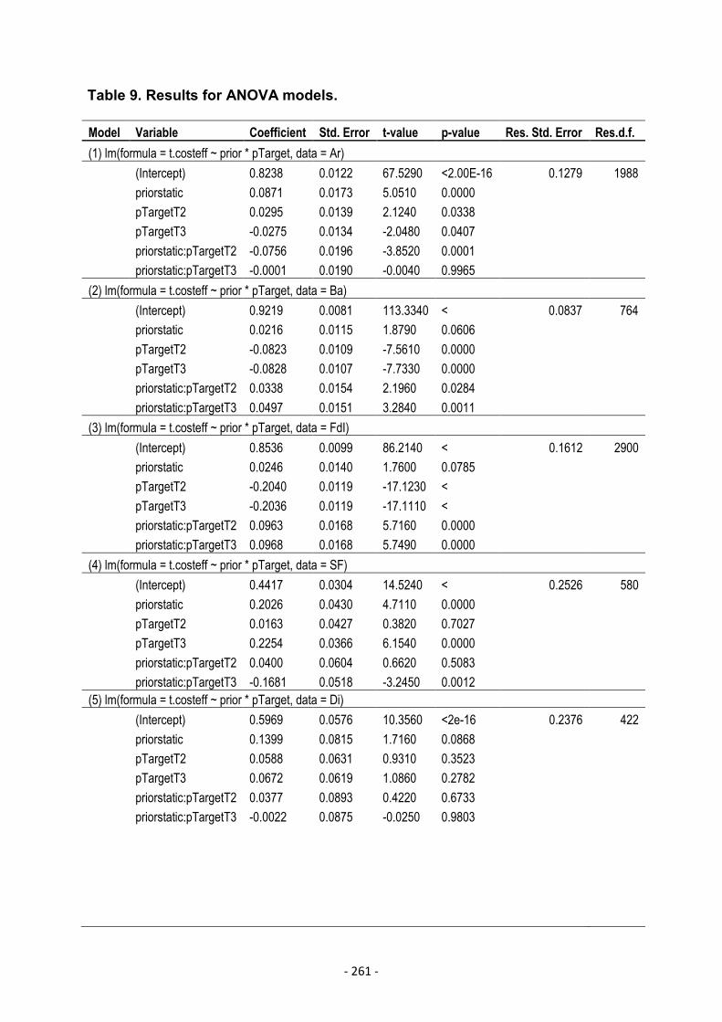
- 261 -

Table 9. Results for ANOVA models.

Model Variable Coefficient Std. Error t-value p-value Res. Std. Error Res.d.f.(1) lm(formula = t.costeff ~ prior * pTarget, data = Ar)

(Intercept) 0.8238 0.0122 67.5290 <2.00E-16 0.1279 1988priorstatic 0.0871 0.0173 5.0510 0.0000pTargetT2 0.0295 0.0139 2.1240 0.0338pTargetT3 -0.0275 0.0134 -2.0480 0.0407priorstatic:pTargetT2 -0.0756 0.0196 -3.8520 0.0001priorstatic:pTargetT3 -0.0001 0.0190 -0.0040 0.9965

(2) lm(formula = t.costeff ~ prior * pTarget, data = Ba)(Intercept) 0.9219 0.0081 113.3340 < 0.0837 764priorstatic 0.0216 0.0115 1.8790 0.0606pTargetT2 -0.0823 0.0109 -7.5610 0.0000pTargetT3 -0.0828 0.0107 -7.7330 0.0000priorstatic:pTargetT2 0.0338 0.0154 2.1960 0.0284priorstatic:pTargetT3 0.0497 0.0151 3.2840 0.0011

(3) lm(formula = t.costeff ~ prior * pTarget, data = FdI)(Intercept) 0.8536 0.0099 86.2140 < 0.1612 2900priorstatic 0.0246 0.0140 1.7600 0.0785pTargetT2 -0.2040 0.0119 -17.1230 <pTargetT3 -0.2036 0.0119 -17.1110 <priorstatic:pTargetT2 0.0963 0.0168 5.7160 0.0000priorstatic:pTargetT3 0.0968 0.0168 5.7490 0.0000

(4) lm(formula = t.costeff ~ prior * pTarget, data = SF)(Intercept) 0.4417 0.0304 14.5240 < 0.2526 580priorstatic 0.2026 0.0430 4.7110 0.0000pTargetT2 0.0163 0.0427 0.3820 0.7027pTargetT3 0.2254 0.0366 6.1540 0.0000priorstatic:pTargetT2 0.0400 0.0604 0.6620 0.5083priorstatic:pTargetT3 -0.1681 0.0518 -3.2450 0.0012

(5) lm(formula = t.costeff ~ prior * pTarget, data = Di)(Intercept) 0.5969 0.0576 10.3560 <2e-16 0.2376 422priorstatic 0.1399 0.0815 1.7160 0.0868pTargetT2 0.0588 0.0631 0.9310 0.3523pTargetT3 0.0672 0.0619 1.0860 0.2782priorstatic:pTargetT2 0.0377 0.0893 0.4220 0.6733priorstatic:pTargetT3 -0.0022 0.0875 -0.0250 0.9803

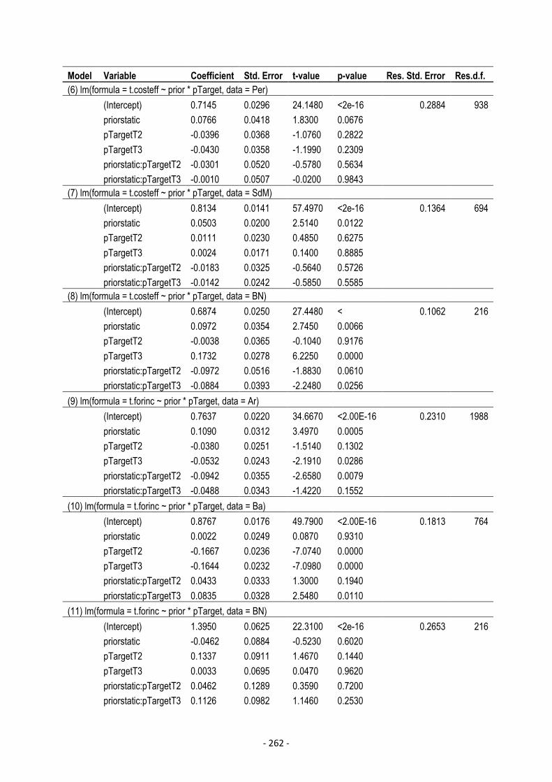
- 262 -

Model Variable Coefficient Std. Error t-value p-value Res. Std. Error Res.d.f.(6) lm(formula = t.costeff ~ prior * pTarget, data = Per)

(Intercept) 0.7145 0.0296 24.1480 <2e-16 0.2884 938priorstatic 0.0766 0.0418 1.8300 0.0676pTargetT2 -0.0396 0.0368 -1.0760 0.2822pTargetT3 -0.0430 0.0358 -1.1990 0.2309priorstatic:pTargetT2 -0.0301 0.0520 -0.5780 0.5634priorstatic:pTargetT3 -0.0010 0.0507 -0.0200 0.9843

(7) lm(formula = t.costeff ~ prior * pTarget, data = SdM)(Intercept) 0.8134 0.0141 57.4970 <2e-16 0.1364 694priorstatic 0.0503 0.0200 2.5140 0.0122pTargetT2 0.0111 0.0230 0.4850 0.6275pTargetT3 0.0024 0.0171 0.1400 0.8885priorstatic:pTargetT2 -0.0183 0.0325 -0.5640 0.5726priorstatic:pTargetT3 -0.0142 0.0242 -0.5850 0.5585

(8) lm(formula = t.costeff ~ prior * pTarget, data = BN)(Intercept) 0.6874 0.0250 27.4480 < 0.1062 216priorstatic 0.0972 0.0354 2.7450 0.0066pTargetT2 -0.0038 0.0365 -0.1040 0.9176pTargetT3 0.1732 0.0278 6.2250 0.0000priorstatic:pTargetT2 -0.0972 0.0516 -1.8830 0.0610priorstatic:pTargetT3 -0.0884 0.0393 -2.2480 0.0256

(9) lm(formula = t.forinc ~ prior * pTarget, data = Ar)(Intercept) 0.7637 0.0220 34.6670 <2.00E-16 0.2310 1988priorstatic 0.1090 0.0312 3.4970 0.0005pTargetT2 -0.0380 0.0251 -1.5140 0.1302pTargetT3 -0.0532 0.0243 -2.1910 0.0286priorstatic:pTargetT2 -0.0942 0.0355 -2.6580 0.0079priorstatic:pTargetT3 -0.0488 0.0343 -1.4220 0.1552

(10) lm(formula = t.forinc ~ prior * pTarget, data = Ba)(Intercept) 0.8767 0.0176 49.7900 <2.00E-16 0.1813 764priorstatic 0.0022 0.0249 0.0870 0.9310pTargetT2 -0.1667 0.0236 -7.0740 0.0000pTargetT3 -0.1644 0.0232 -7.0980 0.0000priorstatic:pTargetT2 0.0433 0.0333 1.3000 0.1940priorstatic:pTargetT3 0.0835 0.0328 2.5480 0.0110

(11) lm(formula = t.forinc ~ prior * pTarget, data = BN)(Intercept) 1.3950 0.0625 22.3100 <2e-16 0.2653 216priorstatic -0.0462 0.0884 -0.5230 0.6020pTargetT2 0.1337 0.0911 1.4670 0.1440pTargetT3 0.0033 0.0695 0.0470 0.9620priorstatic:pTargetT2 0.0462 0.1289 0.3590 0.7200priorstatic:pTargetT3 0.1126 0.0982 1.1460 0.2530

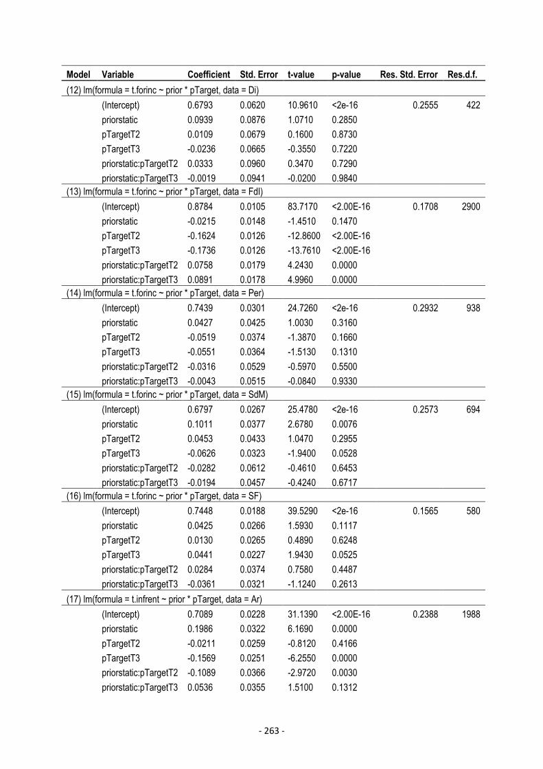
- 263 -

Model Variable Coefficient Std. Error t-value p-value Res. Std. Error Res.d.f.(12) lm(formula = t.forinc ~ prior * pTarget, data = Di)

(Intercept) 0.6793 0.0620 10.9610 <2e-16 0.2555 422priorstatic 0.0939 0.0876 1.0710 0.2850pTargetT2 0.0109 0.0679 0.1600 0.8730pTargetT3 -0.0236 0.0665 -0.3550 0.7220priorstatic:pTargetT2 0.0333 0.0960 0.3470 0.7290priorstatic:pTargetT3 -0.0019 0.0941 -0.0200 0.9840

(13) lm(formula = t.forinc ~ prior * pTarget, data = FdI)(Intercept) 0.8784 0.0105 83.7170 <2.00E-16 0.1708 2900priorstatic -0.0215 0.0148 -1.4510 0.1470pTargetT2 -0.1624 0.0126 -12.8600 <2.00E-16pTargetT3 -0.1736 0.0126 -13.7610 <2.00E-16priorstatic:pTargetT2 0.0758 0.0179 4.2430 0.0000priorstatic:pTargetT3 0.0891 0.0178 4.9960 0.0000

(14) lm(formula = t.forinc ~ prior * pTarget, data = Per)(Intercept) 0.7439 0.0301 24.7260 <2e-16 0.2932 938priorstatic 0.0427 0.0425 1.0030 0.3160pTargetT2 -0.0519 0.0374 -1.3870 0.1660pTargetT3 -0.0551 0.0364 -1.5130 0.1310priorstatic:pTargetT2 -0.0316 0.0529 -0.5970 0.5500priorstatic:pTargetT3 -0.0043 0.0515 -0.0840 0.9330

(15) lm(formula = t.forinc ~ prior * pTarget, data = SdM)(Intercept) 0.6797 0.0267 25.4780 <2e-16 0.2573 694priorstatic 0.1011 0.0377 2.6780 0.0076pTargetT2 0.0453 0.0433 1.0470 0.2955pTargetT3 -0.0626 0.0323 -1.9400 0.0528priorstatic:pTargetT2 -0.0282 0.0612 -0.4610 0.6453priorstatic:pTargetT3 -0.0194 0.0457 -0.4240 0.6717

(16) lm(formula = t.forinc ~ prior * pTarget, data = SF)(Intercept) 0.7448 0.0188 39.5290 <2e-16 0.1565 580priorstatic 0.0425 0.0266 1.5930 0.1117pTargetT2 0.0130 0.0265 0.4890 0.6248pTargetT3 0.0441 0.0227 1.9430 0.0525priorstatic:pTargetT2 0.0284 0.0374 0.7580 0.4487priorstatic:pTargetT3 -0.0361 0.0321 -1.1240 0.2613

(17) lm(formula = t.infrent ~ prior * pTarget, data = Ar)(Intercept) 0.7089 0.0228 31.1390 <2.00E-16 0.2388 1988priorstatic 0.1986 0.0322 6.1690 0.0000pTargetT2 -0.0211 0.0259 -0.8120 0.4166pTargetT3 -0.1569 0.0251 -6.2550 0.0000priorstatic:pTargetT2 -0.1089 0.0366 -2.9720 0.0030priorstatic:pTargetT3 0.0536 0.0355 1.5100 0.1312

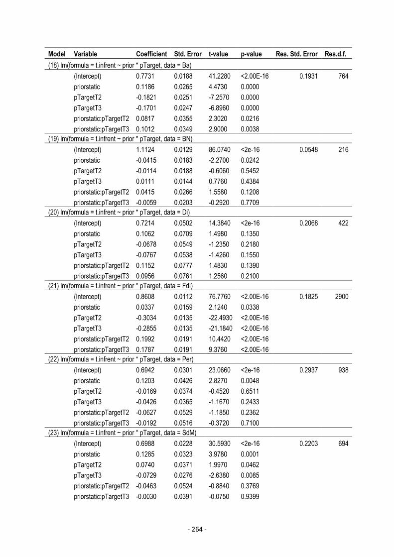
- 264 -

Model Variable Coefficient Std. Error t-value p-value Res. Std. Error Res.d.f.(18) lm(formula = t.infrent ~ prior * pTarget, data = Ba)

(Intercept) 0.7731 0.0188 41.2280 <2.00E-16 0.1931 764priorstatic 0.1186 0.0265 4.4730 0.0000pTargetT2 -0.1821 0.0251 -7.2570 0.0000pTargetT3 -0.1701 0.0247 -6.8960 0.0000priorstatic:pTargetT2 0.0817 0.0355 2.3020 0.0216priorstatic:pTargetT3 0.1012 0.0349 2.9000 0.0038

(19) lm(formula = t.infrent ~ prior * pTarget, data = BN)(Intercept) 1.1124 0.0129 86.0740 <2e-16 0.0548 216priorstatic -0.0415 0.0183 -2.2700 0.0242pTargetT2 -0.0114 0.0188 -0.6060 0.5452pTargetT3 0.0111 0.0144 0.7760 0.4384priorstatic:pTargetT2 0.0415 0.0266 1.5580 0.1208priorstatic:pTargetT3 -0.0059 0.0203 -0.2920 0.7709

(20) lm(formula = t.infrent ~ prior * pTarget, data = Di)(Intercept) 0.7214 0.0502 14.3840 <2e-16 0.2068 422priorstatic 0.1062 0.0709 1.4980 0.1350pTargetT2 -0.0678 0.0549 -1.2350 0.2180pTargetT3 -0.0767 0.0538 -1.4260 0.1550priorstatic:pTargetT2 0.1152 0.0777 1.4830 0.1390priorstatic:pTargetT3 0.0956 0.0761 1.2560 0.2100

(21) lm(formula = t.infrent ~ prior * pTarget, data = FdI)(Intercept) 0.8608 0.0112 76.7760 <2.00E-16 0.1825 2900priorstatic 0.0337 0.0159 2.1240 0.0338pTargetT2 -0.3034 0.0135 -22.4930 <2.00E-16pTargetT3 -0.2855 0.0135 -21.1840 <2.00E-16priorstatic:pTargetT2 0.1992 0.0191 10.4420 <2.00E-16priorstatic:pTargetT3 0.1787 0.0191 9.3760 <2.00E-16

(22) lm(formula = t.infrent ~ prior * pTarget, data = Per)(Intercept) 0.6942 0.0301 23.0660 <2e-16 0.2937 938priorstatic 0.1203 0.0426 2.8270 0.0048pTargetT2 -0.0169 0.0374 -0.4520 0.6511pTargetT3 -0.0426 0.0365 -1.1670 0.2433priorstatic:pTargetT2 -0.0627 0.0529 -1.1850 0.2362priorstatic:pTargetT3 -0.0192 0.0516 -0.3720 0.7100

(23) lm(formula = t.infrent ~ prior * pTarget, data = SdM)(Intercept) 0.6988 0.0228 30.5930 <2e-16 0.2203 694priorstatic 0.1285 0.0323 3.9780 0.0001pTargetT2 0.0740 0.0371 1.9970 0.0462pTargetT3 -0.0729 0.0276 -2.6380 0.0085priorstatic:pTargetT2 -0.0463 0.0524 -0.8840 0.3769priorstatic:pTargetT3 -0.0030 0.0391 -0.0750 0.9399

- 265 -

Model Variable Coefficient Std. Error t-value p-value Res. Std. Error Res.d.f.(24) lm(formula = t.infrent ~ prior * pTarget, data = SF)

(Intercept) 0.8364 0.0083 100.3830 <2.00E-16 0.0692 580priorstatic 0.0958 0.0118 8.1290 0.0000pTargetT2 -0.0016 0.0117 -0.1350 0.8923pTargetT3 0.0331 0.0100 3.2980 0.0010priorstatic:pTargetT2 0.0172 0.0165 1.0380 0.2998priorstatic:pTargetT3 -0.0560 0.0142 -3.9470 0.0001

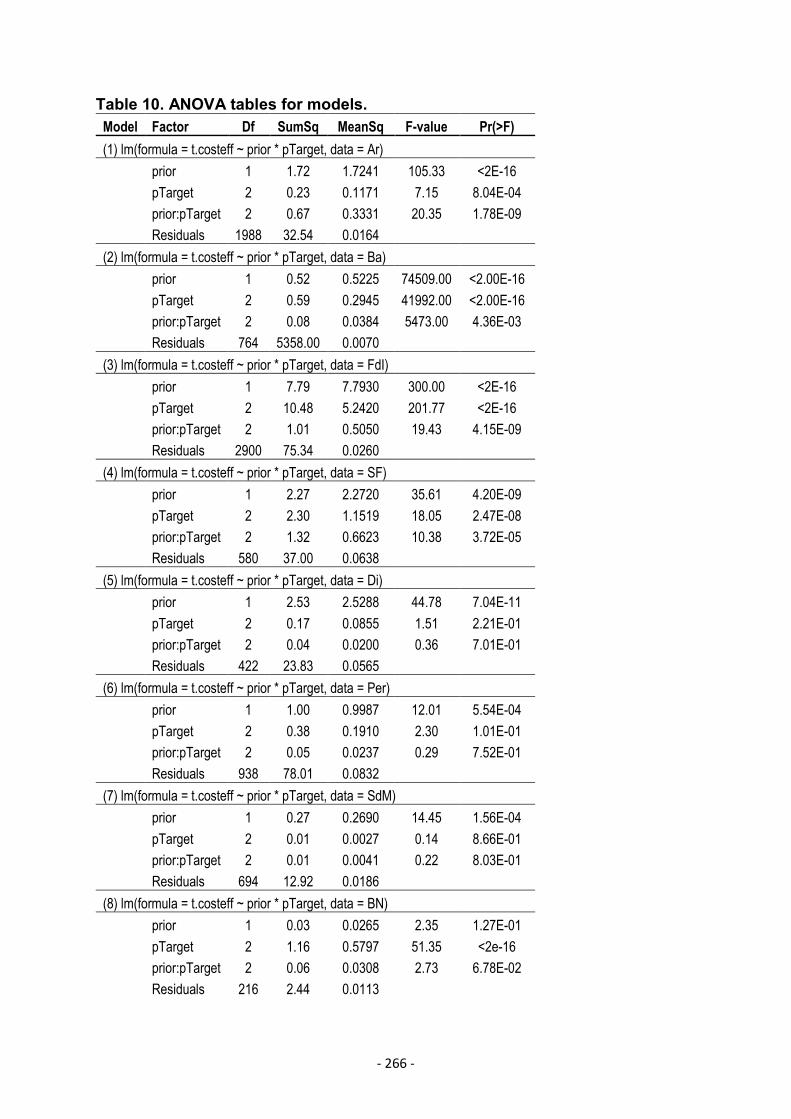
- 266 -

Table 10. ANOVA tables for models.Model Factor Df SumSq MeanSq F-value Pr(>F)(1) lm(formula = t.costeff ~ prior * pTarget, data = Ar)

prior 1 1.72 1.7241 105.33 <2E-16pTarget 2 0.23 0.1171 7.15 8.04E-04prior:pTarget 2 0.67 0.3331 20.35 1.78E-09Residuals 1988 32.54 0.0164

(2) lm(formula = t.costeff ~ prior * pTarget, data = Ba)prior 1 0.52 0.5225 74509.00 <2.00E-16pTarget 2 0.59 0.2945 41992.00 <2.00E-16prior:pTarget 2 0.08 0.0384 5473.00 4.36E-03Residuals 764 5358.00 0.0070

(3) lm(formula = t.costeff ~ prior * pTarget, data = FdI)prior 1 7.79 7.7930 300.00 <2E-16pTarget 2 10.48 5.2420 201.77 <2E-16prior:pTarget 2 1.01 0.5050 19.43 4.15E-09Residuals 2900 75.34 0.0260

(4) lm(formula = t.costeff ~ prior * pTarget, data = SF)prior 1 2.27 2.2720 35.61 4.20E-09pTarget 2 2.30 1.1519 18.05 2.47E-08prior:pTarget 2 1.32 0.6623 10.38 3.72E-05Residuals 580 37.00 0.0638

(5) lm(formula = t.costeff ~ prior * pTarget, data = Di)prior 1 2.53 2.5288 44.78 7.04E-11pTarget 2 0.17 0.0855 1.51 2.21E-01prior:pTarget 2 0.04 0.0200 0.36 7.01E-01Residuals 422 23.83 0.0565

(6) lm(formula = t.costeff ~ prior * pTarget, data = Per)prior 1 1.00 0.9987 12.01 5.54E-04pTarget 2 0.38 0.1910 2.30 1.01E-01prior:pTarget 2 0.05 0.0237 0.29 7.52E-01Residuals 938 78.01 0.0832

(7) lm(formula = t.costeff ~ prior * pTarget, data = SdM)prior 1 0.27 0.2690 14.45 1.56E-04pTarget 2 0.01 0.0027 0.14 8.66E-01prior:pTarget 2 0.01 0.0041 0.22 8.03E-01Residuals 694 12.92 0.0186

(8) lm(formula = t.costeff ~ prior * pTarget, data = BN)prior 1 0.03 0.0265 2.35 1.27E-01pTarget 2 1.16 0.5797 51.35 <2e-16prior:pTarget 2 0.06 0.0308 2.73 6.78E-02Residuals 216 2.44 0.0113

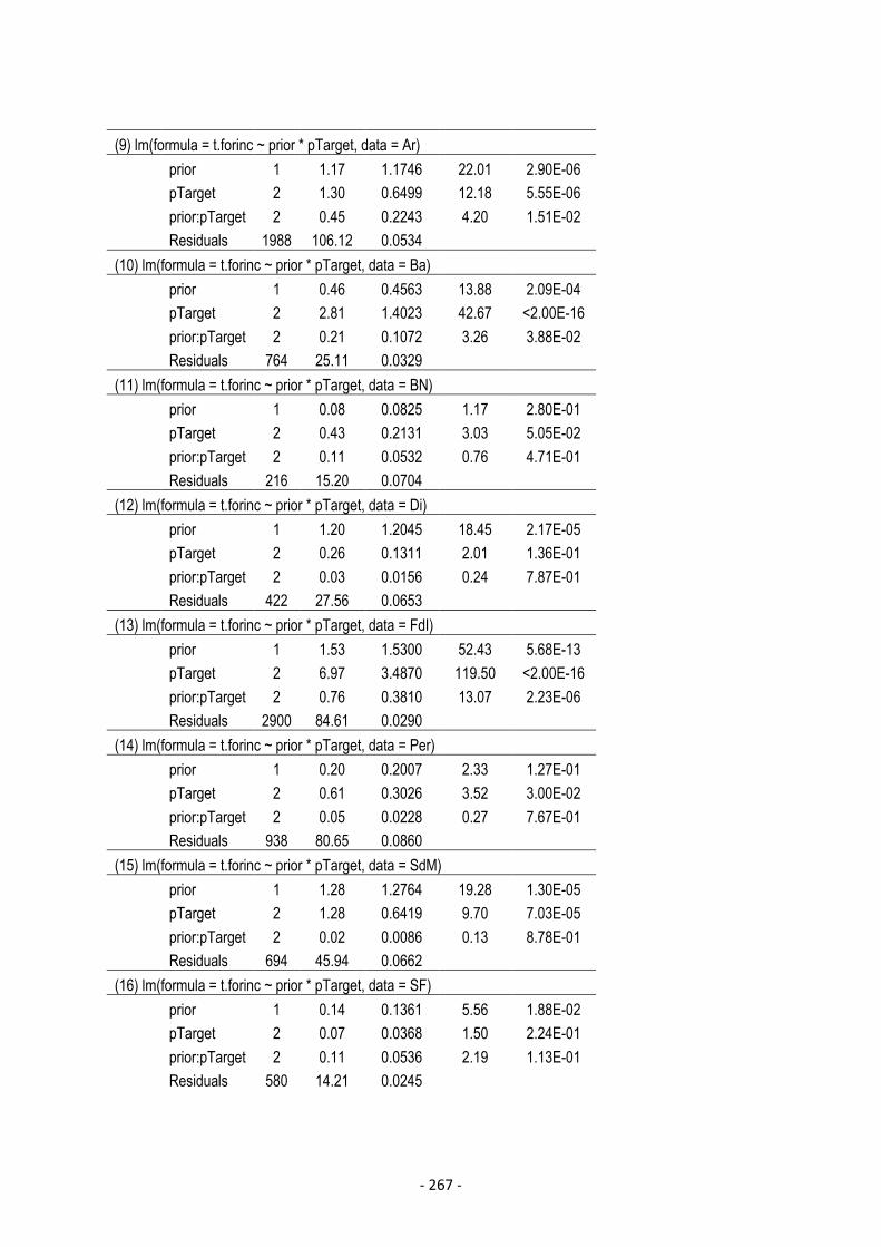
- 267 -

(9) lm(formula = t.forinc ~ prior * pTarget, data = Ar)prior 1 1.17 1.1746 22.01 2.90E-06pTarget 2 1.30 0.6499 12.18 5.55E-06prior:pTarget 2 0.45 0.2243 4.20 1.51E-02Residuals 1988 106.12 0.0534

(10) lm(formula = t.forinc ~ prior * pTarget, data = Ba)prior 1 0.46 0.4563 13.88 2.09E-04pTarget 2 2.81 1.4023 42.67 <2.00E-16prior:pTarget 2 0.21 0.1072 3.26 3.88E-02Residuals 764 25.11 0.0329

(11) lm(formula = t.forinc ~ prior * pTarget, data = BN)prior 1 0.08 0.0825 1.17 2.80E-01pTarget 2 0.43 0.2131 3.03 5.05E-02prior:pTarget 2 0.11 0.0532 0.76 4.71E-01Residuals 216 15.20 0.0704

(12) lm(formula = t.forinc ~ prior * pTarget, data = Di)prior 1 1.20 1.2045 18.45 2.17E-05pTarget 2 0.26 0.1311 2.01 1.36E-01prior:pTarget 2 0.03 0.0156 0.24 7.87E-01Residuals 422 27.56 0.0653

(13) lm(formula = t.forinc ~ prior * pTarget, data = FdI)prior 1 1.53 1.5300 52.43 5.68E-13pTarget 2 6.97 3.4870 119.50 <2.00E-16prior:pTarget 2 0.76 0.3810 13.07 2.23E-06Residuals 2900 84.61 0.0290

(14) lm(formula = t.forinc ~ prior * pTarget, data = Per)prior 1 0.20 0.2007 2.33 1.27E-01pTarget 2 0.61 0.3026 3.52 3.00E-02prior:pTarget 2 0.05 0.0228 0.27 7.67E-01Residuals 938 80.65 0.0860

(15) lm(formula = t.forinc ~ prior * pTarget, data = SdM)prior 1 1.28 1.2764 19.28 1.30E-05pTarget 2 1.28 0.6419 9.70 7.03E-05prior:pTarget 2 0.02 0.0086 0.13 8.78E-01Residuals 694 45.94 0.0662

(16) lm(formula = t.forinc ~ prior * pTarget, data = SF)prior 1 0.14 0.1361 5.56 1.88E-02pTarget 2 0.07 0.0368 1.50 2.24E-01prior:pTarget 2 0.11 0.0536 2.19 1.13E-01Residuals 580 14.21 0.0245

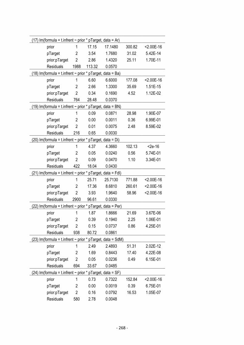
- 268 -

(17) lm(formula = t.infrent ~ prior * pTarget, data = Ar)prior 1 17.15 17.1480 300.82 <2.00E-16pTarget 2 3.54 1.7680 31.02 5.42E-14prior:pTarget 2 2.86 1.4320 25.11 1.70E-11Residuals 1988 113.32 0.0570

(18) lm(formula = t.infrent ~ prior * pTarget, data = Ba)prior 1 6.60 6.6000 177.08 <2.00E-16pTarget 2 2.66 1.3300 35.69 1.51E-15prior:pTarget 2 0.34 0.1690 4.52 1.12E-02Residuals 764 28.48 0.0370

(19) lm(formula = t.infrent ~ prior * pTarget, data = BN)prior 1 0.09 0.0871 28.98 1.90E-07pTarget 2 0.00 0.0011 0.36 6.99E-01prior:pTarget 2 0.01 0.0075 2.48 8.59E-02Residuals 216 0.65 0.0030

(20) lm(formula = t.infrent ~ prior * pTarget, data = Di)prior 1 4.37 4.3660 102.13 <2e-16pTarget 2 0.05 0.0240 0.56 5.74E-01prior:pTarget 2 0.09 0.0470 1.10 3.34E-01Residuals 422 18.04 0.0430

(21) lm(formula = t.infrent ~ prior * pTarget, data = FdI)prior 1 25.71 25.7130 771.88 <2.00E-16pTarget 2 17.36 8.6810 260.61 <2.00E-16prior:pTarget 2 3.93 1.9640 58.96 <2.00E-16Residuals 2900 96.61 0.0330

(22) lm(formula = t.infrent ~ prior * pTarget, data = Per)prior 1 1.87 1.8666 21.69 3.67E-06pTarget 2 0.39 0.1940 2.25 1.06E-01prior:pTarget 2 0.15 0.0737 0.86 4.25E-01Residuals 938 80.72 0.0861

(23) lm(formula = t.infrent ~ prior * pTarget, data = SdM)prior 1 2.49 2.4893 51.31 2.02E-12pTarget 2 1.69 0.8443 17.40 4.22E-08prior:pTarget 2 0.05 0.0236 0.49 6.15E-01Residuals 694 33.67 0.0485

(24) lm(formula = t.infrent ~ prior * pTarget, data = SF)prior 1 0.73 0.7322 152.84 <2.00E-16pTarget 2 0.00 0.0019 0.39 6.75E-01prior:pTarget 2 0.16 0.0792 16.53 1.05E-07Residuals 580 2.78 0.0048

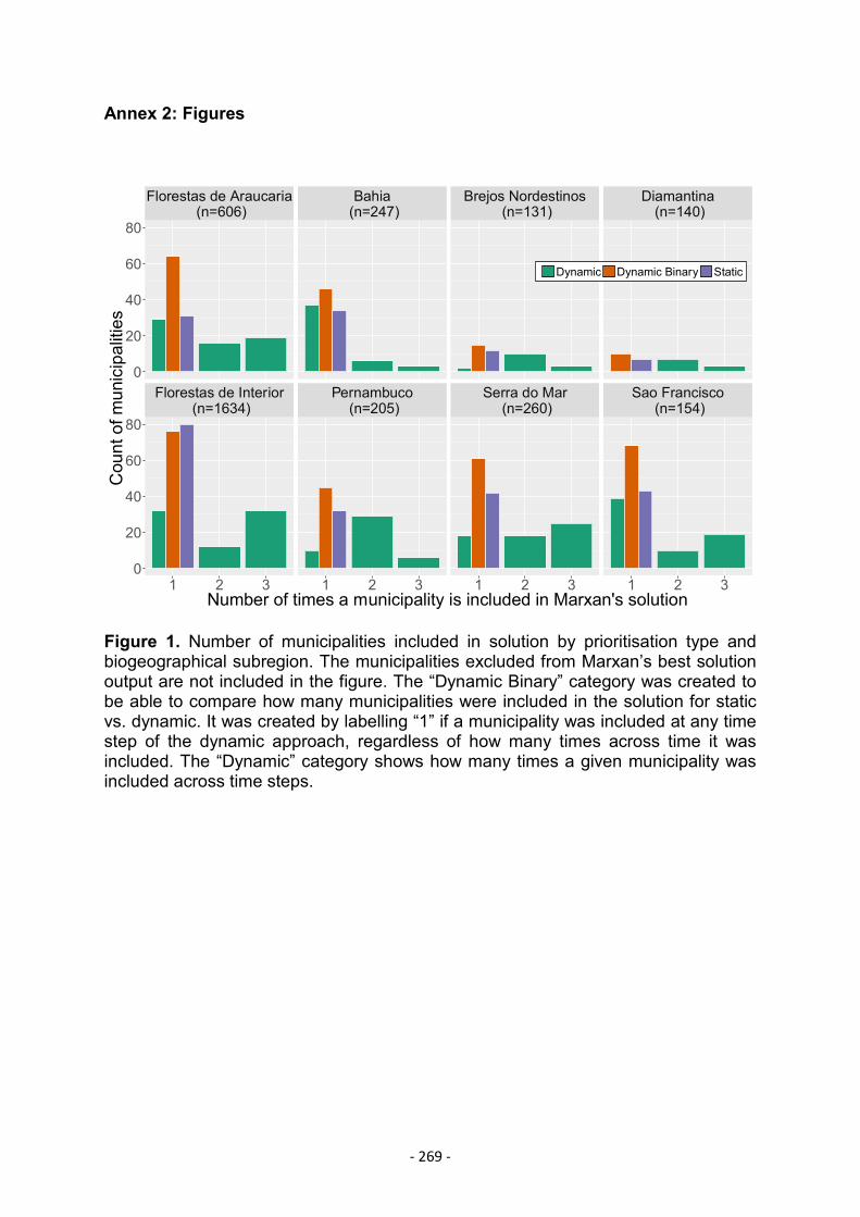
- 269 -

Annex 2: Figures

Figure 1. Number of municipalities included in solution by prioritisation type andbiogeographical subregion. The municipalities excluded from Marxan’s best solutionoutput are not included in the figure. The “Dynamic Binary” category was created tobe able to compare how many municipalities were included in the solution for staticvs. dynamic. It was created by labelling “1” if a municipality was included at any timestep of the dynamic approach, regardless of how many times across time it wasincluded. The “Dynamic” category shows how many times a given municipality wasincluded across time steps.

Florestas de Araucaria(n=606)

Bahia(n=247)

Brejos Nordestinos(n=131)

Diamantina(n=140)

Florestas de Interior(n=1634)

Pernambuco(n=205)

Serra do Mar(n=260)

Sao Francisco(n=154)

0

20

40

60

80

0

20

40

60

80

1 2 3 1 2 3 1 2 3 1 2 3Number of times a municipality is included in Marxan's solution

Countofmunicipalities

Dynamic Dynamic Binary Static

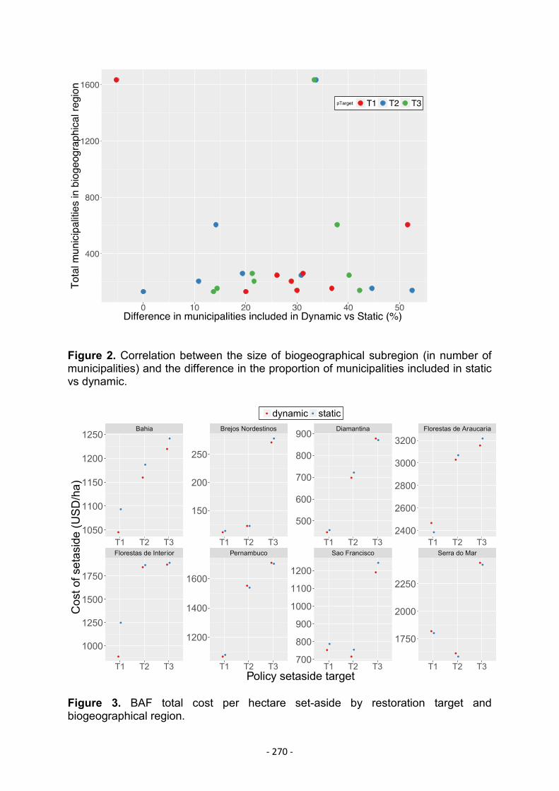
- 270 -

Figure 2. Correlation between the size of biogeographical subregion (in number ofmunicipalities) and the difference in the proportion of municipalities included in staticvs dynamic.

Figure 3. BAF total cost per hectare set-aside by restoration target andbiogeographical region.

●

●

●

●

●

●

●●●●

●●

●●

●●

●●

●

●

●●

●●

●

●

●● ●●

●●

●●

●●

●●

●●

●

●

●●

●●

●●

Bahia Brejos Nordestinos Diamantina Florestas de Araucaria

Florestas de Interior Pernambuco Sao Francisco Serra do Mar

1050

1100

1150

1200

1250

150

200

250

500

600

700

800

900

2400

2600

2800

3000

3200

1000

1250

1500

1750

1200

1400

1600

700

800

900

1000

1100

1200

1750

2000

2250

T1 T2 T3 T1 T2 T3 T1 T2 T3 T1 T2 T3

T1 T2 T3 T1 T2 T3 T1 T2 T3 T1 T2 T3Policy setaside target

Costofsetaside(USD/ha)

● ●dynamic static

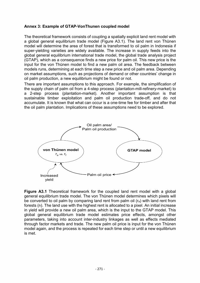
- 271 -

Annex 3: Example of GTAP-VonThunen coupled model

The theoretical framework consists of coupling a spatially explicit land rent model witha global general equilibrium trade model (Figure A3.1). The land rent von Thünenmodel will determine the area of forest that is transformed to oil palm in Indonesia ifsuper-yielding varieties are widely available. The increase in supply feeds into theglobal general equilibrium international trade model, the global trade analysis project(GTAP), which as a consequence finds a new price for palm oil. This new price is theinput for the von Thünen model to find a new palm oil area. The feedback betweenmodels runs, determining at each time step a new price and oil palm area. Dependingon market assumptions, such as projections of demand or other countries’ change inoil palm production, a new equilibrium might be found or not.There are important assumptions to this approach. For example, the simplification ofthe supply chain of palm oil from a 4-step process (plantation-mill-refinery-market) toa 2-step process (plantation-market). Another important assumption is thatsustainable timber exploitation and palm oil production trade-off, and do notaccumulate. It is known that what can occur is a one-time fee for timber and after thatthe oil palm plantation. Implications of these assumptions need to be explored.

Figure A3.1 Theoretical framework for the coupled land rent model with a globalgeneral equilibrium trade model. The von Thünen model determines which pixels willbe converted to oil palm by comparing land rent from palm oil (ra) with land rent fromforests (rf). The land use with the highest rent is allocated to a pixel. An initial increasein yield will provide a new oil palm area, which is the input to the GTAP model. Thisglobal general equilibrium trade model estimates price effects, amongst otherparameters, taking into account inter-industry linkages as well as effects mediatedthrough factor markets and trade. The new palm oil price is input for the von Thünenmodel again, and the process is repeated for each time step or until a new equilibriumis met.

- 272 -

2.2.1 VON THÜNEN MODELThe von Thünen model (von Thünen 1966) is a model of land use that illustrates thetrade-off between land values and the distance from points of attraction, e.g. markets.It is commonly applied to agricultural land use and to explain urban land use patterns.The primary conclusion is that agricultural rent is inversely correlated to distance tomarkets. This model has been used to analyse forest cover change by considering asimple model where land has two uses: agriculture and forest (Angelsen 2007b). Inthis way, land is allocated to the use that yields the highest rent (Equation A3.1 vs.Equation A3.2), and the rents of various land uses are determined by location. Thisdual model simplification is sufficient to capture key policy issues (Angelsen 2010;Phelps et al. 2013).In this model, agricultural rent is determined by Equation A3.1. Agricultural productionper hectare (yield), in this case, oil palm yield (ya) is given by the newly improvedyields. The produce is sold to mills, and the palm oil is sold to refineries in cities orports at a given price (pa). The labour (la) and capital (ka) required per hectare varywith crop, with input prices being the wage (w) and annual costs of capital (q). Thefixed wage assumption implies that labour can move freely in and out of agriculture(Angelsen 2010). Transport costs are the product of costs per distance unit (va) anddistance from selling points (d).

ra = pa*ya - w*la - q*ka - va*d Equation A3.1

Forest rent is determined by Equation A3.2. Angelsen et al. (Angelsen 2010)distinguish three forest product types: (1) private forest products such as sustainabletimber exploitation, (2) local public goods such as water catchment services, and (3)global public goods such as carbon sequestration and storage. The extractive rentvaries with timber prices (pt); yield (yt), labour (lt), and capital (kt) required per hectare;as well as wages (w), capital (q), and transport (vt) costs. Local (pl) and global (pg)forest public goods can be captured with a PES scheme, increasing the overall forestrent from sustainable use.

rf =(pt*yt – w*lt – q*kt – vt*d)+ pl*yl + pg*yg Equation A3.2

There are several assumptions to the von Thünen model that are commonly acceptedbut whose implications for the system would need to be examined. For example, theland manager has well-established property rights, acts independently, has perfectinformation and seeks to maximise economic yield from the land. Other assumptionsare that transportation costs increase with distance and weight, and that there are twopossible land uses, development opportunity costs not included.

2.2.2 GLOBAL TRADE ANALYSIS PROJECT (GTAP)The GTAP Database records the annual flows of goods and services for the entireworld economy in the benchmark years (2004 and 2007); it consists of bilateral trade,transport, and protection matrices that link individual country/regional economicdatabases (Walmsley et al. 2012). The most updated version (2012, eighth version)covers 129 countries, 57 sectors, 5 factors for the two base years (Narayana et al.2012). The GTAP Data Base can be used in comparative static and dynamic

- 273 -

computable general equilibrium models, which are applied to the economic analysisof current global policy issues related to trade, energy and the environment.Standard GTAP model that is a multi-region, multi-sector, computable generalequilibrium model (Hertel 1997b). From the initial shock of increased production dueto high yields, the model estimates consumption, trade, and price effects taking intoaccount inter-industry linkages as well as effects mediated through factor markets andtrade. Model assumptions are perfect competition, constant returns to scale, no inter-temporal choice, and international trade in differentiated products (Armingtonassumption).

ReferencesAngelsen, A., 2007. Forest cover change in space and time: combining the von

Thünen and forest transition theories,Angelsen, A., 2010. Policies for reduced deforestation and their impact on

agricultural production. Proceedings of the National Academy of Sciences ofthe United States of America, 107(46), pp.19639–44.

FAO, 2015. FAO Statistical Pocketbook 2015,FAO United Nations Food and Agriculture Organization, 2015. FAOSTAT. 2016.

Available at: http://faostat.fao.org/.Hertel, T.W. ed., 1997. Global Trade Analysis: Modeling and Applications,

Cambridge, UK.: Cambridge University Press.IBGE, 2016. Sistema IBGE de recuperacion automatica (SIDRA). Agricultural

Census 2006. Available at: https://sidra.ibge.gov.br/pesquisa/censo-agropecuario/censo-agropecuario-2006/segunda-apuracao [Accessed March1, 2016].

Narayana, B., Aguiar, A. & McDougall, R., 2012. Global Trade, Assistance, andProduction: The GTAP 8 Data Base,

Phelps, J. et al., 2013. Agricultural intensification escalates future conservationcosts. Proceedings of the National Academy of Sciences of the United Statesof America, 110(19), pp.7601–6.

von Thünen, J.H., 1966. The Isolated State, Pergamon, New York.Walmsley, T.L., Aguiar, A.H. & Narayanan, B., 2012. Introduction to the Global Trade

Analysis Project and the GTAP Data Base,

- 274 -

Annex 4: Ensuring a robust Marxan analysis

Marxan requires a significant investment in setting up the problem, calibrating thealgorithm, and running sensitivity tests to get robust results. I followed the GoodPractices Handbook (Ardron et al. 2010) guidance on the necessary steps in thatprocess. These included: (1) testing sensitivity of solutions to changes in parametersand targets, (2) for solutions at all time steps checking both targets were met, (3) re-adjusting parameters at each time step, (4) evaluating the quality of solutions in termsof cost and objective function.

(1) The first step was to run Marxan for different conservation penalty factors (SPFs)and conservation targets. The “Getting Started” manual recommended SPFs valuesare 1, 2, 3 for each target, and their combinations (Game et al. 2008). The restorationtarget was set by the different policy targets (targets one, two and three). Forestconnectivity targets tested were 80%, 90% and 100% of the total potential forestconnectivity change for that biogeographical subregion at that time step.

x Forest connectivity target at 90% was the best target in terms of a compromisebetween solution cost-effectiveness and target met. This value was estimatedat each time step for the dynamic approach for all restoration targets.

x SPF combinations generated solutions in which targets were met for all runs,or no target was met for any run. The best SPF combination will have someruns meeting both targets, and some runs that don’t. I increased the SPFcombinations to test solutions and choose the best SPF combination for eachbioregion (table A4.1).

(2) At each time step, after the solution was obtained, I checked targets were met.

(3) For all targets, all SPF combinations were tested and the best combination for eachbioregion was chosen at each time step, and once for the static approach (figure A4.1by restoration target). The final SPF combination for each region at each time step isprovided in tables A4.2, A4.3 and A4.4 by restoration target.

(4) For chosen solutions, I checked cost and targets met following the objectivefunction and compared with “best solution” outputs from Marxan.

- 275 -

Table A4.1. Combinations of conservation penalty factors (SPFs) tested for targetsone and two. Target 1: restoration target; Target two: forest connectivity change target(90% of the total potential forest connectivity change for that biogeographicalsubregion at that time step).

Test Conservation penalty factor (SPF)Target 1 Target two

1 1 12 1 1.53 1 24 1 2.55 1.5 16 1.5 1.57 1.5 28 1.5 2.59 2 110 2 1.511 2 212 2 2.513 2.5 114 2.5 1.515 2.5 216 2.5 2.5

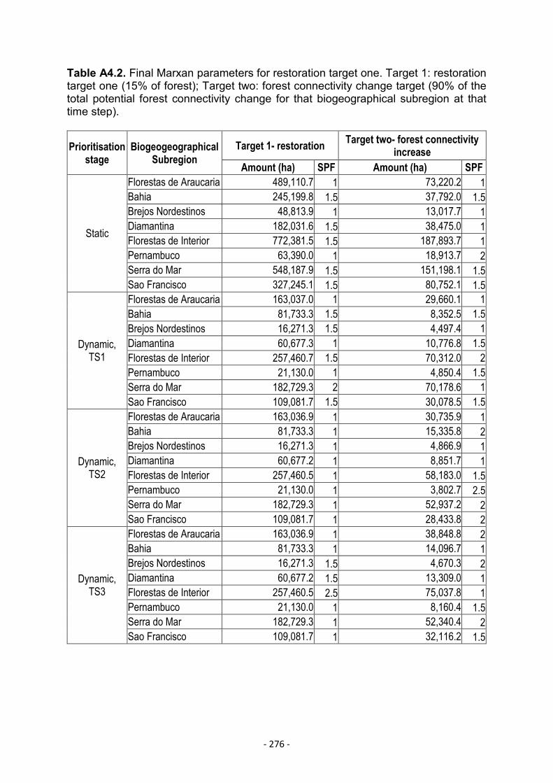
- 276 -

Table A4.2. Final Marxan parameters for restoration target one. Target 1: restorationtarget one (15% of forest); Target two: forest connectivity change target (90% of thetotal potential forest connectivity change for that biogeographical subregion at thattime step).

Prioritisationstage

BiogeogeographicalSubregion

Target 1- restoration Target two- forest connectivityincrease

Amount (ha) SPF Amount (ha) SPF

Static

Florestas de Araucaria 489,110.7 1 73,220.2 1Bahia 245,199.8 1.5 37,792.0 1.5Brejos Nordestinos 48,813.9 1 13,017.7 1Diamantina 182,031.6 1.5 38,475.0 1Florestas de Interior 772,381.5 1.5 187,893.7 1Pernambuco 63,390.0 1 18,913.7 2Serra do Mar 548,187.9 1.5 151,198.1 1.5Sao Francisco 327,245.1 1.5 80,752.1 1.5

Dynamic,TS1

Florestas de Araucaria 163,037.0 1 29,660.1 1Bahia 81,733.3 1.5 8,352.5 1.5Brejos Nordestinos 16,271.3 1.5 4,497.4 1Diamantina 60,677.3 1 10,776.8 1.5Florestas de Interior 257,460.7 1.5 70,312.0 2Pernambuco 21,130.0 1 4,850.4 1.5Serra do Mar 182,729.3 2 70,178.6 1Sao Francisco 109,081.7 1.5 30,078.5 1.5

Dynamic,TS2

Florestas de Araucaria 163,036.9 1 30,735.9 1Bahia 81,733.3 1 15,335.8 2Brejos Nordestinos 16,271.3 1 4,866.9 1Diamantina 60,677.2 1 8,851.7 1Florestas de Interior 257,460.5 1 58,183.0 1.5Pernambuco 21,130.0 1 3,802.7 2.5Serra do Mar 182,729.3 1 52,937.2 2Sao Francisco 109,081.7 1 28,433.8 2

Dynamic,TS3

Florestas de Araucaria 163,036.9 1 38,848.8 2Bahia 81,733.3 1 14,096.7 1Brejos Nordestinos 16,271.3 1.5 4,670.3 2Diamantina 60,677.2 1.5 13,309.0 1Florestas de Interior 257,460.5 2.5 75,037.8 1Pernambuco 21,130.0 1 8,160.4 1.5Serra do Mar 182,729.3 1 52,340.4 2Sao Francisco 109,081.7 1 32,116.2 1.5

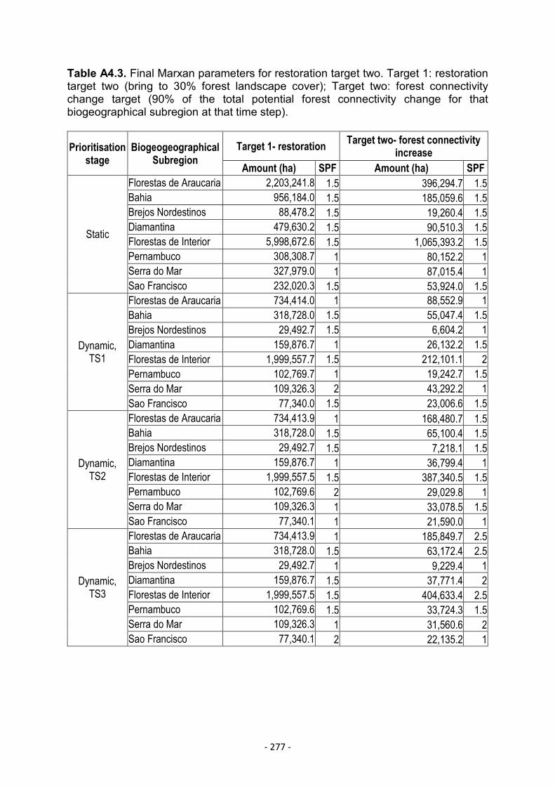
- 277 -

Table A4.3. Final Marxan parameters for restoration target two. Target 1: restorationtarget two (bring to 30% forest landscape cover); Target two: forest connectivitychange target (90% of the total potential forest connectivity change for thatbiogeographical subregion at that time step).

Prioritisationstage

BiogeogeographicalSubregion

Target 1- restoration Target two- forest connectivityincrease

Amount (ha) SPF Amount (ha) SPF

Static

Florestas de Araucaria 2,203,241.8 1.5 396,294.7 1.5Bahia 956,184.0 1.5 185,059.6 1.5Brejos Nordestinos 88,478.2 1.5 19,260.4 1.5Diamantina 479,630.2 1.5 90,510.3 1.5Florestas de Interior 5,998,672.6 1.5 1,065,393.2 1.5Pernambuco 308,308.7 1 80,152.2 1Serra do Mar 327,979.0 1 87,015.4 1Sao Francisco 232,020.3 1.5 53,924.0 1.5

Dynamic,TS1

Florestas de Araucaria 734,414.0 1 88,552.9 1Bahia 318,728.0 1.5 55,047.4 1.5Brejos Nordestinos 29,492.7 1.5 6,604.2 1Diamantina 159,876.7 1 26,132.2 1.5Florestas de Interior 1,999,557.7 1.5 212,101.1 2Pernambuco 102,769.7 1 19,242.7 1.5Serra do Mar 109,326.3 2 43,292.2 1Sao Francisco 77,340.0 1.5 23,006.6 1.5

Dynamic,TS2

Florestas de Araucaria 734,413.9 1 168,480.7 1.5Bahia 318,728.0 1.5 65,100.4 1.5Brejos Nordestinos 29,492.7 1.5 7,218.1 1.5Diamantina 159,876.7 1 36,799.4 1Florestas de Interior 1,999,557.5 1.5 387,340.5 1.5Pernambuco 102,769.6 2 29,029.8 1Serra do Mar 109,326.3 1 33,078.5 1.5Sao Francisco 77,340.1 1 21,590.0 1

Dynamic,TS3

Florestas de Araucaria 734,413.9 1 185,849.7 2.5Bahia 318,728.0 1.5 63,172.4 2.5Brejos Nordestinos 29,492.7 1 9,229.4 1Diamantina 159,876.7 1.5 37,771.4 2Florestas de Interior 1,999,557.5 1.5 404,633.4 2.5Pernambuco 102,769.6 1.5 33,724.3 1.5Serra do Mar 109,326.3 1 31,560.6 2Sao Francisco 77,340.1 2 22,135.2 1

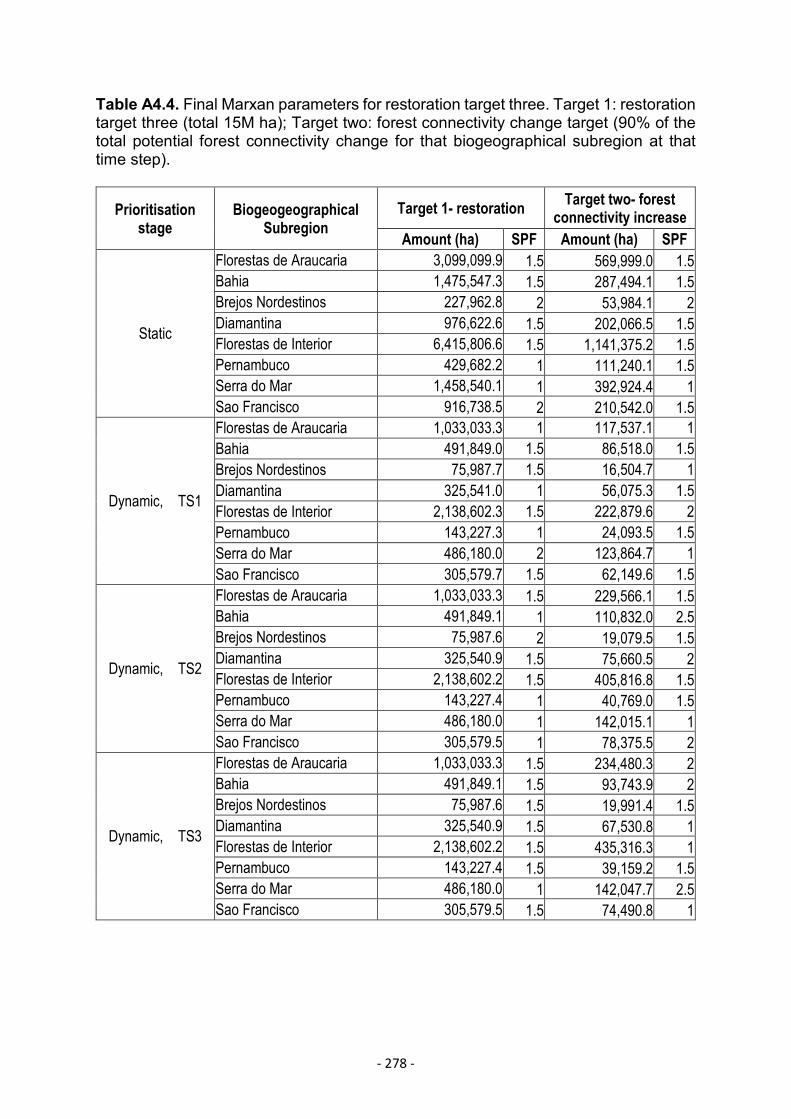
- 278 -

Table A4.4. Final Marxan parameters for restoration target three. Target 1: restorationtarget three (total 15M ha); Target two: forest connectivity change target (90% of thetotal potential forest connectivity change for that biogeographical subregion at thattime step).

Prioritisationstage

BiogeogeographicalSubregion

Target 1- restoration Target two- forestconnectivity increase

Amount (ha) SPF Amount (ha) SPF

Static

Florestas de Araucaria 3,099,099.9 1.5 569,999.0 1.5Bahia 1,475,547.3 1.5 287,494.1 1.5Brejos Nordestinos 227,962.8 2 53,984.1 2Diamantina 976,622.6 1.5 202,066.5 1.5Florestas de Interior 6,415,806.6 1.5 1,141,375.2 1.5Pernambuco 429,682.2 1 111,240.1 1.5Serra do Mar 1,458,540.1 1 392,924.4 1Sao Francisco 916,738.5 2 210,542.0 1.5

Dynamic, TS1

Florestas de Araucaria 1,033,033.3 1 117,537.1 1Bahia 491,849.0 1.5 86,518.0 1.5Brejos Nordestinos 75,987.7 1.5 16,504.7 1Diamantina 325,541.0 1 56,075.3 1.5Florestas de Interior 2,138,602.3 1.5 222,879.6 2Pernambuco 143,227.3 1 24,093.5 1.5Serra do Mar 486,180.0 2 123,864.7 1Sao Francisco 305,579.7 1.5 62,149.6 1.5

Dynamic, TS2

Florestas de Araucaria 1,033,033.3 1.5 229,566.1 1.5Bahia 491,849.1 1 110,832.0 2.5Brejos Nordestinos 75,987.6 2 19,079.5 1.5Diamantina 325,540.9 1.5 75,660.5 2Florestas de Interior 2,138,602.2 1.5 405,816.8 1.5Pernambuco 143,227.4 1 40,769.0 1.5Serra do Mar 486,180.0 1 142,015.1 1Sao Francisco 305,579.5 1 78,375.5 2

Dynamic, TS3

Florestas de Araucaria 1,033,033.3 1.5 234,480.3 2Bahia 491,849.1 1.5 93,743.9 2Brejos Nordestinos 75,987.6 1.5 19,991.4 1.5Diamantina 325,540.9 1.5 67,530.8 1Florestas de Interior 2,138,602.2 1.5 435,316.3 1Pernambuco 143,227.4 1.5 39,159.2 1.5Serra do Mar 486,180.0 1 142,047.7 2.5Sao Francisco 305,579.5 1.5 74,490.8 1

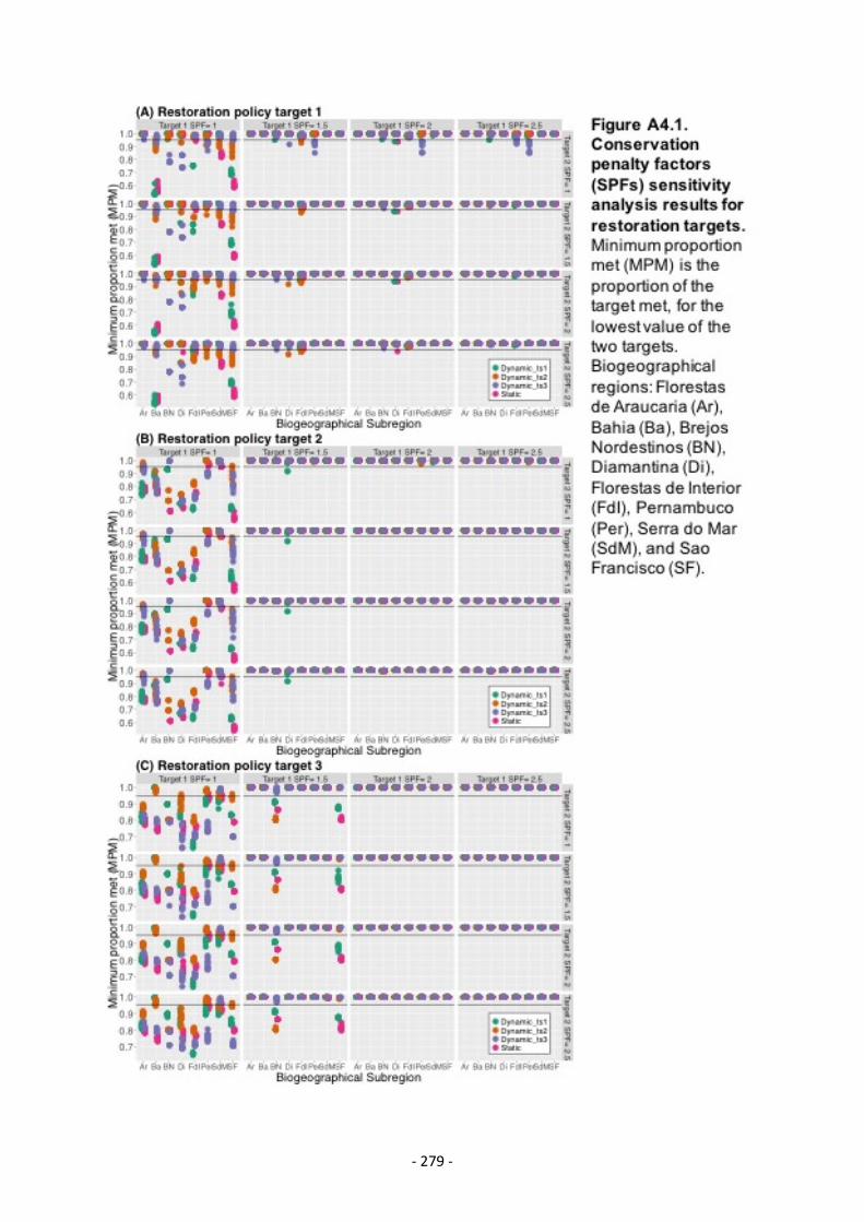
- 279 -

- 280 -

Annex 5: Detailed description of results for chapter 4

2.1 General aggregated solutions (BAF level)The summed forest connectivity benefits are 0.74 ± 0.0004 million hectares (M ha) forthe static solution, and 0.71 ± 0.0007M ha for the dynamic solution (table 4.3). Theseforest connectivity increments are the equivalent of adding one large forest patch of0.74M ha or 0.71M ha under the static or dynamic approach respectively. Thepercentage of each set-aside hectare that directly increases forest connectivity is 27.6±0.0001% for the static solution and 26.4 ±0.0003% for the dynamic solution.Informational rent capture is 963 mill. $ in the static solution and 1,286 mill. $ in thedynamic solution (table 4.3). For each dollar spent, 25% is captured as informationalrents for the static approach, and 36% for the dynamic approach (table 4.3).

Effect of the economic feedbackThe effect of the economic feedback on prioritisation outputs varies withbiogeographical region. For most regions, the cost per hectare for the dynamic solutionis lower than the static solution, percentage differences varying between 1% and 29%(table 4.4, figure 4.4). However, for two regions the cost per hectare for the staticsolution is slightly smaller than for the dynamic solution (Florestas de Araucaria 3.4%,Serra do Mar 0.98%) (table 4.4, figure 4.4).Informational rent capture is higher for the dynamic solution across biogeographicalregions (figure 4.4), with the percentage difference varying from 7% to 81% (table 4.4,figure 4.4). The difference in the percentage of each dollar spent that is captured ininformational rents varies from 11% to 89% (table 4.4, figure 4.4).Set-aside cost-effectiveness for most regions increases when accounting for thefeedback on land rent extraction, the dynamic solution being 1-5% more cost effectivethan the static solution. In Florestas de Interior set-aside cost-effectiveness for thedynamic solution is 40.8% higher than the static solution (table 4.4, figure 4.4). InFlorestas de Araucaria and Serra do Mar, however, set-aside cost-effectiveness is3.3% and 0.97% higher for the static solution, respectively (table 4.4).

Effect of the environmental feedbackThe effect of the environmental feedback on prioritisation outputs varies widely withthe biogeographical region. For most regions, forest connectivity increment is higherfor the static solution (figure 4.4), the difference varying between 1.7% and 28.5%between solutions (table 4.4). Exceptions are Florestas de Interior and Serra do Mar,for which forest connectivity increment for the dynamic solution is higher than the static(table 4.4).Differences in the cost-effectiveness of forest connectivity increment betweensolutions can go both ways, considering results at the biogeographical region level(figure 4.4). In five regions, cost-effectiveness is higher for the static solution, withpercentage differences between 0.3% and 25.2% (table 4.4). In three regions,however, the opposite is observed, with percentage differences under 1%, except inFlorestas de Interior where forest connectivity increment cost-effectiveness is 50%higher for the dynamic solution (table 4.4).

2.2 Solutions across spaceEconomic FeedbackThe economic feedback effectively increases the opportunity cost of land, andaccounting for it when prioritising translates into a small decrease in overall cost of the

- 281 -

dynamic versus the static solution at the biogeographical region of the BAF as a whole.At the municipality level, the difference in cost per hectare between approaches varieswith the region; with Florestas de Araucaria and Serra do Mar presenting the largestvariability in differences (figure 4.4). Spatially, there are more municipalities where theincrease in the opportunity cost of land is larger for the dynamic approach than for thestatic approach, and reaches higher values (figure 4.8a). Informational rent captureper hectare follows a similar spatial pattern to cost per hectare for municipalities wherethere is no difference or which are included only in the static solution.

Environmental FeedbackThe environmental feedback makes increases in forest connectivity larger formunicipalities included in a solution repeatedly over time. Accounting for it in theprioritisation results in a small difference in overall forest connectivity increment at thebiogeographical region, for which the static solution had larger increment than thedynamic solution. At the municipality level, the difference in forest connectivityincrement per hectare between approaches varies with the region; with Florestas deInterior and Serra do Mar presenting the largest variability in differences (figure 2).

2.3 Solutions across timeAggregate solutionsThe annual cost of the static solution is higher than the annual cost of the dynamicsolution at all time steps, both solutions increasing in annual cost with time. The largestincrement in annual cost is between time steps one and two for the static approach,and between time steps two and three for the dynamic approach. Annual set-asidecost-effectiveness also increases with time for both solutions, but the dynamic solutionis more cost effective at all time steps. The largest increase in set-aside cost-effectiveness is between time steps two and three for both solutions (figure 4.6).Both annual forest connectivity increment and its cost-effectiveness have similarbehaviour across time. Initially, the dynamic solution has a higher value for bothvariables, but by time step two the static solution has the highest values. For bothsolutions, both annual forest connectivity increment and its cost-effectivenessincreases with time, and the largest increment takes place between time steps twoand three (figure 4.6).Annual informational rent capture is highest for the dynamic solution at all time steps,and decreases with time for both solutions. The largest reduction in informational rentcapture per year takes place between time steps one and two for both solutions.However, for the static solution, it continues to decrease sharply between time stepstwo and three, whereas for the dynamic solution it remains similar. The proportion ofeach dollar spent that is captured in informational rent per year presents almostopposite behaviour across time for static and dynamic solutions. The dynamic solutionremains similar between time steps one and two, and increases sharply between timesteps two and three. The static solution decreases linearly at each time step (figure4.6).

Effect of the economic feedbackAt the BAF level, the difference in outputs between the static and dynamic solutionpresents different behaviours over time. The percentage difference betweenapproaches in annual informational rent, and in the proportion captured from eachdollar spent increases sharply at each time step, from under 5% to over 1000% (datanot included).

- 282 -

Percentage difference in annual cost increases between time steps one and two, andslightly decreases between two and three. The opposite is observed for percentagedifference in set-aside cost-effectiveness. For both variables, the largest change in thedifference between static and dynamic solution outputs takes place between timesteps one and two (data not included).At the biogeographical region, however, differences in outputs between static anddynamic solutions across time are not homogeneous. Percentage difference in annualcost remains between -10% and 10% across time for most regions. For these regions,the percentage difference in annual cost increases between time steps one and two,and remains similar between time steps two and three for most regions (figure 4.5).One exception is Florestas de Interior, where percentage difference in annual cost isabove 30% at time steps one and two, declining by more than half at time step 3. Thesecond exception is Pernambuco, where percentage difference in annual costincreases from approximately -16% to 21% between time-steps one and two, andsharply decreases to -6% at time step three. A mirrored behaviour is observed forpercentage difference in set-aside cost-effectiveness (figure 4.5).

Effect of environmental feedbackThe percentage difference both in forest connectivity increment and its cost-effectiveness between the static and dynamic solution increases with time at the BAFlevel, with the largest change in the difference happening between time steps one andtwo (data not included). The same behaviour is observed at the biogeographical regionlevel, with Florestas de Interior clearly presenting the largest changes in percentagedifference of forest connectivity (total and per dollar) across time (figure 4.5).

2.4 Municipality characteristics and the effect of feedbacksThe largest significant effect on cost per hectare difference between municipalities isthe biogeographical region. Smaller significant effects of municipality characteristicsare the amount of potential set-aside land, initial forest connectivity and the amount ofvariation within the municipality in the opportunity cost of farmland (SM table 6, model1). The larger the potential set-aside in the municipality, the smaller the value of thedifference in cost per hectare. The same relationship is observed for variation in theopportunity cost of farmland. However, the larger the municipality’s forest connectivity,the larger the value of the difference in cost per hectare. So, for biogeographicalregions with a negative coefficient, such as Florestas de Araucaria and Serra do Mar,the static approach results in lower cost per hectare values, but as variation in theopportunity cost of farmland increases, the dynamic approach becomes a bettersolution. For the remaining regions, larger municipality forest connectivity andpotential set-aside values reduce the cost per hectare benefits of a dynamic approach,whereas larger variation in opportunity cost of farmland increases the benefit (SM table6, model 1).The largest effect on the difference in informational rent capture per hectare is alsothe biogeographical region, however, the only significant factor is Florestas de Interior.Municipality characteristics that have a significant effect are the amount of potentialset-aside, forest connectivity and variation in the opportunity cost of farmland (SMtable 6, model 2). Larger municipality forest connectivity and potential set-aside valuesreduce the difference in informational rent capture per hectare, whereas largervariation in opportunity cost of farmland increases it (SM table 6, model 2).The largest significant effect on forest connectivity increment per hectare difference isthe biogeographical region, however, Florestas the Interior and Serra do Mar are non-

- 283 -

significant levels. Smaller significant effects of municipality characteristics are ofpotential set-aside, and variation in opportunity cost of farmland (SM table 6, model3). For all regions, the larger the municipality’s variation in opportunity cost of farmlandand potential set-aside, the smaller the value of the difference in forest connectivityincrement per hectare, and the smaller the benefit of a dynamic approach (SM table6, model 3).The largest effects on set-aside cost-effectiveness difference come from thebiogeographical region, but only half of the levels have a significant effect: BrejosNordestinos, Diamantina, Pernambuco and Sao Francisco (SM table 6, model 4).Potential set-aside, forest connectivity and variation in the opportunity cost of farmlandall have significant, though small, effects on set-aside cost-effectiveness difference. InFlorestas de Araucaria and Interior, and Serra do mar, the larger the municipality’sforest connectivity, the larger the value of the difference in set-aside cost-effectiveness, and the larger the benefit of a dynamic approach. However, for theremaining regions, the difference first gets to zero and only after that there are benefitsof a dynamic approach. In all biogeographical subregions the larger the municipality’svariation in the opportunity cost of farmland and potential set-aside, the smaller thevalue of the difference in forest connectivity increment per hectare, and the larger thebenefit of a static approach (SM table 6, model 4).The largest significant effect on the difference in the proportional capture ofinformational rent is the biogeographical region, however, Florestas the Interior andSerra do Mar have non-significant effects. Smaller significant effects of municipalitycharacteristics are of potential set-aside, and variation in opportunity cost of farmland(SM table 6, model 5). The larger the municipality’s potential set-aside and variationin the opportunity cost of farmland, the smaller the value of the difference in theproportional capture of informational rent. The larger the municipality’s forestconnectivity, the larger the value of the difference in the proportional capture ofinformational rent (SM table 6, model 5).Significant effects on forest connectivity cost-effectiveness include municipality’svariation in the opportunity cost of farmland, and some levels of the biogeographicalregions factor (Florestas de Interior, Brejos Nordestinos, Diamantina and SaoFrancisco). Municipality’s potential set-aside is non-significant but its removal did notresult in a better model as measured by AIC (p= 0.1009). For all regions, the largerthe municipality’s variation in opportunity cost of farmland and potential set-aside, thesmaller the value of the difference in forest connectivity increment per hectare, andthe smaller the benefit of a dynamic approach (SM table 6, model 6).