reducing unintended bias of ml models on tabular and

HAL Id: hal-03312797https://hal.archives-ouvertes.fr/hal-03312797v2

Submitted on 6 Sep 2021

HAL is a multi-disciplinary open accessarchive for the deposit and dissemination of sci-entific research documents, whether they are pub-lished or not. The documents may come fromteaching and research institutions in France orabroad, or from public or private research centers.

L’archive ouverte pluridisciplinaire HAL, estdestinée au dépôt et à la diffusion de documentsscientifiques de niveau recherche, publiés ou non,émanant des établissements d’enseignement et derecherche français ou étrangers, des laboratoirespublics ou privés.

Reducing Unintended Bias of ML Models on Tabularand Textual Data

Guilherme Alves, Maxime Amblard, Fabien Bernier, Miguel Couceiro,Amedeo Napoli

To cite this version:Guilherme Alves, Maxime Amblard, Fabien Bernier, Miguel Couceiro, Amedeo Napoli. ReducingUnintended Bias of ML Models on Tabular and Textual Data. DSAA 2021 - 8th IEEE InternationalConference on Data Science and Advanced Analytics, Oct 2021, Porto (virtual event), Portugal. pp.1-10. hal-03312797v2

https://hal.archives-ouvertes.fr/hal-03312797v2

https://hal.archives-ouvertes.fr

Reducing Unintended Bias of ML Models onTabular and Textual Data

Guilherme Alves, Maxime Amblard, Fabien Bernier, Miguel Couceiro and Amedeo NapoliUniversite de Lorraine, CNRS, Inria Nancy G.E., LORIA

Vandoeuvre-les-Nancy, Franceguilherme.alves-da-silva, maxime.amblard, fabien.bernier, miguel.couceiro, [email protected]

Abstract—Unintended biases in machine learning (ML) modelsare among the major concerns that must be addressed tomaintain public trust in ML. In this paper, we address processfairness of ML models that consists in reducing the dependenceof models on sensitive features, without compromising theirperformance. We revisit the framework FIXOUT that is inspiredin the approach “fairness through unawareness” to build fairermodels. We introduce several improvements such as automatingthe choice of FIXOUT’s parameters. Also, FIXOUT was originallyproposed to improve fairness of ML models on tabular data.We also demonstrate the feasibility of FIXOUT’s workflow formodels on textual data. We present several experimental resultsthat illustrate the fact that FIXOUT improves process fairnesson different classification settings.

Index Terms—Bias in machine learning, fair classificationmodel, feature importance, feature dropout, ensemble classifier,post-hoc explanations.

I. INTRODUCTION

The pervasiveness of machine learning (ML) models indaily life has raised several issues. One is the need forpublic trust in algorithmic outcomes. In 2016, the EuropeanUnion (EU) enforced the General Data Protection Regulation(GDPR)1 that gives users the right to understand the innerworkings of ML models and to obtain explanations of theiroutcomes, which can increase public trust in ML outcomes.

These explanations can also reveal biases of algorithmicdecisions. ML models are designed to have some bias thatguide them in their target tasks. For instance, a model forcredit card default prediction is intended to be biased so thatusers who have a good credit payment history get a higherscore than those who have not. Similarly, a model for hatespeech detection is intended to be biased such that messagesthat contain offensive terms get higher scores than those whichhave not. However, the model’s outcomes should not rely onsalient nor discriminatory features that carry prejudice towardsunprivileged groups [1]. For instance, the model that predictscredit card defaults should not give lower scores to usersbecause they belong to a particular ethnicity compared to thosewho do not. In the same way, the model to detect hate speechshould not give higher scores to messages that are written ina particular language variant compared to those messages thatare not. These are known as unintended biases [2].

Unintended bias leads to various consequences. If it nega-tively impacts society, in particular against minorities, then it

1https://gdpr-info.eu/

characterizes an unfairness issue [2], [3]. Researchers foundunintended bias and fairness issues in a wide range of do-mains and data types. For instance, it was found racial biasin the system that predicts criminal recidivism, COMPAS2.Gender and ethnic discriminations were also detected in onlineplatforms for job applications [4]. Bias based on languagevariants was found on approaches that detect abusive language,in which messages written in African-American English gothigher toxicity scores than messages in Standard-AmericanEnglish [5].

In order to address algorithmic fairness, various notionsof fairness have been defined based on models’ outcomes[6]. One relies on the fairness metrics based on standardclassification metrics computed on different sub-populations.Another notion is process fairness which, instead of focusingon the final outcomes, is centred on the process that leadsto the outcomes (classifications) [1]. One way to achieve thelatter is to seek fairness through unawareness, i.e., to avoid theuse of any sensitive features when classifying instances [7].However, dropping out sensitive features may compromiseclassification performance [8].

Recently, two frameworks have been proposed to addressalgorithmic unfairness of ML models on tabular data withoutcompromising its classification performance. LIMEOUT [9]and FIXOUT [10] render pre-trained models fairer by decreas-ing their dependence on sensitive features. For that, users mustinput their pre-trained models together with the features theyconsider sensitive. LIMEOUT and FIXOUT then use expla-nation methods to assess fairness of the pre-trained models.In the case a pre-trained model is deemed unfair, FIXOUTapplies a feature dropout followed by an ensemble approach tobuild a model that is fairer compared to the pre-trained model.Both LIMEOUT and FIXOUT use model-agnostic explanationmethods to assess fairness. However, LIMEOUT only relies onLIME explanations [11] where as FIXOUT is able to apply anyexplanation method based on feature importance. In addition,they require beforehand users to define the sampling size ofinstances and the number of features used to assess fairnessof pre-trained models, which raises the need for automationor, at least, fine-tuning.

These frameworks were initially proposed to address algo-

2https://www.propublica.org/article/machine-bias-risk-assessments-in-\criminal-sentencing

rithmic unfairness on tabular data. The empirical studies haveshown that both frameworks improve process fairness withoutcompromising accuracy. However, fairness issues have alsobeen found in textual data. For instance, Papakyriakopouloset al. [12] trained word embeddings on texts from Wikipediaarticles and from political social media (tweets and Facebookcomments) that are written in gendered languages3. They theninvestigated the diffusion of bias when these embeddings areused in ML models. In addition, they proposed approachesto reduce bias in embeddings based on gender, ethnicityand sexual orientation. In spite of eliminating bias in wordembeddings, the authors state that it might include other typesof bias.

In this paper, we take advantage of the existing approachesthat address algorithmic unfairness through unawareness, andextend them to other settings, namely classification scenariosdealing with textual data. Our main hypothesis is that FIXOUTis able to improve process fairness not only in tabular databut also in textual data. It is addressed by investigating tworesearch questions:Q1. How to reduce human intervention in FIXOUT usage on

tabular data?Q2. Does FIXOUT reduce model’s dependence on sensitive

words on textual data?The main contributions of the work described herein can

be summarized as follows: (1) an approach that automaticallyselects the number of features used by FIXOUT to assessfairness, and (2) an instantiation of FIXOUT that is able toimprove process fairness on textual data.

This paper is organized as follows. We first recall relatedwork about fairness and explanations in Section II. We thendescribe FIXOUT, our automation of FIXOUT on tabular dataand the instantiation of FIXOUT to textual data in Sections III,IV, and V, respectively. The experimental setup and results aredriven by questions Q1 and Q2 and discussed in Section VI.We conclude this paper in Section VII together with the futureworks.

II. RELATED WORK

In this section, we introduce the main concepts underlyingthis work. We start by recalling the basics of fairness notionsin Section II-A. We then briefly present the fundamentals ofsome explanation methods in Section II-B.

A. Assessing Fairness in ML Models

Several approaches have been proposed to assess fairnessin ML models; most of them focused on the algorithmicoutcomes [3]. They can be divided into two main familiesof fairness notions [6], as we briefly outline next.• Group fairness considers that groups differing by sensi-

tive features (and ignoring all non-sensitive features) mustbe treated equally [6]. For instance, demographic parity

3The grammar of gendered languages require that speakers mark gender insome parts of speech, for instance in nouns and/or adjectives (e.g. Germanand French).

[3], disparate mistreatment [13], and predictive equality[6] are metrics that belong to this family of fairnessnotions.

• Individual fairness states that similar individuals (non-sensitive features included) should obtain similar prob-abilities of getting similar outcomes [14]. For instance,counterfactual fairness metrics [15] belong to this familyof fairness notions.

In this work, we focus on another type of approach to assessfairness, which is called process fairness [1], [9]. Processfairness is centered on the process itself rather that focusingon the final outcome. The idea is to monitor input featuresused by ML models for ensuring that these ML models donot use sensitive features while making classifications.

B. Explanation Methods

Explanation methods can be divided into two main groups:(1) those that provide local explanations and (2) those thatcompute global explanations [16]. Local explanation methodsgenerate explanations for individual predictions, while globalexplanations give an understanding of the global behaviour ofthe model.

The first group can be divided w.r.t. the type of explanations:methods based on feature importance [11], [17], saliency maps[18], and counterfactual methods [15]. In the same way, globalexplanation methods can be divided into methods based on acollection of local explanations [11], and representation basedexplanations [19]. In this work, we are interested in modelagnostic explanation methods and thus we focus on LIMEand SHAP.

LIME and SHAP provide explanations that are obtainedafter approximating feature values and predictions. Moreover,LIME and SHAP are model-agnostic, which means that bothcan explain any prediction model (classifier).

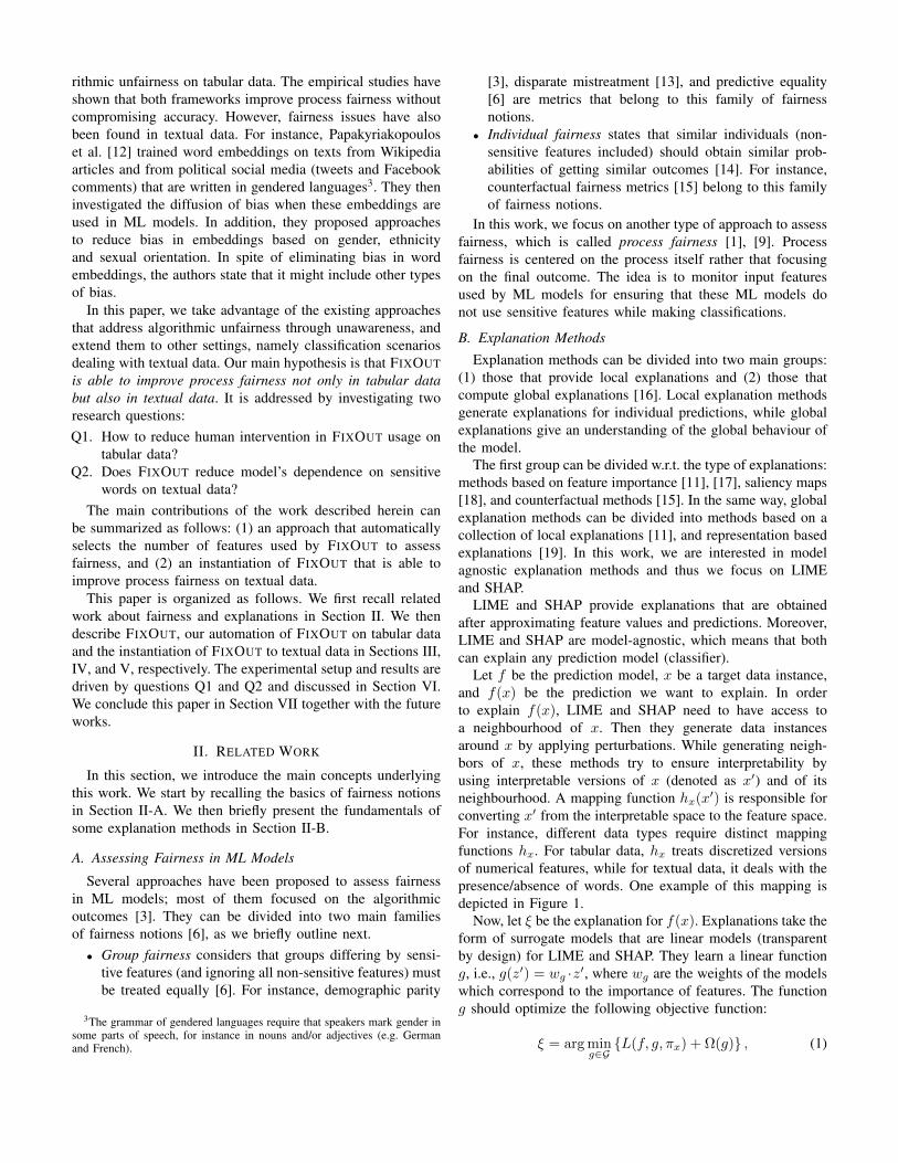
Let f be the prediction model, x be a target data instance,and f(x) be the prediction we want to explain. In orderto explain f(x), LIME and SHAP need to have access toa neighbourhood of x. Then they generate data instancesaround x by applying perturbations. While generating neigh-bors of x, these methods try to ensure interpretability byusing interpretable versions of x (denoted as x′) and of itsneighbourhood. A mapping function hx(x′) is responsible forconverting x′ from the interpretable space to the feature space.For instance, different data types require distinct mappingfunctions hx. For tabular data, hx treats discretized versionsof numerical features, while for textual data, it deals with thepresence/absence of words. One example of this mapping isdepicted in Figure 1.

Now, let ξ be the explanation for f(x). Explanations take theform of surrogate models that are linear models (transparentby design) for LIME and SHAP. They learn a linear functiong, i.e., g(z′) = wg ·z′, where wg are the weights of the modelswhich correspond to the importance of features. The functiong should optimize the following objective function:

ξ = arg ming∈GL(f, g, πx) + Ω(g) , (1)

Ω measures the complexity in order to insure interpretability ofthe linear model given by the explainer. L is the loss functiondefined by:

L(f, g, πx) =∑

z,z′∈Z[f(z)− g(z′)]2πx(z), (2)

where z is the interpretable representation of x, and πx(z)defines the neighborhood of x that is considered to explainf(x).

In spite of sharing some commonalities, LIME and SHAPdiffers in the definition of the kernel πx and also in thecomplexity function Ω used to produce explanations. In thefollowing we recall each method and highlight their differ-ences.

1) LIME: Local Interpretable Model Agostic Explanationsis a model-agnostic explanation method providing local expla-nations [11], [20]. Explanations obtained from LIME take theform of surrogate linear models. LIME learns a linear modelby approximating the prediction and feature values in order tomimic the behavior of ML model. To do so, LIME uses thefollowing RBF kernel πx to define the neighborhood of x andconsidered to explain f(x):

πx(z) = exp(−δ(x, z)2/σ2),

where δ is a distance function between x and z, and σ is thekernel-width. LIME tries to minimize Ω(g) for reducing thenumber of non-zero coefficients in the linear model. and Kis the hyper parameter that limit the desired complexity ofexplanations.

2) SHAP: SHapley Additive exPlanations is also an expla-nation method that provides local explanations. SHAP is basedon coalitional game theory. It uses the notion of coalition offeatures to estimate the contribution of each feature to the pre-diction f(x). Coalition of features defines the representationspace for SHAP and it indicates which features are presentin x (see Figure 1). Lundberg et al. [17] proposed a model-agnostic version of SHAP called KernelSHAP. Like LIME,KernelSHAP also minimizes the loss function described inEq. 2, but it uses a different kernel and, unlike LIME, Ker-nelSHAP sets Ω(g) = 0 for the complexity of explanations.

Let |z| be the number of present features in the coalition z,M be the maximum coalition size, and m be the number ofcoalitions. The kernel function πx(z) used by KernelSHAP isthe following:

πx(z) =M − 1(

M|z|)|z|(M − |z|)

.

Both LIME and SHAP only provide explanations for indi-vidual (local) predictions. However, in order to detect unin-tended bias, a global understanding of the inner workings ofthe ML model is needed. In the following subsection we recalla simple strategy to obtain global explanations from individualexplanations.

Fig. 1. An example of a mapping function hx that converts coalitions tovalid instances (i.e., instances in the feature space).

3) From Local to Global Explanations: Local explanationmethods have been used to explain individual predictions.However, they only provide local explanations which alonecannot provide a global understanding of ML models. Toovercome this issue, Ribeiro et al. [11] proposed the so-called Submodular-pick (SP) for selecting a subset of localexplanations that helps in interpreting the global behavior ofany ML model. SP was originally proposed to work alongwith LIME explanations and it is called SP-LIME. The mainidea on which relies SP-LIME is to sample a set of instanceswhose explanations are not redundant and that has a “highcovering” in the following sense.

Denote by B the desired number of explanations used toexplain f globally, and let V be a set of selected instances, Ian array of feature importance, and W an explanation matrix–columns represent features and rows represent instances– thatcontains the importance (contribution) of d′ features to eachinstance. SP-LIME picks instances that are explaining thanksto:

Pick(W, I) = arg maxV,|V |<B

d′∑j=1

1[i∈V :Wij>0]Ij .

III. FIXOUT

In this section, we revisit the human-centered frameworkFIXOUT that tackles process fairness [10]. FIXOUT is model-agnostic and explainer-agnostic such that it can be applied ontop of any ML model, and in addition it is also able to useany explanation method based on feature importance.

FIXOUT takes as input a quadruple (M,D,S,E) of a pre-trained model M , a dataset D used to train M , a set ofsensitive features S, and an explanation method E. It is basedon two main components which are made precise below.

The first component is in charge of assessing fairness ofM . More precisely, explainer E builds the list L of featuresthat contribute the most to the classifications of M (functionGLOBALEXPLANATIONS in the Algorithm 1). Here, usersmust indicate a value for the parameter k that limits the sizeof this list. FIXOUT then applies the following rule: if at leastone sensitive feature returned by E appears in L, M is deemedunfair. Otherwise, M is deemed fair and no action is taken.

The second component is applied only if M is deemedunfair. The goal of this component is to use feature dropouttogether with an ensemble approach to build an ensembleclassifier Mfinal which is less dependent on sensitive features–or fairer– than M (see Algorithm 1).

Let S′ ⊆ S be the subset of sensitive features appearing inL. FIXOUT uses feature dropout to train |S′| + 1 classifiersin the following way: |S′| classifiers are defined by removingeach of the sensitive features in S′, and an additional classifieris defined by removing all sensitive features in S′.

Now, let x be an instance, C a class value, and Mt the t-thclassifier in the pool of classifiers. FIXOUT uses models thatmake classifications in the form of probabilities P (x ∈ C).Once all classifiers are trained, they are then combined thanksto an aggregation function. LIMEOUT uses only a simpleaverage while FIXOUT is able to employ either a simple orweighted average function.

The aggregation function is responsible for producing thefinal classification. The final probability of x to belong to theclass C is based on the probabilities P (x ∈ C) obtained fromthe pool of classifiers and it is defined as the simple average:

PMfinal(x ∈ C) =

1

|S′|+ 1

|S′|+1∑t=1

PMt(x ∈ C), (3)

where PMt(x ∈ C) is the probability predicted by model Mt.

Algorithm 1: FIXOUT

Data: M : pre-trained model; D: dataset; S: sensitivefeatures; E: explainer; k: number of featuresconsidered.

Result: Mfinal an ensemble model.1 L← GLOBALEXPLANATIONS(E,M,D, k)2 S′ ← st | st ∈ S ∧ st ∈ L3 if |S′| > 0 then4 Mfinal ← TRAIN(Mt, D − st) | st ∈ S′5 Mfinal ←Mfinal ∪ TRAIN(Mt+1, D − S′)6 return Mfinal

IV. AUTOMATING THE CHOICE OF k

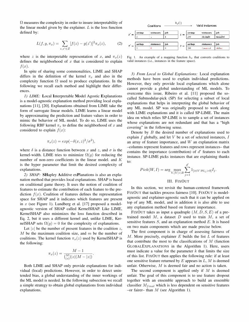
In order to assess fairness of ML models, FIXOUT onlytakes into account the first k most important features. Thus,FIXOUT practitioners must know beforehand a suitable valuefor k so that FIXOUT builds L with the k most importantfeatures. The system then looks at whether sensitive features

TABLE IAN EXAMPLE OF GLOBAL EXPLANATIONS FOR RANDOM FOREST ON THE

GERMAN DATASET.

Original (SHAP)Feature Contrib.statussex -10.758909property 10.676458credithistory 10.264842residencesince 8.108638employmentsince 6.818476existingchecking 6.308758housing -5.649528installmentrate 5.125154duration 4.838629telephone 3.981387

FIXOUT using SHAPFeature Contrib.credithistory 13.246923employmentsince 9.550589property 8.958718residencesince 7.264848installmentrate 5.893469housing -3.829469statussex -3.313667duration 2.678797existingcredits 2.412488telephone 2.269493

are in L. An inappropriate value for k prevents FIXOUT ofcorrectly detecting unfairness issues as all sensitive featuresmay not appear in L.

In this section, we propose an algorithm that automatesthe choice of k, based on the statistical measure kurtosis.Indeed kurtosis indicates the flatness of a distribution. LetX = (xi)i∈N be a random variable, the kurtosis γ of X isdefined as follows:

γ(X) =1

n

∑xi

(xi − µσ

)4

,

where σ is the standard deviation, µ is the mean, xi is a sampleof X . For instance, γ(X) < 3 indicates that X is platykurtic(flattened), while γ(X) = 3 defines a mesokurtic distribution(which is the case of normal distribution), and γ(X) > 3indicates that the distribution is leptokurtic (pointed) [21],[22].

Accordingly we propose the iterative algorithm calledFIND-K (see Algorithm 2), that selects a sub-sample offeatures of L based on the kurtosis measure. FIND-K removesfeatures from L by analyzing the kurtosis γ(L) of L beforeand after the deletion of a subset of features. For that, ititeratively removes features from the less important to the mostimportant. The idea on which relies this algorithm is that oncea feature is removed, the kurtosis of L changes. The algorithmstops when |γ(L) − γ(L′)| > α, where L is the original list,L′ is the list obtained after removing features, and α > 0 is aparameter.

Algorithm 2: FIND-KData: L: sorted list of contributions of all features

(descending order); α: a threshold.Result: L′ a new list of contributions of subset of

features.1 L′ ← L2 for i← |L| to 2 do3 L′ ← L′ − L′[i]4 if |γ(L)− γ(L′)| > α then5 break6 end

V. FIXOUT ON TEXTUAL DATA

In this section we demonstrate the adaptability of theFIXOUT framework to another data type, namely textual data.In this setting, a data instance corresponds to a text andfeatures to words, i.e., the number of features is equal to thevocabulary size. To drop a feature, we remove each occurrenceof the corresponding word in the text. Here words that aresemantically equivalent are not taken into account.

Let M be a classifier for which we want to reduce theimpact of words from a given set S, in the classifier’soutcomes:

S = si | 1 6 i 6 n.

As in tabular data, FIXOUT decreases the contribution of thewords in S to the classifiers outcomes by applying featuredropout and by building an ensemble of the n+ 1 classifiers:• one classifier Mi, for 1 6 i 6 n, trained by ignoring the

word si, and• a classifier M[n+1] trained by ignoring all words in S.However, when n is large, this method becomes inefficient,

for two reasons. The first one is that if we consider a sensitiveword si ∈ S, only two classifiers are ignoring it: Mi andM[n+1], i.e., n− 1 out of the n+ 1 classifiers are taking thefeature si into account. Hence, the dropout of si may thenbecome less significant when n is large. The second reasonis a complexity concern: the more models there are, the morememory and computation time the ensemble takes.

Table II shows satisfactory results for a random forestmodel, which classifies a text as hate speech or not (fromthe hatespeech database, which is described later). We selectn = 3 words for which we want to reduce the contribution.The list of words used here was inspired by the analysisperformed in [5]. We train a new model and globally explainit 50 times (with Random Sampling), in order to retrieve anaverage contribution. We can check that the rank of importanceand contribution of each dropped feature decreases thanks tothe FIXOUT ensemble. We evaluate the gain by calculatingthe difference between the rank obtained and the starting rank,normalised by the smaller of the two. Gaining a few ranks onthe highest features in the ranking allows us to have significantscores, whereas they will be close to 0 for ranks that arevery far away. However, when n increases and more than 3words are added, the method seems to become less effective,as shown in Table III (without grouping), which describes therank and contribution of each one of the selected words whoseimportance should be reduced.

Let us turn our attention to the interest of grouping words.Instead of ignoring a single word or feature, the classifier candrop many words at the same time, then reducing the size ofthe ensemble. We proceeded in this way and the performanceof FIXOUT was improved as it can be observed in Table III.

TABLE IIPROCESS FAIRNESS ASSESSMENT ON A HATE SPEECH CLASSIFIER

(RANDOM FOREST), GLOBAL EXPLANATION WITH SHAP RS, SELECTING3 WORDS

Original model FIXOUT Ensemble DiffWord Rank Contrib. Rank Contrib. Rankniggah 14 0.176 30 0.043 1.14nigger 12 0.213 29 0.045 1.41

nig 7 0.276 55 0.021 6.85

VI. EXPERIMENTAL RESULTS AND DISCUSSION

The main goal of the experiments is to demonstrate theadaptability of FIXOUT on different data types. This sectionis thus divided in two main parts, the first one focusing ontabular data and the second one on textual data. We startby describing the tabular datasets (§ V). We then discussthe empirical results related to the selection of instances for

TABLE IIIPROCESS FAIRNESS ASSESSMENT ON A HATE SPEECH CLASSIFIER

(RANDOM FOREST), GLOBAL EXPLANATION WITH SHAP RS, SELECTING7 WORDS

Without grouping With grouping DiffWord Rank Contrib. Rank Contrib. Rankniggah 18 0.149 23 0.03 0.27nigger 15 0.164 21 0.031 0.40nigguh 22 0.13 83 0.008 2.77

nig 12 0.202 65 0.011 4.41nicca 22 0.107 39 0.018 0.77nigga 20 0.125 12 0.067 -0.66white 25 0.087 36 0.018 0.44

assessing fairness (§ VI-B), and the automation of the choiceof k (§ VI-C). We end up this section by describing the textualdataset (§ VI-D) and by discussing the results obtained fromthe experiments performed on this data type (§ VI-E).

A. Tabular Datasets

The experiments on tabular data were performed on 3 real-world datasets, which contain sensitive features and are brieflyoutlined below.

German. This dataset contains 1000 instances and it isavailable in the UCI repository4. For this dataset, the goalis to predict if the credit risk of a person is good or bad. Eachapplicant is described by 20 features in total out of which 3features, namely “statussex”, “telephone”, “foreign worker”,are considered as sensitive.

Adult. This dataset is also available in the UCI repository5.The task is to predict whether the salary of a American citizenexceeds 50 thousand dollars per year based on census data.It contains more than 32000 instances. Each data instance isdescribed by 14 features out of which 3 features are consideredas sensitive, namely “MaritalStatus”, “Race”, “Sex”.

LSAC. This dataset contains information about 26551 lawstudents6. The task is to classify whether law students passthe bar exam based on information from the study of the LawSchool Admission Council that was collected between 1991and 1997. Each student is characterized by 11 features out ofwhich 3 features, namely “race”, “sex”, “family income”, areconsidered as sensitive.

We split each dataset into 70% for the training set and30% for testing. We then applied the Synthetic MinorityOversampling Technique (SMOTE7) over training data as classlabels are highly imbalanced. In particular, SMOTE generatessamples to balance the class label distribution in order toovercome the imbalanced distribution problem.

B. Tabular data: Selection of instances to assess fairness

We experimented different relative sizes for sampling in-stances. The idea is to verify whether at least one sensitive

4https://archive.ics.uci.edu/ml/datasets/statlog+(german+credit+data5http://archive.ics.uci.edu/ml/datasets/Adult6http://www.seaphe.org/databases.php7https://machinelearningmastery.com/threshold-moving-for-imbalanced\\-classification/

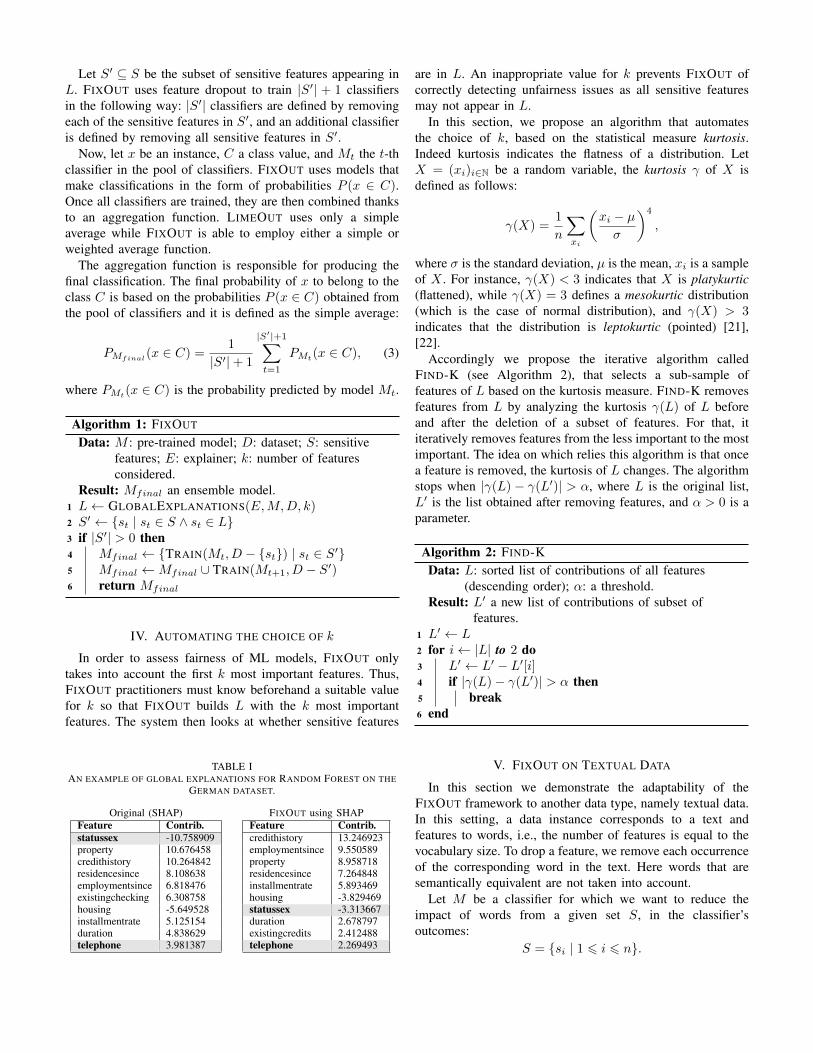
feature appears in the list of the top-10 most important fea-tures. For that, we used the following the relative sizes: 0.1%,0.5%, 1%, 5%, and 10%. The results obtained throughout theperformance of the same experiment 50 times are shown inTable IV.

For the German dataset, we did not evaluate models using0.1% of the instances, as it takes only one instance. On theother hand, for the Adult dataset, the amount of data instancesfrom sampling 10% of instances is large and unfeasible toproduce many explanations (more than 3K) in time. We thusadd an hyphen in Table IV to indicate these particular cases.

TABLE IVNUMBER OF TIMES PRE-TRAINED MODELS ARE DEEMED UNFAIR.EXPERIMENTS WERE PERFORMED BY VARYING THE NUMBER OFINSTANCES SELECTED TO OBTAIN GLOBAL EXPLANATIONS, THE

SAMPLING STRATEGY, AND THE EXPLANATION METHOD.

Dataset Selection Sample size0.1% 0.5% 1% 5% 10%

German

LIME+RS - 38 38 47 50LIME+SP - 47 47 50 50SHAP+RS - 50 50 50 50SHAP+SP - 50 50 50 50

Adult

LIME+RS 46 48 49 45 -LIME+SP 49 49 49 49 -SHAP+RS 49 47 46 47 -SHAP+SP 47 50 49 49 -

LSAC

LIME+RS 50 50 50 50 50LIME+SP 50 50 50 50 50SHAP+RS 50 50 50 50 50SHAP+SP 50 50 50 50 50

To illustrate the impact of the sample size and the samplingmethod in the assessment of fairness, we observed the rankof sensitive features in the list of 10 most important featuresobtained by each of the explainers. These results are presentedin Tables V, VI, and VII for the datasets German, Adult, andLSAC, respectively.

We considered the following classifiers, namely LogisticRegression (LR), Bagging (BAG), AdaBoost (ADA), andRandom Forest (RF), to perform the experiments. We used theimplementation available on Scikit-learn [23] with the defaultparameters. Based on these results we thus set the size as5% for the German dataset (50 instances), 0.5% for the Adultdataset (162 instances), and 0.1% for the LSAC dataset (93instances). These results seem to indicate that LIME is morestable than SHAP independently of the sampling method andsample size.

C. Tabular data: Automating the choice of k

We evaluate the algorithm FIND-K that was conceived toautomatically selects the list of features which is taken intoaccount by FIXOUT for assessing fairness. FIND-K requiresa positive value for the parameter α. Here, we performedexperiments by varying the value of α from 0.5 to 3. In theseexperiments we analyze the impact of this parameter on theoutput of FIND-K. In particular, we are interested in the effectsof different values of α w.r.t. the size of L (i.e., the numberof features kept by FIND-K) and record the number of times

a model is deemed unfair. We discarded values of α < 0.5otherwise FIND-K considers all features as important.

High values of α lead to a smaller size of L, i.e., too manyfeatures are removed by FIND-K. It is harder to find onesensitive feature in a very short list of important features thanin a longer list. As a consequence, high values of α also lead toa low number of times in which a model is deemed unfair. Wecan observe this behavior on Tables VIII and IX. These tablescontain the number of times that the models were deemedunfair throughout 50 repetitions of the same experiment.

A similar behavior can be observed w.r.t. the average valueof k. High values of α lead to low values of k (on average). Wenotice this behavior in Tables VIII and IX. These tables containthe average value of k found by FIND-K. We highlighted theexperiments where the average number of sensitive featuresfound in the list obtained by FIXOUT was greater than orequal to 1. Again, FIXOUT looks for at least one sensitivefeature in the list of the most important features. Then, anaverage smaller than 1 indicates that in most experiments themodels were deemed fair. We also notice that the highlightedvalues are those in which the average value of k are high (seeTables VIII and IX).

We can observe that FIND-K discovers on average the samevalue of k for each dataset. For instance, for the Germandataset, an average k around 10 was found by FIND-K withα = 0.5, and incidentally the same value was used in previousempirical studies [9], [10]. For the LSAC dataset, an averagek around 8 was found using FIND-K with α = 0.5, while anaverage k around 6 was returned by FIND-K using α = 1.

To sum up the analysis of FIND-K, we can also observethat low values of α provide suitable configurations for usersthat do not have any clue of the useful values of k. Moreprecisely, using 0.5 ≤ α ≤ 1 allows FIND-K to automaticallyfind a suitable value of k. In addition, since LIME and SHAPhave stability issues [24] that lead to different lists of featureimportance (for a single type of classifier trained on the samedataset), it may be interesting to considering the threshold αto learn the parameter k. Indeed, one single value of α allowsFIND-K to find a suitable value of k from distinct lists offeature importance. This provides an answer to question Q1introduced at the beginning of this paper.

D. Textual datasets

We also experimented FIXOUT with simple textual clas-sifiers. In particular, we implemented a model used in anexperiment carried out by Davidson et al. [5], whose goalis to classify tweets as hate speech or not. We focus on thehate speech dataset [25], which more precisely labels a tweetas offensive, hate speech, or neither. To stay within a two-classes problem, we merge offensive language and hate speechclasses, to finally deal with two classes, namely non-offensiveor offensive.

However, the resulting dataset appears to be quite un-balanced, including 4163 non-offensive instances and 20620offensive ones. Thus we randomly select only 4163 instancesfrom the offensive group. Moreover, we follow the same

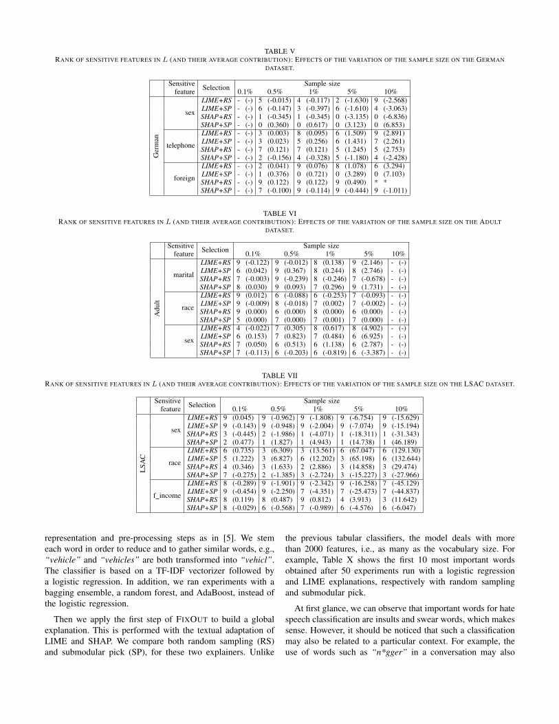
TABLE VRANK OF SENSITIVE FEATURES IN L (AND THEIR AVERAGE CONTRIBUTION): EFFECTS OF THE VARIATION OF THE SAMPLE SIZE ON THE GERMAN

DATASET.

Sensitive Selection Sample sizefeature 0.1% 0.5% 1% 5% 10%

Ger

man

sex

LIME+RS - (-) 5 (-0.015) 4 (-0.117) 2 (-1.630) 9 (-2.568)LIME+SP - (-) 6 (-0.147) 3 (-0.397) 6 (-1.610) 4 (-3.063)SHAP+RS - (-) 1 (-0.345) 1 (-0.345) 0 (-3.135) 0 (-6.836)SHAP+SP - (-) 0 (0.360) 0 (0.617) 0 (3.123) 0 (6.853)

telephone

LIME+RS - (-) 3 (0.003) 8 (0.095) 6 (1.509) 9 (2.891)LIME+SP - (-) 3 (0.023) 5 (0.256) 6 (1.431) 7 (2.261)SHAP+RS - (-) 7 (0.121) 7 (0.121) 5 (1.245) 5 (2.753)SHAP+SP - (-) 2 (-0.156) 4 (-0.328) 5 (-1.180) 4 (-2.428)

foreign

LIME+RS - (-) 2 (0.041) 9 (0.076) 8 (1.078) 6 (3.294)LIME+SP - (-) 1 (0.376) 0 (0.721) 0 (3.289) 0 (7.103)SHAP+RS - (-) 9 (0.122) 9 (0.122) 9 (0.490) * *SHAP+SP - (-) 7 (-0.100) 9 (-0.114) 9 (-0.444) 9 (-1.011)

TABLE VIRANK OF SENSITIVE FEATURES IN L (AND THEIR AVERAGE CONTRIBUTION): EFFECTS OF THE VARIATION OF THE SAMPLE SIZE ON THE ADULT

DATASET.


Adu

lt

marital

LIME+RS 9 (-0.122) 9 (-0.012) 8 (0.138) 9 (2.146) - (-)LIME+SP 6 (0.042) 9 (0.367) 8 (0.244) 8 (2.746) - (-)SHAP+RS 7 (-0.003) 9 (-0.239) 8 (-0.246) 7 (-0.678) - (-)SHAP+SP 8 (0.030) 9 (0.093) 7 (0.296) 9 (1.731) - (-)

race

LIME+RS 9 (0.012) 6 (-0.088) 6 (-0.253) 7 (-0.093) - (-)LIME+SP 9 (-0.009) 8 (-0.018) 7 (0.002) 7 (-0.002) - (-)SHAP+RS 9 (0.000) 6 (0.000) 8 (0.000) 6 (0.000) - (-)SHAP+SP 5 (0.000) 7 (0.000) 7 (0.001) 7 (0.000) - (-)

sex

LIME+RS 4 (-0.022) 7 (0.305) 8 (0.617) 8 (4.902) - (-)LIME+SP 6 (0.153) 7 (0.823) 7 (0.484) 6 (6.925) - (-)SHAP+RS 7 (0.050) 6 (0.513) 6 (1.138) 6 (2.787) - (-)SHAP+SP 7 (-0.113) 6 (-0.203) 6 (-0.819) 6 (-3.387) - (-)

TABLE VIIRANK OF SENSITIVE FEATURES IN L (AND THEIR AVERAGE CONTRIBUTION): EFFECTS OF THE VARIATION OF THE SAMPLE SIZE ON THE LSAC DATASET.


LSA

C

LIME+RS 9 (0.045) 9 (-0.962) 9 (-1.808) 9 (-6.754) 9 (-15.629)LIME+SP 9 (-0.143) 9 (-0.948) 9 (-2.004) 9 (-7.074) 9 (-15.194)SHAP+RS 3 (-0.445) 2 (-1.986) 1 (-4.071) 1 (-18.311) 1 (-31.343)sex

SHAP+SP 2 (0.477) 1 (1.827) 1 (4.943) 1 (14.738) 1 (46.189)LIME+RS 6 (0.735) 3 (6.309) 3 (13.561) 6 (67.047) 6 (129.130)LIME+SP 5 (1.222) 3 (6.827) 6 (12.202) 3 (65.198) 6 (132.644)SHAP+RS 4 (0.346) 3 (1.633) 2 (2.886) 3 (14.858) 3 (29.474)race

SHAP+SP 7 (-0.275) 2 (-1.385) 3 (-2.724) 3 (-15.227) 3 (-27.966)LIME+RS 8 (-0.289) 9 (-1.901) 9 (-2.342) 9 (-16.258) 7 (-45.129)LIME+SP 9 (-0.454) 9 (-2.250) 7 (-4.351) 7 (-25.473) 7 (-44.837)SHAP+RS 8 (0.119) 8 (0.487) 9 (0.812) 4 (3.913) 3 (11.642)f income

SHAP+SP 8 (-0.029) 6 (-0.568) 7 (-0.989) 6 (-4.576) 6 (-6.047)

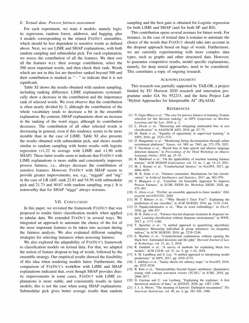
representation and pre-processing steps as in [5]. We stemeach word in order to reduce and to gather similar words, e.g.,“vehicle” and “vehicles” are both transformed into “vehicl”.The classifier is based on a TF-IDF vectorizer followed bya logistic regression. In addition, we ran experiments with abagging ensemble, a random forest, and AdaBoost, instead ofthe logistic regression.

Then we apply the first step of FIXOUT to build a globalexplanation. This is performed with the textual adaptation ofLIME and SHAP. We compare both random sampling (RS)and submodular pick (SP), for these two explainers. Unlike

the previous tabular classifiers, the model deals with morethan 2000 features, i.e., as many as the vocabulary size. Forexample, Table X shows the first 10 most important wordsobtained after 50 experiments run with a logistic regressionand LIME explanations, respectively with random samplingand submodular pick.

At first glance, we can observe that important words for hatespeech classification are insults and swear words, which makessense. However, it should be noticed that such a classificationmay also be related to a particular context. For example, theuse of words such as “n*gger” in a conversation may also

TABLE VIIIAVERAGE VALUE OF k FOR LR AND BAG CLASSIFIERS (NUMBER OF TIMES MODELS ARE DEEMED UNFAIR): EFFECTS OF THE VARIATION OF α OVER

THE NUMBER OF FEATURES KEPT BY FIND-K.

Dat

a. SelectionLR BAGα α

0.5 1 1.5 2 2.5 3 0.5 1 1.5 2 2.5 3

Ger

man

LIME+RS 9.9 (47) 8.7 (42) 6.8 (31) 5.5 (23) 3.5 (13) 2.6 (8) 10.0 (33) 9.58 (31) 8.18 (24) 6.38 (18) 4.26 (8) 2.82 (2)LIME+SP 9.7 (50) 8.2 (49) 6.1 (43) 4.5 (39) 2.1 (29) 1.3 (24) 10.0 (41) 10.0 (41) 9.74 (41) 9.08 (40) 7.04 (30) 4.86 (21)SHAP+RS 10.0 (50) 9.9 (50) 9.5 (50) 7.4 (47) 5.7 (45) 3.8 (43) 9.92 (37) 9.80 (37) 8.78 (33) 7.16 (26) 5.86 (22) 4.86 (19)SHAP+SP 10.0 (50) 9.8 (50) 8.9 (50) 7.0 (49) 5.4 (45) 4.0 (43) 10.0 (45) 9.78 (45) 9.12 (43) 7.72 (36) 6.58 (31) 5.50 (26)

Adu

lt


LSA

C


TABLE IXAVERAGE VALUE OF k FOR RF AND ADA CLASSIFIERS (NUMBER OF TIMES MODELS ARE DEEMED UNFAIR): EFFECTS OF THE VARIATION OF α OVER

THE NUMBER OF FEATURES KEPT BY FIND-K.

Dat

a. SelectionRF ADAα α

0.5 1 1.5 2 2.5 3 0.5 1 1.5 2 2.5 3

Ger

man

LIME+RS 9.90 (49) 8.30 (43) 5.18 (25) 2.72 (8) 1.54 (2) 1.18 (2) 10 (48) 10 (48) 9.76 (48) 9.4 (46) 9.2 (45) 9.04 (44)LIME+SP 10.0 (50) 9.98 (50) 9.74 (50) 8.54 (50) 6.96 (47) 5.46 (46) 10.0 (50) 10.0 (50) 10.0 (50) 10.0 (50) 10.0 (50) 10.0 (50)SHAP+RS 9.92 (50) 8.98 (48) 6.46 (39) 4.52 (29) 2.74 (23) 2.04 (18) 10.0 (48) 8.78 (43) 6.44 (31) 4.28 (23) 3.24 (15) 2.90 (13)SHAP+SP 9.86 (50) 8.70 (47) 5.64 (33) 3.68 (27) 2.28 (22) 1.42 (17) 9.98 (47) 8.68 (42) 6.78 (34) 5.82 (30) 4.92 (24) 4.04 (20)

Adu

lt


LSA

C


TABLE XMEAN CONTRIBUTION OF A LOGISTIC REGRESSION, LIME AS

EXPLAINER, AFTER 50 EXPERIMENTS

Random samplingrank word contrib.

1 faggot 0.6322 fag 0.6253 bitch 0.6224 niggah 0.6205 cunt 0.6136 pussi 0.6087 nigger 0.5978 hoe 0.5809 nigguh 0.522

10 dyke 0.473

Submodular pickrank word contrib.

1 niggah 0.5962 cunt 0.5793 bitch 0.5744 fag 0.5735 faggot 0.5736 nigger 0.5727 pussi 0.5478 hoe 0.5249 nigguh 0.505

10 retard 0.414

be related to a familiar interaction between two very closefriends, and thus not at all indicate an offensive discussion.

This shows that the definition of a sensitive word is notstraightforward in such a case, and that we must find wordsthat are responsible for a bias. Then, in order to completethis experiment, we manually select sensitive features. Ac-cordingly, the objective of the next subsection is to demon-strate that FIXOUT is able to decrease the contribution ofpre-selected words thanks to a FIXOUT ensemble and by

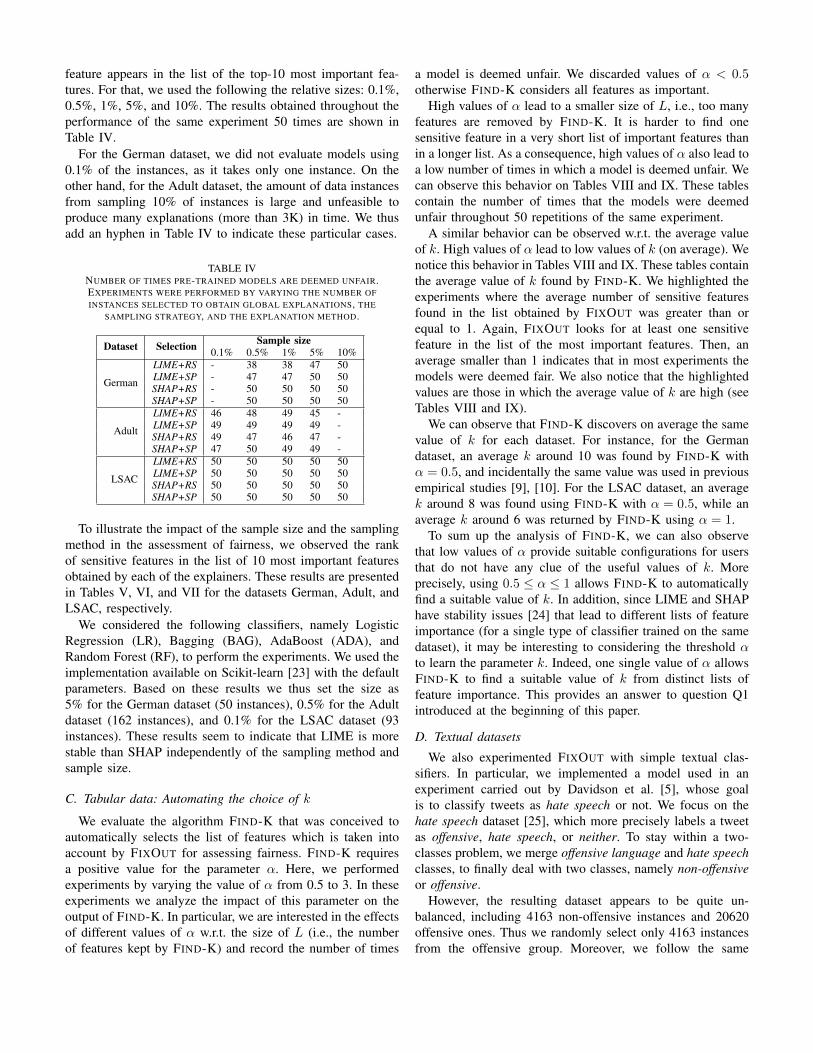
grouping words. For example, considering the groups of wordspresented in Figure 2, the goal of this ensemble is to reducethe contribution of these groups of words.

Classifier 1Ignoring: nigga, niggah, nigguh

Classifier 2Ignoring: nigger, nig, nicca

Classifier 3Ignoring: black, white

Classifier 4Ignoring: nigga, niggah, nigguh

nigger, nig, niccablack, white

FixOut Ensemble

Fig. 2. Illustration of textual classifiers used in the ensemble.

E. Textual data: Process fairness assessment

For each experiment, we train 4 models, namely logis-tic regression, random forest, adaboost, and bagging, plus4 models corresponding to the related FIXOUT ensembles,which should be less dependent to sensitive words as definedabove. Next, we use LIME and SHAP explanations, with bothrandom sampling and submodular pick. For each explanation,we assess the contribution of all the features. We then sortall the features w.r.t. their average contribution, select the500 most important words, and then check their rank. Wordswhich are not in this list are therefore ranked beyond 500 andtheir contribution is marked as “ - ” to indicate that it is notsignificant.

Table XI shows the results obtained with random sampling,including ranking difference. LIME explanations systemati-cally show a decrease in the contribution and the importancerank of selected words. We even observe that the contributionis often nearly divided by 2, although the contribution of thewhole vocabulary tends to decrease a bit in the ensembleexplanation. By contrast, SHAP explanations show an increasein the ranking of the word nigga, although its contributiondecreases. The contribution of all other selected words isdecreasing in general, even if this tendency seems to be moreinstable than in the case of LIME. Table XI also presentsthe results obtained with submodular pick, and shows resultssimilar to random sampling with better results with logisticregression (+1.22 in average with LIME and +1.90 withSHAP). These latter results seem to indicate that FIXOUT withLIME explanations is more stable and consistently improvesprocess fairness, i.e., always decrease the contribution ofsensitive features. However, FIXOUT with SHAP seems toprovide greater improvements; see, e.g., “nigguh” and “nig”in the case of LR (diff. rank 22.81 and 54.56 with submodularpick and 21.73 and 40.67 with random sampling, resp.). It isnoteworthy that for SHAP “nigga” always worsens.

VII. CONCLUSION

In this paper, we revisited the framework FIXOUT that wasproposed to render fairer classification models when appliedto tabular data. We extended FIXOUT in several ways. Weintegrated an approach to automate the choice of the list ofthe most important features to be taken into account duringthe fairness analysis. We also evaluated different samplingstrategies for selecting instances when assessing fairness.

We also explored the adaptability of FIXOUT’s frameworkto classification models on textual data. For that, we adaptedthe notion of feature dropout to bag of words, followed by theensemble strategy. Our empirical results showed the feasibilityof this idea when rendering models fairer. Furthermore, thecomparison of FIXOUT’s workflow with LIME and SHAPexplanations indicated that, even though SHAP provides dras-tic improvements in some cases, FIXOUT with LIME ex-planations is more stable, and consistently results in fairermodels; this is not the case when using SHAP explanations.Submodular pick gives better average results than random

sampling and the best gain is obtained for Logistic regressionfor both LIME and SHAP (and for both SP and RS).

This contribution opens several avenues for future work. Forinstance, in the case of textual data it remains to automate thechoice of the words that FIXOUT should take into account inthe dropout approach based on bags of words. Furthermore,we are currently experimenting with more complex datatypes, such as graphs and other structured data. However,to guarantee competitive results, model specific explanations,namely, for deep neural approaches, need to be considered.This constitutes a topic of ongoing research.

ACKNOWLEDGMENT

This research was partially supported by TAILOR, a projectfunded by EU Horizon 2020 research and innovation pro-gramme under GA No 952215, and the Inria Project Lab“Hybrid Approaches for Interpretable AI” (HyAIAI)

REFERENCES

[1] N. Grgic-Hlaca et al., “The case for process fairness in learning: Featureselection for fair decision making,” in NIPS Symposium on MachineLearning and the Law, 2016, p. 2.

[2] L. Dixon et al., “Measuring and mitigating unintended bias in textclassification,” in AAAI/ACM AIES, 2018, pp. 67–73.

[3] M. Hardt et al., “Equality of opportunity in supervised learning,” inNIPS, 2016, pp. 3323–3331.

[4] D. Hangartner et al., “Monitoring hiring discrimination through onlinerecruitment platforms,” Nature, vol. 589, no. 7843, pp. 572–576, 2021.

[5] T. Davidson et al., “Racial bias in hate speech and abusive languagedetection datasets,” in Proceedings of the Third Workshop on AbusiveLanguage Online, 2019, pp. 25–35.

[6] K. Makhlouf et al., “On the applicability of machine learning fairnessnotions,” ACM SIGKDD Explorations, vol. 23, no. 1, pp. 14–23, 2021.

[7] M. J. Kusner et al., “Counterfactual fairness,” in NeurIPS, 2017, pp.4066–4076.

[8] M. B. Zafar et al., “Fairness constraints: Mechanisms for fair classifi-cation,” in Artificial Intelligence and Statistics, 2017, pp. 962–970.

[9] V. Bhargava et al., “LimeOut: An Ensemble Approach To ImproveProcess Fairness,” in ECML PKDD Int. Workshop XKDD, 2020, pp.475–491.

[10] G. Alves et al., “FixOut: an ensemble approach to fairer models,” HALpreprint hal:03033181, 2020.

[11] M. T. Ribeiro et al., ““Why Should I Trust You?”: Explaining thepredictions of any classifier,” in ACM SIGKDD, 2016, pp. 1135–1144.

[12] O. Papakyriakopoulos et al., “Bias in word embeddings,” in FAccT,2020, pp. 446–457.

[13] M. B. Zafar et al., “Fairness beyond disparate treatment & disparate im-pact: Learning classification without disparate mistreatment,” in WWW,2017, p. 1171–1180.

[14] T. Speicher et al., “A unified approach to quantifying algorithmicunfairness: Measuring individual & group unfairness via inequalityindices,” in ACM SIGKDD, 2018, pp. 2239–2248.

[15] S. Wachter et al., “Counterfactual explanations without opening theblack box: Automated decisions and the gdpr,” Harvard Journal of Law& Technology, vol. 31, no. 2, 2018.

[16] R. Guidotti et al., “A survey of methods for explaining black boxmodels,” ACM CSUR, vol. 51, no. 5, pp. 1–42, 2018.

[17] S. M. Lundberg and S. Lee, “A unified approach to interpreting modelpredictions,” in NIPS, 2017, pp. 4765–4774.

[18] J. Adebayo et al., “Sanity checks for saliency maps,” in NeurIPS, 2018,pp. 9525–9536.

[19] B. Kim et al., “Interpretability beyond feature attribution: Quantitativetesting with concept activation vectors (TCAV),” in ICML, 2018, pp.2668–2677.

[20] D. Garreau and U. von Luxburg, “Explaining the explainer: A firsttheoretical analysis of lime,” in AISTATS, 2020, pp. 1287–1296.

[21] J. J. A. Moors, “The meaning of kurtosis: Darlington reexamined,” TheAmerican Statistician, vol. 40, no. 4, pp. 283–284, 1986.

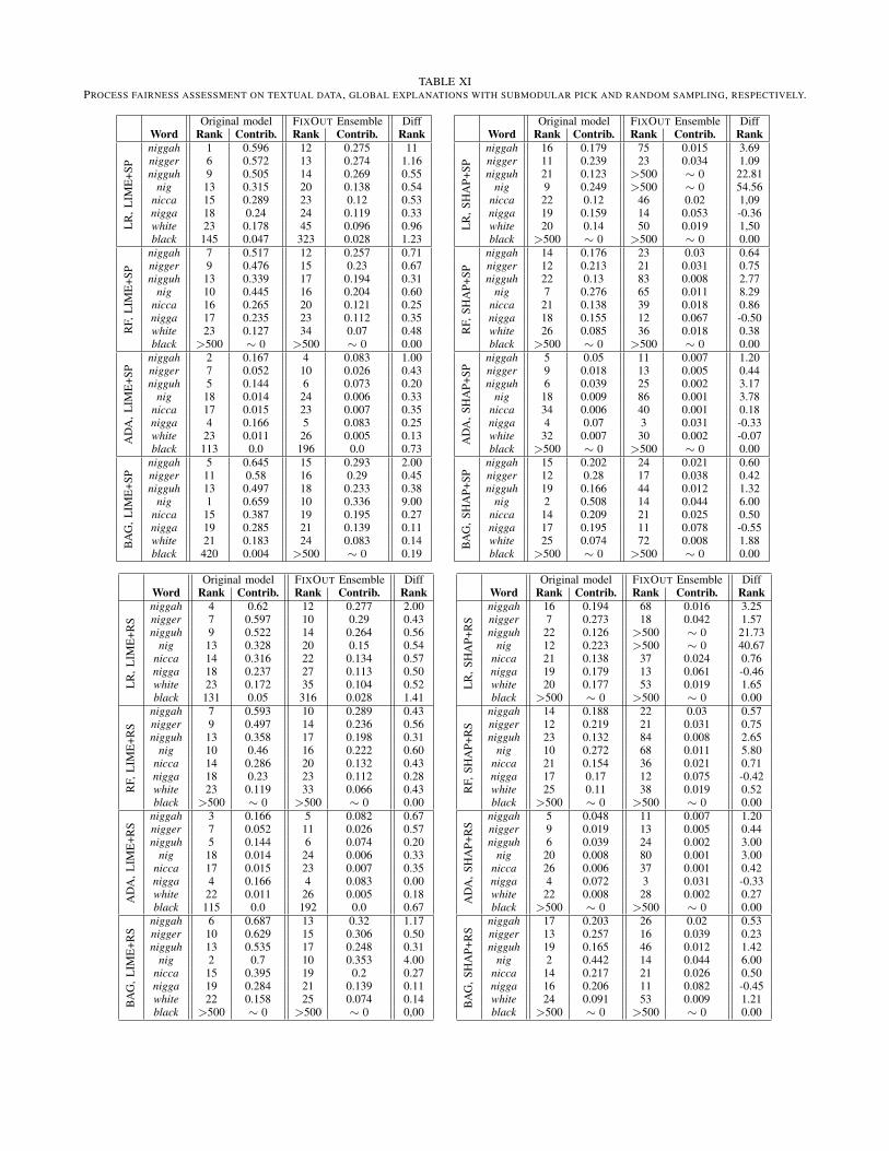
TABLE XIPROCESS FAIRNESS ASSESSMENT ON TEXTUAL DATA, GLOBAL EXPLANATIONS WITH SUBMODULAR PICK AND RANDOM SAMPLING, RESPECTIVELY.

Original model FIXOUT Ensemble DiffWord Rank Contrib. Rank Contrib. Rank

LR

,LIM

E+S

P

niggah 1 0.596 12 0.275 11nigger 6 0.572 13 0.274 1.16nigguh 9 0.505 14 0.269 0.55

nig 13 0.315 20 0.138 0.54nicca 15 0.289 23 0.12 0.53nigga 18 0.24 24 0.119 0.33white 23 0.178 45 0.096 0.96black 145 0.047 323 0.028 1.23

RF,

LIM

E+S

P

niggah 7 0.517 12 0.257 0.71nigger 9 0.476 15 0.23 0.67nigguh 13 0.339 17 0.194 0.31

nig 10 0.445 16 0.204 0.60nicca 16 0.265 20 0.121 0.25nigga 17 0.235 23 0.112 0.35white 23 0.127 34 0.07 0.48black >500 ∼ 0 >500 ∼ 0 0.00

AD

A,L

IME

+SP



BA

G,L

IME

+SP


nig 1 0.659 10 0.336 9.00nicca 15 0.387 19 0.195 0.27nigga 19 0.285 21 0.139 0.11white 21 0.183 24 0.083 0.14black 420 0.004 >500 ∼ 0 0.19


LR

,SH

AP+

SP

niggah 16 0.179 75 0.015 3.69nigger 11 0.239 23 0.034 1.09nigguh 21 0.123 >500 ∼ 0 22.81

nig 9 0.249 >500 ∼ 0 54.56nicca 22 0.12 46 0.02 1,09nigga 19 0.159 14 0.053 -0.36white 20 0.14 50 0.019 1,50black >500 ∼ 0 >500 ∼ 0 0.00

RF,

SHA

P+SP


nig 7 0.276 65 0.011 8.29nicca 21 0.138 39 0.018 0.86nigga 18 0.155 12 0.067 -0.50white 26 0.085 36 0.018 0.38black >500 ∼ 0 >500 ∼ 0 0.00

AD

A,S

HA

P+SP


nig 18 0.009 86 0.001 3.78nicca 34 0.006 40 0.001 0.18nigga 4 0.07 3 0.031 -0.33white 32 0.007 30 0.002 -0.07black >500 ∼ 0 >500 ∼ 0 0.00

BA

G,S

HA

P+SP




LR

,LIM

E+R

S



RF,

LIM

E+R

S


nig 10 0.46 16 0.222 0.60nicca 14 0.286 20 0.132 0.43nigga 18 0.23 23 0.112 0.28white 23 0.119 33 0.066 0.43black >500 ∼ 0 >500 ∼ 0 0.00

AD

A,L

IME

+RS



BA

G,L

IME

+RS


nig 2 0.7 10 0.353 4.00nicca 15 0.395 19 0.2 0.27nigga 19 0.284 21 0.139 0.11white 22 0.158 25 0.074 0.14black >500 ∼ 0 >500 ∼ 0 0,00


LR

,SH

AP+

RS

niggah 16 0.194 68 0.016 3.25nigger 7 0.273 18 0.042 1.57nigguh 22 0.126 >500 ∼ 0 21.73

nig 12 0.223 >500 ∼ 0 40.67nicca 21 0.138 37 0.024 0.76nigga 19 0.179 13 0.061 -0.46white 20 0.177 53 0.019 1.65black >500 ∼ 0 >500 ∼ 0 0.00

RF,

SHA

P+R

S



AD

A,S

HA

P+R

S



BA

G,S

HA

P+R

S



[22] G. Saporta, Probabilites, analyse des donnees et statistique. EditionsTechnip, 2006.

[23] F. Pedregosa et al., “Scikit-learn: Machine learning in Python,” vol. 12,pp. 2825–2830, 2011.

[24] D. Slack et al., “Fooling lime and shap: Adversarial attacks on post hocexplanation methods,” in AAAI/ACM AIES, 2020, pp. 180–186.

[25] T. Davidson et al., “Automated hate speech detection and the problemof offensive language,” in ICWSM, 2017, pp. 512–515.

reducing unintended bias of ml models on tabular and

Documents