unintended impacts of multiple instruments on technological adoption

Environment for Development

Discussion Paper Series March 2009 EfD DP 09-06

Unintended Impacts of Multiple Instruments on Technology Adoption

Jess ica Cor ia

Environment for Development

The Environment for Development (EfD) initiative is an environmental economics program focused on international research collaboration, policy advice, and academic training. It supports centers in Central America, China, Ethiopia, Kenya, South Africa, and Tanzania, in partnership with the Environmental Economics Unit at the University of Gothenburg in Sweden and Resources for the Future in Washington, DC. Financial support for the program is provided by the Swedish International Development Cooperation Agency (Sida). Read more about the program at www.efdinitiative.org or contact [email protected].

Central America Environment for Development Program for Central America Centro Agronómico Tropical de Investigacíon y Ensenanza (CATIE) Email: [email protected]

China Environmental Economics Program in China (EEPC) Peking University Email: [email protected]

Ethiopia Environmental Economics Policy Forum for Ethiopia (EEPFE) Ethiopian Development Research Institute (EDRI/AAU) Email: [email protected]

Kenya Environment for Development Kenya Kenya Institute for Public Policy Research and Analysis (KIPPRA) Nairobi University Email: [email protected]

South Africa Environmental Policy Research Unit (EPRU) University of Cape Town Email: [email protected]

Tanzania Environment for Development Tanzania University of Dar es Salaam Email: [email protected]

© 2009 Environment for Development. All rights reserved. No portion of this paper may be reproduced without permission of the authors.

Discussion papers are research materials circulated by their authors for purposes of information and discussion. They have not necessarily undergone formal peer review.


Jessica Coria

Abstract There are many situations where environmental authorities use a mix of environmental policy

instruments, rather than one single instrument, to address environmental concerns. For example, one instrument may be used to reduce overall emissions of a pollutant while another is used to address specific seasonal concerns. Very little work has been done on the economic impacts of the application of multiple instruments. This paper investigates the unintended impacts of the interaction of a tradable permits scheme with direct seasonal regulations on the rate of adoption of advanced abatement technologies.

Key Words: technology adoption, environmental policy, tradable permits, emissions standards, interaction of policies JEL Classification: O33, Q53, Q55, Q58

Contents

Introduction ............................................................................................................................. 1

1. The Model ........................................................................................................................ 2

2. Interaction of Environmental Policies and the Rate of Adoption .............................. 3

2.1 Adoption Incentives under Direct Regulations and Auctioned Tradable Permits ........ 3

2.2 Adoption Incentives under a Mixed Scheme of Tradable Permits and Direct

Regulations ................................................................................................................... 5

2.3 Adoption Incentives under a System of Differentiated Tradable Permits .................. 9

4. Welfare Comparison ........................................................................................................ 15

5. Optimal Adoption Rate during Endogenous Environmental Emergencies ............ 17

6. Numerical Example ......................................................................................................... 20

7. Conclusions and Further Research ................................................................................ 22

References .............................................................................................................................. 24

Appendices ............................................................................................................................. 25

Environment for Development Coria

1


Jessica Coria∗

Introduction

In some cases, the damages caused by emissions of pollutants depend almost exclusively on their magnitude and on the number of persons whose location makes them vulnerable to the effects. However, under many other circumstances, the effects of a given discharge depend on variables beyond the control of those directly involved. For example, volume of water and speed of flow are critical determinants of a river’s assimilative capacity. Similarly, emissions levels that are acceptable and rather harmless under usual conditions can become intolerable under some meteorological conditions. This is the case in cities like Mexico City and Santiago, Chile, where temperature inversions may prevent air pollution from leaving the atmosphere during winter months, causing occasional environmental crises that prompt the imposition of emergency measures to improve air quality to a satisfactory level. Typically, these crises cannot be predicted far in advance or with any degree of certainty—we can only be certain that at some unforeseen time they will recur.

In most cases, it is virtually impossible to change environmental regulations on short notice. Thus, if one policy is used as the only means of control, it would have to be set at a level high enough to maintain the pollution at acceptable levels during emergency periods. In certain circumstances, such a policy may be unacceptably costly to society. Bawa (1975) showed that the pollution control policy that minimizes total social costs (stationary social costs plus short-term emergency costs) is a mixed policy, in which market-based instruments are used to control the long-term equilibrium of pollution and direct controls are used to maintain the pollution below some predetermined threshold during short-term emergencies. If enforcement is effective, direct controls can induce, with little uncertainty, the prescribed alterations in pollution activities, while the use of market-based policies leads firms to use cleaner technologies in the long run.

One important disadvantage of direct controls is their poor dynamic properties. In fact, the theory of environmental regulation suggests that, since economic instruments induce firms to

∗ Jessica Coria, Gothenburg University, Department of Economics, P.O. Box 640, SE 405 30 Gothenburg, Sweden; (tel) + 46-31-7864867; (email) [email protected].


2

re-optimize their levels of abatement, they create more effective technology adoption incentives than conventional regulatory standards. Thus, it is worth asking whether or not interaction of policies alters the economic incentives provided through market-based instruments, especially if the incidence of environmental crises and the “relative use” of direct controls within the mix vary. The present paper analyzes the unintended impacts of the interaction between tradable permits and short-term emissions standards on the rate of adoption of advanced abatement technologies.

Under this setting, adoption benefits can be decomposed into a “net abatement effect” and a “permit price effect.” The net abatement effect accounts for the increased adoption savings resulting from the additional abatement induced by a situation of environmental distress. The permit price effect accounts for the negative effect of increased availability of technology on the permit price, which encourages trading and discourages adoption. Then, both effects set against themselves and the final rate of adoption depends on the extent to which each effect offsets the other and on the incidence of environmental crises.

If the incidence of environmental crises is exogenous, then a mix of market-based policies and emissions standards does not maximize social welfare. Indeed, if the incidence of environmental crises is low, then a mix of tradable permits and emissions standards leads to an inefficiently large price effect and to a rate of adoption that is lower than the optimal. Similarly, if the incidence is high, then the mix induces an inefficiently small price effect, leading firms to over-invest. However, if the incidence is low and it can be reduced even further through adoption of new technology, then the previous results do not hold and the mixed policy could offer a higher level of social welfare than alternative approaches.

This paper is organized as follows. The next section introduces the adoption model. Section 2 analyzes the adoption incentives under direct regulations and market-based policies separately and under mixed policies. Section 3 compares the total welfare induced by mixed approaches when the incidence of environmental emergencies is exogenous. Section 4 compares the total welfare when the incidence of environmental emergencies can be affected by the rate of adoption. Section 5 presents a numerical example to illustrate the main results. Section 6 concludes the paper.

1. The Model

Consider a competitive industry consisting of a continuum of firms of mass 1. Aggregate emissions without environmental regulation are normalized to unity. Normally, the


3

environmental authority auctions off [1 ]nq− emissions, where nq represents the desired level of

abatement. Each firm must decide whether to buy permits at the market clearing price x to cover its emissions or to abate them. Due to meteorological conditions, critical episodes of bad air quality are declared with exogenous probability μ , where μ corresponds to the rate of critical

episodes per unit of time. To avoid the negative impacts of such episodes, the environmental authority implements a more demanding direct regulation during these environmental emergencies, compelling firms to further decrease their levels of emissions. The direct regulation takes the form of a uniform emissions standard equal to [1 ]cq− , with [ ]c nq q> .

Current abatement costs are homogeneous with total abatement costs equal to 2icq , where

iq represents firm i’s abatement. Firms can invest in an advanced technology, leading to lower

abatement costs, 2icq% [ c c<% ]. Buying and installing the new technology causes a fixed cost, ik

[0,1]U .

Let Bπ and Aπ denote the firms’ profit flows before and after technology adoption, respectively. Firms will adopt new technology as long as the adoption benefits (i.e., the difference in profits associated with the decreased abatement costs) offset the adoption costs. Then, the following arbitrage condition must hold for the marginal adopter:

A Bπ π π⎡ ⎤− = Δ =⎣ ⎦ . (1)

Define λ as the rate of firms adopting the new technology:

λ = = 1- F( ) 1 ( )B AFkππ π πΔ

= − − = = ΔΔ

. (2)

Notice that since firm profits strongly depend on the choice and stringency of environmental policies, the rate of firms adopting the new technology is endogenous.

2. Interaction of Environmental Policies and the Rate of Adoption

This section analyzes the adoption incentives when direct regulations and market-based policies are implemented separately and when they are mixed.

2.1 Adoption Incentives under Direct Regulations and Auctioned Tradable Permits

Several researchers have found that the incentive to adopt new technologies is greater under market-based instruments than under direct regulations (see Milliman and Prince 1989;


4

Jung, Krutilla, and Boyd 1996; Keohane 1999; and Nelissen and Requate 2004). This superiority of market-based policies relies on the fact that firms re-optimize their abatement levels once new technology is available, which leads to larger savings attributable to the adoption decision. If direct regulations are used, firms will enjoy a lower abatement cost only for the emissions they were abating initially. Thus, in this setting, the cost savings resulting from using new technology, when firms’ emissions are restricted to no more than q units of emissions, are given by the

difference in total abatement cost due to reducing emissions to that level:

2( ) ( )( )EE EE c c qπ λ ⎡ ⎤Δ = = −⎣ ⎦% . (3)

Let us compare with the incentives provided by market-based policies. Let x denote the “equilibrium permit price” of emissions. When adopters make abatement decisions, they solve the following problem:

{ }21min ( ) (1 )A

A A Aq

L c q x q= + −% , (4)

where Aq is the level of emissions abated, and 1AL is the minimized sum of abatement costs and

payments for non-reduced emissions. The first order condition (FOC) is given by:

2 ( )Ac q x=% . (5)

That is, adopters reduce emissions until the marginal abatement cost of the new technology equals the price of emissions.

Non-adopters face a similar problem, but with a higher marginal abatement cost:

{ }21min ( ) (1 )NA

NA NA NAq

L c q x q= + − . (6)

The first order condition is given by:

2 ( )NAc q x= . (7)

Thereby, non-adopters’ optimal level of abatement, NAq , is lower than that of adopters because

of higher marginal abatement costs.

Substituting the FOCs into the minimization problem, the adoption profits and the rate of adoption are given by:


5

2TP TP xπ λ αΔ = = , (8)

with

1 1 044 cc

α ⎡ ⎤= − >⎢ ⎥⎣ ⎦% and 2 2( )( )x c c qα ⎡ ⎤> −⎣ ⎦

% .1

If the industry is regulated by permits, the market clearing on the permit market requires:

[ ]( ) ( ) 1 ( ) ( )A NAq x q x x q xλ λ⎡ ⎤ ⎡ ⎤= + −⎣ ⎦ ⎣ ⎦ . (9)

Substituting equations (5) and (7) into equation (9), and differentiating equation (9) with respect to x and λ yields:

014

dx xd

c

αλ λα= − <

+ . (10)

Then, the permit price will drop with adoption since the diffusion of the cost-reducing technology lowers the aggregate marginal abatement costs. This price effect induces more efficient adoption decisions and prevents over-investing since firms with higher costs of adoption have the opportunity to buy cheaper permits instead of investing in new technology.2

2.2 Adoption Incentives under a Mixed Scheme of Tradable Permits and Direct Regulations

Let us now compare the adoption incentives when mixed policies are used. It is assumed that environmental emergencies occur with probability μ and that firms are compelled to abate

cq units of emissions during these periods. Then, the adopters’ problem is to minimize the sum

of 1) abatement costs and payments for non-reduced emissions during normal days and 2) the abatement costs to achieve the emergency standard:

1 In line with most of the literature on the subject, I assume parameters such that, for the same level of stringency, the cost savings provided by tradable permits are larger than those provided by emissions standards. 2 This price effect tends to also support the use of taxes instead of tradable permits to speed up the diffusion of new technology. The fact that the emissions price is fixed by the regulator under the tax, while it depends on the firm behavior under permits, creates a wedge between the tax and the permit systems and between the different rates of adoption they induce.


6

{ } }{2 22min (1 ) ( ) (1 ) ( ) (1 )A

n

A A An c n c c cq

L c q x q c q x qμ μ= − + − + + −% % , (11)

where cx denotes the “equilibrium permit price” of emissions, when both policies are applied and A

n cq q≤ .

The FOC for the optimal level of emissions reduction is given by:

2 ( )An cc q x=% . (12)

Notice that the FOC does not change due to the interaction of policy instruments. That is, adopters abate emissions until the marginal abatement cost of the new technology equals the price of emissions.

Again, non-adopters face a similar problem, but with a higher marginal abatement cost:

{ } }{2 22min (1 ) ( ) (1 ) ( ) (1 )NA

n

NA NA NAn c n c cq

L c q x q c q x qμ μ= − + − + + − , (13)

2 ( )NAn cc q x= . (14)

Substituting the FOC into the minimization problem, the adoption profits and the rate of adoption cλ become:

22(1 )( )cc cx c c qπ λ μ α μ ⎡ ⎤ ⎡ ⎤Δ = = − + −⎣ ⎦ ⎣ ⎦

% . (15)

Differentiating cλ with respect to μ and re-organizing terms yields:

[2 2

Adoption SavingsAdoption SavingsPrice EffecUnder Normal DaysUnder Environmental Emergencies

Net Abatement Effect

( ) 2(1 )( )c

cc c c

xc c q x xλ α μ αμ μ

⎧ ⎫⎪ ⎪ ∂∂ ⎪ ⎪⎡ ⎤ ⎡ ⎤ ⎤= − − + −⎨ ⎬⎦⎣ ⎦ ⎣ ⎦∂ ∂⎪ ⎪

⎪⎪ ⎭⎩

%142431442443

1444444244444443t

144424443

. (16)

In equation (16), the term in brackets on the right-hand side represents the net effect of the more stringent direct regulation under environmental emergencies on the adoption savings, i.e., net abatement effect, while the second term on the right-hand side of equation (15) gives account of the effects of the implementation of the direct regulation on the permit price, i.e., permit price effect.


7

Market clearing in the permit market requires total abatement to be equal to the weighted abatement undertaken by adopters and non-adopters. Then, substituting the optimal rate of adoption into the market-clearing condition, we can solve for the market price cx and for the effect of environmental emergencies on the permit price:

[ ]( , ) ( ) 1 ( , ) ( )A NAn n c n cq x q x x q xλ μ λ μ⎡ ⎤ ⎡ ⎤= + −⎣ ⎦ ⎣ ⎦ . (17)

Substituting equation (15) into equation (17), differentiating with respect to cx andμ , and solving for /cdx dμ , yields (see appendix A):

[22

2 2 2

0

( )

13(1 )( ) ( )( )4

c c cc

c c

x x c c qdxd x c c q

c

α α

μ μ α μ α

>

⎡ ⎤⎡ ⎤ ⎡ ⎤⎤ − −⎦ ⎣ ⎦ ⎣ ⎦⎢ ⎥⎣ ⎦=− + − +

%

%

14444444244444443

. (18)

Since the denominator is positive, the sign of cdxdμ

depends on the net adoption savings.

Substituting equation (18) into equation (16) yields:

[

[

2 2

Adoption SavingsAdoption SavingsUnder Normal DaysUnder Environmental Emergencies


2

2 2

( )

( )2(1 )( )

c

c c

c

c

c c q x

x c cx

λ αμ

αμ α

⎧ ⎫⎪ ⎪∂ ⎪ ⎪⎡ ⎤ ⎡ ⎤ ⎤= − −⎨ ⎬⎦⎣ ⎦ ⎣ ⎦∂ ⎪ ⎪

⎪⎪ ⎭⎩

⎡⎤ − −⎦+ −

%142431442443

1444444244444443

% 2

2 2 2

Price Effect

13(1 )( ) ( )( )4

c

cc

q

x c c qc

μ α μ α

⎡ ⎤⎤ ⎡ ⎤⎣ ⎦ ⎣ ⎦⎢ ⎥⎣ ⎦

− + − +%

14444444444244444444443

. (19)

Thus, if the adoption savings under the emissions standard are larger than the savings firms realize under trading permits, then the net abatement effect is positive while the permit price effect is negative. Similarly, if the savings under tradable permits are larger than those under the emissions standard, then the permit price effect is positive, while the net abatement effect is negative. Therefore, the comparison between adoption savings under emissions standards and permits critically depends on the “relative” stringency of the direct regulation. If the emergency emissions standard is the most demanding policy, then adoption savings under


8

environmental emergencies are larger than those under normal days, and the net abatement effect is positive while the permit price effect is negative.

So, the permit price effect partially offsets the net abatement effect, reducing the rate of adoption. The price effect is negative since the higher rate of adoption induced by more stringent direct regulation lowers the aggregate marginal abatement cost, and therefore lowers the permit price. This decrease in the permit price reduces the rate of adoption because, in order to achieve the environmental regulation, firms prefer to buy “cheaper” permits instead of buying the new technology. The more stringent the emissions standard is, the larger the decrease in the permit price and the larger the impact on the rate of adoption.

Clearly, the magnitude of the permit price effect also depends on the probability of environmental emergencies occurring. If μ increases, the relative importance of the permit price

effect decreases since the chances of using permits, instead of buying the new technology, are very low.

Proposition 1

The rate of adoption under the mix of tradable permits and emissions standards increases with the incidence of environmental emergencies at an increasing rate.

Proof:

Let 0β denote the net abatement effect, and 21 ( )cxβ α= and 2

2 ( )cc c qβ ⎡ ⎤= −⎣ ⎦% the

adoption savings under permits and under the emissions standard, respectively. Then, cλμ

∂∂

can

be re-written as:

10

1 2

21 01 13

(1 ) 4

c

c

β αλ βμ β α β μα

μ

⎡ ⎤⎢ ⎥∂ ⎢ ⎥= − =

∂ ⎡ ⎤⎢ ⎥+ +⎢ ⎥⎢ ⎥− ⎣ ⎦ ⎦⎣

, (20)

where

1

1 2

2 01 13

(1 ) 4c

β α

β α β μαμ

⎡ ⎤⎢ ⎥⎢ ⎥ >

⎡ ⎤⎢ ⎥+ +⎢ ⎥⎢ ⎥− ⎣ ⎦ ⎦⎣

.


9

Thus, the effect of the incidence of environmental emergencies is expressed as a function of the net abatement effect times 1 less the permit price effect. Notice that when 1μ → , the

permit price effect tends to zero and 1 0|c

μλ βμ →

∂→

∂. Thus, if the probability of an environmental

emergency occurring is high, then the degree of substitution between the use of permits and the purchase of new technology is small because it is not profitable to purchase permits that cannot be used regularly. Adopting abatement technology is, therefore, the only alternative available to meet the environmental regulation, and the adoption savings are the largest.

On the other hand, when 0μ → , the degree of substitution between the use of permits

and the purchase of new technology is high, and so is the permit price effect. Then:

10 0 0

1

2| 1 134

c

c

μβ αλ β β

μ β α→

⎡ ⎤⎢ ⎥∂

→ − <⎢ ⎥∂ ⎢ ⎥+⎢ ⎦⎣

.

So, if the probability of an environmental emergency decreases, then the degree of substitution between the use of permits and the purchase of the technology increases, and so does the negative impact of the permit price effect on the rate of adoption.

The intuition behind this result is straightforward. The net abatement effect is positive and overcomes the negative permit price effect. Since the permit price effect decreases with the incidence of environmental emergencies, the total effect increases at an increasing rate.

2.3 Adoption Incentives under a System of Differentiated Tradable Permits

Let us assume that instead of applying a direct regulation to control critical episodes, the environmental authority uses differentiated tradable permits. A “regular” trading program is intended to encourage emissions reductions equal to nq during normal days, while an emergency

tradable permit program is intended to encourage reductions equal to cq during environmental

emergencies. The adopters’ problem becomes how to minimize the sum of abatement costs and payments for non-reduced emissions during normal days plus the sum of abatement costs and payments for non-reduced emissions during environmental emergencies.

{ } }{2 23,

min (1 ) ( ) (1 ) ( ) (1 )A An c

A A A A An n n c s cq q

L c q x q c q x qμ μ= − + − + + −% % , (21)


10

where nx is the “permit price” of emissions during normal days, and sx corresponds to the

“equilibrium permit price” of emissions during environmental emergencies.

The FOCs for the optimal level of emissions reduction under the regular and the emergency program are given, respectively, by:

2 ( )

2 ( )

An n

Ac s

c q x

c q x

=

=

%

% . (22)

That is, in each “state,” the marginal abatement cost of the new technology equals the price of emissions.

As usual, non-adopters face a similar problem, but have a higher marginal abatement cost, leading to the usual FOCs:

2 ( )NAn nc q x= , and (23)

2 ( )NAc sc q x= .

Using the FOC for the optimal level of emissions reduction, we can solve for the adoption profits and the rate of adoption:

2 2 2(1 )( ) ( )TPPn sx xπ λ μ μ α⎡ ⎤Δ = = − +⎣ ⎦ . (24)

Differentiating equation (24) with respect to μ and re-organizing terms yields:

22 2

Adoption Savings Adoption SavingsUnder Environmental Emergencies Under Normal Days

NetAbatementEffect

Price EffectUnder Environmental Em

( ) ( )

( )2 ( )

TPP

s n

ss

x x

xx

λ α αμ

μαμ

⎡ ⎤⎢ ⎥∂

= − +⎢ ⎥∂ ⎢ ⎥⎣ ⎦

∂∂

123 123

144444424444443

{ {Price Effect

ergencies Under Normal Days

( )2(1 ) ( ) nn

xxμ αμ

⎡ ⎤⎢ ⎥

∂⎢ ⎥+ −⎢ ⎥∂⎢ ⎥⎢ ⎥⎣ ⎦

. (25)

The first term in brackets on the right-hand side of equation (25) represents the net effect of the environmental emergency regulation on the adoption savings, or the net abatement effect, while the second term on the right-hand side of equation (26) gives account of the indirect effect of


11

environmental emergencies on the permit price during environmental emergencies and normal days.

The market clearing in the permit markets requires total abatement to be equal to the weighted abatement done by adopters and non-adopters in each state:

2 2( , ) ( ) 1 ( , ) ( )TPP A TPP NAc s c s s c sq x q x x q xλ μ λ μ⎡ ⎤ ⎡ ⎤ ⎡ ⎤= + −⎣ ⎦ ⎣ ⎦ ⎣ ⎦ , and (26)

2 2( , ) ( ) 1 ( , ) ( )TPP A TPP NAn n n n n n nq x q x x q xλ μ λ μ⎡ ⎤ ⎡ ⎤ ⎡ ⎤= + −⎣ ⎦ ⎣ ⎦ ⎣ ⎦ . (27)

And, since the required emissions reduction is larger under environmental emergencies, [ c nq q< ], the permit price that clears “the market of environmental emergencies” is larger,

leading to a positive net abatement effect.

Substituting 2TPPλ into equation (26), and differentiating with respect to Sx andμ , we obtain a solution for /sdx dμ . By analogy, substituting 2TPPλ into equation (27), and differentiating with respect to nx andμ , we obtain a solution for /ndx dμ (see appendix B):

22 2


2 2 2 2

2 2 2 2

Price EffectUnder Environmental Emergencies

( ) ( )

( ) ( ) ( ) ( ) ( ) ( )2 ( ) 2(1 ) ( )13 ( ) (1 )( )

4

TPP

s n

s s n n s ns n

s n

x x

x x x x x xx x

x xc

λ α αμ

α α α α αμα μ α

μ α μ α

∂ ⎡ ⎤= − −⎣ ⎦∂

⎡ ⎤− −⎣ ⎦ + −+ − +

144424443

14444444244444443

2 2 2 2

Price EffectUnder Normal Days

13(1 )( ) ( )4n sx x

c

α

μ α μ α

⎡ ⎤⎢ ⎥⎢ ⎥

⎡ ⎤⎢ ⎥⎣ ⎦⎢ ⎥

− + +⎢ ⎥⎢ ⎥⎢ ⎥⎣ ⎦

144444424444443

(28)

Therefore, since the adoption savings are larger during environmental emergencies than during normal days, the net abatement effect is positive, while the permit price effects during environmental emergencies and normal days are negative and offset the net abatement effect.

Again, permit price effects are negative since permit prices drop when technology is adopted. The lower price stimulates additional permit trading and less adoption since firms prefer to buy permits instead of investing in technology. Notice that the permit price effect during environmental emergencies is larger because a more stringent policy induces larger adoption savings, therefore inducing a higher adoption rate and a larger reduction of the permit price.


12

Proposition 2

The rate of adoption under differentiated tradable permits increases with the incidence of environmental emergencies at a decreasing rate.

Proof:

Let 0γ denote the net abatement effect, and 21 ( )nxγ α= and 2

2 ( )Sxγ α= the adoption

savings during normal days and environmental emergencies, respectively. Then 2TPPλμ

∂∂

can be

re-written as:

22 1

0

2 1 1 2

2 211 1 1 13 (1 ) 3

4 (1 ) 4

TTP

c c

αγ αγλ γμ αγ μ αγ αγ μαγ

μ μ

⎡ ⎤⎢ ⎥∂ ⎢ ⎥= − −

∂ ⎡ ⎤ ⎡ ⎤⎢ ⎥+ − + + +⎢ ⎥ ⎢ ⎥⎢ ⎥−⎣ ⎦ ⎣ ⎦ ⎦⎣

, (29)

where

2

2 1

2 01 13 (1 )

4c

αγ

αγ μ αγμ

>⎡ ⎤+ − +⎢ ⎥⎣ ⎦

and 1

1 2

2 01 13

(1 ) 4c

αγ

αγ μαγμ

>⎡ ⎤+ +⎢ ⎥− ⎣ ⎦

.

Thus, the effect of the incidence of environmental emergencies is expressed as a function of the net abatement effect times 1 less the permit price effect during environmental emergencies and during normal days.

Notice that when 1μ → , the permit price effect during normal days tends to zero, while

during days of environmental emergencies it is at a maximum, and

22

1 0

2

2| 1 134

TPP

c

μαγλ γ

μ αγ→

⎡ ⎤⎢ ⎥∂

→ −⎢ ⎥∂ ⎢ ⎥+⎣ ⎦

.

On the other hand, when 0μ → , the permit price effect during environmental emergencies tends

to zero, while during normal days it is at a maximum, and


13

21

0 0

1

2| 1 134

TPP

c

μαγλ γ

μ αγ→

⎡ ⎤⎢ ⎥∂

→ −⎢ ⎥∂ ⎢ ⎥+⎣ ⎦

.

Notice that the price effect during environmental emergencies is larger than during normal days since the adoption savings during environmental emergencies are larger [ 2 1γ γ> ].

That is, the larger adoption savings induce a higher adoption rate and a larger reduction of the permit price, which offsets the net abatement effect. The positive effect of the incidence of environmental emergencies on the rate of adoption is, therefore, higher when 0μ → , or

2 2

0 1| |TPP TPP

μ μλ λμ μ→ →

∂ ∂>

∂ ∂ .

Finally, notice that 2 2

0 0| |TPP TPP

μ μλ λμ μ→ ≠

∂ ∂>

∂ ∂. That is, 0μ∀ ≠ , the total “price effect” (the

weighted addition of the price effect during environmental emergencies and normal days) is larger than the price effect during normal days, which implies that the rate of adoption increases the most with the incidence of environmental emergencies when 0μ → .

Thus, the rate of adoption increases with the incidence of environmental emergencies, but at a decreasing rate.

Proposition 3

The rate of adoption under a mix of tradable permits and emissions standards is lower/higher than, or the same as, the rate of adoption under a mix of tradable permit programs. If μ μ∗< , the rate of adoption under a mix of tradable permits and

emissions standards is lower than the rate of adoption under a mix of tradable permit programs. The reverse holds if μ μ∗> .

Proof:

Let us compare the rates of adoption in equation (15) and equation (24):

22(1 )( )cc cx c c qλ μ α μ ⎡ ⎤ ⎡ ⎤= − + −⎣ ⎦ ⎣ ⎦

% ,

2 2 2(1 )( ) ( )TPPn Sx xλ μ α μ α= − + .


14

During normal days, the adoption incentives provided by a mixed system of tradable permits are smaller than those provided by a mix of tradable permits and emissions standards. The reverse holds during environmental emergencies. That is, 2 2( ) ( )( )S cx c c qα > − % and

2 2( ) ( )N cx xα α< 0μ∀ ≠ .

There is, therefore, a critical value of μ determining which mix of policies induces the

larger adoption savings and the higher rate of adoption:

2 2

2 2 2 2

0 0

( ) ( )* 0

( ) ( ) ( )( ) ( )c n

c n c s

x x

x x c c q x

αμ

α α> <

⎡ ⎤−⎣ ⎦= >⎡ ⎤⎡ ⎤− − − −⎣ ⎦ ⎣ ⎦

%1442443 14444244443

. (30)

If μ μ∗< , the larger adoption savings provided by a mix of tradable permits and

emissions standards during normal days offset the smaller savings under environmental emergencies, and this mixed policy induces a higher rate of adoption. The reverse holds if μ μ∗> .

Notice that when 0μ → , the negative impact of the price effect is larger under a mix of

tradable permits and emissions standards. That is, 2

0 0| |c TPP

c nx xμ μλ λ

→ →

∂ ∂>

∂ ∂. Since the net

abatement effect is smaller under this mix, the response of the rate of adoption to the incidence

of environmental emergencies is also smaller, 2

0 0| |c TPP


∂ ∂<

∂ ∂ (see appendix C). But, as μ

increases, the price effect disappears in the case of a mix of tradable permits and emissions standards, while it increases in the case of a mixed system of tradable permits. Therefore, cλ increases at an increasing rate with the incidence of environmental emergencies, while 2TPPλ increases at a decreasing rate.

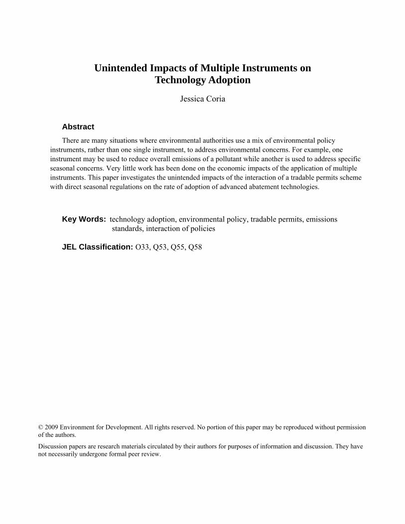
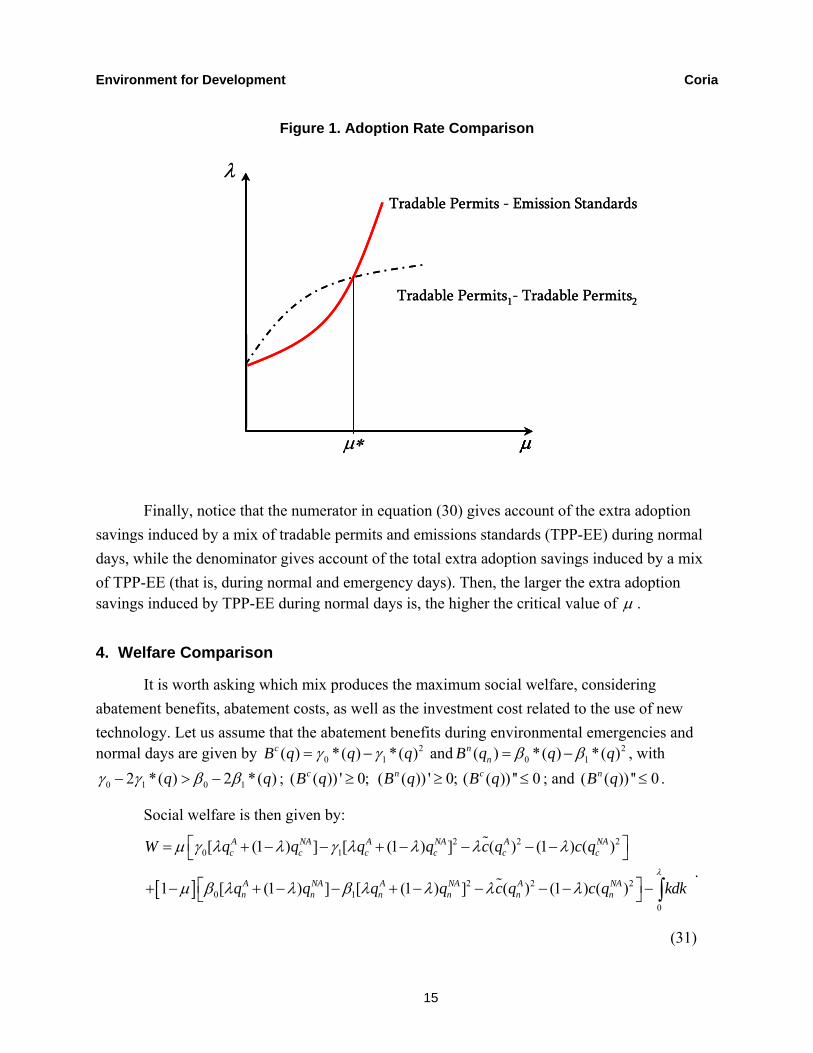
Figure 1 is a sketch of proposition 3. The intuition behind this result is as follows. In the absence of episodes of environmental distress, the incentives provided by the mixed policies coincide, as do the rates of adoption. If μ μ∗< , the larger adoption savings induced by a mix of

tradable permits and emissions standards produce a larger permit price effect, which offsets the savings and reduces the rate of adoption. But, as μ increases, the permit price effect tends to

zero, leading the adoption rate to increase. On the other hand, the total price effect increases with μ when a mixed system of tradable permits is implemented. The larger price effect increasingly offsets the net adoption savings, leading the adoption rate to decrease withμ .


15

Figure 1. Adoption Rate Comparison

Finally, notice that the numerator in equation (30) gives account of the extra adoption savings induced by a mix of tradable permits and emissions standards (TPP-EE) during normal days, while the denominator gives account of the total extra adoption savings induced by a mix of TPP-EE (that is, during normal and emergency days). Then, the larger the extra adoption savings induced by TPP-EE during normal days is, the higher the critical value of μ .

4. Welfare Comparison

It is worth asking which mix produces the maximum social welfare, considering abatement benefits, abatement costs, as well as the investment cost related to the use of new technology. Let us assume that the abatement benefits during environmental emergencies and normal days are given by 2

0 1( ) *( ) *( )cB q q qγ γ= − and 20 1( ) *( ) *( )n

nB q q qβ β= − , with

0 1 0 12 *( ) 2 *( )q qγ γ β β− > − ; ( ( )) ' 0;cB q ≥ ( ( )) ' 0;nB q ≥ ( ( )) '' 0cB q ≤ ; and ( ( )) '' 0nB q ≤ .

Social welfare is then given by:

[ ]

2 2 20 1

2 2 20 1

0

[ (1 ) ] [ (1 ) ] ( ) (1 ) ( )

1 [ (1 ) ] [ (1 ) ] ( ) (1 ) ( )

A NA A NA A NAc c c c c c

A NA A NA A NAn n n n n n

W q q q q c q c q

q q q q c q c q kdkλ

μ γ λ λ γ λ λ λ λ

μ β λ λ β λ λ λ λ

⎡ ⎤= + − − + − − − −⎣ ⎦

⎡ ⎤+ − + − − + − − − − −⎣ ⎦ ∫

%

% .

(31)

μμμ∗

λTradable Permits - Emission Standards

Tradable Permits1- Tradable Permits2

μμμ∗

λTradable Permits - Emission Standards

Tradable Permits1- Tradable Permits2


16

Minimizing equation (31) with respect to [ , , , ]c c n

A NA A NAnq q q q λ , we obtain the following

FOCs:

0 1: 2 (1 ) 2 ( )A A NA Ac c c cq q q c qγ γ λ λ⎡ ⎤− + − =⎣ ⎦

% , (32)

0 1: 2 (1 ) 2 ( )NA A NA NAc c c cq q q c qγ γ λ λ⎡ ⎤− + − =⎣ ⎦ , (33)

0 1: 2 (1 ) 2 ( )A A NA An n n nq q q c qβ β λ λ⎡ ⎤− + − =⎣ ⎦

% , (34)

0 1: 2 (1 ) 2 ( )NA A NA NAn n n nq q q c qβ β λ λ⎡ ⎤− + − =⎣ ⎦ , and (35)

[ ]

2 20 1

2 20 1

: [ ] 2 [ ] ( ) ( )

1 [ ] 2 [ ] ( ) ( )

A NA A NA NA Ac c c c c c

A NA A NA NA An n n n n n

q q A q q c q c q

q q B q q c q c q

λ λ μ γ γ

μ β β

⎡ ⎤= − − − + −⎣ ⎦⎡ ⎤+ − − − − + −⎣ ⎦

%

% , (36)

with (1 )A NAc cA q qλ λ⎡ ⎤= + −⎣ ⎦ being the total abatement during environmental emergencies and

(1 )A NAn nB q qλ λ⎡ ⎤= + −⎣ ⎦ being the total abatement during normal days.

Thus, from equations 32 and 33, and equations 34 and 35, we observe that social welfare is maximized when adopters’ marginal abatement costs are the same as the non-adopters’ in each state, and that this is exactly the outcome produced by a mix of tradable permit programs.

From equation (36), we observe that the optimal rate of adoption equates the marginal cost of adoption, with the marginal expected benefit in terms of 1) increasing abatement across firms during environmental emergencies and normal days and 2) reducing the abatement costs. Thus, the optimal rate of adoption depends on the parameters of the abatement benefit function and on the abatement costs. The flatter the abatement benefit functions, the larger the expected benefit of abatement and the higher the optimal rate of adoption. In terms of abatement costs, the lower the abatement costs of a new technology is, the higher the optimal rate of adoption.

Proposition 4

Social welfare is maximized when a mix of tradable permit programs is implemented.

Proof:

Substituting equations 32–35 into equation (36), we obtain the following expression for the optimal rate of adoption (see appendix D):

* 2 2( ) (1 )( )c nx xλ μ μ α⎡ ⎤= + −⎣ ⎦ . (37)


17

That is, the optimal rate of adoption coincides with the rate of adoption induced by a mix of tradable permit programs. Then, a mixed system of tradable permit programs induces a rate of adoption that maximizes welfare. The intuition behind this result is as follows. Under tradable permits, diffusion of the cost-reducing technology lowers the aggregate marginal abatement costs and therefore lowers the permit price. This price signal prevents firms from over-investing in abatement technology if cheaper permits are available, encouraging a solution such that the marginal cost of adoption equals the marginal expected social net benefit. If a mixed scheme of tradable permits and emissions standards is employed, the price signals are distorted. If μ μ∗< ,

the larger price effect induced by this mix leads to a rate of adoption that is lower than the optimal. On the other hand, if μ μ∗> , the inefficiently smaller price effect induced by this mix

leads firms to over-invest.

5. Optimal Adoption Rate during Endogenous Environmental Emergencies

In the previous analysis, the incidence of environmental emergencies is exogenous. However, if a significant fraction of firms adopt more “environmentally friendly” technologies, it is possible that the probability of environmental crises decreases with the rate of adoption. Then, the socially optimal policy in a static setting (i.e., the policy that minimizes total abatement costs) could no longer be optimal. To analyze this case, let us assume that the probability of environmental emergencies occurring depends on the rate of adoption according to function

( )μ λ , with '( ) 0μ λ < and ''( ) 0μ λ < . That is, the incidence of environmental emergencies

decreases with the rate of adoption at a decreasing rate.

The rate of adoption that maximizes social welfare solves the following problem:

[ ]

2 2 20 1

2 2 20 1

0

( ) [ (1 ) ] [ (1 ) ] ( ) (1 ) ( )

1 ( ) [ (1 ) ] [ (1 ) ] ( ) (1 ) ( )



Max W q q q q c q c q

q q q q c q c q kdk

λ

λ

μ λ γ λ λ γ λ λ λ λ

μ λ β λ λ β λ λ λ λ

⎡ ⎤= + − − + − − − −⎣ ⎦

⎡ ⎤+ − + − − + − − − − −⎣ ⎦ ∫

%

%

(38)

While the FOC for [ , , , ]A NA A NAc c n nq q q q remains unchanged, the FOC for the optimal rate of

adoption solves:


18

{ [ ] [ ]

* 2

2 20 1 0 1

Benefit ofIncreased Abatement

2 2 20

[ (1 ) ] [ (1 ) ] [ (1 ) ] [ (1 ) ]

'( )( ) 1 ( ) ( ) 1

TPP

A NA A NA A NA A NAc c c c n n n n

A NA Ac c N

q q q q q q q q

c q c q c q c

λ λ

γ λ λ γ λ λ β λ λ β λ λ

μ λλ λ λ λ<

= +

+ − − + − − + − + + −

⎡ ⎤− + − − + −⎣ ⎦

1444444444444444442444444444444444443

% % 2

Cost of Increased Abatement

0

( )NANq

>

⎧ ⎫⎪ ⎪⎪ ⎪⎪ ⎪⎨ ⎬⎡ ⎤⎡ ⎤⎪ ⎪⎣ ⎦⎣ ⎦⎪ ⎪

⎪⎪ ⎭⎩1444444444442444444444443

144444444444444444424444444444444444443

(39)

The second term in brackets on the right-hand side of equation (39) accounts for the effect of the adoption rate on the incidence of environmental emergencies, and is equal to the marginal productivity of adoption in terms of reducing such incidence times the net benefit of the increased abatement. Thus, if the net benefit of the increased abatement is positive, then the optimal rate of adoption is lower than the rate induced by a mixed system of tradable permits.

Proposition 5

If the probability of environmental emergencies decreases with the rate of adoption, then the optimal rate of adoption is lower than the rate of adoption induced by a system of trading programs.

Proof:

From equation (39), it is straightforward that the optimal rate of adoption is lower than the rate of adoption induced by a system of tradable permits, insofar as '( ) 0μ λ < and the net

benefit of the increased abatement is positive. The larger the effect of adoption, in terms of decreasing the probability of emergencies, the larger the discrepancy between the optimal rate of adoption and the rate of adoption induced by a system of tradable permits. By analogy, the larger the net benefit of increased abatement, the larger the discrepancy between the optimal rate of adoption and the rate of adoption induced by a mixed policy.

The intuition behind this result is as follows. The optimal rate of adoption increases with the expected benefits of abatement. Since the abatement benefits during normal days are smaller, and since the adoption rate increases the incidence of normal days, the optimal rate decreases in order to offset the reduced expected abatement benefits.

Proposition 6

If the probability of environmental emergencies decreases with the rate of adoption, and if the incidence of environmental emergencies is low, then total welfare under a


19

mixed system of tradable permits is lower/higher than, or the same as, under a mix of tradable permits and emissions standards.

Proof:

Let us compute total welfare under a mix of tradable permits and emissions standards. Substituting equations (12) and (14) into equation (38), we obtain:

2 2 20 1

22

2 20 1

( ) [ ] [ ] ( )( ) ( )

( )1 ( ) [ ] [ ] ( )4 2

c c cc c c c

cc c c

n n c

W q q c c q c q

xq q xc

μ λ γ γ λ

λμ λ β β λ α

⎡ ⎤⎡ ⎤= − + − −⎣ ⎦⎣ ⎦

⎡ ⎤⎡ ⎤ ⎣ ⎦⎡ ⎤ ⎡ ⎤+ − − − + −⎢ ⎥⎣ ⎦ ⎣ ⎦⎣ ⎦

%

. (40)

By analogy, substituting equations (22) and (23) into equation (38), we obtain total welfare under a mixed system of tradable permits:

22 2 2 2 2

0 1

2222 2 2 2

0 1

( )( ) [ ] [ ] ( )4

( )1 ( ) [ ] [ ] ( )4 2

TPP TPP TPP sc c s

TPPTPP TPP n

n n n

xW q q xc

xq q xc

μ λ γ γ λ α

λμ λ β β λ α

⎡ ⎤⎡ ⎤= − − +⎢ ⎥⎣ ⎦

⎣ ⎦

⎡ ⎤⎡ ⎤ ⎣ ⎦⎡ ⎤ ⎡ ⎤+ − − − + −⎢ ⎥⎣ ⎦ ⎣ ⎦⎣ ⎦

. (41)

Let us assume that *μ μ< . That is, the rate of adoption induced by a mix of tradable

permits and emissions standards is lower than that induced by a mixed system of tradable permits. As stated in equation (42), since 2( ) ( )c TPPμ λ μ λ> , the incremental welfare induced by

a mix of tradable permits and emissions standards WΔ is positive, insofar as the larger expected abatement benefits and the lower investment costs offset the higher abatement costs.

(42)

2 2 20 1 0 1

Expected Benefits ofImproved Environmental Quality

22 2 2 2 2

( ) ( ) ( ) ( ) ( ) ( )

( )( ) ( ) ( ) ( )( ) ( )4

c TPPc c n n

TPP TPP c css c c

W q q q q

xx c c q c qc

μ λ μ λ γ γ β β

μ λ λ α μ λ λ

⎡ ⎤⎡ ⎤ ⎡ ⎤⎡ ⎤Δ = − − − − −⎣ ⎦ ⎣ ⎦ ⎣ ⎦⎣ ⎦

⎡ ⎤ ⎡ ⎤+ − − +⎢ ⎥ ⎣⎣ ⎦

1444444444442444444444443

%

2 22 2 2 2

Expected Abatement Costsof Improved Environmental Quality

2 22

( ) ( )1 ( ) ( ) 1 ( ) ( )4 4

2 2

TPP TPP c cn cn c

c TPP

x xx xc c

μ λ λ α μ λ λ α

λ λ

⎡ ⎤⎢ ⎥⎦⎢ ⎥⎢ ⎥⎡ ⎤ ⎡ ⎤⎢ ⎥⎡ ⎤ ⎡ ⎤+ − + − − +⎢ ⎥ ⎢ ⎥⎣ ⎦ ⎣ ⎦⎢ ⎥⎣ ⎦ ⎣ ⎦⎣ ⎦

⎡ ⎡ ⎤ ⎡ ⎤⎣ ⎦ ⎣ ⎦+ −⎣

1444444444444442444444444444443

Investment Savings

⎤⎢ ⎥⎢ ⎥

⎦144424443


20

Thus, the sign of WΔ strongly depends on the parameters of the damage function and on the responsiveness of the incidence of environmental emergencies to changes in the rate of adoption. The larger the abatement benefits during environmental emergencies are, the larger the

WΔ . By analogy, the larger the effect of the rate of adoption reducing the probability of environmental emergencies is, the larger the WΔ .

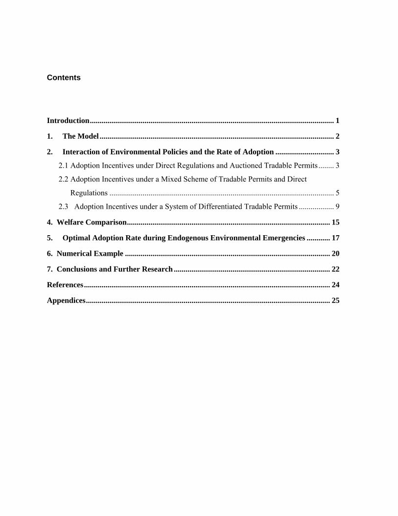
6. Numerical Example

In order to illustrate the results, the following numerical example compares the rate of adoption and total welfare under a mix of tradable permits and emissions standards and a mixed system of tradable permits. Parameters are chosen to ensure an interior solution, i.e., adoption savings range in the interval [ ]0,1 . The value of the parameters is presented in table 1.

Table 1 Simulation Parameters

Abatement benefits normal days 2( ) 3*nB q q q= −

Abatement benefits emergency days 2( ) 5* 0.05*cB q q q= −

Non-adopters’ abatement cost 25*q

Adopters’ abatement cost 22*q

Emission reduction during normal days nq = 0.25

Emission reduction during emergency days cq = 0.5

Notice that the abatement benefit function during environmental emergencies is flatter than that during normal days, leading to a higher level of required abatement. Thus, 25 percent of total emissions must be reduced during normal days and 50 percent during contingencies.

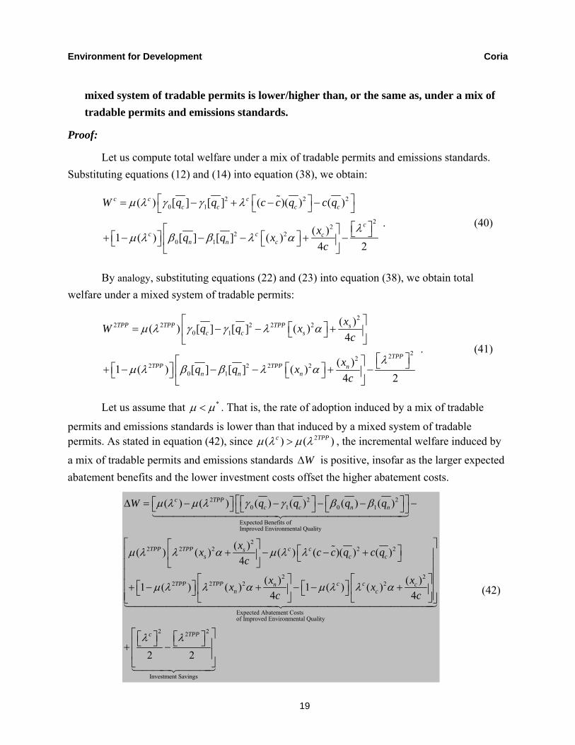
Figure 2 sketches the rate of adoption under both mixes when the probability of environmental emergencies is exogenous. As expected, there is a critical value of the incidence of environmental emergencies that determines which mix of policies induces the highest rate of adoption. If 38%μ < , the rate of adoption under the mix of tradable permits and emissions standards is lower; the reverse holds when 38%μ > .

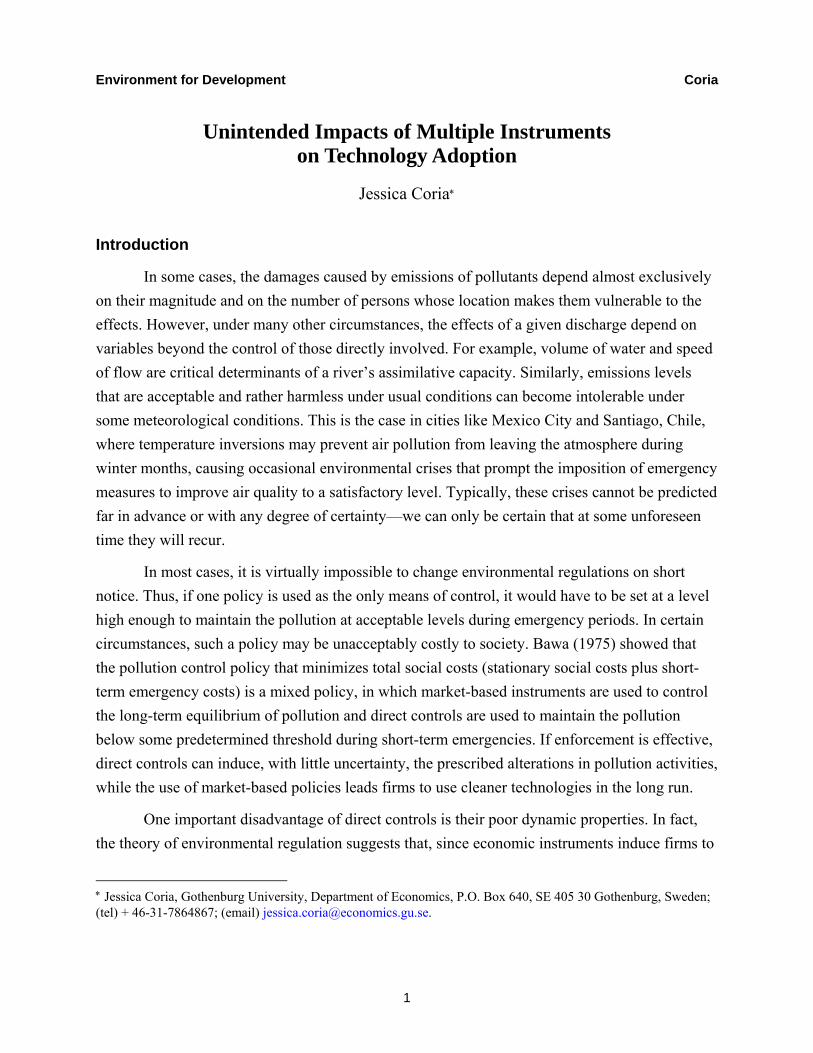
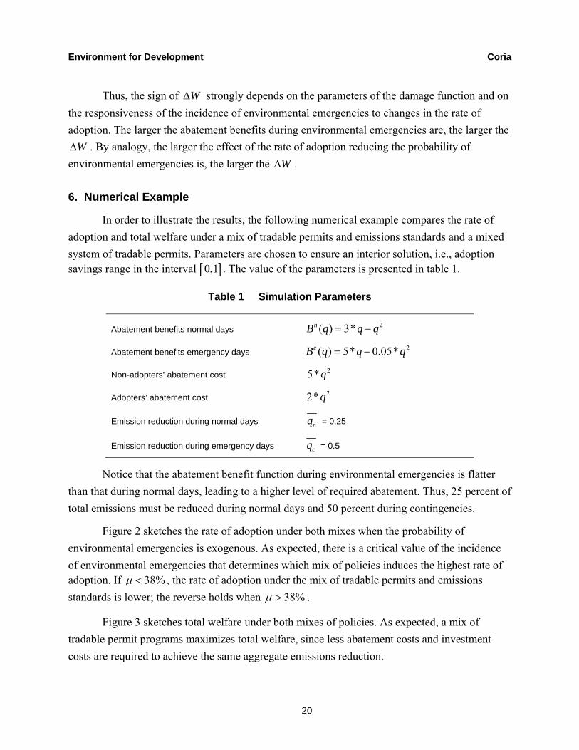
Figure 3 sketches total welfare under both mixes of policies. As expected, a mix of tradable permit programs maximizes total welfare, since less abatement costs and investment costs are required to achieve the same aggregate emissions reduction.


21

Figure 2. Adoption Rate under Different Mixes of Policies

0.22

0.32

0.42

0.52

0.62

0.72

0.00

0.05

0.10

0.15

0.20

0.25

0.30

0.35

0.40

0.45

0.50

0.55

0.60

0.65

0.70

0.75

0.80

0.85

0.90

0.95

1.00

Incidence of Environmental Emergencies

Ado

ptio

n R

ate

TPP-EE* TPP1-TPP2**

For both figures 2 and 3: * TPP-EE: Mix of tradable permits and emission standards. ** TPP1-TPP2: Mixed system of tradable permits.

Figure 3. Welfare under Different Mixes of Policies

0.000

0.200

0.400

0.600

0.800

1.000

1.200

1.400

1.600

1.800

0.000

0.100

0.200

0.300

0.400

0.500

0.600

0.700

0.800

0.900

1.000


Wel

fare

TPP-EE* TPP1-TPP2**


22

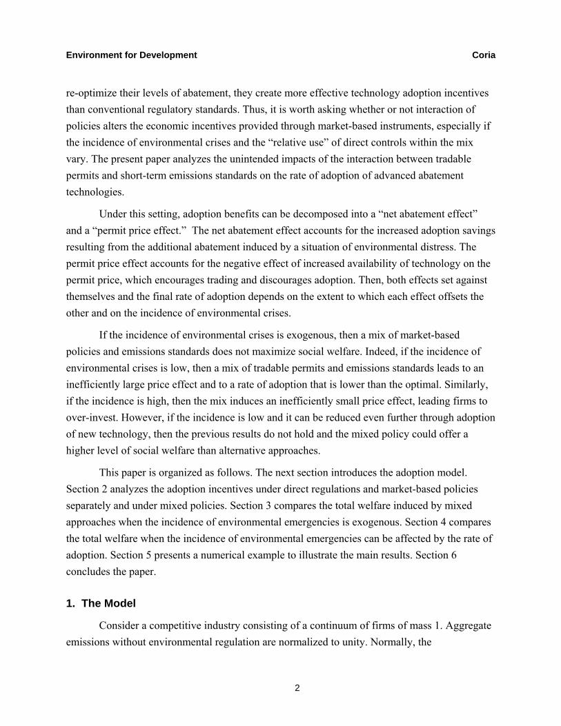
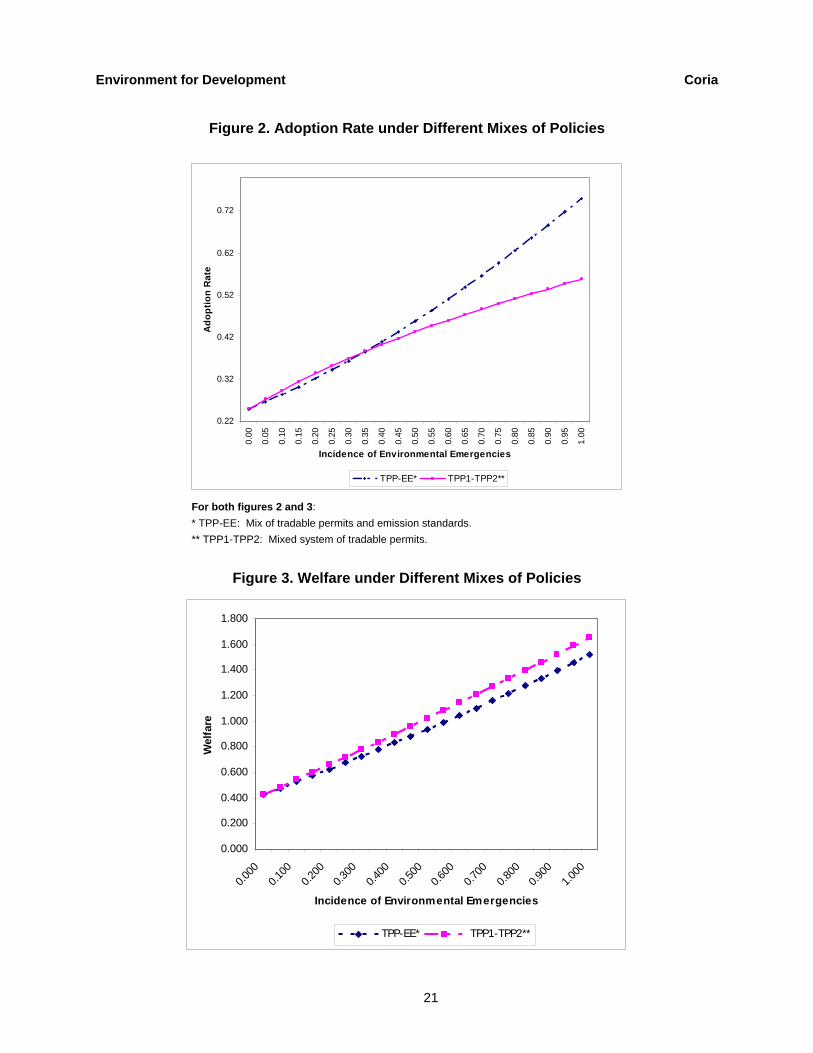
Finally, figure 4 sketches total welfare under both mixes of policies when the incidence of environmental emergencies is endogenous. I assume that the incidence of environmental emergencies decreases with the rate of adoption according to the function 2( ) *(1 0.2 )μ λ μ λ= − . Thus, '( ) 0μ λ < and ''( ) 0μ λ < . For the selected parameters, the mixed system of tradable

permits produces the largest social welfare.

Figure 4. Welfare under Different Mixes of Policies When the Incidence of Environmental Emergencies Is Endogenous

0.000

0.200

0.400

0.600

0.800

1.000

1.200

1.400

1.600

1.800

0.000

0.100

0.200

0.300

0.400

0.500

0.600

0.700

0.800

0.900

1.000


Wel

fare

TPP1-EE TPP1-TPP2

* TPP-EE: Mix of tradable permits and emission standards. ** TPP1-TPP2: Mixed system of tradable permits.

7. Conclusions and Further Research

This paper analyzes the unintended impacts of the interaction of tradable permits with seasonal direct regulations on the rate of adoption of advanced abatement technologies. It shows that if the incidence of environmental emergencies is exogenous, then mixing direct regulations with tradable permits induces an inefficient rate of adoption, while the use of a system of tradable permits maximizes social welfare. On the other hand, if the incidence of environmental


23

emergencies is endogenous, then the mix of tradable permits and emissions standards could eventually offer a higher level of social welfare than the alternative approach.

The results rely on the assumption that transaction and monitoring and enforcement costs are similar in different mixed policies. If this is true, social welfare depends on the comparison between net abatement benefits and investment costs. However, if greater availability of a new technology could reduce the costs of monitoring and enforcing, social welfare maximization could require a higher rate of adoption. On the other hand, if implementing an environmental emergency market is too costly, then the efficiency gains of implementing a mixed system of tradable permits should be disregarded.

This paper addresses the effects of the interaction between emissions standards and tradable permit policies. Both are quantity policies that assure that a fixed level of abatement will be attained in the end, regardless of the total abatement costs required for that purpose. If price policies were used instead, then the emissions price would be fixed by the regulator from the beginning and would not depend on firms’ adoption decisions. The lack of a negative price effect would therefore induce a higher rate of adoption, which could be sub-optimal.

In conclusion, it is not obvious that an additional policy instrument would preserve the efficiency properties of the existent policy. The best “complementary” policy should preserve the benefits of the existing policy to the greatest possible extent and should be administratively feasible at a reasonable cost. Further research is required to clarify the compatibility among policy instruments and what “mix” of instruments is optimal when dealing with situations that require the use of more than one policy.


24

References

Bawa, Vijay. 1975. “On Optimal Pollution Control Policies,” Management Science 21(9).

Baumol, W., and W. Oates. 1998. The Theory of Environmental Policy. Cambridge: CambridgeUniversity Press.

Jung, C., K. Krutilla, and R. Boyd. 1996. “Incentives for Advanced Pollution Abatement Technology at the Industry Level: An Evaluation of Policy Alternatives,” Journal of Environmental Economics and Management 20(1): 95–111.

Keohane, Nathaniel. 1999. “Policy Instruments and the Diffusion of Pollution Abatement Technology.” Photocopy. Political Economy and Government, Harvard University.

Milliman, S.R., and R. Prince. 1989. “Firm Incentives to Promote Technological Change in Pollution Control,” Journal of Environmental Economics and Management 17(3): 247–65.

Nelissen, D., and T. Requate. 2004. “Pollution-Reducing and Resource-Saving Technological Progress.” Economics Working Paper, no. 2004-07. Kiel, Germany: Christian-Aibrechts-Universität.

Requate, T., and W. Unold. 2001. “On the Incentives Created by Policy Instruments to Adopt Advanced Abatement Technology If Firms are Asymmetric,” Journal of Institutional and Theoretical Economics 157(4): 536–54.


25

Appendices

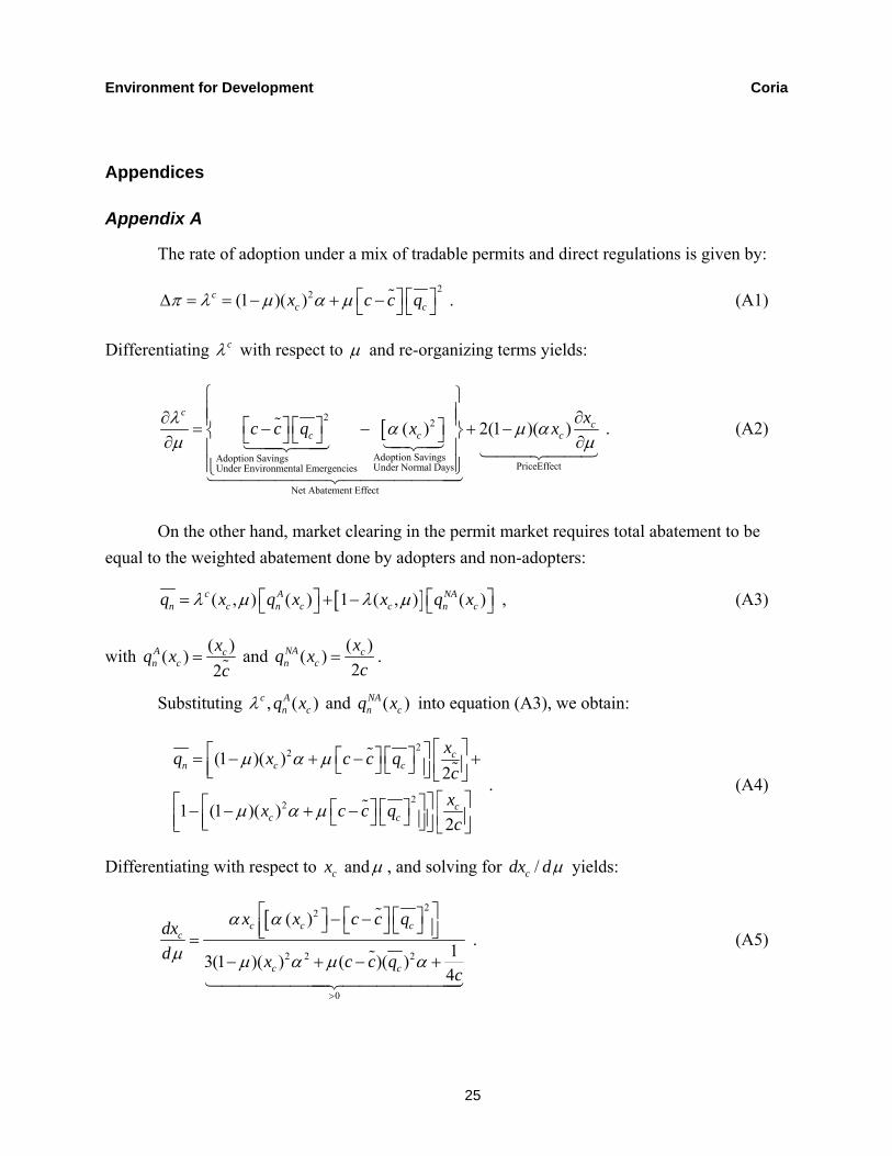
Appendix A

The rate of adoption under a mix of tradable permits and direct regulations is given by:

22(1 )( )cc cx c c qπ λ μ α μ ⎡ ⎤ ⎡ ⎤Δ = = − + −⎣ ⎦ ⎣ ⎦

% . (A1)

Differentiating cλ with respect to μ and re-organizing terms yields:

[2 2

Adoption SavingsAdoption SavingsPriceEffectUnder Normal DaysUnder Environmental Emergencies


( ) 2(1 )( )c

cc c c

xc c q x xλ α μ αμ μ

⎧ ⎫⎪ ⎪ ∂∂ ⎪ ⎪⎡ ⎤ ⎡ ⎤ ⎤= − − + −⎨ ⎬⎦⎣ ⎦ ⎣ ⎦∂ ∂⎪ ⎪

⎪⎪ ⎭⎩

%142431442443

1444444244444443

1442443

. (A2)

On the other hand, market clearing in the permit market requires total abatement to be equal to the weighted abatement done by adopters and non-adopters:

[ ]( , ) ( ) 1 ( , ) ( )c A NAn c n c c n cq x q x x q xλ μ λ μ⎡ ⎤ ⎡ ⎤= + −⎣ ⎦ ⎣ ⎦ , (A3)

with ( )( )2

A cn c

xq xc

=%

and ( )( )2

NA cn c

xq xc

= .

Substituting , ( )c An cq xλ and ( )NA

n cq x into equation (A3), we obtain:

22

22

(1 )( )2

1 (1 )( )2

cn c c

cc c

xq x c c qcxx c c qc

μ α μ

μ α μ

⎡ ⎤⎡ ⎤⎡ ⎤ ⎡ ⎤= − + − +⎢ ⎥⎣ ⎦ ⎣ ⎦⎢ ⎥⎣ ⎦ ⎣ ⎦⎡ ⎤⎡ ⎤⎡ ⎤⎡ ⎤ ⎡ ⎤− − + − ⎢ ⎥⎣ ⎦ ⎣ ⎦⎢ ⎥⎢ ⎥⎣ ⎦⎣ ⎦ ⎣ ⎦

%%

% . (A4)

Differentiating with respect to cx andμ , and solving for /cdx dμ yields:

[22

2 2 2

0

( )

13(1 )( ) ( )( )4

c c cc

c c

x x c c qdxd x c c q

c

α α

μ μ α μ α

>

⎡ ⎤⎡ ⎤ ⎡ ⎤⎤ − −⎦ ⎣ ⎦ ⎣ ⎦⎢ ⎥⎣ ⎦=− + − +

%

%

14444444244444443

. (A5)


26

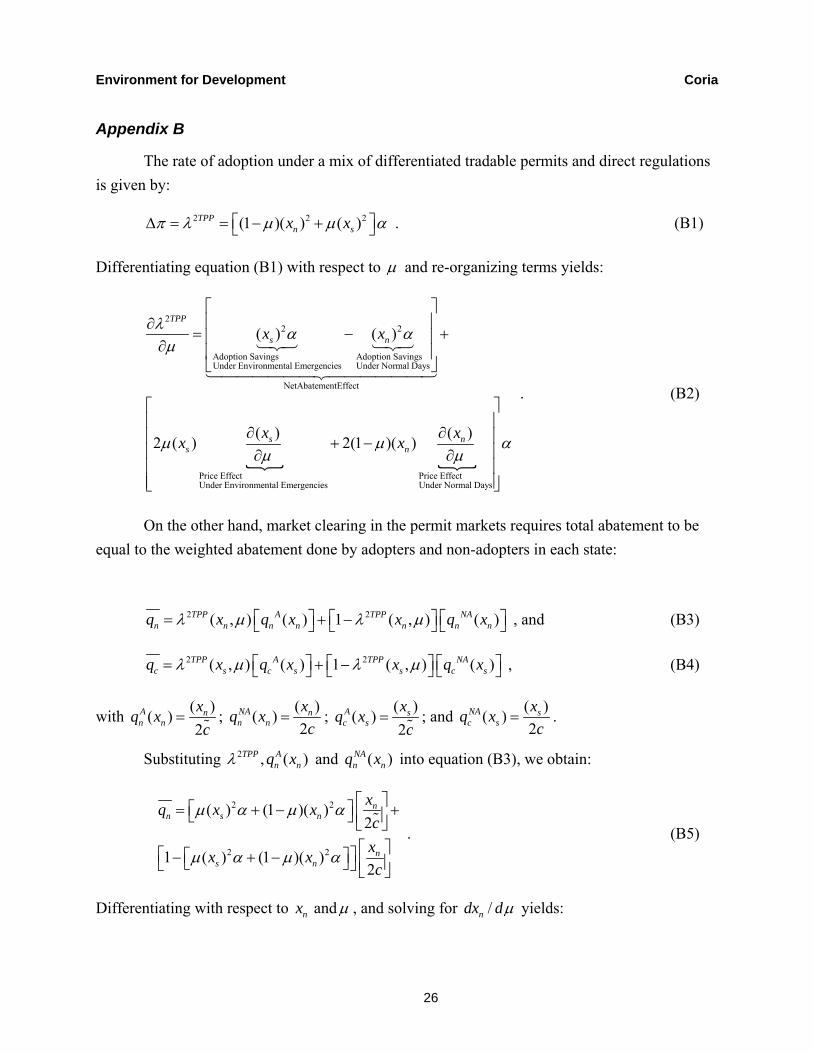
Appendix B

The rate of adoption under a mix of differentiated tradable permits and direct regulations is given by:

2 2 2(1 )( ) ( )TPPn sx xπ λ μ μ α⎡ ⎤Δ = = − +⎣ ⎦ . (B1)

Differentiating equation (B1) with respect to μ and re-organizing terms yields:

22 2

Adoption Savings Adoption SavingsUnder Environmental Emergencies Under Normal Days

NetAbatementEffect

Price EffectUnder Environmental Eme

( ) ( )

( )2 ( )

TPP

s n

ss

x x

xx

λ α αμ

μμ

⎡ ⎤⎢ ⎥∂

= − +⎢ ⎥∂ ⎢ ⎥⎣ ⎦

∂∂

123 123

144444424444443

{ {Price Effect

rgencies Under Normal Days

( )2(1 )( ) nn

xxμ αμ

⎡ ⎤⎢ ⎥

∂⎢ ⎥+ −⎢ ⎥∂⎢ ⎥⎢ ⎥⎣ ⎦

. (B2)

On the other hand, market clearing in the permit markets requires total abatement to be equal to the weighted abatement done by adopters and non-adopters in each state:

2 2( , ) ( ) 1 ( , ) ( )TPP A TPP NAn n n n n n nq x q x x q xλ μ λ μ⎡ ⎤ ⎡ ⎤ ⎡ ⎤= + −⎣ ⎦ ⎣ ⎦ ⎣ ⎦ , and (B3)

2 2( , ) ( ) 1 ( , ) ( )TPP A TPP NAc s c s s c sq x q x x q xλ μ λ μ⎡ ⎤ ⎡ ⎤ ⎡ ⎤= + −⎣ ⎦ ⎣ ⎦ ⎣ ⎦ , (B4)

with ( )( )2

A nn n

xq xc

=%

; ( )( )2

NA nn n

xq xc

= ; ( )( )2

A sc s

xq xc

=%

; and ( )( )2

NA sc s

xq xc

= .

Substituting 2 , ( )TPP An nq xλ and ( )NA

n nq x into equation (B3), we obtain:

2 2

2 2

( ) (1 )( )2

1 ( ) (1 )( )2

nn s n

ns n

xq x xcxx xc

μ α μ α

μ α μ α

⎡ ⎤⎡ ⎤= + − +⎣ ⎦ ⎢ ⎥⎣ ⎦⎡ ⎤⎡ ⎤⎡ ⎤− + −⎣ ⎦ ⎢ ⎥⎣ ⎦ ⎣ ⎦

% . (B5)

Differentiating with respect to nx andμ , and solving for /ndx dμ yields:


27

2 2

2 2 2 2

2 ( ) ( )012 ( ) 6(1 )( )

2

n s nn

s n

x x xdxd x x

c

α α α

μ μ α μ α

⎡ ⎤−⎣ ⎦= − <+ − +

. (B6)

Substituting 2 , ( )TPP Ac sq xλ , and ( )NA

c sq x into equation (B3), we obtain:

2 2

2 2

( ) (1 )( )2

1 ( ) (1 )( )2

sc s n

ss n

xq x xcxx xc

μ α μ α

μ α μ α

⎡ ⎤⎡ ⎤= + − +⎣ ⎦ ⎢ ⎥⎣ ⎦⎡ ⎤⎡ ⎤⎡ ⎤− + −⎣ ⎦ ⎢ ⎥⎣ ⎦ ⎣ ⎦

% . (B7)

Differentiating with respect to sx andμ , and solving for /sdx dμ yields:

2 2

2 2 2 2

2 ( ) ( )012(1 )( ) 6 ( )

2

s s ns

n s

x x xdxd x x

c

α α α

μ μ α μ α

⎡ ⎤−⎣ ⎦= − <− + +

. (B8)

Substituting equations (B6) and (B8) into equation (B2) yields:

22 2


2 2 2 2

2 2 2 2

Price EffectUnder Contingencies

( ) ( )

( ) ( ) ( ) ( ) ( ) ( )2 ( ) 2(1 ) ( )13 ( ) (1 )( ) 3(1 )(

4

TPP

s n

s s n n s ns n

s n

x x

x x x x x xx x

x xc

λ α αμ

α α α α α αμα μ α

μ α μ α μ

∂ ⎡ ⎤= − −⎣ ⎦∂

⎡ ⎤ ⎡ ⎤− −⎣ ⎦ ⎣ ⎦+ −+ − + −

144424443

14444444244444443

2 2 2 2

Price EffectUnder Normal Days

1) ( )4n sx x

cα μ α

⎡ ⎤⎢ ⎥⎢ ⎥⎢ ⎥⎢ ⎥

+ +⎢ ⎥⎢ ⎥⎢ ⎥⎣ ⎦

144444424444443

(B9)


28

Appendix C

The effect of changes in the incidence of environmental emergencies on the rate of adoption is given by:

{ [ }[

22 2 22 2

2 2 2

Net Abament Effect

Price Effect

2(1 )( ) ( )( ) 13(1 )( ) ( )( )

4

c cc c

c cc

c

x x c c qc c q x

x c c qc

μ α αλ αμ μ α μ α

⎡ ⎤⎡ ⎤ ⎡ ⎤⎤− − −⎦ ⎣ ⎦ ⎣ ⎦∂ ⎢ ⎥⎣ ⎦⎡ ⎤ ⎡ ⎤ ⎤= − − +⎦⎣ ⎦ ⎣ ⎦∂ − + − +

%%

%144442444431444444442444444443

. (C1)

Let 0β denote the “net abatement effect,” and 21 ( )cxβ α= and 2

2 ( )cc c qβ ⎡ ⎤= −⎣ ⎦% the

adoption savings under permits and under the emissions standard, respectively. Then, equation (C1) can be rewritten as:

10

1 2

21 01 13

(1 ) 4

c

c

β αλ βμ β α β μα

μ

⎡ ⎤⎢ ⎥∂ ⎢ ⎥= − =

∂ ⎡ ⎤⎢ ⎥+ +⎢ ⎥⎢ ⎥− ⎣ ⎦ ⎦⎣

. (C2)

Computing equation (C2) when 0μ → yields:

10 0

1

2| 1 134

c

c

μβ αλ β

μ β α=

⎡ ⎤⎢ ⎥∂

→ −⎢ ⎥∂ ⎢ ⎥+⎢ ⎦⎣

. (C3)

On the other hand, if a mixed system of tradable permits is used, this effect is given by:


29

22 2


2 2 2 2 2 2 2 2

2 2 2 2

Price EffectEnvironmental Emergencies

( ) ( )

2 ( ) ( ) ( ) 2(1 ) ( ) ( ) ( )13 ( ) (1 )( ) 3(1 )(4

TPP

s n

s s n n s n

s n n

x x

x x x x x x

x x xc

λ α αμ

μα α α μ α α α

μ α μ α μ

∂ ⎡ ⎤= − −⎣ ⎦∂

⎡ ⎤ ⎡ ⎤− − −⎣ ⎦ ⎣ ⎦++ − + −

144424443

144444424444443

2 2 2 2

Price EffectNormal Days

1) ( )4sx

cα μ α

⎡ ⎤⎢ ⎥⎢ ⎥⎢ ⎥⎢ ⎥

+ +⎢ ⎥⎢ ⎥⎢ ⎥⎣ ⎦

144444424444443

. (C4)

Let 0γ denote the “net abatement effect,” and 21 ( )nxγ α= and 2

2 ( )Sxγ α= the adoption

savings during normal days and during environmental emergencies, respectively. Then 2TPPλμ

∂∂

can be re-written as:

22 1

0

2 1 1 2

2 211 1 1 13 (1 ) 3

4 (1 ) 4

TTP

c c

αγ αγλ γμ αγ μ αγ αγ μαγ

μ μ

⎡ ⎤⎢ ⎥∂ ⎢ ⎥= − −

∂ ⎡ ⎤ ⎡ ⎤⎢ ⎥+ − + + +⎢ ⎥ ⎢ ⎥⎢ ⎥−⎣ ⎦ ⎣ ⎦ ⎦⎣

. (C5)

Computing equation (C5) when 0μ → yields:

21

0 0

1

2| 1 134

TPP

c

μαγλ γ

μ αγ=

⎡ ⎤⎢ ⎥∂

→ −⎢ ⎥∂ ⎢ ⎥+⎣ ⎦

. (C6)

Let us compare equations (C3) and (C6). Since 1 1β γ> , the absolute value of the price

effect under a mix of tradable permits and emission standards is higher:

1 1

1 1

2 21 13 34 4c c

β α αγ

β α αγ>

+ + . (C7)

On the other hand, 0 0γ β> since ( ) ( )c nx x≥ and 2 2( )( ) ( )c sc c q x− <% . Then:


30

1 10 0

1 1

2 21 11 13 34 4c c

β α αγβ γβ α αγ

⎡ ⎤ ⎡ ⎤⎢ ⎥ ⎢ ⎥− < −⎢ ⎥ ⎢ ⎥

⎢ ⎥ ⎢ ⎥+ +⎢ ⎦ ⎣ ⎦⎣

. (C8)

In other words, the effect of changes in the incidence of environmental emergencies on the rate of adoption is higher under the mixed system of tradable permits when 0μ → ; i.e.,

2

0 0| |c TPP


∂ ∂<

∂ ∂ .

Appendix D

Social welfare is given by the following expression:

[ ]

2 2 20 1

2 2 20 1

0

[ (1 ) ] [ (1 ) ] ( ) (1 ) ( )

1 [ (1 ) ] [ (1 ) ] ( ) (1 ) ( )



W q q q q c q c q

q q q q c q c q kdkλ

μ γ λ λ γ λ λ λ λ

μ β λ λ β λ λ λ λ

⎡ ⎤= + − − + − − − −⎣ ⎦

⎡ ⎤+ − + − − + − − − − −⎣ ⎦ ∫

%

%.

(D1)

Maximizing equation (D1) with respect to [ , , , ]c c n

A NA A NAnq q q q λ , we obtain the following

FOCs:

0 1: 2 (1 ) 2 ( )A A NA Ac c c cq q q c qγ γ λ λ⎡ ⎤− + − =⎣ ⎦

% , (D2)

0 1: 2 (1 ) 2 ( )NA A NA NAc c c cq q q c qγ γ λ λ⎡ ⎤− + − =⎣ ⎦ , (D3)

0 1: 2 (1 ) 2 ( )A A NA An n n nq q q c qβ β λ λ⎡ ⎤− + − =⎣ ⎦

% , (D4)

0 1: 2 (1 ) 2 ( )NA A NA NAn n n nq q q c qβ β λ λ⎡ ⎤− + − =⎣ ⎦ , and (D5)

[ ]

2 20 1

2 20 1

: [ ] 2 [ ] ( ) ( )

1 [ ] 2 [ ] ( ) ( )

A NA A NA NA Ac c c c c c

A NA A NA NA An n n n n n

q q A q q c q c q

q q B q q c q c q

λ λ μ γ γ

μ β β

⎡ ⎤= − − − + −⎣ ⎦⎡ ⎤+ − − − − + −⎣ ⎦

%

% , (D6)

where (1 )A NAc cA q qλ λ⎡ ⎤= + −⎣ ⎦ and (1 )A NA

n nB q qλ λ⎡ ⎤= + −⎣ ⎦ are the total level of abatement during

environmental emergencies and normal days, respectively.


31

From equations (D2) and (D3), we have that:

2 ( ) 2 ( )A NAc c cc q c q δ= =% . (D7)

Substituting equation (C7) into equation (C2), we have that:

0 12 cAγ γ δ− = . (D8)

From equations (D4) and (D5), we have that:

2 ( ) 2 ( )A NAn n nc q c q δ= =% . (D9)

Substituting equation (D9) into equation (D4), we have that:

0 12 nBβ β δ− = . (D10)

Substituting equations (D8) and (D10) into equation (D6), we have that:

[ ]2 2 2 2[ ] ( ) ( ) 1 [ ] ( ) ( )A NA NA A A NA NA Ac c c c c n n n n nq q c q c q q q c q c qλ μ δ μ δ⎡ ⎤ ⎡ ⎤= − + − + − − + −⎣ ⎦ ⎣ ⎦

% % . (D11)

Finally, substituting equations (D7) and (D9) into equation (D11), we have that:

2 2( ) (1 )( )c nλ μ δ μ δ α⎡ ⎤= + −⎣ ⎦ , (D12)

and since c cxδ = and n nxδ = ,

2 2( ) (1 )( )c nx xλ μ μ α⎡ ⎤= + −⎣ ⎦ (D13)

as it is stated in equation (24).

unintended impacts of multiple instruments on technological adoption

Documents