translational bioinformatics
TRANSCRIPT

Translational Bioinformatics ploscollections.org/translationalbioinformatics
'Translational Bioinformatics' is a collection of PLOS Computational Biology Education articles which reads as a "book" to be used as a reference or tutorial for a graduate level introductory course on the science of translational bioinformatics. Translational bioinformatics is an emerging field that addresses the current challenges of integrating increasingly voluminous amounts of molecular and clinical data. Its aim is to provide a better understanding of the molecular basis of disease, which in turn will inform clinical practice and ultimately improve human health. The concept of a translational bioinformatics introductory book was originally conceived in 2009 by Jake Chen and Maricel Kann. Each chapter was crafted by leading experts who provide a solid introduction to the topics covered, complete with training exercises and answers. The rapid evolution of this field is expected to lead to updates and new chapters that will be incorporated into this collection. Collection editors: Maricel Kann, Guest Editor, and Fran Lewitter, PLOS Computational Biology Education Editor.
Table of Contents
Introduction to Translational Bioinformatics Collection Russ B. Altman PLOS Computational Biology: published 27 Dec 2012 | info:doi/10.1371/journal.pcbi.1002796
Chapter 1: Biomedical Knowledge Integration Philip R. O. Payne PLOS Computational Biology: published 27 Dec 2012 | info:doi/10.1371/journal.pcbi.1002826
Chapter 2: Data-Driven View of Disease Biology Casey S. Greene, Olga G. Troyanskaya PLOS Computational Biology: published 27 Dec 2012 | info:doi/10.1371/journal.pcbi.1002816
Chapter 3: Small Molecules and Disease David S. Wishart PLOS Computational Biology: published 27 Dec 2012 | info:doi/10.1371/journal.pcbi.1002805
Chapter 4: Protein Interactions and Disease Mileidy W. Gonzalez, Maricel G. Kann PLOS Computational Biology: published 27 Dec 2012 | info:doi/10.1371/journal.pcbi.1002819

Chapter 5: Network Biology Approach to Complex Diseases Dong-Yeon Cho, Yoo-Ah Kim, Teresa M. Przytycka PLOS Computational Biology: published 27 Dec 2012 | info:doi/10.1371/journal.pcbi.1002820
Chapter 6: Structural Variation and Medical Genomics Benjamin J. Raphael PLOS Computational Biology: published 27 Dec 2012 | info:doi/10.1371/journal.pcbi.1002821
Chapter 7: Pharmacogenomics Konrad J. Karczewski, Roxana Daneshjou, Russ B. Altman PLOS Computational Biology: published 27 Dec 2012 | info:doi/10.1371/journal.pcbi.1002817
Chapter 8: Biological Knowledge Assembly and Interpretation Ju Han Kim PLOS Computational Biology: published 27 Dec 2012 | info:doi/10.1371/journal.pcbi.1002858
Chapter 9: Analyses Using Disease Ontologies Nigam H. Shah, Tyler Cole, Mark A. Musen PLOS Computational Biology: published 27 Dec 2012 | info:doi/10.1371/journal.pcbi.1002827
Chapter 10: Mining Genome-Wide Genetic Markers Xiang Zhang, Shunping Huang, Zhaojun Zhang, Wei Wang PLOS Computational Biology: published 27 Dec 2012 | info:doi/10.1371/journal.pcbi.1002828
Chapter 11: Genome-Wide Association Studies William S. Bush, Jason H. Moore PLOS Computational Biology: published 27 Dec 2012 | info:doi/10.1371/journal.pcbi.1002822
Chapter 12: Human Microbiome Analysis Xochitl C. Morgan, Curtis Huttenhower PLOS Computational Biology: published 27 Dec 2012 | info:doi/10.1371/journal.pcbi.1002808
Chapter 13: Mining Electronic Health Records in the Genomics Era Joshua C. Denny PLOS Computational Biology: published 27 Dec 2012 | info:doi/10.1371/journal.pcbi.1002823
Chapter 14: Cancer Genome Analysis Miguel Vazquez, Victor de la Torre, Alfonso Valencia PLOS Computational Biology: published 27 Dec 2012 | info:doi/10.1371/journal.pcbi.1002824
Chapter 15: Disease Gene Prioritization Yana Bromberg PLOS Computational Biology: published 25 Apr 2013 | info:doi/10.1371/journal.pcbi.1002902
Chapter 16: Text Mining for Translational Bioinformatics K. Bretonnel Cohen, Lawrence E. Hunter PLOS Computational Biology: published 25 Apr 2013 | info:doi/10.1371/journal.pcbi.1003044

Chapter 17: Bioimage Informatics for Systems Pharmacology Fuhai Li, Zheng Yin, Guangxu Jin, Hong Zhao, Stephen T. C. Wong PLOS Computational Biology: published 25 Apr 2013 | info:doi/10.1371/journal.pcbi.1003043
Collection page URL: www.ploscollections.org/translationalbioinformatics
Education
Introduction to Translational Bioinformatics CollectionRuss B. Altman*
Department of Genetics, Stanford University, Stanford, California, United States of America
This article is part of the ‘‘Transla-
tional Bioinformatics’’ collection for
PLOS Computational Biology.
How should we define translational
bioinformatics? I had to answer this
question unambiguously in March 2008
when I was asked to deliver a review of
‘‘recent progress in translational bioinfor-
matics’’ at the American Medical Infor-
matics Association’s Summit on Transla-
tional Bioinformatics. The lecture
required me to define papers in the field,
and then highlight exciting progress that
occurred over the previous ,12 months. I
have repeated this for the last few years,
and the most difficult part of the exercise is
limiting my review only to those papers
that are within the field.
I have never worried much about
definitions within informatics fields; they
tend to overlap, merge and evolve.
‘‘Informatics’’ seems clear: the study of
how to represent, store, search, retrieve
and analyze information. The adjectives in
front of ‘‘informatics’’ vary but also tend to
make sense: medical informatics concerns
medical information, bioinformatics con-
cerns basic biological information, clinical
informatics focuses on the clinical delivery
part of medical informatics, biomedical
informatics merges bioinformatics and
medical informatics, imaging informatics
focuses on…images, and so on. So what
does this adjective ‘‘translational’’ denote?
Translational medical research has
emerged as an important theme in the
last decade. Starting with top-down lead-
ership from the National Institutes of
Health and its former Director, Dr. Elias
Zerhouni, and moving through academic
medical centers, research institutes and
industrial research and development ef-
forts, there has been interest in more
effectively moving the discoveries and
innovations in the laboratory to the
bedside, leading to improved diagnosis,
prognosis, and treatment. Translational
research encompasses many activities in-
cluding the creation of medical devices,
molecular diagnostics, small molecule
therapeutics, biological therapeutics, vac-
cines, and others. One of the main targets
of translation, however, is revolutionary
explosion of knowledge in molecular
biology, genetics, and genomics. Some
believe that the tremendous progress in
discovery over the last 50+ years since
elucidation of the double helix structure
has not translated (there’s that word!) into
much practical health benefit. While the
accuracy of this claim can be debated,
there can be no debate that our ability to
measure (1) DNA sequence (including
entire genomes!), (2) RNA sequence and
expression, (3) protein sequence, structure,
expression and modification, and (4) small
molecule metabolite structure, presence,
and quantity has advanced rapidly and
enables us to imagine fantastic new
technologies in pursuit of human health.
There are many barriers to translating
our molecular understanding into technol-
ogies that impact patients. These include
understanding health market size and
forces, the regulatory milieu, how to
harden the technology for routine use,
and how to navigate an increasingly
complex intellectual property landscape.
But before those activities can begin, we
must overcome an even more fundamental
barrier: connecting the stuff of molecular
biology to the clinical world. Molecular
and cellular biology studies genes, DNA,
RNA messengers, microRNAs, proteins,
signaling molecules and their cascades,
metabolites, cellular communication pro-
cesses and cellular organization. These
data are freely available in valuable
resources such as Genbank (http://www.
ncbi.nlm.nih.gov/genbank/), Gene Ex-
pression Omnibus (http://www.ncbi.nlm.
nih.gov/geo/), Protein Data Bank (http://
www.wwpdb.org/), KEGG (http://www.
genome.jp/kegg/), MetaCyc (http://
metacyc.org/), Reactome (http://www.
reactome.org), and many other resources.
The clinical world studies diseases, signs,
symptoms, drugs, patients, clinical labora-
tory measurements, and clinical images.
The emergence of clinical and health
information technologies has begun to
make these clinical data available for
research through biobanks, electronic
medical records, FDA resources about
drug labels and adverse events, and claims
data. Therefore, a major challenge for
translational medicine is to connect the
molecular/cellular world with the clinical
world. The published literature, available
in PubMED (http://www.ncbi.nlm.nih.
gov/pubmed), does this, as does the
Unified Medical Language System
(UMLS) that provides a lingua franca
(http://www.nlm.nih.gov/research/umls/
). However, it falls to translational bioin-
formatics to engineer the tools that link
molecular/cellular entities and clinical
entities. Thus, I define ‘‘translational
bioinformatics’’ research as the develop-
ment and application of informatics meth-
ods that connect molecular entities to
clinical entities.
In this collection, Dr. Kann and col-
leagues have assembled a wonderful group
of authors to introduce the key threads of
translational bioinformatics to those new
to the field. The collection first provides
concepts in the field, and then introduces
some of the key methods for informatics
discovery and applications. Just by exam-
ining the table of contents on the collec-
tion page (http://www.ploscollections.
org/translationalbioinformatics), it is clear
that many exciting and emerging health
topics are squarely within the scope of
translational bioinformatics: cancer, phar-
macogenomics, medical genetics, small
molecule drugs, and diseases of protein
malfunction. There is an unmistakable
Citation: Altman RB (2012) Introduction to Translational Bioinformatics Collection. PLoS Comput Biol 8(12):e1002796. doi:10.1371/journal.pcbi.1002796
Editor : Fran Lewitter, Whitehead Institute, United States of America and Maricel Kann, University of Maryland,Baltimore County, United States of America
Published December , 2012
Copyright: � 2012 Russ B. Altman. This is an open-access article distributed under the terms of the CreativeCommons Attribution License, which permits unrestricted use, distribution, and reproduction in any medium,provided the original author and source are credited.
Funding: The author received no specific funding for writing this article.
Competing Interests: The author has declared that no competing interests exist.
* E-mail: [email protected]
PLOS Computational Biology | www.ploscompbiol.org 1 December 2012 | Volume 8 | Issue 12 | e1002796
a conceptual overview of the key data and
s
27

flavor of personalized medicine here as
well (genome association studies, mining
genetic markers, personal genomic data
analysis, data mining of electronic rec-
ords): our molecular and clinical data
resources are now allowing us to consider
individual variations, and not simply
population averages. I congratulate the
editors and authors on creating an impor-
tant collection of articles, and welcome the
reader to an exciting field whose challeng-
es and promise are unbounded.
PLOS Computational Biology | www.ploscompbiol.org 2 December 2012 | Volume 8 | Issue 12 | e1002796
Education
Chapter 1: Biomedical Knowledge IntegrationPhilip R. O. Payne*
The Ohio State University, Department of Biomedical Informatics, Columbus, Ohio, United States of America
Abstract: The modern biomedicalresearch and healthcare delivery do-mains have seen an unparalleledincrease in the rate of innovationand novel technologies over the pastseveral decades. Catalyzed by para-digm-shifting public and private pro-grams focusing upon the formationand delivery of genomic and person-alized medicine, the need for high-throughput and integrative ap-proaches to the collection, manage-ment, and analysis of heterogeneousdata sets has become imperative. Thisneed is particularly pressing in thetranslational bioinformatics domain,where many fundamental researchquestions require the integration oflarge scale, multi-dimensional clinicalphenotype and bio-molecular datasets. Modern biomedical informaticstheory and practice has demonstrat-ed the distinct benefits associatedwith the use of knowledge-basedsystems in such contexts. A knowl-edge-based system can be defined asan intelligent agent that employs acomputationally tractable knowledgebase or repository in order to reasonupon data in a targeted domain andreproduce expert performance rela-tive to such reasoning operations.The ultimate goal of the design anduse of such agents is to increase thereproducibility, scalability, and acces-sibility of complex reasoning tasks.Examples of the application of knowl-edge-based systems in biomedicinespan a broad spectrum, from theexecution of clinical decision support,to epidemiologic surveillance of pub-lic data sets for the purposes ofdetecting emerging infectious diseas-es, to the discovery of novel hypoth-eses in large-scale research data sets.In this chapter, we will review thebasic theoretical frameworks thatdefine core knowledge types andreasoning operations with particularemphasis on the applicability of suchconceptual models within the bio-medical domain, and then go on tointroduce a number of prototypicaldata integration requirements andpatterns relevant to the conduct oftranslational bioinformatics that canbe addressed via the design and useof knowledge-based systems.
This article is part of the ‘‘Transla-
tional Bioinformatics’’ collection for
PLOS Computational Biology.
1. Introduction
The modern biomedical research do-
main has experienced a fundamental shift
towards integrative and translational
methodologies and frameworks over the
past several years. A common thread
throughout the translational sciences are
needs related to the collection, manage-
ment, integration, analysis and dissemina-
tion of large-scale, heterogeneous biomed-
ical data sets. However, well-established
and broadly adopted theoretical and
practical frameworks intended to address
such needs are still largely developmental
[1–3]. Instead, the development and
execution of multi-disciplinary, transla-
tional science programs is significantly
limited by the propagation of ‘‘silos’’ of
both data and knowledge, and a paucity of
reproducible and rigorously validated
methods that may be used to support the
satisfaction of motivating and integrative
translational bioinformatics use cases, such
as those focusing on the identification of
expression motifs spanning bio-molecules
and clinical phenotypes.
In order to provide sufficient context
and scope to our ensuing discussion, we
will define translational science and re-
search per the conventions provided by
the National Institutes of Health (NIH) as
follows:
‘‘Translational research includes
two areas of translation. One is the process
of applying discoveries generated during
research in the laboratory, and in preclin-
ical studies, to the development of trials and
studies in humans. The second area of
translation concerns research aimed at
enhancing the adoption of best practices in
the community. Cost-effectiveness of pre-
vention and treatment strategies is also an
important part of translational science.’’
[4]
Several recent publications have defined
a translational research cycle, which
involves the translational of knowledge
and evidence from ‘‘the bench’’ (e.g.,
laboratory-based discoveries) to ‘‘the bed-
side’’ (e.g., clinical or public health inter-
ventions informed by basic science and
clinical research), and reciprocally from
‘‘the bedside’’ back to ‘‘the bench’’ (e.g.,
basic science studies informed by observa-
tions from the point-of-care) [5]. Within
this translational cycle, Sung and col-
leagues [5] have defined two critical
blockages that exist between basic science
discovery and the design of prospective
clinical studies, and subsequently between
the knowledge generated during clinical
studies and the provision of such evidence-
based care in the clinical or public health
settings. These are known as the T1 and
T2 blocks, respectively. Much of the work
conducted under the auspices of the NIH
Roadmap initiative and more recently as
part of the Clinical and Translational
Science Award (CTSA) program is specif-
ically focused on identifying approaches or
policies that can mitigate these T1 and T2
blockages, and thus increase the speed and
efficiency by which new biomedical knowl-
edge can be realized in terms of improved
health and patient outcomes.
The positive outcomes afforded by the
close coupling of biomedical informatics
Citation: Payne PRO (2012) Chapter 1: Biomedical Knowledge Integration. PLoS Comput Biol 8(12): e1002826.doi:10.1371/journal.pcbi.1002826
Editors: Fran Lewitter, Whitehead Institute, United States of America and Maricel Kann, University of Maryland,Baltimore County, United States of America
Published December , 2012
Copyright: � 2012 Philip R. O. Payne. This is an open-access article distributed under the terms of theCreative Commons Attribution License, which permits unrestricted use, distribution, and reproduction in anymedium, provided the original author and source are credited.
Funding: The author received no specific funding for this article.
Competing Interests: The author has declared that no competing interests exist.
* E-mail: [email protected]
PLOS Computational Biology | www.ploscompbiol.org 1 December 2012 | Volume 8 | Issue 12 | e1002826
27
with the translational sciences have been
described frequently in the published
literature [3,5–7]. Broadly, the critical
areas to be addressed by such informatics
approaches relative to translational re-
search activities and programs can be
classified as belonging to one or more of
the following categories:
The management of multi-dimen-sional and heterogeneous data sets:The modern healthcare and life sciences
ecosystem is becoming increasingly data
centric as a result of the adoption and
availability of high-throughput data sourc-
es, such as electronic health records
(EHRs), research data management sys-
tems (e.g., CTMS, LIMS, Electronic Data
Capture tools), and a wide variety of bio-
molecular scale instrumentation platforms.
As a result of this evolution, the size and
complexity of data sets that must be
managed and analyzed are growing at an
extremely rapid rate [1,2,6,8,9]. At the
same time, the data management practices
currently used in most research settings
are both labor intensive and rely upon
technologies that have not be designed to
handle such multi-dimensional data [9–
11]. As a result, there are significant
demands from the translational science
community for the creation and delivery of
information management platforms capa-
ble of adapting to and supporting hetero-
geneous workflows and data sources
[2,3,12,13]. This need is particularly
important when such research endeavors
focus on the identification of linkages
between bio-molecular and phenotypic
data in order to inform novel systems-level
approaches to understanding disease states.
Relative to the specific topic area of
knowledge representation and utilization in
the translational sciences, the ability to
address the preceding requirements is large-
ly predicated on the ability to ensure that
semantics of such data are well understood
[10,14,15]. This is a scenario often referred
to as semantic interoperability, and requires
the use of informatics-based approaches to
map among various data representations, as
well as the application of such mappings to
support integrative data integration and
analysis operations [10,15].
The application of knowledge-based systems and intelligent agentsto enable high-throughput hypothe-sis generation and testing: Modern
approaches to hypothesis discovery and
testing primarily are based on the intuition
of the individual investigator or his/her
team to identify a question that is of
interest relative to their specific scientific
aims, and then carry out hypothesis testing
operations to validate or refine that
question relative to a targeted data set
[6,16]. This approach is feasible when
working with data sets comprised of
hundreds of variables, but does not scale
to projects involving data sets with mag-
nitudes on the order of thousands or even
millions of variables [10,14]. An emerging
and increasingly viable solution to this
challenge is the use of domain knowledge
to generate hypotheses relative to the
content of such data sets. This type of
domain knowledge can be derived from
many different sources, such as public
databases, terminologies, ontologies, and
published literature [14]. It is important to
note, however, that methods and technol-
ogies that can allow researchers to access
and extract domain knowledge from such
sources, and apply resulting knowledge
extracts to generate and test hypotheses
are largely developmental at the current
time [10,14].
The facilitation of data-analyticpipelines in in-silico research pro-grams: The ability to execute in-silico
research programs, wherein hypotheses are
designed, tested, and validated in existing
data sets using computational methods, is
highly reliant on the use of data-analytic
‘‘pipelining’’ tools. Such pipelines are ideally
able to support data extraction, integration,
and analysis workflows spanning multiple
sources, while capturing intermediate data
analysis steps and products, and generating
actionable output types [17,18]. Such pipe-
lines provide a number of benefits, includ-
ing: 1) they support the design and execution
of data analysis plans that would not be
tractable or feasible using manual methods;
and 2) they provide for the capture meta-
data describing the steps and intermediate
products generated during such data anal-
yses. In the case of the latter benefit, the
ability to capture systematic meta-data is
critical to ensuring that such in-silico research
paradigms generate reproducible and high
quality results [17,18]. There are a number
of promising technology platforms capable
of supporting such data-analytic ‘‘pipelin-
ing’’, such as the caGrid middleware [18]. It
is of note, however, that widespread use of
such pipeline tools is not robust, largely due
to barriers to adoption related to data
ownership/security and socio-technical fac-
tors [13,19].
The dissemination of data, infor-mation, and knowledge generatedduring the course of translationalscience research programs: It is
widely held that the time period required
to translate a basic science discovery into
clinical research, and ultimately evidence-
based practice or public health interven-
tion can exceed 15 years [2,5,7,20]. A
number of studies have identified the lack
of effective tools for supporting the ex-
change of data, information, and knowl-
edge between the basic sciences, clinical
research, clinical practice, and public
health practice as one of the major
contributors to effective and timely trans-
lation of novel biological discoveries into
health benefits [2]. A number of informat-
ics-based approaches have been developed
to overcome such translational impedi-
ments, such as web-based collaboration
platforms, knowledge representation and
delivery standards, public data registries
and repositories [3,7,9,21]. Unfortunately,
the systematic and regular use of such
tools and methods is generally very
poor in the translational sciences, again
as was the prior case, due to a combina-
tion of governance and socio-technical
barriers.
At a high level, all of the aforemen-
tioned challenges and opportunities corre-
spond to an overarching set of problem
statements, as follows:
N Translational bioinformatics is defined
by the presence of complex, heteroge-
neous, multi-dimensional data sets;
N The scope of available biomedical
knowledge collections that may be
applied to assist in the integration
What to Learn in This Chapter
N Understand basic knowledge types and structures that can be applied tobiomedical and translational science;
N Gain familiarity with the knowledge engineering cycle, tools and methods thatmay be used throughout that cycle, and the resulting classes of knowledgeproducts generated via such processes;
N An understanding of the basic methods and techniques that can be used toemploy knowledge products in order to integrate and reason uponheterogeneous and multi-dimensional data sets; and
N Become conversant in the open research questions/areas related to the abilityto develop and apply knowledge collections in the translational bioinformaticsdomain.
PLOS Computational Biology | www.ploscompbiol.org 2 December 2012 | Volume 8 | Issue 12 | e1002826
and analysis of such data is growing at
a rapid pace;
N The ability to apply such knowledge
collections to translational bioinfor-
matics analyses requires an under-
standing of the sources of such knowl-
edge, and methods of applying them to
reasoning applications; and
N The application of knowledge collec-
tions to support integrative analyses in
the translational science domain intro-
duces multiple areas of complexity that
must be understood in order to enable
the optimal selection and use of such
resources and methods, as well as the
interpretation of results generated via
such applications.
2. Key Definitions
In the remainder of this chapter, we will
introduce a set of definitions, frameworks,
and methods that serve to support the
foundational knowledge integration re-
quirements incumbent to the efficient
and effective conduct of translational
studies. In order to provide a common
understanding of key terms and concepts
that will be used in the ensuing discussion,
we will define here a number of those
entities, using the broad context of Knowl-
edge Engineering (KE) as a basis for such
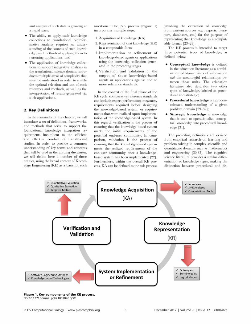
assertions. The KE process (Figure 1)
incorporates multiple steps:
1. Acquisition of knowledge (KA)
2. Representation of that knowledge (KR)
in a computable form
3. Implementation or refinement of
knowledge-based agents or applications
using the knowledge collection gener-
ated in the preceding stages
4. Verification and validation of the
output of those knowledge-based
agents or applications against one or
more reference standards.
In the context of the final phase of the
KE cycle, comparative reference standards
can include expert performance measures,
requirements acquired before designing
the knowledge-based system, or require-
ments that were realized upon implemen-
tation of the knowledge-based system. In
this regard, verification is the process of
ensuring that the knowledge-based system
meets the initial requirements of the
potential end-user community. In com-
parison, validation is the process of
ensuring that the knowledge-based system
meets the realized requirements of the
end-user community once a knowledge-
based system has been implemented [22].
Furthermore, within the overall KE pro-
cess, KA can be defined as the sub-process
involving the extraction of knowledge
from existent sources (e.g., experts, litera-
ture, databases, etc.) for the purpose of
representing that knowledge in a comput-
able format [23–28].
The KE process is intended to target
three potential types of knowledge, as
defined below:
N Conceptual knowledge is defined
in the education literature as a combi-
nation of atomic units of information
and the meaningful relationships be-
tween those units. The education
literature also describes two other
types of knowledge, labeled as proce-
dural and strategic;
N Procedural knowledge is a process-
oriented understanding of a given
problem domain [29–32];
N Strategic knowledge is knowledge
that is used to operationalize concep-
tual knowledge into procedural knowl-
edge [31].
The preceding definitions are derived
from empirical research on learning and
problem-solving in complex scientific and
quantitative domains such as mathematics
and engineering [30,32]. The cognitive
science literature provides a similar differ-
entiation of knowledge types, making the
distinction between procedural and de-
Figure 1. Key components of the KE process.doi:10.1371/journal.pcbi.1002826.g001
PLOS Computational Biology | www.ploscompbiol.org 3 December 2012 | Volume 8 | Issue 12 | e1002826
clarative knowledge. Declarative knowl-
edge is synonymous with conceptual
knowledge as defined above [33].
Conceptual knowledge collections are
perhaps the most commonly used knowl-
edge types in biomedicine. Such knowledge
and its representation span a spectrum that
includes ontologies, controlled terminolo-
gies, semantic networks and database sche-
mas. A reoccurring focus throughout dis-
cussions of conceptual knowledge collections
in the biomedical informatics domain is the
process of representing conceptual knowl-
edge in a computable form. In contrast, the
process of eliciting knowledge has received
less attention and reports on rigorous and
reproducible methods that may be used in
this area are rare. It is also important to note
that in the biomedical informatics domain
conceptual knowledge collections rarely
exist in isolation. Instead, they usually occur
within structures that contain multiple types
of knowledge. For example, a knowledge-
base used in a modern clinical decision
support system might include: (1) a knowl-
edge collection containing potential findings,
diagnoses, and the relationships between
them (conceptual knowledge), (2) a knowledge
collection containing guidelines or algo-
rithms used to logically traverse the previous
knowledge structure (procedural knowledge),
and (3) a knowledge structure containing
application logic used to apply or operatio-
nalize the preceding knowledge collections
(strategic knowledge). Only when these three
types of knowledge are combined, it is
possible to realize a functional decision
support system [34].
3. Underlying TheoreticalFrameworks
The theories that support the ability to
acquire, represent, and verify or validate
conceptual knowledge come from multiple
domains. In the following sub-section,
several of those domains will be discussed,
including:
N Computational science
N Psychology and cognitive science
N Semiotics
N Linguistics
3.1 Computational Foundations ofKnowledge Engineering
A critical theory that supports the ability
to acquire and represent knowledge in a
computable format is the physical symbol
hypothesis. First proposed by Newell and
Simon in 1981 [35], and expanded upon
by Compton and Jansen in 1989 [24], the
physical symbol hypothesis postulates that
knowledge consists of both symbols of
reality, and relationships between those
symbols. The hypothesis further argues
that intelligence is defined by the ability to
appropriately and logically manipulate
both symbols and relationships. A critical
component of this the theory is the
definition of what constitutes a ‘‘physical
symbol system’’, which Newell and Simon
describe as:
‘‘…a set of entities, called symbols, which
are physical patterns that can occur as
components of another type of entity called
an expression (or symbol structure). Thus,
a symbol structure is composed of a number
of instances (or tokens) of symbols related
in some physical way (such as one token
being next to another). At any instant of
time the system will contain a collection of
these symbol structures.’’ [36]
This preceding definition is very similar
to that of conceptual knowledge introduced
earlier in this chapter, which leads to the
observation that the computational repre-
sentation of conceptual knowledge collec-
tions should be well supported by compu-
tational theory. However, as described
earlier, there is not a large body of research
on reproducible methods for eliciting
such symbol systems. Consequently, the
elicitation of the symbols and relationships
that constitute a ‘‘physical symbol system’’,
or conceptual knowledge collection, re-
mains a significant challenge. This chal-
lenge, in turn, is an impediment to the
widespread use of conceptual knowledge-
based systems.
3.2 Psychological and CognitiveBasis for Knowledge Engineering
At the core of the currently accepted
psychological basis for KE is expertise
transfer, which is the theory that humans
transfer their expertise to computational
systems so that those systems are able to
replicate expert human performance.
One theory that helps explain the
process of expertise transfer is Kelly’s
Personal Construct Theory (PCT). This
theory defines humans as ‘‘anticipatory
systems’’, where individuals create tem-
plates, or constructs that allow them to
recognize situations or patterns in the
‘‘information world’’ surrounding them.
These templates are then used to antici-
pate the outcome of a potential action
given knowledge of similar previous expe-
riences [37]. Kelly views all people as
‘‘personal scientists’’ who make sense of
the world around them through the use of
a hypothetico-deductive reasoning system.
It has been argued within the KE
literature that the constructs used by
experts can be used as the basis for
designing or populating conceptual knowl-
edge collections [26]. The details of PCT
help to explain how experts create and use
such constructs. Specifically, Kelly’s fun-
damental postulate is that ‘‘a person’s
processes are psychologically channelized by the
way in which he anticipated events.’’ This is
complemented by the theory’s first corol-
lary, which is summarized by his statement
that:
‘‘Man looks at his world through transparent
templates which he creates and then attempts
to fit over the realities of which the world is
composed… Constructs are used for predic-
tions of things to come… The construct is a
basis for making a distinction… not a class of
objects, or an abstraction of a class, but a
dichotomous reference axis.’’
Building upon these basic concepts,
Kelly goes on to state in his Dichotomy
Corollary that ‘‘a person’s construction system is
composed of a finite number of dichotomous
constructs.’’ Finally, the parallel nature of
personal constructs and conceptual knowl-
edge is illustrated in Kelly’s Organization
Corollary, which states, ‘‘each person charac-
teristically evolves, for his convenience of antici-
pating events, a construction system embracing
ordinal relationships between constructs’’ [26,37].
Thus, in an effort to bring together
these core pieces of PCT, it can be argued
that personal constructs are essentially
templates applied to the creation of
knowledge classification schemas used in
reasoning. If such constructs are elicited
from experts, atomic units of information
can be defined, and the Organization
Corollary can be applied to generate
networks of ordinal relationships between
those units. Collectively, these arguments
serve to satisfy and reinforce the earlier
definition of conceptual knowledge, and
provide insight into the expert knowledge
structures that can be targeted when
eliciting conceptual knowledge.
There are also a number of cognitive
science theories that have been applied to
inform KE methods. Though usually very
similar to the preceding psychological
theories, cognitive science theories specif-
ically describe KE within a broader
context where humans are anticipatory
systems who engage in frequent transfers
of expertise. The cognitive science litera-
ture identifies expertise transfer pathways
as an existent medium for the elicitation of
knowledge from domain experts. This
conceptual model of expertise transfer is
PLOS Computational Biology | www.ploscompbiol.org 4 December 2012 | Volume 8 | Issue 12 | e1002826
often illustrated using the Hawkins
model for expert-client knowledge transfer
[38].
It is also important to note that at a high
level, cognitive science theories focus upon
the differentiation among knowledge types.
As described earlier, cognitive scientists
make a primary differentiation between
procedural knowledge and declarative
knowledge [31]. While cognitive science
theory does not necessarily link declarative
and procedural knowledge, an implicit
relationship is provided by defining proce-
dural knowledge as consisting of three
orders, or levels. For each level, the
complexity of declarative knowledge in-
volved in problem solving increases com-
mensurately with the complexity of proce-
dural knowledge being used [28,31,39].
A key difference between the theories
provided by the cognitive science and
psychology domains is that the cognitive
science literature emphasizes the impor-
tance of placing KA studies within appro-
priate context in order to account for the
distributed nature of human cognition
[25,40–46]. In contrast, the psychology
literature is less concerned with placing
KE studies in context.
3.3 Semiotic Basis for KnowledgeEngineering
Though more frequently associated
with the domains of computer science,
psychology and cognitive science, there
are a few instances where semiotic theory
has been cited as a theoretical basis for
KE. Semiotics can be broadly defined as
‘‘the study of signs, both individually and grouped
in sign systems, and includes the study of how
meaning is transmitted and understood’’ [47]. As
a discipline, much of its initial theoretical
basis is derived from the domain of
linguistics, and thus, has been traditionally
focused on written language. However, the
scope of contemporary semiotics literature
has expanded to incorporate the analysis
of meaning in visual presentation systems,
knowledge representation models and
multiple communication mediums. The
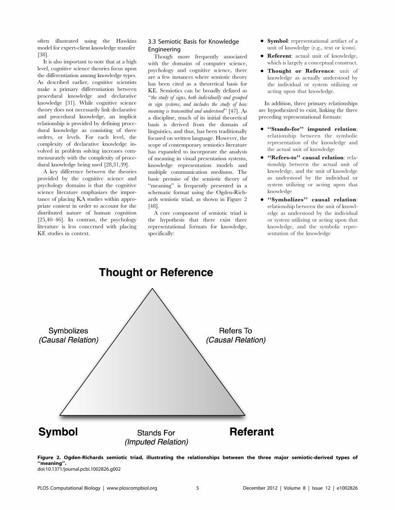
basic premise of the semiotic theory of
‘‘meaning’’ is frequently presented in a
schematic format using the Ogden-Rich-
ards semiotic triad, as shown in Figure 2
[48].
A core component of semiotic triad is
the hypothesis that there exist three
representational formats for knowledge,
specifically:
N Symbol: representational artifact of a
unit of knowledge (e.g., text or icons).
N Referent: actual unit of knowledge,
which is largely a conceptual construct.
N Thought or Reference: unit of
knowledge as actually understood by
the individual or system utilizing or
acting upon that knowledge.
In addition, three primary relationships
are hypothesized to exist, linking the three
preceding representational formats:
N ‘‘Stands-for’’ imputed relation:
relationship between the symbolic
representation of the knowledge and
the actual unit of knowledge
N ‘‘Refers-to’’ causal relation: rela-
tionship between the actual unit of
knowledge, and the unit of knowledge
as understood by the individual or
system utilizing or acting upon that
knowledge
N ‘‘Symbolizes’’ causal relation:
relationship between the unit of knowl-
edge as understood by the individual
or system utilizing or acting upon that
knowledge, and the symbolic repre-
sentation of the knowledge
Figure 2. Ogden-Richards semiotic triad, illustrating the relationships between the three major semiotic-derived types of‘‘meaning’’.doi:10.1371/journal.pcbi.1002826.g002
PLOS Computational Biology | www.ploscompbiol.org 5 December 2012 | Volume 8 | Issue 12 | e1002826
N The strength of these relationships is
usually evaluated using heuristic meth-
ods or criteria [48].
3.4 Linguistic Basis for KnowledgeEngineering
The preceding theories have focused
almost exclusively on knowledge that may
be elicited from domain experts. In
contrast, domain knowledge can also be
extracted through the analysis of existing
sources, such as collections of narrative
text or databases. Sub-language analysis
is a commonly described approach to the
elicitation of conceptual knowledge from
collections of text (e.g., narrative notes,
published literature, etc.). The theoretical
basis for sub-language analysis, known as
sub-language theory was first described
by Zellig Harris in his work concerning
the nature of language usage within
highly specialized domains [49]. A key
argument of his sub-language theory is
that language usage in such highly
specialized domains is characterized by
regular and reproducible structural fea-
tures and grammars [49,50]. At an
application level, these features and
grammars can be discovered through
the application of manual or automated
pattern recognition processes to large
corpora of language for a specific domain.
Once such patterns have been discovered,
templates may be created that describe
instances in which concepts and relation-
ships between those concepts are defined.
These templates can then be utilized to
extract knowledge from sources of lan-
guage, such as text [51]. The process of
applying sub-language analysis to existing
knowledge sources has been empirically
validated in numerous areas, including
the biomedical domain [50,51]. Within
the biomedical domain, sub-language
analysis techniques have been extended
beyond conventional textual language to
also include sub-languages that consist of
graphical symbols [52].
4. Knowledge Acquisition Toolsand Methods
While a comprehensive review of tools
and methods that may be used to facilitate
the knowledge acquisition (KA) is beyond
the scope of this chapter, in the following
section, we will briefly summarize example
cases of such techniques in order to
provide a general overview of this impor-
tant area of informatics research, develop-
ment, and applications.
As was introduced in the preceding
section, KA can be defined as the sub-process
involving the extraction of knowledge
from existent sources (e.g., experts, liter-
ature, databases, etc.) for the purpose of
representing that knowledge in a comput-
able format [23–28]. This definition also
includes the verification or validation of
knowledge-based systems that use the
resultant knowledge collections [27]. Be-
yond this basic definition of KA and its
relationships to KE, there are two critical
characteristics of contemporary ap-
proaches to KA that should be noted, as
follows:
N By convention within the biomedical
informatics domain, KA usually refers
to the process of eliciting knowledge
specifically for use in ‘‘knowledge-
bases’’ (KBs) that are integral to expert
systems or intelligent agents (e.g.,
clinical decision support systems).
However, a review of the literature
concerned with KA beyond this do-
main shows a broad variety of appli-
cation areas for KA, such as the
construction of shared database mod-
els, ontologies and human-computer
interaction models [23,53–57].
N Verification and validation methods
are often applied to knowledge-based
systems only during the final stage of
the KE process. However, such tech-
niques are most effective when em-
ployed iteratively throughout the en-
tire KE process. As such, they also
become necessary components of the
KA sub-process.
Given the particular emphasis of this
chapter on the use of conceptual knowledge
collections for the purpose of complex
integrative analysis tasks, it is important to
understand that the KA methods and tools
available to support the generation of
conceptual knowledge collections can be
broadly divided into three complementary
classes:
N Knowledge unit elicitation: tech-
niques for the elicitation of atomic
units of information or knowledge
N Knowledge relationship elicita-tion: techniques for the elicitation of
relationships between atomic units of
information or knowledge
N Combined elicitation: techniques
that elicit both atomic units of infor-
mation or knowledge, and the rela-
tionships that exist between them
There are a variety of commonly used
methods that target one or more above
these KA classes, as summarized below:
4.1 Informal and StructuredInterviewing
Interviews conducted either individually
or in groups can provide investigators with
insights into the knowledge used by
domain experts. Furthermore, they can
be performed either informally (e.g.,
conversational exchange between the in-
terviewer and subjects) or formally (e.g.,
structured using a pre-defined series of
questions). The advantages of utilizing
such interviewing techniques are that they
require a minimal level of resources, can
be performed in a relatively short time
frame, and can yield a significant amount
of qualitative knowledge. More detailed
descriptions of interviewing techniques are
provided in the methodological reviews
provided by Boy [58], Morgan [59], and
Wood [60].
4.2 Observational StudiesEthnographic evaluations, or observa-
tional studies are usually conducted in
context, with minimal researcher involve-
ment in the workflow or situation under
consideration. These observational meth-
ods generally focus on the evaluation of
expert performance, and the implicit
knowledge used by those experts. Exam-
ples of observational studies have been
described in many domains, ranging from
air traffic control systems to complex
healthcare workflows [61,62]. One of the
primary benefits of such observational
methods is that they are designed to
minimize potential biases (e.g., Hawthorne
effect [63]), while simultaneously allowing
for the collection of information in con-
text. Additional detail concerning specific
observational and ethnographic field study
methods can be found in the reviews
provided by John [62] and Rahat [64].
4.3 Categorical SortingThere are a number of categorical, or
card sorting techniques, including Q-sorts,
hierarchical sorts, all-in-one sorts and
repeated single criterion sorts [65]. All of
these techniques involve one or more
subjects sorting of a group of artifacts
(e.g., text, pictures, physical objects, etc.)
according to criteria either generated by
the sorter or provided by the researcher.
The objective of such methods is to
determine the reproducibility and stability
of the groups created by the sorters. In all
of these cases, sorters may also be asked to
assign names to the groups they create.
Categorical sorting methods are ideally
suited for the discovery of relationships
between atomic units of information or
knowledge. In contrast, such methods are
PLOS Computational Biology | www.ploscompbiol.org 6 December 2012 | Volume 8 | Issue 12 | e1002826
less effective for determining the atomic
units of information or knowledge. How-
ever, when sorters are asked to provide
names for their groups, this data may help
to define domain-specific units of knowl-
edge or information. Further details con-
cerning the conduct and analysis of
categorical sorting studies can be found
in the review provided by Rugg and
McGeorge [65].
4.4 Repertory Grid AnalysisRepertory grid analysis is a method
based on the previously introduced Per-
sonal Construct Theory (PCT). Repertory
grid analysis involves the construction of a
non-symmetric matrix, where each row
represents a construct that corresponds to
a distinction of interest, and each column
represents an element (e.g., unit of infor-
mation or knowledge) under consider-
ation. For each element in the grid, the
expert completing the grid provides a
numeric score using a prescribed scale
(defined by a left and right pole) for each
distinction, indicating the strength of
relatedness between the given element-
distinction pair. In many instances, the
description of the distinction being used in
each row of the matrix is stated differently
in the left and right poles, providing a
frame of reference for the prescribed
scoring scale. Greater detail on the
techniques used to conduct repertory grid
studies can be found in the review
provided by Gaines et al. [26].
4.5 Formal Concept AnalysisFormal concept analysis (FCA) has often
been described for the purposes of devel-
oping and merging ontologies [66,67].
FCA focuses on the discovery of ‘‘natural
clusters’’ of entities and entity-attribute
pairings [66], where attributes are similar
to the distinctions used in repertory grids.
Much like categorical sorting, FCA is
almost exclusively used for eliciting the
relationships between units of information
or knowledge. The conduct of FCA studies
involves two phases: (1) elicitation of
‘‘formal contexts’’ from subjects, and (2)
visualization and exploration of resulting
‘‘concept lattices’’. It is of interest to note
that the ‘‘concept lattices’’ used in FCA
are in many ways analogous to Sowa’s
Conceptual Graphs [68], which are com-
prised of both concepts and labeled
relationships. The use of Conceptual
Graphs has been described in the context
of KR [68–70], as well as a number of
biomedical KE instances [48,71–73].
Recent literature has described the use
of FCA in multi-dimensional ‘‘formal
contexts’’ (i.e., instances where relational
structures between conceptual entities
cannot be expressed as a single many-
valued ‘‘formal context’’). One approach
to the utilization of multi-dimensional
‘‘formal contexts’’ is the agreement con-
text model proposed by Cole and Becker
[67], which uses logic-based decomposi-
tion to partition and aggregate n-ary
relations. This algorithmic approach has
been implemented in a freely available
application named ‘‘Tupleware’’ [74].
Additionally, ‘‘formal contexts’’ may be
defined from existing data sources, such as
databases. These ‘‘formal contexts’’ are
discovered using data mining techniques
that incorporate FCA algorithms, such as
the open-source TOSCANA or CHIAN-
TI tools. Such algorithmic FCA methods
are representative examples of a sub-
domain known as Conceptual Knowledge
Discovery and Data Analysis (CKDD)
[75]. Additional details concerning FCA
techniques can be found in the reviews
provided by Cimiano et al. [66], Hereth et
al. [75], and Priss [76].
4.6 Protocol and Discourse AnalysisThe techniques of protocol and dis-
course analysis are very closely related.
Both techniques are concerned with the
elicitation of knowledge from individuals
while they are engaged in problem-solving
or reasoning tasks. Such analyses may be
performed to determine the unit of
information or knowledge, and relation-
ships between those units of information
or knowledge, used by individuals per-
forming tasks in the domain under study.
During protocol analysis studies, subjects
are requested to ‘‘think out loud’’ (i.e.,
vocalize internal reasoning and thought
processes) while performing a task. Their
vocalizations and actions are recorded
for later analysis. The recordings are then
codified at varying levels of granularity to
allow for thematic or statistical analysis
[77,78]. Similarly, discourse analysis is a
technique by which an individual’s in-
tended meaning within a body of text or
some other form of narrative discourse
(e.g., transcripts of a ‘‘think out loud’’
protocol analysis study) is ascertained by
atomizing that text or narrative into
discrete units of thought. These ‘‘thought
units’’ are then subject to analyses of
both the context in which they appear,
and the quantification and description of
the relationships between those units
[79,80]. Specific methodological ap-
proaches to the conduct of protocol and
discourse analysis studies can be found in
the reviews provided by Alvarez [79] and
Polson et al. [78].
4.7 Sub-Language AnalysisSub-language analysis is a technique for
discovering units of information or knowl-
edge, and the relationships between them
within existing knowledge sources, includ-
ing published literature or corpora of
narrative text. The process of sub-lan-
guage analysis is based on the sub-
language theory initially proposed by
Zellig Harris [49]. The process by which
concepts and relationships are discovered
using sub-language analysis is a two-stage
approach. In the first stage, large corpora
of domain-specific text are analyzed either
manually or using automated pattern
recognition techniques, in an attempt to
define a number of critical characteristics,
which according to Friedman et al. [50]
include:
N Semantic categorization of terms used
within the sub-language
N Co-occurrence patterns or constraints,
and paraphrastic patterns present
within the sub-language
N Context-specific omissions of informa-
tion within the sub-language
N Intermingling of sub-language and
general language patterns
N Usage of terminologies and controlled
vocabularies (i.e., limited, reoccurring
vocabularies) within the sub-language
Once these characteristics have been
defined, templates or sets of rules may be
established. In the second phase, the
templates or rules resulting from the prior
step are applied to narrative text in order
to discover units of information or knowl-
edge, and the relationships between those
units. This is usually enabled by a natural
language processing engine or other sim-
ilar intelligent agent [81–85].
4.8 LadderingLaddering techniques involve the crea-
tion of tree structures that hierarchically
organize domain-specific units of informa-
tion or knowledge. Laddering is another
example of a technique that can be used to
determine both units of information or
knowledge and the relationships between
those units. In conventional laddering
techniques, a researcher and subject
collaboratively create and refine a tree
structure that defines hierarchical relation-
ships and units of information or knowl-
edge [86]. Laddering has also been
reported upon in the context of structuring
relationships between domain-specific pro-
cesses (e.g., procedural knowledge). There-
fore, laddering may also be suited for
discovering strategic knowledge in the
PLOS Computational Biology | www.ploscompbiol.org 7 December 2012 | Volume 8 | Issue 12 | e1002826
form of relationships between conceptual
and procedural knowledge. Additional
information concerning the conduct of
laddering studies can be found in the
review provided by Corbdridge et al. [86].
4.9 Group TechniquesSeveral group techniques for multi-
subject KA studies have been reported,
including brainstorming, nominal group
studies, Delphi studies, consensus decision-
making and computer-aided group ses-
sions. All of these techniques focus on the
elicitation of consensus-based knowledge.
It has been argued that consensus-based
knowledge is superior to the knowledge
elicited from a single expert [27]. Howev-
er, conducting multi-subject KA studies
can be difficult due to the need to recruit
appropriate experts who are willing to
participate, or issues with scheduling
mutually agreeable times and locations
for such groups to meet. Furthermore, it is
possible in multi-subject KA studies for a
forceful or coercive minority of experts or
a single expert to exert disproportionate
influence on the contents of a knowledge
collection [25,27,59,87]. Additional detail
concerning group techniques can be found
in reviews provided by Gaines [26], Liou
[27], Morgan [59], Roth [88], and Wood
[60].
5. Integrating Knowledge in theTranslational Science Domain
Building upon the core concepts intro-
duced in Section 1–4, in the remainder of
this chapter we will synthesize the require-
ments, challenges, theories, and frame-
works discussed in the preceding sections,
in order to propose a set of methodological
approaches to the data, information, and
knowledge integration requirements in-
cumbent to complex translational science
projects. We believe that it is necessary to
design and execute informatics efforts in
such context in a manner that incorporates
tasks and activities related to: 1) the
identification of major categories of infor-
mation to be collected, managed and
disseminated during the course of a project;
2) the determination of the ultimate data
and knowledge dissemination requirements
of project-related stake-holders; and 3) the
systematic modeling and semantic annota-
tion of the data and knowledge resources
that will be used to address items (1) and (2).
Based upon prior surveys of the state of
biomedical informatics relative to the
clinical and translational science domains
[3,89], a framework that is informative to
preceding design and execution pattern
can be formulated. Central to this frame-
work are five critical information or
knowledge types involved in the conduct
of translational science projects, as are
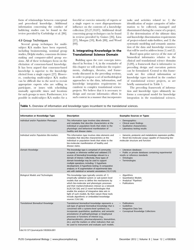
briefly summarized in Table 1.
The preceding framework of informa-
tion and knowledge types ultimately in-
forms a conceptual model for knowledge
integration in the translational sciences.
Table 1. Overview of information and knowledge types incumbent to the translational sciences.
Information or Knowledge Type Description Examples Sources or Types
Individual and/or Population Phenotype This information type involves data elementsand metadata that describe characteristics at theindividual or population levels that relate to thephysiologic and behavioral manifestation ofhealthy and disease states.
N DemographicsN Clinical exam findingsN Qualitative characteristicsN Laboratory testing results
Individual and/or Population Bio-markers This information type involves data elements andmetadata that describe characteristics at theindividual or population levels that relate to thebio-molecular manifestation of healthy anddisease states.
N Genomic, proteomic and metabolomic expression profilesN Novel bio-molecular assays capable of measuring bio-molecular structure and function
Domain Knowledge This knowledge type is comprised of community-accepted, or otherwise verified and validated [17]sources of biomedical knowledge relevant to adomain of interest. Collectively, these types ofdomain knowledge may be used to supportmultiple operations, including: 1) hypothesisdevelopment; 2) hypothesis testing; 3) comparativeanalyses; or 4) augmentation of experimental datasets with statistical or semantic annotations [15,17,125].
N Literature databasesN Public or private databases containing experimentalresults or reference standardsN OntologiesN Terminologies
Biological Models and Technologies This knowledge type typically consists of: 1)empirically validated system or sub-system levelmodels that serve to define the mechanisms bywhich bio-molecular and phenotypic processesand their markers/indicators interact as a network[6,20,124,126]; and 2) novel technologies thatenable the analysis of integrative data sets inlight of such models. By their nature these toolsinclude algorithmic or embedded knowledgesources [124,126].
N AlgorithmsN Quantitative ModelsN Analytical ‘‘Pipelines’’N Publications
Translational Biomedical Knowledge Translational biomedical knowledge represents asub-type of general biomedical knowledge that isconcerned with a systems-level synthesis (i.e.,incorporate quantitative, qualitative, and semanticannotations) of pathophysiologic or biophysicalprocesses or functions of interest (e.g.,pharmacokinetics, pharmacodynamics, bionutrition,etc.), and the markers or other indicators that canbe used to instrument and evaluate such models.
N PublicationsN GuidelinesN Integrative Data SetsN Conceptual Knowledge Collections
doi:10.1371/journal.pcbi.1002826.t001
PLOS Computational Biology | www.ploscompbiol.org 8 December 2012 | Volume 8 | Issue 12 | e1002826
The role of Biomedical Informatics and
KE in this framework is to address the four
major information management challeng-
es enumerated earlier relative to the ability
to generate Translational BiomedicalKnowledge, namely: 1) the collection
and management of high throughput,
multi-dimensional data; 2) the generation
and testing of hypotheses relative to such
integrative data sets; 3) the provision
data analytic ‘‘pipelines’’; and 4) the
dissemination of knowledge collections
resulting from research activities.
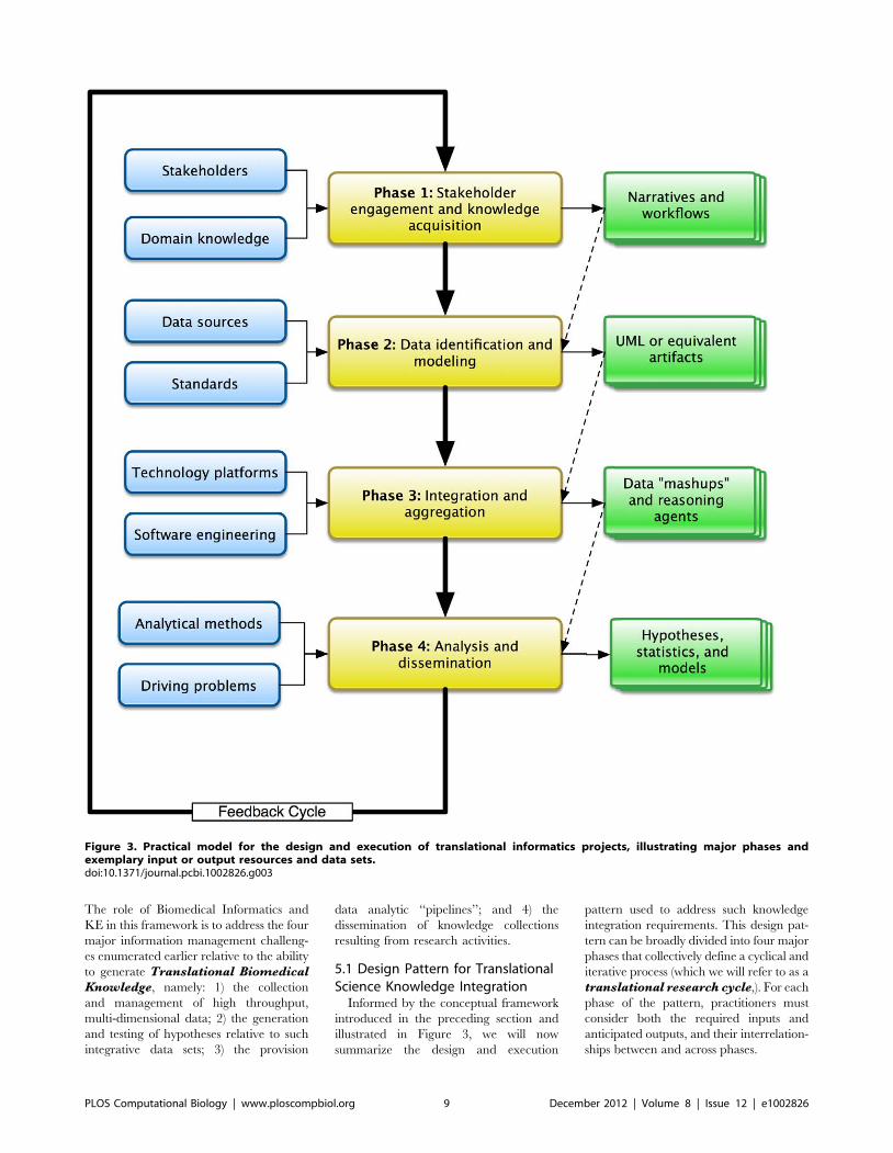
5.1 Design Pattern for TranslationalScience Knowledge Integration
Informed by the conceptual framework
introduced in the preceding section and
illustrated in Figure 3, we will now
summarize the design and execution
pattern used to address such knowledge
integration requirements. This design pat-
tern can be broadly divided into four major
phases that collectively define a cyclical and
iterative process (which we will refer to as a
translational research cycle,). For each
phase of the pattern, practitioners must
consider both the required inputs and
anticipated outputs, and their interrelation-
ships between and across phases.
Figure 3. Practical model for the design and execution of translational informatics projects, illustrating major phases andexemplary input or output resources and data sets.doi:10.1371/journal.pcbi.1002826.g003
PLOS Computational Biology | www.ploscompbiol.org 9 December 2012 | Volume 8 | Issue 12 | e1002826
Phase 1 - Stakeholder engagementand knowledge acquisition: During
this initial phase, key stakeholders who will
be involved in the collection, manage-
ment, analysis, and dissemination of proj-
ect-specific data and knowledge are iden-
tified and engaged in both formal and
informal knowledge acquisition, with the
ultimate goal of defining the essential
workflows, processes, and data sources
(including their semantics). Such knowl-
edge acquisition usually requires the use of
ethnographic, cognitive science, workflow
modeling, and formal knowledge acquisi-
tion techniques [14]. The results of such
activities can be formalized using a
thematic narratives [90–92] and workflow
or process artifacts [92–94]. In some
instances, it may be necessary to engage
domain-specific subject matter experts
(SMEs) who are not involved in a given
project in order to augment available
SMEs, or to validate the findings generat-
ed during such activities [14,92].
Phase 2 - Data identification andmodeling: Informed by the artifacts
generated in Phase 1, in this phase, we
focus upon the identification of specific,
pertinent data sources relative to project
aims, and the subsequent creation of
models that encapsulate the physical and
semantic representations of that data.
Once pertinent data sources have been
identified, we must then model their
contents in an implementation-agnostic
manner, an approach that is most fre-
quently implemented using model-driven
architecture techniques [95–99]. The re-
sults of such MDA processes are common-
ly recorded using the Unified Modeling
Language (UML) [16,100–102]. During
the modeling process, it is also necessary to
identify and record semantic or domain-
specific annotation of targeted data struc-
tures, using locally relevant conceptual
knowledge collections (such as terminolo-
gies and ontologies), in order to enable
deeper, semantic reasoning concerning
such data and information [16,103,104].
Phase 3 - Integration and aggre-gation: A common approach to the
integration of heterogeneous and multi-
dimensional data is the use of technology-
agnostic domain or data models (per
Phases 1–2), incorporating semantic anno-
tations, in order to execute data federation
operations [105] or to transform that data
and load it into an integrative repository,
such as a data warehouse [106–108].
Once the mechanisms needed to integrate
such disparate data sources are imple-
mented, it is then possible to aggregate the
data for the purposes of hypothesis
discovery and testing – a process that is
sometimes referred to as creating a data
‘‘mashup’’ [109–115]. Data ‘‘mashups’’
are often created using a variety of readily
available reasoners, such as those associ-
ated with the semantic web [109–115],
which directly employ both the data
models and semantic annotations created
in the prior phases of the Translational
Informatics Cycle, and enable a knowl-
edge-anchored approach to such opera-
tions.
Phase 4 - Analysis and dissemina-tion: In this phase of the Translational
Informatics Cycle, the integrated/aggre-
gated data and knowledge created in the
preceding phases is subject to analysis. In
most if not all cases, these analyses make
use of domain or task specific applications
and algorithms, such as those implement-
ed in a broad number of biological data
analysis packages, statistical analysis appli-
cations, and data mining tools, and
intelligent agents. These types of analytical
tools are used to address questions per-
taining to one or more of the following
four basic query or data interrogation
patterns: 1) to generate hypotheses con-
cerning relationships or patterns that serve
to link variables of interest in a data set
[116]; 2) to evaluate the validity hypoth-
eses and the strength of their related data
motifs, often using empirically-validated
statistical tests [117,118]; 3) to visualize
complex data sets in order to facilitate
human-based pattern recognition [119–
121]; and 4) to infer and/or verify and
validate quantitative models that formalize
phenomena of interest identified via the
preceding query patterns [122,123].
6. Open Research Questionsand Future Direction
As can be ascertained from the preced-
ing review of the theoretical and practice
bases for the integration of data and
knowledge in the translational science
domain, such techniques and frameworks
have significant potential to positively
impact the speed, efficacy, and impact of
such research programs, and to enable
novel scientific paradigms that would not
otherwise be tractable. However, there are
a number of open and ongoing research
and development questions being ad-
dressed by the biomedical informatics
community relative to such approaches
that should be noted:
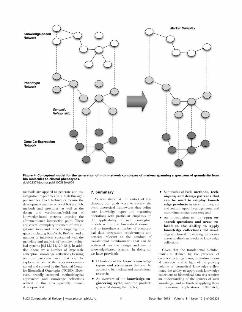
Dimensionality and granularity:the majority of knowledge integration
techniques being designed, evaluated,
and applied relative to the context of the
translational science domain target low-
order levels of dimensionality (e.g., the
integration of data and knowledge corre-
sponding to a single type, per the defini-
tions set forth in Table 1). However, many
translational science problem spaces re-
quire reasoning across knowledge-types
and data granularities (e.g., multidimen-
sional data and knowledge collections).
The ability to integrate and reason upon
data in a knowledge-anchored manner
that addresses such multi-dimensional
context remains an open area of research.
Many efforts to address this gap in
knowledge and practice rely upon the
creation of semantically typed ‘‘vertical’’
linkages spanning multiple integrative
knowledge networks, as is illustrated in
Figure 4.
Scalability: Similar to the challenge of
dimensionality and granularity, the issue
of scalability of knowledge integration
methods also remains an open area of
research and development. Specifically, a
large number of available knowledge
integration techniques rely upon semi-
automated or human-mediated methods
or activities, which significantly curtail the
scalability of such approaches to large-
scale problems. Much of the research
targeting this gap in knowledge and
practice has focused on the use of artificial
intelligence and semantic-reasoning tech-
nologies to enable the extraction, disam-
biguation, and application of conceptual
knowledge collections.
Reasoning and visualization: Once
knowledge and data have been aggregated
and made available for hypothesis discov-
ery and testing, the ability to reason upon
and visualize such ‘‘mashups’’ is highly
desirable. Current efforts to provide reus-
able methods of doing so, such as the tools
and technologies provided by the semantic
web community, as well as visualization
techniques being explored by the comput-
er science and human-computer interac-
tion communities, hold significant promise
in addressing such needs, but are still
largely developmental.
Applications of knowledge-basedsystems for in-silico science para-digms: As has been discussed throughout
this collection, a fundamental challenge in
Translational Bioinformatics is the ability
to both ask and answer the full spectrum of
questions possible given a large-scale and
multi-dimensional data set. This challenge
is particularly pressing at the confluence of
high-throughput bio-molecular measure-
ment methods and the translation of the
findings generated by such approaches to
clinical research or practice. Broadly
speaking, overcoming this challenge re-
quires a paradigm that can be described as
in-silico science, in which informatics
PLOS Computational Biology | www.ploscompbiol.org 10 December 2012 | Volume 8 | Issue 12 | e1002826
methods are applied to generate and test
integrative hypotheses in a high-through-
put manner. Such techniques require the
development and use of novel KA and KR
methods and structures, as well as the
design and verification/validation of
knowledge-based systems targeting the
aforementioned intersection point. There
are several exemplary instances of investi-
gational tools and projects targeting this
space, including RiboWeb, BioCyc, and a
number of initiatives concerned with the
modeling and analysis of complex biolog-
ical systems [6,113,114,120,124]. In addi-
tion, there are a number of large-scale
conceptual knowledge collections focusing
on this particular area that can be
explored as part of the repositories main-
tained and curated by the National Center
for Biomedical Ontologies (NCBO). How-
ever, broadly accepted methodological
approaches and knowledge collections
related to this area generally remain
developmental.
7. Summary
As was stated at the outset of this
chapter, our goals were to review the
basic theoretical frameworks that define
core knowledge types and reasoning
operations with particular emphasis on
the applicability of such conceptual
models within the biomedical domain,
and to introduce a number of prototyp-
ical data integration requirements and
patterns relevant to the conduct of
translational bioinformatics that can be
addressed via the design and use of
knowledge-based systems. In doing so,
we have provided:
N Definitions of the basic knowledgetypes and structures that can be
applied to biomedical and translational
research;
N An overview of the knowledge en-gineering cycle, and the products
generated during that cycles;
N Summaries of basic methods, tech-niques, and design patterns thatcan be used to employ knowl-edge products in order to integrate
and reason upon heterogeneous and
multi-dimensional data sets; and
N An introduction to the open re-search questions and areas re-lated to the ability to applyknowledge collections and knowl-
edge-anchored reasoning processes
across multiple networks or knowledge
collections.
Given that the translational bioinfor-
matics is defined by the presence of
complex, heterogeneous, multi-dimension-
al data sets, and in light of the growing
volume of biomedical knowledge collec-
tions, the ability to apply such knowledge
collections to biomedical data sets requires
an understanding of the sources of such
knowledge, and methods of applying them
to reasoning applications. Ultimately,
Figure 4. Conceptual model for the generation of multi-network complexes of markers spanning a spectrum of granularity frombio-molecules to clinical phenotypes.doi:10.1371/journal.pcbi.1002826.g004
PLOS Computational Biology | www.ploscompbiol.org 11 December 2012 | Volume 8 | Issue 12 | e1002826
these approaches introduce both signifi-
cant opportunities to advance the state of
translational science, while simultaneously
adding areas of complexity to the design of
translational bioinformatics studies, in-
cluding the methods needed to reason in
an integrative manner across multiple
networks or knowledge constructs. As
such, these theories, methods, and frame-
works offer significant benefits as well as a
number of exciting and ongoing areas of
biomedical informatics research and de-
velopment.
8. Exercises
Instructions: Read the following mo-
tivating use case and then perform the
tasks described in each question. The
objective of this exercise is to demonstrate
how available and open-access knowledge
discovery and reasoning tools can be used
to satisfy the information needs incumbent
to biomedical knowledge integration needs
commonly encountered in the clinical and
translational research environment.
Use Case: The ability to identify potentially
actionable phenotype-to-biomarker relationships is
of critical importance in the translational science
domain. In the specific context of integrative cancer
research, it is regularly the case that structural and
functional relationships between genes, gene
products, and clinical phenotypes are used to
design and evaluate diagnostic and therapeutic
approaches to targeted disease states. Large
volumes of domain specific conceptual knowledge
related to such hypothesis generation processes can
be found in publically available literature corpora
and ontologies.
1) Task One: Select a specific cancer
and perform a search for a collection
of recent literature available with full
free text via PubMed Central (the
resulting corpora should contain 5
manuscripts published within the
last three years, selected based upon
their publication dates beginning
with the most recent articles/manu-
scripts). Download the free text for
each such article.
2) Task Two: For each full text article
in the corpora established during
Task One, semantically annotate
genes, gene products, and clinical
phenotype characteristics as found in
the Abstract, Introduction, and Con-
clusion (or equivalent) sections using
applicable Gene Ontology (GO)
concepts, using the NCBO anno-
tator found at: http://bioportal.
bioontology.org/annotator)
3) Task Three: Identify the top 10
most frequently occurring Gene
Ontology (GO) concepts found in
your annotations, per Task Two.
For each such concept, perform a
search of PubMed Central for
articles in which both the appropri-
ate terms describing the cancer
selected in Task One as well as
these concepts co-occur. For the top
5 (most recent) articles retrieved via
each search, retrieve the associate
abstract for subsequent analysis
4) Task Four: Using the NCBO Ontol-
ogy Recommender (http://bioportal.
bioontology.org/recommender), analyze
each of the abstracts retrieved in Task
Three to determine the optimal ontology
for annotating those abstracts, noting the
top ‘‘recommended’’ ontology for each
such textual resource.
5) Task Five: For each abstract
identified in Step Three, again using
the NCBO annotator (found at:
http://bioportal.bioontology.org/
annotator), annotate those abstracts
using the recommended ontologies
identified in Step Four (selecting
only those ontologies that are also
reflects in the NLM’s UMLS). Then,
for the top 2–3 phenotypic (e.g.,
clinically relevant) concepts identi-
fied via that annotation process, use
the UMLS UTS (https://uts.nlm.
nih.gov/) in order to identify poten-
tial phenotype-genotype pathways
linking such phenotypic concepts
and the genes or gene products
identified in Task Two. Please note
that performing this task will require
exploring multiple relationship
types reflected in the UMLS me-
tathesaurus (documentation con-
cerning how to do perform such a
search can be found here: http://
www.ncbi.nlm.nih.gov/books/
NBK9684/).
Answers to the Exercises can be found
in Text S1.
Supporting Information
Text S1 Answers to Exercises
(DOCX)
Further Reading
N Brachman RJ, McGuinness DL (1988) Knowledge representation, connectionism and conceptual retrieval. Proceedings of the11th annual international ACM SIGIR conference on research and development in information retrieval. Grenoble, France: ACMPress.
N Campbell KE, Oliver DE, Spackman KA, Shortliffe EH (1998) Representing thoughts, words, and things in the UMLS. J Am MedInform Assoc 5: 421–431.
N Compton P, Jansen R (1990) A philosophical basis for knowledge acquisition Knowledge Acquisition 2: 241–257.
N Gaines BR (1989) Social and cognitive processes in knowledge acquisition. Knowledge Acquisition 1: 39–58.
N Kelly GA (1955) The psychology of personal constructs. New York: Norton. 2 v. (1218).
N Liou YI (1990) Knowledge acquisition: issues, techniques, and methodology. Orlando, Florida, United States: ACM Press. pp.212–236.
N McCormick R (1997) Conceptual and procedural knowledge. International Journal of Technology and Design Education 7:141–159.
N Newell A, Simon HA (1981) Computer science as empirical inquiry: symbols and search. In: Haugeland J, editor. Mind design.Cambridge: MIT Press/Bradford Books. pp. 35–66.
N Patel VL, Arocha JF, Kaufman DR (2001) A primer on aspects of cognition for medical informatics. J Am Med Inform Assoc 8:324–343.
N Preece A (2001) Evaluating verification and validation methods in knowledge engineering. Micro-Level KnowledgeManagement: 123–145.
N Zhang J (2002) Representations of health concepts: a cognitive perspective. J Biomed Inform 35: 17–24.
PLOS Computational Biology | www.ploscompbiol.org 12 December 2012 | Volume 8 | Issue 12 | e1002826
References
1. Coopers PW (2008) Research rewired. 48 p.
2. Casey K, Elwell K, Friedman J, Gibbons D,
Goggin M, et al. (2008) A broken pipeline? Flat
funding of the NIH puts a generation of science
at risk. 24 p.
3. Payne PR, Johnson SB, Starren JB, Tilson HH,
Dowdy D (2005) Breaking the translational
barriers: the value of integrating biomedical
informatics and translational research. J Investig
Med 53: 192–200.
4. Research NDsPoC (1997) NIH director’s panel
on clinical research report. Bethesda, MD:
National Institutes of Health.
5. Sung NS, Crowley WF, Jr., Genel M, Salber P,
Sandy L, et al. (2003) Central challenges facing
the national clinical research enterprise. JAMA
289: 1278–1287.
6. Butte AJ (2008) Medicine. The ultimate model
organism. Science 320: 325–327.
7. Chung TK, Kukafka R, Johnson SB (2006)
Reengineering clinical research with informatics.
J Investig Med 54: 327–333.
8. Kaiser J (2008) U.S. budget 2009. NIH hopes
for more mileage from roadmap. Science 319:
716.
9. Kush RD, Helton E, Rockhold FW, Hardison
CD (2008) Electronic health records, medical
research, and the Tower of Babel. N Engl J Med
358: 1738–1740.
10. Ruttenberg A, Clark T, Bug W, Samwald M,
Bodenreider O, et al. (2007) Advancing transla-
tional research with the Semantic Web. BMC
Bioinformatics 8 Suppl 3: S2.
11. Fridsma DB, Evans J, Hastak S, Mead CN
(2008) The BRIDG project: a technical
report. J Am Med Inform Assoc 15: 130–
137.
12. Maojo V, Garcıa-Remesal M, Billhardt H,
Alonso-Calvo R, Perez-Rey D, et al. (2006)
Designing new methodologies for integrating
biomedical information in clinical trials. Meth-
ods Inf Med 45: 180–185.
13. Ash JS, Anderson NR, Tarczy-Hornoch P
(2008) People and organizational issues in
research systems implementation. J Am Med
Inform Assoc 15: 283–289.
14. Payne PR, Mendonca EA, Johnson SB, Starren
JB (2007) Conceptual knowledge acquisition in
biomedicine: a methodological review. J Biomed
Inform 40: 582–602.
15. Richesson RL, Krischer J (2007) Data standards
in clinical research: gaps, overlaps, challenges
and future directions. J Am Med Inform Assoc
14: 687–696.
16. Erickson J (2008) A decade and more of UML:
an overview of UML semantic and structural
issues and UML field use. Journal of Database
Management 19: I-Vii.
17. van Bemmel JH, van Mulligen EM, Mons B,
van Wijk M, Kors JA, et al. (2006) Databases for
knowledge discovery. Examples from biomedi-
cine and health care. Int J Med Inform 75: 257–
267.
18. Oster S, Langella S, Hastings S, Ervin D,
Madduri R, et al. (2008) caGrid 1.0: an
enterprise grid infrastructure for biomedical
research. J Am Med Inform Assoc 15: 138–
149.
19. Kukafka R, Johnson SB, Linfante A, Allegrante
JP (2003) Grounding a new information
technology implementation framework in be-
havioral science: a systematic analysis of the
literature on IT use. J Biomed Inform 36: 218–
227.
20. Zerhouni EA (2005) Translational and clinicalscience–time for a new vision. N Engl J Med
353: 1621–1623.
21. Sim I (2008) Trial registration for public trust:making the case for medical devices. J Gen
Intern Med 23 Suppl 1: 64–68.
22. Preece A (2001) Evaluating verification andvalidation methods in knowledge engineering.
Micro-Level Knowledge Management: 123–145.
23. Brachman RJ, McGuinness DL (1988) Knowl-
edge representation, connectionism and concep-
tual retrieval. Proceedings of the 11th annualinternational ACM SIGIR conference on re-
search and development in information retriev-al. Grenoble, France: ACM Press.
24. Compton P, Jansen R (1990) A philosophical
basis for knowledge acquisition. KnowledgeAcquisition 2: 241–257.
25. Gaines BR (1989) Social and cognitive processes
in knowledge acquisition. Knowledge Acquisi-tion 1: 39–58.
26. Gaines BR, Shaw MLG (1993) Knowledge
acquisition tools based on personal construct
psychology.
27. Liou YI (1990) Knowledge acquisition: issues,
techniques, and methodology. Orlando, Florida,
, United States: ACM Press. pp. 212–236.
28. Yihwa Irene L (1990) Knowledge acquisition:issues, techniques, and methodology. Proceed-
ings of the 1990 ACM SIGBDP conference ontrends and directions in expert systems. Or-
lando, Florida, , United States: ACM Press.
29. Glaser R (1984) Education and thinking: the roleof knowledge. American Psychologist 39: 93–104.
30. Hiebert J (1986) Procedural and conceptual
knowledge: the case of mathematics. London:Lawrence Erlbaum Associates.
Glossary
N Data: factual information (as measurements or statistics) used as a basis for reasoning, discussion, or calculation [127]
N Information: knowledge obtained from investigation, study, or instruction [127]
N Knowledge: the circumstance or condition of apprehending truth or fact through reasoning [127]
N Knowledge engineering: a branch of artificial intelligence that emphasizes the development and use of expert systems[128]
N Knowledge acquisition: the act of acquiring knowledge
N Knowledge representation: the symbolic formalization of knowledge
N Conceptual knowledge: knowledge that consists of atomic units of information and meaningful relationships that serve tointerrelate those units.
N Strategic knowledge: knowledge used to infer procedural knowledge from conceptual knowledge.
N Procedural knowledge: knowledge that is concerned with a problem-oriented understanding of how to address a giventask or activity.
N Terminology: the technical or special terms used in a business, art, science, or special subject [128]
N Ontology: a rigorous and exhaustive organization of some knowledge domain that is usually hierarchical and contains allthe relevant entities and their relations [128]
N Multi-dimensional data: data spanning multiple levels or context of granularity or scope while maintaining one or morecommon linkages that span such levels
N Motif: a reproducible pattern
N Mashup: a combination of multiple, heterogeneous data or knowledge sources in order to create an aggregate collection ofsuch elements or concepts.
N Intelligent agent: a software agent that employs a formal knowledge-base in order to replicate expert performance relativeto problem solving in a targeted domain.
N Clinical phenotype: the observable physical and biochemical characteristics of an individuals that serve to define clinicalstatus (e.g., health, disease)
N Biomarker: a bio-molecular trait that can be measure to assess risk, diagnosis, status, or progression of a pathophysiologicor disease state.
PLOS Computational Biology | www.ploscompbiol.org 13 December 2012 | Volume 8 | Issue 12 | e1002826
31. McCormick R (1997) Conceptual and proce-
dural Knowledge. International Journal ofTechnology and Design Education 7: 141–159.
32. Scribner S (1985) Knowledge at work. Anthro-pology & Education Quarterly 16: 199–206.
33. Barsalow LW, Simmons WK, Barbey AK,
Wilson CD (2003) Grounding conceptual knowl-
edge in modaltiy-specific systems. Trends CognSci 7: 84–91.
34. Borlawsky T, Li J, Jalan S, Stern E, Williams R,et al. (2005) Partitioning knowledge bases
between advanced notification and clinicaldecision support systems. AMIA Annu Symp
Proc: 901.
35. Newell A, Simon HA (1981) Computer science
as empirical inquiry: symbols and search. In:Haugeland J, editor. Mind design. Cambridge:
MIT Press/Bradfor Books. pp. 35–66.
36. Newell A, Simon HA (1975) Computer science
as empirical inquiry: symbols and search.Minneapolis.
37. Kelly GA (1955) The psychology of personalconstructs. New York: Norton. 2 v. (1218).
38. Hawkins D (1983) An analysis of expertthinking. Int J Man-Mach Stud 18: 1–47.
39. Zhang J (2002) Representations of healthconcepts: a cognitive perspective. J Biomed
Inform 35: 17–24.
40. Horsky J, Kaufman DR, Oppenheim MI, Patel
VL (2003) A framework for analyzing thecognitive complexity of computer-assisted clini-
cal ordering. J Biomed Inform 36: 4–22.
41. Horsky J, Kaufman DR, Patel VL (2003) The
cognitive complexity of a provider order entryinterface. AMIA Annu Symp Proc: 294–298.
42. Horsky J, Kaufman DR, Patel VL (2004)Computer-based drug ordering: evaluation of
interaction with a decision-support system.Medinfo 11: 1063–1067.
43. Horsky J, Kuperman GJ, Patel VL (2005)Comprehensive analysis of a medication dosing
error related to CPOE. J Am Med Inform Assoc12: 377–382.
44. Horsky J, Zhang J, Patel VL (2005) To err is notentirely human: complex technology and user
cognition. J Biomed Inform 38: 264–266.
45. Patel VL, Arocha JF, Diermeier M, Greenes
RA, Shortliffe EH (2001) Methods of cognitiveanalysis to support the design and evaluation of
biomedical systems: the case of clinical practice
guidelines. J Biomed Inform 34: 52–66.
46. Patel VL, Arocha JF, Kaufman DR (2001) Aprimer on aspects of cognition for medical
informatics. J Am Med Inform Assoc 8: 324–
343.
47. Wikipedia (2006) Semiotics. Wikipedia.
48. Campbell KE, Oliver DE, Spackman KA,
Shortliffe EH (1998) Representing thoughts,words, and things in the UMLS. J Am Med
Inform Assoc 5: 421–431.
49. Harris Z (1976) On a theory of language. The
Journal of Philosophy 73: 253–276.
50. Friedman C, Kra P, Rzhetsky A (2002) Two
biomedical sublanguages: a description based onthe theories of Zellig Harris. J Biomed Inform
35: 222–235.
51. Grishman R, Kittredge R (1986) Analyzing
language in restricted domains: sublangaugedescription and processing. Hillsdale, NJ.: Law-
rence Erlbaum.
52. Starren J (1997) From multimodal sublanguages
to medical data presentations. New York:
Columbia University.
53. Alan LR, Chris W, Jeremy R, Angus R (2001)Untangling taxonomies and relationships: per-
sonal and practical problems in loosely coupled
development of large ontologies. Proceedings ofthe international conference on knowledge
capture. Victoria, British Columbia, Canada:ACM Press.
54. Canas AJ, Leake DB, Wilson DC (1999)Managing, mapping, and manipulating concep-
tual knowledge. Menlo Park: AAAI Press. pp.10–14.
55. Ian N, Adam P (2001) Towards a standard
upper ontology. Proceedings of the international
conference on formal ontology in information
systems - volume 2001. Ogunquit, Maine, ,
United States: ACM Press.
56. Joachim H, Gerd S, Rudolf W, Uta W (2000)
Conceptual knowledge discovery and data
analysis. Springer-Verlag. pp. 421–437.
57. Tayar N (1993) A model for developing large
shared knowledge bases. Washington, (D.C.):
ACM Press. pp. 717–719.
58. Boy GA (1997) The group elicitation method for
participatory design and usability testing. inter-
actions 4: 27–33.
59. Morgan MS, Martz Jr WB (2004) Group
consensus: do we know it when we see it?
Proceedings of the 37th annual Hawaii interna-
tional conference on system sciences (HICSS’04)
- track 1 - volume 1: IEEE Computer Society.
60. Wood WC, Roth RM (1990) A workshop
approach to acquiring knowledge from single
and multiple experts. Orlando, Florida, , United
States: ACM Press. pp. 275–300.
61. Adria HL, William AS, Stephen DK (2003)
GMS: preserving multiple expert voices in
scientific knowledge management. San Fran-
cisco, California: ACM Press. pp. 1–4.
62. John H, Val K, Tom R, Hans A (1995) The role
of ethnography in interactive systems design.
interactions 2: 56–65.
63. Wickstrom G, Bendix T (2000) The
‘‘Hawthorne effect’’–what did the original
Hawthorne studies actually show? Scand
J Work Environ Health 26: 363–367.
64. Rahat I, Richard G, Anne J (2005) A general
approach to ethnographic analysis for systems
design. Coventry, United Kingdom: ACM Press.
pp. 34–40.
65. Rugg G, McGeorge P (1997) The sorting
techniques: a tutorial paper on card sorts,
picture sorts and item sorts. Expert Systems
14: 80–93.
66. Cimiano P, Hotho A, Stumme G, Tane J (2004)
Conceptual knowledge processing with formal
concept analysis and ontologies. 189 p.
67. Cole R, Becker P (2004) Agreement contexts in
formal concept analysis. 172 p.
68. Sowa JF (1980) A conceptual schema for
knowledge-based systems. Pingree Park, Colo-
rado: ACM Press. pp. 193–195.
69. Salomons OW, van Houten FJAM, Kals HJJ
(1995) Conceptual graphs in constraint based re-
design. Proceedings of the third ACM sympo-
sium on solid modeling and applications. Salt
Lake City, Utah, , United States: ACM Press.
70. Yang G, Oh J (1993) Knowledge acquisition and
retrieval based on conceptual graphs. Proceed-
ings of the 1993 ACM/SIGAPP symposium on
applied computing: states of the art and practice.
Indianapolis, Indiana, , United States: ACM
Press.
71. Campbell JR, Carpenter P, Sneiderman C,
Cohn S, Chute CG, et al. (1997) Phase II
evaluation of clinical coding schemes: complete-
ness, taxonomy, mapping, definitions, and
clarity. CPRI Work Group on Codes and
Structures. J Am Med Inform Assoc 4: 238–251.
72. Campbell KE, Oliver DE, Shortliffe EH (1998)
The Unified Medical Language System: toward
a collaborative approach for solving terminolo-
gic problems. J Am Med Inform Assoc 5: 12–16.
73. Cimino JJ (2000) From data to knowledge
through concept-oriented terminologies: experi-
ence with the Medical Entities Dictionary. J Am
Med Inform Assoc 7: 288–297.
74. TOCKIT (2006) Tupleware. 0.1 ed: Technische
Universitaet Darmstadt and University of
Queensland.
75. Hereth J, Stumme G, Wille R, Wille U (2000)
Conceptual knowledge discovery and data
analysis. Springer-Verlag. pp. 421–437.
76. Priss U (2006) Formal concept analysis in
information science. In: Blaise C, editor. Annual
review of information science and technology.
Medford, NJ: Information Today, Inc.
77. Polson PG (1987) A quantitative theory of
human-computer interaction. Interfacingthought: cognitive aspects of human-computer
interaction. MIT Press. pp. 184–235.
78. Polson PG, Lewis C, Rieman J, Wharton C
(1992) Cognitive walkthroughs: a method fortheory-based evaluation of user interfaces.
Int J Man-Mach Stud 36: 741–773.
79. Alvarez R (2002) Discourse analysis of require-
ments and knowledge elicitation interviews.IEEE Computer Society. 255 p.
80. Davidson JE (1977) Topics in discourse analysis.University of British Columbia.
81. Friedman C, Alderson PO, Austin JH, CiminoJJ, Johnson SB (1994) A general natural-
language text processor for clinical radiology.J Am Med Inform Assoc 1: 161–174.
82. Friedman C, Hripcsak G (1998) Evaluatingnatural language processors in the clinical
domain. Methods Inf Med 37: 334–344.
83. Friedman C, Hripcsak G (1999) Natural lan-
guage processing and its future in medicine.Acad Med 74: 890–895.
84. Friedman C, Hripcsak G, Shablinsky I (1998)An evaluation of natural language processing
methodologies. Proc AMIA Symp: 855–859.
85. Hripcsak G, Friedman C, Alderson PO, Du-
Mouchel W, Johnson SB, et al. (1995) Unlockingclinical data from narrative reports: a study of
natural language processing. Ann Intern Med122: 681–688.
86. Corbridge C, Rugg G, Major NO, ShadboltNR, Burton AM (1994) Laddering: technique
and tool use in knowledge acquisition. Knowl-edge Acquisition 6: 315–341.
87. Agostini A, Albolino S, Boselli R, De MichelisG, De Paoli F, et al. (2003) Stimulating
knowledge discovery and sharing; 2003; Sanibel
Island, Florida, , United States: ACM Press. pp.248–257.
88. Roth RM, Wood WC (1990) A Delphi approach
to acquiring knowledge from single and multiple
experts; 1990; Orlando, Florida, , United States:ACM Press. pp. 301–324.
89. Embi PJ, Payne PR (2009) Clinical researchinformatics: challenges, opportunities and defi-
nition for an emerging domain. J Am MedInform Assoc 16: 316–327.
90. Crabtree BF, Miller WL (1992) Doing qualita-tive research. Newbury Park, CA: Sage.
91. Glaser B, Strauss A (1967) The discovery of
grounded theory: strategies for qualitative re-
search. Piscataway, NJ: Aldine Transaction. 271p.
92. Patton MQ (2001) Qualitative research &evaluation methods. New York: Sage Publica-
tions. 688 p.
93. Khan SA, Kukafka R, Payne PR, Bigger JT,
Johnson SB (2007) A day in the life of a clinicalresearch coordinator: observations from com-
munity practice settings. Medinfo 12: 247–251.
94. Khan SA, Payne PR, Johnson SB, Bigger JT,
Kukafka R (2006) Modeling clinical trials work-flow in community practice settings. AMIA
Annual Symposium proceedings/AMIA Sym-posium: 419–423.
95. Rayhupathi W, Umar A (2008) Exploring amodel-driven architecture (MDA) approach to
health care information systems development.
Int J Med Inform 77: 305–314.
96. Aksit M, Kurtev I (2008) Elsevier special issue onfoundations and applications of model driven
architecture. Science of Computer Program-
ming 73: 1–2.
97. Shurville S (2007) Model driven architectureand ontology development. Interactive Learning
Environments 15: 96–99.
98. Uhl A (2003) Model driven architecture is ready
for prime time. IEEE Software 20: 70-+.
99. Soley RM (2003) Model driven architecture: the
evolution of object-oriented systems? Object-Oriented Information Systems 2817: 2-2.
PLOS Computational Biology | www.ploscompbiol.org 14 December 2012 | Volume 8 | Issue 12 | e1002826
100. Vanderperren Y, Mueller W, Dehaene W (2008)
UML for electronic systems design: a compre-hensive overview. Design Automation for Em-
bedded Systems 12: 261–292.
101. Dobing B, Parsons J (2008) Dimensions of UMLdiagram use: a survey of practitioners. Journal of
Database Management 19: 1–18.102. Batra D (2008) Unified modeling language
(UML) topics: the past, the problems, and the
prospects. Journal of Database Management 19:I–Vii.
103. Komatsoulis GA, Warzel DB, Hartel FW,Shanbhag K, Chilukuri R, et al. (2008) caCORE
version 3: Implementation of a model driven,service-oriented architecture for semantic inter-
operability. J Biomed Inform 41: 106–123.
104. Kunz I, Lin MC, Frey L (2009) Metadatamapping and reuse in caBIG. BMC Bioinfor-
matics 10 Suppl 2: S4.105. Chakravarthy S, Whang WK, Navathe SB
(1994) A logic-based approach to query-process-
ing in federated databases. Information Sciences79: 1–28.
106. Ariyachandra T, Watson HJ (2008) Which datawarehouse architecture is best? Communica-
tions of the ACM 51: 146–147.107. DeWitt JG, Hampton PM (2005) Development
of a data warehouse at an academic health
system: knowing a place for the first time. AcadMed 80: 1019–1025.
108. Braa J (2005) A data warehouse approach canmanage multiple data sets. Bull World Health
Organ 83: 638–639.
109. Yu J, Benatallah B, Casati F, Daniel F (2008)Understanding mashup development. IEEE
Internet Computing 12: 44–52.
110. Scotch M, Yip KY, Cheung KH (2008)
Development of grid-like applications for publichealth using web 2.0 mashup techniques. J Am
Med Inform Assoc 15: 783–786.
111. Sahoo SS, Bodenreider O, Rutter JL, SkinnerKJ, Sheth AP (2008) An ontology-driven seman-
tic mashup of gene and biological pathwayinformation: application to the domain of
nicotine dependence. J Biomed Inform 41:
752–765.112. Cheung KH, Yip KY, Townsend JP, Scotch M
(2008) HCLS 2.0/3.0: Health care and lifesciences data mashup using Web 2.0/3.0.
J Biomed Inform 41: 694–705.113. Cheung KH, Kashyap V, Luciano JS, Chen HJ,
Wang YM, et al. (2008) Semantic mashup of
biomedical data. J Biomed Inform s 41: 683–686.
114. Belleau F, Nolin MA, Tourigny N, Rigault P,Morissette J (2008) Bio2RDF: Towards a
mashup to build bioinformatics knowledge
systems. J Biomed Inform 41: 706–716.115. Marks P (2006) ‘Mashup’ websites are a dream
come true for hackers. New Scientist 190: 28–29.116. Payne PR, Borlawsky T, Kwok A, Greaves A
(2008) Supporting the design of translationalclinical studies through the generation and
verification of conceptual knowledge-anchored
hypotheses. AMIA Annu Symp Proc: 566–570.117. Mansmann U (2005) Genomic profiling -
interplay between clinical epidemiology, bioin-formatics and biostatistics. Methods Inf Med 44:
454–460.
118. Xu R, Wunsch D (2005) Survey of clusteringalgorithms. IEEE Transactions on Neural Net-
works 16: 645–678.
119. Ardekani AM, Akhondi MM, Sadeghi MR
(2008) Application of genomic and proteomic
technologies to early detection of cancer.
Archives of Iranian Medicine 11: 427–434.
120. De Fonzo V, Aluffi-Pentini F, Parisi V (2007)
Hidden Markov models in bioinformatics. Curr
Bioinform 2: 49–61.
121. Feng J, Naiman DQ, Cooper B (2007) Proba-
bility-based pattern recognition and statistical
framework for randomization: modeling tan-
dem mass spectrum/peptide sequence false
match frequencies. Bioinformatics 23: 2210–
2217.
122. Oehmen CS, Straatsma TP, Anderson GA, Orr
G, Webb-Robertson BJM, et al. (2006) New
challenges facing integrative biological science in
the post-genomic era. Journal of Biological
Systems 14: 275–293.
123. Way JC, Silver PA (2007) Systems engineering
without an engineer: why we need systems
biology. Complexity 13: 22–29.
124. Knaup P, Ammenwerth E, Brandner R, Brigl B,
Fischer G, et al. (2004) Towards clinical
bioinformatics: advancing genomic medicine
with informatics methods and tools. Methods
Inf Med 43: 302–307.
125. Levy D, Dondero R, Veronneau P (2008)
Research rewired. Price Waterhouse Coopers.
48 p.
126. Webb CP, Pass HI (2004) Translation research:
from accurate diagnosis to appropriate treat-
ment. J Transl Med 2: 35.
127. (2012) Merriam Webster online dictionary.
Merriam Webster.
128. (2012) Wordnet. Princeton University.
PLOS Computational Biology | www.ploscompbiol.org 15 December 2012 | Volume 8 | Issue 12 | e1002826
Education
Chapter 2: Data-Driven View of Disease BiologyCasey S. Greene, Olga G. Troyanskaya*
Lewis-Sigler Institute for Integrative Genomics, Princeton University, Princeton, New Jersey, United States of America
Abstract: Modern experimentalstrategies often generate genome-scale measurements of human tis-sues or cell lines in various physi-ological states. Investigators oftenuse these datasets individually tohelp elucidate molecular mecha-nisms of human diseases. Here wediscuss approaches that effectivelyweight and integrate hundreds ofheterogeneous datasets to gene-gene networks that focus on aspecific process or disease. Diverseand systematic genome-scale mea-surements provide such approach-es both a great deal of power and anumber of challenges. We discusssome such challenges as well asmethods to address them. We alsoraise important considerations forthe assessment and evaluation ofsuch approaches. When carefullyapplied, these integrative data-driv-en methods can make novel high-quality predictions that can trans-form our understanding of themolecular-basis of human disease.
This article is part of the ‘‘Transla-
tional Bioinformatics’’ collection for
PLOS Computational Biology.
1. Introduction
Researchers are using genome-scale
experimental methods (i.e. approaches
that assay hundreds or thousands of genes
at a time) to probe the molecular mech-
anisms of normal biological processes and
disease states across systems from cell
culture to human tissue samples. Data of
this scale can provide a great deal of
information about the process or disease of
interest, the tissue of origin, and the
metabolic state of the organism, among
other factors. To understand biological
processes on a systems level one must
combine data from measurements across
different molecular levels (e.g. proteomic,
metabolomic, and genomic measure-
ments) while incorporating data from
diverse experiments within each individual
level. An effective integrative analysis will
take advantage of these data to develop a
systems level understanding of diseases or
tissues.
Human genome-scale experimental data
include microarrays [1,2,3], genome-wide
association studies [4,5], and RNA interfer-
ence screens [6,7] among many other
experimental designs [8]. These experi-
ments range from those targeted towards
tissue specificity [9] to those targeted
towards specific diseases such as cancer
[10]. The NCBI Gene Expression Omnibus
(GEO) [11], a database of microarrays
alone, contains over 700 human datasets
collected under diverse experimental con-
ditions encompassing more than 8000
individual arrays. The human PeptideAtlas
[12], a similar resource for proteomics
experiments, currently contains almost 6.7
million MS/MS spectra representing al-
most 84,000 non-singleton peptides across
220 samples. In addition to these high
throughput experiments, there are databas-
es of biochemical pathways [13], gene
function [14], pharmacogenomics [15],
and protein-protein interactions [16,17,18].
Integrating heterogeneous genome-scale
experiments and databases is a challenging
task. Beyond the straightforward concern of
experimental noise in each individual data-
set, integrative approaches also face partic-
ular challenges inherent to the process of
unifying heterogeneous data types. Specifi-
cally we are concerned with biological and
computational sources of heterogeneity.
Biological heterogeneity among experiments
emerges from the measurement of many
different processes or the unique probing of
biological systems. The source of biological
material (e.g. whether experiments measure
cells in culture or biopsied tissues) can also
lead to systematic biological heterogeneity.
Computational heterogeneity (e.g. some
datasets have discrete value measurements
while others are continuous) comes from the
diversity of experimental platforms used to
assay biological processes. Integrative ap-
proaches that bring together diverse data
types and experiments must address the
challenge of effectively combining these data
for inference.
There are many strategies for combin-
ing these diverse and heterogeneous data.
These include ridge regression [19,20],
Bayesian inference [21,22,23,24,25], ex-
pectation maximization [26], and support
vector machines [27]. This chapter focuses
on the strategy of Bayesian integration,
which is capable of both predicting the
probability of an interaction between gene
pairs and providing information on the
contribution of each experiment to that
prediction. Bayesian integration allows for
datasets to be combined based on the
strength of evidence from individual data-
sets, which can be either learned from the
data [28] or expert annotated [29]. Intui-
tively the Bayesian strategy works by
evaluating the accuracy and coverage of
each individual dataset and the relevance of
each source of data to the disease or tissue of
interest and using this information to weight
each dataset’s impact on resulting predic-
tions. Here we discuss Bayesian methods
that infer genome-scale functional relation-
ship networks from high throughput exper-
imental data by building on exiting gold
standards. We discuss how these methods
work, how to develop high quality gold
standards, and how to evaluate networks of
predicted functional relationships.
Citation: Greene CS, Troyanskaya OG (2012) Chapter 2: Data-Driven View of Disease Biology. PLoS ComputBiol 8(12): e1002816. doi:10.1371/journal.pcbi.1002816
Editors: Fran Lewitter, Whitehead Institute, United States of America and Maricel Kann, University of Maryland,Baltimore County, United States of America
Published December , 2012
Copyright: � 2012 Greene, Troyanskaya. This is an open-access article distributed under the terms of theCreative Commons Attribution License, which permits unrestricted use, distribution, and reproduction in anymedium, provided the original author and source are credited.
Funding: This work was supported by the National Science Foundation (NSF) CAREER [award DBI-0546275];National Institutes of Health (NIH) [R01 GM071966, R01 HG005998 and T32 HG003284]; National Institute ofGeneral Medical Sciences (NIGMS) Center of Excellence [P50 GM071508]. The funders had no role in thepreparation of the manuscript.
Competing Interests: The authors have declared that no competing interests exist.
* E-mail: [email protected]
PLOS Computational Biology | www.ploscompbiol.org 1 December 2012 | Volume 8 | Issue 12 | e1002816
27
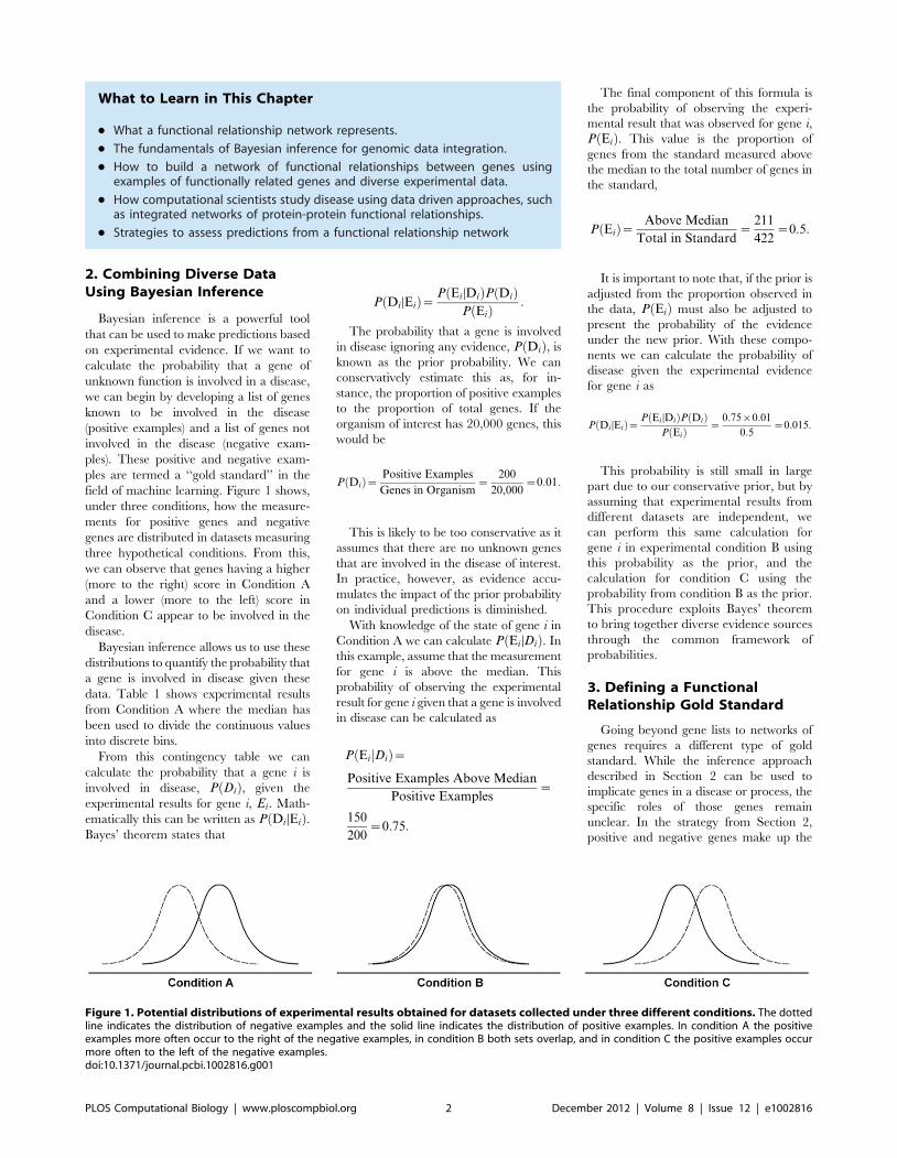
2. Combining Diverse DataUsing Bayesian Inference
Bayesian inference is a powerful tool
that can be used to make predictions based
on experimental evidence. If we want to
calculate the probability that a gene of
unknown function is involved in a disease,
we can begin by developing a list of genes
known to be involved in the disease
(positive examples) and a list of genes not
involved in the disease (negative exam-
ples). These positive and negative exam-
ples are termed a ‘‘gold standard’’ in the
field of machine learning. Figure 1 shows,
under three conditions, how the measure-
ments for positive genes and negative
genes are distributed in datasets measuring
three hypothetical conditions. From this,
we can observe that genes having a higher
(more to the right) score in Condition A
and a lower (more to the left) score in
Condition C appear to be involved in the
disease.
Bayesian inference allows us to use these
distributions to quantify the probability that
a gene is involved in disease given these
data. Table 1 shows experimental results
from Condition A where the median has
been used to divide the continuous values
into discrete bins.
From this contingency table we can
calculate the probability that a gene i is
involved in disease, P Dið Þ, given the
experimental results for gene i, Ei. Math-
ematically this can be written as P Di DEið Þ.Bayes’ theorem states that
P Di DEið Þ~ P Ei DDið ÞP Dið ÞP Eið Þ
:
The probability that a gene is involved
in disease ignoring any evidence, P Dið Þ, is
known as the prior probability. We can
conservatively estimate this as, for in-
stance, the proportion of positive examples
to the proportion of total genes. If the
organism of interest has 20,000 genes, this
would be
P Dið Þ~Positive Examples
Genes in Organism~
200
20,000~0:01:
This is likely to be too conservative as it
assumes that there are no unknown genes
that are involved in the disease of interest.
In practice, however, as evidence accu-
mulates the impact of the prior probability
on individual predictions is diminished.
With knowledge of the state of gene i in
Condition A we can calculate P Ei DDið Þ. In
this example, assume that the measurement
for gene i is above the median. This
probability of observing the experimental
result for gene i given that a gene is involved
in disease can be calculated as
P EijDið Þ~Positive Examples Above Median
Positive Examples~
150
200~0:75:
The final component of this formula is
the probability of observing the experi-
mental result that was observed for gene i,
P Eið Þ. This value is the proportion of
genes from the standard measured above
the median to the total number of genes in
the standard,
P Eið Þ~Above Median
Total in Standard~
211
422~0:5:
It is important to note that, if the prior is
adjusted from the proportion observed in
the data, P Eið Þ must also be adjusted to
present the probability of the evidence
under the new prior. With these compo-
nents we can calculate the probability of
disease given the experimental evidence
for gene i as
P Di DEið Þ~ P Ei DDið ÞP Dið ÞP Eið Þ
~0:75|0:01
0:5~0:015:
This probability is still small in large
part due to our conservative prior, but by
assuming that experimental results from
different datasets are independent, we
can perform this same calculation for
gene i in experimental condition B using
this probability as the prior, and the
calculation for condition C using the
probability from condition B as the prior.
This procedure exploits Bayes’ theorem
to bring together diverse evidence sources
through the common framework of
probabilities.
3. Defining a FunctionalRelationship Gold Standard
Going beyond gene lists to networks of
genes requires a different type of gold
standard. While the inference approach
described in Section 2 can be used to
implicate genes in a disease or process, the
specific roles of those genes remain
unclear. In the strategy from Section 2,
positive and negative genes make up the
What to Learn in This Chapter
N What a functional relationship network represents.
N The fundamentals of Bayesian inference for genomic data integration.
N How to build a network of functional relationships between genes usingexamples of functionally related genes and diverse experimental data.
N How computational scientists study disease using data driven approaches, suchas integrated networks of protein-protein functional relationships.
N Strategies to assess predictions from a functional relationship network
Figure 1. Potential distributions of experimental results obtained for datasets collected under three different conditions. The dottedline indicates the distribution of negative examples and the solid line indicates the distribution of positive examples. In condition A the positiveexamples more often occur to the right of the negative examples, in condition B both sets overlap, and in condition C the positive examples occurmore often to the left of the negative examples.doi:10.1371/journal.pcbi.1002816.g001
PLOS Computational Biology | www.ploscompbiol.org 2 December 2012 | Volume 8 | Issue 12 | e1002816
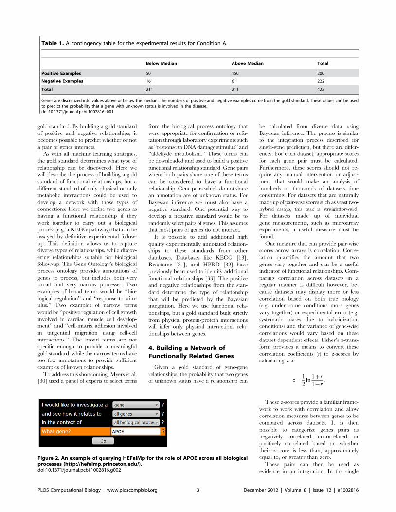
gold standard. By building a gold standard
of positive and negative relationships, it
becomes possible to predict whether or not
a pair of genes interacts.
As with all machine learning strategies,
the gold standard determines what type of
relationship can be discovered. Here we
will describe the process of building a gold
standard of functional relationships, but a
different standard of only physical or only
metabolic interactions could be used to
develop a network with those types of
connections. Here we define two genes as
having a functional relationship if they
work together to carry out a biological
process (e.g. a KEGG pathway) that can be
assayed by definitive experimental follow-
up. This definition allows us to capture
diverse types of relationships, while discov-
ering relationships suitable for biological
follow-up. The Gene Ontology’s biological
process ontology provides annotations of
genes to process, but includes both very
broad and very narrow processes. Two
examples of broad terms would be ‘‘bio-
logical regulation’’ and ‘‘response to stim-
ulus.’’ Two examples of narrow terms
would be ‘‘positive regulation of cell growth
involved in cardiac muscle cell develop-
ment’’ and ‘‘cell-matrix adhesion involved
in tangential migration using cell-cell
interactions.’’ The broad terms are not
specific enough to provide a meaningful
gold standard, while the narrow terms have
too few annotations to provide sufficient
examples of known relationships.
To address this shortcoming, Myers et al.
[30] used a panel of experts to select terms
from the biological process ontology that
were appropriate for confirmation or refu-
tation through laboratory experiments such
as ‘‘response to DNA damage stimulus’’ and
‘‘aldehyde metabolism.’’ These terms can
be downloaded and used to build a positive
functional relationship standard. Gene pairs
where both pairs share one of these terms
can be considered to have a functional
relationship. Gene pairs which do not share
an annotation are of unknown status. For
Bayesian inference we must also have a
negative standard. One potential way to
develop a negative standard would be to
randomly select pairs of genes. This assumes
that most pairs of genes do not interact.
It is possible to add additional high
quality experimentally annotated relation-
ships to these standards from other
databases. Databases like KEGG [13],
Reactome [31], and HPRD [32] have
previously been used to identify additional
functional relationships [33]. The positive
and negative relationships from the stan-
dard determine the type of relationship
that will be predicted by the Bayesian
integration. Here we use functional rela-
tionships, but a gold standard built strictly
from physical protein-protein interactions
will infer only physical interactions rela-
tionships between genes.
4. Building a Network ofFunctionally Related Genes
Given a gold standard of gene-gene
relationships, the probability that two genes
of unknown status have a relationship can
be calculated from diverse data using
Bayesian inference. The process is similar
to the integration process described for
single-gene prediction, but there are differ-
ences. For each dataset, appropriate scores
for each gene pair must be calculated.
Furthermore, these scores should not re-
quire any manual intervention or adjust-
ment that would make an analysis of
hundreds or thousands of datasets time
consuming. For datasets that are naturally
made up of pair-wise scores such as yeast two-
hybrid assays, this task is straightforward.
For datasets made up of individual
gene measurements, such as microarray
experiments, a useful measure must be
found.
One measure that can provide pair-wise
scores across arrays is correlation. Corre-
lation quantifies the amount that two
genes vary together and can be a useful
indicator of functional relationships. Com-
paring correlation across datasets in a
regular manner is difficult however, be-
cause datasets may display more or less
correlation based on both true biology
(e.g. under some conditions more genes
vary together) or experimental error (e.g.
systematic biases due to hybridization
conditions) and the variance of gene-wise
correlations would vary based on these
dataset dependent effects. Fisher’s z-trans-
form provides a means to convert these
correlation coefficients (r) to z-scores by
calculating z as
z~1
2ln
1zr
1{r:
These z-scores provide a familiar frame-
work to work with correlation and allow
correlation measures between genes to be
compared across datasets. It is then
possible to categorize genes pairs as
negatively correlated, uncorrelated, or
positively correlated based on whether
their z-score is less than, approximately
equal to, or greater than zero.
These pairs can then be used as
evidence in an integration. In the single
Table 1. A contingency table for the experimental results for Condition A.
Below Median Above Median Total
Positive Examples 50 150 200
Negative Examples 161 61 222
Total 211 211 422
Genes are discretized into values above or below the median. The numbers of positive and negative examples come from the gold standard. These values can be usedto predict the probability that a gene with unknown status is involved in the disease.doi:10.1371/journal.pcbi.1002816.t001
Figure 2. An example of querying HEFalMp for the role of APOE across all biologicalprocesses (http://hefalmp.princeton.edu/).doi:10.1371/journal.pcbi.1002816.g002
PLOS Computational Biology | www.ploscompbiol.org 3 December 2012 | Volume 8 | Issue 12 | e1002816
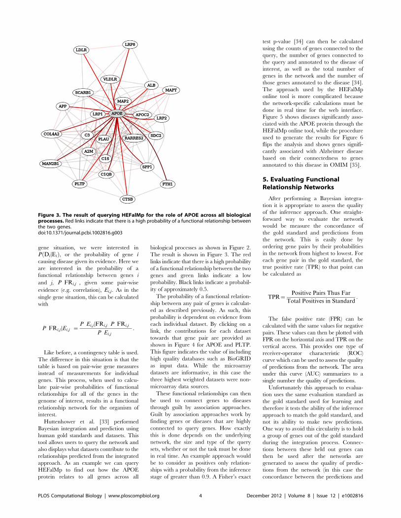
gene situation, we were interested in
P Di DEið Þ, or the probability of gene icausing disease given its evidence. Here we
are interested in the probability of a
functional relationship between genes i
and j, P FRi,j
� �, given some pair-wise
evidence (e.g. correlation), Ei,j . As in the
single gene situation, this can be calculated
with
P FRi,j DEi,j
� �~
P Ei,j DFRi,j
� �P FRi,j
� �
P Ei,j
� � :
Like before, a contingency table is used.
The difference in this situation is that the
table is based on pair-wise gene measures
instead of measurements for individual
genes. This process, when used to calcu-
late pair-wise probabilities of functional
relationships for all of the genes in the
genome of interest, results in a functional
relationship network for the organism of
interest.
Huttenhower et al. [33] performed
Bayesian integration and prediction using
human gold standards and datasets. This
tool allows users to query the network and
also displays what datasets contribute to the
relationships predicted from the integrated
approach. As an example we can query
HEFalMp to find out how the APOE
protein relates to all genes across all
biological processes as shown in Figure 2.
The result is shown in Figure 3. The red
links indicate that there is a high probability
of a functional relationship between the two
genes and green links indicate a low
probability. Black links indicate a probabil-
ity of approximately 0.5.
The probability of a functional relation-
ship between any pair of genes is calculat-
ed as described previously. As such, this
probability is dependent on evidence from
each individual dataset. By clicking on a
link, the contributions for each dataset
towards that gene pair are provided as
shown in Figure 4 for APOE and PLTP.
This figure indicates the value of including
high quality databases such as BioGRID
as input data. While the microarray
datasets are informative, in this case the
three highest weighted datasets were non-
microarray data sources.
These functional relationships can then
be used to connect genes to diseases
through guilt by association approaches.
Guilt by association approaches work by
finding genes or diseases that are highly
connected to query genes. How exactly
this is done depends on the underlying
network, the size and type of the query
sets, whether or not the task must be done
in real time. An example approach would
be to consider as positives only relation-
ships with a probability from the inference
stage of greater than 0.9. A Fisher’s exact
test p-value [34] can then be calculated
using the counts of genes connected to the
query, the number of genes connected to
the query and annotated to the disease of
interest, as well as the total number of
genes in the network and the number of
those genes annotated to the disease [34].
The approach used by the HEFalMp
online tool is more complicated because
the network-specific calculations must be
done in real time for the web interface.
Figure 5 shows diseases significantly asso-
ciated with the APOE protein through the
HEFalMp online tool, while the procedure
used to generate the results for Figure 6
flips the analysis and shows genes signifi-
cantly associated with Alzheimer disease
based on their connectedness to genes
annotated to this disease in OMIM [35].
5. Evaluating FunctionalRelationship Networks
After performing a Bayesian integra-
tion it is appropriate to assess the quality
of the inference approach. One straight-
forward way to evaluate the network
would be measure the concordance of
the gold standard and predictions from
the network. This is easily done by
ordering gene pairs by their probabilities
in the network from highest to lowest. For
each gene pair in the gold standard, the
true positive rate (TPR) to that point can
be calculated as
TPR~Positive Pairs Thus Far
Total Positives in Standard:
The false positive rate (FPR) can be
calculated with the same values for negative
pairs. These values can then be plotted with
FPR on the horizontal axis and TPR on the
vertical access. This provides one type of
receiver-operator characteristic (ROC)
curve which can be used to assess the quality
of predictions from the network. The area
under this curve (AUC) summarizes to a
single number the quality of predictions.
Unfortunately this approach to evalua-
tion uses the same evaluation standard as
the gold standard used for learning and
therefore it tests the ability of the inference
approach to match the gold standard, and
not its ability to make new predictions.
One way to avoid this circularity is to hold
a group of genes out of the gold standard
during the integration process. Connec-
tions between these held out genes can
then be used after the networks are
generated to assess the quality of predic-
tions from the network (in this case the
concordance between the predictions and
Figure 3. The result of querying HEFalMp for the role of APOE across all biologicalprocesses. Red links indicate that there is a high probability of a functional relationship betweenthe two genes.doi:10.1371/journal.pcbi.1002816.g003
PLOS Computational Biology | www.ploscompbiol.org 4 December 2012 | Volume 8 | Issue 12 | e1002816
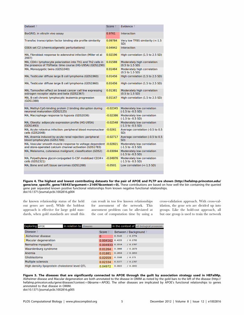
the known relationship status of the held
out genes are used). While the holdout
approach is effective for large gold stan-
dards, when gold standards are small this
can result in too few known relationships
for assessment of the network. This
assessment problem can be alleviated at
the cost of computation time by using a
cross-validation approach. With cross-val-
idation, the gene sets are divided up into
groups. Like the hold-out approach, all
but one group is used to train the network
Figure 4. The highest and lowest contributing datasets for the pair of APOE and PLTP are shown (http://hefalmp.princeton.edu/gene/one_specific_gene/18543?argument = 21697&context = 0). These contributions are based on how well the bin containing the queriedgene pair separated known positive functional relationships from known negative functional relationships.doi:10.1371/journal.pcbi.1002816.g004
Figure 5. The diseases that are significantly connected to APOE through the guilt by association strategy used in HEFalMp.Alzheimer disease and Macular degeneration are both annotated to the disease in OMIM as noted by the gold bars to the left of the disease (http://hefalmp.princeton.edu/gene/diseases?context = 0&name = APOE). The other diseases are implicated by APOE’s functional relationships to genesannotated to that disease in OMIM.doi:10.1371/journal.pcbi.1002816.g005
PLOS Computational Biology | www.ploscompbiol.org 5 December 2012 | Volume 8 | Issue 12 | e1002816
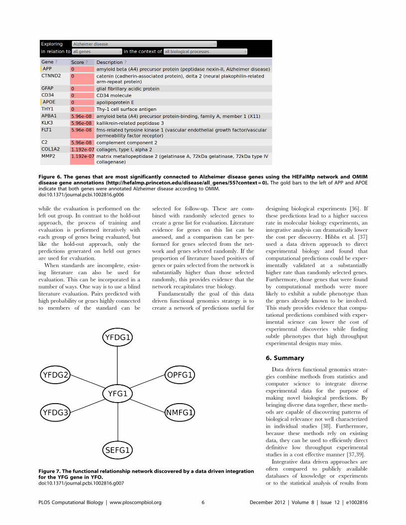
while the evaluation is performed on the
left out group. In contrast to the hold-out
approach, the process of training and
evaluation is performed iteratively with
each group of genes being evaluated, but
like the hold-out approach, only the
predictions generated on held out genes
are used for evaluation.
When standards are incomplete, exist-
ing literature can also be used for
evaluation. This can be incorporated in a
number of ways. One way is to use a blind
literature evaluation. Pairs predicted with
high probability or genes highly connected
to members of the standard can be
selected for follow-up. These are com-
bined with randomly selected genes to
create a gene list for evaluation. Literature
evidence for genes on this list can be
assessed, and a comparison can be per-
formed for genes selected from the net-
work and genes selected randomly. If the
proportion of literature based positives of
genes or pairs selected from the network is
substantially higher than those selected
randomly, this provides evidence that the
network recapitulates true biology.
Fundamentally the goal of this data
driven functional genomics strategy is to
create a network of predictions useful for
designing biological experiments [36]. If
these predictions lead to a higher success
rate in molecular biology experiments, an
integrative analysis can dramatically lower
the cost per discovery. Hibbs et al. [37]
used a data driven approach to direct
experimental biology and found that
computational predictions could be exper-
imentally validated at a substantially
higher rate than randomly selected genes.
Furthermore, those genes that were found
by computational methods were more
likely to exhibit a subtle phenotype than
the genes already known to be involved.
This study provides evidence that compu-
tational predictions combined with exper-
imental science can lower the cost of
experimental discoveries while finding
subtle phenotypes that high throughput
experimental designs may miss.
6. Summary
Data driven functional genomics strate-
gies combine methods from statistics and
computer science to integrate diverse
experimental data for the purpose of
making novel biological predictions. By
bringing diverse data together, these meth-
ods are capable of discovering patterns of
biological relevance not well characterized
in individual studies [38]. Furthermore,
because these methods rely on existing
data, they can be used to efficiently direct
definitive low throughput experimental
studies in a cost effective manner [37,39].
Integrative data driven approaches are
often compared to publicly available
databases of knowledge or experiments
or to the statistical analysis of results from
Figure 6. The genes that are most significantly connected to Alzheimer disease genes using the HEFalMp network and OMIMdisease gene annotations (http://hefalmp.princeton.edu/disease/all_genes/55?context = 0). The gold bars to the left of APP and APOEindicate that both genes were annotated Alzheimer disease according to OMIM.doi:10.1371/journal.pcbi.1002816.g006
Figure 7. The functional relationship network discovered by a data driven integrationfor the YFG gene in YFO.doi:10.1371/journal.pcbi.1002816.g007
PLOS Computational Biology | www.ploscompbiol.org 6 December 2012 | Volume 8 | Issue 12 | e1002816
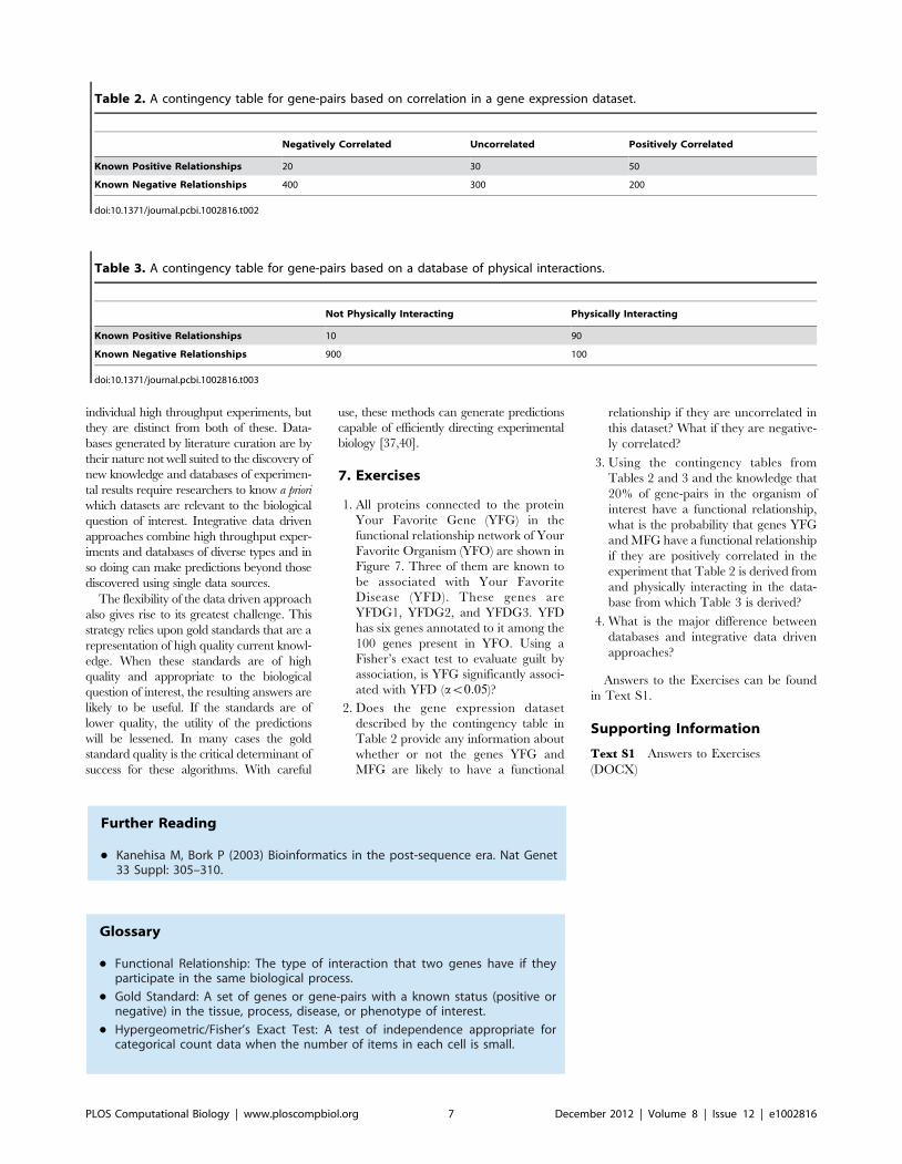
individual high throughput experiments, but
they are distinct from both of these. Data-
bases generated by literature curation are by
their nature not well suited to the discovery of
new knowledge and databases of experimen-
tal results require researchers to know a priori
which datasets are relevant to the biological
question of interest. Integrative data driven
approaches combine high throughput exper-
iments and databases of diverse types and in
so doing can make predictions beyond those
discovered using single data sources.
The flexibility of the data driven approach
also gives rise to its greatest challenge. This
strategy relies upon gold standards that are a
representation of high quality current knowl-
edge. When these standards are of high
quality and appropriate to the biological
question of interest, the resulting answers are
likely to be useful. If the standards are of
lower quality, the utility of the predictions
will be lessened. In many cases the gold
standard quality is the critical determinant of
success for these algorithms. With careful
use, these methods can generate predictions
capable of efficiently directing experimental
biology [37,40].
7. Exercises
1. All proteins connected to the protein
Your Favorite Gene (YFG) in the
functional relationship network of Your
Favorite Organism (YFO) are shown in
Figure 7. Three of them are known to
be associated with Your Favorite
Disease (YFD). These genes are
YFDG1, YFDG2, and YFDG3. YFD
has six genes annotated to it among the
100 genes present in YFO. Using a
Fisher’s exact test to evaluate guilt by
association, is YFG significantly associ-
ated with YFD (av0:05)?
2. Does the gene expression dataset
described by the contingency table in
Table 2 provide any information about
whether or not the genes YFG and
MFG are likely to have a functional
relationship if they are uncorrelated in
this dataset? What if they are negative-
ly correlated?
3. Using the contingency tables from
Tables 2 and 3 and the knowledge that
20% of gene-pairs in the organism of
interest have a functional relationship,
what is the probability that genes YFG
and MFG have a functional relationship
if they are positively correlated in the
experiment that Table 2 is derived from
and physically interacting in the data-
base from which Table 3 is derived?
4. What is the major difference between
databases and integrative data driven
approaches?
Answers to the Exercises can be found
in Text S1.
Supporting Information
Text S1 Answers to Exercises
(DOCX)
Glossary
N Functional Relationship: The type of interaction that two genes have if theyparticipate in the same biological process.
N Gold Standard: A set of genes or gene-pairs with a known status (positive ornegative) in the tissue, process, disease, or phenotype of interest.
N Hypergeometric/Fisher’s Exact Test: A test of independence appropriate forcategorical count data when the number of items in each cell is small.
Further Reading
N Kanehisa M, Bork P (2003) Bioinformatics in the post-sequence era. Nat Genet33 Suppl: 305–310.
Table 2. A contingency table for gene-pairs based on correlation in a gene expression dataset.
Negatively Correlated Uncorrelated Positively Correlated
Known Positive Relationships 20 30 50
Known Negative Relationships 400 300 200
doi:10.1371/journal.pcbi.1002816.t002
Table 3. A contingency table for gene-pairs based on a database of physical interactions.
Not Physically Interacting Physically Interacting
Known Positive Relationships 10 90
Known Negative Relationships 900 100
doi:10.1371/journal.pcbi.1002816.t003
PLOS Computational Biology | www.ploscompbiol.org 7 December 2012 | Volume 8 | Issue 12 | e1002816
References
1. Whitfield ML, Sherlock G, Saldanha AJ, Murray JI,
Ball CA, et al. (2002) Identification of genes periodicallyexpressed in the human cell cycle and their expression
in tumors. Mol Biol Cell 13: 1977–2000.2. Hegde P, Qi R, Gaspard R, Abernathy K,
Dharap S, et al. (2001) Identification of tumor
markers in models of human colorectal cancerusing a 19,200-element complementary DNA
microarray. Cancer Res 61: 7792–7797.3. Lock C, Hermans G, Pedotti R, Brendolan A,
Schadt E, et al. (2002) Gene-microarray analysis
of multiple sclerosis lesions yields new targetsvalidated in autoimmune encephalomyelitis. Nat
Med 8: 500–508.4. Wellcome Trust Case Control Consortium (2007)
Genome-wide association study of 14,000 cases ofseven common diseases and 3,000 shared con-
trols. Nature 447: 661–678.
5. Schymick JC, Scholz SW, Fung HC, Britton A,Arepalli S, et al. (2007) Genome-wide genotyping
in amyotrophic lateral sclerosis and neurologicallynormal controls: first stage analysis and public
release of data. Lancet Neurol 6: 322–328.
6. Kittler R, Pelletier L, Heninger AK, Slabicki M,Theis M, et al. (2007) Genome-scale RNAi
profiling of cell division in human tissue culturecells. Nat Cell Biol 9: 1401–1412.
7. Krishnan MN, Ng A, Sukumaran B, Gilfoy FD,Uchil PD, et al. (2008) RNA interference screen
for human genes associated with West Nile virus
infection. Nature 455: 242–245.8. Ozsolak F, Song JS, Liu XS, Fisher DE (2007)
High-throughput mapping of the chromatinstructure of human promoters. Nat Biotechnol
25: 244–248.
9. Su AI, Wiltshire T, Batalov S, Lapp H, ChingKA, et al. (2004) A gene atlas of the mouse and
human protein-encoding transcriptomes. ProcNatl Acad Sci U S A 101: 6062–6067.
10. Perou CM, Sorlie T, Eisen MB, van de Rijn M,Jeffrey SS, et al. (2000) Molecular portraits of
human breast tumours. Nature 406: 747–752.
11. Edgar R, Domrachev M, Lash AE (2002) GeneExpression Omnibus: NCBI gene expression and
hybridization array data repository. Nucleic AcidsRes 30: 207–210.
12. Desiere F, Deutsch EW, King NL, Nesvizhskii AI,
Mallick P, et al. (2006) The PeptideAtlas project.Nucleic Acids Res 34: D655–D658.
13. Kanehisa M, Goto S (2000) KEGG: kyotoencyclopedia of genes and genomes. Nucleic
Acids Res 28: 27–30.14. Ashburner M, Ball CA, Blake JA, Botstein D,
Butler H, et al. (2000) Gene ontology: tool for the
unification of biology. The Gene OntologyConsortium Nat Genet 25: 25–29.
15. Klein TE, Chang JT, Cho MK, Easton KL,
Fergerson R, et al. (2001) Integrating genotype
and phenotype information: an overview of the
PharmGKB project. Pharmacogenetics Re-
search Network and Knowledge Base
Pharmacogenomics J 1: 167–170.
16. Xenarios I, Salwinski L, Duan XJ, Higney P, Kim
SM, et al. (2002) DIP, the Database of Interacting
Proteins: a research tool for studying cellular
networks of protein interactions. Nucleic Acids
Res 30: 303–305.
17. Bader G, Betel D, Hogue C (2003) BIND: the
Biomolecular Interaction Network Database.
Nucleic Acids Res 31: 248–250.
18. Snel B, Lehmann G, Bork P, Huynen MA (2000)
STRING: a web-server to retrieve and display the
repeatedly occurring neighbourhood of a gene.
Nucleic Acids Res 28: 3442–3444.
19. Mostafavi S, Ray D, Warde-Farley D, Grouios C,
Morris Q (2008) GeneMANIA: a real-time
multiple association network integration algo-
rithm for predicting gene function. Genome Biol
9 Suppl 1: S4.
20. Warde-Farley D, Donaldson SL, Comes O, Zuberi
K, Badrawi R, et al. (2010) The GeneMANIA
prediction server: biological network integration
for gene prioritization and predicting gene func-
tion. Nucleic Acids Res 38: W214–W220.
21. Lee I, Ambaru B, Thakkar P, Marcotte EM, Rhee
SY (2010) Rational association of genes with traits
using a genome-scale gene network for Arabidopsis
thaliana. Nat Biotechnol 28: 149–156.
22. Lee I, Date SV, Adai AT, Marcotte EM (2004) A
probabilistic functional network of yeast genes.
Science 306: 1555–1558.
23. Lee I, Blom UM, Wang PI, Shim JE, Marcotte
EM (2011) Prioritizing candidate disease genes by
network-based boosting of genome-wide associa-
tion data. Genome Res 21: 1109–1121.
24. Kim WK, Krumpelman C, Marcotte EM (2008)
Inferring mouse gene functions from genomic-
scale data using a combined functional network/
classification strategy. Genome Biol 9 Suppl
1: S5.
25. Rhodes DR, Tomlins SA, Varambally S, Maha-
visno V, Barrette T, et al. (2005) Probabilistic
model of the human protein-protein interaction
network. Nat Biotechnol 23: 951–959.
26. Segal E, Wang H, Koller D (2003) Discovering
molecular pathways from protein interaction and
gene expression data. Bioinformatics 19: i264–
i272.
27. Chen X, Lin MZ, Shen XL (2011) PAIR: the
predicted Arabidopsis interactome resource. Nu-
cleic Acids Res 39: D1134–D1140.
28. Myers C, Robson D, Wible A, Hibbs M, Chiriac
C, et al. (2005) Discovery of biological networks
from diverse functional genomic data. Genome
Biol 6: R114–R114.
29. Troyanskaya OG, Dolinski K, Owen AB, Altman
RB, Botstein D (2003) A Bayesian framework for
combining heterogeneous data sources for gene
function prediction (in Saccharomyces cerevisiae).
Proc Natl Acad Sci U S A100: 8348–8353.
30. Myers CL, Barrett DR, Hibbs MA, Huttenhower
C, Troyanskaya OG (2006) Finding function:
evaluation methods for functional genomic data.
BMC Genomics 7: 187.
31. Vastrik I, D’Eustachio P, Schmidt E, Gopinath
G, Croft D, et al. (2007) Reactome: a knowledge
base of biologic pathways and processes. Genome
Biol 8: R39.
32. Peri S, Navarro JD, Amanchy R, Kristiansen TZ,
Jonnalagadda CK, et al. (2003) Development of
human protein reference database as an initial
platform for approaching systems biology in
humans. Genome Res 13: 2363–2371.
33. Huttenhower C, Haley EM, Hibbs MA, Du-
meaux V, Barrett DR, et al. (2009) Exploring the
human genome with functional maps. Genome
Res 19: 1093–1106.
34. Sokal RR, Rohlf FJ (1995) Biometry : the
principles and practice of statistics in biological
research. New York: W.H. Freeman. xix, 887 p.
35. Hamosh A, Scott AF, Amberger J, Valle D,
McKusick VA (2000) Online Mendelian Inheri-
tance in Man (OMIM). Human Mutation 15: 57–
61.
36. Greene CS, Troyanskaya OG (2012) Accurate
evaluation and analysis of functional genomics data
and methods. Ann N Y Acad Sci 1260: 95–100.
37. Hibbs MA, Myers CL, Huttenhower C, Hess DC,
Li K, et al. (2009) Directing experimental biology:
a case study in mitochondrial biogenesis. PLoS
Comput Biol 5: e1000322. doi:10.1371/journal.
pcbi.1000322.
38. Huttenhower C, Hibbs M, Myers C, Troyans-
kaya OG (2006) A scalable method for integration
and functional analysis of multiple microarray
datasets. Bioinformatics 22: 2890–2897.
39. Hess DC, Myers CL, Huttenhower C, Hibbs MA,
Hayes AP, et al. (2009) Computationally driven,
quantitative experiments discover genes required
for mitochondrial biogenesis. PLoS Genet 5:
e1000407. doi:10.1371/journal.pgen.1000407.
40. Guan Y, Dunham M, Caudy A, Troyanskaya O
(2010) Systematic planning of genome-scale
experiments in poorly studied species. PLoS
Comput Biol 6: e1000698. doi:10.1371/journal.
pcbi.1000698.
PLOS Computational Biology | www.ploscompbiol.org 8 December 2012 | Volume 8 | Issue 12 | e1002816
Education
Chapter 3: Small Molecules and DiseaseDavid S. Wishart1,2,3*
1 Department of Biological Sciences, University of Alberta, Edmonton, Alberta, Canada, 2 Department of Computing Science, University of Alberta, Edmonton, Alberta,
Canada, 3 National Research Council, National Institute for Nanotechnology (NINT), Edmonton, Alberta, Canada
Abstract: ‘‘Big’’ molecules such asproteins and genes still continue tocapture the imagination of mostbiologists, biochemists and bioin-formaticians. ‘‘Small’’ molecules, onthe other hand, are the moleculesthat most biologists, biochemistsand bioinformaticians prefer toignore. However, it is becomingincreasingly apparent that smallmolecules such as amino acids,lipids and sugars play a far moreimportant role in all aspects ofdisease etiology and disease treat-ment than we realized. This partic-ular chapter focuses on an emerg-ing field of bioinformatics called‘‘chemical bioinformatics’’ – a disci-pline that has evolved to helpaddress the blended chemical andmolecular biological needs of tox-icogenomics, pharmacogenomics,metabolomics and systems biolo-gy. In the following pages we willcover several topics related tochemical bioinformatics. First, abrief overview of some of the mostimportant or useful chemical bioin-formatic resources will be given.Second, a more detailed overviewwill be given on those particularresources that allow researchers toconnect small molecules to diseas-es. This section will focus ondescribing a number of recentlydeveloped databases or knowl-edgebases that explicitly relatesmall molecules – either as thetreatment, symptom or cause – todisease. Finally a short discussionwill be provided on newly emerg-ing software tools that exploitthese databases as a means todiscover new biomarkers or evennew treatments for disease.
This article is part of the ‘‘Transla-
tional Bioinformatics’’ collection for
PLOS Computational Biology.
1. Introduction
For most of the past 100 years, the fields
of toxicology, pharmacology and clinical
biochemistry have focused on identifying
the chemicals that cause (toxins), cure
(drugs) or characterize (biomarkers) most
human diseases. Historically, this kind of
work has been reliant on the slow, careful
and sometime tedious approaches of
classical analytical chemistry and classical
biochemistry. Nevertheless, it has led to
important discoveries and enormous ad-
vances in our understanding of the actions
of chemicals on genes, proteins and cells.
With the recent emergence of high
throughput ‘‘omics’’ technologies, our
ability to detect, identify, and characterize
small molecules along with their large
molecule targets has been radically
changed [1,2]. Now it is possible to
perform as many sequencing experiments,
mass spectrometry (MS) experiments or
compound identifications in a single day as
used to be done in a single year. As a
result, traditional fields such as toxicology,
pharmacology and biochemistry have
been transformed into totally new fields
called toxicogenomics, pharmacogenomics
and metabolomics. This transformation
has changed not only the fundamentals of
these disciplines, but also the fundamentals
of their data. Rather than trying to
manage a few samples, a few sequences
or a few compounds in a paper notebook
or on an Excel spreadsheet, researchers
are confronted with the task of handling
hundreds of samples, thousands of com-
pounds, thousands of spectra and thou-
sands of genes or protein sequences. This
has led to the development of novel
computational tools and entirely new
bioinformatic disciplines to facilitate the
handling of this data. This particular
chapter focuses on an emerging field of
bioinformatics called ‘‘chemical bioinfor-
matics’’ – a discipline that has evolved to
help address the blended chemical and
molecular biological needs of toxicoge-
nomics, pharmacogenomics, metabolo-
mics and systems biology.
Chemical bioinformatics combines the
sequence-centric tools of bioinformatics
with the chemo-centric tools of ‘‘chemin-
formatics’’. The term cheminformatics,
which is an abbreviated form of ‘‘chemical
informatics’’, was first coined by Frank
Brown nearly 15 years ago [3]. Cheminfor-
matics (as it is known in North America) or
chemoinformatics (as it is known in Europe
and the rest of the world) is actually a close
cousin to bioinformatics. Just as bioinfor-
matics is a field of information technology
concerned with using computers to analyze
molecular biological data, cheminformatics
is a field of information technology that uses
computers to facilitate the collection, stor-
age, analysis and manipulation of large
quantities of chemical data.
However, there are some distinct ‘‘cul-
tural’’ differences between bioinformatics
and cheminformatics. For instance, che-
minformatics software is mostly designed
for use by chemists, while bioinformatics
software is designed for use by molecular
biologists. Consequently there is often a
terminology gap that makes it difficult for
biologists to use cheminformatic software
and chemists to use bioinformatics soft-
ware. Likewise, most cheminformatic soft-
ware is structure-based or picture-driven
while most bioinformatic software is se-
quence-based or text-driven. As a result,
different search and query interfaces have
evolved that are quite specific to either
cheminformatic or bioinformatic software.
Citation: Wishart DS (2012) Chapter 3: Small Molecules and Disease. PLoS Comput Biol 8(12): e1002805.doi:10.1371/journal.pcbi.1002805
Editors: Fran Lewitter, Whitehead Institute, United States of America and Maricel Kann, University of Maryland,Baltimore County, United States of America
Published December , 2012
Copyright: � 2012 David S. Wishart. This is an open-access article distributed under the terms of the CreativeCommons Attribution License, which permits unrestricted use, distribution, and reproduction in any medium,provided the original author and source are credited.
Funding: Funding to develop the databases described in this article was provided by Genome Canada, AlbertaInnovates, and the Canadian Institutes of Health Research. The funders had no role in the preparation of themanuscript.
Competing Interests: The author has declared that no competing interests exist.
* E-mail: [email protected]
PLOS Computational Biology | www.ploscompbiol.org 1 December 2012 | Volume 8 | Issue 12 | e1002805
27
Further compounding this culture gap is
the fact that most cheminformatics soft-
ware and chemical compound databases
were developed without the expectation
that this information would ever be
biologically or medically relevant. Like-
wise, most bioinformatics software and
bioinformatic databases were developed
without the intention of using this data to
facilitate small molecule biomarker identi-
fication or small molecule drug discovery.
Consequently most biological sequence
data is not linked in any meaningful way
to drug or disease information – and vice
versa. However, thanks to the emergence
of new fields such as pharmacogenomics,
toxicogenomics, systems biology and me-
tabolomics, there is now a growing desire
to bring bioinformatics and cheminfor-
matics closer together. This has spawned
the new field of chemical bioinformatics.
In this chapter we will cover several topics
related to chemical bioinformatics. First, a
brief overview of some of the most important
chemical bioinformatic resources will be
given. This will include a discussion of some
of the major databases and classes of
databases. Second, a more detailed overview
will be given on those particular resources
that allow researchers to connect small
molecules to diseases. This section will focus
on describing a number of recently devel-
oped databases or knowledgebases that
explicitly relate small molecules – either as
the treatment, symptom or cause – to
disease. Finally a short discussion will be
provided on newly emerging software tools
that exploit these databases as a means to
discover new biomarkers or even new
treatments for disease.
2. Databases for ChemicalBioinformatics
Electronic databases lie at the heart of
almost any subdiscipline of bioinformatics
– and chemical bioinformatics is no
exception. Indeed, without databases there
is essentially no foundational knowledge to
the discipline, and consequently, no com-
pelling reason to write software. Programs
such as BLAST [4] would be useless
without GenBank [5], likewise, PSIPRED
[6] couldn’t exist without the Protein
Databank [7] and Gene Set Enrichment
Analysis – GSEA [8] would be impossible
without the GEO and KEGG databases
[9,10]. Given their importance, it is
perhaps worthwhile to briefly review the
different types of chemical-bioinformatic
databases that are available and discuss
some of their particular strengths and
limitations.
Currently there are four major classes of
chemical-bioinformatic databases. These
include: 1) small molecule (or metabolic)
pathway databases; 2) metabolite or me-
tabolomic databases; 3) drug databases;
and 4) toxin or toxic substance databases.
In an ideal world each of these database
classes could/should be useful for relating
small molecules to human diseases or
disease treatments. For instance, metabolic
pathway databases would be expected to
be most useful for understanding the ‘‘big-
picture’’ relationship between small mole-
cules and disease – either with regard to
those small molecule compounds causing
disease (i.e. toxins), indicating disease (i.e.
biomarkers) or being used in the treatment
of disease (i.e. drugs). On the other hand,
metabolite or metabolomic databases
would be expected to be most useful for
associating small molecule biomarkers
with specific diseases, such as inborn errors
of metabolism or a variety of chronic or
infectious diseases characterized by me-
tabolite imbalances. Drug databases would
obviously be most relevant for identifying
small molecules with disease treatments,
although they could also be used to
identify small molecule drugs causing
adverse drug reactions. Finally toxin or
toxic compound databases would be
expected to be most useful for identifying
the compounds causing diseases or causing
symptoms associated with certain poison-
ing or environmental exposure incidents.
This could include acute poisonings or
more long-term, environmentally influ-
enced conditions such as cancer, allergies
or birth defects.
However, as detailed below, not all of
the available chemical-bioinformatic data-
bases are particularly suited for these kinds
of disease-associated queries. This likely
reflects the relatively nascent stage of this
field (it’s less than five years old) and the
fact that disease-related information is
much more difficult to gather and codify
than either chemical structure or gene
sequence information. Certainly all of
today’s existing chemical-bioinformatic
databases contain information about dif-
ferent classes of chemicals (metabolites,
drugs or poisons) and most contain some
limited information about the correspond-
ing protein and/or genetic targets. How-
ever, only a very small number of these
databases actually include information on
the diseases or physiological effects that
may be caused, cured or characterized by
these chemicals.
2.1 Metabolic Pathway DatabasesAmong the four major classes of chem-
ical-bioinformatic databases that are avail-
able, metabolic pathway databases are
perhaps the best known and most widely
used. They include a number of popular
web-based resources such as the Kyoto
Encyclopedia of Genes and Genomes – also
known as KEGG [10], the ‘‘Cyc’’ databas-
es [11,12], the Reactome database [13],
WikiPathways [14], the Small Molecule
Pathway Databases or SMPDB [15] and
the Medical Biochemistry Page [http://
themedicalbiochemistrypage.org/]. Sever-
al commercial pathway databases also exist
such as TransPath (from BioBase Inc.),
PathArt (from Jubilant Biosys Inc.), Meta-
Base (from GeneGo Inc.) and Ingenuity
Pathways Analysis (Ingenuity Systems Inc.),
many of which provide nicely illustrated
metabolic pathway diagrams. Most of these
pathway databases were designed to facil-
itate the exploration of metabolism and
metabolites across many different species.
This broad, multi-organism perspective has
been critical to enhancing our basic
understanding of metabolism and our
appreciation of biological diversity. Meta-
bolic pathway databases also serve as the
backbone to facilitate many practical ap-
plications in biology including comparative
genomics and targeted genome annotation.
Table 1 lists the names, web addresses and
general features for these and other useful
pathway databases.
Those metabolic pathway databases
that strive for very broad organism
coverage, such as KEGG and Reactome,
tend to use pathway diagrams that are
very generic and highly schematic, while
What to Learn in This Chapter
N The meaning of chemical bioinformatics
N Strengths and limitations of existing chemical bioinformatic databases
N Using databases to learn about the cause and treatment of diseases
N The Small Molecule Pathway Database (SMPDB)
N The Human Metabolome Database (HMDB)
N DrugBank
N The Toxin and Toxin-Target Database (T3DB)
N PolySearch and Metabolite Set Enrichment Analysis
PLOS Computational Biology | www.ploscompbiol.org 2 December 2012 | Volume 8 | Issue 12 | e1002805
those that are organism-specific (i.e. hu-
man-only), such as SMPDB and the
Medical Biochemistry Page, tend to use
diagrams that are very specific and much
richer in detail, colour and content. Most
pathway databases support interactive
image mapping with hyperlinked informa-
tion content that allows users to view
chemical information (if a compound is
clicked) or brief summaries of genes and/
or proteins (if a protein is clicked). Almost
all of the databases support some kind of
limited text search and a few, such as
Reactome, SMPDB and the ‘‘Cyc’’ data-
bases, support the mapping of gene,
protein and/or metabolite expression data
onto pathway diagrams. As might be
expected, the major focus of most of
today’s small molecule pathway databases
is on basic metabolism. As a result, only
one of these databases (SMPD) actually
includes any pathways associated with
drug action or disease.
2.2 Metabolomic DatabasesThe second major class of chemical-
bioinformatic databases are metabolomic
or metabolite databases. These databases
tend to have a major focus on chemicals
and chemical descriptors with a lesser (or
even absent) focus on biological data.
They are primarily used for metabolite
identification – especially in metabolomic
studies. Some databases are almost exclu-
sively chemical in nature, containing
primarily information on the chemical
name(s), synonyms, InChI (International
Chemical Identifier) identifier, structure,
and molecular weight. These include Lipid
Maps [16], a comprehensive database of
biological lipids; ChEBI [17], a database
of biologically interesting compounds;
PubChem [18], a collection of most
known organic chemicals with links to
PubMed articles and more than 500,000
bioassays; ChemSpider [19], a chemical
databases that is similar in size to Pub-
Chem; KNApSAcK [20], a database of
plant phytochemicals and METLIN [21],
a database of known and presumptive
human metabolites. All of these databases
support a variety of text search options
and a few (such as PubChem, ChemSpi-
der, LipidMaps and ChEBI) support
structure and structure similarity searches.
In addition to these biochemical databas-
es, there are a number of smaller databas-
es that contain spectral (NMR or MS) data
of small molecule metabolites. These
include the BioMagResBank or BMRB
[22] which contains experimental NMR
spectra of mammalian metabolites, Mass-
Bank [23] which contains MS spectra of a
variety of metabolites, drugs and toxic
compounds, MMCD [24] which contains
experimental and predicted NMR spectra
of Arabadopsis metabolites, and the Golm
Metabolome database [25] which contains
MS spectra of different plant metabolites.
These spectral databases are frequently
used to facilitate compound identification
via spectral comparison. More recently, a
much more comprehensive kind of meta-
bolomic database has emerged which
attempts to combine chemical data, spec-
tral data, protein target data, biomarker
data and disease data into a single
resource. Perhaps the best example of this
is the Human Metabolome Database
(HMDB). The HMDB is a database
containing comprehensive data on most
of the known or measurable endogenous
metabolites in humans [26]. Table 2
presents a summary of the names, web
addresses and general features for the
major metabolite/metabolomic databases.
2.3 Pharmaceutical ProductDatabases
The third major class of chemical
bioinformatic databases are the drug or
pharmaceutical product databases. In
particular, two types of electronic drug
databases have started to emerge over the
past five years: 1) clinically oriented drug
databases and 2) chemically oriented drug
databases. Examples of some of the better-
known clinically oriented drug databases
include DailyMed [27] and RxList [28].
These resources typically offer very de-
tailed clinical information (i.e. their for-
mulation, metabolism and indications)
about selected drugs derived from their
FDA labels. As a result, these kinds of
databases are targeted more towards
pharmacists, physicians or consumers.
Examples of chemically or genetically
oriented drug databases include the TTD
[29], PharmGKB [30] and SuperTarget
[31]. TTD (which stands for Therapeutic
Target Database) contains information on
5028 drugs (both approved and experi-
mental) with 1894 identified targets and
links to 560 different diseases or indica-
tions. PharmGKB (which stands for Phar-
macogenomics Knowldege Base) has in-
formation on 1587 approved drugs (with
descriptions and indications), including
pharmacogenomic data on 287 drugs.
SuperTarget contains information on
more than 2500 target proteins, which
are annotated with about 7300 literature-
mined relations to 1500 different drugs.
All three of these databases provide
synoptic data (5–10 data fields per entry)
about the nomenclature, structure and/or
physical properties of small molecule drugs
and, in the case of SuperTarget and TTD,
their drug targets. Both TTD and Super-
Target support text, sequence and chem-
ical structure searches, while PharmGKB
provides mechanistic, pharmacodynamic
and pharmacokinetic pathway informa-
tion for 68 different drugs or drug classes.
As a general rule, chemically oriented
drug databases tend to appeal to medicinal
chemists, biochemists and molecular biol-
ogists. In addition to these somewhat
specialized databases, a much more com-
prehensive ‘‘hybrid’’ database, known as
DrugBank [32] has recently been devel-
oped. Drugbank combines the clinical/
disease information of the clinically ori-
ented drug databases with the biochemi-
cal/chemical information of the chemical-
ly oriented drug databases. As a result, a
typical DrugBank entry contains 80–100
different data fields, instead of 5–10 as
seen with the other kinds of databases.
Like TTD and SuperTarget, DrugBank
supports very extensive text, sequence and
chemical structure searches. It also pro-
vides detailed pathway information on the
mechanism of action for .200 different
drugs or drug classes. Table 3 provides a
short summary of the names, descriptions
and website addresses of the more popular
drug or pharmaceutical product databas-
es.
2.4 Toxic Substance DatabasesThe final class of chemical-bioinfor-
matic databases we will discuss are the
toxic substance databases. These include
the Animal Toxin Database (ATDB),
SuperToxic [33], ACToR [34], the Com-
parative Toxicogenomics Database [35]
and T3DB [36]. Table 4 presents a
summary of the names, web addresses
and general features for these databases.
The Animal Toxin Database (ATDB),
with .3800 peptide toxins, provides data
on the sequence of many peptide/protein
toxins from venomous insects and animals
as well as information on the channel
targets to which these toxins bind. Both
ACToR (which stands for the Aggregated
Computational Toxicology Resource) and
SuperToxic provide bioassy data and
chemical structure information for a very
large number of industrial or pharmaceu-
tically interesting chemicals (.60,000 for
SuperToxic, .500,000 for AcTOR). The
Comparative Toxicogenomics Database
(CTD), with .5000 chemicals, provides
literature-derived information on chemi-
cal-gene interactions. This includes micro-
array information on genes that are up/
down-regulated upon contact or exposure
to these chemicals. T3DB (which stands
for the Toxin, Toxin-Target Database)
provides very extensive structural, physio-
PLOS Computational Biology | www.ploscompbiol.org 3 December 2012 | Volume 8 | Issue 12 | e1002805
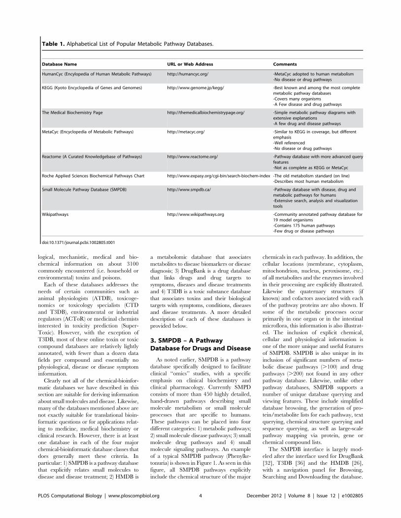
logical, mechanistic, medical and bio-
chemical information on about 3100
commonly encountered (i.e. household or
environmental) toxins and poisons.
Each of these databases addresses the
needs of certain communities such as
animal physiologists (ATDB), toxicoge-
nomics or toxicology specialists (CTD
and T3DB), environmental or industrial
regulators (ACToR) or medicinal chemists
interested in toxicity prediction (Super-
Toxic). However, with the exception of
T3DB, most of these online toxin or toxic
compound databases are relatively lightly
annotated, with fewer than a dozen data
fields per compound and essentially no
physiological, disease or disease symptom
information.
Clearly not all of the chemical-bioinfor-
matic databases we have described in this
section are suitable for deriving information
about small molecules and disease. Likewise,
many of the databases mentioned above are
not exactly suitable for translational bioin-
formatic questions or for applications relat-
ing to medicine, medical biochemistry or
clinical research. However, there is at least
one database in each of the four major
chemical-bioinformatic database classes that
does generally meet these criteria. In
particular: 1) SMPDB is a pathway database
that explicitly relates small molecules to
disease and disease treatment; 2) HMDB is
a metabolomic database that associates
metabolites to disease biomarkers or disease
diagnosis; 3) DrugBank is a drug database
that links drugs and drug targets to
symptoms, diseases and disease treatments
and 4) T3DB is a toxic substance database
that associates toxins and their biological
targets with symptoms, conditions, diseases
and disease treatments. A more detailed
description of each of these databases is
provided below.
3. SMPDB – A PathwayDatabase for Drugs and Disease
As noted earlier, SMPDB is a pathway
database specifically designed to facilitate
clinical ‘‘omics’’ studies, with a specific
emphasis on clinical biochemistry and
clinical pharmacology. Currently SMPD
consists of more than 450 highly detailed,
hand-drawn pathways describing small
molecule metabolism or small molecule
processes that are specific to humans.
These pathways can be placed into four
different categories: 1) metabolic pathways;
2) small molecule disease pathways; 3) small
molecule drug pathways and 4) small
molecule signaling pathways. An example
of a typical SMPDB pathway (Phenylke-
tonuria) is shown in Figure 1. As seen in this
figure, all SMPDB pathways explicitly
include the chemical structure of the major
chemicals in each pathway. In addition, the
cellular locations (membrane, cytoplasm,
mitochondrion, nucleus, peroxisome, etc.)
of all metabolites and the enzymes involved
in their processing are explicitly illustrated.
Likewise the quaternary structures (if
known) and cofactors associated with each
of the pathway proteins are also shown. If
some of the metabolic processes occur
primarily in one organ or in the intestinal
microflora, this information is also illustrat-
ed. The inclusion of explicit chemical,
cellular and physiological information is
one of the more unique and useful features
of SMPDB. SMPDB is also unique in its
inclusion of significant numbers of meta-
bolic disease pathways (.100) and drug
pathways (.200) not found in any other
pathway database. Likewise, unlike other
pathway databases, SMPDB supports a
number of unique database querying and
viewing features. These include simplified
database browsing, the generation of pro-
tein/metabolite lists for each pathway, text
querying, chemical structure querying and
sequence querying, as well as large-scale
pathway mapping via protein, gene or
chemical compound lists.
The SMPDB interface is largely mod-
eled after the interface used for DrugBank
[32], T3DB [36] and the HMDB [26],
with a navigation panel for Browsing,
Searching and Downloading the database.
Table 1. Alphabetical List of Popular Metabolic Pathway Databases.
Database Name URL or Web Address Comments
HumanCyc (Encylopedia of Human Metabolic Pathways) http://humancyc.org/ -MetaCyc adopted to human metabolism-No disease or drug pathways
KEGG (Kyoto Encyclopedia of Genes and Genomes) http://www.genome.jp/kegg/ -Best known and among the most completemetabolic pathway databases-Covers many organisms-A Few disease and drug pathways
The Medical Biochemistry Page http://themedicalbiochemistrypage.org/ -Simple metabolic pathway diagrams withextensive explanations-A few drug and disease pathways
MetaCyc (Encyclopedia of Metabolic Pathways) http://metacyc.org/ -Similar to KEGG in coverage, but differentemphasis-Well referenced-No disease or drug pathways
Reactome (A Curated Knowledgebase of Pathways) http://www.reactome.org/ -Pathway database with more advanced queryfeatures-Not as complete as KEGG or MetaCyc
Roche Applied Sciences Biochemical Pathways Chart http://www.expasy.org/cgi-bin/search-biochem-index -The old metabolism standard (on line)-Describes most human metabolism
Small Molecule Pathway Database (SMPDB) http://www.smpdb.ca/ -Pathway database with disease, drug andmetabolic pathways for humans-Extensive search, analysis and visualizationtools
Wikipathways http://www.wikipathways.org -Community annotated pathway database for19 model organisms-Contains 175 human pathways-Few drug or disease pathways
doi:10.1371/journal.pcbi.1002805.t001
PLOS Computational Biology | www.ploscompbiol.org 4 December 2012 | Volume 8 | Issue 12 | e1002805
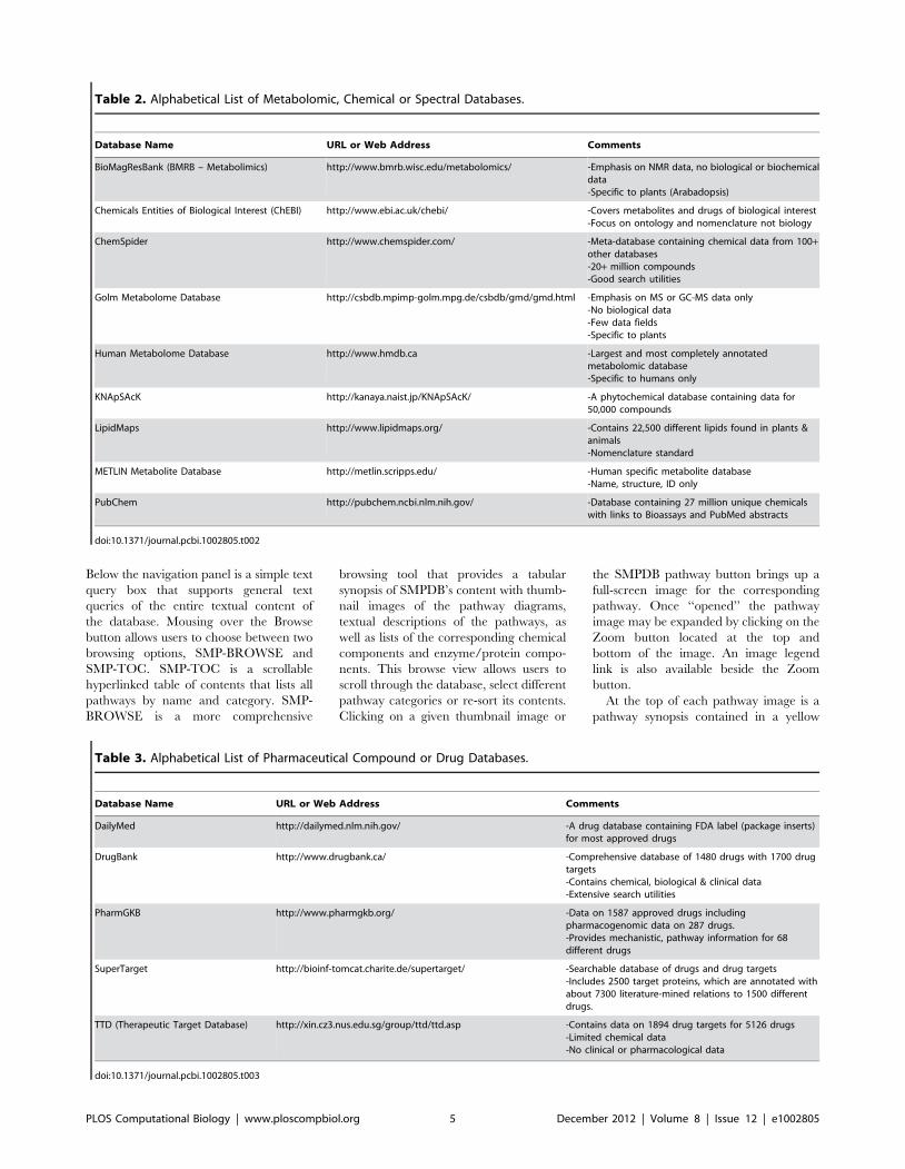
Below the navigation panel is a simple text
query box that supports general text
queries of the entire textual content of
the database. Mousing over the Browse
button allows users to choose between two
browsing options, SMP-BROWSE and
SMP-TOC. SMP-TOC is a scrollable
hyperlinked table of contents that lists all
pathways by name and category. SMP-
BROWSE is a more comprehensive
browsing tool that provides a tabular
synopsis of SMPDB’s content with thumb-
nail images of the pathway diagrams,
textual descriptions of the pathways, as
well as lists of the corresponding chemical
components and enzyme/protein compo-
nents. This browse view allows users to
scroll through the database, select different
pathway categories or re-sort its contents.
Clicking on a given thumbnail image or
the SMPDB pathway button brings up a
full-screen image for the corresponding
pathway. Once ‘‘opened’’ the pathway
image may be expanded by clicking on the
Zoom button located at the top and
bottom of the image. An image legend
link is also available beside the Zoom
button.
At the top of each pathway image is a
pathway synopsis contained in a yellow
Table 2. Alphabetical List of Metabolomic, Chemical or Spectral Databases.
Database Name URL or Web Address Comments
BioMagResBank (BMRB – Metabolimics) http://www.bmrb.wisc.edu/metabolomics/ -Emphasis on NMR data, no biological or biochemicaldata-Specific to plants (Arabadopsis)
Chemicals Entities of Biological Interest (ChEBI) http://www.ebi.ac.uk/chebi/ -Covers metabolites and drugs of biological interest-Focus on ontology and nomenclature not biology
ChemSpider http://www.chemspider.com/ -Meta-database containing chemical data from 100+other databases-20+ million compounds-Good search utilities
Golm Metabolome Database http://csbdb.mpimp-golm.mpg.de/csbdb/gmd/gmd.html -Emphasis on MS or GC-MS data only-No biological data-Few data fields-Specific to plants
Human Metabolome Database http://www.hmdb.ca -Largest and most completely annotatedmetabolomic database-Specific to humans only
KNApSAcK http://kanaya.naist.jp/KNApSAcK/ -A phytochemical database containing data for50,000 compounds
LipidMaps http://www.lipidmaps.org/ -Contains 22,500 different lipids found in plants &animals-Nomenclature standard
METLIN Metabolite Database http://metlin.scripps.edu/ -Human specific metabolite database-Name, structure, ID only
PubChem http://pubchem.ncbi.nlm.nih.gov/ -Database containing 27 million unique chemicalswith links to Bioassays and PubMed abstracts
doi:10.1371/journal.pcbi.1002805.t002
Table 3. Alphabetical List of Pharmaceutical Compound or Drug Databases.
Database Name URL or Web Address Comments
DailyMed http://dailymed.nlm.nih.gov/ -A drug database containing FDA label (package inserts)for most approved drugs
DrugBank http://www.drugbank.ca/ -Comprehensive database of 1480 drugs with 1700 drugtargets-Contains chemical, biological & clinical data-Extensive search utilities
PharmGKB http://www.pharmgkb.org/ -Data on 1587 approved drugs includingpharmacogenomic data on 287 drugs.-Provides mechanistic, pathway information for 68different drugs
SuperTarget http://bioinf-tomcat.charite.de/supertarget/ -Searchable database of drugs and drug targets-Includes 2500 target proteins, which are annotated withabout 7300 literature-mined relations to 1500 differentdrugs.
TTD (Therapeutic Target Database) http://xin.cz3.nus.edu.sg/group/ttd/ttd.asp -Contains data on 1894 drug targets for 5126 drugs-Limited chemical data-No clinical or pharmacological data
doi:10.1371/journal.pcbi.1002805.t003
PLOS Computational Biology | www.ploscompbiol.org 5 December 2012 | Volume 8 | Issue 12 | e1002805
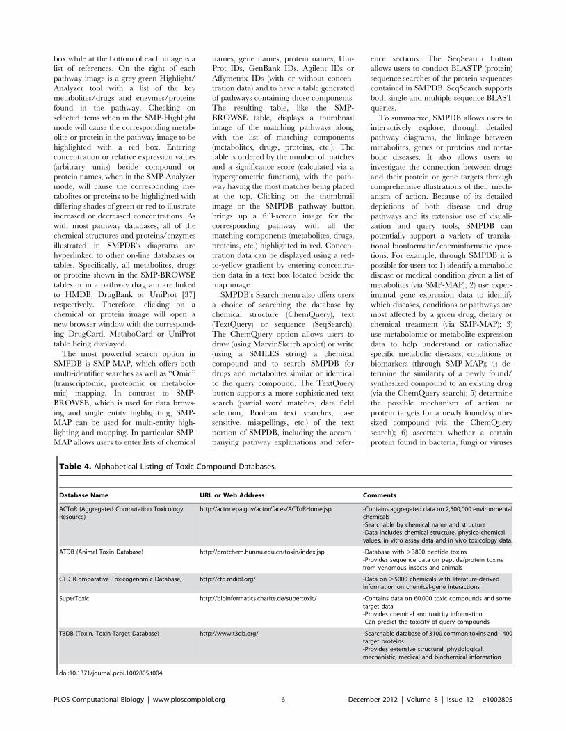
box while at the bottom of each image is a
list of references. On the right of each
pathway image is a grey-green Highlight/
Analyzer tool with a list of the key
metabolites/drugs and enzymes/proteins
found in the pathway. Checking on
selected items when in the SMP-Highlight
mode will cause the corresponding metab-
olite or protein in the pathway image to be
highlighted with a red box. Entering
concentration or relative expression values
(arbitrary units) beside compound or
protein names, when in the SMP-Analyzer
mode, will cause the corresponding me-
tabolites or proteins to be highlighted with
differing shades of green or red to illustrate
increased or decreased concentrations. As
with most pathway databases, all of the
chemical structures and proteins/enzymes
illustrated in SMPDB’s diagrams are
hyperlinked to other on-line databases or
tables. Specifically, all metabolites, drugs
or proteins shown in the SMP-BROWSE
tables or in a pathway diagram are linked
to HMDB, DrugBank or UniProt [37]
respectively. Therefore, clicking on a
chemical or protein image will open a
new browser window with the correspond-
ing DrugCard, MetaboCard or UniProt
table being displayed.
The most powerful search option in
SMPDB is SMP-MAP, which offers both
multi-identifier searches as well as ‘‘Omic’’
(transcriptomic, proteomic or metabolo-
mic) mapping. In contrast to SMP-
BROWSE, which is used for data brows-
ing and single entity highlighting, SMP-
MAP can be used for multi-entity high-
lighting and mapping. In particular SMP-
MAP allows users to enter lists of chemical
names, gene names, protein names, Uni-
Prot IDs, GenBank IDs, Agilent IDs or
Affymetrix IDs (with or without concen-
tration data) and to have a table generated
of pathways containing those components.
The resulting table, like the SMP-
BROWSE table, displays a thumbnail
image of the matching pathways along
with the list of matching components
(metabolites, drugs, proteins, etc.). The
table is ordered by the number of matches
and a significance score (calculated via a
hypergeometric function), with the path-
way having the most matches being placed
at the top. Clicking on the thumbnail
image or the SMPDB pathway button
brings up a full-screen image for the
corresponding pathway with all the
matching components (metabolites, drugs,
proteins, etc.) highlighted in red. Concen-
tration data can be displayed using a red-
to-yellow gradient by entering concentra-
tion data in a text box located beside the
map image.
SMPDB’s Search menu also offers users
a choice of searching the database by
chemical structure (ChemQuery), text
(TextQuery) or sequence (SeqSearch).
The ChemQuery option allows users to
draw (using MarvinSketch applet) or write
(using a SMILES string) a chemical
compound and to search SMPDB for
drugs and metabolites similar or identical
to the query compound. The TextQuery
button supports a more sophisticated text
search (partial word matches, data field
selection, Boolean text searches, case
sensitive, misspellings, etc.) of the text
portion of SMPDB, including the accom-
panying pathway explanations and refer-
ence sections. The SeqSearch button
allows users to conduct BLASTP (protein)
sequence searches of the protein sequences
contained in SMPDB. SeqSearch supports
both single and multiple sequence BLAST
queries.
To summarize, SMPDB allows users to
interactively explore, through detailed
pathway diagrams, the linkage between
metabolites, genes or proteins and meta-
bolic diseases. It also allows users to
investigate the connection between drugs
and their protein or gene targets through
comprehensive illustrations of their mech-
anism of action. Because of its detailed
depictions of both disease and drug
pathways and its extensive use of visuali-
zation and query tools, SMPDB can
potentially support a variety of transla-
tional bionformatic/cheminformatic ques-
tions. For example, through SMPDB it is
possible for users to: 1) identify a metabolic
disease or medical condition given a list of
metabolites (via SMP-MAP); 2) use exper-
imental gene expression data to identify
which diseases, conditions or pathways are
most affected by a given drug, dietary or
chemical treatment (via SMP-MAP); 3)
use metabolomic or metabolite expression
data to help understand or rationalize
specific metabolic diseases, conditions or
biomarkers (through SMP-MAP); 4) de-
termine the similarity of a newly found/
synthesized compound to an existing drug
(via the ChemQuery search); 5) determine
the possible mechanism of action or
protein targets for a newly found/synthe-
sized compound (via the ChemQuery
search); 6) ascertain whether a certain
protein found in bacteria, fungi or viruses
Table 4. Alphabetical Listing of Toxic Compound Databases.
Database Name URL or Web Address Comments
ACToR (Aggregated Computation ToxicologyResource)
http://actor.epa.gov/actor/faces/ACToRHome.jsp -Contains aggregated data on 2,500,000 environmentalchemicals-Searchable by chemical name and structure-Data includes chemical structure, physico-chemicalvalues, in vitro assay data and in vivo toxicology data.
ATDB (Animal Toxin Database) http://protchem.hunnu.edu.cn/toxin/index.jsp -Database with .3800 peptide toxins-Provides sequence data on peptide/protein toxinsfrom venomous insects and animals
CTD (Comparative Toxicogenomic Database) http://ctd.mdibl.org/ -Data on .5000 chemicals with literature-derivedinformation on chemical-gene interactions
SuperToxic http://bioinformatics.charite.de/supertoxic/ -Contains data on 60,000 toxic compounds and sometarget data-Provides chemical and toxicity information-Can predict the toxicity of query compounds
T3DB (Toxin, Toxin-Target Database) http://www.t3db.org/ -Searchable database of 3100 common toxins and 1400target proteins-Provides extensive structural, physiological,mechanistic, medical and biochemical information
doi:10.1371/journal.pcbi.1002805.t004
PLOS Computational Biology | www.ploscompbiol.org 6 December 2012 | Volume 8 | Issue 12 | e1002805
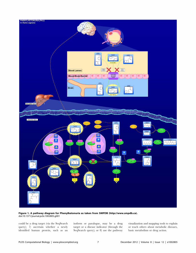
could be a drug target (via the SeqSearch
query); 7) ascertain whether a newly
identified human protein, such as an
isoform or paralogue, may be a drug
target or a disease indicator (through the
SeqSearch query); or 8) use the pathway
visualization and mapping tools to explain
or teach others about metabolic diseases,
basic metabolism or drug action.
Figure 1. A pathway diagram for Phenylketonuria as taken from SMPDB (http://www.smpdb.ca).doi:10.1371/journal.pcbi.1002805.g001
PLOS Computational Biology | www.ploscompbiol.org 7 December 2012 | Volume 8 | Issue 12 | e1002805
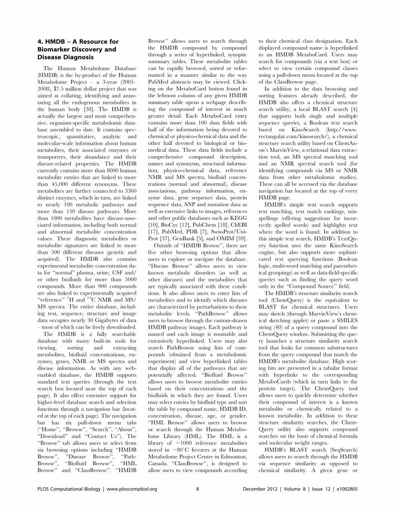
4. HMDB – A Resource forBiomarker Discovery andDisease Diagnosis
The Human Metabolome Database
(HMDB) is the by-product of the Human
Metabolome Project – a 3-year (2005–
2008), $7.5 million dollar project that was
aimed at collating, identifying and anno-
tating all the endogenous metabolites in
the human body [38]. The HMDB is
actually the largest and most comprehen-
sive, organism-specific metabolomic data-
base assembled to date. It contains spec-
troscopic, quantitative, analytic and
molecular-scale information about human
metabolites, their associated enzymes or
transporters, their abundance and their
disease-related properties. The HMDB
currently contains more than 8000 human
metabolite entries that are linked to more
than 45,000 different synonyms. These
metabolites are further connected to 3360
distinct enzymes, which in turn, are linked
to nearly 100 metabolic pathways and
more than 150 disease pathways. More
than 1000 metabolites have disease-asso-
ciated information, including both normal
and abnormal metabolite concentration
values. These diagnostic metabolites or
metabolite signatures are linked to more
than 500 different diseases (genetic and
acquired). The HMDB also contains
experimental metabolite concentration da-
ta for ‘‘normal’’ plasma, urine, CSF and/
or other biofluids for more than 5000
compounds. More than 900 compounds
are also linked to experimentally acquired
‘‘reference’’ 1H and 13C NMR and MS/
MS spectra. The entire database, includ-
ing text, sequence, structure and image
data occupies nearly 30 Gigabytes of data
– most of which can be freely downloaded.
The HMDB is a fully searchable
database with many built-in tools for
viewing, sorting and extracting
metabolites, biofluid concentrations, en-
zymes, genes, NMR or MS spectra and
disease information. As with any web-
enabled database, the HMDB supports
standard text queries (through the text
search box located near the top of each
page). It also offers extensive support for
higher-level database search and selection
functions through a navigation bar (locat-
ed at the top of each page). The navigation
bar has six pull-down menu tabs
(‘‘Home’’, ‘‘Browse’’, ‘‘Search’’, ‘‘About’’,
‘‘Download’’ and ‘‘Contact Us’’). The
‘‘Browse’’ tab allows users to select from
six browsing options including ‘‘HMDB
Browse’’, ‘‘Disease Browse’’, ‘‘Path-
Browse’’, ‘‘Biofluid Browse’’, ‘‘HML
Browse’’ and ‘‘ClassBrowse’’. ‘‘HMDB
Browse’’ allows users to search through
the HMDB compound by compound
through a series of hyperlinked, synoptic
summary tables. These metabolite tables
can be rapidly browsed, sorted or refor-
matted in a manner similar to the way
PubMed abstracts may be viewed. Click-
ing on the MetaboCard button found in
the leftmost column of any given HMDB
summary table opens a webpage describ-
ing the compound of interest in much
greater detail. Each MetaboCard entry
contains more than 100 data fields with
half of the information being devoted to
chemical or physico-chemical data and the
other half devoted to biological or bio-
medical data. These data fields include a
comprehensive compound description,
names and synonyms, structural informa-
tion, physico-chemical data, reference
NMR and MS spectra, biofluid concen-
trations (normal and abnormal), disease
associations, pathway information, en-
zyme data, gene sequence data, protein
sequence data, SNP and mutation data as
well as extensive links to images, references
and other public databases such as KEGG
[10], BioCyc [12], PubChem [18], ChEBI
[17], PubMed, PDB [7], SwissProt/Uni-
Prot [37], GenBank [5], and OMIM [39].
Outside of ‘‘HMDB Browse’’, there are
five other browsing options that allow
users to explore or navigate the database.
‘‘Disease Browse’’ allows users to view
known metabolic disorders (as well as
other diseases) and the metabolites that
are typically associated with these condi-
tions. It also allows users to enter lists of
metabolites and to identify which diseases
are characterized by perturbations to these
metabolite levels. ‘‘PathBrowse’’ allows
users to browse through the custom-drawn
HMDB pathway images. Each pathway is
named and each image is zoomable and
extensively hyperlinked. Users may also
search PathBrowse using lists of com-
pounds (obtained from a metabolomic
experiment) and view hyperlinked tables
that display all of the pathways that are
potentially affected. ‘‘Biofluid Browse’’
allows users to browse metabolite entries
based on their concentrations and the
biofluids in which they are found. Users
may select entries by biofluid type and sort
the table by compound name, HMDB ID,
concentration, disease, age, or gender.
‘‘HML Browse’’ allows users to browse
or search through the Human Metabo-
lome Library (HML). The HML is a
library of ,1000 reference metabolites
stored in 280uC freezers at the Human
Metabolome Project Centre in Edmonton,
Canada. ‘‘ClassBrowse’’, is designed to
allow users to view compounds according
to their chemical class designation. Each
displayed compound name is hyperlinked
to an HMDB MetaboCard. Users may
search for compounds (via a text box) or
select to view certain compound classes
using a pull-down menu located at the top
of the ClassBrowse page.
In addition to the data browsing and
sorting features already described, the
HMDB also offers a chemical structure
search utility, a local BLAST search [4]
that supports both single and multiple
sequence queries, a Boolean text search
based on KinoSearch (http://www.
rectangular.com/kinosearch/), a chemical
structure search utility based on ChemAx-
on’s MarvinView, a relational data extrac-
tion tool, an MS spectral matching tool
and an NMR spectral search tool (for
identifying compounds via MS or NMR
data from other metabolomic studies).
These can all be accessed via the database
navigation bar located at the top of every
HMDB page.
HMDB’s simple text search supports
text matching, text match rankings, mis-
spellings (offering suggestions for incor-
rectly spelled words) and highlights text
where the word is found. In addition to
this simple text search, HMDB’s TextQu-
ery function uses the same KinoSearch
engine, but also supports more sophisti-
cated text querying functions (Boolean
logic, multi-word matching and parenthet-
ical groupings) as well as data-field-specific
queries such as finding the query word
only in the ‘‘Compound Source’’ field.
The HMDB’s structure similarity search
tool (ChemQuery) is the equivalent to
BLAST for chemical structures. Users
may sketch (through MarvinView’s chem-
ical sketching applet) or paste a SMILES
string (40) of a query compound into the
ChemQuery window. Submitting the que-
ry launches a structure similarity search
tool that looks for common substructures
from the query compound that match the
HMDB’s metabolite database. High scor-
ing hits are presented in a tabular format
with hyperlinks to the corresponding
MetaboCards (which in turn links to the
protein target). The ChemQuery tool
allows users to quickly determine whether
their compound of interest is a known
metabolite or chemically related to a
known metabolite. In addition to these
structure similarity searches, the Chem-
Query utility also supports compound
searches on the basis of chemical formula
and molecular weight ranges.
HMDB’s BLAST search (SeqSearch)
allows users to search through the HMDB
via sequence similarity as opposed to
chemical similarity. A given gene or
PLOS Computational Biology | www.ploscompbiol.org 8 December 2012 | Volume 8 | Issue 12 | e1002805
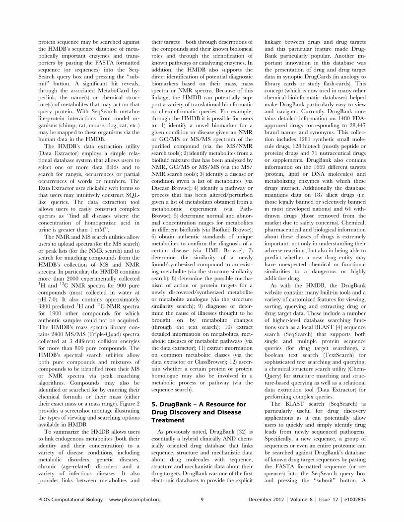
protein sequence may be searched against
the HMDB’s sequence database of meta-
bolically important enzymes and trans-
porters by pasting the FASTA formatted
sequence (or sequences) into the Seq-
Search query box and pressing the ‘‘sub-
mit’’ button. A significant hit reveals,
through the associated MetaboCard hy-
perlink, the name(s) or chemical struc-
ture(s) of metabolites that may act on that
query protein. With SeqSearch metabo-
lite-protein interactions from model or-
ganisms (chimp, rat, mouse, dog, cat, etc.)
may be mapped to these organisms via the
human data in the HMDB.
The HMDB’s data extraction utility
(Data Extractor) employs a simple rela-
tional database system that allows users to
select one or more data fields and to
search for ranges, occurrences or partial
occurrences of words or numbers. The
Data Extractor uses clickable web forms so
that users may intuitively construct SQL-
like queries. The data extraction tool
allows users to easily construct complex
queries as ‘‘find all diseases where the
concentration of homogentisic acid in
urine is greater than 1 mM’’.
The NMR and MS search utilities allow
users to upload spectra (for the MS search)
or peak lists (for the NMR search) and to
search for matching compounds from the
HMDB’s collection of MS and NMR
spectra. In particular, the HMDB contains
more than 2000 experimentally collected1H and 13C NMR spectra for 900 pure
compounds (most collected in water at
pH 7.0). It also contains approximately
3800 predicted 1H and 13C NMR spectra
for 1900 other compounds for which
authentic samples could not be acquired.
The HMDB’s mass spectra library con-
tains 2400 MS/MS (Triple-Quad) spectra
collected at 3 different collision energies
for more than 800 pure compounds. The
HMDB’s spectral search utilities allow
both pure compounds and mixtures of
compounds to be identified from their MS
or NMR spectra via peak matching
algorithms. Compounds may also be
identified or searched for by entering their
chemical formula or their mass (either
their exact mass or a mass range). Figure 2
provides a screenshot montage illustrating
the types of viewing and searching options
available in HMDB.
To summarize the HMDB allows users
to link endogenous metabolites (both their
identity and their concentration) to a
variety of disease conditions, including
metabolic disorders, genetic diseases,
chronic (age-related) disorders and a
variety of infectious diseases. It also
provides links between metabolites and
their targets – both through descriptions of
the compounds and their known biological
roles and through the identification of
known pathways or catalyzing enzymes. In
addition, the HMDB also supports the
direct identification of potential diagnostic
biomarkers based on their mass, mass
spectra or NMR spectra. Because of this
linkage, the HMDB can potentially sup-
port a variety of translational bionformatic
or cheminformatic queries. For example,
through the HMDB it is possible for users
to: 1) identify a novel biomarker for a
given condition or disease given an NMR
or GC/MS or MS/MS spectrum of the
purified compound (via the MS/NMR
search tools); 2) identify metabolites from a
biofluid mixture that has been analyzed by
NMR, GC/MS or MS/MS (via the MS/
NMR search tools); 3) identify a disease or
condition given a list of metabolites (via
Disease Browse); 4) identify a pathway or
process that has been altered/perturbed
given a list of metabolites obtained from a
metabolomic experiment (via Path-
Browse); 5) determine normal and abnor-
mal concentration ranges for metabolites
in different biofluids (via Biofluid Browse);
6) obtain authentic standards of unique
metabolites to confirm the diagnosis of a
certain disease (via HML Browse); 7)
determine the similarity of a newly
found/synthesized compound to an exist-
ing metabolite (via the structure similarity
search); 8) determine the possible mecha-
nism of action or protein targets for a
newly discovered/synthesized metabolite
or metabolite analogue (via the structure
similarity search); 9) diagnose or deter-
mine the cause of illnesses thought to be
brought on by metabolite changes
(through the text search); 10) extract
detailed information on metabolites, met-
abolic diseases or metabolic pathways (via
the data extractor); 11) extract information
on common metabolite classes (via the
data extractor or ClassBrowse); 12) ascer-
tain whether a certain protein or protein
homologue may also be involved in a
metabolic process or pathway (via the
sequence search).
5. DrugBank – A Resource forDrug Discovery and DiseaseTreatment
As previously noted, DrugBank [32] is
essentially a hybrid clinically AND chem-
ically oriented drug database that links
sequence, structure and mechanistic data
about drug molecules with sequence,
structure and mechanistic data about their
drug targets. DrugBank was one of the first
electronic databases to provide the explicit
linkage between drugs and drug targets
and this particular feature made Drug-
Bank particularly popular. Another im-
portant innovation in this database was
the presentation of drug and drug target
data in synoptic DrugCards (in anology to
library cards or study flash-cards). This
concept (which is now used in many other
chemical-bioinformatic databases) helped
make DrugBank particularly easy to view
and navigate. Currently DrugBank con-
tains detailed information on 1480 FDA-
approved drugs corresponding to 28,447
brand names and synonyms. This collec-
tion includes 1281 synthetic small mole-
cule drugs, 128 biotech (mostly peptide or
protein) drugs and 71 nutraceutical drugs
or supplements. DrugBank also contains
information on the 1669 different targets
(protein, lipid or DNA molecules) and
metabolizing enzymes with which these
drugs interact. Additionally the database
maintains data on 187 illicit drugs (i.e.
those legally banned or selectively banned
in most developed nations) and 64 with-
drawn drugs (those removed from the
market due to safety concerns). Chemical,
pharmaceutical and biological information
about these classes of drugs is extremely
important, not only in understanding their
adverse reactions, but also in being able to
predict whether a new drug entity may
have unexpected chemical or functional
similarities to a dangerous or highly
addictive drug.
As with the HMDB, the DrugBank
website contains many built-in tools and a
variety of customized features for viewing,
sorting, querying and extracting drug or
drug target data. These include a number
of higher-level database searching func-
tions such as a local BLAST [4] sequence
search (SeqSearch) that supports both
single and multiple protein sequence
queries (for drug target searching), a
boolean text search (TextSearch) for
sophisticated text searching and querying,
a chemical structure search utility (Chem-
Query) for structure matching and struc-
ture-based querying as well as a relational
data extraction tool (Data Extractor) for
performing complex queries.
The BLAST search (SeqSearch) is
particularly useful for drug discovery
applications as it can potentially allow
users to quickly and simply identify drug
leads from newly sequenced pathogens.
Specifically, a new sequence, a group of
sequences or even an entire proteome can
be searched against DrugBank’s database
of known drug target sequences by pasting
the FASTA formatted sequence (or se-
quences) into the SeqSearch query box
and pressing the ‘‘submit’’ button. A
PLOS Computational Biology | www.ploscompbiol.org 9 December 2012 | Volume 8 | Issue 12 | e1002805
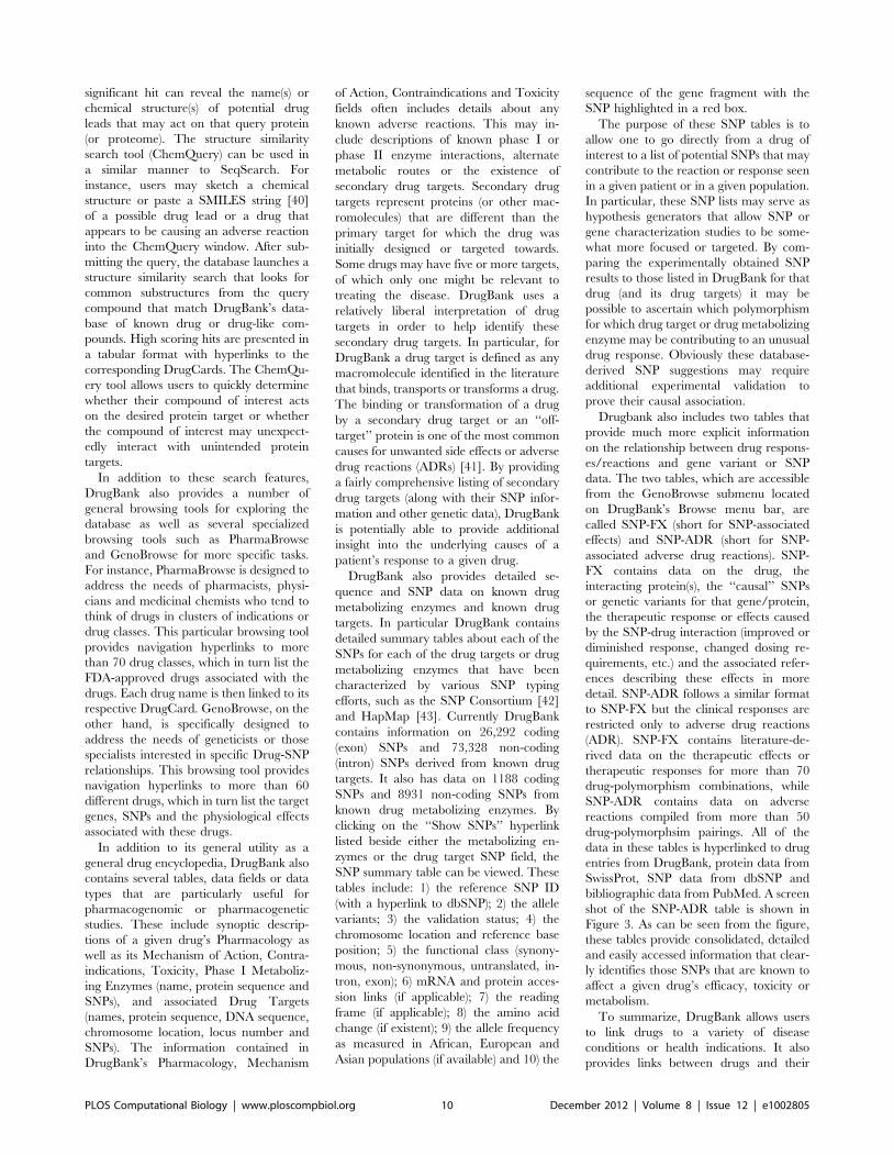
significant hit can reveal the name(s) or
chemical structure(s) of potential drug
leads that may act on that query protein
(or proteome). The structure similarity
search tool (ChemQuery) can be used in
a similar manner to SeqSearch. For
instance, users may sketch a chemical
structure or paste a SMILES string [40]
of a possible drug lead or a drug that
appears to be causing an adverse reaction
into the ChemQuery window. After sub-
mitting the query, the database launches a
structure similarity search that looks for
common substructures from the query
compound that match DrugBank’s data-
base of known drug or drug-like com-
pounds. High scoring hits are presented in
a tabular format with hyperlinks to the
corresponding DrugCards. The ChemQu-
ery tool allows users to quickly determine
whether their compound of interest acts
on the desired protein target or whether
the compound of interest may unexpect-
edly interact with unintended protein
targets.
In addition to these search features,
DrugBank also provides a number of
general browsing tools for exploring the
database as well as several specialized
browsing tools such as PharmaBrowse
and GenoBrowse for more specific tasks.
For instance, PharmaBrowse is designed to
address the needs of pharmacists, physi-
cians and medicinal chemists who tend to
think of drugs in clusters of indications or
drug classes. This particular browsing tool
provides navigation hyperlinks to more
than 70 drug classes, which in turn list the
FDA-approved drugs associated with the
drugs. Each drug name is then linked to its
respective DrugCard. GenoBrowse, on the
other hand, is specifically designed to
address the needs of geneticists or those
specialists interested in specific Drug-SNP
relationships. This browsing tool provides
navigation hyperlinks to more than 60
different drugs, which in turn list the target
genes, SNPs and the physiological effects
associated with these drugs.
In addition to its general utility as a
general drug encyclopedia, DrugBank also
contains several tables, data fields or data
types that are particularly useful for
pharmacogenomic or pharmacogenetic
studies. These include synoptic descrip-
tions of a given drug’s Pharmacology as
well as its Mechanism of Action, Contra-
indications, Toxicity, Phase I Metaboliz-
ing Enzymes (name, protein sequence and
SNPs), and associated Drug Targets
(names, protein sequence, DNA sequence,
chromosome location, locus number and
SNPs). The information contained in
DrugBank’s Pharmacology, Mechanism
of Action, Contraindications and Toxicity
fields often includes details about any
known adverse reactions. This may in-
clude descriptions of known phase I or
phase II enzyme interactions, alternate
metabolic routes or the existence of
secondary drug targets. Secondary drug
targets represent proteins (or other mac-
romolecules) that are different than the
primary target for which the drug was
initially designed or targeted towards.
Some drugs may have five or more targets,
of which only one might be relevant to
treating the disease. DrugBank uses a
relatively liberal interpretation of drug
targets in order to help identify these
secondary drug targets. In particular, for
DrugBank a drug target is defined as any
macromolecule identified in the literature
that binds, transports or transforms a drug.
The binding or transformation of a drug
by a secondary drug target or an ‘‘off-
target’’ protein is one of the most common
causes for unwanted side effects or adverse
drug reactions (ADRs) [41]. By providing
a fairly comprehensive listing of secondary
drug targets (along with their SNP infor-
mation and other genetic data), DrugBank
is potentially able to provide additional
insight into the underlying causes of a
patient’s response to a given drug.
DrugBank also provides detailed se-
quence and SNP data on known drug
metabolizing enzymes and known drug
targets. In particular DrugBank contains
detailed summary tables about each of the
SNPs for each of the drug targets or drug
metabolizing enzymes that have been
characterized by various SNP typing
efforts, such as the SNP Consortium [42]
and HapMap [43]. Currently DrugBank
contains information on 26,292 coding
(exon) SNPs and 73,328 non-coding
(intron) SNPs derived from known drug
targets. It also has data on 1188 coding
SNPs and 8931 non-coding SNPs from
known drug metabolizing enzymes. By
clicking on the ‘‘Show SNPs’’ hyperlink
listed beside either the metabolizing en-
zymes or the drug target SNP field, the
SNP summary table can be viewed. These
tables include: 1) the reference SNP ID
(with a hyperlink to dbSNP); 2) the allele
variants; 3) the validation status; 4) the
chromosome location and reference base
position; 5) the functional class (synony-
mous, non-synonymous, untranslated, in-
tron, exon); 6) mRNA and protein acces-
sion links (if applicable); 7) the reading
frame (if applicable); 8) the amino acid
change (if existent); 9) the allele frequency
as measured in African, European and
Asian populations (if available) and 10) the
sequence of the gene fragment with the
SNP highlighted in a red box.
The purpose of these SNP tables is to
allow one to go directly from a drug of
interest to a list of potential SNPs that may
contribute to the reaction or response seen
in a given patient or in a given population.
In particular, these SNP lists may serve as
hypothesis generators that allow SNP or
gene characterization studies to be some-
what more focused or targeted. By com-
paring the experimentally obtained SNP
results to those listed in DrugBank for that
drug (and its drug targets) it may be
possible to ascertain which polymorphism
for which drug target or drug metabolizing
enzyme may be contributing to an unusual
drug response. Obviously these database-
derived SNP suggestions may require
additional experimental validation to
prove their causal association.
Drugbank also includes two tables that
provide much more explicit information
on the relationship between drug respons-
es/reactions and gene variant or SNP
data. The two tables, which are accessible
from the GenoBrowse submenu located
on DrugBank’s Browse menu bar, are
called SNP-FX (short for SNP-associated
effects) and SNP-ADR (short for SNP-
associated adverse drug reactions). SNP-
FX contains data on the drug, the
interacting protein(s), the ‘‘causal’’ SNPs
or genetic variants for that gene/protein,
the therapeutic response or effects caused
by the SNP-drug interaction (improved or
diminished response, changed dosing re-
quirements, etc.) and the associated refer-
ences describing these effects in more
detail. SNP-ADR follows a similar format
to SNP-FX but the clinical responses are
restricted only to adverse drug reactions
(ADR). SNP-FX contains literature-de-
rived data on the therapeutic effects or
therapeutic responses for more than 70
drug-polymorphism combinations, while
SNP-ADR contains data on adverse
reactions compiled from more than 50
drug-polymorphsim pairings. All of the
data in these tables is hyperlinked to drug
entries from DrugBank, protein data from
SwissProt, SNP data from dbSNP and
bibliographic data from PubMed. A screen
shot of the SNP-ADR table is shown in
Figure 3. As can be seen from the figure,
these tables provide consolidated, detailed
and easily accessed information that clear-
ly identifies those SNPs that are known to
affect a given drug’s efficacy, toxicity or
metabolism.
To summarize, DrugBank allows users
to link drugs to a variety of disease
conditions or health indications. It also
provides links between drugs and their
PLOS Computational Biology | www.ploscompbiol.org 10 December 2012 | Volume 8 | Issue 12 | e1002805
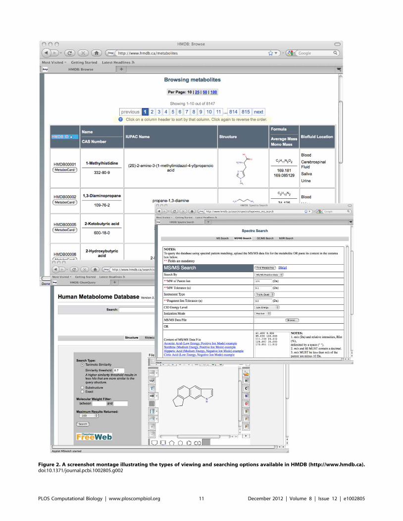
Figure 2. A screenshot montage illustrating the types of viewing and searching options available in HMDB (http://www.hmdb.ca).doi:10.1371/journal.pcbi.1002805.g002
PLOS Computational Biology | www.ploscompbiol.org 11 December 2012 | Volume 8 | Issue 12 | e1002805
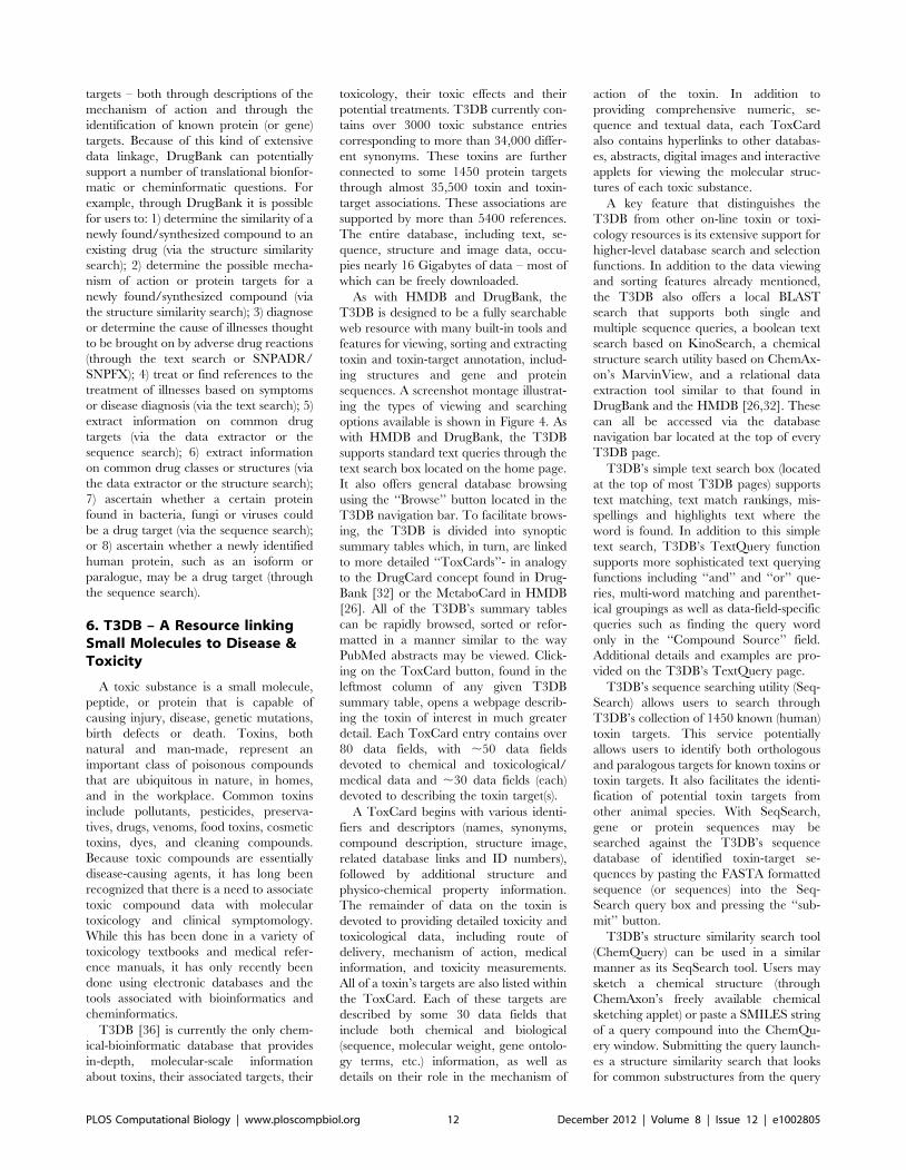
targets – both through descriptions of the
mechanism of action and through the
identification of known protein (or gene)
targets. Because of this kind of extensive
data linkage, DrugBank can potentially
support a number of translational bionfor-
matic or cheminformatic questions. For
example, through DrugBank it is possible
for users to: 1) determine the similarity of a
newly found/synthesized compound to an
existing drug (via the structure similarity
search); 2) determine the possible mecha-
nism of action or protein targets for a
newly found/synthesized compound (via
the structure similarity search); 3) diagnose
or determine the cause of illnesses thought
to be brought on by adverse drug reactions
(through the text search or SNPADR/
SNPFX); 4) treat or find references to the
treatment of illnesses based on symptoms
or disease diagnosis (via the text search); 5)
extract information on common drug
targets (via the data extractor or the
sequence search); 6) extract information
on common drug classes or structures (via
the data extractor or the structure search);
7) ascertain whether a certain protein
found in bacteria, fungi or viruses could
be a drug target (via the sequence search);
or 8) ascertain whether a newly identified
human protein, such as an isoform or
paralogue, may be a drug target (through
the sequence search).
6. T3DB – A Resource linkingSmall Molecules to Disease &Toxicity
A toxic substance is a small molecule,
peptide, or protein that is capable of
causing injury, disease, genetic mutations,
birth defects or death. Toxins, both
natural and man-made, represent an
important class of poisonous compounds
that are ubiquitous in nature, in homes,
and in the workplace. Common toxins
include pollutants, pesticides, preserva-
tives, drugs, venoms, food toxins, cosmetic
toxins, dyes, and cleaning compounds.
Because toxic compounds are essentially
disease-causing agents, it has long been
recognized that there is a need to associate
toxic compound data with molecular
toxicology and clinical symptomology.
While this has been done in a variety of
toxicology textbooks and medical refer-
ence manuals, it has only recently been
done using electronic databases and the
tools associated with bioinformatics and
cheminformatics.
T3DB [36] is currently the only chem-
ical-bioinformatic database that provides
in-depth, molecular-scale information
about toxins, their associated targets, their
toxicology, their toxic effects and their
potential treatments. T3DB currently con-
tains over 3000 toxic substance entries
corresponding to more than 34,000 differ-
ent synonyms. These toxins are further
connected to some 1450 protein targets
through almost 35,500 toxin and toxin-
target associations. These associations are
supported by more than 5400 references.
The entire database, including text, se-
quence, structure and image data, occu-
pies nearly 16 Gigabytes of data – most of
which can be freely downloaded.
As with HMDB and DrugBank, the
T3DB is designed to be a fully searchable
web resource with many built-in tools and
features for viewing, sorting and extracting
toxin and toxin-target annotation, includ-
ing structures and gene and protein
sequences. A screenshot montage illustrat-
ing the types of viewing and searching
options available is shown in Figure 4. As
with HMDB and DrugBank, the T3DB
supports standard text queries through the
text search box located on the home page.
It also offers general database browsing
using the ‘‘Browse’’ button located in the
T3DB navigation bar. To facilitate brows-
ing, the T3DB is divided into synoptic
summary tables which, in turn, are linked
to more detailed ‘‘ToxCards’’- in analogy
to the DrugCard concept found in Drug-
Bank [32] or the MetaboCard in HMDB
[26]. All of the T3DB’s summary tables
can be rapidly browsed, sorted or refor-
matted in a manner similar to the way
PubMed abstracts may be viewed. Click-
ing on the ToxCard button, found in the
leftmost column of any given T3DB
summary table, opens a webpage describ-
ing the toxin of interest in much greater
detail. Each ToxCard entry contains over
80 data fields, with ,50 data fields
devoted to chemical and toxicological/
medical data and ,30 data fields (each)
devoted to describing the toxin target(s).
A ToxCard begins with various identi-
fiers and descriptors (names, synonyms,
compound description, structure image,
related database links and ID numbers),
followed by additional structure and
physico-chemical property information.
The remainder of data on the toxin is
devoted to providing detailed toxicity and
toxicological data, including route of
delivery, mechanism of action, medical
information, and toxicity measurements.
All of a toxin’s targets are also listed within
the ToxCard. Each of these targets are
described by some 30 data fields that
include both chemical and biological
(sequence, molecular weight, gene ontolo-
gy terms, etc.) information, as well as
details on their role in the mechanism of
action of the toxin. In addition to
providing comprehensive numeric, se-
quence and textual data, each ToxCard
also contains hyperlinks to other databas-
es, abstracts, digital images and interactive
applets for viewing the molecular struc-
tures of each toxic substance.
A key feature that distinguishes the
T3DB from other on-line toxin or toxi-
cology resources is its extensive support for
higher-level database search and selection
functions. In addition to the data viewing
and sorting features already mentioned,
the T3DB also offers a local BLAST
search that supports both single and
multiple sequence queries, a boolean text
search based on KinoSearch, a chemical
structure search utility based on ChemAx-
on’s MarvinView, and a relational data
extraction tool similar to that found in
DrugBank and the HMDB [26,32]. These
can all be accessed via the database
navigation bar located at the top of every
T3DB page.
T3DB’s simple text search box (located
at the top of most T3DB pages) supports
text matching, text match rankings, mis-
spellings and highlights text where the
word is found. In addition to this simple
text search, T3DB’s TextQuery function
supports more sophisticated text querying
functions including ‘‘and’’ and ‘‘or’’ que-
ries, multi-word matching and parenthet-
ical groupings as well as data-field-specific
queries such as finding the query word
only in the ‘‘Compound Source’’ field.
Additional details and examples are pro-
vided on the T3DB’s TextQuery page.
T3DB’s sequence searching utility (Seq-
Search) allows users to search through
T3DB’s collection of 1450 known (human)
toxin targets. This service potentially
allows users to identify both orthologous
and paralogous targets for known toxins or
toxin targets. It also facilitates the identi-
fication of potential toxin targets from
other animal species. With SeqSearch,
gene or protein sequences may be
searched against the T3DB’s sequence
database of identified toxin-target se-
quences by pasting the FASTA formatted
sequence (or sequences) into the Seq-
Search query box and pressing the ‘‘sub-
mit’’ button.
T3DB’s structure similarity search tool
(ChemQuery) can be used in a similar
manner as its SeqSearch tool. Users may
sketch a chemical structure (through
ChemAxon’s freely available chemical
sketching applet) or paste a SMILES string
of a query compound into the ChemQu-
ery window. Submitting the query launch-
es a structure similarity search that looks
for common substructures from the query
PLOS Computational Biology | www.ploscompbiol.org 12 December 2012 | Volume 8 | Issue 12 | e1002805
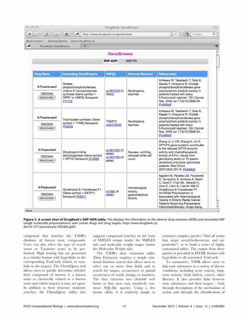
compound that matches the T3DB’s
database of known toxic compounds.
Users can also select the type of search
(exact or Tanimoto score) to be per-
formed. High scoring hits are presented
in a tabular format with hyperlinks to the
corresponding ToxCards (which, in turn,
links to the targets). The ChemQuery tool
allows users to quickly determine whether
their compound of interest is a known
toxin or chemically related to a known
toxin and which target(s) it may act upon.
In addition to these structure similarity
searches, the ChemQuery utility also
supports compound searches on the basis
of SMILES strings (under the SMILES
tab) and molecular weight ranges (under
the Molecular Weight tab).
The T3DB’s data extraction utility
(Data Extractor) employs a simple rela-
tional database system that allows users to
select one or more data fields and to
search for ranges, occurrences or partial
occurrences of words, strings, or numbers.
The data extractor uses clickable web
forms so that users may intuitively con-
struct SQL-like queries. Using a few
mouse clicks, it is relatively simple to
construct complex queries (‘‘find all toxins
that target acetylcholinesterase and are
pesticides’’) or to build a series of highly
customized tables. The output from these
queries is provided in HTML format with
hyperlinks to all associated ToxCards.
To summarize, T3DB allows users to
link toxic substances to a variety of disease
conditions, including acute toxicity, long-
term toxicity, birth defects, cancer, other
illnesses. It also provides links between
toxic substances and their targets – both
through descriptions of the mechanism of
action and through the identification of
Figure 3. A screen shot of DrugBank’s SNP-ADR table. This displays the information on the adverse drug reactions (ADRs) and associated SNP(single nucleotide polymorphisms) with certain drugs and drug targets (http://www.drugbank.ca).doi:10.1371/journal.pcbi.1002805.g003
PLOS Computational Biology | www.ploscompbiol.org 13 December 2012 | Volume 8 | Issue 12 | e1002805
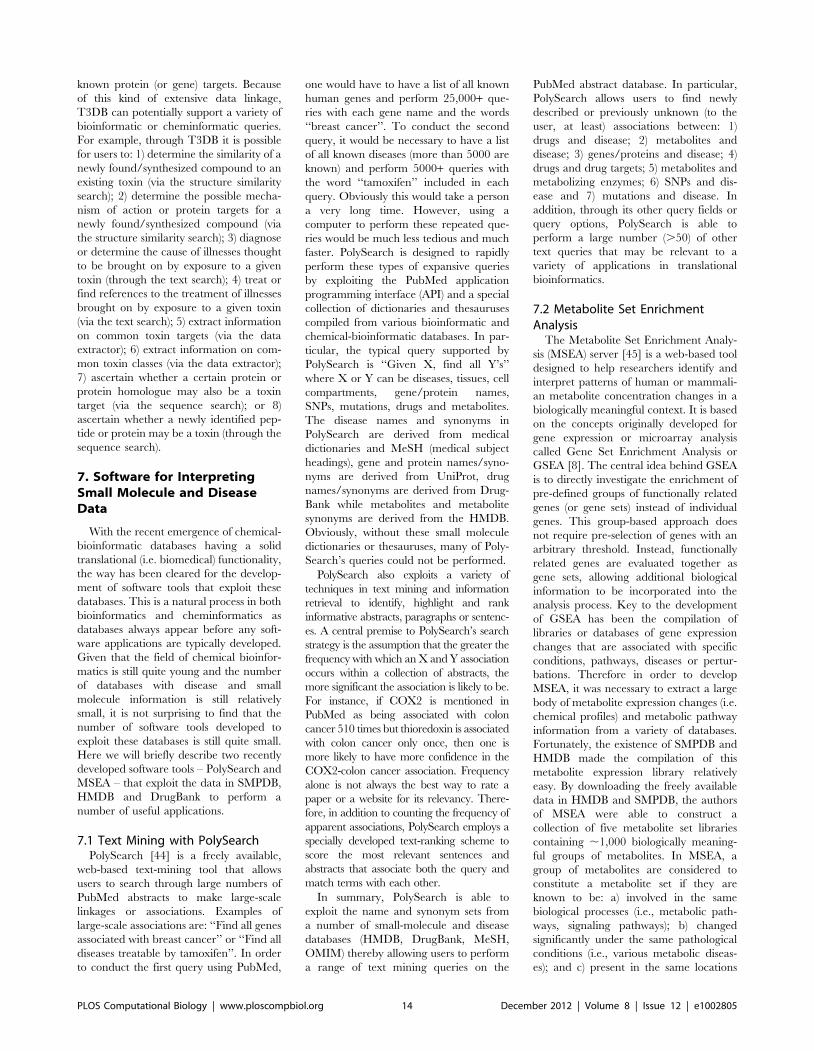
known protein (or gene) targets. Because
of this kind of extensive data linkage,
T3DB can potentially support a variety of
bioinformatic or cheminformatic queries.
For example, through T3DB it is possible
for users to: 1) determine the similarity of a
newly found/synthesized compound to an
existing toxin (via the structure similarity
search); 2) determine the possible mecha-
nism of action or protein targets for a
newly found/synthesized compound (via
the structure similarity search); 3) diagnose
or determine the cause of illnesses thought
to be brought on by exposure to a given
toxin (through the text search); 4) treat or
find references to the treatment of illnesses
brought on by exposure to a given toxin
(via the text search); 5) extract information
on common toxin targets (via the data
extractor); 6) extract information on com-
mon toxin classes (via the data extractor);
7) ascertain whether a certain protein or
protein homologue may also be a toxin
target (via the sequence search); or 8)
ascertain whether a newly identified pep-
tide or protein may be a toxin (through the
sequence search).
7. Software for InterpretingSmall Molecule and DiseaseData
With the recent emergence of chemical-
bioinformatic databases having a solid
translational (i.e. biomedical) functionality,
the way has been cleared for the develop-
ment of software tools that exploit these
databases. This is a natural process in both
bioinformatics and cheminformatics as
databases always appear before any soft-
ware applications are typically developed.
Given that the field of chemical bioinfor-
matics is still quite young and the number
of databases with disease and small
molecule information is still relatively
small, it is not surprising to find that the
number of software tools developed to
exploit these databases is still quite small.
Here we will briefly describe two recently
developed software tools – PolySearch and
MSEA – that exploit the data in SMPDB,
HMDB and DrugBank to perform a
number of useful applications.
7.1 Text Mining with PolySearchPolySearch [44] is a freely available,
web-based text-mining tool that allows
users to search through large numbers of
PubMed abstracts to make large-scale
linkages or associations. Examples of
large-scale associations are: ‘‘Find all genes
associated with breast cancer’’ or ‘‘Find all
diseases treatable by tamoxifen’’. In order
to conduct the first query using PubMed,
one would have to have a list of all known
human genes and perform 25,000+ que-
ries with each gene name and the words
‘‘breast cancer’’. To conduct the second
query, it would be necessary to have a list
of all known diseases (more than 5000 are
known) and perform 5000+ queries with
the word ‘‘tamoxifen’’ included in each
query. Obviously this would take a person
a very long time. However, using a
computer to perform these repeated que-
ries would be much less tedious and much
faster. PolySearch is designed to rapidly
perform these types of expansive queries
by exploiting the PubMed application
programming interface (API) and a special
collection of dictionaries and thesauruses
compiled from various bioinformatic and
chemical-bioinformatic databases. In par-
ticular, the typical query supported by
PolySearch is ‘‘Given X, find all Y’s’’
where X or Y can be diseases, tissues, cell
compartments, gene/protein names,
SNPs, mutations, drugs and metabolites.
The disease names and synonyms in
PolySearch are derived from medical
dictionaries and MeSH (medical subject
headings), gene and protein names/syno-
nyms are derived from UniProt, drug
names/synonyms are derived from Drug-
Bank while metabolites and metabolite
synonyms are derived from the HMDB.
Obviously, without these small molecule
dictionaries or thesauruses, many of Poly-
Search’s queries could not be performed.
PolySearch also exploits a variety of
techniques in text mining and information
retrieval to identify, highlight and rank
informative abstracts, paragraphs or sentenc-
es. A central premise to PolySearch’s search
strategy is the assumption that the greater the
frequency with which an X and Y association
occurs within a collection of abstracts, the
more significant the association is likely to be.
For instance, if COX2 is mentioned in
PubMed as being associated with colon
cancer 510 times but thioredoxin is associated
with colon cancer only once, then one is
more likely to have more confidence in the
COX2-colon cancer association. Frequency
alone is not always the best way to rate a
paper or a website for its relevancy. There-
fore, in addition to counting the frequency of
apparent associations, PolySearch employs a
specially developed text-ranking scheme to
score the most relevant sentences and
abstracts that associate both the query and
match terms with each other.
In summary, PolySearch is able to
exploit the name and synonym sets from
a number of small-molecule and disease
databases (HMDB, DrugBank, MeSH,
OMIM) thereby allowing users to perform
a range of text mining queries on the
PubMed abstract database. In particular,
PolySearch allows users to find newly
described or previously unknown (to the
user, at least) associations between: 1)
drugs and disease; 2) metabolites and
disease; 3) genes/proteins and disease; 4)
drugs and drug targets; 5) metabolites and
metabolizing enzymes; 6) SNPs and dis-
ease and 7) mutations and disease. In
addition, through its other query fields or
query options, PolySearch is able to
perform a large number (.50) of other
text queries that may be relevant to a
variety of applications in translational
bioinformatics.
7.2 Metabolite Set EnrichmentAnalysis
The Metabolite Set Enrichment Analy-
sis (MSEA) server [45] is a web-based tool
designed to help researchers identify and
interpret patterns of human or mammali-
an metabolite concentration changes in a
biologically meaningful context. It is based
on the concepts originally developed for
gene expression or microarray analysis
called Gene Set Enrichment Analysis or
GSEA [8]. The central idea behind GSEA
is to directly investigate the enrichment of
pre-defined groups of functionally related
genes (or gene sets) instead of individual
genes. This group-based approach does
not require pre-selection of genes with an
arbitrary threshold. Instead, functionally
related genes are evaluated together as
gene sets, allowing additional biological
information to be incorporated into the
analysis process. Key to the development
of GSEA has been the compilation of
libraries or databases of gene expression
changes that are associated with specific
conditions, pathways, diseases or pertur-
bations. Therefore in order to develop
MSEA, it was necessary to extract a large
body of metabolite expression changes (i.e.
chemical profiles) and metabolic pathway
information from a variety of databases.
Fortunately, the existence of SMPDB and
HMDB made the compilation of this
metabolite expression library relatively
easy. By downloading the freely available
data in HMDB and SMPDB, the authors
of MSEA were able to construct a
collection of five metabolite set libraries
containing ,1,000 biologically meaning-
ful groups of metabolites. In MSEA, a
group of metabolites are considered to
constitute a metabolite set if they are
known to be: a) involved in the same
biological processes (i.e., metabolic path-
ways, signaling pathways); b) changed
significantly under the same pathological
conditions (i.e., various metabolic diseas-
es); and c) present in the same locations
PLOS Computational Biology | www.ploscompbiol.org 14 December 2012 | Volume 8 | Issue 12 | e1002805
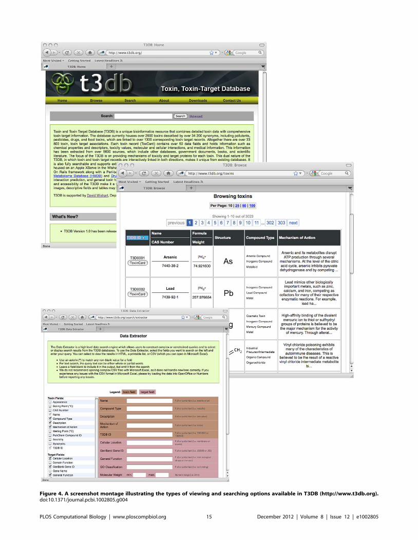
Figure 4. A screenshot montage illustrating the types of viewing and searching options available in T3DB (http://www.t3db.org).doi:10.1371/journal.pcbi.1002805.g004
PLOS Computational Biology | www.ploscompbiol.org 15 December 2012 | Volume 8 | Issue 12 | e1002805
such as organs, tissues or cellular organ-
elles. The resulting metabolite sets were
organized into three categories: pathway-
associated, disease-associated, and location
based. MSEA’s pathway-associated me-
tabolite library contains 84 entries based
on the 84 human metabolic pathways
found in SMPDB. MSEA’s disease-associ-
ated metabolite sets were mainly collected
from information in the HMDB, the
Metabolic Information Center (MIC),
and SMPDB. Using these resources, a
total of 851 physiologically informative
metabolite sets were created. These dis-
ease-associated metabolite sets were fur-
ther divided into three sub-categories
based on the biofluids in which they were
measured: 398 metabolite sets in blood,
335 in urine, and 118 in cerebral-spinal
fluid (CSF). MSEA’s location-based library
contains 57 metabolite sets based on the
‘‘Cellular Location’’ and ‘‘Tissue Loca-
tion’’ listed in the HMDB.
While the exact statistical or enrichment
analysis methods used in MSEA are well
beyond the scope of this chapter, suffice it
to say that MSEA essentially allows one to
take lists of metabolites and to identify
which pathways, diseases or medical
conditions are most likely to be associated
with that metabolite set. It is also possible
to do the same kind of operation with a list
of metabolites and their absolute (or
relative) concentrations. While disease/
metabolite associations can be made
through HMDB and SMPDB, these
primitive search tools do not have the
same statistical rigor that characterizes a
full-fledged enrichment analysis. Further-
more, the MSEA pathway and disease
data set is somewhat larger than what is
found in the HMDB or SMPDB. This
means that MSEA will be far more likely
to find a useful (and statistically significant)
pathway or disease than what could be
done with HMDB or SMPDB.
Overall, MSEA is an example of an
analytical software tool that exploits
chemical-bioinformatic data to perform
robust statistical analyses of metabolomic
or clinical chemistry data. Given their
close similarity, it is reasonable to expect
MSEA could eventually be integrated with
GSEA, thereby allowing a comprehensive
analysis of both gene and metabolite
expression changes on a single integrated
program or website. No doubt this kind of
integrated ‘‘omic’’ analysis tool is not far
away from being developed.
8. Summary
With today’s focus on genes and
proteins as the ‘‘primary’’ causes or
biomarkers of disease, the relationship
between small molecules and human
disease is often overlooked. However it is
important to remember that more than
95% of all diagnostic clinical assays are
designed to detect small molecules (i.e.
blood glucose, serum creatinine, amino
acid analysis, etc.). Likewise nearly 90% of
all known drugs are small molecules, 50%
of all drugs are derived from pre-existing
metabolites and 30% of identified genetic
disorders involve diseases of small mole-
cule metabolism. Clearly, small molecules
are important and given the rapid growth
in metabolomics, pharmacogenomics and
systems biology, it is likely that their role in
disease diagnosis and disease treatment
will continue to grow. Given these exciting
growth prospects and given the impor-
tance of small molecules in medicine and
translational research, scientists are now
realizing that there is a critical need to link
information about small molecules to their
corresponding ‘‘big molecule’’ targets.
This has led to the emergence of a new
field of bioinformatics – called chemical
bioinformatics.
This chapter has covered several topics
related to chemical bioinformatics and the
role that chemical bioinformatics can play
in identifying the chemicals that cause
(toxins), cure (drugs) or characterize
(biomarkers) many human diseases. The
first part of the chapter gave a brief
overview of some of the most important
or widely used chemical bioinformatic
resources along with a more detailed
discussion of some of the major classes
of chemical-bioinformatic databases. In
particular four major database classes
were described: 1) small molecule (or
metabolic) pathway databases; 2) metab-
olite or metabolomic databases; 3) drug
databases; and 4) toxin or toxic substance
databases. Examples of each of these
databases were given and many of their
strengths and limitations were discussed.
While most of these chemical-bioinfor-
matic databases provide links between
small molecules and their large molecule
targets, relatively few provide linkages to
clinical, physiological or disease informa-
tion.
The second part of this chapter focused
on describing a number of recently
developed databases that explicitly relate
small molecules to disease. This included
detailed descriptions of four databases: 1)
the Small Molecule Pathway Database
(SMPDB); 2) the Human Metabolome
Database (HMDB); 3) DrugBank and 4)
the Toxin, Toxin-Target Database
(T3DB). SMPDB is a graphically oriented
pathway database that contains ,450
metabolic pathways, disease pathways
and drug pathways. The HMDB is a
comprehensive metabolomic database that
is primarily oriented to answering ques-
tions in clinical metabolomic and clinical
biochemistry. DrugBank is a comprehen-
sive drug database containing detailed
information about drugs, drug targets
and clinical pharmacology. The T3DB is
a toxicology database containing detailed
information about toxins, toxin targets and
their corresponding toxicological informa-
tion. Each of these databases was de-
scribed in terms of its content, general
design and query/search functions. Addi-
tionally, explicit examples of various
translational or disease-related applica-
tions were provided for each database.
The final part of this chapter provided a
short discussion of some of the newly
emerging software tools that exploit these
databases, including PolySearch and
MSEA (Metabolite Set Enrichment Anal-
ysis). PolySearch is a text-mining tool that
exploits the synonym data found in these
small molecule databases to allow expan-
sive PubMed queries to be performed.
MSEA is a metabolomic analysis tool that
exploits the pathway and disease informa-
tion found in SMPDB and HMDB to
perform pathway and disease identifica-
tion from raw metabolomic data.
Further Reading
N Villas-Boas SG, Nielson J, Smedsgaard J, Hansen MAE, Roessner-Tunali U, editors(2007) Metabolome analysis: an introduction. New York: John Wiley & Sons.
N Wishart DS (2008) DrugBank and its relevance to pharmacogenomics.Pharmacogenomics 9: 1155–1162.
N Krawetz S, editor (2009) Bioinformatics for systems biology. Totowa: HumanaPress.
N Wishart DS (2008) Applications of metabolomics in drug discovery anddevelopment. Drugs R D 9: 307–322.
N Baxevanis A (2003) Current protocols in bioinformatics. New York: John Wiley &Sons – see Chapter 14.
PLOS Computational Biology | www.ploscompbiol.org 16 December 2012 | Volume 8 | Issue 12 | e1002805
While the sub-discipline of chemical
bioinformatics is still quite young, and the
number of tools for translational applications
is still relatively small, it should be clear that
what is now out there has considerable
potential for a wide range of clinical,
biomedical, pharmaceutical and toxicological
applications. Certainly as more tools are
developed and as more databases evolve, it is
likely that chemical bioinformatics will soon
be able to establish itself as one of the most
medically useful sub-disciplines in the entire
field of bioinformatics.
9. Exercises
1) A compound with a molecular weight
of 136.053 daltons has been isolated from
the urine of a 3 month-old baby with
unusually light coloring of the skin,
eczema (an itchy skin rash), and a musty
body odor. What compound is it and what
disease might this baby have?
2) Your natural product chemist neighbor
has just isolated a compound from the
Tanzanian periwinkle – a rare plant species
found only in the highlands of Eastern
Tanzania. Locals use the plant as a treatment
for a variety of blood disorders. The structure
of the compound is given by the following
SMILES string: COC1 = CC = C2C( = C
C1 = O)C(CCC1 = CC(OC) = C(OC)C(OC)
= C21)NC(CO)
What compound is this similar to, what
diseases could it be used to treat and what
proteins might it bind?
3) A viral protein with the following
sequence has been isolated from a number
of dead and dying African Green Monkeys
that were housed at a local zoo.
PQVTLYQRPLVTIRVGGQLKEALIDTGADD
TVLENMNLPGRWKPKMIGAIAGFIKVKQYDQI
TVEICGHKGIGTILVGPTPVNIIGRNLLTLIG
CTLNF
The illness seems to be spreading to
other monkey colonies in the zoo. What
drugs could be used to treat the sick
monkeys and to prevent the spread of the
disease?
4) A farmer who has just finished
harvesting his barley field has come into
the clinic complaining of skin irritation,
burning and itching, a rash and a series of
skin blisters. He also has eye pain,
conjunctivitis, burning sensations about
the eyes, and blurred vision. Other
symptoms have included nausea, vomiting
and fatigue. Suspecting that he may have
been exposed to some toxin or pesticide a
chemical analysis has been performed of
his blood, urine and lacrimal (tear) fluid.
MS analysis of all three fluids has
identified an unusual compound with a
molecular weight of 296.126 daltons.
What compound might this be?
5) What kind of drugs can be used to
treat breast cancer? Describe your search
strategy and your rationale for this search
strategy.
Answers to the Exercises can be found
in Text S1.
Supporting Information
Text S1 Answers to Exercises.
(DOC)
Glossary
Cheminformatics – a field of information technology that uses computers tofacilitate the collection, storage, analysis and manipulation of large quantities ofchemical data.
DrugBank – A database containing chemical and biological data on drugs anddrug targets.
GSEA – Gene Set Enrichment Analysis. GSEA is a statistically based bioinformaticmethod designed to directly investigate the enrichment of pre-defined groups offunctionally related genes (or gene sets) from gene expression data.
HMDB – The Human Metabolome Database. A database containing chemical andbiological data on human metabolites aimed at clinical metabolomic studies.
MS – Mass Spectrometry. An analytical method that measures molecular weightof compounds based on their mass to charge ratio. Mass spectrometry is one ofthe standard methods to determine the molecular formula of new compoundsand to confirm the identity of synthesized chemicals or natural products.
Metabolome – the collection of all small molecule metabolites found in a givencell, tissue, organ or organism.
Metabolomics - a branch of ‘‘omics’’ research that is primarily concerned with thehigh-throughput identification and quantification of small molecule (,1500 Da)metabolites in the metabolome.
MSEA – Metabolite Set Enrichment Analysis. MSEA is a statistically basedbioinformatic method designed to directly investigate the enrichment of pre-defined groups of functionally related metabolites (or metabolite sets) frommetabolomic data.
NMR – Nuclear Magnetic Resonance Spectroscopy. An analytical method thatmeasures nuclear magnetism under very high magnetic fields. NMR is thestandard method used by chemists today to identify and characterize smallmolecules.
Pharmacogenomics – A newly emerging field of pharmacology that integratesgenotyping and gene expression data with classical pharmacological and adversedrug reaction studies.
SMPDB – The Small Molecule Pathway Database. A database containing pathwaydiagrams and interactive viewing tools for small molecules involved inmetabolism, drug action and disease.
T3DB – The Toxin, Toxin-Target Database. A database with chemical andbiological data on common toxins, poisons, household chemicals, pollutants andother harmful substances.
Toxicogenomics – A newly emerging field of toxicology that integratesgenotyping and gene expression data with classical toxicological and toxicitystudies.
PLOS Computational Biology | www.ploscompbiol.org 17 December 2012 | Volume 8 | Issue 12 | e1002805
References
1. Trujillo E, Davis C, Milner J (2006) Nutrige-
nomics, proteomics, metabolomics, and the
practice of dietetics. J Am Diet Assoc 106: 403–
413.
2. Feng X, Liu X, Luo Q, Liu BF (2008) Mass
spectrometry in systems biology: an overview.
Mass Spectrom Rev 27: 635–660.
3. Brown FK. (1998) Chemoinformatics: what is it
and how does it impact drug discovery. Annu
Rep Med Chem 33: 375–384.
4. Altschul SF, Madden TL, Schaffer AA, Zhang J,
Zhang Z, et al. (1997) Gapped BLAST and PSI-
BLAST: a new generation of protein database
search programs. Nucleic Acids Res 25: 3389–
3402.
5. Benson DA, Karsch-Mizrachi I, Lipman DJ,
Ostell J, Sayers EW (2010) GenBank. Nucleic
Acids Res 38: D46–51.
6. McGuffin LJ, Bryson K, Jones DT (2000) The
PSIPRED protein structure prediction server.
Bioinformatics 16: 404–405.
7. Westbrook J, Feng Z, Jain S, Bhat TN, Thanki N,
et al. (2002) The Protein Data Bank: unifying the
archive. Nucleic Acids Res 30: 245–248.
8. Subramanian A, Tamayo P, Mootha VK,
Mukherjee S, Ebert BL, et al. (2005) Gene set
enrichment analysis: a knowledge-based ap-
proach for interpreting genome-wide expression
profiles. Proc Natl Acad Sci U S A 102: 15545–
15550.
9. Edgar R, Domrachev M, Lash AE (2002) Gene
Expression Omnibus: NCBI gene expression and
hybridization array data repository. Nucleic Acids
Res 30: 207–210.
10. Kanehisa M, Goto S, Hattori M, Aoki-Kinoshita
KF, Itoh M, et al. (2006) From genomics to
chemical genomics: new developments in KEGG.
Nucleic Acids Res 34: D354–357.
11. Karp PD, Riley M, Paley SM, Pelligrini-Toole A
(1996) EcoCyc: an encyclopedia of Escherichia
coli genes and metabolism. Nucleic Acids Res 24:
32–39.
12. Krummenacker M, Paley S, Mueller L, Yan T,
Karp PD (2005) Querying and computing with
BioCyc databases. Bioinformatics 21: 3454–3455.
13. Joshi-Tope G, Gillespie M, Vastrik I, D’Eustachio
P, Schmidt E, et al. (2005) Reactome: a knowl-
edgebase of biological pathways. Nucleic Acids
Res 33: D428–432.
14. Pico AR, Kelder T, van Iersel MP, Hanspers K,
Conklin BR, et al. (2008) WikiPathways: pathway
editing for the people. PLoS Biol 6: e184.
doi:10.1371/journal.pbio.0060184
15. Frolkis A, Knox C, Lim E, Jewison T, Law V, et al.
(2010) SMPDB: The Small Molecule Pathway
Database. Nucleic Acids Res 38: D480–487.
16. Fahy E, Sud M, Cotter D, Subramaniam S (2007)
LIPID MAPS online tools for lipid research.Nucleic Acids Res 35: W606–612.
17. Degtyarenko K, de Matos P, Ennis M, Hastings J,Zbinden M, et al. (2008) ChEBI: a database and
ontology for chemical entities of biological
interest. Nucleic Acids Res 36: D344–350.18. Wang Y, Xiao J, Suzek TO, Zhang J, Wang J, et
al. (2009) PubChem: a public information systemfor analyzing bioactivities of small molecules.
Nucleic Acids Res 37: W623–633.
19. Williams AJ (2008) Public chemical compounddatabases. Curr Opin Drug Discov Devel 11:
393–404.20. Shinbo Y, Nakamura Y, Altaf-Ul-Amin M, Asahi
K, Kuokawa M, et al. (2006) KNApSAcK: acomprehensive species-metabolite relationship
database. Biotech Agri Forestry 57: 165–181.
21. Smith CA, O’Maille G, Want EJ, Qin C, TraguerSA, et al. (2005) METLIN: a metabolite mass
spectral database. Ther Drug Monit 27: 747–751.22. Ulrich EL, Akutsu H, Doreleijers JF, Harano Y,
Ioannidis YE, et al. (2008) BioMagResBank.
Nucleic Acids Res 36: D402–408.23. Taguchi R, Nishijima M, Shimizu T (2007) Basic
analytical systems for lipidomics by mass spec-trometry in Japan. Methods Enzymol 432: 185–
211.24. Cui Q, Lewis IA, Hegeman AD, Anderson ME,
Li J, et al. (2008) Metabolite identification via the
Madison Metabolomics Consortium Database.Nat Biotechnol 26: 162–164.
25. Kopka J, Schauer N, Krueger S, Birkemeyer C,Usadel B, et al. (2005) [email protected]: the
Golm Metabolome Database. Bioinformatics 21:
1635–1638.26. Wishart DS, Knox C, Guo AC, Eisner R, Young
N, et al. (2009) HMDB: a knowledgebase for thehuman metabolome. Nucleic Acids Res 37:
D603–610.27. Polen HH, Zapantis A, Clauson KA, Jebrock J,
Paris M (2008) Ability of online drug databases to
assist in clinical decision-making with infectiousdisease therapies. BMC Infect Dis 8: 153.
28. Hatfield CL, May SK, Markoff JS (1999) Qualityof consumer drug information provided by four
Web sites. Am J Health Syst Pharm 56: 2308–
2311.29. Zhu F, Han B, Kumar P, Liu X, Ma X, et al.
(2010) Update of TTD: Therapeutic TargetDatabase. Nucleic Acids Res 38: D787–791.
30. Sangkuhl K, Berlin DS, Altman RB Klein TE(2008) PharmGKB: understanding the effects of
individual genetic variants. Drug Metab Rev 40:
539–551.31. Gunther S, Kuhn M, Dunkel M, Campillos M,
Senger C, et al. (2008) SuperTarget and Matador:
resources for exploring drug-target relationships.
Nucleic Acids Res 36: D919–922.
32. Wishart DS, Knox C, Guo AC, Shrivastava S,
Hassanali M, et al. (2006) DrugBank: a compre-
hensive resource for in silico drug discovery and
exploration. Nucleic Acids Res 34: D668–672.
33. Schmidt U, Struck S, Gruening B, Hossbach J,
Jaeger IS, et al. (2009) SuperToxic: a compre-
hensive database of toxic compounds. Nucleic
Acids Res 37: D295–299.
34. Judson R, Richard A, Dix D, Houck K, Elloumi
F, et al. (2008) ACToR–Aggregated Computa-
tional Toxicology Resource. Toxicol Appl Phar-
macol 233: 7–13.
35. Davis AP, Murphy CG, Saraceni-Richards CA,
Rosenstein MC, Wiegers TC, et al. (2009)
Comparative Toxicogenomics Database: a
knowledgebase and discovery tool for chemical-
gene-disease networks. Nucleic Acids Res 37:
D786–792.
36. Lim E, Pon A, Djoumbou Y, Knox C, Shrivas-
tava S, et al. (2010\) T3DB: a comprehensively
annotated database of common toxins and their
targets. Nucleic Acids Res 38: D781–786.
37. Boutet E, Lieberherr D, Tognolli M, Schneider
M, Bairoch A (2007) UniProtKB/Swiss-Prot.
Methods Mol Biol 406: 89–112.
38. Wishart DS (2007) Proteomics and the human
metabolome project. Expert Rev Proteomics 4:
333–335.
39. Hamosh A, Scott AF, Amberger J, Valle D,
McKusick VA (2000) Online Mendelian Inheri-
tance in Man (OMIM). Hum Mutat 15: 57–61.
40. Weininger D (1988) SMILES 1. Introduction and
encoding rules. J Chem Inf Comput Sci 28: 31–
38.
41. Shoshan MC, Linder S (2008) Target specificity
and off-target effects as determinants of cancer
drug efficacy. Expert Opin Drug Metab Toxicol
4: 273–280.
42. Thorisson GA, Stein LD (2003) The SNP
Consortium website: past, present and future.
Nucleic Acids Res 31: 124–127.
43. International HapMap Consortium (2007) A
second generation human haplotype map of over
3.1 million SNPs. Nature 449: 851–861.
44. Cheng D, Knox C, Young N, Stothard P,
Damaraju S, et al. (2008) PolySearch: a web-
based text mining system for extracting relation-
ships between human diseases, genes, mutations,
drugs and metabolites. Nucleic Acids Res 36:
W399–405.
45. Xia J, Wishart DS (2010) MSEA: a web-based
tool to identify biologically meaningful patterns in
quantitative metabolomic data. Nucleic Acids Res
38: W71–7.
PLOS Computational Biology | www.ploscompbiol.org 18 December 2012 | Volume 8 | Issue 12 | e1002805
Education
Chapter 4: Protein Interactions and DiseaseMileidy W. Gonzalez1, Maricel G. Kann2*
1 National Center for Biotechnology Information, National Library of Medicine, National Institutes of Health, Bethesda, Maryland, United States of America, 2 Biological
Sciences, University of Maryland, Baltimore County, Baltimore, Maryland, United States of America
Abstract: Proteins do not functionin isolation; it is their interactionswith one another and also withother molecules (e.g. DNA, RNA)that mediate metabolic and signal-ing pathways, cellular processes,and organismal systems. Due totheir central role in biologicalfunction, protein interactions alsocontrol the mechanisms leading tohealthy and diseased states inorganisms. Diseases are oftencaused by mutations affecting thebinding interface or leading tobiochemically dysfunctional alloste-ric changes in proteins. Therefore,protein interaction networks canelucidate the molecular basis ofdisease, which in turn can informmethods for prevention, diagnosis,and treatment. In this chapter, wewill describe the computationalapproaches to predict and mapnetworks of protein interactionsand briefly review the experimentalmethods to detect protein interac-tions. We will describe the applica-tion of protein interaction networksas a translational approach to thestudy of human disease and eval-uate the challenges faced by theseapproaches.
This article is part of the ‘‘Transla-
tional Bioinformatics’’ collection for
PLOS Computational Biology.
1. Introduction
Early biological experiments revealed
proteins as the main agents of biological
function. As such, proteins ultimately
determine the phenotype of all organ-
isms. Since the advent of molecular
biology we have learned that proteins
do not function in isolation; instead, it is
their interactions with one another and
also with other molecules (e.g. DNA,
RNA) that mediate metabolic and signal-
ing pathways, cellular processes, and
organismal systems.
The concept of ‘‘protein interaction’’ is
generally used to describe the physical
contact between proteins and their interact-
ing partners. Proteins associate physically to
create macromolecular structures of various
complexities and heterogeneities. Proteins
interact in pairs to form dimers (e.g. reverse
transcriptase), multi-protein complexes (e.g.
the proteasome for molecular degradation),
or long chains (e.g. actin filaments in muscle
fibers). The subunits creating the various
complexes can be identical or heteroge-
neous (e.g. homodimers vs. heterodimers)
and the duration of the interaction can be
transient (e.g. proteins involved in signal
transduction) or permanent (e.g. some
ribosomal proteins). However, protein in-
teractions do not always have to be physical
[1]. The term ‘‘protein interaction’’ is also
used to describe metabolic or genetic
correlations, and even co-localizations.
Metabolic interactions describe proteins
involved in the same pathway (e.g. the
Krebs cycle proteins), while genetically
identified associations identify co-expressed
or co-regulated proteins (e.g. enzymes
regulating the glycolytic pathway). As the
name implies, protein interactions by co-
localization list proteins found in the same
cellular compartment.
Whether the association is physical or
functional, protein-protein interaction
(PPI) data can be used in a larger scale
to map networks of interactions [2,3]. In
PPI network graphs, the nodes represent
the proteins and the lines connecting them
represent the interactions between them
(Figure 1). Protein interaction networks
are useful resources in the abstraction of
basic science knowledge and in the
development of biomedical applications.
By studying protein interaction networks
we can learn about the evolution of
individual proteins and about the different
systems in which they are involved.
Likewise, interaction maps obtained from
one species can be used, with some
limitations, to predict interaction networks
in other species. Protein interaction net-
works can also suggest functions for
previously uncharacterized proteins by
uncovering their role in pathways or
protein complexes [4]. Due to their central
role in biological function, protein inter-
actions also control the mechanisms lead-
ing to healthy and diseased states in
organisms. Diseases are often caused by
mutations affecting the binding interface
or leading to biochemically dysfunctional
allosteric changes in proteins. Therefore,
protein interaction networks can elucidate
the molecular basis of disease, which in
turn can inform methods for prevention,
diagnosis, and treatment [5,6].
The study of human disease experi-
enced extensive advancements once the
biomedical characterization of proteins
shifted to studies taking into account a
protein’s network at different functional
levels (i.e. in pair-wise interactions, in
complexes, in pathways, and in whole
genomes). For instance, consider how our
understanding of Huntington’s disease
(HD) has evolved from the early Mende-
lian single-gene studies to the latest HD-
specific network-based analyses. HD is an
autosomal dominant neurodegenerative
disease with features recognized by Hun-
tington in 1872 [7], and whose specific
patterns of inheritance were documented
in 1908 [8]. After almost a century of
genetics studies, the culprit gene in HD
was identified; in 1993, we learned that
HD was caused by the repeat expansion of
a CAG trinucleotide in the Huntingtin (Htt)
gene [9]. This expansion causes aggrega-
Citation: Gonzalez MW, Kann MG (2012) Chapter 4: Protein Interactions and Disease. PLoS Comput Biol 8(12):e1002819. doi:10.1371/journal.pcbi.1002819
Editor: Fran Lewitter, Whitehead Institute, United States of America
Published December , 2012
This is an open-access article, free of all copyright, and may be freely reproduced, distributed, transmitted,modified, built upon, or otherwise used by anyone for any lawful purpose. The work is made available underthe Creative Commons CC0 public domain dedication.
Funding: This research was funded by the National Institutes of Health (NIH) 1K22CA143148 to MGK (PI); ACS-IRG grant to MGK (PI), and R01LM009722 to MGK (co-investigator). MWG’s research was supported in part bythe Intramural Research Program of the NIH, National Library of Medicine. The funders had no role in thepreparation of the manuscript.
Competing Interests: The authors have declared that no competing interests exist.
* E-mail: [email protected]
PLOS Computational Biology | www.ploscompbiol.org 1 December 2012 | Volume 8 | Issue 12 | e1002819
27
tion of the mutant Htt in insoluble neuronal
inclusion bodies, which consequently leads
to neuronal degeneration. Yet, even when
the key disease-causing protein in HD had
been identified, the mechanism for Htt
aggregation remained unknown. In 2004,
Goehler et al. [10] mapped all the PPIs that
take place in HD and discovered that the
interaction between Htt and GIT1, a
GTPase-activating protein, mediates Htt
aggregation. Further validation ([11,12])
confirmed GTI1’s potential as a target for
therapeutic strategies against HD.
In this chapter, we will describe the main
experimental methods to identify protein
interactions and the computational ap-
proaches to map their networks and to
predict new interactions purely in silico. We
will describe the application of protein
interaction networks as a translational ap-
proach to the study of human disease and
evaluate the challenges faced by these
approaches.
2. Experimental Identificationof PPIs2.1 Biophysical Methods
Protein interactions are identified
through different biochemical, physical,
and genetic methods (Figure 2). Historical-
ly, the main source of knowledge about
protein interactions has come from bio-
physical methods, particularly from those
based on structural information (e.g. X-ray
crystallography, NMR spectroscopy, fluorescence,
atomic force microscopy). Biophysical methods
identify interacting partners and also pro-
vide detailed information about the bio-
chemical features of the interactions (e.g.
binding mechanism, allosteric changes
involved). Yet, since they are time- and
resource-consuming, biophysical character-
izations only permit the study of a few
complexes at a time.
2.2 High-Throughput MethodsTo document protein interactions at a
larger scale, automated methods have been
developed to detect interactions directly or
to deduce them through indirect approach-
es (Figure 2).2.2.1 Direct high-throughput
methods. Yeast two-hybrid (Y2H) is one
of the most-commonly used direct high-
throughput method. The Y2H system tests
the interaction of two given proteins by
fusing each of them to a transcription-
binding domain. If the proteins interact,
the transcription complex is activated,
which transcribes a reporter gene whose
product can be detected. Since it is an in
vivo technique, the Y2H system is highly
effective at detecting transient interactions
and can be readily applied to screen large
genome-wide libraries (e.g. to map an
organisms’ full set of interactions or
interactome). But, the Y2H system is
limited by its biases toward non-specific
interactions. Likewise, Y2H cannot
identify complexes (i.e. it only reports
binary interactions) or interactions of pro-
teins initiating transcription by themselves.
Although protein interactions are usually
detected and studied in pair-wise form, in
reality they often occur in complexes and
as part of larger networks of interaction. In
vitro direct detection methods (e.g. mass
spectrometry, affinity purification) are better
suited to detect macromolecular inte-
ractions, yet, they have their own
limitations: interactions occurring in vitro
do not necessarily occur in vivo (e.g. when
proteins are compartmentalized in
different cell locations) and complexes
are often difficult to purify, which is a
required step in the protocol [13].
2.2.2 Indirect high-throughput
methods. Several high-throughput
methods deduce protein interactions by
looking at characteristics of the genes enco-
ding the putative interacting partners. For
instance, gene co-expression is based on the
assumption that the genes of interacting pro-
teins must be co-expressed to provide the
products for protein interaction. Expression
profile similarity is calculated as a correla-
tion coefficient between relative expression
levels and subsequently compared against a
background distribution for random non-
interacting proteins. Synthetic lethality, on the
other hand, introduces mutations on two
separate genes, which are viable alone but
lethal when combined, as a way to deduce
physically interacting proteins [14].
3. Computational Predictions ofPPIs
As discussed in section 2, experimental
approaches provide the means to either
empirically characterize protein interac-
tions at a small scale or to detect them at a
large scale. Still, experimental detections
only generate pair-wise interaction rela-
tionships and with incomplete coverage
(because of experimental biases toward
certain protein types and cellular localiza-
tions). Experimental identification meth-
ods also exhibit an unacceptably high
fraction of false positive interactions and
often show low agreement when generated
by different techniques [15–17]. Experi-
mental biophysical methods can comple-
ment the high-throughput detections by
providing specific interaction details; but
they are expensive, extremely laborious,
and can only be implemented for a few
complexes at a time.
Computational methods for the predic-
tion of PPIs provide a fast and inexpensive
alternative to complement experimental
efforts. Computational interaction studies
can be used to validate experimental data
and to help select potential targets for
further experimental screening [18]. More
importantly, computational methods give
us the ability to study proteins within the
context of their interaction networks at
different functional levels (i.e. at the
complex, pathway, cell, or organismal
level), thus, allowing us to convert lists of
pair-wise relationships into complete net-
work maps. Since they are based on
different principles, computational tech-
niques can also uncover functional rela-
tionships and even provide information
about interaction details (e.g. domain
interactions), which may elude some
experimental methods.
3.1 Computational Methods for PPIPredictions
Computational interaction prediction
methods can be classified into two types:
methods predicting protein domain inter-
actions from existing empirical data about
protein-protein interactions and methods
relying entirely on theoretical information
to predict protein-protein or domain-
domain interactions (Figure 2).
3.1.1 Empirical predictions. The
computational techniques based on experi-
mental data use the relative frequency of
interacting domains [19], maximum likelihood esti-
mation of domain interaction probability [20,21],
co-expression [22], or network properties [23–27]
to predict protein and domain interactions.
The main disadvantage of empirical com-
putations is that, by relying on an existing
protein network to infer new nodes, they
propagate the inaccuracies of the experi-
mental methods.
3.1.2 Theoretical predictions.
Theoretical techniques to predict PPIs
What to Learn in This Chapter
N Experimental and computational methods to detect protein interactions
N Protein networks and disease
N Studying the genetic and molecular basis of disease
N Using protein interactions to understand disease
PLOS Computational Biology | www.ploscompbiol.org 2 December 2012 | Volume 8 | Issue 12 | e1002819
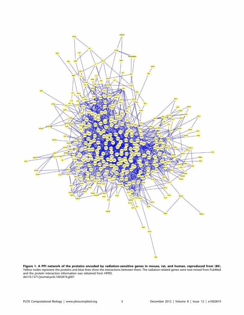
Figure 1. A PPI network of the proteins encoded by radiation-sensitive genes in mouse, rat, and human, reproduced from [89].Yellow nodes represent the proteins and blue lines show the interactions between them. The radiation-related genes were text-mined from PubMedand the protein interaction information was obtained from HPRD.doi:10.1371/journal.pcbi.1002819.g001
PLOS Computational Biology | www.ploscompbiol.org 3 December 2012 | Volume 8 | Issue 12 | e1002819
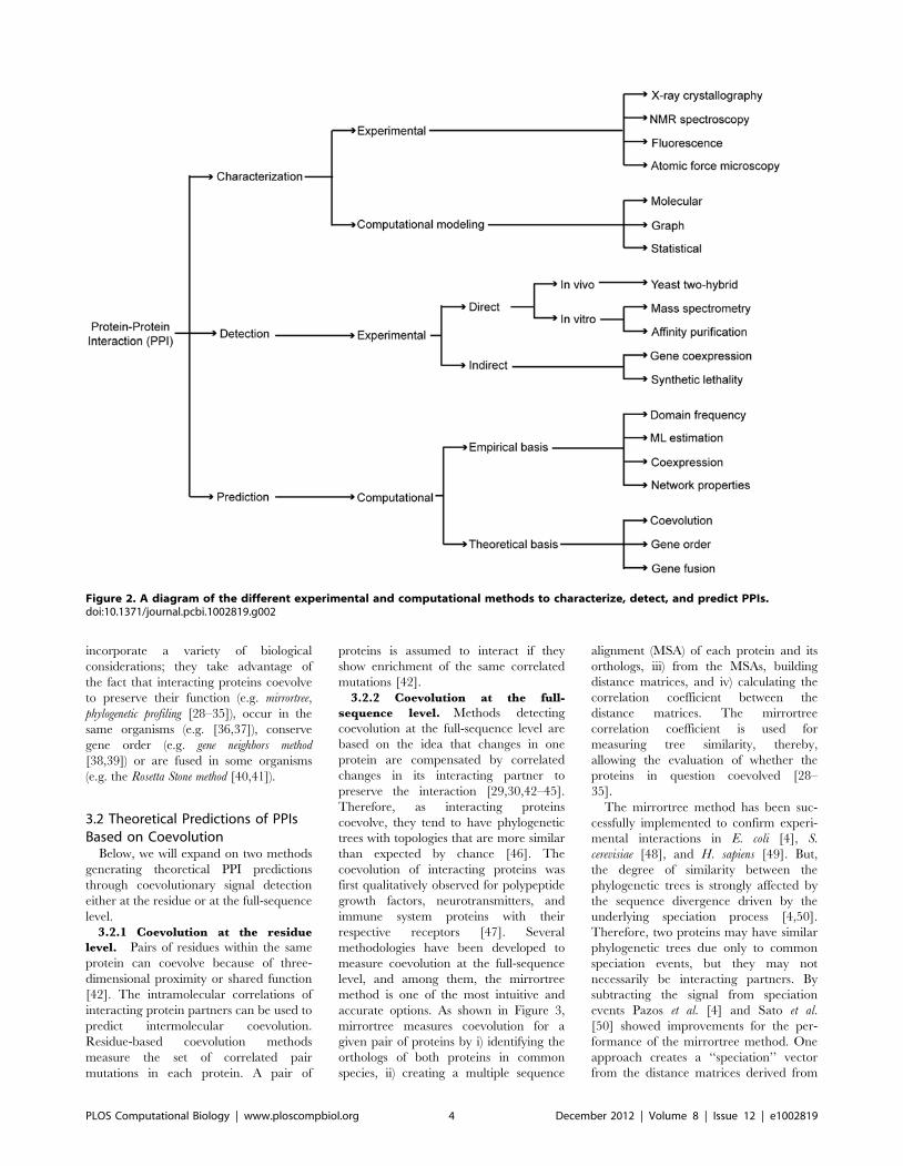
incorporate a variety of biological
considerations; they take advantage of
the fact that interacting proteins coevolve
to preserve their function (e.g. mirrortree,
phylogenetic profiling [28–35]), occur in the
same organisms (e.g. [36,37]), conserve
gene order (e.g. gene neighbors method
[38,39]) or are fused in some organisms
(e.g. the Rosetta Stone method [40,41]).
3.2 Theoretical Predictions of PPIsBased on Coevolution
Below, we will expand on two methods
generating theoretical PPI predictions
through coevolutionary signal detection
either at the residue or at the full-sequence
level.
3.2.1 Coevolution at the residue
level. Pairs of residues within the same
protein can coevolve because of three-
dimensional proximity or shared function
[42]. The intramolecular correlations of
interacting protein partners can be used to
predict intermolecular coevolution.
Residue-based coevolution methods
measure the set of correlated pair
mutations in each protein. A pair of
proteins is assumed to interact if they
show enrichment of the same correlated
mutations [42].
3.2.2 Coevolution at the full-
sequence level. Methods detecting
coevolution at the full-sequence level are
based on the idea that changes in one
protein are compensated by correlated
changes in its interacting partner to
preserve the interaction [29,30,42–45].
Therefore, as interacting proteins
coevolve, they tend to have phylogenetic
trees with topologies that are more similar
than expected by chance [46]. The
coevolution of interacting proteins was
first qualitatively observed for polypeptide
growth factors, neurotransmitters, and
immune system proteins with their
respective receptors [47]. Several
methodologies have been developed to
measure coevolution at the full-sequence
level, and among them, the mirrortree
method is one of the most intuitive and
accurate options. As shown in Figure 3,
mirrortree measures coevolution for a
given pair of proteins by i) identifying the
orthologs of both proteins in common
species, ii) creating a multiple sequence
alignment (MSA) of each protein and its
orthologs, iii) from the MSAs, building
distance matrices, and iv) calculating the
correlation coefficient between the
distance matrices. The mirrortree
correlation coefficient is used for
measuring tree similarity, thereby,
allowing the evaluation of whether the
proteins in question coevolved [28–
35].
The mirrortree method has been suc-
cessfully implemented to confirm experi-
mental interactions in E. coli [4], S.
cerevisiae [48], and H. sapiens [49]. But,
the degree of similarity between the
phylogenetic trees is strongly affected by
the sequence divergence driven by the
underlying speciation process [4,50].
Therefore, two proteins may have similar
phylogenetic trees due only to common
speciation events, but they may not
necessarily be interacting partners. By
subtracting the signal from speciation
events Pazos et al. [4] and Sato et al.
[50] showed improvements for the per-
formance of the mirrortree method. One
approach creates a ‘‘speciation’’ vector
from the distance matrices derived from
Figure 2. A diagram of the different experimental and computational methods to characterize, detect, and predict PPIs.doi:10.1371/journal.pcbi.1002819.g002
PLOS Computational Biology | www.ploscompbiol.org 4 December 2012 | Volume 8 | Issue 12 | e1002819
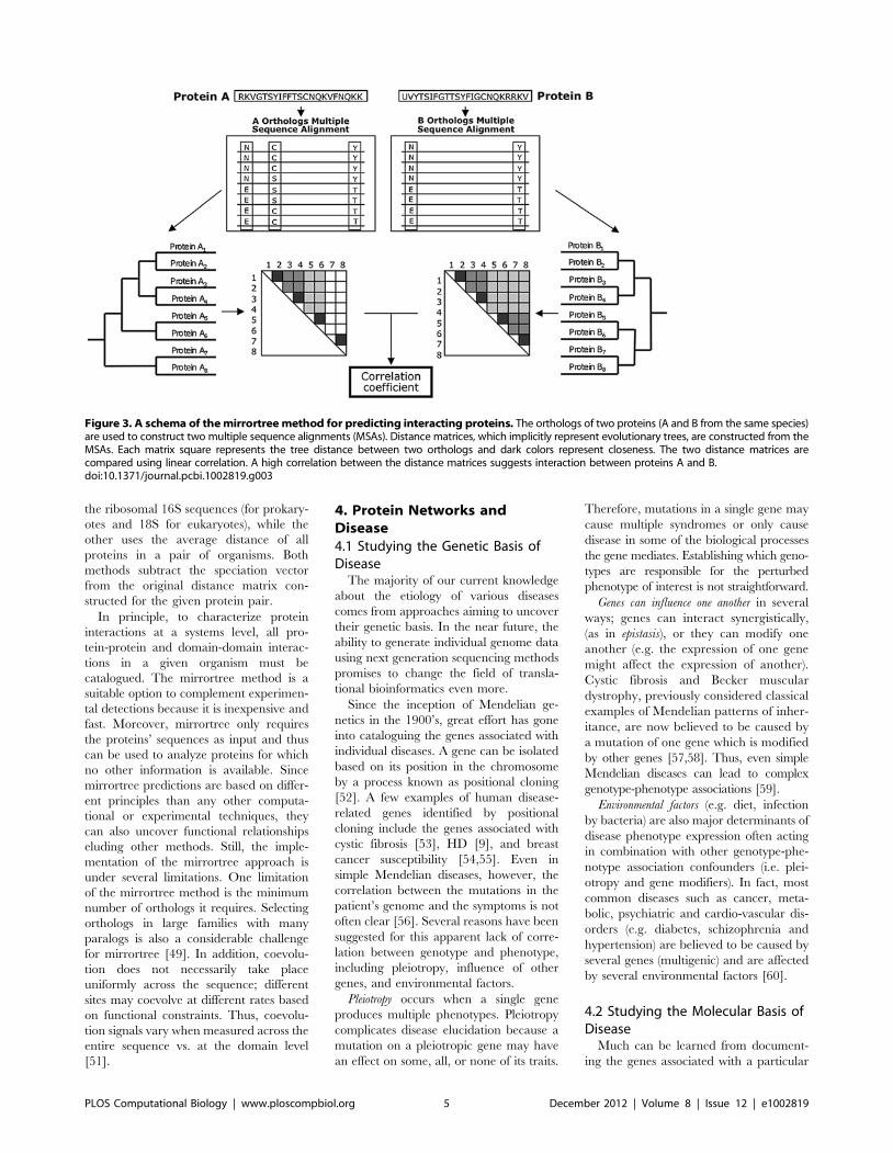
the ribosomal 16S sequences (for prokary-
otes and 18S for eukaryotes), while the
other uses the average distance of all
proteins in a pair of organisms. Both
methods subtract the speciation vector
from the original distance matrix con-
structed for the given protein pair.
In principle, to characterize protein
interactions at a systems level, all pro-
tein-protein and domain-domain interac-
tions in a given organism must be
catalogued. The mirrortree method is a
suitable option to complement experimen-
tal detections because it is inexpensive and
fast. Moreover, mirrortree only requires
the proteins’ sequences as input and thus
can be used to analyze proteins for which
no other information is available. Since
mirrortree predictions are based on differ-
ent principles than any other computa-
tional or experimental techniques, they
can also uncover functional relationships
eluding other methods. Still, the imple-
mentation of the mirrortree approach is
under several limitations. One limitation
of the mirrortree method is the minimum
number of orthologs it requires. Selecting
orthologs in large families with many
paralogs is also a considerable challenge
for mirrortree [49]. In addition, coevolu-
tion does not necessarily take place
uniformly across the sequence; different
sites may coevolve at different rates based
on functional constraints. Thus, coevolu-
tion signals vary when measured across the
entire sequence vs. at the domain level
[51].
4. Protein Networks andDisease
4.1 Studying the Genetic Basis ofDisease
The majority of our current knowledge
about the etiology of various diseases
comes from approaches aiming to uncover
their genetic basis. In the near future, the
ability to generate individual genome data
using next generation sequencing methods
promises to change the field of transla-
tional bioinformatics even more.
Since the inception of Mendelian ge-
netics in the 1900’s, great effort has gone
into cataloguing the genes associated with
individual diseases. A gene can be isolated
based on its position in the chromosome
by a process known as positional cloning
[52]. A few examples of human disease-
related genes identified by positional
cloning include the genes associated with
cystic fibrosis [53], HD [9], and breast
cancer susceptibility [54,55]. Even in
simple Mendelian diseases, however, the
correlation between the mutations in the
patient’s genome and the symptoms is not
often clear [56]. Several reasons have been
suggested for this apparent lack of corre-
lation between genotype and phenotype,
including pleiotropy, influence of other
genes, and environmental factors.
Pleiotropy occurs when a single gene
produces multiple phenotypes. Pleiotropy
complicates disease elucidation because a
mutation on a pleiotropic gene may have
an effect on some, all, or none of its traits.
Therefore, mutations in a single gene may
cause multiple syndromes or only cause
disease in some of the biological processes
the gene mediates. Establishing which geno-
types are responsible for the perturbed
phenotype of interest is not straightforward.
Genes can influence one another in several
ways; genes can interact synergistically,
(as in epistasis), or they can modify one
another (e.g. the expression of one gene
might affect the expression of another).
Cystic fibrosis and Becker muscular
dystrophy, previously considered classical
examples of Mendelian patterns of inher-
itance, are now believed to be caused by
a mutation of one gene which is modified
by other genes [57,58]. Thus, even simple
Mendelian diseases can lead to complex
genotype-phenotype associations [59].
Environmental factors (e.g. diet, infection
by bacteria) are also major determinants of
disease phenotype expression often acting
in combination with other genotype-phe-
notype association confounders (i.e. plei-
otropy and gene modifiers). In fact, most
common diseases such as cancer, meta-
bolic, psychiatric and cardio-vascular dis-
orders (e.g. diabetes, schizophrenia and
hypertension) are believed to be caused by
several genes (multigenic) and are affected
by several environmental factors [60].
4.2 Studying the Molecular Basis ofDisease
Much can be learned from document-
ing the genes associated with a particular
Figure 3. A schema of the mirrortree method for predicting interacting proteins. The orthologs of two proteins (A and B from the same species)are used to construct two multiple sequence alignments (MSAs). Distance matrices, which implicitly represent evolutionary trees, are constructed from theMSAs. Each matrix square represents the tree distance between two orthologs and dark colors represent closeness. The two distance matrices arecompared using linear correlation. A high correlation between the distance matrices suggests interaction between proteins A and B.doi:10.1371/journal.pcbi.1002819.g003
PLOS Computational Biology | www.ploscompbiol.org 5 December 2012 | Volume 8 | Issue 12 | e1002819
disease (e.g. identifying risk factors that
might be used for diagnostic purposes).
Yet, to understand the biological details of
pathogenesis and disease progression and
to subsequently develop methods for
prevention, treatment and even diagnosis,
it is necessary to identify the molecules and
the mechanisms triggering, participating,
and controlling the perturbed biological
process. Deciphering the molecular mech-
anisms leading to diseased states is an even
bigger challenge than elucidating the
genetic basis of complex diseases [61].
Even when the genetic basis of a disease is
well understood, not much is known about
the molecular details leading to the
disorders.
4.2.1 The role of protein
interactions in disease. Protein
interactions provide a vast source of
molecular information; their interactions
(with one another, DNA, RNA, or small
molecules) are involved in metabolic,
signaling, immune, and gene-regulatory
networks. Since protein interactions
mediate the healthy states in all
biological processes, it follows that they
should be the key targets of the molecular-
based studies of biological diseased states.
Disease-causing mutations affecting
protein interactions can lead to
disruptions in protein-DNA interactions,
protein misfolds, new undesired
interactions, or can enable pathogen-host
protein interactions.
Protein-DNA interaction disruptions are most
clearly illustrated by the p53 tumor
suppressor protein and its role in cancer.
Mutations on p53’s DNA-binding domain
destroy its ability to bind to its target DNA
sequences, thus preventing transcriptional
activation of several anti-cancer mecha-
nisms it mediates (e.g. apoptosis, genetic
stability, and inhibition of angiogenesis).
Protein misfolding can result in disruptions
of protein-protein interactions, as occurs
in the Von Hippel-Lindau syndrome
(VHL)—VHL is a rare condition in which
hemangioblastomas are formed in the
cerebellum, spinal cord, kidney, and
retina. A mutation from Tyrosine to
Histidine at residue 98 on the binding site
disrupts binding of the VHL protein to the
hypoxia-inducible factor (HIF) protein. As
a result, the VHL protein no longer
degrades the HIF protein, which leads to
the expression of angiogenic growth fac-
tors and local proliferation of blood vessels
[62,63].
New undesired protein interactions are the
main causes of several diseases, including
Huntington’s disease (see introduction),
cystic fibrosis, and Alzheimer’s disease.
New interactions alter homeostasis since
they can lead to the loss of vital cellular
functions (due to misfolding and aggrega-
tion) and can cause cytotoxicity [11].
Pathogen-host protein interactions also play a
key role in bacterial and viral infections by
facilitating the hijacking of the host’s
metabolism for microbial need. The inter-
action between the Human papillomavirus
(HPV) and its host provides one of the
most striking examples of the centrality of
protein interactions in infectious diseases.
HPV infection occurs in a large fraction of
the population (75–80% of Americans
[64]) by generating lesions of the anogen-
ital tract and for some it leads to cancer.
Upon infection, the HPV genome is
frequently integrated into the host ge-
nome, but only two viral genes (E6 and
E7) are retained and expressed. Remark-
ably, the interactions of only two viral
proteins with the host’s proteins are
enough to cause HPV-induced carcino-
genesis. E6 and E7 bypass the immune
system by interacting with important
negative cell regulatory proteins to target
them for degradation and thus, inactiva-
tion. These two proteins also inhibit
cellular terminal differentiation, induce
cellular transformation and immortaliza-
tion of the host cells, and direct the
proliferation of the tumorigenically-trans-
formed cells [65].
4.2.2 Using PPI networks to
understand disease. PPI networks can
help identify novel pathways to gain basic
knowledge of disease. Note that pathways
are different from PPI networks. PPI
networks map the physical or functional
interaction between protein pairs resulting
in a complex grid of connections (Figure 1).
Pathways, on the other hand, represent
genetic, metabolic, signaling, or neural
processes as a series of sequential
biochemical reactions where substrates
are changed in a linear fashion. For
instance, the glycolysis pathway maps the
conversion of glucose to pyruvate through
a linear chain of ten different steps.
Pathway analysis alone cannot uncover
the molecular basis of disease. When
performing pathway analysis to study
disease, differential expression experi-
ments are the main source of protein
candidates. However, most of the gene
expression candidates are useless to path-
way-based analysis of disease because the
majority of human genes have not been
assigned to a pathway. Protein interaction
networks can be used to identify novel
pathways. Protein interaction subnetworks
tend to group together the proteins that
interact in functional complexes and
pathways [66]. Thus, new methods are
being developed to accurately extract
interaction subnetworks to yield pathway
hypotheses that can be used to understand
different aspects of disease progression
[67,68]. See Table 1 for useful resources
incorporating pathway and PPI informa-
tion in disease elucidation.
Mapping interactomes provide the op-
portunity to identify disease pathways by
identifying key subnetworks. In 2005, Rual
et al. [69] mapped the human protein
interactome. Below are some of the
findings that have been uncovered when
combining PPI and pathway analysis since
then.
(i) Over 39,000 protein interactions
have been identified in the human
cell [70].
(ii) Disease genes are generally non-
essential and occupy peripheral
positions in the human interac-
tome [71], although, in a few
diseases like cancer, disease genes
tend to encode highly-connected
proteins (hubs) [72,73].
(iii) Disease genes tend to cluster to-
gether and co-occur in central
network locations [6].
(iv) Proteins involved in similar pheno-
types (e.g. all cancer proteins) are
highly interconnected [73].
(v) Viral networks differ significantly
from cellular networks, which rais-
es the hypothesis that other intra-
cellular pathogens might also have
distinguishing topologies [74].
(vi) Etiologically unrelated diseases of-
ten present similar symptoms be-
cause separate biological processes
often use common molecular path-
ways [75].
PPI networks can be used to explore the
differences between healthy and diseased
states. Building interaction networks for
systems under different conditions (e.g.
wild type vs. mutant, presence of environ-
mental factor vs. its absence) might be the
key to understanding the differences
between healthy and pathological states.
The work by Charlesworth et al. [76] on
the perturbation of the canonical path-
ways and networks of interactions when
humans are exposed to cigarette smoke
illustrates the potential of such approach-
es. As one might expect, this study found
that the smoking-susceptible genes were
overrepresented in pathways involved in
several aspects of cell death (cell cytotox-
icity, cell lysis), cancer (e.g. tumorigenesis),
and respiratory functions. A somewhat
more unexpected finding, however, con-
firmed that exposure to the smoke envi-
ronmental factor affected a large subnet-
PLOS Computational Biology | www.ploscompbiol.org 6 December 2012 | Volume 8 | Issue 12 | e1002819
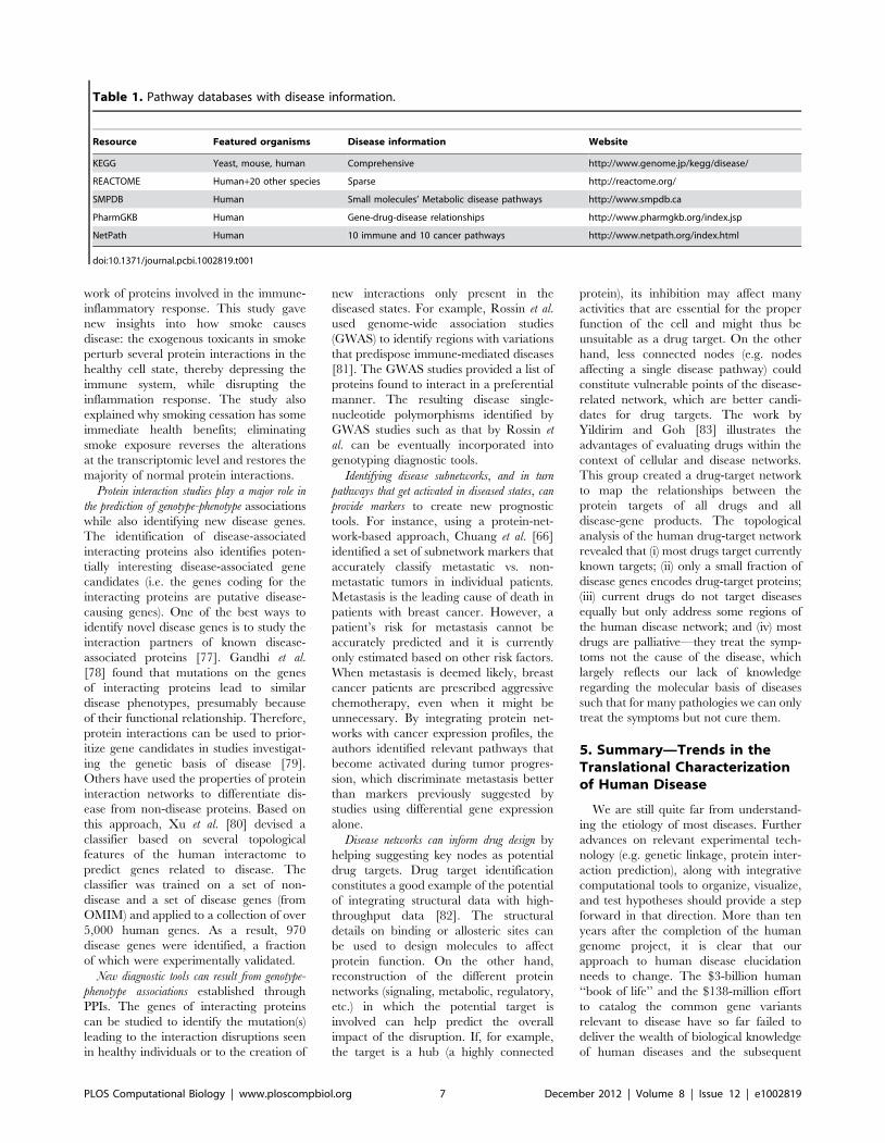
work of proteins involved in the immune-
inflammatory response. This study gave
new insights into how smoke causes
disease: the exogenous toxicants in smoke
perturb several protein interactions in the
healthy cell state, thereby depressing the
immune system, while disrupting the
inflammation response. The study also
explained why smoking cessation has some
immediate health benefits; eliminating
smoke exposure reverses the alterations
at the transcriptomic level and restores the
majority of normal protein interactions.
Protein interaction studies play a major role in
the prediction of genotype-phenotype associations
while also identifying new disease genes.
The identification of disease-associated
interacting proteins also identifies poten-
tially interesting disease-associated gene
candidates (i.e. the genes coding for the
interacting proteins are putative disease-
causing genes). One of the best ways to
identify novel disease genes is to study the
interaction partners of known disease-
associated proteins [77]. Gandhi et al.
[78] found that mutations on the genes
of interacting proteins lead to similar
disease phenotypes, presumably because
of their functional relationship. Therefore,
protein interactions can be used to prior-
itize gene candidates in studies investigat-
ing the genetic basis of disease [79].
Others have used the properties of protein
interaction networks to differentiate dis-
ease from non-disease proteins. Based on
this approach, Xu et al. [80] devised a
classifier based on several topological
features of the human interactome to
predict genes related to disease. The
classifier was trained on a set of non-
disease and a set of disease genes (from
OMIM) and applied to a collection of over
5,000 human genes. As a result, 970
disease genes were identified, a fraction
of which were experimentally validated.
New diagnostic tools can result from genotype-
phenotype associations established through
PPIs. The genes of interacting proteins
can be studied to identify the mutation(s)
leading to the interaction disruptions seen
in healthy individuals or to the creation of
new interactions only present in the
diseased states. For example, Rossin et al.
used genome-wide association studies
(GWAS) to identify regions with variations
that predispose immune-mediated diseases
[81]. The GWAS studies provided a list of
proteins found to interact in a preferential
manner. The resulting disease single-
nucleotide polymorphisms identified by
GWAS studies such as that by Rossin et
al. can be eventually incorporated into
genotyping diagnostic tools.
Identifying disease subnetworks, and in turn
pathways that get activated in diseased states, can
provide markers to create new prognostic
tools. For instance, using a protein-net-
work-based approach, Chuang et al. [66]
identified a set of subnetwork markers that
accurately classify metastatic vs. non-
metastatic tumors in individual patients.
Metastasis is the leading cause of death in
patients with breast cancer. However, a
patient’s risk for metastasis cannot be
accurately predicted and it is currently
only estimated based on other risk factors.
When metastasis is deemed likely, breast
cancer patients are prescribed aggressive
chemotherapy, even when it might be
unnecessary. By integrating protein net-
works with cancer expression profiles, the
authors identified relevant pathways that
become activated during tumor progres-
sion, which discriminate metastasis better
than markers previously suggested by
studies using differential gene expression
alone.
Disease networks can inform drug design by
helping suggesting key nodes as potential
drug targets. Drug target identification
constitutes a good example of the potential
of integrating structural data with high-
throughput data [82]. The structural
details on binding or allosteric sites can
be used to design molecules to affect
protein function. On the other hand,
reconstruction of the different protein
networks (signaling, metabolic, regulatory,
etc.) in which the potential target is
involved can help predict the overall
impact of the disruption. If, for example,
the target is a hub (a highly connected
protein), its inhibition may affect many
activities that are essential for the proper
function of the cell and might thus be
unsuitable as a drug target. On the other
hand, less connected nodes (e.g. nodes
affecting a single disease pathway) could
constitute vulnerable points of the disease-
related network, which are better candi-
dates for drug targets. The work by
Yildirim and Goh [83] illustrates the
advantages of evaluating drugs within the
context of cellular and disease networks.
This group created a drug-target network
to map the relationships between the
protein targets of all drugs and all
disease-gene products. The topological
analysis of the human drug-target network
revealed that (i) most drugs target currently
known targets; (ii) only a small fraction of
disease genes encodes drug-target proteins;
(iii) current drugs do not target diseases
equally but only address some regions of
the human disease network; and (iv) most
drugs are palliative—they treat the symp-
toms not the cause of the disease, which
largely reflects our lack of knowledge
regarding the molecular basis of diseases
such that for many pathologies we can only
treat the symptoms but not cure them.
5. Summary—Trends in theTranslational Characterizationof Human Disease
We are still quite far from understand-
ing the etiology of most diseases. Further
advances on relevant experimental tech-
nology (e.g. genetic linkage, protein inter-
action prediction), along with integrative
computational tools to organize, visualize,
and test hypotheses should provide a step
forward in that direction. More than ten
years after the completion of the human
genome project, it is clear that our
approach to human disease elucidation
needs to change. The $3-billion human
‘‘book of life’’ and the $138-million effort
to catalog the common gene variants
relevant to disease have so far failed to
deliver the wealth of biological knowledge
of human diseases and the subsequent
Table 1. Pathway databases with disease information.
Resource Featured organisms Disease information Website
KEGG Yeast, mouse, human Comprehensive http://www.genome.jp/kegg/disease/
REACTOME Human+20 other species Sparse http://reactome.org/
SMPDB Human Small molecules’ Metabolic disease pathways http://www.smpdb.ca
PharmGKB Human Gene-drug-disease relationships http://www.pharmgkb.org/index.jsp
NetPath Human 10 immune and 10 cancer pathways http://www.netpath.org/index.html
doi:10.1371/journal.pcbi.1002819.t001
PLOS Computational Biology | www.ploscompbiol.org 7 December 2012 | Volume 8 | Issue 12 | e1002819
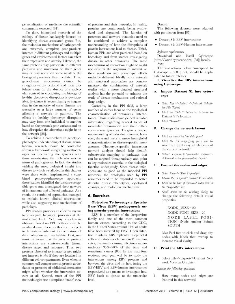
personalization of medicine the scientific
community expected [84].
To date, biomedical research of the
etiology of disease has largely focused on
identifying disease-associated genes. But,
the molecular mechanisms of pathogenesis
are extremely complex; gene-products
interact in different pathways and multiple
genes and environmental factors can affect
their expression and activity. Likewise, the
same proteins may participate in different
pathways and mutations on their genes
may or may not affect some or all of the
biological processes they mediate. Thus,
gene-disease associations cannot be
straightforwardly deduced and their use-
fulness alone (in the absence of a molec-
ular context) in elucidating the biology of
healthy phenotype disruptions is question-
able. Evidence is accumulating to suggest
that in the majority of cases illnesses are
traceable to a large number of genes
affecting a network or pathway. The
effects on healthy phenotype disruption
may vary from one individual to another
based on the person’s gene variants and on
how disruptive the alterations might be to
the network [85].
To achieve a comprehensive genotype-
phenotype understanding of disease, trans-
lational research should be conducted
within a framework integrating methodol-
ogies for uncovering the genetics with
those investigating the molecular mecha-
nisms of pathogenesis. In fact, the studies
yielding the most biological insight into
disease to which we alluded in this chapter
were those which implemented a com-
bined genotype-phenotype approach;
those studies identified the disease-suscep-
tible genes and investigated their network
of interactions and affected pathways. As a
result, the combined approaches managed
to explain known clinical observations
while also suggesting new mechanisms of
pathology.
PPI analysis provides an effective means
to investigate biological processes at the
molecular level. Yet, any conclusions
obtained based on PPI methods must be
validated since these methods are subject
to limitations inherent to the nature of
data collection and availability. First, one
must be aware that the roles of protein
interactions are context-specific (tissue,
disease stage, and response). Thus, two
proteins observed to interact in vitro might
not interact in vivo if they are localized in
different cell compartments. Even when in
common cell compartments, protein abun-
dance or presence of additional interactors
might affect whether the interaction oc-
curs at all. Second, most of the PPI
methodologies use a simplistic ‘static’ view
of proteins and their networks. In reality,
proteins are continuously being synthe-
sized and degraded. The kinetics of
processes and network dynamics need to
be considered to achieve a complete
understanding of how the disruptions of
protein interactions lead to disease. Third,
human PPIs are often predicted based on
homology and from studies investigating
disease in other organisms. The same
mechanisms of interaction might or might
not exist in the organism of interest or
their regulation and phenotypic effects
might be different. Ideally, since network
and structural approaches are comple-
mentary, the combination of network
studies with a more detailed structural
analysis has the potential to enhance the
study of disease mechanisms and rational
drug design.
Currently, in the PPI field, a large
number of studies focus on the topological
characterization of organisms’ interac-
tomes. Those studies have yielded valuable
information regarding general trends of
molecular organization and their differ-
ences across genomes. To gain a deeper
understanding of individual diseases, how-
ever, the trend needs to move from global
characterizations to disease-specific inter-
actomes. Phenotype-specific interaction
network analyses should help identify
subnetworks mapping to pathways that
can be targeted therapeutically and point
to key molecules essential to the biological
function under study. Since disease infer-
ences are as good as the modeled PPI
networks, the ontologies used by PPI
resources need to be expanded to better
describe disease phenotypes, cytological
changes, and molecular mechanisms.
6. Exercises
Objective: To investigate Epstein-Barr Virus (EBV) pathogenesis us-ing protein-protein interactions
EBV is a member of the herpesvirus
family and one of the most common
human viruses. According to the CDC,
in the United States around 95% of adults
have been infected by EBV. Upon infec-
tion in adults, EBV replicates in epithelial
cells and establishes latency in B lympho-
cytes, eventually causing infectious mono-
nucleosis 35%–50% of the time and
sometimes cancer [86]. In the next four
sections, your goal will be to study the
interactions among EBV proteins and
between the virus and its host (using the
EBV-EBV and EBV-human interactomes
respectively) as a means to investigate how
EBV leads to disease at the molecular
level.
Datasets:
The following datasets were adapted
with permission from [87]
N Dataset S1: EBV interactome
N Dataset S2: EBV-Human interactome
Software requirements:
Download and install Cytoscape
(http://www.cytoscape.org, [88]) locally.
Note:
The instructions below correspond to
Cytoscape v. 2.8.0; but, should be appli-
cable to future releases.
I. Visualize the EBV interactomeusing Cytoscape
A. Import Dataset S1 into cytos-cape
N Select File -.Import -.Network (Multi-
ple File Types)
N Click the ‘‘Select’’ button to browse to
Dataset S1’s location
N Click ‘‘Import’’
B. Change the network layout
N Click on View-.Hide data panel
N Click the 1:1 magnifying glass icon to
zoom out to display all elements of
the current network’’
N Select Layout-.Cytoscape Layouts-
.Force-directed (unweighted) Layout
C. Format the nodes and edges
N Select View-.Open Vizmapper
N Choose the ‘‘Default’’ Current Visual Style
N Click on the pair of connected nodes icon in
the ‘‘Defaults’’ box
N Scroll down on the resulting dialog to
change the following default visual
properties:
NODE__SIZE = 20
NODE_FONT_SIZE = 20
N O D E _ L A B E L _ P O S I -
TION = (Node Anchor Points)
SOUTH
N Note: Feel free to click and drag any
nodes with labels that overlap to
increase visual clarity.
D. Print the EBV interactome
N Select File-.Export-.Current Net-
work View as Graphics
Answer the following questions:
i. How many nodes and edges are
featured in this network?
PLOS Computational Biology | www.ploscompbiol.org 8 December 2012 | Volume 8 | Issue 12 | e1002819
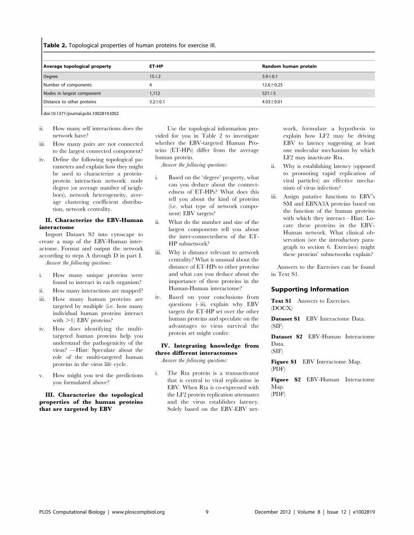
ii. How many self interactions does the
network have?
iii. How many pairs are not connected
to the largest connected component?
iv. Define the following topological pa-
rameters and explain how they might
be used to characterize a protein-
protein interaction network: node
degree (or average number of neigh-
bors), network heterogeneity, aver-
age clustering coefficient distribu-
tion, network centrality.
II. Characterize the EBV-Humaninteractome
Import Dataset S2 into cytoscape to
create a map of the EBV-Human inter-
actome. Format and output the network
according to steps A through D in part I.
Answer the following questions:
i. How many unique proteins were
found to interact in each organism?
ii. How many interactions are mapped?
iii. How many human proteins are
targeted by multiple (i.e. how many
individual human proteins interact
with .1) EBV proteins?
iv. How does identifying the multi-
targeted human proteins help you
understand the pathogenicity of the
virus? —Hint: Speculate about the
role of the multi-targeted human
proteins in the virus life cycle.
v. How might you test the predictions
you formulated above?
III. Characterize the topologicalproperties of the human proteinsthat are targeted by EBV
Use the topological information pro-
vided for you in Table 2 to investigate
whether the EBV-targeted Human Pro-
teins (ET-HPs) differ from the average
human protein.
Answer the following questions:
i. Based on the ‘degree’ property, what
can you deduce about the connect-
edness of ET-HPs? What does this
tell you about the kind of proteins
(i.e. what type of network compo-
nent) EBV targets?
ii. What do the number and size of the
largest components tell you about
the inter-connectedness of the ET-
HP subnetwork?
iii. Why is distance relevant to network
centrality? What is unusual about the
distance of ET-HPs to other proteins
and what can you deduce about the
importance of these proteins in the
Human-Human interactome?
iv. Based on your conclusions from
questions i–iii, explain why EBV
targets the ET-HP set over the other
human proteins and speculate on the
advantages to virus survival the
protein set might confer.
IV. Integrating knowledge fromthree different interactomes
Answer the following questions:
i. The Rta protein is a transactivator
that is central to viral replication in
EBV. When Rta is co-expressed with
the LF2 protein replication attenuates
and the virus establishes latency.
Solely based on the EBV-EBV net-
work, formulate a hypothesis to
explain how LF2 may be driving
EBV to latency suggesting at least
one molecular mechanism by which
LF2 may inactivate Rta.
ii. Why is establishing latency (opposed
to promoting rapid replication of
viral particles) an effective mecha-
nism of virus infection?
iii. Assign putative functions to EBV’s
SM and EBNA3A proteins based on
the function of the human proteins
with which they interact—Hint: Lo-
cate these proteins in the EBV-
Human network. What clinical ob-
servation (see the introductory para-
graph to section 6. Exercises) might
these proteins’ subnetworks explain?
Answers to the Exercises can be found
in Text S1.
Supporting Information
Text S1 Answers to Exercises.
(DOCX)
Dataset S1 EBV Interactome Data.
(SIF)
Dataset S2 EBV-Human Interactome
Data.
(SIF)
Figure S1 EBV Interactome Map.
(PDF)
Figure S2 EBV-Human Interactome
Map.
(PDF)
Table 2. Topological properties of human proteins for exercise III.
Average topological property ET-HP Random human protein
Degree 1562 5.960.1
Number of components 4 12.660.25
Nodes in largest component 1,112 52165
Distance to other proteins 3.260.1 4.0360.01
doi:10.1371/journal.pcbi.1002819.t002
PLOS Computational Biology | www.ploscompbiol.org 9 December 2012 | Volume 8 | Issue 12 | e1002819
References
1. De Las Rivas J, de Luis A (2004) Interactome
data and databases: different types of protein
interaction. Comp Funct Genomics 5: 173–
178.
2. Barabasi AL, Oltvai ZN (2004) Network biology:
understanding the cell’s functional organization.
Nat Rev Genet 5: 101–113.
3. Grindrod P, Kibble M (2004) Review of uses of
network and graph theory concepts within
proteomics. Expert Rev Proteomics 1: 229–238.
4. Pazos F, Ranea JA, Juan D, Sternberg MJ (2005)
Assessing protein co-evolution in the context of
the tree of life assists in the prediction of the
interactome. J Mol Biol 352: 1002–1015.
5. Kann MG (2007) Protein interactions and disease:
computational approaches to uncover the etiology
of diseases. Brief Bioinform 8: 333–346.
6. Ideker T, Sharan R (2008) Protein networks in
disease. Genome Res 18: 644–652.
7. Huntington G (1872) On chorea. Med Surg Rep
26: 320–321.
8. Punnett RC (1908) Mendelism in Relation to
Disease. Proc R Soc Med 1: 135–168.
9. (1993) A novel gene containing a trinucleotide
repeat that is expanded and unstable on Hun-
tington’s disease chromosomes. The Huntington’s
Disease Collaborative Research Group. Cell 72:
971–983.
10. Goehler H, Lalowski M, Stelzl U, Waelter S,
Stroedicke M, et al. (2004) A protein interaction
network links GIT1, an enhancer of huntingtin
aggregation, to Huntington’s disease. Mol Cell
15: 853–865.
11. Duennwald ML, Jagadish S, Giorgini F, Mu-
chowski PJ, Lindquist S (2006) A network of
protein interactions determines polyglutamine
toxicity. Proc Natl Acad Sci U S A 103: 11051–
11056.
12. Giorgini F, Muchowski PJ (2005) Connecting the
dots in Huntington’s disease with protein inter-
action networks. Genome Biol 6: 210.
13. Shoemaker BA, Panchenko AR (2007) Decipher-
ing protein–protein interactions. Part I. Experi-
mental techniques and databases. PLoS Comput
Biol 3: e42. doi:10.1371/journal.pcbi.0030043
14. Costanzo M, Baryshnikova A, Bellay J, Kim Y,
Spear ED, et al. (2010) The genetic landscape of a
cell. Science 327: 425–431.
15. Ito T, Chiba T, Ozawa R, Yoshida M, Hattori
M, et al. (2001) A comprehensive two-hybrid
analysis to explore the yeast protein interactome.
Proc Natl Acad Sci U S A 98: 4569–4574.
16. Mrowka R, Patzak A, Herzel H (2001) Is there a
bias in proteome research? Genome Res 11:
1971–1973.
17. von Mering C, Krause R, Snel B, Cornell M,
Oliver SG, et al. (2002) Comparative assessment
of large-scale data sets of protein-protein interac-
tions. Nature 417: 399–403.
18. Shoemaker BA, Panchenko AR, Bryant SH
(2006) Finding biologically relevant protein do-
main interactions: conserved binding mode
analysis. Protein Sci 15: 352–361.
19. Sprinzak E, Margalit H (2001) Correlated
sequence-signatures as markers of protein-protein
interaction. J Mol Biol 311: 681–692.
20. Deng M, Mehta S, Sun F, Chen T (2002)
Inferring domain-domain interactions from pro-
tein-protein interactions. Genome Res 12: 1540–
1548.
21. Nye TM, Berzuini C, Gilks WR, Babu MM,
Teichmann SA (2005) Statistical analysis of
domains in interacting protein pairs. Bioinfor-
matics 21: 993–1001.
22. Fraser HB, Hirsh AE, Wall DP, Eisen MB (2004)
Coevolution of gene expression among interact-
ing proteins. Proc Natl Acad Sci U S A 101:
9033–9038.
23. Kanaan SP, Huang C, Wuchty S, Chen DZ,
Izaguirre JA (2009) Inferring protein-protein
interactions from multiple protein domain com-
binations. Methods Mol Biol 541: 43–59.
24. Guimaraes KS, Przytycka TM (2008) Interrogat-
ing domain-domain interactions with parsimony
based approaches. BMC Bioinformatics 9: 171.
25. Guimaraes KS, Jothi R, Zotenko E, Przytycka
TM (2006) Predicting domain-domain interac-
tions using a parsimony approach. Genome Biol
7: R104.
26. Riley R, Lee C, Sabatti C, Eisenberg D (2005)
Inferring protein domain interactions from data-
bases of interacting proteins. Genome Biol 6:
R89.
27. Izarzugaza JM, Juan D, Pons C, Ranea JA,
Valencia A, et al. (2006) TSEMA: interactive
prediction of protein pairings between interacting
families. Nucleic Acids Res 34: W315–319.
28. Gertz J, Elfond G, Shustrova A, Weisinger M,
Pellegrini M, et al. (2003) Inferring protein
Further Reading
N Chen JY, Youn E, Mooney SD (2009) Connecting protein interaction data, mutations, and disease using bioinformatics.Methods Mol Biol 541: 449–461.
N Nussinov R, Schreiber G (2009) Computational protein-protein interactions. Boca Raton: CRC Press.
N Ideker T, Sharan R (2008) Protein networks in disease. Genome Res 18: 644–652.
N Juan D, Pazos F, Valencia A (2008) Co-evolution and co-adaptation in protein networks. FEBS Lett 582: 1225–1230.
N Panchenko A, Przytycka T (2008) Protein-protein interactions and networks: identification, computer analysis, and prediction.London: Springer.
N Klussmann E, Scott J, Aandahl EM (2008) Protein-protein interactions as new drug targets. Berlin: Springer.
N Kann MG (2007) Protein interactions and disease: computational approaches to uncover the etiology of diseases. BriefBioinform 8: 333–346.
N Shoemaker BA, Panchenko AR (2007) Deciphering protein-protein interactions. Part II. Computational methods to predictprotein and domain interaction partners. PLoS Comput Biol 3: e43. doi:10.1371/journal.pcbi.0030043
Glossary
Mendelian traits or diseases, named after Gregor Mendel, are the traits inherited and controlled by a single gene.
Positional cloning is a method to find the gene producing a specific phenotype in an area of interest in the genome. The firststep of positional cloning is linkage analysis, in which the gene is mapped using a group of DNA polymorphisms from familiessegregating the disease phenotype.
Epistasis refers to the phenomenon in which one gene masks the phenotypic effect of another.
Angiogenesis is the physiological process leading to growth of new blood vessels. Angiogenesis is a normal and vital processin growth, development, and wound healing; but it is also a fundamental step in the transition of tumors from a dormant to amalignant state.
Hemangioblastomas are tumors of the central nervous system that originate from the vascular system.
PLOS Computational Biology | www.ploscompbiol.org 10 December 2012 | Volume 8 | Issue 12 | e1002819
interactions from phylogenetic distance matrices.
Bioinformatics 19: 2039–2045.29. Goh CS, Bogan AA, Joachimiak M, Walther D,
Cohen FE (2000) Co-evolution of proteins with
their interaction partners. J Mol Biol 299: 283–293.
30. Goh CS, Cohen FE (2002) Co-evolutionaryanalysis reveals insights into protein-protein
interactions. J Mol Biol 324: 177–192.
31. Jothi R, Kann MG, Przytycka TM (2005)Predicting protein-protein interaction by search-
ing evolutionary tree automorphism space. Bioin-formatics 21 Suppl 1: i241–i250.
32. Pazos F, Helmer-Citterich M, Ausiello G, Valen-cia A (1997) Correlated mutations contain
information about protein-protein interaction.
J Mol Biol 271: 511–523.33. Pazos F, Valencia A (2002) In silico two-hybrid
system for the selection of physically interactingprotein pairs. Proteins 47: 219–227.
34. Ramani AK, Marcotte EM (2003) Exploiting the
co-evolution of interacting proteins to discoverinteraction specificity. J Mol Biol 327: 273–284.
35. Jothi R, Cherukuri PF, Tasneem A, PrzytyckaTM (2006) Co-evolutionary Analysis of Domains
in Interacting Proteins Reveals Insights intoDomain-Domain Interactions Mediating Pro-
tein-Protein Interactions. J Mol Biol 362: 861–
875.36. Pellegrini M, Marcotte EM, Thompson MJ,
Eisenberg D, Yeates TO (1999) Assigning proteinfunctions by comparative genome analysis: pro-
tein phylogenetic profiles. Proc Natl Acad
Sci U S A 96: 4285–4288.37. Huynen MA, Bork P (1998) Measuring genome
evolution. Proc Natl Acad Sci U S A 95: 5849–5856.
38. Dandekar T, Snel B, Huynen M, Bork P (1998)Conservation of gene order: a fingerprint of
proteins that physically interact. Trends Biochem
Sci 23: 324–328.39. Overbeek R, Fonstein M, D’Souza M, Pusch GD,
Maltsev N (1999) Use of contiguity on thechromosome to predict functional coupling. In
Silico Biol 1: 93–108.
40. Marcotte EM, Pellegrini M, Ng HL, Rice DW,Yeates TO, et al. (1999) Detecting protein
function and protein-protein interactions fromgenome sequences. Science 285: 751–753.
41. Enright AJ, IliopoulosI., Kyrpides NC, OuzounisCA (1999) Protein interaction maps for complete
genomes based on gene fusion events. Nature
402: 86–90.42. Juan D, Pazos F, Valencia A (2008) Co-evolution
and co-adaptation in protein networks. FEBSLett.
43. Valencia A, Pazos F (2003) Prediction of protein-
protein interactions from evolutionary informa-tion. Methods Biochem Anal 44: 411–426.
44. Valencia A, Pazos F (2002) Computationalmethods for the prediction of protein interactions.
Curr Opin Struct Biol 12: 368–373.
45. Pazos F, Valencia A (2001) Similarity of phylo-genetic trees as indicator of protein-protein
interaction. Protein Eng 14: 609–614.46. Pazos F, Juan D, Izarzugaza JM, Leon E,
Valencia A (2008) Prediction of protein interac-tion based on similarity of phylogenetic trees.
Methods Mol Biol 484: 523–535.
47. Fryxell KJ (1996) The coevolution of gene familytrees. Trends Genet 12: 364–369.
48. Hakes L, Lovell SC, Oliver SG, Robertson DL(2007) Specificity in protein interactions and its
relationship with sequence diversity and coevolu-
tion. Proc Natl Acad Sci U S A 104: 7999–8004.49. Tillier ER, Charlebois RL (2009) The human
protein coevolution network. Genome Res 19:1861–1871.
50. Sato T, Yamanishi Y, Kanehisa M, Toh H (2005)
The inference of protein-protein interactions byco-evolutionary analysis is improved by excluding
the information about the phylogenetic relation-
ships. Bioinformatics 21: 3482–3489.51. Kann MG, Jothi R, Cherukuri PF, Przytycka TM
(2007) Predicting protein domain interactionsfrom coevolution of conserved regions. Proteins
67: 811–820.
52. Botstein D, Risch N (2003) Discovering genotypesunderlying human phenotypes: past successes for
mendelian disease, future approaches for complexdisease. Nat Genet 33 Suppl: 228–237.
53. Kerem B, Rommens JM, Buchanan JA, Markie-wicz D, Cox TK, et al. (1989) Identification of the
cystic fibrosis gene: genetic analysis. Science 245:
1073–1080.54. Miki Y, Swensen J, Shattuck-Eidens D, Futreal
PA, Harshman K, et al. (1994) A strong candidatefor the breast and ovarian cancer susceptibility
gene BRCA1. Science 266: 66–71.
55. Wooster R, Bignell G, Lancaster J, Swift S, SealS, et al. (1995) Identification of the breast cancer
susceptibility gene BRCA2. Nature 378: 789–792.56. Scriver CR, Waters PJ (1999) Monogenic traits
are not simple: lessons from phenylketonuria.Trends Genet 15: 267–272.
57. Groman JD, Meyer ME, Wilmott RW, Zeitlin
PL, Cutting GR (2002) Variant cystic fibrosisphenotypes in the absence of CFTR mutations.
N Engl J Med 347: 401–407.58. Sun H, Smallwood PM, Nathans J (2000)
Biochemical defects in ABCR protein variants
associated with human retinopathies. NatureGenet 26: 242–246.
59. Dipple KM, McCabe ERB (2000) Phenotypes ofpatients with ‘simple’ Mendelian disorders are
complex traits: thresholds, modifiers, and systemsdynamics. Am J Hum Genet 66: 1729–1735.
60. Van Heyningen V, Yeyati PL (2004) Mechanisms
of non-Mendelian inheritance in genetic disease.Hum Mol Genet 13 Spec No 2: R225–233.
61. Mayeux R (2005) Mapping the new frontier:complex genetic disorders. J Clin Invest 115:
1404–1407.
62. Brauch H, Kishida T, Glavac D, Chen F, PauschF, et al. (1995) Von Hippel-Lindau (VHL) disease
with pheochromocytoma in the Black Forestregion of Germany: evidence for a founder effect.
Hum Genet 95: 551–556.63. Ohh M, Park CW, Ivan M, Hoffman MA, Kim
TY, et al. (2000) Ubiquitination of hypoxia-
inducible factor requires direct binding to thebeta-domain of the von Hippel-Lindau protein.
Nat Cell Biol 2: 423–427.64. Association ASH (2007) HPV Resource Center.
65. Scheffner M, Whitaker NJ (2003) Human papil-
lomavirus-induced carcinogenesis and the ubiq-uitin-proteasome system. Semin Cancer Biol 13:
59–67.66. Chuang HY, Lee E, Liu YT, Lee D, Ideker T
(2007) Network-based classification of breast
cancer metastasis. Mol Syst Biol 3: 140.67. Ideker T, Ozier O, Schwikowski B, Siegel AF
(2002) Discovering regulatory and signallingcircuits in molecular interaction networks. Bioin-
formatics 18 Suppl 1: S233–240.68. Hallock P, Thomas MA (2012) Integrating the
Alzheimer’s disease proteome and transcriptome:
a comprehensive network model of a complexdisease. OMICS 16: 37–49.
69. Rual JF, Venkatesan K, Hao T, Hirozane-Kishikawa T, Dricot A, et al. (2005) Towards a
proteome-scale map of the human protein-
protein interaction network. Nature 437: 1173–1178.
70. Keshava Prasad TS, Goel R, Kandasamy K,Keerthikumar S, Kumar S, et al. (2009) Human
Protein Reference Database–2009 update. Nu-
cleic Acids Res 37: D767–772.
71. Goh KI, Cusick ME, Valle D, Childs B, Vidal M,
et al. (2007) The human disease network. Proc
Natl Acad Sci U S A 104: 8685–8690.
72. Wachi S, Yoneda K, Wu R (2005) Interactome-
transcriptome analysis reveals the high centrality
of genes differentially expressed in lung cancer
tissues. Bioinformatics 21: 4205–4208.
73. Jonsson PF, Bates PA (2006) Global topological
features of cancer proteins in the human inter-
actome. Bioinformatics 22: 2291–2297.
74. Uetz P, Dong YA, Zeretzke C, Atzler C, Baiker
A, et al. (2006) Herpesviral protein networks and
their interaction with the human proteome.
Science 311: 239–242.
75. Lim J, Hao T, Shaw C, Patel AJ, Szabo G, et al.
(2006) A protein-protein interaction network for
human inherited ataxias and disorders of Purkinje
cell degeneration. Cell 125: 801–814.
76. Charlesworth JC, Curran JE, Johnson MP,
Goring HH, Dyer TD, et al. Transcriptomic
epidemiology of smoking: the effect of smoking on
gene expression in lymphocytes. BMC Med
Genomics 3: 29.
77. Oti M, Snel B, Huynen MA, Brunner HG (2006)
Predicting disease genes using protein-protein
interactions. J Med Genet 43: 691–698.
78. Gandhi TK, Zhong J, Mathivanan S, Karthick L,
Chandrika KN, et al. (2006) Analysis of the
human protein interactome and comparison with
yeast, worm and fly interaction datasets. Nat
Genet 38: 285–293.
79. Chen L, Tai J, Zhang L, Shang Y, Li X, et al.
(2011) Global risk transformative prioritization
for prostate cancer candidate genes in molecular
networks. Mol Biosyst 7: 2547–2553.
80. Xu J, Li Y (2006) Discovering disease-genes by
topological features in human protein-protein
interaction network. Bioinformatics 22: 2800–
2805.
81. Rossin EJ, Lage K, Raychaudhuri S, Xavier RJ,
Tatar D, et al. (2011) Proteins encoded in
genomic regions associated with immune-mediat-
ed disease physically interact and suggest under-
lying biology. PLoS Genet 7: e1001273.
doi:10.1371/journal.pgen.1001273
82. Jiang Z, Zhou Y (2005) Using bioinformatics for
drug target identification from the genome.
Am J Pharmacogenomics 5: 387–396.
83. Yildirim MA, Goh KI, Cusick ME, Barabasi AL,
Vidal M (2007) Drug-target network. Nat Bio-
technol 25: 1119–1126.
84. Hall SS Revolution postponed. Sci Am 303: 60–
67.
85. Nadeau JH (2009) Transgenerational genetic
effects on phenotypic variation and disease risk.
Hum Mol Genet 18: R202–R210.
86. CDC (2006) Epstein-Barr Virus and Infectious
Mononucleosis. Center for Disease Control and
Prevention/National Center for Infectious Dis-
eases.
87. Calderwood MA, Venkatesan K, Xing L, Chase
MR, Vazquez A, et al. (2007) Epstein-Barr virus
and virus human protein interaction maps. Proc
Natl Acad Sci U S A 104: 7606–7611.
88. Smoot ME, Ono K, Ruscheinski J, Wang PL,
Ideker T (2011) Cytoscape 2.8: new features for
data integration and network visualization. Bioin-
formatics 27: 431–432.
89. Zhang J, Yang Y, Wang Y, Wang Z, Yin M, et al.
(2011) Identification of hub genes related to the
recovery phase of irradiation injury by microarray
and integrated gene network analysis. PLoS ONE
6: e24680. doi:10.1371/journal.pone.0024680
PLOS Computational Biology | www.ploscompbiol.org 11 December 2012 | Volume 8 | Issue 12 | e1002819
Education
Chapter 5: Network Biology Approach to Complex DiseasesDong-Yeon Cho., Yoo-Ah Kim., Teresa M. Przytycka*
National Center for Biotechnology Information, NLM, NIH, Bethesda, Maryland, United States of America
Abstract: Complex diseases arecaused by a combination of geneticand environmental factors. Uncov-ering the molecular pathwaysthrough which genetic factors affecta phenotype is always difficult, butin the case of complex diseases thisis further complicated since geneticfactors in affected individuals mightbe different. In recent years, systemsbiology approaches and, more spe-cifically, network based approachesemerged as powerful tools forstudying complex diseases. Theseapproaches are often built on theknowledge of physical or functionalinteractions between moleculeswhich are usually represented asan interaction network. An interac-tion network not only reports thebinary relationships between indi-vidual nodes but also encodeshidden higher level organization ofcellular communication. Computa-tional biologists were challengedwith the task of uncovering thisorganization and utilizing it for theunderstanding of disease complex-ity, which prompted rich and di-verse algorithmic approaches to beproposed. We start this chapter witha description of the general charac-teristics of complex diseases fol-lowed by a brief introduction tophysical and functional networks.Next we will show how thesenetworks are used to leveragegenotype, gene expression, andother types of data to identifydysregulated pathways, infer therelationships between genotypeand phenotype, and explain diseaseheterogeneity. We group the meth-ods by common underlying princi-ples and first provide a high leveldescription of the principles fol-lowed by more specific examples.We hope that this chapter will givereaders an appreciation for thewealth of algorithmic techniquesthat have been developed for thepurpose of studying complex dis-eases as well as insight into theirstrengths and limitations.
This article is part of the ‘‘Transla-
tional Bioinformatics’’ collection for
PLOS Computational Biology.
1. Introduction
Complex diseases are caused, among other
factors, by a combination of genetic
perturbations. Thus in the case of a
complex disease we do not assume that a
single genetic mutation can be pinned
down as a cause. Many diseases fall in this
category including cancer, autism, diabe-
tes, obesity, and coronary artery disease.
Even though there are other factors
involved in such diseases, this review will
focus on genetic causes.
One of the fundamental difficulties in
studying genetic causes of complex diseas-
es is that different disease cases might be
caused by different genetic perturbations.
In addition, if a disease is caused by a
combinatorial effect of many mutations,
the individual effects of each mutation
might be small and thus hard to discover.
For example, autism is considered to be
one of the most heritable complex disor-
ders, but its underlying genetic causes are
still largely unknown [1]. One of the
proposed factors that contribute to this
difficulty is the role of rare genetic
variations in the emergence of the disease
[2].
An additional difficulty in studying
complex diseases relates to disease hetero-
geneity. Specifically, in a complex disease,
disease phenotypes might vary significant-
ly among patients. The recognition of this
fact has lead, for example, to renaming
‘‘autism’’ to ‘‘autism spectrum disorders’’
(ASDs) referring in this way to a group of
conditions characterized by impairments
in reciprocal social interaction and com-
munication, and the presence of restricted
and repetitive behaviors [1]. Similar
heterogeneity is present in other complex
diseases including cancer.
Given the above challenges, how can we
approach the study of complex diseases? A
useful clue is provided by the fact that
genes, gene products, and small molecules
interact with each other to form a complex
interaction network. Thus a perturbation
in one gene can be propagated through
the interactions, and affect other genes in
the network. However, the fact that we
observe similar disease phenotypes despite
different genetic causes suggests that these
different causes are not unrelated but
rather dys-regulate the same component
of the cellular system [3]. Therefore in
studies of complex diseases researchers
increasingly focus on groups of related/
interconnected genes, referred to as mod-
ules or subnetworks.
2. Interactome
Biomoecules in a living organisim rarely
act individually. Instead, they work to-
gether in a cooperative way to provide
specific functions. A variety of intermolec-
ular interactions including protein-protein
interactions, protein-DNA interactions,
and RNA interactions are essential to
these cooperative activities. These interac-
tions can be conveniently represented as
networks (graphs) with nodes (vertices)
which denote molecules, and links (edges)
which denote interactions between them.
Depending on the type of interaction, the
corresponding edge might be directed or
Citation: Cho D-Y, Kim Y-A, Przytycka TM (2012) Chapter 5: Network Biology Approach to Complex Diseases. PLoSComput Biol 8(12): e1002820. doi:10.1371/journal.pcbi.1002820
Editors: Fran Lewitter, Whitehead Institute, United States of America and Maricel Kann, University of Maryland,Baltimore County, United States of America
Published December , 2012
This is an open-access article, free of all copyright, and may be freely reproduced, distributed, transmitted,modified, built upon, or otherwise used by anyone for any lawful purpose. The work is made available underthe Creative Commons CC0 public domain dedication.
Funding: This work is supported by the intramural program of National Library of Medicine, NIH. The fundershad no role in the preparation of the manuscript.
Competing Interests: The authors have declared that no competing interests exist.
* E-mail: [email protected]
. These authors contributed equally to this work.
PLOS Computational Biology | www.ploscompbiol.org 1 December 2012 | Volume 8 | Issue 12 | e1002820
27
undirected. For example, a binding be-
tween two proteins is usually represented
as an undirected edge while an interaction
between a transcription factor and a gene
whose expression is regulated by the given
transcription factor is usually represented
as a directed edge where the direction goes
from the transcription factor to the gene.
Biological interaction networks have
characteristic topological properties [4].
One of the basic properties observed in
many biological networks is the scale-free
property [5]. A scale free network is
defined as a network whose node degree
distribution follows a power law. Formally,
the function P(k) indicating the fraction of
nodes interacting with k other nodes in the
network follows P(k),ak2c, where a is a
normalization constant and the degree
exponent c is usually in the range of
2,c,3. Obviously, in biological networks
the scale free property holds only approx-
imately and practically the most important
implication of this observation is the fact
that these networks are characterized by a
small number of highly connected nodes
while most nodes interact with only a few
neighbors. These highly connected nodes,
called hubs have been proposed to play
important roles in biological processes [6]
and shown to be related to the modular
structure of the physical and functional
interaction networks [7]. Therefore it
might be interesting to consider disease
related genes in the context of the
topological properties of interaction net-
works such as connectivity or modularity
[8,9]. With respect to connectivity, one
should note that known disease genes tend
to be more studied which might introduce
a bias towards higher connectivity. Impor-
tantly, independently of the source of the
non-uniformity of node degree distribu-
tion, this characteristic property of inter-
action networks needs to be kept in mind
while designing proper null models for
conclusions derived using these networks.
In the following subsections, we briefly
describe how physical and functional
interactions networks are constructed and
how they are applied to analyze complex
diseases. We then explore the modularity
of networks – a widely accepted phenom-
enon in biological networks that has
proven to be helpful in disease studies.
2.1 Physical Interaction NetworksPhysical contacts between proteins are
critical in many biological functions. In fact
much of the molecular machinery respon-
sible for transcription, translation, and
degradation is made of stable protein
complexes. There are two main approaches
for detecting physical protein interactions
[10]. The first approach is to detect
physical interactions between protein pairs.
The most widely used high-throughput
technology for detecting pairwise interac-
tion is yeast two-hybrid (Y2H) method.
Alternatively, physical interactions among
groups of proteins can be detected without
explicit consideration of interacting part-
ners. For this type of approach, interaction
data is typically obtained by tandem affinity
purification coupled to mass spectrometry
(TAP-MS). A more detailed review on
experimental methods for the detection
and analysis of protein-protein interactions
can be found in [11]. It is worth noting that
networks obtained with various technolo-
gies often have different topological prop-
erties [7]. For example, in the case of the
yeast TAP-MS network, hub nodes are
enriched with essential genes (the genes
without which yeast cannot survive in
standard growth medium). In contrast,
hubs in yeast Y2H networks are enriched
with genes that are pleiotropic [12]. Finally,
experimental procedures detecting protein-
protein interactions have also been com-
plemented by various computational meth-
ods using evolutionary-based approaches,
statistical analysis, and/or machine learn-
ing techniques (for a review, see [13]).
While these physical interaction net-
works have significantly advanced our
understanding of the relationships be-
tween molecules, a concern is their level
of noise and incompleteness. Indeed,
physical interaction networks obtained by
high-throughput techniques are found to
include numerous non-functional protein-
protein interactions [14] and at the same
time many missing true interactions.
Therefore physical interactions are often
complemented with functional interac-
tions.
2.2 Functional Interaction NetworksWhile physical interaction networks
provide information on how proteins
interact with each other, sometimes we
may be more interested in how proteins
work together to perform a certain func-
tion. Functional networks aim to connect
genes with similar or related functions
even if they do not necessarily physically
interact. Similarly functional regulatory
networks are constructed so that the
interactions depict direct or indirect regu-
latory relationships. Consequently, several
computational methods have been pro-
posed to derive functional interaction
networks.
Since functionally related genes are
likely to show mutual dependence in their
expression patterns [15], gene expression
data has been often used to detect
functional relationships. Co-expression
networks can be constructed by computing
correlation coefficients or mutual informa-
tion between gene expression profiles of
every pair of genes in different experimen-
tal settings. To build more comprehensive
functional networks, co-expression data is
frequently combined with other types of
data such as Gene Ontology [16,17],
outcome of genetic interaction experi-
ments, and physical interactions. Such
integrated networks have been constructed
for a variety of organisms including yeast
[18], fly [19], mouse [20], and human [21].
Gene regulatory network reconstruction
algorithms such as ARACNE [22] and
SPACE [23] identify regulatory relation-
ships building on the assumption that
changes in the expression level of a
transcription factor should be mirrored in
the expression changes of the genes regu-
lated by the transcription factor (TF).
Causal relations among genes can also be
naturally modeled using Bayesian networks
which can represent conditional dependen-
cies between expression levels (for a primer
on Bayesian network analysis utilizing
expression data (see [24]); for a recent
review see [25]). Considering the temporal
aspects of gene expression profiles, dynamic
What to Learn in this Chapter
N Characteristics and challenges of complex diseases
N Physical and functional networks and the methods to construct them
N Different classes of algorithms that use networks to leverage genotype, geneexpression, and other types of data to identify dys-regulated pathways indiseases:
N Scoring, correlation, and set cover based methods for identification of dys-regulated network modules based on various data types including genotypeand phenotype.
N Distance and flow based methods for inferring information flow fromgenotype to phenotype
N Applications to disease classification and treatment
PLOS Computational Biology | www.ploscompbiol.org 2 December 2012 | Volume 8 | Issue 12 | e1002820
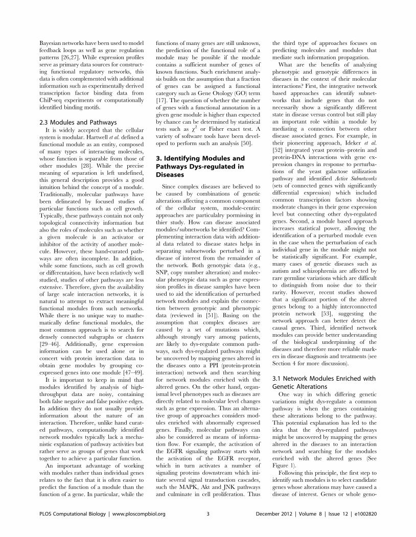
Bayesian networks have been used to model
feedback loops as well as gene regulation
patterns [26,27]. While expression profiles
serve as primary data sources for construct-
ing functional regulatory networks, this
data is often complemented with additional
information such as experimentally derived
transcription factor binding data from
ChiP-seq experiments or computationally
identified binding motifs.
2.3 Modules and PathwaysIt is widely accepted that the cellular
system is modular. Hartwell et al. defined a
functional module as an entity, composed
of many types of interacting molecules,
whose function is separable from those of
other modules [28]. While the precise
meaning of separation is left undefined,
this general description provides a good
intuition behind the concept of a module.
Traditionally, molecular pathways have
been delineated by focused studies of
particular functions such as cell growth.
Typically, these pathways contain not only
topological connectivity information but
also the roles of molecules such as whether
a given molecule is an activator or
inhibitor of the activity of another mole-
cule. However, these hand-curated path-
ways are often incomplete. In addition,
while some functions, such as cell growth
or differentaition, have been relatively well
studied, studies of other pathways are less
extensive. Therefore, given the availability
of large scale interaction networks, it is
natural to attempt to extract meaningful
functional modules from such networks.
While there is no unique way to mathe-
matically define functional modules, the
most common approach is to search for
densely connected subgraphs or clusters
[29–46]. Additionally, gene expression
information can be used alone or in
concert with protein interaction data to
obtain gene modules by grouping co-
expressed genes into one module [47–49].
It is important to keep in mind that
modules identified by analysis of high-
throughput data are noisy, containing
both false negative and false positive edges.
In addition they do not usually provide
information about the nature of an
interaction. Therefore, unlike hand curat-
ed pathways, computationally identified
network modules typically lack a mecha-
nistic explanation of pathway activities but
rather serve as groups of genes that work
together to achieve a particular function.
An important advantage of working
with modules rather than individual genes
relates to the fact that it is often easier to
predict the function of a module than the
function of a gene. In particular, while the
functions of many genes are still unknown,
the prediction of the functional role of a
module may be possible if the module
contains a sufficient number of genes of
known functions. Such enrichment analy-
sis builds on the assumption that a fraction
of genes can be assigned a functional
category such as Gene Otology (GO) term
[17]. The question of whether the number
of genes with a functional annotation in a
given gene module is higher than expected
by chance can be determined by statistical
tests such as x2 or Fisher exact test. A
variety of software tools have been devel-
oped to perform such an analysis [50].
3. Identifying Modules andPathways Dys-regulated inDiseases
Since complex diseases are believed to
be caused by combinations of genetic
alterations affecting a common component
of the cellular system, module-centirc
approaches are particulalry pormissing in
thier study. How can disease associated
modules/subnetworks be identified? Com-
plementing interaction data with addition-
al data related to disease states helps in
separating subnetworks perturbed in a
disease of interest from the remainder of
the network. Both genotypic data (e.g.,
SNP, copy number alteration) and molec-
ular phenotypic data such as gene expres-
sion profiles in disease samples have been
used to aid the identification of perturbed
network modules and explain the connec-
tion between genotypic and phenotypic
data (reviewed in [51]). Basing on the
assumption that complex diseases are
caused by a set of mutations which,
although strongly vary among patients,
are likely to dys-regulate common path-
ways, such dys-regulated pathways might
be uncovered by mapping genes altered in
the diseases onto a PPI (protein-protein
interaction) network and then searching
for network modules enriched with the
altered genes. On the other hand, organ-
ismal level phenotypes such as diseases are
directly related to molecular level changes
such as gene expression. Thus an alterna-
tive group of approaches considers mod-
ules enriched with abnormally expressed
genes. Finally, molecular pathways can
also be considered as means of informa-
tion flow. For example, the activation of
the EGFR signaling pathway starts with
the activation of the EGFR receptor,
which in turn activates a number of
signaling proteins downstream which ini-
tiate several signal transduction cascades,
such the MAPK, Akt and JNK pathways
and culminate in cell proliferation. Thus
the third type of approaches focuses on
predicting molecules and modules that
mediate such information propagation.
What are the benefits of analyzing
phenotypic and genotypic differences in
diseases in the context of their molecular
interactions? First, the integrative network
based approaches can identify subnet-
works that include genes that do not
necessarily show a significantly different
state in disease versus control but still play
an important role within a module by
mediating a connection between other
disease associated genes. For example, in
their pioneering approach, Ideker et al.
[52] integrated yeast protein–protein and
protein-DNA interactions with gene ex-
pression changes in response to perturba-
tions of the yeast galactose utilization
pathway and identified Active Subnetworks
(sets of connected genes with significantly
differential expression) which included
common transcription factors showing
moderate changes in their gene expression
level but connecting other dys-regulated
genes. Second, a module based approach
increases statistical power, allowing the
identification of a perturbed module even
in the case when the perturbation of each
individual gene in the module might not
be statistically significant. For example,
many cases of genetic diseases such as
autism and schizophrenia are affected by
rare germline variations which are difficult
to distinguish from noise due to their
rarity. However, recent studies showed
that a significant portion of the altered
genes belong to a highly interconnected
protein network [53], suggesting the
network approach can better detect the
causal genes. Third, identified network
modules can provide better understanding
of the biological underpinning of the
diseases and therefore more reliable mark-
ers in disease diagnosis and treatments (see
Section 4 for more discussion).
3.1 Network Modules Enriched withGenetic Alterations
One way in which differing genetic
variations might dys-regulate a common
pathway is when the genes containing
these alterations belong to the pathway.
This potential explanation has led to the
idea that the dys-regulated pathways
might be uncovered by mapping the genes
altered in the diseases to an interaction
network and searching for the modules
enriched with the altered genes (See
Figure 1).
Following this principle, the first step to
identify such modules is to select candidate
genes whose alterations may have caused a
disease of interest. Genes or whole geno-
PLOS Computational Biology | www.ploscompbiol.org 3 December 2012 | Volume 8 | Issue 12 | e1002820
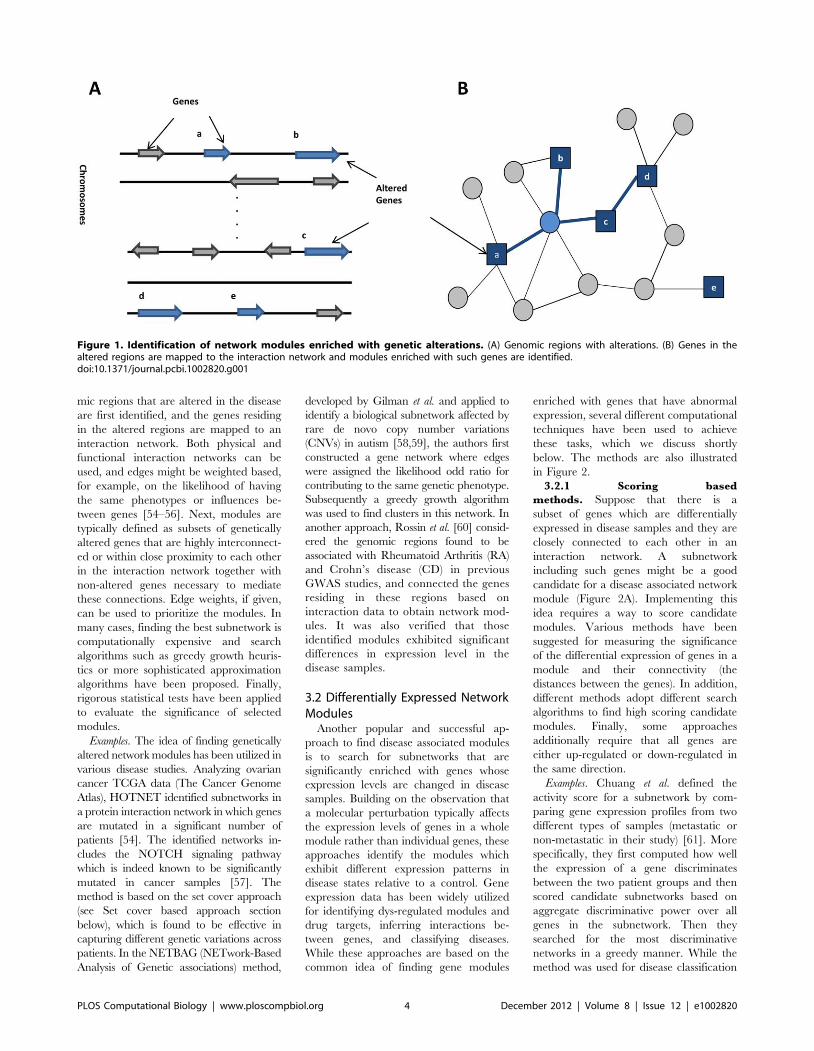
mic regions that are altered in the disease
are first identified, and the genes residing
in the altered regions are mapped to an
interaction network. Both physical and
functional interaction networks can be
used, and edges might be weighted based,
for example, on the likelihood of having
the same phenotypes or influences be-
tween genes [54–56]. Next, modules are
typically defined as subsets of genetically
altered genes that are highly interconnect-
ed or within close proximity to each other
in the interaction network together with
non-altered genes necessary to mediate
these connections. Edge weights, if given,
can be used to prioritize the modules. In
many cases, finding the best subnetwork is
computationally expensive and search
algorithms such as greedy growth heuris-
tics or more sophisticated approximation
algorithms have been proposed. Finally,
rigorous statistical tests have been applied
to evaluate the significance of selected
modules.
Examples. The idea of finding genetically
altered network modules has been utilized in
various disease studies. Analyzing ovarian
cancer TCGA data (The Cancer Genome
Atlas), HOTNET identified subnetworks in
a protein interaction network in which genes
are mutated in a significant number of
patients [54]. The identified networks in-
cludes the NOTCH signaling pathway
which is indeed known to be significantly
mutated in cancer samples [57]. The
method is based on the set cover approach
(see Set cover based approach section
below), which is found to be effective in
capturing different genetic variations across
patients. In the NETBAG (NETwork-Based
Analysis of Genetic associations) method,
developed by Gilman et al. and applied to
identify a biological subnetwork affected by
rare de novo copy number variations
(CNVs) in autism [58,59], the authors first
constructed a gene network where edges
were assigned the likelihood odd ratio for
contributing to the same genetic phenotype.
Subsequently a greedy growth algorithm
was used to find clusters in this network. In
another approach, Rossin et al. [60] consid-
ered the genomic regions found to be
associated with Rheumatoid Arthritis (RA)
and Crohn’s disease (CD) in previous
GWAS studies, and connected the genes
residing in these regions based on
interaction data to obtain network mod-
ules. It was also verified that those
identified modules exhibited significant
differences in expression level in the
disease samples.
3.2 Differentially Expressed NetworkModules
Another popular and successful ap-
proach to find disease associated modules
is to search for subnetworks that are
significantly enriched with genes whose
expression levels are changed in disease
samples. Building on the observation that
a molecular perturbation typically affects
the expression levels of genes in a whole
module rather than individual genes, these
approaches identify the modules which
exhibit different expression patterns in
disease states relative to a control. Gene
expression data has been widely utilized
for identifying dys-regulated modules and
drug targets, inferring interactions be-
tween genes, and classifying diseases.
While these approaches are based on the
common idea of finding gene modules
enriched with genes that have abnormal
expression, several different computational
techniques have been used to achieve
these tasks, which we discuss shortly
below. The methods are also illustrated
in Figure 2.
3.2.1 Scoring based
methods. Suppose that there is a
subset of genes which are differentially
expressed in disease samples and they are
closely connected to each other in an
interaction network. A subnetwork
including such genes might be a good
candidate for a disease associated network
module (Figure 2A). Implementing this
idea requires a way to score candidate
modules. Various methods have been
suggested for measuring the significance
of the differential expression of genes in a
module and their connectivity (the
distances between the genes). In addition,
different methods adopt different search
algorithms to find high scoring candidate
modules. Finally, some approaches
additionally require that all genes are
either up-regulated or down-regulated in
the same direction.
Examples. Chuang et al. defined the
activity score for a subnetwork by com-
paring gene expression profiles from two
different types of samples (metastatic or
non-metastatic in their study) [61]. More
specifically, they first computed how well
the expression of a gene discriminates
between the two patient groups and then
scored candidate subnetworks based on
aggregate discriminative power over all
genes in the subnetwork. Then they
searched for the most discriminative
networks in a greedy manner. While the
method was used for disease classification
Figure 1. Identification of network modules enriched with genetic alterations. (A) Genomic regions with alterations. (B) Genes in thealtered regions are mapped to the interaction network and modules enriched with such genes are identified.doi:10.1371/journal.pcbi.1002820.g001
PLOS Computational Biology | www.ploscompbiol.org 4 December 2012 | Volume 8 | Issue 12 | e1002820
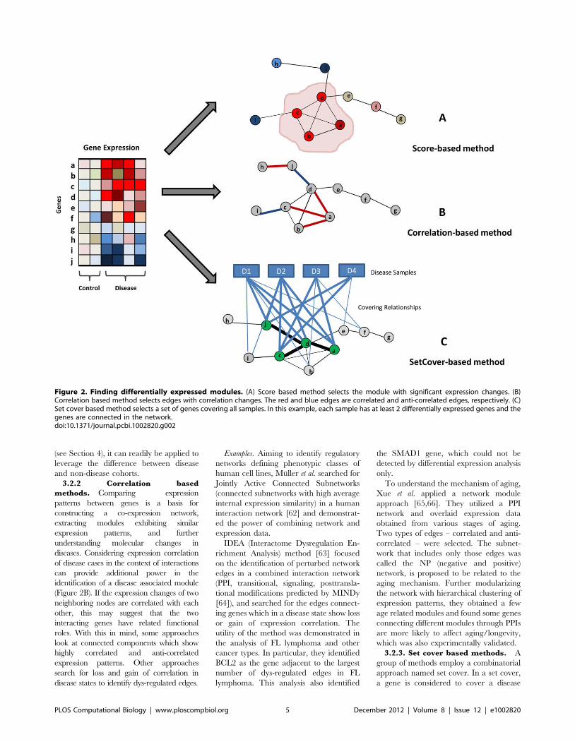
(see Section 4), it can readily be applied to
leverage the difference between disease
and non-disease cohorts.
3.2.2 Correlation based
methods. Comparing expression
patterns between genes is a basis for
constructing a co-expression network,
extracting modules exhibiting similar
expression patterns, and further
understanding molecular changes in
diseases. Considering expression correlation
of disease cases in the context of interactions
can provide additional power in the
identification of a disease associated module
(Figure 2B). If the expression changes of two
neighboring nodes are correlated with each
other, this may suggest that the two
interacting genes have related functional
roles. With this in mind, some approaches
look at connected components which show
highly correlated and anti-correlated
expression patterns. Other approaches
search for loss and gain of correlation in
disease states to identify dys-regulated edges.
Examples. Aiming to identify regulatory
networks defining phenotypic classes of
human cell lines, Muller et al. searched for
Jointly Active Connected Subnetworks
(connected subnetworks with high average
internal expression similarity) in a human
interaction network [62] and demonstrat-
ed the power of combining network and
expression data.
IDEA (Interactome Dysregulation En-
richment Analysis) method [63] focused
on the identification of perturbed network
edges in a combined interaction network
(PPI, transitional, signaling, posttransla-
tional modifications predicted by MINDy
[64]), and searched for the edges connect-
ing genes which in a disease state show loss
or gain of expression correlation. The
utility of the method was demonstrated in
the analysis of FL lymphoma and other
cancer types. In particular, they identified
BCL2 as the gene adjacent to the largest
number of dys-regulated edges in FL
lymphoma. This analysis also identified
the SMAD1 gene, which could not be
detected by differential expression analysis
only.
To understand the mechanism of aging,
Xue et al. applied a network module
approach [65,66]. They utilized a PPI
network and overlaid expression data
obtained from various stages of aging.
Two types of edges – correlated and anti-
correlated – were selected. The subnet-
work that includes only those edges was
called the NP (negative and positive)
network, is proposed to be related to the
aging mechanism. Further modularizing
the network with hierarchical clustering of
expression patterns, they obtained a few
age related modules and found some genes
connecting different modules through PPIs
are more likely to affect aging/longevity,
which was also experimentally validated.
3.2.3. Set cover based methods. A
group of methods employ a combinatorial
approach named set cover. In a set cover,
a gene is considered to cover a disease
Figure 2. Finding differentially expressed modules. (A) Score based method selects the module with significant expression changes. (B)Correlation based method selects edges with correlation changes. The red and blue edges are correlated and anti-correlated edges, respectively. (C)Set cover based method selects a set of genes covering all samples. In this example, each sample has at least 2 differentially expressed genes and thegenes are connected in the network.doi:10.1371/journal.pcbi.1002820.g002
PLOS Computational Biology | www.ploscompbiol.org 5 December 2012 | Volume 8 | Issue 12 | e1002820
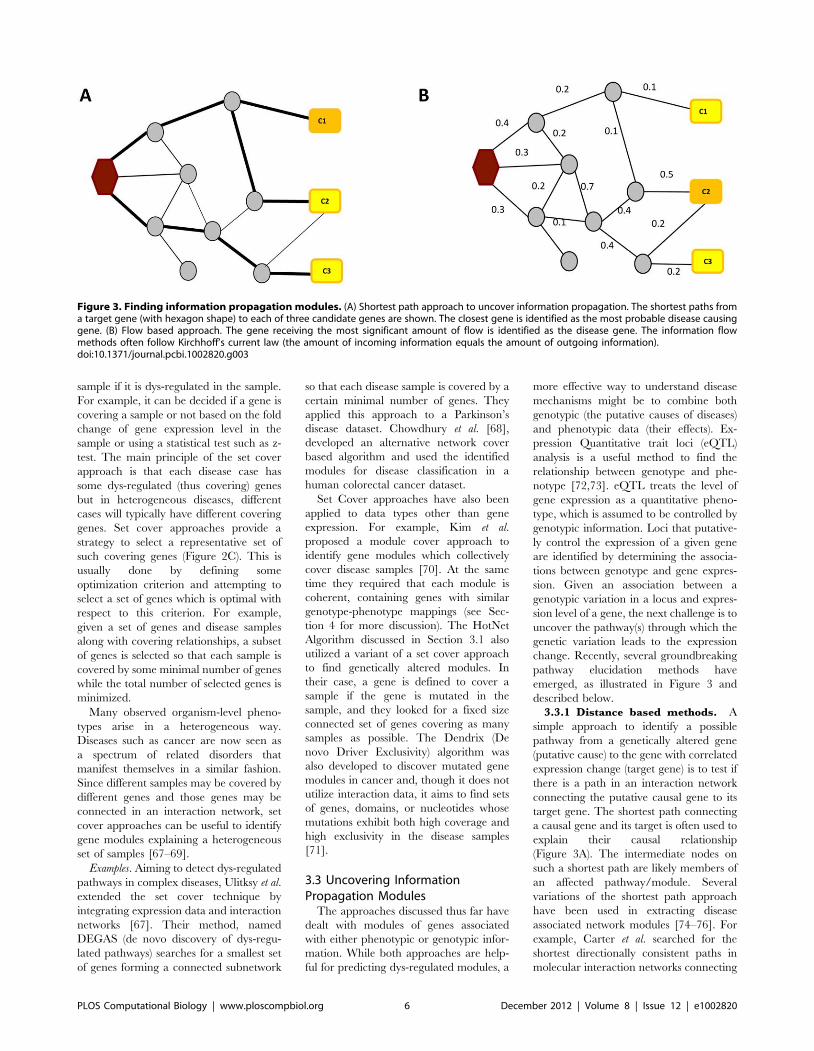
sample if it is dys-regulated in the sample.
For example, it can be decided if a gene is
covering a sample or not based on the fold
change of gene expression level in the
sample or using a statistical test such as z-
test. The main principle of the set cover
approach is that each disease case has
some dys-regulated (thus covering) genes
but in heterogeneous diseases, different
cases will typically have different covering
genes. Set cover approaches provide a
strategy to select a representative set of
such covering genes (Figure 2C). This is
usually done by defining some
optimization criterion and attempting to
select a set of genes which is optimal with
respect to this criterion. For example,
given a set of genes and disease samples
along with covering relationships, a subset
of genes is selected so that each sample is
covered by some minimal number of genes
while the total number of selected genes is
minimized.
Many observed organism-level pheno-
types arise in a heterogeneous way.
Diseases such as cancer are now seen as
a spectrum of related disorders that
manifest themselves in a similar fashion.
Since different samples may be covered by
different genes and those genes may be
connected in an interaction network, set
cover approaches can be useful to identify
gene modules explaining a heterogeneous
set of samples [67–69].
Examples. Aiming to detect dys-regulated
pathways in complex diseases, Ulitksy et al.
extended the set cover technique by
integrating expression data and interaction
networks [67]. Their method, named
DEGAS (de novo discovery of dys-regu-
lated pathways) searches for a smallest set
of genes forming a connected subnetwork
so that each disease sample is covered by a
certain minimal number of genes. They
applied this approach to a Parkinson’s
disease dataset. Chowdhury et al. [68],
developed an alternative network cover
based algorithm and used the identified
modules for disease classification in a
human colorectal cancer dataset.
Set Cover approaches have also been
applied to data types other than gene
expression. For example, Kim et al.
proposed a module cover approach to
identify gene modules which collectively
cover disease samples [70]. At the same
time they required that each module is
coherent, containing genes with similar
genotype-phenotype mappings (see Sec-
tion 4 for more discussion). The HotNet
Algorithm discussed in Section 3.1 also
utilized a variant of a set cover approach
to find genetically altered modules. In
their case, a gene is defined to cover a
sample if the gene is mutated in the
sample, and they looked for a fixed size
connected set of genes covering as many
samples as possible. The Dendrix (De
novo Driver Exclusivity) algorithm was
also developed to discover mutated gene
modules in cancer and, though it does not
utilize interaction data, it aims to find sets
of genes, domains, or nucleotides whose
mutations exhibit both high coverage and
high exclusivity in the disease samples
[71].
3.3 Uncovering InformationPropagation Modules
The approaches discussed thus far have
dealt with modules of genes associated
with either phenotypic or genotypic infor-
mation. While both approaches are help-
ful for predicting dys-regulated modules, a
more effective way to understand disease
mechanisms might be to combine both
genotypic (the putative causes of diseases)
and phenotypic data (their effects). Ex-
pression Quantitative trait loci (eQTL)
analysis is a useful method to find the
relationship between genotype and phe-
notype [72,73]. eQTL treats the level of
gene expression as a quantitative pheno-
type, which is assumed to be controlled by
genotypic information. Loci that putative-
ly control the expression of a given gene
are identified by determining the associa-
tions between genotype and gene expres-
sion. Given an association between a
genotypic variation in a locus and expres-
sion level of a gene, the next challenge is to
uncover the pathway(s) through which the
genetic variation leads to the expression
change. Recently, several groundbreaking
pathway elucidation methods have
emerged, as illustrated in Figure 3 and
described below.
3.3.1 Distance based methods. A
simple approach to identify a possible
pathway from a genetically altered gene
(putative cause) to the gene with correlated
expression change (target gene) is to test if
there is a path in an interaction network
connecting the putative causal gene to its
target gene. The shortest path connecting
a causal gene and its target is often used to
explain their causal relationship
(Figure 3A). The intermediate nodes on
such a shortest path are likely members of
an affected pathway/module. Several
variations of the shortest path approach
have been used in extracting disease
associated network modules [74–76]. For
example, Carter et al. searched for the
shortest directionally consistent paths in
molecular interaction networks connecting
Figure 3. Finding information propagation modules. (A) Shortest path approach to uncover information propagation. The shortest paths froma target gene (with hexagon shape) to each of three candidate genes are shown. The closest gene is identified as the most probable disease causinggene. (B) Flow based approach. The gene receiving the most significant amount of flow is identified as the disease gene. The information flowmethods often follow Kirchhoff’s current law (the amount of incoming information equals the amount of outgoing information).doi:10.1371/journal.pcbi.1002820.g003
PLOS Computational Biology | www.ploscompbiol.org 6 December 2012 | Volume 8 | Issue 12 | e1002820
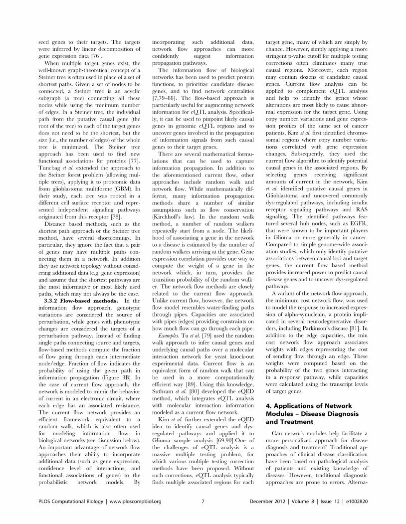
seed genes to their targets. The targets
were inferred by linear decomposition of
gene expression data [76].
When multiple target genes exist, the
well-known graph-theoretical concept of a
Steiner tree is often used in place of a set of
shortest paths. Given a set of nodes to be
connected, a Steiner tree is an acyclic
subgraph (a tree) connecting all these
nodes while using the minimum number
of edges. In a Steiner tree, the individual
path from the putative causal gene (the
root of the tree) to each of the target genes
does not need to be the shortest, but the
size (i.e., the number of edges) of the whole
tree is minimized. The Steiner tree
approach has been used to find new
functional associations for proteins [77].
Tuncbag et al. extended the approach to
the Steiner forest problem (allowing mul-
tiple trees), applying it to proteomic data
from glioblastoma multiforme (GBM). In
their study, each tree was rooted in a
different cell surface receptor and repre-
sented independent signaling pathways
originated from this receptor [78].
Distance based methods, such as the
shortest path approach or the Steiner tree
method, have several shortcomings. In
particular, they ignore the fact that a pair
of genes may have multiple paths con-
necting them in a network. In addition
they use network topology without consid-
ering additional data (e.g. gene expression)
and assume that the shortest pathways are
the most informative or most likely used
paths, which may not always be the case.
3.3.2 Flow-based methods. In the
information flow approach, genotypic
variations are considered the source of
perturbation, while genes with phenotypic
changes are considered the targets of a
perturbation pathway. Instead of finding
single paths connecting source and targets,
flow-based methods compute the fraction
of flow going through each intermediate
node/edge. Fraction of flow indicates the
probability of using the given path in
information propagation (Figure 3B). In
the case of current flow approach, the
network is modeled to mimic the behavior
of current in an electronic circuit, where
each edge has an associated resistance.
The current flow network provides an
efficient framework equivalent to a
random walk, which is also often used
for modeling information flow in
biological networks (see discussion below).
An important advantage of network flow
approaches their ability to incorporate
additional data (such as gene expression,
confidence level of interactions, and
functional associations of genes) to the
probabilistic network models. By
incorporating such additional data,
network flow approaches can more
confidently suggest information
propagation pathways.
The information flow of biological
networks has been used to predict protein
functions, to prioritize candidate disease
genes, and to find network centralities
[7,79–88]. The flow-based approach is
particularly useful for augmenting network
information for eQTL analysis. Specifical-
ly, it can be used to pinpoint likely causal
genes in genomic eQTL regions and to
uncover genes involved in the propagation
of information signals from such causal
genes to their target genes.
There are several mathematical formu-
lations that can be used to capture
information propagation. In addition to
the aforementioned current flow, other
approaches include random walk and
network flow. While mathematically dif-
ferent, many information propagation
methods share a number of similar
assumptions such as flow conservation
(Kirchhoff’s law). In the random walk
method, a number of random walkers
repeatedly start from a node. The likeli-
hood of associating a gene in the network
to a disease is estimated by the number of
random walkers arriving at the gene. Gene
expression correlation provides one way to
compute the weight of a gene in the
network which, in turn, provides the
transition probability of the random walk-
er. The network flow methods are closely
related to the current flow approach.
Unlike current flow, however, the network
flow model resembles water-finding paths
through pipes. Capacities are associated
with pipes (edges) providing constraints on
how much flow can go through each pipe.
Examples. Tu et al. [79] used the random
walk approach to infer causal genes and
underlying causal paths over a molecular
interaction network for yeast knock-out
experimental data. Current flow is an
equivalent form of random walk that can
be used in a more computationally
efficient way [89]. Using this knowledge,
Suthram et al. [80] developed the eQED
method, which integrates eQTL analysis
with molecular interaction information
modeled as a current flow network.
Kim et al. further extended the eQED
idea to identify causal genes and dys-
regulated pathways and applied it to
Glioma sample analysis [69,90].One of
the challenges of eQTL analysis is a
massive multiple testing problem, for
which various multiple testing correction
methods have been proposed. Without
such corrections, eQTL analysis typically
finds multiple associated regions for each
target gene, many of which are simply by
chance. However, simply applying a more
stringent p-value cutoff for multiple testing
corrections often eliminates many true
causal regions. Moreover, each region
may contain dozens of candidate causal
genes. Current flow analysis can be
applied to complement eQTL analysis
and help to identify the genes whose
alterations are most likely to cause abnor-
mal expression for the target gene. Using
copy number variations and gene expres-
sion profiles of the same set of cancer
patients, Kim et al. first identified chromo-
somal regions where copy number varia-
tions correlated with gene expression
changes. Subsequently, they used the
current flow algorithm to identify potential
causal genes in the associated regions. By
selecting genes receiving significant
amounts of current in the network, Kim
et al. identified putative causal genes in
Glioblastoma and uncovered commonly
dys-regulated pathways, including insulin
receptor signaling pathways and RAS
signaling. The identified pathways fea-
tured several hub nodes, such as EGFR,
that were known to be important players
in Glioma or more generally in cancer.
Compared to simple genome-wide associ-
ation studies, which only identify putative
associations between causal loci and target
genes, the current flow based method
provides increased power to predict causal
disease genes and to uncover dys-regulated
pathways.
A variant of the network flow approach,
the minimum cost network flow, was used
to model the response to increased expres-
sion of alpha-synucleain, a protein impli-
cated in several neurodegenerative disor-
ders, including Parkinson’s disease [81]. In
addition to the edge capacities, the min
cost network flow approach associates
weights with edges representing the cost
of sending flow through an edge. These
weights were computed based on the
probability of the two genes interacting
in a response pathway, while capacities
were calculated using the transcript levels
of target genes.
4. Applications of NetworkModules – Disease Diagnosisand Treatment
Can network modules help facilitate a
more personalized approach for disease
diagnosis and treatment? Traditional ap-
proaches of clinical disease classification
have been based on pathological analysis
of patients and existing knowledge of
diseases. However, traditional diagnostic
approaches are prone to errors. Alterna-
PLOS Computational Biology | www.ploscompbiol.org 7 December 2012 | Volume 8 | Issue 12 | e1002820
tively, knowledge about dys-regulated
pathways can be used to subtype diseases
and to develop relevant treatments for
individual disease subgroups. For example,
network modules have been used to
predict patient survival, metastasis, drug
responses for various types of cancer
[61,68,91–94].
4.1 Disease ClassificationA supervised approach to disease
classification starts with a set of samples
with a known partition into disease
subtypes (e.g., metastatic or not) and
attempts to identify a classifying principle
using specific molecular features. The
general strategy for supervised disease
classification is to search for subnetworks,
also called subnetwork markers, whose
activities best discriminate the two disease
subtypes. As in the case of single-gene
disease markers, a network marker will
distinguish some but not all disease cases
and multiple subnetworks might be nec-
essary. Among selected candidate network
markers, the best markers are selected
based on a set of training samples. Some
methods take an unsupervised approach,
where subclasses and their features are
discovered without using a known train-
ing set.
Examples. Chuang et al. showed how dys-
regulated network modules (described in
Section 3.2) provide more robust and
accurate predictions than those by single
gene based classifications when applied to
breast cancer metastasis analysis [61].
Chuang et al.’s work provided the proof
of principle for using network modules in
disease classification. A number of subse-
quent extensions and improvements to
Chuang et al.’s work were suggested. For
example, Lee et al. incorporated curated
pathways, and searched for a subset of
genes with discriminative features for the
disease phenotype [94]. More recently,
Dao et al. developed alternative network
based approaches for classification of
cancer subtypes by identifying densely
connected subnetwork and randomized
algorithms [92,93]. Other techniques for
best marker identification, such as set
cover and bottom-up enumeration tech-
niques, were also proposed [68,91].
Kim et al. identified gene modules using
a module cover approach to capture
disease heterogeneity in brain cancer
samples from Rembrandt and Ovarian
Cancer samples from TCGA [70]. Next,
Kim et al. superimposed the selected
modules onto the results from an inde-
pendently proposed classification scheme
[57]. As a result, Kim et al. uncovered
which disease classes are characterized by
which combinations of modules.
4.2 Disease SimilarityNetwork modules can also be used to
explain disease similarity. Overlaps of
dys-regulated network modules explain
why some complex diseases share sim-
ilar phenotypic traits. Suthram et al.
used a variant of PathBlast [95] to
identify dense subnetworks. Analysis of
disease similarity was achieved by com-
paring expression patterns of various
diseases in the modules [96]. Several
dys-regulated modules were found to be
common to many diseases, which ex-
plains why some drugs can treat many
different diseases.
4.3 Response to TreatmentModules may help determine whether
a given patient will respond to a partic-
ular drug, which is valuable for treatment
design. In addition, understanding molec-
ular differences between responders and
non-responders is likely to help develop-
ment of alternative treatments. For ex-
ample, Chu and Chen used a network
approach to discover apoptosis drug
targets [97]. Chu and Chen constructed
a PPI network for apoptosis in normal
cells and applied a nonlinear stochastic
model to remove false positive interac-
tions using microarray data. Comparing
the resulting subnetworks helped to shed
some light on the mechanisms leading to
apoptosis and to identify potential drug
targets.
5. Summary
Network biology provides powerful
tools for the study of complex diseases.
Network-based approaches leverage the
idea that complex diseases can be better
understood from the perspective of dys-
regulated modules than at the individual
gene level. Modularity is a widely
accepted concept in molecular networks
and module-based approaches provide a
number of advantages including robust-
ness in the identification of dys-regulated
pathways and improved disease classifi-
cation.
In addition, network based formulations
allow using a wealth of methods already
developed in graph theory, such as
shortest paths, network flow, and Steiner
trees. Network-based methods have sever-
al limitations including the lack of mech-
anistic explanations. Despite the limita-
tions, network analysis has been applied
successfully in many disease studies, sug-
gesting testable hypotheses.
6. Exercises
1. Construct coexpression networks fol-
lowing the steps below [98].
a. Download the three expression data-
sets from the following page: http://
www.geneticsofgeneexpression.org/
network/download
b. Compute 3 population-specific corre-
lations for each pair of 4238 genes
with the expression data. (Hint: There
are 8,978,203 pairs of genes.)
c. For gene pairs which have similar
correlations in the 3 datasets, calculate
the weighted average correlation,
weighted by the number of individuals
in each population. Hint: In the
Supplemental Table 1 published with
[98] (http://genome.cshlp.org/content/
suppl/2009/10/02/gr.097600.109.
DC1/nayak_supplemental_material.
pdf), you can find the list of gene
pairs whose correlations differ signif-
icantly among the 3 datasets.
d. Construct the correlation network by
connecting gene pairs whose weighted
average correlations are greater than
a pre-defined threshold (e.g., 0.5).
e. Compute specific parameters describ-
ing the network topology. (Hint: You
can use the NetworkAnalyzer Cytos-
cape plugin http://med.bioinf.mpi-
inf.mpg.de/netanalyzer/)
f. For different correlation thresholds,
compare the networks in terms of
topological properties.
2. Suppose that in a co-expression net-
work two genes are identified to have
correlated expression patterns. Provide
at least two possible biological expla-
nations of this correlation.
3. Some variants of information flow
approaches that identify pathways of
information flow from a mutated gene
to a target gene with correlated ex-
pression require that the last but one
node gene on such a pathway (the node
preceding the target gene) to be a
transcription factor. What is a justifi-
cation for such requirement? What can
be advantages and disadvantages of
such a design?
4. Consider a set cover approach to find a
representative set of genes dys-regulat-
ed in a given set of cancer patients. The
algorithm finds the smallest number of
genes so that each disease case is
covered at least k times. How does
the number of selected genes depend
on k? If you suspect that data for 5%
PLOS Computational Biology | www.ploscompbiol.org 8 December 2012 | Volume 8 | Issue 12 | e1002820
patients might be incorrect, how would
you modify the optimization problem?
5. A Steiner tree connecting a set of nodes
does not need to be unique. In the
graph shown in Figure 4, find two
different Steiner trees connecting genes
C, T1, T2, T3, and T4.
6. In the graph shown in Figure 4, find
the shortest paths connecting C with
each of T1, T2, T3, and T4. Do the
edges used by these paths correspond
to a Steiner tree? Explain why or why
not.
Answers to the exercises are provided in
Text S1.
Supporting Information
Text S1 Answers to Exercises.
(PDF)
Acknowledgments
The authors thank Mileidy W. Gonzalez
(NIH\NLM\NCBI) and Pawel Przytycki
(Princeton University) for their helpful com-
ments on the manuscript.
References
1. Veenstra-Vanderweele J, Christian SL, Cook EH,
Jr. (2004) Autism as a paradigmatic complex
genetic disorder. Annu Rev Genomics Hum
Genet 5: 379–405.
2. Pinto D, Pagnamenta AT, Klei L, Anney R,
Merico D, et al. (2010) Functional impact of
global rare copy number variation in autism
spectrum disorders. Nature 466: 368–372.
3. Schadt EE (2009) Molecular networks as sensors
and drivers of common human diseases. Nature
461: 218–223.
4. Gursoy A, Keskin O, Nussinov R (2008) Topo-
logical properties of protein interaction networks
from a structural perspective. Biochem Soc Trans
36: 1398–1403.
5. Albert R (2005) Scale-free networks in cell
biology. J Cell Sci 118: 4947–4957.
6. Jeong H, Mason SP, Barabasi AL, Oltvai ZN
(2001) Lethality and centrality in protein net-
works. Nature 411: 41–42.
7. Zotenko E, Mestre J, O’Leary DP, Przytycka TM
(2008) Why do hubs in the yeast protein
interaction network tend to be essential: reexam-
ining the connection between the network
topology and essentiality. PLoS Comput Biol 4:
e1000140. doi:10.1371/journal.pcbi.1000140
8. Jonsson PF, Bates PA (2006) Global topological
features of cancer proteins in the human inter-
actome. Bioinformatics 22: 2291–2297.
9. Wachi S, Yoneda K, Wu R (2005) Interactome-
transcriptome analysis reveals the high centrality
of genes differentially expressed in lung cancer
tissues. Bioinformatics 21: 4205–4208.
10. De Las Rivas J, Fontanillo C (2010) Protein-protein
interactions essentials: key concepts to building and
analyzing interactome networks. PLoS Comput Biol
6: e1000807. doi:10.1371/journal.pcbi.1000807
11. Berggard T, Linse S, James P (2007) Methods for
the detection and analysis of protein-protein
interactions. Proteomics 7: 2833–2842.
12. Yu H, Braun P, Yildirim MA, Lemmens I,
Venkatesan K, et al. (2008) High-quality binary
protein interaction map of the yeast interactome
network. Science 322: 104–110.
13. Shoemaker BA, Panchenko AR (2007) Decipher-
ing protein-protein interactions. Part II. Compu-
tational methods to predict protein and domain
interaction partners. PLoS Comput Biol 3: e43.
doi:10.1371/journal.pcbi.0030043
14. Levy ED, Landry CR, Michnick SW (2009) How
perfect can protein interactomes be? Sci Signal 2:
pe11.
15. Eisen MB, Spellman PT, Brown PO, Botstein D
(1998) Cluster analysis and display of genome-
wide expression patterns. Proc Natl Acad Sci U S A
95: 14863–14868.
16. (2010) The Gene Ontology in 2010: extensions
and refinements. Nucleic Acids Res 38: D331–335.
17. Ashburner M, Ball CA, Blake JA, Botstein D,
Butler H, et al. (2000) Gene ontology: tool for the
unification of biology. The Gene Ontology
Consortium. Nat Genet 25: 25–29.
18. Lee I, Date SV, Adai AT, Marcotte EM (2004) A
probabilistic functional network of yeast genes.
Science 306: 1555–1558.
19. Costello JC, Dalkilic MM, Beason SM, Gehlhau-
sen JR, Patwardhan R, et al. (2009) Gene
networks in Drosophila melanogaster: integrating
experimental data to predict gene function.
Genome Biol 10: R97.
20. Guan Y, Myers CL, Lu R, Lemischka IR, Bult
CJ, et al. (2008) A genomewide functional
network for the laboratory mouse. PLoS Comput
Biol 4: e1000165. doi:10.1371/journal.-
pcbi.1000165
21. Ramani AK, Li Z, Hart GT, Carlson MW, Boutz
DR, et al. (2008) A map of human protein
interactions derived from co-expression of human
mRNAs and their orthologs. Mol Syst Biol 4: 180.
22. Margolin AA, Nemenman I, Basso K, Wiggins C,
Stolovitzky G, et al. (2006) ARACNE: an
algorithm for the reconstruction of gene regula-
tory networks in a mammalian cellular context.
BMC Bioinformatics 7 Suppl 1: S7.
23. Peng J, Wang P, Zhou N, Zhu J (2009) Partial
Correlation Estimation by Joint Sparse Regres-
sion Models. J Am Stat Assoc 104: 735–746.
Figure 4. A hypothetical interaction network to be used with Exercises 5 and 6.doi:10.1371/journal.pcbi.1002820.g004
Further Reading
N Schadt EE (2009) Molecular networks as sensors and drivers of common human diseases. Nature 461(7261): 218–223.
N Barabasi AL, Gulbahce N, Loscalzo J (2011) Network medicine: a network-based approach to human disease. Nat Rev Genet12(1): 56–68.
N Przytycka TM, Singh M, Slonim DK (2010) Toward the dynamic interactome: it’s about time. Brief Bioinform 11(1): 15–29.
N Przytycka TM, Cho DY (2012) Interactome. In: Meyers RA, editor. Encyclopedia of molecular cell biology and molecularmedicine. John Wiley and Sons, Inc. doi:10.1002/3527600906.mcb.201100018
N Califano A, Butte AJ, Friend S, Ideker T, Schadt E (2012) Leveraging models of cell regulation and GWAS data in integrativenetwork-based association studies. Nat Genet 44(8): 841–847. doi:10.1038/ng.2355
N Vidal M, Cusick ME, Barabasi AL (2011) Interactome networks and human disease. Cell 144(6): 986–998.
N Kim Y, Przytycka TM (2012) Bridging the gap between genotype and phenotype via network approaches. Frontiers in Geneticsspecial issue on mapping complex disease traits with global gene expression. Front Genet 3: 227. doi:10.3389/fgene.2012.00227
PLOS Computational Biology | www.ploscompbiol.org 9 December 2012 | Volume 8 | Issue 12 | e1002820
24. Pe’er D (2005) Bayesian network analysis of
signaling networks: a primer. Sci STKE 2005:pl4.
25. Alterovitz G, Liu J, Afkhami E, Ramoni MF(2007) Bayesian methods for proteomics. Proteo-
mics 7: 2843–2855.
26. Xuan NV, Chetty M, Coppel R, Wangikar PP
(2012) Gene regulatory network modeling viaglobal optimization of high-order dynamic Bayes-
ian network. BMC Bioinformatics 13: 131.
27. Zou M, Conzen SD (2005) A new dynamic
Bayesian network (DBN) approach for identifyinggene regulatory networks from time course
microarray data. Bioinformatics 21: 71–79.
28. Hartwell LH, Hopfield JJ, Leibler S, Murray AW
(1999) From molecular to modular cell biology.Nature 402: C47–52.
29. Adamcsek B, Palla G, Farkas IJ, Derenyi I, VicsekT (2006) CFinder: locating cliques and overlap-
ping modules in biological networks. Bioinfor-matics 22: 1021–1023.
30. Altaf-Ul-Amin M, Shinbo Y, Mihara K, Kur-okawa K, Kanaya S (2006) Development and
implementation of an algorithm for detection of
protein complexes in large interaction networks.BMC Bioinformatics 7: 207.
31. Arnau V, Mars S, Marın I (2005) Iterative Cluster
Analysis of Protein Interaction Data. Bioinfor-
matics 21: 364–378.
32. Asthana S, King OD, Gibbons FD, Roth FP
(2004) Predicting protein complex membershipusing probabilistic network reliability. Genome
Res 14: 1170–1175.
33. Bader GD, Hogue CW (2003) An automated
method for finding molecular complexes in largeprotein interaction networks. BMC Bioinfor-
matics 4: 2.
34. Bader JS (2003) Greedily building protein net-
works with confidence. Bioinformatics 19: 1869–1874.
35. Brun C, Chevenet F, Martin D, Wojcik J,Guenoche A, et al. (2003) Functional classifica-
tion of proteins for the prediction of cellularfunction from a protein-protein interaction net-
work. Genome Biol 5: R6.
36. Dunn R, Dudbridge F, Sanderson CM (2005)
The use of edge-betweenness clustering toinvestigate biological function in protein interac-
tion networks. BMC Bioinformatics 6: 39.
37. Jiang P, Singh M (2010) SPICi: a fast clustering
algorithm for large biological networks. Bioinfor-matics 26: 1105–1111.
38. King AD, Przulj N, Jurisica I (2004) Proteincomplex prediction via cost-based clustering.
Bioinformatics 20: 3013–3020.
39. Luo F, Yang Y, Chen CF, Chang R, Zhou J, et al.
(2007) Modular organization of protein interac-tion networks. Bioinformatics 23: 207–214.
40. Navlakha S, Schatz MC, Kingsford C (2009)Revealing biological modules via graph summa-
rization. J Comput Biol 16: 253–264.
41. Newman ME (2006) Modularity and community
structure in networks. Proc Natl Acad Sci U S A103: 8577–8582.
42. Pereira-Leal JB, Enright AJ, Ouzounis CA (2004)Detection of functional modules from protein
interaction networks. Proteins 54: 49–57.
43. Qi Y, Balem F, Faloutsos C, Klein-Seetharaman
J, Bar-Joseph Z (2008) Protein complex identifi-cation by supervised graph local clustering.
Bioinformatics 24: i250–258.
44. Rives AW, Galitski T (2003) Modular organiza-
tion of cellular networks. Proc Natl Acad Sci U S A100: 1128–1133.
45. Spirin V, Mirny LA (2003) Protein complexes andfunctional modules in molecular networks. Proc
Natl Acad Sci U S A 100: 12123–12128.
46. Wang C, Ding C, Yang Q, Holbrook SR (2007)
Consistent dissection of the protein interactionnetwork by combining global and local metrics.
Genome Biol 8: R271.
47. Chen J, Yuan B (2006) Detecting functional
modules in the yeast protein-protein interactionnetwork. Bioinformatics 22: 2283–2290.
48. Feng J, Jiang R, Jiang T (2011) A max-flow based
approach to the identification of protein com-
plexes using protein interaction and microarraydata. IEEE/ACM Trans Comput Biol Bioinform
8: 621–634.
49. Maraziotis IA, Dimitrakopoulou K, Bezerianos A
(2007) Growing functional modules from a seedprotein via integration of protein interaction and
gene expression data. BMC Bioinformatics 8: 408.
50. Tipney H, Hunter L (2010) An introduction toeffective use of enrichment analysis software.
Hum Genomics 4: 202–206.
51. Kim Y, Przytycka T (2012) Bridging the gap
between genotype and phenotype via networkapproaches. Frontiers in Genetics special issue on
mapping complex disease traits with global geneexpression. Front Genet 3: 227. doi:10.3389/
fgene.2012.00227
52. Ideker T, Ozier O, Schwikowski B, Siegel AF
(2002) Discovering regulatory and signallingcircuits in molecular interaction networks. Bioin-
formatics 18 Suppl 1: S233–240.
53. O’Roak BJ, Vives L, Girirajan S, Karakoc E,Krumm N, et al. (2012) Sporadic autism exomes
reveal a highly interconnected protein network of
de novo mutations. Nature 485: 246–250.
54. Vandin F, Upfal E, Raphael BJ (2011) Algorithmsfor detecting significantly mutated pathways in
cancer. J Comput Biol 18: 507–522.
55. Rossin EJ, Lage K, Raychaudhuri S, Xavier RJ,
Tatar D, et al. Proteins encoded in genomicregions associated with immune-mediated disease
physically interact and suggest underlying biolo-gy. PLoS Genet 7: e1001273.
56. Gilman SR, Iossifov I, Levy D, Ronemus M,
Wigler M, et al. Rare de novo variants associated
with autism implicate a large functional networkof genes involved in formation and function of
synapses. Neuron 70: 898–907.
57. The Cancer Genome Atlas Research Network(2011) Integrated genomic analyses of ovarian
carcinoma. Nature 474: 609–615.
58. Gilman SR, Iossifov I, Levy D, Ronemus M,
Wigler M, et al. (2011) Rare de novo variantsassociated with autism implicate a large function-
al network of genes involved in formation andfunction of synapses. Neuron 70: 898–907.
59. Levy D, Ronemus M, Yamrom B, Lee YH,
Leotta A, et al. (2011) Rare de novo and
transmitted copy-number variation in autisticspectrum disorders. Neuron 70: 886–897.
60. Rossin EJ, Lage K, Raychaudhuri S, Xavier RJ,
Tatar D, et al. (2011) Proteins encoded in
genomic regions associated with immune-mediat-ed disease physically interact and suggest under-
lying biology. PLoS Genet 7: e1001273.doi:10.1371/journal.pgen.1001273
61. Chuang HY, Lee E, Liu YT, Lee D, Ideker T
(2007) Network-based classification of breast
cancer metastasis. Mol Syst Biol 3: 140.
62. Muller FJ, Laurent LC, Kostka D, Ulitsky I,Williams R, et al. (2008) Regulatory networks
define phenotypic classes of human stem cell lines.Nature 455: 401–405.
63. Mani KM, Lefebvre C, Wang K, Lim WK, Basso
K, et al. (2008) A systems biology approach to
prediction of oncogenes and molecular perturbationtargets in B-cell lymphomas. Mol Syst Biol 4: 169.
64. Wang K NI, Banerjee N, Margolin AA, Califano A.
Genome-wide Discovery of Modulators of Tran-scriptional Interactions in Human B Lymphocytes;
2006; Venice. pp. 348–362.
65. Xue H, Xian B, Dong D, Xia K, Zhu S, et al.
(2007) A modular network model of aging. MolSyst Biol 3: 147.
66. Xia K, Xue H, Dong D, Zhu S, Wang J, et al.
(2006) Identification of the proliferation/differen-
tiation switch in the cellular network of multicel-lular organisms. PLoS Comput Biol 2: e145.
doi:10.1371/journal.pcbi.0020145
67. Ulitsky I, Krishnamurthy A, Karp RM, Shamir R(2010) DEGAS: de novo discovery of dysregulat-
ed pathways in human diseases. PLoS ONE 5:
e13367. doi:10.1371/journal.pone.0013367
68. Chowdhury SA, Koyuturk M (2010) Identification
of coordinately dysregulated subnetworks in com-
plex phenotypes. Pac Symp Biocomput: 133–144.
69. Kim YA, Wuchty S, Przytycka TM (2011)
Identifying causal genes and dysregulated path-
ways in complex diseases. PLoS Comput Biol 7:
e1001095. doi:10.1371/journal.pcbi.1001095
70. Kim Y, Salari R, Wuchty S, Przytycka TM (2013)
Module Cover – a new approach to genotype-
phenotype studies; Pacyfic Synposium on Bio-
computing 18: 103–110.
71. Vandin F, Upfal E, Raphael BJ (2012) De novo
discovery of mutated driver pathways in cancer.
Genome Res 22: 375–385.
72. Stranger BE, Forrest MS, Clark AG, Minichiello
MJ, Deutsch S, et al. (2005) Genome-wide
associations of gene expression variation in hu-
mans. PLoS Genet 1: e78. doi:10.1371/journal.
pgen.0010078
73. Stranger BE, Nica AC, Forrest MS, Dimas A, Bird
CP, et al. (2007) Population genomics of human
gene expression. Nat Genet 39: 1217–1224.
74. Managbanag JR, Witten TM, Bonchev D, Fox LA,
Tsuchiya M, et al. (2008) Shortest-path network
analysis is a useful approach toward identifying
genetic determinants of longevity. PLoS ONE 3:
e3802. doi:10.1371/journal.pone.0003802
75. Shih YK, Parthasarathy S (2012) A single source k-
shortest paths algorithm to infer regulatory path-
ways in a gene network. Bioinformatics 28: i49–58.
76. Carter GW, Prinz S, Neou C, Shelby JP, Marzolf
B, et al. (2007) Prediction of phenotype and gene
expression for combinations of mutations. Mol
Syst Biol 3: 96.
77. Bailly-Bechet M, Borgs C, Braunstein A, Chayes
J, Dagkessamanskaia A, et al. (2011) Finding
undetected protein associations in cell signaling
by belief propagation. Proc Natl Acad Sci U S A
108: 882–887.
78. Tuncbag N, McCallum S, Huang SS, Fraenkel E
(2012) SteinerNet: a web server for integrating ‘omic’
data to discover hidden components of response
pathways. Nucleic Acids Res 40: W505–509.
79. Tu Z, Wang L, Arbeitman MN, Chen T, Sun F
(2006) An integrative approach for causal gene
identification and gene regulatory pathway infer-
ence. Bioinformatics 22: e489–496.
80. Suthram S, Beyer A, Karp RM, Eldar Y, Ideker
T (2008) eQED: an efficient method for inter-
preting eQTL associations using protein net-
works. Mol Syst Biol 4: 162.
81. Yeger-Lotem E, Riva L, Su LJ, Gitler AD,
Cashikar AG, et al. (2009) Bridging high-
throughput genetic and transcriptional data
reveals cellular responses to alpha-synuclein
toxicity. Nat Genet 41: 316–323.
82. Lee E, Jung H, Radivojac P, Kim JW, Lee D
(2009) Analysis of AML genes in dysregulated
molecular networks. BMC Bioinformatics 10
Suppl 9: S2.
83. Kohler S, Bauer S, Horn D, Robinson PN (2008)
Walking the interactome for prioritization of
candidate disease genes. Am J Hum Genet 82:
949–958.
84. Missiuro PV, Liu K, Zou L, Ross BC, Zhao G, et
al. (2009) Information flow analysis of interac-
tome networks. PLoS Comput Biol 5: e1000350.
doi:10.1371/journal.pcbi.1000350
85. Nabieva E, Jim K, Agarwal A, Chazelle B, Singh
M (2005) Whole-proteome prediction of protein
function via graph-theoretic analysis of interac-
tion maps. Bioinformatics 21 Suppl 1: i302–310.
86. Newman M (2005) A measure of betweenness
centrality based on random walks. Social Net-
works 27: 39–54.
87. Stojmirovic A, Yu YK (2007) Information flow in
interaction networks. J Comput Biol 14: 1115–1143.
88. Vanunu O, Magger O, Ruppin E, Shlomi T, Sharan
R (2010) Associating genes and protein complexes
with disease via network propagation. PLoS Comput
Biol 6: e1000641. doi:10.1371/journal.pcbi.1000641
89. Doyle PG SJ (1984) Random walks and electric
networks
PLOS Computational Biology | www.ploscompbiol.org 10 December 2012 | Volume 8 | Issue 12 | e1002820
90. Kim YA, Przytycki JH, Wuchty S, Przytycka TM
(2011) Modeling information flow in biologicalnetworks. Phys Biol 8: 035012.
91. Chowdhury SA, Nibbe RK, Chance MR,
Koyuturk M (2011) Subnetwork state functionsdefine dysregulated subnetworks in cancer.
J Comput Biol 18: 263–281.92. Dao P, Colak R, Salari R, Moser F, Davicioni E,
et al. (2010) Inferring cancer subnetwork markers
using density-constrained biclustering. Bioinfor-matics 26: i625–631.
93. Dao P, Wang K, Collins C, Ester M, Lapuk A, etal. (2011) Optimally discriminative subnetwork
markers predict response to chemotherapy.
Bioinformatics 27: i205–213.94. Lee E, Chuang HY, Kim JW, Ideker T, Lee D
(2008) Inferring pathway activity toward precise
disease classification. PLoS Comput Biol 4:e1000217. doi: 10.1371/journal.pcbi.1000217
95. Kelley BP, Sharan R, Karp RM, Sittler T, RootDE, et al. (2003) Conserved pathways within
bacteria and yeast as revealed by global protein
network alignment. Proc Natl Acad Sci U S A100: 11394–11399.
96. Suthram S, Dudley JT, Chiang AP, Chen R,Hastie TJ, et al. (2010) Network-based elucidation
of human disease similarities reveals common
functional modules enriched for pluripotent drugtargets. PLoS Comput Biol 6: e1000662.
doi:10.1371/journal.pcbi.1000662
97. Chu LH, Chen BS (2008) Construction of acancer-perturbed protein-protein interaction net-
work for discovery of apoptosis drug targets.BMC Syst Biol 2: 56.
98. Nayak RR, Kearns M, Spielman RS, Cheung
VG (2009) Coexpression network based onnatural variation in human gene expression
reveals gene interactions and functions. GenomeRes 19: 1953–1962.
PLOS Computational Biology | www.ploscompbiol.org 11 December 2012 | Volume 8 | Issue 12 | e1002820
Education
Chapter 6: Structural Variation and Medical GenomicsBenjamin J. Raphael*
Department of Computer Science and Center for Computational Molecular Biology, Brown University, Providence, Rhode Island, United States of America
Abstract: Differences between in-dividual human genomes, or be-tween human and cancer genomes,range in scale from single nucleotidevariants (SNVs) through intermediateand large-scale duplications, dele-tions, and rearrangements of geno-mic segments. The latter class, calledstructural variants (SVs), have re-ceived considerable attention in thepast several years as they are apreviously under appreciated sourceof variation in human genomes.Much of this recent attention is theresult of the availability of higher-resolution technologies for measur-ing these variants, including bothmicroarray-based techniques, andmore recently, high-throughputDNA sequencing. We describe thegenomic technologies and computa-tional techniques currently used tomeasure SVs, focusing on applica-tions in human and cancer genomics.
This article is part of the ‘‘Transla-
tional Bioinformatics’’ collection for
PLOS Computational Biology.
1. Introduction
The decade since the assembly of the
human genome has witnessed dramatic
advances in understanding the genetic
differences that distinguish individual hu-
mans and that are responsible for specific
traits. Genome-wide association studies
(GWAS) in humans have identified com-
mon germline, or inherited, DNA variants
that are associated with various common
human diseases, including diabetes, heart
disease, etc. At the same time, cancer
genome sequencing studies have cataloged
numerous somatic mutations that arise
during the lifetime of an individual and
that drive cancer progression. These
successes are ushering in the era of
personalized medicine, where treatment
for a disease is tailored to the genetic
characteristics of the individual.
Despite this progress, significant hurdles
remain in achieving a comprehensive
understanding of the genetic basis of
human traits and disease. The germline
variants discovered by GWAS thus far
explain only a small fraction of the
heritability of many traits, and this ‘‘miss-
ing heritability’’ gap [1] is a major
bottleneck for future GWAS. The somatic
mutations measured in cancer genomes
are very heterogeneous, with relatively few
mutations that are shared by large num-
bers of cancer patients, even those with the
same (sub)type of cancer. This mutational
heterogeneity complicates efforts to distin-
guish functional mutations that drive
cancer development from random passen-
ger mutations [2].
Comprehensive studies of the genetic
basis of disease require the measurement
of all variants that distinguish individual
genomes. Until recently, GWAS focused
on the measurement of single nucleotide
polymorphisms (SNPs), or single nucleo-
tide differences between individual ge-
nomes. In the past few years, it has
become clear that germline variants occu-
py a continuum of scales ranging from
SNPs to larger structural variants (SVs) –
duplications, deletions, inversions, and
translocations of large (w100 nucleotides)
blocks of DNA sequence. Moreover, until
recently GWAS focused attention on
common SNPs, those whose frequency in
the population was at least 5%. This
restriction was part of the ‘‘common
disease, common variant’’ hypothesis
which posits that an appreciable fraction
of susceptibility to common diseases results
from germline variants that are common
in the population. However, this restric-
tion was also dictated by technological
limitations, as it was not cost effective to
measure all genetic variants in the large
number of individual genomes that are
necessary to perform a GWAS.
In the past five years, next-generation
DNA sequencing technologies became
commercially available from companies
such as 454, Illumina, Life Technologies,
and Complete Genomics. These and other
sequencing technologies continue to ad-
vance at a breathtaking pace, and conse-
quently the cost of DNA sequencing has
declined by several orders of magnitude in
the past decade. These technologies pro-
vide an unprecedented opportunity to
measure all variants; germline and somat-
ic; SNPs and SVs, in both normal and
cancer genomes.
In this chapter, we discuss the applica-
tion of these sequencing technologies in
medical genomics, and specifically on the
characterization of structural variation.
2. Germline and SomaticStructural Variation
Structural variants are important con-
tributors to genome variation and consid-
eration of these variants is necessary for
disease association and cancer genetics
studies. In this section, we briefly review
current knowledge about structural varia-
tion in human and cancer genomes.
2.1 Germline Structural VariationCharacterizing the DNA sequence dif-
ferences that distinguish individuals is a
major challenge in human genetics. Until
a few years ago, the primary focus was to
identify single nucleotide polymorphisms
(SNPs), and projects such as HapMap [3]
provide catalogs of common SNPs in
several human populations. Recent
Citation: Raphael BJ (2012) Chapter 6: Structural Variation and Medical Genomics. PLoS Comput Biol 8(12):e1002821. doi:10.1371/journal.pcbi.1002821
Editors: Fran Lewitter, Whitehead Institute, United States of America and Maricel Kann, University of Maryland,Baltimore County, United States of America
Published December , 2012
Copyright: � 2012 Benjamin J. Raphael. This is an open-access article distributed under the terms of theCreative Commons Attribution License, which permits unrestricted use, distribution, and reproduction in anymedium, provided the original author and source are credited.
Funding: This work is supported by National Institutes of Health (R01 HG005690). BJR is supported by anNational Science Foundation CAREER Award (CCF-1053753), a Career Award from the Scientific Interface fromthe Burroughs Wellcome Fund and an Alfred P. Sloan Research Fellowship. The funders had no role in thepreparation of the manuscript.
Competing Interests: The author has declared that no competing interests exist.
* E-mail: [email protected]
PLOS Computational Biology | www.ploscompbiol.org 1 December 2012 | Volume 8 | Issue 12 | e1002821
27
whole-genome sequencing and microar-
ray measurements have shown that struc-
tural variation, including duplications,
deletions, and inversions of large blocks
of DNA sequence, is common in the
human genome [4]. SVs include both
copy number variants – duplications and
deletions – that change the number of
copies of a segment of the genome, and
balanced rearrangements – such as inver-
sions and translocations – that do not
alter the copy number of the genome.
The Database of Genomic Variants [5]
currently (winter 2011) lists apprroxi-
mately 66 thousand copy number variants
and approximately 900 inversion variants
in the human genome, and this number
continues to increase. Some of these
entries are multiple reports of the same
variant due to problems in merging SV
predictions across different platforms/
technologies (see Section 5 below). Nev-
ertheless, SVs are extensive in human
populations.
Germline SVs account for a greater
share of the total nucleotide differences
between two individual human genomes
than SNPs [6]. Copy number variants
alone account for approximately 18% of
genetic variation in gene expression,
having little overlap with variation associ-
ated to SNPs [7], and can affect the
expression of genes up to 300 kb away
from the variant [8]. Both common and
rare SVs have recently been linked to
several human diseases including autism
[9] and schizophrenia [10]. In addition to
SVs that cause disease, SVs segregating in
a population perturb patterns of linkage
disequilibrium and haplotype structure
[11]. Thus, it is essential to catalog SVs
in order to understand their consequences
for human population genetics. Incorrect
identification of SVs in samples can lead to
spurious genetic associations resulting
from the undetected SVs, erroneous
merging of distinct variants in different
samples, and failure to recognize hetero-
zygosity at a locus.
Finally, structural variants are also
present in model organisms such as mouse
and fruit fly. Identifying these variants is
important for animal models of human
diseases.
2.2 Somatic Structural Variation andCancer
Cancer is a disease driven by somatic
mutations that accumulate during the
lifetime of an individual. The inheritance
of mutations by daughter cells during
mitosis and selection for advantageous
mutations make cancer a ‘‘microevolu-
tionary process’’ [12,13] within a popula-
tion of cells. Decades of cytogenetic studies
have shown that somatic structural vari-
ants are a feature of many cancer
genomes. These early studies, particularly
in leukemias and lymphoma, identified a
number of recurrent chromosomal rear-
rangements that are present in many
patients with the same type of cancer.
For example, a significant fraction of
patients with chronic myelogenous leuke-
mia (CML) exhibit a translocation be-
tween chromosomes 9 and 22. The break-
points of this translocation lie in two genes,
BCR and ABL, and the translocation
results in the BCR-ABL fusion gene that
is directly implicated in the development
of this cancer. In addition to fusion genes,
somatic SVs can also lead to altered
expression of oncogenes and tumor sup-
pressor genes due to both genetic and
epigenetic mechanisms [14]. For example,
in Burkitt’s lymphoma, a translocation
activates the MYC oncogene by fusing it
with a strong promoter.
In solid tumors, the situation is more
complicated. Many solid tumors have
genomes that are extensively rearranged
compared to the normal healthy genome
from which they were derived [14]. These
highly rearranged genomes are thought to
be a product of genome instability result-
ing from mutations in the DNA repair
machinery. This complex organization of
cancer genomes obscures functional driver
SVs in a background of passenger muta-
tions. However, with the availability of
higher-resolution genomics technologies,
recurrent fusion genes are also being
found in solid tumors, such as prostate
[15] and lung cancers [16]. These results
suggest that additional events remain to be
discovered [17]. Next-generation DNA
sequencing technologies provide the op-
portunity to reconstruct the organization
of cancer genomes at single nucleotide
resolution [18,19]. Projects including The
Cancer Genome Atlas (TCGA) (http://
cancergenome.nih.gov) and International
Cancer Genome Consortium (ICGC) are
using these technologies to measure so-
matic mutations in thousands of cancer
genomes [20].
2.3 Mechanisms of StructuralVariation
As additional genetic and somatic
structural variants are characterized, there
is increasing opportunity to characterize
the mechanisms that produce these vari-
ants. A distinguishing feature of the
different mechanisms is the amount of
sequence similarity, or homology, at the
breakpoints of the structural variant. One
extreme is little or no sequence similarity.
These variants are thought to result from
random (or near random) double-stranded
breaks in DNA. These breaks might occur
due to exposure to external DNA damag-
ing agents. For example, ultraviolet radi-
ation or various chemotherapy drugs
produce double-stranded breaks. Aberrant
repair of these breaks result in structural
variants. This mechanism is termed non-
homologous end-joining (NHEJ) [21,22].
The opposite extreme is high sequence
similarity at the breakpoints. This mech-
anism is termed non-allelic homologous
recombination (NAHR). This mechanism
is similar to the normal biological process
of homologous recombination that occurs
during meiosis and exchanges DNA be-
tween two homologous chromosomes. But
as the name states, NAHR is a rearrange-
ment that occurs between homologous
sequences that are not the same allele on
homologous chromosomes. Rather
NAHR occurs between repetitive sequenc-
es on the genome (Figure 1) [23–25]. The
human genome contains numerous repet-
itive sequences ranging from Alu elements
of 300 bp to segmental duplications, also
called low copy repeats, of tens to
hundreds of kbp [26]. Thus, there are
numerous substrates for NAHR in the
human genome, and not surprisingly
numerous reported structural variants that
result from NAHR. For example, the 1000
Genomes Project, a large NIH project to
survey all classes of variation – SNPs
through SV – in 1000 human genomes
recently reported that approximately 23%
of deletions were a result of NAHR [27].
Importantly, due to technical limitations in
discovering NAHR-mediated SVs (see
What to Learn in This Chapter
N Current knowledge about the prevalence of structural variation in human andcancer genomes.
N Strategies for using microarray and high-throughput DNA sequencingtechnologies to measure structural variation.
N Computational techniques to detect structural variants from DNA sequencingdata.
PLOS Computational Biology | www.ploscompbiol.org 2 December 2012 | Volume 8 | Issue 12 | e1002821
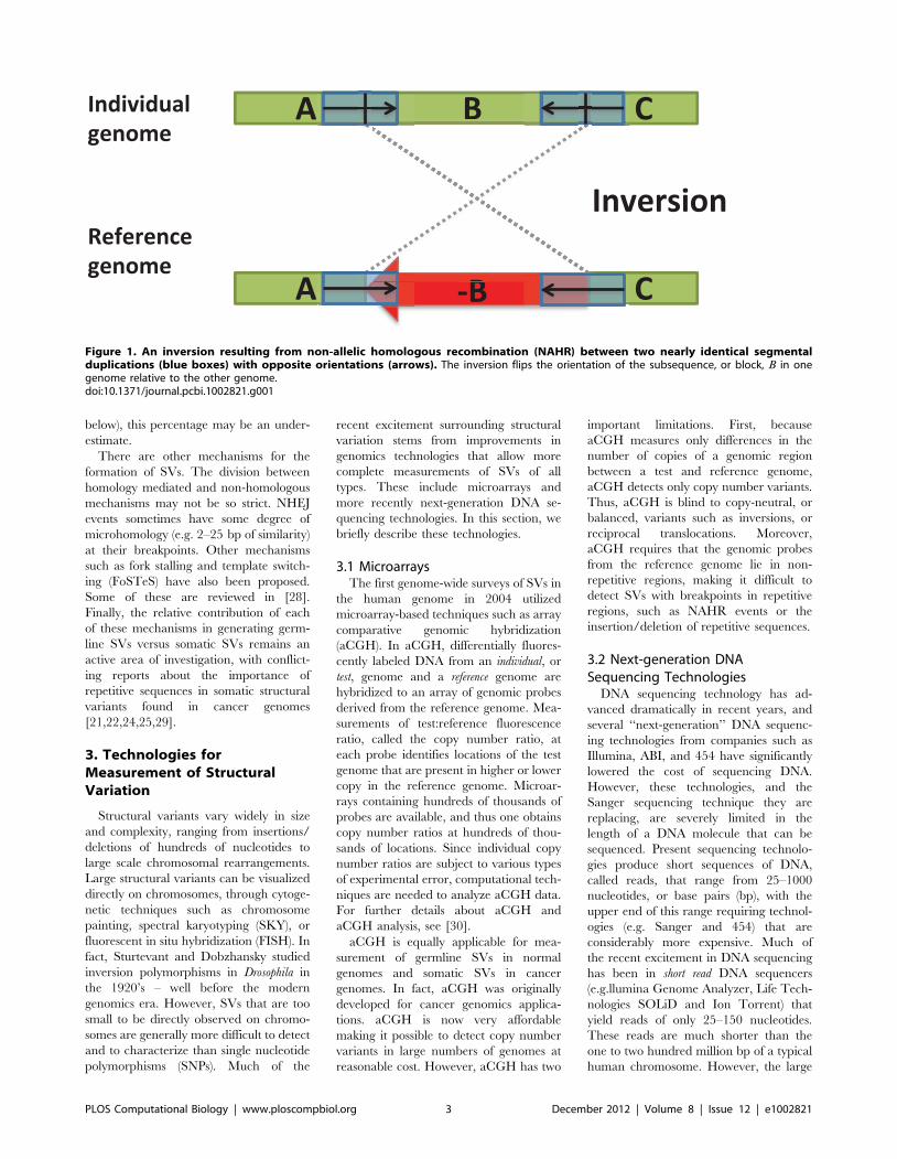
below), this percentage may be an under-
estimate.
There are other mechanisms for the
formation of SVs. The division between
homology mediated and non-homologous
mechanisms may not be so strict. NHEJ
events sometimes have some degree of
microhomology (e.g. 2–25 bp of similarity)
at their breakpoints. Other mechanisms
such as fork stalling and template switch-
ing (FoSTeS) have also been proposed.
Some of these are reviewed in [28].
Finally, the relative contribution of each
of these mechanisms in generating germ-
line SVs versus somatic SVs remains an
active area of investigation, with conflict-
ing reports about the importance of
repetitive sequences in somatic structural
variants found in cancer genomes
[21,22,24,25,29].
3. Technologies forMeasurement of StructuralVariation
Structural variants vary widely in size
and complexity, ranging from insertions/
deletions of hundreds of nucleotides to
large scale chromosomal rearrangements.
Large structural variants can be visualized
directly on chromosomes, through cytoge-
netic techniques such as chromosome
painting, spectral karyotyping (SKY), or
fluorescent in situ hybridization (FISH). In
fact, Sturtevant and Dobzhansky studied
inversion polymorphisms in Drosophila in
the 1920’s – well before the modern
genomics era. However, SVs that are too
small to be directly observed on chromo-
somes are generally more difficult to detect
and to characterize than single nucleotide
polymorphisms (SNPs). Much of the
recent excitement surrounding structural
variation stems from improvements in
genomics technologies that allow more
complete measurements of SVs of all
types. These include microarrays and
more recently next-generation DNA se-
quencing technologies. In this section, we
briefly describe these technologies.
3.1 MicroarraysThe first genome-wide surveys of SVs in
the human genome in 2004 utilized
microarray-based techniques such as array
comparative genomic hybridization
(aCGH). In aCGH, differentially fluores-
cently labeled DNA from an individual, or
test, genome and a reference genome are
hybridized to an array of genomic probes
derived from the reference genome. Mea-
surements of test:reference fluorescence
ratio, called the copy number ratio, at
each probe identifies locations of the test
genome that are present in higher or lower
copy in the reference genome. Microar-
rays containing hundreds of thousands of
probes are available, and thus one obtains
copy number ratios at hundreds of thou-
sands of locations. Since individual copy
number ratios are subject to various types
of experimental error, computational tech-
niques are needed to analyze aCGH data.
For further details about aCGH and
aCGH analysis, see [30].
aCGH is equally applicable for mea-
surement of germline SVs in normal
genomes and somatic SVs in cancer
genomes. In fact, aCGH was originally
developed for cancer genomics applica-
tions. aCGH is now very affordable
making it possible to detect copy number
variants in large numbers of genomes at
reasonable cost. However, aCGH has two
important limitations. First, because
aCGH measures only differences in the
number of copies of a genomic region
between a test and reference genome,
aCGH detects only copy number variants.
Thus, aCGH is blind to copy-neutral, or
balanced, variants such as inversions, or
reciprocal translocations. Moreover,
aCGH requires that the genomic probes
from the reference genome lie in non-
repetitive regions, making it difficult to
detect SVs with breakpoints in repetitive
regions, such as NAHR events or the
insertion/deletion of repetitive sequences.
3.2 Next-generation DNASequencing Technologies
DNA sequencing technology has ad-
vanced dramatically in recent years, and
several ‘‘next-generation’’ DNA sequenc-
ing technologies from companies such as
Illumina, ABI, and 454 have significantly
lowered the cost of sequencing DNA.
However, these technologies, and the
Sanger sequencing technique they are
replacing, are severely limited in the
length of a DNA molecule that can be
sequenced. Present sequencing technolo-
gies produce short sequences of DNA,
called reads, that range from 25–1000
nucleotides, or base pairs (bp), with the
upper end of this range requiring technol-
ogies (e.g. Sanger and 454) that are
considerably more expensive. Much of
the recent excitement in DNA sequencing
has been in short read DNA sequencers
(e.g.llumina Genome Analyzer, Life Tech-
nologies SOLiD and Ion Torrent) that
yield reads of only 25–150 nucleotides.
These reads are much shorter than the
one to two hundred million bp of a typical
human chromosome. However, the large
Figure 1. An inversion resulting from non-allelic homologous recombination (NAHR) between two nearly identical segmentalduplications (blue boxes) with opposite orientations (arrows). The inversion flips the orientation of the subsequence, or block, B in onegenome relative to the other genome.doi:10.1371/journal.pcbi.1002821.g001
PLOS Computational Biology | www.ploscompbiol.org 3 December 2012 | Volume 8 | Issue 12 | e1002821
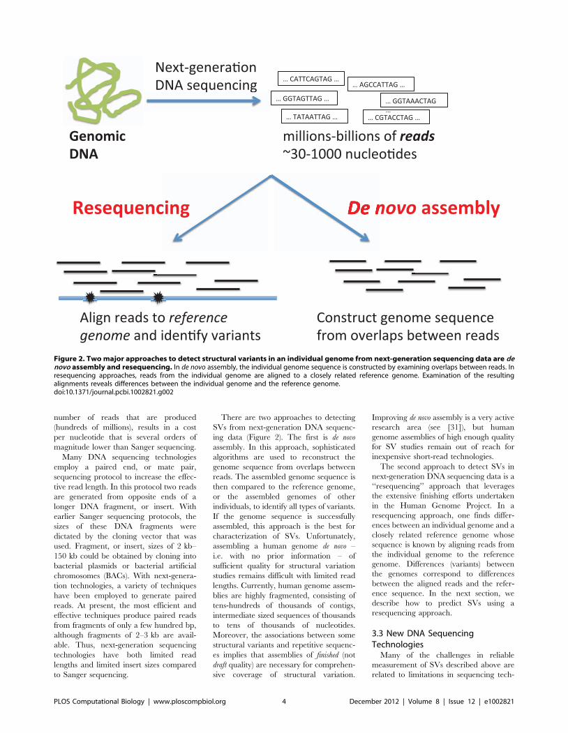
number of reads that are produced
(hundreds of millions), results in a cost
per nucleotide that is several orders of
magnitude lower than Sanger sequencing.
Many DNA sequencing technologies
employ a paired end, or mate pair,
sequencing protocol to increase the effec-
tive read length. In this protocol two reads
are generated from opposite ends of a
longer DNA fragment, or insert. With
earlier Sanger sequencing protocols, the
sizes of these DNA fragments were
dictated by the cloning vector that was
used. Fragment, or insert, sizes of 2 kb–
150 kb could be obtained by cloning into
bacterial plasmids or bacterial artificial
chromosomes (BACs). With next-genera-
tion technologies, a variety of techniques
have been employed to generate paired
reads. At present, the most efficient and
effective techniques produce paired reads
from fragments of only a few hundred bp,
although fragments of 2–3 kb are avail-
able. Thus, next-generation sequencing
technologies have both limited read
lengths and limited insert sizes compared
to Sanger sequencing.
There are two approaches to detecting
SVs from next-generation DNA sequenc-
ing data (Figure 2). The first is de novo
assembly. In this approach, sophisticated
algorithms are used to reconstruct the
genome sequence from overlaps between
reads. The assembled genome sequence is
then compared to the reference genome,
or the assembled genomes of other
individuals, to identify all types of variants.
If the genome sequence is successfully
assembled, this approach is the best for
characterization of SVs. Unfortunately,
assembling a human genome de novo –
i.e. with no prior information – of
sufficient quality for structural variation
studies remains difficult with limited read
lengths. Currently, human genome assem-
blies are highly fragmented, consisting of
tens-hundreds of thousands of contigs,
intermediate sized sequences of thousands
to tens of thousands of nucleotides.
Moreover, the associations between some
structural variants and repetitive sequenc-
es implies that assemblies of finished (not
draft quality) are necessary for comprehen-
sive coverage of structural variation.
Improving de novo assembly is a very active
research area (see [31]), but human
genome assemblies of high enough quality
for SV studies remain out of reach for
inexpensive short-read technologies.
The second approach to detect SVs in
next-generation DNA sequencing data is a
‘‘resequencing’’ approach that leverages
the extensive finishing efforts undertaken
in the Human Genome Project. In a
resequencing approach, one finds differ-
ences between an individual genome and a
closely related reference genome whose
sequence is known by aligning reads from
the individual genome to the reference
genome. Differences (variants) between
the genomes correspond to differences
between the aligned reads and the refer-
ence sequence. In the next section, we
describe how to predict SVs using a
resequencing approach.
3.3 New DNA SequencingTechnologies
Many of the challenges in reliable
measurement of SVs described above are
related to limitations in sequencing tech-
Figure 2. Two major approaches to detect structural variants in an individual genome from next-generation sequencing data are denovo assembly and resequencing. In de novo assembly, the individual genome sequence is constructed by examining overlaps between reads. Inresequencing approaches, reads from the individual genome are aligned to a closely related reference genome. Examination of the resultingalignments reveals differences between the individual genome and the reference genome.doi:10.1371/journal.pcbi.1002821.g002
PLOS Computational Biology | www.ploscompbiol.org 4 December 2012 | Volume 8 | Issue 12 | e1002821
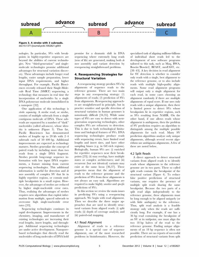
nologies. In particular, SVs with break-
points in highly-repetitive sequences are
beyond the abilities of current technolo-
gies. New ‘‘third-generation’’ and single-
molecule technologies promise additional
advantages for structural variation discov-
ery. These advantages include longer read
lengths, easier sample preparation, lower
input DNA requirements, and higher
throughput. For example, Pacific Biosci-
ences recently released their Single-Mole-
cule Real Time (SMRT) sequencing, a
technology that measures in real time the
incorporation of nucleotides by a single
DNA polymerase molecule immobilized in
a nanopore [32].
One application of this technology is
strobe sequencing. A strobe read, or strobe,
consists of multiple subreads from a single
contiguous molecule of DNA. These sub-
reads are separated by a number of ‘‘dark’’
nucleotides (called advances), whose iden-
tity is unknown (Figure 3). Thus far,
Pacific Biosciences has demonstrated
strobes of lengths up to 20 kb with 2–4
subreads each of 50–400 bp. Additional
improvements are expected as technology
matures. Strobes generalize the concept of
paired reads by including more than two
reads from a single DNA fragment.
Strobes provide long-range sequence in-
formation with low input DNA require-
ments, a feature missing from current
sequencing technologies. This additional
information is useful for detection and de
novo assembly of complex SV that lie in
highly repetitive regions, or contain mul-
tiple breakpoints in a small region. How-
ever, the advantages of strobes are reduced
by higher single-nucleotide error rates.
Thus, realizing the advantages of strobes
requires new algorithms that exploit infor-
mation from multiple, spaced subreads to
overcome high single-nucleotide error
rates [33].
Sequencing technologies continues its
rapid development. Improvements in the
chemistry, imaging, and manufacture of
existing technologies are increasing their
read lengths, insert lengths, and through-
put. Additional sequencing technologies
are under active development. Nanopore-
based technologies that directly read the
nucleotides of long molecules of DNA hold
promise for a dramatic shift in DNA
sequencing where extremely long reads
(tens of kb) are generated, making both de
novo assembly and variant detection by
resequencing straightforward problems.
4. Resequencing Strategies forStructural Variation
A resequencing strategy predicts SVs by
alignments of sequence reads to the
reference genome. There are two main
steps in any resequencing strategy: (1)
alignments of reads; (2) prediction of SVs
from alignments. Resequencing approach-
es are straightforward in principle, but in
practice sensitive and specific detection of
structural variation in human genomes is
notoriously difficult [34,35]. While some
types of SVs are easy to detect with next-
generation sequencing technologies, other
complex SVs are refractory to detection.
This is due to both technological limita-
tions and biological features of SVs. DNA
sequencing technologies produce reads
with sequencing errors, have limited read
lengths and insert sizes, and have other
sampling biases (e.g. in GC-rich regions).
Biologically, human SVs are: (i) enriched
for repetitive sequences near their break-
points [23]; (ii) may overlap, have multiple
states or complex architectures; and (iii)
recurrent (but not identical) variants may
exist at the same locus [36,37]. These
properties mean that the alignment of
reads to the reference genome and the
prediction of SVs from these alignments is
not always an easy task. Algorithms are
required to make highly sensitive and specific
predictions of SVs.
In this section we review the main issues
in predicting SVs using a resequencing
approach. We begin with read alignment.
Then we describe the three major ap-
proaches that are used to identify struc-
tural variants from aligned reads: (i) split
reads; (ii) depth of coverage analysis; and
(iii) paired-end mapping.
4.1 Read AlignmentAlignment of reads to a reference
genome is a special case of sequence
alignment, one of the most researched
problems in bioinformatics. However, the
specialized task of aligning millions-billions
of individual short reads led to the
development of new software programs
tailored to this task, such as Maq, BWA,
Bowtie/Bowtie2, BFAST, mrsFAST, etc.
[38–43]. A key decision in read alignment
for SV detection is whether to consider
only reads with a single, best alignment to
the reference genome, or to also include
reads with multiple high-quality align-
ments. Some read alignment programs
will output only a single alignment for
each read, in some cases choosing an
alignment randomly if there are multiple
alignments of equal score. If one uses only
reads with a unique alignment, then there
is limited power to detect SVs whose
breakpoints lie in repetitive regions, such
as SVs resulting from NAHR. On the
other hand, if one allows reads whose
alignment is ambiguous, then the problem
of SV prediction requires an algorithm to
distinguish among the multiple possible
alignments for each read. Many SV
prediction algorithms analyze only unique
alignments, although several recent algo-
rithms use ambiguous alignments. A few of
these are noted below.
4.2 Split ReadsA direct approach to detect structural
variants from aligned reads is to identify
reads whose alignments to the reference
genome are in two parts. These so called
split reads contain the breakpoint of the
structural variant (Figure 4). To reduce
false positive predictions of structural
variants, one requires the presence of
multiple split reads sharing the same
breakpoint. Because the two parts of a
split read align independently to the
reference genome, these alignments must
be long enough to be aligned uniquely (or
with little ambiguity) to the reference.
Thus, split read analysis is a feasible
strategy only when the reads are suffi-
ciently long. For example, if one has a
36 bp read containing the breakpoint of
an SV at its midpoint, one must align the
two 18 bp halves of the read to the
reference genome. Finding unique align-
ments of an 18 bp sequence is often not
possible. There are no reports of successful
prediction of structural variants from split
Figure 3. A strobe with 3 subreads.doi:10.1371/journal.pcbi.1002821.g003
PLOS Computational Biology | www.ploscompbiol.org 5 December 2012 | Volume 8 | Issue 12 | e1002821
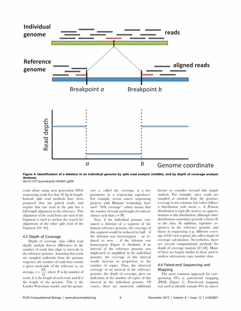
reads alone using next generation DNA
sequencing reads less that 50 bp in length.
Instead, split read methods have been
proposed that use paired reads, and
require that one read in the pair has a
full length alignment to the reference. This
alignment of the read from one end of the
fragment is used to anchor the search for
alignments of the other split read of the
fragment [44–46].
4.3 Depth of CoverageDepth of coverage (also called read
depth) analysis detects differences in the
number of reads that align to intervals in
the reference genome. Assuming that reads
are sampled uniformly from the genome
sequence, the number of reads that contain
a given nucleotide of the reference is, on
average, c~NL
G, where N is the number of
reads, L is the length of each read, and G is
the length of the genome. This is the
Lander-Waterman model, and the param-
eter c, called the coverage, is a key
parameter in a sequencing experience.
For example, recent cancer sequencing
projects with Illumina technology have
used ‘‘30X coverage’’ which means that
the number of reads and length of reads are
chosen such that c~30.
Now, if the individual genome con-
tained a deletion of a segment of the
human reference genome, the coverage of
this segment would be reduced by half – if
the deletion was heterozygous – or re-
duced to zero – if the deletion was
homozygous (Figure 4). Similarly, if an
interval of the reference genome was
duplicated, or amplified, in the individual
genome, the coverage of this interval
would increase in proportion to the
number of copies. Thus, the observed
coverage of an interval of the reference
genome, the depth of coverage, gives an
indication of the number of copies of this
interval in the individual genome. Of
course, there are numerous additional
factors to consider beyond this simple
analysis. For example, since reads are
sampled at random from the genome,
coverage is not constant, but rather follows
a distribution with mean c. A Poisson
distribution is typically used as an approx-
imation to this distribution, although other
distributions sometimes provide a better fit
to the data. In addition, repetitive se-
quences in the reference genome and
biases in sequencing (e.g. different cover-
age of GC-rich regions) also affect depth of
coverage calculations. Nevertheless, there
are several computational methods for
depth of coverage analysis [47,48]. Many
of these are largely similar to those used to
analyze microarray copy number data.
4.4 Paired-end Sequencing andMapping
The most common approach for rese-
quencing SVs is paired-end mapping
(PEM) (Figure 5). Paired-end mapping
was used to identify somatic SVs in cancer
Figure 4. Identification of a deletion in an individual genome by split read analysis (middle), and by depth of coverage analysis(bottom).doi:10.1371/journal.pcbi.1002821.g004
PLOS Computational Biology | www.ploscompbiol.org 6 December 2012 | Volume 8 | Issue 12 | e1002821
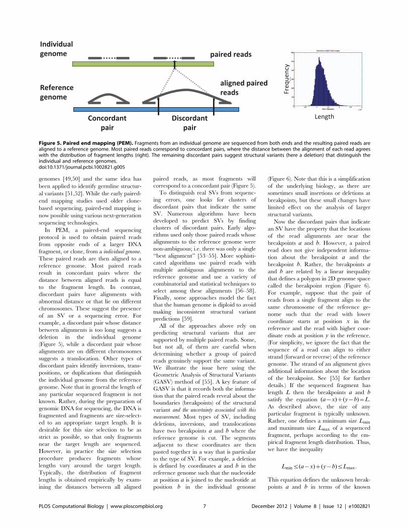
genomes [49,50] and the same idea has
been applied to identify germline structur-
al variants [51,52]. While the early paired-
end mapping studies used older clone-
based sequencing, paired-end mapping is
now possible using various next-generation
sequencing technologies.
In PEM, a paired-end sequencing
protocol is used to obtain paired reads
from opposite ends of a larger DNA
fragment, or clone, from a individual genome.
These paired reads are then aligned to a
reference genome. Most paired reads
result in concordant pairs where the
distance between aligned reads is equal
to the fragment length. In contrast,
discordant pairs have alignments with
abnormal distance or that lie on different
chromosomes. These suggest the presence
of an SV or a sequencing error. For
example, a discordant pair whose distance
between alignments is too long suggests a
deletion in the individual genome
(Figure 5), while a discordant pair whose
alignments are on different chromosomes
suggests a translocation. Other types of
discordant pairs identify inversions, trans-
positions, or duplications that distinguish
the individual genome from the reference
genome. Note that in general the length of
any particular sequenced fragment is not
known. Rather, during the preparation of
genomic DNA for sequencing, the DNA is
fragmented and fragments are size-select-
ed to an appropriate target length. It is
desirable for this size selection to be as
strict as possible, so that only fragments
near the target length are sequenced.
However, in practice the size selection
procedure produces fragments whose
lengths vary around the target length.
Typically, the distribution of fragment
lengths is obtained empirically by exam-
ining the distances between all aligned
paired reads, as most fragments will
correspond to a concordant pair (Figure 5).
To distinguish real SVs from sequenc-
ing errors, one looks for clusters of
discordant pairs that indicate the same
SV. Numerous algorithms have been
developed to predict SVs by finding
clusters of discordant pairs. Early algo-
rithms used only those paired reads whose
alignments to the reference genome were
non-ambiguous; i.e. there was only a single
‘‘best alignment’’ [53–55]. More sophisti-
cated algorithms use paired reads with
multiple ambiguous alignments to the
reference genome and use a variety of
combinatorial and statistical techniques to
select among these alignments [56–58].
Finally, some approaches model the fact
that the human genome is diploid to avoid
making inconsistent structural variant
predictions [59].
All of the approaches above rely on
predicting structural variants that are
supported by multiple paired reads. Some,
but not all, of them are careful when
determining whether a group of paired
reads genuinely support the same variant.
We illustrate the issue here using the
Geometric Analysis of Structural Variants
(GASV) method of [55]. A key feature of
GASV is that it records both the informa-
tion that the paired reads reveal about the
boundaries (breakpoints) of the structural
variant and the uncertainty associated with this
measurement. Most types of SV, including
deletions, inversions, and translocations
have two breakpoints a and b where the
reference genome is cut. The segments
adjacent to these coordinates are then
pasted together in a way that is particular
to the type of SV. For example, a deletion
is defined by coordinates a and b in the
reference genome such that the nucleotide
at position a is joined to the nucleotide at
position b in the individual genome
(Figure 6). Note that this is a simplification
of the underlying biology, as there are
sometimes small insertions or deletions at
breakpoints, but these small changes have
limited effect on the analysis of larger
structural variants.
Now the discordant pairs that indicate
an SV have the property that the locations
of the read alignments are near the
breakpoints a and b. However, a paired
read does not give independent informa-
tion about the breakpoint a and the
breakpoint b. Rather, the breakpoints a
and b are related by a linear inequality
that defines a polygon in 2D genome space
called the breakpoint region (Figure 6).
For example, suppose that the pair of
reads from a single fragment align to the
same chromosome of the reference ge-
nome such that the read with lower
coordinate starts at position x in the
reference and the read with higher coor-
dinate ends at position y in the reference.
(For simplicity, we ignore the fact that the
sequence of a read can align to either
strand (forward or reverse) of the reference
genome. The strand of an alignment gives
additional information about the location
of the breakpoint. See [55] for further
details.) If the sequenced fragment has
length L then the breakpoints a and bsatisfy the equation (a{x)z(y{b)~L.
As described above, the size of any
particular fragment is typically unknown.
Rather, one defines a minimum size Lmin
and maximum size Lmax of a sequenced
fragment, perhaps according to the em-
pirical fragment length distribution. Thus,
we have the inequality
Lminƒ(a{x)z(y{b)ƒLmax:
This equation defines the unknown break-
points a and b in terms of the known
Figure 5. Paired end mapping (PEM). Fragments from an individual genome are sequenced from both ends and the resulting paired reads arealigned to a reference genome. Most paired reads correspond to concordant pairs, where the distance between the alignment of each read agreeswith the distribution of fragment lengths (right). The remaining discordant pairs suggest structural variants (here a deletion) that distinguish theindividual and reference genomes.doi:10.1371/journal.pcbi.1002821.g005
PLOS Computational Biology | www.ploscompbiol.org 7 December 2012 | Volume 8 | Issue 12 | e1002821
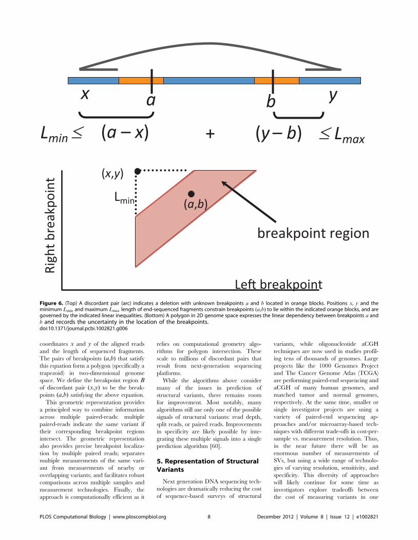
coordinates x and y of the aligned reads
and the length of sequenced fragments.
The pairs of breakpoints (a,b) that satisfy
this equation form a polygon (specifically a
trapezoid) in two-dimensional genome
space. We define the breakpoint region B
of discordant pair (x,y) to be the break-
points (a,b) satisfying the above equation.
This geometric representation provides
a principled way to combine information
across multiple paired-reads: multiple
paired-reads indicate the same variant if
their corresponding breakpoint regions
intersect. The geometric representation
also provides precise breakpoint localiza-
tion by multiple paired reads; separates
multiple measurements of the same vari-
ant from measurements of nearby or
overlapping variants; and facilitates robust
comparisons across multiple samples and
measurement technologies. Finally, the
approach is computationally efficient as it
relies on computational geometry algo-
rithms for polygon intersection. These
scale to millions of discordant pairs that
result from next-generation sequencing
platforms.
While the algorithms above consider
many of the issues in prediction of
structural variants, there remains room
for improvement. Most notably, many
algorithms still use only one of the possible
signals of structural variants: read depth,
split reads, or paired reads. Improvements
in specificity are likely possible by inte-
grating these multiple signals into a single
prediction algorithm [60].
5. Representation of StructuralVariants
Next generation DNA sequencing tech-
nologies are dramatically reducing the cost
of sequence-based surveys of structural
variants, while oligonucleotide aCGH
techniques are now used in studies profil-
ing tens of thousands of genomes. Large
projects like the 1000 Genomes Project
and The Cancer Genome Atlas (TCGA)
are performing paired-end sequencing and
aCGH of many human genomes, and
matched tumor and normal genomes,
respectively. At the same time, smaller or
single investigator projects are using a
variety of paired-end sequencing ap-
proaches and/or microarray-based tech-
niques with different trade-offs in cost-per-
sample vs. measurement resolution. Thus,
in the near future there will be an
enormous number of measurements of
SVs, but using a wide range of technolo-
gies of varying resolution, sensitivity, and
specificity. This diversity of approaches
will likely continue for some time as
investigators explore tradeoffs between
the cost of measuring variants in one
Figure 6. (Top) A discordant pair (arc) indicates a deletion with unknown breakpoints a and b located in orange blocks. Positions x, y and theminimum Lmin and maximum Lmax length of end-sequenced fragments constrain breakpoints (a,b) to lie within the indicated orange blocks, and aregoverned by the indicated linear inequalities. (Bottom) A polygon in 2D genome space expresses the linear dependency between breakpoints a andb and records the uncertainty in the location of the breakpoints.doi:10.1371/journal.pcbi.1002821.g006
PLOS Computational Biology | www.ploscompbiol.org 8 December 2012 | Volume 8 | Issue 12 | e1002821
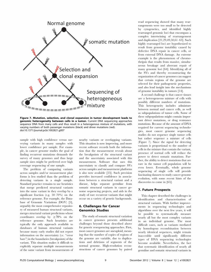
sample with high confidence versus sur-
veying variants in many samples with
lower confidence per sample. For exam-
ple, in cancer genome studies the goal of
finding recurrent mutations demands the
survey of many genomes and thus large
sample sizes might be preferred over high
coverage sequencing of one sample.
The problem of comparing variants
across samples and/or measurement plat-
forms is less studied than the problem of
detecting variants in a single sample.
Standard practice remains to use heuristics
that merge predicted structural variants
into the same variant in they overlap by a
significant fraction (e.g. 50–70%) on the
reference genome. For example, the Data-
base of Genomic Variations (DGV) [5],
arguably the most comprehensive reposito-
ry of measured human structural variants,
merges structural variant predictions whose
coordinates overlap by §70% on the
reference genome. Such heuristics are
typically the only approach available to
databases of human structural variants
because many early studies did not report
information on the uncertainty (i.e. ‘‘error
bars’’) in the boundaries (breakpoints) of the
variant. This situation makes it difficult to
explicitly separate multiple measurements
of the same variant from measurements of
nearby variants or overlapping variants.
This situation is now improving, and more
recent software records both the informa-
tion that the measurement reveals about
the breakpoints of the structural variant
and the uncertainty associated with this
measurement. Software that uses this
uncertainty to classify and compare SVs
across samples and measurement platforms
is also now available [55]. Such precision
provides increased confidence in associa-
tions between a structural variant and a
disease, helps separate germline from
somatic structural variants in cancer ge-
nome sequencing projects, and aids in the
study of rare recurrent variants that might
occur on a variety of genetic backgrounds.
6. Challenges for CancerGenomics Studies
The study of somatic structural variation
in cancer genomes presents additional
challenges beyond those described above
for generic resequencing approaches. First,
most cancer genomes are aneuploid, mean-
ing that the number of copies of regions of
the genome are variable, due to duplica-
tions and deletions of segments of the
normal genome. High-resolution recon-
structions of cancer genomes by paired
read sequencing showed that many rear-
rangements were too small to be detected
by cytogenetics, and identified highly
rearranged genomic loci that encompass a
complex intertwining of rearrangement
and duplication [21,29,49,50,61–63]. Such
highly rearranged loci are hypothesized to
result from genome instability caused by
defective DNA repair in cancer cells, or
from external DNA damage. An extreme
example is the phenomenon of chromo-
thripsis that results from massive, simulta-
neous breakage and aberrant repair of
many genomic loci [64]. Identifying all of
the SVs and thereby reconstructing the
organization of cancer genomes can suggest
that certain regions of the genome are
selected for their pathogenetic properties,
and also lend insight into the mechanisms
of genome instability in tumors [14].
A second challenge is that cancer tissues
are a heterogeneous mixture of cells with
possibly different numbers of mutations.
This heterogeneity includes admixture
between normal and cancer cells, as well
as subpopulations of tumor cells. Some of
these subpopulations might contain impor-
tant driver mutations, or drug resistance
mutations. Because of the amount of DNA
required for current sequencing technolo-
gies, most cancer genome sequencing
studies do not sequence single tumor cells
but rather sequence a mixture of cells
(Figure 7). Since the signal for detecting
variants is proportional to the number of
cells in the mixture that contain the variant,
presence of normal cells will reduce the
power to detect somatic mutations. Fur-
ther, the ability to detect mutations that are
rare in the tumor cell population will be
even lower. Eventually, whole genome
sequencing of single cells will provide
fascinating datasets to study cancer genome
evolution, with some recent hints of the
discoveries to come in [65].
7. Future Prospects
This chapter described the challenges in
identification and characterization of
structural variants. With further improve-
ments in sequencing technologies and
algorithms over the next few years, it will
be possible to systematically measure
nearly all but the most complex variants
in an individual genome. The most
difficult cases, such as variants mediated
by homologous recombination between
nearly identical sequences, might remain
inaccesible until significantly different
types of DNA sequencing technologies
become available. Nevertheless, the fact
that systematic identification of nearly all
germline and somatic structural variants in
Figure 7. Mutation, selection, and clonal expansion in tumor development leads togenomic heterogeneity between cells in a tumor. Current DNA sequencing approachessequence DNA from many cells and thus result in a heterogenous mixture of mutations, withvarying numbers of both passenger mutations (black) and driver mutations (red).doi:10.1371/journal.pcbi.1002821.g007
PLOS Computational Biology | www.ploscompbiol.org 9 December 2012 | Volume 8 | Issue 12 | e1002821
an individual genome is now possible will
enable further progress in human and
cancer genetics.
For genetic association studies, having
complete lists of germline variants from
many individuals means that unexplained
heritability for a trait cannot readily be
blamed on lack of measurement of genetic
information. Unfortunately, this does not
necessarily imply that finding the genetic
basis for specifc traits will become easy.
There remain other challenges, including
the possiblity that combinations of vari-
ants, interactions between genetic and
environmental factors, or other epigenetic
mechanisms, may contribute to pheno-
type. See [66] in this collection for further
discussion of these issues. Finally, translat-
ing genetic information about susceptibil-
ity to a disease or efficacy of particular
treatments into improved medical out-
comes will require additional work.
The opportunities and challenges are
similar in cancer genetics. Systematic mea-
surement of all somatic mutations will yield
information that might guide treatments,
and eventually lead to personalized oncol-
ogy. Current cancer treatments are limited
by the non-specificity of most cancer drugs
and by the fact that cancer cells can evolve
resistance to single drug treatments. Tailor-
ing of treatment to the particular genetic
mutations in a tumor promises to revolu-
tionize cancer therapy. There are already
several examples of such personalized
treatments including the drug Gleevec that
targets the BCR-ABL fusion gene in chronic
myelogenous leukemia (CML) and Iressa
that targets the EGFR gene in lung cancer.
Discovery of additional cancer-specific drug
targets requires not only technologies to
globally survey somatic mutations in cancer
genomes, but also techniques (experimental
and/or computational) to classify the subset
of variants that are functional, and then the
further subset of these functional variants
that are druggable.
The sequencing technologies and algo-
rithms described in this chapter are laying
the foundation for personalized medicine,
but much work remains to translate the
information revealed by genome sequenc-
ing into improved clinical practice.
8. Exercises
(1) Consider the chromosomal inversion
in Figure 1. What signals in next-
generation sequencing data can be
used to detect a chromosomal inver-
sion?
(2) The human genome is diploid with
two copies, maternal and paternal, of
each chromosome. What constraints
does this place on prediction of
germline structural variants?
Answers to the Exercises can be found
in Text S1.
Supporting Information
Text S1 Answers to Exercises.
(PDF)
References
1. Manolio TA, Collins FS, Cox NJ, Goldstein DB,
Hindorff LA, et al. (2009) Finding the missing
heritability of complex diseases. Nature 461: 747–753.
2. Stratton MR (2011) Exploring the genomes of
cancer cells: progress and promise. Science 331:
1553–1558.
3. Frazer K, Ballinger D, Cox D, Hinds D, Stuve L,
et al. (2007) A second generation human
haplotype map of over 3.1 million SNPs. Nature
449: 851–861.
4. Sharp AJ, Cheng Z, Eichler EE (2006) Structural
variation of the human genome. Annu Rev
Genomics Hum Genet 7: 407–442.
5. Iafrate A, Feuk L, Rivera M, Listewnik M,
Donahoe P, et al. (2004) Detection of large-scale
variation in the human genome. Nat Genet 36:
949–951.
6. Redon R, Ishikawa S, Fitch K, Feuk L, Perry G,
et al. (2006) Global variation in copy number in
the human genome. Nature 444: 444–454.
7. Stranger BE, Forrest MS, Dunning M, Ingle CE,
Beazley C, et al. (2007) Relative impact of
nucleotide and copy number variation on gene
expression phenotypes. Science 315: 848–853.
8. Lower KM, Hughes JR, De Gobbi M, Hender-
son S, Viprakasit V, et al. (2009) Adventitious
changes in long-range gene expression caused by
polymorphic structural variation and promoter
competi- tion. Proc Natl Acad Sci USA 106:
21771–21776.
9. Marshall C, Noor A, Vincent J, Lionel A, Feuk L,
et al. (2008) Structural variation of chromosomes
in autism spectrum disorder. Am J Hum Genet
82: 477–488.
10. Stone JL, O’Donovan MC, Gurling H, Kirov
GK, Blackwood DH, et al. (2008) Rare chromo-
somal deletions and duplications increase risk of
schizophrenia. Nature 455: 237–241.
11. Sindi SS, Raphael BJ (2009) Identification and
frequency estimation of inversion polymorphisms
from haplotype data. In: RECOMB. pp. 418–
433.
12. Nowell PC (1976) The clonal evolution of tumor
cell populations. Science 194: 23–28.
13. Merlo LM, Pepper JW, Reid BJ, Maley CC
(2006) Cancer as an evolutionary and ecological
process. Nat Rev Cancer 6: 924–935.
14. Albertson DG, Collins C, McCormick F, Gray
JW (2003) Chromosome aberrations in solid
tumors. Nat Genet 34: 369–76.
15. Tomlins SA, Rhodes DR, Perner S, Dhanase-
karan SM, Mehra R, et al. (2005) Recurrent
fusion of tmprss2 and ets transcription factor
genes in prostate cancer. Science 310: 644–648.
16. Soda M, Choi Y, Enomoto M, Takada S,
Yamashita Y, et al. (2007) Identification of the
trans- forming EML4-ALK fusion gene in non-
small-cell lung cancer. Nature 448: 561–566.
17. Mitelman F, Johansson B, Mertens F (2004)
Fusion genes and rearranged genes as a linear
function of chromosome aberrations in cancer.
Nat Genet 36: 331–334.
18. Meyerson M, Gabriel S, Getz G (2010) Advances
in understanding cancer genomes through sec-
ond-generation sequencing. Nat Rev Genet 11:
685–696.
19. Mardis ER (2012) Genome sequencing and
cancer. Curr Opin Genet Dev 22: 245–250.
20. International Cancer Genome Consortium, Hud-
son TJ, Anderson W, Artez A, Barker AD, et al.
(2010) International network of cancer genome
projects. Nature 464: 993–998.
21. Bignell GR, Santarius T, Pole JCM, Butler AP,
Perry J, et al. (2007) Architectures of somatic
genomic rearrangement in human cancer ampli-
cons at sequence-level resolution. Genome Res
17: 1296–1303.
22. Campbell P, Stephens P, Pleasance E, O’Meara
S, Li H, et al. (2008) Identification of somatically
acquired rearrangements in cancer using ge-
nome-wide massively parallel paired-end se-
quencing. Nat Genet 40: 722–729.
23. Kidd J, Cooper G, Donahue W, Hayden H,
Sampas N, et al. (2008) Mapping and sequencing
of structural variation from eight human ge-
nomes. Nature 453: 56–64.
24. Kolomietz E, Meyn MS, Pandita A, Squire JA
(2002) The role of Alu repeat clusters as mediators
of recurrent chromosomal aberrations in tumors.
Genes Chromosomes Cancer 35: 97–112.
Further Reading
N Alkan C, Coe BP, Eichler EE (2011) Genome structural variation discovery andgenotyping. Nat Rev Genet 12: 363–376.
N Mardis ER (2012) Genome sequencing and cancer. Curr Opin Genet and Dev 22:245–250.
N Meyerson M, Gabriel S, Getz G (2010) Advances in understanding cancergenomes through second-generation sequencing. Nature Reviews Genetics 11:685–696.
N Medvedev P, Stanciu M, Brudno M (2009) Computational methods fordiscovering structural variation with next-generation sequencing. Nat Methods6: 13–20.
N Sindi S, Helman E, Bashir A, Raphael BJ (2009) A geometric approach forclassification and comparison of structural variants. Bioinformatics 25: i222–i230.
N Stratton MR (2011) Exploring the genomes of cancer cells: progress andpromise. Science 331: 1553–1558.
PLOS Computational Biology | www.ploscompbiol.org 10 December 2012 | Volume 8 | Issue 12 | e1002821
25. Darai-Ramqvist E, Sandlund A, Mller S, Klein
G, Imreh S, et al. (2008) Segmental duplications
and evolutionary plasticity at tumor chromosome
break-prone regions. Genome Res 18: 370–379.
26. Bailey J, Eichler E (2006) Primate segmental
duplications: crucibles of evolution, diversity and
disease. Nat Rev Genet 7: 552–564.
27. Mills RE, Walter K, Stewart C, Handsaker RE,
Chen K, et al. (2011) Mapping copy number
variation by population-scale genome sequencing.
Nature 470: 59–65.
28. Stankiewicz P, Lupski JR (2010) Structural
variation in the human genome and its role in
disease. Annu Rev Med 61: 437–455.
29. Raphael B, Volik S, Yu P, Wu C, Huang G, et al.
(2008) A sequence-based survey of the complex
structural organization of tumor genomes. Ge-
nome Biol 9: R59.
30. Pinkel D, Albertson DG (2005) Array compara-
tive genomic hybridization and its applications in
cancer. Nat Genet 37 Suppl: S11–S7.
31. Schatz MC, Delcher AL, Salzberg SL (2010)
Assembly of large genomes using second-genera-
tion sequencing. Genome Res 20: 1165–1173.
32. Eid J, Fehr A, Gray J, Luong K, Lyle J, et al.
(2009) Real-time DNA sequencing from single
polymerase molecules. Science 323: 133–138.
33. Ritz A, Bashir A, Raphael BJ (2010) Structural
variation analysis with strobe reads. Bioinfor-
matics 26: 1291–1298.
34. Medvedev P, Stanciu M, Brudno M (2009)
Computational methods for discovering structural
variation with next-generation sequencing. Nat
Methods 6: 13–20.
35. Alkan C, Coe BP, Eichler EE (2011) Genome
structural variation discovery and genotyping.
Nat Rev Genet 12: 363–376.
36. Scherer S, Lee C, Birney E, Altshuler D, Eichler
E, et al. (2007) Challenges and standards in
integrating surveys of structural variation. Nat
Genet 39: 7–15.
37. Perry G, Ben-Dor A, Tsalenko A, Sampas N,
Rodriguez-Revenga L, et al. (2008) The fine-scale
and complex architecture of human copy-number
variation. Am J Hum Genet 82: 685–695.
38. Li H, Ruan J, Durbin R (2008) Mapping short
DNA sequencing reads and calling variants using
mapping quality scores. Genome Res 18: 1851–
1858.
39. Li H, Durbin R (2009) Fast and accurate short
read alignment with Burrows-Wheeler transform.
Bioinformatics 25: 1754–1760.
40. Langmead B, Trapnell C, Pop M, Salzberg SL
(2009) Ultrafast and memory-efficient alignment
of short DNA sequences to the human genome.
Genome Biol 10: R25.41. Langmead B, Salzberg SL (2012) Fast gapped-
read alignment with bowtie 2. Nat Methods 9:
357–359.42. Homer N, Merriman B, Nelson SF (2009)
BFAST: an alignment tool for large scale genomeresequencing. PLoS ONE 4: e7767. doi:10.1371/
journal.pone.0007767.
43. Hach F, Hormozdiari F, Alkan C, HormozdiariF, Birol I, et al. (2010) mrsfast: a cache-oblivious
algorithm for short-read mapping. Nat Methods7: 576–577.
44. Maher CA, Kumar-Sinha C, Cao X, Kalyana-Sundaram S, Han B, et al. (2009) Transcriptome
sequencing to detect gene fusions in cancer.
Nature 458: 97–101.45. Mills RE, Luttig CT, Larkins CE, Beauchamp A,
Tsui C, et al. (2006) An initial map of insertionand deletion (INDEL) variation in the human
genome. Genome Res 16: 1182–1190.
46. Ye K, Schulz MH, Long Q, Apweiler R, Ning Z(2009) Pindel: a pattern growth approach to
detect break points of large deletions and mediumsized insertions from paired-end short reads.
Bioinformatics 25: 2865–2871.47. Chiang DY, Getz G, Jaffe DB, O’Kelly MJ, Zhao
X, et al. (2009) High-resolution mapping of copy-
number alterations with massively parallel se-quencing. Nat Methods 6: 99–103.
48. Yoon S, Xuan Z, Makarov V, Ye K, Sebat J(2009) Sensitive and accurate detection of copy
number variants using read depth of coverage.
Genome Res 19: 1586–1592.49. Volik S, Zhao S, Chin K, Brebner J, Herndon D,
et al. (2003) End-sequence profiling: sequence-based analysis of aberrant genomes. Proc Natl
Acad Sci USA 100: 7696–7701.50. Raphael B, Volik S, Collins C, Pevzner P (2003)
Reconstructing tumor genome architectures.
Bioinformatics 19 Suppl 2: i162–171.51. Tuzun E, Sharp AJ, Bailey JA, Kaul R, Morrison
VA, et al. (2005) Fine-scale structural variation ofthe human genome. Nat Genet 37: 727–32.
52. Korbel JO, Urban AE, Affourtit JP, Godwin B,
Grubert F, et al. (2007) Paired-end mappingreveals extensive structural variation in the
human genome. Science 318: 420–426.53. Chen K,Wallis JW, McLellan MD, Larson DE,
Kalicki JM, et al. (2009) BreakDancer: analgorithm for high-resolution mapping of geno-
mic structural variation. Nat Methods 6: 677–
681.54. Korbel JO, Abyzov A, Mu XJ, Carriero N,
Cayting P, et al. (2009) PEMer: a computational
framework with simulation-based error models
for inferring genomic structural variants from
mas-sive paired-end sequencing data. Genome
Biol 10: R23.
55. Sindi S, Helman E, Bashir A, Raphael BJ (2009)
A geometric approach for classification and
comparison of structural variants. Bioinformatics
25: i222–230.
56. Hormozdiari F, Alkan C, Eichler EE, Sahinalp
SC (2009) Combinatorial algorithms for structur-
al variation detection in high-throughput se-
quenced genomes. Genome Res 19: 1270–1278.
57. Quinlan AR, Clark RA, Sokolova S, Leibowitz
ML, Zhang Y, et al. (2010) Genome-wide
mapping and assembly of structural variant
breakpoints in the mouse genome. Genome Res
20: 623–635.
58. Lee S, Cheran E, Brudno M (2008) A robust
framework for detecting structural variations in a
genome. Bioinformatics 24: 59–67.
59. Hormozdiari F, Hajirasouliha I, Dao P, Hach F,
Yorukoglu D, et al. (2010) Next-generation Varia-
tionHunter: combinatorial algorithms for trans-
poson insertion discovery. Bioinformatics 26:
i350–357.
60. Sindi SS, Onal S, Peng LC, Wu HT, Raphael BJ
(2012) An integrative probabilistic model for
identification of structural variation in sequencing
data. Genome Biol 13: R22.
61. Volik S, Raphael B, Huang G, Stratton M, Bignel
G, et al. (2006) Decoding the fine-scale structure
of a breast cancer genome and transcriptome.
Genome Res 16: 394–404.
62. Raphael B, Pevzner P (2004) Reconstructing
tumor amplisomes. Bioinformatics 20 Suppl 1:
i265–273.
63. Hampton OA, Den Hollander P, Miller CA,
Delgado DA, Li J, et al. (2009) A sequence-level
map of chromosomal breakpoints in the MCF-7
breast cancer cell line yields insights into the
evolution of a cancer genome. Genome Res 19:
167–177.
64. Stephens PJ, Greenman CD, Fu B, Yang F,
Bignell GR, et al. (2011) Massive genomic
rearrange- ment acquired in a single catastrophic
event during cancer development. Cell 144: 27–
40.
65. Navin N, Kendall J, Troge J, Andrews P, Rodgers
L, et al. (2011) Tumour evolution inferred by
single-cell sequencing. Nature 472: 90–94.
66. Moore J, Bush W (2012) Chapter 11: Genome-
wide association studies. PLoS Comput Biol 8:
e1002802. doi:10.1371/journal.pcbi.1002802.
PLOS Computational Biology | www.ploscompbiol.org 11 December 2012 | Volume 8 | Issue 12 | e1002821
Education
Chapter 7: PharmacogenomicsKonrad J. Karczewski1,2, Roxana Daneshjou2,3, Russ B. Altman2,3*
1 Program in Biomedical Informatics, Stanford University, Stanford, California, United States of America, 2 Department of Genetics, Stanford University, Stanford, California,
United States of America, 3 Department of Medicine, Stanford University, Stanford, California, United States of America
Abstract: There is great variation indrug-response phenotypes, and a‘‘one size fits all’’ paradigm for drugdelivery is flawed. Pharmacoge-nomics is the study of how humangenetic information impacts drugresponse, and it aims to improveefficacy and reduced side effects. Inthis article, we provide an overviewof pharmacogenetics, includingpharmacokinetics (PK), pharmaco-dynamics (PD), gene and pathwayinteractions, and off-target effects.We describe methods for discover-ing genetic factors in drug response,including genome-wide associationstudies (GWAS), expression analysis,and other methods such as che-moinformatics and natural lan-guage processing (NLP). We coverthe practical applications of phar-macogenomics both in the pharma-ceutical industry and in a clinicalsetting. In drug discovery, pharma-cogenomics can be used to aid leadidentification, anticipate adverseevents, and assist in drug repurpos-ing efforts. Moreover, pharmacoge-nomic discoveries show promise asimportant elements of physiciandecision support. Finally, we con-sider the ethical, regulatory, andreimbursement challenges that re-main for the clinical implementationof pharmacogenomics.
This article is part of the ‘‘Transla-
tional Bioinformatics’’ collection for
PLOS Computational Biology.
1. Introduction
A child with leukemia goes to the
doctor’s office to be treated. The oncolo-
gist has decided to use mercaptopurine, a
drug with a narrow therapeutic range.
The efficacy and toxicity of this drug lies in
its ability to act as a myelosuppressant,
which means it suppresses white and red
blood cell production. Despite the dangers
this regimen poses, the oncologist is
confident with his ability to administer
the drug based on his experience with
prior patients. However, after the child has
undergone treatment, he begins experi-
encing unexpected bone marrow toxicity,
immunosuppression, and life-threatening
infections. This type of scenario was
encountered after mercaptopurine first
came on the market in the 1950s. In the
mid-1990s, scientists began to realize that
genetics could explain a majority of the
cases of life-threatening bone marrow
toxicity [1]. Now, many drugs that were
once noted to cause so-called ‘‘unpredict-
able’’ reactions are being re-evaluated for
drug-gene interactions.
The history of medicine is full of
medications with unintended consequenc-
es; the ability to understand some of the
underlying causes has been a recent
development. In the 1950s, succinylcholine
was used by anesthesiologists as a muscle
relaxant during operations. However,
about 1 in 2500 individuals experienced a
horrific reaction – respiratory arrest. Later
research revealed that those individuals had
defects in both copies of cholinesterase, the
enzyme required to metabolize succinyl-
choline into an inactive form. During the
1980s, a drug used to treat angina,
perhexiline, caused neural and liver toxicity
in a subset of patients. Scientists later found
that this toxicity occurred in individuals
with a rare polymorphism of CYP2D6, an
enzyme involved in the drug’s metabolism.
Genetics not only plays a role in adverse
events, but also influences an individual’s
optimal drug dose. Two anticoagulants,
warfarin and clopidogrel, have different
therapeutic doses based on an individual’s
genetic makeup. Scientists are increasingly
learning more about the interaction be-
tween drugs and human genetics in order
to take modern medicine down a more
personalized path.
Modern physicians prescribe medica-
tions based on clinical judgment or evi-
dence from clinical trials. In order to select
a drug and dosage, physicians take clinical
factors such as gender, weight, or organ
function into consideration. The personal
variation that may affect drug selection or
dosing, such as genetics, is not considered
in many settings. Thus, while a daily 75 mg
dose of clopidogrel for a 70 kg adult would
obviously be inappropriate for a 20 kg
child, it is less obvious that two adults with
identical presentations and clinical back-
grounds might require vastly different
doses. However, for an increasing number
of drugs, this appears to be the case. For
instance, two patients with similar clinical
presentations could be given the same dose
of the anti-platelet drug clopidogrel, and
one would be adequately protected against
cardiovascular events while the other
experiences a myocardial infarction due to
inadequate therapeutic protection. What
accounts for this difference? Genetics – the
patient with the inadequate therapeutic
protection likely has a polymorphism of
CYP2C19 with decreased activity, so that
this key enzyme cannot efficiently metab-
olize clopidogrel into its active metabolite.
The interaction between drugs and genetics
has been termed pharmacogenomics.
In general, pharmacogenomics can be
defined as the sum of the word’s parts: the
study and application of genetic factors
(often in a high-throughput, genomic
fashion) relating to the body’s response to
drugs, or pharmacology (for the major
questions in the field of pharmacoge-
Citation: Karczewski KJ, Daneshjou R, Altman RB (2012) Chapter 7: Pharmacogenomics. PLoS ComputBiol 8(12): e1002817. doi:10.1371/journal.pcbi.1002817
Editors: Fran Lewitter, Whitehead Institute, United States of America and Maricel Kann, University of Maryland,Baltimore County, United States of America
Published December , 2012
Copyright: � 2012 Karczewski et al. This is an open-access article distributed under the terms of the CreativeCommons Attribution License, which permits unrestricted use, distribution, and reproduction in any medium,provided the original author and source are credited.
Funding: KJK is supported by NIH/NLM National Library of Medicine training grant ‘‘Graduate Training inBiomedical Informatics’’ T15-LM007033 and the NSF Graduate Research Fellowship Program. RD is supportedby Stanford Medical Scholars. RBA is supported by PharmGKB GM61374. The funders had no role in thepreparation of the manuscript.
Competing Interests: The authors have declared that no competing interests exist.
* E-mail: [email protected]
PLOS Computational Biology | www.ploscompbiol.org 1 December 2012 | Volume 8 | Issue 12 | e1002817
27
nomics, see Box 1). Once a patient takes a
drug, the drug must travel through the
body to its target(s), act on its target(s), and
then leave the body. The first and last of
these processes is facilitated by pharmaco-
kinetic (PK) genes, which may affect a
drug in the ‘‘ADME’’ processes: to be
absorbed into and distributed through the
body, metabolized (either to an active
form or broken down into an inactive
form), and excreted. The action of a drug
on its targets involves pharmacodynamic
(PD) genes, which include the direct
targets themselves, genes affected down-
stream, and the genes responsible for the
clinical outcome. PK and PD genes can be
involved in both intentional ‘‘on-target’’
effects that produce the desired therapeu-
tic response, as well as unintentional ‘‘off-
target’’ effects that cause adverse events
(side effects or other unintended conse-
quences of the drug). Current researchers
are working to tease out genes involved in
both the PK and PD pathways that affect
drug action in order to improve dosing
and avoid adverse drug reactions.
The search for genetic factors that relate
to pharmacological response begins much
like the search for a genetic association of
any trait. Standard association study meth-
ods (such as GWAS) search for significant
associations between a binary or continu-
ous trait and the genetic profiles of case and
control sets. In a GWAS, the trait of interest
can be a disease state or physical trait.
Specifically, in the case of pharmacoge-
nomics, the trait is an actual drug dose,
response, or adverse event profile, though
the study design should be carefully con-
sidered for the specific application (see
below: Methods). Additionally, high-
throughput expression analysis and che-
minformatics have provided investigators
with valuable tools for learning about
physiological drug responses. Finally, as
sequencing technologies become exponen-
tially cheaper and the ‘‘$1,000 Genome’’
becomes an attainable goal, whole-genome
or exome sequencing will soon become
commonplace in pharmacogenomic stud-
ies. As these types of studies become less
expensive and more mainstream, pharma-
cogenomics will transition from simply an
interesting research topic to a main role
player in pharmacological development
and clinical application.
The applications of pharmacogenomics
are of interest to industry, clinicians, academ-
ics, and patients alike. For the biopharma-
ceutical industry, pharmacogenomics can
improve the drug development process
through faster and safer drug trials and the
early identification of drug responders, non-
responders, and those prone to adverse
events. For clinicians and patients, pharma-
cogenomics can aid the decision-making
process in prescriptions and determination
of the optimal dose of a drug.
Many significant challenges remain in the
field of pharmacogenomics, beyond the
simple identification of more genetic variants
related to drug response. First, the transition
to whole-genome sequencing will require
newer analysis methods, as well as more
extensive annotations, to assign meaning to
novel variants. A database of the relation
between genes, variants, and drugs, such as
PharmGKB, will be instrumental in the
aggregation of information curated from the
literature. In addition, the characterization of
adverse events and their underlying causes is
a topic of active research. Finally, the
application of pharmacogenomics to a clin-
ical setting will require the education of
physicians in the utility of genome sequencing
or genotyping for the benefit of their patients.
With the dawn of human genome
sequencing, especially the impending wide-
spread availability of personal genotyping to
the public, and an expanded knowledge of
the clinical impact of genetics and molecular
biology, physicians around the world are
beginning to use patients’ personal genetics in
informing prescription decisions. While still in
its early phases, pharmacogenomics will
undoubtedly lead the way in the development
of personalized medicine.
2. Pharmacogenomics in Action
When a physician administers a drug,
an intricate cascade of events unfolds as
this molecule interacts with the physiolog-
ical environment. In the simplest scenario,
a drug (after interacting with a number of
proteins on its way to its target) may act as
an agonist or an antagonist against a
receptor, which is composed of one or
more proteins. At the molecular level, the
metabolite can bind to the protein’s active
site, which can include ligand-binding
sites, conformation-altering sites, or cata-
lytic sites. This effect can then be propa-
gated through biochemical pathways to
produce a cellular and finally, systemic
physiological effect. Along the way, hu-
man genetic variation can affect the way
these receptors interact with drugs, leading
to consequences in the efficacy of the drug
and causing potential adverse events.
2.1. Drug-Receptor Interactions:Agonists and Antagonists
Agonists interact with a receptor in an
activating fashion: these small molecules
mimic the behavior of the receptor’s natural
ligand, producing a result that is either
weaker than, the same as, or stronger than
the natural ligand. For example, sympatho-
mimetic drugs are a clinically important class
of agonists that interact with the G-protein-
coupled receptors that are endogenously
stimulated by catecholamines. These drugs
are given to produce responses normally
elicited by the sympathetic nervous system.
Some examples of sympathomimetic drug
action include relaxation of bronchial smooth
muscle in asthma, increasing the muscular
contractions of the heart in cases of reversible
heart failure due to cardiogenic or septic
shock, or vasoconstriction of superficial
vasculature to reduce nasal congestion. There
are several subtypes of adrenoreceptors and
different drugs stimulate different receptor
subtypes. For instance, a very clinically
relevant drug, albuterol, can be inhaled to
What to Learn in This Chapter
N Interactions between drugs (small molecules) and genes (proteins)
N Methods for pharmacogenomic discovery
N Association- and expression-based methods
N Cheminformatics and pathway-based methods
N Database resources for pharmacogenomic discovery and application(PharmGKB)
N Applications of pharmacogenomics into a clinical setting
Box 1. Problem Statement
N What are the genes involved in a drug’s mechanism of action?
N How are a drug’s effects propagated through pathways?
N How can this information be applied to characterize ‘‘off-target’’ adverseevents?
N How can pharmacogenomics information be utilized in prescription and dosingdecisions?
PLOS Computational Biology | www.ploscompbiol.org 2 December 2012 | Volume 8 | Issue 12 | e1002817
stimulate b2 receptors (whose natural ligand
is norepinephrine) on the smooth muscle of
the lungs. Its action leads to the activation of
adenylyl cyclase, which ultimately leads to the
dilation of bronchial smooth muscle, provid-
ing life-saving relief for asthma patients (See
Chapter 9 of [2]). However, some studies
have identified that the very agonists that
provide relief to asthmatics can lead to
asthma exacerbation or death in a subset of
patients. Research has indicated that at least
in some populations, this phenomenon could
be related to genetic polymorphisms of the b2
receptors [3].
Antagonists, on the other hand, inhibit the
receptor partially or fully, reversibly or
irreversibly so that the cascade caused by
normal receptor activation cannot occur.
The same adrenergic receptor subclasses
mentioned before can also be antagonized.
b receptor blockers (‘‘beta-blockers’’) are an
antagonist drug class clinically indicated to
treat chronic, irreversible heart failure. The
mechanism of the beneficial effects of bblockers is not well understood. The prevail-
ing theory is that since the high levels of
circulating catecholamines triggered by heart
failure lead to detrimental cardiac remodel-
ing, blocking the cardiac catecholamine
receptors (b1 and b2 receptors) with a bblocker can slow down additional de-com-
pensation. The b blockers for heart failure,
bisoprolol, carvedilol, and metoprolol, antag-
onize (that is, inhibit) b1 and b2 receptors:
their action is substantially greater at the b1
receptor, which is the dominant receptor in
the heart. However, some patients do not
respond as well to this therapy as others, and
clinical studies have suggested that this may
be due to b1 receptor polymorphisms. More
extensive studies of these polymorphisms are
underway to definitively identify the phar-
macogenetic variables affecting b blocker
success [4].
Often in the literature, the discussion of
drugs and proteins has involved vague
notions of ‘‘interactions’’ without any discus-
sion about the underlying molecular mecha-
nisms. A drug’s interaction with any receptor
is dependent on how well the molecular
conformation of the drug can interact with
the structure of the target. Before any
discussion of downstream physiological ef-
fects, a drug’s mechanism of action begins
with the specific molecular reaction between
the drug and cellular proteins. This interac-
tion itself can provide insight into the effect of
drugs on physiology and influence potential
pharmacogenomic knowledge.
2.2. Drug-Receptor Interactions: TheDetails
While biologists tend to represent pro-
teins as colored ovals existing in an
idealized environment, in reality, proteins
are complex molecules with intricate
secondary and tertiary structures: they
harbor rugged landscapes on their surfac-
es, with charged or hydrophobic hills and
valleys serving as pockets to which poten-
tial small molecules can bind. At these
twists and turns, proteins contain their
active sites, including structural sites,
binding sites, and catalytic sites. Metabo-
lites (drugs) that enter a protein’s binding
site or catalytic site can either switch on
the function of the protein (agonists) or
prevent further reactions (antagonists).
Such an effect is especially common if
the drug bears chemical similarity to the
natural ligand of the protein.
Non-steroidal anti-inflammatory drugs
(NSAIDs), which cause both reversible
and irreversible inhibitory processes, are
a familiar drug class that illustrates drug-
protein interactions. In general, NSAIDs
inhibit the action of cyclooxygenases
(coded by the COX genes), which mediate
inflammation (see below: Molecular and
Physiological Effects; reviewed in [5]). For
instance, ibuprofen inhibits cyclooxygen-
ases in a reversible fashion, by localizing to
its critical catalytic site and competing
with arachidonic acid to prevent the
modification of the substrate [6].
Alternatively, a drug can react cova-
lently with a protein’s critical structural,
binding, or catalytic site to affect the
structure of the site or the protein as a
whole. As mentioned previously, drugs can
covalently modify their protein targets,
causing protein inactivation. In the case of
NSAIDs, aspirin irreversibly inactivates
cyclooxygenases by acetylating critical
serine resides (e.g. Serine 530 of COX-
2): the bulky sidechain renders the cata-
lytic sites unable to modify arachidonic
acid [7]. Irreversible reactions can also
work in the opposite direction, where the
protein modifies the structure of the drug,
potentially altering its activity (see below:
PK Interactions).
Often, such an interaction occurs be-
cause a drug bears structural similarity to
the molecule’s natural ligand. For instance,
methotrexate is an antifolate drug used to
treat a number of diseases, including
cancers and autoimmune diseases. Metho-
trexate is structurally similar to dihydrofo-
late (Figure 1A) and as such, binds to the
same region of DHFR (Figure 1B). Dihy-
drofolate typically fits into DHFR in a
known conformation (Figure 1C), but a
phenylalanine to arginine mutation chang-
es this binding conformation (Figure 1D–
E). This mutation is hypothesized to confer
methotrexate resistance in individuals with
this variant [8].
All such drug-protein interactions are
often associated with the ‘‘intended’’
action of the drug, whether they involve
‘‘what the body does to the drug’’
(pharmacokinetics, PK) or ‘‘what the drug
does to the body’’ (pharmacodynamics,
PD). However, drug-protein interactions
may also lead to ‘‘off-target’’ interactions,
which can cause adverse events. Along the
way, variants in genes can affect these
interactions, which influence the pharma-
cological effect of the drug (See Figure 2 of
[9]).
2.2.1. Pharmacokinetic (PK)
interactions. On the way to its target
and on its way out, a drug may interact
with many proteins that aid or hinder its
progress. These interactions define
a drug’s pharmacokinetics, which en-
compass absorption, distribution,
metabolism, and excretion (ADME)
processes. These parameters determine
how quickly a drug reaches its target
and how long its action can last.
When a drug is administered, it must first
be absorbed by the body and distributed to
the relevant organs and cells. One impor-
tant parameter, bioavailability, involves the
fraction of the dose of the drug that ends in
systemic circulation, much of which is
based on mode of administration: intrave-
nous delivery would provide 100% bio-
availability, while an orally ingested tablet
or capsule may be incompletely absorbed
by the gastrointestinal tract or metabolized
before it reaches systemic circulation. For
non-injection methods (as most prescrip-
tion drugs are administered), bioavailability
often depends on absorption and enzymatic
action. If the drug is administered orally,
bioavailability is influenced by gastric
emptying (i.e. transit time), gastrointestinal
enzymatic action, gastrointestinal absorp-
tion, and liver metabolism. Since drugs
absorbed from the gastrointestinal system
are taken to the liver via the portal vein
prior to entering systemic circulation, the
liver can exert a tremendous effect on first
pass metabolism. Once a drug has entered
systemic circulation, issues of molecular
transport affects the drug’s ability to
distribute (or reach its target). Genetic
variation in the proteins that mediate these
processes can affect the absorption and
distribution of certain drugs. For instance,
the class of ABC (ATP binding cassette)
transporters is involved in many of the
transport processes in the circulation of
drugs and metabolites, especially in the gut
and across the blood-brain barrier: poly-
morphisms in these genes is associated with
altered bioavailability of certain drugs, such
as the cardiac drug digoxin (digitalis;
reviewed in [10]).
PLOS Computational Biology | www.ploscompbiol.org 3 December 2012 | Volume 8 | Issue 12 | e1002817
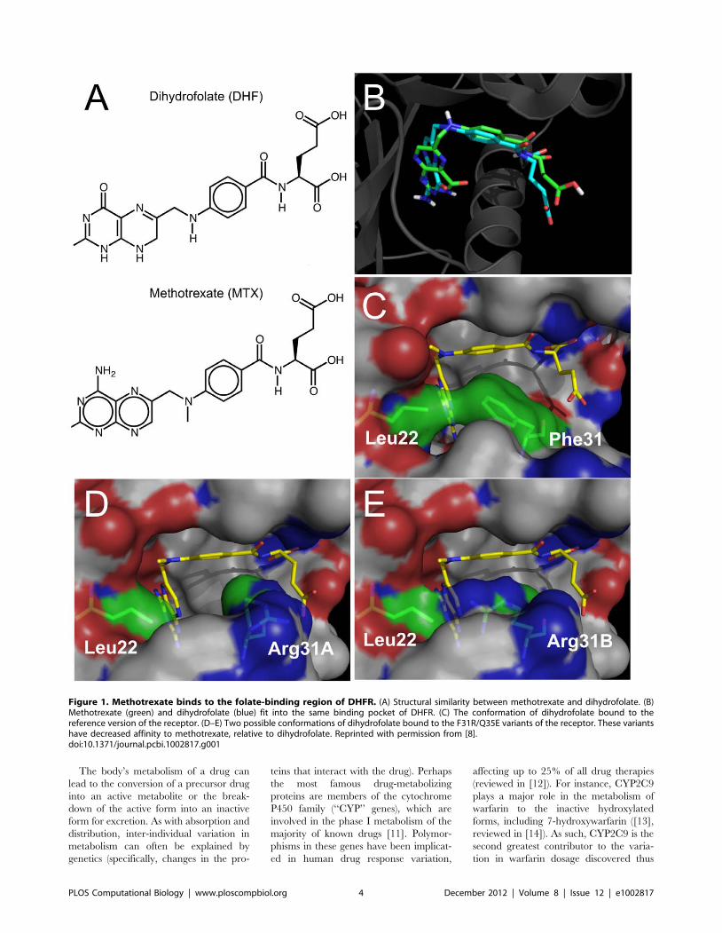
The body’s metabolism of a drug can
lead to the conversion of a precursor drug
into an active metabolite or the break-
down of the active form into an inactive
form for excretion. As with absorption and
distribution, inter-individual variation in
metabolism can often be explained by
genetics (specifically, changes in the pro-
teins that interact with the drug). Perhaps
the most famous drug-metabolizing
proteins are members of the cytochrome
P450 family (‘‘CYP’’ genes), which are
involved in the phase I metabolism of the
majority of known drugs [11]. Polymor-
phisms in these genes have been implicat-
ed in human drug response variation,
affecting up to 25% of all drug therapies
(reviewed in [12]). For instance, CYP2C9
plays a major role in the metabolism of
warfarin to the inactive hydroxylated
forms, including 7-hydroxywarfarin ([13],
reviewed in [14]). As such, CYP2C9 is the
second greatest contributor to the varia-
tion in warfarin dosage discovered thus
Figure 1. Methotrexate binds to the folate-binding region of DHFR. (A) Structural similarity between methotrexate and dihydrofolate. (B)Methotrexate (green) and dihydrofolate (blue) fit into the same binding pocket of DHFR. (C) The conformation of dihydrofolate bound to thereference version of the receptor. (D–E) Two possible conformations of dihydrofolate bound to the F31R/Q35E variants of the receptor. These variantshave decreased affinity to methotrexate, relative to dihydrofolate. Reprinted with permission from [8].doi:10.1371/journal.pcbi.1002817.g001
PLOS Computational Biology | www.ploscompbiol.org 4 December 2012 | Volume 8 | Issue 12 | e1002817
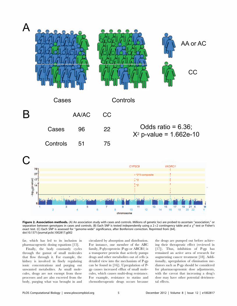
far, which has led to its inclusion in
pharmacogenetic dosing equations [15].
Finally, the body constantly cycles
through the gamut of small molecules
that flow through it. For example, the
kidney is involved in finely regulating
ionic concentrations and purging out
unwanted metabolites. As small mole-
cules, drugs are not exempt from these
processes and are also excreted from the
body, purging what was brought in and
circulated by absorption and distribution.
For instance, one member of the ABC
family, P-glycoprotein (P-gp or ABCB1) is
a transporter protein that actively pumps
drugs and other metabolites out of cells (a
detailed view into the mechanism of P-gp
can be found in [16]). Upregulation of P-
gp causes increased efflux of small mole-
cules, which causes multi-drug resistance.
For example, resistance to statins and
chemotherapeutic drugs occurs because
the drugs are pumped out before achiev-
ing their therapeutic effect (reviewed in
[17]). Thus, inhibition of P-gp has
remained an active area of research for
augmenting cancer treatment [18]. Addi-
tionally, upregulation of elimination me-
diators such as P-gp should be considered
for pharmacogenomic dose adjustments,
with the caveat that increasing a drug’s
dose may have other potential detrimen-
tal effects.
Figure 2. Association methods. (A) An association study with cases and controls. Millions of genetic loci are probed to ascertain ‘‘association,’’ orseparation between genotypes in cases and controls. (B) Each SNP is tested independently using a 262 contingency table and a x2 test or Fisher’sexact test. (C) Each SNP is assessed for ‘‘genome-wide’’ significance, after Bonferroni correction. Reprinted from [64].doi:10.1371/journal.pcbi.1002817.g002
PLOS Computational Biology | www.ploscompbiol.org 5 December 2012 | Volume 8 | Issue 12 | e1002817
2.2.2. Pharmacodynamic (PD)
interactions. Pharmacodynamics (PD)
encapsulates the specific effect of the
drug on its targets and downstream
pathways. The drug-target interactions
can be ‘‘on-target’’, where interactions
lead to a therapeutic effect, or ‘‘off-
target’’, where interactions lead to
undesired effects. PD also deals with how
a drug concentration affects the target –
what concentration is needed to reach the
maximum effect, beyond which additional
drug does not increase response (maximal
effect) and what concentration is required
to reach half of this maximal effect
(sensitivity).
In many cases, structurally similar
molecules (e.g. a drug that is similar to a
protein’s natural ligand) can bind and
affect the same region of a protein and
produce a pharmacological effect. For
instance, vitamin K and warfarin both
interact with VKORC1 (Vitamin K ep-
Oxide Reductase Complex subunit 1), an
enzyme that typically converts the inactive
epoxidized form of Vitamin K back to the
active reduced form [19]. Warfarin binds
to VKORC1 near its catalytic site (See
Figure 3 of [20]), inhibiting the reduction
reaction; the ensuing lack of active Vita-
min K results in the downstream anti-
coagulant effects of warfarin (See Figure 2
of [21] and below: Molecular and Physi-
ological Effects). Polymorphisms in
VKORC1 are intensely linked to the
efficacy of warfarin [22] by affecting
warfarin’s ability to bind to VKORC1
and displace vitamin K. As such, sensitiv-
ity to warfarin varies significantly in
individuals, leading to twenty-fold dose
differences. Warfarin’s optimal dose can
be better estimated by including
VKORC1 polymorphisms in a dosing
equation rather than using clinical factors
alone [15].
Often, a drug’s mechanism of action
involves its localization to some binding
pocket that then disrupts (or enhances) the
function of the protein. For example,
hydrocortisone is a lipid-soluble drug that
diffuses across the cell membrane and
interacts with the glucocorticoid receptors.
These receptors reside in an inactive
conformation because they are bound to
heat shock proteins, which hold the
glucocorticoid receptors in the inactive
state. The binding of hydrocortisone
causes the dissociation of the heat shock
protein and allows the DNA-binding and
transcription-activating binding domains
of the glucocorticoid receptor to enter an
active conformation. Now, target genes
can be transcribed, and the many anti-
inflammatory downstream effects of
hydrocortisone can occur (See Chapter 2
of [2]).
2.3. Propagation through PathwaysAs in the example of hydrocortisone,
once a drug affects a gene (whether ‘‘on-
target’’ or ‘‘off-target’’), the effects can
propagate through multiple proteins in the
same pathway. Biology does not occur in a
vacuum: proteins are dynamic and inter-
act with many other proteins to produce a
physiological function.
In the simplest cases, if the direct effect
of a drug is the inhibition of a functional
protein, all downstream effects of that
protein will be affected. For instance, if a
drug disrupts a kinase’s active site, all
downstream factors in a kinase cascade
would not be phosphorylated. As in the
case of hydrocortisone, a drug’s activation
of a transcription factor’s DNA-binding
domain will switch on the expression of
the transcription factor’s targets. These
downstream targets lead to many of the
biological effects of a given drug. Thus, a
variant in a pharmacogene may be
considerably upstream or downstream of
the drug’s direct protein interactions, but
still affect the action of the drug.
For instance, suppose protein A is
known to interact with proteins B and C.
When a drug is used to block protein A in
order to inhibit protein B’s downstream
effects, the interaction between proteins A
and C may also be affected. If protein A
and C’s interaction is essential for healthy
cellular function, administration of the
drug could lead to severe adverse events.
Most of the interactions discussed so far
comprise ‘‘on-target’’ effects (A and B),
while ‘‘innocent bystander’’ interactions (A
and C) are known as ‘‘off-target’’ events.
In other cases, the drug may exert an
effect on an unrelated protein D (that may,
for example, bear structural resemblance
to protein A).
2.4. Adverse Events (‘‘Off-Target’’)Drugs are designed for their therapeutic
effects, which require the molecule to bind
to one or more targets that then produce
downstream effects. Adverse events, how-
ever, can occur when the ‘‘on-target’’
interaction produces a potentially related,
but unintended effect, or when drugs bind
to ‘‘off-target’’ proteins to produce an
unrelated, unintended effect. Such effects
may be harmful to the patient, but may
occasionally be inadvertently helpful (see
below: Drug Repurposing). For instance,
this adverse event can occur due to the
intended interaction in an unintended
tissue: the b blockers used to treat heart
failure can also block b receptors in the
bronchial smooth muscle, causing bron-
chial spasm, a dangerous event for asth-
matics (See Chapter 13 of [2]). Another
example is tamoxifen, the selective estro-
gen receptor modulator (SERM), which
has improved outcomes in patients with
estrogen receptor positive breast cancers.
This drug antagonizes the estrogen recep-
tor in the breast, blocking one of the
signals that the cancer cells rely on.
However, tamoxifen also has agonist
activity at the estrogen receptors in
endometrial tissue. This off target action
can lead to a 2- to 7-fold increased risk of
endometrial cancer [23].
Alternatively, a drug may interact with
a protein (unrelated to the intended target)
to produce an ‘‘off-target’’ adverse event.
For example, in addition to the ‘‘on-
target’’ adverse events described above,
tamoxifen is also associated with cardiac
abnormalities and muscle cramping. Pre-
liminary data (discovered by docking
methods, see below: Cheminformatics)
suggest that these events may be due to
an ‘‘off-target’’ interaction with sarcoplas-
mic reticulum Ca2+ ion channel ATPase
protein (SERCA) [24].
2.5. Molecular and PhysiologicalEffects
A drug’s interaction with its target and
the downstream effects (through any of the
target’s pathways) leads to the alterations
in cellular physiology. In some cases, a
cellular ‘‘systemic’’ response may be acti-
vated or switched off, such as apoptosis or
inflammation. The cell may signal to other
cells to produce a larger response, which is
then observed in the larger context of the
body. For instance, warfarin’s inhibition of
VKORC1 slows the vitamin K-dependent
clotting pathway. This results in decreased
thrombus formation by platelets, or collo-
quially known as ‘‘blood thinning.’’ In
other cases, a drug may suppress a body’s
natural response. For instance, NSAIDs
such as aspirin and ibuprofen inhibit COX
proteins, preventing the conversion of
arachidonic acid to prostoglandin H2
(PGH2) and blocking the downstream
production of other prostoglandins, which
mediate inflammation and pain response.
While in the case of VKORC1, phar-
macogenomic variation is observed at the
direct site of action of warfarin, variation
in downstream receptors can also influ-
ence the effect of drugs on the body.
For instance, calumenin (CALU) is an
inhibitor of the vitamin K-dependent
clotting pathway. While calumenin’s ef-
fects are downstream of the direct inter-
action between VKORC1 and warfarin,
PLOS Computational Biology | www.ploscompbiol.org 6 December 2012 | Volume 8 | Issue 12 | e1002817
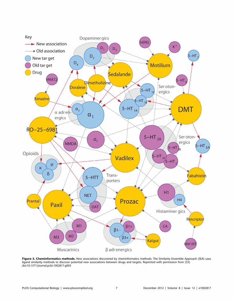
Figure 3. Cheminformatics methods. New associations discovered by cheminformatics methods. The Similarity Ensemble Approach (SEA) usesligand similarity methods to discover potential new associations between drugs and targets. Reprinted with permission from [33].doi:10.1371/journal.pcbi.1002817.g003
PLOS Computational Biology | www.ploscompbiol.org 7 December 2012 | Volume 8 | Issue 12 | e1002817
variants in calumenin are also associated
with differences in warfarin dosage [25].
3. Methods for Discovery ofPharmacogenomic Genes andVariants
Pharmacogenomic research aims to
identify the genes (and gene variants)
involved in the interaction between a drug
and the body. For any of the pharmaco-
genomic applications discussed below,
there exist methods for discovering rele-
vant genes and variants (typically single
nucleotide polymorphisms, or SNPs) relat-
ed to drug response. Traditional SNP-
based methods, such as genome wide
association studies (GWAS), can be used
to discover candidate regions of interest.
Alternatively, analysis of other sources of
data, including expression or biochemical
data, may provide additional gene candi-
dates. Once candidate variants are identi-
fied, further computational and experi-
mental follow-up may be required to fully
characterize all the genes and pathways
involved in the drug’s progression through
the body.
3.1. Association MethodsIn a GWAS, hundreds of thousands or
millions of SNPs (representing regions of
the genome with the most inter-individual
variation) are probed on a DNA micro-
array for each individual in a set of cases
and controls (Figure 2A). For each SNP,
significance of the association between a
SNP and the trait is measured a chi-
squared test, based on a 262 contingency
table of alleles (or genotypes, if a dominant
or recessive model is assumed) and case/
control status (Figure 2B). In the case of a
continuous independent variable, such as
drug dose, a likelihood-ratio test or a Wald
test is applied to measure whether there is
a significantly different dose between the
two groups of genotypes.
Each SNP is tested independently, and
thus significance (p-values) must be cor-
rected for multiple hypotheses, usually
using a Bonferroni correction or False
Discovery Rate (FDR). A SNP that
reaches ‘‘genome-wide significance’’
(Figure 2C) is then a candidate for
follow-up analysis, as are genes in or near
the significant SNP, genes for which the
SNP is an eQTL (a SNP associated with
the expression of some other gene), and
genes in the same pathway as these genes.
The two most important considerations
for the design of any pharmacogenomic
study include the selection of representa-
tive genetic markers, as well as phenotyp-
ically well-characterized patients (includ-
ing cases and controls). The first of these,
design of a suitable genotyping array, is
technically easy and inexpensive, though
the exact design can depend on the desired
balance between unbiased genome-wide
studies and a targeted SNP panel (see
below). As in any trait-association study,
the second consideration: the selection,
characterization, and covariate identifica-
tion of cases and controls provides a
significant challenge.
Because performing a million indepen-
dent tests requires stringent significance
correction, large numbers of cases and
controls, often in the thousands, are
required to discover a SNP that will
achieve ‘‘genome-wide’’ significance.
SNP-based GWAS methods are effective
when there is a strong signal from some
SNP for the size of the study (that is, when
there is good separation between geno-
types for the cases and controls). However,
under this stringent independence model,
weaker signals may be lost among the
noise that plagues genetic association
studies. Thus, combining data from mul-
tiple SNPs in a single gene can boost
power and decrease the number of
hypotheses for multiple hypothesis correc-
tion [26]. Alternatively, if we have prior
information about the drug’s mechanism
of action, we can create targeted SNP
panels, limited to genes in the drug target’s
pathway, to decrease the hypothesis space
[27].
As the price of high-throughput se-
quencing continues to fall, many investi-
gators are turning to exome or whole
genome sequencing to discover genetic
factors of drug response. Such technolo-
gies have the advantage of remaining
unbiased in SNP discovery, detecting less
common (and even personal) mutations,
and capturing larger-scale information,
including copy number variants (CNVs)
and structural variants (SVs).
Often, in major association studies, the
SNP platform (DNA microarray) used is
comprised of SNPs that serve as ‘‘tags’’ for
a larger stretch of nearby SNPs. Such an
approach is possible due to the presence of
‘‘linkage disequilibrium’’ in the genome, a
phenomenon where SNPs tend to be
inherited together (‘‘linked’’); the particu-
lar structure of these ‘‘haploblocks’’ (which
SNPs are typically inherited together) is
specific to each racial population. Because
different populations have different linkage
structures and a different series of poly-
morphisms, platforms that are optimized
for one population may not be the best
choice for another. This problem is further
complicated by underlying differences in
genomes: the effect a given SNP has on
drug response may be different (or even
the opposite) because of a hidden interac-
tion with an alternate variant of another
gene. Specifically, since many of the
original genotyping platforms were devel-
oped for Caucasian populations, studies
on Africans or Asians will require different
approaches. Additionally, the first SNP
identified is typically simply an ‘‘associat-
ed’’ variant, rather than the causative
variant. In order to determine the specific
proteins directly involved in drug re-
sponse, further experimental or informat-
ics analysis must be performed on genes
and variants ‘‘linked’’ to the associated
variant.
3.2. Expression MethodsIn addition, other sources of data can be
used to identify genes involved in drug
response, including RNA expression data
from microarrays or RNA-Seq experi-
ments from drug-treated samples. For
instance, using expression profiles from
patients with a disease of interest, one can
identify the genes involved in the progres-
sion of the disease and identify potential
drug target candidates. Alternatively, ex-
pression profiles generated from a drug
treated sample (compared to control) can
be used to determine a molecular response
to a drug. Ideally, such drug treatment
experiments would be done on humans in
order to generate organic in vivo physio-
logical response. However, such experi-
ments are unethical for experimental
(early phase) drugs, require significant
regulatory approval, and are expensive.
Thus, established cell lines have provided
a valuable, lower-cost resource for inves-
tigators to generate gene expression pro-
files.
One such effort, the connectivity map
(CMAP), a publicly available resource of
gene expression data of cell lines treated
with various small molecules, has been
used to compare expression profiles (See
Figure 1 of [28]) to identify metabolite-
protein interactions, small molecules with
similar binding profiles, and metabolites
that may mimic or suppress disease [28].
For instance, this approach predicted
gedunin to be an inhibitor of HSP90 due
to the similarity between gedunin’s ex-
pression profile and the profile of known
inhibitors. Despite the lack of structural
similarity between gedunin and other
HSP90 inhibitors, CMAP’s predicted re-
sult was validated biochemically.
Thus, cell lines can be used as surro-
gates for individuals, where a cellular
phenotype is used as a proxy for the
individual’s own physiological response
based on the cellular expression response
PLOS Computational Biology | www.ploscompbiol.org 8 December 2012 | Volume 8 | Issue 12 | e1002817
to a drug treatment. For instance, one can
search for associations between a cell line’s
genetic makeup and cell viability after
drug treatment (the IC50 of drug for each
cell lines) [29]. Alternatively, similar meth-
ods can be used to characterize toxicolog-
ical response: treating cell lines with a drug
and measuring gene expression can sug-
gest genes involved in the drug’s toxicity.
While not yet extensively employed in
practice, other sources of high-throughput
experimental ‘‘omics’’ data, such as meta-
bolomics or proteomics data could be used
for similar analyses.
3.3. Cheminformatics/NLP (OtherDiscovery Methods)
While not strictly ‘‘pharmacoge-
nomics’’ methods, cheminformatics has
provided a valuable tool for investigators
in the initial stages of drug discovery. For
instance, combining information about
protein structure and small molecule
structure, docking methods predict the
best fit of a molecule (or all molecules in
a database such as PubChem or
ChEMBL) by minimizing the conforma-
tion energy of the molecule-protein ‘‘fit’’.
Such methods are computationally ex-
pensive, as they explore a large search
space for each pair of molecule and
protein and use molecular dynamics or
genetic algorithms to optimize fits.
Therefore, molecule docking can be
limited to the active site of a protein
with a group of molecules to decrease the
search space. Alternatively, if a given
molecule is previously known to interact
with a protein, molecule similarity met-
rics can be included to suggest similar
molecules as protein-binding candidates.
In this way, a search limited to ligands
that score above a similarity threshold to
the known ligand would be much faster
than a search through all of PubChem.
While such predictions must still be
confirmed through biochemistry (such
as binding assays), these methods can
be used to limit the hypothesis space for
drug discovery, prioritizing the expen-
sive, lower-throughput biochemical as-
says.
For a potential drug target, cheminfor-
matics methods can be used to identify
new ‘‘hits’’ or optimize ‘‘leads’’ by sug-
gesting molecules that may disrupt the
function of the protein. For instance,
docking methods were used to successfully
identify novel molecules that could serve
as inhibitors of CTX-M b-lactamase at
millimolar binding affinities [30]. Various
algorithms have been developed for
screening ligand-target fits using docking
(reviewed in [31]). Additionally, methods
that incorporate the structure of the ligand
along with known interactions can identify
patterns of related drug targets [32]. Such
an approach can suggest new functions for
known drugs, explain ‘‘off-target’’ adverse
events, and importantly, predict ‘‘poly-
pharmacology,’’ or the action of a single
drug on multiple targets [33] (Figure 3).
These methods leverage small molecule
databases such as PubChem and
ChEMBL, which maintain structures and
properties of small molecules and ligands,
as well as bioassay results of these
compounds.
Additionally, a wealth of scientific
information is available in the biomedical
literature as lower-throughput free text.
Thus, text mining techniques such as
natural language processing (NLP), which
exploits sentence syntax to pull structured
knowledge from the literature, can be used
to mine PubMed and other sources of
published information to discover new
drug-protein interactions [34].
3.4. Pathway DiscoveryOnce a candidate gene is identified,
studying the gene’s known genetic net-
works, cascades, and pathways can help
identify other possible candidates that
affect drug action. For instance, if a kinase
is identified as a drug target, the proteins it
phosphorylates (and any proteins affected
downstream) may be relevant to the study
of the drug. Additionally, knowledge of
biological pathways influencing a disease
can aid in the drug discovery process (see
below: Drug Discovery).
Numerous online or downloadable re-
sources exist for pathway and network
analysis, such as Biocarta, Ingenuity,
KEGG, and PharmGKB. For a gene-drug
relationship of interest, information on the
gene’s network or pathway can be used to
limit the hypothesis space of other analyses
and experiments. Pathway analysis can
‘‘connect the dots’’ between known gene-
drug interactions to generate new hypoth-
eses of key genes that may also contribute
to the pharmacogenomics of the drug.
Additionally, a mechanism of action can
be formalized by closing the loop between
all the genes involved.
3.5. Validation and ApplicationThe methods discussed thus far provide
only computational evidence for potential
drug-protein interactions. In order to
prove drug-protein interactions and ef-
fects, follow-up biochemical methods, such
as measuring binding affinity or functional
assays, are required to demonstrate a
molecule’s potential therapeutic activity
or to definitively prove an interaction.
Ideally, multiple sources of evidence can
be integrated to fully characterize the
physiological response to a drug. Once
sufficient confidence is generated for a
potential pharmacogenomic mechanism,
the first step towards clinical application
involves the storage and dissemination of
the information in a curated database, such
as PharmGKB. Combining information
from multiple analyses will allow for more
powerful characterization of the pharmaco-
genomic response. For instance, dosing
equations for sensitive drugs such as warfarin
can be developed by multiple linear regres-
sion of variants (as well as clinical covariates)
on observed doses [15]. Finally, a centralized
resource such as PharmGKB will allow for
systematic pharmacogenomic analysis: such
as for automated annotation of an input of
genomic variants.
4. Pharmacogenomics in DrugDiscovery
Pharmacogenomics can impact how the
pharmaceutical industry develops drugs, as
early as the drug discovery process itself
(Figure 4). First, cheminformatics and path-
way analysis can aid in the discovery of
suitable gene targets, followed by small
molecules as ‘‘leads’’ for potential drugs.
Additionally, discovery of pharmacogenomic
variants for the design of clinical trials can
allow for safer, more successful passage of
drugs through the pharmaceutical pipeline.
4.1. Small Molecule CandidateIdentification
A key starting point in developing a drug
for illness or disease involves finding a suitable
gene to target. Typically, genes implicated in
a disease can be discovered by GWAS,
exome sequencing, analysis of RNA expres-
sion profiles, or other biochemical methods.
These genes and others in the same pathway
can be considered as candidate drug targets.
The potential target space could be limited by
excluding genes on the basis of their similarity
to other genes (possibly due to paralogy) to
avoid ‘‘off-target’’ effects.
Once potential gene or pathway targets
are identified, cheminformatics methods
can be used to generate predictions for
potential ‘‘leads’’ (or drug candidates) for
a high-throughput drug screen. For in-
stance, protein structure information can
be combined with small molecule struc-
ture information to predict favorable
drug-gene interactions. After such predic-
tions are generated, follow-up biochemi-
cal experiments would be required to
confirm the interaction before the small
molecules are considered further.
PLOS Computational Biology | www.ploscompbiol.org 9 December 2012 | Volume 8 | Issue 12 | e1002817
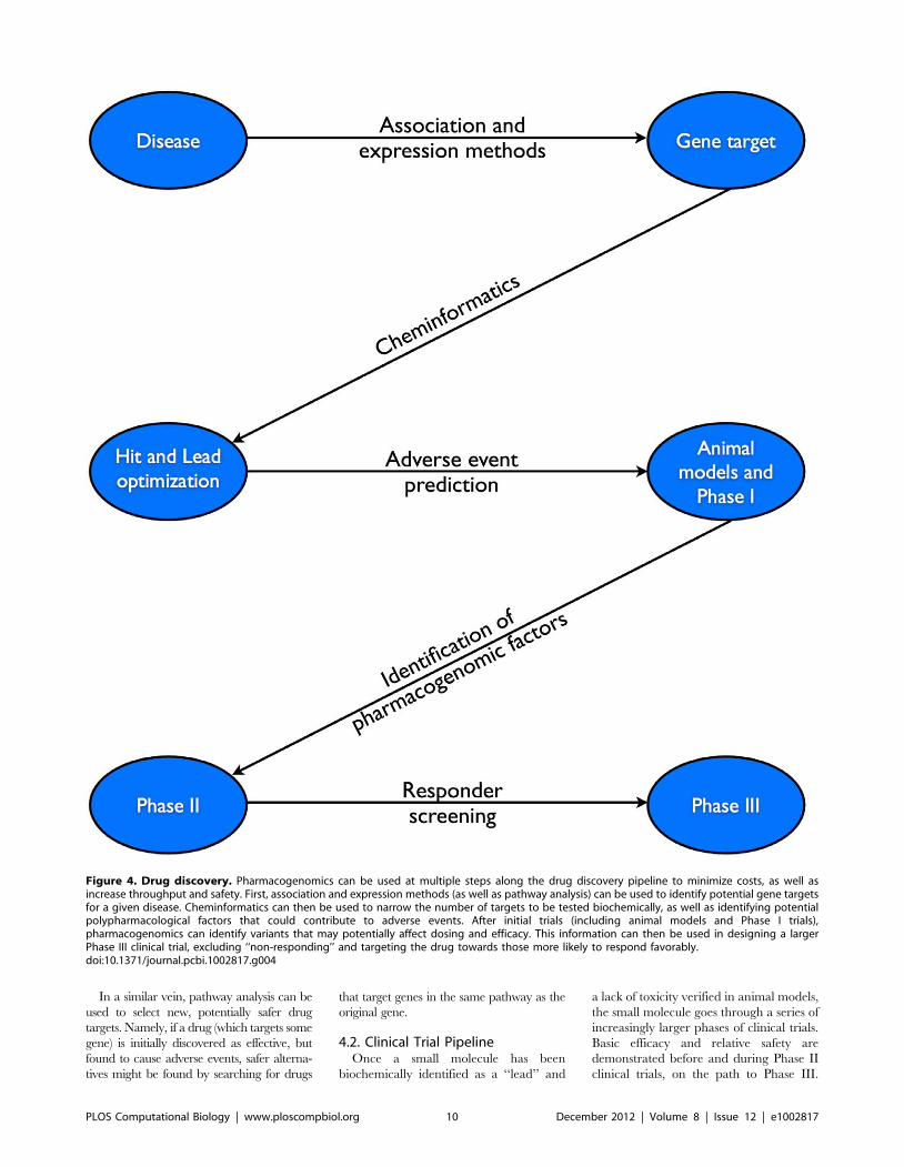
In a similar vein, pathway analysis can be
used to select new, potentially safer drug
targets. Namely, if a drug (which targets some
gene) is initially discovered as effective, but
found to cause adverse events, safer alterna-
tives might be found by searching for drugs
that target genes in the same pathway as the
original gene.
4.2. Clinical Trial PipelineOnce a small molecule has been
biochemically identified as a ‘‘lead’’ and
a lack of toxicity verified in animal models,
the small molecule goes through a series of
increasingly larger phases of clinical trials.
Basic efficacy and relative safety are
demonstrated before and during Phase II
clinical trials, on the path to Phase III.
Figure 4. Drug discovery. Pharmacogenomics can be used at multiple steps along the drug discovery pipeline to minimize costs, as well asincrease throughput and safety. First, association and expression methods (as well as pathway analysis) can be used to identify potential gene targetsfor a given disease. Cheminformatics can then be used to narrow the number of targets to be tested biochemically, as well as identifying potentialpolypharmacological factors that could contribute to adverse events. After initial trials (including animal models and Phase I trials),pharmacogenomics can identify variants that may potentially affect dosing and efficacy. This information can then be used in designing a largerPhase III clinical trial, excluding ‘‘non-responding’’ and targeting the drug towards those more likely to respond favorably.doi:10.1371/journal.pcbi.1002817.g004
PLOS Computational Biology | www.ploscompbiol.org 10 December 2012 | Volume 8 | Issue 12 | e1002817
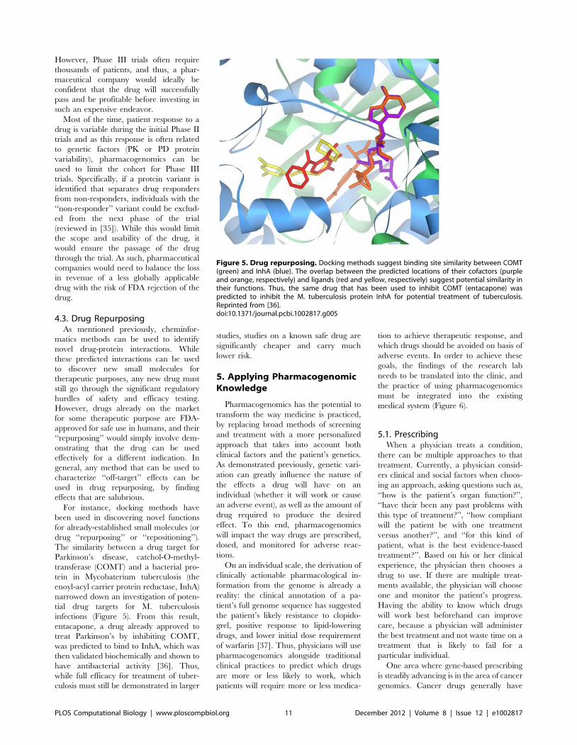
However, Phase III trials often require
thousands of patients, and thus, a phar-
maceutical company would ideally be
confident that the drug will successfully
pass and be profitable before investing in
such an expensive endeavor.
Most of the time, patient response to a
drug is variable during the initial Phase II
trials and as this response is often related
to genetic factors (PK or PD protein
variability), pharmacogenomics can be
used to limit the cohort for Phase III
trials. Specifically, if a protein variant is
identified that separates drug responders
from non-responders, individuals with the
‘‘non-responder’’ variant could be exclud-
ed from the next phase of the trial
(reviewed in [35]). While this would limit
the scope and usability of the drug, it
would ensure the passage of the drug
through the trial. As such, pharmaceutical
companies would need to balance the loss
in revenue of a less globally applicable
drug with the risk of FDA rejection of the
drug.
4.3. Drug RepurposingAs mentioned previously, cheminfor-
matics methods can be used to identify
novel drug-protein interactions. While
these predicted interactions can be used
to discover new small molecules for
therapeutic purposes, any new drug must
still go through the significant regulatory
hurdles of safety and efficacy testing.
However, drugs already on the market
for some therapeutic purpose are FDA-
approved for safe use in humans, and their
‘‘repurposing’’ would simply involve dem-
onstrating that the drug can be used
effectively for a different indication. In
general, any method that can be used to
characterize ‘‘off-target’’ effects can be
used in drug repurposing, by finding
effects that are salubrious.
For instance, docking methods have
been used in discovering novel functions
for already-established small molecules (or
drug ‘‘repurposing’’ or ‘‘repositioning’’).
The similarity between a drug target for
Parkinson’s disease, catchol-O-methyl-
transferase (COMT) and a bacterial pro-
tein in Mycobaterium tuberculosis (the
enoyl-acyl carrier protein reductase, InhA)
narrowed down an investigation of poten-
tial drug targets for M. tuberculosis
infections (Figure 5). From this result,
entacapone, a drug already approved to
treat Parkinson’s by inhibiting COMT,
was predicted to bind to InhA, which was
then validated biochemically and shown to
have antibacterial activity [36]. Thus,
while full efficacy for treatment of tuber-
culosis must still be demonstrated in larger
studies, studies on a known safe drug are
significantly cheaper and carry much
lower risk.
5. Applying PharmacogenomicKnowledge
Pharmacogenomics has the potential to
transform the way medicine is practiced,
by replacing broad methods of screening
and treatment with a more personalized
approach that takes into account both
clinical factors and the patient’s genetics.
As demonstrated previously, genetic vari-
ation can greatly influence the nature of
the effects a drug will have on an
individual (whether it will work or cause
an adverse event), as well as the amount of
drug required to produce the desired
effect. To this end, pharmacogenomics
will impact the way drugs are prescribed,
dosed, and monitored for adverse reac-
tions.
On an individual scale, the derivation of
clinically actionable pharmacological in-
formation from the genome is already a
reality: the clinical annotation of a pa-
tient’s full genome sequence has suggested
the patient’s likely resistance to clopido-
grel, positive response to lipid-lowering
drugs, and lower initial dose requirement
of warfarin [37]. Thus, physicians will use
pharmacogenomics alongside traditional
clinical practices to predict which drugs
are more or less likely to work, which
patients will require more or less medica-
tion to achieve therapeutic response, and
which drugs should be avoided on basis of
adverse events. In order to achieve these
goals, the findings of the research lab
needs to be translated into the clinic, and
the practice of using pharmacogenomics
must be integrated into the existing
medical system (Figure 6).
5.1. PrescribingWhen a physician treats a condition,
there can be multiple approaches to that
treatment. Currently, a physician consid-
ers clinical and social factors when choos-
ing an approach, asking questions such as,
‘‘how is the patient’s organ function?’’,
‘‘have their been any past problems with
this type of treatment?’’, ‘‘how compliant
will the patient be with one treatment
versus another?’’, and ‘‘for this kind of
patient, what is the best evidence-based
treatment?’’. Based on his or her clinical
experience, the physician then chooses a
drug to use. If there are multiple treat-
ments available, the physician will choose
one and monitor the patient’s progress.
Having the ability to know which drugs
will work best beforehand can improve
care, because a physician will administer
the best treatment and not waste time on a
treatment that is likely to fail for a
particular individual.
One area where gene-based prescribing
is steadily advancing is in the area of cancer
genomics. Cancer drugs generally have
Figure 5. Drug repurposing. Docking methods suggest binding site similarity between COMT(green) and InhA (blue). The overlap between the predicted locations of their cofactors (purpleand orange, respectively) and ligands (red and yellow, respectively) suggest potential similarity intheir functions. Thus, the same drug that has been used to inhibit COMT (entacapone) waspredicted to inhibit the M. tuberculosis protein InhA for potential treatment of tuberculosis.Reprinted from [36].doi:10.1371/journal.pcbi.1002817.g005
PLOS Computational Biology | www.ploscompbiol.org 11 December 2012 | Volume 8 | Issue 12 | e1002817
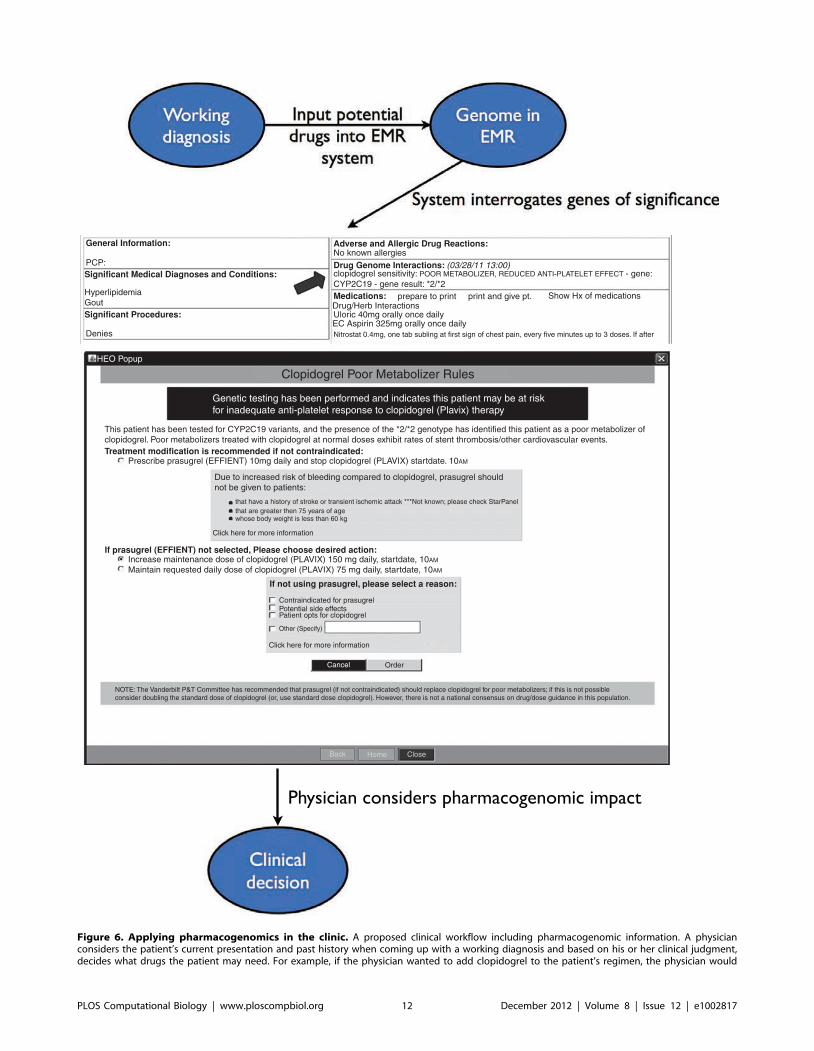
Figure 6. Applying pharmacogenomics in the clinic. A proposed clinical workflow including pharmacogenomic information. A physicianconsiders the patient’s current presentation and past history when coming up with a working diagnosis and based on his or her clinical judgment,decides what drugs the patient may need. For example, if the physician wanted to add clopidogrel to the patient’s regimen, the physician would
PLOS Computational Biology | www.ploscompbiol.org 12 December 2012 | Volume 8 | Issue 12 | e1002817
many toxic side effects, and in many cases
of advanced cancers, physicians ‘‘guess and
test’’ medications by prescribing them and
monitoring progress. In addition, the very
nature of cancer is ‘‘personal,’’ insofar as
each specific cancer is caused by the unique
sum of individual somatic mutations (that
is, mutations that occur in the individual
after birth and are not inherited or passed
on). Certain ‘‘signatures’’ of cancers, or
mutations that produce similar cancer
phenotypes, allow for the grouping of
cancers into distinctions, such as leukemia
or lymphoma, but even these exhibit
significant variability among classifications.
Thus, the ability to sequence and study the
genomes of cancer cells of an individual can
help identify the driving somatic mutations
and provide a tool for rational drug choice.
For example, the median survival for ad-
vanced or recurrent endometrial cancer is
very poor, due to the fact that physicians treat
empirically with chemotherapy, which may
have no therapeutic benefits. Researchers
studying mutations in the pathways of
endometrial cancer cell lines found that
response to doxorubicin, a chemotherapy
used to treat endometrial cancer, was related
to mutations in the Src pathways, which are
involved in cell proliferation, motility, and
survival. By pinpointing mutations in this
pathway, the researchers were able to
rationalize supplementing the drug regimen
with the addition of SU6656, a drug that
competitively inhibits the Src pathway, which
increased the sensitivity of some of the cell
lines to doxorubicin [38]. As cancers are
typically characterized by a lack of error-
correction mechanisms and inhibited apop-
tosis, such an approach is particularly
important, as the initial failure of a chemo-
therapeutic drug allows time for a cancer to
develop further mutations and spread further.
In the future, interrogating cancer genomes
could allow rational drug prescribing, de-
creasing the amount of time spent on
ineffective therapies and increasing the
number of successful cures.
Pharmacogenomics can also play a role in
drug decisions for prevalent conditions,
allowing physicians to predict when a
commonly successful therapy may fail. For
instance, there is an arsenal of drugs doctors
can use to combat the co-morbidities of type
II diabetes. These co-moribidities are usually
cardiac risk factors, such as lipid abnormal-
ities and high blood pressure: the cardiac risk
factor conferred by type II diabetes is
equivalent to that of a prior myocardial
infarction in a nondiabetic individual. Pres-
ently, the physician chooses drugs based on
his best clinical judgment and then monitors
the outcome of the treatment. However, as
the tolerance and efficacy of certain popularly
prescribed drugs has been shown to be tied to
genetics, such information could be used in
prescription decisions. For instance, statins
are a class of drugs that are inhibitors of
HMG-CoA reductase, an enzyme that helps
produce cholesterol in the liver. Thus, statins
are given in an effort to lower cholesterol,
particularly low-density lipoprotein (LDL)
cholesterol, whose increased levels are a
cardiac risk factor. Statins are often pre-
scribed to patients with type II diabetes and
high cholesterol in order to help them reach a
more healthy cholesterol range. Even though
studies have suggested genetic influences on
statin efficacy and tolerance, such findings are
not yet widely applied in clinical medicine.
One study found that in individuals with
diabetes, variation in the HMG-coA reduc-
tase gene was associated with a decreased
response to statin therapy. In this study, a
significantly greater percentage of individuals
heterozygous for the G minor allele of
rs17238540 were unable to reach target
cholesterol and triglyceride goals when
compared to individuals homozygous for
the major allele. Additionally, these individ-
uals had a 13% smaller reduction in total
cholesterol and a 27% smaller reduction in
triglycerides. This is an example of just one
variation in the HMG-coA gene; other
variations certainly exist and can impact
how well a patient responds to statins [39].
Another gene that has been found to affect
response to statins is the APOE gene, which is
associated with the regulation of total
cholesterol and LDL cholesterol. There are
several variants in this gene, and there are
differences between how type II diabetic
individuals carrying these variants respond to
statins. For instance, the individuals homo-
zygous for the E2 variant were all able to
reach their target LDL cholesterol; however
32% of individuals homozygous for the E4
variant failed to reach target LDL cholesterol.
Moreover, E2 variant homozygotes had a
significantly greater lipid lower response to
statins than some of the other variants. Thus,
APOE is another gene that may be predictive
of statin resistance or reduced efficacy.
Knowledge of these genes could play a role
in the future of drug prescribing, as physicians
would be able to predict a priori if a drug was
going to succeed or if another drug would be
a better choice [40].
One major caveat of gene-based pre-
scription decisions (as well as dosing, as
discussed below) involves the applicability
of a finding in one population to other
populations (see above: Association Meth-
ods). While a pharmacogenomic effect
may be true for a given population (with
a certain genetic background, in animal
model parlance), it may not directly apply
to other populations due to unknown
genetic factors, especially combinatorial
effects. Because there is no current stan-
dard for translating a result between
ethnicities, follow-up work is required for
each specific pharmacogenomic interac-
tion before it is applied in a clinical setting.
5.2. Adverse Drug ReactionsAnother factor physicians need to consider
when choosing a drug is the risk of adverse
events, or any detrimental, unintended
consequence of administering a drug at
indicated clinical doses. In a milder form,
an adverse event could be an allergic rash
from penicillin. These events can also be
much more intense: severe adverse drug
reactions (SADRs) are those that can cause
significant injury or even death, and are
estimated to occur in about 2 million patients
a year in the United States. In fact, SADRs
are the fourth leading cause of death in the
United States, with about 100,000 yearly
deaths. Because of the impact of SADRs,
scientists and physicians hope that the
application of pharmacogenomics can help
predict which patients are most susceptible to
experiencing an SADR to a given drug. With
this knowledge in hand, a physician can
either more closely monitor these patients or
choose an alternative therapy [41].
For instance, statins have been associated
with a rare but incredibly severe adverse
reaction: myopathy and rhabdomyolysis. A
study looking at the possible genetic influenc-
es of this reaction found a SNP in the
SLCO1B1 gene associated with this severe
adverse drug reaction, with an odds ratio of
4.5 [42]. However, there are also cases of
individuals who experience milder symptoms
and develop statin intolerance. Some of these
individuals experience an elevation in crea-
tine kinase or alanine aminotransferase while
on statins, indicating possible muscle or liver
damage. A recent study found that the
functional variants V174A and N130D in
the SLCO1B1 gene, which encodes the
input it into the electronic medical record (EMR). The EMR would interrogate the genome and present a message such as ‘‘clopidogrel sensitivity:POOR METABOLIZER, REDUCED ANTI-PLATELET EFFECT - gene: CYP2C19 - gene result *2/*2.’’ Based on this recommendation, the physician mayadjust the dose accordingly or choose another drug. In this case, the physician will likely increase the dose of clopidogrel in order to achievetherapeutic effect. Reprinted with permission from [65].doi:10.1371/journal.pcbi.1002817.g006
PLOS Computational Biology | www.ploscompbiol.org 13 December 2012 | Volume 8 | Issue 12 | e1002817
organic anion transporting polypeptide
OATP1B1, are predictive of statin intoler-
ance [43]. OATP1B1 in these individuals has
reduced maximal transport ability, possibly
leading to higher levels of statins in the
patient’s blood. Currently, studies are under-
way to determine if there is a difference
between the available statin drugs with
regards to these pharmacogenetic compo-
nents, in order to better inform physicians
about the drug choices they make.
In the effort of applying pharmacogenetics
in the clinic, trials have already shown that
screening tests have clinical utility. For
instance, abacavir, a nucleoside reverse-
transcriptase inhibitor used to treat AIDS,
causes a hypersensitivity reaction in 5 to 8%
of patients. This reaction can include fever,
rash, and gastrointestinal or respiratory
symptoms. Since this adverse reaction neces-
sitates stopping therapy (and patients cannot
be put on the drug again because of the risk of
a more severe reaction upon re-exposure),
physicians could avoid prescribing this drug if
they were capable of predicting which
individuals would have a reaction. Recently,
it was identified that HLA-B*5701 was
associated with hypersensitivity to abacavir.
Armed with this information, a double-blind,
randomized, prospective study in nearly 2000
patients was conducted to determine if
screening for this variant could help prevent
hypersensitivity reactions in AIDS patients.
The results supported the use of pharmaco-
genetics in the clinic: prescreening eliminated
immunologically confirmed hypersensitivity
reactions and significantly decreased hyper-
sensitivity symptoms, compared to the con-
trol group [44].
5.3. DosingOnce a physician has chosen a drug based
on efficacy and consideration of adverse
events, the next step is to determine what
the correct dose at which to administer the
drug. Currently, clinical factors such as
gender, weight, and kidney or liver function
may be taken into account when dosing a
medication. However, genetics can play a
large role in how a drug is dosed as well.
As mentioned previously, a major reason
drug doses differ between individuals is due to
polymorphisms in proteins involved in phar-
macokinetics or pharmacodynamics. Varia-
tion in enzymes involved in pharmacokinet-
ics, such as the Cytochrome P450 metabolic
enzymes (and mainly, CYP2D6, CYP2C9,
and CYP3A4), can affect the availability of
drugs reaching their targets. Alternatively, the
targets themselves (PD genes) can respond
differently based on their specific structure.
One of the emerging examples of dosing
based on genetics is the anticoagulant,
warfarin. Prescriptions for warfarin number
about 30 million cases annually and are
indicated to prevent myocardial infarction,
venous thrombosis, and cardioembolic
stroke. However, the dose needed to achieve
adequate anticoagulation can vary by as
much as twentyfold between patients. Cur-
rently, physicians start with an initial dose
and titrate (adjust) over time until the target
international normalized ratio (INR), an
indicator of anticoagulation, is reached.
However, until the therapeutic dose is
reached, there is the opportunity for over-
coagulation, which leads to an increased risk
of thromboembolic events, or under-dosing,
which can lead to ineffectiveness, and thus,
hemorrhaging and bleeding. The discovery
of variants affecting warfarin dosing have led
to the creation of algorithms that use clinical
(such as weight and other drug status) and
pharmacogenetic (variants in CYP2C9 and
VKORC1; see above, PK and PD Interac-
tions, respectively) information in order to
predict a patient’s optimal starting warfarin
dose. One such dosing algorithm, produced
by the International Warfarin Pharmacoge-
netic Consortium, was capable of predicting
doses using a pharmacogenetic algorithm at a
significantly more accurate rate than an
algorithm using clinical factors alone [15].
However, one of the drawbacks is that these
predictions are most accurate in a Caucasian
population; additional research is needed in
populations of different ancestries in order to
produce a more broad-spanning pharmaco-
genetic algorithm.
5.4. Applying Pharmacogenomics inthe Clinic
Though examples exist of how pharmaco-
genomics could impact prescribing drugs,
predicting adverse events, and dosing drugs,
the actual application of pharmacogenomics
is just beginning to gain traction. As
pharmacogenomics knowledge steadily in-
creases and the infrastructure for its usage
continually develops, the day when all
physicians regularly apply genetics to drug
dosing draws closer. The challenges that
remain include surmounting regulatory hur-
dles, developing ways to continually update
known findings, delivering knowledge to
physicians, and integrating genomics into
medicine. However, scientists have worked to
address these challenges, and pharmacoge-
nomics will likely serve as one of the first
major clinical applications of personalized
genomic medicine.
In the United States, the FDA regulates
drugs and drug labels. Therefore, the
communication between scientists and the
FDA will be critical to the adoption of
pharmacogenomic information on drug la-
bels. Evaluation will depend on the trial
design, sample size, reproducibility, and effect
size [45]. One benefit of pharmacogenomics
is that the associations between genetics and
drug effects is more concrete and immedi-
ately applicable than in other translational
bioinformatics concepts such as disease risk
assessment, where scientists are struggling
with ‘‘missing heritability’’ and combinations
of moderate risks. Because of this, unlike
other therapies, which require a randomized
clinical trial in order to prove efficacy, the
application of pharmacogenomic principles
may not require the same level of scrutiny.
Rather than providing some novel therapy,
the vast majority of pharmacogenomic
findings are simply supplementing physician
knowledge about previously approved drugs.
Physicians already utilize the clinical back-
grounds of their patients (i.e. weight, gender,
presumed organ function, drug interactions,
compliance) when making decisions about
drugs. As long as adding the variable of
genetic information is non-inferior to the
current standard of care, there should not be
resistance to its implementation [46].
Once a biomarker is shown to be
important, other decisions will have to be
made: Should testing for the biomarker be
required, or should it just be recommended?
Socio-economic considerations along with
the predictive value of the biomarker will
need to be considered. At first pass, the use of
pharmacogenomic data may be completely
left to the clinician’s judgment until the FDA
has formalized its role in their application.
Once a pharmacogenetic biomarker is ap-
proved, the drug’s label will need to reflect
the genetic components involved: biomarkers
identifying the patient population that should
receive the drug would be printed under
‘‘indication,’’ biomarkers related to drug
mechanism may appear under the ‘‘clinical
pharmacology’’ section, and biomarkers
related to safety may be indicated in ‘‘adverse
events.’’ The challenge for the FDA and
clinicians alike will require vigilance about
updating new information as the onslaught of
pharmacogenetic associations continues to
pour in [45].
Pharmacogenetic research continues to
discover new drug-gene interactions. The
volume of new findings exceeds the capabil-
ities of any individual to parse. Thus,
bioinformatics will have to play an integral
role in the translation of the data to the
bedside. Text mining (see Methods: Chemin-
formatics/NLP) will be instrumental to
extracting structured data from the literature
in order to update knowledge bases, such as
PharmGKB. Ultimately, this knowledge will
be integrated into a centralized database to
make the information accessible to all.
In order to fully translate pharmacoge-
nomics into the clinic, this information must
be well integrated with the electronic medical
PLOS Computational Biology | www.ploscompbiol.org 14 December 2012 | Volume 8 | Issue 12 | e1002817
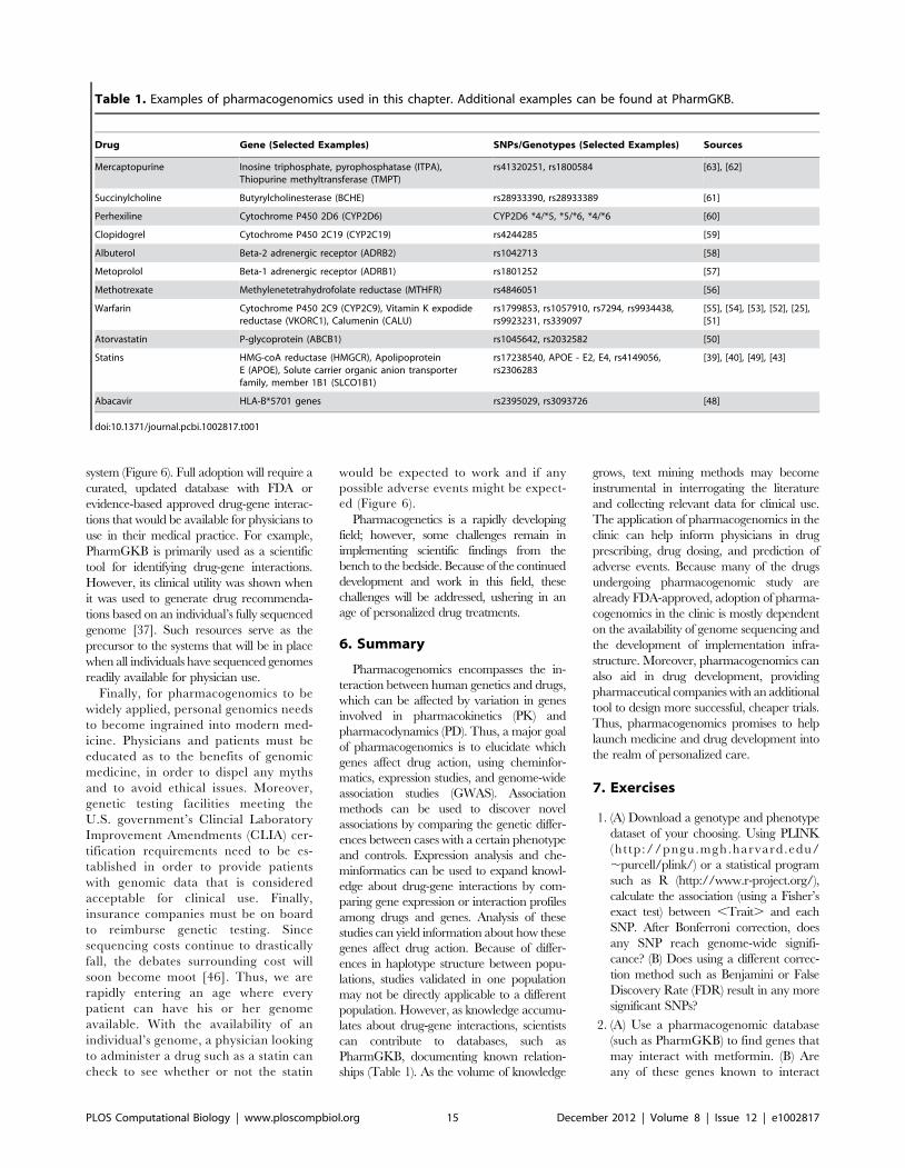
system (Figure 6). Full adoption will require a
curated, updated database with FDA or
evidence-based approved drug-gene interac-
tions that would be available for physicians to
use in their medical practice. For example,
PharmGKB is primarily used as a scientific
tool for identifying drug-gene interactions.
However, its clinical utility was shown when
it was used to generate drug recommenda-
tions based on an individual’s fully sequenced
genome [37]. Such resources serve as the
precursor to the systems that will be in place
when all individuals have sequenced genomes
readily available for physician use.
Finally, for pharmacogenomics to be
widely applied, personal genomics needs
to become ingrained into modern med-
icine. Physicians and patients must be
educated as to the benefits of genomic
medicine, in order to dispel any myths
and to avoid ethical issues. Moreover,
genetic testing facilities meeting the
U.S. government’s Clincial Laboratory
Improvement Amendments (CLIA) cer-
tification requirements need to be es-
tablished in order to provide patients
with genomic data that is considered
acceptable for clinical use. Finally,
insurance companies must be on board
to reimburse genetic testing. Since
sequencing costs continue to drastically
fall, the debates surrounding cost will
soon become moot [46]. Thus, we are
rapidly entering an age where every
patient can have his or her genome
available. With the availability of an
individual’s genome, a physician looking
to administer a drug such as a statin can
check to see whether or not the statin
would be expected to work and if any
possible adverse events might be expect-
ed (Figure 6).
Pharmacogenetics is a rapidly developing
field; however, some challenges remain in
implementing scientific findings from the
bench to the bedside. Because of the continued
development and work in this field, these
challenges will be addressed, ushering in an
age of personalized drug treatments.
6. Summary
Pharmacogenomics encompasses the in-
teraction between human genetics and drugs,
which can be affected by variation in genes
involved in pharmacokinetics (PK) and
pharmacodynamics (PD). Thus, a major goal
of pharmacogenomics is to elucidate which
genes affect drug action, using cheminfor-
matics, expression studies, and genome-wide
association studies (GWAS). Association
methods can be used to discover novel
associations by comparing the genetic differ-
ences between cases with a certain phenotype
and controls. Expression analysis and che-
minformatics can be used to expand knowl-
edge about drug-gene interactions by com-
paring gene expression or interaction profiles
among drugs and genes. Analysis of these
studies can yield information about how these
genes affect drug action. Because of differ-
ences in haplotype structure between popu-
lations, studies validated in one population
may not be directly applicable to a different
population. However, as knowledge accumu-
lates about drug-gene interactions, scientists
can contribute to databases, such as
PharmGKB, documenting known relation-
ships (Table 1). As the volume of knowledge
grows, text mining methods may become
instrumental in interrogating the literature
and collecting relevant data for clinical use.
The application of pharmacogenomics in the
clinic can help inform physicians in drug
prescribing, drug dosing, and prediction of
adverse events. Because many of the drugs
undergoing pharmacogenomic study are
already FDA-approved, adoption of pharma-
cogenomics in the clinic is mostly dependent
on the availability of genome sequencing and
the development of implementation infra-
structure. Moreover, pharmacogenomics can
also aid in drug development, providing
pharmaceutical companies with an additional
tool to design more successful, cheaper trials.
Thus, pharmacogenomics promises to help
launch medicine and drug development into
the realm of personalized care.
7. Exercises
1. (A) Download a genotype and phenotype
dataset of your choosing. Using PLINK
(http://pngu.mgh.harvard.edu/
,purcell/plink/) or a statistical program
such as R (http://www.r-project.org/),
calculate the association (using a Fisher’s
exact test) between ,Trait. and each
SNP. After Bonferroni correction, does
any SNP reach genome-wide signifi-
cance? (B) Does using a different correc-
tion method such as Benjamini or False
Discovery Rate (FDR) result in any more
significant SNPs?
2. (A) Use a pharmacogenomic database
(such as PharmGKB) to find genes that
may interact with metformin. (B) Are
any of these genes known to interact
Table 1. Examples of pharmacogenomics used in this chapter. Additional examples can be found at PharmGKB.
Drug Gene (Selected Examples) SNPs/Genotypes (Selected Examples) Sources
Mercaptopurine Inosine triphosphate, pyrophosphatase (ITPA),Thiopurine methyltransferase (TMPT)
rs41320251, rs1800584 [63], [62]
Succinylcholine Butyrylcholinesterase (BCHE) rs28933390, rs28933389 [61]
Perhexiline Cytochrome P450 2D6 (CYP2D6) CYP2D6 *4/*5, *5/*6, *4/*6 [60]
Clopidogrel Cytochrome P450 2C19 (CYP2C19) rs4244285 [59]
Albuterol Beta-2 adrenergic receptor (ADRB2) rs1042713 [58]
Metoprolol Beta-1 adrenergic receptor (ADRB1) rs1801252 [57]
Methotrexate Methylenetetrahydrofolate reductase (MTHFR) rs4846051 [56]
Warfarin Cytochrome P450 2C9 (CYP2C9), Vitamin K expodidereductase (VKORC1), Calumenin (CALU)
rs1799853, rs1057910, rs7294, rs9934438,rs9923231, rs339097
[55], [54], [53], [52], [25],[51]
Atorvastatin P-glycoprotein (ABCB1) rs1045642, rs2032582 [50]
Statins HMG-coA reductase (HMGCR), ApolipoproteinE (APOE), Solute carrier organic anion transporterfamily, member 1B1 (SLCO1B1)
rs17238540, APOE - E2, E4, rs4149056,rs2306283
[39], [40], [49], [43]
Abacavir HLA-B*5701 genes rs2395029, rs3093726 [48]
doi:10.1371/journal.pcbi.1002817.t001
PLOS Computational Biology | www.ploscompbiol.org 15 December 2012 | Volume 8 | Issue 12 | e1002817
with other drugs? Which drugs? (C)
Bonus question: Are any of these drugs
related (by structure or function) to
metformin?
3. (A) Implement a warfarin dosing
equation (e.g. the one found in [15]).
If you have a personal genotype, input
your information and calculate your
optimal starting warfarin dose; other-
wise, calculate the optimal dose (as
predicted by both the clinical and
pharmacogenetic algorithms) for a 66-
year old Caucasian (175 cm, 75 kg),
not taking amiodarone or enzyme
inhibitors, who is rs9923231 TT and
CYP2C9 *2/*2? (B) Would the clinical
algorithm have over- or under-estimated
his (or your) dose and what are the
potential consequences of such an error?
4. You are a physician and would like to
prescribe simvastatin. What parts of the
genome would you want interrogated to
know about prescribing this drug and
why?
5. Read about the clinical uses of a whole
genome or exome in healthy [37] and
diseased [47] individuals. How can
pharmacogenomics be directly applied
in a clinical setting?
Answers to the Exercises can be found
in Text S1.
Supporting Information
Text S1 Answers to Exercises.
(DOCX)
Glossary
N Adverse event - A ‘‘side effect,’’ or unintended consequence of taking a drug.
N Cheminformatics - Methods that utilize chemical structures of metabolites and/or protein structure to discover potentialdrug-gene interactions.
N Drug Target - The specific protein whose interaction with a drug constitutes that drug’s mechanism of action.
N (Gene) Expression - The relative amount of RNA from a gene in a cell at a given snapshot in time, often used as a proxy foractivity of the gene in the condition in which the experiment was performed.
N Hit - A small molecule that disrupts the function of a potential drug target (for treatment of a disease).
N Lead - An optimized (often chemically modified) ‘‘hit’’ with high specificity for its target and reasonable pharmacogenomicproperties.
N Linkage - The property that multiple SNPs are often inherited together. When a SNP is associated with a trait or disease, it isnot necessarily the causal SNP, but may be ‘‘linked’’ to other variation that is the molecular and physiological cause of theassociation.
N (DNA) Microarray - An experimental method that probes hundreds of thousands or millions of regions of the genome todetermine the genotype at each locus.
N ‘‘Off-target’’ effect - The effects of a drug propagated by interactions with proteins other than the drug target (‘‘innocentbystanders’’).
N ‘‘On-target’’ effect - The effects of a drug propagated by the intended interaction with the drug target.
N Pharmacodynamics - The mechanisms that relate to ‘‘what the drug does to the body,’’ including ‘‘on-target’’ and ‘‘off-target’’effects, intended and unintended, beneficial or harmful.
N Pharmacogenomics - The study and application of genetic factors relating to the body’s response to drugs.
N Pharmacokinetics - The range of mechanisms that relate to ‘‘what the body does to the drug,’’ including absorption,distribution, metabolism, and elimination of a drug.
N Polymorphism - A mutation in the genome that varies among individuals in a sizable fraction (often, minor allele frequency.0.01) of the population.
N Polypharmacology - The interaction of a drug with multiple targets.
N SADR - Severe Adverse Drug Reaction. An adverse event that results in significant injury or death.
N SNP - Single Nucleotide Polymorphism (see Polymorphism)
Further Reading
N Altman RB, Flockhart D, Goldstein DB (2012) Principles of pharmacogenetics and pharmacogenomics. Cambridge: CambridgeUniversity Press. 400 p.
N Altman RB, Kroemer HK, McCarty CA, Ratain MJ, Roden D (2010) Pharmacogenomics: will the promise be fulfilled? Nat RevGenet 12: 69–73.
N Altman RB (2011) Pharmacogenomics: ‘noninferiority’ is sufficient for initial implementation. Clin Pharmacol Ther 89: 348–350.
N Klein TE, Chang JT, Cho MK, Easton KL, Fergerson R, et al. (2001) Integrating genotype and phenotype information: anoverview of the PharmGKB project. Pharmacogenetics Research Network and Knowledge Base. Pharmacogenomics J 1: 167–170.
N Roses AD (2000) Pharmacogenetics and the practice of medicine. Nature 405: 857–865.
N Roses AD (2004) Pharmacogenetics and drug development: the path to safer and more effective drugs. Nat Rev Genet 5: 645–656.
PLOS Computational Biology | www.ploscompbiol.org 16 December 2012 | Volume 8 | Issue 12 | e1002817
References
1. Abbott A (2003) With your genes? Take one ofthese, three times a day. Nature 425: 760–762.
2. Katzung BG, Masters SB, and Trevor AJ (2012)
Basic & clinical pharmacology. New York:McGraw-Hill Medical.
3. Yu I-W, Bukaveckas BL (2008) Pharmacogenetic
tests in asthma therapy. Clin Lab Med 28: 645–665.
4. Azuma J, Nonen S (2009) Chronic heart failure:beta-blockers and pharmacogenetics. Eur J Clin
Pharmacol 65: 3–17.
5. Smith WL, DeWitt DL, Garavito RM (2000)Cyclooxygenases: structural, cellular, and molec-
ular biology. Annu Rev Biochem 69: 145–182.
6. Rome LH, Lands WE (1975) Structural require-ments for time-dependent inhibition of prosta-
glandin biosynthesis by anti-inflammatory drugs.
Proc Natl Acad Sci USA 72: 4863–4865.
7. DeWitt DL, el-Harith EA, Kraemer SA, Andrews
MJ, Yao EF, et al. (1990) The aspirin and heme-
binding sites of ovine and murine prostaglandinendoperoxide synthases. J Biol Chem 265: 5192–
5198.
8. Volpato JP, Yachnin BJ, Blanchet J, Guerrero V,Poulin L, et al. (2009) Multiple conformers in
active site of human dihydrofolate reductase
F31R/Q35E double mutant suggest structuralbasis for methotrexate resistance. J Biol Chem
284: 20079–20089.
9. Giacomini KM, Brett CM, Altman RB, BenowitzNL, Dolan ME, et al. (2007) The pharmacoge-
netics research network: from SNP discovery to
clinical drug response. Clin Pharmacol Ther. pp.328–345.
10. Dietrich CG, Geier A, Oude Elferink RPJ (2003)
ABC of oral bioavailability: transporters asgatekeepers in the gut. Gut 52: 1788–1795.
11. Evans WE, Relling MV (1999) Pharmacoge-
nomics: translating functional genomics intorational therapeutics. Science 286: 487–491.
12. Ingelman-Sundberg M, Sim SC, Gomez A,Rodriguez-Antona C (2007) Influence of cyto-
chrome P450 polymorphisms on drug therapies:
pharmacogenetic, pharmacoepigenetic and clini-cal aspects. Pharmacol Ther 116: 496–526.
13. Rettie AE, Korzekwa KR, Kunze KL, Lawrence
RF, Eddy AC, et al. (1992) Hydroxylation ofwarfarin by human cDNA-expressed cytochrome
P-450: a role for P-4502C9 in the etiology of (S)-
warfarin-drug interactions. Chem Res Toxicol 5:54–59.
14. Goldstein JA, de Morais SM (1994) Biochemistry
and molecular biology of the human CYP2Csubfamily. Pharmacogenetics. pp. 285–299.
15. Consortium IWP, Klein TE, Altman RB, Eriks-
son N, Gage BF, et al. (2009) Estimation of thewarfarin dose with clinical and pharmacogenetic
data. N Engl J Med 360: 753–764.
16. Jones PM, George AM (2004) The ABC trans-porter structure and mechanism: perspectives on
recent research. Cell Mol Life Sci 61: 682–699.
17. Leschziner GD, Andrew T, Pirmohamed M,Johnson MR (2007) ABCB1 genotype and PGP
expression, function and therapeutic drug re-
sponse: a critical review and recommendations forfuture research. Pharmacogenomics J 7: 154–179.
18. Thomas H, Coley HM (2003) Overcoming
multidrug resistance in cancer: an update on theclinical strategy of inhibiting p-glycoprotein.
Cancer Control 10: 159–165.
19. Zimmermann A, Matschiner JT (1974) Biochem-ical basis of hereditary resistance to warfarin in
the rat. Biochem Pharmacol 23: 1033–1040.
20. Oldenburg J, Watzka M, Rost S, Muller CR
(2007) VKORC1: molecular target of coumarins.
J Thromb Haemost 5 Suppl 1: 1–6.
21. Owen RP, Altman RB, Klein TE (2008)
PharmGKB and the International Warfarin
Pharmacogenetics Consortium: the changing rolefor pharmacogenomic databases and single-drug
pharmacogenetics. Human mutation 29: 456–460.
22. Rost S, Fregin A, Ivaskevicius V, Conzelmann E,
Hortnagel K, et al. (2004) Mutations in
VKORC1 cause warfarin resistance and multiple
coagulation factor deficiency type 2. Nature 427:
537–541.
23. Bland AE, Calingaert B, Secord AA, Lee PS,
Valea FA, et al. (2009) Relationship between
tamoxifen use and high risk endometrial cancer
histologic types. Gynecol Oncol 112: 150–154.
24. Xie L, Wang J, Bourne PE (2007) In silico
elucidation of the molecular mechanism definingthe adverse effect of selective estrogen receptor
modulators. PLoS Comput Biol 3: e217.
doi:10.1371/journal.pcbi.0030217
25. Voora D, Koboldt DC, King CR, Lenzini PA,
Eby CS, et al. (2010) A polymorphism in the
VKORC1 regulator calumenin predicts higher
warfarin dose requirements in African Americans.Clin Pharmacol Ther 87: 445–451.
26. Tatonetti NP, Dudley JT, Sagreiya H, Butte AJ,
Altman RB (2010) An integrative method for
scoring candidate genes from association studies:
application to warfarin dosing. BMC Bioinfor-
matics 11 Suppl 9: S9.
27. Thorn CF, Whirl-Carrillo M, Klein TE, Altman
RB (2007) Pathway-based approaches to phar-
macogenomics. Current Pharmacogenomics
5:79–86.
28. Lamb J, Crawford ED, Peck D, Modell JW, BlatIC, et al. (2006) The Connectivity Map: using
gene-expression signatures to connect small
molecules, genes, and disease. Science 313:
1929–1935.
29. Gamazon ER, Huang RS, Cox NJ, Dolan ME
(2010) Chemotherapeutic drug susceptibility as-
sociated SNPs are enriched in expression quan-
titative trait loci. Proc Natl Acad Sci USA 107:9287–9292.
30. Chen Y, Shoichet BK (2009) Molecular docking
and ligand specificity in fragment-based inhibitor
discovery. Nat Chem Biol 5: 358–364.
31. Kolb P, Ferreira RS, Irwin JJ, Shoichet BK (2009)
Docking and chemoinformatic screens for new
ligands and targets. Curr Opin Biotechnol 20:
429–436.
32. Keiser MJ, Roth BL, Armbruster BN, Ernsberger
P, Irwin JJ, et al. (2007) Relating protein
pharmacology by ligand chemistry. Nat Biotech-nol 25: 197–206.
33. Keiser MJ, Setola V, Irwin JJ, Laggner C, Abbas
AI, et al. (2009) Predicting new molecular targets
for known drugs. Nature 462: 175–181.
34. Garten Y, Coulet A, Altman RB (2010) Recent
progress in automatically extracting information
from the pharmacogenomic literature. Pharma-
cogenomics 11: 1467–1489.
35. Roses AD (2004) Pharmacogenetics and drug
development: the path to safer and more effective
drugs. Nat Rev Genet 5: 645–656.
36. Kinnings SL, Liu N, Buchmeier N, Tonge PJ, Xie
L, et al. (2009) Drug discovery using chemical
systems biology: repositioning the safe medicine
Comtan to treat multi-drug and extensively drug
resistant tuberculosis. PLoS Comput Biol 5:
e1000423. doi:10.1371/journal.pcbi.1000423
37. Ashley EA, Butte AJ, Wheeler MT, Chen R,
Klein TE, et al. (2010) Clinical assessment
incorporating a personal genome. Lancet 375:
1525–1535.
38. Indermaur MD, Xiong Y, Kamath SG, Boren T,
Hakam A, et al. (2010) Genomic-directed target-ed therapy increases endometrial cancer cell
sensitivity to doxorubicin. Am J Obstet Gynecol
203: 158.e151–140.
39. Donnelly LA, Doney ASF, Dannfald J, Whitley
AL, Lang CC, et al. (2008) A paucimorphic
variant in the HMG-CoA reductase gene is
associated with lipid-lowering response to statin
treatment in diabetes: a GoDARTS study.
Pharmacogenetics and Genomics 18: 1021–1026.
40. Donnelly LA, Palmer CNA, Whitley AL, Lang
CC, Doney ASF, et al. (2008) Apolipoprotein E
genotypes are associated with lipid-lowering
responses to statin treatment in diabetes: a Go-
DARTS study. Pharmacogenetics and Genomics
18: 279–287.
41. Giacomini KM, Krauss RM, Roden DM,
Eichelbaum M, Hayden MR, et al. (2007) When
good drugs go bad. Nature 446: 975–977.
42. Group SC, Link E, Parish S, Armitage J,
Bowman L, et al. (2008) SLCO1B1 variants and
statin-induced myopathy–a genomewide study.
N Engl J Med 359: 789–799.
43. Donnelly LA, Doney ASF, Tavendale R, Lang
CC, Pearson ER, et al. (2011) Common non-
synonymous substitutions in SLCO1B1 predis-
pose to statin intolerance in routinely treated
individuals with type 2 diabetes: a go-DARTS
study. Clin Pharmacol Ther 89: 210–216.
44. Mallal S, Phillips E, Carosi G, Molina J-M,
Workman C, et al. (2008) HLA-B*5701 screening
for hypersensitivity to abacavir. N Engl J Med
358: 568–579.
45. Surh LC, Pacanowski MA, Haga SB, Hobbs S,
Lesko LJ, et al. (2010) Learning from product
labels and label changes: how to build pharma-
cogenomics into drug-development programs.
Pharmacogenomics 11: 1637–1647.
46. Altman RB (2011) Pharmacogenomics: ‘noninfer-
iority’ is sufficient for initial implementation. Clin
Pharmacol Ther 89: 348–350.
47. Worthey EA, Mayer AN, Syverson GD, Helbling
D, Bonacci BB, et al. (2010) Making a definitive
diagnosis: Successful clinical application of whole
exome sequencing in a child with intractable
inflammatory bowel disease. Genetics in medicine
: official journal of the American College of
Medical Genetics.
48. Mallal S, Nolan D, Witt C, Masel G, Martin AM,
et al. (2002) Association between presence of
HLA-B*5701, HLA-DR7, and HLA-DQ3 and
hypersensitivity to HIV-1 reverse-transcriptase
inhibitor abacavir. Lancet 359: 727–732.
49. Link E, Parish S, Armitage J, Bowman L, Heath
S, et al. (2008) SLCO1B1 variants and statin-
induced myopathy–a genomewide study.
N Engl J Med 359: 789–799.
50. Rebecchi IM, Rodrigues AC, Arazi SS, Genvigir
FD, Willrich MA, et al. (2009) ABCB1 and
ABCC1 expression in peripheral mononuclear
cells is influenced by gene polymorphisms and
atorvastatin treatment. Biochem Pharmacol 77:
66–75.
51. Voora D, Koboldt DC, King CR, Lenzini PA,
Eby CS, et al. A polymorphism in the VKORC1
regulator calumenin predicts higher warfarin dose
requirements in African Americans. Clin Phar-
macol Ther 87: 445–451.
52. D’Andrea G, D’Ambrosio RL, Di Perna P,
Chetta M, Santacroce R, et al. (2005) A
polymorphism in the VKORC1 gene is associat-
ed with an interindividual variability in the dose-
anticoagulant effect of warfarin. Blood 105: 645–
649.
53. Aithal GP, Day CP, Kesteven PJ, Daly AK (1999)
Association of polymorphisms in the cytochrome
P450 CYP2C9 with warfarin dose requirement
and risk of bleeding complications. Lancet 353:
717–719.
54. Rettie AE, Wienkers LC, Gonzalez FJ, Trager
WF, Korzekwa KR (1994) Impaired (S)-warfarin
metabolism catalysed by the R144C allelic
variant of CYP2C9. Pharmacogenetics 4: 39–42.
55. Crespi CL, Miller VP (1997) The R144C change
in the CYP2C9*2 allele alters interaction of the
cytochrome P450 with NADPH:cytochrome
P450 oxidoreductase. Pharmacogenetics 7: 203–
210.
PLOS Computational Biology | www.ploscompbiol.org 17 December 2012 | Volume 8 | Issue 12 | e1002817
56. Hughes LB, Beasley TM, Patel H, Tiwari HK,
Morgan SL, et al. (2006) Racial or ethnicdifferences in allele frequencies of single-nucleo-
tide polymorphisms in the methylenetetrahydro-
folate reductase gene and their influence onresponse to methotrexate in rheumatoid arthritis.
Ann Rheum Dis 65: 1213–1218.57. Johnson JA, Zineh I, Puckett BJ, McGorray SP,
Yarandi HN, et al. (2003) Beta 1-adrenergic
receptor polymorphisms and antihypertensiveresponse to metoprolol. Clin Pharmacol Ther
74: 44–52.58. Israel E, Chinchilli VM, Ford JG, Boushey HA,
Cherniack R, et al. (2004) Use of regularlyscheduled albuterol treatment in asthma: geno-
type-stratified, randomised, placebo-controlled
cross-over trial. Lancet 364: 1505–1512.59. Shuldiner AR, O’Connell JR, Bliden KP, Gandhi
A, Ryan K, et al. (2009) Association of cyto-
chrome P450 2C19 genotype with the antiplatelet
effect and clinical efficacy of clopidogrel therapy.JAMA 302: 849–857.
60. Barclay ML, Sawyers SM, Begg EJ, Zhang M,
Roberts RL, et al. (2003) Correlation of CYP2D6genotype with perhexiline phenotypic metaboliz-
er status. Pharmacogenetics 13: 627–632.61. Nogueira CP, Bartels CF, McGuire MC, Adkins
S, Lubrano T, et al. (1992) Identification of two
different point mutations associated with thefluoride-resistant phenotype for human butyr-
ylcholinesterase. Am J Hum Genet 51: 821–828.
62. Otterness DM, Szumlanski CL, Wood TC,Weinshilboum RM (1998) Human thiopurine
methyltransferase pharmacogenetics. Kindred
with a terminal exon splice junction mutationthat results in loss of activity. J Clin Invest 101:
1036–1044.
63. Stocco G, Cheok MH, Crews KR, Dervieux T,
French D, et al. (2009) Genetic polymorphism of
inosine triphosphate pyrophosphatase is a deter-
minant of mercaptopurine metabolism and tox-
icity during treatment for acute lymphoblastic
leukemia. Clin Pharmacol Ther 85: 164–172.
64. Takeuchi F, McGinnis R, Bourgeois S, Barnes C,
Eriksson N, et al. (2009) A genome-wide associ-
ation study confirms VKORC1, CYP2C9, and
CYP4F2 as principal genetic determinants of
warfarin dose. PLoS Genet 5: e1000433.
doi:10.1371/journal.pgen.1000433
65. Pulley JM, Denny JC, Peterson JF, Bernard GR,
Vnencak-Jones CL, et al. (2012) Operational
implementation of prospective genotyping for
personalized medicine: the design of the Vander-
bilt PREDICT project. Clin Pharmacol Ther 92:
87–95.
PLOS Computational Biology | www.ploscompbiol.org 18 December 2012 | Volume 8 | Issue 12 | e1002817
Education
Chapter 8: Biological Knowledge Assembly andInterpretationJu Han Kim1,2,3*
1 Division of Biomedical Informatics, Seoul National University College of Medicine, Seoul, Korea, 2 Seoul National University Biomedical Informatics (SNUBI), Seoul
National University College of Medicine, Seoul, Korea, 3 Systems Biomedical Informatics National Core Research Center (SBI-NCRC), Seoul National University College of
Medicine, Seoul, Korea
Abstract: Most methods for large-scale gene expression microarrayand RNA-Seq data analysis are de-signed to determine the lists ofgenes or gene products that showdistinct patterns and/or significantdifferences. The most challengingand rate-liming step, however, is todetermine what the resulting lists ofgenes and/or transcripts biologicallymean. Biomedical ontology andpathway-based functional enrich-ment analysis is widely used tointerpret the functional role of tightlycorrelated or differentially expressedgenes. The groups of genes areassigned to the associated biologicalannotations using Gene Ontologyterms or biological pathways andthen tested if they are significantlyenriched with the correspondingannotations. Unlike previous ap-proaches, Gene Set Enrichment Anal-ysis takes quite the reverse approachby using pre-defined gene sets.Differential co-expression analysisdetermines the degree of co-expres-sion difference of paired gene setsacross different conditions. Out-comes in DNA microarray and RNA-Seq data can be transformed into thegraphical structure that representsbiological semantics. A number ofbiomedical annotation and externalrepositories including clinical re-sources can be systematically inte-grated by biological semantics with-in the framework of concept latticeanalysis. This array of methods forbiological knowledge assembly andinterpretation has been developedduring the past decade and clearlyimproved our biological understand-ing of large-scale genomic data fromthe high-throughput technologies.
This article is part of the ‘‘Transla-
tional Bioinformatics’’ collection for
PLOS Computational Biology.
1. Introduction
One of the challenges in DNA micro-
array and RNA-Seq data analysis is to
extract biological meanings from the mas-
sive amounts of transcriptome expression
data. Most of the microarray and RNA-Seq
data analysis methods are designed to
determine the lists of genes or gene
products that show distinct patterns and/
or significant differences. Clustering and
differential expression analysis, for exam-
ple, typically generate lists of ‘significantly’
clustered and Differentially Expressed
Genes (DEGs), respectively. The most
challenging and rate-liming step, however,
is to determine what the resulting lists of
genes or gene products biologically mean.
The first analytic approach for the
biological interpretation of obtained gene
lists was to manually collect and put down
all available descriptive information con-
cerning each gene next to it and to try to
infer the collective meaning of the textual
descriptors for the group of genes under the
biological systems context. The assumption
here is that if a certain keyword is
significantly over-represented or a mean-
ingful pattern is found among the textual
descriptors for a gene group, then the
keyword or the pattern can be regarded as
the semantic interpretation of the gene
group.
It seems that Tavazoie et al. [1] was first to
formally analyze the over-representation of
‘functional annotations’ for the lists of genes
with semantic interpretations. By means of
partitional clustering and motif discovery,
given genome-wide gene-expression clusters,
he analyzed significantly over-represented
regulatory motifs in the upstream sequences
of clustered yeast genes for uncovering new
‘regulons’ (i.e., sets of co-regulated genes)
and their putative cis-regulatory elements.
Here, the discovered motifs seem to be
regarded as functional annotations to the
corresponding genes. Many Functional An-
notation Analysis (FAA) methods have been
developed to test whether certain Gene
Ontology (GO) terms [2] or biological
pathways are significantly enriched within
a particular list of genes. Many GO and
biological pathway-based tools for gene
expression analysis have been developed
and proven to be useful [3–9].
FAA is an attempt to extract biological
semantics from given lists of genes that are
determined without considering any bio-
logical meaning but by a quantitative
statistical analysis like clustering and
DEG analysis methods. Gene Set Enrich-
ment Analysis (GSEA) [10,11], however,
takes quite the reverse way. GSEA uses
pre-defined gene sets with a priori estab-
lished biological meanings like biological
pathways. For each pre-defined gene set,
GSEA tries to determine if it shows
significant expression change. Therefore,
what GSEA essentially tests is if the pre-
defined ‘biological meaning’ assigned to
the gene set shows significant change or
not. It has been successfully demonstrated
that GSEA can successfully detect subtle
but set-wise coordinated expression chang-
es that cannot be detected by individual
gene tests [10].
The gene-set approach greatly improves
biological interpretability by using pre-
defined gene sets with established biological
meanings. The same strategy can be applied
Citation: Kim JH (2012) Chapter 8: Biological Knowledge Assembly and Interpretation. PLoS Comput Biol 8(12):e1002858. doi:10.1371/journal.pcbi.1002858
Editors: Fran Lewitter, Whitehead Institute, United States of America and Maricel Kann, University of Maryland,Baltimore County, United States of America
Published December , 2012
Copyright: � 2012 Ju Han Kim. This is an open-access article distributed under the terms of the CreativeCommons Attribution License, which permits unrestricted use, distribution, and reproduction in any medium,provided the original author and source are credited.
Funding: This work was supported by the basic science research program through the National ResearchFoundation of Korea (NRF) funded by the Ministry of Education, Science and Technology (2010-0028631). Thefunders had no role in the preparation of the manuscript.
Competing Interests: The author has declared that no competing interests exist.
* E-mail: [email protected]
PLOS Computational Biology | www.ploscompbiol.org 1 December 2012 | Volume 8 | Issue 12 | e1002858
27
for the analysis of differential co-expression
analysis. Cho et al. proposed dCoxS algo-
rithm that determines if a pair of gene sets’
coordinated co-expression patterns shows
significant changes across different condi-
tions [12]. If a pair of gene sets (or pathways)
shows a positive co-expression pattern in
normal tissue but a negative co-expression
pattern in cancer cells, then it can be
assumed that the pair of gene sets may play
an important role in the cancerous trans-
formation. This dyadic relation can easily
be extended to create a network of gene sets
showing differential co-expression patterns
across different conditions.
Sometimes, given the genomic scale,
even the extracted list of biological mean-
ings and significant functional annotations
are too big and complex such that they
need to be systematically organized. Or-
dering of obtained semantics using con-
cept lattice analysis improves biological
interpretation of microarray gene-expres-
sion data. BioLattice considers gene ex-
pression clusters as objects and annota-
tions as attributes and provides a graphical
‘executive summary’ (i.e. the context of the
whole experiment) of the order relations
by arranging them on a concept lattice in
an order based on the set inclusion theory
[13].
A wide range of tools and resources in
microarray and RNA-Seq data analysis
have a potential impact on personalized
medicine and are invaluable in biomedical
research. Integrative analysis of heteroge-
neous biological and clinical data is
essential to discover meaningful knowl-
edge. The construction of semantic rela-
tionships of biological resources makes it
possible to unify multi-layered and hetero-
geneously formatted data from genome to
phenome. Semantic analysis integrating
gene expression profiles and annotations
into a unified framework enables us to
interpret complex biomedical data in a
comprehensive and organized fashion.
The outline for this chapter is as follows.
In Section 2, a comprehensive survey of
biomedical annotation resources will be
given with major ontology and biological
pathway-based analysis methods. Section
3 describes gene set-wise differential ex-
pression analysis methods with its semantic
interpretation power. Section 4 describes
differential co-expression analysis. Finally,
in Section 5, application of formal concept
analysis for systematic semantic interpre-
tation of gene expression profiles will be
introduced with the following summary in
section 6.
2. Pathway and Ontology-BasedAnalysis
GO and biological pathway-based anal-
ysis is one of the most powerful methods for
inferring the biological meanings of ob-
served expression changes (Figure 1). It
enables us to analyze a list of interesting
genes resulting from microarray and RNA-
Seq experiments, without molecular biolo-
gist’s help. The genes in the list may be the
ones statistically significantly up or down
regulated between conditions (i.e. DEGs),
where the number of the genes belong to a
list depends on the threshold of signifi-
cance. Another method is to perform a co-
expression (or clustering) analysis grouping
genes with similar expression patterns
across different experimental conditions.
Many genome databases provide GO
annotations to their genes and gene prod-
ucts, which are also members of biological
pathways. FAA determines which biological
pathways or GO terms are significantly
overrepresented in a given list of genes. GO
annotation and pathway membership fre-
quencies for a list of genes obtained by
differential expression analysis (Figure 1 (a))
or co-expression analysis (or clustering)
(Figure 1 (b)) are input to statistical analyses
to test if they are significantly over-repre-
sented. For example, in Figure 1, the genes
in the gene list (i.e. selected genes) are
significantly enriched with a GO term,
GO:000123, but not with GO:000126. It
means that the genes are significantly
associated with the biological meaning of
the GO term, GO:000123.
In principle, any attribute of a gene can
be applied for FAA including transcription
factor binding sites [1], clinical phenotypes
like disease associations, MeSH (Medical
Subject Heading) terms, microRNA bind-
ing sites, protein family memberships,
chromosomal bands, etc. as well as GO
terms and biological pathways. Moreover,
these features may in turn have their own
ontological structures as illustrated in
Figure 2. GO and MeSH have a ‘tree-
ish’ graph structure, which is more
formally a DAG (Directed Acyclic Graph),
in which each term may be a child of one
or more parents. Pathways have directed
graph structures. Clusters may also be
organized into a hierarchical tree or a
graph structure. ArrayXPath [6,9] pro-
vides one of the most comprehensive
collections of these structured features for
annotation analysis [14].
Differential expression analysis deter-
mines significantly down- or up-regulated
genes (or DEGs) between two conditions,
i.e. control and treatment groups to
explore the effect of a drug. Student’s t-
test, Wilcoxon’s rank sum test and AN-
OVA may be applied to detect DEGs.
Given the huge number of genes to be
tested, multiple-hypothesis-testing prob-
lem should be properly managed. Co-
expression analysis puts similar expression
profiles together and different ones apart,
returning lists of co-expressed genes that
are assumed to be tightly co-regulated.
Clustering algorithms can be classified into
hierarchical-tree clustering and partitional
clustering. While some partitional cluster-
ing algorithms do not impose a structure
to the clusters, others like Self Organizing
Feature Maps (SOM) organize clusters
into a grid structure. Imposing a structure
based on cluster similarity may be per-
formed after clustering.
Although DEGs are different from
clusters, biological interpretation of the
resulting lists of significantly up- or down-
regulated DEGs (Figure 1(a)) may also be
benefited by the same ontology and
pathway-based annotation analysis. Clus-
What to Learn in This Chapter
N How to find genes associated with a particular disease (or condition) frommicroarray or RNA-Seq data
N How to find biological pathways and/or biomedical ontology terms for theinterpretation of particular gene groups associated with a particular disease
N How to characterize biological properties of a particular list of genes
N Which data resources are useful for interpreting large-scale gene expressionprofiles
N What are the limitations of individual gene-based analysis for determiningdifferentially expressed genes (even with multiple hypothesis correction)
N How to identify gene groups that are differentially expressed or differentiallyco-expressed between normal and disease samples
N Compare in terms of semantic interpretation the functional annotation analysismethods for co-expressed genes as in clustering and for pre-defined gene setsas in GSEA
N How to organize and visualize a massive and redundant annotation list of genesor gene sets into a unified framework of biological understanding
PLOS Computational Biology | www.ploscompbiol.org 2 December 2012 | Volume 8 | Issue 12 | e1002858
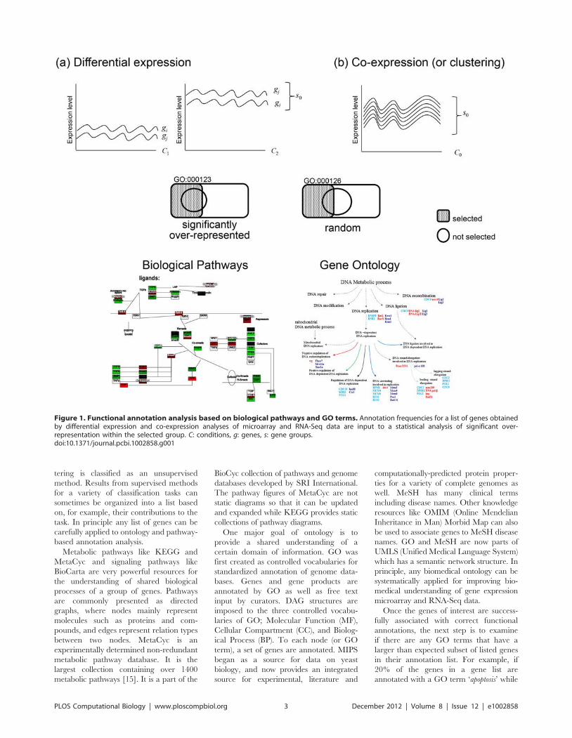
tering is classified as an unsupervised
method. Results from supervised methods
for a variety of classification tasks can
sometimes be organized into a list based
on, for example, their contributions to the
task. In principle any list of genes can be
carefully applied to ontology and pathway-
based annotation analysis.
Metabolic pathways like KEGG and
MetaCyc and signaling pathways like
BioCarta are very powerful resources for
the understanding of shared biological
processes of a group of genes. Pathways
are commonly presented as directed
graphs, where nodes mainly represent
molecules such as proteins and com-
pounds, and edges represent relation types
between two nodes. MetaCyc is an
experimentally determined non-redundant
metabolic pathway database. It is the
largest collection containing over 1400
metabolic pathways [15]. It is a part of the
BioCyc collection of pathways and genome
databases developed by SRI International.
The pathway figures of MetaCyc are not
static diagrams so that it can be updated
and expanded while KEGG provides static
collections of pathway diagrams.
One major goal of ontology is to
provide a shared understanding of a
certain domain of information. GO was
first created as controlled vocabularies for
standardized annotation of genome data-
bases. Genes and gene products are
annotated by GO as well as free text
input by curators. DAG structures are
imposed to the three controlled vocabu-
laries of GO; Molecular Function (MF),
Cellular Compartment (CC), and Biolog-
ical Process (BP). To each node (or GO
term), a set of genes are annotated. MIPS
began as a source for data on yeast
biology, and now provides an integrated
source for experimental, literature and
computationally-predicted protein proper-
ties for a variety of complete genomes as
well. MeSH has many clinical terms
including disease names. Other knowledge
resources like OMIM (Online Mendelian
Inheritance in Man) Morbid Map can also
be used to associate genes to MeSH disease
names. GO and MeSH are now parts of
UMLS (Unified Medical Language System)
which has a semantic network structure. In
principle, any biomedical ontology can be
systematically applied for improving bio-
medical understanding of gene expression
microarray and RNA-Seq data.
Once the genes of interest are success-
fully associated with correct functional
annotations, the next step is to examine
if there are any GO terms that have a
larger than expected subset of listed genes
in their annotation list. For example, if
20% of the genes in a gene list are
annotated with a GO term ‘apoptosis’ while
Figure 1. Functional annotation analysis based on biological pathways and GO terms. Annotation frequencies for a list of genes obtainedby differential expression and co-expression analyses of microarray and RNA-Seq data are input to a statistical analysis of significant over-representation within the selected group. C: conditions, g: genes, s: gene groups.doi:10.1371/journal.pcbi.1002858.g001
PLOS Computational Biology | www.ploscompbiol.org 3 December 2012 | Volume 8 | Issue 12 | e1002858
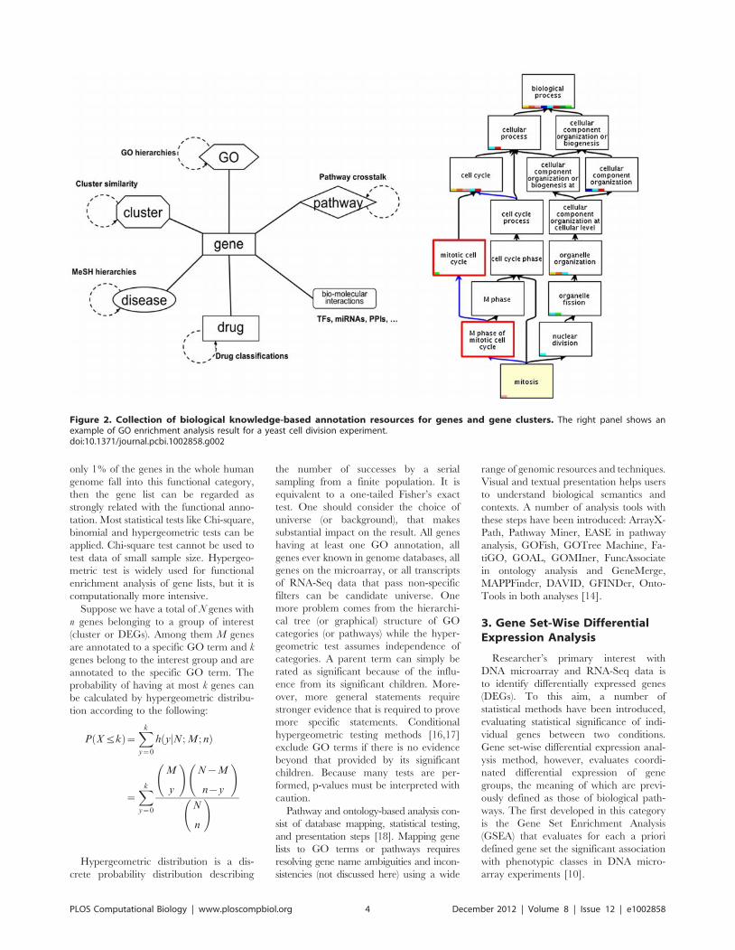
only 1% of the genes in the whole human
genome fall into this functional category,
then the gene list can be regarded as
strongly related with the functional anno-
tation. Most statistical tests like Chi-square,
binomial and hypergeometric tests can be
applied. Chi-square test cannot be used to
test data of small sample size. Hypergeo-
metric test is widely used for functional
enrichment analysis of gene lists, but it is
computationally more intensive.
Suppose we have a total of N genes with
n genes belonging to a group of interest
(cluster or DEGs). Among them M genes
are annotated to a specific GO term and k
genes belong to the interest group and are
annotated to the specific GO term. The
probability of having at most k genes can
be calculated by hypergeometric distribu-
tion according to the following:
P Xƒkð Þ~Xk
y~0
h yjN; M; nð Þ
~Xk
y~0
M
y
!N{M
n{y
!
N
n
!
Hypergeometric distribution is a dis-
crete probability distribution describing
the number of successes by a serial
sampling from a finite population. It is
equivalent to a one-tailed Fisher’s exact
test. One should consider the choice of
universe (or background), that makes
substantial impact on the result. All genes
having at least one GO annotation, all
genes ever known in genome databases, all
genes on the microarray, or all transcripts
of RNA-Seq data that pass non-specific
filters can be candidate universe. One
more problem comes from the hierarchi-
cal tree (or graphical) structure of GO
categories (or pathways) while the hyper-
geometric test assumes independence of
categories. A parent term can simply be
rated as significant because of the influ-
ence from its significant children. More-
over, more general statements require
stronger evidence that is required to prove
more specific statements. Conditional
hypergeometric testing methods [16,17]
exclude GO terms if there is no evidence
beyond that provided by its significant
children. Because many tests are per-
formed, p-values must be interpreted with
caution.
Pathway and ontology-based analysis con-
sist of database mapping, statistical testing,
and presentation steps [18]. Mapping gene
lists to GO terms or pathways requires
resolving gene name ambiguities and incon-
sistencies (not discussed here) using a wide
range of genomic resources and techniques.
Visual and textual presentation helps users
to understand biological semantics and
contexts. A number of analysis tools with
these steps have been introduced: ArrayX-
Path, Pathway Miner, EASE in pathway
analysis, GOFish, GOTree Machine, Fa-
tiGO, GOAL, GOMIner, FuncAssociate
in ontology analysis and GeneMerge,
MAPPFinder, DAVID, GFINDer, Onto-
Tools in both analyses [14].
3. Gene Set-Wise DifferentialExpression Analysis
Researcher’s primary interest with
DNA microarray and RNA-Seq data is
to identify differentially expressed genes
(DEGs). To this aim, a number of
statistical methods have been introduced,
evaluating statistical significance of indi-
vidual genes between two conditions.
Gene set-wise differential expression anal-
ysis method, however, evaluates coordi-
nated differential expression of gene
groups, the meaning of which are previ-
ously defined as those of biological path-
ways. The first developed in this category
is the Gene Set Enrichment Analysis
(GSEA) that evaluates for each a priori
defined gene set the significant association
with phenotypic classes in DNA micro-
array experiments [10].
Figure 2. Collection of biological knowledge-based annotation resources for genes and gene clusters. The right panel shows anexample of GO enrichment analysis result for a yeast cell division experiment.doi:10.1371/journal.pcbi.1002858.g002
PLOS Computational Biology | www.ploscompbiol.org 4 December 2012 | Volume 8 | Issue 12 | e1002858
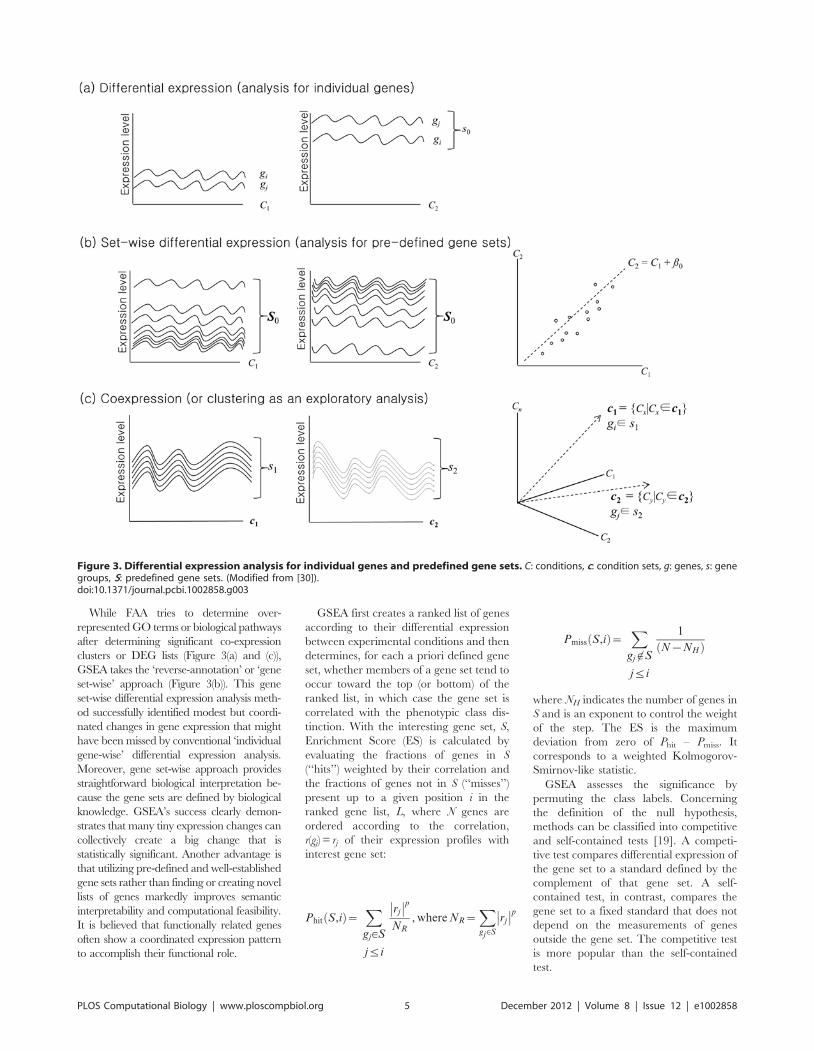
While FAA tries to determine over-
represented GO terms or biological pathways
after determining significant co-expression
clusters or DEG lists (Figure 3(a) and (c)),
GSEA takes the ‘reverse-annotation’ or ‘gene
set-wise’ approach (Figure 3(b)). This gene
set-wise differential expression analysis meth-
od successfully identified modest but coordi-
nated changes in gene expression that might
have been missed by conventional ‘individual
gene-wise’ differential expression analysis.
Moreover, gene set-wise approach provides
straightforward biological interpretation be-
cause the gene sets are defined by biological
knowledge. GSEA’s success clearly demon-
strates that many tiny expression changes can
collectively create a big change that is
statistically significant. Another advantage is
that utilizing pre-defined and well-established
gene sets rather than finding or creating novel
lists of genes markedly improves semantic
interpretability and computational feasibility.
It is believed that functionally related genes
often show a coordinated expression pattern
to accomplish their functional role.
GSEA first creates a ranked list of genes
according to their differential expression
between experimental conditions and then
determines, for each a priori defined gene
set, whether members of a gene set tend to
occur toward the top (or bottom) of the
ranked list, in which case the gene set is
correlated with the phenotypic class dis-
tinction. With the interesting gene set, S,
Enrichment Score (ES) is calculated by
evaluating the fractions of genes in S
(‘‘hits’’) weighted by their correlation and
the fractions of genes not in S (‘‘misses’’)
present up to a given position i in the
ranked gene list, L, where N genes are
ordered according to the correlation,
r(gj) = rj of their expression profiles with
interest gene set:
Phit S,ið Þ~X
gj[S
jƒi
rj
�� ��p
NR
, where NR~X
gj[S
rj
�� ��p
Pmiss S,ið Þ~X
gj 6[S
jƒi
1
N{NHð Þ
where NH indicates the number of genes in
S and is an exponent to control the weight
of the step. The ES is the maximum
deviation from zero of Phit – Pmiss. It
corresponds to a weighted Kolmogorov-
Smirnov-like statistic.
GSEA assesses the significance by
permuting the class labels. Concerning
the definition of the null hypothesis,
methods can be classified into competitive
and self-contained tests [19]. A competi-
tive test compares differential expression of
the gene set to a standard defined by the
complement of that gene set. A self-
contained test, in contrast, compares the
gene set to a fixed standard that does not
depend on the measurements of genes
outside the gene set. The competitive test
is more popular than the self-contained
test.
Figure 3. Differential expression analysis for individual genes and predefined gene sets. C: conditions, c: condition sets, g: genes, s: genegroups, S: predefined gene sets. (Modified from [30]).doi:10.1371/journal.pcbi.1002858.g003
PLOS Computational Biology | www.ploscompbiol.org 5 December 2012 | Volume 8 | Issue 12 | e1002858
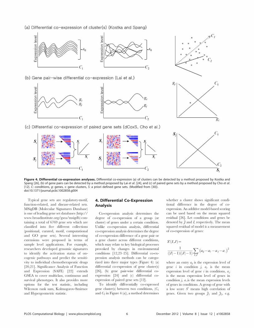
Typical gene sets are regulatory-motif,
function-related, and disease-related sets.
MSigDB (Molecular Signatures Database)
is one of leading gene set databases (http://
www.broadinstitute.org/gsea/msigdb) con-
taining a total of 6769 gene sets which are
classified into five different collections
(positional, curated, motif, computational
and GO gene sets). Several interesting
extensions were proposed in terms of
sample level applications. For example,
researchers developed genomic signatures
to identify the activation status of on-
cogenic pathways and predict the sensiti-
vity to individual chemotherapeutic drugs
[20,21]. Significance Analysis of Function
and Expression (SAFE) [22] extends
GSEA to cover multiclass, continuous and
survival phenotypes. It also provides more
options for the test statistic, including
Wilcoxon rank sum, Kolmogorov-Smirnov
and Hypergeometric statistic.
4. Differential Co-ExpressionAnalysis
Co-expression analysis determines the
degree of co-expression of a group (or
cluster) of genes under a certain condition.
Unlike co-expression analysis, differential
co-expression analysis determines the degree
of co-expression difference of a gene pair or
a gene cluster across different conditions,
which may relate to key biological processes
provoked by changes in environmental
conditions [12,23–25]. Differential co-ex-
pression analysis methods can be catego-
rized into three major types (Figure 4): (a)
differential co-expression of gene cluster(s)
[26], (b) gene pair-wise differential co-
expression [24] and (c) differential co-
expression of paired gene sets [12].
To identify differentially co-expressed
gene cluster(s) between two conditions, (C1
and C2 in Figure 4 (a)), a method determines
whether a cluster shows significant condi-
tional difference in the degree of co-
expression. An additive model-based scoring
can be used based on the mean squared
residual [26]. Let conditions and genes be
denoted by J and I, respectively. The mean
squared residual of model is a measurement
of co-expression of genes:
S’ I ,Jð Þ~1
Ij j{1ð Þ Jj j{1ð ÞX
I ,J
aij{ai:{a:j{a::� �2
where an entry aij is the expression level of
gene i in condition j, ai. is the mean
expression level of gene i in conditions, a.jis the mean expression level of genes in
condition j, a..is the mean expression levels
of genes in conditions. A group of gene with
a low score S9 means high correlation of
genes. Given two groups J1 and J2, e.g.
Figure 4. Differential co-expression anslyses. Differential co-expression (a) of clusters can be detected by a method proposed by Kostka andSpang [26], (b) of gene pairs can be detected by a method proposed by Lai et al. [24], and (c) of paired gene sets by a method proposed by Cho et al.[12]. C: conditions, g: genes, s: gene clusters, S: a priori defined gene sets. (Modified from [30]).doi:10.1371/journal.pcbi.1002858.g004
PLOS Computational Biology | www.ploscompbiol.org 6 December 2012 | Volume 8 | Issue 12 | e1002858
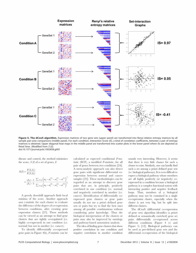
disease and control, the method minimizes
the score, S (I) of a set of genes, I:
S Ið Þ~ S’ I ,J1ð ÞS’ I ,J2ð Þ
~J2j j{1
J1j j{1:
PI ,J1
aij{a1ð Þ
i: {a1ð Þ:j {a
1ð Þ::
� �2
PI ,J2
aij{a2ð Þ
i: {a2ð Þ:j {a
2ð Þ::
� �2
A greedy downhill approach finds local
minima of the score. Another approach
uses t-statistic for each cluster to evaluate
the difference of the degree of co-expression
between conditions, after creating gene
expression clusters [27]. These methods
can be viewed as an attempt to find gene
clusters that are tightly co-regulated (i.e.
highly co-expressed) in one condition (i.e.
normal) but not in another (i.e. cancer).
To identify differentially co-expressed
gene pairs in Figure 4(b), F-statistic can be
calculated as expected conditional F-sta-
tistic (ECF), a modified F-statistic, for all
pair of genes between two conditions [24].
A meta-analytic approach can also detect
gene pairs with significant differential co-
expression between normal and cancer
samples [25]. These methodologies can be
regarded as an attempt to discover gene
pairs that are, in principle, positively
correlated in one condition (i.e. normal)
and negatively correlated in another (i.e.
cancer). Identification of differentially co-
expressed gene clusters or gene pairs
usually do not use a priori defined gene
sets or pairs but try to find the best ones
among all possible combinations without
considering prior knowledge. Thus the
biological interpretation of the clusters or
pairs may also be improved by ontology
and pathway-based annotation analysis.
The idea of finding gene clusters that show
positive correlation in one condition and
negative correlation in another condition
sounds very interesting. However, it seems
that there is very little chance for such a
cluster to exist. Similarly, one can hardly find
such a set among a priori defined gene sets
(i.e. biological pathways). It is even difficult to
expect a biological pathway whose members
are all highly positively (or negatively) co-
expressed in a condition because a biological
pathway is a complex functional system with
interacting positive and negative feedback
loops. Thus, members of a biological
pathway may not be contained in a single
co-expression cluster, especially when the
cluster is not very big, but be split into
different clusters.
The dCoxS (differential co-expression
of gene sets) algorithm identifies (a priori
defined or semantically enriched) gene set
pairs differentially co-expressed across
different conditions (Figure 4 (c) and
Figure 5) [12]. Biological pathways can
be used as pre-defined gene sets and the
differential co-expression of the biological
Figure 5. The dCoxS algorithm. Expression matrices of two gene sets (upper panel) are transformed into Renyi relative entropy matrices by allsample pair-wise comparisons (middle panel). For each condition, Interaction Score (IS), a kind of correlation coefficients, between a pair of entropymatrices is obtained. Upper diagonal heat maps in the middle panel are transformed into scatter plots in the lower panel where ISs are depicted asfitted lines. (Modified from [12]).doi:10.1371/journal.pcbi.1002858.g005
PLOS Computational Biology | www.ploscompbiol.org 7 December 2012 | Volume 8 | Issue 12 | e1002858
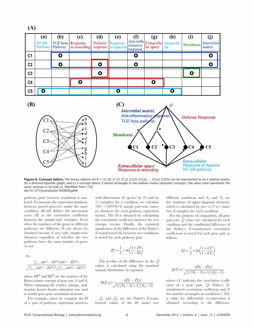
pathway pairs between conditions is ana-
lyzed. To measure the expression similarity
between paired gene-sets under the same
condition, dCoxS defines the interaction
score (IS) as the correlation coefficient
between the sample-wise entropies. Even
when the numbers of the genes in different
pathways are different, IS can always be
obtained because it uses only sample-wise
distances regardless of whether the two
pathways have the same number of genes
or not.
IS~
Pivj (REG1 {REG2 )(REG1 {REG2 )
ffiffiffiffiffiffiffiffiffiffiffiffiffiffiffiffiffiffiffiffiffiffiffiffiffiffiffiffiffiffiffiffiffiffiffiffiffiffiffiffiffiffiffiffiffiPivj (REG1 {REG1 )2
q ffiffiffiffiffiffiffiffiffiffiffiffiffiffiffiffiffiffiffiffiffiffiffiffiffiffiffiffiffiffiffiffiffiffiffiffiffiffiffiffiffiffiffiffiffiPivj (REG2 {REG2 )2
q
where RESi and RESj are the matrices of the
Renyi relative entropy of gene sets, Si and Sj.
When estimating the relative entropy, mul-
tivariate kernel density estimation was used
to model gene-gene correlation structure.
For example, when we compute the IS
of a pair of pathway expression matrices
with dimensions 20 (genes) by 25 and by
15 (samples) for a condition, we calculate
190 ( = (20*19)/2) sample pair-wise entro-
py distances for each pathway expression
matrix. The IS is obtained by calculating
the correlation coefficient between the two
entropy vectors. Finally, the statistical
significance of the difference of the Fisher’s
Z-transformed ISs between two conditions
is tested for each pathway pair.
Zf ~1
2|ln
1zIS
1{IS
�
The p-value of the difference in the Zf
values is calculated using the standard
normal distribution in equation.
P(Z§D(Zf1{Zf2)
ffiffiffiffiffiffiffiffiffiffiffiffiffiffiffiffiffiffiffiffiffiffiffiffiffiffiffiffiffiffiffiffiffiffiffiffiffiffiffiffiffiffiffiffiffiffiffiffi1= N1{3ð Þz1= N2{3ð Þ
p
Zf1 and Zf2 are the Fisher’s Z-trans-
formed values of the IS under two
different conditions and N1 and N2 are
the numbers of upper-diagonal elements,
which is calculated by n(n21)/2 (n = num-
ber of samples) for each condition.
For the purpose of comparison, all gene
pair-wise Zf values are calculated for each
condition and the conditional difference of
the Fisher’s Z-transformed correlation
coefficients is tested for each gene pair as
follows,
Zf ~1
2|ln
1zCC
1{CC
�
p(Z§D(Zf1{Zf2)
ffiffiffiffiffiffiffiffiffiffiffiffiffiffiffiffiffiffiffiffiffiffiffiffiffiffiffiffiffiffiffiffiffiffiffiffiffiffiffiffiffiffiffiffiffiffiffiffi1= N1{3ð Þz1= N2{3ð Þ
p
where CC indicates the correlation coeffi-
cient of a gene pair, Zfi Fisher’s Z-
transformed correlation coefficient and Ni
the number of samples in conditions i. The
p value for differential co-expression is
obtained according to the difference
Figure 6. Concept lattice. The binary relation set R = { (C1,b), (C1,f), (C1,j), (C2,b), (C2,d),…, (C5,e), (C5,h)} can be represented as (a) a relation matrix,(b) a directed bipartite graph, and (c) a concept lattice. Colored rectangles in the relation matrix represent concepts. The same color represents thesame concept in (a) and (c). (Modified from [13]).doi:10.1371/journal.pcbi.1002858.g006
PLOS Computational Biology | www.ploscompbiol.org 8 December 2012 | Volume 8 | Issue 12 | e1002858
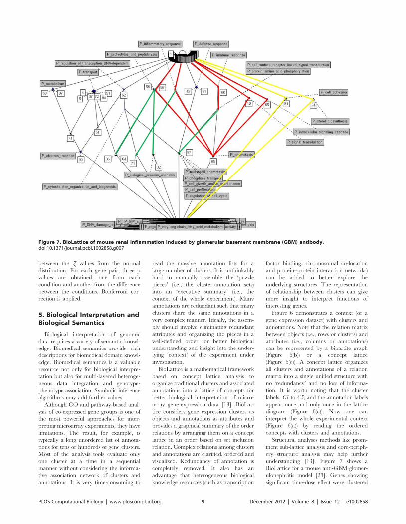
between the Z values from the normal
distribution. For each gene pair, three p
values are obtained, one from each
condition and another from the difference
between the conditions. Bonferroni cor-
rection is applied.
5. Biological Interpretation andBiological Semantics
Biological interpretation of genomic
data requires a variety of semantic knowl-
edge. Biomedical semantics provides rich
descriptions for biomedical domain knowl-
edge. Biomedical semantics is a valuable
resource not only for biological interpre-
tation but also for multi-layered heteroge-
neous data integration and genotype-
phenotype association. Symbolic inference
algorithms may add further values.
Although GO and pathway-based anal-
ysis of co-expressed gene groups is one of
the most powerful approaches for inter-
preting microarray experiments, they have
limitations. The result, for example, is
typically a long unordered list of annota-
tions for tens or hundreds of gene clusters.
Most of the analysis tools evaluate only
one cluster at a time in a sequential
manner without considering the informa-
tive association network of clusters and
annotations. It is very time-consuming to
read the massive annotation lists for a
large number of clusters. It is unthinkably
hard to manually assemble the ‘puzzle
pieces’ (i.e., the cluster-annotation sets)
into an ‘executive summary’ (i.e., the
context of the whole experiment). Many
annotations are redundant such that many
clusters share the same annotations in a
very complex manner. Ideally, the assem-
bly should involve eliminating redundant
attributes and organizing the pieces in a
well-defined order for better biological
understanding and insight into the under-
lying ‘context’ of the experiment under
investigation.
BioLattice is a mathematical framework
based on concept lattice analysis to
organize traditional clusters and associated
annotations into a lattice of concepts for
better biological interpretation of micro-
array gene-expression data [13]. BioLat-
tice considers gene expression clusters as
objects and annotations as attributes and
provides a graphical summary of the order
relations by arranging them on a concept
lattice in an order based on set inclusion
relation. Complex relations among clusters
and annotations are clarified, ordered and
visualized. Redundancy of annotation is
completely removed. It also has an
advantage that heterogeneous biological
knowledge resources (such as transcription
factor binding, chromosomal co-location
and protein–protein interaction networks)
can be added to better explore the
underlying structures. The representation
of relationship between clusters can give
more insight to interpret functions of
interesting genes.
Figure 6 demonstrates a context (or a
gene expression dataset) with clusters and
annotations. Note that the relation matrix
between objects (i.e., rows or clusters) and
attributes (i.e., columns or annotations)
can be represented by a bipartite graph
(Figure 6(b)) or a concept lattice
(Figure 6(c)). A concept lattice organizes
all clusters and annotations of a relation
matrix into a single unified structure with
no ‘redundancy’ and no loss of informa-
tion. It is worth noting that the cluster
labels, C1 to C5, and the annotation labels
appear once and only once in the lattice
diagram (Figure 6(c)). Now one can
interpret the whole experimental context
(Figure 6(a)) by reading the ordered
concepts with clusters and annotations.
Structural analyses methods like prom-
inent sub-lattice analysis and core-periph-
ery structure analysis may help further
understanding [13]. Figure 7 shows a
BioLattice for a mouse anti-GBM glomer-
ulonephritis model [28]. Genes showing
significant time-dose effect were clustered
Figure 7. BioLattice of mouse renal inflammation induced by glomerular basement membrane (GBM) antibody.doi:10.1371/journal.pcbi.1002858.g007
PLOS Computational Biology | www.ploscompbiol.org 9 December 2012 | Volume 8 | Issue 12 | e1002858
into 100 clusters and annotated with GO
terms. The whole complex clusters and
annotations are organized into a single
unified lattice graph, providing an ‘executive
summary.’ The Ganter algorithm [29] can
be used to construct BioLattice. A web-based
tool using Perl, JavaScript and Scalable
Vector Graphics are available at http://
www.snubi.org/software/biolattice/. Prom-
inent sub-lattice analysis reveals a mean-
ingful sub-structure converging into clus-
ter 85, which has the GO term
‘chemotaxis’ and inherits ‘proteolysis and
peptidolysis’ (clusters 58 and 96), ‘inflam-
matory response’, ‘immune response’, ‘protein
amino acid phosphorylation’, and ‘cell surface
receptor linked signal transduction’ (cluster 60),
‘signal transduction’ (cluster 19), ‘intracellular
signaling cascade’ (cluster 65). It is clearly
visualized that cellular immune response
system activation is the core pathological
process in the IgA nephropathy model of
kidney and clusters 19, 58, 60, 65, 5 and
96 are within those concepts.
Context in concept lattice analysis is a
triplet (G, M, I) consisting of two sets G and M
and a relation I between G and M. The
elements of G and M are called objects and
attributes, respectively. We denote gIm or (g,
m) M I to show that object g has attribute m. For
a set A # G of objects, we define A9: = { m M M
| gIm for all g M A } (i.e., the set of attributes
common to the objects in A). Corresponding-
ly, for a set B#M of attributes, we define
B9: = { g M G | gIm for all m M B } (i.e., the set of
objects that have all attributes in B).
Concept lattice analysis models concepts
as units of thought, consisting of two parts.
A concept of the context (G, M, I) is a pair
(A, B) with A#G, B#M, A9 = B and B9 = A.
We call A and B the extent and the intent,
respectively, of concept (A, B). The extent
consists of all objects belonging to the
concept while the intent contains all
attributes shared by the objects. The set of
all concepts of the context (G, M, I) is
denoted by C(G, M, I). A concept lattice is
drawn by ordering (A, B), which are defined
as concepts of the context (G, M, I). The set
of all concepts of a context together with
the partial order (A1, B1)#(A2, B2): u A1
# A2 (which is equivalent to B1 $ B2) is
called a concept lattice.
We regard A as defining gene expression
clusters that share common knowledge
attributes and B as defining the knowledge
terms that are annotated to the clusters.
The concepts are arranged in a hierarchi-
cal order so that the order of C1#C2 uA1 # A2 u B1 $ B2 is defined at
C1 = (A1, B1), C2 = (A2, B2). The top
element of a lattice is a unit concept,
representing a concept that contains all
objects. The bottom element is a zero
concept having no object.
6. Summary
This chapter has shown major compu-
tational approaches to facilitate biological
interpretation of high-throughput micro-
array and RNA-Seq experiments. The
enrichment analysis with ontologies, bio-
logical pathways or external resources is
widely used to interpret the functional role
of correlated genes or differentially ex-
pressed genes. In analysis steps, the groups
of genes are assigned to the associated
biological annotation terms using GO
terms or biological pathways. Then it is
necessary to examine whether gene mem-
bers are statistically enriched in each of the
annotation terms or pathway by compar-
ing background set by measuring statistical
test such as Chi-square, Fisher’s exact,
binomial and hypergeometric test. Unlike
previous approaches identifying a set of
significant genes, Gene Set Enrichment
Analysis uses pre-defined sets to search for
groups of functionally related genes with
coordinated expression across a list of
genes ranked by differentially expression.
Differential co-expression analysis deter-
mines the degree of co-expression differ-
ence of a gene set pair across different
conditions. The dCoxS algorithm identi-
fies differentially co-expressed gene set
under different conditions. Outcomes in
microarray and RNA-Seq data can be
transformed into the graphical structure
that represents biological semantics. A
number of biomedical annotation and
external repositories including clinical
resources can be integrated by biological
semantics analysis tools such as BioLattice.
7. Exercises
1) Select significantly DEGs from the train
dataset of AML (Acute Myelocytic
Leukemia) and ALL (acute lympho-
blastic leukemia) expression data
(http://www.broadinstitute.org/cgi-
bin/cancer/publications/pub_paper.
cgi?mode = view&paper_id = 43) and
find enriched GO terms from an
ontology analysis tool. Dataset and
analysis functions are also included in
R statistical package, golubEsets in
Bioconductor.
2) List significantly enriched pathways
using a pathway analysis tool with
the dataset in Exercise 1.
3) Find KEGG pathways significantly
associated with leukemia subtype in
the 2-sample comparison of AML
and ALL by GSEA through the
Kolmogorov-Smirnoff test. Analysis
and data set are provided by SAFE R
(http://bioconductor.org/packages/
2.0/bioc/html/safe.html).
4) Identify the differentially co-ex-
pressed gene set pairs using dCoxS
with simulated data in (http://www.
snubi.org/publication/dCoxS).
Compute interaction score between
matrix M and M1 using ias function.
And, compute interaction score be-
tween M and M2. Finally, using
compcorr function, estimate signifi-
cance of difference of ias. Note that in
compcorr function, n1 and n2 is the
number of all possible sample pairs.
5) Report semantic relationships of
pathways and GO terms using Bio-
Lattice (http://www.snubi.org/
software/biolattice/). Use the result
of k-means clustering (k = 10) with
Further Reading
N Draghici S (2003) Data analysis tools for DNA microarrays. Chapman and Hall/CRC Press.
N Curtis RK, Oresic M, Vidal-Puig A (2005) Pathways to the analysis of microarraydata. Trends Biotechnol 23(8): 429–435.
N Gentleman R, Carey V, Huber W, Irizarry R, Dudoit S (2005) Bioinformatics andcomputational biology solutions using R and Bioconductor. Springer.
N Deshmukh SR, Purohit SG (2007) Microarray data: statistical analysis using R.Oxford: Alpha Science International Ltd.
N Guerra R, Goldstein DR (2008) Meta-analysis and combining information ingenetics and genomics. Chapman and Hall.
N Werner T (2008) Bioinformatics applications for pathway analysis of microarraydata. Current Opinion in Biotechnology 19 (1): 50–54.
N Emmert-Streib F, Dehmer M (2010) Medical biostatistics for complex diseases.Wiley.
N Kann MG (2010) Advances in translational bioinformatics: computationalapproaches for the hunting of disease genes. Brief Bioinform 11(1): 96–110.
PLOS Computational Biology | www.ploscompbiol.org 10 December 2012 | Volume 8 | Issue 12 | e1002858
DEG in Exercise 1. Select Category
as ‘biological process,’ p-value,0.05.
Answers to the Exercises can be found
in Text S1.
Supporting Information
Text S1 Answers to Exercises
(DOCX)
References
1. Tavazoie S, Hughes JD, Campbell MJ, Cho RJ,
Church GM (1999) Systematic determination ofgenetic network architecture. Nat Genet 22(3):
281–285.
2. Ashburner M, Ball CA, Blake JA, Botstein D,
Butler H, et al. (2000) Gene ontology: tool for theunification of biology. The Gene Ontology
Consortium. Nat Genet 25(1): 25–29.
3. Dahlquist KD, Salomonis N, Vranizan K, Lawlor
SC, Conklin BR (2002) GenMAPP, a new tool forviewing and analyzing microarray data on
biological pathways. Nat Genet 31(1): 19–20.
4. Al-Shahrour F, Dıaz-Uriarte R, Dopazo J (2004)
FatiGO: a web tool for finding significantassociations of Gene Ontology terms with groups
of genes. Bioinformatics 20(4): 578–580.
5. Boyle EI, Weng S, Gollub J, Jin H, Botstein D,
et al. (2004) TermFinder–open source softwarefor accessing Gene Ontology information and
finding significantly enriched Gene Ontologyterms associated with a list of genes. Bioinfor-
matics 20(18): 3710–3715.
6. Chung HJ, Kim M, Park CH, Kim J, Kim JH
(2004) ArrayXPath: mapping and visualizingmicroarray gene-expression data with integrated
biological pathway resources using Scalable
Vector Graphics. Nucleic Acids Res 32(WebServer issue): W460–464.
7. Zhang B, Schmoyer D, Kirov S, Snoddy J (2004)
GOTree Machine (GOTM): a web-based plat-
form for interpreting sets of interesting genesusing Gene Ontology hierarchies. BMC Bioinfor-
matics 5: 16.
8. Zhong S, Storch KF, Lipan O, Kao MC, Weitz CJ,
et al. (2004) GoSurfer: a graphical interactive tool
for comparative analysis of large gene sets in Gene
Ontology space. Appl Bioinformatics 3(4): 261–264.
9. Chung HJ, Park CH, Han MR, Lee S, Ohn JH,
et al. (2005) ArrayXPath II: mapping and
visualizing microarray gene-expression data with
biomedical ontologies and integrated biological
pathway resources using Scalable Vector Graph-
ics. Nucleic Acids Res 33(Web Server issue):
W621–626.
10. Mootha VK, Lindgren CM, Eriksson KF, Sub-
ramanian A, Sihag S, et al. (2003) PGC-1alpha-
responsive genes involved in oxidative phosphor-
ylation are coordinately downregulated in human
diabetes. Nat Genet 34(3): 267–273.
11. Subramanian A, Tamayo P, Mootha VK, Mu-
kherjee S, Ebert BL, et al. (2005) Gene set
enrichment analysis: a knowledge-based approach
for interpreting genome-wide expression profiles.
Proc Natl Acad Sci U S A. 102(43): 15545–15550.
12. Cho SB, Kim J, Kim JH (2009) Identifying set-
wise differential co-expression in gene expression
microarray data. BMC Bioinformatics 10: 109.
13. Kim J, Chung HJ, Jung Y, Kim KK, Kim JH
(2008) BioLattice: a framework for the biological
interpretation of microarray gene expression data
using concept lattice analysis. J Biomed Inform 41
(2): 232–241.
14. Yue L, Reisdorf WC (2005) Pathway and onto-
logy analysis: emerging approaches connecting
transcriptome data and clinical endpoints. Curr
Mol Med 5(1): 11–21.
15. Caspi R, Altman T, Dale JM, Dreher K, Fulcher
CA, et al. (2010) The MetaCyc database of
metabolic pathways and enzymes and the BioCyc
collection of pathway/genome databases. Nucleic
Acids Res 38 (Database issue): D473–479.
16. Alexa A, Rahnenfuhrer J, Lengauer T (2006)
Improved scoring of functional groups from gene
expression data by decorrelating GO graph
structure. Bioinformatics 22(13): 1600–1607.
17. Falcon S, Gentleman R (2007) Using GOstats to
test gene lists for GO term association. Bioinfor-
matics. 23(2): 257–258.
18. Huang da W, Sherman BT, Lempicki RA (2009)
Bioinformatics enrichment tools: paths toward the
comprehensive functional analysis of large gene
lists. Nucleic Acids Res 37(1): 1–13.
19. Goeman JJ, Buhlmann P (2007) Analyzing gene
expression data in terms of gene sets: methodo-
logical issues. Bioinformatics 23 (8): 980–987.
20. Bild AH, Yao G, Chang JT, Wang Q, Potti A,
et al. (2006) Oncogenic pathway signatures in
human cancers as a guide to targeted therapies.
Nature 439(7074): 353–357.
21. Potti A, Dressman HK, Bild A, Riedel RF, Chan
G (2006) Genomic signatures to guide the use of
chemotherapeutics. Nat Med 12(11): 1294–1300.
22. Barry WT, Nobel AB, Wright FA (2005)
Significance analysis of functional categories in
gene expression studies: a structured permutation
approach. Bioinformatics 21(9): 1943–1949.
23. Li KC (2002) Genome-wide co-expression dy-
namics: theory and application. Proc Natl Acad
Sci U S A 99(26): 16875–16880.
24. Lai Y, Wu B, Chen L, Zhao H (2004) A statistical
method for identifying differential gene-gene co-
expression patterns. Bioinformatics 20 (17): 3146–
55.
Glossary
Bioconductor: a free, open source and open development software project forthe analysis and comprehension of genomic data generated by wet labexperiments in molecular biology written in R Statistical Package.
Clustering: algorithm that puts similar things together and different thingsapart.
Gene expression profiling: the measurement of the activity (or expression) ofthousands of genes at once to create a global picture of cellular function usingDNA microarray technology.
Gene set: a meaningful grouping of genes like biological pathways, genessharing certain regulatory-motifs, genes sharing certain functional annotations,and certain disease-related gene sets.
Gene Set Enrichment Analysis: an algorithm to determine whether an a prioridefined set of genes shows statistically significant coordinated differentialexpression between conditions.
Gene Ontology: a set of controlled vocabularies in molecular function,biological process and cellular component for the standardized annotations ofgenes and gene products across all species.
Hypergeometric distribution: a discrete probability distribution that describesthe number of successes in a sequence of n draws from a finite populationwithout replacement, just as the binomial distribution describes the number ofsuccesses for draws with replacement.
Kolmogorov–Smirnov test (K–S test): a nonparametric test for the equality ofcontinuous, one-dimensional probability distributions that can be used tocompare a sample with a reference probability distribution (one-sample K–S test),or to compare two samples (two-sample K–S test).
PLOS Computational Biology | www.ploscompbiol.org 11 December 2012 | Volume 8 | Issue 12 | e1002858

25. Choi JK, Yu U, Yoo OJ, Kim S (2005) Differential
co-expression analysis using microarray data andits application to human cancer. Bioinformatics
21(24): 4348–4355.
26. Kostka D, Spang R (2004) Finding diseasespecific alterations in the co-expression of genes.
Bioinformatics 20 Suppl 1: i194–199.
27. Watson M (2006) CoXpress: differential co-
expression in gene expression data. BMC Bioin-
formatics 7: 509.
28. Kim JH, Ha IS, Hwang CI, Lee YJ, Kim Y, et al.
(2004) Gene expression profiling of anti-GBM
glomerulonephritis model: the role of NFkB in
immune complex-mediated kidney disease. Kid-
ney International, 66(5): 1826–183729. Ganter B, Wille R (1999) Formal concept
analysis: mathematical foundations. Berlin; New
York: Springer.30. Emmert-Streib F, Dehmer M (2010) Medical
Biostatistics for Complex Diseases. Wiley.
PLOS Computational Biology | www.ploscompbiol.org 12 December 2012 | Volume 8 | Issue 12 | e1002858

Education
Chapter 9: Analyses Using Disease OntologiesNigam H. Shah*, Tyler Cole, Mark A. Musen
Center for Biomedical Informatics Research, Stanford University, Stanford, California, United States of America
Abstract: Advanced statistical methodsused to analyze high-throughput datasuch as gene-expression assays result inlong lists of ‘‘significant genes.’’ One wayto gain insight into the significance ofaltered expression levels is to determinewhether Gene Ontology (GO) termsassociated with a particular biologicalprocess, molecular function, or cellularcomponent are over- or under-represent-ed in the set of genes deemed significant.This process, referred to as enrichmentanalysis, profiles a gene-set, and is widelyused to makes sense of the results ofhigh-throughput experiments. The ca-nonical example of enrichment analysisis when the output dataset is a list ofgenes differentially expressed in somecondition. To determine the biologicalrelevance of a lengthy gene list, the usualsolution is to perform enrichment analysiswith the GO. We can aggregate theannotating GO concepts for each genein this list, and arrive at a profile of thebiological processes or mechanisms af-fected by the condition under study.While GO has been the principal targetfor enrichment analysis, the methods ofenrichment analysis are generalizable. Wecan conduct the same sort of profilingalong other ontologies of interest. Just asscientists can ask ‘‘Which biological pro-cess is over-represented in my set ofinteresting genes or proteins?’’ we canalso ask ‘‘Which disease (or class ofdiseases) is over-represented in my setof interesting genes or proteins?‘‘. Forexample, by annotating known proteinmutations with disease terms from theontologies in BioPortal, Mort et al. recentlyidentified a class of diseases—bloodcoagulation disorders—that were associ-ated with a 14-fold depletion in substitu-tions at O-linked glycosylation sites. Withthe availability of tools for automaticannotation of datasets with terms fromdisease ontologies, there is no reason torestrict enrichment analyses to the GO. Inthis chapter, we will discuss methods toperform enrichment analysis using anyontology available in the biomedicaldomain. We will review the generalmethodology of enrichment analysis, theassociated challenges, and discuss thenovel translational analyses enabled bythe existence of public, national compu-tational infrastructure and by the use ofdisease ontologies in such analyses.
This article is part of the ‘‘Transla-
tional Bioinformatics’’ collection for
PLOS Computational Biology.
1. Introduction
Advanced statistical methods are most
often used to perform the analysis of high-
throughput data such as gene-expression
assays [1–5], the result of which is a long
list of ‘‘significant genes.’’ Extracting
biological meaning from such lists is a
nontrivial and time-consuming task,
which is exacerbated by the inconsisten-
cies in free-text gene annotations. The
Gene Ontology (GO) offers a taxonomy
that provides a mechanism to determine
statistically significant functional sub-
groups within gene groups. One way to
gain insight into the biological signifi-
cance of alterations in gene expression
levels is to determine whether the GO
terms associated with the particular bio-
logical process, molecular function, or
cellular component are over- or under-
represented in the set of genes deemed
significant by the statistical analysis [6].
This process, often referred to as ‘‘enrich-
ment analysis,’’ can be used to summarize
a gene-set [7], although it can also be
relevant for other high-throughput mea-
surement modalities including proteo-
mics, metabolomics, and studies using
tissue-microarrays [8].
With the availability of tools for auto-
matic ontology-based annotation of data-
sets with terms from biomedical ontologies
besides the GO, we need not restrict
enrichment analysis to the GO. In this
chapter, we outline the methodology of
enrichment analysis, the associated chal-
lenges, and discuss novel analyses enabled
by performing enrichment analysis using
disease ontologies. We first review the
current methods of GO based enrichment
analysis to provide a foundation for
discussing analyses using Disease Ontolo-
gies. Note that there is also research
underway on the use of ‘‘pathways’’ for
enrichment analyses as well as comparing
statistically significant, concordant differ-
ences between two biological states as in
Gene Set Enrichment Analysis [9], which
are not discussed here.
1.1 Gene Ontology EnrichmentAnalysis
The goal of enrichment analysis is to
determine which biological processes (or
molecular function) might be predomi-
nantly affected in the set of genes that were
deemed interesting or significantly
changed. The simplest approach is to
calculate functional ‘enrichment/deple-
tion’ for each GO term—a higher (or
lower) proportion of genes with certain
annotations among the significantly
changed genes than among all of the
genes measured in the experiment. The
finding of enrichment should not be
interpreted as evidence implicating the
GO term in the process studied without an
appropriate statistical test.
The calculation of GO based functional
enrichment involves two sets of items
(usually genes or proteins): 1) The refer-
ence set, which is the set of items with
which the ‘‘significant-set’’ is to be com-
pared; the reference set may comprise all
of the genes in the genome or all of the
genes for which there were probes in the
high throughput experiment; 2) The set of
interest, which is the subset or list of
significant genes that is to be analyzed for
Citation: Shah NH, Cole T, Musen MA (2012) Chapter 9: Analyses Using Disease Ontologies. PLoS ComputBiol 8(12): e1002827. doi:10.1371/journal.pcbi.1002827
Editors: Fran Lewitter, Whitehead Institute, United States of America and Maricel Kann, University of Maryland,Baltimore County, United States of America
Published December , 2012
Copyright: � 2012 Shah et al. This is an open-access article distributed under the terms of the CreativeCommons Attribution License, which permits unrestricted use, distribution, and reproduction in any medium,provided the original author and source are credited.
Funding: We acknowledge support from NIH grant U54 HG004028 for the National Center for BiomedicalOntology. The funders had no role in the preparation of the manuscript.
Competing Interests: The authors have declared that no competing interests exist.
* E-mail: [email protected]
PLOS Computational Biology | www.ploscompbiol.org 1 December 2012 | Volume 8 | Issue 12 | e1002827
27
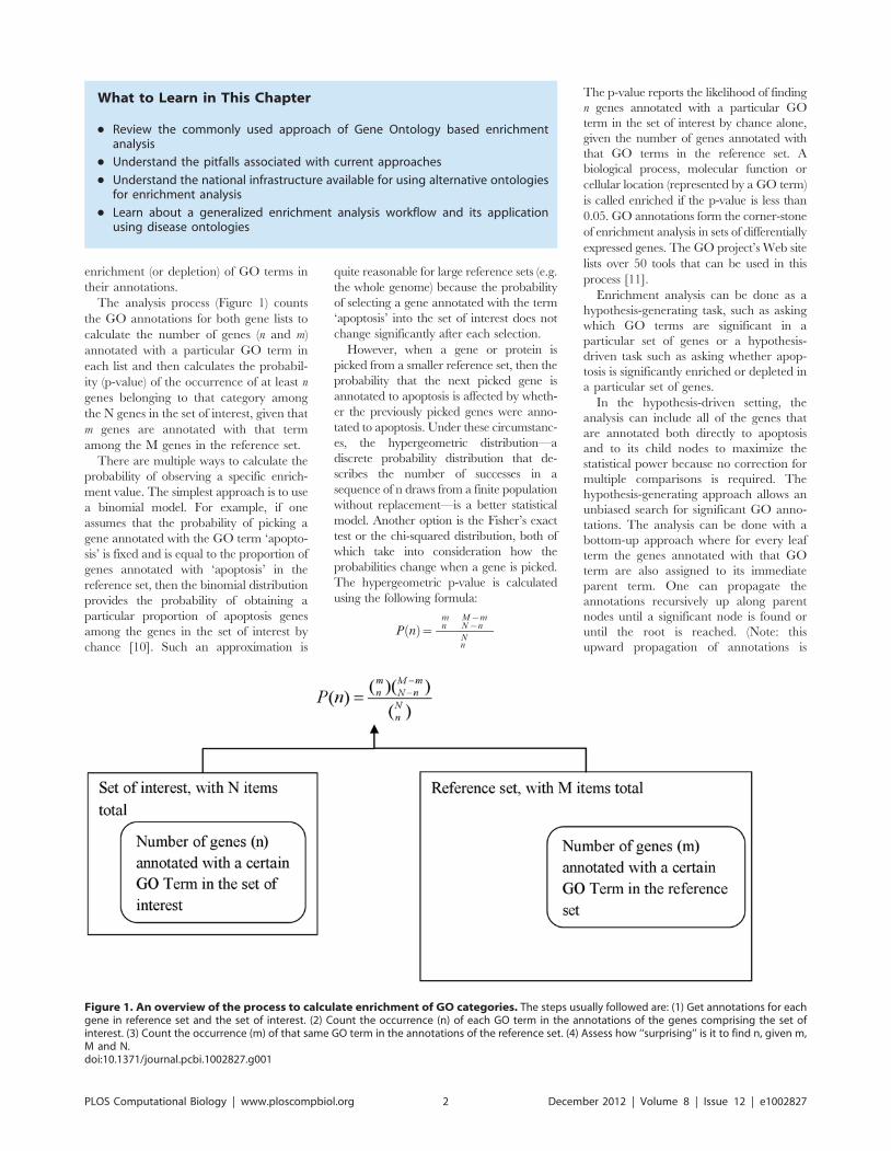
enrichment (or depletion) of GO terms in
their annotations.
The analysis process (Figure 1) counts
the GO annotations for both gene lists to
calculate the number of genes (n and m)
annotated with a particular GO term in
each list and then calculates the probabil-
ity (p-value) of the occurrence of at least n
genes belonging to that category among
the N genes in the set of interest, given that
m genes are annotated with that term
among the M genes in the reference set.
There are multiple ways to calculate the
probability of observing a specific enrich-
ment value. The simplest approach is to use
a binomial model. For example, if one
assumes that the probability of picking a
gene annotated with the GO term ‘apopto-
sis’ is fixed and is equal to the proportion of
genes annotated with ‘apoptosis’ in the
reference set, then the binomial distribution
provides the probability of obtaining a
particular proportion of apoptosis genes
among the genes in the set of interest by
chance [10]. Such an approximation is
quite reasonable for large reference sets (e.g.
the whole genome) because the probability
of selecting a gene annotated with the term
‘apoptosis’ into the set of interest does not
change significantly after each selection.
However, when a gene or protein is
picked from a smaller reference set, then the
probability that the next picked gene is
annotated to apoptosis is affected by wheth-
er the previously picked genes were anno-
tated to apoptosis. Under these circumstanc-
es, the hypergeometric distribution—a
discrete probability distribution that de-
scribes the number of successes in a
sequence of n draws from a finite population
without replacement—is a better statistical
model. Another option is the Fisher’s exact
test or the chi-squared distribution, both of
which take into consideration how the
probabilities change when a gene is picked.
The hypergeometric p-value is calculated
using the following formula:
P nð Þ~mn
� �M{mN{n
� �
Nn
� �
The p-value reports the likelihood of finding
n genes annotated with a particular GO
term in the set of interest by chance alone,
given the number of genes annotated with
that GO terms in the reference set. A
biological process, molecular function or
cellular location (represented by a GO term)
is called enriched if the p-value is less than
0.05. GO annotations form the corner-stone
of enrichment analysis in sets of differentially
expressed genes. The GO project’s Web site
lists over 50 tools that can be used in this
process [11].
Enrichment analysis can be done as a
hypothesis-generating task, such as asking
which GO terms are significant in a
particular set of genes or a hypothesis-
driven task such as asking whether apop-
tosis is significantly enriched or depleted in
a particular set of genes.
In the hypothesis-driven setting, the
analysis can include all of the genes that
are annotated both directly to apoptosis
and to its child nodes to maximize the
statistical power because no correction for
multiple comparisons is required. The
hypothesis-generating approach allows an
unbiased search for significant GO anno-
tations. The analysis can be done with a
bottom-up approach where for every leaf
term the genes annotated with that GO
term are also assigned to its immediate
parent term. One can propagate the
annotations recursively up along parent
nodes until a significant node is found or
until the root is reached. (Note: this
upward propagation of annotations is
Figure 1. An overview of the process to calculate enrichment of GO categories. The steps usually followed are: (1) Get annotations for eachgene in reference set and the set of interest. (2) Count the occurrence (n) of each GO term in the annotations of the genes comprising the set ofinterest. (3) Count the occurrence (m) of that same GO term in the annotations of the reference set. (4) Assess how ‘‘surprising’’ is it to find n, given m,M and N.doi:10.1371/journal.pcbi.1002827.g001
What to Learn in This Chapter
N Review the commonly used approach of Gene Ontology based enrichmentanalysis
N Understand the pitfalls associated with current approaches
N Understand the national infrastructure available for using alternative ontologiesfor enrichment analysis
N Learn about a generalized enrichment analysis workflow and its applicationusing disease ontologies
PLOS Computational Biology | www.ploscompbiol.org 2 December 2012 | Volume 8 | Issue 12 | e1002827
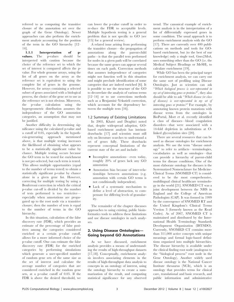
referred to as computing the transitive
closure of the annotation set over the
graph of the Gene Ontology). Newer
approaches can also perform the enrich-
ment analysis accounting for the position
of the term in the GO hierarchy [12–
14].
1.1.1 Interpretation of p-
values. The p-values should be
interpreted with caution because the
choice of the reference set to which the
set of interest is compared affects the p-
value. For whole genome arrays, using the
list of all genes on the array as the
reference set is equivalent to using the
complete list of genes in the genome.
However, for arrays containing a selected
subset of genes associated with a biological
process, the choice of the gene set to use as
the reference set is not obvious. Moreover,
the p-value calculation using the
hypergeometric distribution assumes the
independence of the GO annotation
categories, an assumption that may not
be justified.
Another difficulty in determining sig-
nificance using the calculated p-value and
a cutoff of 0.05, especially in the hypoth-
esis-generating approach mentioned
above, is that multiple testing increases
the likelihood of obtaining what appears
to be a statistically significant value by
chance. Multiple testing occurs because
the GO term to be tested for enrichment
is not pre-selected, but each term is tested.
This allows multiple opportunities (equal
to the number of terms tested) to obtain a
statistically significant p-value by chance
alone in a given gene list. However,
correcting for multiple testing by using a
Bonferroni correction in which the critical
p-value cut-off is divided by the number
of tests performed is too restrictive—
especially when annotations are propa-
gated up to the root node via a transitive
closure; then the number of tests is equal
to the number of terms in the GO
hierarchy.
In this situation, calculation of the false
discovery rate (FDR), which provides an
estimate of the percentage of false posi-
tives among the categories considered
enriched at a certain p-value cutoff,
allows for a more informed choice of the
p-value cutoff. One can estimate the false
discovery rate (FDR) for the enriched
categories by performing simulations
which generate a user-specified number
of random gene sets of the same size as
the set of interest and calculate the
average number of categories that are
considered enriched in the random gene
sets, at a p-value cutoff of 0.05. If the
FDR is above the desired threshold, we
can lower the p-value cutoff in order to
re-duce the FDR to acceptable levels.
Multiple hypothesis testing is a general
problem that is not specific to GO (see
[15] for a general review).
A related issue arising from performing
the transitive closure—the propagation of
annotations along the parent-child
paths—is that the parallel tests performed
for nodes in a given path will be correlated
because the same genes can appear several
times on each path. Correction methods
that assumes independence of categories
might not function well in this situation
and might preclude identification of some
categories that are indeed enriched [6]. It
is possible to use the structure of the GO
to decorrelate the analysis of various terms
[12–14] or to use corrections methods
such as a Benjamini–Yekutieli correction,
which accounts for the dependency be-
tween the multiple tests [16].
1.2 Summary of Existing LimitationsIn 2005, Khatri and Draghici noted
that, despite widespread adoption, GO-
based enrichment analysis has intrinsic
drawbacks [17] and scientists must still
rely on literature searches to understand a
set of genes fully. These drawbacks
represent conceptual limitations of the
current state of the art and include:
N Incomplete annotations—even today,
roughly 20% of genes lack any GO
annotation
N Annotation bias because of inter-rela-
tionships between annotations (e.g.
annotation with certain GO terms is
not conditionally independent).
N Lack of a systematic mechanism to
define a level of abstraction, to com-
pensate for differing levels of granular-
ity.
The remainder of the chapter discusses
approaches to using existing, public bioin-
formatics tools to address these limitations
and use disease ontologies in such analy-
ses.
2. Using Disease Ontologies—Going beyond GO Annotations
As we have discussed, enrichment
analysis provides a means of understand-
ing the results of high-throughput datasets
[17,18]. Conceptually, enrichment analy-
sis involves associating elements in the
results of high-throughput data analysis to
concepts in an ontology of interest, using
the ontology hierarchy to create a sum-
marization of the result, and computing
statistical significance for any observed
trend. The canonical example of enrich-
ment analysis is in the interpretation of a
list of differentially expressed genes in
some condition. The usual approach is to
perform enrichment analysis with the GO
[17]. There are currently over 400 publi-
cations on methods and tools for GO-
based enrichment, but (to the best of our
knowledge) only a single tool, Genes2Mesh,
uses something other than the GO (i.e. the
Medical Subject Headings or MeSH), to
calculate enrichment [19].
While GO has been the principal target
for enrichment analysis, we can carry out
the same sort of profiling using Disease
Ontologies. Just as scientists can ask
‘‘Which biological process is over-represented in
my set of interesting genes or proteins?’’, they also
should be able to ask ‘‘Which disease (or class
of diseases) is over-represented in my set of
interesting genes or proteins?’’ For example, by
annotating known protein mutations with
disease terms from the ontologies in
BioPortal, Mort et al. recently identified
a class of diseases—blood coagulation
disorders—that were associated with a
14-fold depletion in substitutions at O-
linked glycosylation sites [20].
There are several resources that can be
used as disease ontologies for enrichment
analysis. We use the term ‘‘disease ontol-
ogy’’ to refer to artifacts—terminologies,
vocabularies as well as ontologies—that
can provide a hierarchy of parent-child
terms for disease conditions. One of the
most elaborate ontology for diseases is the
Systematized Nomenclature for Medicine-
Clinical Terms (SNOMED CT) is consid-
ered to be the most comprehensive,
multilingual clinical healthcare terminolo-
gy in the world [21]. SNOMED CT was a
joint development between the NHS in
England and the College of American
Pathologists (CAP). It was formed in 1999
by the convergence of SNOMED RT and
the United Kingdom’s Clinical Terms
Version 3 (formerly known as the Read
Codes). As of 2007, SNOMED CT is
maintained and distributed by the Inter-
national Health Terminology Standards
Development Organization (IHTSDO).
Currently, SNOMED CT contains more
than 311,000 active concepts with unique
meanings and formal logic-based defini-
tions organized into multiple hierarchies.
The disease hierarchy is available under
the clinical finding root node (analogous to
the ‘‘biological process’’ root node in the
Gene Ontology). Another widely used
disease ontology is the National Cancer
Institute thesaurus (NCIt), which is an
ontology that provides terms for clinical
care, translational and basic research, and
public information and administrative
PLOS Computational Biology | www.ploscompbiol.org 3 December 2012 | Volume 8 | Issue 12 | e1002827
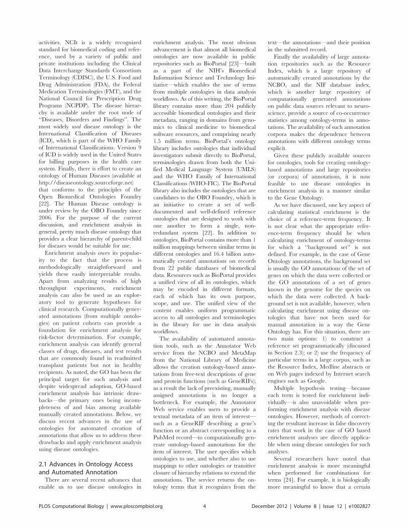
activities. NCIt is a widely recognized
standard for biomedical coding and refer-
ence, used by a variety of public and
private institutions including the Clinical
Data Interchange Standards Consortium
Terminology (CDISC), the U.S. Food and
Drug Administration (FDA), the Federal
Medication Terminologies (FMT), and the
National Council for Prescription Drug
Programs (NCPDP). The disease hierar-
chy is available under the root node of
‘‘Diseases, Disorders and Findings’’. The
most widely used disease ontology is the
International Classification of Diseases
(ICD), which is part of the WHO Family
of International Classifications. Version 9
of ICD is widely used in the United States
for billing purposes in the health care
system. Finally, there is effort to create an
ontology of Human Diseases (available at
http://diseaseontology.sourceforge.net)
that conforms to the principles of the
Open Biomedical Ontologies Foundry
[22]. The Human Disease ontology is
under review by the OBO Foundry since
2006. For the purpose of the current
discussion, and enrichment analysis in
general, pretty much disease ontology that
provides a clear hierarchy of parent-child
for diseases would be suitable for use.
Enrichment analysis owes its popular-
ity to the fact that the process is
methodologically straightforward and
yields these easily interpretable results.
Apart from analyzing results of high
throughput experiments, enrichment
analysis can also be used as an explor-
atory tool to generate hypotheses for
clinical research. Computationally gener-
ated annotations (from multiple ontolo-
gies) on patient cohorts can provide a
foundation for enrichment analysis for
risk-factor determination. For example,
enrichment analysis can identify general
classes of drugs, diseases, and test results
that are commonly found in readmitted
transplant patients but not in healthy
recipients. As noted, the GO has been the
principal target for such analysis and
despite widespread adoption, GO-based
enrichment analysis has intrinsic draw-
backs—the primary ones being incom-
pleteness of and bias among available
manually created annotations. Below, we
discuss recent advances in the use of
ontologies for automated creation of
annotations that allow us to address these
drawbacks and apply enrichment analysis
using disease ontologies.
2.1 Advances in Ontology Accessand Automated Annotation
There are several recent advances that
enable us to use disease ontologies in
enrichment analysis. The most obvious
advancement is that almost all biomedical
ontologies are now available in public
repositories such as BioPortal [23]—built
as a part of the NIH’s Biomedical
Information Science and Technology Ini-
tiative—which enables the use of terms
from multiple ontologies in data analysis
workflows. As of this writing, the BioPortal
library contains more than 204 publicly
accessible biomedical ontologies and their
metadata, ranging in domains from geno-
mics to clinical medicine to biomedical
software resources, and comprising nearly
1.5 million terms. BioPortal’s ontology
library includes ontologies that individual
investigators submit directly to BioPortal,
terminologies drawn from both the Uni-
fied Medical Language System (UMLS)
and the WHO Family of International
Classifications (WHO-FIC). The BioPortal
library also includes the ontologies that are
candidates to the OBO Foundry, which is
an initiative to create a set of well-
documented and well-defined reference
ontologies that are designed to work with
one another to form a single, non-
redundant system [22]. In addition to
ontologies, BioPortal contains more than 1
million mappings between similar terms in
different ontologies and 16.4 billion auto-
matically created annotations on records
from 22 public databases of biomedical
data. Resources such as BioPortal provides
a unified view of all its ontologies, which
may be encoded in different formats,
each of which has its own purpose,
scope, and use. The unified view of the
content enables uniform programmatic
access to all ontologies and terminologies
in the library for use in data analysis
workflows.
The availability of automated annota-
tion tools, such as the Annotator Web
service from the NCBO and MetaMap
from the National Library of Medicine
allows the creation ontology-based anno-
tations from free-text descriptions of gene
and protein functions (such as GeneRIFs);
as a result the lack of preexisting, manually
assigned annotations is no longer a
bottleneck. For example, the Annotator
Web service enables users to provide a
textual metadata of an item of interest—
such as a GeneRIF describing a gene’s
function or an abstract corresponding to a
PubMed record—to computationally gen-
erate ontology-based annotations for the
item of interest. The user specifies which
ontologies to use, and whether also to use
mappings to other ontologies or transitive
closure of hierarchy relations to extend the
annotations. The service returns the on-
tology terms that it recognizes from the
text—the annotations—and their position
in the submitted record.
Finally the availability of large annota-
tion repositories such as the Resource
Index, which is a large repository of
automatically created annotations by the
NCBO, and the NIF database index,
which is another large repository of
computationally generated annotations
on public data sources relevant to neuro-
science, provide a source of co-occurrence
statistics among ontology-terms in anno-
tations. The availability of such annotation
corpora makes the dependence between
annotations with different ontology terms
explicit.
Given these publicly available sources
for ontologies, tools for creating ontology-
based annotations and large repositories
(or corpora) of annotations, it is now
feasible to use disease ontologies in
enrichment analysis in a manner similar
to the Gene Ontology.
As we have discussed, one key aspect of
calculating statistical enrichment is the
choice of a reference-term frequency. It
is not clear what the appropriate refer-
ence-term frequency should be when
calculating enrichment of ontology-terms
for which a ‘‘background set’’ is not
defined. For example, in the case of Gene
Ontology annotations, the background set
is usually the GO annotations of the set of
genes on which the data were collected or
the GO annotations of a set of genes
known in the genome for the species on
which the data were collected. A back-
ground set is not available, however, when
calculating enrichment using disease on-
tologies that have not been used for
manual annotation in a way the Gene
Ontology has. For this situation, there are
two main options: 1) to construct a
reference set programmatically (discussed
in Section 2.3); or 2) use the frequency of
particular terms in a large corpus, such as
the Resource Index, Medline abstracts or
on Web pages indexed by Internet search
engines such as Google.
Multiple hypothesis testing—because
each term is tested for enrichment indi-
vidually—is also unavoidable when per-
forming enrichment analysis with disease
ontologies. However, methods of correct-
ing the resultant increase in false discovery
rates that work in the case of GO based
enrichment analyses are directly applica-
ble when using disease ontologies for such
analyses.
Several researchers have noted that
enrichment analysis is more meaningful
when performed for combinations for
terms [24]. For example, it is biologically
more meaningful to know that a certain
PLOS Computational Biology | www.ploscompbiol.org 4 December 2012 | Volume 8 | Issue 12 | e1002827
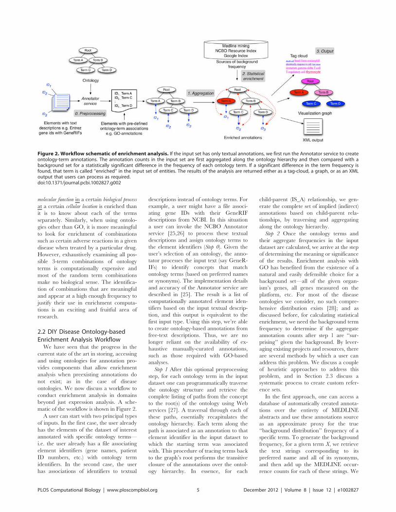
molecular function in a certain biological process
at a certain cellular location is enriched than
it is to know about each of the terms
separately. Similarly, when using ontolo-
gies other than GO, it is more meaningful
to look for enrichment of combinations
such as certain adverse reactions in a given
disease when treated by a particular drug.
However, exhaustively examining all pos-
sible 3-term combinations of ontology
terms is computationally expensive and
most of the random term combinations
make no biological sense. The identifica-
tion of combinations that are meaningful
and appear at a high enough frequency to
justify their use in enrichment computa-
tions is an exciting and fruitful area of
research.
2.2 DIY Disease Ontology-basedEnrichment Analysis Workflow
We have seen that the progress in the
current state of the art in storing, accessing
and using ontologies for annotation pro-
vides components that allow enrichment
analysis when preexisting annotations do
not exist; as in the case of disease
ontologies. We now discuss a workflow to
conduct enrichment analysis in domains
beyond just expression analysis. A sche-
matic of the workflow is shown in Figure 2.
A user can start with two principal types
of inputs. In the first case, the user already
has the elements of the dataset of interest
annotated with specific ontology terms—
i.e. the user already has a file associating
element identifiers (gene names, patient
ID numbers, etc.) with ontology term
identifiers. In the second case, the user
has associations of identifiers to textual
descriptions instead of ontology terms. For
example, a user might have a file associ-
ating gene IDs with their GeneRIF
descriptions from NCBI. In this situation
a user can invoke the NCBO Annotator
service [25,26] to process these textual
descriptions and assign ontology terms to
the element identifiers (Step 0). Given the
user’s selection of an ontology, the anno-
tator processes the input text (say GeneR-
IFs) to identify concepts that match
ontology terms (based on preferred names
or synonyms). The implementation details
and accuracy of the Annotator service are
described in [25]. The result is a list of
computationally annotated element iden-
tifiers based on the input textual descrip-
tion, and this output is equivalent to the
first input type. Using this step, we’re able
to create ontology-based annotations from
free-text descriptions. Thus, we are no
longer reliant on the availability of ex-
haustive manually-curated annotations,
such as those required with GO-based
analyses.
Step 1 After this optional preprocessing
step, for each ontology term in the input
dataset one can programmatically traverse
the ontology structure and retrieve the
complete listing of paths from the concept
to the root(s) of the ontology using Web
services [27]. A traversal through each of
these paths, essentially recapitulates the
ontology hierarchy. Each term along the
path is associated as an annotation to that
element identifier in the input dataset to
which the starting term was associated
with. This procedure of tracing terms back
to the graph’s root performs the transitive
closure of the annotations over the ontol-
ogy hierarchy. In essence, for each
child-parent (IS_A) relationship, we gen-
erate the complete set of implied (indirect)
annotations based on child-parent rela-
tionships, by traversing and aggregating
along the ontology hierarchy.
Step 2 Once the ontology terms and
their aggregate frequencies in the input
dataset are calculated, we arrive at the step
of determining the meaning or significance
of the results. Enrichment analysis with
GO has benefited from the existence of a
natural and easily defensible choice for a
background set—all of the given organ-
ism’s genes, all genes measured on the
platform, etc. For most of the disease
ontologies we consider, no such compre-
hensive distribution exists [28]; and as
discussed before, for calculating statistical
enrichment, we need the background term
frequency to determine if the aggregate
annotation counts after step 1 are ‘‘sur-
prising’’ given the background. By lever-
aging existing projects and resources, there
are several methods by which a user can
address this problem. We discuss a couple
of heuristic approaches to address this
problem, and in Section 2.3 discuss a
systematic process to create custom refer-
ence sets.
In the first approach, one can access a
database of automatically created annota-
tions over the entirety of MEDLINE
abstracts and use these annotations source
as an approximate proxy for the true
‘‘background distribution’’ frequency of a
specific term. To generate the background
frequency, for a given term X, we retrieve
the text strings corresponding to its
preferred name and all of its synonyms,
and then add up the MEDLINE occur-
rence counts for each of these strings. We
Figure 2. Workflow schematic of enrichment analysis. If the input set has only textual annotations, we first run the Annotator service to createontology-term annotations. The annotation counts in the input set are first aggregated along the ontology hierarchy and then compared with abackground set for a statistically significant difference in the frequency of each ontology term. If a significant difference in the term frequency isfound, that term is called ‘‘enriched’’ in the input set of entities. The results of the analysis are returned either as a tag-cloud, a graph, or as an XMLoutput that users can process as required.doi:10.1371/journal.pcbi.1002827.g002
PLOS Computational Biology | www.ploscompbiol.org 5 December 2012 | Volume 8 | Issue 12 | e1002827
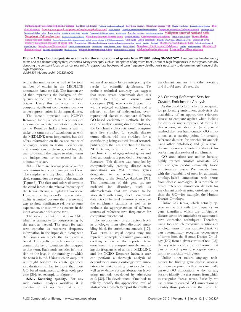
return this number (m) as well as the total
number of entries in the MEDLINE
annotation database (M). The fraction m/
M then represents the background fre-
quency of the term X in the annotated
corpus. Using this frequency we can
compute significant comparative over- or
under-representation in the input dataset.
The second approach uses NCBO’s
Resource Index, which is a repository of
automatically-created annotations. Access
to the Resource Index allows a user to
make the same sort of calculations as with
the MEDLINE term frequencies, but also
offers information on the co-occurrence of
ontological terms in textual descriptions
and annotations of datasets; enabling the
user to quantify the degree to which terms
are independent or correlated in the
annotation space.
Step 3 There are several possible output
mechanisms to such an analysis workflow.
The simplest is a tag cloud, which intui-
tively summarizes the results of the analysis
(Figure 3). The sizes and colors of terms in
the cloud indicate the relative frequency of
the terms offering a high-level overview.
However, a tag cloud’s representative
ability is limited because there is no easy
way to show significance relative to some
expectation, or to show the elements in the
input associated with some term.
The second output format is in XML,
which is amenable to postprocessing by
the user, as needed. The result for each
term contains its respective frequency
information in the input data along with
the counts on which the frequency is
based. The results on each term can also
contain the list of identifiers that mapped
to that term. Each node includes informa-
tion on the level in the ontology at which
the term is found. Using such an output, it
is straight forward to create graphical
visualizations similar to those that most
GO based enrichment analysis tools pro-
vide [29]; see example in Figure 4.
2.2.1. Ensuring quality. For any
such custom analysis workflow it is
essential to set up tests that ensure
technical accuracy before interpreting the
results for scientific significance. To
evaluate technical accuracy, we suggest
that users create benchmark data sets
similar to those of Toronen and
colleagues [30], who created gene lists
with a selected enrichment level and a
selected number of independent, over-
represented classes to compare different
GO-based enrichment methods. In the
case of analyses using disease ontologies,
the benchmark data sets would comprise
gene lists enriched for specific disease
terms, clinical-trial lists enriched for a
specific drug being studied; lists of research
publications that are enriched for known
NCIt terms, and so on. A sample
benchmark list of aging related genes and
their annotations is provided in Section 5.
Exercises. This dataset was compiled by
computationally creating disease term
annotations on 261 human genes
designated to be related to aging
according to the GeneAge database [31].
The annotations of this gene list are
enriched for disorders, such as
atherosclerosis, that are known to be
associated with aging. Such benchmark
data sets can be used to ensure accuracy of
the enrichment statistics as well as to
evaluate the appropriateness of different
sources of reference-term frequencies for
computing enrichment.
The inconsistency of abstraction levels
in ontologies is an often discussed stum-
bling block for enrichment analysis [17].
Two terms at equal depths may not
represent concepts of similar granularity,
creating a bias in the reported term
enrichment. By comprehensively analyz-
ing the frequencies of terms in MEDLINE
and the NCBO Resource Index, a user
can perform a thorough analysis of
dependencies among ontology-term anno-
tations to make existing biases explicit as
well as to define custom abstraction levels
using methods developed by Alterovitz
et al. [32]. The development of methods to
reliably identify the appropriate level of
abstraction at which to report the results of
enrichment analysis is another exciting
and fruitful area of research.
2.3 Creating Reference Sets forCustom Enrichment Analysis
As discussed before, a key pre-requisite
for performing enrichment analysis is the
availability of an appropriate reference
dataset to compare against when looking
for over- or under-represented terms. In
this section, we describe: (i) a general
method that uses hand-curated GO anno-
tations as a starting point, for creating
reference datasets for enrichment analysis
using other ontologies; and (ii) a gene–
disease reference annotation dataset for
performing disease-based enrichment.
GO annotations are unique because
highly trained curators associate GO
terms to gene products manually, based
on literature review. We describe how,
with the availability of tools for automatic
ontology-based annotation with terms
from disease ontologies, it is possible to
create reference annotation datasets for
enrichment analysis using ontologies other
than the GO—for example, the Human
Disease Ontology.
Unlike GO terms, which actually ap-
pear in the text with low frequency, or
gene identifiers, which are ambiguous,
disease terms are amenable to automated,
term extraction techniques. Therefore,
using tools which recognize mentions of
ontology terms in user submitted text, we
can automatically recognize occurrences
of terms from the Human Disease Ontol-
ogy (DO) from a given corpus of text [28];
the key is to identify the text source that
can be relied upon to recognize disease
terms to associate with genes.
Unlike other natural-language tech-
niques for finding gene–disease associa-
tions, our proposed method uses manually
curated GO annotations as the starting
basis to identify the text source from which
to recognize disease terms. Basically, we
use manually curated GO annotations to
identify those publications that were the
Figure 3. Tag cloud output: An example for the annotations of grants from FY1981 using SNOMEDCT. Blue denotes low-frequencyterms and red denotes highly frequent terms. Many concepts, such as ‘‘neoplasm of digestive tract’’, occur at high frequencies in most years, possiblydenoting the constant focus on cancer research. An appropriate background term frequency distribution is necessary to determine significance of thehigh frequency.doi:10.1371/journal.pcbi.1002827.g003
PLOS Computational Biology | www.ploscompbiol.org 6 December 2012 | Volume 8 | Issue 12 | e1002827
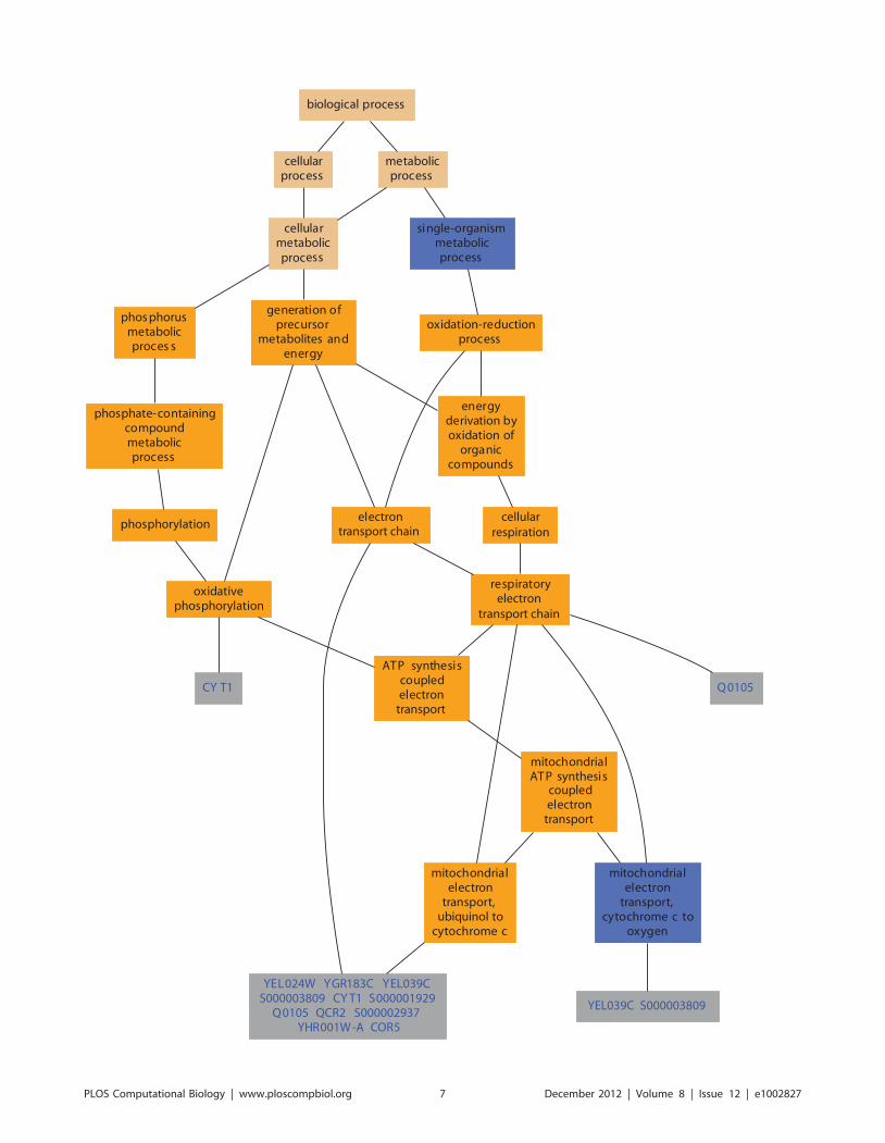
PLOS Computational Biology | www.ploscompbiol.org 7 December 2012 | Volume 8 | Issue 12 | e1002827
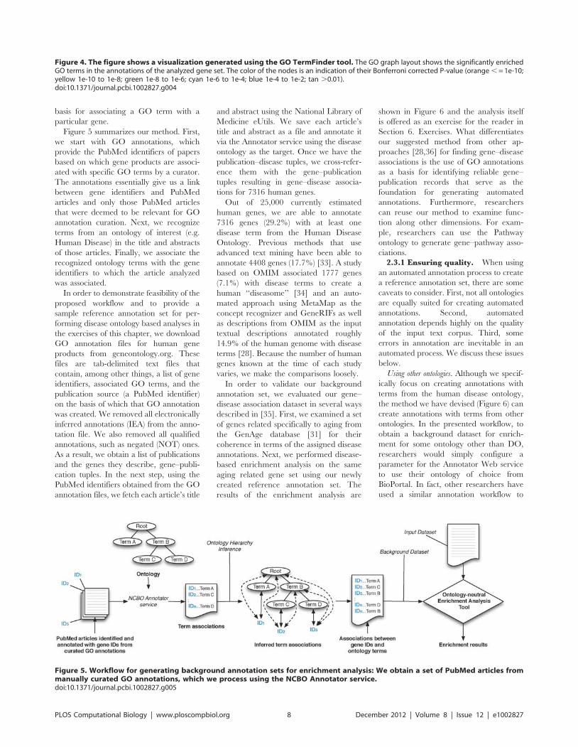
basis for associating a GO term with a
particular gene.
Figure 5 summarizes our method. First,
we start with GO annotations, which
provide the PubMed identifiers of papers
based on which gene products are associ-
ated with specific GO terms by a curator.
The annotations essentially give us a link
between gene identifiers and PubMed
articles and only those PubMed articles
that were deemed to be relevant for GO
annotation curation. Next, we recognize
terms from an ontology of interest (e.g.
Human Disease) in the title and abstracts
of those articles. Finally, we associate the
recognized ontology terms with the gene
identifiers to which the article analyzed
was associated.
In order to demonstrate feasibility of the
proposed workflow and to provide a
sample reference annotation set for per-
forming disease ontology based analyses in
the exercises of this chapter, we download
GO annotation files for human gene
products from geneontology.org. These
files are tab-delimited text files that
contain, among other things, a list of gene
identifiers, associated GO terms, and the
publication source (a PubMed identifier)
on the basis of which that GO annotation
was created. We removed all electronically
inferred annotations (IEA) from the anno-
tation file. We also removed all qualified
annotations, such as negated (NOT) ones.
As a result, we obtain a list of publications
and the genes they describe, gene–publi-
cation tuples. In the next step, using the
PubMed identifiers obtained from the GO
annotation files, we fetch each article’s title
and abstract using the National Library of
Medicine eUtils. We save each article’s
title and abstract as a file and annotate it
via the Annotator service using the disease
ontology as the target. Once we have the
publication–disease tuples, we cross-refer-
ence them with the gene–publication
tuples resulting in gene–disease associa-
tions for 7316 human genes.
Out of 25,000 currently estimated
human genes, we are able to annotate
7316 genes (29.2%) with at least one
disease term from the Human Disease
Ontology. Previous methods that use
advanced text mining have been able to
annotate 4408 genes (17.7%) [33]. A study
based on OMIM associated 1777 genes
(7.1%) with disease terms to create a
human ‘‘diseasome’’ [34] and an auto-
mated approach using MetaMap as the
concept recognizer and GeneRIFs as well
as descriptions from OMIM as the input
textual descriptions annotated roughly
14.9% of the human genome with disease
terms [28]. Because the number of human
genes known at the time of each study
varies, we make the comparisons loosely.
In order to validate our background
annotation set, we evaluated our gene–
disease association dataset in several ways
described in [35]. First, we examined a set
of genes related specifically to aging from
the GenAge database [31] for their
coherence in terms of the assigned disease
annotations. Next, we performed disease-
based enrichment analysis on the same
aging related gene set using our newly
created reference annotation set. The
results of the enrichment analysis are
shown in Figure 6 and the analysis itself
is offered as an exercise for the reader in
Section 6. Exercises. What differentiates
our suggested method from other ap-
proaches [28,36] for finding gene–disease
associations is the use of GO annotations
as a basis for identifying reliable gene–
publication records that serve as the
foundation for generating automated
annotations. Furthermore, researchers
can reuse our method to examine func-
tion along other dimensions. For exam-
ple, researchers can use the Pathway
ontology to generate gene–pathway asso-
ciations.
2.3.1 Ensuring quality. When using
an automated annotation process to create
a reference annotation set, there are some
caveats to consider. First, not all ontologies
are equally suited for creating automated
annotations. Second, automated
annotation depends highly on the quality
of the input text corpus. Third, some
errors in annotation are inevitable in an
automated process. We discuss these issues
below.
Using other ontologies. Although we specif-
ically focus on creating annotations with
terms from the human disease ontology,
the method we have devised (Figure 6) can
create annotations with terms from other
ontologies. In the presented workflow, to
obtain a background dataset for enrich-
ment for some ontology other than DO,
researchers would simply configure a
parameter for the Annotator Web service
to use their ontology of choice from
BioPortal. In fact, other researchers have
used a similar annotation workflow to
Figure 4. The figure shows a visualization generated using the GO TermFinder tool. The GO graph layout shows the significantly enrichedGO terms in the annotations of the analyzed gene set. The color of the nodes is an indication of their Bonferroni corrected P-value (orange , = 1e-10;yellow 1e-10 to 1e-8; green 1e-8 to 1e-6; cyan 1e-6 to 1e-4; blue 1e-4 to 1e-2; tan .0.01).doi:10.1371/journal.pcbi.1002827.g004
Figure 5. Workflow for generating background annotation sets for enrichment analysis: We obtain a set of PubMed articles frommanually curated GO annotations, which we process using the NCBO Annotator service.doi:10.1371/journal.pcbi.1002827.g005
PLOS Computational Biology | www.ploscompbiol.org 8 December 2012 | Volume 8 | Issue 12 | e1002827
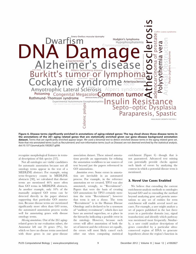
recognize morphological features in textu-
al descriptions of fish species [37].
Not all ontologies are viable candidates
for automatic annotation because not all
ontology terms appear in the text of a
MEDLINE abstract. For example, using
term–frequency counts in MEDLINE
abstracts [38], we calculated that disease
terms are mentioned 46% more often
than GO terms in MEDLINE abstracts.
As another example, only 10% of the
manually assigned GO terms can be
detected directly in the paper abstract
supporting that particular GO annota-
tion. Because disease terms are mentioned
significantly more often than GO terms,
the automated annotation process works
well for annotating genes with disease
ontology terms.
Missing annotations. Out of the 261 aging-
related genes in our evaluation subset, the
Annotator left out 24 genes (9%), for
which we have no disease terms associated
with those genes in our gene–disease
association dataset. These missed annota-
tions provide an opportunity for refining
the annotation workflows to use sources of
text beyond just the papers referenced in
GO annotations.
Annotation errors. Some errors in annota-
tion are inevitable in an automated
process. For example, in the reference
annotation set we created, TP53 was also
annotated, wrongly, to ‘‘Recruitment’’.
Papers that were the basis of creating
GO annotations for TP53 certainly men-
tion the term ‘‘Recruitment’’; however
that term is not a disease. The term
‘‘Recruitment’’ is in the Human Disease
Ontology and is declared to be a synonym
of ‘‘auditory recruitment’’, which does not
have an asserted superclass, or a place in
the hierarchy indicating a possible error in
the ontology. However, because such
errors will affect annotation of both the
set of interest and the reference set equally,
the errors will most likely cancel each
other out when computing statistical
enrichment (Figure 6)—though that is
not guaranteed. Advanced text mining
can potentially provide checks against
such kinds of errors by analyzing the
context in which a potential disease term is
mentioned.
3. Novel Use Cases Enabled
We believe that extending the current
enrichment-analysis methods to ontologies
beyond GO and to extending the method
beyond analyzing gene and protein anno-
tations to any set of entities for term
enrichment will enable several novel use
cases. For example, a user might analyze a
set of papers published in the last three
years in a particular domain (say, signal
transduction) and identify which pathway
was mentioned most frequently. Similar-
ly, a user could analyze descriptions of
genes controlled by a particular ultra-
conserved region of DNA to generate
hypotheses about the region’s function in
Figure 6. Disease terms significantly enriched in annotations of aging-related genes: The tag cloud shows those disease terms inthe annotations of the 261 aging related genes that are statistically enriched given our gene–disease background annotationdataset. Terms that are significantly enriched appear larger. We used a binomial test to detect enriched disease terms in the aging related gene set.Note that mis-annotated terms (such as Recruitment) and non-informative terms (such as Disease) are not deemed enriched by the statistical analysis.doi:10.1371/journal.pcbi.1002827.g006
PLOS Computational Biology | www.ploscompbiol.org 9 December 2012 | Volume 8 | Issue 12 | e1002827
specific disease processes. We discuss the
potential of some of the novel use cases
enabled by disease ontology based en-
richment analysis.
Analysis of protein annotations To demon-
strate the feasibility of performing enrich-
ment analysis and recovering known GO
annotations as well as to demonstrate
enrichment analysis with multiple ontolo-
gies, we analyzed a list of 261 known aging
related genes from the GenAge database
[31]. We started by collecting textual
descriptions for UniProt protein entries
corresponding to each human gene in the
GenAge database. The textual descrip-
tions included the protein name, gene
name, general descriptions of the function
and catalytic activity as well as keywords
and GO terms. We processed this text as
described in the workflow in Figure 6 and
created annotations from Medical Subject
Heading (MSH), Online Mendelian In-
heritance in Man (OMIM), UMLS Me-
tathesaurus (MTH) and Gene Ontology
(GO).
We created a background set of anno-
tations on 19671 proteins by applying the
same protocol to manually annotated and
reviewed proteins from SwissProt (Jan
2010 version). We calculated enrichment
and depletion of specific terms, corrected
for multiple hypotheses and obtained a list
of significant terms for all four ontologies.
Not surprisingly, ‘aging’ is an enriched
term. There were several other terms
enriched such as ‘electron transport’
(2.79e-10), ‘protein kinase activity’ (2.8e-
10) and ‘nucleotide excision repair’ (8.78e-
07) which appeared in MSH, MTH, and
GO. The enriched terms also included
aging associated diseases such as ‘Alzhei-
mer’s disease’ (0.01), ‘Werner syndrome’
(5.3e-05), ‘Diabetes Mellitus’ (1.5e-04) and
‘neurodegeneration’ (2.5e-03) from OMIM.
This case study demonstrate that en-
richment analysis with multiple ontologies
is feasible and it enables a comprehensive
characterization of the biological ‘‘signal’’
present in gene/protein lists [39]. For
example, by annotating known protein
mutations with disease terms from the
ontologies in BioPortal, Mort et al. recently
identified a class of diseases—blood coag-
ulation disorders—that were associated
with a 14-fold depletion in substitutions at
O-linked glycosylation sites [20].
Analysis of funding trends To demonstrate
the feasiblity of such analyses in a novel
domain, we processed the funding alloca-
tions of the NIH in fiscal years 1980–1989.
We aimed to identify trends in institutional
funding priorities over time, as represented
by changes in the relative frequencies of
ontology concepts from year-to-year.
Using a database containing the complete
set of grants in this interval—with their
titles, amounts, recipient institutions,
etc.—we selected grants worth over
$1,250,000 (in constant 2008 dollars). We
annotated the titles of these grants with
SNOMEDCT terms and used the anno-
tation sets to generate tag clouds for each
year, such as the one shown in Figure 3 for
year 1981, to create a visual summary of
funding trends on a per year basis. Further
analysis cross-linking annotation on grants
with annotations on publications from
specific institutions can enable compara-
tive analysis of the research efficacy at
different institutions.
Hypothesis generation for Clinical Research
Finally, enrichment analysis can also be
used as an exploratory tool to generate
hypotheses for clinical research by analyz-
ing annotations on medical records in
conjunction with annotation of molecular
datasets. For example, in the case of
kidney transplants, extended-criteria do-
nor (ECD) organs have a 40% rate of
delayed graft function and a higher
incidence of rejection compared to stan-
dard-criteria donor (SCD) kidneys.
Identifying causes of this difference is
crucial to identify patients in which an
ECD transplant has a high chance of
working.
At several research sites, the datasets
collected to address this question comprise
immunological metrics beyond the stan-
dard clinical risk factors, including multi-
parameter flow-cytometric analysis of the
peripheral immune-cell repertoire, geno-
mic analysis, and donor-specific functional
assessments. These patient data sets can be
annotated using automated methods
[8,26] to enable enrichment analysis for
risk-factor determination.
For example, simple enrichment anal-
ysis might allow identification of classes of
drugs, diseases, and test results that are
commonly found only in readmitted
transplant patients. Enrichment analysis
to identify common pairs of terms of
different semantic types can identify
combinations of drug classes and co-
morbidities, or test risk-factors and co-
morbidities that are common in this
population.
4. Summary
Because enrichment analysis with GO is
widely accepted and scientifically valuable,
we argue that the logical next step is to
extend this methodology to other ontolo-
gies—specifically disease ontologies.
Given the recent advances in ontology
repositories and methods of automated
annotation, we argue that enrichment
analysis based on textual descriptions is
possible.
We have systematically discussed how
to accomplish enrichment analysis using
ontologies other than the Gene Ontology
as well as address some of the limitations
of existing analysis methods. For example,
the roughly 20% of genes that lack
annotations can now be associated, via
their GeneRIFs, with terms from disease
ontologies. We have outlined possible
directions of research for overcoming
other limitations such as inconsistent
abstraction levels in ontologies, perform-
ing the analysis using combinations of
ontology terms, and accounting for anno-
tation bias.
In order to perform enrichment analysis
using ontologies other than the GO, a key
pre-requisite is the availability of a back-
ground set of annotations to enable the
enrichment calculation. We have de-
scribed a general method, which uses
hand-curated GO annotations as a start-
ing point, for creating background datasets
for enrichment analysis using other ontol-
ogies—such as the Human Disease On-
tology, for which hand-curated annota-
tions are not available.
To demonstrate the feasibility and
utility of our proposals, we have created
a background set of annotations to enable
enrichment analysis with the Human
Disease Ontology and validated that
background set by using the created
annotations to examine the coherence of
known aging related genes and by per-
forming enrichment analysis on an aging
related gene set from the GeneAge
database [31]. We make the set of aging
related genes and the reference annotation
set available for reader exercises in
enrichment analysis.
We argue that enrichment analysis
using computationally created ontology-
based annotations from textual descrip-
tions is possible, thus introducing
enrichment analysis as a research meth-
odology in new domains such as hypoth-
esis generation for clinical research;
without requiring manually created anno-
tations.
5. Exercises
(1) For the 260 aging related genes in
Dataset S1, perform enrichment analysis
using the Human Disease ontology, using
Dataset S2 as the reference annotation set.
Some considerations while working
through the problem:
PLOS Computational Biology | www.ploscompbiol.org 10 December 2012 | Volume 8 | Issue 12 | e1002827
N The genes are listed with their Uni-
protIDs.
N Using the notation in Section 1.1, the
values of N and M are the total
number of unique genes in the aging
set and total set, respectively, and not
the number of unique terms. The
values of n and m are the unique genes
that are annotated with a given term in
the corresponding set.
N When performing the hypergeometric
test, if the test calculates the p value
based on finding a value of n greater
than or less than what was observed
(instead of equal to what was observed),
remember to add or subtract 1 from the
number of genes annotated with a given
term when calculating. If you are using a
function to calculate, refer to the
documentation to understand the input
required.
N Consider from which tail of the
hypergeometric distribution you wish
to calculate the p value.
(2) For the 260 aging related genes,
perform enrichment analysis using
SNOMED-CT (Systematized Nomencla-
ture of Medicine-Clinical Terms). Use the
GeneRIF (Gene Reference into Function)
database as the source text to annotate with
disease terms from SNOMED-CT. Choose
an appropriate reference annotation set
and justify the choice. Some considerations
while working through the problem:
N An index of GeneRIFs, maintained
by the National Center for Biotech-
nology Information (NCBI) and
the National Institutes of Health
(NIH), can be downloaded from here:
ftp://ftp.ncbi.nih.gov/gene/GeneRIF/
N Mapping from UniprotIDs to Gen-
eIDs, which are used in the GeneRIF
database, can be done here: http://
www.uniprot.org/help/mapping.
Note that you will get 261 GeneIDs for
the 260 UniprotIDs.
N Annotation using the National Center
for Biomedical Ontology’s BioPortal
Annotator Service requires obtaining
an API key. This can be done after
registration and going to ‘‘Account’’
where your API key will be displayed:
http://bioportal.bioontology.org/
N Information on the programmatic use of
the BioPortal Annotator as a client can be
found here: http://www.bioontology.
org/wiki/index.php/Annotator_Web_
service. Example code from numerous
languages, including Java, R, Python,
Ruby, Excel, HTML, and Perl, can be
found here: http://www.bioontology.
org/wiki/index.php/Annotator_Client_
Examples. All NCBO REST Web
services require the parameter ‘‘api-
key = YourApiKey’’. It is strongly en-
couraged that all users of the NCBO
Annotator Web service use only the
virtual ontology identifier. To do
so, set the ‘‘isVirtualOntolgyId’’ param-
eter to ‘‘true’’. This will ensure that you
access the version of the ontology that is
actually in the database. Failure to do this
will result in your code breaking every
time the database is updated.
N Output from the annotation service
can be conveniently parsed in XML.
To see an example of what this might
look like, visit http://bioportal.
bioontology.org/annotator. Insert the
sample text or use text of your choice,
makes selection(s) under ‘Select Ontol-
ogies’ and ‘Select UMLS Semantic
Types’ and click ‘Get Annotations’. At
the bottom by ‘Format Results As’ you
can select XML to see the XML tree
structure of the Annotator output.
N The suggested ontology for this exercise
is SNOMED-CT (ontology ID: 1353)
and semantic types Anatomical Struc-
ture (T017), Disease or Syndrome
(T047), Neoplastic Process (T191), and
NCBO BioPortal concept (T999).
N Some processing of the GeneRIF text
may be necessary to prevent errors in
annotation. It is suggested to remove
GeneRIFs with new line characters
(‘\n’) and replace single or double
quotes with white space.
N Many GeneIDs have multiple Gen-
eRIF entries. The user will find more
efficient annotation if all of the Gen-
eRIF entries for a given gene are
concatenated and passed to the anno-
tator instead of annotating individual
GeneRIF entries for the same gene.
N Due to the large number of GeneRIFs,
the BioPortal Annotator may timeout
while the user is looping through genes to
annotate. It is suggested that the annota-
tion is done incrementally and joined or
intermittent saves of the annotations is
done to prevent timely re-annotation.
N The given set of aging genes will have
considerably more annotations terms
per gene than the set of all genes in the
GeneRIF database. This bias should
be a consideration when deciding on
an appropriate M. There are numer-
ous approaches to address this, and a
simple method may be to limit the
reference set of genes M to only those
with at least a given number of
annotated terms. You may also want
to limit the results to only those terms
that appear at least a given amount of
times in the aging gene annotations.
Answers to the Exercises can be found
in Text S1.
Supporting Information
Dataset S1 Data file for Exercise 1
(TXT)
Dataset S2 Data file for Exercise 1
(TXT)
Dataset S3 Data file for Exercise 1
(OBO)
Dataset S4 Additional info on genes
mentioned in S1 and S2. Can be used in
lieu of GeneRIFs in Exercise 2.
(TXT)
Text S1 Answers to Exercises
(DOCX)
Table S1 Exercise 1 analysis results
(CSV)
Table S2 Exercise 2 analysis results
(CSV)
Further Reading
N Tirrell R, Evani U, Berman AE, Mooney SD, Musen MA, et al. (2010) An ontology-neutral framework for enrichment analysis. AMIA Annual Symposium proceed-ings/AMIA Symposium AMIA Symposium 2010: 797–801.
N Shah NH, Jonquet C, Chiang AP, Butte AJ, Chen R, et al. (2009) Ontology-drivenindexing of public datasets for translational bioinformatics. BMC Bioinformatics10 Suppl 2: S1.
N Alterovitz G, Xiang M, Mohan M, Ramoni MF (2007) GO PaD: the Gene OntologyPartition Database. Nucleic Acids Res 35(Database issue): D322–D327.
N Myhre S, Tveit H, Mollestad T, Laegreid A (2006) Additional gene ontologystructure for improved biological reasoning. Bioinformatics 22: 2020–2027.
N Toronen P, Pehkonen P, Holm L (2009) Generation of Gene Ontologybenchmark datasets with various types of positive signal. BMC Bioinformatics10: 319.
PLOS Computational Biology | www.ploscompbiol.org 11 December 2012 | Volume 8 | Issue 12 | e1002827
Acknowledgments
We acknowledge use of the publicly available
GO Term Finder server at http://go.princeton.
edu/cgi-bin/GOTermFinder. We also thank
Paea LePendu for assistance in creating solu-
tions to the exercises.
References
1. Altman RB, Raychaudhuri S (2001) Whole-
genome expression analysis: challenges beyond
clustering. Curr Opin Struct Biol 11: 340–347.
2. Brazma A, Vilo J (2000) Gene expression dataanalysis. FEBS Lett 480: 17–24.
3. Quackenbush J (2002) Microarray data normal-
ization and transformation. Nat Genet 32 Suppl:496–501.
4. Tusher VG, Tibshirani R, Chu G (2001)Significance analysis of microarrays applied to
the ionizing radiation response. Proc Natl Acad
Sci U S A 98: 5116–5121.5. Huttenhower C, Hibbs M, Myers C, Troyans-
kaya OG (2006) A scalable method for integrationand functional analysis of multiple microarray
datasets. Bioinformatics 22: 2890–2897.6. Zeeberg BR, Feng W, Wang G, Wang MD, Fojo
AT, et al. (2003) GoMiner: a resource for
biological interpretation of genomic and proteo-mic data. Genome Biol 4: R28.
7. Rhee SY, Wood V, Dolinski K, Draghici S (2008)Use and misuse of the gene ontology annotations.
Nat Rev Genet 9: 509–515.
8. Shah NH, Jonquet C, Chiang AP, Butte AJ, ChenR, et al. (2009) Ontology-driven indexing of
public datasets for translational bioinformatics.BMC Bioinformatics 10 Suppl 2: S1.
9. Subramanian A, Tamayo P, Mootha VK,Mukherjee S, Ebert BL, et al. (2005) Gene set
enrichment analysis: a knowledge-based ap-
proach for interpreting genome-wide expressionprofiles. Proc Natl Acad Sci U S A 102: 15545–
15550.10. Draghici S, Khatri P, Martins RP, Ostermeier GC,
Krawetz SA (2003) Global functional profiling of
gene expression. Genomics 81: 98–104.11. (2002) Gene ontology consortium website.
12. Alexa A, Rahnenfuhrer J, Lengauer T (2006)Improved scoring of functional groups from gene
expression data by decorrelating GO graphstructure. Bioinformatics 22: 1600–1607.
13. Grossmann S, Bauer S, Robinson PN, Vingron
M (2007) Improved detection of overrepresenta-tion of Gene-Ontology annotations with parent
child analysis. Bioinformatics 23: 3024–3031.14. Schlicker A, Rahnenfuhrer J, Albrecht M,
Lengauer T, Domingues FS (2007) GOTax:
investigating biological processes and biochemical
activities along the taxonomic tree. Genome Biol
8: R33.
15. Farcomeni A (2008) A review of modern multiple
hypothesis testing, with particular attention to the
false discovery proportion. Stat Methods Med
Res 17: 347–388.
16. Benjamini Y, Yekutieli D (2001) The control of
the false discovery. Rate under dependency. Ann
Stat 29: 1165–1188.
17. Khatri P, Draghici S (2005) Ontological analysis
of gene expression data: current tools, limitations,
and open problems. Bioinformatics 21: 3587–
3595.
18. Shah NH, Fedoroff NV (2004) CLENCH: a
program for calculating Cluster ENriCHment
using the Gene Ontology. Bioinformatics 20:
1196–1197.
19. Ade AS, States DJ, Wright ZC (2007) Genes2-
Mesh. Ann Arbor, MI: National Center for
Integrative Biomedical Informatics.
20. Mort M, Evani US, Krishnan VG, Kamati KK,
Baenziger PH, et al. (2010) In silico functional
profiling of human disease-associated and poly-
morphic amino acid substitutions. Human Muta-
tion 31: 335–346.
21. Spackman KA (2004) SNOMED CT milestones:
endorsements are added to already-impressive
standards credentials. Healthc Inform 21: 54, 56.
22. Smith B, Ashburner M, Rosse C, Bard J, Bug W,
et al. (2007) The OBO Foundry: coordinated
evolution of ontologies to support biomedical data
integration. Nat Biotechnol 25: 1251–1255.
23. Noy NF, Shah NH, Whetzel PL, Dai B, Dorf M,
et al. (2009) BioPortal: ontologies and integrated
data resources at the click of a mouse. Nucleic
Acids Res 37(Web Server issue): W170–W173.
24. Myhre S, Tveit H, Mollestad T, Laegreid A
(2006) Additional gene ontology structure for
improved biological reasoning. Bioinformatics 22:
2020–2027.
25. Shah NH, Bhatia N, Jonquet C, Rubin D,
Chiang AP, et al. (2009) Comparison of concept
recognizers for building the Open Biomedical
Annotator. BMC Bioinformatics 10 Suppl 9: S14.
26. Jonquet C, Shah NH, Musen MA (2009) The
Open Biomedical Annotator; 2009 March 15–17;
San Francisco, CA. pp. 56–60.
27. (2010) NCBO REST services.
28. Osborne JD, Flatow J, Holko M, Lin SM, Kibbe
WA, et al. (2009) Annotating the human genome
with Disease Ontology. BMC Genomics 10 Suppl1: S6.
29. Boyle EI, Weng S, Gollub J, Jin H, Botstein D, etal. (2004) TermFinder–open source software for
accessing Gene Ontology information and finding
significantly enriched Gene Ontology termsassociated with a list of genes. Bioinformatics
20: 3710–3715.30. Toronen P, Pehkonen P, Holm L (2009) Gener-
ation of Gene Ontology benchmark datasets with
various types of positive signal. BMC Bioinfor-matics 10: 319.
31. de Magalhaes JP, Budovsky A, Lehmann G,Costa J, Li Y, et al. (2009) The Human Ageing
Genomic Resources: online databases and toolsfor biogerontologists. Aging Cell 8: 65–72.
32. Alterovitz G, Xiang M, Hill DP, Lomax J, Liu J,
et al. (2010) Ontology engineering. Nat Biotech-nol 28: 128–130.
33. Altman RB, Bergman CM, Blake J, Blaschke C,Cohen A, et al. (2008) Text mining for biology–
the way forward: opinions from leading scientists.
Genome Biol 9 Suppl 2: S7.34. Goh KI, Cusick ME, Valle D, Childs B, Vidal M,
et al. (2007) The human disease network. ProcNatl Acad Sci U S A 104: 8685–8690.
35. Lependu P, Musen MA, Shah NH (2011)Enabling enrichment analysis with the Human
Disease Ontology. J Biomed Inform 44 Suppl 1:
S31–S38.36. Krallinger M, Leitner F, Valencia A (2010)
Analysis of biological processes and diseases usingtext mining approaches. Methods Mol Biol 593:
341–382.
37. Sarkar N (2010) Using biomedical ontologies toenable morphology based phylogenetics: a feasi-
bility study for fishes; 2010; Boston, MA.38. Xu R, Musen MA, Shah NH (2010) A compre-
hensive analysis of five million UMLS metathe-saurus terms using eighteen million MEDLINE
citations. AMIA Annual Symposium proceed-
ings/AMIA Symposium 2010: 907–911.39. Tirrell R, Evani U, Berman AE, Mooney SD,
Musen MA, et al. (2010) An ontology-neutralframework for enrichment analysis. AMIA An-
nual Symposium proceedings/AMIA Symposium
2010: 797–801.
PLOS Computational Biology | www.ploscompbiol.org 12 December 2012 | Volume 8 | Issue 12 | e1002827
Education
Chapter 10: Mining Genome-Wide Genetic MarkersXiang Zhang1, Shunping Huang2, Zhaojun Zhang2, Wei Wang3*
1 Department of Electrical Engineering and Computer Science, Case Western Reserve University, Ohio, United States of America, 2 Department of Computer Science,
University of North Carolina at Chapel Hill, North Carolina, United States of America, 3 Department of Computer Science, University of California at Los Angeles, California,
United States of America
Abstract: Genome-wide associa-tion study (GWAS) aims to discovergenetic factors underlying pheno-typic traits. The large number ofgenetic factors poses both compu-tational and statistical challenges.Various computational approacheshave been developed for largescale GWAS. In this chapter, we willdiscuss several widely used com-putational approaches in GWAS.The following topics will be cov-ered: (1) An introduction to thebackground of GWAS. (2) Theexisting computational approachesthat are widely used in GWAS. Thiswill cover single-locus, epistasisdetection, and machine learningmethods that have been recentlydeveloped in biology, statistic, andcomputer science communities.This part will be the main focus ofthis chapter. (3) The limitations ofcurrent approaches and future di-rections.
This article is part of the ‘‘Transla-
tional Bioinformatics’’ collection for
PLOS Computational Biology.
1. Introduction
With the advancement of genotyping
technology, genome-wide high-density sin-
gle nucleotide polymorphisms (SNPs) of
human and other organisms are now
available [1,2]. The goal of genome-wide
association studies (GWAS) is to seek
strong associations between phenotype
and genetic variations in a population that
represent (genomically proximal) causal
genetic effects. As the most abundant
source of genetic variation, millions of
SNPs have been genotyped across the
entire genome. Analyzing such large
amount of markers poses great challenges
to traditional computational and statistical
methods. In this chapter, we introduce the
basic concept of genome-wide association
study, and discuss recently developed
methods for GWAS.
Genome-wide association study is an
inter-discipline problem of biology, statis-
tics and computer science [3,4,5,6]. In this
section, we will first provide a brief
introduction to the necessary biological
background. We will then formalize the
problem and discuss both traditional and
recently developed methods for genome-
wide analysis of associations.
A human genome contains over 3 billion
DNA base pairs. There are four possible
nucleotides at each base in the DNA:
adenine (A), guanine (G), thymine (T),
and cytosine (C). In some locations in the
genome, a genetic variation may be found
which involves two or more nucleotides
across different individuals. These genetic
variations are known as single-nucleotide
polymorphism (SNPs), i.e., a variation of a
single nucleotide in the DNA sequence. In
most cases, there are two possible nucleo-
tides for a variant. We denote the more
frequent one as ‘‘0’’, and the less frequent
one as ‘‘1’’. For bases on autosomal
chromosomes, there are two parallel nucle-
otides, which leads to three possible
combinations, ‘‘00’’, ‘‘01’’ and ‘‘11’’. These
genotype combinations are known as
‘‘major homozygous site’’, ‘‘heterozygous
site’’ and ‘‘minor heterozygous site’’ re-
spectively. These genetic variations con-
tribute to the phenotypic differences among
the individuals. (A phenotype is the com-
posite of an organism’s observable charac-
teristics or traits.) Genome-wide association
study (GWAS) aims to find strong associa-
tions between SNPs and phenotypes across
a set of individuals.
More formally, let X~fX1,X2, � � � ,XNg be the set of N SNPs for M
individuals in the study, and Y be the
phenotype of interest. The goal of GWAS
is to find SNPs (markers) in X , that are
highly associated with Y . There are
several challenging issues that need to be
addressed when developing an analytic
method for GWAS [7,8].
Scalability Most GWAS datasets consist
of a large number of SNPs. Therefore the
algorithms for GWAS need to be highly
scalable. For example, for a typical human
GWAS, the dataset may contain up to
millions SNPs and involve thousands of
individuals. Inefficient methods may con-
sume a large amount of computational
resources and time to find highly associated
SNPs.
Missing markers Even with the
current dense genotyping technique, many
genetic variants are still not genotyped.
Current methods usually assume genetic
linkage to enhance the power. Imputation,
which tries to impute the unknown
markers by using existing SNPs databases,
is another popular approach to handle
missing markers. The well known related
projects include the International Hap-
Map project [9] and the 1000 Genomes
Project [10].
Complex traits One approach in
GWAS is to test the association between
the trait and each marker in a genome,
which is successful in detecting a single
gene related disease. However, this ap-
proach may have problems in finding
markers associated with complex traits.
This is because that complex traits are
affected by multiple genes, and each gene
may only have a weak association with the
phenotype. Such markers with low mar-
ginal effects are hard to detect by the
single-locus methods.
Citation: Zhang X, Huang S, Zhang Z, Wang W (2012) Chapter 10: Mining Genome-Wide Genetic Markers. PLoSComput Biol 8(12): e1002828. doi:10.1371/journal.pcbi.1002828
Editors: Fran Lewitter, Whitehead Institute, United States of America and Maricel Kann, University of Maryland,Baltimore County, United States of America
Published December , 2012
Copyright: � 2012 Zhang et al. This is an open-access article distributed under the terms of the CreativeCommons Attribution License, which permits unrestricted use, distribution, and reproduction in any medium,provided the original author and source are credited.
Funding: This work was supported by the following grants: NSF IIS-1162369, NSF IIS-0812464, NIH GM076468and NIH MH090338. The funders had no role in the preparation of the manuscript.
Competing Interests: The authors have declared that no competing interests exist.
* E-mail: [email protected]
PLOS Computational Biology | www.ploscompbiol.org 1 December 2012 | Volume 8 | Issue 12 | e1002828
27
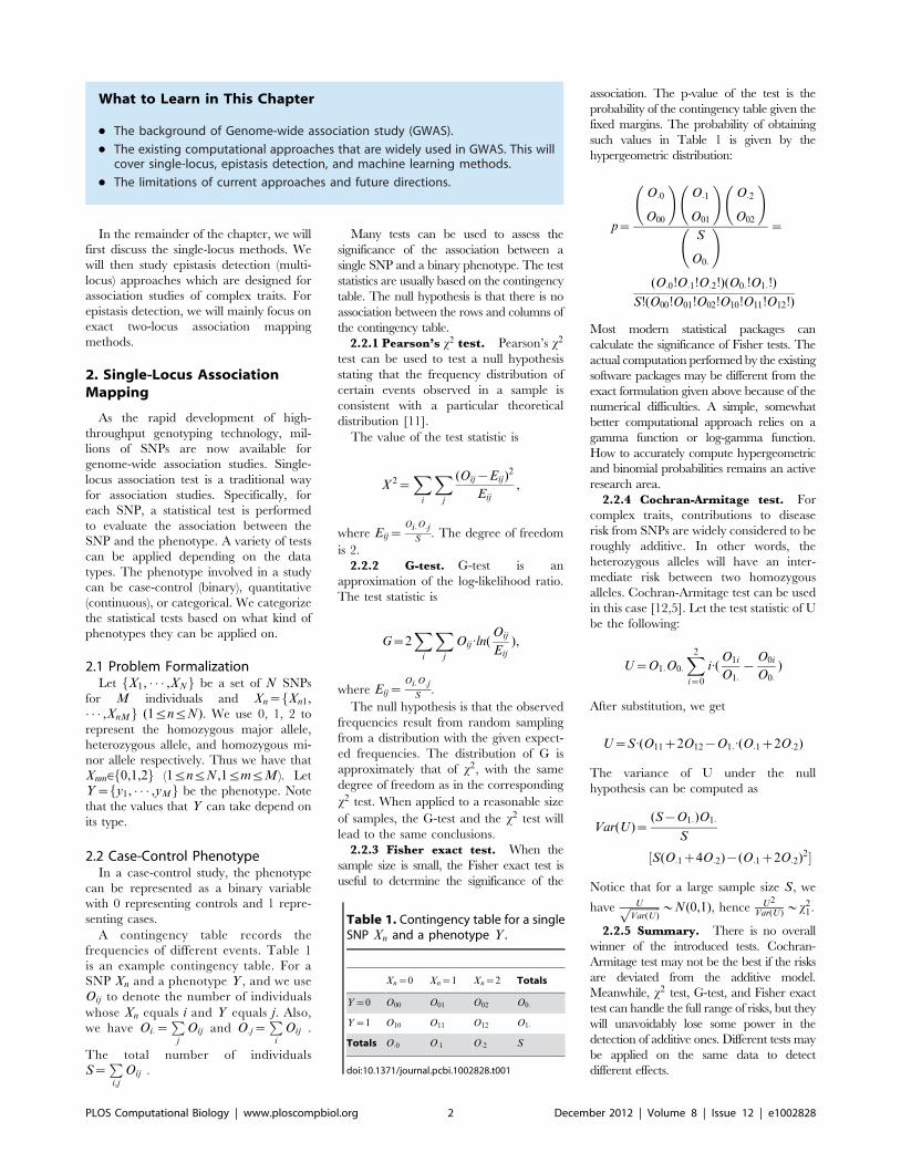
In the remainder of the chapter, we will
first discuss the single-locus methods. We
will then study epistasis detection (multi-
locus) approaches which are designed for
association studies of complex traits. For
epistasis detection, we will mainly focus on
exact two-locus association mapping
methods.
2. Single-Locus AssociationMapping
As the rapid development of high-
throughput genotyping technology, mil-
lions of SNPs are now available for
genome-wide association studies. Single-
locus association test is a traditional way
for association studies. Specifically, for
each SNP, a statistical test is performed
to evaluate the association between the
SNP and the phenotype. A variety of tests
can be applied depending on the data
types. The phenotype involved in a study
can be case-control (binary), quantitative
(continuous), or categorical. We categorize
the statistical tests based on what kind of
phenotypes they can be applied on.
2.1 Problem FormalizationLet fX1, � � � ,XNg be a set of N SNPs
for M individuals and Xn~fXn1,� � � ,XnMg (1ƒnƒN). We use 0, 1, 2 to
represent the homozygous major allele,
heterozygous allele, and homozygous mi-
nor allele respectively. Thus we have that
Xnm[f0,1,2g (1ƒnƒN,1ƒmƒM ). Let
Y~fy1, � � � ,yMg be the phenotype. Note
that the values that Y can take depend on
its type.
2.2 Case-Control PhenotypeIn a case-control study, the phenotype
can be represented as a binary variable
with 0 representing controls and 1 repre-
senting cases.
A contingency table records the
frequencies of different events. Table 1
is an example contingency table. For a
SNP Xn and a phenotype Y , and we use
Oij to denote the number of individuals
whose Xn equals i and Y equals j. Also,
we have Oi:~P
j
Oij and O:j~P
i
Oij .
The total number of individuals
S~P
i,j
Oij .
Many tests can be used to assess the
significance of the association between a
single SNP and a binary phenotype. The test
statistics are usually based on the contingency
table. The null hypothesis is that there is no
association between the rows and columns of
the contingency table.
2.2.1 Pearson’s x2 test. Pearson’s x2
test can be used to test a null hypothesis
stating that the frequency distribution of
certain events observed in a sample is
consistent with a particular theoretical
distribution [11].
The value of the test statistic is
X 2~X
i
X
j
(Oij{Eij)2
Eij
,
where Eij~Oi:O:j
S. The degree of freedom
is 2.
2.2.2 G-test. G-test is an
approximation of the log-likelihood ratio.
The test statistic is
G~2X
i
X
j
Oij:ln(
Oij
Eij
),
where Eij~Oi:O:j
S.
The null hypothesis is that the observed
frequencies result from random sampling
from a distribution with the given expect-
ed frequencies. The distribution of G is
approximately that of x2, with the same
degree of freedom as in the corresponding
x2 test. When applied to a reasonable size
of samples, the G-test and the x2 test will
lead to the same conclusions.
2.2.3 Fisher exact test. When the
sample size is small, the Fisher exact test is
useful to determine the significance of the
association. The p-value of the test is the
probability of the contingency table given the
fixed margins. The probability of obtaining
such values in Table 1 is given by the
hypergeometric distribution:
p~
O:0
O00
!O:1
O01
!O:2
O02
!
S
O0:
! ~
(O:0!O:1!O:2!)(O0:!O1:!)
S!(O00!O01!O02!O10!O11!O12!)
Most modern statistical packages can
calculate the significance of Fisher tests. The
actual computation performed by the existing
software packages may be different from the
exact formulation given above because of the
numerical difficulties. A simple, somewhat
better computational approach relies on a
gamma function or log-gamma function.
How to accurately compute hypergeometric
and binomial probabilities remains an active
research area.
2.2.4 Cochran-Armitage test. For
complex traits, contributions to disease
risk from SNPs are widely considered to be
roughly additive. In other words, the
heterozygous alleles will have an inter-
mediate risk between two homozygous
alleles. Cochran-Armitage test can be used
in this case [12,5]. Let the test statistic of U
be the following:
U~O1:O0:
X2
i~0
i:(O1i
O1:{
O0i
O0:)
After substitution, we get
U~S:(O11z2O12{O1::(O:1z2O:2)
The variance of U under the null
hypothesis can be computed as
Var(U)~(S{O1:)O1:
S
½S(O:1z4O:2){(O:1z2O:2)2�
Notice that for a large sample size S, we
have UffiffiffiffiffiffiffiffiffiffiffiVar(U)p *N(0,1), hence U2
Var(U)*x2
1.
2.2.5 Summary. There is no overall
winner of the introduced tests. Cochran-
Armitage test may not be the best if the risks
are deviated from the additive model.
Meanwhile, x2 test, G-test, and Fisher exact
test can handle the full range of risks, but they
will unavoidably lose some power in the
detection of additive ones. Different tests may
be applied on the same data to detect
different effects.
What to Learn in This Chapter
N The background of Genome-wide association study (GWAS).
N The existing computational approaches that are widely used in GWAS. This willcover single-locus, epistasis detection, and machine learning methods.
N The limitations of current approaches and future directions.
Table 1. Contingency table for a singleSNP Xn and a phenotype Y .
Xn~0 Xn~1 Xn~2 Totals
Y~0 O00 O01 O02 O0:
Y~1 O10 O11 O12 O1:
Totals O:0 O:1 O:2 S
doi:10.1371/journal.pcbi.1002828.t001
PLOS Computational Biology | www.ploscompbiol.org 2 December 2012 | Volume 8 | Issue 12 | e1002828
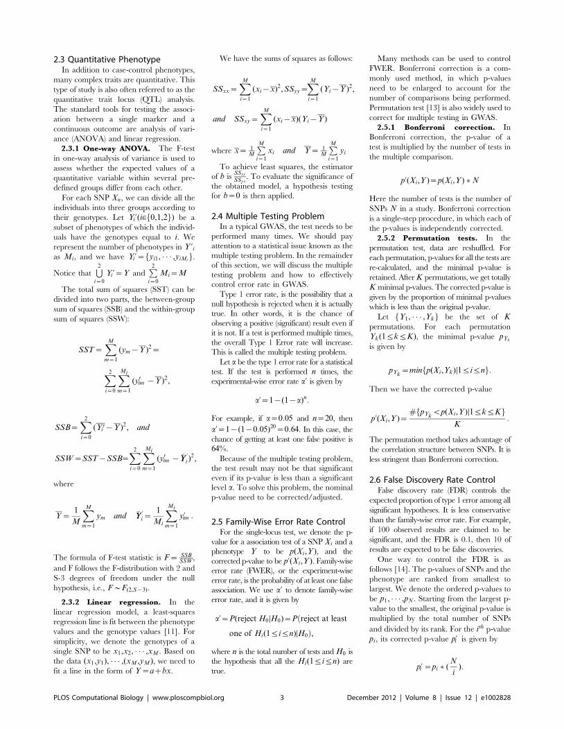
2.3 Quantitative PhenotypeIn addition to case-control phenotypes,
many complex traits are quantitative. This
type of study is also often referred to as the
quantitative trait locus (QTL) analysis.
The standard tools for testing the associ-
ation between a single marker and a
continuous outcome are analysis of vari-
ance (ANOVA) and linear regression.
2.3.1 One-way ANOVA. The F-test
in one-way analysis of variance is used to
assess whether the expected values of a
quantitative variable within several pre-
defined groups differ from each other.
For each SNP Xn, we can divide all the
individuals into three groups according to
their genotypes. Let Y ’i (i[f0,1,2g) be a
subset of phenotypes of which the individ-
uals have the genotypes equal to i. We
represent the number of phenotypes in Y ’ias Mi, and we have Y ’i ~fyi1, � � � ,yiMi
g.
Notice thatS2
i~0
Y ’i ~Y andP2
i~0
Mi~M
The total sum of squares (SST) can be
divided into two parts, the between-group
sum of squares (SSB) and the within-group
sum of squares (SSW):
SST~XM
m~1
(ym{Y )2~
X2
i~0
XMi
m~1
(y0im {Y )2,
SSB~X2
i~0
(Y 0i {Y )2, and
SSW~SST{SSB~X2
i~0
XMi
m~1
(y0im { �YY ’i )
2,
where
Y~1
M
XM
m~1
ym and �YY ’i ~
1
Mi
XMi
m~1
y’im :
The formula of F-test statistic is F~ SSBSSW
,
and F follows the F-distribution with 2 and
S-3 degrees of freedom under the null
hypothesis, i.e., F*F(2,S{3).
2.3.2 Linear regression. In the
linear regression model, a least-squares
regression line is fit between the phenotype
values and the genotype values [11]. For
simplicity, we denote the genotypes of a
single SNP to be x1,x2, � � � ,xM . Based on
the data (x1,y1), � � � ,(xM ,yM ), we need to
fit a line in the form of Y~azbx.
We have the sums of squares as follows:
SSxx~XM
i~1
(xi{x)2,SSyy~XM
i~1
(Yi{Y )2,
and SSxy~XM
i~1
(xi{x)(Yi{Y )
where x~ 1M
PM
i~1
xi and Y~ 1M
PM
i~1
yi
To achieve least squares, the estimator
of b isSSxy
SSxx. To evaluate the significance of
the obtained model, a hypothesis testing
for b~0 is then applied.
2.4 Multiple Testing ProblemIn a typical GWAS, the test needs to be
performed many times. We should pay
attention to a statistical issue known as the
multiple testing problem. In the remainder
of this section, we will discuss the multiple
testing problem and how to effectively
control error rate in GWAS.
Type 1 error rate, is the possibility that a
null hypothesis is rejected when it is actually
true. In other words, it is the chance of
observing a positive (significant) result even if
it is not. If a test is performed multiple times,
the overall Type 1 Error rate will increase.
This is called the multiple testing problem.
Let a be the type 1 error rate for a statistical
test. If the test is performed n times, the
experimental-wise error rate a’ is given by
a’~1{(1{a)n:
For example, if a~0:05 and n~20, then
a’~1{(1{0:05)20~0:64. In this case, the
chance of getting at least one false positive is
64%.
Because of the multiple testing problem,
the test result may not be that significant
even if its p-value is less than a significant
level a. To solve this problem, the nominal
p-value need to be corrected/adjusted.
2.5 Family-Wise Error Rate ControlFor the single-locus test, we denote the p-
value for a association test of a SNP Xi and a
phenotype Y to be p(Xi,Y ), and the
corrected p-value to be p’(Xi,Y ). Family-wise
error rate (FWER), or the experiment-wise
error rate, is the probability of at least one false
association. We use a’ to denote family-wise
error rate, and it is given by
a’~P(reject H0DH0)~P reject at leastð
one of Hi(1ƒiƒn)DH0Þ,
where n is the total number of tests and H0 is
the hypothesis that all the Hi(1ƒiƒn) are
true.
Many methods can be used to control
FWER. Bonferroni correction is a com-
monly used method, in which p-values
need to be enlarged to account for the
number of comparisons being performed.
Permutation test [13] is also widely used to
correct for multiple testing in GWAS.
2.5.1 Bonferroni correction. In
Bonferroni correction, the p-value of a
test is multiplied by the number of tests in
the multiple comparison.
p’(Xi,Y )~p(Xi,Y ) �N
Here the number of tests is the number of
SNPs N in a study. Bonferroni correction
is a single-step procedure, in which each of
the p-values is independently corrected.
2.5.2 Permutation tests. In the
permutation test, data are reshuffled. For
each permutation, p-values for all the tests are
re-calculated, and the minimal p-value is
retained. After K permutations, we get totally
K minimal p-values. The corrected p-value is
given by the proportion of minimal p-values
which is less than the original p-value.
Let fY1, � � � ,Ykg be the set of K
permutations. For each permutation
Yk(1ƒkƒK), the minimal p-value pYk
is given by
pYk~minfp(Xi,Yk)D1ƒiƒng:
Then we have the corrected p-value
p’(Xi,Y )~#fpYk
vp(Xi,Y )D1ƒkƒKgK
:
The permutation method takes advantage of
the correlation structure between SNPs. It is
less stringent than Bonferroni correction.
2.6 False Discovery Rate ControlFalse discovery rate (FDR) controls the
expected proportion of type 1 error among all
significant hypotheses. It is less conservative
than the family-wise error rate. For example,
if 100 observed results are claimed to be
significant, and the FDR is 0.1, then 10 of
results are expected to be false discoveries.
One way to control the FDR is as
follows [14]. The p-values of SNPs and the
phenotype are ranked from smallest to
largest. We denote the ordered p-values to
be p1, � � � ,pN . Starting from the largest p-
value to the smallest, the original p-value is
multiplied by the total number of SNPs
and divided by its rank. For the ith p-value
pi, its corrected p-value p’i is given by
p’i ~pi � (N
i):
PLOS Computational Biology | www.ploscompbiol.org 3 December 2012 | Volume 8 | Issue 12 | e1002828
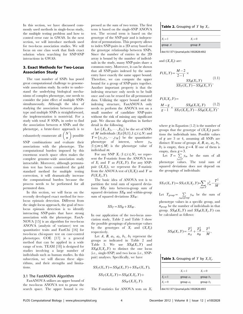
In this section, we have discussed com-
monly used methods in single-locus study,
the multiple testing problem and how to
control error rate in GWAS. In the next
section, we will introduce methods used
for two-locus association studies. We will
focus on one class work that finds exact
solution when searching for SNP-SNP
interactions in GWAS.
3. Exact Methods for Two-LocusAssociation Study
The vast number of SNPs has posed
great computational challenge to genome-
wide association study. In order to under-
stand the underlying biological mecha-
nisms of complex phenotype, one needs to
consider the joint effect of multiple SNPs
simultaneously. Although the idea of
studying the association between pheno-
type and multiple SNPs is straightforward,
the implementation is nontrivial. For a
study with total N SNPs, in order to find
the association between n SNPs and the
phenotype, a brute-force approach is to
exhaustively enumerate allN
n
� �possible
SNP combinations and evaluate their
associations with the phenotype. The
computational burden imposed by this
enormous search space often makes the
complete genome-wide association study
intractable. Moreover, although permuta-
tion test has been considered the gold
standard method for multiple testing
correction, it will dramatically increase
the computational burden because the
process needs to be performed for all
permuted data.
In this section, we will focus on the
recently developed exact method for two-
locus epistasis detection. Different from
the single-locus approach, the goal of two-
locus epistasis detection is to identify
interacting SNP-pairs that have strong
association with the phenotype. FastA-
NOVA [15] is an algorithm for two-locus
ANOVA (analysis of variance) test on
quantitative traits and FastChi [16] for
two-locus chi-square test on case-control
phenotypes. COE [17] is a general
method that can be applied in a wide
range of tests. TEAM [18] is designed for
studies involving a large number of
individuals such as human studies. In this
subsection, we will discuss these algo-
rithms, and their strengths and limita-
tions.
3.1 The FastANOVA AlgorithmFastANOVA utilizes an upper bound of
the two-locus ANOVA test to prune the
search space. The upper bound is ex-
pressed as the sum of two terms. The first
term is based on the single-SNP ANOVA
test. The second term is based on the
genotype of the SNP-pair and is indepen-
dent of permutations. This property allows
to index SNP-pairs in a 2D array based on
the genotype relationship between SNPs.
Since the number of entries in the 2D
array is bound by the number of individ-
uals in the study, many SNP-pairs share a
common entry. Moreover, it can be shown
that all SNP-pairs indexed by the same
entry have exactly the same upper bound.
Therefore, we can compute the upper
bound for a group of SNP-pairs together.
Another important property is that the
indexing structure only needs to be built
once and can be reused for all permutated
data. Utilizing the upper bound and the
indexing structure, FastANOVA only
needs to perform the ANOVA test on a
small number of candidate SNP-pairs
without the risk of missing any significant
pair. We discuss the algorithm in further
detail in the following.
Let fX1,X2, � � � ,XNg be the set of SNPs
of M individuals (Xi[f0,1g,1ƒiƒN) and
Y~fy1,y2, � � � ,yMg be the quantitative
phenotype of interest, where ym
(1ƒmƒM ) is the phenotype value of
individual m.
For any SNP Xi (1ƒiƒN ), we repre-
sent the F-statistic from the ANOVA test
of Xi and Y as F(Xi,Y ). For any SNP-
pair (XiXj), we represent the F-statistic
from the ANOVA test of (XiXj) and Y as
F (XiXj ,Y ).
The basic idea of ANOVA test is to
partition the total sum of squared devia-
tions SST into between-group sum of
squared deviations SSB and within-group
sum of squared deviations SSW :
SST~SSBzSSW :
In our application of the two-locus asso-
ciation study, Table 2 and Table 3 show
the possible groupings of phenotype values
by the genotypes of Xi and (XiXj)
respectively.
Let A, B, a1, a2, b1, b2 represent the
groups as indicated in Table 2 and
Table 3. We use SSB(Xi,Y ) and
SSB(XiXj ,Y ) to distinct the one locus
(i.e., single-SNP) and two locus (i.e., SNP-
pair) analyses. Specifically, we have
SST (Xi,Y )~SSB(Xi,Y )zSSW (Xi,Y ),
SST (XiXj ,Y )~SSB(XiXj ,Y )z
SSW (XiXj ,Y ):
The F-statistics for ANOVA tests on Xi
and (XiXj) are:
F (Xi,Y )~M{2
2{1|
SSB(Xi,Y )
SST (Xi,Y ){SSB(Xi,Y ),
ð1:1Þ
F (XiXj ,Y )~
M{g
g{1|
SSB(XiXj ,Y )
SST (XiXj ,Y ){SSB(XiXj ,Y ),
ð1:2Þ
where g in Equation (1.2) is the number of
groups that the genotype of (XiXj) parti-
tions the individuals into. Possible values
of g are 3 or 4, assuming all SNPs are
distinct: If none of groups A, B, a1, a2, b1,
b2 is empty, then g~4. If one of them is
empty, then g~3.
Let T~P
ym[Y
ym be the sum of all
phenotype values. The total sum of
squared deviations does not depend on
the groupings of individuals:
SST (Xi,Y )~SST (XiXj ,Y )~X
ym[Y
y2m{
T2
M:
Let Tgroup~P
ym[group
ym be the sum of
phenotype values in a specific group, and
ngroup be the number of individuals in that
group. SSB(Xi,Y ) and SSB(XiXj ,Y ) can
be calculated as follows:
SSB(Xi,Y )~T2
A
nA
zT2
B
nB
{T2
M,
Table 2. Grouping of Y by Xi .
Xi~1 Xi~0
group A group B
doi:10.1371/journal.pcbi.1002828.t002
Table 3. Grouping of Y by XiXj .
Xi~1 Xi~0
Xj~1 group a1 group b1
Xj~0 group a2 group b2
doi:10.1371/journal.pcbi.1002828.t003
PLOS Computational Biology | www.ploscompbiol.org 4 December 2012 | Volume 8 | Issue 12 | e1002828
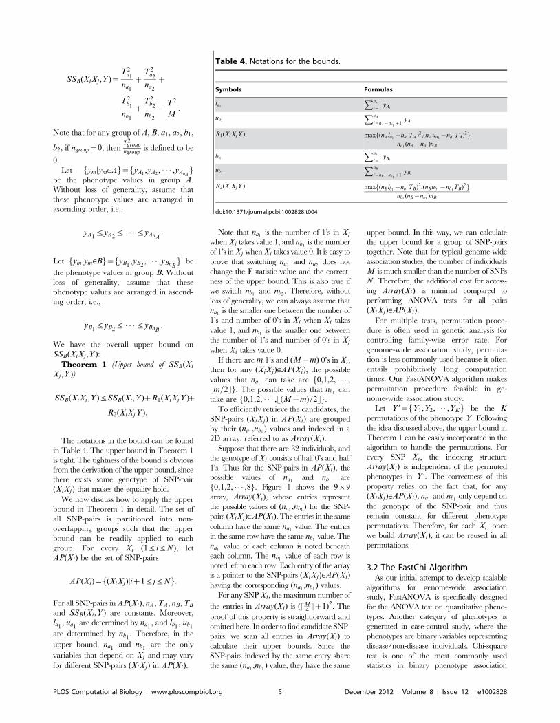
SSB(XiXj ,Y )~T2
a1
na1
zT2
a2
na2
z
T2b1
nb1
zT2
b2
nb2
{T2
M:
Note that for any group of A, B, a1, a2, b1,
b2, if ngroup~0, thenT2
groupngroup
is defined to be
0.
Let fymDym[Ag~fyA1,yA2
, � � � ,yAnAg
be the phenotype values in group A.
Without loss of generality, assume that
these phenotype values are arranged in
ascending order, i.e.,
yA1ƒyA2
ƒ � � �ƒyAnA:
Let fymDym[Bg~fyB1,yB2
, � � � ,yBnBg be
the phenotype values in group B. Without
loss of generality, assume that these
phenotype values are arranged in ascend-
ing order, i.e.,
yB1ƒyB2
ƒ � � �ƒyBnB:
We have the overall upper bound on
SSB(XiXj ,Y ):
Theorem 1 (Upper bound of SSB(Xi
Xj ,Y ))
SSB(XiXj ,Y )ƒSSB(Xi,Y )zR1(XiXjY )z
R2(XiXjY ):
The notations in the bound can be found
in Table 4. The upper bound in Theorem 1
is tight. The tightness of the bound is obvious
from the derivation of the upper bound, since
there exists some genotype of SNP-pair
(XiXj) that makes the equality hold.
We now discuss how to apply the upper
bound in Theorem 1 in detail. The set of
all SNP-pairs is partitioned into non-
overlapping groups such that the upper
bound can be readily applied to each
group. For every Xi (1ƒiƒN), let
AP(Xi) be the set of SNP-pairs
AP(Xi)~f(XiXj)Diz1ƒjƒNg:
For all SNP-pairs in AP(Xi), nA, TA, nB, TB
and SSB(Xi,Y ) are constants. Moreover,
la1, ua1
are determined by na1, and lb1
, ub1
are determined by nb1. Therefore, in the
upper bound, na1and nb1
are the only
variables that depend on Xj and may vary
for different SNP-pairs (XiXj) in AP(Xi).
Note that na1is the number of 1’s in Xj
when Xi takes value 1, and nb1is the number
of 1’s in Xj when Xi takes value 0. It is easy to
prove that switching na1and na2
does not
change the F-statistic value and the correct-
ness of the upper bound. This is also true if
we switch nb1and nb2
. Therefore, without
loss of generality, we can always assume that
na1is the smaller one between the number of
1’s and number of 0’s in Xj when Xi takes
value 1, and nb1is the smaller one between
the number of 1’s and number of 0’s in Xj
when Xi takes value 0.
If there are m 1’s and (M{m) 0’s in Xi,
then for any (XiXj)[AP(Xi), the possible
values that na1can take are f0,1,2, � � � ,
tm=2sg. The possible values that nb1can
take are f0,1,2, � � � ,t(M{m)=2sg.To efficiently retrieve the candidates, the
SNP-pairs (XiXj) in AP(Xi) are grouped
by their (na1,nb1
) values and indexed in a
2D array, referred to as Array(Xi).
Suppose that there are 32 individuals, and
the genotype of Xi consists of half 0’s and half
1’s. Thus for the SNP-pairs in AP(Xi), the
possible values of na1and nb1
are
f0,1,2, � � � ,8g. Figure 1 shows the 9|9array, Array(Xi), whose entries represent
the possible values of (na1,nb1
) for the SNP-
pairs (XiXj)[AP(Xi). The entries in the same
column have the same na1value. The entries
in the same row have the same nb1value. The
na1value of each column is noted beneath
each column. The nb1value of each row is
noted left to each row. Each entry of the array
is a pointer to the SNP-pairs (XiXj)[AP(Xi)
having the corresponding (na1,nb1
) values.
For any SNP Xi, the maximum number of
the entries in Array(Xi) is (qM4rz1)2. The
proof of this property is straightforward and
omitted here. In order to find candidate SNP-
pairs, we scan all entries in Array(Xi) to
calculate their upper bounds. Since the
SNP-pairs indexed by the same entry share
the same (na1,nb1
) value, they have the same
upper bound. In this way, we can calculate
the upper bound for a group of SNP-pairs
together. Note that for typical genome-wide
association studies, the number of individuals
M is much smaller than the number of SNPs
N . Therefore, the additional cost for access-
ing Array(Xi) is minimal compared to
performing ANOVA tests for all pairs
(XiXj)[AP(Xi).
For multiple tests, permutation proce-
dure is often used in genetic analysis for
controlling family-wise error rate. For
genome-wide association study, permuta-
tion is less commonly used because it often
entails prohibitively long computation
times. Our FastANOVA algorithm makes
permutation procedure feasible in ge-
nome-wide association study.
Let Y ’~fY1,Y2, � � � ,YKg be the K
permutations of the phenotype Y . Following
the idea discussed above, the upper bound in
Theorem 1 can be easily incorporated in the
algorithm to handle the permutations. For
every SNP Xi, the indexing structure
Array(Xi) is independent of the permuted
phenotypes in Y ’. The correctness of this
property relies on the fact that, for any
(XiXj)[AP(Xi), na1and nb1
only depend on
the genotype of the SNP-pair and thus
remain constant for different phenotype
permutations. Therefore, for each Xi, once
we build Array(Xi), it can be reused in all
permutations.
3.2 The FastChi AlgorithmAs our initial attempt to develop scalable
algorithms for genome-wide association
study, FastANOVA is specifically designed
for the ANOVA test on quantitative pheno-
types. Another category of phenotypes is
generated in case-control study, where the
phenotypes are binary variables representing
disease/non-disease individuals. Chi-square
test is one of the most commonly used
statistics in binary phenotype association
Table 4. Notations for the bounds.
Symbols Formulas
la1
Xna1
i~1yAi
ua1
XnA
i~nA{na1z1
yAi
R1(XiXjY ) maxf(nAla1{na1
TA)2,(nAua1{na1
TA)2gna1
(nA{na1)nA
lb1
Xnb1
i~1yBi
ub1
XnB
i~nB{nb1z1
yBi
R2(XiXjY ) maxf(nBlb1{nb1
TB)2,(nBub1{nb1
TB)2gnb1
(nB{nb1)nB
doi:10.1371/journal.pcbi.1002828.t004
PLOS Computational Biology | www.ploscompbiol.org 5 December 2012 | Volume 8 | Issue 12 | e1002828
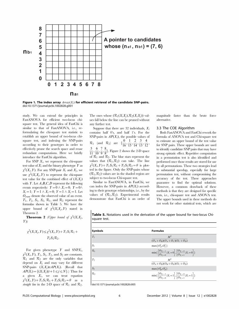
study. We can extend the principles in
FastANOVA for efficient two-locus chi-
square test. The general idea of FastChi is
similar to that of FastANOVA, i.e., re-
formulating the chi-square test statistic to
establish an upper bound of two-locus chi-
square test, and indexing the SNP-pairs
according to their genotypes in order to
effectively prune the search space and reuse
redundant computations. Here we briefly
introduce the FastChi algorithm.
For SNP Xi, we represent the chi-square
test value of Xi and the binary phenotype Y as
x2(Xi,Y ). For any SNP-pair Xi and Xj , we
use x2(XiXj ,Y ) to represent the chi-square
test value for the combined effect of (XiXj)
with Y . Let A,B,C,D represent the following
events respectively: Y~0 ^ Xi~0; Y~0^Xi~1; Y~1 ^ Xi~0; Y~1 ^ Xi~1. Let
Oevent denote the observed value of an event.
T1, T2, S1, S2, R1, and R2 represent the
formulas shown in Table 5. We have the
upper bound of x2(XiXj ,Y ) stated in
Theorem 2.
Theorem 2 (Upper bound of x2(XiXj ,Y ))
x2(XiXj ,Y )ƒx2(Xi,Y )zT1S1R1z
T2S2R2:
For given phenotype Y and SNPXi,
x2(Xi,Y ), T1, S1, T2, and S2 are constants.
R1 and R2 are the only variables that
depend on Xj and may vary for different
SNP-pairs (XiXj)[AP(Xi). (Recall that
AP(Xi)~f(XiXj)Diz1ƒjƒNg.) Thus for
a given Xi, we can treat equation
x2(Xi,Y )zT1S1R1zT2S2R2~h as a
straight line in the 2-D space of R1 and R2.
The ones whose (R1(XiXj),R2(XiXj)) val-
ues fall below the line can be pruned without
any further test.
Suppose that there are 32 individuals, Xi
contains half 0’s, and half 1’s. For the
SNP-pairs in AP(Xi), the possible values of
R1 (and R2) are f 0
16,
1
15,
2
14,
3
13,
4
12,
5
11,
6
10,7
9,8
8g. Figure 2 shows the 2-D space
of R1 and R2. The blue stars represent the
values that (R1,R2) can take. The line
x2(Xi,Y )zT1S1R1zT2S2R2~h is plot-
ted in the figure. Only the SNP-pairs whose
(R1,R2) values are in the shaded region are
subject to two-locus Chi-square test.
Similar to FastANOVA, in FastChi, we
can index the SNP-pairs in AP(Xi) accord-
ing to their genotype relationships, i.e., by the
values of (R1,R2). Experimental results
demonstrate that FastChi is an order of
magnitude faster than the brute force
alternative.
3.3 The COE AlgorithmBoth FastANOVA and FastChi rework the
formula of ANOVA test and Chi-square test
to estimate an upper bound of the test value
for SNP pairs. These upper bounds are used
to identify candidate SNP pairs that may have
strong epistatic effect. Repetitive computation
in a permutation test is also identified and
performed once those results are stored for use
by all permutations. These two strategies lead
to substantial speedup, especially for large
permutation test, without compromising the
accuracy of the test. These approaches
guarantee to find the optimal solutions.
However, a common drawback of these
methods is that they are designed for specific
tests, i.e., chi-square test and ANOVA test.
The upper bounds used in these methods do
not work for other statistical tests, which are
Figure 1. The index array Array(Xi) for efficient retrieval of the candidate SNP-pairs.doi:10.1371/journal.pcbi.1002828.g001
Table 5. Notations used in the derivation of the upper bound for two-locus Chi-square test.
Symbols Formulas
T1 M2
(OAzOB)(OAzOC )(OCzOD)
S1 maxfO2A,O2
Cg
R1minf
OXj ~1
OXj ~0
DXi~0
� �,
OXj ~0
OXj ~1
DXi~0
� �g
T2 M2
(OAzOB)(OBzOD)(OCzOD)
S2 maxfO2B,O2
Dg
R2minf
OXj ~1
OXj ~0
DXi~1
� �,
OXj ~0
OXj ~1
DXi~1
� �g
doi:10.1371/journal.pcbi.1002828.t005
PLOS Computational Biology | www.ploscompbiol.org 6 December 2012 | Volume 8 | Issue 12 | e1002828
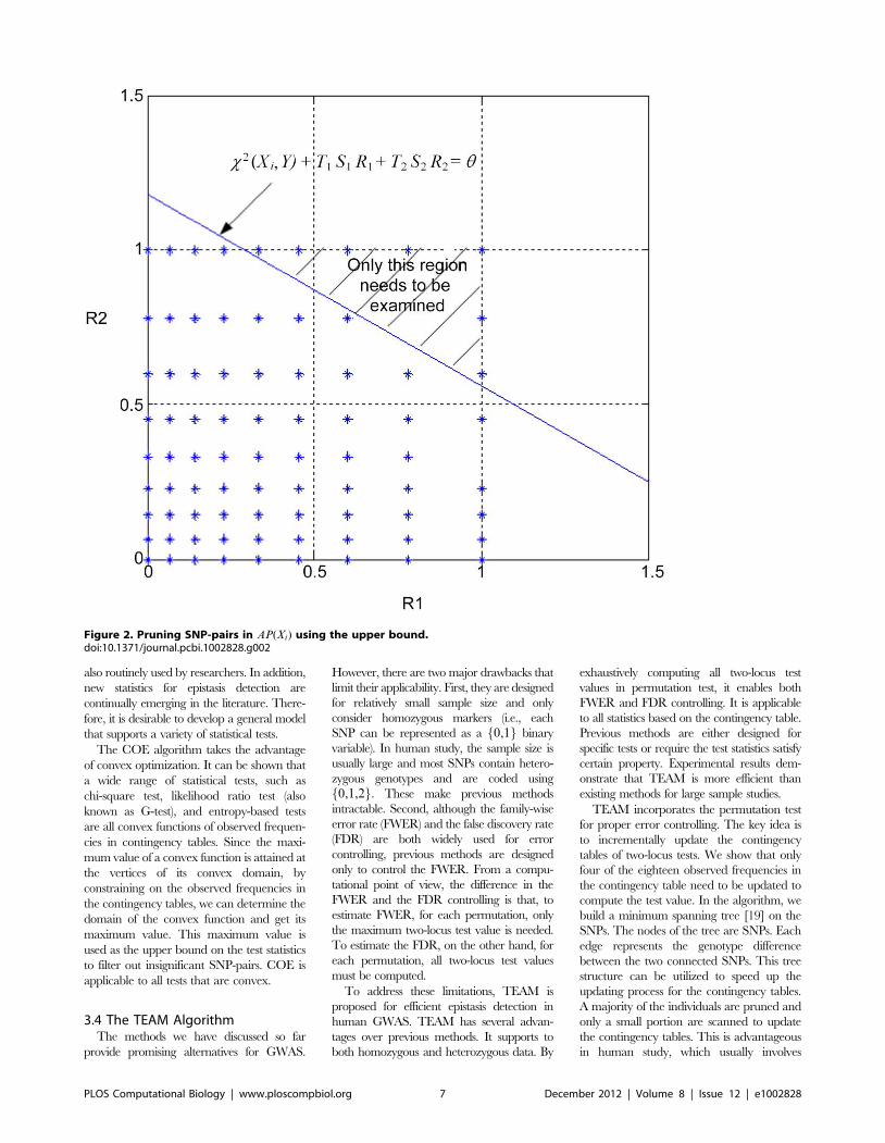
also routinely used by researchers. In addition,
new statistics for epistasis detection are
continually emerging in the literature. There-
fore, it is desirable to develop a general model
that supports a variety of statistical tests.
The COE algorithm takes the advantage
of convex optimization. It can be shown that
a wide range of statistical tests, such as
chi-square test, likelihood ratio test (also
known as G-test), and entropy-based tests
are all convex functions of observed frequen-
cies in contingency tables. Since the maxi-
mum value of a convex function is attained at
the vertices of its convex domain, by
constraining on the observed frequencies in
the contingency tables, we can determine the
domain of the convex function and get its
maximum value. This maximum value is
used as the upper bound on the test statistics
to filter out insignificant SNP-pairs. COE is
applicable to all tests that are convex.
3.4 The TEAM AlgorithmThe methods we have discussed so far
provide promising alternatives for GWAS.
However, there are two major drawbacks that
limit their applicability. First, they are designed
for relatively small sample size and only
consider homozygous markers (i.e., each
SNP can be represented as a f0,1g binary
variable). In human study, the sample size is
usually large and most SNPs contain hetero-
zygous genotypes and are coded using
f0,1,2g. These make previous methods
intractable. Second, although the family-wise
error rate (FWER) and the false discovery rate
(FDR) are both widely used for error
controlling, previous methods are designed
only to control the FWER. From a compu-
tational point of view, the difference in the
FWER and the FDR controlling is that, to
estimate FWER, for each permutation, only
the maximum two-locus test value is needed.
To estimate the FDR, on the other hand, for
each permutation, all two-locus test values
must be computed.
To address these limitations, TEAM is
proposed for efficient epistasis detection in
human GWAS. TEAM has several advan-
tages over previous methods. It supports to
both homozygous and heterozygous data. By
exhaustively computing all two-locus test
values in permutation test, it enables both
FWER and FDR controlling. It is applicable
to all statistics based on the contingency table.
Previous methods are either designed for
specific tests or require the test statistics satisfy
certain property. Experimental results dem-
onstrate that TEAM is more efficient than
existing methods for large sample studies.
TEAM incorporates the permutation test
for proper error controlling. The key idea is
to incrementally update the contingency
tables of two-locus tests. We show that only
four of the eighteen observed frequencies in
the contingency table need to be updated to
compute the test value. In the algorithm, we
build a minimum spanning tree [19] on the
SNPs. The nodes of the tree are SNPs. Each
edge represents the genotype difference
between the two connected SNPs. This tree
structure can be utilized to speed up the
updating process for the contingency tables.
A majority of the individuals are pruned and
only a small portion are scanned to update
the contingency tables. This is advantageous
in human study, which usually involves
Figure 2. Pruning SNP-pairs in AP(Xi) using the upper bound.doi:10.1371/journal.pcbi.1002828.g002
PLOS Computational Biology | www.ploscompbiol.org 7 December 2012 | Volume 8 | Issue 12 | e1002828
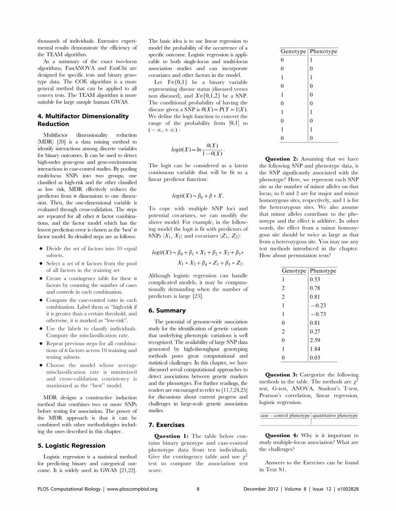
thousands of individuals. Extensive experi-
mental results demonstrate the efficiency of
the TEAM algorithm.
As a summary of the exact two-locus
algorithms, FastANOVA and FastChi are
designed for specific tests and binary geno-
type data. The COE algorithm is a more
general method that can be applied to all
convex tests. The TEAM algorithm is more
suitable for large sample human GWAS.
4. Multifactor DimensionalityReduction
Multifactor dimensionality reduction
(MDR) [20] is a data mining method to
identify interactions among discrete variables
for binary outcomes. It can be used to detect
high-order gene-gene and gene-environment
interactions in case-control studies. By pooling
multi-locus SNPs into two groups, one
classified as high-risk and the other classified
as low risk, MDR effectively reduces the
predictors from n dimensions to one dimen-
sion. Then, the one-dimensional variable is
evaluated through cross-validation. The steps
are repeated for all other n factor combina-
tions, and the factor model which has the
lowest prediction error is chosen as the ‘best’ nfactor model. Its detailed steps are as follows:
N Divide the set of factors into 10 equal
subsets.
N Select a set of n factors from the pool
of all factors in the training set
N Create a contingency table for these nfactors by counting the number of cases
and controls in each combination.
N Compute the case-control ratio in each
combination. Label them as ‘‘high-risk if
it is greater than a certain threshold, and
otherwise, it is marked as ‘‘low-risk’’.
N Use the labels to classify individuals.
Compute the misclassification rate.
N Repeat previous steps for all combina-
tions of n factors across 10 training and
testing subsets.
N Choose the model whose average
misclassification rate is minimized
and cross-validation consistency is
maximized as the ‘‘best’’ model.
MDR designs a constructive induction
method that combines two or more SNPs
before testing for association. The power of
the MDR approach is that it can be
combined with other methodologies includ-
ing the ones described in this chapter.
5. Logistic Regression
Logistic regression is a statistical method
for predicting binary and categorical out-
come. It is widely used in GWAS [21,22].
The basic idea is to use linear regression to
model the probability of the occurrence of a
specific outcome. Logistic regression is appli-
cable to both single-locus and multi-locus
association studies and can incorporate
covariates and other factors in the model.
Let Y[f0,1g be a binary variable
representing disease status (diseased verses
non diseased), and X[f0,1,2g be a SNP.
The conditional probability of having the
disease given a SNP is h(X )~P(Y~1DX ).We define the logit function to convert the
range of the probability from ½0,1� to
({?,z?) :
logit(X )~lnh(X )
1{h(X ):
The logit can be considered as a latent
continuous variable that will be fit to a
linear predictor function:
logit(X )*b0zb � X :
To cope with multiple SNP loci and
potential covariates, we can modify the
above model. For example, in the follow-
ing model the logit is fit with predictors of
SNPs (X1, X2) and covariates (Z1, Z2):
logit(X )*b0zb1 � X1zb2 � X2zb3�
X1 � X2zb4 � Z1zb5 � Z2:
Although logistic regression can handle
complicated models, it may be computa-
tionally demanding when the number of
predictors is large [23].
6. Summary
The potential of genome-wide association
study for the identification of genetic variants
that underlying phenotypic variations is well
recognized. The availability of large SNP data
generated by high-throughput genotyping
methods poses great computational and
statistical challenges. In this chapter, we have
discussed serval computational approaches to
detect associations between genetic markers
and the phenotypes. For further readings, the
readers are encouraged to refer to [11,7,24,25]
for discussions about current progress and
challenges in large-scale genetic association
studies.
7. Exercises
Question 1: The table below con-
tains binary genotype and case-control
phenotype data from ten individuals.
Give the contingency table and use x2
test to compute the association test
score.
Genotype
0
0
1
0
1
0
1
0
1
0
���������������������������
Phenotype
1
0
1
0
0
0
1
0
1
0
Question 2: Assuming that we have
the following SNP and phenotype data, is
the SNP significantly associated with the
phenotype? Here, we represent each SNP
site as the number of minor alleles on that
locus, so 0 and 2 are for major and minor
homozygous sites, respectively, and 1 is for
the heterozygous sites. We also assume
that minor alleles contribute to the phe-
notype and the effect is additive. In other
words, the effect from a minor homozy-
gous site should be twice as large as that
from a heterozygous site. You may use any
test methods introduced in the chapter.
How about permutation tests?
Genotype
1
2
2
1
1
0
2
0
1
0
���������������������������
Phenotype
0:53
0:78
0:81
{0:23
{0:73
0:81
0:27
2:59
1:84
0:03
Question 3: Categorize the following
methods in the table. The methods are x2
test, G-test, ANOVA, Student’s T-test,
Pearson’s correlation, linear regression,
logistic regression.
case� control phenotype����quantitative phenotype
Question 4: Why is it important to
study multiple-locus association? What are
the challenges?
Answers to the Exercises can be found
in Text S1.
PLOS Computational Biology | www.ploscompbiol.org 8 December 2012 | Volume 8 | Issue 12 | e1002828
Supporting Information
Text S1 Answers to Exercises
(PDF)
References
1. Churchill GA, Airey DC, Allayee H, Angel JM,
Attie AD, et al. (2004) The collaborative cross, a
community resource for the genetic analysis of
complex traits. Nat Genet 36: 1133–1137.
2. The International HapMap Consortium (2003)
The international hapmap project. Nature
426(6968): 789–796.
3. Saxena R, Voight B, Lyssenko V, Burtt N, de
Bakker P, et al. (2007) Genome-wide association
analysis identifies loci for type 2 diabetes and
triglyceride levels. Science 316: 1331–1336.
4. Scuteri A, Sanna S, Chen W, Uda M, Albai G, et
al. (2007) Genome-wide association scan shows
genetic variants in the FTO gene are associated
with obesity-related traits. PLoS Genet 3(7): e115.
doi:10.1371/journal.pgen.0030115
5. The Wellcome Trust Case Control Consortium
(2007) Genome-wide association study of 14,000
cases of seven common diseases and 3,000 shared
controls. Nature 447: 661–678.
6. Weedon M, Lettre G, Freathy R, Lindgren C,
Voight B, et al. (2007) A common variant of
HMGA2 is associated with adult and childhood
height in the general population. Nat Genet 39:
1245–1250.
7. Hirschhorn J, Daly M (2005) Genome-wide
association studies for common diseases and
complex traits. Nat Rev Genet 6: 95–108.
8. McCarthy M, Abecasis G, Cardon L, Goldstein
D, Little J, et al. (2008) Genome-wide association
studies for complex traits: consensus, uncertainty
and challenges. Nat Rev Genet 9(5): 356–369.9. Thorisson GA, Smith AV, Krishnan L, Stein LD
(2005) The international hapmap project web site.
Genome Res 15: 1592.10. The 1000 Genomes Project Consortium (2010) A
map of human genome variation from popula-tion-scale sequencing. Nature 467: 1061–1073.
11. Balding DJ (2006) A tutorial on statisticalmethods for population association studies. Nat
Rev Genet 7(10): 781–791.
12. Samani NJ, Erdmann J, Hall AS, HengstenbergC, Mangino M, et al. (2007) Genomewide
association analysis of coronary artery disease.N Engl J Med 357: 443–453.
13. Westfall PH, Young SS (1993) Resampling-based
multiple testing. Wiley: New York.14. Benjamini Y, Hochberg Y (1995) Controlling the
false discovery rate: a practical and powerfulapproach to multiple testing. J R Stat Soc
Series B Stat Methodol 57(1): 289–300.
15. Zhang X, Zou F, Wang W (2008) FastANOVA:an efficient algorithm for genome-wide associa-
tion study. KDD 2008: 821–829.16. Zhang X, Zou F, Wang W (2009) FastChi: an
effcient algorithm for analyzing gene-gene inter-actions. PSB 2009: 528–539.
17. Zhang X, Pan F, Xie Y, Zou F, Wang W (2010)
COE: a general approach for efficient genome-wide two-locus epistatic test in disease association
study. J Comput Biol 17(3): 401–415.
18. Zhang X, Huang S, Zou F, Wang W (2010)
TEAM: Efficient two-locus epistasis tests in
human genome-wide association study. Bioinfor-
matics 26(12): 217–227.
19. Cormen TH, Leiserson CE, Rivest RL, Stein C
(2001) Introduction to algorithms. MIT Press and
McGraw-Hill.
20. Ritchie MD, Hahn LW, Roodi N, Bailey LR,
Dupont WD, et al. (2001) Multifactor-dimension-
ality reduction reveals high-order interactions
among estrogen-metabolism genes in sporadic
breast cancer. Am J Hum Genet 69: 138–147.
21. Cordell HJ (2002) Epistasis: what it means, what
it doesn’t mean, and statistical methods to detect
it in humans. Hum Mol Genet 11: 2463–2468.
22. Wason J, Dudbridge F (2010) Comparison of
multimarker logistic regression models, with
application to a genomewide scan of schizophre-
nia. BMC Genet 11: 80.
23. Yang C, Wan X, Yang Q, Xue H, Tang N, et al.
(2011) A hidden two- locus disease association
pattern in genome-wide association studies. BMC
Bioinformatics 12: 156.
24. Hoh J, Ott J (2003) Mathematical multi-locus
approaches to localizing complex human trait
genes. Nat Rev Genet 4: 701–709.
25. Musani S, Shriner D, Liu N, Feng R, Coffey C, et
al. (2007) Detection of gene6gene interactions in
genome-wide association studies of human pop-
ulation data. Hum Hered 63(2): 67–84.
Further Reading
N Cantor RM, Lange K, Sinsheimer JS (2008) Prioritizing GWAS results: a review of statistical methods and recommendations fortheir application. Nat Rev Genet 9(11): 855–867.
N Cordell HJ (2009) Detecting gene-gene interactions that underlie human diseases. Nat Rev Genet 10(6): 392–404.
N Manolio TA, Collins FS, Cox NJ, Goldstein DB, Hindorff LA, et al. (2009) Finding the missing heritability of complex diseases.Nature 461(7265): 747–753.
N Moore JH, Williams SM (2009) Epistasis and its implications for personal genetics. Am J Hum Genet 85(3): 309–320.
N Phillips PC (2010) Epistasis - the essential role of gene interactions in the structure and evolution of genetic systems. Am JHum Genet 86(1): 6–22.
N Wang K, Li M, Hakonarson H (2010) Analysing biological pathways in genome-wide association studies. Nat Rev Genet 11:843–854.
PLOS Computational Biology | www.ploscompbiol.org 9 December 2012 | Volume 8 | Issue 12 | e1002828
Education
Chapter 11: Genome-Wide Association StudiesWilliam S. Bush1*, Jason H. Moore2
1 Department of Biomedical Informatics, Center for Human Genetics Research, Vanderbilt University Medical School, Nashville, Tennessee, United States of America,
2 Departments of Genetics and Community Family Medicine, Institute for Quantitative Biomedical Sciences, Dartmouth Medical School, Lebanon, New Hampshire, United
States of America
Abstract: Genome-wide associa-tion studies (GWAS) have evolvedover the last ten years into apowerful tool for investigating thegenetic architecture of human dis-ease. In this work, we review thekey concepts underlying GWAS,including the architecture of com-mon diseases, the structure ofcommon human genetic variation,technologies for capturing geneticinformation, study designs, and thestatistical methods used for dataanalysis. We also look forward tothe future beyond GWAS.
This article is part of the ‘‘Transla-
tional Bioinformatics’’ collection for
PLOS Computational Biology.
1. Important Questions inHuman Genetics
A central goal of human genetics is to
identify genetic risk factors for common,
complex diseases such as schizophrenia
and type II diabetes, and for rare Mende-
lian diseases such as cystic fibrosis and
sickle cell anemia. There are many
different technologies, study designs and
analytical tools for identifying genetic risk
factors. We will focus here on the genome-
wide association study or GWAS that
measures and analyzes DNA sequence
variations from across the human genome
in an effort to identify genetic risk factors
for diseases that are common in the
population. The ultimate goal of GWAS
is to use genetic risk factors to make
predictions about who is at risk and to
identify the biological underpinnings of
disease susceptibility for developing new
prevention and treatment strategies. One
of the early successes of GWAS was the
identification of the Complement Factor H
gene as a major risk factor for age-related
macular degeneration or AMD [1–3]. Not
only were DNA sequence variations in this
gene associated with AMD but the bio-
logical basis for the effect was demonstrat-
ed. Understanding the biological basis of
genetic effects will play an important role in
developing new pharmacologic therapies.
While understanding the complexity of
human health and disease is an important
objective, it is not the only focus of human
genetics. Accordingly, one of the most
successful applications of GWAS has been
in the area of pharmacology. Pharmaco-
genetics has the goal of identifying DNA
sequence variations that are associated
with drug metabolism and efficacy as well
as adverse effects. For example, warfarin is
a blood-thinning drug that helps prevent
blood clots in patients. Determining the
appropriate dose for each patient is
important and believed to be partly
controlled by genes. A recent GWAS
revealed DNA sequence variations in
several genes that have a large influence
on warfarin dosing [4]. These results, and
more recent validation studies, have led to
genetic tests for warfarin dosing that can
be used in a clinical setting. This type of
genetic test has given rise to a new field
called personalized medicine that aims to
tailor healthcare to individual patients
based on their genetic background and
other biological features. The widespread
availability of low-cost technology for
measuring an individual’s genetic back-
ground has been harnessed by businesses
that are now marketing genetic testing
directly to the consumer. Genome-wide
association studies, for better or for worse,
have ushered in the exciting era of
personalized medicine and personal ge-
netic testing. The goal of this chapter is to
introduce and review GWAS technology,
study design and analytical strategies as an
important example of translational bioin-
formatics. We focus here on the application
of GWAS to common diseases that have a
complex multifactorial etiology.
2. Concepts Underlying theStudy Design
2.1 Single NucleotidePolymorphisms
The modern unit of genetic variation is
the single nucleotide polymorphism or SNP.
SNPs are single base-pair changes in the
DNA sequence that occur with high
frequency in the human genome [5]. For
the purposes of genetic studies, SNPs are
typically used as markers of a genomic
region, with the large majority of them
having a minimal impact on biological
systems. SNPs can have functional conse-
quences, however, causing amino acid
changes, changes to mRNA transcript
stability, and changes to transcription
factor binding affinity [6]. SNPs are by
far the most abundant form of genetic
variation in the human genome.
SNPs are notably a type of common
genetic variation; many SNPs are present
in a large proportion of human popula-
tions [7]. SNPs typically have two alleles,
meaning within a population there are
two commonly occurring base-pair pos-
sibilities for a SNP location. The fre-
quency of a SNP is given in terms of the
minor allele frequency or the frequency of
the less common allele. For example, a
SNP with a minor allele (G) frequency of
0.40 implies that 40% of a population
has the G allele versus the more common
allele (the major allele), which is found in
60% of the population.
Citation: Bush WS, Moore JH (2012) Chapter 11: Genome-Wide Association Studies. PLoS Comput Biol 8(12):e1002822. doi:10.1371/journal.pcbi.1002822
Editors: Fran Lewitter, Whitehead Institute, United States of America and Maricel Kann, University of Maryland,Baltimore County, United States of America
Published December , 2012
Copyright: � 2012 Bush, Moore. This is an open-access article distributed under the terms of the CreativeCommons Attribution License, which permits unrestricted use, distribution, and reproduction in any medium,provided the original author and source are credited.
Funding: This work was supported by NIH grants ROI-LM010098, ROI-LM009012, ROI-AI59694, RO1-EY022300,and RO1-LM011360. The funders had no role in the preparation of the manuscript.
Competing Interests: The authors have declared that no competing interests exist.
* E-mail: [email protected]
PLOS Computational Biology | www.ploscompbiol.org 1 December 2012 | Volume 8 | Issue 12 | e1002822
27
Commonly occurring SNPs lie in stark
contrast to genetic variants that are
implicated in more rare genetic disorders,
such as cystic fibrosis [8]. These conditions
are largely caused by extremely rare
genetic variants that ultimately induce a
detrimental change to protein function,
which leads to the disease state. Variants
with such low frequency in the population
are sometimes referred to as mutations,
though they can be structurally equivalent
to SNPs - single base-pair changes in the
DNA sequence. In the genetics literature,
the term SNP is generally applied to
common single base-pair changes, and the
term mutation is applied to rare genetic
variants.
2.2 Failures of Linkage for ComplexDisease
Cystic fibrosis (and most rare genetic
disorders) can be caused by multiple
different genetic variants within a single
gene. Because the effect of the genetic
variants is so strong, cystic fibrosis follows
an autosomal dominant inheritance pat-
tern in families with the disorder. One of
the major successes of human genetics was
the identification of multiple mutations in
the CFTR gene as the cause of cystic
fibrosis [8]. This was achieved by geno-
typing families affected by cystic fibrosis
using a collection of genetic markers across
the genome, and examining how those
genetic markers segregate with the disease
across multiple families. This technique,
called linkage analysis, was subsequently
applied successfully to identify genetic
variants that contribute to rare disorders
like Huntington disease [9]. When applied
to more common disorders, like heart
disease or various forms of cancer, linkage
analysis has not fared as well. This implies
the genetic mechanisms that influence
common disorders are different from those
that cause rare disorders [10].
2.3 Common Disease CommonVariant Hypothesis
The idea that common diseases have a
different underlying genetic architecture
than rare disorders, coupled with the
discovery of several susceptibility variants
for common disease with high minor allele
frequency (including alleles in the apolipo-
protein E or APOE gene for Alzheimer’s
disease [11] and PPARg gene in type II
diabetes [12]), led to the development of
the common disease/common variant (CD/CV)
hypothesis [13].
This hypothesis states simply that com-
mon disorders are likely influenced by
genetic variation that is also common in
the population. There are several key
ramifications of this for the study of
complex disease. First, if common genetic
variants influence disease, the effect size
(or penetrance) for any one variant must
be small relative to that found for rare
disorders. For example, if a SNP with 40%
frequency in the population causes a
highly deleterious amino acid substitution
that directly leads to a disease phenotype,
nearly 40% of the population would have
that phenotype. Thus, the allele frequency
and the population prevalence are com-
pletely correlated. If, however, that same
SNP caused a small change in gene
expression that alters risk for a disease by
some small amount, the prevalence of the
disease and the influential allele would be
only slightly correlated. As such, common
variants almost by definition cannot have
high penetrance.
Secondly, if common alleles have small
genetic effects (low penetrance), but com-
mon disorders show heritability (inheri-
tance in families), then multiple common
alleles must influence disease susceptibility.
For example, twin studies might estimate
the heritability of a common disease to be
40%, that is, 40% of the total variance in
disease risk is due to genetic factors. If the
allele of a single SNP incurs only a small
degree of disease risk, that SNP only
explains a small proportion of the total
variance due to genetic factors. As such,
the total genetic risk due to common
genetic variation must be spread across
multiple genetic factors. These two points
suggest that traditional family-based ge-
netic studies are not likely to be successful
for complex diseases, prompting a shift
toward population-based studies.
The frequency with which an allele
occurs in the population and the risk
incurred by that allele for complex diseases
are key components to consider when
planning a genetic study, impacting the
technology needed to gather genetic
information and the sample size needed
to discover statistically significant genetic
effects. The spectrum of potential genetic
effects is sometimes visualized and parti-
tioned by effect size and allele frequency
(figure 1). Genetic effects in the upper right
are more amenable to smaller family-
based studies and linkage analysis, and
may require genotyping relatively few
genetic markers. Effects in the lower right
are typical of findings from GWAS,
requiring large sample sizes and a large
panel of genetic markers. Effects in the
upper right, most notably CFH, have been
identified using both linkage analysis and
GWAS. Effects in the lower left are
perhaps the most difficult challenge, re-
quiring genomic sequencing of large
samples to associate rare variants to
disease.
Over the last five years, the common
disease/common variant hypothesis has
been tested for a variety of common
diseases, and while much of the heritability
for these conditions is not yet explained,
common alleles certainly play a role in
susceptibility. The National Human Ge-
nome Institute GWAS catalog (http://
www.genome.gov/gwastudies) lists over
3,600 SNPs identified for common diseas-
es or traits, and in general, common
diseases have multiple susceptibility alleles,
each with small effect sizes (typically
increasing disease risk between 1.2–2
times the population risk) [14]. From these
results we can say that for most common
diseases, the CD/CV hypothesis is true,
though it should not be assumed that the
entire genetic component of any common
disease is due to common alleles only.
3. Capturing Common Variation
3.1 The Human Haplotype MapProject
To test the common disease/common
variant hypothesis for a phenotype, a
systematic approach is needed to interro-
gate much of the common variation in the
human genome. First, the location and
density of commonly occurring SNPs is
needed to identify the genomic regions
and individual sites that must be examined
by genetic studies. Secondly, population-
specific differences in genetic variation
must be cataloged so that studies of
phenotypes in different populations can
be conducted with the proper design.
Finally, correlations among common ge-
netic variants must be determined so that
genetic studies do not collect redundant
information. The International HapMap
Project was designed to identify variation
What to Learn in This Chapter
N Basic genetic concepts that drive genome-wide association studies
N Genotyping technologies and common study designs
N Statistical concepts for GWAS analysis
N Replication, interpretation, and follow-up of association results
PLOS Computational Biology | www.ploscompbiol.org 2 December 2012 | Volume 8 | Issue 12 | e1002822
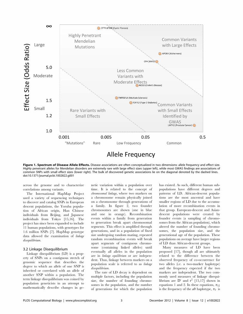
across the genome and to characterize
correlations among variants.
The International HapMap Project
used a variety of sequencing techniques
to discover and catalog SNPs in European
descent populations, the Yoruba popula-
tion of African origin, Han Chinese
individuals from Beijing, and Japanese
individuals from Tokyo [15,16]. The
project has since been expanded to include
11 human populations, with genotypes for
1.6 million SNPs [7]. HapMap genotype
data allowed the examination of linkage
disequilibrium.
3.2 Linkage DisequilibriumLinkage disequilibrium (LD) is a prop-
erty of SNPs on a contiguous stretch of
genomic sequence that describes the
degree to which an allele of one SNP is
inherited or correlated with an allele of
another SNP within a population. The
term linkage disequilibrium was coined by
population geneticists in an attempt to
mathematically describe changes in ge-
netic variation within a population over
time. It is related to the concept of
chromosomal linkage, where two markers on
a chromosome remain physically joined
on a chromosome through generations of
a family. In figure 2, two founder
chromosomes are shown (one in blue
and one in orange). Recombination
events within a family from generation
to generation break apart chromosomal
segments. This effect is amplified through
generations, and in a population of fixed
size undergoing random mating, repeated
random recombination events will break
apart segments of contiguous chromo-
some (containing linked alleles) until
eventually all alleles in the population
are in linkage equilibrium or are indepen-
dent. Thus, linkage between markers on a
population scale is referred to as linkage
disequilibrium.
The rate of LD decay is dependent on
multiple factors, including the population
size, the number of founding chromo-
somes in the population, and the number
of generations for which the population
has existed. As such, different human sub-
populations have different degrees and
patterns of LD. African-descent popula-
tions are the most ancestral and have
smaller regions of LD due to the accumu-
lation of more recombination events in
that group. European-descent and Asian-
descent populations were created by
founder events (a sampling of chromo-
somes from the African population), which
altered the number of founding chromo-
somes, the population size, and the
generational age of the population. These
populations on average have larger regions
of LD than African-descent groups.
Many measures of LD have been
proposed [17], though all are ultimately
related to the difference between the
observed frequency of co-occurrence for
two alleles (i.e. a two-marker haplotype)
and the frequency expected if the two
markers are independent. The two com-
monly used measures of linkage disequi-
librium are D’ and r2 [15,17] shown in
equations 1 and 2. In these equations, p12
is the frequency of the ab haplotype, p1: is
Figure 1. Spectrum of Disease Allele Effects. Disease associations are often conceptualized in two dimensions: allele frequency and effect size.Highly penetrant alleles for Mendelian disorders are extremely rare with large effect sizes (upper left), while most GWAS findings are associations ofcommon SNPs with small effect sizes (lower right). The bulk of discovered genetic associations lie on the diagonal denoted by the dashed lines.doi:10.1371/journal.pcbi.1002822.g001
PLOS Computational Biology | www.ploscompbiol.org 3 December 2012 | Volume 8 | Issue 12 | e1002822
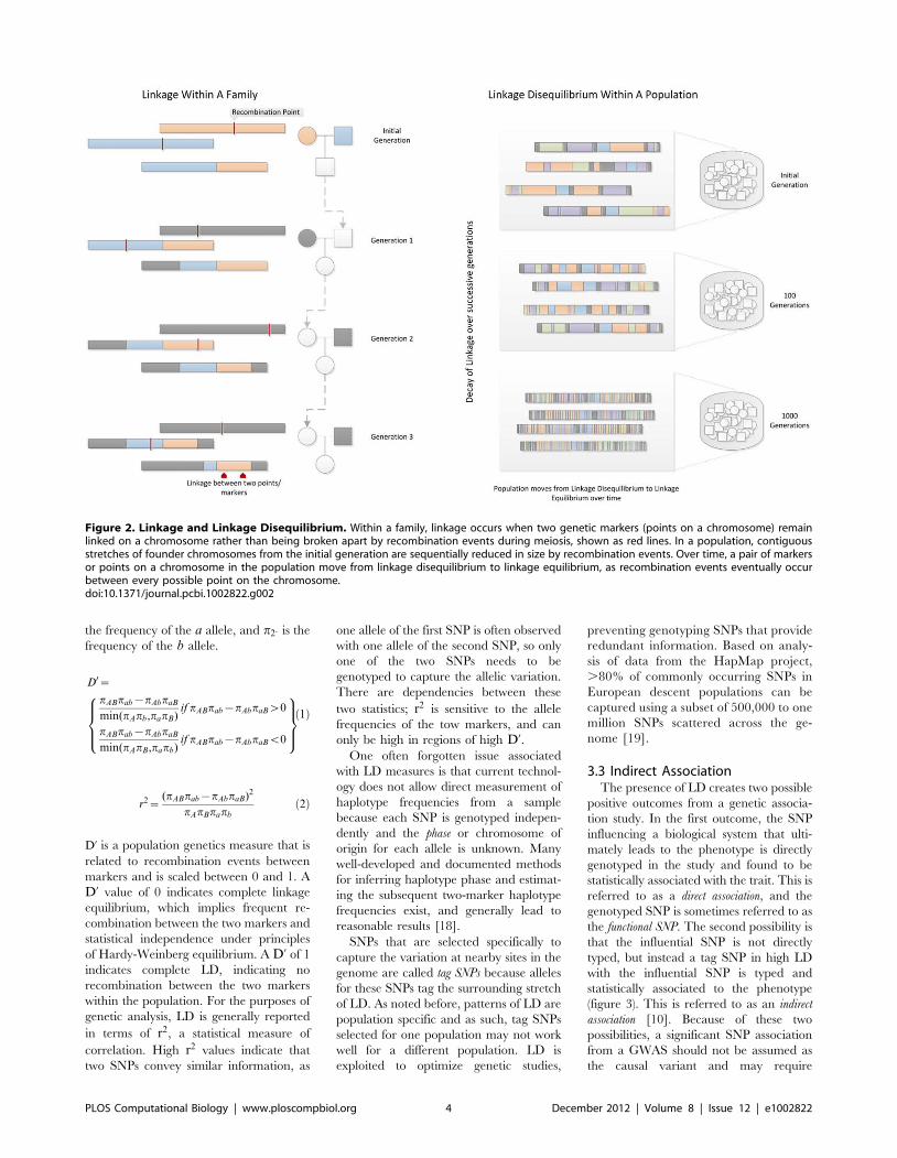
the frequency of the a allele, and p2: is the
frequency of the b allele.
D0~
pABpab{pAbpaB
min(pApb,papB)if pABpab{pAbpaBw0
pABpab{pAbpaB
min(pApB,papb)if pABpab{pAbpaBv0
8>><
>>:
9>>=
>>;
ð1Þ
r2~(pABpab{pAbpaB)2
pApBpapb
ð2Þ
D’ is a population genetics measure that is
related to recombination events between
markers and is scaled between 0 and 1. A
D’ value of 0 indicates complete linkage
equilibrium, which implies frequent re-
combination between the two markers and
statistical independence under principles
of Hardy-Weinberg equilibrium. A D’ of 1
indicates complete LD, indicating no
recombination between the two markers
within the population. For the purposes of
genetic analysis, LD is generally reported
in terms of r2, a statistical measure of
correlation. High r2 values indicate that
two SNPs convey similar information, as
one allele of the first SNP is often observed
with one allele of the second SNP, so only
one of the two SNPs needs to be
genotyped to capture the allelic variation.
There are dependencies between these
two statistics; r2 is sensitive to the allele
frequencies of the tow markers, and can
only be high in regions of high D’.One often forgotten issue associated
with LD measures is that current technol-
ogy does not allow direct measurement of
haplotype frequencies from a sample
because each SNP is genotyped indepen-
dently and the phase or chromosome of
origin for each allele is unknown. Many
well-developed and documented methods
for inferring haplotype phase and estimat-
ing the subsequent two-marker haplotype
frequencies exist, and generally lead to
reasonable results [18].
SNPs that are selected specifically to
capture the variation at nearby sites in the
genome are called tag SNPs because alleles
for these SNPs tag the surrounding stretch
of LD. As noted before, patterns of LD are
population specific and as such, tag SNPs
selected for one population may not work
well for a different population. LD is
exploited to optimize genetic studies,
preventing genotyping SNPs that provide
redundant information. Based on analy-
sis of data from the HapMap project,
.80% of commonly occurring SNPs in
European descent populations can be
captured using a subset of 500,000 to one
million SNPs scattered across the ge-
nome [19].
3.3 Indirect AssociationThe presence of LD creates two possible
positive outcomes from a genetic associa-
tion study. In the first outcome, the SNP
influencing a biological system that ulti-
mately leads to the phenotype is directly
genotyped in the study and found to be
statistically associated with the trait. This is
referred to as a direct association, and the
genotyped SNP is sometimes referred to as
the functional SNP. The second possibility is
that the influential SNP is not directly
typed, but instead a tag SNP in high LD
with the influential SNP is typed and
statistically associated to the phenotype
(figure 3). This is referred to as an indirect
association [10]. Because of these two
possibilities, a significant SNP association
from a GWAS should not be assumed as
the causal variant and may require
Figure 2. Linkage and Linkage Disequilibrium. Within a family, linkage occurs when two genetic markers (points on a chromosome) remainlinked on a chromosome rather than being broken apart by recombination events during meiosis, shown as red lines. In a population, contiguousstretches of founder chromosomes from the initial generation are sequentially reduced in size by recombination events. Over time, a pair of markersor points on a chromosome in the population move from linkage disequilibrium to linkage equilibrium, as recombination events eventually occurbetween every possible point on the chromosome.doi:10.1371/journal.pcbi.1002822.g002
PLOS Computational Biology | www.ploscompbiol.org 4 December 2012 | Volume 8 | Issue 12 | e1002822
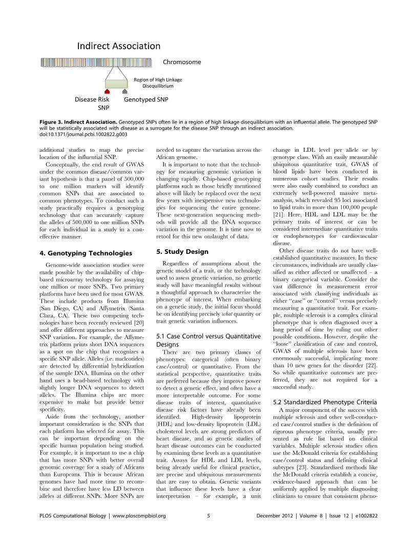
additional studies to map the precise
location of the influential SNP.
Conceptually, the end result of GWAS
under the common disease/common var-
iant hypothesis is that a panel of 500,000
to one million markers will identify
common SNPs that are associated to
common phenotypes. To conduct such a
study practically requires a genotyping
technology that can accurately capture
the alleles of 500,000 to one million SNPs
for each individual in a study in a cost-
effective manner.
4. Genotyping Technologies
Genome-wide association studies were
made possible by the availability of chip-
based microarray technology for assaying
one million or more SNPs. Two primary
platforms have been used for most GWAS.
These include products from Illumina
(San Diego, CA) and Affymetrix (Santa
Clara, CA). These two competing tech-
nologies have been recently reviewed [20]
and offer different approaches to measure
SNP variation. For example, the Affyme-
trix platform prints short DNA sequences
as a spot on the chip that recognizes a
specific SNP allele. Alleles (i.e. nucleotides)
are detected by differential hybridization
of the sample DNA. Illumina on the other
hand uses a bead-based technology with
slightly longer DNA sequences to detect
alleles. The Illumina chips are more
expensive to make but provide better
specificity.
Aside from the technology, another
important consideration is the SNPs that
each platform has selected for assay. This
can be important depending on the
specific human population being studied.
For example, it is important to use a chip
that has more SNPs with better overall
genomic coverage for a study of Africans
than Europeans. This is because African
genomes have had more time to recom-
bine and therefore have less LD between
alleles at different SNPs. More SNPs are
needed to capture the variation across the
African genome.
It is important to note that the technol-
ogy for measuring genomic variation is
changing rapidly. Chip-based genotyping
platforms such as those briefly mentioned
above will likely be replaced over the next
few years with inexpensive new technolo-
gies for sequencing the entire genome.
These next-generation sequencing meth-
ods will provide all the DNA sequence
variation in the genome. It is time now to
retool for this new onslaught of data.
5. Study Design
Regardless of assumptions about the
genetic model of a trait, or the technology
used to assess genetic variation, no genetic
study will have meaningful results without
a thoughtful approach to characterize the
phenotype of interest. When embarking
on a genetic study, the initial focus should
be on identifying precisely what quantity or
trait genetic variation influences.
5.1 Case Control versus QuantitativeDesigns
There are two primary classes of
phenotypes: categorical (often binary
case/control) or quantitative. From the
statistical perspective, quantitative traits
are preferred because they improve power
to detect a genetic effect, and often have a
more interpretable outcome. For some
disease traits of interest, quantitative
disease risk factors have already been
identified. High-density lipoprotein
(HDL) and low-density lipoprotein (LDL)
cholesterol levels are strong predictors of
heart disease, and so genetic studies of
heart disease outcomes can be conducted
by examining these levels as a quantitative
trait. Assays for HDL and LDL levels,
being already useful for clinical practice,
are precise and ubiquitous measurements
that are easy to obtain. Genetic variants
that influence these levels have a clear
interpretation – for example, a unit
change in LDL level per allele or by
genotype class. With an easily measurable
ubiquitous quantitative trait, GWAS of
blood lipids have been conducted in
numerous cohort studies. Their results
were also easily combined to conduct an
extremely well-powered massive meta-
analysis, which revealed 95 loci associated
to lipid traits in more than 100,000 people
[21]. Here, HDL and LDL may be the
primary traits of interest or can be
considered intermediate quantitative traits
or endophenotypes for cardiovascular
disease.
Other disease traits do not have well-
established quantitative measures. In these
circumstances, individuals are usually clas-
sified as either affected or unaffected – a
binary categorical variable. Consider the
vast difference in measurement error
associated with classifying individuals as
either ‘‘case’’ or ‘‘control’’ versus precisely
measuring a quantitative trait. For exam-
ple, multiple sclerosis is a complex clinical
phenotype that is often diagnosed over a
long period of time by ruling out other
possible conditions. However, despite the
‘‘loose’’ classification of case and control,
GWAS of multiple sclerosis have been
enormously successful, implicating more
than 10 new genes for the disorder [22].
So while quantitative outcomes are pre-
ferred, they are not required for a
successful study.
5.2 Standardized Phenotype CriteriaA major component of the success with
multiple sclerosis and other well-conduct-
ed case/control studies is the definition of
rigorous phenotype criteria, usually pre-
sented as rule list based on clinical
variables. Multiple sclerosis studies often
use the McDonald criteria for establishing
case/control status and defining clinical
subtypes [23]. Standardized methods like
the McDonald criteria establish a concise,
evidence-based approach that can be
uniformly applied by multiple diagnosing
clinicians to ensure that consistent pheno-
Figure 3. Indirect Association. Genotyped SNPs often lie in a region of high linkage disequilibrium with an influential allele. The genotyped SNPwill be statistically associated with disease as a surrogate for the disease SNP through an indirect association.doi:10.1371/journal.pcbi.1002822.g003
PLOS Computational Biology | www.ploscompbiol.org 5 December 2012 | Volume 8 | Issue 12 | e1002822
type definitions are used for a genetic
study.
Standardized phenotype rules are par-
ticularly critical for multi-center studies
to prevent introducing a site-based effect
into the study. And even when estab-
lished phenotype criteria are used, there
may be variability among clinicians in
how those criteria are used to assign
case/control status. Furthermore, some
quantitative traits are susceptible to bias
in measurement. For example, with
cataract severity lens photographs are
used to assign cases to one of three types
of lens opacity. In situations where there
may be disagreement among clinicians, a
subset of study records is often examined
by clinicians at multiple centers to assess
interrater agreement as a measure of
phenotyping consistency [24]. High in-
terrater agreement means that phenotype
rules are being consistently applied across
multiple sites, whereas low agreement
suggests that criteria are not uniformly
interpreted or applied, and may indicate
a need to establish more narrow pheno-
type criteria.
5.3 Phenotype Extraction fromElectronic Medical Records
The last few years of genetic research
has seen the growth of large clinical bio-
repositories that are linked to electronic
medical records (EMRs) [25]. The devel-
opment of these resources will certainly
advance the state of human genetics
research and foster integration of genetic
information into clinical practice. From a
study design perspective, identifying phe-
notypes from EMRs can be challenging.
Electronic medical records were estab-
lished for clinical care and administrative
purposes – not for research. As such,
idiosyncrasies arise due to billing practices
and other logistical reasons, and great care
must be taken not to introduce biases into
a genetic study.
The established methodology for con-
ducting ‘‘electronic phenotyping’’ is to
devise an initial selection algorithm
(using structured EMR fields, such as
billing codes, or text mining procedures
on unstructured text), which identifies a
record subset from the bio-repository. In
cases where free text is parsed, natural
language processing (NLP) is used in
conjunction with a controlled vocabulary
such as the Unified Medical Language
System (UMLS) to relate text to more
structured and uniform medical con-
cepts. In some instances, billing codes
alone may be sufficient to accurately
identify individuals with a particular
phenotype, but often combinations of
billing and procedure codes, along with
free text are necessary. Because every
medical center has its own set of policies,
care providers, and health insurance
providers, some algorithms developed in
one clinical setting may not work as well
in another.
Once a manageable subset of records is
obtained by an algorithm, the accuracy of
the results is examined by clinicians or
other phenotype experts as gold-standard
for comparison. The positive predictive
value (PPV) of the initial algorithm is
assessed, and based on feedback from case
reviewers, the selection algorithm is re-
fined. This process of case-review followed
by algorithmic refinement is continued
until the desired PPV is reached.
This approach has been validated by
replicating established genotype-pheno-
type relationships using EMR-derived
phenotypes [16], and has been applied to
multiple clinical and pharmacogenomic
conditions [26–28].
6. Association Test6.1 Single Locus Analysis
When a well-defined phenotype has
been selected for a study population, and
genotypes are collected using sound tech-
niques, the statistical analysis of genetic
data can begin. The de facto analysis of
genome-wide association data is a series of
single-locus statistic tests, examining each
SNP independently for association to the
phenotype. The statistical test conducted
depends on a variety of factors, but first
and foremost, statistical tests are different
for quantitative traits versus case/control
studies.
Quantitative traits are generally ana-
lyzed using generalized linear model (GLM)
approaches, most commonly the Analysis
of Variance (ANOVA), which is similar to
linear regression with a categorical pre-
dictor variable, in this case genotype
classes. The null hypothesis of an ANOVA
using a single SNP is that there is no
difference between the trait means of any
genotype group. The assumptions of GLM
and ANOVA are 1) the trait is normally
distributed; 2) the trait variance within
each group is the same (the groups are
homoskedastic); 3) the groups are inde-
pendent.
Dichotomous case/control traits are
generally analyzed using either contingen-
cy table methods or logistic regression.
Contingency table tests examine and
measure the deviation from independence
that is expected under the null hypothesis
that there is no association between the
phenotype and genotype classes. The most
ubiquitous form of this test is the popular
chi-square test (and the related Fisher’s
exact test).
Logistic regression is an extension of
linear regression where the outcome of a
linear model is transformed using a
logistic function that predicts the proba-
bility of having case status given a
genotype class. Logistic regression is often
the preferred approach because it allows
for adjustment for clinical covariates (and
other factors), and can provide adjusted
odds ratios as a measure of effect size.
Logistic regression has been extensively
developed, and numerous diagnostic pro-
cedures are available to aid interpretation
of the model.
For both quantitative and dichotomous
trait analysis (regardless of the analysis
method), there are a variety of ways that
genotype data can be encoded or shaped
for association tests. The choice of data
encoding can have implications for the
statistical power of a test, as the degrees of
freedom for the test may change depend-
ing on the number of genotype-based
groups that are formed. Allelic association
tests examine the association between one
allele of the SNP and the phenotype.
Genotypic association tests examine the
association between genotypes (or geno-
type classes) and the phenotype. The
genotypes for a SNP can also be grouped
into genotype classes or models, such as
dominant, recessive, multiplicative, or
additive models [29].
Each model makes different assump-
tions about the genetic effect in the data –
assuming two alleles for a SNP, A and a,
a dominant model (for A) assumes that
having one or more copies of the A allele
increases risk compared to a (i.e. Aa or
AA genotypes have higher risk). The
recessive model (for A) assumes that two
copies of the A allele are required to alter
risk, so individuals with the AA genotype
are compared to individuals with Aa and
aa genotypes. The multiplicative model
(for A) assumes that if there is 36 risk for
having a single A allele, there is a 96 risk
for having two copies of the A allele: in
this case if the risk for Aa is k, the risk for
AA is k2. The additive model (for A)
assumes that there is a uniform, linear
increase in risk for each copy of the Aallele, so if the risk is 36 for Aa, there is a
66 risk for AA - in this case the risk for
Aa is k and the risk for AA is 2k. A
common practice for GWAS is to exam-
ine additive models only, as the additive
model has reasonable power to detect
both additive and dominant effects, but it
is important to note that an additive
model may be underpowered to detect
some recessive effects [30]. Rather than
PLOS Computational Biology | www.ploscompbiol.org 6 December 2012 | Volume 8 | Issue 12 | e1002822
choosing one model a priori, some studies
evaluate multiple genetic models coupled
with an appropriate correction for multi-
ple testing.
6.2 Covariate Adjustment andPopulation Stratification
In addition to selecting an encoding
scheme, statistical tests should be adjusted
for factors that are known to influence the
trait, such as sex, age, study site, and
known clinical covariates. Covariate ad-
justment reduces spurious associations due
to sampling artifacts or biases in study
design, but adjustment comes at the price
of using additional degrees of freedom
which may impact statistical power. One
of the more important covariates to
consider in genetic analysis is a measure
of population substructure. There are
often known differences in phenotype
prevalence due to ethnicity, and allele
frequencies are highly variable across
human subpopulations, meaning that in
a sample with multiple ethnicities, ethnic-
specific SNPs will likely be associated to
the trait due to population stratification.
To prevent population stratification, the
ancestry of each sample in the dataset is
measured using STRUCTURE [31] or
EIGENSTRAT [32] methods that com-
pare genome-wide allele frequencies to
those of HapMap ethnic groups. The
results of these analyses can be used to
either exclude samples with similarity to a
non-target population, or they can be used
as a covariate in association analysis.
EIGENSTRAT is commonly used in this
circumstance, where principle component
analysis is used to generate principle
component values that could be described
as an ‘‘ethnicity score’’. When used as
covariates, these scores adjust for minute
ancestry effects in the data.
6.3 Corrections for Multiple TestingA p-value, which is the probability of
seeing a test statistic equal to or greater
than the observed test statistic if the null
hypothesis is true, is generated for each
statistical test. This effectively means that
lower p-values indicate that if there is no
association, the chance of seeing this result
is extremely small.
Statistical tests are generally called
significant and the null hypothesis is
rejected if the p-value falls below a
predefined alpha value, which is nearly
always set to 0.05. This means that 5% of
the time, the null hypothesis is rejected
when in fact it is true and we detect a false
positive. This probability is relative to a
single statistical test; in the case of
GWAS, hundreds of thousands to mil-
lions of tests are conducted, each one with
its own false positive probability. The
cumulative likelihood of finding one or
more false positives over the entire
GWAS analysis is therefore much higher.
For a somewhat morbid analogy, consider
the probability of having a car accident. If
you drive your car today, the probability
of having an accident is fairly low.
However if you drive every day for the
next five years, the probability of you
having one or more accidents over that
time is much higher than the probability
of having one today.
One of the simplest approaches to
correct for multiple testing is the Bonfer-
roni correction. The Bonferroni correction
adjusts the alpha value from a= 0.05 to
a= (0.05/k) where k is the number of
statistical tests conducted. For a typical
GWAS using 500,000 SNPs, statistical
significance of a SNP association would
be set at 1e-7. This correction is the most
conservative, as it assumes that each
association test of the 500,000 is indepen-
dent of all other tests – an assumption that
is generally untrue due to linkage disequi-
librium among GWAS markers.
An alternative to adjusting the false
positive rate (alpha) is to determine the
false discovery rate (FDR). The false
discovery rate is an estimate of the
proportion of significant results (usually
at alpha = 0.05) that are false positives.
Under the null hypothesis that there are
no true associations in a GWAS dataset, p-
values for association tests would follow a
uniform distribution (evenly distributed
from 0 to 1). Originally developed by
Benjamini and Hochberg, FDR proce-
dures essentially correct for this number of
expected false discoveries, providing an
estimate of the number of true results
among those called significant [33]. These
techniques have been widely applied to
GWAS and extended in a variety of ways
[34].
Permutation testing is another approach
for establishing significance in GWAS.
While somewhat computationally inten-
sive, permutation testing is a straightfor-
ward way to generate the empirical
distribution of test statistics for a given
dataset when the null hypothesis is true.
This is achieved by randomly reassigning
the phenotypes of each individual to
another individual in the dataset, effec-
tively breaking the genotype-phenotype
relationship of the dataset. Each random
reassignment of the data represents one
possible sampling of individuals under the
null hypothesis, and this process is repeat-
ed a predefined number of times N to
generate an empirical distribution with
resolution N, so a permutation procedure
with an N of 1000 gives an empirical p-
value within 1/1000th of a decimal place.
Several software packages have been
developed to perform permutation testing
for GWAS studies, including the popular
PLINK software [35], PRESTO [36], and
PERMORY [37].
Another commonly used approach is to
rely on the concept of genome-wide signifi-
cance. Based on the distribution of LD in
the genome for a specific population,
there are an ‘‘effective’’ number of
independent genomic regions, and thus
an effective number of statistical tests that
should be corrected for. For European-
descent populations, this threshold has
been estimated at 7.2e-8 [38]. This
reasonable approach should be used with
caution, however, as the only scenario
where this correction is appropriate is
when hypotheses are tested on the
genome scale. Candidate gene studies or
replication studies with a focused hypoth-
esis do not require correction to this level,
as the number of effective, independent
statistical tests is much, much lower than
what is assumed for genome-wide signif-
icance.
6.4 Multi-Locus AnalysisIn addition to single-locus analyses,
genome-wide association studies provide
an enormous opportunity to examine
interactions among genetic variants
throughout the genome. Multi-locus analy-
sis, however, is not nearly as straightfor-
ward as conducting single-locus tests, and
presents numerous computational, statisti-
cal, and logistical challenges [39].
Because most GWAS genotype be-
tween 500,000 and one million SNPs,
examining all pair-wise combinations of
SNPs is a computationally intractable
approach, even for highly efficient algo-
rithms. One approach to this issue is to
reduce or filter the set of genotyped SNPs,
eliminating redundant information. A
simple and common way to filter SNPs
is to select a set of results from a single-
SNP analysis based on an arbitrary
significance threshold and exhaustively
evaluate interactions in that subset. This
can be perilous, however, as selecting
SNPs to analyze based on main effects
will prevent certain multi-locus models
from being detected – so called ‘‘purely
epistatic’’ models with statistically unde-
tectable marginal effects. With these
models, a large component of the herita-
bility is concentrated in the interaction
rather than in the main effects. In other
words, a specific combination of markers
PLOS Computational Biology | www.ploscompbiol.org 7 December 2012 | Volume 8 | Issue 12 | e1002822
(and only the combination of markers)
incurs a significant change in disease risk.
The benefits of this analysis are that it
performs an unbiased analysis for inter-
actions within the selected set of SNPs. It
is also far more computationally and
statistically tractable than analyzing all
possible combinations of markers.
Another strategy is to restrict examina-
tion of SNP combinations to those that
fall within an established biological con-
text, such as a biochemical pathway or a
protein family. As these techniques rely
on electronic repositories of structured
biomedical knowledge, they generally
couple a bioinformatics engine that gen-
erates SNP-SNP combinations with a
statistical method that evaluates combi-
nations in the GWAS dataset. For exam-
ple, the Biofilter approach uses a variety
of public data sources with logistic
regression and multifactor dimensionality
reduction methods [40,41]. Similarly,
INTERSNP uses logistic regression, log-
linear, and contingency table approaches
to assess SNP-SNP interaction models
[42].
7. Replication and Meta-Analysis7.1 Statistical Replication
The gold standard for validation of any
genetic study is replication in an additional
independent sample. That said, there are a
variety of criteria involved in defining
‘‘replication’’ of a GWAS result. This was
the subject of an NHGRI working group,
which outlined several criteria for estab-
lishing a positive replication [43]. These
criteria are discussed in the following
paragraphs.
Replication studies should have suffi-
cient sample size to detect the effect of the
susceptibility allele. Often, the effects
identified in an initial GWAS suffer from
winner’s curse, where the detected effect is
likely stronger in the GWAS sample than
in the general population [44]. This means
that replication samples should ideally be
larger to account for the over-estimation of
effect size. With replication, it is important
for the study to be well-powered to identify
spuriously associated SNPs where the null
hypothesis is most likely true – in other
words, to confidently call the initial
GWAS result a false-positive.
Replication studies should be conducted
in an independent dataset drawn from the
same population as the GWAS, in an
attempt to confirm the effect in the GWAS
target population. Once an effect is
confirmed in the target population, other
populations may be sampled to determine
if the SNP has an ethnic-specific effect.
Replication of a significant result in an
additional population is sometimes re-
ferred to as generalization, meaning the
genetic effect is of general relevance to
multiple human populations.
Identical phenotype criteria should be
used in both GWAS and replication
studies. Replication of a GWAS result
should be thought of as the replication of a
specific statistical model – a given SNP
predicts a specific phenotype effect. Using
even slightly different phenotype defini-
tions between GWAS and replication
studies can cloud the interpretation of
the final result.
A similar effect should be seen in the
replication set from the same SNP, or a
SNP in high LD with the GWAS-identi-
fied SNP. Because GWAS typically use
SNPs that are markers that were chosen
based on LD patterns, it is difficult to say
what SNP within the larger genomic
region is mechanistically influencing dis-
ease risk. With this in mind, the unit of
replication for a GWAS should be the
genomic region, and all SNPs in high LD are
potential replication candidates. However,
continuity of effect should be demonstrat-
ed across both studies, with the magnitude
and direction of effect being similar for the
genomic region in both datasets. If SNPs
in high LD are used to demonstrate the
effect in replication, the direction of effect
must be determined using a reference
panel to determine two-SNP haplotype
frequencies. For example, if allele A is
associated in the GWAS with an odds
ratio of 1.5, and allele T of a nearby SNP
is associated in the replication set with an
odds ratio of 1.46, it must be demonstrated
that allele A and allele T carry effects in
the same direction. The most straightfor-
ward way to assess this is to examine a
reference panel, such as the HapMap
data, for a relevant population. If this
panel shows that allele A from SNP 1 and
allele T from SNP 2 form a two-marker
haplotype in 90% of the sample, then this
is a reasonable assumption. If however the
panel shows that allele A from SNP 1 and
allele A from SNP 2 form the predomi-
nant two-marker haplotype, the effect has
probably flipped in the replication set.
Mapping the effect through the haplotype
would be equivalent to observing an odds
ratio of 1.5 in the GWAS and 0.685 in the
replication set.
In brief, the general strategy for a
replication study is to repeat the ascertain-
ment and design of the GWAS as closely as
possible, but examine only specific genetic
effects found significant in the GWAS.
Effects that are consistent across the two
studies can be labeled replicated effects.
7.2 Meta-Analysis of MultipleAnalysis Results
The results of multiple GWAS studies
can be pooled together to perform a meta-
analysis. Meta-analysis techniques were
originally developed to examine and refine
significance and effect size estimates from
multiple studies examining the same hypothesis
in the published literature. With the
development of large academic consortia,
meta-analysis approaches allow the syn-
thesis of results from multiple studies
without requiring the transfer of protected
genotype or clinical information to parties
who were not part of the original study
approval – only statistical results from a
study need be transferred. For example, a
recent publication examining lipid profiles
was based on a meta-analysis of 46 studies
[21]. A study of this magnitude would be
logistically difficult (if not impossible)
without meta-analysis. Several software
packages are available to facilitate meta-
analysis, including STATA products and
METAL [45,46].
A fundamental principle in meta-anal-
ysis is that all studies included examined
the same hypothesis. As such, the general
design of each included study should be
similar, and the study-level SNP analysis
should follow near-identical procedures
across all studies (see Zeggini and Ioanni-
dis [47] for an excellent review). Quality
control procedures that determine which
SNPs are included from each site should
be standardized, along with any covariate
adjustments, and the measurement of
clinical covariates and phenotypes should
be consistent across multiple sites. The
sample sets across all studies should be
independent – an assumption that should
always be examined as investigators often
contribute the same samples to multiple
studies. Also, an extremely important and
somewhat bothersome logistical matter is
ensuring that all studies report results
relative to a common genomic build and
reference allele. If one study reports its
results relative to allele A and another
relative to allele B, the meta-analysis result
for this SNP may be non-significant
because the effects of the two studies
nullify each other.
With all of these factors to consider, it is
rare to find multiple studies that match
perfectly on all criteria. Therefore, study
heterogeneity is often statistically quantified
in a meta-analysis to determine the degree
to which studies differ. The most popular
measures of study heterogeneity are the Q
statistic and the I2 index [48], with the I2
index favored in more recent studies.
Coefficients resulting from a meta-analysis
have variability (or error) associated with
PLOS Computational Biology | www.ploscompbiol.org 8 December 2012 | Volume 8 | Issue 12 | e1002822
them, and the I2 index represents the
approximate proportion of this variability
that can be attributed to heterogeneity
between studies [49]. I2 values fall into low
(,25), medium (.25 and ,75), and high
(.75) heterogeneity, and have been pro-
posed as a way to identify studies that
should perhaps be removed from a meta-
analysis. It is important to note that these
statistics should be used as a guide to
identifying studies that perhaps examine a
different underlying hypothesis than others
in the meta-analysis, much like outlier
analysis is used to identify unduly influential
points. Just as with outliers, however, a
study should only be excluded if there is an
obvious reason to do so based on the
parameters of the study – not simply
because a statistic indicates that this study
increases heterogeneity. Otherwise, agnos-
tic statistical procedures designed to reduce
meta-analysis heterogeneity will increase
false discoveries.
7.3 Data ImputationTo conduct a meta-analysis properly, the
effect of the same allele across multiple distinct
studies must be assessed. This can prove
difficult if different studies use different
genotyping platforms (which use different
SNP marker sets). As this is often the case,
GWAS datasets can be imputed to generate
results for a common set of SNPs across all
studies. Genotype imputation exploits
known LD patterns and haplotype frequen-
cies from the HapMap or 1000 Genomes
project to estimate genotypes for SNPs not
directly genotyped in the study [50].
The concept is similar in principle to
haplotype phasing algorithms, where the con-
tiguous set of alleles lying on a specific
chromosome is estimated. Genotype impu-
tation methods extend this idea to human
populations. First, a collection of shared
haplotypes within the study sample is
computed to estimate haplotype frequencies
among the genotyped SNPs. Phased haplo-
types from the study sample are compared
to reference haplotypes from a panel of
much more dense SNPs, such as the
HapMap data. The matched reference
haplotypes contain genotypes for surround-
ing markers that were not genotyped in the
study sample. Because the study sample
haplotypes may match multiple reference
haplotypes, surrounding genotypes may be
given a score or probability of a match based
on the haplotype overlap. For example,
rather than assign an imputed SNP a single
allele A, the probability of possible alleles is
reported (0.85 A, 0.12 C, 0.03 T ) based on
haplotype frequencies. This information can
be used in the analysis of imputed data to
take into account uncertainty in the geno-
type estimation process, typically using
Bayesian analysis approaches [51]. Popular
algorithms for genotype imputation include
BimBam [52], IMPUTE [53], MaCH [54],
and Beagle [55].
Much like conducting a meta-analysis,
genotype imputation must be conducted
with great care. The reference panel (i.e.
the 1000 Genomes data or the HapMap
project) must contain haplotypes drawn
from the same population as the study
sample in order to facilitate a proper
haplotype match. If a study was conducted
using individuals of Asian descent, but only
European descent populations are repre-
sented in the reference panel, the genotype
imputation quality will be poor as there is a
lower probability of a haplotype match.
Also, the reference allele for each SNP must
be identical in both the study sample and
the reference panel. Finally, the analysis of
imputed genotypes should account for the
uncertainty in genotype state generated by
the imputation process.
8. The Future
Genome-wide association studies have
had a huge impact on the field of human
genetics. They have identified new genet-
ic risk factors for many common human
diseases and have forced the genetics
community to think on a genome-wide
scale. On the horizon is whole-genome
sequencing. Within the next few years we
will see the arrival of cheap sequencing
technology that will replace one million
SNPs with the entire genomic sequence of
three billion nucleotides. Challenges asso-
ciated with data storage and manipula-
tion, quality control and data analysis will
be manifold more complex, thus chal-
lenging computer science and bioinfor-
matics infrastructure and expertise. Merg-
ing sequencing data with that from other
high-throughput technology for measur-
ing the transcriptome, the proteome, the
environment and phenotypes such as the
massive amounts of data that come from
neuroimaging will only serve to compli-
cate our goal to understand the genotype-
phenotype relationship for the purpose of
improving healthcare. Integrating these
many levels of complex biomedical data
along with their coupling with experi-
mental systems is the future of human
genetics.
9. Exercises
1. True or False: Common diseases, such
as type II diabetes and lung cancer, are
likely caused by mutations to a single
gene. Explain your answer.
2. Will the genotyping platforms designed
for GWAS of European Descent pop-
ulations be of equal utility in African
Descent populations? Why or why not?
3. When conducting a genetic study, what
additional factors should be measured
and adjusted for in the statistical
analysis?
4. True or False: SNPs that are associated
to disease using GWAS design should
be immediately considered for molec-
ular studies. Explain your answer.
Answers to the Exercises can be found
in Text S1.
Supporting Information
Text S1 Answers to Exercises
(DOCX)
Acknowledgments
Thanks are extended to Ms. Davnah Urbach
for her editorial assistance.
Further Reading
N 1000 Genomes Project Consortium, Altshuler D, Durbin RM, Abecasis GR, Bentley DR, et al. (2010) A map of human genomevariation from population-scale sequencing. Nature 467: 1061–1073.
N Haines JL, Pericak-Vance MA (2006) Genetic analysis of complex disease. New York: Wiley-Liss. 512 p.
N Hartl DL, Clark, AG (2006) Principles of population genetics. Sunderland (Massachusetts): Sinauer Associates, Inc. 545 p.
N NCI-NHGRI Working Group on Replication in Association Studies, Chanock SJ, Manolio T, Boehnke M, Boerwinkle E, et al.(2007) Replicating genotype-phenotype associations. Nature 447: 655–660.
PLOS Computational Biology | www.ploscompbiol.org 9 December 2012 | Volume 8 | Issue 12 | e1002822
References
1. Haines JL, Hauser MA, Schmidt S, Scott WK,Olson LM, et al. (2005) Complement factor H
variant increases the risk of age-related macular
degeneration. Science 308: 419–421. doi:10.1126/science.1110359
2. Edwards AO, Ritter R, III, Abel KJ, Manning A,Panhuysen C, et al. (2005) Complement factor H
polymorphism and age-related macular degener-ation. Science 308: 421–424. doi: 10.1126/
science.1110189
3. Klein RJ, Zeiss C, Chew EY, Tsai JY, Sackler
RS, et al. (2005) Complement factor H polymor-phism in age-related macular degeneration.
Science 308: 385–389. doi: 10.1126/sci-
ence.1109557
4. Cooper GM, Johnson JA, Langaee TY, Feng H,
Stanaway IB, et al. (2008) A genome-wide scanfor common genetic variants with a large
influence on warfarin maintenance dose. Blood112: 1022–1027. doi: 10.1182/blood-2008-01-
134247
5. Genomes Project Consortium (2010) A map of
human genome variation from population-scalesequencing. Nature 467: 1061–1073. doi:
10.1038/nature09534
6. Griffith OL, Montgomery SB, Bernier B, Chu B,
Kasaian K, et al. (2008) ORegAnno: an open-
access community-driven resource for regulatoryannotation. Nucleic Acids Res 36: D107-D113.
doi: 10.1093/nar/gkm967
7. Altshuler DM, Gibbs RA, Peltonen L, Altshuler
DM, Gibbs RA, et al. (2010) Integrating commonand rare genetic variation in diverse human
populations. Nature 467: 52–58. doi: 10.1038/nature09298
8. Kerem B, Rommens JM, Buchanan JA, MarkiewiczD, et al. (1989) Identification of the cystic fibrosis
gene: genetic analysis. Science 245: 1073–1080.
9. MacDonald ME, Novelletto A, Lin C, Tagle D,
Barnes G, et al. (1992) The Huntington’s diseasecandidate region exhibits many different haplo-
types. Nat Genet 1: 99–103. doi: 10.1038/
ng0592-99
10. Hirschhorn JN, Daly MJ (2005) Genome-wide
association studies for common diseases and
complex traits. Nat Rev Genet 6: 95–108. doi:
10.1038/nrg1521
11. Corder EH, Saunders AM, Strittmatter WJ,
Schmechel DE, Gaskell PC, et al. (1993) Gene
dose of apolipoprotein E type 4 allele and the risk
of Alzheimer’s disease in late onset families.
Science 261: 921–923.
12. Altshuler D, Hirschhorn JN, Klannemark M,
Lindgren CM, Vohl MC, et al. (2000) The
common PPARgamma Pro12Ala polymorphism
is associated with decreased risk of type 2 diabetes.
Nat Genet 26: 76–80. doi: 10.1038/79216
13. Reich DE, Lander ES (2001) On the allelic spectrum
of human disease. Trends Genet 17: 502–510.
14. Hindorff LA, Sethupathy P, Junkins HA, Ramos
EM, Mehta JP, et al. (2009) Potential etiologic
and functional implications of genome-wide
association loci for human diseases and traits.
Proc Natl Acad Sci U S A 106: 9362–9367. doi:
10.1073/pnas.0903103106
15. International HapMap Consortium (2005) A
haplotype map of the human genome. Nature
437: 1299–1320. doi: 10.1038/nature04226
16. Ritchie MD, Denny JC, Crawford DC, Ramirez
AH, Weiner JB, et al. (2010) Robust replication of
genotype-phenotype associations across multiple
diseases in an electronic medical record.
Am J Hum Genet 86: 560–572. doi: 10.1016/
j.ajhg.2010.03.003
17. Devlin B, Risch N (1995) A comparison of linkage
disequilibrium measures for fine-scale mapping.
Genomics 29: 311–322. doi: 10.1006/
geno.1995.9003
18. Fallin D, Schork NJ (2000) Accuracy of haplotype
frequency estimation for biallelic loci, via the
expectation-maximization algorithm for un-
phased diploid genotype data. Am J Hum Genet
67: 947–959. doi: 10.1086/303069
19. Li M, Li C, Guan W (2008) Evaluation of
coverage variation of SNP chips for genome-wide
association studies. Eur J Hum Genet 16: 635–
643. doi: 10.1038/sj.ejhg.5202007
20. Distefano JK, Taverna DM (2011) Technological
issues and experimental design of gene association
studies. Methods Mol Biol 700: 3–16. doi:
10.1007/978-1-61737-954-3_1
21. Teslovich TM, Musunuru K, Smith AV, Ed-
mondson AC, Stylianou IM, et al. (2010)
Biological, clinical and population relevance of
95 loci for blood lipids. Nature 466: 707–713. doi:
10.1038/nature09270
22. Habek M, Brinar VV, Borovecki F (2010) Genes
associated with multiple sclerosis: 15 and count-
ing. Expert Rev Mol Diagn 10: 857–861. doi:
10.1586/erm.10.77
23. Polman CH, Reingold SC, Edan G, Filippi M,
Hartung HP, et al. (2005) Diagnostic criteria for
multiple sclerosis: 2005 revisions to the ‘‘McDon-
ald Criteria’’. Ann Neurol 58: 840–846. doi:
10.1002/ana.20703
24. Chew EY, Kim J, Sperduto RD, Datiles MB, III,
Coleman HR, et al. (2010) Evaluation of the age-
related eye disease study clinical lens grading
system AREDS report No. 31. Ophthalmology
117: 2112–2119. doi: 10.1016/j.ophtha.2010.02.
033
25. Denny JC, Ritchie MD, Crawford DC, Schildcr-
out JS, Ramirez AH, et al. (2010) Identification
of genomic predictors of atrioventricular con-
duction: using electronic medical records as a
tool for genome science. Circulation 122: 2016–
2021. doi: 10.1161/CIRCULATIONAHA.110.
948828
26. Wilke RA, Berg RL, Linneman JG, Peissig P,
Starren J, et al. (2010) Quantification of the
clinical modifiers impacting high-density lipopro-
tein cholesterol in the community: Personalized
Medicine Research Project. Prev Cardiol 13: 63–
68. doi: 10.1111/j.1751-7141.2009.00055.x
27. Kullo IJ, Fan J, Pathak J, Savova GK, Ali Z, et al.
(2010) Leveraging informatics for genetic studies:
use of the electronic medical record to enable a
genome-wide association study of peripheral
arterial disease. J Am Med Inform Assoc 17:
568–574. doi: 10.1136/jamia.2010.004366
28. McCarty CA, Wilke RA (2010) Biobanking and
pharmacogenomics. Pharmacogenomics 11: 637–
641. doi: 10.2217/pgs.10.13
Glossary
GWAS: genome-wide association study; a genetic study design that attempts to identify commonly occurring genetic variants that
contribute to disease risk
Personalized Medicine: the science of providing health care informed by individual characteristics, such as genetic variation
SNP: single nucleotide polymorphism; a single base-pair change in the DNA sequence
Linkage Analysis: the attempt to statistically relate transmission of an allele within families to inheritance of a disease
Common disease/Common variant hypothesis: The hypothesis that commonly occurring diseases in a population are caused in part
by genetic variation that is common to that population
Linkage disequilibrium: the degree to which an allele of one SNP is observed with an allele of another SNP within a population
Direct association: the statistical association of a functional or influential allele with a disease
Indirect association: the statistical association of an allele to disease that is in strong linkage disequilibrium with the allele that is
functional or influential for disease
Population stratification: the false association of an allele to disease due to both differences in population frequency of the allele and
differences in ethnic prevalence or sampling of affected individuals
False positive: from statistical hypothesis testing, the rejection of a null hypothesis when the null hypothesis is true
Genome-wide significance: a false-positive rate threshold established by empirical estimation of the independent genomic regions
present in a population
Replication: the observation of a statistical association in a second, independent dataset (often the same population as the first
association)
Generalization: the replication of a statistical association in a second population
Imputation: the estimation of unknown alleles based on the observation of nearby alleles in high linkage disequilibrium
PLOS Computational Biology | www.ploscompbiol.org 10 December 2012 | Volume 8 | Issue 12 | e1002822
29. Lewis CM (2002) Genetic association studies:
design, analysis and interpretation. Brief Bioin-form 3: 146–153.
30. Lettre G, Lange C, Hirschhorn JN (2007) Genetic
model testing and statistical power in population-based association studies of quantitative traits.
Genet Epidemiol 31: 358–362. doi: 10.1002/gepi.20217
31. Falush D, Stephens M, Pritchard JK (2003)
Inference of population structure using multilocusgenotype data: linked loci and correlated allele
frequencies. Genetics 164: 1567–1587.32. Price AL, Patterson NJ, Plenge RM, Weinblatt
ME, Shadick NA, et al. (2006) Principal compo-nents analysis corrects for stratification in ge-
nome-wide association studies. Nat Genet 38:
904–909. doi: 10.1038/ng184733. Hochberg Y, Benjamini Y (1990) More powerful
procedures for multiple significance testing. StatMed 9: 811–818.
34. van den Oord EJ (2008) Controlling false
discoveries in genetic studies. Am J MedGenet B Neuropsychiatr Genet 147B: 637–644.
doi: 10.1002/ajmg.b.3065035. Purcell S, Neale B, Todd-Brown K, Thomas L,
Ferreira MA, et al. (2007) PLINK: a tool set forwhole-genome association and population-based
linkage analyses. Am J Hum Genet 81: 559–575.
doi: 10.1086/51979536. Browning BL (2008) PRESTO: rapid calculation
of order statistic distributions and multiple-testingadjusted P-values via permutation for one and
two-stage genetic association studies. BMC Bioin-
formatics 9: 309. doi: 10.1186/1471-2105-9-30937. Pahl R, Schafer H (2010) PERMORY: an LD-
exploiting permutation test algorithm for power-ful genome-wide association testing. Bioinfor-
matics 26: 2093–2100. doi: 10.1093/bioinfor-matics/btq399
38. Dudbridge F, Gusnanto A (2008) Estimation of
significance thresholds for genomewide associa-
tion scans. Genet Epidemiol 32: 227–234. doi:
10.1002/gepi.20297
39. Moore JH, Ritchie MD (2004) STUDENT-
JAMA. The challenges of whole-genome ap-
proaches to common diseases. JAMA 291:
1642–1643. doi: 10.1001/jama.291.13.1642
40. Grady BJ, Torstenson ES, McLaren PJ, de
Bakker PI, Haas DW, et al. (2011) Use of
biological knowledge to inform the analysis of
gene-gene interactions involved in modulating
virologic failure with efavirenz-containing treat-
ment regimens in art-naive actg clinical trials
participants. Pac Symp Biocomput 253–264.
41. Bush WS, Dudek SM, Ritchie MD (2009)
Biofilter: a knowledge-integration system for the
multi-locus analysis of genome-wide association
studies. Pac Symp Biocomput 368–379.
42. Herold C, Steffens M, Brockschmidt FF, Baur
MP, Becker T (2009) INTERSNP: genome-wide
interaction analysis guided by a priori informa-
tion. Bioinformatics 25: 3275–3281. doi:
10.1093/bioinformatics/btp596
43. Chanock SJ, Manolio T, Boehnke M, Boerwinkle
E, Hunter DJ, et al. (2007) Replicating genotype-
phenotype associations. Nature 447: 655–660.
doi: 10.1038/447655a
44. Zollner S, Pritchard JK (2007) Overcoming the
winner’s curse: estimating penetrance parameters
from case-control data. Am J Hum Genet 80:
605–615. doi: 10.1086/512821
45. Sanna S, Jackson AU, Nagaraja R, Willer CJ,
Chen WM, et al. (2008) Common variants in the
GDF5-UQCC region are associated with varia-
tion in human height. Nat Genet 40: 198–203.
doi: 10.1038/ng.74
46. Willer CJ, Sanna S, Jackson AU, Scuteri A,
Bonnycastle LL, et al. (2008) Newly identified loci
that influence lipid concentrations and risk of
coronary artery disease. Nat Genet 40: 161–169.
doi: 10.1038/ng.76
47. Zeggini E, Ioannidis JP (2009) Meta-analysis in
genome-wide association studies. Pharmacoge-
n o m i c s 1 0 : 1 9 1 – 2 0 1 . d o i : 1 0 . 2 2 1 7 /
14622416.10.2.191
48. Huedo-Medina TB, Sanchez-Meca J, Marin-
Martinez F, Botella J (2006) Assessing heteroge-
neity in meta-analysis: Q statistic or I2 index?
Psychol Methods 11: 193–206. doi: 10.1037/
1082-989X.11.2.193
49. Higgins JP (2008) Commentary: Heterogeneity in
meta-analysis should be expected and appropri-
ately quantified. Int J Epidemiol 37: 1158–1160.
doi: 10.1093/ije/dyn204
50. Li Y, Willer C, Sanna S, Abecasis G (2009)
Genotype imputation. Annu Rev Genomics Hum
Genet 10: 387–406. doi: 10.1146/annurev.-
genom.9.081307.164242
51. Marchini J, Howie B, Myers S, McVean G,
Donnelly P (2007) A new multipoint method for
genome-wide association studies by imputation of
genotypes. Nat Genet 39: 906–913. doi: 10.1038/
ng2088
52. Guan Y, Stephens M (2008) Practical issues in
imputation-based association mapping. PLoS
Genet 4: e1000279. doi: 10.1371/journal.p-
gen.1000279
53. Howie BN, Donnelly P, Marchini J (2009) A
flexible and accurate genotype imputation meth-
od for the next generation of genome-wide
association studies. PLoS Genet 5: e1000529.
doi: 10.1371/journal.pgen.1000529
54. Biernacka JM, Tang R, Li J, McDonnell SK,
Rabe KG, et al. (2009) Assessment of genotype
imputation methods. BMC Proc 3 Suppl 7: S5.
55. Browning BL, Browning SR (2009) A unified
approach to genotype imputation and haplotype-
phase inference for large data sets of trios and
unrelated individuals. Am J Hum Genet 84: 210–
223. doi: 10.1016/j.ajhg.2009.01.005
PLOS Computational Biology | www.ploscompbiol.org 11 December 2012 | Volume 8 | Issue 12 | e1002822
Education
Chapter 12: Human Microbiome AnalysisXochitl C. Morgan1, Curtis Huttenhower1,2*
1 Department of Biostatistics, Harvard School of Public Health, Boston, Massachusetts, United States of America, 2 The Broad Institute of MIT and Harvard, Cambridge,
Massachusetts, United States of America
Abstract: Humans are essentiallysterile during gestation, but duringand after birth, every body surface,including the skin, mouth, and gut,becomes host to an enormousvariety of microbes, bacterial, ar-chaeal, fungal, and viral. Undernormal circumstances, these mi-crobes help us to digest our foodand to maintain our immune sys-tems, but dysfunction of the hu-man microbiota has been linked toconditions ranging from inflamma-tory bowel disease to antibiotic-resistant infections. Modern high-throughput sequencing and bioin-formatic tools provide a powerfulmeans of understanding the con-tribution of the human microbiometo health and its potential as atarget for therapeutic interven-tions. This chapter will first discussthe historical origins of microbiomestudies and methods for determin-ing the ecological diversity of amicrobial community. Next, it willintroduce shotgun sequencingtechnologies such as metage-nomics and metatranscriptomics,the computational challenges andmethods associated with thesedata, and how they enable micro-biome analysis. Finally, it will con-clude with examples of the func-tional genomics of the humanmicrobiome and its influences up-on health and disease.
This article is part of the ‘‘Transla-
tional Bioinformatics’’ collection for
PLOS Computational Biology.
1. Introduction
The question of what it means to be
human is more often encountered in
metaphysics than in bioinformatics, but it
is surprisingly relevant when studying the
human microbiome. We are born consist-
ing only of our own eukaryotic human
cells, but over the first several years of life,
our skin surface, oral cavity, and gut are
colonized by a tremendous diversity of
bacteria, archaea, fungi, and viruses. The
community formed by this complement of
cells is called the human microbiome; it
contains almost ten times as many cells as
are in the rest of our bodies and accounts
for several pounds of body weight and
orders of magnitude more genes than are
contained in the human genome [1,2].
Under normal circumstances, these mi-
crobes are commensal, helping to digest
our food and to maintain our immune
systems. Although the human microbiome
has long been known to influence human
health and disease [1], we have only
recently begun to appreciate the breadth
of its involvement. This is almost entirely
due to the recent ability of high-through-
put sequencing to provide an efficient and
cost-effective tool for investigating the
members of a microbial community and
how they change. Thus, dysfunctions of
the human microbiota are increasingly
being linked to disease ranging from
inflammatory bowel disease to diabetes
to antibiotic-resistant infection, and the
potential of the human microbiome as an
early detection biomarker and target for
therapeutic intervention is a vibrant area
of current research.
2. A Brief History of MicrobiomeStudies
Historically, members of a microbial
community were identified in situ by stains
that targeted their physiological character-
istics, such as the Gram stain [3]. These
could distinguish many broad clades of
bacteria but were non-specific at lower
taxonomic levels. Thus, microbiology was
almost entirely culture-dependent; it was
necessary to grow an organism in the lab
in order to study it. Specific microbial
species were detected by plating samples
on specialized media selective for the
growth of that organism, or they were
identified by features such as the morpho-
logical characteristics of colonies, their
growth on different media, and metabolic
production or consumption. This ap-
proach limited the range of organisms
that could be detected to those that would
actively grow in laboratory culture, and it
led the close study of easily-grown, now-
familiar model organisms such as Esche-
richia coli. However, E. coli as a taxonomic
unit accounts for at most 5% of the
microbes occupying the typical human
gut [2]. The vast majority of microbial
species have never been grown in the
laboratory, and options for studying and
quantifying the uncultured were severely
limited until the development of DNA-
based culture-independent methods in the
1980s [4].
Culture-independent techniques, which
analyze the DNA extracted directly from
a sample rather than from individually
cultured microbes, allow us to investigate
several aspects of microbial communities
(Figure 1). These include taxonomic
diversity, such as how many of which
microbes are present in a community,
and functional metagenomics, which at-
tempts to describe which biological tasks
the members of a community can or do
carry out. The earliest DNA-based meth-
ods probed extracted community DNA
for genes of interest by hybridization, or
amplified specifically-targeted genes by
PCR prior to sequencing. These studies
were typically able to describe diversity at
Citation: Morgan XC, Huttenhower C (2012) Chapter 12: Human Microbiome Analysis. PLoS Comput Biol 8(12):e1002808. doi:10.1371/journal.pcbi.1002808
Editors: Fran Lewitter, Whitehead Institute, United States of America and Maricel Kann, University of Maryland,Baltimore County, United States of America
Published December , 2012
Copyright: � 2012 Morgan, Huttenhower. This is an open-access article distributed under the terms of theCreative Commons Attribution License, which permits unrestricted use, distribution, and reproduction in anymedium, provided the original author and source are credited.
Funding: This work was supported by the NIH grant 1R01HG005969-01. The funders had no role in thepreparation of the manuscript.
Competing Interests: The authors have declared that no competing interests exist.
* E-mail: [email protected]
PLOS Computational Biology | www.ploscompbiol.org 1 December 2012 | Volume 8 | Issue 12 | e1002808
27
a broad level, or detect the presence or
absence of individual biochemical func-
tions, but with few details in either case.
One of the earliest targeted metage-
nomic assays for studying uncultured
communities without prior DNA extrac-
tion was fluorescent in situ hybridization
(FISH), in which fluorescently-labeled,
specific oligonuclotide probes for marker
genes are hybridized to a microbial
community [5]. FISH probes can be
targeted to almost any level of taxonomy
from species to phylum. Although FISH
was initially limited to the 16S rRNA
marker gene and thus to diversity studies,
it has since been expanded to functional
gene probes that can be used to identify
specific enzymes in communities [6].
However, it remains a primarily low-
throughput, imaging-based technology.
To investigate microbial communities
efficiently at scale, almost all current
studies employ high-throughput DNA
sequencing, increasingly in combination
with other genome-scale platforms such as
proteomics or metabolomics. Although
DNA sequencing has existed since the
1970s [7,8], it was historically quite
expensive; sequencing environmental
DNA further required the additional time
and expense of clone library construction.
It was not until the 2005 advent of next-
generation high-throughput sequencing
[9] that it became economically feasible
for most scientists to sequence the DNA of
an entire environmental sample, and
metagenomic studies have since become
increasingly common.
3. Taxonomic Diversity
3.1 The 16S rRNA Marker GeneLike a metazoan, a microbial commu-
nity consists fundamentally of a collection
of individual cells, each carrying a distinct
complement of genomic DNA. Commu-
nities, however, obviously differ from
multicellular organisms in that their com-
ponent cells may or may not carry
identical genomes, although substantial
subsets of these cells are typically assumed
to be clonal. One can thus assign a
frequency to each distinct genome within
the community describing either the
absolute number of cells in which it is
carried or their relative abundance within
the population. As it is impractical to fully
sequence every genome in every cell (a
statement that should remain safely true
no matter how cheap high-throughput
sequencing becomes), microbial ecology
has defined a number of molecular
markers that (more or less) uniquely tag
distinct genomes. Just as the make, model,
and year of a car identify its components
without the need to meticulously inspect
the entirety of every such car, a marker is a
DNA sequence that identifies the genome
that contains it, without the need to
sequence the entire genome.
Although different markers can be
chosen for analyzing different populations,
several properties are desirable for a good
marker. A marker should be present in
every member of a population, should
differ only and always between individuals
with distinct genomes, and, ideally, should
differ proportionally to the evolutionary
distance between distinct genomes. Sever-
al such markers have been defined,
including ribosomal protein subunits,
elongation factors, and RNA polymerase
subunits [10], but by far the most
ubiquitous (and historically significant
[11]) is the small or 16S ribosomal RNA
subunit gene [12]. This 1.5 Kbp gene is
commonly referred to as the 16S rRNA
(after transcription) or sometimes rDNA; it
satisfies the criteria of a marker by
containing both highly conserved, ubiqui-
tous sequences and regions that vary with
greater or lesser frequency over evolution-
ary time. It is relatively cheap and simple
to sequence only the 16S sequences from a
microbiome [13], thus describing the
population as a set of 16S sequences and
the number of times each was detected.
Sequences assayed in this manner have
been characterized for a wide range of
cultured species and environmental iso-
lates; these are stored and can be auto-
matically matched against several data-
bases including GreenGenes [14], the
Ribosomal Database Project [15], and
Silva [16].
3.2 Binning 16S rRNA Sequencesinto OTUs
A bioinformatic challenge that arises
immediately in the analysis of rRNA genes
is the precise definition of a ‘‘unique’’
sequence. Although much of the 16S
rRNA gene is highly conserved, several
of the sequenced regions are variable or
hypervariable, so small numbers of base
pairs can change in a very short period of
evolutionary time [17]. Horizontal trans-
fer, multicopy or ambiguous rDNA mark-
ers, and other confounding factors do,
however, blur the biological meaning of
‘‘species’’ as well as our ability to resolve
them technically [17]. Finally, because
16S regions are typically sequenced using
only a single pass, there is a fair chance
that they will thus contain at least one
sequencing error. This means that requir-
ing tags to be 100% identical will be
extremely conservative and treat essential-
ly clonal genomes as different organisms.
Some degree of sequence divergence is
typically allowed - 95%, 97%, or 99% are
sequence similarity cutoffs often used in
practice [18] - and the resulting cluster of
nearly-identical tags (and thus assumedly
identical genomes) is referred to as an
Operational Taxonomic Unit (OTU) or
sometimes phylotype. OTUs take the
place of ‘‘species’’ in many microbiome
diversity analyses because named species
genomes are often unavailable for partic-
ular marker sequences. The assignment of
sequences to OTUs is referred to as
binning, and it can be performed by A)
unsupervised clustering of similar sequenc-
es [19], B) phylogenetic models incorpo-
rating mutation rates and evolutionary
relationships [20], or C) supervised meth-
ods that directly assign sequences to
taxonomic bins based on labeled training
data [21] (which also applies to whole-
genome shotgun sequences; see below).
The binning process allows a commu-
nity to be analyzed in terms of discrete
bins or OTUs, opening up a range of
computationally tractable representations
for biological analysis. If each OTU is
treated as a distinct category, or each 16S
sequence is binned into a named phylum
or other taxonomic category, a pool of
microbiome sequences can be represented
as a histogram of bin counts [22].
Alternately, this histogram can be binar-
ized into presence/absence calls for each
bin across a collection of related samples.
Because diverse, general OTUs will always
be present in related communities, and
overly-specific OTUs may not appear
outside of their sample of origin, the latter
approach is typically most useful for low-
complexity microbiomes or OTUs at an
What to Learn in This Chapter
N An overview of the analysis of microbial communities
N Understanding the human microbiome from phylogenetic and functionalperspectives
N Methods and tools for calculating taxonomic and phylogenetic diversity
N Metagenomic assembly and pathway analysis
N The impact of the microbiome on its host
PLOS Computational Biology | www.ploscompbiol.org 2 December 2012 | Volume 8 | Issue 12 | e1002808
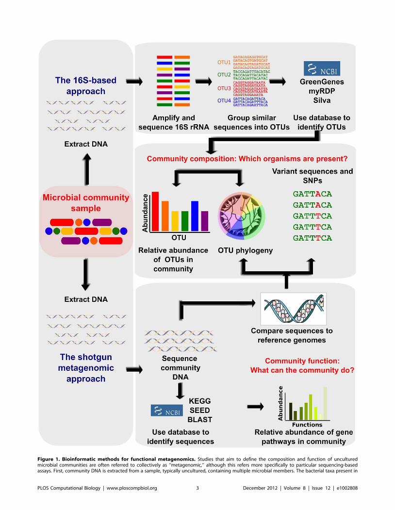
Figure 1. Bioinformatic methods for functional metagenomics. Studies that aim to define the composition and function of unculturedmicrobial communities are often referred to collectively as ‘‘metagenomic,’’ although this refers more specifically to particular sequencing-basedassays. First, community DNA is extracted from a sample, typically uncultured, containing multiple microbial members. The bacterial taxa present in
PLOS Computational Biology | www.ploscompbiol.org 3 December 2012 | Volume 8 | Issue 12 | e1002808
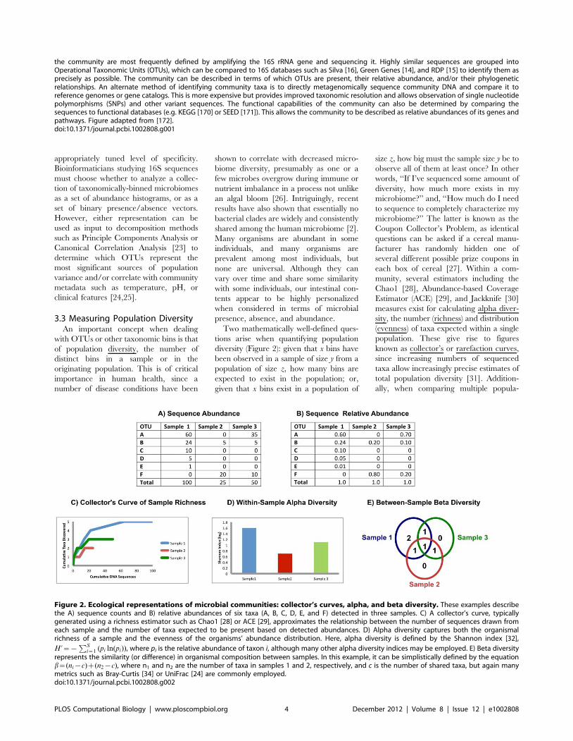
appropriately tuned level of specificity.
Bioinformaticians studying 16S sequences
must choose whether to analyze a collec-
tion of taxonomically-binned microbiomes
as a set of abundance histograms, or as a
set of binary presence/absence vectors.
However, either representation can be
used as input to decomposition methods
such as Principle Components Analysis or
Canonical Correlation Analysis [23] to
determine which OTUs represent the
most significant sources of population
variance and/or correlate with community
metadata such as temperature, pH, or
clinical features [24,25].
3.3 Measuring Population DiversityAn important concept when dealing
with OTUs or other taxonomic bins is that
of population diversity, the number of
distinct bins in a sample or in the
originating population. This is of critical
importance in human health, since a
number of disease conditions have been
shown to correlate with decreased micro-
biome diversity, presumably as one or a
few microbes overgrow during immune or
nutrient imbalance in a process not unlike
an algal bloom [26]. Intriguingly, recent
results have also shown that essentially no
bacterial clades are widely and consistently
shared among the human microbiome [2].
Many organisms are abundant in some
individuals, and many organisms are
prevalent among most individuals, but
none are universal. Although they can
vary over time and share some similarity
with some individuals, our intestinal con-
tents appear to be highly personalized
when considered in terms of microbial
presence, absence, and abundance.
Two mathematically well-defined ques-
tions arise when quantifying population
diversity (Figure 2): given that x bins have
been observed in a sample of size y from a
population of size z, how many bins are
expected to exist in the population; or,
given that x bins exist in a population of
size z, how big must the sample size y be to
observe all of them at least once? In other
words, ‘‘If I’ve sequenced some amount of
diversity, how much more exists in my
microbiome?’’ and, ‘‘How much do I need
to sequence to completely characterize my
microbiome?’’ The latter is known as the
Coupon Collector’s Problem, as identical
questions can be asked if a cereal manu-
facturer has randomly hidden one of
several different possible prize coupons in
each box of cereal [27]. Within a com-
munity, several estimators including the
Chao1 [28], Abundance-based Coverage
Estimator (ACE) [29], and Jackknife [30]
measures exist for calculating alpha diver-
sity, the number (richness) and distribution
(evenness) of taxa expected within a single
population. These give rise to figures
known as collector’s or rarefaction curves,
since increasing numbers of sequenced
taxa allow increasingly precise estimates of
total population diversity [31]. Addition-
ally, when comparing multiple popula-
the community are most frequently defined by amplifying the 16S rRNA gene and sequencing it. Highly similar sequences are grouped intoOperational Taxonomic Units (OTUs), which can be compared to 16S databases such as Silva [16], Green Genes [14], and RDP [15] to identify them asprecisely as possible. The community can be described in terms of which OTUs are present, their relative abundance, and/or their phylogeneticrelationships. An alternate method of identifying community taxa is to directly metagenomically sequence community DNA and compare it toreference genomes or gene catalogs. This is more expensive but provides improved taxonomic resolution and allows observation of single nucleotidepolymorphisms (SNPs) and other variant sequences. The functional capabilities of the community can also be determined by comparing thesequences to functional databases (e.g. KEGG [170] or SEED [171]). This allows the community to be described as relative abundances of its genes andpathways. Figure adapted from [172].doi:10.1371/journal.pcbi.1002808.g001
Figure 2. Ecological representations of microbial communities: collector’s curves, alpha, and beta diversity. These examples describethe A) sequence counts and B) relative abundances of six taxa (A, B, C, D, E, and F) detected in three samples. C) A collector’s curve, typicallygenerated using a richness estimator such as Chao1 [28] or ACE [29], approximates the relationship between the number of sequences drawn fromeach sample and the number of taxa expected to be present based on detected abundances. D) Alpha diversity captures both the organismalrichness of a sample and the evenness of the organisms’ abundance distribution. Here, alpha diversity is defined by the Shannon index [32],
H ’~{PS
i~1 (pi ln(pi)), where pi is the relative abundance of taxon i, although many other alpha diversity indices may be employed. E) Beta diversityrepresents the similarity (or difference) in organismal composition between samples. In this example, it can be simplistically defined by the equationb~(ni{c)z(n2{c), where n1 and n2 are the number of taxa in samples 1 and 2, respectively, and c is the number of shared taxa, but again manymetrics such as Bray-Curtis [34] or UniFrac [24] are commonly employed.doi:10.1371/journal.pcbi.1002808.g002
PLOS Computational Biology | www.ploscompbiol.org 4 December 2012 | Volume 8 | Issue 12 | e1002808
tions, beta diversity measures including
absolute or relative overlap describe how
many taxa are shared between them
(Figure 2). An alpha diversity measure
thus acts like a summary statistic of a single
population, while a beta diversity measure
acts like a similarity score between popu-
lations, allowing analysis by sample clus-
tering or, again, by dimensionality reduc-
tions such as PCA [20]. Alpha diversity is
often quantified by the Shannon Index
[32], H ’~{PS
i~1 (pi ln(pi)), or the
Simpson Index [33], D~PS
i~1 p2i , where
pi is the fraction of total species comprised
by species i. Beta diversity can be mea-
sured by simple taxa overlap or quantified
by the Bray-Curtis dissimilarity [34],
BCij~SizSj{2Cij
SizSj
, where Si and Sj are
the number of species in populations i and
j, and Cij is the total number of species at
the location with the fewest species. Like
similarity measures in expression array
analysis, many alpha- and beta-diversity
measures have been developed that each
reveal slightly different aspects of commu-
nity ecology.
Alternatively, the diversity within or
among communities can be analyzed in
terms of its phylogenetic distribution
rather than by isolating discrete bins. This
method of quantifying community diver-
sity describes it in terms of the total
breadth or depth of the phylogenetic
branches spanned by a microbiome (or
shared among two or more). For example,
consider a collection of n highly-related
16S sequences. These might be treated
either as one OTU or as n distinct taxa,
depending on how finely they are binned,
but a phylogenetic analysis will consider
them to span a small evolutionary distance
no matter how large n becomes. Con-
versely, two highly-divergent binned
OTUs are typically no different than two
similar OTUs, but a phylogenetic method
would score them as spanning a large
evolutionary distance. OTU-based and
phylogenetic methods tend to be comple-
mentary, in that each will reveal different
aspects of community structure. OTUs are
highly sensitive to the specific means by
which taxa are binned, for example,
whereas phylogenetic measures are sensi-
tive to the method of tree construction.
Like the OTU-based diversity estimators
discussed above, several standard metrics
such as UniFrac [20] exist for quantifying
phylogenetic diversity, and these can be
treated as single-sample descriptors or as
multiple-sample similarity measures.
It is critically important in any micro-
biome richness analysis to account for the
contribution that technical noise will make
to apparent diversity. As a simple example,
consider that a single base pair error in a
100 bp sequence read will create a new
OTU at the 99% similarity threshold.
Apparent diversity can thus be dramatically
modified by the choice of marker gene, the
region within it that is sequenced, the
biochemical marker extraction and ampli-
fication processes, and the read length and
noise characteristics of the sequencing
platform. Accounting for such errors com-
putationally continues to be a fruitful area
of research, particularly as 454-based
technologies have transitioned to the Illu-
mina platform, as current solutions can
discard all but the highest-quality sequence
regions [18]. A major confound in many
early molecular richness analyses was the
abundance of chimeric sequences, or reads
in which two unique marker sequences
(typically 16S regions) adhere during the
amplification process, creating an appar-
ently novel taxon. Although sequence
chimeras can now be reliably removed
computationally [13,19,35], this filtering
process is still an essential early step in any
microbiome analysis.
A final consideration in the computa-
tional analysis of community structure
assays is the use of microarray-based
methods for 16S (and other marker)
quantification within a microbiome. Just
as high-throughput RNA sequencing par-
allels gene expression microarrays, 16S
rDNA sequencing parallels phylochips,
microarrays constructed with probes com-
plementary to a variety of 16S and other
marker sequences [36]. The design and
analysis of such arrays can be challenging,
as 16S sequences (or any good genomic
markers) will be highly similar, and the
potential for extensive cross-hybridization
must be taken into account both when
determining what sequences to place on a
chip and how to quantify their abundance
after hybridization [37]. The continued
usefulness of such arrays will be dictated
by future trends in high-throughput se-
quencing costs and barcoding, but at
present phylochips are beginning to be
constructed to capture functional sequenc-
es in combination with measures of taxon
abundances in high throughput, and they
represent an interesting option for popu-
lation-level microbiome assays.
4. Shotgun Sequencing andMetagenomics
While measures of community diversity
have dominated historical analyses, mod-
ern high-throughput methods are being
developed for a host of other ‘‘meta’’
assays from uncultured microbes. The
term metagenomics is used with some
frequency to describe the entire body of
high-throughput studies now possible with
microbial communities, although it also
refers more specifically to whole-metagen-
ome shotgun (WMS) sequencing of geno-
mic DNA fragments from a community’s
metagenome [38,39]. Metatranscrip-
tomics, a close relative, implies shotgun
sequencing of reverse-transcribed RNA
transcripts [40,41], metaproteomics
[42,43] the quantification of protein or
peptide levels, and metametabolomics (or
less awkwardly community metabolomics)
[44,45] the investigation of small-molecule
metabolites. Of these assays, the latter
three in particular are still in their infancy,
but are carried out using roughly the same
technologies as their culture-based coun-
terparts, and the resulting data can
typically be analyzed using comparable
computational methods.
As of this writing, no complete meta-
metabolomic studies from uncultured mi-
crobiomes have yet been published, al-
though their potential usefulness in
understanding e.g. the human gut micro-
biome and its role in energy harvest,
obesity, and metabolic disorders is clear
[44]. Metaproteomic and metatranscrip-
tomic studies have primarily focused on
environmental samples [46,47,48], but
human stool metatranscriptomics [41,49]
and medium-throughput human gut me-
taproteomics [42,43] have also been
successfully executed and analyzed using
bioinformatics similar to those for meta-
genomes (see below) [42]. Quantification
of the human stool metatranscriptome and
metaproteome in tandem with host bio-
molecular activities should yield fascinat-
ing insights into our relationship with our
microbial majority.
DNA extraction and WMS sequencing
from uncultured samples developed, like
many sequencing technologies, concur-
rently with the Human Genome Project
[2,50,51,52], and as with other communi-
ty genomic assays, the earliest applications
were to environmental microbes due to
the ease of isolation and extraction
[53,54]. WMS techniques are in some
ways much the same now as they were
then, modulo the need for complex Sanger
clone library construction: isolate micro-
bial cells of a target size range (e.g. viral,
bacterial, or eukaryotic), lyse the cells
(taking care not to lose DNA to native
DNAses), isolate DNA, fragment it to a
target length, and sequence the resulting
fragments [55,56]. Since this procedure
can be performed on essentially any
heterogeneous population, does not suffer
from the single-copy and evolutionary
PLOS Computational Biology | www.ploscompbiol.org 5 December 2012 | Volume 8 | Issue 12 | e1002808
assumptions of marker genes, and does not
require (although can include) amplifica-
tion, it can to some degree produce a less
biased community profile than does 16S
sequencing [57].
4.1 Metagenome Data AnalysisUnlike whole-genome shotgun (WGS)
sequencing of individual organisms, in
which the end product is typically a single
fully assembled genome, metagenomes
tend not to have a single ‘‘finish line’’
and have been successfully analyzed using
a range of assembly techniques. The
simplest is no assembly at all - the short
reads produced as primary data can, after
cleaning to reduce sequencing error [18],
be treated as taxonomic markers or as
gene fragments and analyzed directly.
Since microbial genomes typically contain
few intergenic sequences, most fragments
will contain pieces of one or more genes;
these can be used to quantify enzymatic or
pathway abundances directly as described
below [1,58,59,60]. Alternatively, meta-
genome-specific assembly algorithms have
been proposed that reconstruct only the
open reading frames from a population (its
ORFeome), recruiting highly sequence-
similar fragments on an as-needed basis to
complete single gene sequences and avoid-
ing assembly of larger contigs [61,62]. The
most challenging option is to attempt full
assemblies for complete genomes present
in the community, which is rarely possible
save in very simple communities or with
extreme sequencing depth [53,54]. When
successful, this has the obvious benefit of
establishing synteny, structural variation,
and opening up the range of tools
developed for whole-genome analysis
[63], and guided assemblies using read
mapping (rather than de novo assembly) can
be used when appropriate reference ge-
nomes are available. However, care must
be taken in interpreting any such assem-
blies, since horizontal transfer and com-
munity complexity prevent unambiguous
assemblies in essentially all realistic cases
[64]. A more feasible middle ground is
emerging around maximal assemblies that
capture the largest unambiguous contigs in
a community [65], allowing e.g. local
operon structure to be studied without
introducing artificial homogeneity into the
data. In any of these cases - direct analysis
of reads, ORF assembly, maximal unam-
biguous scaffolds, or whole genomes -
subsequent analyses typically focus on the
functional aspects of the resulting genes
and pathways as detailed below.
A key bioinformatic tradeoff in analyz-
ing metagenomic WMS sequences, re-
gardless of their degree of assembly, is
whether they should be analyzed by
homology, de novo, or a combination
thereof. An illustrative example is the task
of determining which parts of each
sequence read (or ORF/contig/etc.) en-
code one or more genes, i.e. gene finding
or calling. By homology, each sequence
can be BLASTed [66] against a large
database of reference genomes, which will
retrieve any similar known reading frames;
the boundaries of these regions of similar-
ity thus become the start and stop of the
metagenomic open reading frames. This
method is robust to sequencing and
assembly errors, but it is sensitive to the
contents of the reference database. Con-
versely, de novo methods have been devel-
oped to directly bin [67,68,69] and call
genes within [61,62] metagenomic se-
quences using DNA features alone (GC
content, codon usage, etc.). As with
genome analysis for newly sequenced
single organisms, most de novo methods
rely on interpolated [70] or profile [71]
Hidden Markov Models (HMMs) or on
other machine learners that perform
classification based on encoded sequence
features [72,73]. This is a far more
challenging task, making it sensitive to
errors in the computational prediction
process, but it enables a greater range of
discovery and community characterization
efforts by relying less on prior knowledge.
Hybrid methods for e.g. taxonomic bin-
ning [69] have recently been developed
that consume both sequence similarity and
de novo sequence features as input, and for
some tasks such systems might represent a
sweet spot between computational com-
plexity, availability of prior knowledge,
and biological accuracy. This tradeoff
between knowledge transfer by homology
and de novo prediction from sequence is
even more pronounced when characteriz-
ing predicted genes, as discussed below.
5. Computational FunctionalMetagenomics
Essentially any analysis of a microbial
community is ‘‘functional’’ in the sense
that it aims to determine the overall
phenotypic consequences of the commu-
nity’s composition and biomolecular ac-
tivity. For example, the Human Micro-
biome Project began to investigate what
typical human microbial community
members are doing [60], how they are
affecting their human hosts [2], what
impact they have on health or disease,
and these help to suggest how pro- or
antibiotics can be used to change commu-
nity behavior for the better [74]. The
approaches referred to as computational
functional metagenomics, however, typi-
cally focus on the function (either bio-
chemically or phenotypically) of individual
genes and gene products within a com-
munity and fall into one of two categories.
Top-down approaches screen a metagen-
ome for a functional class of interest, e.g. a
particular enzyme family, transporter or
chelator, pathway, or biological activity,
essentially asking the question, ‘‘Does this
community carry out this function and, if
so, in what way?’’ Bottom-up approaches
attempt to reconstruct profiles, either
descriptive or predictive, of overall func-
tionality within a community, typically
relying on pathway and/or metabolic
reconstructions and asking the question,
‘‘What functions are carried out by this
community?’’
Either approach relies, first, on catalog-
ing some or all of the gene products
present in a community and assigning
them molecular functions and/or biolog-
ical roles in the typical sense of protein
function predictions [53,54,59]. As with so
many bioinformatic methods, the simplest
techniques rely on BLAST [66]: a top-
down investigation can BLAST represen-
tatives of gene families of interest into the
community metagenome to determine
their presence and abundance [63], and
a bottom-up approach can BLAST reads
or contigs from a metagenome into a large
annotated reference database such as nr to
perform knowledge transfer by homology
[75,76,77]. Top-down approaches dove-
tail well with experimental screens for
individual gene product function [6], and
bottom-up approaches are more descrip-
tive of the community as a whole [78].
As each metagenomic sample can
contain millions of reads and databases
such as nr in turn contain millions of
sequences, computational efficiency is a
critical consideration in either approach.
On one hand, stricter nucleotide searches
or direct read mapping to reference
genomes [79,80] improve runtime and
specificity at the cost of sensitivity; on the
other, more flexible characterizations of
sequence function such as HMMs [72,73]
tend to simultaneously increase coverage,
accuracy, and computational expense.
Any of these sequence annotation methods
can be run directly on short reads, on
ORF assemblies, or on assembled contigs,
and statistical methods have been pro-
posed to more accurately estimate the
frequencies of functions in the underlying
community when they are under-sampled
(requiring the estimation of unobserved
values [81]) or over-sampled (correcting
for loci with greater than 16 coverage
[82]). In any of these cases, the end result
PLOS Computational Biology | www.ploscompbiol.org 6 December 2012 | Volume 8 | Issue 12 | e1002808
of such an analysis is an abundance profile
for each metagenomic sample quantifying
the frequency of gene products in the
community; the profiles for several related
communities can be assembled into a
frequency matrix resembling a microarray
dataset. Gene products (rows) in such a
profile can be identified by functional
descriptors such as Gene Ontology [83]
or KEGG [84] terms, protein families
such as Pfams [73] or TIGRfams [72],
enzymatic [85], transport [86], or other
structural classes [87], or most often as
orthologous families such as Homolo-
Genes [88], COGs [89], NOGs [90], or
KOs [84].
A logical next step, given such an
abundance profile of orthologous families,
is to assemble them into profiles of
community metabolic and functional
pathways. This requires an appropriate
catalog of reference pathways such as
KEGG [84], MetaCyc [91], or GO [83],
although it should be noted that none of
these is currently optimized for modeling
communities rather than single organisms
in monoculture [90]. The pathway infer-
ence process is similar to that performed
when annotating an individual newly
sequenced genome [92] and consists of
three main steps: A) assigning each
ortholog to one or more pathways, B)
gap filling or interpolation of missing
annotations, and C) determining the
presence and/or abundance of each
pathway. The first ortholog assignment
step is necessary since many gene families
participate in multiple pathways; phospho-
enolpyruvate carboxykinase, for example,
is used in the TCA cycle, glycolysis, and in
various intercellular signaling mechanisms
[93]. The abundance mass for each
enzyme is distributed across its functions
in one or more possible pathways; meth-
ods for doing this range from the simple
assumption that it is equally active in all
reference pathways (as currently done by
KAAS [94] or MG-RAST [76]) to the
elimination of unlikely pathways and the
redistribution of associated mass in a
maximum parsimony fashion [95]. Sec-
ond, once all observed orthologs have
been assigned to pathways (when possible),
gaps or holes in the reference pathways
can be filled, using the assumption that the
enzymes necessary to operate a nearly
complete pathway should be present
somewhere in the community. Essentially
three methods have been successfully
employed for gap filling: searching for
alternative pathway fragments to explain
the discrepancy [96,97], purely mathemat-
ical smoothing to replace the missing
enzymes’ abundances with numerically
plausible values [81], and targeted search-
es of the metagenome of interest for more
distant homologues with which to fill the
hole [98]. Since we are currently able to
infer function for only a fraction of the
genes in any given complete genome, let
alone metagenome, any of these ap-
proaches should be deemed hypothetical
at best; nevertheless, like any missing value
imputation process, they can provide
numerically stable guesses that are sub-
stantially better than random [99]. Finally,
as described above for taxa, the resulting
data can be used to summarize each
reference pathway either qualitatively (i.e.
with what likelihood is it present in the
community?) or quantitatively (how abun-
dant is it in the community?), and in its
simplest form condenses the abundance
matrix of orthologous families into an
abundance (or presence/absence) matrix
of pathways. Either the ortholog or
pathway matrices can then be tested for
differentially abundant features represent-
ing diagnostic biomarkers with potential
explanatory power for the phenotype of
interest, using statistical methods devel-
oped for identical tests in expression
biomarker discovery [100] and genome-
wide association studies [101].
However, our prior knowledge of (pri-
marily) metabolic pathways can be lever-
aged to produce richer inferences from
such pathway abundance information.
Given sufficient information about the
pathways in a community, it is relatively
straightforward to predict what metabolic
compounds have the potential to be
produced. However, it is much more
difficult to infer what metabolite pools
and fluxes in the community will actually
be under a specific set of environmental
conditions [102,103]. Multi-organism flux
balance analysis (FBA) is an emerging tool
to enable such analyses [104], but given
the extreme difficulty of constructing
accurate models for even single organisms
[105] or of determining model parameters
in a multi-organism community [53], no
successful reconstructions have yet been
performed for complex microbiomes. The
area holds tremendous promise, however,
first with respect to metabolic engineering
- it is not yet clear what successes might be
achieved with respect to biofuel produc-
tion or bioremediation using synthetically
manipulated communities in place of
individual organisms [106,107]. Second,
in addition to metabolite profiling, multi-
organism growth prediction allows the
determination of mutualisms, parasitisms,
and commensalisms among taxa in the
community [108] [109,110], opening the
door to basic biological discoveries regard-
ing community dynamics [25,111,112]
and to therapeutic probiotic treatments
for dysbioses in the human microbiome
[113,114].
6. Host Interactions andInterventions
A final but critical aspect of translation-
al metagenomics lies in understanding not
only a microbial community but also its
environment - that is, its interaction with a
human host. Our microbiota would be of
interest to basic research alone if they were
not heavily influenced by host immunity
and, in turn, a major influence on host
health and disease. The skin of humans
hosts relatively few taxa (e.g. Propionibacte-
rium [115]), the nasal cavity somewhat
more (e.g. Corynebacterium [116]), the oral
cavity (dominated by Streptococcus) several
hundred taxa (with remarkable diversity
even among saliva, tongue, teeth, and
other substrates [117,118]) and the gut
over 500 taxa with densities over 1011
cells/g [2,119]. Almost none of these
communities are yet well-understood, al-
though anecdotes abound. The skin mi-
crobiome is thought to be a key factor in
antibiotic resistant Staphylococcus aureus in-
fections [120,121]; nasal communities
have interacted with the pneumococcus
population to influence its epidemiological
carriage patterns subsequent to vaccina-
tion programs [122]; and extreme dysbio-
sis in cystic fibrosis can be a precursor to
pathogenic infection [123].
The gut, however, is currently the best-
studied human microbiome [119,124,125].
It is a dynamic community changing over
the course of days [126,127], over the
longer time scales of infant development
[112,128,129,130] and aging [131,132], in
response to natural perturbations such as
diet [59,133,134,135] and illness
[114,136], and modified in as-yet-unknown
ways by the modern prevalence of travel,
chemical additives, and antibiotics [126].
Indeed, the human gut microbiome has
proven difficult to study exactly because it is
so intimately related to the physiology of its
host; inasmuch as no two people share
identical microbiota, most microbiomes are
strikingly divergent between distinct host
species, rendering results from model
organisms difficult to interpret [137,138].
Nevertheless, studies in wild type verte-
brates such as mice [139,140] and zebrafish
[141,142] have found a number of similar-
ities in their microbiotic function and host
interactions. In particular, germ-free or-
ganisms have yielded insights into the
microbiota’s role in maturation of the host
immune system and, surprisingly, even
PLOS Computational Biology | www.ploscompbiol.org 7 December 2012 | Volume 8 | Issue 12 | e1002808
anatomical development of the intestine
[143,144]. Similarly, gnotobiotic systems in
which an organism’s natural microbiota are
replaced with their human analog are a
current growth area for closer study of the
phenotypic consequences of controlled
microbiotic perturbations [145].
One of the highest-profile demonstra-
tions of this technique and of the micro-
biota’s influence on human health has
been in an ongoing study of the micro-
biome in obesity [146]. Early studies in
wild-type mice [139] demonstrated gross
taxonomic shifts in the composition and
diversity of the microbiomes of obese
individuals; follow-ups in gnotobiotic mice
confirmed that this phenotype was trans-
missible via the microbiome [147]. These
initial studies were taxonomically focused
and found that, while high-level phyla
were robustly perturbed in obesity (which
incurs a reduction in Bacteroidetes and
concomitant increase in Firmicutes [139]),
few if any specific taxa seemed to be
similarly correlated [138,140]. Subsequent
functional metagenomics, first in mouse
[148] and later a small human cohort [59],
established that the functional consistency
of these shifts operates more consistently,
enriching the microbiome’s capacity for
energy harvest and disregulating fat stor-
age and signaling within the host. While
these observations represent major de-
scriptive triumphs, further computational
and experimental work must yet be
performed to establish the underlying
biomolecular mechanisms and whether
they are correlative, causative, or may be
targeted by interventions to actively treat
obesity [59].
A similarly complex community for
which we have a greater understanding of
the functional mechanisms at play is the
formation of biofilms in the oral cavity
preceding caries (cavities) or periodontitis
[149]. While we are still investigating the
microbiota of the saliva [150] and of the
oral soft tissues [151], colonization of the
tooth enamel is somewhat better under-
stood due to the removal of significant
interaction with host tissue. Even more
strikingly, this biofilm, or physically struc-
tured consortium of multiple microbial
taxa, must reestablish itself from almost
nothing each time we brush our teeth - a
process that can be achieved within hours
[152]. Streptococci in particular possess a
number of surface adhesins and receptors
that enable them to behave as early
colonizers on bare tooth surface and to
bind together a variety of subsequent
microbes [153]. These fairly minimal
bacteria are metabolically supported by
Veillonella and Actinomyces species, and their
aggregation leads to local nutritive and
structural environments favorable to e.g.
Fusobacterium and Porphyromonas [154]. Each
of these steps is mediated by a combination
of cell surface recognition molecules, extra-
cellular physical interactions, metabolic
codependencies, and explicit intercellular
signaling, providing an excellent example
of the complexity with which structured
microbiomes can evolve. Indeed, the evol-
vability of such systems, both as a whole
[155] and at the molecular level [156], is
yet another aspect of the work remaining to
computationally characterize microbiotic
biomolecular and community function.
Finally, the microbiota clearly represent
a key component of future personalized
medicine. First, the number and diversity
of phenotypes linked to the composition of
the microbiota is immense: obesity, diabe-
tes, allergies, autism, inflammatory bowel
disease, fibromyalgia, cardiac function,
various cancers, and depression have all
been reported to correlate with micro-
biome function [157]. Even without caus-
ative or modulatory roles, there is tremen-
dous potential in the ability to use the
taxonomic or metagenomic composition
of a subject’s gut or oral flora (both easily
sampled) as a diagnostic or prognostic
biomarker for any or all of these condi-
tions. Commercial personal genomics
services such as 23andMe (Mountain
View, CA) promise to decode your disease
risk based on somatic DNA from a saliva
sample; bioinformatic techniques have yet
to be developed that will allow us to do the
same using microbial DNA.
Second, the microbiota are amazingly
plastic; they change metagenomically
within hours and metatranscriptomically
within minutes in response to perturba-
tions ranging from broad-spectrum antibi-
otics to your breakfast bacon and eggs
[41,126,127]. For any phenotype to which
they are causally linked, this opens the
possibility of pharmaceutical, prebiotic
(nutrients promoting the growth of bene-
ficial microbes [113,119]), or probiotic
treatments. Indeed, Nobel Prize winner
Ilya Mechnikov famously named Lactoba-
cillus bulgaricus, a primary yogurt-produc-
ing bacterium, for its apparent contribu-
tion to the longevity of yogurt-consuming
Bulgarians [158], and despite a degree of
unfortunate popular hype, the potential
health benefits of a variety of probiotic
organisms are indeed supported by recent
findings [125,159]. Unfortunately, we
currently understand few of the mecha-
nisms by which these interventions oper-
ate. Do the supplemented organisms
outcompete specific pathogens, do they
simply increase their own numbers, or do
they shift the overall systems-level balance
of many taxa within the community? Do
they reduce the levels of detrimental
metabolites in the host, or do they increase
the levels of beneficial compounds? Do
they change biomolecular activity being
carried out in microbial cells, adjacent
host epithelial or immune cells, or distal
cells through host signaling mechanisms?
Or, as in polygenic genetic disorders, does
a combination of many factors result in
health or disease status as an emergent
phenotype?
The human microbiome has been
referred to as a ‘‘forgotten organ’’ [160],
and the truth of both words is striking.
Our trillions of microbial passengers
account for a proportion of our metabo-
lism and signaling as least as great as that
performed by more integral body parts,
and after a century of molecular biology,
we have only begun to realize their
importance within the last few years. To
close with a success story, the popular
press [161] recently reported on the full
recovery of a patient suffering from
Clostridium difficile-associated diarrhea,
which had led her to lose over 60 pounds
in less than a year. C. difficile is often
refractory to antibiotics, with spores able
to repopulate from very low levels, and the
patient’s normal microbiota had been
decimated by the infection and subsequent
treatment. Finally, she received a simple
fecal transplant from her husband, in
which the host microbiome was replaced
with that of a donor. Within days, not only
had she begun a complete recovery, but a
metagenomic survey of her microbiota
showed that the new community was
almost completely established and had
restored normal taxonomic abundances
[162]. While this is an extreme case,
similar treatments have shown a success
rate of some 90% historically [163], all of
which occurred before modern genomic
techniques allowed us to more closely
examine the microbiota. Imagine perform-
ing any other organ transplant with such a
high rate of success - while blindfolded!
Like so many other discoveries of the
genomic era, the study of the human
microbiome has begun with amazing
achievements, and it will require contin-
ued experimental and bioinformatic efforts
to better understand the biology of these
microbial communities and to see it
translated into clinical practice.
7. Summary
The human microbiome consists of
unicellular microbes - mainly bacterial,
but also archaeal, viral, and eukaryotic -
PLOS Computational Biology | www.ploscompbiol.org 8 December 2012 | Volume 8 | Issue 12 | e1002808
that occupy nearly every surface of our
bodies and have been linked to a wide
range of phenotypes in health and disease.
High-throughput assays have offered the
first comprehensive culture-free tech-
niques for surveying the members of these
communities and their biomolecular ac-
tivities at the transcript, protein, and
metabolic levels. Most current technolo-
gies rely on DNA sequencing to examine
either individual taxonomic markers in a
microbial community, typically the 16S
ribosomal subunit gene, or the composite
metagenome of the entire community.
Taxonomic analyses lend themselves to
computational techniques rooted in mi-
crobial ecology, including diversity mea-
sures within (alpha) and between (beta)
samples; these can be defined quantita-
tively (based on abundance) or qualitative-
ly (based on presence/absence), and they
may or may not take into account the
phylogenetic relatedness of the taxa being
investigated. Finally, in the absence of
information regarding specific named
species in a community, sequences are
often clustered by similarity into Opera-
tional Taxonomic Units (OTUs) as the
fundamental unit of analysis within a
sample.
In contrast, whole-genome shotgun
analyses begin with sequences sampled
from the entire community metagenome.
These can also be taxonomically binned,
or they can be assembled, partially assem-
bled into ORFeomes, or characterized
directly at the read level. Characterization
typically consists of function assignment
similar to that performed for genes during
annotation of a single organism’s genome;
once genes in the metagenome are de-
fined, they can be mapped or BLASTed to
reference sequence databases or analyzed
intrinsically using e.g. codon frequencies
or HMM profiles. Finally, the frequencies
of enzymes and other gene products so
determined can be assigned to pathways,
allowing inference of the overall metabolic
potential of the community and inference
of diagnostic and potentially explanatory
functional biomarkers. Ongoing studies
are beginning to investigate the ways in
which the microbiota can be directly
engineered using pharmaceuticals, prebio-
tics, probiotics, or diet as a preventative or
treatment for a wide range of disorders.
8. Exercises
Q1. You have a collection of 16S rRNA
gene sequencing data, which consists of an
Illumina run in which the 100 bp V6
hypervariable region has been amplified.
The error rate of Illumina sequencing has
been estimated as 1.361023 per base pair
[164], and you have 30 million Illumina
reads. Will binning your reads into OTUs
at 100% or 97% give you a more
interpretable estimation of the number of
OTUs present? Why?
Q2. You have collections of 16S rRNA
gene reads from two environmental sam-
ples, A and B. You examine 50 reads each
from sample A and sample B, which
correspond to four taxa in A and two taxa
in B. You examine 25 more reads from
each library and detect two more taxa in A
and one more in B. In total, two of these
taxa are present in both communities A
and B. Which sample has higher alpha
diversity by counting taxonomic richness?
What is the beta diversity between A and
B using simple overlap of taxa? Using
Bray-Curtis dissimilarity?
Q3. You examine 1,000 more sequenc-
es from samples A and B, detecting 10
additional taxa in A and 25 in B. Which
sample has higher alpha diversity now, as
measured by taxonomic richness? Why is
this different from your previous answer?
What statement can you make about the
ecological evenness of communities A and
B as a result?
Q4. What factors in the microbial
environment might you expect to be
reflected in metabolism, signaling, and
biomolecular function between skin bacte-
ria and oral bacteria? What impact would
you expect this to have on the pathways
carried in these community metagenomes,
or on their alpha diversities?
Q5. It is estimated that 2–5% of the
population has Clostridium difficile in their
intestines. Why is this not usually a
problem?
Q6. Consider the impact upon the
human microbiome of two perturbations:
social contact and brushing your teeth.
What short-term and long-term impact do
you expect on alpha diversity? Beta
diversity?
Q7. Calculate richness, the inverse
Simpson index, and the Shannon index
for each sample described in the table
below. Which has the highest alpha
diversity? Why is the answer different
according to which measurement you use?
Answers to the Exercises can be found
in Text S1.
Supporting Information
Text S1 Answers to Exercises.
(DOCX)
Acknowledgments
We thank Nicola Segata for assistance with
figures.
OTU Sample 1 Sample 2 Sample 3
A 20 20 30B 20 20 30C 1 20 30D 1 20 0E 1 0 1
Further Reading
It is difficult to recommend comprehensive literature in an area that is changingso rapidly, but the bioinformatics of microbial community studies are currentlybest covered by the reviews in [22,56,165]. Computational tools for metagenomicanalysis include [13,19,63,75,76,77,166]. An overview of microbial ecology from aphylogenetic perspective is provided in [167,168], and the use of the 16S subunitas a marker gene is reviewed in [12]. Likewise, experimental and computationalfunctional metagenomics are discussed in [6,25,169]. The clinical relevance of thehuman microbiome is far-ranging and is comprehensively reviewed in [157].
PLOS Computational Biology | www.ploscompbiol.org 9 December 2012 | Volume 8 | Issue 12 | e1002808
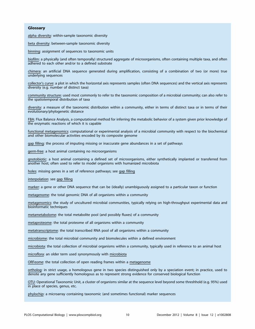
Glossary
alpha diversity: within-sample taxonomic diversity
beta diversity: between-sample taxonomic diversity
binning: assignment of sequences to taxonomic units
biofilm: a physically (and often temporally) structured aggregate of microorganisms, often containing multiple taxa, and oftenadhered to each other and/or to a defined substrate
chimera: an artificial DNA sequence generated during amplification, consisting of a combination of two (or more) trueunderlying sequences
collector’s curve: a plot in which the horizontal axis represents samples (often DNA sequences) and the vertical axis representsdiversity (e.g. number of distinct taxa)
community structure: used most commonly to refer to the taxonomic composition of a microbial community; can also refer tothe spatiotemporal distribution of taxa
diversity: a measure of the taxonomic distribution within a community, either in terms of distinct taxa or in terms of theirevolutionary/phylogenetic distance
FBA: Flux Balance Analysis, a computational method for inferring the metabolic behavior of a system given prior knowledge ofthe enzymatic reactions of which it is capable
functional metagenomics: computational or experimental analysis of a microbial community with respect to the biochemicaland other biomolecular activities encoded by its composite genome
gap filling: the process of imputing missing or inaccurate gene abundances in a set of pathways
germ-free: a host animal containing no microorganisms
gnotobiotic: a host animal containing a defined set of microorganisms, either synthetically implanted or transferred fromanother host; often used to refer to model organisms with humanized microbiota
holes: missing genes in a set of reference pathways; see gap filling
interpolation: see gap filling
marker: a gene or other DNA sequence that can be (ideally) unambiguously assigned to a particular taxon or function
metagenome: the total genomic DNA of all organisms within a community
metagenomics: the study of uncultured microbial communities, typically relying on high-throughput experimental data andbioinformatic techniques
metametabolome: the total metabolite pool (and possibly fluxes) of a community
metaproteome: the total proteome of all organisms within a community
metatranscriptome: the total transcribed RNA pool of all organisms within a community
microbiome: the total microbial community and biomolecules within a defined environment
microbiota: the total collection of microbial organisms within a community, typically used in reference to an animal host
microflora: an older term used synonymously with microbiota
ORFeome: the total collection of open reading frames within a metagenome
ortholog: in strict usage, a homologous gene in two species distinguished only by a speciation event; in practice, used todenote any gene sufficiently homologous as to represent strong evidence for conserved biological function
OTU: Operational Taxonomic Unit, a cluster of organisms similar at the sequence level beyond some threshhold (e.g. 95%) usedin place of species, genus, etc.
phylochip: a microarray containing taxonomic (and sometimes functional) marker sequences
PLOS Computational Biology | www.ploscompbiol.org 10 December 2012 | Volume 8 | Issue 12 | e1002808
References
1. Qin J, Li R, Raes J, Arumugam M, Burgdorf
KS, et al. (2010) A human gut microbial gene
catalogue established by metagenomic sequenc-
ing. Nature 464: 59–65.
2. (2012) Structure, function and diversity of the
healthy human microbiome. Nature 486: 207–
214.
3. Gram HC (1884) Uber die isolierte Farbung der
Schizomyceten in Schnitt- und Trockenprapar-
aten. Fortschritte der Medizin 2: 185–189.
4. Pace NR, Stahl DA, Lane DJ, Olsen GJ (1986)
The analysis of natural microbial populations by
ribosomal RNA sequences. Advances in Micro-
bial Ecology 9: 1–55.
5. Amann RI, Ludwig W, Schleifer KH (1995)
Phylogenetic identification and in situ detection
of individual microbial cells without cultivation.
Microbiol Rev 59: 143–169.
6. Handelsman J (2004) Metagenomics: application
of genomics to uncultured microorganisms.
Microbiol Mol Biol Rev 68: 669–685.
7. Sanger F, Coulson AR (1975) A rapid method
for determining sequences in DNA by primed
synthesis with DNA polymerase. Journal of
molecular biology 94: 441–448.
8. Sanger F, Nicklen S, Coulson AR (1977) DNA
sequencing with chain-terminating inhibitors.
Proceedings of the National Academy of Sci-
ences of the United States of America 74: 5463–
5467.
9. Birney E, Stamatoyannopoulos JA, Dutta A,
Guigo R, Gingeras TR, et al. (2007) Identifica-
tion and analysis of functional elements in 1% of
the human genome by the ENCODE pilot
project. Nature 447: 799–816.
10. Bocchetta M, Ceccarelli E, Creti R, Sanange-
lantoni AM, Tiboni O, et al. (1995) Arrange-
ment and nucleotide sequence of the gene (fus)
encoding elongation factor G (EF-G) from the
hyperthermophilic bacterium Aquifex pyrophi-
lus: phylogenetic depth of hyperthermophilic
bacteria inferred from analysis of the EF-G/fus
sequences. J Mol Evol 41: 803–812.
11. Lane DJ, Pace B, Olsen GJ, Stahl DA, Sogin
ML, et al. (1985) Rapid determination of 16S
ribosomal RNA sequences for phylogenetic
analyses. Proc Natl Acad Sci U S A 82: 6955–
6959.
12. Tringe SG, Hugenholtz P (2008) A renaissance
for the pioneering 16S rRNA gene. Curr Opin
Microbiol 11: 442–446.
13. Caporaso JG, Kuczynski J, Stombaugh J,
Bittinger K, Bushman FD, et al. (2010) QIIME
allows analysis of high-throughput community
sequencing data. Nat Methods 7: 335–336.
14. DeSantis TZ, Hugenholtz P, Larsen N, Rojas
M, Brodie EL, et al. (2006) Greengenes, a
chimera-checked 16S rRNA gene database and
workbench compatible with ARB. Appl Environ
Microbiol 72: 5069–5072.
15. Cole JR, Wang Q, Cardenas E, Fish J, Chai B,
et al. (2009) The Ribosomal Database Project:
improved alignments and new tools for rRNA
analysis. Nucleic Acids Res 37: D141–145.
16. Pruesse E, Quast C, Knittel K, Fuchs BM,
Ludwig W, et al. (2007) SILVA: a comprehen-
sive online resource for quality checked and
aligned ribosomal RNA sequence data compat-
ible with ARB. Nucleic Acids Res 35: 7188–
7196.
17. Achtman M, Wagner M (2008) Microbial
diversity and the genetic nature of microbial
species. Nat Rev Microbiol 6: 431–440.
18. Schloss PD (2010) The effects of alignment
quality, distance calculation method, sequence
filtering, and region on the analysis of 16S rRNA
gene-based studies. PLoS Comput Biol 6:
e1000844.
19. Schloss PD, Westcott SL, Ryabin T, Hall JR,
Hartmann M, et al. (2009) Introducing mothur:
open-source, platform-independent, communi-
ty-supported software for describing and com-
paring microbial communities. Appl Environ
Microbiol 75: 7537–7541.
20. Hamady M, Lozupone C, Knight R (2010) Fast
UniFrac: facilitating high-throughput phyloge-
netic analyses of microbial communities includ-
ing analysis of pyrosequencing and PhyloChip
data. ISME J 4: 17–27.
21. Wang Q, Garrity GM, Tiedje JM, Cole JR
(2007) Naive Bayesian classifier for rapid
assignment of rRNA sequences into the new
bacterial taxonomy. Appl Environ Microbiol 73:
5261–5267.
22. Hamady M, Knight R (2009) Microbial com-
munity profiling for human microbiome pro-
jects: Tools, techniques, and challenges. Ge-
nome Res 19: 1141–1152.
23. Johnson RA, Wichern DW (2007) Applied
Multivariate Statistical Analysis: Prentice
Hall.
24. Lozupone C, Knight R (2005) UniFrac: a new
phylogenetic method for comparing microbial
communities. Appl Environ Microbiol 71:
8228–8235.
25. Gianoulis TA, Raes J, Patel PV, Bjornson R,
Korbel JO, et al. (2009) Quantifying environ-
mental adaptation of metabolic pathways in
metagenomics. Proc Natl Acad Sci U S A 106:
1374–1379.
26. Sellner KG, Doucette GJ, Kirkpatrick GJ (2003)
Harmful algal blooms: causes, impacts and
detection. J Ind Microbiol Biotechnol 30: 383–406.
27. Hildebrand MV (1993) The Birthday Problem.American Mathematical Monthly 100: 643.
28. Chao A (1984) Nonparametric estimation of the
number of classes in a population. ScandinavianJournal of Statistics 11: 265–270.
29. Chao A, Ma M-C, Yang MCK (1993) Stopping
rules and estimation for recapture debuggingwith unequal failure rates. Biometrika 80: 193–
201.
30. Heltshe JF, Forrester NE (1983) Estimatingspecies richness using the jackknife procedure.
Biometrics 39: 1–11.
31. Colwell RK, Coddington JA (1994) Estimating
terrestrial biodiversity through extrapolation.
Phil Trans R Soc London B 345: 101–118.
32. Shannon CE (1948) A mathematical theory of
communication. Bell System Technical Journal27: 379–423, 623–656.
33. Simpson EH (1949) Measurement of diversity.
Nature 163: 688.
34. Bray JR, Curtis JT (1957) An ordination of
upland forest communities of southern Wiscon-
sin. Ecological Monographs 27: 325–349.
35. Huber T, Faulkner G, Hugenholtz P (2004)
Bellerophon: a program to detect chimeric
sequences in multiple sequence alignments.Bioinformatics 20: 2317–2319.
36. Brodie EL, Desantis TZ, Joyner DC, Baek SM,Larsen JT, et al. (2006) Application of a high-
density oligonucleotide microarray approach to
study bacterial population dynamics duringuranium reduction and reoxidation. Appl Envi-
ron Microbiol 72: 6288–6298.
37. Schatz MC, Phillippy AM, Gajer P, DeSantis
TZ, Andersen GL, et al. (2010) Integrated
microbial survey analysis of prokaryotic com-munities for the PhyloChip microarray. Appl
Environ Microbiol 76: 5636–5638.
38. Riesenfeld CS, Schloss PD, Handelsman J(2004) Metagenomics: genomic analysis of
microbial communities. Annu Rev Genet 38:525–552.
39. Chen K, Pachter L (2005) Bioinformatics for
whole-genome shotgun sequencing of microbialcommunities. PLoS Comput Biol 1: 106–112.
40. Gilbert JA, Field D, Huang Y, Edwards R, LiW, et al. (2008) Detection of large numbers of
novel sequences in the metatranscriptomes of
complex marine microbial communities. PLoSOne 3: e3042.
41. Booijink CC, Boekhorst J, Zoetendal EG, Smidt
H, Kleerebezem M, et al. (2010) Metatranscrip-
phylotype: see OTU
prebiotic: a food substance metabolized by the microbiota so as to directly or indirectly benefit the host
probiotic: a live microorganism consumed by the host with direct or indirect health benefits
rarefaction curve: see collector’s curve
richness: see diversity
16S rRNA: the transcribed form of the 16S ribosomal subunit gene, the smaller RNA component of the prokaryotic ribosome,used as the most common taxonomic marker for microbial communities
WGS: Whole-Genome Shotgun, used to describe shotgun sequencing of individual organisms and, sometimes, microbialcommunities, although this is not completely accurate as no ‘‘whole-genome’’ is typically involved
WMS: Whole-Metagenome Shotgun sequencing, used in reference to undirected metagenomic sequencing to distinguish itfrom sequencing directed to specific taxonomic marker genes
PLOS Computational Biology | www.ploscompbiol.org 11 December 2012 | Volume 8 | Issue 12 | e1002808
tome analysis of the human fecal microbiota
reveals subject-specific expression profiles, with
genes encoding proteins involved in carbohy-drate metabolism being dominantly expressed.
Appl Environ Microbiol 76: 5533–5540.
42. Verberkmoes NC, Russell AL, Shah M, GodzikA, Rosenquist M, et al. (2009) Shotgun meta-
proteomics of the human distal gut microbiota.ISME J 3: 179–189.
43. Li X, LeBlanc J, Truong A, Vuthoori R, Chen
SS, et al. (2011) A metaproteomic approach tostudy human-microbial ecosystems at the mu-
cosal luminal interface. PLoS One 6: e26542.
44. Turnbaugh PJ, Gordon JI (2008) An invitationto the marriage of metagenomics and metabo-
lomics. Cell 134: 708–713.
45. Wikoff WR, Anfora AT, Liu J, Schultz PG,Lesley SA, et al. (2009) Metabolomics analysis
reveals large effects of gut microflora on
mammalian blood metabolites. Proc Natl AcadSci U S A 106: 3698–3703.
46. Wilmes P, Bond PL (2006) Metaproteomics:
studying functional gene expression in microbialecosystems. Trends Microbiol 14: 92–97.
47. Poretsky RS, Hewson I, Sun S, Allen AE, Zehr
JP, et al. (2009) Comparative day/night meta-transcriptomic analysis of microbial communi-
ties in the North Pacific subtropical gyre.Environ Microbiol 11: 1358–1375.
48. Shi Y, Tyson GW, DeLong EF (2009) Meta-
transcriptomics reveals unique microbial smallRNAs in the ocean’s water column. Nature 459:
266–269.
49. Giannoukos G, Ciulla DM, Huang K, Haas BJ,
Izard J, et al. (2012) Efficient and robust RNA-seq process for cultured bacteria and complex
community transcriptomes. Genome biology 13:R23.
50. Lander ES, Linton LM, Birren B, Nusbaum C,
Zody MC, et al. (2001) Initial sequencing andanalysis of the human genome. Nature 409:
860–921.
51. Venter JC, Adams MD, Myers EW, Li PW,Mural RJ, et al. (2001) The sequence of the
human genome. Science 291: 1304–1351.
52. (2012) A framework for human microbiomeresearch. Nature 486: 215–221.
53. Tyson GW, Chapman J, Hugenholtz P, Allen
EE, Ram RJ, et al. (2004) Community structureand metabolism through reconstruction of
microbial genomes from the environment.
Nature 428: 37–43.
54. Venter JC, Remington K, Heidelberg JF,
Halpern AL, Rusch D, et al. (2004) Environ-
mental genome shotgun sequencing of theSargasso Sea. Science 304: 66–74.
55. Hugenholtz P, Tyson GW (2008) Microbiology:
metagenomics. Nature 455: 481–483.
56. Kunin V, Copeland A, Lapidus A, MavromatisK, Hugenholtz P (2008) A bioinformatician’s
guide to metagenomics. Microbiol Mol Biol Rev72: 557–578, Table of Contents.
57. Sogin ML, Morrison HG, Huber JA, Mark
Welch D, Huse SM, et al. (2006) Microbialdiversity in the deep sea and the underexplored
‘‘rare biosphere’’. Proc Natl Acad Sci U S A103: 12115–12120.
58. Mavromatis K, Ivanova N, Barry K, Shapiro H,
Goltsman E, et al. (2007) Use of simulated data
sets to evaluate the fidelity of metagenomicprocessing methods. Nat Methods 4: 495–500.
59. Turnbaugh PJ, Hamady M, Yatsunenko T,
Cantarel BL, Duncan A, et al. (2009) A core gutmicrobiome in obese and lean twins. Nature
457: 480–484.
60. Abubucker S, Segata N, Goll J, Schubert AM,Izard J, et al. (2012) Metabolic reconstruction
for metagenomic data and its application to thehuman microbiome. PLoS computational biol-
ogy 8: e1002358.
61. Hoff KJ, Lingner T, Meinicke P, Tech M (2009)Orphelia: predicting genes in metagenomic
sequencing reads. Nucleic Acids Res 37:
W101–105.
62. Rho M, Tang H, Ye Y (2010) FragGeneScan:
predicting genes in short and error-prone reads.
Nucleic Acids Res.
63. Seshadri R, Kravitz SA, Smarr L, Gilna P,
Frazier M (2007) CAMERA: a community
resource for metagenomics. PLoS Biol 5: e75.
64. Nagarajan N, Cook C, Di Bonaventura M, Ge
H, Richards A, et al. (2010) Finishing genomes
with limited resources: lessons from an ensemble
of microbial genomes. BMC Genomics 11: 242.
65. Pop M (2009) Genome assembly reborn: recent
computational challenges. Brief Bioinform 10:
354–366.
66. Camacho C, Coulouris G, Avagyan V, Ma N,
Papadopoulos J, et al. (2009) BLAST+: archi-
tecture and applications. BMC Bioinformatics
10: 421.
67. Teeling H, Meyerdierks A, Bauer M, Amann R,
Glockner FO (2004) Application of tetranucle-
otide frequencies for the assignment of genomic
fragments. Environ Microbiol 6: 938–947.
68. McHardy AC, Martin HG, Tsirigos A, Hugen-
holtz P, Rigoutsos I (2007) Accurate phyloge-
netic classification of variable-length DNA
fragments. Nat Methods 4: 63–72.
69. Brady A, Salzberg SL (2009) Phymm and
PhymmBL: metagenomic phylogenetic classifi-
cation with interpolated Markov models. Nat
Methods 6: 673–676.
70. Salzberg SL, Pertea M, Delcher AL, Gardner
MJ, Tettelin H (1999) Interpolated Markov
models for eukaryotic gene finding. Genomics
59: 24–31.
71. Eddy SR (1998) Profile hidden Markov models.
Bioinformatics 14: 755–763.
72. Haft DH, Selengut JD, White O (2003) The
TIGRFAMs database of protein families. Nu-
cleic Acids Res 31: 371–373.
73. Finn RD, Tate J, Mistry J, Coggill PC, Sammut
SJ, et al. (2008) The Pfam protein families
database. Nucleic Acids Res 36: D281–288.
74. Veiga P, Gallini CA, Beal C, Michaud M,
Delaney ML, et al. (2010) Bifidobacterium
animalis subsp. lactis fermented milk product
reduces inflammation by altering a niche for
colitogenic microbes. Proc Natl Acad Sci U S A.
75. Markowitz VM, Ivanova NN, Szeto E, Pala-
niappan K, Chu K, et al. (2008) IMG/M: a data
management and analysis system for metagen-
omes. Nucleic Acids Res 36: D534–538.
76. Meyer F, Paarmann D, D’Souza M, Olson R,
Glass EM, et al. (2008) The metagenomics
RAST server - a public resource for the
automatic phylogenetic and functional analysis
of metagenomes. BMC Bioinformatics 9: 386.
77. Goll J, Rusch D, Tanenbaum DM, Thiagarajan
M, Li K, et al. (2010) METAREP: JCVI
Metagenomics Reports - an open source tool
for high-performance comparative metage-
nomics. Bioinformatics.
78. Eisen JA (2007) Environmental shotgun se-
quencing: its potential and challenges for
studying the hidden world of microbes. PLoS
Biol 5: e82.
79. Langmead B, Trapnell C, Pop M, Salzberg SL
(2009) Ultrafast and memory-efficient alignment
of short DNA sequences to the human genome.
Genome Biol 10: R25.
80. Li H, Durbin R (2010) Fast and accurate long-
read alignment with Burrows-Wheeler trans-
form. Bioinformatics 26: 589–595.
81. Rodriguez-Brito B, Rohwer F, Edwards RA
(2006) An application of statistics to comparative
metagenomics. BMC Bioinformatics 7: 162.
82. Rusch DB, Halpern AL, Sutton G, Heidelberg
KB, Williamson S, et al. (2007) The Sorcerer II
Global Ocean Sampling expedition: northwest
Atlantic through eastern tropical Pacific. PLoS
Biol 5: e77.
83. Ashburner M, Ball CA, Blake JA, Botstein D,
Butler H, et al. (2000) Gene ontology: tool for
the unification of biology. The Gene Ontology
Consortium. Nat Genet 25: 25–29.
84. Kanehisa M, Goto S, Furumichi M, Tanabe M,
Hirakawa M (2010) KEGG for representation
and analysis of molecular networks involving
diseases and drugs. Nucleic Acids Res 38: D355–
360.
85. NC-IUBMB (1999) Nomenclature committee of
the international union of biochemistry and
molecular biology (NC-IUBMB), Enzyme Sup-
plement 5 (1999). Eur J Biochem 264: 610–650.
86. Ren Q, Chen K, Paulsen IT (2007) Trans-
portDB: a comprehensive database resource for
cytoplasmic membrane transport systems and
outer membrane channels. Nucleic Acids Res
35: D274–279.
87. Emanuelsson O, Brunak S, von Heijne G,
Nielsen H (2007) Locating proteins in the cell
using TargetP, SignalP and related tools. Nat
Protoc 2: 953–971.
88. Sayers EW, Barrett T, Benson DA, Bolton E,
Bryant SH, et al. (2010) Database resources of
the National Center for Biotechnology Informa-
tion. Nucleic Acids Res 38: D5–16.
89. Tatusov RL, Fedorova ND, Jackson JD, Jacobs
AR, Kiryutin B, et al. (2003) The COG
database: an updated version includes eukary-
otes. BMC Bioinformatics 4: 41.
90. Muller J, Szklarczyk D, Julien P, Letunic I, Roth
A, et al. (2010) eggNOG v2.0: extending the
evolutionary genealogy of genes with enhanced
non-supervised orthologous groups, species and
functional annotations. Nucleic Acids Res 38:
D190–195.
91. Caspi R, Altman T, Dale JM, Dreher K,
Fulcher CA, et al. (2010) The MetaCyc database
of metabolic pathways and enzymes and the
BioCyc collection of pathway/genome databas-
es. Nucleic Acids Res 38: D473–479.
92. Nelson KE, Weinstock GM, Highlander SK,
Worley KC, Creasy HH, et al. (2010) A catalog
of reference genomes from the human micro-
biome. Science 328: 994–999.
93. Izui K, Matsumura H, Furumoto T, Kai Y
(2004) Phosphoenolpyruvate carboxylase: a new
era of structural biology. Annu Rev Plant Biol
55: 69–84.
94. Moriya Y, Itoh M, Okuda S, Yoshizawa AC,
Kanehisa M (2007) KAAS: an automatic
genome annotation and pathway reconstruction
server. Nucleic Acids Res 35: W182–185.
95. Ye Y, Doak TG (2009) A parsimony approach
to biological pathway reconstruction/inference
for genomes and metagenomes. PLoS Comput
Biol 5: e1000465.
96. Reed JL, Patel TR, Chen KH, Joyce AR,
Applebee MK, et al. (2006) Systems approach to
refining genome annotation. Proc Natl Acad
Sci U S A 103: 17480–17484.
97. Satish Kumar V, Dasika MS, Maranas CD
(2007) Optimization based automated curation
of metabolic reconstructions. BMC Bioinfor-
matics 8: 212.
98. Green ML, Karp PD (2004) A Bayesian method
for identifying missing enzymes in predicted
metabolic pathway databases. BMC Bioinfor-
matics 5: 76.
99. Durot M, Bourguignon PY, Schachter V (2009)
Genome-scale models of bacterial metabolism:
reconstruction and applications. FEMS Micro-
biol Rev 33: 164–190.
100. Ghosh D, Poisson LM (2009) ‘‘Omics’’ data and
levels of evidence for biomarker discovery.
Genomics 93: 13–16.
101. Hirschhorn JN, Daly MJ (2005) Genome-wide
association studies for common diseases and
complex traits. Nat Rev Genet 6: 95–108.
102. Freilich S, Kreimer A, Borenstein E, Yosef N,
Sharan R, et al. (2009) Metabolic-network-
driven analysis of bacterial ecological strategies.
Genome Biol 10: R61.
103. Tepper N, Shlomi T (2010) Predicting metabolic
engineering knockout strategies for chemical
production: accounting for competing pathways.
Bioinformatics 26: 536–543.
PLOS Computational Biology | www.ploscompbiol.org 12 December 2012 | Volume 8 | Issue 12 | e1002808

104. Stolyar S, Van Dien S, Hillesland KL, Pinel N,
Lie TJ, et al. (2007) Metabolic modeling of a
mutualistic microbial community. Mol Syst Biol
3: 92.
105. Thiele I, Palsson BO (2010) A protocol for
generating a high-quality genome-scale meta-
bolic reconstruction. Nat Protoc 5: 93–121.
106. Lorenz P, Eck J (2005) Metagenomics and
industrial applications. Nat Rev Microbiol 3:
510–516.
107. Sommer MO, Church GM, Dantas G (2010) A
functional metagenomic approach for expand-
ing the synthetic biology toolbox for biomass
conversion. Mol Syst Biol 6: 360.
108. Faust K, Sathirapongsasuti JF, Izard J, Segata
N, Gevers D, et al. (2012) Microbial Co-
occurrence Relationships in the Human Micro-
biome. PLoS computational biology 8:
e1002606.
109. Little AE, Robinson CJ, Peterson SB, Raffa KF,
Handelsman J (2008) Rules of engagement:
interspecies interactions that regulate microbial
communities. Annu Rev Microbiol 62: 375–401.
110. Vartoukian SR, Palmer RM, Wade WG (2010)
Strategies for culture of ‘unculturable’ bacteria.
FEMS Microbiol Lett 309: 1–7.
111. Vaishampayan PA, Kuehl JV, Froula JL,
Morgan JL, Ochman H, et al. (2010) Compar-
ative metagenomics and population dynamics of
the gut microbiota in mother and infant.
Genome Biol Evol 2010: 53–66.
112. Trosvik P, Stenseth NC, Rudi K (2010)
Convergent temporal dynamics of the human
infant gut microbiota. ISME J 4: 151–158.
113. Jia W, Li H, Zhao L, Nicholson JK (2008) Gut
microbiota: a potential new territory for drug
targeting. Nat Rev Drug Discov 7: 123–129.
114. Round JL, Mazmanian SK (2009) The gut
microbiota shapes intestinal immune responses
during health and disease. Nat Rev Immunol 9:
313–323.
115. Grice EA, Kong HH, Conlan S, Deming CB,
Davis J, et al. (2009) Topographical and
temporal diversity of the human skin micro-
biome. Science 324: 1190–1192.
116. Frank DN, Feazel LM, Bessesen MT, Price CS,
Janoff EN, et al. (2010) The human nasal
microbiota and Staphylococcus aureus carriage.
PLoS One 5: e10598.
117. Segata N, Haake SK, Mannon P, Lemon KP,
Waldron L, et al. (2012) Composition of the
adult digestive tract bacterial microbiome based
on seven mouth surfaces, tonsils, throat and stool
samples. Genome biology 13: R42.
118. Dewhirst FE, Chen T, Izard J, Paster BJ,
Tanner AC, et al. (2010) The Human Oral
Microbiome. J Bacteriol.
119. Guarner F, Malagelada JR (2003) Gut flora in
health and disease. Lancet 361: 512–519.
120. Blaser MJ, Falkow S (2009) What are the
consequences of the disappearing human micro-
biota? Nat Rev Microbiol 7: 887–894.
121. Dominguez-Bello MG, Costello EK, Contreras
M, Magris M, Hidalgo G, et al. (2010) Delivery
mode shapes the acquisition and structure of the
initial microbiota across multiple body habitats
in newborns. Proc Natl Acad Sci U S A 107:
11971–11975.
122. Weinberger DM, Trzcinski K, Lu YJ, Bogaert
D, Brandes A, et al. (2009) Pneumococcal
capsular polysaccharide structure predicts sero-
type prevalence. PLoS Pathog 5: e1000476.
123. Cox MJ, Allgaier M, Taylor B, Baek MS, Huang
YJ, et al. (2010) Airway microbiota and
pathogen abundance in age-stratified cystic
fibrosis patients. PLoS One 5: e11044.
124. Nicholson JK, Holmes E, Wilson ID (2005) Gut
microorganisms, mammalian metabolism and
personalized health care. Nat Rev Microbiol 3:
431–438.
125. Garrett WS, Gordon JI, Glimcher LH (2010)
Homeostasis and inflammation in the intestine.
Cell 140: 859–870.
126. Dethlefsen L, Relman DA (2010) Microbes and
Health Sackler Colloquium: Incomplete recov-
ery and individualized responses of the humandistal gut microbiota to repeated antibiotic
perturbation. Proc Natl Acad Sci U S A.
127. Dethlefsen L, Huse S, Sogin ML, Relman DA
(2008) The pervasive effects of an antibiotic onthe human gut microbiota, as revealed by deep
16S rRNA sequencing. PLoS Biol 6: e280.
128. Yatsunenko T, Rey FE, Manary MJ, Trehan I,Dominguez-Bello MG, et al. (2012) Human gut
microbiome viewed across age and geography.
Nature 486: 222–227.
129. Kurokawa K, Itoh T, Kuwahara T, Oshima K,Toh H, et al. (2007) Comparative metagenomics
revealed commonly enriched gene sets in humangut microbiomes. DNA Res 14: 169–181.
130. Koenig JE, Spor A, Scalfone N, Fricker AD,
Stombaugh J, et al. (2010) Microbes and Health
Sackler Colloquium: Succession of microbialconsortia in the developing infant gut micro-
biome. Proc Natl Acad Sci U S A.
131. Claesson MJ, Cusack S, O’Sullivan O, Greene-Diniz R, de Weerd H, et al. (2010) Microbes and
Health Sackler Colloquium: Composition, var-
iability, and temporal stability of the intestinalmicrobiota of the elderly. Proc Natl Acad
Sci U S A.
132. Claesson MJ, Jeffery IB, Conde S, Power SE,O’Connor EM, et al. (2012) Gut microbiota
composition correlates with diet and health in
the elderly. Nature 488: 178–184.
133. Wu GD, Chen J, Hoffmann C, Bittinger K,Chen YY, et al. (2011) Linking long-term dietary
patterns with gut microbial enterotypes. Science334: 105–108.
134. Spencer MD, Hamp TJ, Reid RW, Fischer LM,Zeisel SH, et al. (2011) Association between
composition of the human gastrointestinal mi-crobiome and development of fatty liver with
choline deficiency. Gastroenterology 140: 976–986.
135. Zhang C, Zhang M, Wang S, Han R, Cao Y, etal. (2010) Interactions between gut microbiota,
host genetics and diet relevant to development ofmetabolic syndromes in mice. ISME J 4: 232–
241.
136. Dethlefsen L, McFall-Ngai M, Relman DA
(2007) An ecological and evolutionary perspec-tive on human-microbe mutualism and disease.
Nature 449: 811–818.
137. Muegge BD, Kuczynski J, Knights D, ClementeJC, Gonzalez A, et al. (2011) Diet drives
convergence in gut microbiome functions across
mammalian phylogeny and within humans.Science 332: 970–974.
138. Ley RE, Turnbaugh PJ, Klein S, Gordon JI
(2006) Microbial ecology: human gut microbesassociated with obesity. Nature 444: 1022–1023.
139. Ley RE, Backhed F, Turnbaugh P, LozuponeCA, Knight RD, et al. (2005) Obesity alters gut
microbial ecology. Proc Natl Acad Sci U S A102: 11070–11075.
140. Samuel BS, Gordon JI (2006) A humanized
gnotobiotic mouse model of host-archaeal-bac-
terial mutualism. Proc Natl Acad Sci U S A 103:10011–10016.
141. Rawls JF, Samuel BS, Gordon JI (2004)
Gnotobiotic zebrafish reveal evolutionarily con-served responses to the gut microbiota. Proc
Natl Acad Sci U S A 101: 4596–4601.
142. Rawls JF, Mahowald MA, Ley RE, Gordon JI
(2006) Reciprocal gut microbiota transplantsfrom zebrafish and mice to germ-free recipients
reveal host habitat selection. Cell 127: 423–433.
143. Ivanov, II, Atarashi K, Manel N, Brodie EL,Shima T, et al. (2009) Induction of intestinal
Th17 cells by segmented filamentous bacteria.
Cell 139: 485–498.
144. Ivanov, II, Littman DR (2010) Segmentedfilamentous bacteria take the stage. Mucosal
Immunol 3: 209–212.
145. Turnbaugh PJ, Ridaura VK, Faith JJ, Rey FE,
Knight R, et al. (2009) The effect of diet on the
human gut microbiome: a metagenomic analysis
in humanized gnotobiotic mice. Sci Transl Med1: 6ra14.
146. Ley RE (2010) Obesity and the human micro-biome. Curr Opin Gastroenterol 26: 5–11.
147. Turnbaugh PJ, Ley RE, Mahowald MA,
Magrini V, Mardis ER, et al. (2006) Anobesity-associated gut microbiome with in-
creased capacity for energy harvest. Nature444: 1027–1031.
148. Turnbaugh PJ, Backhed F, Fulton L, Gordon JI(2008) Diet-induced obesity is linked to marked
but reversible alterations in the mouse distal gut
microbiome. Cell Host Microbe 3: 213–223.
149. Marsh PD (2006) Dental plaque as a biofilm and
a microbial community - implications for healthand disease. BMC Oral Health 6 Suppl 1: S14.
150. Nasidze I, Li J, Quinque D, Tang K, StonekingM (2009) Global diversity in the human salivary
microbiome. Genome Res 19: 636–643.
151. Zijnge V, van Leeuwen MB, Degener JE, Abbas
F, Thurnheer T, et al. (2010) Oral biofilmarchitecture on natural teeth. PLoS One 5:
e9321.
152. Guggenheim M, Shapiro S, Gmur R, Guggen-heim B (2001) Spatial arrangements and asso-
ciative behavior of species in an in vitro oralbiofilm model. Appl Environ Microbiol 67:
1343–1350.
153. Yoshida Y, Palmer RJ, Yang J, Kolenbrander
PE, Cisar JO (2006) Streptococcal receptor
polysaccharides: recognition molecules for oralbiofilm formation. BMC Oral Health 6 Suppl 1:
S12.
154. Jenkinson HF, Lamont RJ (2005) Oral microbial
communities in sickness and in health. TrendsMicrobiol 13: 589–595.
155. Ley RE, Hamady M, Lozupone C, TurnbaughPJ, Ramey RR, et al. (2008) Evolution of
mammals and their gut microbes. Science 320:
1647–1651.
156. Hehemann JH, Correc G, Barbeyron T, Helbert
W, Czjzek M, et al. (2010) Transfer ofcarbohydrate-active enzymes from marine bac-
teria to Japanese gut microbiota. Nature 464:908–912.
157. Sekirov I, Finlay BB (2009) The role of theintestinal microbiota in enteric infection.
J Physiol 587: 4159–4167.
158. van de Guchte M, Penaud S, Grimaldi C, BarbeV, Bryson K, et al. (2006) The complete genome
sequence of Lactobacillus bulgaricus revealsextensive and ongoing reductive evolution. Proc
Natl Acad Sci U S A 103: 9274–9279.
159. Martin FP, Wang Y, Sprenger N, Yap IK,
Lundstedt T, et al. (2008) Probiotic modulation
of symbiotic gut microbial-host metabolic inter-actions in a humanized microbiome mouse
model. Mol Syst Biol 4: 157.
160. O’Hara AM, Shanahan F (2006) The gut flora
as a forgotten organ. EMBO Rep 7: 688–693.
161. Zimmer C (2010) How Microbes Defend and
Define Us. The New York Times. New York,NY.
162. Khoruts A, Dicksved J, Jansson JK, Sadowsky
MJ (2010) Changes in the composition of thehuman fecal microbiome after bacteriotherapy
for recurrent Clostridium difficile-associateddiarrhea. J Clin Gastroenterol 44: 354–360.
163. Borody TJ (2000) ‘‘Flora Power’’– fecal bacteriac u r e c h r o n i c C . d i f f i c i l e d i a r r h e a .
Am J Gastroenterol 95: 3028–3029.
164. Degnan PH, Ochman H (2011) Illumina-based
analysis of microbial community diversity. The
ISME journal.
165. Wooley JC, Godzik A, Friedberg I (2010) A
primer on metagenomics. PLoS Comput Biol 6:e1000667.
166. Mitra S, Klar B, Huson DH (2009) Visual andstatistical comparison of metagenomes. Bioinfor-
matics 25: 1849–1855.
167. Atlas RM, Bartha R (1997) Microbial Ecology:
Fundamentals and Applications: Benjamin
Cummings.
PLOS Computational Biology | www.ploscompbiol.org 13 December 2012 | Volume 8 | Issue 12 | e1002808

168. Pace NR (1997) A molecular view of microbial
diversity and the biosphere. Science 276: 734–
740.
169. Raes J, Bork P (2008) Molecular eco-systems
biology: towards an understanding of commu-
nity function. Nat Rev Microbiol 6: 693–699.
170. Kanehisa M, Araki M, Goto S, Hattori M,
Hirakawa M, et al. (2008) KEGG for linkinggenomes to life and the environment. Nucleic
Acids Res 36: D480–484.
171. Overbeek R, Begley T, Butler RM, ChoudhuriJV, Chuang HY, et al. (2005) The subsystems
approach to genome annotation and its use in
the project to annotate 1000 genomes. Nucleic
Acids Res 33: 5691–5702.172. Morgan XC, Segata N, Huttenhower C (in
press) Biodiversity and functional genomics in
the human microbiome. Trends Genet.doi:10.1016/j.tig.2012.09.005. Epub ahead of
print 7 November 2012.
PLOS Computational Biology | www.ploscompbiol.org 14 December 2012 | Volume 8 | Issue 12 | e1002808
Education
Chapter 13: Mining Electronic Health Records in theGenomics EraJoshua C. Denny*
Departments of Biomedical Informatics and Medicine, Vanderbilt University School of Medicine, Nashville, Tennessee, United States of America
Abstract: The combination of im-proved genomic analysis methods,decreasing genotyping costs, andincreasing computing resources hasled to an explosion of clinical geno-mic knowledge in the last decade.Similarly, healthcare systems are in-creasingly adopting robust electronichealth record (EHR) systems that notonly can improve health care, but alsocontain a vast repository of diseaseand treatment data that could bemined for genomic research. Indeed,institutions are creating EHR-linkedDNA biobanks to enable genomicand pharmacogenomic research, us-ing EHR data for phenotypic informa-tion. However, EHRs are designedprimarily for clinical care, not research,so reuse of clinical EHR data forresearch purposes can be challeng-ing. Difficulties in use of EHR datainclude: data availability, missing data,incorrect data, and vast quantities ofunstructured narrative text data.Structured information includes bill-ing codes, most laboratory reports,and other variables such as physio-logic measurements and demograph-ic information. Significant informa-tion, however, remains locked withinEHR narrative text documents, includ-ing clinical notes and certain catego-ries of test results, such as pathologyand radiology reports. For relativelyrare observations, combinations ofsimple free-text searches and billingcodes may prove adequate whenfollowed by manual chart review.However, to extract the large cohortsnecessary for genome-wide associa-tion studies, natural language pro-cessing methods to process narrativetext data may be needed. Combina-tions of structured and unstructuredtextual data can be mined to gener-ate high-validity collections of casesand controls for a given condition.Once high-quality cases and controlsare identified, EHR-derived cases canbe used for genomic discovery andvalidation. Since EHR data includes abroad sampling of clinically-rele-vant phenotypic information, it may
enable multiple genomic investiga-tions upon a single set of genotypedindividuals. This chapter reviews sev-eral examples of phenotype extrac-tion and their application to geneticresearch, demonstrating a viable fu-ture for genomic discovery usingEHR-linked data.
This article is part of the ‘‘Transla-
tional Bioinformatics’’ collection for
PLOS Computational Biology.
1. Introduction and Motivation
Typical genetic research studies have
used purpose-built cohorts or observation-
al studies for genetic research. As of 2012,
more than 1000 genome-wide association
analyses have been performed, not to
mention a vast quantity of candidate gene
studies [1]. Many of these studies have
investigated multiple disease and pheno-
typic traits within a single patient cohort,
such as the Wellcome Trust [2] and
Framingham research cohorts [3–5]. Typ-
ically, patient questionnaires and/or re-
search staff are used to ascertain pheno-
typic traits for a patient. While these study
designs may offer high validity and
repeatability in their assessment of a given
trait, these models are typically very costly
and often represent only a cross-section of
time. In addition, rare diseases may take a
significant time to accrue in these datasets.
Another model that is gaining accep-
tance is genetic discovery based solely or
partially from phenotype information de-
rived solely from the electronic health
record (EHR) [6]. In these models, a
hospital collects DNA for research, and
maintains a linkage between the DNA
sample and the EHR data for that patient.
The primary source of phenotypic infor-
mation, therefore, is the EHR. Depending
on the design of the biobank model, some
EHR-linked biobanks have the ability to
supplement EHR-accrued data with pur-
pose-collected research data.
The EHR model for genetic research
offers several key advantages, but also faces
prominent challenges to successful imple-
mentation. A primary advantage is cost.
EHRs contain a longitudinal record of robust
clinical data that is produced as a byproduct
of routine clinical care. Thus, it is a rich, real-
world dataset that requires little additional
funding to obtain. Both study designs share
costs for obtaining and storing DNA.
Another advantage of EHR-linked
DNA databanks is the potential to reuse
genetic information to investigate a broad
range of additional phenotypes beyond the
original study. This is particularly true for
dense genetic data such as generated
through genome-wide association studies
or large-scale sequencing data. For in-
stance, a patient may be genotyped once
as part of a study on diabetes, and then
later participate in another analysis for
cardiovascular disease.
Major efforts in EHR DNA biobanking
are underway at a number of institutions.
One of the major driving forces has been
the National Human Genome Research
Institute (NHGRI)-sponsored Electronic
Medical Records and Genomics
(eMERGE) network [7], which began in
Citation: Denny JC (2012) Chapter 13: Mining Electronic Health Records in the Genomics Era. PLoS ComputBiol 8(12): e1002823. doi:10.1371/journal.pcbi.1002823
Editors: Fran Lewitter, Whitehead Institute, United States of America and Maricel Kann, University of Maryland,Baltimore County, United States of America
Published December , 2012
Copyright: � 2012 Joshua C. Denny. This is an open-access article distributed under the terms of theCreative Commons Attribution License, which permits unrestricted use, distribution, and reproduction in anymedium, provided the original author and source are credited.
Funding: This article was supported in part by grants from the National Library of Medicine R01 LM 010685and the National Human Genome Research Institute U01 HG004603. The funders had no role in the preparationof the manuscript.
Competing Interests: The author has declared that no competing interests exist.
* E-mail: [email protected]
PLOS Computational Biology | www.ploscompbiol.org 1 December 2012 | Volume 8 | Issue 12 | e1002823
27
2007 and, as of 2012, consists of nine sites
that are performing genome-wide association
studies using phenotypic data derived from
EHR. The National Institutes of Health
(NIH)-sponsored Pharmacogenomics Re-
search Network (PGRN) also include sites
performing genetic research using EHR data
as their source of phenotypic data. Another
example is the Kaiser Permanente Research
Program on Genes, Environment and
Health, which has genotyped 100,000 mem-
bers with linked EHR data [8].
2. Classes of Data Available inEHRs
EHRs are designed primarily to support
clinical care, billing, and, increasingly,
other functions such as quality improve-
ment initiatives aimed at improving the
health of a population. Thus, the types of
data and their methods of storing this data
are optimized to support these missions.
The primary types of information avail-
able from EHRs are: billing data, labora-
tory results and vital signs, provider
documentation, documentation from re-
ports and tests, and medication records.
Billing data and many laboratory results
are available in most systems as structured
‘‘name-value pair’’ data. Clinical docu-
mentation, many test results (such as
echocardiograms and radiology testing),
and medication records are often found in
narrative or semi-narrative text formats.
Researchers creating ‘‘electronic pheno-
type algorithms’’ (discussed in Section 6.2)
typically utilize multiple types of informat-
ics (e.g., billing codes, laboratory results,
medication data, and/or NLP) to achieve
high accuracy when identifying cases and
controls from the EHR.
Table 1 summarizes the types of data
available in the EHR and their strengths
and weaknesses.
2.1 Billing DataBilling data typically consists of codes
derived from the International Classifica-
tion of Diseases (ICD) and Current
Procedural Terminology (CPT). ICD is a
hierarchical terminology of diseases, signs,
symptoms, and procedure codes main-
tained by the World Health Organization
(WHO). While the majority of the world
uses ICD version 10, the United States (as
of 2012) uses ICD version 9-CM; the
current Center for Medicare and Medi-
caid Services guidelines mandate a transi-
tion to ICD-10-CM in the United States
by October 1, 2014. Because of their
widespread use as required components
for billing, and due to their ubiquity within
EHR systems, billing codes are frequently
used for research purposes [9–14]. Prior
research has demonstrated that such
administrative data can have poor sensi-
tivity and specificity [15,16]. Despite this,
they remain an important part of more
complex phenotype algorithms that
achieve high performance [17–19].
CPT codes are created and maintained
by the American Medical Association.
They serve as the chief coding system
providers use to bill for clinical services.
Typically, CPTs are paired with ICD
codes, the latter providing the reason
(e.g., a disease or symptom) for a clinical
encounter or procedure. This satisfies the
requirements of insurers, who require
certain allowable diagnoses and symptoms
to pay for a given procedure. For example,
insurance companies will pay for a brain
magnetic resonance imaging (MRI) scan
that is ordered for a number of complaints
(such as known cancers or symptoms such
as headache), but not for unrelated
symptoms such as chest pain.
Within the context of establishing a
particular diagnosis from EHR data, CPT
codes tend to have high specificity but low
sensitivity, while ICD9 codes have com-
paratively lower specificity but higher
sensitivity. For instance, to establish the
diagnosis of coronary artery disease, one
could look for a CPT code for ‘‘coronary
artery bypass surgery’’ or ‘‘percutaneous
coronary angioplasty’’ disease, or for one
of several ICD9 codes. If the CPT code is
present, there is a high probability that the
patient has corresponding diagnosis of
coronary disease. However, many patients
without these CPT codes also have
coronary disease, but either have not
received these interventions or received
them at a different hospital. In contrast, a
clinician may bill an ICD9 code for
coronary disease based on clinical suspi-
cion without a firm diagnosis. Figure 1
shows the results of a study that compared
the use of natural language processing
(NLP) and CPT codes to detect patients
who have received colorectal cancer
screening, via a colonoscopy within the
last ten years, at one institution. In this
study, only 61% (106 out of 174 total) of
the documented completed colonoscopies
were found via CPT codes [20]. The most
common cause of false negatives was a
colonoscopy completed at another hospi-
tal. CPT codes, however, had a very high
precision (i.e., positive predictive value; see
Box 1), with only one false positive.
2.2 Laboratory and Vital SignsLaboratory data and vital signs form a
longitudinal record of mostly structured
data in the medical record. In addition to
being stored as name-value pair data,
these fields and values can be encoded
using standard terminologies. The most
common controlled vocabulary used to
represent laboratory tests and vital signs is
the Logical Observation Identifiers Names
and Codes (LOINCH), which is a Consol-
idated Health Informatics standard for
representation of laboratory and test
names and is part of Health Language 7
(HL7) [21,22]. Despite the growing use of
LOINC, many (perhaps most) hospital lab
systems still use local dictionaries to
encode laboratory results internally. Hos-
pital laboratory systems or testing compa-
nies may change over time, resulting in
different internal codes for the same test
result. Thus, care is needed to implement
selection logic based on laboratory results.
Indeed, a 2009–2010 data standardization
effort at Vanderbilt University Medical
Center found that the concept of ‘‘weight’’
and ‘‘height’’ each had more than five
internal representations. Weights and
heights were also recorded by different
systems using different field names and
stored internally with different units (e.g.,
kilograms, grams, and pounds for weight;
What to Learn in This Chapter
N Describe the types of information available in Electronic Health Records (EHRs),and the relative sensitivity and positive predictive value of each
N Describe the difference between unstructured and structured information inthe EHR
N Describe methods for developing accurate phenotype algorithms that integratestructured and unstructured EHR information, and the roles played by billingcodes, laboratory values, medication data, and natural language processing
N Describe recent uses of EHR-derived phenotypes to study genome-phenomerelationships
N Describe the cost advantages unique to EHR-linked biobanks, and the ability toreuse genetic data for many studies
N Understand the role of EHRs to enable phenome-wide association studies ofgenetic variants
PLOS Computational Biology | www.ploscompbiol.org 2 December 2012 | Volume 8 | Issue 12 | e1002823
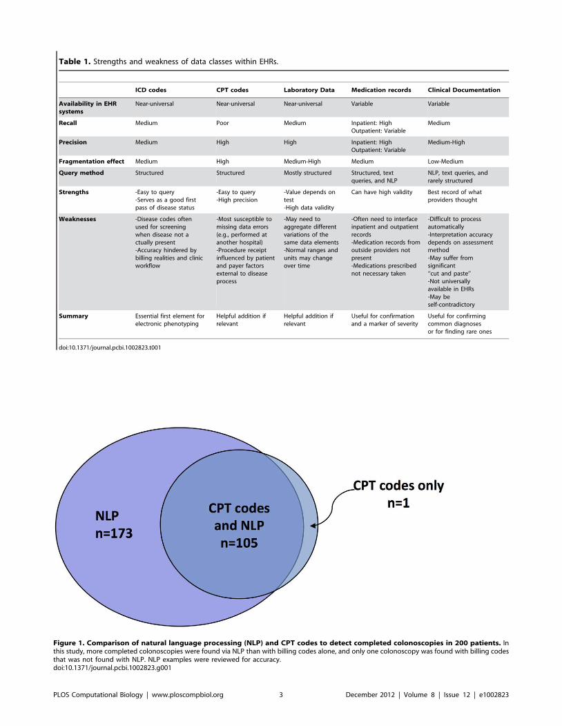
Table 1. Strengths and weakness of data classes within EHRs.
ICD codes CPT codes Laboratory Data Medication records Clinical Documentation
Availability in EHRsystems
Near-universal Near-universal Near-universal Variable Variable
Recall Medium Poor Medium Inpatient: HighOutpatient: Variable
Medium
Precision Medium High High Inpatient: HighOutpatient: Variable
Medium-High
Fragmentation effect Medium High Medium-High Medium Low-Medium
Query method Structured Structured Mostly structured Structured, textqueries, and NLP
NLP, text queries, andrarely structured
Strengths -Easy to query-Serves as a good firstpass of disease status
-Easy to query-High precision
-Value depends ontest-High data validity
Can have high validity Best record of whatproviders thought
Weaknesses -Disease codes oftenused for screeningwhen disease not actually present-Accuracy hindered bybilling realities and clinicworkflow
-Most susceptible tomissing data errors(e.g., performed atanother hospital)-Procedure receiptinfluenced by patientand payer factorsexternal to diseaseprocess
-May need toaggregate differentvariations of thesame data elements-Normal ranges andunits may changeover time
-Often need to interfaceinpatient and outpatientrecords-Medication records fromoutside providers notpresent-Medications prescribednot necessary taken
-Difficult to processautomatically-Interpretation accuracydepends on assessmentmethod-May suffer fromsignificant‘‘cut and paste’’-Not universallyavailable in EHRs-May beself-contradictory
Summary Essential first element forelectronic phenotyping
Helpful addition ifrelevant
Helpful addition ifrelevant
Useful for confirmationand a marker of severity
Useful for confirmingcommon diagnosesor for finding rare ones
doi:10.1371/journal.pcbi.1002823.t001
Figure 1. Comparison of natural language processing (NLP) and CPT codes to detect completed colonoscopies in 200 patients. Inthis study, more completed colonoscopies were found via NLP than with billing codes alone, and only one colonoscopy was found with billing codesthat was not found with NLP. NLP examples were reviewed for accuracy.doi:10.1371/journal.pcbi.1002823.g001
PLOS Computational Biology | www.ploscompbiol.org 3 December 2012 | Volume 8 | Issue 12 | e1002823
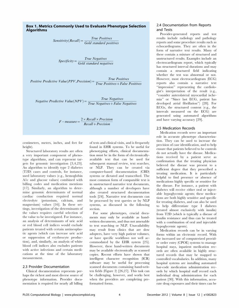
centimeters, meters, inches, and feet for
height).
Structured laboratory results are often
a very important component of pheno-
type algorithms, and can represent tar-
gets for genomic investigation [3,4,23].
An algorithm to identify type 2 diabetes
(T2D) cases and controls, for instance,
used laboratory values (e.g., hemoglobin
A1c and glucose values) combined with
billing codes and medication mentions
[17]. Similarly, an algorithm to deter-
mine genomic determinants of normal
cardiac conduction required normal
electrolyte (potassium, calcium, and
magnesium) values [16]. In these set-
tings, investigation of the determinants of
the values requires careful selection of
the value to be investigated. For instance,
an analysis of determinants of uric acid
or red blood cell indices would exclude
patients treated with certain antineoplas-
tic agents (which can increase uric acid
or suppression of erythrocyte produc-
tion), and, similarly, an analysis of white
blood cell indices also excludes patients
with active infections and certain medi-
cations at the time of the laboratory
measurement.
2.3 Provider DocumentationClinical documentation represents per-
haps the richest and most diverse source of
phenotype information. Provider docu-
mentation is required for nearly all billing
of tests and clinical visits, and is frequently
found in EHR systems. To be useful for
phenotyping efforts, clinical documenta-
tion must be in the form of electronically-
available text that can be used for
subsequent manual review, text searches,
or NLP. They can be created via
computer-based documentation (CBD)
systems or dictated and transcribed. The
most common form of computable text is
in unstructured narrative text documents,
although a number of developers have
also created structured documentation
tools [24]. Narrative text documents can
be processed by text queries or by NLP
systems, as discussed in the following
section.
For some phenotypes, crucial docu-
ments may only be available as hand-
written documents, and thus not amenable
to text searching or NLP. Unavailability
may result from clinics that are slow
adopters, have very high patient volumes,
or have specific workflows not well ac-
commodated by the EHR system [25].
However, these hand-written documents
may be available electronically as scanned
copies. Recent efforts have shown that
intelligent character recognition (ICR)
software may be useful for processing
scanned documents containing hand-writ-
ten fields (Figure 2) [26,27]. This task can
be challenging, however, and works best
when the providers are completing pre-
formatted forms.
2.4 Documentation from Reportsand Tests
Provider-generated reports and test
results include radiology and pathology
reports and some procedure results such as
echocardiograms. They are often in the
form of narrative text results. Many of
these contain a mixture of structured and
unstructured results. Examples include an
electrocardiogram report, which typically
has structured interval durations and may
contain a structured field indicating
whether the test was abnormal or not.
However, most electrocardiogram (ECG)
reports also contain a narrative text
‘‘impression’’ representing the cardiolo-
gist’s interpretation of the result (e.g.,
‘‘consider anterolateral myocardial ische-
mia’’ or ‘‘Since last ECG, patient has
developed atrial fibrillation’’) [28]. For
ECGs, the structured content (e.g., the
intervals measured on the ECG) are
generated using automated algorithms
and have varying accuracy [29].
2.5 Medication RecordsMedication records serve an important
role in accurate phenotype characteriza-
tion. They can be used to increase the
precision of case identification, and to help
ensure that patients believed to be controls
do not actually have the disease. Medica-
tions received by a patient serve as
confirmation that the treating physician
believed the disease was present to a
sufficient degree that they prescribed a
treating medication. It is particularly
helpful to find presence or absence of
medications highly specific or sensitive for
the disease. For instance, a patient with
diabetes will receive either oral or inject-
able hypoglycemic agents; these medica-
tions are both highly sensitive and specific
for treating diabetes, and can also be used
to help differentiate type I diabetes
(treated almost exclusively with insulin)
from T2D (which is typically a disease of
insulin resistance and thus can be treated
with a combination of oral and injectable
hypoglycemic agents).
Medication records can be in varying
forms within an electronic record. With
the increased use of computerized provid-
er order entry (CPOE) systems to manage
hospital stays, inpatient medication rec-
ords are often available in highly struc-
tured records that may be mapped to
controlled vocabularies. In addition, many
hospital systems are installing automated
bar-code medication administration rec-
ords by which hospital staff record each
individual drug administration for each
patient [30]. With this information, accu-
rate drug exposures and their times can be
Box 1. Metrics Commonly Used to Evaluate Phenotype SelectionAlgorithms
Sensitivity Recallð Þ~ True Positives
Gold standard positives
Specificity~True Negatives
Gold standard negatives
Positive Predictive Value PPV ,Precisionð Þ~ True Positives
True PositiveszFalse Positives
Negative Predictive Value NPVð Þ~ True Negatives
True NegativeszFalse Negatives
F{measure~2|Recall|Precision
RecallzPrecision
PLOS Computational Biology | www.ploscompbiol.org 4 December 2012 | Volume 8 | Issue 12 | e1002823
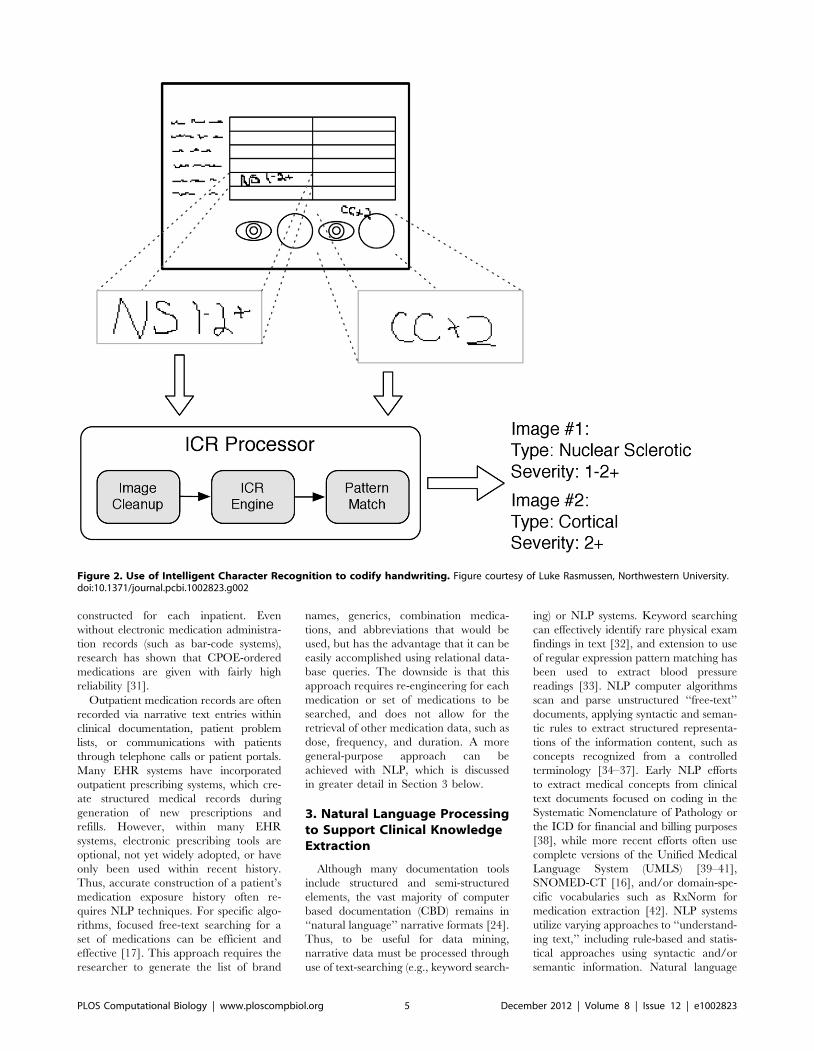
constructed for each inpatient. Even
without electronic medication administra-
tion records (such as bar-code systems),
research has shown that CPOE-ordered
medications are given with fairly high
reliability [31].
Outpatient medication records are often
recorded via narrative text entries within
clinical documentation, patient problem
lists, or communications with patients
through telephone calls or patient portals.
Many EHR systems have incorporated
outpatient prescribing systems, which cre-
ate structured medical records during
generation of new prescriptions and
refills. However, within many EHR
systems, electronic prescribing tools are
optional, not yet widely adopted, or have
only been used within recent history.
Thus, accurate construction of a patient’s
medication exposure history often re-
quires NLP techniques. For specific algo-
rithms, focused free-text searching for a
set of medications can be efficient and
effective [17]. This approach requires the
researcher to generate the list of brand
names, generics, combination medica-
tions, and abbreviations that would be
used, but has the advantage that it can be
easily accomplished using relational data-
base queries. The downside is that this
approach requires re-engineering for each
medication or set of medications to be
searched, and does not allow for the
retrieval of other medication data, such as
dose, frequency, and duration. A more
general-purpose approach can be
achieved with NLP, which is discussed
in greater detail in Section 3 below.
3. Natural Language Processingto Support Clinical KnowledgeExtraction
Although many documentation tools
include structured and semi-structured
elements, the vast majority of computer
based documentation (CBD) remains in
‘‘natural language’’ narrative formats [24].
Thus, to be useful for data mining,
narrative data must be processed through
use of text-searching (e.g., keyword search-
ing) or NLP systems. Keyword searching
can effectively identify rare physical exam
findings in text [32], and extension to use
of regular expression pattern matching has
been used to extract blood pressure
readings [33]. NLP computer algorithms
scan and parse unstructured ‘‘free-text’’
documents, applying syntactic and seman-
tic rules to extract structured representa-
tions of the information content, such as
concepts recognized from a controlled
terminology [34–37]. Early NLP efforts
to extract medical concepts from clinical
text documents focused on coding in the
Systematic Nomenclature of Pathology or
the ICD for financial and billing purposes
[38], while more recent efforts often use
complete versions of the Unified Medical
Language System (UMLS) [39–41],
SNOMED-CT [16], and/or domain-spe-
cific vocabularies such as RxNorm for
medication extraction [42]. NLP systems
utilize varying approaches to ‘‘understand-
ing text,’’ including rule-based and statis-
tical approaches using syntactic and/or
semantic information. Natural language
Figure 2. Use of Intelligent Character Recognition to codify handwriting. Figure courtesy of Luke Rasmussen, Northwestern University.doi:10.1371/journal.pcbi.1002823.g002
PLOS Computational Biology | www.ploscompbiol.org 5 December 2012 | Volume 8 | Issue 12 | e1002823
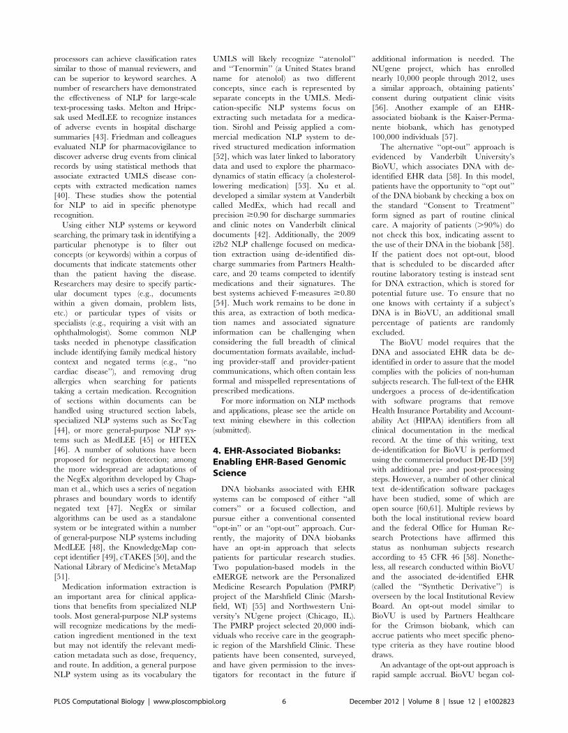
processors can achieve classification rates
similar to those of manual reviewers, and
can be superior to keyword searches. A
number of researchers have demonstrated
the effectiveness of NLP for large-scale
text-processing tasks. Melton and Hripc-
sak used MedLEE to recognize instances
of adverse events in hospital discharge
summaries [43]. Friedman and colleagues
evaluated NLP for pharmacovigilance to
discover adverse drug events from clinical
records by using statistical methods that
associate extracted UMLS disease con-
cepts with extracted medication names
[40]. These studies show the potential
for NLP to aid in specific phenotype
recognition.
Using either NLP systems or keyword
searching, the primary task in identifying a
particular phenotype is to filter out
concepts (or keywords) within a corpus of
documents that indicate statements other
than the patient having the disease.
Researchers may desire to specify partic-
ular document types (e.g., documents
within a given domain, problem lists,
etc.) or particular types of visits or
specialists (e.g., requiring a visit with an
ophthalmologist). Some common NLP
tasks needed in phenotype classification
include identifying family medical history
context and negated terms (e.g., ‘‘no
cardiac disease’’), and removing drug
allergies when searching for patients
taking a certain medication. Recognition
of sections within documents can be
handled using structured section labels,
specialized NLP systems such as SecTag
[44], or more general-purpose NLP sys-
tems such as MedLEE [45] or HITEX
[46]. A number of solutions have been
proposed for negation detection; among
the more widespread are adaptations of
the NegEx algorithm developed by Chap-
man et al., which uses a series of negation
phrases and boundary words to identify
negated text [47]. NegEx or similar
algorithms can be used as a standalone
system or be integrated within a number
of general-purpose NLP systems including
MedLEE [48], the KnowledgeMap con-
cept identifier [49], cTAKES [50], and the
National Library of Medicine’s MetaMap
[51].
Medication information extraction is
an important area for clinical applica-
tions that benefits from specialized NLP
tools. Most general-purpose NLP systems
will recognize medications by the medi-
cation ingredient mentioned in the text
but may not identify the relevant medi-
cation metadata such as dose, frequency,
and route. In addition, a general purpose
NLP system using as its vocabulary the
UMLS will likely recognize ‘‘atenolol’’
and ‘‘Tenormin’’ (a United States brand
name for atenolol) as two different
concepts, since each is represented by
separate concepts in the UMLS. Medi-
cation-specific NLP systems focus on
extracting such metadata for a medica-
tion. Sirohl and Peissig applied a com-
mercial medication NLP system to de-
rived structured medication information
[52], which was later linked to laboratory
data and used to explore the pharmaco-
dynamics of statin efficacy (a cholesterol-
lowering medication) [53]. Xu et al.
developed a similar system at Vanderbilt
called MedEx, which had recall and
precision $0.90 for discharge summaries
and clinic notes on Vanderbilt clinical
documents [42]. Additionally, the 2009
i2b2 NLP challenge focused on medica-
tion extraction using de-identified dis-
charge summaries from Partners Health-
care, and 20 teams competed to identify
medications and their signatures. The
best systems achieved F-measures $0.80
[54]. Much work remains to be done in
this area, as extraction of both medica-
tion names and associated signature
information can be challenging when
considering the full breadth of clinical
documentation formats available, includ-
ing provider-staff and provider-patient
communications, which often contain less
formal and misspelled representations of
prescribed medications.
For more information on NLP methods
and applications, please see the article on
text mining elsewhere in this collection
(submitted).
4. EHR-Associated Biobanks:Enabling EHR-Based GenomicScience
DNA biobanks associated with EHR
systems can be composed of either ‘‘all
comers’’ or a focused collection, and
pursue either a conventional consented
‘‘opt-in’’ or an ‘‘opt-out’’ approach. Cur-
rently, the majority of DNA biobanks
have an opt-in approach that selects
patients for particular research studies.
Two population-based models in the
eMERGE network are the Personalized
Medicine Research Population (PMRP)
project of the Marshfield Clinic (Marsh-
field, WI) [55] and Northwestern Uni-
versity’s NUgene project (Chicago, IL).
The PMRP project selected 20,000 indi-
viduals who receive care in the geograph-
ic region of the Marshfield Clinic. These
patients have been consented, surveyed,
and have given permission to the inves-
tigators for recontact in the future if
additional information is needed. The
NUgene project, which has enrolled
nearly 10,000 people through 2012, uses
a similar approach, obtaining patients’
consent during outpatient clinic visits
[56]. Another example of an EHR-
associated biobank is the Kaiser-Perma-
nente biobank, which has genotyped
100,000 individuals [57].
The alternative ‘‘opt-out’’ approach is
evidenced by Vanderbilt University’s
BioVU, which associates DNA with de-
identified EHR data [58]. In this model,
patients have the opportunity to ‘‘opt out’’
of the DNA biobank by checking a box on
the standard ‘‘Consent to Treatment’’
form signed as part of routine clinical
care. A majority of patients (.90%) do
not check this box, indicating assent to
the use of their DNA in the biobank [58].
If the patient does not opt-out, blood
that is scheduled to be discarded after
routine laboratory testing is instead sent
for DNA extraction, which is stored for
potential future use. To ensure that no
one knows with certainty if a subject’s
DNA is in BioVU, an additional small
percentage of patients are randomly
excluded.
The BioVU model requires that the
DNA and associated EHR data be de-
identified in order to assure that the model
complies with the policies of non-human
subjects research. The full-text of the EHR
undergoes a process of de-identification
with software programs that remove
Health Insurance Portability and Account-
ability Act (HIPAA) identifiers from all
clinical documentation in the medical
record. At the time of this writing, text
de-identification for BioVU is performed
using the commercial product DE-ID [59]
with additional pre- and post-processing
steps. However, a number of other clinical
text de-identification software packages
have been studied, some of which are
open source [60,61]. Multiple reviews by
both the local institutional review board
and the federal Office for Human Re-
search Protections have affirmed this
status as nonhuman subjects research
according to 45 CFR 46 [58]. Nonethe-
less, all research conducted within BioVU
and the associated de-identified EHR
(called the ‘‘Synthetic Derivative’’) is
overseen by the local Institutional Review
Board. An opt-out model similar to
BioVU is used by Partners Healthcare
for the Crimson biobank, which can
accrue patients who meet specific pheno-
type criteria as they have routine blood
draws.
An advantage of the opt-out approach is
rapid sample accrual. BioVU began col-
PLOS Computational Biology | www.ploscompbiol.org 6 December 2012 | Volume 8 | Issue 12 | e1002823
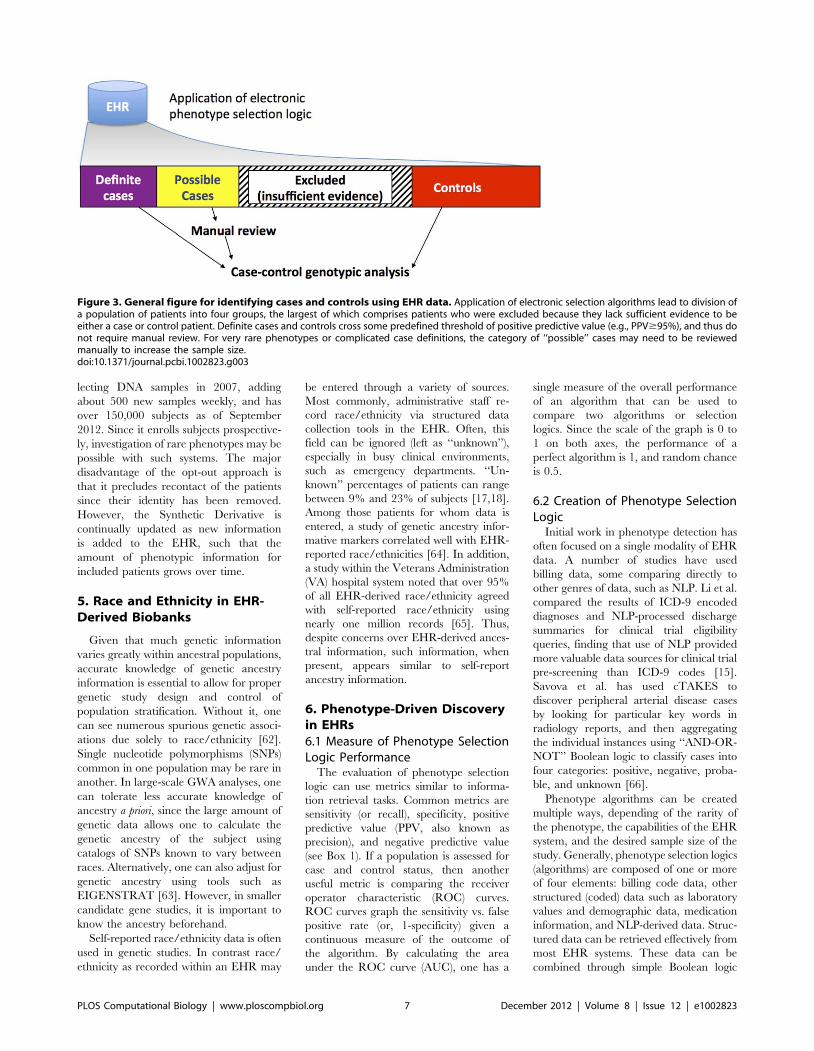
lecting DNA samples in 2007, adding
about 500 new samples weekly, and has
over 150,000 subjects as of September
2012. Since it enrolls subjects prospective-
ly, investigation of rare phenotypes may be
possible with such systems. The major
disadvantage of the opt-out approach is
that it precludes recontact of the patients
since their identity has been removed.
However, the Synthetic Derivative is
continually updated as new information
is added to the EHR, such that the
amount of phenotypic information for
included patients grows over time.
5. Race and Ethnicity in EHR-Derived Biobanks
Given that much genetic information
varies greatly within ancestral populations,
accurate knowledge of genetic ancestry
information is essential to allow for proper
genetic study design and control of
population stratification. Without it, one
can see numerous spurious genetic associ-
ations due solely to race/ethnicity [62].
Single nucleotide polymorphisms (SNPs)
common in one population may be rare in
another. In large-scale GWA analyses, one
can tolerate less accurate knowledge of
ancestry a priori, since the large amount of
genetic data allows one to calculate the
genetic ancestry of the subject using
catalogs of SNPs known to vary between
races. Alternatively, one can also adjust for
genetic ancestry using tools such as
EIGENSTRAT [63]. However, in smaller
candidate gene studies, it is important to
know the ancestry beforehand.
Self-reported race/ethnicity data is often
used in genetic studies. In contrast race/
ethnicity as recorded within an EHR may
be entered through a variety of sources.
Most commonly, administrative staff re-
cord race/ethnicity via structured data
collection tools in the EHR. Often, this
field can be ignored (left as ‘‘unknown’’),
especially in busy clinical environments,
such as emergency departments. ‘‘Un-
known’’ percentages of patients can range
between 9% and 23% of subjects [17,18].
Among those patients for whom data is
entered, a study of genetic ancestry infor-
mative markers correlated well with EHR-
reported race/ethnicities [64]. In addition,
a study within the Veterans Administration
(VA) hospital system noted that over 95%
of all EHR-derived race/ethnicity agreed
with self-reported race/ethnicity using
nearly one million records [65]. Thus,
despite concerns over EHR-derived ances-
tral information, such information, when
present, appears similar to self-report
ancestry information.
6. Phenotype-Driven Discoveryin EHRs
6.1 Measure of Phenotype SelectionLogic Performance
The evaluation of phenotype selection
logic can use metrics similar to informa-
tion retrieval tasks. Common metrics are
sensitivity (or recall), specificity, positive
predictive value (PPV, also known as
precision), and negative predictive value
(see Box 1). If a population is assessed for
case and control status, then another
useful metric is comparing the receiver
operator characteristic (ROC) curves.
ROC curves graph the sensitivity vs. false
positive rate (or, 1-specificity) given a
continuous measure of the outcome of
the algorithm. By calculating the area
under the ROC curve (AUC), one has a
single measure of the overall performance
of an algorithm that can be used to
compare two algorithms or selection
logics. Since the scale of the graph is 0 to
1 on both axes, the performance of a
perfect algorithm is 1, and random chance
is 0.5.
6.2 Creation of Phenotype SelectionLogic
Initial work in phenotype detection has
often focused on a single modality of EHR
data. A number of studies have used
billing data, some comparing directly to
other genres of data, such as NLP. Li et al.
compared the results of ICD-9 encoded
diagnoses and NLP-processed discharge
summaries for clinical trial eligibility
queries, finding that use of NLP provided
more valuable data sources for clinical trial
pre-screening than ICD-9 codes [15].
Savova et al. has used cTAKES to
discover peripheral arterial disease cases
by looking for particular key words in
radiology reports, and then aggregating
the individual instances using ‘‘AND-OR-
NOT’’ Boolean logic to classify cases into
four categories: positive, negative, proba-
ble, and unknown [66].
Phenotype algorithms can be created
multiple ways, depending of the rarity of
the phenotype, the capabilities of the EHR
system, and the desired sample size of the
study. Generally, phenotype selection logics
(algorithms) are composed of one or more
of four elements: billing code data, other
structured (coded) data such as laboratory
values and demographic data, medication
information, and NLP-derived data. Struc-
tured data can be retrieved effectively from
most EHR systems. These data can be
combined through simple Boolean logic
Figure 3. General figure for identifying cases and controls using EHR data. Application of electronic selection algorithms lead to division ofa population of patients into four groups, the largest of which comprises patients who were excluded because they lack sufficient evidence to beeither a case or control patient. Definite cases and controls cross some predefined threshold of positive predictive value (e.g., PPV$95%), and thus donot require manual review. For very rare phenotypes or complicated case definitions, the category of ‘‘possible’’ cases may need to be reviewedmanually to increase the sample size.doi:10.1371/journal.pcbi.1002823.g003
PLOS Computational Biology | www.ploscompbiol.org 7 December 2012 | Volume 8 | Issue 12 | e1002823
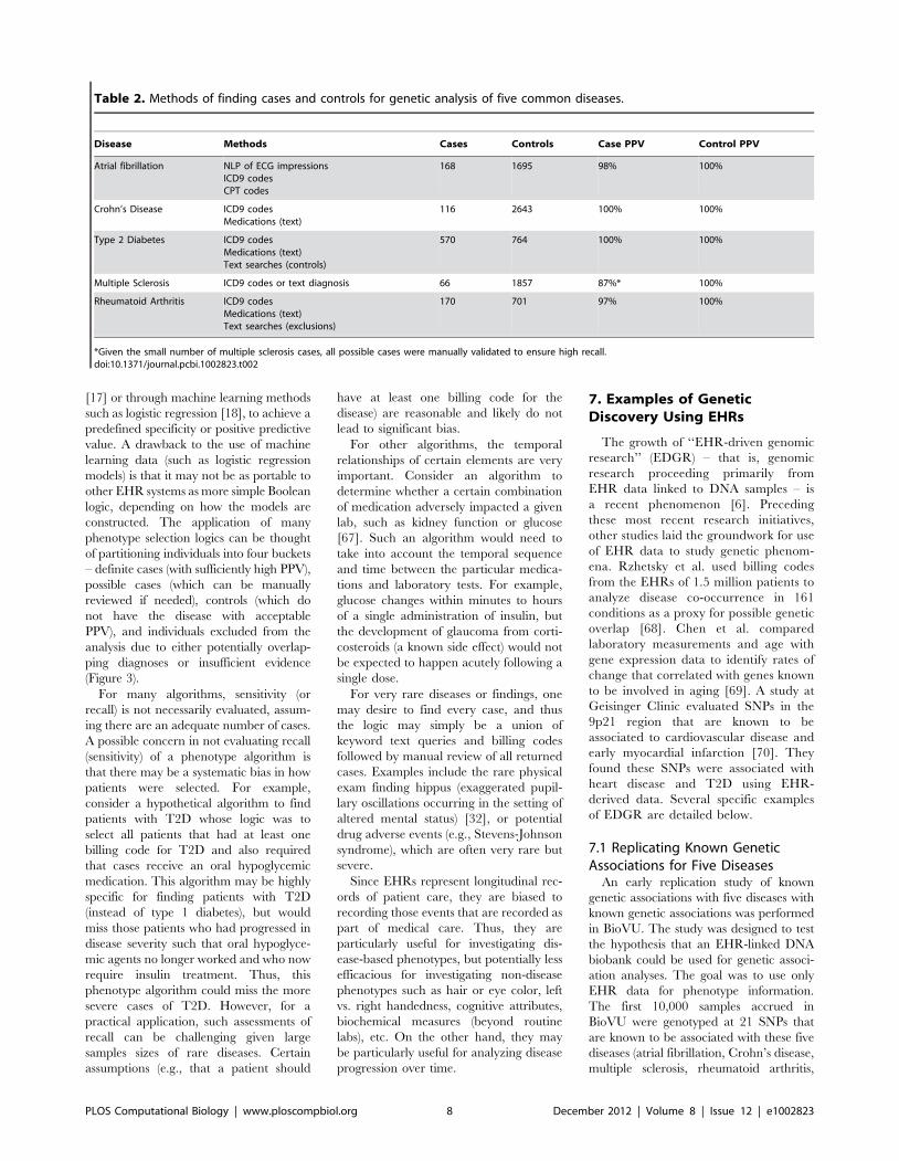
[17] or through machine learning methods
such as logistic regression [18], to achieve a
predefined specificity or positive predictive
value. A drawback to the use of machine
learning data (such as logistic regression
models) is that it may not be as portable to
other EHR systems as more simple Boolean
logic, depending on how the models are
constructed. The application of many
phenotype selection logics can be thought
of partitioning individuals into four buckets
– definite cases (with sufficiently high PPV),
possible cases (which can be manually
reviewed if needed), controls (which do
not have the disease with acceptable
PPV), and individuals excluded from the
analysis due to either potentially overlap-
ping diagnoses or insufficient evidence
(Figure 3).
For many algorithms, sensitivity (or
recall) is not necessarily evaluated, assum-
ing there are an adequate number of cases.
A possible concern in not evaluating recall
(sensitivity) of a phenotype algorithm is
that there may be a systematic bias in how
patients were selected. For example,
consider a hypothetical algorithm to find
patients with T2D whose logic was to
select all patients that had at least one
billing code for T2D and also required
that cases receive an oral hypoglycemic
medication. This algorithm may be highly
specific for finding patients with T2D
(instead of type 1 diabetes), but would
miss those patients who had progressed in
disease severity such that oral hypoglyce-
mic agents no longer worked and who now
require insulin treatment. Thus, this
phenotype algorithm could miss the more
severe cases of T2D. However, for a
practical application, such assessments of
recall can be challenging given large
samples sizes of rare diseases. Certain
assumptions (e.g., that a patient should
have at least one billing code for the
disease) are reasonable and likely do not
lead to significant bias.
For other algorithms, the temporal
relationships of certain elements are very
important. Consider an algorithm to
determine whether a certain combination
of medication adversely impacted a given
lab, such as kidney function or glucose
[67]. Such an algorithm would need to
take into account the temporal sequence
and time between the particular medica-
tions and laboratory tests. For example,
glucose changes within minutes to hours
of a single administration of insulin, but
the development of glaucoma from corti-
costeroids (a known side effect) would not
be expected to happen acutely following a
single dose.
For very rare diseases or findings, one
may desire to find every case, and thus
the logic may simply be a union of
keyword text queries and billing codes
followed by manual review of all returned
cases. Examples include the rare physical
exam finding hippus (exaggerated pupil-
lary oscillations occurring in the setting of
altered mental status) [32], or potential
drug adverse events (e.g., Stevens-Johnson
syndrome), which are often very rare but
severe.
Since EHRs represent longitudinal rec-
ords of patient care, they are biased to
recording those events that are recorded as
part of medical care. Thus, they are
particularly useful for investigating dis-
ease-based phenotypes, but potentially less
efficacious for investigating non-disease
phenotypes such as hair or eye color, left
vs. right handedness, cognitive attributes,
biochemical measures (beyond routine
labs), etc. On the other hand, they may
be particularly useful for analyzing disease
progression over time.
7. Examples of GeneticDiscovery Using EHRs
The growth of ‘‘EHR-driven genomic
research’’ (EDGR) – that is, genomic
research proceeding primarily from
EHR data linked to DNA samples – is
a recent phenomenon [6]. Preceding
these most recent research initiatives,
other studies laid the groundwork for use
of EHR data to study genetic phenom-
ena. Rzhetsky et al. used billing codes
from the EHRs of 1.5 million patients to
analyze disease co-occurrence in 161
conditions as a proxy for possible genetic
overlap [68]. Chen et al. compared
laboratory measurements and age with
gene expression data to identify rates of
change that correlated with genes known
to be involved in aging [69]. A study at
Geisinger Clinic evaluated SNPs in the
9p21 region that are known to be
associated to cardiovascular disease and
early myocardial infarction [70]. They
found these SNPs were associated with
heart disease and T2D using EHR-
derived data. Several specific examples
of EDGR are detailed below.
7.1 Replicating Known GeneticAssociations for Five Diseases
An early replication study of known
genetic associations with five diseases with
known genetic associations was performed
in BioVU. The study was designed to test
the hypothesis that an EHR-linked DNA
biobank could be used for genetic associ-
ation analyses. The goal was to use only
EHR data for phenotype information.
The first 10,000 samples accrued in
BioVU were genotyped at 21 SNPs that
are known to be associated with these five
diseases (atrial fibrillation, Crohn’s disease,
multiple sclerosis, rheumatoid arthritis,
Table 2. Methods of finding cases and controls for genetic analysis of five common diseases.
Disease Methods Cases Controls Case PPV Control PPV
Atrial fibrillation NLP of ECG impressionsICD9 codesCPT codes
168 1695 98% 100%
Crohn’s Disease ICD9 codesMedications (text)
116 2643 100% 100%
Type 2 Diabetes ICD9 codesMedications (text)Text searches (controls)
570 764 100% 100%
Multiple Sclerosis ICD9 codes or text diagnosis 66 1857 87%* 100%
Rheumatoid Arthritis ICD9 codesMedications (text)Text searches (exclusions)
170 701 97% 100%
*Given the small number of multiple sclerosis cases, all possible cases were manually validated to ensure high recall.doi:10.1371/journal.pcbi.1002823.t002
PLOS Computational Biology | www.ploscompbiol.org 8 December 2012 | Volume 8 | Issue 12 | e1002823
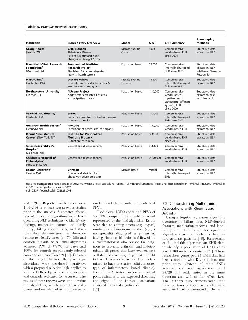
and T2D). Reported odds ratios were
1.14–2.36 in at least two previous studies
prior to the analysis. Automated pheno-
type identification algorithms were devel-
oped using NLP techniques (to identify key
findings, medication names, and family
history), billing code queries, and struc-
tured data elements (such as laboratory
results) to identify cases (n = 70–698) and
controls (n = 808–3818). Final algorithms
achieved PPV of $97% for cases and
100% for controls on randomly selected
cases and controls (Table 2) [17]. For each
of the target diseases, the phenotype
algorithms were developed iteratively,
with a proposed selection logic applied to
a set of EHR subjects, and random cases
and controls evaluated for accuracy. The
results of these reviews were used to refine
the algorithms, which were then rede-
ployed and reevaluated on a unique set of
randomly selected records to provide final
PPVs.
Used alone, ICD9 codes had PPVs of
56–89% compared to a gold standard
represented by the final algorithm. Errors
were due to coding errors (e.g., typos),
misdiagnoses from non-specialists (e.g., a
non-specialist diagnosed a patient as
having rheumatoid arthritis followed by
a rheumatologist who revised the diag-
nosis to psoriatic arthritis), and indeter-
minate diagnoses that later evolved into
well-defined ones (e.g., a patient thought
to have Crohn’s disease was later deter-
mined to have ulcerative colitis, another
type of inflammatory bowel disease).
Each of the 21 tests of association yielded
point estimates in the expected direction,
and eight of the known associations
achieved statistical significance
[17].
7.2 Demonstrating MultiethnicAssociations with RheumatoidArthritis
Using a logistic regression algorithm
operating on billing data, NLP-derived
features, medication records, and labo-
ratory data, Liao et al. developed an
algorithm to accurately identify rheuma-
toid arthritis patients [18]. Kurreeman
et al. used this algorithm on EHR data
to identify a population of 1,515 cases
and 1,480 matched controls [71]. These
researchers genotyped 29 SNPs that had
been associated with RA in at least one
prior study. Sixteen of these SNPs
achieved statistical significance, and
26/29 had odds ratios in the same
direction and with similar effect sizes.
The authors also demonstrated that
these portions of these risk alleles were
associated with rheumatoid arthritis in
Table 3. eMERGE network participants.
Institution Biorepository Overview Model Size EHR SummaryPhenotypingMethods
Group Health1
(Seattle, WA)GHC BiobankAlzheimer’s DiseasePatient Registry and AdultChanges in Thought Study
Disease specificCohort
4000 Comprehensivevendor-based EHRsince 2004
Structured dataextraction, NLP
Marshfield Clinic ResearchFoundation1
(Marshfield, WI)
Personalized MedicineResearch ProjectMarshfield Clinic, an integratedregional health system
Population based 20,000 Comprehensiveinternally developedEHR since 1985
Structured dataextraction, NLP,Intelligent CharacterRecognition
Mayo Clinic1
(Rochester, MN)Disease cohortDerived from vascular laboratory &exercise stress testing labs
Disease specificCohorts
16,500 Comprehensiveinternally developedEHR since 1995
Structured dataextraction, NLP
Northwestern University1
(Chicago, IL)NUgene ProjectNorthwestern affiliated hospitalsand outpatient clinics
Population based .10,000 Comprehensivevendor basedInpatient andOutpatient (differentsystems) EHRsince 2000
Structured dataextraction, textsearches, NLP
Vanderbilt University1
(Nashville, TN)BioVUPrimarily drawn from outpatient routinelaboratory samples
Population based 150,000 Comprehensiveinternally developedEHR since 2000
Structured dataextraction, NLP
Geisinger Health System2
(Pennsylvania)MyCodeEnrollment of health plan participants
Population based .30,000 Comprehensivevendor-based EHR
Structured dataextraction, NLP
Mount Sinai MedicalCenter2 (New York, NY)
Institute for PersonalizedMedicine BiobankOutpatient enrollment
Population based .30,000 Comprehensivevendor-based EHRsince 2004
Structured dataextraction, NLP
Cincinnati Children’sHospital3
(Cincinnati, OH)
General and disease cohorts. Population based .3,000 Comprehensivevendor-based EHR
Structured dataextraction, NLP
Children’s Hospital ofPhiladelphia3
(Philadelphia, PA)
General and disease cohorts. Population based .100,000 Comprehensivevendor-based EHR
Structured dataextraction, NLP
Boston Children’s3
(Boston MA)CrimsonOn-demand, de-identifiedphenotype-driven collection
Disease based Virtual Comprehensiveinternally developedEHR
Structured dataextraction, NLP
Sizes represent approximate sizes as of 2012; many sites are still actively recruiting. NLP = Natural Language Processing. Sites joined with 1eMERGE-I in 2007, 2eMERGE-IIin 2011, or as 3pediatric sites in 2012.doi:10.1371/journal.pcbi.1002823.t003
PLOS Computational Biology | www.ploscompbiol.org 9 December 2012 | Volume 8 | Issue 12 | e1002823
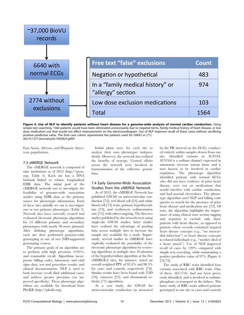
East Asian, African, and Hispanic Amer-
ican populations.
7.3 eMERGE NetworkThe eMERGE network is composed of
nine institutions as of 2012 (http://gwas.
org; Table 3). Each site has a DNA
biobank linked to robust, longitudinal
EHR data. The initial goal of the
eMERGE network was to investigate the
feasibility of genome-wide association
studies using EHR data as the primary
source for phenotypic information. Each
of these sites initially set out to investigate
one or two primary phenotypes (Table 3).
Network sites have currently created and
evaluated electronic phenotype algorithms
for 14 different primary and secondary
phenotypes, with nearly 30 more planned.
After defining phenotype algorithms,
each site then performed genome-wide
genotyping at one of two NIH-supported
genotyping centers.
The primary goals of an algorithm are
to perform with high precision ($95%)
and reasonable recall. Algorithms incor-
porate billing codes, laboratory and vital
signs data, test and procedure results, and
clinical documentation. NLP is used to
both increase recall (find additional cases)
and achieve greater precision (via im-
proved specificity). These phenotype algo-
rithms are available for download from
PheKB (http://phekb.org).
Initial plans were for each site to
analyze their own phenotypes indepen-
dently. However, the network has realized
the benefits of synergy. Central efforts
across the network were involved in
harmonization of the collective genetic
data.
7.4 Early Genome-Wide AssociationStudies from the eMERGE Network
As of 2012, the eMERGE Network has
published GWAS on atrioventricular con-
duction [72], red blood cell [23] and white
blood cell [73] traits, primary hypothyroid-
ism [74], and erythrocyte sedimentation
rate [75], with others ongoing. The first two
studies published by the network were using
single-site GWAS studies; latter studies
have realized the advantage of pooling
data across multiple sites to increase the
sample size available for a study. Impor-
tantly, several studies in eMERGE have
explicitly evaluated the portability of the
electronic phenotype algorithms by review-
ing algorithms at multiple sites. Evaluation
of the hypothyroidism algorithm at the five
eMERGE-I sites, for instance, noted an
overall weighted PPV of 92.4% and 98.5%
for cases and controls, respectively [74].
Similar results have been found with T2D
[76], cataracts [27], and rheumatoid ar-
thritis [77] algorithms.
As a case study, the GWAS for
atrioventricular conduction (as measured
by the PR interval on the ECG), conduct-
ed entirely within samples drawn from one
site, identified variants in SCN10A.
SCN10A is a sodium channel expressed in
autonomic nervous system tissue and is
now known to be involved in cardiac
regulation. The phenotype algorithm
identified patients with normal ECGs
who did not have evidence of prior heart
disease, were not on medications that
would interfere with cardiac conduction,
and had normal electrolytes. The pheno-
type algorithm used NLP and billing code
queries to search for the presence of prior
heart disease and medication use [72]. Of
note, the algorithm highlights the impor-
tance of using clinical note section tagging
and negation to exclude only those
patients with heart disease, as opposed to
patients whose records contained negated
heart disease concepts (e.g., ‘‘no myocar-
dial infarction’’) or heart disease concepts
in related individuals (e.g., ‘‘mother died of
a heart attack’’). Use of NLP improved
recall of cases by 129% compared with
simple text searching, while maintaining a
positive predictive value of 97% (Figure 4)
[78,72].
The study of RBC traits identified four
variants associated with RBC traits. One
of these, SLC17A1, had not been previ-
ously identified, and is involved in sodium-
phosphate co-transport in the kidney. The
latter study of RBC traits utilized patients
genotyped at one site as cases and controls
Figure 4. Use of NLP to identify patients without heart disease for a genome-wide analysis of normal cardiac conduction. Usingsimple text searching, 1564 patients would have been eliminated unnecessarily due to negated terms, family medical history of heart disease, or lowdose medication use that would not affect measurements on the electrocardiogram. Use of NLP improves recall of these cases without sacrificingpositive predictive value. The final case cohort represented the patients used for GWAS in [71].doi:10.1371/journal.pcbi.1002823.g004
PLOS Computational Biology | www.ploscompbiol.org 10 December 2012 | Volume 8 | Issue 12 | e1002823
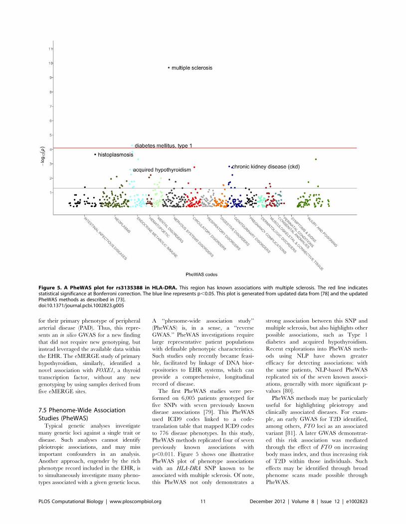
for their primary phenotype of peripheral
arterial disease (PAD). Thus, this repre-
sents an in silico GWAS for a new finding
that did not require new genotyping, but
instead leveraged the available data within
the EHR. The eMERGE study of primary
hypothyroidism, similarly, identified a
novel association with FOXE1, a thyroid
transcription factor, without any new
genotyping by using samples derived from
five eMERGE sites.
7.5 Phenome-Wide AssociationStudies (PheWAS)
Typical genetic analyses investigate
many genetic loci against a single trait or
disease. Such analyses cannot identify
pleiotropic associations, and may miss
important confounders in an analysis.
Another approach, engender by the rich
phenotype record included in the EHR, is
to simultaneously investigate many pheno-
types associated with a given genetic locus.
A ‘‘phenome-wide association study’’
(PheWAS) is, in a sense, a ‘‘reverse
GWAS.’’ PheWAS investigations require
large representative patient populations
with definable phenotypic characteristics.
Such studies only recently became feasi-
ble, facilitated by linkage of DNA bior-
epositories to EHR systems, which can
provide a comprehensive, longitudinal
record of disease.
The first PheWAS studies were per-
formed on 6,005 patients genotyped for
five SNPs with seven previously known
disease associations [79]. This PheWAS
used ICD9 codes linked to a code-
translation table that mapped ICD9 codes
to 776 disease phenotypes. In this study,
PheWAS methods replicated four of seven
previously known associations with
p,0.011. Figure 5 shows one illustrative
PheWAS plot of phenotype associations
with an HLA-DRA SNP known to be
associated with multiple sclerosis. Of note,
this PheWAS not only demonstrates a
strong association between this SNP and
multiple sclerosis, but also highlights other
possible associations, such as Type 1
diabetes and acquired hypothyroidism.
Recent explorations into PheWAS meth-
ods using NLP have shown greater
efficacy for detecting associations: with
the same patients, NLP-based PheWAS
replicated six of the seven known associ-
ations, generally with more significant p-
values [80].
PheWAS methods may be particularly
useful for highlighting pleiotropy and
clinically associated diseases. For exam-
ple, an early GWAS for T2D identified,
among others, FTO loci as an associated
variant [81]. A later GWAS demonstrat-
ed this risk association was mediated
through the effect of FTO on increasing
body mass index, and thus increasing risk
of T2D within those individuals. Such
effects may be identified through broad
phenome scans made possible through
PheWAS.
Figure 5. A PheWAS plot for rs3135388 in HLA-DRA. This region has known associations with multiple sclerosis. The red line indicatesstatistical significance at Bonferroni correction. The blue line represents p,0.05. This plot is generated from updated data from [78] and the updatedPheWAS methods as described in [73].doi:10.1371/journal.pcbi.1002823.g005
PLOS Computational Biology | www.ploscompbiol.org 11 December 2012 | Volume 8 | Issue 12 | e1002823
8. Conclusions and FutureDirections
EHRs have long been seen as a vehicle
to improve healthcare quality, cost, and
safety. However, their growing adoption
in the United States and elsewhere is
demonstrating their capability as a broad
tool for research. Enabling tools include
enterprise data warehouses and software
to process unstructured information, such
as de-identification and NLP. When
linked to biological data such as DNA
or tissue biorepositories, EHRs can be-
come a powerful tool for genomic anal-
ysis. One can imagine future repositories
also storing intermittent plasma samples
to allow for proteomic analyses.
A key advantage of EHR-based genetic
studies is that they allow for the collection
of phenotype information as a byproduct
of routine healthcare. Moreover, this
information collection grows over time
and is continually refined as new informa-
tion may confirm or refute a diagnosis for
a given individual. Through the course of
one’s life, a number of information points
concerning disease, response to treatment,
and laboratory and test data are collected.
Aggregation of this information can allow
for generation of large sample sizes of
patients with certain diseases or medica-
tion exposures. Moreover, once a subject
receives dense genotyping for one EHR-
based study, their genetic data can be
reused for many other genotypic studies,
allowing for relatively low-cost reuse of the
genetic material (once a given phenotype
can be found in the EHR).
Three major rate-limiting steps impede
utilization of EHR data for genetic
analysis. A major challenge is derivation
of accurate collections of cases and
controls for a given disease of interest,
usually achieved through creation and
validation of phenotype selection logics.
These algorithms take significant time and
effort to develop and often require adjust-
ment and a skilled team to deploy at a
secondary site. Another challenge is the
availability of phenotypic information.
Many patients may be observed at a given
healthcare facility only for certain types of
care (e.g., primary care or a certain
subspecialist), leading to fragmented
knowledge of a patient’s medical history
and medication exposures. Future growth
of Health Information Exchanges could
substantially improve these information
gaps. Finally, DNA biobanks require
significant institutional investment and
ongoing financial, ethical, and logistical
support to run effectively. Thus, they are
not ubiquitous.
As genomics move beyond discovery
into clinical practice, the future of person-
alized medicine is one in which our genetic
information could be ‘‘simply a click of the
mouse’’ away [82]. In this future, DNA-
enabled EHR systems will assist in more
accurate prescribing, risk stratification,
and diagnosis. Genomic discovery in
EHR systems provides a real-world test
bed to validate and discover clinically
meaningful genetic effects.
9. Exercises
1) Compare and contrast the basic
types of data available in an Elec-
tronic Health Records (EHR) that
are useful for mining genetic data.
What are some of the strengths and
drawbacks of each type of data?
2) Explain what a phenotype algo-
rithm is and why it is necessary. For
example, how can use of natural
language processing improve upon
use of billing codes alone?
3) Select a clinical disease and design
a phenotype algorithm for it.
4) How might a phenotype algorithm
be different for a very rare disease
(e.g., prion diseases) vs. a more
common one (e.g., Type 2 diabe-
tes)? How would a phenotype
algorithm be different for a phys-
ical exam finding (e.g., hippus or a
particular type of heart murmur) vs.
a disease?
5) Describe the differences between a
DNA biobank linked to an EHR
and one collected as part of a non-
EHR research cohort. What are the
advantages and disadvantages of a
de-identified DNA biobank vs. an
identified DNA biobank (either
linked to an EHR or not).
6) It is often harder to create algo-
rithms to find drug-response pheno-
types (such as adverse drug events)
than for a chronic disease. Give
several reasons why this might be.
Answers to the Exercises can be found
in Text S1.
Supporting Information
Text S1 Answers to Exercises.
(DOCX)
Further Reading
N Shortliffe EH, Cimino JJ, editors (2006) Biomedical informatics: computer applications in health care and biomedicine. 3rdedition. Springer. 1064 p.Chapters of particular relevance: Chapter 2 (‘‘Biomedical data: their acquisition, storage, and use’’), Chapter 8 (‘‘Natural languageand text processing in biomedicine’’), Chapter 12 (‘‘Electronic health record systems’’)
N Hristidis V, editor (2009) Information discovery on electronic health records. 1st edition. Chapman and Hall/CRC. 331 p.Chapters of particular relevance: Chapter 2 (‘‘Electronic health records’’), Chapter 4 (‘‘Data quality and integration issues inelectronic health records’’), 7 (‘‘Data mining and knowledge discovery on EHRs’’).
N Wilke RA, Xu H, Denny JC, Roden DM, Krauss RM, et al. (2011) The emerging role of electronic medical records inpharmacogenomics. Clin Pharmacol Ther 89: 379–386. doi:10.1038/clpt.2010.260.
N Roden DM, Xu H, Denny JC, Wilke RA (2012) Electronic medical records as a tool in clinical pharmacology: opportunities andchallenges. Clin Pharmacol Ther. Available: http://www.ncbi.nlm.nih.gov/pubmed/22534870. Accessed 30 June 2012.
N Kohane IS (2011) Using electronic health records to drive discovery in disease genomics. Nat Rev Genet 12: 417–428.doi:10.1038/nrg2999.
PLOS Computational Biology | www.ploscompbiol.org 12 December 2012 | Volume 8 | Issue 12 | e1002823
References
1. Hindorff LA, Sethupathy P, Junkins HA, Ramos
EM, Mehta JP, et al. (2009) Potential etiologic
and functional implications of genome-wide
association loci for human diseases and traits.
Proc Natl Acad Sci USA 106: 9362–9367.
doi:10.1073/pnas.0903103106.
2. Wellcome Trust Case Control Consortium (2007)
Genome-wide association study of 14,000 cases of
seven common diseases and 3,000 shared con-
trols. Nature 447: 661–678.
3. Dehghan A, Kottgen A, Yang Q, Hwang S-J, Kao
WL, et al. (2008) Association of three genetic loci
with uric acid concentration and risk of gout: a
genome-wide association study. Lancet 372: 1953–
1961. doi:10.1016/S0140-6736(08)61343-4.
4. Benjamin EJ, Dupuis J, Larson MG, Lunetta KL,
Booth SL, et al. (2007) Genome-wide association
with select biomarker traits in the Framingham
Heart Study. BMC Med Genet 8 Suppl 1: S11.
doi:10.1186/1471-2350-8-S1-S11.
5. Kiel DP, Demissie S, Dupuis J, Lunetta KL,
Murabito JM, et al. (2007) Genome-wide association
with bone mass and geometry in the Framingham
Heart Study. BMC Med Genet 8 Suppl 1: S14.
6. Kohane IS (2011) Using electronic health records
to drive discovery in disease genomics. Nat Rev
Genet 12: 417–428. doi:10.1038/nrg2999.
7. Manolio TA (2009) Collaborative genome-wide
association studies of diverse diseases: programs of
the NHGRI’s office of population genomics.
Pharmacogenomics 10: 235–241.
8. Kaiser Permanente, UCSF Scientists Complete
NIH-Funded Genomics Project Involving 100,000
People (n.d.). Available: http://www.dor.kaiser.
org/external/news/press_releases/Kaiser_
Permanente,_UCSF_Scientists_Complete_NIH-
Funded_Genomics_Project_Involving_100,000_
People/. Accessed 13 September 2011.
9. Herzig SJ, Howell MD, Ngo LH, Marcantonio
ER (2009) Acid-suppressive medication use and
the risk for hospital-acquired pneumonia. Jama
301: 2120–2128.
10. Klompas M, Haney G, Church D, Lazarus R,
Hou X, et al. (2008) Automated identification of
acute hepatitis B using electronic medical record
data to facilitate public health surveillance. PLoS
ONE 3: e2626. doi:10.1371/journal.pone.
0002626.
11. Kiyota Y, Schneeweiss S, Glynn RJ, Cannuscio
CC, Avorn J, et al. (2004) Accuracy of Medicare
claims-based diagnosis of acute myocardial in-
farction: estimating positive predictive value on
the basis of review of hospital records. American
heart journal 148: 99–104.
12. Dean BB, Lam J, Natoli JL, Butler Q, Aguilar D,
et al. (2009) Use of Electronic Medical Records
for Health Outcomes Research: A Literature
Review. Med Care Res Rev. Available: http://
www.ncbi.nlm.nih.gov/entrez/query.fcgi?cmd =
Retrieve&db = PubMed&dopt = Citationlistuids =
19279318.
13. Elixhauser A, Steiner C, Harris DR, Coffey RM
(1998) Comorbidity measures for use with
administrative data. Medical care 36: 8–27.
14. Charlson ME, Pompei P, Ales KL, MacKenzie
CR (1987) A new method of classifying prognostic
comorbidity in longitudinal studies: development
and validation. Journal of chronic diseases 40:
373–383.
15. Li L, Chase HS, Patel CO, Friedman C, Weng C
(2008) Comparing ICD9-encoded diagnoses and
NLP-processed discharge summaries for clinical
trials pre-screening: a case study. AMIA. Annual
Symposium proceedings/AMIA Symposium:
404–408.
16. Elkin PL, Ruggieri AP, Brown SH, Buntrock J,
Bauer BA, et al. (2001) A randomized controlled
trial of the accuracy of clinical record retrieval using
SNOMED-RT as compared with ICD9-CM.
Proceedings/AMIA. Annual Symposium: 159–
163.
Glossary
N Candidate gene study: A study of specific genetic loci in which a phenotype-genotype association may exist (e.g.,hypothesis-led genotype experiment)
N Computer-based documentation (CBD): Any electronic note or report found within an EHR system. Typically, these canbe dictated or typed directly into a ‘‘note writer’’ system (which may leverage ‘‘templates’’) available within the EHR. Notably,CBD excludes scanned documents.
N Computerized Provider Order Entry (CPOE): A system for allowing a provider (typically a clinician or a nursepractitioner) to enter, electronically, an order for a patient. Typical examples include medication prescribing or test ordering.These systems allow for a precise electronic record of orders given and also can provide decision support to help improvecare.
N Electronic Health Record (EHR): Any comprehensive electronic medical record system storing all the data about apatient’s encounters with a healthcare system, including medical diagnoses, physician notes, prescribing records. EHRsinclude CPOE and CBD systems (among others), and allow for easy information retrieval of clinical notes and results.
N Genome-wide association study (GWAS): A broad scale study of a number of points selected along a genome withoutusing a prior hypothesis. Typically, these studies analyze more than .500,000 loci on the genome.
N Genotype: The specific DNA sequence at a given location.
N Natural language processing (NLP): Use of algorithms to created structured data from unstructured, narrative textdocuments. Examples include use of comprehensive NLP software solutions to find biomedical concepts in documents, aswell as more focused applications of techniques to find extract features from notes, such as blood pressure readings.
N Phenome-wide association study (PheWAS): A broad scale study of a number phenotypes selected along the genomewithout regard to a prior hypothesis as what phenotype(s) a given genetic locus may be associated.
N Phenotype selection logic (or algorithm): A series of Boolean rules or machine learning algorithms incorporating suchinformation as billing codes, laboratory values, medication records, and NLP designed to derive a case and controlpopulation. from EHR data.
N Phenotype: Any observable attribute of an individual.
N Single nucleotide polymorphism (SNP): a single locus on the genome that shows variation in the human population.
N Structured data: Data that is already recorded in a system in a structured name-value pair format and can be easily queriedvia a database.
N Unified Medical Language System (UMLS): A comprehensive metavocabulary maintained by the National Library ofMedicine which combines .100 individual standardized vocabularies. The UMLS is composed of the Metathesaurus, theSpecialist Lexicon, and the Semantic Network. The largest component of the UMLS is the Metathesaurus, which contains theterm strings, concept groupings of terms, and concept interrelationships.
N Unstructured data: Data contained in narrative text documents such as the clinical notes generated by physicians andcertain types of text reports, such as pathology results or procedures such as echocardiograms.
PLOS Computational Biology | www.ploscompbiol.org 13 December 2012 | Volume 8 | Issue 12 | e1002823
17. Ritchie MD, Denny JC, Crawford DC, RamirezAH, Weiner JB, et al. (2010) Robust replication of
genotype-phenotype associations across multiple
diseases in an electronic medical record.Am J Hum Genet 86: 560–572. doi:10.1016/
j.ajhg.2010.03.003.
18. Liao KP, Cai T, Gainer V, Goryachev S, Zeng-treitler Q, et al. (2010) Electronic medical records
for discovery research in rheumatoid arthritis.Arthritis Care Res (Hoboken) 62: 1120–1127.
doi:10.1002/acr.20184.
19. Conway M, Berg RL, Carrell D, Denny JC, Kho
AN, et al. (2011) Analyzing the heterogeneity andcomplexity of electronic health record oriented
phenotyping algorithms. AMIA Annu Symp Proc2011: 274–283.
20. Denny JC, Peterson JF, Choma NN, Xu H,
Miller RA, et al. (2010) Extracting timing andstatus descriptors for colonoscopy testing from
electronic medical records. J Am Med Inform
Assoc 17: 383–388. doi:10.1136/jamia.2010.004804.
21. Huff SM, Rocha RA, McDonald CJ, De Moor GJ,
Fiers T, et al. (1998) Development of the LogicalObservation Identifier Names and Codes (LOINC)
vocabulary. J Am Med Inform Assoc 5: 276–292.
22. Logical Observation Identifiers Names and Codes(2007). Available: http://www.regenstrief.org/
medinformatics/loinc/.
23. Kullo IJ, Ding K, Jouni H, Smith CY, Chute CG(2010) A genome-wide association study of red
blood cell traits using the electronic medical record.PLoS ONE 5: e13011. doi:10.1371/journal.
pone.0013011
24. Rosenbloom ST, Stead WW, Denny JC, Giuse D,
Lorenzi NM, et al. (2010) Generating ClinicalNotes for Electronic Health Record Systems.
Appl Clin Inform 1: 232–243. doi:10.4338/ACI-2010-03-RA-0019.
25. Rosenbloom ST, Denny JC, Xu H, Lorenzi N,
Stead WW, et al. (2011) Data from clinical notes: aperspective on the tension between structure and
flexible documentation. J Am Med Inform Assoc
18: 181–186. doi:10.1136/jamia.2010.007237.
26. Rasmussen LV, Peissig PL, McCarty CA, Starren
J (2012) Development of an optical character
recognition pipeline for handwritten form fieldsfrom an electronic health record. Journal of the
American Medical Informatics Association: JA-MIA 19: e90–e95. doi:10.1136/amiajnl-2011-
000182.
27. Peissig PL, Rasmussen LV, Berg RL, LinnemanJG, McCarty CA, et al. (2012) Importance of multi-
modal approaches to effectively identify cataract
cases from electronic health records. J Am MedInform Assoc 19: 225–234. doi:10.1136/amiajnl-
2011-000456.
28. Denny JC, Spickard A, Miller RA, Schildcrout J,Darbar D, et al. (2005) Identifying UMLS
concepts from ECG Impressions using Knowl-edgeMap. AMIA. Annual Symposium proceed-
ings/AMIA Symposium: 196–200.
29. Willems JL, Abreu-Lima C, Arnaud P, vanBemmel JH, Brohet C, et al. (1991) The
diagnostic performance of computer programs
for the interpretation of electrocardiograms. TheNew England journal of medicine 325: 1767–
1773.
30. Poon EG, Keohane CA, Yoon CS, Ditmore M,Bane A, et al. (2010) Effect of bar-code technol-
ogy on the safety of medication administration.N Engl J Med 362: 1698–1707. doi:10.1056/
NEJMsa0907115.
31. FitzHenry F, Peterson JF, Arrieta M, Waitman
LR, Schildcrout JS, et al. (2007) Medicationadministration discrepancies persist despite elec-
tronic ordering. J Am Med Inform Assoc 14: 756–764. doi:10.1197/jamia.M2359.
32. Denny JC, Arndt FV, Dupont WD, Neilson EG
(2008) Increased hospital mortality in patientswith bedside hippus. The American journal of
medicine 121: 239–245.
33. Turchin A, Kolatkar NS, Grant RW, MakhniEC, Pendergrass ML, et al. (2006) Using Regular
Expressions to Abstract Blood Pressure andTreatment Intensification Information from the
Text of Physician Notes. Journal of the American
Medical Informatics Association 13: 691–695.doi:10.1197/jamia.M2078.
34. Sager N, Lyman M, Bucknall C, Nhan N, Tick LJ(1994) Natural language processing and the
representation of clinical data. J Am Med InformAssoc 1: 142–160.
35. Haug PJ, Ranum DL, Frederick PR (1990)
Computerized extraction of coded findings fromfree-text radiologic reports. Work in progress.
Radiology 174: 543–548.
36. Friedman C, Hripcsak G, Shablinsky I (1998) An
evaluation of natural language processing meth-
odologies. Proceedings/AMIA. Annual Sympo-sium: 855–859.
37. Denny JC, Smithers JD, Miller RA, Spickard A(2003) ‘‘Understanding’’ medical school curricu-
lum content using KnowledgeMap. J Am MedInform Assoc 10: 351–362.
38. Dunham GS, Pacak MG, Pratt AW (1978)
Automatic indexing of pathology data. Journalof the American Society for Information Science
29: 81–90.
39. Denny JC, Spickard A, Miller RA, Schildcrout J,
Darbar D, et al. (2005) Identifying UMLS
concepts from ECG Impressions using Knowl-edgeMap. AMIA. Annual Symposium proceed-
ings [electronic resource]/AMIA Symposium:196–200.
40. Wang X, Hripcsak G, Markatou M, Friedman C
(2009) Active computerized pharmacovigilanceusing natural language processing, statistics, and
electronic health records: a feasibility study. J AmMed Inform Assoc 16: 328–337.
41. Meystre SM, Haug PJ (2008) Randomizedcontrolled trial of an automated problem list with
improved sensitivity. International journal of
medical informatics. Available: http://www.ncbi.nlm.nih.gov/entrez/query.fcgi?cmd = Retrieve
&db=PubMed&dopt=Citation&list_uids=18280787.
42. Xu H, Stenner SP, Doan S, Johnson KB,
Waitman LR, et al. (2010) MedEx: a medication
information extraction system for clinical narra-tives. J Am Med Inform Assoc 17: 19–24.
doi:10.1197/jamia.M3378.
43. Melton GB, Hripcsak G (2005) Automated
detection of adverse events using natural lan-
guage processing of discharge summaries. J AmMed Inform Assoc 12: 448–457.
44. Denny JC, Spickard A, Johnson KB, PetersonNB, Peterson JF, et al. (2009) Evaluation of a
method to identify and categorize section headersin clinical documents. J Am Med Inform Assoc
16: 806–815. doi:10.1197/jamia.M3037.
45. Friedman C, Shagina L, Lussier Y, Hripcsak G(2004) Automated encoding of clinical documents
based on natural language processing. J Am MedInform Assoc 11: 392–402.
46. Zeng QT, Goryachev S, Weiss S, Sordo M,
Murphy SN, et al. (2006) Extracting principaldiagnosis, co-morbidity and smoking status for
asthma research: evaluation of a natural languageprocessing system. BMC medical informatics and
decision making 6: 30.
47. Chapman WW, Bridewell W, Hanbury P,Cooper GF, Buchanan BG (2001) A simple
algorithm for identifying negated findings anddiseases in discharge summaries. Journal of
biomedical informatics 34: 301–310.
48. Friedman C, Shagina L, Lussier Y, Hripcsak G
(2004) Automated encoding of clinical documents
based on natural language processing. J Am MedInform Assoc 11: 392–402.
49. Denny JC, Miller RA, Waitman LR, Arrieta MA,Peterson JF (2009) Identifying QT prolongation
from ECG impressions using a general-purpose
Natural Language Processor. International jour-nal of medical informatics 78 Suppl 1: S34–42.
50. Savova GK, Masanz JJ, Ogren PV, Zheng J,Sohn S, et al. (2010) Mayo clinical Text Analysis
and Knowledge Extraction System (cTAKES):architecture, component evaluation and applica-
tions. J Am Med Inform Assoc 17: 507–513.doi:10.1136/jamia.2009.001560.
51. Aronson AR, Lang F-M (2010) An overview of
MetaMap: historical perspective and recentadvances. J Am Med Inform Assoc 17: 229–
236. doi:10.1136/jamia.2009.002733.
52. Sirohi E, Peissig P (2005) Study of effect of drug
lexicons on medication extraction from electronicmedical records. Pac Symp Biocomput: 308–318.
53. Wilke RA, Berg RL, Linneman JG, Zhao C,
McCarty CA, et al. (2008) Characterization of low-density lipoprotein cholesterol-lowering efficacy
for atorvastatin in a population-based DNAbiorepository. Basic Clin Pharmacol Toxicol 103:
354–359. doi:10.1111/j.1742-7843.2008.00291.x.
54. Uzuner O, Solti I, Cadag E (2010) Extractingmedication information from clinical text. Journal
of the American Medical Informatics Association17: 514–518. doi:10.1136/jamia.2010.003947.
55. McCarty CA, Nair A, Austin DM, Giampietro
PF (2007) Informed consent and subject motiva-tion to participate in a large, population-based
genomics study: the Marshfield Clinic Personal-ized Medicine Research Project. Community
Genet 10: 2–9. doi:10.1159/000096274.
56. NUgene Project (n.d.). Available: https://www.
nugene.org/. Accessed 16 September 2012.
57. Kaiser Permanente, UCSF Scientists CompleteNIH-Funded Genomics Project Involving 100,000
People (n.d.). Available: http://www.dor.kaiser.org/external/news/press_releases/Kaiser_
Permanente,_UCSF_Scientists_Complete_NIH-
Funded_Genomics_Project_Involving_100,000_People/. Accessed 13 September 2011.
58. Roden DM, Pulley JM, Basford MA, BernardGR, Clayton EW, et al. (2008) Development of a
large-scale de-identified DNA biobank to enablepersonalized medicine. Clinical pharmacology
and therapeutics 84: 362–369.
59. Gupta D, Saul M, Gilbertson J (2004) Evaluationof a deidentification (De-Id) software engine to
share pathology reports and clinical documentsfor research. American journal of clinical pathol-
ogy 121: 176–186.
60. Aberdeen J, Bayer S, Yeniterzi R, Wellner B,Clark C, et al. (2010) The MITRE Identification
Scrubber Toolkit: design, training, and assess-ment. Int J Med Inform 79: 849–859.
doi:10.1016/j.ijmedinf.2010.09.007.
61. Uzuner O, Luo Y, Szolovits P (2007) Evaluating thestate-of-the-art in automatic de-identification. J Am
Med Inform Assoc 14: 550–563. doi:10.1197/jamia.M2444.
62. Cardon LR, Palmer LJ (2003) Population stratifi-cation and spurious allelic association. Lancet 361:
598–604. doi:10.1016/S0140-6736(03)12520-2.
63. Price AL, Patterson NJ, Plenge RM, WeinblattME, Shadick NA, et al. (2006) Principal compo-
nents analysis corrects for stratification in ge-nome-wide association studies. Nat Genet 38:
904–909. doi:10.1038/ng1847.
64. Dumitrescu L, Ritchie MD, Brown-Gentry K,Pulley JM, Basford M, et al. (2010) Assessing the
accuracy of observer-reported ancestry in abiorepository linked to electronic medical records.
Genet Med 12: 648–650. doi:10.1097/GIM.0-
b013e3181efe2df.
65. Sohn M-W, Zhang H, Arnold N, Stroupe K,
Taylor BC, et al. (2006) Transition to the newrace/ethnicity data collection standards in the
Department of Veterans Affairs. Popul HealthMetr 4: 7. doi:10.1186/1478-7954-4-7.
66. Savova GK, Fan J, Ye Z, Murphy SP, Zheng J,
et al. (2010) Discovering peripheral arterialdisease cases from radiology notes using natural
language processing. AMIA Annu Symp Proc2010: 722–726.
67. Tatonetti NP, Denny JC, Murphy SN, Fernald
GH, Krishnan G, et al. (2011) Detecting DrugInteractions From Adverse-Event Reports: Inter-
action Between Paroxetine and Pravastatin In-creases Blood Glucose Levels. Clin Pharmacol
Ther. Available: http://www.ncbi.nlm.nih.gov/pubmed/21613990. Accessed 7 June 2011.
PLOS Computational Biology | www.ploscompbiol.org 14 December 2012 | Volume 8 | Issue 12 | e1002823
68. Rzhetsky A, Wajngurt D, Park N, Zheng T (2007)
Probing genetic overlap among complex humanphenotypes. Proc Natl Acad Sci USA 104:
11694–11699. doi:10.1073/pnas.0704820104.
69. Chen DP, Weber SC, Constantinou PS, FerrisTA, Lowe HJ, et al. (2008) Novel integration of
hospital electronic medical records and geneexpression measurements to identify genetic
markers of maturation. Pac Symp Biocomput:
243–254.70. Wood GC, Still CD, Chu X, Susek M, Erdman R,
et al. (2008) Association of chromosome 9p21 SNPswith cardiovascular phenotypes in morbid obesity
using electronic health record data. Genomic Med 2:33–43. doi:10.1007/s11568-008-9023-z.
71. Kurreeman F, Liao K, Chibnik L, Hickey B,
Stahl E, et al. (2011) Genetic basis of autoanti-body positive and negative rheumatoid arthritis
risk in a multi-ethnic cohort derived fromelectronic health records. Am J Hum Genet 88:
57–69. doi:10.1016/j.ajhg.2010.12.007.
72. Denny JC, Ritchie MD, Crawford DC, Schildcr-out JS, Ramirez AH, et al. (2010) Identification of
genomic predictors of atrioventricular conduc-tion: using electronic medical records as a tool for
genome science. Circulation 122: 2016–2021.doi:10.1161/CIRCULATIONAHA.110.948828.
73. Crosslin DR, McDavid A, Weston N, Nelson SC,
Zheng X, et al. (2012) Genetic variants associated
with the white blood cell count in 13,923 subjects
in the eMERGE Network. Hum Genet 131: 639–
652. doi:10.1007/s00439-011-1103-9.
74. Denny JC, Crawford DC, Ritchie MD, Bielinski SJ,
Basford MA, et al. (2011) Variants Near FOXE1 Are
Associated with Hypothyroidism and Other Thyroid
Conditions: Using Electronic Medical Records for
Genome- and Phenome-wide Studies. Am J Hum
Genet 89: 529–542. doi:10.1016/j.ajhg.2011.09.008.
75. Kullo IJ, Ding K, Shameer K, McCarty CA,
Jarvik GP, et al. (2011) Complement receptor 1
gene variants are associated with erythrocyte
sedimentation rate. Am J Hum Genet 89: 131–
138. doi:10.1016/j.ajhg.2011.05.019.
76. Kho AN, Hayes MG, Rasmussen-Torvik L, Pacheco
JA, Thompson WK, et al. (2012) Use of diverse
electronic medical record systems to identify genetic
risk for type 2 diabetes within a genome-wide
association study. J Am Med Inform Assoc 19:
212–218. doi:10.1136/amiajnl-2011-000439.
77. Carroll RJ, Thompson WK, Eyler AE, Mandelin
AM, Cai T, et al. (2012) Portability of an
algorithm to identify rheumatoid arthritis in
electronic health records. Journal of the American
Medical Informatics Association: JAMIA 19:
e162–e169. doi:10.1136/amiajnl-2011-000583.
78. Denny JC, Kho A, Chute CG, Carrell D,
Rasmussen L, et al. (2010) Use of Electronic
Medical Records for Genomic Research –
Preliminary Results and Lessons from the
eMERGE Network.
79. Denny JC, Ritchie MD, Basford MA, Pulley JM,
Bastarache L, et al. (2010) PheWAS: demonstrat-
ing the feasibility of a phenome-wide scan to
discover gene-disease associations. Bioinformatics
26: 1205–1210. doi:10.1093/bioinformatics/
btq126.
80. Denny JC, Bastarache L, Crawford DC, Ritchie
MD, Basford MA, et al. (2010) Scanning the
EMR Phenome for Gene-Disease Associations
using Natural Language Processing. Proc AMIA
Annu Fall Symp.
81. Scott LJ, Mohlke KL, Bonnycastle LL, Willer CJ,
Li Y, et al. (2007) A genome-wide association
study of type 2 diabetes in Finns detects multiple
susceptibility variants. Science 316: 1341–1345.
82. Collins F (2009) Opportunities and challenges for
the NIH–an interview with Francis Collins.
Interview by Robert Steinbrook. N Engl J Med
361: 1321–1323. doi:10.1056/NEJMp0905046.
PLOS Computational Biology | www.ploscompbiol.org 15 December 2012 | Volume 8 | Issue 12 | e1002823
Education
Chapter 14: Cancer Genome AnalysisMiguel Vazquez, Victor de la Torre, Alfonso Valencia*
Structural Biology and BioComputing Programme, Spanish National Cancer Research Centre (CNIO), Madrid, Spain
Abstract: Although there is greatpromise in the benefits to beobtained by analyzing cancer ge-nomes, numerous challenges hin-der different stages of the process,from the problem of sample prep-aration and the validation of theexperimental techniques, to theinterpretation of the results. Thischapter specifically focuses on thetechnical issues associated with thebioinformatics analysis of cancergenome data. The main issuesaddressed are the use of databaseand software resources, the use ofanalysis workflows and the presen-tation of clinically relevant actionitems. We attempt to aid newdevelopers in the field by describ-ing the different stages of analysisand discussing current approaches,as well as by providing practicaladvice on how to access and useresources, and how to implementrecommendations. Real cases fromcancer genome projects are usedas examples.
This article is part of the ‘‘Transla-
tional Bioinformatics’’ collection for
PLOS Computational Biology.
1. Introduction
Cancer is commonly defined as a
‘‘disease of the genes’’, a definition that
emphasizes the importance of cataloguing
and analyzing tumor-associated muta-
tions. The recent advances in sequencing
technology have underpinned the prog-
ress in several large-scale projects to
systematically compile genomic informa-
tion related to cancer. For example,
the Cancer Genome Atlas (http://
cancergenome.nih.gov/) and the projects
overseen by the International Cancer
Genome Consortium [1] (http://icgc.
org/) have focused on identifying links
between cancer and genomic variation.
Unsurprisingly, the analysis of genomic
mutations associated with cancer is also
making its way into clinical applications
[2–4].
Cancer may be favored by genetic
predisposition, although it is thought to
be primarily caused by mutations in
specific tissues that accumulate over time.
Genetic predisposition is represented by
germline variants and indeed, many com-
mon germline variants have been associ-
ated with specific diseases, as well as with
altered drug susceptibility and/or toxicity.
The association of germline variants with
clinical features and disease is mainly
achieved through Genome Wide Associa-
tion Studies (GWAS). GWAS use large
cohorts of cases to analyze the relationship
between the disease and thousands or
millions of mutations across the entire
genome, and they are the subject of a
separate chapter in this issue.
The study of cancer genomes differs
significantly from GWAS, as during the
lifetime of the organism variants only
accumulate in the tumor or the affected
tissues, and they are not transmitted
from generation to generation. These are
known as somatic mutations. Mutations
accumulate as the tumors progress through
processes that are not completely under-
stood and that depend on the evolution of
the different cell types in the tumor, i.e.,
clonal versus parallel evolution [5]. Re-
gardless of which model is more relevant,
the tumor genome includes mutations that
facilitate tumorigenesis or are that essential
for the generation of the tumor (known
as tumor ‘drivers’), and others that have
accumulated during the growth of the
tumor (known as ‘passengers’) [6]. Distin-
guishing ‘driver’ from ‘passenger’ muta-
tions is crucial for the interpretation of
cancer genomes [5].
Depending on the type of data and the
aim of the analysis, cancer genome
analysis may focus on the cancer type or
on the patient. The first approach consists
of examining a cohort of patients suffering
from a particular type of cancer, and is
used to identify biomarkers, characterize
cancer subtypes with clinical or therapeu-
tic implications, or to simply advance our
understanding of the tumorigenic process.
The second approach involves examining
the genome of a particular cancer patient
in the search for specific alterations that
may be susceptible to tailored therapy.
Although both approaches draw on
common experimental and bioinformatics
techniques, they analyze different types of
information, have different goals and they
require the presentation of the results in
distinct ways.
The development of Next Generation
Sequencing (NGS) has not only helped
identify genetic variants but also, it
represents an important aid in the study
of epigenetics (DNAseq and ChipSeq of
histone methylation marks), transcription-
al regulation and splicing (RNAseq). The
combined power of such genomic data
provides a more complete definition of
‘cancer genomes’.
To aid developers new to the field of
cancer genomics, this chapter will discuss
the particularities of cancer genome
analysis, as well as the main scientific
and technical challenges, and potential
solutions.
2. Overview of Cancer GenomeAnalysis
The sequence of the steps in an
idealized cancer genome analysis pipeline
are presented in Figure 1. For each step
listed, the biological disciplines involved,
the bioinformatics techniques used and
some of the most salient challenges that
arise are listed.
Citation: Vazquez M, de la Torre V, Valencia A (2012) Chapter 14: Cancer Genome Analysis. PLoS ComputBiol 8(12): e1002824. doi:10.1371/journal.pcbi.1002824
Editors: Fran Lewitter, Whitehead Institute, United States of America and Maricel Kann, University of Maryland,Baltimore County, United States of America
Published December , 2012
Copyright: � 2012 Vazquez et al. This is an open-access article distributed under the terms of the CreativeCommons Attribution License, which permits unrestricted use, distribution, and reproduction in any medium,provided the original author and source are credited.
Funding: This article was supported in part by the grant from the Spanish Ministry of Science and InnovationBIO2007-66855 and the EU FP7 project ASSET, grant agreement 259348. The funders had no role in thepreparation of the manuscript.
Competing Interests: The authors have declared that no competing interests exist.
* E-mail: [email protected]
PLOS Computational Biology | www.ploscompbiol.org 1 December 2012 | Volume 8 | Issue 12 | e1002824
27
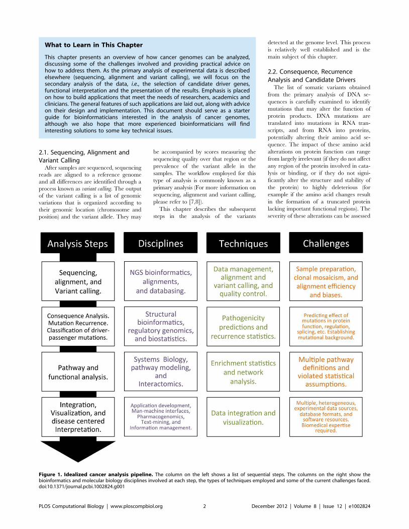
2.1. Sequencing, Alignment andVariant Calling
After samples are sequenced, sequencing
reads are aligned to a reference genome
and all differences are identified through a
process known as variant calling. The output
of the variant calling is a list of genomic
variations that is organized according to
their genomic location (chromosome and
position) and the variant allele. They may
be accompanied by scores measuring the
sequencing quality over that region or the
prevalence of the variant allele in the
samples. The workflow employed for this
type of analysis is commonly known as a
primary analysis (For more information on
sequencing, alignment and variant calling,
please refer to [7,8]).
This chapter describes the subsequent
steps in the analysis of the variants
detected at the genome level. This process
is relatively well established and is the
main subject of this chapter.
2.2. Consequence, RecurrenceAnalysis and Candidate Drivers
The list of somatic variants obtained
from the primary analysis of DNA se-
quences is carefully examined to identify
mutations that may alter the function of
protein products. DNA mutations are
translated into mutations in RNA tran-
scripts, and from RNA into proteins,
potentially altering their amino acid se-
quence. The impact of these amino acid
alterations on protein function can range
from largely irrelevant (if they do not affect
any region of the protein involved in cata-
lysis or binding, or if they do not signi-
ficantly alter the structure and stability of
the protein) to highly deleterious (for
example if the amino acid changes result
in the formation of a truncated protein
lacking important functional regions). The
severity of these alterations can be assessed
What to Learn in This Chapter
This chapter presents an overview of how cancer genomes can be analyzed,discussing some of the challenges involved and providing practical advice onhow to address them. As the primary analysis of experimental data is describedelsewhere (sequencing, alignment and variant calling), we will focus on thesecondary analysis of the data, i.e., the selection of candidate driver genes,functional interpretation and the presentation of the results. Emphasis is placedon how to build applications that meet the needs of researchers, academics andclinicians. The general features of such applications are laid out, along with adviceon their design and implementation. This document should serve as a starterguide for bioinformaticians interested in the analysis of cancer genomes,although we also hope that more experienced bioinformaticians will findinteresting solutions to some key technical issues.
Figure 1. Idealized cancer analysis pipeline. The column on the left shows a list of sequential steps. The columns on the right show thebioinformatics and molecular biology disciplines involved at each step, the types of techniques employed and some of the current challenges faced.doi:10.1371/journal.pcbi.1002824.g001
PLOS Computational Biology | www.ploscompbiol.org 2 December 2012 | Volume 8 | Issue 12 | e1002824
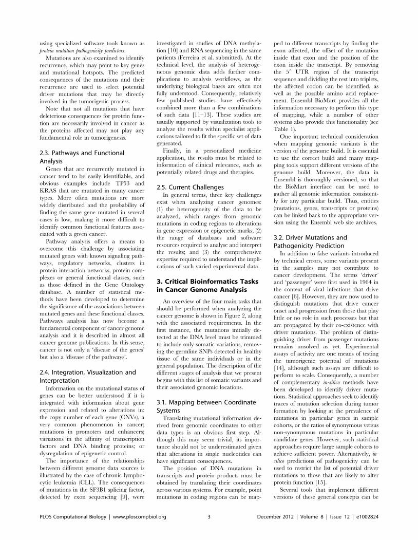
using specialized software tools known as
protein mutation pathogenicity predictors.
Mutations are also examined to identify
recurrence, which may point to key genes
and mutational hotspots. The predicted
consequences of the mutations and their
recurrence are used to select potential
driver mutations that may be directly
involved in the tumorigenic process.
Note that not all mutations that have
deleterious consequences for protein func-
tion are necessarily involved in cancer as
the proteins affected may not play any
fundamental role in tumorigenesis.
2.3. Pathways and FunctionalAnalysis
Genes that are recurrently mutated in
cancer tend to be easily identifiable, and
obvious examples include TP53 and
KRAS that are mutated in many cancer
types. More often mutations are more
widely distributed and the probability of
finding the same gene mutated in several
cases is low, making it more difficult to
identify common functional features asso-
ciated with a given cancer.
Pathway analysis offers a means to
overcome this challenge by associating
mutated genes with known signaling path-
ways, regulatory networks, clusters in
protein interaction networks, protein com-
plexes or general functional classes, such
as those defined in the Gene Ontology
database. A number of statistical me-
thods have been developed to determine
the significance of the associations between
mutated genes and these functional classes.
Pathways analysis has now become a
fundamental component of cancer genome
analysis and it is described in almost all
cancer genome publications. In this sense,
cancer is not only a ‘disease of the genes’
but also a ‘disease of the pathways’.
2.4. Integration, Visualization andInterpretation
Information on the mutational status of
genes can be better understood if it is
integrated with information about gene
expression and related to alterations in:
the copy number of each gene (CNVs), a
very common phenomenon in cancer;
mutations in promoters and enhancers;
variations in the affinity of transcription
factors and DNA binding proteins; or
dysregulation of epigenetic control.
The importance of the relationships
between different genome data sources is
illustrated by the case of chronic lympho-
cytic leukemia (CLL). The consequences
of mutations in the SF3B1 splicing factor,
detected by exon sequencing [9], were
investigated in studies of DNA methyla-
tion [10] and RNA sequencing in the same
patients (Ferreira et al. submitted). At the
technical level, the analysis of heteroge-
neous genomic data adds further com-
plications to analysis workflows, as the
underlying biological bases are often not
fully understood. Consequently, relatively
few published studies have effectively
combined more than a few combinations
of such data [11–13]. These studies are
usually supported by visualization tools to
analyze the results within specialist appli-
cations tailored to fit the specific set of data
generated.
Finally, in a personalized medicine
application, the results must be related to
information of clinical relevance, such as
potentially related drugs and therapies.
2.5. Current ChallengesIn general terms, three key challenges
exist when analyzing cancer genomes:
(1) the heterogeneity of the data to be
analyzed, which ranges from genomic
mutations in coding regions to alterations
in gene expression or epigenetic marks; (2)
the range of databases and software
resources required to analyse and interpret
the results; and (3) the comprehensive
expertise required to understand the impli-
cations of such varied experimental data.
3. Critical Bioinformatics Tasksin Cancer Genome Analysis
An overview of the four main tasks that
should be performed when analyzing the
cancer genome is shown in Figure 2, along
with the associated requirements. In the
first instance, the mutations initially de-
tected at the DNA level must be trimmed
to include only somatic variations, remov-
ing the germline SNPs detected in healthy
tissue of the same individuals or in the
general population. The description of the
different stages of analysis that we present
begins with this list of somatic variants and
their associated genomic locations.
3.1. Mapping between CoordinateSystems
Translating mutational information de-
rived from genomic coordinates to other
data types is an obvious first step. Al-
though this may seem trivial, its impor-
tance should not be underestimated given
that alterations in single nucleotides can
have significant consequences.
The position of DNA mutations in
transcripts and protein products must be
obtained by translating their coordinates
across various systems. For example, point
mutations in coding regions can be map-
ped to different transcripts by finding the
exon affected, the offset of the mutation
inside that exon and the position of the
exon inside the transcript. By removing
the 59 UTR region of the transcript
sequence and dividing the rest into triplets,
the affected codon can be identified, as
well as the possible amino acid replace-
ment. Ensembl BioMart provides all the
information necessary to perform this type
of mapping, while a number of other
systems also provide this functionality (see
Table 1).
One important technical consideration
when mapping genomic variants is the
version of the genome build. It is essential
to use the correct build and many map-
ping tools support different versions of the
genome build. Moreover, the data in
Ensembl is thoroughly versioned, so that
the BioMart interface can be used to
gather all genomic information consistent-
ly for any particular build. Thus, entities
(mutations, genes, transcripts or proteins)
can be linked back to the appropriate ver-
sion using the Ensembl web site archives.
3.2. Driver Mutations andPathogenicity Prediction
In addition to false variants introduced
by technical errors, some variants present
in the samples may not contribute to
cancer development. The terms ‘driver’
and ‘passenger’ were first used in 1964 in
the context of viral infections that drive
cancer [6]. However, they are now used to
distinguish mutations that drive cancer
onset and progression from those that play
little or no role in such processes but that
are propagated by their co-existence with
driver mutations. The problem of distin-
guishing driver from passenger mutations
remains unsolved as yet. Experimental
assays of activity are one means of testing
the tumorigenic potential of mutations
[14], although such assays are difficult to
perform to scale. Consequently, a number
of complementary in-silico methods have
been developed to identify driver muta-
tions. Statistical approaches seek to identify
traces of mutation selection during tumor
formation by looking at the prevalence of
mutations in particular genes in sample
cohorts, or the ratios of synonymous versus
non-synonymous mutations in particular
candidate genes. However, such statistical
approaches require large sample cohorts to
achieve sufficient power. Alternatively, in-
silico predictions of pathogenicity can be
used to restrict the list of potential driver
mutations to those that are likely to alter
protein function [15].
Several tools that implement different
versions of these general concepts can be
PLOS Computational Biology | www.ploscompbiol.org 3 December 2012 | Volume 8 | Issue 12 | e1002824
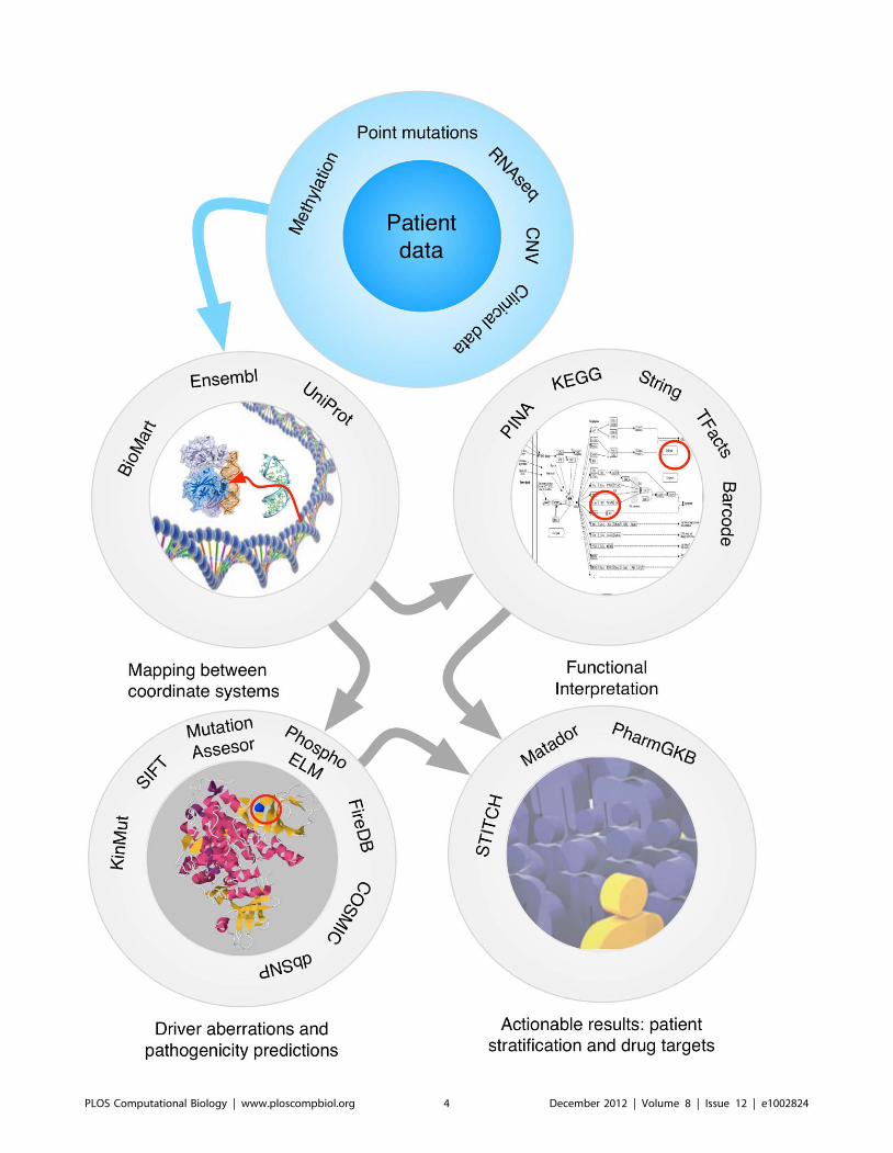
PLOS Computational Biology | www.ploscompbiol.org 4 December 2012 | Volume 8 | Issue 12 | e1002824
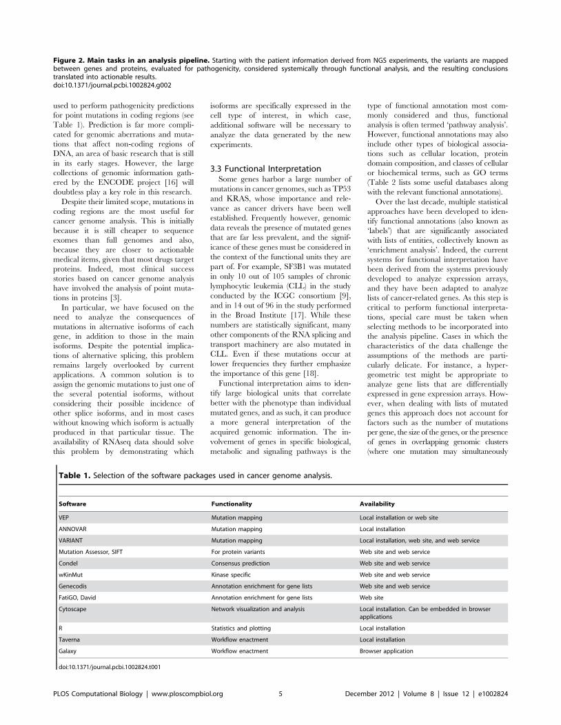
used to perform pathogenicity predictions
for point mutations in coding regions (see
Table 1). Prediction is far more compli-
cated for genomic aberrations and muta-
tions that affect non-coding regions of
DNA, an area of basic research that is still
in its early stages. However, the large
collections of genomic information gath-
ered by the ENCODE project [16] will
doubtless play a key role in this research.
Despite their limited scope, mutations in
coding regions are the most useful for
cancer genome analysis. This is initially
because it is still cheaper to sequence
exomes than full genomes and also,
because they are closer to actionable
medical items, given that most drugs target
proteins. Indeed, most clinical success
stories based on cancer genome analysis
have involved the analysis of point muta-
tions in proteins [3].
In particular, we have focused on the
need to analyze the consequences of
mutations in alternative isoforms of each
gene, in addition to those in the main
isoforms. Despite the potential implica-
tions of alternative splicing, this problem
remains largely overlooked by current
applications. A common solution is to
assign the genomic mutations to just one of
the several potential isoforms, without
considering their possible incidence of
other splice isoforms, and in most cases
without knowing which isoform is actually
produced in that particular tissue. The
availability of RNAseq data should solve
this problem by demonstrating which
isoforms are specifically expressed in the
cell type of interest, in which case,
additional software will be necessary to
analyze the data generated by the new
experiments.
3.3 Functional InterpretationSome genes harbor a large number of
mutations in cancer genomes, such as TP53
and KRAS, whose importance and rele-
vance as cancer drivers have been well
established. Frequently however, genomic
data reveals the presence of mutated genes
that are far less prevalent, and the signif-
icance of these genes must be considered in
the context of the functional units they are
part of. For example, SF3B1 was mutated
in only 10 out of 105 samples of chronic
lymphocytic leukemia (CLL) in the study
conducted by the ICGC consortium [9],
and in 14 out of 96 in the study performed
in the Broad Institute [17]. While these
numbers are statistically significant, many
other components of the RNA splicing and
transport machinery are also mutated in
CLL. Even if these mutations occur at
lower frequencies they further emphasize
the importance of this gene [18].
Functional interpretation aims to iden-
tify large biological units that correlate
better with the phenotype than individual
mutated genes, and as such, it can produce
a more general interpretation of the
acquired genomic information. The in-
volvement of genes in specific biological,
metabolic and signaling pathways is the
type of functional annotation most com-
monly considered and thus, functional
analysis is often termed ‘pathway analysis’.
However, functional annotations may also
include other types of biological associa-
tions such as cellular location, protein
domain composition, and classes of cellular
or biochemical terms, such as GO terms
(Table 2 lists some useful databases along
with the relevant functional annotations).
Over the last decade, multiple statistical
approaches have been developed to iden-
tify functional annotations (also known as
‘labels’) that are significantly associated
with lists of entities, collectively known as
‘enrichment analysis’. Indeed, the current
systems for functional interpretation have
been derived from the systems previously
developed to analyze expression arrays,
and they have been adapted to analyze
lists of cancer-related genes. As this step is
critical to perform functional interpreta-
tions, special care must be taken when
selecting methods to be incorporated into
the analysis pipeline. Cases in which the
characteristics of the data challenge the
assumptions of the methods are parti-
cularly delicate. For instance, a hyper-
geometric test might be appropriate to
analyze gene lists that are differentially
expressed in gene expression arrays. How-
ever, when dealing with lists of mutated
genes this approach does not account for
factors such as the number of mutations
per gene, the size of the genes, or the presence
of genes in overlapping genomic clusters
(where one mutation may simultaneously
Figure 2. Main tasks in an analysis pipeline. Starting with the patient information derived from NGS experiments, the variants are mappedbetween genes and proteins, evaluated for pathogenicity, considered systemically through functional analysis, and the resulting conclusionstranslated into actionable results.doi:10.1371/journal.pcbi.1002824.g002
Table 1. Selection of the software packages used in cancer genome analysis.
Software Functionality Availability
VEP Mutation mapping Local installation or web site
ANNOVAR Mutation mapping Local installation
VARIANT Mutation mapping Local installation, web site, and web service
Mutation Assessor, SIFT For protein variants Web site and web service
Condel Consensus prediction Web site and web service
wKinMut Kinase specific Web site and web service
Genecodis Annotation enrichment for gene lists Web site and web service
FatiGO, David Annotation enrichment for gene lists Web site
Cytoscape Network visualization and analysis Local installation. Can be embedded in browserapplications
R Statistics and plotting Local installation
Taverna Workflow enactment Local installation
Galaxy Workflow enactment Browser application
doi:10.1371/journal.pcbi.1002824.t001
PLOS Computational Biology | www.ploscompbiol.org 5 December 2012 | Volume 8 | Issue 12 | e1002824
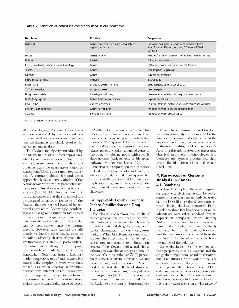
affect several genes). As none of these issues
are accommodated by the standard ap-
proaches used for gene expression analysis,
new developments are clearly required for
cancer genome analysis.
To alleviate the rigidity introduced by
the binary nature of set-based approaches,
whereby genes are either on the list or they
are not, some enrichment analysis ap-
proaches study the over-representation of
annotations/labels using rank-based statis-
tics. A common choice for rank-based
approaches is to use some variation of the
Kolmogorov-Smirnov non-parametric sta-
tistic, as employed in gene set enrichment
analysis (GSEA) [19]. Another benefit of
rank approaches is that the scores used can
be designed to account for some of the
features that are not well handled by set-
based approaches. Accordingly, consider-
ations of background mutation rates based
on gene length, sequencing quality or
heterogeneity in the initial tumor samples
can be incorporated into the scoring
scheme. However, rank statistics are still
unable to handle other issues, such as
mutations affecting clusters of genes that
are functionally related (e.g., proto-cadher-
ins), which still challenge the assumption
of independence made by most statistical
approaches. Note that from a bioinfor-
matics perspective, sets of entities are often
conceptually simpler to work with than
ranked lists when crossing information
derived from different sources. Moreover,
from an application perspective, informa-
tion summarized in terms of sets of entities
is often more actionable than ranks or scores.
A different type of analysis considers the
relationships between entities based on
their connections in protein interaction
networks. This approach has been used to
measure the proximity of groups of cancer-
related genes and other groups of genes or
functions, by labeling nodes with specific
characteristics (such as roles in biological
pathways or functional classes) [20].
Functional interpretation can therefore
be facilitated by the use of a wide array of
alternative analyses. Different approaches
can potentially uncover hidden functional
implications in genomic data, although the
integration of these results remains a key
challenge.
3.4. Applicable Results: Diagnosis,Patient Stratification and DrugTherapies
For clinical applications, the results of
cancer genome analysis need to be trans-
lated into practical advice for clinicians,
providing potential drug therapies, better
tumor classification or early diagnostic
markers. While bioinformatics systems can
support these decisions, it will be up to
expert users to present these findings in the
context of the relevant medical and clinical
information available at any given time. In
the case of our institution’s (CNIO) person-
alized cancer medicine approach, we use
mouse xenografts (also known as ‘avatar’
models) to test the effects of drugs on
tumors prior to considering their potential
to treat patients [4]. In turn, the results of
these xenograft studies are used as a
feedback into the system for future analyses.
Drug-related information and the tools
with which to analyze it is essential for the
analysis of personalized data (some of the
key databases linking known gene variants
to diseases and drugs are listed in Table 2).
Accessing this information and integrating
chemical informatics methodologies into
bioinformatics systems presents new chal-
lenges for bioinformaticians and system
developers.
4. Resources for GenomeAnalysis in Cancer
4.1. DatabasesAlthough complex, the data required
for genome analysis can usually be repre-
sented in a tabular format. Tab separated
values (TSV) files are the de facto standard
when sharing database resources. For a
developer, these files have several practical
advantages over other standard formats
popular in computer science (namely
XML): they are easier to read, write and
parse with scripts; they are relatively
succinct; the format is straight-forward
and the contents can be inferred from the
first line of the file, which typically holds
the names of the columns.
Some databases describe entities and
their properties, such as: proteins and the
drugs that target them; germline variations
and the diseases with which they are
associated; or genes along with the factors
that regulate their transcription. Other
databases are repositories of experimental
data, such as the Gene Expression Omnibus
and ArrayExpress, which contain data from
microarray experiments on a wide range of
Table 2. Selection of databases commonly used in our workflows.
Database Entities Properties
Ensembl Genes, proteins, transcripts, regulatoryregions, variants
Genomic positions, relationships between them,identifiers in different formats, GO terms, PFAMdomains
Entrez Genes, articles Articles for genes, abstracts of articles, links to full text
UniProt Proteins PDBs, known variants
KEGG, Reactome, Biocarta, Gene Ontology Genes Pathways, processes, function, cell location
TFacts Genes Transcription regulation
Barcode Genes Expression by tissue
PINA, HPRD, STRING Proteins Interactions
PharmaGKB Drugs, proteins, variants Drug targets, pharmacogenetics
STITCH, Matador Drugs, proteins Drug targets
Drug clinical trials Investigational drugs Diseases or conditions in they are being tested
GEO, ArrayExpress Genes (microarray probes) Expression values
ICGC, TCGA Cancer Genomes Point mutations, methylation, CNV, structural variants
dbSNP, 1000 genomes Germline variations Association with diseases or conditions
COSMIC Somatic variations Association with cancer types
doi:10.1371/journal.pcbi.1002824.t002
PLOS Computational Biology | www.ploscompbiol.org 6 December 2012 | Volume 8 | Issue 12 | e1002824
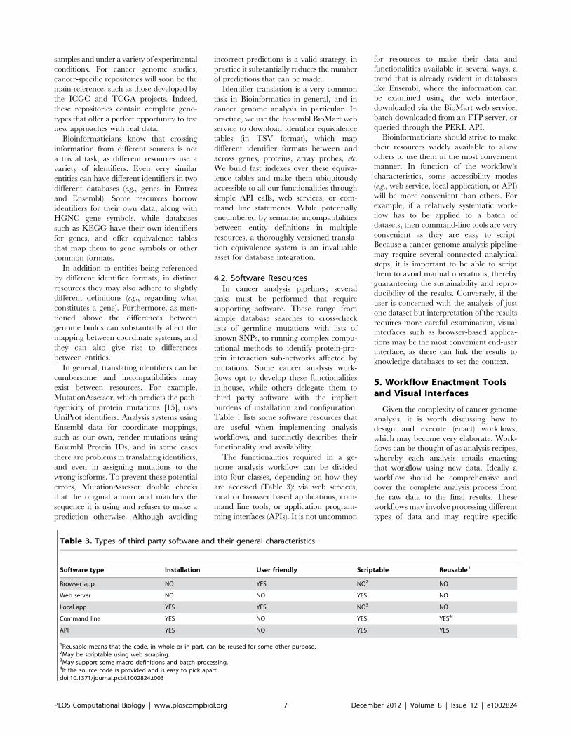
samples and under a variety of experimental
conditions. For cancer genome studies,
cancer-specific repositories will soon be the
main reference, such as those developed by
the ICGC and TCGA projects. Indeed,
these repositories contain complete geno-
types that offer a perfect opportunity to test
new approaches with real data.
Bioinformaticians know that crossing
information from different sources is not
a trivial task, as different resources use a
variety of identifiers. Even very similar
entities can have different identifiers in two
different databases (e.g., genes in Entrez
and Ensembl). Some resources borrow
identifiers for their own data, along with
HGNC gene symbols, while databases
such as KEGG have their own identifiers
for genes, and offer equivalence tables
that map them to gene symbols or other
common formats.
In addition to entities being referenced
by different identifier formats, in distinct
resources they may also adhere to slightly
different definitions (e.g., regarding what
constitutes a gene). Furthermore, as men-
tioned above the differences between
genome builds can substantially affect the
mapping between coordinate systems, and
they can also give rise to differences
between entities.
In general, translating identifiers can be
cumbersome and incompatibilities may
exist between resources. For example,
MutationAssessor, which predicts the path-
ogenicity of protein mutations [15], uses
UniProt identifiers. Analysis systems using
Ensembl data for coordinate mappings,
such as our own, render mutations using
Ensembl Protein IDs, and in some cases
there are problems in translating identifiers,
and even in assigning mutations to the
wrong isoforms. To prevent these potential
errors, MutationAssessor double checks
that the original amino acid matches the
sequence it is using and refuses to make a
prediction otherwise. Although avoiding
incorrect predictions is a valid strategy, in
practice it substantially reduces the number
of predictions that can be made.
Identifier translation is a very common
task in Bioinformatics in general, and in
cancer genome analysis in particular. In
practice, we use the Ensembl BioMart web
service to download identifier equivalence
tables (in TSV format), which map
different identifier formats between and
across genes, proteins, array probes, etc.
We build fast indexes over these equiva-
lence tables and make them ubiquitously
accessible to all our functionalities through
simple API calls, web services, or com-
mand line statements. While potentially
encumbered by semantic incompatibilities
between entity definitions in multiple
resources, a thoroughly versioned transla-
tion equivalence system is an invaluable
asset for database integration.
4.2. Software ResourcesIn cancer analysis pipelines, several
tasks must be performed that require
supporting software. These range from
simple database searches to cross-check
lists of germline mutations with lists of
known SNPs, to running complex compu-
tational methods to identify protein-pro-
tein interaction sub-networks affected by
mutations. Some cancer analysis work-
flows opt to develop these functionalities
in-house, while others delegate them to
third party software with the implicit
burdens of installation and configuration.
Table 1 lists some software resources that
are useful when implementing analysis
workflows, and succinctly describes their
functionality and availability.
The functionalities required in a ge-
nome analysis workflow can be divided
into four classes, depending on how they
are accessed (Table 3): via web services,
local or browser based applications, com-
mand line tools, or application program-
ming interfaces (APIs). It is not uncommon
for resources to make their data and
functionalities available in several ways, a
trend that is already evident in databases
like Ensembl, where the information can
be examined using the web interface,
downloaded via the BioMart web service,
batch downloaded from an FTP server, or
queried through the PERL API.
Bioinformaticians should strive to make
their resources widely available to allow
others to use them in the most convenient
manner. In function of the workflow’s
characteristics, some accessibility modes
(e.g., web service, local application, or API)
will be more convenient than others. For
example, if a relatively systematic work-
flow has to be applied to a batch of
datasets, then command-line tools are very
convenient as they are easy to script.
Because a cancer genome analysis pipeline
may require several connected analytical
steps, it is important to be able to script
them to avoid manual operations, thereby
guaranteeing the sustainability and repro-
ducibility of the results. Conversely, if the
user is concerned with the analysis of just
one dataset but interpretation of the results
requires more careful examination, visual
interfaces such as browser-based applica-
tions may be the most convenient end-user
interface, as these can link the results to
knowledge databases to set the context.
5. Workflow Enactment Toolsand Visual Interfaces
Given the complexity of cancer genome
analysis, it is worth discussing how to
design and execute (enact) workflows,
which may become very elaborate. Work-
flows can be thought of as analysis recipes,
whereby each analysis entails enacting
that workflow using new data. Ideally a
workflow should be comprehensive and
cover the complete analysis process from
the raw data to the final results. These
workflows may involve processing different
types of data and may require specific
Table 3. Types of third party software and their general characteristics.
Software type Installation User friendly Scriptable Reusable1
Browser app. NO YES NO2 NO
Web server NO NO YES NO
Local app YES YES NO3 NO
Command line YES NO YES YES4
API YES NO YES YES
1Reusable means that the code, in whole or in part, can be reused for some other purpose.2May be scriptable using web scraping.3May support some macro definitions and batch processing.4If the source code is provided and is easy to pick apart.doi:10.1371/journal.pcbi.1002824.t003
PLOS Computational Biology | www.ploscompbiol.org 7 December 2012 | Volume 8 | Issue 12 | e1002824
adaptations for the analysis of certain types
of experiments. Often, parts of the analysis
will be repeated in a different context and
thus, one of the objectives of workflow
enactment tools is to reuse code efficiently.
A number of systems have been designed
to facilitate the construction of workflows
(e.g., Taverna [21] and Galaxy [22], which
both offer visual interfaces to orchestrate
workflows across a very wide range of
available functionalities).
Although visual workflow enactment
approaches have become reasonably pop-
ular, they still have several important
limitations. Firstly, despite recent efforts,
these approaches remain overly complex
for non-bioinformaticians. Secondly, they
are quite inflexible in terms of the pre-
sentation and exploration of the results,
and thus, understanding the results re-
quires the user to do additional work
outside of the system. Finally, the expres-
siveness of these approaches is limited
when compared with general purpose
programming languages. Experienced de-
velopers will find them of limited utility,
and prefer to have their functionalities
accessible by APIs derived from general
purpose programming languages.
The information presented to the user
needs to closely match his/her needs,
especially in more translational settings.
Too much information may mask impor-
tant conclusions, while too little may leave
the user unsure as to the validity of their
findings. This further emphasizes the need
to customize workflows and the manner in
which results are displayed, in order to
best fit these aspects to the particularities
of each user.
In a more academic setting, close col-
laboration between the researcher and the
bioinformatician facilitates the develop-
ment of custom interfaces that can better
adapt to given datasets, and answer the
very specific questions that may arise
during data exploration. In our institution,
we use a programmatic workflow enact-
ment system that orchestrates a wide
variety of tasks, ranging from coordinate
mapping to enrichment analysis. This
system is controlled via a browser appli-
cation designed to rapidly produce custom
reports using a template-based HTML
report generation system. It is a system
that was developed entirely in-house but
that makes use of third party software,
allowing us to address the requirements of
our collaborators in a timely manner.
6. Summary
Cancer genome analysis involves the
manipulation of large datasets and the
application of complex methods. The
heterogeneity of the data and the disparity
of the software implementations represent
an additional layer of complexity, which
requires the use of systems that can be
easily adapted and reconfigured. Addition-
ally, interpretation of the results in terms
of specific biological questions is more
effective if done in close collaboration
with experts in the field. This represents a
specific challenge for software development
in terms of interactivity and representation
standards. Cancer genome analysis systems
need to be capable of conveniently man-
aging this complexity and of adapting to the
specific characteristics of each analysis.
Finally, it is worth noting that bioinfor-
matics systems will soon have to move
beyond the current research environ-
ments and into clinical settings, a chal-
lenge that will involve more industrial
development that can better cope with
issues of sustainability, robustness and
accreditation, while still incorporating
the latest bioinformatics components that
will continue to be generated in research
laboratories. This constitutes a new and
exciting frontier for bioinformatics soft-
ware developers.
7. Exercise Questions
I. Name three general issues that
bioinformaticians face when ana-
lyzing cancer genome data?
II. What are the four main tasks in
cancer genome analysis in a
clinical setting once the primary
analysis has been performed?
III. Why is it important to use the
correct genome build?
IV. What do we mean by driver
mutation?
V. There are two key principles that
help determine driver mutations
in-silico. What are they?
VI. Give several reasons why point
mutations in coding regions are so
important.
VII. Name three issues that challenge
the assumptions made by the
standard pathway enrichment
analysis tools when applied to
genomic mutations.
VIII. Discuss the problems that arise with
identifiers when integrating infor-
mation across different databases.
IX. Why are command line tools
generally more convenient than
browser-based applications for
processing a batch analyses?
X. How would an application aimed
at researchers differ from one
aimed at clinicians in terms of
the information presented?
Answers to the Exercises can be found
in Text S1.
Supporting Information
Text S1 Answers to Exercises
(DOCX)
Further Reading
N Weinberg RA (2006) The biology of cancer. 1st ed. Garland Science. 850 p.
N Ng PC, Murray SS, Levy S, Venter JC (2009) An agenda for personalizedmedicine. Nature 461: 724–726. doi:10.1038/461724a.
N Fernald GH, Capriotti E, Daneshjou R, Karczewski KJ, Altman RB (2011)Bioinformatics challenges for personalized medicine. Bioinformatics 27: 1741–1748. doi:10.1093/bioinformatics/btr295.
N Valencia A, Hidalgo M (2012) Getting personalized cancer genome analysis into theclinic: the challenges in bioinformatics. Genome Med 4: 61. doi:10.1186/gm362.
N Whirl-Carrillo M, McDonagh EM, Hebert JM, Gong L, Sangkuhl K, et al. (2012)Pharmacogenomics knowledge for personalized medicine. Clin Pharmacol Ther92: 414–417. doi:10.1038/clpt.2012.96.
N Baudot A, de la Torre V, Valencia A (2010) Mutated genes, pathways andprocesses in tumours. EMBO Rep 11: 805–810. doi:10.1038/embor.2010.133.
N Huang DW, Sherman BT, Lempicki RA (2009) Bioinformatics enrichment tools:paths toward the comprehensive functional analysis of large gene lists. NuclAcids Res 37: 1–13. doi:10.1093/nar/gkn923.
N Khatri P, Sirota M, Butte AJ (2012) Ten years of pathway analysis: currentapproaches and outstanding challenges. PLoS Comput Biol 8: e1002375.doi:10.1371/journal.pcbi.1002375.
N Stein L (2002) Creating a bioinformatics nation. Nature 417: 119–120.doi:10.1038/417119a.
PLOS Computational Biology | www.ploscompbiol.org 8 December 2012 | Volume 8 | Issue 12 | e1002824
References
1. Hudson TJ, Anderson W, Artez A, Barker AD,
Bell C, et al. (2010) International network of
cancer genome projects. Nature 464: 993–998.
doi:10.1038/nature08987.
2. Roychowdhury S, Iyer MK, Robinson DR,
Lonigro RJ, Wu Y-M, et al. (2011) Personalized
oncology through integrative high-throughput
sequencing: a pilot study. Sci Transl Med 3:
111ra121. doi:10.1126/scitranslmed.3003161.
3. Villarroel MC, Rajeshkumar NV, Garrido-La-
guna I, De Jesus-Acosta A, Jones S, et al. (2011)
Personalizing cancer treatment in the age of
global genomic analyses: PALB2 gene mutations
and the response to DNA damaging agents in
pancreatic cancer. Mol Cancer Ther 10: 3–8.
doi:10.1158/1535-7163.MCT-10-0893.
4. Valencia A, Hidalgo M (2012) Getting personal-
ized cancer genome analysis into the clinic: the
challenges in bioinformatics. Genome Med 4: 61.
doi:10.1186/gm362.
5. Baudot A, Real FX, Izarzugaza JMG, Valencia A
(2009) From cancer genomes to cancer models:
bridging the gaps. EMBO Rep 10: 359–366.
doi:10.1038/embor.2009.46.
6. Andrewes C (1964) Tumour-viruses and Virus-
tumours. Br Med J 1: 653–658.
7. Nielsen R, Paul JS, Albrechtsen A, Song YS
(2011) Genotype and SNP calling from next-
generation sequencing data. Nature Reviews
Genetics 12: 443–451. doi:10.1038/nrg2986.
8. Metzker ML (2010) Sequencing technologies - the
next generation. Nat Rev Genet 11: 31–46. doi:
10.1038/nrg2626.
9. Quesada V, Conde L, Villamor N, Ordonez GR,
Jares P, et al. (2011) Exome sequencing identifies
recurrent mutations of the splicing factor SF3B1
gene in chronic lymphocytic leukemia. Nat Genet
44: 47–52. doi:10.1038/ng.1032.
10. Kulis M, Heath S, Bibikova M, Queiros AC,
Navarro A, et al. (2012) Epigenomic analysis
detects widespread gene-body DNA hypomethy-
lation in chronic lymphocytic leukemia. Nat
Genet 44): 1236–1242. doi:10.1038/ng.2443.
11. Chuang H-Y, Rassenti L, Salcedo M, Licon K,
Kohlmann A, et al. (2012) Subnetwork-based
analysis of chronic lymphocytic leukemia identi-
fies pathways that associate with disease progres-
sion. Blood 120: 2639–2649. doi:10.1182/blood-
2012-03-416461.
12. The Cancer Genome Atlas Network (2012)
Comprehensive molecular portraits of human
breast tumours. Nature 490: 61–70. doi:10.1038/
nature11412.
13. Chen R, Mias GI, Li-Pook-Than J, Jiang L, Lam
HYK, et al. (2012) Personal omics profiling
reveals dynamic molecular and medical pheno-
types. Cell 148: 1293–1307. doi:10.1016/
j.cell.2012.02.009.
14. Frohling S, Scholl C, Levine RL, Loriaux M,
Boggon TJ, et al. (2007) Identification of driver
and passenger mutations of FLT3 by high-
throughput DNA sequence analysis and function-
al assessment of candidate alleles. Cancer Cell 12:
501–513. doi:10.1016/j.ccr.2007.11.005.
15. Boris Reva YACS (2011) Predicting the function-
al impact of protein mutations: application to
cancer genomics. Nucleic Acids Res 39: e118.
doi:10.1093/nar/gkr407.16. Bernstein BE, Birney E, Dunham I, Green ED,
Gunter C, et al. (2012) An integrated encyclope-dia of DNA elements in the human genome.
Nature 489: 57–74. doi:10.1038/nature11247.
17. Wang L, Lawrence MS, Wan Y, Stojanov P,Sougnez C, et al. (2011) SF3B1 and other novel
cancer genes in chronic lymphocytic leukemia.N Engl J Med 365: 2497–2506. doi:10.1056/
NEJMoa1109016.
18. Damm F, Nguyen-Khac F, Fontenay M, BernardOA (2012) Spliceosome and other novel muta-
tions in chronic lymphocytic leukemia, andmyeloid malignancies. Leukemia 26: 2027–2031.
19. Subramanian A, Tamayo P, Mootha VK,Mukherjee S, Ebert BL, et al. (2005) Gene set
enrichment analysis: a knowledge-based ap-
proach for interpreting genome-wide expressionprofiles. Proc Natl Acad Sci USA 102: 15545–
15550. doi:10.1073/pnas.0506580102.20. Glaab E, Baudot A, Krasnogor N, Schneider R,
Valencia A (2012) EnrichNet: network-based
gene set enrichment analysis. Bioinformatics 28:i451–i457. doi:10.1093/bioinformatics/bts389.
21. Hull D, Wolstencroft K, Stevens R, Goble C,Pocock MR, et al. (2006) Taverna: a tool for
building and running workflows of services.Nucleic Acids Res 34: W729–W732. doi:10.1093/
nar/gkl320.
22. Giardine B, Riemer C, Hardison RC, Burhans R,Elnitski L, et al. (2005) Galaxy: a platform for
interactive large-scale genome analysis. GenomeRes 15: 1451–1455. doi:10.1101/gr.4086505.
PLOS Computational Biology | www.ploscompbiol.org 9 December 2012 | Volume 8 | Issue 12 | e1002824
Education
Chapter 15: Disease Gene PrioritizationYana Bromberg*
Department of Biochemistry and Microbiology, School of Environmental and Biological Sciences, Rutgers University, New Brunswick, New Jersey, United States of America
Abstract: Disease-causing aberra-tions in the normal function of agene define that gene as a diseasegene. Proving a causal link be-tween a gene and a disease exper-imentally is expensive and time-consuming. Comprehensive priori-tization of candidate genes prior toexperimental testing drastically re-duces the associated costs. Com-putational gene prioritization isbased on various pieces of correl-ative evidence that associate eachgene with the given disease andsuggest possible causal links. A fairamount of this evidence comesfrom high-throughput experimen-tation. Thus, well-developed meth-ods are necessary to reliably dealwith the quantity of information athand. Existing gene prioritizationtechniques already significantly im-prove the outcomes of targetedexperimental studies. Faster andmore reliable techniques that ac-count for novel data types arenecessary for the development ofnew diagnostics, treatments, andcure for many diseases.
This article is part of the ‘‘Transla-
tional Bioinformatics’’ collection for
PLOS Computational Biology.
1. Introduction
In 1904 Dr. James Herrick reported [1]
the findings of ‘‘peculiar elongated and
sickle shaped’’ red blood cells discovered
by Dr. Ernest Irons in a hospital patient
afflicted with shortness of breath, heart
palpitations, and various other aches and
pains. This was the first documented case
of sickle cell disease in the United States.
Forty years later, in 1949, sickle cell
anemia became the first disease to be
characterized on a molecular level [2,3].
Thus, implicitly, the first disease-associat-
ed gene, coding for beta-globin chain of
hemoglobin A, was discovered.
It took another thirty years before in
1983 a study of the DNA of families
afflicted with Huntington’s disease has
revealed its association with a gene on
chromosome 4 called huntigtin (HTT)
[4]. Huntington’s became the first genetic
disease mapped using polymorphism
information (G8 DNA probe/genetic
marker), closely followed by the same
year discovery of phenylketonuria associ-
ation with polymorphisms in a hepatic
enzyme phenylalanine hydroxylase [5].
These advances provided a route for
predicting the likelihood of disease devel-
opment and even stirred some worries
regarding the possibility of the rise of
‘‘medical eugenics’’ [6]. Interestingly, it
took another ten years for HTT’s se-
quence to be identified and for the
precise nature of the Huntigton’s-associ-
ated mutation to be determined [7].
The recent explosion in high-through-
put experimental techniques has contrib-
uted significantly to the identification of
disease-associated genes and mutations.
For instance, the latest release of SwissVar
[8], a variation centered view of the Swiss-
Prot database of genes and proteins [9,10],
reports nearly 20 thousand mutations in
35 hundred genes associated with over
three thousand broad disease classes.
Unfortunately, the improved efficiency in
production of association data (e.g. ge-
nome-wide association studies, GWAS)
has not been matched by its similarly
improving accuracy. Thus, the sheer
quantity of existing but yet unvalidated
data resulted in information overflow.
While association and linkage studies
provide a lot of information, incorporation
of other sources of evidence is necessary to
narrow down the candidate search space.
Computational methods - gene prioritiza-
tion techniques, are therefore necessary to
effectively translate the experimental data
into legible disease-gene associations [11].
2. Background
The Merriam-Webster dictionary de-
fines the word ‘‘disease’’ as a ‘‘a condition
of the living animal or plant body or of one
of its parts that impairs normal functioning
and is typically manifested by distinguishing
signs and symptoms.’’ Thus, disease is
defined with respect to normal function of said
body or body part. Note, that this definition
also describes the malfunction of individual
cells or cell groups. In fact, many diseases
can and should be defined on a cellular
level. Understanding a disease, and poten-
tially finding curative or preventive mea-
sures, requires answering three questions:
(1) What is the affected function? (2) What
functional activity levels are considered
normal given the environmental contexts?
(3) What is the direction and amount of
change in this activity necessary to cause
the observed phenotype?
Contrary to the view that historically
prevailed in classical genetics it is rarely
the case that one gene is responsible for
one function. Rather, an assembly of genes
constitutes a functional module or a
molecular pathway. By definition, a mo-
lecular pathway leads to some specific end
point in cellular functionality via a series of
interactions between molecules in the cell.
Alterations in any of the normally occur-
ring processes, molecular interactions, and
pathways lead to disease. For example,
folate metabolism is an important molec-
ular pathway, the disruptions in which
have been associated with many disorders
including colorectal cancer [12] and
coronary heart disease [13]. Because this
pathway involves 19 proteins interacting
via numerous cycles and feedback loops
[14], it is not surprising that there are a
Citation: Bromberg Y (2013) Chapter 15: Disease Gene Prioritization. PLoS Comput Biol 9(4): e1002902.doi:10.1371/journal.pcbi.1002902
Editors: Fran Lewitter, Whitehead Institute, United States of America and Maricel Kann, University of Maryland,Baltimore County, United States of America
Published April 25, 2013
Copyright: � 2013 Yana Bromberg. This is an open-access article distributed under the terms of the CreativeCommons Attribution License, which permits unrestricted use, distribution, and reproduction in any medium,provided the original author and source are credited.
Funding: YB is funded by Rutgers, New Brunswick start-up funding, Gordon and Betty Moore Foundationgrant, and USDA-NIFA and NJAES grants Project No. 10150-0228906. The funders had no role in thepreparation of the manuscript.
Competing Interests: The author has declared that no competing interests exist.
* E-mail: [email protected]
PLOS Computational Biology | www.ploscompbiol.org 1 April 2013 | Volume 9 | Issue 4 | e1002902
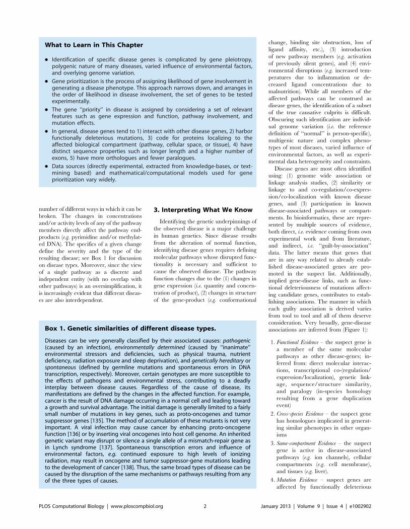
number of different ways in which it can be
broken. The changes in concentrations
and/or activity levels of any of the pathway
members directly affect the pathway end-
products (e.g. pyrimidine and/or methylat-
ed DNA). The specifics of a given change
define the severity and the type of the
resulting disease; see Box 1 for discussion
on disease types. Moreover, since the view
of a single pathway as a discrete and
independent entity (with no overlap with
other pathways) is an oversimplification, it
is increasingly evident that different diseas-
es are also interdependent.
3. Interpreting What We Know
Identifying the genetic underpinnings of
the observed disease is a major challenge
in human genetics. Since disease results
from the alteration of normal function,
identifying disease genes requires defining
molecular pathways whose disrupted func-
tionality is necessary and sufficient to
cause the observed disease. The pathway
function changes due to the (1) changes in
gene expression (i.e. quantity and concen-
tration of product), (2) changes in structure
of the gene-product (e.g. conformational
change, binding site obstruction, loss of
ligand affinity, etc.), (3) introduction
of new pathway members (e.g. activation
of previously silent genes), and (4) envi-
ronmental disruptions (e.g. increased tem-
peratures due to inflammation or de-
creased ligand concentrations due to
malnutrition). While all members of the
affected pathways can be construed as
disease genes, the identification of a subset
of the true causative culprits is difficult.
Obscuring such identification are individ-
ual genome variation (i.e. the reference
definition of ‘‘normal’’ is person-specific),
multigenic nature and complex pheno-
types of most diseases, varied influence of
environmental factors, as well as experi-
mental data heterogeneity and constraints.
Disease genes are most often identified
using: (1) genome wide association or
linkage analysis studies, (2) similarity or
linkage to and co-regulation/co-expres-
sion/co-localization with known disease
genes, and (3) participation in known
disease-associated pathways or compart-
ments. In bioinformatics, these are repre-
sented by multiple sources of evidence,
both direct, i.e. evidence coming from own
experimental work and from literature,
and indirect, i.e. ‘‘guilt-by-association’’
data. The latter means that genes that
are in any way related to already estab-
lished disease-associated genes are pro-
moted in the suspect list. Additionally,
implied gene-disease links, such as func-
tional deleteriousness of mutations affect-
ing candidate genes, contributes to estab-
lishing associations. The manner in which
each guilty association is derived varies
from tool to tool and all of them deserve
consideration. Very broadly, gene-disease
associations are inferred from (Figure 1):
1. Functional Evidence – the suspect gene is
a member of the same molecular
pathways as other disease-genes; in-
ferred from: direct molecular interac-
tions, transcriptional co-(regulation/
expression/localization), genetic link-
age, sequence/structure similarity,
and paralogy (in-species homology
resulting from a gene duplication
event)
2. Cross-species Evidence – the suspect gene
has homologues implicated in generat-
ing similar phenotypes in other organ-
isms
3. Same-compartment Evidence – the suspect
gene is active in disease-associated
pathways (e.g. ion channels), cellular
compartments (e.g. cell membrane),
and tissues (e.g. liver).
4. Mutation Evidence – suspect genes are
affected by functionally deleterious
What to Learn in This Chapter
N Identification of specific disease genes is complicated by gene pleiotropy,polygenic nature of many diseases, varied influence of environmental factors,and overlying genome variation.
N Gene prioritization is the process of assigning likelihood of gene involvement ingenerating a disease phenotype. This approach narrows down, and arranges inthe order of likelihood in disease involvement, the set of genes to be testedexperimentally.
N The gene ‘‘priority’’ in disease is assigned by considering a set of relevantfeatures such as gene expression and function, pathway involvement, andmutation effects.
N In general, disease genes tend to 1) interact with other disease genes, 2) harborfunctionally deleterious mutations, 3) code for proteins localizing to theaffected biological compartment (pathway, cellular space, or tissue), 4) havedistinct sequence properties such as longer length and a higher number ofexons, 5) have more orthologues and fewer paralogues.
N Data sources (directly experimental, extracted from knowledge-bases, or text-mining based) and mathematical/computational models used for geneprioritization vary widely.
Box 1. Genetic similarities of different disease types.
Diseases can be very generally classified by their associated causes: pathogenic(caused by an infection), environmentally determined (caused by ‘‘inanimate’’environmental stressors and deficiencies, such as physical trauma, nutrientdeficiency, radiation exposure and sleep deprivation), and genetically hereditary orspontaneous (defined by germline mutations and spontaneous errors in DNAtranscription, respectively). Moreover, certain genotypes are more susceptible tothe effects of pathogens and environmental stress, contributing to a deadlyinterplay between disease causes. Regardless of the cause of disease, itsmanifestations are defined by the changes in the affected function. For example,cancer is the result of DNA damage occurring in a normal cell and leading towarda growth and survival advantage. The initial damage is generally limited to a fairlysmall number of mutations in key genes, such as proto-oncogenes and tumorsuppressor genes [135]. The method of accumulation of these mutants is not veryimportant. A viral infection may cause cancer by enhancing proto-oncogenefunction [136] or by inserting viral oncogenes into host cell genome. An inheritedgenetic variant may disrupt or silence a single allele of a mismatch-repair gene asin Lynch syndrome [137]. Spontaneous transcription errors and influence ofenvironmental factors, e.g. continued exposure to high levels of ionizingradiation, may result in oncogene and tumor suppressor-gene mutations leadingto the development of cancer [138]. Thus, the same broad types of disease can becaused by the disruption of the same mechanisms or pathways resulting from anyof the three types of causes.
PLOS Computational Biology | www.ploscompbiol.org 2 January 2013 | Volume 9 | Issue 4 | e1002902
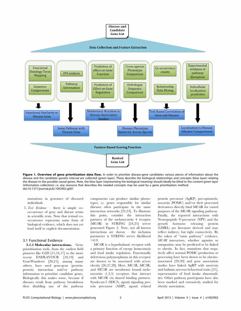
mutations in genomes of diseased
individuals
5. Text Evidence – there is ample co-
occurrence of gene and disease terms
in scientific texts. Note that textual co-
occurrence represents some form of
biological evidence, which does not yet
lend itself to explicit documentation.
3.1 Functional Evidence3.1.1 Molecular interactions. Gene
prioritization tools, from the earliest field
pioneers like G2D [15,16,17] to the more
recent ENDEAVOUR [18,19] and
GeneWanderer [20,21], among many
others, have used gene-gene (protein-
protein) interaction and/or pathway
information to prioritize candidate genes.
Biologically this makes sense, because if
diseases result from pathway breakdown
then disabling any of the pathway
components can produce similar pheno-
types; i.e. genes responsible for similar
diseases often participate in the same
interaction networks [22,23]. To illustrate
this point, consider the interaction
partners of the melanocortin 4 receptor
(MC4R) in STRING [24,25] server
generated Figure 2. Note, not all known
interactions are shown – the inclusion
parameter is STRING server likelihood
.0.9.
MC4R is a hypothalamic receptor with
a primary function of energy homeostasis
and food intake regulation. Functionally
deleterious polymorphisms in this receptor
are known to be associated with severe
obesity [26,27,28]. Here, MC1R, MC3R,
and MC5R are membrane bound mela-
nocortin (1,3,5) receptors that interact
with MC4R via shared binding partners.
Syndecan-3 (SDC3), agouti signaling pro-
tein precursor (ASIP), agouti related
protein precursor (AgRP), pro-opiomela-
nocortin (POMC) and/or their processed
derivatives directly bind MC4R for varied
purposes of the MC4R signaling pathway.
Finally, the reported interactions with
Neuropeptide Y-precursor (NPY) and the
growth hormone releasing protein
(GHRL) are literature derived and may
reflect indirect, but tight connectivity. By
the token of ‘‘same pathway’’ evidence,
MC4R interactors, whether agonists or
antagonists, may be predicted to be linked
to obesity. In fact, mutations that nega-
tively affect normal POMC production or
processing have been shown to be obesity-
associated [29,30] and gene association
studies have linked AgRP with anorexia
and bulimia nervosa behavioral traits [31],
representative of food intake abnormali-
ties. Other pathway participants have also
been marked and extensively studied for
obesity association.
Figure 1. Overview of gene prioritization data flow. In order to prioritize disease-gene candidates various pieces of information about thedisease and the candidate genetic interval are collected (green layer). These describe the biological relationships and concepts (blue layer) relatingthe disease to the possible causal genes. Note, the blue layer (representing the biological meaning) should ideally be blind to the content green layer(information collection); i.e. any resource that describes the needed concepts may be used by a gene prioritization method.doi:10.1371/journal.pcbi.1002902.g001
PLOS Computational Biology | www.ploscompbiol.org 3 April 2013 | Volume 9 | Issue 4 | e1002902
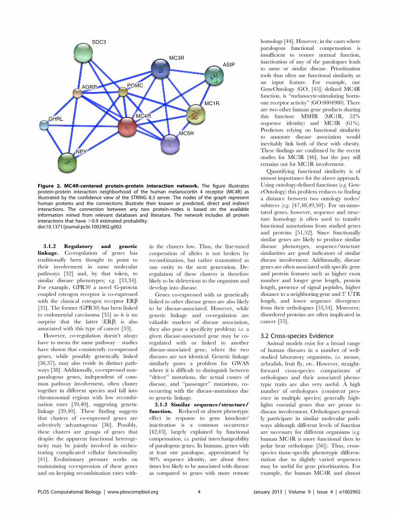
3.1.2 Regulatory and genetic
linkage. Co-regulation of genes has
traditionally been thought to point to
their involvement in same molecular
pathways [32] and, by that token, to
similar disease phenotypes; e.g. [33,34].
For example, GPR30 a novel G-protein
coupled estrogen receptor is co-expressed
with the classical estrogen receptor ERb[33]. The former (GPR30) has been linked
to endometrial carcinoma [35] so it is no
surprise that the latter (ERb) is also
associated with this type of cancer [33].
However, co-regulation doesn’t always
have to mean the same pathway – studies
have shown that consistently co-expressed
genes, while possibly genetically linked
[36,37], may also reside in distinct path-
ways [38]. Additionally, co-expressed non-
paralogous genes, independent of com-
mon pathway involvement, often cluster
together in different species and fall into
chromosomal regions with low recombi-
nation rates [39,40], suggesting genetic
linkage [39,40]. These finding suggests
that clusters of co-expressed genes are
selectively advantageous [36]. Possibly,
these clusters are groups of genes that
despite the apparent functional heteroge-
neity may be jointly involved in orches-
trating complicated cellular functionality
[41]. Evolutionary pressure works on
maintaining co-expression of these genes
and on keeping recombination rates with-
in the clusters low. Thus, the fine-tuned
cooperation of alleles is not broken by
recombination, but rather transmitted as
one entity to the next generation. De-
regulation of these clusters is therefore
likely to be deleterious to the organism and
develop into disease.
Genes co-expressed with or genetically
linked to other disease genes are also likely
to be disease-associated. However, while
genetic linkage and co-regulation are
valuable markers of disease association,
they also pose a specificity problem; i.e. a
given disease-associated gene may be co-
regulated with or linked to another
disease-associated gene, where the two
diseases are not identical. Genetic linkage
similarly poses a problem for GWAS
where it is difficult to distinguish between
‘‘driver’’ mutations, the actual causes of
disease, and ‘‘passenger’’ mutations, co-
occurring with the disease-mutations due
to genetic linkage.
3.1.3 Similar sequence/structure/
function. Reduced or absent phenotypic
effect in response to gene knockout/
inactivation is a common occurrence
[42,43], largely explained by functional
compensation, i.e. partial interchangeability
of paralogous genes. In humans, genes with
at least one paralogue, approximated by
90% sequence identity, are about three
times less likely to be associated with disease
as compared to genes with more remote
homologs [44]. However, in the cases where
paralogous functional compensation is
insufficient to restore normal function,
inactivation of any of the paralogues leads
to same or similar disease. Prioritization
tools thus often use functional similarity as
an input feature. For example, one
GeneOntology (GO, [45]) defined MC4R
function, is ‘‘melanocyte-stimulating horm-
one receptor activity’’ (GO:0004980). There
are two other human gene products sharing
this function: MSHR (MC1R, 52%
sequence identity) and MC3R (61%).
Predictors relying on functional similarity
to annotate disease association would
inevitably link both of these with obesity.
These findings are confirmed by the recent
studies for MC3R [46], but the jury still
remains out for MC1R involvement.
Quantifying functional similarity is of
utmost importance for the above approach.
Using ontology-defined functions (e.g. Gen-
eOntology) this problem reduces to finding
a distance between two ontology nodes/
subtrees (e.g. [47,48,49,50]). For un-anno-
tated genes, however, sequence and struc-
ture homology is often used to transfer
functional annotations from studied genes
and proteins [51,52]. Since functionally
similar genes are likely to produce similar
disease phenotypes, sequence/structure
similarities are good indicators of similar
disease involvement. Additionally, disease
genes are often associated with specific gene
and protein features such as higher exon
number and longer gene length, protein
length, presence of signal peptides, higher
distance to a neighboring gene and 39 UTR
length, and lower sequence divergence
from their orthologues [53,54]. Moreover,
disordered proteins are often implicated in
cancer [55].
3.2 Cross-species EvidenceAnimal models exist for a broad range
of human diseases in a number of well-
studied laboratory organisms, i.e. mouse,
zebrafish, fruit fly, etc. However, straight-
forward cross-species comparisons of
orthologues and their associated pheno-
typic traits are also very useful. A high
number of orthologues (consistent pres-
ence in multiple species) generally high-
lights essential genes that are prone to
disease involvement. Orthologues general-
ly participate in similar molecular path-
ways although different levels of function
are necessary for different organisms (e.g.
human MC4R is more functional then its
polar bear orthologue [56]). Thus, cross-
species tissue-specific phenotypic differen-
tiation due to slightly varied sequences
may be useful for gene prioritization. For
example, the human MC4R and almost
Figure 2. MC4R-centered protein-protein interaction network. The figure illustratesprotein-protein interaction neighborhood of the human melanocortin 4 receptor (MC4R) asillustrated by the confidence view of the STRING 8.3 server. The nodes of the graph representhuman proteins and the connections illustrate their known or predicted, direct and indirectinteractions. The connection between any two protein-nodes is based on the availableinformation mined from relevant databases and literature. The network includes all proteininteractions that have .0.9 estimated probability.doi:10.1371/journal.pcbi.1002902.g002
PLOS Computational Biology | www.ploscompbiol.org 4 January 2013 | Volume 9 | Issue 4 | e1002902
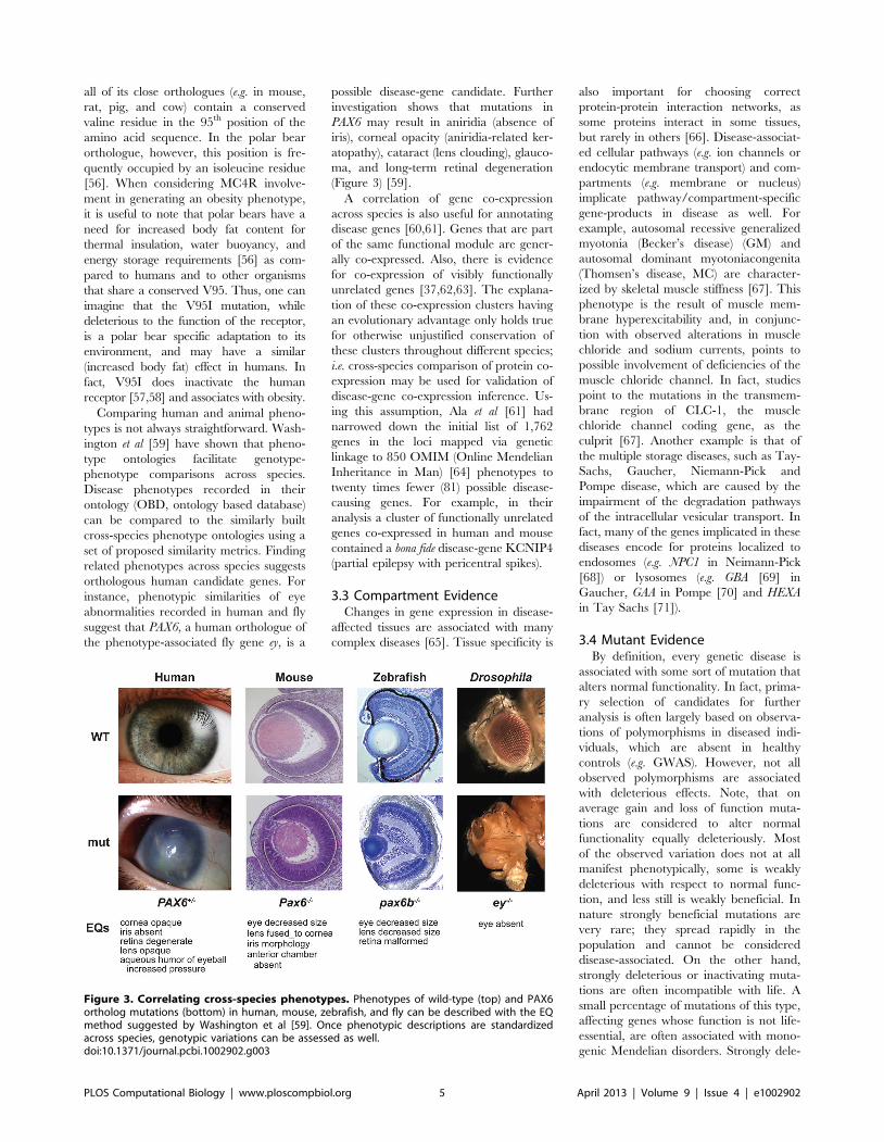
all of its close orthologues (e.g. in mouse,
rat, pig, and cow) contain a conserved
valine residue in the 95th position of the
amino acid sequence. In the polar bear
orthologue, however, this position is fre-
quently occupied by an isoleucine residue
[56]. When considering MC4R involve-
ment in generating an obesity phenotype,
it is useful to note that polar bears have a
need for increased body fat content for
thermal insulation, water buoyancy, and
energy storage requirements [56] as com-
pared to humans and to other organisms
that share a conserved V95. Thus, one can
imagine that the V95I mutation, while
deleterious to the function of the receptor,
is a polar bear specific adaptation to its
environment, and may have a similar
(increased body fat) effect in humans. In
fact, V95I does inactivate the human
receptor [57,58] and associates with obesity.
Comparing human and animal pheno-
types is not always straightforward. Wash-
ington et al [59] have shown that pheno-
type ontologies facilitate genotype-
phenotype comparisons across species.
Disease phenotypes recorded in their
ontology (OBD, ontology based database)
can be compared to the similarly built
cross-species phenotype ontologies using a
set of proposed similarity metrics. Finding
related phenotypes across species suggests
orthologous human candidate genes. For
instance, phenotypic similarities of eye
abnormalities recorded in human and fly
suggest that PAX6, a human orthologue of
the phenotype-associated fly gene ey, is a
possible disease-gene candidate. Further
investigation shows that mutations in
PAX6 may result in aniridia (absence of
iris), corneal opacity (aniridia-related ker-
atopathy), cataract (lens clouding), glauco-
ma, and long-term retinal degeneration
(Figure 3) [59].
A correlation of gene co-expression
across species is also useful for annotating
disease genes [60,61]. Genes that are part
of the same functional module are gener-
ally co-expressed. Also, there is evidence
for co-expression of visibly functionally
unrelated genes [37,62,63]. The explana-
tion of these co-expression clusters having
an evolutionary advantage only holds true
for otherwise unjustified conservation of
these clusters throughout different species;
i.e. cross-species comparison of protein co-
expression may be used for validation of
disease-gene co-expression inference. Us-
ing this assumption, Ala et al [61] had
narrowed down the initial list of 1,762
genes in the loci mapped via genetic
linkage to 850 OMIM (Online Mendelian
Inheritance in Man) [64] phenotypes to
twenty times fewer (81) possible disease-
causing genes. For example, in their
analysis a cluster of functionally unrelated
genes co-expressed in human and mouse
contained a bona fide disease-gene KCNIP4
(partial epilepsy with pericentral spikes).
3.3 Compartment EvidenceChanges in gene expression in disease-
affected tissues are associated with many
complex diseases [65]. Tissue specificity is
also important for choosing correct
protein-protein interaction networks, as
some proteins interact in some tissues,
but rarely in others [66]. Disease-associat-
ed cellular pathways (e.g. ion channels or
endocytic membrane transport) and com-
partments (e.g. membrane or nucleus)
implicate pathway/compartment-specific
gene-products in disease as well. For
example, autosomal recessive generalized
myotonia (Becker’s disease) (GM) and
autosomal dominant myotoniacongenita
(Thomsen’s disease, MC) are character-
ized by skeletal muscle stiffness [67]. This
phenotype is the result of muscle mem-
brane hyperexcitability and, in conjunc-
tion with observed alterations in muscle
chloride and sodium currents, points to
possible involvement of deficiencies of the
muscle chloride channel. In fact, studies
point to the mutations in the transmem-
brane region of CLC-1, the muscle
chloride channel coding gene, as the
culprit [67]. Another example is that of
the multiple storage diseases, such as Tay-
Sachs, Gaucher, Niemann-Pick and
Pompe disease, which are caused by the
impairment of the degradation pathways
of the intracellular vesicular transport. In
fact, many of the genes implicated in these
diseases encode for proteins localized to
endosomes (e.g. NPC1 in Neimann-Pick
[68]) or lysosomes (e.g. GBA [69] in
Gaucher, GAA in Pompe [70] and HEXA
in Tay Sachs [71]).
3.4 Mutant EvidenceBy definition, every genetic disease is
associated with some sort of mutation that
alters normal functionality. In fact, prima-
ry selection of candidates for further
analysis is often largely based on observa-
tions of polymorphisms in diseased indi-
viduals, which are absent in healthy
controls (e.g. GWAS). However, not all
observed polymorphisms are associated
with deleterious effects. Note, that on
average gain and loss of function muta-
tions are considered to alter normal
functionality equally deleteriously. Most
of the observed variation does not at all
manifest phenotypically, some is weakly
deleterious with respect to normal func-
tion, and less still is weakly beneficial. In
nature strongly beneficial mutations are
very rare; they spread rapidly in the
population and cannot be considered
disease-associated. On the other hand,
strongly deleterious or inactivating muta-
tions are often incompatible with life. A
small percentage of mutations of this type,
affecting genes whose function is not life-
essential, are often associated with mono-
genic Mendelian disorders. Strongly dele-
Figure 3. Correlating cross-species phenotypes. Phenotypes of wild-type (top) and PAX6ortholog mutations (bottom) in human, mouse, zebrafish, and fly can be described with the EQmethod suggested by Washington et al [59]. Once phenotypic descriptions are standardizedacross species, genotypic variations can be assessed as well.doi:10.1371/journal.pcbi.1002902.g003
PLOS Computational Biology | www.ploscompbiol.org 5 April 2013 | Volume 9 | Issue 4 | e1002902
terious mutations in the genes whose
function may somehow be compensated
(e.g. via paralogue activity) are associated
with complex disorders, where the level of
compensation affects the observed pheno-
type. Complex disorders may also accu-
mulate weakly deleterious mutations to
generate a strongly negative phenotype.
Intuitively it is clear that a selected
candidate gene, carrying a deleterious
mutation in an affected individual is more
likely to be disease-associated than one
which contains functionally neutral mu-
tants or no variation at all.
3.4.1 Structural variation. Structural
variation (SV) is the least studied of all types
of mutations. It has long been assumed that
less than 10% of human genetic variation is
in the form of genome structural variants
(insertions and deletions, inversions,
translocations, aneuploidy, and copy
number variations - CNVs). However,
because each of the structural variants is
large (kb-Mb scale), the total number of base
pairs affected by SVs may actually be
comparable to the number of base pairs
affected by the much more common SNPs
(single nucleotide polymorphisms).
Moreover, high throughput detection of
structural variants is notoriously difficult
and is only now becoming possible with
better sequencing techniques and CNV
arrays. Thus, more SVs may be discovered
in the near future. We do not currently know
what proportion of genetic disease is caused
by SVs, but we suspect that it is high.
Due to the above mentioned constraints
on SV identification, there are only ,180
thousand structural variants reported in
one of the most complete mutation
collections – the Database of Genomic
Variants, DGV [72]. Gross changes to
genome sequence are very likely to be
disease associated, but also frequently gene
non-specific. For instance, Down’s syn-
drome, trisomy 21, is an example of a
whole extra chromosome gain and cri du
chat syndrome results from the deletion of
the short arm of chromosome 5 [73]. All
of the genes found in these regions of the
genome are, by default, associated with
the observed disease but neither can be
considered primarily causal. When the
damage is less extensive the genes involved
may be further evaluated for causation.
For instance, several epilepsy-associated
genes are known, but functionally-signifi-
cant mutations in these account for only a
small fraction of observed disease cases.
One study [74] reports that CNV mutants
found in epileptic individuals but not in the
general population account for nearly nine
percent of all cases. Among these are CNVs
resulting from deletions in AUTS2 and
CNTNAP2 genes. Both of these genes have
been implicated in other neurological
disorders [75,76] reaffirming the possible
disease link. Inversions, translocations and
large deletions and insertions have all been
implicated in different forms of disease.
Even very small indels, resulting in an open-
reading frame shift (frameshift mutations),
are often sufficient to cause disease. For
instance, one of the causes of Tay-Sachs is a
deletion of a single cytosine nucleotide in
the coding sequence of a lysosomal enzyme
beta-hexosaminidase [71].
In most cases of diseases that are
associated with SVs the prioritization of
disease-causing genes is reduced to finding
those that are directly affected by the
mutation. Lots of work has been done in
this direction, including development of
the CNVinetta package [77] for mining
and visualizing CNVs, GASV approach
for identifying structural variation bound-
aries more precisely [78], and software
created by Ritz et al for searching for
structural variants in strobe sequencing
data [79]. SV identification is still a new
field, but the advances in methodologies
will have a great impact on our under-
standing and study of many of the known
diseases.
3.4.2 Nucleotide polymorphisms. The
other ,90% of human variation exists in
the form of SNPs (single nucleotide
polymorphisms) and MNPs (multi-
nucleotide polymorphisms; consecutive
nucleotide substitutions, usually of length
two or three). A single human genome is
expected to contain roughly 10–15 million
SNPs per person [80]. As many as 93% of
all human genes contain at least one SNP
and 98% of all genes are in the vicinity
(,5 kb) of a SNP [81]. The latest release of
NCBI dbSNP database [82] (build 137)
contains nearly 43 million validated human
SNPs, 17.5 million of which have been
experimentally mapped to functionally
distinct regions of the genome (i.e. mRNA
UTR, intron, or coding regions). Non-
coding region SNPs (,17.2 million) are
trivially more prevalent than coding SNPs
(,432 thousand) as non-coding DNA
makes up the vast majority of the
genome. Coding SNPs, however, are
over-represented in disease associations;
e.g. OMIM contains 2430 non-coding
SNPs (0.0001% of all) and 5327 coding
ones (0.01% of all – 100-fold enrichment).
Due to the redundancy of the genetic code,
coding SNPs can be further subdivided into
synonymous (no effect on protein sequence)
and non-synonymous (single amino acid
substitution) SNPs. Simple statistics of the
genetic code suggest that synonymous
SNPs should account for 24% of all
coding-region SNPs. dbSNP data suggests
an even larger percentage of synonymity –
,188 thousand (44%), which is possibly
due to evolutionary pressure eliminating
functionally deleterious non-synonymous
SNPs. MNPs are rare as compared to
SNPs, but are over-represented amongst
the protein altering variants, almost always
changing the affected amino acid, or two
neighboring ones, or introducing a
nonsense mutation (stop-codon) [83].
Identifying and annotating functional
effects of SNPs and MNPs is important in
the context of gene prioritization because
genes selected for further disease-associa-
tion studies are more likely to contain a
deleterious mutation or be under the
control of one (e.g. mutations affecting
transcription factor or microRNA binding
sites). In recent years a number of methods
were created for identifying mutations as
functionally deleterious. PromoLign [84],
PupaSNP finder [85], and RAVEN [86]
look for SNPs affecting transcription,
SNPper [87] finds and annotates SNP
locations, conservation, and possible func-
tionalities so that they can be visually
assessed, and SNPselector [88] and
FASTSNP [89] assess various SNP fea-
tures such as whether it alters the binding
site of a transcription factor, affects the
promoter/regulatory region, damages the
39 UTR sequence that may affect post-
transcriptional regulation, or eliminates a
necessary splice site. Coding synonymous
SNPs have recently been shown to have
the same chance of being involved in a
disease mechanism as non-coding SNPs
[90]. This effect may be due to codon
usage bias or to changes in splicing or
miRNA binding sites [91]. However, few
(if any) computational methods are able
make predictions with regard to their
functional effects.
Non-synonymous SNPs are somewhat
more studied. Early termination of the
protein is very often associated with
disease so genes with nonsense mutants
are automatically moved up in the list of
possible suspects. Missense SNPs and
MNPs, which alter the protein sequence
without destroying it, may or may not be
disease associated. In fact, most methods
estimate that only 25–30% of the nsSNPs
negatively affect protein function [92].
Databases like OMIM [93], and more
explicitly, SNPdbe [94], SNPeffect [95],
PolyDoms [96], Mutation@A Glance [97]
and DMDM [98] map SNPs to known
structural/functional effects and diseases.
Computational tools that make predictions
about functional and disease-associated
effects of SNPs include SNAP [99,100],
SIFT [101,102], PolyPhen [103,104],
PLOS Computational Biology | www.ploscompbiol.org 6 January 2013 | Volume 9 | Issue 4 | e1002902
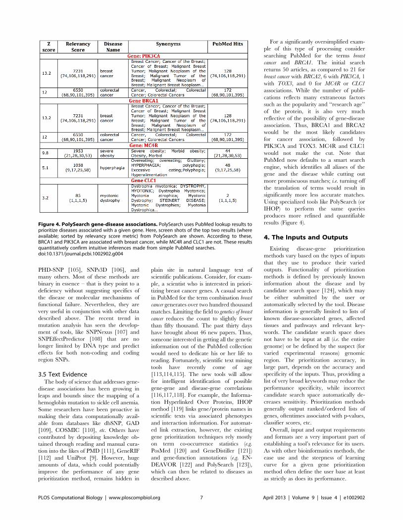
PHD-SNP [105], SNPs3D [106], and
many others. Most of these methods are
binary in essence – that is they point to a
deficiency without suggesting specifics of
the disease or molecular mechanisms of
functional failure. Nevertheless, they are
very useful in conjunction with other data
described above. The recent trend in
mutation analysis has seen the develop-
ment of tools, like SNPNexus [107] and
SNPEffectPredictor [108] that are no
longer limited by DNA type and predict
effects for both non-coding and coding
region SNPs.
3.5 Text EvidenceThe body of science that addresses gene-
disease associations has been growing in
leaps and bounds since the mapping of a
hemoglobin mutation to sickle cell anemia.
Some researchers have been proactive in
making their data computationally avail-
able from databases like dbSNP, GAD
[109], COSMIC [110], etc. Others have
contributed by depositing knowledge ob-
tained through reading and manual cura-
tion into the likes of PMD [111], GeneRIF
[112] and UniProt [9]. However, huge
amounts of data, which could potentially
improve the performance of any gene
prioritization method, remains hidden in
plain site in natural language text of
scientific publications. Consider, for exam-
ple, a scientist who is interested in priori-
tizing breast cancer genes. A casual search
in PubMed for the term combination breast
cancer generates over two hundred thousand
matches. Limiting the field to genetics of breast
cancer reduces the count to slightly fewer
than fifty thousand. The past thirty days
have brought about 46 new papers. Thus,
someone interested in getting all the genetic
information out of the PubMed collection
would need to dedicate his or her life to
reading. Fortunately, scientific text mining
tools have recently come of age
[113,114,115]. The new tools will allow
for intelligent identification of possible
gene-gene and disease-gene correlations
[116,117,118]. For example, the Informa-
tion Hyperlinked Over Proteins, IHOP
method [119] links gene/protein names in
scientific texts via associated phenotypes
and interaction information. For automat-
ed link extraction, however, the existing
gene prioritization techniques rely mostly
on term co-occurrence statistics (e.g.
PosMed [120] and GeneDistiller [121])
and gene-function annotations (e.g. EN-
DEAVOR [122] and PolySearch [123]),
which can then be related to diseases as
described above.
For a significantly oversimplified exam-
ple of this type of processing consider
searching PubMed for the terms breast
cancer and BRCA1. The initial search
returns 50 articles, as compared to 21 for
breast cancer with BRCA2, 6 with PIK3CA, 1
with TOX3, and 0 for MC4R or CLC1
associations. While the number of publi-
cations reflects many extraneous factors
such as the popularity and ‘‘research age’’
of the protein, it is also very much
reflective of the possibility of gene-disease
association. Thus, BRCA1 and BRCA2
would be the most likely candidates
for cancer association, followed by
PIK3CA and TOX3. MC4R and CLC1
would not make the cut. Note that
PubMed now defaults to a smart search
engine, which identifies all aliases of the
gene and the disease while cutting out
more promiscuous matches; i.e. turning off
the translation of terms would result in
significantly more less accurate matches.
Using specialized tools like PolySearch (or
IHOP) to perform the same queries
produces more refined and quantifiable
results (Figure 4).
4. The Inputs and Outputs
Existing disease-gene prioritization
methods vary based on the types of inputs
that they use to produce their varied
outputs. Functionality of prioritization
methods is defined by previously known
information about the disease and by
candidate search space [124], which may
be either submitted by the user or
automatically selected by the tool. Disease
information is generally limited to lists of
known disease-associated genes, affected
tissues and pathways and relevant key-
words. The candidate search space does
not have to be input at all (i.e. the entire
genome) or be defined by the suspect (for
varied experimental reasons) genomic
region. The prioritization accuracy, in
large part, depends on the accuracy and
specificity of the inputs. Thus, providing a
list of very broad keywords may reduce the
performance specificity, while incorrect
candidate search space automatically de-
creases sensitivity. Prioritization methods
generally output ranked/ordered lists of
genes, oftentimes associated with p-values,
classifier scores, etc.
Overall, input and output requirements
and formats are a very important part of
establishing a tool’s relevance for its users.
As with other bioinformatics methods, the
ease use and the steepness of learning
curve for a given gene prioritization
method often define the user base at least
as strictly as does its performance.
Figure 4. PolySearch gene-disease associations. PolySearch uses PubMed lookup results toprioritize diseases associated with a given gene. Here, screen shots of the top two results (whereavailable; sorted by relevancy score metric) from PolySearch are shown. According to these,BRCA1 and PIK3CA are associated with breast cancer, while MC4R and CLC1 are not. These resultsquantitatively confirm intuitive inferences made from simple PubMed searches.doi:10.1371/journal.pcbi.1002902.g004
PLOS Computational Biology | www.ploscompbiol.org 7 April 2013 | Volume 9 | Issue 4 | e1002902

Box 2. Illustrating basic functionality of a standard (on-line fully-interconnected feed-forwardsigmoid-function back-propagating) neural network.
In Figure 5A example network there are three fully interconnected layers of neurons (input, hidden, and output layers); i.e. eachneuron in one layer is connected to every neuron in the next layer. The three input neurons encode biologically relevant piecesof data relating a given gene G to a given disease D. For each G and D, i_neuron1 is the fraction of articles (out of 1000)containing in-text co-occurrences of G and D and i_neuron2 represents the presence/absence of a sequence-similar gene G’associated with D (i_neuron3 = G/G’ sequence identity). The hidden (inference) layer consists of two neurons h_neuron1 andh_neuron2 with activation thresholds h1 and h2, respectively. The single output, o_neuron (threshold hO) represents theinvolvement of G in causing D: 0 = no involvement, 1 = direct causation. The starting weights of the network (wi1-h1, wi1-h2…wh2-o)are arbitrarily assigned random values between 0 and 1. Intuitively, the function of the network is to convert input neuron valuesinto output neuron values via a network of weights and hidden neurons. Mathematically, the network is described as follows:
The value (dx) of neuron x is the sum of inputs into x from the previous layer of neurons (Yi = 1Rn in general; in our example: I1R3,H1R2). Each of the n inputs is a product of value of neuron Yi and weight of connection between Yi and x (wYiRx).
dx~Xn
i~1
YiwYi?x
The value of the output (zx) of a neuron x based on its dx and its threshold hx is:
zx~f (dxzhx)
In our case, the function (f) is a sigmoid, where a is a real number constant (optimized for any given network, but generallyinitially chosen to be between 0.5 and 2).
f (x)~1
1ze{ax
Thus, to compute the output of every neuron in the network we need to use the formula:
zx~1
1ze{a(dxzhx)
Note, that to compute the output of the o_neuron (zO; the prediction made by the network) we first have to compute theoutputs of all h_neurons (zHi = 1Rn).
In a supervised learning paradigm, experimentally established pairs of inputs and outputs are given to the network duringtraining (Figure 5C). After each input, the network output (zO) is compared to the observed result (R). If the network makes aclassification error its weights are adjusted to reflect that error. Establishing the best way to update weights and thresholds inresponse to error is of the major challenges of neural networks. Many techniques use some form of the delta rule – a gradientdescent-based optimization algorithm that makes changes to function variables proportionate to the negative of theapproximate gradient of the function at the given point. [It’s OK if you didn’t understand that sentence – the basic idea is tochange the weights and thresholds in the direction opposite of the direction of the error]. In our example, we use the delta rulewith back-propagation. This means that to compute the error of the hidden layer, the threshold of the output layer (hO) and theweights connecting the hidden layer to the output layer (wh1RO, wh2RO) need to be changed first.
The steps are as follows:
1. Compute the error (eO) of zO as compared to result R. Note, that the difference between the expected and the observed valuesdefines the gradient (g) at the output neuron.
eO~zO(1{zO)(R{zO)
2. Compute the change in the threshold of the output layer (DhO), using a variable l, the learning rate constant - a real number,often initialized to 0.1–0.2 and optimized for each network)
DhO~leO
PLOS Computational Biology | www.ploscompbiol.org 8 January 2013 | Volume 9 | Issue 4 | e1002902
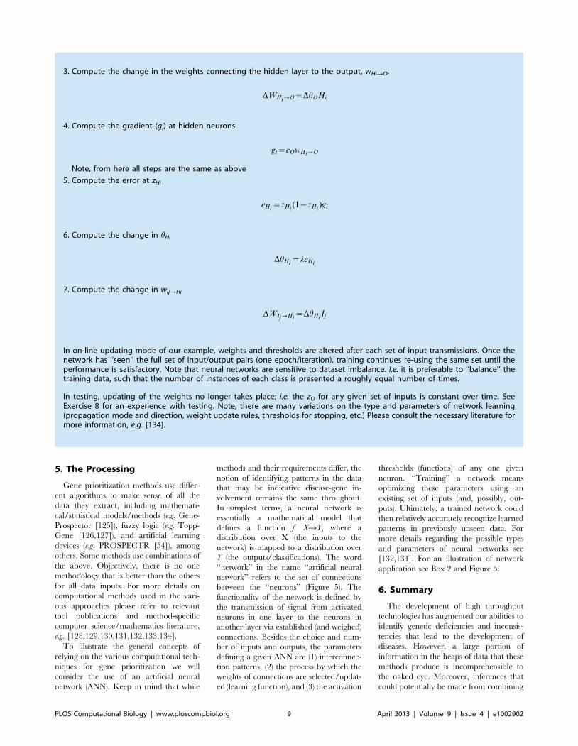
5. The Processing
Gene prioritization methods use differ-
ent algorithms to make sense of all the
data they extract, including mathemati-
cal/statistical models/methods (e.g. Gene-
Prospector [125]), fuzzy logic (e.g. Topp-
Gene [126,127]), and artificial learning
devices (e.g. PROSPECTR [54]), among
others. Some methods use combinations of
the above. Objectively, there is no one
methodology that is better than the others
for all data inputs. For more details on
computational methods used in the vari-
ous approaches please refer to relevant
tool publications and method-specific
computer science/mathematics literature,
e.g. [128,129,130,131,132,133,134].
To illustrate the general concepts of
relying on the various computational tech-
niques for gene prioritization we will
consider the use of an artificial neural
network (ANN). Keep in mind that while
methods and their requirements differ, the
notion of identifying patterns in the data
that may be indicative disease-gene in-
volvement remains the same throughout.
In simplest terms, a neural network is
essentially a mathematical model that
defines a function f: XRY, where a
distribution over X (the inputs to the
network) is mapped to a distribution over
Y (the outputs/classifications). The word
‘‘network’’ in the name ‘‘artificial neural
network’’ refers to the set of connections
between the ‘‘neurons’’ (Figure 5). The
functionality of the network is defined by
the transmission of signal from activated
neurons in one layer to the neurons in
another layer via established (and weighed)
connections. Besides the choice and num-
ber of inputs and outputs, the parameters
defining a given ANN are (1) interconnec-
tion patterns, (2) the process by which the
weights of connections are selected/updat-
ed (learning function), and (3) the activation
thresholds (functions) of any one given
neuron. ‘‘Training’’ a network means
optimizing these parameters using an
existing set of inputs (and, possibly, out-
puts). Ultimately, a trained network could
then relatively accurately recognize learned
patterns in previously unseen data. For
more details regarding the possible types
and parameters of neural networks see
[132,134]. For an illustration of network
application see Box 2 and Figure 5.
6. Summary
The development of high throughput
technologies has augmented our abilities to
identify genetic deficiencies and inconsis-
tencies that lead to the development of
diseases. However, a large portion of
information in the heaps of data that these
methods produce is incomprehensible to
the naked eye. Moreover, inferences that
could potentially be made from combining
3. Compute the change in the weights connecting the hidden layer to the output, wHiRO.
DWHi?O~DhOHi
4. Compute the gradient (gi) at hidden neurons
gi~eOwHi?O
Note, from here all steps are the same as above
5. Compute the error at zHi
eHi~zHi
(1{zHi)gi
6. Compute the change in hHi
DhHi~leHi
7. Compute the change in wIjRHi
DWIj?Hi~DhHi
Ij
In on-line updating mode of our example, weights and thresholds are altered after each set of input transmissions. Once thenetwork has ‘‘seen’’ the full set of input/output pairs (one epoch/iteration), training continues re-using the same set until theperformance is satisfactory. Note that neural networks are sensitive to dataset imbalance. I.e. it is preferable to ‘‘balance’’ thetraining data, such that the number of instances of each class is presented a roughly equal number of times.
In testing, updating of the weights no longer takes place; i.e. the zO for any given set of inputs is constant over time. SeeExercise 8 for an experience with testing. Note, there are many variations on the type and parameters of network learning(propagation mode and direction, weight update rules, thresholds for stopping, etc.) Please consult the necessary literature formore information, e.g. [134].
PLOS Computational Biology | www.ploscompbiol.org 9 April 2013 | Volume 9 | Issue 4 | e1002902
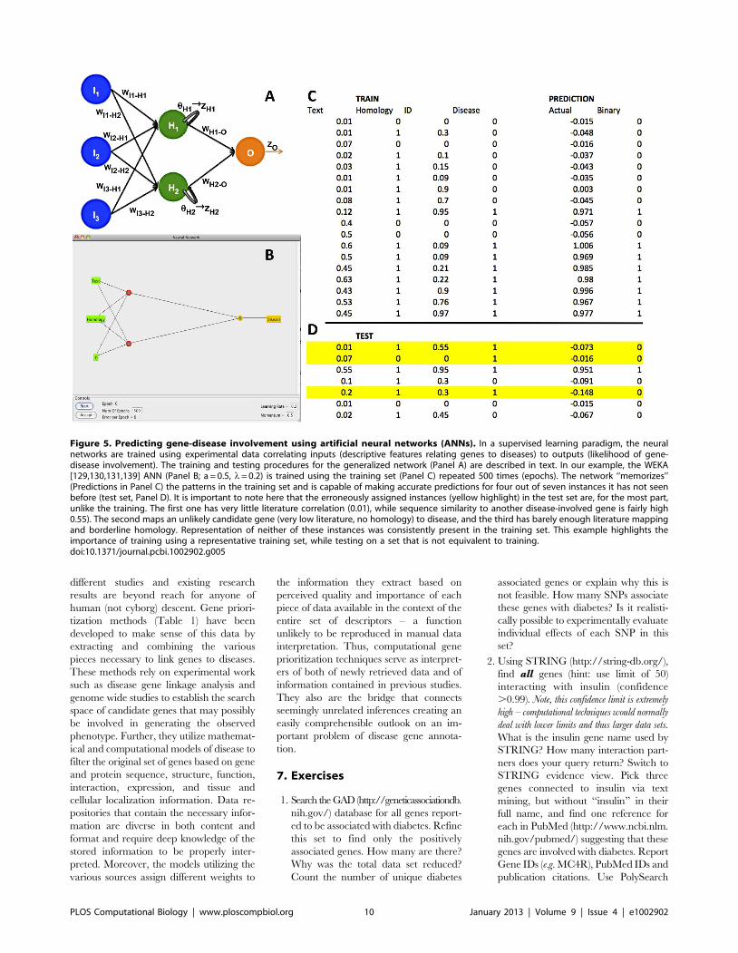
different studies and existing research
results are beyond reach for anyone of
human (not cyborg) descent. Gene priori-
tization methods (Table 1) have been
developed to make sense of this data by
extracting and combining the various
pieces necessary to link genes to diseases.
These methods rely on experimental work
such as disease gene linkage analysis and
genome wide studies to establish the search
space of candidate genes that may possibly
be involved in generating the observed
phenotype. Further, they utilize mathemat-
ical and computational models of disease to
filter the original set of genes based on gene
and protein sequence, structure, function,
interaction, expression, and tissue and
cellular localization information. Data re-
positories that contain the necessary infor-
mation are diverse in both content and
format and require deep knowledge of the
stored information to be properly inter-
preted. Moreover, the models utilizing the
various sources assign different weights to
the information they extract based on
perceived quality and importance of each
piece of data available in the context of the
entire set of descriptors – a function
unlikely to be reproduced in manual data
interpretation. Thus, computational gene
prioritization techniques serve as interpret-
ers of both of newly retrieved data and of
information contained in previous studies.
They also are the bridge that connects
seemingly unrelated inferences creating an
easily comprehensible outlook on an im-
portant problem of disease gene annota-
tion.
7. Exercises
1. Search the GAD (http://geneticassociationdb.
nih.gov/) database for all genes report-
ed to be associated with diabetes. Refine
this set to find only the positively
associated genes. How many are there?
Why was the total data set reduced?
Count the number of unique diabetes
associated genes or explain why this is
not feasible. How many SNPs associate
these genes with diabetes? Is it realisti-
cally possible to experimentally evaluate
individual effects of each SNP in this
set?
2. Using STRING (http://string-db.org/),
find all genes (hint: use limit of 50)
interacting with insulin (confidence
.0.99). Note, this confidence limit is extremely
high – computational techniques would normally
deal with lower limits and thus larger data sets.
What is the insulin gene name used by
STRING? How many interaction part-
ners does your query return? Switch to
STRING evidence view. Pick three
genes connected to insulin via text
mining, but without ‘‘insulin’’ in their
full name, and find one reference for
each in PubMed (http://www.ncbi.nlm.
nih.gov/pubmed/) suggesting that these
genes are involved with diabetes. Report
Gene IDs (e.g. MC4R), PubMed IDs and
publication citations. Use PolySearch
Figure 5. Predicting gene-disease involvement using artificial neural networks (ANNs). In a supervised learning paradigm, the neuralnetworks are trained using experimental data correlating inputs (descriptive features relating genes to diseases) to outputs (likelihood of gene-disease involvement). The training and testing procedures for the generalized network (Panel A) are described in text. In our example, the WEKA[129,130,131,139] ANN (Panel B; a = 0.5, l= 0.2) is trained using the training set (Panel C) repeated 500 times (epochs). The network ‘‘memorizes’’(Predictions in Panel C) the patterns in the training set and is capable of making accurate predictions for four out of seven instances it has not seenbefore (test set, Panel D). It is important to note here that the erroneously assigned instances (yellow highlight) in the test set are, for the most part,unlike the training. The first one has very little literature correlation (0.01), while sequence similarity to another disease-involved gene is fairly high0.55). The second maps an unlikely candidate gene (very low literature, no homology) to disease, and the third has barely enough literature mappingand borderline homology. Representation of neither of these instances was consistently present in the training set. This example highlights theimportance of training using a representative training set, while testing on a set that is not equivalent to training.doi:10.1371/journal.pcbi.1002902.g005
PLOS Computational Biology | www.ploscompbiol.org 10 January 2013 | Volume 9 | Issue 4 | e1002902
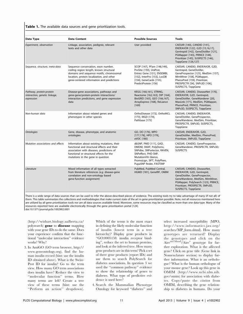
(http://wishart.biology.ualberta.ca/
polysearch) gene to disease mapping
with your gene IDs to do the same. Does
your experience confirm that the func-
tional ‘‘molecular interaction’’ evidence
works? Why?
3. In AmiGO (GO term browser, http://
www.geneontology.org), find the hu-
man insulin record (hint: use the insulin
ID obtained above). What is the Swiss-
Prot ID for insulin? Go to the term
view. How many GO term associations
does insulin have? Reduce the view to
‘‘molecular function’’ terms. How
many terms are left? Create a tree
view of these terms (hint: use the
‘‘Perform an action’’ dropdown).
Which of the terms is the most exact
in defining the likely molecular function
of insulin (lowest term in a tree
hierarchy)? Display gene products in
‘‘GO:0005158: insulin receptor bind-
ing’’, reduce the set to human proteins,
and look at the inferred tree. How many
gene products are in this term? Pick a set
of three gene products (report IDs) and
use them to search PolySearch for
diabetes associations. In question 3 we
used the ‘‘common pathway’’ evidence
to show the relationship of genes to
diabetes. What type of predictive evi-
dence is used here?
4. Search the Mammalian Phenotype
Ontology for keyword ‘‘diabetes’’ and
select increased susceptibility (MPO,
http://www.informatics. jax.org/
searches/MP_form.shtml). How many
genotypes are returned? Display
the genotypes and click on the
Airetm1Mand/Aire+ genotype for fur-
ther exploration. What is the affected
gene? Click on gene title (Gene link in
Nomenclature section) to display fur-
ther information. What is an ortholo-
gue? What is the human orthologue of
your mouse gene? Look up this gene in
OMIM (http://www.ncbi.nlm.nih.
gov/omim) for association with diabe-
tes. Copy/paste the citation from
OMIM, describing the gene relation-
ship to diabetes in humans. Do your
Table 1. The available data sources and gene prioritization tools.
Data Type Data Content Possible Sources Tools
Experiment, observation Linkage, association, pedigree, relevanttexts and other data
User provided CAESAR [140], CANDID [141],ENDEAVOR [122], G2D [15,16,17],Gentrepid [142], GeneDistiller [121],PGMapper [143], PRINCE [144],Prioritizer [145], SUSPECTS [146],ToppGene [126,127]
Sequence, structure, meta-data Sequence conservation, exon number,coding region length, known structuraldomains and sequence motifs, chromosomallocation, protein localization, and othergene-centered information and predictions
SCOP [147], PFam [148,149],ProSite [150], UniProt,Entrez Gene [151], ENSEMBL[152], InterPro [153], LocDB[154], GeneCards [155],PredictProtein [156]
CAESAR, CANDID, ENDEAVOR, G2D,Gentrepid, GeneDistiller,GeneProspector [125], MedSim [157],MimMiner [158], PGMapper,PhenoPred [159], Prioritizer,PROSPECTR [54], SNPs3D [106],SUSPECTS, ToppGene
Pathway, protein-proteininteraction, genetic linkage,expression
Disease-gene associations, pathways andgene-gene/protein-protein interactions/interaction predictions, and gene expressiondata
KEGG [160,161], STRING,Reactome [162,163], DIP [164],BioGRID [165], GEO [166,167],ArrayExpress [168], ReLiance[169]
CAESAR, CANDID, DiseaseNet [170],ENDEAVOR, G2D, Gentrepid,GeneDistiller, GeneWanderer [20],MaxLink [171], MedSim, PGMapper,PhenoPred, PRINCE, Prioritizer,SNPs3D, SUSPECTS, ToppGene
Non-human data Information about related genes andphenotypes in other species
OrthoDisease [172], OrthoMCL[173], MGD [174],Pathbase [175]
CAESAR, CANDID, ENDEAVOR,GeneDistiller, GeneProspector,GeneWanderer, MedSim, Prioritizer,PROSPECTR, SNPs3D, SUSPECTS,ToppGene
Ontologies Gene, disease, phenotype, and anatomicontologies
GO, DO [176], MPO[177,178], HPO [179],eVOC [180]
CAESAR, ENDEAVOR, G2D,GeneDistiller, MedSim, PhenoPred,Prioritizer, SNPs3D, ToppGene
Mutation associations and effects Information about existing mutations, theirfunctional and structural effects and theirassociation with diseases, predictions offunctional or structural effects for themutations in the gene in question
dbSNP, PMD [111], GAD,DMDM, SNAP, PolyDoms,SNPdbe, SNPselector, RAVEN,SNPeffect, PHD-SNP,Mutation@A Glance,PromoLign, SIFT, PolyPhen,PupaSNP finder, FASTSNP
CAESAR, CANDID, GeneProspector,GeneWanderer, PROSPECTR, SNPs3D,SUSPECTS
Literature Mixed information of all types extractedfrom literature references (e.g. disease-genecorrelation and non-ontology basedgene-function assignment)
PubMed, PubMed Central,HGMD [181], GeneRIF, OMIM
CAESAR, CANDID, DiseaseNet,ENDEAVOR, G2D, Gentrepid,GeneDistiller, GeneProspector,GeneWanderer, MedSim, MimMiner,PGMapper, PolySearch [123], PRINCE,Prioritizer, PROSPECTR, SNPs3D,SUSPECTS, ToppGene
There is a wide range of data sources that can be used to infer the above-described pieces of evidence. The existing tools try to take advantage of many (if not all) ofthem. This table summarizes the collections and methodologies that make current state of the art in gene prioritization possible. Note, not all resources mentioned hereare utilized by all gene prioritization tools nor are all data sources available listed. Moreover, some resources may be classified as more than one data-type. Many of theresources reported here are available electronically through the gene prioritization portal [124].doi:10.1371/journal.pcbi.1002902.t001
PLOS Computational Biology | www.ploscompbiol.org 11 April 2013 | Volume 9 | Issue 4 | e1002902
results confirm the ‘‘cross-species’’
evidence?
5. Search GeneCards (http://www.
genecards.org, utilize advanced search)
for genes expressing in the pancreas
(hint: pancreatic tissue is often affected
in diabetes). How many are there?
Explore the GeneCard for CCKBR for
diabetes association. Do you find that
this gene confirms the ‘‘disease com-
partment’’ evidence? What database,
referenced in GeneCards, contains the
CCKBR-diabetes association? Now
look at the GeneCard of PLEKHG4.
Is there evidence for this gene being
associated with diabetes (whether in the
GeneCards record or otherwise)? Ex-
plain your ideas in detail, paying
special attention to the ‘‘disease com-
partment’’ line of evidence.
6. Search UniProt (http://www.uniprot.
org) for all reviewed [reviewed:yes]
human [organism:‘‘Homo sapiens
[9606]’’] protein entries that contain
natural variants with reference to
diabetes [annotation:(type:natural_var-
iations diabetes)]. Use advanced search
with specific limits (i.e. sequence anno-
tation, natural_variations, term diabe-
tes). How many proteins fit this de-
scription? Locate the entry for insulin
(identifier from question 3) and find the
total number of known coding variants
of this sequence. How many are
annotated as associated with any form
of diabetes? (hint: read the general
annotation section for correspondence
of abbreviations to types of diabetes).
Run SNAP (http://www.rostlab.org/
services/snap/) to predict functional
effects of all variants. (hint: use comma
separated batch submit). How many
are predicted to be functionally non-
neutral? Do SNAP predictions of
functional effect correlate with anno-
tated disease associations? Does this
result confirm the ‘‘mutant implica-
tion’’ for nsSNPs?
7. Search PolySearch for all genes associ-
ated with diabetes. How many results
are returned? Look at the PubMed
articles that associate ‘‘hemoglobin’’
with diabetes (follow the link from
PolySearch). How many are there?
Do you find this number large enough
to convince you of hemoglobin-diabe-
tes association and why? From reading
article titles/extracted sentences, can
you identify a biological reason for
connecting hemoglobin to diabetes? If
one looks especially convincing, cite
that article (hint: its OK to not find
one). For the first three articles, can
you identify a biological reason for
connecting hemoglobin to diabetes?
Go back to the list of diabetes related
genes and look at TCF7L2 articles. Are
the biological reasons for matching
TCF7L2 to diabetes clearly defined?
Cite the most convincing article. Why
do you think TCF7L2 is ranked lower
in association than hemoglobin? Is
there significant evidence for calcium
channel (CACNA1E) involvement in
diabetes? Consider the PubMed cita-
tions. Do you agree with PolySearch
classification of this gene-disease asso-
ciation? Does your experience with
PolySearch confirm the ‘‘text evi-
dence’’ function of gene prioritization
methods?
8. WEKA exercises (choose one).
8. Download and install WEKA ( http://
www.cs.waikato.ac.nz/,ml/weka/).
Using a text-editor (or Microsoft Excel)
create comma delimited values (CSV)
files identical to the ones described in
Figure 5C–D (i.e. copy over the train-
ing and testing files and replace spaces
with commas). Save the files and open
the training file in WEKA’s Explorer
GUI. Open the training file in
WEKA’s Explorer GUI. You should
have four columns of data (Text,
Homology, ID, Disease) corresponding
to four attributes of each data instance.
8.1. Defined Questions: Run the Mul-
tiLayer Perceptron with parame-
ters (momentum = 0.5, learn-
ing = 0.2, trained using the
training set, Figure 5C, repeated
500 times/epochs). Test with the
test set (Figure 5D) and output
predictions for each test entry
(make a screenshot). Assuming that
everything predicted below 0 is 0,
and everything above is 1. What is
your performance (number of true/
false positives/negatives, positive/
negative accuracy/coverage, over-
all accuracy)? Try using the Deci-
sion Stump classifier with default
parameters (take screenshot of out-
put). If everything below 0.5 is 0,
and everything above is 1, what is
your performance? Is it better or
worse than the neural net?
8.2. Open ended: Experiment with dif-
ferent tools available from WEKA’s
Classify section setting the testing set
to your test-file’s location. First, run
the MultiLayer Perceptron with
parameters as descr ibed in
Figure 5, then try to alter the
parameters (momentum term,
learning rate, and number of ep-
ochs). Try using Linear Regression,
Decision Table, or Decision Stump
classifiers with default parameters.
Is your performance on the test set
better or worse? Close the WEKA
Explorer, reformat your train/test
files in the text editor to replace
Disease column values by Booleans
(True/False) values, and re-open
the training file. Use BayesianNet
and RandomForest classifiers to test
on the testing file. Does you perfor-
mance improve? Note, that without
further understanding of each of the
tools, it is nearly impossible to
determine which method is applica-
ble to your data.
Answers to the Exercises can be found
in Text S1.
Supporting Information
Text S1 Answers to Exercises.
(DOCX)
Acknowledgments
The author would like to thank Chengsheng
Zhu (Rutgers University), Chani Weinreb
(Columbia University) and Nikolay Samusik
(Max Planck Institute, Dresden) for critical
reading and comments to the manuscript. She
also acknowledges the help of Gregory Behrin-
ger (Rutgers University) and of all of the
students of the Spring 2012 Bioinformatics
course at Rutgers in testing the exercises.
PLOS Computational Biology | www.ploscompbiol.org 12 January 2013 | Volume 9 | Issue 4 | e1002902
Further Reading
N Alterovitz G, Ramoni M, eds. (2010) Knowledge-based bioinformatics: from analysis to interpretation. Padstow, Cornwall: JohnWiley and Sons Ltd.
N Bromberg Y, Capriotti E, eds. (2012) SNP-SIG 2011: identification and annotation of SNPs in the context of structure, functionand disease. Proceedings from SNP-SIG 2011 conference, Vienna, Austria. BMC Genomics 13 Supp 4.
N Chen JY, Youn E, Mooney SD (2009) Connecting protein interaction data, mutations, and disease using bioinformatics.Methods Mol Biol 541: 449–461.
N Dalkilic MM, Costello JC, Clark WT, Radivojac P (2008) From protein-disease associations to disease informatics. Front Biosci 13:3391–3407.
N Evans JA, Rzhetsky A (2011) Advancing science through mining libraries, ontologies, and communities. J Biol Chem 286:23659–23666.
N Kann MG (2007) Protein interactions and disease: computational approaches to uncover the etiology of diseases. BriefBioinform 8: 333–346.
N Krallinger M, Leitner F, Valencia A (2010) Analysis of biological processes and diseases using text mining approaches. MethodsMol Biol 593: 341–382.
N Liberles DA, Teichmann SA, Bahar I, Bastolla U, Bloom J, et al. (2012) The interface of protein structure, protein biophysics, andmolecular evolution. Protein Sci 21: 769–785.
N Maulik U, Bandyopadhyay S, Wang JTL, eds. (2010) Computational intelligence and pattern analysis in biological informatics.Hoboken, NJ: John Wiley and Sons, Inc.
N Mooney SD, Krishnan VG, Evani US (2010) Bioinformatic tools for identifying disease gene and SNP candidates. Methods MolBiol 628: 307–319.
N Moreau Y, Tranchevent LC (2012) Computational tools for prioritizing candidate genes: boosting disease gene discovery. NatRev Genet 13: 523–536.
N Oti M, Brunner HG (2007) The modular nature of genetic diseases. Clin Genet 71: 1–11.
N Piro RM, Di Cunto F (2007) Computational approaches to disease-gene prediction: rationale, classification and successes. FEBSJ 279: 678–696.
Glossary
N Annotation – any additional information about a genetic sequence. Annotation types are extremely varied, includingfunctional, structural, regulatory, location-related, organism-specific, experimentally derived, predicted, etc.
N CNV, copy number variation – an alteration of the genome, which results in an individual having a non-standard number ofcopies of one or more DNA sections.
N Gene prioritization – the process of arranging possible disease causing genes in order of their likelihood in diseaseinvolvement.
N GWAS, genome wide association studies – the examination of all genes in the genome to correlate their variation tophenotypic trait variation across individuals in a given population.
N Genetic linkage – tendency of certain genetic regions on the same chromosome to be inherited together more often thanexpected due to limited recombination between them.
N Genetic marker – a DNA sequence variant with a known location that can be used to identify specific subsets of individuals(cells, species, individual organisms, etc.).
N Homologue – a gene derived from a common ancestor with the reference gene. Generally, gene A is a homologue of gene Bif both are derived from a common ancestor.
N Linkage disequilibrium – tendency of certain genetic regions (not necessarily on the same chromosome) to be inheritedtogether more often that expected from considering their population frequencies. In reference to gene prioritization, thisphenomenon may complicate establishment of causal genes due to their consistent inheritance in complex with non-causalgenetic regions.
N Orthologues – homologous genes separated by a speciation event. Generally, gene A is an orthologue of gene B if A and Bare homologous, but reside in different species. Orthologues often perform the same general function in different organisms.
N Paralogues – homologous genes separated by a duplication event (often followed by copy differentiation). Generally, geneA is a paralogue of gene B if A and B are homologous and reside in the same species. A and B can be functionally identical or,on contraire, very different, but are often only slightly dissimilar.
N Pleiotropy – the influence of a single gene on a number of phenotypic traits.
PLOS Computational Biology | www.ploscompbiol.org 13 April 2013 | Volume 9 | Issue 4 | e1002902
References
1. Herrick JB (2001) Peculiar elongated and sickle-shaped red blood corpuscles in a case of severe
anemia. 1910. Yale J Biol Med 74: 179–184.
2. Pauling L, Itano HA, Singer SJ, Wells IC (1949)
Sickle cell anemia, a molecular disease. Science109: 443.
3. Ingram VM (1956) A specific chemical differ-
ence between the globins of normal human andsickle-cell anaemia haemoglobin. Nature 178:
792–794.
4. Gusella JF, Wexler NS, Conneally PM,
Naylor SL, Anderson MA, et al. (1983) Apolymorphic DNA marker genetically linked
to Huntington’s disease. Nature 306: 234–
238.
5. Woo SL, Lidsky AS, Guttler F, Chandra T,
Robson KJ (1983) Cloned human phenylalaninehydroxylase gene allows prenatal diagnosis and
carrier detection of classical phenylketonuria.Nature 306: 151–155.
6. Robertson M (1984) Towards a medical eugen-
ics? Br Med J (Clin Res Ed) 288: 429–430.
7. (1993) A novel gene containing a trinucleotide
repeat that is expanded and unstable onHuntington’s disease chromosomes. The Hun-
tington’s Disease Collaborative ResearchGroup. Cell 72: 971–983.
8. Yip YL, Famiglietti M, Gos A, Duek PD, David
FP, et al. (2008) Annotating single amino acidpolymorphisms in the UniProt/Swiss-Prot
knowledgebase. Hum Mutat 29: 361–366.
9. UniProt Consortium (2010) The Universal
Protein Resource (UniProt) in 2010. NucleicAcids Res 38: D142–148.
10. Bairoch A, Apweiler R (2000) The SWISS-PROT protein sequence database and its
supplement TrEMBL in 2000. Nucleic Acids
Res 28: 45–48.
11. Moreau Y, Tranchevent LC (2012) Computa-
tional tools for prioritizing candidate genes:boosting disease gene discovery. Nature reviews
Genetics 13: 523–536.
12. Potter JD (1999) Colorectal cancer: molecules
and populations. J Natl Cancer Inst 91: 916–
932.
13. Frosst P, Blom HJ, Milos R, Goyette P,
Sheppard CA, et al. (1995) A candidate geneticrisk factor for vascular disease: a common
mutation in methylenetetrahydrofolate reduc-tase. Nat Genet 10: 111–113.
14. Thomas DC, Conti DV, Baurley J, Nijhout F,
Reed M, et al. (2009) Use of pathway informa-tion in molecular epidemiology. Hum Genomics
4: 21–42.
15. Perez-Iratxeta C, Bork P, Andrade MA (2002)
Association of genes to genetically inheriteddiseases using data mining. Nat Genet 31: 316–
319.
16. Perez-Iratxeta C, Bork P, Andrade-Navarro MA(2007) Update of the G2D tool for prioritization
of gene candidates to inherited diseases. NucleicAcids Res 35: W212–216.
17. Perez-Iratxeta C, Bork P, Andrade MA (2010)G2D: Candidate Genes to Inherited Diseases.
18. Tranchevent LC, Barriot R, Yu S, Van Vooren
S, Van Loo P, et al. (2008) ENDEAVOURupdate: a web resource for gene prioritization in
multiple species. Nucleic Acids Res 36: W377–384.
19. Tranchevent LC, Moreau Y (2009) ENDEAV-OUR.
20. Kohler S, Bauer S, Horn D, Robinson PN
(2008) Walking the interactome for prioritizationof candidate disease genes. Am J Hum Genet 82:
949–958.
21. Kohler S (2008) GeneWanderer.
22. Sun J, Zhao Z (2010) A comparative study ofcancer proteins in the human protein-protein
interaction network. BMC Genomics 11 Suppl
3: S5.
23. Gandhi TK, Zhong J, Mathivanan S, KarthickL, Chandrika KN, et al. (2006) Analysis of the
human protein interactome and comparison
with yeast, worm and fly interaction datasets.
Nat Genet 38: 285–293.
24. Jensen LJ, Kuhn M, Stark M, Chaffron S,
Creevey C, et al. (2009) STRING 8–a global
view on proteins and their functional interac-
tions in 630 organisms. Nucleic Acids Res 37:D412–416.
25. Snel B, Lehmann G, Bork P, Huynen MA
(2000) STRING: a web-server to retrieve and
display the repeatedly occurring neighbourhood
of a gene. Nucleic Acids Res 28: 3442–3444.
26. Huszar D, Lynch CA, Fairchild-Huntress V,
Dunmore JH, Fang Q, et al. (1997) Targeted
disruption of the melanocortin-4 receptor results
in obesity in mice. Cell 88: 131–141.
27. Lubrano-Berthelier C, Le Stunff C, Bougneres
P, Vaisse C (2004) A homozygous null mutationdelineates the role of the melanocortin-4 recep-
tor in humans. J Clin Endocrinol Metab 89:
2028–2032.
28. Farooqi IS, Keogh JM, Yeo GS, Lank EJ,
Cheetham T, et al. (2003) Clinical spectrum of
obesity and mutations in the melanocortin 4
receptor gene. N Engl J Med 348: 1085–1095.
29. Challis BG, Coll AP, Yeo GS, Pinnock SB,
Dickson SL, et al. (2004) Mice lacking pro-
opiomelanocortin are sensitive to high-fat feed-
ing but respond normally to the acute anorectic
effects of peptide-YY(3-36). Proc Natl Acad
Sci U S A 101: 4695–4700.
30. Yaswen L, Diehl N, Brennan MB, Hochgesch-
wender U (1999) Obesity in the mouse model of
pro-opiomelanocortin deficiency responds to
peripheral melanocortin. Nat Med 5: 1066–
1070.
31. Helder SG, Collier DA (2011) The genetics ofeating disorders. Curr Top Behav Neurosci 6:
157–175.
32. van Noort V, Snel B, Huynen MA (2003)
Predicting gene function by conserved co-
expression. Trends Genet 19: 238–242.
33. Huang GS, Gunter MJ, Arend RC, Li M, Arias-
Pulido H, et al. (2010) Co-expression of GPR30
and ERbeta and their association with disease
progression in uterine carcinosarcoma.
Am J Obstet Gynecol 203: 242 e241–245.
34. Jesmin J, Rashid MS, Jamil H, Hontecillas R,Bassaganya-Riera J (2010) Gene regulatory
network reveals oxidative stress as the underly-
ing molecular mechanism of type 2 diabetes and
hypertension. BMC Med Genomics 3: 45.
35. Smith HO, Leslie KK, Singh M, Qualls CR,
Revankar CM, et al. (2007) GPR30: a novel
indicator of poor survival for endometrialcarcinoma. Am J Obstet Gynecol 196: 386
e381–389; discussion 386 e389–311.
36. Elizondo LI, Jafar-Nejad P, Clewing JM,
Boerkoel CF (2009) Gene clusters, molecular
evolution and disease: a speculation. Curr
Genomics 10: 64–75.
37. Spellman PT, Rubin GM (2002) Evidence for
large domains of similarly expressed genes in the
Drosophila genome. J Biol 1: 5.
38. Yu CL, Louie TM, Summers R, Kale Y,
Gopishetty S, et al. (2009) Two distinct path-
ways for metabolism of theophylline and caffeineare coexpressed in Pseudomonas putida CBB5.
J Bacteriol 191: 4624–4632.
39. Singer GA, Lloyd AT, Huminiecki LB, Wolfe
KH (2005) Clusters of co-expressed genes in
mammalian genomes are conserved by natural
selection. Mol Biol Evol 22: 767–775.
40. Hurst LD, Williams EJ, Pal C (2002) Natural
selection promotes the conservation of linkage of
co-expressed genes. Trends Genet 18: 604–606.
41. Dawkins R (1976) The Selfish Gene. New York
City: Oxford University Press.
42. Gu Z, Steinmetz LM, Gu X, Scharfe C, Davis
RW, et al. (2003) Role of duplicate genes ingenetic robustness against null mutations. Na-
ture 421: 63–66.
43. Conant GC, Wagner A (2004) Duplicate genes
and robustness to transient gene knock-downs inCaenorhabditis elegans. Proc Biol Sci 271: 89–
96.
44. Hsiao TL, Vitkup D (2008) Role of duplicate
genes in robustness against deleterious humanmutations. PLoS Genet 4: e1000014.
doi:10.1371/journal.pgen.1000014
45. Ashburner M, Ball CA, Blake JA, Botstein D,Butler H, et al. (2000) Gene ontology: tool for
the unification of biology. The Gene OntologyConsortium. Nat Genet 25: 25–29.
46. Mencarelli M, Walker GE, Maestrini S, AlbertiL, Verti B, et al. (2008) Sporadic mutations in
melanocortin receptor 3 in morbid obeseindividuals. Eur J Hum Genet 16: 581–586.
47. Lord PW, Stevens RD, Brass A, Goble CA
(2003) Investigating semantic similarity measures
across the Gene Ontology: the relationshipbetween sequence and annotation. Bioinfor-
matics 19: 1275–1283.
48. Wang JZ, Du Z, Payattakool R, Yu PS, ChenCF (2007) A new method to measure the
semantic similarity of GO terms. Bioinformatics
23: 1274–1281.
49. del Pozo A, Pazos F, Valencia A (2008) Definingfunctional distances over gene ontology. BMC
Bioinformatics 9: 50.
50. Schlicker A, Albrecht M (2010) FunSimMatupdate: new features for exploring functional
similarity. Nucleic Acids Res 38: D244–D248.
51. Punta M, Ofran Y (2008) The rough guide to in
silico function prediction, or how to usesequence and structure information to predict
protein function. PLoS Comput Biol 4:e1000160. doi:10.1371/journal.pcbi.1000160
52. Rentzsch R, Orengo CA (2009) Protein function
prediction–the power of multiplicity. Trends
Biotechnol 27: 210–219.
53. Lopez-Bigas N, Ouzounis CA (2004) Genome-wide identification of genes likely to be involved
in human genetic disease. Nucleic Acids Res 32:3108–3114.
54. Adie EA, Adams RR, Evans KL, Porteous DJ,
Pickard BS (2005) Speeding disease gene
discovery by sequence based candidate prioriti-zation. BMC Bioinformatics 6: 55.
55. Iakoucheva LM, Brown CJ, Lawson JD, Obra-
dovic Z, Dunker AK (2002) Intrinsic disorder incell-signaling and cancer-associated proteins.
J Mol Biol 323: 573–584.
56. Staubert C, Tarnow P, Brumm H, Pitra C,
Gudermann T, et al. (2007) Evolutionary aspectsin evaluating mutations in the melanocortin 4
receptor. Endocrinology 148: 4642–4648.
57. Xiang Z, Litherland SA, Sorensen NB, PronethB, Wood MS, et al. (2006) Pharmacological
characterization of 40 human melanocortin-4
receptor polymorphisms with the endogenousproopiomelanocortin-derived agonists and the
agouti-related protein (AGRP) antagonist. Bio-chemistry 45: 7277–7288.
58. Hinney A, Hohmann S, Geller F, Vogel C, Hess
C, et al. (2003) Melanocortin-4 receptor gene:
case-control study and transmission disequilibri-um test confirm that functionally relevant
mutations are compatible with a major geneeffect for extreme obesity. J Clin Endocrinol
Metab 88: 4258–4267.
59. Washington NL, Haendel MA, Mungall CJ,
Ashburner M, Westerfield M, et al. (2009)Linking human diseases to animal models using
ontology-based phenotype annotation. PLoSBiol 7: e1000247. doi:10.1371/journal.-
pbio.1000247
60. Mootha VK, Lepage P, Miller K, Bunkenborg J,
Reich M, et al. (2003) Identification of a gene
PLOS Computational Biology | www.ploscompbiol.org 14 January 2013 | Volume 9 | Issue 4 | e1002902
causing human cytochrome c oxidase deficiency
by integrative genomics. Proc Natl Acad
Sci U S A 100: 605–610.
61. Ala U, Piro RM, Grassi E, Damasco C, Silengo
L, et al. (2008) Prediction of human disease
genes by human-mouse conserved coexpression
analysis. PLoS Comput Biol 4: e1000043.
doi:10.1371/journal.pcbi.1000043
62. Michalak P (2008) Coexpression, coregulation,
and cofunctionality of neighboring genes in
eukaryotic genomes. Genomics 91: 243–248.
63. Fukuoka Y, Inaoka H, Kohane IS (2004) Inter-
species differences of co-expression of neighbor-
ing genes in eukaryotic genomes. BMC Geno-
mics 5: 4.
64. McKusick-Nathans Institute of Genetic Medi-
cine (JHUB, MD) and National Center for
Biotechnology Information, National Library of
Medicine (Bethesda, MD) (2010) Online Men-
delian Inheritance in Man, OMIM (TM).
65. Stranger BE, Nica AC, Forrest MS, Dimas A,
Bird CP, et al. (2007) Population genomics of
human gene expression. Nat Genet 39: 1217–
1224.
66. Jiang B-B, Wang J-G, Wang Y, Xiao J-F (2009)
Gene Prioritization for Type 2 Diabetes in
Tissue-specific Protein Interaction Networks.
Systems Biology 10801131: 319–328.
67. Koch MC, Steinmeyer K, Lorenz C, Ricker K,
Wolf F, et al. (1992) The skeletal muscle chloride
channel in dominant and recessive human
myotonia. Science 257: 797–800.
68. Greer WL, Riddell DC, Gillan TL, Girouard
GS, Sparrow SM, et al. (1998) The Nova Scotia
(type D) form of Niemann-Pick disease is caused
by a G3097RT transversion in NPC1. Amer-
ican journal of human genetics 63: 52–54.
69. Liou B, Kazimierczuk A, Zhang M, Scott CR,
Hegde RS, et al. (2006) Analyses of variant acid
beta-glucosidases: effects of Gaucher disease
mutations. The Journal of biological chemistry
281: 4242–4253.
70. Shieh JJ, Wang LY, Lin CY (1994) Point
mutation in Pompe disease in Chinese. Journal
of inherited metabolic disease 17: 145–148.
71. Lau MM, Neufeld EF (1989) A frameshift
mutation in a patient with Tay-Sachs disease
causes premature termination and defective
intracellular transport of the alpha-subunit of
beta-hexosaminidase. J Biol Chem 264: 21376–
21380.
72. Iafrate AJ, Feuk L, Rivera MN, Listewnik ML,
Donahoe PK, et al. (2004) Detection of large-
scale variation in the human genome. Nat Genet
36: 949–951.
73. Chen H (2007) Cri du chat syndrome. Medscape
Reference. Available: http://emedicine.
medscape.com/article/942897-overview. Ac-
cessed 16 January 2013.
74. Mefford HC, Muhle H, Ostertag P, von Spiczak
S, Buysse K, et al. (2010) Genome-wide copy
number variation in epilepsy: novel susceptibility
loci in idiopathic generalized and focal epilep-
sies. PLoS Genet 6: e1000962. doi:10.1371/
journal.pgen.1000962
75. Kalscheuer VM, FitzPatrick D, Tommerup N,
Bugge M, Niebuhr E, et al. (2007) Mutations in
autism susceptibility candidate 2 (AUTS2) in
patients with mental retardation. Hum Genet
121: 501–509.
76. Alarcon M, Abrahams BS, Stone JL, Duvall JA,
Perederiy JV, et al. (2008) Linkage, association,
and gene-express ion analyses identi fy
CNTNAP2 as an autism-susceptibility gene.
Am J Hum Genet 82: 150–159.
77. Wittig M, Helbig I, Schreiber S, Franke A (2010)
CNVineta: a data mining tool for large case-
control copy number variation datasets. Bioin-
formatics 26: 2208–2209.
78. Sindi S, Helman E, Bashir A, Raphael BJ (2009)
A geometric approach for classification and
comparison of structural variants. Bioinformatics
25: i222–230.
79. Ritz A, Bashir A, Raphael BJ (2010) Structural
variation analysis with strobe reads. Bioinfor-
matics 26: 1291–1298.
80. Botstein D, Risch N (2003) Discovering geno-
types underlying human phenotypes: past suc-
cesses for mendelian disease, future approaches
for complex disease. Nat Genet 33 Suppl: 228–
237.
81. Chakravarti A (2001) To a future of genetic
medicine. Nature 409: 822–823.
82. Sherry ST, Ward M, Sirotkin K (1999) dbSNP-
database for single nucleotide polymorphisms
and other classes of minor genetic variation.
Genome Res 9: 677–679.
83. Rosenfeld JA, Malhotra AK, Lencz T (2010)
Novel multi-nucleotide polymorphisms in the
human genome characterized by whole genome
and exome sequencing. Nucleic Acids Res 38:
6102–6111.
84. Zhao T, Chang LW, McLeod HL, Stormo GD
(2004) PromoLign: a database for upstream
region analysis and SNPs. Hum Mutat 23:
534–539.
85. Conde L, Vaquerizas JM, Santoyo J, Al-
Shahrour F, Ruiz-Llorente S, et al. (2004)
PupaSNP Finder: a web tool for finding SNPs
with putative effect at transcriptional level.
Nucleic Acids Res 32: W242–248.
86. Andersen MC, Engstrom PG, Lithwick S,
Arenillas D, Eriksson P, et al. (2008) In silico
detection of sequence variations modifying
transcriptional regulation. PLoS Comput Biol
4: e5. doi:10.1371/journal.pcbi.0040005
87. Riva A, Kohane IS (2002) SNPper: retrieval and
analysis of human SNPs. Bioinformatics 18:
1681–1685.
88. Xu H, Gregory SG, Hauser ER, Stenger JE,
Pericak-Vance MA, et al. (2005) SNPselector: a
web tool for selecting SNPs for genetic associ-
ation studies. Bioinformatics 21: 4181–4186.
89. Yuan HY, Chiou JJ, Tseng WH, Liu CH, Liu
CK, et al. (2006) FASTSNP: an always up-to-
date and extendable service for SNP function
analysis and prioritization. Nucleic Acids Res
34: W635–641.
90. Chen R, Davydov EV, Sirota M, Butte AJ
(2010) Non-synonymous and synonymous cod-
ing SNPs show similar likelihood and effect size
of human disease association. PLoS ONE 5:
e13574. doi:10.1371/journal.pone.0013574
91. Parmley JL, Hurst LD (2007) How do synony-
mous mutations affect fitness? Bioessays 29:
515–519.
92. Ng PC, Henikoff S (2006) Predicting the effects
of amino acid substitutions on protein function.
Annu Rev Genomics Hum Genet 7: 61–80.
93. Amberger J, Bocchini CA, Scott AF, Hamosh A
(2009) McKusick’s Online Mendelian Inheri-
tance in Man (OMIM). Nucleic Acids Res 37:
D793–796.
94. Schaefer C, Meier A, Rost B, Bromberg Y
(2012) SNPdbe: constructing an nsSNP func-
tional impacts database. Bioinformatics 28: 601–
602.
95. Reumers J, Schymkowitz J, Ferkinghoff-Borg J,
Stricher F, Serrano L, et al. (2005) SNPeffect: a
database mapping molecular phenotypic effects
of human non-synonymous coding SNPs. Nu-
cleic Acids Res 33: D527–532.
96. Jegga AG, Gowrisankar S, Chen J, Aronow BJ
(2007) PolyDoms: a whole genome database for
the identification of non-synonymous coding
SNPs with the potential to impact disease.
Nucleic Acids Res 35: D700–706.
97. Hijikata A, Raju R, Keerthikumar S, Ramaba-
dran S, Balakrishnan L, et al. (2010) Muta-
tion@A Glance: an integrative web application
for analysing mutations from human genetic
diseases. DNA Res 17: 197–208.
98. Peterson TA, Adadey A, Santana-Cruz I, Sun Y,
Winder A, et al. (2010) DMDM: domain
mapping of disease mutations. Bioinformatics
26: 2458–2459.
99. Bromberg Y, Rost B (2007) SNAP: predict effect
of non-synonymous polymorphisms on function.Nucleic Acids Res 35: 3823–3835.
100. Bromberg Y, Yachdav G, Rost B (2008) SNAP
predicts effect of mutations on protein function.Bioinformatics 24: 2397–2398.
101. Kumar P, Henikoff S, Ng PC (2009) Predicting
the effects of coding non-synonymous variantson protein function using the SIFT algorithm.
Nat Protoc 4: 1073–1081.
102. Ng PC, Henikoff S (2003) SIFT: Predicting
amino acid changes that affect protein function.
Nucleic Acids Res 31: 3812–3814.
103. Ramensky V, Bork P, Sunyaev S (2002) Human
non-synonymous SNPs: server and survey.Nucleic Acids Res 30: 3894–3900.
104. Adzhubei IA, Schmidt S, Peshkin L, Ramensky
VE, Gerasimova A, et al. (2010) A method andserver for predicting damaging missense muta-
tions. Nat Methods 7: 248–249.
105. Capriotti E, Calabrese R, Casadio R (2006)
Predicting the insurgence of human genetic
diseases associated to single point proteinmutations with support vector machines and
evolutionary information. Bioinformatics 22:2729–2734.
106. Yue P, Melamud E, Moult J (2006) SNPs3D:
candidate gene and SNP selection for associationstudies. BMC Bioinformatics 7: 166.
107. Chelala C, Khan A, Lemoine NR (2009)SNPnexus: a web database for functional
annotation of newly discovered and public
domain single nucleotide polymorphisms. Bioin-formatics 25: 655–661.
108. McLaren W, Pritchard B, Rios D, Chen Y,Flicek P, et al. (2010) Deriving the consequences
of genomic variants with the Ensembl API and
SNP Effect Predictor. Bioinformatics 26: 2069–2070.
109. Becker KG, Barnes KC, Bright TJ, Wang SA(2004) The genetic association database. Nat
Genet 36: 431–432.
110. Forbes SA, Bindal N, Bamford S, Cole C, KokCY, et al. (2011) COSMIC: mining complete
cancer genomes in the Catalogue of SomaticMutations in Cancer. Nucleic Acids Res 39:
D945–950.
111. Kawabata T, Ota M, Nishikawa K (1999) TheProtein Mutant Database. Nucleic Acids Res 27:
355–357.
112. Mitchell JA, Aronson AR, Mork JG, Folk LC,Humphrey SM, et al. (2003) Gene indexing:
characterization and analysis of NLM’s GeneR-IFs. AMIA Annu Symp Proc: 460–464.
113. Hirschman L, Yeh A, Blaschke C, Valencia A
(2005) Overview of BioCreAtIvE: critical assess-ment of information extraction for biology.
BMC Bioinformatics 6 Suppl 1: S1.
114. Altman RB, Bergman CM, Blake J, Blaschke C,
Cohen A, et al. (2008) Text mining for biology–
the way forward: opinions from leading scien-tists. Genome Biol 9 Suppl 2: S7.
115. Blaschke C, Andrade MA, Ouzounis C, Valen-cia A (1999) Automatic extraction of biological
information from scientific text: protein-protein
interactions. Proc Int Conf Intell Syst Mol Biol:60–67.
116. Laurila JB, Naderi N, Witte R, Riazanov A,Kouznetsov A, et al. (2010) Algorithms and
semantic infrastructure for mutation impact
extraction and grounding. BMC Genomics 11Suppl 4: S24.
117. Caporaso JG, Baumgartner WA, Jr., RandolphDA, Cohen KB, Hunter L (2007) MutationFin-
der: a high-performance system for extracting
point mutation mentions from text. Bioinfor-matics 23: 1862–1865.
118. Mika S, Rost B (2004) NLProt: extractingprotein names and sequences from papers.
Nucleic Acids Res 32: W634–637.
119. Hoffmann R, Valencia A (2004) A gene networkfor navigating the literature. Nat Genet 36: 664.
120. Thornblad TA, Elliott KS, Jowett J, Visscher
PM (2007) Prioritization of positional candidate
PLOS Computational Biology | www.ploscompbiol.org 15 April 2013 | Volume 9 | Issue 4 | e1002902
genes using multiple web-based software tools.
Twin Res Hum Genet 10: 861–870.121. Seelow D, Schwarz JM, Schuelke M (2008)
GeneDistiller–distilling candidate genes from
linkage intervals. PLoS ONE 3: e3874.doi:10.1371/journal.pone.0003874
122. Aerts S, Lambrechts D, Maity S, Van Loo P,Coessens B, et al. (2006) Gene prioritization
through genomic data fusion. Nat Biotechnol
24: 537–544.123. Cheng D, Knox C, Young N, Stothard P,
Damaraju S, et al. (2008) PolySearch: a web-based text mining system for extracting relation-
ships between human diseases, genes, mutations,drugs and metabolites. Nucleic Acids Res 36:
W399–405.
124. Tranchevent LC, Capdevila FB, Nitsch D, DeMoor B, De Causmaecker P, et al. (2011) A
guide to web tools to prioritize candidate genes.Briefings in bioinformatics 12: 22–32.
125. Yu W, Wulf A, Liu T, Khoury MJ, Gwinn M
(2008) Gene Prospector: an evidence gatewayfor evaluating potential susceptibility genes and
interacting risk factors for human diseases. BMCBioinformatics 9: 528.
126. Chen J, Bardes EE, Aronow BJ, Jegga AG(2009) ToppGene Suite for gene list enrichment
analysis and candidate gene prioritization.
Nucleic Acids Res 37: W305–311.127. Chen J, Xu H, Aronow BJ, Jegga AG (2007)
Improved human disease candidate gene prior-itization using mouse phenotype. BMC Bioin-
formatics 8: 392.
128. Nilsson N (1997) Artificial Intelligence: A NewSynthesis. San Francisco: Morgan Kaufmann
Publishers. 513 p.129. Bouckaert R, Frank E, Hall M, Holmes G,
Pfahringer B, et al. (2010) WEKA-experienceswith a java open-source project. . Journal of
Machine Learning Research 11: 2533–2541.
130. Frank E, Hall M, Trigg L, Holmes G, Witten IH(2004) Data mining in bioinformatics using
Weka. Bioinformatics 20: 2479–2481.131. Gewehr JE, Szugat M, Zimmer R (2007)
BioWeka–extending the Weka framework for
bioinformatics. Bioinformatics 23: 651–653.132. Steeb W-H (2008) The nonlinear workbook:
chaos, fractals, cellular automata, neural net-works, genetic algorithms, gene expression
programming, support vector machine, wave-lets, hidden Markov models, fuzzy logic with
C++, Java and symbolic C++ programs. 4th
edition. Singapore: World Scientific Publishing.628 p.
133. Ben-Gal I (2007) Bayesian networks. In: RuggeriF, Kennett R, Faltin F, editors. Encyclopedia of
statistics in quality and reliability. Chichester,
England: John Wiley and Sons.134. Habra A (2005) neural networks - an introduc-
tion. Available: http://www.tek271.com/documents/others/into-to-neural-networks. Ac-
cessed 16 January 2013.
135. Sarasin A (2003) An overview of the mechanismsof mutagenesis and carcinogenesis. Mutat Res
544: 99–106.136. Parsonnet J (1999) Microbes and malignancy :
infection as a cause of human cancers. NewYork: Oxford University Press. xii, 465 p.
137. Hitchins MP (2010) Inheritance of epigenetic
aberrations (constitutional epimutations) in can-cer susceptibility. Adv Genet 70: 201–243.
138. Williams D (2008) Radiation carcinogenesis:lessons from Chernobyl. Oncogene 27 Suppl 2:
S9–18.
139. Hall M, Frank E, Holmes G, Pfahringer B,Reutemann P, et al. (2009) The WEKA Data
Mining Software: an update. SIGKDD Explo-rations 11: 10–18.
140. Gaulton KJ, Mohlke KL, Vision TJ (2007) Acomputational system to select candidate genes
for complex human traits. Bioinformatics 23:
1132–1140.141. Hutz JE, Kraja AT, McLeod HL, Province MA
(2008) CANDID: a flexible method for priori-
tizing candidate genes for complex human traits.
Genet Epidemiol 32: 779–790.
142. George RA, Liu JY, Feng LL, Bryson-Richard-
son RJ, Fatkin D, et al. (2006) Analysis of protein
sequence and interaction data for candidate
disease gene prediction. Nucleic Acids Res 34:
e130.
143. Xiong Q, Qiu Y, Gu W (2008) PGMapper: a
web-based tool linking phenotype to genes.
Bioinformatics 24: 1011–1013.
144. Vanunu O, Magger O, Ruppin E, Shlomi T,
Sharan R (2010) Associating genes and protein
complexes with disease via network propagation.
PLoS Comput Biol 6: e1000641. doi:10.1371/
journal.pcbi.1000641
145. Franke L, van Bakel H, Fokkens L, de Jong ED,
Egmont-Petersen M, et al. (2006) Reconstruc-
tion of a functional human gene network, with
an application for prioritizing positional candi-
date genes. Am J Hum Genet 78: 1011–1025.
146. Adie EA, Adams RR, Evans KL, Porteous DJ,
Pickard BS (2006) SUSPECTS: enabling fast
and effective prioritization of positional candi-
dates. Bioinformatics 22: 773–774.
147. Murzin AG, Brenner SE, Hubbard T, Chothia
C (1995) SCOP: a structural classification of
proteins database for the investigation of se-
quences and structures. J Mol Biol 247: 536–
540.
148. Finn RD, Mistry J, Tate J, Coggill P, Heger A,
et al. (2010) The Pfam protein families database.
Nucleic Acids Res 38: D211–222.
149. Bateman A, Birney E, Durbin R, Eddy SR,
Howe KL, et al. (2000) The Pfam protein
families database. Nucleic Acids Res 28: 263–
266.
150. Sigrist CJ, Cerutti L, de Castro E, Langendijk-
Genevaux PS, Bulliard V, et al. (2010) PRO-
SITE, a protein domain database for functional
characterization and annotation. Nucleic Acids
Res 38: D161–166.
151. Maglott D, Ostell J, Pruitt KD, Tatusova T
(2011) Entrez Gene: gene-centered information
at NCBI. Nucleic Acids Res 39: D52–57.
152. Flicek P, Amode MR, Barrell D, Beal K, Brent
S, et al. (2011) Ensembl 2011. Nucleic Acids Res
39: D800–806.
153. Hunter S, Apweiler R, Attwood TK, Bairoch A,
Bateman A, et al. (2009) InterPro: the integra-
tive protein signature database. Nucleic Acids
Res 37: D211–215.
154. Rastogi S, Rost B (2011) LocDB: experimental
annotations of localization for Homo sapiens
and Arabidopsis thaliana. Nucleic Acids Res 39:
D230–234.
155. Rebhan M, Chalifa-Caspi V, Prilusky J, Lancet
D (1997) GeneCards: integrating information
about genes, proteins and diseases. Trends
Genet 13: 163.
156. Rost B, Yachdav G, Liu J (2004) The Pre-
dictProtein server. Nucleic Acids Res 32: W321–
326.
157. Schlicker A, Lengauer T, Albrecht M (2010)
Improving disease gene prioritization using the
semantic similarity of Gene Ontology terms.
Bioinformatics 26: i561–567.
158. van Driel MA, Bruggeman J, Vriend G, Brunner
HG, Leunissen JA (2006) A text-mining analysis
of the human phenome. Eur J Hum Genet 14:
535–542.
159. Radivojac P, Peng K, Clark WT, Peters BJ,
Mohan A, et al. (2008) An integrated approach
to inferring gene-disease associations in humans.
Proteins 72: 1030–1037.
160. Kanehisa M, Goto S (2000) KEGG: kyoto
encyclopedia of genes and genomes. Nucleic
Acids Res 28: 27–30.
161. Kanehisa M, Goto S, Furumichi M, Tanabe M,
Hirakawa M (2010) KEGG for representation
and analysis of molecular networks involving
diseases and drugs. Nucleic Acids Res 38: D355–
360.
162. D’Eustachio P (2011) Reactome knowledgebaseof human biological pathways and processes.
Methods Mol Biol 694: 49–61.
163. Matthews L, Gopinath G, Gillespie M, CaudyM, Croft D, et al. (2009) Reactome knowledge-
base of human biological pathways and process-
es. Nucleic Acids Res 37: D619–622.
164. Xenarios I, Salwinski L, Duan XJ, Higney P,
Kim SM, et al. (2002) DIP, the Database ofInteracting Proteins: a research tool for studying
cellular networks of protein interactions. Nucleic
Acids Res 30: 303–305.
165. Stark C, Breitkreutz BJ, Chatr-Aryamontri A,
Boucher L, Oughtred R, et al. (2011) The
BioGRID Interaction Database: 2011 update.Nucleic Acids Res 39: D698–704.
166. Barrett T, Troup DB, Wilhite SE, Ledoux P,
Evangelista C, et al. (2011) NCBI GEO: archivefor functional genomics data sets–10 years on.
Nucleic Acids Res 39: D1005–1010.
167. Edgar R, Domrachev M, Lash AE (2002) Gene
Expression Omnibus: NCBI gene expression
and hybridization array data repository. NucleicAcids Res 30: 207–210.
168. Parkinson H, Sarkans U, Kolesnikov N, Abey-
gunawardena N, Burdett T, et al. (2011)ArrayExpress update–an archive of microarray
and high-throughput sequencing-based func-
tional genomics experiments. Nucleic AcidsRes 39: D1002–1004.
169. Iacucci E, Tranchevent LC, Popovic D, Pavlo-poulos GA, De Moor B, et al. (2012) ReLiance:
a machine learning and literature-based priori-
tization of receptor–ligand pairings. Bioinfor-matics 28: i569–i574.
170. Navlakha S, Kingsford C (2010) The power of
protein interaction networks for associatinggenes with diseases. Bioinformatics 26: 1057–
1063.
171. Ostlund G, Lindskog M, Sonnhammer EL
(2010) Network-based Identification of novel
cancer genes. Mol Cell Proteomics 9: 648–655.
172. O’Brien KP, Westerlund I, Sonnhammer EL
(2004) OrthoDisease: a database of human
disease orthologs. Hum Mutat 24: 112–119.
173. Li L, Stoeckert CJ, Jr., Roos DS (2003)
OrthoMCL: identification of ortholog groups
for eukaryotic genomes. Genome Res 13: 2178–2189.
174. Bult CJ, Eppig JT, Kadin JA, Richardson JE,Blake JA (2008) The Mouse Genome Database
(MGD): mouse biology and model systems.
Nucleic Acids Res 36: D724–728.
175. Schofield PN, Gruenberger M, Sundberg JP
(2010) Pathbase and the MPATH ontology:
community resources for mouse histopathology.Vet Pathol 47: 1016–1020.
176. Osborne JD, Lin S, Zhu L, Kibbe WA (2007)
Mining biomedical data using MetaMap Trans-fer (MMtx) and the Unified Medical Language
System (UMLS). Methods Mol Biol 408: 153–169.
177. Smith CL, Eppig JT (2009) The mammalian
phenotype ontology: enabling robust annotationand comparative analysis. Wiley Interdiscip Rev
Syst Biol Med 1: 390–399.
178. Smith CL, Goldsmith CA, Eppig JT (2005) TheMammalian Phenotype Ontology as a tool for
annotating, analyzing and comparing phenotyp-
ic information. Genome Biol 6: R7.
179. Robinson PN, Kohler S, Bauer S, Seelow D,
Horn D, et al. (2008) The Human PhenotypeOntology: a tool for annotating and analyzing
human hereditary disease. Am J Hum Genet 83:
610–615.
180. Kelso J, Visagie J, Theiler G, Christoffels A,
Bardien S, et al. (2003) eVOC: a controlled
vocabulary for unifying gene expression data.Genome Res 13: 1222–1230.
181. Stenson PD, Ball EV, Mort M, Phillips AD,Shiel JA, et al. (2003) Human Gene Mutation
Database (HGMD): 2003 update. Hum Mutat
21: 577–581.
PLOS Computational Biology | www.ploscompbiol.org 16 January 2013 | Volume 9 | Issue 4 | e1002902
Education
Chapter 16: Text Mining for Translational BioinformaticsK. Bretonnel Cohen*, Lawrence E. Hunter
Computational Bioscience Program, University of Colorado School of Medicine, Aurora, Colorado, United States of America
Abstract: Text mining for transla-tional bioinformatics is a new fieldwith tremendous research poten-tial. It is a subfield of biomedicalnatural language processing thatconcerns itself directly with theproblem of relating basic biomed-ical research to clinical practice,and vice versa. Applications of textmining fall both into the categoryof T1 translational research—trans-lating basic science results intonew interventions—and T2 transla-tional research, or translationalresearch for public health. Potentialuse cases include better phenotyp-ing of research subjects, and phar-macogenomic research. A variety ofmethods for evaluating text miningapplications exist, including corpo-ra, structured test suites, and posthoc judging. Two basic principlesof linguistic structure are relevantfor building text mining applica-tions. One is that linguistic struc-ture consists of multiple levels. Theother is that every level of linguisticstructure is characterized by ambi-guity. There are two basic ap-proaches to text mining: rule-based, also known as knowledge-based; and machine-learning-based, also known as statistical.Many systems are hybrids of thetwo approaches. Shared tasks havehad a strong effect on the directionof the field. Like all translationalbioinformatics software, text min-ing software for translational bioin-formatics can be consideredhealth-critical and should be sub-ject to the strictest standards ofquality assurance and softwaretesting.
This article is part of the ‘‘Transla-
tional Bioinformatics’’ collection for
PLOS Computational Biology.
1. Introduction
Text mining for translational bioinfor-
matics is a new field with enormous
research potential. It is a subfield of
biomedical natural language processing
(BioNLP) that concerns itself directly with
the problem of relating basic biomedical
research to clinical practice, and vice
versa.
1.1 Use CasesThe foundational question in text min-
ing for translational bioinformatics is what
the use cases are. It is not immediately
obvious how the questions that text mining
for translational bioinformatics should try
to answer are different from the questions
that are approached in BioNLP in general.
The answer lies at least in part in the
nature of the specific kinds of information
that text mining should try to gather, and
in the uses to which that information is
intended to be put. However, these
probably only scratch the surface of the
domain of text mining for translational
bioinformatics, and the latter has yet to be
clearly defined.
One step in the direction of a definition
for use cases for text mining for transla-
tional bioinformatics is to determine
classes of information found in clinical
text that would be useful for basic
biological scientists, and classes of infor-
mation found in the basic science litera-
ture that would be of use to clinicians. This
in itself would be a step away from the
usual task definitions of BioNLP, which
tend to focus either on finding biological
information for biologists, or on finding
clinical information for clinicians. Howev-
er, it is likely that there is no single set of
data that would fit the needs of biological
scientists on the one hand or clinicians on
the other, and that information needs will
have to be defined on a bespoke basis for
any given translational bioinformatics task.
One potential application is better
phenotyping. Experimental experience in-
dicates that strict phenotyping of patients
improves the ability to find disease genes.
When phenotyping is too broad, the
genetic association may be obscured by
variability in the patient population. An
example of the advantage of strict pheno-
typing comes from the work of [1,2]. They
worked with patients with diagnoses of
pulmonary fibrosis. However, having a
diagnosis of pulmonary fibrosis in the
medical record was not, in itself, a strict
enough definition of the phenotype for
their work [1]. They defined strict criteria
for study inclusion and ensured that
patients met the criteria through a number
of methods, including manual review of
the medical record. With their sharpened
definition of the phenotype, they were able
to identify 102 genes that were up-
regulated and 89 genes that were down-
regulated in the study group. This includ-
ed Plunc (palate, lung and nasal epitheli-
um associated), a gene not previously
associated with pulmonary fibrosis. Auto-
mation of the step of manually reviewing
medical records would potentially allow
for the inclusion or exclusion of much
larger populations of patients in similar
studies.
Another use for text mining in transla-
tional bioinformatics is aiding in the
preparation of Cochrane reviews and
other meta-analyses of experimental stud-
ies. Again, text mining could be used to
identify cohorts that should be included in
the meta-analysis, as well as to determine
P-values and other indicators of signifi-
cance levels.
Citation: Cohen KB, Hunter LE (2013) Chapter 16: Text Mining for Translational Bioinformatics. PLoS ComputBiol 9(4): e1003044. doi:10.1371/journal.pcbi.1003044
Editors: Fran Lewitter, Whitehead Institute, United States of America and Maricel Kann, University of Maryland,Baltimore County, United States of America
Published April 25, 2013
Copyright: � 2013 Cohen, Hunter. This is an open-access article distributed under the terms of the CreativeCommons Attribution License, which permits unrestricted use, distribution, and reproduction in any medium,provided the original author and source are credited.
Funding: This work was funded in part by grants NIH 5 R01 LM009254-06, NIH 5 R01 LM008111-07, NIH 5 R01GM083649-04, and NIH 5 R01 LM009254-03 to Lawrence E. Hunter. The funders had no role in the preparationof the manuscript.
Competing Interests: The authors have declared that no competing interests exist.
* E-mail: [email protected]
This article is part of the ‘‘Transla-
tional Bioinformatics’’ collection for
PLOS Computational Biology.
PLOS Computational Biology | www.ploscompbiol.org 1 April 2013 | Volume 9 | Issue 4 | e1003044
Most of the applications discussed here
fall into the category of T1 translational
research—translating basic science results
into new interventions (http://grants.nih.
gov/grants/guide/notice-files/NOT-AG-
08-003.html). There are also applications
in translational research for public health,
also known as T2 translational research (op.
cit.). This is true both in the case of mining
information for public health experts and
for the general public. For public health
experts, there is a growing body of work
on various factors affecting disease moni-
toring in electronic medical records, such
as work by Chapman and colleagues on
biosurveillance and disease and syndrome
outbreak detection (e.g., [3,4], among
others). For the general public, simplifying
technical texts can be helpful. [5] describes
work in this area.
1.1.1 The pharmacogenomics
perspective. One area of research that
has made some steps towards defining a use
case for text mining is pharmacogenomics.
An example of this is the PharmGKB
database. Essential elements of their
definition of pharmacogenomics text
mining include finding relationships
between genotypes, phenotypes, and drugs.
As in the case of other applications that we
will examine in this chapter, mining this
information requires as a first step the ability
to find mentions of the semantic types of
interest when they are mentioned in text.
These will be of increasing utility if they can
be mapped to concepts in a controlled
vocabulary. Each semantic type presents
unique challenges. For example, finding
information about genotypes requires
finding mentions of genes (see Section 4.3
below), finding mentions of mutations and
alleles, and mapping these to each other;
finding mentions of drugs, which is more
difficult than it is often assumed to be [6];
and finding mentions of phenotypes. The
latter is especially difficult, since so many
things can fit within the definition of
‘‘phenotype.’’ A phenotype is the entirety
of observable characteristics of an organism
[7]. The wide range and rapidly changing
technologies for measuring observable
features of patient phenotypes require the
text mining user to be very specific about
what observables they want to capture. For
example, phenotypes can include any
behavior, ranging from duration of mating
dances in flies to alcohol-seeking in humans.
They can also include any measurable
physical characteristic, ranging from very
‘‘macro’’ characteristics such as hair color to
very granular ones such as specific values for
any of the myriad laboratory assays used in
modern clinical medicine.
There is some evidence from the
PharmGKB and the Comparative Tox-
icogenomics Database experiences that
text mining can scale up processing in
terms of the number of diseases studied
and the number of gene-disease, drug-
disease, and drug-gene associations dis-
covered [8]. Furthermore, experiments
with the PharmGKB database suggest
that pharmacogenomics is currently more
powerful than genomics for finding such
associations and has reached the point of
being ready for translation of research
results to clinical practice [9].
1.1.2 The i2b2 perspective. Informatics
for Integrating Biology and the Bedside (i2b2) is a
National Center for Biomedical Computing
devoted to translational bioinformatics. It has
included text mining within its scope of
research areas. Towards this end, it has
sponsored a number of shared tasks (see
Section 5 below) on the subject of text
mining. These give us some insight into
i2b2’s definition of use cases for text mining
for translational bioinformatics. i2b2’s focus
has been on extracting information from free
text in clinical records. Towards this end,
i2b2 has sponsored shared tasks on
deidentification of clinical documents,
determining smoking status, detecting
obesity and its comorbidities, medical
problems, treatments, and tests. Note that
there are no genomic components to this data.
1.2 Text Mining, Natural LanguageProcessing, and ComputationalLinguistics
Text mining, natural language process-
ing, and computational linguistics are
often used more or less interchangeably,
and indeed one can find papers on text
mining and natural language processing at
the annual meeting of the Association for
Computational Linguistics, and papers
from any of these categories at meetings
for any of the other categories. However,
technically speaking, some differences exist
between them. Computational linguistics
strictly defined deals with building com-
putationally testable models of human
linguistic behavior. Natural language pro-
cessing has to do with building a wide
range of applications that take natural
language as their input. Text mining is
more narrow than natural language pro-
cessing, and deals with the construction of
applications that provide a solution to a
specific information need. For example, a
syntactic analyzer would be an example of
a natural language processing application;
a text mining application might use that
syntactic analyzer as part of the process for
filling the very specific information need of
finding information about protein-protein
interactions. This chapter will include
information about both natural language
processing and text mining [10–12].
1.3 Evaluation Techniques andEvaluation Metrics in Text Mining
A variety of methods for evaluating text
mining applications exist. They typically
apply the same small family of metrics as
figures of merit.
1.3.1 Corpora. One paradigm of
evaluation in text mining is based on the
assumption that all evaluation should take
place on naturally occurring texts. These
texts are annotated with data or metadata
about what constitutes the right answers
for some task. For example, if the intended
application to be tested is designed to
locate mentions of gene names in free text,
then the occurrence of every gene name in
the text would be marked. The mark-up is
known as annotation. (Note that this is a
very different use of the word
‘‘annotation’’ from its use in the model
organism database construction
community.) The resulting set of
What to Learn in This Chapter
Text mining is an established field, but its application to translationalbioinformatics is quite new and it presents myriad research opportunities. It ismade difficult by the fact that natural (human) language, unlike computerlanguage, is characterized at all levels by rampant ambiguity and variability.Important sub-tasks include gene name recognition, or finding mentions of genenames in text; gene normalization, or mapping mentions of genes in text tostandard database identifiers; phenotype recognition, or finding mentions ofphenotypes in text; and phenotype normalization, or mapping mentions ofphenotypes to concepts in ontologies. Text mining for translational bioinfor-matics can necessitate dealing with two widely varying genres of text—publishedjournal articles, and prose fields in electronic medical records. Research into thelatter has been impeded for years by lack of public availability of data sets, butthis has very recently changed and the field is poised for rapid advances. Like alltranslational bioinformatics software, text mining software for translationalbioinformatics can be considered health-critical and should be subject to thestrictest standards of quality assurance and software testing.
PLOS Computational Biology | www.ploscompbiol.org 2 April 2013 | Volume 9 | Issue 4 | e1003044
annotated documents is known as a corpus
(plural corpora). Given a corpus, an
application is judged by its ability to
replicate the set of annotations in the
corpus. Some types of corpora are best
built by linguists, e.g., those involving
syntactic analysis, but there is abundant
evidence that biomedical scientists can
build good corpora if they follow best
practices in corpus design (see e.g., [13]).
1.3.2 Structured test suites. Stru-
ctured test suites are built on the principles
of software testing. They contain groups of
inputs that are classified according to
aspects of the input. For example, a test
suite for applications that recognize gene
names might contain sentences with gene
names that end with numbers, that do not
end with numbers, that consist of common
English words, or that are identical to the
names of diseases. Unlike a standard
corpus, test suites may contain data that is
manufactured for the purposes of the test
suite. For example, a test suite for
recognizing Gene Ontology terms [14]
contains the term cell migration, but also the
manufactured variant migration of cells. (Note
that being manufactured does not imply
being unrealistic.) Structured test suites
have the major advantage of making it
much more straightforward to evaluate
both the strengths and the weaknesses of
an application. For example, application of
a structured test suite to an application for
recognizing Gene Ontology terms made it
clear that the application was incapable of
recognizing terms that contain the word in.
This was immediately obvious because the
test suite contained sets of terms that
contain function words, including a set of
terms that all contain the word in. To
duplicate this insight with a corpus would
require assembling all errors, then hoping
that the fact that no terms containing the
word in were recognized jumped out at the
analyst. In general, structured test suites
should not be reflective of performance as
measured by the standard metrics using a
corpus, since the distribution of types of
inputs in the test suite does not reflect the
distribution of those types of inputs in
naturally occurring data. However, it has
been shown that structured test suites can be
used to predict values of metrics for specific
equivalence classes of data (inputs that should
all be expected to test the same condition and
produce the same result) [15]. We return to
the use of test suites in Section 6.
1.3.3 Post hoc judging. Sometimes
preparation of corpora is impractical. For
example, there may be too many inputs that
need to be annotated. In these cases, post hoc
judging is sometimes applied. That is, a
program produces outputs, and then a
human judges whether or not they are
correct. This is especially commonly used
when a large number of systems are being
evaluated. In this case, the outputs of the
systems can be pooled, and the most
common outputs (i.e., the ones produced
by the most systems) are selected for judging.
1.3.4 Metrics. A small family of
related metrics is usually used to evaluate
text mining systems. Accuracy, or the
number of correct answers divided by the
total number of answers, is rarely used.
Precision. Precision is defined as the
number of correct system outputs (‘‘true
positives,’’ or TP) divided by the total
number of system outputs (the count of TP
plus the ‘‘false positives’’ (FP) —erroneous
system outputs). It is often compared
loosely to specificity, but is actually more
analogous to positive predictive value.
Precision~TP
TPzFP
Recall. Recall is defined as the number
of true positives divided by the total
number of potential system outputs, i.e.
true positives plus ‘‘false negatives’’ (FN)
—things that should have been output by
the system, but were not. This will differ
from task type to task type. For example,
in information retrieval (Section 4.1), it is
the number of documents judged relevant
divided by the total number of actual
relevant documents. In named entity
recognition of genes (Section 4.3), it is
defined as the total number of correct gene
names output by the system divided by the
total number of gene names in the corpus.
Recall~TP
TPzFN
Balanced F-measure. The balanced F-
measure attempts to reduce precision and
recall to a single measure. It is calculated as
the harmonic mean of precision and recall.
It includes a parameter b that is usually set
to one, giving precision and recall equal
weight. Setting b greater than one weights
precision more heavily. Setting b less than
one weights recall more heavily.
F~(b2z1)PR
b2PzR
2. Linguistic Fundamentals
Building applications for text mining for
translational bioinformatics is made easier
by some understanding of the nature of
linguistic structure. Two basic principles
are relevant. One is that linguistic struc-
ture consists of multiple layers. The other
is that every layer of linguistic structure is
characterized by ambiguity.
All linguistic analyses in text mining are
descriptive in nature. That is, they seek only
to describe the nature of human linguistic
productions, much as one might attempt
to describe the multi-dimensional structure
of a protein. Linguistic analyses are not
prescriptive—that is, they do not attempt
to prescribe or enforce standards for
language use.
2.1 Layers of Linguistic StructureThe layers of linguistic structure vary
somewhat between written and spoken
language (although many are shared). We
focus here on the layers that are relevant
to written language, focusing particularly
on scientific journal articles and on clinical
documents.
2.1.1 Document structure. The first
layer of the structure of written documents
that is relevant to text mining for
translational bioinformatics is the
structure of individual documents. In the
case of journal articles, this consists first of
all of the division of the document into
discrete sections, typically in what is
known as the IMRD model—an
abstract, introduction, methods section,
results section, discussion, and
bibliography. Acknowledgments may be
present, as well.
The ability to segment a document into
these sections is important because differ-
ent sections often require different pro-
cessing techniques and because different
sections should be focused on for different
types of information. For example, meth-
ods sections are frequent sources of false
positives for various semantic classes,
which led researchers to ignore them in
much early research. However, they are
also fruitful sections for finding informa-
tion about experimental methods, and as it
has become clear that mining information
about experimental methods is important
to biologists [16], it has become clear that
methods must be developed for dealing
with methods sections. Abstracts have
been shown to have different structural
and content characteristics from article
bodies [17]; most research to date has
focused on abstracts, and it is clear that
new approaches will be required to fully
exploit the information in article bodies.
Segmenting and labeling document
sections can be simple when documents
are provided in XML and a DTD is
available. However, this is often not the
PLOS Computational Biology | www.ploscompbiol.org 3 April 2013 | Volume 9 | Issue 4 | e1003044
case; for instance, many documents are
available for processing only in HTML
format. In this situation, two topics exist:
finding the boundaries of the sections,
and labelling the sections. The latter is
made more complicated by the fact that
a surprising range of phrases are used to
label the different sections of a scientific
document. For example, the methods
section may be called Methods, Methods
and Materials, Materials and Methods, Exper-
imental Procedures, Patients and Methods,
Study Design, etc. Similar issues exist for
structured abstracts; in the case of
unstructured abstracts, it has been dem-
onstrated that they can be segmented
into sections using a generative tech-
nique [18].
Clinical documents present a far more
complex set of challenges than even
scientific journal articles. For one thing,
there is a much wider range of clinical
document types—admission notes, dis-
charge summaries, radiology reports, pa-
thology reports, office visit notes, etc.
Hospitals frequently differ from each other
in the types of documents that they use, as
do individual physicians’ practices. Fur-
thermore, even within a given hospital,
different physicians may structure the
same document type differently. For
example, just in the case of emergency
room visit reports, one of the authors built
a classification system that determined, for
a given document, what specialty it would
belong to (e.g., cardiology or pediatrics) if
it had been generated by a specialist. He
found that not only did each hospital
require a different classification system,
but different doctors within the same
emergency room required different classi-
fiers. [19] describes an iterative procedure
for building a segmenter for a range of
clinical document types.
Once the document has been segment-
ed into sections, paragraphs must be
identified. Here the segmentation task is
typically easy, but ordering may present a
problem. For example, it may not be clear
where figure and table captions should be
placed.
2.1.2 Sentences. Once the document
has been segmented into paragraphs, the
paragraphs must be further segmented
into sentences. Sentence segmentation is a
surprisingly difficult task. Even for
newswire text, it is difficult enough to
constitute a substantial homework
problem. For biomedical text, it is
considerably more difficult. Two main
difficulties arise. One is the fact that the
function of periods is ambiguous—that is,
a period may serve more than one
function in a written text, such as
marking the end of an abbreviation (Dr.),
marking the individual letters of an
abbreviation (p.r.n.), indicating the
rational parts of real numbers (3.14), and
so on. A period may even serve two
functions, as for example when etc. is at the
end of a sentence, in which case the period
marks both the end of the abbreviation
and the end of the sentence. Furthermore,
some of the expected cues to sentence
boundaries are absent in biomedical text.
For example, in texts about molecular
biology, it is possible for a sentence to
begin with a lower-case letter when a
mutant form of a gene is being mentioned.
Various approaches have been taken to
the sentence segmentation task. The
KeX/PROPER system [20] uses a rule-
based approach. The LingPipe system
provides a popular machine-learning-
based approach through its LingPipe
API. Its model is built on PubMed/
MEDLINE documents and works well
for journal articles, but it is not likely to
work well for clinical text (although this
has not been evaluated). In clinical
documents, it is often difficult to define
any notion of ‘‘sentence’’ at all.
2.1.3 Tokens. Written sentences are
built up of tokens. Tokens include words,
but also punctuation marks, in cases where
those punctuation marks should be
separated from words that they are
attached to. The process of segmenting a
sentence into tokens is known as
tokenization. For example, consider the
simple case of periods. When a period
marks the end of a sentence, it should be
separated from the word that it is attached
to. regulation. will not be found in any
biomedical dictionary, but regulation will.
However, in many other instances, such as
when it is part of an abbreviation or a
number, it should not be separated. The
case of hyphens is even more difficult.
Hyphens may have several functions in
biomedical text. If they indicate the
absence of a symptom (e.g., -fever), they
should probably be separated, since they
have their own meaning, indicating the
absence of the symptom. On the other
hand, they should remain in place when
separating parts of a word, such as up-
regulate.
The status of tokenization in building
pipelines of text mining applications is
complicated. It may be the case that a
component early in the pipeline requires
tokenized text, while a component later in
the pipeline requires untokenized text.
Also, many applications have a built-in
tokenizer, and conflicts between different
tokenization strategies may cause conflicts
in later analytical strategies.
2.1.4 Stems and lemmata. For
some applications, it is advantageous to
reduce words to stems or lemmata. Stems
are normalized forms of words that reduce
all inflected forms to the same string. They
are not necessarily actual words
themselves—for example, the stem of city
and cities is citi, which is not a word in the
English language. Their utility comes in
applications that benefit from this kind of
normalization without needing to know
exactly which words are the roots—
primarily machine-learning-based
applications.
The term lemma (plural lemmata) is
overloaded. It can mean the root word
that represents a set of related words. For
example, the lemma of the set {phosophor-
ylate, phosphorylates, phosphorylated, phosphory-
lating} is phosphorylate. Note that in this case,
we have an actual word. Lemma can also
mean the set of words that can instantiate
a particular root word form; on this
meaning, the lemma of phosphorylate is
{phosphorylate, phosphorylates, phosphorylated,
phosphorylating}. Lemmas have a clear
advantage of stems for some applications.
However, while it is always possible to
determine the stem of a word (typically
using a rule-based approach, such as the
Porter stemmer [21], it is not always
possible to determine the lemma of a
word automatically. The BioLemmatizer
[22] is a recently released tool that shows
high performance on the lemmatization
task.
2.1.5 Part of speech. It is often
useful to know the part of speech,
technically known as lexical category, of the
tokens in a sentence. However, the notion
of part of speech is very different in
linguistic analysis than in the elementary
school conception, and text mining
systems typically make use of about
eighty parts of speech, rather than the
eight or so that are taught in school. We
go from eight to eighty primarily by
subdividing parts of speech further than
the traditional categories, but also by
adding new ones, such as parts of speech
of sentence-medial and sentence-final
punctuation. Parts of speech are typically
assigned to tokens by applications called
part of speech taggers. Part of speech tagging
is made difficult by the fact that many
words are ambiguous as to their part of
speech. For example, in medical text, the
word cold can be an adjective or it can be a
reference to a medical condition. A word
can have several parts of speech, e.g., still.
A variety of part of speech taggers that are
specialized for biomedical text exist,
including MedPOST [23], LingPipe, and
the GENIA tagger [24].
PLOS Computational Biology | www.ploscompbiol.org 4 April 2013 | Volume 9 | Issue 4 | e1003044
2.1.6 Syntactic structure. The
syntactic structure of a sentence is the way
in which the phrases of the sentence relate
to each other. For example, in the article
title Visualization of bacterial glycocalyx with a
scanning electron microscope (PMID 9520897),
the phrase with a scanning electron microscope is
associated with visualization, not with
bacterial glycocalyx. Automatic syntactic
analysis is made difficult by the existence
of massive ambiguity. For example, while
one possible interpretation of that title is
that the visualization is done with a
scanning electron microscope, another
possible interpretation is that the
bacterial glycocalyx has a scanning
electron microscope. (Consider the
analogous famous example I saw the man
with the binoculars, where one possible
interpretation is that I used the
bionoculars to visualize the man, whereas
another possible interpretation is that I
saw a man and that man had some
binoculars.) It is very easy for humans to
determine which interpretation of the
article title is correct. However, it is very
difficult for computers to make this
determination. There are many varieties
of syntactic ambiguity, and it is likely that
any nontrivial sentence contains at least
one.
Syntactic analysis is known as parsing.
The traditional approach to automated
syntactic analysis attempts to discover the
phrasal structure of a sentence, as de-
scribed above. A new approach called
dependency parsing focuses instead on rela-
tionships between individual words. It is
thought to better reflect the semantics of a
sentence, and is currently popular in
BioNLP.
Along with determining the phrasal or
dependency structure of a sentence, some
parsers also make limited attempts to label
the syntactic functions, such as subject and
object, of parts of a sentence.
2.2 The Nature of Linguistic RulesWhen we think of linguistic rules, we
are most likely to think of the rules that we
learn in school that impose arbitrary
norms on language usage, such as Say
‘‘you and I’’, not ‘‘you and me’’, or a preposition
is a bad thing with which to end a sentence.
These are known as prescriptive rules. Text
mining never deals with prescriptive rules.
Rather, it always deals with descriptive rules.
Descriptive rules describe the parts of the
language and the ways in which they can
combine, without any implied judgement
as to whether they are ‘‘good’’ or ‘‘bad.’’
For example, a linguistic rule might specify
that certain classes of verbs can be
converted to nouns by adding -tion to their
end, or that when a passive form of a verb
is used, the subject can be omitted.
3. The Two Families ofApproaches: Rule-Based andLearning-Based
There are two basic approaches to text
mining: rule-based, also known as knowl-
edge-based, and machine-learning-based,
also known as statistical.
Rule-based approaches to text mining are
based on the application of rules, typically
manually constructed, to linguistic inputs.
For example, a rule-based approach to
syntactic analysis might postulate that
given a string like phosphorylation of MAPK
by MAPKK, the phrase that follows the
word by is the doer of the phosphorylation,
and the phrase that follows the word of is
the undergoer of the phosphorylation. Or,
a rule-based approach might specify that
in the pattern A X noun the X is an
adjective, while in the pattern The adjective
X verb the X is a noun, allowing us to
differentiate between the word cold as an
adjective in the former case and as a
medical condition in the latter case. Rule-
based solutions can be constructed for all
levels of linguistic analysis.
Machine-learning-based approaches to text
mining are based on an initial step of
feeding the system a set of data that is
labelled with the correct answers, be they
parts of speech for tokens or the locations
of gene names in text. The job of the
system is then to figure out cues that
indicate which of the ambiguous analyses
should be applied. For instance, a system
for document classification may learn that
if a document contains the word murine,
then it is likely to be of interest to
researchers who are interested in mice.
Many different algorithms for machine
learning exist, but the key to a successful
system is the set of features that are used to
perform the classification. For example, a
part of speech tagger may use the
apparent parts of speech of the two
preceding words as a feature for deciding
the part of speech of a third word.
It is often claimed that machine learn-
ing systems can be built more quickly than
rule-based systems due to the time that it
takes to build rules manually. However,
building feature extractors is time-con-
suming, and building the labelled ‘‘train-
ing’’ data with the right answers is much
more so. There is no empirical support for
the claim that learning-based systems can
be built more quickly than rule-based
systems. Furthermore, it is frequently the
case that putative learning-based systems
actually apply rules in pre- or post-
processing steps, making them hybrid
systems.
4. Text Mining Tasks
In Section 2.1, we discussed elements of
linguistic analysis. These analytical tasks
are carried out in support of some higher-
level text mining tasks. Many types of text
mining tasks exist. We will discuss only the
most common ones here, but a partial list
includes:
N Information retrieval
N Document classification
N Named entity recognition
N Named entity normalization
N Relation or information extraction
N Question-answering
N Summarization
4.1 Information RetrievalInformation retrieval is the task of, given an
information need and a set of documents,
finding the documents that are relevant to
filling that information need. PubMed/
MEDLINE is an example of a biomedical
information retrieval system for scientific
journal articles; Google is an information
retrieval system for web pages. Early
information retrieval assumed that all
documents were classified with some code
and typically required the assistance of a
librarian to determine the appropriate
code of interest. Keyword-based retrieval,
in which the user enters a set of words that
a relevant text would be expected to
contain and the content of the texts in
the set of documents are searched for those
words, was a revolution made possible by
the introduction of computers and elec-
tronic forms of documents in the hospital
or research environment. The naive ap-
proach to keyword-based retrieval simply
checks for the presence or absence of the
words in the query, known as boolean
search. Modern approaches use relatively
simple mathematical techniques to deter-
mine (a) the relative importance of words
in the query in deciding whether or not a
document is relevant—the assumption
here is that not all words are equally
important—and (b) how well a given word
reflects the actual relevance of a given
document to the query. For example, we
can determine, given a count of how often
the words hypoperfusion and kidney occur in
the set of documents as a whole, that if we
are looking for documents about kidney
hypoperfusion, we should give more
weight to the rarer of the two words;
given a count of how often the words kidney
PLOS Computational Biology | www.ploscompbiol.org 5 April 2013 | Volume 9 | Issue 4 | e1003044
and hypoperfusion occur in two documents,
we can determine which of the two
documents is most relevant to the query.
4.2 Document ClassificationDocument classification is the task of
classifying a document as a member of
one or more categories. In a typical
document classification workflow, one is
supplied with a stream of documents, and
each one requires classification. This
differs from the information retrieval
situation, in which information needs are
typically ad hoc. For example, curators of
a model organism database may require
journal articles to be classified as to
whether or not they are relevant for
further examination. Other classification
tasks motivated by curation have been
classifying journal articles as to whether or
not they are about embryogenesis. Docu-
ment classification typically uses very
simple feature sets, such as the presence
or absence of the words from the training
data. When this is the only feature, it is
known as a ‘‘bag of words’’ representation.
However, it has also been found useful to
use more abstract, conceptual features.
For example, [25] found the presence or
absence of mentions of mouse strains to be
a useful feature, regardless of the identity
of the particular strain.
4.3 Named Entity RecognitionNamed entity recognition is the task of
finding mentions of specific semantic
classes in a text. In general language
processing, the most heavily studied se-
mantic classes have been persons, places,
and organizations—thus, the term
‘‘named entity.’’ In genomic BioNLP, the
most heavily studied semantic class has
been gene and protein names. However,
other semantic classes have been studied
as well, including cell lines and cell types.
In clinical NLP, the range of semantic
classes is wider, encompassing a large
number of types included in the Unified
Medical Language System [26]. The
UMLS includes a ‘‘Metathesaurus’’ which
combines a large number of clinically and
biologically relevant controlled vocabular-
ies, comprising many semantic classes. In
the clinical domain, there is an ‘‘industry
standard’’ tool for named entity recogni-
tion, called MetaMap [27,28]. Biological
named entity recognition remains a sub-
ject of current research. Machine learning
methods predominate. Feature sets gener-
ally include typographical features of a
token—e.g., having mixed-case letters or
not, containing a hyphen or not, ending
with a numeral or not, etc. —as well as
features of the surrounding tokens.
Early results in named entity recogni-
tion were consistent with the hypothesis
that this task could not be achieved by
simply starting with a ‘‘dictionary’’ of gene
names and looking for those gene names
in text. At least three problems were
immediately evident with this ap-
proach—the fact that new gene names
are coined constantly, the fact that a
number of gene names are homographs
of common English words, and the fact
that many genes have names or synonyms
that are unhelpful, such as putative oxidore-
ductase (Entrez Gene ID 6393330). How-
ever, recent evidence has suggested that
dictionary-based approaches can achieve
moderate success if the dictionary and the
data to be processed are subjected to
extensive preprocessing [29] or post-hoc
filtering, e.g., by the success or failure of a
subsequent gene normalization step (see
Section 4.4 [30]).
4.4 Named Entity NormalizationNamed entity normalization is the process of
taking a mention of a named entity in
free text and returning a specific data-
base identifier that it refers to. In the
biological domain, this has been studied
most extensively in the case of genes and
proteins, and the corresponding task is
known as gene normalization. In the clinical
domain, it has been approached simul-
taneously with named entity recognition,
again using the MetaMap application
(see Section 4.3). There are two major
problems in gene normalization. The
first is that many species have genes with
the same name. For example, the
BRCA1 gene is found in an enormous
number of animals. Thus, finding the
appropriate gene identifier requires
knowing the species under discussion,
which is a research problem in itself. The
other problem is that a single species
may have multiple genes with the same
name. For example, humans have five
genes named TRP-1. Gene normaliza-
tion is often approached as a problem in
word sense disambiguation, the task of
deciding which dictionary entry a given
text string refers to (e.g., the cold example
referred to above). A popular approach
to this utilizes knowledge about the gene
and the context in which the gene is
mentioned. For example, the SUMMA-
RY fields of the candidate genes might
be used as a source of words that indicate
what we know about the gene. Then, if
we see the words cation and channel in the
text surrounding the gene name, we
should expect that we have an instance
of the TRP1 with Entrez Gene ID 7220,
while if we see the word proline, we should
suspect that we have an instance of the
TRP1 with Entrez Gene ID 189930.
Approaches might vary with respect to
what they use as the knowledge source
(e.g., Entrez Gene SUMMARY fields,
Entrez Gene PRODUCT fields, the
contents of publications linked to the
Entrez Gene entry), and what they
consider the context of the gene mention,
e.g., the sentence, the surrounding sen-
tences, the entire abstract, etc.
4.5 Relation or InformationExtraction
Information extraction, or more recently
relation extraction, is the process of mining
very specific types of facts from text.
Information extraction systems are by
definition restricted to a very specific
type of information. For example, a
typical genomic information extraction
system might extract assertions about
protein-protein interactions, or a clinical
information extraction system might
mine assertions about relationships be-
tween diseases and their treatments.
Most systems target binary relations,
such as the ones just described. However,
more ambitious systems have extracted
relationships with as many as four
participants. One system [31] targeted
protein transport relations, with a four-
way relationship that included the trans-
porting protein, the transported protein,
the beginning location of the transported
protein, and the destination.
Rule-based approaches use typical sen-
tence patterns. These may consist of text
literals or may involve syntactic analyses
[32]. Learning-based approaches have
classically used bag-of-words representa-
tions (see Section 4.2), but more recent
approaches have had success using fea-
tures taken from syntactic analysis, partic-
ularly dependency parsing [33].
4.6 Question-AnsweringQuestion-answering is the task of taking a
question and a source of information as
input and returning an answer. Early
approaches to question-answering as-
sumed that the source of information was
a database, but modern approaches as-
sume that the answer exists in some
PubMed/MEDLINE document or (for
non-biomedical applications) in some
web page. Question-answering differs
from information retrieval in that the goal
is to return a specific answer, not a
document containing the answer. It differs
from information extraction in that it is
meant to allow for ad hoc queries, while
information extraction focuses on very
specific information needs. Question-an-
PLOS Computational Biology | www.ploscompbiol.org 6 April 2013 | Volume 9 | Issue 4 | e1003044
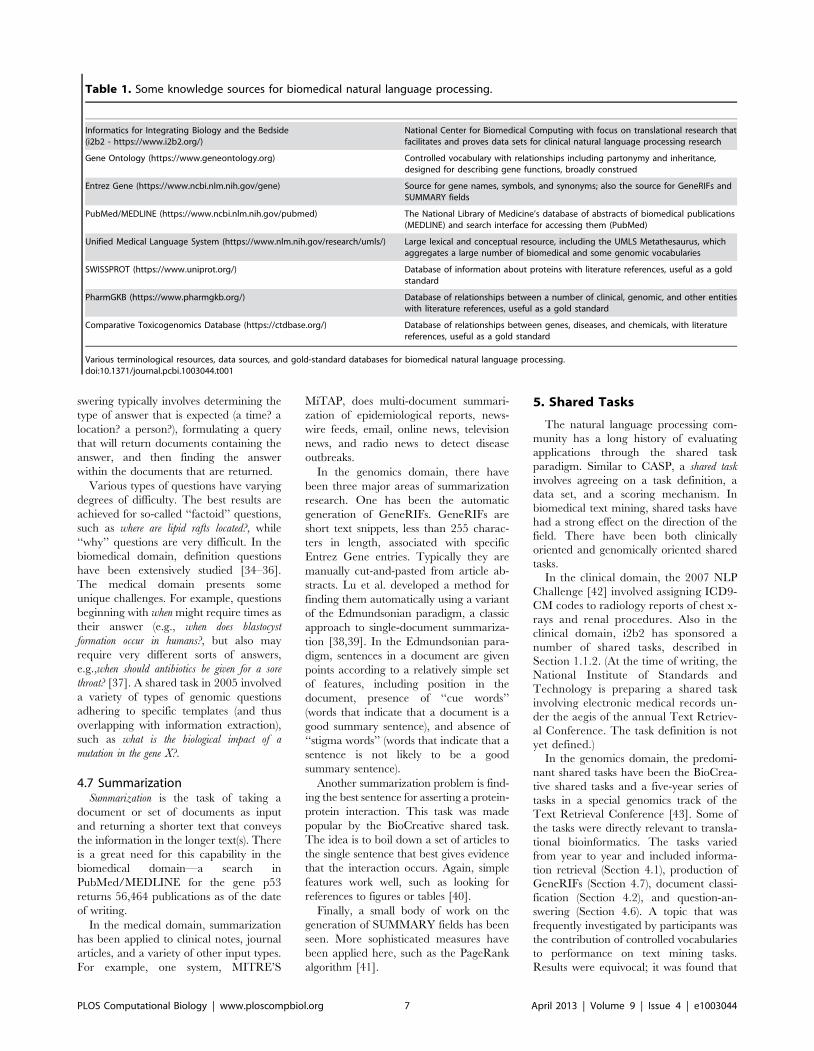
swering typically involves determining the
type of answer that is expected (a time? a
location? a person?), formulating a query
that will return documents containing the
answer, and then finding the answer
within the documents that are returned.
Various types of questions have varying
degrees of difficulty. The best results are
achieved for so-called ‘‘factoid’’ questions,
such as where are lipid rafts located?, while
‘‘why’’ questions are very difficult. In the
biomedical domain, definition questions
have been extensively studied [34–36].
The medical domain presents some
unique challenges. For example, questions
beginning with when might require times as
their answer (e.g., when does blastocyst
formation occur in humans?, but also may
require very different sorts of answers,
e.g.,when should antibiotics be given for a sore
throat? [37]. A shared task in 2005 involved
a variety of types of genomic questions
adhering to specific templates (and thus
overlapping with information extraction),
such as what is the biological impact of a
mutation in the gene X?.
4.7 SummarizationSummarization is the task of taking a
document or set of documents as input
and returning a shorter text that conveys
the information in the longer text(s). There
is a great need for this capability in the
biomedical domain—a search in
PubMed/MEDLINE for the gene p53
returns 56,464 publications as of the date
of writing.
In the medical domain, summarization
has been applied to clinical notes, journal
articles, and a variety of other input types.
For example, one system, MITRE’S
MiTAP, does multi-document summari-
zation of epidemiological reports, news-
wire feeds, email, online news, television
news, and radio news to detect disease
outbreaks.
In the genomics domain, there have
been three major areas of summarization
research. One has been the automatic
generation of GeneRIFs. GeneRIFs are
short text snippets, less than 255 charac-
ters in length, associated with specific
Entrez Gene entries. Typically they are
manually cut-and-pasted from article ab-
stracts. Lu et al. developed a method for
finding them automatically using a variant
of the Edmundsonian paradigm, a classic
approach to single-document summariza-
tion [38,39]. In the Edmundsonian para-
digm, sentences in a document are given
points according to a relatively simple set
of features, including position in the
document, presence of ‘‘cue words’’
(words that indicate that a document is a
good summary sentence), and absence of
‘‘stigma words’’ (words that indicate that a
sentence is not likely to be a good
summary sentence).
Another summarization problem is find-
ing the best sentence for asserting a protein-
protein interaction. This task was made
popular by the BioCreative shared task.
The idea is to boil down a set of articles to
the single sentence that best gives evidence
that the interaction occurs. Again, simple
features work well, such as looking for
references to figures or tables [40].
Finally, a small body of work on the
generation of SUMMARY fields has been
seen. More sophisticated measures have
been applied here, such as the PageRank
algorithm [41].
5. Shared Tasks
The natural language processing com-
munity has a long history of evaluating
applications through the shared task
paradigm. Similar to CASP, a shared task
involves agreeing on a task definition, a
data set, and a scoring mechanism. In
biomedical text mining, shared tasks have
had a strong effect on the direction of the
field. There have been both clinically
oriented and genomically oriented shared
tasks.
In the clinical domain, the 2007 NLP
Challenge [42] involved assigning ICD9-
CM codes to radiology reports of chest x-
rays and renal procedures. Also in the
clinical domain, i2b2 has sponsored a
number of shared tasks, described in
Section 1.1.2. (At the time of writing, the
National Institute of Standards and
Technology is preparing a shared task
involving electronic medical records un-
der the aegis of the annual Text Retriev-
al Conference. The task definition is not
yet defined.)
In the genomics domain, the predomi-
nant shared tasks have been the BioCrea-
tive shared tasks and a five-year series of
tasks in a special genomics track of the
Text Retrieval Conference [43]. Some of
the tasks were directly relevant to transla-
tional bioinformatics. The tasks varied
from year to year and included informa-
tion retrieval (Section 4.1), production of
GeneRIFs (Section 4.7), document classi-
fication (Section 4.2), and question-an-
swering (Section 4.6). A topic that was
frequently investigated by participants was
the contribution of controlled vocabularies
to performance on text mining tasks.
Results were equivocal; it was found that
Table 1. Some knowledge sources for biomedical natural language processing.
Informatics for Integrating Biology and the Bedside(i2b2 - https://www.i2b2.org/)
National Center for Biomedical Computing with focus on translational research thatfacilitates and proves data sets for clinical natural language processing research
Gene Ontology (https://www.geneontology.org) Controlled vocabulary with relationships including partonymy and inheritance,designed for describing gene functions, broadly construed
Entrez Gene (https://www.ncbi.nlm.nih.gov/gene) Source for gene names, symbols, and synonyms; also the source for GeneRIFs andSUMMARY fields
PubMed/MEDLINE (https://www.ncbi.nlm.nih.gov/pubmed) The National Library of Medicine’s database of abstracts of biomedical publications(MEDLINE) and search interface for accessing them (PubMed)
Unified Medical Language System (https://www.nlm.nih.gov/research/umls/) Large lexical and conceptual resource, including the UMLS Metathesaurus, whichaggregates a large number of biomedical and some genomic vocabularies
SWISSPROT (https://www.uniprot.org/) Database of information about proteins with literature references, useful as a goldstandard
PharmGKB (https://www.pharmgkb.org/) Database of relationships between a number of clinical, genomic, and other entitieswith literature references, useful as a gold standard
Comparative Toxicogenomics Database (https://ctdbase.org/) Database of relationships between genes, diseases, and chemicals, with literaturereferences, useful as a gold standard
Various terminological resources, data sources, and gold-standard databases for biomedical natural language processing.doi:10.1371/journal.pcbi.1003044.t001
PLOS Computational Biology | www.ploscompbiol.org 7 April 2013 | Volume 9 | Issue 4 | e1003044
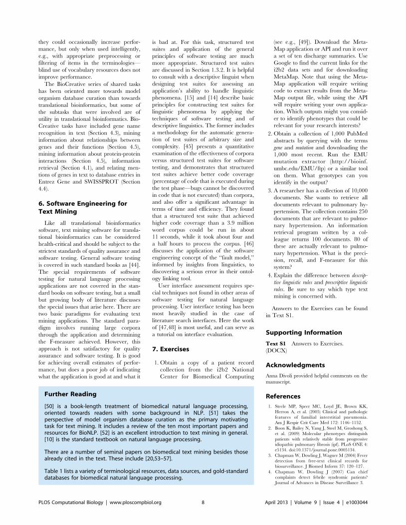
they could occasionally increase perfor-
mance, but only when used intelligently,
e.g., with appropriate preprocessing or
filtering of items in the terminologies—
blind use of vocabulary resources does not
improve performance.
The BioCreative series of shared tasks
has been oriented more towards model
organism database curation than towards
translational bioinformatics, but some of
the subtasks that were involved are of
utility in translational bioinformatics. Bio-
Creative tasks have included gene name
recognition in text (Section 4.3), mining
information about relationships between
genes and their functions (Section 4.5),
mining information about protein-protein
interactions (Section 4.5), information
retrieval (Section 4.1), and relating men-
tions of genes in text to database entries in
Entrez Gene and SWISSPROT (Section
4.4).
6. Software Engineering forText Mining
Like all translational bioinformatics
software, text mining software for transla-
tional bioinformatics can be considered
health-critical and should be subject to the
strictest standards of quality assurance and
software testing. General software testing
is covered in such standard books as [44].
The special requirements of software
testing for natural language processing
applications are not covered in the stan-
dard books on software testing, but a small
but growing body of literature discusses
the special issues that arise here. There are
two basic paradigms for evaluating text
mining applications. The standard para-
digm involves running large corpora
through the application and determining
the F-measure achieved. However, this
approach is not satisfactory for quality
assurance and software testing. It is good
for achieving overall estimates of perfor-
mance, but does a poor job of indicating
what the application is good at and what it
is bad at. For this task, structured test
suites and application of the general
principles of software testing are much
more appropriate. Structured test suites
are discussed in Section 1.3.2. It is helpful
to consult with a descriptive linguist when
designing test suites for assessing an
application’s ability to handle linguistic
phenomena. [15] and [14] describe basic
principles for constructing test suites for
linguistic phenomena by applying the
techniques of software testing and of
descriptive linguistics. The former includes
a methodology for the automatic genera-
tion of test suites of arbitrary size and
complexity. [45] presents a quantitative
examination of the effectiveness of corpora
versus structured test suites for software
testing, and demonstrates that structured
test suites achieve better code coverage
(percentage of code that is executed during
the test phase—bugs cannot be discovered
in code that is not executed) than corpora,
and also offer a significant advantage in
terms of time and efficiency. They found
that a structured test suite that achieved
higher code coverage than a 3.9 million
word corpus could be run in about
11 seconds, while it took about four and
a half hours to process the corpus. [46]
discusses the application of the software
engineering concept of the ‘‘fault model,’’
informed by insights from linguistics, to
discovering a serious error in their ontol-
ogy linking tool.
User interface assessment requires spe-
cial techniques not found in other areas of
software testing for natural language
processing. User interface testing has been
most heavily studied in the case of
literature search interfaces. Here the work
of [47,48] is most useful, and can serve as
a tutorial on interface evaluation.
7. Exercises
1. Obtain a copy of a patient record
collection from the i2b2 National
Center for Biomedical Computing
(see e.g., [49]). Download the Meta-
Map application or API and run it over
a set of ten discharge summaries. Use
Google to find the current links for the
i2b2 data sets and for downloading
MetaMap. Note that using the Meta-
Map application will require writing
code to extract results from the Meta-
Map output file, while using the API
will require writing your own applica-
tion. Which outputs might you consid-
er to identify phenotypes that could be
relevant for your research interests?
2. Obtain a collection of 1,000 PubMed
abstracts by querying with the terms
gene and mutation and downloading the
1,000 most recent. Run the EMU
mutation extractor (http://bioinf.
umbc.edu/EMU/ftp) or a similar tool
on them. What genotypes can you
identify in the output?
3. A researcher has a collection of 10,000
documents. She wants to retrieve all
documents relevant to pulmonary hy-
pertension. The collection contains 250
documents that are relevant to pulmo-
nary hypertension. An information
retrieval program written by a col-
league returns 100 documents. 80 of
these are actually relevant to pulmo-
nary hypertension. What is the preci-
sion, recall, and F-measure for this
system?
4. Explain the difference between descrip-
tive linguistic rules and prescriptive linguistic
rules. Be sure to say which type text
mining is concerned with.
Answers to the Exercises can be found
in Text S1.
Supporting Information
Text S1 Answers to Exercises.
(DOCX)
Acknowledgments
Anna Divoli provided helpful comments on the
manuscript.
References
1. Steele MP, Speer MC, Loyd JE, Brown KK,
Herron A, et al. (2005) Clinical and pathologic
features of familial interstitial pneumonia.
Am J Respir Crit Care Med 172: 1146–1152.
2. Boon K, Bailey N, Yang J, Steel M, Groshong S,
et al. (2009) Molecular phenotypes distinguish
patients with relatively stable from progressive
idiopathic pulmonary fibrosis (ipf). PLoS ONE 4:
e5134. doi:10.1371/journal.pone.0005134.
3. Chapman W, Dowling J, Wagner M (2004) Fever
detection from free-text clinical records for
biosurveillance. J Biomed Inform 37: 120–127.
4. Chapman W, Dowling J (2007) Can chief
complaints detect febrile syndromic patients?
Journal of Advances in Disease Surveillance 3.
Further Reading
[50] is a book-length treatment of biomedical natural language processing,oriented towards readers with some background in NLP. [51] takes theperspective of model organism database curation as the primary motivatingtask for text mining. It includes a review of the ten most important papers andresources for BioNLP. [52] is an excellent introduction to text mining in general.[10] is the standard textbook on natural language processing.
There are a number of seminal papers on biomedical text mining besides thosealready cited in the text. These include [20,53–57].
Table 1 lists a variety of terminological resources, data sources, and gold-standarddatabases for biomedical natural language processing.
PLOS Computational Biology | www.ploscompbiol.org 8 April 2013 | Volume 9 | Issue 4 | e1003044
5. Elhadad N (2006) User-sensitive text summariza-
tion: application to the medical domain [Ph.D.
thesis]. New York: Columbia University.
6. Uzuner O, Solti I, Cadag E (2010) Extractingmedication information from clinical text. J Am
Med Inform Assoc 17: 514–518.
7. Hunter LE (2009) The processes of life: an
introduction to molecular biology. Cambridge(MA): MIT Press.
8. Wiegers TC, Davis AP, Cohen KB, Hirschman
L, Mattingly CJ (2009) Text mining and manual
curation of chemical-gene-disease networks for
the Comparative Toxicogenomics Database(CTD). BMC Bioinformatics 10: 326.
9. Altman RB (2011) Pharmacogenomics: ‘‘nonin-
feriority’’ is sufficient for initial implementation.
Clin Pharmacol Ther 89: 348–350.
10. Jurafsky D, Martin JH (2008) Speech and
language processing: an introduction to natural
language processing, computational linguistics,
and speech recognition. Pearson Prentice Hall.
11. Manning C, Schuetze H (1999) Foundations of
statistical natural language processing. Cam-
bridge (MA): MIT Press.
12. Jackson P, Moulinier I (2002) Natural languageprocessing for online applications: text retrieval,
extraction, and categorization. 2nd edition. John
Benjamins Publishing Company.
13. Cohen KB, Fox L, Ogren PV, Hunter L (2005)Empirical data on corpus design and usage in
biomedical natural language processing. In: AMIA
2005 symposium proceedings. pp. 156–160.
14. Cohen KB, Roeder C, Jr WAB, Hunter L,
Verspoor K (2010) Test suite design for biomed-ical ontology concept recognition systems. In:
Proceedings of the Language Resources and
Evaluation Conference.
15. Cohen KB, Tanabe L, Kinoshita S, Hunter L(2004) A resource for constructing customized test
suites for molecular biology entity identification
systems. In: HLT-NAACL 2004 Workshop:
BioLINK 2004, Linking Biological Literature,
Ontologies and Databases. Association for Com-
putational Linguistics, pp. 1–8.
16. Krallinger M, Morgan A, Smith L, Leitner F,
Tanabe L, et al. (2008) The BioCreative II –
critical assessment for information extraction in
biology challenge. Genome Biol 9.
17. Cohen KB, Johnson HL, Verspoor K, Roeder C,
Hunter LE (2010) The structural and content
aspects of abstracts versus bodies of full text
journal articles are different. BMC Bioinformatics
11: 492.
18. Lin J, Karakos D, Demner-Fushman D, Khu-
danpur S (2006) Generative content models for
struc-tural analysis of medical abstracts. In:
Proceedings of the HLT-NAACL BioNLP Work-
shop on Linking Natural Language and Biology.New York, New York: Association for Computa-
tional Linguistics. pp. 65–72.
19. Demner-Fushman D, Abhyankar S, Jimeno-
Yepes A, Loane R, Rance B, et al. (2011) Aknowledge-based approach to medical records
retrieval. In: Proceedings of TREC 2011.
20. Fukuda K, Tamura A, Tsunoda T, Takagi T
(1998) Toward information extraction: identifying
protein names from biological papers. In: PacSymp Biocomput. pp. 707–718.
21. Porter MF (1980) An algorithm for suffix
stripping. Program 14: 130–137.
22. Liu H, Christiansen T, Baumgartner WA Jr,
Verspoor K (2012) BioLemmatizer: a lemmatiza-
tion tool for morphological processing of biomed-
ical text. J Biomed Semantics 3: 3.
23. Smith L, Rindesch T, Wilbur WJ (2004) Med-post: A part-of-speech tagger for biomedical text.
Bioinformatics 20: 2320–2321.
24. Tsuruoka Y, Tateishi Y, Kim JD, Ohta T,
Mcnaught J, et al. (2005) Developing a robust
part-of-speech tagger for biomedical text. In:
Proceedings of the 10th Panhellenic Conference
on Informatics. pp. 382–392.
25. Caporaso JG, Baumgartner WA Jr, Cohen KB,
Johnson HL, Paquette J, et al. (2005) Concept
recognition and the TREC Genomics tasks. In:
The Fourteenth Text REtrieval Conference
(TREC 2005) Proceedings.
26. Lindberg D, Humphreys B, Mccray A (1993) The
Unified Medical Language System. Methods Inf
Med 32: 281–291.
27. Aronson A (2001) Effective mapping of biomed-ical text to the UMLS Metathesaurus: The
MetaMap program. In: Proc AMIA 2001. pp.
17–21.
28. Aronson AR, Lang FM (2010) An overview of
MetaMap: historical perspective and recent
advances. J Am Med Inform Assoc 17: 229–236.
29. Hanisch D, Fundel K, Mevissen HT, Zimmer R,
Fluck J (2005) ProMiner: rule-based protein and
gene entity recognition. BMC Bioinformatics 6
Suppl 1: S14.
30. Verspoor K, Roeder C, Johnson HL, Cohen KB,
Baumgartner WA Jr, et al. (2010) Exploring
species-based strategies for gene normalization.
IEEE/ACM Trans Comput Biol Bioinform 7:
462–471.
31. Hunter L, Lu Z, Firby J, Baumgartner WA Jr,
Johnson HL, et al. (2008) OpenDMAP: An open-
source, ontology-driven concept analysis engine,
with applications to capturing knowledge regard-
ing pro-tein transport, protein interactions and
cell-specific gene expression. BMC Bioinformatics
9: 78.
32. Kilicoglu H, Bergler S (2009) Syntactic depen-
dency based heuristics for biological event
extraction. In: Proceedings of the BioNLP 2009
Workshop Companion Volume for Shared Task.
Boulder, Colorado: Association for Computation-
al Linguistics. pp. 119–127.
33. Kim JD, Ohta T, Pyysalo S, Kano Y, Tsujii J (2009)
Overview of BioNLP’09 shared task on event
extraction. In: BioNLP 2009 Companion Volume:
Shared Task on Entity Extraction. pp. 1–9.
34. Lin J, Demner-Fushman D (2005) Automatically
evaluating answers to definition questions. In:
Proceedings of the 2005 Human Language
Technology Conference and Conference on
Empirical Methods in Natural Language Process-
ing (HLT/EMNLP 2005). pp. 931–938.
35. Yu H, Wei Y (2006) The semantics of a
definiendum constrains both the lexical semantics
and the lexicosyntactic patterns in the definiens.
In: HTL-NAACL BioNLP Workshop: Linking
Natural Language Processing and Biology: To-
wards Deeper Biological Literature Analysis.
ACL, pp. 1–8.
36. Yu H, Lee M, Kaufman D, Ely J, Osheroff J, et
al. (2007) Development, implementation, and a
cognitive evaluation of a definitional question
answering system for physicians. J Biomed Inform
40: 236–251.
37. Zweigenbaum P (2003) Question answering in
biomedicine. In: Proceedings of the workshop on
natural language processing for question answer-
ing. pp. 1–4.
38. Lu Z, Cohen BK, Hunter L (2006) Finding
GeneRIFs via Gene Ontology annotations. In:
PSB 2006. pp. 52–63.
39. Lu Z, Cohen KB, Hunter L (2007) GeneRIF
quality assurance as summary revision. In: Pacific
Symposium on Biocomputing.
40. Baumgartner WA Jr, Lu Z, Johnson HL,
Caporaso JG, Paquette J, et al. (2008) Concept
recognition for extracting protein interaction
relations from biomedical text. Genome Biol 9
Suppl 2: S9.41. Jin F, Huang M, Lu Z, Zhu X (2009) Towards
automatic generation of gene summary. In:
Proceedings of the BioNLP 2009 Workshop.Boulder, Colorado: Association for Computation-
al Linguistics. pp. 97–105.42. Pestian JP, Brew C, Matykiewicz P, Hovermale
D, Johnson N, et al. (2007) A shared task
involving multi-label classification of clinical freetext. In: Proceedings of BioNLP 2007. Association
for Computational Linguistics.43. Hersh W, Voorhees E (2008) TREC genomics
special issue overview. Information Retrieval.44. Kaner C, Nguyen HQ, Falk J (1999) Testing
computer software. 2nd edition. John Wiley and
Sons.45. Cohen KB, Baumgartner Jr WA, Hunter L (2008)
Software testing and the naturally occurring dataassumption in natural language processing. In:
Software Engineering, Testing, and Qual-ity
Assurance for Natural Language Processing.Columbus, Ohio: Association for Computational
Linguistics. pp. 23–30.46. Johnson HL, Cohen KB, Hunter L (2007) A fault
model for ontology mapping, alignment, andlinking systems. In: Pacific Symposium on
Biocomputing. World Scientific Publishing Com-
pany. pp. 233–244.47. Hearst M, Divoli A, Jerry Y, Wooldridge M
(2007) Exploring the effcacy of caption searchfor bioscience journal search interfaces. In:
Biological, translational, and clinical language
processing. Prague, Czech Republic: Associa-tion for Computational Linguistics. pp.
73–80.48. Divoli A, Hearst MA, Wooldridge MA (2008)
Evidence for showing gene/protein name sugges-tions in bioscience literature search interfaces. Pac
Symp Biocomput 2008: 568–579.
49. Uzuner O, South BR, Shen S, Duvall SL (2011)2010 i2b2/VA challenge on concepts, assertions,
and relations in clinical text. J Am Med InformAssoc 18: 552–556.
50. Cohen KB, Demner-Fushman D (forthcoming)
Biomedical natural language processing. JohnBenjamins Publishing Company.
51. Cohen KB (2010) Biomedical text mining. In:Indurkhya N, Damerau FJ, editors. Handbook of
natural language processing. 2nd edition.52. Jackson P, Moulinier I (2002) Natural language
processing for online applications: text retrieval,
extraction, and categorization. John BenjaminsPublishing Company.
53. Nobata C, Collier N, Tsujii J (1999) Automaticterm identification and classification in biology
texts. In: Proceedings of the fifth Natural
Language Processing Pacific Rim Symposium(NLPRS). pp. 369–374.
54. Blaschke C, Andrade MA, Ouzounis C, ValenciaA (1999) Automatic extraction of biological
information from scientific text: protein-protein
interactions. Proc Int Conf Intell Syst Mol Biol1999: 60–67.
55. Craven M, Kumlien J (1999) Constructingbiological knowledge bases by extracting infor-
mation from text sources. Proc Int Conf IntellSyst Mol Biol 1999: 77–86.
56. Friedman C, Kra P, Yu H, Krauthammer M,
Rzhetsky A (2001) GENIES: a natural-languageprocessing system for the extraction of molecular
pathways from journal articles. Bioinformatics 17:S74–S82.
57. Rzhetsky A, Iossifov I, Koike T, Krauthammer
M, Kra P, et al. (2004) Geneways: a system forextracting, analyzing, visualizing, and integrating
molecular pathway data. J Biomed Inform 37:43–53.
PLOS Computational Biology | www.ploscompbiol.org 9 April 2013 | Volume 9 | Issue 4 | e1003044
Education
Chapter 17: Bioimage Informatics for SystemsPharmacologyFuhai Li, Zheng Yin, Guangxu Jin, Hong Zhao, Stephen T. C. Wong*
NCI Center for Modeling Cancer Development, Department of Systems Medicine and Bioengineering, The Methodist Hospital Research Institute, Weil Medical College of
Cornell University, Houston, Texas, United States of America
Abstract: Recent advances in auto-mated high-resolution fluorescencemicroscopy and robotic handlinghave made the systematic and costeffective study of diverse morpho-logical changes within a large pop-ulation of cells possible under avariety of perturbations, e.g., drugs,compounds, metal catalysts, RNAinterference (RNAi). Cell population-based studies deviate from conven-tional microscopy studies on a fewcells, and could provide strongerstatistical power for drawing exper-imental observations and conclu-sions. However, it is challenging tomanually extract and quantify phe-notypic changes from the largeamounts of complex image datagenerated. Thus, bioimage informat-ics approaches are needed to rapidlyand objectively quantify and analyzethe image data. This paper providesan overview of the bioimage infor-matics challenges and approaches inimage-based studies for drug andtarget discovery. The concepts andcapabilities of image-based screen-ing are first illustrated by a fewpractical examples investigating dif-ferent kinds of phenotypic changescaused by drugs, compounds, orRNAi. The bioimage analysis ap-proaches, including object detection,segmentation, and tracking, are thendescribed. Subsequently, the quanti-tative features, phenotype identifica-tion, and multidimensional profileanalysis for profiling the effects ofdrugs and targets are summarized.Moreover, a number of publiclyavailable software packages for bio-image informatics are listed forfurther reference. It is expected thatthis review will help readers, includ-ing those without bioimage infor-matics expertise, understand thecapabilities, approaches, and toolsof bioimage informatics and applythem to advance their own studies.
1. Introduction
The old adage that a picture is worth a
thousand words certainly applies to the
identification of phenotypic variations in
biomedical studies. Bright field microsco-
py, by detecting light transmitted through
thin and transparent specimens, has been
widely used to investigate cell size, shape,
and movement. The recent development
of fluorescent proteins, e.g., green fluores-
cent protein and its derivatives [1],
enabled the investigation of the phenotyp-
ic changes of subcellular protein struc-
tures, e.g., chromosomes and microtu-
bules, revolutionizing optical imaging in
biomedical studies. Fluorescent proteins
are bound to specific proteins that are
uniformly located in relevant cellular
structures, e.g., chromosomes, and emit
longer wavelength light, e.g., green light,
after exposure to shorter wavelength light,
e.g., blue light. Thus, the spatial morphol-
ogy and temporal dynamic activities of
subcellular protein structures can be
imaged with a fluorescence microscope -
an optical microscope that can specifically
detect emitted fluorescence of a specific
wavelength [2]. In current image-based
studies, five-dimensional (5D) image data
of thousands of cells (cell populations) can
be acquired: spatial (3D), time lapse (1D),
and multiple fluorescent probes (1D).
With advances to automated high-
resolution microscopy, fluorescent label-
ing, and robotic handling, image-based
studies have become popular in drug and
target discovery. These image-based stud-
ies are often referred to as the High
Content Analysis (HCA) [3], which focus-
es on extracting and analyzing quantita-
tive phenotypic data automatically from
large amounts of cell images with ap-
proaches in image analysis, computation
vision and machine learning [3,4]. Appli-
cations of HCA for screening drugs and
targets are referred to as High Content
Screening (HCS), which focuses on iden-
tifying compounds or genes that cause
desired phenotypic changes [5–7]. The
image data contain rich information
content for understanding biological pro-
cesses and drug effects, indicate diverse
and heterogeneous behaviors of individual
cells, and provide stronger statistical power
in drawing experimental observations and
conclusions, compared to conventional
microscopy studies on a few cells. Howev-
er, extracting and mining the phenotypic
changes from the large scale, complex
image data is daunting. It is not feasible to
manually analyze these data. Hence, bio-
image informatics approaches were need-
ed to automatically and objectively ana-
lyze large scale image data, extract and
quantify the phenotypic changes to profile
the effects of drugs and targets.
Bioimage informatics in image-based
studies usually consists of multiple analysis
modules [3,8,9], as shown in Figure 1.
Each of the analysis tasks is challenging,
and different approaches are often re-
quired for the analysis of different types of
images. To facilitate image-based screen-
ing studies, a number of bioimage infor-
matics software packages have been de-
veloped and are publicly available [9].
This chapter provides an overview of the
bioimage informatics approaches in im-
Citation: Li F, Yin Z, Jin G, Zhao H, Wong STC (2013) Chapter 17: Bioimage Informatics for SystemsPharmacology. PLoS Comput Biol 9(4): e1003043. doi:10.1371/journal.pcbi.1003043
Editors: Fran Lewitter, Whitehead Institute, United States of America and Maricel Kann, University ofMarylan d,
Published April 25, 2013
Copyright: � 2013 Li et al. This is an open-access article distributed under the terms of the CreativeCommons Attribution License, which permits unrestricted use, distribution, and reproduction in any medium,provided the original author and source are credited.
Funding: The research is supported by NIH R01 LM008696, NIH R01 CA121225, NIH R01 LM009161, NIH R01
Competing Interests: The authors have declared that no competing interests exist.
* E-mail: [email protected]
This article is part of the ‘‘Transla-
tional Bioinformatics’’ collection for
PLOS Computational Biology.
PLOS Computational Biology | www.ploscompbiol.org 1 April 2013 | Volume 9 | Issue 4 | e1003043
Baltimore County , United States of America
A G028928 NIH U54CA149169 and CPRIT RP110532 . The funders had no role in the preparation of the manuscript. ,
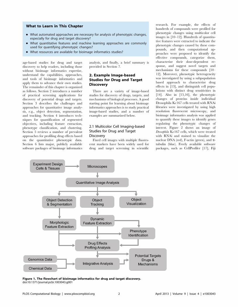
age-based studies for drug and target
discovery to help readers, including those
without bioimage informatics expertise,
understand the capabilities, approaches,
and tools of bioimage informatics and
apply them to advance their own studies.
The remainder of this chapter is organized
as follows. Section 2 introduces a number
of practical screening applications for
discovery of potential drugs and targets.
Section 3 describes the challenges and
approaches for quantitative image analy-
sis, e.g., object detection, segmentation,
and tracking. Section 4 introduces tech-
niques for quantification of segmented
objectives, including feature extraction,
phenotype classification, and clustering.
Section 5 reviews a number of prevalent
approaches for profiling drug effects based
on the quantitative phenotypic data.
Section 6 lists major, publicly available
software packages of bioimage informatics
analysis, and finally, a brief summary is
provided in Section 7.
2. Example Image-basedStudies for Drug and TargetDiscovery
There are a variety of image-based
studies for discovery of drugs, targets, and
mechanisms of biological processes. A good
starting point for learning about bioimage
informatics approaches is to study practical
image-based studies, and a number of
examples are summarized below.
2.1 Multicolor Cell Imaging-basedStudies for Drug and TargetDiscovery
Fixed cell images with multiple fluores-
cent markers have been widely used for
drug and target screening in scientific
research. For example, the effects of
hundreds of compounds were profiled for
phenotypic changes using multicolor cell
images in [10–12]. Hundreds of quantita-
tive features were extracted to indicate the
phenotypic changes caused by these com-
pounds, and then computational ap-
proaches were proposed to identify the
effective compounds, categorize them,
characterize their dose-dependent re-
sponse, and suggest novel targets and
mechanisms for these compounds [10–
12]. Moreover, phenotypic heterogeneity
was investigated by using a subpopulation
based approach to characterize drug
effects in [13], and distinguish cell popu-
lations with distinct drug sensitivities in
[14]. Also in [15,16], the phenotypic
changes of proteins inside individual
Drosophila Kc167 cells treated with RNAi
libraries were investigated by using high
resolution fluorescent microscopy, and
bioimage informatics analysis was applied
to quantify these images to identify genes
regulating the phenotypic changes of
interest. Figure 2 shows an image of
Drosophila Kc167 cells, which were treated
with RNAi and stained to visualize the
nuclear DNA (red), F-actin (green), and a-
tubulin (blue). Freely available software
packages, such as CellProfiler [17], Fiji
What to Learn in This Chapter
N What automated approaches are necessary for analysis of phenotypic changes,especially for drug and target discovery?
N What quantitative features and machine learning approaches are commonlyused for quantifying phenotypic changes?
N What resources are available for bioimage informatics studies?
Figure 1. The flowchart of bioimage informatics for drug and target discovery.doi:10.1371/journal.pcbi.1003043.g001
PLOS Computational Biology | www.ploscompbiol.org 2 April 2013 | Volume 9 | Issue 4 | e1003043
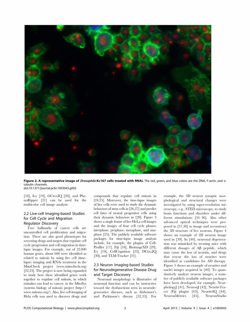
[18], Icy [19], GCELLIQ [20], and Phe-
noRipper [21] can be used for the
multicolor cell image analysis.
2.2 Live-cell Imaging-based Studiesfor Cell Cycle and MigrationRegulator Discovery
Two hallmarks of cancer cells are
uncontrolled cell proliferation and migra-
tion. These are also good phenotypes for
screening drugs and targets that regulate cell
cycle progression and cell migration in time-
lapse images. For example, out of 22,000
human genes, about 600 were identified as
related to mitosis by using live cell (time-
lapse) imaging and RNAi treatment in the
MitoCheck project (www.mitocheck.org)
[22,23]. The project is now being expanded
to study how these identified genes work
together to regulate cell mitosis, in which
mistakes can lead to cancer, in the MitoSys
(systems biology of mitosis) project (http://
www.mitosys.org/). Also, live cell imaging of
Hela cells was used to discover drugs and
compounds that regulate cell mitosis in
[24,25]. Moreover, the time-lapse images
of live cells were used to study the dynamic
behaviors of stem cells in [26,27] and predict
cell fates of neural progenitor cells using
their dynamic behaviors in [28]. Figure 3
shows a single frame of live HeLa cell images
and the images of four cell cycle phases:
interphase, prophase, metaphase, and ana-
phase [25]. The publicly available software
packages for time-lapse image analysis
include, for example, the plugins of Cell-
Profiler [17], Fiji [18], BioimageXD [29],
Icy [19], CellCognition [23], DCELLIQ
[30], and TLM-Tracker [31].
2.3 Neuron Imaging-based Studiesfor Neurodegenerative Disease Drugand Target Discovery
Neuronal morphology is illustrative of
neuronal function and can be instructive
toward the dysfunctions seen in neurode-
generative diseases, such as Alzheimer’s
and Parkinson’s disease [32,33]. For
example, the 3D neuron synaptic mor-
phological and structural changes were
investigated by using super-resolution mi-
croscopy, e.g., STED microscopy, to study
brain functions and disorders under dif-
ferent stimulations [34–36]. Also other
advanced optical techniques were pro-
posed in [37,38] to image and reconstruct
the 3D structure of live neurons. Figure 4
shows an example of 2D neuron image
used in [39]. In [40], neuronal degenera-
tion was mimicked by treating mice with
different dosages of Ab peptide, which
may cause the loss of neuritis, and drugs
that rescue the loss of neurites were
identified as candidates for AD therapy.
Figure 5 shows an example of neurites and
nuclei images acquired in [40]. To quan-
titatively analyze neuron images, a num-
ber of publicly available software packages
have been developed, for example, Neur-
phologyJ [41], NeuronJ [42], NeuriteTra-
cer (Fiji plugin) [43], NeuriteIQ [44],
NeuronMetrics [45], NeuronStudio
Figure 2. A representative image of Drosophila Kc167 cells treated with RNAi. The red, green, and blue colors are the DNA, F-actin, and a-tubulin channels.doi:10.1371/journal.pcbi.1003043.g002
PLOS Computational Biology | www.ploscompbiol.org 3 April 2013 | Volume 9 | Issue 4 | e1003043
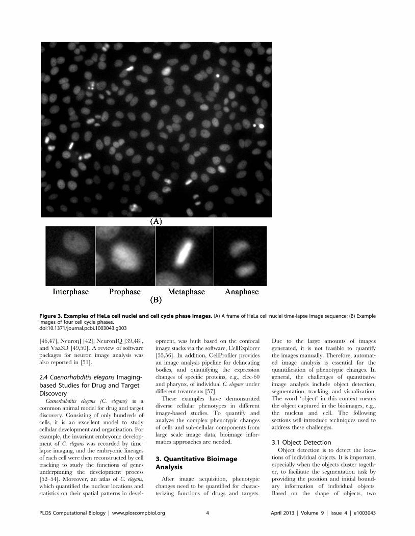
[46,47], NeuronJ [42], NeuronIQ [39,48],
and Vaa3D [49,50]. A review of software
packages for neuron image analysis was
also reported in [51].
2.4 Caenorhabditis elegans Imaging-based Studies for Drug and TargetDiscovery
Caenorhabditis elegans (C. elegans) is a
common animal model for drug and target
discovery. Consisting of only hundreds of
cells, it is an excellent model to study
cellular development and organization. For
example, the invariant embryonic develop-
ment of C. elegans was recorded by time-
lapse imaging, and the embryonic lineages
of each cell were then reconstructed by cell
tracking to study the functions of genes
underpinning the development process
[52–54]. Moreover, an atlas of C. elegans,
which quantified the nuclear locations and
statistics on their spatial patterns in devel-
opment, was built based on the confocal
image stacks via the software, CellExplorer
[55,56]. In addition, CellProfiler provides
an image analysis pipeline for delineating
bodies, and quantifying the expression
changes of specific proteins, e.g., clec-60
and pharynx, of individual C. elegans under
different treatments [57].
These examples have demonstrated
diverse cellular phenotypes in different
image-based studies. To quantify and
analyze the complex phenotypic changes
of cells and sub-cellular components from
large scale image data, bioimage infor-
matics approaches are needed.
3. Quantitative BioimageAnalysis
After image acquisition, phenotypic
changes need to be quantified for charac-
terizing functions of drugs and targets.
Due to the large amounts of images
generated, it is not feasible to quantify
the images manually. Therefore, automat-
ed image analysis is essential for the
quantification of phenotypic changes. In
general, the challenges of quantitative
image analysis include object detection,
segmentation, tracking, and visualization.
The word ‘object’ in this context means
the object captured in the bioimages, e.g.,
the nucleus and cell. The following
sections will introduce techniques used to
address these challenges.
3.1 Object DetectionObject detection is to detect the loca-
tions of individual objects. It is important,
especially when the objects cluster togeth-
er, to facilitate the segmentation task by
providing the position and initial bound-
ary information of individual objects.
Based on the shape of objects, two
Figure 3. Examples of HeLa cell nuclei and cell cycle phase images. (A) A frame of HeLa cell nuclei time-lapse image sequence; (B) Exampleimages of four cell cycle phases.doi:10.1371/journal.pcbi.1003043.g003
PLOS Computational Biology | www.ploscompbiol.org 4 April 2013 | Volume 9 | Issue 4 | e1003043
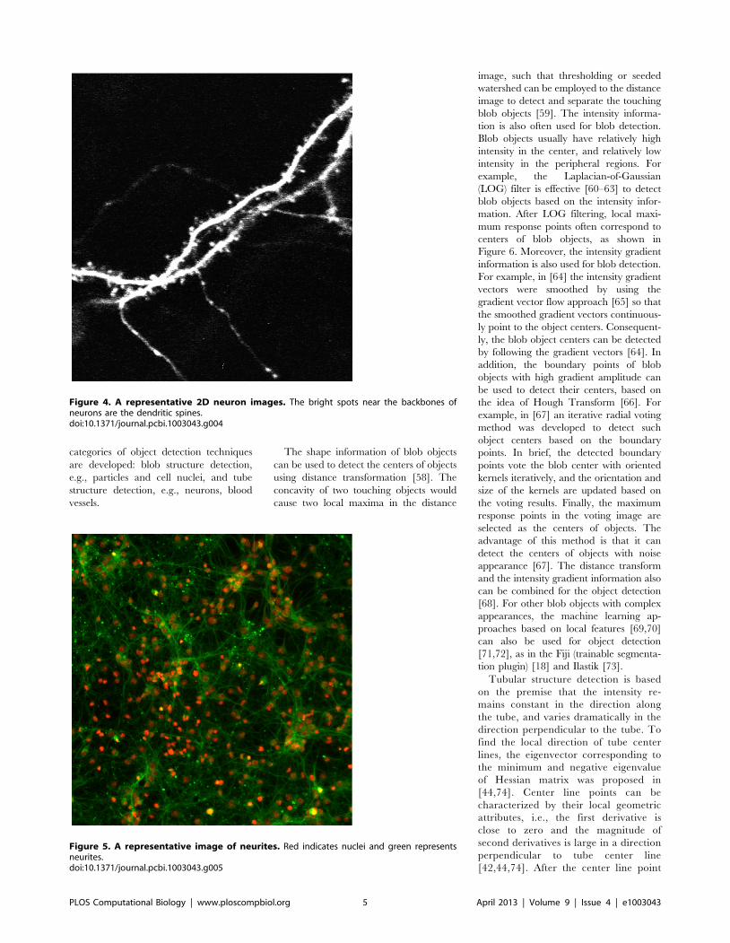
categories of object detection techniques
are developed: blob structure detection,
e.g., particles and cell nuclei, and tube
structure detection, e.g., neurons, blood
vessels.
The shape information of blob objects
can be used to detect the centers of objects
using distance transformation [58]. The
concavity of two touching objects would
cause two local maxima in the distance
image, such that thresholding or seeded
watershed can be employed to the distance
image to detect and separate the touching
blob objects [59]. The intensity informa-
tion is also often used for blob detection.
Blob objects usually have relatively high
intensity in the center, and relatively low
intensity in the peripheral regions. For
example, the Laplacian-of-Gaussian
(LOG) filter is effective [60–63] to detect
blob objects based on the intensity infor-
mation. After LOG filtering, local maxi-
mum response points often correspond to
centers of blob objects, as shown in
Figure 6. Moreover, the intensity gradient
information is also used for blob detection.
For example, in [64] the intensity gradient
vectors were smoothed by using the
gradient vector flow approach [65] so that
the smoothed gradient vectors continuous-
ly point to the object centers. Consequent-
ly, the blob object centers can be detected
by following the gradient vectors [64]. In
addition, the boundary points of blob
objects with high gradient amplitude can
be used to detect their centers, based on
the idea of Hough Transform [66]. For
example, in [67] an iterative radial voting
method was developed to detect such
object centers based on the boundary
points. In brief, the detected boundary
points vote the blob center with oriented
kernels iteratively, and the orientation and
size of the kernels are updated based on
the voting results. Finally, the maximum
response points in the voting image are
selected as the centers of objects. The
advantage of this method is that it can
detect the centers of objects with noise
appearance [67]. The distance transform
and the intensity gradient information also
can be combined for the object detection
[68]. For other blob objects with complex
appearances, the machine learning ap-
proaches based on local features [69,70]
can also be used for object detection
[71,72], as in the Fiji (trainable segmenta-
tion plugin) [18] and Ilastik [73].
Tubular structure detection is based
on the premise that the intensity re-
mains constant in the direction along
the tube, and varies dramatically in the
direction perpendicular to the tube. To
find the local direction of tube center
lines, the eigenvector corresponding to
the minimum and negative eigenvalue
of Hessian matrix was proposed in
[44,74]. Center line points can be
characterized by their local geometric
attributes, i.e., the first derivative is
close to zero and the magnitude of
second derivatives is large in a direction
perpendicular to tube center line
[42,44,74]. After the center line point
Figure 4. A representative 2D neuron images. The bright spots near the backbones ofneurons are the dendritic spines.doi:10.1371/journal.pcbi.1003043.g004
Figure 5. A representative image of neurites. Red indicates nuclei and green representsneurites.doi:10.1371/journal.pcbi.1003043.g005
PLOS Computational Biology | www.ploscompbiol.org 5 April 2013 | Volume 9 | Issue 4 | e1003043
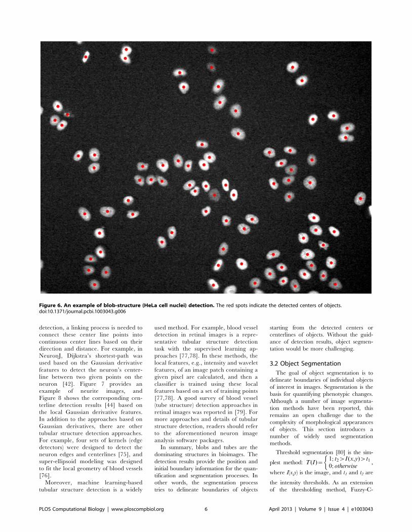
detection, a linking process is needed to
connect these center line points into
continuous center lines based on their
direction and distance. For example, in
NeuronJ, Dijkstra’s shortest-path was
used based on the Gaussian derivative
features to detect the neuron’s center-
line between two given points on the
neuron [42]. Figure 7 provides an
example of neurite images, and
Figure 8 shows the corresponding cen-
terline detection results [44] based on
the local Gaussian derivative features.
In addition to the approaches based on
Gaussian derivatives, there are other
tubular structure detection approaches.
For example, four sets of kernels (edge
detectors) were designed to detect the
neuron edges and centerlines [75], and
super-ellipsoid modeling was designed
to fit the local geometry of blood vessels
[76].
Moreover, machine learning-based
tubular structure detection is a widely
used method. For example, blood vessel
detection in retinal images is a repre-
sentative tubular structure detection
task with the supervised learning ap-
proaches [77,78]. In these methods, the
local features, e.g., intensity and wavelet
features, of an image patch containing a
given pixel are calculated, and then a
classifier is trained using these local
features based on a set of training points
[77,78]. A good survey of blood vessel
(tube structure) detection approaches in
retinal images was reported in [79]. For
more approaches and details of tubular
structure detection, readers should refer
to the aforementioned neuron image
analysis software packages.
In summary, blobs and tubes are the
dominating structures in bioimages. The
detection results provide the position and
initial boundary information for the quan-
tification and segmentation processes. In
other words, the segmentation process
tries to delineate boundaries of objects
starting from the detected centers or
centerlines of objects. Without the guid-
ance of detection results, object segmen-
tation would be more challenging.
3.2 Object Segmentation
The goal of object segmentation is to
delineate boundaries of individual objects
of interest in images. Segmentation is the
basis for quantifying phenotypic changes.
Although a number of image segmenta-
tion methods have been reported, this
remains an open challenge due to the
complexity of morphological appearances
of objects. This section introduces a
number of widely used segmentation
methods.
Threshold segmentation [80] is the sim-
plest method: T(I)~1; t2wI(x,y)wt1
0; otherwise
�,
where I(x,y) is the image, and t1 and t2 are
the intensity thresholds. As an extension
of the thresholding method, Fuzzy-C-
Figure 6. An example of blob-structure (HeLa cell nuclei) detection. The red spots indicate the detected centers of objects.doi:10.1371/journal.pcbi.1003043.g006
PLOS Computational Biology | www.ploscompbiol.org 6 April 2013 | Volume 9 | Issue 4 | e1003043
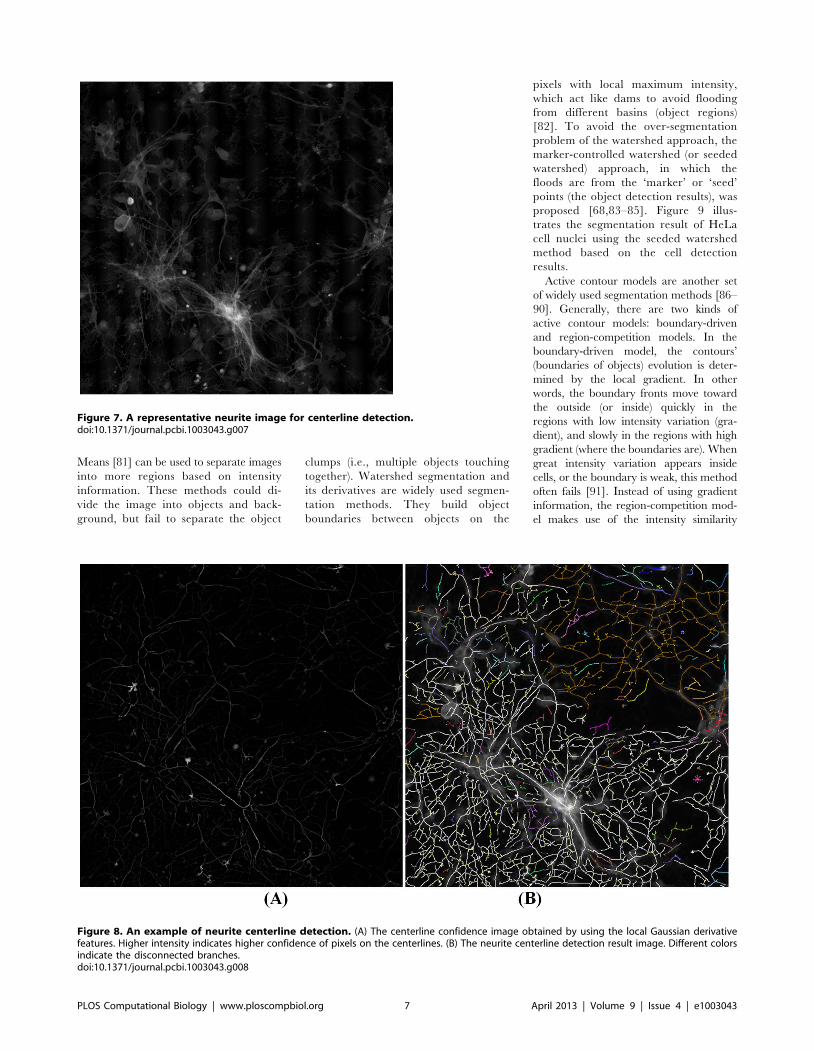
Means [81] can be used to separate images
into more regions based on intensity
information. These methods could di-
vide the image into objects and back-
ground, but fail to separate the object
clumps (i.e., multiple objects touching
together). Watershed segmentation and
its derivatives are widely used segmen-
tation methods. They build object
boundaries between objects on the
pixels with local maximum intensity,
which act like dams to avoid flooding
from different basins (object regions)
[82]. To avoid the over-segmentation
problem of the watershed approach, the
marker-controlled watershed (or seeded
watershed) approach, in which the
floods are from the ‘marker’ or ‘seed’
points (the object detection results), was
proposed [68,83–85]. Figure 9 illus-
trates the segmentation result of HeLa
cell nuclei using the seeded watershed
method based on the cell detection
results.
Active contour models are another set
of widely used segmentation methods [86–
90]. Generally, there are two kinds of
active contour models: boundary-driven
and region-competition models. In the
boundary-driven model, the contours’
(boundaries of objects) evolution is deter-
mined by the local gradient. In other
words, the boundary fronts move toward
the outside (or inside) quickly in the
regions with low intensity variation (gra-
dient), and slowly in the regions with high
gradient (where the boundaries are). When
great intensity variation appears inside
cells, or the boundary is weak, this method
often fails [91]. Instead of using gradient
information, the region-competition mod-
el makes use of the intensity similarity
Figure 7. A representative neurite image for centerline detection.doi:10.1371/journal.pcbi.1003043.g007
Figure 8. An example of neurite centerline detection. (A) The centerline confidence image obtained by using the local Gaussian derivativefeatures. Higher intensity indicates higher confidence of pixels on the centerlines. (B) The neurite centerline detection result image. Different colorsindicate the disconnected branches.doi:10.1371/journal.pcbi.1003043.g008
PLOS Computational Biology | www.ploscompbiol.org 7 April 2013 | Volume 9 | Issue 4 | e1003043
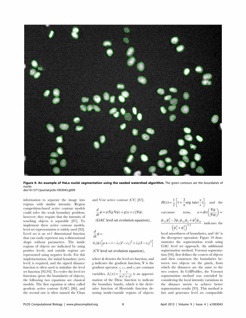
information to separate the image into
regions with similar intensity. Region
competition-based active contour models
could solve the weak boundary problem;
however, they require that the intensity of
touching objects is separable [87]. To
implement these active contour models,
level set representation is widely used [92].
Level set is an n+1 dimensional function
that can easily represent any n dimensional
shape without parameters. The inside
regions of objects are indicated by using
positive levels, and outside regions are
represented using negative levels. For this
implementation, the initial boundary (zero
level) is required, and the signed distance
function is often used to initialize the level
set function [92,93]. To evolve the level set
functions (grow the boundaries of objects),
the following two equations are classical
models. The first equation is often called
geodesic active contour (GAC) [86], and
the second one is often named the Chan
and Vese active contour (CV) [87].
d
dty~a +g:+yð Þzg kzcð Þ +yj j
GAC level set evolution equationð Þ,
d
dty~
de yð Þ m:k{n{l1 I{c1ð Þ2zl2 I{c2ð Þ2h i
CV level set evolution equationð Þ,
where y denotes the level-set function, and
g indicates the gradient function, + is the
gradient operator, c, c1, and c2 are constant
variables. de xð Þ~ 1
p
e
e2zx2is an approxi-
mation of the Dirac function to indicate
the boundary bands), which is the deriv-
ative function of Heaviside function de-
noting inside/outside regions of objects:
H(x)~1
21z
2
parg tan (
x
e)
� �, and the
curvature term, k~div+y
+yj j
� �~
yxxy2y{2yxyxyyyzy2
xyyy
y2xzy2
y
� �3=2indicates the
local smoothness of boundaries, and ‘div’ is
the divergence operation. Figure 10 dem-
onstrates the segmentation result using
GAC level set approach. An additional
segmentation method, Voronoi segmenta-
tion [94], first defines the centers of objects
and then constructs the boundaries be-
tween two objects on the pixels, from
which the distances are the same to the
two centers. In CellProfiler, the Voronoi
segmentation method was extended by
considering the local intensity variations in
the distance metric to achieve better
segmentation results [95]. This method is
fast and generates level set comparable
Figure 9. An example of HeLa nuclei segmentation using the seeded watershed algorithm. The green contours are the boundaries ofnuclei.doi:10.1371/journal.pcbi.1003043.g009
PLOS Computational Biology | www.ploscompbiol.org 8 April 2013 | Volume 9 | Issue 4 | e1003043
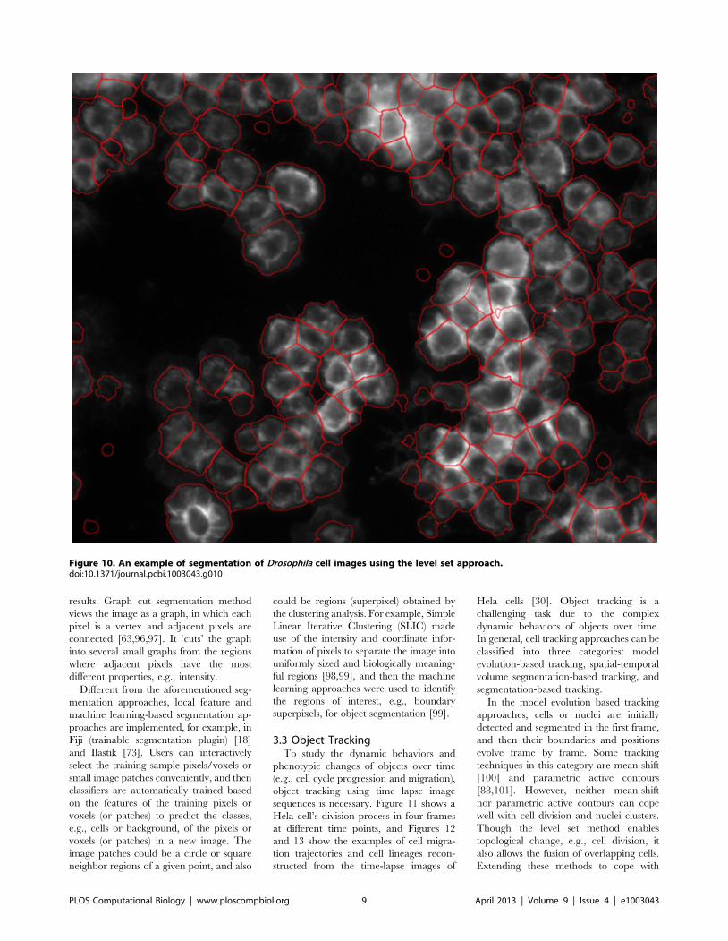
results. Graph cut segmentation method
views the image as a graph, in which each
pixel is a vertex and adjacent pixels are
connected [63,96,97]. It ‘cuts’ the graph
into several small graphs from the regions
where adjacent pixels have the most
different properties, e.g., intensity.
Different from the aforementioned seg-
mentation approaches, local feature and
machine learning-based segmentation ap-
proaches are implemented, for example, in
Fiji (trainable segmentation plugin) [18]
and Ilastik [73]. Users can interactively
select the training sample pixels/voxels or
small image patches conveniently, and then
classifiers are automatically trained based
on the features of the training pixels or
voxels (or patches) to predict the classes,
e.g., cells or background, of the pixels or
voxels (or patches) in a new image. The
image patches could be a circle or square
neighbor regions of a given point, and also
could be regions (superpixel) obtained by
the clustering analysis. For example, Simple
Linear Iterative Clustering (SLIC) made
use of the intensity and coordinate infor-
mation of pixels to separate the image into
uniformly sized and biologically meaning-
ful regions [98,99], and then the machine
learning approaches were used to identify
the regions of interest, e.g., boundary
superpixels, for object segmentation [99].
3.3 Object TrackingTo study the dynamic behaviors and
phenotypic changes of objects over time
(e.g., cell cycle progression and migration),
object tracking using time lapse image
sequences is necessary. Figure 11 shows a
Hela cell’s division process in four frames
at different time points, and Figures 12
and 13 show the examples of cell migra-
tion trajectories and cell lineages recon-
structed from the time-lapse images of
Hela cells [30]. Object tracking is a
challenging task due to the complex
dynamic behaviors of objects over time.
In general, cell tracking approaches can be
classified into three categories: model
evolution-based tracking, spatial-temporal
volume segmentation-based tracking, and
segmentation-based tracking.
In the model evolution based tracking
approaches, cells or nuclei are initially
detected and segmented in the first frame,
and then their boundaries and positions
evolve frame by frame. Some tracking
techniques in this category are mean-shift
[100] and parametric active contours
[88,101]. However, neither mean-shift
nor parametric active contours can cope
well with cell division and nuclei clusters.
Though the level set method enables
topological change, e.g., cell division, it
also allows the fusion of overlapping cells.
Extending these methods to cope with
Figure 10. An example of segmentation of Drosophila cell images using the level set approach.doi:10.1371/journal.pcbi.1003043.g010
PLOS Computational Biology | www.ploscompbiol.org 9 April 2013 | Volume 9 | Issue 4 | e1003043
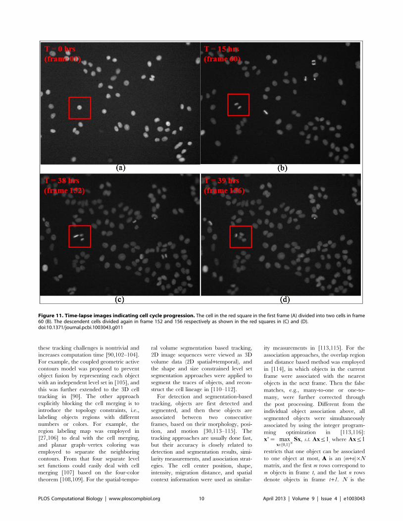
these tracking challenges is nontrivial and
increases computation time [90,102–104].
For example, the coupled geometric active
contours model was proposed to prevent
object fusion by representing each object
with an independent level set in [105], and
this was further extended to the 3D cell
tracking in [90]. The other approach
explicitly blocking the cell merging is to
introduce the topology constraints, i.e.,
labeling objects regions with different
numbers or colors. For example, the
region labeling map was employed in
[27,106] to deal with the cell merging,
and planar graph–vertex coloring was
employed to separate the neighboring
contours. From that four separate level
set functions could easily deal with cell
merging [107] based on the four-color
theorem [108,109]. For the spatial-tempo-
ral volume segmentation based tracking,
2D image sequences were viewed as 3D
volume data (2D spatial+temporal), and
the shape and size constrained level set
segmentation approaches were applied to
segment the traces of objects, and recon-
struct the cell lineage in [110–112].
For detection and segmentation-based
tracking, objects are first detected and
segmented, and then these objects are
associated between two consecutive
frames, based on their morphology, posi-
tion, and motion [30,113–115]. The
tracking approaches are usually done fast,
but their accuracy is closely related to
detection and segmentation results, simi-
larity measurements, and association strat-
egies. The cell center position, shape,
intensity, migration distance, and spatial
context information were used as similar-
ity measurements in [113,115]. For the
association approaches, the overlap region
and distance based method was employed
in [114], in which objects in the current
frame were associated with the nearest
objects in the next frame. Then the false
matches, e.g., many-to-one or one-to-
many, were further corrected through
the post processing. Different from the
individual object association above, all
segmented objects were simultaneously
associated by using the integer program-
ming optimization in [113,116]:
x�~ maxx[f0,1gN
Sx, s.t. Axƒ1, where Axƒ1
restricts that one object can be associated
to one object at most, A is an (m+n)6Nmatrix, and the first m rows correspond to
m objects in frame t, and the last n rows
denote objects in frame t+1. N is the
Figure 11. Time-lapse images indicating cell cycle progression. The cell in the red square in the first frame (A) divided into two cells in frame60 (B). The descendent cells divided again in frame 152 and 156 respectively as shown in the red squares in (C) and (D).doi:10.1371/journal.pcbi.1003043.g011
PLOS Computational Biology | www.ploscompbiol.org 10 April 2013 | Volume 9 | Issue 4 | e1003043
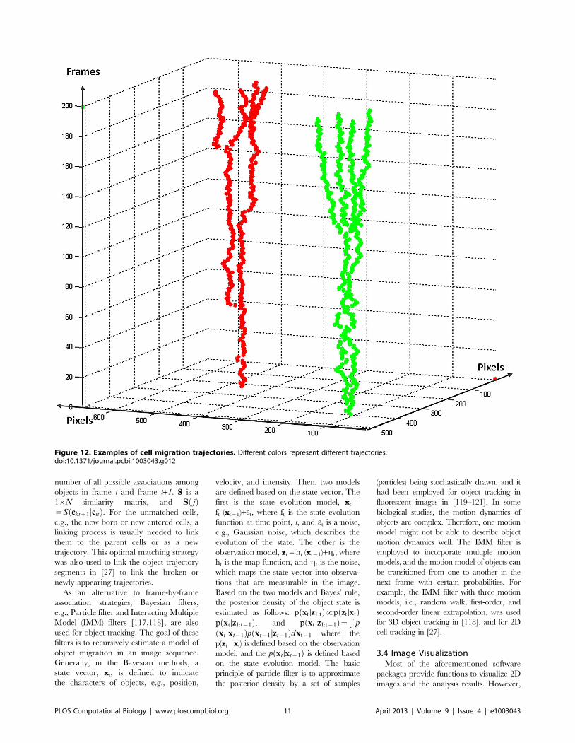
number of all possible associations among
objects in frame t and frame t+1. S is a
16N similarity matrix, and S jð Þ~S cktz1 citjð Þ. For the unmatched cells,
e.g., the new born or new entered cells, a
linking process is usually needed to link
them to the parent cells or as a new
trajectory. This optimal matching strategy
was also used to link the object trajectory
segments in [27] to link the broken or
newly appearing trajectories.
As an alternative to frame-by-frame
association strategies, Bayesian filters,
e.g., Particle filter and Interacting Multiple
Model (IMM) filters [117,118], are also
used for object tracking. The goal of these
filters is to recursively estimate a model of
object migration in an image sequence.
Generally, in the Bayesian methods, a
state vector, xt, is defined to indicate
the characters of objects, e.g., position,
velocity, and intensity. Then, two models
are defined based on the state vector. The
first is the state evolution model, xt =
ft (xt21)+et, where ft is the state evolution
function at time point, t, and et is a noise,
e.g., Gaussian noise, which describes the
evolution of the state. The other is the
observation model, zt = ht (xt21)+gt, where
ht is the map function, and gt is the noise,
which maps the state vector into observa-
tions that are measurable in the image.
Based on the two models and Bayes’ rule,
the posterior density of the object state is
estimated as follows: p xtDz1:tð Þ!p ztDxtð Þp xtDz1:t{1ð Þ, and p xtjz1:t{1ð Þ~
Ðp
xtjxt{1ð Þp xt{1jzt{1ð Þdxt{1 where the
p(zt |xt) is defined based on the observation
model, and the p xtDxt{1ð Þ is defined based
on the state evolution model. The basic
principle of particle filter is to approximate
the posterior density by a set of samples
(particles) being stochastically drawn, and it
had been employed for object tracking in
fluorescent images in [119–121]. In some
biological studies, the motion dynamics of
objects are complex. Therefore, one motion
model might not be able to describe object
motion dynamics well. The IMM filter is
employed to incorporate multiple motion
models, and the motion model of objects can
be transitioned from one to another in the
next frame with certain probabilities. For
example, the IMM filter with three motion
models, i.e., random walk, first-order, and
second-order linear extrapolation, was used
for 3D object tracking in [118], and for 2D
cell tracking in [27].
3.4 Image VisualizationMost of the aforementioned software
packages provide functions to visualize 2D
images and the analysis results. However,
Figure 12. Examples of cell migration trajectories. Different colors represent different trajectories.doi:10.1371/journal.pcbi.1003043.g012
PLOS Computational Biology | www.ploscompbiol.org 11 April 2013 | Volume 9 | Issue 4 | e1003043
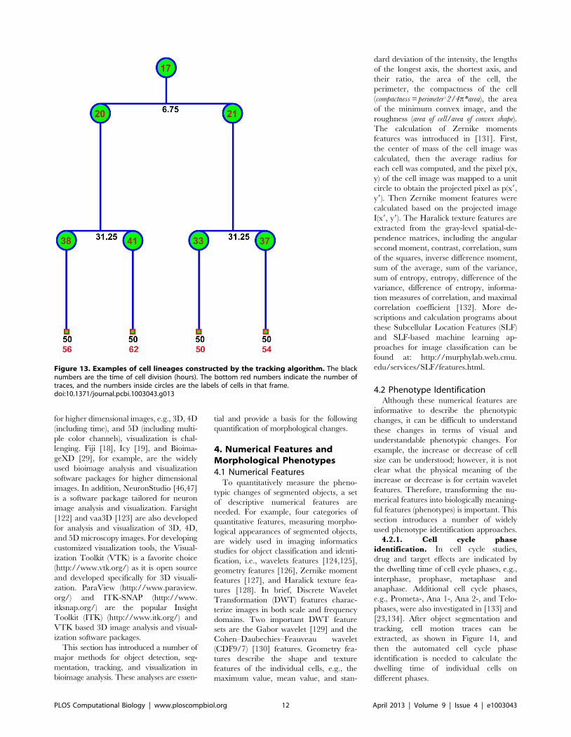
for higher dimensional images, e.g., 3D, 4D
(including time), and 5D (including multi-
ple color channels), visualization is chal-
lenging. Fiji [18], Icy [19], and Bioima-
geXD [29], for example, are the widely
used bioimage analysis and visualization
software packages for higher dimensional
images. In addition, NeuronStudio [46,47]
is a software package tailored for neuron
image analysis and visualization. Farsight
[122] and vaa3D [123] are also developed
for analysis and visualization of 3D, 4D,
and 5D microscopy images. For developing
customized visualization tools, the Visual-
ization Toolkit (VTK) is a favorite choice
(http://www.vtk.org/) as it is open source
and developed specifically for 3D visuali-
zation. ParaView (http://www.paraview.
org/) and ITK-SNAP (http://www.
itksnap.org/) are the popular Insight
Toolkit (ITK) (http://www.itk.org/) and
VTK based 3D image analysis and visual-
ization software packages.
This section has introduced a number of
major methods for object detection, seg-
mentation, tracking, and visualization in
bioimage analysis. These analyses are essen-
tial and provide a basis for the following
quantification of morphological changes.
4. Numerical Features andMorphological Phenotypes
4.1 Numerical FeaturesTo quantitatively measure the pheno-
typic changes of segmented objects, a set
of descriptive numerical features are
needed. For example, four categories of
quantitative features, measuring morpho-
logical appearances of segmented objects,
are widely used in imaging informatics
studies for object classification and identi-
fication, i.e., wavelets features [124,125],
geometry features [126], Zernike moment
features [127], and Haralick texture fea-
tures [128]. In brief, Discrete Wavelet
Transformation (DWT) features charac-
terize images in both scale and frequency
domains. Two important DWT feature
sets are the Gabor wavelet [129] and the
Cohen–Daubechies–Feauveau wavelet
(CDF9/7) [130] features. Geometry fea-
tures describe the shape and texture
features of the individual cells, e.g., the
maximum value, mean value, and stan-
dard deviation of the intensity, the lengths
of the longest axis, the shortest axis, and
their ratio, the area of the cell, the
perimeter, the compactness of the cell
(compactness = perimeter‘2/4p*area), the area
of the minimum convex image, and the
roughness (area of cell/area of convex shape).
The calculation of Zernike moments
features was introduced in [131]. First,
the center of mass of the cell image was
calculated, then the average radius for
each cell was computed, and the pixel p(x,
y) of the cell image was mapped to a unit
circle to obtain the projected pixel as p(x9,
y9). Then Zernike moment features were
calculated based on the projected image
I(x9, y9). The Haralick texture features are
extracted from the gray-level spatial-de-
pendence matrices, including the angular
second moment, contrast, correlation, sum
of the squares, inverse difference moment,
sum of the average, sum of the variance,
sum of entropy, entropy, difference of the
variance, difference of entropy, informa-
tion measures of correlation, and maximal
correlation coefficient [132]. More de-
scriptions and calculation programs about
these Subcellular Location Features (SLF)
and SLF-based machine learning ap-
proaches for image classification can be
found at: http://murphylab.web.cmu.
edu/services/SLF/features.html.
4.2 Phenotype IdentificationAlthough these numerical features are
informative to describe the phenotypic
changes, it can be difficult to understand
these changes in terms of visual and
understandable phenotypic changes. For
example, the increase or decrease of cell
size can be understood; however, it is not
clear what the physical meaning of the
increase or decrease is for certain wavelet
features. Therefore, transforming the nu-
merical features into biologically meaning-
ful features (phenotypes) is important. This
section introduces a number of widely
used phenotype identification approaches.
4.2.1. Cell cycle phase
identification. In cell cycle studies,
drug and target effects are indicated by
the dwelling time of cell cycle phases, e.g.,
interphase, prophase, metaphase and
anaphase. Additional cell cycle phases,
e.g., Prometa-, Ana 1-, Ana 2-, and Telo-
phases, were also investigated in [133] and
[23,134]. After object segmentation and
tracking, cell motion traces can be
extracted, as shown in Figure 14, and
then the automated cell cycle phase
identification is needed to calculate the
dwelling time of individual cells on
different phases.
Figure 13. Examples of cell lineages constructed by the tracking algorithm. The blacknumbers are the time of cell division (hours). The bottom red numbers indicate the number oftraces, and the numbers inside circles are the labels of cells in that frame.doi:10.1371/journal.pcbi.1003043.g013
PLOS Computational Biology | www.ploscompbiol.org 12 April 2013 | Volume 9 | Issue 4 | e1003043
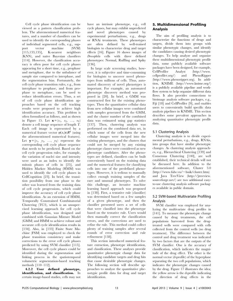
Cell cycle phase identification can be
viewed as a pattern classification prob-
lem. The aforementioned numerical fea-
tures, and a number of classifiers can be
used to identify the corresponding phases
of individual segmented cells, e.g., sup-
port vector machine (SVM)
[115,133,135], K-nearest neighbors
(KNN), and naıve Bayesian classifiers
[114]. However, the classification accu-
racy is often poor for cell cycle phases
appearing for a short time, e.g., prophase
and metaphase, due to the unbalance of
sample size compared to interphase, and
the segmentation bias. Fortunately, the
cell cycle phase transition rules, e.g., from
interphase to prophase, and from pro-
phase to metaphase, can be used to
reduce identification errors. Thus, a set
of cell cycle phase identification ap-
proaches based on the cell tracking
results were proposed to achieve high
identification accuracy. This problem is
often formulized as follows, and as shown
in Figure 15. Let x = (x1, x2, …, xT)
denote a cell image sequence of length T.
Each cell image is represented by a
numerical feature vector Q(xi)[Rd (using
the aforementioned numerical features).
Let y = (y1, y2, …, yT) represent the
corresponding cell cycle phase sequence
that needs to be predicted. Based on the
cell cycle progression rules, for example,
the variation of nuclei size and intensity
were used as an index to identify the
mitosis phases of cells in [25], and
Hidden Markov Modeling (HMM) was
used to identify the cell cycle phases in
CellCognition [23]. In brief, the transi-
tion possibility from one phase to the
other was learned from the training data
of cell cycle progressions, which could
improve the accuracy of cell cycle phase
identification. As an extension of HMM,
Temporally Constrained Combinatorial
Clustering (TC3), which is an unsuper-
vised learning approach for cell cycle
phase identification, was designed and
combined with Gaussian Mixture Model
(GMM) and HMM to achieve robust and
accurate cell cycle identification results in
[134]. Also, in [133] Finite State Ma-
chine (FSM) was employed to check the
phase transition consistency and make
corrections to the error cell cycle phases
predicted by using SVM classifier [115].
Moreover, the cell cycle phases could be
identified during the segmentation and
linking process in the spatiotemporal
volumetric segmentation-based tracking
methods [110–112].
4.2.2 User defined phenotype,
identification, and classification. In
certain image-based studies, cells may not
have an intrinsic phenotype, e.g., cell
cycle phases, but may exhibit unpredicted
and novel phenotypes caused by
experimental perturbations, e.g., drugs
or RNAi treatments. These phenotypes
are often defined by well-trained
biologists to characterize drug and target
effects [16]. Figure 16 shows images of
Drosophila cells with three defined
phenotypes: Normal, Ruffling and Spiky
[136].
In large scale screening studies, how-
ever, it is subjective and time-consuming
for biologists to uncover novel pheno-
types from millions of cells. Thus, auto-
mated discovery of novel phenotypes is
important. For example, an automated
phenotype discovery method was pro-
posed in [20]. In brief, a GMM was
constructed first for the existing pheno-
types. Then the quantitative cellular data
from new cellular images were combined
with samples generated from the GMM,
and the cluster number of the combined
data was estimated using gap statistics
[137]. Then, clustering analysis was
performed on the combined data set, in
which some of the cells from the new
cellular images were merged into the
existing phenotypes, and the clusters that
could not be merged by any existing
phenotype classes were considered as new
phenotype candidates. After the pheno-
types are defined, classifiers can be built
conveniently based on the training data
and the numerical features for classifying
cells into one of the predefined pheno-
types. However, it is tedious to manually
collect enough training samples of the
rare and unusual phenotypes. To solve
this challenge, an iterative machine
learning based approach was proposed
in [138]. First, a tentative rule (classifier)
was determined based on a few samples
of a given phenotype, and then the
classifier presented users a set of cells
that were classified into the phenotype
based on the tentative rule. Users would
then manually correct the classification
errors, and the corrections are used to
refine the rule. This method could collect
plenty of training samples after several
rounds of error correction and rule
refinement [138].
This section introduced numerical fea-
ture extraction, phenotype identification,
and classification. These analyses provide
quantitative phenotypic change data for
identifying candidate targets and drug hits
that cause desirable phenotypic changes.
The following section will describe ap-
proaches to analyze the quantitative phe-
notypic profile data for drug and target
identification.
5. Multidimensional ProfilingAnalysis
The aim of profiling analysis is to
characterize the functions of drugs and
targets, divide them into groups with
similar phenotypic changes, and identify
the candidates causing desired phenotypic
changes. To help analyze and organize
these multidimensional phenotypic profile
data, some publicly available software
packages have been designed, for example,
CellProfiler Analyst (http://www.
cellprofiler.org/) and PhenoRipper
(http://www.phenoripper.org). In addi-
tion, KNIME (http://www.knime.org/)
is a publicly available pipeline and work-
flow system to help organize different data
flows. It also provides connections to
bioimage analysis software packages, e.g.,
Fiji [18] and CellProfiler [9], and enables
users to conveniently build specific data
analysis pipelines in KNIME. This section
describes some prevalent approaches in
analyzing quantitative phenotypic profile
data.
5.1 Clustering AnalysisClustering analysis is to divide experi-
mental perturbations, e.g., drugs, RNAis,
into groups that have similar phenotypic
changes. As clustering analysis approach-
es, e.g., Hierarchical Clustering [139] and
Consensus Clustering [140], are well
established, their technical details will not
be discussed here. In addition to the
aforementioned software, Cluster 3.0
(http://www.falw.vu/,huik/cluster.htm)
and Java TreeView (http://jtreeview.
sourceforge.net/) are two additional easy-
to-use clustering analysis software packag-
es available in public domain.
5.2 SVM-based Multivariate ProfilingAnalysis
SVM classifier was employed for ana-
lyzing the multivariate drug profiles in
[141]. To measure the phenotypic change
caused by drug treatments, the cell
populations harvested from the drug-
treated wells were compared with cells
collected from the control wells (no drug
treatment). The difference between the
control and drug treatment was indicated
by two factors that are the outputs of the
SVM classifier. One is the accuracy of
classification, which indicates the magni-
tude of the drug effect. The other is the
normal vector (d-profile) of the hyperplane
separating the two cell populations, which
indicates the phenotypic changes caused
by the drug. Figure 17 illustrates the idea;
the yellow arrow is the d-profile indicating
the direction of drug effects in the
PLOS Computational Biology | www.ploscompbiol.org 13 April 2013 | Volume 9 | Issue 4 | e1003043
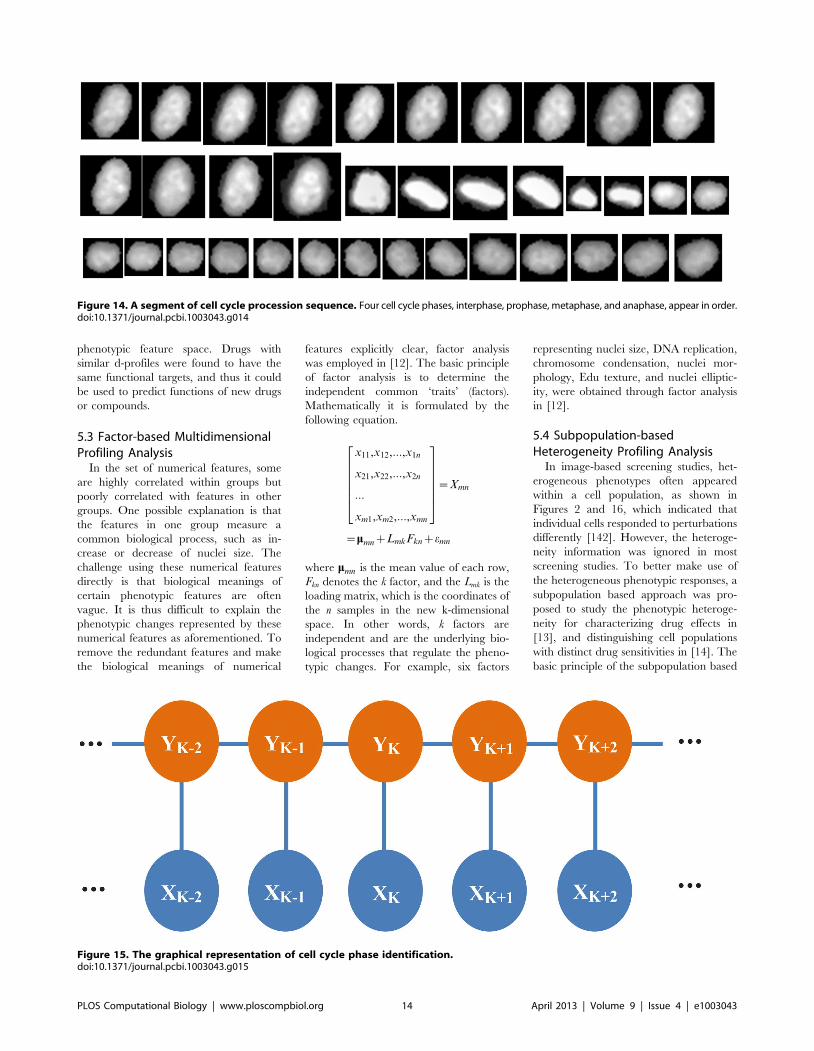
phenotypic feature space. Drugs with
similar d-profiles were found to have the
same functional targets, and thus it could
be used to predict functions of new drugs
or compounds.
5.3 Factor-based MultidimensionalProfiling Analysis
In the set of numerical features, some
are highly correlated within groups but
poorly correlated with features in other
groups. One possible explanation is that
the features in one group measure a
common biological process, such as in-
crease or decrease of nuclei size. The
challenge using these numerical features
directly is that biological meanings of
certain phenotypic features are often
vague. It is thus difficult to explain the
phenotypic changes represented by these
numerical features as aforementioned. To
remove the redundant features and make
the biological meanings of numerical
features explicitly clear, factor analysis
was employed in [12]. The basic principle
of factor analysis is to determine the
independent common ‘traits’ (factors).
Mathematically it is formulated by the
following equation.
x11,x12,:::,x1n
x21,x22,:::,x2n
:::
xm1,xm2,:::,xmn
2
666664
3
777775~Xmn
~mmnzLmkFknzemn
where mmn is the mean value of each row,
Fkn denotes the k factor, and the Lmk is the
loading matrix, which is the coordinates of
the n samples in the new k-dimensional
space. In other words, k factors are
independent and are the underlying bio-
logical processes that regulate the pheno-
typic changes. For example, six factors
representing nuclei size, DNA replication,
chromosome condensation, nuclei mor-
phology, Edu texture, and nuclei elliptic-
ity, were obtained through factor analysis
in [12].
5.4 Subpopulation-basedHeterogeneity Profiling Analysis
In image-based screening studies, het-
erogeneous phenotypes often appeared
within a cell population, as shown in
Figures 2 and 16, which indicated that
individual cells responded to perturbations
differently [142]. However, the heteroge-
neity information was ignored in most
screening studies. To better make use of
the heterogeneous phenotypic responses, a
subpopulation based approach was pro-
posed to study the phenotypic heteroge-
neity for characterizing drug effects in
[13], and distinguishing cell populations
with distinct drug sensitivities in [14]. The
basic principle of the subpopulation based
Figure 15. The graphical representation of cell cycle phase identification.doi:10.1371/journal.pcbi.1003043.g015
Figure 14. A segment of cell cycle procession sequence. Four cell cycle phases, interphase, prophase, metaphase, and anaphase, appear in order.doi:10.1371/journal.pcbi.1003043.g014
PLOS Computational Biology | www.ploscompbiol.org 14 April 2013 | Volume 9 | Issue 4 | e1003043
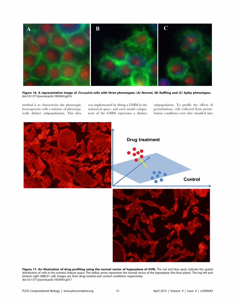
method is to characterize the phenotypic
heterogeneity with a mixture of phenotyp-
ically distinct subpopulations. This idea
was implemented by fitting a GMM in the
numerical space, and each model compo-
nent of the GMM represents a distinct
subpopulation. To profile the effects of
perturbations, cells collected from pertur-
bation conditions were first classified into
Figure 16. A representative image of Drosophila cells with three phenotypes: (A) Normal, (B) Ruffling and (C) Spiky phenotypes.doi:10.1371/journal.pcbi.1003043.g016
Figure 17. An illustration of drug profiling using the normal vector of hyperplane of SVM. The red and blue spots indicate the spatialdistribution of cells in the numeric feature space. The yellow arrow represents the normal vector of the hyperplane (the blue plane). The top left andbottom right (MB231 cell) images are from drug treated and control conditions respectively.doi:10.1371/journal.pcbi.1003043.g017
PLOS Computational Biology | www.ploscompbiol.org 15 April 2013 | Volume 9 | Issue 4 | e1003043
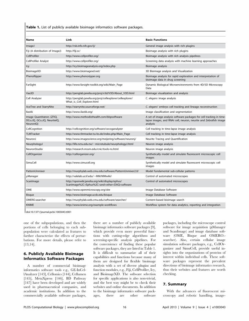
one of the subpopulations, and then the
portions of cells belonging to each sub-
population were calculated as features to
further characterize the effects of pertur-
bations. For more details, please refer to
[13,14].
6. Publicly Available BioimageInformatics Software Packages
A number of commercial bioimage
informatics software tools e.g., GE-InCel-
lAnalyzer [143], Cellomics [144], Cellumen
[145], MetaXpress [146], BD Pathway
[147] have been developed and are widely
used in pharmaceutical companies, and
academic institutions. In addition to the
commercially available software packages,
there are a number of publicly available
bioimage informatics software packages [9],
which provide even more powerful func-
tions with cutting-edge algorithms and
screening-specific analysis pipelines. For
the convenience of finding these popular
software packages, they are listed in Table 1.
It is difficult to summarize all of their
capabilities and functions because many of
them are designed for flexible bioimage
analysis with a set of diverse plugins and
function modules, e.g., Fiji, CellProfiler, Icy,
and BioimageXD. The software selection
for specific applications is also non-trivial,
and the best way might be to check their
websites and online documents. In addition
to the bioimage informatics software pack-
ages, there are other software
packages, including the microscope control
software for image acquisition (mManager
and ScanImage) and image database soft-
ware (OME, Bisque and OMERO.-
searcher). Also, certain cellular image
simulation software packages, e.g., CellOr-
ganizer and SimuCell, provide useful in-
sights into the organizations of proteins of
interest within individual cells. These soft-
ware packages represent the prevalent
directions of bioimage informatics research,
thus their websites and features are worth
checking.
7. Summary
With the advances of fluorescent mi-
croscopy and robotic handling, image-
Table 1. List of publicly available bioimage informatics software packages.
Name Link Basic Functions
ImageJ http://rsb.info.nih.gov/ij/ General image analysis with rich plugins
Fiji (A distribution of ImageJ) http://fiji.sc/ Bioimage analysis with rich plugins
CellProfiler http://www.cellprofiler.org/ Bioimage analysis with rich analysis pipelines
CellProfiler Analyst http://www.cellprofiler.org/ Screening data analysis with machine learning approaches
Icy http://icy.bioimageanalysis.org/index.php Bioimage analysis
BioimageXD http://www.bioimagexd.net/ 3D Bioimage analysis and Visualization
PhenoRipper http://www.phenoripper.org Bioimage analysis for rapid exploration and interpretation ofbioimage data in drug screening
FarSight http://www.farsight-toolkit.org/wiki/Main_Page Dynamic Biological Microenvironments from 4D/5D MicroscopyData
Vaa3D http://penglab.janelia.org/proj/v3d/V3D/About_V3D.html Bioimage visualization and analysis
Cell Analyzer http://penglab.janelia.org/proj/cellexplorer/cellexplorer/What_is_Cell_Explorer.html
C. elegans image analysis
AceTree and StarryNite http://starrynite.sourceforge.net/ C. elegans’ embryo cell tracking and lineage reconstruction
Ilastik http://www.ilastik.org/ Image classification and segmentation
Image Quantitators (ZFIQ,DCELLIQ, GCELLIQ, NeuriteIQ,NeuronIQ)
http://www.methodisthealth.com/bbpsoftware A set of image analysis software packages for cell tracking in time-lapse images, and RNAi cell, neuron, neurite and Zebrafish imageanalysis
CellCognition http://cellcognition.org/software/cecoganalyzer Cell tracking in time-lapse image analysis
TLMTracker http://www.tlmtracker.tu-bs.de/index.php/Main_Page Cell tracking in time-lapse image analysis
NeuronJ http://www.imagescience.org/meijering/software/neuronj/ Neurite Tracing and Quantification
NeurphologyJ http://life.nctu.edu.tw/,microtubule/neurphologyJ.html Neuron image analysis
NeuronStudio http://research.mssm.edu/cnic/tools-ns.html Neuron image analysis
CellOrganizer http://cellorganizer.org/ Synthetically model and simulate fluorescent microscopic cellimages
SimuCell http://www.simucell.org Synthetically model and simulate fluorescent microscopic cellimages
PatternUnmixer http://murphylab.web.cmu.edu/software/PatternUnmixer2.0/ Model fundamental sub-cellular patterns
mManager http://valelab.ucsf.edu/,MM/MMwiki/ Control of automated microscopes
ScanImage http://openwiki.janelia.org/wiki/display/ephus/ScanImage%2C+Ephus%2C+and+other+DAQ+software
Control of automated microscopes
OME http://www.openmicroscopy.org/site Image Database Software
Bisque http://www.bioimage.ucsb.edu/bisque Image Database Software
OMERO.searcher http://murphylab.web.cmu.edu/software/searcher/ Content-based bioimage search
KNIME http://www.knime.org/example-workflows Workflow system for data analytics, reporting and integration
doi:10.1371/journal.pcbi.1003043.t001
PLOS Computational Biology | www.ploscompbiol.org 16 April 2013 | Volume 9 | Issue 4 | e1003043
based screening has been widely used for
drug and target discovery by systematical-
ly investigating morphological changes
within cell populations. The bioimage
informatics approaches to automatically
detect, quantify, and profile the phenotyp-
ic changes caused by various perturba-
tions, e.g., drug compounds and RNAi,
are essential to the success of these image-
based screening studies. In this chapter, an
overview of the current bioimage infor-
matics approaches for systematic drug
discovery was provided. A number of
practical examples were first described to
illustrate the concepts and capabilities of
image-based screening for drug and target
discovery. Then, the prevalent bioimage
informatics techniques, e.g., object detec-
tion, segmentation, tracking and visualiza-
tion, were discussed. Subsequently, the
widely used numerical features, pheno-
types identification, classification, and
profiling analysis were introduced to
characterize the effects of drugs and
targets. Finally, the major publicly avail-
able bioimage informatics software pack-
ages were listed for future reference. We
hope that this review provided sufficient
information and insights for readers to
apply the approaches and techniques of
bioimage informatics to advance their
research projects.
8. Exercises
Q1. Understand the principle of using
green fluorescent protein (GFP) to label
the chromosome of HeLa cells.
Q2. Download a cellular image pro-
cessing software package, then download
some cell images, and use them as
examples to perform the cell detection,
segmentation, and feature extraction, and
provide the analysis results.
Q3. Download a time-lapse image
analysis software package, then download
some time-lapse images, and use them as
examples to perform cell tracking, and cell
cycle phase classification, and provide the
analysis results.
Q4. Download a neuron image analysis
software package, then download some
neuron images, and use them as examples
to perform dendrite and spine detection,
and provide the analysis results.
Q5. Implement the watershed and level
set segmentation methods by using ITK
functions (http://www.itk.org/) and test
them on some cell images.
Answers to the Exercises can be found
in Text S1.
Supporting Information
Text S1 Answers to Exercises.
(DOCX)
Acknowledgments
This paper summarizes over a decade of highly
productive collaborations with many colleagues
worldwide. The authors would like to acknowl-
edge their collaborators, in particular, Norbert
Perrimon, Jeff Lichtman, Bernando Sabatini,
Randy King, Junying Yuan, and Tim Mitchison
from Harvard Medical School; Alexei Degterev
and Eric Miller from Tufts University; Weiming
Xia from Boston VA Medical Center and
Boston University, Jun Lu from Stanford
University; Chris Bakal from Institute of Cancer
Research, Royal Cancer Hospital, U.K.; Yan
Feng of Novartis Institutes of Biomedical
Research; Shih Fu Chang of Columbia Univer-
sity; Marta Lipinski from the University of
Maryland at Baltimore; Jinwen Ma from Peking
University of China; Liang Ji from Tsinghua
University of China; Myong Hee Kim of
EWHA Womans University, Korea; Yong
Zhang from IBM Research; and Guanglei
Xiong from Siemens Corporate Research. The
raw image data presented in this paper were
mostly generated from the labs of our biological
collaborators. We would also like to thank our
colleagues at the Department of Systems
Medicine and Bioengineering, The Methodist
Hospital Research Institute for their discussions,
notably Xiaofeng Xia, Kemi Cui, Zhong Xue,
and Jie Cheng, as well as former members
including Xiaowei Chen, Ranga Srinivasan,
Peng Shi, Yue Huang, Gang Li, Xiaobo Zhou,
Jingxin Nie, Jun Wang, Tianming Liu, Huiming
Peng, Yong Zhang, and Qing Li. We would also
like to thank James Mancuso, Derek Cridebr-
ing, Luanne Novak, and Rebecca Danforth for
proofreading and discussion.
Further Reading
N Taylor DL (2010) A personal perspective on high-content screening (HCS): from the beginning. J Biomol Screen 15(7): 720–255.
N Shariff A, Kangas J, Coelho LP, Quinn S, Murphy RF (2010) Automated image analysis for high-content screening and analysis.J Biomol Screen 15(7): 726–734.
N Dufour A, Shinin V, Tajbakhsh S, Guillen-Aghion N, Olivo-Marin JC, et al. (2005) Segmenting and tracking fluorescent cells indynamic 3-D microscopy with coupled active surfaces. IEEE Trans Image Process 14: 1396–1410.
N Danuser G (2011) Computer vision in cell biology. Cell 147(5): 973–978.
N Murray JI, Bao Z, Boyle TJ, Boeck ME, Mericle BL, et al. (2008) Automated analysis of embryonic gene expression with cellularresolution in C. elegans. Nat Methods 5: 703–709.
N Rodriguez A, Ehlenberger DB, Dickstein DL, Hof PR, Wearne SL (2008) Automated three-dimensional detection and shapeclassification of dendritic spines from fluorescence microscopy images. PLoS ONE 3: e1997. doi:10.1371/journal.pone.0001997.
N Bakal C, Aach J, Church G, Perrimon N (2007) Quantitative morphological signatures define local signaling networksregulating cell morphology. Science 316(5832): 1753–1756.
N Neumann B, Walter T, Heriche JK, Bulkescher J, Erfle H, et al. (2010) Phenotypic profiling of the human genome by time-lapsemicroscopy reveals cell division genes. Nature 464: 721–727.
N Allan C, Burel JM, Moore J, Blackburn C, Linkert M, et al. (2012) OMERO: flexible, model-driven data management forexperimental biology. Nat Methods 9: 245–253.
N Eliceiri KW, Berthold MR, Goldberg IG, Ibanez L, Manjunath BS, et al. (2012) Biological imaging software tools. Nat Methods 9:697–710.
PLOS Computational Biology | www.ploscompbiol.org 17 April 2013 | Volume 9 | Issue 4 | e1003043
References
1. Tsien RY (1998) The green fluorescent protein.
Annu Rev Biochem 67: 509–544.
2. Lichtman JW, Conchello JA (2005) Fluorescencemicroscopy. Nat Methods 2: 910–919.
3. Shariff A, Kangas J, Coelho LP, Quinn S,
Murphy RF (2010) Automated image analysisfor high-content screening and analysis. J Biomol
Screen 15: 726–734.
4. Danuser G (2011) Computer vision in cellbiology. Cell 147: 973–978.
5. Taylor DL (2010) A personal perspective on
high-content screening (HCS): from the begin-
ning. J Biomol Screen 15(7): 720–255.
6. Abraham VC, Taylor DL, Haskins JR (2004)
High content screening applied to large-scale
cell biology. Trends Biotechnol 22: 15–22.
7. Giuliano KA, DeBiasio RL, Dunlay RT, GoughA, Volosky JM, et al. (1997) High-content
screening: a new approach to easing keybottlenecks in the drug discovery process.
J Biomol Screen 2: 249–259.
8. Peng H (2008) Bioimage informatics: a new areaof engineering biology. Bioinformatics 24: 1827–
1836.
9. Eliceiri KW, Berthold MR, Goldberg IG, IbanezL, Manjunath BS, et al. (2012) Biological imaging
software tools. Nat Methods 9: 697–710.
10. Yarrow JC, Feng Y, Perlman ZE, Kirchhausen
T, Mitchison TJ (2003) Phenotypic screening ofsmall molecule libraries by high throughput cell
imaging. Comb Chem High Throughput Screen6: 279–286.
11. Perlman Z, Slack M, Feng Y, Mitchison T, Wu
L, et al. (2004) Multidimensional drug profilingby automated microscopy. Science 306: 1194–
1198.
12. Young DW, Bender A, Hoyt J, McWhinnie E,Chirn G-W, et al. (2008) Integrating high-
content screening and ligand-target prediction
to identify mechanism of action. Nat Chem Biol4: 59–68.
13. Slack MD, Martinez ED, Wu LF, Altschuler SJ
(2008) Characterizing heterogeneous cellularresponses to perturbations. Proc Natl Acad
Sci U S A 105: 19306–19311.
14. Singh DK, Ku C-J, Wichaidit C, Steininger RJ,
Wu LF, et al. (2010) Patterns of basal signaling
heterogeneity can distinguish cellular popula-tions with different drug sensitivities. Mol Syst
Biol 6: 369.
15. Bakal C, Linding R, Llense F, Heffern E,Martin-Blanco E, et al. (2008) Phosphorylation
networks regulating JNK activity in diverse
genetic backgrounds. Science 322: 453–456.
16. Bakal C, Aach J, Church G, Perrimon N (2007)
Quantitative morphological signatures definelocal signaling networks regulating cell morphol-
ogy. Science 316: 1753–1756.
17. Carpenter AE, Jones TR, Lamprecht MR, ClarkeC, Kang IH, et al. (2006) CellProfiler: image
analysis software for identifying and quantifying
cell phenotypes. Genome Biol 7: R100.
18. Schindelin J, Arganda-Carreras I, Frise E,
Kaynig V, Longair M, et al. (2012) Fiji: an
open-source platform for biological-image anal-ysis. Nat Methods 9: 676–682.
19. de Chaumont F, Dallongeville S, Chenouard N,Herve N, Pop S, et al. (2012) Icy: an open
bioimage informatics platform for extended
reproducible research. Nat Methods 9: 690–696.
20. Yin Z, Zhou X, Bakal C, Li F, Sun Y, et al.
(2008) Using iterative cluster merging with
improved gap statistics to perform onlinephenotype discovery in the context of high-
throughput RNAi screens. BMC Bioinformatics
9: 264.
21. Rajaram S, Pavie B, Wu LF, Altschuler SJ
(2012) PhenoRipper: software for rapidly profil-ing microscopy images. Nat Methods 9: 635–
637.
22. Neumann B, Walter T, Heriche JK, BulkescherJ, Erfle H, et al. (2010) Phenotypic profiling of
the human genome by time-lapse microscopyreveals cell division genes. Nature 464: 721–727.
23. Held M, Schmitz MH, Fischer B, Walter T,
Neumann B, et al. (2010) CellCognition: time-resolved phenotype annotation in high-through-
put live cell imaging. Nat Methods 7: 747–
754.
24. Shi Q, King RW (2005) Chromosome nondis-
junction yields tetraploid rather than aneuploid
cells in human cell lines. Nature 437: 1038–1042.
25. Sigoillot FD, Huckins JF, Li F, Zhou X, WongST, et al. (2011) A time-series method for
automated measurement of changes in mitotic
and interphase duration from time-lapse movies.PLoS ONE 6: e25511. doi:10.1371/journal.
pone.0025511
26. Miki T, Lehmann T, Cai H, Stolz DB, StromSC (2005) Stem cell characteristics of amniotic
epithelial cells. Stem Cells 23: 1549–1559.
27. Li K, Miller ED, Chen M, Kanade T, Weiss LE,et al. (2008) Cell population tracking and lineage
construction with spatiotemporal context. MedImage Anal 12: 546–566.
28. Cohen AR, Gomes FL, Roysam B, Cayouette M
(2011) Computational prediction of neuralprogenitor cell fates. Nat Methods 7: 213–218.
29. Kankaanpaa P, Paavolainen L, Tiitta S, Karja-
lainen M, Paivarinne J, et al. (2012) BioIma-geXD: an open, general-purpose and high-
throughput image-processing platform. Nat
Methods 9: 683–689.
Glossary
N Cellular phenotype: A cellular phenotype refers to a distinct morphological appearance or behavior of cells as observedunder fluorescent, phase contrast, or bright field microscopy.
N Green fluorescent protein (GFP): GFP is used as a protein reporter by attaching to specific proteins, and exhibiting brightgreen fluorescence when exposed to light in the blue to ultraviolet range.
N Fluorescence microscope: A fluorescence microscope is an optical microscope that uses higher intensity light source toexcite a fluorescent species in a sample of interest.
N High content analysis (HCA): HCA focuses on extracting and analyzing quantitative phenotypic data automatically fromlarge amounts of cell images with automated image analysis, computer vision and machine learning approaches.
N High content screening (HCS): Applications of HCA for screening drugs and targets are referred to as HCS that aims toidentify compounds or genes that cause desired phenotypic changes.
N RNA interference (RNAi): RNAi is a biological process, in which RNA molecules inhibit gene expression, typically by causingthe destruction of specific mRNA molecules.
N Automated image analysis: Automated image analysis aims to quantitatively analyze images automatically by computerprograms with minimal human interventions.
N Object detection: Object detection is to automatically detect locations of objects of interest in images.
N Blob structure detection: Blob structure detection is to detect positions of objects of interest that have circle, sphere likestructures, e.g., nuclei and particles.
N Tube structure detection: Tube structure is to detect centerlines of objects that have long tube like structures, e.g., neurondendrite and blood vessel.
N Object segmentation: Object segmentation is to automatically delineate boundaries of objects of interest in images.
N Object tracking: Object tracking is to identify the motion traces of objects of interest in time-lapse images.
N Feature extraction: Feature extraction is to quantify the morphological appearances of segmented objects by calculating aset of numerical features.
N Phenotype classification: Phenotype classification is to assign each segmented object into a sub-group that has distinctphenotypes from other sub-groups.
N Cell cycle phase identification: Cell cycle phase identification is to automatically identify the corresponding cell cyclephase that a given cell is in according to its morphological appearances.
PLOS Computational Biology | www.ploscompbiol.org 18 April 2013 | Volume 9 | Issue 4 | e1003043
30. Li F, Zhou X, Ma J, Wong TCS (2010) Multiple
Nuclei Tracking Using Integer Programming for
Quantitative Cancer Cell Cycle Analysis. IEEETrans Med Imaging 29: 96–105.
31. Klein J, Leupold S, Biegler I, Biedendieck R,
Munch R, et al. (2012) TLM-Tracker: software
for cell segmentation, tracking and lineageanalysis in time-lapse microscopy movies. Bioin-
formatics 28: 2276–2277.
32. Segal M (2005) Dendritic spines and long-termplasticity. Nat Rev Neurosci 6: 277–284.
33. Hyman BT (2001) Molecular and anatomical
studies in Alzheimer’s disease. Neurologia 16:
100–104.
34. Ding JB, Takasaki KT, Sabatini BL (2009)Supraresolution imaging in brain slices using
stimulated-emission depletion two-photon laserscanning microscopy. Neuron 63: 429–437.
35. Nagerl UV, Willig KI, Hein B, Hell SW,Bonhoeffer T (2008) Live-cell imaging of
dendritic spines by STED microscopy. ProcNatl Acad Sci U S A 105: 18982–18987.
36. Carter AG, Sabatini BL (2004) State-dependent
calcium signaling in dendritic spines of striatal
medium spiny neurons. Neuron 44: 483–493.
37. Duemani Reddy G, Kelleher K, Fink R, SaggauP (2008) Three-dimensional random access
multiphoton microscopy for functional imagingof neuronal activity. Nat Neurosci 11: 713–720.
38. Iyer V, Hoogland TM, Saggau P (2006) Fast
functional imaging of single neurons using
random-access multiphoton (RAMP) microsco-py. J Neurophysiol 95: 535–545.
39. Cheng J, Zhou X, Miller E, Witt RM, Zhu J, et
al. (2007) A novel computational approach forautomatic dendrite spines detection in two-
photon laser scan microscopy. J Neurosci Meth-
ods 165: 122–134.
40. Ofengeim D, Shi P, Miao B, Fan J, Xia X, et al.(2012) Identification of small molecule inhibitors
of neurite loss induced by Abeta peptide usinghigh content screening. J Biol Chem 287: 8714–
8723.
41. Ho SY, Chao CY, Huang HL, Chiu TW,
Charoenkwan P, et al. (2011) NeurphologyJ: anautomatic neuronal morphology quantification
method and its application in pharmacologicaldiscovery. BMC Bioinformatics 12: 230.
42. Meijering E, Jacob M, Sarria JC, Steiner P,Hirling H, et al. (2004) Design and validation of
a tool for neurite tracing and analysis influorescence microscopy images. Cytometry A
58: 167–176.
43. Pool M, Thiemann J, Bar-Or A, Fournier AE
(2008) NeuriteTracer: a novel ImageJ plugin forautomated quantification of neurite outgrowth.
J Neurosci Methods 168: 134–139.
44. Xiong G, Zhou X, Degterev A, Ji L, Wong STC(2006) Automated neurite labeling and analysis
in fluorescence microscopy images. Cytometry
Part A 69A: 494–505.
45. Narro ML, Yang F, Kraft R, Wenk C, Efrat A,et al. (2007) NeuronMetrics: software for semi-
automated processing of cultured neuron imag-es. Brain Res 1138: 57–75.
46. Rodriguez A, Ehlenberger DB, Dickstein DL,Hof PR, Wearne SL (2008) Automated three-
dimensional detection and shape classification ofdendritic spines from fluorescence microscopy
images. PLoS ONE 3: e1997. doi:10.1371/journal.pone.0001997
47. Wearne SL, Rodriguez A, Ehlenberger DB,Rocher AB, Henderson SC, et al. (2005) New
techniques for imaging, digitization and analysisof three-dimensional neural morphology on
multiple scales. Neuroscience 136: 661–680.
48. Zhang Y, Zhou X, Witt RM, Sabatini BL,
Adjeroh D, et al. (2007) Dendritic spinedetection using curvilinear structure detector
and LDA classifier. Neuroimage 36: 346–360.
49. Peng H, Ruan Z, Atasoy D, Sternson S (2010)Automatic reconstruction of 3D neuron struc-
tures using a graph-augmented deformable
model. Bioinformatics 26: i38–i46.
50. Peng H, Long F, Myers G (2011) Automatic 3D
neuron tracing using all-path pruning. Bioinfor-matics 27: i239–i247.
51. Meijering E (2010) Neuron tracing in perspec-
tive. Cytometry A 77: 693–704.
52. Boyle TJ, Bao Z, Murray JI, Araya CL,
Waterston RH (2006) AceTree: a tool for visual
analysis of Caenorhabditis elegans embryogen-esis. BMC Bioinformatics 7: 275.
53. Bao Z, Murray JI, Boyle T, Ooi SL, Sandel MJ,et al. (2006) Automated cell lineage tracing in
Caenorhabditis elegans. Proc Natl Acad Sci U S A
103: 2707–2712.
54. Sarov M, Murray JI, Schanze K, Pozniakovski
A, Niu W, et al. (2012) A genome-scale resourcefor in vivo tag-based protein function explora-
tion in C. elegans. Cell 150: 855–866.
55. Liu X, Long F, Peng H, Aerni SJ, Jiang M, et al.(2009) Analysis of cell fate from single-cell gene
expression profiles in C. elegans. Cell 139: 623–633.
56. Long F, Peng H, Liu X, Kim SK, Myers E
(2009) A 3D digital atlas of C. elegans and itsapplication to single-cell analyses. Nat Methods
6: 667–672.
57. Wahlby C, Kamentsky L, Liu ZH, Riklin-Raviv
T, Conery AL, et al. (2012) An image analysis
toolbox for high-throughput C. elegans assays.Nat Methods 9: 714–716.
58. Borgefors G (1986) Distance transformations indigital images. Computer Vision, Graphics, and
Image Processing 34: 344–371.
59. Wahlby C, Sintorn I, Erlandsson F, BorgeforsG, Bengtsson E (2004) Combining intensity,
edge and shape information for 2D and 3Dsegmentation of cell nuclei in tissue sections.
J Microsc 215: 67–76.
60. Lindeberg T (1993) Detecting salient blob-likeimage structures and their scales with a scale-
space primal sketch: a method for focus-of-attention. Int J Comput Vision 11: 283–318.
61. Lindeberg T (1998) Feature detection with
automatic scale selection. Int J Comput Vision30: 79–116.
62. Byun J, Verardo MR, Sumengen B, Lewis GP,
Manjunath BS, et al. (2006) Automated tool forthe detection of cell nuclei in digital microscopic
images: application to retinal images. Mol Vis12: 949–960.
63. Al-Kofahi Y, Lassoued W, Lee W, Roysam B
(2010) Improved automatic detection and seg-mentation of cell nuclei in histopathology
images. IEEE Trans Biomed Eng 57: 841–852.
64. Li G, Liu T, Tarokh A, Nie J, Guo L, et al.
(2007) 3D cell nuclei segmentation based on
gradient flow tracking. BMC Cell Biology 8: 40.
65. Xu C, Prince JL (1998) Snakes, shapes, and
gradient vector flow. IEEE Transactions onImage Processing 7: 359–369.
66. Duda RO, Hart PE (1972) Use of the Hough
transformation to detect lines and curves inpictures. Commun ACM 15: 11–15.
67. Parvin B, Yang Q, Han J, Chang H, Rydberg B,
et al. (2007) Iterative voting for inference ofstructural saliency and characterization of sub-
cellular events. IEEE Trans Image Process 16:615–623.
68. Lin G, Adiga U, Olson K, Guzowski JF, Barnes
CA, et al. (2003) A hybrid 3D watershedalgorithm incorporating gradient cues and
object models for automatic segmentation ofnuclei in confocal image stacks. Cytometry A 56:
23–36.
69. Lienhart R, Maydt J (2002) An extended set ofHaar-like features for rapid object detection. pp.
I-900–I-903. Vol. 1. Proceedings of the 2002International Conference on Image Processing.
70. Viola P, Jones M (2001) Rapid object detection
using a boosted cascade of simple features.Proceedings of the 2001 IEEE Computer
Society Conference on Computer Vision andPattern Recognition. pp. I-511–I-518. Vol. 1.
71. He W, Wang X, Metaxas D, Mathew R, White
E (2007) Cell segmentation for division rate
estimation in computerized video time-lapse
microscopy. 643109–643109.
72. Jiang S, Zhou X, Kirchhausen T, Wong ST(2007) Detection of molecular particles in live
cells via machine learning. Cytometry A 71:
563–575.
73. Sommer C, Straehle C, Kothe U, Hamprecht
FA (2011) Ilastik: interactive learning and
segmentation toolkit. pp. 230–233. 2011 IEEEInternational Symposium on Biomedical Imag-
ing; 30 March–2 April 2011.
74. Steger C (1998) An unbiased detector ofcurvilinear structures. IEEE Transactions on
Pattern Analysis and Machine Intellegence 20:113–125.
75. Al-Kofahi KA, Lasek S, Szarowski DH, Pace
CJ, Nagy G, et al. (2002) Rapid automatedthree-dimensional tracing of neurons from con-
focalimage stacks. IEEE Transactions on Infor-
mation Technology in Biomedicine 6: 171–187.
76. Tyrrell JA, di Tomaso E, Fuja D, Ricky T,
Kozak K, et al. (2007) Robust 3-D modeling of
vasculature imagery using superellipsoids. IEEETrans Med Imaging 26: 223–237.
77. Soares JVB, Leandro JJG, Cesar RM, Jelinek
HF, Cree MJ (2006) Retinal vessel segmentationusing the 2-D Gabor wavelet and supervised
classification. IEEE Trans Med Imaging 25:1214–1222.
78. Staal J, Abramoff MD, Niemeijer M, Viergever
MA, van Ginneken B (2004) Ridge-based vesselsegmentation in color images of the retina. IEEE
Trans Med Imaging 23: 501–509.
79. Fraz M, Remagnino P, Hoppe A, Uyyanonvara
B, Rudnicka A, et al. (2012) Blood vesselsegmentation methodologies in retinal images -
a survey. Comput Methods Programs Biomed108(1): 407–433.
80. Otsu N (1978) A threshold selection method
from gray level histgram. IEEE Transactions onSystem, Man, and Cybernetics 8: 62–66.
81. Dunn JC (1973) A fuzzy relative of the
ISODATA process and its use in detectingcompact well-separated clusters. Journal of
Cybernetics 3: 32–57.
82. Vincent L, Soille P (1991) Watersheds in digitalspaces: an efficient algorithm based on immer-
sion simulations. IEEE Transactions on Pattern
Analysis and Machine Intelligence 13: 583–598.
83. Beucher S (1992) The watershed transformation
applied to image segmentation. Scanning Mi-
croscopy International 6: 299–314.
84. Meyer F, Beucher S (1990) Morphological
segmentation. Journal of Visual Communication
and Image Representation 1: 21–46.
85. Wahlby C, Lindblad J, Vondrus M, Bengtsson
E, Bjorkesten L (2002) Algorithms for cytoplasm
segmentation of fluorescence labelled cells.Analytical Cellular Pathology 24: 101–111.
86. Casselles V, Kimmel R, Sapiro G (1997)
Geodesic active contours. International Journalof Computer Vision 22: 61–79.
87. Chan T, Vese L (2001) Active contours without
edges. IEEE Transactions on Image Processing10: 266–277.
88. Zimmer C, Labruyere E, Meas-Yedid V,
Guillen N, Olivo-Marin J (2002) Segmentationand tracking of migrating cells in videomicro-
scopy with parametric active contours: a tool for
cell-based drug testing. IEEE Trans MedImaging 21: 1212–1221.
89. Yan P, Zhou X, Shah M, Wong ST (2008)
Automatic segmentation of high-throughputRNAi fluorescent cellular images. IEEE Trans
Inf Technol Biomed 12: 109–117.
90. Dufour A, Shinin V, Tajbakhsh S, Guillen-Aghion N, Olivo-Marin JC, et al. (2005)
Segmenting and tracking fluorescent cells indynamic 3-D microscopy with coupled active
surfaces. IEEE Transactions on Image Process-
ing 14: 1396–1410.
91. Caselles V, Kimmel R, Sapiro G (1997)
Geodesic active contours. International Journal
of Computer Vision 22: 61–79.
PLOS Computational Biology | www.ploscompbiol.org 19 April 2013 | Volume 9 | Issue 4 | e1003043
92. Osher S, Sethian JA (1988) Fronts propagating
with curvature-dependent speed: Algorithms
based on Hamilton-Jacobi formulations. Journal
of Computation Physics 79: 12–49.
93. Chunming L, Chenyang X, Changfeng G, Fox
MD (2005) Level set evolution without re-
initialization: a new variational formulation.
IEEE Computer Society Conference on Com-
puter Vision and Pattern Recognition; 20–25
June 2005. pp. 430–436. Vol. 1.
94. Aurenhammer F (1991) Voronoi diagrams - a
survey of a fundamental geometric data struc-
ture. ACM Comput Surv 23: 345–405.
95. Jones T, Carpener A, Golland P (2005) Voronoi-
based segmentation of cells on image manifolds.
Lecture Notes in Computer Science: 535–543.
96. Shi J, Malik J (2000) Normalized cuts and image
segmentation. IEEE Trans Pattern Anal Mach
Intell 22: 888–905.
97. Felzenszwalb PF, Huttenlocher DP (2004) Effi-
cient graph-based image segmentation.
Int J Comput Vision 59: 167–181.
98. Radhakrishna A, Shaji A, Smith K, Lucchi A,
Fua P, et al. (June, 2010) SLIC superpixels.
Technical report 149300, EPFL.
99. Lucchi A, Smith K, Achanta R, Lepetit V, Fua
P (2010) A fully automated approach to
segmentation of irregularly shaped cellular
structures in EM images. Proceedings of the
13th International Conference on Medical
Image Computing and Computer-Assisted In-
tervention. Med Image Comput Comput Assist
Interv 13(Pt 2): 463–471.
100. Debeir O, Ham PV, Kiss R, Decaestecker C
(2005) Tracking of migrating cells under phase-
contrast video microscopy with combined mean-
shift processes. IEEE Trans Med Imaging 24:
697–711.
101. Zimmer C, Olivo-Marin JC (2005) Coupled
parametric active contours. IEEE Trans Pattern
Anal Mach Intell 27: 1838–1842.
102. Yang F, Mackey MA, Ianzini F, Gallardo G,
Sonka M (2005) Cell segmentation, tracking,
and mitosis detection using temporal context.
Med Image Comput Comput Assist Interv 8(Pt
1): 302–309.
103. Bunyak F, Palaniappan K, Nath SK, Baskin TL,
Gang D (2006) Quantitative cell motility for in
vitro wound healing using level set-based active
contour tracking. Proc IEEE Int Symp Biomed
Imaging 2006 April 6: 1040–1043.
104. Dzyubachyk O, van Cappellen WA, Essers J,
Niessen WJ, Meijering E (2010) Advanced level-
set-based cell tracking in time-lapse fluorescence
microscopy. IEEE Trans Med Imaging 29: 852–
867.
105. Bo Z, Zimmer C, Olivo-Marin JC (2004)
Tracking fluorescent cells with coupled geomet-
ric active contours. IEEE International Sympo-
sium on Biomedical Imaging; 15–18 April 2004.
pp. 476–479. Vol. 1.
106. Li K, Miller ED, Weiss LE, Campbell PG,
Kanade T (2006) Online tracking of migrating
and proliferating cells imaged with phase-
contrast microscopy. Conference on Computer
Vision and Pattern Recognition Workshop. New
York City, New York. pp. 65.
107. Nath SK, Palaniappan K, Bunyak F (2006) Cell
segmentation using coupled level sets and graph-
vertex coloring. Proceedings of the 9th Interna-
tional Conference on Medical Image Comput-
ing and Computer-Assisted Intervention. Med
Image Comput Comput Assist Interv 9 (Pt 1):
101–108.
108. Appel K, Haken W (1977) Every planar map is
four colorable part I. Discharging. Illinois
Journal of Mathematics: 429–490.
109. Appel K, Haken W, Koch J (1977) Every planar
map is four colorable part II. Reducibility.Illinois Journal of Mathematics: 491–567.
110. Padfield DR, Rittscher J, Sebastian T, Thomas
N, Roysam B (2006) Spatio-temporal cell cycleanalysis using 3D level set segmentation of
unstained nuclei in line scan confocal fluores-cence images. 3rd IEEE International Sympo-
sium on Biomedical Imaging; 6–9 April 2006.
pp. 1036–1039.111. Padfield DR, Rittscher J, Roysam B (2008)
Spatio-temporal cell segmentation and trackingfor automated screening. 5th IEEE International
Symposium on Biomedical Imaging; 14–17 May2008. pp. 376–379.
112. Padfield D, Rittscher J, Thomas N, Roysam B
(2009) Spatio-temporal cell cycle phase analysisusing level sets and fast marching methods.
Medical Image Analysis 13: 143–155.113. Al-Kofahi O, Radke RJ, Goderie SK, Shen Q,
Temple S, et al. (2006) Automated cell lineage
construction: a rapid method to analyze clonaldevelopment established with murine neural
progenitor cells. Cell Cycle 5: 327–335.114. Chen X, Zhou X, Wong STC (2006) Automated
segmentation, classification, and tracking ofcancer cell nuclei in time-lapse microscopy.
IEEE Transactions on Biomedical Engineering
53: 762–766.115. Harder N, Mora-Bermudez F, Godinez WJ,
Ellenberg J, Eils R, et al. (2006) Automatedanalysis of the mitotic phases of human cells in
3D fluorescence microscopy image sequences.
Med Image Comput Comput Assist Interv 9:840–848.
116. Li K, Chen M, Kanade T (2007) Cell popula-tion tracking and lineage construction with
spatiotemporal context. Med Image ComputComput Assist Interv 10: 295–302.
117. Blom HAP (1984) An efficient filter for abruptly
changing systems. Proceedings of 23rd IEEEConference on Decision and Control 23: 656–658.
118. Genovesio A, Liedl T, Emiliani V, Parak WJ,Coppey-Moisan M, et al. (2006) Multiple
particle tracking in 3-D+t microscopy: method
and application to the tracking of endocytosedquantum dots. IEEE Trans Image Process 15:
1062–1070.119. Smal I, Draegestein K, Galjart N, Niessen W,
Meijering E (2007) Rao-blackwellized marginalparticle filtering for multiple object tracking in
molecular bioimaging. Proceedings of the 20th
International Conference on Information Pro-cessing in Medical Imaging. Kerkrade, The
Netherlands: Springer-Verlag.120. Smal I, Niessen W, Meijering E (2006) Bayesian
tracking for fluorescence microscopic imaging;
6–9 April 2006. pp. 550–553.121. Godinez WJ, Lampe M, Worz S, Muller B, Eils
R, et al. (2007) Tracking of virus particles intime-lapse fluorescence microscopy image se-
quences. 12–15 April 2007. pp. 256–259.
122. Luisi J, Narayanaswamy A, Galbreath Z,Roysam B (2011) The FARSIGHT trace editor:
an open source tool for 3-D inspection andefficient pattern analysis aided editing of auto-
mated neuronal reconstructions. Neuroinfor-matics 9: 305–315.
123. Peng H, Ruan Z, Long F, Simpson JH, Myers
EW (2010) V3D enables real-time 3D visualiza-tion and quantitative analysis of large-scale
biological image data sets. Nat Biotechnol 28:348–353.
124. Manjunath B, Ma W (1996) Texture features for
browsing and retrieval of image data. IEEETrans Pattern Anal Mach Intell 18: 837–842.
125. Zhou X, Wong STC (2006) Informatics chal-lenges of high-throughput microscopy. IEEE
Signal Processing Magazine 23: 63–72.
126. Chen X, Zhou X, Wong ST (2006) Automated
segmentation, classification, and tracking of
cancer cell nuclei in time-lapse microscopy.
IEEE Trans Biomed Eng 53: 762–766.
127. Boland M, Murphy R (2001) A neural network
classifier capable of recognizing the patterns of
all major subcellular structures in fluorescence
microscope images of HeLa cells. Bioinformatics
17: 1213–1223.
128. Haralick R (1979) Statistical and structural
approaches to texture. Proceedings of IEEE
67: 786–804.
129. Manjunatha BS, Ma WY (1996) Texture
features for browsing and retrieval of image
data. IEEE Trans Pattern Anal Mach Intell 18:
837–842.
130. Cohen A, Daubechies I, Feauveau JC (1992) Bi-
orthogonal bases of compactly supported wave-
lets. Communications on Pure and Applied
Mathematics 45: 485–560.
131. Zernike F (1934) Beugungstheorie des schnei-
dencerfarhens undseiner verbesserten form, der
phasenkontrastmethode. Physica 1: 689–704.
132. Haralick RM, Shanmugam K, Dinstein I (1973)
Textural features for image classification. IEEE
Transactions on Systems, Man and Cybernetics
6: 610–620.
133. Harder N, Mora-Bermudez F, Godinez WJ,
Wunsche A, Eils R, et al. (2009) Automatic
analysis of dividing cells in live cell movies to
detect mitotic delays and correlate phenotypes in
time. Genome Res 19: 2113–2124.
134. Zhong Q, Busetto AG, Fededa JP, Buhmann
JM, Gerlich DW (2012) Unsupervised modeling
of cell morphology dynamics for time-lapse
microscopy. Nat Methods 9: 711–713.
135. Wang M, Zhou X, Li F, Huckins J, King WR, et
al. (2008) Novel cell segmentation and online
SVM for cell cycle phase identification in
automated microscopy. Bioinformatics 24: 94–
101.
136. Wang J, Zhou X, Bradley PL, Chang SF,
Perrimon N, et al. (2008) Cellular phenotype
recognition for high-content RNA interference
genome-wide screening. J Biomol Screen 13:
29–39.
137. Yan M, Ye K (2007) Determining the number of
clusters using the weighted gap statistic. Biomet-
rics 63: 1031–1037.
138. Jones TR, Carpenter AE, Lamprecht MR,
Moffat J, Silver SJ, et al. (2009) Scoring diverse
cellular morphologies in image-based screens
with iterative feedback and machine learning.
Proc Natl Acad Sci U S A 106: 1826–1831.
139. Young DW, Bender A, Hoyt J, McWhinnie E,
Chirn GW, et al. (2008) Integrating high-content
screening and ligand-target prediction to identify
mechanism of action. Nat Chem Biol 4: 59–68.
140. Frise E, Hammonds AS, Celniker SE Systematic
image-driven analysis of the spatial Drosophila
embryonic expression landscape. Mol Syst Biol
6: 345.
141. Loo LH, Wu LF, Altschuler SJ (2007) Image-
based multivariate profiling of drug responses
from single cells. Nat Methods 4: 445–453.
142. Altschuler SJ, Wu LF (2010) Cellular heteroge-
neity: do differences make a difference? Cell
141: 559–563.
143. GE-InCellAnalyzer. http://www.biacore.com/
high-content-analysis/index.html.
144. Cellomics. http://www.cellomics.com/content/
menu/About_Us/.
145. Cellumen. http://www.cellumen.com/.
146. MetaXpress. http://www.moleculardevices.
com/pages/software/metaxpress.html.
147. BD-Pathway. http://www.bdbiosciences.ca/
bioimaging/cell_biology/pathway/software/.
PLOS Computational Biology | www.ploscompbiol.org 20 April 2013 | Volume 9 | Issue 4 | e1003043

ploscompbiol.org
PLOS is a nonprofit organization founded to accelerate progress in science and medicine by leading a transformation in research communication.