bioinformatics: - cutm courseware
TRANSCRIPT

Bioinformatics:Applications in Life andEnvironmental Sciences

Edited by
M.H. FulekarDepartment of Life SciencesUniversity of Mumbai, India
Bioinformatics:Applications in Life andEnvironmental Sciences
A C.I.P. Catalogue record for this book is available from the Library of Congress.
ISBN 978-1-4020-8879-7 (HB)ISBN 978-1-4020-8880-3 (e-book)
Copublished by Springer,P.O. Box 17, 3300 AA Dordrecht, The Netherlandswith Capital Publishing Company, New Delhi, India.
Sold and distributed in North, Central and South America by Springer,233 Spring Street, New York 10013, USA.
In all other countries, except India, sold and distributed by Springer, Haberstrasse7, D-69126 Heidelberg, Germany.
In India, sold and distributed by Capital Publishing Company,7/28, Mahaveer Street, Ansari Road, Daryaganj, New Delhi, 110 002, India.
www.springer.com
Printed on acid-free paper
All Rights Reserved© 2009 Capital Publishing CompanyNo part of this work may be reproduced, stored in a retrieval system, ortransmitted in any form or by any means, electronic, mechanical, photocopying,microfilming, recording or otherwise, without written permission from thePublisher, with the exception of any material supplied specifically for the purposeof being entered and executed on a computer system, for exclusive use by thepurchaser of the work.
Printed in India.

Preface
Bioinformatics, a multidisciplinary subject, has established itself as a full-fledged discipline that provides scientific tools and newer insights in theknowledge discovery process in the front-line research areas and has becomea growth engine in Biotechnology. It provides a better understanding ofbiomolecules, which is applicable at all levels of the living world startingfrom atomic and molecular levels to the higher complex of systems biology.The discovery of biomolecular sequences and their relation to the functioningof organisms have created a number of challenging problems for computerscientists, and led to emerging interdisciplinary field of Bioinformatics,Computational Biology, Genomics and Proteomics studies. Bioinformatics(Computational Biology) is a relatively new field that applies computerscience and information technology to biology. In recent years, the disciplineof Bioinformatics has allowed the biologist to make full use of the advancesin computer sciences and computational statistics for advancing the biologicaldata. Researchers in the Life Sciences generate, collect and analyze anincreasing number of different types of scientific data, DNA, RNA andprotein sequences, in situ and microarray gene expression including 3Dprotein structures and biological pathways.
This book aims at providing information on Bioinformatics at variouslevels to the post-graduate students and research scholars studying in theareas of Biotechnology/Environmental Sciences/Life Sciences and otherapplied and allied biosciences and technologies. The chapters included in thebook cover from introductory to advanced aspects, including applications ofvarious documented research work and specific case studies related toBioinformatics. The topics covered under Bioinformatics in Life andEnvironmental Sciences include: Role of Computers in Bioinformatics,Comparative Genomics and Proteomics, Bioinformatics – Structural BiologyInterface, Statistical Mining of Gene and Protein Databanks, BuildingBioinformatics Database Systems, Bio-sequence signatures using Chaos GameRepresentation, data mining for Bioinformatics, Environmental clean upapproach using Bioinformatics in Bioremediation and Nanotechnology inrelation to Bioinformatics. This book will also be of immense value to thereaders of different backgrounds such as engineers, scientists, consultantsand policy makers for industry, government, academics and social and private

organizations. Bioinformatics is an innovative field in the area of computerscience and information technology for interpretation and compilation ofdata and gives the opening for advanced research and its applications inbiological sciences.
The book has contributions from expert academicians, scientists fromUniversities, Institutes, IIT, BARC and personnel from research organizationsand industries. This publication is an attempt to provide information onBioinformatics and its application in life and environmental sciences.
I am grateful to Honourable Vijay Khole, the Vice Chancellor of Universityof Mumbai for having provided facilities and encouragement. It gives meimmense pleasure to express deep gratitude to my colleagues and friendswho have helped me directly or indirectly in completing this manuscript andalso to my family in particular my wife Dr. (Mrs.) Kalpana and childrenJaya, Jyoti and Vinay and brothers Dilip and Kishor for their constant supportand encouragement. The technical assistance provided by my PhD studentsis also greatly acknowledged.
M.H. FulekarProfessor and Head
Dept. of Life SciencesUniversity of Mumbai
Mumbai, India
vi Preface

Contributors
M.H. FulekarProfessor & HeadDepartment of Life SciencesUniv. of Mumbai, Mumbai-400 098Email: [email protected]
B.B. MeshramProfessorComputer Engineering DivisionVJTI, MatungaMumbai-400 019Email: [email protected]
Rajani R. JoshiProfessorDepartment of MathematicsIIT Mumbai, PowaiMumbai-400 076Email: [email protected]
M.V. HosurSenior ScientistSolid State Physics Division (SSPD)BARC, TrombayMumbai-400 085Email: [email protected]
T.M. BansodConsultant, Information SecurityMIEL e-security Pvt. Ltd.Andheri (E), MumbaiEmail: [email protected]
Achuthsankar S. NairDirector, Centre for BioinformaticsUniversity of Kerala, TrivandrumEmail: [email protected]
Vrinda V. NairCentre for BioinformaticsUniversity of Kerela, Trivandrum
K.S. ArunCentre for BioinformaticsUniversity of Kerela, Trivandrum
Krishna KantDepartment of Information TechnologyGovt. of India, New Delhi
Alpana DeyDepartment of Information TechnologyGovt. of India, New Delhi
S.I. AhsonProfessor & HeadDepartment of Computer ScienceJamia Millia IslamiaNew DelhiEmail: [email protected]
T.V. PrasadProfessor & HeadDept. of Computer Science &EngineeringLingaya’s Institute of Management &TechnologyFaridabad-121 002, HaryanaEmail: [email protected]
Desh Deepak SinghIndian Institute of Advanced ResearchKoba, GandhinagarGujarat-382 007Email: [email protected]
S.J. GuptaProfessor & HeadDepartment of PhysicsUniversity of MumbaiMumbai-400 098Email: [email protected]

Contents
Preface v
Contributors vii
1. Bioinformatics in Life and Environmental SciencesM.H. Fulekar 1
2. Role of Computers in BioinformaticsTularam M. Bansod 12
3. Comparative Genomics and ProteomicsM.V. Hosur 17
4. Bioinformatics—Structural Biology InterfaceDesh Deepak Singh 25
5. Statistical Mining of Gene and Protein DatabanksRajani R. Joshi 34
6. Building Bioinformatic Database SystemsB.B. Meshram 44
7. Bio-sequence Signatures Using Chaos Game RepresentationAchuthsankar S. Nair, Vrinda V. Nair, Arun K.S.,
Krishna Kant and Alpana Dey 628. Data Mining for Bioinformatics—Microarray Data
T.V. Prasad and S.I. Ahson 779. Data Mining for Bioinformatics—Systems Biology
T.V. Prasad and S.I. Ahson 14510. Environmental Cleanup Approach Using Bioinformatics
in BioremediationM.H. Fulekar 173
11. Nanotechnology—In Relation to BioinformaticsM.H. Fulekar 200
12. Bioinformatics—Research ApplicationsS. Gupta 207
Appendix 1 215Appendix 2 221Index 245
Bioinformatics in Life andEnvironmental Sciences
M.H. Fulekar
INTRODUCTION
Bioinformatics involves close relation between biology and computers thatinfluence each other and synergistically merging more than once. The varietyof data from biology, mainly in the form of DNA, RNA, protein sequencesis putting heavy demand in computer sciences and computational biology. Itis demanding transformation of basic ethos of biological sciences.
The Bioinformaticians are those who specialize in use of computationaltools and systems to answer problems in biology. They include computerscientists, mathematicians, statisticians, engineers and biologists whospecialize in developing algorithms, theories and techniques for such toolsand systems. Bioinformatics has also taken on a new glitter by entering thefield of drug discovery in a big way. System biology promises great growthin modeling silver line using engineering approach with close relation withbiology. Bioinformatic techniques have been developed to identify and analyzevarious components of cells such as gene and protein function, interactionsand metabolic and regulatory pathways. The next decade will belong tounderstanding cellular mechanism and cellular manipulation using theintegration of bioinformatics, wet lab, and cell simulation techniques.Bioinformatics has focus on cellular and molecular levels of biology and hasa wide application in life sciences. Current research in bioinformatics can beclassified into: (i) genomics—sequencing and comparative study of genomesto identify gene and genome functionality, (ii) proteomics—identificationand characterization of protein related properties, (iii) cell visualization andsimulation to study and model cell behaviour, and (iv) application to thedevelopment of drugs and anti-microbial agents. Bioinformatics also offersmany interesting possibilities for bioremediation from environment protectionpoint of view. The integration of biodegradation information, with thecorresponding protein and genomic data, provides a suitable framework forstudying the global properties of the bioremediation network. This disciplinerequires the integration of huge amount of data from various sources—
1

2 M.H. Fulekar
chemical structure and reactivity of organic compounds, sequence, structureand function of proteins (enzymes), comparative genomics, environmentmicrobiology and so on. Bioinformatics has the following major branches:Genomics, Proteomics, Computer Aided Drug Designing, Biodatabase andData Mining, Molecular Phylogenetics, Microarray informatics and Systembiology. Thus, bioinformatics has focused on cellular and molecular levelsof biology and has a wide application in life sciences and environmentprotection.
The study and understanding of cell is prime concern for bioinformatics.
CELL COMPONENTS
The cell is the structural and functional unit of all living organisms, and islsometimes called the “building block of life”. Some organisms, such asbacteria, are unicellular, consisting of a single cell. Other organisms, such ashumans, are multicellular. (Humans have an estimated 100 trillion or 1014
cells; a typical cell size is 10 μm; a typical cell mass is one nanogram.) Allliving organisms are divided into five kingdoms: Monera, Protista, Fungi,Plantae and Animalia.
All cells fall into one of the two major classifications of prokaryotes andeukaryotes.
Prokaryotes
Prokaryotes are unicellular organisms,found in all environments. Prokaryotesare the largest group of organisms,mostly due to the vast array of bacteriawhich comprise the bulk of theprokaryote classification.
Characteristics:• No nuclear membrane (genetic
material dispersed throughoutcytoplasm)
• No membrane-bound organelles• Simple internal structure• Most primitive type of cell (appeared
about four billion years ago)
Examples:• Staphylococcus• Escherichia coli (E. coli)• Streptococcus
Chromosomes are the basic components of a cell. It is usually in the formof chromatin and composed of DNA which contains genetic information.The main component is mitochondria which is known as “power house” of
Eukaryotes
Eukaryotes are generally more advancedthan prokaryotes. There are manyunicellular organisms which areeukaryotic, but all cells in multicellularorganisms are eukaryotic.
Characteristics:• Nuclear membrane surrounding
genetic material• Numerous membrane-bound organelles• Complex internal structure• Appeared approximately one billion
years ago
Examples:• Paramecium• Dinoflagellates
Bioinformatics in Life and Environmental Sciences 3
the cell. This is a highly polymorphic organelle of eukaryotic cells thatvaries from short rod-like structures present in high number to long branchedstructures. It contains DNA and mitoribosomes and has double membranesystem and the inner membrane may contain numerous folds (cristae). Theinner fluid phase has most of the enzymes of the tricarboxylic acid cycle andsome of the urea cycle. The inner membrane contains the components of theelectron transport chain. Its major function is to regenerate ATP by oxidativephosphorylation. The Krebs cycle occurs within the central matrix of themitochondrion and the cytochrome system occurs on the cristae which isbound on the large surface area of the sausage shaped mitochondrion. Theyare found in highly active cells like liver cells but not found in less activecells like red blood cells. Glycosylation and packaging of secreted proteinstakes place in Golgi apparatus, which is an intracellular stack of membranebounded vesicles. It is a net-like structure in the cytoplasm of animal cells(especially in those cells that produce secretions). Golgi apparatus is a cellorganelle named after Camillo Golgi (1898), who first described it. Thegolgi apparatus receives newly synthesized molecules from the endoplasmicreticulum and stores them. It also attaches extra components to the molecule,such as adding carbohydrate to a protein (glycosylation). When the moleculeis in demand, it is secreted in the form of a vesicle, which contains thefinished product.
Nucleus is the major organelle of eukaryotic cells, in which thechromosomes are separated from the cytoplasm by the nuclear envelope.The nucleus has three parts: the nucleolus, the chromatin, and the nuclearenvelope. A specialized, usually spherical mass of protoplasm encased in adouble membrane, and found in most living eukaryotic cells, it directs theirgrowth, metabolism, and reproduction, and functioning in the transmissionof genic characters.
DNA (Deoxyribonucleic Acid)
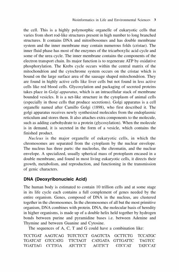
The human body is estimated to contain 10 trillion cells and at some stagein its life cycle each contains a full complement of genes needed by theentire organism. Genes, composed of DNA in the nucleus, are clusteredtogether in the chromosomes. In the chromosomes of all but the most primitiveorganism, DNA combines with protein. DNA, the molecular basis of heredityin higher organisms, is made up of a double helix held together by hydrogenbonds between purine and pyramidine bases i.e. between Adenine andThymine and between Guanine and Cytosine.
The sequences of A, C, T and G could have a combination like:
TCCTGAT AAGTCAG TGTCTCCT GAGTCTA GCTTCTG TCCATGCTGATCAT GTCCATG TTCTAGT CATGATA GTTGATTC TAGTCCTGATTAG CCTTGA ATCTTCT AGTTCT GTCCAT TATCCAT

4 M.H. Fulekar
Biotechnologists are able to isolate the cell, ‘cut’, ‘open’ the nucleus, andpull out the genome to read it using sequencing. These DNA sequencing isthe complete blue print of life, including indication of what diseases thepersons are susceptible to, and may be even predict your infidelity. Moreoverit is the whole history book of life on the earth. The cell of our body has thisinformation. The bioinformatic tools help to identify genome sequences andcharacterize for its significance in life.
RNA (Ribonucleic Acid)
RNA are similar to DNA. The major function of RNA is to copy informationfrom DNA and bring it out of the nucleus to use wherever it is required tobe used. The RNA in the cell has at least four different functions.
1. Messenger RNA (mRNA) is used to direct the synthesis of specificproteins.
2. Transfer RNA (tRNA) is used as an adapter molecule between the mRNAand the amino acids in the process of making the proteins.
3. Ribosomal RNA (rRNA) is a structural component of a large complexof proteins and RNA known as the ribosome. The ribosome is responsiblefor binding to the mRNA and directing the synthesis of proteins.
4. The fourth class of RNA is a catch-all class. There are small, stableRNAs whose functions remain a mystery. Some small, stable RNAshave been shown to be involved in regulating expression of specificregions of the DNA. Other small, stable RNAs have been shown to bepart of large complexes that play a specific role in the cell. In general,RNA is used to convey information from the DNA into proteins.
Like DNA, RNA contains four kinds of molecules—A, G, C and U—thelast one replacing Thymine in DNA. An RNA sequence may run like this:
UCCUGAU AAGUCAG UGUCUCCU GAGUCUA GCUUCUGUCCAUGC UGAUCAU GUCCAUG UUCUAGU CAUGAUA
GUUGAUUC UAGUGUCC UGAUUAG CCUUGA AUCUUGAAUCUUCU AGUUCU GUCCAU UAUCCAU
RNA is of different kinds. Biologists have to text a file of their sequencesand make use in Life Sciences.
PROTEINS AND AMINO ACIDS
The most distinguishing features of reactions that occur in a living cell arethe participation of enzymes as biological catalysts. Almost all enzymes areproteins and have globular structure and many of them carry out their catalyticfunction by relying solely on their protein structure. Many others requirenon-protein components called cofactors, which may be metal ions or organicmolecules referred to as ‘Coenzymes’.

Bioinformatics in Life and Environmental Sciences 5
Proteins are made up of amino acids which are 20 in number. These areAlanine, Arginine, Asparginine, Aspartic acid, Cysteine, Glutamic acid,Glutamine, Glysine, Valine, Serine, Leucine, Isolucine, Methionine,Phenylalanine, Tyrosine, Tryptophane, Proline, Ornithine, Taurine, andThreonine. Proteins carry both positive and negative charges on their surface,largely due to the side chains of acidic and basic amino acids. Positivecharges are contributed by Histidine, Lysine and Arginine and to a lesserextent, N-terminal amino acids; negative charges are due to aspartic andglutamic acids, C-terminal carboxyl groups and to a lesser extent cysteineresidues. The net charge on protein depends on the relative numbers ofpositive and negative charged groups. This varies with pH. The pH wherea protein has an equal number of positive and negative charged groups istermed as iso-electric point (pI). Most proteins have a net negative chargewhile below it their charge is positive.
A protein sequence will look like:
CFPUGEGHILDCLKSTFEWCUWECFPWRDTCEDUSTTWEGHILDNDTEGHTWUWWESPUSTPPUGWRDCCLKSWCUWMFCQEDTWRWEGHILKMFPUSTWYZEGNDTWRDCFPUQEGHILDCLKSTMFEWCUWESTHCFPWRDT
The gene regions of the DNA in the nucleus of the cell is copied(transcribed) into the RNA and RNA travels to protein production sites.DNA-RNA-protein is the central dogma of molecular biology. Each DNA iscrunching out thousands of RNAs which in turn cause thousands of proteinsto be produced. That makes the characteristics of the persons.
GENOMICS
Life sciences have witnessed many important events over the last couple ofdecades, not least of which is the advent of genomics. Lockhart et. al. havenoted that:
…the massive increase in the amount of DNA sequence information andthe development of technologies to exploit its use…(have prompted) newtypes of experiments…observations, analysis and discoveries…on anunprecedented scale…Unfortunately, the billions of bases of DNA sequencedo not tell us what all the genes do, how cells work, how cells form organisms,what goes wrong in disease, how we age or how to develop a drug…Thepurpose of genomics is to understand biology not simply to identify itscomponent parts (Lockhart and Winzeler, 2000).
Genomics is the study of the complete set of genetic information—all theDNA in an organism. This is known as its genome. Genome range is size:the smallest known bacterial genome contains about 600,000 base pairs andthe human genome has some three billion. Typically, genes are segments ofDNA that contain instructions on how to make the proteins that code for

6 M.H. Fulekar
structural and catalytic functions. Combinations of genes, often interactingwith environmental factors, ultimately determine the physical characteristicsof an organism (NABIR, 2003). At the DOE joint genome institute (USA)and other sequencing centre, procedures have been developed which enablerapid sequencing of microorganisms. Microbial genomes are first brokeninto shorter pieces. Each short piece is used as a template to generate a setof fragments that differ in length from each other by a single base. The lastbase is labelled with a fluorescent dye specific to each of the four base types.The fragments in a set are separated by gel electrophoresis. The final baseat the end of each fragment is identified using laser-induced fluorescencewhich discriminates among the different labelled bases. This process recreatesthe original sequence of bases (A, T, G and C) for each short piece generatedin the first step. Automated sequences analyze the resulting electrophorogramsand the output is a four-colour chromogram showing peaks that representeach of the four DNA bases. After the bases are “read”, computers are usedto assemble the short sequences into long continuous stretches that areanalyzed for errors, gene-coding regions and then characteristics. To generatea high quality sequence, additional sequencing is needed to close gaps, andallow for only a single error in every 10,000 bases. By the end of theprocess, the entire genome would have been sequenced, putting that definedfeatures of biological importance must be identified and annotated. Whenthe newly identified gene has a close relative already in a DNA database,gene finding is relatively straight forward. The genes tend to be single,uninterrupted open reading frames (ORFs) that can be translated and comparedwith the database. Scientists in the new discipline of bioinformatics aredeveloping and applying computational tools and algorithms to help identifythe functions of these previously unidentified genes. An accurate descriptionof genes in microbial genomes is essential in describing metabolic pathwaysand often aspects of whole organism’s functions (NABIR, 2003).
Four interlinked areas of interest have emerged from these efforts:
• Genome mapping and sequencing to locate genes on the chromosomes(Boguski and Schuler, 1995) and determining the exact order of thenucleotides that make up the DNA of the chromosomes (InternationalHuman Genome Sequencing Consortium, 2001).
• Structural genomics to provide a model structure for all of the tractablemacromolecules that are encoded by complete genomes (Bremer, 2001).
• Functional genomics to flesh out the relationships between genes andphenotypes (White, 2001).
• Comparative genomics to identify various functional sequences (Bofelli,Nobrega and Rubin, 2004).
Genomics is the complete analysis of DNA sequences that contain thecodes for hereditary behaviours and proteomics. The analysis of completesets of proteins have been the main beneficiaries of bioinformatics.

Bioinformatics in Life and Environmental Sciences 7
PROTEOMICS
Proteomic is the study of the many and diverse properties of proteins inparallel manner with the aim of providing detailed descriptions of the structure,function and control of biological systems in health and disease (Pattersonand Aebersold, 2003).
Proteins are not involved in the majority of all biological processes butcollectively contribute significantly to the understanding of biological system.It comprises protein sequence data, the set of protein sequences and findingtheir similarity, pairwise and multiple sequence alignment, determiningprimary, secondary and tertiary structures of molecule, protein foldingproblem, finding the chemically active part of protein, interaction with anotherprotein, protein-protein interaction, identification of cell component to whichprotein belongs, proteins sub-cellular localization and protein sorting problems.The sequence alignment technique is widely applied in both genomics andproteomics. Since it is very difficult and expensive to evaluate structures bymethods like x-ray diffraction or NMR spectroscopy, there is a big need forunfailing prediction of 3D structure of protein sequence data. Prediction ofprotein structure from sequences is one of the most challenging tasks intoday’s computational Biology which is made possible by bioinformatics.Phylogenetic trees are building up with the information gained from thecomparison of the amino acid sequences of a protein like Cytochrome Csampled from different species. The phylogenetic tree can be created byprediction of protein structures. Proteins of one class often show a fewamino acids that always occur at the same position in the amino acidsequences. By looking for “Patterns” you will be able to gain informationabout the activity of a protein of which only the gene (DNA) is known.Evaluation of such patterns yields information about the architecture ofproteins. The sequence comparison is a very powerful tool in molecularbiology, genetics and proteomics chemistry.
APPLICATION IN ENVIRONMENT
The application of molecular biology-based techniques is being increasinglyused and has provided useful information for improving the strategies andassessing the impact of treatment technology on ecosystems. Recentdevelopments in molecular biology techniques also provide rapid, sensitiveand accurate methods by analyzing bacteria and their catabolic genes in theenvironment. The sustainable development requires the promotion ofenvironmental management and a constant search for new technologies totreat vast quantities of wastes generated by increasing anthropogenic activities.Biotreatment, the processing of wastes using living organisms, is anenvironment friendly, relatively simple and cost-effective alternative tophysico-chemical clean-up options. Confined environments, such asbioreactors, have been engineered to overcome the physical, chemical andbiological-limiting factors of biotreatment processes in highly controlled

8 M.H. Fulekar
systems. The great versatility in the design of confined environments allowsthe treatment of a wide range of wastes under optimized conditions. Toperform a correct assessment, it is necessary to consider variousmicroorganisms having a variety of genomes and expressed transcripts andproteins. A great number of analyses are often required. Using traditionalgenomic techniques, such assessments are limited and time-consuming.However, several high-throughput techniques originally developed for medicalstudies can be applied to assess biotreatment in confined environments.
Bioremediation also takes place in natural environment. However, thenatural biodegradation of the xenobiotics present in the environment is aslow process. Natural attenuation is one of several cost-saving options forthe treatment of polluted environment, in which microorganisms contributeto pollutant degradation. For risk assessments and endpoint forecasting, naturalattenuation sites should be carefully monitored (monitored natural attenuation).When site assessments require rapid removal of pollutants, bioremediation,categorized into biostimulation (introduction of nutrients and chemicals tostimulate indigenous microorganisms) and bioaugmentation (inoculation withexogenous microorganisms), can be applied. In such a case, special attentionshould be paid to its influences on indigenous biota and the dispersal andoutbreak of inoculated organisms. Recent advances in microbial ecologyhave provided molecular technologies, e.g., detection of degradative genes,community fingerprinting and metagenomics, which are applicable to theanalysis and monitoring of indigenous and inoculated microorganisms inpolluted sites. Scientists have started to use some of these technologies forthe assessment of natural attenuation and bioremediation in order to increasetheir effectiveness and reliability.
The study of the fate of persistent organic chemicals in the environmenthas revealed a large reservoir of enzymatic reactions. Novel catalysts can beobtained from metagenomic libraries and DNA-sequence based approaches.The increasing capability in adapting the catalysts to specific reactions andprocess requirements by rational and random mutagenesis broadens the scopefor environmental clean up employing biodegradation in the field. However,these catalysts need to be exploited in whole cell bioconversions or infermentations, calling for system-wide approaches to understanding strainphysiology and metabolism and rational approaches to the engineering ofwhole cells as they are increasingly put forward in the area of environmentbiotechnology.
The efficient utilization of aromatic compounds by bacteria are the enzymeswhich are responsible for their degradation and the regulatory elements thatcontrol the expression of the catabolic operons to ensure the more efficientoutput depending on the presence/absence of the aromatic compounds oralternative environmental signals. Transcriptional regulation seems to be themore common and/or most studied mechanism of expression of catabolicclusters, although post-transcriptional control also plays an important role.Transcription is dependent on specific regulators that channel the information

Bioinformatics in Life and Environmental Sciences 9
between specific signals and the target gene(s). A more complex network ofsignals connects the metabolic and the energetic status of the cell to theexpression of particular catabolic clusters, overimposing the specifictranscriptional regulatory control. The regulatory networks that control theoperons involved in the catabolism of aromatic compounds are endowedwith an extraordinary degree of plasticity and adaptability. The regulatorynetworks elucidate the way for a better understanding of the regulatoryintricacies that control microbial biodegradation of aromatic compounds.
Microarray technology has the unparalleled potential to simultaneouslydetermine the dynamics and/or activities of most, if not all, of the microbialpopulations in complex environments such as soils and sediments. Researchershave developed several types of arrays that characterize the microbialpopulations in these samples based on their phylogenetic relatedness orfunctional genomic content. Several recent studies have used these microarraysto investigate ecological issues; however, most have only analyzed a limitednumber of samples with relatively few experiments utilizing the full high-throughput potential of microarray analysis. Microarrays have theunprecedented potential to achieve this objective as specific, sensitive,quantitative, and high-throughput tools for microbial detection, identification,and characterization in natural environments. Due to rapid advances inbioinformatics, microarrays can now be produced that contain thousands tohundreds of thousands of probes. Microarrays have been primarily developedand used for gene expression profiling of pure cultures of individual organisms,but major advances have recently been made in their application toenvironmental samples. However, the analysis of environmental samplespresents several challenges not encountered during the analysis of purecultures. Like most other techniques, microarrays currently detect only thedominant populations in many environmental samples. In addition, someenvironments contain low levels of biomass, making it difficult to obtainenough material for use in microarray analysis without first amplifying thenucleic acids. Such techniques, even if applied with utmost care, may introducebiases into the analyses, but perhaps the greatest challenge to the analysis ofenvironmental samples using microarrays is the vast number of unknownDNA sequences in these samples. The importance of an organism, whichmay be dominant and critical to the ecosystem under study, can be completelyoverlooked if the organism does not have a corresponding probe on thearray. Probes designed to be specific to known sequences can also cross-hybridize to similar, unknown sequences from related or unrelated genes,resulting in either an underestimated signal due to weaker binding of aslightly divergent sequence or a completely misleading signal due to bindingof a different gene. Furthermore, it is often a challenge to analyze microarrayresults from environmental samples due to the massive amounts of datagenerated and a lack of standardized controls and data analysis procedures.Despite these challenges, several types of microarrays have been successfullyapplied to microbial ecology research.

10 M.H. Fulekar
The numerous techniques can be combined with microarray analysis notonly to validate results but also to produce powerful synergy for investigatingmicrobial interactions and processes. Microarray technologies and theintegration of isotopes produce one of the potentially most powerful combinedapproaches for microbial ecology research. Microarray analysis of DNA orRNA labeled with isotopes can differentiate between active and inactiveorganisms in a sample and/or identify those organisms that metabolize alabeled substrate. These isotopes can be either radioisotopes such as 14C orstable isotopes such as 13C. Scientists used 14C-labeled bicarbonate and aPOA to study ammonia-oxidizing bacterial communities in two samples ofnitrifying activated sludge. Scanning for radioactivity in the rRNA hybridizedto the POA enabled detection of populations that consumed the [14C]bicarbonate. The approach detected populations that composed less than 5–10% of the community. This technique could potentially be applied to 13C-labeled materials also, but it may be more difficult to obtain enough 13C-labeled DNA for microarray analyses since the labeled DNA would have tobe separated from non-labeled DNA before microarray analysis unless thearray could be directly scanned for C.
The recent bioinformatics in bioremediation studies have used microbialenvironment in environmental processes including nitrogen fixation,nitrification, denitrification and sulphate reduction in fresh water and marinesystems; degradation of organic contaminants including polychlorinatedbiphenyls (PCBs) and polycyclic aromatic hydrocarbons (PAHs), in soil andsediments and methane oxidizing capacity and diversity in landfill-simulatingsoil. However, many of these applications were conducted primarily as proofsof concept and did not analyze enough samples or treatments to enablebiological meaningful conclusions to be formed.
BIOINFORMATIC DATABASES
The rise of Genomics and Bioinformatics has had another consequence—theincreasing dependence of biology on results available only in electronicform. Most of the useful genomic data, notably genetic maps, physical mapsas well as DNA and protein sequences, are available only on the World–Wide–Web. Not only are these data unsuited because of their very bulk toprint media, they are of very little use in print because that kind of informationcan only be truly assimilated, used and appreciated with the aid of computersand software. This trend is rapidly being extended to nonsequence data suchas mutant phenotypes, gene expression patterns and gene interactions, whosecomplexity defies simple description. In all such descriptions, there are atleastas many data points as there are genes in an organism, meaning that we canlook forward to data sets comprising literally millions of data points. Ofnecessity, results will only be summarized in print; the real data will resideas binary strings on electronic media. As a result, databases of genomic
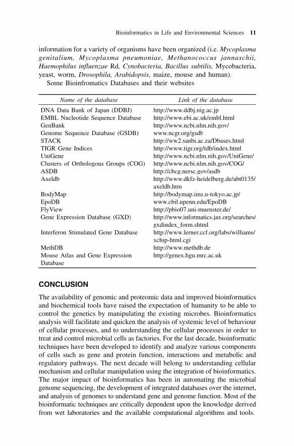
Bioinformatics in Life and Environmental Sciences 11
information for a variety of organisms have been organized (i.e. Mycoplasmagenitalium, Mycoplasma pneumoniae, Methanococcus jannaschii,Haemophilus influenzae Rd, Cynobacteria, Bacillus subtilis, Mycobacteria,yeast, worm, Drosophila, Arabidopsis, maize, mouse and human).
Some Bioinfromatics Databases and their websites
Name of the database Link of the database
DNA Data Bank of Japan (DDBJ) http://www.ddbj.nig.ac.jpEMBL Nucleotide Sequence Database http://www.ebi.ac.uk/embl.htmlGenBank http://www.ncbi.nlm.nih.gov/Genome Sequence Database (GSDB) www.ncgr.org/gsdbSTACK http://ww2.sanbi.ac.za/Dbases.htmlTIGR Gene Indices http://www.tigr.org/tdb/index.htmlUniGene http://www.ncbi.nlm.nih.gov/UniGene/Clusters of Orthologous Groups (COG) http://www.ncbi.nlm.nih.gov/COG/ASDB http://cbcg.nersc.gov/asdbAxeldb http://www.dkfz-heidelberg.de/abt0135/
axeldb.htmBodyMap http://bodymap.ims.u-tokyo.ac.jp/EpoDB www.cbil.upenn.edu/EpoDBFlyView http://pbio07.uni-muenster.de/Gene Expression Database (GXD) http://www.informatics.jax.org/searches/
gxdindex_form.shtmlInterferon Stimulated Gene Database http://www.lerner.ccf.org/labs/williams/
xchip-html.cgiMethDB http://www.methdb.deMouse Atlas and Gene Expression http://genex.hgu.mrc.ac.ukDatabase
CONCLUSION
The availability of genomic and proteomic data and improved bioinformaticsand biochemical tools have raised the expectation of humanity to be able tocontrol the genetics by manipulating the existing microbes. Bioinformaticsanalysis will facilitate and quicken the analysis of systemic level of behaviourof cellular processes, and to understanding the cellular processes in order totreat and control microbial cells as factories. For the last decade, bioinformatictechniques have been developed to identify and analyze various componentsof cells such as gene and protein function, interactions and metabolic andregulatory pathways. The next decade will belong to understanding cellularmechanism and cellular manipulation using the integration of bioinformatics.The major impact of bioinformatics has been in automating the microbialgenome sequencing, the development of integrated databases over the internet,and analysis of genomes to understand gene and genome function. Most of thebioinformatic techniques are critically dependent upon the knowledge derivedfrom wet laboratories and the available computational algorithms and tools.

12 Tularam M. Bansod
Role of Computers inBioinformatics
Tularam M. Bansod
INTRODUCTION
Bioinformatics is a new and rapidly evolving discipline that has emergedfrom the fields of experimental molecular biology and biochemistry, andfrom the artificial intelligence, database, and algorithms disciplines ofcomputer science (http://www.cs.wright.edu/cse/research/facilities-room.phtml?room=307). There are two possibilities to increase research inBioinformatics field, one way is to teach computer science to biologists,biotechnologists and the other way is to teach biology to computer scientists.I think both the departments are doing these things in their capacities. It iseasy to teach new computer technologies to biologists.
If we had taken survey of computer usage in the Life Science departmentsor Biology departments at the university level, we will find that people areusing computers for administrative work, typing some research paper andbrowsing internet. Life science departments lack following things to utilizecomputers or computer networks:
1. Lack of requirement analysis of respective department.2. Proper storage space for displaying research papers on the university
site or department sites is missing or partial.3. Lack of indigenous protein servers or genome server or powerful database
servers.4. Lack of co-ordination of Computer Science department and Life Science
department in the university.5. Lack of course-ware design in the computer technology by the computer
faculty for the biologist.6. Course-ware design by the biologist in the biology field for computer
scientist also missing.7. Lack of focussed research.8. Lack of creative human resource.
2

Role of Computers in Bioinformatics 13
When life science department try to find maximum usage of computernetwork, they should use following steps:
1. Calculate bandwidth requirement of department.2. Calculate storage requirement of department.3. Design computer network from consultants.4. Check the load on the web servers regularly.5. Information security policies should be designed.6. Procure the building blocks of computer networks for bioinformatics lab.7. Calculate assets value of your research work and computer network
resources.8. Regularly do risk analysis and information audits to justify the
expenditure on overall computing resources.9. Train the human resource in latest computer as compulsory component
of lab budget.
Many foreign universities have started undergraduate courses inbioinformatics to create human resource in this upcoming field. We are stillstruggling to get a person to teach bioinformatics to the postgraduate level.In the syllabus of bioinformatics of Colman College, USA (Table 1), wenoticed that around 40% syllabus is based on computer networking (http://www.coleman.edu/academics/undergraduate/bioinformatics.php/).
Table 1: Syllabus of Bio-Informatics Technicians (BIT)course in Colman College, USA
Course Title Units
COM113 Intro to PCs and Networks 4COM107 Intro to Programing 8COM259 UNIX Fundamentals 8COM287 Internet Programing I 4BIT100 General Biology 4COM115 Client Services & Support I 4MAT162 Algebra I 4BIT110 Cellular and Molecular Biology 4MAT250 Statistics for Bioinformatics 4NET130 TCP/IP Fundamentals 4BIT120 Microbiology and Immunology 4NET250 Networking Concepts 4BIT200 MySQL & Oracle (DB Admin) 4BIT240 Bioinformatics 4BIT210 Biotechnology 4BIT260 Sequence and Structure DB 4BIT220 BioPerl 4BIT250 Introduction to BioJava 4BIT230 LAMP 4

14 Tularam M. Bansod
In this paper we will study computer networking and its applications forbioinformatics.
ESSENTIAL COMPUTER NETWORKING FOR BIOLOGIST
What is computer networking? Connection between active and passivecomponents of computing is called networking. What is network of network?Internet is called network of network. Internet has many different types ofnetworks such as Ethernet, SONET, and ATM (Asynchronous Transfer Mode).Following are components of computer networking:
• NIC (Network Interface Card)• Hub• Switches—layers 3 and 4• Router—Cisco, Juniper, Dax• Computer—P-III, P-IV, Servers• Cables—Guided/Unguided
When we attach hub or switch with computer nodes with the help of copperor optical cable, we find active and passive components in the network.Copper cable and optical cables are passive components. Wirelesscommunication is based on unguided signaling. Computer nodes and hubswitches are called active components. Networking building blocks startwith NIC card. This is called Network Interface Card. Now-a-days this cardis inbuilt on the mother board. This NIC is available in different speeds viz.,10 mbps, 100 mbps, 1 gbps. This indicate maximum speed of networkprocessing on your machine. There are different manufacturers of networkcards e.g., D-link, SMC, Intel, Dax, Realtek.
Hub is the device used to connect computers in the LAN (Local AreaNetwork). It is available in 8 ports, 16 ports and 24 ports. It is running inthe physical layer. We can attach 8, 16, 24 computers to the Hubs. Hub isused to divide the speed of network in the number of computers. If we attacheight computers to the Hub and if NIC is of 10 Mbps then every computeris able to send packet by 10/8 mbps speed. There is no IC (Integrate Circuit)to process table of physical addresses. There is only one collision domain inthe Hub. In the switch there are multiple collision domains. Switch lookslike Hub and this also comes in the 8, 16, 24 ports. Switch has IC to processpackets and maintain physical addresses of computers. Generally physicaladdress is 48 bit, written in the hexadecimal bit.
Router is many times a very important device to forward packets to thedissimilar networks. Router works on network layer. We can implementsecurity feature also in the router which will help to stop malicious codes atthe periphery of the network. We can use firewall and DMZ (De-MilitaryZone) to protect bio-informatics network also.

Role of Computers in Bioinformatics 15
Where computer networking affecting Bio-informatics Lab?
• Bandwidth Management• Security Management• Database Management
Bandwidth Management
• Dialup lines – Under-utilized• 56 kbps/4 kbps• Lease line• Virtual Private Network• Triband (Broadband launched by MTNL)
Security Management
• Physical security—Access control• Functional security—Process security• Application security—Bioedit, Rasmol, Browser security settings, SSL
Database Management
• Physical database integrity• Logical database integrity• Access control• Confidentiality• Availability
What are the research themes in Bioinformatics?
Novel computational techniques for the analysis and modeling of complexbiological systems involves, pattern recognition, evolutionary computation,combinatorial and discrete analyses, statistical and probabilistic methods,molecular evolution, population genetics, protein structure, function, andassembly, and even forensic DNA analysis.
Peer-to-peer (P2P) networks have also been initiated to attract attentionfrom those that deal with large datasets such as bioinformatics. P2P networkscan be used to run large programs designed to carry out tests to identify drugcandidates. The first such program was started in 2001 at the Centre forComputational Drug Discovery at Oxford University in cooperation with theNational Foundation for Cancer Research. There are now several similarprograms running under the auspices of the United Devices Cancer ResearchProject. On a smaller scale, a self-administered program for computationalbiologists to run and compare various bioinformatics software is availablefrom Chinook. Tranche is an open-source set of software tools for setting upand administrating a decentralized network. It was developed to solve thebioinformatics data sharing problem in a secure and scalable fashion (http://

16 Tularam M. Bansod
en.wikipedia.org/wiki/Peertopeer#Application_of_P2P_Network_outside_Computer_Science).
Grid computing is a service-oriented architectural approach that uses openstandards to enable distributed computing over the Internet, a private networkor both. Grid computing helps to manage access to huge data, a crucialcapability for making rapid progress in life sciences research.
REFERENCES
Forouzan, B., TCP/IP Protocol. Tata McGraw Hill Publication, 2004.Pfleeger, Charles, Security in Computing. Pearson Publication, 2004.http://www.cs.wright.edu/cse/research/facilities-room.phtml?room=307http://www.coleman.edu/academics/undergraduate/bioinformatics.php/http://en.wikipedia.org/wiki/Peertopeer#Application_of_P2P_Network_outside_
Computer_Science)

Comparative Genomicsand Proteomics
M.V. Hosur
GENOMICS
Over the last decade, research in biology has undergone a qualitativetransformation. Genome sequences, the bounded sets of information thatguide biological development and function, lie at the heart of this revolution.The earlier reductionist approach to simplify complex biological systems hasgiven way to an integrated approach dealing with the system as a whole,thanks to advances in various technologies. It is now possible to sequence,within a short time, entire genomes, which are the blue-prints, at the molecularlevel, for the complex workings of organisms. Genomes of more than 350life-forms, including several mammals, have been sequenced, and manymore are in the pipeline. The genomic sequence data is only the beginning,and to realize the full benefit of this data, the data has to be very skillfullyprocessed and analysed. Comparative genomics is the study of relationshipsbetween the genomes. The broadly available genome sequences of humanand a select set of additional organisms represent foundational informationfor biology and biomedicine. Embedded within this as-yet poorly understoodcode are the genetic instructions for the entire repertoire of cellularcomponents, knowledge of which is needed to unravel the complexities ofbiological systems. Elucidating the structure of genomes and identifying thefunction of the myriad encoded elements will allow connections to be madebetween genomics and biology and will, in turn, accelerate the explorationof all realms of the biological sciences. Interwoven advances in genetics,comparative genomics, high throughput biochemistry and bioinformatics areproviding biologists with a markedly improved repertoire of research toolsthat will allow the functioning of organisms in health and disease to beanalysed and comprehended at an unprecedented level of molecular detail.In short, genomics has become a central and cohesive discipline of biomedicalresearch.
By choosing appropriate genomes, the technique of comparative genomicshas been applied to the following problems: 1. identify positions of genes in
3

18 M.V. Hosur
a genome, 2. annotate functions to genes through comparisons across species,3. quantify evolutionary relationships between species, 4. identify targets fordrug-development against diseases, and 5. probe the theory ‘out of Africa’for human genesis.
PROTEOMICS
The term proteome was first coined to describe the set of proteins encodedby the genome. Proteome analysis is the direct measurement of proteins interms of their presence and relative abundance. The overall aim of proteomicsis the characterization of the complete network of cell regulation. Analysisis required to determine which proteins have been conditionally expressed,by how much, and what post-translational modifications have occurred.
The study of the proteome, called proteomics, now is almost everything‘post-genomic’. One can think of different types of proteomics depending onthe technique used.
Mass Spectrometry-based Proteomics
Initial proteomics efforts relied on protein separation by two-dimensional gelelectrophoresis, with subsequent mass spectrometric identification of proteinspots. An inherent limitation of this approach is the depth of coverage, whichis necessarily constrained to the most abundant proteins in the sample.Recently, the technology of Isotope Coated Affinity Tags (ICAT) has beendeveloped that does away with electrophoresis thereby greatly improvingsensitivity. This technology can easily yield information about how theconcentration of proteins varies over the course of a cell’s lifetime. The rapiddevelopments in mass spectrometry have shifted the balance to direct massspectrometric analysis, and further developments will increase sensitivity,robustness and data handling. The development of statistically sound methodsfor assignment of protein identity from incomplete mass spectral data (softwareSEQEST) will be critical for automated deposition into databases, which iscurrently a painstaking manual and error-prone process (Fig. 1).
Array-based Proteomics
A number of established and emergent proteome-wide platforms complementmass spectrometric methods. The forerunner amongst these efforts is thesystematic two-hybrid screen developed by scientists. Unlike directbiochemical methods that are constrained by protein abundance, two-hybridmethods can often detect weak interactions between low-abundance proteins,albeit at the expense of false positives. Lessons learned from analysis ofDNA microarray data, including clustering, compendium and pattern-matchingapproaches, should be transportable to proteomic analysis, and it isencouraging that the European Bioinformatics Institute and the Human

Comparative Genomics and Proteomics 19
Proteome Organisation (HUPO) have together started an initiative on theexchange of protein–protein interaction and other proteomic data (see http://psidev.sourceforge.net/).
Structural Proteomics
Beyond a description of protein primary structure, abundance and activities,the goal of proteomics is to systematically understand the structural basis forprotein interactions and function. A full description of cell behaviournecessitates structural information at the level not only of all single proteins,but of all salient protein complexes and the organization of such complexesat a cellular scale. This all-encompassing structural endeavour spans severalorders of magnitude in measurement scale and requires a battery of structuraltechniques, from X-ray crystallography (Fig. 2) and nuclear magneticresonance (NMR) at the protein level, to electron microscopy of mega-complexes and electron tomography for high-resolution visualization of theentire cellular milieu. NMR and in silico docking will be necessary to buildin dynamics of protein interactions, much of which may be controlled throughlargely unstructured regions. The recurrent proteomic theme of throughputand sensitivity runs through each of these structural methods.
In the earlier days, crystal structure determinations were too slow to keeppace with sequence determinations. However, recently the following advancesin technology have been achieved. Production and purification of recombinantproteins has been automated to a very large extent. Robots have beendeveloped to rapidly set-up thousands of experiments to crystallize proteins.
Fig. 1:Fi 1 Mass spectrum at 75 min from LC-MS of Amylase digest.M t t 75 i f LC MS f A l di t

20 M.V. Hosur
The amount of reagents and protein used in these crystallization trials isreduced by as much as fifty times compared to manual trials. Very intenseand highly collimated beams of x-rays are produced on synchrotrons enablingdiffraction data collection from micron size crystals. Protein crystallography(Fig. 2) beamlines on these synchrotron sources incorporate automation atevery step in the process of diffraction data collection. A complete diffractiondata set can now be measured within minutes without needing any manualintervention. Some of the ‘high-throughput’ protein crystallography beamlinesallow for remote operation, even making travel to the synchrotronunnecessary! Tunability of x-ray wavelengths at synchrotron sources hasenabled routine solution of the ‘Phase Problem’ by exploiting the physicalphenomenon of anomalous scattering. These developments have substantiallyincreased the speed with which three dimensional structures of proteins canbe determined. In many favourable cases, the three dimensional structure ofa protein may be established much faster than conventional characterizationof the protein through biochemical and genetic methods. Then a comparisonof the three dimensional structure of the new protein with structures of otherproteins with known functions may offer a faster route to annotate functionto proteins.
Fig. 2: Single crystal X-ray Diffraction
Proteomics is set to have a profound impact on clinical diagnosis anddrug discovery. The selection of particular proteins for detailed structureanalysis is dictated by results of comparative proteomics. Very oftenproteomics provides key input for selection of targets for drug-development.In the case of Plasmodium falciparum, comparative proteomics has identifiedhundreds of plasmodium specific proteins, which may provide targets fordevelopment of drugs and vaccines against malaria.
The technique of comparative proteomics has also contributed towardsestablishing protein and gene networking in cellular functioning, screeningof lead molecules for toxicity and other effects.
First order layerySecond order layer
Det
ecto
r

Comparative Genomics and Proteomics 21
Table 1: Comparative summary of the protein lists for each stage
Protein count Sporozoites Merozoites Trophazoites Gametocytes
152 × × × ×197 – × × ×53 × – × ×28 × × – ×36 × × × –148 – – × ×73 – × – ×120 × – – ×84 – × × –80 × – × –65 × × – –376 – – – ×286 – – × –204 – × – –513 × – – –2,415 1,049 839 1,036 1,147
Whole-cell protein lysates were obtained from, on average, 17 × 106 sporozoites,4.5 × 109 traphozoites, 2.75 × 10⁹ merozates, and 6.5 × 10⁹ gametocytes.
METHODS OF COMPARISON
Comparison of genome sequences from evolutionarily diverse species hasemerged as a powerful tool for identifying functionally important genomicelements. Assignment of function de-novo to a new protein is a very tediousprocess, and sequence comparisons may provide a short cut when sequencesimilarity is rather high. Structural comparisons, however, have a highersuccess rate while predicting protein function, because structural variationsare slower compared to sequence variations. The key step in such comparativestudies is the correct alignment of sequences being compared. The sheeramount of information contained in modern genomes and proteomes (severalgigabytes in the case of humans) necessitates that the methods of comparativegenomics and comparative proteomics be highly computational in nature.Parallel developments in the powers of computers has enabled researchers todevelop softwares for the comparison of various types of genomic andproteomic data. Comparative methods involve two steps: (a) alignment ofresidues from the two sequences, and (b) scoring different alignments basedon a chosen substitution matrix, M(I, J). One of the most dependable alignmentmethods is that developed by Needleman and Wunsch to compare proteinsequences. This method for alignment of any two given sequences, A and B,consists of three steps: creation of an alignment matrix, M, in which theelement M(i, j) represents the probability that residue at position i in sequenceA is substituted with residue j in sequence B, modification of matrix Miteratively, using concepts of dynamic programing, in such a way that the

22 M.V. Hosur
modified value of M (i, j) encodes the best alignment path from the start tothe current residue, and finally tracing a path in this matrix M to arrive atthe complete alignment. Two types of substitution matrices, M(i, j), arecurrently in use: PAMn matrix and BLOSUMn matrix. PAM1 matrix estimateswhat rate of substitution would be expected if 1% of the amino acids hadchanged. The PAM1 matrix is used as the basis for calculating other matricesby assuming that repeated mutations would follow the same pattern as thosein the PAM1 matrix, and multiple substitutions can occur at the same site.Using this logic, Dayhoff derived matrices as high as PAM250. DifferentPAM matrices are derived from the multiplication of the PAM1 matrix. APAM250 is equivalent to one unchanged amino acid out of five. Sequencechanges over long evolutionary time scales are not well approximated bycompounding small changes that occur over short time scales. TheBLOSUM62 matrix is calculated from observed substitutions between proteinsthat share 62% sequence identity or less. One would use a higher numberedBLOSUM matrix for aligning two closely related sequences and a lowernumber for more divergent sequences.
The methods developed for sequence alignment have been applied alsofor structure alignment by encoding three dimensional structural informationin the sequence representation. The advantage of this approach is that allpowerful strategies developed for multiple sequence alignment can be directlyapplied to structural alignments. These methods are fully automatic, don’tneed initial alignments, and being very fast can compare thousands ofstructures available in databases. Other methods developed for structuralcomparisons try to maximize the match between geometrical features of thestructures being compared. Comparison of structures of native and drug-resistant mutants would be helpful in the design of more effective drugs.
FUTURE DIRECTIONS
1. Comprehensively identify the structural and functional componentsencoded in the human genome.
2. Elucidate the organization of genetic networks and protein pathwaysand establish how they contribute to cellular and organismal phenotypes.
3. Develop a detailed understanding of the heritable variation in the humangenome.
4. Understand evolutionary variation across species and the mechanismsunderlying it.
5. Develop robust strategies for identifying the genetic contributions todisease and drug response.
6. Develop strategies to identify gene variants that contribute to goodhealth and resistance to disease.
7. Develop genome-based approaches to prediction of disease susceptibilityand drug response, early detection of illness, and molecular taxonomyof disease stages.

Comparative Genomics and Proteomics 23
8. Proteomics will inevitably accelerate drug discovery, although the paceof progress in this area has been slower than was initially envisaged. Anunderstanding of the biological networks that lie below the cell’s exteriorwill provide a rational basis for preliminary decisions on target suitability.The proteomics of host–pathogen interactions should also be an arearich in new drug targets. Regardless of the exact format, robust massspectrometry and protein-array platforms must be moved into clinicalmedicine to replace the more expensive and less reliable biochemicalassays that are the basis of traditional clinical chemistry. Finally, thenascent area of chemiproteomics will not only allow mechanism ofaction to be discovered for many drugs, but also has the potential toresurrect innumerable failed small molecules that have dire off-targeteffects of unknown basis.
TOOLS AND RESOURCES FOR COMPARATIVEGENOMICS AND PROTEOMICS
Databases
This quiet revolution in the biological sciences has been enabled by ourability to collect, manage, analyze and integrate large quantities of data. Inthe process, bioinformatics has itself developed from something consideredto be little more than information management and the creation of sequence-search tools into a vibrant field encompassing both highly sophisticateddatabase development and active pure and applied research programmes inareas far beyond the search for sequence homology.
Databases are, with increasing sophistication, providing the scientific publicwith access to the data. The challenge is not collecting the data but identifyingand annotating features in genomic sequence and presenting them in anintuitive fashion. The general-purpose sequence databases provide uniformaccess to the data and a consistent annotation for an increasing number oforganisms—examples include the EMBL database, GenBank and the DNAdatabase of Japan (DDBJ) and genome databases such as Ensembl and theNational Center for Biotechnology Information (NCBI) Genome Views.Species-specific databases, such as the Saccharomyces Genome Databaseand the Mouse Genome Database, provide much richer and more complexinformation about individual genes. Increasingly, we are coming to realizethat protein-coding genes are not the only important transcribed sequencesin the genome. Rfam is a database of non-coding RNA families. Rfamprovides users with covariance models—which flexibly describe the secondarystructure and primary sequence consensus of an RNA sequence family aswell as multiple sequence alignments representing known non-coding RNAsand provides utilities for searching sequences for their presence, includingentire genomes. UniProtKB/Swiss-Prot is a curated protein sequence database

24 M.V. Hosur
which strives to provide a high level of annotation (such as the descriptionof the function of a protein, its domains structure, post-translationalmodifications, variants, etc.), a minimal level of redundancy and high levelof integration with other databases. The most general structural database isthe Protein Data Bank (PDB). PROSITE is the database describing proteindomains, families and functional sites.
Useful Servers and URL’s
(1) ExPASy, (2) http://www.sbg.bio.ic.ac.uk/services.html, (3)http://genome.ucsc.edu/, (4) www.bakerlab.org/
REFERENCES
Collins, Francis, S., Green, Eric D., Guttmacher, Alan, E. and Guyer, Mark S. (2003).Nature, 422: 835-847.
Das, Amit et al. and Hosur, M.V. (2006). Proc. Natl. Acad. Sci. USA, 103: 18464-18469.
Florens, L. et al. and Carussi, D. J. (2002). Nature, 419: 820-826.Feuk, L., Carson, A. R. and Scherrer, S. W. (2006). Nature Reviews, Genetics, 7: 85-96.Friedberg, I. et al. and Godzik, A. (2006). Bioinformatics, 23: e219-e224.Tyers, Mike and Mann, Matthias (2003). Nature, 422: 193-197.

Bioinformatics—StructuralBiology Interface
Desh Deepak Singh
INTRODUCTION
Bioinformatics is the field of science in which biology, computer science,and information technology merge to form a single discipline. Morespecifically the field conceptualizes biology in terms of physico-chemicalaspects of molecules and then applies informatic techniques (maths, computerscience and statistics) to understand and organize this information on alarge-scale. The ultimate goal of the field is to enable the discovery of newbiological insights as well as to create a global perspective from whichunifying principles in biology can be discerned. At the beginning of the“genomic revolution”, a bioinformatics concern was the creation andmaintenance of a database to store biological information, such as nucleotideand amino acid sequences. Development of this type of database involvednot only design issues but the development of complex interfaces wherebyresearchers could both access existing data as well as submit new or reviseddata. Ultimately, however, all of this information must be combined to forma comprehensive picture of normal cellular activities so that researchers maystudy how these activities are altered in different disease stages. Therefore,the field of bioinformatics has evolved such that the most pressing task nowinvolves the analysis and interpretation of various types of data, includingnucleotide and amino acid sequences, protein domains, and protein structures.
Some of the important milestones in the development of bioinformaticsare: the first theory of molecular evolution; the Molecular Clock concept byLinus Pauling and Emile Zukerkandl in 1962; Atlas of Protein Sequences,the first protein database by Margaret Dayhoff and coworkers in 1965;Needleman-Wunsch algorithm for global protein sequence alignment in 1970;Phylogenetic taxonomy, discovery of archaea and the notion of the threeprimary kingdoms of life introduced by Carl Woese and co-workers in 1977;Smith-Waterman algorithm for local protein sequence alignment in 1981; theconcept of a sequence motif by Russell Doolittle in 1981; Phage genomesequenced by Fred Sanger and co-workers in 1982; fast sequence similarity
4

26 Desh Deepak Singh
searching by William Pearson and David Lipman in 1985; creation of NationalCenter for Biotechnology Information (NCBI) at NIH in 1988: BLAST: fastsequence similarity searching with rigorous statistics by Stephen Altschul,David Lipman and co-workers in 1990; first bacterial genomes completelysequenced in 1995; first archaeal and eukaryotic genome completelysequenced in 1996 and human genome (nearly) completely sequenced in2001.
Some of the important domains of bioinformatics study are databaseresource generation, comparative and functional genomics, phylogeny,modeling and designing and systems biology. National Center for Bio-technology Information (NCBI), European Bioinformatics Institute (EBI),Swissprot, Sanger Research Centre, Kyoto Encyclopedia of Genes andGenomes (KEGG) and Protein Data Bank (PDB), containing information onexperimentally solved structures are some of the important repositories ofdatabases and bioinformatic tools which contain useful information on genomesequences, conserved domains, taxonomy, etc. With the rapid availability ofgenome sequences (available on genomes online database) of diverseorganisms, analysis of the information for prediction of homologues acrossdifferent species has become a very important part of bioinformatics undercomparative genomics. Homologs exist amongst organisms due to a commonevolutionary history and important tools have been developed which arebeing widely used for their identification. An important tool which is utilizedfor this function is BLAST (Basic local alignment search tool) which is aheuristic programme. In functional genomics efforts are made to predictfunction and interactions of various macromolecules in the cellular systemby using available data from techniques like microarrays, etc. and extrapolatingthem.
An equally exciting area is the potential for uncovering evolutionaryrelationships and patterns between different forms of life. With the aid ofnucleotide and protein sequences, it should be possible to find the ancestralties between different organisms. Thus, so far, experience has taught us thatclosely related organisms have similar sequences and that more distantlyrelated organisms have more dissimilar sequences. Proteins that showsignificant sequence conservation, indicating a clear evolutionary relationship,are said to be from the same protein family. By studying protein folds(distinct protein building blocks) and families, scientists are able to reconstructthe evolutionary relationship between two species and estimate the time ofdivergence between two organisms since they last shared a common ancestor.In phylogenetic studies, the most convenient way of visually presentingevolutionary relationships among a group of organisms is through illustrationscalled phylogenetic trees which can be generated using many programs likePHYLIP, MEGA, etc.
In the absence of actually determined protein structure by X-raycrystallography or nuclear magnetic resonance (NMR) spectroscopy,

Bioinformatics—Structural Biology Interface 27
researchers can try to predict the three-dimensional structure using molecularmodeling. This method uses experimentally determined protein structures(templates) to predict the structure of another protein that has a similaramino acid sequence (target). Identifying a protein’s shape, or structure, isa key to understanding its biological function and its role in health anddisease. Illuminating a protein’s structure also paves the way for thedevelopment of new agents and devices to treat a disease. Yet solving thestructure of a protein is no easy feat. It often takes scientists working in thelaboratory months, sometimes years, to experimentally determine a singlestructure. Therefore, scientists have begun to turn towards computers to helppredict the structure of a protein based on its sequence. The challenge liesin developing methods for accurately and reliably understanding this intricaterelationship. Protein modeling involves identification of the proteins withknown three-dimensional structures that are related to the target sequence,constructing a model for the target sequence based on its alignment with thetemplate structure(s) and evaluating the model against a variety of criteria todetermine if it is satisfactory. Some tools used for automated model generationare SWISS-MODEL which is available through Glaxo Wellcome ExperimentalResearch in Geneva, Switzerland; WHAT IF available on EMBL servers andModeller developed by Andrej Sali lab.
An important area of development in bioinformatics is in-silico designingof new therapeutics towards rational drug development and molecularinteractions. The various useful tools in this arena are AutoDock (ScrippsResearch Institute) which is free for academia, CombiBUILD (Sandia NationalLabs), DockVision (University of Alberta), and DOCK (UCSF MolecularDesign Institute) among many others.
The ultimate objective of all the activities in bioinformatics is to quantifythe cellular interactions and wire the cell so as to say and already significantadvances are being made in this direction under the general theme of systemsbiology (Mount, 2004; Greer, 1991; Johnson et al., 1994).
PROTEIN STRUCTURE
The protein structure function correlation is an important paradigm inunderstanding biology in precise molecular terms and hence makes it possibleto undertake useful computational analysis and for this the understanding ofthe 3-D structure of proteins is very essential. A set of 20 different subunits,called amino acids, can be arranged in any order to form a polypeptide thatcan be thousands of amino acids long. These chains can then loop abouteach other or fold, in a variety of ways, but only one of these ways allowsa protein to function properly. The critical feature of a protein is its abilityto fold into a conformation that creates structural features, such as surfacegrooves, ridges and pockets, which allow it to fulfill its role in a cell. Aprotein’s conformation is usually described in terms of levels of structure.Traditionally, proteins are looked upon as having four distinct levels of

28 Desh Deepak Singh
structure, with each level of structure dependent on the one below it. Insome proteins, functional diversity may be further amplified by the additionof new chemical groups after synthesis is complete.
The stringing together of the amino acid chain to form a polypeptide isreferred to as the primary structure. Two amino acids combine togetherchemically through a peptide bond, which is a chemical bond formed betweenthe carboxyl group of one amino acid and the amino group of the second.The peptide bond is planar because it has a partial double bond and this canresult in cis-trans geometric isomerism. Generally in naturally occurringproteins the trans isomer predominates. Secondary structure in proteinsconsists of local inter-residue interactions mediated by hydrogen bonds. Thesecondary structure is generated by the folding of the primary sequence andrefers to the path that the polypeptide backbone of the protein follows inspace. Certain types of secondary structures are relatively common. Twowell-described secondary structures are alpha helix and the beta sheet. Theamino acids in an �-helix are arranged in a right-handed helical structure,5.4 Å wide. The helix has 3.6 residues per turn, and a translation of 1.5 Åalong the helical axis. The amino group of an amino acid forms a hydrogenbond with the carbonyl group of the amino acid four residues earlier and thisrepeated hydrogen bonding defines an �-helix. �-sheets are formed when apolypeptide chain bonds with another chain that is running in the oppositedirection. �-sheets may also be formed between two sections of a singlepolypeptide chain that is arranged such that adjacent regions are in reverseorientation. The �-sheet consists of beta strands connected laterally by threeor more hydrogen bonds, forming a generally twisted, pleated sheet. Themajority of �-strands are arranged adjacent to other strands and form anextensive hydrogen bond network with their neighbours in which the aminogroups in the backbone of one strand establish hydrogen bonds with thecarbonyl groups in the backbone of the adjacent strands.
Amino acids vary in their ability to form the various secondary structureelements. Proline and glycine are sometimes known as “helix breakers”because they disrupt the regularity of the �-helical backbone conformation;however, both have unusual conformational abilities and are commonly foundin turns. Amino acids that prefer to adopt helical conformations in proteinsinclude methionine, alanine, leucine, glutamate and lysine; by contrast, thelarge aromatic residues (tryptophan, tyrosine and phenylalanine) and C�-branched amino acids (isoleucine, valine and threonine) prefer to adopt �-strand conformations. The tertiary structure describes the organization inthree dimensions of all of the atoms in the polypeptide. If a protein consistsof only one polypeptide chain, this level then describes the complete structure.Proteins have a very interesting repertoire of folds or domains into whichthey fold like the beta barrel, Greek key motifs, etc. In spite of the millionsof protein sequences present in diverse organisms, interestingly they foldinto just about 1000 different folds or domains and the study of protein

Bioinformatics—Structural Biology Interface 29
folding phenomenon is a very exciting area of research engaging manyresearchers.
Multimeric proteins, or proteins that consist of more than one polypeptidechain, require a higher level of organization. The quaternary structure definesthe conformation assumed by a multimeric protein. In this case, the individualpolypeptide chains that make up a multimeric protein are often referred toas the protein subunits. The four levels of protein structure are hierarchal,that is, each level of the build process is dependent upon the one below it.A protein’s primary amino acid sequence is crucial in determining its finalstructure. In some cases, amino acid sequence is the sole determinant, whereasin other cases, additional interactions may be required before a protein canattain its final conformation. For example, some proteins require the presenceof a cofactor, or a second molecule that is part of the active protein, beforeit can attain its final conformation. Multimeric proteins often require one ormore subunits to be present for another subunit to adopt the proper higherorder structure. The entire process is cooperative, that is, the formation ofone region of secondary structure determines the formation of the next region.Study of allosteric proteins is interesting because under certain conditionsthey have a stable alternate conformation, or shape, that enables it to carryout a different biological function. The interaction of an allosteric proteinwith a specific cofactor, or with another protein, may influence the transitionof the protein between shapes. In addition, any change in conformationbrought about by an interaction at one site may lead to an alteration in thestructure, and thus function, at another site. One should bear in mind, though,that this type of transition affects only the protein’s shape, not the primaryamino acid sequence. Allosteric proteins play an important role in bothmetabolic and genetic regulation (Branden and Tooze, 1998; Chothia et al.,1977; Chothia, 1984; Lesk, 1991; Rao and Rossman, 1973 and Richardson,1981).
PROTEIN STRUCTURE DETERMINATION
Traditionally, a protein’s structure is determined using one of two techniques:X-ray crystallography or nuclear magnetic resonance (NMR) spectroscopy.Now rapid advancements in cryoelectron microscopy is also enablingdetermination of gross features of protein structure albeit at a low resolution.
X-ray crystallography is done on crystals of a solid form of a substance,which have an ordered array called a lattice in which the component moleculesare arranged periodically. The basic building block of a crystal is called aunit cell and each unit cell contains exactly one unique set of the crystal’scomponents, the smallest possible set that is fully representative of the crystal.When the crystal is placed in an X-ray beam, all of the unit cells present thesame face to the beam; therefore, many molecules are in the same orientationwith respect to the incoming X-rays. The X-ray beam enters the crystal and

30 Desh Deepak Singh
a number of smaller beams emerge: each one in a different direction, eachone with a different intensity. If an X-ray detector, such as a piece of film,is placed on the opposite side of the crystal from the X-ray source, eachdiffracted ray, called a reflection, will produce a spot on the film. However,because only a few reflections can be detected with any one orientation ofthe crystal, an important component of any X-ray diffraction instrument isa device for accurately setting and changing the orientation of the crystal.The set of diffracted, emerging beams contains information about theunderlying crystal structure.
Since its advent in the second decade of the last century, following thediscovery of diffraction of X-rays by crystals in 1912 by Max von Laue,X-ray crystallography has been the method of choice for elucidating thestructure of matter at the atomic and molecular levels. The wavelength ofX-rays is about five thousand times less than that of light and of the sameorder of magnitude as the periodicity of the arrangement of atoms, ions ormolecules in a crystal. Hence, crystals diffract when X-rays fall on themgiving rise to intensity maxima or spots. In optical microscopy, the lightwaves scattered by the object are re-combined by the objective lens to producethe image. But in X-ray crystallography the re-combining has to be done bya mathematical device called Fourier synthesis. Also in X-ray diffraction, thesquare root of intensities gives the amplitudes of the scattered X-ray wavesbut information on phase angles is lost in measurement. Therefore the relativephase angles of the X-ray waves have to be determined before employingthe Fourier synthesis. This is the ‘phase problem’ in X-ray crystallographyand many methods like molecular replacement, isomorphous replacementwith heavy atom derivatives and anomalous dispersion have been devised toovercome it. In the fifties, Max Perutz demonstrated that the phase problemcan be solved using what is called the isomorphous replacement method inwhich derivative crystals are prepared by attaching heavy atoms in a coherentmanner to the protein molecules in the crystal. The early protein structuresolutions almost invariably employed the isomorphous replacement methodwhich is often used in combination with what is called the anomalousdispersion method. Independent use of the anomalous dispersion method hasalso now gained currency. In recent decades, the molecular replacementmethod, which uses structural information on related proteins, is alsoextensively used.
One of the most important advances in the field is the development ofdedicated synchrotron sources for X-ray work. In a synchrotron, an electronbeam is accelerated along a long circular path which then emitselectromagnetic radiation, including X-rays. The X-rays thus produced areusually several orders of magnitude more intense than those generated byconventional laboratory X-ray sources and it is also possible to chooseradiation with a precise wavelength. This tunability is very useful whenemploying the anomalous dispersion method for structure determinations.
Bioinformatics—Structural Biology Interface 31
Biological macromolecular crystallography originated in 1934 when J.D.Bernal and Dorothy Hodgkin recorded the X-ray diffraction pattern from thecrystals of pepsin. However the first structures that were actually solvedwere those of myoglobin and haemoglobin in the late fifties and the earlysixties. John Kendrew and Max Perutz were awarded the Nobel Prize forthis work in 1961. With continued technological innovations, structures ofthousands of proteins have already been determined and macromolecularcrystallography is now recognized as the most important component ofstructural biology. However a major drawback associated with X-raycrystallography technique is that crystallization of the proteins is a difficulttask. Crystals are formed by slowly precipitating proteins under conditionsthat maintain their native conformation or structure. These exact conditionscan only be discovered by repeated trials that entail varying certainexperimental conditions, one at a time and this is a very time consuming andtedious process. But overall it is the technique of choice in structural biologyif conditions can be optimized. It has also grown into an integral and essentialpart of modern biology for much of what we know now on structure-functionrelationships in biology at the molecular level is derived from macromolecularcrystallography and has a major impact on our understanding of cellularbiology and design of rational therapeutics.
Although the basic phenomenon of Nuclear Magnetic Resonance (NMR)Spectroscopy was discovered in 1938, it was in 1946 that Felix Bloch andEdward Mills Purcell refined the technique for use on liquids and solids andfor which they shared the Nobel Prize in physics in 1952. Magnetic nuclei,like 1H and 31P, spin when placed in a magnetic field and these spinningnuclei can absorb radio frequency range energy specific to each nuclei.When this absorption occurs, the nucleus is described as being in resonanceand interestingly, different atoms within a molecule resonate at differentfrequencies at a given field strength based on their chemical environment.These resonating nuclei emit a unique signal that is then picked up by adetector and processed by the Fourier Transform algorithm, a complexequation that translates the language of the nuclei into something a scientistcan understand. The observation of the resonance frequencies of a moleculeallows a user to discover structural information about the molecule. Bymeasuring the frequencies at which different nuclei flip, scientists candetermine molecular structure, as well as many other interesting propertiesof the molecule. In the past 10 years, NMR has proved to be a powerfulalternative to X-ray crystallography for the determination of molecularstructure. NMR has the advantage over crystallographic techniques in thatexperiments are performed in solution as opposed to a crystal lattice. However,the principles that make NMR possible tend to make this technique verytime consuming and limit the application to small- and medium-sizedmolecules (Rossman and Arnold, 2006; Carter and Sweet, 1997a; 1997b,and McPherson, 2003).

32 Desh Deepak Singh
India has a long tradition in crystallography. X-ray crystal structure analysiswas initiated at the Indian Association for the Cultivation of Science atKolkata in the 1930’s by K. Banerjee, who was an associate of Sir C.V.Raman. Prof. G. N. Ramachandran and S. Ramaseshan, both students of SirC.V. Raman were responsible for laying the foundations for X-raycrystallography at the Indian Institute of Science, Bangalore, in the lateforties and fifties. The outstanding contributions of Prof. Ramachandran andhis colleagues resulted in the 3-D structure solution of collagen and Prof.Ramachandran also made extremely useful contributions in the developmentof techniques of X-ray crystallography especially anomalous dispersion. Thefamous Ramachandran map is now text book material and epitomizes thegolden era of Indian Computational Biology (Vijayan, 2007; Subramaniam,2001 and Vijayan et al., 2000).
The bioinformatic analysis of genome sequences and gene annotationhave resulted in a major data mining endeavour and some extensive structuralgenomic initiatives are being undertaken around the world now for 3-Dstructure solution of interesting targets. The structural genomic programmesof National Institute of General Medical Sciences (NIGMS) like the NewYork Structural Genomics Research Consortium, The Midwest Center forStructural Genomics, The TB structural genomics consortium (http://www.doe-mbi.ucla.edu/TB/), the Southeast Collaboratory for Structural Genomics andothers are actively working at the interface of bioinformatics and structuralbiology. India is also actively participating in some of these endeavours,especially the TB structural genomics with some recent successful outcomes.Hopefully future national and international efforts in the area of bioinformatics,and structural biology will lead to a better understanding of the pathogenesisof disease and rational design of precise and specific therapeutics (Norvelland Machalek, 2000; Vijayan, 2005).
REFERENCES
Branden, C. and Tooze, J. (1998). Introduction to protein structure. Garland Publish-ing Inc., New York.
Carter Jr., C.W. and Sweet, R.M. (1997a). Macromolecular Crystallography, Part A.Meth. Enzymol., 276, Academic Press, San Diego.
Carter Jr., C.W. and Sweet, R.M. (1997b). Macromolecular Crystallography, Part A.Meth. Enzymol. 277, Academic Press, San Diego.
Chothia, C., Levitt, M. and Richardson, D. (1977). Structure of proteins: Packing ofalpha helices and beta sheets. Proc. Natl. Acad. Sci. USA, 74: 4130-4134.
Chothia, C. (1984). Principles that determine the structure of proteins. Ann. Rev.Biochem., 53: 537-572.
Greer, J. (1991). Comparative modeling of homologous proteins. Meth. Enzymol.,202: 239-252.
Johnson, M.S., Srinivasan, N., Sowdhamini, R. and Blundell, T.L. (1994). Knowl-edge-based protein modeling. Crit. Rev. Biochem. Mol. Biol., 29: 1-68.
Bioinformatics—Structural Biology Interface 33
Lesk, A.M. (1991). Protein architecture: A practical approach. Oxford UniversityPress, New York.
McPherson, A. (2003). Introduction to Macromolecular Crystallography. John Wiley& Sons, Hoboken, NJ.
Mount, D. (2004). Bioinformatics: Sequence and genome analysis: Cold SpringHarbor Laboratory Press, New York.
Norvell, J.C. and Machalek, A.Z. (2000). Structural genomics programs at the USNational Institute of General Medical Sciences. Nat. Struct. Mol. Biol., 7: 931.
Rao, S.T. and Rossman, M.G. (1973). Comparison of super-secondary structures inproteins, J. Mol. Biol., 76: 241-256.
Richardson, J.S. (1981). The anatomy and taxonomy of protein structure. Adv. Prot.Chem., 34: 167-339.
Rossmann, M.G. and Arnold, E. (Eds.) (2006). International tables for Crystallo-graphy. Volume F: Crystallography of biological molecules. International Unionof Crystallography, Chester, UK.
Subramaniam, E. (2001). G.N. Ramachandran. Nat. Struct. Mol. Biol., 8: 489-491.Vijayan, M., Yathindra, N. and Kolaskar, A.S. (2000). Perspectives in structural
biology. Universities Press (India) Ltd., Hyderabad.Vijayan, M. (2005). Structural biology of mycobacterial proteins: The Bangalore
effort. Tuberculosis (Edinb.), 85: 357-366.Vijayan, M. (2007). Peanut lectin crystallography and macromolecular structural
studies in India: J. Biosci., 32: 1059.
Useful online tutorials
http://www.iucr.org/http://www.ruppweb.org/Xray/101index.html

34 Rajani R. Joshi
Statistical Mining of Gene andProtein Databanks
Rajani R. Joshi
CORRELATION-BASED CLUSTERING OF GENOME DATA
DNA Microarray Data
Identification and characterization of the genes and extraction of ‘knowledge’from the genome databanks essentially requires annotation of promotersequences and exons and interpretation of network relationship betweengene activities. Bioinformatics research in the post-genomic era is largelyfocussed at this difficult task.
Of the several approaches being investigated to tackle this problem, aprominent one is the DNA-Microarray data generation and its analysis. DNAmicroarrays measure the expression of a gene by detecting the amount ofmRNA for that gene. The mRNA is measured by tagging nucleotide sequencein a target sample and a reference sample with red and green fluorescentdyes respectively. Fluorescence intensity images are then obtained. The redand green intensities for the target and reference are measured from theimages, and the ratio of red/green is then log transformed to give an expressionvalue for each target element (Eisen et al., 1998). Positive values indicatehigher expression in the target relative to the reference and negative valuesindicate lower expression. By comparing the expression patterns of a pair ofgenes in an experiment, their similarity can be characterized.
Typically, a microarray data matrix is computed from images ofmulticoloured bands (e.g. see Fig. 1). The horizontal strip in the imagecorresponds to different genes and the columns correspond to differentexperimental conditions. This image is quantified (in terms of intensities ofdifferent colours in the image) into a data-matrix using standard digitalimaging techniques. An example of gene expression data set collected fromthe site (http://rana.lbl.gov/EisenData.htm) is shown in part in Table 1.
5

Statistical Mining of Gene and Protein Databanks 35
Fig. 1: Illustration of a DNA-microarray map. (Picture fromHastie et al., 2001)

36 Rajani R. Joshi
Table 1: Illustration of a DNA-microarray Data Matrix
Genes Data points
RPT6 0.24 –0.23 0.04 0.08 0.18 –0.22RPN9 –0.04 –0.03 –0.03 –0.36 –0.36 0.14BNR1 –0.17 –0.56 –0.23 0.01 0.01 –0.47RPN10 –0.34 –0.32 –0.25 –0.4 –0.17 –0.34PGK1 0.82 0.29 0.62 0.42 0.42 0.19
CLUSTERING TECHNIQUES
Clustering techniques are widely used for analyzing the microarray data.Clustering is a method which devices a classification scheme for groupingthe objects into number of classes or clusters such that objects within theclusters are similar and dissimilar to those from any other class. Some of themethods of clustering are supervised clustering, unsupervised clustering andhierarchical clustering.
Clustering has several advantages like it is important in the areas wherethe relative and sequential nature of similarity between the different entities/members is also important. Also it requires less time than other methods ofdata mining and it can be used with larger data sets.
Correlation Based Average Linkage Hierarchical Clustering
This is a well-known technique extensively used in data mining applicationsincluding mining of the DNA microarray data (Eisen et al., 1998). It aimsto compute a dendrogram that assembles all feature vectors in a given sampleinto a single tree. The leaf nodes of this tree are the individual genes in thegiven sample and the root node is the combined group of all of them.Starting from the leaf nodes, the most similar pairs of genes (feature vectors(( )are grouped together and placed at one node in the next layer in the successivesteps.
At each step, the data matrix is scanned to identify the pair of mostxsimilar genes or group of genes, as the case may be. A new row is createdwith elements equal to the average of those along the rows being grouped.The matrix is updated with this new row replacing the grouped ones, and theprocess is repeated until only a single row remains. This represents theaverage of the feature vectors of the entire sample. The corresponding node(at which it would be represented in the tree) would be the ‘root’ node ofthe dendogram consisting of a single cluster of all the genes under study.
Implementation of Algorithm
The data matrix is constructed as described below. In each row, the missingentries, if any, are replaced by the mean of the non-missing entries. Thismatrix is used to calculate the similarity scores for each pair of allele in the

Statistical Mining of Gene and Protein Databanks 37
class under consideration; this gives a square matrix whose dimension isequal to the number of allele.
The gene similarity score matrix is as follows:
D =11 1
1
n
n nn
a a
a a
� �� �� �� �� �
…� � ��
aij is the correlation coefficient S (S XiXX , XjXX ) given by:
S (S XiXX , XjXX ) =� � � �, ,1 i i mean jm j meanm
mi j
X X X Y
N
� �
Now the entry with the maximum similarity score value is searched in thesimilarity matrix and the corresponding rows are returned. For example saythe entry with maximum correlation is aij, then the rows i and j are returnedindicating that the rows i and j are clustered. Now the rows i and j arejremoved and are replaced by the average of the ith and jth observations. Sothe similarity matrix after one iteration looks like
D =
(1) (1)11 1
(1) (1)( 1)1 ( 1)( 1)
n
n n n
a a
a a� � �
� �� �� �� �� �
…� � �
�
At this stage two rows are deleted and are replaced by a single row whichis the average of the observations in the deleted rows i.e. value in the ith rowis added to jth row column wise. This procedure is repeated till two rows areleft in the similarity matrix i.e. 2 × 2 matrix is left. At every stage we willobtain a pair of genes that will get clubbed. Continuing in this manner wewill obtain all the clustered pairs of genes at different hierarchical levels.The last two genes left in the similarity matrix will club themselves tocomplete the hierarchical clustering procedure.
Application
We had applied the above technique to alignment score data matrix of theVDJ genes and of the protein chains transcribed by them (data from http://imgt.cines.fr). One of the resulting dendograms is illustrated here in Fig. 2.The results revealed interesting properties of the variable genes which areimportant from understanding the role of these genes in immunogeneticdiversity and selectivity (Joshi & Gupta, 2006).
Correlation-based hierarchical clustering by Average-Linkage methods arefound suitable for identification of the gene families. We have extended thisapproach to the germline genes that generate antibodies (Igs) in our body’sdefense mechanism. To the best of our knowledge, no work is reported on

38 Rajani R. Joshi
clustering of these genes. The special structure of the data matrix based onalignment-scores is also a novel contribution, which offers potential in studyingthe functional association and diversity in other gene families as well.
Our results show significant roles of the non-coding portions in thesegenes in generation of hypervariability and also support the experimentallyderived theories of multiple exons separated by introns that account for thedistinct nature of the VDJ genes and diversity in the antibody specificities(Joshi & Gupta, 2006).
Fig. 2: Graphical drawing of the hierarchical clustering tree for Light ChainVariable Genes. The heights (from the first layer, viz., leaf nodes) of thesuccessive layers of nodes are kept proportional to the average between groupdistance at the respective layers. (Figure taken from Joshi & Gupta, 2006.)
NONPARAMETRIC STATISTICS FOR PROTEIN STRUCTUREPREDICTION (The Propainor S/W)
The PROPAINOR (PROtein structure Prediction by AI and NonparametricRegression) is based on nonparametric regression of the 3d-distances between

Statistical Mining of Gene and Protein Databanks 39
residues (centroids or C� atoms) as a function of the primary distances andsome important features of the primary sequence (Joshi & Jyothi, 2003).
In this model, the unfolded polypeptide chain is represented as a linearsequence of amino acid residues, and each residue is depicted by its van derWaal’s sphere. The 3d-distance between the C� atoms of residue � i and jdenoted by dij is then estimated as a function of the corresponding primarydistance pij, where
pij = ri+ 2ri+1rr +2ri+2rr + … + 2rj-1rr +rjrr
Here ri denotes the van der Waal’s radius of the ith residue.We use a sliding window approach to extract the important parameters for
given pairs (say ith and jth) residues in the mth window, say Wm; where,considering the tetrahedron rule of 3D-geometry, each window consistsof successive segments of five residues say ith to (i+4)th, then (i+1)th toh
(i+5)th and so on; where i corresponds to ith primary position on it as shownin Fig. 3.
Fig. 3: Illustration of sliding window segments and the distance variable. Thecircles represent amino acids and the values inside the circles denote
their position numbers.
Computational experiments revealed that the primary distances alone arenot sufficient to explain the variation observed in the 3d-distances in nativeproteins. Hence, in our model, we consider a few other physical, chemicaland geometrical properties of the sequence. In particular, the parametersassociated with the size of the sequence, the hydrophobicity of the residues,the four stable clusters of amino acids and certain heuristics on primary-3ddistance correlations were used. These parameters are found to be significantwith more than 90% statistical confidence level.
Since the idea was to develop a prediction method, which did not rely onhomology, the proteins in the training sample for model estimation wereselected randomly from the class of proteins in the PDB having size up to150 residues. Identical sequences were discarded. The resulting trainingsample had 93 proteins. The proteins in this training set were such that muchless than 1% of the pairwise sequence alignments show more than 40%identity.

40 Rajani R. Joshi
Estimation of Distance Constraints
The short and medium range distances {dijdd | j –j i � 4} are estimated assmooth additive functions of the above sequence parameters. Also, to lendcompactness to the structures, certain long-range distance restraints, obtainedby imposing compactness and hydrophobic core building heuristics usingthe theoretical results on the radius of gyration and hydrophobic residueprobability distribution, are also estimated.
Performance of this method was first validated against other ab-initiomethods that do not rely on energy minimization criteria. Our method wasfound to be better than other extensively used distance-based computationalapproaches. A comparative study of the protein structures predicted by ourmethod with that determined by a few other distance based protein structurecomputation methods like DRAGON and X-PLOR showed that our methodperforms better in terms of the quality and accuracy of the predicted structuresand also in terms of its computational efficiency (Joshi & Jyothi, 2003).
We have further extended and refined this approach so that short, mediumand long range effects of the sequence are extracted in an optimal way forthe estimation of short, medium and long range inter-residue C� distance�intervals. The division of the sequence is again as per the sliding windowmodel. The short and medium range distance {dijdd | j – i � 4} correlations arenow discretized into three classes based on the heuristics on secondarystructure. The long-range distances {dij dd | j – i 20} are discretized into twoclasses based on the distance being less than or greater than the averagedistance.
Nonparametric discriminant analysis with a Gaussian kernel on a set ofsequence parameters which include local and global measures ofhydrophobicity, cluster identity and secondary structure propensity gave thebest cross-validated results for the estimation of the class membership in thetraining sample. In the case of the short and medium range distances, theseestimated correlations are used in the nonparametric regression model forthe estimation of the corresponding distance intervals.
The heuristic globular constraints are also refined using �-turn propensityand hydrophilicity profile plots. In particular, the residues in the sequencehaving �-turn propensity greater than a specified threshold or falling in theregions of local maxima of the hydrophilicity profile plots are constrainedto lie on the surface of the protein.
The C� trace of the protein is obtained by incorporating these distanceinterval estimates in the distance geometry algorithm, dgsol. The distinctstructures obtained from dgsol are further refined using a probabilistic distancelgeometry program using the posterior probabilities from nonparametricdiscriminant analysis. The optimal solutions are selected based on minimalconstraint violations. With this approach, the RMS of the predicted structuresare found to decrease significantly—the RMS in the validation samples nowvary from 4Å to 7Å (Joshi & Jyothi, 2003).

Statistical Mining of Gene and Protein Databanks 41
Applications: This method has successfully predicted the structure of somenew proteins of which the NMR structures were found later. Noted amongthe pharmaceutically important proteins for which the structure is predictedusing this method without and with few NMR distances is the EF-Hand Ca++
Binding Protein of Entamoeba Histolytica (Jyothi et al., 2005).Here again the structure, in spite of the protein having two domains, is
predicted with excellent accuracy (~ 6 Å when no experimental data wereused; ~ 4Å when about 20 NoE distance estimates were used) with the NMRpredicted structure (1jfk.pdb in the protein data bank, http://www.rcsb.org/pdb).
Extension of PROPAINOR for longer and multi-domain proteins and itsweb-implementation is a part of an ongoing project sponsored by the Dept.of Biotechnology.
APPLICATION OF CART IN PROTEINDOMAIN CLASSIFICATION
Classification and Regression Trees (CART) are among the most recent andTTextensively used statistical computational techniques suitable for Financialand Genomic Data Mining. In this project we aim to study these with specialfocus on applying CART to probabilistic relational data, in particular theprotein domain data. We shall also work out some theoretical aspects ofconditional probability distribution represented by CART, which is importantin predictive inference on such data.
CART builds classification trees to predict categorical predictor variablesTand regression trees to predict continuous dependent variables.
A Classification-tree is generated, where we attempt to predict the class(category) of the given feature vector that has one or more continuous and/or categorical predictor variables as components. So for the prediction aboutthe category, values of the predictor variables are moved through the treeuntil we reach a terminal node, then category for that node can be predicted.The tree is constructed from training samples using optimal splitting andstopping criteria.
Consider a simple example. Here our goal is to develop a method that canidentify a person, who will buy credit card produced by a particular company.The letter B means a person is going to buy the card and N meant for aperson who is not going to buy the card. This rule classifies persons as Bor N depending on yes-no answers to at most three questions.
Regression Trees: A regression tree is generated, where we attempt to predictthe values of a continuous variable from one or more continuous and/orcategorical predictor variables. In this case also we travel down the tree toits terminal node, then the average values of the target variable present in aterminal node of the tree is the estimated value. To be more precise, if numberof cases belong to the ith terminal node is ni, and corresponding observed

42 Rajani R. Joshi
values of the response variables are y1, y2, ..., yni then
1
1 in
i ji j
y yn �
� is used
to predict value of the new cases that would belong to this terminal node.
2.5 lakhs?
?
?
Advantages of CART
Simplicity: In most cases, the interpretation of results summarized in a treeis very simple. This simplicity is useful not only for purposes of rapidclassification of new observations but can also often yield a much simpler“model” for explaining why observations are classified or predicted in aparticular manner (e.g., when analyzing business problems, it is much easierto present a few simple if-then statements to management, than some elaborateequations).
Tree methods are nonparametric and nonlinear: Nowhere we areconsidering implicitly that the underlying relationships between the predictorvariables and the dependent variable are linear, or that they are even monotonicin nature.
Selecting Splits
The split at each node is selected so as to generate the greatest improvementin predictive accuracy which is measured as some type of node impurity

Statistical Mining of Gene and Protein Databanks 43
measure, which provides an indication of the relative homogeneity of casesin the terminal nodes. If all cases in each terminal node show identicalvalues, then node impurity is minimal, homogeneity is maximal, and predictionis perfect (predictive validity for new cases is a different matter).
For classification problems, one may use either of several impuritymeasures: the Gini index, Shanon’s informational entropy, Chi-square etc.By definition, it reaches a value of zero when only one class is present ata node. It reaches its maximum value when class sizes at the node are equal.
Application in Predicting the Domain Class of a Protein
We had recently applied a classification tree (CART) approach (Joshi, 2007)TTto analyze relative locations of protein domain boundaries along its length.The optimal trees are constructed using splits in terms of location of adomain point in different equal sized partitions of the protein chain. It isttrained using a non-redundant sample of nearly 2000 proteins from the PDB.It has shown good accuracy of identifying domain classes for a random testsubset (of over 550 proteins having less than 15% pair-wise homology):100% correct allocation of single domain class, 78% for 2-continuousdomains, 45.4% for 2-discontinuous domains, 36% for 3-continuous domainsand 46.3% for 3-discontinuous domain proteins. This approach offers potentialapplication in deciphering relational probabilistic distribution of domainboundaries conditioned on protein-length distribution and other features ofthe proteins sequence.
REFERENCES
Eisen, M.B., Spellman, P.T., Brown, P.O. and Botstein, D. (1998). Cluster Analysisand Display of genome-wide expression patterns. Proc. Natl. Acad. Sci. (USA),95: 14863-14868.
Hastie, T., Tibshirani, R. and Friedman, J.H. (2001). The elements of StatisticalLearning: Data Mining, Inference & Prediction. Springer Series in Statistics.Springer-Verlag, New York.
Joshi, R.R. (2007). Statistical Mining of Gene-Protein Data – CART for StructuralDomains. Invited Paper at INCOB 2006, New Delhi. (Proc. in special issue of J.Bio. Sci.).
Joshi, R.R. and Gupta, V.K. (2006). Data Mining of VDJ Genes Reveals InterestingClues. Protein Peptide Letters, 13(6): 587-593.
Joshi, R.R. and Jyothi, S. (2003). Ab-initio Prediction and Reliability of ProteinStructural Genomics by PROPAINOR. Computational Biology & Chemistry, 27(3):241-252.
Jyothi, S., Mustafi, S.M., Chary, K.V.R. and Joshi, R.R. (2005). Structure Predictionof a Multi-domain EF-hand Ca2+ Binding Protein by PROPAINOR. J. Mol. Mod.,11: 481-488.

44 B.B. Meshram
Building BioinformaticDatabase Systems
B.B. Meshram
INTRODUCTION
We are deluged by data—scientific data, medical data, demographic data,financial data, and marketing data. People have no time to look at this data.Human development has become a precious resource. So, we must findways to automatically analyze data, to automatically classify it, toautomatically summarize it, to automatically discover and characterize trendsin it, and to automatically flag anomalies. This is one of the most active andexciting areas of the database research community. Researchers in areas suchas statistics, visualization, artificial intelligence, and machine learning arecontributing to this field. The breadth of the field makes it difficult to graspits extraordinary progress over the last few years.
Bioinformatics is the application of information technology to store,organize and analyze the vast amount of biological data which is availablein the form of sequences and structures of proteins (the building blocks oforganisms) and nucleic acids (the information carrier). The biologicalinformation of nucleic acids is available as sequences while the data ofproteins is available as sequences and structures. Sequences are representedin single dimension whereas the structure contains the three dimensionaldata of sequences. A biological database is a collection of data that is organizedso that its contents can easily be accessed, managed, and updated. Theactivity of preparing a database can be divided into:
• Collection of data in a form which can be easily accessed• Making it available to a multi-user system (always available for the user)
Databases in general can be classified into primary, secondary andcomposite databases. A primary database contains information of the sequenceor structure alone. Examples of these include Swiss-Prot and PIR for proteinsequences, GenBank and DDBJ for genome sequences and the ProteinDatabank for protein structures. A secondary sequence database containsinformation like the conserved sequence, signature sequence and active site
6

Building Bioinformatic Database Systems 45
residues of the protein families arrived by multiple sequence alignment of aset of related proteins. A secondary structure database contains entries of thePDB in an organized way. These contain entries that are classified accordingto their structure like all alpha proteins, all beta proteins, etc. These alsocontain information on conserved secondary structure motifs of a particularprotein. Some of the secondary database created and hosted by variousresearchers at their individual laboratories include SCOP, developed atCambridge University, CATH developed at University College of London,PROSITE of Swiss Institute of Bioinformatics, and eMOTIF at Stanford.
The sequencing of the human genome and that of other organisms is justone element of an emerging trend in the life sciences: while the knowledge,experience, and insight of researchers remain indispensable elements, theunderstanding of life processes is increasingly a data-driven enterprise. Hugevolumes of bioinformatic data are emerging from sequencing efforts, geneexpression assays, X-ray crystallography of proteins, and many other activities.The bioinformatic industry has grown so quickly that standards for thestructure of data and for computational requirements have not kept pace withthe data volumes. There is increasing realization, however, about the needfor such standards and activity has begun to develop and promulgate them.
Problems faced due to this ever-increasing volume of data are:
• DBMS gave access to the data stored but no analysis of data.• Analysis required to unearth the hidden relationships within the data i.e.
for decision support.• Size of databases has increased e.g. VLDBs need automated techniques
for analysis as they have grown beyond manual extraction.• The emergence of multimedia data like audio, video, images etc. and
typical scientific commercial business applications.• The bioinformatic information contain images, video, and audio data for
various applications of bioinformatics.
These problems can be sorted out by implementing the bioinformatic datawarehouse and internet data bases for various domains of the bioinformatics.The database server, video serrver, audio sever, image server and softwaretools and multimedia networking have sorted out these problems. Theexplosive growth in stored data such as bioinformatics has generated anurgent need for new techniques and automated tools that can intelligentlyassist us in transforming the vast amounts of data into useful informationand knowledge. As these standards emerge Oracle has enhanced its supportto the bioinformatic community by placing implementations of the standardsinside the database.
This article is organized wherein the second section serves to highlightfeatures of data base technology that support bioinformatics community. Weproposed that the data modeling and process modeling can be integratedwith the multimedia data base systems for the design of biological data

46 B.B. Meshram
bases. In the next section we have proposed that graphical user interface ofthe conventional systems can be extended to the authoring systems tocollaborate the various objects of the biological databases. The subsequentsection indicates that the static biological data base system can be extendedto the internet biological data base for the use of distributed access of thebiological data base. We can also build the data warehouse for the distributionof biological databases. The last section concludes the result and futureresearch directions.
PROPOSED SCHEMA FOR BIOINFORMATIC DATABASES
The data model and process model will be combined together for the designof bioinformatic databases.
Data Modeling
The extended relational database provides a gradual migration path to amore object-oriented environment.
Multimedia data types: Oracle interMedia is an object relational technologythat enables Oracle Database 10g to manage multimedia content (image,audio and video) in an integrated fashion with other enterprise information.The multimedia data is stored in interMedia’s objects such as ORDImage,ORDVideo, ORDAudio and ORDDoc.
Relationship: Various multimedia relation types are• is-a subclass; a is a type of b• part-of physical part of (component) sub process of (process)
ORDImage Object Type definition using Oracle interMedia
This section contains information about digitized image concepts and usingthe ORDImage object type to build image applications or specializedORDImage objects.
This object type is defined as follows in the ordispec.sql file:
CREATE OR REPLACE TYPE ORDImageAS OBJECT(–––––––––– TYPE ATTRIBUTES–––––––––-source ORDSource,height INTEGER,width INTEGER,contentLength INTEGER,fileFormat VARCHAR2(4000),contentFormat VARCHAR2(4000),compressionFormat VARCHAR2(4000),mimeType VARCHAR2(4000),

Building Bioinformatic Database Systems 47
––––––––––-– METHOD DECLARATION– CONSTRUCTORS
– Methods associated with image processing operationsMEMBER PROCEDURE processCopy(command IN VARCHAR2, destIN OUT ORDImage),MEMBER FUNCTION getFileFormat RETURN VARCHAR2,MEMBER FUNCTION getContentFormat RETURN VARCHAR2,-MEMBER FUNCTION getCompressionFormat RETURN VARCHAR2,– Methods associated with image property set and check
operations– Methods associated with image attributes accessors– Methods associated with metadata attributes– Methods associated with the local attribute– Methods associated with the date attribute– Methods associated with the mimeType attribute– Methods associated with the source attribute……………………………………………………………………………………………………………………….– Methods associated with file operations on the source);
ORDAudio Object Type definition using Oracle interMedia
This section contains information about digitized audio concepts and usingthe ORDAudio object type to build audio applications or specializedORDAudio objects. This object type is defined as follows in ordaspec.sqlfile of interMedia:
CREATE OR REPLACE TYPE ORDAudioAS OBJECT(— ATTRIBUTEScomments CLOB,— AUDIO RELATED ATTRIBUTESencoding VARCHAR2(256),numberOfChannels INTEGER,samplingRate INTEGER,sampleSize INTEGER,compressionType VARCHAR2(4000),audioDuration INTEGER,— METHODS— CONSTRUCTORSSTATIC FUNCTION init( ) RETURN ORDAudio,STATIC FUNCTION init(srcType IN VARCHAR2,
srcLocation IN VARCHAR2,srcName IN VARCHAR2) RETURN ORDAudio,
— Methods associated with the date attribute— Methods associated with the description attribute— Methods associated with the mimeType attribute— Methods associated with the source attribute— Methods associated with file operations on the source— Methods associated with audio attributes accessors

48 B.B. Meshram
— Methods associated with setting all the properties— Methods associated with audio processing);
Implementing Video Databases using Oracle interMedia
This section contains information about digitized video concepts and usingORDVideo to build video applications or specialized ORDVideo objects.This sample object type is defined as follows in the ordvspec.sql file:
CREATE OR REPLACE TYPE ORDVideoAS OBJECT(— ATTRIBUTES— VIDEO RELATED ATTRIBUTESwidth INTEGER,height INTEGER,frameResolution INTEGER,frameRate INTEGER,videoDuration INTEGER,numberOfFrames INTEGER,compressionType VARCHAR2(4000),numberOfColors INTEGER,bitRate INTEGER,— METHODS— CONSTRUCTORS— Methods associated with the date attribute— Methods associated with the description attribute— Methods associated with the mimeType attribute— Methods associated with the source attribute— Methods associated with the video attributes accessorsMEMBER PROCEDURE setFormat(knownformat IN VARCHAR2),MEMBER FUNCTION getFormat RETURN VARCHAR2,MEMBER PROCEDURE getFrameSize(retWidth OUT INTEGER, retHeightOUT INTEGER),MEMBER PROCEDURE setFrameResolution(knownFrameResolution ININTEGER),MEMBER FUNCTION getFrameResolution RETURN INTEGER,MEMBER PROCEDURE setFrameRate(knownFrameRate IN INTEGER),MEMBER FUNCTION getFrameRate RETURN INTEGER,MEMBER PROCEDURE setVideoDuration(knownVideoDuration ININTEGER),MEMBER FUNCTION getVideoDuration RETURN INTEGER,MEMBER PROCEDURE setNumberOfFrames(knownNumberOfFrames ININTEGER),MEMBER FUNCTION getNumberOfFrames RETURN INTEGER,— Methods associated with setting all the properties— Methods associated with video processing);
Process Modeling
This section indicates the addition of the methods into the classes. Operationson data types for archival and retrieval are

Building Bioinformatic Database Systems 49
• The input operation (insert/record) means that data will be written in thedata base.
• The output (play) operations read the raw data from database.• The modification of the image data should be done by including the
following biological methods: Image Editing, Audio Editing, and VideoEditing.
• Delete operations.• Operations for queries such as search and retrieval of the data based on
comparison operation etc.• Generic biological operations in the botany and zoology should be
implemented and the library should be developed, so that it will be utilisedall over the world to implement the bioinformatic system. For example
• Molecular Function—elemental activity or task nuclease, DNA binding,transcription factor
• Biological Process—broad objective or goal mitosis, signal transduction,metabolism
• Cellular Component operations—location or complex nucleus, ribosome,origin recognition complex
• Gene Expression EBI Array Express, NCBI GEO
Thus data types and operations used in multimedia data bases can beintegrated in both relational model and object relational data model whichwill give the multimedia data base schema used for bioinformatic databases.
Case studies
Case Study 1
This is a sample example case study; you can modify it as per your need.The person is given admission to the hospital for the operation.
CREATE TABLE Person( Admission-id integer PRIMARY KEY, Name string Identification blob Photoimage ORDSYS.ORDIMAGE, thumb ORDSYS.ORDIMAGE); Disease () Medicine Prescribed ( ) )
CREATE TABLE Operation( Admission-id integer operation_1 ORDSYS.ORDVIDEO Comment ORDSYS.ORDAUDIOBill( )ReportedDocuments ( ) )

50 B.B. Meshram
Case Study 2
This is a sample example case study; you can modify it as per your need.
Given two “parent”, how do we produce offspring?CREATE TABLE Father( SSN-id integer PRIMARY KEY, Name string Identification blob Photoimage ORDSYS.ORDIMAGE, thumb ORDSYS.ORDIMAGE); Chromosome 1 string ……………………………… …………………………………… )CREATE TABLE Mother( SSN-id integer PRIMARY KEY, Name string Identification blob Photoimage ORDSYS.ORDIMAGE, thumb ORDSYS.ORDIMAGE); Chromosome 2 string…………………………… )CREATE TABLE Offspring(id integer PRIMARY KEY, Chromosome 1 string Chromosome 2 string
MethodsFitness ( )New population ( ) Selection( )Crossover ( )Mutation ( )Accepting ( )Replace ( )Test ( ) ) ;
In the above two case studies the data modeling i.e. new data types andprocess modeling i.e. biological methods are added into relational data baseschema.
AUTHORING SYSTEM FOR BIOINFORMATIC DATABASES
Multimedia authoring systems (MAS) help users build interactive multimediaapplications through automatic, or assisted, generation. Designing MAS spansa number of critical requirement issues, including the following: Hypermediaapplication design specifications, user interface aspects, embedding or linkingthe stream of object to a main document or presentation, storage of andaccess to multimedia objects and playing back combined streams in asynchronized manner. Multimedia applications have two components:

Building Bioinformatic Database Systems 51
playback and production. Authoring systems usually provide a scriptinglanguage for specifying the playback component. The scripting language canbe divided into different function classifications such as user interface, mediadevice definition, media device control, variable definition, computations,and flow control. Device definitions explain buttons and specify mediacharacteristics and operations. Figure 1 shows a multimedia authoring systemwith a fully integrated multimedia database.
Fig. 1: Authoring system with fully integrated multimedia database.
As shown in Fig. 1, multimedia-authoring systems should include mediaproduction as well as script playback capabilities. Two options are possible:an integrated system that includes bundled utilities or a nonintegrated systemin which external media tools are used. An integrated system is the bestchoice; such a system can also import results from external nonintegratedmedia products into the database. Integrated systems offer the additionaladvantage of seamlessly integrated production and playback. When multimediadatabases become standardized, third-party products will seamlessly integrateinto multimedia authoring tools.
The following steps are proposed for the authoring system of bioinformaticdata.
• Planning the overall structure of application• Planning the content of application• Planning the interactive behaviour for user interaction with the application• Planning the look and feel of the application• Plan the output report of the application• Decide the application workflow• The input and output of the bioinformatic system should be integrated
with the data modeling and process modeling and authoring system shouldbe designed for the complete system.
• Conventional GUI should be integrated with the multimedia GUI.• Universally recognized metaphors for the bioinformatic GUI should be
built as shown in Fig. 2.

52 B.B. Meshram
DNA RNA RNA Viral Molecule
Fig. 2: Sample metaphors for building bioinformatic applications.
For a better understanding, the information of the application for buildingthe bioinformatic system should be organized on the screen into five domainsas shown in Fig. 3.
Menus:The pull down menu of the application should be built here.
Text attributes:All text attributes which can be inputted from the keyboard should bedisplayed here.
Multimedia attributes and its display in front of it:Image, audio, video attributes should be displayed here.
Buttons of the applications:To display, save, modify, edit, to switch over to other screen or toperform the application-related attributes.
Metaphors:The graphical metaphors should be defined here.
Fig. 3: Organization of the screen for designing authoring systemof bioinformatics.
ADVANCED DATABASES FOR THE DISTRIBUTEDBIOINFORMATICS
Members of the bioinformatics community often need to integrate data andservices from different sources to build a complete solution. Because datacome from different processes where each process is executed at a remotesite. To enable these applications, the system needs to support a standards-based infrastructure that enables companies and their enterprise applicationsto communicate with other companies and their applications more efficiently.Oracle Web Services provide this infrastructure for building and deployingsuch applications that share data and services over the internet. Web Servicesconsist of a set of messaging multimedia protocols, programing standards,

Building Bioinformatic Database Systems 53
and network registration and discovery facilities that expose business functionsto authorized parties over the internet from any web connected device.
For the distribution of the information we can build the data warehouseto store the biological databases and internet biological data bases which willbe useful for the decision makers and researchers in bioinformatics acrossthe globe. These topics are beyond the scope of this article.
Data Warehouse Schema for Bioinformatics
Step 1: Build the conventional data warehouse schemaStep 2: Construct class diagramStep 3: Map class diagram to dimension tables.Step 4: Construct Fact Table–Primary keys and factual data about dimensiontables.Step 5: Map Object Entity ID’s from Object Definition Language (ODL) toDimensional Object ID’sStep 6: Map attributes from ODL to attributes of Dimensional ODL (DODL).Step 7: Map method signatures from process model to method signatures ofDimensional Object Modeling (DOM).Step 8: Map ODL model to DODL model by using step 1, step 2 and step 3.Step 9: Design a fact table containing factual or quantitative data about thebusiness. The object ID’s of each object of DODL is a reference attribute (asforeign key in the relational databases) in the fact table.
Thus DODL contains all attributes and methods obtained from integratedobject-oriented analysis for bioinformatic database schema design.
Internet Bioinformatic Databases
This program gets the XML string and prints the table data on to the standardoutput. In this architecture (Fig. 4) there are four tiers:
• A web browser where data and information are presented to and data arecollected from the end user.
• A web server that delivers web pages, collects the data sent by the enduser, and passes data to and from the application server.
• An application server that executes business rules (e.g., user authorization),formulates database queries based on the data passed by the web server,sends the queries to the back-end database, manipulates and formats thedata resulting from the database query, and sends the formatted responseto the web server.
• A Database server where the data are stored and managed and databaserequests are processed.
You can add the image server, audio server and video server dependingon the complexity of your bioinformatic information.

54 B.B. Meshram
Fig. 4: Internet databases for bioinformatics.
Data Intensive XML and Oracle XDB
Oracle XDB is built upon the draft standard for XML Schema 1.0, a languageused to define the structure of XML data. XDB allows the database to leverageits existing data management capabilities on any data that can be representedby an XML schema. The sample organization of the program for accessingthe bioinformatics database from server to client is given in listing 1.
class testXMLSQL { public static void main(String[] argv) { try { // Create the JDBC Connection Connection conn = getConnection(“scott”,”tiger”); DriverManager.registerDriver(new oracle.jdbc.driver.OracleDriver());
//XML Database Connection OracleXMLQuery qry = new OracleXMLQuery(conn, “select *from person”); String str = qry.getXMLString(); // Print the XML output System.out.println(“ The XML output is:\n”+str); qry.close(); }catch(SQLException e) { System.out.println(e.toString()); } }
Listing 1: Program to extract the XML string from the DBMS.The output is given below:
<?xml version=”1.0"?> <ROWSET> <ROW id=”1"> <name>ramesh </ name >……………………………… </ROW> <ROW id=”2"> ..
Web Browser
WebServer
ApplicationServer
DatabaseServers
BBrowse data source,make transactions
Gateway anddocument delivery
Netscape API
CGI
Microsoft API
Brokers requestbetween clientand database
Datarepository

Building Bioinformatic Database Systems 55
CONCLUSION AND FUTURE RESEARCH DIRECTIONS
In this work, we presented how multimedia databases can be integrated withrelational system i.e. multimedia data types system to design the bioinformaticdatabase schema. Case studies have focussed on the data base schema designof bioinformatics. The authoring system give more efficient organization andcontent management of rich-media data in multimedia and bioinformaticapplications. The data warehouse can be useful to implement the decisionsupport system while internet data bases can be useful to access the dataglobally.
The present challenge is to handle a huge volume of data, such as theones generated by the human genome project, to improve database design,develop software for database access and manipulation, and device data-entry procedures to compensate for the varied computer procedures andsystems used in different laboratories is sorted out by the proper data modelingand process modeling and authoring systems of the bioinformatic systems.But still we have to think about the security of the systems.
REFERENCES
Meshram, B.B. and Sontakke, T.R. (2001). Object Oriented Database SchemaDesign, 7th International Conference on Object Oriented Information Systems,Calgary, Canada, 27-29 August 2001. 497-510.
Meshram, B.B. and Sontakke, T.R. (2002). Methods of Database Schema Design.National Conference on recent trends in DBMS concepts and practice. NMAMInstitute of Technology, NITTE, Udipi District, Karnataka State, India. 8-9 March2002. 133-157.
Bansod, T.M. and Meshram, B.B. (2003.) Poster on “Biopython as a potent tool forbioinformatics”, Biothiland 2003, Technology for Life, 17-20 July 2003. Pattaya,Thailand. 322
Patel, B.V. and Meshram, B.B. (2007). Carpace 1.0 for Multimedia Email Security.International Multiconference of Engineers and computer scientists. March 2007,
Hong Kong (Accepted).Bioinformatics databases
Nucleotide DatabasesEMBL www.ebi.ac.uk/emblGenBank www.ncbi.nlm.nih.gov/GenbankDDBJ www.ddbj.nig.ac.jpDbSTS www.ncbi.nlm.nih.gov/dbESTEntrez www.ncbi.nlm.nih.gov/EntrezNCGR www.ncgr.org/gsdb/gsdb.htmlNCBI SNP www.ncbi.nlm.nih.gov/SNP
Protein Sequence Data BasesSWISS PROT us.expasy.org/TrEMBL www.ebi.ac.uk/termblPIR-PSD pir.georgetown.edu/

56 B.B. Meshram
UniProt www.expasy.uniprot.orgUniRef www.ebi.ac.uk/unirefIPI www.ebi.ac.uk/IPI/IPIhelp.htmlBLOCKS www.blocks.fhcrc.orgPRODOM www.sbc.su.se/~erisonEXPASY www.expasy.ch
Protein Structure DatabasesPDB www.rcsb.org/pdbEBI MSD www.ebi.ac.uk/msdNDB ndbserver.rutgers.edu
Microarray DatabasesGEO www.ncbi.nlm.nih.gov/geoArray Express www.ebi.ac.uk/arrayexpress

Building Bioinformatic Database Systems 57
APPENDIX A: FILE FORMATS
BMP Bitmap image formatWMF Windows MetafileGIF Graphics Interchange FormatTIFF Tagged Image Format FileJPEG Joint Photographers Expert Group
-DIB file format for still images-Motion JEPEG Images
RIFF Resource Image File Format-Wave form audio file format-MIDI Music Instrument Digitized interface-DIB Device Independent bitmapping
AVI Audio Video Interleaved file formatHPGL Hewlett Packard Graphics Language.EPS Encapsulated PostScript.DXF The format used by AutoCADCDR The native format of CorelDraw!PCX ZSoft’s format. Used in Corel Photopaint.
APPENDIX B: COMPRESSION
Multimedia CompressionJPEGMPEGH.261or Px64Fractal CompressionDVI (Digital Video Interactive)MHPG
APPENDIX C: PROGRAMING LANGUAGES/TOOLS
MATLAB Bioinformatics ToolboxJava/Bio JavaPerl/ Bio-PerlPython/Bio-PythonR/S-PlusPHP/Bio-PHPORACLE 10 G –Data Base
Appendix D: Sample Implementation Hints
To successfully load the image data, you must have a mediadir directorycreated on your system.
• — create_mediadir.sql•SET SERVEROUTPUT ON;

58 B.B. Meshram
•SET ECHO ON;•CREATE OR REPLACE DIRECTORY mediadir AS ‘C:/mediadir’;•— GRANT READ ON DIRECTORY mediadir TO SCOTT;
Create and Populate the image_table Table
•This script creates the image_table with two columns(id, image), inserts two rows, and initializes the imagecolumn.•— create_imgtable.sql•SET SERVEROUTPUT ON;•SET ECHO ON;•DROP TABLE image_table PURGE;•CREATE TABLE image_table (id NUMBER, image ORDImage)•— Insert rows with empty OrdImage columns and initializethe object attributes.•INSERT INTO image_table VALUES(1,ORDImage.init());•INSERT INTO image_table VALUES(2,ORDImage.init());•COMMIT;
Load the Image Data
•The import_img.sql script imports image data from animage file into the ORDImage column in the image_tabletable using the ORDImage import( ) method. —import_img.sql•SET SERVEROUTPUT ON;•SET ECHO ON;•— Import the two files into the database.•DECLARE•obj ORDIMAGE;•ctx RAW(64) := NULL;•BEGIN•— This imports the image file img71.gif from theMEDIADIR directory• select Image into obj from p.image_table where id = 1for update;•obj.setSource(‘file’,’MEDIADIR’,’img71.gif’);•obj.import(ctx);•update p.image_table set image = obj where id = 1;•commit;— This imports the image file img50.gif from theMEDIADIR directory•select Image into obj from image_table where id = 2 forupdate;•obj.setSource(‘file’,’MEDIADIR’,’img50.gif’);•obj.import(ctx);•update p.image_table set image = obj where id = 2;•commit;•END;
Read the Image Data from the BLOB
•The read_image.sql script : This procedure reads aspecified amount of image data from the BLOB attribute,
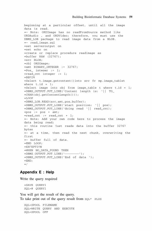
Building Bioinformatic Database Systems 59
beginning at a particular offset, until all the imagedata is read.•— Note: ORDImage has no readFromSource method likeORDAudio , and ORDVideo; therefore, you must use theDBMS_LOB package to read image data from a BLOB.•— read_image.sql•set serveroutput on•set echo on•create or replace procedure readimage as•buffer RAW (32767);•src BLOB;•obj ORDImage;•amt BINARY_INTEGER := 32767;•Pos_ integer := 1;•read_cnt integer := 1;•BEGIN•Select t.image.getcontent()into src fr mp.image_tabletwhere t.id = 1;•Select image into obj from image_table t where t.id = 1;•DBMS_OUTPUT.PUT_LINE(‘Content length is: ‘|| TO_•CHAR(obj.getContentLength()));•LOOP•DBMS_LOB.READ(src,amt,pos,buffer);•DBMS_OUTPUT.PUT_LINE(‘start position: ‘|| pos);•DBMS_OUTPUT.PUT_LINE(‘doing read ‘|| read_cnt);•pos := pos + amt;•read_cnt := read_cnt + 1;•— Note: Add your own code here to process the imagedata being read;•— this routine just reads data into the buffer 32767bytes•— at a time, then read the next chunk, overwriting thefirst•— buffer full of data.•END LOOP;•EXCEPTION•WHEN NO_DATA_FOUND THEN•DBMS_OUTPUT.PUT_LINE(‘————————’);•DBMS_OUTPUT.PUT_LINE(‘End of data ‘);•END;•/
Appendix E : Help
Write the query required
•SAVE QUERY1SQL>@ QUERY1
You will get the result of the query.To take print out of the query result from SQL* PLUS
SQL>SPOOL FILENAMESQL>WRITE QUERY AND EXECUTESQL>SPOOL OFF

60 B.B. Meshram
Output of the query is in FILENAME.LSTTo write programs in PL/SQL
1. SQL> ED FILENAME (PRESS ENTER)
You will get the system editorType Your Program –Procedure or Function
THEN SAVE IT..... —�—— FILE..... —�—— SAVE AS( FILENAME.SQL)
2. To come out of the editor
PRESS..... —�—— ALT F, THEN PRESS X, so that you will get SQL
prompt.
3. On this SQL prompt, for compilation give the command
SQL> @ FILENAME
This will compile your program.4. Then to run your program, give the command
/ (SLASH)
You will get the result as procedure created.5. To invoke a procedure in SQL* PLUS, use the command
SQL> EXECUTE PROCEDURENAME ( PASS PARAMETER)
If there is no error in the program, message will be procedure or functionsuccessfully created.
6. If errors are there, give the command
SQL> SHOW ERRORSQL> L
The program with line number will be displayed.7. To correct your program, go to the editor and give the command
SQL> ED FILE NAME
• Make corrections in the program and save it.• Repeat the process to compile and run.
8. Removing server-side procedure/function
• USING SQL*PLUS;SQL>DROP PROCEDURE PROCEDURE_NAME;SQL>DROP FUNCTION FUNCTION_NAME;
9. Creating package specification example
SQL>CREATE OR REPLACE PACKAGE comm_package ISbandu-comm NUMBER := 10 ;PROCEDURE reset_comm.( v_comm. IN NUMBER) ;END comm_ package ;

Building Bioinformatic Database Systems 61
10. Executing a Public Procedure• Referencing a public variable and executing a public procedure
SQL>EXECUTE comm._package.g_comm.:= 5SQL>EXECUTE comm._package.reset_comm(8)
11. Managing Triggers• Disable or re-enable a database trigger
ALTER TRIGGER trigger_name DISABLE ! ENABLE
• Disable or re-enable ALL triggers for a table
ALTER TABLE table_name DISABLE ! ENABLE ALL TRIGGERS
• Recompile a trigger for a table
ALTER TRIGGER trigger_name COMPILE
• To remove trigger from database
DROP TRIGGER trigger_name;
62 Achuthsankar S. Nair et al.
Bio-sequence Signatures UsingChaos Game Representation
Achuthsankar S. Nair, Vrinda V. Nair, Arun K.S.,Krishna Kant and Alpana Dey
INTRODUCTION
Computational biology/Bioinformatics is the application of computer sciencesand allied technologies to answer the questions of biologists, about themysteries of life. It looks as if computational biology and bioinformatics aremainly concerned with problems involving data emerging from within cellsof living beings. It might be appropriate to say that computational biologyand bioinformatics deal with application of computers in solving problemsof molecular biology, in this context. What are these data emerging from acell? Four important data are: DNA, RNA and Protein sequences and Microarray images. Surprisingly, first three of them are mere text data (strings,more formally) that can be opened with a text editor. The last one is a digitalimage which is only indirectly a cellular data (See Fig. 1).
Our interest is to discuss about deriving signatures for the first three kindsof data. It is well known that the gene regions of the DNA in the nucleusof the cell is copied (transcribed) into the RNA and RNA travels to proteinproduction sites and is translated into proteins. In short, DNA � RNA �Proteins, is the central dogma of molecular biology. ComputationalGenomics and Proteomics are fields which encompass various studies ofthe genome and the proteome, based on their sequences. Both start withsequence data, and attempt to answer questions like this:
Genomics: Given a DNA sequence, where are the genes? (Gene finding);How similar is the given sequence with another one? (Pairwise sequencealignment); How similar are a set of given sequences? (Multiple sequencealignment); Where on this sequence does another given bio-molecule bind?(Transcription factor binding site identification); How can we compress thissequence? How can we visualize this sequence insightfully? (Genomebrowsing)
Proteomics: Given an amino acid sequence data, how similar is it withanother one, or how similar are a set of amino acid sequences (Pairwise and
7

Bio-sequence Signatures Using Chaos Game Representation 63
(a) DNA Data (4-letter strings)
(b) RNA Data (4-letter strings)
(c) Protein Data (20-letter strings)
(d) Micro Array Image Data (traditional digital images)
Fig. 1: Four major kinds of data required to be analyzed in Bioinformatics.

64 Achuthsankar S. Nair et al.
multiple sequence alignment); What is the primary, secondary or tertiarystructure of the molecule? (The great protein folding problem); Which partis most chemically active? (Active site determination problem); How wouldit interact with another protein? (protein-protein interaction problem); Towhich cell compartment is this protein belonging to? (Protein sub-cellularlocalization or protein sorting problem).
A large number of tools and techniques are available in computationalgenomics and proteomics, with varying degrees of success. A technique thathas been developed successfully and used very widely in both genomics andproteomics, is the sequence alignment technique. This forms the basis forcomparative studies of the genome and the proteome. A computationallyintensive problem has been addressed to satisfactory level, providing a servicewhich is quite fast and reliable.
Fig. 2: Typical BLAST output for a query.
For the modern life scientist, the BLAST service which returns localalignment searches of query sequences has become the Google of biology(see Fig. 2). Another example of a successful bioinformatic tool is the UCSCgenome browser. It would be unthinkable to comprehend the genomic datathat is continuously erupting, without a facility such as the genome browser(see Fig. 3).
Color key for alignment scores
Query

Bio-sequence Signatures Using Chaos Game Representation 65
Fig. 3: The genome browser.
Many of the problems in genomics and proteomics have been attacked byvarious researchers using a plethora of tools from the field of mathematics,statistics, soft computing and many others. We discuss here yet anothermethod which is useful in analyzing DNA/protein sequences aimed at solvingsome of the above problems.
CHAOS GAME REPRESENTATION ALGORITHM
During 1970s, a new field of physics was developed known as chaoticdynamical systems or simply chaos (Jeffrey, 1990). This field was closelyassociated with fractals. Fractal geometry, in contrast with Euclidean geometry,deals with objects that possess fractional dimensions like 1.45, 2.79 etc.Fractal geometry considers itself the geometry of the real (rather than theideal) and consequently treats the objects in nature such as clouds, coastlines,trees, landscapes, lightning etc. as possessing fractal dimensions. Amonginteresting properties of the fractals are their unvarying complexity at varyingscales.
Fig. 4: CGR and its I/P and O/P.

66 Achuthsankar S. Nair et al.
The Chaos Game is an algorithm, which is an offshoot of research in theabove area. It allows one to produce unique images of fractal nature, knownas Chaos Game Representation images (CGR images) from symbolicsequences, which can serve as signature images of the sequences. It wasoriginally described by Barnsly in 1988. Chaos Game is an algorithm whoseinput is a sequence of letters (finite alphabets) and output is an image(see Fig. 4).
Even though CGR of any finite sequence with finite set of alphabets ispossible, here we are considering only biological sequences like DNAsequence, RNA sequence and amino acid sequences. Life scientists considerthat key to life processes is centred around the above mentioned three entities.All these entities can be represented by sequences of finite alphabets.
The use of CGRs as useful signature images of bio-sequences such asDNA has been investigated since early 1990s. CGRs of genome sequenceswere first proposed by H. Joel Jeffrey (1990). Later other bio-sequenceswere also explored. We will now briefly introduce the idea of deriving aCGR image of a DNA sequence.
To derive a Chaos Game Representation of a genome, a square is firstdrawn to any desired scale and corners marked A, T, G and C. Points aremarked within the square corresponding to the nucleotides in the sequence.In CGR, the four nucleotides A, G, C and T are assigned to the corners ofa square as in Fig. 5. The choice of the corners is not based on any particularcriteria, and indeed can be assigned in any other way.
Nucleotide A has an assignedposition (0, 0), T has an assignedposition (1, 0), G has an assignedposition (1, 1) and C has anassigned position (0, 1). Now wedefine a procedure for representingany arbitrary nucleotide sequenceas a point inside the square. Forplotting a given sequence we startfrom the centre of the square. Thefirst point is plotted halfwaybetween the centre of the square,and the corner corresponding tothe first nucleotide of the sequence,and successive points are plotted halfway between the previous point, andthe corner corresponding to the base of each successive nucleotides. The midpoint Pm (xm, ym) between two given points P1(x1, y1) and P2 (x2, y2) can becalculated using the following equation.
(i) xm = (m x1 + x2)/2.
(ii) ym = (m y1 + y2)/2.
Fig. 5: CGR square with each nucleotideassigned to corner.

Bio-sequence Signatures Using Chaos Game Representation 67
These steps for plotting a given sequence are concluded below.
1. Select the first nucleotide from the given sequence.2. Calculate the mid point between the centre and the corner corresponding
to the first nucleotide [PN(xNxx , yN)]. Let the mid-point be Pi(xi, yi). Let(xc, yc) be the co-ordinates of the mid-point of the square.
(a) xi = (xc+ xN)/2
(b) yi = (yc+ yN)/2
3. Do the following steps until all the nucleotides are processed.(a) Read the next nucleotide in the sequence.(b) Calculate the mid-point between the current point Pi(xi, yi) and the
corner corresponding to the newly read nucleotide. Let the newmid-point be Pi+1(xi+1, yi+1).
(i) xi+1 = (xi xx + xN)/2(ii) yi+1 = (yi + yN)/2
Now using the above procedure let us plot a DNA sequence TACAGAinto this square. A square is drawn to any desired scale and corners markedA, T, G and C. Points are marked within the square corresponding to thebases in the sequence, as follows:
1. Plot the first point halfway between the centre of the square and theT corner.
2. The next point is plotted halfway between the previous point and theA corner.
3. The next point is plotted halfway between the previous point and theC corner.
4. The next point is plotted halfway between the previous point and theA corner.
5. The next point is plotted halfway between the previous point and theG corner.
6. The next point is plotted halfway between the previous point and theA corner.
Figures 6 to 11 depict the process graphically.
Fig. 6: ‘T’ is plotted. Fig. 7: ‘TA’ is plotted.

68 Achuthsankar S. Nair et al.
Fig. 8: ‘TAC’ is plotted. Fig. 9: ‘TACA’ is plotted.
Fig. 10: ‘TACAG’ is plotted. Fig. 11: ‘TACAGA’ is plotted.
Now, let us see how a real CGR would look like. Figure 12 shows CGRof Hepatitis A virus, full genome, plotted using beta version of a tool C-GRex, discussed later in this article. Figures 13 and 14 show CGR of fullgenome of His 2 virus, and Thermosinus carboxydivorans respectively.
Fig. 12: CGR of Hepatitis A virus full genome.

Bio-sequence Signatures Using Chaos Game Representation 69
Fig. 13: CGR of His 2 virus full genome.
Fig. 14: CGR of Thermosinus carboxydivorans full genome.
The above CGR images clearly indicate that they vary from genome togenome, with characteristic patterns for each. This is what encourages oneto investigate if CGRs can indeed be used as unique signature images forgenomes and also other bio-sequences.
CGR PROPERTIES
A CGR has many properties. Every sequence has a unique CGR. In factevery symbol in a sequence will have a corresponding unique point in theCGR, even though the reverse need not be the case. Every point on the CGRis a representation of all the symbols in the sequence up to that point. Forinstance, in the CGR of the sequence ATTTGGCCATCG, the fifth pointrepresents the sequence ATTTG.

70 Achuthsankar S. Nair et al.
Each sub-square in a CGR has a special significance. If we divide theCGR into four quadrants, then the top right corner will contain pointsrepresenting sub-sequences that end with G, as a mid-point between anyother point in the square and the G-corner has to fall in this quadrant. Henceif we count the points in this quadrant, it will be equal to the count of thebase G in the sequence. If we divide this quadrant into another four squares,in the clockwise order, they would represent subsequences that end in GG,TG, AG and CG, making it possible to derive the 2-mer counts by countingthe points in these sub-squares. In general, by dividing the CGR square intosub-squares of side 2–n, we can find the number of different n-mers presentin the sequence (see Fig. 15).
Side 1/2 - four sub-squares – monomersSide 1/4 - 16 sub-squares – dimersSide 1/8 - 64 sub-squares – trimers and so on
Fig. 15: Correspondence between n-mers and sub-squares of CGR.
Another interesting characteristic of CGR is that images obtained fromparts of a genome show the same pattern as that of the whole genome(Deschavanne et al., 1999). Thus analysis of parts of a genome will resultin a satisfactory genomic signature. This also helps comparing non-homologous genomic sequences when only parts of the genomes are available.
Genomic CGRs
The CGR of various organisms exhibit differing patterns which arecharacteristic of that species. Here we have obtained 20 kbp of a few specieswhich illustrates some interesting patterns and hence features of the group.Main features of CGR images include CG double scoops, diagonals, absenceof diagonals, horizontal variation in intensities from top to bottom or reverse,empty patches and word-rich regions of different shapes.

Bio-sequence Signatures Using Chaos Game Representation 71
(a) Musmusculus (Eukaryote) (b) Bos Taurus (Eukaryote)
(c) Homo Sapiens (Eukaryote) (d) Agrobacterium tumefasciens (Bacteria)
(e) A. fulgidus (Archea) (f) E. coli K12 (Bacteria)
(g) C. elegans (Eukaryote) (h) Arabidopsis Thaliana (Eukaryote)
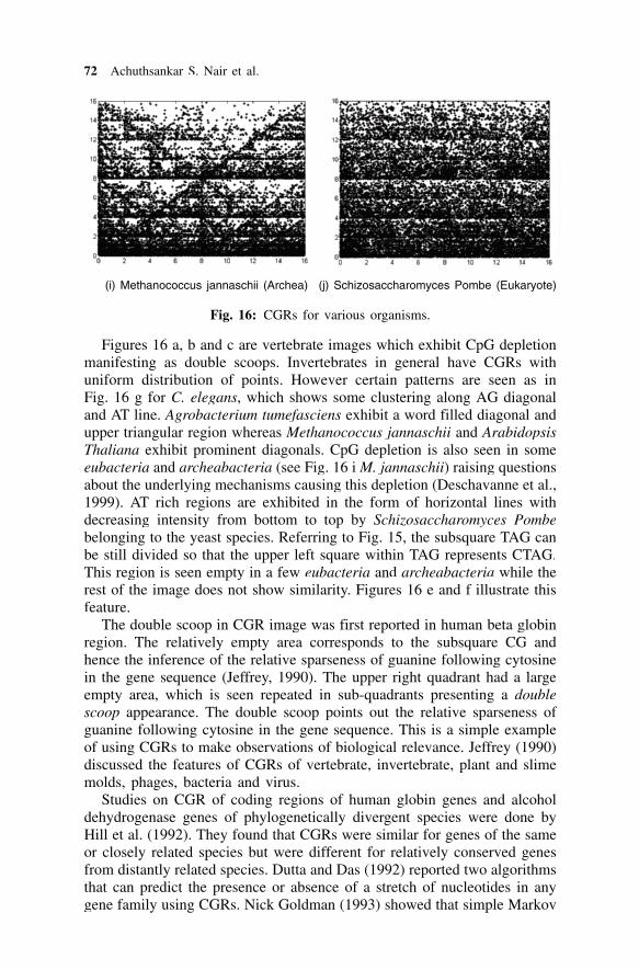
72 Achuthsankar S. Nair et al.
(i) Methanococcus jannaschii (Archea) (j) Schizosaccharomyces Pombe (Eukaryote)
Fig. 16: CGRs for various organisms.
Figures 16 a, b and c are vertebrate images which exhibit CpG depletionmanifesting as double scoops. Invertebrates in general have CGRs withuniform distribution of points. However certain patterns are seen as inFig. 16 g for C. elegans, which shows some clustering along AG diagonaland AT line. Agrobacterium tumefasciens exhibit a word filled diagonal andupper triangular region whereas Methanococcus jannaschii and ArabidopsisThaliana exhibit prominent diagonals. CpG depletion is also seen in someeubacteria and archeabacteria (see Fig. 16 i M. jannaschii) raising questionsabout the underlying mechanisms causing this depletion (Deschavanne et al.,1999). AT rich regions are exhibited in the form of horizontal lines withdecreasing intensity from bottom to top by Schizosaccharomyces Pombebelonging to the yeast species. Referring to Fig. 15, the subsquare TAG canbe still divided so that the upper left square within TAG represents CTAG.This region is seen empty in a few eubacteria and archeabacteria while therest of the image does not show similarity. Figures 16 e and f illustrate thisfeature.
The double scoop in CGR image was first reported in human beta globinregion. The relatively empty area corresponds to the subsquare CG andhence the inference of the relative sparseness of guanine following cytosinein the gene sequence (Jeffrey, 1990). The upper right quadrant had a largeempty area, which is seen repeated in sub-quadrants presenting a doublescoop appearance. The double scoop points out the relative sparseness ofguanine following cytosine in the gene sequence. This is a simple exampleof using CGRs to make observations of biological relevance. Jeffrey (1990)discussed the features of CGRs of vertebrate, invertebrate, plant and slimemolds, phages, bacteria and virus.
Studies on CGR of coding regions of human globin genes and alcoholdehydrogenase genes of phylogenetically divergent species were done byHill et al. (1992). They found that CGRs were similar for genes of the sameor closely related species but were different for relatively conserved genesfrom distantly related species. Dutta and Das (1992) reported two algorithmsthat can predict the presence or absence of a stretch of nucleotides in anygene family using CGRs. Nick Goldman (1993) showed that simple Markov

Bio-sequence Signatures Using Chaos Game Representation 73
chain models based solely on dinucleotide and trinucleotide frequencies canaccount for the complex pattern exhibited in CGRs of DNA sequences.Although later, Almeida et al. (2001) showed that CGR is a generalizedscale independent Markov probability table. A very important and usefulobservation made by Deschavanne et al. (1999) was that subsequences of agenome exhibit the main characteristics of the whole genome, attesting tothe validity of the genomic signature concept. Roschen et al. (2006) haveexplored the potential of CGR representation for making alignment-basedcomparisons of whole genome sequences. Classification of CGR imageshave been done by many researchers (Deschavanne et al., 1999; Deschavanneet al., 2000; Giron et al., 1999; Huang et al., 2004).
Proteomic CGRs
Works on CGR used for visualizing amino-acid sequences were done byAndras Fiser, Gabor E. Tusnady and Istav Simon (1994). They demonstratedthat CGR can also be used for analyzing protein databases. Suggestedapplications include investigating regularities and motifs in the primarystructure of proteins, analyzing possible structural attachments on the super-secondary structure level of proteins and testing structure prediction methods.Zu-Guo Yu, Vo Anh and Ka-Sing Lau (2004) performed multifractal andcorrelation analyses of the measures based on the CGR of protein sequencesfrom complete genomes and hence attempted to construct a more precisephylogenetic tree of bacteria.
Proteomic CGR requires some tinkering with the sequence (or with theimage format) to derive CGR images as amino-acids are 20 in number. Weeither have to group the amino-acids into four categories or change from asquare to a polygon. Early approaches were based on groupings. Amino-acidproperties have been well studied for long and over 500 properties are known(see AA Index, for instance). This would mean that the grouping itselfwould have 500 choices. If we decide to change the groupings from four toany number from 2 to 20, we can produce corresponding n-sided polygonimages. This is a work that is being carried out by some of the authors, andis implemented in an open source tool named C-GRex, discussed next.
C-GRex: A CGR Explorer for Bio-sequences
C-GRex, Chaos Game Representation Explorer, is a tool to explore variousfeatures of CGR, in such a way that an unbelievable number of CGRs canbe derived out of a given sequence, especially an amino-acid sequence,almost resembling a kaleidoscope. It is a handy tool for sequence visualizationand analysis of patterns, hot spots and discoveries. C-GRex packs a widevariety of exploration facilities using Chaos Game Representation in DNA,RNA and Protein sequences and any other sequence. The tool comes witha set of functionalities which makes it unique. The software is designed ina way that a person with little knowledge about CGR will be able to workwith it and manipulate the plot.

74 Achuthsankar S. Nair et al.
The main window of C-GRex is shown in Fig. 17. It contains three areas:plot area, settings display area, sequence panel in addition to menu bar andtool bar. The plot area shows the CGR plot of the loaded sequence. Thesettings applied to the CGR plot is shown in settings display area. Thesequence panel contains the loaded sequence. The user can scroll throughthe sequence. The starting and ending number of the sequence visible in thesequence panel is displayed above the panel.
Fig. 17: The main window of C-GRex.
While it is not the intention here to introduce C-GRex comprehensively,the special feature of C-GRex will be briefly discussed. This relates togenerating n-sided polygonal CGRs, with choice of n resting with the userwith complete freedom to assign thecorners to symbols. Let us assume thata user is interested in exploring variousCGRs of given amino-acid sequence.She can choose the plot-style option inCGRex which brings up a dialog boxas follows. In the space for corners,user can choose from 5 to 26 corners(3 and 4 are covered by triangle andsquare, 26 is set as the limit so thateven plain English can be accepted bythe software). See Fig. 18.
Fig. 18: The plot-style dialog boxof C-GRex.

Bio-sequence Signatures Using Chaos Game Representation 75
Suppose the user chooses eight corners, then 20 amino acids have to beassigned to these eight corners. C-GRex permits this to be done by a manualassignment or by an automatic assignment based on clustering and a choiceof physico-chemical parameter for clustering. For clustering, it uses the wellknown k-means clustering. Figure 19 shows manual selection of amino-acidassignment for eight-cornered polygon. For clustering one of the 500 physico-chemical parameters can be chosen by the user. Figure 20 shows a eight-cornered CGR.
Fig. 19: Selection of amino-acid assignment for eight-cornered polygon.
Fig. 20: Eight-cornered polygonal CGR.
1 2
3
4
8
7
56
6 5
7 4
8 3
21

76 Achuthsankar S. Nair et al.
CONCLUDING REMARKS
We have tried to introduce the concept and application of chaos gamerepresentation of bio-sequences. A versatile tool also was introduced. CGRsare a very different way of analyzing bio-sequences. Only a very smallnumber of studies have been conducted in this area. The scope of CGRs isenormous. With the availability of tools such as C-GRex, it is hoped that alot more of studies can be initiated in this area.
REFERENCES
Almeida, J.S. (2001) Analysis of genomic sequences by chaos game representation.Bioinformatics, 17: 429-437.
Andras Fiser, Gabor E. Tusnady and Istvan Simon (1994). Chaos Game representa-tion of protein structures. J. Mol. Graphics, 12: 302-304.
Deschavanne, P.J., Giron, A., Vilain, J., Dufraigne, C. and Fertil, B. (2000).Genomic Signature is preserved in short DNA fragments. IEEE.
Deschavanne, P.J., Giron, A., Vilain, J., Fagot, G. and Fertil, B. (1999). Genomicsignature: Characterization and classification of species assessed by chaos gamerepresentation of sequences. Mol. Biol. Evol., 16: 1391-1399.
Dutta, Chitra and Das, Jyotirmoy (1992) Mathematical Characterization of ChaosGame Representation New Algorithms for Nucleotide Sequence Analysis. J MolBiol., 228: 715-719.
Giron, A., Vilain, J., Serruys, C., Brahmi, D., Deschavanne, P.J. and Fertil, B.(1999). Analysis of parametric images derived from genomic sequences usingneural network based approaches. IEEE.
Goldman, N. (1993) Nucleotide, dinucleotide and trinucleotide frequencies explainpatterns observed in chaos game representations of DNA sequences. NucleicAcids Res, 21: 2487-2491.
Hill, Kathleen, A., Schisler, Nicholas J. and Shiva M. Singh (1992) Chaos GameRepresentation of coding regions of human globin genes and alcohol dehydroge-nase genes of phylogenetically divergent species. J Mol Evol., 35: 261-269.
Jeffrey, H.J. (1990) Chaos game representation of gene structure. Nucleic Acids Res.18: 2163–2170.
Jijoy Joseph and Roschen, Sasikumar (2006) Chaos Game Representation for com-parison of whole genomes. BMC Bioinformatics, 7: 243.
Xin Huang, De-Shuang Huang, Hong-Qiang Wang and Xing-Ming Zhao (2004).Representation of DNA sequences with multiple resolutions and BP neural net-work based classification. IEEE.
Zu-Guo Yu, Vo Anh and Ka-Sing Lau (2004). Chaos game representation of proteinsequences based on the detailed HP model and their multifractal and correlationanalyses. J. Theor Biol., 226(3): 341-348.
Data Mining for Bioinformatics—Microarray Data
T.V. Prasad and S.I. Ahson
INTRODUCTION
Data could be of any form, symbolic or non-symbolic, continuous or discrete,spatial or non-spatial, it should be understood that whenever the data storebecomes voluminous, it requires efficient algorithms to mine out requireddata as well as provide methods to answer various queries. Though the dataanalysis techniques are useful in almost all disciplines of study, greateremphasis is given in the area of bioinformatics for mining microarray geneexpression data as well as gene sequence data. Considerable work is beingdone in preparation of protein arrays and corresponding visualizationtechniques.
There are different algorithms for different situations and data forms. Thealgorithm that works fine for astronomical and space research cannot workfor gene/protein data extraction, which in turn will be different from the onefor browsing through the Internet. All techniques have different parameters/preconditions of operation as well as advantages and disadvantages associatedwith them. Many require preprocessing and many do not. Many differ indimensionality, many in terms of structure and many in conditions.
In general practice it has been observed that data matrix can be categorizedinto three types, viz.
• Continuous (time series), e.g., blood sugar level of a patient taken afterevery two hours
• Parametric (wherein each dimension or sample has some relationshipwith the same entity under observation), e.g., population database (coveringparameters such as height, weight, eye sight, skin colour, age, hair colour,etc.) and
• Non-parametric (wherein there is no relationship between any of thesamples), e.g., gene expression data, marks of students in five differentsubjects, etc.
8

78 T.V. Prasad and S.I. Ahson
The third form could be considered as a special case of second but sincethere are large number of applications requiring special attention towardsfunctional dependence or independence, three different types have beenenumerated here in which each sample is considered as one dimension.
DATA MINING TECHNIQUES
The complexity of data increases manifold with the increase in dimensionality(or number of features). For instance, consider the university marks processingsystem records having marks of 5000 students over 40 subjects (or eightsemesters) as a one batch, which is already in a 2D form. The difficultyincreases by one time with considering varied courses in the university as itbecomes inevitable to add a new dimension or feature. Add another dimension,if there are going to be one batch per year and a group of five years is tobe considered. Continue adding another dimension, if a group of universitiesis to be taken up. Ordinary analysis programs would take enormous time toprocess the data and remain a failure in answering complex queries, whichcould not be visualized beforehand. The existing data mining techniquescould remain helpless keeping in view the voluminous amount, highdimensionality and heterogeneous nature of data. Since data have not beencollected specifically for the data analysis task, often some form ofpreprocessing is required barring a few experimental methods. Among thevarious goals addressed by data preprocessing, dimensionality reduction orfeature selection has been recognized as a central problem in data analysis(Talavera, 2000).
Data analysis techniques that perform well for lower dimensions fail toperform for higher dimensional data. This problem of increasing dimensionsand inability of the techniques to encompass change in number of featuresis termed as curse of dimensionality.
With massive amounts of data lying across the world, there could benumerous techniques to take out what is required, either by artificial meansor by natural processes. Most common of all these techniques are clusteringand classification. The data mining tasks have been categorized as predictionmethods and description methods. The prediction methods use some variablesto predict unknown or future values of other variables, for instance,classification, regression and deviation detection. The description methodsare used to find human-interpretable patterns that describe the data, forexample, clustering, associations and classification. Techniques drawn fromvarious other fields such as artificial intelligence, pattern recognition, statistics,database management systems and information visualization together provideefficient methods to mine the volumes (Vipin Kumar, 2002).
The data mining algorithms can be used not only for the gene expressiondata but for sequence data, proteomics data and pathway data as well. Thereare not many papers and work available for pooling data into different

Data Mining for Bioinformatics—Microarray Data 79
databases and use powerful data mining tools to mine and analyze them inthe required form. Present software tools need multi-level analysis techniquesto produce little meaningful results.
GENE EXPRESSION MICROARRAY TECHNOLOGY
DNA microarray is a glass slide onto which single-stranded DNA moleculesare attached at fixed locations (or spots). They are composed of thousandsof individual DNA sequences printed in a high-density array on a glassmicroscope slide using a robotic arraying device. The relative abundance ofthese spotted DNA sequences in two DNA or RNA samples may be assessedby monitoring the differential hybridization of the two samples (or a sampleand a control) to the sequences on the array. These may be generated bysingle fluorescent, dual fluorescent, radioactive or colorimetric labels andthe recording methods differ in each case. The arrays with the small solidsubstrate are also referred to as DNA chips. It is so powerful that one caninvestigate the gene information in short time, because at least hundreds ofgenes can be put on the DNA microarray to be analyzed (Cho and Won,2003). With the currently available technologies, DNA microarrays of thecapacity 61,000 genes across 22 conditions or samples can be obtained.Gene expression data indicates when and where genes are turned on (orexpressed) i.e., under- or over-expression. cDNA stands for complementaryDNA and is mRNA artificially translated back into DNA, but without thenon-coding sequence gaps, or introns, found in the original genomic DNA.
Chee et al. (1996) made known to the world on how to use microarraydata, probably when the term gene expression data was not coined. Theimportance of application of microarray technology to areas such as cancerdiagnosis was discussed as early as 1998 (Szallasi, 1998). Bowtell (1999)discussed about various ways of obtaining gene expression data frommicroarray experiments. Bassett et al. (1999) highlighted about the importanceand future applications of gene expression data, whereas White et al. (1999)applied microarray data to explain fruit fly metamorphosis. Golub et al.(1999) published a paper on molecular classification of cancer. This relatesto their study of class discovery and class prediction by gene expressionmonitoring. Slonim et al. (2000) subsequently studied class prediction anddiscovery using gene expression data. Ramaswamy et al. (2001) brought outmulti-class cancer diagnosis using tumor gene expression signature. Followingtypes of microarrays exist (Johnny, 2002):
• DNA hybridization arrays� cDNA based microarrays, comes with two technologies
� nylon membrane based - uses radioactive labeling� glass slides - uses fluorescence labeling
� Oligo nucleotide microarrays for sequencing and polymorphism

80 T.V. Prasad and S.I. Ahson
• Peptide microarray chips� Silicon based micro-fluidics chips, 2000 to 4000 peptide sequence on
a 1.5 cm2 chip• Protein chips
� Secreted� Membranal
• Tissue arrays• Combinatorial chemistry arrays
The problem with microarrays is perverse—a typical microarray experimentprovides both too much information and too little. In most research projects,the idea is to study small number of variables and repeat the measurementsover and over again. But in microarray experiments, there can be thousandsof variables, corresponding to the number of individual genes being studied;but the high cost of the chips means that the number of repeated observationsis usually very low. Most of the early papers only recorded whether geneswere active or not, such as Li et al. (2001). The slide preparation equipmentis shown in Fig. 1.
The importance of visualization of microarray gene expression data wasemphasized in Carr et al. (1997), but not much research was done in thesubsequent years as very few novel techniques have evolved since then. Thevisualization technique described here was used later in Wen et al. (1998) todemonstrate that the gene expression data can be properly mined to generatedifferent forms of outputs such as a mutual information tree, plots ofnormalized time series representation, projection view in 3D stereo plot, etc.A very exhaustive collection of papers/articles on microarray technology andrelated allied techniques can be obtained from Leung (2002).
Fig. 1: The microarray slide preparation equipment consisting ofrobotic arm. Image source: Li et al. (2001).
Butte (2002) gave one of the detailed reviews on preparation and analysisof microarray data, while D’haeseleer et al. (1997), Wen et al. (1998) andTibshirani et al. (1999) were the earliest reviews giving an account of great

Data Mining for Bioinformatics—Microarray Data 81
works on processing gene expression data, clustering techniques and itsvisualization. A wide coverage of various data mining algorithms andtechniques has been given in Han and Kamber (2001).
mRNA abundance: Most popular experimental platform is used forcomparing mRNA abundance in two different samples (a sample and acontrol). For mRNA samples, the two samples are reverse-transcribed intocDNA, labeled using different fluorescent dyes mixed (red-fluorescent dyeCy5 and green-fluorescent dye Cy3). After washing and hybridization ofthese samples with the arrayed DNA probes, the slides are imaged usingscanner that makes fluorescence measurements for each dye. To measure therelative abundance of the hybridized RNA, the array is excited by a laser.If the RNA from the sample population is in abundance, the spot will be red;if the RNA from the control population is in abundance, it will be green. Ifsample and control bind equally, the spot will be yellow, while if neitherbinds, it will not fluoresce and appear black. Thus, from the fluorescenceintensities and colours for each spot, the relative expression levels of thegenes in the sample and control populations can be estimated. The log ratiobetween the two intensities of each dye is used as the gene expression data,
Gene expression = 2Int(Cy5)
logInt(Cy3)
(1)
where Int(Cy5) and Int(Cy3) are the intensities of red and green colours.Since at least hundreds of genes are put on the DNA microarray, genome-wide information can be investigated in short time (Brazma and Vilo, 2000;Cho and Won, 2003). The main focus in genomic research is switching fromsequencing to using the genome sequences in order to understand how genomesare functioning. A detailed procedure of how the gene regulation, informationabout the transcript levels and then understanding gene regulatory networkscan be obtained from DNA microarrays (Pocock and Hubbard, 2000).
Durbin et al. (2002) described about preprocessing using statisticaltechniques. Yang et al. (2000 and 2001) highlighted various methods foranalyzing the scanned image of the microarray gene expression data andnormalization issues, so also experimental design issues for cDNA microarraywere discussed by Churchill (2002) whereas Quackenbush (2002) broughtout issues related to normalization of microarray data. Wong and Li (2001aand 2001b) discussed design issues, model suitability, error computation,etc. issues elaborately. An excellent description of microarray experimentpreparation and data analysis through statistical methods can be found inBergeron (2003).
Gene Expression Data Matrix or Profiles
By measuring the transcription levels of genes in an organism under variousconditions, at different developmental stages and in different tissues, one can

82 T.V. Prasad and S.I. Ahson
build up ‘gene expression profiles’ which characterize the dynamic functioningof each gene in the genome. The expression data represented in a matrixhave rows representing genes, columns representing samples (e.g. varioustissues, developmental stages and treatments), and each cell containing anumber characterizing expression level of the particular gene in the particularsample. Such a table is called a gene expression matrix (Fig. 2, Westheadet al., 2003). Johnny (2002) in the presentation elaborated about variousfeatures of microarrays and discussed gene expression data analysis. Genematrix could be used to compare many samples (of different creatures orpatients) or of same being across different periods (i.e. time series). Thesamples are arranged column-wise and the gene expression value can beobtained row-wise. The first is used for comparative analysis of expressionlevels of genes, whereas the latter is used to determine the transformationpattern (of growth or decay) of the set of genes.
Fig. 2: Schematic of an idealized expression array, in which the results fromthree experiments are combined. Three genes NG (G1, G2, G3) are labeled onvertical axis and three experimental conditions NC (C1, C2, C3) are labeled onhorizontal axis, giving a total of nine data points represented by NC × NG. Theshading of each data point represents the level of gene expression, with darker
colours representing higher expression levels.

Data Mining for Bioinformatics—Microarray Data 83
Interpretation of microarray experiment is carried out by grouping dataaccording to similar expression profiles. It is defined as expressionmeasurements of a given gene over a set of conditions; essentially it meansreading along a row of data in the matrix. Intensity of shading is used torepresent expression levels. With experimental conditions C1 and C2, genesG1 and G2 look functionally similar and G3 appears different. However, ifC3 is included, a functional link between genes G1 and G3 can be seen.
Since the expression levels of most of the genes fall in more or less thesame range, those genes do not seem to reveal or attach specific meaning.Such set of genes are normally avoided from further processing. One of thebest examples can be found in the form of Leukemia: Acute Lymphoblastic(ALL) vs. Acute Myeloid (AML) (Golub et al., 1999), (Fig. 3).
Fig. 3: Illustration of Golub et al.’s work on ALL and AML.Image source: Shapiro and Ramaswamy (2002).
Microarray data format: Unlike sequence and structural data, there is nointernational convention for the representation of data from microarrayexperiments. This is due to the wide variation in experimental design, assayplatforms and methodologies. Recently, an initiative to develop a commonlanguage for the representation and communication of microarray data hasbeen proposed. Experiments can be described in a standard format calledMIAME and communicated using a standardized data exchange model andmicroarray markup language based on XML (Brazma et al., 2001; Spellmanet al., 2002). Real-world microarray data is stored in a number of differentformats and there are no uniform standards as of yet for representation.Broadly speaking, following are the formats in which microarray geneexpression data is represented (see website of Molmine):
• GenePix• Affymetrix• Agilent• ScanAnalyze• ArrayExpress
Microarray data mining challenges: The following issues could prove tobe major challenges while handling microarray gene expression data (Shapiroand Ramaswamy, 2002):
ALL AML

84 T.V. Prasad and S.I. Ahson
• Too few samples, usually < 100• Too many genes, usually > 1000• Too many columns likely to lead to false positives• For exploration, a large set of all relevant genes is desired• For diagnostics or identification of therapeutic targets, smallest reliable
set of genes is needed• Model needs to be explainable to biologists
Gene Expression Data Processing
Before clustering, especially with the SOM, it is essential to preprocess thedata to ward off all genes with insufficient biological variations. Genesnormally exhibit extraordinary level of expression and it becomes essentialto normalize them across samples to limit within mean of 0 and standarddeviation of 1, for each gene separately so that they can be easily plotted/visualized. A detailed manual on gene expression pattern preprocessing byHerroro et al. (2001) lists out 10 different forms of preprocessing activities(Dopazo, 1999, 2002), though all may need not necessarily be applied to theinput dataset. Different preprocessing algorithms can be applied for differenttypes of datasets.
Apart from Hedenfalk et al. (2001), other noted works include Khan etal. (2001), Hwang et al. (2001) and Chen et al. (2000) who used machinelearning techniques for diagnosis and/or prediction/profiling of breast cancer.Alizadeh et al. (2000) used gene expression data for analyzing diffuse largeB-cell in lymphoma dataset. Classification of multiple tumour types wasdescribed by Yeang et al. (2001).
It is desired to have the following features searched in the microarraydata:
• Understandable• Return confidence/probability• Robust even during presence of false positives• Fast enough
While doing so, it must be remembered that the simple approaches are themost robust ones.
Feature reduction: Since microarray datasets are so large, classification andclustering can be labourious and demanding in terms of computer resources.It is possible to use feature reduction, where non-informative or redundantdata points are removed from dataset, to make the algorithms run morequickly. For instance, if two conditions have exactly same effect on geneexpression, these data are redundant and one entire column of the matrix canbe eliminated. If the expression of a particular gene is same over a range ofconditions, it is neither necessary nor beneficial to use this gene in furtheranalysis because it provides no useful information on differential gene

Data Mining for Bioinformatics—Microarray Data 85
expression. In such cases, an entire row can be removed. Approaches likePCA/SVD can be used to automatically select such redundant or non-informative datasets. Redundant data are combined to form a single, compositedataset, thus reducing the dimensions of gene expression matrix andsimplifying analysis (Westhead et al., 2003).
Gene Expression vs. Boolean Representation
The goal of modeling and analyzing temporal gene expression data is todetermine the pattern of excitations and inhibitions between genes whichmake up a gene regulatory network for that organism.
One method of representation is to use Boolean networks in which geneexpression values are indicated as ‘on’ or ‘presence’ and ‘off’ or ‘absence’of specific genes. For example, the gene expression databases for multiplemyeloma (an incurable cancer involving immunoglobulin secreting plasmacells) contain absolute values of gene expression involving Absent, Presentand Marginal. The marginal values occuring large number of times in thedatasets are ignored, thereby with only two absolute values: Absent(represented to ANNs by 0), and Present (1). Any gene that receives no‘excitation’ in a time step will switch itself ‘off’ or ‘on’ in the next timestep. These networks therefore model the interactions between genes in acontrolled and intelligible manner. Gene expression data, including Booleannetworks, are problematic because of their dimensionality (Narayanan et al.,2003).
ARTIFICIAL NEURAL NETWORKS
Numerous advantages of ANNs have been identified in both the AI andbiological literature. Neural networks can perform with better accuracy thanequivalent symbolic techniques (for instance decision trees) on the samedata. Also, while identification tree approaches such as C4.5 can identifydominant factors the importance of which can be represented by their positionshigh up in the tree, ANNs may be able to detect non-dominant relationships(i.e. relationships involving several factors, each of which by itself may notbe dominant) among the attributes. However, there are also a number ofdisadvantages. Data often has to be pre-processed to conform to therequirements of the input nodes of ANNs (e.g. normalized and convertedinto binary form). Training times can be long in comparison with symbolictechniques. Finally, and perhaps most importantly, solutions are encoded inthe weights and therefore are not as immediately obvious as the rules andtrees produced by symbolic approaches (Narayanan et al., 2003).
By preparation of large libraries of voluminous number of molecules, itbecame possible to identify and network the combinatorial interactionsbetween them. A detailed study of the DNA microarray technology can beseen in Baldi and Hatfield (2001). Chakraborty (2004) gave a concise
86 T.V. Prasad and S.I. Ahson
description of microarray production technology and the role of bioinformaticsin processing the obtained data.
Though a number of statistical, neural network and other techniques areavailable, these techniques for microarray gene expression data analysis canbe still considered to be in infancy stage of development (Zhang., 1999). Theapplication of probabilistic models on array data, such as Gaussian model,Bayesian treatment and Bayesian hypothesis testing have been vividlydiscussed in the past (Baldi and Brunak., 2003), as well as implementationof these techniques.
Great stress on clustering and classification of DNA microarray data (orgene expression data) was laid out initially using the k-means, SOM andhierarchical clustering algorithms, which were mostly unsupervised. Classicalreferences are DeRisi (1996), Hacia et al. (1996), Carr et al. (1997), Eisenet al. (1998), Golub et al. (1999), Tavazoie et al. (1999), Toronen et al.(2000) and Sharan et al. (2001). Description of concepts such as the use ofdistance measure, correlation matrix, discovering function of unknown genes,etc. could be seen in Eisen et al. (1998), being the earliest reference, whereasCarr et al. (1997) discusses about gene expression data visualization. Sincethen, a number of papers have become available on application of SOM,many of which clearly described on how it could be used for patternclassification than just clustering purpose.
Anderson (2001), Freeman and Skapura (1991) and Haykin (1999)presented detailed background about the ANNs and analysis of data usingANNs, whereas Baldi and Hatfield (2001) gave a summarized glance of theadvances in the field of bioinformatic applications covering ANNs, geneexpression data and statistics. Lesk (2002) described various tools andtechniques related to proteomics, emphasizing the use of ANNs for processingprotein data like protein folding. Mount (2001) brought out that ANNs havebeen applied to sequence data in both forms viz., genes and proteins, forpromoter recognition, gene prediction and protein classification applications.Other techniques such as Multi-level perceptron (MLP), genetic algorithms(GA), radial basis function (RBF), agglomerative techniques, etc. have beensparsely used in relation to gene expression data.
In the supervised category, the most widely used algorithm is SVM, onesuch application can be found in Furey et al. (2000). Almost no work isavailable on use of LVQ with respect to gene expression data.
There are a number of lesser known ANN and non-ANN techniquesavailable; however, very less has been employed due to various reasons suchas complexity in understanding, lack of proper visualization techniques, wideacceptability, etc.
CLUSTERING AND CLASSIFICATION
Each gene in a gene expression matrix has an expression profile, that is, theexpression measurements over a range of conditions (or samples). The analysis

Data Mining for Bioinformatics—Microarray Data 87
of microarray data involves grouping these data on the basis of similarexpression profiles. If a predefined classification system is used to group thegenes, the analysis is described as supervised. If there is no predefinedclassification, the analysis is described as unsupervised and is known asclustering.
Clustering first involves converting the gene expression matrix into adistance matrix, so genes with similar expression profiles can be groupedtogether. This generally involves calculating the Euclidean distance, thecorrelation measure-based distance or the Pearson linear correlation-baseddistance for each pair of values. Several clustering methods can then be usedincluding hierarchical clustering, k-means clustering and the derivation ofself-organizing maps. Clustering is a method (may be statistical) used togroup a set of objects into a cluster of subgroups of similar objects based ona measure of similarity or “distance” between the objects. The number ofclusters required must be presented before initiating the clustering process inmost cases except in hierarchical clustering.
Clustering is unsupervised (i.e. anything about division is not knowninitially) whereas classification is a supervised learning process where divisionto subtypes is already known. Clustering helps in identifying the genes thatare not known previously. This gives a fair idea of their function since it ispresumed that a particular cluster would contain entities (or genes) havingsimilar homology. This is similar to a classroom where students form groupsor clusters automatically and based on the characteristics of one or twostudents in each cluster, the traits of other students can be predicted. It isbelieved that if not accurately predicted, at least it will give a fair idea of thetraits. A comparison table of various algorithms/techniques is given inAppendix.
Separate algorithms (or modules) are needed for handling a priori data,for detecting outliers, for selecting distances to use, for normalizingmeasurements and finally, for validation/confidence estimation.
Following are some of the known classification techniques whose strongor weak features have been indicated against them (Dudoit and Gentleman,2002a; Dudoit et al., 2000b; Thomas, 2001).
• Decision Trees/Rules - find smallest gene sets, but also false positives• Neural Nets - works well if the number of genes is reduced• SVM - good accuracy, does its own gene selection, hard to understandM• K-nearest neighbour - robust for small number of genesr• Bayesian nets - simple, robust
Additional information (or knowledge) is always needed to predict theresults more precisely, for instance, while working on oncology-relateddatasets, the following additional items would prove to be very useful:

88 T.V. Prasad and S.I. Ahson
• There is an immanent need to combine clinical and genetic data.• Outcome/Treatment prediction
� Age, sex, stage of disease, etc. of the patients are useful.� Issues like incorrect linkages should be handled beforehand e.g. if
dataset has been generated from male, it should not indicate presenceof ovarian cancer.
• Molecular biologists/oncologists seem to be convinced that only a smallsubset of genes are responsible for particular biological properties, sothey want to know which genes are most important in discriminating.
• Practical reasons, a clinical device with thousands of genes is not financiallypractical.
• Possible performance improvement through powerful algorithmic analysistechniques.
Goals of Clustering and Classification
It is usually thought of clustering and classification as techniques to mine thedata and produce logical groups of data. However, there are other goalsrelated to cluster analysis. Broadly speaking, various goals of cluster analysiscould be laid out as the following ways:
• To find natural classes in the data• To identify new classes/gene correlations• To refine existing taxonomies• To support biological analysis/discovery• Application of different methods - hierarchical clustering, SOM’s, etc.
In terms of application of ANN techniques in bioinformatics, only twotechniques have been largely used viz., the SOM for the purpose of clusteringdata and the SVM for classification of data.
The theory of clustering has been categorized into three groups based onthe measurement of distance, optimization or product (Liao, 2002):
Measurement of distance
• Distance [di,j >=j 0; di,I =I 0; di,j = dj j,Id ; dII i,j <= dj i,k + dk k,jd ]• Density• Topology• Probability
Optimization Algorithms
• Bottom-up vs. Top-down• Iterative vs. Recursive• Maximum likelihood vs. Expectation maximization (Bayesian viewpoint)

Data Mining for Bioinformatics—Microarray Data 89
Product
• Hierarchical vs. One-level• Exclusive vs. Overlapping (clustering)• Error tolerant (classification)• Discrete vs. Continuous• Generative vs. Discriminative (classification)
Baldi and Brunak (2003) brought out the prime challenges with clustering,which are as follows:
• Handling noisy signals/data could be difficult.• Considers processing high dimensional data.• Irregular training could lead to unstable state due to stability-plasticity
dilemma.• Clustering methods do not include a priori information.• Euclidean distance and correlation similarity do not reflect co-relational
structure of gene expression data; in such an event, more distance measuresand correlation techniques would be needed.
Almost all the commercially as well as publicly available microarray geneexpression data processing algorithms available today use SOM, k-means,HC and principal component analysis (PCA) techniques. Cluster analysiscame to limelight in 1998, when Eisen et al. (1998) used HC and displayedgenome-wide expression patterns.
The Kohonen’s self-organizing maps (SOM) is the most widely usedclustering algorithm, apart from k-means, hierarchical clustering (HC), etc.Amongst classification algorithms, Vapnik’s support vector machine (SVM),decision support algorithms, reinforced learning algorithms, etc. are popular.
SELF-ORGANIZING MAPS
Tamayo et al. (1999) published about interpreting patterns of gene expressiondata of tumour tissues using self-organizing maps (Fig. 4). Ben-Dor et al.(1999) published a paper highlighting application of various techniques onclustering gene expression patterns. Carr et al. (1997) described about thetemplates for looking at gene expression clustering. In medical discipline,Wen et al. (1998) mapped the development of central nervous system usinglarge-scale gene expression mapping. There are thousands of other applicationsof SOM in various fields of study, as well as in the clustering and visualizationof gene expression data.
The SOM is one of the most popular clustering techniques available. Itis a data visualization technique also, which reduces the dimensions of datathrough the use of self-organizing neural networks.
SOM are also known as topology preserving NN since the topologicalrelationships in external stimuli are preserved and complex multi-dimensional

90 T.V. Prasad and S.I. Ahson
data can be continued to be represented in the lower 2D space (Fig. 5). Asobserved, the serious drawbacks of SOM are that it neither produce ahierarchical classification, nor produce a proportional clustering, and thenumber of clusters have to be fixed beforehand i.e., in other words, SOMalso requires a priori knowledge like any other ANN.
Important features of SOM are:
• Kohonen’s SOM is simple analog of human brain’s way of organizinginformation in a logical manner
• Unsupervised learning process• Arranges information in topological order• Relationships during organization are maintained (topology preserving
mapping)• Consists of one layer of neurons in one, two or multi-dimensional arrays• No standardized initial geometry exists• Strongly depends on the initial inputs• Initial learning based on training from teacher; thereafter, unsupervised• SOM is computationally efficient algorithm located somewhere between
a multi-dimensional scaling algorithm and a clustering/vector quantizationalgorithm
• Adaptation strength is constant over time• New cells can be inserted and existent cells can be removed in order to
adapt output map to distribution of input vectors• Only best matching cells and its neighbourhood is adapted
The work of Iyer et al. (1999) towards application of a transcriptionalprogram for determination of the response of human fibroblasts to serum iswell noted.
SOM is a non-hierarchical clustering technique that combines visualizationof output nodes also. The visualization is also known as feature map oroutput space. The algorithm is very similar to the adaptive k-means algorithm,
Fig. 5: Training/learning processof neurons. Image source: Kim
(2002).
Fig. 4: The self-organizing map. Tamayoet al. (1999) discussed use of SOM ongene expression data forming them into
a 3 × 2 grid of clusters.

Data Mining for Bioinformatics—Microarray Data 91
as the selection of centroid and moving the genes (or data points) towardsthe nearest centroid is concerned. SOM can also be used for dimensionalityreduction, as it can be considered a non-linear generalization of PCA. Thesteps for SOM are as follows:
• Preprocessing� Filter away genes with insufficient biological variation.� Normalize gene expression (across samples) to mean 0, standard
deviation 1, for each gene separately.• Run SOM for many iterations� Randomly assign a data vector (a gene) to each neuron or cluster centre
in the topology.� Find which cluster centre is nearest to the data vector.� All data vectors in the cluster are adjusted to move towards the cluster
centre.• Plot the results
A number of softwares have been developed to work on these areas butalmost none of them cover them in great detail as they remain tilted eithertowards pre-processing only or mostly on visualization. SOM was also usedfor presenting the clustered view as visualization. The GEPAS websiteprovides software that combines the advantages of almost all noted works onSOM together available then, and is publicly available for data submission,analysis and visualization. An interactive and visualization-rich version ofSOM is presented through this work.
The number of input neurons selected depends on the specific problem,and has remained a debatable issue since the beginning. There is a differentperspective on how the input should be selected and the number of inputneurons be chosen. Raw data would more likely be used compared to pre-processed data. This is because one of the important features of SOM is tocluster data into classes, reducing its dimensionality. In other words, theSOM often does the required parameterization. Most works emphasize onusing normalized (or pre-processed) data while working with SOM, whereasthe general guideline is to normalize each input vector in its entirety. Haykin(1999) may also be referred for further details.
On the most fundamental level, normalizing weight vectors is done bydividing each weight vector component by the square root of the sum of thesquares of all the weight vector components. By doing so, the total lengthof each weight vector from all inputs to a given output is 1. If wjiw � is theinitial random weight generated in the interval from 0 to 1, then the normalizedweight wjiw is given by
wjiw =
� �2
0
i
ji
n
jii
w
w�
�
� ��� �
� ��
(2)

92 T.V. Prasad and S.I. Ahson
The “neighbourhood” is the portion of the output slab (in particular, theneurons) within a specified topological radius of a given winning neurode,usually Gaussian or bubble neighbourhood. After defining the initial size ofthe neighbourhood, weights of all neurons in the neighbourhood of the winningneuron are adjusted. Each iteration of a complete training pattern set is adiscrete step in time. Thus, the first pattern set iteration is at t0tt , the next att1, and so on.
For the first set of iterations, the neighbourhood of the winning neuron isrelatively large enough to cover the entire output slab. The neighbourhoodis shrunk in size with the number of iterations, which varies with theapplication but is in the range of few hundred to few thousand. Picking thewinning neuron is done by calculating the Euclidean distance between theinput pattern vector and the weight vector associated with each output node,with the minimum Euclidean distance being the winner. Correspondingly,the radius of neighbourhood also decreases as
R = Rmax (1 )i
n� (3)
where Rmax is the Euclidean distance between two data vectors.To save the computing time, square root calculations are usually not done.
The resulting distance calculation is defined as
djpd = 2
1
( ) ( )in
i jii
i t w t�
� ��� (4)
where djpd (t) is the distance to neuron j for the j ttht iteration of patternh p. Thewinning neuron for the particular iteration of an input pattern is the one withthe smallest distance, that is, the value of djpd (t). Each weight in theneighbourhood of the winning neuron is then adjusted according to equation(4). The learning coefficient � (t) usually decreases with increasing iterations(time).
wjiw (t + 1) = wjiw (t) + � (t) [ii (t) - wjiw (t)] (5)
Equations (4) and (5) are calculated for all iterations of each pattern presentedto the self-organization network during training. Iterations continue until thecorrection in Eq. (5) becomes acceptably small (Al-Kanhal et al., 1992).
One of the drawbacks using SOM is formation of twist by the neuronsduring training. This can be avoided by dynamically decreasing the size ofneighbourhood. Slow learning at the beginning or unstable learning at theend can also lead to differently converging solutions (Eijssen, 2000).
LEARNING VECTOR QUANTIZATION
Though old, Kohonen’s learning vector quantization (LVQ) also performswell for classification of data (Kohenen et al., 1996), The LVQ algorithm

Data Mining for Bioinformatics—Microarray Data 93
has been widely applied earlier for data compression and transmissionpurposes. It was found to be of great importance in the field of imageprocessing (compression, reconstruction and processing/recognition), patternrecognition, data communication through satellite, etc. and most recentlyanti-spam email application.
Eijssen (2000) applied various machine learning techniques and otheralgorithms such as fuzzy c-means and Clique partitioning algorithm forcluster analysis. The work of La Vigna (1989) spoke of non-parametricclassification using LVQ, error computation, etc. aspects. Merelo and Prieto(1994) applied a variant called the G-LVQ, which is a combination of geneticalgorithms and LVQ. A number of other variants such as dynamic LVQ(DLVQ), generalized relevance LVQ (GRLVQ), learning vector classification(LVC), distinction sensitive LVQ (DSLVQ) and LVQ with conscience, arealso available.
The ANN based methods provide outstanding performance as comparedto other methods, especially in cases where a priori knowledge cannot be ofmuch help and when it becomes important for the tool to learn thecharacteristics of data of its own, (Kurimo, 1997). The ANNs are consideredto be excellent tools in learning from local data and produce optimal outputbased on competitive learning.
The basic motivation behind the use of LVQ for analysis of gene expressiondata lies in the fact that LVQ has been used as a tool to minimize classificationerrors. This could become possible by stressing more on the discriminationbetween classes. It has been applied successfully to areas such as audiocompression, data compression, data transmission, facial recognition, radarsignal processing, finance and insurance, production control, sale andmarketing, and so on. Keeping all these issues in view, it was felt that LVQcould be applied to such simple structured data, with higher confidence thanthat of SOM. One of the most amazing features of LVQ algorithm is that itcan take very few vectors to obtain excellent classification results. The geneexpression data provides an abstract idea of the genetic behaviour and asdescribed above, the a priori knowledge is of little use. Moreover, the datapresents itself void of features unlike other applications of LVQ. The geneexpression data provides discrete structure instead of continuous randominput as other applications do.
The unsupervised ANN technique called the Kohonen SOM could beused to transform into a supervised LVQ ANN. The basic algorithm for LVQwas introduced by Kohonen in 1986 and the technique resembles the SOMarchitecture, but is without a topological structure. Both SOM and LVQreplace the input vector by an approximation, which will compulsorilygenerate an error, and the goal here is to use LVQ for picking up the clusteringalgorithm with minimal expected error.
There are three variants of the LVQ algorithm, which basically guideclear discrimination of genes overlapping in different classes. Whereas the

94 T.V. Prasad and S.I. Ahson
original algorithm is called the LVQ1 algorithm, LVQ2 and LVQ3 algorithmsperform classification on the philosophy that if the winning neuron andrunner-up neuron are at equidistance from the input vector, only then boththese weight vectors should be updated.
HIERARCHICAL CLUSTERING
Dougherty et al. (2002) described application of various algorithms (includingfuzzy c-means) on human fibroblast dataset published by Iyer et al. (1999).The concept of tree depth in hierarchical clustering was also described,where experiments for tree depth of 3 were considered. Vijaya et al. (2003)used Leaders-Subleaders algorithm, which is similar to the HC algorithm forclustering of protein sequence data. Of many methods for obtaining partitionsof set of items, hierarchical clustering is the most used method as it produceshighly elegant visual representation. Since the beginning of gene expressiondata mining commenced, the hierarchical clustering occupied the centre-stage along with the SOM.
Fig. 6: The dendrogram output from hierarchical clustering.
Though it appears that the dataset is being split into different classesbased on the parameters and within them subclasses and so forth, differentsets of genes and experiments are combined respectively based on the distance.This combining of sets together leads to clustering of data and gives a fairidea of which set of genes is nearly related to the other sets. The output isnormally a tree represented either in top-down pattern or in a left-rightpattern (Fig. 6) (Eisen et al., 1998).
The hierarchical clustering has become a standard tool for cluster analysisof gene expression data as this was the first tool to be applied for microarraydata analysis. The output is always connected to dendrogram (or tree) output;however, there are limitations with this output form.

Data Mining for Bioinformatics—Microarray Data 95
There is no control within the clustering phase to ensure that the clustersare balanced. The clustered nodes when connected to form the tree providevery badly formed clusters. Probably, this is why average- or complete-linkage methods are preferred over the single-linkage method. Present treeview software do not show identical data under the same parent, as newbranches are created to represent relationships even within the cluster. Thiscannot be true and hence, a modification to the dendrogram was suggestedabove. It was notable that all the methods of HC mentioned could be fusedin a single formula, and parameters could be varied as needed, (Eijssen,2000):
dk,id j = �i dik + �j � djkd + � dij + � �dikd - dk jkd � (6)
where dij indicates the (dis)similarity between cluster i and cluster j, then theclusters to be merged for each of the methods are those corresponding to thesmallest updated dissimilarity or the largest updated similarity. The parametersneeded for selection are given in Table 1.
Table 1: Parameters for consolidated form of HC algorithms
Method �i �j� � �
Nearest neighbour 1/2 1/2 0 –1/2or single linkage
Farthest neighbour 1/2 1/2 0 1/2or complete linkage
Average linkage i
i j
C
C C�j
i j
C
C C�0 0
Centroid linkage i
i j
C
C C�j
i j
C
C C� � �2
– i j
i j
C C
C C�0
Median method 1/2 1/2 –1/4 0
Ward’s methodi k
i j k
C C
C C C
�
� �j k
i j k
C C
C C C
�
� �
– k
i j k
C
C C C� �0
Step 1: Transform (genes × experiments) matrix into (genes × genes)distance matrix. To do this, use a gene similarity metric.
S(X(( , Y) = YY offset offset
1,
– –1 i i
X Yi N
X X Y Y
N �
� � � �� � � �� �� � � �
�G =
2offset
1,
( – )i
i N
G G
N�

96 T.V. Prasad and S.I. Ahson
where Gi equals the (log-transformed) primary data for gene G in conditionG i.For any two genes X andX Y observed overY a series of N conditions, N Goffset isset to 0, corresponding to fluorescence ratio of 1.0. The equation S(X(( , Y) isYYthe same as Pearsons correlation except the one marked with underlinedportion. This process of building a distance matrix is similar to the airdistance matrix available in the table diaries.
Step 2: Cluster genes based on distance matrix until single node remains.Step 3: Once the clustering is done, use the matrix to draw a dendrogram.
The idea behind obtaining tree is to lay out the relationship between genesand cluster of genes, by means of correlation. Representation of the distancebetween them through extremely long branches is not preferable over theimportance of relationships/linkages. The most important fact to be kept inview while using HC is to bring out the relationship between the genes,which can be nicely done using the correlation measures rather than distancemetrics. Though distance metrics provides good results of clustering, thevisualization will not be impressive. Another aspect of obtaining better outputis the use of algorithm. In most of the cases, the complete- and average-linkage algorithms are preferred over the other two methods. The trees thusgenerated are more balanced and clusters nicely interpretable. At a particularstage, the Eisen’s Tree View software is not preferred due to ambiguousrepresentation of the tree (dendrogram). The output might be correct andvalid, but the tree is highly cramped nearer the leaf nodes. This results ininability to visualize the output in suitable form.
k-MEANS CLUSTERINGkk
The k-means clustering algorithm is one of the more popular clusteringalgorithms that has been widely adopted for biological data mining due to

Data Mining for Bioinformatics—Microarray Data 97
its simplicity of design and application. Tavazoie et al. (1999) is one suchwell noted implementation of k-means on gene expression data. The StanfordBiomedical Institute has a web-based application hosted for the analysis,which generates heat map or checks view output. Vijaya et al. (2003) describedabout the use of three variants, viz., k-means, k-medoids and k-modes.Application of an improved version of k-means algorithm that can givehigher accuracy of over 93 percent was reported by Sing et al. (2003).
The algorithm supposes that the datasets are dispersed based on a distance(or similarity) matrix such as Euclidean distance in a two-dimensional space(just like the SOM).
d(X(( , Y) = YY 2
1
( – )m
i ii
X Y� (7)
Fig. 7: k-means clustering. The k-centroids are first placed randomly and arebrought to the centre of each cluster by way of average (mean) or median.

98 T.V. Prasad and S.I. Ahson
Thereafter, one cluster-centre is selected randomly and whereas theremaining k-1 cluster-centres are chosen away from all earlier centres. Allthe points are mapped onto the nearest cluster-centre and also the cluster-centre is slowly moved to the centre of the dataset. Graphical representationof a case is exhibited in Fig. 7. The data points were laid out on the inputspace, figure (a); first cluster cluster-centre or representative is randomlyselected, figure (b) and farthest points are found out. The nearest data pointsare mapped to the representative, figure (c). Remaining k-1 representativesare identified and placed far away from the first representative and datapoints are mapped on to them. The algorithm is re-executed withrepresentatives computed as an average of distance between the nearestpoints one after another until all are covered, figures (d) and (e). The processis repeated until no noticeable change is observed or all points have beencovered, figure (f).
The k-means algorithm takes k number of random centroids and computeskthe means with the nearest points and all the points with minimum meanswould cluster around each centroid. There being three ways of adjusting thepoints to the centroid viz., mean, median and medoid. The mean and medianmethods are the two most popular methods used in k-means algorithm.Following is a brief description of the k-means algorithm:
Step 1: The distance of genes expression patterns are positioned on a 2Dspace based on a distance matrix. This is done by transforming n(genes) × m (experiments) matrix into n (genes) × n (genes) distancematrix.
Step 2: The first cluster centre is chosen randomly and then subsequentcentres by finding the data point farthest from the centres alreadychosen.
Step 3: Each point is assigned to the cluster associated with the closestrepresentative centre.
Step 4: Minimizes the within-cluster sum of squared distances from thecluster mean by moving the centroid that is computing a new clusterrepresentative.
Step 5: Repeat steps 3 and 4 with a new representative.
Step 6: Run steps 3, 4 and 5 until no further change occurs.
A detailed description of k-means implementation can be seen in Nilsson(2002). The algorithm carefully balances the genes across various clusters;however, due to random initialization of centroid, the traceability of resultscannot be ensured.
Mostly, three methods are used, viz., the k-mean, k-median and k-medoidmethods. These methods differ on how the cluster centres are computed. Ink-means, random cluster centres are first assigned to each cluster. All items

Data Mining for Bioinformatics—Microarray Data 99
in the proximity (minimum distance based on average) are assigned to thecluster. This process is repeated for the number of clusters chosen. The k-median algorithm is similar to the k-means except that the minimum distanceis based on median of all items in the cluster, whereas k-medoid is based onthe smallest sum of distance to all items in the cluster (de Hoon, 2004). Thecomputation of minimum distance is done using the expectation minimization(EM) algorithm. k items are randomly assigned to each clusters and EMkalgorithm partitions the items based on optimal solution. Reassignment of anitem to the nearest centroid is done by the algorithm.
PRINCIPAL COMPONENT ANALYSIS
This technique of obtaining clusters is highly useful when the data has to bepartitioned on a large number of variables or features. In addition, it is mostsuited when it is believed that certain level of redundancy is present in thosevariables. The PCA algorithm has been used for dimensionality reduction. Ituses a multi-stage processing for reducing the subspace by eliminating theequal expression. During the initial processing, the phase is known as SVDcalculation, than in during the data normalization. Interestingly, PCA algorithmcan be easily extended to visualize the analyzed knowledge in a most elegantmanner. It is known as Singular Valued Decomposition (SVD) in statisticalterms.
Though this method has been successfully used for few experiments, it isyet to be used extensively for mining the gene expression matrices. Alter etal. (2000) used the SVD for modeling and processing the genome-wideexpression pattern of S. cerevisiae. The processing continues with N × Marray of gene expression data. Corresponding to the input matrix, a matrixspace M × M is created, which is represented in the L × L eigengenes spaceby diagonal matrix. Similar exercise is also carried out for N × N matrixspace for corresponding L × L eigenarray space by diagonal matrix.
Yeung and Ruzzo (2001) used PCA for clustering gene expression data.Application of PCA for analysis of yeast sporulation time series data wastaken up in Raychaudhuri et al. (2000). Wall (2003) described precisedifference between PCA and SVD, and applied to gene expression analysis.The works of Wall et al. (2003) and Klingbiel (2004) have been recorded inaddition to many more other publications on application of PCA/SVD ongene expression data. The description of steps involved in PCA/SVD are asfollows:
Step 1: Data input: N-genes × M-observations
Step 2: Perform SVD calculation: This is done by generating matrix ofdimension M × M corresponding to eigengenes as well as N × Nmatrix corresponding to eigenarrays.
Step 3: Computation of pattern interference: When these two matrix spacesare correlated, the dissimilarity or decorrelation indicate that there

100 T.V. Prasad and S.I. Ahson
must be certain additional relationship between the eigengenes andeigenarrays to be established. This also indicates that these are thegenes that require greater investigation.
Step 4: Data normalization: The decoupling of eigengenes and eigenarraysprovide filtering of data without actually removing the genes fromthe dataset. This filtering is done by replacing all elements with zerothat have corresponding expression equal to zero in the diagonalmatrix thus obtained. This phase also helps in filtering out thoseeigengenes or eigenarrays that are responsible for noise orexperimental anomalies.
Step 5: Degenerate subspace rotation: The matrices thus obtained aremapped/fitted onto a nearest function. This could be sine and cosinefunctions as depicted in the example below.
Step 6: Data sorting: The eigengenes can be sorted by similarity inexpression level rather than by overall similarity. Correlation of anytwo eigengenes can be plotted along the two axes. The angulardistance of each gene from the x-axis can be used to sort the dataset.
The PCA processing using GEDAS generated a detailed and much clearervisualization than other corresponding implementations as shown in Fig. 8.
The output obtained could be seen in a highly interactive manner asoutput corresponding to input dataset, eigen matrix, transposed matrix andthe output matrix was plotted in the form of checks (dendrograph) view. Itcan be seen that while all other samples produced haphazard arrangement,the first two samples (rather principal components) gave interleaved patternand exhibited certain large chunks of symmetry.
PCA is sometimes also referred to as SVD or Karhunen-Loeve (KL)expansion. PCA on one hand provides one of the best clustering anddimensionality reduction support, the only drawback it suffers from is thatit can only lay linear dependencies in multivariate data. It should not be usedfor analysis when the outputs represent non-linear form or multiple lineardependencies. Different methods of PCA application such as supervised PCA,normalized PCA, etc. has been described by Koren and Carmel (2003).
Preprocessing Using PCA before SOM Clustering
As a preprocessing algorithm, the PCA technique was applied to the breastcancer data, which generated regular principal component vectors. All thevectors except the first two principal component vectors were deletedmanually, as the first two PCs would be sufficient to reconstruct the entireinput data matrix. The obtained two-dimensional matrix containing genenames, first and second PCs was preprocessed using log transform and thenfinally, clustered using SOM algorithm.

Data Mining for Bioinformatics—Microarray Data 101
Keeping the parameters standard i.e. number of clusters at 9, LR andweight at 0.5, and number of iterations at 1000, the combination of PCAseparately with SOM and LVQ was worked out.
Fig. 8: The principal component visualizations: (a) The PC visualizationexplains how the data was clustered (or bifurcated) into two sets along themajor principal component; the diagram also explained how the clusters wouldlook once projected onto the first two PCs. (b) The eigen graph explains thatthe first few (say two or three) principal components would suffice forrepresenting the entire input data matrix; and all others have lesser or nosignificance. (c) Full-fledged PCA analysis view; click on any of themathematical alphabet to view the form of data matrix it points to.

102 T.V. Prasad and S.I. Ahson
In this case, the SOM algorithm was used. For the breast cancer data, theclustering accuracy was as high as 97.74 percent. The clusters formed, ascan be seen in the proximity map in Fig. 9, indicate clearly formed clusters.
COMPUTATION OF STANDARD ERROR
The term “standard error” is used quite often to determine the clustering/classification quality and is usually defined in terms of percentage. In statisticalterms, it is known as confidence interval. The clustering error or quantizationerror uses Euclidean distance and is defined as
E =2
( )cx m p x dx�� (8)
where mc is determined by c = arg min{ }ii
x m� .
In other words, the ci is the index of centroid closest to vector i. Thepositions of mc are iteratively adjusted until the factor E does not change anyEmore. For measurement of performance of LVQ or any other clusteringtechnique, the good old measure of mean squared error (MSE) or squared-error distortion (i.e. Euclidean distance), sometimes also known as errorfunction or cost function, could be used:
MSE =1
0
1 n
jn
�
�d(q(xjx ), xjx ) (9)
where d ( x , x) = � �2
1
M
ii
x x�
� .
In clustering the goal of determining error is to minimize the average(squared) error, i.e. the distance between a vector (sample) x and its
Only SOM PCA + SOM
Fig. 9: Proximity map of SOM and LVQ outputs obtained after PCAclustering on breast cancer data.

Data Mining for Bioinformatics—Microarray Data 103
representation mci. Kaski (1997) used the average squared error for clusteringusing k-means and SOM. Square root is usually neglected for speeding upthe computational process.
Nilsson (2002) used the term “figure of merit” or FOM for defining thestandard error. Considering C1, C2C , …, CkC being the clusters obtained, k R(g,e) being the expression of gene g in measurement e, and (e) being theaverage expression level in measurement e of genes in cluster Ci, the FOMcan be defined as
FOM (e, k) = 2
1
1( ( , ) ( ))
i
i
k
Ci x C
R x e en � �
� � (10)
Therefore, FOM is a measure of deviation of the genes in the clusteredoutput indicating misclassified (or missed) entities from respective cluster,over the clustering results of all genes over all measurements. The overallfigure of merit is then computed as
FOM (k) = 1
FOM( , )m
e
e k� (11)
The lower the aggregate FOM, the better the clustering is considered tobe. However, this measure suffers a drawback. When the number of clustersk increases, the aggregate FOM decreases. In order to compare the FOMkbetween different clustering techniques, Yeung (2001b) proposed another
measure n k
n
�known as adjusted FOM (or AFOM), defined as
FOM( , )AFOM( , )
e ke k
n k
n
��
(12)
Since most of the clustering and classification algorithms use Euclideandistance as the standard metric for determining distance between the samplesand their nearest centroid, the error computation also involves the Euclideandistance, as it can be seen in all noted works (Kaski, 1997). In case any otherdistance measure such as Pearson correlation or Manhattan distance hasbeen used, the error function should also change correspondingly. This aspectof finding distance measure based error computation requires detailed review,especially the computation of semi-metric distance measures.
PRE-PROCESSING OF MICROARRAY GENEEXPRESSION DATA
Dopazo (1999, 2002), GEDA, Cluster, etc. software give an excellent inputon the methods of pre-processing including imputation of gene expressiondata. Inputs from various sources was derived and incorporated in the GEDASsoftware.

104 T.V. Prasad and S.I. Ahson
(a)
(b)
(c)
(d)
Fig
. 10
:V
ario
us f
eatu
res
of G
ED
AS:
(a)
The
Filt
er D
ata
tab;
(b)
The
Adj
ust
Dat
a ta
b; (
c) T
he R
emov
e D
ata
tab;
(d)
The
Sta
tistic
s ta
b.

Data Mining for Bioinformatics—Microarray Data 105
Loading, Filtering, Removing, Adjusting and StatisticTests of Data
Loading Data: Before proceeding further with the experiment, the Experimentname and Experimenter name fields may be filled in promptly. The next stepis to import data. Given below are the screen shots of GEDAS softwarerelated to preprocessing gene expression data. Whereas the first row specifiessample names, first column indicates the gene names. When a data file isopened for reading, the number of rows and columns should be checked and,appropriate error messages displayed in accordance with the suitability ofdata.
A number of options have been provided for adjusting, filtering, removingand computing various statistics of the data loaded. These functions couldbe accessed via the Filter Data and Adjust Data, Remove Data and Statisticstabs as shown in Fig. 10 (a) to (d).
Filtering Data: The Filter Data tab can be used to remove genes or samplesthat do not have certain desired properties from the dataset. While the focusshould be restricted to data files and not on the scanned images, the currentlyavailable properties for data filtering are
• % Present >= X. Indicates that all genes that have missing values ingreater than (100 – X) percent of the columns would be removed.XX
• SD (Gene vector) >= X. Indicates that all samples that have standarddeviations of observed values less than X would be removed.
• MaxVal - MinVal >= X. All genes whose differences in the gene expressionvalues are less than X would be removed.X
• Minimum peaks X with threshold ± Y. This option could be used toremove all genes that exhibit flat patterns with X number of minimumpeaks falling within a threshold of ± Y. It is essential to remove non-significant genes, which are usually many in number.
• Remove negative data. This option could be used to replace the negativevalues with zero.
Adjusting Data: From the Adjust Data tab, a number of very importantoperations can be performed that alter the underlying data in the importedtable. These operations include:
• Merging duplicate data: A number of microarray experiments haveduplicate entries for genes, which may not be revealed during themanufacture of microarrays. Such entries should be removed and onlyone entry with suitable value should be placed. There are two methods ofhandling such duplicate gene data. One method is to place the mean ofthe gene expression values for each sample and the other is to place themedian.
• Filling the values of missing data: During the preparation of microarrayexperiment or during the scanning process, or reasons otherwise, the gene

106 T.V. Prasad and S.I. Ahson
expression value for specific genes becomes unavailable, which couldrender the entire dataset unusable. It becomes important to fill such emptyspaces with suitable values (though dummy). The best method of doingit is to fill such vacant places with zeros, row mean or row median. Insome experiments, such samples are completely omitted.
• Mean/Median Centreing: It is very useful in experimental design wherea large number of samples are compared to a reference sample. For eachgene, there is a series of ratio values that are relative to the expressionlevel of that gene in the reference sample. Since the reference sample hasnothing to do with the experiment, analysis should be independent of theamount of a gene present in the reference sample. This is achieved byadjusting the values of each gene to reflect their variation from someproperty of the series of observed values such as the mean or median.This is what mean and/or median centreing of genes does. Centreing thedata for columns/arrays can also be used to remove certain types of biasesof many two-colour fluorescent hybridization experiments. Mean or mediancentreing the data in log-space has the effect of correcting this bias;although this is an assumption that correcting to this bias is being made.In general, the use of median rather than mean centreing is recommended,as it is more robust against outliers.
� Mean Centre Genes and/or Arrays: Subtract the row-wise or column-wise mean from the values in each row and/or column of data, so thatmean value of each row and/or column is 0.
� Median Centre Genes and/or Arrays: Subtract the row-wise or column-wise mean from the values in each row and/or column of data, so thatmedian value of each row and/or column is 0.
• Normalize genes and/or arrays: Normalization sets the magnitude (sumof the squares of the values) of a row/column vector to 1.0. Most of thedistance metrics work with internally normalized data vectors, but thedata are output as they were originally entered. If an output of normalizedvectors is desired, then this option should be selected. A sample series ofoperations for raw data would be:
• Log transform the data• Median centre genes and arrays• Repeat above step five to ten times• Normalize genes and arrays• Repeat above step five to ten times
This results in a log-transformed, median polished (i.e. all row-wise andcolumn-wise median values are close to zero) and normal (i.e. all row andcolumn magnitudes are close to 1.0) dataset. Multiply all values in each rowand/or column of data by a scale factor S so that the sum of the squares ofthe values in each row and/or column is 1.0 (a separate S is computed foreach row/column).

Data Mining for Bioinformatics—Microarray Data 107
• Log transform data: Replace all data values x by log2 (x). This becomesessential since all the genes have to be fitted into a frame limit. Therearises a difficulty that log transformation of gene expression values usuallysuppresses the expression, which could be fatal to the experiment. Theresults of many DNA microarray experiments are fluorescent ratios. Ratiomeasurements are most naturally processed in log space. Whereas someresearchers emphasize on log transformation, others argue that it is notrequired.
All the samples compulsorily follow the normal distribution of expressionvalues as indicated in Fig. 11 for one typical sample, and in case they doprovide normal distribution graph, the data must be log transformed. Datathat is not log transformed and follows normal distribution would probablynot require log transformation.
Removing Data: Sometimes, it is very much required to remove unknowngenes from the table. This software provides the removing of genes andsamples simply by selecting that particular gene or sample. These optionsare included in the Remove data tab.
Fig. 11: The samples produce a normal distribution whenfrequency vs. gene expression values are plotted.
Statistics of data: In this software, two statistical tests have been included,viz., the t-statistic and z-statistic (Fig. 12 and Table 2).
When it is suspected that a particular gene x is linked to the cancer C andxexpression levels of this gene in n tissues with cancer C has been monitored.Further, that the monitored expression levels e1
x, ………., enx are the log-
ratios of raw expression levels (of gene x in a cancerous tissue) relative toxa control (the raw expression level of gene x on a non-cancerous tissue), thenxstatistical techniques can help providing clue in the form of a set ofdifferentially expressed genes (Jagota, 2001). Following are the techniquesimplemented in GEDAS:
608574541507473439405372338304270237203169135101
6834
00–3.6 –3.3 –1.9 –1.5 –1.3 –0.8 –0.4 0 0.3 0.7 1.1 1.5 1.8 2.2 2.6 3 3.3 3.7 4.1 4.4
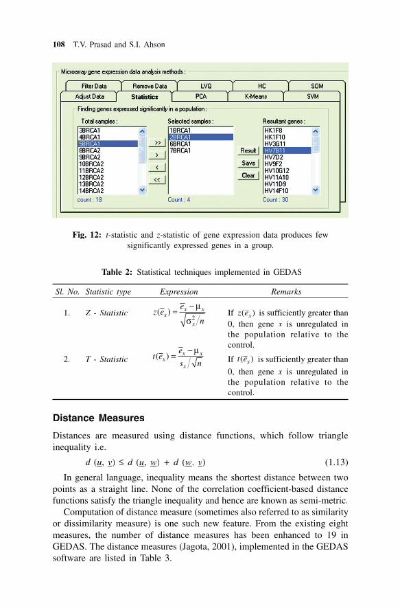
108 T.V. Prasad and S.I. Ahson
Fig. 12: t-statistic and z-statistic of gene expression data produces fewsignificantly expressed genes in a group.
Table 2: Statistical techniques implemented in GEDAS
Sl. No. Statistic type Expression Remarks
1. Z - Statistic2
( ) x xx
x
ez e
n
� ��
�If ( )xz e is sufficiently greater than0, then gene x is unregulated inxthe population relative to thecontrol.
2. T - Statistic ( ) x xx
x
et e
s n
� �� If ( )xt e is sufficiently greater than
0, then gene x is unregulated inxthe population relative to thecontrol.
Distance Measures
Distances are measured using distance functions, which follow triangleinequality i.e.
d (u, v) � d (u, w) + d (w, v) (1.13)
In general language, inequality means the shortest distance between twopoints as a straight line. None of the correlation coefficient-based distancefunctions satisfy the triangle inequality and hence are known as semi-metric.
Computation of distance measure (sometimes also referred to as similarityor dissimilarity measure) is one such new feature. From the existing eightmeasures, the number of distance measures has been enhanced to 19 inGEDAS. The distance measures (Jagota, 2001), implemented in the GEDASsoftware are listed in Table 3.

Data Mining for Bioinformatics—Microarray Data 109
Table 3: Distance measures implemented in GEDAS
Sl. Distance orNo. similarity Expression Remarks
measure
1. Euclideandistance
2. NormalizedEuclideandistance
3. HarmonicallysummedEuclideandistance
4. City-block (orManhattan)distance
� �2
1
n
i ii
d x y�
� �It is a true metric, as it satisfies the triangle inequality,and is the most widely used distance measure of allavailable. In this formula, the expression data xi and yi aresubtracted directly from each other. We should thereforemake sure that the expression data are properly normalizedwhen using the Euclidean distance, for example byconverting the measured gene expression levels to log-ratios. Unlike the correlation-based distance functions, theEuclidean distance takes the magnitude of the expressiondata into account. It, therefore, preserves more informationabout the data and may be preferable. De Hoon et al.(2002) used the Euclidean distance for k-means clustering.
d =d Ed
n
where dEd is the Euclidean distance.E
d =d
12
1
1 1n
i iin x y
�
�
� �� �� �� ��� �� ��
It is a variation of the Euclidean distance, where the termsfor the different dimensions are summed inversely (similarto the harmonic mean), and is more robust against outlierscompared to the Euclidean distance. Note that it is not ametric as it is not based on triangle inequality. For example,consider u = (1, 0); v = (0, 1); w = (1, 1). This yields d(u, v) = 1 while d(u, w) + d (w, v) = 0
d =d1
n
i ii
x y�
�Alternatively known as the Manhattan distance or taxi cabdistance, it is closely related to the Euclidean distance.Whereas the Euclidean distance corresponds to the lengthof the shortest path between two points, the city-blockdistance is the sum of distances along each dimension.
This is equal to the distance a traveller would have towalk between two points in a city. The city-block distanceis a metric, as it satisfies the triangle inequality. As for theEuclidean distance, the expression data are subtracteddirectly from each other, and therefore should be madesure that they are properly normalized.
(Contd.)

110 T.V. Prasad and S.I. Ahson
5. NormalizedCity-blockdistance
6. Canberradistance
7. Bray-Curtisdistance
8. Maximumcoordinatedifference
9. Minimumcoordinatedifference
10. Dot product
11. Pearson’scorrelationcoefficient
12. AbsolutePearson’scorrelation
d =d1
1 n
i ii
x yn �
� or d = Cd
nwhere dC is the city block distance.C
d =d1
1
( )
ni i
i ii
x y
n x y�
�� ,
Result always falls in the range [0, 1].
d =d( )
i i
i i
x y
x y
�
� , Result always falls in the range [0, 1].
max max i id x y� �
Computes maximum absolute difference along acoordinate.
min min i id x y� �Computes the minimum absolute difference along acoordinate.
d0dd = – xoy, where xoy = i ii
x y�This is the dissimilarity version of the dot product measure.
r = r1
1 ni i
x yi
x x y y
n �
� �� �� �� �� �� �� � � �
The Pearson distance is then defined as 1pd r� � .In which andx y are the sample mean of x and yrespectively, while �x and �y are the sample standarddeviation of x and y. It is a measure for how well a straightline can be fitted to a scatter plot of x and y. If all thepoints in the scatter plot lie on a straight line, the Pearsoncorrelation coefficient is either +1 or –1, depending onwhether the slope of line is positive or negative. If it isequal to zero, there is no correlation between x and y. Asthe Pearson correlation coefficient fall between [–1, 1],the Pearson distance lies between [0, 2].
By taking the absolute value of the Pearson correlation, anumber between [0, 1] is obtained. If the absolute valueis 1, all the points in the scatter plot lie on a straight linewith either a positive or a negative slope. If the absolutevalue is equal to 0, there is no correlation between x and y.
The distance is defined as 1Ad r� � where r is thePearson correlation coefficient. As the absolute value of
(Contd.)
(Table 3 Contd.)
Sl. Distance orNo. similarity Expression Remarks
measure

Data Mining for Bioinformatics—Microarray Data 111
13. UncentredPearson’scorrelation
14. AbsoluteuncentredPearson’scorrelation
15. Pearson’slineardissimilarity
16. Pearson’sabsolute valuedissimilarity
the Pearson correlation coefficient falls in the range [0, 1],the corresponding distance falls between [0, 1] as well. Inthe context of gene expression experiments, the absolutecorrelation is equal to 1 if the gene expression data of twogenes/microarrays have a shape that is either exactly thesame or exactly opposite. Therefore, absolute correlationcoefficient should be used with care.
(0) (0)1
1( )( ),
ni i
Ui x y
x yr
n �
�� �
where (0) 2
1
1;
n
x ii
xn �
� � and (0) 2
1
1 n
y ii
yn �
� � .
The distance corresponding to the uncentred correlationcoefficient is defined as 1U Ud r� � where ru is theuncentred correlation.
This is the same as for regular Pearson correlationcoefficient, except that sample means ,x y are set equalto 0. The uncentred correlation may be appropriate if thereis a zero reference state. For instance, in the case of geneexpression data given in terms of log-ratios, a log-ratioequal to 0 corresponds to green and red signal being equal,which means that the experimental manipulation did notaffect the gene expression. As the uncentred correlationcoefficient lies in the range [–1, 1], the correspondingdistance falls between [0, 2].
1AU Ud r� �
where ru is uncentred correlation coefficient. As theabsolute value of ru falls between [0, 1], the correspondingdistance also falls between [0, 1].
1 ( , )( , )
2
x yd x y
� � , where
( ) ( )( , )
x y
x x o y yx y
� � �
� ��This is the dissimilarity version of the Pearson linearcorrelation p between two vectors. DpD (i, j) � [0, 1] with0 indicating perfect similarity and 1 indicating maximumdissimilarity. Notice that p(i, j) is a type of normalized dotproduct.
2 2( ( , ) ( , ) )1 NormEuc
nd d x y q x y
n� �
�
where1
( , ) i ii i
q x y x yn
� �� �� �� �
dNormEucd is the normalized Euclidean distance.
(Contd.)
(Table 3 Contd.)

112 T.V. Prasad and S.I. Ahson
17. Spearman’srankcorrelation
18. Kendall’s !distance
19. Cosinedistance
DATA VISUALIZATION TECHNIQUES
A study of all available visualization techniques and their importance inanalysis of gene expression data was carried out. It was found that differentalgorithms used different visualization techniques for analysis of the data.Some of the classical references are Caron et al. (2001), Chen et al. (2004),Eisen et. al. (1998), Ewing et. al. (2001), Kapushesky et al. (2004), Luo etal. (2003), Tavazoie et al. (1999), Taronen et al. (1999), Colantouni et al.(2000), de Hoon et al. (2004), Kohonen et al. (1996), Stanford BiomedicalInformatics (2004), GEDA, etc.
Earlier, there were cases when the same visualization technique was useddifferently, such as the SOM output as seen in the difference in implementation
(Table 3 Contd.)
Sl. Distance orNo. similarity Expression Remarks
measure
As in the case of the Pearson correlation, a distance measurecorresponding to the Spearman rank correlation can be definedas 1s Sd r� � where rsr is the Spearman rank correlation.
The Spearman rank correlation is an example of a non-parametric similarity measure. It is useful because it is morerobust against outliers than the Pearson correlation. Tocalculate the Spearman rank correlation, each data value isreplaced by their rank if the data in each vector is ordered bytheir value. Then the Pearson correlation between the tworank vectors instead of the data vectors is calculated. Weightscannot be suitably applied to the data if the Spearman rankcorrelation is used, especially since the weights are notnecessarily integers.
A distance measure corresponding to Kendall’s ! can bedefined as
)(1��
��n
iii yxd
Kendall’s ! is another example of a non-parametricsimilarity measure. It is similar to the Spearman rankcorrelation, but instead of the rank those only, the relativeranks are used to calculate !. As in the case of the Spearmanrank correlation, the weights are ignored in the calculation.As Kendall’s ! is defined such that it will lie between [–1, 1],the corresponding distance will be in the range [0, 2].
d = 1
1 1
n
i ii
n n
i ii i
x y
x y
�
� �

Data Mining for Bioinformatics—Microarray Data 113
of the GEPAS server, and the initial SOM version developed by Kohonen etal., 1996. While the former brought out clear and unique clusters as hexagonalgrid, the latter produced many null clusters as well as similarly behavingclusters, which required altogether different visualization containing specialcolour coding and mapping scheme to generate heat map for properidentification. This helped in identification of similar clusters.
Kaski (1997) used SOM on various kinds of datasets, also emphasized onvisualization through SOM and brought a comparison of k-means and SOM.Use of non-linear projection methods such as multi-dimensional scaling(MDS), Sammon’s mapping, principal curves (which are generalization ofprincipal components), triangulation method and replicator neural networkwere also discussed in the work.
The software should provide a platform for holding together all thesevisualization techniques for analysis of preprocessed data and processed dataclusters through the use of group plots and individual plots. Facility shouldbe provided to easily switch from one output form to another by selectingthe corresponding button. Flexibility to save the images of visualization canalso be provided so that they could be incorporated into the reports. Forinstance, histograms of all samples can be viewed in a single shot so as toensure that they follow the normal distribution, as shown in the profile plotsin Fig. 13.
Fig. 13: Profile plots. One histogram for each sample—plots indicate that allsamples follow normal distribution. The overall frequency vs. gene expression
plot of the entire dataset matrix should also produce normal distribution.
It was observed that while one software suite presented well in terms ofstatistical computation, the other presented it in the form of equivalent graphs,

Tab
le 4
:D
escr
iptio
n of
var
ious
vis
ualiz
atio
n te
chni
ques
for
mic
roar
ray
gene
exp
ress
ion
data
Sl.
Visu
aliz
atio
nD
escr
ipti
on o
rSp
ecia
l co
nsid
erat
ions
Adv
anta
ges
and
Com
plex
ity
App
lica
tion
Fig
ure
Ref
eren
ces
No.
tech
niqu
ein
terp
reta
tion
or f
eatu
res
draw
back
s
1.C
lust
er v
iew
-(a
)te
xtua
lvi
ew
2.C
lust
er v
iew
-(b
)te
mpo
ral
or w
ave
grap
h
3.H
eat
map
Clu
ster
s co
ntai
n ac
tual
gen
ena
mes
, as
gen
erat
ed i
n m
ost
of
the
tex
t-b
ased
A
NN
soft
war
e.
It
is
the
mo
stpr
imiti
ve o
f al
l an
d co
uld
beco
nfus
ing
for
extr
emel
y la
rge
data
sets
.
Clu
ster
ed d
ata
is v
isua
lized
inth
e fo
rm o
f a
set o
f w
aves
, in
whi
ch e
ach
wav
e co
rres
pond
sto
a g
ene
acro
ss s
ampl
es o
nth
e X
-axi
s. A
lso
know
n as
the
tem
pora
l or
wav
e gr
aph
view
,th
is v
isua
liza
tion
tec
hniq
ueca
n al
so b
e di
spla
yed
as p
iegr
aph.
Intr
oduc
ed a
s on
e of
the
mos
tel
egan
t g
rap
hic
alre
pres
enta
tion
s of
clu
ster
cont
ents
, it
is v
ery
help
ful
inla
rge
scal
e d
ata
min
ing
appl
icat
ions
.
Non
e
An
extr
a w
ave
is p
lotte
din
bla
ck c
olou
r to
indi
cate
aver
age
valu
e of
eac
hsa
mpl
e in
the
clu
ster
,w
hich
giv
es a
fai
r id
ea o
fth
e ex
pres
sion
lev
el. I
t is
also
ess
entia
l to
dis
play
zoom
ed v
iew
of
each
clus
ter t
o en
able
sci
entis
tsto
see
the
exp
ress
ion
beha
viou
r in
enl
arge
dfo
rm.
It c
an b
e fu
rthe
r enh
ance
db
y
use
o
f co
loru
ing
sch
emes
to
re
pre
sen
tcl
uste
r of
sim
ilar
clus
ters
.T
he c
olou
ring
sch
eme
conv
eys
“log
ical
cla
sses
”in
th
e d
atas
et
or
“kn
ow
led
ge”
ab
ou
t
Out
put
is i
mpr
essi
ve,
but
cou
ld
be
dif
ficu
lt
toun
ders
tand
. It
doe
s no
t gi
vean
id
ea
of
ov
eral
l g
ene
expr
essi
on.
Com
bine
d pl
ot o
f al
l th
ege
nes
can
dete
rmin
e le
vel
ofex
pres
sion
, ove
rall
as w
ell a
sfo
r sp
ecif
ic
gen
es.
Ver
yhe
lpfu
l fo
r re
pres
entin
g tim
ese
ries
dat
a. R
equi
res
a fu
rthe
rG
UI
sup
po
rt
to
extr
act
corr
espo
ndin
g ge
ne n
ames
.F
or
a d
atas
et
con
tain
ing
disc
rete
dat
a (s
uch
as t
hose
con
tain
ing
n
um
ero
us
par
amet
ric
val
ues
),
this
repr
esen
tati
on c
ould
ren
der
no m
eani
ngfu
l us
e.
Whe
n nu
mbe
r of
clu
ster
s is
too
larg
e, t
here
can
be
man
ynu
ll or
em
pty
clus
ters
, whi
chco
nvey
no
mea
ning
and
thu
sb
e el
imin
ated
. It
ca
n
be
appl
ied
to d
atas
ets
havi
ng a
num
ber
of f
eatu
res
in t
hem
.C
olou
red
sect
ions
or
grou
ps
15G
EPA
S w
ebsi
te o
fC
NIO
, E
xpre
ssio
nP
rofi
ler,
G
ED
AS
soft
war
e,
SO
M-
PAK
and
LV
Q-P
AK
by K
ohon
en
16,
GE
PAS
web
site
of
17 C
NIO
, E
xpre
ssio
nP
rofi
ler,
G
ED
AS
soft
war
e,
SO
M-
PAK
and
LV
Q-P
AK
by K
ohon
en
18S
OM
-PA
K
and
LV
Q-P
AK
b
yK
ohon
en
O(n
) if
the
ent
ire
mat
r ix
has
been
sort
ed o
n cl
uste
rnu
mbe
r; o
ther
wis
eO
(n2 ).
O(n
) if
the
ent
ire
mat
rix
has
been
sort
ed o
n cl
uste
rnu
mbe
r; o
ther
wis
eO
(n2 ).
O(n
2 )
SO
M,
LVQ
, S
VM
and
k-m
ean
s;ex
tend
ed to
HC
and
PC
A.
SO
M,
LVQ
, S
VM
and
k-m
ean
s;ex
tend
ed to
HC
and
PC
A
SOM
, LV
Q a
nd k
-m
eans
, S
VM
and
HC
(Con
td.)

(Tab
le 4
Con
td.)
4.D
endr
ogra
phvi
ew
5.M
icro
arra
yvi
ew
19C
aron
et
al.
(200
1),
GE
DA
S
20G
ED
AS
soft
war
e
Als
o ca
lled
as c
heck
s vi
ew, i
tis
ver
y si
mila
r to
den
drog
ram
outp
ut g
ener
ated
by
Che
n et
al.,
2
00
0
or
oth
er
gra
ph
visu
aliz
atio
n so
ftw
are.
It
can
be u
sed
for
visu
al i
nspe
ctio
nof
raw
, pr
epro
cess
ed a
n dcl
ust
ered
d
ata.
T
his
repr
esen
tatio
n al
one
is n
ot a
true
den
drog
ram
out
put
as i
tdo
es n
ot a
ccom
pany
gen
e tr
eean
d ar
ray
tree
.
Ver
y
mu
ch
sim
ilar
to
dend
rogr
aph
view
(or
che
cks
view
) an
d is
use
d fo
r vi
sual
insp
ectio
n of
raw
, pre
proc
esse
dan
d cl
uste
red
data
.
cert
ain
hidd
en p
aram
eter
com
mon
am
ongs
t al
l th
ecl
uste
rs.
Use
r ca
n
con
tro
lse
lect
ion
of c
olou
rs f
orre
pres
entin
g lo
w t
o hi
g hge
ne e
xpre
ssio
n su
ch a
sgr
een
to r
ed o
r bl
ue t
ore
d or
so
on.
Dif
fere
ntco
lou
r co
des
ca
n
be
assi
gned
to r
epre
sent
nul
lva
lues
or
zero
val
ues.
Sh
ades
re
pre
sen
tin
tens
ity o
r m
agni
tude
of
expr
essi
on.
Sam
e as
den
drog
raph
view
.
of c
lust
ers
give
an
idea
of
num
ber
of p
ossi
ble
clas
ses
inth
e da
tase
t. R
equi
res
data
to
be s
ubm
itte
d in
a s
peci
fic
form
at.
Wh
en
ther
e ar
eex
trem
ely
larg
e nu
mbe
rs o
ffe
atur
es (
mic
roar
ray
gene
expr
essi
on d
oes
not
have
man
y),
outp
ut c
ould
bec
ome
cum
bers
ome.
Mo
st
effe
ctiv
e fo
rm
of
v isu
aliz
ing
tren
d of
gen
eex
pres
sion
in
man
y sa
mpl
esan
d
gen
es
in
on
e sh
ot.
How
ever
, if
the
dat
aset
is
very
larg
e, it
req
uire
s an
othe
rG
UI
supp
ort
to e
xtra
ct t
hege
ne n
ames
. Ver
y he
lpfu
l fo
rst
udyi
ng t
rend
in
time
seri
esd
ata
and
d
ata
of
sam
ep
aram
eter
o
ver
d
iffe
ren
tsa
mpl
es.
Sam
e as
den
drog
raph
vie
w.
O(n
) if
the
ent
ire
mat
rix
has
been
sort
ed o
n cl
uste
rnu
mbe
r; o
ther
wis
eO
(n2 ).
O(n
2).
B
igg
est
draw
back
is
that
it
requ
ires
sor
ting
ofth
e en
tire
d
ata
mat
r ix.
SOM
, LV
Q a
ndk-
mea
ns,
SV
M a
ndH
C
SO
M,
LV
Q,
k-m
eans
, H
C,
SV
Man
d PC
A
(Con
td.)

6.Pr
oxim
ity o
rdi
stan
ce m
ap
7.W
hole
mic
roar
ray
grap
h vi
ew
8.Sc
atte
r pl
ot
It
is
a p
lot
of
dis
tan
ces
bet
wee
n
gen
es
vs.
g
enes
sim
ilar
to t
he d
ista
nces
tab
leof
var
ious
citi
es i
n th
e w
orld
as s
een
in t
he d
iari
es.
The
gene
exp
ress
ion
mat
rix
isso
rted
on
clus
ter
num
ber,
and
then
d
ista
nce
m
atri
x
isde
velo
ped,
whi
ch is
a d
iago
nal
mat
rix.
Eac
h va
lue
is t
hen
disp
laye
d in
the
for
m o
f a
colo
ured
box
. W
hile
whi
teco
lour
repr
esen
ts z
ero
dist
ance
,bl
ack
repr
esen
ts m
axim
umdi
stan
ce.
Dia
gona
l li
ne i
sal
wa y
s w
hite
ind
icat
ing
zero
dist
ance
bet
wee
n sa
me
gene
s.
A h
ighl
y ve
rsat
ile r
epre
sent
-at
ion
of g
ene
expr
essi
on d
ata
with
eac
h ba
nd (
or li
ne g
raph
)co
rres
pond
ing
to e
ach
sam
ple.
The
po
rtio
n be
twee
n tw
oho
rizo
ntal
li
nes
cont
ains
expr
essi
on v
alue
s of
100
gen
es.
In a
dditi
on to
plo
t gen
es a
fter
PCA
, it
can
be u
sed
for
MA
plot
s, p
repr
oces
sing
, et
c. F
orPC
A d
ispl
ay o
f tw
o PC
s, o
neve
rtic
al a
nd o
ther
hor
izon
tal.
All
data
poi
nts
are
proj
ecte
don
the
se t
wo
lines
.
Bla
ck
and
w
hit
epr
oxim
ity
map
can
be
give
n a
colo
ured
eff
ect
by d
ispl
ayin
g al
l ban
ds o
fge
nes
in a
sin
gle
colo
ursh
ade
with
in a
clu
ster
.
The
las
t ba
nd i
s us
ed t
ore
pres
ent
med
ian
of a
llth
e sa
mpl
es.
Faci
lity
to
chan
ge
bac
kg
rou
nd
colo
ur
and
co
lou
r o
fba
nds
prov
ided
. V
isua
li-za
tion
can
be z
oom
ed o
rre
duce
d as
per
nee
d.
Dif
fere
nt
colo
urs
fo
rsa
mp
les
may
b
eco
nsid
ered
.
With
jus
t a
smal
l pl
ot,
a fa
irvi
ew o
f cl
uste
r di
stan
ces
can
be d
eter
min
ed. I
t can
pro
vide
bette
r G
UI
so t
hat
a de
sire
dre
ctan
gula
r po
rtio
n ca
n be
sele
cted
and
cor
resp
ondi
ngg
enes
li
sted
o
ut
fro
mda
taba
se.
One
of
the
mos
tp
ow
erfu
l v
isu
aliz
atio
nte
chni
ques
for
ana
lysi
s of
gene
exp
ress
ion
data
.
Wh
ile
beh
avio
ur
of
all
indi
vidu
al s
ampl
es c
an b
ev
isu
ally
m
atch
ed
wit
hn
eig
hb
ou
rin
g
sam
ple
s,
itre
qu
ires
m
ore
ti
me
for
repr
esen
ting
mor
e sa
mpl
es(w
hen
zoom
ed o
ut).
For
PCA
, out
put i
s pr
oces
sed
for
seco
nd t
ime
to p
roje
ct a
llda
ta p
oint
s on
the
PC
s.
O(n
2 ). T
he b
igge
stdr
awba
ck i
s th
at i
tre
quir
es s
ortin
g of
the
enti
re
gen
eex
pre
ssio
n
dat
am
atri
x.
O(n
3 )
O(n
)
SO
M,
LV
Q,
k-m
eans
, H
C,
SV
Man
d PC
A
Raw
d
ata
and
prep
roce
ssed
dat
a;ex
tend
ed t
o S
OM
,LV
Q, k
-mea
ns, H
C,
SVM
and
PC
A
PC
A
21G
ED
AS
, G
AP
by
22,
Che
n (2
004)
23G
ED
AS
soft
war
e24
,
25C
lust
er s
oftw
are
byd
e H
oo
n
et
al.
(20
04
),
GE
DA
S,
GE
DA
sof
twar
e
Sl.
Visu
aliz
atio
nD
escr
ipti
on o
rSp
ecia
l co
nsid
erat
ions
Adv
anta
ges
and
Com
plex
ity
App
lica
tion
Fig
ure
Ref
eren
ces
No.
tech
niqu
ein
terp
reta
tion
or f
eatu
res
draw
back
s
(Con
td.)
(Tab
le 4
Con
td.)

9.Pr
inci
pal
com
pone
ntvi
ew
10.
His
togr
am
11.
Tre
e or
dend
rogr
amvi
ew
PC v
iew
is a
line
gra
ph d
raw
nas
su
m
of
pri
nci
pal
com
pone
nts
(Eig
en v
alue
)an
d in
divi
dual
exp
ress
ion
valu
es. T
houg
h al
l com
pone
nts
are
disp
laye
d, th
e fi
rst t
wo
orth
ree
PCs
play
impo
rtan
t rol
ein
dim
ensi
onal
ity r
educ
tion.
It
is
a co
mm
on
fo
rm
of
visu
aliz
ing
basi
c st
atis
tica
lda
ta.
One
of
the
mos
t eff
ectiv
e an
dpo
wer
ful
repr
esen
tati
ons
ofcl
uste
red
gene
exp
ress
ion
dat
a,
con
sist
ing
o
f th
ree
port
ions
viz
., ge
ne t
ree,
arr
aytr
ee a
nd c
olou
r co
ded
band
of g
ene
expr
essi
on.
Als
okn
own
as m
atri
x tr
ee p
lot
or2-
way
den
drog
ram
s. I
n H
C,
it is
the
mos
t com
mon
out
put.
In o
rder
to
stan
dard
ize
and
prov
ide
com
mon
out
puts
to
all
data
min
ing
appl
icat
ions
,ou
t put
was
con
vert
ed i
nto
clus
ter
view
tha
t fu
rthe
r le
dto
vie
ws
such
as
mic
roar
ray,
text
ual,
who
le g
enom
e, e
tc.
A g
ood
PC
lin
e gr
aph
alw
ays
falls
dow
n on
Xax
is
exp
on
enti
all y
.F
acil
ity
p
rov
ided
to
chan
ge c
olou
rs o
f P
Cs.
Gra
ph c
an b
e re
draw
nw
ith r
equi
red
num
ber
ofPC
s.
Non
e
Sam
e as
den
drog
raph
view
Fir
st t
wo
or t
hree
PC
s ar
eus
ually
suf
fici
ent
to g
ener
ate
the
entir
e da
tase
t.
Can
not
be u
sed
for
com
plex
data
for
ms.
Off
ers
clus
teri
ng o
f bo
thg
enes
an
d
sam
ple
ssi
mul
tane
ousl
y. H
owev
er,
ifth
e da
tase
t is
ver
y la
rge,
it
also
re q
uire
s an
othe
r G
UI
supp
ort
to e
xtra
ct t
he g
ene
nam
es.
Ver
y
hel
pfu
l fo
rst
udyi
ng t
he t
rend
in
tim
ese
ries
dat
a an
d da
ta o
f sa
me
par
amet
er
ov
er
dif
fere
nt
sam
ple
s.
Inte
r-d
ate
rela
tion
ship
wil
l be
los
t by
rep
rese
nti
ng
m
ult
idi
men
sion
al d
ata
in a
2D
tree
form
at.
O(n
)
O(n
)
O(n
3 ); tw
o di
ffer
ent
algo
rith
ms
wor
kto
geth
er t
o bu
ild
up th
e ge
ne tr
ee o
non
e si
de, a
nd a
rray
tree
and
the
colo
urco
ded
b
and
o
fex
pres
sion
val
ues
on t
he o
ther
.
PC
A
All
HC
26G
ED
AS
, C
lust
erso
ftw
are
by d
e H
oon
et a
l. (2
004)
27N
one
2 8T
reeV
iew
sof
twar
eb
y
Eis
en
et
al.
(19
98
),
GE
DA
S,
Luo
et
a l.
(200
3)
(Tab
le 4
Con
td.)
(Con
td.)

12.
Dec
isio
n-sp
ace
or s
earc
h-sp
ace
view
13.
Tre
e-m
apvi
ew
14.
Box
-Whi
sker
plot
15.
Gen
eO
ntol
ogy
Use
d fo
r cl
assi
fica
tion,
eith
erSV
M o
r LV
Q,
and
this
kin
dof
rep
rese
ntat
ion
of g
ene
expr
ess i
on d
ata
com
e ve
ryha
ndy
wit
h ea
ch d
ecis
ion
spac
e co
rres
pond
ing
to e
ach
clas
s of
gen
es. T
he f
igur
e w
asex
trac
ted
from
a d
emo
vers
ion
o f S
VM
, it
coul
d be
app
lied
to a
ny m
ulti-
clas
s cl
assi
ficat
ion.
App
lied
to th
e re
sults
of
gene
exp
ress
ion
d
ata
fro
mhi
erar
chic
al c
lust
erin
g. T
here
are
a la
rge
num
ber
of T
ree -
map
vis
ualiz
atio
n va
rian
ts f
orre
pre
sen
tin
g
hie
rarc
hic
alre
latio
nshi
ps.
Ver
y ha
ndy
in d
ealin
g w
ith ra
wan
d pr
epro
cess
ed
gene
expr
essi
on d
ata.
The
plo
tpr
ovid
es in
form
atio
n on
ove
rall
over
and
und
er e
x pre
ssio
nal
ong
with
mea
n, u
pper
and
low
er q
uart
ile t
o get
her
in o
nepl
ot. I
t can
, in
man
y ca
ses,
be
a ppl
ied
to
redu
ced
ortr
ansf
orm
ed d
atas
ets
with
larg
enu
mbe
r of
ins
igni
fica
nt g
enes
and
sam
ples
pru
ned.
Th
ere
can
b
e d
iffe
ren
tvi
sual
izat
ion
tech
niqu
e to
see
the
proc
esse
d in
form
atio
n in
a s i
ngle
sho
t.
Col
oure
d de
cisi
on s
pace
sgi
ve v
ery
impr
essi
ve lo
okan
d be
tter
unde
rsta
ndin
gof
the
dat
a gr
oupi
ng.
Co
lou
r an
d
dep
thv
aria
tio
n
cou
ld
be
effe
ctiv
ely
used
to
form
clus
ters
, w
hich
fur
ther
exhi
bit
info
rmat
ion
such
as c
lust
er s
ize,
ove
rall
expr
essi
on,
etc.
Col
our
vari
atio
n co
uld
bein
trod
uced
for
dif
fere
ntsa
mpl
es, u
pper
and
low
erqu
artil
e va
riat
ion.
Non
e
Req
u ire
s da
ta t
o be
in
2Dfo
rm;
high
er d
imen
sion
alre
pres
enta
tion
coul
d be
ver
yco
mpl
ex.
Vis
uall
y ve
ry a
ttra
ctiv
e fo
rsm
alle
r da
tase
ts;
can
be v
ery
conf
usin
g or
scr
amm
ed f
orla
rger
dat
aset
s .
Mea
n, m
edia
n as
wel
l as
uppe
r an
d lo
wer
qua
rtile
can
be v
iew
ed s
imul
tane
ousl
y;u
sefu
l fo
r p
reli
min
ary
anal
ysis
and
whe
n a
num
ber
of g
enes
and
/or
sam
ples
hav
ebe
en e
lim
inat
ed,
caus
ing
chan
ge in
the
mea
n an
d ot
her
para
met
ers.
Dep
endi
ng
on
the
requ
irem
ents
, the
vis
ualiz
atio
nca
n be
pla
nned
.
Not
ava
ilabl
e
Not
ava
ilabl
e
O(n
2 )
O(n
)
LV
Q
and
S
VM
.C
ould
be
exte
nded
to S
OM
,k-
mea
ns,
HC
, PC
A,
etc.
if
itis
p
oss
ible
to
rep
rese
nt
thei
rou
tput
in
2D.
HC
, co
uld
b
eex
tend
ed t
o ot
her
clu
ster
ing
an
d/o
rc
las
sif
ica
tio
nte
chni
ques
Ra w
d
ata
and
prep
roce
ssed
dat
a
All
29L
ibSV
M
30T
reeV
iew
of E
isen
et
eal
. (1
998)
, G
EDD
AS,
DE
xpre
ssio
n Pr
ofile
r,fi
lfi
ler
Cle
aver
1.0
31G
ED
AS
, G
ED
A
32A
ll so
ftw
are
Sl.
Visu
aliz
atio
nD
escr
ipti
on o
rSp
ecia
l co
nsid
erat
ions
Adv
anta
ges
and
Com
plex
ity
App
lica
tion
Fig
ure
Ref
eren
ces
No.
tech
niqu
ein
terp
reta
tion
or f
eatu
res
draw
back
s
(Tab
le 4
Con
td.)

Data Mining for Bioinformatics—Microarray Data 119
and still further another suite presented the output in altogether differentgraphical form. Graphs such as group plots, MA plots, etc. that have greatsignificance in biological data mining (Fig. 14). Details of each visualizationtechnique have been described in Table 4.
Fig. 14: The MA group plot provides view of the amount of spread in theoverall gene expression pattern in the data groups. These plots could be obtainedfor data before transformation and cannot be obtained for negative or zero data.
Fig. 15: The textual view exhibits the same clusters as that of temporalview; however, actual gene names are displayed. In this example,
a 3 × 3 SOM configuration output can be seen.

120 T.V. Prasad and S.I. Ahson
Fig. 16: The temporal/wave graph view. Each cluster contains a number ofgenes represented as a wave, the green line is the average expression leve.l
Fig. 17: The zoomed temporal graph view gives the visualization of eachcluster’s behavioural pattern.

Data Mining for Bioinformatics—Microarray Data 121
Fig. 18: Coloured heat map showing clusters of similarly behaving entities asgroup of cells in same colour/shade.
Fig. 19: The checks view (or dendrograph view) visualization is a well-knownmethod of plotting the gene expression levels through colour coded boxes. Itgives a fair idea of gene expression and can be applied to time series as wellas discrete data. It has been applied to raw, preprocessed and clustered data.

122 T.V. Prasad and S.I. Ahson
Fig. 20: The microarray view is very similar to the dendrograph or checks view,except that the individual genes are represented in circular spots. It is a good
visualization for having visual inspection of gene expression data.
Fig. 21: The proximity map visualization is a map of distances plotted genesvs. genes. Usually, it is symmetric/diagonal map. It has been applied to raw,
preprocessed and clustered data.

Data Mining for Bioinformatics—Microarray Data 123
Fig. 22: The proximity map visualization is a map of distances plotted genes vs.genes. Usually, it is symmetric/diagonal map. Proximity maps of raw data set
and clustered data can be seen here.
Fig. 23: The whole (microarray or genome) view output is comparable totemporal view. The samples are always maintained; however, the arrangementof genes may alter after clustering. It is the best suited visualization for having
visual inspection of gene expression.

124 T.V. Prasad and S.I. Ahson
Fig. 24: The whole microarray view has its roots from bio-medical applications.All samples and genes can be visualized in such a form that dis(similarity) canbe easily obtained. The last strip/band is the median of all samples. Somegenes falling between 201 and 300 in samples 8 and 9 have very high gene
expression; similarly in sample 11 between genes 301 and 400.
Fig. 25: The principal component view is essentially a scatter graph in a waythat the space of the genes/samples plotted is usually elliptical.

Data Mining for Bioinformatics—Microarray Data 125
Fig. 26: The Eigen graph is in no way different from a line graph. Each Eigenline is the sum of principal component and individual gene expression value.
Fig. 27: The histogram is the most fundamental visualization of gene expressiondata and can be applied to all forms of datasets.
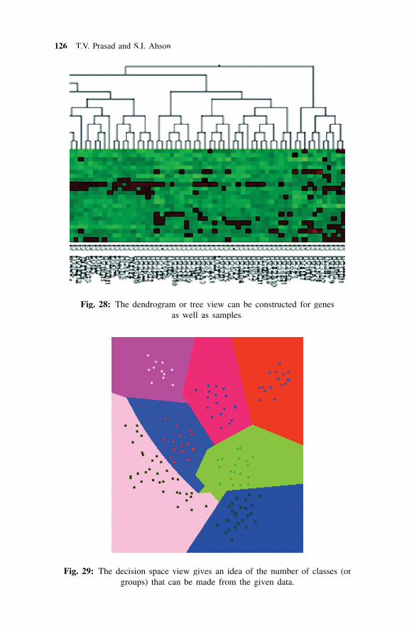
126 T.V. Prasad and S.I. Ahson
Fig. 28: The dendrogram or tree view can be constructed for genesas well as samples.
Fig. 29: The decision space view gives an idea of the number of classes (orgroups) that can be made from the given data.

Data Mining for Bioinformatics—Microarray Data 127
Figure 30: A different tree-map visualization.
Fig. 31: The Box-Whisker plot provides most of the statistics in one graphcovering maximum, minimum, median, upper quartile and the lower quartile.
Fig. 32: The gene ontology view is not a true visualization technique, but alisting of gene number together with their details like gene names and function,
if available in the dataset. It is helpful to further access or understanding thefunction of genes in a particular cluster.

128 T.V. Prasad and S.I. Ahson
Features Table
A consolidation of the views that can be provided for visualization vs.algorithms has been listed in Table 6.
Table 6: Applicability of visualization techniques in various contexts
Visualization/ Raw Pre- SOM k- LVQ HC PCA SVMAlgorithm data processedrr Means (gene)
data
Histogram � � �
Checks view � � � � � � � �
Microarray � � � � � � � �
Whole sample � � � � � � � �
Proximity map � � � � � � � �
Temporal (incl. � � � � � �
zoomed clusterview)Textual � � � � � �
PC view �
Eigen graph �
Tree view �
Scatter plot �
Decision (or � �
search) spaceBox-Whisker plot � �
Gene Ontology � � � � � �
A variety of other visualizations for microarray gene expression data areavailable. The websites of GEDA and SilicoCyte can be converted or presentedusing the techniques as discussed above:
• 2D and 3D score plots• Profile plots• Scatter plots
� 3D scatter plots� PCA visualization - Result on 3D scatter plot� Isomap visualization� Multi-dimensional scaling
• Venn Analysis Diagrams for visualizing similar elements in microarrays,same genes in gene groups or same genes in microarray designs
• SOM visualization of clustering result on� 2D Trellis plot� U-matrix� 1D SOM
There are a number of visualization techniques to represent interaction betweenthe genes in a genetic regulatory network. These network types have beenstandardized (Hwang et al., 2001).

Data Mining for Bioinformatics—Microarray Data 129
SORTING OF DATASET BEFORE CLUSTERING
Sorting of data matrix based on the relative distances computed from one toanother can result in better grouping of the genes. Distance from the firstgene to all other genes can be computed and arranged in ascending order,then distance from the second gene to the remaining genes computing andarranged in ascending order, and the process continued till all the genes areplaced in order. Entire dataset can be then clustered using the SOM algorithmafter which the placement of genes gets enhanced considerably. The qualityof visualization also gets better. The resultant two proximity maps, as shownin Fig. 33, indicate that though the data is clustered, the cluster distancesbecame much clearer and the genes are presented in sorted order.
(a) Proximity map of SOM output (b) Proximity map of SOM output(without sorting) after sorting data
Fig. 33: Enhancing the proximity map by sorting the data before clustering.
For obtaining phenotype classification, the ANN clustering algorithmscan be the best compared to other non-ANN based techniques, (Stolovitzkyet al., 2004). It is essential to cluster both the genes and the samples forobtaining the best phenotypes. The phenotypic extraction reveal:
• If only similar genes are extracted - they are more likely functionallyrelated genes.
• If only similar samples are extracted - they are similar or closely relatedtissue, organ, organism, or disease.
• Subset of both genes and samples are similar - it is called a phenotype.• Contrarily, if subset of both genes and samples are widely varying - this
should not be omitted but can provide the best meaning as to why thegenes that expressed high in a particular group were low expressing in theother. Especially, when one of the groups is control, then the purposewould have fulfilled.

130 T.V. Prasad and S.I. Ahson
A step further, clustering of samples based on the sorted matrix obtainedfrom such experiment help in presenting the data matrix sorted on bothgenes (within clusters) as well as samples.
DISCUSSIONS
Pre-processing
In most of the cases, the ANN models demand considerable amount of pre-processing before actually going for cluster analysis. Certain pre-processingtechniques such as discretization of data, internal sorting, etc. can improvethe computational speed of the algorithms. Removal of genes that fall undera low lying band such as between the expression level of -1 and 1, whichis also the band for noise-like features, can be eliminated from furthercomputation. A combination of these techniques could also prove to behighly useful in cluster analysis.
There has been a continuous debate over whether removal of genes wouldbe proper or not. Though, no concrete decision has been made, it is felt thatpre-processing can be done as far as study remains focussed on identifyingfunctions of certain group of genes; however, the impact of such pruning ormanipulation of genetic data for the purpose of drug designing could bestrong.
Visualization
Unlike SOM and LVQ models, most of the models like perceptron and otherfeed-forward neural networks are not suitable for visualization. ThroughGEDAS a host of visualization techniques were introduced and all algorithmswere standardized so that same set of outputs could be used. The advantageof doing so brought a clear comparison between applications of differentalgorithms.
All software available publicly are either too much tilted towardscomputational aspects or only towards visualization. Moreover, hardly anysoftware tool provides a common platform for analysis/modeling of variousgene expression datasets. The TreeView software by Eisen Lab was reviewedto incorporate changes to fit duplicates and to generate the output from theraw input data instead of the distance matrix. This has brought considerableenhancement to the visualization as both the clarity in tree generation andthe checks (or heat map) was noticeable.
Application of Various Clustering Techniques such as SOM,HC, k-means, PCAkk
The clustering of gene expression data using various clustering techniquesresults in different outcomes. Whereas cluster analysis using SOM is well

Data Mining for Bioinformatics—Microarray Data 131
known, the combination of PCA for dimensionality reduction beforeapplication of SOM brings out that the combination theory would work onlywhen the first algorithm is for pattern classification. Since LVQ (through thethree variants) does the actual grouping of genes, it does not bring anynoticeable change on application of PCA before it.
Clustering using PCA can be highly consistent and logical. The formationof clusters, though only two (due to bifurcation), provides clusters withconsiderable amount of relationship amongst the genes in clusters.
It is worth noting that all the methods use the conventional Euclideandistance for computing misclassification. It is worth pondering as to why notuse any other distance measure such as Pearson correlation coefficient orBray-Curtis distance measure for the purpose.
Data Mining
The definitions of clustering and classification overlap largely, whereas theidea behind both is common - to group or categorize the data into homogenoussets or groups. The standardization of hierarchical clustering output withother clustering techniques vanishes the difference. The standardization ofother output forms in GEDAS homogenized the purposes of clustering andclassification.
The gene expression data alone do not convey the complete informationat any given point of time. Instances and information such as hereditary orhistory of cancer cases in the family, exposure to strong chemicals, foodhabits, drugs being used for cure/prevention, surgeries or therapies undertaken,etc. do not form part of the experimental process even during the dataanalysis stage. It is quite possible that unwanted variation in any one of theseparameters/observations may produce faulty or highly varying results.
Data Preprocessing and Extraction
While working with the hierarchical clustering of gene expression data, itmay be noticed that Pearson’s correlation should be preferred as distancemeasure, even though Euclidean and Manhattan distances provide excellentclustering analysis, since the purpose of using HC is to build a correlationmatrix rather than a distance matrix. An additional parameter “Tree depth”to the tree output can be very useful through the implementation, which canbe used for conversion of Tree View (dendrogram) output into cluster viewformat. Also, the outputs of average- and complete-linkage methods arefound to be better than the single linkage method.
Using the k-means clustering, no two experiments yield identical results.This leads to the fact that the random seed involved in selection of clustercentroid yield clusters of varying sizes, and hence, the results remainuntraceable.

132 T.V. Prasad and S.I. Ahson
It is purely the prerogative of the user to utilize these algorithms/modelsfor extracting different outputs, which can be any of the following order:
• Similarly or differentially expressing• High, averagely or low expressing• Across genes or samples• Obtaining phenotypes or detection of consistently varying gene expression
levels, i.e. high in some but low in others, or vice versa.
PROBLEMS AND SUGGESTIONS FOR FUTURE WORK
1. Compare and contrast different standards of microarray technologycurrently available.
2. Overall, there is a significant requirement of standardization in themicroarray gene expression data analysis scenario, which currently suffersfrom the following limitations due to non-standardization, andconsequently, it can be concluded that efforts would be needed toformalize on which platform, algorithm, technique/model, parameter,and visualization to be used for analysis of various kinds of data:
• Microarray production and techniques not standardized• Preprocessing techniques not yet standardized• No standardized process or model available for analysis• No standardized visualization techniques available• Standardization of minimal information exchange on microarray data
brought out recently under the MIAME project
Support for the text, Microsoft Excel and Microsoft Access baseddatasets, extension to read and process datasets stored in other formatssuch as Oracle, Sybase, and numerous other databases can be provided.Addition of suitable parameters such as function of the genes, class towhich they belong, length, etc. parameters to the microarray geneexpression data matrix will help mining the data in a much precisemanner than being done conventionally.
3. Clustering of gene expression data: The work can be extended to includethe following models, both ANN-based, and non ANN based:
• Classification algorithms like the Linde-Buzo-Gray (LBG) or theGeneralized Lloyd algorithm, etc. could be incorporated (PhaniKumar, 2004). Training the ANNs using the LBG can further improvethe testing capability of LVQ, SVM as well as other clusteringtechniques considerably. Mutual nearest neighbours (Jarvis-Patrick)clustering method is considered to be a robust technique and isparticularly useful on very large data sets.
• Other clustering algorithms such as fuzzy c-means, improved k-means,self-organizing tree algorithm, multi-layer perceptron, geneticalgorithm, agglomerative algorithms, etc. can also be integrated intothe software suite.
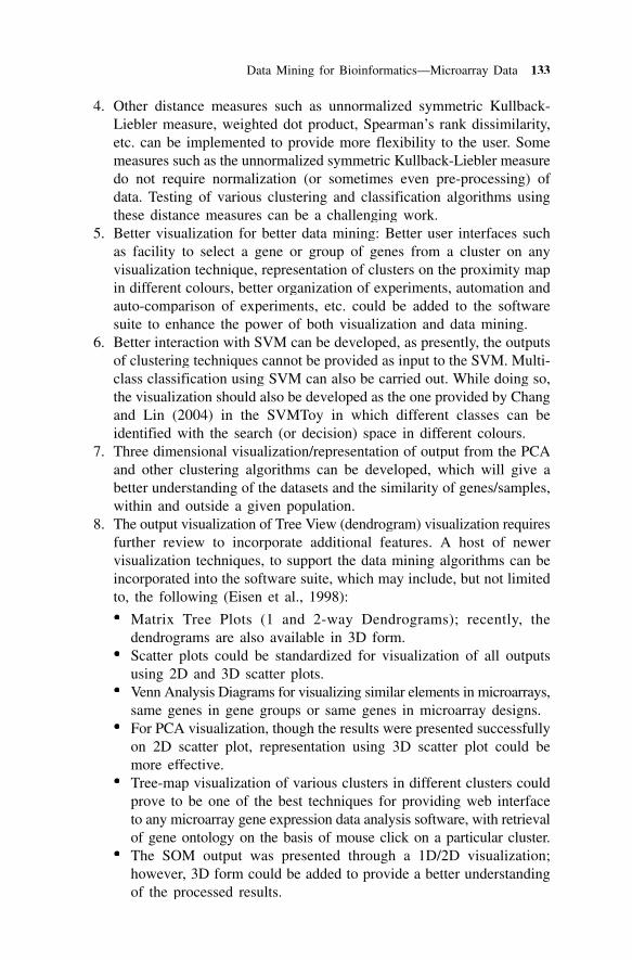
Data Mining for Bioinformatics—Microarray Data 133
4. Other distance measures such as unnormalized symmetric Kullback-Liebler measure, weighted dot product, Spearman’s rank dissimilarity,etc. can be implemented to provide more flexibility to the user. Somemeasures such as the unnormalized symmetric Kullback-Liebler measuredo not require normalization (or sometimes even pre-processing) ofdata. Testing of various clustering and classification algorithms usingthese distance measures can be a challenging work.
5. Better visualization for better data mining: Better user interfaces suchas facility to select a gene or group of genes from a cluster on anyvisualization technique, representation of clusters on the proximity mapin different colours, better organization of experiments, automation andauto-comparison of experiments, etc. could be added to the softwaresuite to enhance the power of both visualization and data mining.
6. Better interaction with SVM can be developed, as presently, the outputsof clustering techniques cannot be provided as input to the SVM. Multi-class classification using SVM can also be carried out. While doing so,the visualization should also be developed as the one provided by Changand Lin (2004) in the SVMToy in which different classes can beidentified with the search (or decision) space in different colours.
7. Three dimensional visualization/representation of output from the PCAand other clustering algorithms can be developed, which will give abetter understanding of the datasets and the similarity of genes/samples,within and outside a given population.
8. The output visualization of Tree View (dendrogram) visualization requiresfurther review to incorporate additional features. A host of newervisualization techniques, to support the data mining algorithms can beincorporated into the software suite, which may include, but not limitedto, the following (Eisen et al., 1998):
• Matrix Tree Plots (1 and 2-way Dendrograms); recently, thedendrograms are also available in 3D form.
• Scatter plots could be standardized for visualization of all outputsusing 2D and 3D scatter plots.
• Venn Analysis Diagrams for visualizing similar elements in microarrays,same genes in gene groups or same genes in microarray designs.
• For PCA visualization, though the results were presented successfullyon 2D scatter plot, representation using 3D scatter plot could bemore effective.
• Tree-map visualization of various clusters in different clusters couldprove to be one of the best techniques for providing web interfaceto any microarray gene expression data analysis software, with retrievalof gene ontology on the basis of mouse click on a particular cluster.
• The SOM output was presented through a 1D/2D visualization;however, 3D form could be added to provide a better understandingof the processed results.

134 T.V. Prasad and S.I. Ahson
REFERENCES
Articles/Papers/Presentations/BooksAl-Kanhal, M.I. and Al-Hendi, R.I. (1992). Arabic phoneme map based on vector
quantization neural networks. Graduate Thesis, King Saud University, Saudi Arabia.Alizadeh, A.A., Eisen, M.B., Davis, R.E., Ma, C., Lossos, I.S., Rosenwald, A.,
Boldrick, J.C., Sabet, H., Tran, T., Yu, X., Powell, J.I., Yang, L., Marti, G.E.,Moore, T., Hudson, J. Jr., Lu, L., Lewis, D.B., Tibshirani, R., Sherlock, G., Chan,W.C., Greiner, T.C., Weisenburger, D.D., Armitage, J.O., Warnke, R., Levy, R.,Wilson, W., Grever, M.R., Byrd, J.C., Botstein, D., Brown, P.O. and Staudt, L.M.(2000). Distinct types of diffuse large B-cell lymphoma identified by geneexpression profiling. Nature, 403(3): 503-511.
Alter, O., Brown, P.O. and Botstein, D. (2000). Singular value decomposition forgenome-wide expression data processing and modeling. Proc. Natl. Acad. of Sc.USA, 97(18): 10101-10106.
Anderson, J.A. (2001). An Introduction to Artificial Neural Networks. Prentice Hallof India, New Delhi.
Baldi, P. and Brunak, S. (2003). Bioinformatics: The Machine Learning Approach.Affiliated East-West Press Pvt. Ltd., New Delhi.
Baldi, P. and Hatfield, G.W. (2001). Microarrays and Gene Expression. CambridgeUniversity Press, Cambridge.
Bassett, D. Jr, Eisen, M.B. and Boguski, M.S. (1999). Gene Expression Informatics- it’s all in your mind. Nature Genetics, Supplement 21.
Ben-Dor, A., Shamir, R. and Yakhini, Z. (1999). Clustering gene expression patterns.Journal of Computational Biology, 6(3/4): 281-297.
Bergeron, B. (2003). Bioinformatics Computing. Prentice Hall of India, New Delhi.Bowtell, D. (1999). Options available - from start to finish - for obtaining expression
data by microarray. Nature Genetics, Supplement 21.Brazma, A., Hingamp, P., Quackenbush, J., Sherlock, G., Spellman, P.T., Stoeckert,
C., Aach, J., Ansorge, W., Ball, C.A., Causton, H.C., Gaasterland, T., Glenisson,P., Holstege, F.C.P., Kim, I.F., Markowitz, V., Matese, J.C., Parkinson, H.,Robinson, A., Sarkans, U., Schulze-Kremer, S., Stewart, J., Taylor, R., Vilo, J.and Vingron, M. (2001). Minimum information about a microarray experiment(MIAME) - toward standards for microarray data. Nature Genetics, 29: 365-371.
Caron, H., van Schaik, B., van der Mee, M., Baas, F., Riggins, G., van Sluis, P.,Hermus, M.C., van Asperen, R., Boon, K., Voute, P.A., van Kampen, A. andVersteeg, R. (2001). The Human Transcriptome Map: Clustering of highly ex-pressed genes in chromosomal domains. Science, 291: 1289-1292.
Carr, D.B., Somogyi, R. and Micheals, G. (1997). Templates for looking at geneexpression clustering. Stat. Comput. & Stat. Graph. Newsletter, 20-29.
Chakraborty, C. (2004). Bioinformatics: Approaches and Applications. Biotech Books,Delhi.
Chee, M.C., Yang, R., Hubbell, E., Berno, A., Huang, X.C., Stern, D., Winkler, J.,Lockhart, D.J., Morris, M.S. and Fodor, S.P.A. (1996). Accessing genetic infor-mation with high-density DNA arrays. Science, 274: 610-614.
Chen, D., Chang, R.F. and Huang, Y.L. (2000). Breast cancer diagnosis using self-organizing map for sonography. Ultrasound Medical Biology, 26(3): 405-411.

Data Mining for Bioinformatics—Microarray Data 135
Chen, C.H. et al. (2004). Generalized Association Plots (GAP), Presentation on“Cluster Analysis and Visualization”. In: Workshop on Statistics and MachineLearning, Institute of Statistical Science.
Cho, S.B. and Won, H.H. (2003). Machine learning in DNA microarray analysis forcancer classification. Conferences in Research and Practice in Information Tech-nology, 19 (Ed. Yi-Ping Phoebe Chen, Australian Computer Society).
Churchill, G.A. (2002). Fundamentals of experimental design for cDNA microarrays.Nature Genetics, 32 Suppl: 490-495.
D’haeseleer, P., Wen, X., Fuhrman, S. and Somogyi, R. (1997). Mining the geneexpression matrix: Inferring gene relationships from large scale gene expressiondata. In: Information processing in cells and tissues (eds. Paton, R.C. andHolcombe, M.). Plenum Press, 203-212.
DeRisi, J., Penland, L., Brown, P.O., Bittner, M.L., Meltzer, P.S., Ray, M., Chen, Y.,Su, Y.A. and Trent, J.M. (1996). Use of a cDNA microarray to analyze geneexpression patterns in human cancer. Nature Genetics, 14(4): 457-460.
Dopazo, J. (2002). Microarray data processing and analysis. In: Microarray DataAnalysis II. Kluwer Academic Publ., 43-63.
Dudoit, S. and Gentleman, R. (2002a). Cluster analysis in DNA microarray experi-ments. Bioconductor Short Course, Presentation slides.
Dudoit, S., Fridlyand, J. and Gentleman, R. (2002b). Classification analysis in DNAMicroarray experiments. Bioconductor Short Course, Presentation slides.
Durbin, B.P., Hardin, J.S., Hawkins, D.M. and Rocke, D.M. (2002). A variance-stabilizing transformation for gene-expression microarray data. Bioinformatics,18(90001): S105-S110.
Eijssen, L. (2000). Cluster analysis of microarray gene expression data. Master’sthesis, Faculty of General Sciences, Maastricht University, The Netherlands.
Eisen, M.B., Spellman, P.T., Brown, P.O. and Botstein, D. (1998). Cluster analysisand display of genome-wide expression patterns. Proc. Natl. Acad. of Sc. USA,95: 14863-14868.
Ewing, R.M. and Cherry, J.M. (2001). Visualization of expression clusters usingSammon’s non-linear mapping. Bioinformatics, 17(7).
Freeman, J.A. and Skapura, D.M. (1991). Neural Networks. Addison Wesley, USA.Furey, T.S., Cristianini, N., Duffy, N., Bednarski, D.W., Schummer, M. and Haussler,
D. (2000). Support vector machine classification and validation of cancer tissuesamples using microarray expression data. Bioinformatics, 16: 906-914.
Golub, T.R., Slonim, D.K., Tamayo, P., Huard, C., Gaasenbeek, M., Mesirov, J.P.,Coller, H., Loh, M.L., Downing, J.R., Caligiuri, M.A., Bloomfield, C.D. andLander, E.S. (1999). Molecular classification of cancer: Class discovery and classprediction by gene expression monitoring. Science, 286: 531-537.
Hacia, J.G., Brody, L.C., Chee, M.S., Fodor, S.P. and Collins, F.S. (1996). Detectionof heterozygous mutations in BRCA1 using high density oligonucleotide arraysand two-colour fluorescence analysis. Nature Genetics, 14: 441-447.
Han, J. and Kamber, M. (2001), Data Mining: Concepts and Techniques. Elsevier,San Francisco, USA.
Haykin, Simon (1999). Artificial Neural Networks: A Comprehensive Foundation2nd ed. Addison Wesley.
Hedenfalk, I., Duggan, D., Chen, Y., Radmacher, M., Bittner, M., Simon, R. et al.(2001). Gene-expression profiles in hereditary breast cancer. New EnglandJournal of Medicine, 344: 539-548.

136 T.V. Prasad and S.I. Ahson
Herroro, J., Valencin, A. and Dopazo, J. (2001). A hierarchical unsupervised growingneural network for clustering gene expression patterns. Bioinformatics, 17:126-136.
Hwang, K.B., Cho, D.Y., Park, S.W., Kim, S.D. and Zhang, B.T. (2001). Applyingmachine learning techniques to analysis of gene expression data: Cancer Diagno-sis. In: Methods of Microarray Data Analysis. Kluwer Academic, 167-182.
Iyer, V.R., Eisen, M.B., Ross, D.T., Schuler, G., Moore, T., Lee, J.C.F., Trent, J.M.,Staudt, L.M., Hudson Jr. J., Boguski, M.S., Lashkari, D., Shalon, D., Botstein, D.and Brown, P.O. (1999). The transcriptional program in response of human fibro-blasts to serum. Science, 283: 83-87.
Jagota, Arun (2001). Microarray data analysis and visualization. Dept. of ComputerEngineering, University of California, CA., USA.
Kaski, S. (1997). Data exploration using self-organizing maps. Doctor of Technol-ogy Thesis, Helsinki University of Technology, Espoo, Finland.
Kapushesky, M., Kemmeren, P., Culhane, A. C., Durinck, S., Ihmels, J., Körner, C.,Kull, M., Torrente, A., Sarkans, U., Vilo, J. and Brazma, A. (2004). ExpressionProfiler: next generation-an online platform for analysis of microarray data. NucleicAcids Research, 32 (Web Server issue): W465-W470.
Khan, J., Wei, J.S., Ringnér, M., Saal, L.H., Ladanyi, M., Westermann, F., Berthold,F., Schwab, M., Antonescu, C.R., Peterson, C. and Meltzer, P.S. (2001). Classi-fication and diagnostic prediction of cancers using gene expression profiling andartificial neural networks, Nature Medicine, 7(6): 673-679.
Klingbiel, D. (2003). Singular value decomposition for feature selection in cDNAarrays, Talk at Max Plank Institute for Molecular Genetics, Germany, availableat http:// compdiag.molgen.mpg.de/docs/talk_03_03_03_klingbiel.pdf.
Koren, Y. and Carmel, L. (2003). Visualization of labeled data using linear transfor-mation, Proceedings of IEEE Information Visualization (InfoVis ’03), IEEE, pp.121-128, Presentation slides, available at http://www.cs.ubc.ca/~tmm/courses/cpsc533c-04-spr/ slides/update.0317.mtan.ppt.
Kurimo, M. (1997). Using self-organizing maps and learning vector quantization formixture density hidden Markov models. Doctor of Technology Thesis, HelsinkiUniversity of Technology, Espoo, Finland.
La Vigna, A. (1989). Non-parametric classification using learning vector quantiza-tion. Ph.D. thesis, University of Maryland, USA.
Li, L., Weinberg, C.R., Darden, T.A. and Pederson, L.G. (2001). Gene selection forsample classification based on gene expression data: Study of sensitivity to choiceof parameters of the GA/KNN method. Bioinformatics, 17(12), 1131-1142.
Liao, L. (2002). Clustering and classification and their applications in bioinformatics.Lecture notes, Discovery Information and High Performance Computing (ELEG667).
Luo, F., Tang, K. and Khan, L. (2003). Hierarchical clustering of gene expressiondata. University of Dallas, TX, USA.
Mount, D.W. (2001). Bioinformatics: Sequence and Genome Analysis. Cold SpringHarbor Laboratory Press, NY, USA.
Narayanan, A., Keedwell, E.C. and Olsson, B. (2003). Artificial intelligence tech-niques for bioinformatics. Applied Bioinformatics, Open Mind Journals.
Nilsson, J. (2002). Methods for classification of gene expressions. Master’s thesis,Centre for Mathematics, Lund University, Lund, Sweden.

Data Mining for Bioinformatics—Microarray Data 137
Phanikumar, B. (2002). Clustering algorithms for microarray data mining. Masters’Thesis, Institute of Systems Research, University of Maryland, USA.
Pocock, M.R. and Hubbard, T.J.P. (2000). A browser for expression data.Bioinformatics, 16(4).
Prasad, T.V. and Ahson, S.I. (2005a). Visualization of microarray gene expressiondata. Bioinformation, 2006.
Prasad, T.V. and Ahson, S.I. (2005b). Application of Learning Vector quantizationon microarray gene expression data. Bioinformation, submitted.
Prasad, T.V., Ravindra Babu, P. and Ahson, S.I. (2005c). GEDAS - Gene ExpressionData Analysis Suite Software, Bioinformation, 2006.
Quackenbush, J. (2002). Microarray data normalization and transformation. NatureGenetics, 32 Suppl: 496-501.
Ramaswamy, S., Tamayo, P., Rifkin, R., Mukherjee, S., Yeang, C.H., Angelo, M.,Ladd, C., Reich, M., Latulippe, E., Mesirov, J.P., Poggio, T., Gerald, W., Loda,M., Lander, E.S. and Golub, T.R. (2001). Multiclass cancer diagnosis using tumorgene expression signatures. Proc. Natl. Acad. of Sc. USA, 98(26): 15149-15154.
Raychaudhuri, S., Stuart, J.M. and Altman, R.B. (2000). Principal components analysisto summarize microarray experiments: Application to sporulation time series.Pacific Symposium of Biology, 5: 452-463.
Sharan, R., Elkon, R. and Shamir, R. (2001). Cluster analysis and its applications togene expression data. Ernst Schering Workshop on Bioinformatics and GenomeAnalysis, Springer Verlag.
Sing, J.K., Basu, D.K., Nasipuri, M. and Kundu, M. (2003). Improved k-meansalgorithm in the design of RBG neural networks. Proceedings of IEEE TENCON2003, Bangalore, India, October 2003.
Slonim, D., Tamayo, P., Mesirov, J., Golub, T.R. and Lander, E. (2000). Classprediction and discovery using gene expression data. Proceedings of RECOMB2000.
Spellman, P.T., Miller, M., Stewart, J., Troup, C., Sarkans, U., Chervitz, S., Bernhart,D., Sherlock, G., Ball, C.A., Lepage, M., Swiatek, M., Marks, W.L., Goncalves,J., Market, S., Iordan, D., Shojatalab, M., Pizarro, A., White, J., Hubley, R.,Deutsch, E., Senger, M., Aronow, B.J., Robinson, A., Bassett, D., Stoeckert, J.Jr. and Brazma, A. (2002). Design and implementation of microarray gene ex-pression markup language (MAGE-ML). Genome Biology, 3(9).
Stolovitzky, G., Lepre, J. and Tu, Y. (2004). Gene expression pattern discovery ingene expression microarrays. Presentation slides, available at http://www.ibm.com/solutions/lifesciences.
Szallasi, Z. (1998). Gene expression patterns and cancer. Nature Biotechnology, 16:1292-1293.
Talavera, L. (2000). Dependency-Based Feature Selection for Clustering SymbolicData. Intelligent Data Analysis, 4: 19-28.
Tavazoie, S., Hughes, J.D., Campbell, M.J., Cho, R.J. and Church, G.M. (1999).Systematic determination of genetic network architecture. Nature Genetics, 22:281-285.
Tibshirani, R., Hastie, T., Eisen, M., Ross, D., Botstein, D. and Brown, P. (1999).Clustering methods for the analysis of DNA microarray data. Technical Report,Stanford University, USA.
Toronen, P., Kolehmainen, M., Wong, G. and Castren, E. (1999). Analysis of geneexpression data using self-organizing maps. FEBS Letters, 451(2): 142-146.

138 T.V. Prasad and S.I. Ahson
Vijaya, P.A., Murty, M.N. and Subramaniam, D.K. (2003). An efficient incrementalprotein sequence clustering algorithm. Proceedings of IEEE TENCON 2003,Bangalore, India, October 2003.
Vipin Kumar (2002). Data Mining Algorithms. Tutorial at IPAM 2002, Presentationslides.
Wall, M.E., Rechtsteiner, A. and Rocha, L.M. (2003). Singular value decompositionand principal component analysis. In: A Practical Approach to Microarray DataAnalysis (eds. Berrar, D.P., Dubitzky, W., Granzow, M.), 91-109, Kluwer, MA,USA.
Wen, X., Fuhrman, S., Michaels, G.S., Carr, D.B., Smith, S., Barker, J.L. and Somogyi,R. (1998). Large-scale temporal gene expression mapping of central nervoussystem development. Proc. Natl. Acad. of Sc. USA, 95(1): 334-339.
Westhead, D.R., Parish, J.H. and Twyman, R.M. (eds) (2003). Instant Notes onBioinformatics. BIOS Scientific Publishers Ltd., Oxford, UK.
White, K.P., Rifkin, S.A., Hurban, P. and Hogness, D.S. (1999). Microarray analysisof Drosophila development during metamorphosis. Science, 286(5447): 2179-2184.
Wong, W.H. and Li, C. (2001a). Model-based analysis of oligonucleotide arrays:Expression index computation and outlier detection. Proc. of Natl. Acad. of Sc.USA, 98(1): 31-36.
Wong, W.H. and Li, C. (2001b). Model-based analysis of oligonucleotide arrays:Model validation, design issues and standard error application. Genome Biology,2(8): research 0032.1-0032.11.
Wooley, J.C. and Lin, H.S. (2001). Catalyzing inquiry at the interface of Computingand Biology. The National Academies Press, Washington D.C., available at http://genomics.energy.gov.
Yang, Y.H., Dudoit, S., Luu, P. and Speed, T.P. (2001). Normalization for cDNAmicroarray data. Microarray Data Technical Report 589, SPIE BiOS 2001, SanJose, California, USA.
Yeang, C.H., Ramaswamy, S., Tamayo, P., Mukherjee, S., Rifkin, R.M., Angelo, M.,Reich, M., Lander, E., Mesirov, J. and Golub, T. (2001). Molecular classificationof multiple tumor types. Bioinformatics, 17: 316S-322S.
Yeung, K.Y. and Ruzzo, W.L. (2001). Principal component analysis for clusteringgene expression data. Bioinformatics, 17: 763-774.
Yeung, K.Y., Haynor, D.R. and Ruzzo, W.L. (2001b). Validating clustering for geneexpression data. Bioinformatics, 17(4): 309-318.
Zhang, M.Q. (1999). Large-scale gene expression data analysis: A new challenge tocomputational biologists. Genome Research, 9: 681-688.
WebsitesChang, C.C. and Lin, C.J. (2004). LibSVM: A library for support vector machine.
Available at http://www.csie.ntu.edu.tw/~cjlin/libsvm.Colantouni, C., Henry, G. and Pevsner, J. (2000). Standardization and Normalization
of Microarray Data (SNOMAD) software. Available at http://pevsnerlab.kennedykrieger.org/snomad.htm.
de Hoon, M., Imoto, S. and Miyano, S. (2004). The C Clustering Library (Cluster 3.0)software. University of Tokyo, Institute of Medical Science, Human Genome Cen-ter, Japan, available at http://bonsai.ims.u-tokyo.ac.jp/~mdehoon/software/cluster.

Data Mining for Bioinformatics—Microarray Data 139
Dopazo, J. (1999). Self-organizing Tree Algorithm (SOTA), DNA-array data analy-sis with SOM, Bioinformatics Unit at CNIO. Available at http://bioinfo.cnio.es/docus/SOTA/#Software.
Eisen Lab (1998). Cluster and TreeView software (Hierarchical clustering, k-meansand tree display). Available at http://rana.lbl.gov/EisenSoftware.htm.
Johnny, R. (2002). Analysis of microarray gene expression data. Presentation slides.Available at www.kuleuven.ac.be/bio/mcb/ internet/downloads/gene_expression.pdf.
Kohonen, T., Hynninen, J., Kangas, J., Laaksonen, J. and Torkkola, K. (1996).LVQ_PAK: The learning vector quantization package. Technical Report A30,Helsinki University of Technology, Finland. Available at http://cs.hut.fi.
Leung, Y.F. (2002). My microarray journal watch. University of Hong Kong. Websiteavailable at http://ihome.cuhk.edu.hk/~b400559/1999j_mray.html.
Merelo, J.J. and Prieto, A. (1994). G-LVQ - a combination of genetic algorithms andLVQ. Available at http://geneura.ugr.es/g-lvq/g-lvq.html.
Shapiro, G. P. and Ramaswamy, S. (2002). SPSS Clementine microarray ClementineApplication Template (CAT). Presentation slides, available at http://www.spssscience.com.
SilicoCyte (2004). SilicoCyte v 1.3 software. Available at http://www.silicocyte.com.Stanford Biomedical Informatics (2004). Cleaver 1.0. Helix Bioinformatics Group,
Stanford School of Medicine, Stanford University, USA. Available at http://classify.stanford.edu.
Thomas, C. (2001). CISC 873, Data Mining Notes: What is Clustering? LectureNotes, Queen’s University. Available at www.cs.queensu.ca/home/ thomas/notes/basic_association.html.
Tom Sawyer (2003). Tom Sawyer software Image Gallery. Website available at http://www.tomsawyer.com/gallery/gallery.php?printable=1.
More suggested literature and website resourcesAltinok, A. (1998). Adaptive pattern classification: Kohonen SOM and LVQ1,
Presentation slides.Bentley, P.J. (2001). Digital Biology. Simon & Schuster, New York, USA.Brazma, A. and Vilo J. (2000). Gene expression data analysis. Mini Review, FEBS
23893, FEBS Letters 480, Elsevier Science.Butte, A. (2002). The use and analysis of microarray data, Nature Reviews, Drug
Discovery, 1: 951-960.Chiang, D.Y., Brown, P.O. and Eisen, M.B. (2001). Visualizing associations between
genome sequences and gene expression data using genome-mean expressionprofiles, Bioinformatics, 17: 49S-55S.
Collobert, R. and Bengio, S. (2001). SVM Torch: Support vector machines for large-scale regression problems. Journal of Machine Learning Research, 1: 143-160.
Cooper, M.C. and Milligan, G.W. (1988). The effect of error on determining thenumber of clusters. Proc. of the International Workshop on Data Analysis, Deci-sion Support and Expert Knowledge Representation in Marketing and RelatedAreas of Research, 319-328.
Cornell University, Web site. Available at http://syntom.cit.cornell.edu/chips.html.Cortes, C. and Vapnik, V. (1995). Support Vector Networks. Machine Learning, 20:
1-25.

140 T.V. Prasad and S.I. Ahson
Davoli, R. (2001). Neural Networks. Dept. of Computer Science, University ofBologna, Italy, Presentation slides.
Dougherty, E.R., Barrera, J., Brun, M., Kim, S., Cesar, R.M., Chen, Y., Bittner, M.and Trent, J.M. (2002). Inference from clustering with application of gene expres-sion microarrays, Journal of Computational Biology, 9(1): 105-126.
DeRisi Lab. Department of Biochemistry & Biophysics, University of California atSan Francisco. Website available at http://www.microarrays.org.
DNA Microarrays (a). Web site available at http://www.biologie.eus.fr/en/genetiqu/puces/microarraysframe.html.
DNA Microarrays (b). Web site available at http://dnamicroarrays.info.Duggan, D.J., Bittner, M., Chen, Y., Meltzer, P. and Trent, J.M. (1999). Expression
profiling using cDNA microarrays. Nature Genetics, 21(1 Suppl.): 10-14.European Bioinformatics Institute (EBI). EBI website available at http://
www.ebi.ac.uk/microarray.Ewing, R.M., Kahla, A.B., Poirot, O., Lopez, F., Audic, S. and Claverie, J.M. (1999).
Large-scale statistical analyses of rice ESTs reveal correlated patterns of geneexpression. Genome Research, 10: 950-959.
Fuente, A. de la and Mendes, P. (2003). Integrative modeling of gene expression andcell metabolism. Applied Bioinformatics, Open Mind Journals, 2(2): 79-90.
Gene Expression Data Analysis (GEDA) Tool. GEDA software. University ofPennsylvania MC Health Systems. Available at http://bioinformatics.upmc.edu/GE2/GEDA.html.
Gene Expression Pattern Analysis Suite (GEPAS) v1.0. the SOM Server. Availableat http://gepas.bioinfo.cnio.es.
GenomeWeb LLC (2005). Microarray Innovators. I. Available at http://www.bioarraynews.com.
Gibas, C. and Jambeck, P. (2001). Developing Bioinformatics Computer Skills.O’Reilly & Associates, CA, USA.
Gutkhe, R., Schmidt-Heck, W., Hahn, D. and Pfaff, M. (2000). Gene expression datamining for functional genomics using fuzzy technology. In: Intelligent Applica-tions in Biomedicine, Advances in Computational Intelligence and Learning.
Hollmen, J., Tresp, V. and Simula, O. (2000). A learning vector quantization algo-rithm for probabilistic models. Proc. of EUSIPCO 2000, Vol. II.
Joachims, T. (1999). Support Vector Machines (SVMlight) software. Available athttp://svmlight.joachims.org.
Kim, H. (2002). Microarray analysis II: Whole-genome expression analysis. CISC889:Bioinformatics course. Presentation slides, available at www.innu.org/~super/dnac/microarray.ppt.
Lesk, A.M. (2002). Introduction to Bioinformatics. Oxford University Press, NY,USA.
Makino, S., Ito A., Endo, M. and Kido, K. (1991). A Japanese text diction recog-nition and a dependency grammar. IEICE Transaction, E 74(7): 1773-1782.
Milligan, G.W. and Cooper, M.C. (1985). An examination of procedures for deter-mining the number of clusters in a data set. Psychometrika, 50: 159-179.
Mitchell, T.M. (1997). Machine Learning. McGraw Hill International Edition, NewDelhi, India.
Molmine. J-Express Pro 2.6 software (Hierarchical clustering, self-organizing maps,and principal components analysis), University of Bergen. Available at http://www.molmine.com.

Data Mining for Bioinformatics—Microarray Data 141
National Cancer Institute (2002). Gene Expression Data Portal (GEDP). NationalInstitutes of Health, USA. Available at http://gedp.nci.nih/gov/dc/servlet/man-ager.
National Centre for Biotechnology Information (2002). Gene Expression Omnibus(GEO). National Institutes of Health, USA Gene expression datasets available atftp://ftp.ncbi.nih.gov/pub/geo/data/gds/soft.
Prasad, T.V. and Ahson, S.I. (2003). Labeling gene expression data using vectorquantization. Proc. of 3rd RECOMB Satellite Conference, Stanford University,USA.
Prasad, T.V. and Ahson, S.I. (2004). Analysis of microarray gene expression data,Proc. of 2nd Intl. Conference on Artificial Intelligence Applications in Engineer-ing and Information Technology (ICAIET), Universiti Malaysia Sabah, Malaysia.
Sasik, R., Hwa, T., Iranfar, N. and Loomis, W.F. (2001). Percolation clustering: Anovel approach to the clustering of gene expression patterns in Dictyosteliumdevelopment. Pacific Symposium of Biocomputing, 335-347.
Shamir, R. and Sharan, R. (2002). Algorithmic approaches to clustering gene expres-sion data. In: Current Topics in Computational Molecular Biology (eds. Jiang etal.), 269-300, MIT Press.
Sturn, A., Quackenbush, J. and Trajanoski, Z. (2002). Genesis: cluster analysis ofmicroarray data. Bioinformatics, 18(1): 207-208.
Pat Brown Lab. Stanford University. Website available at http://cmgm.stanford.edu/pbrown/.
Reich, M., Ohm, K., Tamayo, P., Angelo, M. and Mesirov, J.P. (2004). GeneCluster2.0: An advanced toolset for bioarray analysis. Bioinformatics. Earlier versionavailable from Lander and Golub (1999). Whitehead Institute, MIT, available athttp://www.broad.mit.edu/cancer/software/genecluster2/gc2.html.
Shi, L. (2002), Gene Chips Web site. Available at http://www.gene-chips.com.von Heydebreck, A., Huber, W., Poustka, A. and Vingron, M. (2001), Identifying
splits with clear separation: A new class discovery method for gene expressiondata. Bioinformatics, 17: 107S-114S.
Wang, H., Yan, X. and Zhang, X. (2002). Analysis of gene expression profiles ofhereditary breast cancer using different feature selection and classificationmethods. Available at http://www.columbia.edu/~xy56/project.htm.
Yang, Y.H., Buckley, M., Dudoit, S. and Speed, T. (2000). Comparison of methodsfor image analysis on cDNA microarray data. Berkeley Statistics Department,University of Berkeley, USA, Technical Report 584.
Zhu, H. and Snyder, M. (2001). Protein arrays and microarrays. Current Opinion inChemical Biology, 5: 40-45.

142 T.V. Prasad and S.I. Ahson
AP
PE
ND
IX
Com
paris
on o
f cl
uste
ring
tech
niqu
es
Clu
ster
ing
met
hod
Fea
ture
SOM
HC
PC
ALV
Qk-
mea
ns
Bas
ic i
nfor
mat
ion
Topo
logy
Rec
tang
ular
Hie
rarc
hica
l tr
eeR
ecta
ngul
arR
ecta
ngul
arN
one
Tech
niqu
eA
NN
Cor
rela
tion
Stat
istic
alA
NN
Stat
istic
alG
row
ing
Size
fix
ed f
rom
Agg
rega
tive
Size
fix
ed f
rom
Size
fix
ed f
rom
Fixe
dth
e be
ginn
ing
(fro
m b
otto
mth
e be
ginn
ing
the
begi
nnin
gto
top
)A
pplic
atio
nC
lust
erin
g,C
lust
erin
gPr
e-pr
oces
sing
,C
lass
ific
atio
nC
lust
erin
gvi
sual
izat
ion
clus
teri
ngC
lass
ific
atio
nG
ood
Poor
Ave
rage
Exc
elle
ntG
ood
Pred
ictio
nA
vera
geV
ery
poor
Poor
Ver
y po
orA
vera
ge
Dat
a co
nstr
aint
s
Abi
lity
to c
ope
with
noi
sy d
ata
such
as
Goo
dPo
orA
vera
geG
ood
Ave
rage
gene
exp
ress
ion
data
, st
ock
mar
ket
data
Han
dle
larg
e nu
mbe
r of
inp
uts
effe
ctiv
ely
Goo
dPo
orE
xcel
lent
Exc
elle
ntPo
orA
bilit
y to
rem
embe
r pa
st a
nd p
rese
ntA
vera
geV
ery
poor
Poor
Ver
y po
orA
vera
gest
atis
tics
of d
ata
Net
wor
k ch
arac
teri
stic
s
Abi
lity
to d
etec
t da
ta o
utsi
de t
he d
omai
nG
ood
Poor
Exc
elle
ntG
ood
Goo
dof
tra
inin
g da
ta(C
ontd
.)

Data Mining for Bioinformatics—Microarray Data 143
Mem
ory
requ
irem
ents
Goo
dV
ery
high
Hig
hG
ood
Ave
rage
Lea
rnin
g sp
eed
Ave
rage
Non
eN
one
Ave
rage
Ave
rage
Clu
ster
ing
para
met
ers
Num
ber
of c
lust
ers,
can
be
less
tha
nFi
xed
Var
iabl
eN
ot d
efin
edFi
xed
Fixe
dsp
ecif
ied,
in
case
of
null
clus
ters
Def
initi
on o
f cl
uste
r�
��
��
Prop
ortio
nal
clus
teri
ng�
��
��
Poss
ibili
ty t
o ob
tain
clu
ster
s at
dif
fere
nt�
��
��
hier
arch
ical
lev
els
(can
be
done
by
rem
oval
of
othe
r cl
uste
rs a
nd a
naly
sis
of r
emai
ning
dat
a)
Com
puta
tion
al c
apab
ilit
y
Prov
ide
aver
age
valu
es o
f pr
ofile
s in
��
��
�
the
clus
ter
Rob
ust
agai
nst
nois
e�
��
��
Num
ber
of p
aram
eter
sTo
o m
any
Ver
y fe
wN
one
Too
man
yM
any
Run
time
Lin
ear
Qua
drat
icQ
uadr
atic
Lin
ear
Lin
ear
Ran
ge o
f ac
cura
cy>
85
%40
-80
%40
-80
%90
-97
%85
-94
%
Visu
aliz
atio
n te
chni
ques
His
togr
am�
��
��
Che
cks
view
��
��
�
Mic
roar
ray
view
��
��
�
(Con
td.)
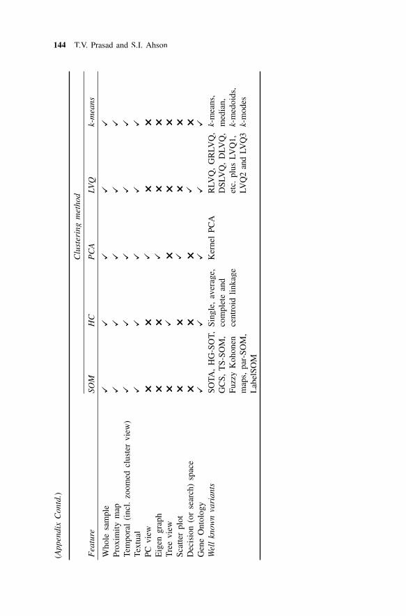
144 T.V. Prasad and S.I. Ahson
Who
le s
ampl
e�
��
��
Prox
imity
map
��
��
�
Tem
pora
l (i
ncl.
zoom
ed c
lust
er v
iew
)�
��
��
Text
ual
��
��
�
PC v
iew
��
��
�
Eig
en g
raph
��
��
�
Tre
e vi
ew�
��
��
Scat
ter
plot
��
��
�
Dec
isio
n (o
r se
arch
) sp
ace
��
��
�
Gen
e O
ntol
ogy
��
��
�
Wel
l kn
own
vari
ants
SOTA
, H
G-S
OT,
Sing
le,
aver
age,
Ker
nel
PCA
RLV
Q,
GR
LVQ
,k-
mea
ns,
GC
S, T
S-SO
M,
com
plet
e an
dD
SLV
Q,
DLV
Q,
med
ian,
Fuzz
y K
ohon
ence
ntro
id l
inka
geet
c. p
lus
LVQ
1,k-
med
oids
,m
aps,
par
-SO
M,
LVQ
2 an
d LV
Q3
LLk-
mod
esL
abel
SOM
Clu
ster
ing
met
hod
Fea
ture
SOM
HC
PC
ALV
Qk-
mea
ns
(App
endi
x C
ontd
.((
)
Data Mining for Bioinformatics—Systems Biology
T.V. Prasad and S.I. Ahson
INTRODUCTION
Biology, like many other sciences, changes when technology brings in newtools that extend the scope of inquiry. The invention of the optical microscopein late 1600 brought an entirely new vista to biology when cellular structurescould be more clearly seen by scientists. Much more modern and recentelectron microscope developed in the 60’s enhanced the visualization ofcells considerably. The application of computing to biological problems hascreated yet another new opportunity for the biologists of the 21st century. Ast
computers continue to change the society at large, there is no doubt thatseveral years of development in databases, software for data analysis,computational algorithms, computer generated visualization, use of computersto determine structures of complex bio-molecules, computational simulationof ecosystem, analysis of evolutionary pathways and many morecomputational methods have brought several new dimensions to biology.The technological revolution, from an ordinary computer to high-performance/grid computing, the processes have further automated, and led to flooding ofdata which cannot be handled properly, due to lack of proper standards atproper time. Billions of records are being pushed by the researchers andscientists into the data repositories across the world.
However, there is a positive thing associated with this. Once thecharacteristics or various genes, proteins or metabolomes are known, thenext step is to draw the relationship between them so that the entire pictureof the “system” function can be known. Now the study of higher levels ofactivities within organisms has become a reality. With the data related tomolecular composition of virus and other disease-causing agencies, scientistscan understand the pattern of diseases like HIV, cancer, etc. It has becomeeasy to understand the nutritional and metabolic activities inside the body,now called nutri-genomics and metabolomics respectively. It has also openedup ways to understand the impact and decomposition due to toxic compounds,now called toxico-genomics. The effect of pharmaceuticals/drugs on tissues
9

146 T.V. Prasad and S.I. Ahson
and entire human body down at the level of genes and proteins can also bestudied, now called pharmaco-genomics.
All these fields of studies lead to one special challenging area called thesystems biology. It will be too early to describe it in great detail but it isessential to know various issues that are known. The growth is so high thata world map of websites of biological data would have to be in place.
The field of systems biology has many similarities to other engineeringdisciplines. The foundations of signaling and transmission in human body orany other organism has analogy with the electrical engineering and so alsothe feedback control mechanism has with the electronics and communicationengineering. The modeling and simulation is a very close associate of thecartoons and animation sector, which needs a fairly high level of visualizationthan any other field.
Lack of proper analysis tools, methods of acquisition/accessing andrepresentations, technical standards, and visualization techniques are the prime-most issues in handling biological data at large. Initially, it was not thoughtthat the situation could turn out to be so cumbersome, but as the data isgrowing hour-after-hour, it is becoming even more difficult to integratedatabases, models, or even compare the data.
Presently, there are almost no methods for integration of data, analysisand visualization tools, standardized models for computation or comparison,etc. for handling genomic data. Leading researchers and research organizationshave laid roadmaps, blueprints, guidelines and so on for taking up new workbut almost all of them prove to be worthless in wake of absence of qualifiedand trained researchers, directions and funding. American, European andAsian countries are pouring in huge funds to tackle the problems, but seemto have achieved little success.
For example, the ASN.1 (Abstract Syntax Notation) is being used only byfew well-known organizations, whereas other agencies—well establishedand amateur—developed their own standards and generated highly voluminousyet very useful databases. This led to incompatibility and inconsistency withother databases across the world.
Scientists and researchers have numerous questions to be answered in thewake of these technological developments in information sciences anddiscoveries in bio-sciences. How the entire set of genes coordinate togetherin the development of human body? How do the genetic networks varyamidst different persons? What makes us separate from other living beings?What is the “blue print” of each person? Will the genetic information beshared publicly in future? Will it be used to clone human beings? What isthe level of security? How will the data be used to find cures for seriousdiseases? The questions are so many and the data being gathered at the dawnof the twenty first century is so enormous that it may likely take almost theentire century to reach to a satisfactory level of understanding.

Data Mining for Bioinformatics—Systems Biology 147
DATA MINING IN SYSTEMS BIOLOGY
Understanding and harnessing the power of ‘biological systems’ using systemsapproaches will open doors to the development of far-reaching applicationsof computing in the 21st century. It will be possible to use blood or tissuet
sample to predict an individual’s susceptibility to large number of afflictions.It will be possible to propose chemotherapy regime using modeling techniquesfor assessing the biological response to a proposed regime. Many otherresearch areas will utilize the systems approach and aided by the advancedcomputation techniques and cyber infrastructure.
Although biology changed drastically in the later years of the 20th centurywith the impact of new developments in molecular biology, the three strandsof inquiry still continue: (a) empirical observation, (b) evolution, and (c)taxonomy of life. Biology is an empirical and descriptive science. The cultureof bioscience is based on visualization—identifying new species, describingphysical appearances, environment, life cycle and diversity of life. Bioscienceis also concerned with taxonomy and classification. The emerging disciplineof semantic web and ontology directly apply to biology. One of the main aimof biological inquiry in the 21st century is the understanding of the underlyingt
mechanisms of life. The modern trend is systems-level understanding ofstructure, dynamics and control mechanisms at the organism level.
Research in bioscience has undergone a paradigm shift with the focus oncellular studies. This shift has been driven by the increasing availability ofhigh-throughput (HT) data. The human genome project was the catalyst fordeveloping HT technologies. The earliest form of HT data were genome andproteome sequences. Many new forms of biological data including geneexpression, protein expression, metabolmics, mass spectrometry, proteinstructure, radiological data, are now available. The increasing quantity andquality of data has led to data curation, annotation, and integration. In orderto understand and derive meaning from data various data mining techniqueshave been developed.
Much beyond the complex issues of data lays the roadmap towardsprocessing biological data of varied forms. This would lead ultimately to theprocessing of complete human system or any other meaningful biologicalsystem. Such a system could be whole genome, genome to genomecomparison or understanding the behaviour of various organism growths.
Broadly speaking, all these systems will comprise study of systems biology.It may be too early to talk about systems biology at a time the constituentfields are in infancy stage. In today’s world, the in silico drug design isconsidered a hot discipline, whereas not many tools are available. Proteinfolding, docking of drug compounds into the targets, identifying the markers,etc. are the buzzword of the day.
148 T.V. Prasad and S.I. Ahson
The ever-growing types and size of databases require tools for exploringcertain hidden patterns in data. The traditional statistics-based techniques,based on a priori hypothesis, can be used to discover new, interesting andpreviously unknown patterns in large amounts of data. The common datamining tools are based on regression, clustering, classification, associationrules, decision trees and other machine learning algorithms. The fields ofdata mining, AI, systems biology, ontology, and database theory are becomingmore interrelated while striving to provide answers to biological questionsthrough computational means.
Data mining algorithms are applied when databases are too massive andare of various formats across different hierarchies of biological informationi.e., DNA, RNA, proteins, macromolecular complexes, signaling networks,cells, organs, organisms, and species. There is a necessity to explore as tohow the techniques of data mining are applied to biological databases inorder to extract patterns which are crucial in making decisions in healthcare.The aim of this course is to discover, train, encourage, and support the newkinds of biologists needed for the 21st century to provide learning opportunitiest
at the interfaces among biology, mathematics, statistics and computer science.Illustrative research areas at the interface of computer science, systems science,AI and biology are:
• Structure determination of biological molecules and complexes• Simulation of protein folding• Whole genome sequence assembly• Whole genome modeling and annotation• Full genome-to-genome comparison• Rapid assessment of polymorphic genetic variations• Relating gene sequences to protein structures• Relating protein structure to function• In silico drug design• Modeling of cellular process• Simulation of genetic-regulatory networks• Modeling of physiological systems in health and disease• Modeling behaviour of schools, swarms and their emergent behaviour• Synthetic biology• Artificial life• Implantable neural prosthetic
We have already understood about the data types and issues associatedwith them in the preceding article titled “Data Mining for Bioinformatics –Microarray Data” as an introduction. Now, let us see the complete pictureof our understanding about biological data forms and their issues (Jagadishand Olken, 2003). The biological data can be in various forms as given inTable 1.

Data Mining for Bioinformatics—Systems Biology 149
Table 1: Different forms of biological data
Biological data type Example
Sequences DNA sequences of various organisms like fruit fly, mice,C. elegans
Graphs Metabolic pathways, genetic networks, signalingpathways
High-dimensional data Microarray gene expression dataGeometric information Protein structure, docking of drug candidate in a binding
siteScalar and vector Molecular models related to the cells, hydrophobicity,
electricity/signal transmission/communication model ina cell
Images Radio-logical images, X-rays, animations, etc.Prose Lot of biological material that contain important
knowledge but running in the form of paragraphs andessays
Within a system with four parts, there are 11 possible modes of interaction.Among a class of 20 students there can be 190 possible interactions, countingjust the pairwise interactions. And among the approximately 25,000 genesthat comprise each human being, there are more than 336 million possiblepairwise interactions. Since genes interact in more than pairs, the total numberof possible interactions is staggering (ISB, 2007). Further, with thousands ofresearchers working on millions of organisms generating numerous forms ofdata using many experimental techniques, the complexities (for quality) ofbiological data have been laid out in the following manner:
• High volume• Accuracy and consistency• Organization• Sharing• Integration• Curation
The computational scientists have to adopt the systems approach to solvingsuch challenging problems, and additionally, the following parameters willalso have to be addressed keeping in view the complexity:
• Interfacing/formats/standards• Retrieval• Validation• Visualization• Modeling/simulation• Maintenance• Documentation• Integration and portability

150 T.V. Prasad and S.I. Ahson
Methods, models, algorithms, databases, visualization and other parametersare required for handling data right from the stage of preparation, acquisition,finalization, conversion, processing, analysis, visualization and then furtheruse on other processes/activities. The process may start with the preparationof samples for NMR, MS, microarray, X-ray crystallography, 2D-PAGE, orany other method, all of which generate data of different formats acrossdifferent platforms.
Kitano in 2003 described that a large portion of the current day’s knowledgeof genetic regulatory networks or systems biology is represented in the formof cartoon like networks (SBI Japan, 2003). Such knowledge cannot berepresented in the form of general text or in the form of general databaseformats. For graphical interfaces, the following criteria could be helpful:
• Expressing the relationships between different entities such as relationshipbetween genes and proteins
• Clarity in expression – there has to be visual and grammatical/semanticclarity in expressing the entities
• Expandability – the graphical representations should be expandable uponaddition of new knowledge as and when required
• Mathematical modeling – it should be possible to derive mathematicalmodels corresponding to the available knowledge, at any given time
• Software support – due to the bulkiness of knowledge, it should be possibleto handle the operations through proper computing support
Interestingly, no graphical model today satisfy all these criteria; however,some of the available systems satisfy some of them. This is a noteworthyitem for all scientists, academicians and researchers for undertaking projectsin this area. A description of various types of models with suitable examplesis given in Table 2.
Table 2: Various types of models used in systems biology
Models Examples
Probabilistic graphical models Hidden Markov models, Bayesian network modelsLogical models Boolean models, fuzzy logical models, rule-based
modelsStatistical models Linear models, neural network models, Bayesian
network modelsComputational models Simulation modelsMulti-scale models Molecular interaction modelsPower law models Generic power model, general theory of power
law scalingHybrid models HMM with partial differential equations, simulation
with differential equationsQualitative modelsQuantitative models

Data Mining for Bioinformatics—Systems Biology 151
MODELING AND SIMULATION
ISB (2007) envisages that the most interesting aspect about systems biologyis the area of predictive, preventive and personalized (PPP) medicine, whosegoals include:
• Identification and classification of diseases and patient populations so thatthe diagnosis becomes more specific and treatment more effective. Tilldate, the diseases were seen as cellular imbalances, which should otherwisebe classified in terms of the cell-type specific biological networks thathave been perturbed by the defective genes and/or environmental stimuli.
• More flexible drug designing, preferably in silico, based on computersimulations of docking of drug compounds in a complex protein or generegulatory network, with an aim to enhance the efficiency and reducingthe side effects.
• To make best use of genetic information to evaluate a person’s healthhistory in real time. The blood can become a window into screening ofhealth and disease.
• Restoration of a disease-perturbed network to its normal state by geneticor pharmacological intervention, with compounds that are speciallydeveloped for the patient and to repair the diseased networks. Also, theidea is to identify changes in cellular networks at the earliest possiblestage and, to find a solution to prevent or limit the effects of the disease.
ISB also envisages that PPP has the potential to transform traditionalmedicine to considerably decrease the effect and mortality of serious diseaseslike cancer, Huntington’s, Parkinson’s and diabetes. Other applications willdefinitely increase the personal and communal well-being as the detrimentaleffect of abnormalities associated with mental illness will be eased.
Some of the oldest references related to the modeling and simulation ofthe genetic regulatory networks are McAdams and Shapiro (1995), Somogyiand Sniegoski (1996), Goldsby et al. (1999) and Forst (1999).
Aravind (2000) used association models for genome analysis, whereasD’haeseler et al. (2000) used genetic network inference to arrive at reverseengineering from co-expression clustering. Other noted works are Diehn andRelman (2001) and Eisenberg (2000). Forst (2001) is one of the first tutorialsin systems biology. Wiechert (2002) termed a new phrase “metabolicengineering” in his work and described various tools for modeling andsimulation used in it. The concepts of electrical engineering, control systemstheory, physics, graph and network theory, etc. are being applied to theregulatory networks as well as other forms of pathways. Wolkenhauer (2002)gave a very lucid explanation of comparing mathematical modeling conceptswith those applicable to genetic networks. Ullah and Wolkenhauer (2007) isa very useful literature that describes in detail the family tree of the Markovmodels that can be applied in systems biology.
152 T.V. Prasad and S.I. Ahson
The study of systems biology though deeply rooted in graph theory andon various simulation and modeling techniques, find implementation in anumber of areas. Wooley and Lin (2001) suggested the roadmap forapplications in the future in the following areas:
1. Molecular and structural biology(a) Prediction of complex protein structures(b) Protein folding(c) Identification/recognition of binding sites/markers (functional and
structural)(d) Clustering/classifying functional class of proteins(e) Molecular docking, in silico
2. Cell biology and physiology(a) Cellular modeling and simulation, pathway reconstruction(b) Cell cycle regulation(c) Inhomogeneities in cellular development and signaling
3. Genetic regulation(a) Regulation of transcription activity as process control computing(b) GRN as finite state automata(c) GRN as electrical circuits(d) Combinatorial synthesis of GRN(e) Combining experimental data with biological network information
4. Organ physiology(a) Multi-scale physiological modeling(b) Hematology for leukemia(c) Immunology(d) Modeling of the cardiac system
5. Neuroscience(a) Landscape of computational neuroscience(b) Large scale neural modeling(c) Muscular control(d) Synaptic transmission(e) Neuropsychiatry(f ) Recovery from injury
6. Virology(a) HIV/AIDS(b) HPV
7. EpidemiologySTD
8. Evolution and ecology(a) Study of commonalities(b) Characteristics of evolution(c) Characteristics of ecology
Before actually working on complex biological systems such as humanand livestock, simpler organisms, especially the single cell organisms suchas yeast and bacteria could be modeled. With fewer genes and simpler

Data Mining for Bioinformatics—Systems Biology 153
genetic regulatory network, it will undoubtedly become far easier to workwith, analyze and predict.
Just as it happens in the agricultural and meteorological forecasting, themodels are required to be tested stringently over and again for many biologicalcycles before stable and more accurate models are arrived at. This rigorousexercise may take many such cycles over long periods, even with the use ofbest tools and techniques. The outcomes from experimental perturbationsduring such exercises can also yield very interesting results.
VISUALIZATION IN SYSTEMS BIOLOGY
In addition to the basic visualization forms described in the earlier article(Data Mining for Bioinformatics – Microarray Data), a variety of othervisualizations for microarray gene expression data are available, at websitesof GEDA and SilicoCyte, which can be easily converted and/or presentedfor biological data representation:
• 2D and 3D score plots• Profile Plots• Scatter plots
� 3D scatter plots� PCA visualization - Result on 3D scatter plot� Isomap visualization� Multi-dimensional scaling
• Venn Analysis Diagrams for visualizing similar elements in microarrays,same genes in gene groups or same genes in microarray designs
• SOM visualization of clustering result on� 2D Trellis plot� U-matrix� 1D SOM
There are a number of visualization techniques to represent interaction betweenthe genes in a genetic regulatory network. The mapping could be interactionbetween protein-protein, protein-DNA, protein-RNA, protein-ligand bindings,DNA-binding ligand, post-translational modifications of proteins, metabolites,etc. One of such excellent work of visualization is given by Sawyer (2003),where a number of methods of presenting different forms of outputs aregiven as examples, and most of which can be used to indicate regulatorynetworks, pathways or interaction networks very comfortably.
In other words, these network types have been more or less standardized.Broadly speaking, though all these visualizations are based on the graphtheory, there are three forms of visualization techniques for representing thenetwork structure of the biological outputs, viz., the hierarchical tree structure,the forest structure (consisting of a number of tree/graph like structures), thecircuit diagram structure (very useful for representing haphazard and complexrelationships between entities) and a hybrid structure. For the sake of clear

154 T.V. Prasad and S.I. Ahson
conceptualization, some of these visualizations have been reproduced inFig. 1. Please refer to the website for clear details.
Fig. 1 (a): Symmetric graph drawing illustrating the BBC News Agencywebsite map. Similar visualization would be useful for representing linkages
of genes/proteins/metabolomes interactions.
Fig. 1 (b): Nested graph drawing organizing and visualizing a workflow taskprocess. When it is desired to indicate the connectivity of different networkstogether to give a complete view of the regulatory network or pathways, this
visualization can be applied.

Data Mining for Bioinformatics—Systems Biology 155
Fig. 1 (c): A circular graph drawing revealing networks of cluster trees radiatingfrom a central hub cluster. There are requirements to plot the entire cycle ofconversion from one phase to another in the genetic regulatory network, which alsohelps in indicating the circular relationships of sub-components or sub-networks.
Fig. 1 (d): Circular layout with multiple clusters. Clusters are a very commonfeature in genomics and proteomics. Indicating individual clusters as well as
their relationship with others can be as effective as this visualization.
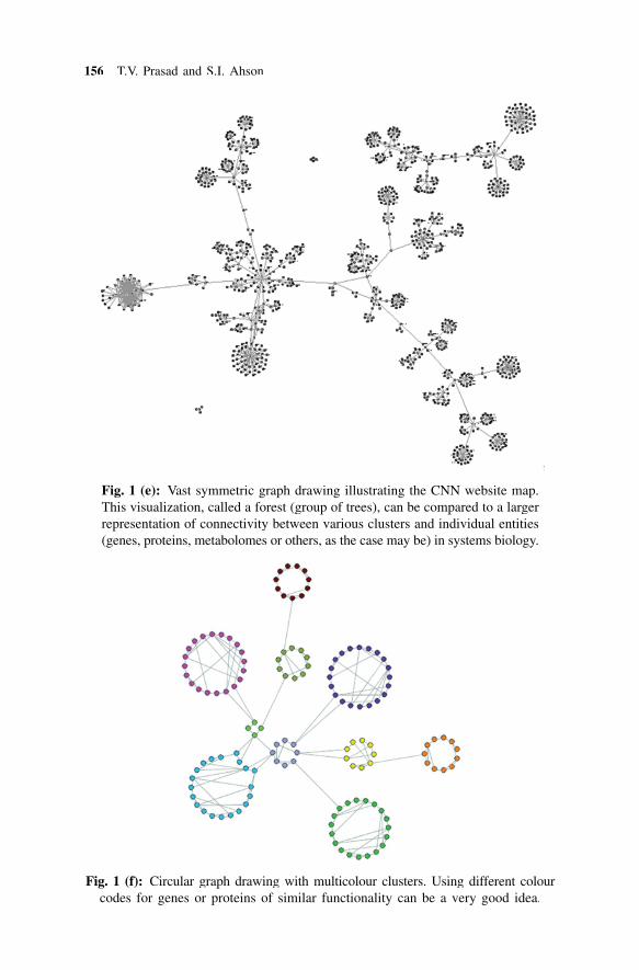
156 T.V. Prasad and S.I. Ahson
Fig. 1 (e): Vast symmetric graph drawing illustrating the CNN website map.This visualization, called a forest (group of trees), can be compared to a largerrepresentation of connectivity between various clusters and individual entities(genes, proteins, metabolomes or others, as the case may be) in systems biology.
Fig. 1 (f): Circular graph drawing with multicolour clusters. Using different colourcodes for genes or proteins of similar functionality can be a very good idea.

Data Mining for Bioinformatics—Systems Biology 157
Fig. 1 (g): Symmetric graph drawing representing objects and their complexrelationships clearly. The relationships between genes, proteins andtranscriptomes need not also be as simple as generally visualized. They mayinvolve a number of stages and regulations as shown in this visualization.
Fig. 1 (h): This graph drawing demonstrates the efficiency of the packingalgorithm, which tightly places groups of connected components. It is importantto realize that in practice the genes and protein regulation is a set of disjointtrees, or forest. For successful systems biology visualization, the software
should consider this aspect.

158 T.V. Prasad and S.I. Ahson
Fig. 1 (i): Orthogonal graph drawing organizing classes and their relationships.In case it becomes difficult to indicate all the intricacies of the regulatorynetwork or pathways, the relationships and transcriptome could be represented
as a set of inter-connected graphs as shown here.
Fig. 1 (j): Orthogonal graph drawing indicates the placement of the sourceand target nodes. Labeling functionality accommodates the space needed to
label the drawing.

Data Mining for Bioinformatics—Systems Biology 159
Fig. 1 (k): An orthogonal graph drawing taken from the domain of roboticsdesign shows how hyper edges (edges between more than two nodes) can berendered and laid out. This is one of the simplest forms of visualization whichcan be easily implemented for a smaller genetic regulatory network or proteininteraction map. The effect of catalyzing inputs over the transcription can beindicated using this method, as given by the initiator/terminal node (triangles).
Fig. 1 (l): Nested graph drawing illustrating a nested UML diagram. Forzooming in and out any complex regulatory network, the nested graph as
shown above could be very useful.

160 T.V. Prasad and S.I. Ahson
Fig. 1 (m): You can control how edges attach to nodes. In case the connectivityare to be shown on different pages, or stages are to be shown, this visualization
can help in organizing the output in the most effective manner.
Fig. 1 (n): Hierarchical graph drawing depicting the Sopranos family tree. Ituses coloured nodes to differentiate separate lineages. Orthogonal edge routingcreates a clear organizational view and horizontal edge routings illustratecouples. For a very simpler regulatory network representation, this visualization
can be employed.
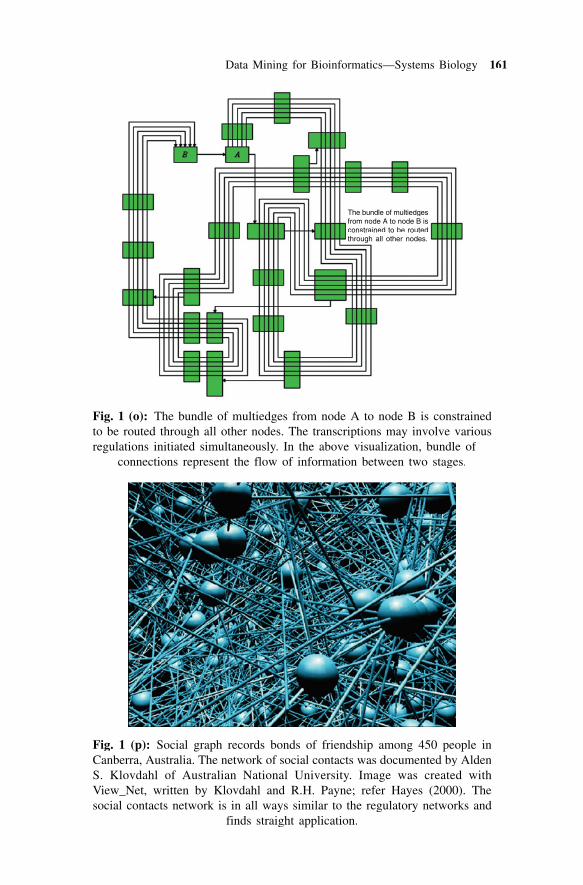
Data Mining for Bioinformatics—Systems Biology 161
Fig. 1 (o): The bundle of multiedges from node A to node B is constrainedto be routed through all other nodes. The transcriptions may involve variousregulations initiated simultaneously. In the above visualization, bundle of
connections represent the flow of information between two stages.
Fig. 1 (p): Social graph records bonds of friendship among 450 people inCanberra, Australia. The network of social contacts was documented by AldenS. Klovdahl of Australian National University. Image was created withView_Net, written by Klovdahl and R.H. Payne; refer Hayes (2000). Thesocial contacts network is in all ways similar to the regulatory networks and
finds straight application.
The bundle of multiedgesfrom node A to node B isconstrained to be routedthrough all other nodes.

162 T.V. Prasad and S.I. Ahson
(a) (b)
Fig. 2 (a) Before – This simply structured symmetric graph drawing is hiding amore complex structure under each of its nodes. (b) After – Entire symmetric
graph drawing after the hidden nodes and edges are revealed.
SYSTEMS BIOLOGY – TOWARDS MOLECULAR PATHWAYS
Reconstructing molecular pathways from expression data is a difficult task.One approach is to simulate pathways using a variety of mathematical modelsand then choose the model that fits the data. Reverse engineering is a lessdemanding approach in which models are built on the basis of the observedbehaviour of molecular pathways. It is possible to represent the geneexpression data by using simultaneous differential equations or representingthe expression as Boolean networks; however, each method suffer fromdisadvantages. A hybrid model such as the finite linear state model couldbring good results (Westhead et al., 2003).
Gene expression and disease link: Gene expression data analysis couldgive important clues for reasons behind cause of various “third world”diseases, e.g., malaria, typhoid, cholera, HIV/AIDS, cancer, dengue, etc.,especially about the behaviour and growth of disease causing germs.
Smaller datasets are preferred for processing: Large samples of over 200genes are not helpful since if all of them are correlated with a particularclass, it is unlikely that they all represent different biological mechanismsand hence are unlikely to add information not already provided by others.Though excellent research work has been carried out in last three decades,there are no general approach for identifying new cancer classes (classdiscovery) or for assigning tumours to known classes (class prediction) (Jagota,2001).
Most of the data in bio-sciences pertain to textual form or numeric formrather than any symbolic or image form. That is why, data mining of biological

Data Mining for Bioinformatics—Systems Biology 163
nature, especially the gene expression, sequence data and other forms ofnon-symbolic data is considered to be efficient and easier than any otherforms. Higher level of data types could be used while describing the proteinstructure data or genetic regulatory networks. However, similar experimentsand exercises can be conducted to study the effect of various chemicals,germs, micro-organisms, drugs, etc. on the human body or on other creaturesduring clinical trials. With the massive reduction in the cost of microarrayexperiments, it is expected that the biochemistry and pathological laboratorieswould be flooded with extremely massive data and most of the chemicalsand experimental procedures would straightaway be replaced by computers,microarrays, data mining algorithms under the title in silico.
New areas such as metabolomics, toxico-genomics and pharmacogenomicshave sprung up in which gene expression data continues to be the back-boneframework. In a recent review by de la Fuente and Mendes (2003), worksrelated to application of various methods of modeling both gene expressionand cell metabolism together have been described in great detail. The threemajor entities transcript, protein and metabolite form the larger frameworkwhereas the enzyme kinetics are responsible for the interactions down belowat the chemical network level. When these chemical networks are analyzedeither at individual (micro) level or of the entire process from transcript tometabolite, features of various constituent elements could be deciphered.
Table 3: Comparison between various concepts in real life and thosein systems biology
Entity Similarity in systems biology
Semantic web Neurological networkInfrastructure for World Map of websites
Petri-nets GRN as circuitsTrees Phylogenetic trees, ancestral trees, hierarchical clusteringFinite state automata Genetic expression pattern in GRNand/or Boolean networks
The most pressing challenges of systems biology fall roughly into thefollowing four categories, ISB (2007):
• Experimental — pertains to strategies for designing experiments andlcollecting reliable data.Technological — pertains to the development of new instrumentation formaking rapid, highly parallel, inexpensive and accurate measurements ofinformational molecules and their sequence, structure, modifications orprocessing, localization and interactions with other components large andsmall.
• Computational — pertains to the development and refinement of networkltheory and effective engineering of simulation tools, so that descriptive
164 T.V. Prasad and S.I. Ahson
networks can be replaced by more accurate dynamic models of the system’smolecular interactions.
• Sociological — pertains to effective communication across disciplines,lthe dynamics of research teams, difficulties obtaining funds, and the like.
Of these computer scientists would like to address the computationalchallenges of systems biology. The ISB has formulated 11 computational ormathematical challenges in contemporary biology:
1. How to fully decipher the (digital) information content of the genome?2. How to do all-versus-all comparisons of thousands of genomes?3. How to extract protein and gene regulatory networks from the challenges
1 and 2 as indicated above?4. How to integrate multiple high-throughput data types dependably?5. How to visualize and explore large-scale, multi-dimensional data?6. How to convert static network maps into dynamic mathematical models?7. How to predict protein function ab initio?8. How to identify signatures for cellular states (e.g. healthy vs. diseased)?9. How to build hierarchical models across multiple scales of time and
space?10. How to reduce complex multi-dimensional models to underlying
principles?11. How to do text searching to bring the literature and experimental data
together?
A large number of areas of research have sprung up due to the need tounderstand the functions of various entities inside the body of an organism.The areas of study not only got added to the biosciences but to the informationsciences as well. Some of them are as follows:
Systems biology as source for computing
• Swarm intelligence• Robotics• Self healing systems• Immunology and computer security• Amorphous computing
Systems biology as implementer for computing
• Evolutionary computing• Robotics – energy management• Neuroscience and computing
� NN� NN inspired sensors
• Ant algorithms

Data Mining for Bioinformatics—Systems Biology 165
Systems biology as physical substrate for computing
• Biomolecular computing• Synthetic biology
� Artificial life� Cellular logic gates
• Nano-fabrication and DNA self-assembly
SYSTEMS BIOLOGY RELATED SOFTWARE
Systems Biology Markup Language (SBML) is a language developed forrepresenting information and exchanging information related to biologicalsystems. It also helps in modeling various biological systems and is basedon XML implementation. It was developed by the Caltech ERATO KirantoSystems Biology Project Group, Caltech.
Details of some software based on SBML are given below; refer Funahashi(2003) for more details:
• SBML compliant, SBW-enabled application� Visual editors – CellDesigner, JDesigner� Simulators – Jarnac, Gepasi, Gibson simulator, Trelis� Others – MathSBML, MATLAB translator, libSBML
• Converters� KEGG to SBML converter� DOQCS to SBML converter
• Jarnac is a biochemical simulation package for Windows written andmaintained by Herbert M. Sauro at the Keck Graduate Institute http://www.sys-bio.org/Jarnac.htm
• Gibson Simulator is a simple stochastic simulator based on Gibson-Bruckvariant of the Gillespie algorithm and is maintained by SBW developmentgroup.
• JDesigner is also a visual editor for designing biochemical network layoutsimilar to the CellDesigner. It is written and maintained by Herbert M.Sauro at the Keck Graduate Institute and is available at http://www.syshttp://www.sys-bio.org/JDesigner.htm.
• Schmidt and Jirstrand (2005) described that the Systems Biology ToolBox (SBTOOLBOX for MATLAB) offers an open and customizableenvironment, which can be used by scientists and researchers to explorenew ideas, prototypes and new algorithms based on the requirements. Italso allows building of application models for the analysis and simulationof biological systems. It provides a number of features:
• Experiment description functionality• Modeling (based on equations of chemical reactions)• Handling of measurement data

166 T.V. Prasad and S.I. Ahson
• Import of SBML models from other software• Simulation (deterministic and stochastic)• Steady-state and stability analysis• Determination of the stoichiometric matrix• Parameter sensitivity analysis• Network identification• Parameter estimation• Simple model reduction• Bifurcation analysis• Localization of mechanisms leading to complex behaviours• Optimization algorithms
• Gepasi is a software package for modeling biochemical systems. It iswritten and maintained by Pedro Mendes at Virginia Tech. University,and is available at http://www.gepasi.org.
Fig. 3: Some symbols and expressions in CellDesigner software based on theproposals of Kitano for SBML. CellDesigner is freely available for download
from http://www.systems-biology.org.
Compartments_SquareCompartments_Oval

Data Mining for Bioinformatics—Systems Biology 167
Fig. 4: The symbols and expressions can be visually laid out to form a model.
• MathSBML is also known as The Mathematica SBML Reader. It is writtenand Maintained by Bruce E. Shapiro at California Institute of Technology,and is available at http://www.sbml.org.
• Trelis is a graphical Monte Carlo simulation tool for modeling the timeevolution of chemical reaction systems, developed by Luigi Warren atCalifornia Institute of Technology, http://sourceforge.net/projects/trelis.
• A host of translator, validation, simulation, etc. tools are available at http://sbw.kgi.edu/. Some of them are as follows:
• SBML layout viewer: displays/creates a layout for SBML models (Fig. 4)• SBML validation: validates SBML models• SBML simulation: simulates SBML models using various simulators• SBML translator: translates SBML to Fortran/Java/Matlab/XPP and a
number of other platforms

168 T.V. Prasad and S.I. Ahson
• University of Washington’s Systems Biology Workbench 2.7.6 releasedduring Oct 2007 is available at http://sys-bio.org/sbwWiki/doku.php?id=sysbio:sbw.
• CompuCell3D is a tissue and organ simulator based on the Cellular PottsModel, available at http://simtk.org/home/compucell3d. In collaborationwith the CompuCell3D team at the University of Bloomington (Glazieret al.) a combined tool was demonstrated linking CompuCell3D withSBW. The software uses Python as a flexible scripting tool that combinesthe Cellular Potts Model with the portable reaction-based simulator(roadRunner) available with the Systems Biology Workbench. All modulescan be run on Linux as well as on Windows or the Mac OS X.
• The Institute for Systems Biology has a range of software products fordifferent activities/analysis under categories such as data generationsoftware, data management software, data visualization and analysissoftware, etc. The details are as follows:
Data Generation Software
ISB proteomics pipeline:http://www.proteomecenter.org/software.phpttp://sashimi.sourceforge.net/
ISB microArray pipeline:http://db.systemsbiology.net/software/ArrayProcess/http://db.systemsbiology.net/software/VERAandSAM/
Data Management Software
The Systems Biology Experiment Analysis Management System (SBEAMS):http://www.sbeams.org/
Juvenile Diabetes Research Foundation’s Center for Bioinformatics at ISBhttp://www.T1DBase.org/
Research Community Database for Huntington’s Diseasehttp://HDBase.org/
Data Visualization and Analysis Software
BioSap (Blast Integrated Oligonucleotide Selection Accelerator Package):http://biosap.sourceforge.net/
BioTapestry (for editing and visualization of genetic networks in developingembryos)http://www.BioTapestry.orghttp://magnet.systemsbiology.net/

Data Mining for Bioinformatics—Systems Biology 169
Cytoscape (for data integration, network visualization, and analysis):http://db.systemsbiology.net/cytoscape/plugins/http://www.cytoscape.org/
Dizzy (simulation of deterministic and stochastic kinetics in biochemicalnetworks) :http://magnet.systemsbiology.net/software/Dizzy/http://magnet.systemsbiology.net/
The GESTALT Workbench for genomic sequence analysis:http://db.systemsbiology.net/gestalt/
Mogul: transcription factor binding site prediction multi-algorithm serverhttp://xerad.systemsbiology.net/Mogul/http://magnet.systemsbiology.net/
The Multiobjective Analyzer for Genetic Marker Selection (MAGMA):http://snp-magma.sourceforge.net/
Pointillist (tools for data integration and network model building)http://magnet.systemsbiology.net/software/Pointillist/http://magnet.systemsbiology.net/
RepeatMasker (screens DNA sequences for interspersed repeats):http://www.repeatmasker.org/
It is also worth notable that the BioPAX and the BioPathways Consortiumsare working in the area of application of semantic web to the biological/signaling pathway representation and re-construction. Substantial amount ofsuccess has been achieved using the PathoLogic software in which semanticweb technique was applied to provide meaningful predictions in E. coli andS. cerevisieae. It has also been applied on the database of marine planktoncyanobacteria, Prochlorococcus marinus.
CONCLUSIONS
Overall, there is a significant requirement of standardization in the microarraygene expression data analysis scenario, which currently suffers from thefollowing limitations due to non-standardization, and consequently, it can beconcluded that efforts would be needed to formalize on which platform,algorithm, technique/model, parameter, and visualization to be used foranalysis of various kinds of data:
• Microarray production and techniques not standardized• Preprocessing techniques not yet standardized• No standardized process or model available for analysis• No standardized visualization techniques available• Standardization of minimal information exchange on microarray data
brought out recently under the MIAME project

170 T.V. Prasad and S.I. Ahson
REFERENCES
Articles/Papers/Presentations/BooksAravind, L. (2000). Guilt by association: Contextual information in genome analy-
sis, Genome Research, 10: 1074–1077.Baldi, P. and Brunak, S. (2003). Bioinformatics: The Machine Learning Approach,
2ed. Affiliated East-West Press Pvt. Ltd., New Delhi.D’haeseler, P., Liang, S. and Somogyi, R. (2000). Genetic network inference: From
co-expression clustering to reverse engineering. Bioinformatics, 16: 707-726.Diehn, M. and Relman, D. (2001). Comparing functional genomic datasets: Lessons
from DNA microarray analyses of host-pathogen interactions. Current Opinionon Microbiology, 4: 95-101.
Eisenberg, D., Marcotte, E.M., Xenarios, I. and Yeates, T.O. (2000). Protein functionin the post-genomic era. Nature, 405: 823-826.
Forst, C.V. and Schulten, K. (1999). Evolution of metabolism: A new method for thecomparison of metabolic pathways using genomic information. Journal of Com-putational Biology, 6: 343-360.
Forst, C.V. (2001). A Tutorial on Network Genomics. International Conference onIntelligent Systems for Molecular Biology, Copenhagen, Denmark.
Funahashi, A. (2003). Introduction to SBML and SBML compliant software. ERATOKitano Symbiotic Systems Project, presentation slides. Available at http://sbml.org/workshops/tokyotutorial/tutorial.htm.
Fuente, A. de la and Mendes, P. (2003). Integrative modeling of gene expression andcell metabolism. Applied Bioinformatics, Open Mind Journals, 2(2): 79-90.
Goldsby, R.A., Kindt, T.J. and Osborne, B.A. (1999). Kuby Immunology. W. H.Freeman & Co., 4 edition.
Han, J. and Kamber, M. (2001). Data Mining: Concepts and Techniques. Elsevier,San Francisco.
Hayes, B. (2000). Graph Theory in Practice: Part 1. American Scientist, 88(1).Available at http://www.americanscientist.org/
Jagadish, H.V. and Olken, F. (2003). Data Management for the Biosciences. Reportof the NSF/NLM Workshop of Data Management for Molecular and CellBiology, Feb 2003. Available at http:/ww.eecs.umich.edu/~jag/wdmbio/AAwdmb_rpt.pdf.
Jagota, Arun (2001). Microarray data analysis and visualization. Dept. of ComputerEngineering, University of California, CA., USA.
McAdams, H. and Shapiro, L. (1995). Circuit simulation of genetic networks.Science, 269: 650-656.
Mitchell, T.M (1997). Machine Learning. McGraw Hill International Edition, NewDelhi.
Schmidt, H. and Jirstrand, M. (2005). Systems Biology Toolbox for MATLAB: Acomputational platform for research in Systems Biology. Bioinformatics AdvanceAccess, available at http://www.fcc.chalmers.se/~henning/SBTOOLBOX/
Somogyi, R. and Sniegoski, C. (1996). Modeling the complexity of genetic net-works. Complexity, 1: 45-63.
Tavazoie, S., Hughes, J.D., Campbell, M.J., Cho, R.J. and Church, G.M. (1999).Systematic determination of genetic network architecture. Nature Genetics, 22:281-285.

Data Mining for Bioinformatics—Systems Biology 171
Ullah, M. and Wolkenhauer, O. (2007). Family tree of Markov models in systemsbiology. IET Systems Biology, 1(4).
White, K.P., Rifkin, S.A., Hurban, P. and Hogness, D.S. (1999). Microarray analysisof Drosophila development during metamorphosis. Science, 286(5447): 2179-2184.
Wiechert, W. (2002). Modeling and simulation: Tools for metabolic engineering.Journal of Biotechnology, 94: 37-63.
Wolkenhauer, O. (2002). Mathematical modelling in the post-genome era: under-standing genome expression and regulation – a system theoretic approach.BioSystems, 65: 1-18.
Wooley, J.C. and Lin, H.S. (2001). Catalyzing inquiry at the interface of Computingand Biology. The National Academies Press, Washington D.C. Available at http://genomics.energy.gov.
Zhu, H. and Snyder, M. (2001). Protein arrays and microarrays. Current Opinion inChemical Biology, 5: 40-45.
WebsitesBiology WorkBench. San Diego Supercomputer Centre, Bioinformatics and Compu-
tational Biology group, Deparment of Bioengineering at University of California,San Diego. Available at http://workbench.sdsc.edu.
BioPathways Consortium. BioPathways website. Available at http://www.biopathways.org.
Colantouni, C., Henry, G. and Pevsner, J. (2000). Standardization and Normalizationof Microarray Data (SNOMAD) software. Available at http://pevsnerlab.kennedykrieger.org/snomad.htm.
de Hoon, M., Imoto, S. and Miyano, S. (2004). The C Clustering Library (Cluster3.0) software. University of Tokyo, Institute of Medical Science, Human GenomeCenter, Japan. Available at http://bonsai.ims.u-tokyo.ac.jp/~mdehoon/software/cluster.
DeRisi Lab. Department of Biochemistry & Biophysics, University of California atSan Francisco. Website available at http://www.microarrays.org.
European Bioinformatics Institute (EBI). EBI website. Available at http://www.ebi.ac.uk/biomodels.
Gene Expression Data Analysis (GEDA) Tool. GEDA software. University of Penn-sylvania MC Health Systems. Available at http://bioinformatics.upmc.edu/GE2/GEDA.html.
Genomes: GTL (32007). Genomes: GTL (formerly Genomes to Life Initiative), USDepartment of Energy. Available at http://doegenomestolife.org.
Harvard Medical School. Department of Systems Biology, Harvard Medical School.Available at http://sysbio.med.harvard.edu/.
IBM. IBM Research website. Available at http://www.research.ibm.com/grape/.Institute for Systems Biology (ISB) (2007). ISB website. Available at http://
www.systemsbiology.org.Joint Center for Structural Genomics. Joint Center for Structural Genomics. Avail-
able at http://www.jcsg.org.Keck Graduate Institute. Keck Computational Systems Biology (California) website.
Available at http://sbw.kgi.edu/.

172 T.V. Prasad and S.I. Ahson
Massachusetts Institute of Technology. Computational and Systems Biology Initia-tive (MIT) website. Available at http://csbi.mit.edu.
Molecular Sciences Institute. Molecular Sciences Institute (Berkeley). Available athttp://www.molsci.org/Dispatch.
National Cancer Institute (2002). Gene Expression Data Portal (GEDP), NationalInstitutes of Health, USA. Available at http://gedp.nci.nih/gov/dc/servlet/manager.
National Centre for Biotechnology Information (2002). Gene Expression Omnibus(GEO), National Institutes of Health, USA. Gene expression datasets available atftp://ftp.ncbi.nih.gov/pub/geo/data/gds/soft.
Ottawa Institute of Systems Biology. Ottawa Institute of Systems Biology (Canada)website. Available at http://mededu.med.uottawa.ca/oisb/eng/.
Pacific Northwest National Laboratory. Systems Biology at PNNL. Available athttp://www.sysbio.org/.
Princeton University. Lewis Siegler Institute for Integrative Genomics, PrincetonUniversity. Available at http://www.genomics.princeton.edu/.
Princeton University. Center for Systems Biology, Institute for Advanced Study,Princeton University. Available at http://www.csb.ias.edu/.
SBML. Caltech ERATO Kiranto Systems Biology Project Group. Available at http://www.cds.caltech.edu/erato.
SilicoCyte (2004). SilicoCyte v 1.3 software. Available at http://www.silicocyte.com.Systems Biology Institute, Japan (2003). The Systems Biology Institute (Japan)
website. Available at http://www.sbi.jp/indexE.html, see also http://www.systems-biology.org/.
Tom Sawyer (2003). Tom Sawyer software Image Gallery. Website available at http://www.tomsawyer.com/gallery/gallery.php?printable=1.
University of Auckland. University of Auckland, New Zealand. Available at http://www.cellml.org.
University of Stuttgart. Systems Biology Group at the University of Stuttgart (Ger-many) website. Available at http://www.sysbio.de/.
Virginia Tech. GEPASI software website, Virginia Bioinformatics Institute, VirginiaTech. Available at http://www.gepasi.org.

Environmental Cleanup ApproachUsing Bioinformatics inBioremediation
M.H. Fulekar
INTRODUCTION
Environmental pollutants have become a major global concern. The moderngrowth of industrialization, urbanization, modern agricultural development,energy generation, have resulted in indiscriminate exploitation of naturalresources for fulfilling the human desires and need, which have contributedin disturbing the ecological balance on which the quality of our environmentdepends. Human beings in true sense are the product of their environment.Man-environment relationship indicates that pollution and deterioration ofenvironment has a social origin. The modern technological advancements inchemical processes have given rise to new products, new pollutants and inmuch abundant level which are above the self cleaning capacities ofenvironment. One of the major issues in recent times is the threat to thehuman life caused due to the progressive deterioration of the environment.
Technological revolution has brought new changes in products andprocesses in industry. The waste generated from the development of productsand processes are of concern to the environmentalist. A variety of pollutantssuch as xenobiotics, polycyclic aromatic hydrocarbons (PAHs), chlorinatedand nitro-aromatic compounds are found depicted to be highly toxic,mutagenic and carcinogenic for living organisms (Zhang and Bennett, 2005;Samanta et al., 2002). Heavy metals are also reported persisting into theenvironment causing toxicity to living organisms through bioaccumulation,adsorption and biotransformation. A number of microorganisms, as a resultof their diversity, versatility and adaptability in the environment, are consideredto be the best candidates among all living organisms to remediate most ofthe environmental contaminants into the natural biogeochemical cycle.
These natural forces of biodegradation can reduce wastes and cleanupsome types of environmental contaminants. Composting can accelerate naturalbiodegradation and convert organic wastes to valuable resources. Wastewater
10

174 M.H. Fulekar
treatment also accelerates natural forces of biodegradation, breaking downorganic matter so that it will not cause pollution problems when the wateris released into the environment. Through bioremediation, microorganismsare used to clean up oil spills and other types of organic pollutants. Thereforebioremediation provides a technique for cleaning up pollution by enhancingthe same biodegradation processes that occur in nature.
Bioremediation of a contaminated site typically works viz. (i) to enhancethe growth of whatever pollution-eating microbes might already be living atthe contaminated site and (ii) specialized microbes are added to degrade thecontaminants.
Bioremediation offers many interesting possibilities from a bioinformaticpoint of view still slightly explored. This discipline requires the integrationof huge amounts of data from various sources: chemical structure andreactivity of organic compounds sequence, structure and function of proteins(enzymes); comparative genomics, environmental microbiology and so on.The accumulation of huge amounts of data on individual genes and proteinsallowed the first studies of biology from a ‘systems’ perspective (Alves etal., 2002; Fraser et al., 2002). The bioinformatics resources devoted tobioremediation is still scarce. Some interesting projects are being carried outto organize and store this huge amount of information relating to this subject.The University of Minnesota Biocatalysts/Biodegradation Database (UMBBD)(Rison and Thornton, 2002) is among the more prominent resource. Thecurrent set of data includes 740 chemical compounds (2167 synonyms), 820reactions, 502 enzymes and 253 organisms (Eills et al., 2003).
The microorganisms display a remarkable range of contaminant degradableability that can efficiently restore natural environmental conditions (Idekeret al., 2001; Jeong et al., 2001). Advances in the molecular biologytechnologies are making a global gene expression profile possible; genome-wide analysis of DNA (genomics), RNA expression (transcriptomics) andprotein expression (proteomics) as well as exploring complexes of proteinaggregation such as protein-protein interaction (interactomics) create theopportunity to systematically study the physiological expressions of suchorganisms. Attempts are made to interpret some of the areas of genomicsand proteomics which have been employed for bioremediation studies. Thestudies on bioinformatic data obtained viz. various sources are interpreted bycombining these techniques and applying them towards future studies ofactive bioremediation to develop environmental cleanup technologies.
Background
The revolution in computer technology has made it possible to model grandchallenge problems such as large scale sequencing of genomes andmanagement of large integrated databases. This availability of data has ledto an explosion of genome and proteome analysis leading to many new

Environmental Cleanup Approach Using Bioinformatics in Bioremediation 175
discoveries and tools. The availability of genomics and proteomics data andimproved bioinformatics and biochemical tools has raised the expectation ofthe humanity to be able to control the genetics by manipulating the existingmicrobes. In addition, bioinformatic analysis has enhanced our understandingabout the genome structure and the microorganisms restructuring process.Bioinformatic analyses have facilitated and quickened the analysis ofsystematic level behaviour of cellular processes, and understanding the cellularprocesses in order to treat and control microbial cells as factories for the lastdecade. Bioinformatic techniques have been developed to identify and analyzevarious components of cells such as gene and protein function, interactions,and metabolic and regulatory pathways. The next decade will belong to theunderstanding of cellular mechanism and manipulation using the integrationof bioinformatics.
GENOMICS, PROTEOMICS AND BIOREMEDIATION
All living things, including microorganisms, have a chemical called DNA(deoxyribo-nucleic acid) that contains information used in the organism tobuild and maintain cell biomass and to reproduce itself. The DNA moleculeis made up of four chemical building blocks (bases): adenosine (A), thymine(T), cytosine (C) and guanine (G). In microorganisms millions of these basesform long strand that pair together (A with T and C with G) in a twistedzipper-like structure known as a “double helix”.
Genomics is the study of the complete set of genetic information—all theDNA in an organism. This is known as its genome. Genomes range in size:the smallest known bacterial genome containing about 600,000 base pairsand the human genome has some three billion. (The size of a genome isdesignated in millions of base pairs of the megabytes, abbreviated Mb.)Typically genes are segments of DNA that contain instructions on how tomake the proteins that code for structural and catalytic functions. Combinationof genes, often interacting with environmental factors, ultimately determinethe physical characteristics of an organism.
Genomes Sequencing
How are the genomes sequenced? Microbial genomes are first broken intoshorter pieces. Each short piece is used as a template to generate a set offragments that differ in length from each other by a single base. The lastbase is labeled with a fluorescent dye specific to each of the four base types.The fragments in a set are separated by gel electrophoresis. The final baseat the end of each fragment is identified using laser induced fluorescence,which discriminates among the different labeled bases. This process recreatesthe original sequence of bases (A, T, C and G) for each short piece generatedin the first step.

176 M.H. Fulekar
Automated sequencers analyze the resulting electropherograms, and theoutput is a four colour chromatogram showing peas that represent each ofthe four DNA bases. After the bases are “read”, computers are used toassemble the short sequences (in blocks of about 500 or more bases each,called the read length) into long continuous stretches that are analyzed forerrors, gene-coding regions and other characteristics. To generate a highquality sequences, additional sequencing is needed to close gaps, reduceambiguities and allow for only a single error every 10,000 bases. By the endof the process, the entire genome will have been sequenced the equivalentof 8 or 9 times. The finished sequence is submitted to major public sequencedatabase, such as GenBAnk (http://www.ncbi.nih.gov).
Once the genome has been sequenced, portions that define features ofbiological importance must be identified and annotated. When the newlyidentified gene has a close relative already in a DNA database, gene findingis relatively straight forward. The genes tend to be simple, uninterruptedopen reading frames (ORFs) that can be translated and compared with thedatabase. However, the discovery of new genes without close relatives ismore problematic. Scientists in the new discipline of bioinformatics aredeveloping and applying computational tools and algorithms to help identifythe functions of these previously unidentified genes. An accurate accountingand description of genes in microbial genome is essential for describingmetabolic pathway and other aspects of whole-organism function.
GENOME SEQUENCING—BIOINFORMATICS
The major contribution of the bioinformatics in genome sequencing has beenin:
• The development of automated sequencing technique that integrate thePCR or BAC based amplification, 2D gel electrophoresis and automatedreading of nucleotides.
• Joining the sequences of smaller fragments (contigs) together to form acomplete genome.
• The prediction of promoters and protein coding regions of the genome.
Polymerase Chain Reaction (PCR) or Bacterial Artificial Chromosome(BAC) based amplification techniques derive limited size fragments of agenome. The available fragment sequences suffer from nucleotide readingerrors, very small repeats and very similar fragments that fit in two or moreparts of a genome. Chimera is two different parts of the genome or artifactscaused by contamination that join end to end giving a artifactual fragment.Generating multiple copies of the fragments, aligning the fragments andusing the majority voting at the same nucleotide positions solve the nucleotidereading error problem. Multiple experimented copies are needed to establish

Environmental Cleanup Approach Using Bioinformatics in Bioremediation 177
repeats and chimeras. Chimeras and repeats are removed before the assemblyof the genome fragments. The joining of the fragments is modeled as amathematical weighted graph where nodes are fragments and the weights ofedges are the number of overlapping nucleotides and the fragments arejoined based upon maximum overlap using a greedy algorithm (Mount,2000; Waterman, 1995). In a greedy algorithm, most nodes having maximum(or minimum) scores are collapsed first. To join contigs, the fragments withlarger nucleotide sequence overlap are joined first.
Automated Identification of Genes
After the contigs are joined, the next issue is to identify the protein codingregions or ORFs (Open Reading Frames) in the genomes. The identificationof ORFs can be done in three ways:
• Using Hidden Markov Mode (HMM) based techniques such as GLIMMER(Delcher et al., 1999) and genemark
• By searching the known database of genes such as GenBank ftp://ftp.ncbi.nih.gov/genbank to identify genes and
• The use of algorithms based on decision trees that identify start codons(Suzek et al., 2001) and stop codons of the coding regions.
HMM-based techniques develop multiple probabilistic state machines eachcapable of identifying an ORF. Each machine predicts the next nucleotidecharacter using a state transition with maximum probability and matches thepredicted nucleotide character with the current nucleotide character in theactual sequence. Statistical training using known sample sequences derivesthe probability of state transition. In the case of microbial genome, HMM-based software such as GLIMM has provided 95-97% accuracy.
Identifying Gene Function: Searching and Alignment
After identifying the ORFs (Open Reading Frames) the next step is to annotatethe gene with proper structure and function. The function of the gene hasbeen identified using popular sequence search and pairwise gene alignmenttechniques. The four most popular algorithms used in functional annotationof the genes are:
• BLAST (Altschul et al., 1990) and its variations (Altschul et al., 1997)• Dynamic programming technique—Smith-Waterman alignment (Waterman,
1995) and its variations• Indexing based scheme FASTA (Pearson and Lipman, 1988) and its
variations, and• BLOCKS (Henikoff et al., 1995) that uses multiple sequence alignment
of conserved domains to identify motifs-characterizing patterns of proteins.

178 M.H. Fulekar
3D Structure Modeling
A protein may live under one or more low free-energy conformational statesdepending upon its interaction with other proteins. Under a stableconformational state certain regions of the protein are exposed for protein-protein or protein-DNA interactions. Since function is also dependent uponexposed active sites, protein function can be predicted by matching the 3Dstructure of an unknown protein with the 3D structure of known protein(Baker and Sali, 2001). However, 3D structure from X-Ray crystallographyand NMR spectroscopy are limited. Thus there is a need for alternatemechanism to match genes. Generally there is close correspondence betweengene sequence and 3D structure. In such cases sequence matching is sufficientfor function annotation. However, many times multiple sequences map to thesame 3D structure; the lack of matching of amino acid sequences does notexclude same 3D structure. In such cases matching 2D structure (Kitagawaet al., 2001; Knaebel and Crawford, 1995)—patterns of alpha helix and betasheets—and matching 3D structure is needed to verify the function of thenewly sequenced protein (Whisstock and Lesk, 2003).
Pairwise Genome Comparison
After the identification of gene-functions, a natural step is to perform pair-wise genome comparisons. Pairwise genome comparison of a genome againstitself provides the details of paralogous genes—duplicated genes that havesimilar sequence with some variation in function. Pairwise genomecomparisons of a genome against other genomes have been used to identifya wealth of information such as orthologous genes—functionally equivalentgenes diverged in two genomes due to specification; different types of gene-groups—adjacent genes that are constrained to occur in close proximity dueto their involvement in some common higher function; lateral gene-transfer—gene transfer from a microorganism that is evolutionary distant; gene-fusion/gene-fission; gene group duplication; gene-duplication and difference analysisto identify gene specific to a group of genomes such as pathogens, andconserved genes (Bansal, 1999; 2002).
Reconstructing Metabolic Pathways
Identification of gene functionality has started a new level of bioinformaticsresearch: automated reconstruction and comparison of pathways of newlysequence organisms (Bansal, 2001; Bono et al., 1998; Kelley et al., 2003;Ogata et al., 1999; Papin et al., 2002; Schilling et al., 2002). There havebeen many efforts and approaches related to pathway reconstruction. Thethree major approaches can be classified as:
• Global network of reactions catalyzed by enzymes;• Network of gene-groups connected through the reactions catalyzed by
enzymes embedded in the gene groups; and• Global modeling of chemical reactions in the microbial cells.

Environmental Cleanup Approach Using Bioinformatics in Bioremediation 179
Current metabolic pathway techniques arelimited by the available gene-functions from wetlaboratories. Another issue is that theidentification of metabolic pathways is notsufficient unless the reaction rates are known.While there have been recent approaches to modelthe reaction rate of metabolic pathway (Schuster,1999), the complete picture cannot be verifiedlargely due to unavailability of gene-functionsfrom wetlabs.
PROTEOMICS
Proteomics is a new branch of science dedicatedto studying all the proteins expressed by a celland how these proteins change under differentgrowth conditions. For example, scientists aretrying to understand the protein expression patternof the organism. The proteins mainly responsiblefor the conversion are located on the outermembrane of the cell. Protein expression can bemeasured by isolating the proteins from cells anddetermining their relative abundance using proteinseparation and detection methods such as two-dimensional gel electrophoresis.
Mass spectrometry-based techniques are alsobeing used to identify the full complement ofcellular proteins, with the ultimate goal ofdetermining how the cell localizes differentproteins on the cell surface when conditionschange from aerobic to anaerobic respiration. Theentire complement of proteins associated withbacterial outer membrane vesicles (MVs) hasbeen determined by a new technique that involvesthe use of both high-resolution separation andhigh-mass accuracy and sensitivity. FourierTransform Ion Cyclotran Resonance (FTICR)mass spectrometry, MVs are unique to gramnegative bacteria and are constantly beingreleased from the cell surface during bacterialgrowth. During their release, MVs trap some ofthe underlying periplasm that contains variousenzymes. MVs explain how bacteria protectenzymes that are secreted extracellularly and also
Toluene
OH
Benzyl alcohol
OH
Benzyldehyde
O
O
Benzoale
CoAO
Benzoyl - CoA
Standard Metabolism
CH3
Toluene
S-
Fig. 1: Metabolic pathwayof toluene

180 M.H. Fulekar
the method by which they deliver lethal enzymes into other bacteria as ameans of predation, and even to eukaryotic cells early in pathogenesis.Identifying the entire protein complement of MVs can lead to predictions oftheir impact on the environments in which they are found.
Phenotype Similarity and Automated Pathway Comparisons
The researchers have taken the next level of study to compare the similarpathways to understand the effect of insertion and detection of genes invarious microorganisms and to understand the evolution of pathway level(Bansal and Woolverton, 2003). To compare two pathways, the genes in thepathway are aligned as follows:
• Two pathways match completely if every protein in the first pathway (ora gene-group within a pathway) has a corresponding homologous gene inanother pathway (or the gene-group within the pathway).
There is a gap if a homologous gene is deleted (inserted) and there is amismatch if the corresponding homologous genes have a low similarityscore. Based upon this modeling, comparison of H.Pylori and Yeast hasshown many similar pathways. More importantly, quantification mechanismhas been found to compare two pathways.
The terms ‘proteomics’ and ‘proteome’ were introduced in 1995 which isa key post-genomic feature that emerged from the growth of large andcomplex genome sequencing datasets. Proteomic analysis is particularly vitalbecause the observed phenotype is a direct result of the Action of the proteinrather than the genome sequence. Traditionally, this technology is based onhighly efficient methods of separation using two-dimensional polyacrylamidegel electrophoresis (2-DE) and modern tools of bioinformatics in conjunctionwith mass spectrometry (MS) (Tatusov, 1996). In bioremediation, the proteomeof the membrane proteins is of high interest, specifically in PAHbiodegradation.
Sudip K. Samanta et al., 2001 discussed the problems of PAH pollutionand PAH degradation and relevant bioremediation. The microbial degradationof PAH is the action of dioxygenase, which incorporates atoms of oxygenat the carbon atoms of a benzene ring of a PAH resulting in the formationof cis-dihydrodiol (Kanaly and Harayama, 2000), which undergoesrearomatization by dehydrogenases to form dihydroxylated intermediates.Dihydroxyated intermediates subsequently undergo ring cleanage and formTCA cycle intermediates (Sabate et al., 1999). A large number of naphthalene-degrading microorganisms—Alcaligenes denitrificans— , mycobacterium sp.,Pseudomonas putida, P. fluorescens, P. paucimobilis, P. vesicularis, P. cepacia,P. testosteroni, Rhodococcus sp., corynebacterium venale, bacillus cereus,moraxella sp., streptomyces sp., vibrio sp. and cyclotrophicus sp.—has beenisolated and examined for mineralization (Hedlund and James, 2001; Samantaet al., 2001).

Environmental Cleanup Approach Using Bioinformatics in Bioremediation 181
During the past decade, a variety of microorganisms has been isolated andcharacterized for the ability to degrade different PAHs and new pathways forPAH degradation elucidated. Further research is needed to explore themicrobial interactions within PAH-degrading consortia, the regulatorymechanisms of various ring structured PAH biodegradation as well as theco-metabolic biodegradation of PAHs. The new approach of advancementsin molecular biology can aid in the detection of PAH-degrading organismsfrom environmental samples (Watanabe, 2001; Watanabe and Baker, 2000).DNA-DNA hybridization has been directly applied to detect and monitor thecrucial populations recovered from the environment (Sayler et al., 1985 andGuo et al.,1997). Laurie and Jones (2000) detected two distinct PAH catabolicgenotypes from aromatic hydrocarbon-contaminated soil using quantitativecompetitive PCR (QC-PCR). A soil-derived consortium capable of rapidlymineralizing benzo[a]pyrene was analysed using Denaturing Gradient GelElectrophoresis (DGGE) profiling of PCR-amplified 165 rDNA fragments(Laurie and Jones, 2000). This analysis detected 165 rDNA sequence typesthat represented organisms closely related to known high molecular weightPAH degrading bacteria. Recently, many PAH degrading bacteria have beenisolated from geographically diverse sites using the 165 rRNA sequencetechnique (Widada et al., 2002).
Discovery of Novel Catabolic Genes Involved inXenobiotic Degradation
There are two different approaches to investigate the diversity of catabolicgenes in environmental samples: culture-dependent and culture-independentmethods. In culture-dependent methods, bacteria are isolated fromenvironmental samples with culture medium. Nucleic acid is then extractedfrom the bacterial culture. In contrast, culture-independent methods employdirect extraction of nucleic acids from environmental samples (Okuta et al.,1998; Watanabe et al., 1998). The description of catabolic gene diversity byculture-independent molecular biological methods often involves theamplification of DNA or cDNA from RNA extracted from environmentalsamples by PCR, and the subsequent analysis of the diversity of amplifiedmolecules (community fingerprinting). Alternatively, the amplified productsmay be cloned and sequenced to identify and enumerate bacterial speciespresent in the sample.
To confirm that the proper gene has been PCR-amplified, it is necessaryto sequence the product, after which the resultant information can be usedto reveal the diversity of the corresponding gene(s). Over the last few years,these molecular techniques have been systematically applied to the study ofthe diversity of aromatic-compound-degrading genes in environmental samples(Table 1).

182 M.H. Fulekar
Tab
le 1
:M
olec
ular
app
roac
hes
for
inve
stig
atin
g th
e di
vers
ity a
nd i
dent
ific
atio
n of
cat
abol
ic g
enes
inv
olve
d in
deg
rada
tion
of x
enob
iotic
s
Targ
et g
ene
Mol
ecul
ar a
ppro
ach
Sour
ceR
efer
ence
Nah
Ac
RT
-PC
R w
ith d
egen
erat
e pr
imer
sRR
Gro
undw
ater
(cu
lture
- in
depe
nden
t)W
ilson
et
al.,
1999
phnA
c, n
ahA
c, a
ndPC
R w
ith s
ever
al p
rim
ers
Soil
sam
ples
(cu
lture
-ind
epen
dent
)L
loyd
-Jon
es e
t al
., 19
99gl
utat
hion
e-S-
tran
sfer
ase
Phen
ol h
ydro
xyla
te (
Lm
PH)
PCR
-DG
GE
with
deg
ener
ate
prim
ers
Act
ivat
ed s
ludg
e (c
ultu
re-d
epen
dent
)W
atan
abe
et a
l., 1
998
RH
DPC
R w
ith d
egen
erat
e pr
imer
sPr
estin
e- a
nd a
rom
atic
hyd
roca
rbon
cont
amin
ated
soi
ls (
cultu
re-i
ndep
ende
nt)
Yea
tes
et a
l., 2
000
PAH
dio
xyge
nase
PCR
with
sev
eral
pri
mer
sPA
H s
oil
bact
eria
(cu
lture
-dep
ende
nt)
Llo
yd-J
ones
et
al.,
1999
Nah
AC
PCR
with
deg
ener
ate
prim
ers
Mar
ine
sedi
men
t ba
cter
iaH
edlu
nd e
t al
., 19
99(c
ultu
re-d
epen
dent
)
Nah
PCR
with
deg
ener
ate
prim
ers
Soil
bact
eria
(cu
lture
-dep
ende
nt)
Ham
ann
et a
l., 1
999
tfdC
PCR
with
de g
ener
ate
prim
ers
Soil
bact
eria
(cu
lture
-dep
ende
nt)
Cav
alca
et
al.,
1999
PAH
dio
xyge
nase
and
PCR
with
deg
ener
ate
prim
ers
Was
tew
ater
and
soi
l ba
cter
iaM
eyer
et
al.,
1999
cate
c hol
dio
xyge
nase
(cul
ture
-dep
ende
nt)
phnA
c, n
ahA
c, P
AH
PCR
with
sev
eral
deg
ener
ate
prim
ers
Riv
er w
ater
, se
dim
ent
and
soil
bact
eria
Wid
ada
et a
l., 2
002a
diox
ygen
ase
(cul
ture
-dep
ende
nt)
RH
DPC
R-D
GG
E w
ith d
egen
erat
e pr
imer
sT
hodo
cocc
us s
p. s
trai
n (R
HA
I)K
itaga
wa
et a
l., 2
001
(cul
ture
-dep
ende
nt)
RT:
Rev
erse
tran
scri
ptio
n, P
CR
: pol
ymer
ase
chai
n re
actio
n, D
GG
E: d
enat
urin
g gr
adie
nt g
el e
lect
roph
ores
is, R
HD
: rin
g hy
drox
ylat
ing
diox
ygen
ase,
PAH
: po
lycy
clic
aro
mat
ic h
ydro
carb
on

Environmental Cleanup Approach Using Bioinformatics in Bioremediation 183
Monitoring of Bioaugmented Microorganismsin Bioremediation
Because different methods for enumeration of microorganisms inenvironmental samples sometimes provide different results, the method usedmust be chosen in accordance with the purpose of the study. Not all detectionmethods provide quantitative data; some only indicate the presence of anorganism and others only detect cells in a particular physiological state.Several molecular approaches have been developed to detect and quantifyspecific microorganisms (Table 2).
Table 2: Molecular approaches for detection and quantification of specificmicroorganisms in environmental samples
Identification method Detection and Cell type monitoredquantification method
Fluorescent tags on Microscopy Primary active cellsrRNA probes Flow cytometry
Lux and luc gene Luminometry/scintillation Active cellscountingCell extract luminescence Total cells with translated
luciferaseLuminescent colonies Curable luminescent cells
Gfp gene Fluorescent coloniesMicroscopy Curable fluorescent cellsFlow cytometry Total cells, including starvedTT
Specific DNA sequence cPCR MPN-PCR, RLD-PCR Total DNA (living and deadcells and free DNA)
Slot/dot blot hybridization Culturable cellsColony hybridization
Specific mRNA Competitive RT-PCR Catabolic activity of cellstranscripting
Slot/dot blot by hybridization
Other marker genes Plate counts colony Culturable marked cells and(e.g., lacZY, gusA, hybridization indigenous cells with markerxyIE, and antibiotic phenotyperesistance genes) Quantitative PCR Total DNA (living and dead
Slot/blot hybridization cells and free DNA)
cPCR: Competitive PCR, MPN-PCR: most probable number PCR, RLD-PCR:replicative limiting dilution PCRSource: J. Widada, H. Nojiri, and T. Omori 2002
In bioremediation, quantitative PCR has been used to monitor and todetermine the concentration of some catabolic genes from bioaugmentedbacteria in environmental samples (Table 3). Recently, quantitative competitive

184 M.H. Fulekar
RT-PCR has been used (Levesque et al., 1997) to quantify the mRNA of thetcbC of Pseudomonas sp. strain P51.
Table 3: PCR detection and quantification of introduced bacteria inbioremediation of xenobiotics
Bacteria Target gene Detection and Referencequantificationmethod
Desulfitobacterium frappieristrain PCP-1(pentachlorophenol-degrader)
Mycobacteriumchlorophenolicum strain PCP-1(pentachlorophenol-degrader)
Sphingomonas chlorophenolica(pentachlorophenol-degrader)
Pseudomonas sp. strain B13(chloroaromatic-degrader)
Pseudomonas putida strain mx(toluene-degrader)
P. putida strain G7(naphthalene-degrader)
P. putida strain mt2 (toluene-degrader)
Alcaligenes eutropus strainJMP 134 [2,4-dichloropheno-xyacetic acid (2,4-D)-degrader]
P. putida ATCC 11172(phenol-degrader)
Pseudomonas sp. strain P51(trichlorobenzene-degrader)
Pseudomonas sp. strain P51(trichlorobenzene-degrader)
Pseudomonas resinovoransstrain CA 10 (carbozole-anddibenzo-dioxin-degrader)
Source: J. Widada, H. Nojiri, and T. Omori 2002
Derivation of regulatory mechanism and pathways
The genomics and proteomics research front has progressively moved frommetabolic pathway reconstruction to the identification of signaling pathwaysand promoter analysis to identify transcription factors for protein-DNAinteractions. There are four major approaches to study protein-DNA interactions:
16 rRNA Nested PCR Levesque et al., 1997
16 rRNA MPN-PCR Elsas van et al., 1997
16 rRNA Competitive PCR Elsas van et al., 1998
16 rRNA Competitive PCR Leser et al., 1995
xyIE Competitive PCR Hallier-Soulier et al.,1996
nahAc PCR-southern blot Herrick et al., 1993
xylM Multiplex PCR- Knaebel andSouthern blot Crawford, 1995
tfdA
dmpN PCR-RT-PCR Selvaratnam et al.,1997
tbcAa, tbcC PCR Tchelet et al., 1999
tbcC Competitive Meckenstock et al.,DT-PCR 1998
carAa Real-time Widada et al., 2001,competitive PCR 2002b

Environmental Cleanup Approach Using Bioinformatics in Bioremediation 185
(i) Micro-array analysis of gene-expressions under different stressconditions of cells;
(ii) Statistical analysis of promoter regions of orthologous genes(functionally equivalent genes in different organisms identified asbest homologs);
(iii) Global analysis of frequency patterns of divers in the intergenicregion—promoter region occurring between adjacent protein codingregions of a genome; and
(iv) Biochemical modeling at the atomic band level to understand how aprotein will bind to nucleotides.
The microarray analysis technique is based upon experimental data, andother three approaches are based on mathematical modeling and sequenceanalysis. Microarray analysis (Sung-Keun et al., 2004) measures the relativechange in the gene-expressions for a stressed (or a stimulated) cell and achange in cellular expression pattern differentiation, cellular cycle, tissueremodeling, sporulating etc.
MICRO-ARRAY TECHNIQUES
Gene Detection in Biodegradation in Microbial Communities
Sung-Keun Rhee (2004) and team of scientists (Atlas, 1981), at EnvironmentalScience Division, Oak Ridge National Laboratory, studied the detection ofgenes involved in biodegradation and biotransformation in microbialcommunities by using 50 mer oligonucleotide Microarrays. Research findingshighlight that to effectively monitor biodegrading populations, acomprehensive 50 mer oligonucleotide microarray was developed based onmost of the 2,402 known genes and pathways involved in biodegradationand metal resistance. This array contained 1,662 unique and group-specificprobes with <85% similarity to their non-target sequences. Based on artificialprobes, results showed that under hybridization conditions of 50oC and 50%formamide, the 50 mer microarray hybridization can differentiate sequenceshaving < 88% similarity. Specificity tests with representative pure culturesindicated that the designated probes on the arrays appeared to be specific totheir corresponding target genes. The detection limit was 5 to 10 ng ofgenomic DNA in the absence of background DNA and 50 to 100 ng of pure-culture genomic DNA in the presence of background DNA or 1.3 × 10⁷ cellsin the presence of background RNA. Strong linear relationships between thesignal intensity and the target DNA and RNA were observed (r2rr = 0.95 to0.99). Application of this type of microarray to analyse naphthalene-amendedenrichment and soil microcosms demonstrated that microflora changeddifferently depending on the incubation conditions, while the naphthalene-degrading genes from rhodococcus type microorganisms were dominant innaphthalene-degrading enrichments. The genes involved in naphthalene (and

186 M.H. Fulekar
polyaromatic hydrocarbon and nitrotoluene) degradation from gram negativemicroorganisms such as Palstonia, Comamonas and Burkholderia were mostabundant in the soil microcosms. In contrast to general conceptions,naphthalene degrading genes from pseudomonas were not detected, althoughpseudomonas is widely known as a model microorganism for studyingnaphthalene degradation. The real-time PCR analysis with four representativegenes showed that the microarray-based quantification was very consistentwith real time PCR (r2 = 0.74). In addition, application of the array to bothpolyaromatic-hydrocarbon and benzene-toluene-ethylbenzene-xylene-contaminated and uncontaminated soils indicated that the developedmicroarrays appeared to be useful for profiling difference in microbialcommunity structures. The results indicate that this technology has potentialas a specific, sensitive and quantitative tool in revealing a comprehensivepicture of the compositions of biodegradation genes and the microbialcommunity in contaminated environments although more work is needed toimprove detection sensitivity.
The transformation of environmental contaminants is a complex processthat is influenced by the nature and amount of contaminant present, thestructure and dynamics of the indigenous microbial community, and theinterplay of geochemical and biological factors of contaminated sites (Gibsonand Sayler, 1992; Leahy and Colwell, 1990; Golyshin et al., 2003). A betterunderstanding of the processes inherent in natural bioremediation requires,in part, a better understanding of microbial ecology. However, conventionalmolecular methods (PCR-based technologies, such as gene cloning, terminal-restriction fragment length polymorphism, and denaturing gradient gelelectrophoresis and in situ hybridization) for assessing microbial communitystructure and activities are labour-intensive. Rapid, quantitative and costeffective tools that can be operated in field scale heterogeneous environmentsare needed for measuring and evaluation bioremediation strategies.
DNA Micro-array in Bioremediation
Even with the complete genome sequences of microorganisms with thepotential for bioremediation (Tiedje, 2002; Seshadri et al., 2005), studies arenot accelerating in a rapid manner with the completed genome sequences. Itis possible to analyse the expression of all genes in each genome undervarious environmental conditions using whole-genome DNA microarrays(Schut et al., 2003; Lovley, 2003; Dennis et al., 2003). Such genome-wideexpression analysis provides important data for identifying regulatory circuitsin these organisms (Rabus et al., 2005; Muffler et al., 2002; Schut et al.,2001). In the past DNA microarrays have been used to evaluate the physiologyof pure environmental cultures (Rhee et al., 2004) and to monitor the catabolicgene expression profile in mixed microbial communities (Ye et al., 2000).More than 100 genes were found to be affected by oxygen-limiting conditions

Environmental Cleanup Approach Using Bioinformatics in Bioremediation 187
when a DNA microarray was used to study changes in mRNA expressionlevels in Bacillus subtilis grown under anaerobic conditions (Denef et al.,2003).
Sensitivity may often be a part of the problem in PCR-based cDNAmicroarrays, since only genes from populations contributing to more than5% of the community DNA can be detected. Several parameters wereevaluated to validate the sensitivity of spotted olifonucleotide for bacterialfunctional genomics (Cho and Tiedje, 2002). Optimal parameters were foundto be 5’-C6 amino-modified 7-mers printed on CMT-GAPS II substrates ata 40 �m concentration combined with the use of tyramide signal amplificationlabelling. Based on most of the known genes and pathways involved inbiodegradation and metal resistance a comprehensive 50-mer-basedoligoneucleotide microarray was developed for effective monitoring ofbiograding population (Kuhner et al., 2005). This type of DNA microarraywas effectively used to analyse naphthalene-amended enrichment and soilmicrocosms demonstrated that microflora changed differentially dependingon the incubation conditions (Kitagawa et al., 2001). A global gene expressionanalysis revealed the co-regulation of several thus-far unknown genes duringthe degradation of alkylbenzene. Besides this, DNA microarray have beenused to determine bacterial species, in quantitative applications of stressgene analysis of microbial genomes and in genome-wide transcriptionalprofiles (Gao et al., 2004).
The microarray is a powerful genome technology that is widely used tostudy biological processes. Although microarray technology has been usedsuccessfully to analyse global gene expression in pure cultures (Liu et al.,2003; Lockhart et al., 1996; Schena et al., 1996; Thompson et al., 2002;Wodicka et al., 1997; Zhou, 2003), adapting microarray hybridization foruse in environmental studies present great challenges in terms of specificity,sensitivity and quantitation (Zhou and Thompson, 2002; Call et al., 2001).Although microarray-based genomic technology has attracted tremendousinterest among microbial ecologists, it has only recently been extended tostudy microbial communities in the environment (Guschin et al., 1997; Loyet al., 2002; Small et al., 2001; Tiquia et al., 2004; Valinsky et al., 2002; Wuet al., 2001; Michael et al., 1999).
A system of cluster analysis for genome-wide expression data from DNAmicroarray hybridization is described that uses standard statistical algorithmsto arrange genes according to similarity in pattern of gene expression. Theoutput is displayed graphically, conveying the clustering and the underlyingexpression data simultaneously in a form intuitive for biologists. It has beenfound in the budding yeast, Saccharomyces Cerevisiae, that clustering geneexpression data groups together and find a similar tendency in human data.Thus patterns seen in genome-wide expression experiments can be interpretedas an indication of the status of cellular processes. Also, co-expression ofgenes of known function with poorly characterized or novel genes mayprovide a simple means of gaining leads to the functions of many genes forwhich information is not available currently.

188 M.H. Fulekar
The rapid advance of genome scale sequencing has driven the developmentof method to exploit this information by characterizing biological processesin new ways. The knowledge of the coding sequences of virtually every genein an organism, for instance, invites development of technology to study theexpression of all of them at once, because the study of gene expression ofgenes one by one has already provided a wealth of biological insight. To thisend, a variety of techniques have been evolved to monitor rapidly andefficiently, transcript abundance for all of an organism’s genea (Michael etal., 1999). Within the mass of numbers produced by these techniques, whichamount to hundreds of data points for thousands or tens of thousands ofgenes it is an immense amount of biological information.
STRUCTURE DETERMINATION
Meta Router is a system for maintaining heterogeneous information relatedto biodegradation in a framework that allows its administration and mining(application of methods for extracting new data). It is an application intendedfor laboratories working in this area which need to maintain public andprivate data, linked internally and with external databases, and to extractnew information from it.
Working with “States” (sets of compounds) attempts to stimulate anenvironment with a set of pollutants where a given reaction, carried out bya given bacteria, can modify one of the pollutants but not the other which“moves” the system to another “state” (another set of compounds) whereanother bacteria can act, etc. One would wonder which enzymes are neededto end up a state and which are the bacteria that have these enzymes.
The properties of compounds required for compound administrationinclude:
• Main technical characteristics• Compound queries• Enzyme queries• Reaction queries• Path finder
The data to be obtained in each of the above are described herewith.
Main Technical Characteristics
Initial Information:
• 740 organic compounds (2,167 synonyms)• 820 reactions• 502 enzymes• 253 organisms

Environmental Cleanup Approach Using Bioinformatics in Bioremediation 189
Selection of compounds by:- Substrate(s)
• synonyms• partial names
- Product(s)• synonyms• partial names
- Enzyme(s)- Organism(s)More than one substrate, product, onenzyme can be selected with AND/OR (at the bottom of the list)
- Name- Synonyms- Part of their name- Part of their smiles code
• C=O >> comps containingcarbonyl group
• CCCCC >> comps with five ormore linear saturated carbons
- A range of molecular weight- A range of values of associated
properties (solubility, density, etc.)
- Name (and synonyms)- Smiles code- Formula- Image of the chemical structure- 3D structure in PDB format- Molecular weight- List of properties and associated
values- UMBBD code- “Find degradative pathway”
Information shown:- Enzyme name- UMBBD code- EC code- Organisms- Associated reactions- Links to each database
Selection of compounds by:- Enzyme name
• part of name- EC code
• part of code- Organisms- Combination of some of these
(i.e. EC= 1 for oxidoreductases, organism=pseudomonas)
Information shown :- Chemical structures
• substrate• products
- Name of enzyme- UMBBD code of reaction- Links to databases
• compounds• enzymes• UMBBD page
Compound Queries
Enzyme Queries
Reaction Queries
- Name- EC code- Organisms- Database sequence identifiers- Links to other databases
- Name- Synonyms- SMILES Code- Molecular weight- User defined properties
• density• evaporation rate• melting point• boiling point• water solubility
- Formula- Image of the chemical structure- Structure including PDB format- Links to other databases

190 M.H. Fulekar
Path Finder
• Localization of pathways from an initial set of compounds to a final oneand/or to the standard metabolism.
• Selection of the pathways by length, organisms where the enzymes arepresent and characteristics of the implicated chemical compounds.
• Representation of the pathways with compound name, compound image,synonyms, formula, molecular weight, SMILES code and enzyme;hyperlinked to the corresponding information for compounds, enzymesand reactions.
• Colouring pathways according with compound properties and/or enzymaticclasses.
• The University of Minnesota Biocatalysis/Biodegradation Database,UMBBD, (http://umbbd.ahc.umn.edu) is the largest resource of informationabout biodegradation on the Internet.
• ENZYME is a repository of information on enzymes (nomenclature,sequence, etc.) (http://www.expasy.ch/enzyme/).
• SMILES is a system for coding chemical compounds as linear strings ofASCII characters. It was developed by Daylight Chemical InformationSystems, Inc. (http://www.daylight.com/smiles/f-smiles.html).
• SRS is a system for indexing, connecting and querying molecular biologydatabases (http://srs.ebi.ac.uk/). Although the system belongs to LionBioscience (http://www.1ionbioscience.con11), they maintain a freeacademic version.
• SQL (Structured Query Language) was developed by IBM as a standardlanguage for interrogating relational databases implemented in mostcommercial and free database systems with little differences. The variantused in MetaRouter is that implemented in PostgreSQL (http://www.postgresql.org).
CONCLUSION
Bioinformatics, despite being a young field, has helped both fundamentalmicrobiology and biotechnology through the development of algorithms,tools and discoveries refining the abstract model of microbial cell functioning.The major impact of the bioinformatics has been in automating the microbialgenome sequencing, the development of integrated databases over the internet,and analysis of genomes to understand gene and genome function. Thecurrent front has moved to the identification of regulation pathwaysidentification of protein-protein interactions, protein-DNA interactions,protein-RNA interactions, and simulations of metabolic reactions to studythe effect of reaction rates and the analysis of experimental data availablefrom microarray data to study the correlation between the gene-expressionand stress conditions. Bioinformatic techniques are critically dependent uponthe knowledge derived from wet laboratories and the available computational

Environmental Cleanup Approach Using Bioinformatics in Bioremediation 191
algorithms and tools. Both the resources have limited capability of handlinga vast amount of data to interpret genomics and proteomics with so manyunknowns. The progress in bioinformatics and wet lab techniques has toremain interdependent and focused complementing each other for their ownprogress and for the progress of biotechnology.
The application of molecular biology-based techniques in bioremediationis being increasingly used and has provided useful information for improvingof bioremediation strategies and assessing the impact of bioremediationtreatments on ecosystems. Recent developments in molecular biologytechniques also provide rapid, sensitive and accurate methods by analyzingbacteria and their catabolic genes in the environment.
FUTURE: SCIENTIFIC UNDERSTANDING
Microbes found in the contaminated subsurface and other environments oftenhave the metabolic capability to degrade or otherwise transform contaminants.Microbes can directly or indirectly, through their influence on sedimentgeochemistry, provide a potential cost-effective bioremediation strategy toimmobilize contaminants. Research is needed to provide useful informationto decision makers on whether remediation is necessary and practical, givean accurate prediction of contaminant mobility, and suggest bioremediationstrategies. A biotreatment technique that works well at one site may performpartly at another site because of lack of understanding of the uniqueinteractions between the microbial community and geochemistry in a particularecosystem. Mostly current research focuses on understanding single microbialspecies having potential for environmental remediation and stabilization inlaboratory-based cultivation which, however, differs in the contaminatedenvironment in the field. Therefore, the understanding needs the following:
• What is the makeup of microbial communities and the need to learn whois there, their physiological states, their individual contributions, how theyrelate to each other and the environment, and how metagenomic DNAsequence can be used to predict the functions, behaviour and evolutionarytrajectory of microbial communities.
• How do microbes identify, access and modify their local geochemicalenvironments to gain energy and nutrients and meet other metabolicrequirements?
• What physiochemical environmental interactions control the dynamicmakeup, structure and function of microbial communities in the subsurface,and what is the resultant impact on contaminant transformation?
• How and why do contaminants impact microbial communities and whatare potential indicators of these impacts?
• How do molecular mechanistic processes to microbes and communitiesrelate to macroscopic behaviour in field environments?

192 M.H. Fulekar
Bioremediation Challenges and Bioinformatics Data
Research Challenges Scale and ComplexityBioremediation Bioinformatics
Analysis of:• Microbial communities and their
metabolic activities that impact thefate and transport of contaminants
• Geochemical changes in subsurfaceenvironments due to microbial orchemical activity
• Microbial processes in heterogeneousenvironments
Towards a deep understanding of bioremediation, new techniques inmolecular biology—particularly genetic engineering, transcriptomics,proteomics and interactions after remarkable advances—promise as tools tostudy the mechanisms involved in regulation of mineralization pathways.The application of these techniques are still in their infancy, but the amountof data that is continuously being generated by today’s genomics andproteomics technocrats needs to be organised in a stepwise manner withininformative databases. The strategies need to be refined in whichtranscriptomics and proteomics data are combining together in order tounderstand the mineralization process in a meaningful way. These techniquesshow great promise in their ability to predict organisms’ metabolism incontaminated environments and to predict the microbial-assisted attenuationof contaminants to accelerate bioremediation.
Sites: Bioremediation
UM-BBD: University of Minesota Biocatalysis/Biodegradation databasehttp://www.umbbd.ahc.umn.edu/index.html
KEGG: Kyoto Encyclopedia of Genes and Genomeshttp://www.genome.ad.jp/kegg/kegg.html
Boehringer Mannhein Biochemical Pathways on the ExPASy server,Switzerlandhttp://www.expasy.org/cgi-bin/search-biochem-index
Needed Research on:• Hundred of different sites, millions
of genes, thousands of unique speciesand functions
• Functional analysis of potentiallythousands of enzymes involved inmicrobe-mineral interactions,hundreds of regulatory processes andinteractions; spatially resolvedcommunity formation, structure;influence on contaminant fate
• Models at the molecular, cellular andcommunity level incorporatingsignaling, sensing, metabolism,transport biofilm, cell-mineralinteractions, incorporated intomacromodels for fate and transport.

Environmental Cleanup Approach Using Bioinformatics in Bioremediation 193
Enzyme and Metabolic Pathway (EMP) database at Argonne NationalLaboratorieshttp://emp.mcs.anl.gov
International Society for the Study of Xenobioticshttp://www.issx.org
Biopathways Consortiumhttp://www.biopathways.org
BioCyc: Knowledge Library of Pathway/Genome Databaseshttp://biocyc.org/
PathDB: Metabolic Pathways Database at NCGRhttp://www.ncgr.org/pathdb/
Metabolic Pathway Minimaps at Trinity College, Dublin, Irelandhttp://www.tcd.ie/Biochemistry/IUBMB-Nicholson/
Yeast Genome Pathways at MIPS, Germanyhttp://www.mips.biochem/mpg.de/proj/yeast/pathways/
REFERENCES
Allison, D.G., Ruiz, B., San-Jose, C., Jaspe, A. and Gilbert, P. (1998). Analysis ofbiofilm polymers of Pseudomonas fluorescens B52 attached to glass and stainlesssteel coupons. In: Abstracts of the General Meeting of the American Society forMicrobiology, Atlanta, Georgia, 98: 325.
Altschul, S.F., Gish, W., Miller, W., Myers, E.W. and Lipman, D.J. (1990). Basicalignment search tools. Journal of Molecular Biology, 215: 403-410.
Altschul, S.F., Madden, T.L., Schaffer, A.A., Zhang, J., Zhang, Z., Miller, W. andLipman, D.J. (1997). Gapped BLAST and PSI-BLAST: A new generation ofprotein database search programs. Nucleic Acids Research, 15(17): 3389-3402.
Alves, R., Chaleil, R.A.G. and Sternberg, M.J.E. (2002). Evolution of enzymes inmetabolism: A network perspective. J. Mol. Biol., 320: 751-770.
Atlas, R.M. (1981). Microbial degradation of petroleum hydrocarbons: Anenvironmental perspective. Microbiol. Rev., 7: 285-292.
Baker, D. and Sali, A. (2001). Protein structure prediction and structural genomics.Science, 294: 93-96.
Bansal, A.K. (2001). Integrating co-regulated gene-groups and pair-wise genomecomparisons to automate reconstruction of microbial pathways. IEEE InternationalSymposium on Bioinformatics and Biomedical Engineering, Washington,209-216.
Bansal, A.K. (1999). An automated comparative analysis of seventeen completemicrobial genomes. Bioinformatics, 15(11): 900-908.
Bansal, A.K. and Meyer, T.E. (2002). Evolutionary analysis by whole genomecomparisons. Journal of Bacteriology, 184(8): 2260-2272.
Bansal, A.K. and Woolverton, C. (2003). Applying automatically derived gene-groupsto automatically predict and refine microbial pathways. IEEE Transactions ofKnowledge and Data Engineering, 15(4): 883-894.

194 M.H. Fulekar
Bono, H., Ogata, H., Goto, S. and Kanehisa, M. (1998). Reconstruction of aminoacid biosynthesis pathways from the complete genome sequence. GenomeResearch, 8(3): 203-210.
Call, D., Chandler, D. and Brockman, F. (2001). Fabrication of DNA microarraysusing unmodified oligonucleotide probes. BioTechniques, 30: 368-379.
Cavalca, L., Hartmann, A., Rouard, N. and Soulas, G. (1999). Diversity of tfdCgenes: distribution and polymorphism among 2,4-dichlorohenoxyacetic aciddegrading soil bacteria. FEMS Microbiol. Ecol., 29: 45-58.
Cho, J.C. and Tiedje, J.M. (2002). Quantitative detection of microbial genes byusing DNA microarrays. Appl. Environ. Microbial., 68: 1425-1430.
Delcher, A.L., Harmon, D., Kasif, S., White, O. and Salzberg, S.L. (1999). Improvedmicrobial gene identification with GLIMMER. Nucleic Acids Research, 27(23):4636-4641.
Denef, V.J., Park, J., Rodrigues, J.L. et al. (2003). Validation of a more sensitivemethod for using spotted oligonucleotide DNA microarrays for functional genomicsstudies on bacterial communities. Environ. Microbial., 5: 933-943.
Dennis, P., Edwards, E.A., Liss, S.N. et al. (2003). Monitoring gene expression inmixed microbial communities by using DNA microarrays. Appl. Environ.Microbial., 69: 769-778.
DeRisi, J.L., Iyer, V.R. and Brown, P.O. (1997). Exploring the metabolic and geneticcontrol of gene expression on a genomic scale. Science, 278: 680-686.
Ellis, L.B., Hou, B.K., Kang, W. and Wackett, L.P. (2003). The University ofMinnesota Biocatalysis/Biodegradation Database: Post-genomic data mining.Nucleic Acids Res., 31: 262-265.
Elsas, J.D. van, Mantynen, V. and Wolters, A.C. (1997). Soil DNA extraction andassessment of the fate of Mycobacterium chlorophenolicum strain PCP-l in differentsoils by 16S ribosomal RNA gene sequence based most-probable-number PCRand immunofluorescence. Bioi. Fertil. Soil, 24: 188-195.
Elsas, J.D. van, Rosado, A., Moore, A.C. and Karlson, V. (1998). Quantitative detectionof Sphingomonas chlorophenoliza in soil via competitive polymerase chainreaction. J. Appl. Microbiol., 85: 463-471.
Fraser, H.B., Hirsh, A.E., Steinmetz, L.M., Scharfe, C. and Feldman, M.W. (2002).Evolutionary rate in the protein interaction network. Science, 296: 750-752.
Gao, H., Wang, Y., Liu, X. et al. (2004). Global transcriptome analysis of the heatshock response of Shewanella oneidensis. J. Bacterial, 186: 7796-7803.
Gibson, D.T. and Sayler, G.S. (1992). Scientific foundations of bioremediation: Currentstatus and future needs. American Academy of Microbiology, Washington, D.C.
Golyshin, P.N., Martins Dos, Santos, V.A., Kaiser, O. et al. (2003). Genome sequencecompleted of Alcanivorax borkumensis: A hydrocarbon-degrading bacterium thatplays a global role in oil removal from marine systems. J. Biotechnol., 106: 215-220.
Guo, C. et al. (1997). Hybridization analysis of microbial DNA from fuel oil-contaminated and noncontaminated soil. Microbial. Ecol., 34: 178-187.
Guschin, D.Y., Mobarry, B.K., Proudnikov, D., Stahl, D.A., Rittman, B.E. andMitzabekov, A.D. (1997). Oligonucleotide microarrays as genosensors fordeterminative environmental studies in microbiology. Appl. Environ. Microbiol.,63: 2397-2402.
Hallier-soulier, S., Ducrocq, V., Mazure, N. and Truffaut, N. (1996) Detection andquantification of degradative genes in soils contaminated by toluene. FEMSMicrobiol. Ecol., 20: 121-133.

Environmental Cleanup Approach Using Bioinformatics in Bioremediation 195
Hamann, C., Hegemann, J. and Hildebrandt, A. (1999). Detection of polycyc1icaromatic hydrocarbon degradation genes in different soil bacteria by polymerasechain reaction and DNA hybridization. FEMS Microbiol. Lett., 173: 255-263.
Hedlund, B.P., Geiselbrecht, A.D., Timothy, 18 and Staley, J.T. (1999). Polycyclicaromatic hydrocarbon degradation by a new marine bacterium, Neptunomonasnapthovorans, sp. nov. Appl. Environ. Microbiol., 65: 251-259.
Henikoff, S., Henikoff, J.G., Alford, W.J. and Pietrokovski, S. (1995). Automatedconstruction and graphical presentation of protein blocks from unaligned sequences.Gene, 163(2): GC17-26.
Herrick, J.B., Madsen, E.L., Batt, C.A. and Ghiorse, W.C. (1993). Polymerase chainreaction amplification of naphthalene-catabolic and 16S rRNA gene sequencesfrom indigenous sediment bacteria. Appl. Environ. Microbiol., 59: 687-694.
Hochstrasser, D.F. (1998). Proteome in perspective. Clin Chem Lab Med. 36: 825-836 [Cross Ref: ISI, Medline].
Ideker, T., Thorsson, V., Ranish, J.A., Christmas, R., Buhler, J., Eng, J.K., Bumgarner,R., Goodlett, D.R., Aebersold, R. and Hood, L. (2001). Integrated genomic andproteomic analyses of a systematically perturbed metabolic network. Science,292: 929-934.
Jansson, J.K. and Prosser, J.I. (1997). Quantification of the presence and activity ofspecific microorganisms in nature. Mol. Biotechnol., 7: 103-120.
Jeong, H., Mason, S.P., Barabási, A.L. and Oltvai, Z.N. (2001). Lethality and centralityin protein networks. Nature, 411: 41-42.
Kanaly, R.A. and Harayama, S. (2000). Biodegradation of high-molecular-weightpolycyclic aromatic hydrocarbons by bacteria. J. Bacteriol., 182: 2059-2067.
Kelley, B.P., Sharan, R., Karp, R.M., Sittler, T., Root, D.E., Stockwell, B.R. andIdeker, T. (2003). Conserved pathways within bacteria and yeast as revealed byglobal protein network alignment. PNAS, 100(20): 11394-11399.
Kitagawa, W., Suzuki, A., Hoaki, T., Masai, E. and Fukuda, M. (2001). Multiplicityof aromatic ring hydroxylation dioxygenase genes in a strong PCB degrader,Rhodococcus sp. strain RHA 1 demonstrated by denaturing gel electrophoresis.Biosci. Biotechnol. Biochem., 65: 1907-1911.
Knaebel, D.B. and Crawford, R.L. (1995). Extraction and purification of microbialDNA from petroleum-contaminated soils and detection of low numbers of toluene,octane and pesticide degraders by multiplex polymerase chain reaction andSouthern analysis. Mol. Ecol., 4: 579-591.
Kuhner, S., Wohlbrand, L., Fritz, I. et al. (2005). Substrate-dependent regulation ofanaerobic degradation pathways for toluene and ethylbenzene in a denitrifyingbacterium, strain EbN1. J. Bacterial, 187: 1493-1503.
Laurie, A.D. and Jones, G.L. (2000). Quantification of phnAc and nahAc incontaminated New Zealand soils by competitive PCR. Appl. Environ. Microbiol.,66: 1814-1817.
Liu, Y., Zhou, J.-Z., Omelchenko, M., Beliaev, A., Venkateswaran, A., Stair, J., Wu,L., Thompson, D.K., Xu, D., Rogozin, I.B., Gaidamakova, E.K., Zhai, M.,Makarova, K.S., Koonin, E.V. and Daly, M.J. (2003). Transcriptome dynamics ofDeinococcus radiodurans recovering from ionizing radiation. Proc. Natl. Acad.Sci. USA, 100: 4191-4196.
Leahy, J.G. and Colwell, R.R. (1990). Microbial degradation of hydrocarbons in theenvironment. Microbiol. Rev., 54: 305-315.

196 M.H. Fulekar
Leser, T.D., Boye, M. and Hendriksen, N.B. (1995). Survival and activity ofPseudomonas sp. strain B 13(FR 1) in a marine microcosm determined byquantitative PCR and an rRNA-targeting probe and its effect on the indigenousbacterioplankton. Appl. Environ. Microbiol., 61: 1201-1207.
Levesque, M.J., La-Boissiere, S., Thomas, J.C., Beaudet, R. and Villemur, R. (1997).Rapid method for detecting Desulfitobacterium frappri strain PCP-1 in soil by thepolymerase chain reaction. Appl. Microbiol. Biotechnol., 47: 719-725.
Lloyd-Jones, G., Laurie, A.D., Hunter, D.W.F. and Fraser, R. (1999). Analysis ofcatabolic genes for naphthalene and phenanthrene degradation in contaminatedNew Zealand Soils. FEMS Microbiol Ecol., 29: 69-79.
Lockhart, D.J., Dong, H., Byrne, M.C., Follettie, M.T., Gallo, M.V., Chee, M.S.,Mittmann, M., Wang, C., Kobayashi, M., Horton, H. and Brown, E.L. (1996).Expression monitoring by hybridization to high-density oligonucleotide arrays.Nat. Biotechnol., 14: 1675-1680.
Lovley, D.R. (2003). Cleaning up with genomic: Applying molecular biology tobioremediation. Nat. Rev. Microbial., 1: 35-44.
Loy, A., Lehner, A., Lee, N., Adamczyk, J., Meier, H., Ernst, J., Schleifer, K.-H. andWagner, M. (2002). Oligonucleotide microarray for 16S rRNA-based detectionsof all recognized lineages of sulfate-reducing prokaryotes in the environment.Appl. Environ. Microbiol., 68: 5064-5081.
Meckenstock, R., Steinle, P., van der Meer, J.R. and Snozzi, M. (1998). Quantificationof bacterial mRNA involved in degradation of 1,2,4-trichlorobenzene byPseudomonas sp. strain P51 from liquid culture and from river sediment byreverse transcriptase PCR (RT/PCR). FEMS Microbiol. Lett., 167: 123-129.
Meta Router: Bioinformatics in BioremediationMeyer, S., Moser, R., Neef, A., Stahl, U. and Kampfer, P. (1999). Differential detection
of key enzymes of polyaromatic-hydrocarbon-degrading bacteria using PCR andgene probes. Microbiol., 145: 1731-1741.
Michael B. Eisen, Paul T. Spellman, Patrick O. Brown and David Botsein. Departmentof Genetics and Department of Biochemistry and Howard Hughes Medical Institute,Stanford University, School of Medicines, CA 94305, Proc. Natl. Acad. Sci. U.S.96(19): 10943.
Mount, D.W. (2000). Bioinformatics: Sequence and Genome Analysis.Cold SpringHarbor Laboratory Press, New York.
Muffler, A., Bettermann, S., Haushalter, M. et al. (2002). Genome-wide transcriptionprofiling of Corynebacterium glutamicum after heat shock and during growth onacetate and glucose. J. Biotechnol., 98: 255-268.
National Research Council (NRC) (1993). In situ bioremediation: When does itwork? National Academies Press, Washington, D.C.
Ogata, H., Goto, S., Fujibuchi, W. and Kanehisa, M. (1999). Computation with theKEGG pathway database. Biosystems, 47: 119-128.
Okuta, A., Ohnishi, K. and Harayama, S. (1998). PCR isolation of catechoI 2,3-dioxygenase gene fragments from environmental samples and their assembly intofunctional genes. Gene, 212: 221-228.
Papin, J.A., Price, N.D. and Palsson, B.Ø. (2002). Extreme pathway lengths andreaction participation in genome-scale metabolic networks. Genome Research,12(12): 1889-1900.
Pearson, W.R. and Lipman, D.J. (1988). Improved tools for biological sequencecomparison. Proceedings National Academy of Science, USA, 85(8): 2444-2448.

Environmental Cleanup Approach Using Bioinformatics in Bioremediation 197
Rabus, R., Kube, M., Heider, J. et al. (2005). The genome sequence of an anaerobicaromatic-degrading denitrifying bacterium, strain EbN1. Arch. Microbial., 183:27-36.
Rhee, S.K., Liu, X., Wu, L. et al. (2004). Detection of genes involved in biodegradationand biotransformation in microbial communities by using 50-mer oligonucleotidemicroarrays. Appl. Environ. Microbial., 70: 4303-4317.
Rison, S.G.C. and Thornton, J.M. (2002). Pathway evolution, structurally speaking.Curr. Opin. Struct. Biol., 12: 374-382.
Sabate, et al. (1999). Isolation and characterization of a 2-methylphenanthrene utilizingbacterium: Identification of ring cleavage metabolites. Appl. Microbiol. Biotechnol.,52: 704-712.
Samanta, S.K. et al. (2001). Efficiency of naphthalene and salicylate degradation bya recombinant Pseudomonas putida mutant strain defective in glucose metabolism.Appl. Microbiol. Biotechnol., 55: 627-631.
Samanta, S.K., Singh, O.V. and Jain, R.K. (2002). Polycyclic aromatic hydrocarbons:environmental pollution and bioremediation. Trends Biotechnol, 20: 243-248.
Sayler, S. et al. (1985). Application of DNA-DNA colony hybridization to the detectionof catabolic genotype in environmental samples. Appl. Environ. Microbiol., 49:1295-1303.
Schena, M., Shalon, D., Heller, R., Chai, A., Brown, P.O. and Davis, R.W. (1996).Parallel human genome analysis: Microarray-based expression monitoring of 1000genes. Proc. Natl. Acad. Sci. USA, 93: 10614-10619.
Schilling, C.H., Covert, M.W., Famili, I., Church, G.M., Edwards, J.S. and Palsson,B.O. (2002). Genome-scale metabolic model of Helicobacter pylori 26695. Journalof Bacteriology, 184(6): 4582-4593.
Schuster, S., Dandekar, T. and Fell, D.A. (1999). Detection of elementary flux modesin biochemical networks: A promising tool for pathway analysis and metabolicengineering. Trends Biotechnology, 17(2): 53-60.
Schut, G.J., Brehm, S.D., Datta, S. et al. (2003). Whole-genome DNA microarrayanalysis of a hyperthermophile and an archaeon: Pyrococcus furiosus grown oncarbohydrates or peptides. J. Bacterial, 185: 3935-3947.
Schut, G.J., Zhou, J. and Adams, M.W. (2001). DNA microarray analysis of thehyperthermophilic archaeon Pyrococcus furiosus: Evidence for a new type ofsulfur-reducing enzyme complex. J. Bacterial, 183: 7027-7036.
Selvaratnam, S., Schoedel, B.A., McFarland, B.L. and Kulpa, C.F. (1997). Applicationof the polymerase chain reaction (PCR) and reverse transcriptase/PCR fordetermining the fate of phenol-degrading Pseudomonas putida A TCC 11172 in abioaugmented sequencing batch reactor. Appl. Microbiol. Biotechnol., 47: 236-240.
Seshadri, R., Adrian, L., Fouts, D.E. et al. (2005). Genome sequence of the PCE-dechlorinating bacterium Dehalococcoides ethenogenes. Science, 307: 105-108.
Small, J., Call, D.R., Brockman, F.J., Straub, T.M. and Chandler, D.P. (2001). Directdetection of 16S rRNA in soil extracts by using oligonucleotide microarrays.Appl. Environ. Microbiol., 67: 4708-4716.
Sung-Keun Rhee, Xueduan Liu, Liyonu Wu, Song C. Chong, Xiufeng Wan, andJizhong Zhou (2004). Environmental Sciences Division, Oak Ridge NationalLaboratory, Oak Ridge, Tennessee TB 37831-6038. Appl. Environ. Microbial,70(7): 4303-4317.
Suzek, B.E., Ermolaeva, M.D., Schreiber, M., Salzberg, S.L. (2001). A probabilisticmethod for identifying start codons in bacterial genomes. Bioinformatics, 17(12):1123-1130.

198 M.H. Fulekar
Tatusov, R.L., Mushegian, M., Bork, P., Brown, N., Hayes, W.S., Borodovsky, M.,Rudd, K.E. and Koonin, E.V. (1996). Metabolism and evolution of HaemophiliusInfluenzae deduced from a whole-genome comparison with Escherichia Coli.Current Biology, 6: 279-291.
Tchelet, R., Meckenstock, R., Steinle, P. and van der Meer, J.R. (1999). Populationdynamics of an introduced bacterium degrading chlorinated benzenes in a soilcolumn and in sewage sludge. Biodegradation, 10: 113-125.
Thompson, D.K., Beliaev, A.S., Giometti, C.S., Tollaksen, S.L., Khare, T., Lies,D.P., Nealson, K.H., Lim, H., Yates, J. III, Brandt, C.C., Tiedje, J.M. and Zhou,J.-Z. (2002). Transcriptional and proteomic analysis of a ferric uptake regulator(Fur) mutant of Shewanella oneidensis: Possible involvement of Fur in energymetabolism, transcriptional regulation, and oxidative stress. Appl. Environ.Microbiol., 68: 881-892.
Tiedje, J.M. (2002). Shewanella - The environmentally versatile genome. Nat.Biotechnol., 20: 1093-1094.
Tiquia, S.M., Chong, S.C., Fields, M.W. and Zhou, J. (2004). Oligonucleotide-basedfunctional gene arrays for analysis of microbial communities in the environment.In: Kowalchuk, G.A., F.J. de Bruijn, I.M. Head, A.D. Lakkennans and J.D. vanElsas (eds), Molecular microbial ecology manual. Kluwer Academic Publishers,Dordrecht, The Netherlands.
Tiquia, S.M., Wu, L., Chong, S.C., Passovets, S., Xu, D., Xu, Y. and Zhou, J.-Z.(2004). Evaluation of 50-mer oligonucleotide arrays for detecting microbialpopulations in environmental samples. BioTechniques, 36: 664-670, 672,674-675.
URL : http://genomicsgtl.energy.gov, August 29, 2006.Valinsky, L., Vedova, G.D., Scupham, A.J., Figueroa, A., Yin, B., Hartin, R.J.,
Chroback, M., Crowley, D.E., Jiang, T. and Borneman, J. (2002). Analysis ofbacterial community composition by oligonucleotide fingerprinting of rRNA genes.Appl. Environ. Microbiol., 68: 3243-3250.
Waddell, Pl. and Kishino, H. (2000). Cluster inference methods and graphical modelsevaluated on NC160 microarray gene expression data. Genome Informatics, 11:129-140.
Wasinger, V.C., Cordwell, S.J., Cerpa-Poljak, A. et al. (1995). Progress with gene-product mapping of the Molecules: Mycoplasma genitallium Electrophoresis. 16:1090-1094 [Cross Ref: ISI, Medline].
Watanabe, K. (2001). Microorganisms relevant to bioremediation. Curr. Opin.Biotechnol., 12: 237-241.
Watanabe, K. and Baker, P.W. (2000). Environmentally relevant microorganisms. J.Biosci. Bioeng., 89: I-II.
Watanabe, K., Teramoto, M., Futamata, H. and Harayama, S. (1998). Moleculardetection, isolation, and physiological characterization of functionally dominantphenol-degrading bacteria in activated sludge. Appl. Environ. Microbiol., 64:4396-4402.
Waterman, M.S. (1995). Introduction to Computational Biology: Maps, Sequence,and Genomes. Chapman & Hall, London.
Whisstock, J.C. and Lesk, A.M. (2003). Prediction of protein function from proteinsequence and structure. Q. Rev. Biophysics, 36(3): 307-340.

Environmental Cleanup Approach Using Bioinformatics in Bioremediation 199
Widada, J., Nijiri, H., Kasuga, K., Yoshida, T., Habe, H. and Omori, T. (2002a).Molecular and diversity of polycyclic aromatic hydrocarbon-degrading bacteriaisolated from geographically diverse sites. Appl. Microbiol. Biotechnol., 58: 202-209.
Widada, J., Nojiri, H., Yoshida, T., Habe, H. and Omori, T. (2002b). Enhanceddegradation of carbazole and 2,3-dichlorodibenzo-p dioxinin soils by Pseudomonasresinovorans strain CA1O. Chemosphere.
Wilson, M.S., Bakerman, C. and Madsen, E.L. (1999). In situ, real-time catabolicgene expression: extraction and characterization of naphthalene dioxygenase mRNAtranscripts from groundwater. Appl. Environ. Microbiol., 65: 80-87.
Wodicka, L., Dong, H., Mittmann, M., Ho, M.H. and Lockhart, D.J. (1997). Genome-wide expression monitoring in Saccharomyces cerevisiae. Nat. Biotechnol., 15:1359-1367.
Wu, L.Y., Thompson, D.K., Li, G., Hurt, R.A., Tiedje, J.M. and Zhou, J. (2001).Development and evaluation of functional gene arrays for detection of selectedgenes in the environment. Appl. Environ. Microbiol., 67: 5780-5790.
Ye, R.W., Tao, W., Bedzyk, L. et al. (2000). Global gene expression profiles ofBacillus subtilis grown under anaerobic conditions. J. Bacterial, 182: 4458-4465.
Yeates, C., Holmes, A.J. and Gillings, M.R. (2000). Novel forms of ring-hydroxylatingdioxygenases are widespread in pristine and contaminated soils. Environ.Microbiol., 2: 644-653.
Zhang, C. and Bennett, G.N. (2005). Biodegradation of xenobiotics by anaerobicbacteria. Appl Microbiol Biotechnol, 67: 600-618.
Zhou, J. (2003). Microarrays for bacterial detection and microbial community analysis.Curr. Opin. Microbiol., 6: 288-294.
Zhou, J.-Z. and Thompson, D.K. (2002). Challenges in applying microarrays toenvironmental studies. Curr. Opin. Biotechnol., 13: 202-204.

200 M.H. Fulekar
Nanotechnology—In Relationto Bioinformatics
M.H. Fulekar
INTRODUCTION
The first use of word “Nanotechnology” has been attributed to Norio Taniguchiin a paper published in 1974. Eric Drexler, in 1986, published book “Enginesof Creation” in which he described his ideas of molecular nanotechnologyused to build miniature machines and devices from the bottom up using self-assembly. Many scientists from mainstream disciplines—biology, chemistryor physics—will argue of course that they are and have been ‘doing’nanotechnology for years and that it is nothing new. Indeed chemists playwith atoms and molecules which are sub-nano and molecular biology dealswith the understanding and application of biological nano-scale components.Nature has used nanotechnology and, in fact, it has taken millions of yearsto develop this by a process of evolution and natural selection. Nano-technology is an emerging research field which promises to have a widerange of interesting applications. Nanotechnology encompasses all technologythat aims to create nanometre-scaled structures or is able to address ormanipulate matter at the nanometre level.
National Science and Technology Council (US) (2000) has definedNanotechnology as: “Research and Technology development at the atomic,molecular, or macromolecular levels in the length of approximately 1-100nm range, to provide fundamental understanding of phenomena and materialsat the nanoscale, and to create and use structures, devices and systems thathave novel properties and functions because of their small size. The noveland differentiating properties and functions are developed at a critical lengthscale of matter typically under l00 nm. Nanotechnology research anddevelopment includes integration of nanoscale structure into larger materialcomponents, systems, and architectures. Within these larger scale assemblies,the control and construction of their structures and component devices remainat the nanometer scale.”
11

Nanotechnology—In Relation to Bioinformatics 201
DNA COMPUTING
DNA computing is just one of the many applied areas of nanotechnologypublished by Dan E. Linstedt in 2004. He described that DNA computing isthe ability to drive computations, store data and retrieve data through thestructure and use of DNA molecules. DNA computing requires understandingof the molecule. For example, molecules are made up of atoms; the atomscontain protons, neutrons and electrons. The molecule can be a combinationof atoms such as water molecule (H2O). The nanotechnology aspect involvesthe ability of man to alter and control the makeup of the atom within themolecule.
DNA computing takes strands of DNA with proteins, enzymes and programspecific states in each molecule in the double helix strand. To begin with, theidea of DNA computing is similar to the action of DNA. One strand of DNAhouses the ‘RAM’ or memory, the other strand is a backup (like Raid 0 +1 on disk). The enzymes are the motors that copy, search, access, read/writethe information into the DNA strands. When the DNA is put into an aqueoussolution (like water), and the data is added, the data or information finds theappropriate DNA component to combine with and attaches itself. The datais usually in the form of a chemical solution with its own enzymes, providingmotion or movement to the atoms. Once the atoms bind, they cannot beunbound without changing the environment. Changing the environment maymean making it “unfriendly” to the data; thus the enzymes uncouple thechemically bonded elements (data) and return it to its previous state.
DNA computing marks require understanding on the data sets and togenerate “software” that programs specific information and knowledge ofchemistry and biology. It is well-known that in general to search across onegram of DNA in an aqueous solution, it might take one to three seconds. Thenano-structures constructed in experimental demonstrations consists of DNAcrossover molecules that self assemble into large lattices that can executecomputations as well as DNA molecules that reconfigure for possible use ofmotors.
DNA computing experiment proved that data can be stored, replicated,searched and retrieved from DNA structures. “DNA bases represented theinformation bits: ATCG (nucleotides) spaced every 0.35 nanometres alongthe DNA molecule, giving DNA a remarkable data density of nearly 18mbits per inch”. This provides hope for computing power. Each nucleotidecan represent a bit. Not only does the bit type make differences, but theorder or sequence as well. A “T” in a third position means somethingcompletely different than a “T” in the first position, leading to limitlesspossibilities for computation.
Furthermore, each of these nucleotides can be complemented by “S” andhybridized. In other words, they can produce double stranded DNA. Forerror correction this is very important. It gives the nano-computer a chance

202 M.H. Fulekar
to correct what should be a comparable equivalent (copy) of the data. Suchis the way of Raid 0+1 disk arrays. For example, if there are four values peratom, each atom taking 0.35 microns across, this would be impressive forstorage sizes. If we want to think about modeling the information, we mustconsider the first two-dimensional mode (2D) atoms with electrons; differentatoms tied together through valence bonding, providing a surface area to themolecule and a chemical make up. The three-dimensional (3D) model allowsfor multiple twists of the atomic layers. Dan E. Linstedt in his documentcited: compression and encryption algorithms have already been developed,tested and used in DNA computing. Terabyte-sized storage has already beenreached and furthermore, quantum level parallel operations have also alreadybeen created, used and proven successful.
There have been similar reports of success from governments and researchlaboratories all over the world.
NANOENGINEERING BIOINFORMATICS
Engineering bioinformatics as a meaningful paradigm to complement modernnanotechnology has been examined by Lyshenski et al. (2003). They considerBioinformatics as a coherent abstraction in devising, prototyping, design,optimization and analysis of complex nanosystems. Nano and microscalebiological systems exist in nature in enormous variety and sophistication.They are applying complex biological patterns in order to devise, analyzeand examine distinct systems. One cannot blindly copy biosystems due tothe fact that many complex phenomena and effects have not beencomprehended and system architectures and functionalities have not beenfully examined. Typical examples include unsolved problems to comprehendthe simplest Eschericchia Coli (E. coli) and Salmonella typhimurium bacteriathat integrate three dimensional biocircuitary, computing processing,networking nanobioelectronics, nanobiomotors, nanobiosensors, etc.Correspondingly, attention is also concentrated on devising novel paradigmsin systematic synthesis through Bioinformatics with the ultimate objective tofabricate these systems applying nanotechnology. This will allow one toderive new operating principles examining functionality of differentsubsystems, researching novel structures, studying advanced architectures(topologies) and characterizing distinct systems, subsystems and devicesreaching the nanoarchitectionomics horizon. The scientist examines complexpatterns in biosystems because superior system can be devised and designedthrough engineering Bioinformatics to achieve ultimate objective ofengineering bioinformatics and system design. These are far-reaching frontiersof modern nanoscience and nanoengineering. The synergetic paradigmreported is demonstrated researching biosystems and coherently examiningdistinct nanostructures, complex and subsystems (Lyshenski et al., 2003).

Nanotechnology—In Relation to Bioinformatics 203
NANOTECHNOLOGY - CANCER TREATMENT
Nanotechnology will complement genomic and proteomic research andaccelerate the ability of scientist to prevent, detect and treat cancer. The on-set of premalignant and malignant transformation will be detected at themolecular level long before the anatomic presence of a tumour is discernible.This will permit less drastic methods of elimination. A greater understandingof the human biology of cancer revealed from patients will complement andstimulate new laboratory investigations in vitro and in silico, linking deliveryback to discovery in the continuum. Tomorrow’s patients will know theirsusceptibility to cancer and the lifestyle factors needed to keep healthy.Molecular epidemiology and gene/environment interactions will helpdetermine populations at risk. Emphasis on cancer biology will permit asystems approach to understand the cancer process. An integrated clinicaltrials system with a common bioinformatics grid will rapidly test and validatenew strategies for early detection, prevention and prediction of cancer (Andrew& Eschenbach, 2004). The development of tools in genomics, proteomics,molecular imaging, bioinformatics, nanotechnology and other advancedtechnologies is a critical step.
BIOINFORMATICS, NANOTECHNOLOGY – DISINFECTANTFOR SEVERE ACUTE RESPIRATORY SYNDROME (SARS)
WHO, on March 12, 2003, issued a global alert on the outbreak of theepidemic – a new form of pneumonia-like disease with symptoms that aresimilar to those of the common flu. This illness is potentially fatal andhighly contagious and had spread quickly to many parts of the world.Nevertheless, Severe Acute Respiratory Syndrome (SARS) was at one pointa public health issue threatening large populations of the world.
Government research centres in Canada and the U.S. decoded the genomeof the oeronavirus which was proved to be the cause of SARS. The BritishColumbia Cancer Agency (BCCA) in Vancouver was the first to sequencethe SARS genome on April 13, 2003, followed closely by the Center forDisease Control and prevention (CDC) of the US on April 14, 2003.
The sequence information itself does not provide a cure, but rather thetest and diagnostics for this particular virus. The sequencing success was acombination of several events, serendipity being one of the most significant.The challenge was to produce a DNA copy of the virus’s RNA genome towork with. After several days of effort, scientists managed to produce onemillionth of a gram of the genetic material on April 6, 2003. To sequencethe SARS genome, the genome was broken in manageable fragments. Withina week, all the fragments had been sequenced. Once started, the sequencingitself was “fairly routine”. The sequenced genome fragments were thenassembled into the complete genome in 12 mers under UV light, electromer

204 M.H. Fulekar
pairs are created. The negative electrons and positive holes create very strongoxidizers, called hydroxide radical, even stronger than chlorine used as asterilizer. When harmful substances stick to the positive holes, they arecompletely broken down into the carbon dioxide and other harmlesscompounds. As a disinfectant, the hydroxide radical can also inhibit thegrowth of bacteria.
Bacteria can be found all over the place and they multiply quickly. Theidea is to have disinfectant agents, such as TiO2 that will kill bacteria fasterthan they multiply to sustain cleanliness. For TiO2 to be effective as adisinfectant, the size has to be in the nanometre (10–9 m) range. In this range,it has been shown that the effectiveness of TiO2 as disinfectant can go ashigh as 70 - 99%. The problem that scientists have is that the cost to grindthe substance increases with diminishing size. Many industries now usemicrometre (10–6 m) range TiO2. Though much cheaper, the effect isdrastically reduced.
There have been technologies developed along this line to deliver one ofthese ingredients at an extremely low concentration to create a powerfulhospital grade disinfectant that is non-hazardous and environmentally safe(Lim, 2003). One particular product line, employing unique nano-emulsivetechnology, is reported to be able to reduce the spread of a broad range ofdiseases caused by microorganisms including E. coli, Salmonella, Listeria,Staph, Strep, Pseudomonas, MRSA, VRE, Norwonk-like Virus, Influenza A,Hepatitis B and C.
Another product has been developed using proprietary technology to createa nanoemulsion. The nanoemulsion can be sprayed, smeared on clothing,vehicles, people or anything that has been exposed to slew of deadlysubstances. It can also be rubbed on the skin, eaten or put into beverages likeorange juice, and used in the water of a hot tub. The working principle isthat the nano-bubbles contain energy that is stored as surface tension. Theenergy is released when bubbles coalesce, thus zapping the contaminant.The hurdle is that a huge amount of energy is needed to make thenanoemulsion, with bubbles of sizes smaller than bacteria and viruses.
The major concern is that opportunists might seize the scope arising fromthe market for cheap prevention kits, disinfectant substances, and sterilizingsystems that are of dubious effectiveness. The risk is that the public maylower their guard under the false impression that they are fully protected.Note that all the products, if they are effective, are good only for preventing,disinfecting or detecting infectious agents; they do not offer cure, yet.
Nanomedicine
Nanomedicine has been described as the process of diagnosing, treating andpreventing disease and traumatic injury, relieving pain and preserving and
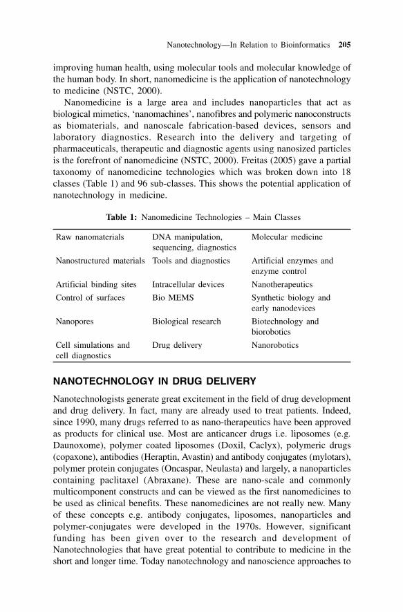
Nanotechnology—In Relation to Bioinformatics 205
improving human health, using molecular tools and molecular knowledge ofthe human body. In short, nanomedicine is the application of nanotechnologyto medicine (NSTC, 2000).
Nanomedicine is a large area and includes nanoparticles that act asbiological mimetics, ‘nanomachines’, nanofibres and polymeric nanoconstructsas biomaterials, and nanoscale fabrication-based devices, sensors andlaboratory diagnostics. Research into the delivery and targeting ofpharmaceuticals, therapeutic and diagnostic agents using nanosized particlesis the forefront of nanomedicine (NSTC, 2000). Freitas (2005) gave a partialtaxonomy of nanomedicine technologies which was broken down into 18classes (Table 1) and 96 sub-classes. This shows the potential application ofnanotechnology in medicine.
Table 1: Nanomedicine Technologies – Main Classes
Raw nanomaterials DNA manipulation, Molecular medicinesequencing, diagnostics
Nanostructured materials Tools and diagnostics Artificial enzymes andenzyme control
Artificial binding sites Intracellular devices Nanotherapeutics
Control of surfaces Bio MEMS Synthetic biology andearly nanodevices
Nanopores Biological research Biotechnology andbiorobotics
Cell simulations and Drug delivery Nanoroboticscell diagnostics
NANOTECHNOLOGY IN DRUG DELIVERY
Nanotechnologists generate great excitement in the field of drug developmentand drug delivery. In fact, many are already used to treat patients. Indeed,since 1990, many drugs referred to as nano-therapeutics have been approvedas products for clinical use. Most are anticancer drugs i.e. liposomes (e.g.Daunoxome), polymer coated liposomes (Doxil, Caclyx), polymeric drugs(copaxone), antibodies (Heraptin, Avastin) and antibody conjugates (mylotars),polymer protein conjugates (Oncaspar, Neulasta) and largely, a nanoparticlescontaining paclitaxel (Abraxane). These are nano-scale and commonlymulticomponent constructs and can be viewed as the first nanomedicines tobe used as clinical benefits. These nanomedicines are not really new. Manyof these concepts e.g. antibody conjugates, liposomes, nanoparticles andpolymer-conjugates were developed in the 1970s. However, significantfunding has been given over to the research and development ofNanotechnologies that have great potential to contribute to medicine in theshort and longer time. Today nanotechnology and nanoscience approaches to
206 M.H. Fulekar
particle design and formulations are beginning to expand the market formany drugs and are forming the basis for a very profitable niche within thepharma industry, wherein some predicted benefits are hyped (Moghimi et al.,2005).
However, examples in the scientific literature which demonstrate thepotential and the reason for excitement surrounding nanomedicine areoverwhelming. The reader is referred to the reviews (Freitas, 2005; Moghimiet al., 2005).
Today, nanomedicine has branched out in hundreds of different directions,but the core concept remains that ability to structure materials and devicesat the molecular scale can bring enormous immediate benefits in the researchand practice of medicine. It has been proposed that miniaturization of medicaltools will provide more accurate, more controllable, more versatile, morereliable, cheaper and faster approaches to enhancing the quality of humanlife.
REFERENCES
Andrew, C. and van Eschenbach (2004). Living with Cancer. OECD Observer, June2004.
Drexler, K.E. (1986). Engines of Creation : The coming era of Nanotechnology.Anchor Books. Garden City, N.Y.
Freitas, R.A. (2005). Nanomedicine. 2-9.http://www.cs.duke.edu/~reif/BMC/reports/BMC.FY99.reports/BMC.DARPA.
FY99.html.Lim, Hwa A (2003). Bioinformatics, Nanotechnology and SARS. 2003Linstedt, Dan E. (2004). DNA Computing. http://arstechnica.com/reviews/2q00/dna/
dna-1.html.Lyshenski, S.E., Kruegel, F.A. and Theodorou, E. (2003). Nanotechnology
Bioinformatics: Nanotechnology paradigm and its applications. Third IEEE con-ference on Nanotechnology, 2003. 2: 896-899.
Moghimi, S.M., Hunter, C.H. and Murray, J.C. (2005). Nanomedicine: Current sta-tus and future prospects. FASEB Journal, 19(3): 311-330.
NSTC (2000). Definition of Nanotechnology: http://www.becon.nih.gov/nstc_def_nano.htm, accessed 12 January, 2006.

Bioinformatics—ResearchApplications
S. Gupta
INTRODUCTION
Bioinformatics is a rapidly developing branch of biology which derivesknowledge from computer analysis of biological data and is highlyinterdisciplinary, using techniques and concepts from informatics, statistics,mathematics, physics, chemistry, biochemistry, and linguistics. It has manypractical applications in different areas of biology and medicine and itdescribes the use of computers to handle biological information. It issynonymous with “computational molecular biology” which means use ofcomputers for the characterization of the molecular components of livingthings and analyzing the information stored in the genetic code as well asexperimental results from various sources, patient statistics, and scientificliterature. Research in bioinformatics includes storage, retrieval, and analysisof the data. Richard Durbin, Head of Informatics at the Wellcome TrustSanger Institute, believes that all biological computing is not bioinformatics,e.g. mathematical modeling is not bioinformatics, even when connected withbiology-related problems. Bioinformatics is mainly management andsubsequent use of biological information, particularly, genetic information.Fredj Tekaia from the Institut Pasteur defines “Classical” bioinformatics asthe mathematical, statistical and computing methods that aim to solvebiological problems using DNA and amino acid sequences and relatedinformation. Medical imaging/image analysis and biologically-inspiredcomputation as well as genetic algorithms and neural networks too areconsidered as part of bioinformatics. These areas interact in strange ways.Neural networks are inspired by crude models of the functioning of nervecells in the brain and are used in a program called PHD to accurately predictthe secondary structures of proteins from their primary sequences.Bioinformatics is thus the processing of large amounts of biologically-derivedinformation pertaining to DNA sequences or X-rays.
The NIH Biomedical Information Science and Technology InitiativeConsortium agreed on the following definitions of bioinformatics and
12
208 S. Gupta
computational biology, recognizing that no definition could completelyeliminate overlap with other activities or preclude variations in interpretationby different individuals and organizations.
Bioinformatics: Research, development or application of computational toolsand approaches for expanding the use of biological, medical, behavioural orhealth data, including those to acquire, store, organize, archive, analyze orvisualize such data.
Computational Biology: The development and application of data-analyticaland theoretical methods, mathematical modeling and computational simulationtechniques to the study of biological, behavioural, and social systems.
The National Center for Biotechnology Information defines bioinformaticsas “the field of science in which biology, computer science, and informationtechnology merge into a single discipline.” There are three important sub-disciplines within bioinformatics:
(i) the development of new algorithms and statistics with which to assessrelationships among members of large data sets;
(ii) the analysis and interpretation of various types of data includingnucleotide and amino acid sequences, protein domains and proteinstructures; and
(iii) the development and implementation of tools that enable efficientaccess and management of different types of information.
APPLICATIONS OF BIOINFORMATICS
Bioinformatics has many applications in the research areas of medicine,biotechnology, agriculture, etc.
1. Genomics: It is an attempt to analyze or compare the entire geneticcomplement of a species. It is possible to compare genomes by comparingrepresentative subsets of genes within genomes.
2. Proteomics: Proteomics is the study of proteins—their location, structureand function. It is the identification, characterization and quantificationof all proteins involved in a particular pathway, organelle, cell, tissue,organ or organism that can provide accurate and comprehensive dataabout that system. It deals with the study of the proteome, calledproteomics viz. all the proteins in any given cell as well as the set ofall protein isoforms and modifications, the interactions between them,the structural description of proteins and their higher-order complexesand everything ‘post-genomic’.
3. Pharmacogenomics: Pharmacogenomics is the application of genomicapproaches and technologies to the identification of drug targets. It usesgenetic information to predict whether a drug will help make a patient
Bioinformatics—Research Applications 209
well or sick and study how genes influence the response of humans todrugs i.e. pharmacogenetics.
4. Pharmacogenetics: Pharmacogenetics is the study of how the actionsof and reactions to drugs vary with the patient’s genes. All individualsrespond differently to drug treatments; some positively, others withlittle obvious change in their conditions and yet others with side effectsor allergic reactions. Much of this variation is known to have a geneticbasis. Pharmacogenetics is a subset of pharmacogenomics which usesgenomic/bioinformatic methods to identify genomic correlates, forexample SNPs (Single Nucleotide Polymorphisms), characteristic ofparticular patient response profiles and use those markers to inform theadministration and development and improvement of therapies.
5. Cheminformatics: It deals with the mixing of information resourcesand appropriate analysis to transform data into information andinformation into knowledge for the specific purpose of drug leadidentification and optimization. Related terms of cheminformatics arechemometrics, computational chemistry, chemical informatics and chemicalinformation management/science.Chemical informatics: Computer-assisted storage, retrieval and analysisof chemical information, from data to chemical knowledge. (Chem. Inf.Lett., 2003, 6: 14)Chemometrics: The application of statistics to the analysis of chemicaldata (from organic, analytical or medicinal chemistry) and design ofchemical experiments and simulations. [IUPAC Computational]
6. Structural genomics or structural bioinformatics refers to the analysisof macromolecular structure, particularly proteins using computationaltools and theoretical frameworks. One of the goals of structural genomicsis the extension of the idea of genomics to obtain accurate three-dimensional structural models for all known protein families, proteindomains or protein folds. Structural alignment is a tool of structuralgenomics.
7. Comparative genomics: The study of human genetics by comparisonswith model organisms such as mice, the fruit fly and the bacterium E.coli.
8. Biophysics: The British Biophysical Society defines biophysics as “aninterdisciplinary field which applies techniques from the physical sciencesto understanding biological structure and function”.
9. Biomedical informatics/Medical informatics: Biomedical informaticsis an emerging discipline that has been defined as the study, invention,and implementation of structures and algorithms to improvecommunication, understanding and management of medical information.
10. Mathematical Biology: Mathematical biology also tackles biologicalproblems. The methods it uses to tackle them need not be numerical

210 S. Gupta
and need not be implemented in software or hardware. It includes thingsof theoretical interest which are not necessarily algorithmic, or molecularin nature nor useful in analyzing collected data.
11. Computational chemistry: Computational chemistry is the branch oftheoretical chemistry whose major goals are to create efficient computerprograms that calculate the properties of molecules (such as total energy,dipole moment, vibrational frequencies) and to apply these programs toconcrete chemical objects. It is also sometimes used to cover the areasof overlap between computer science and chemistry. It is a disciplineusing mathematical methods for the calculation of molecular propertiesor for the simulation of molecular behaviour. It also includes synthesisplanning, database searching, combinatorial library manipulation(Hopfinger, 1981; Ugi et al., 1990). [IUPAC Computational]
12. Functional genomics: Functional genomics is a field of molecularbiology using the vast wealth of data produced by genome sequencingprojects to describe genome function. It uses high-throughput techniqueslike DNA microarrays, proteomics, metabolomics and mutation analysisto describe the function and interactions of genes.
13. Pharmacoinformatics: Pharmacoinformatics concentrates on the aspectsof bioinformatics dealing with drug discovery.
14. In silico ADME-Tox Prediction: Drug discovery is a complex andrisky treasure hunt to find the most efficacious molecule which do nothave toxic effects but at the same time have desired pharmacokineticprofile. Huge amount of research is required to be done to come outwith a molecule which has the reliable binding profile. The moleculewhich shows better binding is then evaluated for its toxicity andpharmacokinetic profiles so that the molecule becomes a successfuldrug.
15. Agroinformatics/Agricultural informatics: Agro informaticsconcentrates on the aspects of bioinformatics dealing with plant genomes.
16. Systems biology: Systems biology is the coordinated study of biologicalsystems by investigating the components of cellular networks and theirinteractions, by applying experimental high-throughput and whole-genome techniques and integrating computational methods withexperimental efforts.
BIOINFORMATICS—TOOLS, SOFTWARES AND PROGRAMS
Bioinformatic tools are software programs that are designed for extractingthe meaningful information from the mass of molecular biology/biologicaldatabases and to carry out sequence or structural analysis.
The following factors must be taken into consideration when designingbioinformatics tools, software and programs:

Bioinformatics—Research Applications 211
(a) The end user (the biologist) may not be a frequent user of computertechnology.
(b) These software tools must be made available over the internet given theglobal distribution of the scientific research community.
Major Categories of Bioinformatic Tools
There are both standard and customized products to meet the requirementsof particular projects. There are data-mining software that retrieve data fromgenomic sequence databases and also visualization tools to analyze andretrieve information from proteomic databases. These can be classified ashomology and similarity tools, protein functional analysis tools, sequenceanalysis tools and miscellaneous tools. Everyday bioinformatics is done withsequence search programs like BLAST, sequence analysis programs like theEMBOSS and Staden packages, structure prediction programs likeTHREADER or PHD or molecular imaging/modeling programs like RasMoland WHATIF.
Homology and Similarity Tools
Homologous sequences are sequences related by divergence from a commonancestor. Thus the degree of similarity between two sequences can bemeasured while their homology is a case of being either true or false. Thisset of tools can be used to identify similarities between novel query sequencesof unknown structure and function and database sequences whose structureand function have been elucidated.
Protein Function Analysis
This group of programs allow you to compare your protein sequence to thesecondary (or derived) protein databases that contain information on motifs,signatures and protein domains. Highly significant hits against these differentpattern databases allow you to approximate the biochemical function of yourquery protein.
Structural Analysis
This set of tools allows the comparison of structures with the known structuredatabases. The function of a protein is more directly a consequence of itsstructure rather than its sequence with structural homologs tending to sharefunctions. The determination of a protein’s 2D/3D structure is crucial in thestudy of its function.
Sequence Analysis
This set of tools allows you to carry out more detailed analysis on yourquery sequence including evolutionary analysis, identification of mutations,hydropathy regions, CpG islands and compositional biases. The identification
212 S. Gupta
of these and other biological properties are all clues that aid the search toelucidate the specific function of your sequence.
Some Examples of Bioinformatic Tools
BLAST: BLAST (Basic Local Alignment Search Tool) comes under thecategory of homology and similarity tools. It is a set of search programsdesigned for the Windows platform and is used to perform fast similaritysearches regardless of whether the query is for protein or DNA. Comparisonof nucleotide sequences in a database can be performed. Also a proteindatabase can be searched to find a match against the queried protein sequence.NCBI has also introduced the new queuing system to BLAST (Q BLAST)that allows users to retrieve results at their convenience and format theirresults multiple times with different formating options. Depending on thetype of sequences to compare, there are different programs:
• blastp compares an amino acid query sequence against a protein sequencedatabase.
• blastn compares a nucleotide query sequence against a nucleotide sequencedatabase.
• blastx compares a nucleotide query sequence translated in all readingframes against a protein sequence database.
• tblastn compares a protein query sequence against a nucleotide sequencedatabase dynamically translated in all reading frames.
• tblastx compares the six-frame translations of a nucleotide query sequenceagainst the six-frame translations of a nucleotide sequence database.
FASTA: It is an alignment program for protein sequences created by Pearsinand Lipman (1988), and is one of the many heuristic algorithms proposedto speed up sequence comparison. The basic idea is to add a fast prescreenstep to locate the highly matching segments between two sequences, andthen extend these matching segments to local alignments using more rigorousalgorithms such as Smith-Waterman.
EMBOSS: EMBOSS (European Molecular Biology Open Software Suite)is a software-analysis package. It can work with data in a range of formatsand also retrieve sequence data transparently from the Web. Extensive librariesare also provided with this package, allowing other scientists to release theirsoftware as open source. It provides a set of sequence-analysis programs,and also supports all UNIX platforms.
Clustalw: It is a fully automated sequence alignment tool for DNA andprotein sequences. It returns the best match over a total length of inputsequences, be it a protein or a nucleic acid.
RasMol: It is a powerful research tool to display the structure of DNA,proteins, and smaller molecules. Protein Explorer, a derivative of RasMol,is an easier to use program.

Bioinformatics—Research Applications 213
PROSPECT: PROSPECT (PROtein Structure Prediction and EvaluationComputer ToolKit) is a protein-structure prediction system that employs acomputational technique called protein threading to construct a protein’s 3-D model.
PatternHunter: PatternHunter, based on Java, can identify all approximaterepeats in a complete genome in a short time using little memory on adesktop computer. Its features are its advanced patented algorithm and datastructures, and the java language used to create it. The Java language versionof PatternHunter is just 40 kB, only 1% the size of Blast, while offering alarge portion of its functionality.
COPIA: COPIA (COnsensus Pattern Identification and Analysis) is a proteinstructure analysis tool for discovering motifs (conserved regions) in a familyof protein sequences. Such motifs can be then used to determine membershipto the family for new protein sequences, predict secondary and tertiarystructure and function of proteins and study evolution history of the sequences.
Application of Programs in Bioinformatics
JAVA in Bioinformatics
Since research centres are scattered all around the globe ranging from privateto academic settings, and a range of hardware and OSs are being used, Javais emerging as a key player in bioinformatics. Physiome Sciences’ computer-based biological simulation technologies and Bioinformatics Solutions’PatternHunter are two examples of the growing adoption of Java inbioinformatics.
Perl in Bioinformatics
String manipulation, regular expression matching, file parsing, data formatinterconversion etc. are the common text-processing tasks performed inbioinformatics. Perl excels in such tasks and is being used by many developers.Yet, there are no standard modules designed in Perl specifically for the fieldof bioinformatics. However, developers have designed several of their ownindividual modules for the purpose, which have become quite popular andare coordinated by the BioPerl project.
Bioinformatic Projects
An exhaustive list of various bioinformatic projects is given here; adetailed description of these projects is available on the internet. This listincludes BioPerl, BioXML, Biocorba, Ensembl, Bioperl-db, Biopythonand BioJava.
Biopython and bioJava are open source projects with very similar goalsto bioPerl. However their code is implemented in python and java,respectively. With the development of interface objects and biocorba, it is

214 S. Gupta
possible to write java or python objects which can be accessed by a bioPerlscript, or to call bioPerl objects from java or python code. Since biopythonand bioJava are more recent projects than bioPerl, most effort to date hasbeen to port bioPerl functionality to biopython and bioJava rather than theother way around. However, in the future, some bioinformatic tasks mayprove to be more effectively implemented in java or python in which casebeing able to call them from within bioPerl will become more important.
Major bioinformatic activities are carried out using three types of MolecularModeling programs viz., AMBER, CHARMM and GROMACS as well asthree types of Genetic Algorithms STRUCTURE OPTIMIZATION,SEQUENCE ALIGNMENT and PSEGA.

Appendix 1
BIOINFORMATICS—WEBSITES
A System for Easy Analysis of Lots of Sequences (SEALS)http://www.ncbi.nlm.nih.gov/CBBresearch/Walker/SEALS/index.html
Applied Bioinformatics Journalhttp://www.openmindjournals.com/bioinformatics.html
Australian Genome Research Facility (AGRF)http://www.agrf.org.au/
Beijing Genomics Institute (BGI)http://coe.genomics.org.cn/
Bielefeld University Bioinformatics Serverhttp://bibiserv.techfak.uni-bielefeld.de/
BIMAS - Bioinformatics and Molecular Analysis Sectionhttp://bimas.cit.nih.gov/
BioInform Bioinformatics News Servicehttp://www.bioinform.com/index.htm
Bioinformatics & Computational Biology at ISUhttp://www.bcb.iastate.edu/
Bioinformatics & Computational Biology Index of Resourceshttp://www.unl.edu/stc-95/ResTools/biotools/biotools4.html
Bioinformatics (Genomics) Selected Papershttp://post.queensu.ca/~forsdyke/bioinfor.htm
Bioinformatics 2001, 2002http://www.ida.his.se/ida/bioinformatics2001/
Bioinformatics and XMLhttp://www.biosino.org/bioinformatics/011212-2.htm
Bioinformatics at NIHhttp://grants1.nih.gov/grants/bistic/bistic.cfm
Bioinformatics Canadahttp://www.bioinformatics.ca/

216 Appendix 1
Bioinformatics Centrehttp://bioinfo.ernet.in/
Bioinformatics Centre (BIC)http://www.bic.nus.edu.sg/
Bioinformatics Education and Researchhttp://bioinf.man.ac.uk/
Bioinformatics Forumhttp://www.biowww.net/forum/list.php?f=4
Bioinformatics Glossaryhttp://www.genomicglossaries.com/content/Bioinformatics_gloss.asphttp://www.incyte.com/glossary/index.shtml
Bioinformatics Grouphttp://life.anu.edu.au/
Bioinformatics Guideshttp://his.cbi.pku.edu.cn:1947/binf/Guides/
Bioinformatics in Indiahttp://www.bioinformatics-india.com/index.php3
Bioinformatics Informationhttp://www.bioinformatics.pe.kr/
Bioinformatics Institute (BII)http://www.bii-sg.org/
Bioinformatics Linkshttp://www.ii.uib.no/~inge/list.html
Bioinformatics Links and Siteshttp://www.colorado.edu/chemistry/bioinfo/
Bioinformatics Organizationhttp://bioinformatics.org/
Bioinformatics Resourceshttp://www.genet.sickkids.on.ca/bioinfo_resources/
Bioinformatics Serviceshttp://www.bioinformaticsservices.com/
Bioinformatics: Biology and Molecular Biology Resourceshttp://www.nwfsc.noaa.gov/protocols/bioinformatics.html
Bioinformatics: Human Genome Project Informationhttp://www.ornl.gov/hgmis/research/informatics.html

Appendix 1 217
Bioinformatics: Sequence and Genome Analysishttp://www.bioinformaticsonline.org/
BioInformer Newsletterhttp://bioinformer.ebi.ac.uk/
BioTech: Bioinformaticshttp://biotech.icmb.utexas.edu/pages/bioinfo.html
BMC Bioinformatics Research Papershttp://www.biomedcentral.com/bmcbioinformatics/
Boston University Bioinformaticshttp://bioinfo.bu.edu/
Buffalo Center of Excellence in Bioinformaticshttp://www.bioinformatics.buffalo.edu/
CBI - Center of BioInformatics, Peking Universityhttp://www.cbi.pku.edu.cn/
Center for Bioinformatics & Computational Biology at Dukehttp://bioinformatics.duke.edu/
Center for Biological Sequence (CBS) Analysishttp://www.cbs.dtu.dk/
Comprehensive Bioinformatics Solutions: What’s new inBioinformatics?http://www.accelrys.com/bio/
Computational Biology At ORNLhttp://compbio.ornl.gov/
Computational Proteomics and Protein Structural Informationhttp://www.strubix.com/
Developing Bioinformatics Computer Skills (Book) 2001http://www.oreilly.com/catalog/bioskills/
European Bioinformatics Institute (EBI)http://www.ebi.ac.uk/
ExPASy Molecular Biology Serverhttp://www.expasy.org/
Gene Alliance - The Key to Genomic Knowledgehttp://www.gene-alliance.com/
GeneBio Geneva Bioinformaticshttp://www.genebio.com/

218 Appendix 1
GeneCards - A Database of Human Geneshttp://genecards.bjmu.edu.cn/
Genome Megasequencing Programhttp://megasun.bch.umontreal.ca/ogmpproj.html
Genome Technology Magazinehttp://www.genome-technology.com/
Google Web Directory: Bioinformaticshttp://directory.google.com/Top/Science/Biology/Bioinformatics/
How to become a Bioinformatics Experthttp://www.techfak.uni-bielefeld.de/bcd/ForAll/Econom/study.html
IBM Bioinformatics & Pattern Discovery Grouphttp://researchweb.watson.ibm.com/bioinformatics/
IEEE Computer Society Bioinformatics Conferencehttp://conferences.computer.org/bioinformatics/
INCOGEN: Institute for Computational Genomicshttp://www.incogen.com/
Institute of Bioinformatics, Tsinghua Universityhttp://www.bioinfo.tsinghua.edu.cn/
Integrated Bioinformaticshttp://www.biosino.org/bioinformatics/010807-3.htm
International Conference on Bioinformatics 2002 (INCoB 2002)http://incob.biotec.or.th/
ISREC Bioinformatics Grouphttp://www.isrec.isb-sib.ch/
Lab for Advanced Sequence Analysishttp://shark.ucsf.edu/gc/
MCW Bioinformatics Research Center (BRC)http://brc.mcw.edu/
Molecular Biology and Bioinformatics Resourceshttp://www.molbio.org/
Molecular Genetics Serverhttp://www.pasteur.fr/recherche/borrelia/Welcome.html
National Bioinformatics Institute (NBI)http://www.bioinfoinstitute.com/
National Center for Biotechnology Information (NCBI)http://www.ncbi.nlm.nih.gov/About/primer/bioinformatics.html

Appendix 1 219
O’Reilly Bioinformatics Conference 2003http://conferences.oreillynet.com/bio2003/
Online Journal of Bioinformatics (OJB)http://www.cpb.ouhsc.edu/ojvr/bioinfo.htm
Online Lectures on Bioinformaticshttp://lectures.molgen.mpg.de/
Open Bioinformatics Foundationhttp://www.open-bio.org/
Open Directory: Bioinformaticshttp://dmoz.org/Science/Biology/Bioinformatics/
Oxford Journals Online: Bioinformaticshttp://bioinformatics.oupjournals.org/
PEDANT: Protein Extraction, Description, and Analysis Toolhttp://pedant.gsf.de/
Peking-Yale Joint Research Center For Plant Molecular Genetics andAgro-Biotechnologyhttp://www.pyc.pku.edu.cn/
Program in Proteomics and Bioinformaticshttp://p-b.med.utoronto.ca/
Protein Data Bank (PDB)http://www.rcsb.org/pdb/
Protein Sequence Analysis: A Practical Guidehttp://www.biochem.ucl.ac.uk/bsm/dbbrowser/jj/prefacefrm.html
Society for Bioinformaticshttp://www.socbin.org/
South African National Bioinformatics Institute (SANBI)http://www.sanbi.ac.za/
Southampton Bioinformatics Data Server (SBDS)http://molbiol.soton.ac.uk/
Stockholm Bioinformatics Center (SBC)http://www.sbc.su.se/
Swiss Institute of Bioinformatics (SIB)http://www.isb-sib.ch/
TBI—Theoretical Bioinformaticshttp://www.dkfz-heidelberg.de/tbi/

220 Appendix 1
TBR—The Bioinformatics Resourceshttp://www.hgmp.mrc.ac.uk/CCP11/index.jsp
Texas A&M Bioinformatics Working Grouphttp://www.csdl.tamu.edu/FLORA/tamuherb.htm
The Asia Pacific Bioinformatics Network (APBioNET)http://www.apbionet.org/
The BioPerl Projecthttp://www.bioperl.org/
The Brutlag Bioinformatics Grouphttp://motif.stanford.edu/
The Genome Databasehttp://gdbwww.gdb.org/
The Virtual Institute of Bioinformaticshttp://www.bioinf.org/vibe/index.html
TUBIC - Tianjin University BioInformatics Centerhttp://tubic.tju.edu.cn/
UCLA Bioinformaticshttp://www.bioinformatics.ucla.edu/
UCSC Genome Bioinformaticshttp://genome.ucsc.edu/
Upenn Center for Bioinformaticshttp://www.pcbi.upenn.edu/
Virginia Bioinformatics Institute (VBI)http://www.vbi.vt.edu/
Visual Bioinformaticshttp://www.visual-bioinformatics.com/
Visualization For Bioinformaticshttp://industry.ebi.ac.uk/~alan/VisSupp/
Weizmann Institute of Science: Genome and Bioinformaticshttp://bioinfo.weizmann.ac.il/bioinfo.html
What Is Bioinformatics?http://bioinformatics.weizmann.ac.il/cards/bioinfo_intro.html
Yale Bioinformaticshttp://bioinfo.mbb.yale.edu/

Appendix 2
BIOIFORMATICS – TERMINOLOGY
A
Accession number: An identifier supplied by the curators of the majorbiological databases upon submission of a novel entry that uniquelyidentifies that sequence (or other) entry.
Active site: The amino acid residues at the catalytic site of an enzyme.These residues provide the binding and activation energy needed to placethe substrate into its transition state and bridge the energy barrier of thereaction undergoing catalysis.
Additive genetic effects: The combined effects of alleles at different loci areequal to the sum of their individual effects.
Adenine: A nitrogenous base, one member as the base pair AT (adenine–thymine).
Agents: Software modules (independent, autonomous) that can search theinternet for data or content pertinent to a particular application such as agene, protein, or biological system.
Aggregation techniques: A technique used in model organisation studies inwhich embryos at the 8-cell stage of development are pushed together toyield a single embryo.
Algorithm: A fixed procedure embodied in a computer program.
Alignment: The process of lining up two or more sequences to achievemaximal levels of identity (and conservation, in case of amino acidsequencing) for the purpose of assessing the degree of similarity and thepossibility of homology.
Allele frequency: Relative proportion of a particular allele among individualsof a population.
Alleles: One of two or more alternate forms of a gene.
Allogenic: Variation in alleles among members of the same species.
Alternative splicing: Alternate combinations of a folded protein that ispossible due to recombination of multiple gene segments during mRNAsplicing that occurs in higher organisms.
Amino acid: The basic building block of proteins.

222 Appendix 2
Amplification: An increase in the number of copies of a specific DNAfragment.
Annotation: Adding pertinent information such as gene coded for aminoacid sequence, or other commentary to the database entry of raw sequenceof DNA bases.
Anticodon: The triplet of contiguous bases on tRNA that binds to the codonsequence of nucleotides, on mRNA. Example: GGG codes for glycine.
Antigen: Any foreign molecule that stimulates an immune response in avertebrate organism. Many antigens act as the surface proteins of foreignorganisms.
Antisense: Nucleic acid that has a sequence exactly opposite to an mRNAmolecule made by the body; binds to the mRNA molecule to prevent aprotein from being made.
Apoptosis: A programed cell death, the body’s normal method of disposingof damaged, unwanted or unneeded cells.
Assay: A method for measuring a biological activity. This may be enzymeactivity, binding affinity, or protein turnover. Most assays utilize ameasurable parameter such as colour, fluorescence or radioactivity tocorrelate with the biological activity.
Assembly: Putting sequenced fragments of DNA into their correctchromosomal positions.
Autosome: When the chromosome is not involved in sex determination.The diploid human genome consists of a total of 46 chromosomes, 22pairs of autosomes, and one pair of sex chromosomes (the X and Ychromosomes).
B
Bacterial artificial chromosome: Cloning vector that can incorporate largefragments of DNA.
Bacteriophage: A virus that infects bacteria. The bacteriophage DNA hasserved as a basis for cloning vectors, and is also utilized to create phaselibraries containing human or other genes.
Baculovirus: Virus which forms the basis of a protein expression system.
Base pair: A pair of nitrogenous bases (a purine and pyrimidine), heldtogether by hydrogen bonds, that form the core of DNA and RNA i.e. theA:T, G:C and A:U interactions.
Base sequence: The order of nucleotide bases in a DNA molecule; determinesstructure of proteins encoded by the DNA.
Base sequence analysis: A method, sometimes automated for determiningthe base sequence.

Appendix 2 223
Bioinformatics: The science of managing and analyzing biological datausing advanced computing techniques.
Bivalent: Two binding sites, having two free electrons available for binding.
BLAST: A computer program that identifies homologous (similar) genes indifferent organisms such as human, fruit fly or nematode.
C
Cancer: A disease in which abnormal cells divide and grow unchecked. Cancercan spread from its original site to other parts of the body and can be fatal.
Candidate gene: A gene located in a chromosome region suspected of beinginvolved in a disease.
Capillary array: Gel-filled silica capillaries used to separate fragments forDNA sequencing. The small diameter of the capillaries permit theapplication of higher electric fields, providing high speed, high throughputseparations that are significantly faster than traditional slab gels.
Carrier: An individual who possesses an unexpressed, recessive trait.
cDNA library: A collection of DNA sequences that code for genes. Thesequences are generated in the laboratory from mRNA sequences.
Cell: The basic unit of any living organism that carries on the biochemicalprocesses of life.
Centromere: A specialized chromosome region to which spindle fibres attachduring cell division.
Chloroplast chromosome: Circular DNA found in the photosynthesizingorganelle (chloroplast) of plants instead of the cell nucleus where mostgenetic material is located.
Chromatin: Chromosome as it appears in its condensed state composed ofDNA and associated proteins.
Chromosomal deletion: The loss of part of a chromosome’s DNA.
Chromosomal inversion: Chromosome segments that have been turned 180degrees. The gene sequence for the segment is reversed with respect tothe rest of the chromosome.
Chromosome: The structure in the cell nucleus that contains the entirecellular DNA together with a number of proteins that compact and packagethe DNA.
Chromosome painting: Attachment of certain fluorescent dyes to targetedparts of the chromosome, which is used for particular disease diagnosis.
Clone: An exact copy mode of biological material such as DNA segment(e.g. a gene or other region), a whole cell, or a complete organism.
Cloning: The formation of clones or exact genetic replicas.
Codon: A sequence of three adjacent nucleotides that designates a specificamino acid or start/stop site transcription.

224 Appendix 2
Coding regions: Portion of a genomic sequences bounded by start and stopcodons that identifies the sequence of the protein being coded for by aparticular gene.
Comparative genomics: The study of human genetics by comparisons withmodel organisms such as mica, fruit fly and the bacterium (E. coli).
Complementary DNA (cDNA): DNA strand copied from mRNA usingreverse transcriptase. A cDNA library represents all of the expressed DNAin a cell.
Complementary sequence: Nucleic acid base sequence that can form adouble-stranded structure with another DNA fragment by following base-pairing rules (A pairs with T and C with G). The complementary sequenceto GTAC, for example, is CATG.
Configuration: The complete ordering and description of all parts of asoftware or database system. Configuration management is the use ofsoftware to identify inventory and maintain the component modules thattogether comprise one or more systems or products.
Confirmation: The precise three dimensional arrangement of atoms and bondsin a nucleotide describing its geometry and hence its molecular function.
Conservation: Changes at a specific position of an amino acid or (lesscommonly, DNA) sequence that preserve the physico-chemical propertiesof the original residue.
Conserved sequence: A base sequence in a DNA molecule (amino acidsequence in a protein) that has remained essentially unchanged throughoutevolution.
Constitutive synthesis: Synthesis of mRNA and protein at an unchangingor constant rate regardless of a cell’s requirements.
Cosmids: DNA vectors that allow the insertion of long fragments of DNA(up to 50 K bases).
Crystal structure: Describe the high resolution molecular structure derivedby X-ray crystallographic analysis of protein or other biomolecualr crystals.
Cytogenetics: The study of the physical appearance of chromosomes.
Cytological map: A type of chromosome map whereby genes are located onthe basis of cytological findings obtained with the aid of chromosomemutations.
Cytoplasm: The medium of the cell between the nucleus and the cell membrane.
Cytosine: A pyrimidine base found in DNA and RNA.
D
Data mining: The ability to query very large databases in order to satisfya hypothesis; or to interrogate a database in order to generate newhypothesis based on rigorous statistical correlations.

Appendix 2 225
Data processing: The systematic performance of operations upon data suchas handling, merging, sorting and computing. The semantic content of theoriginal data should not be changed, but the semantic content of theprocessed data may be changed.
Data warehouse: A collection of databases, data tables and mechanisms toaccess the data on a single subject.
Database: Any file system by which data gets stored following a logicalprocess.
Deconvolution: Mathematical procedure to separate the overlapping effectsof molecules such as mixtures of compounds in a high-throughput screen,or mixtures of cDNAs in a high density array.
Deletion: A loss of part of the DNA from a chromosome can lead to adisease of abnormality.
Deletion map: A description of a specific chromosome that uses definedmutations; specific deleted areas in the genome as ‘biochemical signposts’,or markers for specific areas.
Dimer: A composite molecule formed by the binding of two molecules.
Directed evolution: A laboratory process used on isolated molecules ormicrobes to cause mutations and identify subsequent adaptations to novelenvironments.
Directed mutagenesis: Alteration of DNA at a specific site and its reinsertioninto an organism to study any effects of the change.
Directed sequencing: Alleles carrying particular DNA sequences associatedwith the presence of disease.
DNA: The molecule that encodes genetic information. DNA is a double-stranded molecule held together by weak hydrogen bonds base pairs ofnucleotides. The four nucleotides in DNA contain the bases adenine (A),guanine (G), cytosine (C) and thymine (T). In nature, base pairs formonly between A and T and between G and C; thus the base sequence ofeach single strand can be deduced from that of its partner.
DNA bank: A service that stores DNA extracted from blood samples orother human tissue.
DNA finger printing: A technique for identifying human individuals basedon a restriction enzyme digest of tandemly repeated DNA sequences thatare scattered throughout the human genome, but are unique to eachindividual.
DNA microarrays: The deposition of oligonucleotides or cDNAs onto aninert substrate such as glass or silicon. Thousands of molecules may beorganised spatially into a high density matrix. These DNA chips may beprobed to allow expression monitoring of many thousand of genessimultaneously. Uses include study of polymorphisms in genes, de novosequencing or molecular diagnosis of disease.

226 Appendix 2
DNA polymerase: Enzyme that catalyses the synthesis of DNA from aDNA template given the deoxy ribo-nucleotide precursors.
DNA probes: Short single stranded DNA molecules of specific base sequence,labeled either radioactively or immunologically, that are used to detectand identify the complementary base sequence in a gene or genome byhybridizing specifically to that gene or sequence.
DNA repair genes: Genes encoding proteins that correct errors in DNAsequencing.
DNA replication: The uses of existing DNA as a template for the synthesisof new DNA strands. In humans and other eukaryotes, replication occursin the cell nucleus.
DNase: One of a series of enzymes that can digest DNA.
Domain: A discrete portion of a protein with its own function. Thecombination of domains in a single protein determines its overall function.
Dominant: Allele that is almost always expressed, even if only one copy ispresent.
Drug: An agent that affects a biological process, specifically, a moleculewhose molecular structure can be correlated with its pharmacological activity.
Drug discovery cycle: The cycle of events requested to develop a new drug.Typically, this involves research, pre-clinical testing and clinicaldevelopment, and can take from 5 to 12 years.
E
E. Colia (Escherichia Coli): A bacterium that has been studied intensivelyby geneticists because of its small genome size, normal lack ofpathogenicity and easy growth in the laboratory.
Electrophoresis: A method of separating large molecules (DNA fragmentsor proteins) from a mixture of similar molecules. An electric current ispassed through a medium containing the mixture, and each kind of moleculetravels through the medium at a different rate, depending on its electricalcharge and size. Agarose and acrylamide gels are the media commonlyused for electrophoresis of proteins and nucleic acids.
Electroporation: A process using high voltage current to make cellmembranes permeable to allow the introduction of new DNA, commonlyused in recombinant DNA technology.
Embryonic stem cells: An embryonic cell that can replicate indefinitely,transform into other type of cells and serve as a continuous source of newcells.
Enhancers: DNA sequences that can greatly increase the transcription ratesof genes even though they may be far upstream or downstream from thepromoter they stimulate.

Appendix 2 227
Eukaryote: Cell or organism with membrane-bound, structuring discretenucleus and other well-developed subcellular compartments. For example:Eukaryotes include all organisms except viruses, bacteria and blue greenalgae.
Enzyme: A protein that acts as a catalyst, spreading the rate at which abiochemical reaction proceeds but not altering the direction or nature ofthe reaction.
EST (Expressed Sequence Tag): A short strand of DNA that is a part of acDNA molecule and can act as identifier of a gene. Used in locating andmapping genes.
Exogenous DNA: DNA originating outside an organism that has beenintroduced into the organism.
Exon: The protein-coding DNA sequence of a gene.
Exonuclease: Enzyme that cleans nucleotides frequently from free ends ofa linear nucleic acid substrate.
Expression profile: The level and duration of expression of one or moregenes, selected from a particular cell or tissue type, generally obtained bya variety of high-throughput methods, such as sample sequencing, serialanalysis, or micro array-based detection.
Expression vector: A cloning vector that is engineered to allow the expressionof protein from a cDNA. The expression vector provides an appropriatepromoter and restriction sites that allow insertion of cDNA.
F
FASTA: The first widely used algorithm for database similarity searching.The program looks for optimal local alignments by scanning the sequencefor small matches called “words”. The sensitivity and speed of the searchare inversely related and controlled by the “K-tup” variable which specifiesthe size of a “word”.
Filtering: Also known as masking. The process of hiding regions of (nucleicacid or amino acid) sequence having characteristics that frequently leadto spurious high scores.
Finger printing: In genetics, the identification of multiple specific alleleson a person’s DNA to produce a unique identifier for that person.
Flow karyotyping: Use of flow cytometry to analyze and separatechromosomes according to their DNA content.
Fluorescence In-Situ Hybridization (FISH): A physical mapping approachthat uses fluorescein tags to detect hybridization of probes with metaphasechromosomes and with the less-condensed somatic interphase chromatin.
Frame shift: A deletion, substitution, or duplication of one or more basesthat causes the reading frame of a structural gene to shift the normalseries of triplets.

228 Appendix 2
Full gene sequence: The complete order of bases in gene. This orderdetermines which protein a gene will produce.
Functional genomics: The study of genes, their resulting proteins, and therole played by the proteins, the body’s biochemical processes.
Fusion protein: The protein resulting from the genetic joining and expressionof two different genes.
G
Gamete: Mature male or female reproductive cell (sperm or ovum) with ahaploid set of chromosomes (23 for humans).
Gel electrophoresis: A technique by which molecules are separated by sizeor charge by passing them through a gel under the influence of an externalelectric field.
Gene: The fundamental physical and functional unit of heredity. A gene isan ordered sequence of nucleotides located in a particular position on aparticular chromosome that encodes a specific functional product (i.e. aprotein or RNA molecule).
Gene amplification: Repeated copying of a piece of DNA; a characteristicof tumour cells.
Gene bank: Data bank of genetic sequence operated by a division of theNational Institute of Health.
Gene chip technology: Development of cDNA micro arrays from a largenumber of genes. Used to monitor and measure changes in gene expressionfor each gene represented on the chip.
Gene expression: The conversion of information from gene to protein viatranscription and translation.
Gene families: Subsets of genes containing homologous sequences whichusually correlate with a common function.
Gene library: A collection of cloned DNA fragments created by restrictionendonuclease digestion that represent part or all of an organism’s genome.
Gene pool: All the variations of genes in a species.
Gene prediction: Predictions of possible genes made by a computer programbased on how well a stretch of DNA sequence matches known genesequences.
Gene product: The product, either RNA or protein, that results fromexpression of a gene. The amount of gene product reflects the activity ofthe gene.
Gene project: Research and technology development effort aimed atmapping and sequencing the genome of human beings and certain modelorganisms.

Appendix 2 229
Gene therapy: The use of genetic material for therapeutic purposes. Thetherapeutic gene is typically delivered using recombinant virus or liposomebased delivery systems.
Gene transfer: Incorporation of new DNA into an organism’s cells, usuallyby a vector such as modified virus. Used in gene therapy.
Genetic: The study of inheritance patterns of specific traits.
Genetic code: The mapping of all possible codons into the 20 amino acidsincluding the start and stop codons.
Genetic counselling: Provides patients and their families with education andinformation about genetic-related conditions and helps them make informeddecisions.
Genetic discrimination: Prejudice against those who have or are likely todevelop an inherited disorder.
Genetic engineering: The procedure used to isolate, splice and manipulateDNA outside the cell. Genetic engineering allows a recombinant engineeredDNA segment to be introduced into a foreign cell or organism and be ableto replicate and function normally.
Genetic illness: Sickness, physical disability or other disorders resultingfrom the inheritance of one or more deleterious alleles.
Genetic marker: Any gene that can be readily recognized by its phenotypiceffect, and which can be used as a marker for a cell, chromosome orindividual carrying that gene.
Genetic polymorphism: Difference in DNA sequence among individuals,groups or populations (e.g. genes for blue eyes versus brown eyes).
Genetic predisposition: Susceptibility to a genetic disease. May or may notresult in actual development of the disease.
Genetic testing: Analyzing an individual’s genetic material to determinepredisposition to a particular health condition or to confirm a diagnosisof genetic disease.
Genome: The complete genetic content of an organism.
Genomic DNA: DNA sequence typically obtained from mammalian or otherhigher-order species, which include intron and exon sequence (codingsequence) as well as non-coding regulatory sequences such as promoterand enhanced sequences.
Genomics: The analysis of the entire genome of a chosen organism.
Genotype: The total set of genes present in the cells of an organism. Also,refers to a set of alleles at a single gene locus.
Germ cell: Sperm and egg cells and their precursors. Germ cells are haploidand have only one set of chromosomes (23 in all), while all other cellshave two copies (46 in all).

230 Appendix 2
Germ line: The continuation of a set of genetic information from onegeneration to the next.
Global alignment: The alignment of the nucleic acid or protein sequencesover their entire length.
Glycosylation: The addition of carbohydrate groups (sugars) e.g. topolypeptide chains.
Guanine (G): One of the nitrogenous purine bases found in DNA and RNA
Gyandromorph: Organism that have both male and female cells and thereforeexpress both male and female characteristics.
H
Hairpin: A double-vertical region in a single DNA or RNA strand formedby the hydrogen-bonding between adjacent inverse complementarysequences to form a hairpin shaped structure.
Haploid: A single set of chromosomes present in the egg and sperm cellsof animals and in the egg and pollen cells of plants.
Haplotype: A way of denoting the collective genotype of a number ofclosely linked loci on a chromosome.
Hemizygous: Having only one copy of particular gene, e.g. human malesare hemizygous as only one copy of genes found on Y-chromosomes.
Hereditary cancer: Cancer that occurs due to the inheritance of an alteredgene within a family.
Heterodimer: Protein composed of two different chains or subunits.
Heteroduplex: Hybrid structure formed by the annealing of two DNA strands(or an RNA and DNA) that have sufficient complementary sequence toallow hydrogen bonding.
Highly conserved sequence: DNA sequence that is very similar acrossseveral different types of organisms.
High-throughput sequencing: A fast method of determining the order ofbases in DNA.
Homeodomain: A 60-amino acid protein domain coded by the homeoboxregion of a homeotic gene.
Homeotic gene: A gene that controls the activity of other genes involved inthe development of a body plan. Homeotic genes have been found inorganisms ranging from plants to humans.
Homologous chromosome: Chromosome containing the same linear genesequences as another, each derived from one parent.
Homologous recombination: Swapping of DNA fragments between pairedchromosomes.
Homologue: A member of a chromosome pair in diploid organisms or agene that has the same origin and functions in two or more species.

Appendix 2 231
Homology: Similarity in DNA or protein sequences between individuals ofthe same species or among different species.
Homozygote: An organism that has two identical alleles of a gene.
Housekeeping genes: Genes that are always expressed due to their constantrequirement by the cell.
HSP: High-Scoring Segment Pair. Local alignments with no gaps that achieveone of the top alignment scores in a given search.
Human artificial chromosome (HAC): A vector used to hold large DNAfragments.
Hybrid: The offspring of genetically different parents.
Hybridization: The process of joining two complementary strands of DNAor one each of DNA and RNA to form a double-stranded molecule.
I
Identical twin: Twins produced by the division of a single zygote; both haveidentical genotype.
Identity: The extent to which two (nucleotide or amino acid) sequences areinvariant.
Immunoglobulin: A member of the globulin protein family consisting of thelight and too heavy chains linked by disulfide bends. All antibodies areimmunoglobulin.
Immunotherapy: Using the immune system to treat disease, e.g. in thedevelopment of vaccines. May also refer to the therapy of diseases causedby the immune system.
Inherit: In genetics, to receive genetic material from parents throughbiological processes.
Insertion: A mutation that occurs when an extra nucleotide is inserted intoa gene sequence, causing a frame shift.
In-situ hybridization: A variation of the DNA/RNA hybridization procedurein which the denatured DNA is in place in the cell and is then challengedwith RNA or DNA extracted from another source.
Integration: The physical insertion of DNA into the host cell genome. Theprocess is used by retroviruses where a specific enzyme catalyses theprocess or can occur at random sites with other DNA.
Interphase: The period in the cell cycle when DNA is replicated in thenucleus, followed by mitosis.
Introns: Nucleotide sequences found in the structural genes of eukaryotesthat are non-coding and interrupt the sequences containing informationthat code for polypeptide chains. Intron sequences are spliced out of theirRNA transcripts before maturation and protein synthesis.
232 Appendix 2
In-vitro: Studies performed outside a living organism such as in a laboratory.
In-vivo: Studies carried out in a living organism.
Isoschizomers: Two different restriction enzymes which recognize and cutDNA at the same recognition site.
Isozymes: Two or more enzymes capable of catalyzing the same reactionbut varying in their specificity due to differences in their structures andhence their efficiencies under different environmental conditions.
J
Junk DNA: Term used to describe the excess DNA that is present in thegenome beyond that required to encode proteins. A misleading term sincethese regions are likely to be involved in gene regulation, and other as yetunidentified functions.
K
Karyotype: The constitution of chromosomes in a cell or individual.
Kilobase (Kb): Unit of length for DNA fragments equal to 1000 nucleotides.
Knockernt: Deactivation of specific genes; uses in laboratory organisms tostudy gene function.
L
Lambda: A statistical parameter used in calculating BLAST scores that canbe thought of as a natural scale for scoring. The value lambda is used inconverting a raw score (S) to a bit score (S �).
Lead compounds: A candidate compound identified as the best “hit” (tightbinder) after screening of a combinational (or others) compound library,that is then taken into further rounds of screening to determine its suitabilityas a drug.
Leucine zipper: Protein motif which binds DNA in which 4-5 leucines arefound at 7 amino acid intervals. This motif is present typically intranscription factors and other proteins that bind DNA.
Lexicon: In bioinformatics, a lexicon refers to a pre-defined list of termsthat together completely define the contents of a particular database.
Library: An unordered collection of clones (i.e. clones DNA from a particularorganism) whose relationship to each other can be established by physicalmapping.
Ligand: Any small molecule that binds to a protein or receptor; the cognatepartner of many cellular proteins, enzymes and receptors.
Linkage: The association of genes (or genetic loci) on the same chromosome.Genes that are linked together tend to be transmitted together.

Appendix 2 233
Linkage map: A map of the relative positions of genetic loci on achromosome, determined on the basis of how often the loci are inheritedtogether. Distance is measured in centimorgans (cM).
Local alignment: The alignment of some portion of two nucleic acid orprotein sequences.
Localize: Determination of the original position (locus) of a gene or othermarker on a chromosome.
Locus: The position on a chromosome of a gene or other chromosomemarker; also, the DNN at that position. The use of locus is sometimesrestricted to mean expressed DNA regions.
Low Complexity Region (LCR): Regions of biased composition includinghomopolymeric runs, short-period repeats, and more subtleoverrepresentation of one or a few residues. The program is used to maskor filter LCRs in amino acid queries.
M
Macro restriction map: Map depicting the order of and distance betweensites at which restriction enzymes cleave chromosomes.
Map unit: A measure of genetic distance between two linked genes thatcorresponds to a recombination frequency of 1%.
Mapping population: The group of related organisms used in constructinga genetic map.
Markov chain: Any multivariate probability density, whose independencediagram is a chain. The variables are ordered and each variable “depends”only on its neighbours in the sense of being conditionally independent ofthe others. Markov chains are an integral component of hidden Markovmodels.
Masking: Also known as filtering. The removal of repeated or low complexityregions from a sequence in order to improve the sensitivity of sequencesimilarity searches performed with that sequence.
Mass spectrometry: An instrument used to identify chemicals in a substanceby their mass and charge.
Megabase (Mb): Unit of length for DNA fragments equal to one millionnucleotides and roughly equal to 1 cM.
Meiosis: A process within the cell nucleus that results in the reduction of thechromosome number from diploid (two copies of each chromosome) tohaploid (a single copy) through two reductive divisions in germ cells.
Melting (of DNA): The denaturation of double-stranded DNA into twosingle strands by the application of heat (denaturation breaks the hydrogenbonds holding the double-stranded DNA together).

234 Appendix 2
Merbid map: A diagram showing the chromosomal location of genesassociated with disease.
Messenger RNA (mRNA): Any single-stranded RNA molecule that encodesthe information necessary to synthesize a given protein.
Metaphase: A stage in mitosis or meiosis during which the chromosomesare aligned along the equatorial plane of the cell.
Methylation: The addition of –CH3 (methyl) groups to a target site. Typicallysuch addition occurs on the cytosine bases of DNA.
Mitosis: The nuclear division that results in the replication of the geneticmaterial and its redistribution into each of the daughter cells during celldivision.
Microarray: Sets of miniaturized chemical reaction areas that may also beused to test DNA fragments, antibodies or proteins.
Microbial Genetics: The study of genes and gene function in bacteria,archaea and other microorganisms often used in research in the fields ofbioremediation, alternative energy and disease prevention.
Micronuclei: Chromosomal fragments that are not incorporated into thenucleus at cell division.
Microfumidics: The miniaturization of chemical reactions or pharmacologicalassays into microscopic tubes of vessels in order to greatly increase theirthroughput, in placing many of them side-by-side in an array.
Microinjection: A technique for introducing a solution of DNA into a cellusing a fine microcapillary pipette.
Mimetics: Compounds that mimic the function of other molecules via theirhigh degree of structural (conformational) similarity, and hence physico-chemical properties.
Missense Mutation: A point mutation in which one codon (triplet of bases)is changed into another designating a different amino acid.
Mitochondria: Known as the cell’s power sources, this distinct organellehave two membranes and usually a rod-shape, but also can have roundshape.
Mitochondrial DNA: The genetic material found in mitochondria, theorganelles that generate energy for the cell. Not inherited in the samefashion as nucleic DNA.
Model organism: A laboratory animal or other organism useful for research.
Modeling: The use of statistical analysis, computer analysis or modelorganisms to predict outcomes of research.
Molecular biology: The study of the structure, function and make-up ofbiologically important molecules.
Molecular farming: The development of transgenic animals to producehuman proteins for medical use.

Appendix 2 235
Molecular genetics: The study of macro molecules important in biologicalinheritance.
Molecular medicine: The treatment of injury or disease at the molecularlevel. Examples include the use of DNA-based diagnostic tests or medicinederived from DNA sequence information.
Monogenic disorder: A disorder caused by mutation of a single gene.
Monomer: A single unit of any biological molecule or macromolecule, suchas an amino acid, nucleic acid, polypeptide domain, or protein.
Monosomy: Possessing only one copy of a particular chromosome insteadof the normal two copies.
Monovalent: Having one binding site; strictly an atom with only one pairof electron available for binding in its highest energy shell.
Motif: A short-conserved region in a protein sequence. Motifs are frequentlyhighly conserved parts of domains.
Multigene family: A set of genes derived by duplication of an ancestralgene, followed by independent mutational events resulting in a series ofindependent genes either clustered together on a chromosome or dispersedthroughout the genome.
Multiple sequence alignment: An alignment of three or more sequenceswith gaps inserted in the sequences such that residues with commonstructural positions and/or ancestral residues are aligned in the samecolumn. Crystal W is one of the most widely used multiple sequencealignment programs.
Multiple sequencing: Approach to high-throughput sequencing that usesseveral pooled DNA samples run through gels simultaneously and thenseparated and analyzed
Multiplexing: A laboratory approach that performs multiple sets of reactionsin parallel; greatly increasing speed and throughput.
Mutagen: Any agent that can cause an increase in the rate of mutations inan organism.
Mutagenecity: The capacity of a chemical or physical agent to causepermanent genetic alterations.
Mutation: An inheritable alteration to the genome that includes genetic(joint or single case) changes, or larger scale alterations such aschromosomal deletions or rearrangement.
N
Naked DNA: Pure, isolated DNA devoid of any proteins that may bind to it.
NCEs (New Chemical Entity): Compounds identified as potential drugsthat are sent from research and developments into clinical trials to determinetheir suitability.

236 Appendix 2
Nested PCR: The second round amplification of an already PCR-amplifiedsequence using a new pair of primers which are internal to the originalprimers. Typically done when a single PCR reaction generates insufficientamounts of product.
Nitrogenous base: An important part of DNA that makes up the geneticsequence. The bases are adenine, guanine, thymine (uracil in RNA) andcytosine.
Nonsense strand: A complementary RNA strand to the DNA strand that istranscribed and contains no promoter site.
Northern blot: A gel-based laboratory procedure that locates mRNA sequenceon a gel that are complementary to a piece of DNA used as a probe.
Nuclease: Any enzyme that can clean the phosphodiester bonds of nucleicacid backbones.
Nucleic acid: A large molecule composed of nucleotide subunits.
Nucleolus: A structure within the nucleus that contains a bunch of proteinand RNA gathered together into ribosomes.
Nucleoral organizing region: A part of the chromosome containing rRNAgenes.
Nucleoside: A fine-carbon sugar covalently attached to a nitrogen base.
Nucleotide: A single molecule composed of a phosphate, a fine carbonsugar, and a nitrogenous base that makes up the sequences of DNA.
Nucleus: The brain of a cell, where the DNA is located.
O
Oligogenic: A phenotypic trait produced by two or more genes working together.
Oligonucleotide: A short molecule consisting of several linked nucleotides(typically between 10 and 60) covalently attached by phosphodiester bonds.
Oncogene: A gene, one or more forms of which are associated with cancer;many oncogenes are involved, directly or indirectly.
Open Reading Frame (ORF): The sequence of DNA or RNA locatedbetween the start-code sequence (initiation codon) and the stop-codesequence (termination codon).
Operator: A segment of DNA that interacts with the products of regulatorygenes and facilitates the transcription of one or more structural genes.
Operon: A unit of transcription consisting of one or more structural genes,an operator, and a promoter.
Optimal alignment: An alignment of the sequences with the highest possiblescore.
Orthologous: Homologous sequences in different species that arose from acommon ancestral gene during speciation; may or may not be responsiblefor a similar function.

Appendix 2 237
Overlapping clones: Collection of cloned sequence made by generatingrandomly overlapping DNA fragment with infrequently cutting restrictionenzymes.
P
Paralog: Paralogs are genes related by duplication within a genome; orthologsretain the same function in the course of evolution, whereas paralogsevolve new functions even if these are related to the original one.
Peptide: A short stretch of amino acids each covalently linked by a peptidebond (–CO–NH) or amide bond.
Peptide bond (Amide bond): A covalent bond formed between two aminoacids when the amino group of one is linked to the carboxy group ofanother (resulting in the elimination of one water molecule).
Phage (Bacteriophage): A virus that infects bacterial cells and serves as auseful vector for introducing genes into bacteria for a number of purposes.
Phenotype: The realized expression of the genotype, the observableexpression of a trait which results from the biological activity of proteinsor RNA molecules transcribed from the DNA.
Plasmid: Any replicating DNA element that can exist in the cell independentlyof the chromosomes. Synthetic plasmids are used for DNA cloning. Mostcommonly found in bacterial cells.
Point mutation: A mutation that occurs when one base pair along a chainof DNA is changed, usually in an exon, or region coding for a protein.There are three types of point mutation: substitution, deletion and insertion.
Polypeptide: A chain of amino acid that is connected by links called apeptide bond.
Post-transcriptional modification: Alterations made of pre-mRNA beforeit leaves the nucleus and becomes mature mRNA.
Post-translational modification: Alteration made to a protein after itssynthesis at the ribosome. These modifications, such as the addition ofcarbohydrate or fatty acid chains, may be critical to the function of theprotein.
Primary sequence (Protein): The linear sequence of a polypeptide or protein.
Primer: A short-nucleic acid sequence that is the initiation point for theaddition of nucleotides in DNA replication.
Probe: Any biochemical that is labeled or tagged in some way so that it canbe used to identify or isolate a gene, RNA or protein.
Prokaryote: An organism or cell that lacks a membrane bounded nucleus.Bacteria and blue-green algae are the only surviving prokaryotes.
Promoter: A portion of DNA where RNA polymerase attaches itself tobegin transcription.

238 Appendix 2
Promoter site: The site on DNA where the transcription process begins.Composed of nitrogenous bases.
Protein: Protein made up of a chain of amino acid, and has a specific 3Dshape that defines a job.
Proteome: The entire protein complement of a given organism.
Proteomics: Systematic analysis of protein expression of normal and diseasedtissues that involves the separation, identification and characterization ofall of the proteins in an organism.
Purine: A nitrogen-containing compound with a double-ring structure. Theparent compound of adenine and guanine.
Pyrimidine: A nitrogen-containing compound with a single six-memberedring structure. The parent compound of thymidine and cytosine.
Q
Query: The input sequence (or other type of search term) with which all ofthe entities in a database are to be compared.
Query sequence: A DNA, RNA of protein sequence used to search a sequencedatabase in order to identify close or remote family members (homologs)of known function, or sequences with similar active sites or regions(analogs) from whom the function of the query may be deduced.
R
Rational drug design: The development of drugs based on the 3-dimensionalmolecular structure of a particular target.
Reading frame: A sequence of codons beginning with an initiation codonand ending with a termination codon, typically of at least 150 bases (50amino acids) coding for a polypeptide or protein chain.
Recessive: Any trait that is expressed phenotypically only when present onboth alleles of a gene.
Recessive gene: A gene which will be expressed only if there are twoidentical copies, or for a male, if one copy is present on the X-chromosome.
Recombinant clone: Clone containing recombinant DNA molecules.
Recombinant DNA (rDNA): DNA molecules resulting from the fusion ofDNA from different sources. The technology employed for splicing DNAfrom different sources and for amplifying the resultant heterogeneousDNA.
Recombination: The formation of new gene combinations not originallyfound in the cell.
Regulatory gene: A DNA sequence that functions to control the expressionof other genes by producing a protein that modulates the synthesis of theirproducts.

Appendix 2 239
Relational Database Management System (RDBMS): A software systemthat includes a database architecture, query language and data loading andupdating tools and other ancillary software that together allow the creationof a relational database application.
Replication: The synthesis of an informationally identical macromolecule(e.g. DNA) from a template molecule.
Repressor: The protein product of a regulatory gene that combines with aspecific operator (regulatory DNA sequence) and hence blocks thetranscription of genes in an operon.
Restriction enzyme (Restriction endonuclease): A type of enzyme thatrecognizes specific DNA sequence (usually palindromic sequences 4, 6,8 or 16 base pairs in length) and produces cuts on both strands of DNAcontaining those sequences only. The “molecular scissors” of rDNAtechnology.
Restriction Fragment Length Polymorphisms (RFLPs): Variation withinthe DNA sequences of organisms of a given species that can be identifiedby fragmenting the sequences using restriction enzymes, since the variationlies within the restriction site. RFLPs can be used to measure the diversityof a gene in a population.
Restriction map: A physical map or depiction of a gene (a genome) derivedby overlapping restriction fragments produced by digestion of the DNAwith a member of restriction enzymes.
Reverse genetics: The use of protein information to elucidate the geneticsequence encoding that protein. Used to describe the process of geneisolation starting with a panel of afflicted patients.
Reverse Transcriptase-PCR (RT-PCR): Procedure in which PCRamplification is carried out on DNA that is first generated by the conversionof mRNA to cDNA using reserve transcriptase.
Reverse transcriptase: A DNA polymerase that can synthesize acomplementary DNA (cDNA) strand using RNA as a template also calledRNA dependent DNA polymerase.
Ribonucleic Acid (RNA): A category of nucleic acids in which the componentsugar is ribose and consisting of four nucleotides: thymidine, uracil, guanineand adenine. The three types of RNA are messenger RNA (mRNA),transfer RNA (tRNA) and ribosomal RNA (rRNA).
Ribosomal RNA (rRNA): RNA on globular form, a major component ofribosomes. Its role is protein synthesis.
Ribosome: An organelle located within a cell that has two subunits; itsfunction is protein synthesis.
Risk communication: In genetics, a process in which a genetic counselloror other medical professional interprets genetic test results and advisespatients of the consequences for them and their offspring.

240 Appendix 2
RNA Polymerase: An enzyme used to create mRNA from either a strand ofDNA or RNA.
S
Sanger sequencing: A widely used method of determining the order ofbases in DNA.
Satellite: A chromosomal segment that branches off from the rest of thechromosome but is still connected by a thin filament, a stack.
Scaffold: In genome mapping, a series of configs that are in the right orderbut not necessarily connected in one continuous stretch of sequence.
SEG: A program for filtering low complexity regions in amino acid sequences.Residues that have been masked are pre-presented as “X” in an alignment.
Segregation: The normal biological process whereby the two pieces of achromosome pair are separated during meiosis and randomly distributedto the germ cells.
Sense strand: The strand of DNA where the promoter site is located andmRNA receives its messages from the promoter site.
Sequence assembly: A process whereby the order of multiple sequentialDNA fragments is determined.
Sequence Tagged Site (STS): A unique sequence from a known chromosomelocation that can be amplified by PCR. STSs act as physical markers forgenomic mapping and cloning.
Sequencing: Determination of the order of nucleotides (base sequences) ina DNA or RNA molecule or the order of amino acids in a protein.
Sequencing technology: The instrumentation and procedures used todetermine the order of nucleotides in DNA.
Sex chromosome: The X or Y chromosomes in human being that determinesthe sex of an individual. Females have two X chromosomes in diploidcells, males have one X and one Y chromosome. The sex chromosomescomprise the 23rd chromosome pair in a Karyotype.
Sex-linked: Traits or diseases associated with X or Y chromosomes; generallyseen in males.
Shotgun cloning: The cloning of an entire gene segment or genome bygenerating a random set of fragments using restriction endonucleases tocreate a gene library that can be subsequently mapped and sequenced toreconstruct the entire genome.
Single gene disorder: Hereditary disorder caused by a mutant allele of asingle gene.
Single Nucleotide Polymorphism (SMP): DNA sequence variations thatoccur when a single nucleotide (A, T, C or G) in the genome sequenceis altered.

Appendix 2 241
Somatic cell: Any cell in the body except gametes and their precursors.
Somatic cell gene therapy: Incorporating new genetic material into cells fortherapeutic purposes. The new genetic material cannot be passed to offspring.
Somatic cell genetic mutation: A change in the genetic structure that isneither inherited nor passed to offspring. Also called acquired mutations.
Southern blotting: Transfer by absorption of DNA fragments separated inelectrophoretic gels to membrane filters for detection of specific basesequences by radio-labeled complementary probes.
Splice site: Location in the DNA sequence where RNA removes the non-coding areas to form a continuous gene transcript for translation into aprotein.
Splicing: The cutting of introns and joining of exons to form a completeRNA strand with no introns.
Stem cell: Undifferentiated primitive cells in the bone marrow that have theability, both to multiply and to differentiate into specific blood cells.
Structural gene: Gene which encodes a structured protein.
Structural genomics: The effort to determine the 3D structures of largenumbers of proteins using both experimental techniques and computersimulation.
Substitution: The pressure of a non-identical amino acid at a given positionin an alignment. If the aligned residues have similar physico-chemicalproperties, the substitution is said to be “conservative”.
Suppressor gene: A gene that can suppress the action of another gene.
Syndrome: The group or recognizable pattern of symptoms or abnormalitiesthat indicate a particular trait or disease.
Syngeneic: Genetically identical members of the same species.
Synteny: Genes occurring in the same order on chromosomes of differentspecies.
T
Tandem repeat sequences: Multiple copies of the same base sequence ona chromosome; used as markers in physical mapping.
Targeted mutagenesis: Deliberate change in the genetic structure directedat a specific site on the chromosome. Used in research to determine thetargeted regions function.
Technology transfer: The process of transferring scientific findings fromresearch laboratories to the commercial sector.
Telomerase: The enzyme that directs the replication of telomeres.
Telomeres: The end of a chromosome. This specialized structure is involvedin the replication and stability of linear DNA molecules.

242 Appendix 2
Tertiary Structure: Folding of a protein chain via interactions of sidechainmolecules including formation of disulfide bands between cystein residues.
Thymine: A pyrimidine base found in DBA but not in RNA.
Trans section: The introduction of foreign DNA into a host cell.
Transcript: The single-stranded mRNA chain that is assembled from a genetemplate.
Transcription: The process of a DNA strands being used as a template forthe formation of RNA.
Transcription factors: A group of regulatory proteins required fortranscription in eukaryotes. Transcription factors bind to the promoterregion of a gene and facilitate transcription by RNA polymerase.
Transfer RNA (tRNA): A small RNA molecule that recognizes a specificamino acid, transports it to a specific codon in the mRNA and positionsit properly in the nascent polypeptide chain.
Transformation: A genetic alteration to a cell as a result of the incorporationof DNA from a genetically different cell or virus; can also refer to theintroduction of DNA into bacterial cells for genetic manipulation.
Transgene: A foreign gene that is introduced into a cell or whole organismfor therapeutic or experimental purposes.
Translation: The process of mRNA being translated into amino acids, whichgroup together in chain to form proteins; occur in ribosome.
Translocation: A mutation in which a large segment of one chromosomebreaks off and attaches to another chromosome.
Transposable element: A class of DNA sequences that can move from onechromosomal site to another.
Truncated protein: Occurs when an amino acid is replaced with a certainother amino acid in a gene that causes the insertion of a stop codon,which therefore terminates the production of proteins from that point on.
U
Unidentified Reading Frame (URF): An open reading frame encoding aproblem of undefined function.
Uracil: Nitrogenous pyrimidine base found in RNA but not DNA.
V
Vector: Any agent that transfers material (typically DNA) from one host toanother.
Visualization: The process of representing abstract scientific data as imagesthat can aid in understanding the meaning of the data.

Appendix 2 243
W
Western blot: Technique used to identify and locate proteins based on theirability to bind to specific antibodies.
Wild type: Form of a gene or allele that is considered the “standard” ormost common.
X
X chromosome: In mammals, the sex chromosome that is found in twocopies in the homogametic sex (female in humans) and one copy in theheterogametic sex (male in humans).
Xenograft: Tissue or organ from an individual of one species transplantedinto or grafted onto an organism of another species, genes or family. Acommon example of this is the use of heart valves in humans.
Y
Y chromosome: One of the two sex chromosomes, X and Y.
Yeast Artificial Chromosome (YAC): Constructed from yeast DNA, it is avector used to clone large DNA fragments.
Z
Z-DNA: A conformation of DNA existing as a left handed double helixwhich may play a role in gene regulation.
Zinc finger protein: A secondary feature of some protein containing a zincatom, DNA finding proteins.

Index
�-helix 28�-sheets 28
3D structure modeling 178Abstract syntax notation (ASN.1) 146Agro informatics/Agricultural
informatics 210Alignment 209Allosteric structure 29Animalia 2ANN (Artificial Neural Network) 85,
129, 130, 132Anthropogenic 7ATM 14
Bacterial Artificial Chromosome(BAC) 176
Bayesian treatment 86Bioaugmentation 8Biodatabase 2Bioinformatics 1, 12, 25, 44, 62, 207,
208, 210BioJava 213Biological databases 210Biomedical informatics 209BioPerl 213, 214Biophysics 209Biopython 213, 214Bioremediation 173, 174, 175, 180, 183,
191Biostimulation 8BLAST (Basic Local Alignment Search
Tool) 26, 64, 177, 211, 212Blastn 212Blastp 212Blastx 212BLOSUM 62 22Boolean network 85, 162Bray centers distance 131
cDNA 79Cellular Potts model 168Central dogma 62CHAOS Game Representation (CGR)
65-70, 72, 73, 74, 75, 76Chemical informatics 209Cheminformatics 209Chemiproteomics 23Chemometrics 209Chimeras 176Chromogram 6Chromosomes 2Clique partitioning algorithm 93Class prediction 162Classical bioinformatics 207Clustalw 212Clustering 86-89, 152, 153Coenzymes 4Comparative genomics 6, 209Computational biology 208Computational chemistry 210Computational molecular biology 207Computer aided drug designing 2Conformation 28COPIA (COnsensus Pattern Identification
and Analysis) 213Cosine distance (d) 112CpG islands 211
Data mining 131, 148Data normalization 100Data sorting 100DBMS (Data Base Management System)
45DDBJ (DNA Database of Japan) 23Degenerate subspace rotation 100Demographic data 44Dendograms 37

246 Index
DNA (Deoxyribonucleic Acid) 3, 62DNA microarray 79, 85, 107DNA microarray data 34, 36, 86DRAGON 40Dynamic programming technique 177
Eisens tree view software 96EMBL (European Molecular Biology
Laboratory) 23EMBOSS (European Molecular Biology
Open Software Suit) 212Empirical observation 147Ethernet 14Euclidean distance 87, 92Evolution 147Exons 38
FASTA 212Feature vectors 36Figure of Merit (FOM) 103Fourier Transform Ion Cyclotran Reso-
nance (FTICR) 179Functional genomics 6, 210Fungi 2
Gaussian kernel 40Gaussian model 86Gaussian or bubble neighbourhood 92GEDA and SilicoCyte 153GenBank 23, 44, 175, 176Gene-fusion/gene-fission 178Generalized Lloyd algorithm 132Genes 3Genetic algorithm 86, 207Genome mapping and sequencing 6Genome sequencing 175, 176Genomic CGR’s 70Genomics 1, 17, 62, 174, 175, 183, 185,
192, 193, 208Gibson-Bruck 165Gillespie algorithm 165Glycosylation 3
Hidden Markov Mode (HMM) 177Hierarchical Clustering 94High-throughput data 147Homologous gene 180Homology 23, 211Hub switches 14
Human Proteome Organization 19Hydropathy regions 211
Introns 38Isotope Coated Affinity Tags (ICAT) 18
JAVA 213
KEGG (Kyoto Encyclopedia of Genesand Genomes) 26
Kendalls distance 112K-means clustering 96, 98KKKullback Liebler measure 133
LAN (Local Area Network) 14Leaders –Subleaders algorithm 94Linde-Buzo-Gray 132
Manhattan distance 103Mass spectrometry 18, 179Mathematical biology 209Matrix tree plots 133McAdams 151Metabolic engineering 151Metabolic pathways 178, 193Metabolomics 163MIAME 83, 132Micro-array 185-187Microarray technology 9, 10Mitoribosomes 3Molecular phylogenetics 2Monera 2Monte Carlo stimulation 167Motifs 28, 211, 213mRNA 34Multilevel Perceptron (MLP) 86Multiple sequence alignment 7, 45Mutation 211
Nanoarchitectionomics 202Nanobioelectronics 202Nanobiomotors 202Nanobiosensors 202Nano-emulsive technology 204Nanoengineering 201, 202Nanomedicine 204, 205Nanopores 205Nanotechnology 200, 201, 202, 203, 204,
205Nanotherapeutics 205

Index 247
NCBI (National Center for Biotechno-logy Information) 23, 26, 212
Neighbourhood 92NMR spectroscopy 7, 26, 29, 31, 150
Optical microscope 145ORFs (Open Reading Frames) 176Orthologous genes 177
Paclitaxel 205Pair-wise genome comparison 177Paralogous genes 177Parsing 213PatternHunter 213Pearson correlation 103Pearson linear correlation 87Perl 213Pharmacogenetics 209Pharmacogenomics 146, 208Pharmacoinformatics 210Pharmacokinetics 210PHYLIP 26Phylogenetic taxonomy 25PIR 44Polymerase Chain Reaction (PCR) 176Probes 9Prochlorococcus marinus 169PROSITE 24PROSPECT 213Protein crystallography 20Protein Data Bank (PDB) 24, 26Proteomic CGR’s 73Proteomics 1, 20, 23, 62, 175, 179, 183,
184, 208Protista 2
Quaternary Structure 29
Radial Basis Function (RBF) 86RasMol 211, 212Regression trees 41RNA 4, 62
Self Organizing Maps (SOMs) 89, 90,91, 93, 102, 130, 131
Severe Acute Respiratory Syndrome(SARS) 203
Shapiro 151Singular Valued Decomposition (SVD)
99Smith-Waterman alignment 176Sneigoski 151SNPs (Single Nucleotide Polymorphism)
209Somogyi 151SONET 14Spearman rank correlation 112SQL (Structured Query Language) 190Standard error 102Structural genomics 6Support Vector Machines (SVM) 86,
132, 133Swiss-Prot 23, 44Systems biology 210
tblastn 212tblastx 212Toxicogenomics 145
UniprotKB 23
X-Ray Crystallography 19, 26, 150