B I O I N FO R M AT I C SM E T H O D S FO R T H EG E N E T I C A N DM O L E C U L A RC H A R AC T E R I SAT I O NO F CA NC E R

Dissertation zur Erlangung des Grades des Doktors derNaturwissenschaften der Naturwissenschaftlich-TechnischenFakultäten der Universität des Saarlandes

vo nDA N I E L STÖ C K E L

Universität des Saarlandes,MI – Fakultät für Mathematik und Informatik,Informatik

b e t r e u e rP RO F. D R . H A N S - P E T E R L E N H O F

6 . d e z e m b e r 2 0 1 6

Daten der Verteidigung

Datum 25.11.2016, 15 Uhr ct.

Vorsitzender Prof. Dr. Volkhard Helms

Erstgutachter Prof. Dr. Hans-Peter Lenhof

Zweitgutachter Prof. Dr. Andreas Keller

Beisitzerin Dr. Christina Backes

Dekan Prof. Dr. Frank-Olaf Schreyer

This thesis is also available online at:https://somweyr.de/~daniel/dissertation.zip

ii

a b st r ac t

Cancer is a class of complex, heterogeneous diseases of whichmany types have proven to be difficult to treat due to the high ge-netic variability between and within tumours. To improve ther-apy, some cases require a thorough genetic and molecular charac-terisation that allows to identify mutations and pathogenic pro-cesses playing a central role for the development of the disease.Data obtained from modern, biological high-throughput exper-iments can offer valuable insights in this regard. Therefore, wedeveloped a range of interoperable approaches that support theanalysis of high-throughput datasets on multiple levels of detail.

Mutations are a main driving force behind the developmentof cancer. To assess their impact on an affected protein, we de-signed BALL-SNP which allows to visualise and analyse singlenucleotide variants in a structure context. For modelling the ef-fect of mutations on biological processes we created CausalTrailwhich is based on causal Bayesian networks and the do-calculus.Using NetworkTrail, our web service for the detection of deregu-lated subgraphs, candidate processes for this investigation can beidentified. Moreover, we implemented GeneTrail2 for uncoveringderegulated processes in the form of biological categories usingenrichment approaches. With support for more than 46,000 cat-egories and 13 set-level statistics, GeneTrail2 is the currently mostcomprehensive web service for this purpose. Based on the ana-lyses provided by NetworkTrail and GeneTrail2 as well as know-ledge from third-party databases, we built DrugTargetInspector, atool for the detection and analysis of mutated and deregulateddrug targets.

We validated our tools using a Wilm’s tumour expressiondataset and were able to identify pathogenic mechanisms thatmay be responsible for the malignancy of the blastemal tumoursubtype and might offer opportunities for the development ofnovel therapeutic approaches.

iii

z u sa m m e n fa s s u ng

Krebs ist eine Klasse komplexer, heterogener Erkrankungenmit vielen Unterarten, die aufgrund der genetischen Variabilität,die zwischen und innerhalb von Tumoren herrscht, nur schwerzu behandeln sind. Um eine bessere Therapie zu ermöglichen istdaher in einigen Fällen eine sorgfältige, genetische und moleku-lare Charakterisierung nötig, welche es erlaubt die Mutationenund pathogenen Prozesse zu identifizieren, die eine zentrale Rol-le während der Krankheitsentwicklung spielen. Daten aus mo-dernen, biologischen Hochdurchsatzexperimenten können hier-bei wertvolle Einsichten liefern. Daher entwickelten wir eine Rei-he interoperabler Ansätze, welche die Analyse von Hochdurch-satzdatensätzen auf mehreren Detailstufen unterstützen.

Mutationen sind die treibende Kraft hinter der Entstehungvon Krebs. Um ihren Einfluss auf das betroffene Protein beur-teilen zu können, entwarfen wir die Software BALL-SNP, wel-che es erlaubt einzelne Single Nucleotide Variations in einer Kris-tallstruktur zu visualisieren und analysieren. Um den Effekt ei-ner Mutation innerhalb eines biologischen Prozesses modellie-ren zu können, erstellten wir CausalTrail, das auf kausalen bayes-schen Netzwerken und dem do-calculus basiert. Unter der Ver-wendung von NetworkTrail, unserem Web-Service zur Detektionderegulierter Subgraphen, können Prozesse identifiziert werden,die als Kandidaten für eine solche Untersuchung dienen können.Zur Detektion deregulierter Prozesse in der Form von biologi-schen Kategorien mittels Enrichment-Ansätzen implementiertenwir GeneTrail2. GeneTrail2 unterstützt mehr als 46.000 Kategorienund 13 Statistiken zur Berechnung von Enrichment-Scores. Basie-rend auf den Analysemethoden von NetworkTrail und GeneTrail2,sowie dem Wissen aus Drittdatenbanken konstruierten wir Drug-TargetInspector, ein Werkzeug zur Detektion und Analyse von mu-tierten und deregulierten Wirkstoffzielen.

Wir validierten unsere Werkzeuge unter Verwendung einesWilm’s Tumor Expressionsdatensatzes, für den wir pathogeneMechanismen identifizieren konnten, die für die Malignität desblastemreichen Subtyps verantwortlich sein können und biswei-len die Entwicklung neuartiger, therapeutischer Ansätze ermög-lichen könnten.

v

ACK NOW L E D G E M E N T S

The thesis you hold in your hands marks the end of a six year journey.When I started my PhD, a fledgling Master of Science, I thought I kneweverything about science. Surely I would be done in three years topsand surely my work would be nothing but revolutionising. All the oth-ers were certainly just slacking off! Oh, how naïve I was back then! Andwith the passage of time I learned a lot. Some of the things I learnedconcerned science, while other did not. I learned that succeeding as aresearcher not only takes a lot of theoretical knowledge, but also a lotof dedication and hard work. I learned that the solution to some prob-lems cannot be rushed, but instead requires many small and deliberatesteps. But most importantly, I learned that science is not an one manshow, but a team effort. Because of this I would like to take the timeto thank the persons without which this thesis would not have beenpossible.

First of all, I would like to thank my advisor Prof. Dr. Hans-PeterLenhof for giving me the opportunity to work at his chair. Hans-Peteralso gave me the freedom to independently pursue the research topicsI was interested in. If, however, a problem arose he would selflesslysacrifice his precious time to help with finding a solution. For this I amdeeply grateful. Next, thanks is in order for Prof. Dr. Andreas Keller forreviewing my thesis, bringing many interesting research opportunitiesto my attention and the energy and enthusiasm he is infusing into thepeople that have the pleasure to work with him.

Naturally, this work would have been impossible without my fam-ily and, for obvious reasons, without my parents Thomas and SabineStöckel. It was them who woke my interest in science and technology.As long as I can remember they supported and encouraged me to pur-sue the career I have chosen for myself and, thus, without them I wouldnot have been able to achieve what I achieved. Similarly, I would liketo thank Charlotte De Gezelle for her patience whenever I postponedyet another vacation because: “I am done soon™!” Whenever I wouldbecome frustrated and needed a shoulder to cry on I could rely on herhaving an open ear for me. You truly have made my world a brighterplace!

Of course, there is another group of people who’s importance I can-not stress enough. My proofreaders Lara Schneider, Tim Kehl, FabianMüller, Florian Schmidt, and Andreas Stöckel fought valiantly againstspelling mistakes, layout issues, and incomprehensible prose. Thankyou for setting my head straight whenever I was again convinced thatwhat I wrote was perfectly clear. Hint: it wasn’t. Equally, I would liketo thank my coworkers Alexander Rurainski, Christina Backes, Anna-Katharina Hildebrandt, Oliver Müller, Marc Hellmuth, Lara Schneider,Patrick Trampert, and Tim Kehl for the pleasant and familial workingenvironment. Much of the work presented in this thesis has been a jointendeavour in which they had integral parts. Similarly, I would like to

vii

praise all the awesome people from the Saarland University, as well asthe Universities Mainz and Tübingen that I had the pleasure to workwith. A special shoutout goes to my colleagues and good friends fromthe MPI for Computer Science for the many enjoyable discussions dur-ing lunch. A thank you is also in order for my students, although I amnot certain whether they enjoyed being taught by me as much as I en-joyed the opportunity to teach them. Finally, I am grateful for all myfriends and the time we spent together playing board games, celebrat-ing, or simply hanging out. Without you, I would certainly not havemanaged to pull through and finish this thesis.

viii

co n t e n t s

CO N T E N T S

Contents ix

List of Figures xi

List of Tables xiii

List of Notations xv

1 Introduction 11.1 Motivation . . . . . . . . . . . . . . . . . . . . . . . . . . 21.2 Overview . . . . . . . . . . . . . . . . . . . . . . . . . . . . 4

2 Biological Background 92.1 Cancer . . . . . . . . . . . . . . . . . . . . . . . . . . . . . 112.2 Personalised Medicine . . . . . . . . . . . . . . . . . . . 182.3 Biological Assays . . . . . . . . . . . . . . . . . . . . . . 202.4 Wilm’s Tumour Data . . . . . . . . . . . . . . . . . . . . 30

3 Biological Networks 333.1 Graph Theory . . . . . . . . . . . . . . . . . . . . . . . . . 343.2 Types of Biological Networks . . . . . . . . . . . . . . . 363.3 Causal Bayesian Networks . . . . . . . . . . . . . . . . . 403.4 Gaussian Graphical Models . . . . . . . . . . . . . . . . 553.5 Deregulated Subgraphs . . . . . . . . . . . . . . . . . . 62

4 Enrichment Algorithms 814.1 Statistical Tests . . . . . . . . . . . . . . . . . . . . . . . . 824.2 A Framework for Enrichment Analysis . . . . . . . . . . 864.3 Evaluation . . . . . . . . . . . . . . . . . . . . . . . . . . 994.4 Hotelling’s T 2-Test . . . . . . . . . . . . . . . . . . . . . . 107

5 Graviton 1135.1 The World Wide Web . . . . . . . . . . . . . . . . . . . . . 1145.2 The Graviton Architecture . . . . . . . . . . . . . . . . . 1235.3 GeneTrail2 . . . . . . . . . . . . . . . . . . . . . . . . . . 1335.4 NetworkTrail . . . . . . . . . . . . . . . . . . . . . . . . . 1525.5 Drug Target Inspector . . . . . . . . . . . . . . . . . . . . 157

6 BALL 1636.1 The Biochemical Algorithms Library . . . . . . . . . . . 1656.2 ballaxy . . . . . . . . . . . . . . . . . . . . . . . . . . . . 1686.3 PresentaBALL . . . . . . . . . . . . . . . . . . . . . . . . 1706.4 BALL-SNP . . . . . . . . . . . . . . . . . . . . . . . . . . . 1716.5 Summary . . . . . . . . . . . . . . . . . . . . . . . . . . . 173

7 Conclusion 175

ix

co n t e n t s

7.1 Summary . . . . . . . . . . . . . . . . . . . . . . . . . . . 1757.2 Discussion . . . . . . . . . . . . . . . . . . . . . . . . . . . 177

A Mathematical Background 179A.1 Combinatorics and Probability Theory . . . . . . . . . . 179A.2 Machine Learning . . . . . . . . . . . . . . . . . . . . . . 186

B Wilm’s Dataset - Supplementary Tables 191

C Enrichment Evaluation - Results 199C.1 Enrichments on Synthetic Categories . . . . . . . . . . . 199C.2 Enrichments on Reactome Categories . . . . . . . . . . . 201

D GeneTrail2 - Tables 203D.1 Supported Organisms . . . . . . . . . . . . . . . . . . . 203D.2 List of Human Categories . . . . . . . . . . . . . . . . . 203

Bibliography 207

x

l i s t o f f i g u r e s

L I ST O F F I G U R E S

1.1 Common causes of death in Germany (2014). . . . . . . . . 21.2 Levels of cellular regulatory mechanisms. . . . . . . . . . . 3

2.1 Life expectancy at birth. . . . . . . . . . . . . . . . . . . . . 102.2 The hallmarks of cancer. . . . . . . . . . . . . . . . . . . . . 122.3 Wilm’s tumour treatment straatification according to SIOP

2001 study. . . . . . . . . . . . . . . . . . . . . . . . . . . . . . 142.4 Breast cancer treatment flow chart. . . . . . . . . . . . . . . 182.5 Transcription in an eukaryotic cell. . . . . . . . . . . . . . . . 212.6 Maturation and binding of miRNAs. . . . . . . . . . . . . . 222.7 Overview of a microarry study. . . . . . . . . . . . . . . . . 232.8 Manufacturing process of Affymetrix microarrays. . . . . . . 242.9 Affymetrix microarrays. . . . . . . . . . . . . . . . . . . . . 252.10 Cost of high-throughput sequencing. . . . . . . . . . . . . . . 272.11 Principle of a 454 sequencer. . . . . . . . . . . . . . . . . . . 28

3.1 TP53 STRING v10 neighbourhood. . . . . . . . . . . . . . . . 373.2 KEGG Citrate Cycle pathway. . . . . . . . . . . . . . . . . . 383.3 WikiPathways WNT Signaling pathway. . . . . . . . . . . . 393.4 The student bayesian network. . . . . . . . . . . . . . . . . . 413.5 CausalTrail information flow. . . . . . . . . . . . . . . . . . . 443.6 EM algorithm for fitting BN parameters. . . . . . . . . . . . . 473.7 The twin network approach. . . . . . . . . . . . . . . . . . . 483.8 CausalTrail main window. . . . . . . . . . . . . . . . . . . . 503.9 CausalTrail “Load samples” dialog. . . . . . . . . . . . . . . 503.10 CausalTrail parameter fitting convergence. . . . . . . . . . 523.11 The CBN constructed by Sachs et al. . . . . . . . . . . . . . 533.12 Multivariate Gaussian Distribution. . . . . . . . . . . . . . 553.13 Computing partial correlations using l2-shrinkage. . . . . . 603.14 Partial correlations via the graphical lasso (heatmap). . . . 603.15 Partial correlations via the graphical lasso (network). . . . . 613.16 Linear programming illustration. . . . . . . . . . . . . . . . 653.17 The branch-and-cut algorithm. . . . . . . . . . . . . . . . . 663.18 Illustration of the Subgraph ILP constraints. . . . . . . . . . . 673.19 Biased subgraph selection in a simple path. . . . . . . . . . 703.20 Biased subgraph selection in complex topology. . . . . . . 703.21 Example of a decision tree. . . . . . . . . . . . . . . . . . . . . 713.22 Observed vs. predicted ILP counts (human). . . . . . . . . 78

4.1 Critical region. . . . . . . . . . . . . . . . . . . . . . . . . . . 834.2 Schematic of an enrichment method. . . . . . . . . . . . . . . 874.3 Effect of shrinkage. . . . . . . . . . . . . . . . . . . . . . . . . 914.4 An example KS running sum. . . . . . . . . . . . . . . . . . 954.5 Urn model for the hypergeometric test. . . . . . . . . . . . . . 974.6 Distribution of normalised expression values. . . . . . . . . 100

xi

l i s t o f f i g u r e s

4.7 Distributions of per-gene means and std. deviations. . . . . . 1014.8 Num. false positives for synthetic null-dataset. . . . . . . . . 1044.9 Num. false positives for Reactome null-dataset. . . . . . . . . 1044.10 AUC of set-level statistics with synthetic categories. . . . . 1054.11 Densities of estimated Mahalanobis distances. . . . . . . . 109

5.1 Estimated number of websites. . . . . . . . . . . . . . . . . . 1145.2 Simplified HTTP URL. . . . . . . . . . . . . . . . . . . . . . 1205.3 The GeneTrail2 architecture. . . . . . . . . . . . . . . . . . . 1255.4 The Job state machine. . . . . . . . . . . . . . . . . . . . . . . 1275.5 Job– Resource dependency graph. . . . . . . . . . . . . . . 1295.6 Possible problems of identifier mapping tables. . . . . . . . 1305.7 Comparison of selected enrichment tools. . . . . . . . . . . . 1345.8 Flowchart of the GeneTrail2 workflow. . . . . . . . . . . . . 1365.9 The comparative enrichment view. . . . . . . . . . . . . . . 1405.10 The inverse enrichment view. . . . . . . . . . . . . . . . . . . 1415.11 PCA plot of the Wilm’s tumour mRNA expression data. . . 1435.12 Volcano plot for the WT mRNA expression data. . . . . . . . 1445.13 PCA plot of Wilm’s tumour miRNA expression data. . . . . 1445.14 TRIM71 – LIN28B interaction. . . . . . . . . . . . . . . . . . . 1475.15 Stem cell marker expression. . . . . . . . . . . . . . . . . . . 1485.16 Scatterplot of IGF2 vs. TCF3. . . . . . . . . . . . . . . . . . . . 1515.17 The basic workflow of a NetworkTrail analysis. . . . . . . . 1535.18 Deregulated subgraphs for the WT dataset. . . . . . . . . . 1555.19 The DrugTargetInspector main view. . . . . . . . . . . . . . 1595.20 Consensus deregulated subgraph rooted in EGFR. . . . . . . 161

6.1 The structure of amino acids. . . . . . . . . . . . . . . . . . . 1646.2 Realtime raytracing in BALLView. . . . . . . . . . . . . . . . 1666.3 The BALL plugin system. . . . . . . . . . . . . . . . . . . . . 1676.4 Starting page of the ballaxy web service. . . . . . . . . . . . 1696.5 BALL-SNP cluster view. . . . . . . . . . . . . . . . . . . . . 1736.6 BALL-SNP cluster close-ups. . . . . . . . . . . . . . . . . . . . 174

A.1 Cumulative and probability density function . . . . . . . . 182A.2 The bias–variance tradeoff. . . . . . . . . . . . . . . . . . . . . 187A.3 Training, tuning, and test set. . . . . . . . . . . . . . . . . . 188A.4 The curse of dimensionality. . . . . . . . . . . . . . . . . . . 189

xii

l i s t o f ta b l e s

L I ST O F TA B L E S

2.1 Classification of Wilm’s tumours. . . . . . . . . . . . . . . . . 14

3.1 CausalTrail queries for the Sachs et al. dataset. . . . . . . . . 543.2 Importance of topology descriptors. . . . . . . . . . . . . . 78

4.1 Error-types in hypothesis tests. . . . . . . . . . . . . . . . . . 844.2 Significant categories for Hotelling’s T 2-test. . . . . . . . . . 111

5.1 Performance evaluation of GeneTrail2. . . . . . . . . . . . . 1425.2 Significantly enriched categories per method. . . . . . . . . 1465.3 Significant let-7 miRNA family members. . . . . . . . . . . . 1475.4 Enriched categories containing RSPO1. . . . . . . . . . . . 1495.5 Pearson correlation coefficient between the expression val-

ues of a set of selected genes and TCF3. . . . . . . . . . . . 150

B.1 List of Wilm’s Tumour Biopsies. . . . . . . . . . . . . . . . . . 191B.2 Wilm’s Tumour Histologies. . . . . . . . . . . . . . . . . . . 193B.3 Mapping of biopsy IDs to mRNA array IDs. . . . . . . . . . 195B.4 Mapping of biopsy IDs to miRNA array IDs. . . . . . . . . 196B.5 List of differentially expressed miRNAs. . . . . . . . . . . . . 197

C.1 Sym. row-wise performance on synthetic categories. . . . . 199C.2 Asym. row-wise performance on synthetic categories. . . . 199C.3 Sym. column-wise performance on synthetic categories. . . 200C.4 Asym. column-wise performance on synthetic categories. . 200C.5 Sym. row-wise performance on Reactome categories. . . . . 201C.6 Asym. row-wise performance on Reactome categories. . . . 201C.7 Sym. column-wise performance on Reactome categories. . 202C.8 Asym. column-wise performance on Reactome categories. 202

xiii

L I ST O F NOTAT I O N S

Sets and intervals

N The set of natural numbers 1, 2, 3, . . .. Inclusion ofzero is indicated by an explicit subscript N0.

R The set of real numbers. Subsets such as the set of pos-itive numbers and the set of non-negative numbersare indicated using super- and subscripts e.g. R+

0 .B The set of boolean numbers 0, 1.|A| The number of elements in a (finite) set.P(X) The power set of the set X .A \B The set difference between A and B.Ac The complement of set A.A ⊂ B A is a proper subset of B.A ⊆ B A is equal to or a subset of B.[a, b] ⊂ R The closed interval between a and b.(a, b) ⊂ R The open interval between a and b.[a, b), (a, b] Half-open intervals between a and b.

Linear Algebra

v ∈ Xn A n-dimensional (column) vector with name v.A ∈ Xn×m A matrix with n rows and m columns.At, vt The transposed of the matrix A and vector v.⟨u, v⟩ The dot product between the vectors u and v

Probability Theory

α ∈ (0, 1) A confidence level used in a statistical test.θ A set of unspecified parameters of a statistical model.µ The expected value of a probability distribution.x The sample mean.σ, σ2 The standard deviation and variance of a probability

distribution.s, s2 The sample standard deviation and variance.Ω The set of results in a probability space.

xv

l i s t o f notat i o n s

Σ The σ-algebra of events in a probability space.Pr(X = x),Pr(x) The probability that the random variable X takes on

the value x.X, X A random sample or a matrix of random samples. In

the latter case the rows represent the samples and thecolumns represent measured variables. The numberof rows and columns are represented by n and p.

Σ ∈ Rn×n The covariance matrix.Ω := Σ−1 The precision matrix.S ∈ Rn×n The sample covariance matrix.

xvi

1I N T RO D U C T I O N

You can have data without information, but you cannot haveinformation without data.

— da n i e l k e ys m o r a n

Anthropologists classify eras of human history according to definingtechnologies, concepts, or resources that have irreversibly shaped so-cieties during those times. For example, we refer to ancestral periodsas the stone, bronze or iron age. Later periods became known as the“age of enlightenment” or the “industrial revolution”. While it is un-known how future generations will refer to our times, a reasonableproposition seems to be that, today, we live in the “age of information”.Via the internet, an unprecedented amount of knowledge is open tomore humans than ever before. The omnipresence of networked elec-tronic devices allows to capture profiles of our everyday lives. Socialinteractions, shopping preferences, location data, and other informa-tion is routinely stored in tremendous quantities (cf. [McA+12]). Howto make use of this “Big Data”, for better or worse, remains an openquestion. Whatever will turn out to be the answer to this question, itwill likely redefine every aspect of our modern society. Science is noexception. While natural scientists were among the first users of com-puters, the amount of captured experimental data remained at man-ageable scales for a long time; with the notable exception of varioushigh-profile physics projects [BHS09]. However, this has changed dur-ing the past decade. In biology, thanks to the development of evermore potent high-throughput methods, the size of recorded data setshas increased dramatically. It is possible to capture complete genomes,transcriptomes and sizable parts of both, the proteome and the meta-bolome with a single experiment each. Projects like ENCODE [ENC04],DEEP1, TCGA [McL+08], or 1000 Genomes [10010] have collected vastarchives of high-throughput datasets.

Stephens et al. [Ste+15] estimate that by 2025 data from genomics 1 exabyte (EB) =1000 petabytes (PB) =1018 bytes

alone will require 2 EB to 40 EB of storage. This far exceeds the pro-jected requirements of social platforms such as YouTube (1 EB to 2 EB),Twitter (1 PB to 17 PB), but also of applications from astronomy such asthe data captured by telescopes (1 EB). It is thus fair to say that biologyhas arrived in the realm of “Big Data”. Generating a large amount ofinformation is, however, only a prerequisite for understanding the bio-logical processes that take place in an organism. The determination ofthe human genome’s sequence [Lan+01; Ven+01] already showed con-clusively that the main challenge posed by an open biological problemis not necessarily the data generation process, but rather the analysis ofthe generated measurements. Similarly, making sense of and interpret-ing the data repeatedly proofs to be the main bottleneck in biologicalhigh-throughput experiments. For example, knowing the expression

1 http://www.deutsches-epigenom-programm.de/

1

i n t ro d u c t i o n

Infectious and Parasitic Diseases

Neoplasms

Metabolic Diseases

Mental and Behavioural Disorders

Diseases of the Nervous System

Diseases of the Circulatory System

Diseases of the Respiratory System

Diseases of the Digestive System

Diseases of the Genitourinary System

Others

Infectious and Parasitic Diseases

Neoplasms

Metabolic Diseases

Mental and Behavioural Disorders

Diseases of the Nervous System

Diseases of the Circulatory System

Diseases of the Respiratory System

Diseases of the Digestive System

Diseases of the Genitourinary System

Others

Men

Women

0 10 20 30 40Percentage of total deaths

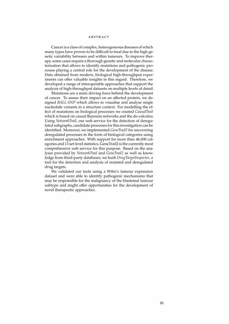
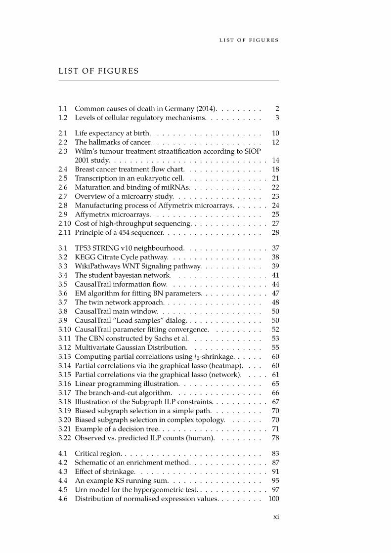
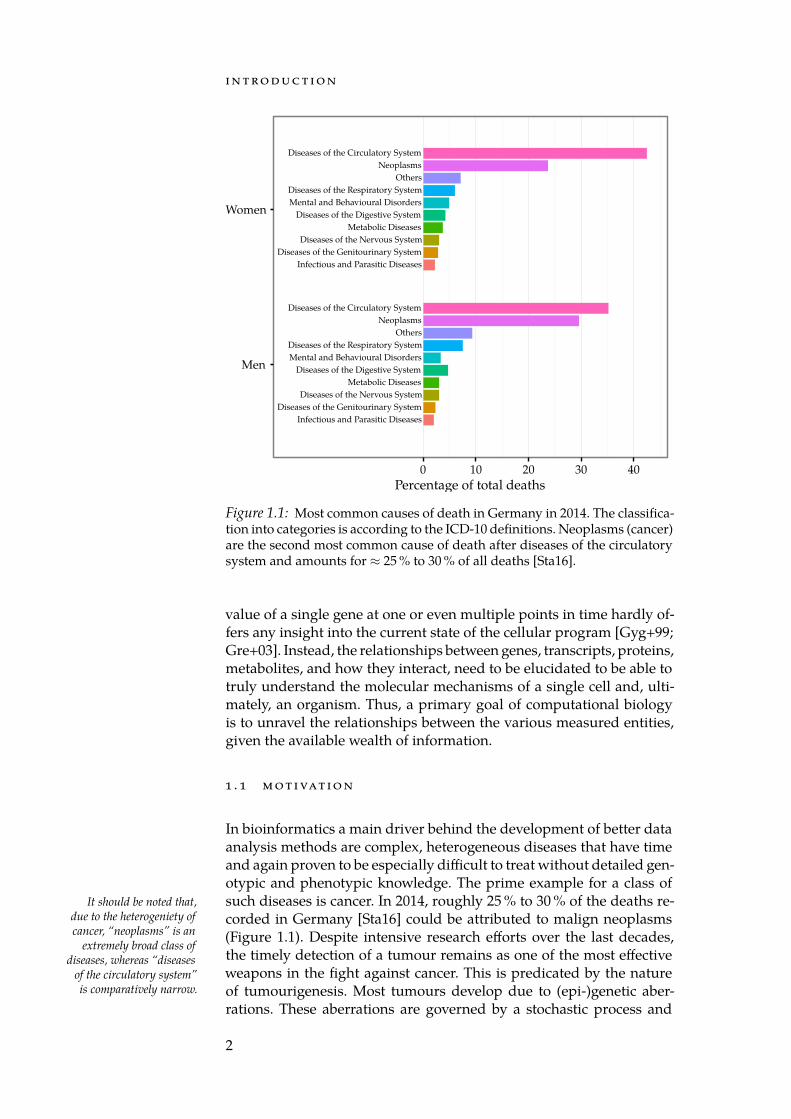
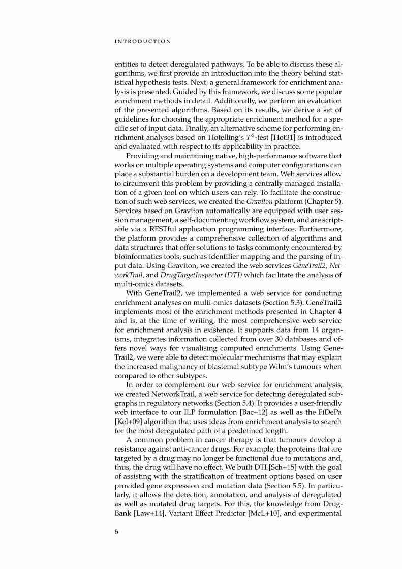
Figure 1.1: Most common causes of death in Germany in 2014. The classifica-tion into categories is according to the ICD-10 definitions. Neoplasms (cancer)are the second most common cause of death after diseases of the circulatorysystem and amounts for ≈ 25 % to 30 % of all deaths [Sta16].

value of a single gene at one or even multiple points in time hardly of-fers any insight into the current state of the cellular program [Gyg+99;Gre+03]. Instead, the relationships between genes, transcripts, proteins,metabolites, and how they interact, need to be elucidated to be able totruly understand the molecular mechanisms of a single cell and, ulti-mately, an organism. Thus, a primary goal of computational biologyis to unravel the relationships between the various measured entities,given the available wealth of information.

1 . 1 m ot i vat i o n

In bioinformatics a main driver behind the development of better dataanalysis methods are complex, heterogeneous diseases that have timeand again proven to be especially difficult to treat without detailed gen-otypic and phenotypic knowledge. The prime example for a class ofsuch diseases is cancer. In 2014, roughly 25 % to 30 % of the deaths re-It should be noted that,

due to the heterogeniety ofcancer, “neoplasms” is an

extremely broad class ofdiseases, whereas “diseases

of the circulatory system”is comparatively narrow.

corded in Germany [Sta16] could be attributed to malign neoplasms(Figure 1.1). Despite intensive research efforts over the last decades,the timely detection of a tumour remains as one of the most effectiveweapons in the fight against cancer. This is predicated by the natureof tumourigenesis. Most tumours develop due to (epi-)genetic aber-rations. These aberrations are governed by a stochastic process and

2

1 . 1 m ot i vat i o n

Flow

of g

enet

ic in

form

atio

n

PhosphorylationUbiquitinylationFolding

RNA interferenceSplicingmRNA degradation

Transcription factorsEnhancer binding

MethylationHistone modificationsChromatin structure

Promoter strength

Ribosome stallingmRNA structure

P

Pol II

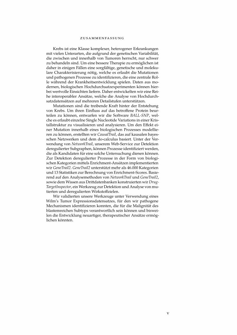
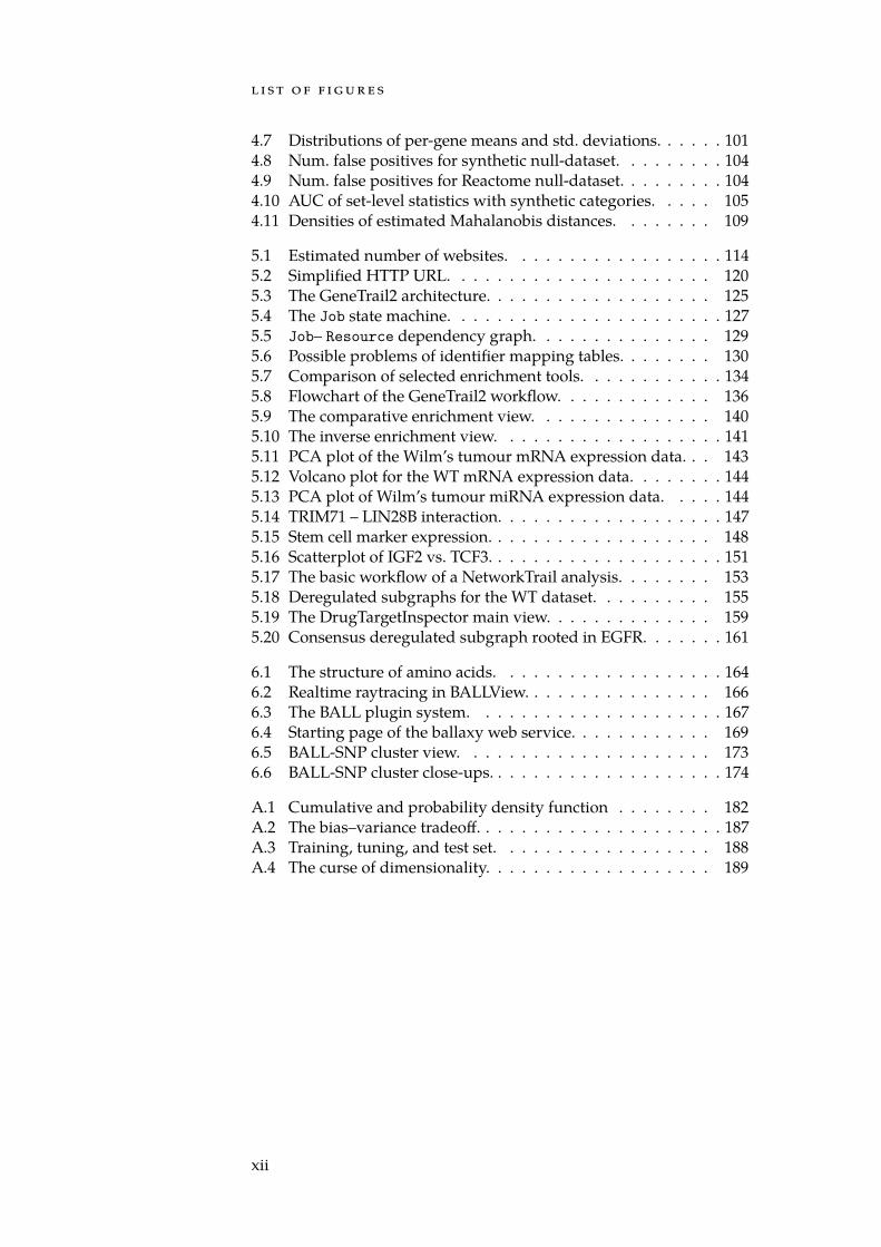
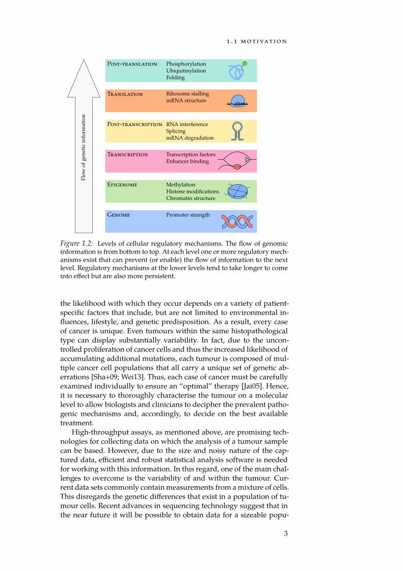
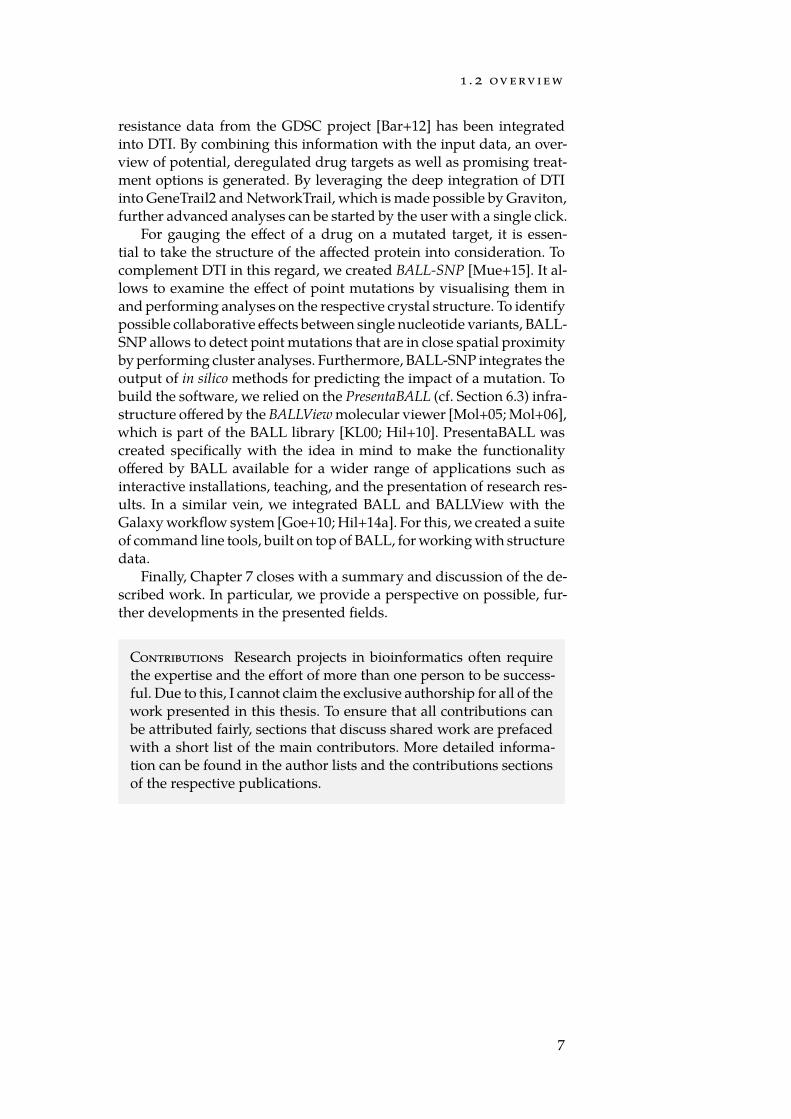
Figure 1.2: Levels of cellular regulatory mechanisms. The flow of genomicinformation is from bottom to top. At each level one or more regulatory mech-anisms exist that can prevent (or enable) the flow of information to the nextlevel. Regulatory mechanisms at the lower levels tend to take longer to comeinto effect but are also more persistent.

the likelihood with which they occur depends on a variety of patient-specific factors that include, but are not limited to environmental in-fluences, lifestyle, and genetic predisposition. As a result, every caseof cancer is unique. Even tumours within the same histopathologicaltype can display substantially variability. In fact, due to the uncon-trolled proliferation of cancer cells and thus the increased likelihood ofaccumulating additional mutations, each tumour is composed of mul-tiple cancer cell populations that all carry a unique set of genetic ab-errations [Sha+09; Wei13]. Thus, each case of cancer must be carefullyexamined individually to ensure an “optimal” therapy [Jai05]. Hence,it is necessary to thoroughly characterise the tumour on a molecularlevel to allow biologists and clinicians to decipher the prevalent patho-genic mechanisms and, accordingly, to decide on the best availabletreatment.

High-throughput assays, as mentioned above, are promising tech-nologies for collecting data on which the analysis of a tumour samplecan be based. However, due to the size and noisy nature of the cap-tured data, efficient and robust statistical analysis software is neededfor working with this information. In this regard, one of the main chal-lenges to overcome is the variability of and within the tumour. Cur-rent data sets commonly contain measurements from a mixture of cells.This disregards the genetic differences that exist in a population of tu-mour cells. Recent advances in sequencing technology suggest that inthe near future it will be possible to obtain data for a sizeable popu-

3

i n t ro d u c t i o n

lation of single cells together with their spatial location in a tumourLonger-term develop-ments such as time-

series data with asingle-cell-resolution

are also imaginable.

biopsy [Ang+16; WN15; Uso+15]. How to handle this kind of data ef-fectively, however, currently is an open research problem.

Furthermore, it is important to note that although a single high-throughput method is able to capture comprehensive datasets for oneso-called omics type, the collected information only provides a smallglimpse at the pathogenic processes that actually take place in a tu-mour. This is due to the fact that many of the cellular processes, andthus the emergence of complex traits, are subject to a tight regulatoryprogram constraining the flow of genetic information (Figure 1.2). Thisprogram manifest as interactions between genes, proteins, miRNAs,and other biological entities that can be modelled as biological net-works, where edges represent interactions and nodes represent inter-action partners. An integrative analysis of data from multiple omics is,therefore, mandatory to gain deeper insights into the deregulated pro-cesses that drive tumour development. Performing such an analysisnecessitates theoretical models and software that, in addition to theabove requirements, can also cope with heterogeneous data sets.

1 . 2 ov e rv i e w

This dissertation introduces tools and methods we developed for theWhile we describe ourmethods with regard to

their applicability in tu-mour research, most of

them can be used to invest-igate arbitrary datasets.

analysis of high-throughput data. Our main goal is to support the ge-netic and molecular characterisation of tumour samples. Commonly,this entails an iterative process in which each step provides informa-tion that is used to guide further, more focused examinations. To sup-port such workflows, the approaches we conceived are each targeted atdifferent levels of detail: some methods are especially suited to quicklynarrow down large amounts of data into a set of interesting systems.These can then be analysed using more specialised software. Natur-ally, this requires that the employed tools are interoperable, which wasan important concern we considered when designing our approaches.Finally, as outlined above, the ability to draw on knowledge from het-erogeneous datasets is essential for understanding complex diseases.Thus, we put special emphasis on methods that allow to perform in-tegrative analyses on multi-omics data.

Throughout this thesis, we illustrate the capabilities of the toolswe developed using a Wilm’s tumour dataset (Section 2.4). Wilm’s tu-mours are childhood renal tumours that, due to various propertiessuch as the relative independence from environmental influences and acomparatively low mutation rate, are an ideal model disease. The maingoal of our investigation was the detection of pathogenic mechanismsthat may explain the increased malignancy of blastemal subtype tu-mours compared to other Wilm’s tumour subtypes. On the basis ofthis case study, we highlight contributions that may be suitable for thecreation of systems that assist researchers and physicians in devisingeffective, personalised cancer treatments.

The remainder of this work is structured as follows: in Chapter 2 therequired biological background and experimental techniques are intro-

4

1 . 2 ov e rv i e w

duced. To this end, a basic discussion of cancer biology is provided. Ac-companying this general discussion, we describe Wilm’s tumours inmore detail. Furthermore, we discuss current treatment options and,especially, the trend towards targeted therapy. Based on this, we mo-tivate the need of advanced, computational methods to enable a moreaccurate, personalised medicine. Afterwards we introduce some of thebiological assays that are available to create detailed, biological patientprofiles and discuss their properties, advantages, and drawbacks.

An important prerequisite for personalised treatments is that thepathogenic processes that play a central role for a given tumour havebeen identified. As biological networks are a natural way to model reg-ulatory and other processes, Chapter 3 introduces a set of methods fortheir analysis, along with some of the most common network types.In particular, we introduce CausalTrail which we implemented to as-sess the causal dependencies in regulatory cascades. Using predefinedcausal Bayesian networks and the do-calculus, CausalTrail is able toassess the impact of a mutation or a drug on nodes down-stream of atarget regulator. For the end user, both, a command line applicationas well as a graphical user interface are provided. With CausalTrail wedeveloped, to the best of our knowledge, the first, freely available toolfor computing the effect of interventions in a causal Bayesian networkstructure.

While many biological networks stem from network databases, ap-proaches for inferring a topology directly from data exist. Here, we takea look at the theory behind Gaussian graphical models (GGMs), which canbe used to infer a network representing the partial correlation structurebetween a set of variables. While we will not use GGMs for network in-ference purposes, we later explore their applicability for enrichmentanalyses (Section 4.4).

A common characteristic of cancer cells is that their regulatory net-works have been reprogrammed. To detect affected parts of this net-work, methods for the search of deregulated subgraphs can be em-ployed. Deregulated subgraphs are small, usually connected parts of abiological network that contain a large number of e.g. differentially ex-pressed genes. In Section 3.5, we discuss our integer linear programming(ILP) formulation for discovering deregulated subgraphs in regulat-ory biological networks [Bac+12]. In contrast to many competing meth-ods, our approach computes an exact solution to the rooted maximum-weight subgraph problem. Furthermore, we describe the first approachfor quantifying the influence of the network topology on the detectedsubgraphs using a combination of sampling and machine learning tech-niques. Our study underlines the need and provides the basis for thedevelopment of a rigorous framework that allows to determine the sig-nificance of a deregulated subgraph. We later revisit the ILP formula-tion during the introduction of the NetworkTrail web service in Sec-tion 5.4.

In Chapter 4, we turn to approaches that are closely related to thedetection of deregulated subgraphs. While the aforementioned moreor less are free to choose any set of connected genes from an inputnetwork, enrichment methods rely on predefined categories of biological

5

i n t ro d u c t i o n

entities to detect deregulated pathways. To be able to discuss these al-gorithms, we first provide an introduction into the theory behind stat-istical hypothesis tests. Next, a general framework for enrichment ana-lysis is presented. Guided by this framework, we discuss some popularenrichment methods in detail. Additionally, we perform an evaluationof the presented algorithms. Based on its results, we derive a set ofguidelines for choosing the appropriate enrichment method for a spe-cific set of input data. Finally, an alternative scheme for performing en-richment analyses based on Hotelling’s T 2-test [Hot31] is introducedand evaluated with respect to its applicability in practice.

Providing and maintaining native, high-performance software thatworks on multiple operating systems and computer configurations canplace a substantial burden on a development team. Web services allowto circumvent this problem by providing a centrally managed installa-tion of a given tool on which users can rely. To facilitate the construc-tion of such web services, we created the Graviton platform (Chapter 5).Services based on Graviton automatically are equipped with user ses-sion management, a self-documenting workflow system, and are script-able via a RESTful application programming interface. Furthermore,the platform provides a comprehensive collection of algorithms anddata structures that offer solutions to tasks commonly encountered bybioinformatics tools, such as identifier mapping and the parsing of in-put data. Using Graviton, we created the web services GeneTrail2, Net-workTrail, and DrugTargetInspector (DTI) which facilitate the analysis ofmulti-omics datasets.

With GeneTrail2, we implemented a web service for conductingenrichment analyses on multi-omics datasets (Section 5.3). GeneTrail2implements most of the enrichment methods presented in Chapter 4and is, at the time of writing, the most comprehensive web servicefor enrichment analysis in existence. It supports data from 14 organ-isms, integrates information collected from over 30 databases and of-fers novel ways for visualising computed enrichments. Using Gene-Trail2, we were able to detect molecular mechanisms that may explainthe increased malignancy of blastemal subtype Wilm’s tumours whencompared to other subtypes.

In order to complement our web service for enrichment analysis,we created NetworkTrail, a web service for detecting deregulated sub-graphs in regulatory networks (Section 5.4). It provides a user-friendlyweb interface to our ILP formulation [Bac+12] as well as the FiDePa[Kel+09] algorithm that uses ideas from enrichment analysis to searchfor the most deregulated path of a predefined length.

A common problem in cancer therapy is that tumours develop aresistance against anti-cancer drugs. For example, the proteins that aretargeted by a drug may no longer be functional due to mutations and,thus, the drug will have no effect. We built DTI [Sch+15] with the goalof assisting with the stratification of treatment options based on userprovided gene expression and mutation data (Section 5.5). In particu-larly, it allows the detection, annotation, and analysis of deregulatedas well as mutated drug targets. For this, the knowledge from Drug-Bank [Law+14], Variant Effect Predictor [McL+10], and experimental

6

1 . 2 ov e rv i e w

resistance data from the GDSC project [Bar+12] has been integratedinto DTI. By combining this information with the input data, an over-view of potential, deregulated drug targets as well as promising treat-ment options is generated. By leveraging the deep integration of DTIinto GeneTrail2 and NetworkTrail, which is made possible by Graviton,further advanced analyses can be started by the user with a single click.

For gauging the effect of a drug on a mutated target, it is essen-tial to take the structure of the affected protein into consideration. Tocomplement DTI in this regard, we created BALL-SNP [Mue+15]. It al-lows to examine the effect of point mutations by visualising them inand performing analyses on the respective crystal structure. To identifypossible collaborative effects between single nucleotide variants, BALL-SNP allows to detect point mutations that are in close spatial proximityby performing cluster analyses. Furthermore, BALL-SNP integrates theoutput of in silico methods for predicting the impact of a mutation. Tobuild the software, we relied on the PresentaBALL (cf. Section 6.3) infra-structure offered by the BALLView molecular viewer [Mol+05; Mol+06],which is part of the BALL library [KL00; Hil+10]. PresentaBALL wascreated specifically with the idea in mind to make the functionalityoffered by BALL available for a wider range of applications such asinteractive installations, teaching, and the presentation of research res-ults. In a similar vein, we integrated BALL and BALLView with theGalaxy workflow system [Goe+10; Hil+14a]. For this, we created a suiteof command line tools, built on top of BALL, for working with structuredata.

Finally, Chapter 7 closes with a summary and discussion of the de-scribed work. In particular, we provide a perspective on possible, fur-ther developments in the presented fields.

Contributions Research projects in bioinformatics often requirethe expertise and the effort of more than one person to be success-ful. Due to this, I cannot claim the exclusive authorship for all of thework presented in this thesis. To ensure that all contributions canbe attributed fairly, sections that discuss shared work are prefacedwith a short list of the main contributors. More detailed informa-tion can be found in the author lists and the contributions sectionsof the respective publications.

7

2B I O LO G I CA L BACKG RO U N D

If you try and take a cat apart to see how it works, the firstthing you have on your hands is a non-working cat.

— d o u g l a s a da m s , t h e s a l m o n o f d o u b t( 2 0 0 2 )

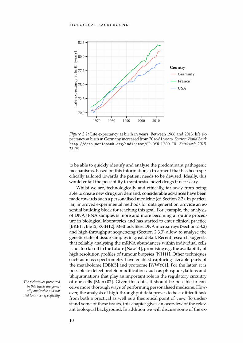
During the last century the life expectancy in developed countries hasincreased dramatically. Between 1970 and 2010 alone, the life expect-ancy at birth has increased by roughly ten years in Germany (see Fig-ure 2.1). This change can be attributed to improved living conditionsdue to significant advances in technology, sanitation, and medicine[Ril01]. For example, the introduction of cyclosporin into clinical prac-tice allowed more reliable organ transplants [Cal+79]. Imaging tech-niques like magnetic resonance imaging (MRI) and computer tomography(CT) made it possible to capture high-resolution images from otherwisedifficult to reach regions of the body [Bec14]. The invention of genet-ically modified organisms [MH70] allowed the production of humaninsulin for the treatment of diabetes [Joh83]. During this period, small-pox were eradicated due to a rigorous vaccination campaign [Fen93].Thanks to the discovery of antiretroviral drugs and effective treatment In 1983, the human im-

munodeficiency virus(HIV) had just been dis-covered [Mon02] and has,since then, claimed mil-lions of lives [HIV+14].

regimens, HIV positive patients at age 20 can expect to live another30 years or more [ART08]. Owing to this development, many of theonce common, deadly diseases are no longer an issue in the 21st cen-tury. Still, modern medicine suffers from certain flaws and shortcom-ings. Through the widespread use of antibiotics, resistant strains arebeginning to form that are only treatable with great difficulties [Neu92;Nik09]. This development has lead to the return of old killers, such astuberculosis, in some countries [Kam95]. Diseases like SARS [Cho+04],bird flu [Pei+04], or Ebola [Tea+15] that spread quickly via aerosols orbody fluids have claimed many victims, especially in lesser developedcountries. Also, genetic diseases such as Huntington’s disease [Wal07]or cystic fibrosis [Rio+89] pose challenges when it comes to finding acure. In particular, many tumour types have eluded effective therapyfor decades, despite remarkable advances that have been made in can-cer research.

Reasons for these problems are manifold. In the case of most viralinfections only few effective antiviral drugs are available [De 04]. Forinfluenza, vaccinations exist that, however, only protect against a lim-ited set of viral strains [Bri+00]. For Ebola, no approved vaccinations ex-ist [Gal+14], although several candidates are in the drug developmentpipeline at the time of writing [Agn+16]. In the case of genetic disordersthe cause of the disease is not an external influence, but instead is en-coded in the patient’s genes. Though a set of best practices has beenestablished for a large number of cancer types (cf. Figure 2.4), the treat-ment for certain tumours needs to be decided on a case by case basisdue to their heterogeneity. To combat the above diseases, it is necessary

9

b i o lo g i ca l bac kg ro u n d

70.0

72.5

75.0

77.5

80.0

82.5

1970 1980 1990 2000 2010

Lif

e ex

pect

ancy

at b

irth

[yea

rs]

Country

Germany

France

USA

Figure 2.1: Life expectancy at birth in years. Between 1966 and 2013, life ex-pectancy at birth in Germany increased from 70 to 81 years. Source: World Bankhttp://data.worldbank.org/indicator/SP.DYN.LE00.IN. Retrieved: 2015-12-03

to be able to quickly identify and analyse the predominant pathogenicmechanisms. Based on this information, a treatment that has been spe-cifically tailored towards the patient needs to be devised. Ideally, thiswould entail the possibility to synthesise novel drugs if necessary.

Whilst we are, technologically and ethically, far away from beingable to create new drugs on demand, considerable advances have beenmade towards such a personalised medicine (cf. Section 2.2). In particu-lar, improved experimental methods for data generation provide an es-sential building block for reaching this goal. For example, the analysisof DNA/RNA samples is more and more becoming a routine proced-ure in biological laboratories and has started to enter clinical practice[BKE11; Bie12; KGH12]. Methods like cDNA microarrays (Section 2.3.2)and high-throughput sequencing (Section 2.3.3) allow to analyse thegenetic state of tissue samples in great detail. Recent research suggeststhat reliably analysing the mRNA abundances within individual cellsis not too far off in the future [Naw14], promising e.g. the availability ofhigh resolution profiles of tumour biopsies [NH11]. Other techniquessuch as mass spectrometry have enabled capturing sizeable parts ofthe metabolome [DBJ05] and proteome [WWY01]. For the latter, it ispossible to detect protein modifications such as phosphorylations andubiquitinations that play an important role in the regulatory circuitryof our cells [Man+02]. Given this data, it should be possible to con-The techniques presented

in this thesis are gener-ally applicable and not

tied to cancer specifically.

ceive more thorough ways of performing personalised medicine. How-ever, the analysis of high-throughput data proves to be a difficult taskfrom both a practical as well as a theoretical point of view. To under-stand some of these issues, this chapter gives an overview of the relev-ant biological background. In addition we will discuss some of the ex-

10

2 . 1 ca nc e r

perimental methods that are frequently encountered throughout thisthesis.

We use cancer as a model disease to illustrate the capabilities of ourmethods. There are various reasons for this choice: first, the diseaseis of great clinical, but also social and economical relevance. Second,a vast corpus of experimental data derived from tumour biopsies hasbeen compiled and is publicly available. And third, although cancer re-search has progressed tremendously over the last decades, many fun-damental aspects of the acting pathogenic mechanisms remain unre-solved. Thus, studying cancer not only serves the improvement of ther-apy, but also promises to yield exciting biological insights.

We start with a discussion of cancer biology in general and the prop-erties of Wilm’s tumours specifically. We then proceed to a more pre-cise definition of personalised medicine and outline the problems thatneed to be solved for implementing personalised medicine schemes. Fi-nally, we introduce the basics of gene expression and discuss the cDNAmicroarray as well as the RNA-seq technology for capturing expressionprofiles.

2 . 1 ca nc e r

Cancer is a heterogeneous class of diseases characterised by the ab- Much of the information inthis section is taken from“The Biology of Cancer” byWeinberg [Wei13]. Addi-tional sources are quotedexplicitly.

normal growth of tissue. Causes for the development of cancer can besought in many factors including life-style, exposure to pathogens andradiation, mutations or epigenetic alterations. Ultimately, these factorsresult in a disruption of the regulatory circuitry of previously healthycells, which transforms them into tumour cells.

Somatic mutations are a well researched mechanism that leads tothe formation of tumour cells. While mutations are usually detected Unless specified otherwise

the term “mutation” isused in its broadest mean-ing: a change or aberrationin the genome.

and neutralised by internal cellular controls or the immune system,some mutations go unnoticed. Interestingly, only few so-called drivermutations are believed to be sufficient for establishing cancer [SCF09].Examples are mutations that lead to the transformation of “normal”

Genes that can be trans-formed to oncogenes arecalled proto-oncogenes.

genes to oncogenes: genes that have the potential to induce cancer. Oneof the first reported transformation mechanisms is the activation of theT24 oncogene in human bladder carcinomas due to the exchange of asingle nucleotide [Red+82]. Once driver mutations have established afoothold, additional mutations are accumulated.

As mentioned above, cancer and especially cancer cells are charac- The definitions here pertainto solid tumours. However,many properties such as tu-mour heterogeneity directlycarry over to non-solid tu-mours such as leukaemia.

terised by their ability to form new tissue and, thus, are able to freelydivide. Two non-exclusive hypotheses explain this behaviour. Either,cancer cells derive from stem cells or they dedifferentiate from ma-ture cells in order to obtain stem cell like characteristics [Sel93]. The

The term neoplasm can bedirectly translated as “newtissue”.

newly formed tissue is denoted as neoplasm or tumour. Not every neo-plasm is immediately life threatening. For example moles, also knownas melanocytic nevi are pigmented neoplasms of the skin that are, usu-ally, harmless. To reflect this, neoplasms are often classified as eitherbenign or malignant. Whereas benign tumours grow locally and donot invade adjacent tissues, malignant tumours commonly invade into

11

b i o lo g i ca l bac kg ro u n d

Resistingcell

death

Deregulatingcellular

energetics

Sustainingproliverative

signaling

Evadinggrowth

suppressors

Avoidingimmune

destruction

Enablingreplicative

immortatlity

Tumour-promoting

inflammation

Activatinginvasion &metastasis

Inducingangiogenesis

Genomeinstability &

mutation

Cyclin-dependentkinase inhibitors

Selective anti-inflammatory drugs

Inhibitors ofHGF/c-Met

Inhibitors ofVEGF signaling

EGFRinhibitors

Telomeraseinhibitors

Immune activatinganti-CTLA4 mAb

Aerobic glycolosisinhibitors

ProapoptoticBH3 mimetics

PARPinhibitors

Figure 2.2: The hallmarks of cancer as proposed by Hanahan and Weinberg[HW00]. The authors postulate that during tumourigenesis normal cells suc-cessively acquire the “hallmark stages” as they evolve towards a malignanttumour. Coloured boxes indicate treatment options for counteracting the mo-lecular changes constituting the respective hallmark.

nearby, healthy tissues and may also able to spawn new tumours, socalled metastases, at different locations.

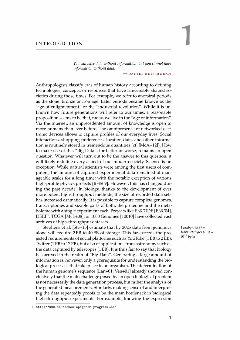
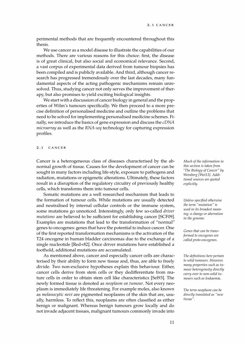
In its development from healthy to neoplastic tissue, cancer cellsgo through an evolution that allows them to grow successfully in ahost organism. This evolution is driven by selection pressure that is,for example, exerted by the immune system, the competition for nutri-ents with surrounding cells, and eventual anti-cancer drugs. Naturally,each successful cancer cell needs to develop the ability to avoid detec-tion by the immune system and must resist programmed cell death(apoptosis). Furthermore, tumours start to induce the growth of newblood vessels (angiogenesis) to account for the increased energy con-sumption due to uncontrolled growth and replication. Hanahan andWeinberg [HW00] summarised these objectives under the term hall-marks of cancer. The hallmarks describe a set of characteristics tumourcells typically achieve during their development (Figure 2.2). In a laterpublication, Hanahan and Weinberg [HW11] added four additionalcharacteristics to the six original hallmarks.

Tumours can be classified according to the cell types they stem from.The most common type of human tumours, carcinomas, derive fromepithelial cells and are hence also dubbed epithelial tumours. Epitheliaare tissues that can be found throughout the body. They are composedof sheets of cells and act as covers of organs, blood vessels, and cavities.The second class of tumours are called sarcomas and only account forroughly 1 % of all tumours. They stem from e.g. fibroblasts, adipocytes,osteoblasts, or myocytes. Tumours stemming from blood-forming cells

12

2 . 1 ca nc e r

are more common. Examples are leukaemias and lymphomas. The lastclass are tumours that derive from cells of the nervous system. Ex-amples are brain tumours such as gliomas and glioblastomas. Whileaccounting for large part of all cancer types, some tumours such asmelanomas or small-cell lung carcinomas derive from cell lineages thatdo not directly fit into this classification, as they stem from differentembryonic tissues or have an unclear origin altogether.

In contrast to healthy tissue that is composed of cells with well-defined tasks, a tumour is usually significantly more heterogeneous.The key to this heterogeneity lies in the rapid rate with which tumourcells tend to accumulate mutations and epigenetic aberrations [LKV98;FT04]. As a specific mutation event only occurs locally in a single cell,it remains specific to this cell and its progeny. This effectively estab-lishes lineages of cancer cell subpopulations. As a direct consequence,measurements from tumour samples often only provide values thathave been averaged over an ensemble of genetically diverse cells. Also, Similar problems exist in

HIV genotyping, whereonly the sequence of one orfew of the most abundantsub-species can be reliablyresolved.

not all cells involved in a tumour necessarily carry a defective (epi-)genome. For instance, cells forming blood vessels, cells from healthytissue, and immune cells can be found there, too. Characterising a tu-mour or predicting its reaction to treatment reliably is thus difficult.Experimental techniques such as single cell sequencing only solve thisproblem to a certain degree. While they may provide complete know-ledge about a set of individual cells, no knowledge is obtained aboutthe billions of remaining cells that make up the tumour.

2 . 1 . 1 Wilm’s Tumour

Wilm’s tumours (WTs) are childhood renal tumours. They comprise 95 % Still, WTs are comparat-ively rare due to the lowprevalence of child cancers.

of all diagnosed kidney tumours and six percent of all cancers in chil-dren under the age of 15. Most WTs are diagnosed in children youngerthan five years [Chu+10]. The clinical name nephroblastoma derives fromthe fact that WTs develop from the metanephrogenic blastema, an em-bryonic tissue. Most often WTs exhibit a triphasic histopathologicalpattern composed of blastemal, stromal, and epithelial cells althoughother compositions do exist [BP78]. According to the Société Interna-tionale D’Oncologie Pédiatrique (SIOP) Wilm’s tumours after preoperat-ive chemotherapy are classified as follows [Vuj+02]: first, the presenceof an anaplasia is determined. For this, the tumour must contain poorlydifferentiated cells, e.g. cells that lost defining morphological character-istics or display other potentially malignant transformations such as anuclear pleomorphism. If the tumour is not anaplastic, the reduction intumour volume due to the chemotherapy is quantified. If no living tu-mour tissue can be detected, the tumour is labelled as completely necrotic.If its volume decreased by more than two thirds the tumour is classifiedas regressive. Otherwise, the classification is based on the predominantcell type. If more than two thirds of the living cells are either blastemal,epithelial or stromal cells, the tumour is labelled accordingly. Tumourswith an even distribution of cell types are classified as triphasic. Based

13

b i o lo g i ca l bac kg ro u n d

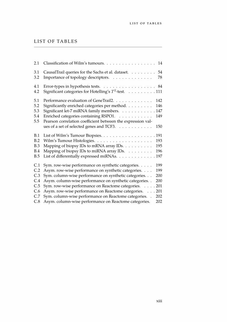
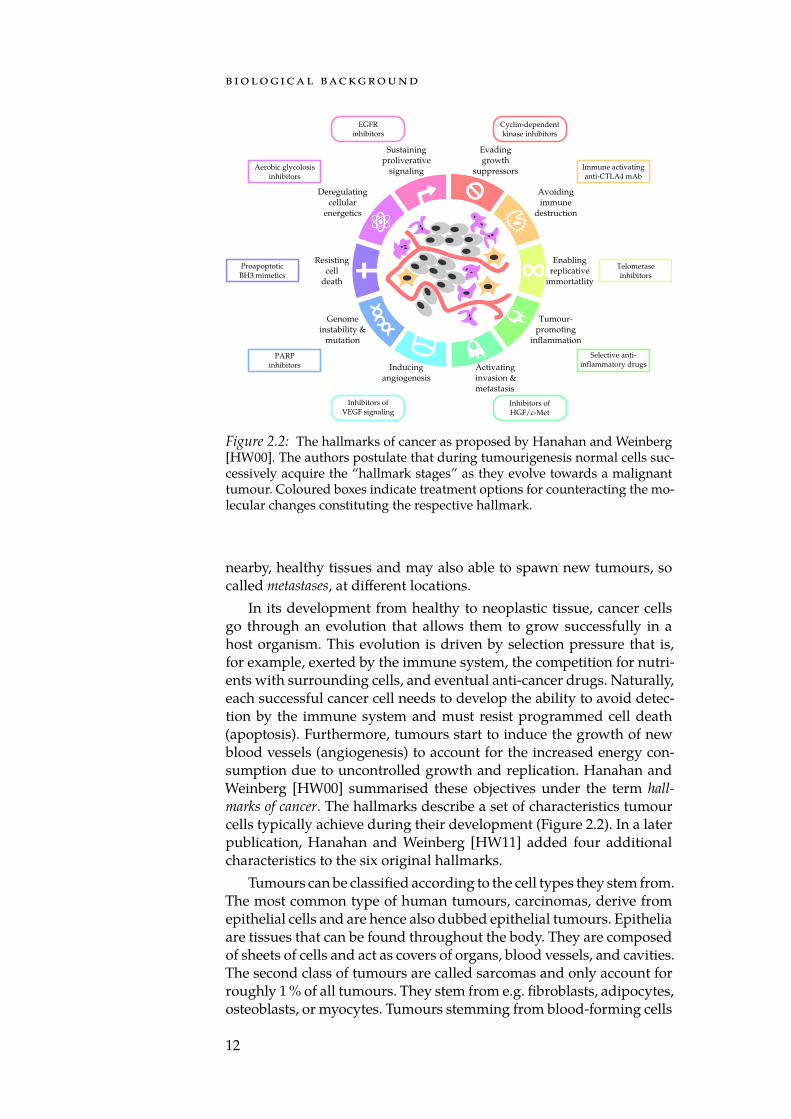
Figure 2.3: An exemplary WT treatment schema as used in the SIOP2001 study. Tumours are stratified into risk groups based on tumour stageand histology. Abbreviations: dactinomycin (A), vincristine (V), doxorubi-cin (D), doxorubicin/carboplatin/cyclophosphamide/etoposide x 34 weeks(HR). Image taken from Dome, Perlman, and Graf [DPG14].

Risk group Classification

Low risk Completely necrotic

Intermediate risk

RegressiveEpithelial typeStromal typeTriphasic typeFocal anaplasia

High risk Blastemal typeDiffuse anaplasia

Table 2.1: Wilm’s tumour classification and risk groups after preoperativechemotherapy according to the SIOP reference [Vuj+02]. Blastemal subtypeand diffuse anaplasia tumours are the most aggressive nephroblastoma sub-types.

on tumour stage, volume, and histology further treatment decisionsare made (Figure 2.3).

While WTs are generally associated with high 5-year survival ratesof ≈ 85 % [Chu+10; Sre+09], the prognosis for some subtypes is signi-ficantly worse. An example for this are the blastemal subtype tumours.While WTs with a high content of blastemal cells generally respondwell to chemotherapy, this is not true in about 25 % of the cases. Suchresistant, blastema-rich tumours, which account for almost 10 % of allWTs, are among the most malignant WT types (cf. Table 2.1) [Kin+12;Heu+15].

One of the earliest identified mutations associated with nephro-blastomas is the inactivation of the tumour suppressor WT1 that likely

14

2 . 1 ca nc e r

plays an important role in genitourinary development [LH01; Roy+08]and is also associated with human leukaemia [MBS92; Ino+97]. A morerecent study by Wegert et al. [Weg+15] links mutations in genes such asSIX1, SIX2, DROSHA, TP53, and IGF2 to specific sub- and phenotypesof WTs.

While other, more aggressive cancer types such as lung cancer mybe of greater medical interest, WTs possess properties that make theman ideal model disease. First, while a range of histological subtypes ex-ist for this tumour, they are relatively homogeneous in the sense thatthey carry a comparatively low amount of mutations [Weg+15]. Thus,most biological processes remain intact, which greatly eases the inter-pretation of the data. Second, as the disease commonly occurs in youngchildren, environmental effects play comparatively small roles in thedevelopment of the tumour. Third, as WT are quite rare [BP78], mostcases are treated by a small community of experts. Accordingly, theyare well and consistently documented.

2 . 1 . 2 Cancer Therapy

A core problem of cancer therapy is the timely detection of neoplasms.Many cancers can be treated effectively if detected at an early stage. Forexample, early stage melanomas can simply be excised with little to noadverse effects. Polyps in the colon, which may later develop to can-cer, can be removed during routine colonoscopies [Win+93]. However,when a tumour is not detected during early stages, treatment becomesmore difficult. Compared to early stage tumours, late stage tumourshad considerably more time to acquire hallmarks of cancer traits (Fig-ure 2.2). Consequently, they possess a less well-defined boundary asthey begin to invade healthy, adjacent tissue preventing effective sur-gery (cf. [Suz+95]). Also, metastases, which spread via blood or lymphand form new, aggressive tumours in other parts of the body, may havebeen established [Fid03]. This makes it difficult to reliably assess thesuccess of a treatment as it is uncertain whether all cancer cells couldbe successfully removed [Bec+98; Wet+02]. While chemotherapy maybe used to combat these developments, drug resistance often limits itsefficacy (cf. [Per99; RY08]). In the following we give a more detailedoverview over the available options for diagnosis and treatment.

Diagnosis

Performing routine cancer screens can considerably lower the risk ofdeveloping cancer [Wen+13; Bre+12]. However, this creates a dilemmawhen planning an effective scheme for preventive care. First, no singletest covering all possible tumour classes exists and it can be assumedthat none will exist in the foreseeable future. This means that signi-ficant parts of the population would need to undergo several med-ical screenings in fixed or maybe age dependent intervals. However,schemes relying on unconditional screenings are problematic. Besidesthe considerable financial implications, there are also statistical issues

15

b i o lo g i ca l bac kg ro u n d

that make such an approach infeasible. The problem is that the likeli-hood to develop a certain type of cancer at a certain point is compar-atively low (let’s assume about 0.1 %). While in itself not problematic,this fact can have important implications together with a fundamentalproperty of tests based on empiric data: all tests make errors. Generally,one can distinguish between two kinds of errors (cf. Table 4.1). The firstclass of errors is to detect an effect (e.g. diagnose cancer) when thereis none, while the second class is to not detect an effect when there isone. Making an error of the second kind may result in an unfavourableStatistical tests are

discussed in more de-tail in Section 4.1.

diagnosis because the tumour is detected too late. Making an error ofthe first kind means that a healthy person must undergo unnecessaryand potentially risky follow-up examinations such as biopsies. This isboth, a waste of resources [OM15] and a burden on the health of thepatient. Unfortunately, we can expect the first kind of error, diagnos-ing cancer although the patient is healthy, to occur far more often thanthe second kind because we previously assumed that the prevalenceof cancer is only 0.1 % (c.f. [ZSM04; Etz+02]). The resulting amount ofunnecessary follow-up examinations render broad, regular screeningsboth ethically as well as economically questionable. Instead, stratifica-tion into risk groups and targeted tests based on a patient’s case his-tory must be used to achieve effective, early diagnostics and is in factrecommended by studies and treatment guidelines [Wen+13; Bre+12;Bur+13].

Techniques from bioinformatics may help in this targeted approach.As sequencing costs for a human genome have dropped dramaticallyin the last decade (Figure 2.10), genotype information as a supplementto classical factors used in risk determination, such as family historyand lifestyle, has the potential to improve the accuracy of diagnosis tre-mendously. Additionally, the development of minimally invasive testswith high specificity can help to reduce the risk for patients signific-antly. To this end, the search for specific biomarkers is a prolific fieldVarious definitions of a

“biomarker” exist. Strimbuand Tavel [ST10] provide

an overview over com-monly used definitions.

of computational biology [Saw08]. In this context, a biomarker is a mo-lecule or a set thereof that can be measured objectively and can be usedas an indicator of the state of a pathogenic process. For this purposealso proteins and miRNA isolated from the blood stream have beenused (cf. [Kel+06; Mit+08]).

Therapy

Cancer therapy is a large field that is impossible to discuss exhaustively.Here, we give a rough outline of the available treatment options.

For treating cancer three main angles of attack exist: surgery, radi-ation therapy, and chemotherapy [DLR14]. Each of these approachescome with distinct advantages and disadvantages. Surgery can be anextremely efficient treatment option, as possibly large tumour volumescan be removed. In ideal cases, all tumour mass can be removed in asingle session [Cof+03]. However, it should be noted that the applic-ability of surgery is severely limited due to its invasiveness: tumoursthat are difficult to reach, too large in volume, or have developed meta-stases can prove difficult to treat with surgery alone [Pet+15]. Besides

16

2 . 1 ca nc e r

curative purposes, surgery is also an important tool for diagnosis, as In recent years technolo-gies for isolating tumourcells from blood have beendeveloped, which may alle-viate the need for surgery(cf. [AP13]).

often only a biopsy allows to determine whether cancer is present andif yes, how treatment should be commenced (cf. [Hei+14]). Also, all ap-proaches that rely on gene expression analysis or genotyping requirethat a biopsy is conducted.

In combination to or instead of surgery, radiation therapy can beused for treatment [Tim+10]. Commonly, radiation therapy directs abeam of ionising radiation at a target tumour. Cells along the beamabsorb energy leading to the formation of free radicals that attack andfragment DNA. In order to minimise the damage to healthy tissue, thebeam is applied from multiple angles leading to an accumulation ofan effective radiation dose only in the tumour [DLR14]. Still, radiationtherapy can have severe adverse effects that can lead to the inductionof secondary cancer (cf. [Tuc+91; Tsa+93; Kry+05; Hal06]).

Complementing surgery and radiation therapy, chemotherapy al-lows to treat tumours via the administration of drugs. As cancer cellsremain by and large human cells, finding drugs that specifically targetcancer cells is difficult [KWL07]. To this end, classical chemotherapyuses cytotoxic or cytostatic agents. These drugs target rapidly divid-ing cells, where they induce cell death or prevent proliferation. Thisoften results in harsh adverse effects such as anæmia, fatigue, hair loss,nausea, or infertility. In contrast to this, targeted therapy attempts toattack specific molecules, most of the time proteins that are respons-ible for the deregulation of signalling pathways that takes place in can-cer cells [Saw04]. Targeted drugs are not universally applicable, butrequire tumours to fulfil certain properties in order to be effective. Ex-amples are the presentation of certain antigenes on the cell membraneor the target protein carrying a mutation [Saw08]. To achieve the ne-cessary specificity, often biomolecules such as antibodies, which areable to detect cancer cell specific epitopes, are used. Thus, to apply tar-geted therapy effectively, an analysis of the tumour on the molecularlevel is necessary. For cases in which the preconditions for targeted To assist with this, we

created the DrugTarget-Inspector tool [Sch+15]which we present in Sec-tion 5.5.

drugs are met, impressive treatment success with comparatively fewadverse effects has been reported. A popular example for targeted ther-apy are drugs targeting the EGF receptor (EGFR) and are only effect-ive in (breast) cancers that carry a certain point mutation in the EGFRkinase domain [Pae+04; Mas+12]. Other types of targeted therapy at-tempt to attack tumour stem cells or the tumours microenvironmentby e.g. preventing blood vessel formation [AS07; EH08].

Usually, none of the previously described techniques is used in isol-ation. Often a combination of surgery, chemotherapy, and radiationtherapy is used in different stages of the therapy. Figure 2.4 showsthe treatment recommendations of the European Society of Medical On-cology (ESMO) for early breast cancer. In this recommendation, variousfactors such as tumour volume or the efficacy of previous treatmentsare considered to recommend the next step in the therapy [Sen+15].

Combining multiple therapy options is sensible for various reas-ons. First, a single treatment option is often not enough to guaranteethe removal of all tumour cells. For example, residues of the tumour(cf. minimal residual disease [Kle+02]) that are difficult to excise during

17

b i o lo g i ca l bac kg ro u n d

Figure 2.4: Flow chart for the treatment of early breast cancer. Abbrevi-ations: chemotherapy (Cht), breast-conserving surgery (BCS), endocrine ther-apy (ET), radiotherapy (RT). Image taken from Senkus et al. [Sen+15].

surgery may be treated using adjuvant chemotherapy. Second, as tu-mours underlie a highly accelerated selection process due to their highproliferation and mutation rates, it is possible that some tumour cellsdevelop a resistance against the employed cancer drugs. Similarly toHIV therapy, using multiple agents and treatment options increasesthe selection pressure and thus reduces the amount of escape mutants[SS08b; HZ12; BL12]. Third, using multiple, cancer specific drugs dur-ing chemotherapy has been reported to be more effective than usingonly a single formulation as this increases the specificity of the treat-ment [Coi+02; Ban+10].

2 . 2 p e r s o na l i s e d m e d i c i n e

In classical medicine, a doctor makes a diagnosis based on the patient’shistory (anamnesis), the displayed symptoms, and, if required, addi-tional measurements. Based on this, the physician chooses an appro-priate therapy. Often, this means administering one of the drugs de-signed for treating the disease. In recent years, it has become clear thatfor some diseases the genetic, epigenetic, and biomolecular propertiesof the patient as well as the disease need to be considered to determinean optimal therapy. The level of detail that needs to be considered canvary by a large margin. In some cases, the membership in a particularethnic group can provide enough information on the genomic back-ground. For example the drug BiDil, which was approved by the FDA

18

2 . 2 p e r s o na l i s e d m e d i c i n e

for treating congestive heart-failure, is only effective for the AfricanAmerican parts of the US population [BH06]. In HIV therapy the gen-ome of the virus can provide crucial information on its resistance or sus-ceptibility to certain antiretroviral drugs [Bee+02]. In heterogeneousdiseases like cancer, taking the genes expressed by the tumour intoaccount can help to dramatically increase treatment success [Kon+06].These observations also become increasingly important for “classical”diseases such as bacterial infections due to the emergence of multi-resistant strains for which an effective antibiotic needs to be chosen[Neu92]. The development of treatment strategies that are tailored spe- Sometimes the term preci-

sion medicine is used.cifically towards a specific case of a disease is called personalised medi-cine. Deploying personalised medicine, however, proofs to be difficultdue to a variety of issues. First, the identification of genomic factors thatcontribute to the risk of developing a disease is problematic. To thisend, genome wide association studies (GWAS) are commonly applied. Forthem to succeed, large cohorts (≥ 10,000 samples) are required [HD05].Even then, rare variations, which are likely to have a large impact onthe disease risk, continue to elude these studies [CG10].

Even if a molecule or process that plays a key role in a diseases has Pharmacogenomics con-cerns itself with the influ-ence of genomic variationson the effect of drugs.

been identified, the selection of an appropriate drug is not always pos-sible. This may be because no appropriate drug exists. However, evenif a drug existed, it may be overlooked as only a small percentage ofthe available drugs is annotated with pharmacogenomic information[Fru+08]. To remedy this situation, studies such as the Cancer Cell LineEncyclopaedia (CCLE) [Bar+12] and the Genomics of Drug Sensitivity inCancer (GDSC) [Gar+12] attempt to compile libraries of the effect ofdrugs on cell lines with a known set of mutations. However, these invitro measurements are only the first step into the direction of morecomprehensive pharacogenomic information: the overlap between thestudies has been reported as “reasonable” by the authors [C+15] andas “highly discordant” [Hai+13] by independent researchers.

Drugs that are only effective given a certain mutation must, as allother drugs, undergo clinical trials to ensure safety and efficacy of thedrug. Unfortunately, classical study designs, where a control group ofpatients receiving the standard treatment is monitored in comparisonto a group receiving the modified treatment, are inefficient for valid-ating the merits of patient specific drugs [Sch15b]. If e.g. the genomictrait responsible for the susceptibility to a drug is comparatively rarethroughput the population, the number of patients that will respondcan be expected to be low and hence the difference between uniformlyselected control and sample groups is likely small. To reliably determ-ine drugs that are only effective for parts of the population, improvedstudy designs need to be employed [Sin05; Fre+10].

For bioinformatics, the development of effective personalised medi-cine schemes poses several challenges such as the reliable analysis oflarge-scale genomic data, the compilation of databases containing phar-macogenetic knowledge, as well as the training of reliable, statisticalrecommendation procedures [Fer+11]. Partly due to this, the road to-wards an “ideal”, personalised medicine is still long. Nevertheless, sig-nificant steps are currently being made towards this goal [Les07]. In

19

b i o lo g i ca l bac kg ro u n d

this work, several tools that my have the potential to assist in choos-ing personalised treatments are presented. The primary example isDrugTargetInspector (Section 5.5), which employs pharmacogenomicinformation to judge the influence of somatic mutations on drug effic-acy. Similarly, the enrichment and network analyses provided by ourproposed tools GeneTrail2 (Section 5.3) and NetworkTrail (Section 5.4)can be used to gain insights into patient data.

2 . 3 b i o lo g i ca l a s says

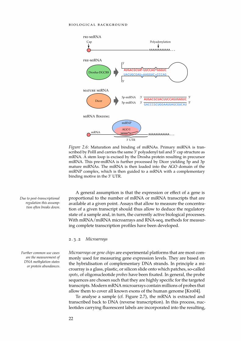
An important task in bioinformatics is the processing of data obtainedfrom biological experiments using methods from statistics and com-puter science. While it is convenient to test new algorithms on syntheticdata, every bioinformatics method eventually needs to work with ac-tual measurements. As a consequence, the developed methods need totake the properties of the data generation process and, thus, the usedbiological assays, into account. Furthermore, with the development ofhigh-throughput assays such as microarrays, short read sequencing, ormodern mass spectrometry the amount of generated biological datahas grown to a staggering amount [Ste+15]. This places two furtherrequirements on computational methods. First, the approach needs tobe efficient enough to potentially process terabytes of data. Second, theemployed statistical methods need to be able to cope with the high di-mensionality of the data.

Here, we discuss the microarray and short-read sequencing tech-nologies as the remainder of this thesis will mostly be concerned withdata obtained from these two experimental setups. Notably, the focuswill lie on expression datasets. To this end, the next section will providea basic introduction of the fundamental mechanisms that underlie geneexpression in eukaryotic cells. Readers familiar with this concept maywant to directly skip to the introduction of the microarray platform inSection 2.3.2.

2 . 3 . 1 Gene Expression

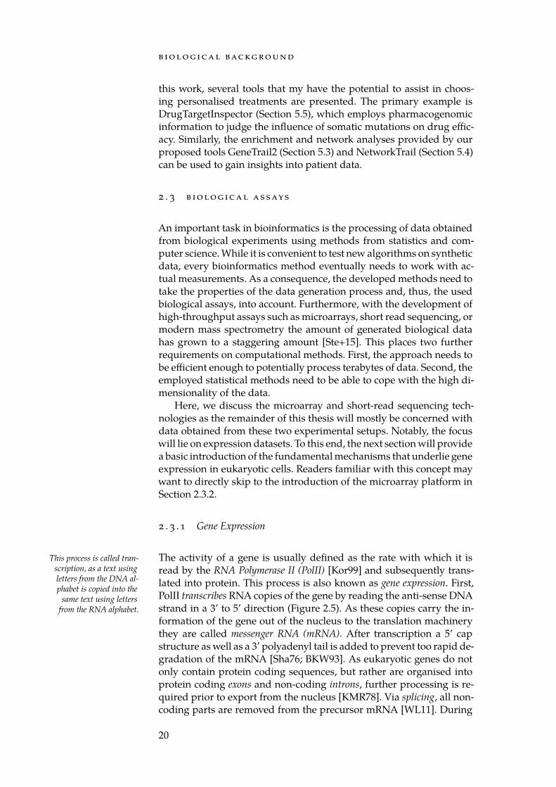
The activity of a gene is usually defined as the rate with which it isThis process is called tran-scription, as a text usingletters from the DNA al-phabet is copied into the

same text using lettersfrom the RNA alphabet.

read by the RNA Polymerase II (PolII) [Kor99] and subsequently trans-lated into protein. This process is also known as gene expression. First,PolII transcribes RNA copies of the gene by reading the anti-sense DNAstrand in a 3’ to 5’ direction (Figure 2.5). As these copies carry the in-formation of the gene out of the nucleus to the translation machinerythey are called messenger RNA (mRNA). After transcription a 5’ capstructure as well as a 3’ polyadenyl tail is added to prevent too rapid de-gradation of the mRNA [Sha76; BKW93]. As eukaryotic genes do notonly contain protein coding sequences, but rather are organised intoprotein coding exons and non-coding introns, further processing is re-quired prior to export from the nucleus [KMR78]. Via splicing, all non-coding parts are removed from the precursor mRNA [WL11]. During

20

2 . 3 b i o lo g i ca l a s says

Exon I Exon II Exon III Exon IV AAAAAAAAAAAA...

5' UTR 3' UTR

Cap Polyadenylation

Introns

Pol II 5'3'

Helicase

transcription bubble

5'

precursor mRNA

anti-sense strand

sense strand

DNA

mature mRNAExon I Exon III Exon IV5' 3'

Exon I Exon II Exon IV5' 3'

Exon I Exon II Exon III Exon IV5' 3'

Figure 2.5: Basic overview of transcription in an eukaryotic cell. After RNAPolymerase II binds at the promoter of a gene, it translates the DNA anti-sensestrand to mRNA. For transcription, the DNA is temporarily unwound by ahelicase protein creating the so-called transcription bubble. After the mRNAhas been transcribed, a 5’ cap and a 3’ polyadenyl tail are added to preventdegradation. Mature mRNA is created by the (alternative) splicing process,which excises intronic and sometimes exonic sequences.

this process some exons may be skipped and thus splicing can producemultiple isoforms of a single gene [Bla03]. This alternative splicing is onemechanism that explains how relatively few genes can give rise to a farlarger amount of diverse proteins. After splicing, the mRNA is expor-ted to the cytosol, where it is translated into proteins.

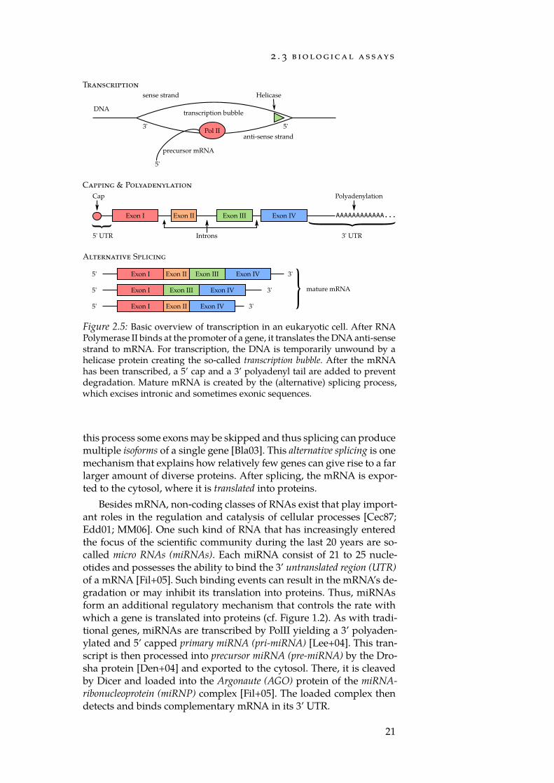
Besides mRNA, non-coding classes of RNAs exist that play import-ant roles in the regulation and catalysis of cellular processes [Cec87;Edd01; MM06]. One such kind of RNA that has increasingly enteredthe focus of the scientific community during the last 20 years are so-called micro RNAs (miRNAs). Each miRNA consist of 21 to 25 nucle-otides and possesses the ability to bind the 3’ untranslated region (UTR)of a mRNA [Fil+05]. Such binding events can result in the mRNA’s de-gradation or may inhibit its translation into proteins. Thus, miRNAsform an additional regulatory mechanism that controls the rate withwhich a gene is translated into proteins (cf. Figure 1.2). As with tradi-tional genes, miRNAs are transcribed by PolII yielding a 3’ polyaden-ylated and 5’ capped primary miRNA (pri-miRNA) [Lee+04]. This tran-script is then processed into precursor miRNA (pre-miRNA) by the Dro-sha protein [Den+04] and exported to the cytosol. There, it is cleavedby Dicer and loaded into the Argonaute (AGO) protein of the miRNA-ribonucleoprotein (miRNP) complex [Fil+05]. The loaded complex thendetects and binds complementary mRNA in its 3’ UTR.

21

b i o lo g i ca l bac kg ro u n d

AAAAAAAAAAAA...

Cap Polyadenylation

AGO I

miRNP

AAAAAAAAAAAA...3' UTR

mRNA

AUGACGCUA UUCCAG GGGUCUACUGCGAU AAGGUC CCCAG

3'

5'

U

G

C

UDrosha-DGCR8

AUGACGCUACUUCCAGUGGGUC3p-miRNA 3' 5'

5p-miRNA GACCCGCUGGAAUUAGCGUCAU3' 5'Dicer

Figure 2.6: Maturation and binding of miRNAs. Primary miRNA is tran-scribed by PolII and carries the same 3’ polyadenyl tail and 5’ cap structure asmRNA. A stem loop is excised by the Drosha protein resulting in precursormiRNA. This pre-miRNA is further processed by Dicer yielding 5p and 3pmature miRNAs. The miRNA is then loaded into the AGO domain of themiRNP complex, which is then guided to a mRNA with a complementarybinding motive in the 3’ UTR.

A general assumption is that the expression or effect of a gene isproportional to the number of mRNA or miRNA transcripts that areDue to post-transcriptional

regulation this assump-tion often breaks down.

available at a given point. Assays that allow to measure the concentra-tion of a given transcript should thus allow to deduce the regulatorystate of a sample and, in turn, the currently active biological processes.With mRNA/miRNA microarrays and RNA-seq, methods for measur-ing complete transcription profiles have been developed.

2 . 3 . 2 Microarrays

Microarrays or gene chips are experimental platforms that are most com-Further common use casesare the measurement of

DNA methylation statesor protein abundances.

monly used for measuring gene expression levels. They are based onthe hybridisation of complementary DNA strands. In principle a mi-croarray is a glass, plastic, or silicon slide onto which patches, so-calledspots, of oligonucleotide probes have been fixated. In general, the probesequences are chosen such that they are highly specific for the targetedtranscripts. Modern mRNA microarrays contain millions of probes thatallow them to cover all known exons of the human genome [Kro04].

To analyse a sample (cf. Figure 2.7), the mRNA is extracted andtranscribed back to DNA (reverse transcription). In this process, nuc-leotides carrying fluorescent labels are incorporated into the resulting,

22

2 . 3 b i o lo g i ca l a s says

Reference

Sample

ProbeA 0.67ProbeB 1.45ProbeC 2.12ProbeD 1.13...

ProbeA 1.97ProbeB 1.25ProbeC 1.92ProbeD 1.63...

GeneA 1.56GeneB -0.21GeneC -0.20GeneD 0.53...

summarisationnormalisation

reverse transcriptionamplificationlabelling

Figure 2.7: Overview of a microarray-based differential gene expressionstudy. The mRNA is extracted from the sample and reference specimens. It isreverse-transcribed to cDNA, amplified, and labelled with fluorescent nucle-otides. The cDNA is then hybridised to a microarray. After fixation and wash-ing steps, the array can be read out using a laser scanner. The obtained rawexpression values are normalised and summarised to obtain per-gene expres-sion values. Afterwards, differentially expressed genes can be detected.

complementary DNA (cDNA). This labelled cDNA is then given onto thechip where it hybridises to the respective complementary probes (seeFigure 2.7). After a washing step that removes excess cDNA and un-specific binding events, the chips can be read out. Using a laser, theamount of fluorescence for every spot and hence the amount of boundcDNA can be determined.

Though the principles underlying the microarray technology are Due to the advent of RNA-seq, only few microarraymanufacturers remain. Themajor ones are Affymetrix,Agilent and Illumina.

straightforward, various practical challenges need to be solved to ob-tain reliable expression values. A central issue is the fixation of probesonto the microarray slide. For this purpose, a set of fundamentally dif-ferent approaches exists. Chips by Affymetrix and Agilent use an insitu process for creating the probes directly on the chip substrate. Affy-metrix uses a photolithographic process for synthesising the probesdirectly on the substrate (Figure 2.8). Agilent uses and ink-jet-like pro-cess similar to a regular printer in which nucleotides are successively The classic pin-spotting

technology is plagued byproblems such as mech-anical wear on the pins.Nowadays, it is hardlybeing employed.

sprayed onto the chip and incorporated into the probe sequence. Thelength of the synthesised probes is, however, limited, as with grow-ing probe length errors start to accumulate depending on the usedtechnology. Thus, the probe length varies from manufacturer to man-ufacturer. For chips from Affymetrix (e.g. GeneChip HuGene 2.0 STarrays), the probe length is 25 bases [Aff07] whereas chips from Agi-lent (e.g. SurePrint G3 arrays) use 60 bases [LeP08]. To account forthe shorter probe length, Affymetrix chips use multiple probes for thesame transcript, whereas Agilent relies on a single probe [Mul+16].In addition, Affymetrix chips carry perfect match (PM) and mismatch(MM) spots for the same transcript that, in theory, should allow to bet-ter quantify the amount of unspecific cross-hybridisation. In practice,the value provided by MM probes is questionable [Iri+03]. Chips man-

23

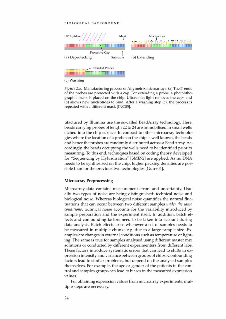
b i o lo g i ca l bac kg ro u n d

UV Light

Substrate

Mask

Protective Cap

Nucleotides

Extended Probes

(a) Deprotecting (b) Extending

(c) Washing

Figure 2.8: Manufacturing process of Affymetrix microarrays. (a) The 5’ endsof the probes are protected with a cap. For extending a probe, a photolitho-graphic mask is placed on the chip. Ultraviolet light removes the caps and(b) allows new nucleotides to bind. After a washing step (c), the process isrepeated with a different mask [INC05].

ufactured by Illumina use the so-called BeadArray technology. Here,beads carrying probes of length 22 to 24 are immobilised in small wellsetched into the chip surface. In contrast to other microarray technolo-gies where the location of a probe on the chip is well known, the beadsand hence the probes are randomly distributed across a BeadArray. Ac-cordingly, the beads occupying the wells need to be identified prior tomeasuring. To this end, techniques based on coding theory developedfor “Sequencing by Hybridisation” [SME92] are applied. As no DNAneeds to be synthesised on the chip, higher packing densities are pos-sible than for the previous two technologies [Gun+04].

Microarray Preprocessing

Microarray data contains measurement errors and uncertainty. Usu-ally two types of noise are being distinguished: technical noise andbiological noise. Whereas biological noise quantifies the natural fluc-tuations that can occur between two different samples under the sameconditions, technical noise accounts for the variability introduced bysample preparation and the experiment itself. In addition, batch ef-fects and confounding factors need to be taken into account duringdata analysis. Batch effects arise whenever a set of samples needs tobe measured in multiple chunks e.g. due to a large sample size. Ex-amples are changes in external conditions such as temperature or light-ing. The same is true for samples analysed using different master mixsolutions or conducted by different experimenters from different labs.These factors introduce systematic errors that can lead to shifts in ex-pression intensity and variance between groups of chips. Confoundingfactors lead to similar problems, but depend on the analysed samplesthemselves. For example, the age or gender of the patients in the con-trol and samples groups can lead to biases in the measured expressionvalues.

For obtaining expression values from microarray experiments, mul-tiple steps are necessary.

24

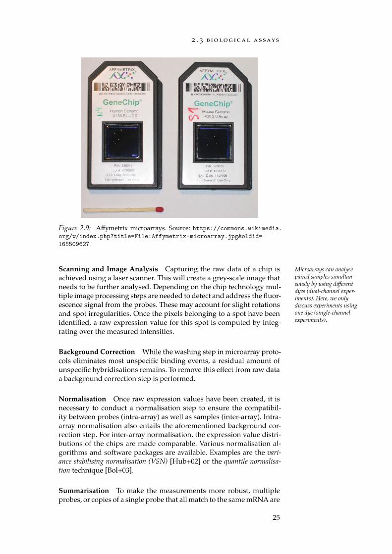
2 . 3 b i o lo g i ca l a s says

Figure 2.9: Affymetrix microarrays. Source: https://commons.wikimedia.org/w/index.php?title=File:Affymetrix-microarray.jpg&oldid=165509627

Scanning and Image Analysis Capturing the raw data of a chip is Microarrays can analysepaired samples simultan-eously by using differentdyes (dual-channel exper-iments). Here, we onlydiscuss experiments usingone dye (single-channelexperiments).

achieved using a laser scanner. This will create a grey-scale image thatneeds to be further analysed. Depending on the chip technology mul-tiple image processing steps are needed to detect and address the fluor-escence signal from the probes. These may account for slight rotationsand spot irregularities. Once the pixels belonging to a spot have beenidentified, a raw expression value for this spot is computed by integ-rating over the measured intensities.

Background Correction While the washing step in microarray proto-cols eliminates most unspecific binding events, a residual amount ofunspecific hybridisations remains. To remove this effect from raw dataa background correction step is performed.

Normalisation Once raw expression values have been created, it isnecessary to conduct a normalisation step to ensure the compatibil-ity between probes (intra-array) as well as samples (inter-array). Intra-array normalisation also entails the aforementioned background cor-rection step. For inter-array normalisation, the expression value distri-butions of the chips are made comparable. Various normalisation al-gorithms and software packages are available. Examples are the vari-ance stabilising normalisation (VSN) [Hub+02] or the quantile normalisa-tion technique [Bol+03].

Summarisation To make the measurements more robust, multipleprobes, or copies of a single probe that all match to the same mRNA are

25

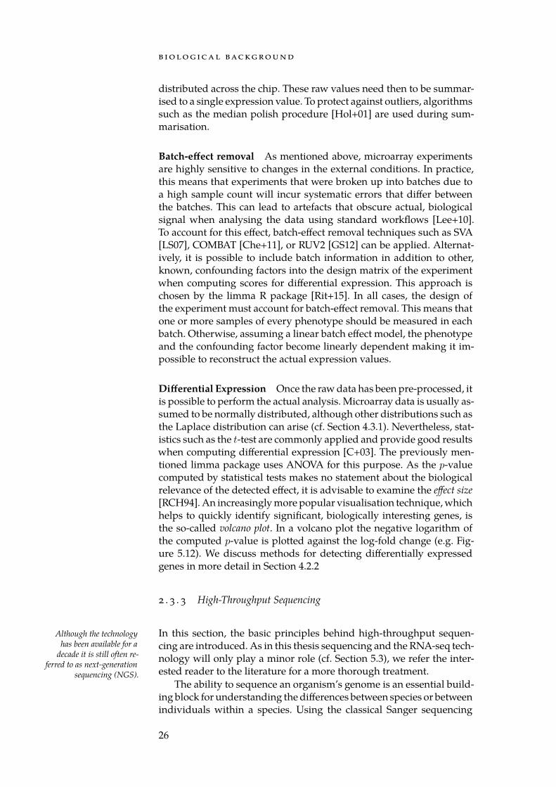
b i o lo g i ca l bac kg ro u n d

distributed across the chip. These raw values need then to be summar-ised to a single expression value. To protect against outliers, algorithmssuch as the median polish procedure [Hol+01] are used during sum-marisation.

Batch-effect removal As mentioned above, microarray experimentsare highly sensitive to changes in the external conditions. In practice,this means that experiments that were broken up into batches due toa high sample count will incur systematic errors that differ betweenthe batches. This can lead to artefacts that obscure actual, biologicalsignal when analysing the data using standard workflows [Lee+10].To account for this effect, batch-effect removal techniques such as SVA[LS07], COMBAT [Che+11], or RUV2 [GS12] can be applied. Alternat-ively, it is possible to include batch information in addition to other,known, confounding factors into the design matrix of the experimentwhen computing scores for differential expression. This approach ischosen by the limma R package [Rit+15]. In all cases, the design ofthe experiment must account for batch-effect removal. This means thatone or more samples of every phenotype should be measured in eachbatch. Otherwise, assuming a linear batch effect model, the phenotypeand the confounding factor become linearly dependent making it im-possible to reconstruct the actual expression values.

Differential Expression Once the raw data has been pre-processed, itis possible to perform the actual analysis. Microarray data is usually as-sumed to be normally distributed, although other distributions such asthe Laplace distribution can arise (cf. Section 4.3.1). Nevertheless, stat-istics such as the t-test are commonly applied and provide good resultswhen computing differential expression [C+03]. The previously men-tioned limma package uses ANOVA for this purpose. As the p-valuecomputed by statistical tests makes no statement about the biologicalrelevance of the detected effect, it is advisable to examine the effect size[RCH94]. An increasingly more popular visualisation technique, whichhelps to quickly identify significant, biologically interesting genes, isthe so-called volcano plot. In a volcano plot the negative logarithm ofthe computed p-value is plotted against the log-fold change (e.g. Fig-ure 5.12). We discuss methods for detecting differentially expressedgenes in more detail in Section 4.2.2

2 . 3 . 3 High-Throughput Sequencing

In this section, the basic principles behind high-throughput sequen-Although the technologyhas been available for a

decade it is still often re-ferred to as next-generation

sequencing (NGS).

cing are introduced. As in this thesis sequencing and the RNA-seq tech-nology will only play a minor role (cf. Section 5.3), we refer the inter-ested reader to the literature for a more thorough treatment.

The ability to sequence an organism’s genome is an essential build-ing block for understanding the differences between species or betweenindividuals within a species. Using the classical Sanger sequencing

26

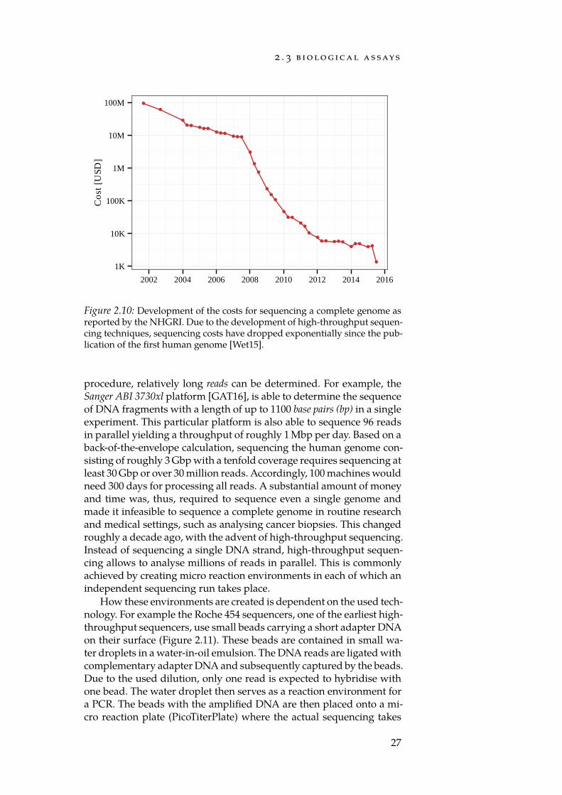
2 . 3 b i o lo g i ca l a s says

1K

10K

100K

1M

10M

100M

2002 2004 2006 2008 2010 2012 2014 2016

Cos

t [U

SD]

Figure 2.10: Development of the costs for sequencing a complete genome asreported by the NHGRI. Due to the development of high-throughput sequen-cing techniques, sequencing costs have dropped exponentially since the pub-lication of the first human genome [Wet15].

procedure, relatively long reads can be determined. For example, theSanger ABI 3730xl platform [GAT16], is able to determine the sequenceof DNA fragments with a length of up to 1100 base pairs (bp) in a singleexperiment. This particular platform is also able to sequence 96 readsin parallel yielding a throughput of roughly 1 Mbp per day. Based on aback-of-the-envelope calculation, sequencing the human genome con-sisting of roughly 3 Gbp with a tenfold coverage requires sequencing atleast 30 Gbp or over 30 million reads. Accordingly, 100 machines wouldneed 300 days for processing all reads. A substantial amount of moneyand time was, thus, required to sequence even a single genome andmade it infeasible to sequence a complete genome in routine researchand medical settings, such as analysing cancer biopsies. This changedroughly a decade ago, with the advent of high-throughput sequencing.Instead of sequencing a single DNA strand, high-throughput sequen-cing allows to analyse millions of reads in parallel. This is commonlyachieved by creating micro reaction environments in each of which anindependent sequencing run takes place.

How these environments are created is dependent on the used tech-nology. For example the Roche 454 sequencers, one of the earliest high-throughput sequencers, use small beads carrying a short adapter DNAon their surface (Figure 2.11). These beads are contained in small wa-ter droplets in a water-in-oil emulsion. The DNA reads are ligated withcomplementary adapter DNA and subsequently captured by the beads.Due to the used dilution, only one read is expected to hybridise withone bead. The water droplet then serves as a reaction environment fora PCR. The beads with the amplified DNA are then placed onto a mi-cro reaction plate (PicoTiterPlate) where the actual sequencing takes

27

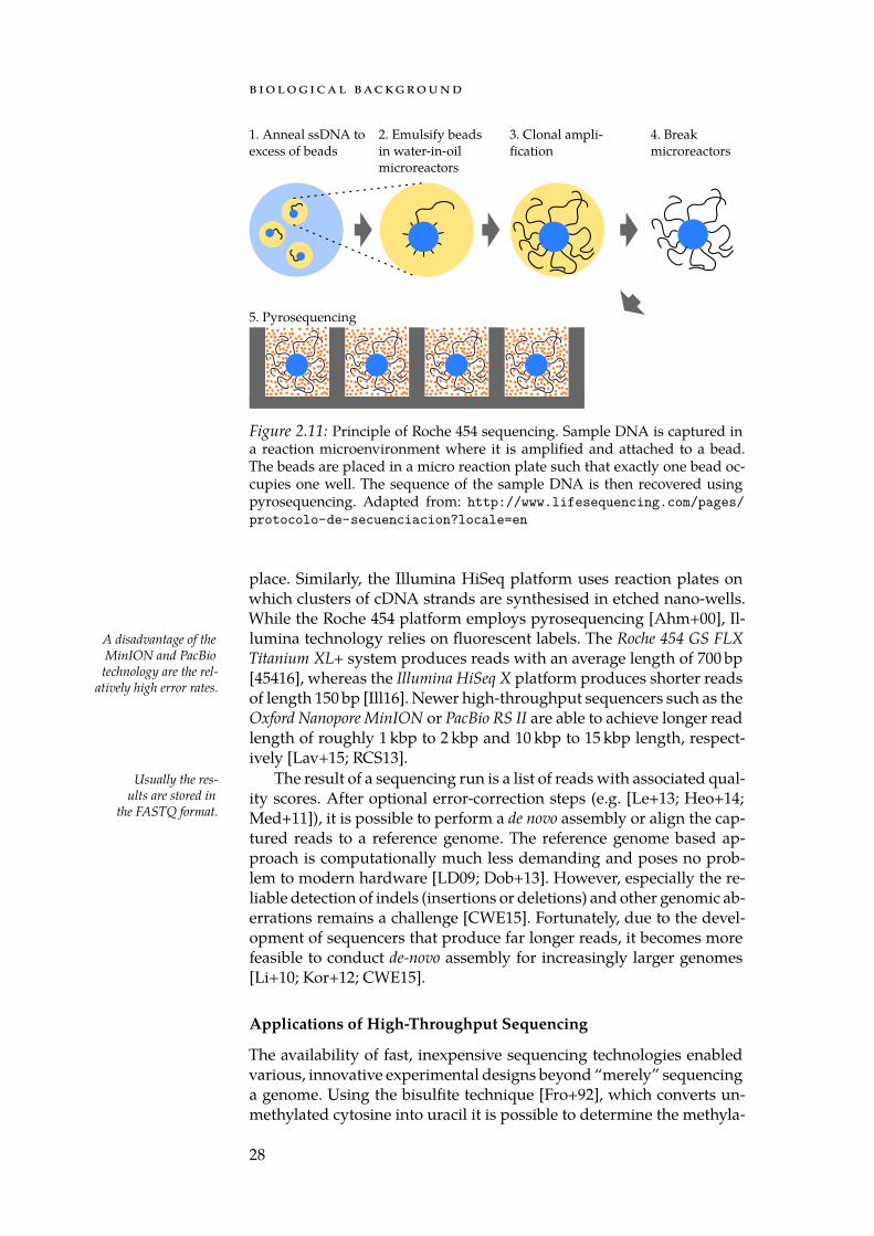
b i o lo g i ca l bac kg ro u n d

1. Anneal ssDNA toexcess of beads

2. Emulsify beadsin water-in-oilmicroreactors

3. Clonal ampli-fication

4. Breakmicroreactors

5. Pyrosequencing

Figure 2.11: Principle of Roche 454 sequencing. Sample DNA is captured ina reaction microenvironment where it is amplified and attached to a bead.The beads are placed in a micro reaction plate such that exactly one bead oc-cupies one well. The sequence of the sample DNA is then recovered usingpyrosequencing. Adapted from: http://www.lifesequencing.com/pages/protocolo-de-secuenciacion?locale=en

place. Similarly, the Illumina HiSeq platform uses reaction plates onwhich clusters of cDNA strands are synthesised in etched nano-wells.While the Roche 454 platform employs pyrosequencing [Ahm+00], Il-lumina technology relies on fluorescent labels. The Roche 454 GS FLXA disadvantage of the

MinION and PacBiotechnology are the rel-

atively high error rates.

Titanium XL+ system produces reads with an average length of 700 bp[45416], whereas the Illumina HiSeq X platform produces shorter readsof length 150 bp [Ill16]. Newer high-throughput sequencers such as theOxford Nanopore MinION or PacBio RS II are able to achieve longer readlength of roughly 1 kbp to 2 kbp and 10 kbp to 15 kbp length, respect-ively [Lav+15; RCS13].

The result of a sequencing run is a list of reads with associated qual-Usually the res-ults are stored in

the FASTQ format.ity scores. After optional error-correction steps (e.g. [Le+13; Heo+14;Med+11]), it is possible to perform a de novo assembly or align the cap-tured reads to a reference genome. The reference genome based ap-proach is computationally much less demanding and poses no prob-lem to modern hardware [LD09; Dob+13]. However, especially the re-liable detection of indels (insertions or deletions) and other genomic ab-errations remains a challenge [CWE15]. Fortunately, due to the devel-opment of sequencers that produce far longer reads, it becomes morefeasible to conduct de-novo assembly for increasingly larger genomes[Li+10; Kor+12; CWE15].

Applications of High-Throughput Sequencing

The availability of fast, inexpensive sequencing technologies enabledvarious, innovative experimental designs beyond “merely” sequencinga genome. Using the bisulfite technique [Fro+92], which converts un-methylated cytosine into uracil it is possible to determine the methyla-

28

2 . 3 b i o lo g i ca l a s says

tion state of the genome down to base resolution. Chromatin immuno-precipitation in combination with sequencing (ChIP-seq) allows to de-termine the occupancy of DNA with binding proteins [Bar+07b; Par09].For this, the proteins are cross-linked to the DNA. Then, using nucle-ases or sonication, the DNA is broken into fragments. After that, allproteins of interest are selected using specific antibodies. Due to thecross-linking, these proteins carry a DNA fragment with them. In thenext step, the bound DNA is removed from the purified protein and se-quenced subsequently. Aligning the obtained reads to a reference gen-ome reveals occupied protein binding sites. This technique is routinelyapplied to analyse the binding sites of transcription factors [Val+08]and histone variants [Bar+07b]. Finally, just as mRNA/miRNA microar-rays, RNA-seq allows to capture the complete transcriptome of a tissuesample. We will now discuss this particular application in more detail.

RNA-seq

For measuring expression using high-throughput sequencing, RNA is Although providing a moredirect measure of tran-scriptional activity thanmicroarrays, RNA-seq doesnot (yet) report abolutetranscript abundances.

extracted from a sample and, depending on the used protocol, filteredfor e.g. short RNA or mRNA [Mar+08a]. Subsequently, the purifiedRNA is transcribed back into cDNA, which is then sequenced [WGS09].By determining the amount of sequencing reads that originated froma given transcript, the abundance of this transcript can be estimated.Traditionally, alignments against a reference genome or transcriptomeare used to determine the transcripts a read originated from. To thisend, aligners should be used that are able to map reads across splicejunctions such as the STAR aligner [Dob+13]. Recently, alignment freemethods such as Sailfish [PMK14] and Kallisto [Bra+15] have been pub-lished. These approached rely on k-mer based algorithms for creating“pseudo-alignments”. Salmon [PDK15] computes “lightweight” align-ments by detecting approximate positions of a read in the reference. Incontrast to the classical, alignment based workflows these algorithmsoffer a much improved runtime behaviour with little to no degradationin accuracy.

After determining a read-to-transcript assignment, the number ofreads that map to a transcript is computed. To directly compare theread counts between two transcripts they need to be normalised withrespect to the transcript length. For this purpose the fragments per kilob-ase of exon per million fragments mapped (FPKM) [Tra+10] and transcriptsper million (TPM) [WKL12] statistics are used. Differentially expressedgenes or transcripts are computed with specialised software such asDESeq2 [LHA14] or EdgeR [RMS10]. These packages take advantageof the discrete probability distribution of read counts to detect differen-tially expressed genes more reliably. Nevertheless, software originallydeveloped for microarray analysis such as limma is used and producesgood results [Rit+15].

29

b i o lo g i ca l bac kg ro u n d

2 . 3 . 4 Comparison of Microarrays and RNA-seq

Microarray have established themselves as a well understood, battle-proven experimental technology for capturing expression profiles. Inrecent years, the RNA-seq technology is gaining popularity, though. Alarge advantage of RNA-seq over microarrays is that the raw data canbe easily reanalysed for newer genome builds and annotations as it isnot tied to a particular probe design. As raw reads are available it is alsopossible to call genomic variations in coding regions [Che+09]. In ad-dition, due to the increasing read length for modern high-throughputsequencers, reliably resolving expressed isoforms becomes more andmore feasible [Chh+15]. A further point in favour of RNA-seq is thatDue to the required read

amplification and norm-alisation based on frag-

ment length an absolutequantification is diffi-

cult even with RNA-seq.

the obtained read counts are a more direct representation of the ac-tual RNA abundance than the indirect fluorescence signals obtainedfrom microarrays. Yet, microarray platforms continue to be used dueto well established protocols and analysis pipelines. Furthermore, theexpression profiles generated using current microarray platforms re-main competitive with RNA-seq based methods in terms of quality.Ultimately, however, RNA-seq is more versatile and can be expectedto replace microarrays for most use cases [Zha+14; Man+14; Zha+15].

2 . 4 w i l m ' s t u m o u r data

Contributions Most WT tissue samples were collected by thegroup of Prof. Manfred Gessler. Some samples as well as clinicaldata were provided by the group of Prof. Norbert Graf. The mi-croarray assays were performed by Nicole Ludwig from the groupof Prof. Eckart Meese. Normalisation of the raw expression valueswas performed by Patrick Trampert.

In Section 2.1.1 we introduced Wilm’s tumour and some of its com-Parts of this sectionhave been adapted fromStöckel et al. [Stö+16].

mon subtypes. We noted that tumours containing a high amount ofblastemal cells after pre-operative chemotherapy, the so called blastemalsubtype, is one of the most aggressive Wilm’s tumour subtypes. To in-vestigate why some tumours with a high blastem content respond wellto chemotherapy while others do not, we generated an expression data-set of Wilm’s tumours that were treated with pre-operative chemother-apy according to the SIOP protocol (cf. [Isr+13; DPG14]).

Patient Samples The dataset consists of 40 mRNA and 47 miRNA ex-pression profiles from 47 tumour biopsies collected from 39 patients.These biopsies contain four healthy tissue samples as well as 16 blaste-mal, nine mixed type and 17 miscellaneous tumour samples that werelabelled as described in Section 2.1.1. Before surgery, patients weretreated using the SIOP standard regimen consisting of Actinomycin-D,Vincristine, and, in the case of metastases, Doxorubicin (cf. Figure 2.3).

30

2 . 4 w i l m ' s t u m o u r data

Clinical details of the patients included in the analysis and an overviewover the generated expression profiles is given in Appendix B. The re-search was approved by the local ethical committee (Ethikkommissionder Ärztekammer des Saarlandes, No. 136/01; 09/16/2010).

RNA Isolation Total RNA including miRNAs was isolated from tu-mour and control tissue using the miRNeasy Kit (Qiagen, Hilden, Ger-many) according to manufacturer’s instructions. The RNA concentra-tion and integrity were assessed using NanoDrop2000 (Thermo FisherScientific, Waltham, MA, USA) and Bioanalyzer runs using the Pico-RNA Chip (Agilent Technologies, Santa Clara, CA, USA).

miRNA Expression Profiles miRNA expression profiles were meas-ured using the SurePrint G3 8x60k miRNA microarray (miRBase v16,Cat. no. G4870A) according to the manufacturer’s recommendations.Background-corrected, log-transformed expression values were extrac-ted using the Agilent Feature Extraction Software and normalised usingquantile normalisation. In total, 47 miRNA expression profiles weregenerated.

mRNA Expression Profiles All mRNA expression profile were meas-ured using SurePrint G3 Human Gene Expression 8x60K v2 microarrays(Cat. no. G4851B, Agilent Technologies, Santa Clara, CA, USA) accord-ing to the manufacturer’s recommendations. Expression values wereextracted, background-corrected, and log-transformed using the Agi-lent Feature Extraction Software and normalised using the GeneSpringsoftware [CSK01]. In total 40 mRNA expression profiles were gener-ated.

31

3B I O LO G I CA L N E T WO R K S

The whole is more than the sum of its parts.— a r i s tot l e , m e t a p hy s i c a

Cells are highly complex, molecular machines, each of which is com-posed of billions of biological entities such as genes, proteins, RNAs,and metabolites. These entities fulfil their tasks through interaction.Examples are proteins binding metabolites to catalyse a metabolic re-action or two proteins forming a complex. When a complex is formed,it again can participate in further interactions. Similarly, miRNAs canbind to mRNAs in order to make the translation process less efficientor completely inhibit it (Section 2.3.1). On the genome level, enhancersand genes can associate with transcription factors. This can lead to theinitiation or repression of expression or even to the remodelling of thechromatin structure. Which molecules are able to interact is determ- Interactions are typically

stochastic. That means thateven a highly specific bind-ing interface still allowsfor unspecific binding, al-beit with low probability[VB86].

ined by the chemical and structural properties of the putative interac-tion partners. In practice, the physical location of the molecules insidethe cell also plays an important role. For example, a molecule inside thenucleus will not react with another molecule in the cytoplasm as theyare separated by the nuclear membrane. Moreover, not every gene isexpressed in every cell and hence not every protein is available every-where. Consequently, reactions that are possible in one cell type neednot be possible in another cell type.

Viewed together, the interactions in a cell form a network in which The number of (protein cod-ing) genes and their tran-scripts continues to vary.The reported numbers weretaken from GENCODE 24.

the entities are connected with edges representing interactions. Con-sidering that there exist approximately 20,000 human genes encodingroughly 80,000 proteins, the amount of possible interactions alreadyranges in the billions [Har+06; Har+12]. This completely disregardsthe vast amount of RNA and metabolites that are present at any pointin time. Even when excluding interactions that are impossible due tochemical considerations or tissue specificity, it is clear that chartingthese networks is a daunting task. In a valiant effort towards reachingthis goal, interaction databases have been created with which research-ers attempt to catalogue all known biological entities and their inter-actions in a structured and well-defined fashion. As opposed to theunstructured representation of knowledge found in the literature, theavailability of databases enables researchers to efficiently search thestored data. Furthermore, it enables the use of bioinformatics analysispipelines, which is imperative for the ability to deal with genome-scaledatasets. This development lead to the emergence of systems biology.In contrast to the classical, bottom-up approach of biology [Laz02], inwhich parts of a biological system are studied in isolation, systems bio-logy attempts to detect general patterns on a global level [Kir05; Kit02].This means that instead of studying biological processes in minute de-tail, systems biology is dedicated to discovering general architecturesand building blocks that nature repeatedly uses to create complex bio-

33

b i o lo g i ca l n e t wo r k s

logical systems. To achieve this, systems biology relies on computa-tional methods and machine learning techniques for extracting the in-formation stored in biological databases.

In this chapter, we will take a look at various methods that assistresearchers in reasoning about biological systems. In each section, wegive a short discussion of the respective state of the art. In addition,we present algorithms that exploit the knowledge stored in interactiondatabases to improve the analysis of experimental data. For this, wefirst introduce some general terminology. Next, an overview over theavailable types of databases is provided. After this, we take a look athow Bayesian networks (BNs), and especially causal Bayesian networks,can be employed to test hypotheses about cellular processes. Based onthis, we introduce our tool CausalTrail [Sch15a; Stö+15] which, to thebest of our knowledge, is the first tool that allows researchers to evalu-ate causal queries on a causal Bayesian network structure. Afterwards,we give a short introduction to Gaussian graphical models (GGMs). Whilewe will not use GGMs to infer networks, Section 4.4 demonstrates howto use the underlying theory to construct an “enrichment algorithm”that corrects for the correlation structure in biological categories.

While the previously mentioned approaches model network struc-tures from a probabilistic point of view, also purely graph theoreticalalgorithms exist. As an example, we present an ILP approach for find-ing deregulated subgraphs in regulatory networks [Bac+12]. In con-trast to many other approaches, our algorithm is exact and highly effi-cient. While algorithms for detecting deregulated subgraphs by designare influenced by the provided topology, it is unclear how large its im-pact on the computed results is. To this end we perform an evaluationdemonstrating how the network topology and input scores affect theproduced solutions.

3 . 1 g r a p h t h e o ry

Before we begin with the explanation of the methods and conceptspresented in this chapter, we first introduce some basic terminologyfrom graph theory. In mathematics, graphs describe binary relations(edges) between a set of objects called nodes or vertices. Thus, graphslend themselves for modelling biological networks. Formally a graphis defined as follows:

Definition 1 (Graph). Let V be an arbitrary, finite set of nodes or verticesand E ⊆ V × V the set of edges. We call the pair of node and edge seta graph and write G(V,E). G is undirected, if for every edge (u, v) ∈ Ealso (v, u) ∈ E holds.

A graph G is called simple, if no edge (v, v) ∈ E exists. Unless men-tioned otherwise, we assume that all graphs mentioned in this thesisare simple.

An often encountered attribute of nodes are their degrees:

34

3 . 1 g r a p h t h e o ry

Definition 2 (In- and out-degree). Given a graph G = (V,E), the in-degree d−v of a node v is the number of edges that end in v. Conversely,the out-degree d+v of v is the number of edges starting in v.

Another important property of a node is whether it is possible toreach it from another node. To give a proper definition of this notion,we first introduce the concept of a path.

Definition 3 (Path). Let G(V,E) be a graph. If the sequence

p = ⟨v1, v2, . . . , vk⟩

of vertices with k ∈ N, k ≥ 2 fulfils (vi, vi+1) ∈ E for all i < k it iscalled a path of length k.

If for two vertices u, v ∈ V there exists a path starting in u andending in v, we say that v is reachable from u. The set of vertices thatis reachable from u is called the descendants of u, whereas all verticesthat can reach v are called its ancestors. Descendants and ancestors thatare only one edge away are called the children and parents of a node,respectively.

A graph is called strongly connected if every node v can be reachedfrom every other node v = u. With E = E ∪ (v, u)|(u, v) ∈ E wedenote the symmetric closure of the edge set. G is called connected, ifH(V, E) is strongly connected. A subgraph H ⊂ G is a graph H(V ′, E′)with V ′ ⊂ V and E′ ⊂ E. A connected component of G is a maximal,connected subgraph.

In some graphs, it is possible to find paths that start from and endin the same vertex v.

Definition 4 (Cycle and circle). A path C = ⟨v1, v2, . . . , vk, v1⟩ is calleda cycle. If no vertex, except v1, appears twice in C, we call C a circle. If agraph does not contain any cycle, it is called acyclic.

In some cases, we refer to edge or node labels. Commonly, these canbe thought of as functions mapping the nodes and edges to a value.

Definition 5 (Node and edge labels). Let G(V,E) be a graph. A node la-bel for G is a function w : V → X , where X is an arbitrary set. Similarlyan edge label is a function l : E → X .

We often refer to vertices using an index i ∈ N. For convenience, weuse the notation wi := w(vi) for referring to the node label of vi ∈ V .Examples for node labels are scores for differential expression that areattached to each node. We call such labels node weights or simply scores.In a regulatory network it is common to label each edge with the typeof the interaction it describes.

35

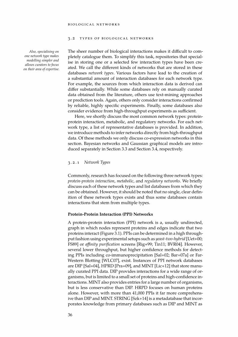
b i o lo g i ca l n e t wo r k s

3 . 2 t y p e s o f b i o lo g i ca l n e t wo r k s

The sheer number of biological interactions makes it difficult to com-Also, specialising onone network type makesmodelling simpler and

allows curators to focuson their area of expertise.

pletely catalogue them. To simplify this task, repositories that special-ise in storing one or a selected few interaction types have been cre-ated. We call the different kinds of networks that are stored in thesedatabases network types. Various factors have lead to the creation ofa substantial amount of interaction databases for each network type.For example, the sources from which interaction data is derived candiffer substantially. While some databases rely on manually curateddata obtained from the literature, others use text-mining approachesor prediction tools. Again, others only consider interactions confirmedby reliable, highly specific experiments. Finally, some databases alsoconsider evidence from high-throughput experiments as sufficient.

Here, we shortly discuss the most common network types: protein-protein interaction, metabolic, and regulatory networks. For each net-work type, a list of representative databases is provided. In addition,we introduce methods to infer networks directly from high-throughputdata. Of these methods we only discuss co-expression networks in thissection. Bayesian networks and Gaussian graphical models are intro-duced separately in Section 3.3 and Section 3.4, respectively.

3 . 2 . 1 Network Types

Commonly, research has focused on the following three network types:protein-protein interaction, metabolic, and regulatory networks. We brieflydiscuss each of these network types and list databases from which theycan be obtained. However, it should be noted that no single, clear defin-ition of these network types exists and thus some databases containinteractions that stem from multiple types.

Protein-Protein Interaction (PPI) Networks

A protein-protein interaction (PPI) network is a, usually undirected,graph in which nodes represent proteins and edges indicate that twoproteins interact (Figure 3.1). PPIs can be determined in a high through-put fashion using experimental setups such as yeast-two-hybrid [Uet+00;FS89] or affinity purification screens [Rig+99; Tin11; BVR04]. However,several lower throughput, but higher confidence methods for detect-ing PPIs including co-immunoprecipitation [Sal+02; Bar+07a] or Far-Western Blotting [WLC07], exist. Instances of PPI network databasesare DIP [Sal+04], HPRD [Pra+09], and MINT [Lic+12] that store manu-ally curated PPI data. DIP provides interactions for a wide range of or-ganisms, but is limited to a small set of proteins and high-confidence in-teractions. MINT also provides entries for a large number of organisms,but is less conservative than DIP. HRPD focuses on human proteinsalone. However, with more than 41,000 PPIs it far more comprehens-ive than DIP and MINT. STRING [Szk+14] is a metadatabase that incor-porates knowledge from primary databases such as DIP and MINT as

36

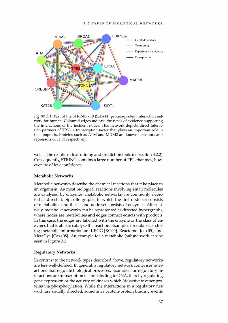
3 . 2 t y p e s o f b i o lo g i ca l n e t wo r k s

CDKN2ABRCA1MDM2

ATM

EP300

MAPK8

CREBBPCDKN1A

KAT2B SIRT1

TP53

Curated database

Textmining

Experimental evidence

Co-expression

Figure 3.1: Part of the STRING v10 [Szk+14] protein-protein interaction net-work for human. Coloured edges indicate the types of evidence supportingthe interactions of the incident nodes. This network depicts direct interac-tion partners of TP53, a transcription factor that plays an important role inthe apoptosis. Proteins such as ATM and MDM2 are known activators andrepressors of TP53 respectively.

well as the results of text-mining and prediction tools (cf. Section 3.2.2).Consequently, STRING contains a large number of PPIs that may, how-ever, be of low confidence.

Metabolic Networks

Metabolic networks describe the chemical reactions that take place inan organism. As most biological reactions involving small moleculesare catalysed by enzymes, metabolic networks are commonly depic-ted as directed, bipartite graphs, in which the first node set consistsof metabolites and the second node set consists of enzymes. Alternat-ively, metabolic networks can be represented as directed hypergraphs,where nodes are metabolites and edges connect educts with products.In this case, the edges are labelled with the enzyme or the class of en-zymes that is able to catalyse the reaction. Examples for databases stor-ing metabolic information are KEGG [KG00], Reactome [Jos+05], andMetaCyc [Cas+08]. An example for a metabolic (sub)network can beseen in Figure 3.2

Regulatory Networks

In contrast to the network types described above, regulatory networksare less well-defined. In general, a regulatory network comprises inter-actions that regulate biological processes. Examples for regulatory in-teractions are transcription factors binding to DNA, thereby regulatinggene expression or the activity of kinases which (de)activate other pro-teins via phosphorylation. While the interactions in a regulatory net-work are usually directed, sometimes protein-protein binding events

37

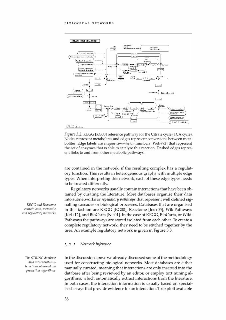
b i o lo g i ca l n e t wo r k s

Figure 3.2: KEGG [KG00] reference pathway for the Citrate cycle (TCA cycle).Nodes represent metabolites and edges represent conversions between meta-bolites. Edge labels are enzyme commission numbers [Web+92] that representthe set of enzymes that is able to catalyse this reaction. Dashed edges repres-ent links to and from other metabolic pathways.

are contained in the network, if the resulting complex has a regulat-ory function. This results in heterogeneous graphs with multiple edgetypes. When interpreting this network, each of these edge types needsto be treated differently.

Regulatory networks usually contain interactions that have been ob-tained by curating the literature. Most databases organise their datainto subnetworks or regulatory pathways that represent well defined sig-nalling cascades or biological processes. Databases that are organisedKEGG and Reactome

contain both, metabolicand regulatory networks.

in this fashion are KEGG [KG00], Reactome [Jos+05], WikiPathways[Kel+12], and BioCarta [Nis01]. In the case of KEGG, BioCarta, or Wiki-Pathways the pathways are stored isolated from each other. To create acomplete regulatory network, they need to be stitched together by theuser. An example regulatory network is given in Figure 3.3.

3 . 2 . 2 Network Inference

In the discussion above we already discussed some of the methodologyThe STRING databasealso incorporates in-

teractions obtained viaprediction algorithms.

used for constructing biological networks. Most databases are eithermanually curated, meaning that interactions are only inserted into thedatabase after being reviewed by an editor, or employ text mining al-gorithms, which automatically extract interactions from the literature.In both cases, the interaction information is usually based on special-ised assays that provide evidence for an interaction. To exploit available

38

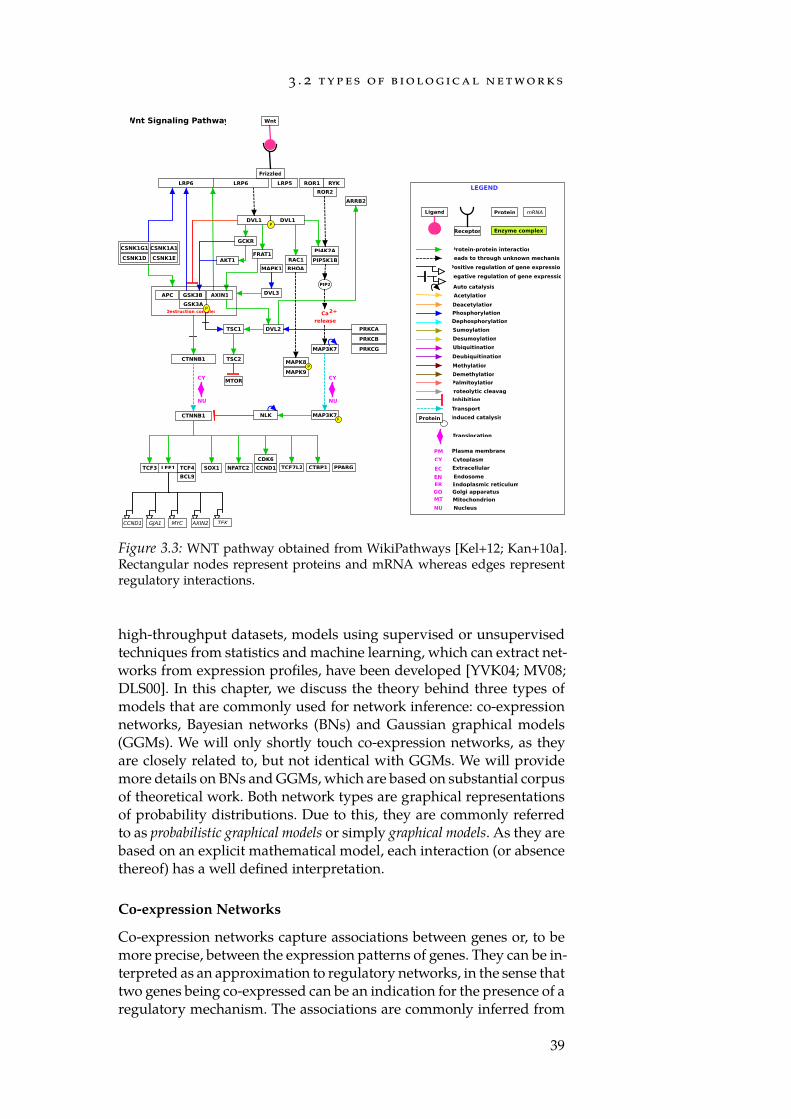
3 . 2 t y p e s o f b i o lo g i ca l n e t wo r k s

PIP2

Destruction complex Carelease

2+

Wnt

Frizzled

AXIN1

RAC1

MYC

CTNNB1

GJA1

LRP5

AXIN2

CSNK1A1

TEK

BCL9

LRP6

AKT1

LRP6

CSNK1G1

DVL1

LEF1

ROR1

SOX1

GSK3A

DVL3

MAP3K7

DVL2

NFATC2TCF4

ARRB2

PIP5K1B

RHOA

PRKCG

CTBP1

DVL1

MAPK1

CTNNB1

MTOR

GCKR

CCND1

APC

TCF3 CCND1

TSC1 PRKCA

CSNK1EFRAT1

CSNK1D

RYK

TCF7L2

PRKCB

PPARG

PI4K2A

CDK6

P

P

GSK3B

ROR2

MAPK9

MAPK8P

MAP3K7P

TSC2

NLK

Inhibition

Auto catalysis

Transport

Positive regulation of gene expression

Leads to through unknown mechanism

Negative regulation of gene expression

Translocation

Ubiquitination

Deubiquitination

Sumoylation

Induced catalysis

Protein-protein interaction

Acetylation

Dephosphorylation

LEGEND

Phosphorylation

Deacetylation

Golgi apparatus

Endosome

Nucleus

Mitochondrion

Desumoylation

Methylation

Demethylation

Palmitoylation

Cytoplasm

EC

Plasma membrane

MT

Endoplasmic reticulum

CY

PM

GO

NU

Extracellular

EREN

Proteolytic cleavage

Wnt Signaling Pathway

CY

NU

CY

NU

mRNA

Receptor

Ligand Protein

Enzyme complex

Protein

Figure 3.3: WNT pathway obtained from WikiPathways [Kel+12; Kan+10a].Rectangular nodes represent proteins and mRNA whereas edges representregulatory interactions.

high-throughput datasets, models using supervised or unsupervisedtechniques from statistics and machine learning, which can extract net-works from expression profiles, have been developed [YVK04; MV08;DLS00]. In this chapter, we discuss the theory behind three types ofmodels that are commonly used for network inference: co-expressionnetworks, Bayesian networks (BNs) and Gaussian graphical models(GGMs). We will only shortly touch co-expression networks, as theyare closely related to, but not identical with GGMs. We will providemore details on BNs and GGMs, which are based on substantial corpusof theoretical work. Both network types are graphical representationsof probability distributions. Due to this, they are commonly referredto as probabilistic graphical models or simply graphical models. As they arebased on an explicit mathematical model, each interaction (or absencethereof) has a well defined interpretation.

Co-expression Networks

Co-expression networks capture associations between genes or, to bemore precise, between the expression patterns of genes. They can be in-terpreted as an approximation to regulatory networks, in the sense thattwo genes being co-expressed can be an indication for the presence of aregulatory mechanism. The associations are commonly inferred from

39

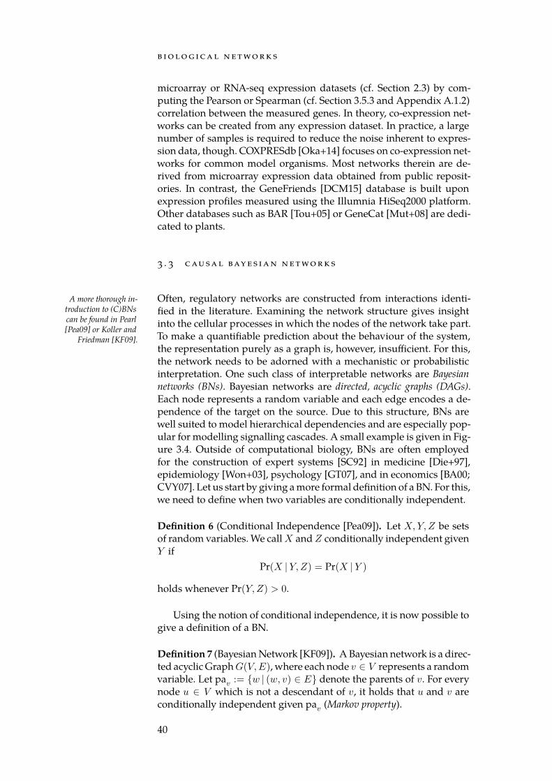
b i o lo g i ca l n e t wo r k s

microarray or RNA-seq expression datasets (cf. Section 2.3) by com-puting the Pearson or Spearman (cf. Section 3.5.3 and Appendix A.1.2)correlation between the measured genes. In theory, co-expression net-works can be created from any expression dataset. In practice, a largenumber of samples is required to reduce the noise inherent to expres-sion data, though. COXPRESdb [Oka+14] focuses on co-expression net-works for common model organisms. Most networks therein are de-rived from microarray expression data obtained from public reposit-ories. In contrast, the GeneFriends [DCM15] database is built uponexpression profiles measured using the Illumnia HiSeq2000 platform.Other databases such as BAR [Tou+05] or GeneCat [Mut+08] are dedi-cated to plants.

3 . 3 cau sa l bay e s i a n n e t wo r k s

Often, regulatory networks are constructed from interactions identi-A more thorough in-troduction to (C)BNscan be found in Pearl[Pea09] or Koller and

Friedman [KF09].

fied in the literature. Examining the network structure gives insightinto the cellular processes in which the nodes of the network take part.To make a quantifiable prediction about the behaviour of the system,the representation purely as a graph is, however, insufficient. For this,the network needs to be adorned with a mechanistic or probabilisticinterpretation. One such class of interpretable networks are Bayesiannetworks (BNs). Bayesian networks are directed, acyclic graphs (DAGs).Each node represents a random variable and each edge encodes a de-pendence of the target on the source. Due to this structure, BNs arewell suited to model hierarchical dependencies and are especially pop-ular for modelling signalling cascades. A small example is given in Fig-ure 3.4. Outside of computational biology, BNs are often employedfor the construction of expert systems [SC92] in medicine [Die+97],epidemiology [Won+03], psychology [GT07], and in economics [BA00;CVY07]. Let us start by giving a more formal definition of a BN. For this,we need to define when two variables are conditionally independent.

Definition 6 (Conditional Independence [Pea09]). Let X,Y, Z be setsof random variables. We call X and Z conditionally independent givenY if

Pr(X |Y, Z) = Pr(X |Y )

holds whenever Pr(Y, Z) > 0.

Using the notion of conditional independence, it is now possible togive a definition of a BN.

Definition 7 (Bayesian Network [KF09]). A Bayesian network is a direc-ted acyclic GraphG(V,E), where each node v ∈ V represents a randomvariable. Let pav := w | (w, v) ∈ E denote the parents of v. For everynode u ∈ V which is not a descendant of v, it holds that u and v areconditionally independent given pav (Markov property).

40

3 . 3 cau sa l bay e s i a n n e t wo r k s

Difficulty (D)

Grade (G)

Letter (L)

Intelligence (I)

SAT (S)

Figure 3.4: The student network is an example of a small BN. Each of the nodesrepresents a binary variable. Whether a student earns a good grade (G), isdependent on whether the course was difficult (D) and whether the studentpossesses a low or a high intelligence (I). Based on the grade, a lecturer maybe more or less inclined to write a letter of recommendation (L). Whether thestudent passes the SAT test only depends on the student’s intelligence.

Given a Bayesian network for a probability distribution, we canwrite the joint probability density as a product of conditional probab-ilities:

Pr(X1, . . . , Xn) =

n∏k=1

Pr(Xk |paXk)

Often, an edge from parent to child in a BN is assumed to model acausal relationship. Yet, this is not true in general. To see why, let us takea look at the chain rule that can be used to represent a joint probabilitydistribution as a product of conditional distributions: To proof this, use

Pr(X|Y ) =Pr(X,Y )/Pr(Y ) andcollapse the resulting tele-scoping product.

Pr(X1, . . . , Xn) =n∏

k=1

Pr(Xk |X1, . . . , Xk−1)

Clearly, this factorisation gives us a simple way to represent every prob-ability distribution as a BN. Each factor in the product represents achild (Xk) to parent(s) (X1, . . . , Xk−1) relation. However, this decom-position is not unique, as it solely depends on the ordering of the vari-ables [Pea09]. As a consequence, we obtain different graph structures,depending on the ordering of the variables. In fact, it is possible to gen-erate cases in which node Xi is a parent of Xj and cases where the op-posite is true. If a causal relationship between the two variables exists,only one of the directions encodes this relationship faithfully. Hence,the topological order in a BN cannot be assumed to model a causalrelationship.

When does an edge in a BN stand for an actual, causal dependency?To answer this question, it is important to understand the concept of in-terventions. By observing a system, e.g. by measuring the expression ofall genes in a cell, for a sufficient amount of time we are able to deducepatterns in its behaviour. An example for such a pattern would be: “ifnode A is in state a1, then node B is in state b2”. However, these obser-vations are only sufficient to conclude that the state of the two nodesis correlated. It is uncertain whether node B is in state b2 because nodeA is in state a1 or vice-versa. It is also possible that the state of the

41

b i o lo g i ca l n e t wo r k s

two nodes causally depends on a third variable and neither directionrepresents a valid causal relationship. To determine which of the threepossibilities is the case, the experimental setup needs to be changed. In-stead of passively observing the system, an external perturbation mustbe introduced. For example, if the state of a node A is artificially fixedat state a1, we can observe the state of node B. If B remains in stateb2 regardless of the other variables, this indicates that the state of A iscausal for the state of B. An example for such perturbations in a biolo-gical setting is the artificial knock-out or overexpression of a gene.

Pearl [Pea09] realised that the concept of interventions is not onlyhelpful for detecting causal relationships, but also is fundamental forgiving a sound definition of causality. Consider the factorisation of thejoint probability induced by the student network (Figure 3.4):

Pr(D, I,G, S, L) = Pr(L |G)Pr(G |D, I)Pr(S | I)Pr(D)Pr(I)

If we want to determine the probability of getting a letter in the casethat we know the grade is good, we set the value of G to “good” andremove the factor Pr(G |D, I) from the factorisation:

PrG=good(D, I, S, L) = Pr(L |G = good)Pr(S | I)Pr(D)Pr(I)

We call PrG=good an interventional distribution. This allows use to definea causal Bayesian network (CBN).

Definition 8 (Causal Bayesian network [Pea09]). A causal Bayesian net-work (CBN) for a distribution P is a Bayesian network which is consist-ent with all possible interventional distributions PX=x. Here, consistentmeans that the network encodes a valid factorisation of PX=x after thenode corresponding to X and all edges going into X have been deleted.

Now we can provide an answer to our initial question: an edge in aBN can only be interpreted as causal, if the BN is, in fact, a CBN.

This definition gives a natural way to examine the effect of externalDue to the lack of meas-urements of exogenousinfluences, a CBN cannot always be uniquely

determined. The resultingset of equivalent CBNs iscalled a causal structure.

influences on the observed system. Given a CBN, the effect of e.g. agene knock-out can be modelled by setting the state of the node rep-resenting the target gene to unexpressed and deleting all edges fromthe parent nodes. As the CBN is consistent with the corresponding in-terventional distribution, we can now query the network for probabilit-ies using standard algorithms. This approach was formalised by Pearl[Pea95a] as the so-called do-calculus. It allows to test hypotheses on howexternal changes (interventions) such as our gene knockout affect a sys-tem’s behaviour. Using the do-calculus it is also possible to answercounterfactual questions such as: “Would the patient have recoveredwhen given drugB, knowing that he did not recover given drug A?” or“Would the plane have crashed, if it had been inspected before take-off,given that it had not been inspected before?”. As such, counterfactualsallow to re-evaluate decisions retrospectively in the light of new evid-ence.

Due to the above properties, BNs and CBNs are popular tools inbioinformatics and have been applied in many scenarios [M+99; Fri+00;

42

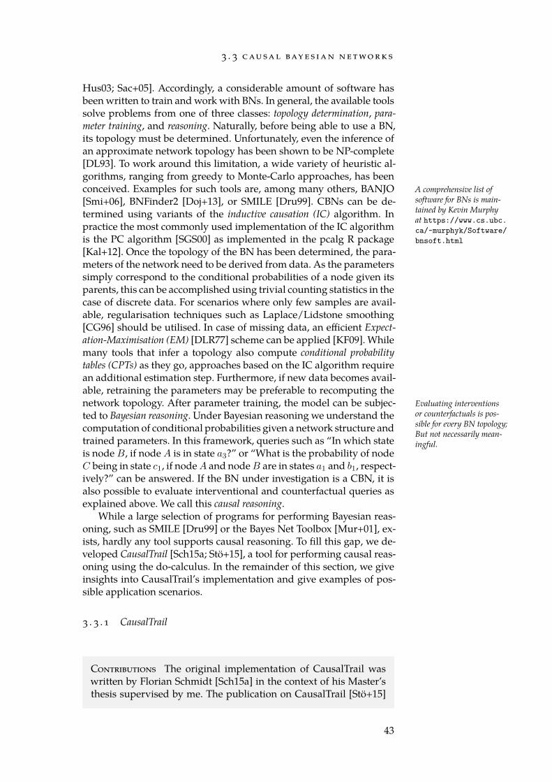
3 . 3 cau sa l bay e s i a n n e t wo r k s

Hus03; Sac+05]. Accordingly, a considerable amount of software hasbeen written to train and work with BNs. In general, the available toolssolve problems from one of three classes: topology determination, para-meter training, and reasoning. Naturally, before being able to use a BN,its topology must be determined. Unfortunately, even the inference ofan approximate network topology has been shown to be NP-complete[DL93]. To work around this limitation, a wide variety of heuristic al-gorithms, ranging from greedy to Monte-Carlo approaches, has beenconceived. Examples for such tools are, among many others, BANJO A comprehensive list of

software for BNs is main-tained by Kevin Murphyat https://www.cs.ubc.ca/~murphyk/Software/bnsoft.html

[Smi+06], BNFinder2 [Doj+13], or SMILE [Dru99]. CBNs can be de-termined using variants of the inductive causation (IC) algorithm. Inpractice the most commonly used implementation of the IC algorithmis the PC algorithm [SGS00] as implemented in the pcalg R package[Kal+12]. Once the topology of the BN has been determined, the para-meters of the network need to be derived from data. As the parameterssimply correspond to the conditional probabilities of a node given itsparents, this can be accomplished using trivial counting statistics in thecase of discrete data. For scenarios where only few samples are avail-able, regularisation techniques such as Laplace/Lidstone smoothing[CG96] should be utilised. In case of missing data, an efficient Expect-ation-Maximisation (EM) [DLR77] scheme can be applied [KF09]. Whilemany tools that infer a topology also compute conditional probabilitytables (CPTs) as they go, approaches based on the IC algorithm requirean additional estimation step. Furthermore, if new data becomes avail-able, retraining the parameters may be preferable to recomputing thenetwork topology. After parameter training, the model can be subjec- Evaluating interventions

or counterfactuals is pos-sible for every BN topology;But not necessarily mean-ingful.

ted to Bayesian reasoning. Under Bayesian reasoning we understand thecomputation of conditional probabilities given a network structure andtrained parameters. In this framework, queries such as “In which stateis node B, if node A is in state a3?” or “What is the probability of nodeC being in state c1, if node A and node B are in states a1 and b1, respect-ively?” can be answered. If the BN under investigation is a CBN, it isalso possible to evaluate interventional and counterfactual queries asexplained above. We call this causal reasoning.

While a large selection of programs for performing Bayesian reas-oning, such as SMILE [Dru99] or the Bayes Net Toolbox [Mur+01], ex-ists, hardly any tool supports causal reasoning. To fill this gap, we de-veloped CausalTrail [Sch15a; Stö+15], a tool for performing causal reas-oning using the do-calculus. In the remainder of this section, we giveinsights into CausalTrail’s implementation and give examples of pos-sible application scenarios.

3 . 3 . 1 CausalTrail

Contributions The original implementation of CausalTrail waswritten by Florian Schmidt [Sch15a] in the context of his Master’sthesis supervised by me. The publication on CausalTrail [Stö+15]

43

b i o lo g i ca l n e t wo r k s

A

B

CD

E

A 0 1 0 1B 2 1 1 2C 1 0 2 1D 1 1 1 2E 0 2 2 2

A 0.3 0.5 0.2 1.0B 2.0 1.3 0.7 2.3C 1.1 0.0 2.3 1.4D 0.6 0.9 1.1 2.3E 0.3 1.7 3.0 1.9

1 0 0.51 1 0.52 0 0.52 1 0.5

B A P(B|A)

?E=2 !do D=1

PrD=1(E=2) = 0.25

Discretisation

Parameter training

Reasoning

Figure 3.5: The flow of information in CausalTrail. The user provides inputdata as well as a predetermined topology. After a discretisation step, the in-put data is used to determine parameters for the topology. This yields theconditional probability parameters that fully describe the joint probabilitydistribution. Using the query language Bayesian and causal reasoning canbe performed.

was written by me with substantial feedback by Florian Schmidtand Hans-Peter Lenhof. Improvements to the initial code were con-tributed by me and Florian Schmidt.

Unlike other tools for working with BN structures, CausalTrail doesnot attempt to infer the topology of a BN. Instead, the topology as wellas data from which parameters should be learned are specified by theuser. For this, software such as the pcalg [Kal+12] package can be used.Afterwards, CausalTrail allows to perform Bayesian and causal reason-ing using a flexible query language. To our knowledge, CausalTrail isthe only freely available software that allows to perform causal reason-ing, in addition to Bayesian reasoning, on CBNs. The only other toolwe are aware of that also support this is the commercial BayesiaLabsoftware1.

Workflow

A typical workflow is structured as follows (Figure 3.5): the user spe-cifies a network topology which can be provided in the simple inter-action format (SIF) and trivial graph format (TGF) formats (see below).Next, a dataset containing measurements for each node in the networkneeds to be supplied. Here, it is important to note that the softwareis able to cope with missing values. This makes CausalTrail especiallysuited for the analysis of multi-omics datasets, where some measure-ments may be missing or must be discarded due to quality issues. Tosimplify the parameter learning process, CausalTrail currently requiresthat each variable in the network only assumes discrete values. Thus, if

1 http://www.bayesialab.com/

44

3 . 3 cau sa l bay e s i a n n e t wo r k s

the provided data contains continuous variables, the user must selectone of several implemented discretisation methods for each such vari-able. After this step, parameters are trained. If the dataset does not con-tain missing values, a maximum likelihood estimate is computed. Oth-erwise, the EM algorithm as described by Koller and Friedman [KF09]is used to provide robust estimates.

Once the model has been trained, the user can perform reasoningusing the provided query language (see below). When using the GUI,queries can be created interactively or entered manually (Section 3.3.1).In this case, the validity of the query is checked during runtime.

We will now take a closer look at the implementation of CausalTrail.Further details can be found in the Master’s thesis by Schmidt [Sch15a].

File Formats

For specifying topologies the SIF and TGF file formats are supported. The SIF and NA fileformat specificationis available at http://wiki.cytoscape.org/Cytoscape_User_Manual/Network_Formats .

The SIF file format is a simple, line-based format. Each line containsone or more edges starting at a single node. Edges are encoded by asingle node id followed by an interaction type, followed by multiplenode ids:

1 -> 2 3

The interaction type is ignored by CausalTrail. For specifying inter-pretable node names, the node attribute (NA) file format is used. EachNA file starts with a header stating the name of the stored attribute andthe type of the attribute as a Java class name:

NodeName (class=java.lang.String)1 = NodeA2 = NodeB3 = NodeC

The TGF file format allows to store node names and edges in a singlefile. The file starts with a newline-separated list of node ids and theirnames. After the last node a # character is inserted. Afterwards a list ofedges follows:

1 NodeA2 NodeB3 NodeC#1 21 3

For specifying measurements, CausalTrail expects a matrix. Eachrow in the matrix corresponds to the name of a node in the network,and each column corresponds to a sample. Missing values can be spe-cified using the string "na".

45

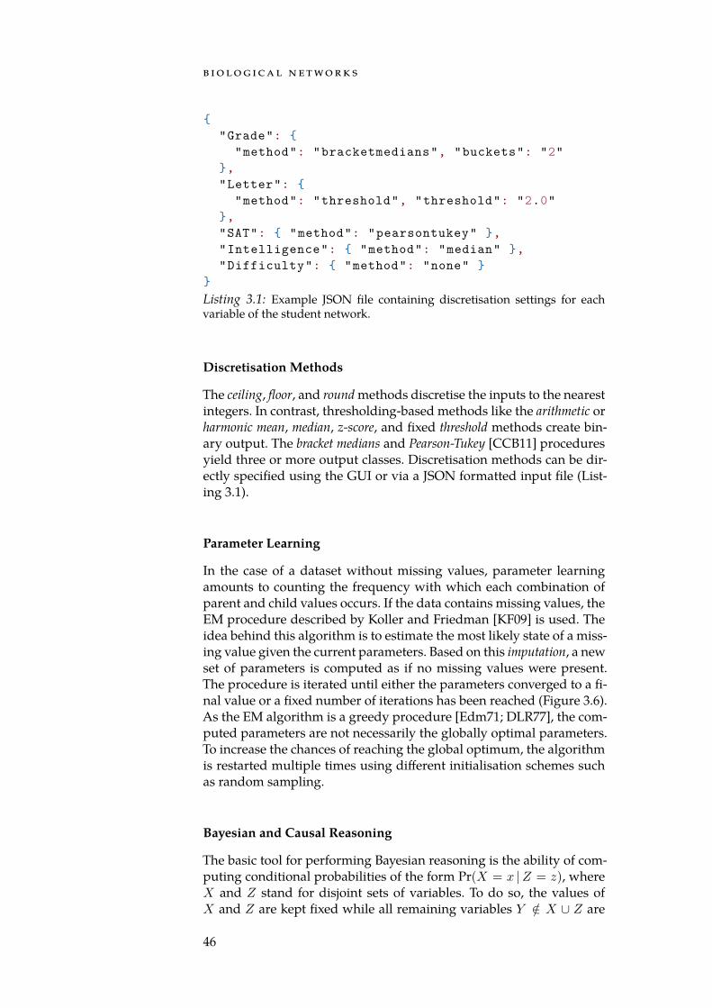
b i o lo g i ca l n e t wo r k s

"Grade":

"method": "bracketmedians", "buckets": "2","Letter":

"method": "threshold", "threshold": "2.0","SAT": "method": "pearsontukey" ,"Intelligence": "method": "median" ,"Difficulty": "method": "none"

Listing 3.1: Example JSON file containing discretisation settings for eachvariable of the student network.

Discretisation Methods

The ceiling, floor, and round methods discretise the inputs to the nearestintegers. In contrast, thresholding-based methods like the arithmetic orharmonic mean, median, z-score, and fixed threshold methods create bin-ary output. The bracket medians and Pearson-Tukey [CCB11] proceduresyield three or more output classes. Discretisation methods can be dir-ectly specified using the GUI or via a JSON formatted input file (List-ing 3.1).

Parameter Learning

In the case of a dataset without missing values, parameter learningamounts to counting the frequency with which each combination ofparent and child values occurs. If the data contains missing values, theEM procedure described by Koller and Friedman [KF09] is used. Theidea behind this algorithm is to estimate the most likely state of a miss-ing value given the current parameters. Based on this imputation, a newset of parameters is computed as if no missing values were present.The procedure is iterated until either the parameters converged to a fi-nal value or a fixed number of iterations has been reached (Figure 3.6).As the EM algorithm is a greedy procedure [Edm71; DLR77], the com-puted parameters are not necessarily the globally optimal parameters.To increase the chances of reaching the global optimum, the algorithmis restarted multiple times using different initialisation schemes suchas random sampling.

Bayesian and Causal Reasoning

The basic tool for performing Bayesian reasoning is the ability of com-puting conditional probabilities of the form Pr(X = x |Z = z), whereX and Z stand for disjoint sets of variables. To do so, the values ofX and Z are kept fixed while all remaining variables Y /∈ X ∪ Z are

46

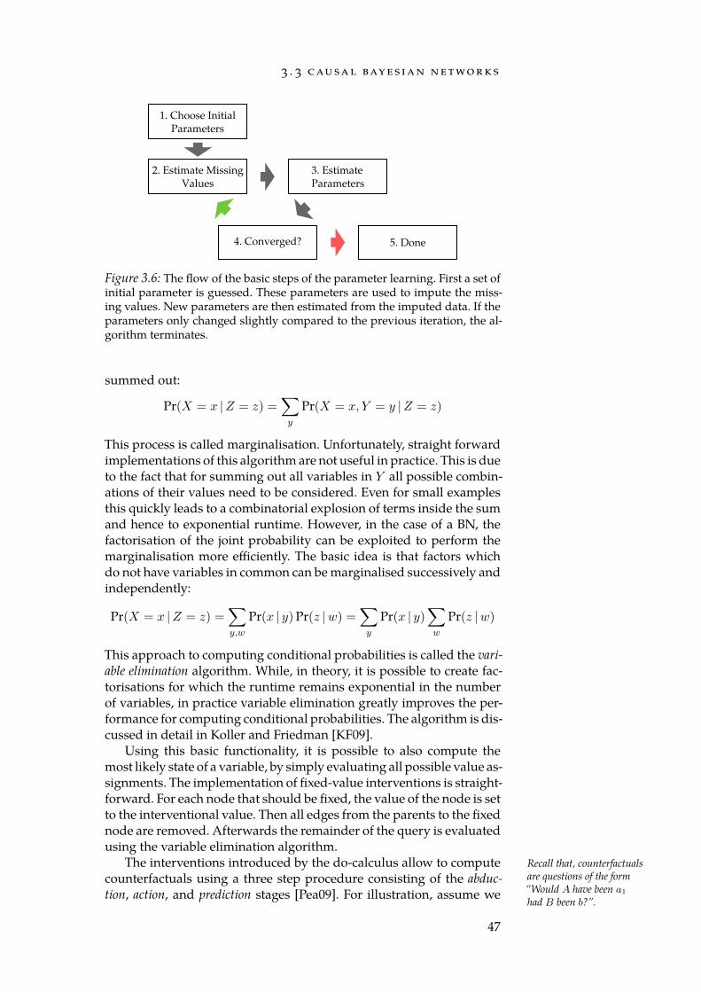
3 . 3 cau sa l bay e s i a n n e t wo r k s

1. Choose InitialParameters

2. Estimate MissingValues

3. EstimateParameters

4. Converged? 5. Done

Figure 3.6: The flow of the basic steps of the parameter learning. First a set ofinitial parameter is guessed. These parameters are used to impute the miss-ing values. New parameters are then estimated from the imputed data. If theparameters only changed slightly compared to the previous iteration, the al-gorithm terminates.

summed out:

Pr(X = x |Z = z) =∑y

Pr(X = x, Y = y |Z = z)

This process is called marginalisation. Unfortunately, straight forwardimplementations of this algorithm are not useful in practice. This is dueto the fact that for summing out all variables in Y all possible combin-ations of their values need to be considered. Even for small examplesthis quickly leads to a combinatorial explosion of terms inside the sumand hence to exponential runtime. However, in the case of a BN, thefactorisation of the joint probability can be exploited to perform themarginalisation more efficiently. The basic idea is that factors whichdo not have variables in common can be marginalised successively andindependently:

Pr(X = x |Z = z) =∑y,w

Pr(x | y)Pr(z |w) =∑y

Pr(x | y)∑w

Pr(z |w)

This approach to computing conditional probabilities is called the vari-able elimination algorithm. While, in theory, it is possible to create fac-torisations for which the runtime remains exponential in the numberof variables, in practice variable elimination greatly improves the per-formance for computing conditional probabilities. The algorithm is dis-cussed in detail in Koller and Friedman [KF09].

Using this basic functionality, it is possible to also compute themost likely state of a variable, by simply evaluating all possible value as-signments. The implementation of fixed-value interventions is straight-forward. For each node that should be fixed, the value of the node is setto the interventional value. Then all edges from the parents to the fixednode are removed. Afterwards the remainder of the query is evaluatedusing the variable elimination algorithm.

The interventions introduced by the do-calculus allow to compute Recall that, counterfactualsare questions of the form“Would A have been a1

had B been b?”.

counterfactuals using a three step procedure consisting of the abduc-tion, action, and prediction stages [Pea09]. For illustration, assume we

47

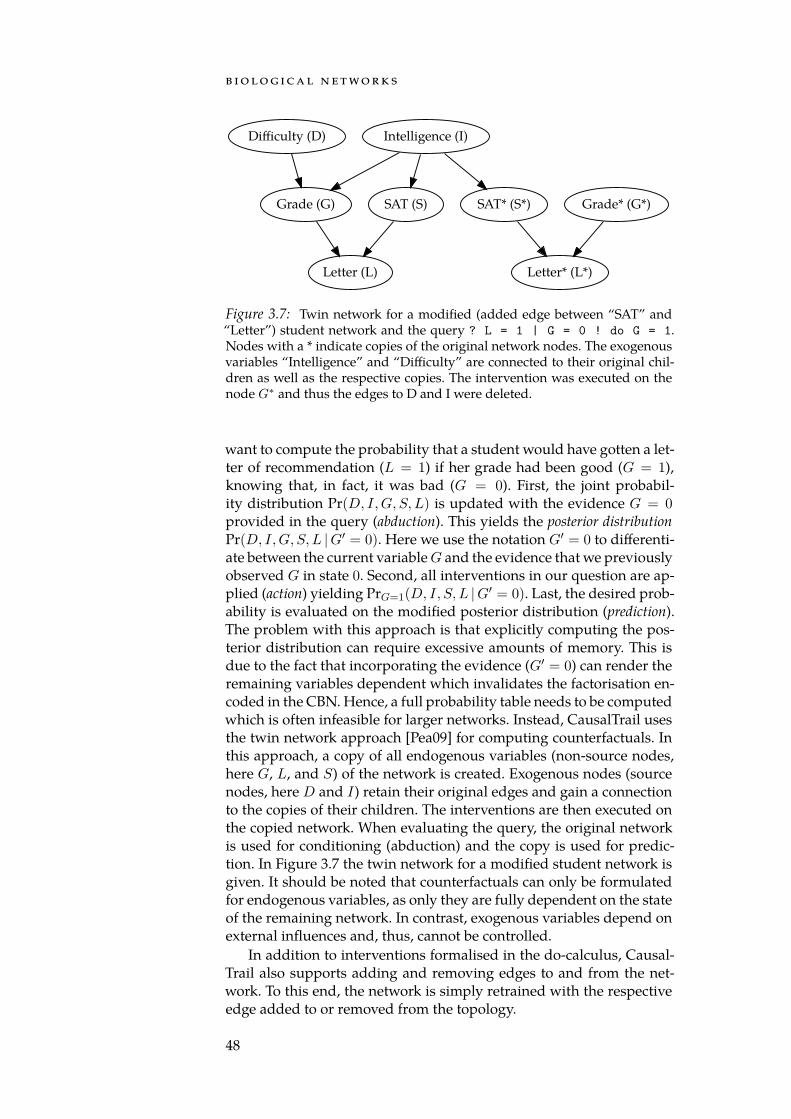
b i o lo g i ca l n e t wo r k s

Difficulty (D)

Grade (G)

Letter (L)

Intelligence (I)

SAT (S) SAT* (S*)

Letter* (L*)

Grade* (G*)

Figure 3.7: Twin network for a modified (added edge between “SAT” and“Letter”) student network and the query ? L = 1 | G = 0 ! do G = 1.Nodes with a * indicate copies of the original network nodes. The exogenousvariables “Intelligence” and “Difficulty” are connected to their original chil-dren as well as the respective copies. The intervention was executed on thenode G∗ and thus the edges to D and I were deleted.

want to compute the probability that a student would have gotten a let-ter of recommendation (L = 1) if her grade had been good (G = 1),knowing that, in fact, it was bad (G = 0). First, the joint probabil-ity distribution Pr(D, I,G, S, L) is updated with the evidence G = 0provided in the query (abduction). This yields the posterior distributionPr(D, I,G, S, L |G′ = 0). Here we use the notation G′ = 0 to differenti-ate between the current variableG and the evidence that we previouslyobserved G in state 0. Second, all interventions in our question are ap-plied (action) yielding PrG=1(D, I, S, L |G′ = 0). Last, the desired prob-ability is evaluated on the modified posterior distribution (prediction).The problem with this approach is that explicitly computing the pos-terior distribution can require excessive amounts of memory. This isdue to the fact that incorporating the evidence (G′ = 0) can render theremaining variables dependent which invalidates the factorisation en-coded in the CBN. Hence, a full probability table needs to be computedwhich is often infeasible for larger networks. Instead, CausalTrail usesthe twin network approach [Pea09] for computing counterfactuals. Inthis approach, a copy of all endogenous variables (non-source nodes,here G, L, and S) of the network is created. Exogenous nodes (sourcenodes, here D and I) retain their original edges and gain a connectionto the copies of their children. The interventions are then executed onthe copied network. When evaluating the query, the original networkis used for conditioning (abduction) and the copy is used for predic-tion. In Figure 3.7 the twin network for a modified student network isgiven. It should be noted that counterfactuals can only be formulatedfor endogenous variables, as only they are fully dependent on the stateof the remaining network. In contrast, exogenous variables depend onexternal influences and, thus, cannot be controlled.

In addition to interventions formalised in the do-calculus, Causal-Trail also supports adding and removing edges to and from the net-work. To this end, the network is simply retrained with the respectiveedge added to or removed from the topology.

48

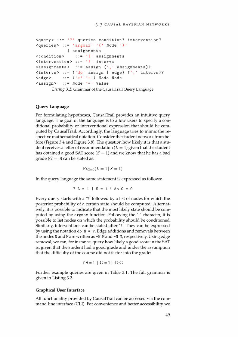
3 . 3 cau sa l bay e s i a n n e t wo r k s

<query> ::= '?' queries condition? intervention?<queries> ::= 'argmax' '(' Node ')'

| assignments<condition > ::= '|' assignments<intervention > ::= '!' intervs<assignments > ::= assign (',' assignments)?<intervs> ::= ('do' assign | edge) (',' intervs)?<edge> ::= ('+'|'-') Node Node<assign> ::= Node '=' Value

Listing 3.2: Grammar of the CausalTrail Query Language

Query Language

For formulating hypotheses, CausalTrail provides an intuitive querylanguage. The goal of the language is to allow users to specify a con-ditional probability or interventional expression that should be com-puted by CausalTrail. Accordingly, the language tries to mimic the re-spective mathematical notation. Consider the student network from be-fore (Figure 3.4 and Figure 3.8). The question how likely it is that a stu-dent receives a letter of recommendation (L = 1) given that the studenthas obtained a good SAT score (S = 1) and we know that he has a badgrade (G = 0) can be stated as:

PrG=0(L = 1 |S = 1)

In the query language the same statement is expressed as follows:

? L = 1 | S = 1 ! do G = 0

Every query starts with a ’?’ followed by a list of nodes for which theposterior probability of a certain state should be computed. Alternat-ively, it is possible to indicate that the most likely state should be com-puted by using the argmax function. Following the ’|’ character, it ispossible to list nodes on which the probability should be conditioned.Similarly, interventions can be stated after ’!’. They can be expressedby using the notation do N = v. Edge additions and removals betweenthe nodes N and M are written as +N M and -N M, respectively. Using edgeremoval, we can, for instance, query how likely a good score in the SATis, given that the student had a good grade and under the assumptionthat the difficulty of the course did not factor into the grade:

? S = 1 | G = 1 ! -D G

Further example queries are given in Table 3.1. The full grammar isgiven in Listing 3.2.

Graphical User Interface

All functionality provided by CausalTrail can be accessed via the com-mand line interface (CLI). For convenience and better accessibility we

49

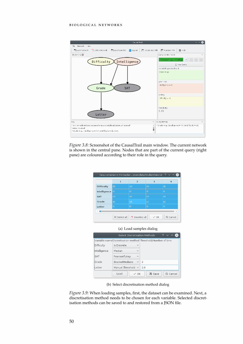
b i o lo g i ca l n e t wo r k s

Figure 3.8: Screenshot of the CausalTrail main window. The current networkis shown in the central pane. Nodes that are part of the current query (rightpane) are coloured according to their role in the query.

(a) Load samples dialog

(b) Select discretisation method dialog

Figure 3.9: When loading samples, first, the dataset can be examined. Next, adiscretisation method needs to be chosen for each variable. Selected discret-isation methods can be saved to and restored from a JSON file.

50

3 . 3 cau sa l bay e s i a n n e t wo r k s

also provide a GUI (cf. Figure 3.8). The GUI is centred around a ren-dering of the Bayesian network as directed, acyclic graph. The layoutfor this graph is generated using the Graphviz [GN00] suite. Quer-ies can be built intuitively via a context menu that can be invoked byright-clicking on network nodes and edges. Alternatively, queries canbe entered directly in the “Query Control Panel” (Figure 3.8, top ofright pane). Queries entered this way are automatically validated whiletyping. If detected, syntactical and semantical errors such as mistypednode names or values, are highlighted. In addition to the plain text rep-resentation in the input field, the “Query Control Panel” also providesa structured view, which breaks each query down into components.Nodes or edges that are part of the current query are colour coded inthe network representation to improve clarity.

An important part of CausalTrail is the management of datasets.To be able to use a BN for reasoning, a dataset needs to be imported,examined, and discretised. To this end, when a dataset is loaded, an in-teractive table showing its contents is displayed to the user that can beused to exclude certain samples from the analysis (Section 3.3.1). After-wards, the user is offered the choice of a discretisation method for eachvariable. After choosing appropriate methods, the user can store themin a JSON file (cf. Section 5.1.7) for later use. Internally, CausalTrailmanages the state of the application as a session. In each session, mul-tiple networks can be loaded and worked on simultaneously. The stateof the session can be saved and restored at any point.

Implementation

CausalTrail is written in C++ using features from the C++14 standard2.To facilitate code reuse, all GUI agnostic functionality such as routinesconcerning parameter inference and reasoning are implemented in aseparate, core library. As dependency only the Boost library collectionis used3. On top of the core library the command line interface (CLI)and a library providing a graphical user interface (GUI) have been built.For creating the GUI the Qt5 toolkit4 was used, which allows to portCausalTrail to all major platforms. For computing graph layouts, theGraphviz [GN00] suite is automatically detected and used at runtime.

We put special emphasis on the performance and reliability of theimplemented methods. To this end, CausalTrail is equipped with a unittest suite written using the Google Test framework5. CMake6 is used forthe build system. CausalTrail can be compiled on Linux and Windows,although only the former platform is officially supported. The sourcecode is licensed under GPLv3 and can be obtained from Github7.

2 http://www.iso.org/iso/catalogue_detail.htm?csnumber=640293 http://www.boost.org/4 https://www.qt.io/5 https://github.com/google/googletest6 https://cmake.org/7 https://github.com/unisb-bioinf/causaltrail

51

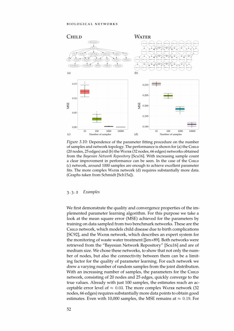
b i o lo g i ca l n e t wo r k s

Number of samples Number of samples

MSE

MSE

10 100 1000 100000.00

0.05

0.10

0.15

0.190

0.195

0.200

0.205

0.210

10 100 1000 10000

(a) (b)

(c) (d)

Disease

Age

Sick DuctFlow CardiacMixing LungParench LungFlow LVH

BirthAsphyxia

Grunting HypDistrib HypoxialnO2 CO2 ChestXray LVHReport

GruntingReport LowerBodyO2 RUQO2 CO2Report XrayReport

C_NI_12_00

C_NI_12_15 CBODD_12_15

C_NI_12_30 CKNI_12_30 CBODD_12_30

CKNI_12_00

CKNI_12_15 CKND_12_15

CKND_12_30CNOD_12_30 CBODN_12_30

CBODD_12_00

CNOD_12_15 CBODN_12_15

CNOD_12_00

CNON_12_15

CBODN_12_00

CKNN_12_30

CKND_12_00

CKNN_12_15

CKNN_12_00

CNON_12_30

CNON_12_00

C_NI_12_45 CBODD_12_45CKNI_12_45 CKND_12_45CNOD_12_45 CBODN_12_45 CKNN_12_45CNON_12_45

Figure 3.10: Dependence of the parameter fitting procedure on the numberof samples and network topology. The performance is shown for (a) the Child(20 nodes, 25 edges) and (b) the Water (32 nodes, 66 edges) networks obtainedfrom the Bayesian Network Repository [Scu16]. With increasing sample counta clear improvement in performance can be seen. In the case of the Child(c) network, around 1000 samples are enough to achieve excellent parameterfits. The more complex Water network (d) requires substantially more data.(Graphs taken from Schmidt [Sch15a]).

3 . 3 . 2 Examples

We first demonstrate the quality and convergence properties of the im-plemented parameter learning algorithm. For this purpose we take alook at the mean square error (MSE) achieved for the parameters bytraining on data sampled from two benchmark networks. These are theChild network, which models child disease due to birth complications[SC92], and the Water network, which describes an expert system forthe monitoring of waste water treatment [Jen+89]. Both networks wereretrieved from the “Bayesian Network Repository” [Scu16] and are ofmedium size. We chose these networks, to show that not only the num-ber of nodes, but also the connectivity between them can be a limit-ing factor for the quality of parameter learning. For each network wedrew a varying number of random samples from the joint distribution.With an increasing number of samples, the parameters for the Childnetwork, consisting of 20 nodes and 25 edges, quickly converge to thetrue values. Already with just 100 samples, the estimates reach an ac-ceptable error level of ≈ 0.03. The more complex Water network (32nodes, 66 edges) requires substantially more data points to obtain goodestimates. Even with 10,000 samples, the MSE remains at ≈ 0.19. For

52

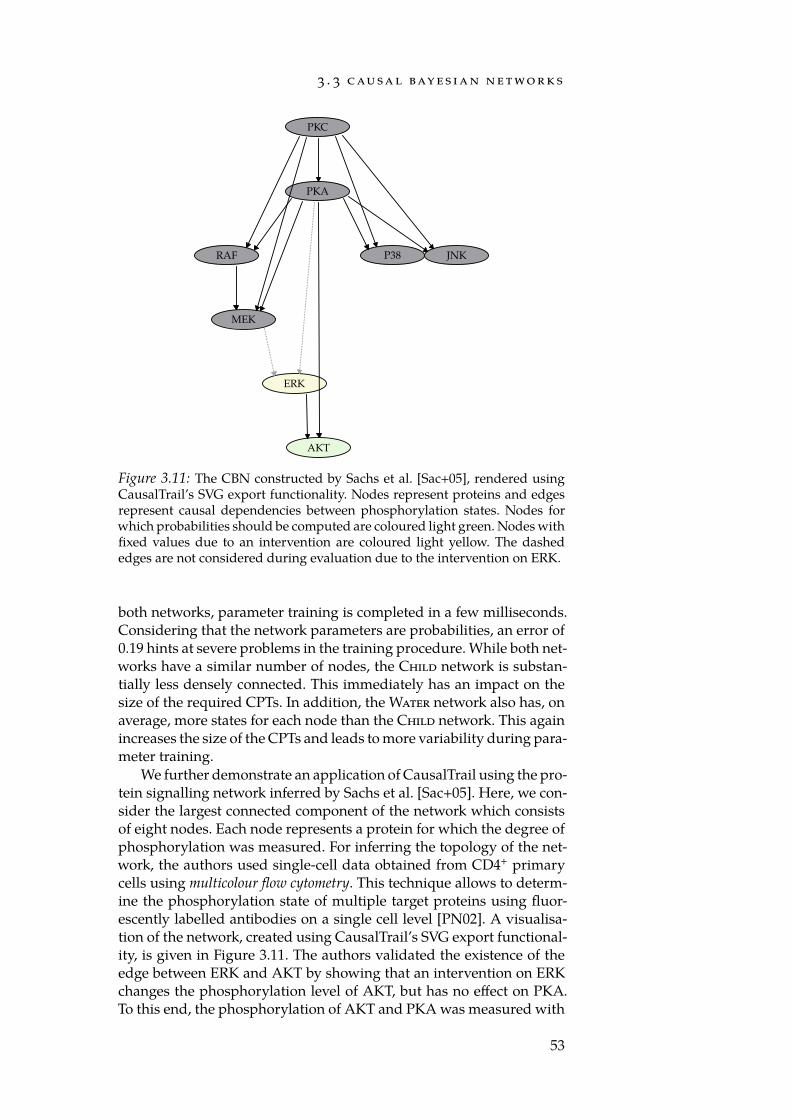
3 . 3 cau sa l bay e s i a n n e t wo r k s

MEK

AKT

PKC

PKA

RAF P38 JNK

ERK

Figure 3.11: The CBN constructed by Sachs et al. [Sac+05], rendered usingCausalTrail’s SVG export functionality. Nodes represent proteins and edgesrepresent causal dependencies between phosphorylation states. Nodes forwhich probabilities should be computed are coloured light green. Nodes withfixed values due to an intervention are coloured light yellow. The dashededges are not considered during evaluation due to the intervention on ERK.

both networks, parameter training is completed in a few milliseconds.Considering that the network parameters are probabilities, an error of0.19 hints at severe problems in the training procedure. While both net-works have a similar number of nodes, the Child network is substan-tially less densely connected. This immediately has an impact on thesize of the required CPTs. In addition, the Water network also has, onaverage, more states for each node than the Child network. This againincreases the size of the CPTs and leads to more variability during para-meter training.

We further demonstrate an application of CausalTrail using the pro-tein signalling network inferred by Sachs et al. [Sac+05]. Here, we con-sider the largest connected component of the network which consistsof eight nodes. Each node represents a protein for which the degree ofphosphorylation was measured. For inferring the topology of the net-work, the authors used single-cell data obtained from CD4+ primarycells using multicolour flow cytometry. This technique allows to determ-ine the phosphorylation state of multiple target proteins using fluor-escently labelled antibodies on a single cell level [PN02]. A visualisa-tion of the network, created using CausalTrail’s SVG export functional-ity, is given in Figure 3.11. The authors validated the existence of theedge between ERK and AKT by showing that an intervention on ERKchanges the phosphorylation level of AKT, but has no effect on PKA.To this end, the phosphorylation of AKT and PKA was measured with

53

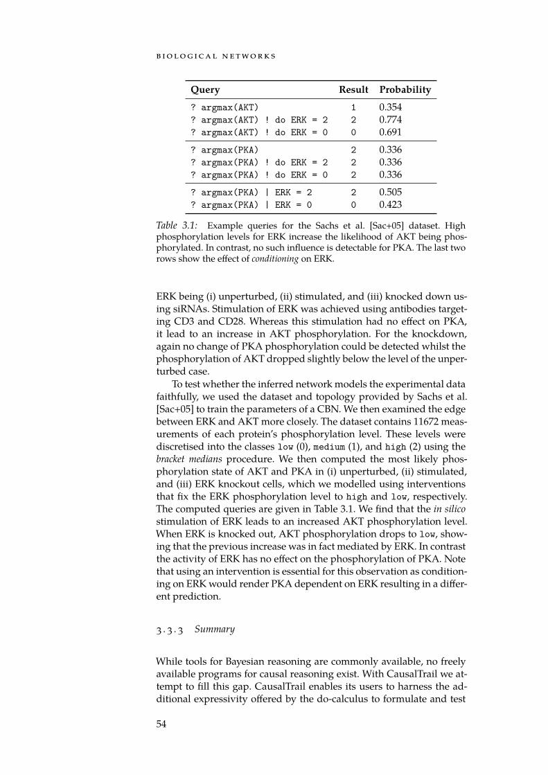
b i o lo g i ca l n e t wo r k s

Query Result Probability

? argmax(AKT) 1 0.354? argmax(AKT) ! do ERK = 2 2 0.774? argmax(AKT) ! do ERK = 0 0 0.691

? argmax(PKA) 2 0.336? argmax(PKA) ! do ERK = 2 2 0.336? argmax(PKA) ! do ERK = 0 2 0.336

? argmax(PKA) | ERK = 2 2 0.505? argmax(PKA) | ERK = 0 0 0.423

Table 3.1: Example queries for the Sachs et al. [Sac+05] dataset. Highphosphorylation levels for ERK increase the likelihood of AKT being phos-phorylated. In contrast, no such influence is detectable for PKA. The last tworows show the effect of conditioning on ERK.

ERK being (i) unperturbed, (ii) stimulated, and (iii) knocked down us-ing siRNAs. Stimulation of ERK was achieved using antibodies target-ing CD3 and CD28. Whereas this stimulation had no effect on PKA,it lead to an increase in AKT phosphorylation. For the knockdown,again no change of PKA phosphorylation could be detected whilst thephosphorylation of AKT dropped slightly below the level of the unper-turbed case.

To test whether the inferred network models the experimental datafaithfully, we used the dataset and topology provided by Sachs et al.[Sac+05] to train the parameters of a CBN. We then examined the edgebetween ERK and AKT more closely. The dataset contains 11672 meas-urements of each protein’s phosphorylation level. These levels werediscretised into the classes low (0), medium (1), and high (2) using thebracket medians procedure. We then computed the most likely phos-phorylation state of AKT and PKA in (i) unperturbed, (ii) stimulated,and (iii) ERK knockout cells, which we modelled using interventionsthat fix the ERK phosphorylation level to high and low, respectively.The computed queries are given in Table 3.1. We find that the in silicostimulation of ERK leads to an increased AKT phosphorylation level.When ERK is knocked out, AKT phosphorylation drops to low, show-ing that the previous increase was in fact mediated by ERK. In contrastthe activity of ERK has no effect on the phosphorylation of PKA. Notethat using an intervention is essential for this observation as condition-ing on ERK would render PKA dependent on ERK resulting in a differ-ent prediction.

3 . 3 . 3 Summary

While tools for Bayesian reasoning are commonly available, no freelyavailable programs for causal reasoning exist. With CausalTrail we at-tempt to fill this gap. CausalTrail enables its users to harness the ad-ditional expressivity offered by the do-calculus to formulate and test

54

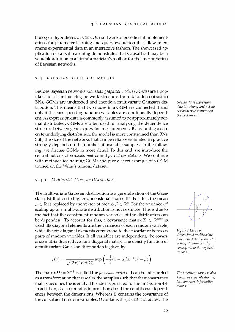
3 . 4 gau s s i a n g r a p h i ca l m o d e l s

biological hypotheses in silico. Our software offers efficient implement-ations for parameter learning and query evaluation that allow to ex-amine experimental data in an interactive fashion. The showcased ap-plication of causal reasoning demonstrates that CausalTrail may be avaluable addition to a bioinformatician’s toolbox for the interpretationof Bayesian networks.

3 . 4 gau s s i a n g r a p h i ca l m o d e l s

Besides Bayesian networks, Gaussian graphical models (GGMs) are a pop-ular choice for inferring network structure from data. In contrast toBNs, GGMs are undirected and encode a multivariate Gaussian dis- Normality of expression

data is a strong and not ne-cessarily true assumption.See Section 4.3.

tribution. This means that two nodes in a GGM are connected if andonly if the corresponding random variables are conditionally depend-ent. As expression data is commonly assumed to be approximately nor-mal distributed, GGMs are often used for analysing the dependencestructure between gene expression measurements. By assuming a con-crete underlying distribution, the model is more constrained than BNs.Still, the size of the networks that can be reliably estimated in practicestrongly depends on the number of available samples. In the follow-ing, we discuss GGMs in more detail. To this end, we introduce thecentral notions of precision matrix and partial correlations. We continuewith methods for training GGMs and give a short example of a GGMtrained on the Wilm’s tumour dataset.

3 . 4 . 1 Multivariate Gaussian Distributions

The multivariate Gaussian distribution is a generalisation of the Gaus-

Figure 3.12: Two-dimensional multivariateGaussian distribution. Theprincipal variances τ2

1,2

correspond to the eigenval-ues of Σ.

sian distribution to higher dimensional spaces Rp. For this, the meanµ ∈ R is replaced by the vector of means µ ∈ Rp. For the variance σ2

scaling up to a multivariate distribution is not as simple. This is due tothe fact that the constituent random variables of the distribution canbe dependent. To account for this, a covariance matrix Σ ∈ Rp×p isused. Its diagonal elements are the variances of each random variable,while the off-diagonal elements correspond to the covariance betweenpairs of random variables. If all variables are independent, the covari-ance matrix thus reduces to a diagonal matrix. The density function ofa multivariate Gaussian distribution is given by

f(x) =1√

(2π)p det(Σ)exp

(−1

2(x− µ)tΣ−1(x− µ)

)The matrix Ω := Σ−1 is called the precision matrix. It can be interpreted The precision matrix is also

known as concentration or,less common, informationmatrix.

as a transformation that rescales the samples such that their covariancematrix becomes the identity. This idea is pursued further in Section 4.4.In addition, Ω also contains information about the conditional depend-ences between the dimensions. Whereas Σ contains the covariance ofthe constituent random variables,Ω contains the partial covariances. The

55

b i o lo g i ca l n e t wo r k s

partial covariance between two random variables can be understood asthe part of their covariance that cannot be explained by the remainingvariables. To explain this in more detail, we first introduce the notionof a least-squares fit. Assume that f : Rp → R is a function of the formf(x) = β1x1+β2x2+ . . .+βpxp. Furthermore, assume that the outcomey is determined via the relation y = f(x) + ϵ where ϵ ∼ N (0, σ2

ϵ ) is anormally distributed noise variable. The task is to find the best estim-ate f∗ of f given a set of N samples (yi, xi). Here, best is defined as thefunction minimising the least-squares loss function:

N∑i=1

(yi − f(xi))2 =

N∑i=1

(yi − ⟨xi, β⟩

)2= ⟨y −Xβ, y −Xβ⟩

Here, we use y ∈ RN as the vector of observations and X ∈ RN×pNote that, assumingcentred predictors,

XtX is proportional tothe covariance matrix.

as the matrix of predictors. After applying basic calculus, we obtain aformula for the weight vector [FHT09]: β∗ = (XtX)−1X y. We referto f∗ as the least-squares fit of y given X with coefficients β∗. It is nowpossible to define the partial covariance:

Definition 9 (Partial Covariance [BSS04]). Let X,Y be two randomvariables and let Z = Z1, . . . , Zn be a set of random variables. De-note the coefficients of the least-squares fit of X and Y given Z as βXand βY , respectively. Then, the partial covariance is defined as the co-variance of the residuals:

rX := X − ⟨Z, βX⟩

rY := Y − ⟨Z, βY ⟩cov(X,Y |Z) := cov(rX , rY )

As with the usual variance the partial covariance permits the defin-ition of a measure of correlation. This correlation is called the partialcorrelation (cf. [BSS04]).

Definition 10 (Partial Correlation). Let X,Y be two random variablesand let Z = Z1, . . . , Zn be a set of random variables. The partial cor-relation of X and Y is defined as

ρXY |Z :=cov(X,Y |Z)√

var(X|Z)√

var(Y |Z)

using var(X|Z) := cov(X,X|Z) or, given Ω:

ρXY |Z := − ΩXY√ΩXXΩY Y

It can be shown that two variables in a GGM are conditionally in-dependent if and only if their partial correlation equals zero [Lau96;BSS04]. Equivalently, two distinct random variables are conditionallyindependent if and only if the corresponding entry in Ω is zero.

56

3 . 4 gau s s i a n g r a p h i ca l m o d e l s

3 . 4 . 2 Covariance Matrix Estimation

In theory, fitting a GGM is straightforward. First, the sample covariancematrix is computed. Given a dataset X = x1, . . . , xn with n ∈ Nsamples and p ∈ N variables. The sample covariance matrix W is thengiven by:

W =1

n− 1

n∑i=1

(xi − µ)(xi − µ)t

where µ is the sample mean. More robust estimates of the (co)variances More information onJames-Stein Shrinkage canbe found in Section 4.2.2.

can be used to obtain estimates of the precision matrix that are less sus-ceptible to noise in the input data. An example is the method proposedby Schäfer and Strimmer [SS05] which is based on James-Stein shrink-age [JS61]. For details the reader is referred to the cited literature.

3 . 4 . 3 Precision Matrix Estimation

The precision matrix can be obtained by computing the inverse of W . The condition number ofa matrix is the ratio of themagnitudes of the highestand lowest singular value.

In practice, the required matrix inversion creates various problems. Iffew samples are available, compared to the number of variables, smallerrors in the estimation of the covariance matrix are amplified by thecondition number of the matrix [Pre+07]. For small sample sizes, whereW is close to singular, the condition number is likely to be high. Ac-cordingly, large differences between the true and estimated precisionmatrix can be expected. To alleviate the effect of small sample sizes, aregularisation approach should be chosen. A direct way to introduceregularisation is to exploit the eigenvalue decomposition of Σ. Given asymmetric matrix A ∈ Rp×p, its eigenvalue decomposition is given by

A = V ΓV t

where V ∈ Rp×p is the orthogonal matrix of eigenvectors and Γ ∈ Rp×p

is the diagonal matrix of eigenvalues. As Σ is positive definite, the ei-genvalues are guaranteed to be non-negative. It is then possible to com-pute Σ−1 = V Γ−1V t where Γ−1 is the (pseudo-)inverse of Γ:

Γ−1ii =

1/Γii if Γii > 0

0 otherwise(3.1)

For small eigenvalues this results in large entries in Γ−1. Under theassumption that eigenvectors corresponding to small eigenvalues canmostly be attributed to noise, setting the inverse of these small eigen-values to zero prevents the amplification of this noise. We thus defineΓ−1 in which only eigenvalues above a user-defined threshold ρ ∈ R+

0

are retained:

Γ−1ii =

1/Γii if Γii > ρ

0 otherwise(3.2)

A similar idea can be derived from linear regression. As linear re-gression requires the inversion of a covariance matrix to compute the

57

b i o lo g i ca l n e t wo r k s

regression coefficients, it also suffers from cases where Σ is near singu-The L2 regularisationin ridge regression is a

special case of Tikhonovregularisation [Tik63].

lar and, thus, has a high condition number. To counteract this, a smallconstant can be added to the diagonal of the covariance matrix to serveas a regulariser. This ensures that the solution to the regression prob-lem is unique. Ledoit and Wolf [LW04] explore this idea for computinga precision matrix and describe an optimisation problem that allows toobtain the optimal value of the regularisation parameter.

If only few variables are expected to be conditionally dependent, anestimator that prefers a sparse precision matrix is advantageous. To thisend, a considerable amount of research has been dedicated towardsthe computation of L1 penalised estimates of the precision matrix. Theidea of using aL1 penalty term stems from the popular lasso regression[Tib96] procedure, which tends toward setting small coefficient to zero,thereby yielding sparse linear models. For the estimate of a precisionmatrix Ω the penalised log-likelihood is given by

l(Θ) = log(det(Θ))− tr(ΣΘ)− ρ||Θ||1 (3.3)

where Θ denotes the estimate for Ω, tr denotes the trace of a matrixand ||.||1 is the L1 matrix norm. The parameter ρ ≥ 0 determines thestrength of the regularisation. For ρ = 0, Equation (3.3) reduces to theconventional log-likelihood of the precision matrix. For larger valuesof ρ the size of the entries of Θ is increasingly penalised and thus theresulting matrix tends to include less non-zero values. To see that Equa-tion (3.3) in fact corresponds to the log-likelihood, we start with thelogarithm of the probability density. W.l.o.g. we assume that the meanof the samples xi is zero.

L(Θ) = log[

N∏i=1

det(Θ)1/2

(2π)p/2exp(−1

2xtiΘxi)

]

=

N∑i=1

log[

det(Θ)1/2

(2π)p/2exp

(−1

2xtiΘxi

)]

=N

2log(det(Θ))− Np

2log(2π)− 1

2

N∑i=1

xtiΘxi

=N

2log(det(Θ))− Np

2log(2π)− 1

2

N∑i=1

p∑l=1

p∑k=1

xilΘlkxik

=N

2log(det(Θ))− Np

2log(2π)− 1

2

p∑l=1

p∑k=1

Θlk(XtX)lk

=N

2log(det(Θ))− Np

2log(2π)− 1

2

p∑l=1

(Θ(XtX))ll

=N

2log(det(Θ))− Np

2log(2π)− N

2tr(ΘΣ)

For fitting the model we can omit the constant (Np/2) log(2π) and res-cale with 2/N to obtain Equation (3.3) without the penalty term. To

58

3 . 4 gau s s i a n g r a p h i ca l m o d e l s

find an approximate solution, Meinshausen and Bühlmann [MB06] em-ploy the lasso in an iterative fashion to compute the partial covari-ances as in Definition 9. Based on this work and the results of Baner-jee, El Ghaoui, and d’Aspremont [BEd08], Friedman, Hastie, and Tib-shirani [FHT08] devised the graphical lasso approach. In contrast tothe method proposed by Meinshausen and Bühlmann [MB06], theirformulation solves the problem accurately and offers a significantlyimproved runtime behaviour for sparse precision matrices. As optim-isation procedure Friedman, Hastie, and Tibshirani [FHT08] proposea cyclic gradient-descent-based method, which they published as theglasso R [R C16] package. The principle behind the cyclic gradient de-cent is the realisation that all entries of the precision matrix are depend-ent. Instead of optimising one variable completely, each variable takesa short step in the direction of the (sub-)gradient in a round-robin fash-ion. Cai, Liu, and Luo [CLL11] propose an alternate optimisation target,which they solve for using a set of linear programs. In the remainderof this work, we restrict ourselves to the more popular graphical lassoapproach.

3 . 4 . 4 Example

To illustrate a possible application of GGMs we fitted a coexpressionmodel using data from the Wilm’s tumour dataset (Section 2.4) as in-put. To restrict the number of genes to a manageable size, we used theTFs found in the consensus network published by Juan et al. [Jua+16],which is based on the colocalisation of epigenomic marks. The networkitself was determined using a GGM based on ChIP-seq data. Edge dir-ections were added based on prior knowledge.

First, we computed the precision matrix for all 47 TFs contained inthe network by pseudo inversion of the covariance matrix (Figure 3.13,left). As the network contains more genes than Wilm’s tumour samples,the computed covariance matrix is singular. Accordingly, the precisionmatrix does not possess a full rank either. This gives rise to a clearlyvisible block structure in the precision matrix due to a linear depend-ence between the columns and rows. By adding a small constant valueλ = 0.01 to the diagonal of the covariance matrix, this block structure isgreatly reduced (Figure 3.13, right). This demonstrates that proper reg-ularisation is crucial to prevent artefacts that hamper the interpretab-ility of the model. While using the ridge strategy is a clear improve-ment over naïve matrix inversion, the resulting precision matrix still isdense, meaning that every variable has a non-zero partial correlationwith the other variables. This makes it difficult to visualise the modelas a network structure. Applying the graphical lasso with a relativelystrict regularisation factor of ρ = 0.5 (Figure 3.14) results in a muchsparser precision matrix.

Of the detected 116 edges, 86 could be verified using a custom data-base collected from TRANSFAC [Mat+06], SignaLink [Faz+13], ChIP-

59

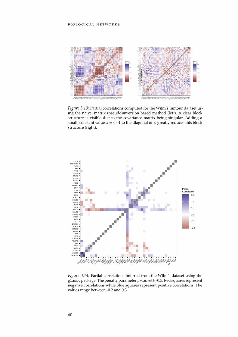
b i o lo g i ca l n e t wo r k s

NIPBLTAF1

MED12SUZ12

POU5F1CBX7CDH4RYBP

HCFC1MBD2TCF3

PHF19RNF2MAFK

KMT2BEZH2

ZNF384RAD21SMC3REST

EP300ESRRB

OGTE2F1

TFCP2L1MAXKLF4

HDAC2SMARCA4

HDAC1SMC1A

TET1KDM1A

MED1KDM2B

SETDB1NANOG

SIN3ACTCF

KDM2AEHMT2

MYCZC3H11A

STAT3CBX3SOX2

MYCN

NIPBLTA

F1

MED12

SUZ12

POU5F1

CBX7

CDH4

RYBP

HCFC1

MBD2

TCF3

PHF19

RNF2

MAFK

KMT2B

EZH2

ZNF384

RAD21

SMC3

REST

EP300

ESRRBOGT

E2F1

TFCP2L1M

AXKLF

4

HDAC2

SMARCA4

HDAC1

SMC1A

TET1

KDM1A

MED1

KDM2B

SETDB1

NANOG

SIN3ACTCF

KDM2A

EHMT2M

YC

ZC3H11

A

STAT3

CBX3

SOX2

MYCN

−0.5

0.0

0.5

PartialCorrelation

NIPBLTAF1

MED12SUZ12

POU5F1CBX7CDH4RYBP

HCFC1MBD2TCF3

PHF19RNF2MAFK

KMT2BEZH2

ZNF384RAD21SMC3REST

EP300ESRRB

OGTE2F1

TFCP2L1MAXKLF4

HDAC2SMARCA4

HDAC1SMC1A

TET1KDM1A

MED1KDM2B

SETDB1NANOG

SIN3ACTCF

KDM2AEHMT2

MYCZC3H11A

STAT3CBX3SOX2

MYCN

NIPBLTA

F1

MED12

SUZ12

POU5F1

CBX7

CDH4

RYBP

HCFC1

MBD2

TCF3

PHF19

RNF2

MAFK

KMT2B

EZH2

ZNF384

RAD21

SMC3

REST

EP300

ESRRBOGT

E2F1

TFCP2L1M

AXKLF

4

HDAC2

SMARCA4

HDAC1

SMC1A

TET1

KDM1A

MED1

KDM2B

SETDB1

NANOG

SIN3ACTCF

KDM2A

EHMT2M

YC

ZC3H11

A

STAT3

CBX3

SOX2

MYCN

−0.6

−0.3

0.0

0.3

0.6

PartialCorrelation

Figure 3.13: Partial correlations computed for the Wilm’s tumour dataset us-ing the naïve, matrix (pseudo)inversion based method (left). A clear blockstructure is visible due to the covariance matrix being singular. Adding asmall, constant value λ = 0.01 to the diagonal of Σ greatly reduces this blockstructure (right).

TFCP2L1

ESRRB

STAT3

KLF4

MAFK

CBX7

POU5F1

KDM2A

MYC

MAX

RAD21

SETDB1

HDAC1

ZNF384

CTCF

SMC3

MED12

KDM1A

EHMT2

MYCN

EZH2

E2F1

PHF19

KDM2B

HDAC2

TCF3

TET1

SOX2

CDH4

NANOG

MBD2

SUZ12

HCFC1

EP300

SIN3A

RNF2

CBX3

TAF1

SMARCA4

OGT

TFCP2L1

ESRRB

STAT3

KLF4

MAFK

CBX7

POU5F1

KDM2A

MYC

MAX

RAD21

SETDB1

HDAC1

ZNF384

CTCF

SMC3

MED12

KDM1A

EHMT2

MYCN

EZH2E2F

1

PHF19

KDM2B

HDAC2TCF3

TET1

SOX2

CDH4

NANOGM

BD2

SUZ12

HCFC1

EP300

SIN3ARNF2

CBX3TA

F1

SMARCA4

OGT

−0.2

−0.1

0.0

0.1

0.2

0.3

PartialCorrelation

Figure 3.14: Partial correlations inferred from the Wilm’s dataset using theglassopackage. The penalty parameter ρwas set to 0.5. Red squares representnegative correlations while blue squares represent positive correlations. Thevalues range between -0.2 and 0.3.

60

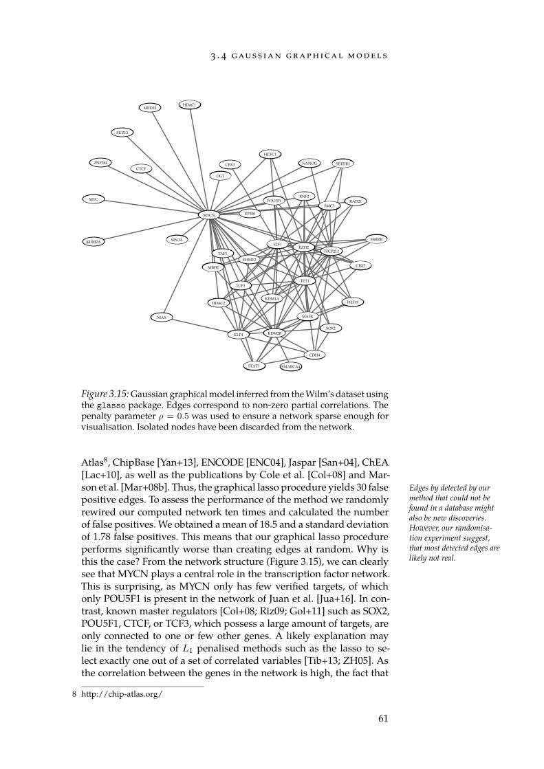
3 . 4 gau s s i a n g r a p h i ca l m o d e l s

PHF19KDM1A

MAFKMAX

HDAC2

NANOG

RAD21POU5F1

EP300

HCFC1

RNF2

SMC3

SETDB1

MYC

CTCF

SIN3AKDM2A

MYCN

SUZ12

MED12

CBX3ZNF384

OGT

HDAC1

STAT3

CDH4

KLF4 KDM2B

SMARCA4

SOX2

CBX7

TFCP2L1

TET1

ESRRBE2F1

EZH2

MBD2

TCF3

EHMT2TAF1

Figure 3.15: Gaussian graphical model inferred from the Wilm’s dataset usingthe glasso package. Edges correspond to non-zero partial correlations. Thepenalty parameter ρ = 0.5 was used to ensure a network sparse enough forvisualisation. Isolated nodes have been discarded from the network.

Atlas8, ChipBase [Yan+13], ENCODE [ENC04], Jaspar [San+04], ChEA[Lac+10], as well as the publications by Cole et al. [Col+08] and Mar-son et al. [Mar+08b]. Thus, the graphical lasso procedure yields 30 false Edges by detected by our

method that could not befound in a database mightalso be new discoveries.However, our randomisa-tion experiment suggest,that most detected edges arelikely not real.

positive edges. To assess the performance of the method we randomlyrewired our computed network ten times and calculated the numberof false positives. We obtained a mean of 18.5 and a standard deviationof 1.78 false positives. This means that our graphical lasso procedureperforms significantly worse than creating edges at random. Why isthis the case? From the network structure (Figure 3.15), we can clearlysee that MYCN plays a central role in the transcription factor network.This is surprising, as MYCN only has few verified targets, of whichonly POU5F1 is present in the network of Juan et al. [Jua+16]. In con-trast, known master regulators [Col+08; Riz09; Gol+11] such as SOX2,POU5F1, CTCF, or TCF3, which possess a large amount of targets, areonly connected to one or few other genes. A likely explanation maylie in the tendency of L1 penalised methods such as the lasso to se-lect exactly one out of a set of correlated variables [Tib+13; ZH05]. Asthe correlation between the genes in the network is high, the fact that

8 http://chip-atlas.org/

61

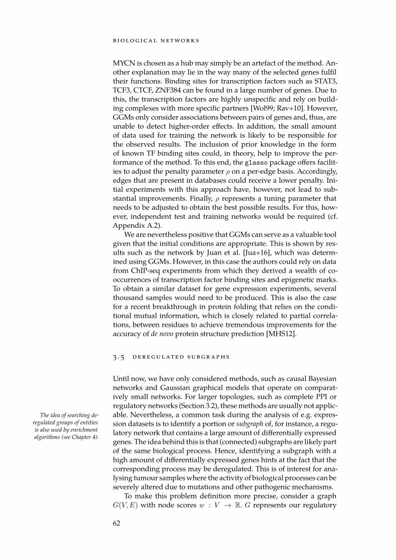
b i o lo g i ca l n e t wo r k s

MYCN is chosen as a hub may simply be an artefact of the method. An-other explanation may lie in the way many of the selected genes fulfiltheir functions. Binding sites for transcription factors such as STAT3,TCF3, CTCF, ZNF384 can be found in a large number of genes. Due tothis, the transcription factors are highly unspecific and rely on build-ing complexes with more specific partners [Wol99; Rav+10]. However,GGMs only consider associations between pairs of genes and, thus, areunable to detect higher-order effects. In addition, the small amountof data used for training the network is likely to be responsible forthe observed results. The inclusion of prior knowledge in the formof known TF binding sites could, in theory, help to improve the per-formance of the method. To this end, the glasso package offers facilit-ies to adjust the penalty parameter ρ on a per-edge basis. Accordingly,edges that are present in databases could receive a lower penalty. Ini-tial experiments with this approach have, however, not lead to sub-stantial improvements. Finally, ρ represents a tuning parameter thatneeds to be adjusted to obtain the best possible results. For this, how-ever, independent test and training networks would be required (cf.Appendix A.2).

We are nevertheless positive that GGMs can serve as a valuable toolgiven that the initial conditions are appropriate. This is shown by res-ults such as the network by Juan et al. [Jua+16], which was determ-ined using GGMs. However, in this case the authors could rely on datafrom ChIP-seq experiments from which they derived a wealth of co-occurrences of transcription factor binding sites and epigenetic marks.To obtain a similar dataset for gene expression experiments, severalthousand samples would need to be produced. This is also the casefor a recent breakthrough in protein folding that relies on the condi-tional mutual information, which is closely related to partial correla-tions, between residues to achieve tremendous improvements for theaccuracy of de novo protein structure prediction [MHS12].

3 . 5 d e r e g u l at e d s u b g r a p h s

Until now, we have only considered methods, such as causal Bayesiannetworks and Gaussian graphical models that operate on comparat-ively small networks. For larger topologies, such as complete PPI orregulatory networks (Section 3.2), these methods are usually not applic-able. Nevertheless, a common task during the analysis of e.g. expres-The idea of searching de-

regulated groups of entitiesis also used by enrichmentalgorithms (see Chapter 4).

sion datasets is to identify a portion or subgraph of, for instance, a regu-latory network that contains a large amount of differentially expressedgenes. The idea behind this is that (connected) subgraphs are likely partof the same biological process. Hence, identifying a subgraph with ahigh amount of differentially expressed genes hints at the fact that thecorresponding process may be deregulated. This is of interest for ana-lysing tumour samples where the activity of biological processes can beseverely altered due to mutations and other pathogenic mechanisms.

To make this problem definition more precise, consider a graphG(V,E) with node scores w : V → R. G represents our regulatory

62

3 . 5 d e r e g u l at e d s u b g r a p h s

network and w are scores that measure the differential expression ofeach gene or protein in G. Assume that a procedure that searches for“interesting” subgraphs inspects all members of a family of admissiblesubgraphs H = Hi ⊂ G | i = 1, . . . , n. For each Hi, the procedurecomputes a score si = S(Hi, w) that represents the degree of deregula-tion of a graph. EachHi that is assigned a score surpassing a predefinedthreshold is called a deregulated subgraph. The deregulated subgraphwith the highest score is called the most deregulated subgraph.

In this chapter, we discuss an algorithm for searching the most de-regulated subgraph in regulatory networks. The central idea behindits development was the ability to detect molecular key players thatare able to trigger regulatory cascades and are thus likely to be causalfor the deregulation observed for the identified subgraph. To achievethis, we developed an algorithm based on integer linear programming(ILP) that searches for a connected subgraph of fixed size that containsa root node. In this context, a root node is a node from which all othervertices in the subgraph are reachable.

After introducing the ILP, we turn our attention to an open prob-lem concerning algorithms for the search of deregulated subgraphs ingeneral. As described above, a subgraph is considered as deregulated,whenever its score exceeds a predefined threshold. Yet, this definitionis somewhat arbitrary and is not connected to any measure of statist-ical significance. It is thus not possible to assess whether the selectedsubgraph refers to a significantly deregulated biological process or not.To remedy this situation, an appropriate H0 hypothesis needs to bechosen first. However, already this step proves to be difficult, as vari-ous, equally reasonable but not equivalent choices are possible. Here,we will not attempt to find an answer to this problem. Instead, we in-vestigate a closely related, even more fundamental problem. In partic-ular, we present an approach for estimating the likelihood with whicha node is selected as part of the most deregulated subgraph, given un-informative scores.

3 . 5 . 1 Related Work

Detecting deregulated subgraphs is a large field in computational bio- In the literature sometimesthe term dysregulatedsubgraph is used.

logy that has brought forth a wide range of conceptually different ap-proaches. The first published algorithm for searching deregulated sub-graphs is the approach by Ideker et al. [Ide+02] which uses a simulatedannealing scheme to iteratively improve the score of the detected sub-networks. As scoring function they generate a background distributionof subgraph weights. Each subgraph score is normalised with the num-ber of vertices. The background generation and the simulated anneal-ing procedure lead to considerable runtime requirements for larger net-works. In addition, the size of the detected subgraph is often too largeto be interpretable. To prevent this behaviour, various improvementsto the scoring function and search heuristics have been published (e.g.Rajagopalan and Agarwal [RA05]). Ulitsky et al. [Uli+10] reduce theproblem of finding a deregulated subnetwork to the NP-hard connec-

63

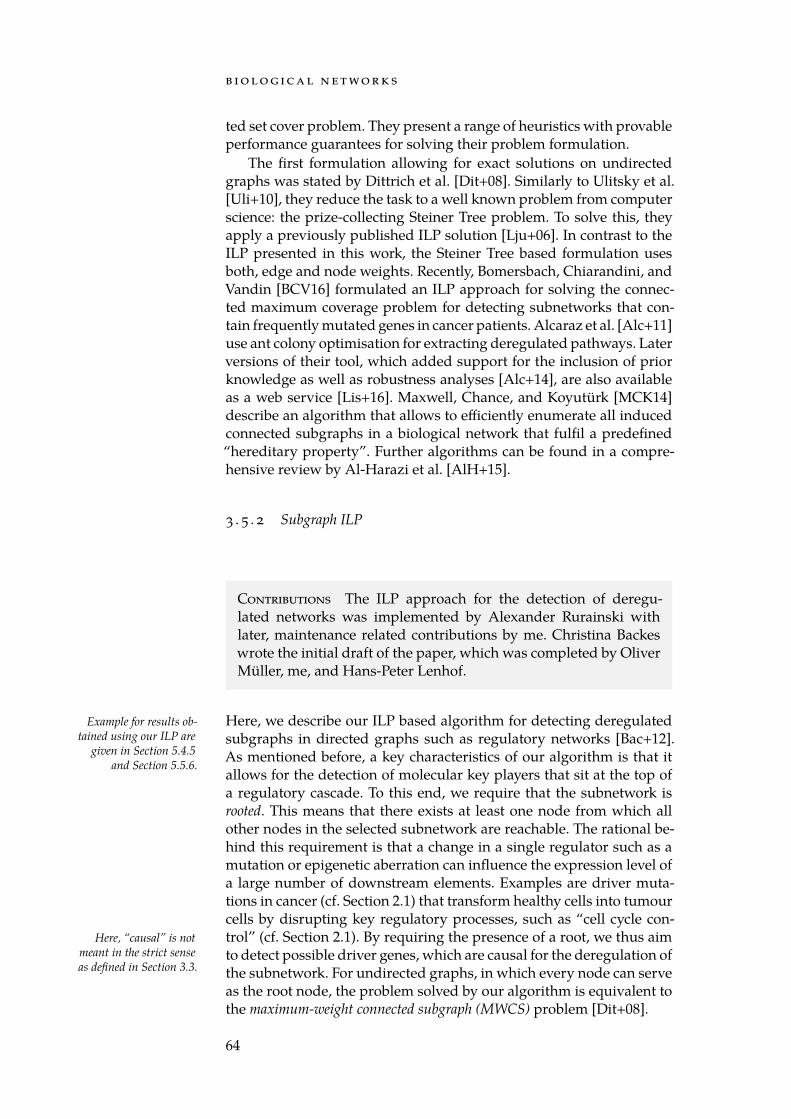
b i o lo g i ca l n e t wo r k s

ted set cover problem. They present a range of heuristics with provableperformance guarantees for solving their problem formulation.

The first formulation allowing for exact solutions on undirectedgraphs was stated by Dittrich et al. [Dit+08]. Similarly to Ulitsky et al.[Uli+10], they reduce the task to a well known problem from computerscience: the prize-collecting Steiner Tree problem. To solve this, theyapply a previously published ILP solution [Lju+06]. In contrast to theILP presented in this work, the Steiner Tree based formulation usesboth, edge and node weights. Recently, Bomersbach, Chiarandini, andVandin [BCV16] formulated an ILP approach for solving the connec-ted maximum coverage problem for detecting subnetworks that con-tain frequently mutated genes in cancer patients. Alcaraz et al. [Alc+11]use ant colony optimisation for extracting deregulated pathways. Laterversions of their tool, which added support for the inclusion of priorknowledge as well as robustness analyses [Alc+14], are also availableas a web service [Lis+16]. Maxwell, Chance, and Koyutürk [MCK14]describe an algorithm that allows to efficiently enumerate all inducedconnected subgraphs in a biological network that fulfil a predefined“hereditary property”. Further algorithms can be found in a compre-hensive review by Al-Harazi et al. [AlH+15].

3 . 5 . 2 Subgraph ILP

Contributions The ILP approach for the detection of deregu-lated networks was implemented by Alexander Rurainski withlater, maintenance related contributions by me. Christina Backeswrote the initial draft of the paper, which was completed by OliverMüller, me, and Hans-Peter Lenhof.

Here, we describe our ILP based algorithm for detecting deregulatedExample for results ob-tained using our ILP are

given in Section 5.4.5and Section 5.5.6.

subgraphs in directed graphs such as regulatory networks [Bac+12].As mentioned before, a key characteristics of our algorithm is that itallows for the detection of molecular key players that sit at the top ofa regulatory cascade. To this end, we require that the subnetwork isrooted. This means that there exists at least one node from which allother nodes in the selected subnetwork are reachable. The rational be-hind this requirement is that a change in a single regulator such as amutation or epigenetic aberration can influence the expression level ofa large number of downstream elements. Examples are driver muta-tions in cancer (cf. Section 2.1) that transform healthy cells into tumourcells by disrupting key regulatory processes, such as “cell cycle con-trol” (cf. Section 2.1). By requiring the presence of a root, we thus aimHere, “causal” is not

meant in the strict senseas defined in Section 3.3.

to detect possible driver genes, which are causal for the deregulation ofthe subnetwork. For undirected graphs, in which every node can serveas the root node, the problem solved by our algorithm is equivalent tothe maximum-weight connected subgraph (MWCS) problem [Dit+08].

64

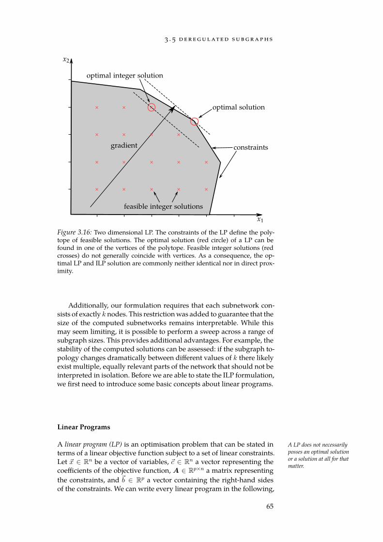
3 . 5 d e r e g u l at e d s u b g r a p h s

Figure 3.16: Two dimensional LP. The constraints of the LP define the poly-tope of feasible solutions. The optimal solution (red circle) of a LP can befound in one of the vertices of the polytope. Feasible integer solutions (redcrosses) do not generally coincide with vertices. As a consequence, the op-timal LP and ILP solution are commonly neither identical nor in direct prox-imity.

Additionally, our formulation requires that each subnetwork con-sists of exactly k nodes. This restriction was added to guarantee that thesize of the computed subnetworks remains interpretable. While thismay seem limiting, it is possible to perform a sweep across a range ofsubgraph sizes. This provides additional advantages. For example, thestability of the computed solutions can be assessed: if the subgraph to-pology changes dramatically between different values of k there likelyexist multiple, equally relevant parts of the network that should not beinterpreted in isolation. Before we are able to state the ILP formulation,we first need to introduce some basic concepts about linear programs.

Linear Programs

A linear program (LP) is an optimisation problem that can be stated in A LP does not necessarilyposses an optimal solutionor a solution at all for thatmatter.

terms of a linear objective function subject to a set of linear constraints.Let x ∈ Rn be a vector of variables, c ∈ Rn a vector representing thecoefficients of the objective function, A ∈ Rp×n a matrix representingthe constraints, and b ∈ Rp a vector containing the right-hand sidesof the constraints. We can write every linear program in the following,

65

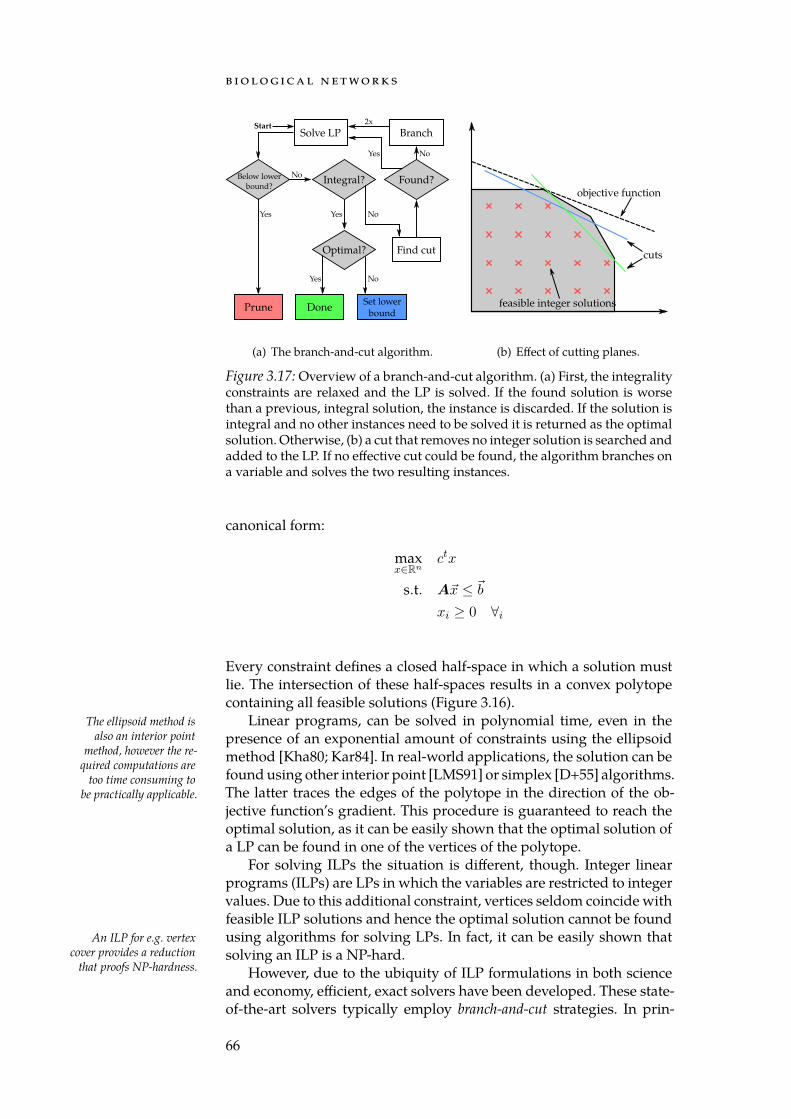
b i o lo g i ca l n e t wo r k s

Solve LP

Integral?

Done

Find cut

Found?

Branch

Below lowerbound?

Prune

Optimal?

Yes

No

Set lowerbound

Yes

No

2x

Yes

No

No

Yes

Start

(a) The branch-and-cut algorithm.

cuts

objective function

feasible integer solutions

(b) Effect of cutting planes.

Figure 3.17: Overview of a branch-and-cut algorithm. (a) First, the integralityconstraints are relaxed and the LP is solved. If the found solution is worsethan a previous, integral solution, the instance is discarded. If the solution isintegral and no other instances need to be solved it is returned as the optimalsolution. Otherwise, (b) a cut that removes no integer solution is searched andadded to the LP. If no effective cut could be found, the algorithm branches ona variable and solves the two resulting instances.

canonical form:

maxx∈Rn

ctx

s.t. Ax ≤ b

xi ≥ 0 ∀i

Every constraint defines a closed half-space in which a solution mustlie. The intersection of these half-spaces results in a convex polytopecontaining all feasible solutions (Figure 3.16).

Linear programs, can be solved in polynomial time, even in theThe ellipsoid method isalso an interior point

method, however the re-quired computations are

too time consuming tobe practically applicable.

presence of an exponential amount of constraints using the ellipsoidmethod [Kha80; Kar84]. In real-world applications, the solution can befound using other interior point [LMS91] or simplex [D+55] algorithms.The latter traces the edges of the polytope in the direction of the ob-jective function’s gradient. This procedure is guaranteed to reach theoptimal solution, as it can be easily shown that the optimal solution ofa LP can be found in one of the vertices of the polytope.

For solving ILPs the situation is different, though. Integer linearprograms (ILPs) are LPs in which the variables are restricted to integervalues. Due to this additional constraint, vertices seldom coincide withfeasible ILP solutions and hence the optimal solution cannot be foundusing algorithms for solving LPs. In fact, it can be easily shown thatAn ILP for e.g. vertex

cover provides a reductionthat proofs NP-hardness.

solving an ILP is a NP-hard.However, due to the ubiquity of ILP formulations in both science

and economy, efficient, exact solvers have been developed. These state-of-the-art solvers typically employ branch-and-cut strategies. In prin-

66

3 . 5 d e r e g u l at e d s u b g r a p h s

(a) Disconnected nodes (b) Connection enforced via Eqn. 3.8

(c) Disconnected cycles (d) Connection enforced via Eqn. 3.9.

Figure 3.18: Effect of the in-edge constraint Equation (3.8) and the cycle con-straint Equation (3.9). Without the in-edge constraint the resulting subgraphdoes not need to be connected (a). With the constraint a connection to theroot is enforced (b). However, disconnected cycles are still legal (c). With thecycle constraint, each cycle either needs to contain the root or has an in-edgefrom a chosen node outside of the cycle. The root node is indicated by a redbackground.

ciple these approaches work as follows (Figure 3.17): in a first step, thealgorithm solves a so called relaxed version of the ILP, in which theintegrality constraints have been dropped. The objective value of thissolution serves as an upper bound on the optimal integer solution. Ifthe solution is not integer, a new constraint is derived that cuts awaythe vertex containing the found solution, thereby tightening the poly-tope around the contained integral points. If no effective cut could befound, the algorithm branches on a variable, meaning that the ILP isdivided into two instances. One, where the variable has a value lowerthan a computed bound and one where its value is higher. For binaryvariables this effectively means that two instances are created wherethe value of the branching variable is fixed to zero and one, respect-ively. Both instances are then solved separately. The objective value ofthe best current integer solution is kept as a lower bound. This allowsto prune instances from the search tree whenever its relaxed LP solu-tion has a lower objective value than the current lower bound. The al-gorithm iterates until an integer solution can be proven to be optimal.This is the case when e.g. no other branches remain to be solved. Formore details on (integer) linear programming, we refer the reader tothe comprehensive introduction by Bertsimas and Tsitsiklis [BT97].

ILP Formulation

Our ILP formulation is based around two types of variables. Let n ∈ N The network is allowed tocontain more than one nodethat can act as root. Theconstraints ensure that oneof these nodes is picked asdesignated root node.

be the number of nodes in the network. Each node i is associated witha binary variable xi ∈ B that indicates whether it is part of the dereg-ulated subgraph (xi = 1) or not (xi = 0). We group these variablesinto the vector x ∈ Bn. Similarly, each node is associated with a binaryvariable yi ∈ B that is equal to one if and only if the node was selec-

67

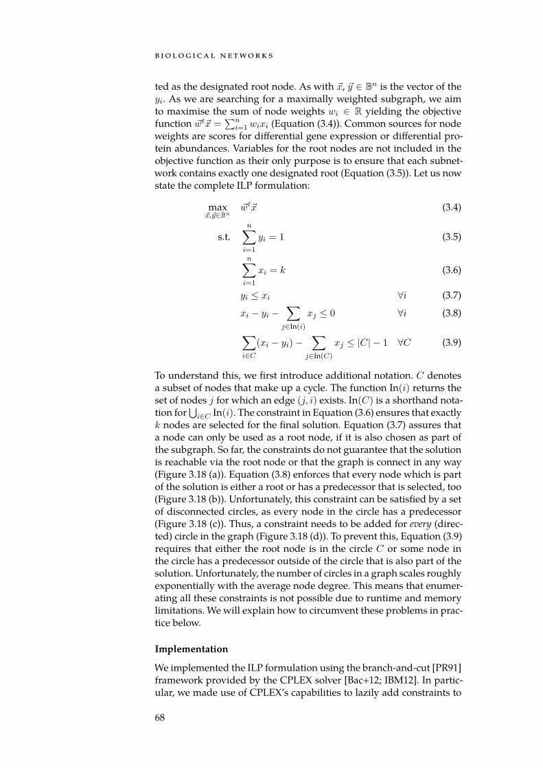
b i o lo g i ca l n e t wo r k s

ted as the designated root node. As with x, y ∈ Bn is the vector of theyi. As we are searching for a maximally weighted subgraph, we aimto maximise the sum of node weights wi ∈ R yielding the objectivefunction wtx =

∑ni=1wixi (Equation (3.4)). Common sources for node

weights are scores for differential gene expression or differential pro-tein abundances. Variables for the root nodes are not included in theobjective function as their only purpose is to ensure that each subnet-work contains exactly one designated root (Equation (3.5)). Let us nowstate the complete ILP formulation:

maxx,y∈Bn

wtx (3.4)

s.t.n∑

i=1

yi = 1 (3.5)

n∑i=1

xi = k (3.6)

yi ≤ xi ∀i (3.7)

xi − yi −∑

j∈In(i)

xj ≤ 0 ∀i (3.8)

∑i∈C

(xi − yi)−∑

j∈In(C)

xj ≤ |C| − 1 ∀C (3.9)

To understand this, we first introduce additional notation. C denotesa subset of nodes that make up a cycle. The function In(i) returns theset of nodes j for which an edge (j, i) exists. In(C) is a shorthand nota-tion for

∪i∈C In(i). The constraint in Equation (3.6) ensures that exactly

k nodes are selected for the final solution. Equation (3.7) assures thata node can only be used as a root node, if it is also chosen as part ofthe subgraph. So far, the constraints do not guarantee that the solutionis reachable via the root node or that the graph is connect in any way(Figure 3.18 (a)). Equation (3.8) enforces that every node which is partof the solution is either a root or has a predecessor that is selected, too(Figure 3.18 (b)). Unfortunately, this constraint can be satisfied by a setof disconnected circles, as every node in the circle has a predecessor(Figure 3.18 (c)). Thus, a constraint needs to be added for every (direc-ted) circle in the graph (Figure 3.18 (d)). To prevent this, Equation (3.9)requires that either the root node is in the circle C or some node inthe circle has a predecessor outside of the circle that is also part of thesolution. Unfortunately, the number of circles in a graph scales roughlyexponentially with the average node degree. This means that enumer-ating all these constraints is not possible due to runtime and memorylimitations. We will explain how to circumvent these problems in prac-tice below.

Implementation

We implemented the ILP formulation using the branch-and-cut [PR91]framework provided by the CPLEX solver [Bac+12; IBM12]. In partic-ular, we made use of CPLEX’s capabilities to lazily add constraints to

68

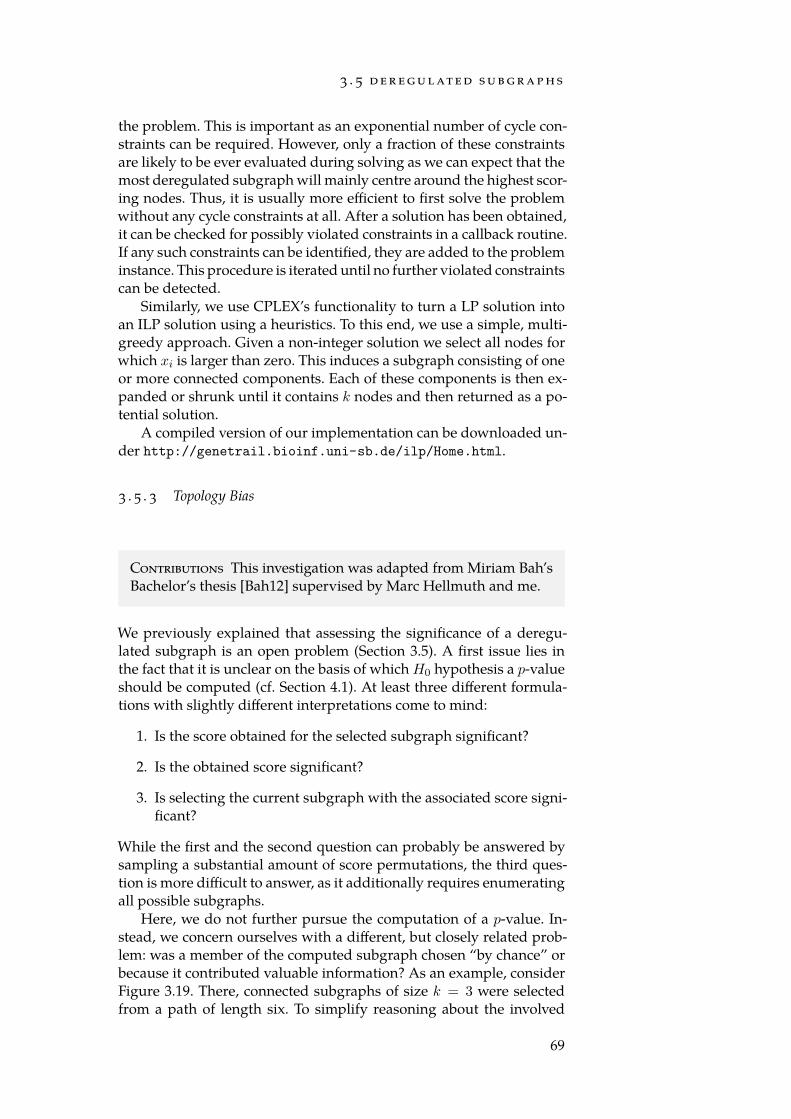
3 . 5 d e r e g u l at e d s u b g r a p h s

the problem. This is important as an exponential number of cycle con-straints can be required. However, only a fraction of these constraintsare likely to be ever evaluated during solving as we can expect that themost deregulated subgraph will mainly centre around the highest scor-ing nodes. Thus, it is usually more efficient to first solve the problemwithout any cycle constraints at all. After a solution has been obtained,it can be checked for possibly violated constraints in a callback routine.If any such constraints can be identified, they are added to the probleminstance. This procedure is iterated until no further violated constraintscan be detected.

Similarly, we use CPLEX’s functionality to turn a LP solution intoan ILP solution using a heuristics. To this end, we use a simple, multi-greedy approach. Given a non-integer solution we select all nodes forwhich xi is larger than zero. This induces a subgraph consisting of oneor more connected components. Each of these components is then ex-panded or shrunk until it contains k nodes and then returned as a po-tential solution.

A compiled version of our implementation can be downloaded un-der http://genetrail.bioinf.uni-sb.de/ilp/Home.html.

3 . 5 . 3 Topology Bias

Contributions This investigation was adapted from Miriam Bah’sBachelor’s thesis [Bah12] supervised by Marc Hellmuth and me.

We previously explained that assessing the significance of a deregu-lated subgraph is an open problem (Section 3.5). A first issue lies inthe fact that it is unclear on the basis of which H0 hypothesis a p-valueshould be computed (cf. Section 4.1). At least three different formula-tions with slightly different interpretations come to mind:

1. Is the score obtained for the selected subgraph significant?

2. Is the obtained score significant?

3. Is selecting the current subgraph with the associated score signi-ficant?

While the first and the second question can probably be answered bysampling a substantial amount of score permutations, the third ques-tion is more difficult to answer, as it additionally requires enumeratingall possible subgraphs.

Here, we do not further pursue the computation of a p-value. In-stead, we concern ourselves with a different, but closely related prob-lem: was a member of the computed subgraph chosen “by chance” orbecause it contributed valuable information? As an example, considerFigure 3.19. There, connected subgraphs of size k = 3 were selectedfrom a path of length six. To simplify reasoning about the involved

69

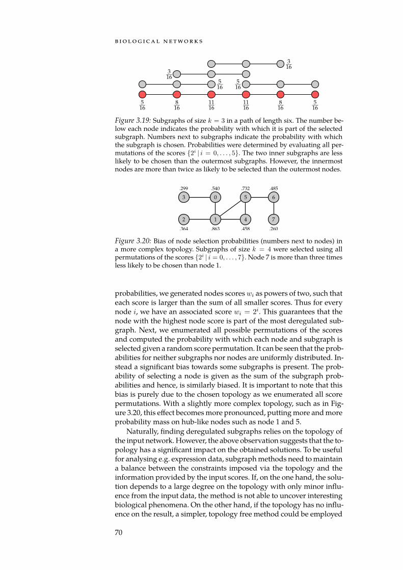
b i o lo g i ca l n e t wo r k s

Figure 3.19: Subgraphs of size k = 3 in a path of length six. The number be-low each node indicates the probability with which it is part of the selectedsubgraph. Numbers next to subgraphs indicate the probability with whichthe subgraph is chosen. Probabilities were determined by evaluating all per-mutations of the scores 2i | i = 0, . . . , 5. The two inner subgraphs are lesslikely to be chosen than the outermost subgraphs. However, the innermostnodes are more than twice as likely to be selected than the outermost nodes.

0

4

3

72

5 6

1

.540

.863.364

.299

.458

.732 .485

.260

Figure 3.20: Bias of node selection probabilities (numbers next to nodes) ina more complex topology. Subgraphs of size k = 4 were selected using allpermutations of the scores 2i | i = 0, . . . , 7. Node 7 is more than three timesless likely to be chosen than node 1.

probabilities, we generated nodes scores wi as powers of two, such thateach score is larger than the sum of all smaller scores. Thus for everynode i, we have an associated score wi = 2i. This guarantees that thenode with the highest node score is part of the most deregulated sub-graph. Next, we enumerated all possible permutations of the scoresand computed the probability with which each node and subgraph isselected given a random score permutation. It can be seen that the prob-abilities for neither subgraphs nor nodes are uniformly distributed. In-stead a significant bias towards some subgraphs is present. The prob-ability of selecting a node is given as the sum of the subgraph prob-abilities and hence, is similarly biased. It is important to note that thisbias is purely due to the chosen topology as we enumerated all scorepermutations. With a slightly more complex topology, such as in Fig-ure 3.20, this effect becomes more pronounced, putting more and moreprobability mass on hub-like nodes such as node 1 and 5.

Naturally, finding deregulated subgraphs relies on the topology ofthe input network. However, the above observation suggests that the to-pology has a significant impact on the obtained solutions. To be usefulfor analysing e.g. expression data, subgraph methods need to maintaina balance between the constraints imposed via the topology and theinformation provided by the input scores. If, on the one hand, the solu-tion depends to a large degree on the topology with only minor influ-ence from the input data, the method is not able to uncover interestingbiological phenomena. On the other hand, if the topology has no influ-ence on the result, a simpler, topology free method could be employed

70

3 . 5 d e r e g u l at e d s u b g r a p h s

Smoker?

Age < 50?

Yes No

Gender?BMI < 30?

Yes No

Low risk Medium risk High risk

Female Male

Medium risk

High risk

BMI < 25?

Medium risk

Yes No

Yes No

Figure 3.21: Example for a (fictive) decision tree stratifying patients into low,medium, and high risk groups for congestive heart disease. In each decisionnode (round), a predictor (Smoker, Age, BMI, Gender) is used to partition thetraining data. Predictions for new datapoints can be made by following a pathfrom the root to a leaf node (rectangles), which contain the predicted value.

instead. Quantifying the influence of topology and input data on theresults of a deregulated subnetwork algorithm is difficult, though.

Here, we propose a procedure that allows to judge the bias incurred For a brief introduction tomachine learning refer toAppendix A.2.

by methods for the detection of deregulated subgraphs towards certainnodes due to the network topology. It is based on predicting the prob-ability that a given node is selected as part of the subnetwork. To thisend, we train a random forest model [Bre01] for predicting node inclu-sion probabilities that were empirically determined by sampling de-regulated subnetworks given uniformly distributed input scores. Thismodel uses a set of node topology descriptors as features. Applyingthe trained predictor to an unknown network allows to estimate thetopology bias without a computationally intensive sampling step.

In the following we explain our procedure in detail. To be able todo so, we first need to introduce the random forest predictor as well asthe used topology descriptors. Next, the used training and validationscheme is outlined. Finally, we present the results of our study.

Random Forests

Random forests are non-linear models for classification and regression For more details on ran-dom forests we refer to theoriginal paper by Breiman[Bre01] and the introduc-tion by Friedman, Hastie,and Tibshirani [FHT09].

(cf. Appendix A.2). In particular, they are an ensemble method that isbased on averaging the output of B ∈ N decision trees fb that weretrained on bootstrap samples of the data (bagging). A decision tree isa machine learning method that partitions its input space via recurs-ive, binary cuts [Qui86; Qui93]. These cuts can be represented as nodesin a tree (cf. Figure 3.21). Which split is used in each node is determ-ined by evaluating a loss function for each dimension. Examples arethe squared-error loss for regression or the Gini index for classifica-

71

b i o lo g i ca l n e t wo r k s

tion. The variable that achieves the smallest loss is chosen for cutting.In contrast to common decision trees, which always evaluate all vari-ables to decide on a split, the random forest procedure randomly se-lects k predictors from which the best candidate must be chosen. Fur-thermore, each tree is built on a bootstrap sample of the training data.A bootstrap sample for a dataset containing N samples is generated byrandomly drawing N samples from the dataset with replacement. Eachtree is grown until it perfectly predicts its training data. In a regressionscenario, the final random forest model is defined as the average pre-diction of all trained decision trees:

f(x) =

B∑b=1

fb(x)

In a classification scenario, the output class label is determined via amajority vote.

Random forests have various advantages that make them especiallyOften B ≈ 500 andk =

√p for classification

and k = ⌊p/3⌋ for regres-sion, with p being the num-

ber of predictors, is used.

suited for quickly obtaining classifiers that offer a performance that iscompetitive with other state-of-the-art approaches. A reason for this isthat random forests models are comparatively straightforward to setup. As inputs they can use continuous, ordinal, and categorical inputsand therefore require no special feature encoding techniques. In addi-tion, the model exposes only two tuning parameters: the number oftrees B and the number of features considered in each split k. For bothparameters good default values are known. Choosing different, butreasonable settings commonly has no critical impact on performance.Due to this, the model is robust with respect to overtraining [Bre01;FHT09].

As each tree is grown on a different bootstrap sample, not everysample has been used for every tree. Thus, for each tree fb the predic-tion error for the samples that have not been used to train fb can bedetermined. This yields the so-called out-of-bag (OOB) error that canserve as an estimate of the test error. Thus cross-validation or a separ-ate tuning set are not strictly required for tuning random forests.

Finally, it is possible to compute feature importances. The featureimportance reflects how large the impact of a feature on the predictedvalue is. There are two ways to compute these importances. The firstversion is based on the OOB error. For each tree, the OOB error is com-puted. Then, to obtain the importance of variable j its values are per-muted and the OOB error is computed again. The difference betweenthe two values is averaged across all trees and returned as the variableimportance [Bre01]. Alternatively, the decrease of the loss function ineach split gives an indication of the influence of the chosen split vari-able. These values are accumulated across all trees and splits to obtainthe final importance [FHT09].

Of course, random forests also have disadvantages. Probably themost important one is that the final model is difficult to interpret. Whilewe can extract the importance of single variables, random forests arehighly non-linear and thus the importance measure does not permit astraightforward interpretation such as: “If the value of variable A in-

72

3 . 5 d e r e g u l at e d s u b g r a p h s

creases by 10 % the risk for cancer increases by 20 %.” In contrast, theweights computed by linear models (Section 3.4.1) or SVMs with linearkernels [FHT09; SS02] have this property. Also, for SVMs with a well-performing, non-linear kernel, examining the feature maps allows togain mechanistic insight into the learning problem. Furthermore, in thepresence of categorical variables, random forests tend to favour thosevariables with more levels. Consequently, the computed variable im-portance measures are not reliable in this case and need to be adjustedusing sampling techniques [Alt+10].

Topology Descriptors

Arguably the most important prerequisites for applying machine learn- The terms feature andpredictor are often usedsynonymously.

ing algorithms is the selection of a suitable set of features and theirrepresentation. For our task, features are needed that capture the topo-logical properties of a graph node. To this end we use a set of topologydescriptors which have originally been developed for analysing the im-portance of nodes in large network structures such as the topology ofthe internet. In this section we describe and define the used descriptors.

First and foremost, we use simple, graph theoretical properties suchas the in- and out-degree of a node. These statistics, however, character-ise the node almost in isolation and pay little regard to the surroundingtopology. To help assessing the importance of a node on a global scale,more sophisticated measures such as the PageRank [Pag+99] or variouscentrality measures have become popular. Let us, however, start withmore basic measures.

A natural choice for topology descriptors are the node degrees asintroduced in Definition 5. The degree of a node, especially relative tothe degrees of the remaining nodes reflects the number of connectionsa node has and should thus be a crude approximation for how “hub-like” the node is. Nodes with a high in-degree are also more likely tobe leafs in a selected subgraph, whereas nodes with a high out-degreeshould be more likely to act as root nodes. The clustering coefficient isa generalisation of this idea and also considers how the neighbours ofthe node are connected. More formally:

Definition 11 (Clustering coefficient). A triangle is a triple of connec-ted nodes. Let τ∆(v) denote the number of triangles containing v ∈ Vand let kv ∈ N be the number of adjacent nodes. Then the clusteringcoefficient for v is defined as

cl(v) = τ∆(v)

kv(kv − 1)

In contrast to the node degrees, centrality measures put a node ina more global context. For example the betweenness centrality [Fre77]counts the number of shortest paths that include a given node.

Definition 12 (Betweenness centrality). Let σ(s, t | v) denote the num-ber of shortest paths between nodes s and t that include v. Furthermore,let σ(s, t) be the total number of shortest paths between the two nodes.

73

b i o lo g i ca l n e t wo r k s

Then the betweenness centrality is given by

cB(v) =1

(|V | − 1)(|V | − 2)

∑s =t=v

σ(s, t|v)σ(s, t)

The closeness centrality [Bav50; Bea65] is also based on the notionof shortest paths. However, it considers the reciprocal of the averagelength of all shortest paths starting from the node of interest v. If allremaining nodes in the graph can be reached quickly, v receives a highcentrality value. Otherwise, if the length of the shortest paths is long,v has a low centrality.

Definition 13 (Closeness centrality). For a node v ∈ V the closenesscentrality is given by

cC(v) =n− 1∑

u∈Xvdist(v, u)

Here dist(v, u) denotes the length of the shortest path from v to u andXv := u |dist(v, u) < ∞.

Whereas betweenness and closeness centrality use shortest paths todetermine the importance of a node, Bonacich [Bon72] proposed to usethe dominant eigenvalue of the adjacency matrix as centrality measure.

Definition 14 (Eigenvector centrality). LetA be the adjacency matrix ofG with Avu = 1 if (v, u) ∈ E and 0 otherwise. Then the out-eigenvectorcentrality cout(v) is defined as the v-th entry of the principal eigenvectorof A. The in-eigenvector centrality cin(v) is the v-th component of theprincipal eigenvector of At.

The principal eigenvector of a matrix can be easily computed usingthe power iteration [MP29]

vt+1 =Avt

∥Avt∥.

Interpreting the eigenvector centrality, though, is not straightforwardas no inherent meaning is attached to an entry of the principal eigen-vector. Probably the best intuition is that a node is assumed to be morecentral, if it is connected to other central nodes [Ruh00].

A measure that is closely related to the eigenvector centrality is theEffectively, the Page-Rank interprets theadjacency matrix as

a Markov process.

PageRank. It models the probability with which a user clicking ran-dom links (edges) on a web page (nodes) ends up on a certain site. Toavoid local attractors such as nodes with no out-edges, the PageRankincludes a constant, uniformly distributed restart probability into itsmodel:

Definition 15 (PageRank). Let In(v) = u | (u, v) ∈ E be the in-neigh-bourhood of v. The PageRank for v and a damping factor α ∈ R+ isdefined as

PR(v) = 1− α

|V |+ α

∑u∈In(v)

PR(u)

d+(u)

74

3 . 5 d e r e g u l at e d s u b g r a p h s

The damping factor α controls the influence of the random restart.The recursive formulation of the PageRank can be rewritten in termsof a matrix power, which allows to obtain the limit distribution via aneigenvalue decomposition [Pag+99].

The above graph measures are well known and implemented inpopular software packages such as Cytoscape [Sha+03; Ass+08]. Asall of them are general purpose measures, none directly estimates thenumber of subgraphs of size k in which a node is contained in. Hence,to supplement the existing measures, we devised our own descriptor.It is based on the number of spanning trees that use the outgoing edgesof a node. The idea behind using spanning trees is that every rooted,deregulated subgraph can be trivially transformed into a spanning treeof the selected nodes (cf. [Dit+08]). Thus, knowing the number of span-ning trees that are present in a neighbourhood of a node, should allowa good estimate of the number of deregulated subgraphs the node is apart of.

The measure relies on Kirchhoff’s theorem [Kir47] which states thatthe number of spanning trees rooted in a vertex can be obtained fromthe cofactors of the Kirchhoff matrix. Let us start with the definition ofa cofactor.

Definition 16 (Cofactor). Given a matrix A ∈ Rn×n. The ij-th cofactorof A is given by

Cij(A) := (−1)i+jdet(Mij)

where Mij ∈ R(n−1)×(m−1) is the matrix obtained by deleting the i-throw and j-th column from A.

The Kirchhoff matrix, also known as graph Laplacian, is based onthe adjacency matrix. It can be interpreted as a discrete analogue ofthe Laplacian operator from calculus or the Laplace-Beltrami operatorfrom vector analysis.

Definition 17 (Directed Kirchhoff Matrix). Given the directed graphG(V,E). Its Kirchhoff matrix K is defined as:

Kij =

d−i if i = j

−1 if (i, j) ∈ E

0 otherwise

By construction, Kt has an eigenvalue of zero corresponding to theeigenvector ⊮n, the vector where each component has the value 1. If Ghas m connected components, the kernel of K has dimension m + 1as for every connected component we can create an eigenvector for theeigenvalue zero by simply setting all coefficients that belong to nodesinside the connected component to one and all others to zero.

We will now describe the relation between the Kirchhoff matrix andthe number of spanning trees. For this we first need to define the notionof an out-tree.

Definition 18 (Out-tree). An out-tree is a connected, directed acyclicgraph which is rooted in a single vertex. The root vertex has in-degreezero and every other vertex has in-degree one.

75

b i o lo g i ca l n e t wo r k s

Given the definitions above we are able to state the following the-orem by Tutte [Tut48] that links the number of spanning trees rooted ina vertex with the cofactors of the Kirchhoff matrix. It is a generalisationof Kirchhoff’s Matrix-Tree theorem [Kir47] for undirected graphs.

Theorem 3.5.1 (Directed Matrix-Tree Theorem). LetK be the Kirchhoffmatrix of G(V,E). For any vertex i ∈ V , the number of out-trees rootedat i equals Cij(K) for an arbitrary choice of j.

We can use this theorem to compute the number of spanning treesof G. For this, we simply need to select a vertex i from which all othervertices are reachable. If no such vertex exists, G has no spanning tree.Otherwise we can select an arbitrary column j and compute the num-ber of spanning trees as Cij(A). For our purposes, this trick is not dir-ectly useful, as the number of spanning trees is necessarily the same forall vertices that can serve as the root of a spanning tree. However, wecan use this technique to compute the number of spanning trees thatuse a given edge e by computing the number of spanning trees in Gminus the number of spanning trees that remain in the graph after ehas been removed:

#spTree(e) = #spTree(G)− #spTree(G− e)

This yields an importance measure for every edge: the more spanningtrees use this edge, the more important it is. For computing vertex im-portances, we can simply accumulate the importances of all incidentedges.

Definition 19 (Spanning tree weight). Let G(V,E) be a directed graph.Define Ev ⊆ E be the set of incident in- and out-edges of the nodev ∈ V . We define the spanning tree weight of v as

sp(v) =∑e∈Ev

#spTree(e)

For computing the degrees, betweenness and closeness centrality,and the clustering coefficient we used the NetworkAnalyzer [Ass+08]Cytoscape [Lop+10] plugin. The PageRank and spanning tree weightswere computed using a C++ implementation based on the BGL [SLL01],Eigen 39, GMP10, and MPFR11 libraries. The eigenvalue centrality wascomputed using Python [VD09] as well as the NetworkX [SS08a] andSciPy [J+01] packages.

Predicting ILP Counts

We finally have all required pieces in place to predict the likelihoodwith which a node is selected as part of a deregulated subgraph. Tothis end, our procedure for obtaining the node selection probabilities

9 http://eigen.tuxfamily.org10 https://gmplib.org/11 http://www.mpfr.org/index.html

76

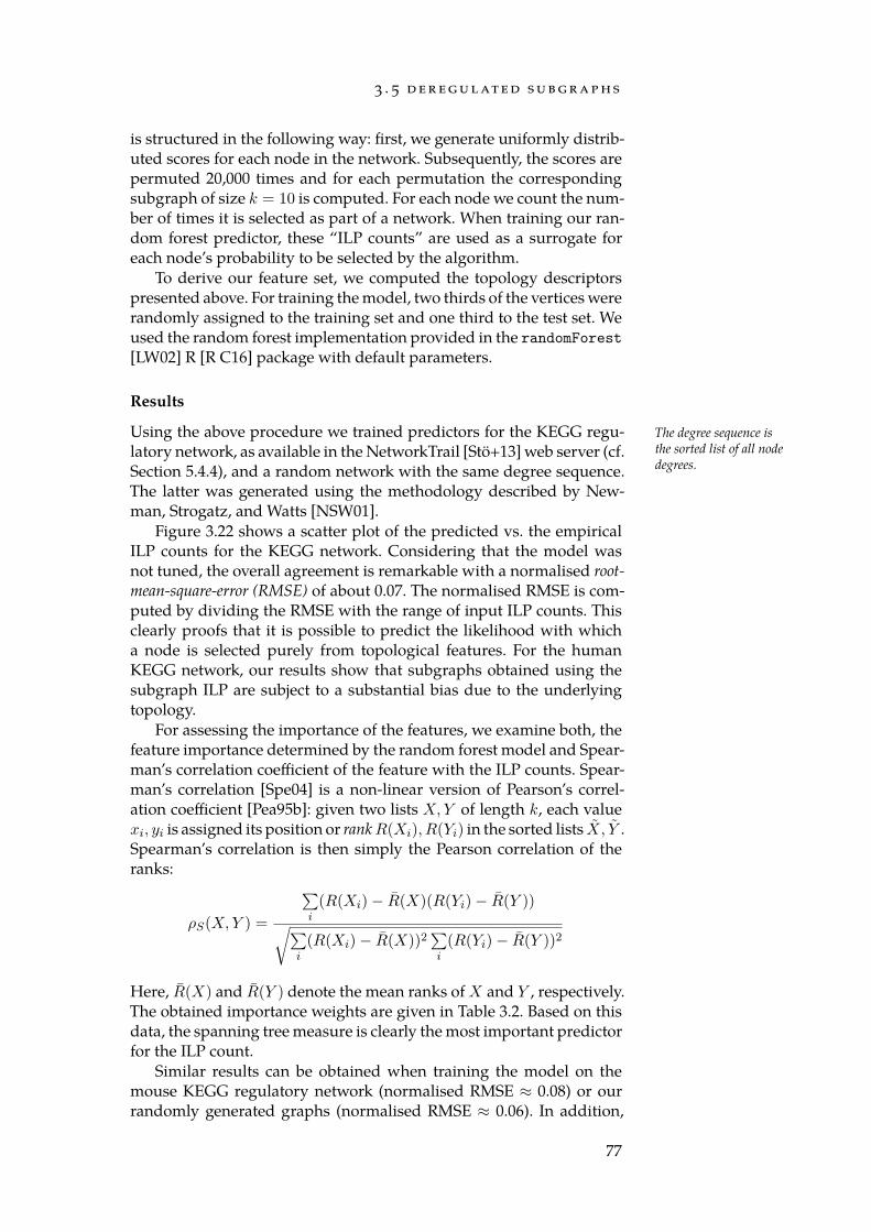
3 . 5 d e r e g u l at e d s u b g r a p h s

is structured in the following way: first, we generate uniformly distrib-uted scores for each node in the network. Subsequently, the scores arepermuted 20,000 times and for each permutation the correspondingsubgraph of size k = 10 is computed. For each node we count the num-ber of times it is selected as part of a network. When training our ran-dom forest predictor, these “ILP counts” are used as a surrogate foreach node’s probability to be selected by the algorithm.

To derive our feature set, we computed the topology descriptorspresented above. For training the model, two thirds of the vertices wererandomly assigned to the training set and one third to the test set. Weused the random forest implementation provided in the randomForest[LW02] R [R C16] package with default parameters.

Results

Using the above procedure we trained predictors for the KEGG regu- The degree sequence isthe sorted list of all nodedegrees.

latory network, as available in the NetworkTrail [Stö+13] web server (cf.Section 5.4.4), and a random network with the same degree sequence.The latter was generated using the methodology described by New-man, Strogatz, and Watts [NSW01].

Figure 3.22 shows a scatter plot of the predicted vs. the empiricalILP counts for the KEGG network. Considering that the model wasnot tuned, the overall agreement is remarkable with a normalised root-mean-square-error (RMSE) of about 0.07. The normalised RMSE is com-puted by dividing the RMSE with the range of input ILP counts. Thisclearly proofs that it is possible to predict the likelihood with whicha node is selected purely from topological features. For the humanKEGG network, our results show that subgraphs obtained using thesubgraph ILP are subject to a substantial bias due to the underlyingtopology.

For assessing the importance of the features, we examine both, thefeature importance determined by the random forest model and Spear-man’s correlation coefficient of the feature with the ILP counts. Spear-man’s correlation [Spe04] is a non-linear version of Pearson’s correl-ation coefficient [Pea95b]: given two lists X,Y of length k, each valuexi, yi is assigned its position or rankR(Xi), R(Yi) in the sorted lists X, Y .Spearman’s correlation is then simply the Pearson correlation of theranks:

ρS(X,Y ) =

∑i(R(Xi)− R(X)(R(Yi)− R(Y ))√∑

i(R(Xi)− R(X))2

∑i(R(Yi)− R(Y ))2

Here, R(X) and R(Y ) denote the mean ranks of X and Y , respectively.The obtained importance weights are given in Table 3.2. Based on thisdata, the spanning tree measure is clearly the most important predictorfor the ILP count.

Similar results can be obtained when training the model on themouse KEGG regulatory network (normalised RMSE ≈ 0.08) or ourrandomly generated graphs (normalised RMSE ≈ 0.06). In addition,

77

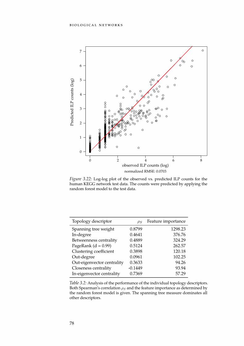
b i o lo g i ca l n e t wo r k s

Pred

icte

d IL

P co

unts

(log

)

observed ILP counts (log)normalized RMSE: 0.0703

0 2 4 6 8

0

1

2

3

4

5

6

7

Figure 3.22: Log-log plot of the observed vs. predicted ILP counts for thehuman KEGG network test data. The counts were predicted by applying therandom forest model to the test data.

Topology descriptor ρS Feature importance

Spanning tree weight 0.8799 1298.23In-degree 0.4641 376.76Betweenness centrality 0.4889 324.29PageRank (d = 0.99) 0.5124 262.57Clustering coefficient 0.3898 120.18Out-degree 0.0961 102.25Out-eigenvector centrality 0.3633 94.26Closeness centrality -0.1449 93.94In-eigenvector centrality 0.7369 57.29

Table 3.2: Analysis of the performance of the individual topology descriptors.Both Spearman’s correlation ρS and the feature importance as determined bythe random forest model is given. The spanning tree measure dominates allother descriptors.

78

3 . 5 d e r e g u l at e d s u b g r a p h s

training the model on the mouse KEGG network and predicting theILP counts for the human network results in a normalised RMSE of≈ 0.09. This result suggests that our predictor is not overfitted for thenetwork it was trained on. Instead, the model generalises to yet unseendata. This further confirms that the node selection bias can in fact bepredicted from purely topological properties.

Discussion

We presented theoretical results that suggest that the probability withwhich a node is selected as part of the most deregulated subgraphhighly depends on its topological properties. To confirm this, we meas-ured the bias of the Subgraph ILP induced by the underlying networktopology by using a sampling technique. To further confirm that thisbias is purely based on a nodes topological properties, we trained a ran-dom forest model on a set of topology descriptors. With this model, wewere able to obtain good predictors for the node inclusion frequency.In particular, our novel spanning tree measure prove to be an excellentpredictor. This suggests that the most deregulated subgraphs obtainedfor scores from an experiment might be influenced considerably by thenetwork topology. While this is desirable to a certain extent, the usershould keep this bias in mind when interpreting a deregulated sub-graph.

For counteracting the described effect, a node reweighing strategymay be employed. We conducted initial experiments in this regard, inwhich we down-weighed the scores si of a node i according to a func-tion of its probability pi to be selected. Examples for potential functionsare si/pi, si/

√pi, and si/p

2i . However, our preliminary results have not

shown a significant impact on the selection probability.There are various ways to continue the presented study. First, con-

firming the reported results for a different, published algorithm woulddemonstrate that the described topology bias is in fact a universal phe-nomenon and is not linked to the particularities of the Subgraph ILP. Acandidate algorithm would need to support computing a high amountof random samples to obtain reliable estimates for the node inclusionprobabilities. Unfortunately, we were not yet able to find a second al-gorithm meeting this requirement. Additionally, the analysis shouldbe rerun using networks from a different source. While our randomnetworks share no common nodes with the KEGG networks, they arebased on the same degree sequence and thus contain the same num-ber of hubs and leaf nodes. Using a completely independent networkcould therefore result in different distributions of the inclusion probab-ilities. We are, however, confident that a similar bias is also detectablefor different algorithms as well as different networks.

Finally, it should be noted that the reported biases were obtainedfor random score permutations and thus non-informative scores. In areal-world scenario the scores used for computing a deregulated sub-graph are likely to contain a signal that manifests as e.g. the differen-tial expression of specific gene sets. In this case, the score distribution

79

b i o lo g i ca l n e t wo r k s

may, to a large degree, overrule the topology bias. For confirming this,a large scale analysis of diverse expression datasets could be used.

80

4E N R I CH M E N T A LG O R I T H M S

The analytical power should not be confounded with simpleingenuity; for while the analyst is necessarily ingenious, theingenious man is often remarkably incapable of analysis.

— e d ga r a l l e n p o e , t h e m u rd e r s i n t h er u e m o rg u e ( 1 8 4 1 )

Comparative microarray and RNA-seq studies (Section 2.3) are exper-imental techniques for detecting the differences in the transcriptionalstate between a sample and reference group. Both techniques typicallyresult in large matrices of measurements where each row correspondsto all expression values of a single gene and each column contains allmeasurements of a single sample. Due to the high number of measuredgenes it is difficult to interpret this data manually. Instead, robust stat-istical methods for performing automated analyses are required thatare capable of condensing the information contained in these high di-mensional datasets into an interpretable report. Ideally, these reportswould allow to quickly deduce the molecular key players and regulat-ory mechanisms that are responsible for the difference between sampleand reference groups.

There are several ways to approach this task. For instance, a classi-fier that uses genes as features can be trained to discriminates betweenthe two groups. Once training is complete, the parameters of the clas-sifier can be examined to derive feature importance measures. The kmost important features are then reported as the “key players” thatare likely to be responsible for the observed differences. The drawbackof this approach is that training a good classifier is by no means a trivialaffair. Even then, the identified features are, while certainly discrimin-ative, not necessarily causal for the observed effect. Thus, the features,which have not been considered by the classifier in lieu of “more in-formative” predictors, may still carry valuable information that is notcaptured using this approach. Alternatively, techniques that do not fo- In practice regularised

versions of PCA or PLSwould be necessary.

cus on classification performance, but rather on providing better un-derstanding of the input data can be employed to circumvent theseissues. Examples are techniques such as principal component analysis(PCA) [Pea01] (see Section 3.4) or partial least squares (PLS) (cf. [FHT09])that decompose the data into orthogonal coordinates which either ex-plain the observed variance (PCR) or the group differences (PLS). Thesecoordinates can, again, serve as feature importances and can, hence, beused to extract the most relevant features.

The above approaches do not employ any kind of prior knowledge.However, a large collection of biological databases such as the Gene On-tology (GO) [Ash+00] exist that contain carefully collected, functionalannotations for genes, proteins, and other biological entities. Instead ofidentifying novel patterns in the data, we can use these annotations tocheck whether known categories of entities behave differently between

81

e n r i c h m e n t a lg o r i t h m s

the sample and reference group. Enrichment algorithms or enrichmentAlgorithms for search-ing deregulated sub-

graphs (Section 3.5) areenrichment methods

that use the admissiblesubgraphs as categories.

methods are a class of procedures that make use of this information.As input, an enrichment algorithm relies on one or more sets of en-tities, so-called categories. Each category commonly corresponds to anannotation such as a GO term. In addition, the algorithm requires aset of measurements such as a gene expression matrix. As output, itcomputes an enrichment score, which reflects the overall “degree of de-regulation”, and an associated significance measure for each input cat-egory.

Owing to this somewhat loose problem definition a multitude ofenrichment procedures have been devised. In this chapter, we discussa selection of popular enrichment methods. In particular, we examinetheir strengths and weaknesses as well as the considerations that arenecessary when choosing between algorithms. First, however, as thecomputation of the significance of an enrichment score is a central partof all enrichment algorithms, we introduce the concepts of a hypothesistests and p-values.

4 . 1 s tat i s t i ca l t e s t s

A central task in science is the verification or falsification of hypotheses.To this end, experiments must be conducted which then provide evid-ence in favour of or against a hypothesis. Evaluating this evidence care-fully and objectively is thus a common responsibility in a research set-ting. For this purpose, statisticians have devised testing strategies thatcan be used to determine if a hypothesis remains valid or needs to berejected in the light of new evidence.

Two frameworks for conducting such hypothesis tests exist. The firstframework was devised by Fisher [Fis25] and is centred around com-puting a p-value that measures how strongly the data contradicts anull hypothesis. The framework by Neyman and Pearson [NP33], on theother hand, has the goal of deciding between a null and an alternat-ive hypothesis. This is achieved by introducing a significance level αthat controls the admissible rate of cases in which the null hypothesisis wrongly rejected. In today’s scientific practice a hybrid between thetwo models is used that explicitly uses both a p-value and a signific-ance level [Lew12]. The validity of this hybrid approach is heavily de-bated as it is, according to some statisticians, an “incoherent mishmash”[Gig93]. The central point of critique is that the current use of hypo-thesis tests neither allows the assessment of the strength of evidencenor allows to control the long-term error rates. Nevertheless, we willintroduce concepts from both frameworks without explicitly differen-tiating between the two.

4 . 1 . 1 Null and Alternative Hypothesis

The central concept of all hypothesis tests is the so-called null hypo-thesis H0. It represents a default, commonly accepted believe that is

82

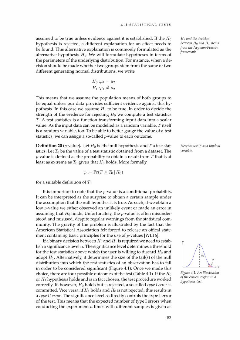
4 . 1 s tat i s t i ca l t e s t s

assumed to be true unless evidence against it is established. If the H0 H1 and the decisionbetween H0 and H1 stemsfrom the Neyman-Pearsonframework.

hypothesis is rejected, a different explanation for an effect needs tobe found. This alternative explanation is commonly formulated as thealternative hypothesis H1. We will formulate hypotheses in terms ofthe parameters of the underlying distribution. For instance, when a de-cision should be made whether two groups stem from the same or twodifferent generating normal distributions, we write

H0 :µ1 = µ2

H1 :µ1 = µ2

This means that we assume the population means of both groups tobe equal unless our data provides sufficient evidence against this hy-pothesis. In this case we assume H1 to be true. In order to decide thestrength of the evidence for rejecting H0 we compute a test statisticsT . A test statistics is a function transforming input data into a scalarvalue. As the input data can be modelled as a random variable, T itselfis a random variable, too. To be able to better gauge the value of a teststatistics, we can assign a so-called p-value to each outcome.

Definition 20 (p-value). Let H0 be the null hypothesis and T a test stat- Here we use T as a randomvariable.istics. Let T0 be the value of a test statistic obtained from a dataset. The

p-value is defined as the probability to obtain a result from T that is atleast as extreme as T0 given that H0 holds. More formally

p := Pr(T ≥ T0 |H0)

for a suitable definition of T .

It is important to note that the p-value is a conditional probability.It can be interpreted as the surprise to obtain a certain sample underthe assumption that the null hypothesis is true. As such, if we obtain alow p-value we either observed an unlikely event or made an error inassuming that H0 holds. Unfortunately, the p-value is often misunder-stood and misused, despite regular warnings from the statistical com-munity. The gravity of the problem is illustrated by the fact that theAmerican Statistical Association felt forced to release an offical state-ment containing basic principles for the use of p-values [WL16].

If a binary decision betweenH0 andH1 is required we need to estab-

µ0

x

y

α

Figure 4.1: An illustrationof the critical region in ahypothesis test.

lish a significance levelα. The significance level determines a thresholdfor the test statistics above which the user is willing to discard H0 andadopt H1. Alternatively, it determines the size of the tail(s) of the nulldistribution into which the test statistics of an observation has to fallin order to be considered significant (Figure 4.1). Once we made thischoice, there are four possible outcomes of the test (Table 4.1). If the H0

orH1 hypothesis holds and is in fact chosen, the test procedure workedcorrectly. If, however, H0 holds but is rejected, a so called type I error iscommitted. Vice versa, if H1 holds and H0 is not rejected, this results ina type II error. The significance level α directly controls the type I errorof the test. This means that the expected number of type I errors whenconducting the experiment n times with different samples is given as

83

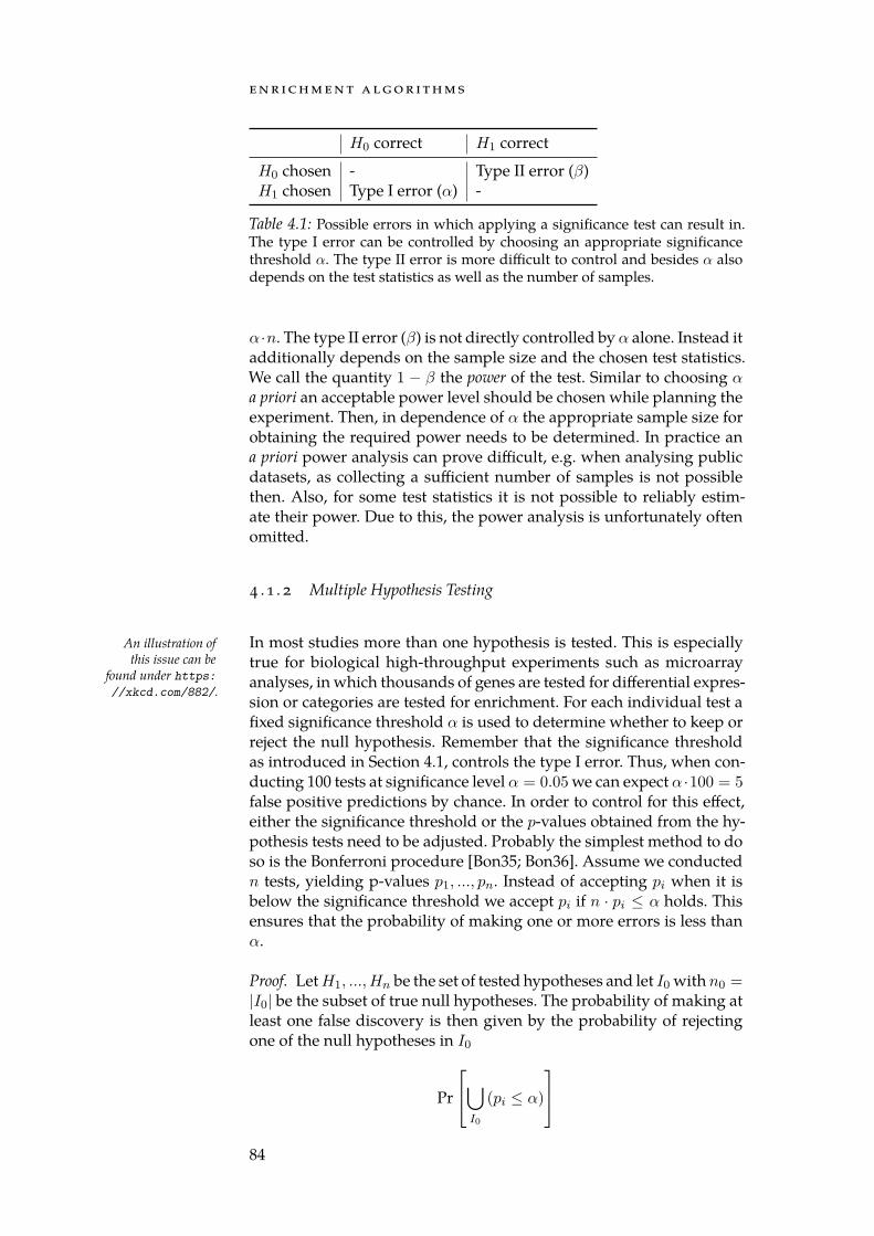
e n r i c h m e n t a lg o r i t h m s

H0 correct H1 correct

H0 chosen - Type II error (β)H1 chosen Type I error (α) -

Table 4.1: Possible errors in which applying a significance test can result in.The type I error can be controlled by choosing an appropriate significancethreshold α. The type II error is more difficult to control and besides α alsodepends on the test statistics as well as the number of samples.

α ·n. The type II error (β) is not directly controlled by α alone. Instead itadditionally depends on the sample size and the chosen test statistics.We call the quantity 1 − β the power of the test. Similar to choosing αa priori an acceptable power level should be chosen while planning theexperiment. Then, in dependence of α the appropriate sample size forobtaining the required power needs to be determined. In practice ana priori power analysis can prove difficult, e.g. when analysing publicdatasets, as collecting a sufficient number of samples is not possiblethen. Also, for some test statistics it is not possible to reliably estim-ate their power. Due to this, the power analysis is unfortunately oftenomitted.

4 . 1 . 2 Multiple Hypothesis Testing

In most studies more than one hypothesis is tested. This is especiallyAn illustration ofthis issue can be

found under https://xkcd.com/882/.

true for biological high-throughput experiments such as microarrayanalyses, in which thousands of genes are tested for differential expres-sion or categories are tested for enrichment. For each individual test afixed significance threshold α is used to determine whether to keep orreject the null hypothesis. Remember that the significance thresholdas introduced in Section 4.1, controls the type I error. Thus, when con-ducting 100 tests at significance level α = 0.05 we can expect α ·100 = 5false positive predictions by chance. In order to control for this effect,either the significance threshold or the p-values obtained from the hy-pothesis tests need to be adjusted. Probably the simplest method to doso is the Bonferroni procedure [Bon35; Bon36]. Assume we conductedn tests, yielding p-values p1, ..., pn. Instead of accepting pi when it isbelow the significance threshold we accept pi if n · pi ≤ α holds. Thisensures that the probability of making one or more errors is less thanα.

Proof. LetH1, ..., Hn be the set of tested hypotheses and let I0 with n0 =|I0| be the subset of true null hypotheses. The probability of making atleast one false discovery is then given by the probability of rejectingone of the null hypotheses in I0

Pr

∪I0

(pi ≤ α)

84

4 . 1 s tat i s t i ca l t e s t s

Substituting α with α/n and applying Boole’s inequality yields

Pr

∪I0

(pi ≤

α

n

) ≤∑I0

Pr(pi ≤

α

n

)≤ n0

α

n≤ n

α

n≤ α

The probability of making at least one false discovery is also calledfamily-wise error rate (FWER). Methods that ensure that the FWER isat most as high as a given threshold are said to control the FWER. Assuch, the Bonferroni procedure is one of the strictest available methods.Other methods that achieve tighter bounds, such as the Šidák [Šid68;Šid71] or the Holm-Bonferroni [Hol79] procedures are available.

In a biological setting, where the statistical power is already lowdue to small sample sizes, controlling the FWER is too conservative[Nak04]. Benjamini and Hochberg [BH95] introduced the concept offalse discovery rate (FDR) as well as a method using this statistics as atarget for adjustment. In contrast to the FWER, the FDR is the expectedproportion of false discoveries among all significant discoveries. Con-trolling the FDR instead of the FWER gives more control over the num-ber of acceptable false positive discoveries and is especially helpful inscenarios, in which false positive detections can be tolerated.

The Benjamini-Hochberg procedure controls the FDR for a set of If the hypothesis are de-pendent the procedure byBenjamini and Yekutieli[BY01] should be usedinstead.

independent hypothesis and works as follows: given the set of inputp-values p1, . . . , pn which w.l.o.g. we assume to be sorted in ascendingorder, find the largest k such that

Pk ≤ k

nq

where q is the desired FDR level. Given k, reject the null-hypothesisfor all Hi with i = 1, . . . , k. Alternatively, each p-value can be adjustedusing the formula [YB99]:

qi = minqi+1,

n

ipi, 1

Note that while the resulting values still fall into the interval [0, 1], theycan no longer be interpreted as p-values. Instead, they indicate the FDRlevel that can be obtained by rejecting the null-hypothesis for all qi ≤ q.

4 . 1 . 3 Enrichment Methods and Hypothesis Tests

In terms of hypothesis tests, another motivation for the use of enrich- We made a similar argu-ment concerning dereg-ulated subgraphs (Sec-tion 3.5).

ment methods, besides the efficient incorporation of prior knowledge,exists. Consider the search for differentially expressed genes, whereeach gene is tested for a significant difference in its expression levelbetween two groups. A limiting factor for these analyses is the statist-ical power of the used hypothesis tests. In this case, the power quan-tifies the ability to detect truly differentially expressed genes. When

85

e n r i c h m e n t a lg o r i t h m s

applied at large scale, such as screening for differentially expressedgenes, classical hypothesis tests tend to have poor power [Efr07]. Efron[Efr08] argues that by pooling entities into predefined groups, and thusperforming less tests, a significant increase in statistical power can beachieved.

Enrichment Method Naming IssuesUnfortunately, the terminology around enrichment methods

is not consistent throughout literature. The terms “gene-set ap-proaches”, “gene-set analysis”, or “gene-set enrichment analysis”are used interchangeably. Furthermore, these names imply that theunderlying methodology is only applicable for analysing gene ex-pression data. In general though, these methods can be applied toany annotation defined over a set of biological entities such as pro-teins, genes, or miRNAs. We, thus do not use the term gene-setenrichment analysis and will instead use the more general term en-richment method. Furthermore, this choice avoids possible mixupswith the general concept of enrichment algorithms and the gene setenrichment analysis (GSEA) method published by Subramanian et al.[Sub+05]. Accordingly, we simply call the result of an enrichmentmethod an enrichment. Instead of using the term gene, we use (biolo-gical) entity in order to refer to genes, mRNA, miRNA, or proteins.

4 . 2 a f r a m e wo r k fo r e n r i c h m e n t a na lys i s

The basic principle behind an enrichment algorithm is to determineA detailed description ofthe mentioned test statist-

ics follows in Section 4.2.4.whether a category contains e.g. more differentially expressed genesor abundant proteins than expected given the remainder of the data-set. There are various ways to compute this. The popular gene set en-richment analysis (GSEA) [Sub+07] sorts the input entities in descendingorder with respect to a relevance score (Section 4.2.4). Next a running-sum is computed by traversing the list and increasing the sum eachtime a member of the category is encountered. Conversely, the sum isdecreased for every entity that is not a member of the category. Themaximum deviation of the sum from zero is then the final enrichmentscore for which a p-value can be computed.

Alternatively, we can determine a set of “interesting” entities, e.g.by imposing a significance cut-off on differential expression. Given acategory, we can then count the number of category members amongthese “interesting” entities. Using a combinatorial model it is possibleto determine how likely it is to obtain at least as many category mem-bers by chance. This is the idea behind the overrepresentation analysis(ORA) [Drǎ+03] approach (Section 4.2.4).

What both approaches have in common is that they first require ameasure or score that reflects the relevance of each input entity. Theseentity-level scores, in combination with a set of categories, are then used

86

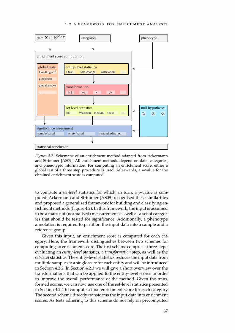
4 . 2 a f r a m e wo r k fo r e n r i c h m e n t a na lys i s

data

entity-level statistics

set-level statistics

global tests

significance assessment

statistical conclusion

null hypotheses

transformation

enrichment score computation

categories phenotype

t-test fold-change correlationHotelling's T2

global test

sample-based entity-based restandardisation

Q1 Q2 Q3

|x| …log

KS medianWilcoxon t-test

…

…

x2…

global ancova

Figure 4.2: Schematic of an enrichment method adapted from Ackermannand Strimmer [AS09]. All enrichment methods depend on data, categories,and phenotypic information. For computing an enrichment score, either aglobal test of a three step procedure is used. Afterwards, a p-value for theobtained enrichment score is computed.

to compute a set-level statistics for which, in turn, a p-value is com-puted. Ackermann and Strimmer [AS09] recognised these similaritiesand proposed a generalised framework for building and classifying en-richment methods (Figure 4.2). In this framework, the input is assumedto be a matrix of (normalised) measurements as well as a set of categor-ies that should be tested for significance. Additionally, a phenotypeannotation is required to partition the input data into a sample and areference group.

Given this input, an enrichment score is computed for each cat-egory. Here, the framework distinguishes between two schemes forcomputing an enrichment score. The first scheme comprises three steps:evaluating an entity-level statistics, a transformation step, as well as theset-level statistics. The entity-level statistics reduces the input data frommultiple samples to a single score for each entity and will be introducedin Section 4.2.2. In Section 4.2.3 we will give a short overview over thetransformations that can be applied to the entity-level scores in orderto improve the overall performance of the method. Given the trans-formed scores, we can now use one of the set-level statistics presentedin Section 4.2.4 to compute a final enrichment score for each category.The second scheme directly transforms the input data into enrichmentscores. As tests adhering to this scheme do not rely on precomputed

87

e n r i c h m e n t a lg o r i t h m s

scores but use the complete data matrix, they can explicitly incorpor-ate interactions between entities into their underlying models. For thisreason, Ackermann and Strimmer [AS09] refer to them as global tests(see Section 4.2.5). After enrichment scores have been computed, thesignificance of the individual scores must be assessed. For this purposethree strategies exist: sample-based evaluation, entity-based evaluation,and the restandardisation method. We will discuss these strategies inmore detail in Section 4.2.1. After this, the raw p-values must be adjus-ted for multiple testing in order to prevent false positive discoveries(Section 4.1.2). First, however, we will start with how to choose the en-richment method that is the most appropriate for a given research task.

4 . 2 . 1 Choosing the Null-Hypothesis

At the beginning of every research task, ideally before any data hasbeen generated, a hypothesis that should either be confirmed or dis-proved, must be chosen. Naturally, this is also true for enrichment ana-lyses. According to Tian et al. [Tia+05], there are two natural ways tostate a null hypothesis for deciding the significance of a single category(gene set):

Hypothesis Q1: “The genes in a gene set show the same pattern ofassociations with the phenotype compared with the rest of thegenes.”

Hypothesis Q2: “The gene set does not contain any genes whose ex-pression levels are associated with the phenotype of interest.”

It is important to note that although Q1 and Q2 appear similar, thereis a subtle difference. Q1 considers how strongly the entities in a cat-egory are associated with the phenotype, compared to entities that arenot members of the category. As a result, even if the category does notcontain entities that are significantly associated with the phenotype, itcan be declared significant, as it (seemingly) shows a stronger patternof association than the remaining genes. In contrast, Q2 only considersthe entities in the category of interest and their association with thephenotype. While Q2 circumvents the problem of Q1, it has its owndrawbacks. In particular larger categories, which are more likely to con-tain relevant genes by chance, would be significant underQ2. Owing tothese interpretations of Q1 and Q2, Goeman and Bühlmann [GB07] cat-egorise enrichment methods employing Q1 as competitive and methodsemploying Q2 as self-contained.

Nam and Kim [NK08] argue that some enrichment methods, in-Ackermann and Strim-mer [AS09] also mention

a Q3 hypothesis that isbased on Efron [Efr08]and is not related to the

hypothesis presented here.

cluding the popular GSEA procedure [Sub+05], neither compute sig-nificance values with respect to Q1 nor to Q2, but rather operate on athird null hypothesis:

Hypothesis Q3: “None of the gene sets considered is associated withthe phenotype.”

88

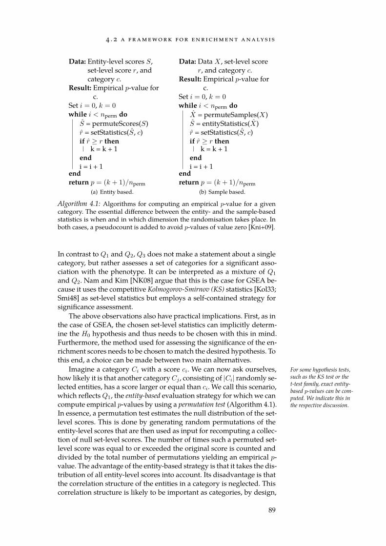
4 . 2 a f r a m e wo r k fo r e n r i c h m e n t a na lys i s

Data: Entity-level scores S,set-level score r, andcategory c.

Result: Empirical p-value forc.

Set i = 0, k = 0while i < nperm do

S = permuteScores(S)r = setStatistics(S, c)if r ≥ r then

k = k + 1endi = i + 1

endreturn p = (k + 1)/nperm

(a) Entity based.

Data: Data X , set-level scorer, and category c.

Result: Empirical p-value forc.

Set i = 0, k = 0while i < nperm do

X = permuteSamples(X)S = entityStatistics(X)r = setStatistics(S, c)if r ≥ r then

k = k + 1endi = i + 1

endreturn p = (k + 1)/nperm

(b) Sample based.

Algorithm 4.1: Algorithms for computing an empirical p-value for a givencategory. The essential difference between the entity- and the sample-basedstatistics is when and in which dimension the randomisation takes place. Inboth cases, a pseudocount is added to avoid p-values of value zero [Kni+09].

In contrast to Q1 and Q2, Q3 does not make a statement about a singlecategory, but rather assesses a set of categories for a significant asso-ciation with the phenotype. It can be interpreted as a mixture of Q1

and Q2. Nam and Kim [NK08] argue that this is the case for GSEA be-cause it uses the competitive Kolmogorov-Smirnov (KS) statistics [Kol33;Smi48] as set-level statistics but employs a self-contained strategy forsignificance assessment.

The above observations also have practical implications. First, as inthe case of GSEA, the chosen set-level statistics can implicitly determ-ine the H0 hypothesis and thus needs to be chosen with this in mind.Furthermore, the method used for assessing the significance of the en-richment scores needs to be chosen to match the desired hypothesis. Tothis end, a choice can be made between two main alternatives.

Imagine a category Ci with a score ci. We can now ask ourselves, For some hypothesis tests,such as the KS test or thet-test family, exact entity-based p-values can be com-puted. We indicate this inthe respective discussion.

how likely it is that another category Cj , consisting of |Ci| randomly se-lected entities, has a score larger or equal than ci. We call this scenario,which reflects Q1, the entity-based evaluation strategy for which we cancompute empirical p-values by using a permutation test (Algorithm 4.1).In essence, a permutation test estimates the null distribution of the set-level scores. This is done by generating random permutations of theentity-level scores that are then used as input for recomputing a collec-tion of null set-level scores. The number of times such a permuted set-level score was equal to or exceeded the original score is counted anddivided by the total number of permutations yielding an empirical p-value. The advantage of the entity-based strategy is that it takes the dis-tribution of all entity-level scores into account. Its disadvantage is thatthe correlation structure of the entities in a category is neglected. Thiscorrelation structure is likely to be important as categories, by design,

89

e n r i c h m e n t a lg o r i t h m s

tend to consist of functionally related entities [ET07].However, we can also ask the question, how likely it is that Ci was

assigned a score larger or equal than ci given that the phenotype labelsof the sample were randomly assigned. We call this scenario, which re-flects Q2, the sample-based evaluation strategy. Clearly, permuting thesamples leaves the correlation structure inside a category intact. Unfor-tunately, the entity-level score distribution is destroyed, as all scoresare recomputed after sample permutation and only the entities in acategory have an influence on the final enrichment score [ET07].

Efron and Tibshirani [ET07] argue that in order to combine theThe terminology usedby [ET07] is randomisa-tion for the entity-basedand permutation for the

sample-based strategy.

strengths of the entity-based and the sample-based evaluation strategy,both should be executed simultaneously. They name this combinedstrategy the restandardisation method and apply it together with theirproposed maxmean statistics.

From a computational point of view, the entity-based strategy isoften more efficient, as it can exploit the distribution of the enrichmentscores. For example it is possible to compute p-values for t-test basedmethods using Student’s t-distribution. In contrast, the sample-basedas well as the restandardisation strategy always necessitate the use ofpermutation tests, which can require considerable amounts of runtimeto compute.

4 . 2 . 2 Entity-level Statistics

Entity-level scores are scalar values that reflect the “importance” of anentity. Commonly, entity-level scores are derived from the differentialanalysis of two sample groups. Scores are computed by evaluating astatistics that reduces the input data to a singe scalar value. Ackermannand Strimmer [AS09] report that the choice of entity-level score onlyhas little effect on the overall results of the enrichment procedure. Itshould be noted, though, that for small sample sizes the choice of anappropriate entity-level statistics may well have a higher influence.

In the following we will list a few popular choices for such entity-See Appendix A.1.3.level statistics. LetX = (x1, x2, . . . , xn) ∈ Rp×n andY = (y1, y2, . . . , yn) ∈Rp×m be the sample and reference set, respectively. The sample meanand sample variance of entity k are denoted by xk and s2Xk, respect-ively.

Fold-Change The most basic entity-level score is the fold change. It isdefined as the ratio between the mean expression of the two groups Xand Y :

fc(k) = xkyk

As expression values are larger than zero, the fold change is also posit-ive and distributed around 1. However, the distribution is asymmetricas cases where yk > xk holds occupy the interval (0, 1) while the con-verse cases occupy the interval [1,∞). To make both ranges comparableit is common to apply a logarithm yielding the log-fold-difference:

log2(fc(k)) = log2 (xk)− log2 (yk)

90

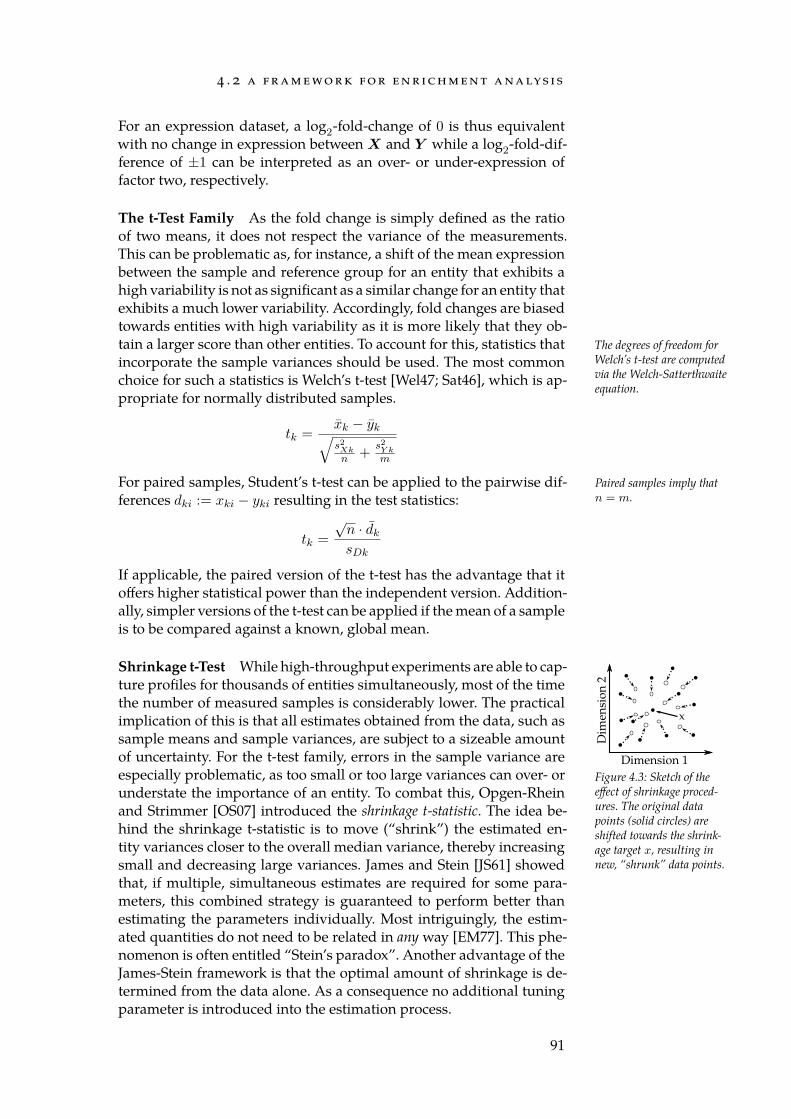
4 . 2 a f r a m e wo r k fo r e n r i c h m e n t a na lys i s

For an expression dataset, a log2-fold-change of 0 is thus equivalentwith no change in expression between X and Y while a log2-fold-dif-ference of ±1 can be interpreted as an over- or under-expression offactor two, respectively.

The t-Test Family As the fold change is simply defined as the ratioof two means, it does not respect the variance of the measurements.This can be problematic as, for instance, a shift of the mean expressionbetween the sample and reference group for an entity that exhibits ahigh variability is not as significant as a similar change for an entity thatexhibits a much lower variability. Accordingly, fold changes are biasedtowards entities with high variability as it is more likely that they ob-tain a larger score than other entities. To account for this, statistics that The degrees of freedom for

Welch’s t-test are computedvia the Welch-Satterthwaiteequation.

incorporate the sample variances should be used. The most commonchoice for such a statistics is Welch’s t-test [Wel47; Sat46], which is ap-propriate for normally distributed samples.

tk =xk − yk√s2Xkn +

s2Y km

For paired samples, Student’s t-test can be applied to the pairwise dif- Paired samples imply thatn = m.ferences dki := xki − yki resulting in the test statistics:

tk =

√n · dksDk

If applicable, the paired version of the t-test has the advantage that itoffers higher statistical power than the independent version. Addition-ally, simpler versions of the t-test can be applied if the mean of a sampleis to be compared against a known, global mean.

Shrinkage t-Test While high-throughput experiments are able to cap-

Dimension 1

Dim

ensi

on 2

x

Figure 4.3: Sketch of theeffect of shrinkage proced-ures. The original datapoints (solid circles) areshifted towards the shrink-age target x, resulting innew, “shrunk” data points.

ture profiles for thousands of entities simultaneously, most of the timethe number of measured samples is considerably lower. The practicalimplication of this is that all estimates obtained from the data, such assample means and sample variances, are subject to a sizeable amountof uncertainty. For the t-test family, errors in the sample variance areespecially problematic, as too small or too large variances can over- orunderstate the importance of an entity. To combat this, Opgen-Rheinand Strimmer [OS07] introduced the shrinkage t-statistic. The idea be-hind the shrinkage t-statistic is to move (“shrink”) the estimated en-tity variances closer to the overall median variance, thereby increasingsmall and decreasing large variances. James and Stein [JS61] showedthat, if multiple, simultaneous estimates are required for some para-meters, this combined strategy is guaranteed to perform better thanestimating the parameters individually. Most intriguingly, the estim-ated quantities do not need to be related in any way [EM77]. This phe-nomenon is often entitled “Stein’s paradox”. Another advantage of theJames-Stein framework is that the optimal amount of shrinkage is de-termined from the data alone. As a consequence no additional tuningparameter is introduced into the estimation process.

91

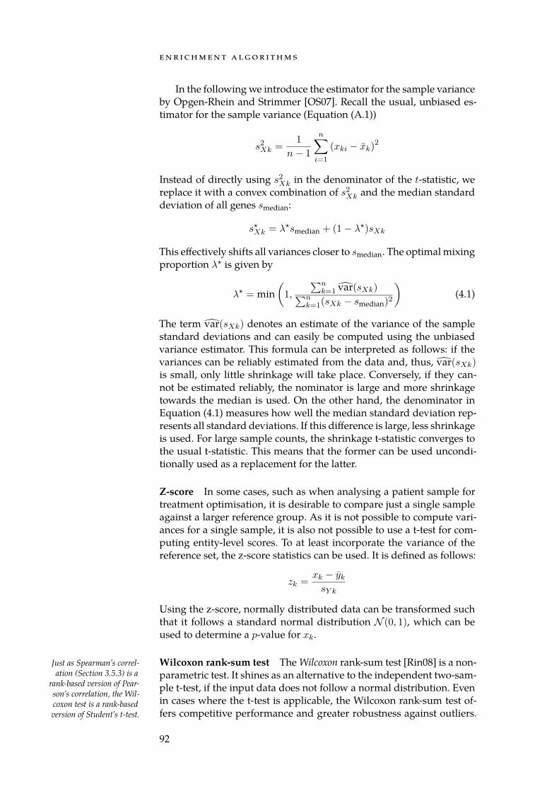
e n r i c h m e n t a lg o r i t h m s

In the following we introduce the estimator for the sample varianceby Opgen-Rhein and Strimmer [OS07]. Recall the usual, unbiased es-timator for the sample variance (Equation (A.1))

s2Xk =1

n− 1

n∑i=1

(xki − xk)2

Instead of directly using s2Xk in the denominator of the t-statistic, wereplace it with a convex combination of s2Xk and the median standarddeviation of all genes smedian:

s⋆Xk = λ⋆smedian + (1− λ⋆)sXk

This effectively shifts all variances closer to smedian. The optimal mixingproportion λ⋆ is given by

λ⋆ = min(1,

∑nk=1 var(sXk)∑n

k=1(sXk − smedian)2

)(4.1)

The term var(sXk) denotes an estimate of the variance of the samplestandard deviations and can easily be computed using the unbiasedvariance estimator. This formula can be interpreted as follows: if thevariances can be reliably estimated from the data and, thus, var(sXk)is small, only little shrinkage will take place. Conversely, if they can-not be estimated reliably, the nominator is large and more shrinkagetowards the median is used. On the other hand, the denominator inEquation (4.1) measures how well the median standard deviation rep-resents all standard deviations. If this difference is large, less shrinkageis used. For large sample counts, the shrinkage t-statistic converges tothe usual t-statistic. This means that the former can be used uncondi-tionally used as a replacement for the latter.

Z-score In some cases, such as when analysing a patient sample fortreatment optimisation, it is desirable to compare just a single sampleagainst a larger reference group. As it is not possible to compute vari-ances for a single sample, it is also not possible to use a t-test for com-puting entity-level scores. To at least incorporate the variance of thereference set, the z-score statistics can be used. It is defined as follows:

zk =xk − yksY k

Using the z-score, normally distributed data can be transformed suchthat it follows a standard normal distribution N (0, 1), which can beused to determine a p-value for xk.

Wilcoxon rank-sum test The Wilcoxon rank-sum test [Rin08] is a non-Just as Spearman’s correl-ation (Section 3.5.3) is a

rank-based version of Pear-son’s correlation, the Wil-coxon test is a rank-basedversion of Student’s t-test.

parametric test. It shines as an alternative to the independent two-sam-ple t-test, if the input data does not follow a normal distribution. Evenin cases where the t-test is applicable, the Wilcoxon rank-sum test of-fers competitive performance and greater robustness against outliers.

92

4 . 2 a f r a m e wo r k fo r e n r i c h m e n t a na lys i s

Just as the t-test, it can be used check whether the expected values oftwo samples coincide. Compared to the latter, it is solely based on therelative order of the values between the two samples. The test statisticsis based on the running sum W :

W =

n∑i=1

R(xi) (4.2)

Here, R(xi) represents the rank of value xi in the sorted and pooled listof sample values. For n > 25 andm > 25,W is approximately normallydistributed [Rin08] with mean µW and variance s2W .

µW =n(n+m+ 1)

2s2W =

n ·m(n+m+ 1)

12(4.3)

For larger sample sizes, this allows to efficiently approximate p-values.For small sample sizes, the exact p-values for W can be looked up in atable [Kan06]. When the Wilcoxon rank-sum test is used as a set-levelstatistics (see below), these p-values need to be interpreted with respectto the entity-based strategy.

4 . 2 . 3 Transformation

Instead of directly using the computed entity-level scores as input forthe set-level statistics (cf. Section 4.2.4), it is possible to first apply ascore transformation to them. Examples for such transformations arethe square root, logarithm, absolute value, or square of the input scores.The main reason for using a transformation is to improve the perform-ance of the enrichment method. In this regard, the most valuable trans-formations are probably the absolute value and the square, as they al-low to fold negative and positive scores together. This is useful whenonly the deregulation of a given category is of interest and not, whetherits constituents are up- or downregulated. Also, for some methods inwhich positive and negative scores are likely to cancel out, applying theabsolute value of square transformation can be crucial (cf. Section 4.3.2).Applying the square root or logarithm transformation can be helpfulfor dampening the effect of outliers.

4 . 2 . 4 Set-level Statistics

The actual enrichment can be obtained by computing a set-level statist- See Section 4.3.ics. Given a list of entity-level scores, it computes a set-level (or enrich-ment) score for a given category. The choice of the set-level statistics canhave a significant impact on the enrichment method’s ability to detectenriched categories. Consequently, a large number of set-level statist-ics has been published. The most popular choices are the KS statistics,used in GSEA [Sub+05], and the hypergeometric test, used in overrep-resentation analysis (ORA) [Drǎ+03]. In the following, we will describe aselection of the most commonly used set-level statistics in more detail.

93

e n r i c h m e n t a lg o r i t h m s

In order to do so, we categorise the methods into non-parametric, para-metric, and averaging methods. The hypergeometric test is not directlycomparable to the other methods and will, thus, be treated in its ownsection. We start with the discussion of non-parametric statistics.

Non-Parametric Statistics

Many hypothesis tests, such as the t-test, assume that the input dataNaturally, paramet-ric tests tend to have

higher power than non-parametric competitors,

if their assumptions hold(cf. [HL56] or [She03]).

follows a certain probability distribution. In real measurements, thisis rarely the case. While applying such parametric statistics will non-etheless yield p-values, these are likely to be skewed. Non-parametricstatistics do not make any assumptions about the distribution underly-ing their input data. Thus, they are extremely robust and universallyapplicable. Even in cases where a parametric statistics applies, non-parametric statistics offer a competitive, albeit slightly lower power[HL56].

Two examples for non-parametric set-level statistics that are com-monly employed for enrichment analysis are the Wilcoxon statisticsand the KS statistics. Both methods are rank-based and are computedby evaluating a running sum. The formulation of the Wilcoxon statisticsas a set-level statistics is identical to the entity-level version presentedin Section 4.2.2.

Whereas the Wilcoxon statistics counts how often samples fromgroup X precede samples from group Y and vice-versa, the KS statist-ics traverses a sorted list of samples and adds or subtracts a constantvalue depending on whether a sample from group X or Y has beenencountered. The maximum deviation from zero is then the output ofthe KS statistics. More formally, let L = l1, l2, . . . , ln be a list of en-tities ordered according to their entity-level scores with n := |L| andC ⊂ L be a category with m := |C|. Now, we are able to define therunning sum RS:

RS(0) = 0

RS(i) = RS(i− 1) +

n−m if li ∈ C

−m otherwise

The value of the test statistics is the maximum deviation RSmax of RSThe version presentedhere is more space effi-

cient than the version pub-lished by Keller, Backes,

and Lenhof [KBL07].

from zero. Figure 4.4 provides an example for the KS running sum. Forthe entity-based strategy, an exact p-value can be computed using dy-namic programming [KBL07]. The idea of this approach is to computethe numberZ of permutations that achieve an (absolute) score less thanRSmax. The final p-value can then be computed as

p = 1− Z(nm

)Let M ∈ N(m+1)×(n−m+1) be the dynamic programming matrix. In or-

94

4 . 2 a f r a m e wo r k fo r e n r i c h m e n t a na lys i s

01020304050

Entities

Not in categoryIn category

Figure 4.4: An example KS running sum. Red dots represent genes in thecategory under consideration. The maximum deviation of the running sumfrom zero (RSmax) is marked with a dashed line and serves as the value of thetest statistics.

der to initialise M we set

M(i, 0) =

1 if i · (n−m) < |RSmax|0 otherwise

M(0, k) =

1 if k ·m < |RSmax|0 otherwise

The recurrence is given by

M(i, k) =

M(i− 1, k) +M(i, k − 1) if (∗)0 otherwise

where (∗) is |RSmax| < i · (n−m)− k ·m < |RSmax|.Subramanian et al. [Sub+05] proposed a weighted version of the

KS statistic. For each entity li ∈ C that is a member of the category, thevalue wi, which is derived from the entity’s score w(li), is added to therunning sum.

wi =|w(li)|p

NR

The term NR :=∑

li∈C |w(li)|p is used as a normalisation factor. Theparameter p ∈ R+

0 allows to control how much high scoring entities arepreferred to low scoring ones. For entities that are not a member of Cthe value (n−m)−1 is subtracted from the running sum. For p = 0 thisformulation is equivalent to the unweighted KS statistics. One benefitof using weights is that it allows to control for scores that are closelydistributed around zero and thus should have little influence on thevalue of the statistics. Additionally, artefacts stemming from entitieswith a low abundance, such as transcripts with low copy number, aremitigated by using weights. Unfortunately, the weighted version of thetest does not allow the computation of an exact p-value even when us-ing the entity-based strategy. Instead the permutation test approachpresented in Algorithm 4.1 needs to be applied.

Parametric Statistics

Representatives of the parametric set-level statistics are the shrinkageand Student’s t-test (cf. Section 4.2.2). As with the Wilcoxon statistics,

95

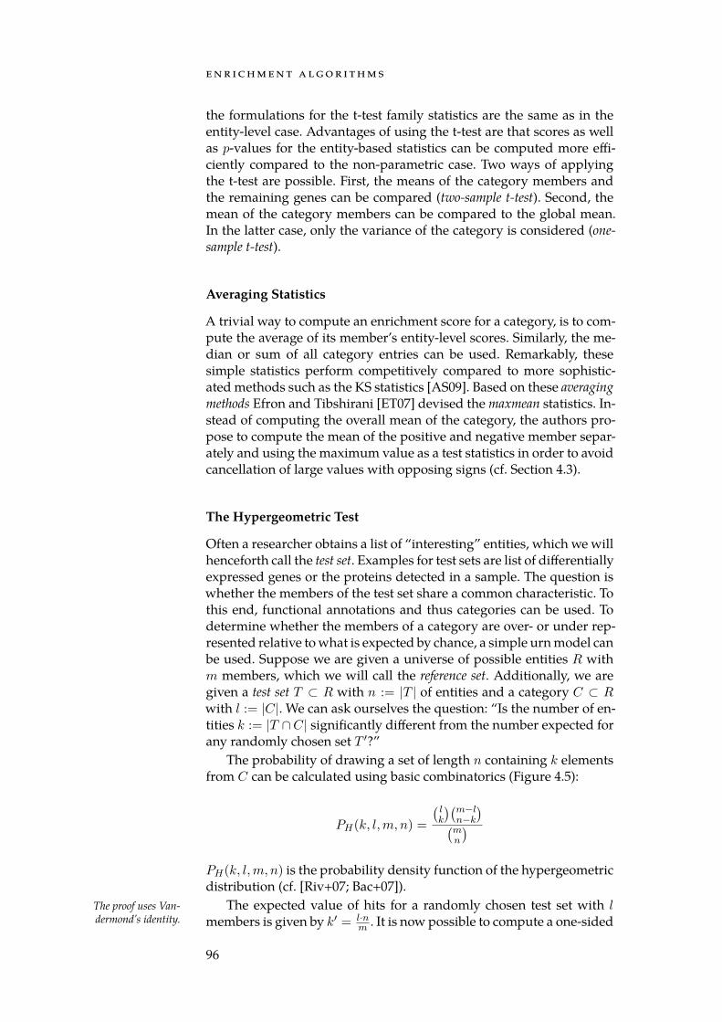
e n r i c h m e n t a lg o r i t h m s

the formulations for the t-test family statistics are the same as in theentity-level case. Advantages of using the t-test are that scores as wellas p-values for the entity-based statistics can be computed more effi-ciently compared to the non-parametric case. Two ways of applyingthe t-test are possible. First, the means of the category members andthe remaining genes can be compared (two-sample t-test). Second, themean of the category members can be compared to the global mean.In the latter case, only the variance of the category is considered (one-sample t-test).

Averaging Statistics

A trivial way to compute an enrichment score for a category, is to com-pute the average of its member’s entity-level scores. Similarly, the me-dian or sum of all category entries can be used. Remarkably, thesesimple statistics perform competitively compared to more sophistic-ated methods such as the KS statistics [AS09]. Based on these averagingmethods Efron and Tibshirani [ET07] devised the maxmean statistics. In-stead of computing the overall mean of the category, the authors pro-pose to compute the mean of the positive and negative member separ-ately and using the maximum value as a test statistics in order to avoidcancellation of large values with opposing signs (cf. Section 4.3).

The Hypergeometric Test

Often a researcher obtains a list of “interesting” entities, which we willhenceforth call the test set. Examples for test sets are list of differentiallyexpressed genes or the proteins detected in a sample. The question iswhether the members of the test set share a common characteristic. Tothis end, functional annotations and thus categories can be used. Todetermine whether the members of a category are over- or under rep-resented relative to what is expected by chance, a simple urn model canbe used. Suppose we are given a universe of possible entities R withm members, which we will call the reference set. Additionally, we aregiven a test set T ⊂ R with n := |T | of entities and a category C ⊂ Rwith l := |C|. We can ask ourselves the question: “Is the number of en-tities k := |T ∩C| significantly different from the number expected forany randomly chosen set T ′?”

The probability of drawing a set of length n containing k elementsfrom C can be calculated using basic combinatorics (Figure 4.5):

PH(k, l,m, n) =

(lk

)(m−ln−k

)(mn

)PH(k, l,m, n) is the probability density function of the hypergeometricdistribution (cf. [Riv+07; Bac+07]).

The expected value of hits for a randomly chosen test set with lThe proof uses Van-dermond’s identity. members is given by k′ = l·n

m . It is now possible to compute a one-sided

96

4 . 2 a f r a m e wo r k fo r e n r i c h m e n t a na lys i s

In category

Not in category

Reference set (|R| = m)Contains l red balls

Test set (|T| = n)Contains k red balls

Red:Blue:

Figure 4.5: Urn model for the hypergeometric test. The reference set containsentities that either belong to the category (red) or not (blue). From the refer-ence set the test set is drawn.

p-value for our input test set T :

pc =

n∑

i=k

PH(i, l,m, n) if k′ < k

k∑i=0

PH(i, l,m, n) if k′ ≥ k

If the test set T contains entities that are not members of R, Fisher’sexact test should be used instead of the hypergeometric test:

PF (i, k, l,m, n) =

(ni

)(m

l+k−i

)(m+nl+k

)The p-values are defined analogously:

pc =

n∑

i=k

PF (i, k, l,m, n) if k′ < k

k∑i=0

PF (i, k, l,m, n) if k′ ≥ k

Due to its reliance on the test and reference sets, the hypergeometrictest is not directly comparable to the other enrichment methods. Inthis regard, requiring a test set is both, the biggest advantage and dis-advantage of the hypergeometric test. On the one hand, the independ-ence from entity-level scores allows to employ the hypergeometric testin settings where the remaining methods are not applicable. An ex-ample would be a differential proteomics pipeline in which the pres-ence (or absence) of proteins is detected, but no quantitative informa-tion has been collected. On the other hand, constructing the test set incases where entity-level scores are available can be difficult. Considera score measuring the degree of differential expression for each gene.Which cut-off should be chosen to distinguish between differentially

97

e n r i c h m e n t a lg o r i t h m s

expressed and “normal” genes? In essence such a thresholding stepintroduces a tuning parameter that can have a large influence on theobtained results. Similarly, the choice of the reference set is also crit-ical for the performance of the method. A larger reference set makesit less likely to randomly draw members of a category and, thus, leadsto overall lower p-values. On the other hand, choosing a reference setthat is too small may lead to low statistical power.

How to choose an appropriate reference set is not always clear. Ingeneral, it should comprise all entities that can be detected by the exper-imental platform. For mRNA microarrays this means that the referenceset should consist of the genes for which probes are present on the ar-ray. For RNA-seq the answer is less clear. As, in theory, all genes thatcan be expressed can be detected by the method, a reasonable choicefor the reference set would be a list of all actively transcribed genes. Forproteomics pipelines, which, at the time of writing, are not capable tocapture all proteins that are present in a sample, there is no clear an-swer. One approach would be to use the union of all detected proteinsacross all samples. Alternatively a list of all proteins can be used. Inthis case, the resulting, lower p-values should then be compensated bya stricter significance threshold.

4 . 2 . 5 Global Tests

Tests that directly transform measurement data into enrichment scoresare called “global tests” by Ackermann and Strimmer [AS09]. The ad-vantage of global tests, as opposed to the previously presented meth-ods, is that they can incorporate the correlation between entities intotheir respective models. Examples are Hotelling’s T 2-test [Hot31], theglobal ANCOVA approach [M+05], and the aptly named global test pro-cedure [Goe+04].

In the remainder of the thesis, global tests will not play a furtherrole. An exception is Hotelling’s T 2-test which we will describe andevaluate in Section 4.4.2. For more details on the remaining methods,we refer the reader to the cited literature.

4 . 2 . 6 Summary

Enrichment analysis is a large field and accordingly a wide variety ofenrichment algorithms has been created. Commonly an enrichment al-gorithm is composed of a procedure for deriving entity-level scores,set-level scores, and finally a method for significance assessment. Ow-ing to the choices made for the above components, each algorithm isbased on different assumptions on how an enriched category is defined.Hence, each algorithm comes with a trade-off between advantages anddisadvantages that need to be carefully vetted each time an enrichmentanalysis is required. Consequently, a wide variety of reviews exist thatattempt to characterise the performance of enrichment methods un-der different conditions [AS09; ET07; HSL09; Hun+11; KSB12; Nae+12].

98

4 . 3 e va luat i o n

This shows that choosing an appropriate enrichment method is by nomeans a trivial task. In the next section, we also attempt to provide acomparison of some enrichment algorithms. However, we focus on de-riving general advice in contrast to recommending a single technique.

4 . 3 e va luat i o n

Choosing a “good” enrichment algorithm is difficult. As outlined be-fore, there exist no experimental datasets for which the truly enrichedcategories are known. Hence, conducting studies on synthetic data re-mains as the only viable option to obtain performance estimates for anenrichment method. In this section, we conduct an evaluation basedon synthetic data with the goal to derive general guidelines for choos-ing an enrichment algorithm that is appropriate for a given situation.It should be noted that this evaluation by no means provides a full cov-erage of every possible usage scenario.

Our evaluation is based on the following procedure: first, we ran-domly create a set of categories. Next, we generate a dataset lacking anykind of differential expression. We will refer to this dataset as the nulldataset. Evaluating our categories on a null dataset gives us a baselinefor the number of false positives that can be expected for each method.Then, all methods are run on datasets that were generated to producea randomly chosen subset of enriched categories. We can treat the in-formation whether a category is enriched or not as a class label. Thisallows us to compute performance metrics for the individual methodsthat are usually used for evaluating classifiers.

Using only categories created by uniformly sampled genes does notnecessarily reflect how collections of categories are structured. As, forexample, some genes fulfil a wider spectrum of functions or are morethoroughly researched, we expect that they can be found more oftenin categories than other genes. Accordingly, the enrichment scores forreal-world categories can be expected to be more correlated than forour synthetic categories. If this is the case, it may prove difficult todistinguish the truly enriched from merely correlated categories. Toaccount for this effect, we also evaluate the algorithms on a set of cat-egories extracted from Reactome [Jos+05]. In summary, the followingexperiments were executed:

1. Synthetic categories on data without differential expression.

2. Synthetic categories on data with differential expression.

3. Real-world categories on data without differential expression.

4. Real-world categories on data with differential expression.

Before we present the results of the experiments, we first outline thedata generation procedure for categories as well as datasets.

99

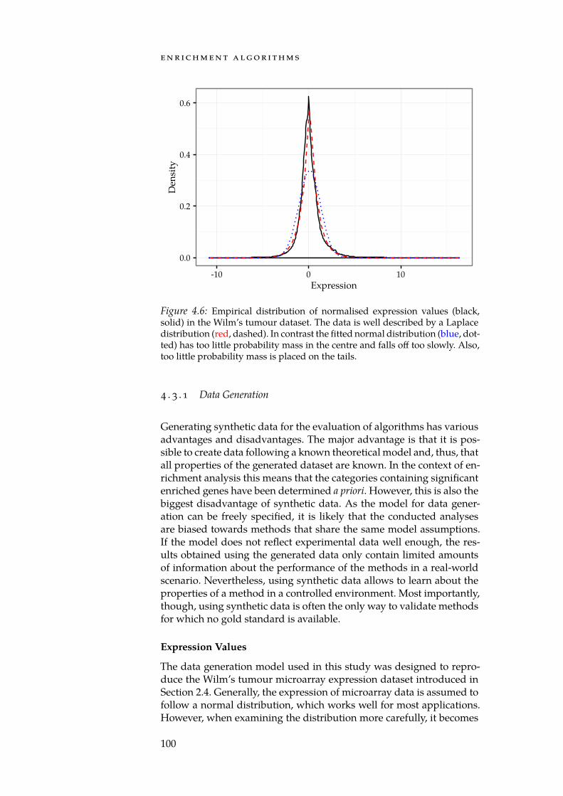
e n r i c h m e n t a lg o r i t h m s

0.0

0.2

0.4

0.6

-10 0 10Expression

Den

sity

Figure 4.6: Empirical distribution of normalised expression values (black,solid) in the Wilm’s tumour dataset. The data is well described by a Laplacedistribution (red, dashed). In contrast the fitted normal distribution (blue, dot-ted) has too little probability mass in the centre and falls off too slowly. Also,too little probability mass is placed on the tails.

4 . 3 . 1 Data Generation

Generating synthetic data for the evaluation of algorithms has variousadvantages and disadvantages. The major advantage is that it is pos-sible to create data following a known theoretical model and, thus, thatall properties of the generated dataset are known. In the context of en-richment analysis this means that the categories containing significantenriched genes have been determined a priori. However, this is also thebiggest disadvantage of synthetic data. As the model for data gener-ation can be freely specified, it is likely that the conducted analysesare biased towards methods that share the same model assumptions.If the model does not reflect experimental data well enough, the res-ults obtained using the generated data only contain limited amountsof information about the performance of the methods in a real-worldscenario. Nevertheless, using synthetic data allows to learn about theproperties of a method in a controlled environment. Most importantly,though, using synthetic data is often the only way to validate methodsfor which no gold standard is available.

Expression Values

The data generation model used in this study was designed to repro-duce the Wilm’s tumour microarray expression dataset introduced inSection 2.4. Generally, the expression of microarray data is assumed tofollow a normal distribution, which works well for most applications.However, when examining the distribution more carefully, it becomes

100

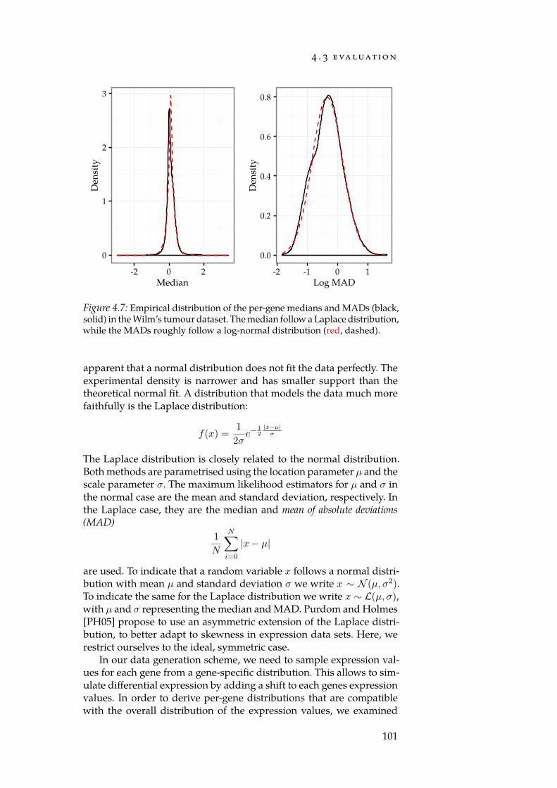
4 . 3 e va luat i o n

0

1

2

3

-2 0 2Median

Den

sity

0.0

0.2

0.4

0.6

0.8

-2 -1 0 1Log MAD

Den

sity

Figure 4.7: Empirical distribution of the per-gene medians and MADs (black,solid) in the Wilm’s tumour dataset. The median follow a Laplace distribution,while the MADs roughly follow a log-normal distribution (red, dashed).

apparent that a normal distribution does not fit the data perfectly. Theexperimental density is narrower and has smaller support than thetheoretical normal fit. A distribution that models the data much morefaithfully is the Laplace distribution:

f(x) =1

2σe−

12

|x−µ|σ

The Laplace distribution is closely related to the normal distribution.Both methods are parametrised using the location parameter µ and thescale parameter σ. The maximum likelihood estimators for µ and σ inthe normal case are the mean and standard deviation, respectively. Inthe Laplace case, they are the median and mean of absolute deviations(MAD)

1

N

N∑i=0

|x− µ|

are used. To indicate that a random variable x follows a normal distri-bution with mean µ and standard deviation σ we write x ∼ N (µ, σ2).To indicate the same for the Laplace distribution we write x ∼ L(µ, σ),with µ and σ representing the median and MAD. Purdom and Holmes[PH05] propose to use an asymmetric extension of the Laplace distri-bution, to better adapt to skewness in expression data sets. Here, werestrict ourselves to the ideal, symmetric case.

In our data generation scheme, we need to sample expression val-ues for each gene from a gene-specific distribution. This allows to sim-ulate differential expression by adding a shift to each genes expressionvalues. In order to derive per-gene distributions that are compatiblewith the overall distribution of the expression values, we examined

101

e n r i c h m e n t a lg o r i t h m s

the distribution of the gene medians (µ0) and MADs (σ0). Again, theLaplace distribution is a good fit for the distribution of the medians.The MADs, however, follow a log-normal distribution (cf. Figure 4.7):

µ0 ∼ L(0, σm)

ln(σ0) ∼ N (µv, σ2v)

Here, σm represents the MAD of the gene medians. The variables µv

and σv are the mean and standard deviation of the log gene standarddeviations, respectively. Together, σm, µv, and σv are hyperparameterswhich we will estimate from the experimental data. We omitted themedian of the gene medians from the model, as a constant shift of allexpression values will cancel out in the entity-level statistics.

Expression values generated following the above scheme do notcorrespond to differentially expressed genes. Instead, they constitutethe null model or “normal” genes. To introduce differential expression,the expression values in the sample group need to be shifted relative tothe expression in the reference group. To create a significant shift, themedian expression value of the sample group is shifted to the corres-ponding α = 0.05 significance threshold, which corresponds to a shiftof δ ≈ 2.303 for the standard Laplace distribution. To create some vari-ation in the gene scores, this adjusted median is modified by addingGaussian noise. Finally, the shift is scaled with the gene expressionMAD in order to account for the different magnitude of dispersionacross the genes. Put together, this yields the following generative mod-els for null and differential gene expression:

xnull ∼ L(µ0, σ0)

xdiff ∼ L(µ0 + ϵσ0, σ0)

ϵ ∼ N (δ, σ2ϵ )

The noise parameter σ2ϵ is set to a constant value of 0.4.

The above model only generates overexpressed genes. This meansthat the distribution of the expression values is asymmetric and all dif-ferentially expressed genes are being shifted to the right. As this mayunfairly bias the results towards certain methods, we additionally gen-erate data where the direction of the shift is chosen via a coin flip.

Categories

The used categories were created by uniformly sampling genes froma list of gene names obtained from the Agilent SurePrint G3 microar-ray platform which was used for measuring the Wilm’s tumour data.In total 500 categories were created. As biological categories are usu-ally not uniformly distributed across the genome, but tend to clusteraround well-studied genes and pathways, we additionally perform thesame evaluation using real biological categories. For both sets of cat-egories, we randomly selected 10 % of their members to serve as en-riched categories. To artificially enrich them, we selected 33 % and 66 %

102

4 . 3 e va luat i o n

of their genes as differentially expressed. The expression values werethen generated as described above.

As biological categories we use the pathway information containedin the Reactome database [Jos+05] to examine the behaviour of theenrichment algorithms on biological categories. In total we extracted1508 categories from Reactome. As with the artificial categories, we ran-domly selected 10 % of the categories as differentially expressed andchose 33 % and 66 % of their members as differentially expressed.

4 . 3 . 2 Results

We evaluated the above model using the parameter settings derivedfrom the Wilm’s tumour dataset (cf. Figure 4.7) as well as the noiseparameter σϵ, which we fix to a small value:

µv ≈ −0.336 σv ≈ 0.499

σm ≈ 0.167 σϵ = 0.4

Furthermore, we consider the following algorithms implemented inthe GeneTrail2 server: mean, sum, median, one sample t-test (1s-t-test), twosample t-test (2s-t-test), Wilcoxon test, weighted and unweighted KS, as wellas ORA. The ORA method could only be evaluated for the entity-basedp-value-strategies, due to limitations in the used C++ implementation.To create the required test set for ORA, we sorted the gene list by scoreand selected the upper and lower 0.025 % into the test set. All compu-tations were repeated ten times with differing random seeds in orderto compute standard deviations.

Null-Model

In order to judge how the algorithms behave if no signal is present inthe data, we generated a dataset without any differentially expressedgenes. For this experiment, we tested all methods using the entity- andsample-based p-value strategies. We evaluate the number of false dis-coveries at the 0.01 significance threshold.

Not many differences for the synthetic categories could be detec-ted between the methods (Figure 4.8). For the entity-based strategy theORA method achieves the lowest number of false positives. For thesample-based strategy no clear winner exists. It should be noted thatin all cases, the number of detected false positives is higher than theexpected proportions of 500 ·0.01 = 5 false discoveries. This highlightsthe importance of adjusting for multiple hypothesis testing.

For the Reactome based categories (Figure 4.9), the results for theentity-based p-value strategy show a higher variance, than those forthe sample-based strategy. Again the ORA method on average detectssubstantially less false positives than competing approaches. For thesample-based strategy, as with the synthetic categories, no clear bestalgorithm can be identified.

103

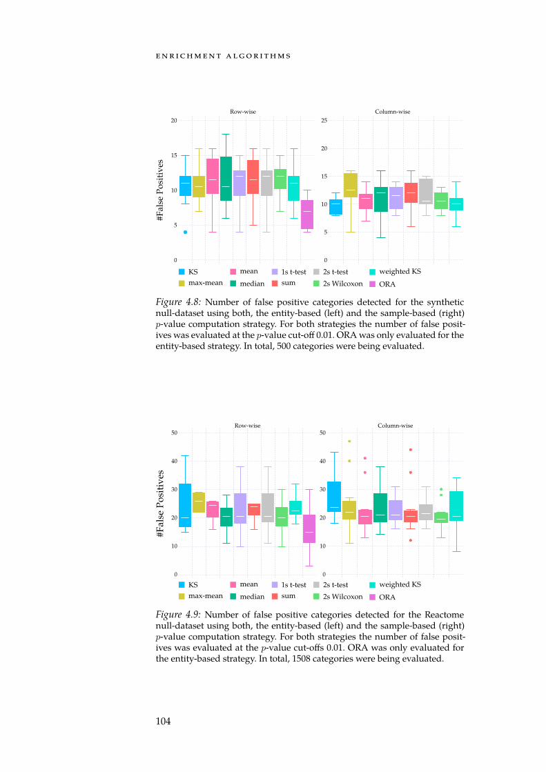
e n r i c h m e n t a lg o r i t h m s

KSmax-mean

mean

median

1s t-testsum

2s t-test

2s Wilcoxon

weighted KS

ORA

0

5

10

15

20

#Fal

se P

osit

ives

0

5

10

15

20

25Row-wise Column-wise

Figure 4.8: Number of false positive categories detected for the syntheticnull-dataset using both, the entity-based (left) and the sample-based (right)p-value computation strategy. For both strategies the number of false posit-ives was evaluated at the p-value cut-off 0.01. ORA was only evaluated for theentity-based strategy. In total, 500 categories were being evaluated.

#Fal

se P

osit

ives

KSmax-mean

mean

median

1s t-testsum

2s t-test

2s Wilcoxon

weighted KS

ORA

0

10

20

30

40

50

0

10

20

30

40

50Row-wise Column-wise

Figure 4.9: Number of false positive categories detected for the Reactomenull-dataset using both, the entity-based (left) and the sample-based (right)p-value computation strategy. For both strategies the number of false posit-ives was evaluated at the p-value cut-offs 0.01. ORA was only evaluated forthe entity-based strategy. In total, 1508 categories were being evaluated.

104

4 . 3 e va luat i o n

AU

C

KSmax-mean

mean

median

1s t-testsum

2s t-test

2s Wilcoxon

weighted KS

ORA

0.80

0.85

0.90

0.95

1.00

0.4

0.5

0.6

0.7

0.8

0.9

1.0

Asymmetric Symmetric

Figure 4.10: AUC of various set-level statistics on synthetic categories wheredifferentially expressed genes are distributed asymmetrically or symmetric-ally. For p-value computation the entity-based strategy was used. If a categorywas chosen as significant, 66 % of the genes were generated as differentiallyexpressed.

Significant Categories

Next, we take a look at the results of the datasets for which significantcategories were generated as explained above. For the datasets whereonly 33 % of the genes in an enriched category were chosen as differ-entially expressed, all methods perform poorly with AUC values of ap-proximately 0.5. For datasets with 66 % significant genes, the perform-ance of the methods improved significantly (Figure 4.10). The most ap-parent difference can be seen between the symmetric and the asym-metric datasets. Here, all methods except ORA hardly misclassify anycategories for the asymmetrically distributed case. The failure of ORAin this case can be attributed to the thresholding used to determinethe most up- and downregulated genes, whereas the dataset only con-tains upregulated genes. In the symmetric case, only the (weighted) KS,max-mean, and ORA set-level statistics manage to achieve near perfectscores. The Wilcoxon statistics relies on comparing the sum of ranks ofcategory members against the ranks of the non-members. If the entitylevel scores are symmetrically distributed each category roughly con-tains the same number low ranking and high ranking genes which ef-fectively cancel out. This effect is also visible for the remaining methodsthat are all based on averaging. As with the Wilcoxon test, if genes witha positive and a negative enrichment score are member of a categorytheir sum is expected to lie in the vicinity of zero. Consequently thesemethods should only be employed if the scores have been transformedusing the absolute value or square transformation (cf. Section 4.2.3).When applying the set-level statistics to the biological categories, nosignificant change in behaviour could be detected. (cf. Appendix C.2).

105

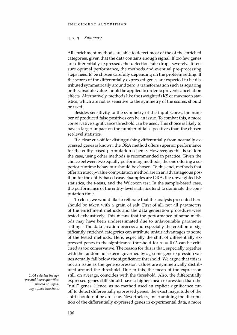
e n r i c h m e n t a lg o r i t h m s

4 . 3 . 3 Summary

All enrichment methods are able to detect most of the of the enrichedcategories, given that the data contains enough signal. If too few genesare differentially expressed, the detection rate drops severely. To en-sure optimal performance, the methods and eventual pre-processingsteps need to be chosen carefully depending on the problem setting. Ifthe scores of the differentially expressed genes are expected to be dis-tributed symmetrically around zero, a transformation such as squaringor the absolute value should be applied in order to prevent cancellationeffects. Alternatively, methods like the (weighted) KS or maxmean stat-istics, which are not as sensitive to the symmetry of the scores, shouldbe used.

Besides sensitivity to the symmetry of the input scores, the num-ber of produced false positives can be an issue. To combat this, a moreconservative significance threshold can be used. This choice is likely tohave a larger impact on the number of false positives than the chosenset-level statistics.

If a clear cut-off for distinguishing differentially from normally ex-pressed genes is known, the ORA method offers superior performancefor the entity-based permutation scheme. However, as this is seldomthe case, using other methods is recommended in practice. Given thechoice between two equally performing methods, the one offering a su-perior runtime behaviour should be chosen. To this end, methods thatoffer an exact p-value computation method are in an advantageous pos-ition for the entity-based case. Examples are ORA, the unweighted KSstatistics, the t-tests, and the Wilcoxon test. In the sample-based case,the performance of the entity-level statistics tend to dominate the com-putation time.

To close, we would like to reiterate that the analysis presented hereshould be taken with a grain of salt. First of all, not all parametersof the enrichment methods and the data generation procedure weretested exhaustively. This means that the performance of some meth-ods may have been underestimated due to unfavourable parametersettings. The data creation process and especially the creation of sig-nificantly enriched categories can attribute unfair advantages to someof the tested methods. Here, especially the shift of differentially ex-pressed genes to the significance threshold for α = 0.05 can be criti-cised as too conservative. The reason for this is that, especially togetherwith the random noise term governed by σϵ, some gene expression val-ues actually fall below the significance threshold. We argue that this isnot an issue as the gene expression values are symmetrically distrib-uted around the threshold. Due to this, the mean of the expressionstill, on average, coincides with the threshold. Also, the differentiallyORA selected the up-

per and lower quantilesinstead of impos-

ing a fixed threshold.

expressed genes still should have a higher mean expression than the“null” genes. Hence, as no method used an explicit significance cut-off to detect differentially expressed genes, the exact magnitude of theshift should not be an issue. Nevertheless, by examining the distribu-tion of the differentially expressed genes in experimental data, a more

106

4 . 4 h ot e l l i ng ' s t2-t e s t

realistic, albeit more complex, model could be derived. Another biasmay stem from the fact that the significantly enriched genes are ran-domly chosen and considered independent from each other. This as-sumption closely resembles the urn model underlying the hypergeo-metric test used by ORA. However, for biological datasets, gene ex-pression is most certainly not independent within a category. There-fore the sample-based p-value strategy, which considers the correlationstructure within a category in fact is at a disadvantage in this evalu-ation. On the other hand the ORA method depends on the choice ofthe threshold that selects the differentially expressed genes. While inthis case, the 95 % quantile is appropriate due to the data generationprocedure, the true value of the threshold is usually not known a priori.Nevertheless, the chosen parameters reflect the settings a user of theGeneTrail2 server would use by default and, therefore, the presentedevaluation gives some insight into possible real-world usage.

4 . 4 h o t e l l i ng ' s T 2-t e s t

We previously discussed enrichment procedures, like the Over Repres- The sample-based per-mutation strategy (Sec-tion 4.2.1) accounts for apart of the entity interde-pendence.

entation Analysis (ORA) [Drǎ+03] and the Gene Set Enrichment Ana-lysis (GSEA) [Sub+05], that treat the entities contained in each categoryas independent. However, we previously assumed that a category con-sists of genes that are functionally related and thus are likely to be co-regulated. Of course, this suggests that these entities are anything butindependent.

Here, we examine the suitability of Hotelling’s T 2-test as an enrich-ment algorithm. Hotelling’s T 2-test is a global enrichment procedure(Figure 4.2) that accounts for the correlation structure between entities.We structure our presentation as follows: first we give a general intro-duction to Hotelling’s T 2-test. Afterwards, we perform a brief evalu-ation to illustrate some of its properties.

4 . 4 . 1 Mahalanobis Distance

A concept that is central for understanding Hotelling’s T 2-test [Hot31]is the Mahalanobis distance [Mah36]. To explain it, we need to recall themultivariate generalisation of the Gaussian distribution as introducedin Section 3.4.1. Again, consider the univariate Gaussian distribution

N (x, µ, σ2) =1√2πσ

exp(−(x− µ)2

2σ2

)(4.4)

Here, µ, σ2 ∈ R represent the mean and variance of the distribution,respectively. Disregarding the normalisation factor in front of the ex-ponential function, the value of the distribution solely depends on thesquared distance of x to the mean which is scaled inversely by the vari-ance: (x− µ)2/(2σ2). In the multivariate Gaussian distribution

N (x, µ,Σ) = c · exp(−1

2(x− µ)tΣ−1(x− µ)

)(4.5)

107

e n r i c h m e n t a lg o r i t h m s

this is replaced by the term (x − µ)tΣ−1(x − µ). In other words, thedistance of x from the centroid µ ∈ Rp is rescaled by the inverse cov-ariance (or precision) matrix Σ−1 ∈ Rp×p. The constant

c := det(Σ)−12 /(2π)

p2

serves as the normalisation factor.The covariance matrix and, thus, Σ−1 are positive definite matrices.

Hence, Σ−1 defines a scalar product and a corresponding metric. Thismetric is called the Mahalanobis distance [Mah36].

4 . 4 . 2 Hotelling’s T 2-Statistics

A common question in statistics is, whether two samples originate fromthe same or two different distributions (Section 4.1). The entity- andset-level statistics presented in earlier sections (cf. Section 4.2.2) answerthis question for a range of univariate cases. However, if the samplesfollow a multivariate Gaussian distribution, Hotelling’s T 2-statistics isthe appropriate test statistics. It is a straightforward generalisation ofStudent’s t-test [Stu08] (Section 4.2.2). Let N be the number of samplesand n,m the size of each group, respectively. Using Sx :=

∑nxi=1(xi −

µx)(xi − µx)t and the analogously defined Sy, we obtain the pooled

covariance matrix S:S =

Sx + Sy

N − 2(4.6)

This allows us to compute the T 2-statistics as the weighted differenceof the sample means

T 2 =nxny

N(µx − µy)

tS−1(µx − µy) (4.7)

In order to evaluate the significance of T 2, the appropriate quantilescan be computed from the F -distribution via the relationship

N − p− 1

(N − 2)pT 2 ∼ F (p,N − 1− p) (4.8)

The probability density function of the F -distribution is given as:

f(x, d1, d2) =

√(d1x)d1d

d22

(d1x+d2)d1+d2

xB(d12 ,

d22

) (4.9)

where d1, d2 ∈ R+ and

B(x, y) =

1∫0

tx−1(1− t)y−1 dt (4.10)

is the beta-function. As the parameters of the F -distribution must bepositive, computing an exact p-value requires more samples than ob-served genes (N ≥ p + 2). Thus, it is infeasible to test for a difference

108

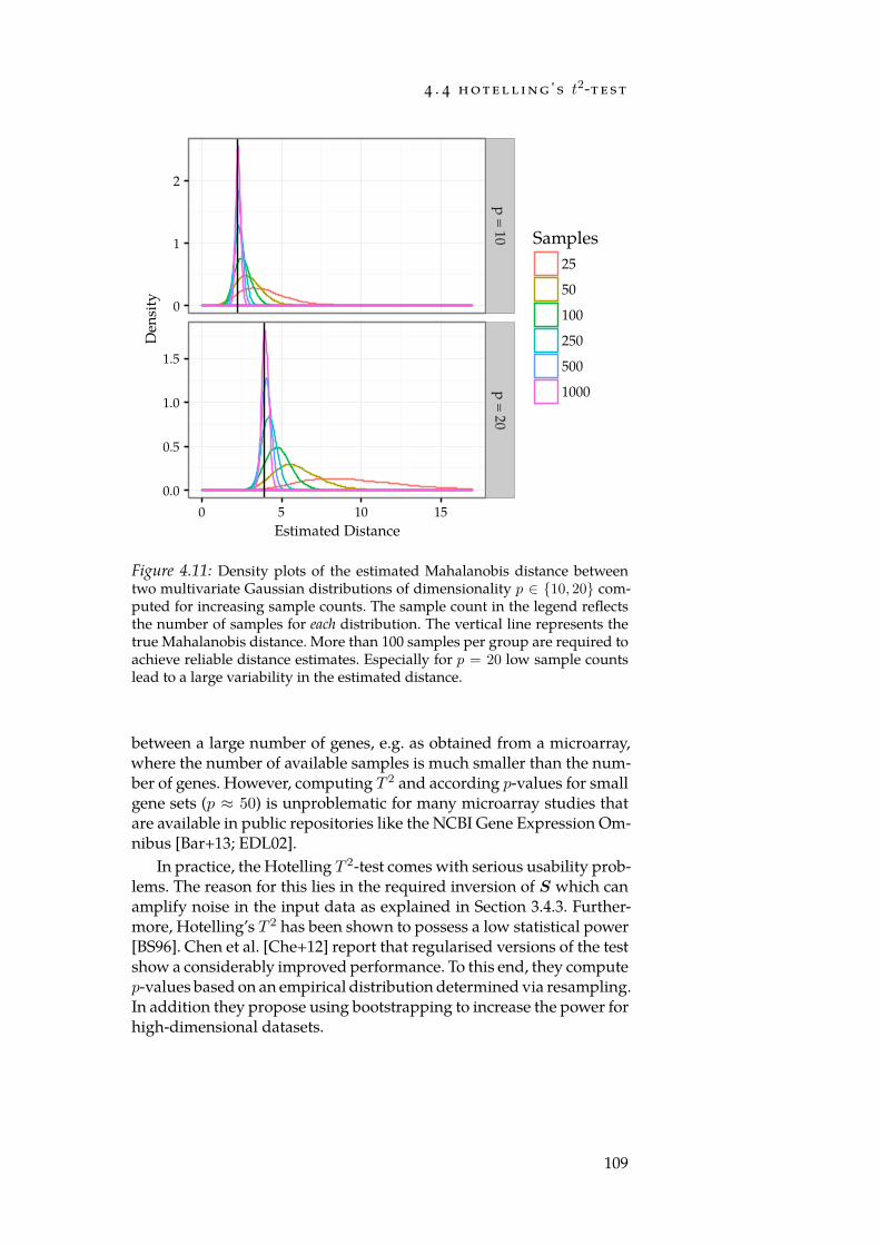
4 . 4 h ot e l l i ng ' s t2-t e s t

0

1

2

0.0

0.5

1.0

1.5p = 10

p = 20

0 5 10 15Estimated Distance

Den

sity

Samples25

50

100

250

500

1000

Figure 4.11: Density plots of the estimated Mahalanobis distance betweentwo multivariate Gaussian distributions of dimensionality p ∈ 10, 20 com-puted for increasing sample counts. The sample count in the legend reflectsthe number of samples for each distribution. The vertical line represents thetrue Mahalanobis distance. More than 100 samples per group are required toachieve reliable distance estimates. Especially for p = 20 low sample countslead to a large variability in the estimated distance.

between a large number of genes, e.g. as obtained from a microarray,where the number of available samples is much smaller than the num-ber of genes. However, computing T 2 and according p-values for smallgene sets (p ≈ 50) is unproblematic for many microarray studies thatare available in public repositories like the NCBI Gene Expression Om-nibus [Bar+13; EDL02].

In practice, the Hotelling T 2-test comes with serious usability prob-lems. The reason for this lies in the required inversion of S which canamplify noise in the input data as explained in Section 3.4.3. Further-more, Hotelling’s T 2 has been shown to possess a low statistical power[BS96]. Chen et al. [Che+12] report that regularised versions of the testshow a considerably improved performance. To this end, they computep-values based on an empirical distribution determined via resampling.In addition they propose using bootstrapping to increase the power forhigh-dimensional datasets.

109

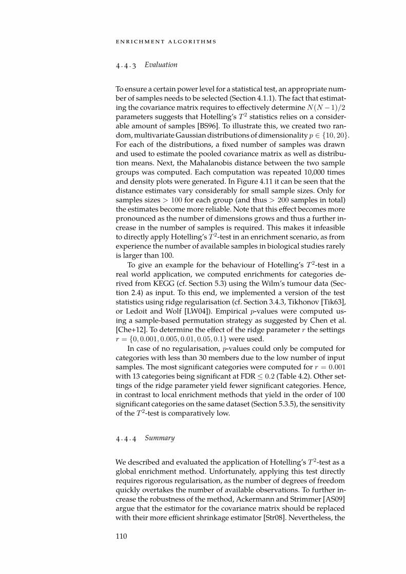
e n r i c h m e n t a lg o r i t h m s

4 . 4 . 3 Evaluation

To ensure a certain power level for a statistical test, an appropriate num-ber of samples needs to be selected (Section 4.1.1). The fact that estimat-ing the covariance matrix requires to effectively determine N(N −1)/2parameters suggests that Hotelling’s T 2 statistics relies on a consider-able amount of samples [BS96]. To illustrate this, we created two ran-dom, multivariate Gaussian distributions of dimensionality p ∈ 10, 20.For each of the distributions, a fixed number of samples was drawnand used to estimate the pooled covariance matrix as well as distribu-tion means. Next, the Mahalanobis distance between the two samplegroups was computed. Each computation was repeated 10,000 timesand density plots were generated. In Figure 4.11 it can be seen that thedistance estimates vary considerably for small sample sizes. Only forsamples sizes > 100 for each group (and thus > 200 samples in total)the estimates become more reliable. Note that this effect becomes morepronounced as the number of dimensions grows and thus a further in-crease in the number of samples is required. This makes it infeasibleto directly apply Hotelling’s T 2-test in an enrichment scenario, as fromexperience the number of available samples in biological studies rarelyis larger than 100.

To give an example for the behaviour of Hotelling’s T 2-test in areal world application, we computed enrichments for categories de-rived from KEGG (cf. Section 5.3) using the Wilm’s tumour data (Sec-tion 2.4) as input. To this end, we implemented a version of the teststatistics using ridge regularisation (cf. Section 3.4.3, Tikhonov [Tik63],or Ledoit and Wolf [LW04]). Empirical p-values were computed us-ing a sample-based permutation strategy as suggested by Chen et al.[Che+12]. To determine the effect of the ridge parameter r the settingsr = 0, 0.001, 0.005, 0.01, 0.05, 0.1 were used.

In case of no regularisation, p-values could only be computed forcategories with less than 30 members due to the low number of inputsamples. The most significant categories were computed for r = 0.001with 13 categories being significant at FDR ≤ 0.2 (Table 4.2). Other set-tings of the ridge parameter yield fewer significant categories. Hence,in contrast to local enrichment methods that yield in the order of 100significant categories on the same dataset (Section 5.3.5), the sensitivityof the T 2-test is comparatively low.

4 . 4 . 4 Summary

We described and evaluated the application of Hotelling’s T 2-test as aglobal enrichment method. Unfortunately, applying this test directlyrequires rigorous regularisation, as the number of degrees of freedomquickly overtakes the number of available observations. To further in-crease the robustness of the method, Ackermann and Strimmer [AS09]argue that the estimator for the covariance matrix should be replacedwith their more efficient shrinkage estimator [Str08]. Nevertheless, the

110

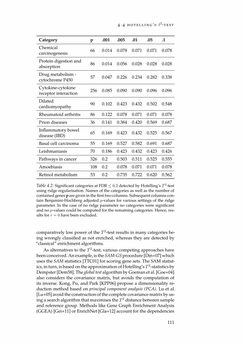
4 . 4 h ot e l l i ng ' s t2-t e s t

Category p .001 .005 .01 .05 .1

Chemicalcarcinogenesis 66 0.014 0.078 0.071 0.071 0.078

Protein digestion andabsorption 86 0.014 0.056 0.028 0.028 0.028

Drug metabolism -cytochrome P450 57 0.047 0.226 0.234 0.282 0.338

Cytokine-cytokinereceptor interaction 256 0.085 0.090 0.090 0.096 0.096

Dilatedcardiomyopathy 90 0.102 0.423 0.432 0.502 0.548

Rheumatoid arthritis 86 0.122 0.078 0.071 0.071 0.078

Prion diseases 36 0.141 0.384 0.420 0.569 0.687

Inflammatory boweldisease (IBD) 65 0.169 0.423 0.432 0.525 0.567

Basal cell carcinoma 55 0.169 0.527 0.582 0.691 0.687

Leishmaniasis 70 0.186 0.423 0.432 0.423 0.426

Pathways in cancer 326 0.2 0.503 0.511 0.525 0.555

Amoebiasis 108 0.2 0.078 0.071 0.071 0.078

Retinol metabolism 53 0.2 0.735 0.722 0.620 0.562

Table 4.2: Significant categories at FDR ≤ 0.2 detected by Hotelling’s T 2-testusing ridge regularisation. Names of the categories as well as the number ofcontained genes p are given in the first two columns. Subsequent columns con-tain Benjamini-Hochberg adjusted p-values for various settings of the ridgeparameter. In the case of no ridge parameter no categories were significantand no p-values could be computed for the remaining categories. Hence, res-ults for r = 0 have been excluded.

comparatively low power of the T 2-test results in many categories be-ing wrongly classified as not enriched, whereas they are detected by“classical” enrichment algorithms.

As alternatives to the T 2-test, various competing approaches havebeen conceived. An example, is the SAM-GS procedure [Din+07] whichuses the SAM statistics [TTC01] for scoring gene sets. The SAM statist-ics, in turn, is based on the approximation of Hotelling’s T 2-statistics byDempster [Dem58]. The global test algorithm by Goeman et al. [Goe+04]also considers the covariance matrix, but avoids the computation ofits inverse. Kong, Pu, and Park [KPP06] propose a dimensionality re-duction method based on principal component analysis (PCA). Lu et al.[Lu+05] avoid the construction of the complete covariance matrix by us-ing a search algorithm that maximises the T 2 distance between sampleand reference group. Methods like Gene Graph Enrichment Analysis(GGEA) [Gei+11] or EnrichNet [Gla+12] account for the dependencies

111

e n r i c h m e n t a lg o r i t h m s

between entities by explicitly including connectivity information ob-tained from known, biological networks.

112

5G R AV I TO N

All problems in computer science can be solved by anotherlevel of indirection. But that usually will create another prob-lem.

— dav i d w h e e l e r , ac co r d i ng to b e a u t i f u lc o d e ( 2 0 0 7 )

An important part of bioinformatics is the development of new meth-ods for the analysis of experimental data. Due to this, a large toolboxof specialised software is available to the end user. In many areas ofbioinformatics, such as DNA sequencing, the state-of-the-art is con-stantly evolving. The same is true for biology, where the size of publicdatabases that organise the available knowledge is constantly growing.Keeping up with this change requires a considerable amount of timeand sophistication on the user-side. For researchers writing software,the maintenance burden of ensuring that their code can be deployedon any available platform takes time away from developing new, im-proved methods. A way to avoid this burden is to offer tools as web ser-vices, which comes with the advantage that only a single, centralisedinstallation of the required third-party software and databases needs tobe maintained. Additionally, web based user interfaces work on everycomputer with a browser and, if designed properly, can be easily con-trolled via client-side scripts. Users of a service no longer need to up-date their software regularly and do not need to track databases forupdates.

Still, despite the fact that maintaining a web server requires farless effort than maintaining a native application, useful bioinformaticsweb services that integrate well into existing workflows, are challen-ging to construct. As with traditional software packages a considerableamount of code for parsing file formats, handling malformed user in-put, and performing statistical analyses needs to be implemented. Inaddition, business logic for handling user data and sessions or con-trolling database access is required. Furthermore, a functional and ap-pealing user interface needs to be designed. Especially this latter part isoften not necessary when rolling out a package for a scripting languageor a native command line application.

In order to avoid reimplementing common functionality for everyweb service, we built the Graviton framework. To give a comprehens-ive description of the framework, we first need to familiarise ourselveswith the available technologies for implementing a web service. Next,we outline the requirements that Graviton should fulfil. We then give ageneral overview of the architecture of Graviton followed by a more in-depth discussion of the individual components GeneTrail2, Network-Trail, and DrugTargetInspector.

113

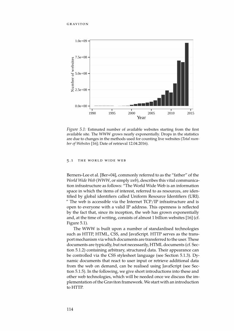
g r av i to n

0.0e+00

2.5e+08

5.0e+08

7.5e+08

1.0e+09

1990 1995 2000 2005 2010 2015Year

Num

ber

of w

ebsi

tes

Figure 5.1: Estimated number of available websites starting from the firstavailable site. The WWW grows nearly exponentially. Drops in the statisticsare due to changes in the methods used for counting live websites (Total num-ber of Websites [16]; Date of retrieval 12.04.2016).

5 . 1 t h e wo r l d w i d e w e b

Berners-Lee et al. [Ber+04], commonly referred to as the “father” of theWorld Wide Web (WWW, or simply web), describes this vital communica-tion infrastructure as follows: “The World Wide Web is an informationspace in which the items of interest, referred to as resources, are iden-tified by global identifiers called Uniform Resource Identifiers (URI).” The web is accessible via the Internet TCP/IP infrastructure and isopen to everyone with a valid IP address. This openness is reflectedby the fact that, since its inception, the web has grown exponentiallyand, at the time of writing, consists of almost 1 billion websites [16] (cf.Figure 5.1).

The WWW is built upon a number of standardised technologiessuch as HTTP, HTML, CSS, and JavaScript. HTTP serves as the trans-port mechanism via which documents are transferred to the user. Thesedocuments are typically, but not necessarily, HTML documents (cf. Sec-tion 5.1.2) containing arbitrary, structured data. Their appearance canbe controlled via the CSS stylesheet language (see Section 5.1.3). Dy-namic documents that react to user input or retrieve additional datafrom the web on demand, can be realised using JavaScript (see Sec-tion 5.1.5). In the following, we give short introductions into these andother web technologies, which will be needed once we discuss the im-plementation of the Graviton framework. We start with an introductionto HTTP.

114

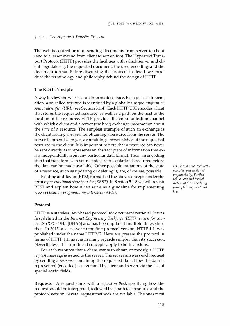
5 . 1 t h e wo r l d w i d e w e b

5 . 1 . 1 The Hypertext Transfer Protocol

The web is centred around sending documents from server to client(and to a lesser extend from client to server, too). The Hypertext Trans-port Protocol (HTTP) provides the facilities with which server and cli-ent negotiate e.g. the requested document, the used encoding, and thedocument format. Before discussing the protocol in detail, we intro-duce the terminology and philosophy behind the design of HTTP.

The REST Principle

A way to view the web is as an information space. Each piece of inform-ation, a so-called resource, is identified by a globally unique uniform re-source identifier (URI) (see Section 5.1.4). Each HTTP URI encodes a hostthat stores the requested resource, as well as a path on the host to thelocation of the resource. HTTP provides the communication channelwith which a client and a server (the host) exchange information aboutthe state of a resource. The simplest example of such an exchange isthe client issuing a request for obtaining a resource from the server. Theserver then sends a response containing a representation of the requestedresource to the client. It is important to note that a resource can neverbe sent directly as it represents an abstract piece of information that ex-ists independently from any particular data format. Thus, an encodingstep that transforms a resource into a representation is required beforethe data can be made available. Other possible mutations of the state HTTP and other web tech-

nologies were designedpragmatically. Furtherrefinement and formal-isation of the underlyingprinciples happened posthoc.

of a resource, such as updating or deleting it, are, of course, possible.Fielding and Taylor [FT02] formalised the above concepts under the

term representational state transfer (REST). In Section 5.1.8 we will revisitREST and explain how it can serve as a guideline for implementingweb application programming interfaces (APIs).

Protocol

HTTP is a stateless, text-based protocol for document retrieval. It wasfirst defined in the Internet Engineering Taskforce (IETF) request for com-ments (RFC) 1945 [BFF96] and has been updated multiple times sincethen. In 2015, a successor to the first protocol version, HTTP 1.1, waspublished under the name HTTP/2. Here, we present the protocol interms of HTTP 1.1, as it is in many regards simpler than its successor.Nevertheless, the introduced concepts apply to both versions.

For each resource that a client wants to obtain or modify, a HTTPrequest message is issued to the server. The server answers each requestby sending a response containing the requested data. How the data isrepresented (encoded) is negotiated by client and server via the use ofspecial header fields.

Requests A request starts with a request method, specifying how therequest should be interpreted, followed by a path to a resource and theprotocol version. Several request methods are available. The ones most

115

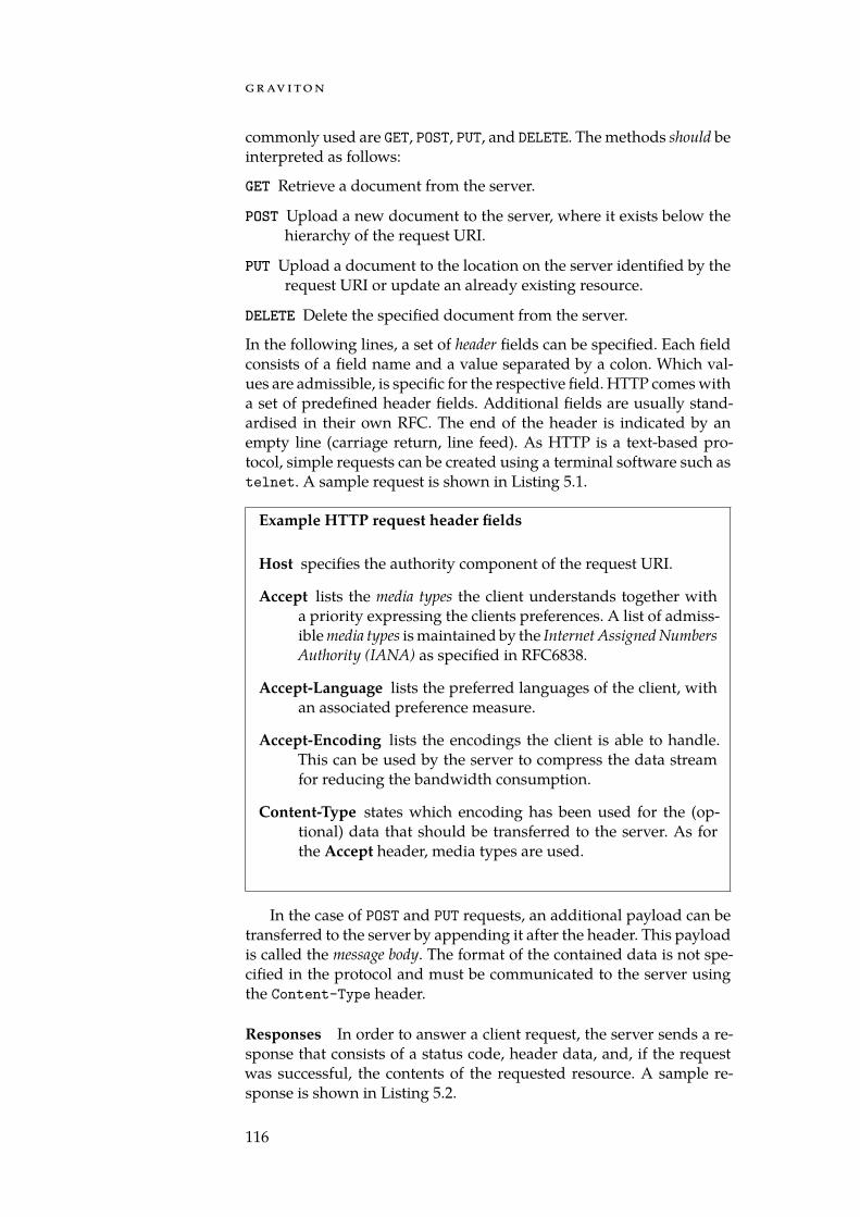
g r av i to n

commonly used are GET, POST, PUT, and DELETE. The methods should beinterpreted as follows:

GET Retrieve a document from the server.

POST Upload a new document to the server, where it exists below thehierarchy of the request URI.

PUT Upload a document to the location on the server identified by therequest URI or update an already existing resource.

DELETE Delete the specified document from the server.

In the following lines, a set of header fields can be specified. Each fieldconsists of a field name and a value separated by a colon. Which val-ues are admissible, is specific for the respective field. HTTP comes witha set of predefined header fields. Additional fields are usually stand-ardised in their own RFC. The end of the header is indicated by anempty line (carriage return, line feed). As HTTP is a text-based pro-tocol, simple requests can be created using a terminal software such astelnet. A sample request is shown in Listing 5.1.

Example HTTP request header fields

Host specifies the authority component of the request URI.

Accept lists the media types the client understands together witha priority expressing the clients preferences. A list of admiss-ible media types is maintained by the Internet Assigned NumbersAuthority (IANA) as specified in RFC6838.

Accept-Language lists the preferred languages of the client, withan associated preference measure.

Accept-Encoding lists the encodings the client is able to handle.This can be used by the server to compress the data streamfor reducing the bandwidth consumption.

Content-Type states which encoding has been used for the (op-tional) data that should be transferred to the server. As forthe Accept header, media types are used.

In the case of POST and PUT requests, an additional payload can betransferred to the server by appending it after the header. This payloadis called the message body. The format of the contained data is not spe-cified in the protocol and must be communicated to the server usingthe Content-Type header.

Responses In order to answer a client request, the server sends a re-sponse that consists of a status code, header data, and, if the requestwas successful, the contents of the requested resource. A sample re-sponse is shown in Listing 5.2.

116

5 . 1 t h e wo r l d w i d e w e b

POST /api/job/setup/ HTTP/1.1Host: genetrail2.bioinf.uni-sb.deUser-Agent: Mozilla/5.0 (X11; Fedora; Linux x86_64;

rv:40.0) Gecko/20100101 Firefox/40.0Accept: text/html,application/xhtml+xml,

application/xml;q=0.9,*/*;q=0.8Accept-Language: en-GB,en;q=0.5Accept-Encoding: gzip, deflateConnection: keep-alive

name=gseaListing 5.1: Example HTTP POST request. The first line contains the HTTP re-quest method (red), the path of the requested resource (blue), and the protocolversion (green). The following lines contain the request header. Each headeris composed of a field name (orange) and a value (black). The optional requestbody (grey) starts after an empty line and contains arbitrarily encoded datafor transfer to the server.

Properties From the description of the protocol we can make two ob-servations that have important implications on how web services canbe implemented. First, the HTTP protocol itself is stateless. This means,the protocol does not keep track of previous requests by the client orresponses by the server. For web applications that rely on state, such asuser logins, being tracked, custom state handling must be implementedon top of HTTP. Another implication of statelessness is that subsequentGET request for the same resource should always receive the same re-sponse, as GET leaves all resources unchanged. Accordingly, GET re-sponses can be cached by the browser to avoid unnecessary round-triptimes. In addition, caching can greatly reduce bandwidth consump-tion, which is especially important on bandwidth constraint connec-tions such as mobile devices. For web application developers, this im-plies that to achieve optimal performance the amount of changes toexisting resources should be minimised such that caching can take ef-fect.

Second, due to the ordering between requests and responses, it is WebSockets alleviate this tosome degree.not possible to send information from server to client without the client

sending a request first. This implies that the client must periodicallyquery for the status of a long running computation on the server sidein order to be notified about its progress.

5 . 1 . 2 The Hypertext Markup Language

The next core technology of the web is the Hypertext Markup Lan- HTML was a StandardGeneralized MarkupLanguage (SGML) (ISO8879:1986) based specific-ation. However, recentversions have forgone allSGML compatibility.

guage (HTML) [HH16]. HTML allows to represent documents as a se-mantically annotated hierarchical structure. The hierarchy is createdby nesting so-called elements. An element usually consists of a start(<p>) and end (</p>) tag that delimit a sequence of text and other ele-ments. Each element can furthermore be supplied with one or more at-

117

g r av i to n

HTTP/1.1 200 OKCache-Control: publicContent-Length: 36Content-Type: text/plainLast-Modified: Sun, 13 Sep 2015 09:46:05 GMTDate: Fri, 16 Oct 2015 19:29:07 GMT

This is the content of the response!Listing 5.2: Example HTTP response. The first line contains the protocol ver-sion (green) and a status code (blue). Subsequent lines contain response head-ers. Each header is composed of a field name (orange) and a value (black). Theend of the header and start of the response body (gray), which contains therequested document, is indicated by an empty line.

<!DOCTYPE html><html lang="en"><head>

<title>Hello world!</title></head><body>

<h1>Hello world!</h1>This is an example HTML page.<p>And this is a new paragraph.</p>

</body></html>Listing 5.3: Example HTML5 document. The type of the document is con-trolled via the DOCTYPE statement. Metainformation is encoded in the <head>tag, whereas user visible information is encoded in the <body> tag.

tributes (<input type="text">) that determine element specific prop-erties. While HTML offers tags like <i> (italic), <b> (bold), <br> (linebreak), and <font> (font properties) that directly control the appear-ance of the HTML in a browser, the use of these tags is deprecated inmodern documents. Instead, the used annotations should express thesemantics of their content. For example, HTML offers tags to indicatethat some text should be interpreted as an address (<address>), sec-tion (<section>), paragraph (<p>), dates and times (<time>), or head-ing (<h1>). One annotation that deserves special attention is the anchortag (<a>). It allows the creation of hyperlinks, which are cross-documentHyperlinks add the “Web”

to World Wide Web. and even cross-site references that can point to other resources. The im-portance of these links cannot be overstated, as they make it possible toadd additional information to a document by referencing other, supple-mentary or explanatory documents. This allows the creation of discov-erable document systems such as Wikipedia, that, since its inceptionin 2001, has rendered most printed encyclopediæ obsolete.

HTML is available in two flavours: the traditional, SGML inspiredXML is, in fact, a sim-plified version of SGML syntax (text/html) and a more recent, XML [W3C06] compliant syn-

tax (application/xhtml+xml). While the first version has a few syn-

118

5 . 1 t h e wo r l d w i d e w e b

tactic irregularities, such as tags lacking end tags or attributes withoutvalues, it is often preferred by web developers due to its relative con-ciseness when compared to the XML variant. The latter, however, canbe processed using standard XML parsers and thus is better suited forautomatic processing.

The much-hyped fifth version of HTML adds additional semantictags to the language that allow the creation of documents that are morefriendly towards algorithms such as screen readers. Examples are tagslike <figure>, <summary>, and <header>. In addition, tags for embed-ding audio (<audio>) and video (<video>) into sites have been intro-duced. Moreover, owing to the desire of web developers to offer lessstatic user experiences, the interoperability with JavaScript has greatlybeen improved.

5 . 1 . 3 Cascading Style Sheets

An important task of a web browser is to generate a visual represent- Although it should beavoided, HTML also allowsnon-semantic markup.

ation of an HTML document. As HTML is meant to only provide se-mantic annotation, the document itself possesses no explicit informa-tion on how to visualise its content. This means that the final renderingis completely up to the browser and cannot be controlled by the user.While this guarantees a uniform appearance of the documents, the cre-ation of visually appealing sites requires more direct control over theirstyling. This can be achieved via the cascading stylesheet (CSS) language[Not15]. CSS allows to specify visual properties for HTML elements byspecifying a set of rules. Each rule consists of a selector and a propertiespart. Rules can either match to a certain element type, a set of elementsannotated with a given class, or a single element with a given id. Classesand ids can be assigned to elements via accordingly named attributes.Once a rule matches an element, the properties specified in the ruleare applied to it. If multiple rules match an element all of their prop-erties are applied. In the case of conflicts, the most specific rule takesprecedence. Using CSS allows to decouple the semantics of the docu-ment specified in the HTML file from its representation as determinedby the browser [KN09]. This allows to change the appearance of a doc- Accessibility refers to the

ability of handicappedusers to access the informa-tion of the document.

ument by simply exchanging a CSS file. Furthermore, it ensures thatdocuments are interpretable without the styling information which isimportant for implementing accessibility features such as enlarged fontsizes or screen readers.

5 . 1 . 4 Uniform Resource Identifier

The anchor tag and its ability to refer to arbitrary documents is a cent-ral pillar of HTML and the architecture of the web. Unsurprisingly, hy-perlinks are ubiquitous in web-based applications. The anatomy of alink, meaning how a valid link needs to be formatted, is specified inRFC3986 [BFM05]. Similarly to the HTTP protocol, which is not tied toone document type, links are not required to refer to other web pages.

119

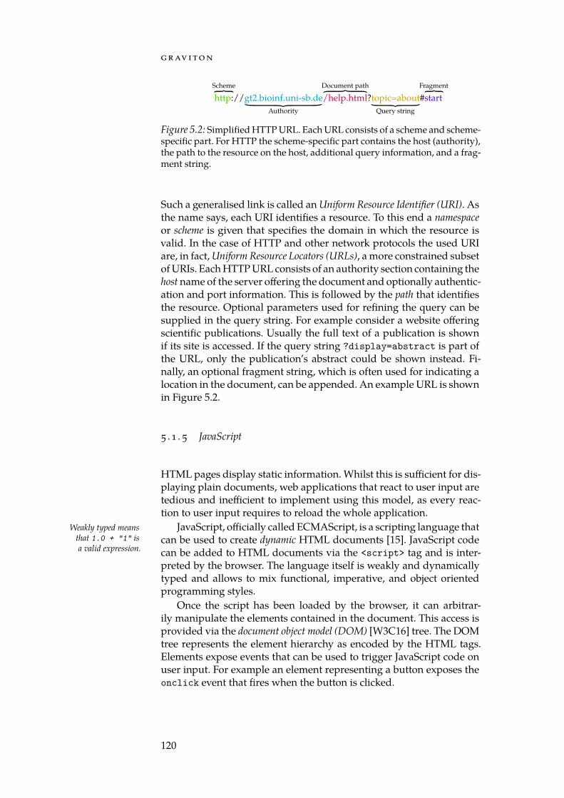
g r av i to n

http://gt2.bioinf.uni-sb.de/help.html?topic=about#start

Authority

Scheme FragmentQuery string

Document path

Figure 5.2: Simplified HTTP URL. Each URL consists of a scheme and scheme-specific part. For HTTP the scheme-specific part contains the host (authority),the path to the resource on the host, additional query information, and a frag-ment string.

Such a generalised link is called an Uniform Resource Identifier (URI). Asthe name says, each URI identifies a resource. To this end a namespaceor scheme is given that specifies the domain in which the resource isvalid. In the case of HTTP and other network protocols the used URIare, in fact, Uniform Resource Locators (URLs), a more constrained subsetof URIs. Each HTTP URL consists of an authority section containing thehost name of the server offering the document and optionally authentic-ation and port information. This is followed by the path that identifiesthe resource. Optional parameters used for refining the query can besupplied in the query string. For example consider a website offeringscientific publications. Usually the full text of a publication is shownif its site is accessed. If the query string ?display=abstract is part ofthe URL, only the publication’s abstract could be shown instead. Fi-nally, an optional fragment string, which is often used for indicating alocation in the document, can be appended. An example URL is shownin Figure 5.2.

5 . 1 . 5 JavaScript

HTML pages display static information. Whilst this is sufficient for dis-playing plain documents, web applications that react to user input aretedious and inefficient to implement using this model, as every reac-tion to user input requires to reload the whole application.

JavaScript, officially called ECMAScript, is a scripting language thatWeakly typed meansthat 1.0 + "1" isa valid expression.

can be used to create dynamic HTML documents [15]. JavaScript codecan be added to HTML documents via the <script> tag and is inter-preted by the browser. The language itself is weakly and dynamicallytyped and allows to mix functional, imperative, and object orientedprogramming styles.

Once the script has been loaded by the browser, it can arbitrar-ily manipulate the elements contained in the document. This access isprovided via the document object model (DOM) [W3C16] tree. The DOMtree represents the element hierarchy as encoded by the HTML tags.Elements expose events that can be used to trigger JavaScript code onuser input. For example an element representing a button exposes theonclick event that fires when the button is clicked.

120

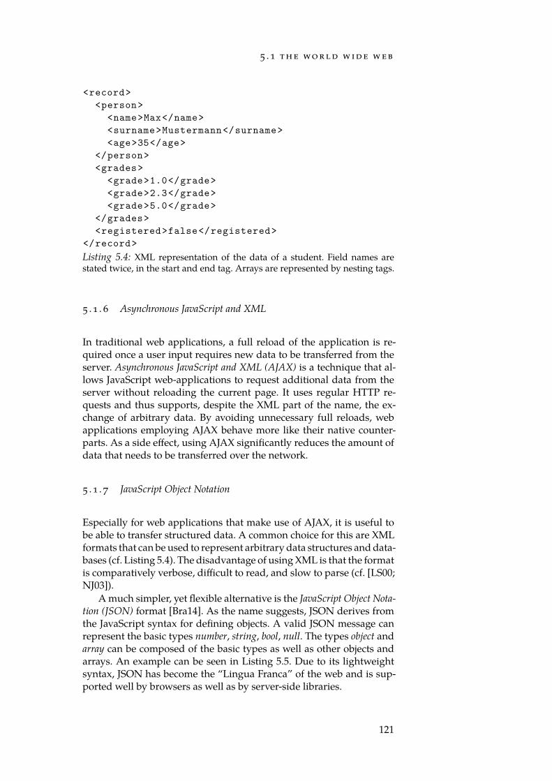
5 . 1 t h e wo r l d w i d e w e b

<record><person>

<name>Max</name><surname>Mustermann</surname><age>35</age>

</person><grades>

<grade>1.0</grade><grade>2.3</grade><grade>5.0</grade>

</grades><registered>false</registered>

</record>Listing 5.4: XML representation of the data of a student. Field names arestated twice, in the start and end tag. Arrays are represented by nesting tags.

5 . 1 . 6 Asynchronous JavaScript and XML

In traditional web applications, a full reload of the application is re-quired once a user input requires new data to be transferred from theserver. Asynchronous JavaScript and XML (AJAX) is a technique that al-lows JavaScript web-applications to request additional data from theserver without reloading the current page. It uses regular HTTP re-quests and thus supports, despite the XML part of the name, the ex-change of arbitrary data. By avoiding unnecessary full reloads, webapplications employing AJAX behave more like their native counter-parts. As a side effect, using AJAX significantly reduces the amount ofdata that needs to be transferred over the network.

5 . 1 . 7 JavaScript Object Notation

Especially for web applications that make use of AJAX, it is useful tobe able to transfer structured data. A common choice for this are XMLformats that can be used to represent arbitrary data structures and data-bases (cf. Listing 5.4). The disadvantage of using XML is that the formatis comparatively verbose, difficult to read, and slow to parse (cf. [LS00;NJ03]).

A much simpler, yet flexible alternative is the JavaScript Object Nota-tion (JSON) format [Bra14]. As the name suggests, JSON derives fromthe JavaScript syntax for defining objects. A valid JSON message canrepresent the basic types number, string, bool, null. The types object andarray can be composed of the basic types as well as other objects andarrays. An example can be seen in Listing 5.5. Due to its lightweightsyntax, JSON has become the “Lingua Franca” of the web and is sup-ported well by browsers as well as by server-side libraries.

121

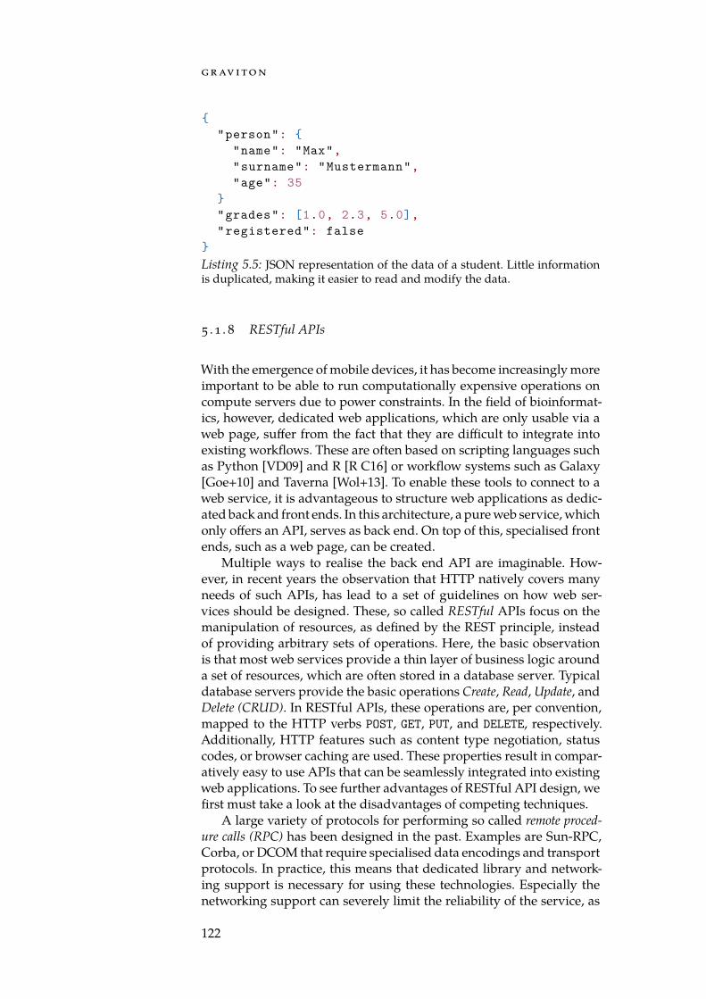
g r av i to n

"person":

"name": "Max","surname": "Mustermann","age": 35

"grades": [1.0, 2.3, 5.0],"registered": false

Listing 5.5: JSON representation of the data of a student. Little informationis duplicated, making it easier to read and modify the data.

5 . 1 . 8 RESTful APIs

With the emergence of mobile devices, it has become increasingly moreimportant to be able to run computationally expensive operations oncompute servers due to power constraints. In the field of bioinformat-ics, however, dedicated web applications, which are only usable via aweb page, suffer from the fact that they are difficult to integrate intoexisting workflows. These are often based on scripting languages suchas Python [VD09] and R [R C16] or workflow systems such as Galaxy[Goe+10] and Taverna [Wol+13]. To enable these tools to connect to aweb service, it is advantageous to structure web applications as dedic-ated back and front ends. In this architecture, a pure web service, whichonly offers an API, serves as back end. On top of this, specialised frontends, such as a web page, can be created.

Multiple ways to realise the back end API are imaginable. How-ever, in recent years the observation that HTTP natively covers manyneeds of such APIs, has lead to a set of guidelines on how web ser-vices should be designed. These, so called RESTful APIs focus on themanipulation of resources, as defined by the REST principle, insteadof providing arbitrary sets of operations. Here, the basic observationis that most web services provide a thin layer of business logic arounda set of resources, which are often stored in a database server. Typicaldatabase servers provide the basic operations Create, Read, Update, andDelete (CRUD). In RESTful APIs, these operations are, per convention,mapped to the HTTP verbs POST, GET, PUT, and DELETE, respectively.Additionally, HTTP features such as content type negotiation, statuscodes, or browser caching are used. These properties result in compar-atively easy to use APIs that can be seamlessly integrated into existingweb applications. To see further advantages of RESTful API design, wefirst must take a look at the disadvantages of competing techniques.

A large variety of protocols for performing so called remote proced-ure calls (RPC) has been designed in the past. Examples are Sun-RPC,Corba, or DCOM that require specialised data encodings and transportprotocols. In practice, this means that dedicated library and network-ing support is necessary for using these technologies. Especially thenetworking support can severely limit the reliability of the service, as

122

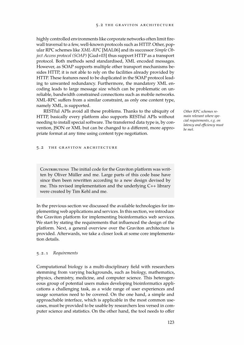
5 . 2 t h e g r av i to n a rc h i t e c t u r e

highly controlled environments like corporate networks often limit fire-wall traversal to a few, well-known protocols such as HTTP. Other, pop-ular RPC schemes like XML-RPC [MAL06] and its successor Simple Ob-ject Access protocol (SOAP) [Gud+03] thus support HTTP as a transportprotocol. Both methods send standardised, XML encoded messages.However, as SOAP supports multiple other transport mechanisms be-sides HTTP, it is not able to rely on the facilities already provided byHTTP. These features need to be duplicated in the SOAP protocol lead-ing to unwanted redundancy. Furthermore, the mandatory XML en-coding leads to large message size which can be problematic on un-reliable, bandwidth constrained connections such as mobile networks.XML-RPC suffers from a similar constraint, as only one content type,namely XML, is supported.

RESTful APIs avoid all these problems. Thanks to the ubiquity of Other RPC schemes re-main relevant where spe-cial requirements, e.g. onlatency and efficiency mustbe met.

HTTP, basically every platform also supports RESTful APIs withoutneeding to install special software. The transferred data type is, by con-vention, JSON or XML but can be changed to a different, more appro-priate format at any time using content type negotiation.

5 . 2 t h e g r av i to n a rc h i t e c t u r e

Contributions The initial code for the Graviton platform was writ-ten by Oliver Müller and me. Large parts of this code base havesince then been rewritten according to a new design devised byme. This revised implementation and the underlying C++ librarywere created by Tim Kehl and me.

In the previous section we discussed the available technologies for im-plementing web applications and services. In this section, we introducethe Graviton platform for implementing bioinformatics web services.We start by stating the requirements that influenced the design of theplatform. Next, a general overview over the Graviton architecture isprovided. Afterwards, we take a closer look at some core implementa-tion details.

5 . 2 . 1 Requirements

Computational biology is a multi-disciplinary field with researchersstemming from varying backgrounds, such as biology, mathematics,physics, chemistry, medicine, and computer science. This heterogen-eous group of potential users makes developing bioinformatics appli-cations a challenging task, as a wide range of user experiences andusage scenarios need to be covered. On the one hand, a simple andapproachable interface, which is applicable in the most common use-cases, must be provided to be usable by researchers less versed in com-puter science and statistics. On the other hand, the tool needs to offer

123

g r av i to n

enough flexibility to cover non-standard usage scenarios and should al-low bioinformaticians to integrate it into their existing pipelines. Natur-ally, these requirements are difficult to fulfil simultaneously. Whilst theideal user interface for a bioinformatician consists of an API or a soph-isticated GUI allowing to tweak all parameters, a biologist requires aninterface with few, essential or no parameter settings at all. Similarly,the presentation of the results needs to be clean and should containas little elements as possible to allow the user to focus on relevantpieces of information. To accommodate both needs, Graviton providesa RESTful API on top of which specialised user interfaces can be cre-ated. While expert users can choose to directly access this program-ming interface to integrate the offered facilities into their workflows,non-experts may choose the web-based GUI. In case of the GeneTrail2server (Section 5.3), a simplified and an advanced web interface areprovided.

Another requirement that must be met by a research tool is to pro-duce reproducible results. At the absolute minimum this entails that allused input data as well as every parameter setting is recorded. For in-put data not provided by the user, such as identifier mapping tables orbiological pathways, detailed provenance information containing ori-gin and date of retrieval, must be made accessible. In some cases, lossytransformations must be applied to user data. The prime example forthis is identifier mapping (Section 5.2.3) where an input identifier canbe mapped to multiple targets or not at all. To ensure reproducibilityand minimise unpleasant surprises such transformations should keepdetailed logs that allow to audit the flow of information.

5 . 2 . 2 Design

Graviton is a framework for building fully integrated bioinformaticswebservices. To this end, it provides implementations of basic func-tionality such as identifier mapping, file parsers, database access, jobscheduling and workflow organisation. This functionality is organisedin layers that each provide abstractions over the layers below them. Thefollowing layers can be distinguished:

1. Plumbing layer

2. Resource layer

3. API layer

4. Front end layer

In the lowest layer, the plumbing layer, implementations of largely inde-pendent, basic functionality is provided. The Resource layer ties theseblocks together by means of the Resource and Job abstractions. Basedon these concepts, the API layer presents a RESTful API to the client.On top of this API, a front end can be developed. We will now discussthe individual layers in more detail.

124

5 . 2 t h e g r av i to n a rc h i t e c t u r e

GeneTrail2 C++

Boost

Eigen 3

GMP

Identifier Mapping Pathway DBs

KEGG Reactome

GO ...

EntrezGene

Ensembl

GeneTrail 2 Frontend

ThymeleafJQuery DataTables

Uniprot

...

RESTful API

JAX-RS Swagger JavaEE

Apache Tom

catResource LayerResource PostgreSQL MapDBJob

Figure 5.3: The GeneTrail2 architecture. Core algorithms are implemented inan optimised C++ library based on Boost, Eigen 3, and GMP. On top of thislibrary we implemented a JAX-RS based RESTful API. The frontend is basedon the Thymeleaf template engine and JQuery. As application server we useApache Tomcat. Figure adapted from Stöckel et al. [Stö+16]

Plumbing Layer

The most common tasks in bioinformatics are the parsing of files andthe conversion between database identifiers. As a web service needsto support a wide range of user-supplied input data, solid support forboth tasks must be available in Graviton.

At the time of writing, Graviton supports parsers for identifier lists,score lists, matrices, the variant call format (VCF), the gene matrix trans-posed (GMT) format, the browser extensible data (BED) format, and theGEO [Bar+13] GSE and GDS formats. Besides reading the content of afile, the parsers are also responsible for determining the format of usersupplied data and validating its contents. More information about thesupported file types can be found in Section 5.3. For mapping iden-tifiers, a flexible system, which can use mapping information from awide range of sources (Section 5.2.3), has been implemented. Further-more, the plumbing layer offers implementations of statistical meth-ods such as hypothesis tests (Section 4.1) and enrichment procedures(Chapter 4).

Resource Layer

The Resource layer introduces a first level of abstraction from the ser- Graviton Resources arenot HTTP resources. Toavoid confusion we willcapitalise the Gravitonversion.

vices offered by the plumbing layer. This is achieved by offering theinterfaces Resource and Job that provide abstractions over data andanalyses. A Session represents a collection of Resources and Jobs thatwere created by the same user. Both anonymous as well as authentic-ated users are supported. For representing the latter the type User isemployed.

125

g r av i to n

A Resource is a representation of data stored on the file system to-gether with assorted metadata. Every Resource is associated with aunique identifier through which it can be accessed from the GravitonAPI. Besides the path to the location of the represented file on disk, aresource stores the used identifier type and organism. For document-ation purposes, every Resource also tracks the date of its creation aswell as the time its metadata was last modified. A Resource belongs toexactly one user session. New Resources can be created by uploadingdata or by executing an analysis. Once created, the Resource is immut-able in the sense that the file to which the Resource refers cannot bechanged. However, it is possible to add further metadata and use it asinput for an arbitrary number of Jobs. To model different kinds of data,Graviton comes with several, predefined Resource subtypes that placerestrictions on the data they represent. Currently available subclassesare Scores, Identifiers, ExpressionMatrix, Category, Enrichment, Subgraph,and Variations.

Properties of a Graviton Resource

id A unique id, through which the Resource can be accessed.

creationDate The time a Resource was created.

modificationDate The last time the metadata of a Resource hasbeen changed.

session The Session this Resource is a part of.

organism The organism from which the data represented by theResource has been derived.

identifierType The database identifier used in the represented file.

comment A free text field that can carry any user supplied inform-ation.

shared Boolean flag indicating that the file represented by thisResource is shared between multiple sessions. Each user stillowns a private copy of the Resourcesmetadata. This mechan-ism allows to substantially reduce the on-disk memory con-sumption of Graviton.

intermediate Boolean flag indicating that the Resource is an inter-mediate result of an analysis or workflow. This allows front-ends to hide such Resources unless otherwise requested.

normalized Boolean flag indicating that the identifiers used in thefile are guaranteed to conform to Gravitons internal identifierdatabase.

displayName A user visible name that should be displayed toidentify the Resource. This name does not necessarily needto be unique.

126

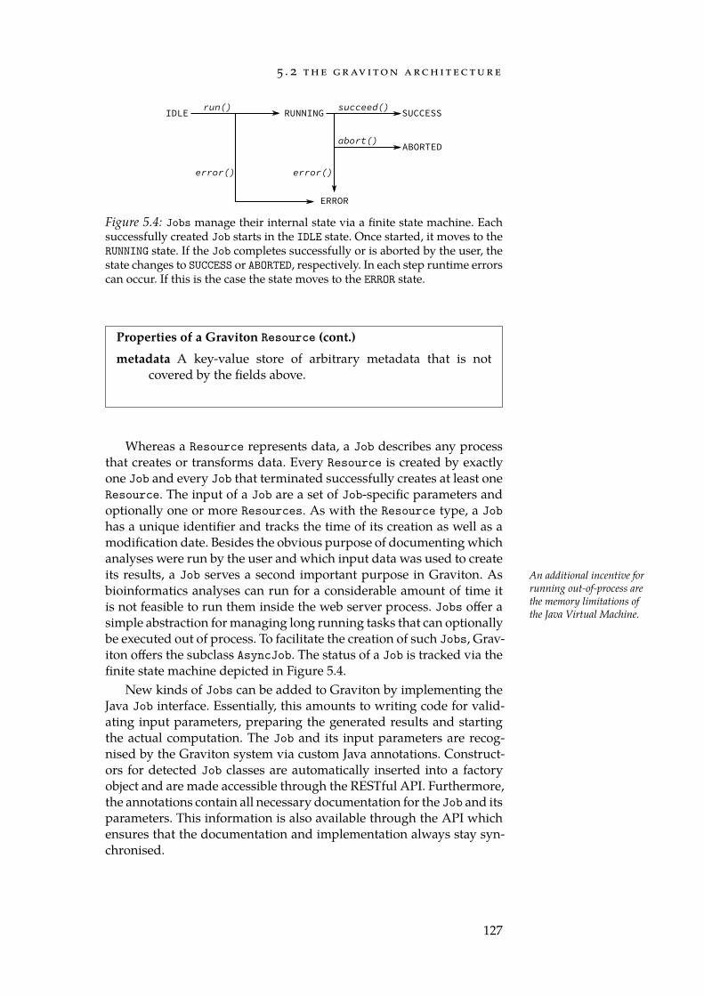
5 . 2 t h e g r av i to n a rc h i t e c t u r e

IDLE RUNNING SUCCESS

ERROR

ABORTED

run() succeed()

abort()

error()error()

Figure 5.4: Jobs manage their internal state via a finite state machine. Eachsuccessfully created Job starts in the IDLE state. Once started, it moves to theRUNNING state. If the Job completes successfully or is aborted by the user, thestate changes to SUCCESS or ABORTED, respectively. In each step runtime errorscan occur. If this is the case the state moves to the ERROR state.

Properties of a Graviton Resource (cont.)metadata A key-value store of arbitrary metadata that is not

covered by the fields above.

Whereas a Resource represents data, a Job describes any processthat creates or transforms data. Every Resource is created by exactlyone Job and every Job that terminated successfully creates at least oneResource. The input of a Job are a set of Job-specific parameters andoptionally one or more Resources. As with the Resource type, a Jobhas a unique identifier and tracks the time of its creation as well as amodification date. Besides the obvious purpose of documenting whichanalyses were run by the user and which input data was used to createits results, a Job serves a second important purpose in Graviton. As An additional incentive for

running out-of-process arethe memory limitations ofthe Java Virtual Machine.

bioinformatics analyses can run for a considerable amount of time itis not feasible to run them inside the web server process. Jobs offer asimple abstraction for managing long running tasks that can optionallybe executed out of process. To facilitate the creation of such Jobs, Grav-iton offers the subclass AsyncJob. The status of a Job is tracked via thefinite state machine depicted in Figure 5.4.

New kinds of Jobs can be added to Graviton by implementing theJava Job interface. Essentially, this amounts to writing code for valid-ating input parameters, preparing the generated results and startingthe actual computation. The Job and its input parameters are recog-nised by the Graviton system via custom Java annotations. Construct-ors for detected Job classes are automatically inserted into a factoryobject and are made accessible through the RESTful API. Furthermore,the annotations contain all necessary documentation for the Job and itsparameters. This information is also available through the API whichensures that the documentation and implementation always stay syn-chronised.

127

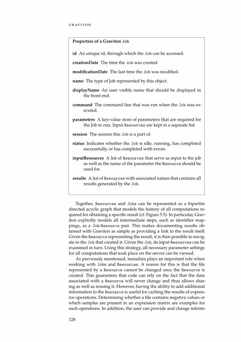
g r av i to n

Properties of a Graviton Job

id An unique id, through which the Job can be accessed.

creationDate The time the Job was created.

modificationDate The last time the Job was modified.

name The type of Job represented by this object.

displayName An user visible name that should be displayed inthe front end.

command The command line that was run when the Job was ex-ecuted.

parameters A key-value store of parameters that are required forthe Job to run. Input Resources are kept in a separate list.

session The session this Job is a part of.

status Indicates whether the Job is idle, running, has completedsuccessfully, or has completed with errors.

inputResources A list of Resources that serve as input to the jobas well as the name of the parameter the Resource should beused for.

results A list of Resourceswith associated names that contains allresults generated by the Job.

Together, Resources and Jobs can be represented as a bipartitedirected acyclic graph that models the history of all computations re-quired for obtaining a specific result (cf. Figure 5.5). In particular, Grav-iton explicitly models all intermediate steps, such as identifier map-pings, as a Job-Resource pair. This makes documenting results ob-tained with Graviton as simple as providing a link to the result itself.Given the Resource representing the result, it is then possible to navig-ate to the Job that created it. Given the Job, its input Resources can beexamined in turn. Using this strategy, all necessary parameter settingsfor all computations that took place on the server can be viewed.

As previously mentioned, metadata plays an important role whenworking with Jobs and Resources. A reason for this is that the filerepresented by a Resource cannot be changed once the Resource iscreated. This guarantees that code can rely on the fact that the dataassociated with a Resource will never change and thus allows shar-ing as well as reusing it. However, having the ability to add additionalinformation to the Resource is useful for caching the results of expens-ive operations. Determining whether a file contains negative values orwhich samples are present in an expression matrix are examples forsuch operations. In addition, the user can provide and change inform-

128

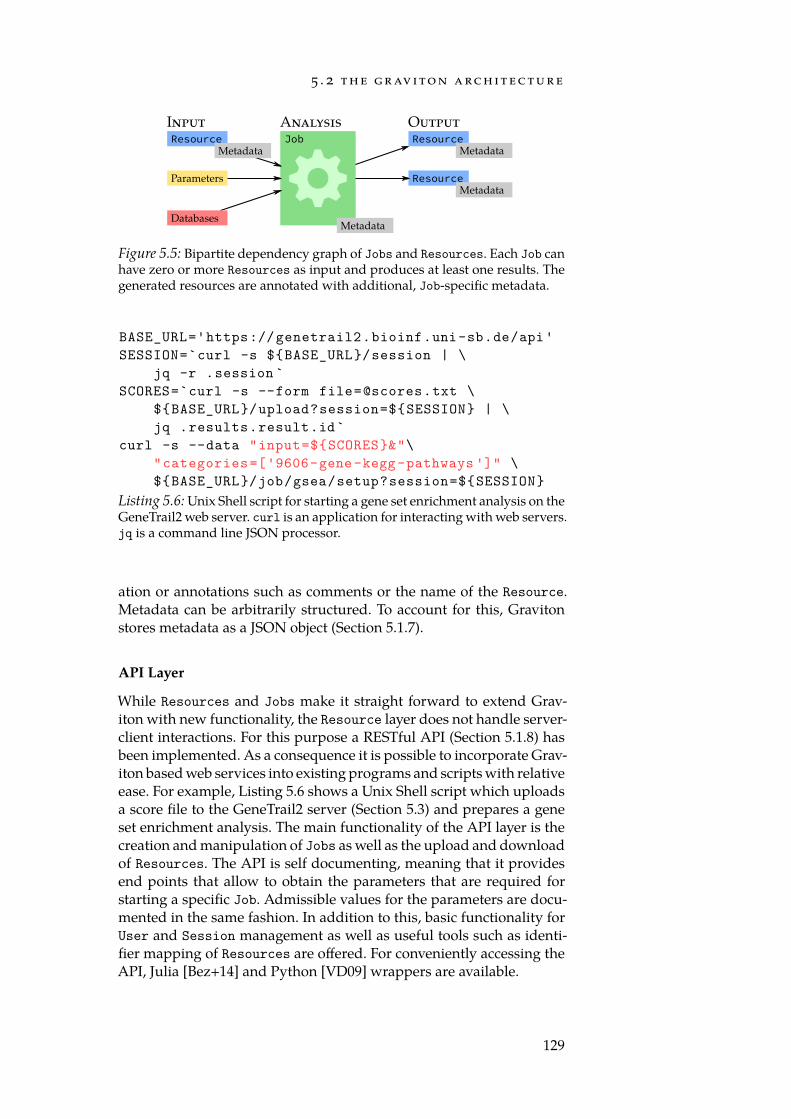
5 . 2 t h e g r av i to n a rc h i t e c t u r e

ResourceMetadata

ResourceMetadata

Job

Metadata

Resource

Parameters

Databases

Metadata

Figure 5.5: Bipartite dependency graph of Jobs and Resources. Each Job canhave zero or more Resources as input and produces at least one results. Thegenerated resources are annotated with additional, Job-specific metadata.

BASE_URL='https://genetrail2.bioinf.uni-sb.de/api'SESSION=`curl -s $BASE_URL/session | \

jq -r .session`SCORES=`curl -s --form file=@scores.txt \

$BASE_URL/upload?session=$SESSION | \jq .results.result.id`

curl -s --data "input=$SCORES&"\"categories=['9606-gene-kegg-pathways ']" \$BASE_URL/job/gsea/setup?session=$SESSION

Listing 5.6: Unix Shell script for starting a gene set enrichment analysis on theGeneTrail2 web server. curl is an application for interacting with web servers.jq is a command line JSON processor.

ation or annotations such as comments or the name of the Resource.Metadata can be arbitrarily structured. To account for this, Gravitonstores metadata as a JSON object (Section 5.1.7).

API Layer

While Resources and Jobs make it straight forward to extend Grav-iton with new functionality, the Resource layer does not handle server-client interactions. For this purpose a RESTful API (Section 5.1.8) hasbeen implemented. As a consequence it is possible to incorporate Grav-iton based web services into existing programs and scripts with relativeease. For example, Listing 5.6 shows a Unix Shell script which uploadsa score file to the GeneTrail2 server (Section 5.3) and prepares a geneset enrichment analysis. The main functionality of the API layer is thecreation and manipulation of Jobs as well as the upload and downloadof Resources. The API is self documenting, meaning that it providesend points that allow to obtain the parameters that are required forstarting a specific Job. Admissible values for the parameters are docu-mented in the same fashion. In addition to this, basic functionality forUser and Session management as well as useful tools such as identi-fier mapping of Resources are offered. For conveniently accessing theAPI, Julia [Bez+14] and Python [VD09] wrappers are available.

129

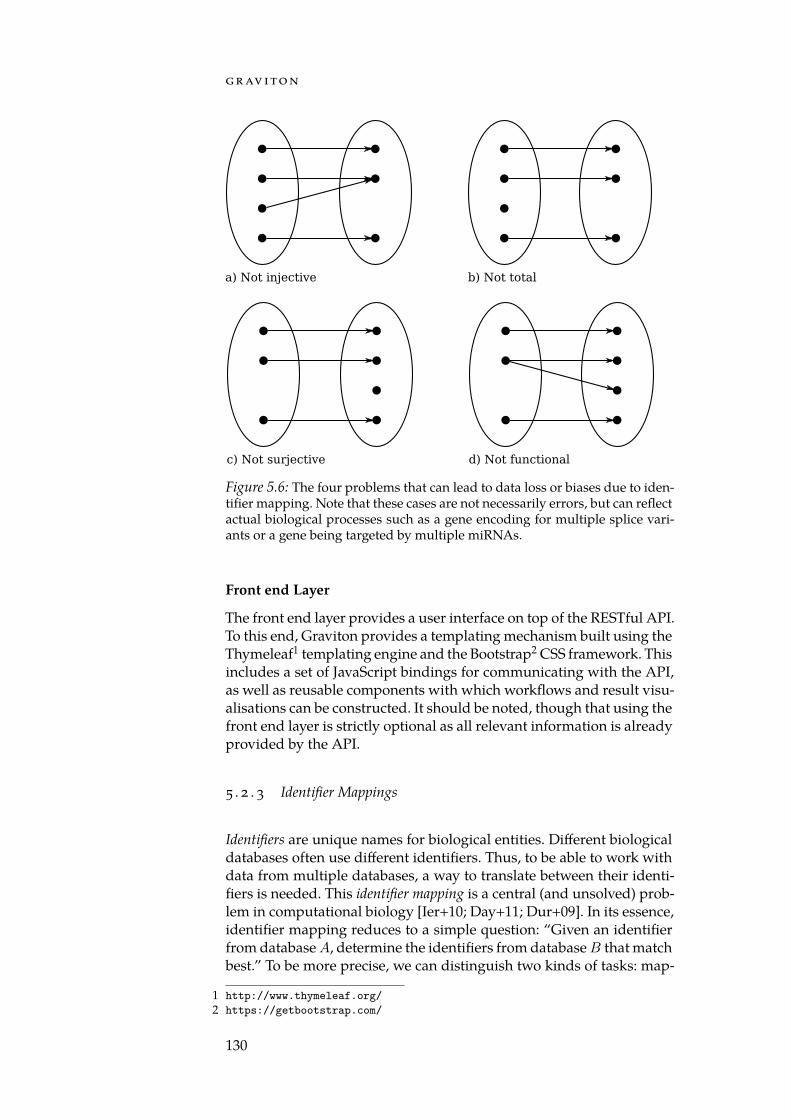
g r av i to n

c) Not surjective d) Not functional

a) Not injective b) Not total

Figure 5.6: The four problems that can lead to data loss or biases due to iden-tifier mapping. Note that these cases are not necessarily errors, but can reflectactual biological processes such as a gene encoding for multiple splice vari-ants or a gene being targeted by multiple miRNAs.

Front end Layer

The front end layer provides a user interface on top of the RESTful API.To this end, Graviton provides a templating mechanism built using theThymeleaf1 templating engine and the Bootstrap2 CSS framework. Thisincludes a set of JavaScript bindings for communicating with the API,as well as reusable components with which workflows and result visu-alisations can be constructed. It should be noted, though that using thefront end layer is strictly optional as all relevant information is alreadyprovided by the API.

5 . 2 . 3 Identifier Mappings

Identifiers are unique names for biological entities. Different biologicaldatabases often use different identifiers. Thus, to be able to work withdata from multiple databases, a way to translate between their identi-fiers is needed. This identifier mapping is a central (and unsolved) prob-lem in computational biology [Ier+10; Day+11; Dur+09]. In its essence,identifier mapping reduces to a simple question: “Given an identifierfrom database A, determine the identifiers from database B that matchbest.” To be more precise, we can distinguish two kinds of tasks: map-

1 http://www.thymeleaf.org/2 https://getbootstrap.com/

130

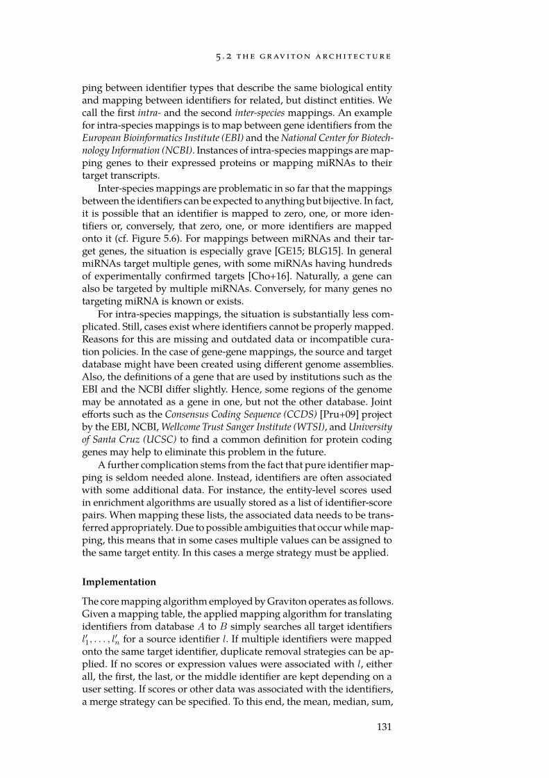
5 . 2 t h e g r av i to n a rc h i t e c t u r e

ping between identifier types that describe the same biological entityand mapping between identifiers for related, but distinct entities. Wecall the first intra- and the second inter-species mappings. An examplefor intra-species mappings is to map between gene identifiers from theEuropean Bioinformatics Institute (EBI) and the National Center for Biotech-nology Information (NCBI). Instances of intra-species mappings are map-ping genes to their expressed proteins or mapping miRNAs to theirtarget transcripts.

Inter-species mappings are problematic in so far that the mappingsbetween the identifiers can be expected to anything but bijective. In fact,it is possible that an identifier is mapped to zero, one, or more iden-tifiers or, conversely, that zero, one, or more identifiers are mappedonto it (cf. Figure 5.6). For mappings between miRNAs and their tar-get genes, the situation is especially grave [GE15; BLG15]. In generalmiRNAs target multiple genes, with some miRNAs having hundredsof experimentally confirmed targets [Cho+16]. Naturally, a gene canalso be targeted by multiple miRNAs. Conversely, for many genes notargeting miRNA is known or exists.

For intra-species mappings, the situation is substantially less com-plicated. Still, cases exist where identifiers cannot be properly mapped.Reasons for this are missing and outdated data or incompatible cura-tion policies. In the case of gene-gene mappings, the source and targetdatabase might have been created using different genome assemblies.Also, the definitions of a gene that are used by institutions such as theEBI and the NCBI differ slightly. Hence, some regions of the genomemay be annotated as a gene in one, but not the other database. Jointefforts such as the Consensus Coding Sequence (CCDS) [Pru+09] projectby the EBI, NCBI, Wellcome Trust Sanger Institute (WTSI), and Universityof Santa Cruz (UCSC) to find a common definition for protein codinggenes may help to eliminate this problem in the future.

A further complication stems from the fact that pure identifier map-ping is seldom needed alone. Instead, identifiers are often associatedwith some additional data. For instance, the entity-level scores usedin enrichment algorithms are usually stored as a list of identifier-scorepairs. When mapping these lists, the associated data needs to be trans-ferred appropriately. Due to possible ambiguities that occur while map-ping, this means that in some cases multiple values can be assigned tothe same target entity. In this cases a merge strategy must be applied.

Implementation

The core mapping algorithm employed by Graviton operates as follows.Given a mapping table, the applied mapping algorithm for translatingidentifiers from database A to B simply searches all target identifiersl′1, . . . , l

′n for a source identifier l. If multiple identifiers were mapped

onto the same target identifier, duplicate removal strategies can be ap-plied. If no scores or expression values were associated with l, eitherall, the first, the last, or the middle identifier are kept depending on auser setting. If scores or other data was associated with the identifiers,a merge strategy can be specified. To this end, the mean, median, sum,

131

g r av i to n

Data: List of identifiers L, mapping m : A → P(B),data d : A → X .Result: List of mapped identifiers L′, mapped data d′ : B → X .L′ = []d′ = ∅dtmp = ∅// Perform mapping and collect datafor l ∈ L do

for l′ ∈ m(l) dodtmp(l

′) = dtmp(l′) ∪ d(l)

endL′ = appendAll(L′,m(l))

end// Merge the mapped datafor l′ ∈ L′ do

d′(l′) = merge(dtmp(l′))

endL′ = removeDuplicates(L′)return (L′, d′)

Algorithm 5.1: Core mapping algorithm used in Graviton. The “merge” and“removeDuplicate” functions can be supplied by the user. We model data asa function that assigns a value from a set X to each identifier.

maximum, or minimum value can be used. Support for non-numericaldata has not yet been implemented. Pseudo-code for the mapping al-gorithm is given in Algorithm 5.1.

Graviton uses identifier mapping to solve three distinct problems.The GeneTrail2 webservice uses (HGNC)

gene symbols internally.First, user provided input data needs to be converted to the same iden-tifier types as used internally. Second, user input must be sanitisedbefore it can be used for further analysis. Reasons for this may be in-valid, outdated, or misspelled identifiers in the input data that, whennot corrected for, can bias downstream statistics. Third, Graviton sup-ports inter-species mappings for advanced analyses and, in the caseof GeneTrail2, for expanding the range of available categories. Each ofthese tasks has different requirements on the mapping engine whichwe will outline in the following.

Mapping from the identifiers in the user data to internal identifiersmainly exercises the core mapping algorithm. From a software engin-eering point of view, its only requirement are the availability of effi-cient lookup tables. For this, high performance dictionary implement-ations using b-trees such as LMDB3, LevelDB4, and MapDB5 are avail-able. As Graviton is written in Java, the Java-based MapDB engine waschosen to ease the integration with the remaining server code.

Sanitising user input requires that a list of known, “good” identi-fiers is kept for reference. Each identifier that is read from user data

3 https://symas.com/products/lightning-memory-mapped-database/4 http://leveldb.org/5 http://www.mapdb.org/

132

5 . 3 g e n e t r a i l 2

must then be validated against this list. This lookup must take the pe-culiarities of some identifier types into account. For example, mirBaseidentifiers are case sensitive, whereas gene symbols and other identi-fiers are commonly case insensitive. In addition, outdated identifiersand known aliases need to be upgraded to the most current or canon-ical version. For this, database vendors sometimes provide mappingfiles that can be used to upgrade user inputs. If available, these filesare integrated into the Graviton mapping database.

Intra-species mappings are, despite the problems mentioned above,no different from mappings between external and internal identifiers.Inter-species mappings, however, commonly exist in multiple versions.As an example consider miRNA–target mappings, where different cri-teria can be used to conclude whether a miRNA targets a certain tran-script or not. Accordingly, a wide range of miRNA–target mappingshave been produced that differ in the considered experimental meth-ods and chosen significance cut-offs. To accommodate for this, Grav-iton labels each mapping with a quadruple

(organism, from, to,variant).

While the first three items depend on the source Resource and the de-sired output identifier type, the variant field allows to choose betweenalternative mapping definitions. For example the mapping

(9606, mirBase21, GeneSymbol, mirTarBase-westernBlot)

corresponds to a mapping of human miRNA identifiers to target genesobtained from mirTarBase [Cho+16] that were validated using a west-ern blot.

To make the mapping process transparent, Graviton exposes theavailable mappings on a web page6 and via the RESTful API. Addi-tionally, for each performed mapping, an audit log is kept that allowsto reconstruct which identifiers of the source Resource were mappedonto which identifiers in the target Resource.

5 . 3 g e n e t r a i l 2

Contributions The GeneTrail2 web server and the enrichmentmethods it offers were implemented by Tim Kehl and me. Theincluded data was collected and curated by Tim Kehl, PatrickTrampert, and me. The corresponding manuscript [Stö+16] waswritten by me and Hans-Peter Lenhof.

As shown in Chapter 4 a large variety of enrichment algorithms ex-ists. We argued that it is difficult to determine a “best” enrichment al-gorithm, as the published methods assume different null hypotheses.

6 https://genetrail2.bioinf.uni-sb.de/mappings.html

133

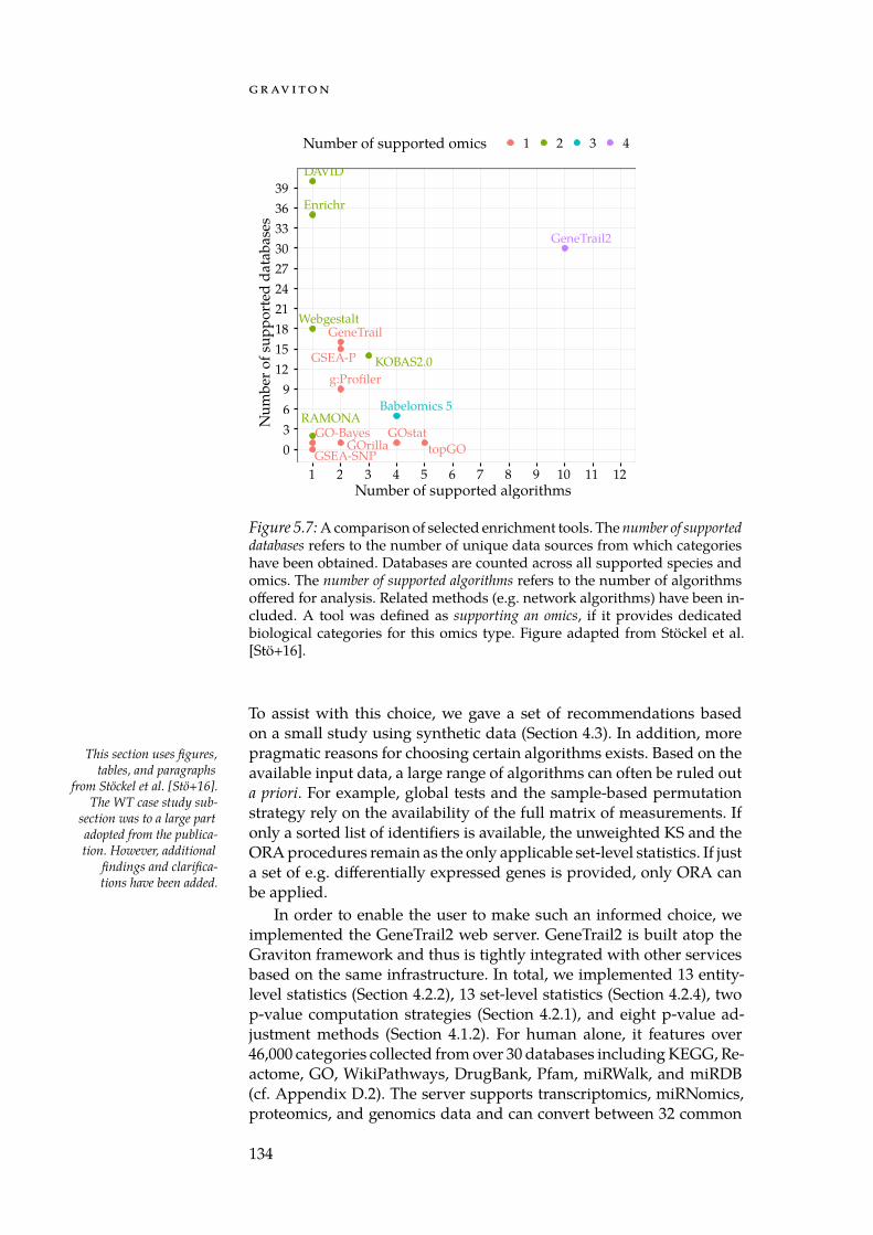
g r av i to n

WebgestaltGeneTrail

DAVID

GSEA-P

GSEA-SNP

GO-BayestopGO

GeneTrail2

Babelomics 5

g:ProfilerKOBAS2.0

GOstatGOrilla

RAMONA

Enrichr

0369

12151821242730333639

1 2 3 4 5 6 7 8 9 10 11 12Number of supported algorithms

Num

ber o

f sup

port

ed d

atab

ases

Number of supported omics 1 2 3 4

Figure 5.7: A comparison of selected enrichment tools. The number of supporteddatabases refers to the number of unique data sources from which categorieshave been obtained. Databases are counted across all supported species andomics. The number of supported algorithms refers to the number of algorithmsoffered for analysis. Related methods (e.g. network algorithms) have been in-cluded. A tool was defined as supporting an omics, if it provides dedicatedbiological categories for this omics type. Figure adapted from Stöckel et al.[Stö+16].

To assist with this choice, we gave a set of recommendations basedon a small study using synthetic data (Section 4.3). In addition, morepragmatic reasons for choosing certain algorithms exists. Based on theThis section uses figures,

tables, and paragraphsfrom Stöckel et al. [Stö+16].

The WT case study sub-section was to a large partadopted from the publica-tion. However, additional

findings and clarifica-tions have been added.

available input data, a large range of algorithms can often be ruled outa priori. For example, global tests and the sample-based permutationstrategy rely on the availability of the full matrix of measurements. Ifonly a sorted list of identifiers is available, the unweighted KS and theORA procedures remain as the only applicable set-level statistics. If justa set of e.g. differentially expressed genes is provided, only ORA canbe applied.

In order to enable the user to make such an informed choice, weimplemented the GeneTrail2 web server. GeneTrail2 is built atop theGraviton framework and thus is tightly integrated with other servicesbased on the same infrastructure. In total, we implemented 13 entity-level statistics (Section 4.2.2), 13 set-level statistics (Section 4.2.4), twop-value computation strategies (Section 4.2.1), and eight p-value ad-justment methods (Section 4.1.2). For human alone, it features over46,000 categories collected from over 30 databases including KEGG, Re-actome, GO, WikiPathways, DrugBank, Pfam, miRWalk, and miRDB(cf. Appendix D.2). The server supports transcriptomics, miRNomics,proteomics, and genomics data and can convert between 32 common

134

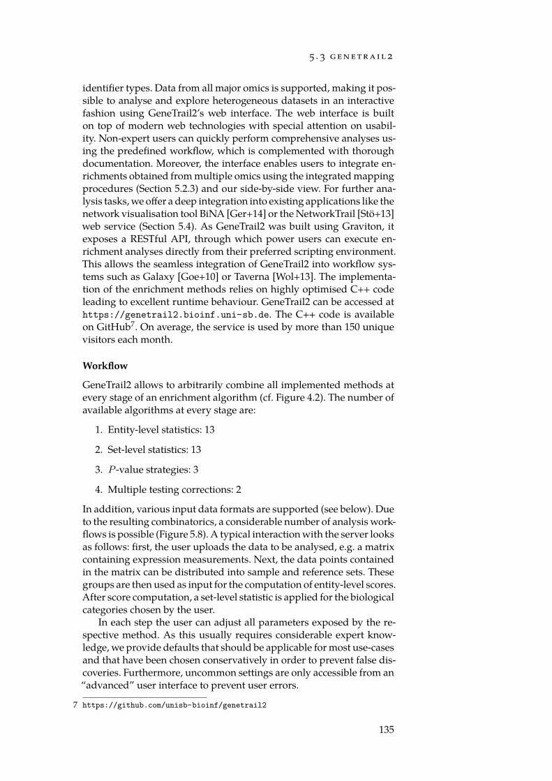
5 . 3 g e n e t r a i l 2

identifier types. Data from all major omics is supported, making it pos-sible to analyse and explore heterogeneous datasets in an interactivefashion using GeneTrail2’s web interface. The web interface is builton top of modern web technologies with special attention on usabil-ity. Non-expert users can quickly perform comprehensive analyses us-ing the predefined workflow, which is complemented with thoroughdocumentation. Moreover, the interface enables users to integrate en-richments obtained from multiple omics using the integrated mappingprocedures (Section 5.2.3) and our side-by-side view. For further ana-lysis tasks, we offer a deep integration into existing applications like thenetwork visualisation tool BiNA [Ger+14] or the NetworkTrail [Stö+13]web service (Section 5.4). As GeneTrail2 was built using Graviton, itexposes a RESTful API, through which power users can execute en-richment analyses directly from their preferred scripting environment.This allows the seamless integration of GeneTrail2 into workflow sys-tems such as Galaxy [Goe+10] or Taverna [Wol+13]. The implementa-tion of the enrichment methods relies on highly optimised C++ codeleading to excellent runtime behaviour. GeneTrail2 can be accessed athttps://genetrail2.bioinf.uni-sb.de. The C++ code is availableon GitHub7. On average, the service is used by more than 150 uniquevisitors each month.

Workflow

GeneTrail2 allows to arbitrarily combine all implemented methods atevery stage of an enrichment algorithm (cf. Figure 4.2). The number ofavailable algorithms at every stage are:

1. Entity-level statistics: 13

2. Set-level statistics: 13

3. P -value strategies: 3

4. Multiple testing corrections: 2

In addition, various input data formats are supported (see below). Dueto the resulting combinatorics, a considerable number of analysis work-flows is possible (Figure 5.8). A typical interaction with the server looksas follows: first, the user uploads the data to be analysed, e.g. a matrixcontaining expression measurements. Next, the data points containedin the matrix can be distributed into sample and reference sets. Thesegroups are then used as input for the computation of entity-level scores.After score computation, a set-level statistic is applied for the biologicalcategories chosen by the user.

In each step the user can adjust all parameters exposed by the re-spective method. As this usually requires considerable expert know-ledge, we provide defaults that should be applicable for most use-casesand that have been chosen conservatively in order to prevent false dis-coveries. Furthermore, uncommon settings are only accessible from an“advanced” user interface to prevent user errors.

7 https://github.com/unisb-bioinf/genetrail2

135

g r av i to n

Identifier list

NetworkTrailIntegration

Set-level statistic

Multiple testingcorrection

Examineenrichment

File Upload

NCBI GEO

Matrix

Entity-levelstatisticsScore list

Score transformation

Networkvisualisation

Subgraph analysis

Figure 5.8: Simplified flowchart of the GeneTrail2 workflow. Round greenand red boxes depict start and end states, respectively. Boxes with orangebackground represent input files types, whereas a blue background repres-ents processing steps. Diamonds are decision nodes. Figure adapted fromStöckel et al. [Stö+16].

Supported Input Data

GeneTrail2 is able to read various input file formats through which theuser can provide measurement data or categories that should be ana-lysed. Using the infrastructure provided by Graviton, GeneTrail2 willtry to automatically detect type and format of the uploaded data. In ad-dition, the database identifiers and the organism, from which the datastems, are estimated. In the following, we discuss the expected inputformats and the assumptions GeneTrail2 makes about their contents.

Identifier Lists The simplest way to provide input data to GeneTrail2is to upload a list of identifiers. To this end, GeneTrail2 accepts a plaintext file containing exactly one identifier per line. There are two ways tointerpret such a file: as an unordered set or a sorted list. In the first case,the list can only be used as an input to ORA as no scores are availableand, thus, all identifiers need to be considered as equally important.In the second case, the order of the identifiers defines an importanceranking, which can be used by non-parametric methods such as theunweighted KS statistics.

136

5 . 3 g e n e t r a i l 2

Entity-Level Score Lists Similarly to identifier lists, score lists can beprovided in a text-based format. In addition to an identifier, each linecontains an entity-level score. The two columns are separated by a tabor space character. In general, score lists are preferable to identifier listsas a score list can be used as an input for virtually every enrichment al-gorithm. In addition, score lists are less prone to problems which arefrequently encountered with identifier list. A common example for thisare unsorted identifier lists being used as input to the KS statistics. Itshould be noted that GeneTrail2 does not verify whether the uploadedscores follow a certain distribution or not. While most of the implemen-ted methods work surprisingly well if their assumptions are violated, itis strongly recommend to avoid such unsound statistics. If the distribu-tion of the data is unclear or unknown, the (unweighted) KS-statisticsand the Wilcoxon test are non-parametric enrichment methods that donot require a specific score distribution (cf. Section 4.2.4).

Measurements GeneTrail2 provides support for directly analysingmatrices containing high-throughput measurements. These can be nor-malised expression values obtained from microarray or RNA-seq ex-periments or protein abundances from mass-spectrometry runs. Addi-tionally, rudimentary support for analysing raw count data obtainedvia RNA-seq is offered. More involved processing steps such as qualitycontrol, batch effect removal, and normalisation must be performed bythe user.

Measurements can be uploaded as a plain text, tab-separated mat-rix. Optionally, the first row provides names for each of the containedsamples. Each subsequent row contains the measurement data for oneidentifier in all samples. Thus each row except the first starts with anidentifier followed by N numerical values, where N ∈ N is the numberof samples.

Sample1 Sample2 Sample3GeneA 0.1 4.3 2.3GeneB 3.2 -1.2 1.1GeneC 2.7 9.1 0.3

The main advantage of uploading matrices of measurements instead ofentity-level scores is that sample-based instead of row-based permuta-tion schemes can be used for determining the significance of enrichedcategories (cf. Section 4.2.1).

Microarray data A major use case of GeneTrail2 is the analysis of mi-croarray data. For this platform, well established normalisation pipe-lines exist that usually generate normal or log-normal distributed ex-pression values. GeneTrail2 can directly work with this normaliseddata and offers a range of statistics that can be used to derive scoresfrom expression matrices.

137

g r av i to n

RNA-seq data RNA-seq data usually comes in the form of count data.This means that for each transcript, the number of mapped reads is re-ported. The distribution of this data is fundamentally different to thedistribution of microarray data, and hence specialised methods for theanalysis of count data have been developed (Section 2.3.3). GeneTrail2implements basic support for some of these methods. The user canchoose between the DESeq2 [LHA14], edgeR [RMS10], and RUVSeq[Ris+14] algorithms for computing entity-level scores. All implementa-tions are based on R packages from the Bioconductor [Gen+04] repos-itory.

Note that currently sample-based permutations are not possible forcount data due to the prohibitive runtime of the score computationprocess. In addition, while the used packages provide some level ofnormalisation, GeneTrail2 performs no quality control or batch effectremoval.

miRNA Data Besides mRNA expression data, GeneTrail2 also sup-ports the analysis of miRNA expression data (cf. Section 2.3). Two mainanalysis modes are available: specialised miRNA categories and map-pings to miRNA target genes. For the first mode, we integrated cat-egories obtained from the mirWalk 2.0 [DG15], HMDD 2.0[Li+13], andTAM [Lu+10] miRNA databases. We also defined categories based ontarget information from mirTarBase [Hsu+10; Hsu+14; Cho+16]. En-richments of chromosomal regions can be computed using categoriesderived from mirBase [Gri+06]. In addition, custom categories createdby Backes et al. [Bac+16] have been integrated. All performed compu-tations are completely analogous to the mRNA case.

The target mapping strategy, however, works fundamentally differ-ent. As miRNAs are able to target a wide range of genes, transferringmiRNA scores directly to target genes would result in a skewed scoredistribution that contains many ties. To circumvent this, a set of differ-entially expressed miRNAs is selected. These are then mapped to theirtargets as found e.g. in mirTarBase. These targets then serve as the in-put to an ORA enrichment using gene categories. The idea behind thisis that the function of a miRNA is defined by its target genes and hencethe annotations of the target genes can be “transferred” to the miRNA.The advantage of this strategy is that it vastly increases the number ofcategories that are available for miRNA data. However, various disad-vantages exist. As miRNAs can have many targets, the test set for thesubsequent ORA analysis can grow rapidly and unpredictably. Also,the target genes in the test set are highly dependent, which violates theassumptions underlying the hypergeometric test. This can lead to lowstatistical power and considerable artefacts [BLG15; GE15].

Protein Data Using GeneTrail2, it is also possible to analyse proteinabundances. Basically, the same strategies as for the miRNA data ap-ply. However, as a protein usually can be mapped unambiguously toits encoding gene, the mapping based strategy is considerably betterbehaved than in the miRNA case. Hence, protein abundances can be

138

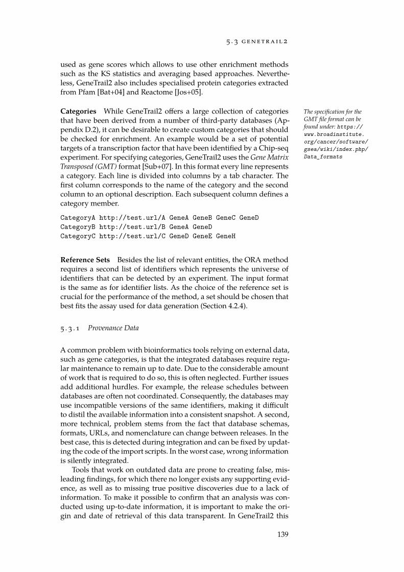
5 . 3 g e n e t r a i l 2

used as gene scores which allows to use other enrichment methodssuch as the KS statistics and averaging based approaches. Neverthe-less, GeneTrail2 also includes specialised protein categories extractedfrom Pfam [Bat+04] and Reactome [Jos+05].

Categories While GeneTrail2 offers a large collection of categories The specification for theGMT file format can befound under: https://www.broadinstitute.org/cancer/software/gsea/wiki/index.php/Data_formats

that have been derived from a number of third-party databases (Ap-pendix D.2), it can be desirable to create custom categories that shouldbe checked for enrichment. An example would be a set of potentialtargets of a transcription factor that have been identified by a Chip-seqexperiment. For specifying categories, GeneTrail2 uses the Gene MatrixTransposed (GMT) format [Sub+07]. In this format every line representsa category. Each line is divided into columns by a tab character. Thefirst column corresponds to the name of the category and the secondcolumn to an optional description. Each subsequent column defines acategory member.

CategoryA http://test.url/A GeneA GeneB GeneC GeneDCategoryB http://test.url/B GeneA GeneDCategoryC http://test.url/C GeneD GeneE GeneH

Reference Sets Besides the list of relevant entities, the ORA methodrequires a second list of identifiers which represents the universe ofidentifiers that can be detected by an experiment. The input formatis the same as for identifier lists. As the choice of the reference set iscrucial for the performance of the method, a set should be chosen thatbest fits the assay used for data generation (Section 4.2.4).

5 . 3 . 1 Provenance Data

A common problem with bioinformatics tools relying on external data,such as gene categories, is that the integrated databases require regu-lar maintenance to remain up to date. Due to the considerable amountof work that is required to do so, this is often neglected. Further issuesadd additional hurdles. For example, the release schedules betweendatabases are often not coordinated. Consequently, the databases mayuse incompatible versions of the same identifiers, making it difficultto distil the available information into a consistent snapshot. A second,more technical, problem stems from the fact that database schemas,formats, URLs, and nomenclature can change between releases. In thebest case, this is detected during integration and can be fixed by updat-ing the code of the import scripts. In the worst case, wrong informationis silently integrated.

Tools that work on outdated data are prone to creating false, mis-leading findings, for which there no longer exists any supporting evid-ence, as well as to missing true positive discoveries due to a lack ofinformation. To make it possible to confirm that an analysis was con-ducted using up-to-date information, it is important to make the ori-gin and date of retrieval of this data transparent. In GeneTrail2 this

139

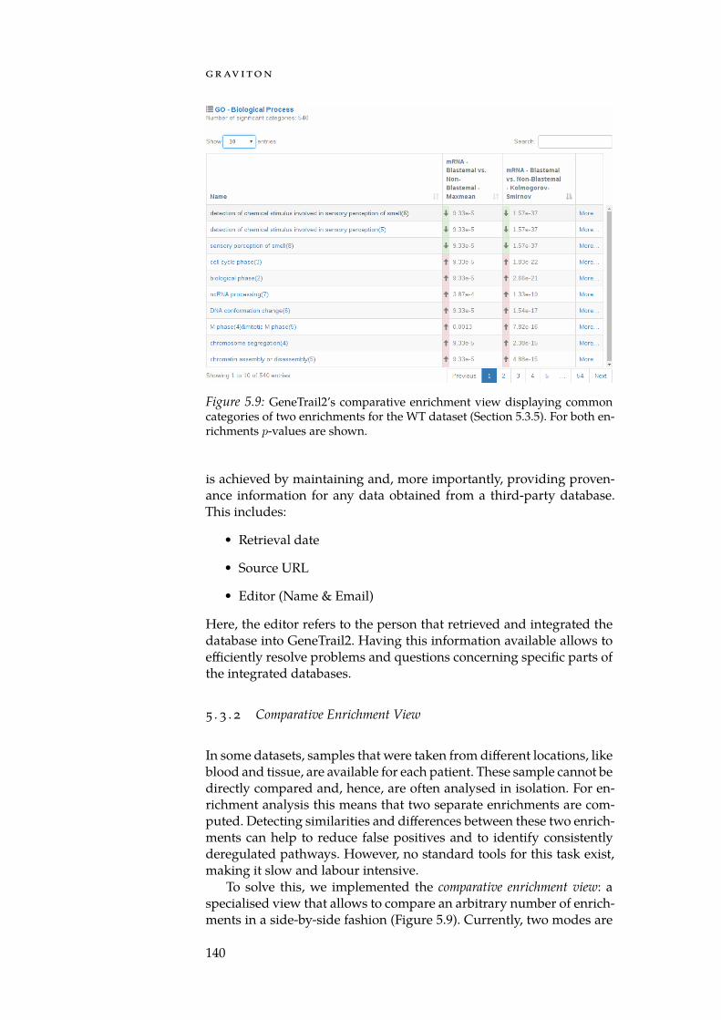
g r av i to n

Figure 5.9: GeneTrail2’s comparative enrichment view displaying commoncategories of two enrichments for the WT dataset (Section 5.3.5). For both en-richments p-values are shown.

is achieved by maintaining and, more importantly, providing proven-ance information for any data obtained from a third-party database.This includes:

• Retrieval date

• Source URL

• Editor (Name & Email)

Here, the editor refers to the person that retrieved and integrated thedatabase into GeneTrail2. Having this information available allows toefficiently resolve problems and questions concerning specific parts ofthe integrated databases.

5 . 3 . 2 Comparative Enrichment View

In some datasets, samples that were taken from different locations, likeblood and tissue, are available for each patient. These sample cannot bedirectly compared and, hence, are often analysed in isolation. For en-richment analysis this means that two separate enrichments are com-puted. Detecting similarities and differences between these two enrich-ments can help to reduce false positives and to identify consistentlyderegulated pathways. However, no standard tools for this task exist,making it slow and labour intensive.

To solve this, we implemented the comparative enrichment view: aspecialised view that allows to compare an arbitrary number of enrich-ments in a side-by-side fashion (Figure 5.9). Currently, two modes are

140

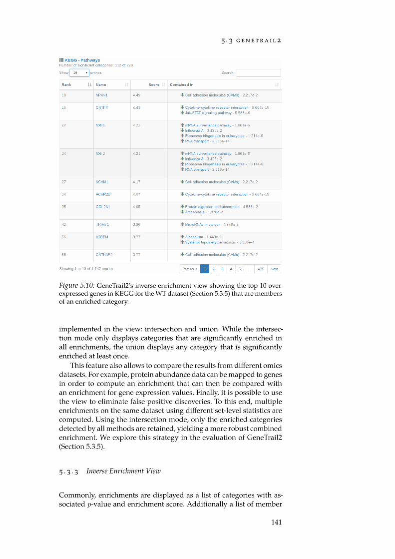
5 . 3 g e n e t r a i l 2

Figure 5.10: GeneTrail2’s inverse enrichment view showing the top 10 over-expressed genes in KEGG for the WT dataset (Section 5.3.5) that are membersof an enriched category.

implemented in the view: intersection and union. While the intersec-tion mode only displays categories that are significantly enriched inall enrichments, the union displays any category that is significantlyenriched at least once.

This feature also allows to compare the results from different omicsdatasets. For example, protein abundance data can be mapped to genesin order to compute an enrichment that can then be compared withan enrichment for gene expression values. Finally, it is possible to usethe view to eliminate false positive discoveries. To this end, multipleenrichments on the same dataset using different set-level statistics arecomputed. Using the intersection mode, only the enriched categoriesdetected by all methods are retained, yielding a more robust combinedenrichment. We explore this strategy in the evaluation of GeneTrail2(Section 5.3.5).

5 . 3 . 3 Inverse Enrichment View

Commonly, enrichments are displayed as a list of categories with as-sociated p-value and enrichment score. Additionally a list of member

141

g r av i to n

Broad GSEA GeneTrail 2

KS entity 400s (± 7.3s) ∗9.3s (± 0.15s)sample 428.8s (± 4.32s) 84.5s (± 0.6s)

Mean entity N/A 3s (±0.02)sample N/A 74.8s (± 1.7s)

Table 5.1: Performance data for enrichments computed on the KEGG cat-egories using the (unweighted) KS and mean set-level statistics. For compar-ison the KS implementation of the Broad GSEA package [Sub+07] was used.Mean run times over five runs are given in seconds; standard deviations areprovided in parenthesis. Both, entity- and sample-based p-value strategieswere measured. In the comparison, the t-test was used as scoring method, nop-value correction has been performed, and 10,000 iterations were used forpermutation tests. Results marked with a ∗ employed an exact p-value com-putation method. Timings were obtained on an Intel Core i7-3770 processor.Table adapted from [Stö+16].

genes is displayed. This view is extremely helpful for quickly identi-fying deregulated processes. Sometimes, however, it is of interest toknow in which deregulated processes a particular gene takes part. An-swering this question using the traditional enrichment representationis tedious. To make this more efficient, we crated the inverse enrichmentview. It shows every gene that is a member of at least one enriched cat-egory together with its entity-level score as well as the categories it iscontained in (Figure 5.10). This allows to conveniently assess the influ-ence of a gene on the computed enrichments.

5 . 3 . 4 Performance

Enrichment analysis is a basic building block for bioinformatics work-flows and, hence, the runtime performance of these methods is crit-ical. To this end, the algorithms included in GeneTrail2 use an effi-cient C++ implementation to guarantee optimal throughput. In gen-eral, the main bottleneck concerning execution time is the computationof p-values. The entity-based strategy commonly executes one order ofmagnitude faster than the sample-based strategy (Table 5.1). For thelatter, the choice of the entity-level statistics can have a significant in-fluence on the computation time, as it needs to be reevaluated for everysample permutation. In contrast, the used set-level statistics has littleinfluence on the overall computation time. GeneTrail2 significantly out-performs the Broad Institute GSEA application [Sub+05] for both, theentity-based and the sample-based strategy (cf. Table 5.1).

5 . 3 . 5 Case study: Wilm’s Tumour

In Section 2.1.1 we introduced Wilm’s tumours (WTs), a type of child-hood renal tumours. Based on the composition of a biopsy after pre-

142

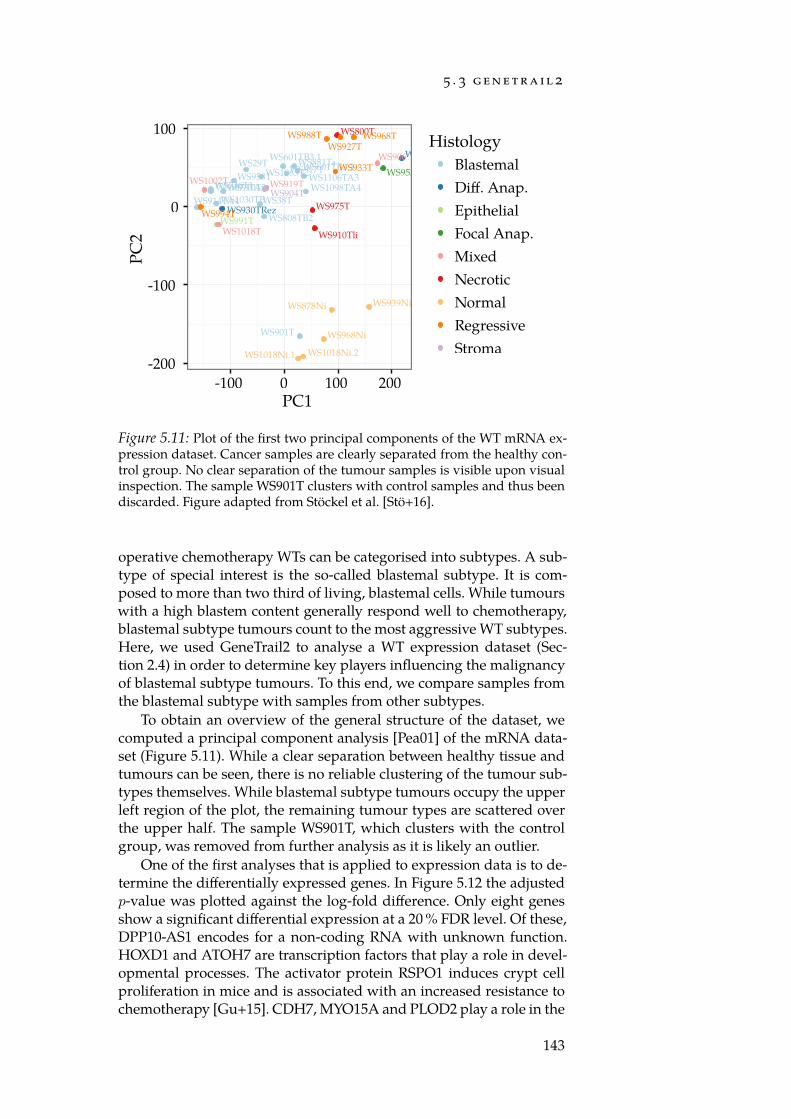
5 . 3 g e n e t r a i l 2

WS29T

WS38T

WS601TB3.1

WS746T1

WS808TB2

WS881TaWS958T

WS914TA4

WS917TWS601TB3.2

WS1030TB

WS1063T2WS1073TA3 WS1098TA4

WS1106TA3

WS901T

WS910Tre

WS800T

WS910Tli

WS975T

WS968TWS927T

WS988T

WS994T

WS933T

WS904T

WS991T

WS1002T

WS1018T

WS906T

WS919T

WS930T

WS930TRez

WS953T

WS878Ni WS939Ni

WS968Ni

WS1018Ni.1 WS1018Ni.2-200

-100

0

100

-100 0 100 200PC1

PC2

HistologyBlastemalDiff. Anap.EpithelialFocal Anap.MixedNecroticNormalRegressiveStroma

Figure 5.11: Plot of the first two principal components of the WT mRNA ex-pression dataset. Cancer samples are clearly separated from the healthy con-trol group. No clear separation of the tumour samples is visible upon visualinspection. The sample WS901T clusters with control samples and thus beendiscarded. Figure adapted from Stöckel et al. [Stö+16].

operative chemotherapy WTs can be categorised into subtypes. A sub-type of special interest is the so-called blastemal subtype. It is com-posed to more than two third of living, blastemal cells. While tumourswith a high blastem content generally respond well to chemotherapy,blastemal subtype tumours count to the most aggressive WT subtypes.Here, we used GeneTrail2 to analyse a WT expression dataset (Sec-tion 2.4) in order to determine key players influencing the malignancyof blastemal subtype tumours. To this end, we compare samples fromthe blastemal subtype with samples from other subtypes.

To obtain an overview of the general structure of the dataset, wecomputed a principal component analysis [Pea01] of the mRNA data-set (Figure 5.11). While a clear separation between healthy tissue andtumours can be seen, there is no reliable clustering of the tumour sub-types themselves. While blastemal subtype tumours occupy the upperleft region of the plot, the remaining tumour types are scattered overthe upper half. The sample WS901T, which clusters with the controlgroup, was removed from further analysis as it is likely an outlier.

One of the first analyses that is applied to expression data is to de-termine the differentially expressed genes. In Figure 5.12 the adjustedp-value was plotted against the log-fold difference. Only eight genesshow a significant differential expression at a 20 % FDR level. Of these,DPP10-AS1 encodes for a non-coding RNA with unknown function.HOXD1 and ATOH7 are transcription factors that play a role in devel-opmental processes. The activator protein RSPO1 induces crypt cellproliferation in mice and is associated with an increased resistance tochemotherapy [Gu+15]. CDH7, MYO15A and PLOD2 play a role in the

143

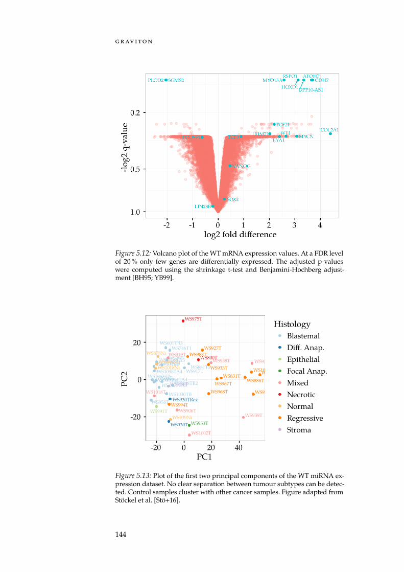
g r av i to n

Figure 5.12: Volcano plot of the WT mRNA expression values. At a FDR levelof 20 % only few genes are differentially expressed. The adjusted p-valueswere computed using the shrinkage t-test and Benjamini-Hochberg adjust-ment [BH95; YB99].

WS601TB3

WS901T

WS1063T2

WS1073TA3

WS1106TA3

WS917TWS1098TA4

WS808TB2

WS958T

WS746T1

WS38T

WS881Ta

WS914TA4

WS1030TB

WS29T

WS910Tre

WS910TliB

WS967TWS968T

WS1001TWS831T WS878T

WS927T

WS933T

WS886T

WS954T

WS988T

WS994T

WS878Ni

WS939Ni

WS968NiWS1018Ni

WS1002T

WS1018T

WS938T

WS906T

WS919TWS938Trez

WS939T

WS930T

WS930TRez

WS953T

WS800T

WS975T

WS991T

WS904T

-20

0

20

-20 0 20 40PC1

PC2

HistologyBlastemalDiff. Anap.EpithelialFocal Anap.MixedNecroticNormalRegressiveStroma

Figure 5.13: Plot of the first two principal components of the WT miRNA ex-pression dataset. No clear separation between tumour subtypes can be detec-ted. Control samples cluster with other cancer samples. Figure adapted fromStöckel et al. [Stö+16].

144

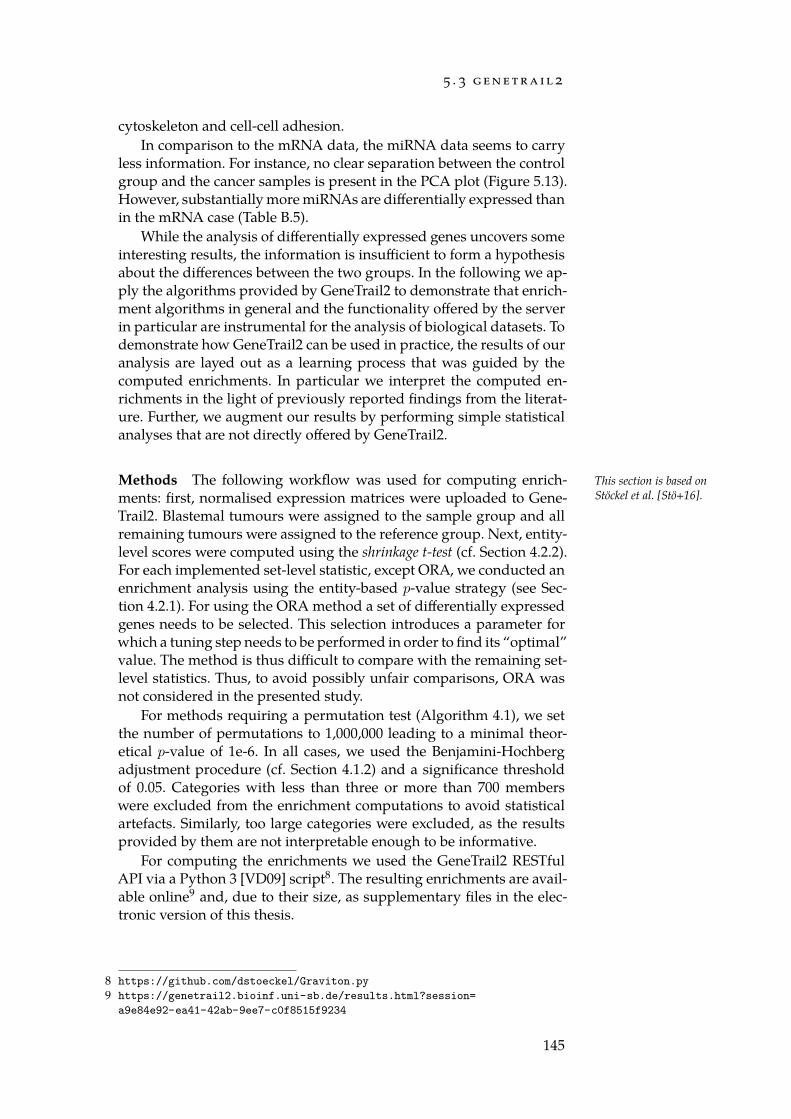
5 . 3 g e n e t r a i l 2

cytoskeleton and cell-cell adhesion.In comparison to the mRNA data, the miRNA data seems to carry

less information. For instance, no clear separation between the controlgroup and the cancer samples is present in the PCA plot (Figure 5.13).However, substantially more miRNAs are differentially expressed thanin the mRNA case (Table B.5).

While the analysis of differentially expressed genes uncovers someinteresting results, the information is insufficient to form a hypothesisabout the differences between the two groups. In the following we ap-ply the algorithms provided by GeneTrail2 to demonstrate that enrich-ment algorithms in general and the functionality offered by the serverin particular are instrumental for the analysis of biological datasets. Todemonstrate how GeneTrail2 can be used in practice, the results of ouranalysis are layed out as a learning process that was guided by thecomputed enrichments. In particular we interpret the computed en-richments in the light of previously reported findings from the literat-ure. Further, we augment our results by performing simple statisticalanalyses that are not directly offered by GeneTrail2.

Methods The following workflow was used for computing enrich- This section is based onStöckel et al. [Stö+16].ments: first, normalised expression matrices were uploaded to Gene-

Trail2. Blastemal tumours were assigned to the sample group and allremaining tumours were assigned to the reference group. Next, entity-level scores were computed using the shrinkage t-test (cf. Section 4.2.2).For each implemented set-level statistic, except ORA, we conducted anenrichment analysis using the entity-based p-value strategy (see Sec-tion 4.2.1). For using the ORA method a set of differentially expressedgenes needs to be selected. This selection introduces a parameter forwhich a tuning step needs to be performed in order to find its “optimal”value. The method is thus difficult to compare with the remaining set-level statistics. Thus, to avoid possibly unfair comparisons, ORA wasnot considered in the presented study.

For methods requiring a permutation test (Algorithm 4.1), we setthe number of permutations to 1,000,000 leading to a minimal theor-etical p-value of 1e-6. In all cases, we used the Benjamini-Hochbergadjustment procedure (cf. Section 4.1.2) and a significance thresholdof 0.05. Categories with less than three or more than 700 memberswere excluded from the enrichment computations to avoid statisticalartefacts. Similarly, too large categories were excluded, as the resultsprovided by them are not interpretable enough to be informative.

For computing the enrichments we used the GeneTrail2 RESTfulAPI via a Python 3 [VD09] script8. The resulting enrichments are avail-able online9 and, due to their size, as supplementary files in the elec-tronic version of this thesis.

8 https://github.com/dstoeckel/Graviton.py9 https://genetrail2.bioinf.uni-sb.de/results.html?session=

a9e84e92-ea41-42ab-9ee7-c0f8515f9234

145

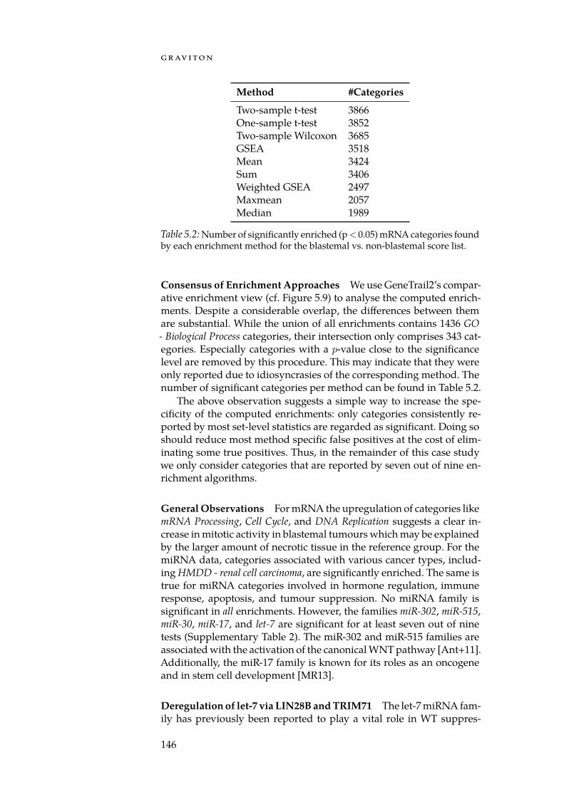
g r av i to n

Method #Categories

Two-sample t-test 3866One-sample t-test 3852Two-sample Wilcoxon 3685GSEA 3518Mean 3424Sum 3406Weighted GSEA 2497Maxmean 2057Median 1989

Table 5.2: Number of significantly enriched (p< 0.05) mRNA categories foundby each enrichment method for the blastemal vs. non-blastemal score list.

Consensus of Enrichment Approaches We use GeneTrail2’s compar-ative enrichment view (cf. Figure 5.9) to analyse the computed enrich-ments. Despite a considerable overlap, the differences between themare substantial. While the union of all enrichments contains 1436 GO- Biological Process categories, their intersection only comprises 343 cat-egories. Especially categories with a p-value close to the significancelevel are removed by this procedure. This may indicate that they wereonly reported due to idiosyncrasies of the corresponding method. Thenumber of significant categories per method can be found in Table 5.2.

The above observation suggests a simple way to increase the spe-cificity of the computed enrichments: only categories consistently re-ported by most set-level statistics are regarded as significant. Doing soshould reduce most method specific false positives at the cost of elim-inating some true positives. Thus, in the remainder of this case studywe only consider categories that are reported by seven out of nine en-richment algorithms.

General Observations For mRNA the upregulation of categories likemRNA Processing, Cell Cycle, and DNA Replication suggests a clear in-crease in mitotic activity in blastemal tumours which may be explainedby the larger amount of necrotic tissue in the reference group. For themiRNA data, categories associated with various cancer types, includ-ing HMDD - renal cell carcinoma, are significantly enriched. The same istrue for miRNA categories involved in hormone regulation, immuneresponse, apoptosis, and tumour suppression. No miRNA family issignificant in all enrichments. However, the families miR-302, miR-515,miR-30, miR-17, and let-7 are significant for at least seven out of ninetests (Supplementary Table 2). The miR-302 and miR-515 families areassociated with the activation of the canonical WNT pathway [Ant+11].Additionally, the miR-17 family is known for its roles as an oncogeneand in stem cell development [MR13].

Deregulation of let-7 via LIN28B and TRIM71 The let-7 miRNA fam-ily has previously been reported to play a vital role in WT suppres-

146

5 . 3 g e n e t r a i l 2

TRIM71 LIN28Blet-7family

CDKN1AmiR-290/miR-302families

Differentiation

+u

G1-S CellCycle

TCF3

Figure 5.14: TRIM71 degrades LIN28B using ubiquitin-mediatedproteosomal degradation. LIN28B regulates the maturation of let-7miRNAs [Pis+11], which promote cell differentiation and act on TRIM71 andLIN28B via a negative feedback loop [Mar+08b]. TRIM71 as well as AGO2 incomplex with miR-290/302 miRNAs repress CDKN1A expression leadingto increased proliferation [Lee+14]. TCF3 acts on most of the above players[Mar+08b], effectively amplifying the currently predominant signal in thefeedback loop. Figure adapted from Stöckel et al. [Stö+16].

miRNA t Effect Size

hsa-let-7f-5p 3.858 792.184hsa-let-7a-5p 3.486 1622.645hsa-let-7g-5p 2.834 199.181hsa-let-7e-5p 2.566 94.476hsa-let-7d-5p 2.273 15.424

Table 5.3: Significantly upregulated let-7 miRNA family members. t is thevalue of the shrinkage t-statistic as computed by GeneTrail2. The effect sizeis the difference between the unlogarithmised means of the sample and refer-ence groups.

sion [Urb+14]. However, many highly abundant family members areupregulated (see Table 5.3), which is unexpected due to let-7 miRNAsacting as tumour suppressors. A possible explanation for this beha-viour may be the differential expression of TRIM71, which is amongthe top-scoring genes (t ≈ 3.96) and has the highest correlation of allgenes with the absolute blasteme content r ≈ 0.76. TRIM71 degradesLIN28B via ubiquitin-mediated proteosomal degradation [Lee+14] (cf.Figure 5.14). However, LIN28B in turn suppresses the maturation ofpri-let-7 miRNA. Hence, the upregulation of TRIM71 induces an up-regulation of the let-7 family, which, in theory, promotes cell differen-tiation [Urb+14]. However, Chang et al. [Cha+12] found that TRIM71can promote rapid embryonic stem cell (ESC) proliferation in mice andreport that it inhibits the expression of CDKN1A, a cyclin-dependentkinase inhibitor, which acts as a cell-cycle regulator. As high expression

147

g r av i to n

Normal NE Regressive E S FA DA Mixed Blastemal

−10

0

10

20

WS10

18Ni.1

WS10

18Ni.2

WS87

8Ni

WS93

9Ni

WS96

8Ni

WS80

0TW

S975T

WS93

3TW

S988T

WS96

8TW

S927T

WS99

4TW

S991T

WS90

4TW

S953T

WS93

0TW

S906T

WS91

9TW

S1018

TW

S1002

TW

S1030

TBW

S1063

T2W

S1073

TA3

WS10

98TA

4W

S1106

TA3

WS29

TW

S38T

WS60

1TB3.1

WS60

1TB3.2

WS74

6T1

WS80

8TB2

WS88

1Ta

WS90

1TW

S914T

A4W

S917T

WS95

8T

expr

essi

onLegend

CITED1EYA1SIX2LIN28BTRIM71

Figure 5.15: Expression of TRIM71 and LIN28B in comparison with the capmesenchyme stem cell markers CITED1, EYA1, and SIX2. Samples are classi-fied as normal, necrotic (NE), regressive, epithelial (E), stromal (S), focal anaplasia(FA), diffuse anaplasia (DA), mixed, and blastemal. The size of a coloured barrepresents the absolute expression value of the associated gene. Figure takenfrom Stöckel et al. [Stö+16].

levels of TRIM71 are commonly observed in undifferentiated cells, theauthors conclude that TRIM71 is an important factor for maintainingproliferation in stem cells. Urbach et al. [Urb+14] report that LIN28Bis able to induce WTs under certain conditions and note that in thesetumour the cap mesenchymal (CM) specific stem cell markers CITED1,EYA1, and SIX2 are upregulated. Generally, this trend is present in ourdata, however, we find that the expression of the markers is more con-sistent with TRIM71’s expression pattern (Figure 5.15). In summary,our initial results indicate that miRNA and genes associated with stemcell fate play an essential role in blastemal tumours.

Activation of cancer related WNT signalling Deregulation of theWNT signalling pathway is often prevalent in cancer samples [Pol12].Indeed, our enrichment analysis contains categories associated withthe WNT pathway (see Supplementary Table 1). This is especially vis-ible in the inverse enrichment view (Section 5.3.3). There it becomesapparent that the previously discussed RSPO1 is a member of mul-tiple, upregulated categories directly associated with WNT signalling(cf. Table 5.4). RSPO1 has been reported to regulate the WNT pathwayvia inhibition of ZNRF3 [Hao+12] and DKK1 [Kim+08]. In fact, DKK1is downregulated in blastemal tumours, suggesting that the overex-pression of RSPO1 may causally affect the measured expression signa-ture. In addition, signalling molecules activated by RSPO1 have beenshown to be sufficient for the induction of ovarian cancer [Zho+16].

148

5 . 3 g e n e t r a i l 2

Category p-value

Positive regulation of canonical WNT signaling pathway 1.144e-2Regulation of WNT signaling pathway 1.062e-3Regulation of canonical WNT signaling pathway 1.529e-2Regulation of endocytosis 3.340e-2Canonical WNT signaling pathway 8.367e-3Non-canonical WNT signaling pathway 1.756e-3Positive regulation of WNT signaling pathway 2.775e-3Receptor mediated endocytosis 4.959e-2

Table 5.4: Enriched categories for RSPO1. The gene is one of the most dereg-ulated genes in the blastemal vs. non-blastemal comparison (t ≈ 5.17) andplays a role in the activation of WNT signalling.

Besides RSPO1, other members of the WNT signalling pathway suchas TCF21 can be found via the inverse enrichment view. These resultsare consistent with the pathway’s previously reported, prominent rolein most WTs and particularly in blastemal WTs [Fuk+09]. The activa-tion of the canonical WNT pathway usually leads to degradation ofthe destruction complex that, as long as it is functional, degrades thetranscriptional coactivator β-catenin [SW13]. Thus degradation of thedestruction complex leads to higher amounts of β-catenin in the cyto-plasm that is transported to the nucleus where it builds complexes withTCF/LEF proteins. Degradation of the destruction complex lies at thecore of developmental processes, ESC self-renewal, and differentiation.As a result, it changes the transcriptional landscape of the cell dramatic-ally. This is also consistent with reports that RSPO1 activates β-cateninin mammalian ovaries thereby controlling the differentiation process[Cha+08].

TCF3 as potential WT master regulator We argued that factors asso-ciated with stem cell fate and the canonical WNT pathway play an essen-tial role in blastemal tumours. To further substantiate this claim we takea closer look at TCF21. TCF21 has been reported to bind the transcrip-tion factor (TF) TCF3, thereby inhibiting the expression of the KISS1, aknown metastasis suppressor [Ara+11]. TCF3 itself is a well known linkbetween the WNT pathway and the core regulatory circuitry of ESCs.Together with the pluripotency factors POU5F1 (OCT4), NANOG, andSOX2, TCF3 constitutes the set of “ESC master regulators” [Col+08]. Ifthe WNT pathway is inactive, TCF3 is mainly repressing pluripotencyfactors and promoting differentiation. However, if the WNT pathwayis activated, the repressive complex converts to an activating complex,promoting pluripotency [Col+08]. To study the influence of ESC masterregulators, we constructed a new set of gene categories that we subjec-ted to the KS test using the blastemal vs. non-blastemal scores as input.For each of the four TFs, we defined two categories containing genesfor which “strong evidence” exists that they are regulated by the re-spective TF. In particular, we add a gene to a category for a TF if the

149

g r av i to n

Gene Correlation Gene Correlation

BMI1 0.91 CCND2 0.75CDK4 0.83 EYA1 0.91HMGA2 0.75 IGF2 0.89LEFTY1 0.74 MAX -0.76MEIS1 0.68 MYC -0.57MYCN 0.86 NOTCH1 0.6SMAD3 0.74 TP53 0.76TRIM71 0.65

Table 5.5: Pearson correlation coefficient between the expression values of aset of selected genes and TCF3.

TF occupies a site in the gene’s promoter region and the correlationbetween the TF’s and the gene’s expression is larger than 0.5 (positivecategory) or smaller than -0.5 (negative category). For the identifica-tion of the promoters occupied by the master regulators, we used themouse ESC ChIP-Chip dataset of Cole et al. [Col+08] and the ChIP-Seqdata set of Marson et al. [Mar+08b]. Using this procedure we obtainedmore than 1500 genes, including many other TFs and genes involvedin ESC fate, influenced by mainly TCF3 and OCT4. For a selection seeTable 5.5. Our Kolmogorov-Smirnov enrichment10 revealed that genespositively regulated by TCF3 (p ≈ 10−40) and NANOG (p ≈ 10−13)are strongly enriched, whereas genes negatively regulated by TCF3(p ≈ 10−40) are strongly depleted. Conversely, genes positively regu-lated by OCT4 are strongly depleted, and genes negatively regulatedby OCT4 are strongly enriched. This is consistent with a correlation ofTCF3 with OCT4 of −0.7. SOX2 and NANOG both seem to be of lesserimportance in our data.

However, the four master regulators do not only regulate proteincoding genes. Marson et al. [Mar+08b] revealed that they are also “as-sociated with promoters for miRNAs that are preferentially expressedin ESCs”. Examples are the miR-302, miR-515, and let-7 families whichwe previously discussed (cf. Figure 5.14). Additionally, our data indic-ates that TCF3 regulates the expression of the miR-17 cluster (all cor-relations > 0.5).

IGF2 as Putative WNT Activator In the above section, we have out-lined how the ESC regulatory circuitry is driven by TCF3 via the WNTpathway. However, the mechanisms that activate WNT signalling stillremain unclear. Whereas certain genetic mutations occur with relat-ively low frequency (≤ 30 %), among them genes that may induce WNTsignalling, the loss of heterozygosity and imprinting at the IGF2/H19locus have been reported for 81 % of all blastemal WTs [Weg+15] lead-ing to an overexpression of IGF2. Morali et al. [Mor+01] showed thatIGF2 can induce the expression and import of β-catenin and TCF3 into

10 https://genetrail2.bioinf.uni-sb.de/results.html?session=cbc86903-4248-47a2-b916-bc682924c242

150

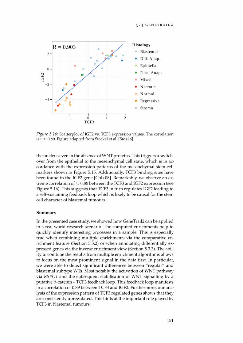
5 . 3 g e n e t r a i l 2

R = 0.903

−4

−2

0

2

−1 0 1 2TCF3

IGF2

Histology

Blastemal

Diff. Anap.

Epithelial

Focal Anap.

Mixed

Necrotic

Normal

Regressive

Stroma

Figure 5.16: Scatterplot of IGF2 vs. TCF3 expression values. The correlationis r ≈ 0.89. Figure adapted from Stöckel et al. [Stö+16].

the nucleus even in the absence of WNT proteins. This triggers a switch-over from the epithelial to the mesenchymal cell state, which is in ac-cordance with the expression patterns of the mesenchymal stem cellmarkers shown in Figure 5.15. Additionally, TCF3 binding sites havebeen found in the IGF2 gene [Col+08]. Remarkably, we observe an ex-treme correlation of ≈ 0.89 between the TCF3 and IGF2 expression (seeFigure 5.16). This suggests that TCF3 in turn regulates IGF2 leading toa self-sustaining feedback loop which is likely to be causal for the stemcell character of blastemal tumours.

Summary

In the presented case study, we showed how GeneTrail2 can be appliedin a real world research scenario. The computed enrichments help toquickly identify interesting processes in a sample. This is especiallytrue when combining multiple enrichments via the comparative en-richment feature (Section 5.3.2) or when annotating differentially ex-pressed genes via the inverse enrichment view (Section 5.3.3). The abil-ity to combine the results from multiple enrichment algorithms allowsto focus on the most prominent signal in the data first. In particular,we were able to detect significant differences between “regular” andblastemal subtype WTs. Most notably the activation of WNT pathwayvia RSPO1 and the subsequent stabilisation of WNT signalling by aputative β-catenin – TCF3 feedback loop. This feedback loop manifestsin a correlation of 0.89 between TCF3 and IGF2. Furthermore, our ana-lysis of the expression pattern of TCF3 regulated genes shows that theyare consistently upregulated. This hints at the important role played byTCF3 in blastemal tumours.

151

g r av i to n

5 . 4 n e t wo r k t r a i l

Contributions The NetworkTrail web service and the applicationnote [Stö+13] was written by Oliver Müller and me. Tim Kehlcreated the site design and implemented the Cytoscape.js visual-isation, the scoring methods, and the FiDePa algorithm. AndreasGerasch implemented the BiNA visualisation plugin.

The deregulation of signalling pathways plays an important role dur-ing tumour development (cf. Section 2.1). Enrichment methods allowto search for deregulated pathways but treat them as “bags of genes”(Chapter 4). This neglects the interaction data that is stored in pathwaydatabases. However, methods that exploit this information to improvetheir accuracy by explicitly taking network structure into account exist.In Section 3.5 we previously discussed some of the available methodsfor detecting deregulated subgraphs. As an example, we presented thetheory around the approach by Backes et al. [Bac+12]. Here, we focuson the practical side and present NetworkTrail, a webservice for detect-ing deregulated subgraphs which we built using the Graviton frame-work. We start with a short survey of available software packages fordetecting deregulated subnetworks.

5 . 4 . 1 Software for Searching Deregulated Subgraphs

The simulated-annealing-based method of Ideker et al. [Ide+02] forthe detection of active subgraphs is available as a Cytoscape [Sha+03]plug-in. The BioNet software developed by Dittrich et al. [Dit+08] canbe downloaded as a R package [R C16], which implements an exactsolver for the prize-collecting Steiner-Tree problem. The algorithms de-veloped by Keller et al. [Kel+09] and Dao et al. [Dao+11] are providedas C++ source code. The original implementation of the ILP proposedby Backes et al. [Bac+12] is available as an executable.

The majority of the tools above does neither provide a graphical userinterface (GUI) nor an option to visualise the resulting subgraphs dir-ectly. Instead, most need to be executed from the command line andthe produced output needs to be processed using third party packages.Thus, besides installing the software properly, users are also requiredto possess intricate technical knowledge of the complete tool chain.According to our experiences, both tasks can be challenging for non-expert users. As we argued at the beginning of this chapter, a commonstrategy to prevent these problems is to make the tool accessible via aweb interface. The same line of reasoning not only holds for enrichmentmethods, but also for algorithms that detect deregulated subnetworks.The HotNet algorithm [VUR11], for instance, is accessible as MATLABsource code and via a basic web interface. Also, List et al. [Lis+16] madethe KeyPathwayMiner algorithm [Alc+11; Alc+14] available as a webservice.

152

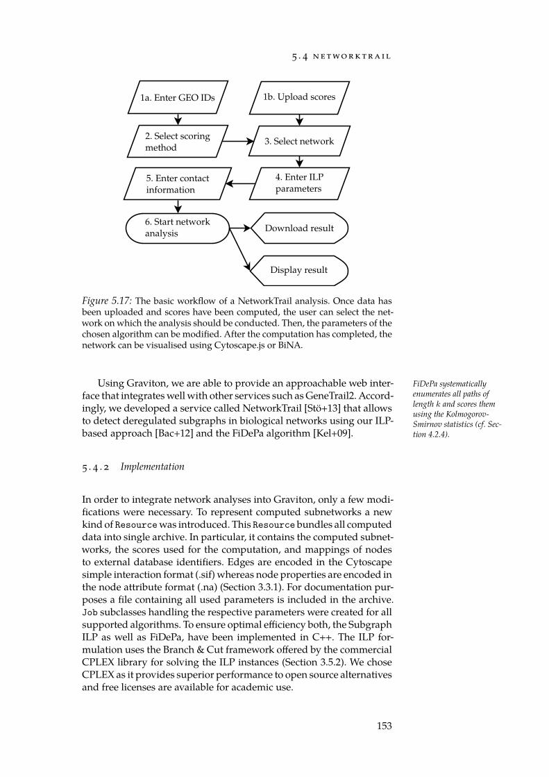
5 . 4 n e t wo r k t r a i l

1a. Enter GEO IDs 1b. Upload scores

2. Select scoringmethod

3. Select network

4. Enter ILPparameters

5. Enter contactinformation

6. Start networkanalysis Download result

Display result

Figure 5.17: The basic workflow of a NetworkTrail analysis. Once data hasbeen uploaded and scores have been computed, the user can select the net-work on which the analysis should be conducted. Then, the parameters of thechosen algorithm can be modified. After the computation has completed, thenetwork can be visualised using Cytoscape.js or BiNA.

Using Graviton, we are able to provide an approachable web inter- FiDePa systematicallyenumerates all paths oflength k and scores themusing the Kolmogorov-Smirnov statistics (cf. Sec-tion 4.2.4).

face that integrates well with other services such as GeneTrail2. Accord-ingly, we developed a service called NetworkTrail [Stö+13] that allowsto detect deregulated subgraphs in biological networks using our ILP-based approach [Bac+12] and the FiDePa algorithm [Kel+09].

5 . 4 . 2 Implementation

In order to integrate network analyses into Graviton, only a few modi-fications were necessary. To represent computed subnetworks a newkind of Resourcewas introduced. This Resource bundles all computeddata into single archive. In particular, it contains the computed subnet-works, the scores used for the computation, and mappings of nodesto external database identifiers. Edges are encoded in the Cytoscapesimple interaction format (.sif) whereas node properties are encoded inthe node attribute format (.na) (Section 3.3.1). For documentation pur-poses a file containing all used parameters is included in the archive.Job subclasses handling the respective parameters were created for allsupported algorithms. To ensure optimal efficiency both, the SubgraphILP as well as FiDePa, have been implemented in C++. The ILP for-mulation uses the Branch & Cut framework offered by the commercialCPLEX library for solving the ILP instances (Section 3.5.2). We choseCPLEX as it provides superior performance to open source alternativesand free licenses are available for academic use.

153

g r av i to n

5 . 4 . 3 Workflow

With Graviton, NetworkTrail and GeneTrail2 share a common basis.An overview over anexample workflow isgiven in Figure 5.17.

Thus, the accepted input formats are, to a large degree, the same (cf.Section 5.3). As input, a list of entity-level scores is required, which caneither be uploaded directly or computed from an expression matrix ora Gene Expression Omnibus (GEO) [EDL02] record. Once scores are avail-able, the user can select the network that should be used for the ana-lysis. Next, for both implemented algorithms, a range of desired sub-network sizes can be entered. Subsequently, the algorithm computesthe maximally deregulated subnetwork.

The result can be visualised using a custom, Cytoscape.js [Fra+16]based view or the Biological Network Analyzer [Ger+14]. Both tools dis-play the union of all computed subgraphs using a hierarchical layout.Detailed information about each node is available. For genes, knownaliases and references to external databases are displayed. For proteinfamilies and complexes the respective members are shown recursively.The subnetworks for specific values of k can be highlighted individu-ally. The degree of deregulation of each node is indicated by its colour.White represents no change and shades of red and green represent up-and downregulation, respectively. Moreover, the BiNA based visualisa-tion permits the complete customisation of the visualisation, includinglayout, colours, and node styles (cf. Figure 5.18).

5 . 4 . 4 The KEGG Regulatory Network

The KEGG database [KG00; Kan+10b; Kan+06] is a comprehensive cata-logue of regulatory and metabolic processes (Section 3.2.1). Similar toother pathway databases such as Reactome [Jos+05] and WikiPathways[Kel+12] it is structured into pathways that describe a specific biolo-gical process in detail. We extracted the regulatory information con-tained in KEGG to create a complete regulatory network. To under-stand this process it is important to know how KEGG structures itsinformation. Each pathway is described by a file in the KGML format.Every file contains the pathway’s nodes as well as their interactions. Ingeneral three node types can be distinguished:

Gene A gene, unsurprisingly, represents a single gene.

Family A family represents a group of genes. Each of the genes in afamily are able to perform the interactions the node is a part of.

Complex A complex represents a group of genes or smaller complexesthat must form a physical complex before they can take part inspecific interactions.

Each interaction is labelled with an interaction type. This can beactivation, inhibition, genomic interaction, or association events. Addi-tional modifiers, such as indicators for phosphorylation and ubiquit-ination, can be attached to each edge. It also possible that complexes

154

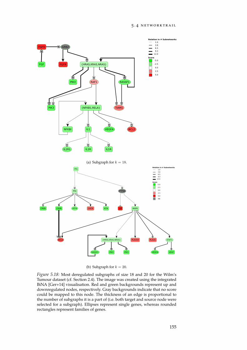
5 . 4 n e t wo r k t r a i l

(a) Subgraph for k = 18.

NA

(b) Subgraph for k = 20.

Figure 5.18: Most deregulated subgraphs of size 18 and 20 for the Wilm’sTumour dataset (cf. Section 2.4). The image was created using the integratedBiNA [Ger+14] visualisation. Red and green backgrounds represent up anddownregulated nodes, respectively. Gray backgrounds indicate that no scorecould be mapped to this node. The thickness of an edge is proportional tothe number of subgraphs it is a part of (i.e. both target and source node wereselected for a subgraph). Ellipses represent single genes, whereas roundedrectangles represent families of genes.

155

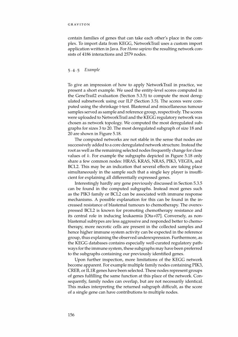
g r av i to n

contain families of genes that can take each other’s place in the com-plex. To import data from KEGG, NetworkTrail uses a custom importapplication written in Java. For Homo sapiens the resulting network con-sists of 4186 interactions and 2579 nodes.

5 . 4 . 5 Example

To give an impression of how to apply NetworkTrail in practice, wepresent a short example. We used the entity-level scores computed inthe GeneTrail2 evaluation (Section 5.3.5) to compute the most dereg-ulated subnetwork using our ILP (Section 3.5). The scores were com-puted using the shrinkage t-test. Blastemal and miscellaneous tumoursamples served as sample and reference group, respectively. The scoreswere uploaded to NetworkTrail and the KEGG regulatory network waschosen as network topology. We computed the most deregulated sub-graphs for sizes 3 to 20. The most deregulated subgraph of size 18 and20 are shown in Figure 5.18.

The computed networks are not stable in the sense that nodes aresuccessively added to a core deregulated network structure. Instead theroot as well as the remaining selected nodes frequently change for closevalues of k. For example the subgraphs depicted in Figure 5.18 onlyshare a few common nodes: HRAS, KRAS, NRAS, PIK3, VEGFA, andBCL2. This may be an indication that several effects are taking placesimultaneously in the sample such that a single key player is insuffi-cient for explaining all differentially expressed genes.

Interestingly hardly any gene previously discussed in Section 5.3.5can be found in the computed subgraphs. Instead most genes suchas the PIK3 family or BCL2 can be associated with immune responsemechanisms. A possible explanation for this can be found in the in-creased resistance of blastemal tumours to chemotherapy. The overex-pressed BCL2 is known for promoting chemotherapy resistance andits central role in inducing leukaemia [Ota+07]. Conversely, as non-blastemal subtypes are less aggressive and responded better to chemo-therapy, more necrotic cells are present in the collected samples andhence higher immune system activity can be expected in the referencegroup, thus explaining the observed underexpression. Furthermore, asthe KEGG databases contains especially well-curated regulatory path-ways for the immune system, these subgraphs may have been preferredto the subgraphs containing our previously identified genes.

Upon further inspection, more limitations of the KEGG networkbecome apparent. For example multiple family nodes containing PIK3,CREB, or IL1R genes have been selected. These nodes represent groupsof genes fulfilling the same function at this place of the network. Con-sequently, family nodes can overlap, but are not necessarily identical.This makes interpreting the returned subgraph difficult, as the scoreof a single gene can have contributions to multiple nodes.

156

5 . 5 d ru g ta rg e t i n s p e c to r

5 . 4 . 6 Summary

Here, we presented NetworkTrail, a web service for detecting deregu-lated subnetworks in biological network data. The availability of such aweb service allows non-experts to carry out network analyses withouthaving to struggle with technical details such as compiling/installingsoftware or learning cryptic commands. We are convinced that sucheasy-to-use web services will help to elucidate pathogenic mechanismsand that they may also proof useful for therapy stratification in cancertherapy. Our example showed that NetworkTrail makes computing de-regulated subgraphs simple. The integration with GeneTrail2 allows todirectly reuse scores that were used for computing enrichments. How-ever, the limiting factor of the analysis is the underlying network. Dueto the topology of KEGG, some pathways seem to be preferred overother parts of the network (cf. Section 3.5.3). Also, the concept of fam-ily nodes and, to a lesser extent, complexes makes arguing about thenetwork difficult. In the future, NetworkTrail will be enhanced by in-cluding further analysis methods and more complete, predefined net-works.

5 . 5 d ru g ta rg e t i n s p e c to r

Contributions DrugTargetInspector [Sch+15] was implementedby Lara Schneider with design input and code review by me. An-dreas Gerasch implemented the BiNA visualisation plugin.

As outlined in Section 2.2, a detailed understanding of a tumour’s mo-lecular properties can be essential for optimising the treatment for apatient. To this end, biological high throughput assays can providevaluable information complementing the classical, histological exam-ination of a biopsy. For example, gene expression profiles allow to de-tect parts of the metabolism that are deregulated in tumour cells whencompared to healthy tissue (cf. Section 2.3). Mutations can dramatic-ally alter the function of a protein or even lead to the creation of new,fusion proteins [Sod+07]. Also, mutations in untranslated parts of thegenome can result in increased or decreased transcriptional efficienciesfor a gene as enhancer or promoter regions my be impacted [Lei+95;WKG83; BSM93]. Thus, knowledge about the mutations accumulatedby a tumour can provide critical information necessary for interpretingthe obtained expression patterns. Furthermore, epigenetic marks, suchas methylation and histone occupancies, may prove useful for augment-ing the knowledge derived from the mutation data. Finally, proteinabundances can give a more detailed picture about the actual physiolo-gical processes that are taking place in a tumour cell. Making sense outof this host of information is a difficult task. For a physician trying todetermine the optimal treatment for a patient, a succinct summary of

157

g r av i to n

the data can serve as a stepping stone for assessing treatment options.As previously discussed, enrichment methods are a useful tool to focuson essential pathogenic processes. Nevertheless, an enrichment doesnot provide a quick way to determine possible treatment options. In-stead, a considerable amount of work is required to interpret the com-puted results. For each category, it must be determined whether thecorresponding biological process is of clinical relevance. If this is thecase, the reason why the category is reported as significant needs to bedetermined. In particular it is important to identify potential key play-ers that are e.g. differentially expressed and are the target of a cancerdrug. To do so requires substantial time and expertise. We thus arguethat enrichments alone are a suboptimal starting point for selecting atreatment.

As an alternative, we created the DrugTargetInspector (DTI) webservice [Sch+15]. DTI integrates expression and mutation data as wellas the knowledge about available (anticancer) drugs and establishedtreatment regimes into a condensed, single-page overview. Startingfrom this overview, additional information can be accessed and ad-vanced analyses can be performed. The service is built on top of theGraviton framework (Section 5.2) and, hence, integrates tightly withGeneTrail2 (Section 5.3) and NetworkTrail (Section 5.4).

In the following, we give a detailed explanation of DTI’s features.We start with the information directly visible in the main view. After-wards we discuss additional information that can be accessed via ana-lyses. Finally, we describe DTI’s integration into GeneTrail2, Network-Trail, and the BiNA network visualisation tool.

5 . 5 . 1 Integrated Databases

A key feature of DTI is the aggregation of information from externaldatabases into an internal storage. For each case, DTI uses this know-ledge base to identify pieces of information that are relevant for thesamples which are currently being examined. This information is thendisplayed in a succinct summary. Here, we shortly discuss the integ-rated databases. As the primary data source we use DrugBank [Wis+06].The database entries for a wide range of drugs including the knowntargets for each drug. We use this information to classify drugs intocategories such as cancer drugs, vitamins, or inhibiting drugs and to as-sign them to their target genes. The list of recommended drugs for eachcancer type was obtained from the American Cancer Society (ACS)11. Tobe able to better assess the influence of a mutation on the efficacy of adrug we incorporated the pharmacogenomics data provided by the Ge-nomics of Drug Sensitivity in Cancer (GDSC) project [Gar+12]. Informa-tion about each gene is provided by the Entrez Gene database [Mag+05].For each drug–gene combination, links to relevant PubMed [Med97]publications are displayed.

11 http://www.cancer.org/

158

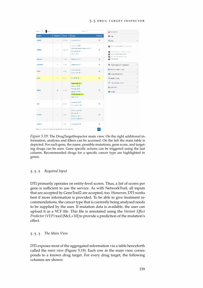
5 . 5 d ru g ta rg e t i n s p e c to r

Figure 5.19: The DrugTargetInspector main view. On the right additional in-formation, analyses and filters can be accessed. On the left the main table isdepicted. For each gene, the name, possible mutations, gene score, and target-ing drugs can be seen. Gene specific actions can be triggered using the lastcolumn. Recommended drugs for a specific cancer type are highlighted ingreen.

5 . 5 . 2 Required Input

DTI primarily operates on entity-level scores. Thus, a list of scores pergene is sufficient to use the service. As with NetworkTrail, all inputsthat are accepted by GeneTrail2 are accepted, too. However, DTI worksbest if more information is provided. To be able to give treatment re-commendations, the cancer type that is currently being analysed needsto be supplied by the user. If mutation data is available, the user canupload it as a VCF file. This file is annotated using the Variant EffectPredictor (VEP) tool [McL+10] to provide a prediction of the mutation’seffect.

5 . 5 . 3 The Main View

DTI exposes most of the aggregated information via a table henceforthcalled the main view (Figure 5.19). Each row in the main view corres-ponds to a known drug target. For every drug target, the followingcolumns are shown:

159

g r av i to n

Target Name the HGNC symbol of the drug target. For each gene alink to the respective Entrez Gene [Mag+05] site is provided.

Mutations Indicates whether mutations for this gene were found. Ifso, the detected mutations can be accessed by hovering over thedisplayed symbol.

Score The degree of differential expression between the sample andthe reference.

Corresponding Drugs Drugs known to target the current gene.

Analyses Further, gene-specific analyses can be performed by clickingon the displayed symbol.

Rows in the main view can be sorted in ascending as well as des-cending order according to the “Target Name” and “Score” column.Filtering for specific genes or drugs is possible using a search field.For each drug a link to its DrugBank page as well as a link to relevantPubMed [Med97] entries is available. Drugs can be shown or hiddenbased on whether they are cancer relevant, inhibiting, vitamins or illi-cit. If the investigated sample is a tumour sample, DTI highlights drugsrecommended by the American Cancer Society for the respective tumourtype. Mutations in drug targets are detected and annotated using theEnsembl Variant Effect Predictor [McL+10].

5 . 5 . 4 Analyses

Besides displaying information aggregated from databases, DTI is ableto perform additional analyses of the input data. For every drug tar-get, it is possible to compute an enrichment using the Kolmogorov-Smirnov statistics (Section 4.2.4). To this end, categories extracted fromthe KEGG database [KG00; Kan+10b; Kan+06], which contain the drugtarget, are subjected to an enrichment procedure. All categories arethen displayed in the side bar with an indicator for enrichment or de-pletion of the category. In addition, links to the relevant KEGG site areprovided for each category.

Besides computing enrichments, it is possible to conduct a networkanalysis using the ILP formulation by Backes et al. [Bac+12] (cf. Sec-tion 5.4 and Section 3.5). Here, in contrast to the ILP presented in theoriginal paper, the root of the network is predetermined as the querydrug target. This allows to identify the most deregulated subnetworkdownstream of the drug target. This information may be helpful formore reliably assessing the effect of a drug, as often drug targets arereceptors acting via a signalling cascade.

5 . 5 . 5 Integration Into Other Tools

DTI is tightly integrated into other tools. For its target specific analyses,the functionality of GeneTrail2 and NetworkTrail is used. Furthermore,

160

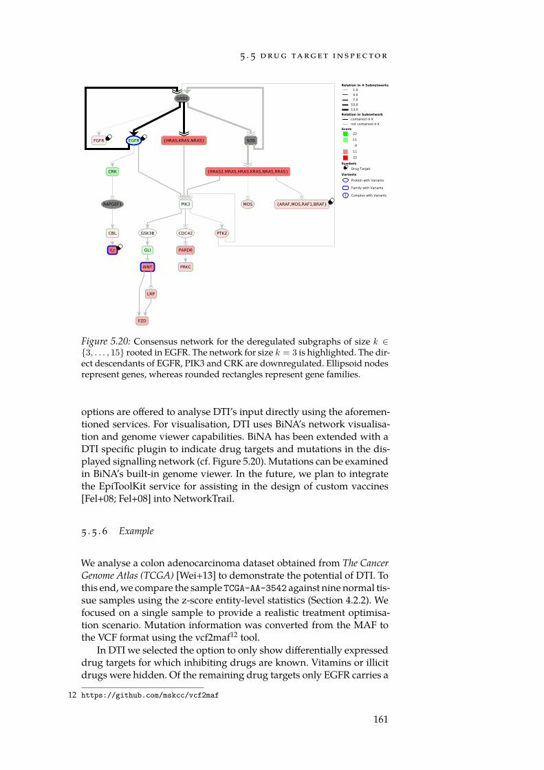
5 . 5 d ru g ta rg e t i n s p e c to r

Figure 5.20: Consensus network for the deregulated subgraphs of size k ∈3, . . . , 15 rooted in EGFR. The network for size k = 3 is highlighted. The dir-ect descendants of EGFR, PIK3 and CRK are downregulated. Ellipsoid nodesrepresent genes, whereas rounded rectangles represent gene families.

options are offered to analyse DTI’s input directly using the aforemen-tioned services. For visualisation, DTI uses BiNA’s network visualisa-tion and genome viewer capabilities. BiNA has been extended with aDTI specific plugin to indicate drug targets and mutations in the dis-played signalling network (cf. Figure 5.20). Mutations can be examinedin BiNA’s built-in genome viewer. In the future, we plan to integratethe EpiToolKit service for assisting in the design of custom vaccines[Fel+08; Fel+08] into NetworkTrail.

5 . 5 . 6 Example

We analyse a colon adenocarcinoma dataset obtained from The CancerGenome Atlas (TCGA) [Wei+13] to demonstrate the potential of DTI. Tothis end, we compare the sample TCGA-AA-3542 against nine normal tis-sue samples using the z-score entity-level statistics (Section 4.2.2). Wefocused on a single sample to provide a realistic treatment optimisa-tion scenario. Mutation information was converted from the MAF tothe VCF format using the vcf2maf12 tool.

In DTI we selected the option to only show differentially expresseddrug targets for which inhibiting drugs are known. Vitamins or illicitdrugs were hidden. Of the remaining drug targets only EGFR carries a

12 https://github.com/mskcc/vcf2maf

161

g r av i to n

point mutation. Two recommended drugs, Cetuximab and Panitumu-mab, are targeting EGFR, which is downregulated in this sample (cf.Figure 5.19). A network analysis with DTI’s NetworkTrail integrationreveals that the direct descendants of EGFR, PIK3 and CRK are downregulated. As EGFR serves as an activator of both gene families, thissuggests that the mutation may, in fact, be a loss of function mutation.Thus, a treatment regimen for this patient might want to forego therecommended drugs Cetuximab and Panitumumab in favour of e.g.the also recommended Bevacizumab which, amongst other proteins,targets the slightly upregulated vascular endothelial growth factor A (VE-GFA).

Further treatment options may include targeting highly upregu-lated genes such as the DNA polymerase POLB or the matrix metal-loproteases MMP3 and MMP7. To this end the drugs Cytarabine andMarimastat could be administered. The analysis can be accessed at theGeneTrail2 website13.

5 . 5 . 7 Summary

We presented DrugTargetInspector, a Graviton-based webservice fordetecting and evaluating deregulated drug targets. DTI integrates userprovided information, such as expression measurements and mutationdata, with knowledge stored in databases such as DrugBank or GDSC.This is a first step towards assisting users to make informed choicesfor optimising e.g. cancer therapy. In this regard, the tool could also beused to assess the efficacy of recommended treatment options. “Drugrepurposing” is another usage-scenario for which DTI might be em-ployed. There, the task is to detect drugs that were designed for differ-ent disease but may be effective in the examined sample as they targeta specific mutation or regulatory pattern that can be observed in thedata.

13 http://genetrail2.bioinf.uni-sb.de/drug_targets.html?session=c2761f9c-4a3a-430b-9712-8f833d320e2d&scores=10078&vcf=10080&subtype=colonandrectumcancer

162

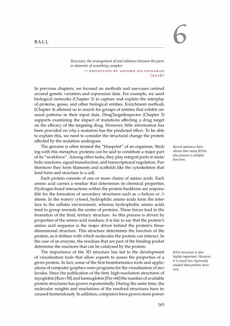
6BA L L

Structure: the arrangement of and relations between the partsor elements of something complex.

— d e f i n i t i o n by ox fo r d d i c t i o na r i e s( 2 0 1 6 )

In previous chapters, we focused on methods and use-cases centredaround genetic variation and expression data. For example, we usedbiological networks (Chapter 3) to capture and explain the interplayof proteins, genes, and other biological entities. Enrichment methods(Chapter 4) allowed us to search for groups of entities that exhibit un-usual patterns in their input data. DrugTargetInspector (Chapter 5)supports examining the impact of mutations affecting a drug targeton the efficacy of the targeting drug. However, little information hasbeen provided on why a mutation has the predicted effect. To be ableto explain this, we need to consider the structural change the proteinaffected by the mutation undergoes.

The genome is often termed the “blueprint” of an organism. Stick- Recent advances haveshown that many RNAsalso possess a catalyticfunction.

ing with this metaphor, proteins can be said to constitute a major partof its “workforce”. Among other tasks, they play integral parts in meta-bolic reactions, signal transduction, and transcriptional regulation. Fur-thermore they form filaments and scaffolds like the cytoskeleton thatlend form and structure to a cell.

Each protein consists of one or more chains of amino acids. Eachamino acid carries a residue that determines its chemical properties.Hydrogen-bond interactions within the protein backbone are respons-ible for the formation of secondary structures such as α-helices or β-sheets. In the watery cytosol, hydrophilic amino acids form the inter-face to the cellular environment, whereas hydrophobic amino acidstend to group towards the centre of proteins. These forces lead to theformation of the final, tertiary structure. As this process is driven byproperties of the amino acid residues, it is fair to say that the protein’samino acid sequence is the major driver behind the protein’s three-dimensional structure. This structure determines the function of theprotein, as it defines with which molecules the protein can interact. Inthe case of an enzyme, the residues that are part of the binding pocketdetermine the reactions that can be catalysed by the protein.

The importance of the 3D structure has led to the development RNA structure is alsohighly important. However,it is much less rigorouslystudied than protein struc-ture.

of visualisation tools that allow experts to assess the properties of agiven protein. In fact, some of the first bioinformatics tools and applic-ations of computer graphics were programs for the visualisation of mo-lecules. Since the publication of the first, high-resolution structures ofmyoglobin [Ken+58] and hæmoglobin [Per+60] the number of availableprotein structures has grown exponentially. During the same time, themolecular weights and resolutions of the resolved structures have in-creased tremendously. In addition, computers have grown more power-

163

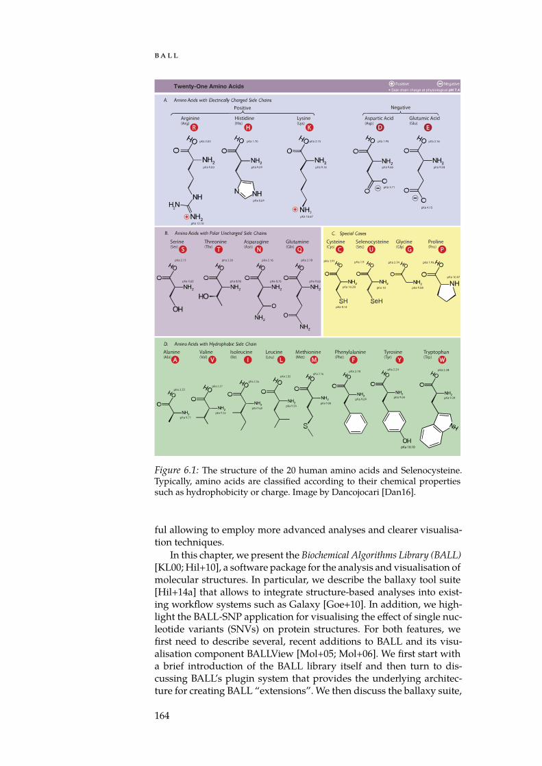
ba l l

Figure 6.1: The structure of the 20 human amino acids and Selenocysteine.Typically, amino acids are classified according to their chemical propertiessuch as hydrophobicity or charge. Image by Dancojocari [Dan16].

ful allowing to employ more advanced analyses and clearer visualisa-tion techniques.

In this chapter, we present the Biochemical Algorithms Library (BALL)[KL00; Hil+10], a software package for the analysis and visualisation ofmolecular structures. In particular, we describe the ballaxy tool suite[Hil+14a] that allows to integrate structure-based analyses into exist-ing workflow systems such as Galaxy [Goe+10]. In addition, we high-light the BALL-SNP application for visualising the effect of single nuc-leotide variants (SNVs) on protein structures. For both features, wefirst need to describe several, recent additions to BALL and its visu-alisation component BALLView [Mol+05; Mol+06]. We first start witha brief introduction of the BALL library itself and then turn to dis-cussing BALL’s plugin system that provides the underlying architec-ture for creating BALL “extensions”. We then discuss the ballaxy suite,

164

6 . 1 t h e b i o c h e m i ca l a lg o r i t h m s l i b r a ry

which makes use of this system for interfacing with a ballaxy server.A further application of the plugin system is the PresentaBALL plu-gin [Nic+13]. PresentaBALL enables researchers to quickly create in-teractive showcases and presentations without the need to modify theBALLView source code. BALL-SNP uses the functionality provided byPresentaBALL to provide an interactive and appealing user interface.

6 . 1 t h e b i o c h e m i ca l a lg o r i t h m s l i b r a ry

The Biochemical Algorithms Library (BALL) [KL00; Hil+10] is a librarydesigned for rapid prototyping of structure-based bioinformatics tools.It is being developed by scientists from the Universities Saarbrücken,Tübingen, and Mainz. BALL is divided into two main parts: the BALLlibrary, containing foundation classes as well as the code for workingwith and manipulating 3D structures, and the VIEW library that imple-ments visualisation capabilities and user interface components. Bothlibraries are written in C++ and comprise around 347,000 lines of code1.BALL is available for the MS Windows, MacOS X, and Linux platforms.For the creation of small, custom extensions which do not warrant towrite or modify C++ source code, BALL provides bindings for the Py-thon 2 [VD09] scripting language.

BALL represents structures using a hierarchical datastructure. Theroot node of the datastructure is called a System and acts as a containerfor a set of molecules. Molecules themselves can contain Chains ofResidues or simply a set of Atoms. This hierarchy is realised by imple-menting the Composite design pattern [Vli+95]. BALL provides parsers(and generators) for the most common structure file formats such asPDB files2, SYBYL3 MOL and MOL2 files, as well as HyperChem4 HINfiles. The implementation of the parsers is highly efficient and, in somecases, even beats implementations using template metaprogrammingtechniques [LCB10].

Due to experimental constraints, structural data is often incomplete.To enable scientists to work with 3D structures, while avoiding most ofthe tedious preprocessing steps, BALL offers automatic curation facil-ities via a database of well-known fragments. This allows to completemissing or partial residue information as well as the physically plaus-ible placement of hydrogen atoms. For simulating molecular dynam-ics, implementations of the AMBER [PC03], CHARMM [Bro+83], andMMFF94 [Hal96] molecular force fields are available. For locally min-imising the energy of a conformation, various efficient algorithms suchas conjugated gradients [FR64] and the memory-limited BFGS method[AlB99] have been implemented. Additionally, computing electrostaticpotentials using finite differences Poisson-Boltzmann [NH91] is pos-sible. Besides molecular mechanics, geometric tools for the design of

1 https://github.com/BALL-Project/ball2 http://www.wwpdb.org/documentation/file-format3 https://www.certara.com/software/molecular-modeling-and-simulation/

sybyl-x-suite/4 http://www.hyper.com/

165

ba l l

Figure 6.2: Screenshot of BALLView using the RTfact-based realtime raytra-cing renderer. The displayed structure is the glucocorticoid receptor (NR3C1)interacting with DNA. The crystal structure was taken from the PDB [Ber+00]record 1GLU [Lui+91]. Image by Andreas Hildebrandt.

docking algorithms [Koh12] and the analysis of docking results areprovided. Examples are binding pocket detection with the PASS al-gorithm [BS00], procedures for determining the solvent accessible (SAS)and solvent excluded (SES) molecular surfaces [Con83], as well as anhighly efficient clustering algorithm that is able to deal with large num-bers of docking poses [Hil+14b].

The VIEW library contains methods for visualising structures andassociated datasets, such as electrostatic fields, as well as componentsfor building user interfaces. It is based around the concept of Represen-tations that define how a structure, or a part thereof, should be visual-ised. Each Representation consists of a collection of geometric objectssuch as spheres, cylinders, or meshes together with colouring informa-tion. Amongst others, available representations are the SES, SAS, Ball-and-Stick, and Cartoon models. Applications built on top of VIEW, theprime example here being BALLView, are able to produce interactive,stereoscopic renderings of the loaded molecules. Publication qualityimages can be generated using the integrated, RTfact-based [GS08] re-altime raytracing renderer (cf. Figure 6.2). Besides traditional keyboardand mouse input, virtual reality input devices are supported via an in-tegration of the VRPN daemon [Tay+01].

166

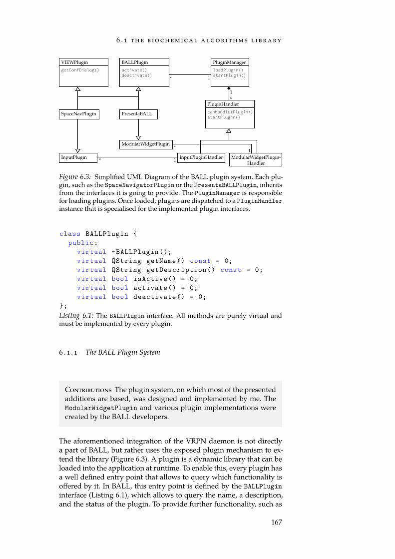
6 . 1 t h e b i o c h e m i ca l a lg o r i t h m s l i b r a ry

InputPluginHandler ModularWidgetPlugin-Handler

PluginManagerloadPlugin()startPlugin()

PluginHandlercanHandle(Plugin*)startPlugin()

VIEWPlugingetConfDialog()

BALLPluginactivate()deactivate()

InputPlugin

ModularWidgetPlugin

1*

1*

SpaceNavPlugin PresentaBALL

*1

* 1

Figure 6.3: Simplified UML Diagram of the BALL plugin system. Each plu-gin, such as the SpaceNavigatorPlugin or the PresentaBALLPlugin, inheritsfrom the interfaces it is going to provide. The PluginManager is responsiblefor loading plugins. Once loaded, plugins are dispatched to a PluginHandlerinstance that is specialised for the implemented plugin interfaces.

class BALLPlugin public:

virtual ~BALLPlugin();virtual QString getName() const = 0;virtual QString getDescription() const = 0;virtual bool isActive() = 0;virtual bool activate() = 0;virtual bool deactivate() = 0;

;Listing 6.1: The BALLPlugin interface. All methods are purely virtual andmust be implemented by every plugin.

6 . 1 . 1 The BALL Plugin System

Contributions The plugin system, on which most of the presentedadditions are based, was designed and implemented by me. TheModularWidgetPlugin and various plugin implementations werecreated by the BALL developers.

The aforementioned integration of the VRPN daemon is not directlya part of BALL, but rather uses the exposed plugin mechanism to ex-tend the library (Figure 6.3). A plugin is a dynamic library that can beloaded into the application at runtime. To enable this, every plugin hasa well defined entry point that allows to query which functionality isoffered by it. In BALL, this entry point is defined by the BALLPlugininterface (Listing 6.1), which allows to query the name, a description,and the status of the plugin. To provide further functionality, such as

167

ba l l

methods that allow the query the state of an input device, a pluginneeds to implement further interfaces defined in the BALL and VIEWlibrary. Every plugin is loaded by the PluginManager class. It is thendispatched by the PluginManager to the appropriate PluginHandler.The task of a PluginHandler is to provide an interface through whichthe application can access loaded plugins. An example is a class man-aging a list of available input devices.

Currently, BALL comes with interfaces that permit to implementadditional input devices (InputPlugin) and for adding new graphicaluser interface (GUI) components (ModularWidgetPlugin). We also cre-ated a RendererPlugin interface which makes it possible to move therendering logic of BALLView into plugins5. In turn, this allows to sim-plify the VIEW library considerably, while making it easier to intro-duce new rendering techniques. As a proof of concept, we created anew, OpenGL-based [S+09] renderer [Bür13] 6.

6 . 2 ba l l a x y

Contributions The ballaxy tool suite was implemented in a jointeffort by researchers of the Universities Tübingen and Saarbrücken.The manuscript and the BALLView plugin was written by Anna-Katharina Hildebrandt and Andreas Hildebrandt.

Workflow systems offer a user-friendly interface for building pipelinesfrom individual, specialised tools. In contrast to shell scripts, work-flows can easily be created by researchers that have no prior training inusing the command line and programming. Additionally, the createdworkflows are self-documenting, highly reproducible, and allow shar-ing within research communities. Popular examples for such systemsare Galaxy [Goe+10], Taverna [Wol+13], and the commercial KNIMEsoftware [Ber+08]. A default distribution of Galaxy is well-equippedfor working with sequencing data. Support for other areas of bioin-formatics, however, is lacking. For structural bioinformatics only fewplatforms such as MoSGrid [Her+12] that offer limited workflow func-tionality to the user are available. To remedy this situation, we pre-pared a Galaxy distribution called ballaxy [Hil+14a]. It consists of asuite of command line programs with associated Galaxy tool defini-tions (cf. Figure 6.4). In addition we created a ModularWidgetPluginthat allows to use data from BALLView directly in ballaxy and vice-versa. The ballaxy suite can be installed from the BALL source code orvia a Docker7 image8.

5 https://github.com/dstoeckel/BALL/tree/renderer_plugins6 https://github.com/dstoeckel/BALL/tree/modern_gl_renderer7 https://www.docker.com/8 https://hub.docker.com/r/anhi/ballaxy/

168

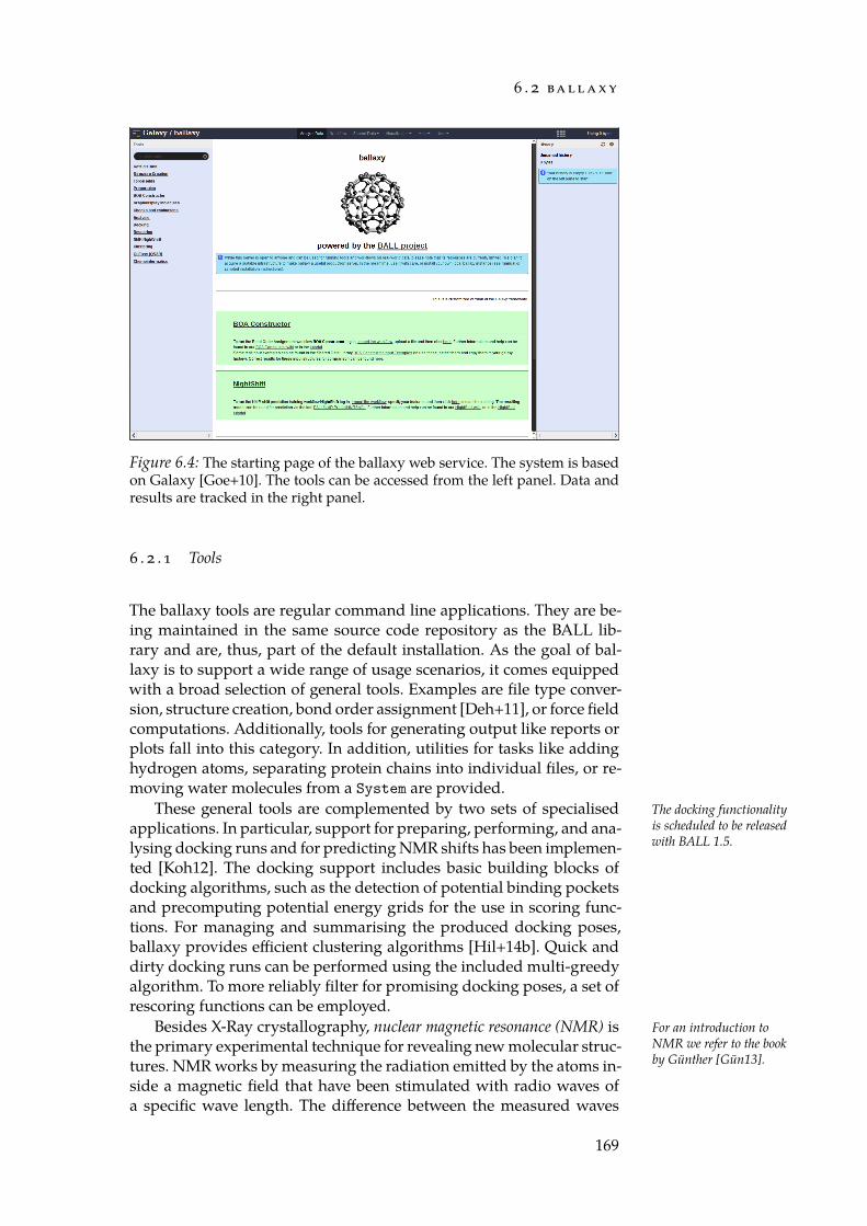
6 . 2 ba l l a x y

Figure 6.4: The starting page of the ballaxy web service. The system is basedon Galaxy [Goe+10]. The tools can be accessed from the left panel. Data andresults are tracked in the right panel.

6 . 2 . 1 Tools

The ballaxy tools are regular command line applications. They are be-ing maintained in the same source code repository as the BALL lib-rary and are, thus, part of the default installation. As the goal of bal-laxy is to support a wide range of usage scenarios, it comes equippedwith a broad selection of general tools. Examples are file type conver-sion, structure creation, bond order assignment [Deh+11], or force fieldcomputations. Additionally, tools for generating output like reports orplots fall into this category. In addition, utilities for tasks like addinghydrogen atoms, separating protein chains into individual files, or re-moving water molecules from a System are provided.

These general tools are complemented by two sets of specialised The docking functionalityis scheduled to be releasedwith BALL 1.5.

applications. In particular, support for preparing, performing, and ana-lysing docking runs and for predicting NMR shifts has been implemen-ted [Koh12]. The docking support includes basic building blocks ofdocking algorithms, such as the detection of potential binding pocketsand precomputing potential energy grids for the use in scoring func-tions. For managing and summarising the produced docking poses,ballaxy provides efficient clustering algorithms [Hil+14b]. Quick anddirty docking runs can be performed using the included multi-greedyalgorithm. To more reliably filter for promising docking poses, a set ofrescoring functions can be employed.

Besides X-Ray crystallography, nuclear magnetic resonance (NMR) is For an introduction toNMR we refer to the bookby Günther [Gün13].

the primary experimental technique for revealing new molecular struc-tures. NMR works by measuring the radiation emitted by the atoms in-side a magnetic field that have been stimulated with radio waves ofa specific wave length. The difference between the measured waves

169

ba l l

and the expected, theoretical value of an isolated atom, the chemicalshift, allows to derive distance constraints between the atoms. Fromthese, ensembles of possible models can be determined. The inversestep, predicting NMR shifts given a structure model, also plays an im-portant role in structural biology. Various algorithms for predictingNMR shifts exist that are based on differing methodology. Recently, hy-brid methods that combine explicit formulas for NMR shift from phys-ics with machine learning techniques have shown to provide excellentperformance [Han+11]. The NightShift model Dehof et al. [Deh+13] fur-ther improves upon the performance of previously published methodsand is included in ballaxy.

6 . 2 . 2 BALLView Plugin

As already outlined above, working with structure data sometimes re-quires to examine 3D representations. An important example is veri-fying that a docking algorithm produces sensible results. For this pur-pose, molecular visualisation tools such as RasMol [SB92; OS00], Py-MOL [DeL02], VMD [HDS96], Chimera [Pet+04], and our tool BALL-View [Mol+06; Mol+05] have been created. Replicating the completefunctionality of one of these tools in a web interface is a monumentaltask. To combine the rich functionality of BALLView with the workflowinterface offered by ballaxy, we implemented a ModularWidgetPluginthat is able to communicate with a running ballaxy instance. As thecommunication is bidirectional, the client can start computations onthe server and the server can push data to the client. For example, it ispossible to prepare a structure in BALLView. This structure can then bedirectly uploaded to the ballaxy server for running the workflow. Oncethe computation has completed, the results can again be downloadedto be visualised within BALLView.

6 . 3 p r e s e n ta ba l l

Contributions The PresentaBALL system has been created by me.It was later substantially improved by Stefan Nickels and SabineMüller.

An important part of academic practice is teaching and the presenta-tion of results. This is both, simple and difficult at the same time forstructural computational biology. While renderings of protein or RNAstructures are in themselves impressive, it is challenging to generaterenderings that not only are aesthetically pleasing, but also easy to in-terpret. A reason for this is that 2D depictions of 3D structures canobscure important details due to the choice of perspective. The same istrue for the choice of representation and colour, which can either helpto emphasise important parts of the structure or distract the viewer

170

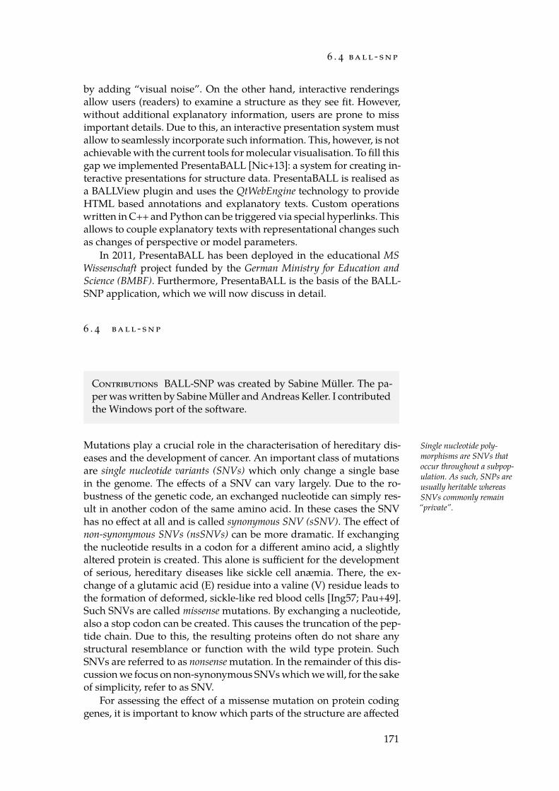
6 . 4 ba l l - s n p

by adding “visual noise”. On the other hand, interactive renderingsallow users (readers) to examine a structure as they see fit. However,without additional explanatory information, users are prone to missimportant details. Due to this, an interactive presentation system mustallow to seamlessly incorporate such information. This, however, is notachievable with the current tools for molecular visualisation. To fill thisgap we implemented PresentaBALL [Nic+13]: a system for creating in-teractive presentations for structure data. PresentaBALL is realised asa BALLView plugin and uses the QtWebEngine technology to provideHTML based annotations and explanatory texts. Custom operationswritten in C++ and Python can be triggered via special hyperlinks. Thisallows to couple explanatory texts with representational changes suchas changes of perspective or model parameters.

In 2011, PresentaBALL has been deployed in the educational MSWissenschaft project funded by the German Ministry for Education andScience (BMBF). Furthermore, PresentaBALL is the basis of the BALL-SNP application, which we will now discuss in detail.

6 . 4 ba l l - s n p

Contributions BALL-SNP was created by Sabine Müller. The pa-per was written by Sabine Müller and Andreas Keller. I contributedthe Windows port of the software.

Mutations play a crucial role in the characterisation of hereditary dis- Single nucleotide poly-morphisms are SNVs thatoccur throughout a subpop-ulation. As such, SNPs areusually heritable whereasSNVs commonly remain“private”.

eases and the development of cancer. An important class of mutationsare single nucleotide variants (SNVs) which only change a single basein the genome. The effects of a SNV can vary largely. Due to the ro-bustness of the genetic code, an exchanged nucleotide can simply res-ult in another codon of the same amino acid. In these cases the SNVhas no effect at all and is called synonymous SNV (sSNV). The effect ofnon-synonymous SNVs (nsSNVs) can be more dramatic. If exchangingthe nucleotide results in a codon for a different amino acid, a slightlyaltered protein is created. This alone is sufficient for the developmentof serious, hereditary diseases like sickle cell anæmia. There, the ex-change of a glutamic acid (E) residue into a valine (V) residue leads tothe formation of deformed, sickle-like red blood cells [Ing57; Pau+49].Such SNVs are called missense mutations. By exchanging a nucleotide,also a stop codon can be created. This causes the truncation of the pep-tide chain. Due to this, the resulting proteins often do not share anystructural resemblance or function with the wild type protein. SuchSNVs are referred to as nonsense mutation. In the remainder of this dis-cussion we focus on non-synonymous SNVs which we will, for the sakeof simplicity, refer to as SNV.

For assessing the effect of a missense mutation on protein codinggenes, it is important to know which parts of the structure are affected

171

ba l l

by the mutation [WM01]. Especially mutations in highly conserved re-gions, which are important for maintaining the structure of the pro-tein or are a part of the protein’s active site, are likely to have a sig-nificant impact on the function of the protein [MK01; NH06]. For pre-dicting the effect of a SNV, various packages that use statistical learn-ing methods or consult databases of known SNVs exist. Examples arethe Variant Effect Predictor [McL+10], SnpEff [Cin+12], and ANNOVAR[WLH10]. However, as these tools operate on the sequence level, the in-terpretation of the prediction is difficult. If multiple SNVs accumulatein the same protein, structure information becomes crucial for investig-ating potential, synergistic effects. Visualising the mutated residues ina three-dimensional representation can facilitate the interpretation ofSNV data and allows to quickly check for the presence of interactionsbetween SNVs. To this end, we developed BALL-SNP: a tool for thevisualisation of SNVs in protein structures [Mue+15].

6 . 4 . 1 Implementation

BALL-SNP integrates structure data available from the PDB [Ber+00]with knowledge about non-synonymous SNVs. To display this inform-ation, it uses the PresentaBALL (Section 6.3) framework which allowsto combine a structural representation of the protein with pathogen-icity information. This information is derived from annotation data-bases such as SwissProt/UniProt [Bai+05] and the dbSNV [She+01]based ClinVar [Lan+14]. Annotation is performed using the ANNO-VAR [WLH10] package. As input, BALL-SNP accepts the widely usedvariant call format (VCF). Alternatively, the user can provide input forBALL-SNP in a simple, tab-separated file format. Protein structures aredownloaded from the PDB using the largest structure referenced in thecorresponding UniProt annotation. Alternatively, the desired PDB re-cord can be entered manually.

As is illustrated by the example of sickle cell anæmia, a SNV can im-pact the structure of a protein. To account for this, BALL-SNP providesfacilities to compute putative changes in protein stability. For this a webservice running the I-Mutant 2.0 software [CFC05] is provided. Similarto mutations that impact protein stability, mutations in the active siteof the protein can be highly relevant for pathogenicity. In order to helpthe user to find these binding pockets, BALL-SNP uses BALL’s imple-mentation of the PASS algorithm for binding pocket detection [BS00].To detect groups of potentially interacting SNVs, a cluster analysis ofthe SNVs can be performed based on the euclidean distance and aver-age linkage clustering. This is especially useful for identifying cooper-ative mutations.

6 . 4 . 2 Example

To illustrate the capabilities of BALL-SNP, we perform an analysis ofSNP data from a dilated cardiomyopathy (DCM) high throughput sequen-

172

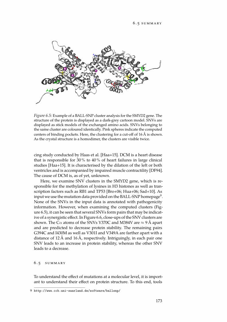
6 . 5 s u m m a ry

Figure 6.5: Example of a BALL-SNP cluster analysis for the SMYD2 gene. Thestructure of the protein is displayed as a dark-grey cartoon model. SNVs aredisplayed as stick models of the exchanged amino acids. SNVs belonging tothe same cluster are coloured identically. Pink spheres indicate the computedcenters of binding pockets. Here, the clustering for a cut-off of 16 Å is shown.As the crystal structure is a homodimer, the clusters are visible twice.

cing study conducted by Haas et al. [Haa+15]. DCM is a heart diseasethat is responsible for 30 % to 40 % of heart failures in large clinicalstudies [Haa+15]. It is characterised by the dilation of the left or bothventricles and is accompanied by impaired muscle contractility [DF94].The cause of DCM is, as of yet, unknown.

Here, we examine SNV clusters in the SMYD2 gene, which is re-sponsible for the methylation of lysines in H3 histones as well as tran-scription factors such as RB1 and TP53 [Bro+06; Hua+06; Sad+10]. Asinput we use the mutation data provided on the BALL-SNP homepage9.None of the SNVs in the input data is annotated with pathogenicityinformation. However, when examining the computed clusters (Fig-ure 6.5), it can be seen that several SNVs form pairs that may be indicat-ive of a synergistic effect. In Figure 6.6, close-ups of the SNV clusters areshown. The Cα atoms of the SNVs Y370C and M384V are ≈ 9 Å apartand are predicted to decrease protein stability. The remaining pairsG394C and I430M as well as V301I and V349A are farther apart with adistance of 12 Å and 16 Å, respectively. Intriguingly, in each pair oneSNV leads to an increase in protein stability, whereas the other SNVleads to a decrease.

6 . 5 s u m m a ry

To understand the effect of mutations at a molecular level, it is import-ant to understand their effect on protein structure. To this end, tools

9 http://www.ccb.uni-saarland.de/software/ballsnp/

173

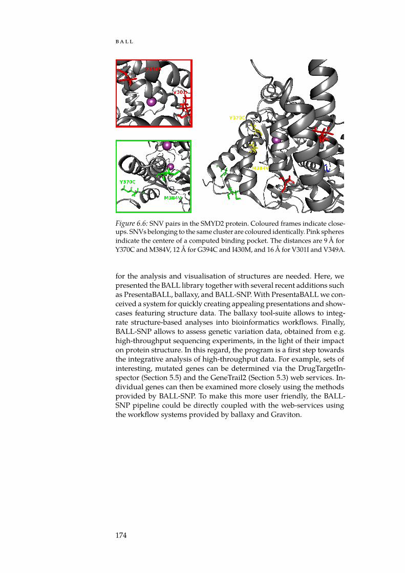
ba l l

Figure 6.6: SNV pairs in the SMYD2 protein. Coloured frames indicate close-ups. SNVs belonging to the same cluster are coloured identically. Pink spheresindicate the centere of a computed binding pocket. The distances are 9 Å forY370C and M384V, 12 Å for G394C and I430M, and 16 Å for V301I and V349A.

for the analysis and visualisation of structures are needed. Here, wepresented the BALL library together with several recent additions suchas PresentaBALL, ballaxy, and BALL-SNP. With PresentaBALL we con-ceived a system for quickly creating appealing presentations and show-cases featuring structure data. The ballaxy tool-suite allows to integ-rate structure-based analyses into bioinformatics workflows. Finally,BALL-SNP allows to assess genetic variation data, obtained from e.g.high-throughput sequencing experiments, in the light of their impacton protein structure. In this regard, the program is a first step towardsthe integrative analysis of high-throughput data. For example, sets ofinteresting, mutated genes can be determined via the DrugTargetIn-spector (Section 5.5) and the GeneTrail2 (Section 5.3) web services. In-dividual genes can then be examined more closely using the methodsprovided by BALL-SNP. To make this more user friendly, the BALL-SNP pipeline could be directly coupled with the web-services usingthe workflow systems provided by ballaxy and Graviton.

174

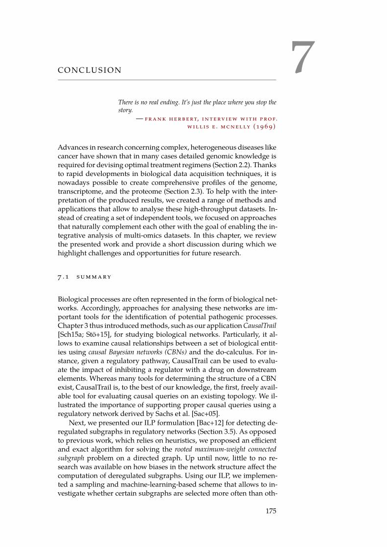
7CO NC LU S I O N

There is no real ending. It’s just the place where you stop thestory.

— f r a n k h e r b e rt, i n t e rv i e w w i t h p ro f.w i l l i s e . m c n e l ly ( 1 9 6 9 )

Advances in research concerning complex, heterogeneous diseases likecancer have shown that in many cases detailed genomic knowledge isrequired for devising optimal treatment regimens (Section 2.2). Thanksto rapid developments in biological data acquisition techniques, it isnowadays possible to create comprehensive profiles of the genome,transcriptome, and the proteome (Section 2.3). To help with the inter-pretation of the produced results, we created a range of methods andapplications that allow to analyse these high-throughput datasets. In-stead of creating a set of independent tools, we focused on approachesthat naturally complement each other with the goal of enabling the in-tegrative analysis of multi-omics datasets. In this chapter, we reviewthe presented work and provide a short discussion during which wehighlight challenges and opportunities for future research.

7 . 1 s u m m a ry

Biological processes are often represented in the form of biological net-works. Accordingly, approaches for analysing these networks are im-portant tools for the identification of potential pathogenic processes.Chapter 3 thus introduced methods, such as our application CausalTrail[Sch15a; Stö+15], for studying biological networks. Particularly, it al-lows to examine causal relationships between a set of biological entit-ies using causal Bayesian networks (CBNs) and the do-calculus. For in-stance, given a regulatory pathway, CausalTrail can be used to evalu-ate the impact of inhibiting a regulator with a drug on downstreamelements. Whereas many tools for determining the structure of a CBNexist, CausalTrail is, to the best of our knowledge, the first, freely avail-able tool for evaluating causal queries on an existing topology. We il-lustrated the importance of supporting proper causal queries using aregulatory network derived by Sachs et al. [Sac+05].

Next, we presented our ILP formulation [Bac+12] for detecting de-regulated subgraphs in regulatory networks (Section 3.5). As opposedto previous work, which relies on heuristics, we proposed an efficientand exact algorithm for solving the rooted maximum-weight connectedsubgraph problem on a directed graph. Up until now, little to no re-search was available on how biases in the network structure affect thecomputation of deregulated subgraphs. Using our ILP, we implemen-ted a sampling and machine-learning-based scheme that allows to in-vestigate whether certain subgraphs are selected more often than oth-

175

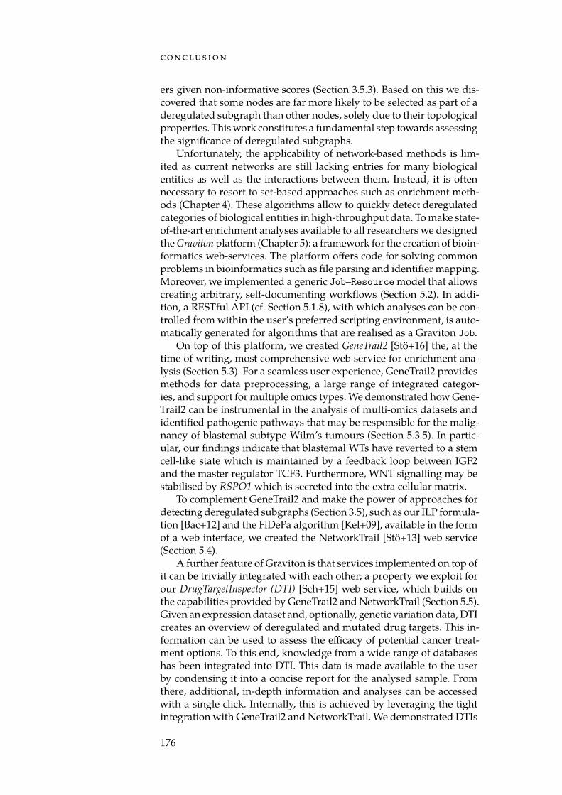
co nc lu s i o n

ers given non-informative scores (Section 3.5.3). Based on this we dis-covered that some nodes are far more likely to be selected as part of aderegulated subgraph than other nodes, solely due to their topologicalproperties. This work constitutes a fundamental step towards assessingthe significance of deregulated subgraphs.

Unfortunately, the applicability of network-based methods is lim-ited as current networks are still lacking entries for many biologicalentities as well as the interactions between them. Instead, it is oftennecessary to resort to set-based approaches such as enrichment meth-ods (Chapter 4). These algorithms allow to quickly detect deregulatedcategories of biological entities in high-throughput data. To make state-of-the-art enrichment analyses available to all researchers we designedthe Graviton platform (Chapter 5): a framework for the creation of bioin-formatics web-services. The platform offers code for solving commonproblems in bioinformatics such as file parsing and identifier mapping.Moreover, we implemented a generic Job–Resource model that allowscreating arbitrary, self-documenting workflows (Section 5.2). In addi-tion, a RESTful API (cf. Section 5.1.8), with which analyses can be con-trolled from within the user’s preferred scripting environment, is auto-matically generated for algorithms that are realised as a Graviton Job.

On top of this platform, we created GeneTrail2 [Stö+16] the, at thetime of writing, most comprehensive web service for enrichment ana-lysis (Section 5.3). For a seamless user experience, GeneTrail2 providesmethods for data preprocessing, a large range of integrated categor-ies, and support for multiple omics types. We demonstrated how Gene-Trail2 can be instrumental in the analysis of multi-omics datasets andidentified pathogenic pathways that may be responsible for the malig-nancy of blastemal subtype Wilm’s tumours (Section 5.3.5). In partic-ular, our findings indicate that blastemal WTs have reverted to a stemcell-like state which is maintained by a feedback loop between IGF2and the master regulator TCF3. Furthermore, WNT signalling may bestabilised by RSPO1 which is secreted into the extra cellular matrix.

To complement GeneTrail2 and make the power of approaches fordetecting deregulated subgraphs (Section 3.5), such as our ILP formula-tion [Bac+12] and the FiDePa algorithm [Kel+09], available in the formof a web interface, we created the NetworkTrail [Stö+13] web service(Section 5.4).

A further feature of Graviton is that services implemented on top ofit can be trivially integrated with each other; a property we exploit forour DrugTargetInspector (DTI) [Sch+15] web service, which builds onthe capabilities provided by GeneTrail2 and NetworkTrail (Section 5.5).Given an expression dataset and, optionally, genetic variation data, DTIcreates an overview of deregulated and mutated drug targets. This in-formation can be used to assess the efficacy of potential cancer treat-ment options. To this end, knowledge from a wide range of databaseshas been integrated into DTI. This data is made available to the userby condensing it into a concise report for the analysed sample. Fromthere, additional, in-depth information and analyses can be accessedwith a single click. Internally, this is achieved by leveraging the tightintegration with GeneTrail2 and NetworkTrail. We demonstrated DTIs

176

7 . 2 d i s c u s s i o n

capabilities using an adenocarcinoma sample from TCGA for whichwe could detect a loss-of-function mutation in the EGFR gene. Thissuggests that some recommended drugs targeting EGFR may not beeffective in this case and should be foregone in favour of other options.

Unfortunately, determining the effect of genomic variations solelyfrom sequence information is difficult. To be able to make better pre-dictions, we implemented BALL-SNP [Mue+15], a tool for visualisingand analysing SNVs in a structure context (Section 6.4). For each SNVits malignancy and its effect on the stability of the affected proteincan be predicted. Possible collaborative SNVs can be detected usingthe built-in cluster analysis. For constructing BALL-SNP we relied onthe functionality provided by the Biochemical Algorithms Library (BALL)[KL00; Hil+10] maintained by the universities Saarbrücken, Tübingen,and Mainz. To make BALL’s features available to a more diverse groupof users, we developed technologies that increase the flexibility of thelibrary. Examples for this are facilities such as PresentaBALL [Nic+13],which allows to create interactive presentations (Section 6.3), and theballaxy [Hil+14a] suite, which integrates BALL into the Galaxy [Goe+10]workflow system.

7 . 2 d i s c u s s i o n

The methods outlined in this thesis allow to gain a deeper insight intothe physiological processes that take place in a tumour, as is illustratedby our Wilm’s tumour study. In particular, our methods enable re-searchers and physicians to perform analyses on multiple levels of de-tail. Using GeneTrail2 or NetworkTrail, it is possible to quickly identifyrelevant pathological mechanisms. DTI uses this information to enablethe discovery of promising treatment options for a specific tumour. Tothis end, drug targets carrying a SNV can be examined on the structurelevel using BALL-SNP. This allows to gauge whether the targeting drugwill actually be effective. Finally, if the detected target is part of a reg-ulatory cascade, it is possible to use CausalTrail to model the responseof downstream elements to e.g. a knockout.

Naturally, for each presented method many details can be improvedand extended in several ways. CausalTrail can be enhanced with sup-port for continuous random variables and more robust parameter fit-ting procedures by leveraging shrinkage techniques. Furthermore, wecan expand GeneTrail2, NetworkTrail, and DTI with additional meth-ods, add more supported data formats, and provide better heuristicsand guidelines for determining optimal parameter settings. BALL andBALLView can be extended with additional algorithms and advancedvisualisation capabilities, respectively.

Each of these additions may significantly improve the flexibilityand applicability of the discussed methods and may advance the state-of-the-art of the respective field of computational biology. However,we also believe that it is of utmost importance to increase the interop-erability of available approaches to enable examining multi-omics data-sets. Thus, the major theme of this work has been the attempt to bridge

177

co nc lu s i o n

gaps between methods to facilitate such integrative analyses. With thecreation of the Graviton framework, we made a significant contribu-tion in this regard. In particular, the support for a wide range of in-put formats and datatypes as well as utilities such as the comparativeenrichment view, help to perform joint evaluations of e.g. expression,protein abundance, and genomic variation data.

As integrative methods require to explicitly take the relationshipsbetween biological entities into account, network-based methods are anatural choice as an algorithmic basis. Currently, interpreting the res-ults of, for instance, methods for detecting deregulated subgraphs isdifficult, though. This is due to the fact that it is unknown how to com-pute the significance of the obtained subgraphs. To chart the terrainin this direction, we provided a scheme for quantifying the likelihoodwith which a subgraph is selected given non-informative node scores.The presented results (Section 3.5.3) suggest that there is a pressingneed for a rigorous framework for assessing the significance of deregu-lated subgraphs that helps to ensure the interpretability of these meth-ods.

For an application in a medical setting, methods that allow to jointlyanalyse multi-omics data are only a part of the puzzle. To assist inchoosing an appropriate treatment for a tumour, assistance platformsare needed that support the clinician in every step of the decision mak-ing process. To achieve this, the tools should, on the one hand, aggreg-ate and visualise relevant information from external databases and, onthe other hand, allow their users to trigger further, in-depth analyses.DTI and BALL-SNP are examples for how such assistance platformscould be structured. They allow to study genomic data in combina-tion with expression profiles and protein crystal structures, respect-ively. Ideally, the functionality of both applications would be mergedto enable workflows where potential drug targets carrying mutationscan be identified and seamlessly analysed on the structure level.

Bioinformatics methods have shown that they can provide valuableinformation for combatting heterogeneous diseases. A prime exampleis HIV therapy optimisation for which platforms such as Geno2Pheno[Bee+03; TL12] are routinely used in practice. For complex, heterogen-eous diseases like cancer, which have proven to be even more elusivethan HIV, integrative methods may give physicians and researchers themeans to devise effective, personalised treatments. However, until thisis the case, the task of making these tools reliable enough to be applic-able in practice, will provide the grounds for a wide range of excitingand challenging research.

178

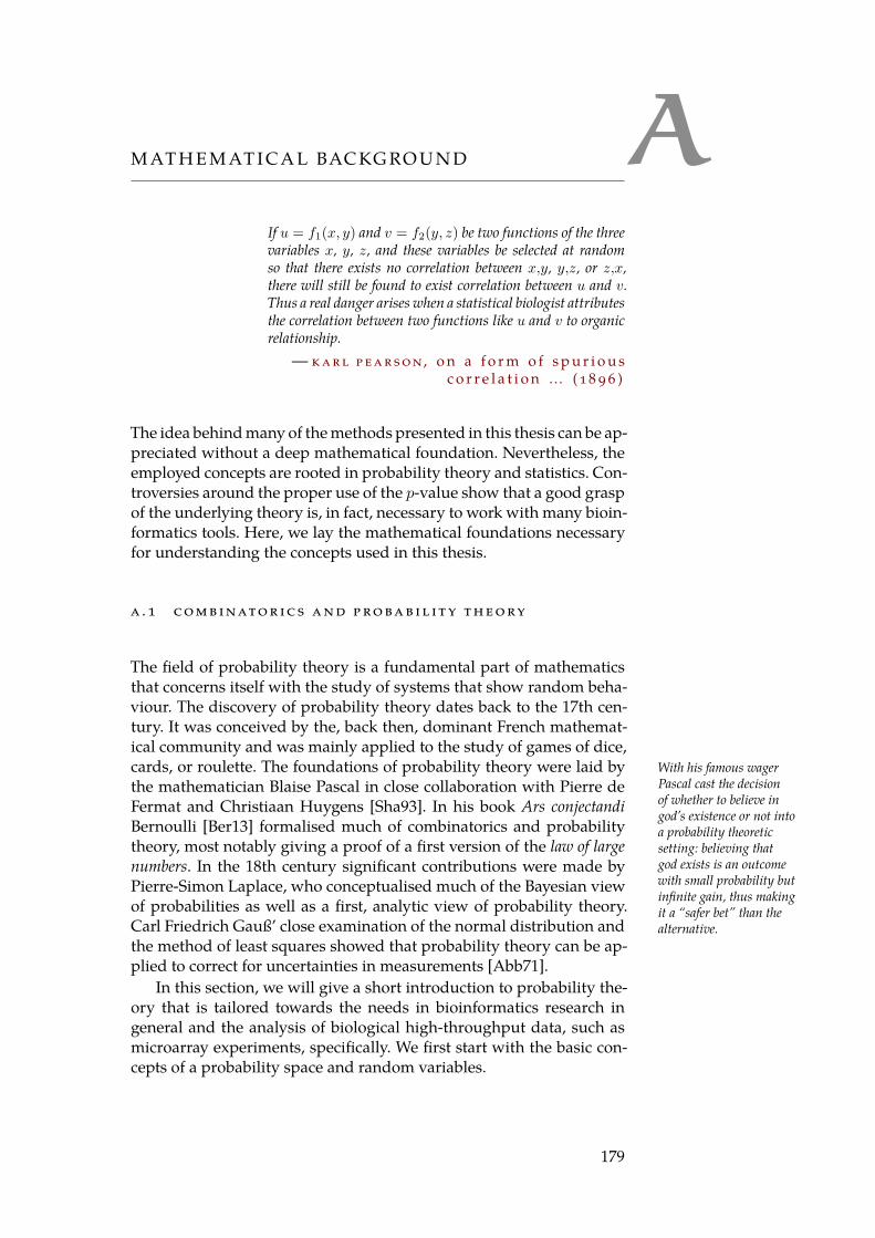
AM AT H E M AT I CA L BACKG RO U N D

If u = f1(x, y) and v = f2(y, z) be two functions of the threevariables x, y, z, and these variables be selected at randomso that there exists no correlation between x,y, y,z, or z,x,there will still be found to exist correlation between u and v.Thus a real danger arises when a statistical biologist attributesthe correlation between two functions like u and v to organicrelationship.

— k a r l p e a r s o n, o n a fo r m o f s p u r i o u sc o r r e l a t i o n … ( 1 8 9 6 )

The idea behind many of the methods presented in this thesis can be ap-preciated without a deep mathematical foundation. Nevertheless, theemployed concepts are rooted in probability theory and statistics. Con-troversies around the proper use of the p-value show that a good graspof the underlying theory is, in fact, necessary to work with many bioin-formatics tools. Here, we lay the mathematical foundations necessaryfor understanding the concepts used in this thesis.

a . 1 co m b i nato r i c s a n d p ro ba b i l i t y t h e o ry

The field of probability theory is a fundamental part of mathematicsthat concerns itself with the study of systems that show random beha-viour. The discovery of probability theory dates back to the 17th cen-tury. It was conceived by the, back then, dominant French mathemat-ical community and was mainly applied to the study of games of dice,cards, or roulette. The foundations of probability theory were laid by With his famous wager

Pascal cast the decisionof whether to believe ingod’s existence or not intoa probability theoreticsetting: believing thatgod exists is an outcomewith small probability butinfinite gain, thus makingit a “safer bet” than thealternative.

the mathematician Blaise Pascal in close collaboration with Pierre deFermat and Christiaan Huygens [Sha93]. In his book Ars conjectandiBernoulli [Ber13] formalised much of combinatorics and probabilitytheory, most notably giving a proof of a first version of the law of largenumbers. In the 18th century significant contributions were made byPierre-Simon Laplace, who conceptualised much of the Bayesian viewof probabilities as well as a first, analytic view of probability theory.Carl Friedrich Gauß’ close examination of the normal distribution andthe method of least squares showed that probability theory can be ap-plied to correct for uncertainties in measurements [Abb71].

In this section, we will give a short introduction to probability the-ory that is tailored towards the needs in bioinformatics research ingeneral and the analysis of biological high-throughput data, such asmicroarray experiments, specifically. We first start with the basic con-cepts of a probability space and random variables.

179

m at h e m at i ca l bac kg ro u n d

a. 1 . 1 Probability Spaces

In order to be able to talk about probabilities of some events, a formaldefinition of an observable event is required. As a next step, a way toexpress how probable it is to observe such a result is needed. This willlead us to the definition of a probability space.

Consider a simple random experiment where a six-sided dice isrolled once. We can now ask how likely it is that we roll a 6 or thatthe number shown is even. Whereas “rolling a 6” corresponds to onlyobserving the outcome 6, “rolling an even number” corresponds to ob-serving the outcomes 2, 4, or 6. Observable events can thus consist ofindividual or multiple outcomes. This means that the set of events Σ isa subset of the power set P(Ω) of the set of outcomes Ω. In addition tothat, some additional constraints need to be fulfilled:

Definition 21 (σ-Algebra). Let Ω be a set. A set Σ ⊆ P(Ω) is called aσ-algebra if it fulfils the following conditions:

1. ∅ ∈ Σ

2. Closed under complement: A ∈ Σ → Ω \A ∈ Σ

3. Closed under countable unions: A1, A2, . . . ∈ Σ →∪

iAi ∈ Σ

The definition of a σ-algebra ensures that our events have some con-For our dice example wehave Ω = 1, 2, 3, 4, 5, 6

and Σ = P(Ω).venient properties. Given an event A, there is a well defined comple-mentary event Ac such that either A or Ac takes place. Furthermore,given the events A,B, we can ask whether both happened (A∩B) or atleast one of both happened (A ∪ B). This is possible as both, the inter-section as well as the union, of two events are guaranteed to be eventsagain.

Having defined the space of events, we now need a way to assignprobabilities to each of the events.

Definition 22 (Probability Measure). Let Ω be a set of outcomes and ΣThe 2nd conditionis not strictly neces-

sary as it follows fromPr(Ai) = Pr(Ai ∪

∅) = Pr(Ai) + Pr(∅)

a corresponding σ-algebra of events. A probability measure on Σ is afunction Pr : Σ → [0, 1] that fulfils the following conditions:

1. Pr(Ω) = 1

2. Pr(∅) = 0

3. Let Ai ⊂ Σ be a countable set of pairwise disjoint events, then

Pr(∪·

i

Ai

)=∑i

Pr(Ai)

We are now ready to define a probability space, which ties the con-cepts of outcome space, event space, and probability measure together.

Definition 23 (Probability Space). A probability space (Ω,Σ, p) is atriple where Ω is the set of possible outcomes, Σ ⊆ P(Ω) is a σ-algebraon Ω, and p : Σ → [0, 1] is a probability measure.

180

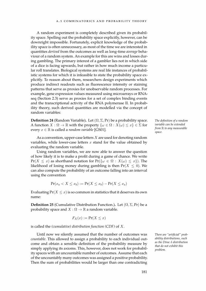
a . 1 co m b i nato r i c s a n d p ro ba b i l i t y t h e o ry

A random experiment is completely described given its probabil-ity space. Spelling out the probability space explicitly, however, can bedownright impossible. Fortunately, explicit knowledge of the probab-ility space is often unnecessary, as most of the time we are interested inquantities derived from the outcomes as well as long-time average beha-viour of a random system. An example for this are wins and losses dur-ing gambling. The primary interest of a gambler lies not in which sideof a dice is facing upwards, but rather in how much income a particu-lar roll translates. Biological systems are real life instances of probabil-istic systems for which it is infeasible to state the probability space ex-plicitly. To reason about them, researchers design experiments whichproduce indirect readouts such as fluorescence intensity or stainingpatterns that serve as proxies for unobservable random processes. Forexample, gene expression values measured using microarrays or RNA-seq (Section 2.3) serve as proxies for a set of complex binding eventsand the transcriptional activity of the RNA polymerase II. In probab-ility theory, such derived quantities are modelled via the concept ofrandom variables:

Definition 24 (Random Variable). Let (Ω,Σ,Pr) be a probability space. The definition of a randomvariable can be extendedfrom R to any measurablespace.

A function X : Ω → R with the property ω ∈ Ω : X(ω) ≤ x ∈ Σ forevery x ∈ R is called a random variable [GS01].

As a convention, upper-case lettersX are used for denoting randomvariables, while lower-case letters x stand for the value obtained byevaluating the random variable.

Using random variables, we are now able to answer the questionof how likely it is to make a profit during a game of chance. We writePr(X ≤ x) as shorthand notation for Pr(ω ∈ Ω : X(ω) ≤ x). Thelikelihood of losing money during gambling is then Pr(X ≤ 0). Wecan also compute the probability of an outcome falling into an intervalusing the convention

Pr(xa < X ≤ xb) := Pr(X ≤ xb)− Pr(X ≤ xa)

Evaluating Pr(X ≤ x) is so common in statistics that it deserves its ownname:

Definition 25 (Cumulative Distribution Function.). Let (Ω,Σ,Pr) be aprobability space and X : Ω → R a random variable.

FX(x) := Pr(X ≤ x)

is called the (cumulative) distribution function (CDF) of X .

Until now we silently assumed that the number of outcomes was There are “artificial” prob-ability distributions, suchas the Dirac δ distributionthat do not exhibit thisproblem.

countable. This allowed to assign a probability to each individual out-come and obtain a sensible definition of the probability measure bysimply applying its axioms. This, however, does not work for probabil-ity spaces with an uncountable number of outcomes. Assume that eachof the uncountably many outcomes was assigned a positive probability.Then the sum of probabilities would be larger than one contradicting

181

m at h e m at i ca l bac kg ro u n d

the definition of a probability measure. Hence, for most outcomes ωHere “most” means: allexcept countably many. we have Pr(ω) = 0. This is intuitively correct, as a single, infinitesim-

ally small point out of an uncountable set of possibilities should neverbe selected twice by a random process. However, when we look at in-tervals as opposed to single points, some intervals that are more likelyto contain the values of a random variable than other intervals exist.We can take this observation to the extreme by observing smaller andsmaller intervals around a point x.

Pr(x− ϵ < X ≤ x) = Pr(X ≤ x)− Pr(X ≤ x− ϵ) = FX(x)−FX(x− ϵ)

The difference above suggests that we should be able to write FX as theantiderivative of some function fX . Let us make this notion concrete:

Definition 26 (Continous random variable). The random variable X is

x

y

Figure A.1: The cumu-lative (red) and prob-ability (blue) density

function of a Gaussiannormal distribution.

called continuous if its CDF FX can be expressed as

FX(x) =

x∫−∞

fX(u)du

for some integrable function fX : R → [0,∞) called the (probability)density function of X [GS01].

If a random variable only maps to a countable subset ofR, a simplerdefinition can be given:

Definition 27 (Discrete random variable). The random variable X iscalled discrete if it takes values in some countable subset x1, x2, . . . ∈R, only. The discrete random variable X has the (probability) densityfunction fX : R → [0, 1] given by fX(x) = Pr(X = x) [GS01].

With random variables we can describe random processes in termsof higher level statistics instead of the underlying probability spaces.In the following, two fundamental examples for such statistics are in-troduced: the expected value and the variance.

a . 1 . 2 Expected Value and Variance

Often the outcome of a single random experiment is not of interest foran investigation. For example consider a study that tries to determinethe effect of a drug administered to a patient. As every patient reactsslightly differently to a drug, measuring a single response does notprovide sufficient evidence that a drug is actually working. Instead,Actually, we use the av-

erage to gain informationabout the expected value …

we are interested in the effect the drug has on average. In statistics thisaverage effect is captured by the expected value.

Definition 28 (Expected Value). Let X : Ω → R be a random variable.If the limit

E(X) :=

∞∫−∞

xfx(x)dx

182

a . 1 co m b i nato r i c s a n d p ro ba b i l i t y t h e o ry

or, for discreet variables

E(X) :=∞∑i=1

xi Pr(X = xi)

exists, E(X) is called the expected value of X .

Per convention the Greek letter µ is used to designate the expectedvalue of a random variable. Note that not every random variable pos-sesses an expected value, as the value of the integral or the series in theabove definitions does not necessarily need to be defined.

While the expected value provides information about the outcomeof a random experiment “on average”, it should not be confused withthe most likely outcome of a random experiment. Instead, the expectedvalue may be the result of two likely events cancelling each other. Forexample in a game where the player wins a set amount of money if afair coin shows “heads” and looses the same amount of money if thecoin shows “tails” the expected value is zero. To be able to get a betterunderstanding of a random experiment a measure is needed that tellsus how the results vary around the expected value. This measure is thevariance:

Definition 29 (Variance). Let X : Ω → R be a random variable withexpected value E(X). Then the variance var(X) is defined as

var(X) := E[(X − E(X))2

]We will also use σ2 to denote the variance. The square root of the vari-ance σ is called the standard deviation.

In other words, the variance measures the expected, squared devi-ation from the expected value. Again, the variance only makes a state-ment about the distribution of outcomes in the long run. It furthermoredoes not capture any information about the shape of the distributionwith the exception of its spread. It is possible to compute higher (cent-ral) moments of a distribution, such as the skewness or the kurtosis, toobtain more information concerning the distributions shape. Here, wewill refrain from defining these concepts, as they will not be needed inthe remainder of this thesis.

The variance measures how the results of a single random variableare spread. When two dependent random variables are given, it is oftenof interest to examine how the variances of the two variables are related.To this end, we define the covariance of two random variables.

Definition 30 (Covariance). Let X,Y : Ω → R be two random vari-ables with expected values E(X) and E(Y ). Furthermore, assume thatE(XY ) exists. The covariance cov(X,Y ) is defined as

cov(X,Y ) := E [(X − E(X))(Y − E(Y ))]

Note that the covariance is a generalisation of the variance and itholds that var(X) = cov(X,X). A commonly used statistics that can

183

m at h e m at i ca l bac kg ro u n d

be derived from the covariance is Pearson’s correlation coefficient r[Pea95b].

r :=cov(X,Y )√

var(X)var(Y )

Pearson’s correlation coefficient measures the strength of the linear de-pendency between two variables. If r = 0 there is no linear dependency.In contrast, if r = ±1 then a scatter plot of the two variables would res-ult in a perfect line. It is important to note that a correlation of 0 doesnot imply that the two random variables are independent. Converselydependent variables do not guarantee that their correlation is differentfrom 0.

a . 1 . 3 Populations, Samples, and Estimators

In practice, the exact parameters of a distribution, for example the ex-pected value or the variance, are unknown. In this case, it may be ne-cessary to estimate the parameters from observations. The availableobservations for doing so are called the population. Populations can becountable or, at least in theory, uncountable [Ass13]. Examples for pop-ulations are all products produced by some factory or all citizens of acountry. Given a population, consisting of observations x1, ..., xn froma random variable X we can define estimators for the parameters ofX . We call a function f(x1, ..., xn) = θ that estimates the value of aparameter θ of the underlying distribution an estimator. We will usethe convention to denote the estimate of some quantity q with q. Giventhe above definition, a valid estimator for the mean of any distributionwould be the constant function returning 0. Naturally, this is a terribleestimator for all intents and purposes. A good estimator for the pop-ulation mean µ is given by µ := 1

n

∑ni=1 xi. Similarly, the population

variance σ2 is given by [Liu74]

σ2 :=1

n

n∑i=1

(xi − µ)2 =1

n

n∑i=1

x2i − µ2

Sometimes, not the complete population is available. This can beNote that “sample”can refer to both: a set

of observations anda single observation.

the case if not all members of the population can be observed or thepopulation is prohibitively large. In this case we need to draw conclu-sions from a subset of observations.

Definition 31 (Random sample). LetP be a population of observationsobtained from a random variable X . A subset S = x1, ..., xn ⊂ P iscalled a random sample of P . If the observations are chosen independ-ently of each other we call them independent identically distributed (iid).

To obtain better estimators the definition of an estimator needs to benarrowed down by requiring further properties. A reasonable propertyis that the estimator should yield better results when we increase thesample size.

184

a . 2 m ac h i n e l e a r n i ng

Definition 32 (Consistent estimator). An estimator f for a property θis consistent if it converges in probability to the true parameter. Thismeans that for a sample S = x1, ..., xn and all ϵ > 0

limn→∞

P (|f(S)− θ| ≥ ϵ) = 0

Another useful property is that the estimator returns the true valueon average. This leads us to the definition of unbiased estimators.

Definition 33 (Unbiased estimator). Let X ∼ D(θ) be a random vari-able following some distributionD with parameters θ and furthermorelet S = x1, ..., xn be samples of X . We call a function f(S) = θ an un-biased estimator for θ iff

E(f(S)) = θ

An unbiased estimator for the population mean is given by thesample mean x := 1

n

∑ni=1 xi.

Proof. The proof is straight-forward and exploits the linearity of theexpected value.

E(x) = E

[1

n

n∑i=1

xn

]=

1

n

n∑i=1

E(xn)

=1

n

n∑i=1

E(X) =1

nnE(X) = E(X)

Similarly the sample variance The n − 1 in the denomin-ator is due to the fact thata degree of freedom hasalready been “consumed”when computing x.

1

n− 1

n∑i=1

(xi − x)2 (A.1)

where x denotes the sample mean, is an unbiased estimator for the pop-ulation variance. We omit the proof that is no more difficult, but some-what lengthier, than for the sample mean and refer the reader to oneof the many proofs available online (e.g. Anderson [And99]).

Using unbiased estimators guarantees that the obtained estimateis eventually the true value of some parameter and is not affected bya systematic error. While generally desirable, a considerable numberof samples may be required for this property to be beneficial. In thecase that only few samples are available, it may pay off to use biasedestimators that introduce a systematic error, while on the other handbeing much less susceptible to outliers and noise in the samples. Anexample for such a biased estimator is the shrinkage estimator for thesample variance presented in Section 4.2.2. Intentionally introducingbias into an estimator is an instance of the bias variance trade-off, whichwe will investigate more closely in Appendix A.2.2.

185

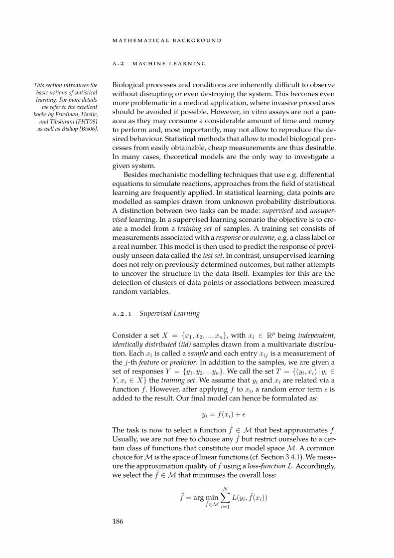
m at h e m at i ca l bac kg ro u n d

a. 2 m ac h i n e l e a r n i ng

Biological processes and conditions are inherently difficult to observeThis section introduces thebasic notions of statisticallearning. For more details

we refer to the excellentbooks by Friedman, Hastie,

and Tibshirani [FHT09]as well as Bishop [Bis06].

without disrupting or even destroying the system. This becomes evenmore problematic in a medical application, where invasive proceduresshould be avoided if possible. However, in vitro assays are not a pan-acea as they may consume a considerable amount of time and moneyto perform and, most importantly, may not allow to reproduce the de-sired behaviour. Statistical methods that allow to model biological pro-cesses from easily obtainable, cheap measurements are thus desirable.In many cases, theoretical models are the only way to investigate agiven system.

Besides mechanistic modelling techniques that use e.g. differentialequations to simulate reactions, approaches from the field of statisticallearning are frequently applied. In statistical learning, data points aremodelled as samples drawn from unknown probability distributions.A distinction between two tasks can be made: supervised and unsuper-vised learning. In a supervised learning scenario the objective is to cre-ate a model from a training set of samples. A training set consists ofmeasurements associated with a response or outcome, e.g. a class label ora real number. This model is then used to predict the response of previ-ously unseen data called the test set. In contrast, unsupervised learningdoes not rely on previously determined outcomes, but rather attemptsto uncover the structure in the data itself. Examples for this are thedetection of clusters of data points or associations between measuredrandom variables.

a . 2 . 1 Supervised Learning

Consider a set X = x1, x2, ..., xn, with xi ∈ Rp being independent,identically distributed (iid) samples drawn from a multivariate distribu-tion. Each xi is called a sample and each entry xij is a measurement ofthe j-th feature or predictor. In addition to the samples, we are given aset of responses Y = y1, y2, ...yn. We call the set T = (yi, xi) | yi ∈Y, xi ∈ X the training set. We assume that yi and xi are related via afunction f . However, after applying f to xi, a random error term ϵ isadded to the result. Our final model can hence be formulated as:

yi = f(xi) + ϵ

The task is now to select a function f ∈ M that best approximates f .Usually, we are not free to choose any f but restrict ourselves to a cer-tain class of functions that constitute our model space M. A commonchoice forM is the space of linear functions (cf. Section 3.4.1). We meas-ure the approximation quality of f using a loss-function L. Accordingly,we select the f ∈ M that minimises the overall loss:

f = arg minf∈M

N∑i=1

L(yi, f(xi))

186

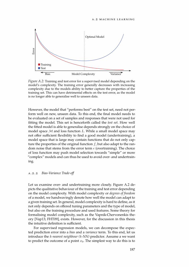
a . 2 m ac h i n e l e a r n i ng

Model Complexity

Erro

r

TrainingTest

Optimal Model

Bias Variance

Figure A.2: Training and test error for a supervised model depending on themodel’s complexity. The training error generally decreases with increasingcomplexity due to the models ability to better capture the properties of thetraining set. This can have detrimental effects on the test error, as the modelis no longer able to generalise well to unseen data.

However, the model that “performs best” on the test set, need not per-form well on new, unseen data. To this end, the final model needs tobe evaluated on a set of samples and responses that were not used forfitting the model. This set is henceforth called the test set. How wellthe fitted model is able to generalise depends strongly on the choice ofmodel space M and loss function L. While a small model space maynot offer sufficient flexibility to find a good model (undertraining), amodel space that is large may contain functions that do not only cap-ture the properties of the original function f , but also adapt to the ran-dom noise that stems from the error term ϵ (overtraining). The choiceof loss function may push model selection towards “simple” or more“complex” models and can thus be used to avoid over- and undertrain-ing.

a . 2 . 2 Bias-Variance Trade-off

Let us examine over- and undertraining more closely. Figure A.2 de-picts the qualitative behaviour of the training and test error dependingon the model complexity. With model complexity or degrees of freedomof a model, we handwavingly denote how well the model can adapt toa given training set. In general, model complexity is hard to define, as itnot only depends on offered tuning parameters and the type of model,but also on the training procedure and used features. Some theory forformalising model complexity, such as the Vapnik-Chervonenkis the-ory [Vap13; FHT09], exists. However, for the discussion in this thesisthe intuitive definition is sufficient.

For supervised regression models, we can decompose the expec-ted prediction error into a bias and a variance term. To this end, let usintroduce the k-nearest neighbour (k-NN) predictor. Assume a we wantto predict the outcome of a point x0. The simplest way to do this is to

187

m at h e m at i ca l bac kg ro u n d

Training Tuning Test

Figure A.3: Splitting the available data into independent training, tuning, andtest sets. Commonly splits that achieve a ratio of 2:1:1 are used.

select the k ∈ N nearest points in the training set Nk(x0) and to assigntheir average outcome to x0:

y0 =1

k

∑i∈Nk(x0)

yi

We denote the fit of the k-NN predictor with fk. Assume that Y =f(X) + ϵ with E(ϵ) = 0 and var(ϵ) = σ2. Then the expected predictionerror (EPE) can be written as [FHT09]

EPEk(xo) = E[(Y − fk(x0))2|X = x0]

= σ2 + Bias2(fk(x0)) + varT (fk(x0))

Here varT denotes the variance on the training set. The bias measuresthe systematic error incurred by the model due to its inability to adaptto the data. Conversely, for a model with high variance, small changesin the input features can lead to large changes in the output. Generally,simple models have a high bias and a low variance as they come witha large systematic error, whereas complex models have a low bias anda high variance as they are able to adapt to the random noise in thetraining set. Thus, to select the predictor that generalises the best tounseen data, it might pay off to select a model with a slightly largerbias if this leads to a substantial decrease in variance and vice versa.

a . 2 . 3 Model Selection and Evaluation

Probably the most important topic in machine learning is proper modelselection and evaluation. Finding the sweet spot of parameters thatyield a good training error without overtraining is fundamental for thequality of the predictor. Here, it is of utmost importance to properly val-idate the model on unseen data. For this, the available data is separatedinto a training and a test set. If parameters need to be tuned, usually anadditional tuning set, on which the error for various parameter settingis evaluated, is required (Figure A.3).

However, in many scenarios from computational biology too fewsamples are available to afford the luxury of a completely independ-ent test set. To work around this issue, strategies such as k-fold cross-validation are commonly applied. Here, the idea is to divide the train-ing set into k equally sized folds. Each of the folds is then used as a testset once, whereas the remaining k − 1 folds serve as the training set.An approximation of the test error is then computed as the average ofthe errors achieved in each fold.

188

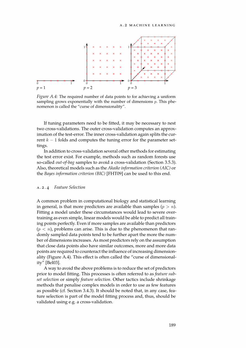
a . 2 m ac h i n e l e a r n i ng

0 1 0 1

0

1

0 1

0

1

p = 1 p = 2 p = 3

Figure A.4: The required number of data points to for achieving a uniformsampling grows exponentially with the number of dimensions p. This phe-nomenon is called the “curse of dimensionality”.

If tuning parameters need to be fitted, it may be necessary to nesttwo cross-validations. The outer cross-validation computes an approx-imation of the test-error. The inner cross-validation again splits the cur-rent k − 1 folds and computes the tuning error for the parameter set-tings.

In addition to cross-validation several other methods for estimatingthe test error exist. For example, methods such as random forests useso-called out-of-bag samples to avoid a cross-validation (Section 3.5.3).Also, theoretical models such as the Akaike information criterion (AIC) orthe Bayes information criterion (BIC) [FHT09] can be used to this end.

a . 2 . 4 Feature Selection

A common problem in computational biology and statistical learningin general, is that more predictors are available than samples (p > n).Fitting a model under these circumstances would lead to severe over-training as even simple, linear models would be able to predict all train-ing points perfectly. Even if more samples are available than predictors(p < n), problems can arise. This is due to the phenomenon that ran-domly sampled data points tend to be further apart the more the num-ber of dimensions increases. As most predictors rely on the assumptionthat close data points also have similar outcomes, more and more datapoints are required to counteract the influence of increasing dimension-ality (Figure A.4). This effect is often called the “curse of dimensional-ity” [Bel03].

A way to avoid the above problems is to reduce the set of predictorsprior to model fitting. This processes is often referred to as feature sub-set selection or simply feature selection. Other tactics include shrinkagemethods that penalise complex models in order to use as few featuresas possible (cf. Section 3.4.3). It should be noted that, in any case, fea-ture selection is part of the model fitting process and, thus, should bevalidated using e.g. a cross-validation.

189

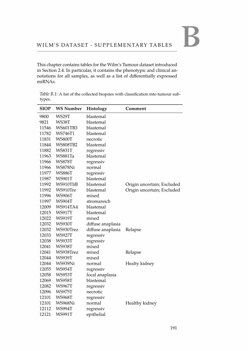
BW I L M ' S DATA S E T - S U P P L E M E N TA RY TA B L E S

This chapter contains tables for the Wilm’s Tumour dataset introducedin Section 2.4. In particular, it contains the phenotypic and clinical an-notations for all samples, as well as a list of differentially expressedmiRNAs.

Table B.1: A list of the collected biopsies with classification into tumour sub-types.

SIOP WS Number Histology Comment

9800 WS29T blastemal9821 WS38T blastemal11546 WS601TB3 blastemal11782 WS746T1 blastemal11831 WS800T necrotic11844 WS808TB2 blastemal11882 WS831T regressiv11963 WS881Ta blastemal11966 WS878T regressiv11966 WS878Ni normal11977 WS886T regressiv11987 WS901T blastemal11992 WS910TliB blastemal Origin uncertain; Excluded11992 WS910Tre blastemal Origin uncertain; Excluded11996 WS906T mixed11997 WS904T stromareich12009 WS914TA4 blastemal12015 WS917T blastemal12022 WS919T mixed12032 WS930T diffuse anaplasia12032 WS930Trez diffuse anaplasia Relapse12033 WS927T regressiv12038 WS933T regressiv12041 WS938T mixed12041 WS938Trez mixed Relapse12044 WS939T mixed12044 WS939Ni normal Healty kidney12055 WS954T regressiv12058 WS953T focal anaplasia12069 WS958T blastemal12082 WS967T regressiv12096 WS975T necrotic12101 WS968T regressiv12101 WS968Ni normal Healthy kidney12112 WS994T regressiv12121 WS991T epithelial

191

w i l m ' s data s e t - s u p p l e m e n ta ry ta b l e s

SIOP WS Number Histology Comment

12124 WS988T regressiv12125 WS1001T regressiv12146 WS1002T mixed12171 WS1018T mixed12171 WS1018Ni normal Healthy kidney12197 WS1030TA blastemal No WT; Excluded12197 WS1030TB blastemal12260 WS1063T2 blastemal12263 WS1073TA3 blastemal12322 WS1106TA3 blastemal12331 WS1098TA4 blastemal

192

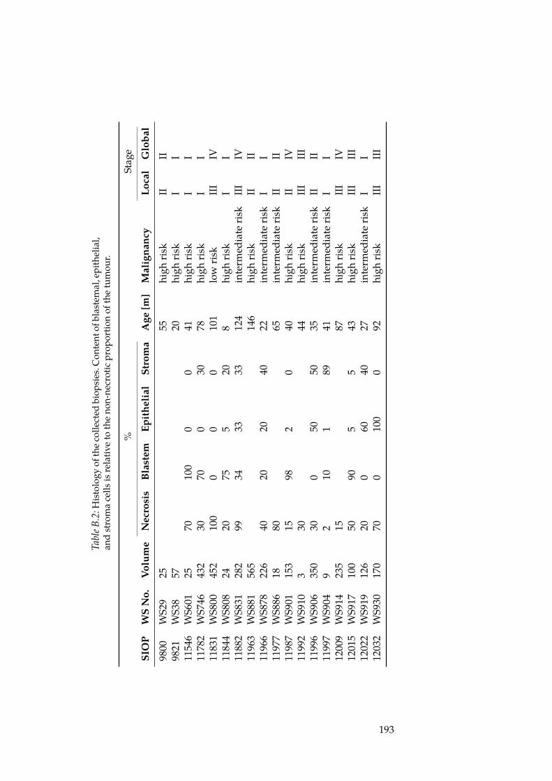
Tabl

eB.2

:His

tolo

gyof

thec

olle

cted

biop

sies

.Con

tent

ofbl

aste

mal

,epi

thel

ial,

and

stro

ma

cells

isre

lativ

eto

the

non-

necr

otic

prop

ortio

nof

the

tum

our.

%St

age

SIO

PW

SN

o.V

olum

eN

ecro

sis

Blas

tem

Epit

helia

lSt

rom

aA

ge[m

]M

alig

nanc

yLo

cal

Glo

bal

9800

WS2

925

55hi

ghris

kII

II98

21W

S38

5720

high

risk

II

1154

6W

S601

2570

100

00

41hi

ghris

kI

I11

782

WS7

4643

230

700

3078

high

risk

II

1183

1W

S800

452

100

00

010

1lo

wris

kIII

IV11

844

WS8

0824

2075

520

8hi

ghris

kI

I11

882

WS8

3128

299

3433

3312

4in

term

edia

teris

kIII

IV11

963

WS8

8156

514

6hi

ghris

kII

II11

966

WS8

7822

640

2020

4022

inte

rmed

iate

risk

II

1197

7W

S886

1880

65in

term

edia

teris

kII

II11

987

WS9

0115

315

982

040

high

risk

IIIV

1199

2W

S910

330

44hi

ghris

kIII

III11

996

WS9

0635

030

050

5035

inte

rmed

iate

risk

IIII

1199

7W

S904

92

101

8941

inte

rmed

iate

risk

II

1200

9W

S914

235

1587

high

risk

IIIIV

1201

5W

S917

100

5090

55

43hi

ghris

kIII

III12

022

WS9

1912

620

060

4027

inte

rmed

iate

risk

II

1203

2W

S930

170

700

100

092

high

risk

IIIIII

193

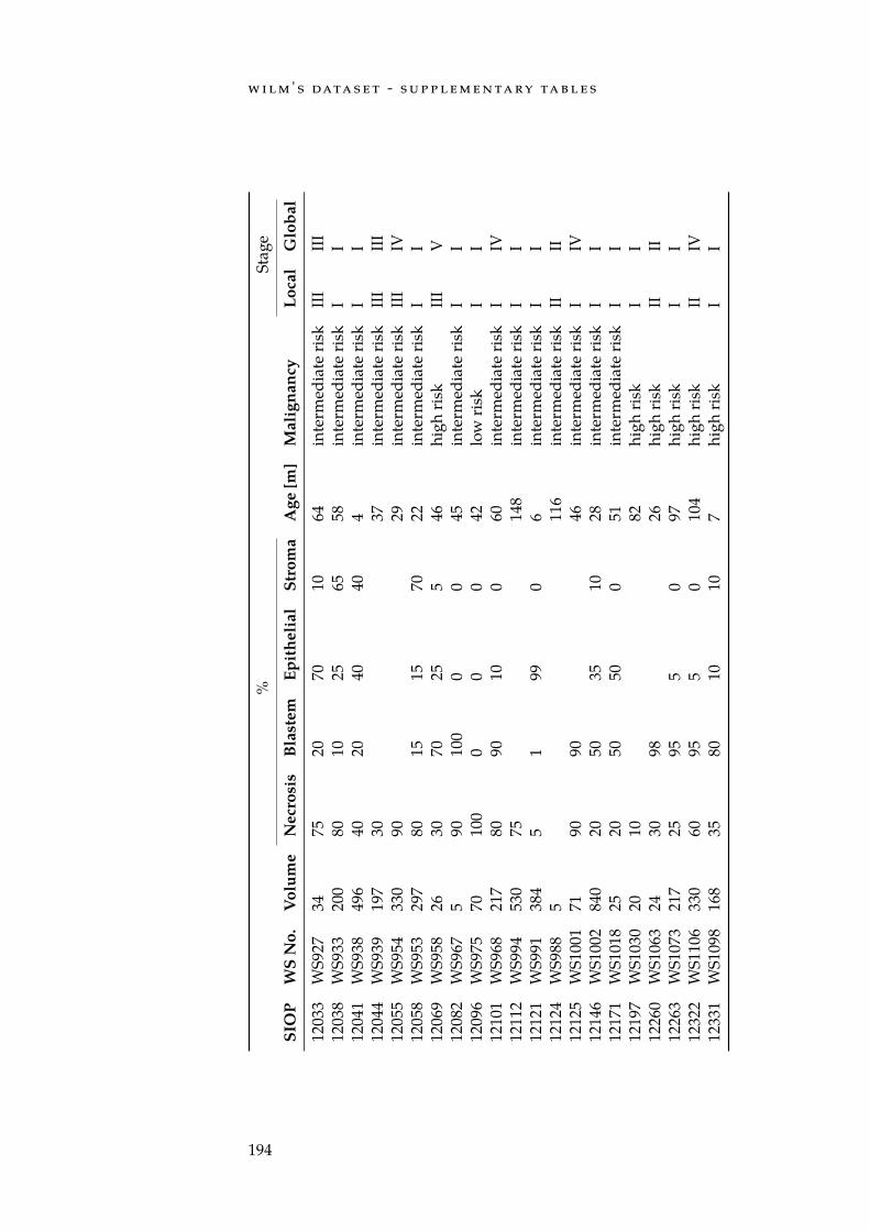
w i l m ' s data s e t - s u p p l e m e n ta ry ta b l e s

%St

age

SIO

PW

SN

o.V

olum

eN

ecro

sis

Blas

tem

Epit

helia

lSt

rom

aA

ge[m

]M

alig

nanc

yLo

cal

Glo

bal

1203

3W

S927

3475

2070

1064

inte

rmed

iate

risk

IIIIII

1203

8W

S933

200

8010

2565

58in

term

edia

teris

kI

I12

041

WS9

3849

640

2040

404

inte

rmed

iate

risk

II

1204

4W

S939

197

3037

inte

rmed

iate

risk

IIIIII

1205

5W

S954

330

9029

inte

rmed

iate

risk

IIIIV

1205

8W

S953

297

8015

1570

22in

term

edia

teris

kI

I12

069

WS9

5826

3070

255

46hi

ghris

kIII

V12

082

WS9

675

9010

00

045

inte

rmed

iate

risk

II

1209

6W

S975

7010

00

00

42lo

wris

kI

I12

101

WS9

6821

780

9010

060

inte

rmed

iate

risk

IIV

1211

2W

S994

530

7514

8in

term

edia

teris

kI

I12

121

WS9

9138

45

199

06

inte

rmed

iate

risk

II

1212

4W

S988

511

6in

term

edia

teris

kII

II12

125

WS1

001

7190

9046

inte

rmed

iate

risk

IIV

1214

6W

S100

284

020

5035

1028

inte

rmed

iate

risk

II

1217

1W

S101

825

2050

500

51in

term

edia

teris

kI

I12

197

WS1

030

2010

82hi

ghris

kI

I12

260

WS1

063

2430

9826

high

risk

IIII

1226

3W

S107

321

725

955

097

high

risk

II

1232

2W

S110

633

060

955

010

4hi

ghris

kII

IV12

331

WS1

098

168

3580

1010

7hi

ghris

kI

I

194

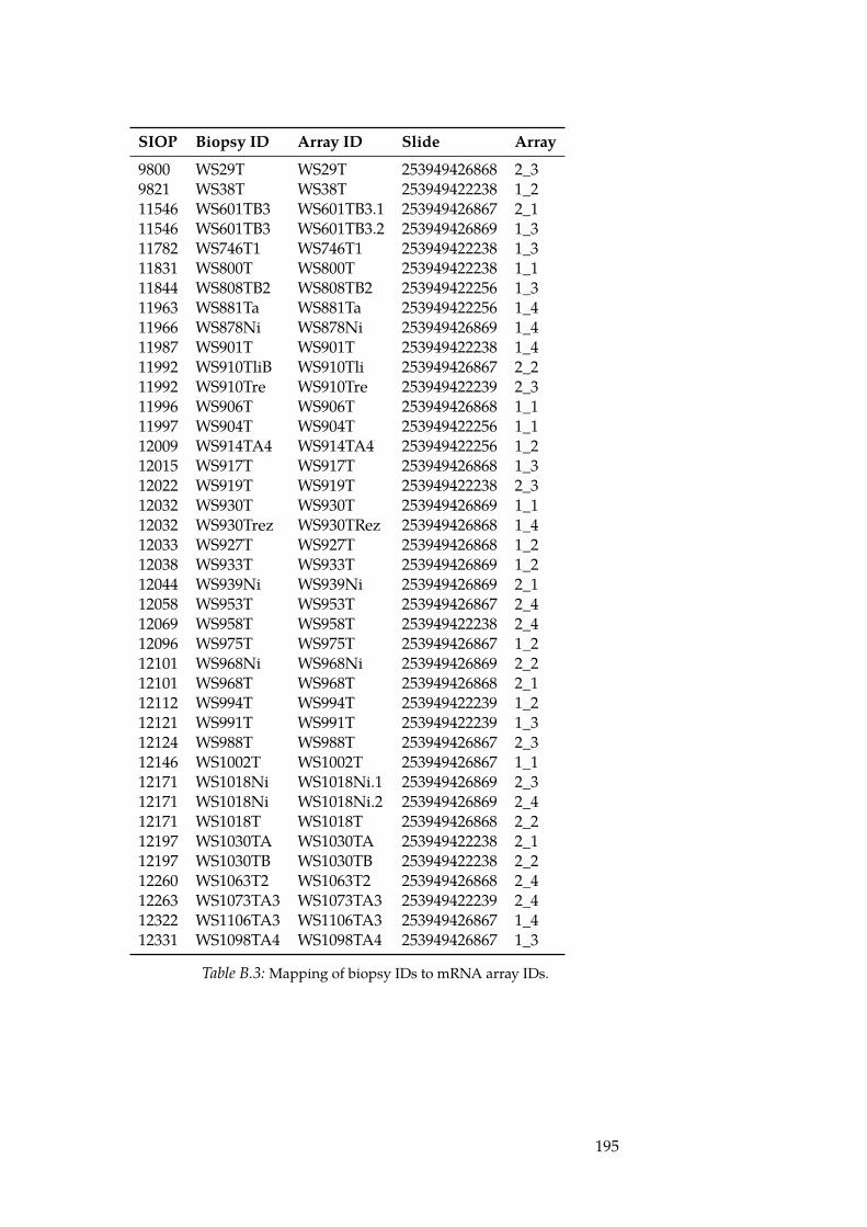
SIOP Biopsy ID Array ID Slide Array

9800 WS29T WS29T 253949426868 2_39821 WS38T WS38T 253949422238 1_211546 WS601TB3 WS601TB3.1 253949426867 2_111546 WS601TB3 WS601TB3.2 253949426869 1_311782 WS746T1 WS746T1 253949422238 1_311831 WS800T WS800T 253949422238 1_111844 WS808TB2 WS808TB2 253949422256 1_311963 WS881Ta WS881Ta 253949422256 1_411966 WS878Ni WS878Ni 253949426869 1_411987 WS901T WS901T 253949422238 1_411992 WS910TliB WS910Tli 253949426867 2_211992 WS910Tre WS910Tre 253949422239 2_311996 WS906T WS906T 253949426868 1_111997 WS904T WS904T 253949422256 1_112009 WS914TA4 WS914TA4 253949422256 1_212015 WS917T WS917T 253949426868 1_312022 WS919T WS919T 253949422238 2_312032 WS930T WS930T 253949426869 1_112032 WS930Trez WS930TRez 253949426868 1_412033 WS927T WS927T 253949426868 1_212038 WS933T WS933T 253949426869 1_212044 WS939Ni WS939Ni 253949426869 2_112058 WS953T WS953T 253949426867 2_412069 WS958T WS958T 253949422238 2_412096 WS975T WS975T 253949426867 1_212101 WS968Ni WS968Ni 253949426869 2_212101 WS968T WS968T 253949426868 2_112112 WS994T WS994T 253949422239 1_212121 WS991T WS991T 253949422239 1_312124 WS988T WS988T 253949426867 2_312146 WS1002T WS1002T 253949426867 1_112171 WS1018Ni WS1018Ni.1 253949426869 2_312171 WS1018Ni WS1018Ni.2 253949426869 2_412171 WS1018T WS1018T 253949426868 2_212197 WS1030TA WS1030TA 253949422238 2_112197 WS1030TB WS1030TB 253949422238 2_212260 WS1063T2 WS1063T2 253949426868 2_412263 WS1073TA3 WS1073TA3 253949422239 2_412322 WS1106TA3 WS1106TA3 253949426867 1_412331 WS1098TA4 WS1098TA4 253949426867 1_3

Table B.3: Mapping of biopsy IDs to mRNA array IDs.

195

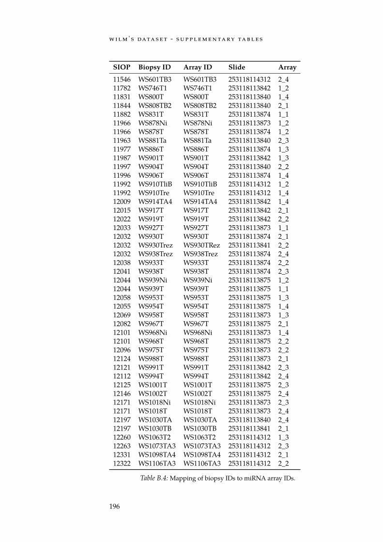
w i l m ' s data s e t - s u p p l e m e n ta ry ta b l e s

SIOP Biopsy ID Array ID Slide Array

11546 WS601TB3 WS601TB3 253118114312 2_411782 WS746T1 WS746T1 253118113842 1_211831 WS800T WS800T 253118113840 1_411844 WS808TB2 WS808TB2 253118113840 2_111882 WS831T WS831T 253118113874 1_111966 WS878Ni WS878Ni 253118113873 1_211966 WS878T WS878T 253118113874 1_211963 WS881Ta WS881Ta 253118113840 2_311977 WS886T WS886T 253118113874 1_311987 WS901T WS901T 253118113842 1_311997 WS904T WS904T 253118113840 2_211996 WS906T WS906T 253118113874 1_411992 WS910TliB WS910TliB 253118114312 1_211992 WS910Tre WS910Tre 253118114312 1_412009 WS914TA4 WS914TA4 253118113842 1_412015 WS917T WS917T 253118113842 2_112022 WS919T WS919T 253118113842 2_212033 WS927T WS927T 253118113873 1_112032 WS930T WS930T 253118113874 2_112032 WS930Trez WS930TRez 253118113841 2_212032 WS938Trez WS938Trez 253118113874 2_412038 WS933T WS933T 253118113874 2_212041 WS938T WS938T 253118113874 2_312044 WS939Ni WS939Ni 253118113875 1_212044 WS939T WS939T 253118113875 1_112058 WS953T WS953T 253118113875 1_312055 WS954T WS954T 253118113875 1_412069 WS958T WS958T 253118113873 1_312082 WS967T WS967T 253118113875 2_112101 WS968Ni WS968Ni 253118113873 1_412101 WS968T WS968T 253118113875 2_212096 WS975T WS975T 253118113873 2_212124 WS988T WS988T 253118113873 2_112121 WS991T WS991T 253118113842 2_312112 WS994T WS994T 253118113842 2_412125 WS1001T WS1001T 253118113875 2_312146 WS1002T WS1002T 253118113875 2_412171 WS1018Ni WS1018Ni 253118113873 2_312171 WS1018T WS1018T 253118113873 2_412197 WS1030TA WS1030TA 253118113840 2_412197 WS1030TB WS1030TB 253118113841 2_112260 WS1063T2 WS1063T2 253118114312 1_312263 WS1073TA3 WS1073TA3 253118114312 2_312331 WS1098TA4 WS1098TA4 253118114312 2_112322 WS1106TA3 WS1106TA3 253118114312 2_2

Table B.4: Mapping of biopsy IDs to miRNA array IDs.

196

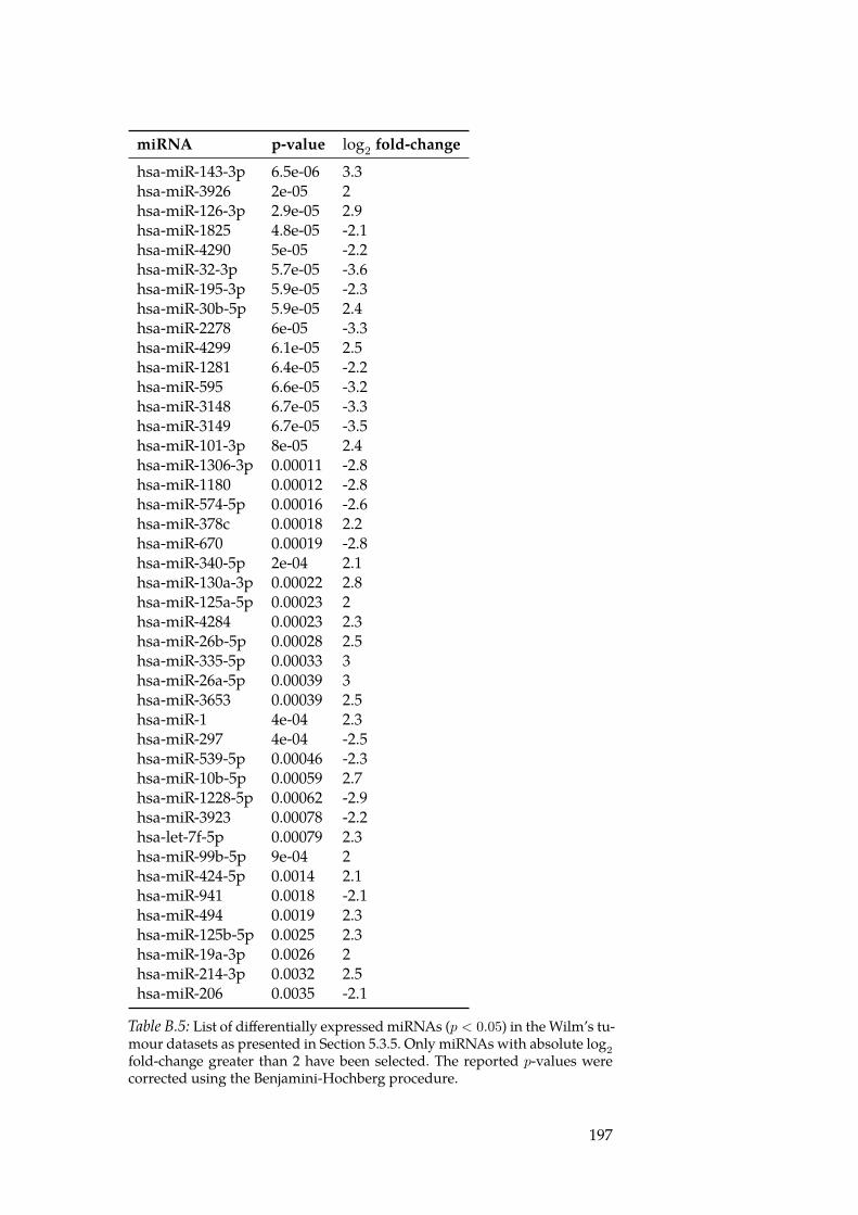
miRNA p-value log2 fold-change

hsa-miR-143-3p 6.5e-06 3.3hsa-miR-3926 2e-05 2hsa-miR-126-3p 2.9e-05 2.9hsa-miR-1825 4.8e-05 -2.1hsa-miR-4290 5e-05 -2.2hsa-miR-32-3p 5.7e-05 -3.6hsa-miR-195-3p 5.9e-05 -2.3hsa-miR-30b-5p 5.9e-05 2.4hsa-miR-2278 6e-05 -3.3hsa-miR-4299 6.1e-05 2.5hsa-miR-1281 6.4e-05 -2.2hsa-miR-595 6.6e-05 -3.2hsa-miR-3148 6.7e-05 -3.3hsa-miR-3149 6.7e-05 -3.5hsa-miR-101-3p 8e-05 2.4hsa-miR-1306-3p 0.00011 -2.8hsa-miR-1180 0.00012 -2.8hsa-miR-574-5p 0.00016 -2.6hsa-miR-378c 0.00018 2.2hsa-miR-670 0.00019 -2.8hsa-miR-340-5p 2e-04 2.1hsa-miR-130a-3p 0.00022 2.8hsa-miR-125a-5p 0.00023 2hsa-miR-4284 0.00023 2.3hsa-miR-26b-5p 0.00028 2.5hsa-miR-335-5p 0.00033 3hsa-miR-26a-5p 0.00039 3hsa-miR-3653 0.00039 2.5hsa-miR-1 4e-04 2.3hsa-miR-297 4e-04 -2.5hsa-miR-539-5p 0.00046 -2.3hsa-miR-10b-5p 0.00059 2.7hsa-miR-1228-5p 0.00062 -2.9hsa-miR-3923 0.00078 -2.2hsa-let-7f-5p 0.00079 2.3hsa-miR-99b-5p 9e-04 2hsa-miR-424-5p 0.0014 2.1hsa-miR-941 0.0018 -2.1hsa-miR-494 0.0019 2.3hsa-miR-125b-5p 0.0025 2.3hsa-miR-19a-3p 0.0026 2hsa-miR-214-3p 0.0032 2.5hsa-miR-206 0.0035 -2.1

Table B.5: List of differentially expressed miRNAs (p < 0.05) in the Wilm’s tu-mour datasets as presented in Section 5.3.5. Only miRNAs with absolute log2fold-change greater than 2 have been selected. The reported p-values werecorrected using the Benjamini-Hochberg procedure.

197

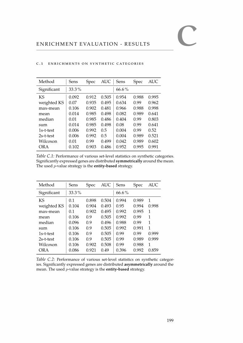
CE N R I CH M E N T E VA LUAT I O N - R E S U LT S

c . 1 e n r i c h m e n t s o n sy n t h e t i c cat e g o r i e s

Method Sens Spec AUC Sens Spec AUC

Significant 33.3 % 66.6 %

KS 0.092 0.912 0.505 0.954 0.988 0.995weighted KS 0.07 0.935 0.495 0.634 0.99 0.962max-mean 0.106 0.902 0.481 0.966 0.988 0.998mean 0.014 0.985 0.498 0.082 0.989 0.641median 0.01 0.985 0.486 0.404 0.99 0.803sum 0.014 0.985 0.498 0.08 0.99 0.6411s-t-test 0.006 0.992 0.5 0.004 0.99 0.522s-t-test 0.006 0.992 0.5 0.004 0.989 0.521Wilcoxon 0.01 0.99 0.499 0.042 0.989 0.602ORA 0.102 0.903 0.486 0.952 0.995 0.991

Table C.1: Performance of various set-level statistics on synthetic categories.Significantly expressed genes are distributed symmetrically around the mean.The used p-value strategy is the entity-based strategy.

Method Sens Spec AUC Sens Spec AUC

Significant 33.3 % 66.6 %

KS 0.1 0.898 0.504 0.994 0.989 1weighted KS 0.104 0.904 0.493 0.95 0.994 0.998max-mean 0.1 0.902 0.495 0.992 0.995 1mean 0.106 0.9 0.505 0.992 0.99 1median 0.096 0.9 0.496 0.988 0.99 1sum 0.106 0.9 0.505 0.992 0.991 11s-t-test 0.106 0.9 0.505 0.99 0.99 0.9992s-t-test 0.106 0.9 0.505 0.99 0.989 0.999Wilcoxon 0.106 0.902 0.508 0.99 0.988 1ORA 0.086 0.921 0.49 0.396 0.992 0.859

Table C.2: Performance of various set-level statistics on synthetic categor-ies. Significantly expressed genes are distributed asymmetrically around themean. The used p-value strategy is the entity-based strategy.

199

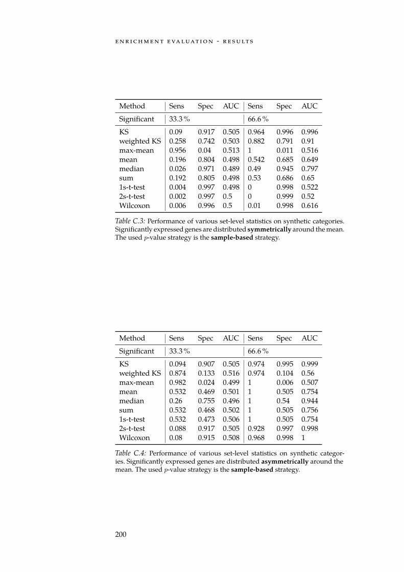
e n r i c h m e n t e va luat i o n - r e s u lt s

Method Sens Spec AUC Sens Spec AUC

Significant 33.3 % 66.6 %

KS 0.09 0.917 0.505 0.964 0.996 0.996weighted KS 0.258 0.742 0.503 0.882 0.791 0.91max-mean 0.956 0.04 0.513 1 0.011 0.516mean 0.196 0.804 0.498 0.542 0.685 0.649median 0.026 0.971 0.489 0.49 0.945 0.797sum 0.192 0.805 0.498 0.53 0.686 0.651s-t-test 0.004 0.997 0.498 0 0.998 0.5222s-t-test 0.002 0.997 0.5 0 0.999 0.52Wilcoxon 0.006 0.996 0.5 0.01 0.998 0.616

Table C.3: Performance of various set-level statistics on synthetic categories.Significantly expressed genes are distributed symmetrically around the mean.The used p-value strategy is the sample-based strategy.

Method Sens Spec AUC Sens Spec AUC

Significant 33.3 % 66.6 %

KS 0.094 0.907 0.505 0.974 0.995 0.999weighted KS 0.874 0.133 0.516 0.974 0.104 0.56max-mean 0.982 0.024 0.499 1 0.006 0.507mean 0.532 0.469 0.501 1 0.505 0.754median 0.26 0.755 0.496 1 0.54 0.944sum 0.532 0.468 0.502 1 0.505 0.7561s-t-test 0.532 0.473 0.506 1 0.505 0.7542s-t-test 0.088 0.917 0.505 0.928 0.997 0.998Wilcoxon 0.08 0.915 0.508 0.968 0.998 1

Table C.4: Performance of various set-level statistics on synthetic categor-ies. Significantly expressed genes are distributed asymmetrically around themean. The used p-value strategy is the sample-based strategy.

200

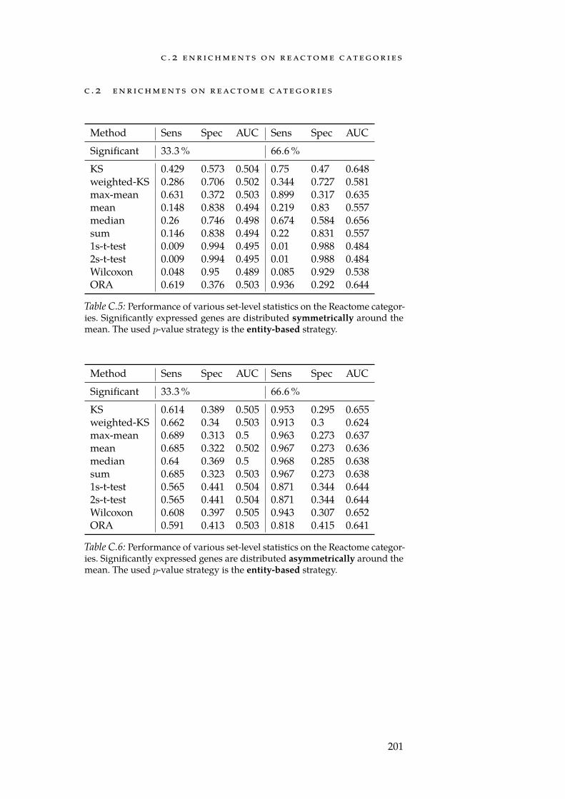
c . 2 e n r i c h m e n t s o n r e ac to m e cat e g o r i e s

c . 2 e n r i c h m e n t s o n r e ac to m e cat e g o r i e s

Method Sens Spec AUC Sens Spec AUC

Significant 33.3 % 66.6 %

KS 0.429 0.573 0.504 0.75 0.47 0.648weighted-KS 0.286 0.706 0.502 0.344 0.727 0.581max-mean 0.631 0.372 0.503 0.899 0.317 0.635mean 0.148 0.838 0.494 0.219 0.83 0.557median 0.26 0.746 0.498 0.674 0.584 0.656sum 0.146 0.838 0.494 0.22 0.831 0.5571s-t-test 0.009 0.994 0.495 0.01 0.988 0.4842s-t-test 0.009 0.994 0.495 0.01 0.988 0.484Wilcoxon 0.048 0.95 0.489 0.085 0.929 0.538ORA 0.619 0.376 0.503 0.936 0.292 0.644

Table C.5: Performance of various set-level statistics on the Reactome categor-ies. Significantly expressed genes are distributed symmetrically around themean. The used p-value strategy is the entity-based strategy.

Method Sens Spec AUC Sens Spec AUC

Significant 33.3 % 66.6 %

KS 0.614 0.389 0.505 0.953 0.295 0.655weighted-KS 0.662 0.34 0.503 0.913 0.3 0.624max-mean 0.689 0.313 0.5 0.963 0.273 0.637mean 0.685 0.322 0.502 0.967 0.273 0.636median 0.64 0.369 0.5 0.968 0.285 0.638sum 0.685 0.323 0.503 0.967 0.273 0.6381s-t-test 0.565 0.441 0.504 0.871 0.344 0.6442s-t-test 0.565 0.441 0.504 0.871 0.344 0.644Wilcoxon 0.608 0.397 0.505 0.943 0.307 0.652ORA 0.591 0.413 0.503 0.818 0.415 0.641

Table C.6: Performance of various set-level statistics on the Reactome categor-ies. Significantly expressed genes are distributed asymmetrically around themean. The used p-value strategy is the entity-based strategy.

201

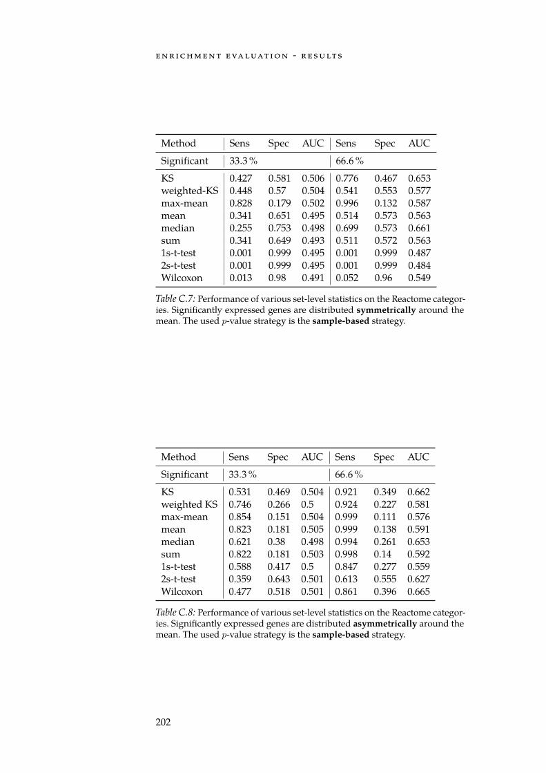
e n r i c h m e n t e va luat i o n - r e s u lt s

Method Sens Spec AUC Sens Spec AUC

Significant 33.3 % 66.6 %

KS 0.427 0.581 0.506 0.776 0.467 0.653weighted-KS 0.448 0.57 0.504 0.541 0.553 0.577max-mean 0.828 0.179 0.502 0.996 0.132 0.587mean 0.341 0.651 0.495 0.514 0.573 0.563median 0.255 0.753 0.498 0.699 0.573 0.661sum 0.341 0.649 0.493 0.511 0.572 0.5631s-t-test 0.001 0.999 0.495 0.001 0.999 0.4872s-t-test 0.001 0.999 0.495 0.001 0.999 0.484Wilcoxon 0.013 0.98 0.491 0.052 0.96 0.549

Table C.7: Performance of various set-level statistics on the Reactome categor-ies. Significantly expressed genes are distributed symmetrically around themean. The used p-value strategy is the sample-based strategy.

Method Sens Spec AUC Sens Spec AUC

Significant 33.3 % 66.6 %

KS 0.531 0.469 0.504 0.921 0.349 0.662weighted KS 0.746 0.266 0.5 0.924 0.227 0.581max-mean 0.854 0.151 0.504 0.999 0.111 0.576mean 0.823 0.181 0.505 0.999 0.138 0.591median 0.621 0.38 0.498 0.994 0.261 0.653sum 0.822 0.181 0.503 0.998 0.14 0.5921s-t-test 0.588 0.417 0.5 0.847 0.277 0.5592s-t-test 0.359 0.643 0.501 0.613 0.555 0.627Wilcoxon 0.477 0.518 0.501 0.861 0.396 0.665

Table C.8: Performance of various set-level statistics on the Reactome categor-ies. Significantly expressed genes are distributed asymmetrically around themean. The used p-value strategy is the sample-based strategy.

202

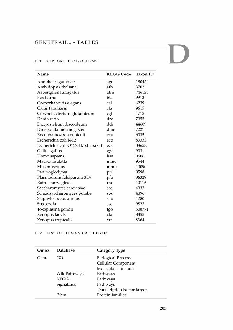
DG E N E T R A I L 2 - TA B L E S

d . 1 s u p p o rt e d o rga n i s m s

Name KEGG Code Taxon ID

Anopheles gambiae age 180454Arabidopsis thaliana ath 3702Aspergillus fumigatus afm 746128Bos taurus bta 9913Caenorhabditis elegans cel 6239Canis familiaris cfa 9615Corynebacterium glutamicum cgl 1718Danio rerio dre 7955Dictyostelium discoideum ddi 44689Drosophila melanogaster dme 7227Encephalitozoon cuniculi ecu 6035Escherichia coli K-12 eco 83333Escherichia coli O157:H7 str. Sakai ecs 386585Gallus gallus gga 9031Homo sapiens hsa 9606Macaca mulatta mmc 9544Mus musculus mmu 10090Pan troglodytes ptr 9598Plasmodium falciparum 3D7 pfa 36329Rattus norvegicus rno 10116Saccharomyces cerevisiae sce 4932Schizosaccharomyces pombe spo 4896Staphylococcus aureus sau 1280Sus scrofa ssc 9823Toxoplasma gondii tgo 508771Xenopus laevis xla 8355Xenopus tropicalis xtr 8364

d . 2 l i s t o f h u m a n cat e g o r i e s

Omics Database Category Type

Gene GO Biological ProcessCellular ComponentMolecular Function

WikiPathways PathwaysKEGG PathwaysSignaLink Pathways

Transcription Factor targetsPfam Protein families

203

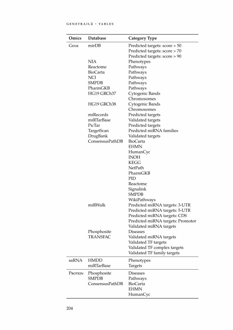
g e n e t r a i l 2 - ta b l e s

Omics Database Category Type

Gene mirDB Predicted targets: score > 50Predicted targets: score > 70Predicted targets: score > 90

NIA PhenotypesReactome PathwaysBioCarta PathwaysNCI PathwaysSMPDB PathwaysPharmGKB PathwaysHG19 GRCh37 Cytogenic Bands

ChromosomesHG19 GRCh38 Cytogenic Bands

ChromosomesmiRecords Predicted targetsmiRTarBase Validated targetsPicTar Predicted targetsTargetScan Predicted miRNA familiesDrugBank Validated targetsConsensusPathDB BioCarta

EHMNHumanCycINOHKEGGNetPathPharmGKBPIDReactomeSignalinkSMPDBWikiPathways

miRWalk Predicted miRNA targets: 3-UTRPredicted miRNA targets: 5-UTRPredicted miRNA targets: CDSPredicted miRNA targets: PromotorValidated miRNA targets

Phosphosite DiseasesTRANSFAC Validated miRNA targets

Validated TF targetsValidated TF complex targetsValidated TF family targets

miRNA HMDD PhenotypesmiRTarBase Targets

Protein Phosphosite DiseasesSMPDB PathwaysConsensusPathDB BioCarta

EHMNHumanCyc

204

d . 2 l i s t o f h u m a n cat e g o r i e s

Omics Database Category Type

Protein ConsensusPathDB INOHKEGGNetPathPharmGKBPIDReactomeSignalinkSMPDBWikiPathways

NCI Pathway Interaction DatabasePfam Protein familiesReactome Pathways

SNP GWAS cataloguePheWAS catalogue

205

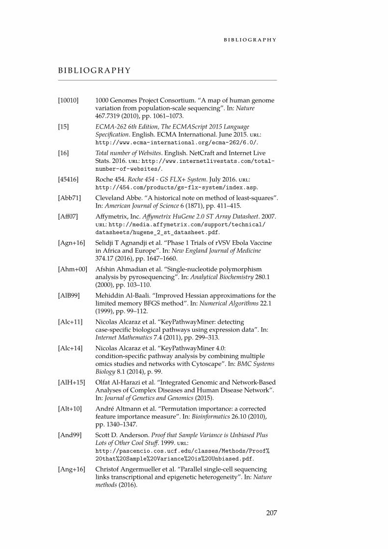
b i b l i o g r a p h y

B I B L I O G R A P H Y

[10010] 1000 Genomes Project Consortium. “A map of human genomevariation from population-scale sequencing”. In: Nature467.7319 (2010), pp. 1061–1073.

[15] ECMA-262 6th Edition, The ECMAScript 2015 LanguageSpecification. English. ECMA International. June 2015. url:http://www.ecma-international.org/ecma-262/6.0/.

[16] Total number of Websites. English. NetCraft and Internet LiveStats. 2016. url: http://www.internetlivestats.com/total-number-of-websites/.

[45416] Roche 454. Roche 454 - GS FLX+ System. July 2016. url:http://454.com/products/gs-flx-system/index.asp.

[Abb71] Cleveland Abbe. “A historical note on method of least-squares”.In: American Journal of Science 6 (1871), pp. 411–415.

[Aff07] Affymetrix, Inc. Affymetrix HuGene 2.0 ST Array Datasheet. 2007.url: http://media.affymetrix.com/support/technical/datasheets/hugene_2_st_datasheet.pdf.

[Agn+16] Selidji T Agnandji et al. “Phase 1 Trials of rVSV Ebola Vaccinein Africa and Europe”. In: New England Journal of Medicine374.17 (2016), pp. 1647–1660.

[Ahm+00] Afshin Ahmadian et al. “Single-nucleotide polymorphismanalysis by pyrosequencing”. In: Analytical Biochemistry 280.1(2000), pp. 103–110.

[AlB99] Mehiddin Al-Baali. “Improved Hessian approximations for thelimited memory BFGS method”. In: Numerical Algorithms 22.1(1999), pp. 99–112.

[Alc+11] Nicolas Alcaraz et al. “KeyPathwayMiner: detectingcase-specific biological pathways using expression data”. In:Internet Mathematics 7.4 (2011), pp. 299–313.

[Alc+14] Nicolas Alcaraz et al. “KeyPathwayMiner 4.0:condition-specific pathway analysis by combining multipleomics studies and networks with Cytoscape”. In: BMC SystemsBiology 8.1 (2014), p. 99.

[AlH+15] Olfat Al-Harazi et al. “Integrated Genomic and Network-BasedAnalyses of Complex Diseases and Human Disease Network”.In: Journal of Genetics and Genomics (2015).

[Alt+10] André Altmann et al. “Permutation importance: a correctedfeature importance measure”. In: Bioinformatics 26.10 (2010),pp. 1340–1347.

[And99] Scott D. Anderson. Proof that Sample Variance is Unbiased PlusLots of Other Cool Stuff. 1999. url:http://pascencio.cos.ucf.edu/classes/Methods/Proof%20that%20Sample%20Variance%20is%20Unbiased.pdf.

[Ang+16] Christof Angermueller et al. “Parallel single-cell sequencinglinks transcriptional and epigenetic heterogeneity”. In: Naturemethods (2016).

207

b i b l i o g r a p h y

[Ant+11] Roman Anton et al. “A systematic screen for micro-RNAsregulating the canonical Wnt pathway”. In: PloS One 6.10(2011), e26257.

[AP13] Catherine Alix-Panabières and Klaus Pantel. “Circulatingtumor cells: liquid biopsy of cancer”. In: Clinical chemistry 59.1(2013), pp. 110–118.

[Ara+11] Khelifa Arab et al. “Epigenetic deregulation of TCF21 inhibitsmetastasis suppressor KISS1 in metastatic melanoma”. In:Carcinogenesis 32.10 (2011), pp. 1467–1473.

[ART08] ART-CC. “Life expectancy of individuals on combinationantiretroviral therapy in high-income countries: a collaborativeanalysis of 14 cohort studies”. In: The Lancet 372.9635 (2008),pp. 293–299.

[AS07] Adriana Albini and Michael B Sporn. “The tumourmicroenvironment as a target for chemoprevention”. In: NatureReviews Cancer 7.2 (2007), pp. 139–147.

[AS09] Marit Ackermann and Korbinian Strimmer. “A generalmodular framework for gene set enrichment analysis”. In: BMCBioinformatics 10.1 (2009), p. 47.

[Ash+00] Michael Ashburner et al. “Gene Ontology: tool for theunification of biology”. In: Nature Genetics 25.1 (2000),pp. 25–29.

[Ass+08] Yassen Assenov et al. “Computing topological parameters ofbiological networks”. In: Bioinformatics 24.2 (2008), pp. 282–284.

[Ass13] Walter Assenmacher. Induktive Statistik. Springer-Verlag, 2013.[BA00] Jeffrey G Blodgett and Ronald D Anderson. “A Bayesian

network model of the consumer complaint process”. In: Journalof Service Research 2.4 (2000), pp. 321–338.

[Bac+07] Christina Backes et al. “GeneTrail – advanced gene setenrichment analysis”. In: Nucleic Acids Research 35.suppl 2(2007), W186–W192.

[Bac+12] Christina Backes et al. “An integer linear programmingapproach for finding deregulated subgraphs in regulatorynetworks”. In: Nucleic Acids Research 40.6 (2012), e43–e43.

[Bac+16] Christina Backes et al. “miEAA: microRNA enrichmentanalysis and annotation”. In: Nucleic Acids Research (2016),gkw345.

[Bah12] Miriam Bah. “Measuring the relevance of topology in networksfor finding deregulated subgraphs”. Bachelor’s Thesis.Saarland University, 2012.

[Bai+05] Amos Bairoch et al. “The universal protein resource (UniProt)”.In: Nucleic Acids Research 33.suppl 1 (2005), pp. D154–D159.

[Ban+10] Yung-Jue Bang et al. “Trastuzumab in combination withchemotherapy versus chemotherapy alone for treatment ofHER2-positive advanced gastric or gastro-oesophageal junctioncancer (ToGA): a phase 3, open-label, randomised controlledtrial”. In: The Lancet 376.9742 (2010), pp. 687–697.

208

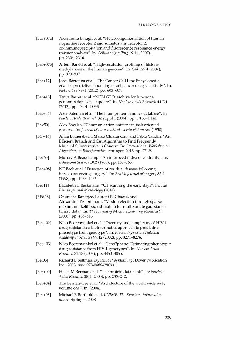
b i b l i o g r a p h y

[Bar+07a] Alessandra Baragli et al. “Heterooligomerization of humandopamine receptor 2 and somatostatin receptor 2:co-immunoprecipitation and fluorescence resonance energytransfer analysis”. In: Cellular signalling 19.11 (2007),pp. 2304–2316.

[Bar+07b] Artem Barski et al. “High-resolution profiling of histonemethylations in the human genome”. In: Cell 129.4 (2007),pp. 823–837.

[Bar+12] Jordi Barretina et al. “The Cancer Cell Line Encyclopediaenables predictive modelling of anticancer drug sensitivity”. In:Nature 483.7391 (2012), pp. 603–607.

[Bar+13] Tanya Barrett et al. “NCBI GEO: archive for functionalgenomics data sets—update”. In: Nucleic Acids Research 41.D1(2013), pp. D991–D995.

[Bat+04] Alex Bateman et al. “The Pfam protein families database”. In:Nucleic Acids Research 32.suppl 1 (2004), pp. D138–D141.

[Bav50] Alex Bavelas. “Communication patterns in task-orientedgroups.” In: Journal of the acoustical society of America (1950).

[BCV16] Anna Bomersbach, Marco Chiarandini, and Fabio Vandin. “AnEfficient Branch and Cut Algorithm to Find FrequentlyMutated Subnetworks in Cancer”. In: International Workshop onAlgorithms in Bioinformatics. Springer. 2016, pp. 27–39.

[Bea65] Murray A Beauchamp. “An improved index of centrality”. In:Behavioral Science 10.2 (1965), pp. 161–163.

[Bec+98] NE Beck et al. “Detection of residual disease followingbreast-conserving surgery”. In: British journal of surgery 85.9(1998), pp. 1273–1276.

[Bec14] Elizabeth C Beckmann. “CT scanning the early days”. In: TheBritish journal of radiology (2014).

[BEd08] Onureena Banerjee, Laurent El Ghaoui, andAlexandre d’Aspremont. “Model selection through sparsemaximum likelihood estimation for multivariate gaussian orbinary data”. In: The Journal of Machine Learning Research 9(2008), pp. 485–516.

[Bee+02] Niko Beerenwinkel et al. “Diversity and complexity of HIV-1drug resistance: a bioinformatics approach to predictingphenotype from genotype”. In: Proceedings of the NationalAcademy of Sciences 99.12 (2002), pp. 8271–8276.

[Bee+03] Niko Beerenwinkel et al. “Geno2pheno: Estimating phenotypicdrug resistance from HIV-1 genotypes”. In: Nucleic AcidsResearch 31.13 (2003), pp. 3850–3855.

[Bel03] Richard E Bellman. Dynamic Programming. Dover PublicationInc., 2003. isbn: 978-0486428093.

[Ber+00] Helen M Berman et al. “The protein data bank”. In: NucleicAcids Research 28.1 (2000), pp. 235–242.

[Ber+04] Tim Berners-Lee et al. “Architecture of the world wide web,volume one”. In: (2004).

[Ber+08] Michael R Berthold et al. KNIME: The Konstanz informationminer. Springer, 2008.

209

b i b l i o g r a p h y

[Ber13] Jakob Bernoulli. Ars conjectandi. Impensis Thurnisiorum,fratrum, 1713.

[Bez+14] Jeff Bezanson et al. “Julia: A fresh approach to numericalcomputing”. In: arXiv preprint arXiv:1411.1607 (2014).

[BFF96] Tim Berners-Lee, R. Fielding, and H. Frystyk. Hypertext TransferProtocol – HTTP/1.0. IETF - Network Working Group. May 1996.url: https://www.ietf.org/rfc/rfc1945.txt.

[BFM05] Tim Berners-Lee, R. Fielding, and L. Masinter. RFC3986:Uniform Resource Identifier (URI): Generic Syntax. IETF - NetworkWorking Group. 2005. url:https://tools.ietf.org/rfc/rfc3986.txt.

[BH06] Howard Brody and Linda M Hunt. “BiDil: assessing arace-based pharmaceutical”. In: The Annals of Family Medicine4.6 (2006), pp. 556–560.

[BH95] Yoav Benjamini and Yosef Hochberg. “Controlling the falsediscovery rate: a practical and powerful approach to multipletesting”. In: Journal of the Royal Statistical Society. Series B(Methodological) (1995), pp. 289–300.

[BHS09] Gordon Bell, Tony Hey, and Alex Szalay. “Beyond the datadeluge”. In: Science 323.5919 (2009), pp. 1297–1298.

[Bie12] Leslie G Biesecker. “Opportunities and challenges for theintegration of massively parallel genomic sequencing intoclinical practice: lessons from the ClinSeq project”. In: Geneticsin Medicine 14.4 (2012), pp. 393–398.

[Bis06] Christopher M. Bishop. Pattern Recognition and MachineLearning. 1st ed. Springer, 2006. isbn: 978-0387310732.

[BKE11] Jonathan S Berg, Muin J Khoury, and James P Evans.“Deploying whole genome sequencing in clinical practice andpublic health: meeting the challenge one bin at a time”. In:Genetics in Medicine 13.6 (2011), pp. 499–504.

[BKW93] Silke Bienroth, Walter Keller, and Elmar Wahle. “Assembly of aprocessive messenger RNA polyadenylation complex.” In: TheEMBO journal 12.2 (1993), p. 585.

[BL12] Christoph Bock and Thomas Lengauer. “Managing drugresistance in cancer: lessons from HIV therapy”. In: NatureReviews Cancer 12.7 (2012), pp. 494–501.

[Bla03] Douglas L Black. “Mechanisms of alternative pre-messengerRNA splicing”. In: Annual review of biochemistry 72.1 (2003),pp. 291–336.

[BLG15] Thomas Bleazard, Janine A Lamb, and Sam Griffiths-Jones.“Bias in microRNA functional enrichment analysis”. In:Bioinformatics (2015), btv023.

[Bol+03] Benjamin M Bolstad et al. “A comparison of normalizationmethods for high density oligonucleotide array data based onvariance and bias”. In: Bioinformatics 19.2 (2003), pp. 185–193.

[Bon35] C. E. Bonferroni. “Il calcolo delle assicurazioni su gruppi diteste.” In: Studi in Onore del Professore Salvatore Ortu Carboni(1935).

[Bon36] C. E. Bonferroni. “Teoria statistica delle classi e calcolo delleprobabilita.” In: Pubblicazioni del R Istituto Superiore di ScienzeEconomiche e Commerciali di Firenze (1936).

210

b i b l i o g r a p h y

[Bon72] Phillip Bonacich. “Factoring and weighting approaches tostatus scores and clique identification”. In: Journal ofMathematical Sociology 2.1 (1972), pp. 113–120.

[BP78] JB Beckwith and NF Palmer. “Histopathology and prognosis ofWilms tumor Results from the first national wilms’ tumorstudy”. In: Cancer 41.5 (1978), pp. 1937–1948.

[Bra+15] Nicolas Bray et al. “Near-optimal RNA-Seq quantification”. In:arXiv preprint arXiv:1505.02710 (2015).

[Bra14] Tim Bray. “The javascript object notation (json) datainterchange format”. In: (2014).

[Bre+12] Independent UK Panel on Breast Cancer Screening et al. “Thebenefits and harms of breast cancer screening: an independentreview”. In: The Lancet 380.9855 (2012), pp. 1778–1786.

[Bre01] Leo Breiman. “Random forests”. In: Machine learning 45.1(2001), pp. 5–32.

[Bri+00] Carolyn Buxton Bridges et al. “Effectiveness and cost-benefit ofinfluenza vaccination of healthy working adults: a randomizedcontrolled trial”. In: Jama 284.13 (2000), pp. 1655–1663.

[Bro+06] Mark A Brown et al. “Identification and characterization ofSmyd2: a split SET/MYND domain-containing histone H3lysine 36-specific methyltransferase that interacts with the Sin3histone deacetylase complex”. In: Molecular cancer 5.1 (2006),p. 1.

[Bro+83] Bernard R Brooks et al. “CHARMM: a program formacromolecular energy, minimization, and dynamicscalculations”. In: Journal of computational chemistry 4.2 (1983),pp. 187–217.

[BS00] G Patrick Brady Jr and Pieter FW Stouten. “Fast prediction andvisualization of protein binding pockets with PASS”. In: Journalof computer-aided molecular design 14.4 (2000), pp. 383–401.

[BS96] Zhidong Bai and Hewa Saranadasa. “Effect of high dimension:by an example of a two sample problem”. In: Statistica Sinica(1996), pp. 311–329.

[BSM93] Gabriele Basi, Elisabeth Schmid, and Kinsey Maundrell. “TATAbox mutations in the Schizosaccharomyces pombe nmt1promoter affect transcription efficiency but not thetranscription start point or thiamine repressibility”. In: Gene123.1 (1993), pp. 131–136.

[BSS04] Kunihiro Baba, Ritei Shibata, and Masaaki Sibuya. “Partialcorrelation and conditional correlation as measures ofconditional independence”. In: Australian & New ZealandJournal of Statistics 46.4 (2004), pp. 657–664.

[BT97] Dimitris Bertsimas and John N Tsitsiklis. Introduction to linearoptimization. Vol. 6. Athena Scientific Belmont, MA, 1997.

[Bur+13] Randall W Burt et al. “Colorectal cancer screening”. In: Journalof the National Comprehensive Cancer Network 11.12 (2013),pp. 1538–1575.

[Bür13] Jonas Bürse. “Advanced Rendering for BALLView”. MA thesis.Saarland University, 2013.

211

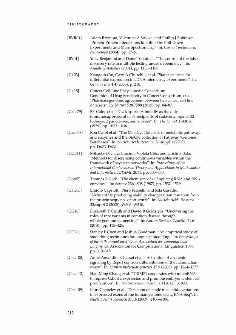
b i b l i o g r a p h y

[BVR04] Adam Brymora, Valentina A Valova, and Phillip J Robinson.“Protein-Protein Interactions Identified by Pull-DownExperiments and Mass Spectrometry”. In: Current protocols incell biology (2004), pp. 17–5.

[BY01] Yoav Benjamini and Daniel Yekutieli. “The control of the falsediscovery rate in multiple testing under dependency”. In:Annals of statistics (2001), pp. 1165–1188.

[C+03] Xiangqin Cui, Gary A Churchill, et al. “Statistical tests fordifferential expression in cDNA microarray experiments”. In:Genome Biol 4.4 (2003), p. 210.

[C+15] Cancer Cell Line Encyclopedia Consortium,Genomics of Drug Sensitivity in Cancer Consortium, et al.“Pharmacogenomic agreement between two cancer cell linedata sets”. In: Nature 528.7580 (2015), pp. 84–87.

[Cal+79] RY Calne et al. “Cyclosporin A initially as the onlyimmunosuppressant in 34 recipients of cadaveric organs: 32kidneys, 2 pancreases, and 2 livers”. In: The Lancet 314.8151(1979), pp. 1033–1036.

[Cas+08] Ron Caspi et al. “The MetaCyc Database of metabolic pathwaysand enzymes and the BioCyc collection of Pathway/GenomeDatabases”. In: Nucleic Acids Research 36.suppl 1 (2008),pp. D623–D631.

[CCB11] Mihaela-Daciana Craciun, Violeta Chis, and Cristina Bala.“Methods for discretizing continuous variables within theframework of bayesian networks”. In: Proceedings of theInternational Conference on Theory and Applications in Mathematicsand Informatics, ICTAMI. 2011, pp. 433–443.

[Cec87] Thomas R Cech. “The chemistry of self-splicing RNA and RNAenzymes”. In: Science 236.4808 (1987), pp. 1532–1539.

[CFC05] Emidio Capriotti, Piero Fariselli, and Rita Casadio.“I-Mutant2.0: predicting stability changes upon mutation fromthe protein sequence or structure”. In: Nucleic Acids Research33.suppl 2 (2005), W306–W310.

[CG10] Elizabeth T Cirulli and David B Goldstein. “Uncovering theroles of rare variants in common disease throughwhole-genome sequencing”. In: Nature Reviews Genetics 11.6(2010), pp. 415–425.

[CG96] Stanley F Chen and Joshua Goodman. “An empirical study ofsmoothing techniques for language modeling”. In: Proceedingsof the 34th annual meeting on Association for ComputationalLinguistics. Association for Computational Linguistics. 1996,pp. 310–318.

[Cha+08] Anne-Amandine Chassot et al. “Activation of β-cateninsignaling by Rspo1 controls differentiation of the mammalianovary”. In: Human molecular genetics 17.9 (2008), pp. 1264–1277.

[Cha+12] Hao-Ming Chang et al. “TRIM71 cooperates with microRNAsto repress Cdkn1a expression and promote embryonic stem cellproliferation”. In: Nature communications 3 (2012), p. 923.

[Che+09] Iouri Chepelev et al. “Detection of single nucleotide variationsin expressed exons of the human genome using RNA-Seq”. In:Nucleic Acids Research 37.16 (2009), e106–e106.

212

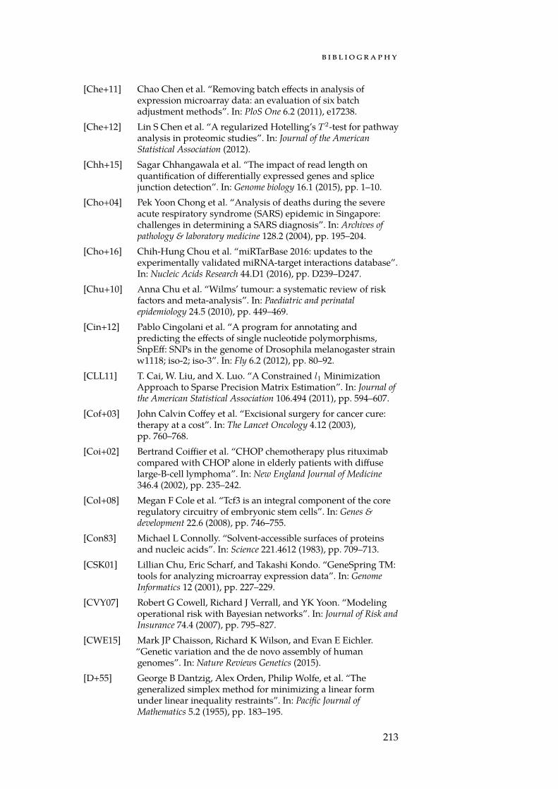
b i b l i o g r a p h y

[Che+11] Chao Chen et al. “Removing batch effects in analysis ofexpression microarray data: an evaluation of six batchadjustment methods”. In: PloS One 6.2 (2011), e17238.

[Che+12] Lin S Chen et al. “A regularized Hotelling’s T 2-test for pathwayanalysis in proteomic studies”. In: Journal of the AmericanStatistical Association (2012).

[Chh+15] Sagar Chhangawala et al. “The impact of read length onquantification of differentially expressed genes and splicejunction detection”. In: Genome biology 16.1 (2015), pp. 1–10.

[Cho+04] Pek Yoon Chong et al. “Analysis of deaths during the severeacute respiratory syndrome (SARS) epidemic in Singapore:challenges in determining a SARS diagnosis”. In: Archives ofpathology & laboratory medicine 128.2 (2004), pp. 195–204.

[Cho+16] Chih-Hung Chou et al. “miRTarBase 2016: updates to theexperimentally validated miRNA-target interactions database”.In: Nucleic Acids Research 44.D1 (2016), pp. D239–D247.

[Chu+10] Anna Chu et al. “Wilms’ tumour: a systematic review of riskfactors and meta-analysis”. In: Paediatric and perinatalepidemiology 24.5 (2010), pp. 449–469.

[Cin+12] Pablo Cingolani et al. “A program for annotating andpredicting the effects of single nucleotide polymorphisms,SnpEff: SNPs in the genome of Drosophila melanogaster strainw1118; iso-2; iso-3”. In: Fly 6.2 (2012), pp. 80–92.

[CLL11] T. Cai, W. Liu, and X. Luo. “A Constrained l1 MinimizationApproach to Sparse Precision Matrix Estimation”. In: Journal ofthe American Statistical Association 106.494 (2011), pp. 594–607.

[Cof+03] John Calvin Coffey et al. “Excisional surgery for cancer cure:therapy at a cost”. In: The Lancet Oncology 4.12 (2003),pp. 760–768.

[Coi+02] Bertrand Coiffier et al. “CHOP chemotherapy plus rituximabcompared with CHOP alone in elderly patients with diffuselarge-B-cell lymphoma”. In: New England Journal of Medicine346.4 (2002), pp. 235–242.

[Col+08] Megan F Cole et al. “Tcf3 is an integral component of the coreregulatory circuitry of embryonic stem cells”. In: Genes &development 22.6 (2008), pp. 746–755.

[Con83] Michael L Connolly. “Solvent-accessible surfaces of proteinsand nucleic acids”. In: Science 221.4612 (1983), pp. 709–713.

[CSK01] Lillian Chu, Eric Scharf, and Takashi Kondo. “GeneSpring TM:tools for analyzing microarray expression data”. In: GenomeInformatics 12 (2001), pp. 227–229.

[CVY07] Robert G Cowell, Richard J Verrall, and YK Yoon. “Modelingoperational risk with Bayesian networks”. In: Journal of Risk andInsurance 74.4 (2007), pp. 795–827.

[CWE15] Mark JP Chaisson, Richard K Wilson, and Evan E Eichler.“Genetic variation and the de novo assembly of humangenomes”. In: Nature Reviews Genetics (2015).

[D+55] George B Dantzig, Alex Orden, Philip Wolfe, et al. “Thegeneralized simplex method for minimizing a linear formunder linear inequality restraints”. In: Pacific Journal ofMathematics 5.2 (1955), pp. 183–195.

213

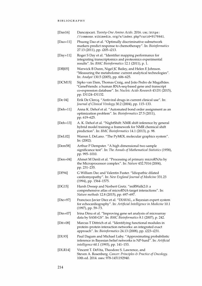
b i b l i o g r a p h y

[Dan16] Dancojocari. Twenty-One Amino Acids. 2016. url: https://commons.wikimedia.org/w/index.php?curid=9176441.

[Dao+11] Phuong Dao et al. “Optimally discriminative subnetworkmarkers predict response to chemotherapy”. In: Bioinformatics27.13 (2011), pp. i205–i213.

[Day+11] Roger S Day et al. “Identifier mapping performance forintegrating transcriptomics and proteomics experimentalresults”. In: BMC Bioinformatics 12.1 (2011), p. 1.

[DBJ05] Warwick B Dunn, Nigel JC Bailey, and Helen E Johnson.“Measuring the metabolome: current analytical technologies”.In: Analyst 130.5 (2005), pp. 606–625.

[DCM15] Sipko van Dam, Thomas Craig, and João Pedro de Magalhães.“GeneFriends: a human RNA-seq-based gene and transcriptco-expression database”. In: Nucleic Acids Research 43.D1 (2015),pp. D1124–D1132.

[De 04] Erik De Clercq. “Antiviral drugs in current clinical use”. In:Journal of Clinical Virology 30.2 (2004), pp. 115–133.

[Deh+11] Anna K. Dehof et al. “Automated bond order assignment as anoptimization problem”. In: Bioinformatics 27.5 (2011),pp. 619–625.

[Deh+13] A. K. Dehof et al. “NightShift: NMR shift inference by generalhybrid model training-a framework for NMR chemical shiftprediction”. In: BMC Bioinformatics 14.1 (2013), p. 98.

[DeL02] Warren L DeLano. “The PyMOL molecular graphics system”.In: (2002).

[Dem58] Arthur P Dempster. “A high dimensional two samplesignificance test”. In: The Annals of Mathematical Statistics (1958),pp. 995–1010.

[Den+04] Ahmet M Denli et al. “Processing of primary microRNAs bythe Microprocessor complex”. In: Nature 432.7014 (2004),pp. 231–235.

[DF94] G William Dec and Valentin Fuster. “Idiopathic dilatedcardiomyopathy”. In: New England Journal of Medicine 331.23(1994), pp. 1564–1575.

[DG15] Harsh Dweep and Norbert Gretz. “miRWalk2.0: acomprehensive atlas of microRNA-target interactions”. In:Nature methods 12.8 (2015), pp. 697–697.

[Die+97] Francisco Javier Diez et al. “DIAVAL, a Bayesian expert systemfor echocardiography”. In: Artificial Intelligence in Medicine 10.1(1997), pp. 59–73.

[Din+07] Irina Dinu et al. “Improving gene set analysis of microarraydata by SAM-GS”. In: BMC Bioinformatics 8.1 (2007), p. 242.

[Dit+08] Marcus T Dittrich et al. “Identifying functional modules inprotein–protein interaction networks: an integrated exactapproach”. In: Bioinformatics 24.13 (2008), pp. i223–i231.

[DL93] Paul Dagum and Michael Luby. “Approximating probabilisticinference in Bayesian belief networks is NP-hard”. In: Artificialintelligence 60.1 (1993), pp. 141–153.

[DLR14] Vincent T. DeVita, Theodore S. Lawrence, andSteven A. Rosenberg. Cancer: Principles & Practice of Oncology.10th ed. 2014. isbn: 978-1451192940.

214

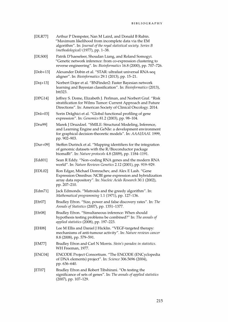
b i b l i o g r a p h y

[DLR77] Arthur P Dempster, Nan M Laird, and Donald B Rubin.“Maximum likelihood from incomplete data via the EMalgorithm”. In: Journal of the royal statistical society. Series B(methodological) (1977), pp. 1–38.

[DLS00] Patrik D’haeseleer, Shoudan Liang, and Roland Somogyi.“Genetic network inference: from co-expression clustering toreverse engineering”. In: Bioinformatics 16.8 (2000), pp. 707–726.

[Dob+13] Alexander Dobin et al. “STAR: ultrafast universal RNA-seqaligner”. In: Bioinformatics 29.1 (2013), pp. 15–21.

[Doj+13] Norbert Dojer et al. “BNFinder2: Faster Bayesian networklearning and Bayesian classification”. In: Bioinformatics (2013),btt323.

[DPG14] Jeffrey S. Dome, Elizabeth J. Perlman, and Norbert Graf. “Riskstratification for Wilms Tumor: Current Approach and FutureDirections”. In: American Society of Clinical Oncology. 2014.

[Drǎ+03] Sorin Drǎghici et al. “Global functional profiling of geneexpression”. In: Genomics 81.2 (2003), pp. 98–104.

[Dru99] Marek J Druzdzel. “SMILE: Structural Modeling, Inference,and Learning Engine and GeNIe: a development environmentfor graphical decision-theoretic models”. In: AAAI/IAAI. 1999,pp. 902–903.

[Dur+09] Steffen Durinck et al. “Mapping identifiers for the integrationof genomic datasets with the R/Bioconductor packagebiomaRt”. In: Nature protocols 4.8 (2009), pp. 1184–1191.

[Edd01] Sean R Eddy. “Non–coding RNA genes and the modern RNAworld”. In: Nature Reviews Genetics 2.12 (2001), pp. 919–929.

[EDL02] Ron Edgar, Michael Domrachev, and Alex E Lash. “GeneExpression Omnibus: NCBI gene expression and hybridizationarray data repository”. In: Nucleic Acids Research 30.1 (2002),pp. 207–210.

[Edm71] Jack Edmonds. “Matroids and the greedy algorithm”. In:Mathematical programming 1.1 (1971), pp. 127–136.

[Efr07] Bradley Efron. “Size, power and false discovery rates”. In: TheAnnals of Statistics (2007), pp. 1351–1377.

[Efr08] Bradley Efron. “Simultaneous inference: When shouldhypothesis testing problems be combined?” In: The annals ofapplied statistics (2008), pp. 197–223.

[EH08] Lee M Ellis and Daniel J Hicklin. “VEGF-targeted therapy:mechanisms of anti-tumour activity”. In: Nature reviews cancer8.8 (2008), pp. 579–591.

[EM77] Bradley Efron and Carl N Morris. Stein’s paradox in statistics.WH Freeman, 1977.

[ENC04] ENCODE Project Consortium. “The ENCODE (ENCyclopediaof DNA elements) project”. In: Science 306.5696 (2004),pp. 636–640.

[ET07] Bradley Efron and Robert Tibshirani. “On testing thesignificance of sets of genes”. In: The annals of applied statistics(2007), pp. 107–129.

215

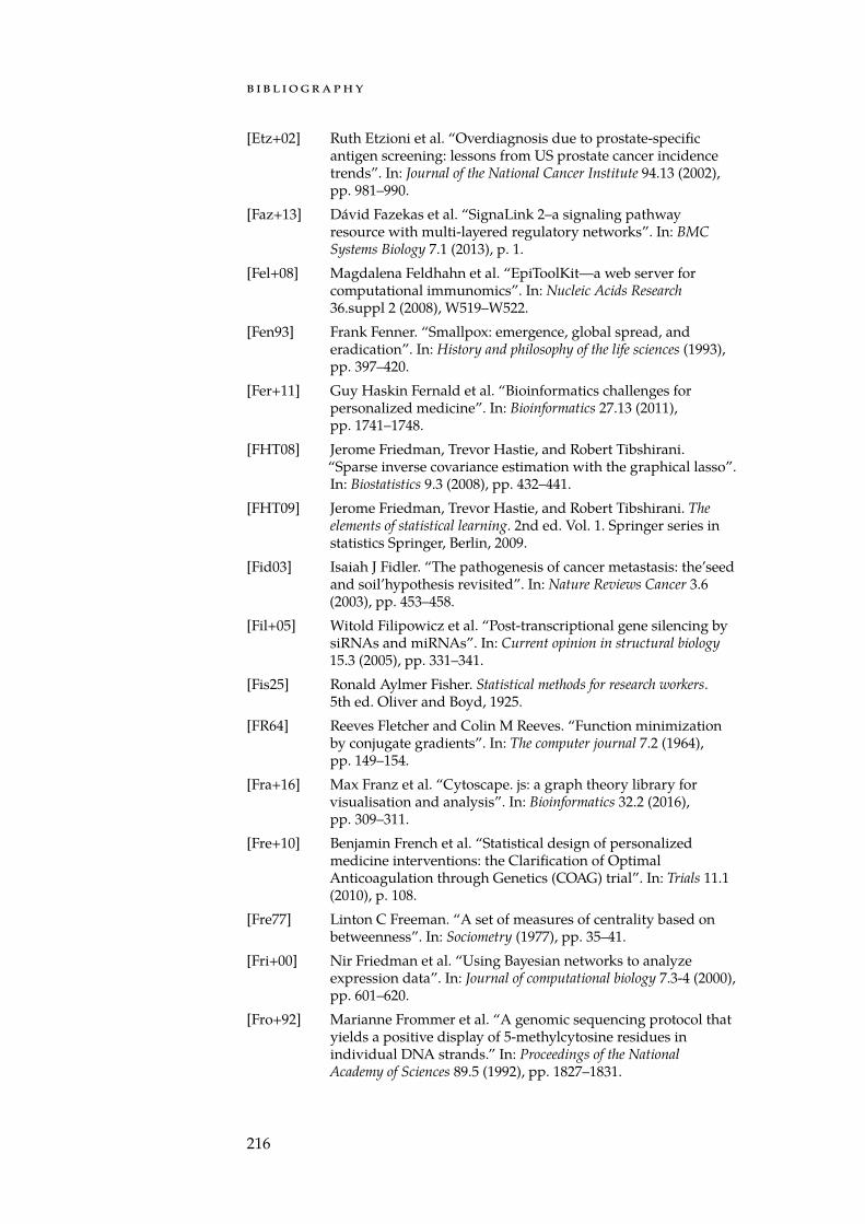
b i b l i o g r a p h y

[Etz+02] Ruth Etzioni et al. “Overdiagnosis due to prostate-specificantigen screening: lessons from US prostate cancer incidencetrends”. In: Journal of the National Cancer Institute 94.13 (2002),pp. 981–990.

[Faz+13] Dávid Fazekas et al. “SignaLink 2–a signaling pathwayresource with multi-layered regulatory networks”. In: BMCSystems Biology 7.1 (2013), p. 1.

[Fel+08] Magdalena Feldhahn et al. “EpiToolKit—a web server forcomputational immunomics”. In: Nucleic Acids Research36.suppl 2 (2008), W519–W522.

[Fen93] Frank Fenner. “Smallpox: emergence, global spread, anderadication”. In: History and philosophy of the life sciences (1993),pp. 397–420.

[Fer+11] Guy Haskin Fernald et al. “Bioinformatics challenges forpersonalized medicine”. In: Bioinformatics 27.13 (2011),pp. 1741–1748.

[FHT08] Jerome Friedman, Trevor Hastie, and Robert Tibshirani.“Sparse inverse covariance estimation with the graphical lasso”.In: Biostatistics 9.3 (2008), pp. 432–441.

[FHT09] Jerome Friedman, Trevor Hastie, and Robert Tibshirani. Theelements of statistical learning. 2nd ed. Vol. 1. Springer series instatistics Springer, Berlin, 2009.

[Fid03] Isaiah J Fidler. “The pathogenesis of cancer metastasis: the’seedand soil’hypothesis revisited”. In: Nature Reviews Cancer 3.6(2003), pp. 453–458.

[Fil+05] Witold Filipowicz et al. “Post-transcriptional gene silencing bysiRNAs and miRNAs”. In: Current opinion in structural biology15.3 (2005), pp. 331–341.

[Fis25] Ronald Aylmer Fisher. Statistical methods for research workers.5th ed. Oliver and Boyd, 1925.

[FR64] Reeves Fletcher and Colin M Reeves. “Function minimizationby conjugate gradients”. In: The computer journal 7.2 (1964),pp. 149–154.

[Fra+16] Max Franz et al. “Cytoscape. js: a graph theory library forvisualisation and analysis”. In: Bioinformatics 32.2 (2016),pp. 309–311.

[Fre+10] Benjamin French et al. “Statistical design of personalizedmedicine interventions: the Clarification of OptimalAnticoagulation through Genetics (COAG) trial”. In: Trials 11.1(2010), p. 108.

[Fre77] Linton C Freeman. “A set of measures of centrality based onbetweenness”. In: Sociometry (1977), pp. 35–41.

[Fri+00] Nir Friedman et al. “Using Bayesian networks to analyzeexpression data”. In: Journal of computational biology 7.3-4 (2000),pp. 601–620.

[Fro+92] Marianne Frommer et al. “A genomic sequencing protocol thatyields a positive display of 5-methylcytosine residues inindividual DNA strands.” In: Proceedings of the NationalAcademy of Sciences 89.5 (1992), pp. 1827–1831.

216

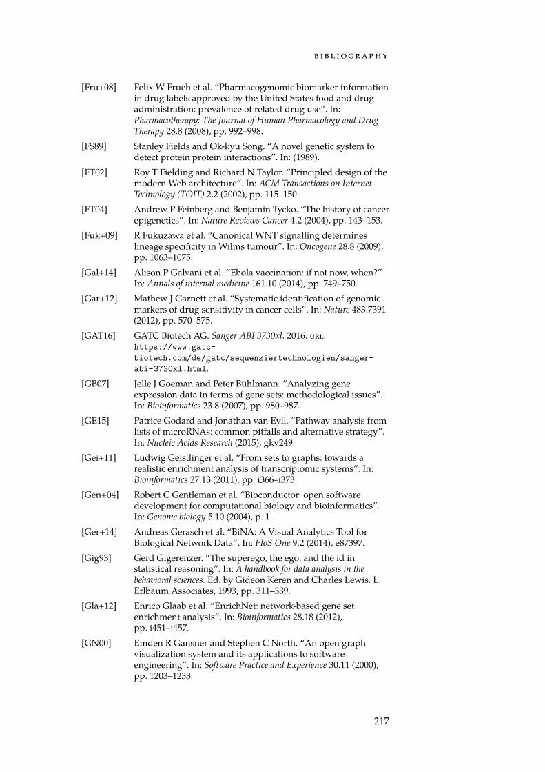
b i b l i o g r a p h y

[Fru+08] Felix W Frueh et al. “Pharmacogenomic biomarker informationin drug labels approved by the United States food and drugadministration: prevalence of related drug use”. In:Pharmacotherapy: The Journal of Human Pharmacology and DrugTherapy 28.8 (2008), pp. 992–998.

[FS89] Stanley Fields and Ok-kyu Song. “A novel genetic system todetect protein protein interactions”. In: (1989).

[FT02] Roy T Fielding and Richard N Taylor. “Principled design of themodern Web architecture”. In: ACM Transactions on InternetTechnology (TOIT) 2.2 (2002), pp. 115–150.

[FT04] Andrew P Feinberg and Benjamin Tycko. “The history of cancerepigenetics”. In: Nature Reviews Cancer 4.2 (2004), pp. 143–153.

[Fuk+09] R Fukuzawa et al. “Canonical WNT signalling determineslineage specificity in Wilms tumour”. In: Oncogene 28.8 (2009),pp. 1063–1075.

[Gal+14] Alison P Galvani et al. “Ebola vaccination: if not now, when?”In: Annals of internal medicine 161.10 (2014), pp. 749–750.

[Gar+12] Mathew J Garnett et al. “Systematic identification of genomicmarkers of drug sensitivity in cancer cells”. In: Nature 483.7391(2012), pp. 570–575.

[GAT16] GATC Biotech AG. Sanger ABI 3730xl. 2016. url:https://www.gatc-biotech.com/de/gatc/sequenziertechnologien/sanger-abi-3730xl.html.

[GB07] Jelle J Goeman and Peter Bühlmann. “Analyzing geneexpression data in terms of gene sets: methodological issues”.In: Bioinformatics 23.8 (2007), pp. 980–987.

[GE15] Patrice Godard and Jonathan van Eyll. “Pathway analysis fromlists of microRNAs: common pitfalls and alternative strategy”.In: Nucleic Acids Research (2015), gkv249.

[Gei+11] Ludwig Geistlinger et al. “From sets to graphs: towards arealistic enrichment analysis of transcriptomic systems”. In:Bioinformatics 27.13 (2011), pp. i366–i373.

[Gen+04] Robert C Gentleman et al. “Bioconductor: open softwaredevelopment for computational biology and bioinformatics”.In: Genome biology 5.10 (2004), p. 1.

[Ger+14] Andreas Gerasch et al. “BiNA: A Visual Analytics Tool forBiological Network Data”. In: PloS One 9.2 (2014), e87397.

[Gig93] Gerd Gigerenzer. “The superego, the ego, and the id instatistical reasoning”. In: A handbook for data analysis in thebehavioral sciences. Ed. by Gideon Keren and Charles Lewis. L.Erlbaum Associates, 1993, pp. 311–339.

[Gla+12] Enrico Glaab et al. “EnrichNet: network-based gene setenrichment analysis”. In: Bioinformatics 28.18 (2012),pp. i451–i457.

[GN00] Emden R Gansner and Stephen C North. “An open graphvisualization system and its applications to softwareengineering”. In: Software Practice and Experience 30.11 (2000),pp. 1203–1233.

217

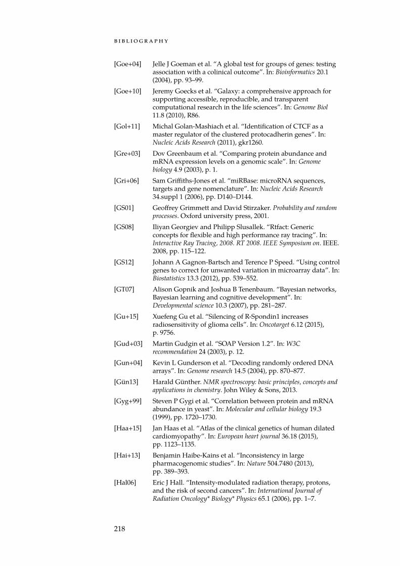
b i b l i o g r a p h y

[Goe+04] Jelle J Goeman et al. “A global test for groups of genes: testingassociation with a colinical outcome”. In: Bioinformatics 20.1(2004), pp. 93–99.

[Goe+10] Jeremy Goecks et al. “Galaxy: a comprehensive approach forsupporting accessible, reproducible, and transparentcomputational research in the life sciences”. In: Genome Biol11.8 (2010), R86.

[Gol+11] Michal Golan-Mashiach et al. “Identification of CTCF as amaster regulator of the clustered protocadherin genes”. In:Nucleic Acids Research (2011), gkr1260.

[Gre+03] Dov Greenbaum et al. “Comparing protein abundance andmRNA expression levels on a genomic scale”. In: Genomebiology 4.9 (2003), p. 1.

[Gri+06] Sam Griffiths-Jones et al. “miRBase: microRNA sequences,targets and gene nomenclature”. In: Nucleic Acids Research34.suppl 1 (2006), pp. D140–D144.

[GS01] Geoffrey Grimmett and David Stirzaker. Probability and randomprocesses. Oxford university press, 2001.

[GS08] Iliyan Georgiev and Philipp Slusallek. “Rtfact: Genericconcepts for flexible and high performance ray tracing”. In:Interactive Ray Tracing, 2008. RT 2008. IEEE Symposium on. IEEE.2008, pp. 115–122.

[GS12] Johann A Gagnon-Bartsch and Terence P Speed. “Using controlgenes to correct for unwanted variation in microarray data”. In:Biostatistics 13.3 (2012), pp. 539–552.

[GT07] Alison Gopnik and Joshua B Tenenbaum. “Bayesian networks,Bayesian learning and cognitive development”. In:Developmental science 10.3 (2007), pp. 281–287.

[Gu+15] Xuefeng Gu et al. “Silencing of R-Spondin1 increasesradiosensitivity of glioma cells”. In: Oncotarget 6.12 (2015),p. 9756.

[Gud+03] Martin Gudgin et al. “SOAP Version 1.2”. In: W3Crecommendation 24 (2003), p. 12.

[Gun+04] Kevin L Gunderson et al. “Decoding randomly ordered DNAarrays”. In: Genome research 14.5 (2004), pp. 870–877.

[Gün13] Harald Günther. NMR spectroscopy: basic principles, concepts andapplications in chemistry. John Wiley & Sons, 2013.

[Gyg+99] Steven P Gygi et al. “Correlation between protein and mRNAabundance in yeast”. In: Molecular and cellular biology 19.3(1999), pp. 1720–1730.

[Haa+15] Jan Haas et al. “Atlas of the clinical genetics of human dilatedcardiomyopathy”. In: European heart journal 36.18 (2015),pp. 1123–1135.

[Hai+13] Benjamin Haibe-Kains et al. “Inconsistency in largepharmacogenomic studies”. In: Nature 504.7480 (2013),pp. 389–393.

[Hal06] Eric J Hall. “Intensity-modulated radiation therapy, protons,and the risk of second cancers”. In: International Journal ofRadiation Oncology* Biology* Physics 65.1 (2006), pp. 1–7.

218

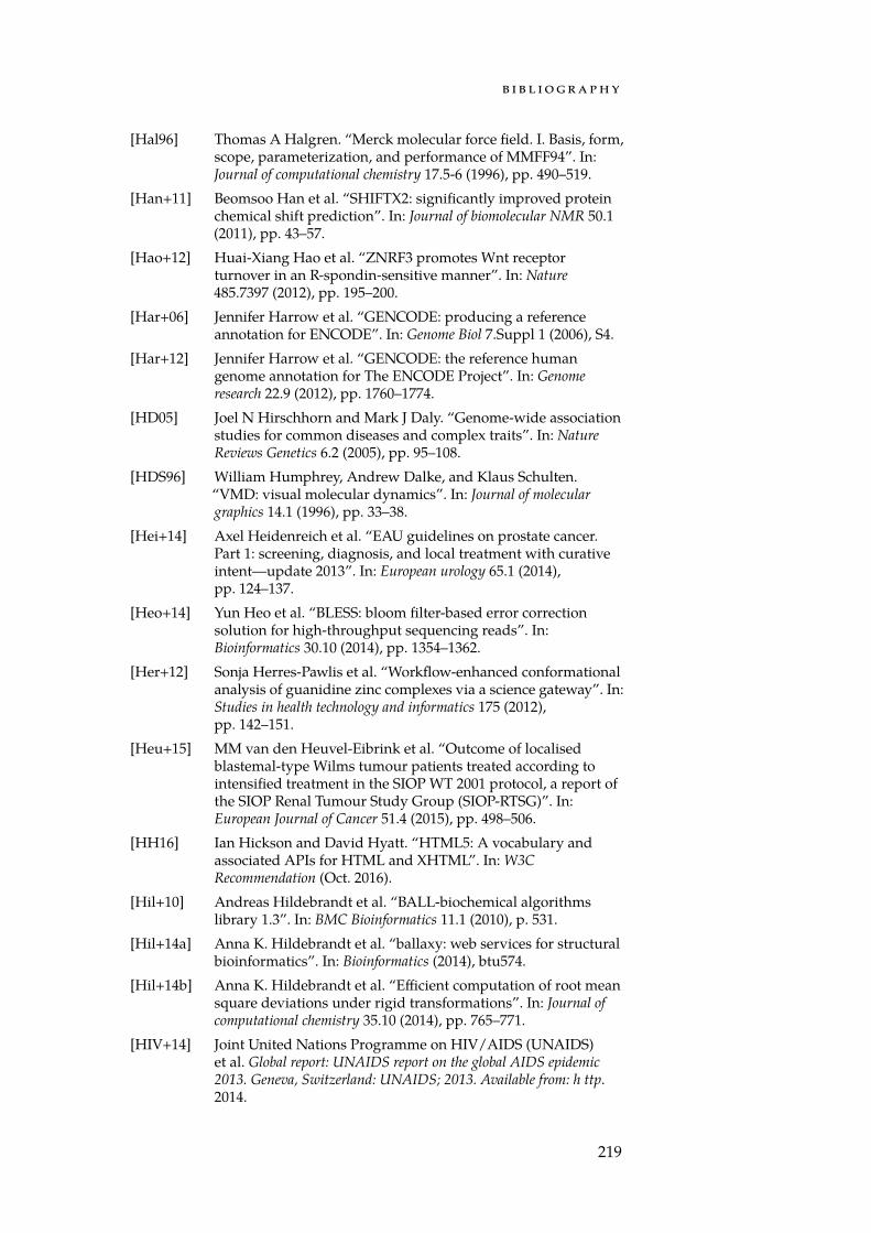
b i b l i o g r a p h y

[Hal96] Thomas A Halgren. “Merck molecular force field. I. Basis, form,scope, parameterization, and performance of MMFF94”. In:Journal of computational chemistry 17.5-6 (1996), pp. 490–519.

[Han+11] Beomsoo Han et al. “SHIFTX2: significantly improved proteinchemical shift prediction”. In: Journal of biomolecular NMR 50.1(2011), pp. 43–57.

[Hao+12] Huai-Xiang Hao et al. “ZNRF3 promotes Wnt receptorturnover in an R-spondin-sensitive manner”. In: Nature485.7397 (2012), pp. 195–200.

[Har+06] Jennifer Harrow et al. “GENCODE: producing a referenceannotation for ENCODE”. In: Genome Biol 7.Suppl 1 (2006), S4.

[Har+12] Jennifer Harrow et al. “GENCODE: the reference humangenome annotation for The ENCODE Project”. In: Genomeresearch 22.9 (2012), pp. 1760–1774.

[HD05] Joel N Hirschhorn and Mark J Daly. “Genome-wide associationstudies for common diseases and complex traits”. In: NatureReviews Genetics 6.2 (2005), pp. 95–108.

[HDS96] William Humphrey, Andrew Dalke, and Klaus Schulten.“VMD: visual molecular dynamics”. In: Journal of moleculargraphics 14.1 (1996), pp. 33–38.

[Hei+14] Axel Heidenreich et al. “EAU guidelines on prostate cancer.Part 1: screening, diagnosis, and local treatment with curativeintent—update 2013”. In: European urology 65.1 (2014),pp. 124–137.

[Heo+14] Yun Heo et al. “BLESS: bloom filter-based error correctionsolution for high-throughput sequencing reads”. In:Bioinformatics 30.10 (2014), pp. 1354–1362.

[Her+12] Sonja Herres-Pawlis et al. “Workflow-enhanced conformationalanalysis of guanidine zinc complexes via a science gateway”. In:Studies in health technology and informatics 175 (2012),pp. 142–151.

[Heu+15] MM van den Heuvel-Eibrink et al. “Outcome of localisedblastemal-type Wilms tumour patients treated according tointensified treatment in the SIOP WT 2001 protocol, a report ofthe SIOP Renal Tumour Study Group (SIOP-RTSG)”. In:European Journal of Cancer 51.4 (2015), pp. 498–506.

[HH16] Ian Hickson and David Hyatt. “HTML5: A vocabulary andassociated APIs for HTML and XHTML”. In: W3CRecommendation (Oct. 2016).

[Hil+10] Andreas Hildebrandt et al. “BALL-biochemical algorithmslibrary 1.3”. In: BMC Bioinformatics 11.1 (2010), p. 531.

[Hil+14a] Anna K. Hildebrandt et al. “ballaxy: web services for structuralbioinformatics”. In: Bioinformatics (2014), btu574.

[Hil+14b] Anna K. Hildebrandt et al. “Efficient computation of root meansquare deviations under rigid transformations”. In: Journal ofcomputational chemistry 35.10 (2014), pp. 765–771.

[HIV+14] Joint United Nations Programme on HIV/AIDS (UNAIDS)et al. Global report: UNAIDS report on the global AIDS epidemic2013. Geneva, Switzerland: UNAIDS; 2013. Available from: h ttp.2014.

219

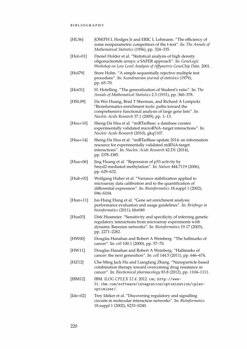
b i b l i o g r a p h y

[HL56] JOSEPH L Hodges Jr and ERIC L Lehmann. “The efficiency ofsome nonparametric competitors of the t-test”. In: The Annals ofMathematical Statistics (1956), pp. 324–335.

[Hol+01] Daniel Holder et al. “Statistical analysis of high densityoligonucleotide arrays: a SAFER approach”. In: GeneLogicWorkshop on Low Level Analysis of Affymetrix GeneChip Data. 2001.

[Hol79] Sture Holm. “A simple sequentially rejective multiple testprocedure”. In: Scandinavian journal of statistics (1979),pp. 65–70.

[Hot31] H. Hotelling. “The generalization of Student’s ratio”. In: TheAnnals of Mathematical Statistics 2.3 (1931), pp. 360–378.

[HSL09] Da Wei Huang, Brad T Sherman, and Richard A Lempicki.“Bioinformatics enrichment tools: paths toward thecomprehensive functional analysis of large gene lists”. In:Nucleic Acids Research 37.1 (2009), pp. 1–13.

[Hsu+10] Sheng-Da Hsu et al. “miRTarBase: a database curatesexperimentally validated microRNA–target interactions”. In:Nucleic Acids Research (2010), gkq1107.

[Hsu+14] Sheng-Da Hsu et al. “miRTarBase update 2014: an informationresource for experimentally validated miRNA-targetinteractions”. In: Nucleic Acids Research 42.D1 (2014),pp. D78–D85.

[Hua+06] Jing Huang et al. “Repression of p53 activity bySmyd2-mediated methylation”. In: Nature 444.7119 (2006),pp. 629–632.

[Hub+02] Wolfgang Huber et al. “Variance stabilization applied tomicroarray data calibration and to the quantification ofdifferential expression”. In: Bioinformatics 18.suppl 1 (2002),S96–S104.

[Hun+11] Jui-Hung Hung et al. “Gene set enrichment analysis:performance evaluation and usage guidelines”. In: Briefings inbioinformatics (2011), bbr049.

[Hus03] Dirk Husmeier. “Sensitivity and specificity of inferring geneticregulatory interactions from microarray experiments withdynamic Bayesian networks”. In: Bioinformatics 19.17 (2003),pp. 2271–2282.

[HW00] Douglas Hanahan and Robert A Weinberg. “The hallmarks ofcancer”. In: cell 100.1 (2000), pp. 57–70.

[HW11] Douglas Hanahan and Robert A Weinberg. “Hallmarks ofcancer: the next generation”. In: cell 144.5 (2011), pp. 646–674.

[HZ12] Che-Ming Jack Hu and Liangfang Zhang. “Nanoparticle-basedcombination therapy toward overcoming drug resistance incancer”. In: Biochemical pharmacology 83.8 (2012), pp. 1104–1111.

[IBM12] IBM. ILOG CPLEX 12.4. 2012. url: http://www-01.ibm.com/software/integration/optimization/cplex-optimizer/.

[Ide+02] Trey Ideker et al. “Discovering regulatory and signallingcircuits in molecular interaction networks”. In: Bioinformatics18.suppl 1 (2002), S233–S240.

220

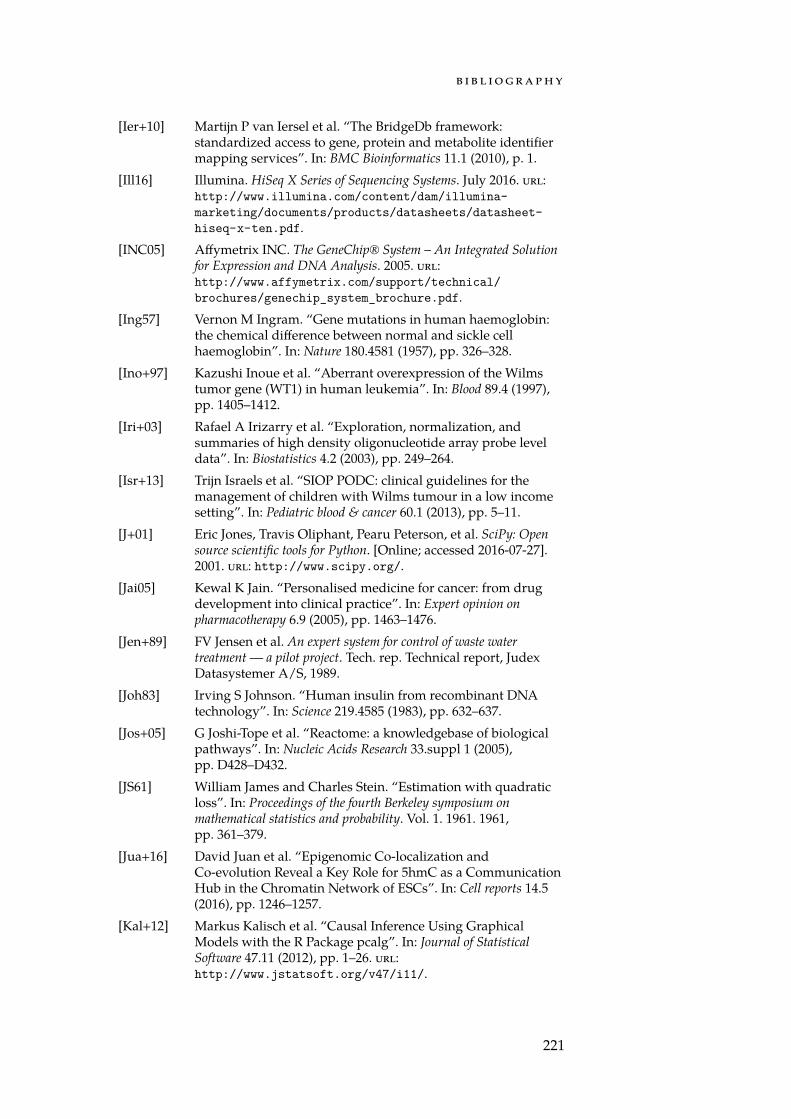
b i b l i o g r a p h y

[Ier+10] Martijn P van Iersel et al. “The BridgeDb framework:standardized access to gene, protein and metabolite identifiermapping services”. In: BMC Bioinformatics 11.1 (2010), p. 1.

[Ill16] Illumina. HiSeq X Series of Sequencing Systems. July 2016. url:http://www.illumina.com/content/dam/illumina-marketing/documents/products/datasheets/datasheet-hiseq-x-ten.pdf.

[INC05] Affymetrix INC. The GeneChip® System – An Integrated Solutionfor Expression and DNA Analysis. 2005. url:http://www.affymetrix.com/support/technical/brochures/genechip_system_brochure.pdf.

[Ing57] Vernon M Ingram. “Gene mutations in human haemoglobin:the chemical difference between normal and sickle cellhaemoglobin”. In: Nature 180.4581 (1957), pp. 326–328.

[Ino+97] Kazushi Inoue et al. “Aberrant overexpression of the Wilmstumor gene (WT1) in human leukemia”. In: Blood 89.4 (1997),pp. 1405–1412.

[Iri+03] Rafael A Irizarry et al. “Exploration, normalization, andsummaries of high density oligonucleotide array probe leveldata”. In: Biostatistics 4.2 (2003), pp. 249–264.

[Isr+13] Trijn Israels et al. “SIOP PODC: clinical guidelines for themanagement of children with Wilms tumour in a low incomesetting”. In: Pediatric blood & cancer 60.1 (2013), pp. 5–11.

[J+01] Eric Jones, Travis Oliphant, Pearu Peterson, et al. SciPy: Opensource scientific tools for Python. [Online; accessed 2016-07-27].2001. url: http://www.scipy.org/.

[Jai05] Kewal K Jain. “Personalised medicine for cancer: from drugdevelopment into clinical practice”. In: Expert opinion onpharmacotherapy 6.9 (2005), pp. 1463–1476.

[Jen+89] FV Jensen et al. An expert system for control of waste watertreatment — a pilot project. Tech. rep. Technical report, JudexDatasystemer A/S, 1989.

[Joh83] Irving S Johnson. “Human insulin from recombinant DNAtechnology”. In: Science 219.4585 (1983), pp. 632–637.

[Jos+05] G Joshi-Tope et al. “Reactome: a knowledgebase of biologicalpathways”. In: Nucleic Acids Research 33.suppl 1 (2005),pp. D428–D432.

[JS61] William James and Charles Stein. “Estimation with quadraticloss”. In: Proceedings of the fourth Berkeley symposium onmathematical statistics and probability. Vol. 1. 1961. 1961,pp. 361–379.

[Jua+16] David Juan et al. “Epigenomic Co-localization andCo-evolution Reveal a Key Role for 5hmC as a CommunicationHub in the Chromatin Network of ESCs”. In: Cell reports 14.5(2016), pp. 1246–1257.

[Kal+12] Markus Kalisch et al. “Causal Inference Using GraphicalModels with the R Package pcalg”. In: Journal of StatisticalSoftware 47.11 (2012), pp. 1–26. url:http://www.jstatsoft.org/v47/i11/.

221

b i b l i o g r a p h y

[Kam95] SL Kamholz. “Resurgence of tuberculosis: the perspective adozen years later.” In: Journal of the Association for AcademicMinority Physicians 7.3 (1995), pp. 83–86.

[Kan+06] Minoru Kanehisa et al. “From genomics to chemical genomics:new developments in KEGG”. In: Nucleic Acids Research34.suppl 1 (2006), pp. D354–D357.

[Kan+10a] Kumaran Kandasamy et al. “NetPath: a public resource ofcurated signal transduction pathways”. In: Genome biology 11.1(2010), p. 1.

[Kan+10b] Minoru Kanehisa et al. “KEGG for representation and analysisof molecular networks involving diseases and drugs”. In:Nucleic Acids Research 38.suppl 1 (2010), pp. D355–D360.

[Kan06] Gopal K Kanji. 100 statistical tests. Sage, 2006. isbn:978-1446222508.

[Kar84] Narendra Karmarkar. “A new polynomial-time algorithm forlinear programming”. In: Proceedings of the sixteenth annual ACMsymposium on Theory of computing. ACM. 1984, pp. 302–311.

[KBL07] Andreas Keller, Christina Backes, and Hans-Peter Lenhof.“Computation of significance scores of unweighted Gene SetEnrichment Analyses”. In: BMC Bioinformatics 8.1 (2007),pp. 1–7. issn: 1471-2105. doi: 10.1186/1471-2105-8-290. url:http://dx.doi.org/10.1186/1471-2105-8-290.

[Kel+06] Andreas Keller et al. “A minimally invasive multiple markerapproach allows highly efficient detection of meningiomatumors”. In: BMC Bioinformatics 7.1 (2006), p. 1.

[Kel+09] Andreas Keller et al. “A novel algorithm for detectingdifferentially regulated paths based on gene set enrichmentanalysis”. In: Bioinformatics 25.21 (2009), pp. 2787–2794.

[Kel+12] Thomas Kelder et al. “WikiPathways: building researchcommunities on biological pathways”. In: Nucleic Acids Research40.D1 (2012), pp. D1301–D1307.

[Ken+58] John C Kendrew et al. “A three-dimensional model of themyoglobin molecule obtained by x-ray analysis”. In: Nature181.4610 (1958), pp. 662–666.

[KF09] Daphne Koller and Nir Friedman. Probabilistic graphical models:principles and techniques. MIT press, 2009.

[KG00] M. Kanehisa and S. Goto. “KEGG: kyoto encyclopedia of genesand genomes.” eng. In: Nucleic Acids Res 28.1 (Jan. 2000),pp. 27–30.

[KGH12] Alexander Kohlmann, Vera Grossmann, and Torsten Haferlach.“Integration of next-generation sequencing into clinicalpractice: are we there yet?” In: Seminars in oncology. Vol. 39. 1.Elsevier. 2012, pp. 26–36.

[Kha80] Leonid G Khachiyan. “Polynomial algorithms in linearprogramming”. In: USSR Computational Mathematics andMathematical Physics 20.1 (1980), pp. 53–72.

[Kim+08] Kyung-Ah Kim et al. “R-Spondin family members regulate theWnt pathway by a common mechanism”. In: Molecular biologyof the cell 19.6 (2008), pp. 2588–2596.

222

b i b l i o g r a p h y

[Kin+12] Yoshiaki Kinoshita et al. “The prognostic significance ofblastemal predominant histology in initially resected Wilms’tumors: A report from the Study Group for Pediatric SolidTumors in the Kyushu Area, Japan”. In: Journal of pediatricsurgery 47.12 (2012), pp. 2205–2209.

[Kir05] Marc W Kirschner. “The meaning of systems biology”. In: Cell121.4 (2005), pp. 503–504.

[Kir47] G Kirchhoff. “Über die Auflösung der Gleichungen, auf welcheman bei der Untersuchung der linearen Verteilunggalvanischer Ströme geführt wird”. In: Poggendorf Ann. Physik72 (1847), pp. 497–508.

[Kit02] Hiroaki Kitano. “Systems biology: a brief overview”. In: Science295.5560 (2002), pp. 1662–1664.

[KL00] Oliver Kohlbacher and Hans-Peter Lenhof. “BALL—rapidsoftware prototyping in computational molecular biology”. In:Bioinformatics 16.9 (2000), pp. 815–824.

[Kle+02] Christoph A Klein et al. “Genetic heterogeneity of singledisseminated tumour cells in minimal residual cancer”. In: TheLancet 360.9334 (2002), pp. 683–689.

[KMR78] Alan J Kinniburgh, Janet E Mertz, and Jeffrey Ross. “Theprecursor of mouse β-globin messenger RNA contains twointervening RNA sequences”. In: Cell 14.3 (1978), pp. 681–693.

[KN09] Matthias Keller and Martin Nussbaumer. “Cascading stylesheets: a novel approach towards productive styling withtoday’s standards”. In: Proceedings of the 18th internationalconference on World wide web. ACM. 2009, pp. 1161–1162.

[Kni+09] Theo A Knijnenburg et al. “Fewer permutations, more accurateP-values”. In: Bioinformatics 25.12 (2009), pp. i161–i168.

[Koh12] Oliver Kohlbacher. “CADDSuite-a workflow-enabled suite ofopen-source tools for drug discovery.” In: J. Cheminformatics4.S-1 (2012), O2.

[Kol33] Andrej N Kolmogorov. Sulla determinazione empirica di una leggedi distribuzione. Vol. 4. G. Inst. Ital. Attuari, 1933.

[Kon+06] Gottfried E Konecny et al. “Activity of the dual kinase inhibitorlapatinib (GW572016) against HER-2-overexpressing andtrastuzumab-treated breast cancer cells”. In: Cancer research 66.3(2006), pp. 1630–1639.

[Kor+12] Sergey Koren et al. “Hybrid error correction and de novoassembly of single-molecule sequencing reads”. In: Naturebiotechnology 30.7 (2012), pp. 693–700.

[Kor99] Roger D Kornberg. “Eukaryotic transcriptional control”. In:Trends in Biochemical Sciences 24.12 (1999), pp. M46–M49.

[KPP06] Sek Won Kong, William T Pu, and Peter J Park. “A multivariateapproach for integrating genome-wide expression data andbiological knowledge”. In: Bioinformatics 22.19 (2006),pp. 2373–2380.

[Kro04] Mel N Kronick. “Creation of the whole human genomemicroarray”. In: Expert review of proteomics 1.1 (2004), pp. 19–28.

223

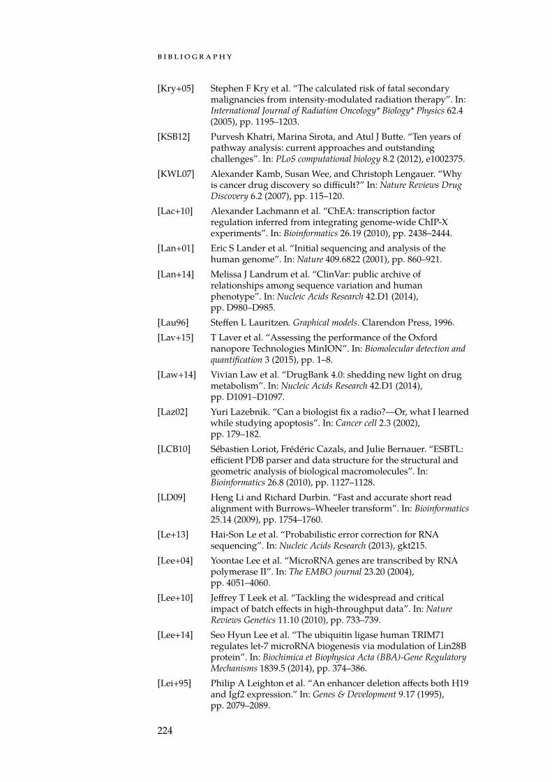
b i b l i o g r a p h y

[Kry+05] Stephen F Kry et al. “The calculated risk of fatal secondarymalignancies from intensity-modulated radiation therapy”. In:International Journal of Radiation Oncology* Biology* Physics 62.4(2005), pp. 1195–1203.

[KSB12] Purvesh Khatri, Marina Sirota, and Atul J Butte. “Ten years ofpathway analysis: current approaches and outstandingchallenges”. In: PLoS computational biology 8.2 (2012), e1002375.

[KWL07] Alexander Kamb, Susan Wee, and Christoph Lengauer. “Whyis cancer drug discovery so difficult?” In: Nature Reviews DrugDiscovery 6.2 (2007), pp. 115–120.

[Lac+10] Alexander Lachmann et al. “ChEA: transcription factorregulation inferred from integrating genome-wide ChIP-Xexperiments”. In: Bioinformatics 26.19 (2010), pp. 2438–2444.

[Lan+01] Eric S Lander et al. “Initial sequencing and analysis of thehuman genome”. In: Nature 409.6822 (2001), pp. 860–921.

[Lan+14] Melissa J Landrum et al. “ClinVar: public archive ofrelationships among sequence variation and humanphenotype”. In: Nucleic Acids Research 42.D1 (2014),pp. D980–D985.

[Lau96] Steffen L Lauritzen. Graphical models. Clarendon Press, 1996.[Lav+15] T Laver et al. “Assessing the performance of the Oxford

nanopore Technologies MinION”. In: Biomolecular detection andquantification 3 (2015), pp. 1–8.

[Law+14] Vivian Law et al. “DrugBank 4.0: shedding new light on drugmetabolism”. In: Nucleic Acids Research 42.D1 (2014),pp. D1091–D1097.

[Laz02] Yuri Lazebnik. “Can a biologist fix a radio?—Or, what I learnedwhile studying apoptosis”. In: Cancer cell 2.3 (2002),pp. 179–182.

[LCB10] Sébastien Loriot, Frédéric Cazals, and Julie Bernauer. “ESBTL:efficient PDB parser and data structure for the structural andgeometric analysis of biological macromolecules”. In:Bioinformatics 26.8 (2010), pp. 1127–1128.

[LD09] Heng Li and Richard Durbin. “Fast and accurate short readalignment with Burrows–Wheeler transform”. In: Bioinformatics25.14 (2009), pp. 1754–1760.

[Le+13] Hai-Son Le et al. “Probabilistic error correction for RNAsequencing”. In: Nucleic Acids Research (2013), gkt215.

[Lee+04] Yoontae Lee et al. “MicroRNA genes are transcribed by RNApolymerase II”. In: The EMBO journal 23.20 (2004),pp. 4051–4060.

[Lee+10] Jeffrey T Leek et al. “Tackling the widespread and criticalimpact of batch effects in high-throughput data”. In: NatureReviews Genetics 11.10 (2010), pp. 733–739.

[Lee+14] Seo Hyun Lee et al. “The ubiquitin ligase human TRIM71regulates let-7 microRNA biogenesis via modulation of Lin28Bprotein”. In: Biochimica et Biophysica Acta (BBA)-Gene RegulatoryMechanisms 1839.5 (2014), pp. 374–386.

[Lei+95] Philip A Leighton et al. “An enhancer deletion affects both H19and Igf2 expression.” In: Genes & Development 9.17 (1995),pp. 2079–2089.

224

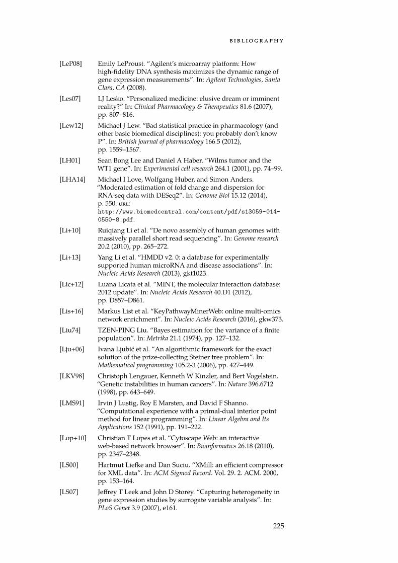
b i b l i o g r a p h y

[LeP08] Emily LeProust. “Agilent’s microarray platform: Howhigh-fidelity DNA synthesis maximizes the dynamic range ofgene expression measurements”. In: Agilent Technologies, SantaClara, CA (2008).

[Les07] LJ Lesko. “Personalized medicine: elusive dream or imminentreality?” In: Clinical Pharmacology & Therapeutics 81.6 (2007),pp. 807–816.

[Lew12] Michael J Lew. “Bad statistical practice in pharmacology (andother basic biomedical disciplines): you probably don’t knowP”. In: British journal of pharmacology 166.5 (2012),pp. 1559–1567.

[LH01] Sean Bong Lee and Daniel A Haber. “Wilms tumor and theWT1 gene”. In: Experimental cell research 264.1 (2001), pp. 74–99.

[LHA14] Michael I Love, Wolfgang Huber, and Simon Anders.“Moderated estimation of fold change and dispersion forRNA-seq data with DESeq2”. In: Genome Biol 15.12 (2014),p. 550. url:http://www.biomedcentral.com/content/pdf/s13059-014-0550-8.pdf.

[Li+10] Ruiqiang Li et al. “De novo assembly of human genomes withmassively parallel short read sequencing”. In: Genome research20.2 (2010), pp. 265–272.

[Li+13] Yang Li et al. “HMDD v2. 0: a database for experimentallysupported human microRNA and disease associations”. In:Nucleic Acids Research (2013), gkt1023.

[Lic+12] Luana Licata et al. “MINT, the molecular interaction database:2012 update”. In: Nucleic Acids Research 40.D1 (2012),pp. D857–D861.

[Lis+16] Markus List et al. “KeyPathwayMinerWeb: online multi-omicsnetwork enrichment”. In: Nucleic Acids Research (2016), gkw373.

[Liu74] TZEN-PING Liu. “Bayes estimation for the variance of a finitepopulation”. In: Metrika 21.1 (1974), pp. 127–132.

[Lju+06] Ivana Ljubić et al. “An algorithmic framework for the exactsolution of the prize-collecting Steiner tree problem”. In:Mathematical programming 105.2-3 (2006), pp. 427–449.

[LKV98] Christoph Lengauer, Kenneth W Kinzler, and Bert Vogelstein.“Genetic instabilities in human cancers”. In: Nature 396.6712(1998), pp. 643–649.

[LMS91] Irvin J Lustig, Roy E Marsten, and David F Shanno.“Computational experience with a primal-dual interior pointmethod for linear programming”. In: Linear Algebra and ItsApplications 152 (1991), pp. 191–222.

[Lop+10] Christian T Lopes et al. “Cytoscape Web: an interactiveweb-based network browser”. In: Bioinformatics 26.18 (2010),pp. 2347–2348.

[LS00] Hartmut Liefke and Dan Suciu. “XMill: an efficient compressorfor XML data”. In: ACM Sigmod Record. Vol. 29. 2. ACM. 2000,pp. 153–164.

[LS07] Jeffrey T Leek and John D Storey. “Capturing heterogeneity ingene expression studies by surrogate variable analysis”. In:PLoS Genet 3.9 (2007), e161.

225

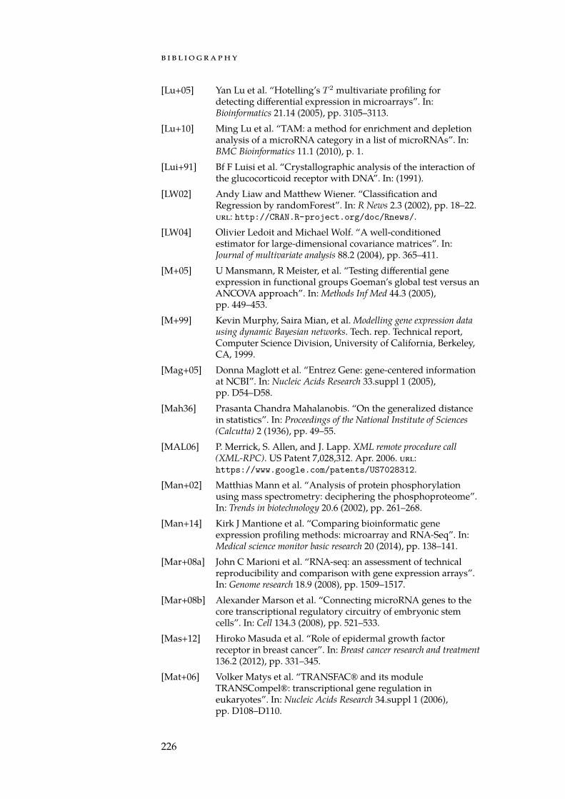
b i b l i o g r a p h y

[Lu+05] Yan Lu et al. “Hotelling’s T 2 multivariate profiling fordetecting differential expression in microarrays”. In:Bioinformatics 21.14 (2005), pp. 3105–3113.

[Lu+10] Ming Lu et al. “TAM: a method for enrichment and depletionanalysis of a microRNA category in a list of microRNAs”. In:BMC Bioinformatics 11.1 (2010), p. 1.

[Lui+91] Bf F Luisi et al. “Crystallographic analysis of the interaction ofthe glucocorticoid receptor with DNA”. In: (1991).

[LW02] Andy Liaw and Matthew Wiener. “Classification andRegression by randomForest”. In: R News 2.3 (2002), pp. 18–22.url: http://CRAN.R-project.org/doc/Rnews/.

[LW04] Olivier Ledoit and Michael Wolf. “A well-conditionedestimator for large-dimensional covariance matrices”. In:Journal of multivariate analysis 88.2 (2004), pp. 365–411.

[M+05] U Mansmann, R Meister, et al. “Testing differential geneexpression in functional groups Goeman’s global test versus anANCOVA approach”. In: Methods Inf Med 44.3 (2005),pp. 449–453.

[M+99] Kevin Murphy, Saira Mian, et al. Modelling gene expression datausing dynamic Bayesian networks. Tech. rep. Technical report,Computer Science Division, University of California, Berkeley,CA, 1999.

[Mag+05] Donna Maglott et al. “Entrez Gene: gene-centered informationat NCBI”. In: Nucleic Acids Research 33.suppl 1 (2005),pp. D54–D58.

[Mah36] Prasanta Chandra Mahalanobis. “On the generalized distancein statistics”. In: Proceedings of the National Institute of Sciences(Calcutta) 2 (1936), pp. 49–55.

[MAL06] P. Merrick, S. Allen, and J. Lapp. XML remote procedure call(XML-RPC). US Patent 7,028,312. Apr. 2006. url:https://www.google.com/patents/US7028312.

[Man+02] Matthias Mann et al. “Analysis of protein phosphorylationusing mass spectrometry: deciphering the phosphoproteome”.In: Trends in biotechnology 20.6 (2002), pp. 261–268.

[Man+14] Kirk J Mantione et al. “Comparing bioinformatic geneexpression profiling methods: microarray and RNA-Seq”. In:Medical science monitor basic research 20 (2014), pp. 138–141.

[Mar+08a] John C Marioni et al. “RNA-seq: an assessment of technicalreproducibility and comparison with gene expression arrays”.In: Genome research 18.9 (2008), pp. 1509–1517.

[Mar+08b] Alexander Marson et al. “Connecting microRNA genes to thecore transcriptional regulatory circuitry of embryonic stemcells”. In: Cell 134.3 (2008), pp. 521–533.

[Mas+12] Hiroko Masuda et al. “Role of epidermal growth factorreceptor in breast cancer”. In: Breast cancer research and treatment136.2 (2012), pp. 331–345.

[Mat+06] Volker Matys et al. “TRANSFAC® and its moduleTRANSCompel®: transcriptional gene regulation ineukaryotes”. In: Nucleic Acids Research 34.suppl 1 (2006),pp. D108–D110.

226

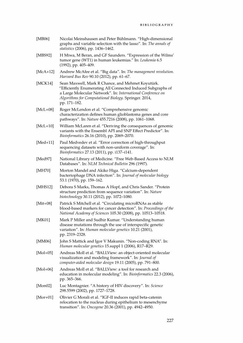
b i b l i o g r a p h y

[MB06] Nicolai Meinshausen and Peter Bühlmann. “High-dimensionalgraphs and variable selection with the lasso”. In: The annals ofstatistics (2006), pp. 1436–1462.

[MBS92] H Miwa, M Beran, and GF Saunders. “Expression of the Wilms’tumor gene (WT1) in human leukemias.” In: Leukemia 6.5(1992), pp. 405–409.

[McA+12] Andrew McAfee et al. “Big data”. In: The management revolution.Harvard Bus Rev 90.10 (2012), pp. 61–67.

[MCK14] Sean Maxwell, Mark R Chance, and Mehmet Koyutürk.“Efficiently Enumerating All Connected Induced Subgraphs ofa Large Molecular Network”. In: International Conference onAlgorithms for Computational Biology. Springer. 2014,pp. 171–182.

[McL+08] Roger McLendon et al. “Comprehensive genomiccharacterization defines human glioblastoma genes and corepathways”. In: Nature 455.7216 (2008), pp. 1061–1068.

[McL+10] William McLaren et al. “Deriving the consequences of genomicvariants with the Ensembl API and SNP Effect Predictor”. In:Bioinformatics 26.16 (2010), pp. 2069–2070.

[Med+11] Paul Medvedev et al. “Error correction of high-throughputsequencing datasets with non-uniform coverage”. In:Bioinformatics 27.13 (2011), pp. i137–i141.

[Med97] National Library of Medicine. “Free Web-Based Access to NLMDatabases”. In: NLM Technical Bulletin 296 (1997).

[MH70] Morton Mandel and Akiko Higa. “Calcium-dependentbacteriophage DNA infection”. In: Journal of molecular biology53.1 (1970), pp. 159–162.

[MHS12] Debora S Marks, Thomas A Hopf, and Chris Sander. “Proteinstructure prediction from sequence variation”. In: Naturebiotechnology 30.11 (2012), pp. 1072–1080.

[Mit+08] Patrick S Mitchell et al. “Circulating microRNAs as stableblood-based markers for cancer detection”. In: Proceedings of theNational Academy of Sciences 105.30 (2008), pp. 10513–10518.

[MK01] Mark P Miller and Sudhir Kumar. “Understanding humandisease mutations through the use of interspecific geneticvariation”. In: Human molecular genetics 10.21 (2001),pp. 2319–2328.

[MM06] John S Mattick and Igor V Makunin. “Non-coding RNA”. In:Human molecular genetics 15.suppl 1 (2006), R17–R29.

[Mol+05] Andreas Moll et al. “BALLView: an object-oriented molecularvisualization and modeling framework”. In: Journal ofcomputer-aided molecular design 19.11 (2005), pp. 791–800.

[Mol+06] Andreas Moll et al. “BALLView: a tool for research andeducation in molecular modeling”. In: Bioinformatics 22.3 (2006),pp. 365–366.

[Mon02] Luc Montagnier. “A history of HIV discovery”. In: Science298.5599 (2002), pp. 1727–1728.

[Mor+01] Olivier G Morali et al. “IGF-II induces rapid beta-cateninrelocation to the nucleus during epithelium to mesenchymetransition”. In: Oncogene 20.36 (2001), pp. 4942–4950.

227

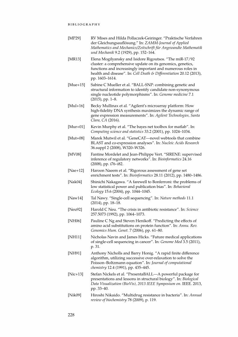
b i b l i o g r a p h y

[MP29] RV Mises and Hilda Pollaczek-Geiringer. “Praktische Verfahrender Gleichungsauflösung.” In: ZAMM-Journal of AppliedMathematics and Mechanics/Zeitschrift für Angewandte Mathematikund Mechanik 9.2 (1929), pp. 152–164.

[MR13] Elena Mogilyansky and Isidore Rigoutsos. “The miR-17/92cluster: a comprehensive update on its genomics, genetics,functions and increasingly important and numerous roles inhealth and disease”. In: Cell Death & Differentiation 20.12 (2013),pp. 1603–1614.

[Mue+15] Sabine C Mueller et al. “BALL-SNP: combining genetic andstructural information to identify candidate non-synonymoussingle nucleotide polymorphisms”. In: Genome medicine 7.1(2015), pp. 1–8.

[Mul+16] Becky Mullinax et al. “Agilent’s microarray platform: Howhigh-fidelity DNA synthesis maximizes the dynamic range ofgene expression measurements”. In: Agilent Technologies, SantaClara, CA (2016).

[Mur+01] Kevin Murphy et al. “The bayes net toolbox for matlab”. In:Computing science and statistics 33.2 (2001), pp. 1024–1034.

[Mut+08] Marek Mutwil et al. “GeneCAT—novel webtools that combineBLAST and co-expression analyses”. In: Nucleic Acids Research36.suppl 2 (2008), W320–W326.

[MV08] Fantine Mordelet and Jean-Philippe Vert. “SIRENE: supervisedinference of regulatory networks”. In: Bioinformatics 24.16(2008), pp. i76–i82.

[Nae+12] Haroon Naeem et al. “Rigorous assessment of gene setenrichment tests”. In: Bioinformatics 28.11 (2012), pp. 1480–1486.

[Nak04] Shinichi Nakagawa. “A farewell to Bonferroni: the problems oflow statistical power and publication bias”. In: BehavioralEcology 15.6 (2004), pp. 1044–1045.

[Naw14] Tal Nawy. “Single-cell sequencing”. In: Nature methods 11.1(2014), pp. 18–18.

[Neu92] Harold C Neu. “The crisis in antibiotic resistance”. In: Science257.5073 (1992), pp. 1064–1073.

[NH06] Pauline C Ng and Steven Henikoff. “Predicting the effects ofamino acid substitutions on protein function”. In: Annu. Rev.Genomics Hum. Genet. 7 (2006), pp. 61–80.

[NH11] Nicholas Navin and James Hicks. “Future medical applicationsof single-cell sequencing in cancer”. In: Genome Med 3.5 (2011),p. 31.

[NH91] Anthony Nicholls and Barry Honig. “A rapid finite differencealgorithm, utilizing successive over-relaxation to solve thePoisson–Boltzmann equation”. In: Journal of computationalchemistry 12.4 (1991), pp. 435–445.

[Nic+13] Stefan Nickels et al. “PresentaBALL—A powerful package forpresentations and lessons in structural biology”. In: BiologicalData Visualization (BioVis), 2013 IEEE Symposium on. IEEE. 2013,pp. 33–40.

[Nik09] Hiroshi Nikaido. “Multidrug resistance in bacteria”. In: Annualreview of biochemistry 78 (2009), p. 119.

228

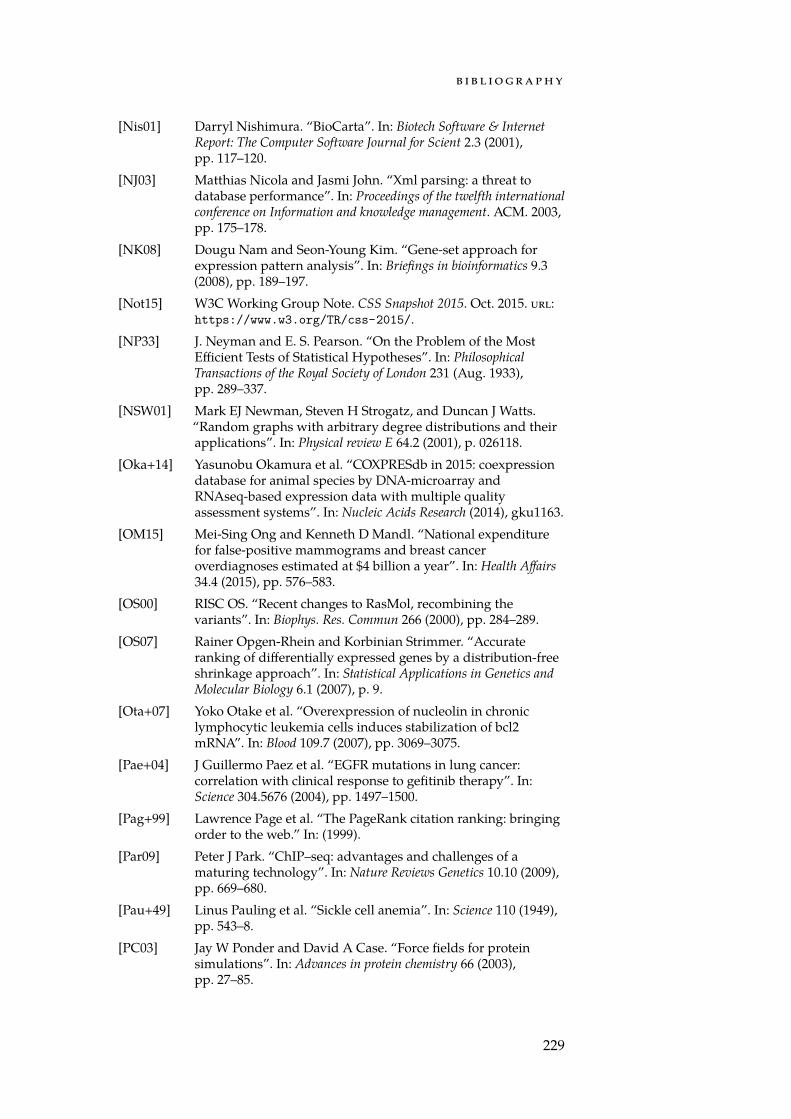
b i b l i o g r a p h y

[Nis01] Darryl Nishimura. “BioCarta”. In: Biotech Software & InternetReport: The Computer Software Journal for Scient 2.3 (2001),pp. 117–120.

[NJ03] Matthias Nicola and Jasmi John. “Xml parsing: a threat todatabase performance”. In: Proceedings of the twelfth internationalconference on Information and knowledge management. ACM. 2003,pp. 175–178.

[NK08] Dougu Nam and Seon-Young Kim. “Gene-set approach forexpression pattern analysis”. In: Briefings in bioinformatics 9.3(2008), pp. 189–197.

[Not15] W3C Working Group Note. CSS Snapshot 2015. Oct. 2015. url:https://www.w3.org/TR/css-2015/.

[NP33] J. Neyman and E. S. Pearson. “On the Problem of the MostEfficient Tests of Statistical Hypotheses”. In: PhilosophicalTransactions of the Royal Society of London 231 (Aug. 1933),pp. 289–337.

[NSW01] Mark EJ Newman, Steven H Strogatz, and Duncan J Watts.“Random graphs with arbitrary degree distributions and theirapplications”. In: Physical review E 64.2 (2001), p. 026118.

[Oka+14] Yasunobu Okamura et al. “COXPRESdb in 2015: coexpressiondatabase for animal species by DNA-microarray andRNAseq-based expression data with multiple qualityassessment systems”. In: Nucleic Acids Research (2014), gku1163.

[OM15] Mei-Sing Ong and Kenneth D Mandl. “National expenditurefor false-positive mammograms and breast canceroverdiagnoses estimated at $4 billion a year”. In: Health Affairs34.4 (2015), pp. 576–583.

[OS00] RISC OS. “Recent changes to RasMol, recombining thevariants”. In: Biophys. Res. Commun 266 (2000), pp. 284–289.

[OS07] Rainer Opgen-Rhein and Korbinian Strimmer. “Accurateranking of differentially expressed genes by a distribution-freeshrinkage approach”. In: Statistical Applications in Genetics andMolecular Biology 6.1 (2007), p. 9.

[Ota+07] Yoko Otake et al. “Overexpression of nucleolin in chroniclymphocytic leukemia cells induces stabilization of bcl2mRNA”. In: Blood 109.7 (2007), pp. 3069–3075.

[Pae+04] J Guillermo Paez et al. “EGFR mutations in lung cancer:correlation with clinical response to gefitinib therapy”. In:Science 304.5676 (2004), pp. 1497–1500.

[Pag+99] Lawrence Page et al. “The PageRank citation ranking: bringingorder to the web.” In: (1999).

[Par09] Peter J Park. “ChIP–seq: advantages and challenges of amaturing technology”. In: Nature Reviews Genetics 10.10 (2009),pp. 669–680.

[Pau+49] Linus Pauling et al. “Sickle cell anemia”. In: Science 110 (1949),pp. 543–8.

[PC03] Jay W Ponder and David A Case. “Force fields for proteinsimulations”. In: Advances in protein chemistry 66 (2003),pp. 27–85.

229

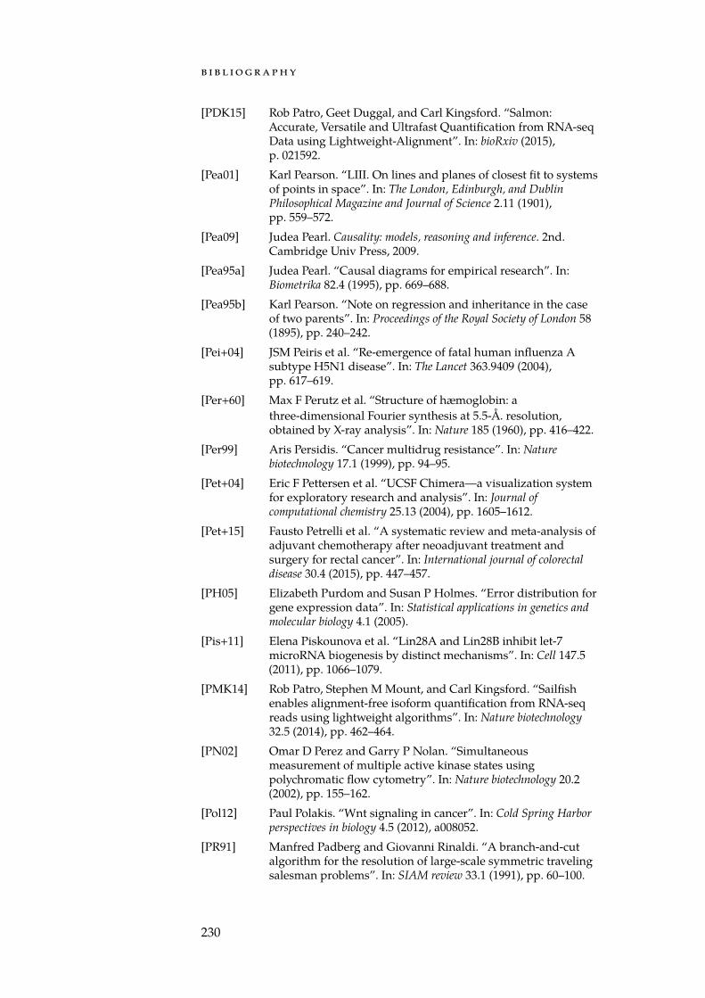
b i b l i o g r a p h y

[PDK15] Rob Patro, Geet Duggal, and Carl Kingsford. “Salmon:Accurate, Versatile and Ultrafast Quantification from RNA-seqData using Lightweight-Alignment”. In: bioRxiv (2015),p. 021592.

[Pea01] Karl Pearson. “LIII. On lines and planes of closest fit to systemsof points in space”. In: The London, Edinburgh, and DublinPhilosophical Magazine and Journal of Science 2.11 (1901),pp. 559–572.

[Pea09] Judea Pearl. Causality: models, reasoning and inference. 2nd.Cambridge Univ Press, 2009.

[Pea95a] Judea Pearl. “Causal diagrams for empirical research”. In:Biometrika 82.4 (1995), pp. 669–688.

[Pea95b] Karl Pearson. “Note on regression and inheritance in the caseof two parents”. In: Proceedings of the Royal Society of London 58(1895), pp. 240–242.

[Pei+04] JSM Peiris et al. “Re-emergence of fatal human influenza Asubtype H5N1 disease”. In: The Lancet 363.9409 (2004),pp. 617–619.

[Per+60] Max F Perutz et al. “Structure of hæmoglobin: athree-dimensional Fourier synthesis at 5.5-Å. resolution,obtained by X-ray analysis”. In: Nature 185 (1960), pp. 416–422.

[Per99] Aris Persidis. “Cancer multidrug resistance”. In: Naturebiotechnology 17.1 (1999), pp. 94–95.

[Pet+04] Eric F Pettersen et al. “UCSF Chimera—a visualization systemfor exploratory research and analysis”. In: Journal ofcomputational chemistry 25.13 (2004), pp. 1605–1612.

[Pet+15] Fausto Petrelli et al. “A systematic review and meta-analysis ofadjuvant chemotherapy after neoadjuvant treatment andsurgery for rectal cancer”. In: International journal of colorectaldisease 30.4 (2015), pp. 447–457.

[PH05] Elizabeth Purdom and Susan P Holmes. “Error distribution forgene expression data”. In: Statistical applications in genetics andmolecular biology 4.1 (2005).

[Pis+11] Elena Piskounova et al. “Lin28A and Lin28B inhibit let-7microRNA biogenesis by distinct mechanisms”. In: Cell 147.5(2011), pp. 1066–1079.

[PMK14] Rob Patro, Stephen M Mount, and Carl Kingsford. “Sailfishenables alignment-free isoform quantification from RNA-seqreads using lightweight algorithms”. In: Nature biotechnology32.5 (2014), pp. 462–464.

[PN02] Omar D Perez and Garry P Nolan. “Simultaneousmeasurement of multiple active kinase states usingpolychromatic flow cytometry”. In: Nature biotechnology 20.2(2002), pp. 155–162.

[Pol12] Paul Polakis. “Wnt signaling in cancer”. In: Cold Spring Harborperspectives in biology 4.5 (2012), a008052.

[PR91] Manfred Padberg and Giovanni Rinaldi. “A branch-and-cutalgorithm for the resolution of large-scale symmetric travelingsalesman problems”. In: SIAM review 33.1 (1991), pp. 60–100.

230

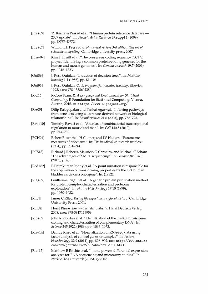
b i b l i o g r a p h y

[Pra+09] TS Keshava Prasad et al. “Human protein reference database —2009 update”. In: Nucleic Acids Research 37.suppl 1 (2009),pp. D767–D772.

[Pre+07] William H. Press et al. Numerical recipes 3rd edition: The art ofscientific computing. Cambridge university press, 2007.

[Pru+09] Kim D Pruitt et al. “The consensus coding sequence (CCDS)project: Identifying a common protein-coding gene set for thehuman and mouse genomes”. In: Genome research 19.7 (2009),pp. 1316–1323.

[Qui86] J. Ross Quinlan. “Induction of decision trees”. In: Machinelearning 1.1 (1986), pp. 81–106.

[Qui93] J. Ross Quinlan. C4.5: programs for machine learning. Elsevier,1993. isbn: 978-1558602380.

[R C16] R Core Team. R: A Language and Environment for StatisticalComputing. R Foundation for Statistical Computing. Vienna,Austria, 2016. url: https://www.R-project.org/.

[RA05] Dilip Rajagopalan and Pankaj Agarwal. “Inferring pathwaysfrom gene lists using a literature-derived network of biologicalrelationships”. In: Bioinformatics 21.6 (2005), pp. 788–793.

[Rav+10] Timothy Ravasi et al. “An atlas of combinatorial transcriptionalregulation in mouse and man”. In: Cell 140.5 (2010),pp. 744–752.

[RCH94] Robert Rosenthal, H Cooper, and LV Hedges. “Parametricmeasures of effect size”. In: The handbook of research synthesis(1994), pp. 231–244.

[RCS13] Richard J Roberts, Mauricio O Carneiro, and Michael C Schatz.“The advantages of SMRT sequencing”. In: Genome Biol 14.6(2013), p. 405.

[Red+82] E Premkumar Reddy et al. “A point mutation is responsible forthe acquisition of transforming properties by the T24 humanbladder carcinoma oncogene”. In: (1982).

[Rig+99] Guillaume Rigaut et al. “A generic protein purification methodfor protein complex characterization and proteomeexploration”. In: Nature biotechnology 17.10 (1999),pp. 1030–1032.

[Ril01] James C Riley. Rising life expectancy: a global history. CambridgeUniversity Press, 2001.

[Rin08] Horst Rinne. Taschenbuch der Statistik. Harri Deutsch Verlag,2008. isbn: 978-3817116959.

[Rio+89] John R Riordan et al. “Identification of the cystic fibrosis gene:cloning and characterization of complementary DNA”. In:Science 245.4922 (1989), pp. 1066–1073.

[Ris+14] Davide Risso et al. “Normalization of RNA-seq data usingfactor analysis of control genes or samples”. In: Naturebiotechnology 32.9 (2014), pp. 896–902. url: http://www.nature.com/nbt/journal/v32/n9/abs/nbt.2931.html.

[Rit+15] Matthew E Ritchie et al. “limma powers differential expressionanalyses for RNA-sequencing and microarray studies”. In:Nucleic Acids Research (2015), gkv007.

231

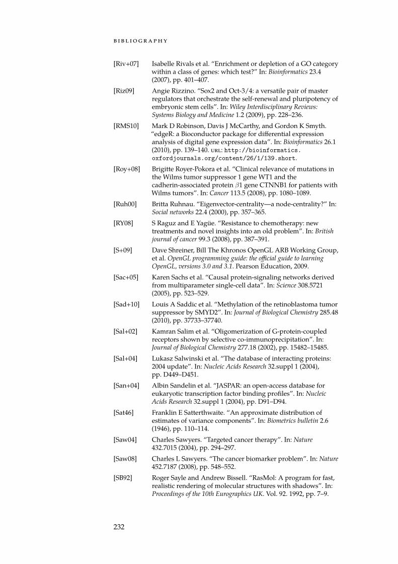
b i b l i o g r a p h y

[Riv+07] Isabelle Rivals et al. “Enrichment or depletion of a GO categorywithin a class of genes: which test?” In: Bioinformatics 23.4(2007), pp. 401–407.

[Riz09] Angie Rizzino. “Sox2 and Oct-3/4: a versatile pair of masterregulators that orchestrate the self-renewal and pluripotency ofembryonic stem cells”. In: Wiley Interdisciplinary Reviews:Systems Biology and Medicine 1.2 (2009), pp. 228–236.

[RMS10] Mark D Robinson, Davis J McCarthy, and Gordon K Smyth.“edgeR: a Bioconductor package for differential expressionanalysis of digital gene expression data”. In: Bioinformatics 26.1(2010), pp. 139–140. url: http://bioinformatics.oxfordjournals.org/content/26/1/139.short.

[Roy+08] Brigitte Royer-Pokora et al. “Clinical relevance of mutations inthe Wilms tumor suppressor 1 gene WT1 and thecadherin-associated protein β1 gene CTNNB1 for patients withWilms tumors”. In: Cancer 113.5 (2008), pp. 1080–1089.

[Ruh00] Britta Ruhnau. “Eigenvector-centrality—a node-centrality?” In:Social networks 22.4 (2000), pp. 357–365.

[RY08] S Raguz and E Yagüe. “Resistance to chemotherapy: newtreatments and novel insights into an old problem”. In: Britishjournal of cancer 99.3 (2008), pp. 387–391.

[S+09] Dave Shreiner, Bill The Khronos OpenGL ARB Working Group,et al. OpenGL programming guide: the official guide to learningOpenGL, versions 3.0 and 3.1. Pearson Education, 2009.

[Sac+05] Karen Sachs et al. “Causal protein-signaling networks derivedfrom multiparameter single-cell data”. In: Science 308.5721(2005), pp. 523–529.

[Sad+10] Louis A Saddic et al. “Methylation of the retinoblastoma tumorsuppressor by SMYD2”. In: Journal of Biological Chemistry 285.48(2010), pp. 37733–37740.

[Sal+02] Kamran Salim et al. “Oligomerization of G-protein-coupledreceptors shown by selective co-immunoprecipitation”. In:Journal of Biological Chemistry 277.18 (2002), pp. 15482–15485.

[Sal+04] Lukasz Salwinski et al. “The database of interacting proteins:2004 update”. In: Nucleic Acids Research 32.suppl 1 (2004),pp. D449–D451.

[San+04] Albin Sandelin et al. “JASPAR: an open-access database foreukaryotic transcription factor binding profiles”. In: NucleicAcids Research 32.suppl 1 (2004), pp. D91–D94.

[Sat46] Franklin E Satterthwaite. “An approximate distribution ofestimates of variance components”. In: Biometrics bulletin 2.6(1946), pp. 110–114.

[Saw04] Charles Sawyers. “Targeted cancer therapy”. In: Nature432.7015 (2004), pp. 294–297.

[Saw08] Charles L Sawyers. “The cancer biomarker problem”. In: Nature452.7187 (2008), pp. 548–552.

[SB92] Roger Sayle and Andrew Bissell. “RasMol: A program for fast,realistic rendering of molecular structures with shadows”. In:Proceedings of the 10th Eurographics UK. Vol. 92. 1992, pp. 7–9.

232

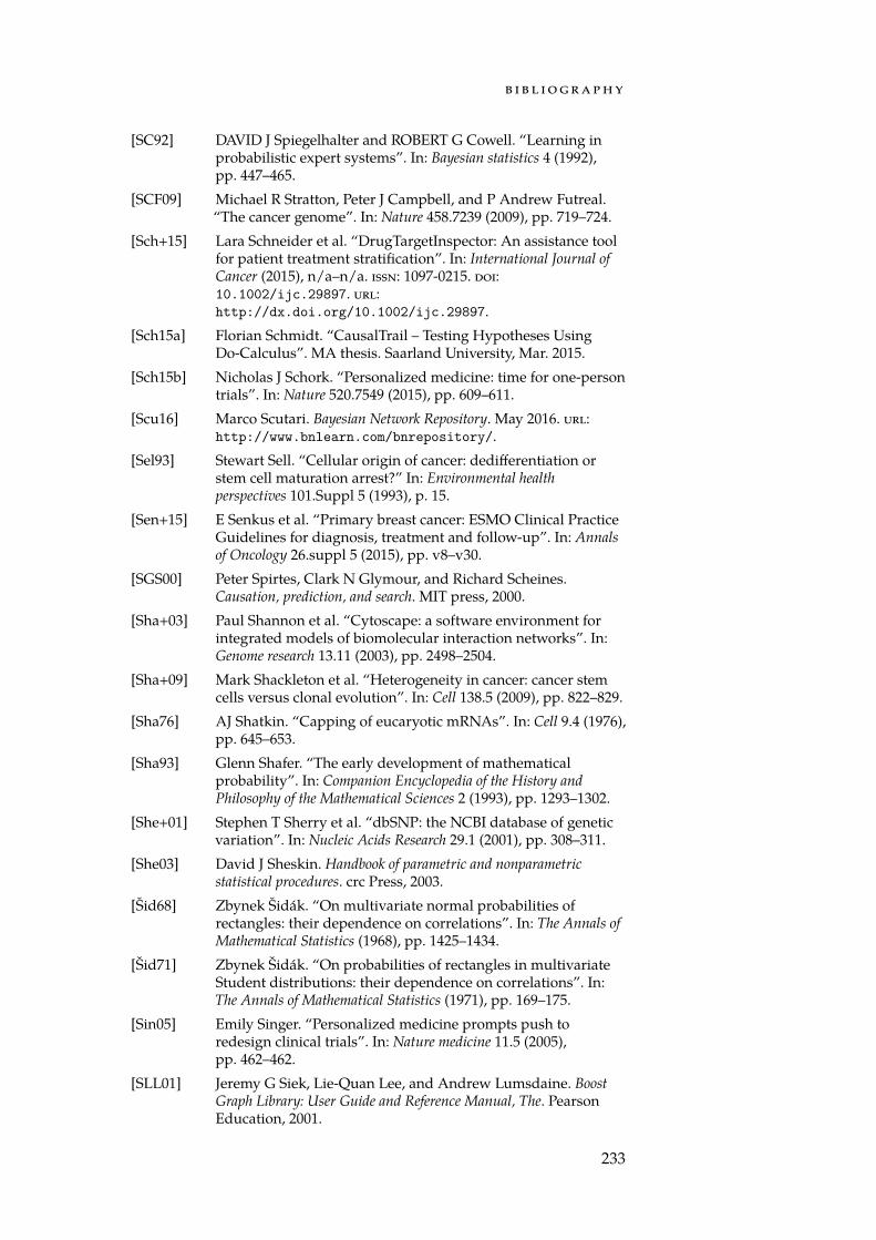
b i b l i o g r a p h y

[SC92] DAVID J Spiegelhalter and ROBERT G Cowell. “Learning inprobabilistic expert systems”. In: Bayesian statistics 4 (1992),pp. 447–465.

[SCF09] Michael R Stratton, Peter J Campbell, and P Andrew Futreal.“The cancer genome”. In: Nature 458.7239 (2009), pp. 719–724.

[Sch+15] Lara Schneider et al. “DrugTargetInspector: An assistance toolfor patient treatment stratification”. In: International Journal ofCancer (2015), n/a–n/a. issn: 1097-0215. doi:10.1002/ijc.29897. url:http://dx.doi.org/10.1002/ijc.29897.

[Sch15a] Florian Schmidt. “CausalTrail – Testing Hypotheses UsingDo-Calculus”. MA thesis. Saarland University, Mar. 2015.

[Sch15b] Nicholas J Schork. “Personalized medicine: time for one-persontrials”. In: Nature 520.7549 (2015), pp. 609–611.

[Scu16] Marco Scutari. Bayesian Network Repository. May 2016. url:http://www.bnlearn.com/bnrepository/.

[Sel93] Stewart Sell. “Cellular origin of cancer: dedifferentiation orstem cell maturation arrest?” In: Environmental healthperspectives 101.Suppl 5 (1993), p. 15.

[Sen+15] E Senkus et al. “Primary breast cancer: ESMO Clinical PracticeGuidelines for diagnosis, treatment and follow-up”. In: Annalsof Oncology 26.suppl 5 (2015), pp. v8–v30.

[SGS00] Peter Spirtes, Clark N Glymour, and Richard Scheines.Causation, prediction, and search. MIT press, 2000.

[Sha+03] Paul Shannon et al. “Cytoscape: a software environment forintegrated models of biomolecular interaction networks”. In:Genome research 13.11 (2003), pp. 2498–2504.

[Sha+09] Mark Shackleton et al. “Heterogeneity in cancer: cancer stemcells versus clonal evolution”. In: Cell 138.5 (2009), pp. 822–829.

[Sha76] AJ Shatkin. “Capping of eucaryotic mRNAs”. In: Cell 9.4 (1976),pp. 645–653.

[Sha93] Glenn Shafer. “The early development of mathematicalprobability”. In: Companion Encyclopedia of the History andPhilosophy of the Mathematical Sciences 2 (1993), pp. 1293–1302.

[She+01] Stephen T Sherry et al. “dbSNP: the NCBI database of geneticvariation”. In: Nucleic Acids Research 29.1 (2001), pp. 308–311.

[She03] David J Sheskin. Handbook of parametric and nonparametricstatistical procedures. crc Press, 2003.

[Šid68] Zbynek Šidák. “On multivariate normal probabilities ofrectangles: their dependence on correlations”. In: The Annals ofMathematical Statistics (1968), pp. 1425–1434.

[Šid71] Zbynek Šidák. “On probabilities of rectangles in multivariateStudent distributions: their dependence on correlations”. In:The Annals of Mathematical Statistics (1971), pp. 169–175.

[Sin05] Emily Singer. “Personalized medicine prompts push toredesign clinical trials”. In: Nature medicine 11.5 (2005),pp. 462–462.

[SLL01] Jeremy G Siek, Lie-Quan Lee, and Andrew Lumsdaine. BoostGraph Library: User Guide and Reference Manual, The. PearsonEducation, 2001.

233

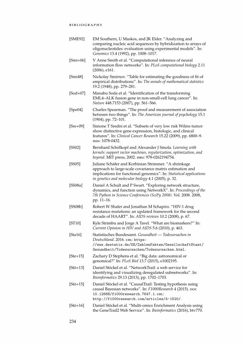
b i b l i o g r a p h y

[SME92] EM Southern, U Maskos, and JK Elder. “Analyzing andcomparing nucleic acid sequences by hybridization to arrays ofoligonucleotides: evaluation using experimental models”. In:Genomics 13.4 (1992), pp. 1008–1017.

[Smi+06] V Anne Smith et al. “Computational inference of neuralinformation flow networks”. In: PLoS computational biology 2.11(2006), e161.

[Smi48] Nickolay Smirnov. “Table for estimating the goodness of fit ofempirical distributions”. In: The annals of mathematical statistics19.2 (1948), pp. 279–281.

[Sod+07] Manabu Soda et al. “Identification of the transformingEML4–ALK fusion gene in non-small-cell lung cancer”. In:Nature 448.7153 (2007), pp. 561–566.

[Spe04] Charles Spearman. “The proof and measurement of associationbetween two things”. In: The American journal of psychology 15.1(1904), pp. 72–101.

[Sre+09] Simone T Sredni et al. “Subsets of very low risk Wilms tumorshow distinctive gene expression, histologic, and clinicalfeatures”. In: Clinical Cancer Research 15.22 (2009), pp. 6800–9.issn: 1078-0432.

[SS02] Bernhard Schölkopf and Alexander J Smola. Learning withkernels: support vector machines, regularization, optimization, andbeyond. MIT press, 2002. isbn: 978-0262194754.

[SS05] Juliane Schäfer and Korbinian Strimmer. “A shrinkageapproach to large-scale covariance matrix estimation andimplications for functional genomics”. In: Statistical applicationsin genetics and molecular biology 4.1 (2005), p. 32.

[SS08a] Daniel A Schult and P Swart. “Exploring network structure,dynamics, and function using NetworkX”. In: Proceedings of the7th Python in Science Conferences (SciPy 2008). Vol. 2008. 2008,pp. 11–16.

[SS08b] Robert W Shafer and Jonathan M Schapiro. “HIV-1 drugresistance mutations: an updated framework for the seconddecade of HAART”. In: AIDS reviews 10.2 (2008), p. 67.

[ST10] Kyle Strimbu and Jorge A Tavel. “What are biomarkers?” In:Current Opinion in HIV and AIDS 5.6 (2010), p. 463.

[Sta16] Statistisches Bundesamt. Gesundheit — Todesursachen inDeutschland. 2016. url: https://www.destatis.de/DE/ZahlenFakten/GesellschaftStaat/Gesundheit/Todesursachen/Todesursachen.html.

[Ste+15] Zachary D Stephens et al. “Big data: astronomical orgenomical?” In: PLoS Biol 13.7 (2015), e1002195.

[Stö+13] Daniel Stöckel et al. “NetworkTrail: a web service foridentifying and visualizing deregulated subnetworks”. In:Bioinformatics 29.13 (2013), pp. 1702–1703.

[Stö+15] Daniel Stöckel et al. “CausalTrail: Testing hypothesis usingcausal Bayesian networks”. In: F1000Research 4 (2015). doi:10.12688/f1000research.7647.1. url:http://f1000research.com/articles/4-1520/.

[Stö+16] Daniel Stöckel et al. “Multi-omics Enrichment Analysis usingthe GeneTrail2 Web Service”. In: Bioinformatics (2016), btv770.

234

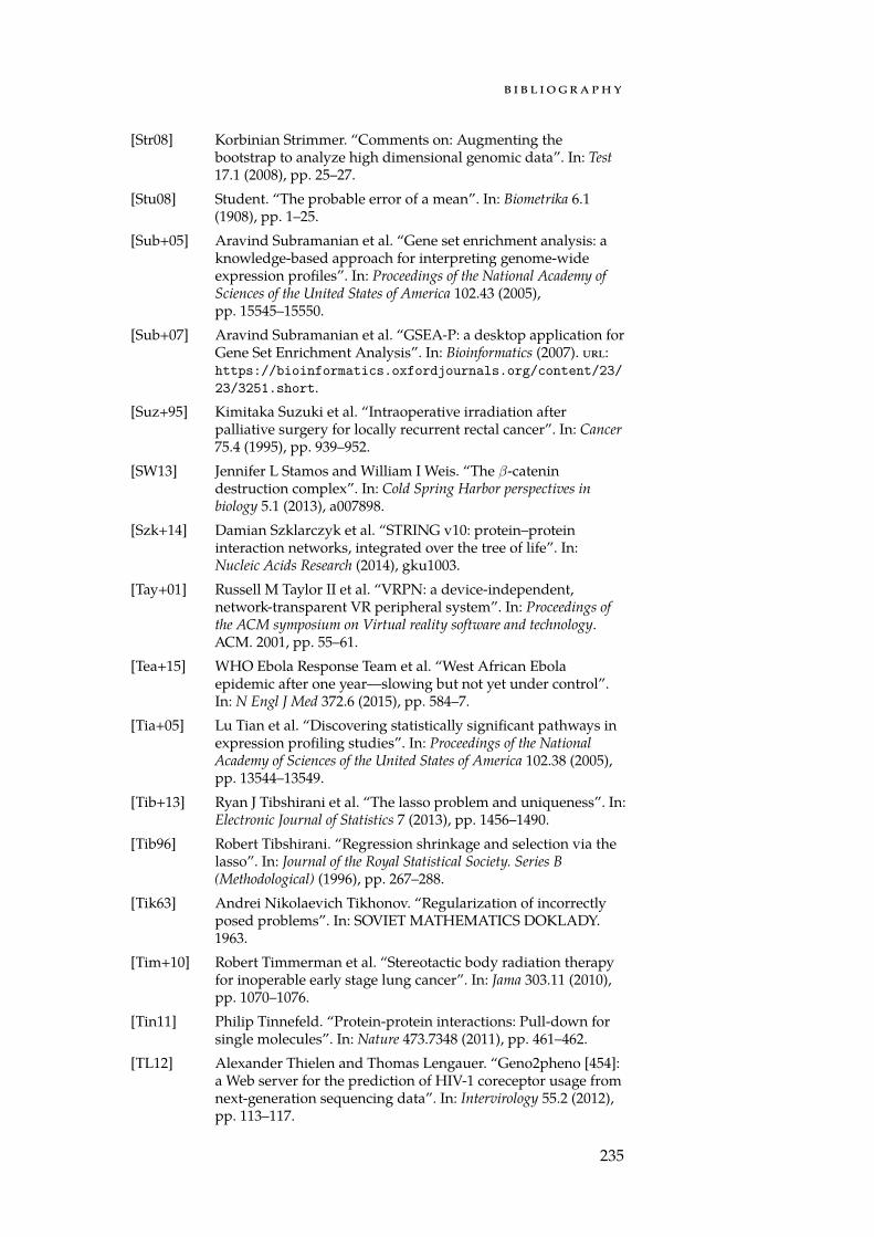
b i b l i o g r a p h y

[Str08] Korbinian Strimmer. “Comments on: Augmenting thebootstrap to analyze high dimensional genomic data”. In: Test17.1 (2008), pp. 25–27.

[Stu08] Student. “The probable error of a mean”. In: Biometrika 6.1(1908), pp. 1–25.

[Sub+05] Aravind Subramanian et al. “Gene set enrichment analysis: aknowledge-based approach for interpreting genome-wideexpression profiles”. In: Proceedings of the National Academy ofSciences of the United States of America 102.43 (2005),pp. 15545–15550.

[Sub+07] Aravind Subramanian et al. “GSEA-P: a desktop application forGene Set Enrichment Analysis”. In: Bioinformatics (2007). url:https://bioinformatics.oxfordjournals.org/content/23/23/3251.short.

[Suz+95] Kimitaka Suzuki et al. “Intraoperative irradiation afterpalliative surgery for locally recurrent rectal cancer”. In: Cancer75.4 (1995), pp. 939–952.

[SW13] Jennifer L Stamos and William I Weis. “The β-catenindestruction complex”. In: Cold Spring Harbor perspectives inbiology 5.1 (2013), a007898.

[Szk+14] Damian Szklarczyk et al. “STRING v10: protein–proteininteraction networks, integrated over the tree of life”. In:Nucleic Acids Research (2014), gku1003.

[Tay+01] Russell M Taylor II et al. “VRPN: a device-independent,network-transparent VR peripheral system”. In: Proceedings ofthe ACM symposium on Virtual reality software and technology.ACM. 2001, pp. 55–61.

[Tea+15] WHO Ebola Response Team et al. “West African Ebolaepidemic after one year—slowing but not yet under control”.In: N Engl J Med 372.6 (2015), pp. 584–7.

[Tia+05] Lu Tian et al. “Discovering statistically significant pathways inexpression profiling studies”. In: Proceedings of the NationalAcademy of Sciences of the United States of America 102.38 (2005),pp. 13544–13549.

[Tib+13] Ryan J Tibshirani et al. “The lasso problem and uniqueness”. In:Electronic Journal of Statistics 7 (2013), pp. 1456–1490.

[Tib96] Robert Tibshirani. “Regression shrinkage and selection via thelasso”. In: Journal of the Royal Statistical Society. Series B(Methodological) (1996), pp. 267–288.

[Tik63] Andrei Nikolaevich Tikhonov. “Regularization of incorrectlyposed problems”. In: SOVIET MATHEMATICS DOKLADY.1963.

[Tim+10] Robert Timmerman et al. “Stereotactic body radiation therapyfor inoperable early stage lung cancer”. In: Jama 303.11 (2010),pp. 1070–1076.

[Tin11] Philip Tinnefeld. “Protein-protein interactions: Pull-down forsingle molecules”. In: Nature 473.7348 (2011), pp. 461–462.

[TL12] Alexander Thielen and Thomas Lengauer. “Geno2pheno [454]:a Web server for the prediction of HIV-1 coreceptor usage fromnext-generation sequencing data”. In: Intervirology 55.2 (2012),pp. 113–117.

235

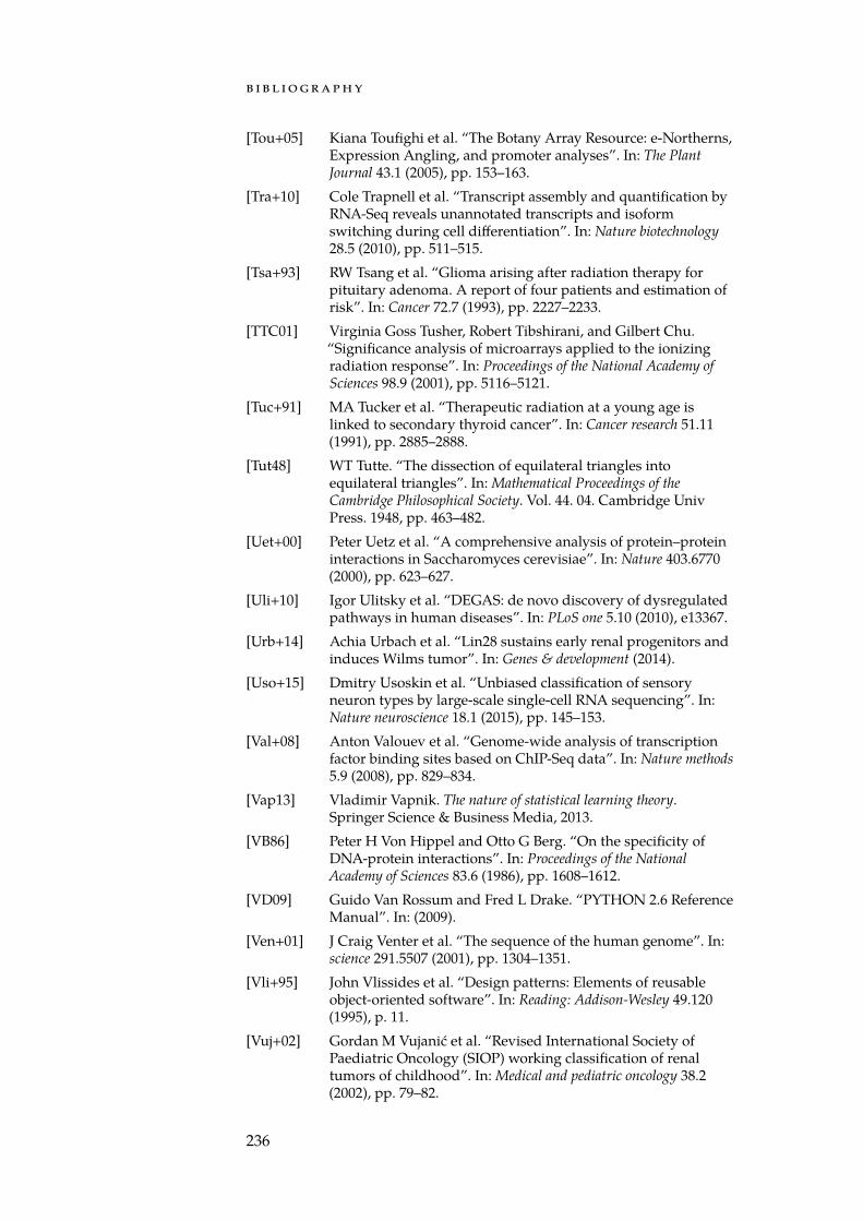
b i b l i o g r a p h y

[Tou+05] Kiana Toufighi et al. “The Botany Array Resource: e-Northerns,Expression Angling, and promoter analyses”. In: The PlantJournal 43.1 (2005), pp. 153–163.

[Tra+10] Cole Trapnell et al. “Transcript assembly and quantification byRNA-Seq reveals unannotated transcripts and isoformswitching during cell differentiation”. In: Nature biotechnology28.5 (2010), pp. 511–515.

[Tsa+93] RW Tsang et al. “Glioma arising after radiation therapy forpituitary adenoma. A report of four patients and estimation ofrisk”. In: Cancer 72.7 (1993), pp. 2227–2233.

[TTC01] Virginia Goss Tusher, Robert Tibshirani, and Gilbert Chu.“Significance analysis of microarrays applied to the ionizingradiation response”. In: Proceedings of the National Academy ofSciences 98.9 (2001), pp. 5116–5121.

[Tuc+91] MA Tucker et al. “Therapeutic radiation at a young age islinked to secondary thyroid cancer”. In: Cancer research 51.11(1991), pp. 2885–2888.

[Tut48] WT Tutte. “The dissection of equilateral triangles intoequilateral triangles”. In: Mathematical Proceedings of theCambridge Philosophical Society. Vol. 44. 04. Cambridge UnivPress. 1948, pp. 463–482.

[Uet+00] Peter Uetz et al. “A comprehensive analysis of protein–proteininteractions in Saccharomyces cerevisiae”. In: Nature 403.6770(2000), pp. 623–627.

[Uli+10] Igor Ulitsky et al. “DEGAS: de novo discovery of dysregulatedpathways in human diseases”. In: PLoS one 5.10 (2010), e13367.

[Urb+14] Achia Urbach et al. “Lin28 sustains early renal progenitors andinduces Wilms tumor”. In: Genes & development (2014).

[Uso+15] Dmitry Usoskin et al. “Unbiased classification of sensoryneuron types by large-scale single-cell RNA sequencing”. In:Nature neuroscience 18.1 (2015), pp. 145–153.

[Val+08] Anton Valouev et al. “Genome-wide analysis of transcriptionfactor binding sites based on ChIP-Seq data”. In: Nature methods5.9 (2008), pp. 829–834.

[Vap13] Vladimir Vapnik. The nature of statistical learning theory.Springer Science & Business Media, 2013.

[VB86] Peter H Von Hippel and Otto G Berg. “On the specificity ofDNA-protein interactions”. In: Proceedings of the NationalAcademy of Sciences 83.6 (1986), pp. 1608–1612.

[VD09] Guido Van Rossum and Fred L Drake. “PYTHON 2.6 ReferenceManual”. In: (2009).

[Ven+01] J Craig Venter et al. “The sequence of the human genome”. In:science 291.5507 (2001), pp. 1304–1351.

[Vli+95] John Vlissides et al. “Design patterns: Elements of reusableobject-oriented software”. In: Reading: Addison-Wesley 49.120(1995), p. 11.

[Vuj+02] Gordan M Vujanić et al. “Revised International Society ofPaediatric Oncology (SIOP) working classification of renaltumors of childhood”. In: Medical and pediatric oncology 38.2(2002), pp. 79–82.

236

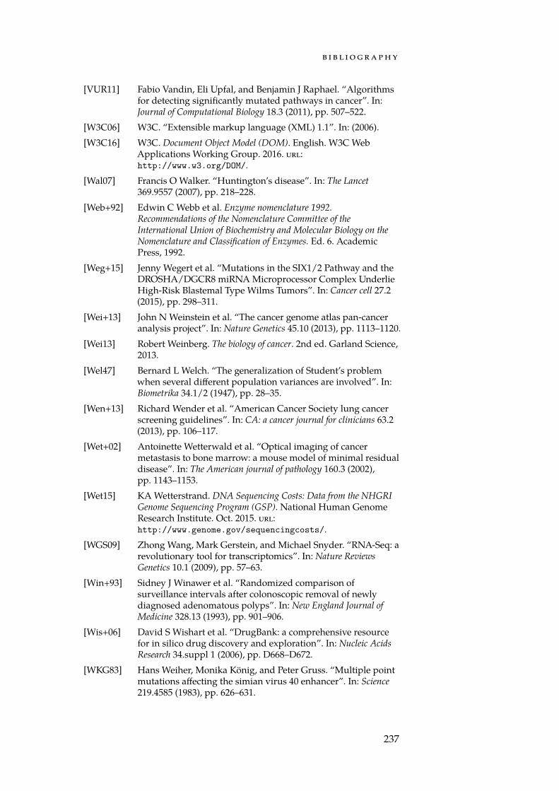
b i b l i o g r a p h y

[VUR11] Fabio Vandin, Eli Upfal, and Benjamin J Raphael. “Algorithmsfor detecting significantly mutated pathways in cancer”. In:Journal of Computational Biology 18.3 (2011), pp. 507–522.

[W3C06] W3C. “Extensible markup language (XML) 1.1”. In: (2006).[W3C16] W3C. Document Object Model (DOM). English. W3C Web

Applications Working Group. 2016. url:http://www.w3.org/DOM/.

[Wal07] Francis O Walker. “Huntington’s disease”. In: The Lancet369.9557 (2007), pp. 218–228.

[Web+92] Edwin C Webb et al. Enzyme nomenclature 1992.Recommendations of the Nomenclature Committee of theInternational Union of Biochemistry and Molecular Biology on theNomenclature and Classification of Enzymes. Ed. 6. AcademicPress, 1992.

[Weg+15] Jenny Wegert et al. “Mutations in the SIX1/2 Pathway and theDROSHA/DGCR8 miRNA Microprocessor Complex UnderlieHigh-Risk Blastemal Type Wilms Tumors”. In: Cancer cell 27.2(2015), pp. 298–311.

[Wei+13] John N Weinstein et al. “The cancer genome atlas pan-canceranalysis project”. In: Nature Genetics 45.10 (2013), pp. 1113–1120.

[Wei13] Robert Weinberg. The biology of cancer. 2nd ed. Garland Science,2013.

[Wel47] Bernard L Welch. “The generalization of Student’s problemwhen several different population variances are involved”. In:Biometrika 34.1/2 (1947), pp. 28–35.

[Wen+13] Richard Wender et al. “American Cancer Society lung cancerscreening guidelines”. In: CA: a cancer journal for clinicians 63.2(2013), pp. 106–117.

[Wet+02] Antoinette Wetterwald et al. “Optical imaging of cancermetastasis to bone marrow: a mouse model of minimal residualdisease”. In: The American journal of pathology 160.3 (2002),pp. 1143–1153.

[Wet15] KA Wetterstrand. DNA Sequencing Costs: Data from the NHGRIGenome Sequencing Program (GSP). National Human GenomeResearch Institute. Oct. 2015. url:http://www.genome.gov/sequencingcosts/.

[WGS09] Zhong Wang, Mark Gerstein, and Michael Snyder. “RNA-Seq: arevolutionary tool for transcriptomics”. In: Nature ReviewsGenetics 10.1 (2009), pp. 57–63.

[Win+93] Sidney J Winawer et al. “Randomized comparison ofsurveillance intervals after colonoscopic removal of newlydiagnosed adenomatous polyps”. In: New England Journal ofMedicine 328.13 (1993), pp. 901–906.

[Wis+06] David S Wishart et al. “DrugBank: a comprehensive resourcefor in silico drug discovery and exploration”. In: Nucleic AcidsResearch 34.suppl 1 (2006), pp. D668–D672.

[WKG83] Hans Weiher, Monika König, and Peter Gruss. “Multiple pointmutations affecting the simian virus 40 enhancer”. In: Science219.4585 (1983), pp. 626–631.

237

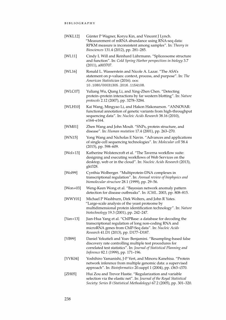
b i b l i o g r a p h y

[WKL12] Günter P Wagner, Koryu Kin, and Vincent J Lynch.“Measurement of mRNA abundance using RNA-seq data:RPKM measure is inconsistent among samples”. In: Theory inBiosciences 131.4 (2012), pp. 281–285.

[WL11] Cindy L Will and Reinhard Lührmann. “Spliceosome structureand function”. In: Cold Spring Harbor perspectives in biology 3.7(2011), a003707.

[WL16] Ronald L. Wasserstein and Nicole A. Lazar. “The ASA’sstatement on p-values: context, process, and purpose”. In: TheAmerican Statistician (2016). doi:10.1080/00031305.2016.1154108.

[WLC07] Yuliang Wu, Qiang Li, and Xing-Zhen Chen. “Detectingprotein–protein interactions by far western blotting”. In: Natureprotocols 2.12 (2007), pp. 3278–3284.

[WLH10] Kai Wang, Mingyao Li, and Hakon Hakonarson. “ANNOVAR:functional annotation of genetic variants from high-throughputsequencing data”. In: Nucleic Acids Research 38.16 (2010),e164–e164.

[WM01] Zhen Wang and John Moult. “SNPs, protein structure, anddisease”. In: Human mutation 17.4 (2001), pp. 263–270.

[WN15] Yong Wang and Nicholas E Navin. “Advances and applicationsof single-cell sequencing technologies”. In: Molecular cell 58.4(2015), pp. 598–609.

[Wol+13] Katherine Wolstencroft et al. “The Taverna workflow suite:designing and executing workflows of Web Services on thedesktop, web or in the cloud”. In: Nucleic Acids Research (2013),gkt328.

[Wol99] Cynthia Wolberger. “Multiprotein-DNA complexes intranscriptional regulation”. In: Annual review of biophysics andbiomolecular structure 28.1 (1999), pp. 29–56.

[Won+03] Weng-Keen Wong et al. “Bayesian network anomaly patterndetection for disease outbreaks”. In: ICML. 2003, pp. 808–815.

[WWY01] Michael P Washburn, Dirk Wolters, and John R Yates.“Large-scale analysis of the yeast proteome bymultidimensional protein identification technology”. In: Naturebiotechnology 19.3 (2001), pp. 242–247.

[Yan+13] Jian-Hua Yang et al. “ChIPBase: a database for decoding thetranscriptional regulation of long non-coding RNA andmicroRNA genes from ChIP-Seq data”. In: Nucleic AcidsResearch 41.D1 (2013), pp. D177–D187.

[YB99] Daniel Yekutieli and Yoav Benjamini. “Resampling-based falsediscovery rate controlling multiple test procedures forcorrelated test statistics”. In: Journal of Statistical Planning andInference 82.1 (1999), pp. 171–196.

[YVK04] Yoshihiro Yamanishi, J-P Vert, and Minoru Kanehisa. “Proteinnetwork inference from multiple genomic data: a supervisedapproach”. In: Bioinformatics 20.suppl 1 (2004), pp. i363–i370.

[ZH05] Hui Zou and Trevor Hastie. “Regularization and variableselection via the elastic net”. In: Journal of the Royal StatisticalSociety: Series B (Statistical Methodology) 67.2 (2005), pp. 301–320.

238

b i b l i o g r a p h y

[Zha+14] Shanrong Zhao et al. “Comparison of RNA-Seq and microarrayin transcriptome profiling of activated T cells”. In: PloS One 9.1(2014), e78644.

[Zha+15] Wenqian Zhang et al. “Comparison of RNA-seq andmicroarray-based models for clinical endpoint prediction”. In:Genome biology 16.1 (2015), pp. 1–12.

[Zho+16] Linyan Zhou et al. “Rspo1-activated signalling molecules aresufficient to induce ovarian differentiation in XY medaka(Oryzias latipes)”. In: Scientific reports 6 (2016), p. 19543.

[ZSM04] Per-Henrik Zahl, Bjørn Heine Strand, and Jan Mæhlen.“Incidence of breast cancer in Norway and Sweden duringintroduction of nationwide screening: prospective cohortstudy”. In: Bmj 328.7445 (2004), pp. 921–924.

239