- 1 -

Trading Constraints and Illiquidity Discounts

Wenxuan Hou a,*

, Sydney Howell b

a

Durham Business School, Durham University, Mill Hill Lane, Durham, DH1 3LB, UK b

Manchester Business School, University of Manchester, Manchester, UK

We appreciate helpful comments from Michael Brennan, Edward Lee, Ser-Huang Poon,

Mark Freeman, Dean Paxson, Alessandra Guariglia, and participants in the 2008 European

Accounting Association Conference at Rotterdam, the 2008 British Accounting Association

Conference at Blackpool, the 2007 Scottish Doctoral Management Conference at the

University of St Andrews (Best Paper Award), the 2006 European Doctoral Research

Conference at Imperial College, and an Xfi Centre seminar at the University of Exeter. We

also thank Degan Yu from the China Centre for Economic Research for providing the data.

We are especially indebted to two anonymous referees for their valuable comments and

suggestions.

* Corresponding author. Tel: +44 (0)191 334 5321; Fax: +44 (0)191 334 5201

Email Address: wenxuan.hou@durham.ac.uk

- 2 -

Abstract

Acting as the source of exogenous illiquidity, trading constraints prevent free trading

of restricted shares and discount their value relative to their freely-traded counterparts

with identical dividends and voting rights. This paper numerically solves the

theoretical illiquidity discounts for the case of long constraint horizons and then

reconciles the contradictions in the results of various theoretical models by identifying

the effects of the unlimited and costless borrowings assumed in Longstaff (2001).

With control of leveraged positions, illiquidity discounts increase with the volatility,

and their size is greatly diminished. We also empirically test the theories within the

unique setting of China, which has the largest population of restricted shares

worldwide. Large discounts are documented in two forms of occasional transactions

in restricted shares: namely auctions and transfers. The results empirically verify the

theoretical findings by showing that illiquidity discounts in auctions increase with

both the volatility and constraint horizons. The results from transfers, however, are

not always significant as the transfers are made privately and may be subject to price

manipulation when the involved parties are related.

Keywords: Exogenous Illiquidity, Restricted Share, Trading Constraint, Constraint

Horizon, Illiquidity Discount

JEL Classification: G11, G12, G30

- 3 -

1. Introduction

This paper theoretically and empirically studies the effects of exogenous illiquidity

stemming from trading constraints on asset prices. It focuses on the world‟s largest

population of restricted shares, namely two thirds of the shares in the Chinese stock

market. Such shares have been priced at a discount relative to otherwise identical

freely-traded shares from the same listed firms when they have occasionally changed

hands. Illiquidity refers to the degree of difficulty, infrequency and uncertainty with

which assets can be converted into cash. Endogenous illiquidity is mainly studied in

terms of bid-ask spread and transaction costs, and in such cases investors can still

trade unlimited amount at some costs. However, in the cases of exogenously imposed

illiquidity addressed in this paper, investors are forbidden to do so within the

constraint horizon.

Many important classes of assets are restricted from free trading. For example,

subscribers in IPOs (Initial Public Offerings) get shares at discounts, but are not

allowed to resell them immediately (Brav and Gompers, 2000; Ofek and Richardson,

2000; Field and Hanka, 2001). Initial dominant shareholders sometimes also promise

not to sell any shares for a period following the IPO. Another example is equity-based

compensation. Ofek and Yermack (2000) note that 17.2% of the executives receive in

their sample receive restricted shares as a part of executives‟ compensation packages

to align their long-run interests with the shareholders and to reduce agency problem.

The annually awarded restricted shares are, on average, 6.84 and 2.60 thousand

respectively for CEOs and non-CEO. Kole (1997) finds constraint horizons for

equity-based compensation as long as 31 and 74 months respectively for firms with

- 4 -

medium and high levels of research and development. In addition, restricted shares

are also obtained by managers and key employees from the target firm in a merger

and by corporate insiders (Bettis et al., 2000). Letter Stock (Osborne, 1982; Silber,

1991) is a widely investigated example: traded shares in the U.S. that are not

registered with the SEC (Securities and Exchange Commission) are not allowed to be

resold within 2 years under SEC Rule 144. Other cases of restricted assets include

bank-issued restricted options in Israel (Brenner et al., 2001).

The largest population of restricted shares has been the restricted shares in the

Chinese stock market, which accounted for around 70% of the total number of shares.

There have been two types of restricted share (see Sun and Tong, 2003): State Shares

are directly owned by the Chinese government; whereas Legal Person Shares (also

known as Institutional Shares) are owned by corporations, including private and

partially private corporations, non-bank financial institutions and state-owned-

enterprises (SOEs). The rest of the shares are freely-traded ordinary shares, which can

be legally held by any firms or individuals, and are effectively continuously traded in

the Shenzhen and Shanghai Stock Exchanges. The two classes of shares in the same

firm enjoy identical voting rights and dividends. .

A series of theoretical papers have examined the restricted assets. Mayers (1972, 1973)

and Brito (1977) show that illiquidity discounts can occur in equilibrium models, and

their size falls as the optimal portfolio strategy approximates “buy-and-hold”.

Longstaff (1995) derives an analytical expression for the upper bound of illiquidity

discounts by using option-pricing theory. Longstaff (2001) obtains the optimal

portfolio weight and theoretical discounts for restricted portfolios. Kahl et al. (2003)

- 5 -

model optimal consumption and portfolio choice, as well as the economic costs of

trading constraints. Longstaff (2009) finds that trading constraints not only decrease

the price of restricted shares, but also increase the price of their freely-traded

counterparts. Although virtually all of these studies derive illiquid discounts, the

predicted sizes differ greatly, and inconsistent results are suggested about the effects

of volatility in various frameworks. Such inconsistency limits the investor‟s

understanding and application of the models.

There are also some weaknesses in the empirical studies of restricted assets: they fail

to incorporate or test important considerations from theoretical studies and their

investigations are based on small samples. Pratt (1989) documents the illiquidity

discounts ranging from 25.8% to 45.0% when summarising the evidence from eight

studies of restricted shares spanning 1966 to 1984. Silber (1991) shows that Letter

Stocks in the U.S. are sold at an average price discount of 33.75%, within a range

from 12.7% to 84%, and the illiquidity discounts vary with the characteristics of the

firm and the issue characteristics. Brenner et al. (2001) find a 21% gap between the

prices of freely-traded options and restricted options; a difference that cannot be

arbitraged away. Chen and Xiong (2001) document 77.93% and 85.59% average

discounts on the restricted shares involved in auctions and transfers from August 2000

to July 2001 in the Chinese stock market. Recently, Huang and Xu (2008), and Chen

et al. (2008) respectively report 72% and 71% discounts based on 233 transfers from

2002 to 2003, and 131 ones from 1996 to 2000. These empirical works are not well

integrated with theoretical ones.

- 6 -

This paper intends to address and solve these problems in the literature. In the

theoretical part, we first apply the models of Longstaff (1995, 2001) to numerically

solve the theoretical optimal portfolio weight and the illiquidity discounts for the case

of China with long constraint horizons. Then, we relax the unrealistic assumption of

unlimited and costless borrowing, and find that a big proportion of documented

illiquidity discounts in Longstaff (2001) are attributed to this condition, and we

identify it as the source of the contradictions in the theoretical results about the effects

of volatility on the illiquidity discounts. With the leveraged positions of investors

controlled, the illiquidity discounts are diminished significantly and the volatility is

found to have a positive effect on the illiquidity discounts. This result shows that the

effects of trading constraints should be less pronounced in reality than what are

suggested in Longstaff (2001).

In the empirical part of this paper, we incorporate and test the key inputs of the

theoretical models, with control variables capturing firm performance, firm

characteristics and transaction characteristics, using a large sample of transactions in

restricted shares in the forms of auctions and transfers from 1994 to 2004 in the

Chinese stock market. After controlling for other influencing factors, our findings

empirically confirm the theoretical results that both the constraint horizons and the

volatility have positive effects on the illiquidity discounts in auctions. The results

from transfers are not always significant presumably because the transfers are made

privately and may be subject to price manipulations when the involved parties are

related.

- 7 -

We then investigate the effects of the announcements of transactions, and find that

they typically cause the price of the freely-traded shares to drop in that occasional

transactions in restricted shares may be regarded as signals of gradually loosing

trading constraints, threatening the price premium of freely-traded counterparts. We

also separately investigate the two types of restricted shares in the Chinese stock

market, namely State Shares held by the government and Legal Person Shares mainly

held by state-owned enterprises (SOEs) and some other non-bank institutions. The

results show that larger discounts are offered when Legal Person Shares are converted

into State Shares in transactions. This may reflect the lower liquidity of the State

Shares, or a confiscation of resources from SOEs to the state.

This study contributes to the literature in several ways. Firstly, it is the first study, to

our knowledge, to empirically verify the findings of the theoretical models of

restricted assets, by providing evidence of the effects of exogenous illiquidity on asset

prices. Secondly, it reconciles the contradicting results from the theoretical studies by

demonstrating how the assumption of unlimited and costless borrowing affects the

magnitude of the illiquidity discounts. Thirdly, it extends the research on the Chinese

stock market, by focusing on the predominant restricted shares, comparing the two

forms of transactions in them. Finally, it also has practical implications for the holders

of restricted shares, and for the regulatory commissions and firm boards which

impose trading constraints.

The remainder of the paper proceeds as follows: Section 2 introduces the institutional

background and develops the hypotheses. Section 3 numerically solves the theoretical

illiquidity discounts by using the theoretical models and then reconciles the

- 8 -

inconsistency by modifying the framework of Longstaff (2001). Section 4 presents the

data and empirical models. Section 5 presents and describes the empirical results.

Section 6 offers conclusions.

2. Institutional Background and Hypotheses

The motivation for the Chinese government for imposing trading constraints at the

IPO of each firm was to control privatisation and maintain its influence. Unlike the

constraint horizon for letter stocks in the U.S. fixed at 2 years, it for the restricted

shares in China was neither specified by the government nor explicitly observable by

investors, and the restricted shares occasionally change hands in two forms of

transactions, namely transfers and auctions, subject to approval from regulatory

commissions. Their prices only become observable in these transactions. The split

share structure due to imposed trading constraints horizon have been found to hold

back the corporate governance of the Chinese listed firms and harm the market

liquidity. In the addition, the government do not need to hold such a large proportion

of shares to maintain its control. Therefore, it then launched two major processes to

terminate the trading constraints.

In the first, named State Share Holding Reduction (Guo You Gu Jian Chi), which

started on 12 June 2001, the government offered a tranche of State Shares to the

market at the price of their freely-traded counterparts, and simultaneously terminated

the trading constraints imposed on them (see Calomiris et al., 2010). Due to the

dramatic increase in the supply, the price premium of the freely-traded counterparts

was diluted, and the market collapsed, forcing the suspension of the attempt. In the

- 9 -

second ongoing process, named the Split-Share Structure Reform (Gu Quan Fen Zhi,

also known as Division Reform), which started on 29 April 2005, the holders of the

restricted shares in each listed-firm offered some consideration to compensate the

holders of freely-traded shares to exchange the consent to eventually terminate all

trading constraints and the government had stopped imposing trading constraints on

newly listed firms (see Firth et al., 2010).

Although the restricted share in the Chinese stock market is in the process of

becoming history, it has provided an ideal sample to investigate the effects of

exogenous illiquidity on asset prices, as reflected by the magnitude of the illiquidity

discount. It is not difficult to forecast that, with this institutional background, if the

volatility of a stock is low, there is less uncertainty about the price at which the

restricted shares can be sold when trading constraints terminate. If it is high, however,

the investors would value the restricted shares at larger illiquidity discounts to

mitigate the increased uncertainty. In addition, uncertainty induces the needs of

rebalancing portfolio, and investors of restricted shares suffer larger losses in a more

volatile market for being unable to do so. In a market with moderate volatility, by

contrast, rebalancing is less necessary and the effects of trading constraints are less

pronounced. We thereby hypothesize that:

Hypothesis 1: Illiquidity discounts increase with volatility.

The constraint horizon, as one of the main characteristics of a trading constraint, is

also expected to influence the illiquidity discount. Longer horizon implies larger

opportunity losses due to the inability to rebalance restricted portfolios. Conversely,

- 10 -

the liquidity premium enjoyed by the freely-traded counterparts has longer to run.

With the volatility constant, longer constraint horizon is also associated with larger

uncertainty about the price at which the restricted shares can be sold at the termination

of constraints. We thereby hypothesize that:

Hypothesis 2: Illiquidity discounts increase with the constraint horizons.

We also expect the results from auctions and transfers to be different due to their

distinct pricing mechanisms. Auctions are publicly visible, and the successful prices

are bids by commercially motivated organisations, whereas transfers are privately

negotiated between possibly related parties, and are not necessarily motivated by

commercial profit. The politically motivated transfer of resources to another

bureaucrat or SOE may also be present, and even if the transfer represents an

economically motivated exchange, not all of the „payments‟ may be visible within the

transfer itself. We thereby hypothesize that:

Hypothesis 3: The effects of volatility or constraint horizons may differ between

auctions and transfers.

3. Theoretical Models

In this section, we apply the two theoretical models from Longstaff (1995, 2001) to

the case of China, and numerically solve the optimal portfolio weights and illiquidity

discounts for restricted shares with long constraint horizons. We also present the

contradictions in the theoretical results and identify the assumption of costless and

- 11 -

unlimited borrowing in Longstaff (2001) as the source of the inconsistency. We

modify the model by releasing this assumption, to reconcile the theoretical results and

to justify our hypotheses about the effects of volatility and the constraint horizon on

illiquidity discounts.

The models of Longstaff (1995, 2001) both assume two hypothetical investors, and in

Longstaff (1995) each of the investors is endowed with a single asset worth S0;

whereas in Longstaff (2001) each of them is endowed with a portfolio worth W0,

composed of a risky asset and a riskless bond or cash. Trading constraints are then

imposed on the assets held by one of the investors and make the restricted investors

being unable to change their positions until the end of the constraint horizon at time T.

The freely-traded asset and portfolio serve as benchmarks to compare with the

restricted case and to calculate the latter‟s illiquidity discount.

There are four major differences between these two frameworks. Firstly, the

hypothetical investors in Longstaff (1995) are assumed to have perfect timing ability.

This assumption maximises the terminal wealth of the freely-traded benchmark; hence

it sets an upper bound of the discount. Secondly, the trading constraints are imposed

at time 0 in Longstaff (1995), but at time 1 in Longstaff (2001). Consequently, both

investors in Longstaff (2001) are free to select optimal initial portfolio weights, which

benefit their terminal wealth. Thirdly, the unrestricted investor in Longstaff (2001)

can continuously rebalance his portfolio, whereas the unrestricted investor in

Longstaff (1995) can only convert the endowed asset into cash all at once. Lastly, the

volatility of the risky asset is assumed to be constant in Longstaff (1995) but

stochastic in Longstaff (2001).

- 12 -

Although Longstaff (2001) is a more plausible model, accommodating some of the

complications of the real world, it retains some unrealistic assumptions. These include

that the volatility of volatility is a fixed parameter and known to the investor; that the

investor can deduce the instantaneous volatility level; that there is no effect of

volatility change on the drift of the underlying cash flow; that interest rate is fixed at

zero; and that the restricted investor is free to select the make-up of the endowment

portfolio at time 0.

3.1 Optimal Portfolio Choices

The optimal portfolio weight for liquid benchmark, denoted as )(* tw , is found

analytically as follows in Longstaff (2001):

)(

)()(

2

2*

tV

tVtw

(1)

where and are constants and respectively set equal to 0.1 and 0; )(tV is the

instantaneous volatility of returns. The remaining proportion of the wealth, ( )(1 * tw ),

is invested in a riskless money market account with price 1)( tB and interest rate

0)( tr .

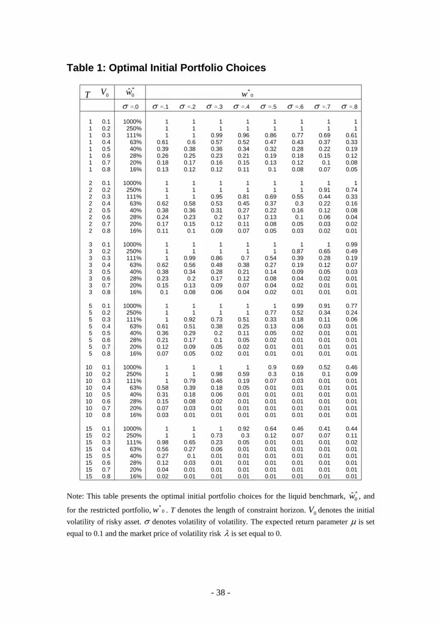
[Insert Table 1 Here]

- 13 -

As seen in Table 1, if a constant growth trend is given, *

0w is heavily influenced by

the initial volatility 0V . When the initial volatility is above 0.3, the investor of the

freely-traded portfolio only invests a proportion of his wealth in the risky asset, and

puts the rest in the cash account with zero interest rate. When the initial volatility is

below 0.3, however, the investor borrows heavily so as to invest more than the

endowment in the risky asset. For example when the initial volatility is 0.1 the

investor invests ten times the initial endowment in the risky asset. We attribute the

strategy of huge leverage to the fixed return drift in the model, which does not

interact with the volatility. The investor borrows to take advantage of the fixed

when risk is fairly low.

Table 1 also reports the optimal initial portfolio choice 0*w for the restricted case for

a wide range of constraint horizon, denoted as T , initial volatility as 0V and the

volatility of volatility as . We solve it numerically as described in Longstaff (2001).

To reflect the Chinese situation we have extended the calculations to long constraint

horizons of up to 15 years, whereas Longstaff (2001) only solved for 1 and 2 years1,

being interested in letter stocks. We see that optimal initial risky fraction 0*w

decreases with increases in the initial volatility 0V , the volatility of volatility , and

the constraint horizon T. When T is larger, 0*w is more sensitive to changes in 0V and

. The result implies that, due to the long constraint horizon in China, the investors

are better of not investing much of their wealth in restricted assets even if the risks are

at moderate levels. The implication, however, does not necessarily apply to the

Chinese government, because it may have other motives than profits, such as

- 14 -

maintaining state control. In addition, the risks are diversified to some extent as the

state holds restricted shares from many listed firms from various industries.

3.2 Illiquidity Discounts and Contradictions in the Results

The trading constraint reduces the derived utility of wealth; hence, if a restricted asset

is offered for an auction or transfer, a price discount must be offered, relative to the

freely-traded counterparts, as a compensation for the inability of trading. The soloved

illiquidity discount D is expressed as follows in Longstaff (2001):

)))0(;,,,,(),,(exp(

11

*wtVSNWJtVWJD

(2)

where ),,( tVWJ and ))0(;,,,,( *wtVSNWJ are, respectively, the logarithmic utilities

of the liquid benchmark and the illiquid portfolio; N denotes the number of risky

assets in the portfolio; S denotes its price; and W denotes the wealth.

The upper bound of the illiquidity discount in the framework of Longstaff (1995),

denoted as D

, is expressed as follows:

2 2 2 2

11

2 exp2 2 2 8

DV T V T V T V T

N S

(3)

- 15 -

where N is the cumulative normal distribution function; V is the volatility and it is

assumed to be a constant (i.e. 0 ).

[Insert Table 2 Here]

Table 2 presents the illiquidity discounts suffered by the restricted portfolio, relative

to the freely-traded benchmark, given by the models of Longstaff (1995, 2001). The

sizes of initial volatility 0V and constraint horizon T are found to have a positive

influence on the upper bound of the illiquidity discount defined in Longstaff (1995),

denoted as D

. When T=2, D

increases by nearly 10 times, from 11.79% to 100.00%,

as 0V increases from 0.1 to 0.8. When 3.00 V , D

rises from 26.28% to 100.00% as

T increases from 1 to 15 years. When D

reaches 100%, it does not mean that the

restricted portfolio is worth exactly zero, but that the incremental cash flow generated

by the freely-traded benchmark accounts for a very large fraction of its terminal

wealth. For investors in the real world, without perfect timing ability, the illiquidity

discount could fall well below the suggested upper bound.

The illiquidity discounts D given by Longstaff (2001) are also presented in the table.

In this framework, volatility is stochastic and the investor in the liquid benchmark can

continuously rebalance his portfolio. Both the volatility of volatility and constraint

horizon T are found to have positive effects on the illiquidity discount D . For 3T

and initial volatility 4.00 V , D increases dramatically from 1.02% to 99.42% when

is raised from 0.1 to 0.8. When 0V and are both fixed at the level of 0.4, D

goes up from 1.48% to 100% as T increases from 1 to 15 years. Both the results of

- 16 -

Longstaff (1995, 2001) confirm our hypothesis about the effects of constraint

horizons, suggesting that the restricted shares in China should be valued substantially

lower than their freely-traded counterparts.

In contrast, the volatility 0V has different effects on D

and D. For example, given

3T , if 0V rises from 0.1 to 0.8, D

increases from 14.59% to 100%, whereas D

falls from 95.40% to 4.61% (if 4.0 ). The difference between their suggested

illiquidity discounts could be as large as 95.39%. The source of the contradictions is

identified and discussed below.

3.3 Leveraged Position and Illiquidity Discounts

The illiquidity discount as a relative measure depends on the terminal values of both

the restricted portfolio and the liquid benchmark respectively given by their optimal

portfolio choices *

0w and 0*w in Longstaff (2001). Recalling the values of *

0w in

Table 1, when 0V is low, *

0w is as large as 1000%, whereas 0*w remains below 100%.

The ability of costless and unlimited borrowing boosts the incremental cash flow

generated by the liquid benchmark, consequently flipping up the illiquidity discounts

given by Longstaff (2001). We attribute the contradiction in the results to the

leveraged position allowed in Longstaff (2001), which is also neither plausible nor

realistic in many situations. For example, it is not permitted in China to borrow

money from banks to invest in stocks. We would like to control its influence by

imposing a ban on the leveraged positions to identify the components of the illiquidity

discount respectively attributable to the leveraged positions and the trading constraints.

- 17 -

We hereby modify the model and numerical solution of Longstaff (2001) by bounding

the optimal portfolio weight of the liquid benchmark between 0% and 100%. The sub-

optimal portfolio weight, denoted as *~tw , is expressed as follows:

1,

)(

)(min~

2

2*

tV

tVwt

(4)

Without leveraged positions, we can no longer use the closed-form solution (Equation

1) to calculate the terminal wealth of the liquid benchmark. Instead, we need solve it

numerically, as described in Appendix 1, by inputting Equation (4) directly into the

following dynamics of the wealth:

dZWwVdtWwVdW ttttt tt

**2 ~~)( (5)

where Z is a standard Brownian motion. By inputting the numerically solved terminal

wealth of the freely-traded benchmark and the restricted case into Equation (2), we

can get the core element of the illiquidity discount denoted as D~

. The other element

attributable to unlimited and costless borrowing is eliminated.

[Insert Table 3 Here]

Table 3 reports the results of D~

. Due to limits in the numerical and statistical

accuracy of the simulation methods, there are a few examples of numerical errors,

such as negative discounts when 0V and T are small. Nonetheless, the pattern is clear:

- 18 -

the volatility of volatility and the constraint horizon T are still positively related to

the core element of the illiquidity discount. For fixed 3T and 3.00 V , D~

increases from 0.49% to 18.29% as rises from 0.1 to 0.8. The corresponding

increase in D in Table 2 is from 1.41% to 99.99%, showing that the core element

accounts for a smaller proportion of the total illiquidity discount for larger . Hence,

leveraged positions play a more important role as rises. For 2.00 V and 4.0 ,

D~

increases from 0.12% to 66.61% as T increases from 1 to 15 years. The

corresponding increase in D in Table 2 is from 8.05% to 100%. It shows that the

leveraged positions exaggerate the effects of the trading constraints on the illiquidity

discounts.

More importantly, the contradiction in the effects of volatility is reconciled and the

documented positive effect on illiquidity discounts is consistent with the result of

Longstaff (1995) and also our hypothesis. When 10T and 3.0 , D~

increases

from 3.72% to 31.58% when 0V increases from 0.1 to 0.7. The corresponding

increase in D in Table 2 given by the model of Longstaff (2001) is from 100% to

40.77%. As the volatility increases, the core element accounts for a larger proportion

of the illiquidity discount.

Although the two theoretical frameworks provide useful justification for our

hypotheses, they nonetheless oversimplify the real-life problems. For example, they

do not consider the benefits of control. Due to the small proportion of freely-traded

shares in the Chinese stock market, investors may have to hold restricted shares in

order to maintain control of the firms. Furthermore, Longstaff (2001) only considers

- 19 -

one risky asset in the portfolio. An investor can hedge his restricted asset by holding

another asset with small or negative correlation in their volatility of returns. In

addition, the applicability of the model is also subject to the methods of observing the

instantaneous volatility, and volatility of volatility.

4. Data and Research Design

4.1 Data and Models

In addition to the theoretical works, we also intend to empirically test our hypotheses.

For this we use the largest and most complete data set yet seen in the literature,

namely 3260 auctions and 2890 transfers of restricted shares in the Chinese stock

market from 1994 to 2004. Our sample is drawn from the China Centre for Economic

Research (CCER).

We study the illiquidity discounts observed in auctions and transfers separately

because they have different pricing mechanisms. We use auctionD to denote the

illiquidity discounts observed in auctions and transferD to denote the illiquidity

discounts observed in transfers. In order to avoid problems of multicollinearity2, we

model the effects of the volatility and the constraint horizon in two separate

regression equations as follows:

ExchangeSOEROEPBAGE

MCRTTFRVolatilityDauction

98765

4321 (6)

- 20 -

ExchangeSOEROEPBAGE

MCRTTFRTDauction

98765

4321 (7)

The variables are explained after equation (9). For the illiquidity discounts observed

in transfers, denoted astransferD , there are more data available for the transaction

characteristics and the two regression models are expressed as follows:

ClearChangenivatisatio

CashofitExchangeSOEROEPB

AGEMCRTTFRVolatilityDtransfer

141312

11109876

54321

Pr

Pr (8)

ClearChangenivatisatio

CashofitExchangeSOEROEPB

AGEMCRTTFRTDtransfer

141312

11109876

54321

Pr

Pr (9)

where Volatility denotes the volatility of returns; T denotes the constraint horizon;

FR denotes the ratio of freely-traded shares in the firm; RTT denotes the ratio of

restricted shares involved in occasional transactions; MC denotes the market

capitalisation of the freely-traded shares of the firm; AGE denotes the number of

years since the firms was listed; PB denotes the price-to-book ratio; ROE denotes

the returns on equity; SOE is a dummy variable equal to 1, if the firm is a state-owned

enterprise, and 0 otherwise; Exchange is a dummy variable equal to 1 if the firm is

listed on the Shanghai Stock Exchange; and 0 if on the Shenzhen Stock Exchange.

For the model of transferD , Profit is a dummy variable equal to 1 if the firm has not

experienced 2 or more years of consecutive losses prior to the transfer, and 0

otherwise; Cash is a dummy variable equal to 1 if the transaction is paid in cash, and

0 otherwise; Privatisation is a dummy variable equal to 1 if shares are transferred

- 21 -

from a state-owned enterprise to a non-state-owned enterprise, and 0 otherwise;

Change is a dummy variable equal to 1 if the transfer changes the dominant

shareholder, and 0 otherwise; Clearis a dummy variable equal to 1 if the seller sells

out all his shares in a transfer, and 0 otherwise.

Two specifications for the illiquidity discount can be obtained by using the following

equations:

t

ttauction

FP

RPFPD

(10)

1

1

t

ttauction

FP

RPFPD (11)

where tRP is the price of restricted shares as announced in occasional transactions;

tFP is the closing price of their freely-traded counterparts on the announcement day;

and 1tFP is the closing price of the freely-traded shares one day before the

announcement. In the same way, transferD and transferD can be obtained. If the market is

efficient, a change in tFP reflects the information content of the transaction

announcement, and the reaction of the freely-traded share‟s price to an occasional

transaction of restricted shares can be simply captured by the difference between

auctionD andauctionD , denoted as

auctionDD . Similarly, the difference between transferD and

transferD , can be denoted as transferDD . Both auctionDD and transferDD are equal to

t

t

t

t

F

RP

F

RP

1

. When permission is given for any transaction in restricted shares, the

market may treat this as a signal of gradually loosing trading constraints. Since this

- 22 -

would erode the liquidity premium of the freely-traded shares, we expect 1 tt FPFP

and therefore 01 tt DD .

How the price of freely-traded shares reacts to the characteristics of the involved

firms and to the characteristics of the occasional transaction itself is captured by a

regression model for auctionDD or

transferDD as follows:

ClearChangenivatisatioCashofit

ExchangeSOEAgeMCTFRRTTDDauction

12111098

7654321

PrPr (12)

4.2 Variables in the Models

Chen and Xiong (2001) incorporate volatility in their empirical model and interpret it

as a proxy for the firm‟s quality and viability as well as for the truthfulness of the

management. In theoretical models such as Longstaff (1995, 2001, 2005) and Kahl et

al. (2003) volatility can predict the value that the liquid benchmark gains from the

ability to rebalance the portfolio. When leveraged portfolios are banned, as in China,

higher volatility increases the opportunities for liquid investors, and thereby raises the

discounts suffered by illiquid assets.

The remaining length of the constraint horizon in the theoretical models of Longstaff

(1995, 2001, 2005) and Kahl et al. (2003) increases the incremental value generated

by the liquid benchmark, and therefore positively influences the illiquidity discount.

However, this effect has never been tested empirically. Unlike the fixed trading

- 23 -

constraints for letter stocks (Silber, 1991) and for bank-issued options (Brenner et al.,

2001), the constraint horizons in the Chinese stock market were not explicitly

specified. Two reforms had influence investors‟ expected constraint horizons. We

assume that the investors prior to 2001 expected the trading constraints to be

terminated in 2007, 6 years after the launch of the eventually failed State Share

Holding Reduction, due to its small scale. Chen and Xiong (2001) had similar

conjectures. The Split Share Structure Reform launched in 2005 mandates the

termination of the majority of trading constraints in about 3 to 4 years i.e. 2009. Even

if our assumptions cannot capture the expectation precisely, they are able to reflect the

trend of the expected constraint horizons affected by these two processes. This rough

proxy for investors‟ expectations about the remaining constraint horizon is expressed

as follows:

,2009

,2007

tT

tT

2001

2001

t

t (13)

Control variables capturing the firm‟s performance include ROE (Chen and Xiong,

2001) and Profit (Silber, 1991); these of the firm characteristics include MC (Huang

and Xu, 2008), AGE , PB , SOE , and Exchange (Chen and Xiong, 2001); these of

the transaction characteristics include RTT , Cash , Privatisation, Change , and

Clear (Huang and Xu, 2008).

We winsorise the top and bottom 1% of the sample and control for the industry effect

and year effect. The industry dummy is based on the Global Industry Classification

Standard (GICS) code.

- 24 -

5. Empirical Findings

5.1 Characteristics of Transactions and Illiquidity Discounts

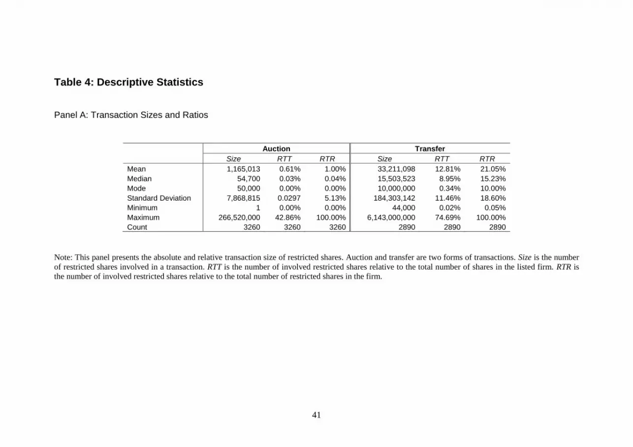
Panel A of Table 4 presents the descriptive statistics of two forms of transaction. It

shows both absolute and relative measures of transaction scale. Size denotes the

number of restricted shares involved in a transaction; RTT denotes the ratio of the

involved restricted shares in the firm; RTR denotes the ratio of restricted shares

involved in a transaction. The average auction size is on average 1,165,013 shares,

whereas the average transfer size is 33,211,098 shares, 30 times greater in scale. RTT

(RTR) in auctions is only 0.61% (1.00%), whereas RTT (RTR) in transfers is 12.81%

(21.05%). It seems that transfers are much more likely to lead to changes in the

control of listed firms.

[Insert Table 4 Here]

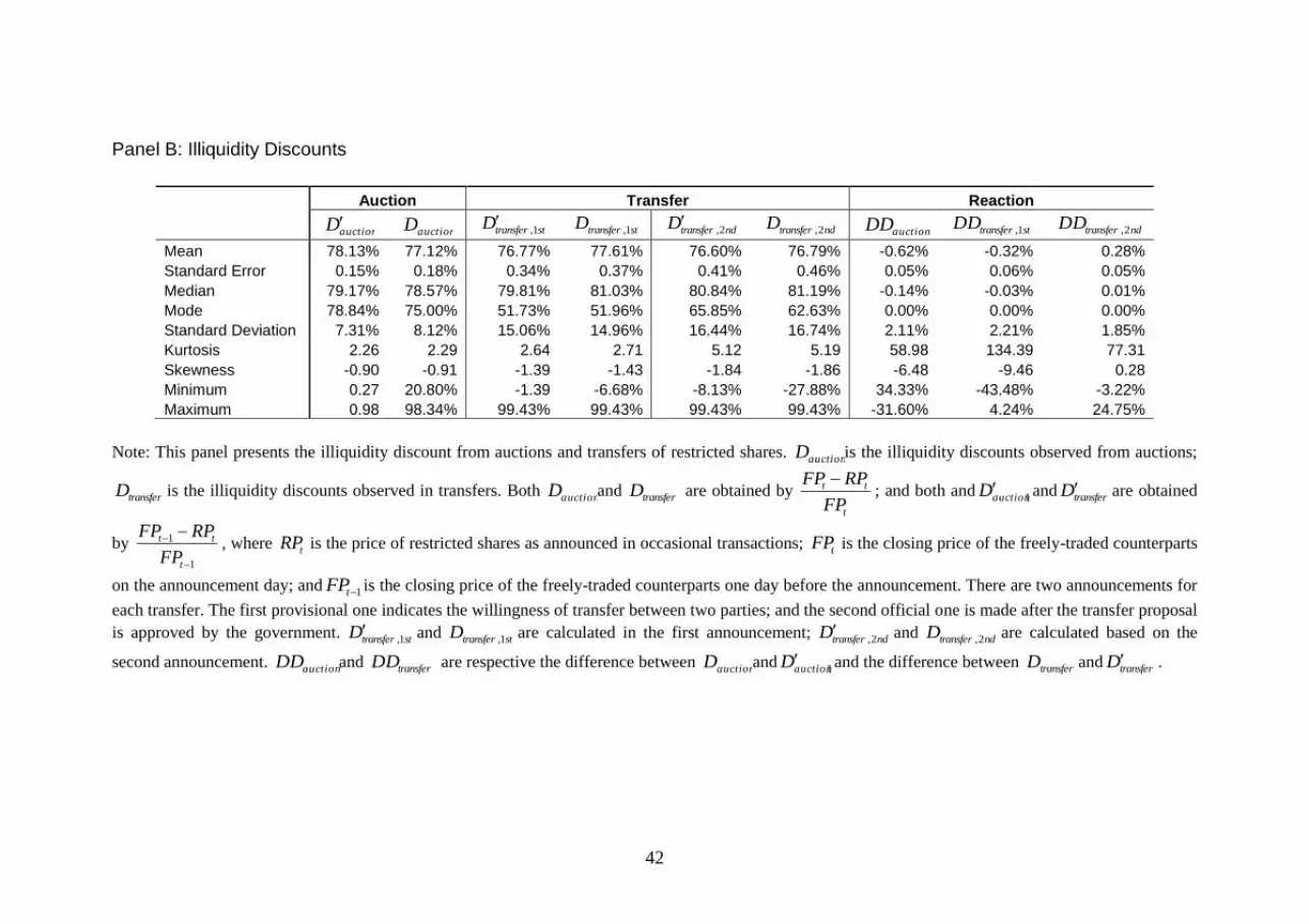
Panel B of Table 4 displays the descriptive statistics of the illiquidity discounts from

auctions and transfers. The mean of auctionD and auctionD respectively are 78.13% and

77.12%. For each transfer two announcements were made: the first/provisional

announcement was made after a transfer proposal was made between two parties; the

second/official announcement was made after the proposal was approved by

regulatory commissions. sttransferD 1, , the illiquidity discount before the first

announcement, and ndtransferD 2, , the illiquidity discount before the second

- 25 -

announcement are, respectively, 76.77% and 76.60% with standard deviation 0.34%

and 0.41%. The discounts sttransferD 1,

and ndtransferD 2,

observed on the announcement

day are 77.61% and 76.79%.

The illiquidity discounts documented in the Chinese stock market are greater than any

from American samples, such as the 35% discount from privately-placed shares

(Wruck, 1989) and the 34% discount from letter stocks (Silber, 1991). Compared with

other empirical evidence from the Chinese stock market, the documented discounts

from auctions are very close to 77.93% in Chen and Xiong (2001). Discounts from

transfers, however, are roughly 7% smaller than the 85.59% documented in Chen and

Xiong (2001) and roughly 5% greater than the 72% discount from Huang and Xu

(2008). The difference may be attributed to the longer sample period in this paper.

Our sample covers 1994 to 2004, whereas that in Chen and Xiong (2001) covers 2000

to 2001 and in Huang and Xu (2008) 2002 to 2003 only.

The gap between the discounts from auctions and those from transfers is around 1.5%

before the announcement and less than 0.5% after the announcement, despite distinct

characteristics for the two types of transaction: the auction is a market-driven pricing

mechanism, which is believed to be more efficient, whereas the transfer is privately

negotiated between two possibly related parties and seems more open to price

manipulation. As possible evidence, Panel B shows that restricted shares are

sometimes transferred at a premium rather than a discount. Why do the purchasers not

simply buy the liquid counterparts from the market at a lower price? These

observations may signal the existence of price manipulation, but they may also signal

the effects of time lags in the transfer negotiation and authorisation process.

- 26 -

Silber (1991) sets up a dummy variable for transactions between related parties.

Huang and Xu (2008) claim exclude this kind of transactions from their samples.

However, the data we used in this study does not include such information. In the

absence of additional information, the similarity of the discounts for the two distinct

forms of transactions may imply that any price manipulations in transfers were evenly

split in oppose directions.

Market reaction to announcements of transactions is simply inferred by the

differences in discounts before and after the announcements, denoted as DD in Panel

B. The fact that 0auctionauction DD and 01,1,

sttransfersttransfer DD implies that the

price of freely-traded shares falls after the announcement. If this is the case, it is

interesting to see that 0transfertransfer DD , i.e. the second announcement increases

the relative price of the freely-traded shares. For interpretation, it is useful to note that

there is a difference between the two announcements. Unlike the second

announcement, the first announcement leaves some uncertainty in terms of whether

the deal will be approved, and how long the approval process may take. The second

announcement bounds this uncertainty, and consequently may support the price of

freely-traded shares.

Considering the effects of transaction scale, we expected transactions of a larger scale

to have a greater influence on the price of their freely-traded counterparts; however,

the reaction measured by DD from auctions was twice the reaction from transfers,

despite the fact that auctions are generally much smaller than transfers in scale. This

- 27 -

may be attributed to the wider participation in auctions and/or the more efficient

pricing mechanism of auctions.

In addition to the general pattern, we also compare the illiquidity discounts from

different types of restricted shares. Panel C of Table 4 shows that there were 747

transactions of State Shares and 915 of Legal Person Shares. The latter are more

frequently involved in transactions, implying in turn that the trading constraints

imposed on State Shares are tighter. State Shares were converted to Legal Person

Shares in 431 transactions and Legal Person Shares were converted to State Shares in

146 transactions. It also shows that an investor is willing to buy State Shares at a

smaller discount when they are converted into Legal Person Shares, which are

associated with looser trading constraints; and further discounts are offered to

compensate the investor when the Legal Person Shares are converted into State Shares

with tighter trading constraints.

Panel D of Table 4 shows the illiquidity discounts for firms in different industries.

Firms in the Consumer Discretionary industry are most frequently involved in both

forms of transactions and firms in the Telecommunication Services and Energy

industries are least frequently involved. The patterns for auctions and transfers are

similar and the frequency captures the tightness of the trading constraints due to the

government‟s varying intention to maintain the control of these industries. For

example, heavily regulated industries such as the Energy and Telecommunication

Services industries are either under-represented in transactions or associated with

smaller discounts.

- 28 -

Panel E of Table 4 reports the transactions in each year from 1994 to 2004. Most of

the auctions are concentrated in 2001, whereas the transfers are relatively evenly

distributed among different years. The pattern of auctionD is clearly consistent with the

theoretical results that the discount falls with T. As auctionD approaches the State

Shares Holding Reduction in 2001, it decreases from 81.85% to 76.99%; as it

approaches the Split Share Structure Reform in 2005, auctionD decreases from 79.24%

to 71.77%. We also observe that auctionD increases from 76.99% to 78.24% after the

suspension of the State Shares Holding Reduction at the end of 2001. The decreasing

trend of sttransferD 1, after 2001 is clear; however, it increases from 66.92% to 85.96%

with fluctuations from 1994 to 2000, and falls slightly to 84.17% in 2001. Compared

with the auctionD in the same year, sttransferD 1, is around 7% larger. This difference may

be attributed to either the different expectations of the constraint horizons or the

distinct pricing mechanisms.

Panel F in Table 4 shows the descriptive statistics of the explanatory variables. Firms

involved in auctions are generally larger and older than those in transfers. In the

sample, 82.17% of firms in auctions and only 31.13% of firms in transfers were SOEs;

93.39% of firms in auctions had not experienced a 2-year or longer consecutive period

of loss prior to the transactions, but the percentage of these in transfers was only

11.49%. As firms with a 2-year or longer consecutive period of loss are under the

threat of being delisted, price manipulations are more likely to happen in transfers in

order to manipulate the performance of these firms. The panel also shows that only

5.89% of transfers were paid in cash, 27.70% of transfers led to partial privatisation,

77.93% of transfers led to changes in the dominant shareholder, and 54.24% of sellers

- 29 -

in transfers sold all the shares they held. Characteristics of the transfers involving

State Shares and Legal Person Shares are also presented. More transfers of State

Shares led to privatisation but less to changes of the dominant shareholder compared

with the transfers of Legal Person Shares.

5.2 Empirical Results of Illiquidity Discounts

Panel A in Table 5 reports the regression results for the observed illiquidity discounts

from both forms of transaction. Volatilities and constraint horizons from our

hypotheses are tested separately in order to solve the problem of multicollinearity.

The first model incorporates the volatility with other control variables; and the second

model incorporates the constraint horizon with other control variables.

[Insert Table 5 Here]

The coefficient 2.6199 for Volatility from the first model of auctionD indicates that the

volatility, as a proxy for risk, increases the illiquidity discount in auctions. This is

consistent with our Hypothesis 1 and the theoretical results of this paper that investors

suffer more for being unable to rebalance their portfolios in more volatile markets.

The coefficient for T is 0.0329 in auctions. As Hypothesis II states and the theoretical

models suggest, illiquidity discounts also increase with constraint horizons.

Particularly, a 1-year increase in the constraint horizon led to a 3.29% larger

illiquidity discount in auctions. The coefficients for Volatility , however, are not

- 30 -

significant in the models of sttransferD 1,

and ndtransferD 2,

, and the coefficient of T is only

significant for ndtransferD 2, . The different results from auctions and transfers may be

attributed to their distinct pricing mechanism: the market-driven mechanism of

auctions makes their participants react to the changes in volatility and constraint

horizons rationally; however, the privately-negotiated transfers between possibly-

related parties are subject to price manipulations.

In addition, some control variables are also found to influence the illiquidity discounts

significantly. Same as Chen and Xiong (2001), using tAge to proxy the viability of a

business, this paper also documents different preferences between the participants in

the two forms of transactions: a negative relationship in auctions but a positive one in

transfers: with a 1-year increase in Age , the illiquidity discounts decrease by around

0.38% in auctions but increase 0.34% in transfers.

The effects of firm size captured by MC are also different in auctions and transfers.

Larger firms have smaller illiquidity discounts than smaller firms in auctions but have

bigger illiquidity discounts than smaller firms in transfers. This may be attributed to

the different preferences of the participants. As the transaction size in transfers is

much larger than it is in auctions, the recipients of transfers normally become big

blockholders. In line with the benefit control argument of Huang and Xu (2008),

investors in transfers request a larger illiquidity discount if they find it is difficult to

extract control benefits from the larger firms which are normally better covered by the

media and better monitored. On the contrary, the participants in auctions tend to be

minority shareholders, and they impose smaller illiquidity discounts for restricted

shares in larger firms, whose corporate governance tends to be better monitored.

- 31 -

The ratio of freely-traded shares relative to total shares, denoted as FR, proxies the

marketability or inverse of the scale of the trading constraints. It is found to have

negative impacts on the illiquidity discounts in transfers. This is consistent with Silber

(1991) and Huang and Xu (2008). However, FR is not significant in the model for

auctions. Huang and Xu (2008) believe tFR also captures the corporate governance

characteristics of the firm and argue that with a lower tFR , the holders of restricted

shares tend to dominate corporate voting; and restricted shares as voting shares are

priced at a larger discount when their proportion is large (see Bergstrom and Rydqvist,

1992); in addition, with a lower tFR , blockholders are only willing to pay a lower

price for restricted shares because they have to share the control benefits with others.

Positive effects on the illiquidity discounts in auctions are found from the ratio of

restricted shares involved in the transactions, denoted astRTT . Similar control

discount is found in Chen and Xiong (2001) and they attribute it to the pre-fixed

supply of shares in auctions. The negative effects documented in transfers are

consistent with a control premium for a larger block of shares documented in Barclay

and Holderness (1989), Wruck (1989), Chen and Xiong (2001) and Huang and Xu

(2008).

Same as Chen and Xiong (2001), we find that growth firms, with a larger tPB (price

of freely-traded share to Book Value), are associated with larger illiquidity discounts,

and that tRoE (the return on equity) is positively affects illiquidity discounts in

transfers, but negatively affects them in auctions. They attribute the positive effects to

- 32 -

information asymmetry: the participants in transfers have better information and do

not trust the reported earnings. We, however, believe that the positive effects signal

price manipulation, especially in firms with consecutive poor performance, captured

by the dummy variable Profit. Its coefficient indicates that restricted shares from

firms experiencing 2 or 3 years of consecutive losses before the transfers are priced

have a 10.12% smaller discount. These firms are under threat of being delisted in the

exchange; hence, corporate restructuring is more likely to happen in those firms.

The coefficient for the dummy variables SOE indicates that restricted shares from

SOEs (state-owned-enterprises) are priced at a 2.13% larger discount than those from

non-SOEs in transfers; The larger discount for shares in SOEs may be attributed to

their worse corporate governance or performance (see Fan et al., 2007; and Cheung et

al., 2010). The coefficient for the dummy variables Exchange shows Illiquidity

discounts for firms listed on the Shanghai Stock Exchange are 2.84% smaller in

auctions, and 1.38% and 1.72% smaller in transfers than those from firms listed in the

Shenzhen Stock Exchange. This result is consistent with Chen and Xiong (2001),

although the effects documented here are larger.

The results for the variables of the transaction characteristics show that cash payment

decreases the discounts by 4.31% as this has lower uncertainty and is preferred in

mergers and acquisitions. A seller‟s clearing-out of his holding leads to a 1.25%

decrease in discounts. Huang and Xu (2008) argue that investors in restricted shares

tend to quit if the control benefits are small or difficult to extract. Our findings,

however, imply that the holders of restricted shares are reluctant to quit unless a

higher price for the restricted shares is offered.

- 33 -

By investigating the transfers of two types of restricted shares separately, we can infer

the effects of restriction tightness on illiquidity discounts. State Shares and Legal

Person Shares are two types of restricted shares and some transfers are associated

with a conversion of type of share. We incorporated a dummy in the regression model.

In Panel B of Table 5, 1Conversion if the type of share is converted into another

one and 0 otherwise. The result shows that a conversion from Legal Person Shares to

State Shares is associated with a larger discount. This may be attributed to the tighter

trading constraint on State Shares. Recall the observations in Panel C of Table 4, that

transactions in State Shares are more frequent than transactions in Legal Person

Shares. Hence, a larger discount is offered to compensate for the tighter trading

constraints.

Panel C of Table 5 presents the market reaction of freely-traded shares. Instead of

running a systematic event study, we simply take the difference between D and D ,

denoted as DD , to inversely measure the drop in the price of freely-traded shares

when their restricted counterparts are involved in occasional transactions. As the

transactions of restricted shares may signal the looseness of the trading constraints

and an increase in the supply of freely-traded shares, the price premiums of freely-

traded shares are threatened. The first column shows that the drops in price after

auctions are smaller for firms with larger FR, T, and for SOEs, implying that firms

with a larger ratio of freely-traded shares are less affected by the looseness of the

trading constraints; and investors are more sensitive when the end of the constraint

horizon approaches and when the involved firms are state-owned enterprises.

Auctions for larger firms and older firms, respectively measured by MC and Age,

- 34 -

however, lead to larger drops in value. The market reaction to the second

announcement is not significantly affected by any of the variables. If the approval of

the transfers after the provisional announcement can be forecasted by the investors,

they do not react to the second confirming announcement.

6. Conclusion

This paper studies the effects of exogenously imposed illiquidity on asset prices by

modifying the theoretical models from Longstaff (2001), and by empirically

investigating a sample of restricted shares from 1994 to 2004 in the Chinese stock

market. Large illiquidity discounts are obtained and documented respectively from the

theoretical and empirical sections. Our theoretical study reconciles the contradicting

results in the theoretical literature about the effects of volatility on the illiquidity

discounts by forbidding the assumption of unrealistic unlimited and costless

borrowing. We find that the illiquidity discounts are greatly diminished and the

volatility has positive effects on the illiquidity discounts when the leveraged positions

are controlled. Our empirical results extend earlier empirical studies by incorporating

and testing the key inputs from the theoretical studies (Longstaff, 1995, 2001, 2009;

Kahl et al., 2003). Consistent with the theory, we find that the volatility and constraint

horizons have positive effects on the illiquidity discounts in auctions, after controlling

for firm performance, firm characteristics and transaction characteristics. The results

from transfers are not significant due to the distinct pricing mechanism of the two

forms of transactions: an auction is a market-driven pricing mechanism whereas a

transfer is negotiated privately between two parties, which may allow imperfect

and/or asymmetric information and the manipulation of prices.

- 35 -

The results imply that the trading constraints, especially those with long horizons, as a

tool to maintain the control of existing dominant shareholders or a tool to retain

executives and important employees, could be very costly. As the trading constraints

obstruct them from selling the shares to realise returns, they may go for other

alternative approaches to the cost of the other shareholders. For example, dominant

shareholders may get loans from banks by asking the listed firm to be warrantor; and

executives may make unnecessary acquisitions to diversify their risks.

There are some possible directions for future studies. For example, the consequence

of the occasional transactions in restricted shares is worth investigating. They may

improve the performance of the firms, as the corporate governance could be improved

if the state‟s absolute control is weakened. Similarly, it would also be interesting to

examine the ongoing Split Share Structure Reform and its consequences.

1 By using the inputs of Longstaff (2001), we compared the results given by our numerical solution

with his, and find that they are consistent. 2 The correlation matrices in Appendix 2 document the correlation between Volatility and T as large as

0.1741 in the sample of auctions, and 0.3590 in the sample of transfers.

- 36 -

References:

Barclay, M., and C. Holderness. 1989. Private benefits from control of public

corporations. Journal of Financial Economics 25: 371-395.

Bergstorm, C., and K. Rydqvist. 1992. Differentiated bids for voting and restricted

voting shares in public tender offers. Journal of Banking and Finance, 16, 97-114.

Bettis, J. C., Coles, J. L., and M. L. Lemmon. 2000. Corporate policies restricting

trading by insiders. Journal of Financial Economics 57: 191-200

Brav, A. and P. Gompers. 2000. Insider trading subsequent to initial public offerings:

evidence from expirations of lock-up provisions. Working Paper, Duke University,

North Carolina and Harvard University.

Brenner, M., R. Eldor, and S. Hauser. 2001. Price of options illiquidity. Journal of

Finance 56: 789-805.

Brito, N. O., 1977. Marketability restrictions and the valuation of capital assets under

uncertainty. Journal of Finance 332: 1109-1123

Calomiris, C. W., R. Fisman, and Y. Wang. 2010. Profiting from government stakes

in a command economy: Evidence from Chinese asset sales. Journal of Financial

Economics 96: 399-412

Chen, G., M. Firth, Y. Xin, and L. Xu. 2008. Control Transfers, Privatization, and

Corporate Performance: Efficiency Gains in China‟s Listed Companies. Journal of

Financial and Quantitative Analysis 43: 161-190

Chen, Z., and P. Xiong. 2001. Discounts on illiquid stocks: evidence from China.

Working Paper, No.00-56, Yale International Centre of Finance.

Cheung, Y., P. Jiang, P. Limpaphayom, and T. Lou. 2010. Corporate Governance in

China: a Step Forward. European Financial Management, 16, 94-123

Fan J., T. J. Wong, and T. Zhang. 2007. Politically-connected CEOs, corporate

governance and post-IPO performance of China's partially privatized firms. Journal of

Financial Economics 84: 300-357.

Field, L., and G. Hanka. 2001. The Expiration of IPO share lockups. Journal of

Finance 56: 471–500.

Firth M., C. Lin, and H. Zou. 2010. Friend or Foe? The Role of State and Mutual

Fund Ownership in the Split Share Structure Reform in China. Journal of Financial

and Quantitative Analysis 445: 685-706

Huang, Z., and X. Xu. 2008. Marketability, control and the pricing of block. Journal

of Banking and Finance, forthcoming.

- 37 -

Kahl, M., Liu, J., and F. Longstaff. 2003. Paper millionaires: how valuable is stock to

a stockholder who is restricted from selling it? Journal of Financial Economics 67:

385-410.

Kole, S., 1997. The complexity of compensation contracts. Journal of Financial

Economics 43: 79–104.

Longstaff, F., 1995. How much can marketability affect security values? Journal of

Finance 50: 1767-1774.

Longstaff, F., 2001. Optimal portfolio choice and the valuation of illiquid securities.

Review of Financial Studies 14: 407-431.

Longstaff, F., 2009, Portfolio Claustrophobia: Asset Pricing in Markets with Illiquid

Assets. American Economic Review 99: 1119-1144.

Mayers, D., 1973. Nonmarketable assets and the determination of capital asset prices

in the absence of riskless asset. Journal of Business 46: 258-267.

Mayers, D., 1976. Nonmarketable assets, market segmentation and the level of asset

prices. Journal of Financial and Quantitative Analysis 11: 1-12.

Nicodano, G., and A. Sembenelli. 2004. Private benefits, block transaction premiums

and ownership structure. International Review of Financial Analysis 13: 227-244.

Ofek. E., and D. Yermack. 2000. Taking stock: Equity-based compensation and the

evolution of Managerial Ownership. Journal of Finance 55: 1367–1384

Ofek, E., and M. Richardson. 2000. The IPO lock-up period: implications for market

efficiency and downward sloping demand curves. Working Paper, New York

University.

Osborne, A., 1982. Rule 144 volume limitations and the sale of restricted stock in the

over-the-counter market. Journal of Finance 37: 505–517.

Pratt, S. P., 1989. Valuating a Business. Irwin: Homewood, III

Silber, W. L., 1991. Discounts on restricted stock: the impact of illiquidity on stock

prices. Financial Analysts Journal July/August: 60-64.

Sun Q., and W. H. S. Tong. 2003. China share issue privatization: the extent of its

success. Journal of Financial Economics 70: 183-222

Wruck, K., 1989. Equity ownership concentration and firm value: evidence from

private equity financings. Journal of Financial Economics 23: 3-28.

- 38 -

Table 1: Optimal Initial Portfolio Choices

T 0V *

0w 0

*w

=.0 =.1 =.2 =.3 =.4 =.5 =.6 =.7 =.8

1 0.1 1000% 1 1 1 1 1 1 1 1 1 0.2 250% 1 1 1 1 1 1 1 1 1 0.3 111% 1 1 0.99 0.96 0.86 0.77 0.69 0.61 1 0.4 63% 0.61 0.6 0.57 0.52 0.47 0.43 0.37 0.33 1 0.5 40% 0.39 0.38 0.36 0.34 0.32 0.28 0.22 0.19 1 0.6 28% 0.26 0.25 0.23 0.21 0.19 0.18 0.15 0.12 1 0.7 20% 0.18 0.17 0.16 0.15 0.13 0.12 0.1 0.08 1 0.8 16% 0.13 0.12 0.12 0.11 0.1 0.08 0.07 0.05

2 0.1 1000% 1 1 1 1 1 1 1 1 2 0.2 250% 1 1 1 1 1 1 0.91 0.74 2 0.3 111% 1 1 0.95 0.81 0.69 0.55 0.44 0.33 2 0.4 63% 0.62 0.58 0.53 0.45 0.37 0.3 0.22 0.16 2 0.5 40% 0.38 0.36 0.31 0.27 0.22 0.16 0.12 0.08 2 0.6 28% 0.24 0.23 0.2 0.17 0.13 0.1 0.06 0.04 2 0.7 20% 0.17 0.15 0.12 0.11 0.08 0.05 0.03 0.02 2 0.8 16% 0.11 0.1 0.09 0.07 0.05 0.03 0.02 0.01

3 0.1 1000% 1 1 1 1 1 1 1 0.99 3 0.2 250% 1 1 1 1 1 0.87 0.65 0.49 3 0.3 111% 1 0.99 0.86 0.7 0.54 0.39 0.28 0.19 3 0.4 63% 0.62 0.56 0.48 0.38 0.27 0.19 0.12 0.07 3 0.5 40% 0.38 0.34 0.28 0.21 0.14 0.09 0.05 0.03 3 0.6 28% 0.23 0.2 0.17 0.12 0.08 0.04 0.02 0.01 3 0.7 20% 0.15 0.13 0.09 0.07 0.04 0.02 0.01 0.01 3 0.8 16% 0.1 0.08 0.06 0.04 0.02 0.01 0.01 0.01

5 0.1 1000% 1 1 1 1 1 0.99 0.91 0.77 5 0.2 250% 1 1 1 1 0.77 0.52 0.34 0.24 5 0.3 111% 1 0.92 0.73 0.51 0.33 0.18 0.11 0.06 5 0.4 63% 0.61 0.51 0.38 0.25 0.13 0.06 0.03 0.01 5 0.5 40% 0.36 0.29 0.2 0.11 0.05 0.02 0.01 0.01 5 0.6 28% 0.21 0.17 0.1 0.05 0.02 0.01 0.01 0.01 5 0.7 20% 0.12 0.09 0.05 0.02 0.01 0.01 0.01 0.01 5 0.8 16% 0.07 0.05 0.02 0.01 0.01 0.01 0.01 0.01

10 0.1 1000% 1 1 1 1 0.9 0.69 0.52 0.46 10 0.2 250% 1 1 0.98 0.59 0.3 0.16 0.1 0.09 10 0.3 111% 1 0.79 0.46 0.19 0.07 0.03 0.01 0.01 10 0.4 63% 0.58 0.39 0.18 0.05 0.01 0.01 0.01 0.01 10 0.5 40% 0.31 0.18 0.06 0.01 0.01 0.01 0.01 0.01 10 0.6 28% 0.15 0.08 0.02 0.01 0.01 0.01 0.01 0.01 10 0.7 20% 0.07 0.03 0.01 0.01 0.01 0.01 0.01 0.01 10 0.8 16% 0.03 0.01 0.01 0.01 0.01 0.01 0.01 0.01

15 0.1 1000% 1 1 1 0.92 0.64 0.46 0.41 0.44 15 0.2 250% 1 1 0.73 0.3 0.12 0.07 0.07 0.11 15 0.3 111% 0.98 0.65 0.23 0.05 0.01 0.01 0.01 0.02 15 0.4 63% 0.56 0.27 0.06 0.01 0.01 0.01 0.01 0.01 15 0.5 40% 0.27 0.1 0.01 0.01 0.01 0.01 0.01 0.01 15 0.6 28% 0.12 0.03 0.01 0.01 0.01 0.01 0.01 0.01 15 0.7 20% 0.04 0.01 0.01 0.01 0.01 0.01 0.01 0.01 15 0.8 16% 0.02 0.01 0.01 0.01 0.01 0.01 0.01 0.01

Note: This table presents the optimal initial portfolio choices for the liquid benchmark, *

0w , and

for the restricted portfolio, 0*w . T denotes the length of constraint horizon. 0V denotes the initial

volatility of risky asset. denotes volatility of volatility. The expected return parameter is set

equal to 0.1 and the market price of volatility risk is set equal to 0.

- 39 -

Table 2: Theoretical Illiquidity Discounts

T 0V D

D

=.0 =.1 =.2 =.3 =.4 =.5 =.6 =.7 =.8

1 0.1 8.23 33.79 35.37 38.08 42.16 47.83 55.40 64.91 75.94 1 0.2 16.98 4.48 5.17 6.41 8.05 10.60 14.24 19.66 27.20 1 0.3 26.28 0.07 0.48 1.48 2.26 3.93 5.99 8.87 12.93 1 0.4 36.13 0.26 0.37 0.81 1.48 2.41 3.50 5.23 7.62 1 0.5 46.56 0.16 0.26 0.58 0.91 1.37 2.21 3.45 5.03 1 0.6 57.59 0.18 0.31 0.51 0.81 1.16 1.62 2.41 3.64 1 0.7 69.24 0.16 0.26 0.41 0.62 0.90 1.28 1.86 2.66

1 0.8 81.52 0.15 0.25 0.34 0.49 0.70 1.04 1.48 2.14

2 0.1 11.79 56.85 60.97 67.94 77.50 88.19 96.57 99.73 100.00 2 0.2 24.64 9.25 11.88 16.50 24.01 36.09 53.75 76.10 94.45 2 0.3 38.60 0.57 2.28 4.95 10.26 17.43 29.04 47.08 72.42 2 0.4 53.73 0.44 1.57 3.19 5.96 10.48 17.65 30.32 51.70 2 0.5 70.09 0.46 1.15 2.37 4.13 7.00 11.98 20.87 37.36 2 0.6 87.72 0.65 1.07 1.89 3.09 5.16 8.62 15.18 27.90 2 0.7 100.00 0.57 1.00 1.62 2.39 3.94 6.56 11.47 21.36 2 0.8 100.00 0.63 0.80 1.27 2.04 3.13 5.20 8.95 16.84

3 0.1 14.59 72.33 78.18 86.87 95.40 99.54 100.00 100.00 100.00 3 0.2 30.78 14.29 19.73 29.99 47.10 71.18 93.31 99.89 100.00 3 0.3 48.67 1.41 5.05 12.18 23.82 42.45 70.18 95.20 99.99 3 0.4 68.38 1.02 3.25 7.55 14.50 27.22 49.58 81.99 99.42 3 0.5 89.99 0.99 2.55 5.25 10.15 18.79 35.82 66.72 96.29 3 0.6 100.00 1.17 2.27 4.13 7.44 13.72 26.69 53.51 89.85 3 0.7 100.00 1.11 2.04 3.47 5.79 10.43 20.53 43.08 81.39 3 0.8 100.00 1.20 1.88 2.86 4.61 8.22 16.22 35.10 72.44

5 0.1 16.98 89.17 94.79 99.20 100.00 100.00 100.00 100.00 100.00 5 0.2 36.13 24.67 38.15 62.53 90.28 99.88 100.00 100.00 100.00 5 0.3 57.59 3.66 14.32 34.05 64.84 95.05 100.00 100.00 100.00 5 0.4 81.52 2.93 9.35 21.78 45.14 81.82 99.83 100.00 100.00 5 0.5 100.00 2.79 7.18 15.73 32.67 66.63 98.31 100.00 100.00 5 0.6 100.00 3.03 5.79 11.92 24.44 53.51 94.12 100.00 100.00 5 0.7 100.00 2.87 5.08 9.35 18.92 43.10 87.56 100.00 100.00 5 0.8 100.00 2.86 4.35 7.55 14.93 35.18 79.76 99.97 100.00

10 0.1 19.13 99.24 99.98 100.00 100.00 100.00 100.00 100.00 100.00 10 0.2 40.98 49.34 82.05 99.73 100.00 100.00 100.00 100.00 100.00 10 0.3 65.77 13.23 50.99 93.03 100.00 100.00 100.00 100.00 100.00 10 0.4 93.72 10.71 36.03 78.61 99.96 100.00 100.00 100.00 100.00 10 0.5 100.00 10.38 27.46 63.52 99.34 100.00 100.00 100.00 100.00 10 0.6 100.00 10.08 21.49 50.74 96.95 100.00 100.00 100.00 100.00 10 0.7 100.00 8.94 17.12 40.77 92.32 100.00 100.00 100.00 100.00 10 0.8 100.00 7.84 13.74 33.23 86.03 100.00 100.00 100.00 100.00

15 0.1 27.84 99.97 100.00 100.00 100.00 100.00 100.00 100.00 100.00 15 0.2 61.30 70.36 98.65 100.00 100.00 100.00 100.00 100.00 100.00 15 0.3 100.00 28.19 85.53 100.00 100.00 100.00 100.00 100.00 100.00 15 0.4 100.00 22.50 69.04 99.85 100.00 100.00 100.00 100.00 100.00 15 0.5 100.00 21.01 54.87 98.46 100.00 100.00 100.00 100.00 100.00 15 0.6 100.00 18.57 43.58 94.52 100.00 100.00 100.00 100.00 100.00 15 0.7 100.00 15.97 34.75 88.21 100.00 100.00 100.00 100.00 100.00 15 0.8 100.00 13.20 28.18 80.60 100.00 100.00 100.00 100.00 100.00

Note: This table presents the theoretical illiquidity discounts denoted as D for various constraint

horizon T, initial volatility 0V , and volatility of volatility . D

is upper bound of illiquidity

discount from Longstaff (1995) framework. Both D and D

are in percentage. The expected

return parameter is set equal to 0.1 and the market price of volatility risk is set equal to 0.

- 40 -

Table 3: The Core Element of Illiquidity Discounts

T 0V D

D~

=.0 =.1 =.2 =.3 =.4 =.5 =.6 =.7 =.8

1 0.1 8.23 -0.02 -0.02 -0.02 -0.02 -0.02 0.01 0.04 0.15 1 0.2 16.98 -0.01 -0.01 0.03 0.12 0.29 0.56 1.04 1.57 1 0.3 26.28 0.02 0.21 0.60 0.96 1.64 2.11 2.79 3.41 1 0.4 36.13 0.14 0.50 0.99 1.45 2.13 2.57 3.12 3.62 1 0.5 46.56 0.20 0.48 0.81 1.28 1.81 2.44 2.95 3.39 1 0.6 57.59 0.16 0.35 0.67 1.05 1.52 2.01 2.58 3.10 1 0.7 69.24 0.14 0.38 0.57 0.88 1.34 1.89 2.27 2.80

1 0.8 81.52 0.18 0.27 0.43 0.75 1.04 1.56 2.06 2.43

2 0.1 11.79 -0.04 -0.04 -0.04 -0.01 0.10 0.43 0.90 1.83 2 0.2 24.64 -0.03 0.01 0.30 0.92 2.07 3.73 6.17 8.19 2 0.3 38.60 0.19 0.95 2.20 3.96 5.64 7.36 8.86 10.49 2 0.4 53.73 0.63 1.87 3.38 4.82 6.41 7.76 9.35 10.43 2 0.5 70.09 0.62 1.74 3.01 4.49 6.05 7.43 8.90 9.93 2 0.6 87.72 0.68 1.44 2.69 4.08 5.48 6.74 8.12 9.34 2 0.7 100.00 0.65 1.19 2.16 3.32 4.70 6.21 7.36 8.52 2 0.8 100.00 0.64 1.07 1.83 2.91 4.29 5.29 6.65 7.83

3 0.1 14.59 -0.06 -0.06 -0.04 0.12 0.58 1.71 3.94 6.99 3 0.2 30.78 -0.04 0.15 1.04 2.85 6.02 9.86 13.64 16.47 3 0.3 48.67 0.49 2.18 4.98 8.16 11.29 14.22 16.48 18.29 3 0.4 68.38 1.35 3.66 6.68 9.36 12.15 14.37 16.44 17.82 3 0.5 89.99 1.40 3.48 6.24 8.87 11.29 13.79 15.55 16.91 3 0.6 100.00 1.41 2.95 5.42 7.88 10.48 12.62 14.40 16.07 3 0.7 100.00 1.38 2.66 4.61 7.05 9.48 11.45 13.35 14.94 3 0.8 100.00 1.30 2.41 4.04 6.22 8.52 10.41 12.54 14.17

5 0.1 16.98 -0.10 -0.10 0.18 1.32 4.30 9.79 17.11 23.01 5 0.2 36.13 -0.04 0.95 4.28 10.45 19.08 25.39 29.53 32.00 5 0.3 57.59 1.45 6.35 12.81 19.30 24.45 28.36 30.83 32.51 5 0.4 81.52 3.50 9.23 15.13 20.31 24.70 27.74 29.98 31.51 5 0.5 100.00 3.68 8.88 14.35 19.64 23.35 26.16 28.49 30.41 5 0.6 100.00 3.58 7.99 13.26 17.73 21.70 24.61 27.15 29.29 5 0.7 100.00 3.31 6.82 11.50 16.06 19.97 23.35 26.07 28.52 5 0.8 100.00 3.17 5.80 10.02 14.34 18.47 21.98 25.09 27.66

10 0.1 19.13 -0.20 0.17 3.72 14.57 32.54 44.76 50.99 53.53 10 0.2 40.98 0.28 6.75 23.88 42.22 51.70 55.92 57.94 59.25 10 0.3 65.77 5.94 22.25 37.85 48.20 53.00 55.62 57.49 58.84 10 0.4 93.72 12.30 27.66 39.99 47.22 51.27 54.18 56.37 58.15 10 0.5 100.00 13.06 27.13 38.02 44.65 49.26 52.64 55.51 57.44 10 0.6 100.00 12.21 24.41 34.73 42.12 47.38 51.33 54.47 56.77 10 0.7 100.00 10.55 21.39 31.58 39.67 45.69 50.14 53.66 56.27 10 0.8 100.00 9.03 17.97 28.88 37.54 43.92 49.22 52.82 55.60

15 0.1 27.84 -0.30 1.69 14.35 42.75 61.09 67.86 69.93 69.62 15 0.2 61.30 1.31 18.60 51.11 66.61 71.51 73.56 74.56 74.97 15 0.3 100.00 13.34 42.20 60.74 67.83 70.86 72.83 74.29 75.25 15 0.4 100.00 23.95 47.33 59.92 65.69 69.36 71.87 73.70 74.94 15 0.5 100.00 25.06 45.58 57.04 63.48 67.88 71.02 73.13 74.63 15 0.6 100.00 22.60 41.36 53.44 61.38 66.52 70.08 72.66 74.31 15 0.7 100.00 19.54 37.07 50.48 59.20 65.27 69.37 72.12 74.05 15 0.8 100.00 16.00 32.92 47.48 57.51 64.12 68.57 71.71 73.76

Note: This table presents the core element of the illiquidity discount denoted as D~

when

unlimited borrowing is forbidden for the liquid benchmark i.e. leverage position is controlled. T is

the length of constraint horizon. 0V is the initial volatility of risky asset, and is the volatility of

volatility. D

is upper bound of illiquidity discount from Longstaff (1995)framework. Both D

and

D~

are in percentage. The expected return parameter is set equal to 0.1 and the market price of

volatility risk is set equal to 0.

41

Table 4: Descriptive Statistics

Panel A: Transaction Sizes and Ratios

Auction Transfer

Size RTT RTR Size RTT RTR

Mean 1,165,013 0.61% 1.00% 33,211,098 12.81% 21.05%

Median 54,700 0.03% 0.04% 15,503,523 8.95% 15.23%

Mode 50,000 0.00% 0.00% 10,000,000 0.34% 10.00%

Standard Deviation 7,868,815 0.0297 5.13% 184,303,142 11.46% 18.60%

Minimum 1 0.00% 0.00% 44,000 0.02% 0.05%

Maximum 266,520,000 42.86% 100.00% 6,143,000,000 74.69% 100.00%

Count 3260 3260 3260 2890 2890 2890

Note: This panel presents the absolute and relative transaction size of restricted shares. Auction and transfer are two forms of transactions. Size is the number

of restricted shares involved in a transaction. RTT is the number of involved restricted shares relative to the total number of shares in the listed firm. RTR is

the number of involved restricted shares relative to the total number of restricted shares in the firm.

42

Panel B: Illiquidity Discounts

Auction Transfer Reaction

auctionD

auctionD sttransferD 1,

sttransferD 1,

ndtransferD 2,

ndtransferD 2,

auctionDD sttransferDD 1, ndtransferDD 2,

Mean 78.13% 77.12% 76.77% 77.61% 76.60% 76.79% -0.62% -0.32% 0.28%

Standard Error 0.15% 0.18% 0.34% 0.37% 0.41% 0.46% 0.05% 0.06% 0.05%

Median 79.17% 78.57% 79.81% 81.03% 80.84% 81.19% -0.14% -0.03% 0.01%

Mode 78.84% 75.00% 51.73% 51.96% 65.85% 62.63% 0.00% 0.00% 0.00%

Standard Deviation 7.31% 8.12% 15.06% 14.96% 16.44% 16.74% 2.11% 2.21% 1.85%

Kurtosis 2.26 2.29 2.64 2.71 5.12 5.19 58.98 134.39 77.31

Skewness -0.90 -0.91 -1.39 -1.43 -1.84 -1.86 -6.48 -9.46 0.28

Minimum 0.27 20.80% -1.39 -6.68% -8.13% -27.88% 34.33% -43.48% -3.22%

Maximum 0.98 98.34% 99.43% 99.43% 99.43% 99.43% -31.60% 4.24% 24.75%

Note: This panel presents the illiquidity discount from auctions and transfers of restricted shares. auctionD is the illiquidity discounts observed from auctions;

transferD is the illiquidity discounts observed in transfers. Both auctionD and transferD are obtained by

t

tt

FP

RPFP ; and both and 1auctionD and transferD are obtained

by 1

1

t

tt

FP

RPFP, where tRP is the price of restricted shares as announced in occasional transactions; tFP is the closing price of the freely-traded counterparts

on the announcement day; and 1tFP is the closing price of the freely-traded counterparts one day before the announcement. There are two announcements for

each transfer. The first provisional one indicates the willingness of transfer between two parties; and the second official one is made after the transfer proposal

is approved by the government. sttransferD 1, and sttransferD 1, are calculated in the first announcement; ndtransferD 2,

and ndtransferD 2, are calculated based on the

second announcement. auctionDD and transferDD are respective the difference between auctionD and 1auctionD and the difference between transferD and transferD .

43

Panel C: Two Types of Restricted Shares in Transfers

Type Mean Std. D Min. Max. Obs.

State 75.97% 14.72% 11.18% 96.80% 316

State – Legal Person 75.08% 17.38% 3.69% 98.71% 431

Legal Person 79.28% 13.34% 22.49% 99.43% 768

Legal Person - State 79.87% 14.38% -8.13% 97.08% 146

Note: There are two types of restricted shares in Chinese stock markets: State Shares, denoted as State, and Legal Person Shares, denoted as Legal Person.

The transaction of restricted shares sometimes is associated with a conversion of the type of restricted shares. State – Legal Person denotes transfers in which

State Shares are converted into Legal Person Shares; Legal Person - State denotes the transfers in which Legal Person Shares are converted into State Shares.

Panel D: Firms in Various Industries

Industry auctionD sttransferD 1,

Mean Std. D. Obs. Mean Std.D. Obs.

Energy 78.67% 3.34% 24 73.38% 15.07% 24

Materials 79.62% 6.31% 314 75.33% 15.47% 221

Industrials 79.39% 7.11% 376 78.68% 14.11% 322

Consumer Discretionary 75.58% 8.39% 513 76.58% 16.88% 339

Consumer Staples 79.34% 7.89% 58 73.06% 15.30% 121

Health Care 81.20% 7.62% 82 77.33% 15.29% 167

Financials 74.77% 8.48% 189 78.57% 11.99% 138

Information Technology 78.95% 6.70% 272 82.25% 12.89% 237

Telecommunication Services 0 69.54% 1

Utilities 69.25% 9.45% 186 75.81% 14.52% 67

Note: This panel presents the descriptive statistics of illiquidity discounts from firms in various industries.

44

Panel E: Illiquidity Discounts in Various Years

auctionD sttransferD 1,

Year T Mean Std. D. Obs. Mean Std. D. Obs.

1994 13 66.92% . 1

1995 12 36.11% . 1

1996 11 77.49% 5.77% 6

1997 10 80.72% 8.56% 71

1998 9 80.83% 8.91% 143

1999 8 81.85% 3.27% 2 80.22% 10.72% 148

2000 7 80.51% 7.62% 98 85.96% 9.52% 244

2001 6 76.99% 7.27% 1693 84.17% 8.82% 264

2002 7 79.24% 11.94% 127 77.06% 13.63% 235

2003 6 78.11% 11.41% 104 71.27% 17.62% 277

2004 5 71.77% 12.54% 66 66.97% 18.31% 273

Note: This panel presents the illiquidity discounts in each year from 1994 to 2004.

The expected constraint horizon, denoted as T, is obtained by the equation:

tT

tT

2009

2007

2001

2001

t

t

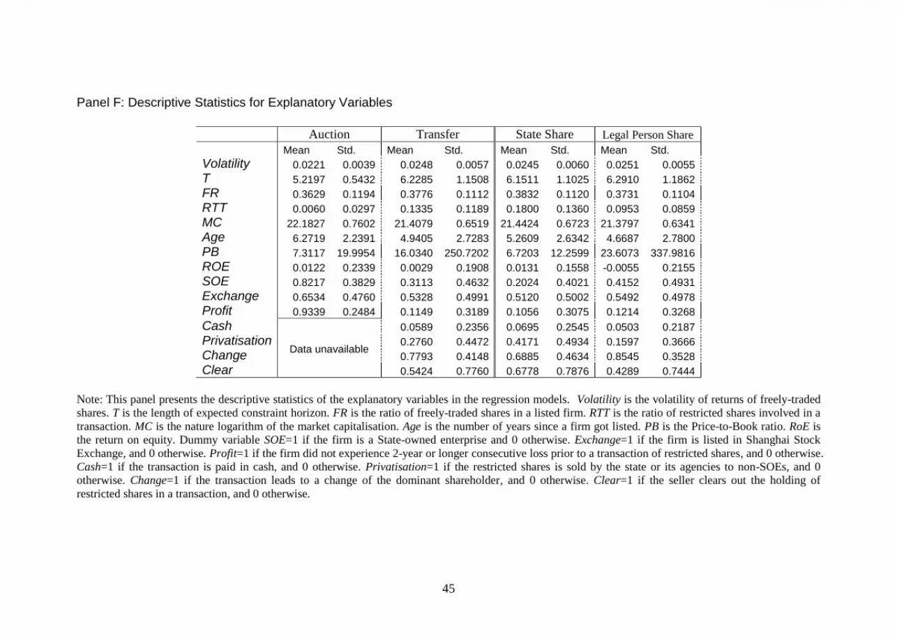
45

Panel F: Descriptive Statistics for Explanatory Variables

Auction Transfer State Share Legal Person Share

Mean Std. Mean Std. Mean Std. Mean Std.

Volatility 0.0221 0.0039 0.0248 0.0057 0.0245 0.0060 0.0251 0.0055

T 5.2197 0.5432 6.2285 1.1508 6.1511 1.1025 6.2910 1.1862

FR 0.3629 0.1194 0.3776 0.1112 0.3832 0.1120 0.3731 0.1104

RTT 0.0060 0.0297 0.1335 0.1189 0.1800 0.1360 0.0953 0.0859

MC 22.1827 0.7602 21.4079 0.6519 21.4424 0.6723 21.3797 0.6341

Age 6.2719 2.2391 4.9405 2.7283 5.2609 2.6342 4.6687 2.7800

PB 7.3117 19.9954 16.0340 250.7202 6.7203 12.2599 23.6073 337.9816

ROE 0.0122 0.2339 0.0029 0.1908 0.0131 0.1558 -0.0055 0.2155

SOE 0.8217 0.3829 0.3113 0.4632 0.2024 0.4021 0.4152 0.4931

Exchange 0.6534 0.4760 0.5328 0.4991 0.5120 0.5002 0.5492 0.4978

Profit 0.9339 0.2484 0.1149 0.3189 0.1056 0.3075 0.1214 0.3268

Cash

Data unavailable

0.0589 0.2356 0.0695 0.2545 0.0503 0.2187

Privatisation 0.2760 0.4472 0.4171 0.4934 0.1597 0.3666

Change 0.7793 0.4148 0.6885 0.4634 0.8545 0.3528

Clear 0.5424 0.7760 0.6778 0.7876 0.4289 0.7444

Note: This panel presents the descriptive statistics of the explanatory variables in the regression models. Volatility is the volatility of returns of freely-traded

shares. T is the length of expected constraint horizon. FR is the ratio of freely-traded shares in a listed firm. RTT is the ratio of restricted shares involved in a

transaction. MC is the nature logarithm of the market capitalisation. Age is the number of years since a firm got listed. PB is the Price-to-Book ratio. RoE is

the return on equity. Dummy variable SOE=1 if the firm is a State-owned enterprise and 0 otherwise. Exchange=1 if the firm is listed in Shanghai Stock

Exchange, and 0 otherwise. Profit=1 if the firm did not experience 2-year or longer consecutive loss prior to a transaction of restricted shares, and 0 otherwise.

Cash=1 if the transaction is paid in cash, and 0 otherwise. Privatisation=1 if the restricted shares is sold by the state or its agencies to non-SOEs, and 0

otherwise. Change=1 if the transaction leads to a change of the dominant shareholder, and 0 otherwise. Clear=1 if the seller clears out the holding of

restricted shares in a transaction, and 0 otherwise.

46

Table 5: Regression Models

Panel A: Illiquidity Discounts

Note: auctionD is the illiquidity discount observed from auctions; sttransferD 1, is the illiquidity discount observed in the provisional announcements of transfers; and sttransferD 1,

is the illiquidity discount observed in the official announcements of transfers. Volatility is the volatility of returns of freely-traded shares. T is the length of expected

constraint horizon. FR is the ratio of freely-traded shares in a listed firm. RTT is the ratio of restricted shares involved in a transaction. MC is the nature logarithm of the

market capitalisation. Age is the number of years since a firm got listed. PB is the Price-to-Book ratio. RoE is the return on equity. Dummy variable SOE=1 if the firm is a

State-owned enterprise, and 0 otherwise. Exchange=1 if the firm is listed in Shanghai Stock Exchange, and 0 otherwise. Profit=1 if the firm did not experience 2-year or

longer consecutive loss prior to a transaction of restricted shares, and 0 otherwise. Cash=1 if the transaction is paid in cash, and 0 otherwise. Privatisation=1 if the restricted

shares is sold by the state or its agencies to non-SOEs, and 0 otherwise. Change=1 if the transaction leads to a change of the dominant shareholder and 0 otherwise. Clear=1

if the seller clears out the holding of restricted shares in a transaction, and 0 otherwise.

47

Panel B: Two Types of Restricted Shares

State Share Legal Person Share

Coef. t Coef. t

Constant -0.0139 -1.83 0.1949 0.86

Conversion 0.0191 0.56 0.1425 4.92

Volatility 0.2981 0.21 -1.4705 -1.65

T -0.0220 -2.40 0.0535 5.68

FR -0.3770 -6.17 -0.2302 -4.53

RTT -0.0116 -0.20 -0.0257 -0.41

MC 0.0255 1.98 0.0172 1.68

Age 0.0043 1.49 -0.0015 -0.79

PB 0.0044 4.00 0.0014 2.78

ROE -0.1058 -1.67 -0.0249 -0.69

SOE -0.0138 -0.86 0.0144 1.42

Exchange 0.0057 0.45 -0.0349 -3.19

Profit 0.0894 3.81 0.1106 7.14

Cash -0.0158 -0.57 -0.0707 -2.86

Privatisation 0.0170 0.51 -0.1625 -6.00

Change -0.0214 -1.61 0.0548 3.95

Clear 0.0191 0.56 0.0033 0.62

2R 0.5055 0.5632

Note: There are two types of restricted shares in China Stock Markets: State Shares and Legal Person Shares. Dummy variable 1Conversion if the type of

the involved restricted shares is converted to another one in a transfer, and 0 otherwise.

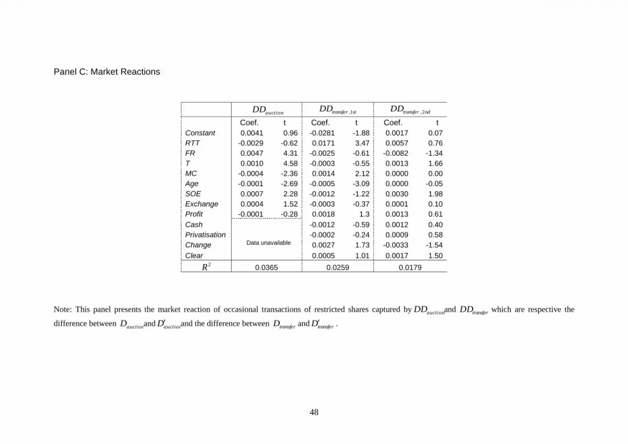
48

Panel C: Market Reactions

auctionDD sttransferDD 1,

ndtransferDD 2,

Coef. t Coef. t Coef. t

Constant 0.0041 0.96 -0.0281 -1.88 0.0017 0.07

RTT -0.0029 -0.62 0.0171 3.47 0.0057 0.76

FR 0.0047 4.31 -0.0025 -0.61 -0.0082 -1.34

T 0.0010 4.58 -0.0003 -0.55 0.0013 1.66

MC -0.0004 -2.36 0.0014 2.12 0.0000 0.00

Age -0.0001 -2.69 -0.0005 -3.09 0.0000 -0.05

SOE 0.0007 2.28 -0.0012 -1.22 0.0030 1.98

Exchange 0.0004 1.52 -0.0003 -0.37 0.0001 0.10

Profit -0.0001 -0.28 0.0018 1.3 0.0013 0.61

Cash

Data unavailable

-0.0012 -0.59 0.0012 0.40

Privatisation -0.0002 -0.24 0.0009 0.58

Change 0.0027 1.73 -0.0033 -1.54

Clear 0.0005 1.01 0.0017 1.50 2R 0.0365 0.0259 0.0179

Note: This panel presents the market reaction of occasional transactions of restricted shares captured by auctionDD and transferDD which are respective the

difference between auctionD and auctionD and the difference between transferD and transferD .

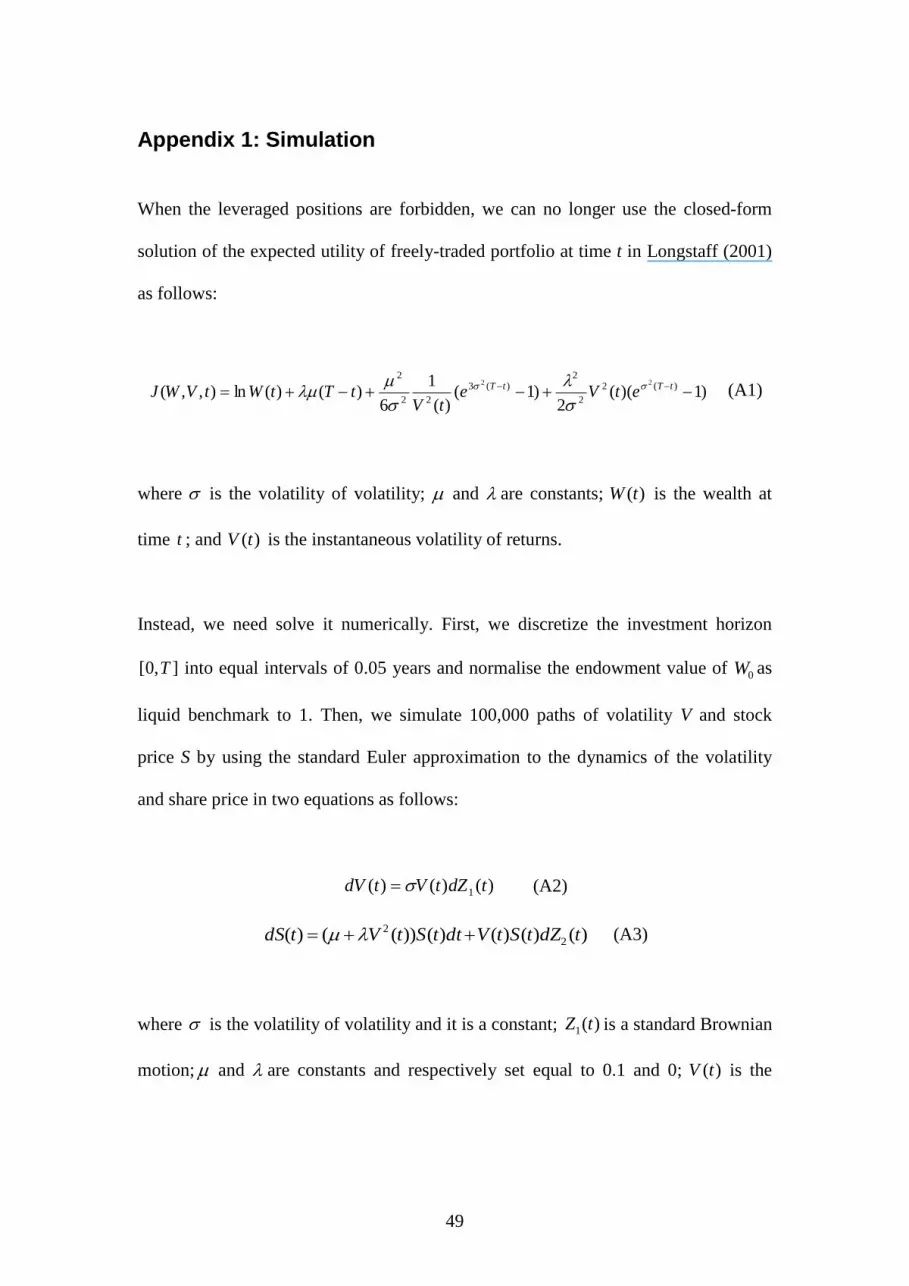
49

Appendix 1: Simulation

When the leveraged positions are forbidden, we can no longer use the closed-form

solution of the expected utility of freely-traded portfolio at time t in Longstaff (2001)

as follows:

)1)((2

)1()(

1

6)()(ln),,( )(2

2

2)(3

22

222

tTtT etVetV

tTtWtVWJ

(A1)

where is the volatility of volatility; and are constants; )(tW is the wealth at

time t ; and )(tV is the instantaneous volatility of returns.

Instead, we need solve it numerically. First, we discretize the investment horizon

],0[ T into equal intervals of 0.05 years and normalise the endowment value of 0W as

liquid benchmark to 1. Then, we simulate 100,000 paths of volatility V and stock

price S by using the standard Euler approximation to the dynamics of the volatility

and share price in two equations as follows:

)()()( 1 tdZtVtdV (A2)

)()()()())(()( 2

2 tdZtStVdttStVtdS (A3)

where is the volatility of volatility and it is a constant; )(1 tZ is a standard Brownian

motion; and are constants and respectively set equal to 0.1 and 0; )(tV is the

50

instantaneous volatility of returns, and )(2 tZ is a standard Brownian motion

independent of )(1 tZ .

By inputting Vt,j along each sample path to Equation (4), the sub-optimal portfolio

weight *

,~

jtw is obtained. Then, we input *

,~

jtw into the dynamics of wealth in Equation

(5) to get the terminal wealth *

,

~jTW . By taking the average of all *

,

~jTW along 100,000

paths, we get the expected terminal wealth of the liquid benchmark under the

borrowing constraint.

100,000

, 0

1

0

ln ( ; )

ln ( ; )100,000

j T T

j

T T

W S w

W S w

(A4)

The terminal wealth for illiquid portfolio );,,,,(*

0wtVSNWJ can be obtained by

following the simulation described in Longstaff (2001). Finally, the illiquidity

discount can be obtained by inputting the terminal wealth of liquid and illiquid

portfolios to Equation (2).

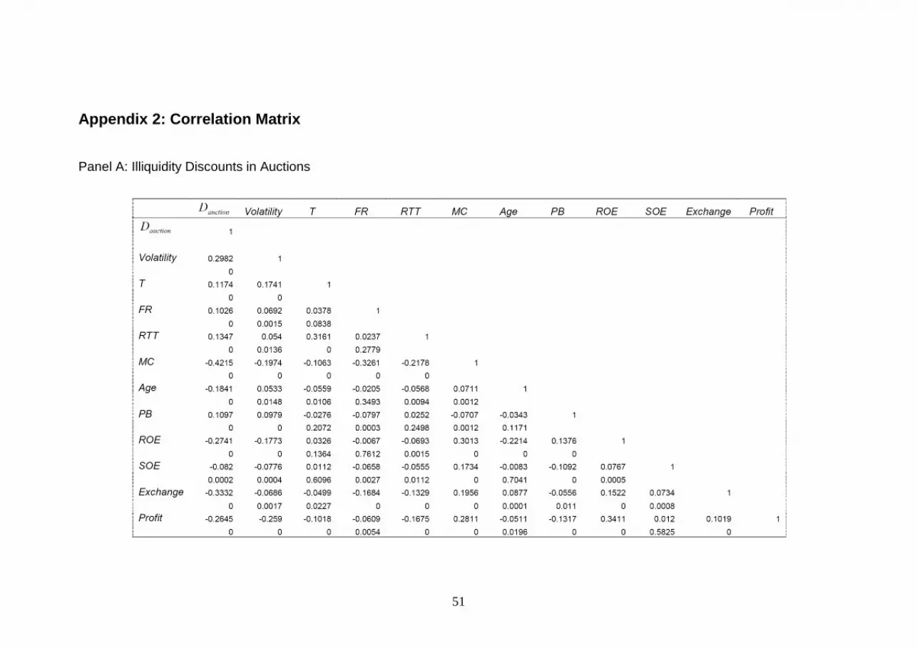
51

Appendix 2: Correlation Matrix

Panel A: Illiquidity Discounts in Auctions

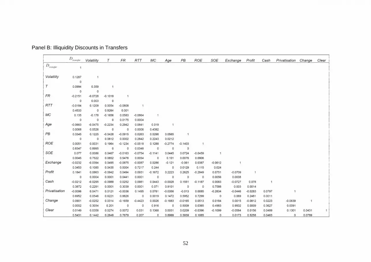
52

Panel B: Illiquidity Discounts in Transfers