an analysis of the amihud illiquidity premium
TRANSCRIPT

Electronic copy available at: http://ssrn.com/abstract=1859632
February 29, 2012
An Analysis of the Amihud Illiquidity Premium
Michael Brennana
Sahn-Wook Huhb
Avanidhar Subrahmanyamc,*
a The Anderson School, University of California at Los Angeles, Los Angeles, CA 90095-1481; King Abdulaziz University, Jeddah, Saudi Arabia; and Manchester Business School, The University of Manchester. E-mail: [email protected]. b School of Management, State University of New York at Buffalo, Buffalo, NY 14260-4000. E-mail: [email protected]. c The Anderson School, University of California at Los Angeles, Los Angeles, CA 90095-1481. E-mail: [email protected]. *Corresponding Author.
We are grateful for the helpful comments of an anonymous referee and of the editor, Maureen
O’Hara. We also thank David Lesmond, Weimin Liu, and Joseph Ogden for helpful suggestions,
and Azi Ben-Rephael for advice on estimating the illiquidity measures used in Ben-Rephael et al.
(2010). Research assistance was ably provided by Mi-Ae Kim and Yue Wang. Brennan
acknowledges financial support from the Catedra de Excelentia of Universidad Carlos III,
Madrid. Huh acknowledges financial support from the School of Management at SUNY-
Buffalo, the Social Sciences and Humanities Research Council of Canada (SSHRC), and the
Ministry of Research and Innovation of Ontario.

Electronic copy available at: http://ssrn.com/abstract=1859632
An Analysis of the Amihud Illiquidity Premium
Abstract
This paper analyzes the Amihud (2002) measure of illiquidity and its role in asset-pricing. It is shown first that the effect of illiquidity on asset pricing is clarified by using the turnover version of the Amihud measure and including firm size as a separate variable. When we decompose the Amihud measure into elements that correspond to positive (up) and negative (down) return days, we find that in general, only the down-day element commands a return premium. Further analysis of the up- and down-day elements using order flows shows that a sidedness variable, which captures the tendency for orders to cluster on the sell side on down days, is associated with a more significant return premium than the other components of the Amihud measure. JEL Classification: G12 Keywords: Illiquidity Premium; Decomposition of the Amihud Illiquidity Measure; Asset Pricing

1
In an important paper, Amihud (2002) develops a measure of stock illiquidity that is easily and
cheaply calculated using daily price and volume data,1 and shows that it is strongly priced in the
cross-section of stock returns. This finding has been confirmed by Chordia, Huh, and
Subrahmanyam (2009) among others. In this paper we decompose the Amihud (2002) measure
into more fundamental components and ask whether these components have differential effects
on stock returns, or whether for pricing purposes they can be combined into a single measure of
illiquidity as assumed by Amihud (2002).
Our analysis is motivated by the recent findings of Brennan et al (2010) who show that,
while the Kyle (1985) framework assumes a symmetric relation between stock price changes and
order flows, asymmetry in this relation plays an important role in determining equilibrium rates
of return. In particular, they find that equilibrium rates of return are sensitive to the relation
between seller-initiated trades and stock price changes, but are not sensitive to the relation
between buyer-initiated trades and stock price changes. Buyer-initiated trades and seller-initiated
trades, and price increases and decreases, are treated symmetrically in the Kyle (1985) and
Amihud (2002) measures of illiquidity. Therefore, given the finding that it is only the price
response to seller-initiated trades that is priced in the cross-section of returns, it is natural to
analyze the Amihud (2002) measure into more fundamental elements that reflect the sign of the
price change and the order flow, and to see whether these elements are also priced differentially.
It is well known that trading volume and price changes are positively correlated.2 As a
result of this correlation we expect the Amihud measure computed using only returns and
volume on positive return days to be different from the same measure calculated using data from
negative return days. The models of Anshuman and Viswanathan (2005), Brunnermeier and
Pedersen (2009), and Garleanu and Pedersen (2007) show that liquidity in down markets may
be very different from liquidity in up markets on account of liquidity shocks, margin-induced
price spirals, and tighter risk management by institutions. Hameed et al. (2010) show empirically
1 The Amihud (2002) measure is the ratio of the absolute return to the dollar volume of trading. Related measures which attempt to capture the relation between the volume of trading and price changes were developed by the Amivest Corporation and reported in their publication Liquidity Ratios since 1972 and by Martin (1975). For a fuller discussion, see Cooper et al. (1985) and Dubovsky and Groth (1984). 2 For a survey of the evidence, see Karpoff (1987). One reason for this may be the disposition effect which causes investors who hold a security to be less willing to sell after a price decline than after a price rise. Odean (1998) shows that stocks with gains are sold by individual investors at twice the rate of stocks with losses. Similar results have been reported by others.

2
that illiquidity in individual stocks as measured by the bid-ask spread of individual stocks
increases following negative returns on the stock and negative returns on the market. Thus there
are both empirical and theoretical reasons to expect that the Amihud and other measures will be
different for positive and negative return days. This raises the issue of whether equilibrium rates
of return are affected differently by liquidity in up markets and in down markets.
The empirical results of Brennan et al. (2010) give us one reason to suspect that
equilibrium expected returns are likely to be more sensitive to estimates of the Amihud measure
that are calculated using only data from negative return days than to estimates that use all the
data. A further reason to expect a difference in the relations between expected rates of return and
measures of illiquidity in up markets and down markets is that leverage constraints may compel
levered investors to sell in down markets, while they are never compelled to buy – for this reason
they are more likely to be concerned about liquidity in the event of a price decline than about
liquidity in the event of a price increase.3 A final reason that investors may be more concerned
about liquidity in down markets is that they may fear the risk of being trapped in an illiquid stock
in a falling market, unable to get out of their position without a major price concession.4 This
would reduce the demand for stocks whose liquidity dries up in down markets. Short sellers may
be similarly fearful of being trapped in a short position in an illiquid stock in a rising market, but
the effect of this would be to reduce the supply of the stock provided by short-sellers, and
therefore to decrease the stock’s expected rate of return. Overall, it seems natural to conjecture
that illiquidity in down markets is more important for asset pricing than illiquidity in up markets.
Our empirical findings can be summarized as follows. First, we confirm the importance
of differences in liquidity between up and down days by showing that, whether we measure
illiquidity by the Amihud measure, by the quoted spread, by market depth, or by a composite
measure that takes account of both depth and spread, there is significantly lower average
liquidity on down days, and this is true for small as well as for large firms. Secondly, we verify
that there is a return premium associated with the original Amihud (2002) measure for
3 Coval and Stafford (2007) show that concentrated selling (or buying) by mutual funds on account of fund outflows (inflows) can cause considerable price impact. 4 Lakonishok et al. (1991) show that pension fund managers like to window-dress their portfolios by selling losing stocks before the end of the reporting period.

3
NYSE/AMEX (henceforth, NYAM) stocks over the period 1971-2009, and for NASDAQ stocks
over the period 1983-2009.
While the Amihud (2002) measure treats the dollar volume of trading (the product of
firm size and turnover) as a measure of trading activity, we argue that it makes sense to estimate
the illiquidity return premium using a measure of illiquidity that relies on turnover as the
measure of trading activity and to account separately for firm size effects.5 Strictly speaking, if
firm size is included as a separate regressor, then it is not possible to distinguish between models
that include firm size in the measure of illiquidity as the Amihud (2002) measure does and those
that do not include it. However, we find that for NYAM stocks the Amihud (2002) measure of
illiquidity does not account for the whole of the effect of firm size on returns: indeed, when firm
size is included as a separate variable along with the original Amihud measure, the coefficient of
firm size is positive for NYAM stocks (and insignificant for NASDAQ stocks), implying that
investors require lower rates of return on small firms, holding liquidity constant. Since no one
has suggested a reason why small firms should have lower rates of return, we prefer to rely on
the turnover version of the Amihud measure.
Our major finding is that when the (turnover-version) Amihud (2002) measure is
decomposed into elements that correspond to positive and negative return days (up days and
down days), which we term “half-Amihud” measures, the half-Amihud measure associated with
down days is strongly priced in the cross-section of stock returns, while the coefficient of the
half-Amihud measure that corresponds to up days is small and statistically insignificant. Thus,
while Brennan et al. (2010) find that it is the element of the Kyle (1985) measure that is
associated with seller-initiated trades which commands a return premium, we find that it is the
element of the Amihud (2002) measure that is associated with down days that commands a return
premium. The significant down-day effect is apparent for both NYAM and NASDAQ samples.
When the component stocks are divided into three sub-samples according to market value, we
find that the half-Amihud measure for down days is strongly priced for all three size groups of
NYAM stocks, while the half-Amihud measure for up days is either not significantly priced or
has a negative premium associated with it (for the large-size group). For NASDAQ stocks, the
5 As Cochrane (2005) points out, the Amihud measure imposes an automatic scaling of illiquidity with firm size, so that ‘smaller stocks which have smaller dollar volume for the same turnover (fraction of outstanding shares that trade) are automatically more illiquid.’ See Florakis et al. (2011) for a similar argument.

4
half-Amihud measure for down days is significantly priced only for the stocks in the lowest third
by market value, although the coefficient is positive for all three groups. The coefficient of the
half-Amihud measure for up days is insignificant and much smaller than that for down days for
the small-size group. For the mid-size group the coefficient is positive and insignificant, and for
the large-size group it is positive but not significant.
In order to determine whether buyer and seller initiated trading volume have different
roles in the liquidity measure, we classify individual transactions into buyer-initiated and seller-
initiated trades. Then each of the two half-Amihud measures is further analyzed into a
“directional half-Amihud” measure and a term that captures the fraction of turnover that is
buyer-initiated (on up days) or seller-initiated (on down days), which, extending Sarkar and
Schwartz (2009),6 we term “up-sidedness” and “down-sidedness,” respectively. The directional
half-Amihud measure for up (down) days is obtained by dividing the absolute return for up
(down) days by the buyer (seller)-initiated turnover for those days. It is a measure of how much
the price moves in response to trading pressure on one side of the market. The sidedness
measures, on the other hand, capture the tendency of trades to cluster on one side of the market
or the other on up and down days.
When we regress returns on these four components of illiquidity, we find that the
coefficient of the directional half-Amihud measure for down days is positive and highly
significant, but the coefficient of the corresponding measure for up days is small and statistically
insignificant. This is consistent with our earlier results for the simple half-Amihud measures: it is
the down day element that is priced. Furthermore, while the magnitude of the coefficients of up-
sidedness and down-sidedness are similar, only the coefficient of down-sidedness is significant
in general.
We also attempt to decompose each of the two half-Amihud measures into a “half-Kyle”
measure and a term that depends on the net turnover ratio. For the half-Kyle measures, the return
for up and down days is divided by the net buyer- and seller-initiated turnover, respectively. We
refer to these as half-Kyle measures because the Kyle (1985) lambda is equal to the return
divided by the net order flow. We find, however, that decomposing the half-Amihud measures in
6 Sarkar and Schwartz (2009) interpret a high correlation between buyer-initiated and seller-initiated trades within brief time intervals as an indication of two-sidedness which indicates heterogeneity of information, while a low correlation is indicative of one-sidedness and information asymmetry. They find that market sidedness is associated with order imbalances.

5
this way is not feasible for our analyses, because negative values make it impossible to calculate
log-transforms for too many observations.
The remainder of the paper is organized as follows. In Section I, we decompose the
Amihud (2002) measure into elements that depend, first on firm size and the sign of the return,
and then into elements that depend also on the sign of trading volume. Section II discusses data
sources, variable definitions, and descriptive statistics. Section III describes the estimation
procedures. Section IV verifies the results of Amihud (2002), and investigates in detail which
components of the Amihud measure are priced in the cross-section of stock returns. In Section V,
we examine the robustness of our empirical findings. Section VI concludes.
I. Analyzing the Amihud (2002) Measure of Illiquidity
A. Basic Analysis
We denote the original Amihud (2002) measure, which is constructed using the dollar volume of
trading, by Ao. It is defined as the average of the daily values of:7
,DVOL
rAo = (1)
where r is a daily stock return, and DVOL is daily dollar volume. Since dollar volume is the
product of firm size (market value of equity) and share turnover, the relative importance for asset
pricing of turnover and firm size is unclear when only Ao is included in the regression. Therefore,
we start by decomposing the Amihud (2002) measure into its turnover version and a size-related
element as follows:
=
===
SA
STr
DVOLT
Tr
DVOLr
Ao 11 (2)
7 For simplicity, we use the same notations for both daily and monthly (averaged) variables.
6
( )
( )
≤
=
−
≥
=
=
−−
++
.0if,11
0if,11
rS
AST
r
rS
AST
r
(3)
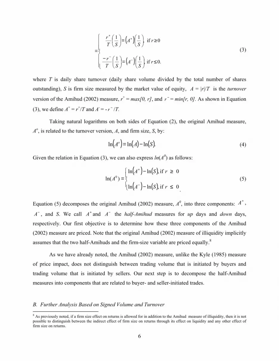
where T is daily share turnover (daily share volume divided by the total number of shares
outstanding), S is firm size measured by the market value of equity, A = |r|/T is the turnover
version of the Amihud (2002) measure, r+ = max[0, r], and −r = min[r, 0]. As shown in Equation
(3), we define A+ = r+/T and A- = - −r /T.
Taking natural logarithms on both sides of Equation (2), the original Amihud measure,
Ao, is related to the turnover version, A, and firm size, S, by:
( ) ( ) ( ).lnlnln SAAo −= (4)
Given the relation in Equation (3), we can also express ln(A0) as follows:
( ) ( )
( ) ( )
≤−
≥−=
−
+
0 if ,lnln
0 if ,lnln)ln( 0
r SA
r SAA
.
(5)
Equation (5) decomposes the original Amihud (2002) measure, A0, into three components: +A ,
−A , and S. We call +A and −A the half-Amihud measures for up days and down days,
respectively. Our first objective is to determine how these three components of the Amihud
(2002) measure are priced. Note that the original Amihud (2002) measure of illiquidity implicitly
assumes that the two half-Amihuds and the firm-size variable are priced equally.8
As we have already noted, the Amihud (2002) measure, unlike the Kyle (1985) measure
of price impact, does not distinguish between trading volume that is initiated by buyers and
trading volume that is initiated by sellers. Our next step is to decompose the half-Amihud
measures into components that are related to buyer- and seller-initiated trades.
B. Further Analysis Based on Signed Volume and Turnover 8 As previously noted, if a firm size effect on returns is allowed for in addition to the Amihud measure of illiquidity, then it is not possible to distinguish between the indirect effect of firm size on returns through its effect on liquidity and any other effect of firm size on returns.

7
If we distinguish between buyer-initiated trades and seller-initiated trades, then daily share
turnover (T) can be separated into buyer-initiated turnover (TB) and seller-initiated turnover (TS):
T = TB + TS. Then, using the signed turnover, we can further decompose the two half-Amihud
measures (A+ and A-) defined in Equation (5) as follows:
0for,
0for,
≤
−=−=
≥
==
−−−
+++
rTT
Tr
TrA
rTT
Tr
TrA
S
S
B
B (6)
Taking natural logarithms on both sides of Equation (6), we have:
),ln()ln(lnlnln)ln(
)ln()ln(lnlnln)ln(
21
21
−−−−
−
++++
+
+≡
+
−=
−=
+≡
+
=
=
AATT
Tr
TrA
AATT
Tr
TrA
S
S
B
B (7)
where BT
rA+
+ ≡1 is the directional half-Amihud for up days andSTrA
−− −≡1 is the directional half-
Amihud for down days. The first directional half-Amihud is defined as the return divided by the
buyer-initiated turnover for up days and the second directional half-Amihud is defined
analogously for down days. The two sidedness components, TT
A B≡+2 and
TT
A S≡−2 , are the
proportions of trading volume or turnover that are attributable to buyer- and seller-initiated
trades on up and down days, respectively. We refer to them as the up-sidedness and down-
sidedness components, respectively.
The sidedness components for up and down days ( and ) are closely related to the
Sarkar and Schwartz’ (2009) measure of market (one-)sidedness which captures the tendency of
orders to cluster on the buy side or the sell side. Thus, our up-sidedness (down-sidedness)
measure captures the tendency of orders to cluster on up days (down days) and, as Sarkar and
Schwartz (2009) suggest, provides a measure of information asymmetry on those days.

8
An alternative decomposition of the half-Amihud measures is suggested by the Kyle
(1985) lambda, which depends on the ratio of price changes to net buyer- or sell-initiated trading
volume. Specifically, we can rewrite each of the two half-Amihud measures as:
0for,)
0for,
≤
−
−
−=−=
≥
−
−
==
−−−
+++
rT
TTTT
rTrA
rT
TTTT
rTrA
BS
BS
SB
SB (8)
Taking logarithms on both sides of Equation (8), we have
).ln()ln()
lnln)ln(
)ln()ln(lnln)ln(
21
21
−−−
−
+++
+
+=
−+
−
−=
+=
−+
−
=
KKT
TTTT
rA
KKT
TTTT
rA
BS
BS
SB
SB (9)
We refer to SB TT
rK−
=+
+1 and
BS TTrK−
−=−
−1 in Equations (8) and (9) as the half-Kyle for up
days and the half-Kyle for down days, respectively, since both measures divide the daily return
by that day’s net buyer- or seller-initiated turnover. The two net turnover ratios, T
TTK SB −
=+2
and T
TTK BS −
=−2 , are proportional net buyer-initiated turnover on up days and proportional net
seller-initiated turnover on down days, respectively; like the sidedness measures, they capture the
tendency of orders to cluster on the buy (sell) side on up (down) days.
Figure 1 summarizes the relations between the various decompositions of the Amihud
(2002) measure described above. We will estimate monthly Fama and MacBeth (1973)-type
cross-sectional regressions to investigate which components of the Amihud (2002) measure
shown in Figure 1 are most important for asset pricing. Following Amihud (2002), we obtain the
monthly variables by averaging the daily values of the Amihud (2002) measure and its
components within each month. As shown above, the log-transformation allows us to decompose

9
the Amihud (2002) measure in a simple additive fashion. Moreover, the transformation (at the
monthly level) reduces the influence of extreme observations in our empirical analyses.9
II. Data and Variable Construction
Our primary data are taken from CRSP for NYAM-listed stocks over the 462 months from July
1971 to December 2009 and for NASDAQ-listed stocks over the 324 months from January 1983
to December 2009 at daily and monthly frequencies. For more detailed decomposition of the
Amihud measure, we also use transaction-level data from the Institute for the Study of Securities
Markets (ISSM) and the NYSE Trades and Automated Quotations (TAQ) over the 324 months
from January 1983 to December 2009 (for NYAM stocks only).
To survive in the CRSP sample in a given month, stocks must have no more than five
zero-volume days within the month for NYAM stocks, or must have at least 50 trades within the
month for NASDAQ stocks.10 In addition, for the availability of the risk-adjusted return, Re2,
which is described in Section III below, stocks must have at least 24 monthly returns in the past
60 months. Only common stocks (share code 10 or 11 in CRSP) are used. When we process
transaction-level data, for consistency with the above filtering, stocks must have at least 50
trades per month (on average 2.5 trades per day) for each firm in the ISSM/TAQ databases.
Since trading protocols have differed between NYAM and NASDAQ, trading volume is
not comparable between the markets and this affects the computation of the Amihud measure.
Therefore we treat the NYAM and NASDAQ stocks separately in our analysis.
A. The Amihud (2002) Measure and its Components
The original Amihud (2002) measure (A0), its basic components (A, A+, −A , and S), daily stock
returns, daily CRSP value-weighted market returns, and the number of shares outstanding are
obtained from the CRSP daily file. The daily turnover ratio, T, is computed using CRSP as well 9 To reduce the influence of extreme observations, Hasbrouck (1999, 2005, and 2009) and Chordia, Huh, and Subrahmanyam (2009) apply a square-root transformation to illiquidity measures, while others prefer a logarithmic transformation. 10 In the CRSP database, the information about the number of trades is available for NASDAQ stocks only, which is why we cannot apply the same filter to NYAM stocks.

10
as ISSM/TAQ.11 The buyer- and seller-initiated turnover ratios, TB and TS, are computed using
ISSM/TAQ.
To calculate the sub-components ( +1A , +
2A , −1A , and −
2A ) that depend on the direction of
trades, we take intraday transaction data from ISSM/TAQ. For this purpose, each trade is
classified into a buyer- or seller-initiated trade according to the Lee and Ready (1991) algorithm
using trades and quotes data from ISSM for 1983-1992 and from TAQ for 1993-2009. To obtain
signed volume (order flow), we focus on NYAM stocks because the availability of transaction-
level data on NASDAQ-listed stocks is limited to us and the NASDAQ market has different
trading protocols (Atkins and Dyl, 1997). Trades and quotes that are out of sequence, recorded
before the open or after the close, or involved in errors or corrections, are expunged.
To match trades and quotes using the Lee and Ready (1991) algorithm, any quote less
than five seconds prior to the trade is ignored and the first one at least five seconds prior to the
trade is retained for the years from 1983 to 1998. Based on reports from microstructure scholars
that timing differences in recording trades and quotes have declined dramatically in recent years,
we do not impose this five-second-delay rule for the last 11 years of the sample. Instead, the
quote that is closest in time to the transaction, with a time stamp of two seconds or more before
the transaction, is retained for the years from 1999 to 2009. The transactions data are then signed
as follows. If a trade occurs above (below) the prevailing quote mid-point, it is regarded as
buyer-initiated (seller-initiated). To minimize possible signing errors in processing order flows,
if a trade occurs exactly at the quote mid-point, we discard the trade, following Sadka (2006).
Approximately 5% of the trades from the intradaily databases transact at the quote mid-points.12
Although the algorithm is imperfect, Lee and Radhakrishna (2000) and Odders-White (2000)
show that it is quite accurate, and errors arising from the signing algorithm will only make it
harder to distinguish buy and sell transactions, thus making it more difficult to detect differences
between the effects of the different components of the Amihud measure on asset returns.
11 When necessary, we will distinguish the turnover ratio computed using the ISSM/TAQ databases (denoted by T*) from T, which is the turnover ratio computed using CRSP. 12 For example, 5.3% of the total trades in 2002 occur exactly at the quote mid-points. When a trade occurs exactly at the quote mid-point, we also try to classify the trade using an alternative method called a tick test. That is, if a trade occurs at the quote mid-point, it is signed using the previous transaction price: buyer-initiated if the sign of the last non-zero price change is positive, and vice versa. This method does not change our main results.

11
Denote the total number of shares outstanding by #SHARE, aggregate daily buyer-
initiated trades in shares by SBUY, and aggregate daily seller-initiated trades in shares by SSELL,
and define SVOL* = SBUY + SSELL. Also define: total share turnover T*SHARESVOL
#∗= , buyer-initiated
turnover TB SHARESBUY
#= , and seller-initiated turnover TS SHARESSELL
#= . Then T* = TB + TS. Note that for
the finer decomposition as well as for robustness tests we use ISSM/TAQ-based turnover, T*,
which is slightly different from usual CRSP-based turnover, T. Similarly, CRSP-based share
volume, SVOL, is slightly different from ISSM/TAQ-based share volume, SVOL* (= SBUY +
SSELL), because when intradaily trades are processed, not all trades are classified into the two
categories. Moreover, when intradaily trades are classified, other filters are applied (e.g., trades
and quotes are discarded if they are out of time sequence, recorded before the opening or after
the close, or involved in errors or corrections). Therefore, usually SVOL > SVOL* (= SBUY +
SSELL), and T ( SHARESVOL
#= ) > T* ( SHARE
SVOL#
∗= ).
Table 1 reports descriptive statistics for the above variables. The Amihud (2002)
measure, A0, and its components shown in Panels A and D are constructed and defined as
follows:
A0: the original Amihud (2002) measure, which is the monthly average of daily |r|/DVOL,
where r is a daily stock return and DVOL is daily dollar volume (in $1,000).
A: the turnover version of the Amihud (2002) measure, which is the monthly average of
daily |r|/T, where T is CRSP-based daily share turnover [(daily share volume (SVOL) divided by
the total number of shares outstanding (#SHARE)]. Instead of T, ISSM/TAQ-based turnover,
T*SHARESVOL
#∗= , is also used for robustness tests.
A+ ( −A ): the half-Amihud measure for up days (down days), which is the monthly average of
daily r+/T (r-/T), where r+ = max[0, r], r- = min[0, r], and T is CRSP-based daily share
turnover. Instead of T, ISSM/TAQ-based turnover, T*, is also used for robustness tests.
A+,m ( mA ,− ): the half-Amihud measure for up-market days (down-market days). The measures
are defined by the averages of daily |r|/T over the days with positive (negative) CRSP value-
weighted market returns within a month.

12
+1A )( 1
−A : the directional half-Amihud measure for up days (down days), which is the
monthly average of daily r+/TB (-r-/TS), where TB (TS ) is ISSM/TAQ-based daily buyer-
initiated turnover (seller-initiated turnover), which is in turn defined as buyer-initiated share
volume (seller-initiated share volume) divided by the total number of shares outstanding (i.e., TB
= SHARESBUY
# , TS = SHARESSELL
# ).
+2A ( −
2A ): the sidedness component for up days (down days), which is the proportion of
turnover that is attributable to buyer-initiated trades on up days (seller-initiated trades on down
days): +2A = TB/T* and −
2A = TS/T*.
S: the average of daily market values within a month (in $1,000).
B. Other Variables
Firm characteristics that are used as control variables in the asset pricing regressions are defined
as follows:
BTM: the Winsorized value (each month at the 0.5th and 99.5th percentiles) of the book-to-
market ratio (= BV/MV), where the book value (BV) is common equity and the market value
(MV) is the previous month-end stock price times the number of shares outstanding. In the spirit
of Fama and French (1992), the quarterly book-to-market ratio is lagged two quarters. The
monthly series is constructed by assigning the same value to all months in a given quarter.
MOM1, MOM2, MOM3, and MOM4: the compounded holding period returns of a stock over
the most recent three months (from month t-3 to month t-1), from month t-6 to month t-4, from
month t-9 to month t-7, and from month t-12 to month t-10, respectively. For each of the four
momentum variables to exist, a stock must have all three monthly returns over the corresponding
three-month period.
Monthly stock prices, returns, and the number of shares outstanding are available from
the CRSP monthly file, and the book value is from the CRSP/Compustat Merged (quarterly) file.
The Fama-French (FF, 1993) factors are available from Kenneth French's website.

13
Panels A and D of Table 1 reports time-series average values of monthly means, medians,
standard deviations, and other descriptive statistics for the original Amihud (2002) measure, A0,
and its components. The cross-sectional value for each of the five statistics is calculated each
month and the time-series average of those values is reported. The average number of sample
firms used each month is 1,758.6 (a minimum of 1,447 and a maximum of 2,170) for NYAM
stocks and 2,166.1 (a minimum of 148 and a maximum of 3,376) for NASDAQ stocks. The
average size (S) of the NYAM (NASDAQ) sample firms is $2.67 ($0.59) billion over the sample
period. Most of the variables in Panels A and D are highly leptokurtic as well as significantly
skewed (mostly to the left). The large kurtoses imply that the sample distributions of the
variables contain a significant number of extreme observations.
To reduce the influence of extreme observations in the empirical analyses and to permit a
simple additive decomposition of the Amihud measure, we apply a logarithmic transformation
[denoted by ln(.)] to all of the A-associated variables reported in Panels A and D. Statistics for
the transformed variables are shown in Panels B and E. The log-transformation decreases the
skewness and kurtosis of the variables substantially. After the log-transformation, both of the
illiquidity components for down days [ln(A-) and ln( −1A )] are larger than the corresponding
components for up days [ln(A+) and ln( +1A )] for both samples (where applicable). This implies
that the average price change per unit of turnover is greater on down days, and the average price
change per unit of sell volume on down days is greater than the average price change per unit of
buy volume on up days. On the other hand, the average and median up-sidedness component is
greater than average and median down-sidedness component: on average 56% of turnover on up
days is classified as buyer-initiated, and 44% of turnover on down days is classified as seller
initiated.
To investigate further the differences between liquidity on up and down days, we
calculate each month three (il)liquidity measures for up days and down days separately: (i)
proportional quoted spread in % (%QSPR); (ii) dollar depth in $1,000 (DDepth); and (iii)
composite illiquidity (ComposIlliq),13 which is calculated following Chordia, Roll, and
Subrahmanyam (2001). The data for these calculations are taken from the ISSM/TAQ databases.
To test the null hypothesis that the differences between the two mean values are equal to zero,
13 For more detailed information about the definitions and data, see the note to Table A1 in the appendix.
14
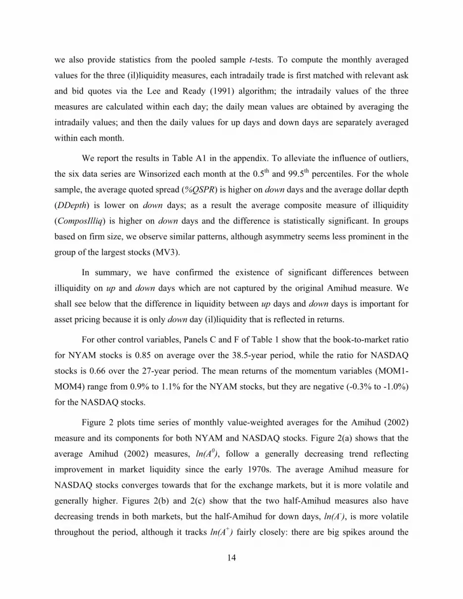
we also provide statistics from the pooled sample t-tests. To compute the monthly averaged
values for the three (il)liquidity measures, each intradaily trade is first matched with relevant ask
and bid quotes via the Lee and Ready (1991) algorithm; the intradaily values of the three
measures are calculated within each day; the daily mean values are obtained by averaging the
intradaily values; and then the daily values for up days and down days are separately averaged
within each month.
We report the results in Table A1 in the appendix. To alleviate the influence of outliers,
the six data series are Winsorized each month at the 0.5th and 99.5th percentiles. For the whole
sample, the average quoted spread (%QSPR) is higher on down days and the average dollar depth
(DDepth) is lower on down days; as a result the average composite measure of illiquidity
(ComposIlliq) is higher on down days and the difference is statistically significant. In groups
based on firm size, we observe similar patterns, although asymmetry seems less prominent in the
group of the largest stocks (MV3).
In summary, we have confirmed the existence of significant differences between
illiquidity on up and down days which are not captured by the original Amihud measure. We
shall see below that the difference in liquidity between up days and down days is important for
asset pricing because it is only down day (il)liquidity that is reflected in returns.
For other control variables, Panels C and F of Table 1 show that the book-to-market ratio
for NYAM stocks is 0.85 on average over the 38.5-year period, while the ratio for NASDAQ
stocks is 0.66 over the 27-year period. The mean returns of the momentum variables (MOM1-
MOM4) range from 0.9% to 1.1% for the NYAM stocks, but they are negative (-0.3% to -1.0%)
for the NASDAQ stocks.
Figure 2 plots time series of monthly value-weighted averages for the Amihud (2002)
measure and its components for both NYAM and NASDAQ stocks. Figure 2(a) shows that the
average Amihud (2002) measures, ln(A0), follow a generally decreasing trend reflecting
improvement in market liquidity since the early 1970s. The average Amihud measure for
NASDAQ stocks converges towards that for the exchange markets, but it is more volatile and
generally higher. Figures 2(b) and 2(c) show that the two half-Amihud measures also have
decreasing trends in both markets, but the half-Amihud for down days, ln(A-), is more volatile
throughout the period, although it tracks ln(A+) fairly closely: there are big spikes around the

15
months of the 1987 stock market crash and the recent financial crisis. Figure 2(d) shows that
most of the variation in the Amihud measure is attributable to variation in the directional half-
Amihud measures rather than the sidedness measures. The directional half-Amihud measure for
down days, ln( −1A ), is larger and more volatile than that for up days, ln( +
1A ). The down-
sidedness component, ln( −2A ), tends to be smaller than the up-sidedness component, ln( +
2A ),
until mid-2007 when the measures converge. We do not show plots for the equal-weighted
averages, but they are comparable to those of the value-weighted series. As one would expect,
however, the levels of the equal-weighted series are much higher (and more volatile).
Table 2 reports average correlations between the key variables. The lower triangle in the
table contains the correlation coefficients for NYAM stocks, while the upper triangle does the
same for NASDAQ stocks. The correlation between the Amihud (2002) measure, Ao, and its log-
transform, ln(Ao), is only around 0.35, reflecting the extreme skewness of the untransformed
measure. More importantly, the correlation between ln(Ao) and the turnover version, ln(A), is
0.80 (0.87) while the correlation between ln(Ao) and ln(S) is -0.94 (-0.88) for the two sets of
stocks, confirming the important role of firm size in the original Amihud measure of illiquidity.
The turnover-version Amihud measure, ln(A), has a slightly higher correlation with the
half-Amihud measure for down days (0.95) than for up days (0.94). Decomposition of the half-
Amihud measures is possible only for the NYAM stocks for which tick data are available to us.
The correlations show that the major determinants of the half-Amihud measures are the
corresponding directional half-Amihud measures: the correlation between these measures is 0.90
for up days [ln(A+) and ln( +1A )] and 0.88 for down days [ln(A-) and ln( −
1A )]. In contrast, the
correlations of the half-Amihud measures with the corresponding sidedness components are -
0.12 and 0.20. Similarly, there is little correlation between the directional half-Amihud measure
and the corresponding sidedness measure: -0.26 for up days and 0.07 for down days. Note that
the up-sidedness measure, ln( +2A ), is strongly negatively correlated (-0.95) with the down-
sidedness measure, ln( −2A ). Therefore, if in a given month selling in a stock is a high proportion
of turnover on down days which implies a high down-sidedness measure, then there is also a
tendency for selling to be a high proportion of turnover on up days which means a low up-
sidedness measure: thus the negative correlation is driven by the pervasiveness of buying or
selling in a stock in a given month.

16
The Amihud, half-Amihud, and directional half-Amihud measures all have negative
correlations (about -0.10) with the momentum variables (MOM1-MOM4) for both markets, so
that higher momentum is associated with reduced illiquidity or improved liquidity.14 As we see
in the lower triangle, however, up-sidedness, ln( +2A ), is slightly positively correlated with
momentum, while down-sidedness, ln( −2A ), is slightly negatively correlated with it: this is
consistent with a tendency for buy orders to be high relative to sell orders after a price increase.
III. Estimation Procedure
To determine which components of the Amihud (2002) measure play an important role in asset
pricing, we follow the Brennan, Chordia, and Subrahmanyam (BCS, 1998) approach which uses
individual stock data. This avoids the data-snooping biases inherent in portfolio-based
approaches15 and also eliminates any bias caused by errors in estimating the Fama-French (FF,
1993) factor loadings. Ang, Liu, and Schwarz (2008) also argue that using individual stocks
provides more efficient tests of whether factors are priced.
The dependent variable in the estimation is defined as the return adjusted for the three
Fama-French (1993) factors (FF3: MKTt, SMBt, and HMLt).16 Let jR~ and FR denote the monthly
return for stock j and the risk-free rate, respectively. We estimate the FF3 factor loadings in two
ways yielding two different estimates of the FF3-adjusted returns. First, we use the entire sample
period, denoting the resulting FF3-adjusted excess return by 1ejtR . Secondly, for each month we
use rolling estimates of the factor loadings ( jβ ) that are estimated using the time series of the
past 60 months (at least 24 months). We denote the corresponding estimate of the FF3-adjusted
return by 2ejtR . The FF3-adjusted return, eh
jtR (h = 1, 2), for stock j in each month t is calculated
as the sum of the intercept and the residual from time-series regressions in which the dependent
variable is the stock return in excess of the one-month T-bill rate. Then the FF3-adjusted returns
may be written as: 14 See Lee and Swaminathan (2000). 15 See Roll (1977) and Lo and MacKinlay (1990). 16 For details, see Brennan, Chordia, and Subrahmanyam (1998) and Chordia, Huh, and Subrahmanyam (2009).

17
.2or 1 ),ˆˆˆ()~( 321 =++−−≡ hHMLSMBMKTRRR tjtjtjFtjtehjt βββ (10)
One of the two sets of FF3-adjusted returns is then used as the dependent variable in the
following Fama-Macbeth (1973) cross-sectional regressions:
,11
0 jtlnjtn
N
nlijti
M
i
ehjt eZccR ++Λ+= −
=−
=∑∑φ h = 1 or 2, (11)
where ijtΛ (i = 1,2,...,M) are the M components of the Amihud (2002) measure for stock j in
month t, as discussed in Sections I and II, Znjt (n = 1,…, N) are control variables for firm j in
month t, and l is the number of months by which the explanatory variables are lagged. We
control for firm characteristics such as book-to-market equity (BTM) and past returns (MOM1-
MOM4) since, according to Avramov and Chordia (2006), a constant-beta version of the Fama
and French (1993) three-factor model cannot adequately capture the predictive ability of firm
characteristics in stock returns. Following Brennan, Chordia, and Subrahmanyam (1998), we lag
the explanatory variables by two months.
We report statistics for regressions with three different dependent variables: (i) the
unadjusted excess returns, ejtR ; (ii) the FF3-adjusted excess return using the first method, 1e
jtR ;
and (iii) the FF3-adjusted excess return using the second method, 2ejtR . Following Fama and
MacBeth (1973), we estimate the vector of coefficients [ ]′= NM ccccc ...... 21210 φφφ in Equation
(11) each month by ordinary least-squares regressions, and the final estimator is the time-series
average of the monthly coefficients. The standard error of this estimator is taken from the time
series of the monthly coefficient estimates.
Asparouhova, Bessembinder, and Kalcheva (2010) propose that weighted least-squares
(WLS) regressions can alleviate biases in estimation that are caused by the well known bid-ask
bounce. Therefore, as a robustness check we also estimate WLS regressions using the prior-
month gross return as a weighting variable.
IV. Priced Components of the Amihud (2002) Measure
A. The Amihud (2002) Measure

18
We first verify that there is a return premium associated with the log-transformed original
Amihud (2002) measure, ln(Ao). We estimate Equation (11) including only ln(Ao) and control
variables using monthly individual stock data for the period from July 1971 to December 2009
for NYAM-listed stocks and from January 1983 to December 2009 for NASDAQ-listed stocks.
The results for the two samples are reported in Panels A and B of Table 3. For
expositional convenience, regression coefficients are multiplied by 100 throughout the tables.
The average number of stocks in the cross-sectional regressions ranges from 1,597.0 to 1,757.8
for NYAM stocks and from 2,003.3 to 2,166.1 for NASDAQ stocks, depending on the method of
FF3-adjustment and whether control variables are included or not.17 When the dependent
variable is the FF3-adjusted return, the average adjusted R-squared (Avg R-sqr) for both samples
is 0.8% without control variables, rising to 2.1-3.0% when the control variables are included.
As can be seen in Panel A for NYAM stocks, the coefficient of the Amihud (2002)
measure, ln(Ao), is positive and highly significant in all of the regressions, and is little affected
by whether or not the return is FF3-adjusted and by whether or not the control variables are
included in the regressions. Using the standard deviation of the Amihud measure reported in
Table 1, the estimated coefficient implies that a one standard deviation change in the log-
transformed Amihud measure (in Specification 2a with Re1) will change expected (excess)
returns on a security by (2.74 x 0.13 =) 0.36% per month or 4.27% per year. This is puzzlingly
high, considering that the average monthly (raw) return reported by Chordia, Huh, and
Subrahmanyam (2007) is 1.19% for an average of 1,647 NYAM-listed stocks over the past 40
years. The effect is even stronger for NASDAQ stocks, as shown in Panel B: in the
corresponding specification (2b) with Re1, a one standard deviation increase in the log-
transformed Amihud measure will lead to higher expected (excess) returns of 0.56% per month
or 6.75% per year. The coefficient of the Amihud measure for NASDAQ stocks in Panel B is
approximately 50% higher than the corresponding coefficient for NYAM stocks shown in Panel
A. As we shall see below, this discrepancy is removed when we employ the turnover version of
the measure and treat firm size as a separate variable. 17 While the average number of stocks used each month is 1,757.8 over the sample period in Specification 1a with Re2 in Panel A (NYAM stocks), for example, the number of stocks used in a month varies month by month: the minimum number is 1,447 and the maximum number is 2,170 in this case. In the corresponding specification (1b) in Panel B (NASDAQ stocks), the minimum is 148 (in March 1983) while the maximum is 3,376.

19
The three past returns (MOM1-MOM3) are strongly positively related to current month
returns for NYAM stocks; the effect is somewhat weaker for NASDAQ stocks. The book-to-
market (BTM) effect for NYAM stocks becomes insignificant when returns are risk-adjusted
using rolling estimates of the factor loadings. In contrast, Panel B shows that the BTM effect
remains strong for NASDAQ stocks even after the FF3-adjustments.
B. Decomposing the Amihud (2002) Measure
We decompose the Amihud (2002) measure, ln(Ao), into its turnover version, ln(A), and
firm size, ln(S), including them as separate regressors:
.)ln()ln( 2
5
122210 jtnjtn
njtjtjt eZcSAcY ++++= −
=−− ∑φφ (12)
The estimates of Equation (12) are reported in Panels A and B of Table 4. The turnover-
version Amihud measure, ln(A), has a highly significant positive effect on returns in both NYAM
and NASDAQ samples. Moreover, in contrast to the results in Table 3, where the coefficient of
ln(A0) was around 50% higher for the NASDAQ sample, now the coefficient is of similar
magnitude in the two samples. The coefficients of the size component, ln(S), are negative and
statistically significant in every case. However, while the original Amihud (2002) measure
constrains the coefficients of ln(A) and ln(S) to be equal and of the opposite sign, we find that for
the NYAM sample the absolute value of the coefficient of ln(S) is only 38-69% of that of ln(A)
in specification 4a, and the hypothesis that the sum of the two coefficients is equal to zero is
rejected at the 5% level. In contrast, for the NASDAQ sample, the coefficient of the firm size
variable is greater in absolute value than the coefficient of ln(A).
For comparison purposes, Panels C and D of Table 4 report the results of regressions that
include the firm size variable along with the original Amihud measure, ln(A0). For the NYAM
sample, the coefficient of ln(S) tends to be significant, but with a positive sign, suggesting that
large firms have higher rates of return, ceteris paribus. If we accept the conventional view that
the size effect is negative (or zero), this is consistent with the original Amihud measure over-
adjusting for the effects of firm size by its use of the dollar volume of trading in the denominator.
The choice between the two Amihud measures is less clear for NASDAQ stocks for which, as
shown in Panel D, the coefficient of the size variable is insignificant in the presence of ln(A0). As

20
noted above, it is not possible to identify the size effect and the (il)liquidity effect separately if
both firm size and either of the two Amihud measures are included in the same regression.
However, if we restrict the sign of any size effect to being negative, then we can conclude from
the NYAM results that the pure illiquidity effect is captured better by the turnover version, ln(A).
In our subsequent regressions, we shall include firm size as a separate variable, and it is
open to the reader who wishes to interpret its coefficient as part of the illiquidity effect to do so,
although the turnover-based specification of the Amihud measure implies a more reasonable
magnitude for the illiquidity effect. The estimates in Tables 1 and 4 (e.g., Specification 4a with
Re1 in Panel A of Table 4) indicate that a one standard deviation change in ln(A) is associated
with incremental expected return of about (1.11 x 0.23 =) 0.26% per month or about 3.06% per
annum for NYAM stocks. The corresponding NASDAQ calculation in Panel B yields 0.29% per
month or 3.52% per annum. In contrast, as we have seen above, a one standard deviation change
in the original Amihud (2002) measure corresponds to a change in expected returns of 4.27% per
annum for NYAM stocks and as much as 6.75% per annum for NASDAQ stocks!
Our findings for the effect of the Amihud (2002) measure on returns are generally
consistent with those of Amihud (2002) and Chordia, Huh, and Subrahmanyam (2009). More
recently, however, Ben-Rephael, Kadan, and Wohl (2012, hereafter “BKW”) provide evidence
that the illiquidity premium has declined over time, and that the coefficient of the Amihud (2002)
measure in risk premium regressions has become statistically insignificant in recent periods. For
comparison, therefore, we estimate cross-sectional regressions by sub-period using monthly
estimates of the turnover-version Amihud measure that are constructed in a fashion similar to
theirs. Following BKW, we compute the annual average of daily (turnover-scaled) Amihud
values for the previous year (yt-1) and, for monthly regressions, convert the annual series into a
monthly series by keeping the annual value constant for the 12 months of the current year (yt).
Note that this approach contrasts with our method that estimates the measures month by month
by averaging the daily values within each. We do not use the log-transformed version of the
measure, censoring it at the 1st and 99th percentiles in order to preserve comparability with
BKW.18
18 Note that our procedure of taking natural logarithms in the main analysis of the paper mitigates the need to censor extreme observations.
21
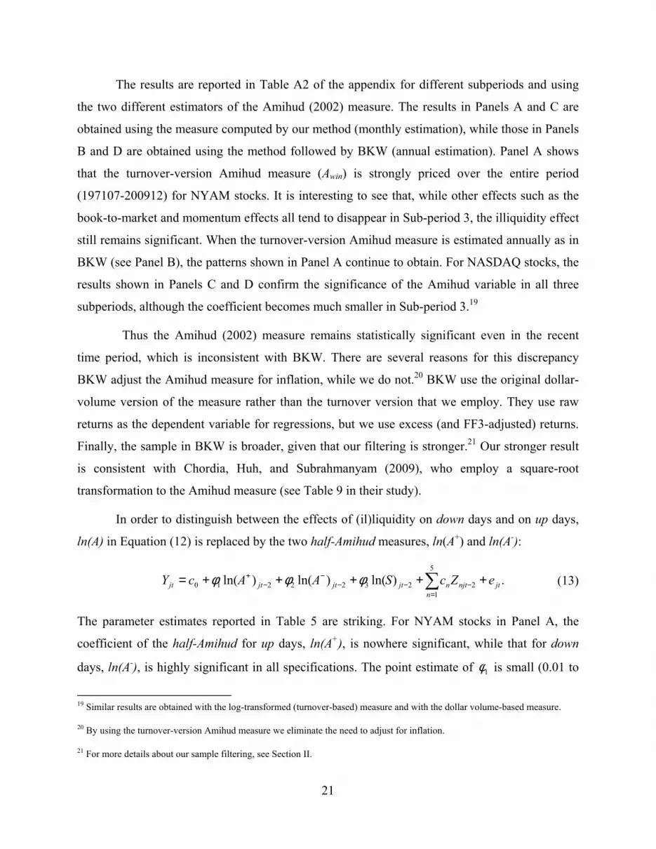
The results are reported in Table A2 of the appendix for different subperiods and using
the two different estimators of the Amihud (2002) measure. The results in Panels A and C are
obtained using the measure computed by our method (monthly estimation), while those in Panels
B and D are obtained using the method followed by BKW (annual estimation). Panel A shows
that the turnover-version Amihud measure (Awin) is strongly priced over the entire period
(197107-200912) for NYAM stocks. It is interesting to see that, while other effects such as the
book-to-market and momentum effects all tend to disappear in Sub-period 3, the illiquidity effect
still remains significant. When the turnover-version Amihud measure is estimated annually as in
BKW (see Panel B), the patterns shown in Panel A continue to obtain. For NASDAQ stocks, the
results shown in Panels C and D confirm the significance of the Amihud variable in all three
subperiods, although the coefficient becomes much smaller in Sub-period 3.19
Thus the Amihud (2002) measure remains statistically significant even in the recent
time period, which is inconsistent with BKW. There are several reasons for this discrepancy
BKW adjust the Amihud measure for inflation, while we do not.20 BKW use the original dollar-
volume version of the measure rather than the turnover version that we employ. They use raw
returns as the dependent variable for regressions, but we use excess (and FF3-adjusted) returns.
Finally, the sample in BKW is broader, given that our filtering is stronger.21 Our stronger result
is consistent with Chordia, Huh, and Subrahmanyam (2009), who employ a square-root
transformation to the Amihud measure (see Table 9 in their study).
In order to distinguish between the effects of (il)liquidity on down days and on up days,
ln(A) in Equation (12) is replaced by the two half-Amihud measures, ln(A+) and ln(A-):
.)ln()ln()ln( 2
5
12322210 jtnjtn
njtjtjtjt eZcSAAcY +++++= −
=−−
−−
+ ∑φφφ (13)
The parameter estimates reported in Table 5 are striking. For NYAM stocks in Panel A, the
coefficient of the half-Amihud for up days, ln(A+), is nowhere significant, while that for down
days, ln(A-), is highly significant in all specifications. The point estimate of 1φ is small (0.01 to
19 Similar results are obtained with the log-transformed (turnover-based) measure and with the dollar volume-based measure.
20 By using the turnover-version Amihud measure we eliminate the need to adjust for inflation.
21 For more details about our sample filtering, see Section II.

22
0.06), while that of 2φ ranges from 0.16 to 0.26. A value for 2φ of 0.26 implies that an increase
of one standard deviation in ln(A-) is associated with 0.30% higher monthly (excess) returns. The
t-statistics for the difference between the estimates of 2φ and 1φ in the two FF3-adjusted
specifications with control variables are greater than 2.80, and when the dependent variable is
Re2, the estimate of 2φ is larger than that of 1φ by a factor of 7. Thus there is strong evidence that
the asymmetry between the effects of buy-liquidity and sell-liquidity on expected returns
reported by Brennan et al. (2010) is mirrored in an asymmetry between the effects of liquidity on
up and down days on expected returns. The absolute value of the coefficient of ln(S), which
continues to be highly significant, is now only about one third of that of ln(A-) in the
specifications using the FF3-adjusted returns.
Panel B of Table 5 shows that for the NASDAQ sample also the coefficient of the half-
Amihud for up days, ln(A+), is nowhere significant, while that for down days, ln(A-), is highly
significant in the specifications that use the FF3-adjusted returns. The estimated coefficient of
ln(S) continues to be larger in absolute value than the coefficient of ln(A-).
In Table 5, the half-Amihud measures (for up and down days) of a stock are computed
using the stock’s own returns to distinguish between up and down days. However, investors may
be more concerned about selling when the whole market is going down and the values of their
entire diversified portfolios are declining. To consider this possibility, we construct the half-
Amihud measures using market movements to define up and down days. The new half-Amihud
measure for up (down) days is defined as the average of daily |r|/T over the up-market (down-
market) days (days with positive (negative) CRSP value-weighted returns) within a month. It is
denoted by A+, m (A-, m ).
The new regression results corresponding to Equation (13) are reported in Table 6. In
both panels the coefficients of ln(A+, m) and ln(A-, m) are generally smaller and less significant
than those on the two corresponding half-Amihud measures in Table 5. However, constructing
the half-Amihud measures on the basis of market returns does not alter the basic pattern
observed in Table 5. The coefficient of the half-Amihud for up days, ln(A+, m), is not statistically
significant, while that for down days, ln(A-, m), is generally significant.

23
We have seen in Tables 5 and 6 that for the whole sample it is only the half-Amihud for
down days, ln(A-), that commands a return premium. To determine whether the effect is
consistent across firm size groups, we allocate firms each month to one of three size groups
according to the market value at the end of the previous month, estimating the relation between
the FF3-adjusted returns and the measures of illiquidity for each group separately. To save space,
we report results only for regressions that include the control variables and use Re2 as the
dependent variable. As can be seen in Panel A of Table A3 in the appendix, for NYAM stocks,
the differential pricing effects between ln(A+) and ln(A-) exist in all three size groups. The
coefficient of ln(A-) is positive and highly significant for each group while the coefficient of
ln(A+) is insignificant for small and medium size firms, becoming negative and significant for
the group of large firms (MV3). Panel B shows that for NASDAQ stocks the coefficient of the
half-Amihud for down days, ln(A-), is positive and highly significant for the small-size group
(MV1), while the coefficient of ln(A+) is insignificant. On the other hand, there is no significant
evidence that either half-Amihud is priced for the groups of medium- and large-size firms. We
note however that the point estimate of the coefficient of ln(A-) for large firms (0.136) is close to
the corresponding estimate for the whole sample reported in Panel B of Table 5 (0.161).
C. Further Analysis Using Signed Turnover
The asymmetry between the role of the half-Amihud measures for up and down days is broadly
consistent with the finding by Brennan et al. (2010) that investors price the association between
price changes (or returns) and seller-initiated trades. We have found that they price the
association between negative returns (down days) and trading volume. Since seller-initiated
trades are associated with negative returns, it is natural to consider whether it is the association
between negative returns and seller-initiated trading volume that gives rise to the pricing of the
half-Amihud measure for down days.
To assess the importance of the relation between seller-initiated trades and the returns on
down days, we classify intradaily transactions into buyer-initiated trades or seller-initiated trades
using the ISSM/TAQ databases, aggregating them into daily signed volume and turnover (i.e.,
buyer-initiated turnover, TB, and seller-initiated turnover, TS, separately). This allows us to obtain

24
the two directional half-Amihud measures as well as the two sidedness variables defined in
Equation (7). Because of data availability, however, we limit this type of decomposition to
NYAM-listed stocks over the period from January 1983 to December 2009. For consistency in
sampling with the previous analyses, we ensure that stocks have at least 50 trades per month (on
average 2.5 trades per day) when processing the ISSM/TAQ data. We then estimate the
following equation:
∑=
−
−−−
−−
−+
−+
++
+++++=5
12
252242132222110
.
)ln()ln()ln()ln()ln(
njtnjtn
jtjtjtjtjtjt
eZc
SAAAAcY ϕϕϕϕϕ
(14)
The parameter estimates are reported in Table 7. The average number of component
stocks used in the cross-sectional regressions increases substantially (9-28%), compared to the
previous tables for NYAM-listed stocks (e.g., Panel A in Table 5), because the ISSM database
starts more recently, in 1983. Consistent with the results for the half-Amihud measures reported
in Table 5, the coefficients of the directional half-Amihud for up days, ln( ), are not
statistically significant and their point estimates are in the range of 0.03-0.06. When the control
variables are included in the regressions (Specification 8), the up-sidedness variable, ln( ), does
not have any significant impact either, although the point estimates seem large.
In contrast to the case for up days, the coefficients of the directional half-Amihud for
down days, ln( ), are significant at the 1% level, which is again consistent with the results in
Table 5. Thus, as we expect from the above discussion, the relation between negative returns
(returns on down days) and seller-initiated turnover is reflected in average returns: the greater is
the magnitude of the negative return for a given level of seller-initiated turnover, the higher is the
return premium. This is consistent with Brennan et al. (2010) in that the directional half-Amihud
for down days is closely related to the sell side ‘lambda’ calculated using the order flow and
price changes.22
22 The Kyle ‘lambda’ is based on the relation between price changes and the net order flow, whereas the directional half-Amihuds depend on the relation between the price change and the gross signed order flow.

25
We find that the coefficients of the down-sidedness variable, ln( ), are also significant
when the dependent variable is FF3-adjusted (Re1 or Re2). This indicates that the significant role
of the half-Amihud measure for down days cannot be attributed entirely to the directional half-
Amihud component. Indeed, the coefficients of the down-sidedness component are two to three
times greater than those of the directional half-Amihud for down days when the dependent
variable is FF3-adjusted, although a standard t-test is unable to reject at the 5% level the equality
of the coefficients of the two variables that is implied by the Amihud (2002) formulation. The
point estimates imply that a tendency for trades to cluster on the sell-side on down days is also a
key determinant of returns. As Sarkar and Schwartz (2009) point out, such one-sided clustering
of trades is indicative of trading motivated by asymmetric information (see also Easley and
O’Hara, 1992). It is noteworthy that the estimates of the coefficient of the variable that measures
clustering on the buy-side on up days are similar in size to the corresponding coefficient
estimates for down days, though the up-sidedness coefficients are generally not significant.
In addition to the decompositions and analyses presented above, we have also attempted
to decompose the two half-Amihud measures into the half-Kyle measures and their residuals as
shown in Equations (8) and (9). The half-Kyle measures divide the absolute return for up (down)
days by the net buyer-initiated (seller-initiated) turnover, in contrast to the directional half-
Amihud measures which use the gross buyer-initiated (seller-initiated) turnover. Unfortunately,
the logarithmic decomposition is infeasible because there are too many days on which the sign of
the net order flow is opposite to that of the price change, causing the ratio to be negative.
Two results thus far are noteworthy. First, only the component of the Amihud measure
of illiquidity that pertains to down days is important to asset pricing. Second, the two
subcomponents of this half-Amihud measure, which correspond to price sensitivity to seller-
initiated turnover and the tendency of sell-orders to cluster on down days, both contribute
significantly to the explanatory power of the half-Amihud measure. We turn next to some tests of
the robustness of our findings.
V. Robustness Tests
A. TAQ Period (1993-2009) Sample

26
To confirm that our results are not due to problems associated with the ISSM database,23 the tests
are repeated after restricting the sample to the TAQ period (17 years: 1993-2009). Excluding the
10-year non-TAQ period (1983-1992) also allows us to verify that the results are robust to the
changes that have taken place in financial markets since then.
Table 8 reports the results from monthly Fama-MacBeth regressions in which the
dependent variable is Re1, the FF3-adjusted excess return using factor loadings estimated from
the whole sample. For brevity, we do not report the results with Re2, but the patterns are virtually
the same. To facilitate comparisons with the results reported in the previous sections, the
specifications are labeled as 2c, 4c, 6c, and 8c, which correspond to Specifications 2a, 4a, 6a,
and 8, respectively, in the previous tables. Panel A shows the results with the Amihud (2002)
measure, ln(A0) and its components that do not involve signing trades, ln(A), ln(A+), ln(A-), and
ln(S). From this point on, the turnover ratio [to be used for computing ln(A), ln(A+),and ln(A-)] is
calculated using the transaction-level data (not the CRSP file) for robustness tests and
comparison purposes: that is, T* is used instead of T in Panel A, as Panel B uses TAQ-based
turnover. Panel B reports the results for the components that depend on signed volume computed
using the TAQ database, ln( ), ln( ), ln( ), and ln( ). Exclusion of the first 10 years (the
ISSM period) increases the average number of stocks in the cross-sectional regressions from
around 1,740 (in Table 7) to almost 1,950.
In Panel A, we find that the size effect remains significant but that the book-to-market
and momentum effects disappear or become much weaker [note that this is similar to the result
of Sub-period 3 (199601-200912) reported in Panel A of Table A2]. However, the basic patterns
observed in the previous sections obtain. As we see in Specification 2c, the original Amihud
(2002) measure, ln(A0), is priced significantly for the 1993-2009 period. When the Amihud
(2002) measure is decomposed into its turnover version and size components (Specification 4c),
the turnover-version Amihud, ln(A), again plays a strong role, with its coefficient being
substantially larger than that of the original measure, ln(A0). When the turnover-version measure
is decomposed into the two half-Amihud measures in Specification 6c, only the coefficient of
23 In the early years of ISSM the data were entered by hand, which could have caused errors. Also some condition codes of TAQ trade types are not exactly the same as those of ISSM.

27
ln(A-), the half-Amihud for down days, is statistically significant, consistent with our earlier
results.
Panel B shows that when each of the two half-Amihuds is decomposed into the
directional half-Amihud and sidedness components, the coefficient of the directional half-
Amihud for down days, ln( ), is statistically significant, but that for up days, ln( ), is not.
This is also consistent with the results shown in the previous tables. Now there is no evidence
that up-sidedness, ln( ), is priced, but the point estimate of the coefficient on down-sidedness,
ln( ), remains comparable to the value reported in Table 7 and it is at the margin of statistical
significance (t = 1.95).
B. Corrections for Microstructure Biases: WLS Regressions
Asparouhova, Bessembinder, and Kalcheva (2010) suggest the use of weighted least-squares
(WLS) estimation to reduce biases caused by bid-ask bounce or temporary price pressures due to
order imbalances. Therefore we perform WLS regressions using one plus the previous month
return as a weighting variable. The Fama-MacBeth regression results with WLS estimation are
presented in Table 9. To save space, only the results with Re2 as the dependent variable are
reported. The specifications 2d, 4d, 6d, and 8d correspond to specifications 2a, 4a, 6a, and 8 in
the previous tables. The turnover ratio [used for computing ln(A), ln(A+),and ln(A-)] in Panel A is
again calculated using the ISSM/TAQ databases as in Panel B.
Both panels again confirm our earlier results. The original Amihud (2002) measure
(Specification 2d in Panel A) is priced in the cross-section of stock returns. Specification 6d also
shows that only the half-Amihud measure for down days, ln(A-), is significantly positively
related to returns. When the half-Amihud measures are further decomposed into the ISSM/TAQ-
based components in Panel B, the directional half-Amihud for down days, ln( ), is priced, but
that for up days, ln( ), is not. In addition, there is a significant pricing effect associated with the
down-sidedness component, ln( ). Noticeable in this table is that with the WLS estimation the
size and momentum effects survive the corrections, while the book-to-market effect does not.

28
VI. Conclusion
In this paper we have first confirmed that the Amihud (2002) measure of illiquidity is reliably
priced in the cross-section of asset returns, using a broad and long data sample starting from the
early 1970s. A sub-period analysis shows that the Amihud measure also commands a return
premium during a more recent time period. We have also shown that the return premium is
captured better when turnover is used as the measure of trading activity and firm size effects are
accounted for separately.
When we decompose the Amihud measure into components related to positive (up) and
negative (down) return days, we find that only the half-Amihud corresponding to down days is
priced. When this half-Amihud was further decomposed into an element corresponding to the
sensitivity of the price change to seller-initiated turnover and an element that measures the
clustering of sell-orders on down days, both elements contribute significantly to the return
premium associated with illiquidity. The pricing of the first element is consistent with the finding
by Brennan et al. (2010) that only the Kyle lambda for seller-initiated trades is priced. The
pricing of the second element is consistent with the findings by Sarkar and Schwartz (2009), who
associate market sidedness with the presence of asymmetric information.

29
References
Amihud, Y., 2002, Illiquidity and stock returns: Cross-section and time-series effects, Journal of
Financial Markets 5, 31-56.
Ang, A., J. Liu, and K. Schwarz, 2008, Using stocks or portfolios in tests of factor models,
Working paper, Columbia University.
Anshuman, R., and S. Viswanathan, 2005, Costly collateral and illiquidity, Working paper, Duke
University.
Atkins, A. and E. Dyl, 1997, Market structure and reported trading volume: NASDAQ versus
the NYSE, Journal of Financial Research 20, 291-304.
Avramov, D. and T. Chordia, 2006, Asset pricing models and financial market anomalies,
Review of Financial Studies 19, 1002-1040.
Asparouhova, E., H. Bessembinder, and I. Kalcheva, 2010, Liquidity biases in asset pricing tests,
Journal of Financial Economics 96, 215-237.
Ben-Rephael, A., O. Kadan, and A. Wohl, 2012, The diminishing liquidity premium, Working
paper, Washington University.
Blume, M. and R. Stambaugh, 1983, Biases in computed returns: an application to the size
effect, Journal of Financial Economics 12, 387-404.
Brennan, M., T. Chordia, and A. Subrahmanyam, 1998, Alternative factor specifications,
security characteristics, and the cross-section of expected stock returns, cross-sectional
determinants of expected returns, Journal of Financial Economics 49, 345--373.
Brennan, M., T. Chordia, and A. Subrahmanyam, Q. Tong, 2010, Sell-order liquidity and the
cross-section of expected stock returns, Journal of Financial Economics, Forthcoming.
Brunnermeier, M. and L. Pedersen, 2009, Market liquidity and funding liquidity, The Review of
Financial Studies 22, 2201-2238.

30
Chordia, T., S. Huh, and A. Subrahmanyam, 2007, The cross-section of expected trading
activity, Review of Financial Studies 20, 709-740.
Chordia, T., S. Huh, and A. Subrahmanyam, 2009, Theory-based illiquidity and asset pricing,
Review of Financial Studies 22, 3629-3668.
Chordia, T., R. Roll, and A. Subrahmanyam, 2001, Market liquidity and trading activity, Journal
of Finance 56, 501-530.
Cochrane, J., 2005, Asset pricing program review, NBER Reporter.
Cooper, S., J. Groth, and W. Avera, 1984, Liquidity, exchange listing and common stock
performance, Journal of Economics and Business 37, 19-33.
Coval, J. and E. Stafford, 2007, Asset fire sales (and purchases) in equity markets, Journal of
Financial Economics 86, 479-512.
Dubofsky, F. and J. Groth, 1984, Exchange listing and stock liquidity, Journal of Financial
Research 7, 291-302. J ECO BUSN 1 937:19-33
Easley, D., and M. O’Hara, 1992, Time and the process of security price adjustment, Journal of
Finance 47, 577-605.
Fama, E. and K. French, 1992, The cross-section of expected stock returns, Journal of Finance
47, 427-466.
Fama, E. and K. French, 1993, Common risk factors in the returns on stocks and bonds, Journal
of Financial Economics 33, 3-56.
Fama, E. and J. MacBeth, 1973, Risk, return, and equilibrium: Empirical tests, Journal of
Political Economy 81, 607-636.
Florakis, C., A. Gregoriou, and A. Kostakis, 2011, Trading frequency and asset pricing on the
London Stock Exchange: evidence for a new price impact ratio, Journal of Banking and
Finance 35, 3335-3350.
Garleanu, N., and L. Pedersen, 2007, Liquidity and risk management, American Economic
Review 97, 193-197.
31
Hameed, A., W. Kang, and S. Viswanathan, 2010, Stock market declines and liquidity, Journal
of Finance 65, 257-293.
Hasbrouck, J., 1999, The dynamics of discrete bid and ask quotes, Journal of Finance 54, 2109-
2142.
Hasbrouck, J., 2005, Trading costs and returns for US equities: The evidence from daily data,
Working paper, New York University.
Hasbrouck, J., 2009, Trading costs and returns for US equities: Estimating effective costs from
daily data, Journal of Finance 64, 1479-1512.
Jegadeesh, N. and S. Titman, 1993, Returns to buying winners and selling losers: Implications
for stock market efficiency, Journal of Finance 48, 65-92.
Karpoff, J., 1987, The relation between price changes and trading volume: A survey, Journal of
Financial and Quantitative Analysis 22, 109-126.
Kyle, A., 1985, Continuous auctions and insider trading, Econometrica 53, 1315-1335.
Lakonishok, J., A. Shleifer, R. Thaler, and R. Vishny, 1991, Window dressing by pension fund
managers, American Economic Review 81, 227-31.
Lee, C. and M. Ready, 1991, Inferring trade direction from intraday data, Journal of Finance 46,
733-747.
Lee, C., and B. Swaminathan, 2000, Price momentum and trading volume, Journal of Finance
60, 2017-2069.
Lo, A., and C. MacKinlay, 1990, Data-snooping biases in tests of financial asset pricing models,
Review of Financial Studies 3, 431-468.
Martin, P., 1975, Analysis of the impact of competitive rates of the liquidity of NYSE stocks,
Economic Staff Paper 75-3, Securities and Exchange Commission.
Odean, T., 1998, Are investors reluctant to realize their losses?, Journal of Finance, 53 1775–98.

32
Roll, R., 1977, A critique of the asset pricing theory's tests: on past and potential testability of
theory, Journal of Financial Economics 4, 129-176.
Sadka, R., 2006, Momentum and post-earnings-announcement drift anomalies: the role of
liquidity risk, Journal of Financial Economics 80, 309-349.
Sarkar, A. and R. Schwartz, 2009, Market sidedness: insights into motives for trade initiation,
Journal of Finance 64, 375-423.

33
Table 1
Descriptive Statistics This table reports descriptive statistics of key variables for NYSAM stocks from July 1971 to December 2009 and for NASDAQ stocks from January 1983 to December 2009. Panels A and D show statistics for the Amihud (2002) measure and its components, while Panels B and E show statistics for their log-transformed values [indicated by ln(.)]. Panels C and F contain statistics for other variables. The cross-sectional value for each statistic is first calculated each month and then the time-series average of those values over the sample period is reported here. STD stands for the standard deviation. The variables are defined as follows: A0: the original Amihud (2002) measure defined as the monthly average of daily ratios of absolute returns to dollar volume in $1,000; A: the turnover version of the Amihud measure, which is the monthly average of daily ratios of absolute return to share turnover computed using CRSP; A+ (A-):the half-Amihud measure for up (down) days, which is the monthly average of daily ratios of absolute returns to turnover on positive (negative) return days ]; ( ): the directional half-Amihud measure for up (down) days which is the monthly average of daily ratios of absolute returns to buyer (seller) initiated turnover on up (down) computed using ISSM/TAQ; ( ): the up-sidedness (down-sidedness )measure, which is the proportion of turnover that is attributable to buyer-initiated trades on up (down); BTM: the Winsorized value (at the 0.5th and 99.5th percentiles) of a book-to-market ratio (= BV/MV), where the book value (BV) is common equity and the market value (MV) is the previous month-end stock price times the number of shares outstanding; MOM1, MOM2, MOM3: the compounded holding period returns of a stock over the the 3 months ending at months t-1, t-4, and t-9 t-. To survive in the CRSP sample, stocks have five zero-volume days or fewer within a month (for NYSAM stocks), or 50 trades or more within a month (for NASDAQ stocks). In addition, for the availability of Re2, stocks have monthly returns for the past 60 months (at least 24 months). Only common stocks (share code 10 or 11 in CRSP) are used. The values for ISSM/TAQ-based variables ( , , and their log-transforms) are available only for NYSAM-listed stocks from January 1983 to December 2009. In the ISSM/TAQ databases, stocks must have at least 50 trades per month (on average 2.5 trades per day) for each firm. The average number of component stocks used each month for this table is 1,758.6 (a minimum of 1,447 and a maximum of 2,170) for NYSAM stocks and 2,166.1 (a minimum of 148 and a maximum of 3,376) for NASDAQ stocks.

34
(Table 1: continued)
NYAM Stocks NASDAQ Stocks Mean Median STD Skewness Kurtosis Mean Median STD Skewness Kurtosis
Variables Panel A: Amihud (2002) Measure and its Components Panel D: Amihud (2002) Measure and its Components
A0 0.297 x 10⁻² 0.015 x 10⁻² 0.02 18.60 485.12 0.593 x 10⁻² 0.025 x 10⁻² 0.06 20.47 611.20 A 34.60 13.70 111.04 15.47 379.83 78.71 15.99 404.27 15.34 428.92 A+ 16.18 6.20 59.30 16.46 425.65 39.00 6.50 267.67 16.93 490.29 A- 18.42 6.91 64.43 15.76 391.14 39.71 7.69 232.37 15.61 427.60
31.37 8.22 150.46 18.52 502.41 - - - - -
0.56 0.57 0.08 -0.54 1.73 - - - - -
39.44 11.56 173.70 17.92 495.73 - - - - -
0.44 0.43 0.08 0.54 1.73 - - - - - S 2,669,286.6 447,989.3 9,020,199.3 11.3 191.9 592,149.9 103,061.7 4,332,810.4 18.8 534.1
Variables Panel B: Log-transformed Measure and its Components Panel E: Log-transformed Measure and its Components
ln(A0) -10.00 -10.26 2.74 0.34 -0.28 -8.73 -8.71 2.68 -0.03 -0.28 ln(A) 2.52 2.31 1.11 0.80 1.13 2.74 2.61 1.52 0.39 -0.12 ln(A+) 1.72 1.53 1.13 0.77 1.19 1.89 1.74 1.53 0.45 0.07 ln(A-) 1.80 1.61 1.17 0.68 1.11 2.02 1.89 1.55 0.36 0.03 ln( ) 2.22 2.03 1.21 0.80 1.65 - - - - - ln( ) -0.60 -0.57 0.16 -1.59 7.16 - - - - - ln( ) 2.50 2.31 1.20 0.71 1.60 - - - - - ln( ) -0.84 -0.83 0.19 -0.47 3.25 - - - - - ln(S) 12.53 12.54 1.94 0.02 -0.36 11.48 11.41 1.54 0.29 0.19
Variables Panel C: Other Key Variables Panel F: Other Key Variables
BTM 0.853 0.734 0.596 2.304 9.993 0.657 0.537 0.528 2.270 10.049 MOM1 0.011 0.016 0.200 -0.270 7.345 -0.010 0.003 0.279 -0.535 6.404 MOM2 0.009 0.014 0.194 -0.202 6.429 -0.006 0.005 0.270 -0.295 4.801 MOM3 0.010 0.014 0.191 -0.146 5.978 -0.003 0.006 0.266 -0.176 4.323 MOM4 0.010 0.015 0.189 -0.116 5.741 -0.003 0.006 0.264 -0.121 4.170
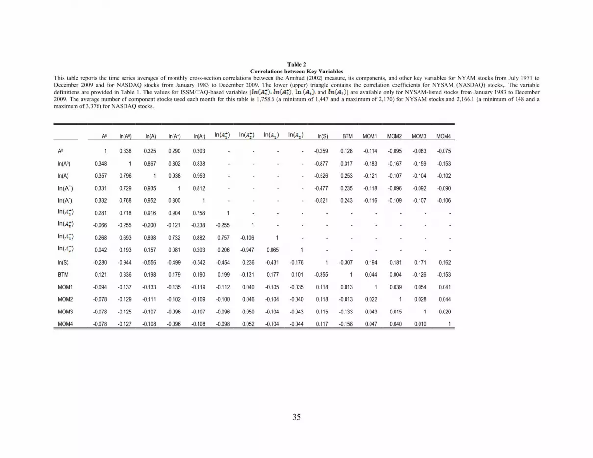
35
Table 2
Correlations between Key Variables This table reports the time series averages of monthly cross-section correlations between the Amihud (2002) measure, its components, and other key variables for NYAM stocks from July 1971 to December 2009 and for NASDAQ stocks from January 1983 to December 2009. The lower (upper) triangle contains the correlation coefficients for NYSAM (NASDAQ) stocks,. The variable definitions are provided in Table 1. The values for ISSM/TAQ-based variables [ , and ] are available only for NYSAM-listed stocks from January 1983 to December 2009. The average number of component stocks used each month for this table is 1,758.6 (a minimum of 1,447 and a maximum of 2,170) for NYSAM stocks and 2,166.1 (a minimum of 148 and a maximum of 3,376) for NASDAQ stocks.
A0 ln(A0) ln(A) ln(A+) ln(A-) ln( ) ln( ) ln( ) ln( ) ln(S) BTM MOM1 MOM2 MOM3 MOM4
A0 1 0.338 0.325 0.290 0.303 - - - - -0.259 0.128 -0.114 -0.095 -0.083 -0.075
ln(A0) 0.348 1 0.867 0.802 0.838 - - - - -0.877 0.317 -0.183 -0.167 -0.159 -0.153
ln(A) 0.357 0.796 1 0.938 0.953 - - - - -0.526 0.253 -0.121 -0.107 -0.104 -0.102
ln(A+) 0.331 0.729 0.935 1 0.812 - - - - -0.477 0.235 -0.118 -0.096 -0.092 -0.090
ln(A-) 0.332 0.768 0.952 0.800 1 - - - - -0.521 0.243 -0.116 -0.109 -0.107 -0.106
ln( ) 0.281 0.718 0.916 0.904 0.758 1 - - - - - - - - -
ln( ) -0.066 -0.255 -0.200 -0.121 -0.238 -0.255 1 - - - - - - - -
ln( ) 0.268 0.693 0.898 0.732 0.882 0.757 -0.106 1 - - - - - - -
ln( ) 0.042 0.193 0.157 0.081 0.203 0.206 -0.947 0.065 1 - - - - - -
ln(S) -0.280 -0.944 -0.556 -0.499 -0.542 -0.454 0.236 -0.431 -0.176 1 -0.307 0.194 0.181 0.171 0.162
BTM 0.121 0.336 0.198 0.179 0.190 0.199 -0.131 0.177 0.101 -0.355 1 0.044 0.004 -0.126 -0.153
MOM1 -0.094 -0.137 -0.133 -0.135 -0.119 -0.112 0.040 -0.105 -0.035 0.118 0.013 1 0.039 0.054 0.041
MOM2 -0.078 -0.129 -0.111 -0.102 -0.109 -0.100 0.046 -0.104 -0.040 0.118 -0.013 0.022 1 0.028 0.044
MOM3 -0.078 -0.125 -0.107 -0.096 -0.107 -0.096 0.050 -0.104 -0.043 0.115 -0.133 0.043 0.015 1 0.020
MOM4 -0.078 -0.127 -0.108 -0.096 -0.108 -0.098 0.052 -0.104 -0.044 0.117 -0.158 0.047 0.040 0.010 1

36
Table 3
The Pricing of the Amihud (2002) Measure This table reports the results of monthly Fama-MacBeth (1973) cross-sectional regressions that include the log-transformed Amihud (2002) measure, ln(A0). Panel A contains the result for NYAM-listed stocks from July 1971 to December 2009, while Panel B does the same for NASDAQ-listed stocks from January 1983 to December 2009. The dependent variable is Re, Re1, or Re2. . Re is the monthly excess return (in excess of the one-month T-bill rate); Re1 is the FF3-adjusted excess return, i.e., the constant term plus the residual from the time-series regression of the excess return on the FF 3 factors using the entire sample range of the data; Re2: the FF3-adjusted excess return using the Fama-French (FF) 3 factors with factor loadings estimated from the 5-year rolling regressions (past monthly returns should be available for at least 24 months); A0: the original Amihud (2002) measure defined as the monthly average of daily ratios of absolute return to dollar volume in $1,000. The other variables are defined in Table 1. The values in the first row for each explanatory variable are the coefficient estimates, and the values italicized in the second row of each variable are t-statistics computed based on Fama-MacBeth (1973). To survive in the sample, stockshave five zero-volume days or fewer within a month (for NYAM stocks) or 50 trades or more within a month (on average 2.5 trades or more per day) (for NASDAQ stocks). In addition, for the availability of Re2, stocks have monthly returns for the past 60 months (at least 24 months). Only common stocks (share code 10 or 11 in CRSP) are used. The sample loses the first two observations in the cross-sectional regressions due to the 2-month lagging. The coefficients are all multiplied by 100. Avg R2 is the average of monthly adjusted R-squared values. Avg Obs is the monthly average number of companies used in the cross-sectional regressions. Significance at the 1% and 5% levels is indicated by ** and *, respectively.

37
(Table 3: continued)
Panel A: The Pricing of the Amihud (2002) Measure for NYAM Stocks (197107-200912)
Re Re1 Re2
Explanatory Variables 1a 2a 1a 2a 1a 2a
Intercept 2.288 ** 2.022 ** 1.143 ** 1.160 ** 1.145 ** 1.316 **
4.28 4.92 4.21 5.66 3.97 6.04
ln(A0) 0.154 ** 0.165 ** 0.109 ** 0.130 ** 0.107 ** 0.134 **
3.96 5.34 4.51 7.09 4.27 7.02
BTM 0.256 ** 0.160 * 0.086
3.12 2.42 1.23
MOM1 0.857 ** 0.872 ** 0.838 **
2.89 3.49 3.02
MOM2 0.983 ** 0.954 ** 0.782 **
3.52 4.11 3.01
MOM3 1.349 ** 1.277 ** 1.130 **
5.60 6.22 4.62
MOM4 0.200 0.199 0.033
0.94 1.05 0.14
Avg R-sqr 0.019 0.046 0.008 0.027 0.008 0.030
Avg Obs 1757.8 1597.6 1755.3 1597.0 1757.8 1597.6

38
(Table 3: continued)
Panel B: The Pricing of the Amihud (2002) Measure for NASDAQ Stocks (198301-200912)
Re Re1 Re2
Explanatory Variables 1b 2b 1b 2b 1b 2b
Intercept 2.818 ** 2.254 ** 1.996 ** 1.625 ** 2.236 ** 1.986 **
5.08 4.73 4.61 4.17 4.71 4.92
ln(A0) 0.221 ** 0.225 ** 0.198 ** 0.210 ** 0.225 ** 0.238 **
4.80 5.83 5.06 6.06 5.18 6.58
BTM 0.777 ** 0.635 ** 0.609 **
6.12 6.18 5.48
MOM1 0.645 * 0.690 ** 0.639 *
2.05 2.73 2.12
MOM2 0.775 ** 0.668 ** 0.654 *
2.65 2.78 2.28
MOM3 0.715 ** 0.544 * 0.482
2.81 2.55 1.87
MOM4 0.123 0.091 0.026
0.53 0.47 0.11
Avg R-sqr 0.011 0.033 0.008 0.021 0.009 0.025
Avg Obs 2166.1 2004.6 2164.5 2003.3 2166.1 2004.6

39
Table 4
The Pricing of the Basic Components of the Amihud (2002) Measure Panels A and B report the results of monthly Fama-MacBeth (1973) regressions that include the basic components (log-transformed) of the Amihud (2002) measure, ln(A) and ln(S). Panel A contains the result for NYAM-listed stocks from July 1971 to December 2009, while Panel B does the same for NASDAQ-listed stocks from January 1983 to December 2009. To compare the effect of the turnover-version Amihud measure in Panels A and B with that of the original Amihud (2002) measure, the analogs of the two panels in Table 3 are reported in Panels C and D, which include ln(S). The dependent variable is Re, Re1, or Re2. Re is the monthly excess return (in excess of the one-month T-bill rate); Re1 is the FF3-adjusted excess return, i.e., the constant term plus the residual from the time-series regression of the excess return on the FF 3 factors using the entire sample range of the data; Re2 is the FF3-adjusted excess return using the Fama-French (FF) 3 factors with factor loadings estimated from the 5-year rolling regressions (past monthly returns should be available for at least 24 months); ln(A) is the natural logarithm of A, which is the turnover version of the Amihud (2002) measure. The other variables are defined in Table 1. The values in the first row for each explanatory variable are coefficient estimates, and the values italicized in the second row of each variable are t-statistics computed based on Fama-MacBeth (1973). To survive in the sample, stocks have five zero-volume days or fewer within a month (for NYSAM stocks) or50 trades or more within a month (on average 2.5 trades or more per day) (for NASDAQ stocks). In addition, for the availability of Re2, stocks have monthly returns for the past 60 months (at least 24 months). Only common stocks (share code 10 or 11 in CRSP) are used. The sample loses the first two observations in the cross-sectional regressions due to the 2-month lagging. The coefficients are all multiplied by 100. Avg R2 is the average of monthly adjusted R2. Avg Obs is the average monthly number of companies used in the cross-sectional regressions. Significance at the 1% and 5% levels is indicated by ** and *, respectively.

40
(Table 4: continued)
Panel A: The Pricing of the Basic Components of the Amihud (2002) Measure for NYAM Stocks (197107-200912)
Re Re1 Re2
Explanatory Variables 3a 4a 3a 4a 3a 4a
Intercept 2.457 ** 1.674 * 0.765 0.374 0.647 0.465
2.86 2.40 1.88 1.22 1.51 1.39
ln(A) 0.152 ** 0.216 ** 0.166 ** 0.225 ** 0.177 ** 0.236 **
3.14 5.05 4.38 6.64 4.44 6.63
ln(S) -0.166 ** -0.148 ** -0.090 ** -0.089 ** -0.081 ** -0.089 **
-3.13 -3.50 -3.07 -4.22 -2.66 -3.98
BTM 0.274 ** 0.182 ** 0.109
3.25 2.71 1.53
MOM1 0.905 ** 0.922 ** 0.890 **
3.09 3.71 3.22
MOM2 0.990 ** 0.978 ** 0.812 **
3.64 4.25 3.13
MOM3 1.351 ** 1.297 ** 1.150 **
5.74 6.35 4.71
MOM4 0.221 0.217 0.053
1.06 1.16 0.23
Avg R-sqr 0.024 0.050 0.010 0.029 0.010 0.031
Avg Obs 1757.8 1597.6 1755.3 1597.0 1757.8 1597.6

41
(Table 4: continued)
Panel B: The Pricing of the Basic Components of the Amihud (2002) Measure for NASDAQ Stocks (198301-200912)
Re Re1 Re2
Explanatory Variables 3b 4b 3b 4b 3b 4b
Intercept 3.387 * 2.986 * 2.566 * 2.140 * 2.396 * 2.210 *
2.19 2.40 2.24 2.33 1.97 2.24
ln(A) 0.203 * 0.192 ** 0.173 ** 0.193 ** 0.232 ** 0.244 **
2.33 2.83 3.48 4.44 4.11 5.18
ln(S) -0.259 ** -0.270 ** -0.235 ** -0.243 ** -0.233 ** -0.251 **
-2.64 -3.49 -2.82 -3.63 -2.61 -3.51
BTM 0.735 ** 0.606 ** 0.587 **
5.40 5.72 5.15
MOM1 0.751 * 0.755 ** 0.709 *
2.54 3.12 2.42
MOM2 0.797 ** 0.705 ** 0.673 *
2.91 3.09 2.43
MOM3 0.738 ** 0.569 ** 0.504 *
3.12 2.79 2.02
MOM4 0.107 0.089 0.023
0.49 0.47 0.09
Avg R-sqr 0.019 0.038 0.012 0.023 0.012 0.028
Avg Obs 2166.1 2004.6 2164.5 2003.3 2166.1 2004.6

42
(Table 4: continued)
Panel C: The Pricing of the Amihud (2002) Measure for NYAM Stocks (197107-200912) [including ln(S)]
Re Re1 Re2
Explanatory Variables 3c 4c 3c 4c 3c 4c
Intercept 2.446 ** 1.673 * 0.757 0.374 0.646 0.469
2.86 2.40 1.87 1.23 1.52 1.41
ln(A0) 0.153 ** 0.215 ** 0.166 ** 0.224 ** 0.176 ** 0.235 **
3.17 5.07 4.40 6.63 4.43 6.60
ln(S) -0.012 0.068 0.077 0.136 ** 0.095 * 0.146 **
-0.17 1.09 1.75 3.52 2.06 3.54
BTM 0.274 ** 0.182 ** 0.109
3.24 2.70 1.53
MOM1 0.903 ** 0.920 ** 0.888 **
3.08 3.70 3.21
MOM2 0.989 ** 0.978 ** 0.811 **
3.63 4.24 3.13
MOM3 1.351 ** 1.297 ** 1.149 **
5.74 6.35 4.71
MOM4 0.221 0.217 0.053
1.06 1.16 0.23
Avg R-sqr 0.024 0.050 0.010 0.029 0.010 0.031
Avg Obs 1757.8 1597.6 1755.3 1597.0 1757.8 1597.6

43
(Table 4: continued)
Panel D: The Pricing of the Amihud (2002) Measure for NASDAQ Stocks (198301-200912) [including ln(S)]
Re Re1 Re2
Explanatory Variables 3d 4d 3d 4d 3d 4d
Intercept 3.383 * 2.982 * 2.564 * 2.136 * 2.397 * 2.209 *
2.20 2.40 2.25 2.33 1.97 2.24
ln(A0) 0.202 * 0.191 ** 0.172 ** 0.193 ** 0.230 ** 0.243 **
2.34 2.85 3.50 4.45 4.13 5.19
ln(S) -0.056 -0.079 -0.063 -0.050 -0.003 -0.008
-0.35 -0.64 -0.55 -0.56 -0.03 -0.08
BTM 0.735 ** 0.606 ** 0.587 **
5.39 5.72 5.15
MOM1 0.749 * 0.754 ** 0.708 *
2.53 3.11 2.41
MOM2 0.798 ** 0.706 ** 0.674 *
2.91 3.09 2.43
MOM3 0.739 ** 0.569 ** 0.504 *
3.11 2.79 2.02
MOM4 0.108 0.090 0.024
0.50 0.48 0.10
Avg R-sqr 0.019 0.038 0.012 0.023 0.012 0.028
Avg Obs 2166.1 2004.6 2164.5 2003.3 2166.1 2004.6

44
Table 5
The Pricing of the Half-Amihud Measures
This table reports the results of monthly Fama-MacBeth (1973) cross-sectional regressions that include the two (log-transformed) half-Amihud measures, ln(A+) and ln(A-), as well as the logarithm of firm size, ln(S). Panel A contains the result for NYAM-listed from July 1971 to December 2009, while Panel B does the same for NASDAQ-listed stocks from January 1983 to December 2009. The dependent variable is Re, Re1, or Re2. Re is the monthly excess return (in excess of the one-month T-bill rate); Re1is the FF3-adjusted excess return, i.e., the constant term plus the residual from the time-series regression of the excess return on the FF 3 factors using the entire sample range of the data; Re2 is the FF3-adjusted excess return using the Fama-French (FF) 3 factors with factor loadings estimated from the 5-year rolling regressions (past monthly returns must be available for at least 24 months); A+ (A-) is the half-Amihud measure for up (down) days, the monthly average of daily ratios of absolute returns to turnover on up (down) days. The other variables are defined in Table 1. The values in the first row for each explanatory variable are estimated coefficients , and the values italicized in the second row of each variable are t-statistics computed based on Fama-MacBeth (1973). To survive in the sample, stocks have five zero-volume days or fewer within a month (for NYSAM stocks) or 50 trades or more within a month (on average 2.5 trades or more per day) (for NASDAQ stocks). In addition, for the availability of Re2, stocks must have monthly returns for the past 60 months (at least 24 months). Only common stocks (share code 10 or 11 in CRSP) are used. The sample loses the first two observations in the cross-sectional regressions due to the 2-month lagging. The coefficients are all multiplied by 100. Avg R2 is the average of monthly adjusted R2. Avg Obs is the monthly average number of companies used in the cross-sectional regressions. Significance at the 1% and 5% levels is indicated by ** and *, respectively.

45
(Table 5: continued)
Panel A: The Pricing of the Half-Amihud Measures for NYAM Stocks (197107-200912) Explanatory Re Re1 Re2
Variables 5a 6a 5a 6a 5a 6a
Intercept 2.413 ** 1.640 ** 0.742 0.372 0.629 0.460
2.89 2.46 1.83 1.25 1.48 1.41
ln(A+) 0.048 0.066 0.033 0.063 0.009 0.036
0.85 1.28 0.72 1.45 0.18 0.70
ln(A-) 0.160 ** 0.210 ** 0.184 ** 0.217 ** 0.219 ** 0.258 **
3.42 4.95 4.44 5.55 4.37 5.41
ln(S) -0.161 ** -0.141 ** -0.084 ** -0.082 ** -0.075 * -0.081 **
-3.08 -3.38 -2.88 -3.89 -2.46 -3.61
BTM 0.273 ** 0.182 ** 0.107
3.22 2.67 1.48
MOM1 0.885 ** 0.910 ** 0.868 **
3.06 3.69 3.15
MOM2 0.986 ** 0.978 ** 0.814 **
3.70 4.32 3.20
MOM3 1.296 ** 1.248 ** 1.099 **
5.58 6.14 4.49
MOM4 0.181 0.186 0.013
0.88 1.01 0.06
Avg R-sqr 0.025 0.051 0.011 0.029 0.012 0.033
Avg Obs 1752.1 1592.5 1749.6 1591.9 1752.1 1592.5
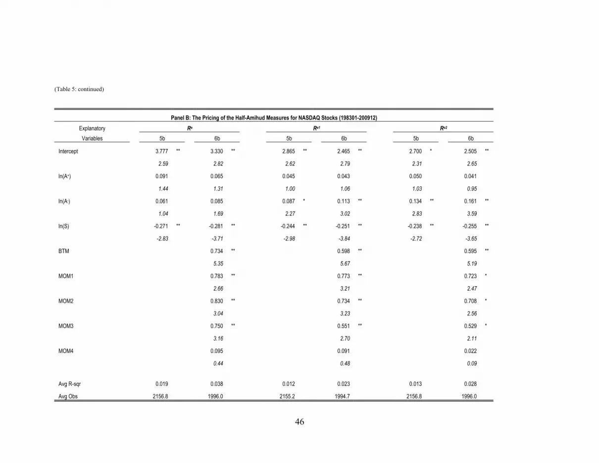
46
(Table 5: continued)
Panel B: The Pricing of the Half-Amihud Measures for NASDAQ Stocks (198301-200912) Explanatory Re Re1 Re2
Variables 5b 6b 5b 6b 5b 6b
Intercept 3.777 ** 3.330 ** 2.865 ** 2.465 ** 2.700 * 2.505 **
2.59 2.82 2.62 2.79 2.31 2.65
ln(A+) 0.091 0.065 0.045 0.043 0.050 0.041
1.44 1.31 1.00 1.06 1.03 0.95
ln(A-) 0.061 0.085 0.087 * 0.113 ** 0.134 ** 0.161 **
1.04 1.69 2.27 3.02 2.83 3.59
ln(S) -0.271 ** -0.281 ** -0.244 ** -0.251 ** -0.238 ** -0.255 **
-2.83 -3.71 -2.98 -3.84 -2.72 -3.65
BTM 0.734 ** 0.598 ** 0.595 **
5.35 5.67 5.19
MOM1 0.783 ** 0.773 ** 0.723 *
2.66 3.21 2.47
MOM2 0.830 ** 0.734 ** 0.708 *
3.04 3.23 2.56
MOM3 0.750 ** 0.551 ** 0.529 *
3.16 2.70 2.11
MOM4 0.095 0.091 0.022
0.44 0.48 0.09
Avg R-sqr 0.019 0.038 0.012 0.023 0.013 0.028
Avg Obs 2156.8 1996.0 2155.2 1994.7 2156.8 1996.0

47
Table 6
The Pricing of the Half-Amihud Measures Based on Market Movements This table reports the results of monthly Fama-MacBeth (1973) cross-sectional regressions that include the two (log-transformed) half-Amihud measures, ln(A+) and ln(A-) that use market returns to define up and down days, as well as the logarithm of firm size, ln(S). Panel A contains the result for NYAM-listed from July 1971 to December 2009, while Panel B does the same for NASDAQ-listed stocks from January 1983 to December 2009. The dependent variable is Re, Re1, or Re2. Re is the monthly excess return (in excess of the one-month T-bill rate); Re1is the FF3-adjusted excess return, i.e., the constant term plus the residual from the time-series regression of the excess return on the FF 3 factors using the entire sample range of the data; Re2 is the FF3-adjusted excess return using the Fama-French (FF) 3 factors with factor loadings estimated from the 5-year rolling regressions (past monthly returns must be available for at least 24 months); A+ (A-) is the half-Amihud measure for up (down) days, the monthly average of daily ratios of absolute returns to turnover on up (down) days. The other variables are defined in Table 1. The values in the first row for each explanatory variable are estimated coefficients , and the values italicized in the second row of each variable are t-statistics computed based on Fama-MacBeth (1973). To survive in the sample, stocks have five zero-volume days or fewer within a month (for NYSAM stocks) or 50 trades or more within a month (on average 2.5 trades or more per day) (for NASDAQ stocks). In addition, for the availability of Re2, stocks must have monthly returns for the past 60 months (at least 24 months). Only common stocks (share code 10 or 11 in CRSP) are used. The sample loses the first two observations in the cross-sectional regressions due to the 2-month lagging. The coefficients are all multiplied by 100. Avg R2 is the average of monthly adjusted R2. Avg Obs is the monthly average number of companies used in the cross-sectional regressions. Significance at the 1% and 5% levels is indicated by ** and *, respectively.
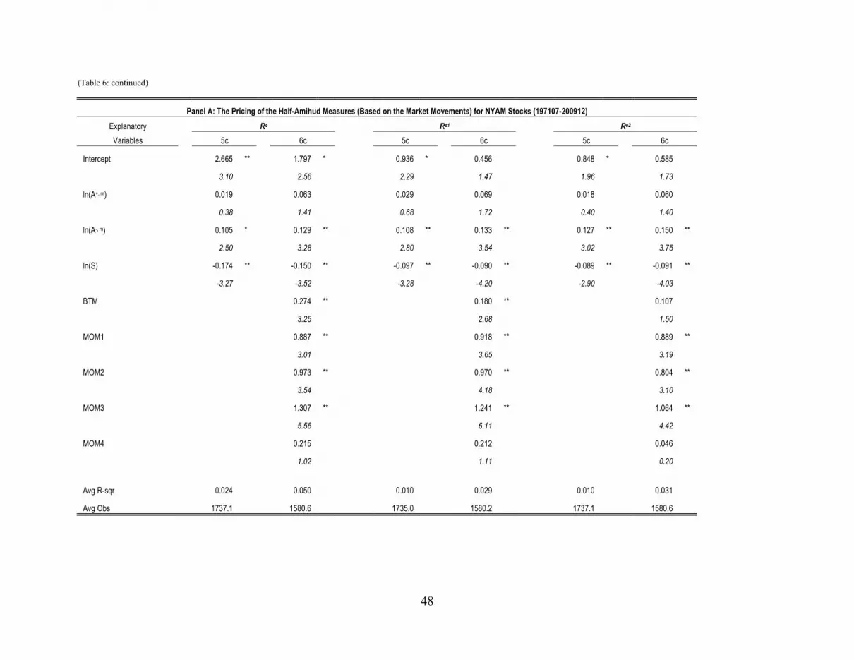
48
(Table 6: continued)
Panel A: The Pricing of the Half-Amihud Measures (Based on the Market Movements) for NYAM Stocks (197107-200912) Explanatory Re Re1 Re2
Variables 5c 6c 5c 6c 5c 6c
Intercept 2.665 ** 1.797 * 0.936 * 0.456 0.848 * 0.585
3.10 2.56 2.29 1.47 1.96 1.73
ln(A+, m) 0.019 0.063 0.029 0.069 0.018 0.060
0.38 1.41 0.68 1.72 0.40 1.40
ln(A-, m) 0.105 * 0.129 ** 0.108 ** 0.133 ** 0.127 ** 0.150 **
2.50 3.28 2.80 3.54 3.02 3.75
ln(S) -0.174 ** -0.150 ** -0.097 ** -0.090 ** -0.089 ** -0.091 **
-3.27 -3.52 -3.28 -4.20 -2.90 -4.03
BTM 0.274 ** 0.180 ** 0.107
3.25 2.68 1.50
MOM1 0.887 ** 0.918 ** 0.889 **
3.01 3.65 3.19
MOM2 0.973 ** 0.970 ** 0.804 **
3.54 4.18 3.10
MOM3 1.307 ** 1.241 ** 1.064 **
5.56 6.11 4.42
MOM4 0.215 0.212 0.046
1.02 1.11 0.20
Avg R-sqr 0.024 0.050 0.010 0.029 0.010 0.031
Avg Obs 1737.1 1580.6 1735.0 1580.2 1737.1 1580.6
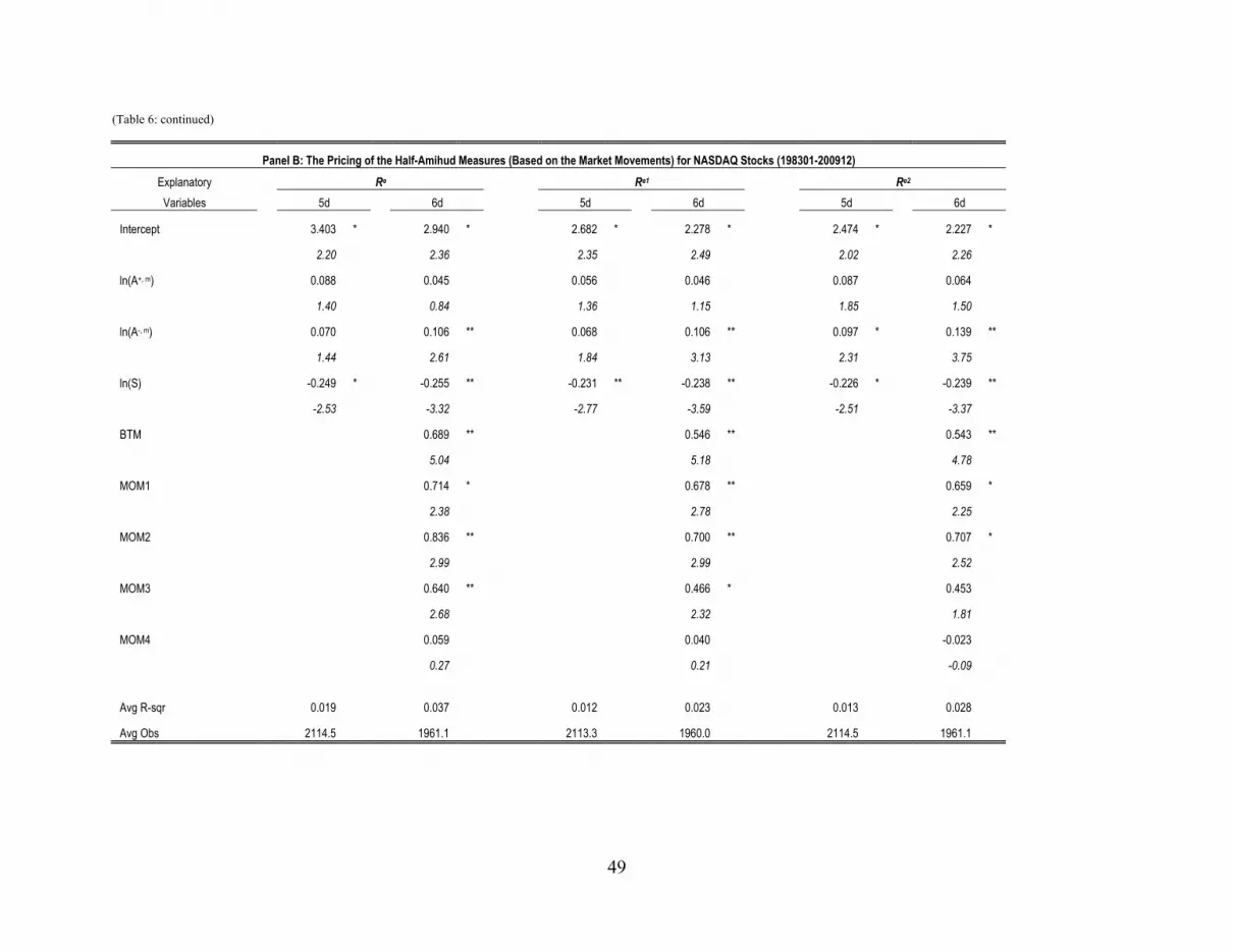
49
(Table 6: continued)
Panel B: The Pricing of the Half-Amihud Measures (Based on the Market Movements) for NASDAQ Stocks (198301-200912) Explanatory Re Re1 Re2
Variables 5d 6d 5d 6d 5d 6d
Intercept 3.403 * 2.940 * 2.682 * 2.278 * 2.474 * 2.227 *
2.20 2.36 2.35 2.49 2.02 2.26
ln(A+, m) 0.088 0.045 0.056 0.046 0.087 0.064
1.40 0.84 1.36 1.15 1.85 1.50
ln(A-, m) 0.070 0.106 ** 0.068 0.106 ** 0.097 * 0.139 **
1.44 2.61 1.84 3.13 2.31 3.75
ln(S) -0.249 * -0.255 ** -0.231 ** -0.238 ** -0.226 * -0.239 **
-2.53 -3.32 -2.77 -3.59 -2.51 -3.37
BTM 0.689 ** 0.546 ** 0.543 **
5.04 5.18 4.78
MOM1 0.714 * 0.678 ** 0.659 *
2.38 2.78 2.25
MOM2 0.836 ** 0.700 ** 0.707 *
2.99 2.99 2.52
MOM3 0.640 ** 0.466 * 0.453
2.68 2.32 1.81
MOM4 0.059 0.040 -0.023
0.27 0.21 -0.09
Avg R-sqr 0.019 0.037 0.012 0.023 0.013 0.028
Avg Obs 2114.5 1961.1 2113.3 1960.0 2114.5 1961.1

50
Table 7 The Pricing of the Two Directional Half-Amihud Measures and the Sidedness Components
This table reports the results of monthly Fama-MacBeth (1973) cross-sectional regressions that include the two directional half-Amihud measures, ln( ) and ln( ), and the other three components, ln( ), ln( ), and ln(S), for NYSAM from January 1983 to December 2009. The dependent variable is Re, Re1, or Re2. ( ,) ( is the directional half-Amihud measure for up (down) days which is the monthly average of daily ratios of absolute returns to buyer-initiated (seller-initiated) volume on up (down) days ( ) is ( the up-sidedness (downsidedness) component, which is the monthly average of daily ratios of buyer initiated (sell-initiated) turnover to total turnover on up (down) based on ISSM/TAQ S isthe monthly average of daily market values in $1,000. The other variables are defined in previous tables. To survive in the sample, stocks have at least 50 trades per month (on average 2.5 trades per day) in ISSM/TAQ. The values in the first row for each explanatory variable are the estimated coefficients, and the values italicized in the second row of each variable are t-statistics computed based on Fama-MacBeth (1973). The sample loses the first two observations in the cross-sectional regressions due to the 2-month lagging. The coefficients are all multiplied by 100. Avg R2 is the average of monthly adjusted R2. Avg Obs is the monthly average number of companies used in the cross-sectional regressions. Significance at the 1% and 5% levels is indicated by ** and *, respectively.
The Pricing of the Two Directional Half-Amihud Measures and the Sidedness Components
Explanatory Re Re1 Re2
Variables 7 8 7 8 7 8
Intercept 2.125 ** 1.907 ** 1.480 ** 1.262 ** 1.514 ** 1.609 **
3.44 2.87 3.85 3.53 3.83 4.27 ln( ) 0.029 0.064 0.052 0.053 0.037 0.028
0.50 1.09 1.20 1.10 0.77 0.51 ln( ) 0.250 0.277 0.352 * 0.307 0.404 * 0.303
1.10 1.35 1.97 1.59 2.09 1.44 ln( ) 0.159 ** 0.131 ** 0.120 ** 0.151 ** 0.132 ** 0.168 **
2.57 2.72 2.77 3.57 2.79 3.33 ln( ) 0.259 0.331 * 0.307 * 0.386 * 0.428 ** 0.475 **
1.39 1.96 2.21 2.47 2.83 2.88
ln(S) -0.120 ** -0.124 ** -0.112 ** -0.115 ** -0.105 ** -0.123 **
-2.85 -3.04 -3.95 -4.92 -3.62 -4.95
BTM 0.244 * 0.156 0.060
2.36 1.87 0.66
MOM1 0.668 0.710 * 0.743 *
1.89 2.34 2.29
MOM2 1.001 ** 0.988 ** 0.821 **
3.16 3.60 2.71
MOM3 1.047 ** 0.931 ** 0.750 **
3.51 3.83 2.81
MOM4 -0.022 -0.045 -0.087
-0.09 -0.20 -0.33
Avg R-sqr 0.020 0.049 0.012 0.032 0.012 0.035
Avg Obs 2244.3 1742.4 2244.3 1742.4 2244.3 1742.4

51
Table 8 With the Sample from the TAQ-Period (1993-2009) Only
This table reports the results of monthly Fama-MacBeth (1973)-type cross-sectional regressions for NYAM stocks over the TAQ-period: 204 months from January 1993 to December 2009. Panel A contains the results using the Amihud (2002) measure, ln(A0), and its CRSP-based components, ln(A), ln(A+), and ln(A-), while Panel B does the same using the TAQ-based components, ln( ), ln( ), ln( ), and ln( ). For robustness tests and comparison purposes, TAQ-based turnover (T*) is used in both panels (where applicable). The dependent variable is Re1, which is the FF3-adjusted excess return, i.e., the constant term plus the residual from the time-series regression of the excess return on the FF 3 factors using the entire sample range of the data. The other variables are defined in the previous tables. The values in the first row for each explanatory variable are estimated coefficients, and the values italicized in the second row of each variable are t-statistics computed based on Fama-MacBeth (1973). To survive in the sample, stocks have five zero-volume days or fewer within a month in CRSP, or 50 trades or more within a month (on average 2.5 trades or more per day) in TAQ. The sample loses the first two observations in the cross-sectional regressions due to the 2-month lagging. The coefficients are all multiplied by 100. Avg R2 is the average of monthly adjusted R2. Avg Obs is the monthly average number of companies used in the cross-sectional regressions. Significance at the 1% and 5% levels is indicated by ** and *, respectively.
With the Sample from the TAQ Period (1993-2009) Only
Panel A: With CRSP-based Components Panel B: With TAQ-based Components
Explanatory Dep. Var. = Re1 Explanatory Dep. Var. = Re1
Variables 2c 4c 6c Variables 8c
Intercept 1.172 ** 0.744 0.633 Intercept 0.920 *
3.49 1.83 1.42 2.05
ln(A0) 0.114 ** ln( ) -0.001
4.32 -0.01
ln(A) 0.169 ** ln( ) -0.009
4.08 -0.03
ln(A+) -0.027 ln( ) 0.199 **
-0.34 3.36
ln(A-) 0.238 ** ln( ) 0.428
3.05 1.95
ln(S) -0.091 ** -0.078 ** ln(S) -0.092 **
-3.26 -2.58 -3.21
BTM 0.127 0.134 0.140 BTM 0.120
1.19 1.26 1.32 1.14
MOM1 0.516 0.529 0.555 MOM1 0.512
1.27 1.30 1.37 1.26
MOM2 0.621 0.625 0.610 MOM2 0.613
1.78 1.80 1.77 1.77
MOM3 0.972 ** 0.984 ** 0.975 ** MOM3 0.935 **
3.26 3.32 3.31 3.19
MOM4 -0.481 -0.472 -0.478 MOM4 -0.477
-1.84 -1.80 -1.85 -1.86
Avg R-sqr 0.028 0.029 0.030 Avg R2 0.031
Avg Obs 1948.5 1948.5 1948.1 Avg Obs 1944.9
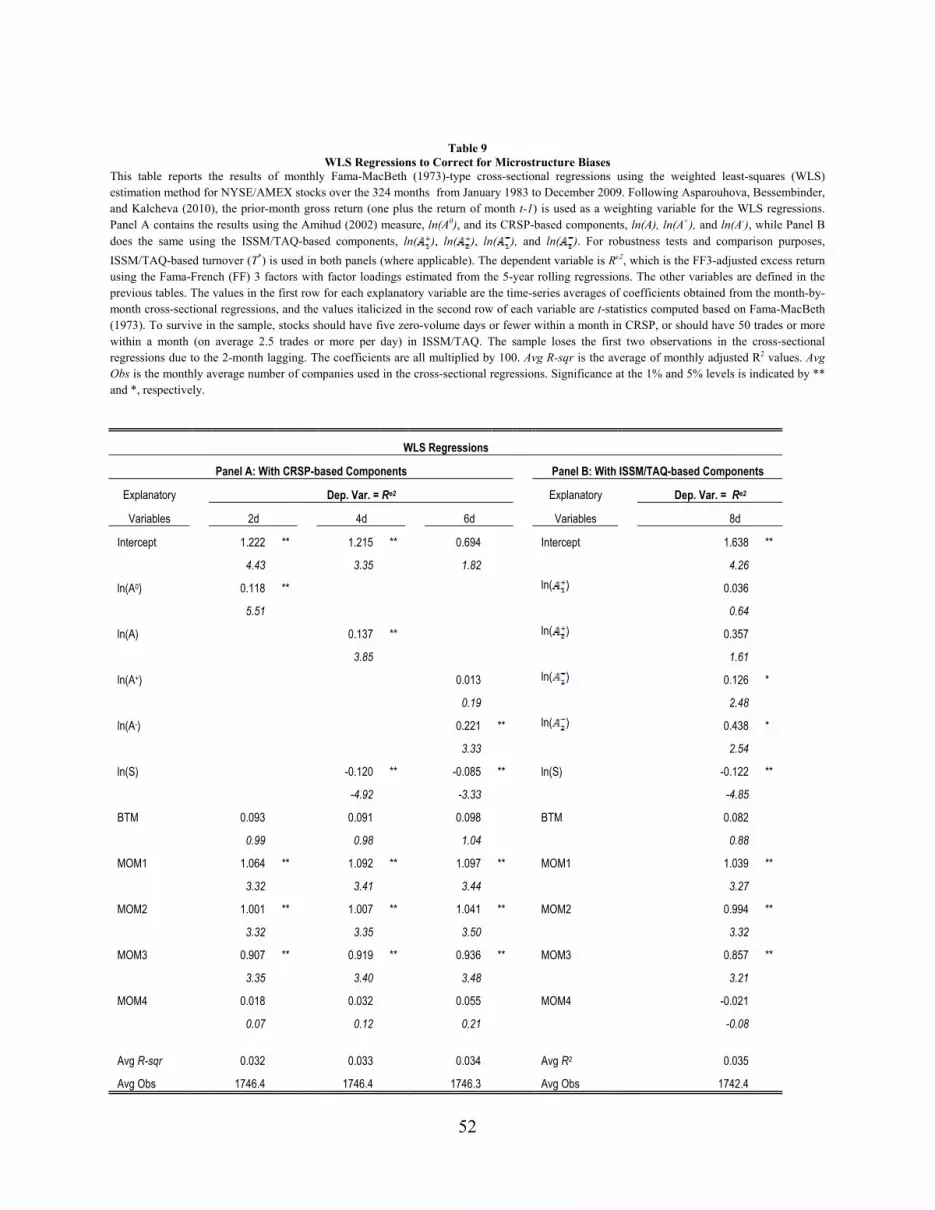
52
Table 9 WLS Regressions to Correct for Microstructure Biases
This table reports the results of monthly Fama-MacBeth (1973)-type cross-sectional regressions using the weighted least-squares (WLS) estimation method for NYSE/AMEX stocks over the 324 months from January 1983 to December 2009. Following Asparouhova, Bessembinder, and Kalcheva (2010), the prior-month gross return (one plus the return of month t-1) is used as a weighting variable for the WLS regressions. Panel A contains the results using the Amihud (2002) measure, ln(A0), and its CRSP-based components, ln(A), ln(A+), and ln(A-), while Panel B does the same using the ISSM/TAQ-based components, ln( ), ln( ), ln( ), and ln( ). For robustness tests and comparison purposes, ISSM/TAQ-based turnover (T*) is used in both panels (where applicable). The dependent variable is Re2, which is the FF3-adjusted excess return using the Fama-French (FF) 3 factors with factor loadings estimated from the 5-year rolling regressions. The other variables are defined in the previous tables. The values in the first row for each explanatory variable are the time-series averages of coefficients obtained from the month-by-month cross-sectional regressions, and the values italicized in the second row of each variable are t-statistics computed based on Fama-MacBeth (1973). To survive in the sample, stocks should have five zero-volume days or fewer within a month in CRSP, or should have 50 trades or more within a month (on average 2.5 trades or more per day) in ISSM/TAQ. The sample loses the first two observations in the cross-sectional regressions due to the 2-month lagging. The coefficients are all multiplied by 100. Avg R-sqr is the average of monthly adjusted R2 values. Avg Obs is the monthly average number of companies used in the cross-sectional regressions. Significance at the 1% and 5% levels is indicated by ** and *, respectively.
WLS Regressions
Panel A: With CRSP-based Components Panel B: With ISSM/TAQ-based Components
Explanatory Dep. Var. = Re2 Explanatory Dep. Var. = Re2
Variables 2d 4d 6d Variables 8d
Intercept 1.222 ** 1.215 ** 0.694 Intercept 1.638 **
4.43 3.35 1.82 4.26
ln(A0) 0.118 ** ln( ) 0.036
5.51 0.64
ln(A) 0.137 ** ln( ) 0.357
3.85 1.61
ln(A+) 0.013 ln( ) 0.126 *
0.19 2.48
ln(A-) 0.221 ** ln( ) 0.438 *
3.33 2.54
ln(S) -0.120 ** -0.085 ** ln(S) -0.122 **
-4.92 -3.33 -4.85
BTM 0.093 0.091 0.098 BTM 0.082
0.99 0.98 1.04 0.88
MOM1 1.064 ** 1.092 ** 1.097 ** MOM1 1.039 **
3.32 3.41 3.44 3.27
MOM2 1.001 ** 1.007 ** 1.041 ** MOM2 0.994 **
3.32 3.35 3.50 3.32
MOM3 0.907 ** 0.919 ** 0.936 ** MOM3 0.857 **
3.35 3.40 3.48 3.21
MOM4 0.018 0.032 0.055 MOM4 -0.021
0.07 0.12 0.21 -0.08
Avg R-sqr 0.032 0.033 0.034 Avg R2 0.035
Avg Obs 1746.4 1746.4 1746.3 Avg Obs 1742.4

53
Figure 1. Decomposition of the Amihud (2002) Measure of Illiquidity
The following figure shows: (i) how (the log-transform of) the original Amihud (2002) measure (A0) can be decomposed into the firm size (S) and the turnover-version Amihud measure (A); (ii) how the turnover-version Amihud measure (A) can be decomposed into the (two) ‘half-Amihud’ measures for up days and down days (A+ and A-); and (iii) how each of the two half-Amihud measures (A+ and A-) can be decomposed either (a) into the (two) ‘directional half-Amihud’ measures ( and ) as well as the (two) fractional turnover ratios (sidedness components,
and ), or (b) into the (two) ‘half-Kyle’ measures ( and ) as well as the (two) net turnover ratios ( and ). For details about the decomposition and variable definitions, see Section I in the main text.
Original Turnover-version Amihud Amihud Half-Amihud Directional Half-Amihud Measure Measure Measures and Half-Kyle Measures -------------- ------------------------- ------------------- -----------------------------------
= ln(S) + ln( ) + ln( ): Amihud
= ln(S) + ln(A+)
Up
Days = ln(S) + ln( ) + ln( ): Kyle
ln(A0) = ln(S) + ln(A)
Down = ln(S) + ln( ) + ln( ): Amihud
Days
= ln(S) + ln(A-)
= ln(S) + ln( ) + ln( ): Kyle

54
Figure 2. Time-Series Plots of the Amihud (2002) Measure and its Components The following figure shows the time-series plots of the Amihud (2002) measure and its components. The monthly cross-sectional average is weighted by the previous month-end market value of each stock. Figure 2(a) plots the original Amihud (2002) measure, ln(A0), for NYSE/AMEX stocks (denoted by “lnA0_NYAM” in the legend) over the 462 months (197107-200912) and for NASDAQ Stocks (“lnA0_NAS” in the legend) over the 324 months (198301-200912). Figure 2(b) plots the two half-Amihud measures, ln(A+) and ln(A-), for NYSE/AMEX stocks (denoted by “lnA_plus_NYAM” and “lnA_minus_NYAM,” respectively), while Figure 2(c) does the same for NASDAQ stocks. Figure 2(d) plots the two directional half-Amihud measures, ln( ) and ln( ) (denoted by “lnA1_plus” and “lnA1_minus,” respectively) as well as the two sidedness components, ln( ) and ln( ) (denoted by “lnA2_plus” and “lnA2_minus,” respectively) for NYSE/AMEX stocks.
(a) Value-weighted Average of the Amihud (2002) Measure in Both Markets
(b) Value-weighted Averages of the Half-Amihud Measures for NYSE/AMEX Stocks
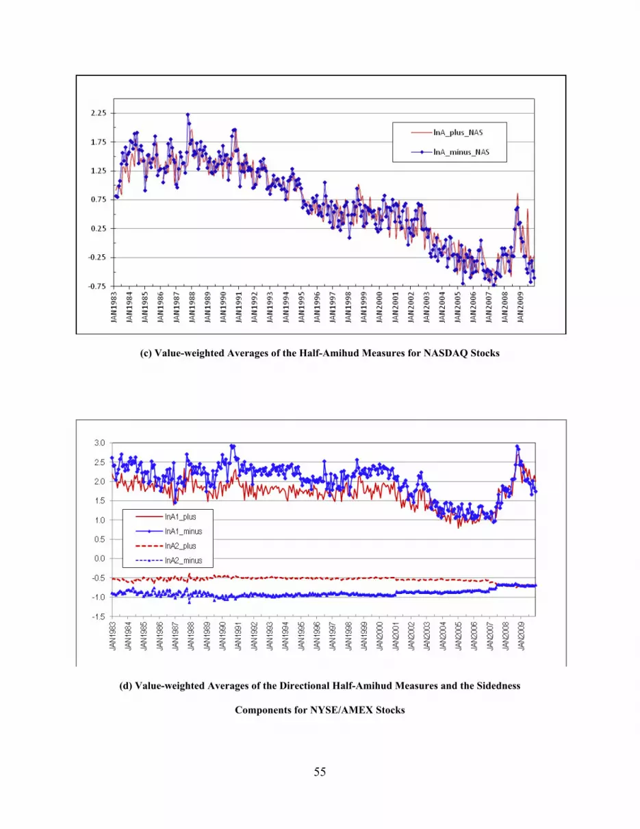
55
(c) Value-weighted Averages of the Half-Amihud Measures for NASDAQ Stocks
(d) Value-weighted Averages of the Directional Half-Amihud Measures and the Sidedness
Components for NYSE/AMEX Stocks

56
Table A1
Up Days vs. Down Days: ISSM/TAQ-based (Il)liquidity Measures for NYSE/AMEX Stocks
This table reports the mean values of three ISSM/TAQ-based (il)liquidity measures (%QSPR, DDepth, and ComposIlliq) for up days and down days separately as well as the t-statistics to test the null hypothesis that the difference between the two mean values (up-day mean – down-day mean) is equal to zero, using NYSE/AMEX-listed stocks over the 324 months (27 years) from January 1983 to December 2009. To obtain the monthly averaged values for the three (il)liquidity measures, each intradaily trade is first matched with relevant ask and bid quotes via the Lee and Ready (1991) algorithm; the intradaily values of the three measures are calculated within each day; the daily average values are obtained by averaging the intradaily values; and then the daily values for up days and down days are separately averaged within each month. The three (il)liquidity measures are defined as follows: %QSPR: the monthly mean proportional quoted spread (in %), obtained by averaging the daily mean values (within a month), which are in turn computed by averaging the intradaily values of [(ask price – bid price)/quote midpoint] x 100 within a day; DDepth: the monthly mean dollar depth (in $1,000), obtained by averaging the daily mean values (within a month), which are in turn computed by averaging the intradaily values of [(bid lot size x 100 x price + ask lot size x 100 x price)/2]/1,000 within a day; ComposIlliq: the monthly mean composite illiquidity, obtained by averaging the daily mean values (within a month), which are in turn computed by averaging the intradaily equivalents of %QSPR/DDepth within a day. All six series (3 measures x 2 categories) are Winsorized each month at the 0.5th and 99.5th percentiles. To form the tercile portfolios (MV1-MV3), each month the component stocks are split into three equal-numbered portfolios after being sorted on the previous month-end market value (MV: stock price times the number of shares outstanding) in ascending order. So MV1 consists of smallest stocks. For the pooled sample t-test, the total number of firm-months for the whole sample ranges from 491,969 to 511,269, while that for the tercile portfolios ranges from 163,814 to 170,195.
Up Days vs. Down Days: ISSM/TAQ-based (Il)liquidity Measures for NYSE/AMEX Stocks (198301-200912)
Whole Sample MV1 MV2 MV3
Variables Up/Down Days mean t-value mean t-value mean t-value mean t-value
Up Days 1.524 3.247 0.876 0.455 %QSPR
Down Days 1.546
-2.80 3.275
-1.86
0.904
-2.31
0.463
-0.71
Up Days 77.26 16.36 52.07 163.09 DDepth
Down Days 76.24
4.02 15.81
6.62
51.18
4.00
161.54
2.52
Up Days 5.630 16.144 0.647 0.125 ComposIlliq
Down Days 6.013
-5.65 17.233
-5.49
0.681
-4.02
0.141
-3.21

57
Table A2
The Pricing of the Turnover-version Amihud (2002) Measure by Sub-period This table reports the results of monthly Fama-MacBeth (1973)-type cross-sectional regressions (by sub-period) that include the turnover-version Amihud (2002) measure (not log-transformed but Winsorized), Awin. Panels A and B show the results for NYSE/AMEX-listed stocks over the entire period (462 months: 197107-200912) as well as its three sub-periods [Sub-period 1 (197107-198212), Sub-period 2 (198301-199512), and Sub-period 3 (199601-200912)], while Panels C and D do the same for NASDAQ-listed stocks over the entire period (324 months: 198301-200912) as well as its two sub-periods [Sub-period 2 (198301-199512) and Sub-period 3 (199601-200912)]. Panels A and C use the monthly average of daily turnover-version Amihuds within a month; and Panels B and D use the annual average of daily turnover-version Amihuds within a year (converted to a monthly series by filling the 12 months of the following year with the previous year’s annual average value). The dependent variable is Re1. The definitions of the variables are as follows. Re1: the FF3-adjusted excess return, i.e., the constant term plus the residual from the time-series regression of the excess return on the FF 3 factors using the entire sample range of the data; and Awin: the Winsorized (at the 1st and 99th percentiles) turnover-version Amihud measure, computed by the average of daily |r|/T within a month (Panels A and C) or within a year (Panels B and D), where r is the daily stock return and T is daily share turnover based on CRSP. The other variables are defined in Table 1. The values in the first row for each explanatory variable are the time-series averages of coefficients obtained from the month-by-month cross-sectional regressions, and the values italicized in the second row of each variable are t-statistics computed based on Fama-MacBeth (1973). To survive in the sample, stocks should have five zero-volume days or fewer within a month (for NYSE/AMEX stocks), or should have 50 trades or more within a month (on average 2.5 trades or more per day) (for NASDAQ stocks). In addition, for the availability of Re2, stocks should have monthly returns for the past 60 months (at least 24 months). Only common stocks (share code 10 or 11 in CRSP) are used. The sample loses the first two observations in the cross-sectional regressions due to the 2-month lagging. The coefficients are all multiplied by 100. Avg R-sqr is the average of monthly adjusted R2 values. Avg Obs is the monthly average number of companies used in the cross-sectional regressions. Significance at the 1% and 5% levels is indicated by ** and *, respectively.
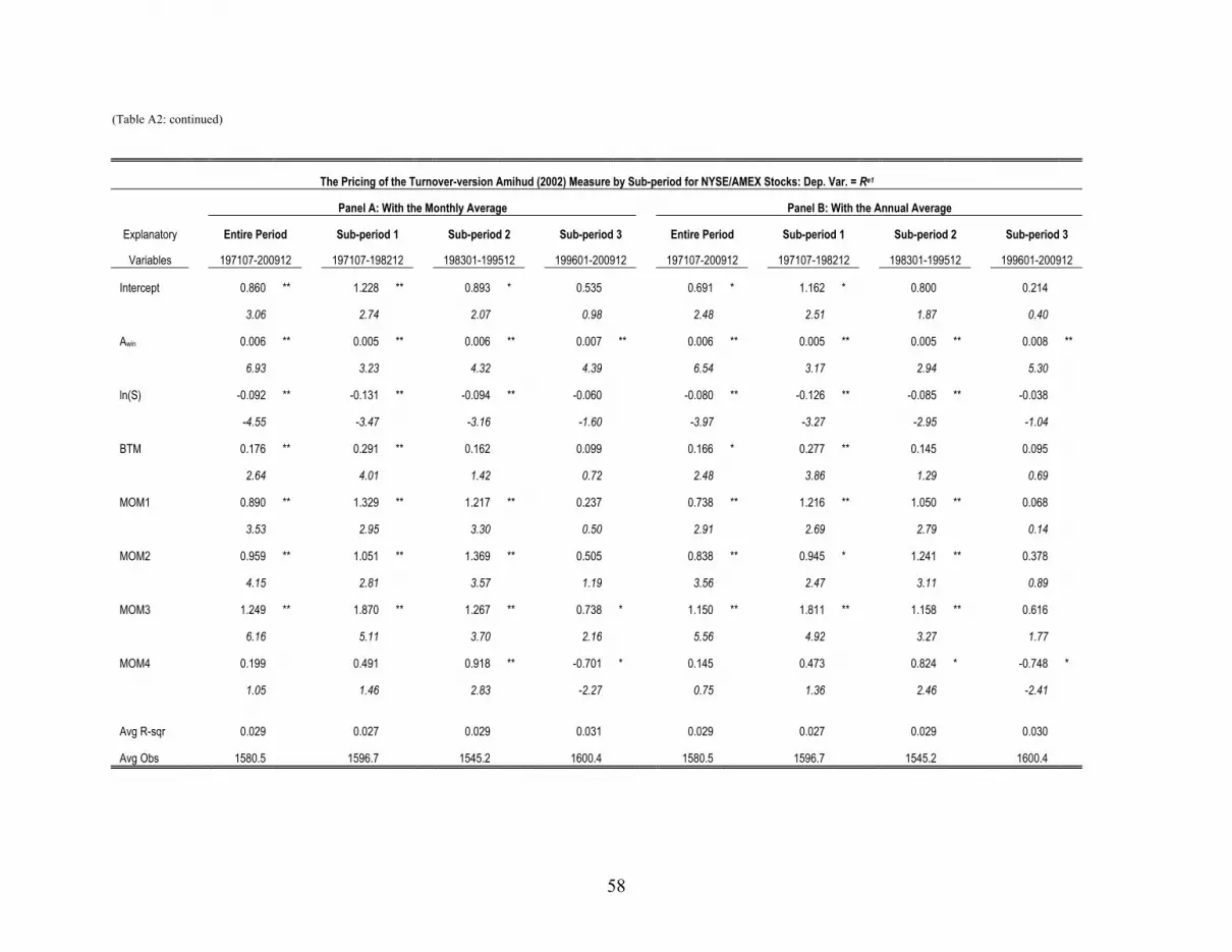
58
(Table A2: continued)
The Pricing of the Turnover-version Amihud (2002) Measure by Sub-period for NYSE/AMEX Stocks: Dep. Var. = Re1
Panel A: With the Monthly Average Panel B: With the Annual Average
Explanatory Entire Period Sub-period 1 Sub-period 2 Sub-period 3 Entire Period Sub-period 1 Sub-period 2 Sub-period 3
Variables 197107-200912 197107-198212 198301-199512 199601-200912 197107-200912 197107-198212 198301-199512 199601-200912
Intercept 0.860 ** 1.228 ** 0.893 * 0.535 0.691 * 1.162 * 0.800 0.214
3.06 2.74 2.07 0.98 2.48 2.51 1.87 0.40
Awin 0.006 ** 0.005 ** 0.006 ** 0.007 ** 0.006 ** 0.005 ** 0.005 ** 0.008 **
6.93 3.23 4.32 4.39 6.54 3.17 2.94 5.30
ln(S) -0.092 ** -0.131 ** -0.094 ** -0.060 -0.080 ** -0.126 ** -0.085 ** -0.038
-4.55 -3.47 -3.16 -1.60 -3.97 -3.27 -2.95 -1.04
BTM 0.176 ** 0.291 ** 0.162 0.099 0.166 * 0.277 ** 0.145 0.095
2.64 4.01 1.42 0.72 2.48 3.86 1.29 0.69
MOM1 0.890 ** 1.329 ** 1.217 ** 0.237 0.738 ** 1.216 ** 1.050 ** 0.068
3.53 2.95 3.30 0.50 2.91 2.69 2.79 0.14
MOM2 0.959 ** 1.051 ** 1.369 ** 0.505 0.838 ** 0.945 * 1.241 ** 0.378
4.15 2.81 3.57 1.19 3.56 2.47 3.11 0.89
MOM3 1.249 ** 1.870 ** 1.267 ** 0.738 * 1.150 ** 1.811 ** 1.158 ** 0.616
6.16 5.11 3.70 2.16 5.56 4.92 3.27 1.77
MOM4 0.199 0.491 0.918 ** -0.701 * 0.145 0.473 0.824 * -0.748 *
1.05 1.46 2.83 -2.27 0.75 1.36 2.46 -2.41
Avg R-sqr 0.029 0.027 0.029 0.031 0.029 0.027 0.029 0.030
Avg Obs 1580.5 1596.7 1545.2 1600.4 1580.5 1596.7 1545.2 1600.4

59
(Table A2: continued)
The Pricing of the Turnover-version Amihud (2002) Measure by Sub-period for NASDAQ Stocks: Dep. Var. = Re1
Panel C: With the Monthly Average Panel D: With the Annual Average
Explanatory Entire Period Sub-period 2 Sub-period 3 Entire Period Sub-period 2 Sub-period 3
Variables 198301-200912 198301-199512 199601-200912 198301-200912 198301-199512 199601-200912
Intercept 2.135 ** 1.536 2.673 * 2.065 * 1.723 2.373
2.64 1.63 2.09 2.51 1.79 1.82
Awin 0.005 ** 0.009 ** 0.002 ** 0.006 ** 0.009 ** 0.002 **
4.85 4.01 3.94 3.52 2.85 3.86
ln(S) -0.21 ** -0.19 ** -0.23 * -0.21 ** -0.20 ** -0.21 *
-3.47 -2.60 -2.41 -3.31 -2.71 -2.14
BTM 0.530 ** 0.832 ** 0.258 0.519 ** 0.825 ** 0.244
5.00 5.53 1.77 4.90 5.51 1.66
MOM1 0.654 ** 1.661 ** -0.251 0.451 1.348 ** -0.355
2.67 5.51 -0.69 1.87 4.51 -0.98
MOM2 0.680 ** 1.430 ** 0.006 0.530 * 1.216 ** -0.085
2.90 4.72 0.02 2.27 3.99 -0.25
MOM3 0.469 * 1.091 ** -0.090 0.346 0.905 ** -0.157
2.32 4.16 -0.30 1.72 3.41 -0.53
MOM4 0.044 0.506 -0.371 -0.036 0.393 -0.422
0.23 1.66 -1.65 -0.19 1.27 -1.89
Avg R-sqr 0.023 0.022 0.023 0.022 0.021 0.023
Avg Obs 1961.0 1293.7 2560.7 1961.0 1293.7 2560.7
60
Table A3
The Pricing of the Half-Amihud Measures in Portfolios Formed by Sorting on Market Value This table reports the results of monthly Fama-MacBeth (1973)-type cross-sectional regressions that include the two half-Amihud measures (log-transformed), ln(A+) and ln(A-), as well as the logarithm of firm size, ln(S), presenting the detailed analyses for the three portfolios formed by sorting on market capitalization. Panel A contains the result for NYSE/AMEX-listed stocks over the 462 months (38.5 years) from July 1971 to December 2009, while Panel B does the same for NASDAQ-listed stocks over the 324 months (27 years) from January 1983 to December 2009. Each month the component stocks are split into three equal-numbered portfolios (MV1-MV3) after being sorted on the previous month-end market value (MV: stock price times the number of shares outstanding) in ascending order. So MV1 consists of smallest stocks. The dependent variable is Re2. The definitions of the variables are as follows. Re2: the FF3-adjusted excess return using the Fama-French (FF) 3 factors with factor loadings estimated from the 5-year rolling regressions (past monthly returns should be available for at least 24 months); ln(A+): the natural logarithm of A+, which is the half-Amihud measure for up days, computed by the average of daily r+/T (within a month), where r+ = max[0, r], T is daily share turnover obtained from CRSP, and r is a daily stock return; ln(A-): the natural logarithm of A-, which is the half-Amihud measure for down days, computed by the average of daily -r-/T (within a month), where r- = min[r, 0]; ln(S): the natural logarithm of S, which is the average of daily market values (daily stock price times the total number of shares outstanding) (within a month) in $1,000. The other variables are defined in Table 1. The values in the first row for each explanatory variable are the time-series averages of coefficients obtained from the month-by-month cross-sectional regressions, and the values italicized in the second row of each variable are t-statistics computed based on Fama-MacBeth (1973). To survive in the sample, stocks should have five zero-volume days or fewer within a month (for NYSE/AMEX stocks), or should have 50 trades or more within a month (on average 2.5 trades or more per day) (for NASDAQ stocks). In addition, for the availability of Re2, stocks should have monthly returns for the past 60 months (at least 24 months). Only common stocks (share code 10 or 11 in CRSP) are used. The sample loses the first two observations in the cross-sectional regressions due to the 2-month lagging. The coefficients are all multiplied by 100. Avg R-sqr is the average of monthly adjusted R2 values. Avg Obs is the monthly average number of companies used in the cross-sectional regressions. Significance at the 1% and 5% levels is indicated by ** and *, respectively.

61
(Table A3: continued)
The Pricing of the Half-Amihud Measures in Portfolios Formed by Sorting on MV: Dep. Var. = Re2 Explanatory Panel A: NYSE/AMEX Stocks (197107-200912) Panel B: NASDAQ Stocks (198301-200912)
Variables MV1 MV2 MV3 MV1 MV2 MV3
Intercept 6.838 ** -3.639 ** -0.691 16.553 ** -7.342 ** -1.274
6.09 -4.62 -1.54 8.11 -3.67 -1.69
ln(A+ ) 0.103 -0.003 -0.209 ** 0.098 0.084 -0.065
1.76 -0.04 -2.84 1.61 1.52 -0.72
ln(A-) 0.207 ** 0.236 ** 0.304 ** 0.362 ** 0.051 0.136
3.83 3.33 4.18 5.35 0.88 1.58
ln(S) -0.693 ** 0.254 ** 0.029 -1.772 ** 0.607 ** 0.083
-6.96 4.31 1.10 -9.23 3.58 1.55
BTM 0.150 0.002 -0.052 0.455 ** 0.441 ** 0.209
1.68 0.02 -0.56 2.99 2.93 1.20
MOM1 1.491 ** 0.822 ** 0.057 0.937 * 1.443 ** 0.742 *
4.59 2.59 0.16 2.52 4.58 2.07
MOM2 0.925 ** 0.830 ** 0.856 ** 0.996 ** 1.089 ** 0.782 **
2.97 2.80 2.87 2.68 3.45 2.61
MOM3 1.158 ** 1.151 ** 1.359 ** 0.434 1.116 ** 0.502
3.89 4.37 4.28 1.33 3.67 1.64
MOM4 0.036 0.073 0.369 0.338 -0.044 0.048
0.13 0.28 1.19 1.01 -0.17 0.16
Avg R-sqr 0.036 0.038 0.057 0.028 0.028 0.036
Avg Obs 512.6 535.6 544.4 660.3 657.0 678.7