EXPLAINING THE DIVERSIFICATIONDISCOUNT

José Manuel Campa*Simi Kedia**

RESEARCH PAPER No 424October, 2000

* Professor of Financial Management, IESE** Professor of Harvard University

Research DivisionIESEUniversity of NavarraAv. Pearson, 2108034 Barcelona

Copyright © 2000, IESE

Do not quote or reproduce without permission

CIIFCENTRO INTERNACIONAL DEINVESTIGACION FINANCIERA

IESEUNIVERSIDAD DE NAVARRA

The CIIF (Centro Internacional de Investigación Financiera) is being set up as aresult of concerns from an interdisciplinary group of professors at IESE aboutfinancial research and will function as part of IESE’s core activities. Itsobjectives are: to unite efforts in the search for answers to the questions raisedby the managers of finance companies and the finance staff of all types ofcompanies during their daily work; to develop new tools for financialmanagement; and to go more deeply into the study and effects of thetransformations that are occurring in the financial world.

The development of the CIIF’s activities has been possible thanks to sponsorshipfrom: Aena, A.T. Kearney, Caja Madrid, Datastream, Grupo Endesa, FundaciónRamón Areces, Telefónica and Unión Fenosa.

EXPLAINING THE DIVERSIFICATION DISCOUNT

Abstract

Diversified firms trade at a discount relative to similar single-segment firms. We arguein this paper that this observed discount is not per se evidence that diversification destroysvalue. Firms choose to diversify. Firm characteristics which make firms diversify might alsocause them to be discounted. Not taking into account these firm characteristics might lead to theobserved discount being wrongly attributed to diversification. Data from the CompustatIndustry Segment File from 1978 to 1996 are used to select a sample of single-segment anddiversifying firms. We use three alternative econometric techniques to control for theendogeneity of the diversification decision. All three methods suggest the presence of self-selection in the decision to diversify and a negative correlation between firms’ choice todiversify and firm value. The diversification discount always drops, and sometimes turns into apremium, when we control for the endogeneity of the diversification decision. We do a similaranalysis in a sample of refocusing firms. Again, some evidence of self-selection by firms existsand we now find a positive correlation between firms’ choice to refocus and firm value. Theseresults consistently suggest the importance of taking the endogeneity of the diversificationstatus into account when analyzing its effect on firm value.

We thank Ben Esty, Stuart Gilson, Bill Greene, Charles Himmelberg, VojislavMaksimovic, Scott Mayfield, Richard Ruback, Myles Shaver, Jeremy Stein, Emilio Venezianand seminar participants at Harvard Business School, Western Finance Association Meetingsat Los Angeles, NBER Summer Conference in Corporate Finance, Cornell University,Georgetown University and Rutgers for helpful comments. We thank Sarah Woolverton forhelp with the data. Simi Kedia gratefully acknowledges financial support from the Divisionof Research at Harvard Business School. All errors remain our responsibility.

EXPLAINING THE DIVERSIFICATION DISCOUNT

Firms choose to diversify. They choose to diversify when the benefits of diversificationoutweigh the costs of diversification and stay focused when they do not. The characteristics offirms that diversify which make the benefits of diversification greater than the costsof diversification may also cause firms to be discounted. A proper evaluation of the effect ofdiversification on firm value should take into account the firm-specific characteristics which bearboth on firm value and on the decision to diversify.

Research by Lang and Stulz (1994), Berger and Ofek (1995) and Servaes (1996)shows unambiguously that diversified firms trade at a discount relative to non-diversified firmsin their industries. Other research confirms the existence of this discount on diversifiedfirms and this result seems to be robust to different time periods and different countries (1).There is a growing consensus that the discount on diversified firms implies a destruction ofvalue on account of diversification, i.e. on account of firms operating in multiple divisions.

This study shows that the failure to control for firm characteristics which lead firmsto diversify, and to be discounted, may wrongly attribute the discount to diversificationinstead of to the underlying characteristics. For example, consider a firm facing technologicalchange which adversely affects its competitive advantage in its industry. This poorlyperforming firm will trade at a discount relative to other firms in the industry. Such a firmwill also have lower opportunity costs of assigning its scarce resources in other industries,and this might lead it to diversify. If poorly performing firms tend to diversify, then nottaking into account past performance and its effect on the decision to diversify will result inattributing the discount to diversification activity rather than to the firm’s poor performance.

Also consider the case of a firm that possesses some unique organizationalcapability that it wants to exploit. Incomplete information may force this firm to enter intocostly search through diversification to find industries with a match to its organizationalcapital. Matsusaka (1995) proposes a model in which a value maximizing firm forgoes thebenefits of specialization to search for a better match. During the search period the marketvalue of the firm will be lower than the value of a comparable single-segment firm.Maksimovic and Philips (1998) also develop a model where the firm optimally chooses thenumber of segments in which it operates depending on its comparative advantage. Not takinginto account firm characteristics which make diversification optimal, in this case searching

(1) Servaes (1996) finds a discount for conglomerates during the 1960s, while Matsusaka (1993) documentsgains to diversifying acquisitions in the late 1960s in the United States. Lins and Servaes (1999) documenta significant discount in Japan and UK, though none exists for Germany. The evidence from emergingeconomies is mixed. While Khanna and Palepu (1999), Fauver, Houston and Naranjo (1998) find littleevidence of a diversification discount in emerging markets, Lins and Servaes (1998) report a diversificationdiscount in a sample of firms from seven emerging markets.

for a match, may again attribute the discount wrongly to value destruction arising fromdiversification.

This does not imply that there are no agency costs associated with firms operating inmultiple divisions. Consider the impact of cross sectional variation in private benefits ofmanagers. A firm with a manager who has high private benefits will undertake activitieswhich are at conflict with shareholder value maximization. Such a firm will be discountedrelative to other firms in its industry. Such a manager is also more likely to undertake value-destroying diversification. However, even in this case the observed discount on multi-segment years is partially accounted for by the ex ante discount at which the firm is trading,on account of high private benefits, before diversification. Not taking into account firmcharacteristics, in this case high agency costs, leads to an overestimation of the valuedestruction attributed to diversification.

In this paper, we attempt to control for this endogeneity of a firm’s decision todiversify when evaluating the effect of diversification on firm value. The arguments suggestthat the decision to diversify depends on the presence of firm-specific characteristics that leadsome firms to generate more value from diversification than others. Choice of organizationstructure should therefore be treated as an endogenous outcome that maximizes firm value,given a set of exogenous determinants of diversification, i.e. the set of firm characteristics.Evaluating the impact of diversification on firm value therefore requires taking into accountthe endogeneity of the diversification decision.

Controlling for the endogeneity of the diversification decision requires identifyingvariables that affect the decision to diversify while being uncorrelated with firm value. Thisbecomes difficult as most variables that bear on the diversification decision also impact firmvalue. We build on the methodology of Berger and Ofek (1995) and the insights of Lang andStulz (1994) to control for the endogeneity of the diversification decision. Like Berger and Ofek(1995), we value firms relative to the median single-segment firm in the industry. This measurehas the advantage of being neutral to industry and time shocks that affect all firms in a similarway. However, Lang and Stulz (1994) show that industry characteristics are important in afirm’s decision to diversify (2). We explore the data for systematic industry differences amongsingle-segment and diversifying firms that might help explain the decision to diversify.

We first reproduce the results existing in the literature and identify a diversificationdiscount in our sample. Preliminary data analysis shows that conglomerates differ from single-segment firms in their underlying characteristics. We control for the endogeneity of thediversification decision in three ways. Firstly, we control for unobservable firm characteristicsthat affect the diversification decision by introducing fixed firm effects. Secondly, we modelthe firm’s decision to diversify as a function of industry, firm and macroeconomiccharacteristics. We use the probability of diversifying as an instrument for the diversificationstatus in evaluating the effect of multiple-segment operations on firm value. Lastly, we modelan endogenous self-selection model and use Heckman’s correction to control for the self-selection bias induced on account of a firm’s choosing to diversify.

The diversification discount always drops, and sometimes turns into a premium,when we control for the endogeneity of the diversification decision. The evidence in all three

2

(2) Lang and Stulz (1994) find that firms that diversify tend to be in slow-growing industries. They also reportthat diversified firms have lower Tobin’s q than focused firms, but this difference was driven by differencesamong firms across industries rather than within an industry.

methods indicates that the discount on multiple-segment firm-years is partly due toendogeneity. The coefficient of the correction for self-selection is negative, indicating thatthere is a negative correlation between a firm’s choice to diversify and firm value. Thissupports the view that firm characteristics, which cause firms to diversify, also cause them tobe discounted.

Finally, we do a similar analysis in a sample of refocusing firms. Comment and Jarrell(1995), John and Ofek (1995) and Berger and Ofek (1996) document an increase in firm valueassociated with the decision to refocus. Much like the decision to diversify, the decision torefocus is also endogenous: Firms choose to refocus when the presence of firm-specificcharacteristics makes the benefits of refocusing greater than the costs of refocusing (3).Consider the case when changes in industry conditions generate higher-than-expected growthopportunities in one segment. This might increase the cost of an inefficient internal capitalmarket, increasing the cost of operating in multiple divisions and making refocusing optimal. Inthis case, firm characteristics which make the refocusing decision optimal, i.e. growthopportunities, also cause the firm to be more highly valued. Unlike the diversification decision,the refocusing decision is positively correlated with firm value. Not taking firm characteristics(in this case growth opportunities) into account prior to refocusing may erroneously attributethe associated premium to multi-segment operations of firms. This would lead to anunderestimation of the discount associated with multi-segment operations prior to refocusing.Controlling for firm characteristics which make the refocusing decision optimal may furtherincrease the discount associated with multi-segment operations of these firms. We documentevidence in support of this view.

The rest of the paper is organized as follows. In the next section we briefly discussrelated literature. Section III describes the data, sample selection criteria and preliminaryanalysis. Section IV discusses the estimation methodology. Section V presents the evidence fordiversifying firms and Section VI does the same for refocusing firms. Section VII concludes.

Related literature

There is a vast and well-developed literature on the benefits and costs of diversification.The gains from diversification could arise from many sources. Gains to diversification arise frommanagerial economies of scale as proposed by Chandler (1977) and from increased debt capacityas argued by Lewellen (1971). Diversified firms also gain from more efficient resourceallocation through internal capital markets. Weston (1970) argues that the larger internal capitalmarkets in diversified firms help them allocate resources more efficiently. Stulz (1990) showsthat larger internal capital markets help diversified firms reduce the underinvestment problemdescribed by Myers (1977). Stein (1997) argues that the winner-picking ability of headquartersmay allow internal capital markets in diversified firms to work more efficiently than externalcapital markets. Gains to diversification also arise from the ability of diversified firms tointernalize market failures. Khanna and Palepu (1999) document gains to business group

3

(3) In a static model, the above arguments would suggest that when the net benefit to operating in multiplesegments is negative, the firm should immediately refocus. In practice, the decision to diversify and refocusinvolves large amounts of sunk and irreversible costs that lead to a lot of persistence in diversificationstatus. There is as yet no clear understanding of the dynamic theory of firms’ diversification status, but onecan draw an analog from recent theory on irreversible investment decisions (see Dixit and Pindyck, 1994).This literature has emphasized that temporary shocks can have permanent effects due to hysteresis, which isconsistent with an observed discount of multiple-segment firms.

affiliation in India and emphasize the role of diversified groups in replicating the functions ofinstitutions that are missing in emerging markets. Hadlock, Ryngaert and Thomas (1998) arguethat diversified firms gain from a reduction of the adverse selection problem at the time of equityissues. Montgomery and Wernerfelt (1988), Matsusaka and Nanda (1994) and Bodnar, Tang andWeintrop (1998) propose gains to diversification based on the presence of firm specific assetswhich can be exploited in other markets. Schoar (1999) finds that diversified firms are moreproductive than firms within their industry on average, though they still appear to be discounted.

There are costs to diversification as well. The costs can arise from inefficientallocation of capital among divisions of a diversified firm. Stulz (1990) and Scharfstein(1998) show that diversified firms invest more than single-segment firms in poor lines ofbusiness or in businesses with low Tobin’s q. Lamont (1997) and Rajan, Servaes and Zingales(1997) also report evidence on inefficient allocation of capital within conglomerates. Meyer,Milgrom and Roberts (1992) make a related argument of cross subsidization of failingbusiness segments. The difficulty of designing optimal incentive compensation for managersof diversified firms also generates costs of multi-segment operations. Aron (1988, 1989),Rotemberg and Saloner (1994) and Hermalin and Katz (1994) show the greater difficulty ofmotivating managers in diversified firms in comparison to focused firms. Informationasymmetries between central management and divisional managers will also lead to highercosts of operating in multiple segments, as has been shown by Myerson (1982) and Harris,Kriebel and Raviv (1982). Lastly, costs of operating in multiple segments could arise onaccount of increased incentive for rent seeking by managers within the firm (see Scharfsteinand Stein (1997)) and opportunities for managers of firms with free cash flow to engage invalue destroying investments (see Jensen (1986), (1988)). Denis, Denis and Sarin (1997)provide empirical evidence that agency costs are related to the diversification decision. Theyfind that the level of diversification is negatively related to managerial ownership. Hyland(1999) examines firm characteristics including agency costs, and finds no support that agencycosts explain the decision of firms to diversify.

Our focus in this paper is not on identifying any of the above-mentioned individualbenefits and costs of diversification, but rather to concentrate on the net gain todiversification. Firms are likely to diversify when there are net gains to diversification andstay focused when there are net costs to diversifying. Most importantly for us, the aboveresearch shows that the benefits and costs of diversification are related to firm-specificcharacteristics. We control for firm characteristics which cause firms to diversify, i.e. whichgenerate a net gain to multi-segment operations, and isolate the net impact of thediversification decision.

Our paper is not the first to take into account the endogeneity of the diversificationdecision. A growing theoretical literature has been modeling the decision to diversify as a valueincreasing strategy for the firm. Matsusaka (1995) develops a model in which the firm choosesto diversify when the gains from searching for a better organizational fit outweigh the costs ofreduced specialization. Fluck and Lynch (1999) propose that diversification allows marginallyprofitable projects which could not get financed as stand-alone entities to get financed. Perold(1999) models the diversification decision in financial intermediaries and shows thatdiversification reduces firms’ deadweight costs of capital and so permits divisions to operate ona larger scale than stand-alone firms. Maksimovic and Philips (1998) also develop a modelwhere the firm optimally chooses the number of segments in which to operate depending on itscomparative advantage. They further show empirically that conglomerates allocate resourcesoptimally, based on the relative efficiency of divisions.

4

There has been other recent empirical work that provides evidence in support of theimportance of selection bias and the endogeneity of the diversification decision. Chevalier(2000) finds that even prior to merging, diversifying firms display investment patterns thatcould be identified as cross subsidization. Whited (1999) finds that after controlling for themeasurement problems in Tobins Q, there is no evidence of inefficient allocation of resourcesin diversified firms. Graham, Lemmon and Wolf (1999) propose that diversified firms arediscounted because they acquire discounted firms.

Data

Sample Selection

The sample consists of all firms with data reported on the Compustat IndustrySegment database from 1978 to 1996. We follow the Berger and Ofek (1995) [from here onBO(95)] sample selection criteria and exclude from the sample years where firms reportsegments in the financial sector (SIC 6000-6999), years with sales less than $20 million,years with a missing value of total capital and years in which the sum of segment salesdeviated from total sales by more than 1% (4). Additionally, we excluded years where thefirm did not report four-digit SICs for all its segments. The final sample consists of 8,815firms with a total of 58,965 firm years.

Measure of Excess Value

To examine whether diversification increases or decreases value, we use the excessvalue measure developed by BO (95), which compares a firm’s value to its imputed value ifeach of its segments operated as a single-segment firm. Each segment of a multiple-segmentfirm is valued using median industry sales and asset multipliers of single-segment firms. Theimputed value of the firm is the sum of the segment values. Excess value is defined as the log ofthe ratio of firm value to imputed value. Negative excess value implies that the firm trades at adiscount while positive excess values are indicative of a premium (5).

5

(4) Years with segments in the financial services were excluded on account of the difficulty in valuing financialfirms using multipliers. Years with sales less than 20 million dollars were excluded to prevent distortionscaused by including very small firms.

(5) The imputed value of a segment is obtained by multiplying segment sales (asset) with the median sales(asset) multiplier of all single-segment firm years in that SIC. The sales (asset) multipliers are the medianvalue of the ratio of total capital to sales (assets). Total capital is the sum of market value of equity, longand short-term debt and preferred stock. The industry definitions are based on the narrowest SIC groupingthat includes at least 5 firms. Extreme excess values, where the natural log of the ratio of actual to imputedvalue is greater than 1.386 or less than –1.386, were excluded. The imputed value using sales multipliers ofabout 50% of all firms was based on matches at the four-digit SIC code, 26.5% were based on matches atthe three-digit SIC code and 23.5% were based on matches at the two-digit or lower SIC code. The resultsusing asset multipliers are similar. This is in line with the results reported in BO (95) of 44.6% matches atthe four-digit level, 25.4% matches at the three-digit level and 30% matches at the two-digit level or lower.See BO (95) for further details on methodology.

Documenting the Discount

In this section, we document the existence of a discount in line with prior work. Wefind that the median discount on multi-segment years is 10.9% (11.6%) using sales (asset)multipliers for the entire sample from 1978 to 1996, similar to the discount of 10.6% (16.2%)reported by BO (95) for the years 1986 to 1991 (6). We begin by estimating a model ofexcess value as specified by BO (95) so as to guarantee that any differences in the finalresults are not driven by differences in sample or methodology. They model excess value as afunction of firm size, proxied by log of total assets, profitability (EBIT/SALES), investment(CAPX/SALES) and diversification, proxied by D, a dummy which takes the value 1 foryears when the firm operates in multiple segments and zero otherwise. As seen in Table I, thecoefficient of D is –0.13 (–0.12) and significant at the 1% (1%) level when sales (assets)multipliers are used. When we restrict the sample to the years 1986-1991, the coefficient of Dis –0.12 (–0.13) using sales (asset) multipliers, which is very close to the value of –0.144(–0.127) reported by BO (95). The estimated discount in our sample is similar to thatdocumented by BO (95).

We test the robustness of the estimated discount to model specification by includinglagged values of firm size, profitability and investment. Past profitability and investment maycontrol for firm characteristics which affect firm value. We also include log of total assetssquared to control for the possibility of a non-linear effect of firm size on firm value. Thecoefficient of the square of firm size is negative, suggesting that the positive effect of firmsize on excess value diminishes as firm size increases. We also include the ratio of long-termdebt to total assets. The results, reported in columns 3 and 6 of Table 1, show that theestimated discount is about 11% with both sales and asset multipliers. There is weak evidencethat firms with high past profitability (high EBIT/SALES) and high past investments (highCAPX/SALES) are valued higher than the median single-segment firm in the industry,though the coefficients are not significant. Summarizing, multiple-segment firms show asignificant discount and this discount is robust to the inclusion of additional variables in thevaluation equation. We report all results with this extended model. As a comparison, theresults with the basic BO (95) model are similar and are discussed in Sections 5.5 and 6.5.

Are multi-segment firms different?

In this section, we examine the characteristics of conglomerates which might causethem to diversify. We also examine if conglomerates differ from single-segment firms in theirunderlying characteristics.

6

(6) For the years 1986 to 1991, we find that the median multiple-segment discount in our sample is 7.6%(10.3%) using sales (asset) multipliers. This difference with the BO (95) results is possibly due to adifference in sample size. The number of firm years, in the period 1986 to 1991, in our sample is 17875,greater than the 16181 reported by BO (95). There are 4565 firms in our sample as opposed to 3659 firmsreported by BO (95). Our sample size is larger by 1142 (977) observations when using sales (asset)multiplier regressions. This increase in the sample size could arise on two accounts. Firstly, if firms restatetheir results such that they are no longer excluded due to one or more sample selection criteria, they mightbe included in our sample while not being included in the BO (95) sample. Secondly, Compustat might addfirms to the database along with the data for prior years. The largest category in this group (according toCompustat sources) consists of small firms which trade on OTC markets and are added when they changelisting or on client request. Our overall sample, from 1978 to 1996, of 8815 firms and 58965 observations issimilar to the sample of 8467 firms and 58332 observations reported by Graham, Lemmon and Wolf(1999).

The 8,815 firms in our sample differ in their diversification profiles. The largestgroup consists of 5,387 single-segment firms, which accounted for 30,284 firm years, asshown in Table II. The rest are firms which report operating in multiple segments at somepoint in the time period under consideration. These firms will be referred to as multiple-segment firms or conglomerates in the paper. Among these multiple-segment firms, therewere broadly four kinds: Firms which diversify, those that refocus, those that do both andlastly conglomerate firms which do not change the number of segments in which theyoperate. The largest group consists of 1,371 firms (13,133 firm years) which report bothincreasing and decreasing the number of segments in this time period. The next largest groupconsists of 873 firms (7,987 firm years) who refocused. There are 606 firms (4,326 firmyears) which report diversifying in this period (7).

Next we examine the characteristics of single-segment and multiple-segment firmyears. Table III reports average value of firm size, investment, profitability, leverage, researchand development and industry growth rates for the different diversification profiles. Industrygrowth rate is the increase in industry sales, defined at the two-digit SIC level. SICclassification was obtained from the business segment data. Divisional sales for conglomerateswere included in the respective SICs for the calculation of total industry sales (8).

Single-segment years of conglomerates are significantly different from single-segmentfirms in their characteristics. Single-segment years of conglomerates are bigger, have higherleverage and lower R&D than single-segment firms. This is consistent with Hyland (1999), whofinds that diversifying firms have lower research and development expenses. With regard toCAPX/SALES and EBIT/SALES, not only do single-segment years of conglomerates differfrom single-segment firms, but they also differ significantly among them. Single-segment yearsof diversified firms have higher CAPX/SALES and higher EBIT/SALES, while single-segmentyears of refocusing firms and firms which both refocus and diversify have lower CAPX/SALESand lower EBIT/SALES than single-segment firms. In summary, firm characteristics differacross single-segment years in different diversification profiles.

There are also significant differences in the characteristics of multi-segment years ofconglomerates. Multiple segment years of diversifying firms tend to invest more in researchand development (RND/SALES) than others. They also have higher capital investment(CAPX/SALES) and higher profitability (EBIT/SALES) than multiple-segment years ofrefocusing firms and firms which both refocus and diversify. Conglomerates that do notchange diversification status seem to be in mature industries with lower growth and have lowresearch and development costs while enjoying a higher profitability (EBIT/SALES) andhigher capital investment (CAPX/SALES). Multiple segment years of refocusing firms tendto have the lowest profitability and capital investment. This suggests that differences incharacteristics of multiple-segment years might be related to the choice of diversificationstrategy.

Next we examine the characteristics of the discount over time and across thedifferent diversification profiles. Table IVa documents the average annual discount from 1978to 1996 estimated using sales and asset multipliers. There is substantial variation, with the

7

(7) Firms were classified using all available data, i.e. the years excluded on account of sample selection criteriawere also taken into account for the purpose of categorizing firms. This ensures that restructuring activity inyears that were excluded from the sample is also taken into account.

(8) Total industry sales is a function of firms entering and leaving Compustat, of restructuring activities offirms and of accounting changes which cause firms to report sales in different SICs over the years. Thesegrowth rates therefore have been estimated with noise and have high volatility.

median discount using sales multipliers being as low as –0.058 in 1982 and zero for years1987 to 1991. The excess value measures firm value relative to the median single-segmentfirm in the industry for that year. This makes the excess value measure industry- and time-neutral. What generates these time patterns in the excess value measure?

Time patterns in the excess value measure could arise on account of two factors.Firstly, the distribution of single-segment firms around the median could change. As can beseen from Columns 2 and 3 of Table IVb, though the median excess value of all single-segmentfirm years used to estimate median industry multipliers is zero by construction, the mean variesfrom –0.02 in 1992 to +0.01 in 1989. Secondly, time effects could also arise on account of entryand exit of firms in the sample. Table IVb, columns 4-7, documents the average annual excessvalues (using sales multipliers) for the last and first year of firms in the data. There are twointeresting facts which emerge from Table IVb. First, firms have negative excess value in thelast year in the data. This effect is not limited to just the last year in the dataset but these firmsare not average discounted. Let us refer to these firms that exit the sample, i.e. are included inthe Compustat research tapes, as exiting firms. In contrast, new firms in the data set havepositive excess values in their first year. These new firms entering the data are valuedsystematically higher relative to the median single-segment firm in the industry. Secondly, thereis variation over time in the number of firms exiting and entering the data. Exit (entry) of firmswith low (high) excess values reduces (raises) the median industry multiplier in that year,consequently increasing (decreasing) the relative valuation of existing firms in the industry.Though the median excess values of single-segment years have been normalized to zero, themedian excess values of conglomerates will have a time pattern related to the changes inindustry composition rather than to changes in its intrinsic value.

This would not be of much concern in the estimation of the impact of diversificationstatus on firm value if firms entered and exited the sample randomly. This is because thevalues of all firms, single and conglomerate, change proportionately over time, leaving therelative valuation of multiple-segment firm years unchanged. However, if changes in industrycomposition are not random but related to the decision of firms to diversify or refocus, thenchanges in industry composition become a source of concern. Consider, for instance, a firmwhich diversifies when poorly performing firms in the industry exit on account of few growthopportunities in the industry. Exit of poor performers raises the median industry multiplierand increases the imputed value of the diversifying firm when it diversifies. This will causethe firm to trade at a discount after diversification. This discount is due to change in industrycomposition (exit of poor performers), which is correlated with the decision to diversify,rather than due to any change in the firm’s intrinsic value.

To examine whether changes in industry composition differ by diversificationdecision, we study the distribution and percentage sales accounted for by exiting firms. Foreach firm, we calculate the share of sales accounted for by exiting firms in their industry (atthe two digit SIC level) for that year. For conglomerates, we weight each segment’s exposureto exiting firms by its sales. We also calculate the fraction of all firms in an industry that exit.Table IVc documents the average exposure to exiting firms for the different diversificationprofiles, and highlights some interesting patterns. Single-segment years of diversifying firmsoperate in industries with the highest incidence of exit. In these industries, 28% of all firmsexit in a given year and the exiting firms account for 15% of industry sales. Single-segmentfirms in contrast belong to industries where exiting firms account for only 14% of all firmsand 6% of industry sales. While single-segment years of diversifying firms have the highestexposure to exiting firms, multiple-segment years of diversifying firms have one of thelowest exposures to exiting firms. In contrast, single-segment years of refocusing firmsoperate in industries with the lowest fraction of exiting firms while multiple-segment years of

8

refocusing firms tend to be in industries with the highest incidence of exiting firms. Weobserve that firms are moving towards industries where the exit rate is significantly lower,which suggests that firms both diversify and refocus, from industries experiencing difficulties(higher exit) into industries with better prospects (lower exit). This also supports the findingin Lang and Stulz (1995) that diversifying firms tend to be in bad industries characterized byhigher exit. This is consistent with our view that firms endogenously choose to diversify andrefocus and indicates that changes in industry composition are related to the firms’diversification strategy.

Firms also show systematic patterns in their discounts prior to whether they decideto diversify or exit the industry. Single-segment years of diversifying firms do not trade at adiscount. This indicates that these firms do not do badly compared to the median firm in theindustry prior to diversifying. However, as seen from Table IVc these firms are in industrieswith high incidence of exit. Combining these two results suggests that single-segment yearsof diversifying firms might be better than the firms which exit the industry but worse than thefirms which continue as single-segment firms in the industry. This intuition is confirmed bythe statistics reported in Table IVd. Single-segment years of diversifying firms which do notexit, have a median discount of zero. This is better than the 4% discount for single-segmentfirms in the same four-digit SIC which exit and worse than the 2% premium for single-segment firms in the same four-digit SIC which do not exit.

Summarizing, there are significant differences in firm characteristics between single-segment firms and single-segment years of conglomerates. There are also significantdifferences in firm characteristics between multiple-segment years of conglomerates withdifferent diversification profiles. There are also differences in industry compositions over time.Firms which diversify (focus) come from industries with high exit rates. These firms havevalues prior to diversification that are significantly higher than those of firms that exit theindustry but lower than those of the firms that remain as single-segment firms. These changesin industry composition seem to be correlated with the decision to diversify and refocus. Wewill try to control for both firm specific as well as these industry specific changes which mightcause the decision to diversify/refocus to be correlated with the estimated discount. The nextsection discusses the methodology to control for this endogeneity.

Estimation methodology

We examine the effect of diversification on firm value by modeling firm value as afunction of firm characteristics. We define our measure of relative firm value, Vit, as:

(1)

where Xit is a set of exogenous observable characteristics of the firm, Dit is adummy variable that takes the value of 1 if the firm operates in more than one segment and 0otherwise, δ = {δ0, δ1, δ2} is a vector of parameters to be estimated, and eit is an error term.

Our hypothesis is that firms that choose to diversify are not a random sample offirms. If the decision of these firms to diversify is correlated with the relative value of the firm,Dit will be correlated with the error term in equation (1). The OLS estimate of δ2 will thereforebe biased. Specifically, we assume that a firm’s decision to diversify is determined by

9

V X D eit it it it= + + +δ δ δ0 1 2

(2)

where Dit* is an unobserved latent variable, Zit is a set of firm characteristics that affect the

decision to diversify, and µit is an error term. The correlation between Dit and eit in equation (1)will arise when: (a) some of the exogenous variables in the diversification equation, Zit, affectthe firm’s relative value but are not included as regressors in the value equation; or (b) the errorterms eit and µit are correlated. In either case the estimation of δ2 using ordinary least squareswill be biased.

We use three different techniques to control for the correlation between Dit and eit inequation (1) and come up with an unbiased estimator of δ2. First, we take advantage of theavailability of a panel data-set and use a fixed-effect estimator in equation (1), assuming thatall the unobserved heterogeneity that leads to the correlation between the error terms isconstant over time.

Secondly, we attempt to jointly estimate equations (1) and (2) in a simultaneousequation framework. The estimation of this system of simultaneous equations is not easybecause the natural instruments for Dit, the observed firm characteristics, are already includedin the firm value equation (equation (1)), causing the system to be unidentified (9). As Vit isthe firm’s value relative to the median firm in the industry in any given year, it is, byconstruction, independent of any observable characteristics which affect the value of all firmsin a given industry and year in the same manner (10). Lang and Stulz (1994) show thatindustry characteristics influence the decision to diversify. Maksimovic and Philips (1999)highlight the importance of time characteristics and document that assets are reallocatedacross firms during economic expansions. We too have documented systematic patterns at theindustry level that result in a correlation among a firm’s relative value and its decision todiversify (11).

To capture the overall attractiveness of a given industry to conglomerates, we usethe fraction of all firms in the industry which are conglomerates (PNDIV). The higher thefraction of multi-segment firms (PNDIV), the more attractive the industry factors are todiversification (12). We also include, for each firm, the fraction of sales by other firms in theindustry accounted for by diversified firms (PSDIV). As these two variables are highlycorrelated, we evaluate them jointly to determine the effect of industry factors on thediversification decision. We instrument time effects on the diversification decision in variousways. Firstly, we capture time trends as evidenced by the existence of merger waves. We

10

D Z

D D

D

it it it

it it

it

*

*

= +

= >= <

β µ

1 0

0 0

if

if Dit

(9) Strictly speaking, identification could be obtained only from the non-linearity of Dit in equation (2), butrelying exclusively on the functional form will lead to very weak identification.

(10) Notice that the estimation of equation (1), where Vit is defined as firm value relative to the median firm inan industry, is almost analogous to the estimation of an industry fixed-effect estimator.

(11) As stated in the introduction, Lang and Stulz (1994) report that diversified firms have on average lowerTobin’s q than single-segment firms, and that the q for diversifying firms was not significantly lower thanthe q for the median firm in their industry. This observation led them to the conclusion that industrycharacteristics influence the decision to diversify. These industry characteristics could, therefore, serve asinstruments for diversification. Wernerfelt and Montgomery (1988) also find significant industry effects.

(12) The industry specific factors which influence the decision to diversify may range from changes in industryregulation, introduction of new technology, market structure and business risk. We use two-digit SIC codesfor industry classification. Firms were classified into industries based on their segment SIC. Forconglomerates we use a sales weighted average of all its segments.

include the number of merger/acquisition announcements in a given year (MNUM). Themore active the market for mergers/acquisitions, the higher the probability that a firm willdiversify. We also include the annual value of announced merger/acquisitions, in billions ofUS $ (MVOL). Secondly, we capture time trends in the macroeconomic conditions andbusiness cycles. We include real growth rates of gross domestic product (GDP) and its laggedvalue (GDP1). We also include the number of months in the calendar year that the economywas in a recession (CONTRAC) and its lagged value (CONTRAC1) (13).

We also include exchange listing of the firm to predict the decision to diversify. Wecreate a dummy (MAJOREX) which takes the value 1 when the firm is listed on NYSE,NASDAQ, or AMEX and zero otherwise. Firms are more likely to diversify or refocus ifthey are listed on the major exchanges. Listing on major exchanges facilitates firms’acquisition and divestiture by generating greater visibility and reducing informationasymmetries (making it easier to raise external financing) through greater analyst coverage.However, firms listed on major exchanges are also likely to have greater liquidity. As firmswith higher liquidity might be valued higher this might also affect relative firm value. Wecreate a dummy variable (SNP) which takes the value 1 if the firm belongs to the S&Pindustrial index or the S&P transportation index, and zero otherwise. This dummy variable(SNP) controls for liquidity as firms belonging to the S&P index have higher liquidity. Asliquidity impacts both relative firm value and the decision to diversify, we include this SNPvariable in both equations 1 and 2.

Finally, we also use whether or not the firm is a foreign firm as an instrument. Wecreate a dummy (FOREIGN) which takes the value 1 when the firm is incorporated abroadand zero otherwise. Foreign firms might list in the US prior to major financing or as part ofacquisition/corporate restructuring strategy. Foreign firms are therefore more likely to engagein both diversification and refocusing activities. Though being foreign may predict theprobability of diversifying and refocusing, it does not affect relative firm value. We alsocontrol for average firm characteristics by including the historical average value of log oftotal assets, EBIT/Sales and CAPX /Sales.

The third method to control for endogeneity is to control for the self-selection of firmsthat diversify using Heckman’s (1979) two-stage procedure. We estimate expected firm valueconditional on the firm being diversified as E (Vit / Dit = 1) = δ0 + δ1Xit + δ2 +E (eit / Dit = 1).Assuming that the errors in equations (1) and (2), eit and µit, have a bivariate normaldistribution with mean zero, standard deviation σe and 1 and with correlation ρ, we have

are respectively the

density and cumulative distribution functions of the standard normal. Similarly, we estimatethe expected firm value conditional on the firm being focused as

11

(13) We thank Scott Mayfield for the suggestion of using merger waves, and the editor, Rene Stulz, for thesuggestion of using business cycles to instrument for time trends. The data on merger volume and numberis from Securities Data Corporation and data on GDP growth rates and business cycles is from NBER.

E (e ( where andit

(.) (.)

/ = ρ λ β ) λ

ββ1 1 φD Zit e it Øσ

φ( )

( )

( ),βZ

Øit

it

it

Z

Z=

E (V it / = ) = 0Dit 0 01δ δ+ + =X E e Dit it it( / )

In this case,

The difference in the value of single-segment and diversified firms, is given by

(3)

The right-hand side of the equation (3) is what is estimated by the OLS coefficient ofDit in equation (1). This estimated discount, using OLS, will therefore be biased downward if ρ,the correlation of the error terms, is negative, as hypothesized for diversifying firms. Thisestimated discount will be biased upward if ρ is positive, as hypothesized for refocusing firms.

In line with the Heckman two-step procedure, we first estimate equation (2) using aprobit model to get consistent estimates of β denoted by . These are then used to getestimates of λ1 and λ2, the correction for self-selection. In the second step, we estimate δ byestimating

(4)

where δλ = ρσe. The sign of δλ in the above regression is determined by the sign ofρ, the correlation between the error terms in equations (1) and (2). We separately examinediversifying and refocusing firms and control for the endogeneity of the diversification/refocusing decision (14).

Diversifying firms

We select a sample of all single-segment firms and all diversifying firms.Diversifying firms included in the sample are those that diversify once from single tomultiple segments, those that diversify once from multiple to multiple segments and thosethat diversify multiple times (15). In this sample, we examine whether or not there is any lossof value associated with operating in multi-segments. We first estimate the model by ordinaryleast squares. Columns 2 and 7 in Table V report the results of the estimation of the BO (95)model in this sample. The estimated multi-segment discount is –0.13 (–0.11) using sales(asset) multipliers. The estimated discount in this sample of single-segment firms anddiversifying firms is similar to the discount reported for the entire sample in Table I. Columns3 and 8 report the OLS results for the extended model. The discount using sales (asset)multiples is 0-0.11 (–0.09) and is significant at the 1% (1%) level.

12

E (e D where ( (it it/ ) ( ) ( )

)).= = −

−ρσ λ β λ β βΖ

φ β2 2e Z ZZit it

it

it

Ø

1

E E e (V / D (V / D ( Z

it it ititØ= − = = +1 0 2) ))))

.it it

δ σρ βφ (βΖ

V X D Z D Z D

X D D

it it it it it it

it it it it

= + + + + + + − +

= + + + + +

δ δ δ λ λ β η

δ δ δ δ δ λ η

λ

λ

0 1 2 1 2

0 1 2 2

1 [ ( ) * ( ) * ( )]^ ^

β

(14) Given our lack of understanding of the full dynamics of diversification and refocusing by firms, wecondition the sample based on whether firms choose to diversify or to refocus rather than pool allobservations in one sample.

(15) To ensure that the sample of firms stays the same across all methods, firms with only one year of data havebeen removed. These firms would not have been included in the fixed-effects estimation. Further, outliershave also been excluded.

β̂

Fixed-effect estimation

As discussed in the previous section, we introduce fixed firm effects to control forunobservable firm characteristics and year effects to control for time effects which affect thediversification decision. The results of this estimation are reported in Columns 4 and 9 ofTable V. The introduction of two-way fixed effects reduces the estimated discount to 6%(4%) significant at the 1% (5%) level with sales (asset) multipliers.

The introduction of firm fixed effects reduces the inter-firm variability in the dataand might increase the noise-to-signal ratio in the estimation. However, the signs andsignificance of the coefficients on all other variables in the estimation, with the exception ofleverage and square of assets, remain practically identical to the OLS estimation. The onlycoefficient that significantly changes in the regression is the coefficient on D. This resultsupports the view that diversification appears to be correlated with unobserved firmcharacteristics.

Estimating the probability to diversify: Probit Estimation

In this section, we discuss the estimation of the probability of diversifying. Theresults of this estimation will be used both in the two-stage least squares estimation and in theHeckman self-selection model.

Firm specific characteristics influence a firm’s decision to diversify. Firms with lowprofitability in their current operations may diversify into other segments in search of morelucrative opportunities. To control for current and past profitability, we include EBIT/SALESand its lagged values. Firms with a high level of investment in current operations are lesslikely to diversify. We therefore include CAPX/SALES and its lagged values. R&D/SALEScan also be used to control for firm level growth opportunities and section 5.5 reports theresults including this variable in the model. We also control for firm size by including log oftotal assets and its lagged values. We also include historical average values of log of totalassets, EBIT/Sales and CAPX /Sales to control further for firm characteristics.

As discussed in Section 4, we identify four instruments which predict the decision todiversify while leaving firm value unaffected. The first instrument is the attractiveness of theindustry to conglomerates and is proxied by PNDIV (the fraction of all firms in the industrywhich are conglomerates) and PSDIV (fraction of sales by other firms in the industryaccounted for by conglomerates). The second instrument captures time trends which mightinfluence the decision to diversify. These are the number of merger/acquisitionannouncements in a given year (MNUM) and their annual value in billions of US $ (MVOL).We also include real growth rates of gross domestic product (GDP), its lagged value (GDP1),the number of contractionary months in the year (CONTRAC) and its lagged value(CONTRAC1). The third instrument is the exchange listing of the firm. Firms listed on majorexchanges (MAJOREX) are more likely to engage in acquisition/divestiture programs. Wecontrol for the effect of liquidity by including SNP (a dummy variable equal to 1 if the firm ison the S&P industrial index and zero otherwise). The fourth instrument is FOREIGN, whichindicates whether the firm is foreign or not. Foreign firms are more likely to engage indiversification.

The maximum likelihood estimates of the probit coefficients are reported in TableVI. As probit coefficients are difficult to interpret, the table also reports the marginal effectsof the change in each explanatory variable calculated at its sample mean. Small firms (low

13

average historical size) with an increase in assets in recent years are more likely to diversify.There is weak evidence that firms with low profitability (EBIT/SALES) and low investment(CAPX/Sales) in recent past years but with high average historical profitability andinvestment are more likely to diversify. The coefficients are not significant however. Firmlevel characteristics are not highly significant in explaining the diversification decision.

Industry and time instruments significantly explain the probability of diversifying.The coefficient of PNDIV is positive and significant. The coefficient of PSDIV is positivethough not significant at conventional levels. An increase in the fraction of conglomerates inthe industry, by 4% from its mean of 48.6%, increases the probability of operating in multiplesegments by 1%. An increase in merger/acquisition activity leads to an increase in theprobability of operating in multiple segments, i.e. increases the probability of diversifying.An increase in the number of deals announced (MNUM) by 0.7 thousands, from its mean of2.03 thousand, leads to an increase of 1% in the probability of multi-segment operations.Macroeconomic conditions, however, do not significantly influence the probability ofdiversifying, with the coefficients of both GDP (GDP1) and CONTRAC (CONTRAC1)being insignificant. Firms listed on major exchanges are significantly more likely to diversify.The coefficient of MAJOREX is positive and significant as hypothesized. The coefficient ofSNP is negative and significant. Firms in the S&P industrial or transportation index are lesslikely to diversify. Foreign firms are also more likely to diversify, though this effect is notsignificant.

2SLS estimation

We use the estimated probability of operating in multiple segments from the probitmodels reported in Table VI as a generated instrument for the diversification status. In thefirst stage, we use all the exogenous variables along with the probability of diversifying asexplanatory variables in the decision to diversify, i.e. D (16). In the second stage we use thefitted value from the first stage as an instrument for D. The results are reported in Columns 5and 10 of Table V. We find that the coefficient of the instrumented D is 0.30 (0.19) with sales(asset) multipliers and is significant at the 1% (1%) level.

To test for the existence of endogeneity, we use Hausman’s test. The Hausman test isbased on the difference between the OLS estimator (which is consistent and efficient underthe null hypothesis of no endogeneity and inconsistent under the alternative) and the IVestimator (which is consistent under both but inefficient under the null). We can reject thenull of no endogeneity at the 1% level for both sales and asset mutlipliers. Bound, Jaeger andBaker (1995) show that when instruments are weakly correlated with the endogenousexplanatory variable, then even a small correlation between the instruments and the error canseriously bias estimates and lead to a large inconsistency in the IV estimates. They suggestreporting partial R2 and F statistics on the instruments in the first stage regression as usefulguides. We find that the probability of diversifying is highly significant, with a t statistic

14

(16) This involves regressing D on the estimated probability of diversification as well as on all the exogenousvariables in the excess value equation. We also estimated an alternative model, in which we included allindependent variables including the instruments in the probit equation in lieu of the predicted probability ofdiversifying. This alternative model does not impose the non-linear functional form of the probit. We foundthat the alternate specification was always dominated by the probit specification and therefore report theprobit results.

of 22 (referred to as T stats: first stage), and a partial R2 of 0.02 (17). This alleviates theconcern that our estimation suffers from biases introduced on account of having weakinstruments.

Self-Selection Model

Lastly, we report the results of a two-stage estimation of the endogenous self-selectionmodel. The estimated parameters of the OLS estimation of equation (4) are reported inColumns 6 and 11 of Table V. The estimated coefficient of D is 0.18 when using salesmultipliers and is significant at the 1% level. The estimated coefficient is 0.01 when using assetmultipliers and is not significant. The coefficient of λ, the self-selection parameter, is –0.14(–0.04) and is significant at the 1% (10%) level when using sales (asset) multipliers. Theestimated coefficient of λ is negative as expected and significant. This indicates the prevalenceof self-selection and suggests that characteristics which make firms choose to diversify arenegatively correlated with firm value. Firms with a higher probability of diversifying also tendto be discounted.

In summary, there is significant evidence of endogeneity with both 2SLS and self-selection models. The multi-segment discount turns positive under both methods and in threeof the four cases it is significant at the 1% level.

Robustness Checks

To test the robustness of our results we ran various specifications of our model. Webriefly report the results of some of these specifications. We include RND/SALES to controlfor growth opportunities within the firm. As firms are required to report research anddevelopment expenses only when they exceed 1% of sales, including RND/SALES gives toomany missing observations and generates concerns about sample selection. We consequentlyestimate two models. In the first model, we treat all missing observations as having a value ofzero. Results for this are reported in the first panel of Table VII. In the second model, weexclude all missing values of RND/SALES. The results for this are reported in the secondpanel of Table VII. As RND/SALES also affects relative firm value, we include it in both theprobit and the value equation. The results for both models are similar. We find that higherlevels of RND/SALES significantly increase relative firm value. We also found that firmswith higher RND/SALES are significantly less likely to diversify (results not reported),consistent with results reported in Hyland (1999).

When missing values of RND/SALES are included as zeros, controlling forRND/SALES does not materially affect the results on the multi-segment discount. There issignificant evidence of endogeneity, with both λ and the Hausman test being significant.When we use two-way fixed effects the discount drops in comparison to its OLS estimate andchanges to a significant premium with 2SLS and self-selection models. However, whenmissing values of RND/SALES are excluded, we find mixed evidence in support of theendogeneity of the diversification decision. The evidence with sales multipliers is like before.

15

(17) The R2 of the first-stage regression without including the generated probability of diversification was 0.035(0.028) and increases to 0.053 (0.04) when the generated probabilities are included in the regression withsales (asset) multipliers. The partial R2 is the increase in R2 by including the probability to diversify and is0.022.

However, with asset multipliers, the coefficient of λ is not significant while the estimateddiscount of 17% is significant. Excluding missing values of RND/SALES substantiallyshrinks the sample. This significant discount with asset multipliers may be due to the sampleselection bias. The estimated discount in the same sample but without including theRND/SALES variable is a significant 16%, with multiple-segment years accounting for only4.8% of all observations. This is much lower in comparison to 6.7% of multiple-segmentyears in the sample with sales multipliers (with missing RND excluded). It is also muchlower in comparison to the 6.7% (8%) in the full sample with asset (sales) multipliers. Thissuggests that sample selection issues might be important in this asset-multiplier sample.

The last two panels of Table VII report the results including industry growth andwithout including the lagged values of firm size, profitability and investment. As can be seen,there continues to be significant evidence of endogeneity. The discount also drops. It is smallwhen fixed effects are introduced and changes to a premium with 2SLS and self-selectionmodels.

Overall, there is significant evidence of endogeneity and a negative correlationbetween a firm’s decision to diversify and its value. There is little evidence that multi-segment years of diversifying firms are discounted, and sometimes multi-segment years areassociated with a significant premium. The inclusion/exclusion of variables leaves our initialresults unchanged, indicating strong evidence of the endogeneity of the diversificationdecision. The sign, magnitude and significance of the estimated discount/premium remainintact. This supports the view that for firms that diversify, diversification is not a value-destroying decision and could possibly be a value-enhancing decision.

Refocusing firms

Evidence on the value destruction associated with multiple segment firms alsocomes from observed gains achieved by refocusing firms. Comment and Jarrell (1995), Johnand Ofek (1995) and Berger and Ofek (1996) all document gains achieved by refocusingfirms. In this section, we follow the same empirical strategy detailed in the previous sectionand examine the firm’s decision to refocus in a sample of single-segment firms and allrefocusing firms. In this sample, the estimated discount in the BO (95) model is 17% (13%)using sales (asset) multipliers. This discount drops to 13% (11%) with sales (asset)multipliers in the extended BO (95) model as seen in columns 3 and 8 of Table VIII.Columns 4 and 9 of Table VIII report the results of the two-way fixed effects. The estimateddiscount increases marginally from 13% to 14% with sales multiples. It is unchanged at 11%when excess values are estimated using asset multipliers.

We find that we can better explain the decision to refocus in comparison to thedecision to diversify. The likelihood ratio index (as seen in Table IX) in the estimation of theprobability to refocus is 0.21, compared with 0.079 for the probability to diversify. Firmswith high historical average investments (average CAPX /Sales) and low recent investmentsare less likely to operate in multiple segments, i.e. more likely to refocus. Firms with highhistorical average profitability and high recent profitability are less likely to operate inmultiple segments or more likely to refocus. Firms with high historical average value ofassets are more likely to operate in multiple segments. In summary, profitability, investments,and firm size all significantly explain the decision to refocus, which is in contrast to theirinability to significantly explain the decision to diversify.

16

Besides, firm characteristics, industry characteristics and time trends significantlydetermine the probability to refocus. The coefficient of both PNDIV and PSDIV aresignificantly positive. An increase in the number of conglomerates, as well as an increase inthe share of sales accounted for by conglomerates, leads to an increase in the probability ofoperating in multiple segments, i.e. firms in industries which are attractive to conglomeratesare less likely to refocus. Increase in merger activity, as captured by an increase in thenumber of mergers/acquisitions, leads to a decrease in the probability of operating in multiplesegments, i.e. an increase in the probability of refocusing. This is in contrast to thediversification results, where an increase in merger activity increased the probability ofoperating in multiple segments. Favorable merger/acquisition conditions prompt firms both todiversify and to refocus.

Macroeconomic conditions significantly explain the refocusing decision. This is incontrast to the diversification decision, where the coefficient of GDP growth and CONTRACwere not significant. Firms are more likely to operate in multiple segments when in a recession.There is also evidence that high GDP growth rates increase the probability of operating inmultiple segments. This suggests that extreme macroeconomic conditions reduce theprobability of refocusing. This is only partially consistent with the evidence in Maksimovic andPhilips (1999), who document that asset reallocations are highest in expansions.

Aside from the significance of individual variables, a better fit of the probit model isalso reflected in the significance of the fitted probabilities in the first stage of the two-stageleast squares estimation. The probability of refocusing is highly significant, with a t-statisticof 52 and a partial R2 of 0.079 (18). The estimated discount increases from 13% to 21% withsales multipliers. The Hausman test rejects the null of no endogeneity at the 7% level. Theresults with asset multipliers are much weaker. There is no evidence of endogeneity and theestimated discount drops from 8% to 7%, though it is still significant.

Similar results are obtained when the self-selection model is estimated. Thecoefficient of λ, the selectivity correction, is positive as expected and is significant at the 5%level when using sales multipliers. The estimated discount increases to 21%. However, thecoefficient is not significant when we use asset multipliers, and the estimated discount staysroughly the same at 10%. In line with the results of the two-stage least squares, there existsevidence of self-selection only when sales multipliers are used. With sales multipliers there isevidence that, controlling for the endogeneity of the refocusing decision, there is an increase inthe estimated discount associated with multi-segment operations. Also, the coefficient of theestimated selectivity bias with sales multipliers is positive as hypothesized, i.e. characteristicswhich make firms choose to refocus are positively correlated with excess value. This is incontrast to the results reported for diversifying firms, where it was estimated with a significantnegative coefficient.

Robustness checks

We estimate the variants of the basic model to check the robustness of our results,analogously to what we did in the previous section with the diversification decision. Theestimated results, including the RND/SALES variable, where missing values of RND have

17

(18) Though this high significance may merely be a manifestation of a good instrument, it has to be interpretedcarefully. If the instrument is very highly correlated with the endogenous variable, it may also be correlatedwith the error, making it an unfit instrument to control for endogeneity. The relatively low R2 in the first-stage regression suggests this is not a problem in this case.

been replaced with zero (Panel A), including only non-missing values of RND/SALES (PanelB), including industry growth rates (Panel C), and excluding lagged values of the explanatoryvariables (Panel D), appear in Table X. Similarly to the analysis for the diversifying sample,the results do not change significantly. Our estimated discount for multiple-segment years ofrefocusing firms is robust to the inclusion of these variables. As reported in Table VIII, thereis strong (weak) evidence of endogeneity using sales (asset) multipliers.

Conclusion

Firms choose the extent of their operations and decide whether to operate in a singleindustry, diversify into multiple industries or refocus their operations. A firm’s choice todiversify is likely to be a response to exogenous changes in the firm’s environment that alsoaffect firm value. In this case, the observed correlation between diversification and firm valueis not causal.

There are systematic patterns in diversification strategies and relative value of firms.Firms are more likely to move away from industries with relatively low growth and high exitrates. Firms that choose to diversify have higher value than exiting firms in their industry andlower value than other firms in the industry that remain focused.

We model the effect this endogeneity has on the observed correlation betweendiversification and firm value. We use panel data and instrumental variables to control for theexogenous characteristics that predict the decision to diversify. Once these observed firmcharacteristics and firm fixed effects are controlled for, the evidence in favor of the assertionthat diversification destroys value is substantially weaker. When we jointly estimate thedecision of a firm to diversify and firm value, the diversification discount is more likely to bea premium. The evidence in this paper suggests that diversification is a value-enhancingstrategy for those firms that actually pursue it.

We follow a similar strategy to evaluate the correlation between firm value and thedecision to refocus. The results are remarkably similar for this case. Firms that refocus theiroperations would have suffered a significant decrease in value if they had remaineddiversified. This evidence suggests that the observed correlation between diversificationstatus and firm value need not be causal but rather the outcome of actions by profit-maximizing firms reacting to shocks in their environments.

Our results highlight the value of constructing more complete models of theinteraction between firm strategies and firm value. The development of a dynamic model thatwill jointly allow for both diversification and focus by firms in response to changes in theireconomic environment and that can also be structurally estimated with the available dataseems to us to be the long-run objective. Short of a full dynamic structural model, the evidencein this paper highlights the importance of identifying large exogenous shocks to firms toadequately evaluate the relationship between firm choices and equilibrium outcomes.

18

References

Aron, Debra, 1988, “Ability, Moral Hazard, Firm Size and Diversification”, TheRAND Journal of Economics, Vol. 19, pp. 72-87.

Aron, Debra, 1989, “Corporate Spin-offs in An Agency Framework”, NorthwesternUniversity, Working Paper.

Berger, Philip G. and Eli Ofek, 1995, “Diversification’s effect on firm value”,Journal of Financial Economics, Vol. 37, 39-65.

Berger, Philip G. and Eli Ofek, 1996, “Bustup takeovers of value destroyingdiversified firms”, Journal of Finance, Vol. LI, No. 4, 1175-1200.

Bodnar, Gordon M., Charles Tang and Joseph Weintrop, 1998, “Both sides ofCorporate Diversification: The value impacts of geographic and industrial diversification”,Working paper.

Bound, John, David A. Jaeger and Regina M. Baker, 1995, “Problems withInstrumental Variables Estimation when the Correlation between the Instruments and theEndogenous Explanatory Variable is Weak”, Journal of the American Statistical Association,Vol. 90, No. 430.

Chandler, R.B., The Visible Hand, Belknap Press Cambridge MA.

Chevalier, Judith A., “Why do Firms Undertake Diversifying Mergers? An Analysisof the Investment Policies of Merging Firms”, Working Paper, University of Chicago.

Comment, Robert and Gregg A. Jarrel, 1995, “Corporate focus and stock returns”,Journal of Financial Economics, Vol. 37, 67-87.

Denis, David J., Diane Denis and Atulya Sarin, 1997, “Agency Problems, EquityOwnership, and Corporate Diversification”, Journal of Finance, Vol. 52, pp. 135-160.

Dixit, A. and R. Pindyck, 1994, Investment under Uncertainty, Princeton UniversityPress.

Fauver, Larry, Joel Houston and Andy Narnajo, 1998, “Capital market development,legal systems and the value of corporate diversification: A cross country analysis”, Workingpaper, University of Florida.

Fluck, Suzanna and Anthony W. Lynch, 1999, “Why do Firms Merge and Divest? Atheory of financial synergies”, Journal of Business, Vol. 72, No. 3, pp. 319-346.

Graham, John R., Michael L. Lemmon and Jack Wolf, 1999, “Does CorporateDiversification Destroy Value?”, Working Paper, University of Duke.

Hadlock, Charles, Michael Ryngaert and Shawn Thomas, 1998, “CorporateStructure and Equity Offerings: Are there benefits to diversification?”, Working paper,University of Florida.

19

Harris, M., C.H. Kriebel and R. Raviv, 1982, “Asymmetric information, incentivesand intrafirm resource allocation”, Management Science, Vol. 28, No. 6, 604-620.

Hausman, J., 1978, “Specification Tests in Econometrics”, Econometrica, Vol. 46,1251-1271.

Heckman, J., 1979, “Sample selection bias as specification error”, Econometrica,Vol. 47, 153-161.

Hyland, David. C., “Why Firms Diversify: An Empirical Examination”, WorkingPaper, University of Texas at Arlington.

Jensen, M.C., 1986, “Agency costs of free cash flow, corporate finance, andtakeovers”, American Economic Review, 76, pp. 323-329.

Jensen, M.C., 1988, “Takeovers, their causes and consequences”, Journal of EconomicPerspectives, 2, pp. 21-48.

John, Kose and Eli Ofek, 1995, “Asset Sales and Increase in Focus”, Journal ofFinancial Economics, Vol. 37, 105-126.

Khanna, Tarum and Krishna Palepu, 1999, “Is Group Affiliation Profitable inEmerging Markets? An Analysis of Diversified Indian Business Groups”, ForthcomingJournal of Finance.

Lamont, O., 1997, “Cash flow and Investment: Evidence from Internal CapitalMarkets”, Journal of Finance, 52, 83-110.

Lamont, O. and Chris Polk, 1999, “The Diversification Discount: Cash Flows vs.Returns”, Working Paper, University of Chicago.

Lang, Larry and Rene Stulz, 1994, “Tobin’s q, corporate diversification and firmperformance”, Journal of Political Economy, Vol. 102, No. 6, 1248-1280.

Lewellen, Wilbur G., 1971, “A Pure Financial Rationale for the ConglomerateMerger”, Journal of Finance, Vol. 26, 521-537.

Lins, Karl and Henri Servaes, 1999, “International evidence on the value ofcorporate diversification”, Forthcoming Journal of Finance, 1999.

Lins, Karl and Henri Servaes, 1998, “Is corporate diversification beneficial inemerging markets”, Working Paper.

Matsusaka, John G., 1995, “Match-Seeking: A Dynamic Theory of CorporateDiversification”, University of Southern California, mimeo.

Matsusaka, John G. and Vikram Nanda, 1994, “A theory of the diversified firm,refocusing, and divestiture”, University of Southern California, mimeo.

Maksimovic, Vojislav and Gordon Philips, 1998, “Do Conglomerate Firms AllocateResources Inefficiently?”, Working paper, University of Maryland.

20

Maksimovic, Vojislav and Gordon Philips, 1999, “The Market for Corporate Assets:Who engages in Mergers and Assets Sales and are there Efficiency Gains?”, Working paper,University of Maryland.

Montgomery, C.A. and B. Wernerfelt, 1988, “Diversification, Ricardian rents, andTobin’s q”, Rand Journal of Economics, Vol. 19, No. 4, 623-632.

Meyer, M., P. Milgrom and J. Roberts, 1992, “Organizational prospects, influencecosts and ownership changes”, Journal of Economics and Management Strategy 1, 9-35.

Meyerson, R.B., 1982, “Optimal Coordination mechanisms in Generalized PrincipalAgent Problem”, Journal of Mathematical Economics 10, 67-81.

Myers, S.C., 1977, “The Determinants of Corporate Borrowing”, Journal ofFinancial Economics 6, 146-175.

Perold, Andre. F., 1999, “Capital Allocation in Financial Firms”, Working Paper,Harvard Business School.

Rajan, Raghuram, Henri Servaes, and Luigi Zingales, 1998, “The cost of diversity,the diversification discount and inefficient investment”, NBER Working paper No. 6368.

Rotemberg, Julio J. and Garth Saloner, 1994, “Benefits of Narrow BusinessStrategies”, American Economic Review, Vol. 84, pp. 1330-1349.

Scharfstein, David and Jeremy Stein, 1996, “The Dark Side of Internal CapitalMarkets: Divisional Rent Seeking and Inefficient Investment”, National Bureau of EconomicResearch, Working Paper No. 97-4.

Scharfstein, David S., 1998, “The Dark Side of Internal Capital Markets II:Evidence from Diversified Conglomerates”, NBER Working paper No. 6352.

Schoar, Antionette S., 1999, “Effects of Corporate Diversification on Productivity”,Working Paper, University of Chicago.

Servaes, Henri, 1996, “The value of Diversification during the ConglomerateMerger Wave”, Journal of Finance, Vol. LI, No. 4, 1201-1225.

Stein, Jeremy, 1997, “Internal Capital Markets and the Competition for CorporateResources”, Journal of Finance, Vol. LII, No. 1, 111-133.

Stulz, Rene M., 1990, “Managerial discretion and optimal financial policies”,Journal of Financial Economics, Vol. 26, 3-27.

Wernerfelt, B. and C.A. Montgomery, 1988, “Tobin’s q and the Importance of Focusin Firm Performance”, American Economic Review, Vol. 78., No. 1, 246-250.

Weston, J.F., 1970, “The nature and significance of Conglomerate Firms”, St. JohnLaw Review 44, 66-80.

Whited, Toni M., 1999, “Is it Inefficient Investment that Causes the DiversificationDiscount?”, Working Paper, University of Maryland.

21

Table I

Estimation of the Diversification Discount

The dependent variable is excess value, defined as the log of the ratio of total marketvalue to imputed value using median industry multipliers. D is a dummy variable which takesthe value 1 when the firm operates in multi-segments and 0 otherwise, EBIT/SALES is theratio of EBIT to sales, CAPX/SALES is the ratio of capital expenditures to sales. LEV is theratio of long-term debt to total assets and ASS2 is the square of log of total assets. The firstthree columns report the results when sales multipliers are used to estimate imputed firmvalues and the last three columns report the results using asset multipliers. The second andfifth columns report the estimation of the BO (95) specification for the full sample, whileColumns 3 and 6 report the estimation of the BO (95) specification for the years 1986-1991.Columns 4 and 7 report the results of the extended model for the full sample (1978-1996).The t statistics are reported in the parenthesis below.

22

SALES MULTIPLIER ASSET MULTIPLIER

BO BO Extended BO BO BO Extended BO1978-1996 1986-1991 1978-1996 1978-1996 1986-1991 1978-1996

Constant –0.29 –0.32 –0.77 –0.07 –0.09 –0.45(39) (24) (36) (10.39) (7.76) (24)

D –0.13 –0.12 –0.11 –0.12 –0.13 –0.11(26) (12) (20) (27) (14) (21)

Log of Total Assets 0.03 0.04 0.52 0.00 0.01 0.36(22) (17) (43) (0.35) (3.67) (33)

CAPX/SALES 0.33 0.29 0.17 0.05 0.03 –0.05(25) (12) (9.88) (5.02) (1.70) (3.77)

EBIT/SALES 1.05 0.95 0.86 0.82 0.73 0.76(57) (31) (42) (56) (30) (45)

Log of Total Assets (1 lag) –0.16 –0.09(11) (–7.17)

CAPX/SALES (1 lag) 0.05 0.01(4.15) (1.20)

EBIT/SALES (1 lag) 0.00 0.00(0.47) (1.40)

Log of Total Assets (2 lag) –0.19 –0.15(22) (20)

CAPX/SALES (2 lag) 0.00 0.00(0.86) (1.35)

EBIT/SALES (2 lag) 0.00 0.00(0.71) (0.64)

LEV 0.10 0.01(8.26) (0.78)

ASS2 –0.01 –0.01(17) (15)

Number of observations 54451 16429 45291 52126 15524 43194Adjusted R2 0.11 0.11 0.17 0.08 0.08 0.12

Table II

Distribution of Firms by Diversification Profiles

This table reports the breakdown of firms in our sample by different diversificationprofiles. The sample consists of all firms reported in Compustat, from 1978 to 1996, subjectto the sample selection criteria described in the text. The entire data for the firm were used toclassify firms into the categories (rather than just the years, which would be included after thesample selection criteria have been employed).

Firm Years Number of Firms

Firms which were always in single segments 30,284 5,387

Firms which diversify 4,326 606Firms that diversified once from 1 segment to more 2,519 379Firms that diversified once from multiple segments to more 791 105Firms that diversified multiple times 1,016 122

Firms which refocus 7,987 873Firms that refocused once from multiple to single 3,633 422Firms that refocused once from multiple to multiple 1,588 183Firm that refocused multiple times 2,766 268

Firms that both focused and diversified 13,133 1,371

Multi-segment firms which did not change the number of segments 3,235 578

Total 58,965 8,815

23

Tabl

e II

I

Sum

mar

y St

atis

tics

by

Div

ersi

fica

tion

Pro

file

The

tabl

e di

spla

ys d

escr

iptiv

e st

atis

tics

for

firm

s cl

assi

fied

acc

ordi

ng to

thei

r di

vers

ific

atio

n pr

ofile

. Tot

al a

sset

s ar

e m

easu

red

in m

illio

nsof

dol

lars

. CA

PX/S

AL

ES

is th

e ra

tio o

f ca

pita

l exp

endi

ture

s to

tota

l sal

es, E

BIT

/SA

LE

S is

the

ratio

of

EB

IT to

tota

l sal

es, D

EB

T/T

A is

the

ratio

oflo

ng-t

erm

deb

t to

tot

al a

sset

s, I

ND

GR

OW

is

the

grow

th i

n in

dust

ry s

ales

in

the

prev

ious

yea

r, an

d R

&D

/SA

LE

S is

the

rat

io o

f R

&D

expe

nditu

reto

sal

es.

a. T

he d

iffe

renc

e w

ith s

ingl

e-se

gmen

t fir

ms

is s

igni

fica

nt a

t 1%

b.

The

dif

fere

nce

with

sin

gle-

segm

ent f

irm

s is

sig

nifi

cant

at 5

%c.

The

dif

fere

nce

with

mul

tiple

-seg

men

t yea

rs o

f di

vers

ifyi

ng f

irm

s is

sig

nifi

cant

at 1

%d.

The

dif

fere

nce

with

mul

tiple

-seg

men

t yea

rs o

f di

vers

ifyi

ng f

irm

s is

sig

nifi

cant

at 5

%.

24

TO

TA

L A

SSE

TS

CA

PX

/ SA

LE

SE

BIT

/SA

LE

SD

EB

T /

TA

IND

GR

OW

R&

D /S

AL

ES

Med

ian

Mea

nM

edia

nM

ean

Med

ian

Mea

nM

edia

nM

ean

Med

ian

Mea

nM

edia

nM

ean

Wer

e al

way

s si

ngle

-seg

men

t fir

ms

4.50

4.71

0.05

0.10

0.08

0.09

0.14

0.19

8.80

10.9

30.

020.

06

All

Firm

s w

hich

Div

ersi

fy5.

285.

540.

050.

120.

100.

120.

190.

227.

979.

750.

020.

03Si

ngle

-seg

men

t yea

rs

5.01

a5.

27a

0.05

a0.

12 a

0.10

a0.

13 a

0.17

a0.

21 a

8.80

10.6

70.

020.

04 a

Mul

tiple

-seg

men

t yea

rs5.

575.

720.

060.

110.

100.

100.

210.

237.

869.

180.

020.

03

All

Firm

s w

hich

Ref

ocus

5.05

5.23

0.04

0.08

0.08

0.08

0.19

0.21

7.68

9.39

0.02

0.03

Sing

le-s

egm

ent y

ears

4.

82 a

5.02

a0.

04 a

0.09

0.07

a0.

08 a

0.18

a0.

21 a

8.05

a9.

62 a

0.02

a0.

04 a

Mul

tiple

-seg

men

t yea

rs5.

19c

5.36

c0.

04 c

0.07

c0.

08 c

0.09

c0.

19 c

0.21

c7.

51 d

9.21

0.02

d0.

03 c

Mul

ti-se

gmen

t fir

ms

with

no

chan

ge

5.14

c5.

31 c

0.05

c0.

08 c

0.10

0.

11 d

0.19

d0.

20 c

7.68

9.12

0.01

c0.

02 c

in d

iver

sifi

catio

n st

atus

Firm

s th

at b

oth

focu

sed

and

dive

rsif

ied

5.53

5.67

0.04

0.08

0.08

0.08

0.21

0.24

8.02

9.58

0.01

0.03

Sing

le-s

egm

ent y

ears

4.

86 a

5.12

a0.

04 a

0.09

b0.

08 a

0.09

0.22

a0.

25 a

8.06

b9.

84 a

0.01

a0.

03 a

Mul

tiple

-seg

men

t yea

rs5.

84 c

5.90

c0.

05 c

0.08

c0.

08 c

0.08

c0.

210.

247.

959.

470.

01 c

0.02

c

Table IV (A)

The Distribution of Excess Value over Time

This table displays summary statistics for the estimated excess value using sales andasset multipliers over time. The table includes all firms’ years, single-segment as well asmultiple-segment.

25

Sales multipliers Asset multipliers

Median Mean Std. Dev. Number Median Mean Std. Dev. Number

1978 -0.026 -0.044 0.493 2438 -0.017 -0.025 0.396 22811979 -0.040 -0.056 0.507 2393 -0.033 -0.053 0.430 22781980 -0.032 -0.057 0.542 2393 -0.028 -0.039 0.461 22571981 -0.057 -0.084 0.544 2527 -0.048 -0.078 0.456 23471982 -0.058 -0.074 0.549 2470 -0.040 -0.055 0.465 23271983 -0.052 -0.071 0.541 2643 -0.030 -0.045 0.453 24541984 -0.028 -0.045 0.538 2703 -0.022 -0.031 0.440 25361985 -0.030 -0.045 0.536 2690 -0.024 -0.025 0.446 24841986 -0.028 -0.041 0.539 2781 -0.031 -0.025 0.441 25781987 0.000 -0.013 0.553 2885 -0.017 -0.018 0.456 27291988 0.000 -0.022 0.543 2808 -0.005 -0.010 0.443 26931989 0.000 -0.009 0.553 2712 -0.002 -0.001 0.472 26321990 0.000 -0.028 0.578 2708 -0.006 -0.012 0.491 26261991 0.000 -0.033 0.576 2771 -0.011 -0.025 0.520 26971992 -0.017 -0.042 0.578 3049 -0.023 -0.026 0.524 29941993 -0.019 -0.039 0.572 3403 -0.024 -0.029 0.514 33321994 -0.020 -0.036 0.567 3682 -0.015 -0.029 0.495 36321995 -0.009 -0.027 0.583 3896 -0.011 -0.010 0.516 38951996 -0.005 -0.029 0.597 4182 -0.005 -0.013 0.522 4252

Table IV (B)

Effect of Changes in Industry Composition on Excess Value

The table reports results of excess value measured using sales multipliers. Columns2 and 3 show average excess values for single-segment firm years. Column 4 documents themedian excess values for the last years of firms in the data while column 5 shows the numberof such firms. Column 6 shows the median excess value for the first year of firms in the datawhile column 7 shows the number of such firms.

26

Median (for last Number of firms Median (for first Number of firms Year Median Mean year in sample) with last year year in sample) with first year

1978 0.0 0.0 0.019 781979 0.0 -0.008 -0.026 73 0 1061980 0.0 -0.005 0 66 0.098 1071981 0.0 -0.015 -0.061 84 0 2031982 0.0 -0.012 -0.063 81 0.112 1161983 0.0 -0.000 -0.165 134 0.135 2341984 0.0 0.011 -0.037 128 0.089 2271985 0.0 0.011 -0.024 147 0.134 2011986 0.0 -0.004 -0.041 152 0.105 2741987 0.0 0.006 -0.14 211 0.072 2691988 0.0 -0.006 -0.126 179 0.139 2061989 0.0 0.011 -0.011 117 0.129 1751990 0.0 -0.009 -0.197 119 0.078 1581991 0.0 -0.011 -0.286 90 0.207 2251992 0.0 -0.019 -0.15 117 0.259 2801993 0.0 -0.009 -0.112 175 0.159 3941994 0.0 -0.009 -0.063 253 0.109 3971995 0.0 -0.013 -0.125 271 0.144 4331996 0.0 -0.013 0.158 500

Tabl

e IV

(C

)

Sum

mar

y St

atis

tics

for

the

Dis

trib

utio

n of

Exi

ting

Fir

ms

Thi

s ta

ble

disp

lays

the

dis

trib

utio

n of

fir

ms

that

exi

t th

e sa

mpl

e (i

.e.

wer

e m

oved

to

the

rese

arch

file

s in

the

CO

MPU

STA

Tda

taba

se).

The

per

cent

age

shar

e of

the

se f

irm

s in

sal

es i

s th

e pe

rcen

tage

of

over

all

indu

stry

sal

es i

n a

give

n ye

ar (

defi

ned

at t

he t

wo-

digi

tSI

C l

evel

) ac

coun

ted

for

by a

ll fi

rms

that

exi

t th

e sa

mpl

e. F

or a

con

glom

erat

e, w

e ta

ke t

he s

ales

wei

ghte

d av

erag

e of

eac

h se

gmen

t.Si

mila

rly,

the

% o

f ex

iting

fir

ms

in t

he i

ndus

try

is t

he f

ract

ion

of a

ll fi

rms

in t

he i

ndus

try

(def

ined

at

the

two-

digi

t SI

C)

in a

giv

en y

ear

acco

unte

d fo

r by

fir

ms

in th

e re

sear

ch f

ile.

27

Per

cent

age

shar

e of

exi

ting

fir

ms

Per

cent

age

of e

xiti

ng f

irm

s in

indu

stry

in in

dust

ry s

ales

Med

ian

Mea

nSt

d. D

evia

tion

Num

ber

Med

ian

Mea

nSt

d. D

evia

tion

Num

ber

Sing

le-s

egm

ent F

irm

s6.

4411

.22

13.2

2179

414

.28

19.8

718

.721

794

Sing

le-s

egm

ent y

ears

of

cong

lom

erat

es9.

7414

.00

13.9

6615

21.9

424

.94

18.8

6615

Mul

tiple

-seg

men

t yea

rs o

f co

nglo

mer

ates

13.0

915

.75

13.2

1383

127

.28

28.6

319

.013

831

Div

ersi

fyin

g fi

rms

9.65

13.3

112

.732

8721

.71

24.0

717

.932

87Si

ngle

-seg

men

t yea

rs o

f di

vers

ifyi

ng f

irm

s15

.14

17.6

013

.414

2428

.47

31.2

416

.514

24M

ultip

le-s

egm

ent y

ears

of

dive

rsif

ying

fir

ms

6.13

10.0

411

.118

6314

.53

18.5

916

.918

63

Focu

sing

fir

ms

11.5

614

.91

13.2

4934

26.3

527

.74

19.2

4934

Sing

le-s

egm

ent y

ears

of

focu

sing

fir

ms

5.82

9.89

11.2

2024

14.5

219

.12

17.1

2024

Mul

tiple

-seg

men

t yea

rs o

f fo

cusi

ng f

irm

s17

.02

18.4

013

.329

137

.00

33.7

18.2

291

Firm

s w

hich

bot

h di

vers

ify

and

focu

s13

.19

16.1

213

.810

444

27.8

428

.79

19.1

1044

4Si

ngle

-seg

men

t yea

rs10

.80

15.0

015

.031

6722

.78

25.8

419

.631

67M

ultip

le-s

egm

ent y

ears

14.1

316

.60

13.2

7277

30.3

630

.08

18.8

7277

Con

glom

erat

es w

hich

did

not

cha

nge

dive

rsif

icat

ion

stat

us9.

8713

.95

12.9

1781

21.8

224

.88

18.9

1781

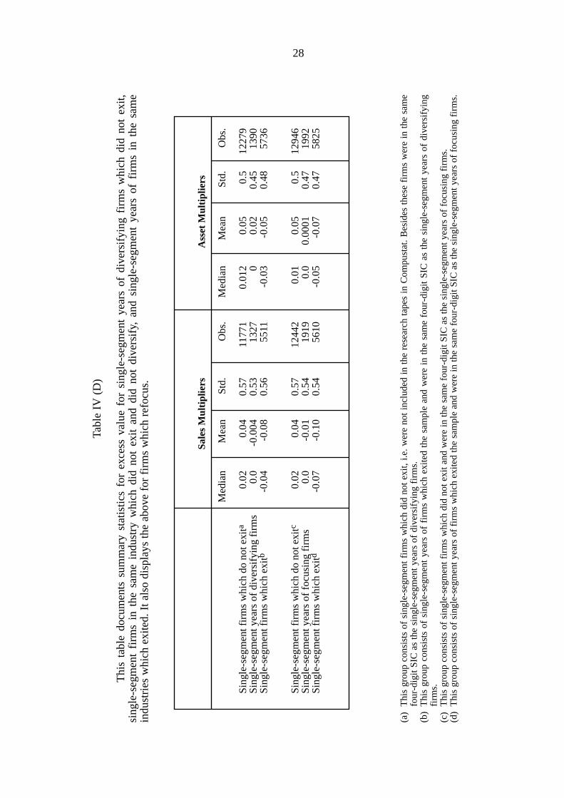
Tabl

e IV

(D

)

Thi

s ta

ble

docu

men

ts s

umm

ary

stat

istic

s fo

r ex

cess

val

ue f

or s

ingl

e-se

gmen

t ye

ars

of d

iver

sify

ing

firm

s w

hich

did

not

exi

t,si

ngle

-seg

men

t fi

rms

in t

he s

ame

indu

stry

whi

ch d

id n

ot e

xit

and

did

not

dive

rsif

y, a

nd s

ingl

e-se

gmen

t ye

ars

of f

irm

s in

the

sam

ein

dust

ries

whi

ch e

xite

d. I

t als

o di

spla

ys th

e ab

ove

for

firm

s w

hich

ref

ocus

.

(a)

Thi

s gr

oup

cons

ists

of

sing

le-s

egm

ent

firm

s w

hich

did

not

exi

t, i.e

. wer

e no

t in

clud

ed i

n th

e re

sear

ch t

apes

in

Com

pust

at. B

esid

es t

hese

fir

ms

wer

e in

the

sam

efo

ur-d

igit

SIC

as

the

sing

le-s

egm

ent y

ears

of

dive

rsif

ying

fir

ms.

(b

)T

his

grou

p co

nsis

ts o

f si

ngle

-seg

men

t ye

ars

of f

irm

s w

hich

exi

ted

the

sam

ple

and

wer

e in

the

sam

e fo

ur-d

igit

SIC

as

the

sing

le-s

egm

ent

year

s of

div

ersi

fyin

gfi

rms.

(c)

Thi

s gr

oup

cons

ists

of

sing

le-s

egm

ent f

irm

s w

hich

did

not

exi

t and

wer

e in

the

sam

e fo

ur-d

igit

SIC

as

the

sing

le-s

egm

ent y

ears

of

focu

sing

fir

ms.

(d

)T

his

grou

p co

nsis

ts o

f si

ngle

-seg

men

t yea

rs o

f fi

rms

whi

ch e

xite

d th

e sa

mpl

e an

d w

ere

in th

e sa

me

four

-dig

it SI

C a

s th

e si

ngle

-seg

men

t yea

rs o

f fo

cusi

ng f

irm

s.

28

Sale

s M

ulti

plie

rsA

sset

Mul

tipl

iers

Med

ian

Mea

nSt

d.O

bs.

Med

ian

Mea

nSt

d.O

bs.

Sing

le-s

egm

ent f

irm

s w

hich

do

not e

xita

0.02

0.04

0.57

1177

10.

012

0.05

0.5

1227

9Si

ngle

-seg

men

t yea

rs o

f di

vers

ifyi

ng f

irm

s0.

0-0

.004

0.53

1327

00.

020.

4513

90Si

ngle

-seg

men

t fir

ms

whi

ch e

xitb

-0.0

4-0

.08

0.56

5511

-0.0

3-0

.05

0.48

5736

Sing

le-s

egm

ent f

irm

s w

hich

do

not e

xitc

0.

020.

040.

5712

442

0.01

0.05

0.5

1294

6Si

ngle

-seg

men

t yea

rs o

f fo

cusi

ng f

irm

s0.

0-0

.01

0.54

1919

0.0

0.00

010.

4719

92Si

ngle

-seg

men

t fir

ms

whi

ch e

xitd

-0.0

7-0

.10

0.54

5610

-0.0

5-0

.07

0.47

5825

Table V

Effect of Multiple-Segment Operations on Firm Value of Diversifying Firms

The sample consists of single-segment firms and all diversifying firms. Thedependent variable is excess value, which is the ratio of firm value to its imputed value. D is adummy variable which takes the value 1 when the firm operates in multi-segments and 0otherwise, EBIT/SALES is the ratio of EBIT to sales and CAPX/SALES is the ratio of capitalexpenditures to sales. SNP is a dummy variable that takes the value of 1 when the firm is partof the S&P Index and zero otherwise, LEV is the ratio of long-term debt to total assets andASS2 is the square of the log of total assets. Columns 2 to 6 (Columns 7 to 11) report resultswhen sales (asset) multipliers are used to calculate imputed value. Year dummies wereincluded in the 2SLS model as well as the Self-Selection Model. The Fixed Effects Model hastwo-way fixed effects. The standard errors are corrected for autocorrelation and thecorresponding T-statistics are given in parentheses below.

29

Sales Multipliers Asset Multipliers

OLS OLS Fixed 2SLS Self- OLS OLS Fixed 2SLS Self- (BO) Effects Selection (BO) Effects Selection

Constant –0.36 –0.75 –0.09 –0.72 –0.68 –0.14 –0.43 0.68 –0.34 –0.32(33) (26) (1.67) (30) (30) (14) (17) (14) (15) (15)

D –0.13 –0.11 –0.06 0.30 0.18 -0.11 –0.09 –0.04 0.19 0.01(10) (9.13) (2.88) (5.03) (4.03) (9.09) (7.94) (2.08) (3.29) (0.24)

Log of Total Assets 0.04 0.61 0.33 0.55 0.54 0.01 0.42 0.00 0.24 0.24(19) (36) (16) (40) (39) (4.75) (28) (0.24) (19) (18)

EBIT/SALES 1.15 0.69 0.39 0.44 0.44 0.98 0.77 0.71 0.63 0.62(42) (19) (13) (13) (13) (44) (26) (27) (16) (15)

CAPX/SALES 0.33 0.06 0.19 0.16 0.16 0.04 –0.06 –0.03 –0.02 –0.02(15) (1.96) (7.25) (5.65) (5.68) (2.22) (2.38) (1.44) (0.98) (0.90)

Log of TA (1 lag) –0.25 –0.28 –0.25 –0.25 –0.15 –0.12 –0.04 –0.04(12) (19) (13) (13) (8.10) (8.75) (2.32) (2.50)

EBIT/SALES (1 lag) 0.20 0.16 0.20 0.20 0.07 0.14 0.10 0.10(5.57) (5.99) (5.49) (5.42) (2.18) (6.11) (2.31) (2.28)

CAPX/SALES (1 lag) 0.08 0.05 0.09 0.09 –0.05 –0.04 –0.01 –0.02(2.45) (2.04) (3.51) (3.40) (1.91) (1.89) (0.67) (0.86)

Log of TA (2 lag) –0.20 –0.14 –0.14 –0.14 –0.17 –0.11 –0.12 –0.12(16) (14) (13) (13) (16) (13) (12) (12)

EBIT/SALES (2 lag) 0.09 0.09 0.08 0.08 –0.02 0.05 –0.003 –0.002(3.58) (4.84) (3.14) (3.19) (1.06) (3.02) (0.11) (0.09)

CAPX/SALES (2 lag) 0.08 0.06 0.07 0.07 0.05 0.02 0.04 0.04(3.65) (3.08) (3.94) (3.80) (2.78) (1.08) (2.79) (2.65)

SNP 0.25 0.25 0.29 0.28(27) (28) (33) (33)

LEV –0.03 0.22 0.09 0.11 –0.06 0.12 0.03 0.04(1.48) (10) (6.81) (8.11) (3.94) (5.72) (2.21) (3.61)

ASS2 –0.01 0.01 –0.01 –0.01 –0.01 0.01 –0.01 –0.01(11) (6.12) (19) (19) (10) (6.38) (16) (16)

Lambda –0.14 –0.04(6.07) (1.83)

Hausman Test 43 20(P-Value) (0.0) (0.0)T statistics: First Stage 22.0 21.0Partial R2: First Stage 0.018 0.018

No. of Observations 24964 24964 24964 24964 24964 25480 25480 25480 25480 25480Adjusted R2 0.13 0.20 0.65 0.14 0.14 0.09 0.14 0.59 0.08 0.08F statistic 932 518 13.05 138 135 607 350 10.20 73 72

Table VI

Probit Estimates for Diversifying Firms

The dependent variable takes the value 1 when the firm operates in multiplesegments and zero otherwise. The results reported are for a sample of single-segment firmsand all diversifying firms included in the excess value regressions using sales multipliers.Columns 2 to 4 display the estimated coefficients, t-statistics, and marginal effects estimatedat the mean values of the exogenous variables. The probit model was also estimated for thesample of firms included when asset multipliers were used to calculate excess values. Theseestimates were qualitatively similar and have not been reported in the paper. Though theyhave not been reported, the estimates were used to calculate the fitted probabilities andselectivity correction for the corresponding estimation of the 2SLS model and the self-selection model using asset multipliers. EBIT/SALES is the ratio of EBIT to sales andCAPX/SALES is the ratio of capital expenditures to sales. PNDIV is the fraction of all firmsin the industry which are conglomerates and PSDIV is the fraction of sales by other firms inthe industry accounted for by conglomerates. MNUM is the number of announcedmergers/acquisitions in the year, while MVOL is the US $ value of these. GDP (GDP1) is thegrowth rate in real GDP (and its lagged value) while CONTRACTION (CONTRACTION1)is the number of months in the year the economy was in recession (and its lagged value).MAJOREX is a dummy variable which takes the value 1 if the firm is listed in NASDAQ,NYSE or AMEX and zero otherwise. FOREIGN is a dummy variable which takes the value 1if the firm is incorporated outside the US and zero otherwise. SNP is a dummy variablewhich takes the value 1 if the firm is part of the S&P Index and zero otherwise.

30

Coefficient T-statistic Marginal Effect

Constant -3.47 -31.03 -0.21Log of Total Assets 0.22 3.98 0.03EBIT/SALES -0.07 -0.50 -0.01CAPX/SALES 0.03 0.29 0.00Log of TA (1 lag) -0.10 -1.19 -0.01EBIT/SALES (1 lag) -0.07 -0.48 -0.01CAPX/SALES (1 lag) -0.11 -0.80 -0.02Log of TA (2 lag) 0.23 4.18 0.02EBIT/SALES (2 lag) -0.10 -1.02 -0.01CAPX/SALES (2 lag) -0.09 -0.87 -0.02SNP -0.19 -4.08 -0.03PNDIV 0.02 15.85 0.003PSDIV 0.001 1.45 0.0002MVOL -0.0001 -0.36 0.00MNUM 0.11 3.69 0.01GDP -0.01 -1.26 -0.002GDP1 0.004 0.36 0.001Contraction -0.08 -0.80 -0.02Contraction 1 -0.02 -0.24 -0.01A_TA -0.20 -6.15 -0.02A_EBIT 0.10 1.35 0.01A_CAPX 0.04 0.39 0.01MAJOREX 0.16 6.02 0.02FOREIGN 0.06 1.22 0.02

No. of observations 24964Maximized likelihood -6478Likelihood index 0.08Percentage multi-segmentobservations 8.13

Table VII

Effect of Multiple-Segment Operations on Firm Value of Diversifying Firms

The sample consists of single-segment firms and all diversifying firms. We reportpartial results of alternate specifications of the model. All explanatory variables included intable V were included but are not reported here as the results were qualitatively similar tothose in table V. Panel A includes RND/Sales, replacing missing values of R&D with zero.Panel B also includes RND/Sales but excludes all missing values of R&D. Panel C includesINDGROW (the growth in industry sales and its lagged value). Panel D reports resultsexcluding all lagged values of firm size, EBIT/Sales and CAPX/Sales. Year dummies havebeen included in the estimation of the 2SLS as well as the estimation of the Self-Selectionmodel. Standard errors have been corrected for auto-correlation and corresponding T-statisticsare reported in parentheses below.

31

Sales Multipliers Asset Multipliers

OLS OLS Fixed 2SLS Self- OLS OLS Fixed 2SLS Self-(BO) Effects Selection (BO) Effects Selection

A: Years with Missing R&D have been assigned a value of zero

D -0.13 -0.10 -0.06 0.33 0.17 -0.11 -0.09 -0.04 0.40 0.12(-10.6) (-8.53) (-2.87) (5.43) (3.66) (-9.1) (-7.51) (-2.04) (6.79) (2.76)

RND/SALES 0.75 0.42 0.78 0.77 0.38 0.32 0.40 0.38 (15.56) (5.52) (15.48) (15.40) (9.91) (5.02) (10.34) (9.78)Lambda -0.13 -0.10

(-5.52) (-4.16)Hausman Test 46.92 63.00(P-value) (0.00) (0.00)T stats: First stage 22 22Partial R2: First stage 0.019 0.019

No. of observations 24964 24964 24964 24964 24964 25480 25480 25480 25480 25480Adjusted R2 0.13 0.21 0.65 0.15 0.15 0.09 0.15 0.59 0.08 0.08F statistic 932 502 13 143 139 607 332 10 74 72

D -0.14 -0.08 -0.09 0.40 0.21 -0.16 -0.13 -0.05 0.07 -0.17(-7.37) (-4.55) (-2.91) (6.37) (3.84) (-8.3) (-6.45) (-1.43) (0.97) (-2.82)

RND/SALES 0.73 0.58 0.78 0.77 0.47 0.53 0.48 0.46(13) (7.04) (13) (13) (10) (7.42) (10) (10)

Lambda -0.15 0.03(-5.00) (1.06)

Hausman Test 56.00 5.01(P-value) (0.00) (0.03)T stats: First stage 23.00 22.00Partial R2: First stage .036 0.035 No. of observations 13055 13055 13055 13055 13055 13286 13286 13286 13286 13286Adjusted R2 0.17 0.24 0.65 0.17 0.17 0.12 0.18 0.60 0.11 0.12F statistic 670 319 12.5 89 86 467 228 10.2 55 55

B: Years with Missing R&D have been excluded

Table VII (continued)

32

D -0.13 -0.11 -0.05 0.33 0.22 -0.11 -0.09 -0.05 0.21 0.05 (-10) (-8.88) (-2.64) (5.29) (4.65) (-10) (-8.00) (-2.35) (3.39) (1.01)INDGROW x 10-2 -0.20 -0.10 -0.10 -0.10 -0.20 -0.10 -0.10 -0.10 (-7.12) (-4.78) (-4.04) (-4.14) (-7.64) (-3.79) (-4.94) (-5.03)INDGROW1 x 10-2 -0.10 -0.10 -0.04 -0.04 -0.10 -0.04 -0.10 -0.10 (-4.13) (-3.09) (-1.90) (-2.02) (-4.04) (-2.12) (-2.88) (-3.01)Lambda -0.16 -0.06 (-6.58) (-2.56)

Hausman Test 44 20 (P-value) (0.00) (0.00) T stats: First stage 21 20 Partial R2: First stage 0.017 0.017 No. of observations 23110 23110 23110 23110 23110 23568 23568 23568 23568 23568Adjusted R2 0.14 0.21 0.66 0.15 0.15 0.09 0.15 0.60 0.08 0.09F statistic 933 443 13.4 126 124 614 303 10.6 69 67 D -0.14 -0.12 -0.03 0.61 0.40 -0.11 -0.10 -0.02 0.67 0.29 (-11.9) (-10.2) (-1.48) (9.92) (9.38) (-10.8) (-8.64) (-1.16) (10.58) (6.89)Lambda -0.26 -0.19 (-11) (-8.48) Hausman Test 136 158 (P-value) (0.00) (0.00) T stats: First stage 22 22 Partial R2: First stage 0.017 0.017 No. of observations 27812 27812 27812 27812 27812 28491 28491 28491 28491 28491Adjusted R2 0.12 0.13 0.61 0.08 0.08 0.08 0.09 0.56 0.06 0.06F statistic 983 704 11.0 101.3 99.5 654 477 9.3 69.4 67.5

Sales Multipliers Asset Multipliers

OLS(BO)

OLS FixedEffects

2SLS Self-Selection

OLS(BO)

OLS FixedEffects

2SLS Self-Selection

C: Including Industry Growth Rates

D: Excluding all Lagged values of Firm size, EBIT/SALES and CAPX/SALES

Table VIII

Effect of Multiple-Segment Operations on Firm Value of Refocusing Firms

The sample consists of single-segment firms and all refocusing firms. The dependentvariable is excess value, which is the ratio of firm value to its imputed value. D is a dummyvariable which takes the value 1 when the firm operates in multi-segments and 0 otherwise,EBIT/SALES is the ratio of EBIT to sales and CAPX/SALES is the ratio of capital expendituresto sales. SNP is a dummy variable that takes the value of 1 when the firm is part of the S&PIndex and zero otherwise, LEV is the ratio of long-term debt to total assets and ASS2 is thesquare of the log of total assets. Columns 2 to 5 (Columns 6 to 9) report results when sales (asset)multipliers are used to calculate imputed value. Year dummies have been included for theestimation of the 2SLS as well as of the self-selection model. Standard errors have beencorrected for autocorrelation and T-statistics are reported in parentheses below.

33

Constant -0.38 -0.76 -0.14 -0.68 -0.68 -0.17 -0.43 0.62 -0.31 -0.31 (36) (28) (2.82) (32) (32) (18) (17) (13) (15) (15)D -0.17 -0.13 -0.14 -0.21 -0.21 -0.13 -0.11 -0.11 -0.11 -0.10 (17) (14) (9.20) (9.60) (10) (14) (12) (7.05) (4.51) (4.48)Log of Total Assets 0.05 0.59 0.35 0.53 0.53 0.01 0.39 0.01 0.22 0.22 (22) (36) (17) (41) (41) (7.23) (28) (0.69) (18) (18)EBIT/SALES 1.14 0.66 0.37 0.40 0.40 1.00 0.76 0.67 0.59 0.59 (43) (19) (13) (12) (12) (46) (27) (28.) (15) (16)CAPX/SALES 0.32 0.10 0.18 0.17 0.17 0.04 -0.03 -0.03 -0.004 -0.004 (15) (3.43) (7.46) (6.64) (6.64) (2.44) (1.30) (1.24) (0.21) (0.20)Log of TA (1 lag) -0.24 -0.27 -0.24 -0.24 -0.14 -0.12 -0.04 -0.04 (12) (19) (14) (14) (8.09) (9.43) (2.79) (2.78)EBIT/SALES (1 lag) 0.26 0.21 0.23 0.23 0.13 0.20 0.16 0.16 (7.15) (7.60) (6.25) (6.25) (4.38) (8.74) (3.81) (3.84)CAPX/SALES (1 lag) 0.03 0.04 0.05 0.05 -0.07 -0.04 -0.03 -0.03 (0.83) (1.91) (2.03) (2.04) (2.79) (2.19) (1.59) (1.60)Log of TA (2 lag) -0.18 -0.12 -0.11 -0.12 -0.15 -0.10 -0.10 -0.10 (15) (13) (11) (11) (15) (12) (11) (11)EBIT/SALES (2 lag) 0.12 0.12 0.09 0.10 -0.02 0.05 -0.01 -0.01 (4.60) (5.86) (3.48) (3.56) (1.10) (2.76) (0.28) (0.24)CAPX/SALES (2 lag) 0.09 0.06 0.06 0.06 0.06 0.02 0.04 0.04 (3.72) (3.16) (3.23) (3.22) (2.93) (1.49) (2.46) (2.46)SNP 0.25 0.25 0.28 0.29 (29) (29) (35) (35)LEV 0.02 0.25 0.17 0.17 -0.04 0.15 0.09 0.08 (1.43) (12) (13) (12) (2.58) (7.59) (7.23) (7.05)ASS2 -0.01 0.01 -0.01 -0.01 -0.01 0.01 -0.01 -0.01 (12) (3.48) (21) (21) -9.85) (5.76) (15) (15)Lambda 0.03 -0.01 (2.44) (0.48)Hausman Test 3.20 0.08 (P-Value) (0.07) (0.45) T statistics: First Stage 52 47 Partial R2: First Stage 0.079 0.066 No. of Observations 27995 27995 27995 27995 27995 28161 28161 28161 28161 28161Adjusted R2 0.13 0.19 0.64 0.13 0.14 0.09 0.14 0.58 0.08 0.08F statistic 1064 557 13.00 142 142 732 383 10.30 77 77

Sales Multipliers Asset Multipliers

OLS(BO)

OLS FixedEffects

2SLS Self-Selection

OLS(BO)

OLS FixedEffects

2SLS Self-Selection

Table IX

Probit Estimates for Refocusing Firms

The dependent variable takes the value 1 when the firm operates in multiple segmentsand zero otherwise. The results reported are for a sample of single-segment firms and allfocusing firms included in the excess value regressions using sales multipliers. Columns 2 to 4display the estimated coefficients, t-statistics, and marginal effects estimated at the mean valuesof the exogenous variables. The probit model was also estimated for the sample of firms includedwhen asset multipliers were used to calculate excess values. These estimates were qualitativelysimilar and have not been reported in the paper. Though they have not been reported, theestimates were used to calculate the fitted probabilities and selectivity correction for thecorresponding estimation of the 2SLS model and the self-selection model using asset multipliers.EBIT/SALES is the ratio of EBIT to sales and CAPX/SALES is the ratio of capital expendituresto sales. PNDIV is the fraction of all firms in the industry which are conglomerates and PSDIV isthe fraction of sales by other firms in the industry accounted for by conglomerates. MNUM is thenumber of announced mergers/acquisitions in the year, while MVOL is the US $ value of these.GDP (GDP1) is the growth rate in real GDP (and its lagged value) while CONTRACTION(CONTRACTION1) is the number of months in the year the economy was in recession (and itslagged value). MAJOREX is a dummy variable which takes the value 1 if the firm is listed inNASDAQ, NYSE or AMEX and zero otherwise. FOREIGN is a dummy variable which takesthe value 1 if the firm is incorporated outside the US and zero otherwise. SNP is a dummyvariable which takes the value 1 if the firm is part of the S&P Index and zero otherwise.

34

Coefficient T-statistics Marginal Effect Constant -3.40 -35.21 -0.24Log of Total Assets -0.09 -1.53 0.00EBIT/SALES -0.28 -1.94 -0.07CAPX/SALES 0.24 1.58 -0.02LOG OF TA (1 lag) -0.20 -2.29 -0.02EBIT/SALES (1 lag) 0.05 0.29 -0.03CAPX/SALES (1 lag) 0.85 4.77 0.01Log of TA (2 lag) 0.11 1.88 -0.01EBIT/SALES (2 lag) -0.14 -1.07 -0.01CAPX/SALES (2 lag) 0.88 5.20 -0.02SNP -0.06 -1.54 0.01PNDIV 0.02 14.97 0.003PSDIV 0.01 12.87 0.001MVOL 0.0003 1.02 0.0002MNUM -0.21 -8.10 -0.04GDP 0.04 4.62 0.01GDP1 0.01 0.93 -0.001Contraction 0.32 3.90 0.10Contraction 1 0.25 3.15 0.05A_TA 0.43 11.56 0.07A_EBIT -0.52 -4.40 -0.07A_CAPX -3.68 -13.97 -0.11MAJOREX 0.20 7.94 0.03FOREIGN -0.33 -5.64 -0.05 No. of observations 27995Maximized likelihood -8381Likelihood index 0.21% of positive observations 12.60

Table X

Effect of Multiple-Segment Operations on Firm Value of Refocusing Firms

The sample consists of single-segment firms and all focusing firms. We report partialresults of alternate specifications of the model. All explanatory variables included in table Vwere included but are not reported here as the results were qualitatively similar to those intable V. Panel A includes RND/Sales, replacing missing values of R&D with zero. Panel Balso includes RND/Sales but excludes all missing values of R&D. Panel C includesINDGROW (the growth in industry sales and its lagged value). Panel D reports resultsexcluding all lagged values of firm size, EBIT/Sales and CAPX/Sales. Year dummies havebeen included in the estimation of the 2SLS as well as the estimation of the Self-Selectionmodel. Standard errors have been corrected for auto-correlation and corresponding T-statisticsare reported in parentheses below.

35

Sales Multipliers Asset Multipliers

OLS(BO)

OLS FixedEffects

2SLS Self-Selection

OLS(BO)

OLS FixedEffects

2SLS Self-Selection

D -0.17 -0.12 -0.14 -0.19 -0.20 -0.13 -0.10 -0.10 -0.11 -0.10 (17) (13) (9.17) (8.83) (9.69) (14.44) (11) (7.01) (4.43) (4.52)RND/SALES 0.75 0.39 0.70 0.69 0.41 0.31 0.35 0.35 (15) (5.12) (14) (14) (10) (4.93) (9.42) (9.42)Lambda 0.03 0.00 (2.23) (0.27) Hausman Test 9.30 0.18 (P-Value) (0.0) (.35) T stats: First stage 51.0 47.0 Partial R2: First stage 0.073 0.073 No. of Observations 27995 27995 27995 27995 27995 28161 28161 28161 28161 28161Adjusted R2 0.13 0.20 0.64 0.14 0.14 0.09 0.14 0.58 0.08 0.08F statistic 1064 537 13.1 145 146 732 363 10.2 76 76 D -0.21 -0.15 -0.16 -0.20 -0.22 -0.16 -0.12 -0.12 -0.15 -0.15 (17) (11) (7) (8.15) (9.29) (14) (8.89) (5.14) (5.83) (6.32)RND/SALES 0.79 0.85 0.90 0.89 0.54 0.79 -0.03 -0.04 (13) (8.34) (17) (11) (9.36) (1.74) (1.91)Lambda 17.68 0.03 -0.35 0.02 (2.36) (10) (1.65) Hausman Test 5.15 2.79 (P-Value) (0.03) (0.10) T stats: First Stage 49.0 47.0 Partial R2: First Stage 0.113 0.107 No. of Observations 15162 15162 15162 15162 15162 15174 15174 15174 15174 15174Adjusted R2 0.18 0.24 0.65 0.17 0.18 0.14 0.18 0.60 0.11 0.12F statistic 842 370 13.1 100 104 598 260 10.5 64 63

A: Years with missing R&D have been assigned a value zero

B: Years with missing R&D have been excluded

Table X (continued)

36

D -0.16 -0.13 -0.14 -0.22 -0.22 -0.13 -0.11 -0.10 -0.11 -0.09 (18) (14) (8.96) (9.65) (10) (15) (11) (6.78) (4.60) (4.23)INDGROW 1 0.00 0.00 0.00 0.00 0.00 0.00 0.00 0.00 (7.68) (4.92) (5.04) (5.15) (7.71) (4.95) (5.97) (6.01)INDGROW 2 0.00 0.00 0.00 0.00 0.00 0.00 0.00 0.00 (3.76) (2.65) (3.09) (3.20) (3.38) (2.15) (3.29) (3.33)Lambda 0.03 -0.01 (2.74) (0.52) Hausman Test 14.21 0.26 (P-Value) (0.00) (0.35) T stats: First Stage 49.0 45.0 Partial R2: First Stage 0.076 0.067 No. of Observations 25968 25968 25968 25968 25968 26097 26097 26097 26097 26097Adjusted R2 0.14 0.20 0.65 0.14 0.14 0.10 0.15 0.59 0.08 0.08F statistic 1058 478 13.4 131 131 732 328 10.5 72 71

D -0.18 -0.17 -0.15 -0.77 -0.66 -0.14 -0.14 -0.11 -0.37 -0.33 (20) (18) (9.95) (35) (32) (17) (15) (7.46) (16) (15)Lambda 0.27 0.11 (23) (9.50) Hausman Test 800 130 (P-Value) (0.0) (0.0) T stats: First Stage 55.0 51.0 Partial R2: First Stage 0.08 0.069 No. of Observations 30818 30818 30818 30818 30818 31129 31129 31129 31129 31129Adjusted R2 0.13 0.13 0.60 0.07 0.08 0.09 0.10 0.56 0.05 0.06F statistic 1117 794 11.2 111.2 111.1 771 551 9.3 72 75

Sales Multipliers Asset Multipliers

OLS(BO)

OLS FixedEffects

2SLS Self-Selection

OLS(BO)

OLS FixedEffects

2SLS Self-Selection

C: Including Industry Growth Rates

D: Excluding all Lagged values of Firm size, EBIT/SALES and CAPX/SALES