explaining the diversification discount

Explaining the Diversification Discount

JOSE MANUEL CAMPA and SIMI KEDIA*

ABSTRACT

This paper argues that the documented discount on diversified firms is not per seevidence that diversification destroys value. Firms choose to diversify. We use threealternative econometric techniques to control for the endogeneity of the diversifi-cation decision, and find evidence supporting the self-selection of diversifying firms.We find a strong negative correlation between a firm’s choice to diversify and firmvalue. The diversification discount always drops, and sometimes turns into a pre-mium. There also exists evidence of self-selection by refocusing firms. These re-sults point to the importance of explicitly modeling the endogeneity of thediversification status in analyzing its effect on firm value.

Firms choose to diversify. They choose to diversify when the benefits of di-versification outweigh the costs of diversification and stay focused whenthey do not. The characteristics of firms that diversify, which make the ben-efits of diversification greater than the costs of diversification, may alsocause firms to be discounted. A proper evaluation of the effect of diversifi-cation on firm value should take into account the firm-specific characteris-tics that bear both on firm value and on the decision to diversify.

Research by Lang and Stulz ~1994!, Berger and Ofek ~1995!, and Servaes~1996! shows unambiguously that diversified firms trade at a discount rel-ative to nondiversified firms in their industries. Other research confirmsthe existence of this discount on diversified firms, and this result seems to

*Campa is with IESE Business School, Madrid, Spain. Kedia is with Harvard University. Wethank Philip Berger; Ben Esty; Stuart Gilson; Bill Greene; Charles Himmelberg; Kose John;Vojislav Maksimovic; Scott Mayfield; Maureen O’Hara; Richard Ruback; Henri Servaes; JeremyStein; Emilio Venezian; Michael Weisbach; and seminar participants at the 1999 Western Fi-nance Association Meetings, 1999 NBER Summer Conference in Corporate Finance, 2001 Eu-ropean Finance Association Meetings, 2001 European Financial Management Association Meetings,2002 American Finance Association Meetings, Harvard Business School, Cornell University,Georgetown University, Rutgers University, Darden School, University of Navarra, and Mich-igan State University for helpful comments. We thank Chris Allen and Sarah Eriksen for helpwith the data. Financial support from the Division of Research at Harvard Business School andthe Center for Investments and International Finance Research ~CIIF! at IESE Business Schoolare gratefully acknowledged. All errors remain our responsibility.

THE JOURNAL OF FINANCE • VOL. LVII, NO. 4 • AUGUST 2002

1731

be robust to different time periods and different countries.1 There is a grow-ing consensus that the discount on diversified firms implies a destruction ofvalue on account of diversification, that is, on account of firms operating inmultiple divisions.

This study shows that the failure to control for firm characteristics thatlead firms to diversify and be discounted may wrongly attribute the discountto diversification instead of the underlying characteristics. For example, con-sider a firm facing technological change, which adversely affects its compet-itive advantage in its industry. This poorly performing firm will trade at adiscount relative to other firms in the industry. Such a firm will also havelower opportunity costs of assigning its scarce resources in other industries,and this might lead it to diversify. If poorly performing firms tend to diver-sify, then not taking into account past performance and its effect on thedecision to diversify will result in attributing the discount to diversificationactivity, rather than to the poor performance of the firm.

Also consider the case of a firm that possesses some unique organizationalcapability that it wants to exploit. Incomplete information may force thisfirm to enter into a costly search through diversification to find industrieswith a match to its organizational capital. Matsusaka ~2001! proposes a modelin which a value-maximizing firm forgoes the benefits of specialization tosearch for a better match. During the search period, the market value of thefirm will be lower than the value of a comparable single-segment firm. Mak-simovic and Phillips ~2002! also develop a model where the firm optimallychooses the number of segments in which it operates depending on its com-parative advantage. Not taking into account firm characteristics, which makediversification optimal, in this case searching for a match, may again attributethe discount wrongly to value destruction arising from diversification.

This does not imply that there are no agency costs associated with firms op-erating in multiple divisions. Consider the impact of cross-sectional variationin private benefits of managers. A firm with a manager who has high privatebenefits will undertake activities that are at conf lict with shareholder valuemaximization. Such a firm will be discounted relative to other firms in its in-dustry. Such a manager is also more likely to undertake value-destroying di-versification. However, even in this case, the observed discount on multisegmentyears is partially accounted for by the ex ante discount at which the firm istrading, on account of high private benefits, before diversification. Not takinginto account firm characteristics, in this case high agency costs, leads to anoverestimation of the value destruction attributed to diversification.

1 Servaes ~1996! finds a discount for conglomerates during the 1960s while Matsusaka ~1993!documents gains to diversifying acquisitions in the late 1960s in the United States. Lins andServaes ~1999! document a significant discount in Japan and the United Kingdom, though noneexists for Germany. The evidence from emerging economies is mixed. While Khanna and Palepu~2000!, and Fauver, Houston, and Naranjo ~1998! find little evidence of a diversification dis-count in emerging markets, Lins and Servaes ~1998! report a diversification discount in asample of firms from seven emerging markets.

1732 The Journal of Finance

In this paper, we attempt to control for this endogeneity of a firm’s decisionto diversify in evaluating the effect of diversification on firm value. The ar-guments suggest that the decision to diversify depends on the presence of somefirm-specific characteristics that lead some firms to generate more value fromdiversification than others. Choice of organization structure should, there-fore, be treated as an endogenous outcome that maximizes firm value, givena set of exogenous determinants of diversification, that is, the set of firm char-acteristics. Evaluating the impact of diversification on firm value, therefore,requires taking into account the endogeneity of the diversification decision.

Controlling for the endogeneity of the diversification decision requires iden-tifying variables that affect the decision to diversify while being uncorre-lated with firm value. This becomes difficult, as most variables that bear onthe diversification decision also impact firm value. We build on the meth-odology of Berger and Ofek ~1995! and the insights of Lang and Stulz ~1994!to control for the endogeneity of the diversification decision. As do Bergerand Ofek, we value firms relative to the median single-segment firm in theindustry. This measure has the advantage of being neutral to industry andtime shocks that affect all firms in a similar way. However, Lang and Stulzshow that industry characteristics are important in a firm’s decision to di-versify.2 We explore the data for systematic industry differences among single-segment and diversifying firms that might help explain the decision todiversify.

We first reproduce the results existing in the literature and identify adiversification discount in our sample. Preliminary data analysis shows thatconglomerates differ from single-segment firms in their underlying charac-teristics. We control for the endogeneity of the diversification decision inthree ways. First, we control for unobservable firm characteristics that af-fect the diversification decision by introducing fixed-firm effects. Second, wemodel the firm’s decision to diversify as a function of industry, firm, andmacroeconomic characteristics. We use the probability of diversifying as aninstrument for the diversification status in evaluating the effect of multiplesegment operations on firm value. Last, we model an endogenous self-selection model and use Heckman’s correction to control for the self-selectionbias induced on account of firms’ choosing to diversify.

The diversification discount always drops, and sometimes turns into apremium, when we control for the endogeneity of the diversification deci-sion. The evidence in all three methods indicates that the discount on multiple-segment firm years is partly due to endogeneity. The coefficient of thecorrection for self-selection is negative, indicating that there is a negativecorrelation between a firm’s choice to diversify and firm value. This sup-ports the view that firm characteristics, which cause firms to diversify, alsocause them to be discounted.

2 Lang and Stulz ~1994! find that firms that diversify tend to be in slow-growing industries.They also report that diversified firms have lower Tobin’s q than focused firms, but this dif-ference was driven by differences among firms across industries rather than within an industry.

Explaining the Diversification Discount 1733

Finally, we do a similar analysis in a sample of refocusing firms. Commentand Jarrell ~1995!, John and Ofek ~1995!, and Berger and Ofek ~1996! doc-ument an increase in firm value associated with the decision to refocus.Much like the decision to diversify, the decision to refocus is also endog-enous: Firms choose to refocus when the presence of firm-specific charac-teristics makes the benefits of refocusing greater than the costs of refocusing.3Consider the case when changes in industry conditions generate higher thanexpected growth opportunities in one segment. This might increase the cost ofinefficient internal capital markets, increasing the cost of operating in mul-tiple divisions and making refocusing optimal. In this case, firm characteris-tics that make the refocusing decision optimal, that is, growth opportunities,also cause the firms to be more highly valued. Unlike the diversificationdecision, the refocusing decision is positively correlated with firm value. Nottaking into account firm characteristics prior to refocusing, in this case,growth opportunities, may erroneously attribute the associated premium tomultisegment operations of firms. This would lead to an underestimation ofthe discount associated with multisegment operations prior to refocusing.Controlling for firm characteristics, which make the refocusing decision op-timal, may further increase the discount associated with multisegments op-erations of these firms. We document evidence in support of this view.

The rest of the paper is organized as follows. In the next section, we brief lydiscuss related literature. Section II describes the data, sample selectioncriteria, and preliminary analysis. Section III discusses the estimation meth-odology. Section IV presents the evidence for diversifying firms, and Sec-tion V does the same for refocusing firms. Section VI concludes.

I. Related Literature

There is a vast and well-developed literature on the benefits and costs ofdiversification. The gains from diversification could arise from many sources.Gains to diversification arise from managerial economies of scale as pro-posed by Chandler ~1977! and from increased debt capacity as argued byLewellen ~1971!. Diversified firms also gain from more efficient resourceallocation through internal capital markets ~see Weston ~1970!, Stulz ~1990!,and Stein ~1997!!. Gains to diversification also arise from the ability of di-versified firms to internalize market failures ~Khanna and Palepu ~2000!!.Hadlock, Ryngaert, and Thomas ~2001! argue that diversified firms gainfrom a reduction of the adverse selection problem at the time of equity is-

3 In a static model, the above arguments would suggest that when the net benefit to oper-ating in multiple segments is negative, the firm should immediately refocus. In practice, thedecision to diversify and refocus involves large amounts of sunk and irreversible costs that leadto a lot of persistence in diversification status. As yet, there is no clear understanding of thedynamic theory of a firm’s diversification status, but one can draw an analog from recenttheory on irreversible investment decisions ~see Dixit and Pindyck ~1994!!. This literature hasemphasized that temporary shocks can have permanent effects due to hysteresis, which is con-sistent with an observed discount of multiple segment firms prior to refocusing.


sues. Wernerfelt and Montgomery ~1988! and Bodnar, Tang, and Weintrop~1997! propose gains to diversification based on the presence of firm-specificassets, which can be exploited in other markets. Schoar ~1999! finds thatdiversified firms are more productive than others within their industry, thoughthey still appear to be discounted.

There are costs to diversification as well. The costs can arise from ineffi-cient allocation of capital among divisions of a diversified firm ~see Stulz~1990!, Lamont ~1997!, Scharfstein ~1998!, and Rajan, Servaes, and Zingales~2000!!. The difficulty of designing optimal incentive compensation for man-agers of diversified firms also generates costs of multisegment operations~Aron ~1988! and Rotemberg and Saloner ~1994!!. Information asymmetriesbetween central management and divisional managers will also lead to highercosts of operating in multiple segments, as has been shown by Harris, Krie-bel, and Raviv ~1982!. Last, costs of operating in multiple segments couldarise because of increased incentive for rent seeking by managers within thefirm ~see Scharfstein and Stein ~2000!! and opportunities for managers offirms with free cash f low to engage in value-destroying investments ~seeJensen ~1986, 1988!!. Denis, Denis, and Sarin ~1997! provide empirical evi-dence that agency costs are related to the diversification decision. Hyland~1999! examines firm characteristics including agency costs, and finds nosupport for the idea that agency costs explain the decision of firms to diversify.

Our focus in the paper is not in identifying any of the above-mentionedindividual benefits and costs of diversification, but rather to concentrate onthe net gain to diversification. Firms are likely to diversify when there arenet gains to diversification and stay focused when there are net costs todiversifying. Most importantly for us, the above research shows that thebenefits and costs of diversification are related to firm-specific characteris-tics. We control for firm characteristics that cause firms to diversify, that is,which generate a net gain to multisegment operations and isolate the netimpact of the diversification decision.

Our paper is not the first to take into account the endogeneity of thediversification decision. A growing theoretical literature has been modelingthe decision to diversify as a value-increasing strategy for the firm. Mat-susaka ~2001! develops a model in which the firm chooses to diversify whenthe gains from searching for a better organizational fit outweigh the costs ofreduced specialization. Fluck and Lynch ~1999! propose that diversificationallows marginally profitable projects, which could not get financed as stand-alone entities, to be financed. Perold ~1999! models the diversification deci-sion in financial intermediaries and shows that diversification reduces afirm’s deadweight costs of capital and so permits divisions to operate on alarger scale than stand-alone firms. Maksimovic and Phillips ~2002! alsodevelop a model where the firm optimally chooses the number of segmentsin which it operates, depending on its comparative advantage. They furthershow empirically that conglomerates allocate resources optimally, based onthe relative efficiency of divisions. There has been other recent empiricalwork that provides evidence in support of the importance of selection bias


and the endogeneity of the diversification decision ~Chevalier ~2000!, Lam-ont and Polk ~2001!, Whited ~2001!, Graham, Lemmon, and Wolf ~2002!, andVillalonga ~2002!!.

II. Data

A. Sample Selection

The sample consists of all firms with data reported on the CompustatIndustry Segment database from 1978 to 1996. We follow the Berger andOfek ~1995! @henceforth BO~95!# sample selection criteria and exclude yearswhere firms report segments in the financial sector ~SIC 6000–6999!, yearswith sales less than $20 million, years with a missing value of total capital,and years in which the sum of segment sales deviated from total sales bymore than one percent. Additionally, we also excluded years where the firmdid not report four-digit SICs for all its segments. The final sample consistsof 8,815 firms with a total of 58,965 firm-years.

B. Measure of Excess Value

To examine whether diversification increases or decreases value, we usethe excess value measure developed by BO~95!, which compares a firm’svalue to its imputed value if each of its segments operated as single-segmentfirms. Each segment of a multiple-segment firm is valued using mediansales and asset multipliers of single-segment firms in that industry. Theimputed value of the firm is the sum of the segment values. Excess value isdefined as the log of the ratio of firm value to its imputed value. Negativeexcess value implies that the firm trades at a discount, while positive excessvalues are indicative of a premium.4

C. Documenting the Discount

In this section, we document the existence of a discount in line with priorwork. We find that the median discount on multisegment years is 10.9 per-

4 The imputed value of a segment is obtained by multiplying segment sales ~asset! with themedian sales ~asset! multiplier of all single-segment firm-years in that SIC. The sales ~asset!multipliers are the median value of the ratio of total capital over sales ~assets!. Total capital isthe sum of market value of equity, long-term and short-term debt, and preferred stock. Theindustry definitions are based on the narrowest SIC grouping that includes at least five firms.Extreme excess values, where the natural log of the ratio of actual to imputed value is greaterthan 1.386 or less than 21.386, were excluded. The imputed values using sales multipliers ofabout 50 percent of all firms were based on matches at the four-digit SIC code, 26.5 percentwere based on matches at the three-digit SIC code, and 23.5 percent were based on matches atthe two-digit or lower SIC code. The results using asset multipliers are similar. This is in linewith the results reported in BO~95! of 44.6 percent matches at the four-digit level, 25.4 percentmatches at the three-digit level, and 30 percent matches at the two-digit level or lower. SeeBO~95! for further details on methodology.


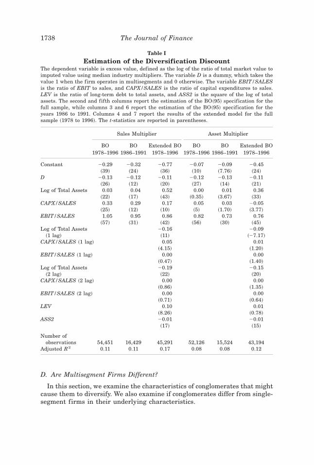
cent ~11.6 percent! using sales ~asset! multipliers for the entire sample from1978 to 1996, similar to the discount of 10.6 percent ~16.2 percent! reportedby BO~95! for the years 1986 to 1991.5 We begin by estimating a model ofexcess value as specified by BO~95! so as to guarantee that any differencesin the final results are not driven by differences in sample or methodology.BO~95! model excess value as a function of firm size, proxied by the log oftotal assets, profitability ~EBIT/SALES!, investment ~CAPX/SALES!, anddiversification, proxied by D, a dummy which takes the value 1 for yearswhen the firm operates in multiple segments and 0 otherwise. As seen inTable I, the coefficient of D is 20.13 ~20.12! and significant at the one per-cent ~one percent! level when sales ~assets! multipliers are used. When werestrict the sample to the years 1986 to 1991, the coefficient of D is 20.12~20.13! using sales ~asset! multipliers, which is close to the value of 20.144~20.127! reported by BO~95!. The estimated discount in our sample is sim-ilar to that documented by BO~95!.

We test the robustness of the estimated discount to model specifica-tion by including lagged values of firm size, profitability, and investment.Past profitability and investment may control for firm characteristics,which affect firm value. We also include the log of total assets squared tocontrol for the possibility of a nonlinear effect of firm size on firm value.The coefficient of the square of firm size is negative, suggesting that thepositive effect of firm size on excess value diminishes as firm size in-creases. We also include the ratio of long-term debt to total assets. Theresults, reported in columns 3 and 6 of Table I, show that the estimateddiscount is about 11 percent with both sales and asset multipliers. There isweak evidence that firms with high past profitability ~high EBIT/SALES!and high past investments ~high CAPX/SALES! are valued higher thanthe median single-segment firm in the industry, though the coefficients arenot significant. Summarizing, multiple-segment firms show a significantdiscount, and this discount is robust to the inclusion of additional vari-ables in the valuation equation. We report all results with this extendedmodel.

5 For the years 1986 to 1991, we find that the median multiple segment discount in oursample is 7.6 percent ~10.3 percent! using a sales ~asset! multiplier. This difference with theBO~95! results is possibly due to a difference in sample size. The number of firm-years in theperiod 1986 to 1991 in our sample is 17,875, greater than the 16,181 reported by BO~95!. Thereare 4,565 firms in our sample as opposed to 3,659 firms reported by BO~95!. Our sample sizeafter deleting observations with missing values is larger by 1,142 ~977! observations whenusing sales ~asset! multiplier regressions. This increase in the sample size could arise on twoaccounts. First, if firms restate their results such that they are no longer excluded due to oneor more sample selection criteria, they might be included in our sample while not being in-cluded in BO~95!’s sample. Second, Compustat might add firms to the database along with thedata for prior years. The largest category in this group ~according to Compustat sources! con-sists of small firms that trade on OTC markets and are added when they change listing or onclient request. Our overall sample, from 1978 to 1996, of 8,815 firms and 58,965 observationsis similar to the sample of 8,467 firms and 58,332 observations reported by Graham et al.~2002!.


D. Are Multisegment Firms Different?

In this section, we examine the characteristics of conglomerates that mightcause them to diversify. We also examine if conglomerates differ from single-segment firms in their underlying characteristics.

Table I

Estimation of the Diversification DiscountThe dependent variable is excess value, defined as the log of the ratio of total market value toimputed value using median industry multipliers. The variable D is a dummy, which takes thevalue 1 when the firm operates in multisegments and 0 otherwise. The variable EBIT/SALESis the ratio of EBIT to sales, and CAPX/SALES is the ratio of capital expenditures to sales.LEV is the ratio of long-term debt to total assets, and ASS2 is the square of the log of totalassets. The second and fifth columns report the estimation of the BO~95! specification for thefull sample, while columns 3 and 6 report the estimation of the BO~95! specification for theyears 1986 to 1991. Columns 4 and 7 report the results of the extended model for the fullsample ~1978 to 1996!. The t-statistics are reported in parentheses.

Sales Multiplier Asset Multiplier

BO BO Extended BO BO BO Extended BO1978–1996 1986–1991 1978–1996 1978–1996 1986–1991 1978–1996

Constant 20.29 20.32 20.77 20.07 20.09 20.45~39! ~24! ~36! ~10! ~7.76! ~24!

D 20.13 20.12 20.11 20.12 20.13 20.11~26! ~12! ~20! ~27! ~14! ~21!

Log of Total Assets 0.03 0.04 0.52 0.00 0.01 0.36~22! ~17! ~43! ~0.35! ~3.67! ~33!

CAPX/SALES 0.33 0.29 0.17 0.05 0.03 20.05~25! ~12! ~10! ~5! ~1.70! ~3.77!

EBIT/SALES 1.05 0.95 0.86 0.82 0.73 0.76~57! ~31! ~42! ~56! ~30! ~45!

Log of Total Assets 20.16 20.09~1 lag! ~11! ~27.17!

CAPX/SALES ~1 lag! 0.05 0.01~4.15! ~1.20!

EBIT/SALES ~1 lag! 0.00 0.00~0.47! ~1.40!

Log of Total Assets 20.19 20.15~2 lag! ~22! ~20!

CAPX/SALES ~2 lag! 0.00 0.00~0.86! ~1.35!

EBIT/SALES ~2 lag! 0.00 0.00~0.71! ~0.64!

LEV 0.10 0.01~8.26! ~0.78!

ASS2 20.01 20.01~17! ~15!

Number ofobservations 54,451 16,429 45,291 52,126 15,524 43,194

Adjusted R2 0.11 0.11 0.17 0.08 0.08 0.12


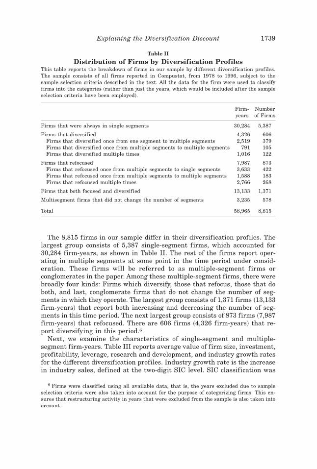
The 8,815 firms in our sample differ in their diversification profiles. Thelargest group consists of 5,387 single-segment firms, which accounted for30,284 firm-years, as shown in Table II. The rest of the firms report oper-ating in multiple segments at some point in the time period under consid-eration. These f irms will be referred to as multiple-segment f irms orconglomerates in the paper. Among these multiple-segment firms, there werebroadly four kinds: Firms which diversify, those that refocus, those that doboth, and last, conglomerate firms that do not change the number of seg-ments in which they operate. The largest group consists of 1,371 firms ~13,133firm-years! that report both increasing and decreasing the number of seg-ments in this time period. The next largest group consists of 873 firms ~7,987firm-years! that refocused. There are 606 firms ~4,326 firm-years! that re-port diversifying in this period.6

Next, we examine the characteristics of single-segment and multiple-segment firm-years. Table III reports average value of firm size, investment,profitability, leverage, research and development, and industry growth ratesfor the different diversification profiles. Industry growth rate is the increasein industry sales, defined at the two-digit SIC level. SIC classification was

6 Firms were classified using all available data, that is, the years excluded due to sampleselection criteria were also taken into account for the purpose of categorizing firms. This en-sures that restructuring activity in years that were excluded from the sample is also taken intoaccount.

Table II

Distribution of Firms by Diversification ProfilesThis table reports the breakdown of firms in our sample by different diversification profiles.The sample consists of all firms reported in Compustat, from 1978 to 1996, subject to thesample selection criteria described in the text. All the data for the firm were used to classifyfirms into the categories ~rather than just the years, which would be included after the sampleselection criteria have been employed!.

Firm-years

Numberof Firms

Firms that were always in single segments 30,284 5,387

Firms that diversified 4,326 606Firms that diversified once from one segment to multiple segments 2,519 379Firms that diversified once from multiple segments to multiple segments 791 105Firms that diversified multiple times 1,016 122

Firms that refocused 7,987 873Firms that refocused once from multiple segments to single segments 3,633 422Firms that refocused once from multiple segments to multiple segments 1,588 183Firms that refocused multiple times 2,766 268

Firms that both focused and diversified 13,133 1,371

Multisegment firms that did not change the number of segments 3,235 578

Total 58,965 8,815


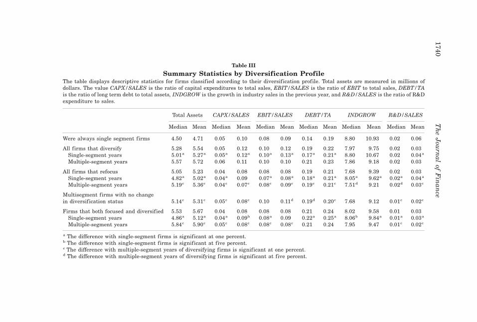
Table III

Summary Statistics by Diversification ProfileThe table displays descriptive statistics for firms classified according to their diversification profile. Total assets are measured in millions ofdollars. The value CAPX/SALES is the ratio of capital expenditures to total sales, EBIT/SALES is the ratio of EBIT to total sales, DEBT/TAis the ratio of long term debt to total assets, INDGROW is the growth in industry sales in the previous year, and R&D/SALES is the ratio of R&Dexpenditure to sales.

Total Assets CAPX/SALES EBIT/SALES DEBT/TA INDGROW R&D/SALES

Median Mean Median Mean Median Mean Median Mean Median Mean Median Mean

Were always single segment firms 4.50 4.71 0.05 0.10 0.08 0.09 0.14 0.19 8.80 10.93 0.02 0.06

All firms that diversify 5.28 5.54 0.05 0.12 0.10 0.12 0.19 0.22 7.97 9.75 0.02 0.03Single-segment years 5.01a 5.27a 0.05a 0.12a 0.10a 0.13a 0.17a 0.21a 8.80 10.67 0.02 0.04a

Multiple-segment years 5.57 5.72 0.06 0.11 0.10 0.10 0.21 0.23 7.86 9.18 0.02 0.03

All firms that refocus 5.05 5.23 0.04 0.08 0.08 0.08 0.19 0.21 7.68 9.39 0.02 0.03Single-segment years 4.82a 5.02a 0.04a 0.09 0.07a 0.08a 0.18a 0.21a 8.05a 9.62a 0.02a 0.04a

Multiple-segment years 5.19c 5.36c 0.04c 0.07c 0.08c 0.09c 0.19c 0.21c 7.51d 9.21 0.02d 0.03c

Multisegment firms with no changein diversification status 5.14c 5.31c 0.05c 0.08c 0.10 0.11d 0.19d 0.20c 7.68 9.12 0.01c 0.02c

Firms that both focused and diversified 5.53 5.67 0.04 0.08 0.08 0.08 0.21 0.24 8.02 9.58 0.01 0.03Single-segment years 4.86a 5.12a 0.04a 0.09b 0.08a 0.09 0.22a 0.25a 8.06b 9.84a 0.01a 0.03a

Multiple-segment years 5.84c 5.90c 0.05c 0.08c 0.08c 0.08c 0.21 0.24 7.95 9.47 0.01c 0.02c

a The difference with single-segment firms is significant at one percent.b The difference with single-segment firms is significant at five percent.c The difference with multiple-segment years of diversifying firms is significant at one percent.d The difference with multiple-segment years of diversifying firms is significant at five percent.

1740T

he

Jou

rnal

ofF

inan

ce

obtained from the business segment data. Divisional sales for conglomerateswere included in the respective SIC’s for the calculation of total industrysales.7

Single-segment years of conglomerates are significantly different from single-segment firms in their characteristics. Single-segment years of conglomer-ates are bigger, have higher leverage, and lower R&D than single-segmentfirms. This is consistent with Hyland ~1999!, who finds that diversifyingfirms have lower research and development expenses. With regard to CAPX/SALES and EBIT/SALES, not only do single-segment years of conglomer-ates differ from single-segment firms, but they also differ significantly amongthem. Single-segment years of diversified firms have higher CAPX/SALESand higher EBIT/SALES, while single-segment years of refocusing firmsand firms that both refocus and diversify have lower CAPX/SALES andlower EBIT/SALES than single-segment firms. In summary, firm charac-teristics differ across single-segment years in different diversification profiles.

There are also significant differences in the characteristics of multiseg-ment years of conglomerates. Multiple-segment years of diversifying firmstend to invest more in research and development ~RND/SALES! than oth-ers. They also have higher capital investment ~CAPX/SALES! and higherprofitability ~EBIT/SALES! than multiple-segment years of refocusing firmsand firms which both refocus and diversify. Conglomerates that do not changediversification status seem to be in mature industries with lower growthand have low research and development expenses, while enjoying higherprofitability ~EBIT/SALES! and higher capital investment ~CAPX/SALES!.Multiple-segment years of refocusing firms tend to have the lowest profit-ability and capital investment. This suggests that difference in characteris-tics of multiple-segment years might be related to the choice of diversificationstrategy.

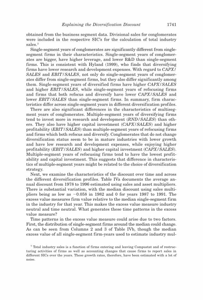
Next, we examine the characteristics of the discount over time and acrossthe different diversification profiles. Table IVa documents the average an-nual discount from 1978 to 1996 estimated using sales and asset multipliers.There is substantial variation, with the median discount using sales multi-pliers being as low as 20.058 in 1982 and 0 for years 1987 to 1991. Theexcess value measures firm value relative to the median single-segment firmin the industry for that year. This makes the excess value measure industryneutral and time neutral. What generates these time patterns in the excessvalue measure?

Time patterns in the excess value measure could arise due to two factors.First, the distribution of single-segment firms around the median could change.As can be seen from Columns 2 and 3 of Table IVb, though the medianexcess value of all single-segment firm-years used to estimate industry mul-

7 Total industry sales is a function of firms entering and leaving Compustat and of restruc-turing activities of firms as well as accounting changes that cause firms to report sales indifferent SICs over the years. These growth rates, therefore, have been estimated with a lot ofnoise.


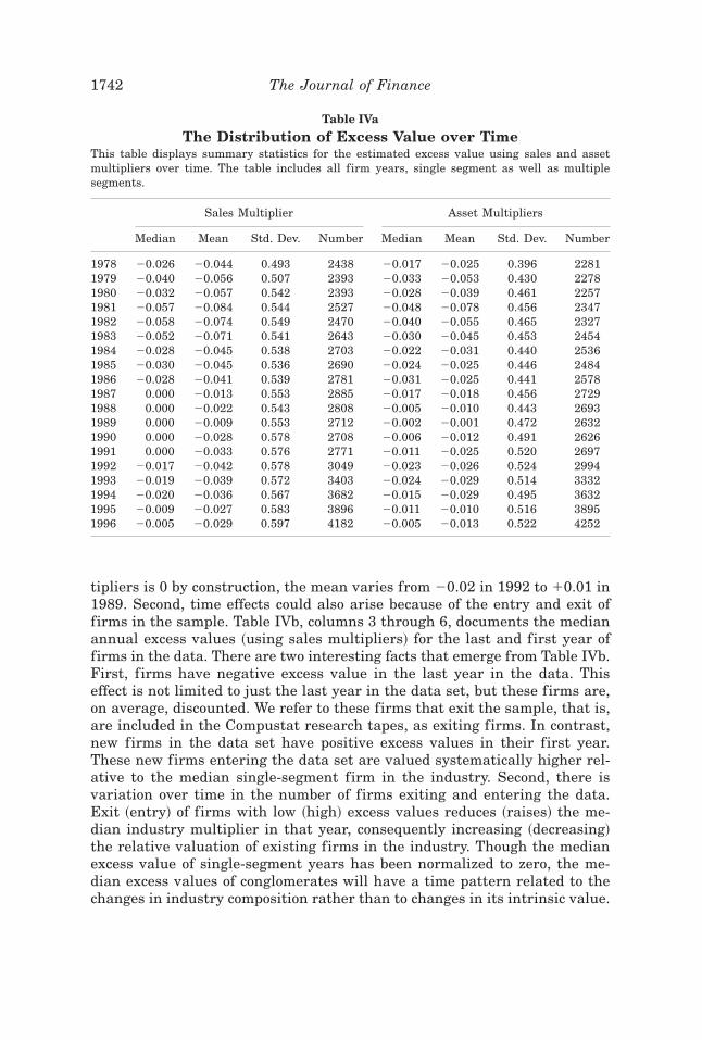
tipliers is 0 by construction, the mean varies from 20.02 in 1992 to 10.01 in1989. Second, time effects could also arise because of the entry and exit offirms in the sample. Table IVb, columns 3 through 6, documents the medianannual excess values ~using sales multipliers! for the last and first year offirms in the data. There are two interesting facts that emerge from Table IVb.First, firms have negative excess value in the last year in the data. Thiseffect is not limited to just the last year in the data set, but these firms are,on average, discounted. We refer to these firms that exit the sample, that is,are included in the Compustat research tapes, as exiting firms. In contrast,new firms in the data set have positive excess values in their first year.These new firms entering the data set are valued systematically higher rel-ative to the median single-segment firm in the industry. Second, there isvariation over time in the number of firms exiting and entering the data.Exit ~entry! of firms with low ~high! excess values reduces ~raises! the me-dian industry multiplier in that year, consequently increasing ~decreasing!the relative valuation of existing firms in the industry. Though the medianexcess value of single-segment years has been normalized to zero, the me-dian excess values of conglomerates will have a time pattern related to thechanges in industry composition rather than to changes in its intrinsic value.

Table IVa

The Distribution of Excess Value over TimeThis table displays summary statistics for the estimated excess value using sales and assetmultipliers over time. The table includes all firm years, single segment as well as multiplesegments.

Sales Multiplier Asset Multipliers

Median Mean Std. Dev. Number Median Mean Std. Dev. Number

1978 20.026 20.044 0.493 2438 20.017 20.025 0.396 22811979 20.040 20.056 0.507 2393 20.033 20.053 0.430 22781980 20.032 20.057 0.542 2393 20.028 20.039 0.461 22571981 20.057 20.084 0.544 2527 20.048 20.078 0.456 23471982 20.058 20.074 0.549 2470 20.040 20.055 0.465 23271983 20.052 20.071 0.541 2643 20.030 20.045 0.453 24541984 20.028 20.045 0.538 2703 20.022 20.031 0.440 25361985 20.030 20.045 0.536 2690 20.024 20.025 0.446 24841986 20.028 20.041 0.539 2781 20.031 20.025 0.441 25781987 0.000 20.013 0.553 2885 20.017 20.018 0.456 27291988 0.000 20.022 0.543 2808 20.005 20.010 0.443 26931989 0.000 20.009 0.553 2712 20.002 20.001 0.472 26321990 0.000 20.028 0.578 2708 20.006 20.012 0.491 26261991 0.000 20.033 0.576 2771 20.011 20.025 0.520 26971992 20.017 20.042 0.578 3049 20.023 20.026 0.524 29941993 20.019 20.039 0.572 3403 20.024 20.029 0.514 33321994 20.020 20.036 0.567 3682 20.015 20.029 0.495 36321995 20.009 20.027 0.583 3896 20.011 20.010 0.516 38951996 20.005 20.029 0.597 4182 20.005 20.013 0.522 4252


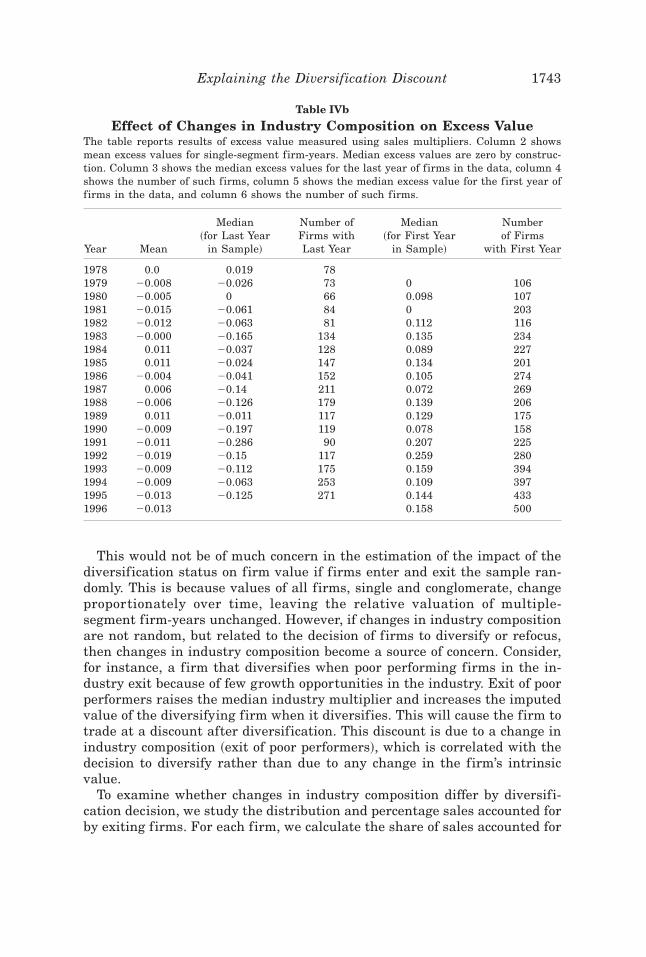
This would not be of much concern in the estimation of the impact of thediversification status on firm value if firms enter and exit the sample ran-domly. This is because values of all firms, single and conglomerate, changeproportionately over time, leaving the relative valuation of multiple-segment firm-years unchanged. However, if changes in industry compositionare not random, but related to the decision of firms to diversify or refocus,then changes in industry composition become a source of concern. Consider,for instance, a firm that diversifies when poor performing firms in the in-dustry exit because of few growth opportunities in the industry. Exit of poorperformers raises the median industry multiplier and increases the imputedvalue of the diversifying firm when it diversifies. This will cause the firm totrade at a discount after diversification. This discount is due to a change inindustry composition ~exit of poor performers!, which is correlated with thedecision to diversify rather than due to any change in the firm’s intrinsicvalue.

To examine whether changes in industry composition differ by diversifi-cation decision, we study the distribution and percentage sales accounted forby exiting firms. For each firm, we calculate the share of sales accounted for

Table IVb

Effect of Changes in Industry Composition on Excess ValueThe table reports results of excess value measured using sales multipliers. Column 2 showsmean excess values for single-segment firm-years. Median excess values are zero by construc-tion. Column 3 shows the median excess values for the last year of firms in the data, column 4shows the number of such firms, column 5 shows the median excess value for the first year offirms in the data, and column 6 shows the number of such firms.

Year Mean

Median~for Last Year

in Sample!

Number ofFirms withLast Year

Median~for First Year

in Sample!

Numberof Firms

with First Year

1978 0.0 0.019 781979 20.008 20.026 73 0 1061980 20.005 0 66 0.098 1071981 20.015 20.061 84 0 2031982 20.012 20.063 81 0.112 1161983 20.000 20.165 134 0.135 2341984 0.011 20.037 128 0.089 2271985 0.011 20.024 147 0.134 2011986 20.004 20.041 152 0.105 2741987 0.006 20.14 211 0.072 2691988 20.006 20.126 179 0.139 2061989 0.011 20.011 117 0.129 1751990 20.009 20.197 119 0.078 1581991 20.011 20.286 90 0.207 2251992 20.019 20.15 117 0.259 2801993 20.009 20.112 175 0.159 3941994 20.009 20.063 253 0.109 3971995 20.013 20.125 271 0.144 4331996 20.013 0.158 500


by exiting firms in their industry ~at the two-digit SIC level! for that year.For conglomerates, we weight each segment’s exposure to exiting firms byits sales. We also calculate the fraction of all firms in an industry that exit.Table IVc documents the percentage of exiting firms in each industry for thedifferent diversification profiles and highlights some interesting patterns.Single-segment years of diversifying firms operate in industries with thehighest incidence of exit. In these industries, 28 percent of all firms exit ina given year and the exiting firms account for 15 percent of industry sales.Single-segment firms in contrast belong to industries where exiting firmsaccount for only 14 percent of all firms and 6 percent of industry sales.While single-segment years of diversifying firms have the highest exposureto exiting firms, multiple-segment years of diversifying firms have one ofthe lowest exposures to exiting firms. In contrast, single-segment years ofrefocusing firms operate in industries with the lowest fraction of exitingfirms, while multiple-segment years of refocusing firms tend to be in indus-tries with the highest incidence of exiting firms. We observe that firms movetowards industries where the exit rate is low. This is suggestive of the factthat firms both diversify and refocus, from industries experiencing difficul-ties ~higher exit! into industries with better prospects ~lower exit!. This alsosupports the finding in Lang and Stulz ~1994! that diversifying firms tendto be in bad industries characterized by higher exit. This is consistent withour view that firms endogenously choose to diversify and refocus and isindicative of the fact that changes in industry composition are related to thefirm’s diversification strategy.

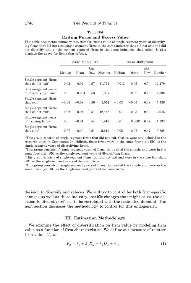
Firms also show systematic patterns in their discounts prior to whetherthey decide to diversify or exit the industry. Single-segment years of diver-sifying firms do not trade at a discount. This indicates that these firms donot do badly compared to the median firm in the industry prior to diversi-fying. However, as seen from Table IVc, these firms are in industries with ahigh incidence of exit. Combining these two results suggests that single seg-ment years of diversifying firms might be better than the firms that exit theindustry, but worse than the firms that continue as single-segment firms inthe industry, which is confirmed in Table IVd. Single-segment years of di-versifying firms which do not exit have a median discount of zero. This isbetter than the four percent discount for single-segment firms in the samefour-digit SIC that exit and worse than the two percent premium for single-segment firms in the same four-digit SIC that do not exit.

Summarizing, there are significant differences in firm characteristics be-tween single-segment firms and single-segment years of conglomerates. Thereare also significant differences in firm characteristics between multiple-segment years of conglomerates with different diversification profiles. Thereare also differences in industry composition over time. Firms that diversify~focus! come from industries with high exit rates. These firms have excessvalues prior to diversification that are higher than those of firms that exitthe industry but lower than those of firms that remain as single-segmentfirms. These changes in industry composition seem to be correlated with the


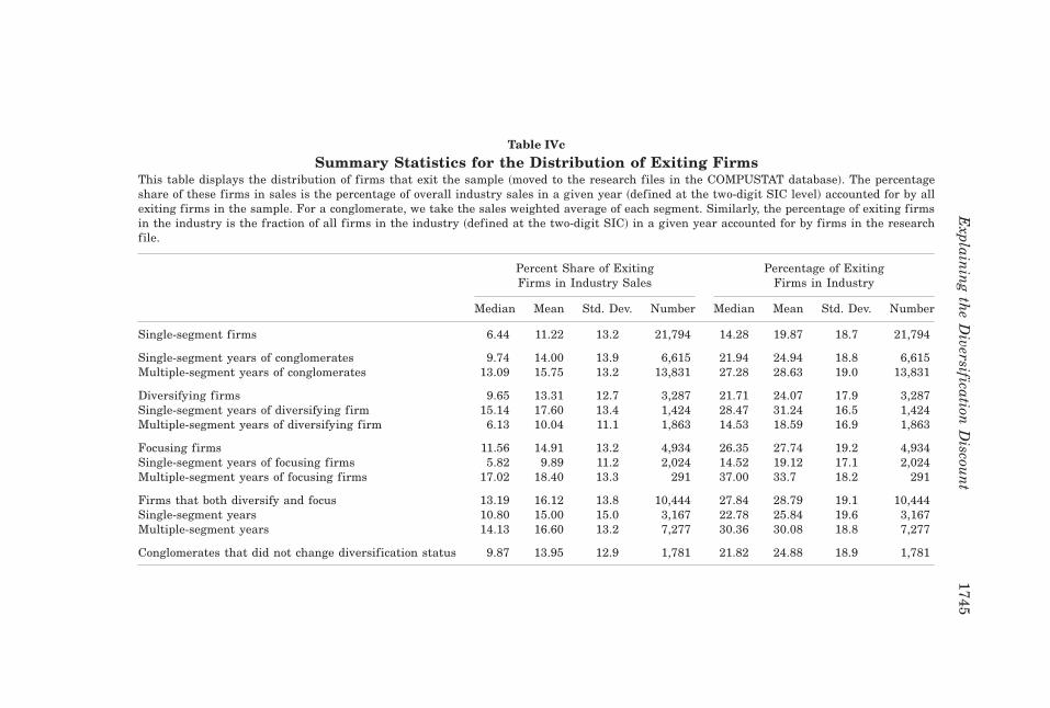
Table IVc

Summary Statistics for the Distribution of Exiting FirmsThis table displays the distribution of firms that exit the sample ~moved to the research files in the COMPUSTAT database!. The percentageshare of these firms in sales is the percentage of overall industry sales in a given year ~defined at the two-digit SIC level! accounted for by allexiting firms in the sample. For a conglomerate, we take the sales weighted average of each segment. Similarly, the percentage of exiting firmsin the industry is the fraction of all firms in the industry ~defined at the two-digit SIC! in a given year accounted for by firms in the researchfile.

Percent Share of ExitingFirms in Industry Sales

Percentage of ExitingFirms in Industry

Median Mean Std. Dev. Number Median Mean Std. Dev. Number

Single-segment firms 6.44 11.22 13.2 21,794 14.28 19.87 18.7 21,794

Single-segment years of conglomerates 9.74 14.00 13.9 6,615 21.94 24.94 18.8 6,615Multiple-segment years of conglomerates 13.09 15.75 13.2 13,831 27.28 28.63 19.0 13,831

Diversifying firms 9.65 13.31 12.7 3,287 21.71 24.07 17.9 3,287Single-segment years of diversifying firm 15.14 17.60 13.4 1,424 28.47 31.24 16.5 1,424Multiple-segment years of diversifying firm 6.13 10.04 11.1 1,863 14.53 18.59 16.9 1,863

Focusing firms 11.56 14.91 13.2 4,934 26.35 27.74 19.2 4,934Single-segment years of focusing firms 5.82 9.89 11.2 2,024 14.52 19.12 17.1 2,024Multiple-segment years of focusing firms 17.02 18.40 13.3 291 37.00 33.7 18.2 291

Firms that both diversify and focus 13.19 16.12 13.8 10,444 27.84 28.79 19.1 10,444Single-segment years 10.80 15.00 15.0 3,167 22.78 25.84 19.6 3,167Multiple-segment years 14.13 16.60 13.2 7,277 30.36 30.08 18.8 7,277

Conglomerates that did not change diversification status 9.87 13.95 12.9 1,781 21.82 24.88 18.9 1,781

Explain

ing

the

Diversification

Discou

nt

1745

decision to diversify and refocus. We will try to control for both firm-specificchanges as well as these industry-specific changes that might cause the de-cision to diversify0refocus to be correlated with the estimated discount. Thenext section discusses the methodology to control for this endogeneity.

III. Estimation Methodology

We examine the effect of diversification on firm value by modeling firmvalue as a function of firm characteristics. We define our measure of relativefirm value, Vit as

Vit 5 d0 1 d1 Xit 1 d2 Dit 1 eit , ~1!

Table IVd

Exiting Firms and Excess ValueThis table documents summary statistics for excess value of single-segment years of diversify-ing firms that did not exit, single-segment firms in the same industry that did not exit and didnot diversify, and single-segment years of firms in the same industries that exited. It alsodisplays the above for firms that refocus.

Sales Multipliers Asset Multipliers

Median MeanStd.Dev. Number Median Mean

Std.Dev. Number

Single-segment firmsthat do not exita 0.02 0.04 0.57 11,771 0.012 0.05 0.5 12,279

Single-segment yearsof diversifying firms 0.0 20.004 0.53 1,327 0 0.02 0.45 1,390

Single-segment firmsthat exitb 20.04 20.08 0.56 5,511 20.03 20.05 0.48 5,736

Single-segment firmsthat do not exitc 0.02 0.04 0.57 12,442 0.01 0.05 0.5 12,946

Single-segment yearsof focusing firms 0.0 20.01 0.54 1,919 0.0 0.0001 0.47 1,992

Single-segment firmsthat exitd 20.07 20.10 0.54 5,610 20.05 20.07 0.47 5,825

aThis group consists of single-segment firms that did not exit, that is, were not included in theresearch tapes in Compustat. In addition, these firms were in the same four-digit SIC as thesingle-segment years of diversifying firms.bThis group consists of single-segment years of firms that exited the sample and were in thesame four-digit SIC as the single-segment years of diversifying firms.cThis group consists of single-segment firms that did not exit and were in the same four-digitSIC as the single-segment years of focusing firms.dThis group consists of single-segment years of firms that exited the sample and were in thesame four-digit SIC as the single-segment years of focusing firms.


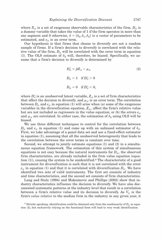
where Xit is a set of exogenous observable characteristics of the firm, Dit isa dummy variable that takes the value of 1 if the firm operates in more thanone segment and 0 otherwise, d 5 $d0, d1, d2% is a vector of parameters to beestimated, and eit is an error term.

Our hypothesis is that firms that choose to diversify are not a randomsample of firms. If a firm’s decision to diversify is correlated with the rela-tive value of the firm, Dit will be correlated with the error term in equation~1!. The OLS estimate of d2 will, therefore, be biased. Specifically, we as-sume that a firm’s decision to diversify is determined by

Dit* 5 bZit 1 mit ~2!

Dit 5 1 if Dit* . 0

Dit 5 0 if Dit* , 0,

where Dit* is an unobserved latent variable, Zit is a set of firm characteristics

that affect the decision to diversify, and mit is an error term. The correlationbetween Dit and eit in equation ~1! will arise when ~a! some of the exogenousvariables in the diversification equation, Zit , affect the firm’s relative valuebut are not included as regressors in the value equation; or ~b! the errors eitand mit are correlated. In either case, the estimation of d2 using OLS will bebiased.

We use three different techniques to control for the correlation betweenDit and eit in equation ~1! and come up with an unbiased estimator of d2.First, we take advantage of a panel data set and use a fixed-effect estimatorin equation ~1!, assuming that all the unobserved heterogeneity that leads tothe correlation between the error terms is constant over time.

Second, we attempt to jointly estimate equations ~1! and ~2! in a simulta-neous equation framework. The estimation of this system of simultaneousequations is not easy because the natural instruments for Dit , the observedfirm characteristics, are already included in the firm value equation ~equa-tion ~1!!, causing the system to be unidentified.8 The characteristic of a goodinstrument for diversification is such that it is not correlated with the erroreit in equation ~1! and that it is correlated with diversification Dit . We haveidentified two sets of valid instruments. The first set consists of industryand time characteristics, and the second set consists of firm characteristics.

Lang and Stulz ~1994! and Maksimovic and Phillips ~2002! show that in-dustry characteristics inf luence the decision to diversify. We have also doc-umented systematic patterns at the industry level that result in a correlationbetween a firm’s relative value and its decision to diversify. As Vit is thefirm’s value relative to the median firm in the industry in any given year, it

8 Strictly speaking, identification could be obtained only from the nonlinearity of Dit in equa-tion ~2!, but exclusively relying on the functional form will lead to very weak identification.


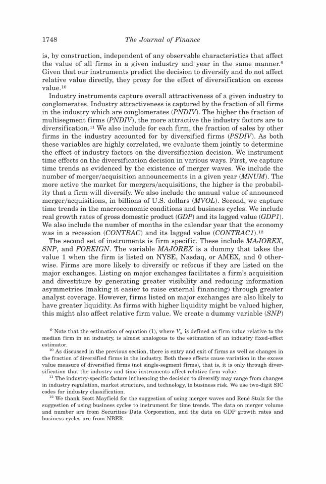
is, by construction, independent of any observable characteristics that affectthe value of all firms in a given industry and year in the same manner.9Given that our instruments predict the decision to diversify and do not affectrelative value directly, they proxy for the effect of diversification on excessvalue.10

Industry instruments capture overall attractiveness of a given industry toconglomerates. Industry attractiveness is captured by the fraction of all firmsin the industry which are conglomerates ~PNDIV!. The higher the fraction ofmultisegment firms ~PNDIV!, the more attractive the industry factors are todiversification.11 We also include for each firm, the fraction of sales by otherfirms in the industry accounted for by diversified firms ~PSDIV!. As boththese variables are highly correlated, we evaluate them jointly to determinethe effect of industry factors on the diversification decision. We instrumenttime effects on the diversification decision in various ways. First, we capturetime trends as evidenced by the existence of merger waves. We include thenumber of merger0acquisition announcements in a given year ~MNUM!. Themore active the market for mergers0acquisitions, the higher is the probabil-ity that a firm will diversify. We also include the annual value of announcedmerger0acquisitions, in billions of U.S. dollars ~MVOL!. Second, we capturetime trends in the macroeconomic conditions and business cycles. We includereal growth rates of gross domestic product ~GDP! and its lagged value ~GDP1!.We also include the number of months in the calendar year that the economywas in a recession ~CONTRAC! and its lagged value ~CONTRAC1!.12

The second set of instruments is firm specific. These include MAJOREX,SNP, and FOREIGN. The variable MAJOREX is a dummy that takes thevalue 1 when the firm is listed on NYSE, Nasdaq, or AMEX, and 0 other-wise. Firms are more likely to diversify or refocus if they are listed on themajor exchanges. Listing on major exchanges facilitates a firm’s acquisitionand divestiture by generating greater visibility and reducing informationasymmetries ~making it easier to raise external financing! through greateranalyst coverage. However, firms listed on major exchanges are also likely tohave greater liquidity. As firms with higher liquidity might be valued higher,this might also affect relative firm value. We create a dummy variable ~SNP!

9 Note that the estimation of equation ~1!, where Vit is defined as firm value relative to themedian firm in an industry, is almost analogous to the estimation of an industry fixed-effectestimator.

10 As discussed in the previous section, there is entry and exit of firms as well as changes inthe fraction of diversified firms in the industry. Both these effects cause variation in the excessvalue measure of diversified firms ~not single-segment firms!, that is, it is only through diver-sification that the industry and time instruments affect relative firm value.

11 The industry-specific factors inf luencing the decision to diversify may range from changesin industry regulation, market structure, and technology, to business risk. We use two-digit SICcodes for industry classification.

12 We thank Scott Mayfield for the suggestion of using merger waves and René Stulz for thesuggestion of using business cycles to instrument for time trends. The data on merger volumeand number are from Securities Data Corporation, and the data on GDP growth rates andbusiness cycles are from NBER.


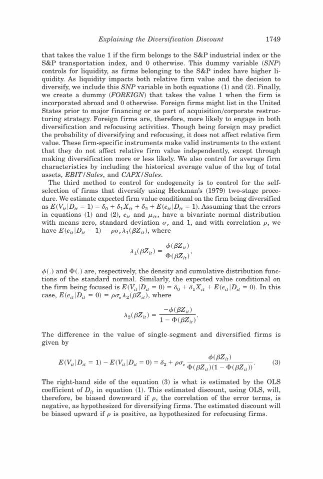
that takes the value 1 if the firm belongs to the S&P industrial index or theS&P transportation index, and 0 otherwise. This dummy variable ~SNP!controls for liquidity, as firms belonging to the S&P index have higher li-quidity. As liquidity impacts both relative firm value and the decision todiversify, we include this SNP variable in both equations ~1! and ~2!. Finally,we create a dummy ~FOREIGN! that takes the value 1 when the firm isincorporated abroad and 0 otherwise. Foreign firms might list in the UnitedStates prior to major financing or as part of acquisition0corporate restruc-turing strategy. Foreign firms are, therefore, more likely to engage in bothdiversification and refocusing activities. Though being foreign may predictthe probability of diversifying and refocusing, it does not affect relative firmvalue. These firm-specific instruments make valid instruments to the extentthat they do not affect relative firm value independently, except throughmaking diversification more or less likely. We also control for average firmcharacteristics by including the historical average value of the log of totalassets, EBIT/Sales, and CAPX/Sales.

The third method to control for endogeneity is to control for the self-selection of firms that diversify using Heckman’s ~1979! two-stage proce-dure. We estimate expected firm value conditional on the firm being diversifiedas E~Vit 6Dit 5 1! 5 d0 1 d1 Xit 1 d2 1 E~eit 6Dit 5 1!. Assuming that the errorsin equations ~1! and ~2!, eit and mit , have a bivariate normal distributionwith means zero, standard deviation se and 1, and with correlation r, wehave E~eit 6Dit 5 1! 5 rsel1~bZit !, where

l1~bZit ! 5f~bZit !

F~bZit !,

f~.! and F~.! are, respectively, the density and cumulative distribution func-tions of the standard normal. Similarly, the expected value conditional onthe firm being focused is E~Vit 6Dit 5 0! 5 d0 1 d1 Xit 1 E~eit 6Dit 5 0!. In thiscase, E~eit 6Dit 5 0! 5 rsel2~bZit !, where

l2~bZit ! 52f~bZit !

1 2 F~bZit !.

The difference in the value of single-segment and diversif ied firms isgiven by

E~Vit 6Dit 5 1! 2 E~Vit 6Dit 5 0! 5 d2 1 rse

f~bZit !

F~bZit !~1 2 F~bZit !!. ~3!

The right-hand side of the equation ~3! is what is estimated by the OLScoefficient of Dit in equation ~1!. This estimated discount, using OLS, will,therefore, be biased downward if r, the correlation of the error terms, isnegative, as hypothesized for diversifying firms. The estimated discount willbe biased upward if r is positive, as hypothesized for refocusing firms.


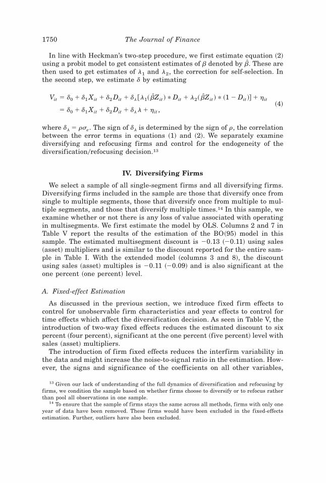
In line with Heckman’s two-step procedure, we first estimate equation ~2!using a probit model to get consistent estimates of b denoted by Zb. These arethen used to get estimates of l1 and l2, the correction for self-selection. Inthe second step, we estimate d by estimating

Vit 5 d0 1 d1 Xit 1 d2 Dit 1 dl @l1~ ZbZit ! * Dit 1 l2~ ZbZit ! * ~1 2 Dit !# 1 hit

5 d0 1 d1 Xit 1 d2 Dit 1 dl l 1 hit ,~4!

where dl 5 rse. The sign of dl is determined by the sign of r, the correlationbetween the error terms in equations ~1! and ~2!. We separately examinediversifying and refocusing firms and control for the endogeneity of thediversification0refocusing decision.13

IV. Diversifying Firms

We select a sample of all single-segment firms and all diversifying firms.Diversifying firms included in the sample are those that diversify once fromsingle to multiple segments, those that diversify once from multiple to mul-tiple segments, and those that diversify multiple times.14 In this sample, weexamine whether or not there is any loss of value associated with operatingin multisegments. We first estimate the model by OLS. Columns 2 and 7 inTable V report the results of the estimation of the BO~95! model in thissample. The estimated multisegment discount is 20.13 ~20.11! using sales~asset! multipliers and is similar to the discount reported for the entire sam-ple in Table I. With the extended model ~columns 3 and 8!, the discountusing sales ~asset! multiples is 20.11 ~20.09! and is also significant at theone percent ~one percent! level.

A. Fixed-effect Estimation

As discussed in the previous section, we introduce fixed firm effects tocontrol for unobservable firm characteristics and year effects to control fortime effects which affect the diversification decision. As seen in Table V, theintroduction of two-way fixed effects reduces the estimated discount to sixpercent ~four percent!, significant at the one percent ~five percent! level withsales ~asset! multipliers.

The introduction of firm fixed effects reduces the interfirm variability inthe data and might increase the noise-to-signal ratio in the estimation. How-ever, the signs and significance of the coefficients on all other variables,

13 Given our lack of understanding of the full dynamics of diversification and refocusing byfirms, we condition the sample based on whether firms choose to diversify or to refocus ratherthan pool all observations in one sample.

14 To ensure that the sample of firms stays the same across all methods, firms with only oneyear of data have been removed. These firms would have been excluded in the fixed-effectsestimation. Further, outliers have also been excluded.


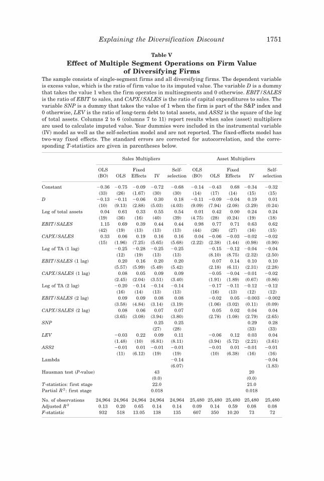
Table V

Effect of Multiple Segment Operations on Firm Valueof Diversifying Firms

The sample consists of single-segment firms and all diversifying firms. The dependent variableis excess value, which is the ratio of firm value to its imputed value. The variable D is a dummythat takes the value 1 when the firm operates in multisegments and 0 otherwise. EBIT/SALESis the ratio of EBIT to sales, and CAPX/SALES is the ratio of capital expenditures to sales. Thevariable SNP is a dummy that takes the value of 1 when the firm is part of the S&P index and0 otherwise, LEV is the ratio of long-term debt to total assets, and ASS2 is the square of the logof total assets. Columns 2 to 6 ~columns 7 to 11! report results when sales ~asset! multipliersare used to calculate imputed value. Year dummies were included in the instrumental variable~IV! model as well as the self-selection model and are not reported. The fixed-effects model hastwo-way fixed effects. The standard errors are corrected for autocorrelation, and the corre-sponding T-statistics are given in parentheses below.


OLS~BO! OLS

FixedEffects IV

Self-selection

OLS~BO! OLS

FixedEffects IV

Self-selection

Constant 20.36 20.75 20.09 20.72 20.68 20.14 20.43 0.68 20.34 20.32~33! ~26! ~1.67! ~30! ~30! ~14! ~17! ~14! ~15! ~15!

D 20.13 20.11 20.06 0.30 0.18 20.11 20.09 20.04 0.19 0.01~10! ~9.13! ~2.88! ~5.03! ~4.03! ~9.09! ~7.94! ~2.08! ~3.29! ~0.24!

Log of total assets 0.04 0.61 0.33 0.55 0.54 0.01 0.42 0.00 0.24 0.24~19! ~36! ~16! ~40! ~39! ~4.75! ~28! ~0.24! ~19! ~18!

EBIT/SALES 1.15 0.69 0.39 0.44 0.44 0.98 0.77 0.71 0.63 0.62~42! ~19! ~13! ~13! ~13! ~44! ~26! ~27! ~16! ~15!

CAPX/SALES 0.33 0.06 0.19 0.16 0.16 0.04 20.06 20.03 20.02 20.02~15! ~1.96! ~7.25! ~5.65! ~5.68! ~2.22! ~2.38! ~1.44! ~0.98! ~0.90!

Log of TA ~1 lag! 20.25 20.28 20.25 20.25 20.15 20.12 20.04 20.04~12! ~19! ~13! ~13! ~8.10! ~8.75! ~2.32! ~2.50!

EBIT/SALES ~1 lag! 0.20 0.16 0.20 0.20 0.07 0.14 0.10 0.10~5.57! ~5.99! ~5.49! ~5.42! ~2.18! ~6.11! ~2.31! ~2.28!

CAPX/SALES ~1 lag! 0.08 0.05 0.09 0.09 20.05 20.04 20.01 20.02~2.45! ~2.04! ~3.51! ~3.40! ~1.91! ~1.89! ~0.67! ~0.86!

Log of TA ~2 lag! 20.20 20.14 20.14 20.14 20.17 20.11 20.12 20.12~16! ~14! ~13! ~13! ~16! ~13! ~12! ~12!

EBIT/SALES ~2 lag! 0.09 0.09 0.08 0.08 20.02 0.05 20.003 20.002~3.58! ~4.84! ~3.14! ~3.19! ~1.06! ~3.02! ~0.11! ~0.09!

CAPX/SALES ~2 lag! 0.08 0.06 0.07 0.07 0.05 0.02 0.04 0.04~3.65! ~3.08! ~3.94! ~3.80! ~2.78! ~1.08! ~2.79! ~2.65!

SNP 0.25 0.25 0.29 0.28~27! ~28! ~33! ~33!

LEV 20.03 0.22 0.09 0.11 20.06 0.12 0.03 0.04~1.48! ~10! ~6.81! ~8.11! ~3.94! ~5.72! ~2.21! ~3.61!

ASS2 20.01 0.01 20.01 20.01 20.01 0.01 20.01 20.01~11! ~6.12! ~19! ~19! ~10! ~6.38! ~16! ~16!

Lambda 20.14 20.04~6.07! ~1.83!

Hausman test ~P-value! 43 20~0.0! ~0.0!

T-statistics: first stage 22.0 21.0Partial R2: first stage 0.018 0.018

No. of observations 24,964 24,964 24,964 24,964 24,964 25,480 25,480 25,480 25,480 25,480Adjusted R2 0.13 0.20 0.65 0.14 0.14 0.09 0.14 0.59 0.08 0.08F-statistic 932 518 13.05 138 135 607 350 10.20 73 72


with the exception of leverage and square of assets, remain practically iden-tical to the OLS estimation. The only coefficient that significantly changesin the regression is the coefficient on D. This result supports the view thatdiversification appears to be correlated with unobserved firm characteristics.

B. Estimating the Probability to Diversify: Probit Estimation

In this section, we discuss the estimation of the probability of diversifying.The results of this estimation will be used in the instrumental variable es-timation as well as in Heckman’s self-selection model.

Firm-specific characteristics inf luence the decision of firms to diversify.Firms with low profitability in their current operations may diversify intoother segments in search of more lucrative opportunities. To control for cur-rent and past profitability, we include EBIT/SALES and its lagged values.Firms with a high level of investment in current operations are less likely todiversify. We therefore include CAPX/SALES and its lagged values. We alsocontrol for firm size by including the log of total assets and its lagged values.We also include historical average values of the log of total assets, EBIT/SALES, and CAPX/SALES.

As discussed in Section IV, we identify two sets of instruments that predictthe decision to diversify while leaving firm value unaffected. The first set ofinstruments consists of industry and time variables. We include the attrac-tiveness of the industry to conglomerates proxied by PNDIV ~the fraction ofall firms in the industry that are conglomerates! and PSDIV ~the fraction ofindustry sales accounted for by conglomerates!. We capture time trends byincluding the number of merger0acquisition announcements in a given year~MNUM! and their annual value in billions of U.S. dollars ~MVOL!. We alsoinclude real growth rates of gross domestic product ~GDP!, its lagged value~GDP1!, the number of contractionary months in the year ~CONTRAC!, andits lagged value ~CONTRAC1!. The second set of instruments are firm char-acteristics. We include the exchange listing and country of incorporation ofthe firm. Firms listed on major exchanges ~MAJOREX! as well as firmsincorporated outside the United States ~FOREIGN! are more likely to en-gage in acquisition0divestiture programs. We control for the effect of liquid-ity by including SNP ~a dummy variable equal to 1 if the firm is on the S&Pindustrial index and 0 otherwise!.

The maximum likelihood estimates of the probit coefficients are reportedin Table VI. As probit coefficients are difficult to interpret, the table alsoreports the marginal effects of the change in each explanatory variable cal-culated at its sample mean. Small firms ~low average historical size! with anincrease in assets in recent years are more likely to diversify. There is weakevidence that firms with low profitability ~EBIT/SALES! and low invest-ment ~CAPX/SALES! in recent past years, but with high average historicalprofitability and investment, are more likely to diversify. The coefficientsare not significant however. Firm-level characteristics are not highly signif-icant in explaining the diversification decision.


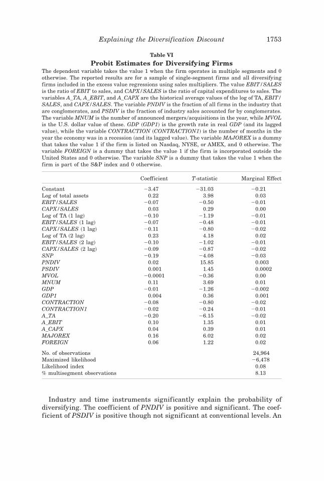
Industry and time instruments significantly explain the probability ofdiversifying. The coefficient of PNDIV is positive and significant. The coef-ficient of PSDIV is positive though not significant at conventional levels. An

Table VI

Probit Estimates for Diversifying FirmsThe dependent variable takes the value 1 when the firm operates in multiple segments and 0otherwise. The reported results are for a sample of single-segment firms and all diversifyingfirms included in the excess value regressions using sales multipliers. The value EBIT/SALESis the ratio of EBIT to sales, and CAPX/SALES is the ratio of capital expenditures to sales. Thevariables A_TA, A_EBIT, and A_CAPX are the historical average values of the log of TA, EBIT/SALES, and CAPX/SALES. The variable PNDIV is the fraction of all firms in the industry thatare conglomerates, and PSDIV is the fraction of industry sales accounted for by conglomerates.The variable MNUM is the number of announced mergers0acquisitions in the year, while MVOLis the U.S. dollar value of these. GDP ~GDP1! is the growth rate in real GDP ~and its laggedvalue!, while the variable CONTRACTION ~CONTRACTION1! is the number of months in theyear the economy was in a recession ~and its lagged value!. The variable MAJOREX is a dummythat takes the value 1 if the firm is listed on Nasdaq, NYSE, or AMEX, and 0 otherwise. Thevariable FOREIGN is a dummy that takes the value 1 if the firm is incorporated outside theUnited States and 0 otherwise. The variable SNP is a dummy that takes the value 1 when thefirm is part of the S&P index and 0 otherwise.

Coefficient T-statistic Marginal Effect

Constant 23.47 231.03 20.21Log of total assets 0.22 3.98 0.03EBIT/SALES 20.07 20.50 20.01CAPX/SALES 0.03 0.29 0.00Log of TA ~1 lag! 20.10 21.19 20.01EBIT/SALES ~1 lag! 20.07 20.48 20.01CAPX/SALES ~1 lag! 20.11 20.80 20.02Log of TA ~2 lag! 0.23 4.18 0.02EBIT/SALES ~2 lag! 20.10 21.02 20.01CAPX/SALES ~2 lag! 20.09 20.87 20.02SNP 20.19 24.08 20.03PNDIV 0.02 15.85 0.003PSDIV 0.001 1.45 0.0002MVOL 20.0001 20.36 0.00MNUM 0.11 3.69 0.01GDP 20.01 21.26 20.002GDP1 0.004 0.36 0.001CONTRACTION 20.08 20.80 20.02CONTRACTION1 20.02 20.24 20.01A_TA 20.20 26.15 20.02A_EBIT 0.10 1.35 0.01A_CAPX 0.04 0.39 0.01MAJOREX 0.16 6.02 0.02FOREIGN 0.06 1.22 0.02

No. of observations 24,964Maximized likelihood 26,478Likelihood index 0.08% multisegment observations 8.13


increase in the fraction of conglomerates in the industry, by 4 percent fromits mean of 48.6 percent, increases the probability of operating in multiplesegments by 1 percent. An increase in merger0acquisition activity leads toan increase in the probability of operating in multiple segments, that is,increases the probability of diversifying. An increase in the number of dealsannounced ~MNUM! by 0.7 thousands, from its mean of 2.03 thousand, leadsto an increase of 1 percent in the probability of multisegment operations.Macroeconomic conditions, however, do not significantly inf luence the prob-ability to diversify with the coefficients of both GDP ~GDP1! and CONTRAC~CONTRAC1! being insignificant. Firms listed on major exchanges are sig-nificantly more likely to diversify. The coefficient of MAJOREX is positiveand significant as hypothesized. The coefficient of SNP is negative and sig-nificant. Firms in the S&P industrial or transportation index are less likelyto diversify. Foreign firms are also more likely to diversify, though this effectis not significant.15

C. Instrumental Variables Estimation

We use the estimated probability of operating in multiple segments fromthe probit models as a generated instrument for the diversification status.In the first stage, we use all the exogenous variables along with the proba-bility of diversifying as explanatory variables in the decision to diversify,that is, D.16 In the second stage, we use the fitted value from the first stageas an instrument for D. The coefficient of the instrumented D, as reportedin Table V, is 0.30 ~0.19! with sales ~asset! multipliers and is significant atthe one percent ~one percent! level.

To test for the existence of endogeneity, we use Hausman’s test ~see Haus-man ~1978!!. The Hausman test is based on the difference between the OLSestimator ~which is consistent and efficient under the null hypothesis of noendogeneity and inconsistent under the alternative! and the IV estimator~which is consistent under both but inefficient under the null!. We can rejectthe null of no endogeneity at the one percent level for both sales and assetmultipliers. Bound, Jaeger, and Baker ~1995! show that when instrumentsare weakly correlated with the endogenous explanatory variable, then evena small correlation between the instruments and the error can seriously bias

15 The probit model reported in Table VI was also estimated for the sample of firms includedwhen asset multipliers were used to calculate excess values. These estimates were qualitativelysimilar and have not been reported in the paper. Though they have not been reported, theestimates were used to calculate the fitted probabilities and selectivity correction for the cor-responding estimation of the instrumental variable model and the self-selection model usingasset multipliers.

16 This involves regressing D on the estimated probability of diversification as well as on allthe exogenous variables in the excess value equation. We also estimated an alternative model,in which we included all independent variables including the instruments in the probit equa-tion in lieu of the predicted probability of diversifying. This alternative model does not imposethe nonlinear functional form of the probit. We found that the alternate specification was al-ways dominated by the probit specification and, therefore, we report the probit results.


estimates and lead to a large inconsistency in the IV estimates. They sug-gest reporting partial R2 and F-statistics on the instruments in the first-stage regression as useful guides. We find that the probability of diversifyingis highly significant, with a t-statistic of 22 ~referred to as T-stats: firststage! and a partial R2 of 0.02.17 This alleviates the concern that our esti-mation suffers from biases introduced by having weak instruments.

D. Self-selection Model

Last, we report the results of a two-stage estimation of the endogenousself-selection model. The estimated parameters of the OLS estimation of equa-tion ~4! are reported in Columns 6 and 11 of Table V. The estimated coeffi-cient of D is 0.18 when using sales multipliers and is significant at the onepercent level. The estimated coefficient is 0.01 when using asset multipliersand is not significant. The coefficient of l, the self-selection parameter is20.14 ~20.04! and is significant at the 1 percent ~10 percent! level whenusing sales ~asset! multipliers. The estimated coefficient of l is negative, asexpected, and significant. This indicates the prevalence of self-selection andsuggests that characteristics that make firms choose to diversify are nega-tively correlated with firm value. Firms with a higher probability of diver-sifying also tend to be discounted.

In summary, there is significant evidence of endogeneity with both theinstrumental variables and self-selection models. The multisegment dis-count turns positive under both methods and in three of the four cases, it issignificant at the one percent level.18

V. Refocusing Firms

Evidence on the value destruction associated with multiple segment firmsalso comes from observed gains achieved by refocusing firms. Comment andJarrell ~1995!, John and Ofek ~1995!, and Berger and Ofek ~1996! all docu-ment gains achieved by refocusing firms. In this section, we follow the sameempirical strategy detailed in the previous section and examine the firm’sdecision to refocus in a sample of single-segment firms and all refocusingfirms. In this sample of firms, the estimated discount in the BO~95! modelis 17 percent ~13 percent! using sales ~asset! multipliers. This discount dropsto 13 percent ~11 percent! with sales ~asset! multipliers in the extended BO~95!

17 The R2 of the first stage regression without including the generated probability of diver-sification was 0.035 ~0.028! and increases to 0.053 ~0.04! when the generated probabilities areincluded in the regression with sales ~asset! multipliers. The partial R2 is the increase in R2 byincluding the probability to diversify and is 0.018 ~0.012!.

18 To test the robustness of our results, we run various specifications of our model. Thesespecifications involve including RND/SALES to control for growth opportunities within thefirm, including industry growth estimates and excluding lagged values of firm size, profitabil-ity, and investment. The inclusion0exclusion of variables leaves unchanged our initial results,indicating strong evidence of the endogeneity of the diversification decision. The sign, magni-tude, and significance of the estimated discount0premium remain intact.


model as seen in columns 3 and 8 of Table VII. The estimated discount, inthe two-way fixed effects model, increases marginally from 13 percent to 14percent with sales multiples. It is unchanged at 11 percent when excessvalues are estimated using asset multipliers.

We find that we can better explain the decision to refocus in comparisonto the decision to diversify. The likelihood ratio index ~as seen in Table VIII!in the estimation of the probability to refocus is 0.21, in comparison to 0.079for the probability to diversify. Firms with high historical average invest-ments ~average CAPX/SALES! and low recent investments are less likely tooperate in multiple segments, that is, more likely to refocus. Firms withhigh historical average profitability and high recent profitability are lesslikely to operate in multiple segments or more likely to refocus. Firms withhigh historical average value of assets are more likely to operate in multiplesegments. In summary, firm characteristics like profitability, investments,and firm size all significantly explain the decision to refocus that is in con-trast to their inability to significantly explain the decision to diversify.

Besides, firm characteristics, industry characteristics, and time trends alsosignificantly determine the probability to refocus. The coefficients of bothPNDIV and PSDIV are significantly positive. An increase in the number ofconglomerates, as well as an increase in the share of sales accounted for byconglomerates, leads to an increase in the probability of operating in mul-tiple segments, that is, firms in industries that are attractive to conglomer-ates are less likely to refocus. Increase in merger activity, as captured by anincrease in the number of mergers0acquisitions, leads to a decrease in theprobability of operating in multiple segments, that is, an increase in theprobability of refocusing. This is in contrast to the diversification results,where an increase in merger activity increased the probability of operatingin multiple segments. Favorable merger0acquisition conditions prompt firmsto both diversify and refocus.

Macroeconomic conditions significantly explain the refocusing decision. Thisis in contrast to the diversification decision, where the coefficients of GDP growthand CONTRAC were not significant. Firms are more likely to operate in mul-tiple segments when in a recession. There is also evidence that high GDP growthrates increase the probability of operating in multiple segments. This sug-gests that extreme macroeconomic conditions reduce the probability of re-focusing. This is only partially consistent with the evidence in Maksimovic andPhillips ~2001!, who document that asset reallocations are highest in expansions.

Aside from the significance of individual variables, a better fit of the probitmodel is also ref lected in the significance of the fitted probabilities in the firststage of the two-stage least squares estimation. The probability of refocus-ing is highly significant with a t-statistic of 52 and a partial R2 of 0.079.19

19 Though this high significance may merely be a manifestation of a good instrument, it has tobe interpreted carefully. If the instrument is very highly correlated with the endogenous variable,it may also be correlated with the error, making it an unfit instrument to control for endogeneity.The relatively low R2 in the first-stage regression suggests this is not a problem in this case.


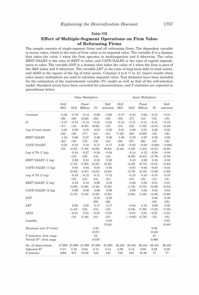
Table VII

Effect of Multiple-Segment Operations on Firm Valueof Refocusing Firms

The sample consists of single-segment firms and all refocusing firms. The dependent variableis excess value, which is the ratio of firm value to its imputed value. The variable D is a dummythat takes the value 1 when the firm operates in multisegments and 0 otherwise. The valueEBIT/SALES is the ratio of EBIT to sales, and CAPX/SALES is the ratio of capital expendi-tures to sales. The variable SNP is a dummy that takes the value of 1 when the firm is part ofthe S&P index and 0 otherwise, The variable LEV is the ratio of long-term debt to total assets,and ASS2 is the square of the log of total assets. Columns 2 to 6 ~7 to 11! report results whensales ~asset! multipliers are used to calculate imputed value. Year dummies have been includedfor the estimation of the instrumental variable ~IV! model as well as that of the self-selectionmodel. Standard errors have been corrected for autocorrelation, and T-statistics are reported inparentheses below.


OLS~BO! OLS

FixedEffects IV

Self-selection

OLS~BO! OLS

FixedEffects IV

Self-selection

Constant 20.38 20.76 20.14 20.68 20.68 20.17 20.43 0.62 20.31 20.31~36! ~28! ~2.82! ~32! ~32! ~18! ~17! ~13! ~15! ~15!

D 20.17 20.13 20.14 20.21 20.21 20.13 20.11 20.11 20.11 20.10~17! ~14! ~9.20! ~9.60! ~10! ~14! ~12! ~7.05! ~4.51! ~4.48!

Log of total assets 0.05 0.59 0.35 0.53 0.53 0.01 0.39 0.01 0.22 0.22~22! ~36! ~17! ~41! ~41! ~7.23! ~28! ~0.69! ~18! ~18!

EBIT/SALES 1.14 0.66 0.37 0.40 0.40 1.00 0.76 0.67 0.59 0.59~43! ~19! ~13! ~12! ~12! ~46! ~27! ~28! ~15! ~16!

CAPX/SALES 0.32 0.10 0.18 0.17 0.17 0.04 20.03 20.03 20.004 20.004~15! ~3.43! ~7.46! ~6.64! ~6.64! ~2.44! ~1.30! ~1.24! ~0.21! ~0.20!

Log of TA ~1 lag! 20.24 20.27 20.24 20.24 20.14 20.12 20.04 20.04~12! ~19! ~14! ~14! ~8.09! ~9.43! ~2.79! ~2.78!

EBIT/SALES ~1 lag! 0.26 0.21 0.23 0.23 0.13 0.20 0.16 0.16~7.15! ~7.60! ~6.25! ~6.25! ~4.38! ~8.74! ~3.81! ~3.84!

CAPX/SALES ~1 lag! 0.03 0.04 0.05 0.05 20.07 20.04 20.03 20.03~0.83! ~1.91! ~2.03! ~2.04! ~2.79! ~2.19! ~1.59! ~1.60!

Log of TA ~2 lag! 20.18 20.12 20.11 20.12 20.15 20.10 20.10 20.10~15! ~13! ~11! ~11! ~15! ~12! ~11! ~11!

EBIT/SALES ~2 lag! 0.12 0.12 0.09 0.10 20.02 0.05 20.01 20.01~4.60! ~5.86! ~3.48! ~3.56! ~1.10! ~2.76! ~0.28! ~0.24!

CAPX/SALES ~2 lag! 0.09 0.06 0.06 0.06 0.06 0.02 0.04 0.04~3.72! ~3.16! ~3.23! ~3.22! ~2.93! ~1.49! ~2.46! ~2.46!

SNP 0.25 0.25 0.28 0.29~29! ~29! ~35! ~35!

LEV 0.02 0.25 0.17 0.17 20.04 0.15 0.09 0.08~1.43! ~12! ~13! ~12! ~2.58! ~7.59! ~7.23! ~7.05!

ASS2 20.01 0.01 20.01 20.01 20.01 0.01 20.01 20.01~12! ~3.48! ~21! ~21! ~29.85! ~5.76! ~15! ~15!

Lambda 0.03 20.01~2.44! ~0.48!

Hausman test ~P-value! 3.20 0.08~0.07! ~0.45!

T-statistics: first stage 52 47Partial R2: first stage 0.079 0.066

No. of observations 27,995 27,995 27,995 27,995 27,995 28,161 28,161 28,161 28,161 28,161Adjusted R2 0.13 0.19 0.64 0.13 0.14 0.09 0.14 0.58 0.08 0.08F-statistic 1064 557 13.00 142 142 732 383 10.30 77 77


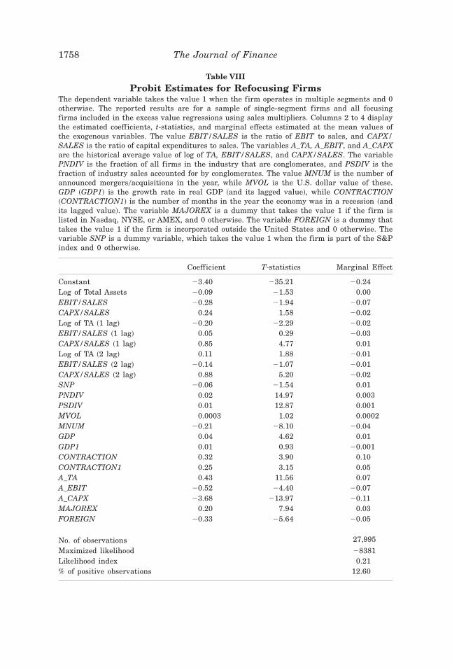
Table VIII

Probit Estimates for Refocusing FirmsThe dependent variable takes the value 1 when the firm operates in multiple segments and 0otherwise. The reported results are for a sample of single-segment firms and all focusingfirms included in the excess value regressions using sales multipliers. Columns 2 to 4 displaythe estimated coefficients, t-statistics, and marginal effects estimated at the mean values ofthe exogenous variables. The value EBIT/SALES is the ratio of EBIT to sales, and CAPX/SALES is the ratio of capital expenditures to sales. The variables A_TA, A_EBIT, and A_CAPXare the historical average value of log of TA, EBIT/SALES, and CAPX/SALES. The variablePNDIV is the fraction of all firms in the industry that are conglomerates, and PSDIV is thefraction of industry sales accounted for by conglomerates. The value MNUM is the number ofannounced mergers0acquisitions in the year, while MVOL is the U.S. dollar value of these.GDP ~GDP1! is the growth rate in real GDP ~and its lagged value!, while CONTRACTION~CONTRACTION1! is the number of months in the year the economy was in a recession ~andits lagged value!. The variable MAJOREX is a dummy that takes the value 1 if the firm islisted in Nasdaq, NYSE, or AMEX, and 0 otherwise. The variable FOREIGN is a dummy thattakes the value 1 if the firm is incorporated outside the United States and 0 otherwise. Thevariable SNP is a dummy variable, which takes the value 1 when the firm is part of the S&Pindex and 0 otherwise.

Coefficient T-statistics Marginal Effect

Constant 23.40 235.21 20.24Log of Total Assets 20.09 21.53 0.00EBIT/SALES 20.28 21.94 20.07CAPX/SALES 0.24 1.58 20.02Log of TA ~1 lag! 20.20 22.29 20.02EBIT/SALES ~1 lag! 0.05 0.29 20.03CAPX/SALES ~1 lag! 0.85 4.77 0.01Log of TA ~2 lag! 0.11 1.88 20.01EBIT/SALES ~2 lag! 20.14 21.07 20.01CAPX/SALES ~2 lag! 0.88 5.20 20.02SNP 20.06 21.54 0.01PNDIV 0.02 14.97 0.003PSDIV 0.01 12.87 0.001MVOL 0.0003 1.02 0.0002MNUM 20.21 28.10 20.04GDP 0.04 4.62 0.01GDP1 0.01 0.93 20.001CONTRACTION 0.32 3.90 0.10CONTRACTION1 0.25 3.15 0.05A_TA 0.43 11.56 0.07A_EBIT 20.52 24.40 20.07A_CAPX 23.68 213.97 20.11MAJOREX 0.20 7.94 0.03FOREIGN 20.33 25.64 20.05

No. of observations 27,995

Maximized likelihood 28381Likelihood index 0.21% of positive observations 12.60


The estimated discount increases from 13 percent to 21 percent with sales mul-tipliers. The Hausman test rejects the null of no endogeneity at the 7 percentlevel. The results with asset multipliers are much weaker. There is no evi-dence of endogeneity and the estimated discount drops from 8 percent to 7 per-cent, though it is still significant.

Similar results are obtained when the self-selection model is estimated.The coefficient of l, the selectivity correction, is positive as expected and issignificant at the 5 percent level when using sales multipliers. The esti-mated discount increases to 21 percent. However, the coefficient l is notsignificant when we use asset multipliers and the estimated discount staysroughly the same at 10 percent. In line with the results of the instrumentalvariable estimation, there exists evidence of self-selection only when salesmultipliers are used. With sales multipliers there is evidence that, control-ling for the endogeneity of the refocusing decision, there is an increase inthe estimated discount associated with multisegment operations. Also, thecoefficient of the estimated selectivity bias with sales multipliers is positiveas hypothesized, that is, characteristics that make firms choose to refocusare positively correlated with excess value. This is in contrast to the resultsreported for diversifying firms, where l was estimated with a significantnegative coefficient.20

VI. Conclusion

Firms choose the extent of their operations and decide whether to operatein a single industry, diversify into multiple industries, or refocus their op-erations. A firm’s choice to diversify is likely to be a response to exogenouschanges in the firm’s environment that also affect firm value. In this case,the observed correlation between diversification and firm value is not causal.

There are systematic patterns in diversification strategies and relativevalue of firms. Firms are more likely to move away from industries withrelatively low growth and high exit rates. Firms that choose to diversifyhave higher value than exiting firms in their industry and lower value thanother firms in the industry that remain focused.

We model the effect this endogeneity has on the observed correlation be-tween diversification and firm value. We use panel data and instrumentalvariables to control for the exogenous characteristics that predict the deci-sion to diversify. Once these observed firm characteristics and firm fixedeffects are controlled for, the evidence in favor of the assertion that diver-sification destroys value is substantially weaker. When we jointly estimatethe decision of a firm to diversify and its firm value, the diversification

20 We estimate the variants of the basic model to check for the robustness of our resultsanalogously to the robustness checks for the diversification decision. The estimated resultsincluding RND/SALES, including industry growth rates, and excluding lagged values of theexplanatory variables, are qualitatively unchanged. These results are not reported and areavailable from the authors.


discount is more likely to be a premium. The evidence in this paper suggeststhat diversification is a value-enhancing strategy for those firms that actu-ally pursue it.

We follow a similar strategy to evaluate the correlation between firm valueand the decision to refocus. The results are similar for this case. Firms thatrefocus their operations would have suffered a significant decrease in valueif they had remained diversified. This evidence suggests that the observedcorrelation between diversification status and firm value need not be causal,but rather the outcome of actions by profit-maximizing firms reacting toshocks in their environments.

Our results highlight the value of constructing more complete models ofthe interaction between firm strategies and firm value. The development ofa dynamic model that will jointly allow for both diversification and focus byfirms in response to changes in their economic environment and that couldalso be structurally estimated with the available data should be the long-runobjective. Short of a full dynamic structural model, the evidence in this pa-per highlights the importance of identifying large exogenous shocks to firmsto adequately evaluate the relationship between firm choices and equilib-rium outcomes.

REFERENCES

Aron, Debra, 1988, Ability, moral hazard, firm size and diversification, The Rand Journal ofEconomics 19, 72–87.

Berger, Phillip, and Eli Ofek, 1995, Diversification’s effect on firm value, Journal of FinancialEconomics 37, 39–65.

Berger, Phillip, and Eli Ofek, 1996, Bustup takeovers of value destroying diversified firms,Journal of Finance 51, 1175–1200.

Bodnar, Gordon, Charles Tang, and Joseph Weintrop, 1997, Both sides of corporate diversifi-cation: The value impacts of geographic and industrial diversification, Working paper 6224,NBER.

Bound, John, David Jaeger, and Regina Baker, 1995, Problems with instrumental variablesestimation when the correlation between the instruments and the endogenous explanatoryvariable is weak, Journal of the American Statistical Association 90, 443–450.

Chandler, Alfred, 1977, The Visible Hand ~Belknap Press, Cambridge, MA!.Chevalier, Judith, 2000, Why do firms undertake diversifying mergers? An analysis of the

investment policies of merging firms, Working paper, University of Chicago.Comment, Robert, and Gregg Jarrell, 1995, Corporate focus and stock returns, Journal of Fi-

nancial Economics 37, 67–87.Denis, David, Diane Denis, and Atulya Sarin, 1997, Agency problems, equity ownership, and

corporate diversification, Journal of Finance 52, 135–160.Dixit, Avinash, and Robert Pindyck, 1994, Investment under Uncertainty ~Princeton University

Press, Princeton, NJ!.Fauver, Larry, Joel Houston, and Andy Naranjo, 1998, Capital market development, legal sys-

tems and the value of corporate diversification: A cross-country analysis, Working paper,University of Florida.

Fluck, Zsusanna, and Anthony Lynch, 1999, Why do firms merge and then divest? A theory offinancial synergies, Journal of Business 72, 319–346.

Graham, John, Michael Lemmon, and Jack Wolf, 2002, Does corporate diversification destroyvalue? Journal of Finance, 57, 695–720.


Hadlock, Charles, Michael Ryngaert, and Shawn Thomas, 2001, Corporate structure and equityofferings: Are there benefits to diversification? Journal of Business 74, 613–635.

Harris, Milton, C. H. Kriebel, and Artur Raviv, 1982, Asymmetric information, incentives, andintrafirm resource allocation, Management Science 28, 604–620.

Hausman, Jerry, 1978, Specification tests in econometrics, Econometrica 46, 1251–1271.Heckman, James, 1979, Sample selection bias as specification error, Econometrica 47, 153–161.Hyland, David, 1999, Why firms diversify: An empirical examination, Working paper, Univer-

sity of Texas at Arlington.Jensen, Michael, 1986, Agency costs of free cash f low, corporate finance, and takeovers, Amer-

ican Economic Review 76, 323–329.Jensen, Michael, 1988, Takeovers, their causes and consequences, Journal of Economic Per-

spectives 2, 21–48.John, Kose, and Eli Ofek, 1995, Asset sales and increase in focus, Journal of Financial Eco-

nomics 37, 105–126.Khanna, Tarun, and Krishna Palepu, 2000, Is group affiliation profitable in emerging markets?

An analysis of diversified Indian business groups, Journal of Finance 55, 867–891.Lamont, Owen, 1997, Cash f low and investment: Evidence from internal capital markets, Jour-

nal of Finance 52, 83–110.Lamont, Owen, and Christopher Polk, 2001, The diversification discount: Cash f lows versus

returns, Journal of Finance, 56, 1693–1721.Lang, Larry, and René Stulz, 1994, Tobin’s q, corporate diversification and firm performance,

Journal of Political Economy 102, 1248–1280.Lewellen, Wilbur, 1971, A pure financial rationale for the conglomerate merger, Journal of

Finance 26, 521–537.Lins, Karl, and Henri Servaes, 1998, Is corporate diversification beneficial in emerging mar-

kets?, Working paper, London Business School.Lins, Karl, and Henri Servaes, 1999, International evidence on the value of corporate diversi-

fication, Journal of Finance 54, 2215–2239.Maksimovic, Vojislav, and Gordon Phillips, 2001, The market for corporate assets: Who engages

in mergers and asset sales and are there efficiency gains? Journal of Finance 56, 2019–2065.

Maksimovic, Vojislav, and Gordon Phillips, 2002, Do conglomerate firms allocate resources in-efficiently across industries? Journal of Finance, 57, 721–767.

Matsusaka, John, 1993, Takeover motives during the conglomerate merger wave, The RandJournal of Economics 24, 357–379.

Matsusaka, John, 2001, Corporate diversification, value maximization, and organizational ca-pabilities, Journal of Business 74, 409–431.

Perold, Andre, 1999, Capital allocation in financial firms, Working paper, Harvard BusinessSchool.

Rajan, Raghuram, Henri Servaes, and Luigi Zingales, 2000, The cost of diversity: The diversi-fication discount and inefficient investment, Journal of Finance 55, 35–80.

Rotemberg, Julio, and Garth Saloner, 1994, Benefits of narrow business strategies, AmericanEconomic Review 84, 1330–1349.

Scharfstein, David, 1998, The dark side of internal capital markets II: Evidence from diversi-fied conglomerates, Working paper 6352, NBER.

Scharfstein, David, and Jeremy Stein, 2000, The dark side of internal capital markets: Divi-sional rent seeking and inefficient investment, Journal of Finance 55, 2537–2567.

Schoar, Antonette, 1999, Effects of corporate diversification on productivity, Working paper,University of Chicago.

Servaes, Henri, 1996, The value of diversification during the conglomerate merger wave, Jour-nal of Finance 51, 1201–1225.

Stein, Jeremy, 1997, Internal capital markets and the competition for corporate resources, Jour-nal of Finance 52, 111–133.

Stulz, René, 1990, Managerial discretion and optimal financial policies, Journal of FinancialEconomics 26, 3–27.


Villalonga, Belen, 2002, Does diversification cause the “diversification discount”? Working pa-per, Harvard Business School.

Wernerfelt, Birger, and Cynthia Montgomery, 1988, Tobin’s q and the importance of focus infirm performance, American Economic Review 78, 246–250.

Weston, James, 1970, The nature and significance of conglomerate firms, St. John Law Review44, 66–80.

Whited, Toni, 2001, Is it inefficient investment that causes the diversification discount? Jour-nal of Finance 56, 1667–1691.


explaining the diversification discount

Documents