The Movement of Cohesive Sediment in a Large Combined Sewer

David J.J. Wotherspoon

Ph.D. 1994

THE MOVEMENT OF COHESIVE SEDIMENT IN A LARGE COMBINED SEWER

David J.J. Wotherspoon, B.Sc.

A Thesis submitted in partial fulfilment of the requirements of the University of Abertay Dundee

for the degree of Doctor of Philosophy

This research programme was carried out in collaboration with Tayside Regional Council Department of Water Services

and the Water Research Centre Pic.

I certify that this thesis is the true and accurate version of the thesis approved by the examiners.

September 1994

udies)Signed Date H. ISQ4

ABSTRACT

The presence of sediment deposits within sewerage systems may lead to operational (premature surcharging and surface flooding) and potential environmental problems (sediments act as a store of pollutants which can be released during erosion events). The consequences of allowing these problems to persist have been recognised internationally. In the U.K., the water industry has promoted fundamental and applied research to develop the necessary operational and analytical tools to manage these problems. Under the Urban Pollution Management Research Programme the major aspects of sediments in sewers have been studied and their effects included in new methodologies and tools.

Most studies in the U.K. and elsewhere have concentrated on the movement of non - cohesive sediments, whilst it has been recognised that combined sewer sediment deposits possess cohesive characteristics (although this cohesion primarily arises from agglutination and biological processes in the combined sewer rather than classical concepts of cohesion). New computer based models, e.g Mosqito (Moys 1987) and MOUSETRAP (WRc 1993) , are based on sediment transport capacity theories with the limited availability of sediment within the system recognised through storage layers which become available only when certain threshold levels of shear stress are exceeded. Studies in the U.K. to estimate the release of pollutants stored within sewer sediment beds also require a knowledge of the hydraulic shear stress conditions at which the sediment beds will erode and become entrained into the flow.

The reported study examines the apparent cohesive nature of a sediment bed in a large diameter sewer concurrently with flow hydraulics, sediment bed deposit depth and suspended solids flux for a number of dry and wet weather periods. Instrumentation was developed and assessed for hydraulic measurements within the study sewer system and in

(i)

particular, a novel system was devised to improve flow measurement accuracy in large diameter sewers. Development work was also undertaken on an ultrasonic device to monitor the temporal variation in sediment deposit depth at a point. The constituent materials of the sediment bed were examined and rheological techniques were employed to assess the structural strength of the sediment bed present in the study sewer. The results confirmed the apparent cohesive nature of the sediment bed, with the structural strength of the bed far exceeding the normal hydraulic shear stress ranges encountered in the sewerage system.

A relationship between apparent yield strength and liquid content of the sediment bed was obtained from the rheological tests. The bed structural strength was then compared with temporal changes in the flow - induced shear forces. An empirical model was developed to predict the availability for erosion of the cohesive deposits in the combined sewer studied. This model was tested against further temporally varying data sets from the sewer and was found to predict the erosion of the sediment bed under varying levels of applied shear stress together with changes in the sediment transport flux.

It was concluded that when Dry Weather Flows induce bed shear stresses in excess of 1-2 N/m erosion of the sediment bed structure can be caused, with storm flows which induce shear stresses in excess of 4-6 N/m eroding the bed to a greater depth. The sediment bed was observed to be rapidly re-established following an erosion event.

The investigation and model developed contribute significantly to knowledge about the behaviour of sediments in sewers and provide for the first time a model to simulate erosion of a sediment bed with apparently cohesive properties and consequent increase in sediment and pollutant transport rates.

(ii)

ACKNOWLEDGEMENTS

In a project of this type, there are many people to thank for the assistance and advice freely given and gratefully received:

The Science and Engineering Council and the Water Research Centre for the full financial support for this project.

The Department of Civil Engineering, Surveying and Building of Dundee Institute of Technology. Professor S. Sarkar, head of department, who balances the needs of research and teaching, allowing both to coexist and interact as they should.

Mr. R. Ashley, supervisor and mentor, whose entrepreneurial skills overcame many obstacles and whose guidance, enthusiasm, questioning and demands are all greatly appreciated.

Dr. K.O. Oduyemi, study supervisor, and Mr. C. Jefferies who were always available to comment on the work undertaken and assist in the solution of difficulties in the project. The technical staff of the department for fabricating the many and varied items required during field and laboratory work. Mr. I. McGregor and Mr. B. Coghlan, fellow research staff, who always managed to see the humourous side of sewerage research.

Tayside Regional Council Water Services Department, without whose financial and logistical support this project would not have been possible. Particular thanks must go to Mr. N. Watson and Mr. J. White, Dundee Division, who went out of their way to accommodate the sometimes audacious requests made to them.

Dr. D. Williams and Dr. R. Williams, Chemical Engineering Department, University College Swansea, for the training and advice given on both the project generally and in particular the rheological aspects of sewer sediments.

(iii)

The Water Research Centre Pic., whose staff provided advice, information and financial assistance.

Detectronic Limited, now Montec International, for advice on the use of their flow measurement apparatus and for responding to the need to further investigate flow measurement systems for sewers.

Hydraulics Research Limited for providing experimental apparatus for measuring the settling velocities of sewage particulates.

And finally, to Janice, who for over three years lived with the fact that our lives revolved around the weather - and Dundee can be a very wet place sometimes (but never when you want it to be !)

Dr. Chandra Nalluri, Department of Civil Engineering,University of Newcastle, for acting as a supervisor forthis work and providing a link to laboratory based studies.

(iv)

TABLE OF CONTENTS

PageAbstract iAcknowledgements iiiTable of Contents vList of Figures ixList of Tables xiiiList of Plates xvNotation xviAbbreviations xviii

CHAPTER 1INTRODUCTION 1

1.1 Background 11.2 Present Design Practice 21.3 Research Requirements 51.4 Scope of the Research 61.4.1 Thesis Contents 8

CHAPTER 2SEDIMENT MOVEMENT LITERATURE REVIEW 9

2.1 General Sediment Movement 112.2 Non-Cohesive Sediments 12

2.2.1 Initiation of Motion 122.2.2 Bedforms 172.2.3 Bed Load 222.2.4 Total Load 252.2.5 Suspended Load 31

2.3 Non-Cohesive Transport in Pipes and CircularChannels 352.3.1 Initiation of Movement 362.3.2 Pseudohomogeneous Flow (Wash Load) 372.3.3 Heterogeneous Flow (Suspended Load) 382.3.4 Flow Over a Deposited Bed 45

(v)

2.4 Cohesive Sediments 482.4.1 Flocculation 492.4.2 Settling and Deposition 512.4.3 Consolidation 562.4.4 Erosion 61

2.5 Sewer Sediments 672.5.1 Sources of Sewer Sediments 672.5.2 Sediment Properties 692.5.3 Cohesive Sewer Sediments 76

2.6 Summary 7 9

CHAPTER 3FIELD SITE 83

3.1 Overall Catchment 833.2 Sewer Studied 873.3 Sediment in Study Sewer 903.4 Measured Parameters 91

CHAPTER 4INSTRUMENTATION 93

4.1 Hydraulics 934.1.1 Detectronic Flow Survey Loggers 934.1.2 Electromagnetic Velocity Meters 964.1.3 Arx Level Monitors 974.1.4 WRc Pypscan 99

4.2 Bed Erosion and Deposition 1004.3 Sediment and Sewage Sampling 1024.4 Settling Velocity 1044.5 Laboratory 104

4.5.1 Malvern Autosizer 1044.5.2 Rheometer 105

(vi)

CHAPTER 5 STUDY RESULTS 106

5.1 Hydraulics 1065.1.1 Velocity Profiles and Shear Stress -

Theory 1085.1.2 Results 112

5.2 Bed Erosion/Deposition 1195.3 Suspended Solids 1305.4 Particle Sizes 1335.5 Settling Velocity 139

5.5.1 WRc/SDD Method 1395.5.2 DIT/Aston University Method 1405.5.3 Owen Tube 1405.5.4 Summary 149

5.6 Rheology and the Rheological Properties ofSewer Sediments 1495.6.1 Introduction 1495.6.2 Rheology and Sewer Sediments 1525.6.3 Rheometry 1525.6.4 Testing Procedure Adopted 1585.6.5 Results 1635.6.6 Comparison With Other Published Data 173

5.7 Results - Discussion Summary 1805.7.1 Hydraulics 1805.7.2 Sediment Deposition and Erosion 1805.7.3 Suspended Material 1825.7.4 Settling Velocity 1825.7.5 Rheology 183

CHAPTER 6MODEL DEVELOPMENT 184

6.1 Erosion of Cohesive Sewer Sediments 1846.2 Model Conception 1866.3 Model Description 187

6.3.1 Deposition 1926.4 Sensitivity 1926.5 Application 198

(vii)

6.6 Data for Model Initiation and Verification 2006.7 Model Results - Discussion 208

CHAPTER 7CONCLUSIONS AND RECOMMENDATIONS FORFURTHER RESEARCH 216

7.1 Instrumentation 2167.2 Sediment Characteristics 2187.3 Erosion of Sediment Deposits 2197.4 Model 2217.5 Further Research 222

References 226

AppendicesAppendix A - Review of Flow Instrumentation A.1Appendix B - Ultrasonic Array B.lAppendix C - Electromagnetic Velocity Meter Results C.l Appendix D - Sonar Development D.1Appendix E - Settling Velocity Tests E.lAppendix F - Tables and Result Figures F.lAppendix G - Publications G.1

(viii)

LIST OF FIGURES

1.1 Variation of Velocity and Shear Stresswith Pipe Diameter 4

1.2 Variation of Velocity and Shear Stresswith Pipe Diameter 4

2.1 Transport Load Fractions 112.2 Extended Shields Diagram 152.3 Hjulstrom and Postima Diagram 162.4 Engelund and Hansen's Diagram 212.5 Newitt's Transition Velocity 402.6 Macke's Function 432.7 Graf and Acaroglu - total load comparisons 472.8 Delo - Variation of Settling Velocity with

Concentration 532.9 Owen - Bed Level Change With Time 572.10 Owen - Density Change With Time 572.11 Density Variation With Depth and Time 582.12 Dimensionless Density-Depth Profiles 592.13 Floe Aggregates 78

3.1 Dundee Interceptor Sewer - Overall Catchment 843.2 Interceptor Sewer and Control Gates 853.3 Longitudinal Section of Interceptor Sewer 883.4 Survey Plan 89

4.1 Ultrasonic Flow Logger 944.2 WRc Recommendations for Sewer Flow

Survey Sites 954.3 ARX versus Detectronic Logged Depths 984.4 Sewer Invert Shape From WRc "Pypscan" Device 994.5 3-D "Snapshot" of Sediment Bed 1004.6 Sonar Sediment Depth Gauge 1014.7 Sediment Sampler 102

(ix)

5.1 Stage-Discharge Curve 1075.2 Kleijwegt's Flow Cells ill5.3 Shear Stress Distribution - Alvarez 1125.4a Velocity Profiles to Obtain ks 1145.4b ks From Flow Monitoring 1155.5 Hydraulic Gradient and Sediment Bed Slope 1175.6 Day Average Hydraulic Gradient 1185.7 Study Sewer Instrumentation 1205.8 Logged Voltages on Sonar Sediment

Depth Gauge 1225.9 Sediment Bed Depth from Sonar Sediment

Depth Gauge 1225.10 Sediment Depth Vs. Bed Shear Stress 1245.11 "Flush" of Solids Passing Sediment Sensors 1255.12 Sediment Bed Longitudinal Profile 1275.13 Sediment Bed Longitudinal Profiles

- R2 Changes 1285.14 Shields Diagram With Bedform Classification 1285.15 Change in Average Sediment Depth 1305.16 DWF Suspended Solids Profiles 1325.17 Particle Size Envelopes 1345.18 Bed Material Particle Size Distribution 1355.19 Suspended Solids Particle Size Distribution 1365.20 Suspended Solids Particle PSD 1375.21 SDD Settling Velocity Apparatus 1415.22 Owen Tube Settling Velocity Results 1455.23 Rheological Models 1505.24 Vane Geometry 1555.25 Rheological Elements Analogy 1595.26 Berger Model 1605.27 Creep Test 1645.28 Yield Stress Vs. Bulk Density 1665.29 Yield Stress Vs. Moisture Content 1665.30a Relationship change due to outlying points 1685.30b 95%le Confidence Limits 1695.31 Yield Stress Vs. Dry Density 1695.32 Water Content Predictors For Volumetric

Solids and Yield Stress 1725.33 Bulk Density Variation with Water Content

and Specific Gravity(x)

173

5.34 Dundee Sewer Sediment Results in Same Formas O'Brien and Julien 175

5.35 Comparison of Results - O'Brien and Julien 1765.36 Comparison of Results - Beyer 1785.37 Comparison of results - Migniot 179

6.1a Model Flow Diagram 1886.1b Model Erosion Layers 1916.2 Erodable Densities 1936.3a Test on Coefficient £ 1956.3b Test on Coefficient C 1956.4 Test on Coefficient £ 1966.5a Theoretical Bed Erosion 1966.5b Theoretical Bed Erosion 1976.6 Measured and simulated bed depths 2016.7 Measured and simulated bed depths 2056.8 Solids flux comparisons 212

A.l Burrow's Logger Calibrations A.16A. 2 Burrow's Logger Calibrations A.17

B. l Whaleback Spectral Curve B.4B.2a Surface Scattering Effects B.4B.2b High Level of Turbulence B.4B.3 Ideal Uniform Flow Case B.4B.4 Doppler Array Information Envelopes B.8B.5 Change to Frequency/Velocity Relationships

due to low flow depths B.12B.6 Altered Transducer Relationships B.14B.7 Large Flume Data B.17B.8 Signals and Sensor Heads B.18B.9 Signals and Sensor Heads B.19B.10 Signals at Transducer 1A B.20

(xi)

C.l Logged Signals From at Interceptor

Marsh-McBirney unitC . 9

C. 2 Logged Signals From at Perth Road

Marsh-McBirney unitC.10

C. 3 Spectral Analysis - Interceptor C . 14C. 4 Spectral Analysis - Perth Road C . 15C. 5 Spectral Analysis - laboratory C . 16C. 6 Harmonics - Marsh McBirney C . 17C.l Harmonics - Sensa C . 18

D.l Raw Voltage Information D. 8D . 2 Processed Data D. 9D . 3 Diurnal Flow Pattern D . 11D . 4 Sonar Logger "jumps" D . 14

E.l Settling Velocity Apparatus E.7

(xii)

LI ST OF TABLES

1.1 U.K. Sewer Sediments Research Studies 1986-1992 6

2.1 Straub's Coefficients for Du-Boy's Formula 232.2 Enhanced Settling Velocity Due to Flocculation 512.3 WRc Sediment Classes 732.4 Physical Characteristics of Sewer Sediment

Types 742.5 Physical Characteristics of Suspended Sediment 75

3.1 Dundee Interceptor Sewer - ContributingCatchments 86

3.2 Interceptor Sewer Cleaning Programme 913.3 Measured Parameters 92

5.1 Vertical Velocity Profile Results F.165.2 Sewer Wall Equivalent Sand Roughness From

Flow Logging Results F.195.3 Hydraulic Gradient 12/2/91 - 5/6/91 F.215.4 Longitudinal Sediment Profile Results F.245.5 Particle Size Distribution - Bed Deposits F.255.6 Particle Size Distribution - Suspended Solids F.295.7 Summary of Particle Size Distribution

Information 1395.8 Settling Velocity Results 1465.9 Vane Dimensions and Torque 1615.10 Rheological Test Results F.37

6.1 Yield Stress for Laponite-Sand-Water Mixtures 1856.2 Yield Stress/Erodable Density 1936.3 Dundee Interceptor Sewer Sediments 1946.4 Original Model Data 2006.5 Verification Data 204

(xiii)

B . 6B.l Variation in Doppler Shift with TemperatureB .2 Variation in Doppler Shift with Transmission

AngleB.3 Initial DataB.4 Transducer Frequency/Velocity RelationshipsB. 5 Altered Transducer Relationships

C. l Metals Content

D. l Initial WRc Calibration

B . 6 B. 10 B. 11 B . 13

C . 12

D . 5

(xiv)

L i s t Of Pl a t e s

Plate 1 Sediment Deposit F . 5Plate 2 Instrumentation F . 6Plate 3 Electromagnetic Vlocity Meter F. 7Plate 4 ARX Level Monitor F. 8Plate 5 Sonar Sediment Depth Gauge F. 9Plate 6 Sonar Head F. 10Plate 7 Rubble on Sewer Invert F . 11Plate 8 Malvern Particle Sizer F.llPlate 9 Owen Tube F . 12Plate 10 Array in Laboratory Flume F. 12Plate 11 Carrimed Rheometer F. 13

(xv)

NOTATION

A cross-sectional area of flowA' parameter in Ackers-White equationC suspended sediment concentration at time tCQ original suspended sediment concentrationC volumetric concentrationV

D pipe diameterDe depth eroded (of sediment bed)Dl depth left (of sediment bed)d5Q median sediment particle diametere voids ratioE sediment bed thicknessf Darcy-Weisbach friction factorFn Froude Numberg acceleration due to gravitygs mass sediment transport per unit widthGs specific gravity of solidsh flow depthH sediment bed depthk equivalent sand roughnessk equivalent wall roughnesskfe equivalent (sediment) bed roughnessL lengthm water content (mass water over mass solids as %) M erosion rate Pb bed wetted perimeter P wall wetted perimeter

w

Q volumetric dischargeq sediment discharge per unit widthR mean hydraulic radiusRe Reynolds numberRe# grain Reynolds numberS pipe slopeSg sediment specific gravitySs sediment relative densityS' slope corresponding to grain roughness

(xvi)

t t i m e

u l o c a l f l o w v e l o c i t y

u # s h e a r v e l o c i t y

u * c c r i t i c a l s h e a r v e l o c i t y

u * 7 7 f o r m s h e a r v e l o c i t y

V m e a n f l o w v e l o c i t y

V t t h r e s h o l d v e l o c i t y

V t s t h r e s h o l d v e l o c i t y i n s m o o t h p i p e s

w s p a r t i c l e s e t t l i n g v e l o c i t y

w s o m e d i a n s e t t l i n g v e l o c i t y

Y f l o w d e p t h

Y o n o r m a l f l o w d e p t h

a e x p o n e n t v a l u e

A b e d f o r m h e i g h t

K s p e c i f i c w e i g h t

I f r a t e o f s h e a r

lu d y n a m i c v i s c o s i t y

v k i n e m a t i c v i s c o s i t y

A f r i c t i o n c o e f f i c i e n t

Ab b e d f r i c t i o n c o e f f i c i e n t

p f l u i d d e n s i t y

p d e n s i t y o f s e d i m e n tSx s t r e s s

t b e d s h e a r s t r e s sb

r bc c r i t i c a l b e d s h e a r s t r e s s

T q a v e r a g e b o u n d a r y s h e a r s t r e s s

X Q7 s h e a r s t r e s s d u e t o g r a i n r o u g h n e s s

x q 77 s h e a r s t r e s s d u e t o f o r m r o u g h n e s s

r oc c r i t i c a l a v e r a g e b o u n d a r y s h e a r s t r e s s

x s e d i m e n t y i e l d s t r e s sy

0 t r a n s p o r t p a r a m e t e r

(p f l o w i n t e n s i t y p a r a m e t e r

i f s p e c i f i c w e i g h t

^ i c o e f f i c i e n t s i n e r o s i o n m o d e l

€ J

( x v i i )

ABBREVIATIONS

A S C E A m e r i c a n S o c i e t y o f C i v i l E n g i n e e r s

B S I B r i t i s h S t a n d a r d s I n s t i t u t e

C I R I A C o n s t r u c t i o n I n d u s t r y R e s e a r c h a n d I n f o r m a t i o n

A s s o c i a t i o n

C S O C o m b i n e d S e w e r O v e r f l o w

D I T D u n d e e I n s t i t u t e o f T e c h n o l o g y

D W F D r y W e a t h e r F l o w

S D D S c o t t i s h D e v e l o p m e n t D e p a r t m e n t

S E R C S c i e n c e a n d E n g i n e e r i n g R e s e a r c h C o u n c i l

S S S u s p e n d e d S o l i d s

T R C W S D T a y s i d e R e g i o n a l C o u n c i l W a t e r S e r v i c e s D e p a r t m e n t

U A D U n i v e r s i t y o f A b e r t a y D u n d e e

U P M U r b a n P o l l u t i o n M a n a g e m e n t

WAA W a t e r A u t h o r i t i e s A s s o c i a t i o n

W R c W a t e r R e s e a r c h C e n t r e p i c

( x v i i i )

1 .0 INTRODUCTION

1 . 1 B a c k g r o u n d

S e d i m e n t d e p o s i t s w i t h i n s e w e r a g e s y s t e m s r e s u l t f r o m a

l a c k o f t r a n s p o r t c a p a c i t y a n d e r o d i n g p o t e n t i a l i n s e w e r

f l o w s . T h e s e d e p o s i t s h a v e a l w a y s o c c u r r e d , b u t i t i s o n l y

i n r e c e n t y e a r s f o l l o w i n g p u b l i c a t i o n o f t h e W a t e r

A u t h o r i t i e s A s s o c i a t i o n / W a t e r R e s e a r c h C e n t r e ' s ( W A A / W R c ,

1 9 8 7 ) S e w e r a g e R e h a b i l i t a t i o n M a n u a l s e t t i n g o u t g u i d e l i n e s

f o r t h e a s s e s s m e n t o f s e w e r a g e s y s t e m s a n d t h e i n t r o d u c t i o n

o f s e w e r s i m u l a t i o n t e c h n i q u e s b y c o m p u t e r m o d e l l i n g , s u c h

a s W A S S P a n d m o r e r e c e n t l y W A L L R U S ( H y d r a u l i c s R e s e a r c h

L t d , 1986, 1990) , t h a t t h e e x t e n t o f s e d i m e n t d e p o s i t i o n s

a n d t h e i r e f f e c t o n t h e h y d r a u l i c p e r f o r m a n c e o f s e w e r a g e

s y s t e m s , a s w e l l a s t h e q u a l i t y o f d i s c h a r g e s f r o m s e w e r s ,

h a s b e c o m e b e t t e r k n o w n ( T h o m s o n , 1 9 8 6 ) .

S e d i m e n t d e p o s i t s h a v e b e e n s h o w n ( C I R I A , 1 9 8 7 ) t o o c c u r i n

m a n y U . K . s e w e r a g e s y s t e m s , p a r t i c u l a r l y o l d e r c o m b i n e d

s e w e r s . U p t o 2 5 , 0 0 0 k m o f s e w e r s a n d d r a i n s m a y b e a f f e c t e d

b y s e d i m e n t a t i o n . T o s o m e e x t e n t s e d i m e n t a t i o n h a s a l w a y s

o c c u r r e d i n s e w e r a g e s y s t e m s , b u t h i s t o r i c a l l y t h i s h a s

a t t r a c t e d l i t t l e a t t e n t i o n e x c e p t i n f l a t c a t c h m e n t s o r o l d

c o r e a r e a s s u b j e c t t o s u r c h a r g i n g e v e n u n d e r n o r m a l f l o w

c o n d i t i o n s . I t h a s b e e n e s t i m a t e d ( C I R I A , 1 9 8 7 ) t h a t t h e

a n n u a l c o s t o f s e d i m e n t r e l a t e d p r o b l e m s i n U . K . s e w e r a g e

s y s t e m s m a y b e a r o u n d £ 6 0 m i l l i o n .

S e d i m e n t d e p o s i t s i n c o m b i n e d s e w e r s c a n d e c r e a s e t h e l e v e l

o f p e r f o r m a n c e b y r e d u c i n g t h e h y d r a u l i c c a p a c i t y , l e a d i n g

t o s u r c h a r g e , s u r f a c e f l o o d i n g a n d p r e m a t u r e o p e r a t i o n o f

c o m b i n e d s e w e r o v e r f l o w s ( C S O s ) . T h e d i s c h a r g e o f

p o l l u t a n t s a s s o c i a t e d w i t h s e d i m e n t d e p o s i t s d u r i n g s t o r m

e v e n t s m a y a l s o r e s u l t i n s i g n i f i c a n t s h o r t - t e r m ( a c u t e )

a n d l o n g - t e r m ( c h r o n i c ) p o l l u t i o n o f w a t e r c o u r s e s .

I m p r o v e m e n t s i n t h e s t a n d a r d o f h y d r a u l i c d e s i g n h a v e

1

e n s u r e d t h a t t h e p r o b l e m s a r e r e d u c e d i n m o d e r n s y s t e m s ,

n e v e r t h e l e s s , i n m a n y o l d e r s e w e r a g e s y s t e m s t h e p r o b l e m s

r e m a i n , p a r t l y b e c a u s e n o r e l i a b l e m e t h o d o f p r e d i c t i n g a l l

a s p e c t s o f s e d i m e n t m o v e m e n t i s k n o w n .

R e s u s p e n s i o n o f t h e s o l i d s , t o g e t h e r w i t h t h e f l u s h i n g o u t

o f l a r g e a m o u n t s o f s o l u b l e p o l l u t a n t s r e s u l t i n g f r o m ( i n

p a r t ) d e g r a d a t i o n o f t h e s o l i d s d e t a i n e d , g i v e s r i s e t o

i n c r e a s i n g a m o u n t s o f p o l l u t i n g m a t t e r p a s s i n g o v e r

o v e r f l o w s o r a r r i v i n g a t t r e a t m e n t w o r k s i n t i m e s o f s t o r m ;

a n d a t t h o s e o v e r f l o w s w h i c h a r e o p e r a t i n g m o r e f r e q u e n t l y

d u e t o l o s s o f c a p a c i t y i n d o w n s t r e a m s e d i m e n t e d s e w e r s ,

t h e a m o u n t o f p o l l u t i n g m a t e r i a l d i s c h a r g e d i s f u r t h e r

i n c r e a s e d . T h i s p r o b l e m h a s b e e n w i d e l y r e c o g n i s e d

( C r a b t r e e 1989, G e i g e r 1987, L a r s o n e t a l 1990, S t o t z &

K r a u t h 1986, V e r b a n c k 1989) . A l t h o u g h i t i s t h e

r e s u s p e n s i o n o f t h e s e d i m e n t d e p o s i t s a n d a s s o c i a t e d

i n t e r s t i t i a l l i q u i d w h i c h g i v e s m o s t c a u s e f o r c o n c e r n ,

t h i s p r o c e s s i s t h e l e a s t u n d e r s t o o d . S o l u t i o n o f t h i s

a s p e c t o f t h e p r o b l e m i s a g g r a v a t e d b y t h e f a c t t h a t t h e

m i x t u r e s o f o r g a n i c a n d i n o r g a n i c s o l i d s f o u n d i n s e w a g e

a n d s e w e r s e d i m e n t s p r o d u c e p a r t i c l e s o f w i d e l y v a r y i n g

s p e c i f i c g r a v i t y a n d c o h e s i v e n e s s b y c o m p l e x i n t e r a c t i o n s

i n c l u d i n g a t t a c h m e n t o f o n e p a r t i c l e t o t h e o t h e r t h e r e b y

r e q u i r i n g v a r y i n g h y d r a u l i c c o n d i t i o n s f o r p a r t i c l e

r e s u s p e n s i o n a n d t r a n s p o r t i n t h e f l o w .

R e c e n t s t u d i e s o f c o m b i n e d s e w e r s e d i m e n t s ( C r a b t r e e , 1988)

h a v e r e c o g n i s e d t h a t t h e s e d e p o s i t s m a y p o s s e s s c o h e s i v e

c h a r a c t e r i s t i c s . M a n y e m p i r i c a l s t u d i e s b o t h a t l a b o r a t o r y

a n d f i e l d s c a l e h a v e b e e n b a s e d o n n o n - c o h e s i v e p a r t i c l e s ,

a n d t h e r e f o r e t h e a p p l i c a t i o n o f t h e d e r i v e d r e s u l t s m a y

n o t b e v a l i d f o r c o m b i n e d s e w e r s y s t e m s .

1 . 2 P r e s e n t D e s i g n P r a c t i c e * 2

A t t e m p t s t o d e s i g n s e w e r s t o c o n t r o l t h e b e h a v i o u r o f s e w e r

s e d i m e n t s h a v e r e l i e d o n t h e s p e c i f i c a t i o n o f a " s e l f -

c l e a n s i n g " c o n d i t i o n b a s e d o n e i t h e r a m i n i m u m s h e a r s t r e s s

2

o r m o r e c o m m o n l y a c r i t i c a l v e l o c i t y , a s s u m e d , t o b e

a c h i e v e d a t l e a s t o n c e p e r d a y . I t i s n o t u s u a l t o t a k e t h e

s u p p l y o f s e d i m e n t o r t r a n s p o r t c a p a c i t y o f t h e f l o w i n t o

c o n s i d e r a t i o n .

C u r r e n t l y , i n t h e U . K . , t h e v e l o c i t y c o n d i t i o n i s s e t a t

t h e a c h i e v e m e n t o f a p e a k f l o w v e l o c i t y i n a g i v e n s e w e r o f

0 . 7 5 m / s a t l e a s t o n c e e a c h d a y o n a v e r a g e ( B . S . I . 1937) .

F o r g i v e n d e s i g n d i s c h a r g e s t h i s c o n d i t i o n o f t e n d e t e r m i n e s

t h e s i z e o f t h e p i p e o r i t s g r a d i e n t , b u t t a k e s n o a c c o u n t

o f t h e e f f e c t s o f d i f f e r e n t p i p e s i z e s , o r t h e

c o n c e n t r a t i o n a n d s i z e o f t h e s e d i m e n t , a n d h a s b e e n t h e

s u b j e c t o f m u c h c r i t i c i s m ( A c k e r s & W h i t e 1 9 8 4 , A s h l e y &

J e f f e r i e s 1988, C r a b t r e e e t a l 1 9 8 9 , M a y 1982)

F i g u r e s 1 . 1 a n d 1 . 2 s h o w d i a g r a m a t i c a l l y t h e v a r i a t i o n o f

v e l o c i t y a n d a v e r a g e b o u n d a r y s h e a r s t r e s s w i t h p i p e

d i a m e t e r ( C r a b t r e e e t a l 1989) . I t c a n b e s e e n t h a t f o r a

g i v e n v e l o c i t y , t h e s h e a r s t r e s s d e c r e a s e s a s p i p e d i a m e t e r

i n c r e a s e s , s u g g e s t i n g t h a t f o r l a r g e r d i a m e t e r p i p e s t h e

f i x e d v e l o c i t y d e s i g n i s l e s s e f f e c t i v e i n e s t a b l i s h i n g a

" s e l f - c l e a n s i n g " v e l o c i t y c r i t e r i o n .

T h e d e s i g n m e t h o d s p r o p o s e d b y A c k e r s a n d W h i t e (1984) a n d

M a y (1982) d i f f e r f r o m t h e e x c l u s i v e s e l f - c l e a n s i n g

v e l o c i t y a p p r o a c h i n t h a t t h e y t a k e s e d i m e n t t r a n s p o r t

c a p a c i t y i n t o a c c o u n t b y m a k i n g s p e c i f i c p r o v i s i o n f o r t h e

e n t r y o f s e d i m e n t d i a m e t e r s a n d d e n s i t y i n t h e i r e q u a t i o n s

o f f l o w . B o t h m e t h o d s g i v e a l m o s t i d e n t i c a l r e s u l t s w h e n

t h e p i p e s i z e d o e s n o t e x c e e d 7 5 0 m m . B e y o n d t h i s s i z e t h e

r e q u i r e m e n t s o f t h e s e d i m e n t t r a n s p o r t c a p a c i t y m e t h o d t e n d

t o d i c t a t e a n d s e w e r s w i t h g r a d i e n t s s t e e p e r t h a n t h o s e

n e c e s s a r y t o a c h i e v e t h e ' s t a n d a r d 7 s e l f - c l e a n s i n g

v e l o c i t y w o u l d b e d e s i r a b l e .

L y s n e (1969) p r e s e n t e d a d e s i g n f o r a t r a p e z o i d a l - i n v e r t

s e w a g e t u n n e l w i t h a c r i t i c a l s h e a r s t r e s s o f 2 - 4 N / m 2

b a s e d o n t h e n e e d t o p r e v e n t d e p o s i t i o n o f s a n d a n d g r i t .

T h e s h e a r s t r e s s v a l u e i n c l u d e d a n a l l o w a n c e f o r t h e

i n c r e a s e d c o h e s i o n d u e t o o r g a n i c m a t e r i a l i n t h e s e w a g e .

3

Av B

ound

ary

Shea

r St

ress

<N/

m^2

)

-B- 0.3 n/s -X- 0.5 n/s -9- 0.75 rVs

F igure 1.1 Variation of velocity and shear stress(Crabtree et al 1 9 8 9 )

F igure 1 .2 Variation of velocity and shear stress(Crabtree et al 1989)

4

Y a o (1974) c o m p a r e d t h e e f f e c t s o n s e w e r d e s i g n o f u s i n g

c r i t i c a l s h e a r s t r e s s o r m i n i m u m v e l o c i t y c r i t e r i a . Y a o

s u g g e s t s v a l u e s o f 1 - 2 N / m 2 f o r " s a n i t a r y s e w e r s " a n d 3 - 4

N / m 2 f o r s t o r m s e w e r s . H e s t a t e s t h a t " t h e p r e s e n t p r a c t i c e

i n u s i n g a c o n s t a n t m i n i m u m v e l o c i t y f o r a l l s e w e r s i z e s

t e n d s t o e i t h e r u n d e r d e s i g n l a r g e r s e w e r s o r o v e r d e s i g n

s m a l l e r s e w e r s . F o r p a r t i a l l y f u l l f l o w w i t h t h e f l o w d e p t h

l e s s t h a n 0 . 4 o f t h e s e w e r d i a m e t e r , t h e c r i t i c a l s h e a r

s t r e s s a p p r o a c h p r o v i d e s a m u c h m o r e e c o n o m i c a l d e s i g n ” .

1 . 3 R e s e a r c h R e q u i r e m e n t s

T h e C I R I A (1987) r e p o r t i d e n t i f i e d t h e n e e d t o r e - e x a m i n e

t h e c u r r e n t s t a t e o f k n o w l e d g e r e g a r d i n g t h e p r o c e s s e s o f

s e d i m e n t t r a n s p o r t i n t o a n d t h r o u g h s e w e r s y s t e m s . A

c o l l a b o r a t i v e r e s e a r c h e f f o r t w a s i n i t i a t e d b y W R c u n d e r

t h e a u s p i c e s o f t h e i r R i v e r B a s i n M a n a g e m e n t ( R B M )

p r o g r a m m e ( s u b s e q u e n t l y t h e U r b a n P o l l u t i o n M a n a g e m e n t

( U P M ) p r o g r a m m e ) , w i t h v a r i o u s r e s e a r c h a n d e d u c a t i o n a l

e s t a b l i s h m e n t s t h r o u g h o u t t h e U K w o r k i n g o n d i f f e r e n t

a s p e c t s o f t h e o v e r a l l p r o g r a m m e , a s s h o w n i n t a b l e 1 . 1 .

T h i s r e s e a r c h i s n o w b r o a d e n i n g t o b e c o m e a E u r o p e a n

c o l l a b o r a t i v e v e n t u r e , w i t h t h e r e c o g n i t i o n o f t h e

f u n d a m e n t a l n a t u r e o f t h e p r o b l e m b y t h e I n t e r n a t i o n a l

A s s o c i a t i o n o n W a t e r Q u a l i t y ( I A W Q ) ( p r e v i o u s l y t h e

I n t e r n a t i o n a l A s s o c i a t i o n f o r W a t e r P o l l u t i o n R e s e a r c h a n d

C o n t r o l , I A W P R C ) , a n d t h e s e t t i n g u p o f a T a s k G r o u p o n

" R e a l S e w e r S e d i m e n t s " t o c o - o r d i n a t e f u r t h e r r e s e a r c h a n d

t h e d i s s e m i n a t i o n o f r e s e a r c h f i n d i n g s ( V e r b a n c k e t a l

1 9 9 4 ) .

T h e w o r k d e t a i l e d i n t h i s r e p o r t f o r m s p a r t o f t h e U P M

p r o g r a m m e a n d w a s f u n d e d b y t h e S c i e n c e a n d E n g i n e e r i n g

R e s e a r c h C o u n c i l ( S E R C ) , t h e W a t e r R e s e a r c h C e n t r e P i c .

( W R c ) a n d T a y s i d e R e g i o n a l C o u n c i l W a t e r S e r v i c e s

D e p a r t m e n t ( T R C W S D ) .

5

T a b l e 1 . 1U . K S e w e r S e d i m e n t s R e s e a r c h S t u d i e s 1 9 8 6 - 1 9 9 2

1 ) I n f l u e n c e o f c o h e s i o n o n s e d i m e n t b e h a v i o u r i n s e w e r s

U n i v e r s i t y N e w c a s t l e - U p o n - T y n e

1 9 8 7 -

L a b o r a t o r y s t u d y t o i d e n t i f y i n f l u e n c e o f c o h e s i v e

a d d i t i v e s t o e r o s i o n t h r e s h o l d o f n o n - c o h e s i v e

s e d i m e n t s ; e s t a b l i s h h y d r a u l i c p a r a m e t e r s a n d

f r i c t i o n a l d a t a r e l e v a n t t o r e - e n t r a i n m e n t a n d

t r a n s p o r t .

2 ) S e d i m e n t a t i o n i n s t o r a g e t a n k s / C S O d e s i g n a n d

o p e r a t i o n f o r s e l f - c l e a n s i n g .

U n i v e r s i t i e s o f M a n c h e s t e r a n d S h e f f i e l d .

1 9 8 6 -

L a b o r a t o r y a n d f i e l d s t u d y t o o p t i m i s e d e s i g n a n d

m i n i m i s e e f f e c t s o f s e d i m e n t s .

3 ) T i m e - d e p e n d e n t c h a n g e s i n t h e c h a r a c t e r i s t i c s o f s e w e r

s e d i m e n t s .

U n i v e r s i t y B i r m i n g h a m .

1 9 8 8 -

L a b o r a t o r y s t u d y o f r e a l s e w a g e a n d s e d i m e n t s

b a c t e r i a , r e d o x p o t e n t i a l , s u l p h i d e s e t c ;

a g e i n g / p o l l u t i o n p o t e n t i a l .

4 ) T h e n a t u r e a n d m o v e m e n t o f s e w e r s e d i m e n t s i n c o m b i n e d

s e w e r s .

D u n d e e I n s t i t u t e o f T e c h n o l o g y .

1 9 8 7 -

I n v e s t i g a t e a l l a s p e c t s o f s e w e r s e d i m e n t o r i g i n s ,

m o v e m e n t a n d p o l l u t i n g p o t e n t i a l .

5 ) T h e r h e o l o g y o f s e w e r s e d i m e n t s a n d t h e d e v e l o p m e n t o f

a s y n t h e t i c s e d i m e n t f o r l a b o r a t o r y c o h e s i v e s e d i m e n t

s t u d i e s .

U n i v e r s i t y C o l l e g e S w a n s e a .

1 9 8 7 - 1 9 9 2

M e a s u r e t h e s h e a r r e s i s t a n c e o f s e w e r s e d i m e n t s t o

e s t a b l i s h d a t a b a s e . D e v e l o p s u i t a b l e s u r r o g a t e f o r

l a b o r a t o r y e r o s i o n e x p e r i m e n t s .

6 ) T r a n s p o r t o f g r a n u l a r s e d i m e n t s i n p i p e s .

H y d r a u l i c s R e s e a r c h L t d .

1 9 8 6 -

S t u d y t r a n s p o r t o f n o n - c o h e s i v e s e d i m e n t s i n p i p e s a t

l a b o r a t o r y s c a l e i n c l u d i n g b e d - f o r m e f f e c t s .

1 . 4 S c o p e o f t h e R e s e a r c h

T h e D u n d e e s e w e r a g e s y s t e m h a s p r o v i d e d t h e s e t t i n g f o r a

n u m b e r o f i n t e r l i n k e d i n v e s t i g a t i o n s i n t o s e w e r a g e s y s t e m

p e r f o r m a n c e , s e d i m e n t t r a n s p o r t a n d p o l l u t i o n p o t e n t i a l

( A s h l e y e t a l i 9 8 9 b , A s h l e y a n d G o o d i s o n 1991, A s h l e y

1993a ) . P r e v i o u s r e s e a r c h w o r k f u n d e d b y W R c a n d T R C W S D

6

h a d d e m o n s t r a t e d t h e p r o v e n a n c e a n d d i s p o s i t i o n o f s e d i m e n t

d e p o s i t s t h r o u g h o u t t h e s y s t e m a n d t h e g r o s s s u s p e n d e d

s e d i m e n t f l u x m o n i t o r e d i n a p a r t i c u l a r l e n g t h o f

i n t e r c e p t o r s e w e r ( C o g h l a n 1993) . T h e p o l l u t a n t p o t e n t i a l

o f r e c o v e r e d s a m p l e s o f t h e s e d i m e n t d e p o s i t s h a s a l s o b e e n

a s s e s s e d ( M c G r e g o r a n d A s h l e y 1990) . T h e s t u d y d e s c r i b e d

h e r e i n p r o v i d e s a n e s s e n t i a l l i n k b y r e l a t i n g s e d i m e n t

e r o s i o n t o t h e c h a r a c t e r i s t i c s o f t h e s e d i m e n t b e d a n d

h y d r a u l i c s o f t h e i m p o s e d f l o w .

T h e r e p o r t e d s t u d y w a s p r i m a r i l y f i e l d - b a s e d . A l a b o r a t o r y

s t u d y u s i n g s y n t h e t i c c o h e s i v e s e d i m e n t s h a s b e e n c a r r i e d

o u t c o n c u r r e n t l y a t t h e U n i v e r s i t y o f N e w c a s t l e - u p o n - T y n e

( A l v a r e z , 1992) . T h e t w o p r o j e c t s w e r e i n a n u m b e r o f

r e s p e c t s c o m p l i m e n t a r y : b o t h p r o j e c t s a t t e m p t e d t o d e f i n e

t h e c o h e s i v e s t r u c t u r e o f s e w e r s e d i m e n t s t h r o u g h

r h e o l o g i c a l i n v e s t i g a t i o n s a n d r e l a t e t h i s t o e r o s i o n o f a

s e d i m e n t b e d u n d e r f l o w - i n d u c e d s h e a r s t r e s s e s . T h e t w o

p r o j e c t s a l s o a t t e m p t e d t o d e f i n e t h e l e v e l o f s h e a r s t r e s s

r e q u i r e d t o e r o d e t h e t w o m a j o r t y p e s o f c o h e s i v e s e w e r

s e d i m e n t .

T h e m a i n o b j e c t i v e s o f t h e f i e l d s t u d y r e p o r t e d h e r e w e r e

t o c h a r a c t e r i s e c o m b i n e d s e w e r s e d i m e n t p r o p e r t i e s ; e x a m i n e

a n d q u a n t i f y t h e c o h e s i v e n a t u r e o f s e d i m e n t d e p o s i t s i n a

c o m b i n e d s e w e r a n d r e l a t e t h e s e d i m e n t p r o p e r t i e s t o t h e

m e c h a n i c s o f s e d i m e n t e r o s i o n , t r a n s p o r t a n d d e p o s i t i o n a n d

d e t e r m i n e a p p r o p r i a t e t h r e s h o l d s f o r e r o s i o n o f s e d i m e n t

b e d s .

A s i t e f o r s t u d y w a s s e l e c t e d w h i c h p r o v i d e d g o o d a c c e s s t o

a l a r g e ( 1 . 5 m d i a m e t e r ) c o m b i n e d i n t e r c e p t o r s e w e r w i t h

r e l a t i v e l y f e w s t r u c t u r a l i n f l u e n c e s t o t h e f l o w r e g i m e

s u c h a s c h a n g e s i n d i r e c t i o n a n d i n v e r t s l o p e . M o n i t o r i n g

s t a t i o n s w e r e s e t u p a t a c c e s s p o i n t s ( m a n h o l e s ) t o t h e

s e w e r t o a l l o w i n s t a l l a t i o n o f a p p r o p r i a t e i n s t r u m e n t a t i o n .

I t i s o n l y r e l a t i v e l y r e c e n t l y t h a t t h e n e e d t o i n v e s t i g a t e

t h e o p e r a t i o n o f s e w e r a g e s y s t e m s h a s l e d t o t h e

d e v e l o p m e n t o f a p p r o p r i a t e i n s t r u m e n t a t i o n . T h e v a r i a b l e

7

m e a s u r e m e n t r e g i m e s u n d e r w h i c h t h e s e i n s t r u m e n t s a r e

r e q u i r e d t o o p e r a t e r e s t r i c t t h e r a n g e o f n o r m a l

a p p l i c a t i o n , a n d s p e c i a l i s e d r e q u i r e m e n t s a r e n o t g e n e r a l l y

c a t e r e d f o r . V a r i o u s f i e l d t e s t s o f a v a i l a b l e

i n s t r u m e n t a t i o n w e r e p e r f o r m e d t o a s s e s s t h e s u i t a b i l i t y o f

t h e i n s t r u m e n t s f o r t h e h a r s h o p e r a t i n g e n v i r o n m e n t i n

s e w e r a g e s y s t e m s , a n d n e w i n s t r u m e n t a t i o n w a s d e v e l o p e d f o r

s p e c i f i c a p p l i c a t i o n t o t h e m o n i t o r i n g o f s e d i m e n t b e d

e r o s i o n a n d t h e d e t a i l e d m e a s u r e m e n t o f v e l o c i t y p r o f i l e s .

S e w a g e a n d s e d i m e n t s a m p l e s w e r e e x t r a c t e d f o r a n a l y s i s t o

a l l o w c h a r a c t e r i s a t i o n o f p r o p e r t i e s s u c h a s p a r t i c l e s i z e

a n d d i s t r i b u t i o n , s e t t l i n g v e l o c i t y , s o l i d s c o n t e n t a n d

y i e l d s t r e n g t h a s a p p r o p r i a t e . H y d r a u l i c c h a r a c t e r i s t i c s

w e r e m o n i t o r e d f o r t h e t e m p o r a l l y v a r y i n g d i u r n a l a n d s t o r m

f l o w s i n t h e s t u d y s e w e r .

1 . 4 . 1 T h e s i s C o n t e n t s

C h a p t e r 2 c o n t a i n s a r e v i e w o f g e n e r a l s e d i m e n t t r a n s p o r t ,

s e w e r s e d i m e n t c h a r a c t e r i s t i c s a n d c u r r e n t s t a t e o f

k n o w l e d g e o f s e d i m e n t a t i o n w i t h i n s e w e r a g e s y s t e m s a n d t h e

s i g n i f i c a n c e o f t h i s k n o w l e d g e t o t h e r e s e a r c h . C h a p t e r 3

d e s c r i b e s t h e f i e l d s i t e s t u d i e d a n d p r e v i o u s k n o w l e d g e

( o b t a i n e d f r o m e a r l i e r a n d p a r a l l e l r e s e a r c h ) o f t h e

s e d i m e n t d e p o s i t s w i t h i n t h e s e w e r s e l e c t e d . T h e

i n s t r u m e n t a t i o n u s e d t o o b t a i n t h e n e c e s s a r y f i e l d d a t a a n d

s u b s e q u e n t l a b o r a t o r y a n a l y s i s d a t a a r e d e s c r i b e d i n

C h a p t e r 4 . T h e s t u d y r e s u l t s a r e t h e n p r e s e n t e d a n d

d i s c u s s e d i n C h a p t e r 5 . C h a p t e r 6 d e a l s w i t h t h e

d e v e l o p m e n t a n d v e r i f i c a t i o n o f a n e m p i r i c a l m o d e l t o

d e s c r i b e t h e e r o s i o n o f c o h e s i v e s e w e r s e d i m e n t b e d s . T h e

m a i n c o n c l u s i o n s f r o m t h e r e s e a r c h a r e s u m m a r i s e d i n

C h a p t e r 7 t o g e t h e r w i t h r e c o m m e n d a t i o n s f o r f u t u r e

i n v e s t i g a t i o n s .

S i x a p p e n d i c e s a r e i n c l u d e d w h i c h d e s c r i b e i n d e t a i l t h e

i n v e s t i g a t i o n s u n d e r t a k e n t o s e l e c t a n d d e v e l o p a p p r o p r i a t e

i n s t r u m e n t a t i o n , t e s t r e s u l t s , t a b l e s a n d i l l u s t r a t i v e

f i g u r e s n o t i n c l u d e d w i t h i n t h e m a i n t e x t o f t h e t h e s i s .

8

2 . SEDIMENT MOVEMENT LITERATURE REVIEW

T h e m e c h a n i s m s g o v e r n i n g t h e m o v e m e n t o f s e d i m e n t t h r o u g h a

s e w e r a g e s y s t e m a r e c o m p l e x a n d d e p e n d u p o n m a n y f a c t o r s ,

i n c l u d i n g :

( i ) t h e p h y s i c a l a n d c h e m i c a l c h a r a c t e r i s t i c s o f t h e

s e d i m e n t - g r a i n s i z e a n d s i z e d i s t r i b u t i o n , o r g a n i c

c o n t e n t , d e n s i t y , c o h e s i v e n e s s a n d g r a i n s h a p e ;

( i i ) t h e f l o w c h a r a c t e r i s t i c s , p a r t i c u l a r l y i t s

u n s t e a d y n a t u r e ;

( i i i ) t h e p h y s i c a l d e t a i l s a n d c o n s t r a i n t s o f t h e

c h a n n e l o r p i p e s y s t e m ;

( i v ) t h e s u p p l y r a t e o f s e d i m e n t t o t h e s y s t e m .

S e d i m e n t m o v e m e n t h a s b e e n e x t e n s i v e l y s t u d i e d i n o p e n

c h a n n e l c o n d i t i o n s ( p a r t i c u l a r l y r i v e r a n d e s t u a r i n e

s i t u a t i o n s ) a n d p r o v i d e s a r a t i o n a l f r a m e w o r k f r o m w h i c h

t h e s t u d y o f s e w e r s e d i m e n t s i s d e v e l o p e d . T h e f o l l o w i n g

s e c t i o n s d e s c r i b e s o m e o f t h e f u n d a m e n t a l m o d e s o f s e d i m e n t

m o v e m e n t w h i c h w o u l d r e q u i r e t o b e c o n s i d e r e d i n a n y s t u d y

o f s e d i m e n t m o v e m e n t .

T h i s r e v i e w w a s i n i t i a t e d a t t h e s t a r t o f t h e p r o j e c t w i t h

i t s a i m b e i n g t o e x a m i n e t h e e s t a b l i s h e d s t a t e o f k n o w l e d g e

i n g e n e r a l s e d i m e n t t r a n s p o r t a n d i n v e s t i g a t e h o w t h i s

k n o w l e d g e h a s b e e n t r a n s p o s e d t o t h e p r o b l e m o f s e d i m e n t

t r a n s p o r t i n s e w e r a g e s y s t e m s , t h u s i d e n t i f y i n g a r e a s f o r

f u r t h e r r e s e a r c h . T h e r e v i e w w a s u p d a t e d a s k n o w l e d g e

b e c a m e a v a i l a b l e u n t i l t h e p r i m a r y p r o j e c t a i m , t h a t o f

r e l a t i n g t h e h y d r a u l i c c o n d i t i o n s i n a s e w e r t o t h e

m a t e r i a l p r o p e r t i e s o f a p p a r e n t l y c o h e s i v e s e d i m e n t s v i a

f i e l d - b a s e d i n v e s t i g a t i o n s , w a s f i x e d .

T h e f i e l d s t u d i e s w e r e t o b e c a r r i e d o u t i n a r e a l s e w e r a g e

s y s t e m w i t h a v a r i e t y o f t r a n s p o r t m e c h a n i s m s a n d

t e m p o r a l l y a n d s p a t i a l l y v a r y i n g s e d i m e n t p r o p e r t i e s ,

i n c l u d i n g t h e e s t a b l i s h m e n t o r b u i l d - u p o f a s e d i m e n t b e d

9

u n d e r v a r i o u s f l o w c o n d i t i o n s . T h e r e v i e w t h e r e f o r e

i n c o r p o r a t e s s t a t e m e n t s o n t h e s t a g e s o f , a n d p r o g r e s s i o n

b e t w e e n , s e d i m e n t t r a n s p o r t m e c h a n i s m s .

S e c t i o n 2 . 1 d e s c r i b e s t h e f u n d a m e n t a l m o d e s o f t r a n s p o r t

a c c e p t e d i n g e n e r a l s e d i m e n t m o v e m e n t t h e o r i e s .

S e c t i o n 2 . 2 s u m m a r i s e s t h e c o n c e p t s o f n o n - c o h e s i v e

s e d i m e n t t r a n s p o r t a n d d e s c r i b e s p r e v i o u s f i e l d a n d

l a b o r a t o r y i n v e s t i g a t i o n s f o r t h e v a r i o u s s t a g e s o f

s e d i m e n t m o v e m e n t . T h i s i n t r o d u c e s t h e c o n c e p t o f a

" c r i t i c a l " c o n d i t i o n f o r t r a n s p o r t t o b e g i n , e x a m i n e s

f a c t o r s d u e t o t h e p r e s e n c e o f s e d i m e n t i n a f l o w w h i c h

a f f e c t t h e f l o w r e s i s t a n c e , a n d d e s c r i b e s h o w p r e v i o u s

i n v e s t i g a t i o n s h a v e a t t e m p t e d t o q u a n t i f y t h e d i f f e r e n t

m o d e s o f t r a n s p o r t .

S e c t i o n 2 . 3 p r o c e e d s t o r e v e a l t h e p r o g r e s s i o n f r o m

c o n s i d e r a t i o n o f t r a n s p o r t f u n d a m e n t a l s i n o p e n c h a n n e l s t o

t h o s e r e q u i r e d f o r t r a n s p o r t i n c l o s e d c o n d u i t s . A g a i n , t h e

v a r i o u s t y p e s o f t r a n s p o r t m e c h a n i s m a r e c o n s i d e r e d ,

i n c l u d i n g i n i t i a t i o n o f m o t i o n , w a s h l o a d , s u s p e n d e d l o a d

a n d f l o w o v e r a d e p o s i t e d b e d a n d t h e t r a n s i t i o n b e t w e e n

t h e s e m o d e s o f t r a n s p o r t .

S e c t i o n 2 . 4 i n t r o d u c e s c o h e s i v e s e d i m e n t s a n d p r e s e n t s t h e

b a c k g r o u n d f u n d a m e n t a l s t o b e g l e a n e d f r o m p r e v i o u s

i n v e s t i g a t i o n s i n e s t u a r i n e a n d m a r i n e e n v i r o n m e n t s ,

i n c l u d i n g t h e p a r t i c u l a r c o n s i d e r a t i o n s o f f l o c c u l a t i o n ,

s e t t l i n g a n d d e p o s i t i o n , c o n s o l i d a t i o n , s h e a r s t r e n g t h a n d

e r o s i o n .

T h e p r o p e r t i e s o f a n d p r o b l e m s a s s o c i a t e d w i t h s e w e r

s e d i m e n t s a r e d e s c r i b e d i n s e c t i o n 2 . 5 w i t h a n e m p h a s i s o n

k n o w n c h a r a c t e r i s t i c s a n d t y p e s o f s e d i m e n t t h o u g h t t o

p o s s e s s c o h e s i v e - l i k e p r o p e r t i e s .

10

2 . 1 G e n e r a l S e d i m e n t M o v e m e n t

S e d i m e n t t r a n s p o r t i s u s u a l l y d e f i n e d a s o c c u r r i n g i n t h r e e

l o a d f r a c t i o n s : b e d l o a d , s u s p e n d e d l o a d a n d w a s h l o a d ( s e e

f i g u r e 2 . 1 ) .

B e d l o a d c o n s i s t s o f p a r t i c l e s r o l l i n g , s l i d i n g o r

s a l t a t i n g a l o n g c l o s e t o t h e b a s e o f t h e c h a n n e l .

S u s p e n d e d l o a d c o n s i s t s o f p a r t i c l e s t h a t h a v e b e e n s w e p t

u p w a r d i n t o t h e f l o w f r o m t h e b e d .

W a s h l o a d i s c o m p r i s e d o f m a t e r i a l s o s m a l l o r l i g h t t h a t

i t t r a v e l s t h r o u g h t h e f l o w s y s t e m w i t h o u t d e p o s i t i n g a t

a n y t i m e .

F igure 2.1 Transport Load Fractions

T h e t o t a l s e d i m e n t t r a n s p o r t h a s b e e n d e f i n e d a s t h e s u m o f

t h e s u s p e n d e d l o a d a n d t h e b e d l o a d . H o w e v e r , G r a f ( i 9 7 n a n d

S h e n ( i 9 7 i ) ' b o t h d e f i n e t h i s a s b e d m a t e r i a l l o a d , p o i n t i n g

o u t t h a t t h e t e r n t o t a l l o a d c a n b e m i s l e a d i n g s i n c e m o r e

t h a n 5 0 % o f t h e t o t a l m a t e r i a l m o v i n g m a y b e w a s h l o a d .

E i n s t e i n (1950) a n d G r a f (1971) a l s o p r o v i d e a

s i m p l i f i c a t i o n o f w a s h l o a d c h a r a c t e r i s t i c s , c o n s i d e r i n g

w a s h l o a d t o c o n s i s t o f m a t e r i a l s h a v i n g d i a m e t e r s l e s s t h a n

t h o s e i n t h e s m a l l e s t 1 0 % o f t h e b e d l o a d . S h e n (1981)

1 1

s t a t e s t h a t t h e l i m i t i n g s i z e b e t w e e n w a s h l o a d a n d b e d

s e d i m e n t l o a d c o r r e s p o n d s t o t h e p o i n t a t w h i c h s e d i m e n t

t r a n s p o r t c a p a c i t y e q u a l s t h e s e d i m e n t s u p p l y f r o m

u p s t r e a m .

T h e t e r m s a l t a t i o n , u s e d t o d e s c r i b e t h e m o v e m e n t o f

p a r t i c l e s w h i c h a p p e a r t o b o u n c e a l o n g t h e b e d , h a s

r e s e a r c h e r s d i v i d e d o n w h e t h e r t h i s m o d e o f t r a n s p o r t

s h o u l d b e c o n s i d e r e d a s b e d - l o a d ( e . g . B a g n o l d (1966) , v a n

R i j n ( i 9 8 4 a ) ) o r a s s u s p e n d e d l o a d ( e . g . E i n s t e i n (1950) ,

E n g e l u n d & F r e d s o e ( 1982) ) . T h e r e i s a c o n t i n u a l e x c h a n g e

o f m a t e r i a l b e t w e e n t h e r e g i o n s o f s u s p e n d e d l o a d a n d b e d

l o a d a n d b e t w e e n t h e s t a t i o n a r y b e d a n d t h e t r a n s p o r t e d

s e d i m e n t ; t h e m a j o r p r o c e s s e s a r e t h e r e f o r e n o t

i n d e p e n d e n t , f o r m a t e r i a l w h i c h a p p e a r s a s b e d l o a d a t o n e

s e c t i o n m a y b e i n s u s p e n s i o n a t a n o t h e r .

2 . 2 N o n - C o h e s i v e S e d i m e n t s

2 . 2 . 1 I n i t i a t i o n o f M o t i o n

T h e t h r e s h o l d o f s e d i m e n t m o t i o n r e p r e s e n t s t h e c r i t i c a l

c o n d i t i o n b e t w e e n t r a n s p o r t a n d n o t r a n s p o r t . M a n y o f t h e

s e d i m e n t t r a n s p o r t f o r m u l a e d e v e l o p e d b a s e t h e s e d i m e n t

t r a n s p o r t c a p a c i t y o n t h e a m o u n t b y w h i c h a s e l e c t e d

h y d r a u l i c p a r a m e t e r i n t h e p a r t i c u l a r f o r m u l a e x c e e d s t h e

c r i t i c a l v a l u e o f t h a t p a r a m e t e r a t t h e t h r e s h o l d o f

m o t i o n .

T h i s t h r e s h o l d o f m o t i o n c a n n o t b e a b s o l u t e l y d e f i n e d .

E r o s i o n s t a r t s a t t h e f l o w / s e d i m e n t b o u n d a r y w h e n t h e

a p p l i e d h y d r o d y n a m i c l i f t a n d d r a g f o r c e s o n a p a r t i c l e

e x c e e d t h e r e s t o r i n g f o r c e s . T h e s e d i s t u r b i n g h y d r o d y n a m i c

f o r c e s , w h i c h i n c l u d e v i s c o u s f o r c e s , f l u c t u a t e w i t h t i m e ,

d u e t o t h e p r o d u c t i o n a n d d e c a y o f t u r b u l e n t e d d i e s w i t h i n

t h e f l o w , a n d p r e s s u r e g r a d i e n t s c o u p l e d w i t h v i s c o u s

f o r c e s e n c o u r a g e p a r t i c l e s t o r e m a i n i n s u s p e n s i o n o r t o b e

r e - e n t r a i n e d f r o m t h e b e d . W e a k e r s e c o n d a r y f o r c e s a r i s e

f r o m f l o w s i n t o o r o u t o f t h e d e p o s i t e d b e d a n d p a r t i c l e

c o l l i s i o n s .

1 2

F o r a n o n - c o h e s i v e m a t e r i a l t h e r e s t o r i n g f o r c e s a r e t h e

s t e a d y s u b m e r g e d s e l f - w e i g h t a n d a n y i n t e r l o c k i n g w i t h

o t h e r p a r t i c l e s . T h e d e g r e e o f e x p o s u r e o f a p a r t i c u l a r

p a r t i c l e o n a b e d w i l l a f f e c t t h e p o i n t a t w h i c h i t

i n i t i a l l y m o v e s . T h e m o r e e x p o s e d p a r t i c l e s o n t h e b e d

c r e a t e w a k e s b e h i n d t h e m , r e s u l t i n g i n a p r e s s u r e

d i f f e r e n c e a c r o s s t h e i n d i v i d u a l g r a i n s . T h i s t e n d s t o

d i s l o d g e t h e g r a i n s f r o m t h e b e d , b u t w h e t h e r i t d o e s o r

n o t i s a f u n c t i o n o f t h e i n t e n s i t y o f t h e t u r b u l e n c e a n d

t h e s t a b i l i t y o f t h e g r a i n o n t h e b e d .

T h r e s h o l d h a s b e e n d e f i n e d b y v a r i o u s r e s e a r c h e r s f r o m

m e a s u r e m e n t s o f s e d i m e n t f l u x ( e . g . S h i e l d s <1936)

e x t r a p o l a t i o n t o a s o - c a l l e d z e r o t r a n s p o r t r a t e o r T a y l o r

a n d V a n o n i ' s (1972) w o r k a t f i n i t e f l u x v a l u e s ) o r f r o m

v i s u a l o b s e r v a t i o n o f p a r t i c l e m o t i o n s . K r a m e r ( 1935)

d e f i n e d t h e f o l l o w i n g i n t e n s i t i e s o f m o t i o n o f m i x e d b e d

s e d i m e n t s n e a r t h e t h r e s h o l d c o n d i t i o n :

( i ) N o t r a n s p o r t - a b s o l u t e l y n o p a r t i c l e s a r e i n m o t i o n ;

( i ) W e a k t r a n s p o r t - a f e w o f t h e s m a l l e s t s a n d p a r t i c l e s

a r e i n m o t i o n a t i s o l a t e d s p o t s ;

( i i ) M e d i u m t r a n s p o r t - m a n y g r a i n s o f m e a n d i a m e t e r a r e i n

m o t i o n , b u t d i s c h a r g e i s s m a l l ;

( i i i ) G e n e r a l m o v e m e n t - p a r t i c l e s o f a l l s i z e s a r e i n

m o t i o n a n d m o v e m e n t i s o c c u r r i n g i n a l l p a r t s o f t h e b e d a t

a l l t i m e s .

P a i n t a l ' s (1971) w o r k a t v e r y l o w r a t e s o f s e d i m e n t f l u x

d e m o n s t r a t e s t h a t e x t r a p o l a t i o n o f s m a l l q u a n t i t i e s o f d a t a

r e l a t i n g t o s e d i m e n t f l u x c a n l e a d t o e r r o n e o u s

c o n c l u s i o n s , a n d t h a t l o n g o b s e r v a t i o n t i m e s a r e r e q u i r e d

f o r m e a s u r e m e n t s a t l o w v a l u e s o f s t r e s s .

T h e d i f f i c u l t y i n d e f i n i n g t h e c r i t i c a l o r t h r e s h o l d

c o n d i t i o n m a y p a r t l y e x p l a i n t h e v a r i a t i o n i n r e s u l t s

a c h i e v e d b y d i f f e r e n t w o r k e r s . S e d i m e n t m o v e m e n t t h u s t e n d s

t o b e a n i n t e r m i t t e n t p r o c e s s a t l o w f l o w r a t e s a n d i t i s

u s u a l t o i n t r o d u c e t h e c o n c e p t o f a c r i t i c a l e r o s i o n

1 3

v e l o c i t y o r b e d s h e a r s t r e s s b e l o w w h i c h t h e m o v e m e n t i s

v i r t u a l l y z e r o .

S h i e l d s (1935) r e a s o n e d t h a t t h e p a r t i c l e e n t r a i n m e n t m u s t

b e s o m e f u n c t i o n o f t h e R e y n o l d s N u m b e r , a n d t h a t t h e f o r m

o f t h e R e y n o l d s N u m b e r u s e d s h o u l d r e l a t e t o c o n d i t i o n s a t

t h e g r a i n , r a t h e r t h a n t o t h e g e n e r a l f l u i d f l o w .

R e * = u „ c d 5o ( 2 . 0 1 )V

S h i e l d s p l o t t e d t h e r a t i o o f s h e a r f o r c e t o g r a v i t y f o r c e

( T o c / ( p s - p ) g d 5Q) a g a i n s t R e * , a n d d e m o n s t r a t e d t h a t t h e

n a t u r e a n d e f f e c t s o f t h e t r a n s p o r t p r o c e s s w e r e a f u n c t i o n

o f p o s i t i o n o n t h i s d i a g r a m . S h i e l d s o r i g i n a l d i a g r a m

r e f e r s t o t h e i n c i p i e n t t r a n s p o r t o f n e a r l y s p h e r i c a l

s h a p e d g r a n u l a r s o l i d s c o n t a i n e d a t t h e s u r f a c e o f a f l a t

b e d ( c o m p o s e d o f s i m i l a r a n d a l m o s t e q u a l s i z e d s o l i d s ) b y

a t w o - d i m e n s i o n a l q u a s i - u n i f o r m o p e n c h a n n e l f l o w . O t h e r

r e s e a r c h e r s h a v e a d d e d t o t h e d i a g r a m , e . g . R o u s e (1937a)

a n d M a n t z (1977) ( s e e F i g 2 . 2 ) .

E g i a z a r o f f (1950) a p p e a r e d t o d e m o n s t r a t e t h a t f o r t h e

f i n e s t s e d i m e n t ( ^ l O O p m ) , t h e c r i t i c a l s h e a r s t r e s s , i c ,

b e c o m e s i n d e p e n d e n t o f s e d i m e n t s i z e s i n c e f o r R * < 2 , t h e

S h i e l d s c u r v e h a s a n e g a t i v e s l o p e o f u n i t y . M a n t z ' s

e x t e n s i o n t o t h e S h i e l d s d i a g r a m i n d i c a t e s t h a t T c i s i n

f a c t d e p e n d e n t o n s e d i m e n t s i z e . M a n t z ' s w o r k i s m o r e

c r e d i b l e s i n c e i t w a s s u p p o r t e d b y r e c o r d e d d a t a l a c k i n g i n

t h e w o r k o f E g i a z a r o f f f o r R * < 2 .

H j u l s t r o m a n d P o s t i m a (1935) g a v e a d i a g r a m m a t i c

p r e s e n t a t i o n o f t h e r e l a t i o n s h i p b e t w e e n s e d i m e n t s i z e a n d

c r i t i c a l v e l o c i t y o f e r o s i o n , b a s e d o n l a b o r a t o r y

e x p e r i m e n t s ( F i g u r e 2 . 3 ) . F i e l d d a t a s u g g e s t s t h a t t h e

s o l i d l i n e s o v e r s i m p l i f y r e a l i t y i n t h e s i l t a n d c l a y r a n g e

b u t d e m o n s t r a t e t h a t t h e m o s t e a s i l y e r o d e d p a r t i c l e s a r e

f i n e t o m e d i u m s a n d s w h i l e t h e c o h e s i v e n e s s o f t h e f i n e r

s i l t s a n d c l a y s c a n r e q u i r e m u c h h i g h e r v e l o c i t i e s f o r

e r o s i o n .

1 4

Figure 2.2 Extended Shield’s diagram (after Mantz 1977

1.0

0.1

0.01

s------V\ \ \ h^Sh elrij

• s VN\ S;\

v' IN\ Q>hj■__ • Vjnoni icnlic.il mol• Vanoni Imeali molio ▼ While. C.M. (oil)__ * Najy, el *1.o While, SJ.(»aler|• While, S.J. (oil) ---- + GusiV Mini IV o • Regieivon

on) TTil • v • %

>

0.01 0.1> 1.0\

\\

\\

\\

\\

N\

\

10.0

XX X

XX

XX

x rX

X

Sym Qetcnot'on 3,o Amber ) 1 06•• S E T . «*■ — ' 1.272.7• 8onfe ) 4.25• Sand (Coiey) 2 65Sond (Kromer) 2.65♦ Sand (US WE S) 2.65• Sond (Gilbert) 2.65Sond (Vononil 2.65-• Glou beodi (Vononi l 2 49o Sond (White) 2 6lCD Sond in air ( White) 2,»0a Steel thot (White) 7 9

Me

an

v

elo

cit

y

(m

/s

)' Sill Sand Gravel rJO

L L F 1 M 1 C F | M | C~ T T mT T CP* ***m- 1

Erosion - - :

:-A— ‘” Transport SedimefTtation

• » t i t * r I l f ___ 1___I__L-J____ C-----» 1. i- ___(___t ,t.L ___t. l , H0/001 0*01 0*1 1 10 100 tooSediment size’ d (mm)

F igure 2 . 3 Hjulstrom and Postima Diagram

S u c h r e l a t i o n s h i p s c o r r e l a t e m o v e m e n t t o t h e m o s t c o m m o n l y

k n o w n v e l o c i t y , i . e . t h e m e a n ( o r d e p t h - a v e r a g e ) v e l o c i t y ,

w h e r e a s t h e v e l o c i t y a d j a c e n t t o t h e s e d i m e n t b e d i s

a r g u a b l y m o r e i m p o r t a n t . T h e i m p l i e d r e l a t i o n s h i p b e t w e e n

m e a n a n d ' n e a r - b e d ' v e l o c i t i e s i s k n o w n n o t t o b e f i x e d i n

p r a c t i c e . I n i t i a l m o t i o n i n s t e a d y f l o w s i s t h u s o f t e n

r e l a t e d t o t h e c r i t i c a l s h e a r s t r e s s a c t i n g o n t h e w h o l e

s u r f a c e s o t h a t t h e d i f f i c u l t y o f i d e n t i f y i n g t h e v e l o c i t y

a t g r a i n l e v e l i s a v o i d e d . O n c e m o v e m e n t o f a p a r t i c l e h a s

b e e n i n i t i a t e d t h e n t h e h y d r o d y n a m i c f o r c e s a c t i n g o n i t

a r e a l t e r e d b y i t s m o v e m e n t a n d i t s s e p a r a t i o n f r o m t h e

s e d i m e n t ' s u r f a c e . I f t h e i n i t i a l m o v e m e n t i s a r o l l i n g o f

t h e p a r t i c l e t h e n t h e v e l o c i t y o f t h e f l o w a r o u n d i t w i l l

n o t b e s i g n i f i c a n t l y a l t e r e d a n d i t m a y t h e r e f o r e c o n t i n u e

t o m o v e i n a n e s s e n t i a l l y r o l l i n g m o d e a l o n g t h e b e d . I f

h o w e v e r t h e p a r t i c l e i s f i n e a n d h a s b e e n e r o d e d b y a h i g h

s h e a r s t r e s s t h e n i t i s l i k e l y t h a t t h e f l o w w i l l b e h i g h l y

t u r b u l e n t a n d t h e p a r t i c l e w i l l b e l i f t e d o f f t h e b e d a n d

m a i n t a i n e d i n s u s p e n s i o n .

1 6

T h e a b o v e d i s c u s s i o n i s e s s e n t i a l l y c o n c e r n e d w i t h t h e

e n t r a i n m e n t o f p a r t i c l e s f r o m a n e a r h o r i z o n t a l b e d i n a

s t e a d y f l o w , o r o n e t h a t i s v e r y g r a d u a l l y i n c r e a s i n g . I n a

r e a l f l o w s y s t e m a n u m b e r o f o t h e r f a c t o r s h a v e t o b e

c o n s i d e r e d :

- t h e f l o w , p a r t i c u l a r l y a t l e v e l s s u f f i c i e n t t o e n t r a i n

s e d i m e n t , i s n o t a l w a y s s t e a d y b u t m a y b e r a p i d l y c h a n g i n g

i n t i m e ;

- t h e s e d i m e n t i s n o r m a l l y a c o m p o s i t e c o n s i s t i n g n o t o f

s i n g l e - s i z e d g r a i n s b u t a g r a d e d m i x t u r e w i t h o r g a n i c

m a t e r i a l a n d b i o l o g i c a l s l i m e s i n c l u d e d ;

p h y s i c a l f e a t u r e s o f t h e s y s t e m a f f e c t b o t h w h e r e

c o n c e n t r a t i o n s o f s e d i m e n t o c c u r a n d h o w t h e y a r e

d i s t u r b e d .

I t i s a p p a r e n t f r o m t h e a b o v e r e v i e w t h a t t h e d e f i n i t i o n o f

t h r e s h o l d , a n d i n d e e d t h e q u e s t i o n o f w h e t h e r a t h r e s h o l d

f o r m o v e m e n t a c t u a l l y e x i s t s , i s a m a j o r p r o b l e m i n

s e d i m e n t t r a n s p o r t s t u d i e s . T h i s d e f i n i t i o n p r o b l e m w i l l b e

e x a c e r b a t e d u n d e r a v a r y i n g f l o w r e g i m e a n d i n a n y

i n v e s t i g a t i o n w h e r e v i s u a l o b s e r v a t i o n o f t h e s e d i m e n t b e d

i s n o t p o s s i b l e ( e . g . f i e l d i n v e s t i g a t i o n s ) . A n y d e f i n i t i o n

o f a " t h r e s h o l d " c o n d i t i o n s h o u l d t h e r e f o r e b e a c c o m p a n i e d

b y a d e s c r i p t i o n o f h o w t h i s c o n d i t i o n w a s m e a s u r e d o r

d e f i n e d .

I t i s a l s o a p p a r e n t t h a t t h e d i f f e r e n t f o r m s o f s e d i m e n t

t r a n s p o r t w i l l r e q u i r e t o b e c o n s i d e r e d i n d i v i d u a l l y a s

w e l l a s g l o b a l l y i n t h i s r e v i e w .

2 . 2 . 2 B e d f o r m s

I n n a t u r a l o p e n - c h a n n e l f l o w c o n d i t i o n s , s e d i m e n t t r a n s p o r t

s t u d i e s a r e i n e x t r i c a b l y l i n k e d w i t h t h e p r e s e n c e o f a

s e d i m e n t b e d . D e p e n d i n g o n t h e m a t e r i a l a n d f l o w

c h a r a c t e r i s t i c s , t h e b e d m a y d e v e l o p r i d g e d d e p o s i t

1 7

p a t t e r n s ( b e d f o r m s ) w h i c h a f f e c t t h e f u r t h e r e r o s i o n a n d

d e p o s i t i o n o f m a t e r i a l a n d a l t e r t h e h y d r a u l i c s o f t h e f l o w

s y s t e m . I n a r t i f i c i a l c h a n n e l s ( e . g . s e w e r a g e s y s t e m s ) t h e

b e d d e p o s i t m u s t f i r s t a c c u m u l a t e , w i t h t h e b e d f o r m s

b e c o m i n g a p p a r e n t d u r i n g t h e a c c u m u l a t i o n p r o c e s s

s e p a r a t e d d e p o s i t s w i t h c l e a r c h a n n e l i n v e r t s p a c e s b e t w e e n

t h e m g r a d u a l l y l i n k i n g t o g e t h e r s u c h t h a t t h e e n t i r e l e n g t h

o f c h a n n e l c o n t a i n s d e p o s i t e d m a t e r i a l .

A s s e d i m e n t p a r t i c l e s b e c o m e m o b i l e , a n i n i t i a l l y f l a t b e d

d e f o r m s i n t o a s e r i e s o f u n d u l a t i o n s w h i c h i n t u r n a f f e c t

s e d i m e n t t r a n s p o r t r a t e s a n d c a u s e a n i n c r e a s e i n

r e s i s t a n c e t o f l o w . A t h i g h e r v e l o c i t i e s t h e d e p t h s a n d

l e n g t h o f t h e f o r m s m a y i n c r e a s e s i g n i f i c a n t l y . T h e s e f o r m s

m o v e d o w n s t r e a m a t a v e l o c i t y l e s s t h a n t h a t o f t h e f l o w

v e l o c i t y . T h e A S C E ( s e e v a n o n i 1 9 7 5 ) d e f i n e f o r m s w i t h w a v e

l e n g t h s l e s s t h a n a p p r o x i m a t e l y 0 . 3 m a s r i p p l e s , a n d t h o s e

w i t h w a v e l e n g t h s l o n g e r t h a n a p p r o x i m a t e l y 0 . 3 m a s d u n e s .

R i p p l e s m a y b e s u p e r i m p o s e d o n t h e u p s t r e a m s i d e s o f t h e

d u n e s . I f t h e f l o w v e l o c i t y i s i n c r e a s e d f u r t h e r , t h e

r i p p l e s o r d u n e s , o r b o t h , d i s a p p e a r a n d t h e b e d b e c o m e s

f l a t . W i t h a f u r t h e r i n c r e a s e i n v e l o c i t y , a w a v e o f

s i n u s o i d a l s h a p e d e v e l o p s , w h i c h u s u a l l y m o v e s u p s t r e a m a n d

i s a c c o m p a n i e d b y w a v e s o n t h e w a t e r s u r f a c e - t h e s e a r e

k n o w n a s a n t i d u n e s .

K e n n e d y ( i 9 6 i ) s t a t e s t h a t t h e r e a r e g e n e r a l f e a t u r e s o f

t h e f o r m a t i o n o f r i p p l e s , d u n e s a n d a n t i d u n e s t h a t a r e

c o m m o n t o t h e m a l l a n d t h a t t h e y a r e a r e s u l t o f a n o r d e r l y

p a t t e r n o f s c o u r a n d d e p o s i t i o n . T h e i r g r o w t h r e s u l t s f r o m

m a t e r i a l b e i n g s c o u r e d f r o m t h e t r o u g h r e g i o n s a n d

d e p o s i t e d o v e r t h e c r e s t s .

2 . 2 . 2 . 1 B e d f o r m P r e d i c t o r s

V a r i o u s r e s e a r c h e r s h a v e e x a m i n e d t h e d e v e l o p m e n t o f

b e d f o r m s a n d p r o d u c e d a n u m b e r o f m e t h o d o l o g i e s f o r

p r e d i c t i n g t h e b e d f o r m t y p e a n d d i m e n s i o n s u n d e r g i v e n f l o w

c o n d i t i o n s . T h i s a s p e c t o f s e d i m e n t t r a n s p o r t w a s n o t

1 8

c o n s i d e r e d u n d e r t h i s r e s e a r c h p r o g r a m m e , b u t f u r t h e r

i n f o r m a t i o n m a y b e g a i n e d b y r e f e r r i n g t o S i m o n s a n d

R i c h a r d s o n ( i 96i ) , Y a l i n ( 1 9 6 3 ) , Z n a m e n s k a y a (1963) a n d V a n

R i j n ( i 9 8 4 c ) .

K l e i j w e g t (1992) i n v e s t i g a t e d n o n - c o h e s i v e s e d i m e n t

b e d f o r m s i n p i p e s , r e l a t i n g t h i s t o s t u d i e s o f s e w e r a g e

s y s t e m s . F o r c o n t i n u o u s b e d s , K l e i j w e g t s u g g e s t s t h a t t h e

d u n e h e i g h t , H , m a y b e p r e d i c t e d b y :

H = i ^ Yo t1 ' v ) I1 - ^ ] (2' 02)

a n d d u n e l e n g t h , L d , f r o m :

L d = 7 . 3 Y o ( 2 . 0 3 )

E q u a t i o n 2 . 0 3 i s t a k e n f r o m V a n R i j n ( i 9 8 4 c ) , a l t h o u g h

K l e i j w e g t s t a t e s t h a t t h i s m a y u n d e r e s t i m a t e t h e a c t u a l

d u n e l e n g t h s .

K l e i j w e g t ' s f o r m u l a e w e r e d e r i v e d f r o m a f o r m u l a p r e s e n t e d

b y G i l l ( i 9 7 i ) f o r r e c t a n g u l a r c h a n n e l s :

Ha ( 1 - F n 2 )

2 n a( 2 . 0 4 )

w h e r e :

n = 3 , a n d i s a n u m e r i c a l e x p o n e n t i n G i l l ' s t r a n s p o r t

f o r m u l a ,

a i s a s h a p e f a c t o r ,

r i s t h e b e d s h e a r s t r e s s ,

a i s t h e w a t e r d e p t h ,

F n i s t h e F r o u d e n u m b e r ,

R b i s t h e b e d h y d r a u l i c r a d i u s .

2 . 2 . 2 . 2 R o u g h n e s s D u e T o B e d f o r m s

T h e r e s i s t a n c e o f f l o w d u r i n g t h e f o r m a t i o n o f b e d f o r m s

d e p e n d s o n t h e w o r k d o n e i n t r a n s p o r t i n g t h e s e d i m e n t a n d

o n e n e r g y l o s s e s d u e t o t h e r e s i s t a n c e o f t h e b e d i t s e l f .

1 9

T h e b e d r e s i s t a n c e m a y i t s e l f b e s e p a r a t e d i n t o t w o

c o m p o n e n t s : i n t r i n s i c r e s i s t a n c e d u e t o t h e r o u g h n e s s o f

t h e s e d i m e n t a n d b e d f o r m r e s i s t a n c e d u e t o t h e s h a p e o f t h e

r i p p l e s o r d u n e s .

E i n s t e i n (1950) a s s u m e s t h a t t h e f l o w r e s i s t a n c e i s g i v e n

b y :

T o = T o ' + T o ' ' ( 2 . 0 5 )

w h e r e T o ' i s t h e s h e a r s t r e s s d u e t o g r a i n r o u g h n e s s a n d

T o ' ' i s t h e s h e a r s t r e s s d u e t o f o r m r o u g h n e s s . T h i s m a y b e

r e w r i t t e n a s :

T o = y S ( R ' + R' ' ) ( 2 . 0 6 )

w h e r e R' a n d R' ' a r e t h e h y d r a u l i c r a d i i d u e t o g r a i n

r o u g h n e s s a n d b e d f o r m s r e s p e c t i v e l y .

E i n s t e i n ( 1950) a l s o p o i n t e d o u t t h a t t h e r e e x i s t e d a

r e l a t i o n b e t w e e n f l o w r e s i s t a n c e d u e t o b e d f o r m s a n d t h e

t o t a l s e d i m e n t t r a n s p o r t , s u g g e s t i n g :

w h e r e 1fi i s t h e s h e a r i n t e n s i t y o n r e p r e s e n t a t i v e

p a r t i c l e s , g i v e n b y :

i p 3 5 = p ( S s - l ) d 3 5 ( 2 . 0 8 )

R'Sw h e r e d i s t h e s i e v e s i z e o f w h i c h 3 5 % o f t h e b e d

35

m a t e r i a l i s f i n e r .

T h i s r e l a t i o n s h i p w a s e x t e n d e d b y E i n s t e i n a n d B a r b a r o s s a

(1952) t o g i v e :

u.u

/ / *

c35

V.

W,

V( 2 . 0 9 )

E n g e l u n d a n d H a n s e n (1967) e x p r e s s e d t h e f l o w r e s i s t a n c e

d u e t o b e d f o r m s i n t h e f o r m o f a n e x p a n s i o n - l o s s e q u a t i o n

t o g i v e :

T ^ = T / + T / ' ( 2 . 1 0 )

w h e r e , t ' *yYoS

7 (Ss-l)

20

T . ' = Y o S '

( S s - l ) d S oT , , = F m^ a ( A ) 2

* 8 ( S s - l ) d s o L

w h e r e F n i s F r o u d e n u m b e r , A i s t h e b e d f o r m h e i g h t , L t h e

b e d f o r m l e n g t h , y i s t h e s p e c i f i c w e i g h t o f t h e f l u i d .

T h e r e l a t i o n s h i p i s s h o w n g r a p h i c a l l y i n f i g u r e 2 . 4 , w h e r e

d i m e n s i o n l e s s b e d s h e a r d u e t o s k i n f r i c t i o n i s p l o t t e d

a g a i n s t t h e t o t a l d i m e n s i o n l e s s b e d s h e a r t o g e t h e r w i t h t h e

d a t a o f G u y e t a l 0 9 6 6 ) .

F igure 2 . 4 Engelund and Hansen' s diagram

R a u d k i v i 0 9 6 7 ) d e m o n s t r a t e d e x p e r i m e n t a l l y h o w s h e a r

s t r e s s v a r i e d w i t h a v e r a g e v e l o c i t y . I t s h o u l d b e n o t e d

t h a t a g i v e n s h e a r s t r e s s v a l u e m a y o c c u r a t s e v e r a l

d i f f e r e n t v e l o c i t i e s , i n d i c a t i n g t h a t s h e a r s t r e s s a l o n e

d o e s n o t d e s c r i b e t h e f l o w a d e q u a t e l y ( a n d v i c e v e r s a ) i f

b e d f o r m s a r e p r e s e n t .

2 1

T h e v a r i a t i o n i n r o u g h n e s s i s c o n s i d e r e d t o b e d u e t o t w o

p r o c e s s e s , t h e m a j o r f a c t o r b e i n g t h e e x i s t e n c e o f b e d f o r m s

a n d s e c o n d l y t h e d a m p e n i n g e f f e c t o f s u s p e n d e d s e d i m e n t

m a t e r i a l , V a n o n i e t a l ( 1 9 6 7 ) . B r o o k s (1958) u s e d

l a b o r a t o r y e x p e r i m e n t s t o s h o w t h a t s i n g l e v a l u e d f u n c t i o n s

o f n e i t h e r s h e a r s t r e s s n o r a c o m b i n a t i o n o f s l o p e a n d f l o w

d e p t h c a n d e s c r i b e t h e f l o w v e l o c i t y o r t h e b e d m a t e r i a l

t r a n s p o r t i n t h e t r a n s i t i o n r e g i o n b e t w e e n u p p e r a n d l o w e r

r e g i m e s .

E x p r e s s i o n s t o d e s c r i b e f r i c t i o n f a c t o r s d u e t o f o r m

r o u g h n e s s h a v e b e e n d e r i v e d b y V a n o n i e t a l ( 1 9 6 7 ) , W h i t e

e t a l (1979) a n d V a n R i j n U 9 8 4 c ) .

T h e a b o v e s e c t i o n r e v e a l s t h e i m p o r t a n c e o f c o n s i d e r i n g t h e

v a r i o u s c o m p o n e n t s o f o v e r a l l f l o w r e s i s t a n c e a n d t h e r o l e

o f b e d f o r m s i n c o n t r i b u t i n g t o t h i s r e s i s t a n c e a n d

i n f l u e n c i n g t h e s e d i m e n t t r a n s p o r t r a t e .

2 . 2 . 3 B e d L o a d

T r a d i t i o n a l l y , t h e a n a l y s i s o f b e d - l o a d t r a n s p o r t h a s b e e n

b a s e d o n t h e e q u a t i o n p r o p o s e d b y D u B o y s (1879) , w h i c h

r e l a t e d s e d i m e n t t r a n s p o r t t o t h e s h e a r s t r e s s :

q = f (t o ) ( 2 . 1 1 )sw h e r e q s i s t h e v o l u m e o f s e d i m e n t t r a n s p o r t e d p e r u n i t

w i d t h p e r s e c o n d . T h i s h a s c o m e t o b e r e c o g n i s e d i n t h e

f o r m :

q = X t ( r - t ) ( 2 . 1 2 )s 0 0 0 cw h e r e t i s t h e m e a n s h e a r s t r e s s , t i s t h e c r i t i c a lo o cs h e a r s t r e s s f o r i n c i p i e n t m o t i o n a n d x i s a c o e f f i c i e n t

d e p e n d i n g o n s e d i m e n t s i z e .

A n u m b e r o f v a r i a t i o n s o n t h e o r i g i n a l D u B o y s e q u a t i o n

h a v e b e e n p r o p o s e d , a l l u s i n g t h e c o n c e p t o f a c r i t i c a l

s h e a r s t r e s s t o i n i t i a t e m o t i o n , e . g . S h i e l d s (1936) ,

M e y e r - P e t e r & M u l l e r (1948) , B a g n o l d (1966) a n d Y a l i n

( 1 9 6 3 ) .

2 2

T h e a p p l i c a t i o n o f t h e D u B o y s f o r m u l a d e p e n d s o n t h e

proper selection of the coefficient x • S t r a u b (1 9 3 5 ), for3/4

e x a m p l e , g i v e s x = 0 . 1 7 3 / d , a s s h o w n i n T a b l e 2 . 1 .

S t r a u b ' s w o r k w a s b a s e d o n l a b o r a t o r y d a t a w i t h s m a l l f l u m e

d i m e n s i o n s a n d a l i m i t e d r a n g e o f p a r t i c l e s i z e s .

T a b l e 2 . 1 - S t r a u b ' s c o e f f i c i e n t s f o r t h e

D u - B o y * s F o r m u l a

P a r t i c l e

D i a m e t e r ( m m )

X

( m 6 / k g 2 s )

T 0 c

( k g / m 2 )

0 . 1 2 5 0 . 0 0 3 2 0 . 0 7 8

0 . 2 5 0 . 0 0 1 9 0 . 0 8 3

0 . 5 0 . 0 0 1 1 0 . 1 0 7

1 0 . 0 0 0 7 0 . 1 5 6

2 0 . 0 0 0 4 0 . 2 4 9

4 0 . 0 0 0 2 0 . 4 3 9

T h e D u B o y s t y p e o f a p p r o a c h i g n o r e s t u r b u l e n c e c o n c e p t s

w h i c h a f f e c t t h e e n t r a i n m e n t o f b e d p a r t i c l e s . T h e

d e t e r m i n i s t i c v i e w o f t h r e s h o l d s u p p o s e s t h a t t h e t i m e - m e a n

b e d s t r e s s m o v e s t h e p a r t i c l e s , w h i l s t t h e s t o c h a s t i c v i e w

i s t h a t i n s t a n t a n e o u s s t r e s s i n t h e t u r b u l e n t f l o w m o v e s

i n d i v i d u a l p a r t i c l e s , a n d s i n c e t h e s e s t r e s s e s h a v e

m a g n i t u d e s t h a t f l u c t u a t e a b o u t t h e m e a n s t r e s s a n d h e n c e

o c c a s i o n a l t r a n s p o r t c a n o c c u r a t a l l t i m e - m e a n b e d s t r e s s

v a l u e s u n d e r t u r b u l e n t c o n d i t i o n s ( L a v e l l e & M o f j e l d

(1987) ) .

K a l i n s k e (1947) c o n s i d e r e d t h e r o l e t h a t t u r b u l e n c e h a s t o p l a y i n b e d l o a d m o t i o n , a n d p r o v i d e d t h e f o l l o w i n g e x p r e s s i o n :

q su * d

r

v. j( 2 . 1 3 )

w h e r e f i s a f u n c t i o n d e p e n d e n t o n t h e i n t e n s i t y o f

t u r b u l e n c e . F o r q / ( u * d ) > 0 . 1 a n d ( 1 / i p ) > 0 . 1 , t h i s f u n c t i o nSa p p r o x i m a t e s t o :

q su * d

10 4i ( 2 . 1 4 )

2 3

E i n s t e i n ( 1942, 1950) d e v e l o p e d h i s c l a s s i c b e d l o a d e q u a t i o n

f o r a l e v e l b e d b a s e d o n a p h y s i c a l m o d e l a n d a v o i d i n g t h e

u s e o f a c r i t i c a l c o n d i t i o n f o r t h e i n i t i a t i o n o f s e d i m e n t

m o t i o n . T h e r e l a t i o n s h i p e x c l u d e s a l l p a r t i c l e s f i n e r t h a n

1 0 p e r c e n t i l e s i z e o f t h e b e d m a t e r i a l , a n d a l l b e d

m a t e r i a l m o v i n g i n s u s p e n s i o n .

E i n s t e i n d e f i n e d t h e i n t e n s i t y o f b e d - l o a d t r a n s p o r t a s :

( 2 . 1 5 )0

<P

p 1

J ( P s - P ) g d 3

a s :

( P s " P } dS R '

( 2 . 1 6 )

w h e r e g s i s t h e b e d l o a d r a t e i n w e i g h t p e r u n i t t i m e a n d

w i d t h , y i s t h e s e d i m e n t s p e c i f i c w e i g h t , S t h e c h a n n e lSs l o p e a n d R ' t h e h y d r a u l i c r a d i u s w i t h r e s p e c t t o t h e

g r a i n s .

F o l l o w i n g E i n s t e i n , a n u m b e r o f r e s e a r c h e r s h a v e

i n v e s t i g a t e d t h e r e l a t i o n s h i p b e t w e e n <p a n d i p . B r o w n (1950)

o b t a i n e d t h e f o r m u l a ( k n o w n a s t h e E i n s t e i n - B r o w n f o r m u l a ) :

0 4 0

r -)310

f o r 1 / 0 > 0 . 0 9 a n d 0 > 0 . 0 3 ( 2 . 1 7 )

A t l o w v a l u e s o f 0 , a n d t h e r e f o r e q , t h e c u r v e o f t h e d a t ass w i n g s a w a y f r o m t h i s l i n e t o t h e a s y m p t o t e :

| = 0 . 0 5 6

c o r r e s p o n d i n g t o a t h r e s h o l d c o n d i t i o n o f S h i e l d s '

f u n c t i o n .

M e y e r - P e t e r a n d M u l l e r (1948) p r e s e n t e d t h e e q u a t i o n :

y R h ( k / k ' ) 3 / 2 S

d- 0 . 0 4 7 ( y s - y ) 0 . 2 5 3i p

( 9 s )2/3

( 2 . 1 8 )

w h e r e g ' i s t h e b e d l o a d w e i g h t i n b u o y a n t w e i g h t p e r u n i t

t i m e a n d w i d t h : g ' = g (7 - y)/y , d i s t h e m e a n d i a m e t e r o fs s s st h e s e d i m e n t a n d R h i s t h e h y d r a u l i c r a d i u s w h i c h e q u a l s

2 4

t h e d e p t h o f f l o w Y w h e n b a n k r e s i s t a n c e i s n e g l i g i b l e o r

d o e s n o t e x i s t .

M e y e r - P e t e r & M u l l e r d i v i d e d t h e b e d r e s i s t a n c e , S , i n t o t w o

c o m p o n e n t s : g r a i n r e s i s t a n c e S ' a n d b e d f o r m r e s i s t a n c e S ' '

( c . f . E i n s t e i n ' s d i v i s i o n o f t h e h y d r a u l i c r a d i u s i n t o t w o

c o m p o n e n t s ) .

C h i e n c ig54 ) h a s s h o w n t h a t e q u a t i o n 2 . 1 8 i s s i m i l a r t o

E i n s t e i n ' s 1 9 5 0 b e d l o a d e q u a t i o n , a n d c a n b e w r i t t e n , f o r

u n i f o r m m a t e r i a l , a s :

0 =r4

0

"'I 3 / 2

0 . 1 8 8

j( 2 . 1 9 )

F o r s e d i m e n t m i x t u r e s , t h e E i n s t e i n e q u a t i o n p r o d u c e s

s i m i l a r r e s u l t s t o t h e M e y e r - P e t e r f o r m u l a i f t h e

r e p r e s e n t a t i v e f r a c t i o n s u s e d a r e d 35 a n d d 5Q r e s p e c t i v e l y .

T h e E i n s t e i n a n d M e y e r - P e t e r a n d M u l l e r e q u a t i o n s a r e m o s t

w i d e l y u s e d f o r b e d - l o a d c a l c u l a t i o n . T h e s e e q u a t i o n s a n d

t h e t h e o r i e s b e h i n d h a v e b e e n u s e d b y o t h e r s t o r e l a t e n e w

r e s e a r c h w o r k t o p r e v i o u s i n v e s t i g a t i o n s i n n o n - c o h e s i v e

t r a n s p o r t . I t i s a p p a r e n t t h a t t h e p a r t i c l e s i z e

d i s t r i b u t i o n o f a n y m a t e r i a l u n d e r e x a m i n a t i o n r e q u i r e s t o

b e a d e q u a t e l y d e f i n e d i f t h e a p p r o p r i a t e s i z e f r a c t i o n i s

t o b e u s e d i n t h e t r a n s p o r t a n a l y s i s .

2 . 2 . 4 T o t a l L o a d

T h e t o t a l l o a d m a y b e c o n s i d e r e d a s t h e s u m m a t i o n o f t h e

b e d l o a d a n d t h e s u s p e n d e d l o a d ( a n d d o e s n o t i n c l u d e t h e

w a s h l o a d ) , w i t h t h e t r a n s p o r t r a t e s b e i n g d e r i v e d f r o m

a p p r o p r i a t e f o r m u l a e a s d i s c u s s e d i n t h e p r e c e d i n g

s e c t i o n s . H o w e v e r , s o m e r e s e a r c h e r s h a v e t a c k l e d t h e

p r o b l e m o f t o t a l l o a d d i r e c t l y b y u s e o f r e l a t i o n s h i p s

d e r i v e d f r o m f i e l d m e a s u r e m e n t s a n d t h e s e a r e d i s c u s s e d

b e l o w .

2 5

2 . 2 . 4 . 1 E i n s t e i n

T h e E i n s t e i n M e t h o d u s e s E i n s t e i n ' s b e d l o a d f o r m u l a a s

d i s c u s s e d i n s e c t i o n 2 . 2 . 3 t o g e t h e r w i t h a c o m p l e x

i n t e g r a t e d f u n c t i o n t o o b t a i n t h e s u s p e n d e d s e d i m e n t

d i s c h a r g e . T o r e l a t e t h e s u s p e n d e d l o a d t o t h e b e d l o a d ,

E i n s t e i n a s s u m e d t h a t t h e b e d l o a d t r a n s p o r t w a s r e s t r i c t e d

t o a l a y e r t w o g r a i n d i a m e t e r s t h i c k , a n d t h u s d e r i v e d t h e

l o w e r l i m i t i n h i s s e d i m e n t s u s p e n s i o n e q u a t i o n f r o m t h e

b e d l o a d .

M a n y m e a s u r e m e n t s o f s u s p e n d e d l o a d o f r i v e r s a r e m a d e

u s i n g s a m p l e r s w h i c h s a m p l e o n l y t o w i t h i n a f e w i n c h e s o f

t h e b e d . T h e r e f o r e , t h e b e d l o a d a n d s u s p e n d e d l o a d

t r a n s p o r t e d n e a r t h e b e d a r e n o t m e a s u r e d . C o l b y & H e m b r e e

d 9 5 5 ) d e v e l o p e d a n a n a l y t i c a l m e t h o d f o r c a l c u l a t i n g t h a t

p a r t o f t h e s e d i m e n t d i s c h a r g e n o t m e a s u r e d b y s u s p e n d e d

l o a d s a m p l e r s , n o w k n o w n a s t h e " M o d i f i e d E i n s t e i n M e t h o d " .

T h i s m e t h o d , s i n c e i t u s e s m e a s u r e d t r a n s p o r t d a t a ,

i n c l u d e s t h e w a s h l o a d . S h e n & H u n g (1983) h a v e

s u b s e q u e n t l y p r o p o s e d a " R e m o d i f i e d E i n s t e i n P r o c e d u r e " b y

p r o p o s i n g a n a l t e r e d r e l a t i o n s h i p b e t w e e n t h e v a r i a t i o n o f

s u s p e n d e d s e d i m e n t c o n c e n t r a t i o n a n d t h e f a l l v e l o c i t y o f

s e d i m e n t p a r t i c l e s .

2 . 2 . 4 . 2 T o f f a l e t i

T h e T o f f a l e t i d 969) m e t h o d m a k e s u s e o f e x t e n s i v e f i e l d

m e a s u r e m e n t s t o a l l o w u s e o f e m p i r i c a l r e l a t i o n s h i p s

t o g e t h e r w i t h t h e o r e t i c a l e q u a t i o n s . T h i s m e t h o d

e s s e n t i a l l y c a l c u l a t e s t h e b e d l o a d o n t h e b a s i s o f a

s u s p e n d e d s e d i m e n t c o n c e n t r a t i o n c u r v e ( c . f . E i n s t e i n

c a l c u l a t i n g s u s p e n d e d l o a d f r o m b e d l o a d ) .

2 . 2 . 4 . 3 B a g n o l d

B a g n o l d (1966) d e r i v e d a n e q u a t i o n b a s e d o n t h e i m m e r s e d

w e i g h t o f s e d i m e n t p e r u n i t b e d a r e a .

I n d e r i v i n g t h e b e d l o a d c o m p o n e n t , B a g n o l d c o n s i d e r s t h a t

m o v e m e n t w i l l o c c u r w h e n t h e d r a g f o r c e i s g r e a t e r t h a n t h e

r e s i s t a n c e , w h i c h i s a s s u m e d t o b e a f u n c t i o n o f t h e

i m m e r s e d w e i g h t o f t h e p a r t i c l e s a n d t h e c o e f f i c i e n t o f

2 6

s o l i d f r i c t i o n , t a n § .

I f a s u s p e n d e d l o a d e x i s t s , t h e n B a g n o l d c o n s i d e r s t h a t t h e

f l u i d m u s t s u p p l y a n e f f e c t i v e u p w a r d v e l o c i t y , w h i c h m u s t

b e e q u a l a n d o p p o s i t e t o t h e s e t t l i n g v e l o c i t y ,

B a g n o l d e q u a t e s t h e p o w e r a v a i l a b l e t i m e s a n e f f i c i e n c y t o

t h e r a t e o f d o i n g w o r k f o r b o t h t h e b e d l o a d a n d t h e

s u s p e n d e d l o a d .

T h e B a g n o l d t o t a l l o a d e q u a t i o n c a n b e r e g a r d e d p r i m a r i l y

a s a " s a n d i n w a t e r " t r a n s p o r t e q u a t i o n f o r w a t e r d e p t h s >

1 5 0 m m a n d p a r t i c l e s i z e s l i m i t e d t o t h e r a n g e g i v e n a b o v e .

2 . 2 . 4 . 4 A c k e r s - W h i t e T h e o r y

A c k e r s (1972) d e v i s e d a n u m e r i c a l m o d e l o f s e d i m e n t

t r a n s p o r t i n p i p e s b y c o m b i n i n g t h e A c k e r s - W h i t e ( A - W )

t r a n s p o r t e q u a t i o n w i t h t h e C o l e b r o o k - W h i t e r e s i s t a n c e

e q u a t i o n . T h e A - W m e t h o d w a s d e v e l o p e d f o r a l l u v i a l

c h a n n e l s b y c o n s i d e r i n g t h e t r a n s p o r t o f c o a r s e m a t e r i a l

( b e d l o a d ) a n d f i n e m a t e r i a l ( s u s p e n d e d l o a d ) a n d g i v e s t h e

r a t e o f t r a n s p o r t p e r u n i t w i d t h o f l o a d .

T h e o r i g i n a l t h e o r y ( 1972) i s b a s e d o n t h e a s s u m p t i o n o f a

p l a n e g r a n u l a r s u r f a c e i n a w i d e o p e n c h a n n e l . A c k e r s u s e s

a f o r m o f t h e v e l o c i t y d e f i c i e n c y e q u a t i o n f o r r o u g h -

t u r b u l e n t f l o w t o r e l a t e g r a i n s h e a r s t r e s s t o t h e m e a n

v e l o c i t y o f f l o w . H e f u r t h e r a s s u m e s t h a t t h e s h e a r s t r e s s

a c t s o n a s i n g l e l a y e r o f g r a i n s , w i t h t h e i r r e s i s t a n c e t o

s l i d i n g o r r o l l i n g b e i n g a r e s u l t o f t h e i r i m m e r s e d w e i g h t

a n d a c o e f f i c i e n t o f f r i c t i o n .

T h e f u n c t i o n d e s c r i b i n g s e d i m e n t m o b i l i t y i s a r a t i o o f t h e

a p p l i e d s h e a r s t r e s s t o t h e r e s i s t a n t s t r e s s , w i t h t h e

a s s u m p t i o n t h a t t h e c o e f f i c i e n t o f f r i c t i o n a n d t h e p a c k i n g

o f t h e g r a i n s m a k i n g u p t h e s e d i m e n t c a n b e t a k e n a s b e i n g

c o n s t a n t .

I n c o n s i d e r i n g t h e s u s p e n s i o n o f f i n e p a r t i c l e s , A c k e r s

a p p l i e s S t o k e s L a w t o d e s c r i b e t h e f a l l v e l o c i t y o f

2 7

p a r t i c l e s , a n d a s s u m e s t h a t t h e d e s c r i p t i o n o f s e d i m e n tm o b i l i t y i s g i v e n b y t h e r a t i o o f s h e a r v e l o c i t y t o t h ef a l l v e l o c i t y .

T h e A c k e r s - W h i t e t h e o r y w a s f u r t h e r d e v e l o p e d f o r o p e n

c h a n n e l s b y a n a l y s i n g e x p e r i m e n t a l d a t a i n o r d e r t o

e v a l u a t e c e r t a i n p a r a m e t e r s o r i g i n a l l y a s s u m e d ( 1973) . T h e

d e r i v a t i o n o f t h e s e d i m e n t m o b i l i t y f u n c t i o n f o r c o a r s e

s e d i m e n t s i n c l u d e d a c o n s t a n t i n c o r p o r a t i n g a n u m e r i c a l

f a c t o r f r o m t h e r o u g h - t u r b u l e n t e q u a t i o n a n d t h e c o n s t a n t

o f p r o p o r t i o n a l i t y r e l a t i n g k ^ t o t h e m e d i a n s e d i m e n t

d i a m e t e r . E x a m i n a t i o n o f e x p e r i m e n t a l d a t a s u g g e s t e d a

v a l u e o f 1 0 w a s a c c e p t a b l e f o r t h i s c o n s t a n t , a l t h o u g h i t

w a s n o t e d t h a t a n i n t e r a c t i o n b e t w e e n t h e b e d r o u g h n e s s a n d

t h e f r e e - s u r f a c e c o u l d c h a n g e t h e a p p a r e n t m o b i l i t y o f a

s e d i m e n t . E x p e r i m e n t a l d a t a t o e x a m i n e t h e v a l u e o f t h e

d i m e n s i o n l e s s g r a i n s i z e t h a t s e p a r a t e s c o a r s e s e d i m e n t

f r o m t r a n s i t i o n a l s i z e s w e r e e x a m i n e d , b u t o n l y f o r F r o u d e

n u m b e r s < 0 . 8 ( i . e . o n l y s u b c r i t i c a l f l o w w a s e x a m i n e d ) .

T h i s d a t a i n d i c a t e d c o a r s e s e d i m e n t a t D = 6 0 a n d f i n e

s e d i m e n t a t D = 1 ( = 2 . 5 m m a n d 0 . 0 4 m m s a n d p a r t i c l e s

r e s p e c t i v e l y ) .

F r o m t h i s a n a l y s i s , A c k e r s p r o p o s e d a r e v i s e d f u n c t i o n

f o r s e d i m e n t t r a n s p o r t b a s e d o n a d i m e n s i o n l e s s t r a n s p o r t

f u n c t i o n , G , a m o b i l i t y n u m b e r F , a n d a d i m e n s i o n l e s sg r g r

g r a i n s i z e :

g r

g r

r mG

g r( 2 . 2 0 )

' 1-nV

( 2 . 2 1 )

Dg ( S s - l ) ( 2 . 2 2 )

g r

2 8

w h e r e i s t h e s h e a r v e l o c i t y , d i s t h e p a r t i c l e d i a m e t e r ,

a i s a c o e f f i c i e n t t a k e n t o b e e q u a l t o 1 0 , a n d n i s a

f a c t o r w h i c h r e f l e c t s t h e s e d i m e n t s i z e ( r a n g i n g f r o m 0 f o r

c o a r s e m a t e r i a l t o 1 f o r f i n e m a t e r i a l ) a n d i s g i v e n b y :

n = 1 . 0 - 0 . 5 6 l o g D ( 2 . 2 3 )g r

V a l u e s o f C , A ' a n d m a r e g i v e n f o r t r a n s i t i o n a l a n d

c o a r s e s e d i m e n t :

T r a n s i t i o n a l ( 1 < D g r < 6 0 )

l o g C = 2 . 8 6 l o g D - ( l o g D ) 2 - 3 . 5 3g r g r

A ' 0 . 2 3

J^ gr+ 0 . 1 4

m = 9 . 6 6 + 1 . 3 4

Dg r

C o a r s e ( D g r > 6 0 ) C = 0 . 0 2 5

A ' = 0 . 1 7

m = 1 . 5 0

U s e o f t h e A c k e r s - W h i t e E q u a t i o n

T h e b a s i c e q u a t i o n i s t h a t f o r t h e s e d i m e n t m o b i l i t y

n u m b e r , F g r , g i v e n a b o v e . E v a l u a t i o n o f t h i s n u m b e r f o r t h e

p r e v a i l i n g s h e a r v e l o c i t y , u # , a n d p a r t i c l e d i a m e t e r g i v e s

a m e a s u r e o f t h e l i k e l i h o o d o f s e d i m e n t m o v e m e n t . T h i s i s

d e t e r m i n e d b y c o m p a r i s o n w i t h a s p e c i f i e d m o b i l i t y n u m b e r

t h r e s h o l d f o r i n i t i a l m o v e m e n t , A * .

I f F g r < A ' , t h e n n o s e d i m e n t t r a n s p o r t w i l l o c c u r .

I f F g r > A J , t h e n t h e d i m e n s i o n l e s s s e d i m e n t t r a n s p o r t

r a t e i s g i v e n b y G g r , a b o v e .

T h e m a s s f l u x o f s e d i m e n t p e r u n i t m a s s o f f l o w r a t e , X , i s

t h e n o b t a i n e d f r o m G g r .

Gg r

A X lS s d

r n

U *

XTV. . /

( 2 . 2 4 )

2 9

A d a p t a t i o n o f A c k e r s - W h i t e F o r N o n - U n i f o r m S e d i m e n t s

D a y (1980) h a s t a k e n t h e A c k e r s - W h i t e (1973) m e t h o d f o r

u n i f o r m s e d i m e n t s a n d a d a p t e d i t f o r u s e w i t h n o n - u n i f o r m

s e d i m e n t s . T h i s w a s d o n e b y u s i n g a n i n i t i a l m o t i o n

p a r a m e t e r a p p r o p r i a t e f o r e a c h s i z e f r a c t i o n a n d m a t c h i n g

p r e d i c t e d s m a l l t r a n s p o r t r a t e s ( h i s t h r e s h o l d c o n d i t i o n s )

f o r e a c h g r a i n s i z e t o m e a s u r e d v a l u e s .

D a y s u g g e s t s t h e s t a b i l i t y o f a p a r t i c l e i n a g r a d e d b e d

m a t e r i a l i s d e t e r m i n e d b y i t s s i z e r e l a t i v e t o a c r i t i c a l

d i a m e t e r , D , t h i s b e i n g t h e p a r t i c l e s i z e i n a m i x t u r e

w h i c h b e g i n s t o m o v e u n d e r t h e s a m e c o n d i t i o n s a s a u n i f o r m

b e d m a t e r i a l . F o r D < D , t h e p a r t i c l e i s s h i e l d e d f r o m t h e

f l o w a n d i t s i n i t i a l m o t i o n r e q u i r e s a g r e a t e r t r a c t i v e

f o r c e t h a n s u g g e s t e d b y i t s d i a m e t e r . F o r D > D a , t h e

p a r t i c l e i s m o r e e x p o s e d ( t h a n w o u l d b e t h e c a s e i n a

h o m o g e n e o u s b e d ) a n d r e q u i r e s l e s s t r a c t i v e f o r c e t o b e g i n

m o v e m e n t .

D a i s r e p o r t e d a s v a r y i n g i n v e r s e l y w i t h b e d m a t e r i a l

g r a d i n g , w i t h D a < D sq f o r w i d e l y g r a d e d s e d i m e n t s a n d D a >

D 5q f o r n a r r o w l y g r a d e d s e d i m e n t s , a l t h o u g h t h e

r e l a t i o n s h i p b e t w e e n g r a d i n g , D a a n d D ^ r e q u i r e s f u r t h e r

i n v e s t i g a t i o n .

P r o f f i t & S u t h e r l a n d (1983) p r o p o s e d a f u r t h e r m o d i f i c a t i o n

t o t h e A c k e r s - W h i t e m e t h o d f o r a p p l i c a t i o n t o s e d i m e n t

m i x t u r e s a t h i g h e r t r a n s p o r t r a t e s . T h e y a d a p t e d t h e A - W

t r a n s p o r t r a t e f o r u n i f o r m s e d i m e n t o f s i z e , d , f o r

a p p l i c a t i o n t o n o n - u n i f o r m s e d i m e n t s .

T h e y c o n c l u d e d f r o m t h e i r e x p e r i m e n t s t h a t t h e e f f e c t o f a

n o n - u n i f o r m m i x t u r e w a s t o i n c r e a s e t h e m o b i l i t y o f t h e

l a r g e r m a t e r i a l a n d t o d e c r e a s e t h a t o f t h e s m a l l e r

m a t e r i a l , a s c o m p a r e d w i t h a u n i f o r m m a t e r i a l o f t h e s a m e

s i z e . T h e e x p o s u r e c o r r e c t i o n a l l o w e d f o r t h i s d i f f e r e n c e .

30

It is apparent from the preceding section on "Total Load" that the primary problem in field investigations is the accurate measurement of the various load components. The use of depth integrated samplers may not be feasible in sewer conditions where the depth is limited to 1 - 1.5m, access directly over the flow is not always possible and the rainfall conditions producing large flow depths are intermittent and unpredictable. Therefore any sampling of the flow through the depth will require to be at a number of fixed heights and automated such that manual triggering is not required.

2.2.5 Suspended Load

Suspension of a sediment particle is considered to occur when the immersed self-weight of the particle is entirely supported by the fluid. Fluctuating vertical and horizontal components of velocity are an integral part of a turbulent flow. Flow separation over the top of the particle provides an initial lift force which tends to draw it upwards. Providing that the eddy activity is sufficiently intense, then the mixing action in the flow will sweep particles along and up into the body of the flow.

The mass-balance for suspended sediment in a flowing stream can be expressed in the form of a partial differential equation describing the processes of advection, turbulent diffusion and settling in terms of the local sediment concentration. The general two-dimensional nonequlibrium equation for suspended sediment transport is:

V = V. 5C3 d£x 6C,5y + Sx 5x

8 & y 8C S 5y 8 y + 8 x

s2aS x ‘

+ 8 ys 2c cS y £

where C s = sediment concentration for a particular size of particle

Vs = settling velocity 8 = mixing coefficient x = longitudinal dimensiony = vertical dimension

31

A detailed derivation and explanation of this equation may be found in the ASCE Sedimentation Engineering Manual, pp 69-81. This of course does not take into account any temporal variation of concentration.

In the field of river and coastal sediment research, much effort has been directed towards deriving a function which would describe the vertical variation of sediment concentration in the stream. Such a function combined with a vertical distribution of flow velocity would permit calculation of suspended-load transport. The suspended sediment transport rate will be equal to the integral through depth of the suspended sediment flux, the product of the velocity and concentration:

hqs = JuC dz

O

But it must be remembered that:h h hUC dz does not equal U dz . C dz

since the depth mean velocity is near mid-depth, well above the level of the mean concentration. Consequently the velocity/concentration product must be considered at each increment of height in the integration. For most situations the level of mean suspended sediment transport is within the bottom few percent of the flow.

At the free surface the vertical sediment flux should be zero. The lower boundary condition is commonly applied at a height, Za, above the bed. The specification of the near­bed concentration, Ca, is a crucial factor in models for suspended sediment transport. Various possibilities for the bed boundary condition can be used, e.g. an empirical formulation in terms of the local bed shear stress, or the assumption that Ca corresponds to the equilibrium concentration distribution that would exist under the local flow conditions.

32

Rouse's (1937b) equation for concentration distribution in the vertical is frequently used in sediment studies, often in preference to more recent models for suspended sediment distribution.

Rouse's equation is:CzCa

1 W sh-z a (3 K U# z h-a (2.25)

Ca = the concentration at z = aCz = the concentration at any height z relative to a

reference height a. h = water depth W s = particle settling velocity U# = friction velocityK = Von Karmans constant ( approx = 0.4 for clear

water)Ks eddy diffusion coefficient for sediment

' ~ ~ eddy diffusion coefficient for fluid motion

Other concentration distributions are given by Antsyferov & Kos'yan U98o), Itakura & Kishi (i98o), McTigue (i98i) ,Navntoft ( 1 9 7 0 ) , and Willis ( 1 9 7 9 ) . However, all these models have been developed for uniform sediments. Samaga et al ( 1 9 8 6 a ) considered the validity of the aforementioned equations for individual fractions thrown into suspension from a bed of non-uniform sediment. They concluded that the best predictors for their data were those of McTigue and Navntoft ( 69% of data within + /- 40% of the predictedvalues and 73% respectively).

They proposed an alternative analysis based on a two-layer model and a predictor for the reference concentration at z = 0.2h for sediment mixtures, relating the settling velocity of an individual particle of size di to that of a particle of size d a = the arithmetic mean size of the mixture.

In order to avoid the problems of a too simplistic formula or a too complex and expensive model, many river and

33

estuarine models have been developed as depth-integrated models. This is not sufficient to find an equation for the depth averaged concentration Cav. An extra empirical relation is needed for the rate of sediment exchange between the flow and bed.

Galappatti and Vreugdenhil (1985) proposed a depth- integrated model for suspended sediment transport in which the vertical dimension is eliminated by means of an asymptotic solution, without the use of empirical relationships.

Wang and Ribberink (1986) tested the above model theoretically and experimentally. They concluded that the model was only valid for gradually varying flow. i.e. the time and length scale of the flow variation should be much larger than h/U^ and Uh/U# ( h = depth of suspended flow, U# = friction velocity and U = depth averaged value of horizontal velocity) . They also concluded that the model was only valid for relatively fine sediments ( Ws/U# < 0.3 -0.4 where Ws = fall velocity of sediment particles).

Alternatively, given sediment samples at one or two depths, the total sediment load could be calculated in a manner analogous to that of current-meter gauging of flow. Several functions have been developed which conform reasonably well with observed sediment-concentration variations in the vertical.

However, such functions can only apply to a limited particle-size range and must be summed over the total range of particle size. When these functions are applied to the range of particle sizes in the bed material, a fair approximation to the transport of suspended bed material seems possible, but a large and variable wash-load component precludes a reliable computation of total suspended load.

34

2.3 Non-Cohesive Transport in Pipes and Circular Channels

Transport of sediment in pipelines has been utilised for a variety of industrial applications such as coal and ore conveyance, waste product disposal and slurrytransportation.

There are similarities between sediment transport in a pipe and in an alluvial channel, but certain special conditionsIapply to the pipe flow case, as given by May ( 1 9 8 2 ) :

(i) Channel flow considerations assume an unlimited supply of material so that the transporting power of the flow determines both the rate and the mode of transport. In a pipe or lined channel, the rate of transport may be fixed independently by the rate of supply of material. Therefore, the same rate of transport may result from a high velocity flow carrying material in suspension, or from a lower velocity carrying the material as bed-load.

(ii) The nature of the boundary over which the sediment particles travel may vary. At low rates of transport the bed-load particles may be travelling over the relatively smooth surface of the pipe, but when deposits form at higher rates the particles move over a stationary surface formed by other particles.

(iii) The width of the sediment moving along the base of the pipe does not remain constant, but will increase as deposition occurs or decrease as erosion occurs.

(iv) The head loss gradient along the pipe, which may be affected by energy losses due to the physical construction of the system, is determined by the composite roughness of the pipe and the deposited sediment, with the proportions of the two surfaces varying according to the rate and mode of transport of the sediment.

(v) The presence of a sediment bed has a more direct effect on the flow conditions in a pipe than on those in an

35

alluvial channel. If the pipe flows full, the deposit reduces the area of the flow and thereby increases its velocity; in an alluvial channel the presence of a free surface prevents such a direct effect.

(vi) Pipe flow may be subject to transient conditions, rather than the steady, uniform flows commonly assumed.

Pipe transport may be considered as occurring in one of four different regimes (Vanoni ( 1 9 7 5 ) and CIRIA U 987) )

once movement has begun:

(i) Transport over a deposited bed. Initially the sediment would move over a stationary bed on the pipe invert. As flow velocity increases the surface of the sediment may become rippled or duned. At higher velocities the surface may revert to being plane or enough sediment would be in motion to leave only a series of dunes moving slowly downstream separated by sections of clear pipe.

(ii) Bed load transport without deposition, where the particles are moving along the invert of the pipe in continuous rolling/sliding contact or saltating.

(iii) Suspended load (heterogeneous flow), where the sediment is maintained in suspension by turbulence, but is more concentrated towards the invert of the pipe.

(iv) Wash load (pseudohomogeneous flow) , where all of the sediment particles are transported in suspension by turbulence and are uniformly distributed through the depth of flow.

2.3.1 Initiation of Movement

Novak and Nalluri (1975) conducted initiation of motion experiments on isolated particles, under uniform flow conditions, in smooth (A = 0.024 - 0.033) circular andrectangular flumes with a variety of materials with

36

relative densities ranging from 1.18 to 11.74 and size up to 50mm.

They proposed the equation:

Vtp = 0.61 (Ss - 1)J~gd

where V is the critical velocity for incipient motion, dt pis the particle size and R the hydraulic radius.

- 0 . 27

(2.26)

The same authors ( i 9 8 4 ) carried out further experimental work on incipient motion of individual and groups of particles over fixed smooth and rough (roughness less than particle size) beds. They obtained equations of the general form (for 0.01 < d/R < 0.3 and 3.5 < d/k < oo) :

bV . a

' ■> d

4gd R - -

Condition a b1 0.61 -0.272 0.54 -0.383 0.50 -0.404 1.7 - 1.9 -0.095 to-0.167

where the conditions are:1 - smooth bed, single particles2 - rough bed, single particles3 - rough and smooth bed, touching particles4 - movable bed

2.3.2 Pseudo-homogeneous Flow (Wash load)

Durand and Condolios (1952) found that the head loss occurring with a sediment/water mixture could be related tothe clear water head loss in the following manner:

i - im _

where i and i are the head losses associated with them37

mixture and clear fluid respectively, is the sediment concentration by volume and $ is a sediment transport parameter.C should be sufficiently small that the material behaves as close to a Newtonian fluid as possible. Newitt et al ( 1 9 5 5 ) found that $ = ( S s - 1 ) for horizontalpipelines, suggesting that $ is dependent solely on the density of the solid particles, and suggested a relation between pseudohomogeneous flow and heterogeneous flow as:

Vh = 3J 1800g wsD

where V h = transition velocityws = particle settling velocity D = pipe diameter

Graf (i97i) suggests that pseudohomogeneous flow is limited to particles of less than 30/nm diameter.

2.3.3 Heterogeneous Flow (Suspended load)

Durand and Condolios ( 1 9 5 2 ) carried out experiments in pipes ranging from 40 to 5 80mm in diameter with uniform sediments of 0.2 to 25mm size and relative densities of between 1.6 and 3.95. They suggested that a sediment transport parameter could be given in the form:

$D

K'D

\ rgD ( S s - 1 )

- 1.5(2.27)

For spherical particles, CD = ^ ^ ^ Ss2 , and $ is givenws2

by:r -1-1.51 1

V 2 r r r W Q c — 1 \ (2.28)$D = Kdv 2 gD ( S s - 1 )

gD (Ss-1) *

---1

CMW£

with K' = 150 or K = 121 according to Newitt et al. d d 3

The lower limit of the Durand-Condolios relationship for heterogeneous flow was given as:

38

(2.29)V c d

4 2gD ( S s - 1 )= Fc d

where V is the critical velocity separating the deposit­edfree regime from the deposit regime, and Fcd is a non- dimensional parameter.

May (1982) states that the definition of the limit of deposition provided by Laursen U956) in Laursen's summary of the experimental work of four researchers can be approximated by:

V.4 2g ( S s - 1 ) y

= 7.0 C. 1 /3 (2.30)

where y is the flow depth and Vs is the average flow velocity above which all particles are transported by fluid forces.

Newitt et al ( 1 9 5 5 ) divided heterogeneous flow into a "suspension flow" and a "flow with a moving bed". They gavethe following relationship for suspension flow:

i - iC„i

= K ( S s - 1 ) ^N Y

gDV 2

and,- 1

C v i= K'

NSs - i ) 2 5

V

(2.31)

(2.32)

for flow with a moving bed.

Newitt et al derived values for K and K' from experiments covering concentrations from 0 to 37%, sediment relative densities from 1.18 to 4.6 and settling velocities from 10 to 250 mm/s in a one inch diameter pipe. They gave:

K = 1100 and K' = 66N N

This led to the derivation of a transition velocity marking the change from suspension to flow with a moving bed (see figure 2.8),given by:

V = 17 wcB s

39

and the transition from heterogeneous to pseudohomogeneous flow given by:

3 _________________________V = J l 800 gD ws ’

H

F i g u r e 2 . 5 N e w i t t ' s T r a n s i t i o n V e l o c i t y

Another definition used in heterogeneous flow is that of "limit deposition". This refers to the condition when transported particles are just about to form a stationary deposit on the channel invert.

Ambrose ( 1 9 5 3 ) performed experiments in smooth pipes with uniform sands and presented an equation defining impending deposition. If:

_____________ Q_____________2 / 5 — 2 * 1 / 5 , _ . , 2 / 5g D Q s ( S s - 1 )

^ 2.9 (2.33)

no deposition will occur. Qs is the absolute volume rate of transport.

40

Novak and Nalluri ( 1 9 7 5 ) in their studies of bed load transport in smooth channels - which they defined as the maximum possible rate of transport along the bed without tendency for deposition - used uniform sands of size 0.15 to 2 mm. They presented a limit deposition equation in the form:

- 2 .0 4

(p = 11.6(y ] (2.34)

where 0 Cv Vcd R ■ \

« (Ss-l)gd3and 0 = (Ss-1) d

IR

where R is the hydraulic radius and i is the slope of the energy grade line.

Equation 2.37 was rearranged by combining with Manning's equation to give:

° * 175 0 .3 2 5 - 0 . 6 6 2

C X (2.35)V

May (1982) provided a best-fit equation for his experimental data from tests performed in two smooth pipes with sands of 0.6 to 7.9 mm size:

V,cd8cr (Ss-1)R

0.632

r 0 . 6 -* 1 . 5

C = 0 . 0 2 0 5 D2A

W -

dR Vs2 Vc

1 - %g ( S s - 1 ) Dw -

where Vc is an effective threshold velocity calculated from Novak & Nalluri's equation for initiation of motion of isolated particles on a smooth bed, and A is the cross- sectional area of the pipe.

Macke ( 1 9 8 2 ) developed a theory for the transport of cohesionless suspended sediment in pipes: energy expendedin overcoming frictional resistance is converted to turbulent fluctuations in the flow which maintain the sediment in suspension. He carried out tests in pipes flowing both full and part-full and further analysed data from several other sources, thus covering a wide range of

41

hydraulic and sediment conditions, to relate the average wall shear stress r at the limit of deposition to valuesOof the quantity:

Qs »= Qs P g ( S s - 1 ) w i ' 5 ( 2 . 3 6 )

where Q is the volumetric rate of sediment transport, p is sthe fluid density and ws the particle settling velocity.

Macke produced a logarithmic plot, shown in figure 2.6, divided into two regions; one representing theheterogeneous flow condition with solids being held extensively in suspension, the second region where solids are transported completely in close proximity to the wall. On the left side of the regression line, flow conditions with sedimentation exist. On the right side, flowconditions are sediment-free and solids are transported in a pseudo-homogeneous condition with increasing wall shear stress, and:

Q . = 0.000164 T 3 (2.37)S * ofor Q > 0.0002 s*Equation 2.40 may be rewritten as:

V = 1.98 A."0'6 ws°-3 j^Ss " A Cv j (2.38)

where A is the cross-sectional area of the flow.

In his derivation, Macke considers that the energy gradient for the partly-filled sewer pipe relates to the gradient of the pipe invert.

The relationship applied to part-full pipes with proportional depths between 0.3 and 0.9, and forproportional depths of less than 0.3 the gradient should be increased by 15%.

42

Pg(8 - l)w

TRANSPORT PARAMETER VS. MEAN SHEAR STRESS FOR PIPES (Macke, 1982)

F i g u r e 2 . 6 M a c k e ' s F u n c t i o n

43

Broeker (1984) uses Macke's relationship to provide a table of "self-cleansing" velocities for different pipe diameters for volumetric solids concentrations of less than or equal to 0.05 parts per thousand:

D (mm)____ V s (m/s)150 0.48200 0.50250 0.52300 0.56350 0.62400 0.67450 0.72500 0.76600 0.84700 0.91

D (mm)_____ V s (m/s)800 0.98900 1.05

1000 1.121200 1.241400 1.341800 1.542000 1.622400 1.792800 1.963000 2.03

Hare ( 1 9 8 8 ) studied the transport capacity at the limit of deposition, covering transport rates of 0.16 - 50 g/s and velocities of 0.7 - 2.15 m/s in a 300 mm diameter concrete pipe. The material used was a sand of d5Q= 0.72mm with a narrow uniform grading. Hare defined the limit of deposition as the point at which particles would bunch together and cease to move for a few seconds before being dispersed and carried away by the flow. Hare found his results to predict lower concentrations at the limit of deposition than those given by Laursen (1956), Macke (1982), May (1982) and Nalluri & Mayerle (1987).

In a later study, May et al U989) found that limiting concentrations in the same concrete pipe used in Hare's 1988 study were approximately half those expected in a smooth pipe of similar diameter. Tests were also carried out with small depths of deposition and showed that a mean sediment depth of 1% of the pipe diameter enabled the flow to transport significantly more sediment than at the limit of deposition with effectively no head loss. Both May and Macke predict limiting concentrations in a pipe flowing half full to be twice that in a pipe flowing full. Nalluri & Mayerle predict that, for the same velocity, limiting concentration should be equal in pipes flowing full and half-full. May et al's 1989 experiments demonstrated

44

results between the two, and they proposed the formula:

4r 0.36 r -1 f 0.6 r IC = 2.11x10 2 y A d 1 - vt VLV D D2 R g(Ss-1)D

V. J l J V- J l J L -1The use of this formula requires the accurate determination of the threshold velocity.

For smooth pipes, V = 0.61

and for concrete pipes, V =

[g(Ss-l)d ]

4 Vts 3

r ■dR

- 0 . 2 7

V. . /

Alvarez ( 1 9 9 2 ) studied limit of deposition criteria in pipe flows, and introduced a parameter (Y0/P) to account for channel shape effects. He gave the function as:

r ■> - 1 . 3 2

Tb - 0 n 6 C °'63 d50 0 .3 5

p (Ss-i) gd50 - u *“b

r----

---

crv _

____ A s b P

s . ^

where R is the bed hydraulic radius, X is the bedb s bfriction coefficient, Y is the normal flow depth and P theowetted perimeter.

2.3.4 Flow Over a Deposited Bed

2.3.4.1 Initiation of Erosion

Alvarez ( 1 9 9 2 ) found that initiation of motion for loose sediment beds in pipes could be approximated by the Shields function, provided that bed shear stress was used (i.e. the contribution of the pipe wall was eliminated using the Einstein-Vanoni separation technique).

45

(2.39)

Alvarez proposed an entrainment function given by:0. 38r 0.17 r

T b c - 0 77 Y 0 XyP- 90 Y 0 + Ep ( S s - 1 ) gd P

i./ *’b D

where t is the bed shear stress, p is the fluid density,beY is the normal flow depth, P is the wetted perimeter, X,

is the bed friction factor, E is the sediment bed thickness and D is the pipe diameter. The equation is valid for sand sizes of 0.5 to 4.1 mm, relative densities of 2.48 to 2.61 and sediment bed thickness E/D =0.12.

2.3.4.2 Bedform Prediction and Flow Resistance

Perrusquia (1988) studied the effects of part-full flow in pipes with a sediment bed. As part of this study, the prediction of bedform dimensions and the flow resistance were examined. He concluded that Fredsoe's (1982) method was most applicable for bedform dimension prediction, and Engelund and Hansen's (1967) method should be used for flow resistance.

Graf and Acaroglu (1968) used total load data from open channels, rivers and pipes to obtain the relationship:

$A = 10.39 (W)"2'52 (2.40)

Figure 2.7 shows how this relationship compares with the closed-conduit data only. Equation 2.40 may be rewritten as (May et al U989)) :

V*1 8g ( S s - 1 ) R

0.732 dR

0. 252£ 0 .2 4 8

v X- 0 . 6 2 4

V.

( 2 . 4 1 )

46

/ <St- l)*d3

F i g u r e 2 . 7 G r a f a n d A c a r o g l u - t o t a l l o a d c o m p a r i s o n s

2.3.4.3 Transport

May e t al (1989) studied transport over deposited beds of limited depth (< 1% of pipe diameter) and found that the transition from flume traction to movement with a deposited bed did not significantly decrease the sediment transporting capacity of the flow. Beyond the limit of deposition, transport rate was found to increase as mean sediment depth increased. The change in hydraulic resistance caused by the deposited bed was not found to be significant until the deposit depth became approximately equal to 0.03 of the pipe diameter. It was suggested that a mean deposited depth of 1% of the pipe diameter could provide a suitable criteria for the design of self- cleansing sewers.

Alvarez (1992) conducted transport experiments over cohesionless beds and derived the following equation:

«/> = 1 . 9 3 7 ____________-v 1 .644

■ 0 . 1 8 8(2.42)

47

Perrusquia (1991) proposed an equation for the prediction of bedload transport in pipes with a deposited sediment bedas:

where, <p

0b

D*

Z

Y

t

(p = 46137 0 2,9 D " 1'2 Z0’7 Y°-7 t "°-62 (2.43^ b b * r r

qbg ( S s - 1 ) d50

- , transport parameter

RbS(S s-1) d^Q

g (S s - 1 )

v

1 / 3

^50~Y^

YD

tD

, dimensionless bed shear stress

, particle mobility number

, relative grain size

, relative flow depth

, relative bed thickness

2.4 Cohesive Sediments

Cohesive sediments have different thresholdcharacteristics, packing structure and physical and hydraulic properties from cohesionless sands.

Williams, Williams & Crabtree (1989) suggested that sewer sediments exhibited a cohesive nature, although little was known as to which properties were significant in this behaviour.

Cohesive sediments have been studied for some time in the field of marine sediments, and this may provide the fundamental framework from which the study of cohesive sewer sediments may be advanced.

48

2.4.1 Flocculation

If a suspension of large solid particles experiences mainly gravitational forces, there will be a tendency for the particles to settle to the bottom. For a dispersed suspension of very fine particles where physiochemical forces are dominant, the particles may or may not settle out, even after a considerable period of time. However, if many of these fine cohesive particles come together and form floes, the effective weight of the agglomerate would increase and it would tend to settle out. This process is referred to as flocculation. Flocculation of sediment particles is then the consequence of particles "sticking" together as they are brought into contact with each other, the essential processes being collision and cohesion.

Pierce and Williams (1966) observed that floes at low concentrations exist as individual units (granular flocculation) but join together at higher concentrations to form a network (structural flocculation).

Extensive studies of flocculation have been carried out by Kruyt ( 1 9 5 2 ), Einstein & Krone ( 1962) , Krone ( 1 9 7 2 ) .

Cohesion is understood to be determined by the attractive forces of clay and other particles. A floe platelet will have a negative charge on its face but a positive charge at its edge. The overall particle charge is usually negative for clay minerals and its overall magnitude can be calculated by measuring its speed of movement within a known electric field. From this the 'zeta potential' of the particle can be calculated. This zeta potential varies from face to edge, and is also affected by the mineralogy of the particle, as well as by the pH and ionic concentration in the surrounding field.

If the charge on the face were the only factor, then the particles, being similarly charged, would continually repel one another, the electrostatic force Vr being repulsive and decreasing exponentially with distance. However, there is

also a molecular attractive force Va, known as the "van der Waals force". This varies inversely proportionally to the square of the distance of separation and tends to counteract the repulsive force under certain conditions.

In a saline fluid the free ions in the water interact with the charges on the particle to produce an electrical double layer which tends to reduce the negative charge on the particle and the attractive force dominates, and there is a greater tendency for particles to flocculate.

In river water, when the double layer is not significant, the electrostatic repulsive forces are large and generally dominate, tending to prevent the particles flocculating. There is the possibility of the positively charged edges meeting the negatively charged faces and a very open "house of cards" structure being formed. This is likely to be a very weak bonding which could be easily broken by turbulent shearing.

As temperature increases, the thermal motions of the ions increase in magnitude and this leads to increased repulsion. Consequently flocculation is less effective as the temperature rises.

Organic material on the particles, such as mucal films caused by bacterial activity and organics adsorbed from suspension, have positive charges and significantly enhance flocculation. Organic binding makes the flocculate very much harder to break up.

Collisions of particles may result from Brownian motion of the suspended particles, internal shear of the water and differential settling velocities of the particles or floes.

50

2.4.2 Settling and Deposition

One of the basic parameters used in determining the rate of deposition of sediment is the settling velocity.(See also section 5.5). The description and measurement of settling velocity for cohesive sediment floes is further complicated by a number of factors.

Floes are very much less dense than the individual particles making them up. Consequently the floe size and surface area will be much larger than that of a quartz grain having the same fall velocity, i.e. the size and settling velocity of the floes may be much larger than that of the individual particles and rapid deposition may occur as a result of flocculation. Table 2.2 shows the degree of enhancement of the settling velocity due to flocculation (Mehta et al (1989)).

Table 2.2 Enhanced Settling Velocity Due to FlocculationPrimary particle dia (jum)

Stokes s.v. (mm/s)

Aggregate s .V. (mm/s)

Aggdia(Mm)

Agg sv/ Stokes sv

20 0.24 0.27 88 1.12 0.0024 0.17 56 710.2 0.000024 0.11 34 4600

It is to be noted that whilst Stokes velocity decreases rapidly with particle size, aggregate settling velocity as well as diameter retain the same orders of magnitude due to increasing aggregation with decreasing particle size.

As the concentration is increased, the increased frequency of interparticle collision causes enhanced flocculation, resulting in larger, low density floes. The net effect is to cause an increase in the settling velocity, i.e. settling velocities increase with higher suspended solids concentrations (Burt & Stevenson ( 1983) , Krone ( 1 9 7 2 ) , Puls & Keuhl (1986)). Field sampling also suggests that the variation in settling velocity from site to site is considerable (Delo 1988) . However, increasing concentration eventually means that the floes interact hydrodynamically

51

so that effectively the floes in settling cause an upward flow of the liquid they displace. Thus hindered settling occurs and the settling velocity is reduced. Laboratory experiments by Thorn (i98i) demonstrate this effect. Figure2.8 shows the variation of settling velocity with sediment concentration taken from an estuarine environment.

The maximum floe size is governed by the particle size, concentration, mineralogy, pH and ionic strength of the mud, by the chemical composition of the pore and suspending water, and by the hydrodynamic parameters of the water such as the velocity and turbulence structure, internal shear and bed shear stress. The settling unit is therefore the floe rather than the discrete particle grains as in non- cohesive sediments. The behaviour of a cohesive sediment also varies considerably in quantitative terms from one source to another. This interdependence therefore inhibits the development of a set of universal equations.

There are great difficulties in measuring the size and fall velocity in-situ since sampling of the suspension will cause the velocity field to change and the floes grow by settling, or are disrupted by pumping through sampling tubes. Owen (1971) developed a tube for measuring settling velocities of sea samples by trapping a horizontal volume of the flowing suspension and rotating the tube into a vertical position. Direct measurements of settling are taken as soon as possible, before drastic change in the floe structure occurs. The techniques of measuring, sampling and analysing suspended sediment in rivers and sea conditions have been reviewed by McCave (1979).

Experiments have been carried out in flumes to examine the deposition from a flowing suspension (Einstein & Krone (1962), Partheniades (1965)). These experiments were conducted by establishing a suspension which produced neither deposition or erosion and then, by reducing the velocity whilst monitoring the concentration, determining the net deposition. The results of these experiments must be treated with caution, since recirculation through pumps

52

F I G U R E

CONCENTRATION (AFTER DELO i 9 8 8 )

2 . 8 V a r i a t i o n o f s e t t l i n g v e l o c i t y w i t h

53

Medi

an s

ettli

ng v

eloc

ity W

^lm

ms-1

F igure 2 . 8 Va r i a t i o n of set tl i ng v e l o c i t y w i t hCONCENTRATION (AFTER DELO 1988)

53

It has been found that there is a critical velocity above which material stays in suspension and another below which material is deposited. The deposition of floes appears to be controlled by the near-bed turbulence (Mehta & Partheniades 1 9 7 5 ) . The turbulent shear controls the size and strength of the floes, so that it is only a floe which is strong enough to withstand these forces which will settle onto the bed. Others will be disrupted and re­entrained into the body of the flow. Krone ( 1 9 7 2 ) concluded that the rate of deposition is equal to the product of the near-bed fall velocity and concentration and the probability that a settling particle becomes attached to the bed. The re-entrainment coefficient, the complement of the probability of attachment, was considered equal to the ratio of the applied shear stress at the bed and the Bingham yield stress of the bed material. Odd & Owen ( 1 9 7 2 )

then incorporated the Krone relationship in their cohesive sediment model replacing the Bingham yield stress by a critical depositional shear stress. Partheniades supports the concept of a critical depositional stress, but states that below this stress all suspended material is deposited and above this stress a certain proportion remains in suspension, this proportion being related to the initial concentration and the applied shear stress.

Einstein & Krone ( 1 9 6 2 ) demonstrated that at low flow velocities and with initial marine sediment concentrations of less than 300ppm, the suspended sediment concentration falls exponentially with time, but with fall velocities equivalent to a Stokes diameter of 0.019mm. It therefore appeared that, for these experiments, little flocculation was occurring. The concentration variation could be represented by the relationship:

may produce notable flocculation and deflocculation; andalthough bed shear stress may be comparable betweenexperiments, the turbulence intensities may not be.

54

_cCn exp -p t W,

h (2.44)

where C = suspended sediment concentrationp = probability of a particle reaching the bed, Ws= settling velocity, h = water depth, t = time

From their data they implied that no deposition occurred when t exceeded 0.06 N/m2 (when the initial suspension concentration was less than 300mg/l), and below which all of the sediment will eventually deposit. Therefore, p = (1

t /t ) where t is a critical shear stress for deposition.

Mehta & Partheniades ( 1 9 7 5 ) found that for a sediment with a broader size distribution (coarse silt to fine clay), the critical shear stress for deposition had a range of values from 0.18 N/m2 to 1.1 N/m2.

For a given flowing disturbed suspension ( i.e one which is not easily characterised by a single settling velocity and critical bed shear stress for deposition ), there exists a high bed shear stress, r , above which none of them 2sediment will deposit ( t = 0.5 - 1.0 N/m ) (Delom( 1 9 8 8 ) ) .

The proportion of the suspended sediment which remains in suspension after a few hours at a constant bed shear stress, , may be estimated by: (Mehta & Partheniades1 9 7 5 )

CfC0

(2.45)

where C = final suspended sediment concentration (kg/m3)Cq = initial suspended sediment concentration (kg/m )

2t = bed shear stress (N/m )b55

r = critical bed shear stress for total deposition,di.e. C f / C o = 0 (N/m2)

t = critical bed shear stress for no depositionm(N/m2)

oc = index ( approx = 0.5)

2.4.3 Consolidation

When a column of suspended sediment settles in still water, there is a sequence of settling, deposition and consolidation (Been & Sills (i98D). From an initial homogeneous suspension, the suspension/water interface forms and falls at a near constant rate. At the bottom, a layer of relatively high density forms, partly as a result of coarse particles settling quickly before being incorporated into floes and partly as a result of the rapid consolidation of the layer when it is still thin. As the bottom layer thickens the consolidation rate declines because the pore water is expelled less readily, and the top of the layer has an intermediate density, but there remains a distinct interface between the bottom layer and the suspension above it.

The bed level during formation rises with time, either linearly (Owen 1 9 7 0 ) or with the reciprocal of time (Einstein & Krone 1 9 6 2 ) , until it meets the falling upper surface of the suspension. Thereafter, the surface continues to fall, but at a very much reduced rate caused by consolidation in the settled deposit (Been & Sills, Owen 1 9 7 0 ) . See figure. 2.9

Owen, from his experiments on Avonmouth mud, concluded that the mean bed density remains constant during the deposition , or formation period, but thereafter increased rapidly and ultimately approached a fully consolidated value asymptotically. See figure 2.10.

56

F igure 2 . 9 Bed l ev el c h a n g e w i t h t i m e (a f t e r Ow e n i970)

F igure 2 . 1 0 De n s i t y c h a n g e w i t h t im e (a ft e r Ow e n 1970)

57

Within a settled deposit of sediment there will be an increasing density with depth. The density at any depth below the surface will increase with time, as pore water escapes, towards a final value, as shown in figure 2 .1 1 . When the rate of sedimentation is slow enough for the expulsion of pore water and the consolidation process to keep pace with it, the mud becomes normally consolidated. With a higher sedimentation rate the water cannot completely escape and some of the load from the overlying sediment is borne by the pore water rather than entirely on the sediment particle framework. These sediments are then under-consolidated. Since the shear strength of the sediment is largely a function of the moisture content, as well as composition, underconsolidated muds are weak. Under-consolidated sediments have an almost constant value

Height above base (mm)

F igure 2.11 De n s i t y v a r i a t i o n w i t h d e p t h and t i m e

(Afte r Delo 1 9 9 1 )

of moisture content and shear strength with depth, whereas with normally consolidated sediments moisture content decreases with depth and there is a linear increase in shear strength with depth.

58

Delo ( 1 9 8 8 ) provides a summary of existing knowledge of the main processes of estuarial cohesive sediment behaviour. He presents a diagram from which the density at a certain depth within a bed may be estimated. This figure is reproduced in figure 2.12 and has the data of Mehta and Partheniades (1982) superimposed for comparison.

F igure 2.12 D i me n s i o n l e s s d e n s i t y -d ep th p r o f i l e s

(a f t e r De lo i 988)

Mehta and Partheniades (1982) produced a relationship describing the variation of sediment dry density with depth as a function of average density and overall bed depth, with the use of two dimensionless parameters:

59

P d

P dc

r *v

Z

Hw -

Pd is the depth-average dry density, p is the density at depth z,dH is the bed thickness, z is the distance below the bed surface, z' = H - zC and £ are dimensionless coefficients.

(2.46)

C and £ were found to be 0.794 and 0.288 respectively for kaolinite in tap water, whilst re-examination of the data of Owen (1976) and Thorn and Parsons (1980) gave values of 0.660 and 0.347 respectively for natural muds.

Parchure and Mehta (1985) proposed a bed shear strength profile consisting of three zones. Zone 1 (the uppermost region) represents a region of rapidly increasing shear strength towards a value beyond which (in zone 2) further increase is gradual until a maximum constant value is reached (zone 3 ) . This implicitly states that erosion will occur mainly in zone 1 with further erosion occurring in zone 2 at higher shear stresses.

Concentration gradients in sediments have also been observed by Migniot U968) . Edge and Sills (1989) note that sediments laid down under water are frequently layered, the layers being identified by changes in particle size and density.

Recent experimental work (Ockenden & Delo (1988)) has indicated that the density of the near surface region of a consolidating mud bed is increased if sand has settled through the depth of this surface region.

These latter observations indicate that sediment properties are deemed to vary with depth, the variation may not be uniform and cycles of increasing and decreasing density or particle size distribution may occur.

60

2.4.4 Erosion

Studies of the erodibility of cohesive sediments are relatively rare in comparison with those on the erodibility of cohesionless sediments.

Sediments composed of or containing significant fractions of fine-grained material in the silt and clay sizes have greater resistance to entrainment than coarser sediments consisting only of sand.

The initiation and rate of erosion is conventionally represented as a function of the temporal and spatial variation of bed shear stress and bed erosion resistance. Many experiments have been aimed at defining a critical erosion velocity or shear stress to denote the threshold of movement. There is a difficulty in comparing results from different researchers for different sediments, as some measure the threshold of movement visually whilst others measure increased suspended concentrations.

Also, the relevant parameters have not always been fully documented for a comparison to be made. However, it appears that for a particular sediment, the critical shear stress for erosion exceeds the critical shear stress for deposition.

Dunn ( 1 9 5 9 ) carried out experiments on remoulded consolidated samples of sediments ranging from sand to silty clay. The samples were subjected to erosion by a submerged jet of water, the shear stress being determined by measuring the fluid force on a 1 inch square plate placed at the sample erosion level. Dunn measured the sample shear strength using a vane shear device and found an apparently linear relationship between critical shear stress and vane shear strength.

Abdel-Rahmann (1964) studied the erosion resistance of a clayey sediment in an open flume. He performed two series of tests - one in which the vane shear strength of the

61

sediment bed was kept constant and the applied shear stress was varied, and the second in which the bed shear stress was kept constant and the degree of compaction and water content of the sediment were varied to provide different vane shear strengths. Erosion of the bed always occurred in Abdel-Rahmann's experiments, regardless of the values of bed shear stress and vane shear strength, with the majority of the erosion occurring near the beginning of the experiment and the erosion rate decreasing with time until negligible. When erosion ceased, the bed surface was covered by a thin layer of sticky material, suggesting that some physio-chemical change had occurred in the sediment structure to alter the erosion rate.

Erosion rate experiments have various threshold definitions. Partheniades (1965) measured transients in concentrations in flumes for beds of fine sediments on which a known stress was imposed. His results showed little erosion at low stress and large changes in the erosion rate at higher stress. He argued that the high rates could be extrapolated to a point of no erosion, the associated stress being designated "threshold". Erosion occurred below this threshold, but Partheniades judged the rates to be insignificant.

Lavelle & Mof jeld (1987) reported that the data of Thorn & Parsons (1 9 8 0) also showed non-zero rates of erosion below the stress value indicated as critical. Gularte et al d98o) used the same extrapolation procedure, though Nickel d983) argued that the point labelled critical stress might better be called Bingham yield stress. Parchure & Mehta d985) noted that floes are entrained even at threshold.

Previous research can be broadly divided into two categories by the nature of the bed investigated: those on newly deposited sediments (underconsolidated), and those having undergone a degree of consolidation (normally consolidated) . The main conclusions can be summarised as (Mehta et al (1982), Parchure (1984)) :

62

(i) A consolidating bed of cohesive sediment has an increasing density with depth.

(ii) The resistance to erosion is a function of the density of the exposed bed.

(iii) A recently deposited bed will be in a loose state with floe aggregates forming an open structure, and will therefore be more easily eroded than a homogeneous consolidated bed.

(iv) Erosion takes place either by the removal of relatively large pieces of the bed (continuous body erosion) at high values of shear stress, or by the detachment of individual floe aggregates (particle detachment or surface erosion) at low shear stresses, (Partheniades), the mechanism of detachment being one of interparticle sliding or traction.

(v) The resistance of a cohesive bed to erosion also depends on the bed material types, the structure of the bed (itself dependent on the environment in which the bed materials were deposited), time, temperature, chemical compositions of the pore and eroding fluids, stress history, and organic matter and its state of oxidation.

Parchure & Mehta (1985) studied the erosion of softcohesive deposits. They refer to previous erosion studies using uniform beds (i.e. uniform properties over depth) which indicated that the depth averaged suspended mass concentration, C, increased linearly with time, t, during erosion, corresponding to a constant rate of surface erosion, E ( = hdC/dt, where h is the depth of flow) in units of mass eroded per unit area per unit time. The studies established the dependence of E on the excess shear stress, t - t , where r is the time-mean value of the

b c b

bed shear stress under which erosion occurs and t is thec

critical shear stress. Parchure & Mehta and also Partheniades (1965) state that the critical shear stress can be estimated by measuring and plotting E at various

63

values of , and considering z as the value of zbobtained by extrapolating the best fit line through the data points to the E=0 axis. Since z of a uniform bed does not vary with depth, E remains constant under a constant z . Therefore, for uniform, but generally more densebdeposited beds:

E (2.47)

where M = rate of erosion when z = 2 z .b c

Earlier investigations on the erosion of deposited beds (stratified with respect to cohesive property variations with depth) reveal that after an initially high increase, the rate of change of concentration, 3C/3t, decreases with time, and C approaches a constant value (Mehta et al d982) f Parchure (1984)). The corresponding rate, E, therefore approaches zero, since shear strength, z , in general increases with depth. Parchure & Mehta concluded that if this variation was known, an erosion rate expression could be related to E, z and z in a similar manner to the above equation. Their experiments provided the following equation after analysis failed to provide a non-dimensional expression as above:

Inr -\EEfV- J

a (Tb ■ T ) 1/2 (2.48)

where E is the floe erosion rate, the value of E when (rf ' b- z ) = 0 i.e. when no mean flow velocity dependent surfaceSerosion occurs; and a is a factor which is inversely proportional to the absolute temperature.

This equation may be used to model erosion of the less dense top layer (with a varying density) whilst the previous equation is used for the layer below.

Odd & Owen (1972) in their two-dimensional mud model stated that experimental investigations revealed that the rate of erosion of the Thames mud studied was relatively slow

64

compared with the highest rates of deposition and to a first approximation varied linearly with the shear applied by flowing water. They suggested that there may be an interaction between suspended sediment and the bed surface during the erosion process but assumed that the rate of erosion was independent of the concentration of suspended mud in the eroding flow. They then used the empirical linear relationship proposed by Partheniades to calculate the rate of erosion of a low density mud bed:

dm = M Tdt - - 1V. Je - _

where r is the critical shear stress which must beeexceeded before erosion can occur, and M is a constant, equal to the erosion rate at r = 2 t .

2.4.4.1 Erosion of Cohesive/Non-Cohesive Mixtures

The mechanism of erosion of cohesionless material is totally different from that of cohesive material, as the former is dominated by particle size and specific gravity. Clearly, if fine grained particles or other contaminants are added to a cohesionless matrix there will be a change in the response of the sediment to a given bed shear stress.

It is possible that the addition of a small quantity of cohesive sediment will have little effect on the potential resistance to scour. It is probable that the finerparticles of the sediment will be entrained before the coarse particles move, provided that the packing of the particles within the sediment is fairly loose and not uniformly graded.

Ockenden & Delo U988) state that the introduction into a cohesive bed of a small quantity of fine sand(approximately 15% by weight) can reduce the erosionrate,E, by 50% and E was also found to be dependent on the

65

rate of increase of bed shear stress.

Murray ( 1 977) suggests that the grain size distribution is an important factor in determining the erodibility of a given soil, and found that the bed shear stress necessary to attain a given rate of sediment transport increased as the percentage of fine material increased in the soil. He also suggests that the transport rate remains proportional to a power of the bed shear stress as for large cohesionless sediments reported by Paintal ( 1 97 1 ) .

Murray's experiments were, however, carried out in a small flume with a limited range of hydraulic radius, and assumed a linear relationship between average velocity and shear velocity. The application of any relationships derived from this work to large scale pipes should be treated with caution. It does, however, serve to establish some of the concepts of cohesive sediment erosion.

Another important role is played by the presence of sand insediment transport - that of an abrading material when insuspension. Kamphuis (1 9 9 0) conducted tests using bothclear water and water containing sand as the erodingmechanism and found that the presence of small amounts ofgranular material greatly increased erosion throughabrasion. The increased erosion was significant in thatsamples which hardly eroded at a clear water shear stress

2 2of 2 0 N/m eroded at 1.3 N/m with sand. The erosion volume, as well as the erosion rate, increased greatly.

Kamphuis found that the erosion rate was greatest when the the sand saltated. Erosion took place by abrasion of the exposed portions of the bed, protecting depressions from further erosion until surrounding higher areas had been abraded away. He states that the critical shear stress which begins to erode the cohesive soil is the same as the critical shear stress that sets the eroding granular material in motion, i.e. whenever the fluid shear stress is sufficient to move the granular material, the cohesive bottom becomes abraded and erodes. This suggests that

66

It is apparent from the above that whilst the transport mechanisms of non-cohesive sediments are now relatively well understood and those of cohesive sediments are becoming better understood, transport of cohesive/non- cohesive mixtures and the action of particles released from cohesive matrices requires more detailed investigation.

cohesion is only important in modifying the erosion rate(i.e. increased shear stress required for onset of erosion)as found by Murray.

2.5 Sewer Sediments

2.5.1 Sources of Sewer Sediments

In the past it has generally been considered that most of the sediment or solid matter entering a system with the stormwater element of the flow is the silts, sands and grit which are flushed from the catchment that is being drained (Thomson ( 1 9 8 6 )) . For this reason it was thought that they would be largely inorganic and inoffensive. As a result, hydraulic transport has been considered the main cause for concern. However, with increasing use of roads and the other surface areas that are drained, increasing amounts of polluting matter are entering sewers with these solids in the form of heavy metals, road salts, rubber and hydrocarbons, and creating severe problems at their points of discharge whether this is to a sewage treatment works or through overflows to the nearest stream or watercourse. In addition, solids infiltrate to the sewers through failed areas in the fabric of the sewerage system and in combined sewers, putrescible solids from the foul sewage flows mix with the solids from the catchments and thereby increase the polluting matter that is discharged. When the flows are not capable of transporting the incoming solids through the system further pollution occurs due to the degradation of the solids that are detained.

67

Similar conclusions have been reached elsewhere regarding the sources of sewer sediments. Broeker (1984) lists the main sources and entry mechanisms, other than waste water, as dust deposits, dirt and organic matter off surface areas and damages in sewer lines. He also notes that a 30 times larger sediment load was washed off the surface in areas near construction sites compared with a "normal" surface.

The total amount of sediment on a given area of road depends on a number of factors (May ( 1 9 7 5 ) ) , including:

(1) the location, rural or urban;(2) time of year;(3) time since last heavy rainfall;(4) frequency of road cleaning operations;(5) occurrence of road-salting operations.

The sediment will tend to collect along the kerbs from where it will be washed into road gullies when the rainfall is sufficiently intense. At the gullies it should be prevented from entering the sewers by sediment traps, but these may be quickly overcome due to inefficient operation, limited capacity or blockages.

The CIRIA (1987) report included the findings of a series of questionnaires returned by interested parties detailing the recognised sources for sewer sediments. These were ranked in order of importance as:

(1) Winter gritting operations.Rocksalt, sand and grit.

(2) Road surfacing materials and roadworks.Tar and chippings from initial construction, resurfacing and damage during working life.

(3) Ingress of surrounding ground.Finer size solids washed in through broken pipes, collapsed areas of sewer and joints.

(4) Industrial/commercial processes.Bitumen discharges,sands,dyeing products, solvents, heavy metals, hydrocarbons, fats, vegetable and animal debris, etc.

(5) Construction work.Stored material or debris, concrete mixing, etc.

(6) Flooding.Ingress of sea or river water, with material

68

(7)carried in remaining as a deposit.Runoff from impervious areas.Fine particulate matter flushed in from roads and other paved areas. Includes rubber, hydrocarbons and metal particles.

(8) Domestic sewage.Largest source of organic materials.

(9) Soil eroded from pervious areas.Depends upon local geology and land use. Most material washed in from roadside verges through gullies.

(10) Windblown sand.Problem in seaside towns and other areas where soil is of a fine sandy nature.

The commonest materials found in sewer sediment deposits are grits, sands and other non-cohesive particles. However, in combined sewer systems the organic content of deposits has been found to be as much as 87% (Ashley & Jefferies (1988), Crabtree (1989)) .

Ashley (1993) suggests that, given the CIRIA report findings of the primary source of sewer sediments being surface washoff, gully pots act as "selectors" of sediments for transmission into sewers. Ashley quotes Ellis (1 9 8D to state that gullies are ineffective at trapping the finer particles and can even act as apparent "sources" of the finer materials.

Previous studies in the Dundee sewerage system (Ashley et al 1990) state that seasonal variations are also an important factor in determining sediment properties, particularly for biochemical processes. Volatile solids fractions were found to be higher in summer, suggesting more inorganic material was being washed in during winter months.

2.5.2 Sediment Properties

The mixture of organic, inorganic and industrially generated materials noted above suggests that many sewer sediments will have a tendency to agglomerate. This mayoccur initially by flocculation and coagulation when in

69

suspension, and further flocculation may arise fromelectrostatic cohesion, chemical cementation, oragglutination due to tars and greases. The aggregation ofparticles to form cohesive masses in the case of combinedsewer sediments is likely to increase as bed depositsconsolidate and decompose with time. It is also probablethat the nature of the deposits is time-dependant due tochemical and micro-biological activity. Recent rheologicaltests on samples have revealed visco-elastic properties andsignificant mechanical rigidity with yield stresses ofgreater than 800 N/m2 (Williams Williams & Crabtree(1989)) . Even fairly transient deposits exhibit asignificant rigidity, as, for example, tests on samplestaken from short term material deposits (washed out in2times of storm) which show yield stresses of 25 N/m (Williams & Williams (1987)) .

The mechanisms of sediment movement depend not only on the characteristics of the flow involved, but also on the properties of the sediment itself. Those properties of most importance can be divided into properties of the individual particles and of the sediment as a whole. The important characteristics of a sediment particle are size, shape, density and settling velocity. The frequency distributions of these characteristics are of importance to the sediment as a whole, along with factors such as flocculation.

2.5.2.1 Sampling

Samples of sewage are generally obtained using either a 24 bottle automatic sampler (small volume 100-200 ml) or by bulk extraction from the flow using a bucket (sample volume >> 1 1). The gross (normally floating) solids obtained from the latter procedure are normally removed prior to analysis (Ashley and Jefferies (1988)).

A recent review of sampling techniques (Ristenpart et al (1992)) for sewer sediments concluded that cryogenic sampling was the best means of ensuring that a

70

representative sample was obtained, and this system has been used successfully in France (Laplace et al ( 1 990) ) to look at the stratification of deposits. However, this system has a major drawback in that the freezing action would disrupt and destroy inter-particle bonds, thereby invalidating any subsequent measurements of the sample's structural strength.

2.5.2.2 Particle Size

The size of particles making up the sediment may vary over a wide range, and it is therefore necessary to determine averages or statistical values. The size of a sediment particle may be defined by its diameter. However, natural sediment particles are of irregular shape and any single length or diameter that is to characterise the size of a group of grains must be chosen according to a convenient method of measurement such as:

1) Sieve Diameter - the length of the side of a square sieve opening through which the given particle will just pass;2) Sedimentation Diameter - the diameter of a sphere of the same specific weight and the same terminal settling velocity as the given particle in the same sedimentation fluid.3) Nominal Diameter - the diameter of a sphere of the same volume as the given particle.

The sediments deposits found in the interceptor sewer were found (see section 5.4) to consist of a wide ranging mixture of particles from gravel sizes downwards. The fraction of fine materials (< 60 11m) was generally found to be < 10%. Sewage (suspended) particle sizes were determined by laser diffraction using a Malvern Autosizer on loan from SERC (see section 5).

71

2.5.2.3 Bed Deposit Material

The variability of the constituent materials of sewer sediment deposits is confirmed by the published data recording grain size distributions.

Laplace et al (1990) recorded a mean sediment particle size varying between 0.5mm and 8mm in a combined trunk sewer in France, similar to sizes recorded by GCG.

Data collected by Coghlan ( 1 9 9 3 ) in an interceptor sewer in Dundee shows less variation in particle size ranges (though mean sizes are very much smaller), with 0.18 < D5q mm < 1.5 and a coefficient of uniformity between 2.4 and 12.0.

Data collected by the writer in the upstream section of the same Interceptor sewer as Coghlan exhibited a more uniform grain size, with 0.217 < D mm < 0.610 and a coefficient of uniformity of between 2.4 and 5.7.

Verbanck (198 9) suggests that the fine particles are believed to be washed out under the scouring action of daily peak flows. He notes, from examination of a sediment sample through its depth, that the sediment layer near the bottom exhibits higher organic contents (associated with the finer fractions) suggesting protection of fine particles from the scouring processes at the surface of the bed. This is corroborated by the writer's own findings with the analysis of the top and bottom of sediment samples noted above.

The U.K. survey (CIRIA 1 9 8 7) of sediments and sediment transport in sewerage systems identified the main sources of sediment supply. These sources created deposits which were considered to be mainly sands and grits with small proportions of organic material.

A further data collection programme (Crabtree 1 9 8 8) was undertaken in order to create a framework for the identification of sewer sediment types. This survey

72

presents a subjective categorisation of sewer sediments into five classes:

Table 2.3WRc Sediment Classes

Type A coarse, loose, granular, predominantly mineral material found in the inverts of pipes

Type B as A but concreted by the addition of fat, bitumen, cement, etc. into a solid mass

Type C mobile, highly organic, fine grained deposits found in slack flow zones, either in isolation or above type A material.

Type D organic pipe wall slimes and zoogloeal biofilms found in the invert of fast flowing pipes without any other sediment deposit and around the mean flow level along pipe walls

Type E fine grained mineral and organic deposits found in Storm Sewer Overflow (SSO) storage tanks

Physical and chemical characteristics can be approximately related to each separate type of sewer sediment once identified. The data base for this association is at present very limited, with current research activities and sampling programmmes being undertaken to expand present knowledge (Coghlan 1993) . These elements may also expand the range of classifications available if appropriate.

The classification system proposed for sewer sediment deposits is based on the identification of commonly encountered deposit types by physical and bio-chemical characteristics. Particle size analysis plays a major role in this classification, but even here the division between types is not clearly defined due to the variation and range between each type. Table 2.4 summarises the size ranges for four sediment classes (Crabtree 1 9 8 8 , 1 9 8 9 )

73

T a b l e 2 . 4

Physical Characteristics of Sewer Sediment TypesCrabtree 1 9 8 9

Parameter Sediment TypePercentage Particle Size A C D E

Gravel Mean 33 0 6 9(2.0-50mm) Maximum 90 0 20 80

Minimum 3 0 1 4Sand Mean 61 55 62 69

(0.063-2.0mm) Maximum 87 71 83 85Minimum 3 5 1 1

Silt Sc Clay Mean 6 45 32 22(<0.063mm) Maximum 30 73 52 80

Minimum 1 29 17 1Wet Bulk Density kg/m3 1720 1170 1210 1460% Total Solids 73 27 26 48Mean Organic Content % 7 50 61 22

Laplace et al (1990) record their deposits to be "corresponding to the type A of the British classification scheme".

The bulk density and organic content figures are typical of those reported elsewhere. Broeker (1984) records "non­mineral matters" of 3.3% to 67.8% with a wet bulk density of 1063 to 2163 kg/m3, with a general trend that the lowest percentages of "non-mineral matters" were recorded with the densest sediments, i.e. those with the highest wet bulk densities.

2.5.2.4 Suspended Material

Ellis et al (1 9 8D examined the composition of suspended solids in an urban stormwater sewer. They found that suspended solids during storm flows were characterised by finer particulates (< 10 microns) in the initial stage,rising to a median particle size of 18 microns at peak flow. This increase in median size is suggested as being

74

due to the initial re-entrainment of dry-weather pipe deposits at the onset of the storm, the supply being depleted as the peak flow is reached, at which there is an influx of larger particulates from surface washoff.

Chebbo et al (1990) also concluded that fine particles (30 < D5q < 38 microns) predominated in solids transferred into suspension in storm flow events, with 70-80% of the particles being smaller than 100 microns, with solids transferred during dry weather having similar size characteristics (but differing density and settling velocity characteristics). These findings are also confirmed by Verbanck et al (1990) .

Crabtree's classification system for combined sewer sediments lists percentage particle sizes for suspended sediment is shown in table 2.5 below:

Table 2.5Physical Characteristics of Suspended Sediments

Crabtree 1 9 8 9

Gravel 5 0-2mm

Sand2 - 0.063mm

Silt Sc Clay <0.063mm

% Organic

Mean 0 65 35 19.0Maximum 0 97 70 35.0Minimum 0 1 2 5.0

No distinction was noted for the suspended sediments being either dry-weather or storm flow samples. These values are significantly greater than those reported by Ellis et al ( i 9 8 i ) , Chebbo et al ( 1 9 9 0 ) , Verbanck et al (1990) and Laplace et al (1990) .

The writer also measured the particle size distribution of suspended materials in samples extracted from both storm and DWF events. The results are similar to those observed by Chebbo et al (1990) and Laplace et al ( 1 9 9 0 ), with Dso of between 20 and 150 microns.

75

2.5.2.5 Shape

The shape or roundness of a sediment particle can exert a major influence on the settling velocity of particles and resistance to movement. Shape describes the form of the particle without reference to the sharpness of its edges, while roundness depends on the sharpness or radius of curvature of the edges. Angular grains in a sediment bed will have a higher degree of interlocking than round grains, and consequently a higher resistance to erosion. Particles with a flat platelike shape will generally have a lower settling velocity than spherical particles of the same volume (Vanoni ( 1 9 7 5 ) ) .

Little information is available regarding the shape factors and mineralogy influencing sewer sediment deposits or suspended materials, although work has been done in this area (Chebbo et al ( 1 9 9 0 ), Hamilton et al ( 1 9 8 D , Roberts(1 9 8 7 ) ) .

2.5.3 Cohesive Sewer Sediments

A study by the Geotechnical Consulting Group (1986)

considered the erosion of recently deposited cohesive materials. They basically summarised findings of Partheniades & Paaswell (1970) and Obsubo & Murqoka (1 9 8 5 ) . They considered that a recently deposited bed would be in a loose state with floe aggregates forming an open structure. Under gradual consolidation, the voids between the floe aggregates would be reduced in size until a homogeneous bed forms (See figure 2.13). The mechanism of erosion was considered to be dominated by "continuous body erosion" (removal of relatively large pieces of the bed) rather than "particle detachment" (detachment of individual floe aggregates) . The justification for this lay in the observation that the peak sediment load in the first flush occurs before the peak flow rate, implying that all

76

erodible material had been removed, leaving only the granular bed; this occurring within a relatively short erosion period.

Yao (1 9 7 4), in a study of the application of a critical shear stress approach to the hydraulic design of circular sewers, concluded that a critical shear stress, t , of 1 toC

2 2 2 N/m would be applicable for foul sewers and 3 to 4 N/mfor storm sewers.

Stotz & Krauth (1986) concluded that agglutination and consolidation processes have a significant influence on the flushing behaviour of sewer deposits.

Recent laboratory investigations using an artificialcohesive sediment (Nalluri & Alvarez 1 9 9 0, Alvarez (1 9 9 2))have found that even a low level of cohesion couldsignificantly increase the critical shear stress forerosion of the sediment when compared with equivalent non-cohesive sediments. The analogy was that freshly depositedweak sediments (type C) would erode at shear stresses ofaround 2.5 N/m, whilst slightly consolidated sediments(type A) would erode at 6 - 7 N/m This may be comparedwith the results of this study, reported in section 7,which indicate that for a real cohesive sewer sediment thetop layer (probably type C) eroded at approximately 1.5N/m , and erosion of the underlying layer (probable type2A/C mixed) occurred at approximately 4 N/m .

77

H o c o g g r e q a te

Failure plane

Schem atic oicture of flocculated State B of structure of cohesive bed at its loosest clay bed .a f te r P arth en iad esstate , State A after P crth en icd es .

5 ‘a te C of structure of day bed . after Partheniades

Schem atic arran gem en t of clay particles.in hom ogeneous flocculated clay bed. State 0 . after Partheniades

F i gure 2 . 1 3 F loc a g g reg a tes ( a f t e r G . C. G. 1 9 8 6 )

78

Further tests by the same authors indicated that bed load transport rates for non-cohesive sediments were comparable to Einstein's curve for wide channel transport, if bed shear stresses (calculated by the Einstein-Vanoni separation technique) were used in the analysis, and their data could be summarised by:

<p = 9.931 00 .1 2 3 (2.50)

Cohesive sediment transport tests carried out over a fixed bed (as opposed to equilibrium conditions for the non- cohesive bed-load transport mentioned above) indicated that the cohesive analogues (they claim cohesive sediments) once in motion behaved more like non-cohesive sediments:

0.9mm dia sed. fixed bed

Cohesive Non-Cohesive

(p = 4.15 0- 0 .3 2 2(p = 3.74 0- 0 . 3 8 7

Non-Cohesive sediment transport:

(Ps - p) gd50 =1.5978 C.0. 639 l50

Rv

- 1 .2 6 7 6

U«h) 0 .6 2 3 3

Cohesive transport:

-(--- ~~t = 0.964 Cv°‘457(ps - p)gd5o)r - 0 . 765

^50RvbV. 7

U Jsb0 .4 1 4

2.6 Summary

The above sections describe previous and concurrent research in sediment transport in general and sewer sediment transport in particular.

The various mechanisms for transport discussed in section2.1 indicate that no single measurement regime will

79

quantify sediment transport accurately. It is apparent that the primary difficulties lie in the definition of critical shear stresses and the measurement of bedload transport. It would not be possible to define the point at which erosion just begins through visual observation in a field investigation in a real sewerage system, nor will it be possible to distinguish the transition between zero transport and general sediment transport as per Kramer ( 1 9 3 5 ) . Any definition of critical shear stress (Shields 1936 and Mantz 1 9 7 7 ) should incorporate knowledge of the sediment characteristics to allow the "critical" shear stress to vary as the sediment characteristics vary.

Bedforms present a particular difficulty for closed-pipe field investigations. Measurement of their presence can only be performed under dry-weather flow conditions and only then by manual entry to the sewer. The measurement of bedform celerity under varying flow conditions, particularly storm flow conditions, would not be possible without a means of viewing the whole bed structure over a set length. Therefore, whilst acknowledging their presence and their effects on flow hydraulics, it will be necessary for the purposes of this investigation to make certain assumptions on their overall effect, e.g. assume that the beds are plane rather than three-dimensional dune shapes.

The solids flux measurement regime will be established to monitor the sediment bed deposit depth at a point or points to allow erosion (and thus movement) to be monitored together with sampling of the suspended material and measurement of the flow rate. This ignores the bed load, but it should be possible to deduce bed material load from measurement of variations in the bed deposit depth concurrently with suspended solids flux. It will be necessary to establish wash load (e.g. dry weather flow suspended solids) quantities and characteristics to separate this fraction from material taken into suspension from the bed (e.g. Einstein 1950) . It is apparent that the suspended solids measurements will have to be undertaken at more than one point in the vertical to examine the

8 0

heterogeneity of the flow (Vanoni 1 9 7 5, Durand and Condolios 1 9 5 2)

Section 2.3 (p.36) reveals some of the major differencesbetween sediment transport in an open channel and that in a pipeline. The unlimited sediment supply rate in open channels is not necessarily present in a pipeline system such as sewers. This aspect is particularly important in the prediction of sediment flux in sewerage pollutant models such as MOSQITO and MOUSETRAP and has been acknowledged by the presence of storage layers which release sediments for erosion once a certain critical shear stress has been exceeded for two types of sewer sediment (Type A and Type C - Crabtree 1989) . This aspect may be enhanced when considering consolidation of the sediment bed as discussed in section 2.4. Given that the bed density increases with depth (e.g. Mehta and Partheniades 1982) in a recently deposited cohesive sediment, it is apparent that an increased shear stress will be required to erode a sediment surface exposed by erosion of surficial layers. This also incorporates the idea of the "critical" shear stress not being a fixed value but rather varies with sediment characteristics, in this case density.

Given that the mode of sediment transport can vary considerably (e.g. Newitt et al 1 95 5 ) as deposits form and flow varies temporally and spatially, this investigation will have to be limited to one particular aspect and not investigate the range of processes occurring from having a clean invert (e.g. Novak and Nalluri 1 9 7 5 ) to having a deposited bed (Alvarez 1 992) . In this case, the previous investigations in the study sewer (Coghlan 1 99 3 ) indicate that a sediment bed is established over a relatively short time period and therefore transport with a sediment bed would be most pertinent.

Initial investigations into the nature of sewer sediment deposits as discussed in section 2.5 have indicated that beds in combined sewers possess a cohesive nature (Williams, Williams and Crabtree 1989) . The database for

these measurements was rather limited and should be expanded, using the same methodology if possible, to incorporate a wider range of sediment types and characteristics. The preliminary investigations into the rheology of sewer sediments have been utilised by Alvarez (1992) to create cohesive analogues for use in laboratory investigations into the effects of cohesion on sewer sediment transport. Alvarez has employed the separated bed shear stress in his studies and it would be pertinent to adopt the same methodology for comparability.

The processes of settling, deposition and consolidation are of further significance. Settling velocity of flocculent materials will require the disturbance introduced by sampling and testing methodologies to be minimised. The methods employed for settling velocity measurement in estuarine investigations are examined in section 2.4.2. The Owen tube apparatus (Owen 1 9 7 1 ) appears to have found common acceptance and will therefore be pursued in this investigation.

82

3 . FIELD SITE

The selection of the field site for this study was based on previous research experience by a team of investigators from the Dundee Institute of Technology (DIT), now the University of Abertay Dundee. Studies of the distribution of sediment deposits within the sewerage system had previously been carried out, e.g. Ashley et al 1 99 0 ,

indicating that the Interceptor sewer in the city centre area possessed type A and C sediment deposits (WRc classification system). The site also offered some degree of control over flow patterns with the presence of gates in the system (see below) and, being located in a pedestrian precinct, allowed relatively easy access.

3.1 Overall Catchment

The City of Dundee is drained by a gravity combined sewerage system and currently discharges via more than 30 untreated outfalls into the River Tay. The overall catchment is shown diagrammatically in figure 3.1, together with the main outfalls, and a description of the overall system has been provided by Rennet et al ( 1 9 8 9 ) .

The sewer selected for this study was situated in the city centre as shown in figure 3.2 and this sewer receives flows from the surrounding catchments depending upon the way in which the 250 control gates in the contributing catchment are set. The usual patterns of flow are for the sub­catchments shown in table 3.1 to contribute to the studied sewer. For storms with a return period in excess of five years, additional flows can also reach the sewer by overtopping some of the gates, but there were no storms of this magnitude during the period of this research.

83

Fig

ur

e 3

.1

Du

nd

ee

int

er

ce

pt

or

s

ew

er

-

ov

er

al

l c

at

ch

me

nt

to outfall

MEADOW ENTRYmaininterceptor se w e r 5 - 0 x 5 - 3T

F igure 3 . 2 In t e r c e p t o r s ew e r and control g a tes

85

Table 3.1Dundee Interceptor Sewer - Contributing Catchments

Sub-catchment Population ( '000's)

Area(ha)

Description

Hawkhill 0.270 6.8 T, I, PBlackness 1.010 20.2 T,H,S,PPolepark 6.470 159.9 T,H,S,P,IGuthrie St. 0.470 19.3 T, ILochee Rd. 0.130 14.2 T, I,S,PConstitution Rd 2.660 64.6 T, H, I, P,HoHilltown 2.080 30.3 T, H,I, S , P

ACity Centre' 1.500* ±25.0 T, S, PTotals 14.590 340.3f - part only $ - estimatedT - Tenements/high rise housingI - Industrial/commercial - only light industry: motor vehicle maintenance, electronics, food processing and

one dye works.S - Retail Shopping P - Park/permeable areas Ho - HospitalThe population data in table 3.1 refer only to the census records, and being a city centre, it is to be expected that the precise population would differ markedly both diurnally and seasonally.

The control gates within the sewerage system are simply hinged doors which cover either the whole or part of the cross-section of the sewer at a junction, and have to be set manually by sewer entry. There are no conventional overflows within the sewer network contributing to the studied sewer. Figure 3.2 shows the pattern of flow as directed by the configuration of the control gates for the area immediately surrounding the sewer in which the study was carried out. By re-setting the gates the sewer could be emptied, or within a range, flows could be controlled by diverting flow from contributing sewers either into or away from the studied sewer.

86

3 . 2 S e w e r S t u d i e d

All studies were carried out in the Murraygate main intercepting sewer (see Figure 3.2). This sewer begins at a chamber in which there is a half gate and a silt trap. The total sewer length, from this trap to the outfall , is some 2.2km. Over most of this length the sewer is of brick construction , built in the 1880s, and in good condition. The overall average gradient is approximately 0.07%, but there are discontinuities in the invert (localised backfalls) and changes of section. Figure 3.3 shows a longitudinal section of the sewer in the Murraygate area. This shows irregularities in the invert and localised depressions. At a recent workshop (Verbanck, Ashley and Bachoc, 19 9 2 ) , the importance of these localised features for the initial deposition of sediment in 'smoothing' sewer inverts was highlighted. Such locations will arrest bed­load transport following sewer cleaning until the depression is filled to the ambient invert of the profile.

The sewer studied was slightly off-circular in section with a height of 1524mm and a breadth of 1600mm. The study section was over a 175m length of sewer which is virtually straight in plan. There is an abrupt change in section (rise in soffit level) to 1778mm by 1600mm at Chainage 167m and a manhole with a side entry and an outlet gate at Chainage 82m. There are four other manholes at Chainages 0m, 40m, 126m and 176m. The first two of these are located directly over the sewer, whilst the latter two are side entry. The manholes at Chainages 82m and 126m can cause noticeable localised disturbance to the pattern of sediment deposition. There are sewer inlets along the length, but none of these produce flows of any significance. The largest of these (no longer in use) is 1215mm by 915mm at Chainage 47m at main sewer invert level and this causes distortion to the uniformity of flow patterns due simply to geometric effects.

87

Fig

ur

e 3

.3

Lo

ng

itu

din

al

se

ct

ion

o

f in

te

rc

ep

to

r

se

we

r

MURRAVGATE INTERCEPTOR SEUIER

RE

LA

TI

VE

L

EV

EL

C

m)

MURRAVGATE INTERCEPTOR SEUER

CHAINAGE Cm )

ON

IHJL

HO

NF

igure 3

.4 Survey P

lan

MURRAVGATE INTERCEPTOR SEWER

Hydraulic conditions are influenced principally by the connection from the Commercial Street sewer at the head of the length (Chainage -2m) and the Panmure Street connection at the end of the length (Chainage 190m) . Whilst the Commercial Street sewer inlet could be entirely closed using a full gate, the inlet to the study length which is gradual and extends over 1-2 metres, induces considerable turbulence due to its size. The downstream sewer connection from Panmure Street could not be entirely closed, and inflow at this point results in noticeable deposition just upstream in the main sewer on the inside of the bend. Figure 3.4 shows a survey plan of the study sewer length produced by electronic distance measuring equipment. The plan shows two straight sections intersecting immediately upstream of the "Dixons" manhole.

The normal pattern of flow (Figure 3.2) is for the inlet to the main intercepting sewer to be open at the silt trap chamber and for the Commercial Street gate also to be open to allow flow into the Interceptor. The Panmure Street connection is also normally open. During the study the Panmure Street gate was closed and most of the flow from the Meadowside sewers was thus diverted around to the Commercial Street sewer. The Commercial Street gate was either open or closed into the study sewer depending upon the flow conditions to be set up. i.e. with the gate closed lower dry weather or combined (i.e. with storm) flow rates could be achieved than with the gate open. The sewer was drained as required by first closing the upstream gates and then opening the gate at Chainage 82m (Horse Wynd) together with other gates further downstream. Because of the slack gradient and the sediment deposits downstream, draining often had to be done by backflowing the sewage standing in the downstream part of the sewer to the Horse Wynd gate.

3.3 Sediment in Study Sewer

The length of sewer selected for these experiments has previously been utilised by other researchers for earlier

90

studies into the nature and provenance of sediment deposits (Ashley et al ( 1 990) ) . Sediment deposits have been observed, in a regular series of surveys since 1987, semi- continuously along the length of this interceptor sewer from the silt trap chamber and extending downstream to a point which varies depending upon how recently the sewer was cleaned, and in which areas the cleaning was carried out. The material encountered was classified as a mixed type A/C on the WRc classification with a median particle diameter of 0.217 < D50 mm < 0.610 and deposit depths of 50 to 150 mm. The material available for movement into the downstream length was also affected by how recently the silt trap was cleaned out. Table 3.2 lists the major cleaning operations carried out in this sewer by the Regional Council's Water services Department since 1987.

Table 3.2Interceptor Sewer Cleaning Programme

Date Cleaning carried out ObservationsFeb 1987 Panmure St sewer

downstream for 1kmSept 1988- Complete clean-outFeb 1989 from city centre to

outfall

Subsequent rapid (3 months) build up in deposits. Significant change in hydraulic conditions

Following this the silt trap at the head of the sewer was boarded over, re-opened from January 1990.July 1990 Main sewer length Sediment build-up

cleaned rate retarded dueto trap collecting sediment.

3.4 Measured Parameters

The principal parameters measured are listed below in table3.3. These parameters were selected to allow the hydraulic conditions within the study sewer to be accurately measured, the general and point specific patterns of sediment deposition and erosion to be assessed and thephysical characteristics of the sediment present to be

91

monitored. During the course of this investigation it became apparent that development work was required on techniques and instrumentation for the detailed measurement of velocity, the erosion of bed deposits and the structural strength of the bed. These developments are described in subsequent chapters. Particular attention was paid to assessing particle size, settling velocity and the yield strength of sediment samples.

Table 3.3Measured ParametersHydraulic Parameters

Surface profile/hydraulic gradientVelocity distributionThese were used to evaluate:Flow rateRoughness/friction parameters Shear stresses

Bed ParametersBed depth - time-varying at a point

- along the test length at discrete time intervals

Sediment physical characteristics Sediment structural strength

Suspended/moving particlesConcentration Physical characteristics

Chapter 4 describes the instrumentation used to obtain the necessary hydraulic information and sediment and sewage samples, and chapter 5 describes the results of these measurements. Appendix A contains a review of flow measurement methodologies, together with a description of investigations carried out to assess the suitability of available instrumentation for work in sewers (particularly large diameter sewers) and the development of new instrumentation for the same. Appendices B, C, D and E contain further information on instrumentation. Appendix F contains photographic plates, tables and figures referred to, but not included within, the text of the thesis.

92

4. In s t r u m e n t a t i o n

Field instrumentation was deployed during the course of this study to monitor the parameters listed in table 3.3. The primary objective was to concurrently measure the flow field (depth, mean velocity and hydraulic gradient) and the deposition/erosion of the sediment bed. During the study, it was necessary to evaluate available commercial instrumentation and to develop and test novel items of equipment. Further information on evaluations and developments are contained in Appendices A to D.

4.1 Hydraulics

To meet the requirements of the study, equipment was needed to monitor the surface profile/hydraulic gradient, the average flow velocity/velocity profile/velocity at a point. All these measurements were required to be monitored temporally.

4.1.1 Detectronic Flow Survey Loggers

A maximum of three Detectronic flow survey loggers were installed along the principal study length at known points at any one time. The loggers measure the "average" velocity by doppler ultrasonics (the ultrasonic transmission being reflected back by solids and air bubbles in the flow), and depth of flow via a differential pressure transducer (see figure 4.1). These instruments meet the criteria for robustness and versatility of operation noted in Appendix A. Having three loggers at known positions, with respect to distance along sewer and height above datum, allows the surface profile to be monitored. The loggers were checked and calibrated in the laboratory prior to installation, and re-calibrated upon removal. The correction required due to drift in the calibration of a particular logger was evenly distributed with respect to time when applied to the field measurements.

93

F i g u r e 4 . 1 U l t r a s o n i c f l o w l o g g e r

Jefferies and Ashley (1985) state that the accuracy of the standard flow survey unit with respect to volumetric flowrate • was of the order of * / - 2 0 %, even in ideal conditions. They also claim that the lower limits for the instruments' depth and velocity readings are 80mm and 0.3m/s respectively.

However, these results are based on the individual effects of the pressure and velocity transducers respectively. Theyneglect the fact that the relative depth of flow can

94

significantly affect the measurement of velocity. The writer has found that in a laboratory flume, velocities recorded would be affected by a flow depth of 130mm or less.(See Appendix B ) .

Figure 4.2 illustrates the WRc (1987) recommendations as to acceptable sewer flow monitoring sites in terms of flow depth, flow velocity and sewer size. It is apparent from this diagram that the study sewer falls outside these guidelines in terms of its physical dimensions (>1200m m ) .

Effluentdepth(mm)

Sewersize(mm)

2000

12001000900

800

700

600

500

400

300

225

F i g u r e 4.2 WRc r e c o m m e n d a t i o n s f o r s e w e r f l o w s u r v e y

s i t e s

95

In an attempt to improve upon the accuracy of the standard flow logger and transform the measurement of "average" velocity to a velocity profile, the development of an ultrasonic array was instigated and is detailed in Appendix B. Unfortunately, this development required more time and resources than were available to this study and was therefore only partially completed. The array's potential for use in further investigations has been demonstrated by the results obtained to date (Appendix B) , (Ashley et al(1993)). Hand-held ultrasonic velocity meters were also used to obtain velocity profiles and estimate sewer wall roughness (see section 5.1).

4.1.2 Electromagnetic Velocity Meters

Electromagnetic velocity meters were used in an attempt to measure the velocity at, or very close to, the sediment bed/fluid interface and to produce vertical velocity profile measurements. This type of meter senses the velocity of flow within approximately 25mm of the sensor head by measuring the voltage produced as the moving fluid cuts through the magnetic field created by the instrument. The voltage measured is proportional to the flow velocity. However, electromagnetic velocity meters are not commonly used for long-term sewer flow monitoring purposes in theU.K., and it was necessary to evaluate the operation of these and other commercially available flow meters (see Appendix C ) .

The first meter tested, produced by Marsh-McBirney Ltd, took the form of a wedge-shaped sensor head and portable signal processing assembly which gave an LCD readout of the velocity being measured. A simple 8 -bit logger (Technolog Ltd) was later added to allow longer monitoring periods. However, this meter suffered from poor operational characteristics giving spurious unstable readings and was not considered suitable for this study. An alternative meter was tested when it became apparent that the Marsh- McBirney unit was unreliable. This meter, produced by Aqua

96

Data Systems Ltd, also took the form of a shaped sensor head with separate portable signal processing unit. Again, the unit initially supplied by the manufacturer for evaluation was not capable of logging signals andcontinuous monitoring was not possible. A second unit provided at a later date had internal logging facilities. These meters operated reliably, although the battery power supply limited the length of continuous monitoring time, and data were lost as logged information was wiped from the memory if the power supply failed. It was found that monitoring velocities close to the sediment bed was difficult due to the fact that the intrusive mounting arrangement tended to collect sediment and the sensor head quickly became covered, reducing the sensed signal and hence producing low velocity readings.

4.1.3 Arx Level Monitors

Although the flow surface profile was being monitored by the pressure transducers within the Detectronic flow survey loggers, a check on the drift of these instruments was required. Two Scan Technologies Arx level monitors were installed within the study length. These instruments operate on a "time of flight" ultrasonic principle by transmitting an ultrasonic signal upwards to the water surface and monitoring the time taken for the signal to travel to this surface and return. The sensor head must be fully submerged and oriented correctly to emit a vertical signal beam.

The ARX units operated successfully under DWF and low stage storm flow conditions, but at highest flow stages (depths > lm) the signal beam was obstructed by the curvature of the sewer wall, leading to lower surface levels being detected than were actually present (see figure 4.3. It was not possible to mount the units in the centre of the pipe invert due to the presence of the sediment deposits. The units also suffered from rags collecting on the surface of the instrument, occasionally blocking the ultrasonic signal. Low flow levels during the early hours of the

97

When all instruments were free from fouling, a high degree of correlation was found between the ARX levels and those obtained from the Detectronic units (see figure 4.3) .

morning in periods of dry weather led to the surface of thesensor being exposed, giving erroneous readings over thesetimes.

F i g u r e 4 . 3 A r x v e r s u s D e t e c t r o n i c l o g g e d d e p t h s

98

RELA

TIVE

LEVE

L C

m)

4.1.4 WRc nPypscann

The WRc "Pypscan" high resolution sonar was used for profiling of the sewer invert to obtain accurate dimensions of the clean sewer invert below standing water level (see Figures 4.4 and 4.5). The equipment consists of an Underwater Acoustic Scanning Profiler, a suitable mounting arrangement (e.g. float), a cable reel with incremental payout sensor, a surface control unit and a high resolution monitor. The 2MHz acoustic signal is amplified and converted to a digitally generated 16 colour screen display. Generated images were stored on a miniature tape cartridge (a standard VHS video monitor may also be used). Information was later retrieved for measurements to be taken.

F i g u r e 4 . 4 S e w e r i n v e r t s h a p e f r o m W R c " P y p s c a n " d e v i c e

M u r r a y g a t e I n t e r c e p t o r B u i l d - u p

F i g u r e 4 . 5 3 -D "s n a p s h o t " o f s e d i m e n t b e d

4.2 Bed Erosion and Deposition

The erosion and deposition of sediment along the study length was monitored using physical profiles of the sediment depth present at discrete times to produce "snapshots" of the bed profile. This was simply done by the writer and colleagues walking along the sewer during DWF and using a calibrated stick to measure the distance between the top of the sediment and the flow surface level and then pushing the stick through the sediment deposit to the pipe invert to take a second reading, the difference being equal to the depth of sediment.

This allowed the evaluation of the average bed sediment profile and its interaction with the flow surface profile, and a gross estimation of the overall sediment budget and presence of bedforms.

1 0 0

The erosion and deposition of the sediment bed at a point was also monitored continuously using a calibrated sonar device. This unit comprised an ultrasonic transducer pivoted within a sealed head at the end of a rigid tube which in turn was attached to the soffit of the sewer. An inclinometer was attached to the axis of the soffit pivot and the combination of angle and distance signals allowed the sediment bed depth to be obtained from the known measured physical dimensions of the sewer (see Figure 4.6). Full details of the development of this instrument are contained in Appendix D.

I N C LIN O M E T E R

s t o r m

s o n a rs u p p o r ta r m

S C A L E 1:10

F i g u r e 4 . 6 So n a r s e d i m e n t d e p t h g a u g e

1 0 1

4.3 Sediment and Sewage Sampling

Sediment samples were obtained from the sewer invert by two main devices. The first device, developed by Coghlan(1993) , consists of an open-ended box and closure lid (see figure 4.7). To obtain a sample the box was forced through and along the sediment bed and the lid pushed down over the box to close off the ends. Drainage holes allowed the trapped sewage (and, unfortunately, fine sediment) to escape before the sample was transferred to a separate sealable container.

f tt*:*»;

Rod connected to in n e r casing

Holes d rille d to allow expulsion o f sewage when closing

Tube connected to o u te r casing

Open end o f inner

casing (same a t o p p o s ite end o f

inner cas in g )

Locating ta b o f

inn e r casing

projecting th rough s lo t in o u te r

casing

B o t to m o f o u te r casing

open to allow inner casing

to move in and ou t

F i g u r e 4.7 S e d i m e n t s a m p l e r (a f t e r C o g h l a n 1 9 9 3 )102

A standard 37mm diameter geotechnical corer with the top end capped was also used to obtain sediment samples simply by pushing the corer through the sediment and raising it around the sewer wall to a horizontal position to allow the open end to be capped.

Sediment samples thus obtained were tested in the laboratory for particle size distribution, bulk density, dry solids content and were also used in the rheological assessment of yield strength.

Sewage samples were generally obtained using automatic samplers with 24No. 500ml capacity containers (Epic or Sirco samplers) . At each of three sites a rigid PVC tube was fixed to the sewer wall and oriented to point out into the sewage flow, such that all samples were obtained from a fixed point approximately 100mm and 300 mm above invert level. A flexible PVC hose connected the tube to the sampler at ground level. The sampling rate was varied according to whether DWF or storm conditions were under investigation. For DWF, a sampling interval of 1 hour was selected to cover one full day; a 10 minute sampling interval was used if the morning peak DWF was to be studied, for which the samplers were started by means of a pre-set timing device. For storm conditions, the samplers were linked to a float switch in which a reed contact, held closed for at least 10 seconds (to avoid accidental triggering by possible turbulence or wave action), would trigger all linked samplers. Generally, a sampling interval of 5 minutes was used for storm flow conditions. Bulk (large volume) samples of sewage were also obtained by lowering a bucket into the sewage flow.

Sewage samples thus obtained were tested for TSS, VSS and particle size distribution.

103

4.4 Settling Velocity

Settling velocity was determined on sewage particulates returned to the laboratory from bulk samples and from samples obtained from automatic samplers merged into a bulk sample. The apparatus used for this procedure was an adaptation of the Scottish Development Department test and is further described in Appendix E.

Settling velocity was also determined "in-situ" under DWF conditions using the Owen tube method more commonly applied to estuarine studies. The procedure adopted was as recommended in the definitive report (Owen (1976) ) with the following alterations: due to access restrictions and the limited flow depth available under DWF conditions, the tube was not mounted on a frame but was simply placed in the flow by hand. Time zero was taken as the moment the tube was removed from the flow and raised to ground level, where the test was completed.

4.5 Laboratory

Specialised laboratory equipment was used for the determination of sewage particle size distribution and sediment yield strength. This equipment was only available for a short period on loan from the SERC Engineering Board Instrument Pool.

4.5.1 Malvern Autosizer

The Malvern Autosizer uses a laser diffraction principle to measure the size of solids contained within the sample under test.

The Autosizer transmits a low power visible Helium-Neon laser through a sample cell. In this study, the sample was pumped vertically upwards through a closed cell from a reservoir in which a large volume of sample was kept

104

continuously agitated to prevent settlement. The laser light is diffracted by the illuminated particles through a Fourier transform lens to be focused onto a photo-electric detector. A direct interface to a computer allows the diffraction pattern to be analysed using a least squares analysis to find the size distribution which gave the most closely fitting diffraction pattern.

The analysis gives a size distribution by volume and the derived diameters d , d , d (the volume distribution

50 90 10percentiles); d the mean diameter derived from thevolume distribution and d 4 the Sauter Mean Diameter

(3 ,2 )

which is a measure of the ratio of the total volume of particles to the total surface area.

4.5.2 Rheometer

The recognised application of rheometry to the study of sewer sediments (Crabtree et al U989)) instigated the use of a specialised rheometer for this study. The rheometer used, A Carrimed CSL 100 controlled stress rheometer, was almost completely controlled by computer software and measurements were taken via a direct interface.

A non-standard measuring geometry based on previous investigations carried out by Williams and Williams (1989b) was utilised. Full details are included in section 5.6.

105

5. STUDY RESULTS

The following sections detail the main results of the separate sections of the overall investigation

5.1 Hydraulics

Over a two and a half year period for this study, the standard Detectronic flow survey loggers were used at various locations along the study length of sewer to examine, generally, the diurnal and storm flow patterns present.

Stage-discharge curves for the upstream end of the study length (see figure 5.1) show only a slight hysteresis on higher-stage flows, indicating that the rising stage hydrograph (acceleration) is only slightly skewed from the falling stage hydrograph (deceleration). Two curves are shown representing data taken in January 1989 and April 1991. This effect may, however, change with different depths and distribution of sediment deposits.

The same Interceptor sewer has been used for other earlier studies for which hydraulic data were gathered at either end of a 175m length (Sites 98 and 99 on figure 3.2) . The presence of the sharp bend and Panmure Street inlet at site 98 meant that this end of the study length was unsuitable for the particular study reported here as the effects of the bend and inlet on the hydraulics of the area immediately upstream were difficult to quantify. It was also known, from use of the draindown facility of the study length, that a backflow occurred between the Peter Street and Horse Wynd manholes when the sewer was being emptied. The influence of this phenomenon on both the hydraulics of the system in this area and the deposition and erosion of the sediment bed led to the decision to limit the main study, as far as was practically possible, to the upstream length between Site 99 and Horse Wynd.

106

DE

PT

H

CM

)MURRAYGATE INTERCEPTOR SEWER

STAGE - DISCHARGE

400 500 600FLOW ( L / S )

+ April 91

F i g u r e 5 .1 St a g e -d i s c h a r g e c u r v e

For the correct calculation of flow magnitudes from measured depth and velocity data, it was necessary to physically measure the dimensions of the off-circular brick built sewer. The presence of control gates within the Dundee sewerage system allowed the study length to be closed to flows and drained down to allow such examination. However, a standing depth of water was always present up to a depth of 300mm due to downstream sediment deposits and irregularities in the sewer invert profile. This made the accurate '.measurement of the lowest part of the sewer shape more difficult. After one of the Regional Council's sewer maintenance programmes in August 1990 in which the sediment was removed from the invert of the study length, the opportunity was taken to float the WRc "Pypscan" sonar device along the sewer to obtain an accurate profile of the sewer shape below standing water level. The shape obtained is shown in figure 4.4.

107

<W >

HX

dBO

At the same time the opportunity was also taken to obtain vertical velocity profiles in order to assess the sewer wall roughness (i.e. without the influence of a sediment bed) . During DWF conditions the flow was virtually uniform longitudinally (see figure 5.1). The profiles could only be taken at the two manholes at the upstream end of the study length which were constructed over the centreline of the sewer (the others being side-entry manholes). The pipe roughness was then calculated from the semi-empirical theory of pipe resistance using the velocity-deficiency equation.

5.1.1 Velocity Profiles and Shear Stress - Theory

The theoretical investigations of Prandtl ( 1952) and Nikuradse (1933) gave rise to rational formulae for velocity distributions and hydraulic resistance for turbulent flow over flat plates and pipes running full.

By assuming that the total shear stress in turbulent flow is approximately equal to the mean shear stress and that the fluctuating velocity components in the axial and transverse directions were equal, Prandtl gave the general equation of turbulence as:

where l is the mixing length.

Prandtl then made two further simplifying assumptions that:(i) the shear stress x was constant and equal to the shear stress Xq at the boundary; and,(ii) the mixing length, t , had a linear relationship with y, the distance from the boundary (i.e. I = /cy) ;

V. J

(5.01)

g i v i n g : dvx = p k 2 y2 dyo

-\ 2

(5.02)J

108

Given v = J op the equation 5.02 can be rearranged to:

dv _ v* 1dy ~ k y

and hence, by integrating:v*V = — In y + constant (5.03)/c

From the velocity profiles of Nikuradse, be expressed for rough surfaces as:

V_v* 5.75 log 33y

V- J

equation 5.03 can

(5.04)

where k is Nikuradse's equivalent sand roughness.

For the position of maximum velocity (y = h ) , equation 5.04 can be written a s :

VmaxV *

5.75 logr33h

V- J(5.05)

Subtracting (5.04) gives:

Vmax - V V *

= 5 . 7 5 log (5.06)

This is known as the velocity-deficiency equation.

5.1.1.1 Side Wall Elimination

The wetted perimeter of a channel or pipe may be composed of surfaces of dissimilar roughness, for example where a sediment bed has deposited on the invert of a sewer pipe. The cross section cannot be regarded as wide, as it might be for alluvial channels, and therefore the properties of the sediment bed must be assessed separately from those of the side walls. Alvarez (1992) and Perrusquia (1991) have

109

successfully used the Einstein-Vanoni separation technique to eliminate the influence of the side walls in laboratory pipe studies. Kleijwegt (1992) tested the same separation technique and found that a maximum, rather than a mean, shear stress was obtained.

The procedure is based on the assumption that the cross section can be divided into two subsections; one related to the sediment bed and the other to the side walls. Each of these subsections is assumed to have the same average velocity and hydraulic gradient.

The method is based on the concept of an equivalent friction factor for the whole wetted perimeter and utilises the expression:

PA = P A + P Aw w b b

(5.07)

derived from the fact that the assumption V = V = V when~ w b

combined with the Darcy-Weisbach equation gives:

Re. Rev Re (5.08)

Using the Colebrook-White equation, the method normallyrequires a successive approximation approach to achieve asolution for R and R . The hydraulic radius of the bed can w b 2then be written as:

Rb*b v 2 8 g S (5.09)

and therefore the bed shear stress can be expressed as:

rb = p g R S (5.10)

1 1 0

5.1.1.2 Bed Shear Stress

Bed shear stress calculations are used to determine both initiation of movement and transport of sediment in channels. In pipe flow, the presence of the side walls will influence the velocity and shear stress distributions.

The shear stress distribution will also depend on the presence of secondary flow patterns within the longitudinal primary flow. Kleijwegt ( 1992) discussed the influence of secondary flow cells on shear stress distributions, attributing shear maxima and minima to downstream and upstream secondary flow respectively, representing this graphically as reproduced in figure 5.2.

F i g u r e 5 .2 F l o w c e l l s (a f t e r K l e i j w e g t 1992)

Alvarez ( 1992) found shear stress distributions with similar shapes to those of Kleijwegt (1992) from his measurements of velocity profiles in a circular laboratory flume, although the shapes were achieved with flow patterns that were basically two-dimensional (i.e. little or no secondary currents). Alvarez attributes the different shear

1 1 1

distributions to shape effects, although he acknowledges the presence and importance of secondary currents at deeper flow depths. Alvarez shows the changing shear distributions for various flow depths over a constant sediment bed thickness (see figure 5.3).

F i g u r e 5 . 3 S h e a r s t r e s s d i s t r i b u t i o n ( a f t e r A l v a r e z 1 9 9 2 )

5.1.2 Results

Using measured

versus 5.75 log

velocity profiles and plotting (V - V)

hyw -

gives a straight line. Hence the shear

velocity v0 can be obtained from the slope of the line. v m can then be substituted back into equation 5.05 to obtaink .

1 1 2

Due to the natural tendency of the sewer to form a sediment deposit, the sewer wall roughness could only be estimated over a short period of time after the Regional Council's cleaning operations. It is not possible to obtain clear water roughness values in an operational sewer and therefore the influence of varying sediment transport rates on hydraulic resistance could not be eliminated.

On two separate days, velocity profiles were taken at two locations (Site 99 and Dixons Manhole on figure 3.2). The results are shown in Figure 5.4a and Table 5.1 (Appendix F) , giving an average sewer wall roughness over this length of sewer as k = 10mm. This value, which is also consistentswith values for sewers in comparable condition as published in the WAA/WRc Sewerage Rehabilitation Manual (1987), was then used for calculations of bed shear stress when a sediment bed was present by the use of the Einstein-Vanoni separation technique.

Due to the high-pressure water jetting technique used in the sewer cleaning operations, all instrumentation had to be removed from the sewer when cleaning was taking place. Therefore, measurements from the flow logging equipment are sparse for no-deposit conditions. A major cleaning operation was instigated over the period September 1988 to January 1989 for the system upstream and downstream of the study length. Flow logging data from November 1988 was used to assess the sewer wall roughness, although a minimal depth of sediment was present (8mm average depth) . Using this data (shown in Table 5.2, Appendix F) and figure 5.4b, an average k value of 12mm was deduced. A constant value of hydraulic gradient was used equal to the slope of the invert as modified by the sediment deposits ( = 1/2600), i.e. assuming steady uniform flow.

113

Umsx

- U

y

Cm)

S e w e r V e l o c i t y P r o f i0.40

0.35

0.30

0.25

0.20

0.15

0.10

0.05

0.00G.C0 0.05 0.10 0.15 0.20 0.25 0.30 0.33 0.40U e l o c i t y C m / s )

T b = 0 . 4 2 N / m 2 k s = 1 2 mm

1 ©

S © u ; © ] r *v^© l o c i * t y P r o f i

0.0 1.0 2.0 3.0 4.0 3.0 6.0 7.0 8.0 9.0 10.0

1 ©

— 5 . 7 5 l o g C y / h )

F i g u r e 5 . 4 a V e l o c i t y p r o f i l e s t o o b t a i n k - .. -------- _ . s

1 1 4

< M

M )

M u r r a y g a t e I n t e r c e p t o r S e w e r

F i g u r e 5 . 4 b k f r o m f l o w m o n i t o r i n g _______________ s__________________________

The value of k in this case was obtained in the followingsmanner:

For open channels, the Darcy-Weisbach equation may be written as:

S was taken to be minimal sediment

. 8 g R Sv 2

(5.11

equal to the invert slope modified by the deposit = 1/2600.

The equivalent sand roughness value was then calculated using the Colebrook-White equation (rough channel law):

kr

14.8 R10

1(5.12)

115

The wall roughness value deduced in this manner varied from 4mm to 2 6mm over the five day period studied. It is noticeable that the minimum values occurred during the periods of deepest depth of flow (morning peak DWF) , suggesting that the minimal sediment bed (and irregularities in the invert profile) had an effect on the flows at low depths, this effect decreasing as flow depths increased.

Over the period 11/2/91 to 17/6/91 flows in the study length with a sediment bed deposit were continually monitored, although the sewer was drained down from 19/5/91 to 29/5/91 for the Regional Council's need to carry out works downstream. During this period, three Detectronic flow survey loggers and two ARX level monitors were installed at the Commercial Street (Site 99) , Horse Wynd and Peter Street manholes.

The time average hydraulic gradient (from levels measured at three separate positions) determined from these instruments is shown in figure 5.5 and table 5.3 (appendix F) together with the average invert gradient created by the sediment deposits. It can be seen that the hydraulic gradient increases with time, tending towards the invert gradient. The hydraulic gradient in figure 5.5 was taken as a day average as illustrated in figure 5.6, thus including both dry weather and storm flows. It was necessary to make this approximation because:(i) during the early morning DWF conditions, the flow surface level often decreased to, or below, the minimum height above the sensor head required for accurate measurement (these periods were omitted from any calculation).(ii) during storm flow events the flow surface level at each logger location was changing so rapidly that interpolation of results between logged times (to correct for timer drift on loggers) became inaccurate. Future studies should record hydraulic data at time intervals of less than the two minute periods employed in this study.

116

GR

AD

IEN

T

Figure 5.6 shows a maximum gradient of 1 in 2747, a minimum of 1 in 1876 and an overall average of 2154. Over the 85m primary test length these gradients represent a difference in level of 31mm, 45mm and 39mm. The difference in these figures is well within the accuracy bands expected from the positioning of the equipment in the sewer and instrument resolution. Figure 5.6 is therefore valid in demonstrating overall change in hydraulic gradient with time.The sediment bed gradient is determined by adding the measured sediment depth at a point to the sewer invert level and then producing a regression line through all such points within the study length (as shown in figure 5.12a et seq) .

1 2 F e b r u a r y - 5 J u n e 1 9 9 1f hydraulic grade + sedinent bed grade

F i g u r e 5 . 5 Hy d r a u l i c g r a d i e n t a n d s e d i m e n t b e d s l o p e

Over the period 1/5/91 to 21/5/91 a continuous decrease in the hydraulic gradient was observed on both the Detectronic loggers and the ARX level monitors, indicating that some form of downstream control had been applied. This wasconfirmed by manual entry to the sewer some 200m downstream

117

of the study length where rubble from sewer reconstruction works in another part of the sewerage system had entered the interceptor sewer and deposited over the invert (see plate 7, Appendix F) . This rubble was cleared from the sewer and the hydraulic gradient reverted to its previous trend.

H Y D R A U L IC G R A D IE N T I N IN T E R C E P T O R

T IM E ( H O U R S )1 flow depth - f av neas hyd grad

F i g u r e 5 . 6 Da y a v e r a g e h y d r a u l i c g r a d i e n t

£V£¥QOfa30H

IL

Other researchers (Laplace (1991) ) have noted a trend for the depth of sediment deposit to reach a state of equilibrium after a period of time (> 1 year) , following which a balance is reached between gross flux of sediment into and out of a sewer length. Unfortunately, this mechanism could not be observed in this case due to the limited timescale of continuous observation of the bed deposits.Any equilibrium condition is likely to be altered by long-term changes in the input of solids to the sewerage system contributing to the sewer under consideration (e.g. start of winter gritting operations, new construction inthe catchment), or by catastrophic rainfall events washing-

118

in or out large volumes of sediment.

5.2 Bed Erosion/Deposition

The development of the instrumentation described in Appendix D allowed the temporal variation in sediment bed depth at a point to be monitored. A similar technique was used in studies in France (Laplace et al 1990) .

As the sonar sediment depth gauge instrument used was a prototype, considerable time and effort was expended on testing, calibrating and developing a form suitable for installation in the brick study sewer. Early trials of the sonar arm produced repeatable results and indicated areas for improvement. After slight modifications, a second series of trials again produced reliable results, although the instrument began to exhibit signs of malfunction. Unfortunately, during the main study period of February to June 1991, the instrument developed a series of faults. Due to its prototype nature, no reference manual had been built up to indicate what the source of the faults was likely to be, and therefore repairs were time consuming and sometimes performed on a trial-and-error basis. However, the earlier reliable results had served their purpose in demonstrating relationships between deposit depths and sediment structural strengths and the applied hydraulic stresses sufficiently for the later breakdowns in the equipment to be less important than would otherwise have been the case.

The sonar device was installed and operated semi- continuously over the following periods:

22/2/90 - 30/3/90 23/4/90 - 3/5/90 11/2/91 - 29/3/91 22/4/91 - 3/5/91 13/5/91 - 17/6/91

1st Trial2nd TrialFaults exhibitedResults nullified - FaultyFaults exhibited

During the main study period the sonar device was installed in the sewer in conjunction with the other instrumentation as shown in figure 5.7

119

Figure 5.7 Study

sewer

instrumentatio

n

DIAGRAMMATIC INSTRUMENTATION LAYOUT

The instrument, previously shown schematically in figure4.6, was calibrated in the laboratory to give an expression of the form:

Depth = K Vi_n (mm) for the sonar unit

where depth is the distance from the unit head to the sediment surface,K is a constant,V is the sonar output voltage, andn is a constant index.and:

Angle = A - (B V ) (degrees) for the inclinometer

where the angle is measured from the horizontal, A and B are constants, and V2 is the inclinometer output voltage.

The unit head had an arm length of 1322mm, with a shaped counterweight at the soffit pivot which acted as a stop and prevented the head sinking too close to the sediment bed under DWF conditions such that the minimum resolution distance (approximately 100mm) was compromised. As illustrated in figure 4.6, the "footprint" of the area of bed examined varied due to the spread of the ultrasonic cone (25mm + < 5°) , and the horizontal and vertical travel of the tip of the instrument as the flow depth altered. In the section of sewer selected (approximately 5m upstream of Dixons Manhole) the depth of sediment was consistently uniform over the 0.6m long area (dry to wet weather flow range) examined by the beam from the sonar unit. Direct field measurements were taken of the bed depth at the sonar device for comparison with the output from this instrument (see Appendix D) . No attempt was made to assess the solids concentration at which the sonar sensed a "bed". This should be performed for future research.

Knowing the physical dimensions of both the sewer and the sonar arm, and the calibration for both depth and angle, the logged voltages (See figure 5.8) could be converted to sediment bed depth (figure 5.9). These depths could then berelated to the hydraulics of the sewer system, including

1 2 1

M U R R A Y G A T E I N T E R C E P T O R S E H E R

-B- SONAR -X- INCLINOMETER

F i g u r e 5 . 8 L o g g e d v o l t a g e s o n s o n a r s e d i m e n t d e p t h g a u g e

MURRAYGATE INTERCEPTOR SEMER

TIME <HOURS)

F i g u r e 5 . 9 S e d i m e n t b e d d e p t h f r o m s o n a r s e d i m e n t d e p t h

g a u g e

122

applied bed shear stresses as illustrated in figure 5.10A. These plots indicate that the erosion of the sediment bed is most closely related to increasing levels of bed shear stress. This erosion is the bulk erosion of the bed and does not relate to particle erosion (often taken to be the point at which erosion starts). The "bed" sensed by the sonar device may be the static deposit only or may include an element of the bed load layer. This cannot be ascertained conclusively as the minimum sediment concentration at which the device senses a "bed" was not established and it is also not certain, from this or previous research projects, what sediment concentration is regarded as being a fixed bed or bed load layer, the bed being defined as having a measurable structural rigidity and the bed load behaving as a non-newtonian fluid. The depth of any layer of bed load is also likely to be smaller than the resolution of the instrument.

The sonar depth gauge plots also indicate that the sediment bed very quickly re-establishes itself after the peak bed shear stress has passed. The conclusion is that the sediment bed structure gains strength rapidly after the peak disturbance has ceased (see section 5.6) and is able to resist further erosion. The rapid build up of sediment following erosion may be due to the redeposition of larger particles washed into the study area from upstream. During the rising storm stage, the bed load layer is washed out as erosion of the bed occurs; when erosion ceases, deposition may occur and therefore a bed-load layer re-establishes. The rapid reinstatement of deposit depth following erosion has also been monitored by researchers in Germany (Ristenpart 1993) using deposit depth sensors based on thermal conductivity. The German researchers also noticed a phenomena that is present in many, but not all, of the sonar plots - a small but noticeable increase in deposit depth prior to erosion taking place. This may be due to the "first flush" effect passing a concentrated solids layer downstream, with the concentration being sufficient for the devices to sense a "bed", shown diagrammatically in figure 5 . 1 1 .

1 2 3

Be

d

Sh

ea

r

St

re

ss

<

N/n

~2

>

M U R R A Y G A T E I N T E R C E P T O R S E N E R

-e- sediaent -X- depth -e- velocity

MURRAYGATE INTERCEPTOR SEMER27/2/90

F i g u r e 5 . 1 0 a S e d i m e n t d e p t h v e r s u s b e d s h e a r s t r e s s

(SEE APPENDIX F FOR OTHER FIGURES)1 2 4

se

ns

ed

de

pth

time

F i g u r e 5 . 1 1 "Fl u s h " o f s o l i d s p a s s i n g s e d i m e n t s e n s o r s

The main features of the sediment depth plots (figures 5.10A et seq) may be summarised as:

(i) erosion may occur during the peak DWF period, but depends on the magnitude of shear stress exerted and the bed density;(ii) storms erode the bed structure significantly, but not, in the majority of cases, completely;(iii) bed structure quickly re-establishes itself after erosion, usually close to the depth existing before the erosion event;(iv) bulk erosion of the bed starts at bed shear stresses in the range 1.5 - 2.0 N/m2;(v) small apparent increases in deposits of sediment arefrequently noted immediately prior to the erosion event

125

As previously indicated in section 5.2, gross evaluations of the depth of sediment present along the study length were made by manual measurement. The results of these surveys performed on various dates are given in Table 5.4 and shown in Figure 5.12a et seq, with chainage zero being Site 99 as shown in Figure 3.2. These figures serve to illustrate the position of sediment build up and the variation in depth along the length, illustrating the presence of gross bedforms and temporal variations.

Figure 5.12 n and o (from data by Coghlan) show the importance of localised variations in the invert profile in the establishment of bed deposits. The depression in the invert over chainages 40-75m, particularly the rise at Ch.75m, "traps" sediment which then spreads back upstream to "smooth" out the invert profile. This phenomenon has been recognised in research undertaken in Germany (Lorenzen et al 1 9 92) where initial deposits were consistently found in the same kind of localised depression.

Figure 5.13 shows that as the sediment depth builds up, less variance from the average depth occurs, as illustrated by the increasing regression analysis R2 value of the straight line regression along the sewer length. This corresponds to the formation, over time, of bedforms from separated dunes to linked forms to dunes and ripples superimposed on an established bed.

Examination of the Shields diagram with bedform classification (Figure 5.14) suggests that the sewer (assuming cohesionless sediment) would exhibit dune-type bedforms. The effect of cohesion on the development of bedforms has not been studied to any extent, due to the limited time and resources available, and therefore its influence in this case cannot be ascertained and must be neglected. This is a major drawback for this type of field study as the presence of bedforms affects both the hydraulic calculations and the sediment transport functions.

126

rela

tive

le

vel

MURRAVGATE IN TER CEPTO R SEWER

C H A I N A G E C m ;0 s e d iM e n t + i n v e r t

F i g u r e 5.12a S e d i m e n t b e d l o n g i t u d i n a l p r o f i l e

M U R R A V G A T E I N T E R C E P T O R S E W E R

C H A I N A G E C m )0 sediMent + invert

F i g u r e 5.12b S e d i m e n t b e d l o n g i t u d i n a l p r o f i l e

(SEE APPENDIX F FOR OTHER FIGURES)127

p(3,

-

l)g

d

MURRAYGATE INTERCEPTOR SEWER

days

F i g u r e 5.13 S e d i m e n t b e d l o n g i t u d i n a l p r o f i l e s - R2CHANGES

F i g u r e 5.14 Sh i e l d s d i a g r a m w i t h b e d f o r m c l a s s i f i c a t i o n

128

It should be possible for future studies to utilise a device such as the WRc "Pypscan" device (section 4.1.4) linked to a video recorder to monitor bedforms along a sewer length under DWF conditions. This device would enable researchers to view the depth of sediment present and the variation in depth along the length to give a three- dimensional representation of the sediment bed structure in a given sewer. It would still not be possible to monitor changes in bedforms due to the occurrence of storm flow events.

The Pypscan device was tested as part of this study to ascertain its potential for use. Figure 4.5 shows a three- dimensional representation of the sediment bed present in the study sewer. This was obtained by recording the sediment depths present at 5 metre intervals (not continuous recording with a video camera). The figure does show that the cohesive beds present exhibit dune-like formations with A = 50 - 100 mm (above the plane of the sediment bed) and L = 10 - 15 m (although intermediate dunes may have been missed by the coarse sampling interval). The figure also demonstrates that the dune crest is not even across the sewer section and its formation is probably influenced by local variations in the velocity profile.

The data collected appear to indicate long, shallow bed forms with a A/L relationship in the range 0 to 0.01. This is due to the coarse longitudinal sampling rate used, as the main requirement for data collection was to assess the volume of sediment present, and not to assess bedform dimensions. It is probable that the bedform shapes which appear on the sediment depth plots (fig 5.12a et seq) are interspersed with subsidiary forms, therefore giving a larger range for A/L.

It is only possible to draw the general conclusion that sediment bedforms are apparently present in cohesive sewer sediment beds, affecting the estimation of shear stress and pertinent hydraulic characteristics for sediment transport

129

studies.

The data on gross sediment deposits also show the importance of DWF conditions on the generation of a sediment deposit. Figure 5.15 shows the change in average sediment bed depth with time against the number of DWF and storm flow days during the period. As the number of DWF days exceeds the number of days on which storm flows occurred, the sediment bed depth increases, with frequent storm events causing either erosion or deposition . As the intervening period between storm events increases, the sediment build-up rate increases.

MURRAYGATE INTERCEPTOR SEWERa SEDIMENT BED PROFILE

F i g u r e 5.15 C h a n g e in a v e r a g e s e d i m e n t d e p t h

5.3 Suspended Solids

Samples of sewage obtained as described in section 4.3 were analysed for total and volatile suspended solids (TSS and VSS) . These samples show the temporal variation of solids being transported in suspension both into and out of thestudy length. As the sewer hydraulics were measured

130

simultaneously, the mass flux of solids in suspension was readily obtained, assuming a homogeneous distribution of solids. Since the study length chosen had no input points between inlet and outlet, the mass flux may be taken to indicate erosion or deposition of the sediment bed. The mass flux data were used in this way to analyse the model developed in this study to represent erosion of a cohesive sewer sediment bed (Chapter 6).

The temporal variation of suspended solids in both dry weather and storm flow situations was analysed in conjunction with particle size information to examine whether there was flux in certain size ranges and particle types.

Suspended solids concentrations during DWF ranged from 50 mg/1 to 500 mg/1, whilst during storm flows maximum concentrations of up to 1500 mg/1 were obtained.

Attempts were made to monitor the variation in the vertical distribution of suspended solids. Earlier research by others (Coghlan) utilised a number of sampling tubes at different heights in the sewer to examine vertical distributions during storm flow conditions. No significant variation in suspended solids content with height was recorded, with his sampling tubes having been set too high to monitor variations in depth during dry weather flow.

During this study a single sampler was used to extract samples at smaller height intervals than used previously by mounting the sampling tube on a rigid pole and manually raising it through the depth. During DWF, significant variations in suspended solids concentrations were noted (figure 5.16), in common with observations in Brussels (Verbanck 1 9 92) .

131

Fi

gu

re

5.16a S

us

pe

nd

ed

s

ol

id

s

pr

of

il

es

(SEE APPENDIX F FOR OTHER FIGURES)

O'*$3wCQUxMC

lu00wz>0m<LE-*103MWX

CD9

132

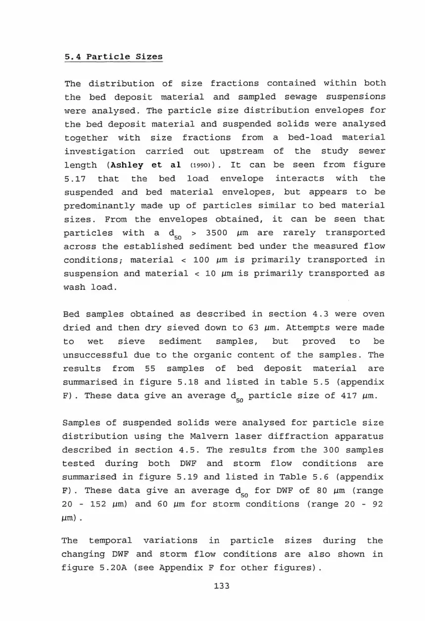
5.4 Particle Sizes

The distribution of size fractions contained within both the bed deposit material and sampled sewage suspensions were analysed. The particle size distribution envelopes for the bed deposit material and suspended solids were analysed together with size fractions from a bed-load material investigation carried out upstream of the study sewer length (Ashley et al ( 1 9 9 0 ) ) . It can be seen from figure5.17 that the bed load envelope interacts with the suspended and bed material envelopes, but appears to be predominantly made up of particles similar to bed material sizes. From the envelopes obtained, it can be seen that particles with a dgo > 3500 fim are rarely transported across the established sediment bed under the measured flow conditions; material < 100 /urn is primarily transported in suspension and material < 10 /urn is primarily transported as wash load.

Bed samples obtained as described in section 4.3 were oven dried and then dry sieved down to 63 jum. Attempts were made to wet sieve sediment samples, but proved to be unsuccessful due to the organic content of the samples. The results from 55 samples of bed deposit material are summarised in figure 5.18 and listed in table 5.5 (appendix F) . These data give an average d5Q particle size of 417 /urn.

Samples of suspended solids were analysed for particle size distribution using the Malvern laser diffraction apparatus described in section 4.5. The results from the 300 samples tested during both DWF and storm flow conditions are summarised in figure 5.19 and listed in Table 5.6 (appendix F) . These data give an average d5Q for DWF of 80 11m (range 20 - 152 fim) and 60 jLim for storm conditions (range 20 - 92 /im) .

The temporal variations in particle sizes during the changing DWF and storm flow conditions are also shown in figure 5.20A (see Appendix F for other figures).

133

103

90

90

70

60

50

40

30

20

10

0

MJRRAYGATE INTERCEPTOR SEWER

103

93

83

73

63

53

43

33

£0

10

0

M U R R A V G A T E I N T E R C E P T O R S E U E RBED MATERIAL

10P A R T I C L E S I Z E Cm i c r o n s )

range

ON I 3 3 Wei HO W JLNHOHHH

Figure 5.19 Suspended

solids particle

size distribution

MURRAVGATE INTERCEPTOR SEUIER

Fig

ur

e 5.20

a Su

spen

de

d so

lid

s sa

mpl

e p

ar

tic

le

size

DISTRIBUTION - 07/03/91

SAMPLER No.3

- SAMPLES 1-12

IiOJ

rrin

lOhs

03in

'll'T-t

■s-i

cncn

roCO

nm

mCD

mrn

tn;r;

cntn

mm

np-)

ncn

mQ

oO

oO

oo

oo

oo

ors

Tsrs.

INK

(S.[S.

iNk

fs.o

oO

oo

OO

OO

oo

O

137

There is a general trend that as TSS decreases, particle size increases. It can be seen that the average d5Q is greater during DWF than storm events. This tends to suggest, considering the Sauter Mean Diameters, that the DWF contains particles with larger surface areas than storm events; and, considering the higher volatile percentages normally present during DWF, that these larger particles are more organic. Since the material transported during DWF is also carried by storm flows, the material difference must be due to an ingress of new material, i.e. washed in from the surface or eroded from the bed. The decrease in dgo during storm conditions is probably due to the ingress of large quantities of fine material washed into and through the sewer from the surface.

However, these material differences do not appear to be significant enough to suggest a complete change in characteristics. In terms of particle sizes, storm flow solids are similar to solids encountered during the peak DWF. A summary of particle sizes is given in Table 5.7 below.

These data tend to corroborate the hypothesis that the sewer sediment bed consists of a weak organic layer (Type C) overlying a denser, less organic layer (Type A) . Peak DWF events may entrain the type C deposit which will redeposit on the recession limb of a DWF event. Storm flows quickly entrain the type C deposit and may then begin to erode the surficial layers of the Type A deposit.

138

Table 5.7 - Summary of Particle Size Information

Fraction Lower Limit Upper Limit AverageSuspended

Dio 5 22 13D35 13 91 52D50 20 152 80D75 41 325 181Dgo 91 422 257

Bed Material|

Dio 86 179 132D35 171 352 262D50 216 619 417D75 363 2244 1303Dgo 765 5724 3244

Bed Load |

Dio not recorded 128 60D35 86 323 174D50 141 542 251D75 192 1293 587Dgo 267 2604 1314

5.5 Settling Velocity

5.5.1 Water Research Centre/Scottish Development Department (WRc/SDD) Method

Research into the performance of storm-sewage overflows (SSO) led to a requirement to examine the rise/fall velocity characteristics of particulate matter in sewage.

The Water Research Centre developed apparatus for determining the rise/fall characteristics of particulates in sewage and this was utilised in a more detailed study for the SDD. This equipment and its use are described in Appendix E .

139

The apparatus consisted of two main elements, the first to remove floating matter from that which sinks, and the second to determine the settling velocities of the sinking particles (see figure 5.21).

The tests carried out on combined sewage flows under the SDD study using the above method indicated a median settling velocity (W ) of approximately 7mm/s.

5.5.2 Dundee Institute of Technology/Aston University Settling Velocity Test

Both establishments named above have carried out similar settling velocity testing procedures based on adaptations of the procedure used for the WRc/SDD apparatus.

The modified equipment consisted of a single tube of 50mm internal diameter (as per second item of equipment in 5.5.1), but with two valves at either end, the inner valve set in 250mm from the outer, and no central valve. The tube was again pivoted at its centre point to allow rotation through 360°. The procedures adopted are very similar and are summarised in Appendix E.

5.5.3 Owen Tube

The Owen Tube as used in estuarine studies appears to offer the best means of obtaining and testing samples as rapidly as possible before changes take place in the structure of the materials in suspension.

This methodology has been tested and adopted for analysis of sewer flow suspensions by researchers at Dundee Institute of Technology and the results obtained are discussed below.

140

€

£

F i g u r e 5.21 SDD s e t t l i n g v e l o c i t y a p p a r a t u s

141

A full description of the apparatus, test procedures and results analysis may be found in Hydraulics Research Station Report No. IT 161 - Determination of the Settling Velocities of Cohesive Muds. A general description of the apparatus and calculation of results is given here.

The Owen tube consists of a lm long perspex tube of 50mm internal diameter. It was initially open at both ends and was lowered into the flow to the depth required and suspended horizontally. After the flow through the tube had been allowed to establish a stable regime, both ends were closed simultaneously and the tube was raised to the surface whilst at the same time swinging into a vertical position, and settling began.

The tube was then placed into a frame assembly, and samples were withdrawn from the bottom of the tube at predetermined time intervals. The samples withdrawn were measured for volume and suspended solids concentration in the laboratory.

The results were obtained by the following procedure (explained in full in Owen 1976) :

(1) The height of water in the tube after each sample has been removed was calculated from the cumulative volume of samples divided by the cross-sectional area of the tube. This also gave the height through which the solids in each sample settled.

(2) Cumulative dry weight for each sample was calculated and expressed as a percentage of the total weight of sediment.

(3) The concentration of solids in the original tube was obtained by dividing the total weight of sediment by the total volume of water.

(4) The settling velocity grading curve was then obtained by a graphical method which essentially evaluated the

142

percentage of floes in the suspension which had a settling velocity less than that defined by a specified time, from a semi-log plot of cumulative percentage weight against time.

5.5.3.1 Tests Performed at Dundee Institute of Technology

The tests recorded below were undertaken on samples extracted under dry-weather flow conditions only. Due to the limited working space available in the sewers from which samples were taken, it was not possible to lower the Owen tube mounted in a frame (as used in estuarine studies) into the sewers to extract samples during storm flow conditions. The limited field and laboratory investigation was designed to provide information on:

(1) estimation of settling velocity of material in suspension under dry weather flow conditions, with:(a) comparison between trunk and interceptor sewers;(b) comparison between field and laboratory testing procedures;(2) estimation of possible errors introduced by sampling procedures.

(i) Equipment and Methodology (a) Owen Tube

An Owen Tube was used to estimate settling velocities in the field. The procedure adopted was as recommended in the definitive report with the following alterations: due to the limited flow depth available under dry-weather flow conditions, the tube was not mounted on a frame but was simply placed in the flow by hand. Time zero was taken as the moment the tube was removed from the flow and raised to ground level, where the test was completed.

Six tests were carried out in the Murraygate length of the Interceptor sewer in the central area of Dundee (see figure3.2), and two tests carried out at the Perth Road/Sinderins

143

location of a trunk sewer.

Four comparative tests were undertaken in the laboratory, with samples extracted from bulk samples obtained at each site. These samples were agitated by turning the containers end-over-end for 30 seconds to break up the floe blanket which had formed at the base in the time from sample recovery to testing, which varied between 2 and 24 hours.

(b) Laboratory Test

The method adopted for estimation of the settling velocity of samples returned to the laboratory was an adaptation of the Scottish Development Department test, as described in5.5.2. and Appendix E .

Six samples were tested from the interceptor sewer (four from bulk samples and two from automatic samplers) ; and three samples were tested from the trunk sewer (two bulk and one automatic sampler).

The sample containers were turned end-over-end for 30 seconds before taking a subsample for settling velocity testing.

(c) Comparative Sampling Automatic Sampling

The sampler used was an EPIC 1011 Portable Wastewater Sampler with 24 No. 500ml containers. At each site, a rigid PVC tube had been fixed to the sewer wall, pointing out into the sewage flow, such that all samples were recovered from a fixed point in the sewer cross-section. A flexible PVC hose connected the tube to the sampler. The sampling interval was set to two minutes and the sample volume fixed at approximately 500ml.

144

belo

w sta

ted se

ttling

velo

city

Bulk Sampling-

Bulk samples were recovered simply using a bucket lowered into the flow. A 500ml aliquot was then taken off by beaker from the bucket sample. A separate bucket-beaker sample was taken from the flow at the same time as the automatic sampler was drawing a sample.

(d) Flow Recording

At each site, the flow velocity and depth were monitored using a standard flow survey package (Detectronic Ltd) for each period of sampling undertaken.

(ii) Results

The settling velocity plots obtained for each site are shown in figures 5.22a et seq. and results listed in Table5.8.

S.OO''

1 0 0 j—90-}..

2 ° i1

0 .001settling velocity mm/s24/4/90 — t— 26/4/90

F i g u r e 5.22a Ow e n t u b e s e t t l i n g v e l o c i t y r e s u l t s

NTERCEPTOR SEWER (SEE APPENDIX F FOR OTHER FIGURES)145

Table 5.8a Owen Tube Results

DateDepth(m)

FlowVelocity(m/s)

Cone(mg/1)

W5 0

(mm/s)

W7 5

(mm/s)W /W

7 5 5 0

24/4/90 0.33 0.28 178 <0.001 0.0457 > 46

25/4/90 0.33 0.29 225 0.0062 0.3860 62.3

25/4/90 0.31 0.26 226 0.0076 1.0926 143.8

26/4/90 0.33 0.30 208 0.0130 0.2384 18.3

30/5/90 0.32 0.33 224 0.2333 2.6578 11.4

31/5/90 0.33 0.31 263 0.0219 1.3263 60.6

5/6/90 281 0.1385 1.4785 10.7

6/6/90 190 <0.0010 0.5000 >500

30/5/90 — — 276 0.0038 3.9295 1034.1

31/5/90 — — 225 0.0071 0.4380 61.7

31/5/90 — — 237 0.0059 0.3930 66.6

Table 5.8b SDD Test Results

30/5/90 — — 186 0.5229 1.7101 3.330/5/90 — — 190 0.1046 3.9105 37.430/5/90 — — 241 1.0112 5.7185 5.731/5/90 — — 237 0.6184 2.8278 4.631/5/90 — — 210 0.1564 0.8000 5.231/5/90 — — 279 0.4782 2.3913 5.05/6/90 — — 202 0.4642 1.8287 3.96/6/90 — — 233 0.7478 2.4182 3.26/6/90 — — 190 0.6253 2.7346 4.4

(iii) Discussion

The median settling velocities (W ) obtained by the Owen Tube method were very much lower than those reported

146

elsewhere for sewage particulates (approximately 0.04mm/s c.f. 0.1-8.3mm/s of Chebbo et al 1 9 9 0 ) . The SDD test also produced settling velocity estimates of approximately one order of magnitude difference from the Owen Tube tests (approximately 0.5mm/s c.f. 0.04mm/s).

The results reported by Chebbo et al were obtained using pipette and settling column methods, and may therefore be reasonably expected to produce results of a similar nature to the SDD test, as is the case. This would then indicate that a drastic difference occurs in the test results due to the different methodology adopted for the Owen Tube. The time taken between sample extraction and testing in laboratory based procedures allows the formation of larger floes and macro-floes (many floes joined together), which does not' occur in the Owen Tube test, in which the sample retrieval time and commencement of testing are identical, which means that the floe sizes are, initially, as would be produced by the shear forces within the flow of sewage. Although the agitation of the sample bottle prior to testing in the SDD method would break up some of the floes, it is not possible to specify what degree of agitation should be applied to reproduce the sizes encountered within the sewer at the time of sampling.

Not only are the median settling velocities produced by the two methods different, but the shape of the upper part of the settling curve is also different. Examination of the ratio w75/w50 indicates that the Owen Tube method generally results in ratios of between 10 and 150, whilst the SDD method produces ratios of the order of 3 to 6, indicating that the SDD method would allow all the sample to settle out in a very much shorter time period than the Owen Tube method.

Results obtained from the Owen Tube for sewage particulates also differ from those obtained for estuarine work (W

50

0.04mm/s c.f. 0.1 to 1.0 mm/s) . This may be due to the presence of buoyant particles with a negative settling velocity in the sewage suspensions which are not present in

147

the estuarine work. These rising particles would affect the overall distribution of settling velocities. In the case of the SDD test, these rising particles may first be removed by allowing the sample to stand for a period of not less than one hour in a tube with a mid-point valve which is closed after the set time to separate rising and falling particles. This was not possible with the Owen Tube method, where any rising particles were sampled with the appropriate falling particles depending on the position reached in the tube at the time of sub-sample extraction.

The standard SDD method assumes that all particulate matter is allowed first to settle to one end of the tube, then the tube is inverted and a valve closed after a set period of time. The settling velocity of this sample is then simply taken as the tube height divided by the sampling time.

This methodology is considered inappropriate for flocculant particles (allowing the formation of macro-floes at one end with higher settling velocities than original particles/flocs) , and therefore Coghlan (1993) (unpublished methodology and results, Dundee Institute of Technology) proposed a revised method whereby the tube is turned end- over-end several times to produce a relatively evenly distributed suspension which is then allowed to settle for a set time.

The selection of sampling times significantly influences the apparent settling velocities obtained from the laboratory tests. The analysis of results depends on the assumption, in the D.I.T. version of the SDD test, that an even distribution of particles of differing settling velocities is present, so that it may be assumed that each time step sample contains particles from the whole length of the tube and may therefore be averaged to represent a single mass which has settled half the tube height.

148

5.5.4 Summary

The site method has its drawbacks, as without an unlimited number of tubes being available, only one section of the depth of flow at any one time can be examined. With storm flow events, the nature of the material in suspension will be changing with time, and therefore samples have to be collected during the course of the whole event. This means that laboratory test methods are essential, and it may be that the laboratory test results can be referenced back to a datum on one part of the storm provided by the Owen T u b e .

It may be argued that the results obtained by the Owen Tube method are influenced by the fact that the rising particles are not removed prior to testing of the falling particles, i.e. rising particles may collide with falling particles and thus reduce the apparent settling velocity. This argument is outweighed by the fact that the nature of the flocculant settling particles is considerably altered when allowed to settle out. Also, the results obtained from samples retrieved by automatic sampling devices at a known point in the depth of flow should reflect the fact that the "floating" or rising material was present and would actually be colliding with sinking particles in reality.

The Owen Tube site method appears to offer the bestreference point for settlement velocity testing.

5.6 Rheology and the Rheological Properties of Sewer Sediments

5.6.1 Introduction

Rheology may be defined as the science of the deformation and flow of matter (Barnes et al 1989) , and is generally used to study materials which do not obey either Hooke's Law of elasticity or Newton's Law of viscosity. Rheological

149

properties such as yield stress permit parameterisation of the strength of resistance to deformation and flow of cohesive materials, and can be of importance in matters associated with sediment transport phenomena within a bed deposit and at the deposit/fluid interface.

There are many different models available to describe rheological behaviour (see figure 5.23), and some of the most commonly used are discussed below:

F i g u r e 5.23 Rh e o l o g i c a l m o d e l s

(a) Newtonian z = stress(b) Bingham r = rate of strain(c) Pseudoplastic(d) Dilatant(e) Herschel-Bulkley

150

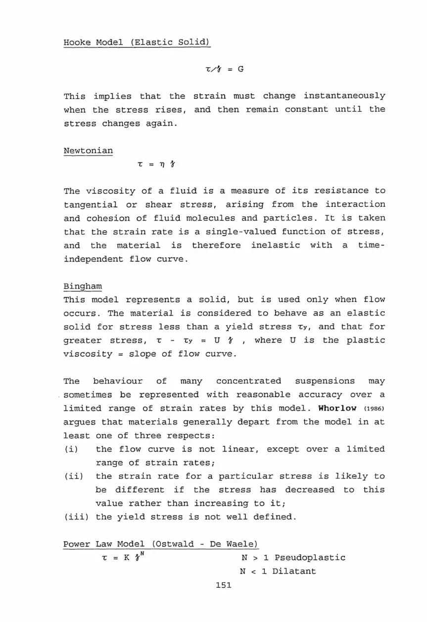
Hooke Model (Elastic Solid)

T/fr = G

This implies that the strain must change instantaneously when the stress rises, and then remain constant until the stress changes again.

NewtonianT = T) t

The viscosity of a fluid is a measure of its resistance to tangential or shear stress, arising from the interaction and cohesion of fluid molecules and particles. It is taken that the strain rate is a single-valued function of stress, and the material is therefore inelastic with a time- independent flow curve.

BinghamThis model represents a solid, but is used only when flow occurs. The material is considered to behave as an elastic solid for stress less than a yield stress ry, and that for greater stress, r - ry = U fr , where U is the plastic viscosity = slope of flow curve.

The behaviour of many concentrated suspensions may sometimes be represented with reasonable accuracy over a limited range of strain rates by this m odel. Whorlow (1986) argues that materials generally depart from the model in at least one of three respects:(i) the flow curve is not linear, except over a limited

range of strain rates;(ii) the strain rate for a particular stress is likely to

be different if the stress has decreased to this value rather than increasing to it;

(iii) the yield stress is not well defined.

Power Law Model (Qstwald - De Waele)r = K frN N > 1 Pseudoplastic

N < 1 Dilatant151

Herschel-BulkleyT = Ty + K t ”

The equations above for inelastic materials may be applicable to elastic materials under conditions of steady shear, provided that at each rate of strain the stress reaches an equilibrium value.

5.6.2 Rheology and Sewer Sediments

Recent studies of combined sewer sediment deposits (Crabtree, 1988) have recognised that these deposits may possess cohesive characteristics due to organic binding. Such deposits may have a higher critical yield stress than a similar non-cohesive deposit and hence require a higher bed shear stress to initiate erosion. This is of importance in the design of sewerage systems for 'self-cleansing' flow conditions.

From the foregoing, it would appear appropriate to apply rheological techniques to characterise the "strength" of sewer sediment deposits.

5.6.3 Rheometry

The fundamental problem in rheometry i s : Given an unknown substance and an instrument which can impose known and controllable boundary conditions on the substance, what are the rheological properties of the substance ? The only factors that may be assumed to be definitely known are:(i) the equations of motion;(ii) the boundary conditions.

To solve the problem a further assumption must be made; one of the following is chosen:(iii) a rheological model;(iv) a velocity field within the substance.

152

Methods of examining the rheological properties of matter include rheometers which impose variable conditions at rigid boundaries such a s :

(i) a sudden stress which is subsequently held constant;(ii) a sudden strain which is subsequently held constant;(iii) a periodically varying motion.

The third case is by far the most important in examining the dynamic properties of matter. The two former cases of step changes in input are of more frequent use in the examination of solids.

5.6.3.1 Investigations Carried out on Rheometrv for Cohesive Sediments

The rheometry of concentrated cohesive sediments is complicated by the non-linear, dissipative and thixotropic characteristics of these materials which may also possess an apparent yield stress (Crabtree et al, 1989) . A linear material is one in which the ratio of stress to strain for any history is a function of time only, i.e. if the stress applied to a material at all times prior to the time under consideration had been increased by a certain factor, the strain at all such times would have increased by a directly related factor.

Preliminary investigations into the rheology of sewer sediment deposits (Williams & Crabtree 1 9 8 9 , Williams & Williams, 1987) indicate that these deposits are non- Newtonian materials which exhibit elastico-viscous behaviour (simultaneous existence of viscous and elastic properties). As sewer sediment deposits are inhomogeneous and also contain coarse material, this imposes restrictions upon the choice of rheometrical techniques and complicates data analysis.

153

Steady shear techniques are inappropriate as sediments can exhibit a fluctuating shear stress under steady applied shear rate as observed in sewage sludges (Kirby, 1988) . Williams and Williams, i989a have developed a methodology incorporating the complementary techniques of applied stress rheometry and shear wave propagation. These techniques minimise disruption of the sample structure. The shear wave propagation apparatus developed by the Williams' allows evaluation of the wave rigidity (shear) modulus, G. This modulus is related to, and a measure of, the structure of the undisturbed material (James et al,i987) .

Following a certain degree of structural disruption, for example that involved in introducing a sample into testingapparatus, sediments may recover some or all theirstructure, or remain at an equilibrium level untildisturbed again. Tests on sewer sediments (Crabtree etal,i989) have shown that they develop a degree of rigidity, denoted by G, with time, to an equilibrium level. The time taken for the sample to recover to this equilibrium level (te) can be incorporated into further examination, e.g. following testing to a certain level of applied stress, the sample is left for a time, te, until the test is repeated at a higher level of applied stress.

Shear wave propagation also f o r m s the basis of the in-situ rheometrical apparatus currently being developed by researchers at University College Swansea (Ashley et al,1988) , albeit at a much higher frequency (102 - 104 Hz) than is commonly employed in the laboratory device mentioned above (220 Hz) . This in-situ device is intended to monitor the vertically distributed rheological properties of viscoelastic cohesive sediment beds under a range of post consolidation/pre-erosional conditions. The applied stress rheometrical technique uses a vane geometry.

The vane geometry has been used successfully to measure the shear strength of soils (American Society for Testing of Materials 1 9 7 5 , British Standards Institute 199 0 ) . The vane geometry, when employed in conjunction with applied stress

154

rheometry, has the following advantages over conventional rheometrical measuring geometries (Dzuy & Boger 1985, James et al 1987) :

(i) The possibility of wall slip is avoided by allowing the material to yield within itself;

(ii) Insertion of the vane involves far less structural disruption than is occasioned by conventional geometries;

(iii) The narrow angular gaps of conventional geometries are avoided ( particularly important with respect to sediment deposits containing large sized particles).

The use of the cruciform vane geometry involves the assumption of a cylindrical failure surface around' the perimeter of the blades (see figure 5.24) to allow the measured applied torque to be converted to a corresponding yield stress. The application also assumes that a uniform stress distribution occurs over the vane. This assumption has been investigated (Aas 196 5 , Dzuy & Boger i 9 8s) for a number of different vane geometries and found to give a reliable measurement of yield strength.

Jh Dt +

F i g u r e 5.24 Va n e g e o m e t r y

155

Typically, the vanes used in soil testing have a height/diameter ratio of 2. Aas studied vanes with H/D ratios of between 0.5 and 4, and found that the linear relationship presumed by the assumption of a uniformly distributed shear stress held for most geometries, with the exception of those with H/D ratios of three or more. Dzuy & Boger (1983) investigated the use of the vane geometry in rheological apparatus, using vanes with H/D ratios of between 0.5 and 2. The effect of vane shape was considered using three vanes having H/D ratios of 0.95, 1.48 and 1.92 and it was found that the differences in yield values obtained were well within the range of expected experimental error, concluding that effects due to vane dimensions could be neglected for the dimension ratios tested. The effect of rotational speed was also tested and it was found that for the experimental setup used by Dzuy & Boger, significant increases in measured yield stress were obtained for speeds in excess of 8 r.p.m. In a later paper (1985), Dzuy & Boger also established criteria relating vane dimensions to sample container dimensions to avoid boundary influences. With reference to figure 5.24, the following ratios should be observed:

H/D < 3.5 (c.f Aas H/D < 3.0)D t / D > 2 . 0

Zi/D > 1.0Z2/D > 0 . 5

5.6.3.2 Yield Stress of Sewer Sediments

Concentrated solid-liquid suspension systems having strong interparticle interactions, such as sewer sediment deposits, often exhibit a unique plastic flow behaviour and the presence of a yield stress. Under the application of small stress these systems deform elastically with finite rigidity, but when the applied stress exceeds the yield value continuous deformation occurs with the material flowing like a viscous fluid. The yield stress can thus be regarded as a material property denoting a transition between solid-like and liquid-like behaviour (Dzuy & Boger,

156

The only known published values for rheological measurements of sewer sediments were published by Williams & Crabtree (1989) in the U.K. and Beyer (1989) in France. These data are sparse, since the U.K. tests were carried out on only a limited number of samples from a variety of locations, and therefore no general trends can be inferred from the reported results. The French tests, also limited, were carried out on samples prepared by washing through an 80 micron sieve and then centrifuged to a specific concentration. These latter tests are likely to have been performed in this way due to the limitations of the measuring device used (couette cylinder), i.e. a narrow annular gap only allowing fine particles to be tested.

1983) . The yield stress is the minimum shear stresscorresponding to the first evidence of flow, i.e. the valueof the shear stress at zero velocity gradient.

5.6 .3.3 Rigidity (Shear) Modulus

Values of rigidity (shear) modulus, G, reported (Williams & Crabtree 1989) ranged from 52 kN/m to 4095 kN/m , with the possibility of the low modulus values being associated with a high proportion of coarse (33% > 0.5mm) particles. The narrow angle cone and plate and narrow, angular gap, coaxial cylinders employed in the majority of dynamic oscillatory shear studies of concentrated suspensions and sediments provide homogeneous stress and strain distributions within the sample under test. However, they are generally unsuited to the study of natural cohesive sediments or suspensions containing particles or aggregates greater than 10 fim in size. There is therefore a need for the further development of instruments such as that under development by Williams & Williams (i989b) . The time to equilibrium reported for these samples appears to be more consistent than the yield and rigidity values reported. The time to equlibirum, te, varied from 7 to 20 minutes, with four of the eight samples tested having a te of 15 minutes. The report also noted that the value of G exhibited a

157

highly non-linear response to increases in solids concentration, little elastic response being noted at a bulk density of 1.11 g/ml, but with rapidly increasing values of G noted for densities greater than 1.13 g/ml. This may be associated with the formation of a space­filling network structure and is therefore of importance in the consideration of solids transport.

Yield strength measurements utilising the vane geometry discussed above also exhibited a wide range of values, from 25 N/m2 to > 800 N/m2 (the limit of measurement of the instrument utilised). Again the limited number of samples and their considerable variation in physical and biochemical properties preclude the inference of possible associations of yield strength with sediment type. The measurement technique employed (gradual increases in the value of constant applied stress) demonstrates the rapidity of breakdown of the elastic response of the sediment structure with small increases in stress. This phenomenon is characteristic of the critical stress noted by researchers using flume studies of sediment bed behaviour, who note that beyond a certain critical applied bed shear stress, the bed structure breaks down rapidly (Nalluri & Alvarez, 1 9 9 0 ) .

5.6.4 Testing Procedure Adopted

The procedure adopted for the experiments described here was the applied stress technique utilised by Williams and Williams (i989b). This allowed the sediments encountered to be tested without altering the range of particle sizes known to be present (see section 5.4 and Figure 5.18), whereas other available techniques would only allow the finer fractions to be tested after samples had been sieved. It should be noted that the measurement is of an apparent yield stress, no attempt being made to measure ultimate or true yield stress (stress below which no viscous flow occurs). Some viscous flow occurs under all conditions employed in the form of experiment adopted if sufficient

158

time is allowed.

5.6.4.1 Applied Stress (Creep) Test

Creep is defined as : The slow deformation of a material; usually measured under constant stress (Barnes et al 1 9 8 9 ) .

Applied stress rheometers allow the elasticoviscous properties of cohesive materials to be investigated under a range of gradually increasing levels of applied stress. They avoid forcing the material instantly to take up a pre­selected deformation rate, thereby minimising structural disruption under test, prior to yield. A mechanical analogue may be used to visualise the constituent elements of an elasticoviscous material. The extension of an ideal spring is proportional to the force applied and will occur instantaneously. If the force is taken as being analogous to the shear stress in the material and the extension of the spring as analogous to the strain, the spring will simulate the behaviour of an ideally elastic material which deforms instantaneously (Whorlow 1986) . Similarly, for an ideal dashpot the force is proportional to the rate of elongation, and the dashpot simulates steady flow in a viscous material (see figure 5.25).

ELASTIC DEFORMATION VISCOUS FLOW VISCO-ELASTIC RESPONSE

SPRING DASHPOT VOIGT UNIT

% l

aapplied removed applied removedcr 0* cr cr

appied crremoved

F i g u r e 5 .2 5 R h e o l o g i c a l e l e m e n t s a n a l o g y

159

The Berger model is commonly used to model a viscoelastic response (figure 5.26).

F i g u r e 5 . 2 6 B e r g e r M o d e l

The Berger model consists of three parts: a purely elastic response J o , a purely viscous response Tjo, and a viscoelastic response known as a Voigt unit. The creep technique employs a relatively large time frame together with small applied stresses, such that all the elements within a sample (elastic, viscous and viscoelastic) are given time to respond.

5.6.4.2 Vane Sizing

The size of vane used was derived by considering the maximum torque available from the rheometer, the expected range of yield stresses, the restrictions on dimensions noted previously, and the maximum size of sample likely to be obtained.

Rheometer Maximum Torque = 0.01 NmSampling of sediments was via 37mm diameter geotechnical hand corers, therefore Dt = 37mm.For Dt = 37mm, Dmax = 18.5mm3.5 > H/D > 2 . 0

160

From preliminary investigations into the rheology of sewer sediments (Williams & Crabtree 1989) , a significant number of samples (five out of eleven tested) had a yield strength in excess of 800 N/m2 ( the limit of measurement of the instrument employed). It was decided to extend this measurement range by a factor of at least two. The vane and the unyielded material within the vane blades may be considered as a cylinder and a torque balance established to include the components involving shearing at the cylindrical wall and the two end surfaces:

T = (27rrH) Tw r + 2 < 2 n Jre(r)rdri (5.13)

where: T = torquer = D/2 = Radius of vane H = vane height Tw= shear stress at wall T e = shear stress at ends

The assumption of a uniform stress distribution over both ends of the cylinder gives:

.3T = ttDv H 1

D + 3 ty (5.14)

Table 5.9 Vane Dimensions and Torque

VaneDiameter Height 2

T m a x (N/m )1 5 4 0 5 0 3

1 5 3 0 6 4 6

1 0 3 0 1 5 2 7

1 0 2 5 1 7 9 8

1 0 2 0 2 1 8 3

The vane adopted was 10mm diameter by 20mm height, which met all the specified limits on dimensions whilst providing the greatest measurement range.

161

5.6.4.3 Rheometer

The rheometer employed was a Carrimed CSL-100 controlled stress rheometer (Carrimed Ltd., Dorking, Surrey) (See Plates 12 and 13, Appendix F) . The rheometer operates almost entirely from a PC-based software package, with measurements made through digital micro-processor electronics. The rheometer incorporates a torque motor assembly, the drive shaft of which is supported on an air­bearing, providing a virtually frictionless support. An optical encoder mounted on the drive shaft detects angular movements as low as 2xl0~5 of a radian. The computer also manages the temperature control system, with normal operation in the range 5°C. to 60°C.

5.6.4.4 Test Procedure

Samples retrieved from either the geotechnical sampling tube or Dundee Institute of Technology sampling device (see section 4.3) were placed in 40mm diameter by 60mm high pyrex beakers and the sediment structure allowed to reform for 24 hours at 5 ° C . It was not possible to perform the tests required to determine the equilibriation time, te (see section 5 . 6 . 3.1), (Williams & Crabtree 1 9 8 9 ) for each sample. This was due to*.

(a) the large particles present in the samples;(b) the limitations of the instrumentation available (a gap width of 10-100 times the largest constituent particle diameter is required for adequate bulk measurement of material properties which would, for the sewer sediments under test, severely impair the precision of stress and strain determination) and,(c) the need to preserve the samples available for yield strength testing.

As a compromise a standard time between application of increments in stress of 15 minutes was adopted, corresponding to an average value of te obtained for sewer sediments by others (Williams & Crabtree 1 9 8 9 ) . The air

supply to the rheometer was switched on, followed by the water supply to the Peltier temperature control system (all tests were carried out at 20°C.) . The micrometer on the loading ram was adjusted such that when raised, the sample jar and vane were in positions corresponding to the limits on dimensions noted previously. The computer was then switched on and the system allowed to self-test. The spindle restraint was removed and the vane attached. The sample in its container was then placed on the loading ram and fixed into position using adhesive tape (to prevent accidental rotation or movement of the jar), and the sample introduced to the vane by raising the ram via the software package. The sample was then left for the specified time until an equilibrium condition had been reached before the first application of stress. A specified torque was applied for 30 seconds and a relaxation time of 30 seconds was also monitored using the creep package within the software. This was repeated after the equilibration period for torques corresponding to higher increments of stress until strain for constant stress (see figure 5.27).

It should be noted that the strain was measured as an angular movement and hence this was not true strain due to the geometry of the vane and the sediment included within the blades.

Samples were tested for moisture content and particle size distribution.

5.6.5 Results

Results are shown in table 5.10 in Appendix F. Sample preparation was such that inclusion of air was avoided and samples could be assumed to be 100% saturated (Sr = 1).

163

(pg

j) q

.U0

W0

oe

tds

ipFigure

5.2

7 Creep

test

164

CREEP

C a r r 1 -M ed CS R h e o m e te r

Sixty-one samples of bed material from the study length of sewer were tested for apparent yield strength. Of these, four samples had yield strengths in excess of the maximum range of application of the rheometer and vane (2650 N/m ) . To ensure that these samples were included in data analysis, they were assigned a yield strength = 2650 N/m , despite this being known to be a possible underestimate.

Linear regression analyses of the data were performed for parameters which could possibly influence the yield strength of the sediments. Regressions against more than one parameter were attempted, but correlation did not improve significantly above single parameter relationships.

Table 5.11 Yield Stress Regression EquationsParameter Regression Equation R2V o lu m e tr ic S o l i d s T y = 2 . 5 7 2 8 e x p (1 0 .9 1 0 5 Cv) 0 . 802

B ulk D e n s i ty T y = exp ( - 8 4 .6 6 1 ) p l 2 . 2 6 7 1 0. 592

M o is tu re C on ten t (w ater c o n te n t )

T y = exp (18. 3865) ITT3 * 1682 0. 920

V o id s R a t io T y = exp (6 . 4563) e ~ 2 ’ 5 7 0 7 0. 848

Dry S o l i d s T y = exp ( - 3 3 .1 8 9 ) p d 5 * 6221 0. 867

Yield versus bulk Density

See Figure 5.28Although there was a general trend of increasing yield strength with increasing bulk density, as can be seen from Figure 5.28, there was also considerable scatter of results and linear regression analyses were oniy able to provide R2 values of 0.592. This would not provide an accurate basis for estimating yield strength.

165

VIEL

D ST

RESS

CN/m

a2)

VIEL

D ST

RESS

CN/m

a2!>

M U R R A V G A T E I N T E R C E P T O R

B U L K D E N S I T V C 5

F i g u r e 5 . 2 8 Y i e l d s t r e s s v e r s u s b u l k d e n s i t y

F i g u r e 5 . 2 9 Y i e l d s t r e s s v e r s u s w a t e r c o n t e n t

166

Yield versus Moisture Content

The moisture or water content of a sample was found to be a good predictor of yield strength; the samples having a higher water content possessing a lower yield strength, decaying exponentially (see figure 5.29) This measurement (i.e. water content) is also subject to the least degree of experimental error, since other possible predictors also required the measurement of sample volume for their evaluation. Here the moisture or water content is defined as the weight of water divided by the weight of soil and therefore if the liquid phase exceeds the solid phase the percentage water content may exceed 100 (the sediment being assumed to be fully saturated with no gaseous phase).

The water content/yield stress relationship appears to have two significant outlying points, one at an approximate water content of 180% and the other at 120%. It was necessary to investigate the effect of these outliers on the form of the relationship and so the results were re­analysed with these data points omitted. The relationship then became:

-3 PAR4. pz = e x p (18.6764)m (R=0.90)y

The two relationships are plotted in figure 5.30a. It can be seen that within the 0 - 1 0 N/m range of yield stresses, a 3 to 5% decrease in moisture content is obtained for a given yield value. This is not significant in terms of experimental error and overall sediment transport rates.

The majority of the data lie within the 95 percentile confidence limits as shown in figure 5.30b.

Yield versus Voids Ratio

Since voids ratio and volumetric solids can be directly related, one may expect that a similar degree of correlation would be found between the two parameters and the yield strength, as is the case.

167

VIEL

D ST

RESS

CN/m

a£J

N U R R A V G A T E I N T E R C E P T O R S E W E R

F i g u r e 5 . 3 0 a R e l a t i o n s h i p c h a n g e d u e t o o u t l y i n g p o i n t s

Yield versus Dry Solids

The correlation of dry solids with yield stress shows a degree of scatter at the upper range of densities measured (see Figure 5.31), but provides a better relationship than bulk density.

168

VIEL

D ST

RESS

CN/m

a2)

LN V

IELD

STRE

SS C

N/ma2

)

M U R R A V G A T E I N T E R C E P T O R S E U J E R

F i g u r e 5 . 3 0 b 957 . l e c o n f i d e n c e l i m i t s

MU RRA VGA TE IN TER CEPTO R

D R V D E N S I T V C k g / M A 3?F i g u r e 5 .3 1 Y i e l d s t r e s s v e r s u s d r y d e n s i t y

169

LN V

IELD

STRE

SS C

N/ma£

)

The possible influential parameters were also tested against each other*.

Table 5.12 Sediment Characteristics Regression Equations

P aram eter M o is tu re c o n te n t r e g r e s s i o n e q u a t io n

R2

B ulk D e n s i ty p = e x p ( 8 .0 2 3 3 ) m - 0 * 1617 0. 609

V o id s R a t io e = 0.02861171 - 0 .2 2 0 7 3 0. 950

V o lu m etr ic S o l i d s Cv = -0.00367111 + 0 .6 6 2 3 5 0 .8 1 5

Bulk Density versus Moisture Content

Again, although there was a general trend of decreasing bulk density with increasing moisture content, there was a significant degree of scatter in the results, probably due to the differing specific gravities and particle sizes of the sediment constituent materials.

Voids Ratio and Volumetric Solids versus Moisture Content

Because the samples were saturated, a good degree of correlation would be expected between the voids ratio, volumetric solids and moisture content.

The usefulness of the predictor relationships may be examined by graphical comparison against the data points used in their derivation.

170

(i) Yield versus Volumetric Solids

T y = 2.5728 exp{lO.91505 Cv}

Theoretically, Cv = 1

where Sg m e “ 100

and Sg is particle specific gravityTherefore, by taking a range of moisture content values it is possible, for a given specific gravity, to calculate Cv and hence Ty.

(ii) Moisture Content relationship used to predict Volumetric Solids/Yield Strength

For any given moisture content, it is possible to predict Ty using the derived relationship:

Ty = exp{ 18.38647} m-3-16815

This may then be compared with the theoretical value of Cv at that same moisture content (for a given Sg) , and a linear regression equation derived over the range of moisture contents under consideration, in the form Ty = exp{A.Cv + B} . This then enables a plot to be made of values of Ty against Cv for a range of Sg as shown in Figure 5.32, demonstrating the data is consistent with having been obtained form materials of varying specific gravity.

171

m u R R A V G A T E I N T E R C E P T O R

«v>o 1 a M e t r 1 o s o l i d sGs=i.7 Gs=2.0 Gs=2.3 Gs=2.6 Gs=2.9

F i g u r e 5 .3 2 W a t e r c o n t e n t p r e d i c t o r s f o r v o l u m e t r i c s o l i d s

AND Y IE L D STRESS

(iii) Bulk Density versus Moisture Content

The data scatter may again be examined against the theoretical relationships, with varying values of Sc. See Figure 5.33.

1 7 2

VIEL

D ST

RESS

CN/

ma8)

M U R R A V G A T E I N T E R C E P T O R

m o I s t a r e c o n - t e n - tGsr2.9 Gs=2.6 Gs=2.3 Gs=2.0 Gs=1.7

U1-PinC0!Tl

X3

F i g u r e 5 .3 3 Bu l k d e n s i t y v a r i a t i o n w i t h w a t e r c o n t e n t

AND S P E C I F I C GRAVITY

5.6.6 Comparison With Other Published Data

O'Brien and Julien (1988) used a rotational viscometer to measure the rheological properties of silt and clay mudflows, using a Bingham model to derive yield stresses. They note that both the viscosity and yield stress increase exponentially with sediment concentration. They also studied the influence of the addition of sand particles to the matrix, noting no significant change in the rheological properties unless the volumetric concentration of the sand

1 7 3

exceeded 0.20, but were unable to state what this effect would be without further investigation. They also reported the work of Chinese researchers in their paper, presenting equations in the same form as their own.

/3CvZy = a exp'

These results are plotted in Figures 5.35a and b. The results from the Dundee Interceptor Sewer sediment samples gave:

Z y = 2.5728 exp{l0.9105Cv}

However, this relationship was derived from data containing a range of material with differing specific gravities, whereas O'Brien and Julien's individual samples were likely to be more uniform in nature. If the t y / m relationship derived is considered, it is possible to state, using*.

m = 100e/SG and e = (1-Cv)/Cv

r -x -3.16815that, Ty = exp{l8.38647} •-{ 100 (1-Cv) l

Cv Sg JThis function may then be plotted for a range of Sg values as shown in figure 5.34.

The two types of relationship concur very well for C v > 0 . 3 ,

but depart below this value, with that derived from the moisture content relationship tending to fall more within the range of data published by O'Brien and Julien. The majority of samples extracted from the Interceptor sewer had Cv values > 0 . 3 , with only three data points falling below this value. Extrapolating the t ^/Cv to the origin axes leads to the erroneous conclusion that the sewer sediments possess a yield stress for C v = 0 . Therefore, it must be concluded that further investigation of more dilute samples of sewer sediments are required to extrapolate the derived relationships below C v = 0 . 3 .

174

+ Gs=2.6 □ Gs=2.3 X Gs=2.1 0 Gs=1.9

F i g u r e 5.34 Du n d e e s e w e r s e d i m e n t r e s u l t s in s a m e f o r m a s

O'Brien a n d Julien

175

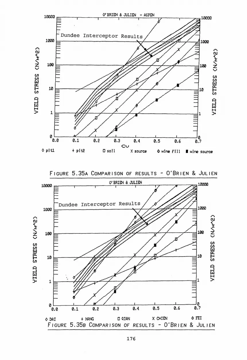
VIEL

D ST

RESS

CN/

maE)

VI

ELD

STRE

SS C

N/ma2

) CU<2\2vWGOWKHWCJW

0 p itl + pit2 □ soil X source 0 Mine fill I Mine source

0 DAI + KANG □ QIAN X CHIEN 0 FEIF i g u r e 5.35b Co m p a r i s o n o f r e s u l t s - O ’B r i e n & Ju l i e n

176

Beyer (1989) examined the rheology of the fine fraction ( < 100 jum) of sewer sediments from the town of Entzheim, France, using a couette cylinder. His results indicate that the percentage of organic material in the sediments affects the yield strength; more organic materials having a higher yield strength for a given volumetric solids concentration (see Figure 5.36).

Beyer bases his relationship on the form produced by Higniot ( 1 9 6 8 ) :

Ty = /3 pc

where a. varied from 3 to 6,and 13 ranged from 10 12 to 10 15 (Migniot)

Beyer's data, in the same form as Migniot, over a range of organic contents, Mo, gives:

Mo % 8 11 15 20b 1.48E-8 8.08E-7 1.03E-9 1.98E-6a 3.0 2.6 3.8 2.6

The results concur reasonably well when taken over the range of shear stresses expected to be exhibited in the sewerage system of 0-30 N/m2 (Figure 5.36b), particularly for organic contents of > 8%. Results of the Dundee sewer sediment samples compare well with Migniot's results (Figure 5.37) in the plastic range (i.e m ^ 5 - 6), because of the structural connectivity existing in the sewer sediment test method (rheometrical measurement using creep analysis in applied stress rheometry.)

1 7 7

VIEL

D ST

RESS

CN/

ma2)

VI

ELD

STRE

SS C

N/ma2

5

0 Mo = 8 x + M o s l i x □ Mo=15X X Mo=20X 0 UOTHERSPOON

F i g u r e 5 . 3 6 a C o m p a r i s o n w i t h B e y e r ' s r e s u l t s

D R V D E N S I T V C k g / M A 3 )0 Mo=8X + M orllJC □ M o r i5X X M o=20X 0 UOTHERSPOON

F i g u r e 5 . 3 6 b C o m p a r i s o n w i t h B e y e r ' s r e s u l t s

178

VIEL

D CN

/ma25

VI

ELD

CN/ma

2)

+ M=5,n=-14 0 mt5, re-12 X M=6,n=-15 0 mt&,rc-14 I UotherspoonF i g u r e 5 . 3 7 a C o m p a r i s o n w i t h M i g n i o t 's r e s u l t s

D R V D E N S I T V C 5+ mt5, re-14 0 kc5, re-12 X m=6, re-i5 0 m=6,re-14 I LJotherspoon

F i g u r e 5 . 3 7 b C o m p a r i s o n w i t h M i g n i o t 's r e s u l t s

179

5.7 Results - Discussion Summary

5.7.1 Hydraulics

The flow in the study sewer has been shown to be unsteady and slightly non - uniform. The sewer has an equivalent sand roughness value, ks, of 10 - 12 mm for the brick sewer walls, in line with expected roughness for this type of construction. The presence of a sediment bed influenced the overall flow resistance, and downstream deposits were found to have significant effects on the hydraulic gradient through the study length.

It was found that the hydraulic gradient increased as the bed deposit gradient increased. The tendency towards a steady state for sediment deposit depths has been noted by other researchers (Laplace 1 9 9 1 ) and this work suggests that the flow conditions and sediment deposits interact to produce a steady state condition for the long-term average transport requirements. This steady state would only be affected by the occurrence of catastrophic events (heavy sediment wash - in , multiple storms at short time intervals producing sediment erosion, non - natural interference (building rubble deposition etc.))

5.7.2 Sediment Deposition and Erosion

It has been noted by others (Lorenzen et al 1 9 9 2 ) that accumulations of sediment in a length of sewer start to collect in discontinuities or local irregularities in the sewer invert. The deposit then collects behind each of these starting localities and spreads back upstream until deposits are joined and a continuous bed forms.

The sediment bed deposits found in the interceptor studysewer have a d size of - 400fim, which size has not been 50measured in samples of suspended material. It is only the smallest 35% of bed size particles which appear in suspension. Samples of bed-load material taken during other

180

studies of the interceptor study sewer have found sizes of up to 13 00jum moving in this mode, which corresponds to the d75 size of deposit material. This suggests that 25% of bed deposit material is not capable of being transported once a bed has been established. The data also tend to suggest that particles of less than approximately 50jiim move as wash load through the sewerage system ( size not found in bed load or bed deposit material ) , and that preferential erosion of the finer fractions of deposit material occurs.

The sonar depth gauge and hydraulic studies suggest thaterosion of the sediment bed occurs at shear stresses of 1.5

2.0 N/m2 during DWF i.e. the morning peak DWF issufficient to cause erosion of the bed. This erosion ishowever only of the surficial layers of sediment. Storm2flows cause further erosion at shear stresses of 4 - 6 N/m ,but the magnitude of erosion depends on the time of day during which the storm occurs, i.e. whether or not the morning peak DWF has already eroded the surficial bed layers. This also suggests an erosion dependence on a change in bed structural strength with depth.

The use of sonar devices and manual surveys has shown (in a coarse fashion) that bed forms are present in the cohesive sediment bed structure. These forms are three dimensional, varying over width as well as length. The data collected tend to show that the height of these forms over the average bed depth is reduced as the overall bed depth increases (i.e. the dunes are washed out and the bed surface becomes flatter.)

The studies have also shown that bed deposition and erosion are interactive. It has previously been suggested that due to the cohesion of the bed structure, if erosion starts at a certain bed shear stress value z , it would continuebuntil the shear stress value fell below z . This has notbbeen found to be the case, with deposition occurring before the peak bed shear stress has occurred. Because of the varying nature of flows, bed characteristics and inputs from upstream sources, bed erosion and deposition are

interactive. Re-deposited beds are seen to rapidly gain resistance to erosion, and the bed structure quickly (hours rather than days) re-establishes to the previously existing quasi-equilibrium depth.

5.7.3 Suspended Material

As previously mentioned, the maximum size of material in suspension was measured as approximating to the d35 size of the bed deposit material; or the d50 size of the bed load material. This suggests only a limited interaction between bed and suspension. Up to 35% of suspended material moves as wash load.

A concentration profile was found to be present under DWF conditions, but not under storm flow conditions. It was not possible to account for the redistribution of the DWF concentration profile due to the coarse sampling intervals used.

5.7.4 Settling Velocity

The measurement of settling velocity of sewage sediment particulates proved to be troublesome. Different testing methodologies were found to produce different results. In particular, the measurement of the settling velocity, SV, of the suspended sediment depended not only on the testing method used, but also on the fact that the samples were often left to completely settle and coagulate in the sampling compartments and frequently incurred lengthy time delays between sampling and testing.

To counteract these problems, an in-situ test method was adapted from estuarine studies - the Owen Tube. This test regime produced drastically different SV results from previously reported data. SV's were found to be V50 = 0.001 - 0.23 mm/s c.f. 0.1 - 8mm/s (Chebbo et al 1990) and 0.5 - lmm/s (SDD method) . The Owen Tube results correspond with

182

the presence of significant quantities of wash load material (d < 50 /urn) .

50

5.7.5 Rheology

The rheological study results demonstrate that the sediment found in the study interceptor sewer possess a structural strength far in excess of the shear forces exerted by the fluid flow. A relationship has been established which demonstrates that the degree of structural strength is closely related to the proportion of the liquid phase in the sediment bed.

183

6 . M o d e l D e v e l o p m e n t

In the U.K., interest in the cohesive properties of sewer sediments has been developed by the WRc - led Urban Pollution Management programme. Initial laboratory studies have been undertaken on sediment rheological properties (Williams and Williams 1 9 8 7 ) and synthetically cohesive sediment movement in laboratory flumes (Nalluri and Alvarez 1 9 9 0 ) . The study presented in this report features the first field data programme dedicated to cohesive sewer sediments.

6.1 Erosion of Cohesive Sewer Sediments

From their initial studies of the rheological properties of sewer sediments, Williams and Williams (Williams and Crabtree 1 9 8 9 ) developed a synthetic sewer sediment for laboratory flume studies used by Nalluri and Alvarez( 1 9 9 0 ) .

They suggested the use of Laponite clay mixed with sand to provide the rheological properties required of a synthetic sewer sediment (see Table 6.1). The Laponite/water mixtures give a "dispersive" or flocculated structure.

Appropriate mixtures of Laponite-sand-water were used to mimic the rheological characteristics of cohesive sewer sediments, although simplifying the actual complexity of the natural sediment arising from the interaction of physical, chemical and biological characteristics.The concentration of Laponite clay gel was set between 18 and 40 g/1 (Nalluri 1 9 9 1 ) , with the upper limit of 40 g/1 representing "Type A" sediments and the the lower limit of 18 g/1 representing "Type C" sediments.

1 8 4

Table 6.1 Yield Stress for Laponite-sand-water mixturesSolidsCone(g/ml)

Proportion % (by w t .)

BulkDensity(kg/m3)

RigidityModulus(N/m2)

YieldStress(N/m2)sand clay

0.172 14.5 2.7 1042 410 17.50.220 19.5 2.5 1106 220 16.00.278 25.5 2.3 1200 500 23.00.410 37.8 2.2 1300 600 30.00.487 47.0 1.9 1380 1300 43.00.548 53.0 1.8 1440 2300 58.0

From their work with the artificial cohesive sediment, Nalluri and Alvarez ( 1 9 9 0 ) concluded that:

(i) the presence of small quantities of cohesive additive increased the critical shear stress by up to 10 times that of equivalent non-cohesive sediments;

(ii) the size of the sand component (0.12mm to 2mm) of the sediment had no significant effect on the critical shear stress;

(iii) an optimum sand to clay gel ratio existed for which a maximum critical shear stress was obtained;

(iv) the mix used to represent freshly deposited cohesive sewer sediment with slight consolidation (Type A) had a maximum critical shear stress of approximately 6 to 7 N/m2.

(v) the Type C sediment analogue was found to erode at a2shear stress of around 2.5 N/m .

185

6.2 Model Conception

The cohesion-like resistance to shearing exhibited by combined sewer deposits was first investigated by Williams and Williams (1987) . Their investigations revealed that combined sewer sediments were non-Newtonian visco-elastic materials which exhibited apparent yield stresses from 25 N/m2 to in excess of 800 N/m2. Further investigations (this thesis) observed yield stresses of up to 2650 N/m , with the apparent yield stress being related to the liquid content of the sediment (see section 5.6).

These yield stresses may be compared with typical fluid induced separated bed shear stresses of up to 20 N/m which may be typically encountered in the study sewer in this report. The apparent dichotomy between the magnitudes of the measured sediment yield strength and the shear stress required to erode sediment in-situ may be reconciled by considering the sediment deposit to be stratified with respect to yield strength with depth.

Consideration of this stratification is essential in modelling bed erosion since the susceptibility of the bed to erosion will decrease with time (at a constant value of applied shear stress) due to the increase in shear strength with depth, and the accompanying density increase changes the mass of sediment eroded per unit bed thickness.

A model of the erosion (or material available for erosion) of the sediment deposits in the study sewer was obtained by relating the results obtained from the flow monitoring (section 5.1), erosion monitoring (section 5.2) and the rheological testing (section 5.6).

Significant simplification in results analyses were required. Detailed analysis of the hydraulics at a single section in a sewer is complex because of the spatial variation and unsteadiness of the flow, the effects of changing cross-sectional shape and the inhomogeneity of the bed material.

186

6.3 Model Description

The model derived is shown diagrammatically in Figure 6.1a .

1 - Average flow velocity and depth were measured using standard ultrasonic flow logging equipment. Use of two or more units allowed the hydraulic gradient to be determined. Data available for use were limited by existing instrumentation to recording intervals of 2 minutes during storm events or 15 to 30 minutes during dry weather flow periods (see section 4.1 and Appendices A, B and C ) .

Cross-sectional area data were derived from physical in- situ measurement and a scanning-sonar device was used to determine sewer dimensions below standing water level.

2 - Sediment depths were physically measured along the study length and at a point using the sonar sediment depth gauge (see sections 4.2 and 5.2).

Assumption of a constant (mean) depth of sediment along the length gave bed width and area and perimeter information for both the sediment deposit and sewage flow, and allowed hydraulic radii to be determined. It should be noted that bedforms are not predicted with this model and the mean measured depth along the study length is likely to represent the mean bed form level.

The sonar sediment depth gauge information was also used to provide initial sediment depth and calibration of the model (see below).

187

Figure 6.1a Model Flow Diagram

TIMELOOP

1 FIELD MEASUREMENTS

f lo w d e p th , v e l o c i t y , h y d r a u l i c g r a d i e n t , sew er c . s . a .

2 STARTING VALUES FIELD MEASUREMENTS

sed im en t b u lk d e n s i t y , S . G . , l i q u i d c o n t e n t , i n i t i a l s ed im en t d ep th

RHEOLOGY

y i e l d s t r e n g t h / l i q u i d c o n te n t

3 BED SHEAR STRESS

V/S'

-> 5 MAX DENSITY WHICH

CAN ERODE<- DEFINE

CEOFFICIENTSMODIFY COEFF OR DENSITY

tNEXT 6 MODEL

7—>-........................................................... DOES MODEL

TIME ero ded d ep th , i n i t i a l i s a t i o n MATCH OBSERVED ?STEP bed w idth o n l y

3 - Estimation of the sewer wall roughness value (see section 5.1.2) allowed bed roughness values to be determined from overall roughness derived from measured hydraulic data. This enabled the separated bed shear stress to be estimated by assuming a flat sediment bed. This provides the starting point for the model calculations - bed shear stress for the whole time period to be considered, calculated from the data provided by the monitoring equipment, i.e two minute intervals or 30 minute intervals as appropriate.

188

4 - From the rheological measurements performed on sediment samples obtained from the study sewer, a relationship relating yield strength to the liquid content of the sample was derived (section 5.6.5).

t = exp (18.3865) m"3-1682 (6.01)y

The derivation of the yield strength was such that below the yield value, the sediment structure remained intact whilst at or above the yield value the sediment material flows plastically (no longer having a linked structure) and is no longer part of the bed. The percentage figure for liquid content is used in this equation rather than the decimal fraction. It should be noted that the water content is expressed as the weight of water over the weight of solids in the sample and it is therefore possible to have percentage figures of greater than 100 for highly liquid sediments.

By stating that the applied bed shear stress is equal to the yield stress of the sediment a criteria is derived for directly relating the applied hydraulic shear stress to the structural strength of the sediment bed.

5 - As stated previously, examination of the calculatedapplied hydraulic bed shear stresses (1 - 2 0 N/m ) and of the measured yield stress values (10 - >2650 N/m2)indicated that the strength of the bed must vary with depth or it would never erode (as physical and ultrasonic measurements indicated it did). Further research will be required into the density and shear strength variations with depth of the relatively coarse sediment structures in sewers; although it is known that particle size varies with depth and that in combined sewers a weak surficial layer generally overlies a denser consolidated layer. For the present investigation, it was necessary to utilise the form of a density/depth relationship derived from estuarine investigations of cohesive sediments. Mehta and Partheniades (1982) produced a relationship describing the variation of sediment dry density with depth as a function

189

of average density and overall bed depth, with the use of two dimensionless parameters (see chapter 2.4.3 and Figure 2 .1 2 ) :

Pd is the average dry density,Pd is the density at depth z,H is the bed thickness,z is the distance below the bed surface, z ' = H - zC and £ are dimensionless coefficients.

C and £ were found to be 0.794 and 0.288 respectively for kaolinite in tap water, whilst re-examination of the data of Owen (1975) and Thorn and Parsons (i98o) gave values of 0.660 and 0.347 respectively for natural muds. The coefficients C and £ control the erodible density and erosion rate respectively.

The Mehta and Partheniades model was used as a first estimate of the response of the bed structure to flow- induced shear forces. Although Mehta and Partheniades used sediment dry density as their variable, in this case the most suitable form was bulk density. This allowed the use of the rheological equation describing sediment structural strength to be incorporated, to effectively produce a relationship providing yield strength variation with depth, as well as recognising that the water content of a sediment bed will vary with depth.

The model proposed may be thought of as comprising of a number of finite layers, each with a defined yield strength. The definition of yield strength measured in the rheometer is such that below the yield stress, the sediment maintains a structure and therefore remains as part of the bed, whilst above the yield stress the sediment no longer has a linked structure and is therefore available for erosion. Therefore, the layer does not erode until the

190

applied hydraulic shear stress (r ) is equal to the specified yield strength (t ). Therefore, for a calculated bed shear stress, for erosion to occur r ^ t as shown inb yfigure 6 . 1 b below:

Figure 6.1b Model Erosion LayersA t t o , I < T y A t t l , T = T y i A t t 2 , T = T y i + 1NO E R O S I O N

T y iT y i + 1T y i + 2

T y i + n

It is possible to calculate the water content that such a bed would have to possess for this erosion to occur from equation (6.01). Then, for a given value of specific gravity, the bed density at this water content value can be calculated from:

PeSg pw + e pw

1 + e (6.03)

where e = mSG and m is the water content expressed as a decimal fraction rather than a percentage figure

The sediment beds studied consisted primarily of granular material with specific gravities of 2.4 to 2.7, commonly 2 .6 .

6 - An erodible depth of bed may be obtained by rearranging equation 6.02 to give:

H e

where H = erodible depth,eHq = initial average bed depth, and Po = average initial bed density.

(6.04)

191

7 - Initial values of C and £ were set to 0.7 and 0.35 as per Mehta and Partheniades, and initial sediment bulk density from field measurements. To characterise the sediment under study, the predicted bed depths were compared with the sonar depth gauge observations. If a good fit of predicted to observed was achieved, an output of sediment mass available for erosion was readily obtained. If the fit was not good, the coefficients were adjusted. These coefficient values were set for the initial status only and remained fixed throughout the remaining time of analysis. The only continually changing parameter was the calculated time varying shear stress which drives the remaining analysis.

6.3.1 Deposition

From the sonar sediment depth plots obtained, it is apparent that deposition as well as erosion take place as the shear stress varies with time. Although the above calculations do not explicitly cater for deposition, it may be allowed for by letting deposition take place at a rate related to that determined by the mathematical expressions used for calculating erosion, i.e. "negative erosion" values.

6.4 Sensitivity

Considering the range of imposed hydraulic bed stresses which may be expected to be encountered in a sewer system, approximately 0 - 2 0 N/m , it is possible to plot the bed densities which are likely to be eroded at these stresses for different values of Sg . See Figure 6.2 and Table 6.2.

192

DENS

ITY A

T ST

A

T a b l e 6 . 2 Y i e l d S t r e s s / E r o d i b l e D e n s i t y

Yield Stress (N/m2)

Water Content for r b = r y

(%)

Erodible Density for given Gs (kg/m3)

1.8 2.1 2.6 2.850.1 686 1060 1071 1085 10900.5 412 1095 1114 1136 11451.0 332 1115 1138 1166 11771.5 292 1128 1154 1186 11992.0 266 1138 1167 1202 12152.5 248 1147 1177 1215 12293.0 234 1153 1186 1226 12414.0 214 1165 1200 1244 12615.0 199 1174 1212 1259 12776.0 188 1182 1222 1271 12918.0 172 1195 1239 1292 1314

10.0 160 1206 1252 1310 133212.0 151 1215 1263 1324 134814.0 144 1223 1273 1337 136216.0 138 1229 1282 1348 137418.0 133 1326 1290 1359 138620.0 129 1241 1297 1368 1396

D E N S I T V V A R IA T IO N W ITH D E P T H

0 Gs=i.8 + Gs=2.i 0 Gs=2.6 X Gs=2.85

F i g u r e 6 . 2 E r o d i b l e D e n s i t i e s

193

It can be seen from this figure that under the range of bed shear stresses considered only the less dense beds (<1400kg/m3) would be completely eroded, even under the storm flow conditions required to produce a shear stress of 20 N/m2. Considering the data obtained on the depth-average bulk density of samples from the interceptor sewer and other areas of the Dundee sewerage system (Table 6.3), it is apparent that partial erosion of the bed must be considered.

Table 6.3 Dundee Interceptor Sewer Sediments

Sediment ClassA/C C - Bed Load

Mean Range Mean RangeBulk Density (kg/m3)

1560 <2150 1070 <1450

Total Solids (%)

56 0.6 - 82 5 2.9 - 50

Volatile Solids (%)

3 0.2 - 18 76 15 - 97

The two coefficients C, and £ control the erosion. C fixes the bulk density at which erosion starts. As C increases, for a given value of applied shear stress, the bed bulk density at which erosion begins also increases (see Figure6.3). In Figure 6.3, for example, if C changes from 0.9 to 0.7, the depth average bulk density at which erosion is initiated increases from 1340 to 1710 kg/m .

The second coefficient £ controls the rate at which erosion occurs (see Figure 6.4). For example, once C has been fixed to provide the initiation depth average bulk density, then depths of erosion will occur depending on the value of £ (e.g.for C = 0.7, 8mm if £ = 0.8 and 15mm if £ = 0.4 for a density of 1500 kg/m ) . Similarly deposition will occur if calculated bulk densities are greater than the initiation density.

194

D e n s i t y /D e p t h R e la t io n s h iplest on Coefficient C (Coef € constant)

-0- ,4 -jf- i5 16 + i? -9- 18 -&■ i3

2 N/m2 0.05m 0.35

F i g u r e 6.3a T e s t o n c o e f f i c i e n t ^

D e n s i ty /D e p th R e l a t i o n s h i p

F i g u r e 6.3 b T e s t o n c o e f f i c i e n t ^

195

D e n s ity /D e p th R e la t io n s h iplest on Coefficient € (CoefC constant)

-0- -,3 -)(- ".4 “i5 + *.6 ^ ".7 a- -.8F i g u r e 6.4 T e s t o n c o e f f i c i e n t ^

D e n s i ty /D e p th r e l a t i o n s h i p

F i g u r e 6.5a Th e o r e t i c a l b e d e r o s i o n - ^ = 0 .eet f = 0.35

196

D e n s i ty /D e p th R e l a t i o n s h i p

F i g u r e 6.5b T h e o r e t i c a l b e d e r o s i o n - ^ =

Together the two coefficients can be used to determine the depth of erosion for a bed of varying bulk density (see Figure 6.5a). e.g. if the bed is 50mm deep and there is an imposed shear stress of 2 N/m2, then for £ = 0.66 and £ = 0.35, a bed of 1800 kg/m3 bulk density would erode by 2mm whilst a 1500 kg/m3 would erode by 21mm. If, however, C = 0.8, then there would be no erosion of the 1800 kg/m bed whilst erosion of the 1500 kg/m bed would just be imminent (Figure 6.5 b ) .

197

6 . 5 A p p l i c a t i o n

During the normal diurnal flow, the sonar depth gauge results showed little or no bulk erosion of the sediment bed during early morning, as would perhaps be expected. This therefore represents a minimum criteria in which the bed can resist the applied fluid shear force and the surficial layers will be composed of material deposited from the fluid flow during these low shear stress conditions. During the minimum shear stress period (in this sewer from 03.00 to 06.00 hours) ry for the sediment may be set equal to rb for the fluid flow. This value is then set in equation 6.01 to derive the water content of the sediment and thus the erodable density from equation 6.03. This is the density of the section of bed which could erode at this specific value of applied bed shear stress (not the depth-average bed density) and is termed "erodible density".

For example, if the minimum bed shear stress is found to be 2 N/m2 for a stable bed of 100mm depth (H0) , the liquid content (m) of the erodible section of the bed may be found from equation 6.01 by setting xy = 2 N/m2. For Sg = 2.6, the derived value of m, which in this case is 266% (mass of water over mass of solids), is substituted in equation 6.03 to find the erodable density, pe = 1202 kg/m3.

To determine the appropriate value of C, equation 6.04 is utilised to set up a simple spreadsheet calculation to produce a chart (see Figure 6.3b) showing the different degrees of erosion which would occur for various values of depth average bulk density, p0. The value of £ remains unknown at this stage and is simply entered as a constant value, e.g. 0.3, as it does not affect the determination of £ for zero erosion (refer to Figure 6.4 where it can be seen that all values of £ meet at an origin for zero erosion).

198

From Figure 6.3b , if the depth average bulk density of the sediment was known to be 1800 kg/m3, then C would be set to a value of 0.67 for zero erosion.

The value of £ to be set determines the degree of bed erosional response to imposed shear stress. Appropriate values were determined from comparison of predicted with measured erosion and are discussed below in section 6.6.

With the density/depth profile being obtained from the Mehta and Partheniades relationship (with £ and £ set as appropriate), the depth of erosion may be obtained from equation 6.04. This then gives the sediment depth, DL, for the next time step. As the flow rises and bed shear stress increases for each time step at which bed shear stress has been calculated, ry is reset to the new rb, the erodable density recalculated and the depth eroded, De, during that time step calculated. For example, with £ set to 0.4:

T => m => Pe => De => d l(N/m2) (%) (kg/m3) (mm) (mm)

Timestep 0 2.0 266 1202 -0.8 100.8Timestep 1 2.2 258 1207 0.3 100.5Timestep 2 2.5 248 1215 1.8 98.7e t c ....

It can be seen that a slight deposition is calculatedthe "zero erosion” stress of 2 N/m2 . This is duerounding errors in the number of decimal places used to specify the values of £ and

Timesteps of 2 minutes were commonly employed during analysis of storm flow events as this was the minimum time interval setting on the standard flow logging device. This timestep is recommended as a minimum for storm flow analysis where conditions may change significantly within short time intervals, although longer time steps of up to 30 minutes may be employed during dry weather flow analysis where shear stresses do not vary rapidly over a significant magnitude.

199

6 . 6 D a t a f o r M o d e l I n i t i a t i o n a n d V e r i f i c a t i o n

The model was developed to predict erosion of the cohesive sediment bed in the study sewer and calibrated against seven sets of data from February to March 1990 - one storm event and six DWF events (Table 6.4).

Table 6.4 Original Model Data

ORIGINAL MODEL DATADate Event Initial sediment Initial Density c €

Depth (mm) (kg/m3 )27/2/90 Storm 90 1700 0.70 0.228/2/90 DWF 95 1700 0.69 0.41/3/90 DWF 100 1775 0.66 0.42/3/90 DWF 115 1750 0.66 0.33/3/90 DWF 120 1750 0.65 0.44/3/90 DWF 140 1750 0.65 0.45/3/90 DWF 130 1775 0.66 0.5

The sonar and bed shear information for these dates are given in Figures 6.6a-g. The information is plotted as lines only as the inclusion of data points on either the sonar information or the model prediction would have obscured the comparison. Further data were then collected for verification of the model from February to March 1991 and June 1991. One DWF and six storm events were obtained and suspended solids measurements were taken for the DWF and four of the six storm events.

200

SED

IMEN

T D

EPTH

<M

>AiVIQ010¥cm£■M"fl

MURRAYGATE INTERCEPTOR SEWER

F i g u r e 6.6a M e a s u r e d a n d s i m u l a t e d b e d d e p t h s

MURRAYGATE INTERCEPTOR SEWER

F i g u r e 6.6b M e a s u r e d a n d s i m u l a t e d b e d d e p t h s

201

se

dim

en

t

de

pth

SE

DIMEN

T DE

PTH

Cm}

M U R R A V G A T E I N T E R C E P T O R S E U JE R

F i g u r e 6.6c M e a s u r e d a n d s i m u l a t e d b e d d e p t h s

MURRAYGATE INTERCEPTOR SEWER

F i g u r e 6.6d M e a s u r e d a n d s i m u l a t e d b e d d e p t h s

202

SED

IMEN

T D

EPTH

(n

> S

ed in

ent

Dep

th

(n>

MURRAYGATE INTERCEPTOR SEWER

T in e (H o u rs )

F i g u r e 6.6e M e a s u r e d a n d s i m u l a t e d b e d d e p t h s

MURRAYGATE INTERCEPTOR SEWER

TIME (H o u rs )F i g u r e 6.6f M e a s u r e d a n d s i m u l a t e d b e d d e p t h s

203

Sed

inen

t D

epth

C m

>

MURRAYGATE INTERCEPTOR SEWER

T in e (H o u rs )

F i g u r e 6.6g M e a s u r e d a n d s i m u l a t e d b e d d e p t h s

Table 6.5 Model Verification Data

Date Event Ho

(mm)e

(kg/m3)c s Susp. Solids

(Y/N)

23/2/91 S 45 1750 0.68 0.3 Y26/2/91 S 40 1750 0.68 0.25 N27/2/91 s 50 1775 0.68 0.25 Y8/3/91 s 40 1750 0.68 0.2 Y

15/3/91 s 60 1825 0.66 0.25 Y3/6/91 DWF 70 1850 0.66 0.45 Y

12/6/91 S 105 1775 0.67 0.25 N

The sonar information for these dates are given in Figures 6.7a et seq.

204

£

£¥Q0T3¥Cfl£13GJ

MURRAYGATE INTERCEPTOR SEWER

TIME

F i g u r e 6.7a M e a s u r e d a n d s i m u l a t e d b e d d e p t h s

£

IHQ.Hi0hZwEHQUJW

MURRAYGATE INTERCEPTOR SEWER26/2/91

TIME (H o u rs )F i g u r e 6.7b M e a s u r e d a n d s i m u l a t e d b e d d e p t h s

- 205

Sed

iMen

t D

epth

< m

> S

ed in

ent

Beef

D

epth

MURRAYGATE INTERCEPTOR SEWER

TIME

F i g u r e 6.7c M e a s u r e d a n d s i m u l a t e d b e d d e p t h s

MURRAYGATE INTERCEPTOR SEWER

0 2 4 6 8 10 12 14 16 18 20 22 24TIME (H o u rs )

F i g u r e 6.7d M e a s u r e d a n d s i m u l a t e d b e d d e p t h s

206

Sed

inen

t D

epth

<*

-*>

MURRAYGATE INTERCEPTOR SEWER

A£v

£¥12

¥Cfll£VH00

F i g u r e 6.7 e M e a s u r e d a n d s i m u l a t e d b e d d e p t h s

MURRAYGATE INTERCEPTOR SEWER03/06/91

F i g u r e 6.7 f M e a s u r e d a n d s i m u l a t e d b e d d e p t h s

207

12/6/91 0,35

MURRAYGATE INTERCEPTOR SEWER

* 0,30Z

0,25££ 0,200

0,15¥C® 0,10•HS 0,05

-o.oo-0 2 4 6 8 10 12 14 16 18 20 22 24 .

T in e (H o u rs )

F i g u r e 6.7g M e a s u r e d a n d s i m u l a t e d b e d d e p t h s

6.7 Model results - Discussion

The results from the data sets used to originally construct the model of erosion demonstrate that the significant parameters p , C/ £ vary within narrow bands:

p 1700 - 1775 kg/m3C 0.65 - 0.70£ 0.2 - 0.5

The model prediction produces general trends of erosion anddeposition which closely match the sonar monitoring, and closely matches specific values of deposit depth. The model does not predict the "flush" noted prior to erosion by the sonar device. It is felt that this "flush" is part of the kinetics of sediment transport, rather than an erosion/deposition event from the bed and would thereforenot be expected to be predicted.

208

downstream from the point of suspension. The model represents an average depth of a flat sediment bed and will not represent bed forms.

General trends are for deposition, if any, to occur during early morning (02.00 - 06.00) DWF, with erosion occurring at the morning peak flow (08.00 - 10.00) . Storm events produce deeper erosion depths due to higher shear force exerted. Bed recovery to "equilibrium" depth during storms takes place during the recession limb (2 - 4 hours) . The DWF morning peak erodes the material deposited during early morning to maintain the previously existing bed depth. The model results also show that erosion does not occur under certain dry weather diurnal flow conditions.

The model typically predicts depths which are, on average, within 1 3mm of the measured bed depth, although excursions of up to 35mm are present at times. These "excursions" are partly due to signal noise in the sonar sediment depth gauge on both the sonar and inclinometer devices. This is an area for obvious improvement in future applications of such an instrument. The sonar arm also traverses along a short (approximately lm) length of bed as the flow rises and falls. There is the possibility that the arm is moving along the length of a bedform, which itself may be travelling downstream. This would result in the measurement of apparent deposition and erosion. This apsect may be confirmed by future investiagtions utilising a number of sensors along the study length or by visual observation in a purpose-built artificial sewer section or laboratory flume. Visula observation in the study sewer under dry weather flow conditions did, however, observe a uniform deposition pattern within the reach of the sonar instrument. A measurement error of 3mm bed depth may be acceptable for considering hydraulic restrictions caused by sediment deposition in a sewer. However, the difference in suspended solids caused by an erosion and transportation of an additional 3mm of sediment bed over a sewer length would be significant.

209

The model's validity was confirmed by the second set of data at a later date. The specific sediment depth values are not as closely matched in this case. This is due more to the intermittent faults displayed by the sonar device rather than model inaccuracies. The general erosion/deposition trends are still maintained. Again it can be seen that the significant parameters are within similar bands comparable with the original data set.

p = 1750 - 1850 kg/m3C = 0 .6 6 - 0 .6 8£ = 0.2 - 0.45

The density used for model prediction is the depth average bulk density. It can be seen from Table 6.2 that the model is only predicting erosion of the less dense surficial layers p = 1085 - 1370 Kg/m3 ( for Sg = 2.65 and Tfa= 0.1 - 20 N/m2) .

This corresponds to the densities observed for the "heavy fluid layer." (Verbanck et al 1992) or the " fluid sediment" layer (Ashley et al 1993).

For the purposes of predictive modelling where no data is initially available the model may be used in the following way. Minimum required data is the sediment bed depth, average density and a knowledge of the time-varying flow in the sewer. If considering dry weather flows, coefficient £ may be set to 0.4 and for storm flows £ may be set to 0.25. For the known minimum bed shear stress set ry = rb. The sediment water content may then be derived from equation6.01 and the erodible density from equation 6.03. A spreadsheet may be set up to plot erosion depths (from equation 6.04) against average bulk density. If this density is already known, the coefficient C may be read directly from the spreadsheet as the value which will give zero erosion at this density and shear stress (as per Figure 6.4a). With the two coefficients now fixed, the calculation may proceed with erosion recalculated at each new time step for the new value of bed shear stress.

210

It can be seen from the different values of coefficient £ for storm flows and dry weather flows that there are other factors influencing bed erosion as well as the magnitude of applied shear stress. As the model is based on a rheological analysis in which equilibrium conditions are applied, the fact that the sediment in a sewerage system is constantly under a varying applied stress will influence results. The rate of increase of applied shear stress will therefore be significant and it is this factor which is likely to divide the appropriate coefficients for storm flows from dry weather flows (i.e. rapidly varying flow as opposed to gradually varying flow). This factor may also account for the general underprediction of erosion exhibited during storm flows, e.g. Figures 6.7a-g . The controlling parameters are generally set during the DWF period of the day whilst the deeper depths of erosion occur during the rapidly varying storm flows. Further rheological analysis of sewer sediment samples should examine the influence of rate of increase of shear stress by ramping the applied constant stress over short time intervals. The analysis of the rheological groundstate conditions would be complicated as the increases in applied stress would be imposed without an equilibrium condition.

An attempt was made to further test the veracity of the model by testing the bed erosion prediction against measurements of suspended solids influx and efflux from the study length of sewer.

This was done on a simplistic basis. All sediment predicted to be eroded was converted to a dry mass and assumed to be evenly distributed throughout the measured volume flow rate during a particular time step. This additional suspended solids concentration (mg/1) was then added to the measured inflow suspended solids and compared with the measured outflow. Results were found to compare reasonably well, with peaks tending to be overpredicted, probably due to the assumption that all sediment moved into suspension.

211

Sus

pend

ed

Sol

ids-

< m

g/ 1

> S

uspe

nded

S

oli

ds

C ng

/ 1 >

MURRAYGATE INTERCEPTOR SEWER23/02/91 - Stom Event

F i g u r e 6.8a So l i d s f l u x c o m p a r i s o n s

MURRAYGATE INTERCEPTOR SEWER

T in e (H o u rs )-fl- neas in -X- neas out -f woth pred ft-H

F i g u r e 6.8b So l i d s f l u x c o m p a r i s o n s

= 400 jLim

d = 225 Mm

212

Sus

pend

ed

So

lid

s.

C ng

/ 1 >

M u r r a y g a te I n t e r c e p t o r S ew er15/3/91 - Stom event 1000

900 800 700 800 500 400 300 200 100

u ................................................................................................. 016,2 16,4 16,6 16,8 17,0 17,2 17,4 17,6 17,8 18,0 18,2 T in e (H o u rs )

-0- neas in 1 neasout -f uothpred -a- A-H d = soo umF i g u r e 6.8 c So l i d s f l u x c o m p a r i s o n s

MURRAYGATE INTERCEPTOR SEHER27/02/91

-B- neas in -X- neas out -0- woth pred a- ft-HF i g u r e 6.8d So l i d s f l u x c o m p a r i s o n s

d 425 jum

213

The use of the Ackers - White equation to predict sediment movement was tested. There are practical difficulties in determining the sediment's characteristics to be used with this equation. In this instance, it was decided to use the bed material characteristics together with the full bed width as being active. Use of the recommended d35 value produced overestimates of material transported for the storm flows monitored, but gave a reasonable representation of the DWF event. Increasing the particle size to the upper limits of the d5Q range (Table 5.7) produced reasonable fits to the measured storm flow data, except for the storm of 27/2/91 (see Figures 6 . 8 a - d ) . This event was preceded by rainfall events on the 23rd, 24th and 26th.

The measured suspended solids were found to peak on the rising flow limb and reduce as the flow continued to rise, indicating that available sediment supplies had been utilised by the preceding storm events and that the sediment transport in this case was limited by sediment availability rather than flow transport capacity. Ackers - White is dependent on a transport capacity regime and this limits its applicability in this instance.

This aspect of the sediment transport problem in sewers has been recognised by the inclusion in MOSQITO (Moys 1987) and MOUSETRAP (WRc 1993) of an "active bed layer." Although available information on this particular aspect of these models is limited, it is known that the models contain an "active" bed layer and a "storage" layer. The storage layer becomes active when a pre-set shear stress value is exceeded. If this shear stress value is not exceeded, the storage layer does not become active. Thus, the transport rate becomes limited by sediment availability.

The model may be employed in a simulation mode with the minimum data requirements being a known sediment bed depth, measured at a time when the average bed shear stress is at a known minimum, and the average bed bulk density.

It is in this respect that the model of cohesive sewer214

sediment erosion has its practical application. Inclusion of the model as a sub-model in MOSQITO or MOUSETRAP (the pollutant prediction sub-model of MOUSE) would allow more accurate evaluation to be made of the release of sediments from deposits. The interaction of applied hydraulic shear stress and sediment erosion (availability) is a dynamic relationship. Erosion starts and stops at varying values of shear stress as the resistance to shear of the sediment alters due to erosion of the previously surficial layers. The model presented above caters for this interaction by making use of a bed structure with depth-varying yield stress.

The further development and use of this interacting model would enhance research into the release of pollutants from eroded sediments currently ongoing (McGregor and Ashley 1990, Crabtree and Forster 1989) . The accurate modelling of pollutant release, given adequate methods of determining sediment associated pollutants and their release once entrained into the sewer flow, depends upon the accuracy of sediment erosion prediction.

Ristenpart (1993) is further developing the application of the model presented in this report using field data collected in the German town of Hildesheim.

215

7 . C O N C L U S I O N S A N D R E C O M M E N D A T IO N S F O R F U R T H E R R E S E A R C H

This programme of research has produced the first field data for the study of cohesive influences on the movement of sediment in a combined sewer. It has been possible for the first time to relate changes in bed properties to the overlying flow field and, via an empirical model, to predict the onset of erosion and increases in sediment flux. The nature of field-based investigations is such that many aspects of the overall programme are worthy of note for future research alongside the principal conclusions. In this respect the conclusions of this study have been detailed in separate sections on instrumentation, sediment characteristics and the erosion of sediment deposits.

7.1 Instrumentation

The instrumentation aspect proved to be one of the major obstacles to be overcome .in this field investigation. The operating environment in sewerage systems is such that instrumentation requires to be extremely robust. The main problems, apart from equipment malfunction due to water ingress or condensation affecting electronic components, is that of fouling of the sensors by debris in the sewage flow. Unfortunately there is little that can be done with this problem other than manual intervention by regular cleaning. Equipment malfunction also occurred with the in- situ rheological apparatus developed by University College Swansea, limiting its applicability to studies within sewerage system until it is developed in a more robust format. The study reported here also required the operation of several separate items of equipment simultaneously, leading to logistical problems. Future studies should, once each item of equipment has been proven to operate effectively, concentrate on a specific period of study during which a high complement of staff are available to operate a regime of cleaning and maintenance, with back-up items of standard instrumentation made available.

216

(i) Existing instrumentation for velocity measurement within sewerage systems lack reliability and are prone to fouling. Doppler ultrasonic flow measurement devices are the most robust instruments currently available. Novel development work was initiated on a doppler "array" and sufficient information was gathered to provide justification for further development to proceed. Standard doppler ultrasonic velocity measurement devices are acknowledged to be inaccurate at flows depths exceeding 1 - 1.2m. The array device is intended to overcome this limitation to extend the measurement methodology to larger diameter sewers. The array will also provide a three- dimensional representation of velocity profiles within a section of sewer. Development work on this device is continuing at the University of Abertay Dundee.

(ii) The use of electromagnetic velocity meters can provide accurate "spot" measurements of localised velocity in sewers. These meters can be used manually to obtain velocity profile information, but are too prone to fouling to be used in close proximity to the sediment bed.

(iii) The sonar sediment depth monitoring device developed during the project was able to provide evidence of the changes (erosion and deposition) in sediment bed depth in response to imposed flow shear stresses. Development work should be undertaken on this device to improve its robustness and resolution. A study of the correlation between the sensed bed surface and the actual surface density of a deposit would improve knowledge of what was actually being measured with the ultrasonic signals employed.

(iv) Laboratory based equipment provided a great deal of invaluable information on sediment structural strength (rheometer) and sizes of material in suspension (laser diffraction apparatus). Extension of the database provided on these aspects during this study is recommended with the continued use of these devices.

217

7 . 2 S e d i m e n t C h a r a c t e r i s t i c s

Characterisation of the sediment present in the sewer required the removal of samples from the sewer environment, thus disturbing their natural condition. The change from the natural to the as-tested condition should be minimised or reconstituted materials should be tested at an equilibrium condition such as those tested in the Carrimed rheometer. Combined sewers present all the problems of cohesive flocculant material when examining the suspended matter and an organic cohesive/non-cohesive mixture when examining the bed deposit material. Whilst in-situ rheometrical studies of fine-grained cohesive materials are possible, the relatively coarse particle size distribution present in the deposits encountered in sewer inverts do not permit these techniques. Methods of sample abstraction whilst minimising disturbance to sample structure should be pursued in future investigations. Cryogenic freezing was considered but may have destroyed any biological or biochemical materials thought to be responsible in part for the cohesive nature of sewer sediments and was therefore not though appropriate for sample recovery where structural tests are to be performed on the sediment samples. Freezing may be appropriate for sample recovery where physical characteristics such as particle size distributions are to be examined.

(i) Particle size data indicates that, under the range of flows studied, particles of size <50Aim move as wash load through the sewerage system and that particles >15 00jum are rarely transported across an established sediment bed. The vertical profile samples obtained during the study indicated that a strong gradient of solids concentration exists under dry weather flow conditions with this profile being weaker during storm flows.

(ii) Different methods of testing the settling velocities of sewerage particulates were found to produce different results. The "Owen Tube" in-situ testing procedure was adopted in order to minimise changes in sample structure

218

between sampling and testing times. The Owen Tube produced results for suspended sediments with Vs of 0.04 mm/s, consistent with high concentrations of wash load particulates.

(iii) Rheometrical investigations of sediment bed structural strength were undertaken using an applied stress rheometer and vane measuring geometry.Tests were performed on small volume samples recovered from the sewer using a geotechnical corer manually inserted into the bed to attempt to minimise structural disturbance. Disrupted samples recovered were reconstituted in the laboratory and allowed to reach an equilibrium condition prior to testing. Results confirmed the cohesive nature of the sediment encountered in the combined interceptor sewer. Sediment structural strength ( 7 - >2650 N/m2 ) was found to be far in excess of the range imposed by hydraulic shear stresses ( 0 - 2 0 N/m2) encountered in the study sewer. The results also indicated that the bed strength was closely related to the proportion of liquid in the bed.

7.3 Erosion of Sediment Deposits

The erosion of sediment deposits from sewers is of primary concern in for sewer maintenance and predicting the release of associated pollutants from sewerage systems. Studies to date have concentrated on non-cohesive sediments, but the biochemical agglutination which, in part, gives sewer sediments their polluting potential also endows them with a cohesive characteristic. This aspect also has significant implications for the design of self cleansing sewers as a deposit in a combined sewerage system may require a much higher applied shear stress for movement than a similar (in terms of location, depth and age) non-cohesive deposit. The erosion of these apparently cohesive deposits has been identified under a variety of flow induced shear forces as follows:

2 1 9

(i) Bulk erosion (as opposed to particle detachment) of thesuperficial layers of the sediment deposits occurs at 1-2

2N/m under DWF conditions.

(ii) Erosion under storm flow conditions is initiated at shear stresses of 4-6 N/m2 and progresses to deeper depths in the deposit.

(iii) The shear stresses in (i) and (ii) above are comparable with the stresses predicted by Alvarez (1992) for laboratory tests on cohesive sediment analogues.

(iv) The structural strength of the overall cohesive sediment bed is far in excess of the typically applied hydraulic shear stresses. This apparent dichotomy may be explained by a spatial and temporal change in structural strength with depth through the deposit.

(v) Sediment deposits are very quickly re-established on the recession limb of storm flows often proceeding at lower shear stresses than those for which erosion was found to be occurring at immediately preceding times.

(vi) Erosion appears to be preceded by a concentrated flush front of solids from upstream sources apparently moving close to the bed.

(vii) The fluidisation of surface layers of sediment deposits and the movement of the "fluid sediment" merit further laboratory and field investigations. It was not possible in this study to identify the method of surface erosion, i.e. removal of individual floes or particles or bulk erosion by removal of sections of the bed in sudden bursts as observed in laboratory studies (Alvarez 1992) .

220

7 . 4 M o d e l

An empirical model has been developed which relates the sediment bed yield stress at a section in a combined sewer to applied hydraulic (separated) bed shear stresses (not average boundary shear stress).

The model predicts that only sediments with a bulk density of between 1000 and 1400 kg/m3 will erode under the applied hydraulic shear stresses present in the sewer system. This limits erosion potential in an established sediment bed to the superficial layers in a bed structure stratified over its depth with respect to density and structural yield strength.

The model assumes that the erosion occurs over the whole width and length of the sediment bed under consideration (i.e. does not account for varying deposition patterns along a sewer length and represents a mean bedform level). The relationships derived apply for sediment beds with characteristics within the ranges given in Table 6.3 for Class A/C sediments and particle sizes within the range for bed material given in Table 5.7, i.e bulk density 1550 - 2150 kg/m3, D50 2 0 0 - 6 0 0 i±m. The model must be applied in short time increments and is not suitable for long term prediction without disaggregation of the time period to short intervals. Calculation intervals of 2 minutes or less are recommended for storm flow conditions or up to 30 minutes for dry weather flow conditions. Minimum data requirements for its application are sediment depth, depth averaged bulk density and minimum shear stress. The model is driven by the variations in bed shear stress during a flow event and therefore a means of measuring or predicting the shear stress at short (< 2 minute) time intervals is required. The model assumes a homogeneous bed and should therefore be applied over relatively short lengths in which the sediment deposit is known to be relatively homogeneous.

Application to the Ackers-White theory has shown that the model may be used to predict the availability for erosion

221

of sediment from a bed under measured hydraulic conditions and may therefore be used to limit transport equations governed by transport capacity rather than sediment availability. In sewer flow quality models such as MOSQITO the limiting of sediment availability is currently achieved by providing storage layers which do not become active until a certain shear stress threshold has been surpassed. By replacing the storage layer with the model presented here, the sediment may be allowed to erode at lower shear stresses as with the "first foul flush" effect but will also represent the higher stresses then required to erode sediment below the previously eroded surficial layer.

7.5 Further Research

The interaction between cohesive sewer sediment beds and sewage flows merits further investigation to enhance prediction of potential pollution impacts from sewerage systems and to improve the design of sewers to limit sedimentation. The cohesive structure of combined sewer sediments has been shown to significantly influence the release of sediment and, therefore, associated pollutants. To assist in the development of understanding in this field the undernoted aspects are highlighted as areas requiring further consideration.

(i) Further development is required to improve velocity measurement accuracy for semi-permanent installations in sewerage systems. Electromagnetic velocity meters have been developed principally for use in river-gauging applications and have previously lacked the debris-shedding shaping required in sewerage systems. Mounting such instruments close to the sediment/sewage interface is problematical due to the varying sediment depths either exposing the mounting arrangement to fouling or covering the instrument and blocking the signal.

The accuracy of doppler ultrasonics for flow measurements may be improved. The effect of surface scattering on signal

222

frequency may be particularly useful for low (DWF) flow situations. Signal power and penetration depth through flows of varying suspended sediment concentration remains an area with little published information and requires clarification.

One area which has been addressed in this study is that of flow measurement accuracy in large diameter sewers. The doppler array system developed has shown potential and is being further developed at the University of Abertay Dundee.

(ii) The accuracy of the sonar sediment depth gauge may be improved. More sophisticated logging devices would improve resolution accuracy. The transmission frequency/sediment density relationship for this instrument should be ascertained by laboratory testing. Settling of a dense suspension in a multi-port column may be monitored by the sonar device and the results from the sonar compared against suspended material concentrations drawn off over the depth of the column at various time intervals.

(iii) An established laboratory methodology should be obtained for the measurement of particle settling characteristics. Field measurements using devices such as the Owen tube will minimise disturbance to the flocculant material, but it will not be possible to have a range of such tests covering the passage of a storm event both temporally and with depth through a sewer flow.

(iv) The formation of bed structures in sewers should be the subject of a field investigation. This study should include the effect of bed-forms on flow resistance. A tool such as the "Pypscan" scanning sonar linked to a dedicated video camera would assist such a study by minimising disturbance to bed structures occurring with researchers entering the sewer to measure deposit depths.

(v) The formation of cohesive sediment beds should be examined to assess their depth-varying characteristics in

2 2 3

detail. Particular areas of interest should be preferential sedimentation of particle size bands and density changes with depth and time. Sample recovery using freezing techniques may be applied to assess particle size/density changes with depth through the bed. The development of knowledge in this area would allow the erosion model presented here to be further refined to account for layering effects in sediment beds.

The development of structural strength with time should be assessed in the field from clean-sewer condition until an equilibrium depth of sediment bed has formed. As in-situ rheology would not be applicable to all stages of sediment formation or characteristics, the resistance to erosion would have to be assessed by visually observing the sediment surface and monitoring the flow field simultaneously. Studies such as that underway in Dundee (Ashley et al 1 9 9 3 b) using an artificial sewer prosthesis would allow such observations.

(vi) Laboratory studies should be undertaken which use temporally varying inputs of solids laden flows (suspended solids, particle size) in pipe channels. This would more realistically reflect the in-situ conditions for real sewerage systems. Particular interest should be paid to erosion and deposition of sediment beds with these varying inputs. This would also allow the possibility of examining the effect of rate of increase of flow on the erosion of sediment beds (i.e. rapidly varying flow). It may be possible to transpose real sewer sediment beds to the laboratory by placing trays sized to fit the laboratory flume in the sewer to be filled with sediment under the sewer transport regimes. These experiments should employ measuring techniques such as Laser Doppler Anemometry and high-speed photography to allow analysis of the varying conditions.

(vii) An ideal situation would be the development of an in- situ laboratory for sewer studies. This may not be possible given safety restrictions in an underground environment.

224

However, numerous wastewater treatment plants exist where such an installation in a purpose-built enclosure may precede the preliminary treatment phase such that all elements of sewage flows were still present. The cost of such an undertaking would, however, be significant.

225

REFERENCES

Aas, G. (1965) A study of the effect of vane shape and rate of strainon the measured values of in-situ shear strength of clays. Proc. 6th.Int. Conf. Soil Mech. Found. E n g ., Montreal.Abdel-Rahmann (1964) Reported in ASCE Sedimentation Engineering Manual (see Vanoni (1975)) .Ackers, P. (1972) Sediment transport in channels: Analternative approach. Report INT 102, H.R.S.Ackers, P. & White, W.R. (1973) Sediment transport: Newapproach and analysis. Jour. Hyd. Div., ASCE, Vol 99, HY 1 1 .Ackers, P. & White, W.R. (1978) Urban drainage: Theeffects of sediment on performance and design criteria.Proc. Int. Conf. on Urban Storm Drainage, Southampton.Ackers, P. & White, W.R. (1984) Sediment transport insewers and the design implications. Int. Conf. on the Planning, Construction, Maintenance and Operation of Sewerage Systems. BHRA/WRc.Alvarez-Hernandez, E. (1992) The influence of cohesion on sediment movement in channels of circular cross-section. PhD thesis University of Newcastle Upon Tyne.Ambrose, H.H. (1953) The transportation of sand in pipes, Part II, free-surface flow. Proc. 5th Hyd. Conf., Eng. Bull. No.34, Univ. Iowa.ASTM standards (1975) Ptl9,D 2573-72:321.Antsyferov, S.M. & Kos’yan, R.D. (1980) Sediment suspended in stream flow. Jou. Hyd. Div. ASCE, Vol 106, HY 2.Aqua Data Systems Ltd, Chippenham, Wiltshire, UK.Ariathuria, R. & Mehta, A.J. (1973) Fine sediments in waterways and harbor shoaling problems. Proc. of the Int. Conf. on Coastal and Port Engineering in Developing Countries, Sri Lanka.Ariathuria, R. & Krone, R.B. (1976) Finite element model for cohesive sediment transport. Jou. Hyd. Div., ASCE, Vol 102, HY 3, pp 323-338.Ashley, R.M. & Jefferies, C. (1988) Sediment transport research in combined sewers in Dundee. First ScottishFluid Mechanics Meeting, University of Dundee.Ashley, R.M., Longair, I. and Williams, D.J.A. (1988) Themovement of sediment in combined sewers. SERC ResearchGrant No. GR/E 76308.

226

Ashley, R.M. & Jefferies, C. (1989) Recent drainage research work in Dundee. Civil Engineering Technology, Volll, No.3.Ashley, R.M., Jefferies, C. and Goodison, M.J. (1989a)Sewer simulation in Tayside and Fife. Paper presented to the Dundee Area Branch,I.C .E ., 17 October 1989.Ashley, R.M., Coghlan, B.P. and Jefferies, C.J. (1989b) Thequality of sewage flows and sediment in Dundee. 2nd. Wageningen Conference on Urban Storm Water Quality and Ecological effects Upon Receiving Waters. CHO/IAWPRC/IAC.Ashley, R.M., Coghlan, B.P and Crabtree, R.W. (1990) Sewer Sediments - their occurrence, movement and polluting potential. Paper presented to Scottish branch meeting IWEM, 23.Ashley, R.M., Wotherspoon, D.J.J., Coghlan, B.P. (1991a)Erosion and movement of sediments in combined sewers Wat. Sci. Tech., 25 (8), pplOl-114.Ashley, R.M. and Goodison, M.J. (1991b) The development of best optimum solutions to drainage problems. Wat. Sci. Tech., Vol 24, No.6, pp 89-99.Ashley, R.M., Longair, I. and Williams, D.J.A., Williams, R.P., Wotherspoon, D.J.J. (1992a) The movement of sediment in combined sewers. Final Report to SERC.Ashley, R.M., Wotherspoon, D.J.J., Goodison, M.J., McGregor, I, Coghlan, B.P. (1992b) The deposition and erosion of sediments in sewers. Wat. Sci. Tech., 26 (5-6), ppl283-1293.Ashley, R.M. and Crabtree, R.W. (1992) Sediment origins, deposition and build-up in combined sewer systems. Wat. Sci. T e c h ., 25, 8.Ashley, R.M. (1993) Sediment behaviour in combined sewers - Report on a programme of research for WRc.Ashley, R.M., Longair, I.M., Wotherspoon, D.J.J. and Kirby,K. (1993a) Flow and sediment monitoring in large sewers. 6th IAWPRC workshop on Instrumentation, Control and Automation of Water and Wastewater Treatment and Transport Systems.Ashley, R.M., Arthur, S., Coghlan, B.P. and McGregor, I. (1993) Fluid sediment movement and first flush incombined sewers. Proc. 6th I.C.U.S.D., Niagara Falls.Baker, R.C. Effects of non-uniform conductivity fluids in electromagnetic flowmeters J. Phys D:Applied Physics, 3.Bagnold, R.A. (1966) An approach to the sediment transport problem from general physics. Professional Paper, 422-1, Washington DC: U.S. Geological Survey.

227

Barnes, H.A., Hutton, J.F. and Walters, K. (1989) AnIntroduction to Rheology. Elsevier publishers.Been, K. & Sills, G.C. (1981) Self weight consolidation of soft soils: An experimental and theoretical study.Geotechnique, 31.du Boys, P. (1879) Le rhone et les rivieres a lit affouillable. Ann. Ponts Chaussees, Ser. 5, Vol 18.British Standards Institute BS 1377:1990. Methods of test for soils for civil engineering purposes.British Standards Institute BS 8005:1987, Sewerage.

Brody,W.R and Meindl,J.D. (1974) Theoretical analysis of the CW doppler ultrasonic flowmeter, I.E.E.E. Trans. Biomed. Eng.,BME-21.Broeker, H.W. (1984) Impact of depositions on sewer operation. Proc. 3rd. Int. Conf. Urban Storm Drainage, Gothenburg.Brooks, N.H. (1958) Mechanics of streams with moveable beds of fine sand. Trans. ASCE, 123.Brown, C.B. (1950) Sediment Transportation. Chap XII, Engineering Hydraulics, H. Rouse (Ed.), Wiley & Sons.Burrows, R. et al.(1989) Sewer flow surveys: An appraisal of combined velocity / depth logger performance by laboratory studies. Conference on Drainage and Waste Management into the 1990's, Dundee Institute of Technology.Burt, T.N. & Stevenson, J.R. (1983) Field settling velocities of thames mud. H.R., Wallingford, Report IT 251.Chebbo, G; Musquere, P. and Bachoc, A. (1990) Solids transferred into sewers. 5th. Int. Conf. Urban Storm Drainage, Osaka.Chien, N. (1954) The present status of research on sediment. Proc. ASCE, 80, 1.Clayton, C.G. (Ed.) (1972) Modern Developments in FlowMeasurement. Peter Peregrinus Ltd.Clemens, F.H.L.R. (1988) Transport of suspended solids in sewers. Int.Symp. on Hydrological Processes and Water Management in Urban Areas. IHP/OHP.Coghlan, B.P. (1993) Modelling of sewer sediment movement and pollutant strength in an interceptor sewer. Ph.D. Thesis (in preparation), Dundee Institute of Technology.C.I.R.I.A. (1987) Sediment movement in combined sewerage and storm-water drainage systems. CIRIA, Project Report 1.

228

Colby, B.R. & Hembree, C.H. (1955) Computations of total sediment discharge, Niobrava River near Cody, Nebraska. U.S. Geological Survey Water Supply Paper 1357.Cole, P. & Miles, G.V. (1983) Two-dimensional model of mud transport. Jou. Hyd. Eng., ASCE, Vol 109, No. 1 , pp 1-12.Cousins, T. (1978) The doppler ultrasonic flowmeter. In: Flow Measurement of Fluids. Eds: H.H. Dij stelbergen andE.A. Spencer,North-Holland Publ. Co.Crabtree, R.W. (1988) A classification of combined sewer sediment types and characteristics. WRc, Report No. ER 324E.Crabtree, R.W. (1989) Sediments in sewers. Jou. I.W.E.M., 3 .Crabtree, R.W., Ashley, R.M. and Saul, A..J. (1991) Reviewof research into sediments in sewers and ancillary structures. FWR Report FR0205.Crabtree, R.W. and Forster, C.F. (1989) Preparation protocols for the analysis of combined sewer sediment samples. W.Rc. Report No. ER 354E.Crabtree, R.W.; Forster, C.F.; Nalluri, C and Williams,D.J.A. (1989) Recommendations for further research into combined sewer sediment deposits. FWR Report No: FR0040.Craig, R.F. (1983) Soil Mechanics. Van Nostrand Reinhold Ltd.Day, T.J. (1980) A study of the transport of graded sediments. H.R.S., IT 190.Delo, E.A. (1988) Estuarine Muds Manual. H.R.,Wallingford, Report SR 164.Detectronic Ltd., Blackburn, U.K.

Dunn, I.S. (1959) Tractive resistance of cohesive channels. Proc. ASCE, 85, 3.Durand, R. & Condolios, E. (1952) Deuxiemes Journees de 1'Hydraulique. Soc. Hyd. de France, Grenoble.Dzuy, N.Q. and Boger, D.V. (1983) Yield stressmeasurements for concentrated suspensions. Journal of Rheology, 27(4), 321-349.Dzuy, N.Q. and Boger, D.V. (1985) Direct yield stress measurement using the vane method. Journal of Rheology, 29(3), 335-347.Edge, M.J. and Sills, G.C. (1989) The development of layered sediment beds in the laboratory as an illustartion of possible field processes. Quarterly J. Eng. Geology, Vol. 22, Pt. 4, pp 271-9.

229

Egiazaroff (1950) Reported in ASCE Sedimentation Engineering Manual (see Vanoni ( 1 9 7 5 ) )

Einstein, H. A. (1942) Formiulas for the transportation of bed load. Trans. ASCE, 107.Einstein, H.A. (1950) The bed load function for sediment transport in open channels, Tech. Bull. 1026, USDA, S C S .Einstein, H.A. & Krone, R.B. (1961) Estuarial sediment transport patterns, Proc. ASCE, Vol 87, HY 2.Einstein, H.A. & Krone, R.B. (1962) Experiments to determine modes of cohesive sediment transport in salt water. Jour. Geophysical Research, 67.Ellis, J.B., Hamilton, R. and Roberts, A. H. (1981)Composition of suspended solids in urban stormwater. Proc. 2nd. Int. Conf. on Urban Storm Drainage.Engelund, F. (1964) Flow resistance and hydraulic radius. Acts Polytechnica Scandanavia, Civ. Eng. & Bldg. Constr. Series, No 24.Engelund and Fredsoe, J. (1982) Hydraulic theory of alluvial rivers. Advances in Hydroscience, Vol 13.Engelund, F. & Hansen, E. (1967) A monograph on sediment transport in alluvial streams. Teknish Vorlag, Copenhagen, Denmark.Fedder, D. and Breth, H. (1973) Rheological investigations by a new apparatus. Proc. 8th. Int. Conf. on Soil Mechanics and Foundation Engineering, Moscow.

Field, W.G. (1967) Effects of density ratio on sedimentary similtude. Jou. Hyd. Div., ASCE, Vol 93, HY4, pp 705-719.Fredsoe, J. (1982) Shape and dimensions of stationary dunes in rivers. J. Hyd. Div., ASCE, 108, 8.Galappati, G. & Vreugdenhil, C.B. (1985) A depth- integrated model for suspended sediment transport. Jou. Hyd. Res., Vol 23.Geiger, W.F. (1984) Characteristics of combined sewer run­off. Proc.3rd. Int. Conf. Urban Storm Drainage.Geiger, W.F. (1987) Flushing effects in combined sewer systems. 4th.Int. Conf. Urban Storm Drainage, Lausanne.Geotechnical Consulting Group. (1986) Re-entrainment of cohesive sediments in combined sewers. Report for WRc.

Graf, W.H. (1971) Hydraulics of Sediment Transport. McGraw Hill., New York.Graf, W.H. and Acaroglu, E.R. (1968) Sediment transport in conveyance systems: Part 1. Bull. Int. Ass. Sci. Hyd,No. 2 .

Green, M.J. and Drinkwater, A. (1985) Guide to sewer flow surveys -Discussion document. WRc Report No. ER 175E.Greenspan and Tschiegg. In: P.N.T. Wells, Physicalprinciples of Ultrasonic diagnosis)Gularte, R.C.; Kelly, W.E. & Nacci, V.A. (1980) Erosion of cohesive sediments as a rate process. Ocean Engineering, Vol 7, pp 539-551.Guy, H.P., Simons, D.B. and Richardson, E.V. (1966) Summary of alluvial channel data from flume experiments, 1956-1961. USGS Prof. Paper 462-1.Hamilton, R . , Roberts, A.H. and Ellis, J.B. (1981) Scanning electron microscopy of recent urban sediments, in Whalley, W.B. and Krinsley, D.H. (Eds) Scanning Electron Microscopy in Geology,Geobooks)Hare, G.R. (1988) Sediment movement in sewers. H.R., Wallingford, SR Report 179.Hayward, A.T.J (1979) Flowmeters - A basic guide and source-book for users. Macmillan Press.Heywood, N.I. & Mehta, K. (1988) A survey of non-invasive flowmeters for pipeline flow of high concentration non­settling slurries. 11th Int Conf on the Hyd. Trans, of solids in pipes, BHRA.Hjulstrom & Postima. In reference (Vanoni - ASCE Manual)Hydraulics Research Limited (1986), WASSP - Program Users Guide.Hydraulics Research Limited (1990), WALLRUS - Program Users GuideImhoff, K. and Fair, G.M. (1956) Sewage Treatment. John Wiley.Itakura, T. & Kishi, T. (1980) Open channel flow with suspended sediments. Jou. Hyd. Div. ASCE, Vol 106, HY 8.James, A.E., Williams, D.J.A. and Williams, P.R. (1987)Direct measurement of static yield properties of cohesive suspensions. Rheologica Acta 26:437-446.Jefferies, C. and Ashley, R.M. (1985) The use of amicrocomputer for the simulation of flows in the Dunfermline sewerage system. Proc 2nd. Int.Conf. on Civil and Structural Engineering Computing, Vol 2, pp229-236.Kalinske, A.A. (1947) Movement of sediment as bed load in rivers. Trans. Am. Geophys. Union, 28,4.

Kamphuis, J.W. (1990) Influence of sand or gravel on the erosion of cohesive sediment. J. Hyd. Res., Vol. 28, No.l

231

Kamphius, J.W. & Hall,erosion by unidirectional Vol 109, No. 1, pp 49-61.

K.R. (1983) Cohesive material current. Jou. Hyd. Eng., ASCE,

Kazemipour, A.K. & Apelt, C.J.resistance to uniform flow in Res., Vol 17, No 2.

(1979) Shape open channels.

effects on J n l . H y d .

Kazemipour, A.K. & Apelt, C.J. (1980) Shape effects on resistance to flow in smooth semicircular channels. Univ. Queensland, Research Report No CE 18.Kennedy, J.F. (1961) Stationary waves and antidunes in alluvial channels. California Institute of Technology, Report No. KH-R-Z.Kirby, J.M. (1988) Rheological characteristics of sewage sludge: a granuloviscous material. Rheologia Acta, 27, 326-334.Kleijwegt, R.A. (1992) On sediment transport in circular sewers with non-cohesive deposits. Report No. 92-1, Delft Univ. of Tech.Kramer, H. (1935) Sand mixtures and sand movement in fluvial models. Transactions, ASCE, Vol 100, pp 798-878.Krone, R.B. (1962) Flume studies of the transport of sediment in estuarial shoaling processes, Univ. Calif.Krone, R.B. (1972) A field study of flocculation as a factor in esturial shoaling processes. U.S. Army Corps of Engineering, Comm. Tidal Hydraulics, Tech. Bull. No. 19.Kruyt, H.R. (Ed.) (1952) Colloid Science, Vol 1, Elsevier.Laplace, D. (1991) Dynamique du depot en d'assainissement. PhD thesis Institut Polythechnique de Toulouse.

collecteurNational

Laplace, D; Sanchez, Y; Dartus, D. and Bachoc, A. (1990)Trunk sewers clogging development observation and first interpretations, Osaka.Laplace, D. and Bachoc, A. (1990) Programme de recherche sur le transfert des solides en reseaux d'assainissement. Suivi des depots dans le collecteur 13 a Marseille Methodologie et mesures.I.M.F.T./E.S .L . Rapport No. 401 pp40 .Larson, M; Berndtsson, R; Hogland, W; Spangberg, A. and Bennerstedt, K. (1990) Field measurements and mathematical modelling of pollution build-up and pipe-deposit wash-out in combined sewers. 5th.Int. Conf. Urban Storm Drainage, Osaka.Lau, L.Y.resistance 763 .

(1983) Suspended sediment effect on flow Jou. Hyd. Eng., ASCE, Vol 109, No. 5, pp 757-

232

Laursen, E.M. (1956) The hydraulics of a storm-drain system for sediment transporting flow. Bull. No.5, Iowa Highway Res. Board.Lavelle, J.W. & Mofjeld, H.O. (1987) Do critical stresses for incipient motion and erosion really exist ? Jou. Hyd. Eng., ASCE, Vol 113, No. 3.Lavelle, J.W. & Mofjeld, H.O. (1987) Bibliography on sediment threshold velocity. Jou. Hyd. Eng., ASCE, Vol 113, pp 389-393.Lazarus, M.D. & Lazarus, J.H. Development of an ultrasonic doppler bed load velocimeter. 11th Int Conf on the Hydraulic Transport of solids in pipes.Van Leussen, W. (1988) Aggregation of particles, settling velocity of mud floes - A review. In: Physical Pocesses in Estuaries, Eds:Dronkers, J & Van Leussen, W, Springer Verlag.Lorenzen, A.; Willms, M. and Dinkelacker, A. (1992) TheGottingen Boat. Wat. Sci. Tech, 25, No.8Low, H.S. (1989) Effect of sediment density on bed-load transport. Jou. Hyd. Eng., Vol 115, No. 1.Lysne, D.K. (1969) Hydraulic design of self-cleansing sewage tunnels. Proc. ASCE, Vol 95, SA 1.McCave, I.N. (1979) Suspended sediment. In: Dyer (Ed.),Estuarine Hydrography and Sedimentation. Camb. Univ. Press.McGregor, I. (1989) Gully inflow monitoring. Unpublished report, Dundee Institute of Technology.McGregor, I. and Ashley, R.M. (1990) The determination of pollutant loads associated with sewer sediments by means of partitioning. Report for WRc, 1990.McShane, J.L. (1974) Ultrasonic flowmeters. In: Flow - its measurement and control in science and industry, Ed R.B. Dowdell, Inst. Soc of America, pp 897-913.McTigue, D.F. (1981) Mixture theory for suspended sediment transport. Jou. Hyd. Div. ASCE, HY 6.Macke, E. (1982) About sedimentation at low concentrations in partly filled pipes. Mitteilungen, Leichtweiss Institut fur Wasserbau der Technischen Universitat Braunschweig, Heft 76, pp 1-151.Macke, E. (1983) Determination of sediment-free flow conditions in sewer pipes. Korrespondenz Abwasser, 30, No. 7, pp 462-469.

Mantz, P.A. (1977) Incipient transport of fine grains and flakes by fluids - Extended Shields diagram. Jou. Hyd. Div., ASCE, Vol 103, HY 6, pp 601-615.

233

Marsh-McBirney Inc. Model 201/201D portable flowmeter instructionmanual. Maryland, USA.Mat Suki, R.B. and Nik Hassan, N.M.K. (1990) Effective bed width of sediment transport in storm sewer design criterion. 5th. Int. Conf. Urban Storm Drainage, Osaka.May, R.W.P. (1975) Deposition of grit in pipes: Literature survey. H.R.S., Wallingford, Report No INT 139.May, R.W.P. (1982) Sediment transport in sewers. H.R.S., Report No. IT 222.May, R.W.P., Brown, P.M., Hare, G.R. Jones, K.D. (1989)Self-cleansing conditions for sewers carrying sediment. Report No. SR221, Hydraulics Research Ltd.Mehta, A.J. et al (1989) Cohesive sediment transport. I: Process description. J. Hyd. Eng., V o l . 115, No.8.Mehta, A.J. & Partheniades, E. (1975) An investigation of the depositional properties of flocculated fine sediments. Jou. Hyd. Res., No. 4.Mehta, A.J.; Parchure, T.M.; Dixit, J.G. & Ariathurai, R. (1982) Resuspension of deposited cohesive sediment beds. Estuarine Comparisons, V.S. Kennedy (Ed.), Academic Press, New York.Meyer-Peter, E. & Muller, R. (1948) Formulas for bed load transport. Proc. 2nd. Cong, of Int. Assoc, for Hyd. Struct. Res., Stockholm.Montedoro-Whitney, San Luis Obispo, California, USA.

Moys, G.D.(1987) Modelling of stormwater quality including tanks and overflows (MOSQITO) - design specification. Hydraulics Research Report SR 127.Murphy, P.J. (1985) Equilibrium boundary condition for suspension. Jou. Hyd. Eng., ASCE, Vol 111, No. 1, pp 108- 117.

Murray, W.A. (1977) Erodibility of coarse sand-clayey silt mixtures. Jou. Hyd. Div. , ASCE, Vol 103, HY 10, pp 1222- 1227.

Nalluri, C. & Adepoju, B.A. (1985) Shape effects onresistance to flow in smooth channels of circular cross- section. Jou. Hyd. Res., Vol 23, No.l.Nalluri, C. and Alvarez, E. (1990) The influence ofcohesion on sediment behaviour in pipes and open channels. Final report to SERC.

Nalluri, C. and Alvarez, E. (1987) Erosion of cohesive sediment beds in open channels. Euromech 215, Genoa, Italy.

234

Nalluri, C. and Mayerle, R (1987) Sediment transport in pipes and channels. Seminar on sediments in sewers at Hydraulics Research Ltd.National Water Council (UK) (1982) The Wallingford procedure for the design and analysis of urban storm drainage.Navntoft, E. (1970) A theory for velocity and suspended load distribution in a two-dimensional steady and- uniform open channel flow. Report No 3, Tech. Univ. Denmark.Newitt, D.M., Richardson, J.F., Abbott, M and Turtle, R.B. (1955) Hydraulic conveying of solids in horizontal pipes. Trans. Inst. Chem. Engrs., 33.Nicholson, J. & 0 * Connor, B. (1986) Cohesive sedimenttransport model. Jou. Hyd. Eng., ASCE, 112, No. 7, pp621- 640.Nickel, S.H. (1983) Erosion resistance of cohesive soils. Jou. Hyd. Eng., ASCE, Vol 109, No. 1, pp 142-144.Nikuradse, J. (1933) Stromungsgetze in rauhen Rohern.V.D.I. - Forschungsheft, No. 356.

Novak, P. & Nalluri, C. (1972) A Study into the correlation of sediment motion in pipe and open channel flow. Hydrotransport 2, The Second Int. Conf. on the Hyd. Transport of Solids in Pipes, BHRA.Novak, P. & Nalluri, C. (1975) Sediment transport in smooth fixed bed channels. Jou. Hyd. Div. , ASCE, Vol 101, HY9, pp 1139-1154.Novak, P. & Nalluri, C. (1978) Sewer design for no-sediment deposition. Proc. I.C.E., Part 2, Vol 65, pp 669-674.Novak, P. & Nalluri, C. (1984) Incipient motion of sediment particles over fixed beds. Jou. Hyd. Research, Vol 22, No. 3, pp 181-197.Novak, P. & Nalluri, C. (1987) Sediment transport in sewers and their sea outfalls. Fourth Int. Conf. on Urban Storm Drainage, Lausanne, 1987.Nyugen, Q.D. and Boger, D.V. (1989) Direct yield stress measurement with the vane method. J. Rheology, 29,335.Obsubo, K. and Murqoka, K. (1985) Re-suspension ratefunction for cohesive sediments in stream. J. Hydroscience and Hydraulic Engineering, Vol. 3, No. 2.Ockenden, M.C. & Delo, E.A. (1988) Consolidation and erosion of estuarine mud and sand mixtures. H.R., Wallingford, Report Sr 149.

Odd, N.V.M. & Owen, M.W. (1972) A two-layer model of mud transport in the Thames estuary. Proc. I.C.E.

235

Owen. M.W. (1970) Properties of consolidating mud. H.R., Wallingford, Report INT 78.Owen, M.W. (1971) The effect of turbulence on the settling velocities of silt floes, H.R., Wallingford.Owen, M.W. (1976) Determination of the settling velocities of cohesive muds. H.R.S. Report No. IT161.Paintal, A.S. (1971) Concept of critical shear stress in loose boundary open channels. J. Hyd. Res., V o l . 9, No.l.Parchure, T.M. (1984) Erosional behaviour of deposited cohesive sediments. Thesis to Univ. Florida.Parchure, T.M. & Mehta, A.J. (1985) Erosion of soft cohesive sediment deposits. Jou. Hyd. Eng., ASCE, Vol 111, No. 10, pp 1308-1326.Partheniades, E. (1965) Erosion and deposition of cohesive soils. Jou. Hyd. Div., ASCE, 91, HY 1, pp 105-139.Partheniades, E. & Paaswell, R.T. (1970) Erodability of channels with cohesive boundaries. Jou. Hyd. Div., ASCE, HY 3 .Perrusquia, G.S. (1988) Part full flow in pipes with a sediment bed. Report Series A:17, Chalmers University of Technology.Perrusquia, G.S. (1991) Bedload transport in storm sewers: stream traction in pipe channels. PhD thesis, Chalmers University of Technology, Sweden.Pierce, B.R. & Williams, D.J. (1966) Experiments on certain aspects of sedimentation of estuarine muds. Proc. ICE, pp 391-402.Pinkard, D. (1989) WRc developments in doppler flow monitoring for large diameter sewers. WaPUG Co n f . and workshop, Scarborough.Pisano, W.C.; Aronson, G.L; Queiroz, C.S.; Blanc, F.C. and O’ Shaughnessy, J.C. (1979) Dry-weather deposition and flushing for combined sewer overflow pollution control. USEPA Report No. EPA-600/2-79-133.Prandtl, L. (1952) Essentials of fluid dynamics. Blackie publishers.Proffit, G.T. & Sutherland, A.J. (1983) Transport of non- uniform sediments. Jou. Hyd. Res., Vol 21, No. 1.Puls, W. and Keuhl, H. (1986) Field Measurements of the settling velocities of estuarine floes. Third Int. Symp. on River Sedimentation, Jackson, Mississippi.Raudkivi, A.J. (1967) Loose Boundary Hydraulics. Pergamon Press.

236

Raudkivi, A.J. & Hutchison, D.L. (1974) Erosion of kaolinite clay by flowing water. Proc. Royal Society, Series A, Vol 337.

Raudkivi, A.J. & Tan, S.K. (1984) Erosion of cohesive soils. Jou. Hyd. Res., Vol 22, No. 4.Reinhold, I. (1978) Velocity profile influence on electromagnetic flow meter accuracy. In: Flow Measurement of Fluids, p u b l . North Holland Publ. Co.Rennet, R.J. Ashley, R.M. and Haddrill, M. (1989)Wastewater management for the city of Dundee. Proc. Conf. Drainage and waste management into the 1990's. Dundee Institute of Technology.van Rijn, L.C. (1984a) Sediment transport, part 1: Bed load transport. Jou. Hyd. Eng., ASCE, Vol 110, No. 10, pp 1431- 1456 .van Rijn, L.C. (1984b) Sediment transport, part 2: suspended load transport. Jou. Hyd. Eng., ASCE, Vol 110, No. 11, Nov 1984, pp 1613-1641.

van Rijn, L.C. (1984c) Sediment transport, part 3: Bedforms and alluvial roughness, J. Hyd. Eng., Vol 110, No. 12.Ristenpart, E. (1991) Presentation given at the First International Workshop on Sewer Sediments, IAWPRC/IAHR, Brussels, September.Ristenpart, E, Gitzel, R. and Uhl, M. (1992) Examination of sediment samplers. Wat. Sci. Tech., Vol. 25, No. 8, pp. 63- 69.Ristenpart, E. (1993) Private communication.Roberts, A.H. (1987) Identification of fine sediment from stormdrains and retention tanks by scanning electron microscopy: A set of micrographs for WRcRottner, J. (1959) A formula for bed-load transportation. La Houille Blanche, Vol 14, pp 285-300.Rouse, H. (1937a) Nomogram for the settling velocity of spheres. Division of Geology and Geography Exhibit D of the Report of the Commission on Sedimentation, 1936-37, National Research Council, Washington DC.

Rouse, H. (1937b) Modern conceptions of mechanics of fluid turbulence. Trans ASCE, Vol 102.Rowse, A.A. (1984) Measurement of flow in part-filled sewer pipes using the electromagnetic technique. Int Conf on the Planning, Construction,Maintenance and Operation of Sewerage Systems, WRc/BHRA.

237

Samaga, B.R. , Ranga Raju, K.R. & Garde, R.J. (1986a)Suspended load transport of sediment mixtures. Jou. Hyd. Eng., ASCE, Vol 112, No. 11, pp 1019-1035.Samaga, B.R., Ranga Raju, K.R. & Garde, R.J. (1986b) Bedload transport of sediment mixtures. Jou. Hyd. Eng., ASCE, Vol 112, No. 11, pp 1003-1018.Scott, R.W.W. (Ed.) (1982) Developments in flow measurment - 1. Applied Science Publishers.Shen, H.W. (Ed.) (1971) River Mechanics, Water ResourcesPublications.Shen H.W. (1981) Some basic concepts on sediment transport in urban storm drainage systems. 2nd. Int. Con f . on Urban Storm Drainage, Urbana, Illinois, USA.Shen, H.W. & Hung, C.S. (1983) Remodified Einstein procedure for sediment load. Jou. Hyd. Eng., ASCE, Vol 109, No. 4.Shields, A. (1936) Anwendung der ahnlichkeitsmechanik und der turbulenzforschung auf die geschiebeb ewegung, Heft 26, Berlin: Preuss. Vers, fur Wasserbau und Shiffbau.Simons, D.B. and Richardson, E.V. (1961) Forms of bed roughness in alluvial channels. J. Hyd. Div. ASCE, 87, H Y 3 .Simons, D.B. and Richardson, E.V. (1963) A study ofvariables affecting flow characteristics and sediment transport in alluvial channels. US Dept. Ag. publication No. 970.Smisson, R.P.M. (1990) A note on the effect the grading of the sewage would have on the S.S. efficiency of a Storm King overflow, HydroResearch and Development Ltd.Stotz, G. & Krauth, K. (1986) Depositions in combined sewers and their flushing behaviour. Proc. Int. Symp. on Comparison of Urban Drainage Models with Real CatchmentData, U.D.M. '86, Dubrovnik, Yugoslavia.Stotz, G. & Krauth, K. Factors affecting first flushes in combined sewers. Proc. 3rd Int Conf. on Urban Storm Drainage, Goteborg, Sweden.Straub, L.G. (1935) H.R. Doc. No. 238, 73d Cong., 2d Sess.

Taylor and Vanoni (1972) In reference (Vanoni, 1975)Thomson, J.L. (1986) Sediment transport and deposition -effects on pollution. Developments In Storm Sewerage Management, IPHE.Thorn, M.F.C. (1981) Physical processes of siltation intidal channels. Proc. Conf. on Hydraulic Modelling Applied To Maritime Engineering Problems. ICE, London, pp 47-55.

238

Thorn, M.F.C. & Parsons, J.G. (1980) Erosion of cohesive sediments in estuaries: An engineering guide. Third Int. Symp. On Dredging Technology, BHRA, pp 349-358.Toffaleti, F.B. (1969) Definitive computations of sand discharge in rivers. J. Hyd. Div., ASCE, pp225-248.

Vanoni, V.A. (Ed.) (1975) Sedimentation Engineering, ASCEmanual No. 54.Vanoni, V.A. (1984) Fifty years of sedimentation. Jou. Hyd. Eng., ASCE, Vol 110, No. 8, pp 1022-1057.Vedula, S. & Achanta, R.R. (1985) Bed shear from velocity profiles: A new approach. Jou. Hyd. Eng., ASCE, Vol 111, No. 1, pp 131-143.Verbanck, M. (1989) Sewer sediment and its relation with the quality characteristics of combined sewer flows. 2nd Int. Conf. on Urban Storm Water quality and Ecological effects upon Receiving Waters,Wageningen.Verbanck, M . , Vanderborght, J.P. and Wollast, P. (1990)Size distributions of suspended particles in combined sewers during dry and wet weather. 5th. Int. Conf. Urban Storm Drainage, Osaka, 1990.Verbanck, M. , Ashley, R.M. and Bachoc, A. (1992)International workshop on origin, occurrence and behaviour of sediments in sewers: summary of conclusions.Walton, E. et al. (1984) Assessing a sewer network in the middle east. Int Conf on the Planning, Construction, Maintenance and Operation of Sewerage Systems, WRc/BHRA.Wang, Z.B. & Ribberink, J.S. (1986) The validity of a depth-integrated model for suspended sediment transport. Jou. Hyd. Res., Vol 24, No. 1.W.A.A/W.R.c. (1987) Sewerage Rehabilitation Manual (2nd. Ed.) .W.R.c. (1987) A guide to short term flow surveys of sewer systems. WRc Engineering, Swindon.Wells, Phys. Princ. Ultr. Diagnosis, pl95White, W.R., Milli, H. & Crabbe, A.D. (1975) Sediment transport theories: A review. Proc. I.C.E., Part 2, 59,June, 265-292.White, W.R., Paris, E. and Bettes, R. (1979) A new method for predicting the frictional characteristics of alluvial streams. Hydraulics Research Station report No IT 187.Whorlow, R.W.(1986) Rheological Techniques. Ellis Horwood.

239

Widberg, P.L. & Smith, J.D. (1989) Model for calculating bed load transport of sediment. Jou. Hyd. Eng., Vol 115, No. 1.Williams, D.J.A. Williams, P.R. & Crabtree (1989) FWRReport No. FR0016 - Preliminary investigation into therheological properties of sewer sediment deposits and the development of a synthetic sewer sediment material for laboratory studies. WRc.Williams, D.J.A. and Williams, P.R. (1987) Rheology ofsewer sediments - Report for WRc.Williams, D.J.A. and Williams, P.R. (1989a) Rheology ofconcentrated cohesive sediments. Journal of Coastal research, Special Issue No.5,1989.Williams, D.W. (1984) Hydraulic analysis - the role of sewer flow surveys. WRc External Report No. 136E.Williams, P.R. and Williams, D.J.A. (1989b) Rheometry of concentrated cohesive sediments. J. Coastal Res., Special Issue N o .5.Willis, J.C. (1979) Suspended load from error functionmodels. Jou. Hyd. Div. ASCE, Vol 105, HY 7.Willis, J.C. (1985) Near-bed velocity distribution. Jou. Hyd. Eng., ASCE, Vol 111, No. 5, pp 741-753.Yao, K.M. (1974) Sewer line design based on critical shear stress. Jou. Environ. Eng. Div., ASCE, Vol 100, EE2, pp507-520.Yalin, M.S. (1963) An expression for bed loadtransportation. Proc. ASCE, Vol 89, HY 3, pp 221-250.Zech, Y. et al (1984) Control and operation of seweragesystems - problems of instrumentation and measurement. Int Conf on the Planning, Construction, Maintenance and Operation of Sewerage Systems, WRc/BHRA.Znamenskaya, N.S. (1963) Experimental study of the dune movement of sediment. Soviet Hydrology Selected Papers, N o . 3 .

240

APPENDIX A

HYDRAULIC MEASUREMENT AND INSTRUMENTATION IN SEWERAGE SYSTEMS

A.1 Hydraulics of System A.1A.1.1 Restrictions Imposed by Sewerage Systems A.1

A.2 Flow Measurement Methodologies A.3A.2.1 Required Timescale of Measurements A.4

A.3 Practical Instrumentation A.5A.3.1 Electromagnetic Meters A.7A.3.2 Ultrasonic Flowmeters A.11

A.1 Hydraulics of System

In considering the hydraulics of flow within a sewerage system, the main considerations are: what is to bemeasured, over what time periods are measurements to be taken, and what are the restrictions imposed by the system within which measurements are to be made ?

A.1.1 Restrictions Imposed By Sewerage Systems

(a) Hydraulic Conditions

(i) Locally non-uniform conditions may be present due to bends, joints, junctions or changes in gradient, the latter most prevalent in the channel within the manhole.

(ii) Flow may be free surface, free surface drowned (backup) or surcharge. Surcharge flow can either be pressure flow when the hydraulic gradient is greater than the pipe gradient or backwater flow when the hydraulic

A. 1

gradient is less than the pipe gradient.

(iii) Velocities may range from zero, with possible reverse flow, to in excess of 6m/s.

(iv) Depths may range from zero to in excess of the full bore of the pipe.

(v) Pipe sizes 250mm to 1800mm would cover the majority of locations but the flow in larger trunk sewers and storm water culverts may need to be measured.

(vi) Shapes - basically circular, but a significant number of old sewers are ovoid (egg-shaped) or rectangular.

(vii) Sewer material - brick, concrete, clayware, cast iron.

(b) Sewage Environment

(i) Sewage can be divided into a number of components, i.e. domestic, trade effluent, stormwater and groundwater. The proportions are dependent on the particular type of sewer, i.e. separate, combined, and on the degree of groundwater infiltration.

(ii) Sewage is primarily a liquid containing both suspended and floating solid matter with or without the presence of dissolved or immiscible corrosive contaminants.

(iii) Within the sewer, deposits of solids in the pipe invert is common and this is often referred to as silt. Variable silt deposits up to one third of the cross section of the sewer may be present.

(iv) Temperatures of +2 to approximately +30 degrees Celcius may be reached near industrial discharges.

A.2

(c) Manhole Environment

(i) The atmosphere is damp and corrosive with possible explosive gas/air mixtures. The atmosphere is likely to contain concentrations of H2S, S02, CO, inflammable gases, chlorine and ammonia.

(ii) Temperature -5 to +30 degrees Celcius.

(iii) Complete flooding of manhole to road surface may occur.

(iv) Access is restricted to a circular or rectangular aperture, usually approximately 600mm x 600mm.

(v) Depths from manhole cover level to pipe invert are on average 2.5m.

A.2 Flow Measurement Methodologies

Flow measurement in sewerage systems may be carried out by any of the following methodologies:

(a) Point Velocity

Instruments are available with which the velocity, V, of a fluid at a point can be measured. These are often called "current meters" if intended for use in the sea, river or other open channel, and "insertion meters" if intended for use inside an enclosed pipe or a duct.

(b) Mean Pipe Velocity

Mean pipe velocity, v, is related to volumetric flowrate, Q , and pipe cross-sectional area, A, by:

A.3

Q = vAV

v can be determined in three ways: by measuring and A and then employing the above relationship; by measuring v at numerous points on one cross-section and then taking an appropriately weighted mean; or by measuring the velocity at a single point (e.g. at the surface of the flow) and applying an empirical relationship to correlate the point velocity to a mean velocity.

(c) Theoretical Considerations

Theoretically flow can be calculated from depth using values for diameter and pipe gradient, and an estimated roughness assuming that flow is at normal depth and unaffected by backwater. The uncertainties involved in the assumptions made make it impossble for an accurate determination of flow in anything other than an ideal situation to be estimated to any degree of accuracy.

A.2.1 Required Timescale of Measurements

To adequately monitor the flow patterns within combined sewerage systems, two types of event duration must be considered:

(a) Dry Weather Flow

This low flow condition may last for periods of several days, duirng which a regular diurnal pattern is exhibited. In this case it may be adequate to take spot readings of velocity and depth at regular times each day over several days to establish the pattern of flow. However, even this type of flow may be subject to variations in input e.g. differences between weekdays and weekends, intermittent industrial inputs etc., which may be missed by spot checks, and therefore continuous monitoring is preferable.

A.4

(b) Storm Flow Events

With this type of event, it would be possible to monitor velocities from ground level whilst the event was occurring. This would require manual intervention over the duration of the event, which may range from minutes to hours. Manual data collection may also miss the build-up in velocity during the early part of the storm. No single storm will repeat itself in terms of time of occurence, duration and intensity. Again, continuous monitoring is preferable.

A.3 Practical Instrumentation

The foregoing sections present a valuable indication as to what methods of flow measurement are or are not practical for sewerage systems.

Surcharged flows could not be catered for by weirs and flumes which would lose calibration once "drowned", and would also create sedimentation problems which would again affect calibration.

Differential pressure meters are invalidated by the requirement for flow measurement devices to have a low head loss. It must be remembered that the main design criteria for sewers was the ability to convey sewage by gravitational forces, and thus minimal head loss is essential. This type of meter would also suffer from sediment deposition and corrosion.

Any meter operating on mechanical principles would quickly become fouled by rags, papers and sediment particles, e.g. total volume, volumetric flowrate or mass flowrate meters.

A.5

If flow metering was to be employed as a means to gauge flows in sewerage systems, non-mechanical and non-intrusive methods must be utilised. Only two practical methods are commercially available: electromagnetic meters andultrasonic meters. These instruments have found common usage in industrial applications for permanent monitoring of pipe flows where the pipeline is readily accessible, or they have been constructed as an integral part of the pipeline. Unfortunately, this is not likely to be the case with sewerage systems. Historically, no means of measuring flows in sewers have been built within sewerage systems, other than at inlets to treatment works. The vast majority of the critical pipe lengths (i.e. those large enough to convey flows of a significant magnitude) in existing sewerage networks are usually to be found in densely urbanised areas, where operations to install flowmeters to the outside of the pipe would be extremely disruptive and costly. The two systems are discussed subsequently as they do have a possible use in long term monitoring in major new sewerage systems, and provide background information for their velocity meter counterparts.

Preclusion of flow meters leaves velocity (insertion) meters which operate on non-mechanical methods and can continuosly monitor flows as the most likely means of being able to monitor flows in sewers.

From the foregoing sections, it can be stated that a velocity meter which is to be used for long periods in sewers has, ideally, to meet the following criteria:

(i) It must be capable of measuring flow in part-full pipes with depths ranging from about 15% of pipe diameter to surcharge, where there is no relationship between level and flow.(ii) It must be capable of measuring reverse flow.(iii) It must not be excessively affected by deposition of solid material or grease.(iv) It must operate in raw sewage, containing paper, rag

A . 6

and solids.(v) The sensors must not create a significant head loss, nor act as a trap for catching debris, rag, paper etc.

Sewer velocity/depth monitors fall into three main groups:

(i) Permanent monitors required to measure velocity and/or depth over a period of time in excess of 12 months. These are usually associated with long term measurement.

(ii) Transportable/temporary monitors capable of measuring and storing the velocity and/or depth for a limited period of time, in a digital form suitable for use in a detailed computer analysis. Short term sewer flow surveys rely almost entirely on this type of monitor.

(iii) Handheld meters required to give an instantaneous measurement of velocity without requiring any semi­permanent fixtures. This type of equipment is used to check the calibration of the permanent and transportable types. It consists of a sensor and a data recorder. The sensor has to be sited within the sewer.

A.3.1 Electromagnetic Meters

(a) Electromagnetic Flowmeters

The electomagnetic flowmeter utilises the same basic priciple as the electrical generator: when a conductormoves across a magnetic field a voltage is induced in the conductor, and the magnitude of the voltage is directly proportional to the speed of the moving conductor. If the conductor is a section of conductive liquid flowing in a non-conductive pipe through a magnetic field, and electrodes are mounted in the pipe-wall at appropriate positions, the voltage induced in the electrodes should be proportional to flowrate.

A. 7

In such a situation, provided that the velocity profile is symmetrical and the magnetic field is uniform over a fairly long section of the pipe, the induced voltage can be shown to be a product of the magnetic flux density, the mean velocity of flow and the pipe diameter.

In reality, magnetic fields are not completely uniform and flow profiles are not perfectly symmetrical. Therefore, if high accuracy is required, electromagnetic flowmeters require to be calibrated.

The main practical problems with this type of flowmeter installation are:

(i) At practical flow velocities the value of the induced voltage is very small and hence difficult to measure accurately, especially if 'stray' voltages are not completely eliminated.(ii) If the system is mains operated, mains voltage and frequency are never completely stable, and therefore the circuit must be designed to compensate for these input fluctuations, otherwise spurious output fluctuations will arise.(iii) Ordinary direct current cannot be used to power the electromagnets without causing polarisation of the electrodes, but if ordinary alternating current is used, this causes a kind of transformer effect which generates troublesome out-of-phase voltages.The most common type of electromagnetic flowmeter operates with liquids which are electrolytes. Electrolytic conduction is due to the movement of ions in the liquid. Under normal conditions there is a dissociation in a water- based solution and the resulting ions move randomly about within the body of the fuid until an external emf is applied, the ions then migrate to one or other electrode depending on their charge, and here chemical combination occurs resulting in an electrical current. However, the chemical combination may result in the release of gas at the electrodes. This gas layer partially insulates the electrodes from the liquid and causes a change of apparent

A. 8

resistance between the electrodes. This process, known as polarisation of electrolytes, may be greatly reduced by using an alternating voltage across the electrolyte. Because of this, the electromagnetic flowmeters for use with water-based fluids have usually used alternating excitation for the field coils.(iv) It is difficult to obtain a completely stable electrical zero; in other words 'zero drift' can be a serious problem.(v) Some liquids (sewage being amongst them) quickly foul the electodes, thereby causing the meter to give false readings unless remedial action is taken.(vi) Meter readings may be affected by entrained air bubbles passing over the electrodes.(vii) Interfering signals may be picked up by probes (e.g. radio stations, electic mains leakage etc.)(viii) Wave action may create electrical noise.

Square-wave alternating current (pulsed or switched direct current) provides a good way of dealing with problems (iii) and (iv).

Advantages

(i) No obstruction to the flow. Therefore well suited for the measurement of heavy suspensions.(ii) Zero effective head loss.(iii) Not too seriously affected by upstream flow disturbances, unless severs asymmetry of velocity profile is present (Reinhold 1 9 7 s ) .

This is true provided the profile is axi-symmetric and does not vary along the direction of flow (Heywood & Mehta1 9 88) .

(iv) Practically unaffected by variations in density, viscosity, pressure, temperature, and (within limits) electrical conductivity. Baker found that a 30% variation in conductivity caused less than 1% change in output signal for a turbulent velocity profile.

A.9

Pis advant ages

(i) Best accuracy obtainable is approximately +/- 1% over a flowrate range of 5:1, with accuracies falling off at flowrates below 20% of full scale.(ii) Meter readings may be affected by entrained air bubbles passing over the electodes.(iii) E.M. flowmeters are usually designed and calibrated for pipes which always run full.(iv) Interfering signals may be picked up by probes (e.g. radio stations, electric mains leakage etc.)(v) Wave action may create electrical noise (Rowse).

Problem (iii) appears now to have been overcome, allowingE.M. flowmeters to be used for measuring flow in part filled pipes (Rowse 1984) .

(b) Electromagnetic Velocity Meters

This meter is rather like a miniature electromagnetic flowmeter turned inside out, with the field coils inside a small probe causing a small voltage to be generated when water passes by the outside of the probe.

This meter measures flow using the Faraday principle which states that as a conductor moves through and cuts the lines of magnetic flux, a voltage is produced. The magnitude of the generated voltage is directly proportional to the velocity at which the conductor moves through the magnetic field. With the ciorrect orientation of electrodes, when the flow approaches the sensor from directly in front, the direction of flow, the magnetic field and the sensed voltage are mutually perpendicular to each other, and thus, the voltage output represents the velocity of the flow at the electrodes. The sensor unit is equipped with an electromagnetic coil that produces the magnetic field and a set of electrodes that measure the voltage produced by the velocity of the conductor (the flowing sewage).

A. 10

Little, if any, data has been published on the operation of electromagnetic velocity meters in sewerage systems.

A.3.2 Ultrasonic Meters

(a) Ultrasonic Flowmeters

Ultrasound can be used in several different ways to measure the mean velocity or flowrate of fluid in a pipe, and therefore the tern 'ultrasonic flowmeter' may refer to any one of a number of widely different devices.

(i) Single-path Diagonal-beam Meter

This meter depends on the fact that a sound wave moves faster with the current than against it. The difference in velocity between the upstream and downstream beams will depend upon the velocity of the flowing liquid, and will be practically unaffected by the velocity of sound in the liquid, since this will almost cancel out in the subtraction.

Modern meters of this type use only one pair of transducers and the upstream and downstream beams follow the same path, with the beams being transmitted in pulses so that each transducer can act as both transmitter and receiver alternately.

The main snag of this type of meter is that it measures the (unweighted) mean velocity across a diameter - and this is not the same as the mean pipe velocity, which is a weighted mean. A calibration factor therefore has to be applied to allow for this difference, and the meter is only accurate when it is used in a situation where the actual flow profile is the same as the profile where it was calibrated. The effect of pipe wall roughness can change the flow profile and swirl and asymmetry arising from upstream disturbances can cause errors.

A. 11

(ii) Multi-chordal Diagonal-beam Meter

The disadvantage of the single diagonal beam can be largely overcome by using, say, four-chordal paths.

By integrating over four suitably spaced chordal paths it is possible to give almost the correct weighting to the mean flow velocity thus derived. In this way the meter is very much less sensitive to variations in flow profile.

(iii) Doppler-effect Ultrasonic Meter

The Doppler effect is familiar to eveyone who has noticed the pitch of a siren changing as the vehicle carrying it passes by. This is the principle that the frequency of a sound vibration emanating or reflected from a moving object changes in frequency, and the magnitude of the frequency change is proportional to the speed of the object.

The Doppler-effeet ultrasonic meter works by measuring the velocity of dirt particles or small air bubbles naturally occuring in the liquid. Ultrasound from a transmitter is reflected from dirt particles and picked up by a receiver, which in practical instruments is sometimes combined with the transmitter. The receiver circuitry is designed to give a mean value of the frequency shifts caused by many dirt particles, and hence a mean velocity.

Once again the mean is not correctly weighted, and therefore the meter is sensitive to flow profile variations and to the distribution of dirt particles in the cross- section. A further disadvantage of this type of meter is that, unlike the other types of ultrasonic meter mentioned above, its readings are affected by changes in the velocity of sound in the liquid, so that it is both density- sensitive and temperature sensitive.

A.12

(b) Ultrasonic Velocity Meters

(i) Available Instrumentation

Combined ultrasonic (Doppler-shift) velocity and depth probes have been adopted as a standard for short-term surveys of sewerage systems in the U.K. (Green and Drinkwater 1985, WRc 1987) .

These instruments measure the deepth of flow by using a pressure transducer to measure the differential pressure across the flow, and twinned sender/receiver ultrasonic transducers that measure the flow velocity by using the Doppler shift principle.

This type of instrument, a popular example being that manufactured by Detectronic Ltd., has the ability to provide flow data under both free surface and surcharged conditions. Programmable control software allows the operator to preset the logger to vary the recordinginterval to suit flow conditions; a slow rate for low (dry weather) flow conditions and a fast rate for storm flows, initiated by a trip level (usually set to be 50 - 100mmabove peak D W F ) . Recorded data is stored in an 8 bit solidstate data logger (Technolog Ltd ) with a 16K memory, which can then be retreived using a portable field computer.

Jefferies and Ashley (1985) state that the accuracy of the standard flow survey unit is of the order of + / - 2 0% when expressed in terms of volumetric flowrate, even in idealconditions. From plots of laboratory test data they claim that the lower limits of the instrument's depth and velocity readings are 80mm and 0.3m/s respectively. However, these results are based on the individual effects of the pressure and velocity transducers respectively. They neglect the fact that the depth of flow can significantly affect the measurement of velocity. The writer has found that in a laboratory flume, velocities recorded would be affected by a flow depth of 130mm or less (see Appendix B ) .

A.13

In another paper, (Ashley et al 1986) the same authors make the following statements:(1) individual instruments have different error ranges;(2) an accuracy of flow measurement to within 20% is attainable, provided:

the flow depth is greater than 100mm,the velocity is between 0.3 m/s and 2.5 m/s;

(3) shallower sloping pipes give more precise results, non-uniform conditions and steep velocity gradients give poorest results;(4) pressure (depth) measurement transducers are subject to zero drift errors.

The WRc "Guide To Sewer Flow Surveys" (Green & Drinkwater1985) states that velocities given by this type of instrumentation are repeatable to + /- 5% and flows accurate to + /- 10 - 15%, the measurement technique being efficient in small diameter sewers ( < 600mm).

Ultrasonic velocity measurement using a singletransmit/receive unit cannot be very accurate as the instrument has a wide beam divergence and there is no way of knowing exactly where in the depth of flow the velocity is being measured. It must also be appreciated that these instruments look at the vertical velocity distribution as being representative. These limitations may be minimised if the vertical velocity distribution is 'square7, i.e. if the profile is only gradually changing across the section, there are no discontinuities, and the profile relates consistently to the mean. This usually pertains in free gravity flows only, backwater effects and surcharging causing problems.

Tests carried out on "off the shelf" loggers (Burrows et al1 9 8 9 ) have cast some doubt as to the accuracy of the velocity measurements due to differences in flow conditions between the initial calibration and the on-site use.

Burrows carried out tests on logger velocity and depth measurements in a large-scale flume producing a non-sheared

A.14

flow and hence a uniform velocity profile (c.f. velocity increase with distance from bed in sheared flow). The tests performed on depth measurements concluded that the pressure transducers picked up a component of the velocity head of the flow under examination, but for the low sheared flows in sewers, this would only present a measurement error of less than 25mm. The tests on the velocity measurement are rather more inconclusive. The tests presented show a "sluggish" response at velocities of less than lm/s (i.e. logged velocity less than actual velocity). Burrows argues that part of the errors observed may be explained by considering the variations occurring in the cross-sectional velocity profiles from calibration (in a narrow rectangular flume) to application in a pipe, or in the experiment, a uniform profile in a flume. On the basis of considering the actual velocity components intercepted by the radial beam from the transducer, it was suggested that the velocity in the radial beam would be equal to 1.52 times the mean velocity across the section of a narrow rectangular flume, and hence for the uniform profile in the experimental flume, a correction factor of 1/1.52 would more accurately correspond to the logged velocities (see figures A.l and A.2) .

However, Burrows has been slightly misled by the scale of the figures selected in the consideration of the flow cross-sections. The rectangular flume used in the manufacturers calibration of the instruments is of such a small size that the variations in profile shape across the section are negligably small, i.e. the profile develops very quickly, such that in terms of the accuracy limits of the instruments the velocity across the section is uniform and hence logged velocity is equal to the mean velocity.

Burrows shows a line corresponding to his 1/1.52 correction factor in the plots of the experimental data, claiming that this follows the basic trends of the recorded instrument readings. However, if the plot is examined further it is apparent that after a certain threshold (between 0.5m/s and l.Om/s), the increases in the logged velocities are a

A.15

-?7 5Of

i 709O*o*— i 5&OPO

VO . 3 _ , - — — r:3 u |m / $ IFlume Velocity

T.n*GEORGE CROWDER S*3S0C:A TESr' 'Scrp CO*Sut,n*G C vu F**C:slt«S FLOW SURVEY LOGGER 1.«* FLUME TESTS 19|C|88

rb:h m

F i g u r e A . 1 B u r r o w ’ s L o g g e r c a l i b r a t i o n s

A.16

<- cvelocity ANO OE?Th DATA FCS'NEVICG P0 0 9 ES

3 C

T«jr under non-sheared flow m high SBQQd fluma m Mechm<af Engineering Oooar*men* of Liverpool University

Oefetfromc probes (of typor —indicated) under rest

NEWLOG >06 hand held with rxnzbeam

A Por-ea:e probe (d s 300mm)

A porr»aie probe I d a 600 mm)

3 0 t 0 (mis)Plume Vetocify • x

w 1 c <T l --------

>•0 2 0 3 0 *.0 im/s)Flume Velocity

A GfORGE CROWCER ASSOCIATES T ■ tic ficorisotfiwc civil (WCiNftRS FLOW SURVEY LOGGER

FLUME TESTS 19KI88.2leiaMItMtAOiOAfi -O*: ••••*. «t»S4*VQi :•»0VI|} Mr * b :uu

F i g u r e A . 2 B u r r o w ’ s L o g g e r c a l i b r a t i o n s

A.17

reflection of the increase in flume velocity. Hence, it would appear that the problem of more concern is the "sluggish" response at velocities less than lm/s, which the authors acknowledge is "still of concern". For this problem to be accurately identified, further tests would have to be carried out in non-sheared flow conditions over the velocity range 0 - lm/s.

(ii) The Recommended Use Of Flow Survey Units

WRc install loggers and attempt to calibrate the sewer rather than the logger by measuring the peak velocity (and where possible the whole vertical profile) and comparing this with the logged velocity. Installation must be in a good hydraulic location where there are no backwater effects. These peak/mean velocities are calibrations of the sewer with respect to depth, i.e. the calibration is aimed at determining the degree of uncertainty of velocity measurement for each site rather than each logger. Any calibration adjustments made to surcharged measurements are theoretically based with only a small amount of empirical support due to the impossibility of calibrating loggers in surcharged sewers.

Selection Of Specific Monitor Sites

DepthAccurate data cannot be obtained when the depth of flow is 100mm or less. This is because an unacceptable disturbance is caused by the flow passing over the sensor's streamlined housing.

Due regard should be given to the maximum depth that the instrument can measure. The pressure transducers currently used in most instruments measure linearly up to a depth of 2m.

A . 1 8

Velocity/Flow conditions

When intrusive sensing equipment is used, the measurement of velocity will be carried out by using a sensor within a streamlined housing that is placed in the flow. As a consequence, sites with steady flow conditions must be selected.

(1) Ideally the velocity distribution should be as uniform as practically possible so as to minimise any errors due to velocity variations.

(2) Unstable flow is undesirable.

(3) To avoid skewed flow patterns, monitoring sites in straight-through manholes are strongly recommended.

(4) The most suitable place to monitor flow is in the incoming sewer. If it is at all practical and safe to do so the instrument's sensing head should be ideally placed at a distance of between 2 and 4 times the sewer diameter upstream of the manhole.

(5) Monitoring sites should be sufficiently far away from sewer junctions to avoid any interference caused by combining flows.

(6) Sites prone to silting are usually unsuitable:flow computations can be severely affected by silt so accurate indications of silt depth, taken at regular intervals, are essential. Furthermore, silt will adversely affect the velocity readings when intrusive doppler equipment is used. If no alternative site is available the instrument's measuring head will need to be offset.

(7) In slow flowing sewers the doppler signal can be insensitive, resulting in an inaccurate velocity measurement (c.f. Burrows findings).

A.19

(8) In sewers that are 1200mm and greater in diameter/height accurate velocity data might not be obtained when the effluent depth is above 1200mm if single point doppler velocity equipment is used. This is because one velocity measurement might not be representative of the average.

The WRc recommendations are illustrated in figure 4.2 and highlight acceptable monitoring sites in terms of effluent depth, sewer size and velocity.

(iii) New Developments Bed Load Velocimeter

Lazarus (1985) desribed the development of an ultrasonic doppler velocimeter for measuring the bed load velocity of high concentration slurries. The device employed is, unfortunately, of the clamp-on type applicable only to readily accessible pipework, but would be of use in the theoretical laboratory examination of solids transport in pipe systems, and possibly could be developed to be inserted within a pipe.

Two piezoelectric ceramic crystals are mounted in a wedge mounting structure set at a defined angle to the flow, one acting as a transmitter (1 kHz) and the other as a receiver (c.f. standard sewer flow instrument). The transmit and receive angles are minimised so as to minimise the standard deviation of the doppler frequency measurement.

Water Research Centre Developments For Large Diameter Sewers

Pinkard (1989) describes work currently being undertaken by WRc to provide some form of velocity profiling or averaging in order to obtain improved accuracy ( + /- 3%) of flowmeasurement in large diameter sewers.

A . 20

Range gating (using only reflected ultrasound signals from around a set time delay) was considered, but was found to have only a limited applicability caused by problems with signal processing and the maximum resolution of doppler frequency at a given distance from the transmitter.

A geometrical array system is also considered, whereby the geometry of the transducers is arranged such that the transmit and receive beams cross in predictable positions. A trial instrument is described whereby a single transmitter is used with three or four receivers. Fast Fourier Transform techniques are employed in the signal analysis, with initial trial results showing promise.

Dundee Institute of Technology / Detectronic Array System

Appendix B describes the work undertaken as part of this thesis to develop more accurate instrumentation for the measurement of velocities in large diameter sewers.

A.21

APPENDIX B

PETECTRQNIC/DUNDEE INSTITUTE OF TECHNOLOGY DOPPLER ULTRASONIC ARRAY SYSTEM FOR THE MEASUREMENT OF FLOW

VELOCITIES IN LARGE DIAMETER SEWERS

B.l Introduction B.l

B.2 Elements of Background Theory B.2

B.3 Basis of Investigation B.6

B.4 Initial Data Collection B.9

B.1 Introduction

The accurate use of the U.K. standard flow survey monitor in large diameter pipes has been a matter of concern. As stated previously, these instruments look at the vertical velocity profile as being representative which, in small daimeter sewers where the profile only changes gradually, is acceptable for accuracy. However, in larger pipes a number of problems occur: large flow depths will have steep velocity gradients and large variations across the section. Thus, the vertical section at the centre of the pipe, as measured by the instrument, will not be representative of the complete section (as argued by Burrows previously). Also the ability of the instrument to truly integrate velocities across larger distances to produce an "average" velocity has been questioned (Burrows et al 1989) .These restrictions have led to a recognition by both instrument manufacturers and the water industry (Guide to sewer flow surveys) that the use of the standard flow logger in sewers of greater than 1200mm diameter is not acceptable.The National Water Council ( 1 9 7 7 ) estimated that the diameter and length of all sewers in the U.K. as:

B . l

Diameter (mm) in rangeo,o>1000 5%

300-1000 25%<300 70%

Total Length = 234 000 km

This leads to an estimate that there are some 11,700 km of sewer pipe in the U.K. in which the use of standard flow survey instruments will not produce accurate results.The requirement to refine flow measurement must deal with improvements to depth monitoring, cross-sectional area measurements and velocity measurement. An appropriate method of improving the accuarcy of velocity measurement would be to measure velocities throughout the depth of flow to produce a velocity profile (Pinkard 1989) measure velocities at different points both throughout the depth of flow and across the section of flow. An instrument capable of the latter (or indeed the former) type would present a vast improvement in accuracy and would play an important part in the understanding and measurement of the hydraulics of large-scale sewer systems.

B.2. Elements Of Background Theory

When an ultrasonic beam is projected into an inhomogeneous fluid, some acoustic energy is scattered back towards the transmitter. If the fluid is in motion with respect to the transmitter and if the scatterers move with the fluid, the received signal differes in frequency from the transmitted signal because of the doppler effect. With v << c (v = fluid velocity component, c = celerity of sound prorogation), the frequency shift is given by:

f = f - f = (2f v cos 0/c)t r t

where f and f are transmitted and received frequencies respectively, and 0 is the angle between either the transmitted or the received beam and the flow axis.

B . 2

The system senses the velocity in a limited region, where the transmitted and received beams cross (Mcshane 1 9 7 4 ) .

Because the path of the transmitted signal passes through areas of differing velocities, the Doppler shift frequency extends over a spectrum (Wells). The received signal is a changing response with time. The analysis of the amplitude distribution of the received wave train into its frequency spectrum is based on Fourier's theorem. The Fourier Theorem is a limiting case whereby any periodic waveform can be expressed as a series of harmonic frequencies of definite amplitude and phase. The Transform consists of performing Fourier series analysis on sequential time intervals of the waveform and treating each as a non-repetitive case, the successive analyses are then averaged on a per Hertz basis, the resultant being an average representation of the frequency components present in a non-periodic signal such as that originating from a continuous wave.

The frequency spectrum of the Doppler signal is in effect a signature of the velocity distribution of inclusions in the section.

The whaleback curve shown in figure B.l is typical of most measurement situations. It consists predominantly of flow in one direction, with a small reverse flow which can be due to a variety of reasons. It may be due to the broad beamwidth of the transducer assembly which "sees" flow from past the head and hence resolves this as a reverse flow, or it may be due to high turbulence giving rise to reverse localised flow within a body of liquid with a net unidirectional flow.

The main body of the whaleback is broadened by similar turbulent or statistical processes causing a deviation from wholly parallel or laminar flow.

B . 3

AMPL

ITUD

E

i i

F i g u r e B.1 W h a l e b a c k s p e c t r a l c u r v e

F i g u r e B.2a Su r f a c e s c a t t e r i n g e f f e c t s

F i g u r e B.2b H igh l e v e l o f t u r b u l e n c e

F i g u r e B.3 Id e a l u n i f o r m f l o w c a s e

B . 4

Figure B.2 shows the effect of measurement when there is considerable surface scattering. This situation typically exists when there is a shallow depth of water in the channel causing excessive surface turbulence and hence excessive surface scattering. There is an enhanced negative velocity component due to scattering from beyond the plane of the head.

Figure B.3 shows an idealised case where relatively uniform flow conditions exist and the velocity profile is strongly peaked, (c.f. Burrows lab test*s) .

Other features that appear in the basic equation of the Doppler relationship above are that the frequency shift is dependant on both the angle, 0, between the transmit or receive beam and the velocity vector and the propagation velocity of ultrasound through the fluid. Estimates of the influence of these variables can be made:

The propogation velocity of ultrasound is itself dependant on the temperature of the fluid. "Normal" combined sewer flows may be expected to have a temperature of between 10°C and 20°C, which we may take for theoretical examination of the relative influence of temperature changes. Data given by Greenspan and Tschiegg for distilled water at atmospheric pressure provides the following approximate values:

T (oC) c (m/s)10 145012 145614 146516 147218 147820 1483

Adopting a transmit frequency of 1 MHz, and an angle of 20° the difference in shifted frequency for various values of flow velocity at 10°C and 20°C may be calculated:

B . 5

Table B.l Variation In Doppler Shift With Temperature

V (m/s) T=10 °C T=20°C % Diff0.1 130 127 2.40.2 259 253 2.40.4 518 507 2.20.6 778 760 2.40.8 1037 1014 2.31.0 1296 1267 2.31.5 1944 1901 2.32.0 2592 2534 2.3

We can also examine the difference caused by different "angles of attack" by examining the frequency values calculated using a temperature of 20°C and a transmit frequency of 1 M H z :

Table B.2 Variation in Doppler Shift With Transmit Angle

V (m/s) 20 25 30 40 45 50 60 700.1 127 122 117 103 95 87 67 460.2 253 244 234 207 191 173 135 920.4 507 489 467 413 381 347 270 1850.6 760 733 701 620 572 520 405 277

0 00 1014 978 934 826 763 693 539 3691.0 1267 1222 1168 1033 954 867 674 4611.5 1901 1833 1752 1550 1431 1301 1011 6922.0 2534 2444 2336 2066 1908 1734 1348 922

B.3 Basis Of Investigation

The basis of the original proposal to investigate a possible system to measure velocity profiles is the principle that velocity information from a transmit/receive pairing of transducers is received from a limited area where the transmit and receive beams cross. This principle has been used in biomedical and other applications (Brody and Meindl 1 9 7 4 , Cousins 1 9 7 8) . A number oftransmit/receive pairs of transducers are mounted around the perimeter of the sewer with different transmit/receive angles to provide an overlapping sequences of information

B . 6

envelopes. See Figure B.4. The system also has a single sensor dedicated to the observance of the velocity in the near-invert region to detect the velocity close to any existing bed deposits.

The development of this instrument is taking place in three distinct stages.The first stage has been completed and involved the laboratory testing and calibration of the individual sensor heads and their installation in a test length of sewer. Data from this installation was collected manually and served to identify initial design problems and to test whether the principle of operation was likely to function in practice.

The second stage of development was to construct a logging device for this instrument such that a sufficient quantity of both DWF and storm flow data are collected for an accurate analysis of the instrument to be undertaken. This stage has only been partially successful to date. The prototype logging device required a PC of sufficient physical size to take a large circuit board. The PC's available required an external power supply to operate on site, and this caused major difficulties for data collection during rainfall periods, with the power being supplied through a portable generator with an in-line filter. The extent of power supply problems was such that insufficient data was captured during this section of the study. Access to the study sewer was then not possible due to the operational requirements of the Regional Council.

The third stage will now be to collect further calibration and test data, to refine the prototype model and develop data analysis and presentation software. This will not be undertaken as part of this programme of work.

B . 7

transducers on left of sewer

SEWER CROSS SECTION

F i g u r e B.4 Do p p l e r a r r a y i n f o r m a t i o n e n v e l o p e s

B. 4 Initial Data Collection

The first stage of the instrument development was restricted in its time-scale by field application problems. A development site had been selected, in the central area of Dundee (a 1.5m diameter brick-built sewer previously used for sediment movement studies ref (Ashley et al 1 9 8 9 a , i 9 8 9 b , Ashley and Jefferies 1 9 3 9 , ) which was required to be closed off at a known date due to Regional Authority operational requirements. The first stage prototype instrument was therefore installed in the sewer at an early stage to allow adequate data collection before this closure. The instrument was then removed to the laboratory for further calibration testing.

The prototype array system was installed over the period 15-16 Februray 1990 and removed from the sewer on 3 May 1990. During this period some 18 dry weather flow and three storm flow recordings were obtained, with varying combinations of transmit and receive combinations. An example of the data obtained is shown in Table B.3.

The instrument initially installed consisted of eight individual sensor heads supplied by Detectronics Ltd. with an assessment of the frequency shift/velocity relationship for each head. During the course of data collection it was decided to install an additional two sensor heads to enhance the data collected in the dry weather flow region.

Upon removal from the sewer, each sensor head was tested individually in the laboratory to further examine and verify the frequency/velocity relationship.

The first stage of this test was to check the variations in velocity occurring across the section and through the depth of flow in the hydraulic flume. The flume consisted of a glass-walled 305mm wide section tilting section supplied through a constant speed pump with volumetric flowrate controlled via a manually controlled valve. A variable tailgate allowed flow depth to be altered for a fixed

B . 9

Table B.3 Example of Original Data

Date Trans Rec Max Min Vmax Vmin Vave2 0 / 2 / 9 0 1A 1A 2 4 4 1 8 6 0 . 1 8 4 0 . 1 4 0 0 . 1 6 2

(DWF) 1 1 3 2 4 2 7 4 0 . 2 4 6 0 . 2 0 8 0 . 2 2 72 1 / 2 / 9 0 1A 1 A 2 4 3 2 0 5 0 . 1 8 3 0 . 1 5 4 0 . 1 6 9(A.M.) 1 1 3 8 4 3 8 3 0 . 2 9 2 0 . 2 9 1 0 . 2 9 1(P.M.) 1A 1A 2 2 3 1 7 1 0 . 1 6 8 0 . 1 2 9 0 . 1 4 8

1 1 2 7 9 2 4 8 0.212 0 . 1 8 8 0.2002 2 / 2 / 9 0 1 A 1A 2 4 0 210 0 . 1 8 1 0 . 1 5 8 0 . 1 6 9

(DWF) 1 1 3 3 3 2 7 5 0 . 2 5 3 0 . 2 0 9 0 . 2 3 12 3 / 2 / 9 0 1A 1A 210 1 7 9 0 . 1 5 8 0 . 1 3 5 0 . 1 4 6

(DWF) 1 1 2 6 8 2 2 9 0 . 2 0 3 0 . 1 7 4 0 . 1 8 92 4 / 2 / 9 0 1 A 1 A 2 4 5 1 9 8 0 . 1 8 4 0 . 1 4 9 0 . 1 6 7(STORM) 1 1 6 0 6 4 9 2 0 . 4 6 0 0 . 3 7 4 0 . 4 1 7

2 2 4 5 6 4 0 3 0 . 3 6 5 0 . 3 2 2 0 . 3 4 43 3 4 1 2 3 7 0 0 . 4 3 4 0 . 3 8 9 0 . 4 1 24 4 3 6 0 3 3 6 0 . 4 2 4 0 . 3 9 5 0 . 4 0 95 5 3 2 6 2 9 8 0 . 3 8 4 0 . 3 5 1 0 . 3 6 76 6 3 9 9 3 6 8 0 . 4 6 9 0 . 4 3 3 0 . 4 5 17 7 4 2 8 3 7 8 0 . 5 0 4 0 . 4 4 5 0 . 4 7 41 2 5 9 3 5 4 5 0 . 4 7 4 0 . 4 3 6 0 . 4 5 51 3 5 5 9 5 1 3 0 . 5 8 8 0 . 5 4 0 0 . 5 6 41 4 5 2 0 4 8 1 0 . 6 1 2 0 . 5 6 6 0 . 5 8 91 5 4 6 4 4 2 8 0 . 5 4 6 0 . 5 0 4 0 . 5 2 51 6 5 4 0 4 9 6 0 . 6 3 5 0 . 5 8 4 0 . 6 0 91 7 5 5 0 5 1 0 0 . 6 4 7 0 . 6 0 0 0 . 6 2 42 3 4 8 6 4 3 8 0 . 5 1 2 0 . 4 6 1 0 . 4 8 62 4 3 7 0 3 4 7 0 . 4 3 5 0 . 4 0 8 0 . 4 2 22 5 3 8 2 3 4 3 0 . 4 4 9 0 . 4 0 4 0 . 4 2 62 6 4 7 5 4 4 7 0 . 5 5 9 0 . 5 2 6 0 . 5 4 22 7 4 6 9 4 4 3 0 . 5 5 2 0 . 5 2 1 0 . 5 3 6

8 / 3 / 9 0 1 A 1 A 3 2 1 2 8 5 0 . 2 4 2 0 . 2 1 4 0 . 2 2 8(STORM) 1 2 2 9 6 2 6 8 0 . 2 3 7 0 . 2 1 4 0 . 2 2 6

1 3 2 2 5 1 8 2 0 . 2 3 7 0 . 1 9 2 0 . 2 1 41 7 2 3 1 1 9 1 0 . 2 7 2 0 . 2 2 5 0 . 2 4 82 2 5 4 5 4 9 8 0 . 4 3 6 0 . 3 9 8 0 . 4 1 72 3 5 3 7 4 9 8 0 . 5 6 5 0 . 5 2 4 0 . 5 4 52 4 5 0 1 4 8 4 0 . 5 8 9 0 . 5 6 9 0 . 5 7 92 5 2 4 8 210 0 . 2 9 2 0 . 2 4 7 0 . 2 6 92 6 6 1 8 5 8 4 0 . 7 2 7 0 . 6 8 7 0 . 7 0 72 7 6 0 1 4 9 6 0 . 7 0 7 0 . 6 8 7 0 . 6 4 53 1 5 1 6 4 9 6 0 . 3 9 2 0 . 3 7 7 0 . 3 8 43 2 5 0 3 4 7 5 0 . 4 0 2 0 . 3 8 0 0 . 3 9 13 3 4 7 0 3 6 3 0 . 4 9 5 0 . 3 8 2 0 . 4 3 83 4 4 8 0 4 5 9 0 . 5 6 5 0 . 5 4 0 0 . 5 5 23 6 5 5 7 5 4 1 0 . 6 5 5 0 . 6 3 6 0 . 6 4 63 7 5 4 0 5 2 0 0 . 6 3 5 0 . 6 1 2 0 . 6 2 4

B . 1 0

volumetric flowrate.

Vertical velocity profiles were taken at fixed positions across the flow section using a micro-propellor velocity meter at various flowrates and depths. The data collected (see table B.4) shows that the variation in velocity throughout the flow section is generally within the resolution limits of the instrument, and hence the section may be regarded as being uniform for calibration purposes.

The second stage in calibration was to verify the frequency/velocity relationship for each sensor. The sensor heads originally provided by Detectronic Ltd. had the following calibration figures:

Table B.4 Transducer Frequency/Velocity Relationships

Head No. Hz per m/s1A 13171 13292 12503 9504 8505 8506 8507 8508 850

The calibration check was achieved by testing each head under a number of flow conditions, using the tailgate to alter the depth of flow and hence average velocity for a given flowrate. Small slope adjustments allowed near- unifrom flow to be maintained.

During the initial calibration check, whilst attempting to obtain a maximum velocity for the maximum pump flowrate, it was discovered that the frequency relationship altered after a certain minimum depth of flow was reached (see figures B.5a et seq) . This was found to be around 130mm (c.f. Ashley et al & WRc) . The reason for the change lies in the explanation given earlier for the spectral envelope patterns. When the depth reaches a minima, the degree of surface scattering occurring

B.ll

D E T E C T R O N I C S D O P P L E R U L T R A S O N I C S

F i g u r e B.5 a C h a n g e t o f r e q u e n c y /v e l o c i t y r e l a t i o n s h i p

DUE TO LOW FLOW DEPTHS

D E T E C T R O N I C S D O P P L E R U L T R A S O N I C S

N

>0zu3cw £ IL

DUE TO LOW FLOW DEPTHSB. 12

significantly influences the envelope pattern, broadening the envelope and enhancing the negative velocity component. This is reflected in the figures by the flattening of the frequency/velocity line.

This occurrence limited the range over which the heads could be calibrated with the limited flowrate available from the single pump. This was then uprated by the use of an additional flow from a second pump to allow higher velocities to be reached without compromising the depth factor. The extended relationships are listed in table B.5 and shown in figures B.6a et seq. Note that the frequency maxima and minima were obtained by observation of output from a signal processing box over a period of approximately 30 seconds for each reading. The difference in the calibrations between the range covered by the single pump and those obtained from the extended range also emphasise that calibration should be taken over the full range of velocities which are likely to be of interest.

Table B.5Altered Transducer Relationships

Head No Hz per m/s1A 12811 13452 11813 8614 7295 6876 6917 721

The small dimensions of the glass-walled flume were ideal for individual calibration of the sensor heads, but there was also a requirement to examine the operation of a number of sensors across a sufficiently varied section to produce a velocity profile under laboratory conditions.

This work took place in a large (700mm wide by 900mm deep) concrete built flume. The velocity gradient in the flume

B . 13

D E T E C T R O N I C S D O P P L E R U L T R A S O N I C SAVERAGE ROM VELOCITIES - UNIT 4

F i g u r e B . 6 a A l t e r e d t r a n s d u c e r r e l a t i o n s h i p s

NX

>0zu3

cn

D E T E C T R O N I C S D O P P L E R U L T R A S O N I C S

F i g u r e B . 6 b A l t e r e d t r a n s d u c e r r e l a t i o n s h i p s

B.14

was enhanced by the addition of 50mm high wooden battens to the base to provide a rough invert. Due to the large dimensions of the flume and the requirement to obtain velocities at least approaching those encountered in the sewer under examination, the installed pump was supplemented by flow from an additional two pumps providing a total flow capacity of approximately 150 1/s. The delivery of flow was to a stilling well at the head of the flume, but such was the enhancement to the original flowrate that flow straighteners were required. These took the form of two baffle boards aligned parallel with the direction of flow.

The flow cross-section was profiled with a micro-propellor at three section for each given flowrate (due to the inability to ensure uniform flow conditions as no adjustment could be made to the bed slope) . The frequency for given pairings of transmit/receive were again observed. This data is shown graphically in figure B.7.

Using the frequency/velocity relationships derived from above it was possible to examine, in general terms, some of the site data obtained, relating velocities to the frequency signal received at any one of the sensor heads. As can be seen from figures B.8 and B.9, each of the individual heads appears to receive velocity signals within definable limits, these limits being related to the height of the sensor head above the invert of the sewer. Also, if we examine the signals received at any one head, as shown in figure B.10 for transducer 1A, the range of velocities is also defined by the source of the signal, i.e. each transmitter's signal appears within definable limits at an individual receiving transducer.

At present there is insufficient site data, particularly storm flow data, to attach statistical significance to the signals recorded. However, the general trends noted above indicate that the methodology adopted is likely to be able to identify differences in velocities across the cross- section of a large diameter sewer.From the flume study, it

B . 15

can be stated that the signals recorded at each transducer are representative of the changes of flume velocity with depth. It can also be seen from figures B.7 that the skewed velocity profile presented by the pumped flow is detected by the sensor heads, the velocity one one side of the flume being higher than that on the other. However, a more sophisticated analysis of the signals must be carried out to examine the relative influence of the velocity profiles, both with depth and across the section, on the frequency signals.

The development of the profiling of flow velocities has two possible options. The first is based on locating the intersection of the centrelines of the transmit/receive cones and allocating this point a velocity. The second is based on identifying those flow volumes within different cones of intersection responsible for creating differences in the velocity signals between alternate pairings of transmit/receive transducers, and by relating these to a common datum point, construct a pattern of velocity differences and hence a velocity field across the sewer section.

B . 16

O.JO0.550.500.450.400.350.300.350.20

0.1510.10

0.05- 0.00

0.0

A R R A Y L A R G E F L U M E S T U D YARRAY RESPONSE - 2FLYGT + LAB PUMP

50,0 100.0 150.0 200.0 250.0HEIGHT

300.0 350.0

60.0155.050.045.040.035.030.025.020.0

15.010.0

5.00.0450.0

F i g u r e B.7 La r g e f l u m e d a t a

UE

LO

CIT

Y

<C

M/S

) U

EL

OC

ITV

<

CM

/S >

ULTRASONIC ARRAYI W M i m S E B

AVERAGE VELOCITY OF TRANSDUCERS

F i g u r e B . 8 S i g n a l s a n d s e n s o r h e a d s

B. 18

>H

Hc0JU1

u044U:4

AVERAGE UELOCITY

F i g u r e B.9 S i g n a l s a n d s e n s o r h e a d s

B . 19

AU

ER

AG

E

UE

LO

CIT

V

U L T R A S O N I C A R R A YRECEIVER ID

F i g u r e B . 1 0 S i g n a l s a t t r a n s d u c e r 1AB . 20

APPENDIX C

ELECTROMAGNETIC FLOWMETERS EVALUATION AND RESULTS

C.l Introduction

C.2 Equipment Specifications C.2

C.3 Laboratory and Field Tests C.4C.3.1 First Field Test C.4C.3.2 Laboratory Tests to Examine Poor Performance C.5C.3.3 Influence of Site Characteristics C.6C.3.4 Second Field Trial and EM System Comparison C.8C.3.5 Further Examination of Site Characteristics C.ll

C.l Introduction

Four possible suppliers of elecromagnetic velocity meters were identified:

Marsh-McBirney - USA based - UK distributorMontedoro-Whitney - USA based - no known distributorValeport - UK based (took over Colnbrook

inAugust 1989)Aqua Data Systems Ltd - UK based

Little if any data has been published on the operation of electromagnetic velocity meters in sewerage systems. Initially, only the Marsh-McBirney model was available in a form suitable for use in sewer systems, i.e. the sensor head was profiled into a debris-shedding wedge. Other systems had only sensors more commonly employed in marine work. This instrument was therefore adopted for initial trial work.

The instrument selected was a hybrid version of the Marsh- McBirney Model 201D portable flowmeter, operating on the principles outlined in Appendix A.

C.l

This type of meter was originally selected as:

(i) It appeared to allow a point velocity to be measured in close proximity to the sediment bed.(ii) The profiled head used presents little obstruction to the flow, thereby limiting head loss, fouling by rags and velocity profile disturbance.(iii) The meter was claimed to be practically unaffected by variations in density, pressure, temperature and (within limits) electrical conductivity.

C.2 Equipment Specifications

Marsh-McBirney Model 201D Velocity Measurement:Range : -0.5 to +20 ft/s (-0.15 to +6.1m/s)Zero stability: +/- 0.05 ft/s (0.015m/s)Accuracy : +/- 2% of reading

Outputs:Digital: three half-digit display in feeet, metres

persecond or knots.Input/Output: connector provides 0.IV per 1 ft/s Input power +8 to +12V DC @ 40mA average.

Materials:Sensor : Polyurethane exposed to flow Cable : Twinax polyurethane exposed to flow Electrode: Not stated

Environmental conditions:Sensor: flow temperture 0°C to 65°C.

Power Requirements:Batteries: six D cells give 100 hours continuous operation. External : requires +8 to +12V DC @ 40mA average.

This specification is similar to that previously provided by another manufacturer of EM systems. The Montedoro- Whitney (M-W) PVM-2 portable velocity meter had anidentical range, but with a claimed accuracy of +/- 1% of

C . 2

full scale and a resolution of O.Olm/s. The sensor electrode in this model was of Nickel construction, unaffected by electrolytic action. Montedoro-Whitney ceased distribution of their electromagnetic flowmeters after litigation in the USA with Marsh-McBirney.

The Marsh-McBirney EM has been used for flow velocity measurement in sewerage systems with apparent success (Walton et al 1984, Zech et al 1984) . The M-W was used in Belgium to measure velocity at the flow surface (Verbanck1989) . It has been reported (private communication - M. Verbanck) that although the M-W system appeared to operate reliably, maintenance of the equipment proved to be troublesome as it had to be returned to the U.S.A. It is also interesting to note that Montedoro-Whitney have now started to produce a flow survey package, "System Q", based on doppler ultrasonics, and have now ceased production of electromagnetic velocity measurement instruments.

Another EM system which became available in the U.K. is the SENSA EM produced by Aqua Data Systems Ltd. This appears to have improved operational characteristics in comparison with the two instruments listed above:

Aqua Data Systems SENSA-RC2 Velocity MeasurementRange: O.OOm/s to 4.00m/sResolution: 0 - 0.2 m/s = 0.001

0.2 - 0.4 m/s = 0.002 0.4 - 2.0 m/s = 0.012.0 - 4.0 m/s = 0.02

Accuracy: 0.5% of reading

Materials:Probe: moulded in epoxy resin with titanium electrodes

polyurethane sheathed cable

Environmental:operating temperature: -5°C to + 40°C.

(surface unit)-5°C to + 70°C.(probe)

C . 3

This manufacturer also claims that the instrument has a low susceptibility to interference from power cables and motors.

C.3 Laboratory and Field Tests.

Several stages of laboratory and field testing of the Marsh-McBirney electromagnetic (MM EM) meter have been carried o u t .

Simple laboratory studies using "clean" water in a hydraulic rig with a recirculating pump have shown that the MM EM unit performs satisfactorily in these conditions, providing stable, repeatable and accurate readings.

C.3.1 First Field Test

Having regard to the performance under laboratoryconditions, field tests were carried out by installing the EM unit on a steel backing plate mounted to the wall (300mm above invert level) of a 1.8m diameter brick sewer, forming the downstream monitoring site of the study length mentioned previously. At this stage facilities for logging the signal from the unit did not exist and thus readings from the instrument's digital display had to be manually recorded. Readings were compared with those obtained from a doppler-shift ultrasonic unit mounted approximately 2mdownstream, at the same height above invert. The firstfield trial did not prove to be successful as the display readings fluctuated rapidly from zero to approximately 1.2m/s with no consistent pattern to the fluctuations and the "average" velocity being 0.2m/s. After a monitoring period of one week the unit recorded zero velocities,probably due to grease in the sewage insulating the electrodes.

C.3.2 Laboratory Tests To Examine Poor Performance

The unit was returned to the laboratory to undergo further

C . 4

tests. Without cleaning the sensor head, the EM unit was mounted (still on its backing plate) in a hydraulic flume. Upon switching on the display reading decreased from 0.21m/s to 0.04m/s within 30 seconds, indicating that it was still not functioning correctly. The surface of the sensor was cleaned with a proprietry cleaning agent but no difference was noted in the erroneous readings once returned to the flume. Battery power was checked and found to be satisfactory.

A second MM EM unit (not having been subjected to a field test) was placed in the flume to provide a comparison. A constant reading of 0.13m/s was obtained from this unit under the hydraulic conditions imposed, compared with 0.02m/s from the unit from the sewer.

Whilst in the flume, the reading from the first MM EM (that taken from the sewer) suddenly switched to read from approximately 0.15m/s to 4.8m/s. The surface of the sensor head was cleaned, and the reading fluctuated in the range 0.1 - 0.18m/s before increasing rapidly to 4.8m/s. The surface of the sensor was again cleaned and the readings changed in an apparently random manner between 0.04 and 0.4 m/s, rose to approximately 3m/s and fell back to a range of 0.17 - 0.25 m/s. During the same time, the reading on the second EM unit remained constant at 0.13m/s.

The units were left in a flowing stream of water in the hydraulic flume, and after a period of approximately four hours the readings from the MM EM unit removed from the sewer then stabilised at the correct level.

(a) Mounting Arrangement Interference

Further runs were carried out with and without a steel backing plate on the sensor which indicated that the plate did not cause any interference with the sensor unit's magnetic field.

C. 5

(b) Interference From Other Instrumentation

The possibility of interference from the ultrasonic unit which had been in close proximity to the MM EM unit was discounted after studies in the hydraulic flume with an ultrasonic unit mounted 0.5m from the EM unit demonstrated no problems.

(c) Fouling Of Sensor Head

Further laboratory tests carried out on the MM EM units have shown that a single sheet of normal household tissue paper (as would be encountered within a sewer) covering the surface of the sensor can dramatically reduce the display readings, with a double layer thickness sheet producing zero or negative readings.

A 2mm to 3mm thick layer of fine sand deposited over the sensor head was shown to be sufficient for zero readings to be recorded on the unit.

Attempts were made to assess the effect of sediment concentration on the MM EM units by introducing an artificial sediment (graded sawdust) into the flow in the recirculating hydraulic. Concentrations of up to 700mg/l were seen to have no attributable effect on the recorded readings.

C.3.3 Influence of Site Characteristics

In all laboratory tests carried out, the apparently random variation of the sensor readings was not reproduced (other than on the sensor straight from the sewer) , and it was therefore decided to investigate the site specific conditions.

(a) Corrosive Fluid

Instruments installed in the same study length byC . 6

This raised the possibility of chemical attack on the electrodes of the EM unit being responsible for the erroneous readings. A "chemical" smell had been recorded previously by Regional Authority sewerage operatives at the test site and other locations. The Authority undertook to attempt to trace the source of the "chemical", by physical examination of the sewerage system at various points along contributing lengths. One industrial company was found to be disposing of a substance, used as a paint stripping agent, illegally to the sewerage system. No other illegal discharges were traced.

(b) Electrical Interference

The North of Scotland Hydro-Electric Board have provided plans showing the locations of low and high voltage supply lines along the length of the study site. No high voltage cables were noted in close proximity to the test site, although low voltage cables are present, and the Board indicated that their cables were fully cased and earthed at either end. This was therefore unlikely to have been the source of any interference.

(c) Site Characteristics Comparison

A second site was selected, separate from the interceptor area, to perform further tests on the EM units. The site (Perth Road/Sinderins) forms part of a study area for gully inflow monitoring (McGregor 1989) and was already equipped with a proprietry ultrasonic flow logger.

The site selected had a higher average velocity of flow than the interceptor site (0.6m/s c.f. 0.25m/s) and did not suffer from sediment deposition. At this location the MM EM unit was found to perform more accurately, producing readings which were more stable and accurate. Ragging of

C. 7

r e se a r c h e r s from U n iv e r s ity C o lle g e Swansea s u f fe r e d from aform o f c o r r o s iv e a t ta c k , w ith th e in s u la t io n o f e l e c t r i c a le lem en ts b e in g broken down and c a b le sh e a th in g d is c o lo u r e d .

the sensor had produced low velocity recordings, but clearing the head physically produced an immediate return to the normal velocity reading. After a period of ten days at this location the sensor produced negative readings, indicating a fouling problem with the electrodes. The sensor head was cleaned by brushing (without removing it from the sewer) and readings thereupon returned to the expected range.

This unit later suffered from water ingress to the electronics housing, causing complete failure of the device.

C.3.4 Second Field Trial and EM System Comparison

A further attempt was made to monitor flow velocities in the interceptor sewer by installing an MM EM unit at the upstream end of the study length. Upon installation, velocity readings varied over a range of 0.15-0.3m/s, and within a day, the unit was producing fluctuating readings from 0.72m/s to -0.68m/s.

Logging facilities for the MM EM unit were acquired, and monitoring continued with voltage readings from the unit being recorded. Examination of the recorded voltages indicated that there was no consistent pattern to the fluctuations in readings previously noted.

Results may be seen in figure C.l, which shows the variability of the voltage signal produced by the unit in comparison to that produce by a standard ultrasonic logger.

Comparison of figure C.l with figure C.2 shows the more reliable performance of the Marsh-McBirney unit in the Perth Road trunk sewer site in comparison to the Interceptor site.

C . 8

1,0

MURRAYGATE INTERCEPTORH M H f B I N I

1.0

0 1

F i g u r e C.1 Lo g g e d s i g n a l s f r o m M a r s h -M c B i r n e y u n i t a t

In t e r c e p t o r s e w e r

PERTH ROAD/SINDERINS

M 2,0 U I t t,g 10.0 12.0 14,0 11.0 10,0 10.0 11.0 11.0

TIME (HOURS GMT) 0 4 / 0 6 / 9 0

fl- EH tUOfflO -j-IHBOlF i g u r e C.2 Lo g g e d s i g n a l s f r o m M a r s h - M c B i r n e y u n i t a t

In t e r c e p t o r s e w e r

c . i o

C .3 .4 .1 SENSA EM F ie ld T est

A second proprietry EM system was also tested in the field. Operating on exactly the same principles as the Marsh- McBirney unit, the SENSA EM was employed as a portable device to be used to obtain vertical point velocity profiles for on-site calibration tests. This unit operated satisfactorily under dry-weather flow conditions, providing stable and accurate readings in the Interceptor sewer. However, when first tested under storm flow conditions, a problem was encountered with velocity readings on the SENSA unit suddenly varying to extremely high values ( of the order of 4m/s when average flow velocity was 0.5m/s). This failure of the SENSA unit was attributed by the manufacturer to a loss of earthing at the sensor head. The unit was repaired and again installed in the Interceptor sewer and performed very well, providing accurate and repeatable readings. The instrument provided by the manufacturer for evaluation was not capable of logging signals within the unit itself. The data output format was not compatible with the loggers obtained to evaluate the Marsh-McBirney unit, and therfore continuous monitoring was not initially possible.

Short site monitoring periods were undertaken by transferring the signal directly to a printer. These tests confirmed the reliable performance noted above.

C.3.5 Further Examination Of Site Characteristics

Further site tests carried out attempted to identify why the Marsh-McBirney EM system would operate in a reasonably satisfactory manner at the Perth Road trunk sewer site, but not at the Interceptor site.

C . l l

(a) C o n d u c t iv ity

The conductivity of the sewage flow at the interceptor site has been examined, with results of 1300 micro-siemens per centimetre (jLiS/cm) under dry-weather flow conditions and 900 n S / c m under storm conditions. Flows at the Perth Road had a conductivity of 900-1200 jitS/cm. These readings are adequate for accurate performance of EM systems.

(b) Metals Content

Tests on the heavy metals content of both storm and dry- weather flow samples have been performed by Tayside Regional Council's Water Services Laboratory, and the results are listed in Table C.l below. Further tests still require to be undertaken to ascertain whether the sewage and/or sediment bed contain a high proportion of ferrous and non-ferrous metal particles (possibly produced by light industries within the interceptor catchment area). If these are present to any great extent, it may be that the particles were causing a short-circuit across the electrodes of the Marsh-McBirney EM sensor, thus producing very high readings. However, if this were the case, it would be expected that both systems would suffer from such a problem.

TABLE C.l - SEWAGE SAMPLE METALS CONTENT All results expressed as m g / 1 .

Fe Cu Pb Cd Ni Zn CrDWF 1.56 0.15 0.07 <0.001 <0.01 0.32 0.14DWF 0.77 0.11 0.10 <0.001 <0.01 0.25 0.07DWF 0.70 0.07 0.08 <0.001 <0.01 0.20 0.06STORM 4.51 0.19 0.16 <0.001 <0.01 0.36 <0.01STORM 4.90 0.15 0.22 <0.001 <0.01 0.34 0.08STORM 4.65 0.16 0.19 <0.001 <0.01 0.31 <0.01

DWF samples from 12/3/90 taken within 10 minute period. STORM samples from 8/3/90 taken within 10 minute period.

C . 12

(c) E l e c t r i c a l Spectrum

A spectral analysis (see figures C.3a and b) of the electromagnetic fields present at the interceptor test site has been carried out to pick up and identify possible sources of signal interference (e.g. radio broadcasts, electrical mains leakage). This has revealed no unexpected signals, and cannot account for the variations encountered with the EM sensor. The analysis was also carried out at the Perth Road site, producing a very similar signal pattern (see figures C.4a and b ) . There is little, if any, attenuation of noise signals when comparing above ground to in-sewer recordings.The electromagnetic spectra was also examined in the laboratory, to examine the possibility that the MM EM unit only worked in the laboratory because there was less interference. This hypothesis is not borne out by the signals recorded, which were of a similar magnitude to those encountered at the test sites (see figure C.5)The electromagnetic field produced by the velocity sensors were confirmed as being produced only in close proximity to the head by recording signals with the detector head in close proximity to, and at a distance from, the sensors. The results show that the two instruments operate in a similar manner, producing fields of a similar order of magnitude. The MM EM differs from the SENSA unit in terms of the harmonic signals produced (see figures C.6a and b) . The possible significance of this difference is not known at this time.

It is not possible to provide an explanation of the differences between the two operating systems without full access to design and construction details from both manufacturers.

C. 13

.14

F i g u r e C.3a S p e c t r a l a n a l y s i s - In t e r c e p t o r a t s u r f a c e

68 Hz

415 Hz

O

.15

F i g u r e C.4a S p e c t r a l a n a l y s i s - P e r t h R o a d a t s u r f a c e

440 Hz

nF i g u r e C.4 b S p e c t r a l a n a l y s i s - P e r t h R o a d in s e w e r

438 Hz474 Hz

.16

.17

.18

APPENDIX D

DEVELOPMENT OF SONAR SEDIMENT DEPTH GAUGE

D.l Introduction D.l

D.2 Erosion/Deposition D.2

D.3 Sonar Sediment Depth Gauge - InstrumentConstruction D.3D.3.1 Sonar Head D.3D.3.2 Data Logger D.3D.3.3 Inclinometer < D.4D.3.4 Pivoted Arm D.4D.3.5 Laboratory Calibration D.4

D.4 Installation D.6

D.5 Sonar Sediment Depth Gauge - Results Analysis D.7D.5.1 Operational Problems D.10

D.6 Possible Improvements D.15D.6.1 Inclinometer D.15D.6.2 Logger D.15

D.1 Introduction

The difficulties caused by the presence of sediment deposits within sewerage systems relate to both hydraulics (loss of capacity) and pollution (sediment acts as a store of pollutants).The ubiquitous nature of the deposits was highlighted by the recent survey of U.K. sewerage systems (CIRIA 1987) which stated that up to 25000 km of sewers and drains were thought to be affected by sedimentation.In the U.K., the problem is being addressed by the Water Industry sponsored Urban Pollution Management (UPM) programme, which seeks to develop the necessary analytical and

D.l

Investigations into the transport of non-cohesive sediments are continuing (Hare 1988,May 1982), but it is thought that sediment cohesion may exert a considerable influence on the erosional behaviour of sewer sediments (Crabtree 1989, Crabtree et al 1989) . Studies have been underway to provide information on the nature of cohesive sewer sediments (Ashley et al 1988, Nalluri and Alvarez 1990) . Laboratory studies of cohesive sediments (Williams and Crabtree 1989) have utilised rheological techniques to develop a synthetic sewer sediment. Field studies of the fundamental nature of the erosion of sediments (Ashley et al 1988) also attempted to utilise novel rheological apparatus to monitor in-situ bed strength. The ability to monitor the rigidity of the sediment bed as the point of erosion occurs was developed by researchers at University College Swansea (Williams and Williams 1989) . Meaningful application of this ability to monitor bed strengths also required the development of further instrumentation to monitor the degree of erosion occurring, i.e. the depth of sediemnt bed removed, ( as well as instrumentation to monitor near-bed flow velocities and.velocities associated with deposition and further erosion of the sediment bed.)

m ath em atica l t o o l s . For t h i s to su cceed i t i s n e c e s s a r y toi d e n t i f y th e fundam ental n a tu re and c h a r a c t e r i s t i c s o fsed im en t d e p o s i t s w ith in sew ers .

D,2 Erosion/Deposition

The monitoring of sediment movement within sewerage systems must involve the measurement of patterns of erosion and deposition of the sediment bed. This pattern will affect hydraulic measurements and is also required to correctly correlate suspended solids measurements with sources for the suspended material (e.g. wash load, material eroded from the bed or material washed in from the surface) . Measurements of the pattern of bed deposits have been made (Coghlan 1993 and Laplace 1991) by physically measuring the deposit depths at certain points. However, this does not

D . 2

reveal how deposit depths vary with time and flow conditions. Therefore, WRc have, in conjunction withD.I.T., developed a sonar depth gauge to provide continuous monitoring of sediment bed depth at a point (this report).

D,3 Sonar Sediment Depth Gauge - Instrument Construction

The instrument developed consisted of a sonar head mounted in a rigid plastic tube of known length. The tube was itself attached at it's upper end to a pivoted clamp for mounting to the soffit end of the sewer. At the pivot point, an inclinometer was attached to monitor the position of the arm. The signals from both the sonar head and inclinometer were fed to a box containing the process electronics, and recorded as voltage signals on an external logging device.

D.3.1 Sonar Head

The sonar device was developed by W.R.c. from whom further details are available. It consisted essentially of a pivoted transducer emitting a burst of ultrasound pulses of 2MHz, the echo from which was passed to the control box and converted to an analogue signal. The control box also contained a regulated supply for the inclinometer and it's incoming signal, an internal 12V battery, a connection for a larger 12V external battery and a data logger connection point.

D.3.2 Data Logger

The logger used was a Newlog universal data logging module (Technolog Ltd). The unit was configured to receive a dual channel voltage input, i.el voltage from sonar on channel 1 and inclinometer on channel 2, as well as recording time internally with each set of data received. Input voltage range is 0 - 2.54 volts. For a voltage input, the logger

D. 3

had an a ccu ra cy and r e s o lu t io n o f + /- 0.5%.

D.3.3 Inclinometer

The inclinometer consisted of a fluid damped pendulum suspended from the shaft of a rotary transducer. The inclinometer used was a Penny and Giles CETS 200 .

D.3.4 Pivoted Arm

The arm and pivot were constructed as site-specific elements. To avoid access, maintenance and fouling problems, the pivot point had to be kept as close to the soffit of the sewer as possible. This limited the amount of counterbalance achievable in order to allow the sonar head to operate close to the water surface and effectively "float" there. Thus a combined counterbalance/buoyancy system was adopted. The counterweight also acted as a"stop" to prevent the head from sinking too close to the sediment bed under low flow conditions.

D.3.5 Laboratory Calibration

The voltage signals from both the sonar and inclinometer were calibrated in the laboratory to provide voltage/distance and voltage/angle relationships respectively.

D.3.5.1 Sonar Calibration

The sonar was originally calibrated by W.R.c. by suspending the head vertically in a column of water at various levels. (See Table D.l) This provided the relationship:

Depth (mm)

D. 4

TABLE D.1 INITIAL W .R.c. SONAR CALIBRATIONDEPTH

CALCULATED (mm)DEPTH

MEASURED (mm)VOLTAGEOUTPUT

140 142 0.498283 280 0.966403 400 1.366418 417 1.416593 593 1.995767 768 2.580792 792 2.663957 957 3.205

1097 1100 3.6741128 1130 3.7741234 1233 4.1191344 1343 4.486

Note: Depth was measured from the outer case of thetransmitter head uni t .

The output voltage was later modified to be represented by a voltage of 2.54V (i.e. same as maximum input voltage on logger), thus altering the calibration to:

^ . foutput voltage * 4.486/2.541 „ . _Depth (mm) = |--- *-----q .003206------- '-----) ' 8 ‘49

Once mounted in the pivoted arm, the calibration was checked once more. This check accounted for the change in measurement point due to the head no longer being in a vertical position:

Depth (mm) = joutput voltage^ 4.486/2.54| _ 2 8 4 9

D.3.5.2 Inclinometer Calibration

The inclinometer was calibrated by physically measuring the angle of the arm and comparing with voltage outputs. The inclinometer was set in a fixed position relative to the arm's horizontal position and then allowed to tilt with the arm.This provided the relationship:

D. 5

Inclinometer angle = 89.1351 -(24.8103 * Output Voltage (degrees)

D.3.5.3 Further Site Measurements

To correctly correlate the voltage outputs to the depth of sediment present, two further measurements were required once installation was complete:

(i) Total height of sewer invert to soffit.(ii) Height from invert to pivot point.

D.4 Installation

The device was installed in the brick-built interceptor study sewer of approximately 1.5m diameter. The arm and pivot were mounted to the soffit of the sewer by drilling location holes and using rawlbolt fasteners. Cables from the sonar and inclinometer were pinned to the brickwork and fed to a manhole shaft. The control box and logger were sealed in a waterproof box and set on a frame fixed to the manhole shaft brickwork.

Standard sewer flow survey doppler ultrasonic logger were placed in the study length to monitor flow depths and velocities.

The initial installation of the sonar depth gauge was during week beginning Monday 19 February 1990. The flow survey logger was installed week beginning 26 February 1990. Problems with the flow survey loggers meant that the original installation was replaced twice. The sonar depth gauge control box was also removed for a period to allow maintenance and improvement to a sealed waterproof box housing the control box.

Three overlapping periods of data were recovered (i.e. both sediment depth and flow information):

(i) 22/2/90 - 6/3/90D. 6

(ii) 14/3/90 - 30/3/90(iii) 23/4/90 - 3/5/90

After the third period, the complete installation was removed from the sewer due to Local Authority maintenance and operational requirements.

Susequent monitoring was undertaken from February to June 1991, although during this tiem the device exhibited faults arising from component failure, probably due to the harsh operating environment.

D.5 Sonar Sediment Depth Gauge - Results Analysis

This section deals with the results analysed to develop the prototype instrument. The main study results are given in Section 5.

The raw logged voltage information from the sonar depth gauge is shown in Figure D.l, with the processed sediment depth information in Figure D.2. It is useful to view the raw voltage information as any apparent anomalies in the processed data may be identified. This proved to be a necessary requirement in the prototype development, as discussed below:

The processed results were initially thought to be correct, apparently showing a gradual build-up of sediment bed depth, with periods of erosion and deposition during storm events and peak dry-weather flows.At a later date, however, the data obtained was scrutinised further, highlighting some operational problems and apparent anomalies in the interpretation of the results.

D . 7

MURRAYGflTE INTERCEPTOR

m ■ m

DECIMAL DAYS FROM 1 2 / 3 / 9 0

F i g u r e D . 1 Ra w v o l t a g e i n f o r m a t i o n

D . 8

n u r r a y g a t e i n t e r c e p t o r12/3/50 - 13/3/30

d e c i n a l d a y s f r o n 1 2 / 3 / 9 0

F i g u r e D . 2 P r o c e s s e d d a t a

D .5.1 Operational Problems

D.5.1.1 Drift

The further analysis of the processed results revealed discrepancies between the results from the sediment gauge, a flow survey logger and physical measurements. The sonar gauge results indicated a gradual build-up of the sediment bed depth over a period of days. e.g. Figure D.3 represents an increase in the sediment bed depth of approximately 40mm.

If the bed had increased by 40mm it may have been expected that there would be a noticeable increase in the depth of flow over the bed measured from invert level during typical diurnal DWF patterns. Figure D.3 indicated that this had not occurred.

Also, physical measurements of the sediment bed depth did not show the increase indicated by the sonar gauge.

The voltage signals from both the inclinometer and sonar are shown in figure D.l. At first, it may be thought that the signals shown are indeed indicative of correct operation of the instrument; i.e. constant sonar signal and decreasing inclinometer signal. This would be consistent with a sediment bed depth increase causing an increase in the level of the flow, thereby making the sonar arm rise. However, the arguments relating to the flow survey logger measurements and the physical depth measurements negate this idea and therefore the recorded voltage signals become more indicative of a drift problem with the inclinometer.

Date Bed Depth (mm)12/3/9019/3/9023/3/9027/3/90

1051051 1 01 0 0

It was not thought that drift would be due to temperature variations as the air temperature within the test sewer is

D.10

0,150

MURRAYGATE INTERCEPTOR

12/3/50 • 30/3/50

\E

> 1-H00JHI3

«

£

:h

11110

20Jli. “ j i l i u m i j u u i! h is ii li ii 1) ii

DECIMAL DAYS FROM 1 2 / 3 / 9 0

F i g u r e D . 3 D i u r n a l f l o w p a t t e r n

D . 11

reasonably stable and the inclinometer has an operational temperature range of -20°C to +60°C, with a mean temperature coefficient of 0.8 mV/°C over the temperature range +10°C to +40 °C.

The sonar arm was set up in the laboratory in a fixed position to test for the possible drift of the inclinometer signal over the period 6-26 August 1990. However, the internal battery had been damaged by being allowed to discharge too far and the test results proved of little value. The recharged battery lost its charge very quickly, and at this time it was noted that as the battery voltage decreased, the inclinometer signal decreased:

Battery Voltage at pin 5 Voltage Inclinometer

Voltage at pin 1 Data Logger

12 .59 7 ..5512 ..31 7,.3412 ..19 7 .. 2710 ,.44 5 ,.98

1.631.521.491.05

These results were indicative of a problem with the regulated supply to the inclinometer, i.e. 12V battery delivery is regulated to 10V to the inclinometer.

Further investigations were carried out using a variable voltage supply to replace the battery:

Supply Volt Pin 1 Volt Pin 1Voltage Data Logger Inclin

Volt Pin 5 Inclin

Volt Pin 1 Head Unit

14.00 1.66 1013.50 1.65 1013.00 1.65 1012.50 1.59 1012.00 1.43 10

57 7.56 12.63 57 7.55 12.12 57 7.55 11.62 53 7.44 11.12 37 7.15 10.64

The above readings were taken for a fixed position of the inclinometer.Pin 1 Data Logger = Calibrated inclinometer output Pin 1 Inclinometer = 10 Volt regulated supply Pin 5 Inclinometer = Raw output from inclinometer Pin 1 Head Unit = Supply Voltage

These readings appeared to indicate that the regulator worked as long as the voltage to it was greater than 11.5V. However, although the supply voltage was in excess of 12V,

D . 1 2

the voltage reaching the regulator was always 1.4V less than supply; therefore, with a normal 12V battery, the regulaor would never receive 11.5 V if there was a 1.4V drop in the supply. The circuit diagrams supplied by WRc were studied and the results above indicated a problem with either the FET transistor or the transistor switch (i.e. this is where the 1.4V drop was occurring).

D.5.1.2 Logger "Loading”

A second problem which appeared was that of a "jump" in the recorded voltage occurring on both channels (inclinometer and sonar) when loggers were changed over (see figure D . 4 ) . The "jumps" exhibited in figure D.2 are of the order 0.02 - 0.04V, which may be explained by logger resolution (+/- 0.5% of 2.54V = +/- 0.013V), but more significant "jumps" have been recorded of the order 0.1 - 0.15V as shown in figure D.4.

The "jumps" in voltage were not due to calibration errors in the loggers. Both loggers used in the field trials were checked by feeding a voltage signal directly into the loggers via the logger/control box connecting lead. The vast majority of the recorded signals were within the stated resolution, i.e. +/- 0.01V.

Input VoltageVoltage recorded on Logger

A B2.50 2.51 2.50 - 2.512.00 2.02 - 2.03 2.01 - 1.991.50 1.52 1.511.00 1.02 1.010.50 not tested 0.510.25 not tested 0.270.11 not tested 0.12

It may be that the voltage "jumps" were due to a loading problem with the control box circuitry in some way connected to the transistor problem identified as being responsible for the drift. Another possibility was that the

D. 13

MURRAYGATE INTERCEPTOR

DECIMAL DAYS

F i g u r e D . 4 S o n a r l o g g e r " j u m p s "D. 14

damp environment within the sewer manhole was causing a build-up of resistance on the connector pins between the control box and the data logger, which was "released" when the connections were broken and re-made as loggers are changed over. This second option proved to be more likely as the "jumps" did not occur during later testing periods when the control box and logger were housed in an above­ground enclosure, out of the damp sewer environment.

D.6 Possible Improvements

D.6.1 InclinometerThe inclinometer installed was a Penny & Giles Ltd. CETS/200. This model had a range of 200°.

The construction of the arm was such that the range used was from horizontal to 70° dip, i.e. output voltage 6 - 9.5 Volts. the manufacturers literature listed the output sensitivity of this device as 45mV per degree. The use of a CETS/100 model (range 100°) would increase the output sensitivity to 90mV per degree, allowing greater resolution of the volts per degree of arc.

The inclinometer fixing initially used gave a maximum scaled voltage of 2.54 volts whilst at its maximum angle of dip, i.e. during DWF. This was altered during later tests, i.e. moved to the opposite face, such that the maximum voltage was obtained during storm flow conditions to minimise resolution error during storm flow events, (logger resolution was +/- 0.5% of full scale, not 0.5% of reading).

D .6.2 Logger

The resolution of the logger can be improved. A maximum resolution of +/- 0.01V on a full scale range of 2.54V means that the position of the tip of the sonar head can only be resolved to +/- 4mm if a 70° arc is required.

D. 15

A 12 bit logger would provide better resolution than the standard Newlog unit currently employed. Alternatively, Technolog can provide a voltage or current to frequency interface to give a higher resolution (Newlogs can accept a direct frequency input between the range 0 to 16000 Hz giving a maximum resolution of 1 in 16000). Different options are available for powering the interface units with either commoned or isolated signals. These involve accommodating different voltage drops across the interface input terminals and therfore their applicability would need to be assessed.

D. 16

APPENDIX E

SETTLING VELOCITY TESTS

E.1 Introduction E.l

E.2 Sewage Settling Velocities E.4

E.3 Methodologies E.5E.3.1 Multi-Port Column E.5E.3.2 WRc/SDD Method E.6E.3.3 D.I.T./Aston University Settlement

Velocity Testing E.9E.3.4 "French" Method for Sediments E.10E .3.5 Owen Tube E. 11

E.1 Introduction

The entrainment, transportation and subsequent deposition of a sediment depend not only on the characteristics of the flow involved, but also on the properties, and the frequency distributions of these properties, of the sediment itself (Delo 1988, Vanoni 1975) .

The measurement of the settling velocity of particulate matter in sewerage systems will not only assist in the prediction of the movement and deposition of solids, but will also influence the design of ancillary structures within sewerage systems such as combined sewage overflows.

The settling velocity of a particle characterizes its reaction to hydraulic conditions and is therefore an important factor when consdiering sewer sediment deposition. Associated with settling velocity, flocculation is of importance in the behaviour of fine sediments, and in sewer sysstems may be the major factor in determining the particle response to hydraulic gradients and its settling

E.l

c h a r a c t e r i s t i c s .

Sediment deposits within sewerage systems contain particles ranging in size from gravel down to fine sands, silts and clays and therefore cover a wide range of theoretical expressions for settling velocity. The material in suspension will comprise a proportion of fine organic floes, and therefore the settling velocity of these particle groups has to be considered separately from those of the individual grains of sand sized particles.

The settling velocity is also be affected by the specific weight, shape and concentration of particles. Any settling velocity data obtained from experiments will also be influenced by the sampling and laboratory procedures used; in particular the size and configuration of the settling column used. In a sewer, the level of turbulence will also play a major part in influencing the changing nature of the particulates and the rate at which they will settle.

It is not generally recognised that the range of standard tests normally used to determine the settling characteristics of sewage are imprecise, and that tests carried out using different apparatus are not directly comparable. Considering the importance of settling velocity as a predictive parameter for models of sedimentation, very few compqrative studies of the various test methodologies available have been reported.

Estuarine and river studies have developed apparatus and methodologies for the determination of settling velocities of cohesive muds, and these techniques, and results therefrom, are of relevance to studies of sewage and sewer sediments.

Delo (1988), presented a summary of existing knowledge from data collated during a literature survey on settling velocities of estuarine cohesive sediment:

(1) Measurement of the settling velocity of flocculatedE . 2

sediment must be done in the field as removal of a sample to the laboratory changes the floe structure.

(2) Settling velocity of cohesive sediment is very dependant on the suspended sediment concentration, with settling velocities increasing with higher suspended concentrations, unless concentartions are so high that hindered settling occurs.

(3) Variation in settling velocities is considerable for sediment from different locations.

(4) Individual floes of a suspension have settling velocities which differ considerably.

(5) Hindered settling of floes in high concentrationsuspensions results in a reduction of the settling velocity.

The statement which has had most bearing on thedetermination of the settling velocity of estuarine cohesive sediments is (1) above. The "Owen Tube" (Owen1976) has become an accepted standard tool with estuarine researchers (Van Leussen i988) . This methodology takes a step towards obtaining the settling velocity of the mud in suspension in natural conditions by obtaining an undisturbed sample of the suspension and measuring thesettling velocity of the floes immediately. Because the sample is undisturbed, the floe sizes and specific gravities are those determined by the flow turbulence, and the effect of suspended concentration and temperature are also automatically included.

Typically reported values for Wsq (the median settling velocity) range from 0.01 to 1.0 mm/s for concentrations of less than 500mg/l (Delo 1988, Van Leussen 1988) .

E. 3

E . 2 S e w a g e S e t t l i n g V e l o c i t i e s

The settling velocity of sewage particulates is commonly employed in the design of sedimentation tanks in sewage treatment works. Design is based on a surface loading rate, from which the settling velocity of particles likely to settle out in the tank of given dimensions can be found. Typical loading rates are 30 - 45 m3/m2d giving a settling velocity of 0.35 - 0.5 mm/s.

Imhoff and Fair list a range of settling velocities for different particle sizes and specific gravity:

Diam (mm) Settling Velocity (mm/s)1.0 34 - 0.40.5 17 - 0.0850.2 5 - 0.0040.1 0.85 - 0.0040.05 <= 0.2120.01 <= 0.00850.005 <= 0.0021

The problem to be appreciated for the determination of settling velocities within sewerage systems is the difference in the nature of the material in suspension between dry weather and storm flows. During DWF, the low velocities occurring in typical combined sewerage systems tend to ensure that only material with very low settling velocties remain in suspension, whereas storm events scour material from a deposited bed and thus suspended material may vary from organic floes to sand sized particles.

Data presented by Smisson ( 1 9 9 0 ) indicates a median settling velocity (determined at vAston University - see method 2 below) of approximately 0.5 - 10 mm/s occuring at theinflow point to two storm event ancillary structures.

E . 4

Chebbo et al ( 1 9 9 0 ) present data which indicates that fine size particles ( 30 < D50 < 38 microns) predominate instorm flow suspensions. The dry-weather flow suspensions have similar size characteristics, but differing settling velocity characteristics. The authors also report that the fine particles have a tendency to agglomerate, which tends to suggest that the suspended material has a cohesive structure, however weak the particle bonding may be. The floe formation has been observed visually during settling tests undertaken at Dundee Institute of Technology (see below).

The settling velocities reported by Chebbo et al ( 1 9 9 0 )

indicate that storm flow suspensions settle much more rapidly than dry weather suspensions (2 - 55 mm/s c.f. 0.1

8.3 mm/s), with storm particles being denser than particles in suspension in dry weather flows.

E.3 Methodologies

The settling velocity of individual particles may be determined by timing their fall through a known depth of fluid, but for graded suspensions a settling column analysis is more useful.

E.3.1 Multi-Port Column

This experimental apparatus is commonly used to estimate the requirements for sedimentation tanks in sewage treatment works.

The appartus commonly consists of perspex tube of 2 -3m length and 150-200mm diameter with sampling tappings set at equal increments of height over the length of the tube.

This type of settling column analysis was adopted by a U.S.E.P.A. investigation (Dalrymple et al) into the settling characteristics of particulates in wastewaters and the procedure followed may be summarised as follows.

E. 5

The test was performed as soon as possible after sample collection to limit changes in the sample and its temperature (recorded at the start and finish of the test). The test column consisted of a 6-foot, 8-inch diameter Plexiglass cylinder with sampling ports at 1-foot intervals. The sample was thoroughly mixed in the column, using a plunger to agitate the contents throughout the depth of the column. The timer was then started and the column sampled in sequence within 30 seconds at each port, starting from the top. These "time zero" samples were averaged to provide the initial SS of the sample. The column was then sampled (approximately 500ml volume) from each port at the following time intervals: 10, 20, 40, 60, 80 and 120 minutes, and the SS content of each determined by gravimetric analysis.

The depth of liquid in the column was recorded initially and after each set of samples had been removed.

Using this methodolgy, a limited number of tests were carried out on sanitary (foul) sewage, with a median settling velocity of 0.54 mm/s being obtained, and stormwater flows where a median settling velocity of 0.1 mm/s was obtained.

E.3.2 Water Research Centre/Scottish Development Department (WRc/SDD) Method

Research into the performance of storm-sewage overflows (SSO) led to a requirement to examine the rise/fall velocity characteristics of particulate matter in sewage.

The Water Research Centre developed apparatus for determining the rise/fall characteristics of particultes in sewage and this was utilised in a more detailed study for the SDD. This equipment and its use are described below and shown in figure E.l.

E . 6

+

F i g u r e E .1 S e t t l i n g v e l o c i t y a p p a r a t u s

E. 7

The apparatus consists of two main elements, the first to remove floating matter from that which sinks, and the second to determine the settling velocities of the sinking particles.

The first piece of apparatus consists of a PVC tube of 115mm internal diameter and 800mm length, with a valve at either end. The tube is pivoted at its mid-point and can be rotated through 360°. A flap valve at the mid-section can be closed to divide the tube into two separate cylinders.

This tube is placed with its axis vertical (the central flap valve being open), the lower valve shut and the upper open. The sewage sample is poured into the tube, clean water added until it is almost full, and then left in this position for at least one hour, at which time the mid­section valve is closed. The upper half of the tube now contains only the floating fraction, and the lower half contains only the sinking fraction. The contents of each half are placed in suitable containers and the test continued with the second piece of apparatus.

The second perspex tube has an inside diameter of 50mm and an overall length of 1800mm, and has three valves along its length; one at each end and another placed 300mm from one end. The tube is pivoted at its mid-point and can be rotated through 360°.

Initially the tube is vertical with valve A closed and at the bottom, and valves B and C open. The sinking particle sample is poured into the tube, clear water added to completely fill it and valve C closed. When all the particulate has settled to the bottom to the bottom of the tube, the tube (with valve B still open) is rotated through 180° and a timer started. Ten seconds later, valve B is closed trapping between valves B and C that particulate matter which has a sinking velocity of greater than 1500/10 = 150mm/s. Opening valve C allows this part of the sample to be decanted for solids content analysis. The tube is rotated through 180°, valve B opened and more clear water

E . 8

added to completely fill the tube again. When the remaining particulate matter has settled to the bottom again, the procedure is repeated. This can be done for time intervals of 20, 40, 80 and 180 seconds.

The floating particulate matter can be classified in a similar way.

The tests carried on out combined sewage flows under the SDD study using this methodolgy indicated a median settling velocity (W ) of approximately 7mm/s.

E.3.3 Dundee Institute Of Technology / Aston University Settlement Velocity Testing

Both establishments named above have carried out similar settlement velocity testing procedures based on adaptations of the procedure outlined in section E.3.2.

The equipment consists of a single tube of 50mm internal diameter (as per E.3.2 second item of equipment), but with two valves at either end, the inner valve set in 250mm from the outer, and no central valve. The tube is again pivoted at its centre point to allow rotation through 360°.

The procedures adopted are very similar and may be summarised as follows:

(1) With cell B at the bottom and valve 1 shut, the column is filled with a well mixed sewage sample. Valves 2and 3 are closed and opened to release trapped air and set closed. This is repeated also for valve 4, which is topped up with sewage if necessary.

(2) Valves 2 and 3 are opened and the column rotated to ensure the contents are well mixed. The column is then locked in a vertical position and valves 2 and 3 closed.

E. 9

(3) Valve 1 is opened and cell B drained. The column is then rotated through 180° and cell A drained. In this position cell B is filled with clean water and valve 1 closed. The column is again rotated through 180° and cell A is then filled with clean water and valve 4 closed.

(4) The column is again rotated through 180°so cell B is uppermost and left in this position for a period of time, which results in all floaters collecting beneath valve 2 and all sinkers by valve 3.

(5) The column is again rotated through 180°, a timer started and valves 2 and 3 opened.

(6) After a pre-selected time ti valves 2 and 3 are closed, valve 1 is opened and cell B drained.

(7) The stop-clock is restarted, the column rotated through 180°, valve 4 opened and cell A drained. In this position cell B is refilled with clean water.

(8) Two minutes after the column was rotated to bring cell B to the top, the column is rotated again, the timer started for the next sample period and valve 2 opened. Cell A at the top is now filled with clean water, valve 4 closed and valve 3 opened. The procedure form (v) to (viii) is then repeated for selected time periods.

(9) After the final samples are taken from cells A and B, the whole column is drained so that the residual concentration and hence mass of SS can be determined.

The procedure followed at D.I.T. differs slightly in that the sample is agitated at the start of each time step to attempt to resuspend the material throughout the tube length. Also, the Aston version specifies samples at time intervals of up to 300 minutes, whereas in Dundee, a maximum time of only 30 minutes was used.

E.10

i

E . 3 . 4 " F r e n c h " M e t h o d F o r S e d i m e n t s

The method outlined below is based on a verbal description given by Laplace, and is not necessarily exactly as used in France.

(i) A weighed sample is placed in the bottom of a suitable glass cylinder, which is then filled with distilled water and capped.

(ii) A number of pre-weighed sample collection dishes are placed in the bottom of a large open circular container filled with water.

(iii) The cylinder containing the sample is inverted and simultaneously submerged in the container over the first collection dish and the end cap removed.

(iv) At the end of a pre-selected time period, the cylinder is gently moved to the next collection dish. This is repeated for subsequent time steps.

(v) The collection dishes are then carefully removed from the container and the solids collected determined.

E .3.5 Owen Tube

The Owen Tube as used in estuarine studies appears to offer the best means of obtaining and testing samples as rapidly as possible before changes take place in the structure of the materials in suspension.

This methodolgy has been adopted for analysis of sewer flow suspensions by researchers at Dundee Institute of Technolgy (this report), and the results obtained are discussed below.

A full description of the apparatus, test procedures and results analysis may be found in Hydraulics Research

E.ll

The Owen tube consists of a lm long perspex tube of 50mm internal diameter. It is initially open at both ends and is lowered into the flow to the depth required and suspended horizontally. After the flow through the tube has been allowed to establish a stable regime, both ends are closed simultaneously and the tube is raised to the surface whilst at the same time swinging into a vertical position, and settling begins.

The tube is then placed into a frame assembly, and samples can be withdrawn from the bottom of the tube at predetermined time intervals. The samples withdrawn are measured for volume and suspended solids concentration in the laboratory.

The results are obtained by the following procedure (explained in full in Owen 1976) :

(1) The height of water in the tube after each sample has been removed is calculated from the cumulative volume of samples divided by the cross-sectional area of the tube. This also gives the height through which the solids in each sample settled.

(2) Cumulative dry weight for each sample is calculated and expressed as a percentage of the total weight of sediment.

(3) The concentration of solids in the original tube is obtained by dividing the total weight of sediment by the total volume of water.

(4) The settling velocity grading curve is then obtained by a graphical method which essentially evaluates the percentage of floes in the suspension which have a settling velocity less than that defined by a specified time, from a semi-log plot of cumulative percentage weight against time.

E . 1 2

S t a t i o n R e p o r t N o . I T 1 6 1 - D e t e r m i n a t i o n o f t h e S e t t l i n gV e l o c i t i e s o f C o h e s i v e M u d s . A g e n e r a l d e s c r i p t i o n o f t h ea p p a r a t u s a n d c a l c u l a t i o n o f r e s u l t s i s g i v e n h e r e .

A P P E N D IX F

PLATES, FIGURES AND TABLES

PlatesDescription F.2Plate 1 - Sediment Deposit F.5Plate 2 - Instrumentation F .6Plate 3 - Electromagnetic Velocity Meter F.7Plate 4 - ARX Level Monitor F .8Plate 5 - Sonar Sediment Depth Gauge F.9Plate 6 - Sonar Head F.10Plate 7 - Rubble on Sewer Invert F.llPlate 8 - Malvern Particle Sizer F.llPlate 9 - Owen Tube F.12Plate 10 - Array in Laboratory Flume F.12Plate 11 - Carrimed Rheometer F.13

TablesDescription F.14Table 5.1 - ks values from velocity profiles F.16Table 5.2 - ks values from flow logging F.19Table 5.3 - Hydraulic gradient 12/2/91 - 5/6/91 F.21Table 5.4 - Sediment bed longitudinal profiles F.24Table 5.5 - Particle size distribution bed deposits F.25Table 5.6 - Suspended solids particle sizes F.29Table 5.10 - Rheological test results F.37

FiguresDescription F.39Fig 5.4a-g - Velocity profiles F.40Fig 5.10a-m - Sediment depth/shear stress plots F.46Fig 5.12c-o - Sediment bed longitudinal profiles F.60Fig 5.16a&b - Suspended solids profiles F.67Fig 5.20a-f - Example suspended solids particle size

distributions F.69Fig 5.22b&c - Settling velocity results F.73

F . l

D e s c r i p t i o n o f P h o t o g r a p h i c P l a t e s

Plate 1 shows a typical sediment deposit present in the study sewer. The main body of sediment consists of a black coloured matrix of sands and fine grit with organic material completing the matrix. A thin layer of highly organic brown "sludge" can be seen on top of the black sediment. This has been deposited from the flow as the sewer was closed off to allow inspection of the deposits.

Plate 2 shows some of the instrumentation employed in the study in a surface enclosure. The electronic control boxes for the ultrasonic array system and the SENSA electromagnetic velocity meter can be seen on the ground in front of the enclosure and the sewage sampling devices on the right inside the enclosure. Cables and sampling tubes were fed into the access manhole (bottom left of plate) via a buried duct from the enclosure.

Plate 3 shows the SENSA electromagnetic velocity meter mounted on a metal band ready for placement within the sewer. The head of the device was placed on adjustable studs such that it was at the surface of the sediment bed when in the sewer. However, any protrusions above the bed tended to collect rags and paper which quickly fouled the head itself. The control box on the right is for a single unit whilst that on the left is capable of controlling up to six separate heads to obtain an array of results.

Plate 4 shows the ARX level monitor. The unit is shown mounted on the study sewer wall with the flow partly drained down for installation purposes. The base plate was able to be bent to obtain a horizontal alingnment for the instrument to ensure a vertical signal transmission.

F . 2

Plate 5 has been taken at an angle and shows the tilting sonar arm installed in the sewer. The arm is actually mounted in a vertical position in the centre of the sewer. The sonar head is submerged in the flow with the blue section immediately above the flow surface being a bouyancy aid. The inclinometer can be seen at the top right of the sonar arm at the pivot mounting.

Plate 6 show the sonar device with the head lifted out of the flow. The sonar signal is emitted through the polypopylene casing whose tip can be seen at the end of the device. This plate also shows some of the hazardous conditions in which this research was carried out. The flow in which the author can be seen standing is predominantly foul and the safety equipment consists of thick rubber waders, waterproof suit, harness for emergency rescue, portable oxygen mask (in yellow pack on back) and torch.

Plate 7 shows some of the rubble which entered the interceptor sewer downstream of the study site in May 1991 (see section 5.1.2)

Plate 8 shows the Malvern Particle Sizer in the laboratory. The laser beam passes from the emitter on the left of the plate, through the flow cell (through which the sample is recirculated) to the receiver where the scattering of the laser light is interpreted. Immediately behind the reciver is an ultrasonic bath where the sample can be dispersed to ensure that cohesive particles are separated.

F . 3

Plate 9 shows the Owen Tube in use. The device (without the yellow frame) was placed by hand in the flow and left for a few minutes for initial disturbance to the flow pattern to disappear. The sealing device was then operated to obtain a representative sample of the flow and the device returned to the surafce and mounted vertically in the frame. Sample were then drawn off from the base at predetermined times for analysis to obtain the settling curve.

Plate 10 shows four of the heads of the ultrasonic array device mounted in a laboratory flume. Detailed cross- sections of the flow velocity were taken with a vane micropropellor device (centre of plate) to correlate the ultrasonic readings with.

Plate 11 shows the Carrimed Rheometer in the laboratory. The rheometer with its filtered air supply are on the left of the plate. The vane device is mounted on the spidle of the rheometer and the rheometer operations are controlled via the computer on the right.

F . 4

mcn

P L A T E 1

INSTRUMENTATION

o

31 "*-5P

"T: X'-k.

■' ^W .

| | | - •., :•.;- ’ <• ••.£-< 5-: •.-. r'T’r. «

.--r. • •,- . -'5 • - • •• ■■ ■' •>&* : \ ' . -'•■ ■ *V ■ %K :"*• .• - • •' */v '•• .- *1- • * *•' ‘'j » ‘r>4'-^j. -'~‘>3feg^ . . • ' %'. .-•• >. •• * v .^ ..i

| ^ / ^ . f *■ • ■ % M ■. - . V H • • C - ^ & l' ;-v \ ; *-v -~ V--- v ; - '" %:.;

P L A T E 3 electrom agnetic veloc ity meter

F.10

P L A T E 7 RUBBLE ON SEWER INVERT

PLATE 8 MALVERN PARTICLE SIZER

F.11

ro

P L A T E 9 OWEN TUBE

IN1 0 ARRAY LABORATORY FLUME

T a b l e s

Table 5.1 gives the values used to determine the average wall roughness of the study sewer. Vertical profiles using a SENSA electromagnetic velocity meter were taken from two locations where access was available over the centre of the sewer.

Table 5.2 gives the values taken from sewer flow monitoring using the standard detectronic flow logger to determine the equvalent sand roughness values for the study sewer. These values are shown plotted in figure 5.4b.

Table 5.3 lists the average hydraulic gradient in the study sewer over the period 12/2/91 to 5/6/91 as determined from the detectronic flow loggers.

Table 5.4 Lists the measurements of sediment deposits taken at 5m intervals over the 85m study length on the given dates. The relative levels given are obtained from the deposit depth added to the invert level at each chainage mark.

Table 5.5 lists the data analysis for particle size distribution of samples of the bed deposit material in the study sewer on the given dates.

Table 5.6 lists the suspended solids particle size analysis for samples recovered from the study sewer on the given dates. Six samplers were installed, two each at Site 99 (see figure 3.4), Dixons MH and Horse Wynd MH with one sampler tube at each site being set 100mm above invert level and the other 300mm above invert level.Therefore, Sampler No.l = Site 99 lower tube

Sampler No.2 = Site 99 upper tube Sampler No.3 = Dixons lower tube Sampler No.4 = Dixons upper tube Sampler No.5 = Horse Wynd lower tube Sampler No.6 = Horse Wynd lower tube

Unfortunately, samples were not recovered for all six sitesF . 14

simultaneously due to equipment failure and fouling of the sampling tubes.

Table 5.10 lists the results of the Rheometrical analysis of the sediment samples recovered form the study sewer.

F . 15

T a b l e 5 . 1

Date: 14.09.90 Location: Site 99 MH Flow Depth: 400mm

I n t e r c e p t o r S e v e r V e r t i c a l V e l o c i t y P r o f i l e s

Height above Invert

FlowVelocity

U - umax -5.751og [ 1 ]

0.02 0.19 0.16 7.28620.07 0.24 0.11 4.15780.12 0.27 0.08 2.81190.17 0.30 0.05 1.94210.22 0.31 0.04 1.29820.27 0.32 0.03 0.78680.32 0.33 0.02 0.36250.37 0.35 0.00 0.0000

Shear Velocity U, = 0.0205 m/sBed Shear Stress T b = 0.42 N/mEquivalent Sand Roughness k

s= 12 mm

Date: 14.09.90 Location: Dixons MH Flow Depth: 400mm

Height above Invert

FlowVelocity

U - Umax -5.751ogm

0.02 0.17 0.16 7.28620.07 0.22 0.11 4.15780.12 0.24 0.09 2.81190.17 0.26 0.07 1.94210.22 0.28 0.05 1.29820.27 0.30 0.03 0.78680.32 0.31 0.02 0.36250.37 0.33 0.00 0.0000

Shear Velocity U, = 0.0191 m/sBed Shear Stress T b = 0.36 N/mEquivalent Sand Roughness k

s= 11 mm

F . 16

Date: 18.09.90 10:40am Location: Site 99 MH Flow Depth: 380mm

T a b l e 5 . 1 ( c o n t i n u e d )I n t e r c e p t o r S e w e r V e r t i c a l V e l o c i t y P r o f i l e s

Height above Invert

FlowVelocity

U - Umax -5.751og [-£-]

0.02 0.19 0.16 7.28620.07 0.23 0.12 4.15780.12 0.27 0.08 2.81190.17 0.29 0.06 1.94210.22 0.30 0.05 1.29820.27 0.32 0.03 0.78680.32 0.33 0.02 0.36250.37 0.35 0.00 0.0000

Shear Velocity U » = 0.0199 m/sBed Shear Stress T b = 0.40 N/mEquivalent Sand Roughness k s = 11 mm

Date: 18.09.90 11:25 amLocation: Site 99 MH Flow Depth: 390mmHeight above

InvertFlow

VelocityU - Umax -S.VSiog ( y ]

0.02 0.18 0.17 7.28620.07 0.24 0.11 4.15780.12 0.27 0.08 2.81190.17 0.28 0.07 1.94210.22 0.30 0.05 1.29820.27 0.31 0.04 0.78680.32 0.33 0.02 0.36250.37 0.35 0.00 0.0000

Shear Velocity U» = 0.0198 m/ sBed Shear Stress T b = 0.39 N/mEquivalent Sand Roughness k = 11 mm

F . 17

Date: 18.09.90 10:40 amLocation: Dixons MH Flow Depth: 390mm

T a b l e 5 . 1 ( c o n t i n u e d )I n t e r c e p t o r S e v e r V e r t i c a l V e l o c i t y P r o f i l e s

Height above Invert

FlowVelocity

U - Umax -S.’Siog [ y ]

0.02 0.19 0.14 7.28620.07 0.26 0.07 4.15780.12 0.28 0.05 2.81190.17 0.30 0.03 1.94210.22 0.31 0.02 1.29820.27 0.32 0.01 0.78680.32 0.32 0.01 0.36250.37 0.33 0.00 0.0000

Shear Velocity U . = 0.0190 m/sBed Shear Stress T b = 0.36 N/mEquivalent Sand Roughness k s = 12 mm

Date: 18.09.90 11:25 amLocation: Dixons MH Flow Depth: 400mmHeight above

InvertFlow

VelocityU - Umax -5.751og f-X-

0.02 0.19 0.13 7.28620.07 0.24 0.08 4.15780.12 0.26 0.06 2.81190.17 0.28 0.04 1.94210.22 0.30 0.02 1.29820.27 0.30 0.02 0.78680.32 0.31 0.01 0.36250.37 0.32 0.00 0.0000

Shear Velocity U, = 0.0179 m/sBed Shear Stress T b = 0.32 N/mEquivalent Sand Roughness k s = 10 mm

F . 18

T a b l e 5 . 2Wall Roughness From Flow Survey Logger Data

Time(hrs)

Depth(m)

Vel(m/s)

Perim(m)

C.S.A.(m2)

lamda(mm)

14.5 0.311 0.34 1.1236 0.1763 0.04098 7.315 0.297 0.31 1.0859 0.1632 0.04720 11.015.5 0.286 0.35 1.0563 0.1540 0.03592 4.116 0.282 0.3 1.0455 0.1506 0.04833 11.216.5 0.287 0.33 1.0590 0.1548 0.04052 7.517 0.289 0.29 1.0644 0.1565 0.05277 14.417.5 0.288 0.27 1.0617 0.1556 0.06071 20.218 0.283 0.26 1.0482 0.1515 0.06453 22.918.5 0.283 0.28 1.0482 0.1515 0.05564 16.119 0.288 0.29 1.0617 0.1556 0.05262 14.319.5 0.287 0.26 1.0590 0.1548 0.06528 23.820 0.28 0.27 1.0402 0.1490 0.05931 18.720.5 0.269 0.29 1.0106 0.1398 0.04965 11.621 0.263 0.24 0.9944 0.1348 0.07104 26.621.5 0.266 0.27 1.0025 0.1373 0.05671 16.022 0.268 0.29 1.0079 0.1389 0.04949 11.422.5 0.267 0.28 1.0052 0.1381 0.05291 13.523 0.266 0.28 1.0025 0.1373 0.05273 13.423.5 0.264 0.26 0.9971 0.1356 0.06074 18.724 0.25 0.25 0.9594 0.1239 0.06239 18.924.5 0.241 0.25 0.9333 0.117 0.06070 17.325 0.229 0.24 0.8985 0.108 0.06325 18.325.5 0.217 0.24 0.8637 0.099 0.06043 15.726 0.208 0.24 0.8376 0.0929 0.05816 13.826.5 0.204 0.23 0.8260 0.0900 0.06218 15.827 0.2 0.23 0.8144 0.0870 0.06100 14.927.5 0.198 0.25 0.8088 0.0857 0.05556 11.828 0.196 0.26 0.8031 0.0844 0.04694 7.6028.5 0.195 0.24 0.8003 0.0837 0.05485 11.329 0.196 0.25 0.8031 0.0844 0.05077 9.3429.5 0.197 0.24 0.8059 0.0851 0.05533 11.630 0.2 0.26 0.8144 0.0870 0.04774 8.0930.5 0.206 0.28 0.8318 0.0915 0.04235 5.9931 0.215 0.29 0.8579 0.0981 0.04105 5.7131.5 0.236 0.31 0.9188 0.1136 0.03884 5.2632 0.265 0.32 0.9998 0.1364 0.04023 6.4432.5 0.299 0.33 1.0913 0.1648 0.04187 8.0033 0.32 0.36 1.1478 0.1851 0.03755 6.2333.5 0.305 0.31 1.1074 0.1705 0.04837 12.034 0.307 0.32 1.1128 0.1724 0.04569 10.434.5 0.309 0.3 1.1182 0.1744 0.05231 14.935 0.313 0.34 1.1289 0.1783 0.04124 8.0235.5 0.311 0.32 1.1236 0.1763 0.04627 10.936 0.309 0.31 1.1182 0.1744 0.04899 12.636.5 0.312 0.33 1.1263 0.1773 0.04364 9.3737 0.306 0.3 1.1101 0.1715 0.05181 14.437.5 0.305 0.33 1.1074 0.1705 0.04268 8.6138 0.303 0.29 1.1020 0.1686 0.05491 16.538.5 0.296 0.33 1.0832 0.1623 0.04154 7.7639 0.291 0.35 1.0698 0.1581 0.03643 5.2039.5 0.283 0.31 1.0482 0.1515 0.04539 9.5840 0.286 0.29 1.0455 0.1506 0.04526 9.47F . 19

Wall Roughness From Flow Survey Logger DataT a b l e 5 . 2 ( c o n t i n u e d )

Time(hrs)

Depth(m)

Vel(m/s)

Perim(m)

C.S.A.(m2)

lamda(mm)

40.5 0.29 0.27 1.0671 0.1573 0.06105 20.641 0.292 0.35 1.0724 0.1590 0.03653 5.2641.5 0.29 0.27 1.0671 0.1573 0.06105 20.642 0.284 0.28 1.0509 0.1523 0.05581 16.342.5 0.287 0.3 1.0590 0.1548 0.04903 11.943 0.291 0.35 1.0698 0.1581 0.03643 5.2043.5 0.291 0.32 1.0698 0.1581 0.04358 8.7644 0.283 0.34 1.0482 0.1515 0.03773 5.6544.5 0.271 0.27 1.0159 0.1414 0.05766 17.045 0.267 0.28 1.0052 0.1381 0.05291 13.545.5 0.272 0.28 1.0186 0.1423 0.05379 14.346 0.27 0.26 1.0132 0.1406 0.06198 20.146.5 0.266 0.28 1.0025 0.1373 0.05273 13.447 0.269 0.27 1.0106 0.1398 0.05728 16.647.5 0.265 0.29 0.9998 0.1364 0.04899 11.048 0.252 0.28 0.9648 0.1256 0.05012 11.248.5 0.244 0.27 0.9420 0.1195 0.05253 12.349 0.232 0.25 0.9072 0.1106 0.05891 15.649.5 0.217 0.26 0.8637 0.099 0.05149 10.650 0.207 0.28 0.8347 0.0922 0.04254 6.1050.5 0.203 0.27 0.8231 0.0892 0.04491 6.9651 0.2 0.25 0.8144 0.0870 0.05163 9.9251.5 0.197 0.27 0.8059 0.0851 0.04371 6.2952 0.195 0.24 0.8003 0.0837 0.05485 11.352.5 0.194 0.27 0.7975 0.0831 0.04315 5.9853 0.195 0.26 0.8003 0.0837 0.04674 7.4853.5 0.195 0.26 0.8003 0.0837 0.04674 7.4854 0.198 0.28 0.8088 0.0857 0.04082 5.2054.5 0.206 0.29 0.8318 0.0915 0.03948 4.9055 0.216 0.3 0.8608 0.0988 0.03852 4.7655.5 0.237 0.32 0.9217 0.114 0.03657 4.4056 0.265 0.34 0.9998 0.1364 0.03564 4.4956.5 0.295 0.32 1.0805 0.1615 0.04406 9.1357 0.317 0.32 1.1397 0.1821 0.04712 11.757.5 0.316 0.34 1.1370 0.1812 0.04161 8.3058 0.316 0.31 1.1370 0.1812 0.05006 13.658.5 0.313 0.3 1.1289 0.1783 0.05297 15.659 0.314 0.34 1.1316 0.1792 0.04136 8.1159.5 0.319 0.35 1.1451 0.1841 0.03962 7.2760 0.315 0.31 1.1343 0.1802 0.04991 13.5

F . 20

T a b l e 5 , 3 - H y d r a u l i c G r a d i e n t 1 2 / 2 / 9 1 t o 5 / 6 / 9 1

Note:N/A in ARX UNITS column - no data available Sed Bed - data only available on given days

Date GRAD1 IN ARX UNITS

Feb 12 2653 N/A13 2168 N/A14 2334 N/A15 2336 N/A16 2425 N/A17 2331 N/A18 1964 N/A19 2171 N/A20 1899 N/A21 1914 N/A22 2192 N/A23 2212 N/A24 2166 N/A25 1967 N/A26 2152 N/A27 1896 N/A28 2522 N/A

Mar 1 2207 N/A2 2015 N/A3 1864 N/A4 2105 N/A5 1930 N/A6 1807 N/A7 2040 N/A8 2285 N/A9 2263 N/A

10 1903 N/A11 1801 N/A12 1761 N/A13 1800 N/A14 1757 N/A15 1816 N/A16 1816 N/A17 1816 N/A18 2400 N/A19 1948 N/A20 1971 N/A21 1811 N/A22 1741 N/A23 1713 N/A24 1668 N/A25 1744 N/A26 1771 N/A27 1740 N/A28 1785 N/A29 1763 N/A30 1748 N/A31 1655 N/A

SedBed1687

1550

1875

1261

1 3 5 9

F . 21

T a b l e 5 . 3 - H y d r a u l i c G r a d i e n t 1 2 / 2 / 9 1 t o 5 / 6 / 9 1 ( C o n t i n u e d )

Date GRAD 1 IN ARX UNI'

Apr 1 1612 N/A2 2175 N/A3 2220 N/A4 2199 N/A5 1724 N/A6 1902 N/A7 1582 N/A8 1828 N/A9 2134 N/A

10 1551 N/A11 1671 N/A12 2134 N/A13 1562 N/A14 1474 N/A15 1555 N/A16 1619 N/A17 1567 N/A18 1560 N/A19 1735 N/A20 N/A21 N/A22 N/A23 N/A24 N/A25 N/A26 1651 164427 1498 156428 1450 170629 1491 152830 1528 1392

May 1 1674 16232 1840 16813 1976 20974 1861 22895 1882 23146 2001 21147 1923 22678 1988 19149 1952 1946

10 1926 195311 1965 224112 2022 221813 2251 281114 2482 243915 2445 243516 2260 206817 2535 230918 2440 241319 2535 236520 2672 301721 no flow N/A22 no flow N/A23 no flow N/A24 no flow N/A

sedbed

1163

1125

1231

1223

1366

1214

F . 22

Table 5,3 - Hydraulic Gradient 12/2/91 to 5/6/91 (Continued)

Date GRAD1 IN ARX UNITS

25 no flow N/A26 no flow N/A27 no flow N/A28 1612 N/A29 1623 164030 1571 175431 1504 1717

Jun 1 1713 17752 1356 16673 1431 N/A4 1441 N/A5 1465 N/A6 1521 N/A7 1565 N/A8 1441 N/A9 1368 N/A

10 1356 151211 1427 150012 1469 145713 1344 139514 1303 N/A15 1463 152216 1394 N/A

sedbed

1151

1322

F . 23

Table 5.4 - Sediment Bed Profile Data

CHAINAGE 12/02 18/02DATE

27/02 15/03 27/03 03/04 10/040 5 0 0 1 4 9 9 8 4 9 8 2 5 0 0 1 4 9 9 9 5 0 0 1 5 0 0 8

5 4 9 9 8 4 9 9 5 4 9 8 0 4 9 9 7 4 9 9 5 4 9 9 7 5 0 0 4

10 4 9 9 5 4 9 9 2 4 9 7 8 4 9 9 3 4 9 9 2 4 9 9 2 4 9 9 9

15 4 9 9 2 4 9 8 8 4 9 7 6 4 9 8 9 4 9 8 8 4 9 8 8 4 9 9 5

20 4 9 8 9 4 9 8 5 4 9 7 3 4 9 8 5 4 9 8 4 4 9 8 4 4 9 9 1

25 4 9 8 6 4 9 8 2 4 9 7 1 4 9 8 1 4 9 8 1 4 9 7 9 4 9 8 6

30 4 9 8 3 4 9 7 9 4 9 6 9 4 9 7 7 4 9 7 7 4 9 7 5 4 9 8 2

35 4 9 8 0 4 9 7 5 4 9 6 6 4 9 7 4 9 7 3 4 9 7 1 4 9 7 7

40 4 9 7 7 4 9 7 2 4 9 6 4 4 9 6 9 4 9 7 0 4 9 6 7 4 9 7 3

45 4 9 7 4 4 9 6 9 4 9 6 2 4 9 6 5 4 9 6 6 4 9 6 2 4 9 6 8

50 4 9 7 1 4 9 6 6 4 9 6 0 4 9 6 1 4 9 6 2 4 9 5 8 4 9 6 4

55 4 9 6 8 4 9 6 2 4 9 5 7 4 9 5 7 4 9 5 9 4 9 5 4 4 9 5 9

60 4 9 6 5 4 9 5 9 4 9 5 5 4 9 5 3 4 9 5 5 4 9 4 9 4 9 5 5

65 4 9 6 3 4 9 5 6 4 9 5 3 4 9 4 9 4 9 5 1 4 9 4 5 4 9 5 1

70 4 9 6 0 4 9 5 3 4 9 5 1 4 9 4 5 4 9 4 8 4 9 4 1 4 9 4 6

75 4 9 5 7 4 9 5 0 4 9 4 8 4 9 4 1 4 9 4 4 4 9 3 6 4 9 4 2

80 4 9 5 4 4 9 4 6 4 9 4 6 4 9 3 7 4 9 4 0 4 9 3 2 4 9 3 7

85 4 9 5 1 4 9 4 3 4 9 4 4 4 9 3 3 4 9 3 6 4 9 2 8 4 9 3 3

CHAINAGE 17/04 01/05DATE

08/05 16/05 29/05 06/060 5 0 0 5 5 0 1 3 5 0 1 4 5 0 1 9 5 0 2 4 5 0 2 6

5 5 0 0 0 5 0 0 9 5 0 1 0 5 0 1 5 5 0 2 0 5 0 2 3

10 4 9 9 6 5 0 0 5 5 0 0 7 5 O i l 5 0 1 5 5 0 1 9

15 4 9 9 2 5 0 0 1 5 0 0 3 5 0 0 7 5 O i l 5 0 1 5

20 4 9 8 8 4 9 9 7 4 9 9 9 5 0 0 3 5 0 0 7 5 O i l

25 4 9 8 4 4 9 9 3 4 9 9 6 4 9 9 9 5 0 0 2 5 0 0 7

30 4 9 8 0 4 9 8 9 4 9 9 2 4 9 9 4 4 9 9 8 5 0 0 4

35 4 9 7 6 4 9 8 5 4 9 8 8 4 9 9 0 4 9 9 3 5 0 0 0

40 4 9 7 2 4 9 8 1 4 9 8 5 4 9 8 6 4 9 8 9 4 9 9 6

45 4 9 6 8 4 9 7 7 4 9 8 1 4 9 8 2 4 9 8 5 4 9 9 2

50 4 9 6 4 4 9 7 2 4 9 7 7 4 9 7 8 4 9 8 0 4 9 8 8

55 4 9 6 0 4 9 6 8 4 9 7 4 4 9 7 4 4 9 7 6 4 9 8 5

60 4 9 5 6 4 9 6 4 4 9 7 0 4 9 7 0 4 9 7 2 4 9 8 1

65 4 9 5 2 4 9 6 0 4 9 6 6 4 9 6 6 4 9 6 7 4 9 7 7

70 4 9 4 8 4 9 5 6 4 9 6 3 4 9 6 2 4 9 6 3 4 9 7 3

75 4 9 4 4 4 9 5 2 4 9 5 9 4 9 5 7 4 9 5 9 4 9 7 0

80 4 9 4 0 4 9 4 8 4 9 5 5 4 9 5 3 4 9 5 4 4 9 6 6

85 4 9 3 5 4 9 4 4 4 9 5 2 4 9 4 9 4 9 5 0 4 9 6 2

F . 24

Table 5.5 Particle Size Distribution - Bed Deposits

SIEVESIZE 11/10/89

PERCENTAGE PASSING 11/10/89 11/10/89 18/10/89 18/10/89

10 .000 99 .5 100 99.9 99.9 1006 .300 98 .5 99 .9 96.7 99.0 99 65 .000 98 .0 99 .7 95.4 98.0 99 23 .350 96 .2 99 .4 94.1 95.8 98 12 .000 91 .9 97 .4 90.7 91.5 95 61 .180 87 .1 94 .4 86.0 86.1 92 .00 .600 80 .8 89 .1 79.3 77.0 83 .20 .425 74 .3 83 .7 75.1 69.7 73 00 .300 60 .5 72 .4 68.6 54.2 52 50 .212 41 .2 50 .4 57.6 26.8 25 .30 .150 26 .9 25 .8 35.7 9.1 10 50 .063 2 .6 0 .2 0.6 0.9 1 1

SIEVESIZE 19/10/89

PERCENTAGE PASSING 19/10/89 20/10/89 23/10/89

10 .000 96.1 100 100 98 .66 .300 95.4 99 2 99 .2 96 .55 .000 94.7 98 9 98 .4 95 .63 .350 93.2 97 8 97 .5 92 .82 .000 90.4 95 2 94 .5 87 .31 .180 86.9 91 8 88 .7 80 .20 .600 81.1 84 3 75 .4 66 .20 .425 75.8 77 6 62 .5 54 .00 .300 63.5 63 1 39 . 7 33 . 70 .212 36.6 35 8 14 .9 12 .90 .150 13.6 13 8 4 .8 4 . 70 .063 1.3 1 4 0 .4 0 .5

SIEVESIZE 24/04/90

PERCENTAGE PASSING 24/04/90 24/04/90 24/04/90 24/04/90

10.000 99.8 100 100 99.7 1006.300 98.6 99.0 99.9 99.6 1005.000 97.8 98.8 99.9 99.6 99.93.350 95.6 98.2 99.4 98.9 99.32.000 89.6 95.5 98.3 97.3 97.31.180 77.4 89.6 95.7 94.0 91.50.600 58.2 79.3 89.6 85.6 72.90.425 47.1 64.5 83.2 78.2 59.10.300 35.3 45.9 68.6 63.6 41.30.212 24.0 27.9 40.6 37.8 22.90.150 14.4 15.8 15.6 15.9 8.80.063 3.2 2.0 1.3 1.2 0.6

F . 25

Table 5.5 Particle Size Distribution - Bed Deposits(Continued)

SIEVESIZE 26/04/90

PERCENTAGE PASSING 26/04/90 03/05/90 03/05/90

10 .000 100 100 100 1006 .300 100 99 .8 99.9 99. 95 .000 97. 1 99 .4 99.6 99 .83 .350 91. 9 95 .3 98.9 99. 22 .000 84. 7 85 .7 96.5 97. 21 .180 75 .8 74 . 1 93.4 92 .90 .600 66. 3 60 . 1 86.1 79. 90 .425 59. 7 51 .8 79.4 68. 00 .300 48 .4 39 . 1 66.3 48. 10 .212 29. 0 21 .3 43.2 24. 70 .150 11. 2 8 .6 18.4 19. 30 .063 0. 6 0 .6 1.6 1. 0

SIEVESIZE 10/04/91

PERCENTAGE PASSING 10/04/91 04/91 04/91 04/91

10 .000 100 100 100 100 1006 .300 97.2 100 100 100 1005 .000 94.4 99 4 100 98 1 99 13 .350 89.8 97 8 95 6 95 4 92 .82 .000 80.8 91 .9 87 0 88 .8 82 .21 .180 70.5 84 .2 76 7 79 5 71 .50 .600 56.5 73 .7 65 3 66 .5 63 .40 .425 46.8 66 5 58 1 57 .4 56 .40 .300 33.1 54 .0 46 1 41 7 39 .70 .212 19.2 32 5 27 1 20 .6 20 .50 .150 9.4 11 .9 11 2 6 .8 6 .40 .063 0.7 0 .5 0 .4 0 .4 0 .5

SIEVESIZE 04/91

PERCENTAGE PASSING 04/91 04/91 04/91 04/91

10 .000 100 100 100 100 1006 .300 99 2 100 100 100 1005 .000 98 .3 99.8 99 .8 100 99 .83 .350 94 .1 98.4 97 .1 96 .9 99 .32 .000 83 .1 95.4 89 . 7 90 2 97 91 .180 71 .9 90.0 80 .4 81 5 94 .10 .600 57 .9 78.8 67 .0 71 .5 86 .00 .425 49 .0 69.6 58 .1 64 .6 79 .20 .300 35 .6 54.7 44 .5 51 .9 67 .20 .212 19 .7 32.4 25 .2 32 .0 47 .40 .150 8 6 10.1 9 .3 12 8 23 60 .063 1 .1 0.5 0 .8 0 .8 1 .4

F . 26

Table 5.5 Particle Size Distribution - Bed Deposits(Continued)

SIEVESIZE 04/91

PERCENTAGE PASSING 22/04/91 22/04/91 22/04/91

* * *22/04/91*

10.000 100 100 100 97.0 95.46.300 99.9 100 100 96.5 94.45.000 99.9 100 97.1 95.7 94.43.350 99.6 99.7 89.6 93.3 89.92.000 97.4 98.0 77.5 88.8 82.51.180 93.9 94.6 63.4 82.4 74.70.600 85.9 87.3 49.4 72.0 65.00.425 79.2 80.7 41.5 63.5 59.00.300 67.4 68.9 30.3 48.9 48.30.212 47.2 48.8 16.8 28.6 29.00.150 22.1 25.6 7.0 11.5 12.20.063 1.3 1.3 0.5 0.5 1.4

SIEVESIZE 22/04/91*

PERCENTAGE PASSING 22/04/91 29/04/91 29/04/91 * * *

29/04/91*10 .000 100 100 100 100 1006 .300 99 .5 96 .3 93.9 98 .5 99 .45 .000 99 .5 93 4 91.7 98 .0 97 .13 .350 97 .6 90 .4 86.7 96 .4 93 .02 .000 92 .2 84 1 78.3 91 9 86 .01 .180 83 .5 76 0 68.4 83 9 77 . 10 .600 67 .4 61 2 56.6 68 3 64 .50 .425 58 . 1 49 6 49.0 55 8 56 .30 .300 45 .9 33 .1 37.1 38 3 43 .80 .212 28 .2 15 9 21.9 19 6 26 .20 .150 12 . 7 3 .8 10.4 6 4 11 .50 .063 0 .7 0 .2 1.4 0 .4 1 .0

SIEVESIZE 01/05/91*

PERCENTAGE PASSING 03/05/91 03/05/91 03/05/91 * * *

03/05/91*10.000 100 100 100 100 1006.300 100 100 100 100 1005.000 99.2 99.9 100 99.3 98.43.350 98.3 98.9 99.7 95.7 94.72.000 95.0 94.7 98.6 83.1 89.01.180 90.2 90.2 95.2 68.8 80.40.600 81.7 82.1 86.9 54.4 61.40.425 75.5 75.3 79.2 46.3 47.60.300 66.1 63.2 66.0 34.5 30.40.212 50.4 43.1 44.7 19.4 13.50.150 30.9 20.9 20.8 7.0 4.00.063 1.3 1.2 0.7 0.4 1.3

F . 27

(Continued)Table 5.5 Particle Size Distribution - Bed Deposits

SIEVESIZE 03/05/91*

PERCENTAGE PASSING 03/05/91 03/05/91 03/05/91 03/05/91*

10 .000 100 100 100 100 1006 .300 100 100 99 9 100 99 .45 .000 100 99 .7 99 8 100 99 .43 .350 98 4 96 5 99 3 99 4 96 .92 . 000 94 5 87 9 97 3 97 3 92 . 71 . 180 87 0 74 7 93 9 94 1 87 .50 .600 71 3 58 .0 86 3 86 .4 78 .40 .425 58 .4 47 .2 79 .1 79 .5 71 .00 .300 40 9 32 .0 65 9 68 .0 58 .20 . 212 21 .4 15 .4 42 .4 48 .0 39 .80 .150 7 .4 5 .0 18 .5 24 .4 18 .80 .063 0 7 0 .7 0 .7 1 .3 1 .1

SIEVESIZE 08/05/91*

PERCENTAGE PASSING 08/05/91 16/05/91 16/05/91 16/05/91*

10 000 100 95.1 100 100 1006 300 100 91.9 100 100 1005 000 100 88.2 100 100 99 93 350 99.4 82.8 98 9 99 .5 99 72 000 96.1 73.8 97 .0 97 .7 97 11 180 90.6 65.7 93 .4 94 .3 92 80 600 81.9 54.6 86 7 86 .2 82 50 425 76.0 46.6 80 7 79 .0 73 80 300 66.2 34.3 69 .3 66 .4 59 60 212 46.7 19.1 47 .4 45 .3 38 .20 150 23.6 6.6 22 4 22 .8 17 .80 063 1.0 0.2 1 .5 1 .6 1 .1

SIEVESIZE 16/05/91*

PERCENTAGE PASSING 16/05/91 *

10.000 100 1006.300 100 1005.000 99.5 1003.350 98.3 99.92.000 95.0 98.31.180 91.3 95.40.600 84.6 88.80.425 78.7 82.40.300 67.4 69.90.212 47.4 47.40.150 23.3 22.50.063 1.5 1.2

F . 28

Table 5.6 Particle Size Distribution - Suspended Solids

The following tables present the data derived from passing samples of suspended solids from the study sewer through the Malvern Particle sizer. The samples were obtained using an automatic sampler with 24 separate sampling cells. A sample is drawn from the flow at a predetermined time interval and deposited in an individual sample cell. The data is therefore presented by sample number (1-24) . The samplers used are numbered from 1 to 6 as described on pageF. 14 .

Date: 8/3/91 Sampler No.3 Start 01:00 Interval 5 minutes

SAMPLE No D50 D90 DIO D4,3 D3,21 27. 5 96. 4 5. 5 44. 7 14. 82 29. 1 205. 7 5. 7 68. 2 153 41.9 294 7. 2 93. 4 20. 24 33. 4 240. 2 5. 7 77. 8 16. 45 45. 1 301.8 7. 8 96. 3 20. 96 42. 5 235. 7 9 83. 1 21.57 42. 8 258. 6 9. 5 87 248 34. 6 241.9 6. 6 78 199 49. 3 293 13. 3 98. 5 26. 510 50. 8 289. 3 12. 9 100. 3 . 23. 911 43. 9 225. 2 10. 3 82. 7 24. 612 43 266. 7 10. 8 89 24. 313 36. 3 125. 9 8. 4 60. 5 21.514 34. 6 222. 1 7. 1 72. 8 2015 36. 9 146. 4 8. 1 62. 6 21.516 49. 8 160. 3 15. 2 76. 1 26. 317 44. 6 194. 3 12. 1 77. 7 26. 818 45 318. 5 11.8 99. 8 23. 319 51.4 241.7 14. 9 88. 2 26. 720 48. 8 177. 5 14 78. 6 28. 3

• 21 46. 3 212. 9 13. 3 80. 6 24. 522 31.4 163. 4 6. 2 65. 7 16. 723 48 202. 9 14. 4 81.8 27. 424 53. 6 305. 4 14. 6 104. 5 30. 1

F . 29

Date 8/3/91 Sampler No.3 Start 12:05 Interval 5 minutes

SAMPLE No D50 D90 DIO D4,3 D3» 21 20.1 120. 6 4. 9 49 12. 3a 19. 6 94. 4 5 40.7 lO. 33 28. 8 164. 5 5. 8 59. 7 14. 94 22. 4 110. 4 5. 1 47. 5 12. 75 28. 8 133. 9 5. 7 54. 8 14. 86 25. 3 134. 4 5. 3 54. 9 14. 17 30. 8 136. 8 6 57 16. 68 27. 6 118. 3 5. 3 52. 5 14. 49 28. 1 158. 1 5. 5 60 14. 510 30. 1 134. 3 5. 7 58. 9 15. 911 39. 9 193. 7 7 73. 8 19. 612 39. 1 171.9 7. 2 70 19. 613 35. 8 154. 2 6. 5 63. 5 19. 414 39. 1 158. 2 7. 2 66. 5 19. 615 36. 4 188. 1 6. 3 70. 4 17. 916 34. 7 161.2 7 64. 3 18. 317 35. 2 124. 5 6. 4 60. 1 17. 818 32. 2 128. 3 6 55. 6 16. 419 42. 8 172. 9 9. 1 72. 4 2320 39. 9 139. 3 8. 5 65. 5 22. 421 39. 2 174 7. 3 70. 9 19.7222324

Date 29/4/91 Sampler No.l Start 13:55 Interval 60 minutes

r11'" 1 D3* 2SAMPLE No D50 DQO DIO D4,312 72. 9 353. 5 6 133. 2 21.63 72. 8 354. 8 6. 5 131.8 21.54 115. 2 338. 8 12. 5 152 27. 85 96. 4 374. 7 8 151.8 24. 86 89. 4 362. 4 6. 7 142. 5 23. 17 89. 4 361.7 6. 6 143. 6 22. 58 80. 8 349. 6 6. 2 134. 8 21.39 68. 5 327. 7 6. 2 122. 5 21.910 87. 8 342. 6 7.7 136. 8 2411 62. 1 331.9 6. 7 119. 8 22. 312 69.5 345. 5 6.6 127.2 23. 213 72. 4 347.5 10. 4 131.2 28. 514 121.9 352. 8 18. 6 157. 3 41.415 65. 7 320. 9 6. 6 119. 3 21.216 105. 9 382. 1 9. 3 160 30. 217 134. 9 373. 2 27. 4 171.7 44. 118 90. 8 348. 7 12. 3 141.2 28. 819 61.3 340. 9 7. 2 122. 1 21.520 59. 8 332 5. 9 119. 1 14. 821 43. 2 309. 6 5. 5 102 16. 222 39. 6 301.6 5. 3 96. 9 16. 423 46 321.4 5. 3 107. 6 16. 824 42. 6 291.9, 5. 6 99. 2 16. 3

F . 30

Date 29/4/91 Sampler No.3 Start 13:55 Interval 60 minutes

1SAMPLE No D50 D0O DIO D4,3 D3,21 15. 9 211.9 cvi 58. 8 7.2234 81.8 312. 5 6. 7 123. 1 22. 55 58. 4 286. 2 6 106. 2 20. 46 41.5 271.4 5. 8 95. 7 17. 47 62. 5 310. 7 5. 7 114. 3 19. 58 26.1 218. 7 5. 2 70. 8 13. 29 21.7 214. 9 5. 1 65. 7 11.5

10 30. 3 283. 5 5. 2 88. 4 13. 811 31.3 273. 7 5. 4 86. 4 15. 112 28. 6 255. 9 5. 9 81.2 15. 313 46. 4 315. 5 6. 9 107 21.414 73. 4 305. 2 15. 5 118. 3 30. 715 73. 2 337. 5 13. 8 127. 8 29. 416 147. 6 394. 4 25. 2 185. 8 41.517 77. 5 384. 5 9. 8 146. 5 26. 218 61.4 319. 6 9. 4 109. 4 27. 119 67. 7 316. 7 13. 4 118. 1 27. 62021222324

Date 29/4/91 Sampler No.4 Start 13:55 Interval 60 minutes

SAMPLE No D50 D90 DIO D4,3 D3,21 19. 2 133. 2 4. 5 51.6 10. 82 63. 9 303. 8 6. 5 112. 7 203 58 328. 1 6.1 116 18. 64 59. 5 319 6. 4 114. 6 19. 65 58. 3 334. 1 6 118. 2 19. 66 67. 4 342. 1 6. 4 126. 2 18. 17 63. 1 326. 9 6. 2 119. 2 19. 38 46. 1 287. 2 5. 8 99. 8 18.19 46. 3 309. 5 6. 5 105. 1 20. 5

10 54. 7 303. 2 6. 9 109. 4 20. 31112131415

■ 161718

61.5 323. 2 7. 3 116. 4 22

19 52. 7 317. 8 10. 7 110. 1 24. 220 54. 7 324. 8 6. 6 113. 5 19. 821 55. 9 320. 6 6.1 113. 3 16. 722 53. 9 309. 6 6. 1 108. 9 18. 423 51.2 316. 7 5. 8 109. 2 14. 224 58 332. 5 5.9 116.9 r 18. 6

F.31

Date 29/4/91 Sampler No. 5 Start 13:55 Interval 60 minutes

ISAMPLE No D5Q D90 DIO D4,3 D3*21 1 78. 7 351.1 9 136. 7 24.51 2 69. 8 316. 5 7. 8 122.6 23.2

3 68 329. 9 6. 8 124. 7 22. 24 69. 2 316. 4 8 120. 6 25.55 82 320. 3 14. 6 128. 9 30. 66 129. 5 329. 8 23 156. 4 40.57 102. 7 305. 2 17 134. 8 33. 18 111.1 372. 4 20. 7 159. 7 42. 89 86. 3 324 14. 7 133. 4 32. 9

10 69. 8 327. 1 14. 5 123. 8 28. 711 70. 3 341.9 8. 2 128. 9 2612 66. 7 332. 1 6. 6 124. 1 23.113 81.3 355. 7 7. 2 139 23. 214 64. 4 336. 9 6. 3 124. 7 21.815 69 328. 7 6. 1 124. 2 21.516 67. 7 334. 8 6. 4 126 22. 817 78. 5 339. 3 7. 5 132. 8 25.918 64 329. 1 6. 3 121.9 20. 619 65 322. 5 6. 8 120. 2 21.620 61.5 315 6. 7 116. 1 21.121 58. 1 324. 3 6. 3 115. 5 19. 822 59. 6 326. 5 6. 1 117. 9 15. 123 53. 6 329. 3 5. 9 117. 1 18. 424 64 351.9 6. 6 128. 2 21.2

Dat e 29/4/91 Sampler No. 6 Start 13:55 Interval 60 minutes

SAMPLE No D50 D90 DIO D4,3 D3,21 99. 7 369. 8 6. 2 153 21.42 123. 2 365. 6 12. 7 162. 4 31.83 123. 5 404. 8 7. 2 175. 8 24. 84 82. 8 320. 1 8. 5 127. 6 24. 45 52. 6 269. 7 6. 2 97. 7 20. 76 82. 4 339. 7 6. 4 130. 2 23. 17 80. 4 357. 6 6. 6 137. 9 21.88 79. 1 307. 8 8. 3 124. 8 27.19 51.4 266. 5 7. 8 97. 7 21.9

10 52 304. 7 6. 2 107. 5 15. 211 50. 7 279. 6 6. 9 100. 8 20.912 50. 4 280 6. 7 99.7 20. 413 72. 6 287. 4 13 112. 4 28. 614 70. 8 254. 9 14. 8 103.7 29.6.15 85. 9 336. 2 18. 2 131 33. 816 79. 2 345. 9 16. 1 129. 9 32. 517 96. 2 379. 1 17. 5 152 33. 418 93.1 335. 9 21.7 135. 7 43. 219 66 285. 9 13. 7 107. 5 28.220 51.6 322. 1 6. 8 110. 6 22. 521 48. 5 311.5 6. 2 107. 3 18. 622 49. 7 269. 5 5. 5 97. 4 16. 823 48. 9 285. 9 6. 3 100. 9 20. 1- ? 24 34. 6 243. 6 5. 7 78. 8 13. 8

F . 32

Date 3/5/91 Sampler No.2 Start 16:55 Interval 5 minutes

[sample No D50 D90 DIO D4» 3 D3,2 |1 1 42. 9 269. 2 5. 9 91.7 182 |

a 76. 7 348. 3 6 135. 2 21.33 57. 2 315. 9 5.7 116. 5 18. 54 86. 3 362. 6 6. 3 145. 7 21.15 71.1 324. 3 5. 9 125. 2 20. 36 92. 6 364. 5 6. 6 148. 7 22. 67 76. 4 338. 7 6. 3 132 20. 78 82. 7 336. 6 6. 7 135. 4 21.79 89. 7 350. 6 6. 2 143. 6 22. 810 91.5 356. 3 6. 4 146 21.811 94. 6 352. 6 6. 9 146. 2 23. 412 79. 4 302. 4 6. 1 120. 9 20.613 76. 5 346. 6 6. 3 132. 9 22. 514 83. 8 356. 5 5.6 141.3 19. 815 65. 6 346. 6 5. 8 128. 7 1816 90. 1 351.5 6. 7 142. 6 22. 917 50. 5 265. 9 6.5 94. 8 19.718 44. 8 276 6 92. 9 18. 719 67.5 217. 5 17. 6 96. 4 31.5ao 57. 9 254. 7 15. 4 93. 9 29. 2ai 80 339. 3 13. 8 132 29. 32a 52. 8 308. 9 6. 6 108. 8 2223 36. 4 262. 5 5. 6 84. 7 13. 224 33. 9 220. 5 5.7 74. 1 16

> 3/5/91 Sampler No.5 Start 16 .55 Interval 5 minutes

SAMPLE No D50 D90 DIO D4,3 D3* 21 62. 1 331.9 6. 9 118 21.32 73. 6 336. 4 7 127. 1 22. 33 55. 3 317 6. 3 109. 5 21.24 64. 6 309. 7 7. 7 114 24. 65 70. 1 320. 6 6. 8 119 21.86 48. 9 306. 9 5.7 104. 1 17. 47 48. 4 323 5. 8 106. 9 17. 88 59. 9 341.2 6. 2 119 21.29 76. 4 336. 3 8. 5 126. 8 26. 410 66 345. 5 7. 4 122. 8 22.411 63. 9 344. 7 7.5 121.2 24. 412 62. 5 344. 5 6. 7 119. 7 21.313 55. 5 293. 1 8. 1 104. 8 22. 314 50. 2 259.3 8. 6 92. 9 22

. 15 39. 2 236 6. 6 79. 8 19. 716 43. 7 319.8 5. 5 105. 4 13.517 48. 7 317. 4 5. 8 106. 4 14.218 43. 8 324. 8 5.7 105. 9 17. 319 48 330. 3 5.7 110 17. 420 36. 9 275. 6 5. 2 87. 8 15.321 49. 6 330. 5 6. 1 112. 3 20. 122 35. 6 320. 2 4. 9 99. 5 14.323 45. 4 316. 6 5. 7 103. 4 15.324 43.3 300. 2 5. 7 98. 1 18.1

F . 33

Date 29/5/91 Sampler No.l Start

| SAMP06:00 Interval 60 minutes

: No D50 D90 DIO D4,3 D3,3la345678 65 305. 8 11.5 113. 7 35. 69 58. 3 306 8.5 110. a aa. 910 103. a 374. 8 10. 3 156. 1 30. 911 58. 8 331.4 6. 4 116. 6 ao. aia 58. 7 335. 6 6. 3 115. 4 ai.713 70. 6 344. 9 7. a 138. 6 3514 56 330. 3 6. a 114. 9 1915 65. a 335 6. 4 iai.5 ao.516 48. a 318. 8 5. 6 108. 3 18. 517 55. 1 335. 5 5. 9 116. 8 18.618 68. a 340. 3 6 135 ai. 419 64. 9 341 5. 6 iaa. 7 19. aao 65 334 5. 9 lao. l 19. 3ai 59. 8 339. 3 5. 9 117. 3 18. 8aa 51.9 334 5. 7 111 . 5 18. 733 55. 1 331 5. 7 na. l 19. a34 64. 9 331.4 5. 7 118. 9 18. 6

Date 29/5/91 Sampler No.3 Start 06:00 Interval 60 minutesB=“~SAMPLE No D50 D90 DIO D4,3 D3,2

1 59. 7 379. 6 lO. 6 103. 6 24.1a 48. 4 389. 5 5. 6 99. 3 183 53. 6 330. 8 5. 8 111. 4 19. 64 63. 6 313. 9 8. 1 114. 1 23. 35 47. 4 335. 9 7. 3 84. 6 22. 66 50. 6 348. 9 8. 1 90. 1 21.97 63. 8 387. 9 13. 5 108. 3 31.88 58. 3 305. 6 10. 7 108. 5 259 39. 4 316. 8 6. 8 77. 7 18. 810 43. 3 341.8 7. 3 83. 5 19. 911 40. a 338. 5 7.1 80 19. 2ia 39 306. 6 5. 3 68. 9 13. 613 40 395. 8 5. 8 94 16. 314 31.8 316. 3 6 73. 4 15. 4

. 15 33. 6 377. 6 5. 8 85.5 12.716 33. a 363. 5 5. 7 83. 9 15.117 30 358. 3 5. 4 80. 5 13. 918 49. 5 354.5 5. 8 119. 8 18. 319 33. 5 183. 7 5. 4 59. 8 12. 9ao 34. 5 310 5. 3 65. 1 11ai 36. 3 348. a 5. 3 74. 4 11.2aa 35 337. 3 5.1 73. 3 12.733 35. 4 197. 3 5.-4 65 13. 934 14. 7 75. 4 4. 5 38. 3 9. 7

F. 34

Date 29/5/91 Sampler No.6 Start 06:00 Interval 60 minutes

SAMPLE No D50 DQO DIO D4,3 D3,2 11 93. 6 371.9 14. 4 148. 1 34.2 12 62.2 328 11.3 117. 9 27. 73 60. 5 326. 6 12. 4 114. 8 28. 74 64.8 290.1 14.7 108. 9 27.65 86. 6 348. 6 17.4 137. 3 36.26 68. 8 348.9 11.4 125. 9 25.57 63.6 339. 7 12.1 119. 4 25.58 65. 8 341.9 10.6 123. 9 24. 8 |9 49.1 223. 7 8. 1 86. 5 21.610 38. 4 242. 6 6. 1 82. 6 18. 211 52. 3 281.4 7. 8 99. 4 21.912 41.6 260. 4 6. 4 89. 2 19. 513 41.3 257. 2 6. 4 88. 9 19. 414 44. 1 275. 5 6. 2 95.1 17. 715 41.5 280 6 93.7 15.216 41.3 271.1 5. 8 91.5 13. 317 32. 8 235. 5 5.1 79. 3 14.518 40. 6 286.5 5. 4 94. 5 15. 419 33 259.9 5. 6 83 14. 920 47. 4 308. 6 5. 9 104. 5 17. 321 39. 3 293. 9 5. 7 94. 4 16. 922 44. 8 317. 8 5. 7 103. 7 16. 623 8. 9 11.2 3. 2 7.8 6. 124 3. 6 8. 2 2.1 4. 4 3. 4 |

J

Date 3/6/91 Sampler No.l Start 06:00 Interval 60 minutes

SAMPLE No D50 D90 DIO D4,3 D3,21 42. 2 147. 6 6.5 60 192 49. 9 296. 8 6. 3 100. 8 21.13 48 193. 9 6 76. 8 17. 84 63. 3 231.5 7 88 21.65 49. 3 306. 8 6 98. 4 19. 16 60. 7 355. 1 6. 9 117. 2 237 57. 1 340. 2 7 111. 8 21.68 59. 7 350. 9 7. 8 120. 4 22. 69 55. 3 240.1 8. 8 112 25. 310 65. 4 347. 6 11.7 125. 4 28. 611 55. 4 321.3 8. 9 113. 1 24. 812 56. 2 349. 5 7.7 118. 9 22.113 31.5 127. 6 6 59.6 1614 45. 5 290.6 6.3 92. 4 18.8

. 15 50. 9 275 6.3 95. 6 19. 416 53. 8 308. 5 6. 2 105. 2 19. 317 53.1 311 6. 1 105 20. 318 51.2 296. 3 5. 9 100.1 19. 719 52. 8 311.8 6 104. 4 18. 620 46. 7 287. 3 5.5 94 17. 421 41.2 184. 1 5. 4 78 16. 622 49. 3 291.5 5. 7 97. 7 75. 823 54. 4 319. 3 5. 8 108.5 19. 624 50. 6 271.7 5. 5 96. 6 16. 9

F. 35

Date 3/6/91 Sampler No.5 Start 06:00 Interval 60 minutes

SAMPLE No D50 D90 DIO D4,3 D3,21 40. 2 96. 6 7.5 44. 8 . 20. 42 39 155. 8 6 59. 9 16.73 46. 2 188. 2 5.5 74 17. 64 72. 7 312. 9 12. 4 121 28. 65 67. 6 300. 1 8.5 115. 8 24. 36 59.2 283. 1 7.6 107. 7 22. 67 54.5 252. 7 6.7 96. 4 20.98 65. 8 323. 3 12. 2 120 28. 89 74. 3 346 11.8 131.2 28. 810 66 339. 5 9 127 24. 211 84. 6 366. 6 8. 4 142. 1 24.612 87.1 376. 2 9. 2 147. 8 27.513 87. 9 362. 4 8. 1 142. 3 24. 414 92. 5 365. 3 8. 3 145. 4 24. 615 80. 9 350. 9 7.5 135. 3 23. 616 78. 4 339. 9 6. 6 131 2217 89. 9 361.5 6. 9 141.9 23. 318 78. 7 354. 1 6. 3 134. 6 23. 219 69 336.1 6 126 21.320 79. 1 357. 2 6. 2 136. 9 21.321 69. 3 328 5. 9 124. 4 20. 722 88. 3 357. 7 6. 3 140. 6 21.723 75. 8 354. 8 6. 1 134. 4 21.924 72. 6 348. 4 6. 4 130. 6 21.2

F . 36

123456789

1011121314151617181920212223242526272829303132

Table 5.10 Rheological Test Results

Moist Cont (%)

Voidse

Bulk Density (kg/m3)

DryDensity(kg/m3)

Vol' c Solids

YieldStress(N/m2)

27.9 0.626 1766 1381 0.615 265039.8 0.987 1745 1249 0.503 56335.0 0.949 1879 1392 0.513 139135.3 0.946 1863 1377 0.514 192232.1 0.888 1934 1463 0.530 198832.4 0.782 1795 1356 0.561 172339.5 0.920 1691 1212 0.521 60340.1 0.917 1672 1193 0.522 109335.1 0.803 1714 1268 0.554 82844.4 0.914 1553 1076 0.523 62938.5 0.768 1561 1127 0.566 76244.9 0.897 1526 1054 0.527 43736.7 0.859 1721 1259 0.538 132536.0 0.745 1613 1186 0.573 208727.9 0.561 1648 1289 0.641 265031.3 0.640 1637 1247 0.610 86138.7 0.921 1718 1239 0.521 145828.0 0.674 1839 1437 0.597 265041.7 0.904 1615 1140 0.525 86133.7 0.755 1708 1277 0.570 132538.5 0.878 1682 1214 0.533 165637.6 0.977 1809 1315 0.506 64931.8 0.755 1782 1352 0.570 231933.2 0.756 1727 1297 0.569 62934.3 0.739 1663 1239 0.575 107340.3 0.846 1596 1137 0.542 76234.7 0.791 1714 1272 0.558 265044.3 0.886 1529 1060 0.530 62955.8 1.158 1498 961 0.463 29856.5 1.079 1437 919 0.481 36470.4 1.773 1548 908 0.361 136179.2 4.970 1297 465 0.168 7

F . 37

Table 5.10 Rheological Test Results (Continued)

JarNo

Moist Cont (%)

Voidse

BulkDensity(kg/m3)

DryDensity(kg/m3)

Vol'CSolidsCone

Yield Stress (N/m2)

33 38.3 1.020 1824 1319 0.495 125934 118.8 3.209 1404 642 0.238 4635 82.3 1.822 1430 784 0.354 4336 49.0 1.258 1694 1136 0.443 29837 58.4 1.408 1586 1002 0.415 30538 48.8 1.170 1644 1105 0.461 33839 68.2 1.770 1576 937 0.361 23240 72.4 1.953 1575 914 0.339 15941 78.2 1.901 1493 838 0.345 16642 64.2 1.709 1614 983 0.369 19243 57.0 1.522 1662 1059 0.397 34544 61.8 1.701 1649 1019 0.370 23245 57.2 1.261 1533 975 0.442 36446 47.9 1.196 1681 1137 0.455 29847 46.4 1.175 1704 1164 0.460 34548 52.4 1.129 1542 1012 0.470 25249 55.7 1.165 1505 966 0.462 18650 69.6 1.778 1560 920 0.360 19951 66.5 1.760 1596 959 0.362 14652 68.8 1.676 1537 910 0.374 14653 68.3 1.792 1581 939 0.358 17254 75.4 2.178 1594 909 0.315 10655 75.9 2.487 1652 939 0.287 8056 78.7 2.493 1620 906 0.286 6 657 74.2 1.511 1412 811 0.398 7358 70.9 1.540 1461 855 0.394 10659 62.9 1.429 1523 935 0.412 15260 64.4 1.571 1560 949 0.389 20561 60.7 1.424 1556 968 0.413 166

F . 3 8

Figures

Figures 5.4a et seq show the velocity profiles taken to obtain the equivalent sand roughness values for the study sewer.

Figures 5.10a et seq show the temporal variation in flow in the study sewer on specified days with the data recorded by the sonar sediment depth gauge showing the variation in sediment bed depth.

Figures 5.12a et seq display the sediment depth longitudinal profiles taken in the study sewer. Spot heights of sediment at specific pointa along the length are superimposed on the measured sewer invert profile. A linear regression line is superimposed showing the average bed gradient in the study length produced by sediment deposition.

Figures 5.16a and b show the velocity and suspended sediment profiles taken in the study sewer, demonstrating the definite soids gradient experienced during dry weather flow conditions.

Figures 5.20a et seq show the suspended solids particle size distributions produced by the Malvern particle sizer. The samples are from batches of 24 samples taken individually at specific time intervals. These data are summarised in table 5.6. The first four figures on the legend represent the date with the fifth figure representing the sample number. The sixth figure represents the sample number (1-24). All samples were not always successfully retrieved and therefore there are occassional gaps in the data.

Figures 5.22a et seq show the settling velocity results obtained from the Owen tube tests.

F . 39

UMax

-

LI

y

Cm

)

I n t e r c e p t o r Sewer* V e l o c i t y P r o f f i e

V e l o o i t y C m / s )

I n t e r c e p t o r S e w e r * V e l o c i t y P r o f i l e

-5.75 log Cy/h5

rb = 0.42 N/m2 ks = 12mmF i g u r e 5.4a V e l o c i t y p r o f i l e s t o o b t a i n k s

F . 40

UMax

- U

y Cm

>I n t e r o e p t o r S e w e r ' ^ e l o o l t y P r o f l i e0.48

0.35

0.30

0.25

0.20

0.15

0.10

0.05

0.000.00 0.05 0.10 0.13 0.20 0.23 0.30 0.33 0.40looi ±.y C m / s I>

Dixons PW - 14/9/90! 0i 0

• I...................i ....................i-

I r v b e x ' c e j p ' b o r ' S e w e r ' V e l o c i t y P r o f i l e

—5.75 log Cy/PO

rb = 0.36 N/m2 ks = 11mmF i g u r e 5 . 4 b V e l o c i t y p r o f i l e s t o o b t a i n k s

F . 41

UM

ax

-

U

y

C

m)

I n t e r o e p t o r S e w e r ' V e l o o ! t y P r o f I 1 e

V e 1 o o I “by C m / s I>

I n t e r c e p t o r S e w e r U e 1 o o i t y P r o f i l e

— 5 . 7 5 l o g C y / 1 O

rb = 0.40 N/m2 ks = 11mmF i g u r e 5.4c V e l o c i t y p r o f i l e s t o o b t a i n k s

F . 42

UMax

- U

y Cm

>I n o e y ? - t o : r S e w e r M e l o o i t y P r o f ! l e

1 o o 5 ± .y C m / s >

I n t e r c e p t o r S e w e r V e l o c i t y P r o f i l e

— 5 . ’P S l o g C y / h )

Tb = 0.39 N/m2 ks = 11mmF i g u r e 5.4d V e l o c i t y p r o f i l e s t o o b t a i n k s

F . 43

UMax

- U

y

Cm)

I n t e r c e p t o r S e w e r M e l o o ! t y P r o f x 1e

'v’e l o c i -by C m / s ~>

I n t e r c e p t o r S e w e r V e l o c i t y P r o f i l e

- 5 . 7 5 l o g C y / W

Tb = 0.36 N/m2 ks = 12mmF i g u r e 5.4 e V e l o c i t y p r o f i l e s t o o b t a i n k s

F . 44

UM

ax

-

U

y

C

m)

I n t e r c e p t o r S e w e r U e l o o i t y P r o f i l e

1 o c i - t y C m /s }

I n t e r c e p t o r S e w e r V e l o c i t y P r o f i 1 e

- 5 . 7 5 l o g C y / h )

rb = 0.32 N/m2 ks = 10mmF i g u r e 5 . 4 f V e l o c i t y p r o f i l e s t o o b t a i n k s

F . 45

Bed

Shea

r St

ress

<N/

>»~2

> Fl

ow D

epth

<n>

&

Uelo

city

<n/

s>

F i g u r e

Murraygate Interceptor Sewer27/2/90

8 10 12 14 16T ihe (Hours)uelocity

-0.00

sedinent

27/2/90

sedinent -+- shear stress

5 . 10 a S e d i m e n t d e p t h v e r s u s b e d s h e a r s t r e s s

F . 46

Sedi

nent

Dep

th <

n>

Sedi

nent

Dep

th <

n)

Be

d

Sh

ea

r

St

re

ss

C

N/m

a2

)

Flo

w

De

pth

C

m)

&

Ve

loc

ity

C

m/

s)

M U R R A V G A T E I N T E R C E P T O R S E W E R

I«w>£•pft0)ft•PcQJI

IW

<DCO

0 sediMentT i n h s * C H o u . r ' s I>+ depth □ velocity

M U R R A V G A T E I N T E R C E P T O R S E W E R

T

Pft111ftPCQiIir-tTHI00

T i m © C H o a r s ) 0 shear stress

F i g u r e ; 5 . . 1 0 b S e d i m e n t d e p t h v e r s u s b e d s h e a r s t r e s s

F . 47

F i g u r e 5 . 10 c S e d i m e n t d e p t h v e r s u s b e d s h e a r s t r e s s

r T

Be

dS

he

ar

S t

re

ss

CN

/ma

2)

Qi~-

H*

ruro

o)

b)CM o

3cn (S

38

CN

Qo

S

tn G>

Se

diM

en

t D

ep

th

Cm

)M U R R A V G A T E I N T E R C E P T O R S E W E R1/3/90

0 sediMent + depth □ v elo city

Fl

ow

D

ep

th

Cm

) &

V

elo

cit

y

Cm

/s

)

OO

Os

OO

r»>CD

8CN

<r*V3

(9<S>

C9O

O

Se

diM

en

t

De

pth

C

m)

MU R R A V G A T E I N T E R C E P T O R S E W E R1/3/90

Be

d

Sh

ea

r

St

re

ss

<

N/m

a2

)

Flo

w

De

pth

C

m)

&

Ve

loc

ity

C

m/

s)

M U R R A V G A T E I N T E R C E P T O R S E W E R

T I M e C H o a r s I>0 sedinent + depth □ velocity

M U R R A V G A T E I N T E R C E P T O R S E W E R

T I M e C H o u r s > 0 shear stress

F i g u r e 5. 10d Se d i m e n t d e p t h v e r s u s b e d s h e a r s t r e s s

F . 49

Se

diM

en

t D

ep

th

Cm

) S

ed

iMe

nt

De

pth

C

m)

Be

d

Sh

ea

r

St

re

ss

C

N/m

aS

) F

lo

w

De

pth

C

m>

&

V

elo

cit

y

Cm

/s

)

M U R R A V G A T E I N T E R C E P T O R S E W E R

T i Nie- C H o uiins I>0 sediMent + depth □ velocity

N U R R A V G A T E I N T E R C E P T O R S E W E R

0 shear stress

F i g u r e 5 . 1 0 e S e d i m e n t d e p t h v e r s u s b e d s h e a r s t r e s s

F . 50

Se

diM

en

t

De

pth

C

m)

Se

diM

en

t

De

pth

C

m)

Be

d

Sh

ea

r

St

re

ss

C

N/m

a2

)

Fl

ow

D

ep

th

Cm

}

&

Ve

loc

ity

C

m/

s}

M U R R A V G A T E I N T E R C E P T O R S E W E R

T 5 C H o mans? }0 sediMent + depth □ velocity

n2

+»0«OQ+>&2IN0GO

M U R R A V G A T E I N T E R C E P T O R S E W E R

T i M e ( H o u r s ?

r>2

a0QC0TJ0GO

F i g u r e 5 . 1 0 f Se d i m e n t d e p t h v e r s u s b e d s h e a r s t r e s s

F . 51

F i g u r e 5 . 1 0 g S e d i m e n t d e p t h v e r s u s b e d s h e a r s t r e s s

Be

d

Sh

ea

r

St

re

ss

C

N/m

a2

)

CJ

GJ

f—

h-

ru

ro

oj

to

QO

IQ

OI

QU

OU

Se

diM

en

t

De

pth

C

m)

M U R R A V G A T E I N T E R C E P T O R S E W E R5/3/90

T I Mee C H o ULr ss D0 sediMent + depth □ velocity

Fl

ow

D

ep

th

Cm

) &

V

elo

cit

y

Cm

/s

)

o(9

(9o

C3O

oo

§H*

rou>

£CM

<r*SJ

Oo

<S>o

Se

diM

en

t D

ep

th

Cm

)

M U R R A V G A T E I N T E R C E P T O R S E W E R5/3/90

Be

d

Sh

ea

r

St

re

ss

<

N/m

a2

)

Flo

w

De

pth

C

m)

&

Ve

loc

ity

C

m/

s)

M U R R A V G A T E I N T E R C E P T O R S E W E R

T i M e C H o u r s0 sediwent + depth □ velocity

M U R R A V G A T E I N T E R C E P T O R S E W E R

T i M e C H o u r s ^0 shear stress

F i g u r e 5.10h Se d i m e n t d e p t h v e r s u s b e d s h e a r s t r e s s

F . 53

Se

diM

er

it

De

pth

S

ed

iMe

nt

D

ep

th

Be

d

Sh

ea

r

St

re

ss

CN

/m^)

Fl

ow

D

ep

th Cm

) &

’v

te

loc

ity

Cm

/s)

M U R R A V G A T E I N T E R C E P T O R S E W E R

1

■Ha0Q-PC1U1Q)00

0 sediMent + depth □ velocity

MU R R A V G A T E I N T E R C E P T O R S E W E R

Iv+»P.OJ+*catzTf0)to

T I M e C H o u r s !>0 shear stress

F i g u r e 5 . 1 0 i S e d i m e n t d e p t h v e r s u s b e d s h e a r s t r e s s

F . 54

Bed

Shea

r St

ress

CN

/ma2

) Fl

ow D

epth

Cm)

& Ve

loci

ty C

m/s

)

M U R R A V G A T E I N T E R C E P T O R SEUJER

T i M e C H o u r s Z>0 sediMent + depth 0 velocity

r>Iv-P0<(LiQTJCDCQ-PC(DITIDoo

M U R R A V G A T E I N T E R C E P T O R S E W E R

0 shear strass

IVX.-p04IDQT(D

-PCIDIl»-4TJIDOO

F i g u r e 5 . 1 0 j S e d i m e n t d e p t h v e r s u s b e d s h e a r s t r e s s

F . 55

Bed

Shea

r St

ress

<N/

ma2

) Fl

ow D

epth

Cm)

& Ve

loci

ty C

m/s

)

M U R R A V G A T E I N T E R C E P T O R S E W E R

T iM e C Hounds >0 sediMent + depth □ velocity

M U R R A V G A T E I N T E R C E P T O R S E W E R

T I M e C H o u r s I> 0 shear stress

F i g u r e 5 . 1 0 k S e d i m e n t d e p t h v e r s u s b e d s h e a r s t r e s s

F . 56

Sedi

Ment

Dep

th C

m)

Sed.

5Mer

it D

epth

Cm)

Bed

Shea

r St

ress

CN

/ma2

) Fl

ow D

epth

Cm)

Sc Ve

loci

ty C

m/s

)M U R R A V G A T E I N T E R C E P T O R S E W E R

15/3/91 — ,0.25

0.20

0.15

0 sediMent

6 8 10 12 14 IS 18 20 22 24T i M e C H o u r s )

+ depth □ velocity

M U R R A V G A T E I N T E R C E P T O R S E W E R

T i M e C H o u r s Z> 0 shear stress

F j g u r e_5.10l S e d i m e n t d e p t h v e r s u s s h e a r s t r e s s

F . 57

Sedi

Ment

Dep

th C

m)

Sedi

Ment

Dep

th C

m)

Bed

Shea

r St

ress

CN

/m^)

Flow

Dep

th C

m)

& Ve

loci

ty C

m/s

)M U H R A V G A T E I N T E R C E P T O R S E W E R

T I m s C H o u r s I>0 sedlMent + depth □ velocity

2V-/-paaiQ-pcHi2IMTjaioo

M U R R A V G A T E I N T E R C E P T O R S E W E R

T 3 M e C H o u r s I>0 sheer stress

F i g u r e 5.10m S e d i m e n t d e p t h v e r s u s b e d s h e a r s t r e s s

F . 58

Bed

Shea

r St

ress

CN

/ma2

) Fl

ow D

epth

Cm)

& Ve

loci

ty C

m/s

)

M U R R A V G A T E I N T E R C E P T O R S E W E R

T i m «s C H o u r s 50 sediMent + depth 0 velocity

M U R R A V G A T E I N T E R C E P T O R S E W E R

T f M e CH o u r s 2 0 shear stress

F i g u r e 5.10n S e d i m e n t d e p t h v e r s u s b e d s h e a r s t r e s s

F . 59

Sedi

Ment

Dep

th

Sedi

Ment

Dep

th

M U R R A V G A T E I N T E R C E P T O R S E W E R

C H A IN A G E C m )0 sediMent + invert

F i g u r e 5.12c S e d i m e n t b e d l o n g i t u d i n a l p r o f i l e

M U R R A V G A T E I N T E R C E P T O R S E W E R

C H A IN A G E Cm )0 sedinent + invert

F i g u r e 5 . 1 2 d S e d i m e n t b e d l o n g i t u d i n a l p r o f i l e

F. 60

rela

tive

le

vel

rela

tive

le

vel

M U R R A V G A T E I N T E R C E P T O R S E W E R

C H A IN A G E Cm )0 sediMent + invert

F i g u r e 5.12e S e d i m e n t b e d l o n g i t u d i n a l p r o f i l e

N U R R A V G A T E I N T E R C E P T O R S E W E R

C H A IN A G E Cm )0 sediMent + invert

F i g u r e 5.12f S e d i m e n t b e d l o n g i t u d i n a l p r o f i l e

F . 61

rela

tive

le

vel

rela

tive

le

vel

0 3 10 13 20 23 3 0 3 3 40 43 3 0 33 6 0 63 7 0 73 8 0 85C H A I N A G E C m )

0 sediMent + invert

F i g u r e 5.12g S e d i m e n t b e d l o n g i t u d i n a l p r o f i l e

M U R R A V G A T E I N T E R C E P T O R S E W E R

C H A I N A C E C m )0 sediMent + invert

F i g u r e 5.12h Se d i m e n t b e d l o n g i t u d i n a l p r o f i l e

F . 62

rela

tive

le

vel

rela

tive

le

vel

M U R R A V G A T E I N T E R C E P T O R S E W E R

C H A IN A G E Cm )0 sediMent + invert

F ig u r e 5 . 1 2 i Se d im e n t bed l o n g it u d in a l p r o f il e

M U R R A V G A T E I N T E R C E P T O R S E W E R

C H A IN A C E Cm )0 sediMent + invert

F ig u r e 5.12 j Se d im e n t bed l o n g it u d in a l p r o f il e

F.63

rela

tive

le

vel

M U R R A V G A T E I N T E R C E P T O R S E W E R

CHAINAGE Cm}0 sediMent + invert

F i g u r e 5.12m S e d i m e n t b e d l o n g i t u d i n a l p r o f i l e

F . 65

M U R R A V G A T E I N T E R C E P T O R

C H A I N A G E C M )0 21/11/38 + 19/12/38

F i g u r e 5.12n S e d i m e n t b e d l o n g i t u d i n a l p r o f i l e

M U R R A V G A T E I N T E R C E P T O R

C H A I N A G E C M )0 13/1/89 + 31/1/89

F i g u r e 5.12o S e d i m e n t b e d l o n g i t u d i n a l p r o f i l e

F . 66

SUSP

ENDE

D SO

LIDS

ssr/1'

MURRAVGATE INTERCEPTOR

HEIGHT ABOVE SEDIMENT BED0 16/10/90 + 17/10/90 D 24/10/90 X 29/10/90

UELO

CITV

(m

/

MURRAVGATE INTERCEPTOR

HEIGHT ABOVE SEDIMENT BED0 16/10/90 + 17/10/90 □ 24/10/90 X 29/10/90

Figure 5.16a DWF

suspended solids

profile

SUSP

ENDE

D SO

LIDS

Cg/

1)

0.5 0,4 0.3 0.1 0.0

HEIGHT ABOVE SEDIMENT BED0 16/10/90 + 17/10/90 0 34/10/90 X 29/10/90

VELO

CITY

MURRAVGATE INTERCEPTOR

0 16/10/90 + 17/10/90 0 24/10/90 )(29/10/90

.69

INSTRUMENTS Date 12-Jun~i9.9i Time 13: tfa

07033 13

--------0703.V :i: •

_ 07033 16

- c?033 1

_____ 07033 19

_____ 07033 19

_____ 07033 20

____ „ 0/033 1 'i

_____ 07033 22

_____ 0/033 29

_____ 07033 24

*

xto>"0

-H5mto

~noc70mCJ1r\3o>i

GOcto*umomotoo

ato~ocoaoX>zomto

/

F i g u r e 5.20 b - S u s p e n d e d s o l i d s PSD c h a n g e s

WITH SAMPLE TIMES

F . 70

INSTRUMENTS On^z lil-Jun-nD iF

igure 5.20c

- Suspended solids PSD

changes

WIT

H

SA

MP

LE

TIM

ES

F. 71

\ J.IM$n*HUMKNTMF

igure 5.20d - Suspended solids PSD

changes

WIT

H

SA

MP

LE

TIM

ES

cuPI

■V- ■

10N

%-tTl

—T1V

o•Tj

oo

oo

0)3i

o>CTj

O)CD

cu■'

cur j

cucui

o«r*

cu0D

Tiri

n•--1

Ti>»■

TTV

Oo

Oo

oCD

cr,CD

OlCUi1

r- •CU«i1

:cu1l

F. 72

belo

w stated settling velocity

vO

MURRAYGATE INTERCEPTOROWEN TUBE TEST - 2 5 / 4 / 9 0

100i :— : r-r-.-rt :t : :— : r r :- ;-;;-; :_i j i.....' j .I .....1... j i— 90- 80- 70- 60-504030-20-10-00.001

v-i'-l c = 225 ma/l r . . . v • •/

iwrr.

T-ePf1?

VV*1

vrrn

c = 228 mg/i

?7 ; 7"::.... yfrrr rvi.f*>y": TfcJrT*1..

ET-f3-:

> I T T II 1

r T T H T.i .J .J .A .i . l .

•r r r r v r

•r-vrrrrI ) M i l ) I i i l litli

0.010 0.100■mi— 1.000

settling velocity (mm/s)

■H10.000

25/4/90am — e — 25/4/90pm

F i g u r e 5.22b O w e n t u b e s e t t l i n g v e l o c i t y r e s u l t s

F . 73

% bel

ow stated settling velocity

OWEN TUBE RESULTSMURRAYGATE & PERTH ROAD

100- 90- 80-- 70-

50-40+30-... 420-ID 00.001

Jc = 1 SO rng/i j

l

i ...... r * V T 7J*CI t « * • I t j r f I | » » *

•• i-r- i-T ................i—

SPf:

tS FT

T ..........f.- .-T — -r

J £ krrrn.r"b = 251 mg/l I

j Jc = 263 r n . n / 11

1 1

.pj-----1—fc — «Ld-4 l i

i l l lit 1 i i i rTTTT0.010 0.100

I

e -;• • js-y: M - /s

•ir-r-r-

I I I I I II1 . 0 0 0 1 0 . 0 0 0

Settling Velocity (mm/s)

30/5/90 31/5/90 5/6/90PR - B - 6/6/90PR

F i g u r e 5.22c O w e n t u b e s e t t l i n g v e l o c i t y r e s u l t s

Appendix GL ist o f p u b l i c a t i o n s

Ashley R.M., Wotherspoon D.J.J.tCoghlan B.P. and RistenpartE. (1993) Cohesive sediment erosion in combined sewers. 6th ICUSD, Niagara Falls.

Ashley R.M., Longair I., Wotherspoon D.J.J., Williams D.J.A. and Williams P.R. (1992) The movement of sediment in combined sewers - Final report to SERC (Grant No. GR/E76308).

Ashley R.M., Wotherspoon Coghlan B.P., McGregor I (1992). The erosion and movement of sediments and associated pollutants in combined sewers. Wat. Sci. Tech, Vol. 25, No.8.

Wotherspoon D.J.J. and Ashley R.M. (1992) Rheological measurement of the yield strength of combined sewer sediment deposits. Wat. Sci. Tech, Vol. 25, No. 8.

Wotherspoon D.J.J., Ashley R.M. and Woods S.J. (1990).Imaging in sewer systems. In: Applications of information technology in construction. Maxwell J.W.S. et al (Eds), Thomas Telford, London.

G.l