ARTICLE IN PRESS

Continental Shelf Research 30 (2010) 859–870

Contents lists available at ScienceDirect

Continental Shelf Research

0278-43

doi:10.1

� Corr

E-m

journal homepage: www.elsevier.com/locate/csr

The erosion rates of cohesive sediments in Venice lagoon, Italy

Carl L. Amos a,�, G. Umgiesser b, C. Ferrarin b, C.E.L. Thompson a, R.J.S. Whitehouse c,T.F. Sutherland d, A. Bergamasco e

a School of Ocean and Earth Science, National Oceanography Centre, Southampton, Hampshire, UKb ISMAR-CNR, Venice, Italyc HRWallingford, Howbery Park, Wallingford, Oxfordshire, UKd DFO-CAER, West Vancouver Marine labs, W. Vancouver, BC, Canadae CNR, Istituto Talassografico, Messina, Italy

a r t i c l e i n f o

Article history:

Received 21 July 2009

Received in revised form

18 November 2009

Accepted 1 December 2009Available online 16 December 2009

Keywords:

Venice lagoon

Tidal mudflats

Erosion rate

Sediment stability

43/$ - see front matter & 2009 Elsevier Ltd. A

016/j.csr.2009.12.001

esponding author.

ail address: carllamos@gmail.com (C.L. Amos)

a b s t r a c t

The stability of cohesive sediments from Venice lagoon has been measured in situ using the benthic

flume Sea Carousel. Twenty four stations were occupied during summertime, and a sub-set of 13

stations was re-occupied during the following winter. Erosion thresholds and first-order erosion rates

were estimated and showed a distinct difference between inter-tidal and sub-tidal stations. The higher

values for inter-tidal stations are the result of exposure that influences consolidation, density, and

organic adhesion. The thresholds for each state of sediment motion are well established. However, the

rate of erosion once the erosion threshold has been exceeded has been poorly treated. This is because

normally a time-series of sediment concentration (C) and bed shear stress (t0(t)) is used to define

threshold stress or cohesion (tcrit,z) and erosion rate (E). Whilst solution of the onset of erosion, tcrit,0, is

often reported, the evaluation of the erosion threshold variation through the process of erosion (eroded

depth) is usually omitted or not estimated. This usually leads to assumptions on the strength profile of

the bed which invariably has no credibility within the topmost mm of the bed where most erosion takes

place. It is possible to extract this information from a time-series through the addition of a step in data

processing. This paper describes how this is done, and the impact of this on the accuracy of estimates of

the excess stress (t0(t)–tcrit,z) on E.

& 2009 Elsevier Ltd. All rights reserved.

1. Introduction and background

The focus of measurements of the stability of marine cohesivesediments has been largely based upon the surface erosionthreshold (tcrit,0). This is often used as an index of stability andhas been related to a wide range of sediment properties such aswater content, bulk density, cation exchange capacity, claycontent, and organic content (Otsubo and Muraoka, 1988; Mehta,1989). Results have been scattered, inconclusive, and at variance.Indeed, the very existence of a threshold has been questioned(Lavelle and Mofjeld, 1987). At the very least, resistance to erosionis due to the submerged weight of bed material as defined by thebalance of forces used to define the Shields function and StokesLaw (Van Rijn, 1993). Erosion resistance appears to correlatepositively with sediment shear strength (Migniot, 1968; Eiseleet al., 1974), though this is questionable (Partheniades andPaaswell, 1970); shear strength appears to be positively corre-lated with buoyant effective stress (often referred to as the

ll rights reserved.

.

geostatic load) which increases with depth beneath the sedimentsurface (Eisele et al., 1974; Hayter, 1984; Merckelbach andKranenburg, 2004). Whatever the nature of the relationship,shear strength and hence erosion resistance increases asympto-tically with depth, z (usually in proportion to sediment bulkdensity rb, Feagin et al., 2009). To first order, erosion resistancemay be considered analogous to the failure envelope of a standardMohr–Coulomb plot (Lambe and Whitman, 1969); the surfaceintercept (cohesion) is the surface erosion threshold (Migniot,1968). The locus of this ‘‘envelope’’ is continuous and expressesthe change in strength with depth. The rate of change in bedstrength (tcrit,z) with depth or effective stress (s) is defined by thefriction angle (Mehta and Lee, 1994), and by analogy the changein erosion resistance with depth is defined by the frictioncoefficient (j)

s¼ ðrs�rÞgzþP ð1Þ

tcrit;z ¼ tcrit;0þs tanðfÞ ð2Þ

where t0 (the bed shear stress) at threshold is equated with tcrit,0

and is referred to as the ‘‘cohesion’’ of a bed (Terzaghi and Peck,1967) and P is the in-situ excess pore pressure (usually considered

ARTICLE IN PRESS

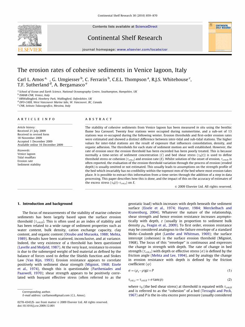
Fig. 1. A synthetic core of site 22 in Venice lagoon occupied during summer 1998.

The plot is derived from a time-series of erosion undertaken in the benthic flume

Sea Carousel. The black dots denote the applied bed shear stress; the arrows

indicate where D¼E¼0. Erosion rate goes to zero at the points t4 to t9 i.e. when the

excess stress (Dt)-0. The bed strength profile is defined as the locus joining

points tn in depth-stress space (open dots). The loci are defined by Eqs. (1) and (2)

and uses measured bulk density from Catscan analyses of syringe cores collected

at each site. The friction coefficients have been estimated from the two loci.

C.L. Amos et al. / Continental Shelf Research 30 (2010) 859–870860

hydrostatic in the near surface). It follows that Eq. (2) is a muchfuller description of the stability of a cohesive sediment than isthe surface erosion threshold, though in practice it is much harderto define. This is especially true as s - 0, where theory suggestsj-901 (Lambe and Whitman, 1969), though curiously, Hawley(1981) suggests that no consolidation takes place if the thicknessis less than 1 cm.

It is generally agreed that erosion rate per unit area of bed, orbenthic flux (@M/@t, where M is dry mass) is a robust measure ofsediment stability (McDowell and O’Connor, 1977) and is anessential precursor to the prediction of eroded depth and thesuspended sediment concentration (C) for a given applied bedshear stress (t0).

In the confines of an enclosed benthic flume, such as the oneused in this study (described in Amos et al., 1992), the rate oferosion is defined as

@M

@t¼ E¼

ðCtþDt�CtÞV

DtaþmDCUr ð3Þ

where V is the volume of water under consideration (0.218 m3), athe bed area (0.87 m2), m a (dimensionless) dispersion coefficient(2.4�10�5), DC the gradient in concentration inside and outsidethe flume, and Ur the rotational flow speed inside the flume. Thefirst term accounts for the change in mass within the flume, thesecond term accounts for losses through leakage or dispersion.

The erosion rate is commonly expressed (Thorn and Parsons,1980; Ariathurai and Arulanadan, 1978; Mehta and Parthenaides,1979; Kusuda et al, 1982; Lavelle and Mofjeld, 1987; Villaret andPaulic, 1986; Houwing, 1999) as an empirical power function:f=E0ec, where E0 is considered to be floc or background erosion(often related to bioturbation rate) and c is an empirical constant(Pa�1). It is also defined as a function of the excess bed shearstress

@M

@t¼ f ðt0�tcrit;zÞ

nð4Þ

The coefficient n is usually defined as less than unity and oftenas 0.5 (Mehta et al., 1989; Parchure and Mehta, 1984). Erosionrate is largely classified into two types: Type I erosion whichpeaks rapidly after onset of super-critical flow, and thereafterdecreases asymptotically to zero; and Type II erosion which isconstant in time. Type I erosion is interpreted as the response toan excess shear stress as defined by Eq. (4). The excess stressdiminishes in time through the erosion process and ceases whenthe applied stress is equal to the erosion threshold at the erodeddepth, which is equated to the bed shear strength: t0=tcrit,z=tb,z.This is shown graphically in Fig. 1 (based upon field data from site22 of this study; decades of station numbers cluster together inFig. 2). The black dots trace a time-series of applied stress throughan applied erosion event at increasing increments of flow speed.At each (excess) speed, erosion ceases when the applied stresslocus and the failure envelope meet (points illustrated as t4 ,y, t9).At such times, D=E=0 (Parchure and Mehta, 1984): If we know t0

at these times, then by inference we can define tcrit,z. This is animportant first step as, in most cases, tcrit,z is either unknown, orgiven as a constant; a fundamental flaw in most analyses is that itis almost always defined a priori.

Eq. (4) specifies that erosion and deposition do not occurtogether, an assumption supported by Lau and Krishnappan(1994) and assumed herein, though contested by Neumeier et al.(2008). Assuming P to be hydrostatic, one can define the effec-tive stress at any point throughout an erosion event by solutionof M in Eq. (3) and then by applying the Exner equation to solvefor z

rb

@z

@t¼@M

@t¼ ðD�EÞ ð5Þ

where D is mass deposition and E is mass erosion per unit bedarea. However, at this point, the process of assessment of thefactors controlling erosion rate becomes problematic, as wecannot solve Eq. (4) without knowledge of tcrit,z. This may beovercome by knowledge of the internal friction coefficient orfailure envelope. Thus, the construction of synthetic cores and thedefinition of the failure envelope is an essential second step in theevaluation of erosion rates.

Parchure and Mehta (1984) attempted to define tcrit,z andfound three zones of consolidation: (1) a surface zone about 2 mmthick of rapidly increasing bed strength with depth; (2) anasymptotic transitional zone several cm thick; and (3) a zone ofnear-constant bed strength. They presented an equation topredict tcrit,z as follows:

tcrit;z

tcrit;max¼

tcrit;0

tcrit;max

� �b=b0

ð6Þ

where tcrit,max is the maximum bed strength, tcrit,0 is the surfaceerosion threshold, b is the slope of a plot of ln(E) against excessbed shear stress ((t0�tcrit,z)/tcrit,z)), and b=b0 when t0=tcrit,0. bwas found to be linearly proportional to the inverse of bed shearstrength between a maximum of about 7 (at tcrit,0) and zero

ARTICLE IN PRESS

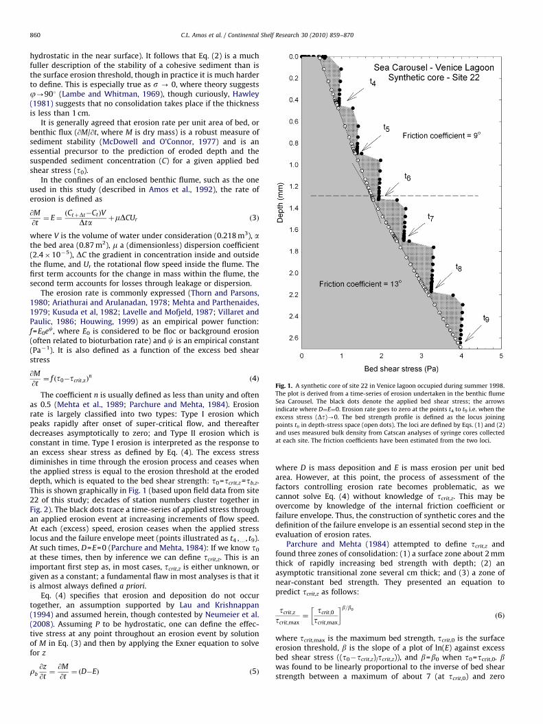
Fig. 2. The sites occupied during the summer (A) and winter (B) surveys of this paper. Also shown are the regions of surface erosion threshold (tcrit,0) interpolated across

the entire lagoon. Notice that in both periods, the highest threshold is found in the northern lagoon, and the lowest in a broad region around the city of Venice.

C.L. Amos et al. / Continental Shelf Research 30 (2010) 859–870 861

(at tcrit,max). Implicit in this formulation is the assumption that E

varies with depth as a non-linear function of excess stress. Thisdiffers from most approaches that assume a constant relationshipwith eroded depth.

The purpose of this paper is to examine the factors influencingerosion rate with reference to measurements made in Venicelagoon. In so doing, a method is presented to transform a time-series of erosion measurements to synthetic cores from which thefriction coefficient may be defined. The time-dependent excessshear stress is then derived based upon local values of time-varying bed strength and the results put into context of measurederosion rates and environmental setting. The results of theproposed method are placed into context of available publishedinformation for purposes of general application of the method.

2. Study region

The study was undertaken in Venice lagoon, Italy. It formedpart of a multi-disciplinary programme (F-ECTS) described byBergamasco et al. (2004). Stations throughout the lagoon wereoccupied during summer, 1998 and the following February, 1999.The benthic flumes Sea Carousel and Mini Flume were deployed ateach station. The details of this survey and descriptions of theflumes are found in Amos et al. (1998, 2000). Sites were chosen tobe representative of the wide range of bottom types that typifyVenice lagoon. Inter-tidal and sub-tidal sites were occupied asthey were representative of the northern, central and southernsub-basins of the lagoon (Fig. 2).

Results on the erosion thresholds of the lagoon bed have beenreviewed in Amos et al. (2004), wherein the mean erosionresistance measured in situ with Sea Carousel yielded an overallmean summertime value of 1.1070.69 Pa, and a wintertime valueof 0.6670.27 Pa (Tables 1a and 1b). Stability was generallyhighest the northern lagoon and lowest in the southern lagoon.A (seasonally averaged) mean erosion threshold of 0.9370.61was so derived. The eroded material was an order of magnitudehigher in organics than that of the bulk bottom sediment. Also,the sedimentation diameter of material suspended was much

larger (63723mm) than the disaggregated bottom sediment(29716mm). A seasonal comparison yielded a mean sedimen-tation diameter of 65742 (summertime) and 31711mm(wintertime). There was a weak positive correlation betweenthe median diameter of suspended material (D50) and fluore-scence during the summer, but none during the winter. Theinference is that erosion took place through the release of organic-rich aggregates which then behaved (hydrodynamically) like veryfine sand, though this was seasonally dependent: the largeraggregates were suspended during summer.

The physical and biological character of the lagoon have beendescribed in a series of recent publications (Guerzoni andTagliapietra, 2006; Bondesan and Meneghel, 2004). The bathy-metric evolution of Venice lagoon has been monitored throughrepetitive surveys (1901, 1930, 1970, 1990, 2000, and 2006, Basoet al., 2003, Sarretta et al., this issue) and show considerable lossesthrough time (1–4�105 m3/a). The mechanisms responsible forthese losses have been postulated by Cappucci et al. (2004),Solidoro et al. (2004), and Umgiesser et al. (2004) amongst others.Defina et al. (2006) propose that the distribution and elevation ofthe tidal mudflats is controlled by the peak wave-induced bedshear stress, which they define as 0.7 Pa. This corresponds wellwith the mean erosion resistance measurements described above.

Thus it is evident that much is know about the threshold oferosion of cohesive sediments in Venice lagoon. What are lesswell know are the rates of erosion that take place once thethreshold has been exceeded, and what factors influence erosionrates. Sutherland et al. (1998a) have shown that erosion rates canvary by a factor of 7 along the axis of a small bay, while associatederosion thresholds vary only by a factor of 2, suggesting a greatersensitivity of sediment response through erosion rate estimates.

3. Methods

The methods of deployment and data analysis, as well asrelevant calibration data are summarized in Amos et al. (2004).They are based upon Sea Carousel time-series which usuallylasted about 90 min and comprised 8–9 steps of velocity; each

ARTICLE IN PRESS

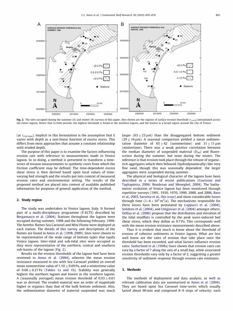
Table 1aA summary of the results of Sea Carousel deployments made during summer, 1998.

Site Depth (m) Site type scrit,0 (Pa) U (degrees) g1/r2 g2/r2 g3/r2 Z (mm) S (%)

(a) Summer (1998)

(1) Northern lagoon

20 1.4 5 0.35 7,40 1.15/0.87 0.25/0.03 0.44/0.13 1.7 10.8

21 1.0 5 0.22 11,30 1.32/0.94 0.73/0.16 1.16/0.21 1.6 18.8

22 1.2 7 0.44 9,13 1.04/0.96 0.69/0.09 1.23/0.40 2.7 14.4

30 1.8 3 0.80 62,12,42 1.02/0.97 1.12/0.22 0.62/0.32 0.9 15.4

31 1.2 7 1.90 62,30 2.51/0.96 1.57/0.16 0.19/– 0.6 –

32 1.4 2 0.83 24,13 1.06/0.96 0.81/0.27 0.60/0.40 1.6 –

33 0.8 7 0.79 30 1.93/0.90 0.84/0.33 0.88/0.42 0.8 6.3

40 0.7 1 3.06 – – – – – 8.2

41 1.2 1 1.51 30,20 0.76/0.98 0.90/0.35 0.47/0.13 7.5 13.4

42 1.0 5 0.83 40,48 1.04/0.97 0.17/– 0.32/0.12 3.4 9.7

43 3.4 7 1.37 55 1.87/0.97 2.13/0.38 0.61/0.43 0.5 –

44 1.3 2 0.86 46 0.88/0.97 0.64/0.09 0.72/0.20 0.5 30.8

50 1.5 3 1.42 10 2.42/0.96 2.12/0.41 – 4.8 4.3

51 2.5 3 1.51 31,6,13 1.38/0.97 1.07/0.2 – 4.0 –

52 2.2 3 2.12 40,0,10 1.38/0.97 1.07/0.28 0.91/0.22 3.8 –

53 0.8 1 2.23 75,54 2.46/0.94 1.24/0.21 0.56/0.39 0.6 7.8

Means 1.2670.75 307201 1.4870.58 1.0270.55 0.6770.29 2.371.95 12.777.0

(2) Central lagoon

60 2.0 8 0.36 83,88 0.63/0.52 – – 0.04 62.5

61 2.1 7 1.13 20 1.92/0.97 1.03/0.19 1.05/0.27 0.9 71.8

70 1.3 8 0.59 27,12 1.27/0.95 1.18/0.25 0.99/0.51 1.2 45.4

80 0.5 8 0.85 30,21 1.84/0.97 1.43/0.42 1.14/0.41 1.3 15.1

Means 0.7370.29 407291 1.4170.52 1.2170.16 1.0670.06 0.8670.49 48.7721.6

(3) Southern lagoon

90 1.6 8 0.86 30 1.82/0.94 1.61/0.27 2.42/0.48 0.3 –

100 2.0 8 0.39 60,35,78 1.53/0.97 0.93/0.35 0.39/0.10 0.7 17.5

110 1.2 3 0.88 6,37 2.51/0.86 0.22/– 0.09/– 1.5 14

Means 0.7170.23 41723 1.9570.41 0.9270.57 0.9771.03 0.8370.50 1974.8

The site types are: (1) Cyanobacteria and microphytobenthos; (2) microphytobenthos (no plants); (3) Zostera noltii patches (sea grass); (4) Ulva rigida sheets; (5) bare

mudflat; (6) Cymadocea nodosa (sea grass); (7) shell debris lag; (8) sandy bed. tcrit,o is the surface threshold erosion bed shear stress (Pa), j is the friction coefficient derived

from synthetic cores in each layer (separated by commas); Z1..3 are the slopes of the best fits of equations of (1) bed shear stress versus C; (2) erosion rate (E) versus bed

shear stress; and (3) erosion rate (E) versus excess bed shear stress with associated regression correlations; S is the organic content of suspended material; and z is the

maximum eroded depth (in mm).

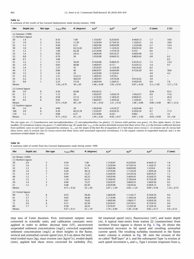
Table 1bA summary table of results from Sea Carousel deployments made during winter 1999.

Site Depth (m) Site type scrit,0 (Pa) U (degrees) g1/r2 g2/r2 g3/r2 Z (mm)

(b) Winter (1999)

(1) Northern lagoon

20 2.0 5 0.30 7,40 1.15/0.87 0.25/0.03 0.44/0.13 1.8

21 1.6 5 1.13 11,30 1.32/0.94 0.73/0.16 1.16/0.21 1.6

22 1.2 5 0.44 9,13 3.36/0.96 0.69/0.09 1.23/0.4 2.8

30 1.6 2 0.30 40,14 1.97/0.96 1.71/0.20 1.50/0.24 1.6

31 1.4 7 0.76 15,27 3.34/0.93 2.91/0.54 0.85/0.27 1.1

40 1.2 1 0.84 45,23 3.05/0.96 2.49/0.45 0.54/0.22 0.8

41 1.2 1 1.16 63,21 5.10/0.95 3.79/0.64 0.75/0.28 0.6

50 1.4 3 0.99 75,27 3.62/0.97 3.80/0.55 1.04/0.26 0.5

51 1.2 3 0.48 65,45 2.05/0.98 1.82/0.42 0.58/0.12 0.3

Means 0.7170.32 327201 2.6771.20 2.0271.25 0.9070.34 1.2370.75

(2) Central lagoon

60 2.5 8 0.53 58,44 1.68/0.99 1.11/0.17 0.74/0.34 0.4

61 2.7 7 0.62 58,40 2.11/0.98 1.10/0.24 0.29/0.04 0.4

70 2.5 8 0.61 76,62 1.00/0.96 1.08/0.17 0.58/0.20 0.2

71 2.9 8 0.71 62,50 2.03/0.97 2.07/0.51 0.75/0.23 0.4

80 1.7 3 0.38 42,25 1.97/0.97 1.53/0.30 0.72/0.16 0.6

Means 0.5770.11 527141 1.7670.40 1.3870.38 0.6270.17 0.470.13

C.L. Amos et al. / Continental Shelf Research 30 (2010) 859–870862

step was of 5 min duration. First, instrument outputs wereconverted to scientific units, and calibration constants wereapplied in order to define: decimal time (UT), uncorrectedsuspended sediment concentration (mg/L), corrected suspendedsediment concentration (mg/L) at three heights in the flume,vertical and azimuthal current speed (m/s, 8.5 cm above the bed);total eroded mass (kg), mass erosion rate (kg/m2/s), eroded depth(mm), applied bed shear stress corrected for turbidity (Pa),

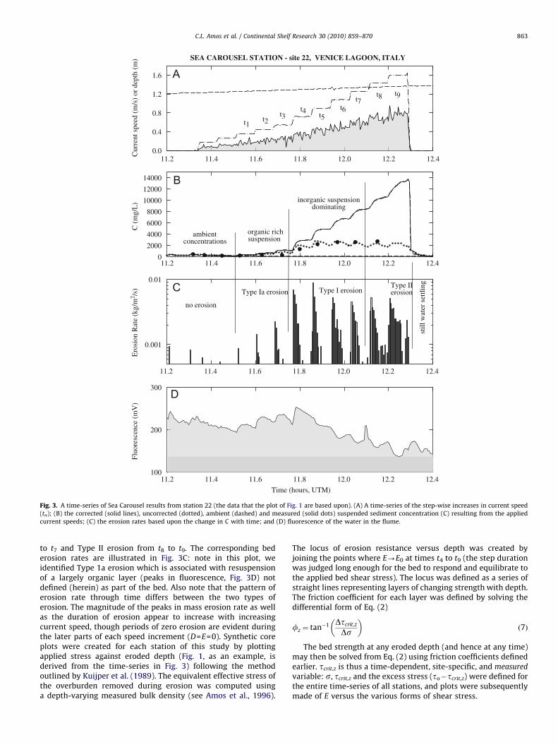
lid rotational speed (m/s), fluorescence (mV), and water depth(m). A typical time-series from station 22 (summertime) fromnorthern Venice lagoon is shown in Fig. 3. Fig. 3A shows theincremental increases in lid speed and resulting azimuthalcurrent speed. The resulting turbidity monitored in the flumewater column is evident in Fig. 3B: note the erosion of theso-called ‘‘fluff layer’’ at t1 and the subsequent Type 1a erosion ateach speed increment t2 and t3, Type I erosion responses from t4

ARTICLE IN PRESS

11.2

Cur

rent

spe

ed (

m/s

) or

dep

th (

m)

0.0

0.4

0.8

1.2

1.6

SEA CAROUSEL STATION - site 22, VENICE LAGOON, ITALY

11.2

C (

mg/

L)

0

2000

4000

6000

8000

10000

12000

14000

11.2

Ero

sion

Rat

e (k

g/m

2 /s)

0.001

0.01

Time (hours, UTM)

11.2

Fluo

resc

ence

(m

V)

100

200

300

ambientconcentrations

organic richsuspension

inorganic suspensiondominating

t1t2

t3t4

t5t6

t7t8 t9

no erosion

Type Ia erosion Type I erosionType II erosion

still

wat

er s

ettli

ng

11.4 11.6 11.8 12.0 12.2 12.4

11.4 11.6 11.8 12.0 12.2 12.4

11.4 11.6 11.8 12.0 12.2 12.4

11.4 11.6 11.8 12.0 12.2 12.4

Fig. 3. A time-series of Sea Carousel results from station 22 (the data that the plot of Fig. 1 are based upon). (A) A time-series of the step-wise increases in current speed

(tn); (B) the corrected (solid lines), uncorrected (dotted), ambient (dashed) and measured (solid dots) suspended sediment concentration (C) resulting from the applied

current speeds; (C) the erosion rates based upon the change in C with time; and (D) fluorescence of the water in the flume.

C.L. Amos et al. / Continental Shelf Research 30 (2010) 859–870 863

to t7 and Type II erosion from t8 to t9. The corresponding bederosion rates are illustrated in Fig. 3C: note in this plot, weidentified Type 1a erosion which is associated with resuspensionof a largely organic layer (peaks in fluorescence, Fig. 3D) notdefined (herein) as part of the bed. Also note that the pattern oferosion rate through time differs between the two types oferosion. The magnitude of the peaks in mass erosion rate as wellas the duration of erosion appear to increase with increasingcurrent speed, though periods of zero erosion are evident duringthe later parts of each speed increment (D=E=0). Synthetic coreplots were created for each station of this study by plottingapplied stress against eroded depth (Fig. 1, as an example, isderived from the time-series in Fig. 3) following the methodoutlined by Kuijper et al. (1989). The equivalent effective stress ofthe overburden removed during erosion was computed usinga depth-varying measured bulk density (see Amos et al., 1996).

The locus of erosion resistance versus depth was created byjoining the points where E-E0 at times t4 to t9 (the step durationwas judged long enough for the bed to respond and equilibrate tothe applied bed shear stress). The locus was defined as a series ofstraight lines representing layers of changing strength with depth.The friction coefficient for each layer was defined by solving thedifferential form of Eq. (2)

fz ¼ tan�1 Dtcrit;z

Ds

� �ð7Þ

The bed strength at any eroded depth (and hence at any time)may then be solved from Eq. (2) using friction coefficients definedearlier. tcrit,z is thus a time-dependent, site-specific, and measured

variable: s, tcrit,z and the excess stress (to�tcrit,z) were defined forthe entire time-series of all stations, and plots were subsequentlymade of E versus the various forms of shear stress.

ARTICLE IN PRESS

C.L. Amos et al. / Continental Shelf Research 30 (2010) 859–870864

4. Results and discussion

4.1. Composition of the seabed

All stations (24 sites in summer 1998, 13 sites re-occupiedduring winter 1999) were analyzed herein. The erosion rates,friction coefficients and best-fit relationships to excess bed stressare summarized in Table 1a (summer) and 1b (winter). Thereappears to be no relationship between vane shear strength andtcrit,0, friction coefficient or station water depth. Nor was thereany difference between inter-tidal and sub-tidal station vanestrengths; the highest strengths were generally associated withsediments with the lowest water contents though differenceswere small. The mean summertime and wintertime wet bulkdensities (measured in the topmost 1 cm of syringe cores) weresimilar (17817174 and 1773789 kg/m3); that is, highly con-solidated for recent marine sediments (Terzaghi and Peck, 1967)and close to the sediment densities reported by Mehta andParchure (1984) discussed later. They showed no obvious trendsacross the lagoon, with water depth, or with seabed habitat. Thiswas also true for sand/silt/clay ratios and sediment sorting(Table 2). Silt and clay were dominant components of thelagoon seabed with the exception of the sites in the southernlagoon, which were sand dominated. In the northern lagoon, thesand content was greatest in the topmost 10 cm and decreasedwith depth to minima at about 1 m (Fig. 4). This trend is inkeeping with the bypassing of fine and very fine sand around Lidoinlet northern breakwater and possible influx into the northernlagoon (Helsby, 2008). Elsewhere, the sand content variedconsiderably in content with depth. In almost all cases, the finescontent exceeded 15%; the minimum considered to inducecohesive behaviour (Mitchener et al., 1996): stations with lowerfines contents were not considered further in this study.

4.2. The factors influencing the erosion thresholds of the seabed

Interpolated plots of the distribution of erosion thresholdthroughout Venice lagoon are shown in Fig. 2(A and B) forsummer and winter, respectively. The summer thresholds were

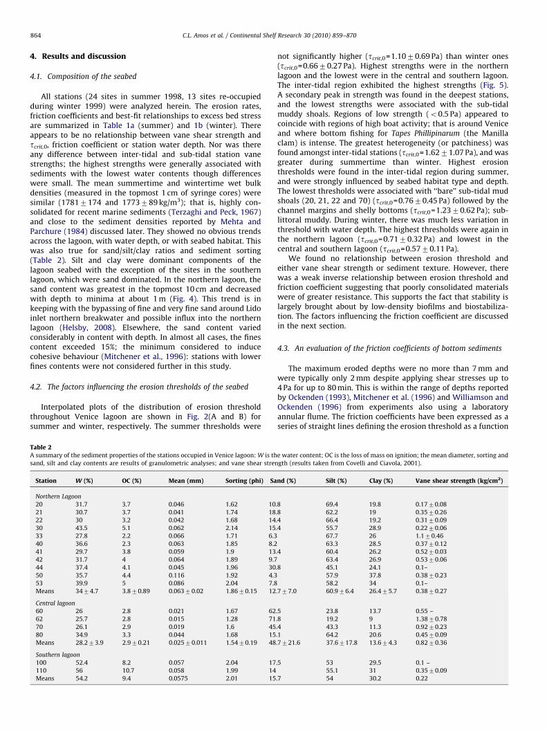
Table 2A summary of the sediment properties of the stations occupied in Venice lagoon: W is th

sand, silt and clay contents are results of granulometric analyses; and vane shear stren

Station W (%) OC (%) Mean (mm) Sorting (phi) Sa

Northern Lagoon

20 31.7 3.7 0.046 1.62 10

21 30.7 3.7 0.041 1.74 18

22 30 3.2 0.042 1.68 14

30 43.5 5.1 0.062 2.14 15

33 27.8 2.2 0.066 1.71 6.3

40 36.6 2.3 0.063 1.85 8.2

41 29.7 3.8 0.059 1.9 13

42 31.7 4 0.064 1.89 9.7

44 37.4 4.1 0.045 1.96 30

50 35.7 4.4 0.116 1.92 4.3

53 39.9 5 0.086 2.04 7.8

Means 3474.7 3.870.89 0.06370.02 1.8670.15 12

Central lagoon

60 26 2.8 0.021 1.67 62

62 25.7 2.8 0.015 1.28 71

70 26.1 2.9 0.019 1.6 45

80 34.9 3.3 0.044 1.68 15

Means 28.273.9 2.970.21 0.02570.011 1.5470.19 48

Southern lagoon

100 52.4 8.2 0.057 2.04 17

110 56 10.7 0.058 1.99 14

Means 54.2 9.4 0.0575 2.01 15

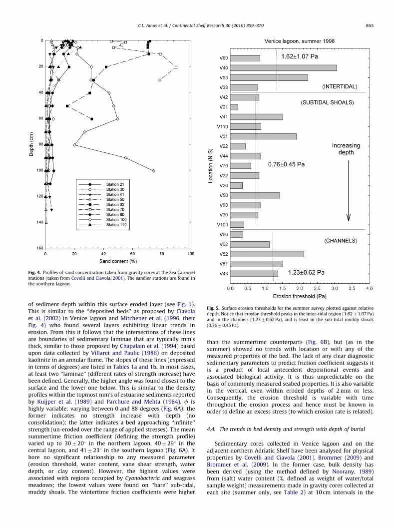
not significantly higher (tcrit,0=1.1070.69 Pa) than winter ones(tcrit,0=0.6670.27 Pa). Highest strengths were in the northernlagoon and the lowest were in the central and southern lagoon.The inter-tidal region exhibited the highest strengths (Fig. 5).A secondary peak in strength was found in the deepest stations,and the lowest strengths were associated with the sub-tidalmuddy shoals. Regions of low strength (o0.5 Pa) appeared tocoincide with regions of high boat activity; that is around Veniceand where bottom fishing for Tapes Phillipinarum (the Manillaclam) is intense. The greatest heterogeneity (or patchiness) wasfound amongst inter-tidal stations (tcrit,0=1.6271.07 Pa), and wasgreater during summertime than winter. Highest erosionthresholds were found in the inter-tidal region during summer,and were strongly influenced by seabed habitat type and depth.The lowest thresholds were associated with ‘‘bare’’ sub-tidal mudshoals (20, 21, 22 and 70) (tcrit,0=0.7670.45 Pa) followed by thechannel margins and shelly bottoms (tcrit,0=1.2370.62 Pa); sub-littoral muddy. During winter, there was much less variation inthreshold with water depth. The highest thresholds were again inthe northern lagoon (tcrit,0=0.7170.32 Pa) and lowest in thecentral and southern lagoon (tcrit,0=0.5770.11 Pa).

We found no relationship between erosion threshold andeither vane shear strength or sediment texture. However, therewas a weak inverse relationship between erosion threshold andfriction coefficient suggesting that poorly consolidated materialswere of greater resistance. This supports the fact that stability islargely brought about by low-density biofilms and biostabiliza-tion. The factors influencing the friction coefficient are discussedin the next section.

4.3. An evaluation of the friction coefficients of bottom sediments

The maximum eroded depths were no more than 7 mm andwere typically only 2 mm despite applying shear stresses up to4 Pa for up to 80 min. This is within the range of depths reportedby Ockenden (1993), Mitchener et al. (1996) and Williamson andOckenden (1996) from experiments also using a laboratoryannular flume. The friction coefficients have been expressed as aseries of straight lines defining the erosion threshold as a function

e water content; OC is the loss of mass on ignition; the mean diameter, sorting and

gth (results taken from Covelli and Ciavola, 2001).

nd (%) Silt (%) Clay (%) Vane shear strength (kg/cm2)

.8 69.4 19.8 0.1770.08

.8 62.2 19 0.3570.26

.4 66.4 19.2 0.3170.09

.4 55.7 28.9 0.2270.06

67.7 26 1.170.46

63.3 28.5 0.3770.12

.4 60.4 26.2 0.5270.03

63.4 26.9 0.5370.06

.8 45.1 24.1 0.1–

57.9 37.8 0.3870.23

58.2 34 0.1–

.777.0 60.976.4 26.475.7 0.3870.27

.5 23.8 13.7 0.55 –

.8 19.2 9 1.3870.78

.4 43.3 11.3 0.9270.23

.1 64.2 20.6 0.4570.09

.7721.6 37.6717.8 13.674.3 0.8270.36

.5 53 29.5 0.1 –

55.1 31 0.3570.09

.7 54 30.2 0.22

ARTICLE IN PRESS

Fig. 4. Profiles of sand concentration taken from gravity cores at the Sea Carousel

stations (taken from Covelli and Ciavola, 2001). The sandier stations are found in

the southern lagoon.

Fig. 5. Surface erosion thresholds for the summer survey plotted against relative

depth. Notice that erosion threshold peaks in the inter-tidal region (1.6271.07 Pa)

and in the channels (1.2370.62 Pa), and is least in the sub-tidal muddy shoals

(0.7670.45 Pa).

C.L. Amos et al. / Continental Shelf Research 30 (2010) 859–870 865

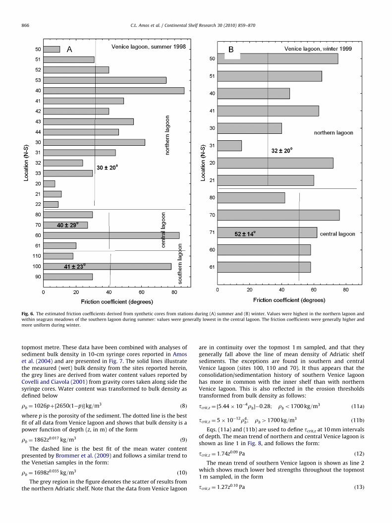
of sediment depth within this surface eroded layer (see Fig. 1).This is similar to the ‘‘deposited beds’’ as proposed by Ciavolaet al. (2002) in Venice lagoon and Mitchener et al. (1996, theirFig. 4) who found several layers exhibiting linear trends inerosion. From this it follows that the intersections of these linesare boundaries of sedimentary laminae that are typically mm’sthick, similar to those proposed by Chapalain et al. (1994) basedupon data collected by Villaret and Paulic (1986) on depositedkaolinite in an annular flume. The slopes of these lines (expressedin terms of degrees) are listed in Tables 1a and 1b. In most cases,at least two ‘‘laminae’’ (different rates of strength increase) havebeen defined. Generally, the higher angle was found closest to thesurface and the lower one below. This is similar to the densityprofiles within the topmost mm’s of estuarine sediments reportedby Kuijper et al. (1989) and Parchure and Mehta (1984). f ishighly variable: varying between 0 and 88 degrees (Fig. 6A): theformer indicates no strength increase with depth (noconsolidation); the latter indicates a bed approaching ‘‘infinite’’strength (un-eroded over the range of applied stresses). The meansummertime friction coefficient (defining the strength profile)varied up to 307201 in the northern lagoon, 407291 in thecentral lagoon, and 417231 in the southern lagoon (Fig. 6A). Itbore no significant relationship to any measured parameter(erosion threshold, water content, vane shear strength, waterdepth, or clay content). However, the highest values wereassociated with regions occupied by Cyanobacteria and seagrassmeadows; the lowest values were found on ‘‘bare’’ sub-tidal,muddy shoals. The wintertime friction coefficients were higher

than the summertime counterparts (Fig. 6B), but (as in thesummer) showed no trends with location or with any of themeasured properties of the bed. The lack of any clear diagnosticsedimentary parameters to predict friction coefficient suggests itis a product of local antecedent depositional events andassociated biological activity. It is thus unpredictable on thebasis of commonly measured seabed properties. It is also variablein the vertical, even within eroded depths of 2 mm or less.Consequently, the erosion threshold is variable with timethroughout the erosion process and hence must be known inorder to define an excess stress (to which erosion rate is related).

4.4. The trends in bed density and strength with depth of burial

Sedimentary cores collected in Venice lagoon and on theadjacent northern Adriatic Shelf have been analysed for physicalproperties by Covelli and Ciavola (2001), Brommer (2009) andBrommer et al. (2009). In the former case, bulk density hasbeen derived (using the method defined by Noorany, 1989)from (salt) water content (%, defined as weight of water/totalsample weight) measurements made in gravity cores collected ateach site (summer only, see Table 2) at 10 cm intervals in the

ARTICLE IN PRESS

Fig. 6. The estimated friction coefficients derived from synthetic cores from stations during (A) summer and (B) winter. Values were highest in the northern lagoon and

within seagrass meadows of the southern lagoon during summer: values were generally lowest in the central lagoon. The friction coefficients were generally higher and

more uniform during winter.

C.L. Amos et al. / Continental Shelf Research 30 (2010) 859–870866

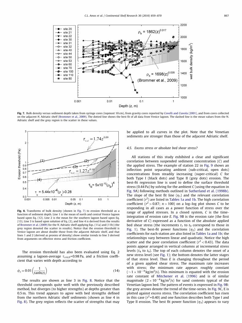
topmost metre. These data have been combined with analyses ofsediment bulk density in 10-cm syringe cores reported in Amoset al. (2004) and are presented in Fig. 7. The solid lines illustratethe measured (wet) bulk density from the sites reported herein,the grey lines are derived from water content values reported byCovelli and Ciavola (2001) from gravity cores taken along side thesyringe cores. Water content was transformed to bulk density asdefined below

rb ¼ 1026pþ½2650ð1�pÞ�kg=m3 ð8Þ

where p is the porosity of the sediment. The dotted line is the bestfit of all data from Venice lagoon and shows that bulk density is apower function of depth (z, in m) of the form

rb ¼ 1862z0:017 kg=m3 ð9Þ

The dashed line is the best fit of the mean water contentpresented by Brommer et al. (2009) and follows a similar trend tothe Venetian samples in the form:

rb ¼ 1698z0:035 kg=m3 ð10Þ

The grey region in the figure denotes the scatter of results fromthe northern Adriatic shelf. Note that the data from Venice lagoon

are in continuity over the topmost 1 m sampled, and that theygenerally fall above the line of mean density of Adriatic shelfsediments. The exceptions are found in southern and centralVenice lagoon (sites 100, 110 and 70). It thus appears that theconsolidation/sedimentation history of southern Venice lagoonhas more in common with the inner shelf than with northernVenice lagoon. This is also reflected in the erosion thresholdstransformed from bulk density as follows:

tcrit;z ¼ ½5:44� 10�4rb��0:28; rbo1700 kg=m3 ð11aÞ

tcrit;z ¼ 5� 10�12r4b ; rb41700 kg=m3 ð11bÞ

Eqs. (11a) and (11b) are used to define tcrit,z at 10 mm intervalsof depth. The mean trend of northern and central Venice lagoon isshown as line 1 in Fig. 8, and follows the form:

tcrit;z ¼ 1:74z0:09 Pa ð12Þ

The mean trend of southern Venice lagoon is shown as line 2which shows much lower bed strengths throughout the topmost1 m sampled, in the form

tcrit;z ¼ 1:27z0:10 Pa ð13Þ

ARTICLE IN PRESS

Fig. 7. Bulk density versus sediment depth taken from syringe cores (topmost 10 cm), from gravity cores reported by Covelli and Ciavola (2001), and from cores collected

on the adjacent N. Adriatic shelf (Brommer et al., 2009). The dotted line shows the best fit of all data from Venice lagoon. The dashed line is the mean values from the N.

Adriatic shelf and the grey region is the scatter in these values.

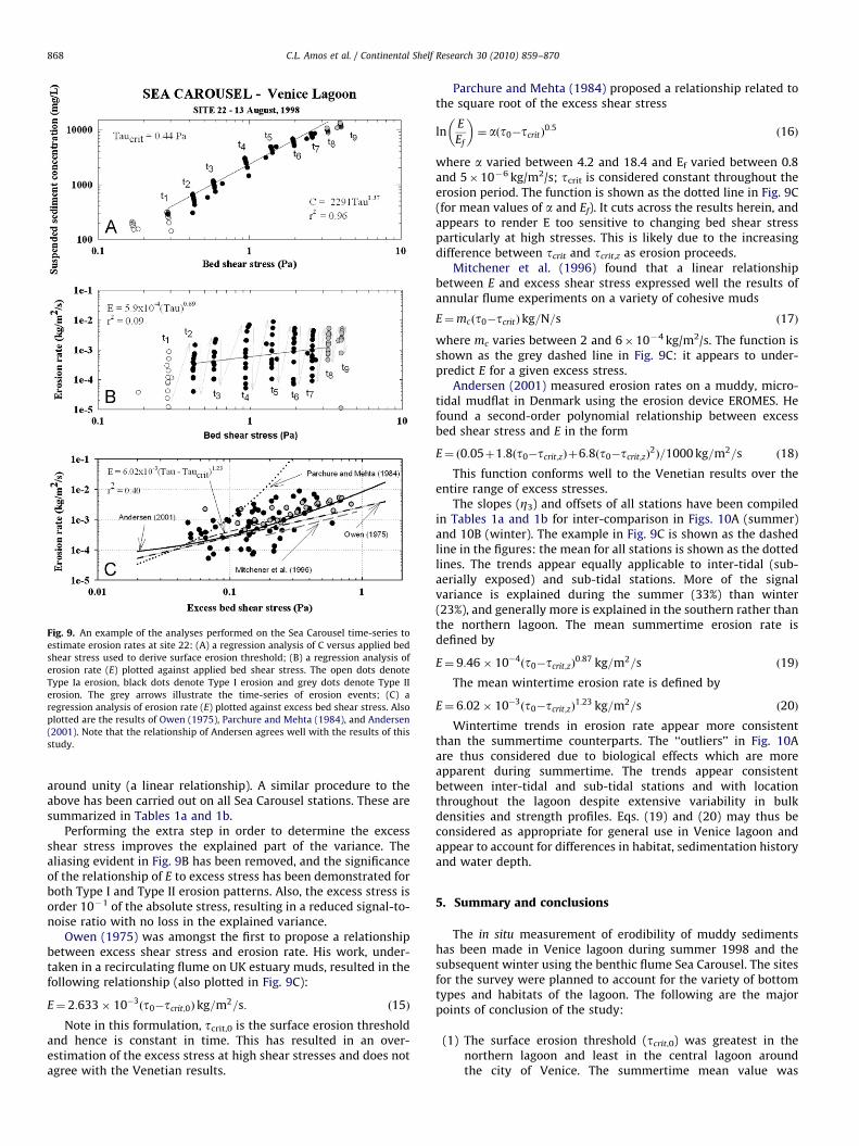
Fig. 8. Transforms of bulk density (shown in Fig. 7) to erosion threshold as a

function of sediment depth. Line 1 is the mean of north and central Venice lagoon

based upon Eq. (12). Line 2 is the mean for the southern lagoon based upon Eq.

(13). Line 3 is based upon solution of Eq. (2), and line 4 is derived from the results

of Brommer et al. (2009) for the N. Adriatic shelf applying Eqs. (11a) and (11b) (the

grey region denoted the scatter in results). Notice that the erosion threshold is

Venice lagoon are about double those from the adjacent Adriatic shelf, and that

lines 1 and 2 (derived as proxies of density) show similar trends to line 3 derived

from arguments on effective stress and friction coefficient.

C.L. Amos et al. / Continental Shelf Research 30 (2010) 859–870 867

The erosion threshold has also been evaluated using Eq. 2assuming a lagoon-average tcrit,0=0.98 Pa, and a friction coeffi-cient that varies with depth according to

fz ¼ 0:011

tanhðzÞ

� �ð14Þ

The results are shown as line 3 in Fig. 8. Notice that thethreshold corresponds quite well with the previously describedmethod, but diverges (to higher strengths) at depths greater than0.5 m. This trend appears to agree with bed strengths definedfrom the northern Adriatic shelf sediments (shown as line 4 inFig. 8). The grey region reflects the scatter of strengths that may

be applied to all curves in the plot. Note that the Venetiansediments are stronger than those of the adjacent Adriatic shelf.

4.5. Excess stress or absolute bed shear stress?

All stations of this study exhibited a clear and significantcorrelation between suspended sediment concentration (C) andthe applied stress. The example of station 22 in Fig. 9 shows aninflection point separating ambient (sub-critical, open dots)concentrations from steadily increasing (super-critical) C forboth Type I (black dots) and Type II (grey dots) erosion. Thebest-fit regression line is used to define the surface thresholdstress (0.44 Pa) by solving for the ambient C (using the equation inFig. 9A) following methods outlined in Sutherland et al. (1998b).The slope of the best fit line (Z1) and the relevant correlationcoefficient (r2) are listed in Tables 1a and 1b. The high correlationcoefficient (r240.87; n4100) on a log–log plot shows C to beresponding in all cases as a power function of stress over therange of applied stresses. In a closed system, C is the time-integration of erosion rate E. Fig. 9B is the erosion rate (the firstderivative of C) expressed as a function of the absolute appliedbed shear stress (the increments t1 to t9 correspond to those inFig. 1). The best-fit power functions (Z2) and the correlationcoefficients for each station are also listed in Tables 1a and 1b; therelationships vary between linear and quadratic. Notice the highscatter and the poor correlation coefficient (r2o0.43). The datapoints appear arranged in vertical columns at incremental stresslevels (t4 to t9). The top of each column denotes the onset of anew stress level (see Fig. 1); the bottom denotes the latter stagesof that stress level. Thus E is changing throughout the periodof a given applied shear stress. The maximum rate increaseswith stress; the minimum rate appears roughly constant(�1�10�4 kg/m2/s). This minimum is equated with the erosionrate constant of Mitchener et al. (1996) and is of similarmagnitude (2�10�4 kg/m2/s) for sand contents typical of theVenetian lagoon bed. The pattern of events is expressed in Fig. 9B:the grey arrows denote the trend of the time-series. In Fig. 9C, E isplotted against excess stress. The correlation coefficient has risenin this case (r2=0.40) and one function describes both Type I andType II erosion. The best fit power function (Z3) appears to vary

ARTICLE IN PRESS

Fig. 9. An example of the analyses performed on the Sea Carousel time-series to

estimate erosion rates at site 22: (A) a regression analysis of C versus applied bed

shear stress used to derive surface erosion threshold; (B) a regression analysis of

erosion rate (E) plotted against applied bed shear stress. The open dots denote

Type Ia erosion, black dots denote Type I erosion and grey dots denote Type II

erosion. The grey arrows illustrate the time-series of erosion events; (C) a

regression analysis of erosion rate (E) plotted against excess bed shear stress. Also

plotted are the results of Owen (1975), Parchure and Mehta (1984), and Andersen

(2001). Note that the relationship of Andersen agrees well with the results of this

study.

C.L. Amos et al. / Continental Shelf Research 30 (2010) 859–870868

around unity (a linear relationship). A similar procedure to theabove has been carried out on all Sea Carousel stations. These aresummarized in Tables 1a and 1b.

Performing the extra step in order to determine the excessshear stress improves the explained part of the variance. Thealiasing evident in Fig. 9B has been removed, and the significanceof the relationship of E to excess stress has been demonstrated forboth Type I and Type II erosion patterns. Also, the excess stress isorder 10�1 of the absolute stress, resulting in a reduced signal-to-noise ratio with no loss in the explained variance.

Owen (1975) was amongst the first to propose a relationshipbetween excess shear stress and erosion rate. His work, under-taken in a recirculating flume on UK estuary muds, resulted in thefollowing relationship (also plotted in Fig. 9C):

E¼ 2:633� 10�3ðt0�tcrit;0Þkg=m2=s: ð15Þ

Note in this formulation, tcrit,0 is the surface erosion thresholdand hence is constant in time. This has resulted in an over-estimation of the excess stress at high shear stresses and does notagree with the Venetian results.

Parchure and Mehta (1984) proposed a relationship related tothe square root of the excess shear stress

lnE

Ef

� �¼ aðt0�tcritÞ

0:5ð16Þ

where a varied between 4.2 and 18.4 and Ef varied between 0.8and 5�10�6 kg/m2/s; tcrit is considered constant throughout theerosion period. The function is shown as the dotted line in Fig. 9C(for mean values of a and Ef). It cuts across the results herein, andappears to render E too sensitive to changing bed shear stressparticularly at high stresses. This is likely due to the increasingdifference between tcrit and tcrit,z as erosion proceeds.

Mitchener et al. (1996) found that a linear relationshipbetween E and excess shear stress expressed well the results ofannular flume experiments on a variety of cohesive muds

E¼mcðt0�tcritÞkg=N=s ð17Þ

where mc varies between 2 and 6�10�4 kg/m2/s. The function isshown as the grey dashed line in Fig. 9C: it appears to under-predict E for a given excess stress.

Andersen (2001) measured erosion rates on a muddy, micro-tidal mudflat in Denmark using the erosion device EROMES. Hefound a second-order polynomial relationship between excessbed shear stress and E in the form

E¼ ð0:05þ1:8ðt0�tcrit;zÞþ6:8ðt0�tcrit;zÞ2Þ=1000 kg=m2=s ð18Þ

This function conforms well to the Venetian results over theentire range of excess stresses.

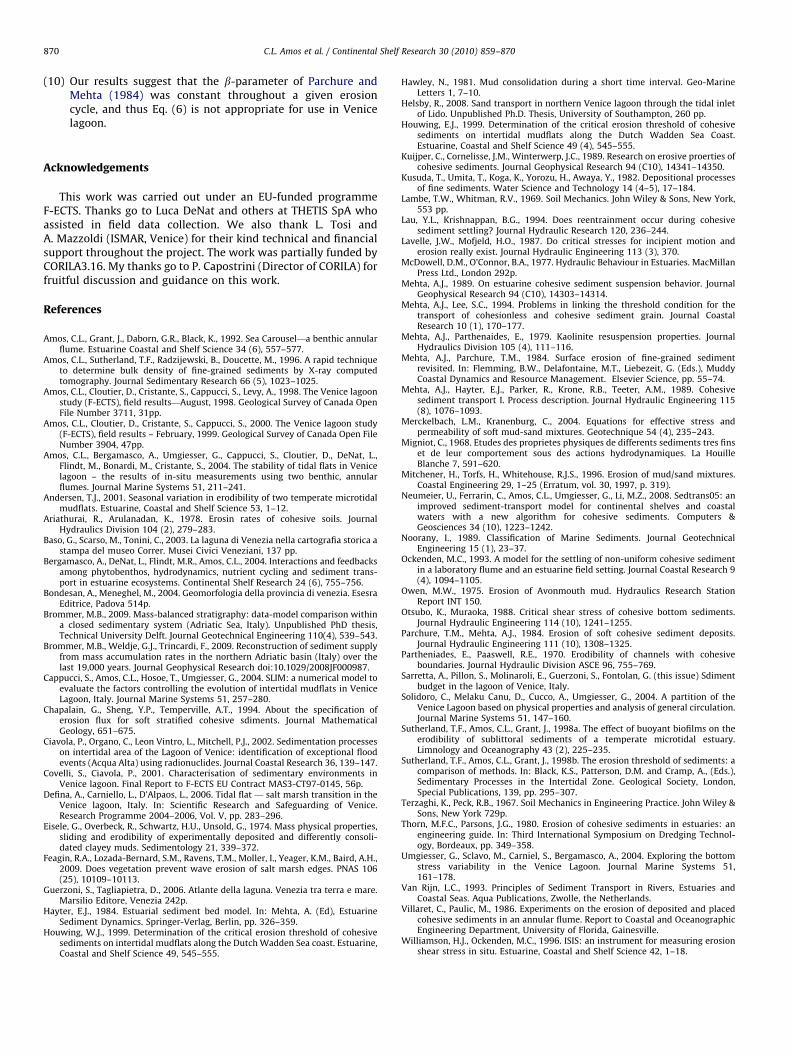
The slopes (Z3) and offsets of all stations have been compiledin Tables 1a and 1b for inter-comparison in Figs. 10A (summer)and 10B (winter). The example in Fig. 9C is shown as the dashedline in the figures: the mean for all stations is shown as the dottedlines. The trends appear equally applicable to inter-tidal (sub-aerially exposed) and sub-tidal stations. More of the signalvariance is explained during the summer (33%) than winter(23%), and generally more is explained in the southern rather thanthe northern lagoon. The mean summertime erosion rate isdefined by

E¼ 9:46� 10�4ðt0�tcrit;zÞ

0:87 kg=m2=s ð19Þ

The mean wintertime erosion rate is defined by

E¼ 6:02� 10�3ðt0�tcrit;zÞ

1:23 kg=m2=s ð20Þ

Wintertime trends in erosion rate appear more consistentthan the summertime counterparts. The ‘‘outliers’’ in Fig. 10Aare thus considered due to biological effects which are moreapparent during summertime. The trends appear consistentbetween inter-tidal and sub-tidal stations and with locationthroughout the lagoon despite extensive variability in bulkdensities and strength profiles. Eqs. (19) and (20) may thus beconsidered as appropriate for general use in Venice lagoon andappear to account for differences in habitat, sedimentation historyand water depth.

5. Summary and conclusions

The in situ measurement of erodibility of muddy sedimentshas been made in Venice lagoon during summer 1998 and thesubsequent winter using the benthic flume Sea Carousel. The sitesfor the survey were planned to account for the variety of bottomtypes and habitats of the lagoon. The following are the majorpoints of conclusion of the study:

(1)

The surface erosion threshold (tcrit,0) was greatest in thenorthern lagoon and least in the central lagoon aroundthe city of Venice. The summertime mean value was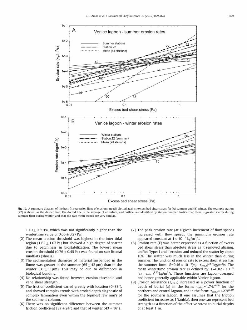

ARTICLE IN PRESS

Fig. 10. A summary diagram of the best-fit regression lines of erosion rate (E) plotted against excess bed shear stress for (A) summer and (B) winter. The example station

(22) is shown as the dashed line. The dotted line is the average of all values, and outliers are identified by station number. Notice that there is greater scatter during

summer than during winter, and that the two mean trends are very similar.

C.L. Amos et al. / Continental Shelf Research 30 (2010) 859–870 869

1.1070.69 Pa, which was not significantly higher than thewintertime value of 0.6670.27 Pa.

(2)

The mean erosion threshold was highest in the inter-tidalregion (1.6271.07 Pa) but showed a high degree of scatterdue to patchiness in biostabilization. The lowest meanerosion threshold (0.7670.45 Pa) was found on sub-littoralmudflats (shoals).

(3)

The sedimentation diameter of material suspended in theflume was greater in the summer (65742mm) than in thewinter (31711mm). This may be due to differences inbiological bonding.

(4)

No relationship was found between erosion threshold andvane shear strength.

(5)

The friction coefficient varied greatly with location (0–881),and showed complex trends with eroded depth diagnostic ofcomplex lamination even within the topmost few mm’s ofthe sediment column.

(6)

There was no significant difference between the summerfriction coefficient (377241) and that of winter (437161).

(7)

The peak erosion rate (at a given increment of flow speed)increased with flow speed; the minimum erosion rateappeared constant at 1�10�4 kg/m2/s.

(8)

Erosion rate (E) was better expressed as a function of excessbed shear stress than absolute stress as it removed aliasing,unified Types I and II erosion, and reduced the scatter by about10%. The scatter was much less in the winter than duringsummer. The function of erosion rate to excess shear stress hasthe summer form: E=9.46�10�4(t0�tcrit,z)

0.87 kg/m2/s. Themean wintertime erosion rate is defined by: E=6.02�10�3

(t0�tcrit,z)1.23 kg/m2/s. These functions are lagoon-averaged

and hence generally applicable within Venice lagoon.

(9) Erosion resistance (tcrit,z) increased as a power function of

depth of burial (z) in the form: tcrit,z=1.74z0.09 for thenorthern and central lagoon, and in the form: tcrit,z=1.27z0.10

for the southern lagoon. If one assumes that the frictioncoefficient increases as 1/tanh(z), then one can represent bedstrength as a function of the effective stress to burial depthsof at least 1 m.

ARTICLE IN PRESS

C.L. Amos et al. / Continental Shelf Research 30 (2010) 859–870870

(10)

Our results suggest that the b-parameter of Parchure andMehta (1984) was constant throughout a given erosioncycle, and thus Eq. (6) is not appropriate for use in Venicelagoon.

Acknowledgements

This work was carried out under an EU-funded programmeF-ECTS. Thanks go to Luca DeNat and others at THETIS SpA whoassisted in field data collection. We also thank L. Tosi andA. Mazzoldi (ISMAR, Venice) for their kind technical and financialsupport throughout the project. The work was partially funded byCORILA3.16. My thanks go to P. Capostrini (Director of CORILA) forfruitful discussion and guidance on this work.

References

Amos, C.L., Grant, J., Daborn, G.R., Black, K., 1992. Sea Carousel—a benthic annularflume. Estuarine Coastal and Shelf Science 34 (6), 557–577.

Amos, C.L., Sutherland, T.F., Radzijewski, B., Doucette, M., 1996. A rapid techniqueto determine bulk density of fine-grained sediments by X-ray computedtomography. Journal Sedimentary Research 66 (5), 1023–1025.

Amos, C.L., Cloutier, D., Cristante, S., Cappucci, S., Levy, A., 1998. The Venice lagoonstudy (F-ECTS), field results—August, 1998. Geological Survey of Canada OpenFile Number 3711, 31pp.

Amos, C.L., Cloutier, D., Cristante, S., Cappucci, S., 2000. The Venice lagoon study(F-ECTS), field results – February, 1999. Geological Survey of Canada Open FileNumber 3904, 47pp.

Amos, C.L., Bergamasco, A., Umgiesser, G., Cappucci, S., Cloutier, D., DeNat, L.,Flindt, M., Bonardi, M., Cristante, S., 2004. The stability of tidal flats in Venicelagoon – the results of in-situ measurements using two benthic, annularflumes. Journal Marine Systems 51, 211–241.

Andersen, T.J., 2001. Seasonal variation in erodibility of two temperate microtidalmudflats. Estuarine, Coastal and Shelf Science 53, 1–12.

Ariathurai, R., Arulanadan, K., 1978. Erosin rates of cohesive soils. JournalHydraulics Division 104 (2), 279–283.

Baso, G., Scarso, M., Tonini, C., 2003. La laguna di Venezia nella cartografia storica astampa del museo Correr. Musei Civici Veneziani, 137 pp.

Bergamasco, A., DeNat, L., Flindt, M.R., Amos, C.L., 2004. Interactions and feedbacksamong phytobenthos, hydrodynamics, nutrient cycling and sediment trans-port in estuarine ecosystems. Continental Shelf Research 24 (6), 755–756.

Bondesan, A., Meneghel, M., 2004. Geomorfologia della provincia di venezia. EsesraEditrice, Padova 514p.

Brommer, M.B., 2009. Mass-balanced stratigraphy: data-model comparison withina closed sedimentary system (Adriatic Sea, Italy). Unpublished PhD thesis,Technical University Delft. Journal Geotechnical Engineering 110(4), 539–543.

Brommer, M.B., Weldje, G.J., Trincardi, F., 2009. Reconstruction of sediment supplyfrom mass accumulation rates in the northern Adriatic basin (Italy) over thelast 19,000 years. Journal Geophysical Research doi:10.1029/2008JF000987.

Cappucci, S., Amos, C.L., Hosoe, T., Umgiesser, G., 2004. SLIM: a numerical model toevaluate the factors controlling the evolution of intertidal mudflats in VeniceLagoon, Italy. Journal Marine Systems 51, 257–280.

Chapalain, G., Sheng, Y.P., Temperville, A.T., 1994. About the specification oferosion flux for soft stratified cohesive sdiments. Journal MathematicalGeology, 651–675.

Ciavola, P., Organo, C., Leon Vintro, L., Mitchell, P.J., 2002. Sedimentation processeson intertidal area of the Lagoon of Venice: identification of exceptional floodevents (Acqua Alta) using radionuclides. Journal Coastal Research 36, 139–147.

Covelli, S., Ciavola, P., 2001. Characterisation of sedimentary environments inVenice lagoon. Final Report to F-ECTS EU Contract MAS3-CT97-0145, 56p.

Defina, A., Carniello, L., D’Alpaos, L., 2006. Tidal flat — salt marsh transition in theVenice lagoon, Italy. In: Scientific Research and Safeguarding of Venice.Research Programme 2004–2006, Vol. V, pp. 283–296.

Eisele, G., Overbeck, R., Schwartz, H.U., Unsold, G., 1974. Mass physical properties,sliding and erodibility of experimentally deposited and differently consoli-dated clayey muds. Sedimentology 21, 339–372.

Feagin, R.A., Lozada-Bernard, S.M., Ravens, T.M., Moller, I., Yeager, K.M., Baird, A.H.,2009. Does vegetation prevent wave erosion of salt marsh edges. PNAS 106(25), 10109–10113.

Guerzoni, S., Tagliapietra, D., 2006. Atlante della laguna. Venezia tra terra e mare.Marsilio Editore, Venezia 242p.

Hayter, E.J., 1984. Estuarial sediment bed model. In: Mehta, A. (Ed), EstuarineSediment Dynamics. Springer-Verlag, Berlin, pp. 326–359.

Houwing, W.J., 1999. Determination of the critical erosion threshold of cohesivesediments on intertidal mudflats along the Dutch Wadden Sea coast. Estuarine,Coastal and Shelf Science 49, 545–555.

Hawley, N., 1981. Mud consolidation during a short time interval. Geo-MarineLetters 1, 7–10.

Helsby, R., 2008. Sand transport in northern Venice lagoon through the tidal inletof Lido. Unpublished Ph.D. Thesis, University of Southampton, 260 pp.

Houwing, E.J., 1999. Determination of the critical erosion threshold of cohesivesediments on intertidal mudflats along the Dutch Wadden Sea Coast.Estuarine, Coastal and Shelf Science 49 (4), 545–555.

Kuijper, C., Cornelisse, J.M., Winterwerp, J.C., 1989. Research on erosive proerties ofcohesive sediments. Journal Geophysical Research 94 (C10), 14341–14350.

Kusuda, T., Umita, T., Koga, K., Yorozu, H., Awaya, Y., 1982. Depositional processesof fine sediments. Water Science and Technology 14 (4–5), 17–184.

Lambe, T.W., Whitman, R.V., 1969. Soil Mechanics. John Wiley & Sons, New York,553 pp.

Lau, Y.L., Krishnappan, B.G., 1994. Does reentrainment occur during cohesivesediment settling? Journal Hydraulic Research 120, 236–244.

Lavelle, J.W., Mofjeld, H.O., 1987. Do critical stresses for incipient motion anderosion really exist. Journal Hydraulic Engineering 113 (3), 370.

McDowell, D.M., O’Connor, B.A., 1977. Hydraulic Behaviour in Estuaries. MacMillanPress Ltd., London 292p.

Mehta, A.J., 1989. On estuarine cohesive sediment suspension behavior. JournalGeophysical Research 94 (C10), 14303–14314.

Mehta, A.J., Lee, S.C., 1994. Problems in linking the threshold condition for thetransport of cohesionless and cohesive sediment grain. Journal CoastalResearch 10 (1), 170–177.

Mehta, A.J., Parthenaides, E., 1979. Kaolinite resuspension properties. JournalHydraulics Division 105 (4), 111–116.

Mehta, A.J., Parchure, T.M., 1984. Surface erosion of fine-grained sedimentrevisited. In: Flemming, B.W., Delafontaine, M.T., Liebezeit, G. (Eds.), MuddyCoastal Dynamics and Resource Management. Elsevier Science, pp. 55–74.

Mehta, A.J., Hayter, E.J., Parker, R., Krone, R.B., Teeter, A.M., 1989. Cohesivesediment transport I. Process description. Journal Hydraulic Engineering 115(8), 1076–1093.

Merckelbach, L.M., Kranenburg, C., 2004. Equations for effective stress andpermeability of soft mud-sand mixtures. Geotechnique 54 (4), 235–243.

Migniot, C., 1968. Etudes des proprietes physiques de differents sediments tres finset de leur comportement sous des actions hydrodynamiques. La HouilleBlanche 7, 591–620.

Mitchener, H., Torfs, H., Whitehouse, R.J.S., 1996. Erosion of mud/sand mixtures.Coastal Engineering 29, 1–25 (Erratum, vol. 30, 1997, p. 319).

Neumeier, U., Ferrarin, C., Amos, C.L., Umgiesser, G., Li, M.Z., 2008. Sedtrans05: animproved sediment-transport model for continental shelves and coastalwaters with a new algorithm for cohesive sediments. Computers &Geosciences 34 (10), 1223–1242.

Noorany, I., 1989. Classification of Marine Sediments. Journal GeotechnicalEngineering 15 (1), 23–37.

Ockenden, M.C., 1993. A model for the settling of non-uniform cohesive sedimentin a laboratory flume and an estuarine field setting. Journal Coastal Research 9(4), 1094–1105.

Owen, M.W., 1975. Erosion of Avonmouth mud. Hydraulics Research StationReport INT 150.

Otsubo, K., Muraoka, 1988. Critical shear stress of cohesive bottom sediments.Journal Hydraulic Engineering 114 (10), 1241–1255.

Parchure, T.M., Mehta, A.J., 1984. Erosion of soft cohesive sediment deposits.Journal Hydraulic Engineering 111 (10), 1308–1325.

Partheniades, E., Paaswell, R.E., 1970. Erodibility of channels with cohesiveboundaries. Journal Hydraulic Division ASCE 96, 755–769.

Sarretta, A., Pillon, S., Molinaroli, E., Guerzoni, S., Fontolan, G. (this issue) Sdimentbudget in the lagoon of Venice, Italy.

Solidoro, C., Melaku Canu, D., Cucco, A., Umgiesser, G., 2004. A partition of theVenice Lagoon based on physical properties and analysis of general circulation.Journal Marine Systems 51, 147–160.

Sutherland, T.F., Amos, C.L., Grant, J., 1998a. The effect of buoyant biofilms on theerodibility of sublittoral sediments of a temperate microtidal estuary.Limnology and Oceanography 43 (2), 225–235.

Sutherland, T.F., Amos, C.L., Grant, J., 1998b. The erosion threshold of sediments: acomparison of methods. In: Black, K.S., Patterson, D.M. and Cramp, A., (Eds.),Sedimentary Processes in the Intertidal Zone. Geological Society, London,Special Publications, 139, pp. 295–307.

Terzaghi, K., Peck, R.B., 1967. Soil Mechanics in Engineering Practice. John Wiley &Sons, New York 729p.

Thorn, M.F.C., Parsons, J.G., 1980. Erosion of cohesive sediments in estuaries: anengineering guide. In: Third International Symposium on Dredging Technol-ogy, Bordeaux, pp. 349–358.

Umgiesser, G., Sclavo, M., Carniel, S., Bergamasco, A., 2004. Exploring the bottomstress variability in the Venice Lagoon. Journal Marine Systems 51,161–178.

Van Rijn, L.C., 1993. Principles of Sediment Transport in Rivers, Estuaries andCoastal Seas. Aqua Publications, Zwolle, the Netherlands.

Villaret, C., Paulic, M., 1986. Experiments on the erosion of deposited and placedcohesive sediments in an annular flume. Report to Coastal and OceanographicEngineering Department, University of Florida, Gainesville.

Williamson, H.J., Ockenden, M.C., 1996. ISIS: an instrument for measuring erosionshear stress in situ. Estuarine, Coastal and Shelf Science 42, 1–18.