Parallel Simulations of Dynamic Fracture

Using Extrinsic Cohesive Elements

Isaac Dooley, Graduate Student∗

Sandhya Mangala, Graduate Student†

Laxmikant Kale, Professor‡

Philippe Geubelle, Professor§

July 12, 2007

Suggested Running Head:Parallel Simulations of Dynamic Fracture Using Extrinsic Cohesive Ele-ments

Submission For:Journal of Scientific Computing (Springer)

Address(for office use):Isaac DooleySeibel Center for Computer Science201 North Goodwin AveUrbana, IL, 61801phone: 217-244-4583fax: 217-265-4035idooley2@uiuc.edu

∗Department of Computer Science, University of Illinois Urbana-Champaign, Urbana,Illinois

†Department of Aerospace Engineering, University of Illinois Urbana-Champaign,Urbana, Illinois

‡Department of Computer Science, University of Illinois Urbana-Champaign, Urbana,Illinois

§Department of Aerospace Engineering, University of Illinois Urbana-Champaign,Urbana, Illinois

1

Abstract

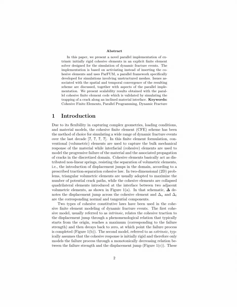
In this paper, we present a novel parallel implementation of ex-trinsic initially rigid cohesive elements in an explicit finite elementsolver designed for the simulation of dynamic fracture events. Theimplementation is based on activiating instead of inserting the co-hesive elements and uses ParFUM, a parallel framework specificallydeveloped for simulations involving unstructured meshes. Issues as-sociated with the spatial and temporal convergence of the resultingscheme are discussed, together with aspects of the parallel imple-mentation. We present scalability results obtained with the paral-lel cohesive finite element code which is validated by simulating thetrapping of a crack along an inclined material interface. Keywords:Cohesive Finite Elements, Parallel Programming, Dynamic Fracture

1 Introduction

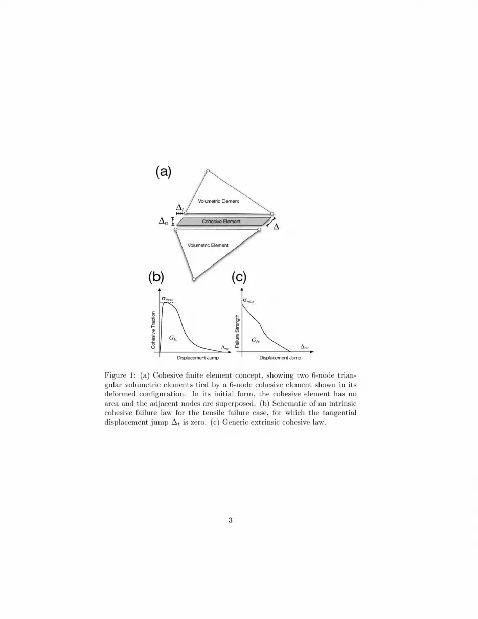
Due to its flexibility in capturing complex geometries, loading conditions,and material models, the cohesive finite element (CFE) scheme has beenthe method of choice for simulating a wide range of dynamic fracture eventsover the last decade [?, ?, ?, ?]. In this finite element formulation, con-ventional (volumetric) elements are used to capture the bulk mechanicalresponse of the material while interfacial (cohesive) elements are used tomodel the progressive failure of the material and the associated propagationof cracks in the discretized domain. Cohesive elements basically act as dis-tributed non-linear springs, resisting the separation of volumetric elements,i.e., the introduction of displacement jumps in the domain, according to aprescribed traction-separation cohesive law. In two-dimensional (2D) prob-lems, triangular volumetric elements are usually adopted to maximize thenumber of potential crack paths, while the cohesive elements are collapsedquadrilateral elements introduced at the interface between two adjacentvolumetric elements, as shown in Figure 1(a). In that schematic, ∆ de-notes the displacement jump across the cohesive element and ∆n and ∆t

are the corresponding normal and tangential components.Two types of cohesive constitutive laws have been used in the cohe-

sive finite element modeling of dynamic fracture events. The first cohe-sive model, usually referred to as intrinsic, relates the cohesive traction tothe displacement jump through a phenomenological relation that typicallystarts from the origin, reaches a maximum (corresponding to the failurestrength) and then decays back to zero, at which point the failure processis completed (Figure 1(b)). The second model, referred to as extrinsic, typ-ically assumes that the cohesive response is initially rigid and therefore onlymodels the failure process through a monotonically decreasing relation be-tween the failure strength and the displacement jump (Figure 1(c)). These

2

Volumetric Element

Volumetric Element

Cohesive Element!n

!t

(a)Co

hesiv

e Tr

actio

n

Displacement Jump

GIc

!nc

!max

Failu

re S

treng

th

GIc

Displacement Jump

!nc

!max

(b) (c)

!

Figure 1: (a) Cohesive finite element concept, showing two 6-node trian-gular volumetric elements tied by a 6-node cohesive element shown in itsdeformed configuration. In its initial form, the cohesive element has noarea and the adjacent nodes are superposed. (b) Schematic of an intrinsiccohesive failure law for the tensile failure case, for which the tangentialdisplacement jump ∆t is zero. (c) Generic extrinsic cohesive law.

3

two approaches thus differ in the way they capture the initial response ofthe cohesive element. In the intrinsic scheme, the cohesive elements arepresent in the finite element mesh from the start and, due to their finiteinitial stiffness, contribute to the deformation of the medium even in theabsence of damage. In the extrinsic scheme, the cohesive elements are ini-tially rigid and are only introduced in the finite element mesh based on anexternal traction-based criterion.

The key characteristics of the failure process are, however, identicalfor both models: in both cases, the failure process is captured with theaid of a phenomenological traction-separation law defined primarily by thefailure strength (denoted by σmax for the tensile failure case depicted inFigures 1(b) and (c)) and the critical value of the displacement jump (∆nc)beyond which complete failure is assumed. The area under the cohesivefailure curve defines the fracture toughness (usually denoted by GIc in thetensile (mode I) case). Although various cohesive laws have been usedin the past (linear, bilinear, exponential, polynomial, trapezoidal, etc.),the actual shape of the cohesive failure curve is considered to play only asecondary role on the failure process in many situations, especially in brittlematerials for which the cohesive failure zone is very small. A discussion ofthe similarities and differences between the two cohesive failure models canbe found in [?].

Due to its relative simplicity of implementation, the intrinsic cohesivefinite element scheme has been more widely adopted than its extrinsic coun-terpart. However, as shown in [?, ?], intrinsic elements suffer from conver-gence issues associated with the impact of the initial cohesive stiffness onthe computed strain and stress fields, and thereby, on the fracture process.To achieve convergence, intrinsic cohesive elements should be used only tosimulate dynamic fracture problems for which the crack path is prescribed(such as in interfacial fracture events). In the case of arbitrary crack mo-tion and branching, a finite distance should be introduced between cohesivefailure surfaces. The issues of spatial and temporal convergence for intrin-sic and extrinsic cohesive elements are discussed in [?, ?] and are revisitedin Section 4.1 for the case of both straight and arbitrary crack paths.

Dynamic fracture simulations need a very fine mesh near the failurezone to accurately capture the stress concentrations and the failure process,especially for brittle systems. Also, there is a need for a large domain tocapture the loading accurately and avoid premature wave reflections fromthe boundary. Very large domain combined with fine mesh requirementsmake the problem computationally very challenging. Parallel simulations,where the problem domain can be partitioned into smaller domains andsolved for on different processors, provide a powerful tool to solve theseproblems. Parallel computing can be used in conjunction with adaptivemesh refinement and coarsening [?].

4

The objective of this paper is to develop and implement a parallel CFEscheme based on activated extrinsic cohesive elements. As mentioned ear-lier, extrinsic cohesive elements are chosen over intrinsic elements to pre-vent the effects of artificial compliance due to the initially elastic part ofintrinsic cohesive elements. The parallel implementation of this schemeposes a set of challenges pertaining to the partitioning of the finite elementmesh and to inter-processor communication due to the presence of cohesiveelements at the interfaces. The complexities of communication are furtherincreased with extrinsic cohesive elements because there are multiple typesof elements in the discretization, each containing different fields.

To implement the CFE code in parallel, we use the Parallel Frameworkfor Unstructured Meshing (ParFUM) [?], a portable library for buildingparallel applications involving unstructured finite difference, finite element,or finite volume discretizations. The parallel framework is used in this workto partition the unstructured mesh, to distribute the partitions to proces-sors and to setup the inter-processor communication lists. ParFUM is builton the Charm++/AMPI Adaptive Runtime System and thereby providesadditional features such as dynamic load balancing between processors andadaptive overlapping of communication and computation [?].

This paper describes the use of the parallel framework ParFUM to im-plement our CFE scheme. Only a small number of libraries for handlingparallel unstructured meshes exist. Other large parallel frameworks couldhave been used in place of ParFUM. Unfortunately some of the most fullyfeatured production level frameworks are not available to the public andthus would not be suitable candidates for our application. Sandia Na-tional Laboratories’ SIERRA[SE04] is one such unreleased framework. TheUniversity of Heidelberg’s UG [?] is a large publicly available framework.Both SIERRA and UG support fully unstructured meshes on distributedmemory supercomputers with a variety of compatible solvers. The AOMDframework[?] also provides a parallel mesh abstraction which works on dis-tributed memory machines. deal.ii is a common finite element framework,which unfortunately works in parallel only on shared memory machines.Although deal.ii cannot utilize a distributed memory computer system, itdoes interface with solver libraries such as PETSc which are parallelizedfor clusters[?]. libMesh can similarly use parallel solvers in these regardsto deal.ii [?]. The extrinsic scheme proposed in this paper uses explicittimestepping and therefore does not require support for a solver library.The scheme requires just support for partitioning, distributing, and access-ing an unstructured mesh on a distributed memory computer cluster.

The emphasis of this work is on the inter-process communication in par-allel simulations performed with the extrinsic CFE scheme. Though meshadaptivity would further improve the efficiency of the proposed parallelimplementation, only the parallel implementation of extrinsic cohesive ele-

5

ments is discussed here. This paper provides in Section 2 the extrinsic con-stitutive law and the associated CFE formulations along with the stabilityconditions. Section 3 describes our parallel methodology and implemen-tation for the extrinsic cohesive elements that overcomes various issues ofpartitioning and inter-processor communications. Section 4 presents a se-ries of test simulations to verify and validate the developed parallel extrinsicCFE scheme. The validation study involves the numerical simulation of dy-namic fracture experiments performed on brittle specimens bonded alongan inclined interface [?]. Finally, in Section 5, we present scaling resultsfor the interface problems using the current parallel implementation.

2 Cohesive constitutive law and cohesive fi-nite element formulations

The cohesive failure law adopted in this work is the linear extrinsic relationused by [?], in which the cohesive traction T during the failure process isdescribed by

T =T

∆(β2∆t + ∆nn), (1)

where T denotes the effective cohesive traction defined by

T =√

β−2|Tt|2 + T 2n (2)

and Tn and Tt are the normal and tangential tractions, respectively. In(1), ∆, ∆n and ∆t are defined by

∆ =√

β2∆2n + ∆2

t ∆n = ∆ · n∆t = |∆t| = |∆ − ∆nn| (3)

where n is the normal vector defining the undeformed orientation of thecohesive element. The parameter β in (1)-(3) assigns different weights tothe sliding and normal opening displacements.

The traction vector T before the activation of cohesive element is com-puted from the stress fields of the neighboring volumetric elements as

T = σavern, (4)

where σaver is the average stress tensor of the two adajacent volumetricelements.

The failure process is initiated when either the normal traction Tn acrossthe cohesive interface reaches the critical tensile failure strength σmax orthe tangential component Tt, while Tn > 0 (i.e, failure is initated onlyfor tensile loading), reaches the corresponding shear failure strength τmax.A cohesive element completely fails when either of the displacement jump

6

Root Node

Node Copies

Cohesive ElementCohesive Element

Cohesive Element

Cohesive Element

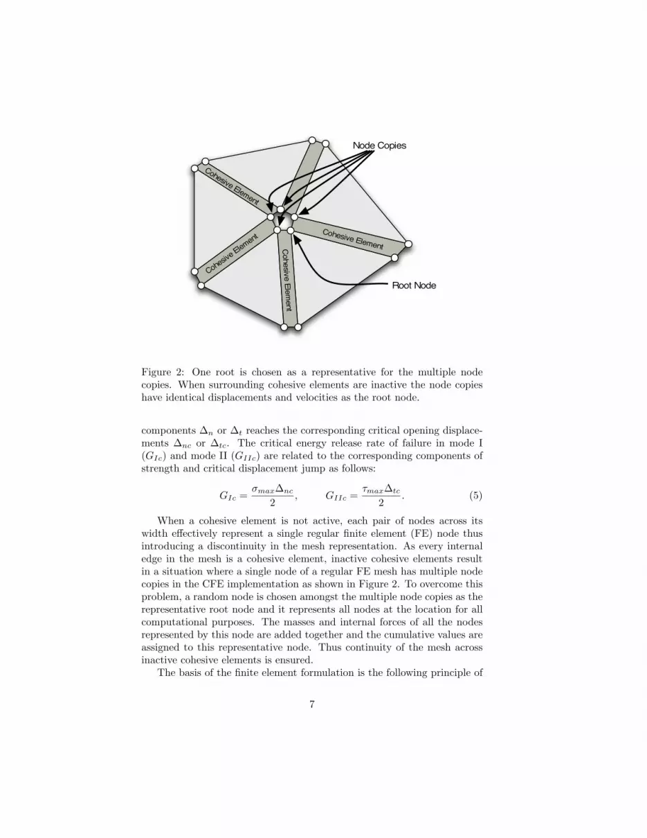
Figure 2: One root is chosen as a representative for the multiple nodecopies. When surrounding cohesive elements are inactive the node copieshave identical displacements and velocities as the root node.

components ∆n or ∆t reaches the corresponding critical opening displace-ments ∆nc or ∆tc. The critical energy release rate of failure in mode I(GIc) and mode II (GIIc) are related to the corresponding components ofstrength and critical displacement jump as follows:

GIc =σmax∆nc

2, GIIc =

τmax∆tc

2. (5)

When a cohesive element is not active, each pair of nodes across itswidth effectively represent a single regular finite element (FE) node thusintroducing a discontinuity in the mesh representation. As every internaledge in the mesh is a cohesive element, inactive cohesive elements resultin a situation where a single node of a regular FE mesh has multiple nodecopies in the CFE implementation as shown in Figure 2. To overcome thisproblem, a random node is chosen amongst the multiple node copies as therepresentative root node and it represents all nodes at the location for allcomputational purposes. The masses and internal forces of all the nodesrepresented by this node are added together and the cumulative values areassigned to this representative node. Thus continuity of the mesh acrossinactive cohesive elements is ensured.

The basis of the finite element formulation is the following principle of

7

virtual work defined over the deformable solid Ω:∫Ω

(S : δE− ρou.δu) d Ω −∫

Γex

Tex.δu d Γ −∫

Γin

T.δ∆ d Γ = 0

where Tex denotes the external tractions on the external boundary Γex andT corresponds to the cohesive tractions acting along the internal boundaryΓin across which the displacement jumps ∆ exist. In (6), ρo is the materialdensity, u is the displacement field, a superposed dot denotes differentia-tion with time, S and E are the second Piola-Kirchoff stress tensor andthe Lagrangian strain tensor, respectively. The principle of virtual workdescribed by (6) is of standard form except for the presence of the lastterm, which is the contribution from cohesive tractions. The semi-discretefinite element formulation can be expressed in the following matrix form:

M a = Rin + Rex (6)

where M is the lumped mass matrix, a is the nodal acceleration vector andRin, Rex respectively denote the internal and external force vectors [?].

With the aid of the second-order central difference time stepping scheme[?], the nodal displacements, velocities and accelerations at every time stepare computed as

dn+1 = dn + ∆tvn +12∆t2an, (7)

an+1 = M−1(Rinn+1 + Rex

n+1), (8)

vn+1 = vn +12∆t(an + an+1), (9)

where a subscript n denotes a quantity computed at time t = n∆t. Thetime step size ∆t is chosen such that it satisfies the CFL stability condition[?]

∆t = χse

Cdχ < 1, (10)

where se is the smallest edge in the mesh and χ is Courant number. Cd isthe dilatational wave speed, given in the plane strain isotropic case by

Cd =

√E(1 − ν)

(1 + ν)(1 − 2ν)ρo, (11)

where E is the stiffness of the material and ν is the Poisson’s ratio.To reduce the numerical oscillations inherent in the explicit scheme,

artificial viscosity is also incorporated in the finite element formulation [?].

8

3 Parallel implementation

The main goal for the implementation of the CFE scheme was to guaranteeexcellent parallel performance on hundreds of processors while quickly par-allelizing the initial serial Fortran code. This section describes the parallelimplementation and some of the design considerations. The implementa-tion uses the ParFUM framework because it is one of the best free, scalable,and portable frameworks that provides support for unstructured meshes.

The ParFUM (Parallel Framework for Unstructured Meshing) frame-work is a flexible framework for building unstructured mesh based FiniteDifference, Finite Volume, or Finite Element applications [?]. It can alsosimplify porting of serial codes that utilize unstructured discretizations toparallel computing platforms. This section summarizes the steps used toparallelize the extrinsic cohesive element scheme. Section 5 describes theefficiency and scalability of the resulting parallel implementation, whichis highly portable across most major types of high performance systemsincluding clusters, shared memory machines, and custom parallel machinessuch as IBM BlueGene/L.

ParFUM is a framework is built upon Charm++ and AMPI[?, ?].Charm++ is a parallel language and adaptive runtime system that pro-vides a robust, efficient, and portable system for writing parallel programs.The model of parallel programming used in Charm++ is that of migratableobjects. A program written in Charm++ is a collection of C++ objectswith remote asynchronous method invocations for communication betweenobjects. The Charm++ runtime system determines the mapping of objectsto processors and provides dynamic load balancing by migrating objects be-tween processors. AMPI is an adaptive MPI implementation built uponCharm++ that supports multiple MPI processes on each physical proces-sor. Charm++ and AMPI support a variety of dynamic instrumented loadbalancing schemes [?, ?, ?, ?, ?, ?] as well as a number of advanced faulttolerance schemes [?, ?, ?]. ParFUM therefore provides a number of usefulproductivity enhancing features without requiring a user to be an expertparallel programmer.

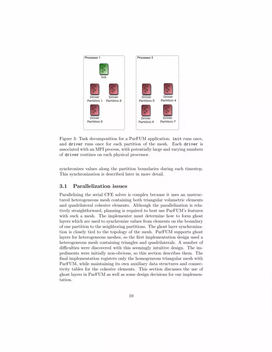
To port the serial CFE application to the parallel ParFUM framework,a key modification is to split the code into two parts as shown in Figure 3.The first part of the application is an init function that loads a serial meshon a single processor. The second part is a driver function that performsthe majority of the computation across multiple processors. After inithas finished, ParFUM partitions the mesh and builds communication lists.Then the user’s driver function runs in parallel, with an instance asso-ciated with each partition of the mesh. The driver routine creates someauxiliary data structures and then performs the explicit integrations forthe associated mesh partition in a timestep loop. The driver routine also

9

Processor 1 Processor 2

Init

Driver Partition 1

Driver Partition 2

Driver Partition 5

Driver Partition 3

Driver Partition 4

Driver Partition 6

Driver Partition 7

Figure 3: Task decomposition for a ParFUM application. init runs once,and driver runs once for each partition of the mesh. Each driver isassociated with an MPI process, with potentially large and varying numbersof driver routines on each physical processor.

synchronizes values along the partition boundaries during each timestep.This synchronization is described later in more detail.

3.1 Parallelization issues

Parallelizing the serial CFE solver is complex because it uses an unstruc-tured heterogeneous mesh containing both triangular volumetric elementsand quadrilateral cohesive elements. Although the parallelization is rela-tively straightforward, planning is required to best use ParFUM’s featureswith such a mesh. The implementer must determine how to form ghostlayers which are used to synchronize values from elements on the boundaryof one partition to the neighboring partitions. The ghost layer synchroniza-tion is closely tied to the topology of the mesh. ParFUM supports ghostlayers for heterogeneous meshes, so the first implementation design used aheterogeneous mesh containing triangles and quadrilaterals. A number ofdifficulties were discovered with this seemingly intuitive design. The im-pediments were initially non-obvious, so this section describes them. Thefinal implementation registers only the homogeneous triangular mesh withParFUM, while maintaining its own auxiliary data structures and connec-tivity tables for the cohesive elements. This section discusses the use ofghost layers in ParFUM as well as some design decisions for our implemen-tation.

10

In most parallel FE applications written for distributed memory ma-chines, the mesh is partitioned and distributed across the nodes in themachine with one or more partitions belonging to each processor. In addi-tion to each partition, a set of ghost elements and nodes is required. Theseghost elements are essentially read-only copies of elements from a neigh-boring partition. Values, such as displacements and forces, associated withthe elements in the ghost layer are updated from the original elements. InParFUM there are shared nodes, which are nodes that belong to multiplepartitions, as well as ghost elements and ghost nodes, which are read-onlycopies of elements and nodes from a neighboring partition. Collectively,the set of ghost nodes, ghost elements, and shared nodes for a partition isconsidered the partition’s ghost layer.

Different types of ghost layers are supported by ParFUM because FEapplications have differing requirements depending upon the order of theintegration scheme. Often a layer of depth one or two elements is required.ParFUM supports a generic specification of what type of ghost layers togenerate when it partitions the initial mesh. In a triangular mesh, twocommon types of ghost layers are used. Figure 4(a) displays the first typewhich specifies that an element should be included in the ghost layer if itshares an edge with a local element. Figure 4(b) displays the second typeof ghost layer which includes any element in the ghost layer if it has at leastone node in common with a local element. ParFUM applications specifythe desired type of ghost layer using an abstract set of tuples that definesa neighboring relation. This relation is used to determine if an elementis a neighbor of a local element and thus should be included in the ghostlayer. One relation would be the set of 3 pairs representing each of thethree edges in a triangle as in the case of (0, 1), (1, 2), (2, 0). The pair(1, 2) means that an edge of the element is defined by nodes 1 and 2 of theelement. Alternatively three values could specify the nodes of a triangleas in the case (0), (1), (2). When ParFUM partitions the mesh, it usesthe relation specified by the sets of tuples provided by the user in initto determine which elements should be included in the ghost layer for aparticular partition. The determination of whether to include an elementuses a simple criterion. The tuples are a template applied to each element toproduce sets of nodes for each element. If any of the resulting sets of nodesfor a remote element intersects the set of nodes from some local elementin a given partition, the former element is included in the partition’s ghostlayer. The same tuple relations can also be used in ParFUM to buildtopological adjacency tables.

The problem with the extrinsic CFE application is that after cohesiveelements are added to the mesh, the heterogeneous mesh contains topo-logical holes at vertices of the original triangular mesh, as illustrated inFigure 5. The presence of a hole causes problems when trying to create

11

Node-Based Ghosts forPartition 1

Partition 1

PartitionBoundaryPartition 1

Edge-Based Ghosts forPartition 1

PartitionBoundary

a)

b)

Figure 4: Two types of ghost layers supported by ParFUM. a) shows threeelements included in the ghost layer for Partition 1 because they shareat least one node with an element in Partition 1. b) shows two elementsincluded in the ghost layer for Partition 1 because these two share edgeswith triangles in Partition 1.

12

Figure 5: A topological hole is present in the heterogeneous mesh wherevera single node is present in the original triangular mesh.

ghost layers. In order to use ParFUM’s automatic ghost layer creation, theuser registers a simple triangular mesh with ParFUM in the initializationroutine. We specify the ghost layers to be node-based as in Figure 4(a), sothat any remote element sharing a node with a local element is includedin the ghost layer. In the driver routine, we then create auxiliary datastructures to represent the cohesive elements in the mesh. Thus the ap-plication code maintains a heterogeneous mesh while the framework onlyknows about a simple homogeneous triangular mesh. This allows the codeto take advantage of the mesh refinement features of the framework in thefuture, since the framework can dynamically refine triangular meshes. Thecreation of the application’s secondary heterogeneous mesh on each proces-sor in the driver routine is identical to the initial mesh creation code usedin the original serial version.

After ghost layers are created, the element and nodal data associatedwith the ghost elements and nodes must be synchronized each step. TheParFUM framework provides a simple mechanism for performing this syn-chronization. The application synchronizes only nodal data, such as dis-placements, velocities, and accelerations. The synchronization copies thedata from the nodes where the data is computed to any corresponding ghostcopies on adjacent partitions. We do this by treating the nodal data as el-ement data because of the unusual topology of the CFE mesh as shownin Figure 5. There are multiple copies of a node for each original node,each with slightly different nodal data. Each of these copies of a node is

13

Figure 6: Nodal data is copied to the elements, The elements sync withghost copies, and the updated data is copied from ghost elements to thenodes.

14

associated with one triangular element. The data is copied to the elementsprior to synchronization and then copied back to the nodes after synchro-nization. This process is shown schematically in Figure 6. In total, only asmall number of lines of code is required for the whole ghost value synchro-nization process because the ParFUM framework handles the significantwork involved in building all required send and receive lists as well as thedata packing and sending.

The ParFUM framework disallows global variables in any applicationsbuilt upon it. Global variables in FORTRAN programs are those declaredwith COMMON or SAVE.Therefore the parallel implementaiton of the CFEscheme wraps all COMMON or SAVE variables in a module. Using a moduleto wrap these variables is sufficient to meet this requirement of ParFUM.

3.2 Floating-point stability

Dynamic fracture problems are unstable physically. This inherent instabil-ity translates into a numerical instability as the limitations of floating-pointarithmetic can cause the solution to be affected by the number of partitionsinto which the mesh is partitioned. This numerical instability is caused bydiffering orders in which floating point operations are applied when sum-ming nodal force vectors. Since the parallel code adds values from localelements to a node before adding on the ghost element values, the order ofthese additions for a single logical shared node differs between the differentprocessors sharing that node. This difference in the order of the additionsaffects the solution because addition is neither associative nor commutativein floating point arithmetic, i.e., a + b + c 6= c + a + b, especially if the val-ues have widely differing exponents in their binary representation. Due tothe inherently unstable nature of dynamic fracture simulations, these smallerrors tend to accumulate over time and can affect the numerical results,including the predicted crack path.

The classic solution to numerical problems caused by non-commutativityor non-associativity of floating-point additions is to sort all the values thensum them from smallest to largest. Sorting however is expensive and sig-nificantly complicates an application’s source code. Additionally, in FEcodes, the common practice is to simply iterate over all elements adjacentto a given node, accumulating the sum. The code chooses this standardpractice. Unfortunately, this method of iterating over elements withoutregard to the values being summed is inherently flawed when maximal ac-curacy is required. We have not yet implemented the more complicatedmethod for summing the nodal force values using sorted lists. It should benoted that this problem does not just occur in parallel. The order in whichthe forces are added at each node produces slightly different results for theactivation time (and ultimately the failure time) of extrinsic cohesive ele-

15

ments. Since the specific order in which the elements are added matters,even in the serial case, attention should be paid to correctly add the forcesin a sorted order, whether in parallel or serial.

3.3 Load Balancing

Maintaining a uniform load balance across processors is critical to obtain-ing good performance and scalability to large numbers of processors. Inthe parallel implementation, a good load balance is achieved without anyexplicit load balancing. Section 5 shows that the parallel efficiency of theimplementation exceeded 99% in many cases without applying any dynamicload balancing. Since the parallel efficiency is high, the load is necessarilywell distributed among almost all processors. For this reason the supportfor load balancing provided by ParFUM is not used. However, other dy-namic fracture applications may require load balancing to achieve optimalperformance [?].

3.4 Implementation Summary

The main parallelization steps are as follows:

• Restructure the serial code into two main subroutines driver andinit

• Load an unpartitioned mesh in init

• Add ghost layer synchronization calls in driver

• Modify the output subroutine to create filenames based on processorid

• Eliminate global variables (COMMON or SAVE) by wrapping them in amodule

4 Verification and validation study

4.1 Convergence study

As indicated in the introduction, the spatial and temporal convergence ofthe CFE scheme needs to be addressed. To that effect, we investigate inthis section two fracture problems involving the dynamic mode I failureof a thick pre-notched PMMA specimen of length L = 0.05m and widthW = 0.03m, with an initial crack length a0 = 0.005m. The bulk materialproperties are defined by the Young’s modulus E = 3.45GPa, Poisson’s

16

W = 0.05 m

L=

0.03

m

V*(t)

V*(t)

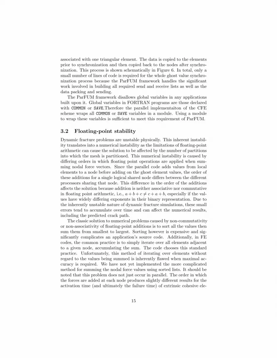
Figure 7: Mesh and boundary conditions used for crack propagation alonga pre-defined straight line problem. Only the elements along this line areallowed to be activated in this simulation. A larger view of the notch tipis in figure 8.

ratio ν = 0.35 and material density ρ0 = 1190kg/m3. The cohesive failureproperties adopted in this work are defined by the tensile and shear strengthvalues σmax = τmax = 20MPa and by the mode I and mode II fracturetoughness values GIc = GIIc = 352J/m2, which corresponds to a modemixity parameter β = 1.

In both fracture problems, the loading is symmetric with respect tothe initial crack plane, so the crack is expected to travel straight, unless itreaches a sufficiently high speed at which crack branching might occur. Twodiscretizations are considered here. In the first one (Figure 7), the crackis confined to propagate along its original plane, which acts like a straightmaterial interface. In the second one, the crack path is not pre-defined anda random mesh is used in the region ahead of the notch tip (Figure 12). Asalluded to in the introduction, convergence issues are expected to arise onlyin the second case. However, the first problem is studied for completenessand to compare the intrinsic and extrinsic CFE schemes. In both cases,the analysis is performed in plane strain, and the applied loading consistsof an applied vertical velocity V ∗(t) that increases linearly from 0 to peakvalue V0 for 0 < t ≤ tramp and remains constant afterwards.

The introduction of a cohesive model introduces a new length scale inthe problem, the length of the cohesive failure zone, the small region inthe vicinity of the advancing crack front where the cohesive failure process

17

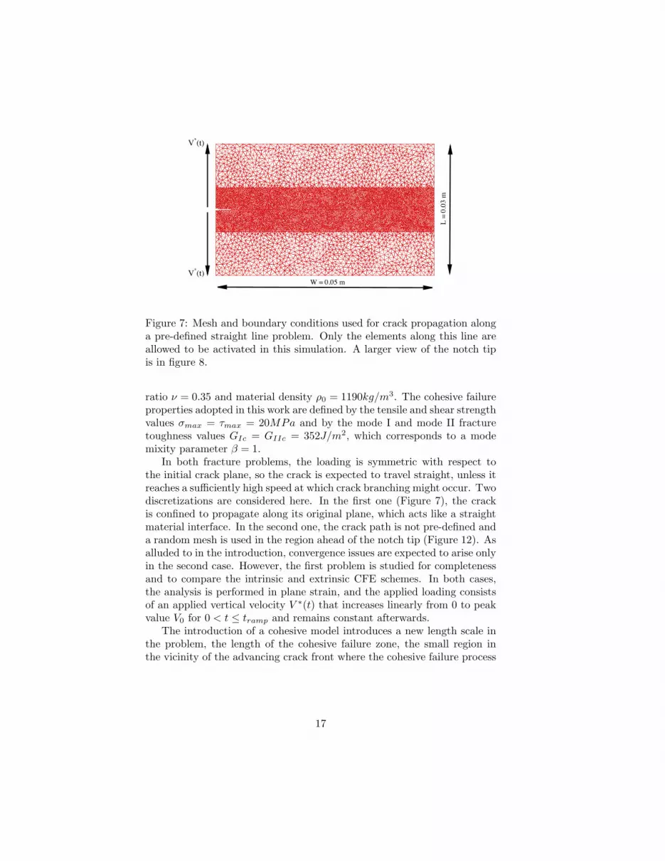
Notch Tip

Figure 8: Zoomed view of notch tip of mesh in figure 7. The mesh containsa pre-defined horizontal straight line path that the crack can follow.

takes place. A static estimate of the mode I cohesive zone size is

R =π

8E

1 − ν2

GIc

σ2max

. (12)

Although R is expected to decrease as the crack speed increases, (12) isused to compare various levels of mesh refinement. As illustrated in Figures7 and 12, since the crack motion is expected to remain in the vicinity ofthe mid-plane, only a limited region around the mid-plane is meshed witha fine mesh, while the remainder of the domain is meshed more coarsely toreduce the computational cost. At all times, the time step size ∆t is keptbelow the CFL stability conditions.

In the first problem, for which a straight crack path is prescribed (Fig-ure 7), the imposed vertical velocity is applied along the left edge of thedomain, while the remaining boundary is left traction-free. The peak valueof velocity is V0 = 2.5m/s and the ramp time is tramp = 0.058L/Cd. Fig-ure 9 present the time evolution of the crack length obtained with variousmeshes, with the time step size kept at a constant value of the Courantnumber χ = 0.05. The mesh density is characterized by the average num-ber of elements in the static cohesive zone size R. As apparent there, theCFE scheme is spatially convergent and about five cohesive elements areneeded in the active cohesive zone.

Figure 10 addresses the issue of temporal convergence of the CFE sim-ulation, showing the time evolution of the straight crack length for four

18

0 0.2 0.4 0.6 0.8 1 1.2 1.4

x 10−4

0.005

0.01

0.015

0.02

0.025

0.03

0.035

time (s)

tota

l cra

ck le

ngth

(m

)7.12

5.82

4.12

3.36

Average number of elements in cohesive zone

Figure 9: Spatial convergence of the crack motion for the case of a pre-scribed straight crack path, for four mesh densities defined as the ratioof the static cohesive zone size R given by equation (12) and the averagecohesive element size.

0 0.2 0.4 0.6 0.8 1 1.2 1.4

x 10−4

0.005

0.01

0.015

0.02

0.025

0.03

time (s)

tota

l cra

ck le

ngth

(m

)

0.033

0.05

0.1

0.2

χ

Figure 10: Temporal convergence of evolution of the total crack length, forthe straight line crack propagation problem for 4 different Courant numbersχ. The mesh density is fixed at about 4 cohesive elements in the cohesivezone.

19

0 0.2 0.4 0.6 0.8 1 1.2 1.4

x 10−4

0.005

0.01

0.015

0.02

0.025

0.03

0.035

time (s)

tota

l cra

ck le

ngth

(m

)

Extrinsic

Intrinsic − Sin

=0.98

Intrinsic − Sin

=0.9995

Intrinsic − Sin

=0.9999

Figure 11: Extrinsic vs. intrinsic CFE predictions of the straight crackpropagation history for a constant mesh density of about 4 elements in thecohesive zone and a constant time step size χ = 0.05.

values of the time step size (described through the corresponding value ofthe Courant number χ defined in (10). It should be noted that the use ofextrinsic cohesive modeling allows us to use time steps much larger thanthose commonly adopted in the intrinsic case, at least for problems involv-ing prescribed crack paths. In intrinsic CFE simulations, values of χ aretypically an order of magnitude smaller.

The evolution of the crack length is also used to compare the intrinsicand extrinsic FE solutions. In the intrinsic case, a bilinear cohesive failurelaw is adopted [?] that uses the same values of failure strength σmax andfracture toughness GIc. The initial cohesive stiffness Kc0, i.e., the slope ofthe rising part of the cohesive traction-separation curve, is defined by theparameter Sinit as in

Kc0 =σmax

(1 − Sinit)∆nc. (13)

The closer Sinit is to unity, the stiffer the cohesive element is, with the caseSinit = 1 corresponding to the limiting case of an initially rigid cohesiveelement. A direct comparison between extrinsic and intrinsic CFE predic-tions of the evolution of the crack length is presented in Figure 11. In theintrinsic case, three values of the non-dimensional parameter Sinit are used.As expected, as the initial stiffness of the intrinsic cohesive elements tendsto infinity, the extrinsic CFE solution is recovered, verifying the extrinsicimplementation of the cohesive finite element solver.

20

Vy(t)

Vy(t)

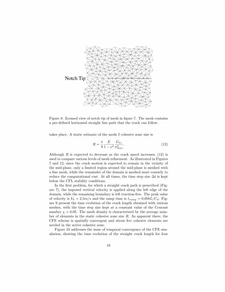
Figure 12: Mesh and boundary conditions used for the crack propagationproblem with arbitrary crack path, for which a random discretization isused in the central refined zone. The notch tip is enlarged in figure 13

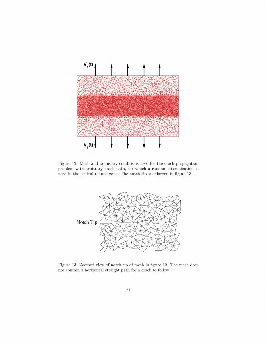
Notch Tip

Figure 13: Zoomed view of notch tip of mesh in figure 12. The mesh doesnot contain a horizontal straight path for a crack to follow.

21

0 0.005 0.01 0.015 0.02 0.025 0.03 0.035 0.04 0.045 0.050

0.005

0.01

0.015

0.02

0.025

0.03

x−location (m)

y−lo

catio

n (m

)

2.90

3.56

4.12

5.05

7.12

Average number of elements in cohesive zone

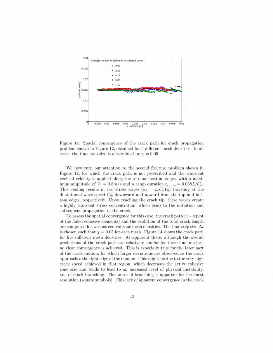
Figure 14: Spatial convergence of the crack path for crack propagationproblem shown in Figure 12, obtained for 5 different mesh densities. In allcases, the time step size is determined by χ = 0.05.

We now turn our attention to the second fracture problem shown inFigure 12, for which the crack path is not prescribed and the transientvertical velocity is applied along the top and bottom edges, with a maxi-mum amplitude of V0 = 0.5m/s and a ramp duration tramp = 0.058L/Cd.This loading results in two stress waves (σ0 = ρoCdV0) traveling at thedilatational wave speed Cd, downward and upward from the top and bot-tom edges, respectively. Upon reaching the crack tip, these waves createa highly transient stress concentration, which leads to the initiation andsubsequent propagation of the crack.

To assess the spatial convergence for this case, the crack path (x−y plotof the failed cohesive elements) and the evolution of the total crack lengthare computed for various central zone mesh densities. The time step size ∆tis chosen such that χ = 0.05 for each mesh. Figure 14 shows the crack pathfor five different mesh densities. As apparent there, although the overallpredictions of the crack path are relatively similar for these four meshes,no clear convergence is achieved. This is especially true for the later partof the crack motion, for which larger deviations are observed as the crackapproaches the right edge of the domain. This might be due to the very highcrack speed achieved in that region, which decreases the active cohesivezone size and tends to lead to an increased level of physical instability,i.e., of crack branching. This onset of branching is apparent for the finestresolution (square symbols). This lack of apparent convergence in the crack

22

0.6 0.8 1 1.2 1.4 1.6

x 10−4

0.005

0.01

0.015

0.02

0.025

0.03

0.035

0.04

0.045

0.05

0.055

time (s)

tota

l cra

ck le

ngth

(m

)

2.90

3.56

4.12

5.05

7.12

Average number of elements in cohesive zone

Figure 15: Spatial convergence of the evolution of the crack length for thefive simulations shown in Figure 14.

path prediction obtained with unstructured meshes has been alluded toelsewhere [?]. This apparent lack of spatial convergence translates, but toa smaller degree, to the evolution of the total crack length (i.e., the sumof the length of all failed cohesive elements), as shown in Figure 15. Thistype of simulation provides an indication of the scatter of the numericalpredictions of the macroscopic crack path.

The issue of temporal convergence is addressed in Figures 16 and 17,which respectively present the crack path and crack length evolution resultsobtained for a fixed mesh (with an average of 4.12 cohesive elements in thecohesive zone) and for four values of the time step size. Although thetemporal convergence for the arbitrary crack path is less conclusive thanfor the prescribed path case, the results obtained for the four values of χ arevery similar especially during the initial stage of the crack motion. After awhile, however, the numerical results start to deviate from each other, firstslightly, then in a more pronounced fashion. Note once again, however,that a stable numerical solution is obtained with the extrinsic CFE schemefor values of χ larger than 0.2, while a value as small as χ = 0.033 has tobe used in the intrinsic case to achieved stability [?].

As the final step of this convergence study, we compare the results forthe serial and parallel implementations of the extrinsic CFE scheme. Theparallel results are obtained on a four-processor platform. The mesh andtime step sizes are kept constant, an average of 4.12 elements in the cohesivezone and a Courant number χ = 0.05. It can be inferred from the Figure

23

0 0.005 0.01 0.015 0.02 0.025 0.03 0.035 0.04 0.045 0.050

0.005

0.01

0.015

0.02

0.025

0.03

x−location (m)

y−lo

catio

n (m

)0.033

0.05

0.1

0.2

χ

Figure 16: Temporal convergence of the extrinsic CFE simulations for ar-bitrary crack path, for a fixed mesh density of about 4 elements in thecohesive zone size.

0.9 1 1.1 1.2 1.3 1.4 1.5 1.6

x 10−4

0.005

0.01

0.015

0.02

0.025

0.03

0.035

0.04

0.045

0.05

0.055

time (s)

tota

l cra

ck le

ngth

(m

)

0.033

0.05

0.1

0.2

χ

Figure 17: Temporal convergence of the crack length vs. time curves forthe simulations shown in Figure 16.

24

0 0.005 0.01 0.015 0.02 0.025 0.03 0.035 0.04 0.045 0.050

0.005

0.01

0.015

0.02

0.025

0.03

x−location (m)

y−lo

catio

n (m

)

Serial

Parallel chunk 1

Parallel chunk 2

Parallel chunk 3

Parallel chunk 4

Figure 18: Serial vs. parallel simulations of the extrinsic CFE dynamicfracture modeling showing the crack propagating across the four partitionsand the slight deviations obtained towards the end of the simulation.

0.9 1 1.1 1.2 1.3 1.4 1.5 1.6

x 10−4

0

0.01

0.02

0.03

0.04

0.05

0.06

0.07

time (s)

tota

l cra

ck le

ngth

(m

) Serial

Parallel

Figure 19: Crack length vs. time curves obtained for the serial and parallelruns shown in Figure 18.

25

L = 0.457m

W=

0.25

4m! = 60!

bonded interface

V! (

t)V

! (t)

Figure 20: Schematic of the inclined interface fracture problem (not toscale). The initial crack length is a0 = 29.58mm and the inclined interfaceis located 46.82mm ahead of the initial crack tip.

18 that the crack paths derived from the serial and parallel simulationsdo not match exactly, especially during the later stage of the dynamicfailure process. This difference between serial and parallel solutions is alsoapparent in Figure 19, which presents the evolution of the total crack path.This difference is related to the numerical inaccuracies induced by finitearithmetic, as alluded to in Section 3.

4.2 Validation study

The apparent lack of convergence and the inherent instability of dynamicfracture processes tend to cast some doubts on the ability of the extrinsicCFE scheme to provide accurate predictions of actual fracture events inwhich the crack path is not prescribed a priori. To address this issue, wenow turn our attention to a validation exercise in which we use the paral-lel extrinsic CFE code to solve the dynamic fracture problem depicted inFigure 20. This problem, investigated experimentally by [?], consists of apre-notched compact tension specimen made of Homalite 100, with lengthL = 0.457m, width W = 0.254m, initial crack length a0 = 0.02958m.Dividing the domain almost diagonally, an inclined bonded interface hasbeen introduced in the specimen at an angle θ = 60 degrees, creatinga straight material interface that interferes with the propagation of therapidly propagating crack. The bonded interface has failure properties

26

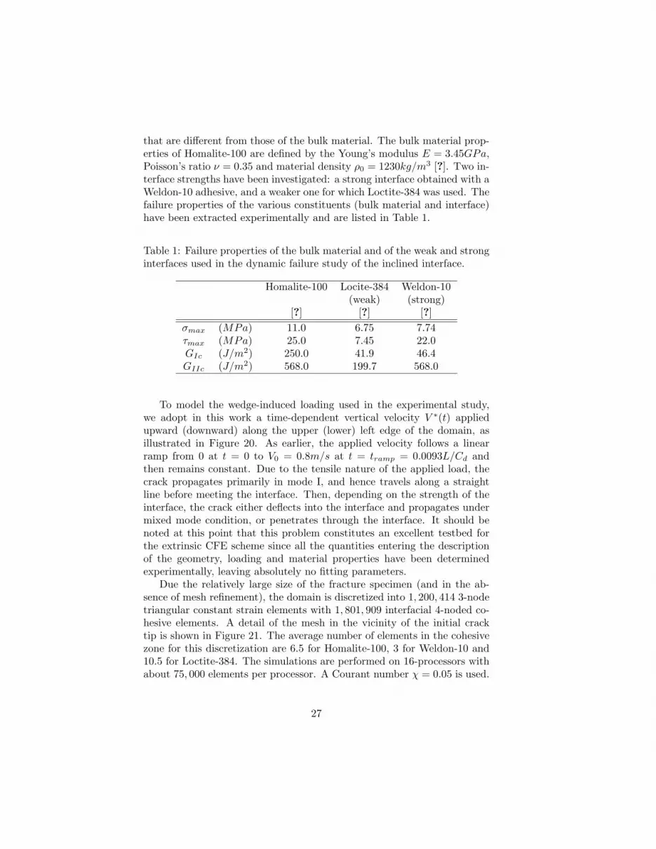
that are different from those of the bulk material. The bulk material prop-erties of Homalite-100 are defined by the Young’s modulus E = 3.45GPa,Poisson’s ratio ν = 0.35 and material density ρ0 = 1230kg/m3 [?]. Two in-terface strengths have been investigated: a strong interface obtained with aWeldon-10 adhesive, and a weaker one for which Loctite-384 was used. Thefailure properties of the various constituents (bulk material and interface)have been extracted experimentally and are listed in Table 1.

Table 1: Failure properties of the bulk material and of the weak and stronginterfaces used in the dynamic failure study of the inclined interface.

Homalite-100 Locite-384 Weldon-10(weak) (strong)

[?] [?] [?]σmax (MPa) 11.0 6.75 7.74τmax (MPa) 25.0 7.45 22.0GIc (J/m2) 250.0 41.9 46.4GIIc (J/m2) 568.0 199.7 568.0

To model the wedge-induced loading used in the experimental study,we adopt in this work a time-dependent vertical velocity V ∗(t) appliedupward (downward) along the upper (lower) left edge of the domain, asillustrated in Figure 20. As earlier, the applied velocity follows a linearramp from 0 at t = 0 to V0 = 0.8m/s at t = tramp = 0.0093L/Cd andthen remains constant. Due to the tensile nature of the applied load, thecrack propagates primarily in mode I, and hence travels along a straightline before meeting the interface. Then, depending on the strength of theinterface, the crack either deflects into the interface and propagates undermixed mode condition, or penetrates through the interface. It should benoted at this point that this problem constitutes an excellent testbed forthe extrinsic CFE scheme since all the quantities entering the descriptionof the geometry, loading and material properties have been determinedexperimentally, leaving absolutely no fitting parameters.

Due the relatively large size of the fracture specimen (and in the ab-sence of mesh refinement), the domain is discretized into 1, 200, 414 3-nodetriangular constant strain elements with 1, 801, 909 interfacial 4-noded co-hesive elements. A detail of the mesh in the vicinity of the initial cracktip is shown in Figure 21. The average number of elements in the cohesivezone for this discretization are 6.5 for Homalite-100, 3 for Weldon-10 and10.5 for Loctite-384. The simulations are performed on 16-processors withabout 75, 000 elements per processor. A Courant number χ = 0.05 is used.

27

X (m)

Y(m

)

0.04 0.06 0.08

0.22

0.24

Figure 21: Details of the deformed mesh in the vicinity of the initial cracktip and the inclined interface for the domain in Figure 20.

Figure 22: σ22 stress contour plot at time t = 1.857L/Cd for (a) weakinterface strength, showing the trajectory of the crack trapped momentarilyalong the inclined interface and (b) for the strong interface case.

28

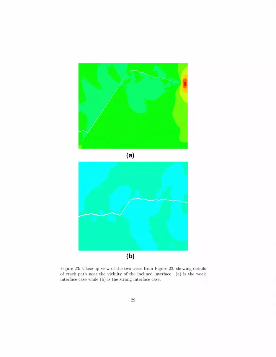
Figure 23: Close-up view of the two cases from Figure 22, showing detailsof crack path near the vicinity of the inclined interface. (a) is the weakinterface case while (b) is the strong interface case.

29

0 0.02 0.04 0.06 0.08 0.1 0.12 0.14 0.160

0.05

0.1

0.15

0.2

0.25

0.3

0.35

x−location (m)

y−lo

catio

n (m

)

Strong interface

Weak interface

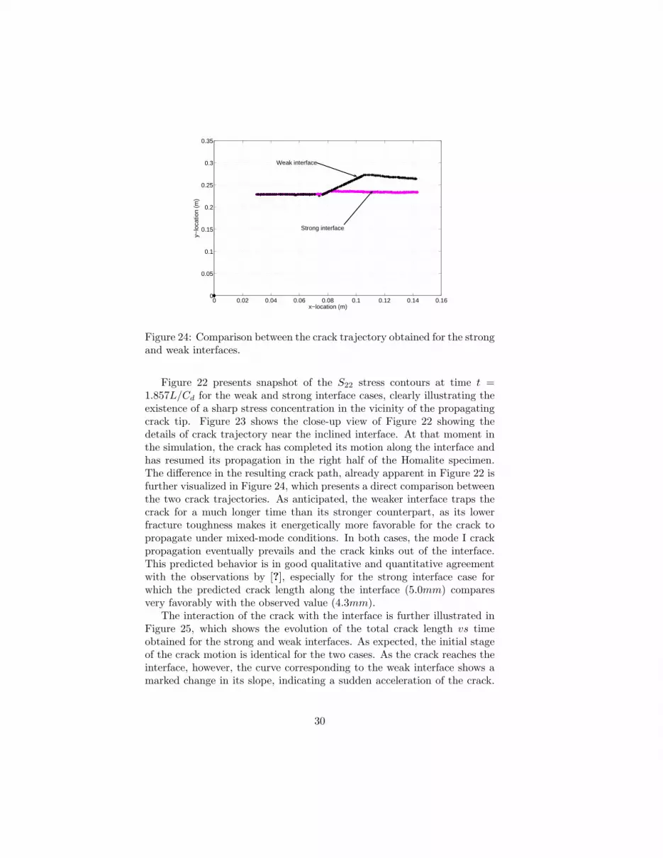
Figure 24: Comparison between the crack trajectory obtained for the strongand weak interfaces.

Figure 22 presents snapshot of the S22 stress contours at time t =1.857L/Cd for the weak and strong interface cases, clearly illustrating theexistence of a sharp stress concentration in the vicinity of the propagatingcrack tip. Figure 23 shows the close-up view of Figure 22 showing thedetails of crack trajectory near the inclined interface. At that moment inthe simulation, the crack has completed its motion along the interface andhas resumed its propagation in the right half of the Homalite specimen.The difference in the resulting crack path, already apparent in Figure 22 isfurther visualized in Figure 24, which presents a direct comparison betweenthe two crack trajectories. As anticipated, the weaker interface traps thecrack for a much longer time than its stronger counterpart, as its lowerfracture toughness makes it energetically more favorable for the crack topropagate under mixed-mode conditions. In both cases, the mode I crackpropagation eventually prevails and the crack kinks out of the interface.This predicted behavior is in good qualitative and quantitative agreementwith the observations by [?], especially for the strong interface case forwhich the predicted crack length along the interface (5.0mm) comparesvery favorably with the observed value (4.3mm).

The interaction of the crack with the interface is further illustrated inFigure 25, which shows the evolution of the total crack length vs timeobtained for the strong and weak interfaces. As expected, the initial stageof the crack motion is identical for the two cases. As the crack reaches theinterface, however, the curve corresponding to the weak interface shows amarked change in its slope, indicating a sudden acceleration of the crack.

30

0 0.5 1 1.5 2 2.5 3 3.5 4 4.5

x 10−4

0.02

0.04

0.06

0.08

0.1

0.12

0.14

0.16

0.18

0.2

time (s)

tota

l cra

ck le

nght

(m

)weak interface

strong interface

Figure 25: Total crack length vs. time for the strong and weak interfacecases.

0 1 2 3 4

x 10−4

0

200

400

600

800

1000

1200

1400

time (s)

crac

k tip

vel

ocity

(m

/s)

Figure 26: Evolution of crack tip velocity for the weak interface. Thedashed vertical line shows the instant the crack hits the interface.

31

This transient crack motion is also illustrated in Figure 26, which shows theevolution of the crack speed for the weak interface case. After an incubationperiod associated with the creation of the transient stress concentrationin the vicinity of the initial crack tip, the initially mode I crack quicklyaccelerates to reach the experimentally observed speed of about 400m/s.As it reaches the interface (at the time indicated by the dashed line), thecrack accelerates rapidly before decelerating to the observed value of about650 to 700m/s. After kinking out of the interface, the crack velocity dropsback to its initial value of about 400m/s. It should be noted, however,that the peak in the crack tip speed obtained during the initial stages ofthe interfacial failure (about 1200m/s) exceeds substantially that observedby [?]. This might be due to the inaccuracy in the description of theloading conditions, and, in particular, with the absence of compressive(lateral) component of the applied velocity. This error in peak velocityalso explains the discrepency of the calculated crack length along the weakinterface from the experimental value.

5 Parallel performance analysis

The parallel implementation of the CFE scheme exhibits excellent scaling tohundreds of processors. This section describes the measured performanceand its dependence upon an interesting parameter called virtualization.All parallel runs described in this section were performed on the Turingcluster at the University of Illinois Urbana-Champaign. Each node in thecluster is an Apple Xserve with dual 2.0 GHz G5 processors. The nodes areconnected via a Myrinet network. The performance results were obtainedby using both processors on a node for computation. For example, the256 processor timings were performed on 128 dual-processor nodes. Theimplementation uses no hand-optimized code tailored to any particularplatform or machine; It only uses some standard compiler optimizationflags.

The performance analysis presented in this section was performed onthe same cohesive finite element problem described in Section 4.2 with amesh containing 1.2 million elements. Since the implementation uses theParFUM framework to implement the CFE method, the user can configurea runtime parameter called virtualization. Virtualization in ParFUM is de-fined to be the average number of mesh partitions per physical processor.Increasing the number of mesh partitions per processor can improve perfor-mance by overlapping communication and computation and by improvingcache performance. The cache effects in ParFUM applications occur be-cause smaller partitions contain fewer elements and thus may fit inside asmaller faster level of cache[?]. The term virtualization comes from AMPI

32

[?] where multiple MPI processes, or virtual processors, are run inside asingle processor. ParFUM is built partially upon AMPI, and thus it in-herits this terminology. When multiple mesh partitions reside on a singleprocessor, computation for one partition can overlap the latency of com-munication for a different partition.

Using multiple mesh partitions per processor benefits performance forour implementation. On 8 physical processors, we found the execution timeof 1000 timestep loop iterations to be 145 seconds when using 1 partitionper processor. The time decreases by 20% to 116 seconds when using32 partitions per processor. Beyond 32 partitions per processor, the timeincreases due to extra overhead. Figure 27 shows that 256 to 1024 partitionsgives the best runtimes when using 8 to 32 processors. This range or sweetspot was determined experimentally, but approximate rules of thumb canalso be used for a particular application. To maximize the performance ofthis implementation on each partition should contain between one thousandand four thousand elements.

Scalability to a large number of processors is crucial for large FE codes.One common measure of the performance and scalability of a parallel ap-plication is speedup which is defined to be the ratio of the parallel runtimedivided by the sequential runtime. When the speedup is close to the numberof processors, an application is scaling well. The CFE application scaleswell to a large number of processors. Figure 28 displays the speedup ofthe application for up to 512 processors while using 512 partitions in allcases. For the baseline serial version, we run the same application, but justrun it with one partition on one processor, thus there is no communicationoverhead. Table 2 shows the same speedup data along with execution timesand parallel efficiency. The parallel efficiency is a ratio of the speedup tothe number of processors used. A parallel efficiency of 1.0 on 128 processorsmeans that the parallel version was 128 times faster than the serial version.Parallel efficiencies of greater than 1.0 are rarely seen, but can occur for anumber of reasons including cache effects, suboptimal serial performance,or poor algorithm choices. The application scales almost perfectly to 256processors. At 512 physical processors there is no benefit from virtualiza-tion because the 512 partitions are mapped one-to-one onto the physicalprocessors. Thus there is one virtual processor on each physical processorand hence no opportunity for overlapping communication and computationfrom different partitions on a single processor.

6 Conclusion

Initially rigid (extrinsic) cohesive elements are better suited for simula-tion of dynamic fracture events when the crack path is not pre-defined in

33

Figure 27: Execution time (in seconds) with varying numbers of partitions(Virtual Processors).

Figure 28: Speedup results for up to 512 processors for a fixed number of512 partitions (Virtual Processors). The same input mesh is used in allcases.

34

Table 2: Speedup and parallel efficiency with a 1.2M element mesh, 512Virtual Processors.

Processors Execution time (s) Speedup Efficiency1 946.32 581.7 1.63 0.813 366.4 2.58 0.864 255.6 3.7 0.935 209.8 4.51 0.96 171.5 5.52 0.927 145.7 6.49 0.938 125.9 7.52 0.94

12 81.3 11.64 0.9716 60.2 15.72 0.9820 49.2 19.23 0.9628 34.9 27.11 0.9732 29.8 31.76 0.9964 14.9 63.51 0.99

128 7.4 127.88 1.00256 3.9 242.64 0.95512 2.18 434.08 0.85

35

comparison to their intrinsic counterparts. A novel methodology for par-allel implementation of extrinsic cohesive elements based on activation ofelements, and implemented with the aid of the Parallel framework for Un-structured Meshes (ParFUM). The implementation was tested for spatialand temporal convergence, and though the crack behavior was capturedwell, spatial convergence was not clearly observed. The developed parallelCFE scheme was validated against the experimental studies performed onthe dynamic crack deflection-penetration behavior in inhomogeneous spec-imens by [?]. Simulated results are in very good agreement with experi-mental observations. A detailed scalability study performed on up to 512processors shows excellent speedup for the parallel cohesive finite elementsolver.

The authors gratefully acknowledge the support of NSF through grantEIA 01-03645, and of the Center for the Simulation of Advanced Rocketsunder contract number B341494 by the U.S. Department of Energy, and ofthe U.S. Department of Energy HPCS Fellowship Program.

References

[SE04] James R. Stewart and H. Carter Edwards. A framework approachfor developing parallel adaptive multiphysics applications. FiniteElements in Analysis and Design, 40:1599–1617, 2004.

36