The Impact of Topology on Energy Consumption for Collection Tree Protocols: anExperimental Assessment through Evolutionary Computation

Doina Bucura, Giovanni Iaccab, Giovanni Squilleroc, Alberto Tondad

aJohann Bernoulli Institute, University of Groningen, Nijenborgh 9, 9747 AG Groningen, The NetherlandsbINCAS3, Dr. Nassaulaan 9, 9401 HJ, Assen, The Netherlands

cPolitecnico di Torino, Corso Duca degli Abruzzi 24, 10129, Torino, ItalydINRA UMR 782 GMPA, 1 Avenue Lucien Bretignieres, 78850, Thiverval-Grignon, France

Abstract

The analysis of worst-case behavior in wireless sensor networks is an extremely difficult task, due to the complex interactions thatcharacterize the dynamics of these systems. In this paper, we present a new methodology for analyzing the performance of routingprotocols used in such networks. The approach exploits a stochastic optimization technique, specifically an evolutionary algorithm,to generate a large, yet tractable, set of critical network topologies; such topologies are then used to infer general considerations onthe behaviors under analysis. As a case study, we focussed on the energy consumption of two well-known ad-hoc routing protocolsfor sensor networks: the multi-hop link quality indicator and the collection tree protocol. The evolutionary algorithm started froma set of randomly generated topologies and iteratively enhanced them, maximizing a measure of “how interesting” such topologiesare with respect to the analysis. In the second step, starting from the gathered evidence, we were able to define concrete, protocol-independent topological metrics which correlate well with protocols’ poor performances. Finally, we discovered a causal relationbetween the presence of cycles in a disconnected network, and abnormal network traffic. Such creative processes were madepossible by the availability of a set of meaningful topology examples. Both the proposed methodology and the specific resultspresented here – that is, the new topological metrics and the causal explanation – can be fruitfully reused in different contexts, evenbeyond wireless sensor networks.

Keywords: Collection Tree Protocol (CTP), MultiHopLQI (MHLQI), Wireless Sensor Networks (WSN), EvolutionaryAlgorithms (EA), Routing protocols, Verification, Energy consumption

1. Introduction

Back in 1620, Sir Francis Bacon steadfastly championed themethodical observation of facts as the means of studying andinterpreting phenomena. The original “Baconian method”, asdescribed in the Novum Organum Scientiarum1, has since beenreplaced in science, yet the importance of collecting and cata-loging evidence is not called into question. Oddly enough, afterfour centuries, a common problem in computer science is pre-cisely the limited availability of “facts” to start formulating newhypothesis from.

The size and complexity of modern computer systems is sky-rocketing, posing serious problems to designers and practition-ers. While usually a single component, function or facet maybe completely verified, the number of all possible interactionsof constituent parts prevents a thorough analysis of the full sys-tems. The problem is further exacerbated whenever the envi-ronment must be taken into consideration, since the real worldis asynchronous and hardly predictable.

Email addresses: d.bucur@rug.nl (Doina Bucur),giovanniiacca@incas3.eu (Giovanni Iacca),giovanni.squillero@polito.it (Giovanni Squillero),alberto.tonda@grignon.inra.fr (Alberto Tonda)

1The New Instrument of Sciences

In many practical cases, the existence of some problem, orbug if in a software component, is demonstrated by the incorrectfunctioning of the system. In theory, to conjecture the explana-tion of an incorrect behavior, one might collect and analyze aset of distinct malfunctioning cases. In practice, however, itmay be difficult to pinpoint existing issues: there might be in-sufficient evidence to faithfully reproduce the scenario, or thetriggering cause may be so improbable that pure random simu-lation would never uncover the fault again.

A paradigmatic example of complex computer systems con-nected with the environment is represented by wireless sensornetworks (WNSs). In particular, the analysis of ad-hoc WSN’srouting protocols is extremely hard, as protocol designers havelittle to nihil post-deployment information about the occurrenceand cause of malfunctions: “We frequently failed to understandperformance results and could not determine who was to blame(i.e., the testbed characteristics, or the routing layer?)” [1].WSN protocols which performed well in controlled environ-ments had as low as 2% data delivery in the field [2, 3]. Theobserved network lifetimes were also sometimes inexplicablylower than expected: “[the] network dies out: three weeks intothe deployment most sensor nodes ran out of batteries. We con-jecture that the difference is caused by overhearing less traffic,but [...] there must be another factor contributing significantly

Preprint submitted to Applied Soft Computing Journal April 23, 2014

to the nodes’ power consumption” [4]. Yet, both scholars andpractitioners openly admit their inability to reproduce faultyscenarios: “it is unclear why collection performs well in con-trolled situations yet poorly in practice, even at low data rates”[5].

Such a lack of understanding is not surprising. The indoorWSN testbeds used for testing (e.g., MoteLab [6]) form rela-tively well-connected networks, unlikely to reproduce the typeof extreme challenges encountered later in environmental de-ployments. Furthermore, “experimental results obtained on asingle testbed are very difficult to generalize” [1]. Since worst-case scenarios are statistically rare events in the state-space ofthe problem, non-exhaustive methods, such as testbed analysis[7] or random testing [8], are likely to miss them. On the otherhand, using formal verification for analyzing such protocols iscomputationally prohibitive, and has met with limited successin the past [9, 10, 11, 12]. At best, it succeeds in identifying un-safe behavior of a WSN protocol in a few concrete, small-sizeWSN topologies, which makes it impossible to perform statis-tics and generalize the cause of the behavior.

This paper addresses the lack of experimental evidence whentackling lifetime anomalies in WSNs collection routing, byproposing a general methodology and presenting results for acomplex real-world application from the field of ad-hoc net-working. We exploit an evolutionary algorithm (EA) to gener-ate a set of distinct, significant scenarios where the WSN is notbehaving correctly. The scenarios are initially generated ran-domly, and then iteratively refined to potentially trigger criticalsituations. To let the algorithm evaluate a possible scenario, itis only necessary to define quantitative functions which roughlyexpress “how interesting” that particular scenario is. For ex-ample, in our case study, the EA evaluates (i) the overall net-work radio traffic, and (ii) the maximum node-local radio traf-fic among all WSN nodes. These two functions measure energydrain for all nodes, and the highest energy drain at a single node,respectively, which are two of the basic definitions for networklifetime used in the literature [13].

In the current contribution, we coupled the meta-heuristicoptimization technique and a WSN simulator for generatingtopologies with abnormally high routing traffic. Then, wedemonstrated how these data can be used to discover the causeof the behavior. In more details, we experimented with the col-lection tree protocol (CTP) and the multi-hop link quality in-dicator protocol (MHLQI). For both protocols, we acquired alarge set of samples of anomalous WSN lifetime. Using suchexperimental evidence, we demonstrated that it is possible toestablish the cause of the misbehavior, and we detected whichfeatures of the underlying physical topologies cause a partic-ular protocol logic to trigger unusually high traffic (and thuslow lifetime). We call these features topological metrics. Foreach protocol, we first showed the correlation between pairs of〈fitness, topological metric〉 in the samples generated with theEA, then we tested the reverse, i.e., that topologies artificiallygenerated so that they maximize a given topological metric aresufficient cause for the protocol to show high traffic.

At the time of writing, no attempt to perform a quantitativecausality analysis of worst-case lifetime in WSN routing proto-

cols has been reported in mainstream scientific literature. Wefind that this lack of knowledge in the field of protocol analysiscan be suitably remedied by the application of an EA in a novel,practical methodology, which contributes to the set of real-world applications of EA techniques, as called for in [14, 15].

We structure the paper as follows. In Section 2, we give back-ground information on WSN collection routing protocols, evo-lutionary computation and the specific EA used in the experi-ence. Section 3 describes the method to generate evidence forextreme lifetime in the system, and the method to analyze theevidence and extract a topological correlation and cause. Thefollowing three sections present experimental results for bothprotocols, from obtaining the EA-driven samples of protocolbehavior (Section 4), to writing empirical topological metricsand showing their correlation with high network traffic (Section5), to showing causality by reverse testing (Section 6). Finally,Section 7 draws the conclusions of our work and outlines futuredevelopments.

2. Background

2.1. WSN Collection RoutingA WSN is a distributed, wirelessly networked, and self-

organizing system most often employed for distributed mon-itoring tasks. Powerful and relatively inexpensive, they arewidely adopted in many applications, ranging from buildingsurveillance to environmental monitoring [2, 3, 4]. In a WSN,each node is a resource-constrained embedded system, and thephysical topology of the wireless network typically exhibitsheavy link dynamics. Sensing nodes deployed at locations ofinterest sense, store and forward data to one or more sink nodesfor collection; in turn, a sink may also disseminate commandsback to the nodes.

For successful data collection and dissemination, a WSN of-ten employs an ad-hoc collection routing protocol. WSN rout-ing protocols are usually designed for datagram-based rout-ing (i.e., they route each data packet independently from anyother packet), and are based on adaptive route selection (i.e.,they choose a route to forward a packet based on current net-work traffic conditions, instead of statically). WSN collectionrouting aims at organizing the nodes, for data collection, intoa multi-hop loop-free spanning-tree logical topology rooted insink nodes. Such protocols are distance-vector protocols whichoften implement an adaptiveness of the route selection with linkdynamics by continuously measuring the quality of a link in alink-quality indicator (LQI), i.e., link costs estimated throughlink connectivity statistics. This LQI estimation is done on thebasis of broadcasted beacon packets (used in all distance-vectorprotocols by nodes to announce to neighbor nodes both theirpresence, and their total costs to reach a sink node). Typically,a node broadcasts beacon packets at a fixed interval, and a rout-ing table is maintained by each node on the basis of neighborinformation.

All distance-vector protocols are prone to routing loops, i.e.,inconsistencies in forming a routing tree. Protocols implementvarious correcting mechanisms for routing loops, such as drop-ping (instead of forwarding) packets when loops are detected at

2

a node, or speeding up the beaconing interval in a bid to aid treerecovery. Thus, the performance of collection routing dependson the logic implemented by the protocol, on node characteris-tics (such as radio transmitting power), on the physical topologyof the network, and on environmental conditions.

Among the distance-vector collection routing mechanismsapplied to wireless sensor networks, MHLQI and CTP are al-legedly the most used protocols. MHLQI is an early version ofcollection routing designed with periodic beaconing (at a fixedrate of 1 beacon per 30 seconds), and with packet dropping, i.e.,a node discards packets when it detects a loop, until a new nexthop is found at that node [16]. CTP is the current de-facto stan-dard for WSN collection routing: it builds on the concept ofcombining the basic distance-vector, beacon-based mechanismwith adaptive beacon intervals, designed to broadcast beaconsmore often in order to reconstruct the routing tree when the net-work is changing. Sink nodes have a cost of zero; a node’scost is the cost of its next hop plus the cost of their link [5].Both MHLQI and CTP have been deployed in battery-poweredtestbeds for environmental, medical or infrastructure monitor-ing, e.g., [2, 17, 18].

2.2. Related performance evaluation studiesExisting performance studies of such ad-hoc protocols have

quite low coverage of the state-space of the protocol. For in-stance, Boukerche [7] simulates protocols on random topolo-gies of 50 and 100 nodes, of which up to 30 packet-injectingnodes. The author empirically learns that two general protocolfeatures cause comparatively high traffic: the use of network-wide flooding, and the use of periodic beacon packets. How-ever, the influence of topological metrics on overhead is notstudied, nor is overhead quantified through other than randomtesting.

In the area of applied model checking based on qualitativespecifications (i.e., distributed assertions and non-metric tem-poral logics), Mottola et al. [10] apply formal verification onup to 30 nodes over a data dissemination protocol – the dual ofcollection. They locate a small set of concrete topologies overwhich the protocol violates a distributed liveness property. In asimilar way, T-Check [9] locates node-local safety and livenessbugs, including some over small static topologies running theCTP implementation in TinyOS.

Regarding quantitative analysis, scholars already discoveredfew interesting properties for WSN collection protocols. Forinstance, Puccinelli et al. [8] find a protocol-independent met-ric that correlates with the protocol performance factor. Intheir case, this performance factor is the ratio of data deliv-ery to the sink node, and the metric is the sum of packet re-ception rates (gathered experimentally) over all shortest pathsfrom every sensing node to the sink; for this purpose, the short-est paths are calculated post-experiment using Dijkstra’s algo-rithm. They limit the analysis to a small sample of large-scale,well-connected physical topologies. Quite interestingly, such achoice led them to overlook the worst-case scenarios that wefound with our methodology.

Concerning the creation of evidence, Baldi et al. presented aseminal work on the use of an evolutionary algorithm for gen-

erating a critical test case for an oversimplified TCP/IP network[19]. More recently, Begum et al. proposed a semi-automaticmethod to generate worst-case data-throughput scenarios forthe IEEE 802.11 MAC protocol [20]. Their approach is basedon a search algorithm through the state-space of an abstractmodel in state-machine syntax; this has the disadvantage thatthe modeling makes some simplifying assumptions for somesystem features, e.g., the presence of a global clock, and thelack of a capture effect. More importantly, the method onlygenerates worst-case scenarios for a small number of given ref-erence topologies, which (as also in the cases [9, 10] above)does not allow for a generalization of the causes of the lowperformance in terms of network context. Finally, the feasibil-ity of coupling an evolutionary algorithm and a WSN simulatorfor generating a set of critical network topologies was shown[21]2.

2.3. Evolutionary ComputationEvolution is the biological theory that the origin of all liv-

ing species is caused by modifications occurring in successivegenerations. Natural evolution is not a random process: onlychanges that are beneficial to the individuals are likely to spreadinto subsequent generations. It is based on random variations,but some are rejected, while others are preserved on the basis ofthe “fitness” they convey to the individual. Darwin called thisprinciple “natural selection”, a quite simple process where ran-domness “afford materials” [22]. Strikingly, the process onlyrequires to assess the effect of random changes, not the abilityto design intelligent modifications.

Evolutionary computation (EC) is the offshoot of computerscience focusing on algorithms loosely inspired by the theory ofevolution – the “evolutionary algorithms” [23]. The definitionis deliberately vague since the boundaries of the field are not,and cannot be, sharply defined. EC is a branch of computationalintelligence, and it is also included into the broad framework ofbio-inspired heuristics. As noted before, EAs may provide aneffective methodology for trying random modifications whereno preconceived idea about the optimal solution is required.

Most of the jargon of evolutionary computation mimics theprecise terminology of biology. In an EA, a single candidate so-lution is termed individual; the set of all candidate solutions thatexist at a particular step of the algorithm is called population.Evolution proceeds through discrete steps called generations.

2This contribution extendeds [21] and includes novel points:

• The scope of the study was broadened adding a second mainstream pro-tocol (MHLQI)

• The maximum size of the networks was increased by five times.

• The set of relevant topological metrics for the energy behavior of bothprotocols was extended by five times.

• A brand new experimental campaign was added.

• The analysis of correlations in the experimental data was extended.

• A causality link between certain topological features of a network and theenergy behavior of certain protocol features was experimentally demon-strated. This result may be effectively used by network engineers in theprocess of evaluating a protocol design.

3

Generate and

evaluate initial

set of solutions

Evaluate new

solutions

Stop

condition

reached?

Select parents and

create offspring

Remove worst

solutions

Return best

solution(s)

Yes

No

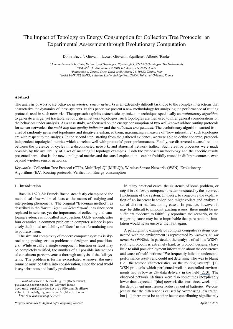
Figure 1: Flowchart of a generic Evolutionary Algorithm (EA). Parent selectionis usually stochastic, with the best candidate solutions having a higher probabil-ity to generate offspring. Removal of individuals is usually deterministic: thesolutions are sorted by fitness values, and the worst ones are deleted.

In each of them, the population is first expanded and then col-lapsed, mimicking the processes of breeding and struggling forsurvival (Fig. 1)3.

The ability of an individual to solve the target problem ismeasured by the fitness function, which influences the likeli-hood of a solution to propagate its characteristics to the nextgeneration. In some approaches individuals may die of old age,while in other they remain in the population until replaced byfitter ones.

The word genome denotes the whole genetic material of theorganism, although its actual implementation strongly differsfrom one approach to another. The gene is the functional unitof inheritance, or, operatively, the smallest fragment of thegenome that may be modified in the evolution process. Genesare positioned in the genome at specific positions called loci.The alternative genes that may occur at a given locus are calledalleles.

To generate the offspring, EAs implement both sexual andasexual reproduction. The former is named recombination; itinvolves two or more participants, and implies the possibilityfor the offspring to inherit different characteristics from differ-ent parents. When recombination is achieved through an ex-

3It should be noted that some evolutionary algorithms do not store a collec-tion of distinct individuals, but rather evolution is depicted through the variationof the statistical parameters that describe the population, see e.g. the algorithmsbelonging to the class of compact optimization [24], or the “Selfish Gene” algo-rithm [25, 26]. Other algorithms mimic the evolution of competition betweenspecies [27] or cooperation between individuals [28], for problems with specificcharacteristic [29, 30].

change of genetic material between the parents, it often takesthe name of crossover. Asexual reproduction may be namedreplication, to indicate that a copy of an individual is created,or, more commonly, mutation, to stress that the copy is notexact. All operators exploited during reproduction can be cu-mulatively called evolutionary operators, or genetic operatorsbecause they act at the genotypical level.

An EA outperforms a pure random approach and, at the sametime, is more robust than pure hill climbing and other localsearch mechanisms. Considering their intuitive structure, EAsare quite simple to set up, and require no human interventionwhen running. Finally, it’s easy to trade-off between computa-tional resources and the quality of the results, simply by defin-ing a proper stop condition for the algorithm.

2.4. µGP

The EA used in the experiments is µGP, a general-purposeevolutionary toolkit developed at Politecnico di Torino [31, 32].µGP internally represents an individual as a multi-graph, whereeach node roughly corresponds to a locus of the genome. It isinteresting to notice that, differently from most EAs, loci can beoccupied by alleles with different characteristics, e.g. integer,float or fixed values, and the probability of appearance of eachallele can be tuned. This feature will be extensively used in thefollowing.

In µGP, parameter µ indicates the size of the population; λ thenumber of genetic operators applied at each step (controlling,indirectly, the offspring size); τ the number of individuals in thetournament selection [33] used to select the parent individuals;and σ the initial strength of the genetic operators, tweaking thesimilarity between parents and offspring.

An additional parameter, called inertia, controls the self-adapting mechanisms. Self-adapting in EAs is used to slowlyshift the focus of the algorithm between exploration and ex-ploitation, depending on the current and past state of the pop-ulation, improving efficiency and quality of the results [34]. InµGP, in particular, inertia regulates the activation probabilitiesof the genetic operators, rewarding the most effective ones; andinfluences σ, usually reducing the difference between parentand offspring individuals during exploitation.µGP can use a great variety of genetic operators, depending

on the specific characteristics of the individuals’ genome. Inthe following experiments, 4 operators are used: a single-pointcrossover, a two-point crossover, and two mutation operators.Their behavior, with specific reference to the case study, is sum-marized in Figure 2 (see Section 3.1 for a detailed descriptionof the individual encoding and Table 1 for the µGP parametersetting).

3. Proposed methodology

We propose to exploit an EA to generate a set of distinct,significant scenarios where the WSN does not behave correctly.Such scenarios are initially generated randomly, then iterativelyrefined (“evolved”) in the attempt of worsening their behavior.Then, the scenarios are analyzed, and one or more metric with

4

high correlation with the network behavior are selected. Even-tually, and hopefully, at this point some causal relation may bediscovered (Fig. 3).

As stated before, the meta-heuristic optimizer is not used todemonstrate the incorrectness of the system, as some erroneousbehavior has already been recorded. Nor is it used to minimizethe network performance and lifetime in a single case. On thecontrary, the EA affords materials for a systematic study, pro-viding the researchers with a conspicuous set of significant ex-amples.

To generate the scenarios, the user is requested to provideone or more qualitative fitness functions related to the targetproblem, i.e. a rough measure of the attractiveness of the facts.Such functions do not need to be exact, since they are used asa mere proxy to direct exploration towards the most interestingregions of the state-space of the system at hand.

It is also important to stress that, unlike most applications ofevolutionary optimizers, in this study the final fitness value isnot so relevant, while it is of capital importance that generatedscenarios are different one from another: several examples ofmoderate malfunctioning are far more useful in an analysis thana single disastrous case. Indeed, the generated set will probablyinclude spurious scenarios, but it will nevertheless provide astarting point far more significant than random sampling, andfar more tractable than an exhaustive enumeration.

A conceptual scheme of the evolutionary system adopted totest the WSN behavior is depicted in Fig. 4. For both MH-LQI and CTP, we analyze the corresponding implementation inTinyOS [35], the standard operating system designed for WSNnodes. To give µGP an adequate degree of control upon networktopologies, we employ configurable TOSSIM [36] simulationsof each routing protocol, over a standard full-power data-linkprotocol. TOSSIM is a real-code simulator, which enables us toanalyze the complete software implementation of the protocol,instead of having to remodel the protocol logic into a differentlanguage—which is an error-prone task.

Aiming at creating examples of excessive power consump-tion, we adopt two fitness functions (the overall network trafficand the maximum node-local traffic among network nodes) asproxy for evaluating the attractiveness of a scenario; these fac-tors directly dictate network and node energy consumption, andthus lifetime. In other words, we quantify energy consumptionfor sensor nodes indirectly, and in a platform-independent man-ner: knowing that radio transmission and reception have thehighest battery current draw, we estimate energy consumptionby simply counting radio system calls at each node (see Section3.2).

As shown in Fig. 4, the evolutionary core of µGP is re-sponsible for creating candidate network configurations, whileTOSSIM simulates each and logs all radio system calls (i.e.,transmissions and receptions of routing protocol beacons andperiodic data packets) generated on each node. These logs areparsed to create an event hash map, which in turn is processedin order to count the radio events raised by the nodes, and obtainthe fitness function.

For experimentation, for each evaluated topology we config-ure all nodes to boot at simulation time 0. Node 0 is the sink

in all experiments; at network level, all nodes run either MH-LQI or CTP collection routing, while an application-level logicmakes all nodes inject data packets in the network periodically,at 5-second intervals. Every single simulation is allowed a sim-ulation runtime of 200 seconds, during which all radio systemcalls are logged for post-processing and fitness evaluation; thissimulation runtime is sufficiently long to allow either protocolto build a logical routing tree (if one can be built over the givenphysical topology).

In order to handle the overall randomness of simulations overa network configuration (which then produces a noisy compo-nent of both MAX and SUM fitness functions), for every topol-ogy evaluation in each of our experiments we execute n = 16simulations, and then average the value of the fitness func-tion obtained over these repetitions. This number of repetitionsguarantees a 95% confidence interval of width σ, where σ de-notes the standard deviation of the fitness function over an n-dimensional sample of repeated simulations.

3.1. Encoding of evolutionary individuals

For our purposes, an individual is a WSN topology repre-sented as a directed graph. A graph may have various encod-ings; we choose an N × N matrix, with N the network size.Each position {i, j} in the matrix encodes the signal gain fromnode i to j, and is measured in dB. Diagonal elements (whichmodel node self-connectivity) are not part of the encoding. Weremark that, given the directional asymmetry of wireless trans-mission, we encode topologies as asymmetric matrices, to pre-serve generality. The long-term asymmetry of communicationlinks is motivated in, for example, [37], which found that di-rectional links “can result from factors such as heterogene-ity of receiver and transmitter hardware (leading to differingtransmission ranges), power control algorithms (in which nodesvary their transmission power based on their current energyreserves), or topology control algorithms (aimed at reducinginterference in the network by computing the lowest transmitpower that each node needs to stay connected to the network).”

In TOSSIM, a viable directional link has a floating-point gaingreater than -110 dB. Besides gain, link qualities are affected bystochastic effects (i.e., external radio-frequency noise, packetcollision, and a capture effect which allows only the strongestof two signals to be received). These effects introduce a dy-namic, noisy component difficult to filter out. These effects areimplemented in a TOSSIM simulation, both through an accu-rate model of the CC2420 radio stack common to many hard-ware platforms, and by adding a statistical noise model to thereceived signal strength—with this noise model generated froma noise trace [38].

To bound the state-space of the individual encoding, we dis-cretize the problem. First, we only work with integer gain val-ues, and further limit their range by having:

1. strong links, encoded with a set of 30 equidistant valuesabove -110 dB; strong links are then superimposed with alow-noise trace which allows a high signal-to-noise ratio;

2. weak links, or non-viable links, encoded with a single gainvalue below -110 dB.

5

Thus, in the individual genome, each gene may present one oftwo alleles: a weak link, represented by a fixed arbitrary con-stant, and a strong link, represented by an integer. The choiceswe make have two main consequences: on one hand, the low-strength noise limits the statistical variation among simulationsof the same topology, raising the confidence level of the evo-lutionary experiments; on the other, the individual’s encodingshapes the search space so that an individual having a weak linkin position {i, j} is close to an individual having a strong link inthe same position, regardless of the link’s gain. Eventually, thisscheme helps the EA explore the search space more effectively,allowing the mutation operators to either switch the allele for agiven gene, or fine tune the gain of a strong link4, see Figure 2.

Second, we do a further discretization by only working withparticular network sizes, and also particular network densities,i.e., the percentages of strong links out of the total number ofpossible network links. For examples, for 50-node WSNs, weanalyze networks densities of 1/16 (i.e., a low-density config-uration in which each node has on average just over 3 neigh-bors), 1/8 (a mid-density), and 1/4 (a high-density configura-tion where a node has on average over 12 neighbors). In µGP,one can associate a user-defined occurrence probability to eachallele: in this study, we use this feature to bias the allele proba-bilities in the initial population, thus focusing each evolutionaryexperiment on a specific network density.

3.2. Fitness functions

It is a well-known fact that the fitness function heavily af-fects the behavior of an EA. In particular, an EA produces thebest results when there exists a gradual slope towards the bestsolutions. An almost completely flat (or, on the contrary, anextremely rugged) fitness function is hard to optimize; on theother hand, if one or more “peaks” of attraction are present inthe fitness landscape, an EA will naturally converge towardsthem.

Bearing in mind these considerations, it is then crucial to de-fine a fitness function characterized by a certain slope in itslandscape. Following the intuitive idea that the more a sys-tem is stressed, the more likely it is to exhibit faults, we searchfor WSN configurations where the routing protocol causes anabnormally high number of network radio events. Thus, weconsider, in independent experiments, the following objectives:

1. MAX, the maximum traffic count at a node, calculated asthe maximum number of node-local radio system calls(i.e., beacon and data-packet reception and transmission)among all network nodes;

2. SUM, the total network traffic count, calculated as theadded number of node-local radio system calls for allnodes in the network.

Both fitnesses are calculated accurately, using added loggingmechanisms into the chip-level network driver implementation

4To obtain this effect, the mutation operators are implemented in such away that mutating a strong link creates a weak link in 50% of the offspring,regardless the original gain value.

in TinyOS. By maximizing the MAX fitness function, we aimat finding WSN topologies where at least one node executes anabnormally high number of radio events, consuming more en-ergy and having diminished lifetime. By maximizing the SUMfitness, we instead aim at finding WSN topologies where mul-tiple nodes in the network cause a traffic storm, which in turnwill lead to higher energy consumption and decreased lifetimefor all nodes involved. Based on our experimental results (seeSection 4), we can conclude that the landscape of these two fit-ness functions has features which allow to discriminate betweenwell-behaved and high-traffic WSN topologies.

4. Gathering evidence from EA-driven simulation

4.1. Experimental results

Table 2 (for MHLQI) and Table 3 (for CTP) summarize theconfigurations of all the experiments performed in this study.All the topologies generated are available through a publicrepository5. Table 1 reports the parameters used for the EAµGP. All experiments have been run on 6 Intel Xeon 2.40 GHzcores, on a system with 8GB RAM, Ubuntu 12.04, and kernel3.2.0-29 x86 64. It should be noted that the wall clock time foreach (repeated) simulation of a given topology heavily dependson the protocol (through the number of radio events it gener-ates), on network size, and network density. Larger WSNs com-bined with high fitnesses do require a longer wall clock time,and thus allow for fewer evolutionary generations and evalua-tions per time unit: this is intuitively explained by the addedcomputation load needed to simulate, log and process highercounts of radio events. As a consequence, since for the evo-lutionary experiments we define the stop condition in terms ofmaximum allowed runtime (24 ÷ 72 h), the number of individ-uals (and generations) evaluated during each experiment is notfixed among experiments.

To provide a reference point for our results, for each experi-mental configuration we measure through simulation the fitnessvalues of simple, connected, 2D-grid “reference” topologies (astandard topology for basic testing of protocols in simulation).We consider grids of sizes 2×5, 4×5, 5×6, and 5×10, respec-tively. In all these cases, the sink node is situated in a cornerof the grid. We make this choice due to the fact that, for theseprotocols, we experimentally verified that topologies with sinkson the corners are the worst-cases with respect to traffic, com-pared all other possible sink placements (such as a centered sinknode). We report the value of the fitness functions for such ref-erence grid topologies in column (A) of Tables 2-3. In column(B), we show the highest fitnesses obtained by the EA for eachconfiguration. Finally, column (C) shows for each configura-tion the results obtained with the corresponding reverse testing,as explained in Section 6; the fitness here is greyed if it is nothigher than that obtained by the EA in column (B).

From Tables 2-3, it becomes clear that (i) MHLQI was notfound to exhibit anomalous traffic, while (ii) for all the CTP

5https://github.com/doinab/evo-network-verification.

6

Parameter Valueµ 40λ 5τ 2σ 0.9

inertia 0.9

Operator Activation probabilityTwo-point crossover 0.25One-point crossover 0.25

Single-parameter mutation 0.25Replacement mutation 0.25

Table 1: Parameters for the EA, used in all the experiments. Note that the activation probabilities for all operators and the value of σ, regulating the strength of themutations, are constantly modified by the self-adapting mechanism during the runs.

experiments using the SUM fitness and some of the CTP ex-periments using the MAX fitness, the best fitness value foundby the EA is over an order of magnitude higher than that of thestandard, grid reference topology.

Fig. 5 illustrates the sequences of generations created by oneMHLQI experiment and two of the CTP experiments. Eachgeneration is shown as the minimum, average and maximumfitness of its individuals. It can be seen that in all cases theevolutionary algorithm is able to constantly improve upon thecurrent solutions along subsequent generations. However, thealgorithm behavior (which, in turn, indicates some properties ofthe fitness landscape) depends heavily on the protocol and thenetwork density. In particular, the difference in the amplitude ofthe improvement is very large between the protocols: while forMHLQI the total number of network packets increases roughlyby 1000 over 250 generations, for CTP this improvement is al-most 100 times as high. This provides evidence for a fitnesslandscape which is extremely different, even for protocols ofthe same family.

Furthermore, in one case (CTP with network density: 1/2),the algorithm shows a smooth fitness trend which graduallyconverges to the steady state (as it is also clear looking at thefitness diversity, i.e. the min-max fitness interval which pro-gressively shrinks). In the other CTP experiment shown (net-work density: 1/8), the fitness trend is instead characterized byabrupt “evolutionary leaps” interspersed with phases where thefitness diversity is low. These behaviors provide evidence for amore complex fitness landscape.

Similar evidence to the difference of fitness landscapes be-tween protocols, and the complexity of the fitness landscapefor the CTP protocol can be seen in Fig. 6, which shows thedifferent outcomes in exploring topologies between random andevolutionary experiments. For a given network size of 20 nodesand two network densities (1/2 and 1/4), the figure shows, foreach protocol (i) the values of the SUM fitness function for 100randomly sampled topologies, each evaluated over 16 simula-tions (as also for the EA-driven experimentation), and (ii) thefitness values for the top 100 unique individuals resulted fromour EA experiments. Here, we call a topology “unique” in aset if its directional graph is distinct (disregarding the concretegain value of a strong link) from all others in the set.

On one hand, MHLQI evolutionary experiments never im-prove significantly over random experiments. On the other, forthe particular CTP experimental configuration (network size:20, network density: 1/2, fitness: MAX) in Fig. 6, the randomtests exhibit a seemingly homogeneous field of consistent lowfitness values, while the counterpart evolutionary experiment

reaches solutions with higher fitness values, and delivers a largeset of intermediate solutions of close-to-top fitness. Such WSNconfigurations are exactly the cases for which random testingis never an effective means for analyzing worst-case protocolbehavior.

4.2. Guidelines on EA-driven simulation

In order for WSN practitioners and scientists to reproduceour results and fruitfully use our methodology, a few details ofthe EA configuration should be borne in mind, namely:

1. Computational budget: defining an optimal runtime for anEA applied to a given verification problem is not a straight-forward task. There are several possible stop conditionsfor an EA, each one offering a trade-off in terms of com-putational time versus quality of the final result. In ourexperiments, we assigned a time slot to each experiment.Another possible stop condition is stagnation (or steadystate): if the best individual in the population does notchange over a given number of generations, the executionis terminated. A third possible stop criterion is reachinga user-specified value in the fitness of the best individual:for example, if domain knowledge of the problem allowsan expert to state a threshold value that highlights a pos-sible fault, the algorithm can be configured to stop oncesuch a fitness value is reached. However, the definition ofthis threshold for the CTP validation task is impracticableand can only be defined a posteriori.

2. Local optima: one problem which may affect the validityof our approach is the presence of local optima in the fit-ness landscape. This is a serious and well-studied issuefor all optimization techniques. Compared to most clas-sic local search methods, such as the Rosenbrock algo-rithm [39] or the Hooke-Jeeves pattern search [40], whoseperformance heavily depends on the initial solution (andconvergence guaranteed, within some conditions, only to-wards the closest local optimum), EAs are however moreresistant to the attractiveness of local optima: first of all,because of the stochastic element underneath their pro-cess; secondly, because they are population-based, andthus sample in a single generation multiple points in thesearch space. This parallel, scattered sampling of thesearch space is likely to prevent the algorithm from beingtrapped into local optima, and helps it converge towardsthe global one. However, due to the complexity of thesearch space, the top solutions obtained are not guaranteedto be the global optimum.

7

▼�✁✂✄☎ ✆✝✝ ✞✟✠✡☛☞ ✌✝✍✠☛✡✎ ✏☛✑☛✒☛✓✔✎✕ ✖✕☛✞✏✎✡✗

✥

✘✠✎✏♥☛✞✙ ✡✎✠✕✔✏✚☎ ✆✛✌

✥

✘

✝ ✆✝ ✌✝ ✥✝ ✜✝ ✢✝ ✘✝ ✣✝ ✤✝ ✦✝

❙✧★

✩✪✫✬✬✬✭

✄✠✡✎■ ☛✮ ✞✟✠✡☛☞ ✏☛✑☛✒☛✓✚

✠✎✏♥☛✞✙ ✡✎✠✕✔✏✚☎ ✆✛✜

▼�✁✂✄☎ ✆✝✞ ✟✠✠ ✡✠☛☞✝✌✍ ✎☞✏✑✎✍ ✍✒✝✓✎✔✏✝☞✕✖✗ ✏☞✌✏✒✏✌✎✕✓✘

✥

✙

☞✍✔♥✝✖✚ ✌✍☞✘✏✔✗☎ ✟✛✡

✥

✙

✠ ✟✠ ✡✠ ✥✠ ✜✠ ✢✠ ✙✠ ✣✠ ✤✠ ✦✠

❙✧★

✩✪✫✬✬✬✭

✄☞✌✍■ ✝✮ ✏☞✌✏✒✏✌✎✕✓

☞✍✔♥✝✖✚ ✌✍☞✘✏✔✗☎ ✟✛✜

❈�✁✂ ✄☎☎ ✆✝✞✟✠✡ ☛☎☞✞✠✟✌ ✍✠✎✠✏✠✑✒✌✓ ✔✓✠✆✍✌✟✕

✥☎

✄☛☎✞✌✍♥✠✆✖ ✟✌✞✓✒✍✗✂ ✄✘☛

✥☎

✄☛☎

☎ ✄☎ ☛☎ ✙☎ ✚☎ ✛☎ ✥☎ ✜☎ ✢☎ ✣☎

❙✤✦

✧★✩✪✪✪✫

■✞✟✌✬ ✠✭ ✆✝✞✟✠✡ ✍✠✎✠✏✠✑✗

✞✌✍♥✠✆✖ ✟✌✞✓✒✍✗✂ ✄✘✚

❈�✁✂ �✄☎ ✆✝✝ ✞✝✟✠✄✡☛ ☞✠✌✍☞☛ ☛✎✄✏☞✑✌✄✠✒✓✔ ✌✠✡✌✎✌✡☞✒✏✕

✥✝

✆✞✝

✠☛✑♥✄✓✖ ✡☛✠✕✌✑✔✂ ✆✗✞

✥✝

✆✞✝

✝ ✆✝ ✞✝ ✘✝ ✙✝ ✚✝ ✥✝ ✛✝ ✜✝ ✢✝

❙✣✤

✦✧★✩✩✩✪

■✠✡☛✫ ✄✬ ✌✠✡✌✎✌✡☞✒✏

✠☛✑♥✄✓✖ ✡☛✠✕✌✑✔✂ ✆✗✙

Figure 6: Fitness evaluations for 100 random topologies and the top 100 unique evolutionary individuals, (network size: 20, network density 1/2, 1/4) for bothprotocols and the SUM fitness. Every fitness value is plotted as the mean over the 16 fitness evaluations per topology, with the standard deviation over theseevaluations shown as an error bar.

8

Tabl

e2:

Mul

tiHop

LQ

I:C

onfig

urat

ion

ofex

peri

men

tsan

dre

sults

.C

olum

n(A

)sh

ows

the

fitne

ssva

lues

for

aco

nnec

ted

grid

topo

logy

whi

chw

eus

eas

refe

renc

e.C

olum

n(B

)gi

ves

the

resu

ltsof

the

EA

-driv

enex

peri

men

ts;w

ede

note

by(d

)and

(c)(

disc

onne

cted

orco

nnec

ted)

the

type

ofto

pto

polo

gies

obta

ined

.Col

umn

(C)i

sob

tain

edth

roug

hre

vers

ete

stin

g,as

desc

ribe

din

Sect

ion

6;he

re,t

hefit

ness

isgr

eyed

ifis

low

erth

anin

colu

mn

(B).

Mul

tiHop

LQ

I(A

)Ref

eren

cegr

idto

polo

gy(B

)Evo

lutio

nary

-dri

ven

sim

ulat

ion

(C)R

ever

sete

stin

g

Fitn

essf

unct

ion

Net

wor

ksi

zeN

etw

ork

dens

ityB

estfi

tnes

s(x

1000

)R

untim

ebu

dget

(day

s)G

ener

atio

ns/

indi

vidu

als

Type

ofto

polo

gies

Bes

tfitn

ess

(x10

00)

Type

ofto

polo

gies

Bes

tfitn

ess

(x10

00)

MA

X:

Max

imum

traffi

cco

unt

ata

node

101/

40.

451

877

/52

12(d

)1.

07(d

)0.

821/

21

930

/51

66(d

,c)

1.17

(d)

0.94

201/

40.

691

469

/26

27(d

)1.

15(d

)1.

111/

21

430

/25

59(c

)1.

25(d

)1.

09

301/

81.

002

339

/19

37(d

)1.

00(d

)1.

011/

42

316

/18

85(d

)1.

28(d

)1.

131/

22

288

/18

41(c

)1.

37(d

)1.

24

501/

161.

043

516

/32

27(d

)0.

94(d

)1.

041/

83

542

/31

03(d

)1.

15(d

)1.

181/

43

496

/30

22(c

,d)

1.33

(d)

1.26

SUM

:To

tal

netw

ork

traffi

cco

unt

101/

42.

051

894

/51

59(d

)3.

62(d

)2.

381/

21

474

/27

03(d

,c)

3.19

(d)

2.74

201/

44.

831

239

/14

10(d

)5.

89(d

)5.

421/

21

419

/25

25(d

,c)

6.94

(d)

5.87

301/

89.

652

294

/19

36(d

)8.

51(d

)7.

501/

42

163

/18

31(d

)9.

18(d

)8.

651/

22

148

/18

27(c

)10

.58

(d)

9.61

501/

1616

.08

349

4/

3208

(d)

12.6

8(d

)12

.64

1/8

349

0/

3102

(d)

14.5

3(d

)13

.86

1/4

349

4/

2912

(d,c

)16

.49

(d)

15.5

9

Tabl

e3:

CT

P:C

onfig

urat

ion

ofex

peri

men

tsan

dre

sults

.C

olum

n(A

)sho

ws

the

fitne

ssva

lues

fora

conn

ecte

dgr

idto

polo

gyw

hich

we

use

asre

fere

nce.

Col

umn

(B)g

ives

the

resu

ltsof

the

EA

-driv

enex

peri

men

ts;

we

deno

teby

(d)

and

(c)

(dis

conn

ecte

dor

conn

ecte

d)th

ety

peof

top

topo

logi

esob

tain

ed.

Col

umn

(C)

isob

tain

edth

roug

hre

vers

ete

stin

g,as

desc

ribe

din

Sect

ion

6;he

re,t

hefit

ness

isgr

eyed

ifis

low

erth

anin

colu

mn

(B).

Col

lect

ion

Tree

Prot

ocol

(A)R

efer

ence

grid

topo

logy

(B)E

volu

tiona

ry-d

rive

nsi

mul

atio

n(C

)Rev

erse

test

ing

Fitn

essf

unct

ion

Net

wor

ksi

zeN

etw

ork

dens

ityB

estfi

tnes

s(x

1000

)R

untim

ebu

dget

(day

s)G

ener

atio

ns/

indi

vidu

als

Type

ofto

polo

gies

Bes

tfitn

ess

(x10

00)

Type

ofto

polo

gies

Bes

tfitn

ess

(x10

00)

MA

X:

Max

imum

traffi

cco

unt

ata

node

101/

40.

71

455

/24

37(d

)19

.1(d

)13

.51/

21

381

/22

80(d

)13

.8(d

)13

.3

201/

41.

31

203

/10

98(d

)13

.9(d

)15

.51/

21

228

/14

33(d

)11

.3(d

)13

.7

301/

82.

02

369

/22

62(d

)16

.7(d

)15

.61/

42

221

/14

24(d

)14

.2(d

)16

.91/

22

308

/19

38(c

)7.

2(d

)13

.1

501/

163.

23

456

/29

06(d

)16

.1(d

)15

.41/

83

288

/18

22(d

)13

.8(d

)13

.91/

43

157

/94

6(d

)10

.5(d

)13

.9

SUM

:To

tal

netw

ork

traffi

cco

unt

101/

42.

81

225

/12

62(d

)71

.3(d

)11

4.5

1/2

114

9/

1013

(d)

105.

1(d

)97

.6

201/

48.

01

198

/11

45(d

)12

3.2

(d)

254.

61/

21

220

/14

66(d

)98

.6(d

)16

4.2

301/

814

.82

309

/18

02(d

)19

3.2

(d)

370.

51/

42

228

/14

57(d

)17

7.8

(d)

370.

21/

22

263

/17

26(c

)16

2.5

(d)

224.

0

501/

1633

.43

407

/27

12(d

)21

5.9

(d)

633.

61/

83

258

/15

28(d

)23

9.1

(d)

593.

21/

43

135

/87

3(d

)31

2.7

(d)

435.

0

9

3. Repeatability: the experiments we reported here are re-peatable, although with some limitations. In particular,the sequence of the stochastic operations performed byµGP can be replicated exactly by setting the random num-ber generator’s seed in the initialization phase of the al-gorithm. On the other hand, the remaining stochasticitydue to the randomness of the internal logic of CTP andTOSSIM’s communication model is difficult to control; toovercome this, it is advisable to simply run multiple simu-lations for each topology.

5. Inferring quantitative correlations

The sets of top solutions obtained with EA-driven experi-mentation (Section 4) allow us to conjecture convincingly a setof topological factors which correlate with extreme traffic undercollection routing.

To achieve this, we first collected a set of topological fea-tures which were hypothetically noted in the literature as likelyto have caused a problem with a real-world deployment [4, 5].This set consisted of graph metrics measuring both the over-all connectivity of the topology, and the average and maximumnode connectivity, for both the directed graph and its transla-tions into undirected graphs. To this set, we added novel topo-logical metrics written particularly for CTP; these metrics wereempirically motivated by the topological features of the top in-dividuals found by the EA for CTP. We then computed, for allsamples of unique top individuals obtained as evidence with theEA, the correlations between the value of the fitness functionand the value of all the topological metrics in our list. For eachprotocol, we report here the topological metrics which showedhighest correlation. As intuitive from the large difference in fit-ness found by the EA between CTP and MHLQI (Tables 2 and3), the sets of topological metrics we found to correlate bestwith high fitness for the two protocols are also different.

In this section, we first motivate empirically the novel topo-logical metrics we defined for CTP, then formally define ourbest metrics, and finally give the quantitative correlations ob-tained.

5.1. CTP: Empirical motivation for topological metrics

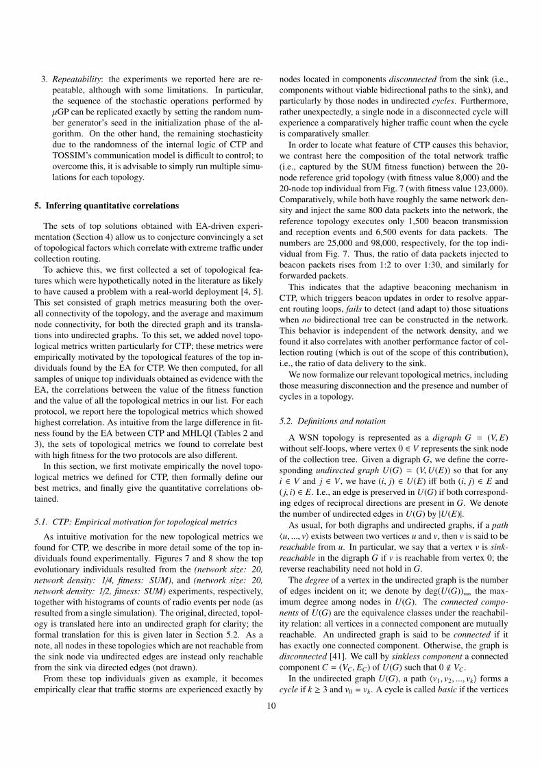
As intuitive motivation for the new topological metrics wefound for CTP, we describe in more detail some of the top in-dividuals found experimentally. Figures 7 and 8 show the topevolutionary individuals resulted from the (network size: 20,network density: 1/4, fitness: SUM), and (network size: 20,network density: 1/2, fitness: SUM) experiments, respectively,together with histograms of counts of radio events per node (asresulted from a single simulation). The original, directed, topol-ogy is translated here into an undirected graph for clarity; theformal translation for this is given later in Section 5.2. As anote, all nodes in these topologies which are not reachable fromthe sink node via undirected edges are instead only reachablefrom the sink via directed edges (not drawn).

From these top individuals given as example, it becomesempirically clear that traffic storms are experienced exactly by

nodes located in components disconnected from the sink (i.e.,components without viable bidirectional paths to the sink), andparticularly by those nodes in undirected cycles. Furthermore,rather unexpectedly, a single node in a disconnected cycle willexperience a comparatively higher traffic count when the cycleis comparatively smaller.

In order to locate what feature of CTP causes this behavior,we contrast here the composition of the total network traffic(i.e., captured by the SUM fitness function) between the 20-node reference grid topology (with fitness value 8,000) and the20-node top individual from Fig. 7 (with fitness value 123,000).Comparatively, while both have roughly the same network den-sity and inject the same 800 data packets into the network, thereference topology executes only 1,500 beacon transmissionand reception events and 6,500 events for data packets. Thenumbers are 25,000 and 98,000, respectively, for the top indi-vidual from Fig. 7. Thus, the ratio of data packets injected tobeacon packets rises from 1:2 to over 1:30, and similarly forforwarded packets.

This indicates that the adaptive beaconing mechanism inCTP, which triggers beacon updates in order to resolve appar-ent routing loops, fails to detect (and adapt to) those situationswhen no bidirectional tree can be constructed in the network.This behavior is independent of the network density, and wefound it also correlates with another performance factor of col-lection routing (which is out of the scope of this contribution),i.e., the ratio of data delivery to the sink.

We now formalize our relevant topological metrics, includingthose measuring disconnection and the presence and number ofcycles in a topology.

5.2. Definitions and notation

A WSN topology is represented as a digraph G = (V, E)without self-loops, where vertex 0 ∈ V represents the sink nodeof the collection tree. Given a digraph G, we define the corre-sponding undirected graph U(G) = (V,U(E)) so that for anyi ∈ V and j ∈ V , we have (i, j) ∈ U(E) iff both (i, j) ∈ E and( j, i) ∈ E. I.e., an edge is preserved in U(G) if both correspond-ing edges of reciprocal directions are present in G. We denotethe number of undirected edges in U(G) by |U(E)|.

As usual, for both digraphs and undirected graphs, if a path〈u, ..., v〉 exists between two vertices u and v, then v is said to bereachable from u. In particular, we say that a vertex v is sink-reachable in the digraph G if v is reachable from vertex 0; thereverse reachability need not hold in G.

The degree of a vertex in the undirected graph is the numberof edges incident on it; we denote by deg(U(G))max the max-imum degree among nodes in U(G). The connected compo-nents of U(G) are the equivalence classes under the reachabil-ity relation: all vertices in a connected component are mutuallyreachable. An undirected graph is said to be connected if ithas exactly one connected component. Otherwise, the graph isdisconnected [41]. We call by sinkless component a connectedcomponent C = (VC , EC) of U(G) such that 0 < VC .

In the undirected graph U(G), a path 〈v1, v2, ..., vk〉 forms acycle if k ≥ 3 and v0 = vk. A cycle is called basic if the vertices

10

0 sink

1

10 14

2

3

16

17

4

9 15

5

8 13 6

12

7

1918

11

✥

�

✁

✂

✄

☎✥

☎�

✵✆✝ ✝✆✷ ✷✆✹ ✹✆✻ ✻✆✽✵ ✽✵✆✽✝ ✽✝✆✽✷ ✽✷✆✽✹ ✽✹✆✽✻

◆✞✟✠✡☛☞✌✍☞✎✡✏

■✑✒✓✔✕✖✗✘ ✙✚ ✔✖✛✜✙ ✓✕✓✑✒✘ ✢✓✔ ✑✙✛✓ ✣✤☎✥✥✥✦

Figure 7: CTP: Top EA individual for (network size: 20, network density: 1/4,fitness: SUM), with resulted best fitness SUM=123,000. In the histogram ofradio events per node, nodes 2, 3, 4, 7, 9, 15, 16, and 19 fall into the top twobuckets; the sink 0 node falls in the lowest bucket.

0 sink

16

1

7

810

14

2

36

12 13

9

11

4

15

5

1817 19

✥

�

✁

✂

✄

☎✥

☎�

✵✆✝ ✝✆✷ ✷✆✹ ✹✆✻ ✻✆✽✵ ✽✵✆✽✝ ✽✝✆✽✷ ✽✷✆✽✹ ✽✹✆✽✻

◆✞✟✠✡☛☞✌✍☞✎✡✏

■✑✒✓✔✕✖✗✘ ✙✚ ✔✖✛✜✙ ✓✕✓✑✒✘ ✢✓✔ ✑✙✛✓ ✣✤☎✥✥✥✦

Figure 8: CTP: Top EA individual for (network size: 20, network density: 1/2,fitness: SUM), with SUM=98,000. All nodes besides the sink have similar,comparably low counts of radio events.

v1, v2, ..., vk−1 are all distinct. The cycle basis of U(G) is theset of basic cycles in the graph; any given cycle in the graphcan thus be written as a union of cycles in the cycle basis. Theclosure of the cycle basis is the largest union of basic cycles.

Definition 1. (SU-component) Given a directed graph G, aconnected component C = (VC , EC) of the corresponding undi-rected graph U(G) is called a sinkless undirected component(SU-component) if (1) it is sinkless, and (2) any vertex v ∈ VC

is sink-reachable in G.

Such a sinkless, but sink-reachable undirected component isessentially a connected subgraph of G in which any vertex isreachable from (but cannot itself reach) the sink 0.

Definition 2. (DD) For a digraph G, the degree of disconnec-tion (DD) is the total number of vertices in SU-components.

Definition 3. (SU-cycle) Given a directed graph G, a cycle〈v1, v2, ..., vk〉 of the corresponding undirected graph U(G) iscalled a sinkless undirected cycle (SU-cycle) if vi , 0,∀i = 1..k(i.e., 0 is not part of the cycle).

Notation 1. (NSUC) For a digraph G, we denote by NSUC thetotal number of vertices on only those SU-cycles which are con-tained in SU-components. These vertices are reachable fromthe sink, but cannot themselves reach the sink.

Notation 2. (CSUC) We denote by CSUC the number of com-ponents containing at least one SU-cycle.

5.3. Correlation coefficients fitness-metrics

We calculate quantitative correlations between the occur-rence of high traffic counts and metrics from our set of topo-logical metrics. In Tables 4 (for MHLQI) and 5 (for CTP), wereport the strongest correlations we found for the two protocols,for all sets of individuals resulted from the various EA-drivenexperiments. When a particular EA experiment did not yield atleast 100 unique topologies of an appropriate type to compute

correlations with a particular metric, we mark r with “–”; thisoccurs, e.g., when too few disconnected topologies were gen-erated for a correlation with the degree of disconnection, DD,and also other metrics pertaining to disconnected topologies.Similarly, we mark r with “–” if the sample does not exhibitsufficient variation in the values of the relevant metric.

Table 4: MHLQI: correlation coefficients r, fitness vs. topological metrics, forthe top unique individuals resulted from the EA-driven experiments. When noappropriate sample is available for a calculation, r is marked as “–”.

(MHLQI) SUM vs.: (MHLQI) MAX vs.:Size Density DD |U(E)| DD deg(U(G))max

10 1/4 0.71 0.50 0.85 0.711/2 0.71 0.02 0.68 0.20

20 1/4 0.64 0.46 0.55 0.531/2 – 0.69 – –

301/8 0.86 0.83 0.69 0.781/4 0.65 0.41 0.70 0.721/2 – 0.74 – 0.68

501/16 0.72 0.77 0.85 0.761/8 0.39 0.75 0.29 0.601/4 – 0.87 0.64 0.43

These best correlations that we found support the differencefound in top fitnesses by the EA-driven experiments. MHLQIshows positive, but weak correlations with those topologicalmetrics which are often expected to have an influence on net-work traffic; for the SUM fitness, these metrics are the densityof the undirected topology |U(E)|, i.e., the percentage of net-work links which are bidirectionally strong, and also the degreeof disconnection DD; both DD and the maximum degree of anode correlate with the MAX fitness.

For CTP, we found not only that the best correlations are withNSUC and CSUC (i.e., the number of nodes in SU-cycles, andthe number of components containing such cycles), but also thatthese correlations are very strong. The more disconnected com-

11

Table 5: CTP: correlation coefficients r, fitness vs. topological metrics, for thetop unique individuals resulted from the EA-driven experiments. When no ap-propriate sample is available for a calculation, r is marked as “–”.

(CTP) SUM vs.: (CTP) MAX vs.:Size Density CSUC NSUC CSUC

10 1/4 0.94 0.94 0.921/2 0.97 0.91 0.95

20 1/4 0.95 0.91 0.821/2 0.99 0.99 0.73

301/8 0.95 0.97 0.971/4 0.94 0.91 0.901/2 – – –

501/16 – – –1/8 0.95 0.93 0.861/4 0.75 0.76 0.75

ponents containing SU-cycles exist in the topology, the higherthe MAX fitness of that topology; this is intuitively motivatedby the top individual in Fig. 7, where the nodes in the top buck-ets of the histogram (which form small cycles of sizes 3 and 5)have much higher traffic counts than any of the nodes in Fig. 8(which form a single, large closure of the cycle basis).

6. Establishing causal relationship

Given the set of topological metrics with best correlationsto the two fitness functions (described in Section 5), we aimto verify that, for both protocols, the metrics are a sufficientcause of high fitness. This is particularly important for the caseof CTP, where both fitness functions were found by the EA toreach values an order of magnitude higher than the referencetopology, and establishing a sufficient cause of this occurrenceis crucial.

For this, we designed additional experiments in which weautomatically generated, for every tuple (network size, networkdensity, fitness function) in our experimental configuration, 100random test topologies each. These topologies are generated sothat they maximize, as much as possible, the topological met-rics relevant for that configuration; for example, in the case ofCTP, we try to reach high values for both NSUC (whose maxi-mum value is network size -1), and CSUC. For CTP, we used theempirical generation algorithm in Fig. 9. For MHLQI, the gen-eration algorithm is simpler: random graphs are constructed, sothat no node can reach the sink, one node has the maximumnode degree possible, all edges are bidirectional, and all otheredges randomly generated up to the required density.

Tables 2 (for MHLQI) and 3 (for CTP) in Section 4 alsopresent, in column (C), the top fitnesses found through thesereverse tests. For MHLQI, this small amount of reverse test-ing reached high values for the fitness functions, but did notsurpass the EA-driven simulation. On the other hand, for CTP,they show that (i) for all the experimental configurations, thereverse testing confirms the results of the evolutionary-drivensimulation, and (ii) in 15 out of 20 experiments, the results ofthe EA-driven tests are surpassed by nearly 200%, as in the

case of (network size: 50, network density: 1/16, fitness: SUM).This great increase occurs for the most “difficult” configura-tions, i.e., those configurations where the fitness landscape isintuitively more complex: experiments pertaining to the SUMfitness function, and large network sizes. We note that this in-crease in SUM fitness occurred across all network densities.Finally, we try to generalize the behavior of CTP among thevarious densities analyzed for a given network size. For this,we show in Fig. 12 the amount of traffic experienced by bothall reverse-generated topologies (in red) and all EA-generatedones, plotted against one of the two relevant topological met-rics, NSUC; this shows, qualitatively, the strong correlation be-tween the two across both densities 1/2 and 1/4, with the lowestdensity showing the highest traffic, and the ability of the reversetesting to generate high-traffic network configurations.

To summarize the large proportion of traffic increase foundfor CTP, Fig. 13 depicts the ratios between the highest MAXand SUM fitness value found (by either the EA or the reversetesting) and the respective fitness values for the reference topol-ogy, across all network sizes and densities. While for MAX,this ratio is under 10 in most of the 10 experimental configu-rations, a minimum of 10-fold increase in traffic is found forSUM.

To further contrast the top topologies obtained through re-verse testing with those obtained with the EA, Figures 10 and11 present the top CTP topologies from reverse testing resultedfrom the (network size: 20, network density: 1/4, fitness: SUM),and (network size: 20, network density: 1/2, fitness: SUM) ex-periments, respectively, together with histograms of counts ofradio events per node (as resulted from a single simulation).These should be contrasted with Figures 7 and 8 obtained orig-inally with the EA-driven experiments. For both densities, thefitness value was nearly doubled through reverse testing us-ing our topology-generation algorithm, with both higher traf-fic counts for single nodes, and higher number of nodes expe-riencing high traffic. (It is to note that these new top fitnessvalues obtained may increase further through longer reverse-testing experiments.)

The results from reverse testing confirm that, after havingdiscovered topological causes for high fitness in a particularprotocol using EA-driven simulations, it is sufficient to eval-uate the particular protocol with this type of efficient reverserandom testing.

7. Conclusions

In this paper, we have presented a novel and practical Evo-lutionary methodology for analyzing worst-cases scenarios ofWSN routing protocols. We collected a large set of evolution-arily generated network topologies, from which we deducedheuristic topological metrics correlated with the most problem-atic cases. In summary:

1. We set up an evolutionary-driven simulation tool chaincoupling the standard WSN simulator TOSSIM with anEA. This tool chain “evolves” generations of WSN topolo-gies aiming at maximizing two relevant fitness functions.

12

0 sink

1

2

3

4

5

6 7

8

9

10

11

12

13

14

15

16

17

18

19

✥

�

✁

✂

✄

☎✥

☎�

✵✆✝ ✝✆✷ ✷✆✹ ✹✆✻ ✻✆✽✵ ✽✵✆✽✝ ✽✝✆✽✷ ✽✷✆✽✹ ✽✹✆✽✻

◆✞✟✠✡☛☞✌✍☞✎✡✏

■✑✒✓✔✕✖✗✘ ✙✚ ✔✖✛✜✙ ✓✕✓✑✒✘ ✢✓✔ ✑✙✛✓ ✣✤☎✥✥✥✦

Figure 10: CTP: top topology resulted from reverse testing, for (network size:20, network density: 1/4, fitness: SUM), with SUM=254,478. All nodes except0,1, and 2 fall in the top buckets with counts of radio events per node of over10,000; the sink 0 node falls in the lowest bucket.

0 sink 15

1

2

3

4

6

7

8

9

1011

12

13

5

16

14

17

1819

✥

�

✁

✂

✄

☎✥

☎�

✵✆✝ ✝✆✷ ✷✆✹ ✹✆✻ ✻✆✽✵ ✽✵✆✽✝ ✽✝✆✽✷ ✽✷✆✽✹ ✽✹✆✽✻

◆✞✟✠✡☛☞✌✍☞✎✡✏

■✑✒✓✔✕✖✗✘ ✙✚ ✔✖✛✜✙ ✓✕✓✑✒✘ ✢✓✔ ✑✙✛✓ ✣✤☎✥✥✥✦

Figure 11: CTP: top topology resulted from reverse testing, for (network size:20, network density: 1/2, fitness: SUM), with SUM=164,239. Nodes 13 to 19fall in the top two buckets; the sink 0 node falls in the lowest bucket.

We ran extensive evolutionary experiments and obtainedlarge samples of topologies (of up to 50 nodes and variousnetwork densities) over which the protocol logic triggershigh fitness values, i.e., high traffic;

2. We empirically extracted predictive topological metricsthat were shown to correlate with high fitness values inthe samples above, and separately verified that the metricsare also a sufficient cause of high fitness. These metricsmake our approach quantitative, thus comparatively dis-tinct from qualitative methods which develop a model ofthe WSN behavior by analyzing the actual software imple-mentation of the routing protocol, see [9, 10].

Here, we focused our analysis on two well-known WSN rout-ing protocols, namely MHLQI and CTP. Although the two pro-tocols belong to the same family, they exhibit extremely differ-ent worst-case lifetime. Taking as “reference” point, for bothprotocols, the amount of traffic triggered over a standard gridtopology, we observed that (i) MHLQI, the more simplistic ofthe protocols, is well-behaved, i.e., does not significantly ex-ceed the reference amount of traffic, while (ii) CTP, the newerand “smarter” protocol, exhibits worst-case traffic one order ofmagnitude higher than the reference.

In addition to that, we showed that for MHLQI modestlyhigher traffic is caused by topological metrics which are in-tuitive and expected, e.g., higher network density and highernode degrees. On the other hand, for CTP, extremely high traf-fic is caused, less intuitively, by the existence (and number) ofphysical loops in the network. Finally, we proved that randomtopologies generated so that they maximize exactly these topo-logical metrics can be used efficiently as worst-case test sce-narios by protocol designers.

Future works. The piece of research shown here paves theway to a number of extensions. In our future studies, we willfocus our research on various aspects—both methodological

and practical—concerning the proposed EA-driven simulationframework and its applications:

1. Further analysis of Wireless Sensor Networks: both ourmethodology for evolutionary-driven simulation, and theresulting worst-case test generation method, are applica-ble to other WSN routing protocols and other fitness func-tions. In our further research, we will show the applica-bility of this approach to other routing protocols, differentfitness functions (e.g., the ratio of data delivery to sink)and networks with dynamic composition.

2. Extension of the evolutionary framework: another pos-sibility to explore will be the application of a domain-specific local search within the evolutionary framework.Incorporating prior domain knowledge into the meta-heuristic, the resulting memetic algorithm will likely gen-erate comparatively more interesting scenarios.

3. Applications beyond WSN: although we focused here onthe specific problem of generating misbehaving WSNtopologies, the proposed EA-driven methodology is ap-plicable to different contexts. In principle, for every op-timization problem where a large search space co-existswith the possibility of taking advantage of human exper-tise, an EA could be effectively used to explore the mostinteresting areas, obtaining a large set of significant sam-ples that could be later exploited to uncover hidden laws,or derive heuristic considerations on the system under test.

Acknowledgements

INCAS3 is co-funded by the Province of Drenthe, the Munic-ipality of Assen, the European Fund for Regional Developmentand the Ministry of Economic Affairs, Peaks in the Delta.

13

References

[1] K. Langendoen, Apples, oranges, and testbeds, in: In Proc. IEEE Inter-national Conference on Mobile Adhoc and Sensor Systems (MASS ’06),pp. 387–396.

[2] G. Werner-Allen, K. Lorincz, J. Johnson, J. Lees, M. Welsh, Fidelity andyield in a volcano monitoring sensor network, in: Proceedings of the 7thsymposium on Operating systems design and implementation, OSDI ’06,USENIX Association, 2006, pp. 381–396.

[3] P. Corke, T. Wark, R. Jurdak, W. Hu, P. Valencia, D. Moore, Environ-mental wireless sensor networks, Proceedings of the IEEE 98 (2010)1903 –1917.

[4] K. Langendoen, A. Baggio, O. Visser, Murphy loves potatoes: expe-riences from a pilot sensor network deployment in precision agricul-ture, in: Proceedings of the 20th international conference on Parallel anddistributed processing, IPDPS’06, IEEE Computer Society, Washington,DC, USA, 2006, pp. 174–174.

[5] O. Gnawali, R. Fonseca, K. Jamieson, D. Moss, P. Levis, Collectiontree protocol, in: Proceedings of the 7th ACM Conference on EmbeddedNetworked Sensor Systems, SenSys ’09, ACM, New York, NY, USA,2009, pp. 1–14.

[6] G. Werner-Allen, P. Swieskowski, M. Welsh, MoteLab: a wireless sensornetwork testbed, in: Proceedings of the 4th international symposium onInformation processing in sensor networks, IPSN ’05, IEEE Press, Pis-cataway, NJ, USA, 2005.

[7] A. Boukerche, Performance evaluation of routing protocols for ad hocwireless networks, Mob. Netw. Appl. 9 (2004) 333–342.

[8] D. Puccinelli, O. Gnawali, S. Yoon, S. Santini, U. Colesanti, S. Giordano,L. Guibas, The impact of network topology on collection performance, in:Proc. 8th European Conference on Wireless Sensor Networks (EWSN),pp. 17–32.

[9] P. Li, J. Regehr, T-Check: Bug finding for sensor networks, in: Proc. 9thInternational Conference on Information Processing in Sensor Networks(IPSN), ACM, 2010, pp. 174–185.

[10] L. Mottola, T. Voigt, F. Osterlind, J. Eriksson, L. Baresi, C. Ghezzi, An-quiro: Enabling efficient static verification of sensor network software,in: Proc. Workshop on Software Engineering for Sensor Network Appli-cations (SESENA) ICSE(2).

[11] M. Zheng, J. Sun, Y. Liu, J. Dong, Y. Gu, Towards a model checker fornesc and wireless sensor networks, in: S. Qin, Z. Qiu (Eds.), FormalMethods and Software Engineering, volume 6991 of Lecture Notes inComputer Science, Springer Berlin Heidelberg, 2011, pp. 372–387.

[12] D. Bucur, M. Kwiatkowska, On software verification for sensor nodes,Journal of Systems and Software 84 (2011) 1693 – 1707.

[13] I. Dietrich, F. Dressler, On the lifetime of wireless sensor networks, ACMTrans. Sen. Netw. 5 (2009) 5:1–5:39.

[14] Z. Michalewicz, Quo vadis, evolutionary computation?: on a grow-ing gap between theory and practice, in: Proceedings of the 2012World Congress conference on Advances in Computational Intelligence,WCCI’12, Springer-Verlag, 2012, pp. 98–121.

[15] Z. Michalewicz, Some thoughts on a gap between theory and practice ofevolutionary algorithms, IEEE Congress on Evolutionary Computation,2012. Invited lecture, http://education.ieee-cis.org/lectures/Invited-Lectures/Some-thoughts-on-a-gap-between-

theory-and-practice-of-evolutionary-algorithms.[16] The MultiHopLQI collection protocol, 2007. www.tinyos.net/

tinyos-2.x/tos/lib/net/lqi.[17] J. Ko, T. Gao, A. Terzis, Empirical study of a medical sensor applica-

tion in an urban emergency department, in: Proceedings of the FourthInternational Conference on Body Area Networks, BodyNets ’09, ICST,Brussels, Belgium, Belgium, pp. 10:1–10:8.

[18] O. Chipara, C. Lu, T. C. Bailey, G.-C. Roman, Reliable clinical monitor-ing using wireless sensor networks: experiences in a step-down hospitalunit, in: Proceedings of the 8th ACM Conference on Embedded Net-worked Sensor Systems, SenSys ’10, ACM, New York, NY, USA, 2010,pp. 155–168.

[19] M. Baldi, F. Corno, M. Rebaudengo, G. Squillero, GA-based perfor-mance analysis of network protocols, in: Proc. Ninth IEEE InternationalConference on Tools with Artificial Intelligence, 1997, pp. 118–124.

[20] S. Begum, A. Helmy, S. Gupta, Modeling and test generation for worst-case performance evaluation of mac protocols for wireless ad hoc net-works, in: IEEE International Symposium on Modeling, Analysis Sim-

ulation of Computer and Telecommunication Systems (MASCOTS), pp.1–10.

[21] D. Bucur, G. Iacca, G. Squillero, A. Tonda, An Evolutionary Frame-work for Routing Protocol Analysis in Wireless Sensor Networks,in: EvoStar/EvoApplications/EvoCOMNET: 15th European Conferenceon the Applications of Evolutionary and bio-inspired Computation,Springer-Verlag, 2013.

[22] C. Darwin, On the Origin of the Species by Means of Natural Selection:Or, The Preservation of Favoured Races in the Struggle for Life, JohnMurray, 1859.

[23] A. Eiben, J. Smith, Introduction to Evolutionary Computing, NaturalComputing Series, Springer, 2003.

[24] F. Neri, G. Iacca, E. Mininno, Compact optimization, in: Handbook ofOptimization, Springer Berlin Heidelberg, 2013, pp. 337–364.

[25] F. Corno, M. S. Reorda, G. Squillero, A new evolutionary algorithm in-spired by the selfish gene theory, in: Evolutionary Computation Proceed-ings, 1998. IEEE World Congress on Computational Intelligence., The1998 IEEE International Conference on, IEEE, pp. 575–580.

[26] F. Corno, M. Sonza Reorda, G. Squillero, Optimizing deceptive functionswith the SG-clans algorithm, in: Evolutionary Computation, 1999. CEC99. Proceedings of the 1999 Congress on, volume 3, IEEE.

[27] P. J. Angeline, J. B. Pollack, Competitive environments evolve bettersolutions for complex tasks, in: Proceedings of the Fifth InternationalConference on Genetic Algorithms, San Mateo, California, pp. 264–270.

[28] M. A. Potter, K. A. De Jong, Cooperative coevolution: An architecture forevolving coadapted subcomponents, Evolutionary computation 8 (2000)1–29.

[29] P. J. Darwen, X. Yao, Co-evolution in iterated prisoner’s dilemma withintermediate levels of cooperation: Application to missile defense, Inter-national Journal of Computational Intelligence and Applications 2 (2002)83–107.

[30] A. Tonda, E. Lutton, G. Squillero, A benchmark for cooperative coevolu-tion, Memetic Computing 4 (2012) 263–277.

[31] E. Sanchez, M. Schillaci, G. Squillero, Evolutionary Optimization: theµGP toolkit, Springer Publishing Company, Incorporated, 1st edition,2011.

[32] G. Squillero, MicroGP-an evolutionary assembly program generator, Ge-netic Programming and Evolvable Machines 6 (2005) 247–263.

[33] A. Brindle, Genetic algorithms for function optimization (1981).[34] K. A. De Jong, An analysis of the behavior of a class of genetic adaptive

systems, Ph.D. thesis, PhD thesis, Dept. of Computer and Comm. Sci-ences, Univ. of Michigan, Ann Arbor, MI, 1975. Univ. Microfilms, 1975.

[35] P. Levis, D. Gay, V. Handziski, J.-H. Hauer, B. Greenstein, M. Turon,J. Hui, K. Klues, C. Sharp, R. Szewczyk, J. Polastre, P. Buonadonna,L. Nachman, G. Tolle, D. Culler, A. Wolisz, T2: A second generation OSfor embedded sensor networks, Technical Report TKN-05-007, Technis-che Universitat Berlin, 2005.

[36] P. Levis, N. Lee, M. Welsh, D. E. Culler, TOSSIM: Accurate and scalablesimulation of entire TinyOS applications, in: Proceedings of the ACMconference on Embedded Networked Sensor Systems (SenSys), pp. 126–137.

[37] J. G. Jetcheva, D. B. Johnson, Routing characteristics of ad hoc networkswith unidirectional links, Ad Hoc Netw. 4 (2006) 303–325.

[38] H. Lee, A. Cerpa, P. Levis, Improving wireless simulation through noisemodeling, in: Proceedings of the 6th international conference on Infor-mation processing in sensor networks, IPSN ’07, ACM, New York, NY,USA, 2007, pp. 21–30.

[39] H. H. Rosenbrock, An automatic Method for finding the greatest or leastValue of a Function, The Computer Journal 3 (1960) 175–184.

[40] R. Hooke, T. A. Jeeves, Direct search solution of numerical and statisticalproblems, Journal of the ACM 8 (1961) 212–229.

[41] T. H. Cormen, C. E. Leiserson, R. L. Rivest, C. Stein, Introduction toAlgorithms (3. ed.), MIT Press, 2009.

14

a. one-point crossover b. two-point crossover

- x 0, x ☎

Fixed value A

c. single-parameter

mutation

d. replacement

mutation

-29 -15

-7 A

Figure 2: µGP genetic operators selected for the experiments. The single-point(a) and two-point (b) crossovers produce children individuals by mixing thegenome of two parents. In the chosen individual structure, every locus in thegenome can host two different types of parameters, an integer in the interval[-30,0] and a fixed value A. Thus, two different mutation operators are used:the single-parameter mutation (c) changes the value of an integer parameter;while the replacement mutation (d) can switch a locus from an integer to afixed parameter, and vice-versa.

Figure 3: From correlation to causality: conceptual scheme for learning thetopological causes for high-fitness WSNs.

Figure 4: Conceptual scheme of the proposed approach to the evolutionary-driven simulation of WSN routing protocols.

✥

�

✁

✂ ✄✂ ☎✂✂ ☎✄✂ ✆✂✂ ✆✄✂❋✝✞✟✠✡✡✝✟✞✠☛☞✌✍✎✏✑✒✒✒✓

✔✠☛✕✠✟✠☛✌✞✝✖✟

●✗✘✗✙✚✛✜✢✘✣

▼✤✦✧★✩ ✪✫✗ ✣✗✬✭✗✘✮✗ ✢✯ ✰✗✘✗✙✚✛✜✢✘✣ ✯✢✙

✱✂✲✘✢✳✗ ✴✵✶✣✷ ✳✗✘✣✜✛✸ ☎✹✁✷ ✵✺▼ ✯✜✛✘✗✣✣

▼✜✘✹✚✻✰✹✼✚✽ ✯✜✛✘✗✣✣ ✾✗✙ ✰✗✘✗✙✚✛✜✢✘

✥�

✁�

✂�

✄�

☎��

☎✥�

☎✁�

☎✂�

☎✄�

� ✆� ☎�� ☎✆� ✥�� ✥✆�❋✝✞✟✠✡✡✝✟✞✠☛☞✌✍✎✏✑✒✒✒✓

✔✠☛✕✠✟✠☛✌✞✝✖✟

●✗✘✗✙✚✛✜✢✘✣

❈✤✦✧ ✤★✗ ✣✗✩✪✗✘✫✗ ✢✬ ✭✗✘✗✙✚✛✜✢✘✣ ✬✢✙

✮�✯✘✢✰✗ ✱✲✳✣✴ ✰✗✘✣✜✛✵ ☎✶✥✴ ✲✷✸ ✬✜✛✘✗✣✣

✸✜✘✶✚▼✭✶✹✚✺ ✬✜✛✘✗✣✣ ✻✗✙ ✭✗✘✗✙✚✛✜✢✘

✥�

✁�

✂�

✄�

☎��

☎✥�

☎✁�

☎✂�

☎✄�

✥��

� ✆� ☎�� ☎✆� ✥�� ✥✆� ✝��❋✞✟✠✡☛☛✞✠✟✡☞✌✍✎✏✑✒✓✓✓✔

✕✡☞✖✡✠✡☞✍✟✞✗✠

●✘✙✘✚✛✜✢✣✙✤

❈✦✧★ ✦✩✘ ✤✘✪✫✘✙✬✘ ✣✭ ✮✘✙✘✚✛✜✢✣✙✤ ✭✣✚

✝�✯✙✣✰✘ ✱✲✳✤✴ ✰✘✙✤✢✜✵ ☎✶✄✴ ✲✷✸ ✭✢✜✙✘✤✤

✸✢✙✶✛▼✮✶✹✛✺ ✭✢✜✙✘✤✤ ✻✘✚ ✮✘✙✘✚✛✜✢✣✙

Figure 5: Fitness trend obtained by EA-driven experiments (top) for MHLQIwith (network size: 30, network density 1/8, fitness: SUM), (middle) for CTPwith (network size: 30, network density 1/8, fitness: SUM), and (bottom) forCTP with (network size: 30, network density 1/2, fitness: SUM).

15

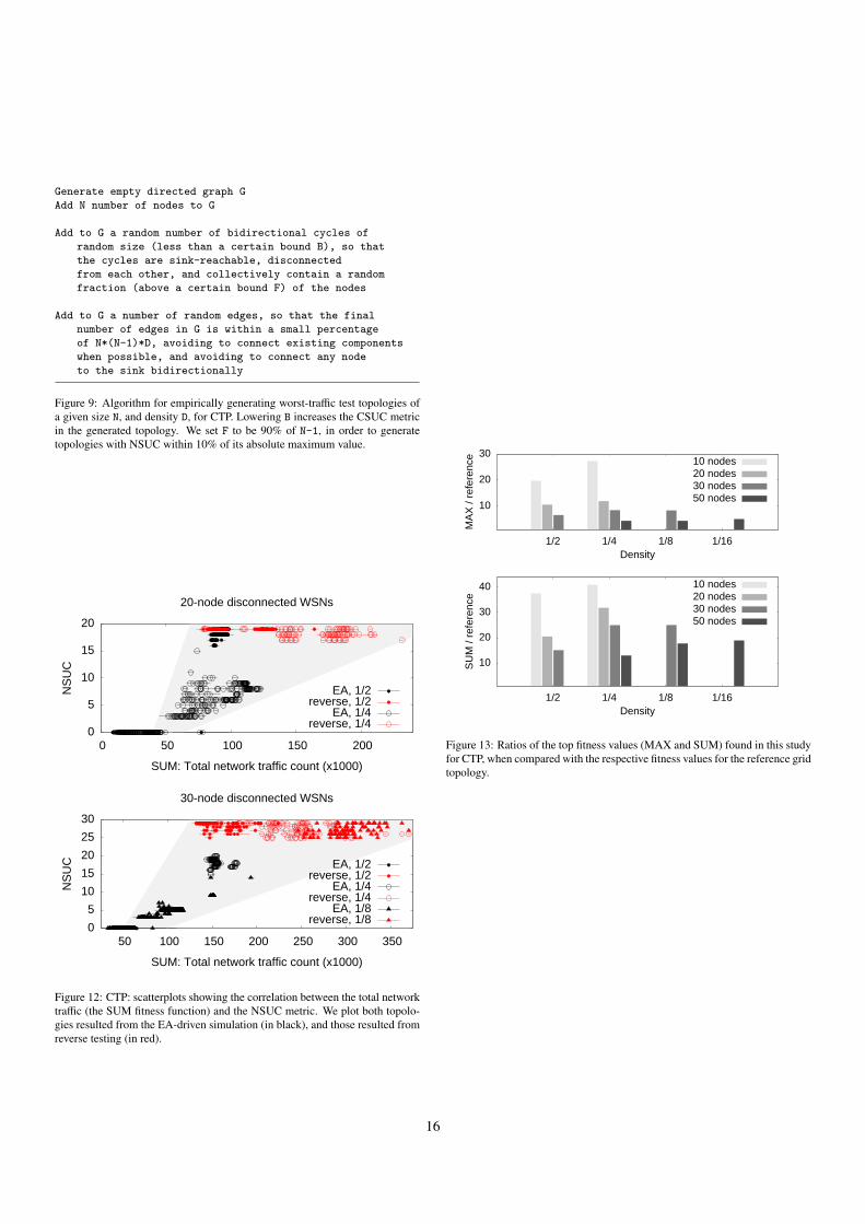
Generate empty directed graph G

Add N number of nodes to G

Add to G a random number of bidirectional cycles of

random size (less than a certain bound B), so that

the cycles are sink-reachable, disconnected

from each other, and collectively contain a random

fraction (above a certain bound F) of the nodes

Add to G a number of random edges, so that the final

number of edges in G is within a small percentage

of N*(N-1)*D, avoiding to connect existing components

when possible, and avoiding to connect any node

to the sink bidirectionally

Figure 9: Algorithm for empirically generating worst-traffic test topologies ofa given size N, and density D, for CTP. Lowering B increases the CSUC metricin the generated topology. We set F to be 90% of N-1, in order to generatetopologies with NSUC within 10% of its absolute maximum value.

0

5

10

15

20

0 50 100 150 200

NS

UC

SUM: Total network traffic count (x1000)

20-node disconnected WSNs

EA, 1/2reverse, 1/2

EA, 1/4reverse, 1/4

0

5

10

15

20

25

30

50 100 150 200 250 300 350

NS

UC

SUM: Total network traffic count (x1000)

30-node disconnected WSNs

EA, 1/2reverse, 1/2

EA, 1/4reverse, 1/4

EA, 1/8reverse, 1/8

Figure 12: CTP: scatterplots showing the correlation between the total networktraffic (the SUM fitness function) and the NSUC metric. We plot both topolo-gies resulted from the EA-driven simulation (in black), and those resulted fromreverse testing (in red).

10

20

30

1/2 1/4 1/8 1/16

MA

X /

refe

renc

e

Density

10 nodes20 nodes30 nodes50 nodes

10

20

30

40

1/2 1/4 1/8 1/16

SU

M /

refe

renc

e

Density

10 nodes20 nodes30 nodes50 nodes

Figure 13: Ratios of the top fitness values (MAX and SUM) found in this studyfor CTP, when compared with the respective fitness values for the reference gridtopology.

16