Autonomic MANET Routing ProtocolsYangcheng Huang, Sidath Handurukande

Ericsson Network Management Lab, LM Ericsson, Athlone, Ireland

Email: {yangcheng.huang, sidath.handurukande}@ericsson.com

Saleem BhattiSchool of Computer Science, University of St Andrews, UK

Email: saleem@cs.st-andrews.ac.uk

Abstract— In Mobile Ad hoc Networks (MANETs), timershave been used widely to maintain routing (state) informa-tion. The use of fixed-interval timers is simple to implementbut, in practise, may be difficult to configure in dynamicoperational environments, and so may give reduced perfor-mance in the presence of frequent topology changes. Thispaper proposes a self-tuning timer approach within a simplecontrol system for MANET routing protocols with the aimof allowing dynamic, autonomic, re-calibration of routingupdate frequencies. A novel dynamic timer algorithm ispresented to automatically tune routing performance byadapting timer intervals to network conditions. Our simula-tion results have shown that, compared to the default fixedtimer approach, the proposed algorithm could effectivelyimprove routing throughput without manual configuration.

Index Terms— Autonomic, self-configuration, MANET, rout-ing, performance, OLSR, DSDV.

I. INTRODUCTION

Mobile Ad hoc Networks (MANETs) are self-

organising, multi-hop, wireless networks, consisting of

mobile nodes connected by radio links. There is no other

network infrastructure, so the mobile nodes act as routers

of traffic for other nodes in the network, as well as being

sources and sinks of traffic. The nodes in MANETs are

free to move arbitrarily. Also, the nodes might not take

part in routing when conserving power or if they are re-

started. Thus, the network topology may change randomly

and rapidly, through a combination of node mobility, node

power management policy and node failure. Meanwhile,

each node has to maintain certain routing information to

other nodes in the network.

A. Use of timers and soft-state

After initial start-up, timers have been used widely in

neighbour detection mechanisms and topology advertise-

ments of MANET routing protocols to keep the routing

information up-to-date and maintain the correctness of

route selection. The two main functions that need to be

performed are:

• Neighbour Detection. In most MANET routing

protocols, periodic messages (e.g. HELLO messages)

are exchanged between neighbouring nodes to detect

This paper is based on “Autonomic Tuning of Routing for MANETs”,by Y. Huang, S. Bhatti, and S. Handurukande, which appeared in theProceedings of the 2nd IEEE Workshop on Autonomic Communicationsand Network Management (ACNM2008), 11 April 2008. c© 2008 IEEE.

link dynamics and to maintain node status. This is

true for a wide range of protocols: proactive proto-

cols like OLSR (Optimised Link State Routing pro-

tocol) [1], DSDV (Destination-Sequenced Distance-

Vector Routing) [2], TBRPF (Topology Broadcast

based on Reverse-Path Forwarding) [3]; or reactive

protocols like AODV (Ad hoc On-Demand Distance

Vector Routing) [4], TORA (Temporally-Ordered

Routing Algorithm) [5]; or even hybrid protocols

like ZRP (Zone Routing Protocol) [6],

• Topology Advertisements. Proactive routing pro-

tocols like OLSR [1], TORA [5] and TBRPF [3]

propagate periodic network-wide topology update (or

topology control (TC)) messages to advertise topol-

ogy changes. In addition to initiating new link state in

topology repositories of each node, for example, the

topology advertisement process in OLSR removes

obsolete topology state, either implicitly by assigning

sequence numbers to topology advertisements, or by

state time-out.

Use of timers for controlling state updates and state

maintenance – the soft-state approach [7] – have the

following benefits:

• Resilience. Routing state is expected to be self-

healing in the presence of network failures, so that

the loss of the routing update state would not result

in more than a temporary loss of service given that

connectivity exists.

• Simplicity. Reliable message delivery is not re-

quired, since message loss can be restored by sub-

sequent messages. In addition, routing state would

eventually expire and be removed unless periodically

refreshed by the receipt of a refresh message indicat-

ing its validity. Accordingly, no explicit state removal

is required.

B. Problems with use of timers

It is clear that crucial for effective operation of a soft-

state approach is the value of the timer interval used

to control state updates and state maintenance [8]. De-

spite the simplicity of a timer-based approach, significant

concerns have been raised about the use of fixed timer

intervals in MANET protocols. State validity of each

route repository is determined by the value of these inter-

vals. Despite its simplicity and widespread use, the fixed-

JOURNAL OF NETWORKS, VOL. 4, NO. 8, OCTOBER 2009 743

© 2009 ACADEMY PUBLISHERdoi:10.4304/jnw.4.8.743-753

interval timer approach may not provide the best routing

performance under highly dynamic network conditions as

in MANETs. Some issues with the timer-based approach

are:

• Manual configuration. Timers with fixed intervals

have to be manually configured by administrators.

The value of the timer intervals is determined mainly

based on (perhaps, arbitrary chosen, or untested)

recommendations of original protocol designers, or

estimated by network administrators at deployment

time. Usually, it is not practical to perform analytical

evaluations or experimental evaluations in order to

configure and re-configure the intervals of various

soft-state timers. Moreover, timers may be related

making configuration more complex. For instance,

the timer interval of HELLO messages [1], [2] should

be (much) smaller than the time-out interval of

neighbour entries. Consequently, existing approaches

have been found to be expensive in manpower, prone

to errors, and incapable of scaling to the needs of

large networks. So, as an arbitrary choice, different

timers often use the same (fixed) interval.

• Unawareness of network conditions. Fixed-interval

timers do not allow for differences in network condi-

tions, such as node velocity and link loss rate, which

impact directly routing performance. Questions then

arise regarding the configuration of timer intervals.

For example: does the default value of timer intervals

work well against all types of link failures under

various scenarios? Or: given requirements on system

consistency, how do we determine the value of the

timer intervals in order to achieve the best balance

between performance and overhead? For instance,

in order to keep low the traffic overhead due to

control messages, topology advertisement intervals

of MANET routing protocols are usually set to

relatively large values, e.g. 5s in OLSR [1]. In a

high-density network with fast mobility, the change

rate of topology is relatively high. However, topology

changes would not be advertised until the update

timer expires. Under such circumstances, topology

changes might be too frequent to be captured by

periodic updates.

Another consequence of such unawareness is re-

source wastage. In real-world scenarios, the nodes’

mobility is more likely to be intermittent. Also, there

might be only a fraction of the node population

moving during a certain time period. Therefore,

keeping a constant refresh rate, i.e. maintaining fixed

timer values, for all nodes may lead to unnecessary

resource consumption: of network capacity, due to

extra transmissions; of CPU and memory usage due

to additional processing; and, of course, this impacts

battery usage.

• Balancing throughput and overhead. It is com-

monly believed that a smaller timer interval for

refreshing soft-state could speed up adaptation to

changes at the expense of increased overhead. How-

ever, there are no studies on how much it could

improve the consistency against the amount of traf-

fic overhead. This question is critical to MANET

protocols. On one hand, topology changes require

effective signalling (i.e. smaller timer intervals) to

maintain routes and so maximise the throughput. On

the other hand, the resource constraints of MANETs

require minimum control overhead to reduce channel

contention and battery consumption.

C. Our work and contribution

This paper proposes a solution to these problems by

providing a self-tuning method for MANET routing pro-

tocols, to adjust refresh timer intervals based on network

conditions. One of the objectives of our solution is to

increase the throughput while limiting the control mes-

sage overhead. Compared with existing approaches, our

proposal could effectively improve routing performance

without manual configuration, or reliance on any exter-

nal services for information. To demonstrate adaptable,

autonomic control, a dynamic timer algorithm is pro-

posed as part of a feedback control system to adjust

the timing of routing state updates and maintenance for

DSDV (Destination Sequenced Distance-Vector Routing;

based on the Bellman-Ford algorithm) [2] and OLSR

(Optimised Link-State Routing; based on the shortest-

path-first algorithm) [1], two classical MANET routing

protocols. The protocols’ behaviour is tuned (by setting

parameter values) according to the features of the hosting

environment, such as node mobility and channel loss rate,

in order to improve routing performance and eliminate the

need for manual tuning. Our contributions are:

• Independent operation. The operations of the pro-

posed algorithm are independent of network mea-

surement or node mobility detection. Through inter-

nal monitoring of link change events, we propose a

simple method in detecting network conditions and

tuning timer intervals.

• Simple configuration and implementation. The

adaptability process in this paper is inspired by

feedback-based control theory to be fully automated,

introducing no extra control parameters. The pro-

posed algorithm can be introduced incrementally into

other MANET routing protocols.

• Demonstration of operation. We have shown

through simulations that the proposed self-tuning

algorithm outperforms traditional MANET routing

protocols.

The rest of the paper is organised as follows. Section II

lists several recent studies on adaptive routing proposals

for mobile networks. Section III gives some background

information on existing MANET routing algorithms and

presents an analytical study on the route convergence

latency. Section IV gives a general description of the pro-

posed automatic MANET routing principles. Section V

presents our simulation configurations and defines the

performance metrics. Section VI applies these principles

744 JOURNAL OF NETWORKS, VOL. 4, NO. 8, OCTOBER 2009

© 2009 ACADEMY PUBLISHER

to DSDV & OLSR and evaluates the performance of the

proposed self-tuning algorithms based on ns2 simulations.

Conclusions are summarised in Section VII.

II. RELATED WORK

There have been several adaptive routing proposals for

mobile networks. For instance, Sharma et al [8] proposed

a scalable timer approach to constrain the volume of

control traffic in a per-session based timer approach,

where the refresh interval is adjusted according to the

fixed available bandwidth (pre-allocated for control traf-

fic) and the amount of state to be refreshed. Benzaid et

al [9] presented an approach that adjusts refresh frequency

based on node mobility and the multi-point relay (MPR)

status of its neighbouring nodes. Boppana et al [10]

proposed an Adaptive Distance Vector (ADV) routing

algorithm by adopting flexible route update strategies

according to network conditions.

These approaches are usually targeted to reduce control

overhead. In addition, the performance of these proposals

depends primarily on the accuracy of network measure-

ment [9], [10]. That is, information for the purpose of

controlling routing updates is dependent upon accurate

estimates of real-time network/traffic characteristics, and

in practise these may not be available, either from addi-

tional services (e.g. network management or measurement

function), or from the application itself. These approaches

also lead to increased systems complexity.

For example, let us consider ADV [10]. The operations

in zone maintenance and continuous network monitoring

not only introduce extra processing overhead but also

increase the complexity in configuration and implementa-

tion. The performance of ADV is determined by constant

trigger thresholds, which need to be manually configured.

Furthermore, the performance bounds of these proposals

are not well-defined. For example, in ADV, the route

update frequency increases quickly with node mobility,

which brings larger overheads than periodic updates.

Also, since only partial route information is maintained,

ADV takes longer for a new connection to find a valid

route [10].

III. PROTOCOLS FOR MANET ROUTING

In this section, we give an overview of the two proto-

cols we will be using in our evaluation – the Destination

Sequenced Distance-Vector (DSDV) protocol and the Op-

timised Link-State Routing (OLSR) protocol. Then, we

present an analysis of the route convergence latency of

these MANET routing protocols, in order to introduce

the model we will use for our evaluation.

A. Overview of DSDV

The Destination Sequenced Distance-Vector

(DSDV) [2] routing protocol is a table-driven proactive

routing algorithm based on the Bellman-Ford routing

algorithm. Each node in the network maintains a routing

table that records distance vectors, i.e. the number of

hops to all of the possible destinations within the network

and the corresponding next-hop nodes.

The main improvement made to the basic Bellman-

Ford algorithm is the loop-free property by use sequence

numbers, which are used to distinguish stale routes from

new ones. A DSDV update packet contains an unique

sequence number (SN). The transmitter assigns this SN,

and the receiver selects the packet with the highest SN,

i.e. the most recent route. The route labelled with the most

recent sequence number is always used. In the event that

two updates have the same sequence number, the route

with the best metric (i.e. lowest number of hops) is used

in order to optimise the path. An advantage of DSDV is

that in relatively stable networks like a Wireless Personal

Area Network (WPAN), incremental updates are sent to

avoid extra traffic. Its main disadvantage is that in fast

changing networks, like mobile networks, as the number

of incremental update packets increases rapidly, then full

dumps are preferred, or DSDV requires bidirectional links

to operate, so that links are treated as symmetric in terms

of metrics and so routing state is reduced. In summary,

the salient DSDV functions are:

• Neighbour sensing. New neighbours can be detected

by exchanging periodically the routing tables. There

are two proposals for link breakage detection: either

by use of the layer-2 protocol, or by use of a time-out

(if no routing table updates have been received for

a period from an existing neighbour). When a link

to a next hop is broken, any route through that next

hop is immediately assigned a metric of ∞ so that it

should not be selected for data delivery.

• Topology update. DSDV requires each node to

advertise its own routing table by broadcasting its

entries to each of its current neighbours locally.

In order to reduce the amount of state informa-

tion carried in each update and help alleviate the

potentially large amount of topology update traffic,

DSDV employs two types of update packets. A full

update carries all available routing information and

might require multiple network protocol data units

(NPDUs). Full updates can be transmitted relatively

infrequently when no movement of mobile nodes oc-

curs. An incremental update carries only information

that has changed since the last full update. The size

of incremental updates is smaller than that of full

updates, and can normally fit into a standard NPDU.

When movement becomes frequent, and the size of

an incremental update increases, approaching the size

of a NPDU, then, a full update can be scheduled so

that the next incremental update will be smaller.

B. Overview of OLSR

In Link State (LS) protocols like OLSR [1], each node

discovers and maintains a complete and consistent view

of the network topology, by which each node computes a

shortest path tree with itself as the root (i.e. shortest path

first (SPF) algorithm), and applies the results to build its

JOURNAL OF NETWORKS, VOL. 4, NO. 8, OCTOBER 2009 745

© 2009 ACADEMY PUBLISHER

forwarding table. This assures that packets are forwarded

along the shortest paths to their destinations.

LS protocols rely on periodic refresh messages to

reflect topology changes and maintain correct topology in-

formation. Each node sends HELLO messages (keep-alive

messages) periodically to discover new neighbours and

detect link failures. LS protocols in MANETs advocate

periodic topology update to avoid the large volumes of of

topology update messages triggered by frequent topology

change events.

OLSR inherits the concept of the link state (LS) routing

but with flooding optimisations. In traditional LS-based

routing protocols, each node sends its local link-state

information to its adjacent nodes once it detects the

link changes between itself and its neighbours, and the

adjacent nodes then forward the information to their

neighbours resulting in flooding of the routing messages.

Unlike the traditional LS method, OLSR uses multi-

point relays (MPRs) [11–13] to optimise the flooding

mechanism. Each node selects a set of its neighbour nodes

as MPRs. A node, which has selected its neighbour A as

its MPR, is called the MPR Selector of node A.

The selective flooding based on MPR is efficient in

terms of control message delivery. In [12] it is shown

that, such flooding eventually reaches all the nodes in

the graph. Also, for each node pair in the network, the

subgraph consisting of the unidirectional MPR links in

the network and all adjacent links (of the node pair)

contains a shortest path with respect to the original graph.

To summarise, the MPR solution provides an efficient

method for flooding control traffic by reducing the number

of transmissions required and the amount of control traffic

flooded. Further details of OLSR and MPR can be found

in [1], [11–13].

C. Convergence Analysis

Here, we analyse the route convergence latency L,

i.e. the period from the occurrence of the change (i.e.

when route inconsistency occurs) to the time the nodes

in the network update their route state repositories (i.e.

converging to route state consistency again). A summary

of definitions is given in Table I.

A node running a MANET routing protocol detects link

changes and updates its route tables. These link changes

are advertised by exchanging route tables or topology

control messages. So, the route convergence latency is the

sum of link detection latency, Ld , and route advertisement

latency, La. To illustrate, here we take DV routing as the

example. However, similar analysis can be derived easily

for LS routing protocols.

We assume that:

• The message exchange events in each node are

independent. The intervals of message broadcasting

in any two nodes conform to a uniform random

distribution.

• The change event of links is an independent, identi-

cally distributed Poisson process with arrival rate λ.

The assumption is reasonable, if the node degree is

small and the nodes are moving randomly so that the

process of route change is also random.

TABLE I.

DEFINITIONS IN CONVERGENCE ANALYSIS

L Route convergence latency

Ld Link detection latency

La Route advertisement latency

r Route table update interval

di Time gaps between successive messagessent by neighbouring nodes

m Route length [hops]

p Channel loss probability

1) Route Advertisement Latency La: Let r be the

update interval. Let di (i = 1,2,3, ...m) be the time gaps

between successive messages sent by neighbouring nodes.

If we assume di ∼U(0,r), then:

E(La) =m

∑i=1

E(di)

= m.r

2(1)

So, we can see that the route advertisement latency, La,

is directly proportional to the refresh interval, r.

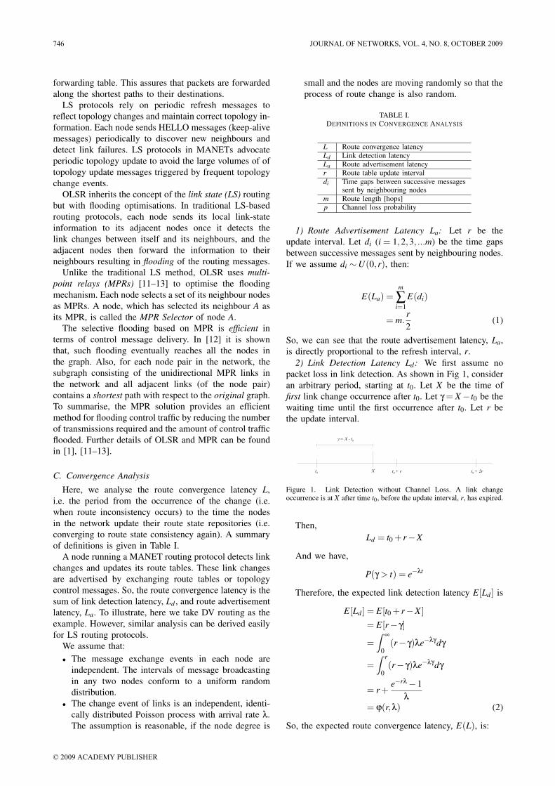
2) Link Detection Latency Ld: We first assume no

packet loss in link detection. As shown in Fig 1, consider

an arbitrary period, starting at t0. Let X be the time of

first link change occurrence after t0. Let γ = X − t0 be the

waiting time until the first occurrence after t0. Let r be

the update interval.

Figure 1. Link Detection without Channel Loss. A link changeoccurrence is at X after time t0, before the update interval, r, has expired.

Then,

Ld = t0 + r−X

And we have,

P(γ > t) = e−λt

Therefore, the expected link detection latency E[Ld ] is

E[Ld ] = E[t0 + r−X ]= E[r− γ]

=Z ∞

0(r− γ)λe−λγdγ

=Z r

0(r− γ)λe−λγdγ

= r +e−rλ −1

λ= ϕ(r,λ) (2)

So, the expected route convergence latency, E(L), is:

746 JOURNAL OF NETWORKS, VOL. 4, NO. 8, OCTOBER 2009

© 2009 ACADEMY PUBLISHER

E(L) = E(Ld)+E(La)

= r +e−rλ −1

λ+m.

r

2(3)

Now, consider the case with channel loss, as depicted

in Fig. 2. Let Y be the time of first failure occurrence

after the last state refresh.

P(Y > t) = e−λt

For a refresh interval S, the expected link detection

latency is:

E[Ld ] = E[S−Y ] = g(s)

Figure 2. Link Detection with Channel Loss. Y marks the occurrenceof a failure, taken from the last time of a successful refresh.

Let p be the channel loss probability. With channel

loss, the length of the refresh interval observed at the

other end of the channel could be r,2r, ...,kr, subject to

certain probability. Let the refresh interval be the random

variable S.

The probability of successful refresh on each trial is

1− p. The probability that k (k = 1,2,3, ...) attempts are

needed to achieve a successful refresh is:

P(S = r) = 1− p

P(S = 2r) = p(1− p)...

P(S = kr) = pk−1(1− p) (4)

Then according to the Geometric distribution density

function:

E[S] =r

1− p

E[S−Y ] = E[ϕ(S)]

= ∑(ϕ(kr)pk−1(1− p))= ϕ(r)(1− p)+ϕ(2r)p(1− p)

+ϕ(kr)pk−1(1− p)+ ...

=r

1− p−

erλ −1

λ(erλ − p)(5)

So, the expected route convergence latency, E(L), is:

E(L) = E(Ld)+E(La)

=r

1− p−

erλ −1

λ(erλ − p)+m.

r

2(6)

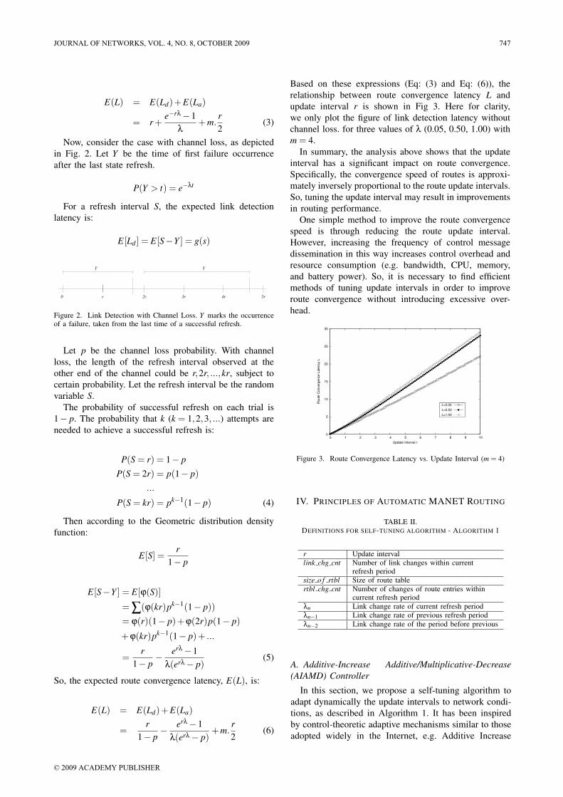
Based on these expressions (Eq: (3) and Eq: (6)), the

relationship between route convergence latency L and

update interval r is shown in Fig 3. Here for clarity,

we only plot the figure of link detection latency without

channel loss. for three values of λ (0.05, 0.50, 1.00) with

m = 4.

In summary, the analysis above shows that the update

interval has a significant impact on route convergence.

Specifically, the convergence speed of routes is approxi-

mately inversely proportional to the route update intervals.

So, tuning the update interval may result in improvements

in routing performance.

One simple method to improve the route convergence

speed is through reducing the route update interval.

However, increasing the frequency of control message

dissemination in this way increases control overhead and

resource consumption (e.g. bandwidth, CPU, memory,

and battery power). So, it is necessary to find efficient

methods of tuning update intervals in order to improve

route convergence without introducing excessive over-

head.

0

5

10

15

20

25

30

0 1 2 3 4 5 6 7 8 9 10

Ro

ute

Co

nve

rge

nce

La

ten

cy L

Update Interval r

λ=0.05

λ=0.50

λ=1.00

Figure 3. Route Convergence Latency vs. Update Interval (m = 4)

IV. PRINCIPLES OF AUTOMATIC MANET ROUTING

TABLE II.

DEFINITIONS FOR SELF-TUNING ALGORITHM - ALGORITHM 1

r Update interval

link chg cnt Number of link changes within currentrefresh period

size o f rtbl Size of route table

rtbl chg cnt Number of changes of route entries withincurrent refresh period

λn Link change rate of current refresh period

λn−1 Link change rate of previous refresh period

λn−2 Link change rate of the period before previous

A. Additive-Increase Additive/Multiplicative-Decrease

(AIAMD) Controller

In this section, we propose a self-tuning algorithm to

adapt dynamically the update intervals to network condi-

tions, as described in Algorithm 1. It has been inspired

by control-theoretic adaptive mechanisms similar to those

adopted widely in the Internet, e.g. Additive Increase

JOURNAL OF NETWORKS, VOL. 4, NO. 8, OCTOBER 2009 747

© 2009 ACADEMY PUBLISHER

Algorithm 1 Self-tuning Algorithm

Calculate(link chg cnt) and Calculate(rtbl chg cnt)

λn ⇐link chg cnt

r

if (λn > λn−1) then

if ( λn−λn−1

λn−1−λn−2> 1) then

r ⇐ r2

else

r ⇐ r− 1size o f rtbl.r

end if

end if

if (λn < λn−1) then

r ⇐ r + λn−1

λn. 1

rtbl chg cnt.rend if

λn−2 ⇐ λn−1

λn−1 ⇐ λn

r ⇐ r.(0.75+Random(0,0.25)) {to prevent synchronisa-tion}

Multiplicative Decrease (AIMD) of TCP, which is used

to adjust sending rates in response to network congestion.

Our approach in this algorithm uses an Additive-Increase

Additive/Multiplicative-Decrease (AIAMD) controller to

adapt the update interval, r, to the conditions of node

mobility.

Briefly, if there are more link change events during

the previous update period (i.e. λn > λn−1), the update

interval is reduced additively, so that the failure rate dur-

ing the next update cycle should be smaller, considering

the reduced update interval. However, if the variances

between link change rates during previous update periods

increase (i.e. λn − λn−1 > λn−1 − λn−2), this indicates a

larger change and so we need to react more quickly

and to reduce the update interval more aggressively (i.e.

halving).

Whenever there is a reduction in the occurrences of

link change events (i.e. λn < λn−1), the update interval

is incremented additively, in order to reduce the routing

overhead and reduce resource wastage. The additive in-

crease element of the algorithm is inversely proportional

to the update interval r and the number of route changes.

In addition, a deliberate random variation (jitter) in

timing [14] of update generation,is employed in order to

reduce simultaneous packet transmissions from multiple

nodes (i.e. synchronisation).

B. Explanation

This algorithm uses link change events as an indicator

of node mobility. It assumes that, with the increase of

node velocity, the link change rate increases. We clarify

this issue in the following paragraphs.

Any change in the set of links of a node may be either

due to the set-up of a new link or to the loss of an active

link. Thus, the expected link change rate for a node, ψ,

is equal to the sum of the expected new link arrival rate,

η, and the expected link breakage rate, ξ.

Samar and Wicker studied the theoretical quantitative

relationship between link change rate, ψ, and factors

including node velocity in [15]. They found that, in a

practical ad hoc or sensor network where “... the number

of neighbours of a node is bounded ...”, the expected rate

of link breakages ξ is equal to the expected rate of new

link arrivals η. Therefore, the expected link change rate

for a node, ψ, is twice the expected new link arrival rate,

η. Equation (7) describes the expected new link arrival

rate [15]:

˙η(v) =2Rδ

πb

[v2

4

Z π

0p(φ) log

(b+

√b2 − v2 sin2 φ

v+ vcosφ

)

dφ

+b2ε

(v

b

)]

(7)

Here, ε is the standard Complete Elliptic Integral of the

Second Kind; φ is the direction of motion (i.e. the degree

of the angle with x axis); p(φ) equals 1+3cos(2φ); R is

the transmission range; σ is the average density of nodes

within a transmission zone; b is the maximum velocity.

Consider the impacts of node velocity, v, on link change

rate ψ, i.e.dψdv

the derivative of ψ with respect to v. We

obtain:

ψ̇′t > 0 (8)

From Equation (8), with the increase of node velocity,

the expected link change rate increases. Therefore, we

can examine the dynamics of link change rate in order to

detect any changes of node mobility.

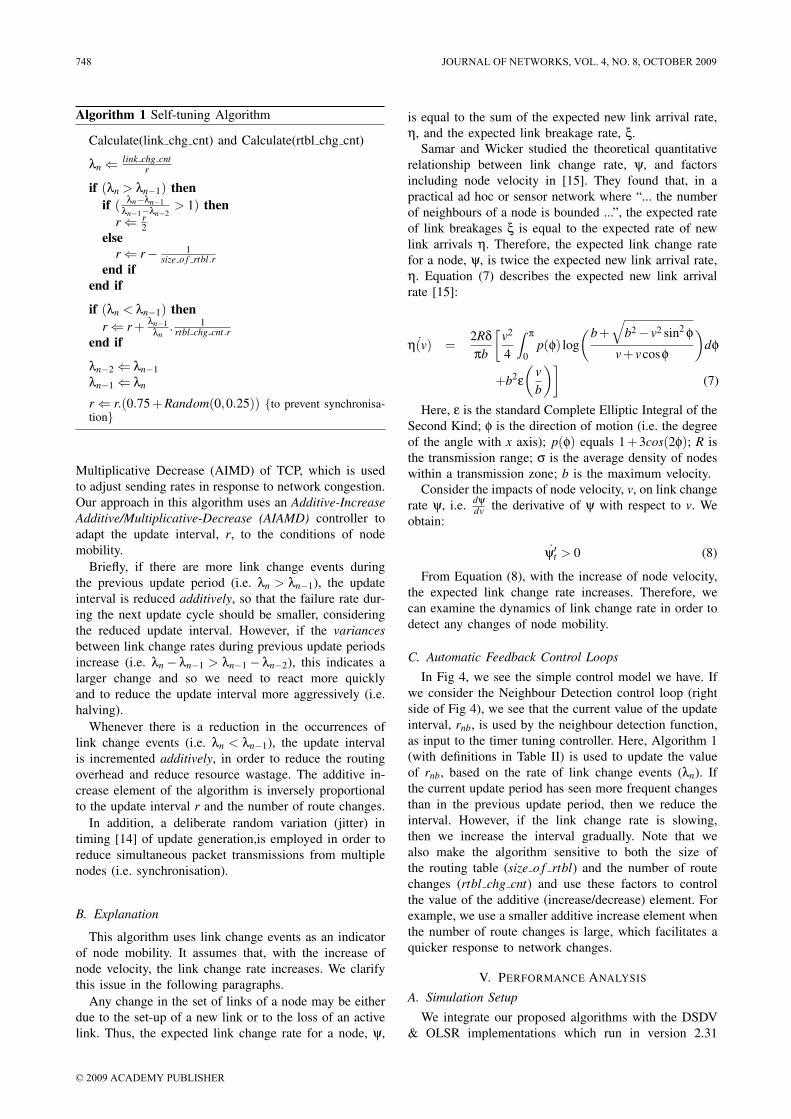
C. Automatic Feedback Control Loops

In Fig 4, we see the simple control model we have. If

we consider the Neighbour Detection control loop (right

side of Fig 4), we see that the current value of the update

interval, rnb, is used by the neighbour detection function,

as input to the timer tuning controller. Here, Algorithm 1

(with definitions in Table II) is used to update the value

of rnb, based on the rate of link change events (λn). If

the current update period has seen more frequent changes

than in the previous update period, then we reduce the

interval. However, if the link change rate is slowing,

then we increase the interval gradually. Note that we

also make the algorithm sensitive to both the size of

the routing table (size o f rtbl) and the number of route

changes (rtbl chg cnt) and use these factors to control

the value of the additive (increase/decrease) element. For

example, we use a smaller additive increase element when

the number of route changes is large, which facilitates a

quicker response to network changes.

V. PERFORMANCE ANALYSIS

A. Simulation Setup

We integrate our proposed algorithms with the DSDV

& OLSR implementations which run in version 2.31

748 JOURNAL OF NETWORKS, VOL. 4, NO. 8, OCTOBER 2009

© 2009 ACADEMY PUBLISHER

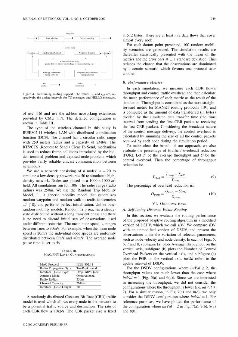
Figure 4. Self-tuning routing support. The values rtc and rnd are, re-spectively, the update intervals for TC messages and HELLO messages.

of ns2 [16] and use the ad-hoc networking extensions

provided by CMU [17]. The detailed configuration is

shown in Table III.

The type of the wireless channel in this study is

IEEE802.11 wireless LAN with distributed coordination

function (DCF). The channel has a circular radio range

with 250 meters radius and a capacity of 2Mb/s. The

RTS/CTS (Request to Send / Clear To Send) mechanism

is used to reduce frame collisions introduced by the hid-

den terminal problem and exposed node problem, which

provides fairly reliable unicast communication between

neighbours.

We use a network consisting of n nodes: n = 20 to

simulate a low-density network, n = 50 to simulate a high-

density network. Nodes are placed in a 1000× 1000 m2

field. All simulations run for 100s. The radio range (radio

radius) was 250m. We use the Random Trip Mobility

Model, ”... a generic mobility model that generalizes

random waypoint and random walk to realistic scenarios

...” [18], and performs perfect initialisation. Unlike other

random mobility models, Random Trip reaches a steady-

state distribution without a long transient phase and there

is no need to discard initial sets of observations. used

under different scenarios. The mean node speed, v, ranges

between 1m/s to 30m/s. For example, when the mean node

speed is 20m/s the individual node speeds are uniformly

distributed between 0m/s and 40m/s. The average node

pause time is set to 5s.

TABLE III.

MAC/PHY LAYER CONFIGURATIONS

MAC Protocol IEEE 802.11

Radio Propagation Type TwoRayGround

Interface Queue Type DropTailPriQueu

Antenna Model OmniAntenna

Radio Radius 250m

Channel Capacity 2Mbits

Interface Queue Length 50

A randomly distributed Constant Bit Rate (CBR) traffic

model is used which allows every node in the network to

be a potential traffic source and destination. The rate of

each CBR flow is 10kb/s. The CBR packet size is fixed

at 512 bytes. There are at least n/2 data flows that cover

almost every node.

For each datum point presented, 100 random mobil-

ity scenarios are generated. The simulation results are

thereafter statistically presented with the mean of the

metrics and the error bars at ± 1 standard deviation. This

reduces the chance that the observations are dominated

by a certain scenario which favours one protocol over

another.

B. Performance Metrics

In each simulation, we measure each CBR flow’s

throughput and control traffic overhead and then calculate

the mean performance of each metric as the result of the

simulation. Throughput is considered as the most straight-

forward metric for MANET routing protocols [19], and

is computed as the amount of data transferred (in bytes)

divided by the simulated data transfer time (the time

interval from sending the first CBR packet to receiving

the last CBR packet). Considering the broadcast nature

of the control message delivery, the control overhead is

calculated by summing the size of all the control packets

received by each node during the simulation period.

To make clear the benefit of our approach, we also

evaluate the percentage of (traffic / overhead) reduction

(POR). Let T be the average throughput and O be the

control overhead. Then the percentage of throughput

reduction is:

TPOR =Tr=r0

−TsDV

Tr=r0

(9)

The percentage of overhead reduction is:

OPOR =Or=r0

−OsDV

Or=r0

(10)

VI. OBSERVATIONS

A. Self-tuning Distance Vector Routing

In this section, we evaluate the routing performance

of the proposed adaptive routing algorithm in a modified

version of DSDV, which we call sDV. We compare sDV

with an unmodified version of DSDV, and present the

observations under the variation of selected parameters,

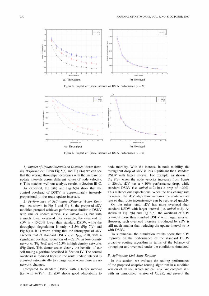
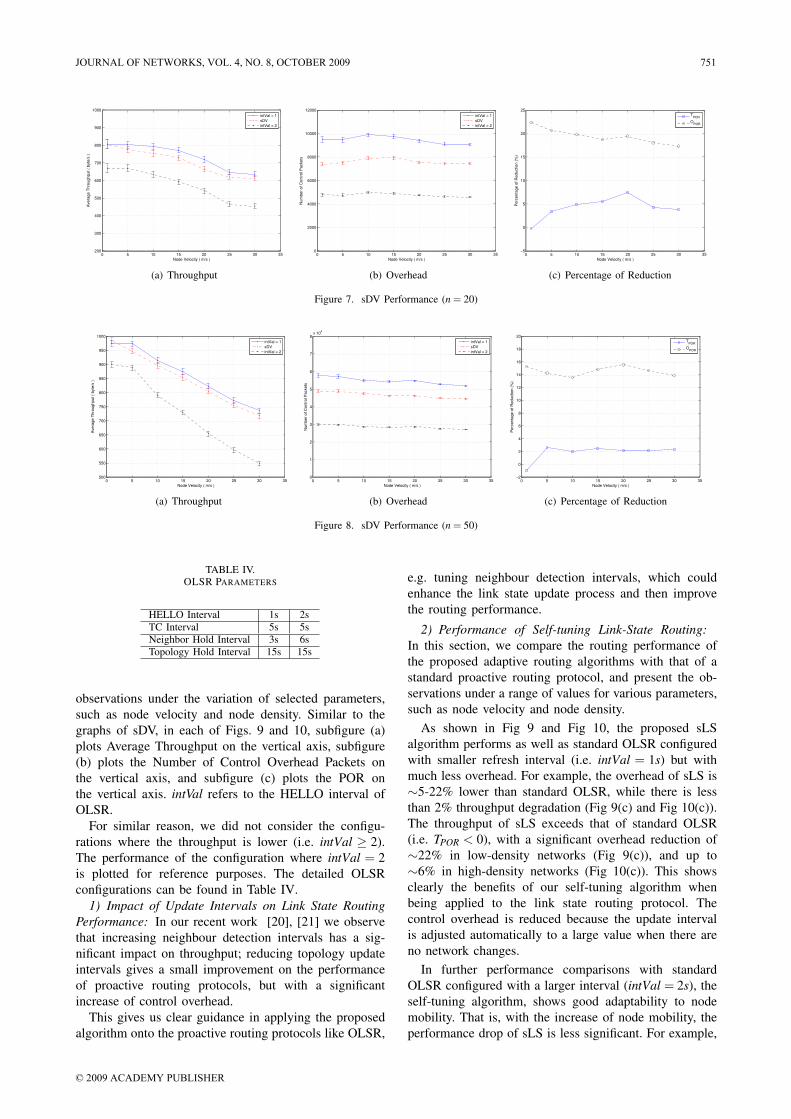
such as node velocity and node density. In each of Figs. 5,

6, 7 and 8, subfigure (a) plots Average Throughput on the

vertical axis, subfigure (b) plots the Number of Control

Overhead Packets on the vertical axis, and subfigure (c)

plots the POR on the vertical axis. intVal refers to the

update interval of DSDV.

For the DSDV configurations where intVal ≥ 2, the

throughput values are much lower than the case where

intVal = 1 (Fig. 5(a) and 6(a)). Since we are interested

in increasing the throughput, we did not consider the

configurations where the throughput is lower (i.e. intVal ≥2). For a similar reason, in Fig 7(c) and 8(c), we only

consider the DSDV configuration where intVal = 1. For

reference purposes, we have plotted the performance of

the configuration where intVal = 2 in Fig. 7(a), 7(b), 8(a)

and 8(b).

JOURNAL OF NETWORKS, VOL. 4, NO. 8, OCTOBER 2009 749

© 2009 ACADEMY PUBLISHER

0 1 2 3 4 5 6 7 8 9 10 11200

300

400

500

600

700

800

900

1000

Update Interval ( s )

Avera

ge T

hro

ughput (

byte

/s )

v = 1

v = 5

v = 20

(a) Throughput

0 1 2 3 4 5 6 7 8 9 10 110

2000

4000

6000

8000

10000

12000

Update Interval ( s )

Nu

mb

er

of

Co

ntr

ol O

ve

rhe

ad

Pa

cke

ts

v = 1

v = 5

v = 20

(b) Overhead

Figure 5. Impact of Update Intervals on DSDV Performance (n = 20)

0 1 2 3 4 5 6 7 8 9 10 11200

300

400

500

600

700

800

900

1000

Update Interval ( s )

Avera

ge T

hro

ughput (

byte

/s )

v = 1

v = 10

v = 20

(a) Throughput

0 1 2 3 4 5 6 7 8 9 10 110

1

2

3

4

5

6x 10

4

Update Interval ( s )

Nu

mb

er

of

Co

ntr

ol O

ve

rhe

ad

Pa

cke

ts

v = 1

v = 10

v = 20

(b) Overhead

Figure 6. Impact of Update Intervals on DSDV Performance (n = 50)

1) Impact of Update Intervals on Distance Vector Rout-

ing Performance: From Fig 5(a) and Fig 6(a) we can see

that the average throughput decreases with the increase of

update intervals across different values of node velocity,

v. This matches well our analytic results in Section III-C.

As expected, Fig 5(b) and Fig 6(b) show that the

control overhead of DSDV is approximately inversely

proportional to the route update intervals.

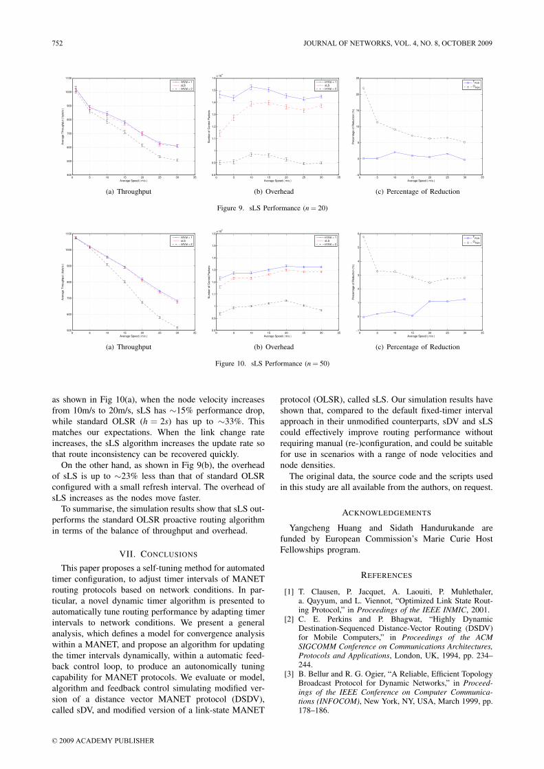
2) Performance of Self-tuning Distance Vector Rout-

ing: As shown in Fig 7 and Fig 8, the proposed sDV

modified protocol achieves performance similar to DSDV

with smaller update interval (i.e. intVal = 1), but with

a much lower overhead. For example, the overhead of

sDV is ∼15-20% lower than standard DSDV, while the

throughput degradation is only ∼2-5% (Fig 7(c) and

Fig 8(c)). It is worth noting that the throughput of sDV

exceeds that of standard DSDV (i.e. TPOR < 0), with a

significant overhead reduction of ∼22.5% in low-density

networks (Fig 7(c)) and ∼15.5% in high-density networks

(Fig 8(c)). This demonstrates clearly the benefits of our

self-tuning algorithm described in Section IV. The control

overhead is reduced because the route update interval is

adjusted automatically to a large value when there are no

network changes.

Compared to standard DSDV with a larger interval

(i.e. with intVal = 2), sDV shows good adaptability to

node mobility. With the increase in node mobility, the

throughput drop of sDV is less significant than standard

DSDV with larger interval. For example, as shown in

Fig 8(a), when the node velocity increases from 10m/s

to 20m/s, sDV has a ∼10% performance drop, while

standard DSDV (i.e. intVal = 2) has a drop of ∼20%.

This matches our expectations. When the link change rate

increases, the sDV algorithm increases the route update

rate so that route inconsistency can be recovered quickly.

On the other hand, sDV has more overhead than

standard DSDV with larger interval (i.e. intVal = 2). As

shown in Fig 7(b) and Fig 8(b), the overhead of sDV

is ∼40% more than standard DSDV with larger interval.

However, such overhead increase introduced by sDV is

still much smaller than reducing the update interval to 1s

with DSDV.

To summarise, the simulation results show that sDV

improves on the performance of the standard DSDV

proactive routing algorithm in terms of the balance of

throughput and overhead under the conditions simulated.

B. Self-tuning Link State Routing

In this section, we evaluate the routing performance

of the proposed adaptive routing algorithm in a modified

version of OLSR, which we call sLS. We compare sLS

with an unmodified version of OLSR, and present the

750 JOURNAL OF NETWORKS, VOL. 4, NO. 8, OCTOBER 2009

© 2009 ACADEMY PUBLISHER

0 5 10 15 20 25 30 35200

300

400

500

600

700

800

900

1000

Node Velocity ( m/s )

Ave

rag

e T

hro

ug

hp

ut

( b

yte

/s )

intVal = 1

sDV

intVal = 2

(a) Throughput

0 5 10 15 20 25 30 350

2000

4000

6000

8000

10000

12000

Node Velocity ( m/s )

Nu

mb

er

of

Co

ntr

ol P

acke

ts

intVal = 1

sDV

intVal = 2

(b) Overhead

0 5 10 15 20 25 30 35−5

0

5

10

15

20

25

Node Velocity ( m/s )

Pe

rce

nta

ge

of

Re

du

ctio

n (

%)

T

POR

OPOR

(c) Percentage of Reduction

Figure 7. sDV Performance (n = 20)

0 5 10 15 20 25 30 35500

550

600

650

700

750

800

850

900

950

1000

Node Velocity ( m/s )

Ave

rag

e T

hro

ug

hp

ut

( b

yte

/s )

intVal = 1

sDV

intVal = 2

(a) Throughput

0 5 10 15 20 25 30 350

1

2

3

4

5

6

7

8x 10

4

Node Velocity ( m/s )

Nu

mb

er

of

Co

ntr

ol P

acke

ts

intVal = 1

sDV

intVal = 2

(b) Overhead

0 5 10 15 20 25 30 35−2

0

2

4

6

8

10

12

14

16

18

20

Node Velocity ( m/s )

Pe

rce

nta

ge

of

Re

du

ctio

n (

%)

T

POR

OPOR

(c) Percentage of Reduction

Figure 8. sDV Performance (n = 50)

TABLE IV.

OLSR PARAMETERS

HELLO Interval 1s 2s

TC Interval 5s 5s

Neighbor Hold Interval 3s 6s

Topology Hold Interval 15s 15s

observations under the variation of selected parameters,

such as node velocity and node density. Similar to the

graphs of sDV, in each of Figs. 9 and 10, subfigure (a)

plots Average Throughput on the vertical axis, subfigure

(b) plots the Number of Control Overhead Packets on

the vertical axis, and subfigure (c) plots the POR on

the vertical axis. intVal refers to the HELLO interval of

OLSR.

For similar reason, we did not consider the configu-

rations where the throughput is lower (i.e. intVal ≥ 2).

The performance of the configuration where intVal = 2

is plotted for reference purposes. The detailed OLSR

configurations can be found in Table IV.

1) Impact of Update Intervals on Link State Routing

Performance: In our recent work [20], [21] we observe

that increasing neighbour detection intervals has a sig-

nificant impact on throughput; reducing topology update

intervals gives a small improvement on the performance

of proactive routing protocols, but with a significant

increase of control overhead.

This gives us clear guidance in applying the proposed

algorithm onto the proactive routing protocols like OLSR,

e.g. tuning neighbour detection intervals, which could

enhance the link state update process and then improve

the routing performance.

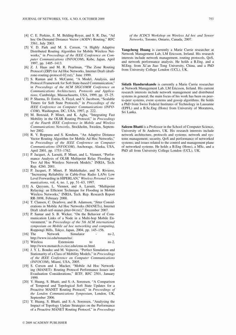
2) Performance of Self-tuning Link-State Routing:

In this section, we compare the routing performance of

the proposed adaptive routing algorithms with that of a

standard proactive routing protocol, and present the ob-

servations under a range of values for various parameters,

such as node velocity and node density.

As shown in Fig 9 and Fig 10, the proposed sLS

algorithm performs as well as standard OLSR configured

with smaller refresh interval (i.e. intVal = 1s) but with

much less overhead. For example, the overhead of sLS is

∼5-22% lower than standard OLSR, while there is less

than 2% throughput degradation (Fig 9(c) and Fig 10(c)).

The throughput of sLS exceeds that of standard OLSR

(i.e. TPOR < 0), with a significant overhead reduction of

∼22% in low-density networks (Fig 9(c)), and up to

∼6% in high-density networks (Fig 10(c)). This shows

clearly the benefits of our self-tuning algorithm when

being applied to the link state routing protocol. The

control overhead is reduced because the update interval

is adjusted automatically to a large value when there are

no network changes.

In further performance comparisons with standard

OLSR configured with a larger interval (intVal = 2s), the

self-tuning algorithm, shows good adaptability to node

mobility. That is, with the increase of node mobility, the

performance drop of sLS is less significant. For example,

JOURNAL OF NETWORKS, VOL. 4, NO. 8, OCTOBER 2009 751

© 2009 ACADEMY PUBLISHER

0 5 10 15 20 25 30 35400

500

600

700

800

900

1000

1100

Average Speed ( m/s )

Ave

rag

e T

hro

ug

hp

ut

( b

yte

/s )

intVal = 1

sLS

intVal = 2

(a) Throughput

0 5 10 15 20 25 30 350.8

0.9

1

1.1

1.2

1.3

1.4

1.5

1.6x 10

4

Average Speed ( m/s )

Nu

mb

er

of

Co

ntr

ol P

acke

ts

intVal = 1

sLS

intVal = 2

(b) Overhead

0 5 10 15 20 25 30 35−5

0

5

10

15

20

25

Average Speed ( m/s )

Pe

rce

nta

ge

of

Re

du

ctio

n (

%)

T

POR

OPOR

(c) Percentage of Reduction

Figure 9. sLS Performance (n = 20)

0 5 10 15 20 25 30 35500

600

700

800

900

1000

1100

Average Speed ( m/s )

Ave

rag

e T

hro

ug

hp

ut

( b

yte

/s )

intVal = 1

sLS

intVal = 2

(a) Throughput

0 5 10 15 20 25 30 350.8

0.9

1

1.1

1.2

1.3

1.4

1.5

1.6x 10

5

Average Speed ( m/s )

Nu

mb

er

of

Co

ntr

ol P

acke

ts

intVal = 1

sLS

intVal = 2

(b) Overhead

0 5 10 15 20 25 30 35−1

0

1

2

3

4

5

6

Average Speed ( m/s )

Pe

rce

nta

ge

of

Re

du

ctio

n (

%)

T

POR

OPOR

(c) Percentage of Reduction

Figure 10. sLS Performance (n = 50)

as shown in Fig 10(a), when the node velocity increases

from 10m/s to 20m/s, sLS has ∼15% performance drop,

while standard OLSR (h = 2s) has up to ∼33%. This

matches our expectations. When the link change rate

increases, the sLS algorithm increases the update rate so

that route inconsistency can be recovered quickly.

On the other hand, as shown in Fig 9(b), the overhead

of sLS is up to ∼23% less than that of standard OLSR

configured with a small refresh interval. The overhead of

sLS increases as the nodes move faster.

To summarise, the simulation results show that sLS out-

performs the standard OLSR proactive routing algorithm

in terms of the balance of throughput and overhead.

VII. CONCLUSIONS

This paper proposes a self-tuning method for automated

timer configuration, to adjust timer intervals of MANET

routing protocols based on network conditions. In par-

ticular, a novel dynamic timer algorithm is presented to

automatically tune routing performance by adapting timer

intervals to network conditions. We present a general

analysis, which defines a model for convergence analysis

within a MANET, and propose an algorithm for updating

the timer intervals dynamically, within a automatic feed-

back control loop, to produce an autonomically tuning

capability for MANET protocols. We evaluate or model,

algorithm and feedback control simulating modified ver-

sion of a distance vector MANET protocol (DSDV),

called sDV, and modified version of a link-state MANET

protocol (OLSR), called sLS. Our simulation results have

shown that, compared to the default fixed-timer interval

approach in their unmodified counterparts, sDV and sLS

could effectively improve routing performance without

requiring manual (re-)configuration, and could be suitable

for use in scenarios with a range of node velocities and

node densities.

The original data, the source code and the scripts used

in this study are all available from the authors, on request.

ACKNOWLEDGEMENTS

Yangcheng Huang and Sidath Handurukande are

funded by European Commission’s Marie Curie Host

Fellowships program.

REFERENCES

[1] T. Clausen, P. Jacquet, A. Laouiti, P. Muhlethaler,a. Qayyum, and L. Viennot, “Optimized Link State Rout-ing Protocol,” in Proceedings of the IEEE INMIC, 2001.

[2] C. E. Perkins and P. Bhagwat, “Highly DynamicDestination-Sequenced Distance-Vector Routing (DSDV)for Mobile Computers,” in Proceedings of the ACMSIGCOMM Conference on Communications Architectures,Protocols and Applications, London, UK, 1994, pp. 234–244.

[3] B. Bellur and R. G. Ogier, “A Reliable, Efficient TopologyBroadcast Protocol for Dynamic Networks,” in Proceed-ings of the IEEE Conference on Computer Communica-tions (INFOCOM), New York, NY, USA, March 1999, pp.178–186.

752 JOURNAL OF NETWORKS, VOL. 4, NO. 8, OCTOBER 2009

© 2009 ACADEMY PUBLISHER

[4] C. E. Perkins, E. M. Belding-Royer, and S. R. Das, “Adhoc On-Demand Distance Vector (AODV) Routing,” RFC3561, July 2003.

[5] V. D. Park and M. S. Corson, “A Highly AdaptiveDistributed Routing Algorithm for Mobile Wireless Net-works,” in Proceedings of the IEEE Conference on Com-puter Communications (INFOCOM), Kobe, Japan, April1997, pp. 1405–1413.

[6] Z. J. Haas and M. R. Pearlman, “The Zone RoutingProtocol (ZRP) for Ad Hoc Networks, Internet Draft (draft-zone-routing-protocol-02.txt),” June 1999.

[7] S. Raman and S. McCanne, “A Model, Analysis, andProtocol Framework for Soft State-based Communication,”in Proceedings of the ACM SIGCOMM Conference onCommunications Architectures, Protocols and Applica-tions, Cambridge, Massachusetts, USA, 1999, pp. 15–25.

[8] P. Sharma, D. Estrin, S. Floyd, and V. Jacobson, “ScalableTimers for Soft State Protocols,” in Proceedings of theIEEE Conference on Computer Communications (INFO-COM), Washington, DC, USA, 1997, p. 222.

[9] M. Benzaid, P. Minet, and K. Agha, “Integrating FastMobility in the OLSR Routing Protocol,” in Proceedingsof the Fourth IEEE Conference in Mobile and WirelessCommunications Networks, Stockholm, Sweden, Septem-ber 2002.

[10] R. V. Boppana and S. Konduru, “An Adaptive DistanceVector Routing Algorithm for Mobile Ad Hoc Networks,”in Proceedings of the IEEE Conference on ComputerCommunications (INFOCOM), Anchorage, Alaska, USA,April 2001, pp. 1753–1762.

[11] P. Jacquet, A. Laouiti, P. Minet, and L. Viennot, “Perfor-mance Analysis of OLSR Multipoint Relay Flooding inTwo Ad Hoc Wireless Network Models,” INRIA, Tech.Rep. 4260, 2001.

[12] P. Jacquet, P. Minet, P. Muhlethaler, and N. Rivierre,“Increasing Reliability in Cable-Free Radio LANs LowLevel Forwarding in HIPERLAN,” Wireless Personal Com-munications, vol. 4, no. 1, pp. 51–63, 1997.

[13] A. Qayyum, L. Viennot, and A. Laouiti, “MultipointRelaying: an Efficient Technique for Flooding in MobileWireless Networks,” INRIA, Tech. Rep. Research ReportRR-3898, February 2000.

[14] T. Clausen, C. Dearlove, and B. Adamson, “Jitter Consid-erations in Mobile Ad Hoc Networks (MANETs), InternetDraft (draft-ietf-manet-jitter-04.txt),” December 2007.

[15] P. Samar and S. B. Wicker, “On the Behavior of Com-munication Links of a Node in a Multi-hop Mobile En-vironment,” in Proceedings of the 5th ACM internationalsymposium on Mobile ad hoc networking and computing,Roppongi Hills, Tokyo, Japan, 2004, pp. 145–156.

[16] The Network Simulator - ns-2,http://www.isi.edu/nsnam/ns/.

[17] Wireless Extensions to ns-2,http://www.monarch.cs.rice.edu/cmu-ns.html.

[18] J. Y. L. Boudec and M. Vojnovic, “Perfect Simulation andStationarity of a Class of Mobility Models,” in Proceedingsof the IEEE Conference on Computer Communications(INFOCOM), Miami, USA, 2005.

[19] S. Corson and J. Macker, “Mobile Ad Hoc Network-ing (MANET): Routing Protocol Performance Issues andEvauluation Considerations,” IETF, RFC 2501, January1999.

[20] Y. Huang, S. Bhatti, and S.-A. Sorensen, “A Comparisonof Temporal and Topological Soft State Updates for aProactive MANET Routing Protocol,” in Proceedings ofthe London Communications Symposium, London, UK,September 2006.

[21] Y. Huang, S. Bhatti, and S.-A. Sorensen, “Analysing theImpact of Topology Update Strategies on the Performanceof a Proactive MANET Routing Protocol,” in Proceedings

of the ICDCS Workshop on Wireless Ad hoc and SensorNetworks, Toronto, Ontario, Canada, 2007.

Yangcheng Huang is currently a Marie Currie researcher atNetwork Management Lab, LM Ericsson, Ireland. His researchinterests include network management, routing protocols, QoS,and network performance analysis. He holds a B.Eng. and aM.Eng. from Xi’an Jiao Tong University, China, and a PhDfrom University College London (UCL), UK.

Sidath Handurukande is currently a Marie Currie researcherat Network Management Lab, LM Ericsson, Ireland. His currentresearch interests include network management and distributedsystems in general; the main focus of his work has been on peer-to-peer systems, event systems and gossip algorithms. He holdsa PhD from Swiss Federal Institutes of Technology in Lausanne(EPFL) and a B.Sc.Eng (Hons) from University of Moratuwa,Sri Lanka.

Saleem Bhatti is a Professor in the School of Computer Science,University of St Andrews, UK. His research interests includenetwork architecture, protocols and systems; network and sys-tems management; security, QoS and performance of networkedsystems; and issues related to the control and management planeof networked systems. He holds a B.Eng (Hons), a MSc, and aPhD all from University College London (UCL), UK.

JOURNAL OF NETWORKS, VOL. 4, NO. 8, OCTOBER 2009 753

© 2009 ACADEMY PUBLISHER