the exploration of unknown environments by affective agents
TRANSCRIPT
Universidade de Coimbra
Faculdade de Ciências e Tecnologia Departamento de Engenharia Informática
The Exploration of Unknown
Environments by Affective Agents
Luís Miguel Machado Lopes Macedo
Coimbra, Portugal, 2006

The Exploration of Unknown
Environments by Affective Agents
by
Luís Miguel Machado Lopes Macedo
A thesis
submitted to the University of Coimbra
in partial fulfilment of the requirements for the degree of
Doctor of Philosophy
in
Informatics Engineering
Supervisor:
Prof. Doutor Fernando Amílcar Bandeira Cardoso
Professor Associado
Departamento de Engenharia Informática
Faculdade de Ciências e Tecnologia
Universidade de Coimbra
Coimbra, Portugal, 2006

v
Acknowledgements
First, I would like to thank my advisor, Professor Amílcar Cardoso, who gave me the freedom to pursue my ideas and interests while teaching me the fundamentals of good scientific research.
I have also benefited greatly from the collaboration of Professor Rainer Reisenzein. I thank him for many enlightening discussions on a diverse set of topics of Psychology, namely emotion, motivation, and specially surprise.
I want to thank the Centre for Informatics and Systems of the University of Coimbra, specially the Artificial Intelligence Lab, the Department of Informatics Engineering of the University of Coimbra, and the Institute of Engineering of the Polytechnic Institute of Coimbra for making this task possible. Many people of those institutions have helped shaping my research. My thanks extend to them.
Last but not least, I want to express my gratitude to all my family. This thesis is as much theirs as it is mine. A special word to my mother-in-law, who spent most of the time with my son while most of the words of this thesis were written. I deeply thank my parents for teaching me the most important lessons of life and for supporting me in every stage of my life. I also would like to express my gratitude to my brother for always helping me when I need. I owe the greatest debt of thanks, though, to my beloved wife, Carla, and my fascinating son, Luís, whose love and support allowed me to finish this thesis. Particularly, I thank my wife for her patience and understanding for the time I have spent in front of the computer, and for always encouraging me. Thank you Luís for keeping me awake so many nights (after all you are right: sleeping is a waste of time!), for teaching me the true meaning of happiness and for showing me the real beauty of life, behind science, with your many, many smiles, funny words, interesting questions, jokes, songs, poems, etc.
This thesis was supported by Programa PRODEP III – Medida 5 (FSE) - Acção 5.3 – Formação Avançada de Docentes do Ensino Superior.
União Europeia
Fundo Social Europeu

vii
Agradecimentos
Gostaria, em primeiro lugar, de agradecer ao meu orientador, Professor Amílcar Cardoso, que me concedeu liberdade para seguir as minhas próprias ideias e interesses e me ensinou os fundamentos de uma investigação científica de qualidade.
Beneficiei largamente da colaboração do Professor Rainer Reisenzein. Agradeço-lhe pelas inúmeras e agradáveis discussões sobre diversos tópicos da Psicologia, nomeadamente emoção, motivação, e especialmente surpresa.
Quero também agradecer ao Centro de Informática e Sistemas da Universidade de Coimbra, em especial ao Laboratório de Inteligência Artificial, ao Departamento de Engenharia Informática da Universidade de Coimbra, e ao Instituto Superior de Engenharia de Coimbra por tornarem esta tarefa exequível. Os meus agradecimentos são extensivos às várias pessoas que fazem parte dessas instituições.
Quero expressar a minha gratidão a toda a minha família. Esta tese é tanto minha como dela. Uma palavra especial para a minha sogra que passou a maior parte do tempo com o meu filho enquanto a maioria destas palavras eram escritas. Agradeço particularmente aos meus pais por me terem ensinado as lições de vida mais importantes e por me terem ajudado sempre em todas as etapas da minha vida. Quero expressar também a minha gratidão ao meu irmão, Zé, que me tem auxiliado sempre que preciso. Acima de tudo, no entanto, quero agradecer à minha querida esposa, Carla, e ao meu fascinante filho, Luís, cujo amor e apoio permitiram que esta tese fosse terminada. Particularmente, agradeço à minha esposa a paciência e a compreensão pelo tempo que passei em frente ao computador e as suas palavras de muito encorajamento. Obrigado Luís por me manteres acordado em tantas noites (afinal, tu estás certo: dormir é um desperdício de tempo!), por me ensinares o verdadeiro sentido da felicidade e por me mostrares a real beleza da vida, por detrás da ciência, com os teus muitos, muitos sorrisos, palavras engraçadas, interessantes questões, graças, canções, poemas, etc.
Esta tese teve o apoio do Programa PRODEP III – Medida 5 (FSE) - Acção 5.3 – Formação Avançada de Docentes do Ensino Superior.
União Europeia
Fundo Social Europeu

ix
Abstract
In this thesis, we study the problem of the exploration of unknown environments populated with entities by affective autonomous agents. The goal of these agents is twofold: (i) the acquisition of maps of the environment – metric maps – to be stored in memory, where the cells occupied by the entities that populate that environment are represented; (ii) the construction of models of those entities. We examine this problem through simulations because of the various advantages this approach offers, mainly efficiency, more control, and easy focus of the research. Furthermore, the simulation approach can be used because the simplifications that we made do not influence the value of the results. With this end, we have developed a framework to build multi-agent systems comprising affective agents and then, based on this platform, we developed an application for the exploration of unknown environments. This application is a simulated multi-agent environment in which, in addition to inanimate agents (objects), there are agents interacting in a simple way, whose goal is to explore the environment.
By relying on an affective component plus ideas from the Belief-Desire-Intention model, our approach to building artificial agents is that of assigning agents mentalistic qualities such as feelings, basic desires, memory/beliefs, desires/goals, and intentions. The inclusion of affect in the agent architecture is supported by the psychological and neuroscience research over the past decades which suggests that emotions and, in general, motivations play a critical role in decision-making, action, and reasoning, by influencing a variety of cognitive processes (e.g., attention, perception, planning, etc.). Reflecting the primacy of those mentalistic qualities, the architecture of an agent includes the following modules: sensors, memory/beliefs (for entities - which comprises both analogical and propositional knowledge representations -, plans, and maps of the environment), desires/goals, intentions, basic desires (basic motivations/motives), feelings, and reasoning.
The key components that determine the exhibition of the exploratory behaviour in an agent are the kind of basic desires, feelings, goals and plans with which the agent is equipped. Based on solid, psychological experimental evidence, an agent is equipped in advance with the basic desires for minimal hunger, maximal information gain (maximal reduction of curiosity), and maximal surprise, as well as with the correspondent feelings of hunger, curiosity and surprise. Each one of those basic desires drives the agent to reduce or to maximize a particular feeling. The desire for minimal hunger, maximal information gain and maximal surprise directs the agent, respectively, to reduce the feeling of hunger, to reduce the feeling of curiosity (by maximizing information gain) and to maximize the feeling of surprise. The desire to reduce curiosity does not mean that the agent dislike curiosity. Instead, it means the agent desires selecting actions whose execution maximizes the reduction of curiosity, i.e., actions that are preceded by maximal levels of curiosity and followed by minimal levels of curiosity, which corresponds to maximize information gain. The intensity of these feelings is, therefore, important to compute the degree of satisfaction of the basic desires. For the basic desires of minimal hunger and maximal surprise it is given by the expected intensities of the feelings of hunger and surprise, respectively, after performing an action, while for the desire of maximal information gain it is given by the intensity of the feeling of curiosity before performing the action (this is the expected information gain).
The memory of an agent is setup with goals and decision-theoretic, hierarchical task-network plans for visiting entities that populate the environment, regions of the environment, and for going to places where the agent can recharge its battery. New goals are generated for each unvisited

x
entity of the environment, for each place in the frontier of the explored area, and for recharging battery, by adapting past goals and plans to the current world state computed based on sensorial information and on the generation of expectations and assumptions for the gaps in the environment information provided by the sensors. These new goals and respective plans are then ranked according to their Expected Utility which reflects the positive and negative relevance for the basic desires of their accomplishment. The first one, i.e., the one with highest Expected Utility is taken as an intention.
Besides evaluating the computational model of surprise, we experimentally investigated through simulations the following issues: the role of the exploration strategy (role of surprise, curiosity, and hunger), environment complexity, and amplitude of the visual field on the performance of the exploration of environments populated with entities; the role of the size or, to some extent, of the diversity of the memory of entities, and environment complexity on map-building by exploitation. The main results show that: the computational model of surprise is a satisfactory model of human surprise; the exploration of unknown environments populated with entities can be robustly and efficiently performed by affective agents (the strategies that rely on hunger combined or not with curiosity or surprise outperform significantly the others, being strong contenders to the classical strategy based on entropy and cost).
xi
Table of Contents Resumo alargado em língua portuguesa........................................................................................... 1
1.1 Introdução............................................................................................................................... 1 1.2 Afirmação da Tese/Questão de Investigação.......................................................................... 7 1.3 Abordagem ............................................................................................................................. 7 1.4 Experimentação .................................................................................................................... 11 1.5 Conclusões............................................................................................................................ 20
1.5.1 Contribuições Científicas .............................................................................................. 22 1.5.2 Trabalho Futuro ............................................................................................................. 25
Chapter 1 Introduction.................................................................................................................... 29 1.1 Motivation ............................................................................................................................ 29 1.2 Thesis Statement/Research Question.................................................................................... 34 1.3 Approach .............................................................................................................................. 35 1.4 Scientific Contribution ......................................................................................................... 39 1.5 Thesis Structure .................................................................................................................... 42
Chapter 2 Background.................................................................................................................... 45 2.1 Agents and Multi-Agent Systems......................................................................................... 45
2.1.1 Agent: Definition and Taxonomies ............................................................................... 45 2.1.2 Agent Architectures....................................................................................................... 47 2.1.3 Agent Environments ...................................................................................................... 49 2.1.4 Multi-Agent Systems: definition and taxonomies ......................................................... 50 2.1.5 Agent and Multi-Agent Systems Applications .............................................................. 51
2.2 Emotion and Motivation....................................................................................................... 54 2.2.1 Introduction to Emotion and Motivation: definitions, terminology and typology ........ 54 2.2.2 Emotion Theories .......................................................................................................... 56 2.2.3 Origins and Functions of Emotion and Motivation ....................................................... 57 2.2.4 Affective Artificial Agents ............................................................................................ 59
2.3 Exploration of Unknown Environments............................................................................... 66 2.3.1 Human Exploratory Behaviour...................................................................................... 66 2.3.2 Exploration of Unknown Environments by Artificial Agents ....................................... 67
2.4 Exploration of Unknown Environments with Affective Agents .......................................... 87 2.5 Other Related Fields ............................................................................................................. 87
2.5.1 Knowledge Representation............................................................................................ 88
xii
2.5.2 Planning under Uncertainty in Dynamic Environments: Probabilistic and Decision-
Theoretic Planning ................................................................................................................. 95 2.5.3 HTN Planning ............................................................................................................... 97 2.5.4 Creativity..................................................................................................................... 100
Chapter 3 The Exploration of Unknown Environments by Affective Agents ............................. 103 3.1 A Multi-Agent System Composed of Affective Agents .................................................... 104
3.1.1 Overview of the Affect-based Multi-Agent System ................................................... 104 3.1.2 Environment................................................................................................................ 105 3.1.3 Agent Architecture...................................................................................................... 106
3.2 Affect-based Exploration of Unknown Environments....................................................... 145 3.3 A Running Session............................................................................................................. 146
Chapter 4 Experimental Evaluation ............................................................................................. 149 4.1 Experiment I – Computational Model of Surprise............................................................. 152
4.1.1 Experiment I-A ........................................................................................................... 153 4.1.2 Experiment I-B............................................................................................................ 155
4.2 Experiment II – The role of surprise, curiosity and hunger on exploration performance.. 160 4.2.1 One Way Repeated Measures Design ......................................................................... 164 4.2.2 Two Way Repeated Measures Design ........................................................................ 174 4.2.3 Three Way repeated measures design with the problem as a random factor .............. 204 4.2.4 Summary of Results .................................................................................................... 212 4.2.5 Discussion ................................................................................................................... 221
4.3 Experiment III –Map-building by exploiting the knowledge in memory .......................... 222 4.3.1 Materials and Method ................................................................................................. 223 4.3.2 Results......................................................................................................................... 223 4.3.3 Discussion ................................................................................................................... 224
Chapter 5 Related Work............................................................................................................... 225 5.1 Autonomous Agents and Multi-Agent Systems................................................................. 225 5.2 Emotion and Motivation .................................................................................................... 226 5.3 Exploration of Unknown Environments ............................................................................ 228 5.4 Knowledge Representation ................................................................................................ 230 5.5 Planning ............................................................................................................................. 231 5.6 Creative Evaluation............................................................................................................ 232
Chapter 6 Conclusions ................................................................................................................. 235 6.1 Contributions...................................................................................................................... 243 6.2 Future Work ....................................................................................................................... 246
Bibliography ................................................................................................................................ 251

xiii
Appendix A Environments ........................................................................................................... 295 Appendix B SPSS outputs of Experiment II ................................................................................ 305 Appendix C Paths of Experiment II ............................................................................................. 307

xv
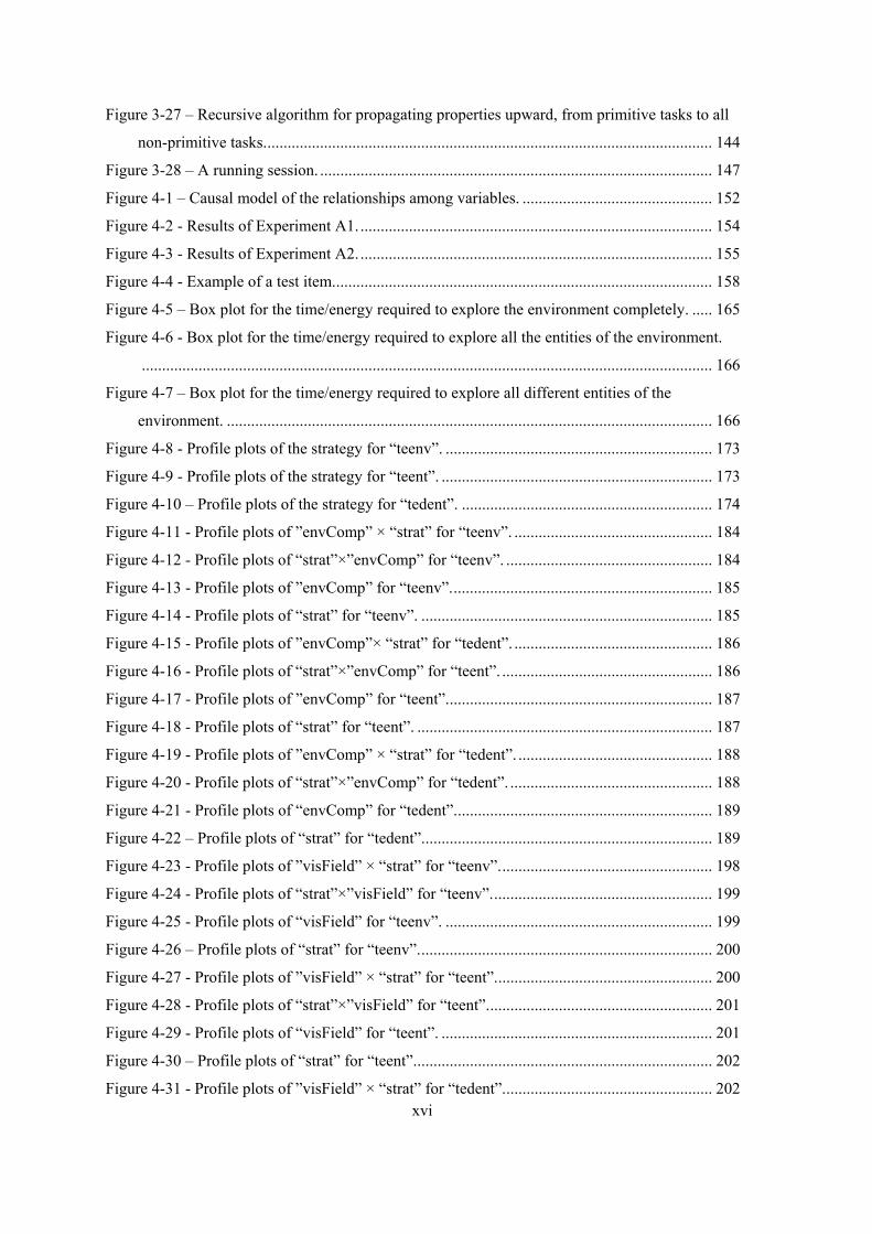
List of Figures Figure 3-1 – Illustrative sketch of an environment.......................................................................106 Figure 3-2 – Architecture of an agent...........................................................................................107 Figure 3-3 – An example of a metric map....................................................................................109 Figure 3-4 – Example of the histogram of a cell. .........................................................................109 Figure 3-5 – Example of the episodic memory of entities. ..........................................................110 Figure 3-6 – Example of a semantic memory of entities..............................................................111 Figure 3-7 – Example of an exploration plan. ..............................................................................113 Figure 3-8 - Example of an abstract plan from the logistic domain. ............................................113 Figure 3-9 - Schematic representation of a generic task in an abstract plan. ...............................115 Figure 3-10 - Schematic representation of tasks in an abstract plan of the exploration domain. .116 Figure 3-11 - Schematic representation of a task in an abstract plan of the logistic domain. ......117 Figure 3-12 - Example of a case-base with two concrete plans of the logistic domain................118 Figure 3-13 - Schematic representation of a generic primitive task in a concrete plan................118 Figure 3-14 - Schematic representation of a primitive task in a concrete plan of the exploration
domain. .................................................................................................................................119 Figure 3-15 - Schematic representation of a primitive task in a concrete plan of the logistic
domain. .................................................................................................................................119 Figure 3-16 - Categories of knowledge. .......................................................................................123 Figure 3-17 – Surprise as a function of the difference between P(Eh) and P(Eg). ........................126 Figure 3-18 – Algorithm for Sequential Decision-Making. .........................................................133 Figure 3-19 – Illustration of the computation of the probabilistic analogical description of an
entity.....................................................................................................................................135 Figure 3-20 – Algorithm for the generation and ranking of goals................................................138 Figure 3-21 – Illustrative example of the sketch of the metric map of an initial state of the
environment in the logistics domain.....................................................................................139 Figure 3-22 – Algorithm for the construction of an abstract plan. ...............................................139 Figure 3-23 – Illustrative example of the decomposition of an abstract task, i.e., OR-
decomposition of an abstract task.........................................................................................140 Figure 3-24 - Illustrative example of the decomposition of a compound task, i.e., AND-
decomposition of a regular compound task..........................................................................141 Figure 3-25 – Algorithm for constructing the structure of an HTN. ............................................143 Figure 3-26 – Algorithm for computing the conditional effects (and respective probabilities) and
the EU of primitive tasks. .....................................................................................................144
xvi
Figure 3-27 – Recursive algorithm for propagating properties upward, from primitive tasks to all
non-primitive tasks............................................................................................................... 144 Figure 3-28 – A running session. ................................................................................................. 147 Figure 4-1 – Causal model of the relationships among variables. ............................................... 152 Figure 4-2 - Results of Experiment A1........................................................................................ 154 Figure 4-3 - Results of Experiment A2........................................................................................ 155 Figure 4-4 - Example of a test item.............................................................................................. 158 Figure 4-5 – Box plot for the time/energy required to explore the environment completely. ..... 165 Figure 4-6 - Box plot for the time/energy required to explore all the entities of the environment.
............................................................................................................................................. 166 Figure 4-7 – Box plot for the time/energy required to explore all different entities of the
environment. ........................................................................................................................ 166 Figure 4-8 - Profile plots of the strategy for “teenv”. .................................................................. 173 Figure 4-9 - Profile plots of the strategy for “teent”. ................................................................... 173 Figure 4-10 – Profile plots of the strategy for “tedent”. .............................................................. 174 Figure 4-11 - Profile plots of ”envComp” × “strat” for “teenv”. ................................................. 184 Figure 4-12 - Profile plots of “strat”×”envComp” for “teenv”. ................................................... 184 Figure 4-13 - Profile plots of ”envComp” for “teenv”................................................................. 185 Figure 4-14 - Profile plots of “strat” for “teenv”. ........................................................................ 185 Figure 4-15 - Profile plots of ”envComp”× “strat” for “tedent”. ................................................. 186 Figure 4-16 - Profile plots of “strat”×”envComp” for “teent”. .................................................... 186 Figure 4-17 - Profile plots of ”envComp” for “teent”.................................................................. 187 Figure 4-18 - Profile plots of “strat” for “teent”. ......................................................................... 187 Figure 4-19 - Profile plots of ”envComp” × “strat” for “tedent”. ................................................ 188 Figure 4-20 - Profile plots of “strat”×”envComp” for “tedent”. .................................................. 188 Figure 4-21 - Profile plots of “envComp” for “tedent”................................................................ 189 Figure 4-22 – Profile plots of “strat” for “tedent”........................................................................ 189 Figure 4-23 - Profile plots of ”visField” × “strat” for “teenv”..................................................... 198 Figure 4-24 - Profile plots of “strat”×”visField” for “teenv”....................................................... 199 Figure 4-25 - Profile plots of “visField” for “teenv”. .................................................................. 199 Figure 4-26 – Profile plots of “strat” for “teenv”......................................................................... 200 Figure 4-27 - Profile plots of ”visField” × “strat” for “teent”...................................................... 200 Figure 4-28 - Profile plots of “strat”×”visField” for “teent”........................................................ 201 Figure 4-29 - Profile plots of “visField” for “teent”. ................................................................... 201 Figure 4-30 – Profile plots of “strat” for “teent”.......................................................................... 202 Figure 4-31 - Profile plots of ”visField” × “strat” for “tedent”.................................................... 202

xvii
Figure 4-32 - Profile plots of “strat”×”visField” for “tedent”. .....................................................203 Figure 4-33 - Profile plots of “visField” for “tedent”...................................................................203 Figure 4-34 – Profile plots of “strat” for “tedent”. .......................................................................204 Figure 4-35 - Results of experiment III. .......................................................................................223

xix
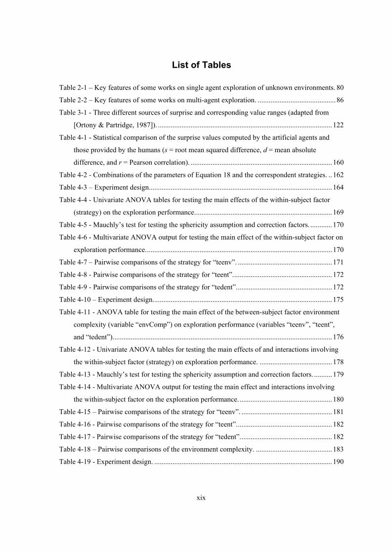
List of Tables
Table 2-1 – Key features of some works on single agent exploration of unknown environments. 80 Table 2-2 – Key features of some works on multi-agent exploration. ...........................................86 Table 3-1 - Three different sources of surprise and corresponding value ranges (adapted from
[Ortony & Partridge, 1987]). ................................................................................................122 Table 4-1 - Statistical comparison of the surprise values computed by the artificial agents and
those provided by the humans (s = root mean squared difference, d = mean absolute
difference, and r = Pearson correlation). ..............................................................................160 Table 4-2 - Combinations of the parameters of Equation 18 and the correspondent strategies. ..162 Table 4-3 – Experiment design.....................................................................................................164 Table 4-4 - Univariate ANOVA tables for testing the main effects of the within-subject factor
(strategy) on the exploration performance............................................................................169 Table 4-5 - Mauchly’s test for testing the sphericity assumption and correction factors. ............170 Table 4-6 - Multivariate ANOVA output for testing the main effect of the within-subject factor on
exploration performance.......................................................................................................170 Table 4-7 – Pairwise comparisons of the strategy for “teenv”. ....................................................171 Table 4-8 - Pairwise comparisons of the strategy for “teent”.......................................................172 Table 4-9 - Pairwise comparisons of the strategy for “tedent”.....................................................172 Table 4-10 – Experiment design...................................................................................................175 Table 4-11 - ANOVA table for testing the main effect of the between-subject factor environment
complexity (variable “envComp”) on exploration performance (variables “teenv”, “teent”,
and “tedent”).........................................................................................................................176 Table 4-12 - Univariate ANOVA tables for testing the main effects of and interactions involving
the within-subject factor (strategy) on exploration performance. ........................................178 Table 4-13 - Mauchly’s test for testing the sphericity assumption and correction factors. ..........179 Table 4-14 - Multivariate ANOVA output for testing the main effect and interactions involving
the within-subject factor on the exploration performance....................................................180 Table 4-15 – Pairwise comparisons of the strategy for “teenv”. ..................................................181 Table 4-16 - Pairwise comparisons of the strategy for “teent”.....................................................182 Table 4-17 - Pairwise comparisons of the strategy for “tedent”...................................................182 Table 4-18 – Pairwise comparisons of the environment complexity. ..........................................183 Table 4-19 - Experiment design. ..................................................................................................190
xx
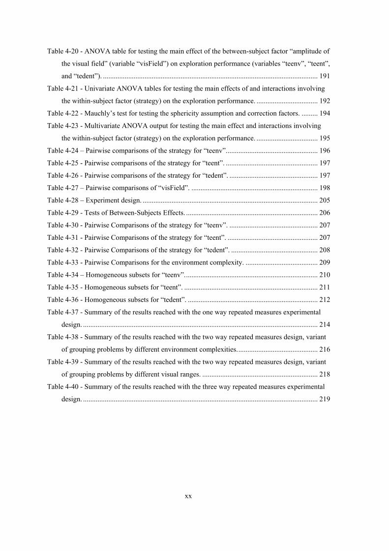
Table 4-20 - ANOVA table for testing the main effect of the between-subject factor “amplitude of
the visual field” (variable “visField”) on exploration performance (variables “teenv”, “teent”,
and “tedent”). ....................................................................................................................... 191 Table 4-21 - Univariate ANOVA tables for testing the main effects of and interactions involving
the within-subject factor (strategy) on the exploration performance. .................................. 192 Table 4-22 - Mauchly’s test for testing the sphericity assumption and correction factors. ......... 194 Table 4-23 - Multivariate ANOVA output for testing the main effect and interactions involving
the within-subject factor (strategy) on the exploration performance. .................................. 195 Table 4-24 – Pairwise comparisons of the strategy for “teenv”................................................... 196 Table 4-25 - Pairwise comparisons of the strategy for “teent”. ................................................... 197 Table 4-26 - Pairwise comparisons of the strategy for “tedent”. ................................................. 197 Table 4-27 – Pairwise comparisons of “visField”. ...................................................................... 198 Table 4-28 – Experiment design. ................................................................................................. 205 Table 4-29 - Tests of Between-Subjects Effects. ......................................................................... 206 Table 4-30 - Pairwise Comparisons of the strategy for “teenv”. ................................................. 207 Table 4-31 - Pairwise Comparisons of the strategy for “teent”. .................................................. 207 Table 4-32 - Pairwise Comparisons of the strategy for “tedent”. ................................................ 208 Table 4-33 - Pairwise Comparisons for the environment complexity. ........................................ 209 Table 4-34 – Homogeneous subsets for “teenv”.......................................................................... 210 Table 4-35 - Homogeneous subsets for “teent”. .......................................................................... 211 Table 4-36 - Homogeneous subsets for “tedent”. ........................................................................ 212 Table 4-37 - Summary of the results reached with the one way repeated measures experimental
design. .................................................................................................................................. 214 Table 4-38 - Summary of the results reached with the two way repeated measures design, variant
of grouping problems by different environment complexities............................................. 216 Table 4-39 - Summary of the results reached with the two way repeated measures design, variant
of grouping problems by different visual ranges. ................................................................ 218 Table 4-40 - Summary of the results reached with the three way repeated measures experimental
design. .................................................................................................................................. 219
xxi
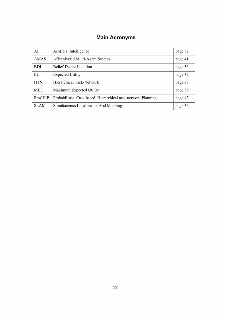
Main Acronyms
AI Artificial Intelligence page 32
AMAS Affect-based Multi-Agent System page 41
BDI Belief-Desire-Intention page 36
EU Expected Utility page 37
HTN Hierarchical Task-Network page 37
MEU Maximum Expected Utility page 36
ProCHiP Probabilistic, Case-based, Hierarchical task-network Planning page 42
SLAM Simultaneous Localization And Mapping page 32

1
Resumo alargado em língua portuguesa
ste capítulo descreve sucintamente o conteúdo desta tese. Uma exposição mais pormenorizada dos diversos aspectos da tese podem ser encontrados nos capítulos subsequentes, escritos em língua inglesa. Começamos com uma introdução do tema da
tese, a que se segue a descrição da questão a investigar. Depois, apresentamos a abordagem adoptada para investigar essa questão e, posteriormente, a avaliação experimental realizada. Por fim, apresentamos as conclusões, nas quais se incluem as contribuições científicas e algumas questões que, ao ficarem sem resposta, constituem objecto de um trabalho futuro.
1.1 Introdução
A ciência ainda está longe de saber como é que a mente humana funciona. Um dos seus mais intricados aspectos é a relação entre emoção e racionalidade. Durante muitos anos assumiu-se que as emoções eram obstáculos à inteligência. Desde Platão, vários filósofos delinearam uma fronteira entre razão e emoção, assumindo que as emoções interferem com a racionalidade e que são factores potenciadores de um raciocínio incorrecto. Em Phaedrus, Platão compara a parte racional da alma a um condutor de uma carruagem que deve controlar os cavalos que simbolizam a parte emocional da alma [Plato, 1961]. Hoje em dia, os cientistas são tidos como os paradigmas da racionalidade, e o pensamento racional é geralmente assumido como sendo independente do pensamento emocional. Esta visão tradicional sobre a natureza da racionalidade separa claramente razão de emoção. Para que um ser humano seja racional, não deverá permitir a influência das emoções no raciocínio. No entanto, estudos recentes feitos no âmbito da Neurociência indicam precisamente o contrário, ao mostrarem que as emoções têm um papel fundamental em processos cognitivos como a percepção, aprendizagem, atenção, memória, e principalmente planeamento e tomada de decisões, bem como em outros aspectos habitualmente associados ao comportamento racional básico. Na verdade, estudos recentes com pacientes com lesões no córtex pré-frontal sugerem um papel crítico das emoções na tomada de decisão [Bechara et al., 1997; Churchland, 1996; Damásio, 1994]. Embora os pacientes consigam responder com sucesso a uma variedade de testes de memória e de inteligência, quando colocados em situações da vida real eles parecem ser incapazes de tomar decisões correctas. Aparentemente, estes pacientes denotam uma falta de faculdades de intuição, que segundo vários investigadores podem ser baseadas em memórias de experiências emocionais passadas. Estas descobertas levaram António Damásio e seus colegas a sugerir que o raciocínio humano e a tomada de decisões envolvem vários mecanismos a diferentes níveis, desde os que regulam funções básicas do corpo até àqueles que se relacionam com raciocínio e tomada de decisão. Um aspecto particularmente interessante e novo deste ponto de vista é o de o raciocínio também depender das emoções e sentimentos que lhes estão associados.
A perspectiva evolucionária da emoção permite uma melhor compreensão do seu papel no pensamento racional e na tomada de decisão. Este papel é parte integrante das principais funções da emoção: proporcionar a sobrevivência e o bem-estar. De facto, a sobrevivência e o bem-estar de alguém dependem obviamente das decisões tomadas ao longo da vida. Decisões erradas podem conduzir-nos a situações más ou mesmo fatais. Nesta perspectiva, e com base na sua influência na tomada de decisão, as emoções não são obstáculos à racionalidade, nem sequer adereços
E
2 Resumo alargado em língua portuguesa
desnecessários do ser humano, mas sim aspectos vitais para a inteligência e, consequentemente, para tudo o que desta depende.
Quando um ser humano atinge os seus objectivos avalia como positivo este facto, enquanto que, quando o contrário acontece, resultam emoções negativas [Carver & Scheier, 1990]. As emoções são, deste modo, consideradas como prémios ou castigos. Um ser humano normalmente age de uma determinada forma porque espera que esse comportamento o faça sentir-se melhor (ver, por exemplo, [Thayer et al., 1994]). De acordo com princípios simples de reforço, os seres humanos repetem usualmente acções que tiveram consequências emocionais positivas no passado. Isto constitui uma espécie de hedonismo na medida, segundo estas ideias, os seres humanos procuram o prazer e evitam a dor. Mas este tipo de hedonismo não explica todas as variedades do fenómeno da motivação. Ao contrário destas teorias de hedonismo e neo-hedonismo [W. Cox & Klinger, 2004; Mellers, 2000; Zeelenberg et al., 2000], existe uma outra teoria, ou classe de teorias, para o efeito motivacional da emoção na tomada de decisão e na acção, que pode ser denominada teoria dos impulsos de acção específicos de emoções [Frijda, 1994; Lazarus, 1991; B. Weiner, 2005]. Esta defende que existem tendências de acção para cada emoção (por exemplo, evitar o perigo quando se sente medo, atacar em caso de raiva, ajudar quando se sente pena, etc.). O hedonismo assume a existência de um único desejo básico, enquanto que a teoria dos impulsos de acção específicos de emoções assume uma visão pluralista da motivação [Havercamp & Reiss, 2003; McDougall, 1908; Reiss, 2000; Schwartz, 1992; B. Weiner, 1980] ao defender a existência de vários desejos básicos (por exemplo, curiosidade, poder, hedonismo, etc.). No entanto, alguns investigadores acreditam que o princípio do prazer está aqui presente embora de forma indirecta.
Motivação e emoção são conceitos que estão muito relacionados e, por isso, nem sempre é fácil estabelecer uma fronteira entre eles. Emoção e motivação dependem da relação entre um organismo e o ambiente. A motivação é relacionada com a geração de objectivos e da acção, enquanto que a emoção diz respeito à avaliação do ambiente por parte do agente. No caso da emoção, a ênfase está em como uma determinada situação provoca determinados sentimentos numa pessoa. No caso da motivação, o interesse é colocado na forma como um indivíduo actua perante uma determinada situação [Kuhl, 1986]. De uma forma geral, a motivação é definida como sendo o conjunto de factores que levam a que um organismo se comporte de uma determinada forma num determinado momento.
Uma das características do ser humano é a sua irreverente tendência para explorar as partes desconhecidas do mundo que o rodeia. Embora a exploração já exista desde o aparecimento do Homem, o seu auge pode ser considerado durante a Época dos Descobrimentos, um período que se iniciou no começo do século XV e que terminou nos primórdios do século XVII, período este durante o qual navegadores Europeus (Portugueses, Espanhóis, Ingleses, etc.) viajaram “por mares nunca dantes navegados”, descobrindo novas regiões e culturas. Estes grandes feitos, juntamente com a exploração do espaço sideral, dos planetas e satélites do sistema solar nos nossos dias, constituem um exemplo fidedigno do espírito de explorar da espécie humana. Não existem limites para a exploração humana: desde vulcões inóspitos, montanhas e oceanos enormes, até planetas agrestes como Marte, e satélites hostis como Titã e a Lua, o ser humano está constantemente a tentar adquirir conhecimento do ambiente apesar muitas vezes da adversidade deste.
Mas o que é que motiva este comportamento? A “atenção selectiva” de James [James, 1890], a “catexia” de Freud [Freud, 1938], e o “instinto de curiosidade” de McDougall [McDougall, 1908] são conceitos fundamentais da relação entre motivação e o comportamento de exploração. Desde
Resumo alargado em língua portuguesa 3
há muito tempo que este comportamento de exploração tem sido expresso pela ideia de que os organismos respondem à novidade e à mudança no ambiente que habitam quando as suas necessidades básicas (sede, fome, etc.) estão satisfeitas. Quando a novidade e a mudança não existem no ambiente, os organismos têm tendência a procurá-las. Evidências deste comportamento em diversas espécies foram descritas por vários autores [Lester, 1969]. No ser humano, este tipo de comportamento está patente desde as primeiras horas de vida, tal como foi documentado por vários investigadores que estudaram a atenção selectiva (uma forma simples de comportamento de exploração) em recém-nascidos. Os recém-nascidos preferem certos padrões visuais em vez de outros. Eles não dão igual importância a todos os estímulos. Exploram o ambiente com os olhos, fixam o olhar nos objectos mais interessantes, i.e., naqueles que lhes proporcionam novos estímulos.
Alguns dos investigadores que demonstraram que os organismos tendem a explorar objectos ou locais novos na ausência de necessidades básicas chamam-lhe necessidade de explorar [Butler, 1953, 1954, 1957, 1958; Montegomery, 1952, 1953, 1954, 1955]. Outros, tais como Berlyne [Berlyne, 1950] e Shand [Shand, 1914], adoptaram as ideias de McDougall sobre curiosidade. Para estes últimos autores, a curiosidade é o conceito psicológico que tem sido directamente relacionado com este tipo de comportamento. Berlyne considera que a curiosidade é inata, mas que também pode ser adquirida. Ele defende que um novo estímulo causa curiosidade, que diminui com a contínua exposição ao estímulo [Berlyne, 1950]. Num trabalho posterior [Berlyne, 1955, 1960, 1967], Berlyne reformulou e completou a sua anterior teoria sobre a curiosidade. Para além da novidade, Berlyne considera que outras variáveis como a mudança, complexidade, incerteza, incongruência, o inesperado e o conflito também determinam este tipo de comportamento relacionado com actividades de exploração e investigação. Partilhando ideias similares com Berlyne e McDougall, Shand [Shand, 1914] considera a curiosidade como uma emoção primária que define como sendo um simples impulso para conhecer, que controla e sustém a atenção e provoca os movimentos do corpo que permitem que se adquira informação de um objecto. Estas abordagens estão bastante relacionadas com o conceito de “interesse-excitação” proposto pela teoria das emoções diferenciadas para explicar a exploração, a aventura, a resolução de problemas, criatividade e a aquisição de capacidades e competências quando não existem necessidades básicas [Izard, 1977, 1991]. De facto, os termos curiosidade e interesse são usados geralmente como sinónimos, por exemplo, por Berlyne. Nunnally e Lemond [Nunnally & Lemond, 1973] fizeram experiências sobre os efeitos da novidade e complexidade na exploração visual. Concluíram que novidade e conflito de informação provocam e são responsáveis pela manutenção da atenção.
Em suma, não existem dúvidas que a novidade causa curiosidade/interesse, conceitos estes que estão na base do comportamento de exploração. No entanto, a novidade parece não ser suficiente para explicar todos os tipos de comportamento de exploração. Outras variáveis como a mudança, a complexidade, a incerteza, a incongruência, o inesperado e o conflito também determinam o comportamento de exploração. Algumas destas variáveis provocam surpresa, outro conceito psicológico que explica este comportamento. Avanços recentes no domínio da Neurociência indicam que a emoção influencia os processos cognitivos dos humanos, particularmente o planeamento e a tomada de decisão [Adolphs et al., 1996; Bechara et al., 1997; Damásio, 1994]. Sendo um processo de tomada de decisão, a exploração de ambientes desconhecidos é assim forçosamente influenciada pela emoção. Existe, deste modo, um vasto leque de motivações por detrás da tarefa de exploração.
4 Resumo alargado em língua portuguesa
A mente humana parece ser paradoxalmente ilimitada. Para enriquecerem as suas capacidades de lidar com situações adversas ou problemas, os seres humanos foram capazes de construir sistemas, chamados agentes artificiais, que tentam fazer de forma inteligente coisas tal como ou melhor que os humanos: percepcionar o ambiente e produzir acções correctas. Isto constitui um paradoxo porque é simultaneamente a prova da engenhosa faceta da mente humana de ultrapassar as suas limitações, mas também de reconhecer as suas limitações em lidar com certas situações ou pelo menos em lidar facilmente com elas. O objectivo da Inteligência Artificial é precisamente o de entender e construir tais agentes inteligentes artificiais. Obviamente, esses agentes não possuem (ainda) os órgãos dos sentidos, os efectores e a mente dos seres humanos, mas em vez disso possuem câmaras, braços robóticos, software, etc. No entanto, esses agentes exibem formas de percepção, de raciocínio e tomada de decisão, e de actuação. Embora não possam fazer todas as coisas que os seres humanos fazem, talvez façam outros tipos de coisas melhor que os seres humanos. Até à data, quase todas as capacidades dos seres humanos foram exploradas pela Inteligência Artificial, incluindo, sem surpresa, a exploração de ambientes desconhecidos.
A exploração de ambientes desconhecidos por agentes artificiais (normalmente robots) tem sido uma área de investigação bastante activa. A exploração pode ser definida como sendo o processo de selecção e execução de acções no sentido de adquirir o máximo de conhecimento do ambiente. Deste processo resultam modelos físicos do ambiente. Desta forma, a exploração de ambientes desconhecidos envolve a construção de mapas, mas não se confina a este processo. De facto, podem identificar-se dois aspectos distintos na exploração. Primeiro, o agente ou robot tem de interpretar a informação adquirida pelos seus sensores para que possa obter uma correcta representação do estado do ambiente. Este é o problema da construção de mapas. Este problema de mapeamento tem vários aspectos que têm vindo a ser estudados intensamente, dos quais se destacam a localização do veículo durante o mapeamento e a construção de mapas apropriados do ambiente. A representação fidedigna do ambiente nos mapas depende destes factores. Este problema fundamental em robótica móvel é chamado de localização e mapeamento simultâneo e pode ser definido como um problema do tipo “ovo-e-galinha”: enquanto o robot navega num ambiente desconhecido, deve incrementalmente construir um mapa do que o rodeia e, ao mesmo tempo, ser capaz de se localizar nesse mapa construído. O segundo, mas não menos importante aspecto da exploração de ambientes desconhecidos, é o de o agente ou robot seleccionar os pontos de observação onde se vai colocar de forma a que os seus sensores adquiram informação nova e útil. Trata-se, neste caso, do problema de exploração propriamente dito. Este envolve conduzir o veículo de tal forma que todo o ambiente seja coberto pelos seus sensores. A representação fidedigna do ambiente no mapa depende também desta escolha dos pontos de observação durante a exploração.
Infelizmente, a exploração de ambientes desconhecidos consome recursos dos agentes tais como tempo e energia. Existe uma situação de compromisso entre a quantidade de conhecimento adquirido e o custo para o adquirir. O objectivo de um explorador é o de obter o máximo de conhecimento do ambiente ao mínimo custo (tempo/energia). Várias técnicas têm sido propostas e testadas em ambientes simulados e reais, em ambientes externos e internos, usando um só agente ou múltiplos agentes. Os domínios de exploração incluem a exploração do espaço sideral e dos planetas e satélites destes (por exemplo, Marte, Titã e a Lua), a procura de meteoritos na Antártida, o mapeamento do fundo dos oceanos, a exploração de vulcões, mapeamento de interiores de edifícios, etc. A principal vantagem de usar agentes artificiais nestes ambientes em vez de seres humanos é a de a maioria destes ambientes serem hostis, sendo a sua exploração uma tarefa demasiado perigosa para os seres humanos. No entanto, muito há ainda para se fazer
Resumo alargado em língua portuguesa 5
especialmente em ambientes dinâmicos tais como os supracitados. Estes ambientes reais possuem normalmente vários objectos. Por exemplo, os escritórios contêm cadeiras, portas, caixotes do lixo, etc., e as cidades são formadas por diversos tipos de edifícios (casas, hospitais, igrejas, etc.). Muitos destes objectos são não estacionários, i.e., as suas localizações podem variar ao longo do tempo. Este aspecto é motivo de investigação na senda de novos algoritmos de geração de mapas que representem os ambientes como conjuntos de objectos. Pelo menos, tais modelos dos objectos deverão permitir a um robot anotar as mudanças que ocorrem no ambiente. Por exemplo, um robot de limpezas ao entrar num escritório à noite deverá ficar a saber facilmente que um caixote do lixo foi mudado de local. Um robot deverá fazer isto sem necessidade de ter de construir o modelo do caixote do lixo novamente a partir das novas observações. A representação de objectos oferece uma outra importante vantagem relacionada com o facto de muitos ambientes possuírem vários objectos do mesmo tipo. Por exemplo, a maioria das cadeiras de escritório são exemplos de uma mesma cadeira genérica e por isso são semelhantes, tal como acontece com a maioria das portas, caixotes do lixo, etc. Como estes exemplos sugerem, vários objectos partilham os mesmo atributos formando classes de objectos que são de primordial importância para a robótica móvel. Em particular, algoritmos que adquirem propriedades (aparência, movimento) de classes de objectos poderiam ser capazes de transferir essas propriedades de um objecto para outro dentro da mesma classe. Isto teria um impacto profundo na exactidão dos modelos de objectos e na rapidez com que esses modelos podem ser adquiridos. Por exemplo, se um robot de limpezas entrar num compartimento que nunca visitou antes, poderá perceber que um determinado objecto dentro desse compartimento tem uma aparência semelhante à de outros objectos vistos noutros compartimentos. Este robot pode então ser capaz de adquirir o mapa deste objecto mais rapidamente. Por outro lado, o robot poderá prever as propriedades deste novo objecto, tais como o facto de ser não estacionário, sem precisar de ter visto este objecto a mover-se. Um outro aspecto a ter em consideração para além do problema dos ambientes dinâmicos é o da autonomia dos robots que necessita forçosamente de ser melhorada, como acontece por exemplo na exploração planetária que continua a ser demasiado dependente do ser humano (os planos são determinados por um operador humano, bem como os pontos a visitar).
Tal como foi mencionado anteriormente, a emoção é essencial para a sobrevivência, bem-estar e comunicação dos seres humanos, desempenhando um papel central em actividades cognitivas tais como a tomada de decisão, o planeamento e a criatividade. Nesta ordem de ideias, podemos colocar as questões: Porque não dotar agentes artificiais com emoções de forma a tirarem benefício das mesmas tal como os seres humanos o fazem? O que podem os agentes artificiais afectivos fazer melhor do que aqueles que não são afectivos? O que é que a emoção pode oferecer aos agentes artificiais? Certamente, nem todas as vantagens de que os seres humanos beneficiam são aplicáveis aos agentes artificiais. No entanto, podemos encontrar uma série de situações em que se vislumbra a vantagem emocional como por exemplo: sistemas de geração de voz a partir de texto, dando uma entoação mais natural ao discurso; entretenimento; medicina preventiva; ajuda a pessoas autistas; animais de estimação artificiais; agentes pessoais que podem seleccionar música, notícias, etc., para uma pessoa de acordo com o seu estado de humor; obtenção do “feedback” de clientes face a um produto específico através da aferição da sua resposta emocional, etc. Tais aplicações requerem capacidades de reconhecimento, expressão, e sentimento de emoções [Picard, 1997]. Embora esta influência da emoção no raciocínio tenha sido esquecida durante algum tempo na área de Inteligência Artificial, assistiu-se na última década a uma inversão desta situação, uma vez que estas capacidades de reconhecimento, expressão, e sentimento de emoções têm vindo a ser envolvidas em modelos computacionais de emoção e
6 Resumo alargado em língua portuguesa
motivação (por exemplo, [Bates, 1994; Botelho & Coelho, 1998; Dias & Paiva, 2005; Elliott, 1992; Macedo & Cardoso, 2001a, 2001b; Maes, 1995; Oliveira & Sarmento, 2003; Ortony et al., 1988; Paiva et al., 2004; Pfeifer, 1988; Picard, 1997; Reilly, 1996; Schmidhuber, 1991]). Algumas das aplicações que poderão tirar partido da emoção estão já desenvolvidas ou a serem desenvolvidas (por exemplo, animais de estimação artificiais capazes de expressar emoções, emoção em sistemas de conversão de texto em voz, etc.) e, desta forma, já não pertencem ao domínio da ficção científica. No entanto, muitas delas precisam certamente de melhoramentos. Outras aplicações, como o computador HAL [Clarke, 1997], estão ainda na prateleira da ficção científica.
No que se refere particularmente à exploração de ambientes desconhecidos, poderá ser vantajoso ter em conta as emoções neste processo. Pelo que sabemos, não existe praticamente nenhum trabalho que use explicitamente emoções neste tipo de tarefa (excepção feita a [Blanchard & Cañamero, 2006; Oliveira & Sarmento, 2002; Velásquez, 1997], embora a abordagem seja superficial e o objectivo não seja a completa exploração de ambientes com entidades). Poderemos entender que alguns estudos sobre exploração consideram implicitamente formas rudimentares de motivações. Por exemplo, quando alguns trabalhos referem o uso de equações matemáticas que avaliam o ambiente em termos da quantidade de informação para um agente ou que calculam o custo para obter determinada informação, estão, de certa forma, a modelar no agente formas rudimentares, por exemplo, de curiosidade/interesse e fome, respectivamente. Tais trabalhos estão na verdade a considerar variáveis, como a novidade, incerteza, diferença ou mudança, que, de acordo com teorias da Psicologia, estão na base do processo de desencadeamento da curiosidade/interesse.
Para construir agentes artificiais que ajam e pensem como os humanos [S. Russell & Norvig, 1995], devemos conferir a esses agentes, entre outras, a capacidade de explorar ambientes desconhecidos de uma forma semelhante à humana. Tendo em conta, por um lado, as diversas teorias da Psicologia a relacionar emoções e motivações com comportamento de exploração nos humanos, e por outro, a evidência vinda da Neurociência suportando que a emoção influencia capacidades cognitivas como a tomada de decisão e planeamento (de notar que a exploração é um processo que envolve tomadas de decisão), é razoável considerar que a emoção e a motivação, ou se quisermos simplesmente a motivação no seu significado mais lato, influenciam esta actividade. Podemos sonhar com um robot a explorar Marte ou outro corpo celeste inóspito, evitando situações perigosas porque é capaz de sentir medo, seleccionando as coisas mais interessantes para visitar/analisar porque é capaz de sentir surpresa e curiosidade ou uma forma de interesse, sendo alarmado para recarregar a bateria porque é capaz de sentir fome, etc. Podemos também imaginar esse robot a mapear o ambiente que o rodeia e a construir modelos dos objectos que visita e analisa para que possam ser usados no futuro, não só como forma de simplificar o processo de exploração (conforme mencionado anteriormente), mas também como meios que contribuam para a sua sobrevivência e promovam o seu bem-estar. Obviamente, nesta tese não podemos ir tão longe, mas podemos fazer uma tentativa modesta de sermos uns dos precursores. Neste sentido, desenvolvemos um sistema multi-agente no qual os agentes são providos de sentimentos e desejos básicos. Outros módulos importantes da arquitectura destes agentes são o da memória e do raciocínio. Este último é, na verdade, essencialmente um planeador, i.e., um sistema que estabelece sequências de decisões. Embora esta plataforma multi-agente tenha outras aplicações potenciais, nesta tese, usámo-la apenas para o estudo do problema de exploração de ambientes desconhecidos que contêm entidades (objectos e outros agentes) por parte de agentes autónomos e afectivos. Assim, usando esta plataforma construímos um ambiente multi-agente no
Resumo alargado em língua portuguesa 7
qual, para além de entidades inanimadas (objectos), existem também agentes animados que interagem de uma forma simples e cujo objectivo é explorar o ambiente, mapeando-o, analisando-o, estudando-o e avaliando-o.
1.2 Afirmação da Tese/Questão de Investigação
Nesta tese tentamos verificar a hipótese de que a exploração de ambientes desconhecidos que contêm entidades pode ser feita de uma forma robusta e eficiente por agentes capazes de processar motivações e emoções. Ao investigar o papel de algumas emoções e motivações neste tipo de tarefa, este trabalho demonstra os benefícios do uso de agentes afectivos na execução desta actividade de exploração. Além disso, estudamos a influência, nas emoções e motivações e consequentemente na “performance” da exploração, de outras variáveis/aspectos dos agentes e do próprio sistema multi-agente, como a memória dos agentes e a diversidade do ambiente.
1.3 Abordagem
Nesta tese, estudamos o problema da exploração, por agentes autónomos afectivos, de ambientes desconhecidos contendo entidades. Neste tipo de trabalho com ambientes multi-agente, podemos seguir dois tipos de abordagem: usar ambientes simulados ou reais. Alguns investigadores constroem softbots que depois usam em ambientes simulados para testar teorias e algoritmos. Outros optam por construir robots que colocam em ambientes reais. Era necessário escolher entre estas duas abordagens.
A simulação tem vantagens. Por exemplo, podemos ter resultados de um algoritmo muito mais rapidamente usando softbots em ambientes simulados do que usando robots em ambientes reais. O investigador é capaz de fazer experiências sem as restrições temporais e financeiras habitualmente associadas ao uso de robots. Além disso, as simulações permitem ao investigador focar-se exclusivamente no aspecto preciso do problema em questão. Acrescente-se ainda o facto de o investigador ter mais controlo das variáveis do sistema envolvidas na experiência.
No entanto, os ambientes simulados também têm algumas desvantagens. Para construir um softbot que modele um robot, o investigador tem de abstrair aspectos essenciais do robot que está a ser modelado. Esta abstracção envolve necessariamente algum grau de simplificação. Em robótica móvel isto acontece principalmente na modelação dos sensores. Os sensores simulados são na maior parte das vezes diferentes dos reais. Embora a investigação baseada em tais simplificações possa conduzir a bons resultados, existe sempre o perigo de no processo de simplificação se terem ignorado aspectos essenciais do robot de tal forma que os resultados não sejam válidos quando o robot for testado em ambiente real. Por esta razão, a simulação é considerada uma boa abordagem desde que todas as variáveis que possam influenciar os resultados no mundo real estejam presentes no modelo computacional. Escolhemos usar simulações pelas vantagens mencionadas acima e porque as simplificações que fizemos (apresentadas mais à frente nesta secção) não influenciam os resultados. Por exemplo, assumimos que os agentes conhecem a sua localização precisa mediante GPS porque este não é um aspecto relevante para testar a influência das emoções e motivações na exploração.
Desenvolvemos um sistema multi-agente que compreende agentes afectivos. Embora antevejamos um potencial alargado para este sistema multi-agente (isto depende principalmente do tipo de objectivos e planos colocados na memória dos agentes), nesta tese estudamos a
8 Resumo alargado em língua portuguesa
capacidade dos agentes afectivos explorarem ambientes desconhecidos. Desta forma, não estamos a usar o sistema multi-agente em problemas comuns como o controlo de processos, entretenimento, ou eComerce, mas sim para o problema de exploração de ambientes desconhecidos, e mais especificamente, para a simulação desta actividade. A exploração de regiões inóspitas, como planetas, por robots móveis é um exemplo de um domínio onde esta capacidade é necessária. Outro exemplo é a “World Wide Web”.
Tendo o sistema multi-agente como plataforma, desenvolvemos um ambiente simulado no qual, para além de entidades inanimadas (objectos), existem agentes que interagem de uma forma simples. Estes agentes analisam, estudam, avaliam e constroem o mapa do ambiente.
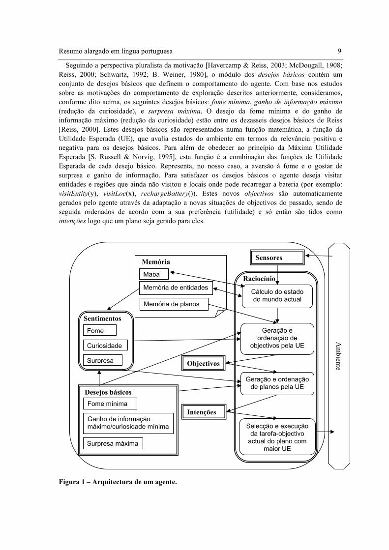
Adoptamos a abordagem de considerar os agentes como agindo e actuando como humanos [S. Russell & Norvig, 1995] e baseamo-nos nas principais ideias da arquitectura “Belief-Desire-Intention” (BDI) para direccionar a nossa implementação. Na nossa plataforma, a arquitectura de um agente (Figura 1) inclui os seguintes módulos: sensores, memória (para entidades, planos e mapas do ambiente), desejos/objectivos, intenções, desejos básicos (motivações básicas), sentimentos, e raciocínio. A componente chave que determina o comportamento dos agentes é o tipo de objectivos, planos, desejos básicos e sentimentos que lhe são conferidos. Neste caso específico de comportamento de exploração, objectivos e planos para visitar entidades e regiões do ambiente, e para recarregar a bateria são colocados na memória dos agentes. No nosso caso, e de acordo com os estudos mencionados anteriormente, o agente é equipado com os desejos básicos de fome mínima, ganho de informação máximo (redução da curiosidade), e surpresa máxima. Cada um destes desejos básicos levam o agente a reduzir ou maximizar um determinado sentimento. O desejo de fome mínima, ganho de informação máximo e surpresa máxima conduzem o agente a reduzir o sentimento de fome, a reduzir o sentimento de curiosidade (através da maximização do ganho de informação) e a maximizar o sentimento de surpresa. É de salientar que o desejo de redução da curiosidade não significa que o agente não goste de se sentir curioso. Significa que o agente deseja seleccionar acções que maximizem a curiosidade antes destas serem executadas, porque após a sua execução é esperada a maximização do ganho de informação e, portanto, que haja uma maximização da redução da curiosidade. A intensidade dos sentimentos é importante para calcular o grau de satisfação dos desejos básicos. Para os desejos básicos de fome mínima e surpresa máxima, o grau de satisfação é dado pelos valores esperados para as intensidades dos sentimentos de fome e surpresa, respectivamente, após a execução de uma acção, enquanto que para o desejo básico de ganho de informação máximo é dado pela intensidade do sentimento de curiosidade antes da execução da acção (a curiosidade é, de certa forma, o ganho de informação esperado). A memória do agente é dotada de objectivos e planos para visitar entidades e regiões do ambiente, e para recarregar a bateria porque a sua execução pode levar o agente a satisfazer os desejos básicos. Os próximos parágrafos descrevem com mais detalhe os módulos da arquitectura e as suas relações.
A memória de um agente armazena informação (crenças) sobre o mundo. Esta informação inclui a configuração do mundo que o rodeia, como a posição das entidades (objectos e outros agentes animados) que o habitam, a descrição dessas próprias entidades, e descrições dos planos executados pelas entidades. A informação é armazenada em várias secções da memória. Existe um mapa métrico para modelar espacialmente o ambiente físico que rodeia o agente. As descrições das entidades (estrutura física e função) e planos são armazenados na memória de episódios e na memória semântica.
Resumo alargado em língua portuguesa 9
Seguindo a perspectiva pluralista da motivação [Havercamp & Reiss, 2003; McDougall, 1908; Reiss, 2000; Schwartz, 1992; B. Weiner, 1980], o módulo dos desejos básicos contém um conjunto de desejos básicos que definem o comportamento do agente. Com base nos estudos sobre as motivações do comportamento de exploração descritos anteriormente, consideramos, conforme dito acima, os seguintes desejos básicos: fome mínima, ganho de informação máximo (redução da curiosidade), e surpresa máxima. O desejo da fome mínima e do ganho de informação máximo (redução da curiosidade) estão entre os dezasseis desejos básicos de Reiss [Reiss, 2000]. Estes desejos básicos são representados numa função matemática, a função da Utilidade Esperada (UE), que avalia estados do ambiente em termos da relevância positiva e negativa para os desejos básicos. Para além de obedecer ao princípio da Máxima Utilidade Esperada [S. Russell & Norvig, 1995], esta função é a combinação das funções de Utilidade Esperada de cada desejo básico. Representa, no nosso caso, a aversão à fome e o gostar de surpresa e ganho de informação. Para satisfazer os desejos básicos o agente deseja visitar entidades e regiões que ainda não visitou e locais onde pode recarregar a bateria (por exemplo: visitEntity(y), visitLoc(x), rechargeBattery()). Estes novos objectivos são automaticamente gerados pelo agente através da adaptação a novas situações de objectivos do passado, sendo de seguida ordenados de acordo com a sua preferência (utilidade) e só então são tidos como intenções logo que um plano seja gerado para eles.
Figura 1 – Arquitectura de um agente.
Memória de entidades
Geração e ordenação de
objectivos pela UE
Sensores
Memória de planos
Memória
Fome
Sentimentos
Cálculo do estado do mundo actual
Geração e ordenação de planos pela UE
Selecção e execução da tarefa-objectivo
actual do plano com maior UE
Raciocínio
Fome mínima
Ganho de informação máximo/curiosidade mínima
Surpresa máxima
Mapa
Intenções
Objectivos
Am
bienteSurpresa
Curiosidade
Desejos básicos
10 Resumo alargado em língua portuguesa
O módulo dos sentimentos recebe informação sobre o estado do mundo e calcula as intensidades dos sentimentos. Seguindo Clore [Clore, 1992], este módulo inclui sentimentos afectivos (aqueles que estão ligados ao prazer), sentimentos cognitivos e sentimentos corporais. As últimas duas categorias unem-se para formar a categoria dos sentimentos não afectivos. Como foi dito anteriormente, os sentimentos são de primordial importância para o cálculo do grau de satisfação dos desejos básicos.
O módulo de raciocínio recebe informação sobre o estado interno e externo do mundo e calcula e devolve uma acção que entretanto foi seleccionada para ser executada. O agente começa por calcular o estado actual do mundo mediante a geração de expectativas ou suposições para as faltas de informação do ambiente proporcionada pelos sensores. Então, novos desejos/objectivos (por exemplo, visitEntity(y), visitLoc(x), rechargeBattery()) são gerados com base na memória de planos, e a sua Utilidade Esperada é calculada com base no grau de satisfação dos desejos básicos estimado para a execução das acções necessárias para o cumprimento desses objectivos. De acordo com esta Utilidade Esperada, o conjunto de objectivos do agente é ordenado e para cada um é gerado um plano (ver, por exemplo, [Erol et al., 1994b]). O objectivo do topo da lista, i.e., o de maior Utilidade Esperada é então considerado como intenção.
O planeador é o núcleo do módulo de raciocínio. O agente usa o planeador que combina técnicas de “Decision-Theoretic Planning” com a metodologia de “Hierarchical Task-Network Planning” para poder lidar com domínios reais, dinâmicos e onde existe incerteza. Ao contrário do clássico “Hierarchical Task-Network Planning”, o planeador pode gerar planos em domínios onde não existe uma teoria do domínio. Isto é conseguido mediante o uso de casos de planos com sucesso no passado em vez dos habituais métodos de decomposição de tarefas do “Hierarchical Task-Network Planning” clássico. O planeador gera uma variante de uma “Hierarchical Task-Network” – uma espécie de árvore AND/OR de tarefas condicionais probabilísticas – que expressa todas as possíveis decomposições de uma rede de tarefas inicial. A Utilidade Esperada dos planos alternativos é calculada de antemão, quando a “Hierarchical Task-Network” é construída, com base nos sentimentos esperados se o plano for executado pelo agente. É atribuída maior Utilidade Esperada a planos cuja execução se espera que produza maior satisfação dos desejos básicos.
Uma vez seleccionada a abordagem de simulação, assumimos alguns aspectos que nos parecem não interferir com os propósitos desta tese:
• Confinamos o conjunto de sentimentos e desejos básicos àqueles que foram sugeridos como tendo uma relação com o comportamento de exploração dos humanos. Assim, conforme dito anteriormente, consideramos apenas os desejos básicos fome mínima, ganho de informação máximo (redução da curiosidade), e surpresa máxima, que estão associados aos sentimentos de fome, curiosidade/interesse, e surpresa;
• Não consideramos as componentes de reconhecimento e expressão emocional, restringindo o modelo ao processo de activação das emoções;
• Não nos dedicamos ao problema do reconhecimento de aspectos tais como a forma geométrica dos objectos ou de partes deles. Assumimos que o agente é capaz de reconhecer algumas formas geométricas, o que nos permitiu concentrar apenas no esboço de algoritmos baseados nesta capacidade;
• Assumimos que os agentes têm conhecimento das suas localizações precisas. Deste modo, não abordamos o problema SLAM (“Simultaneous Localization and Mapping”),
Resumo alargado em língua portuguesa 11
principalmente o seu aspecto relacionado com a localização, uma vez que o mapeamento é de certa forma considerado;
• Assumimos que os agentes possuem sensores ideais, i.e., a informação capturada pelos sensores é livre de ruído.
1.4 Experimentação
Como projecto de investigação que é, o processo de avaliação experimental foi conduzido começando por uma análise de dados exploratória que resultou na obtenção de um modelo causal envolvendo as variáveis do sistema. A esta fase seguiram-se experiências confirmatórias das hipóteses geradas no estudo exploratório [P. Cohen, 1995]. Esta experimentação segue a abordagem de outros investigadores do problema da exploração de ambientes desconhecidos que têm testado em ambientes simulados e reais diferentes abordagens para a exploração, alterando variáveis do sistema, como a configuração e complexidade do ambiente, a estratégia de exploração de um agente e o seu campo de visão.
Para testar a abordagem adoptada nesta tese para a exploração de ambientes desconhecidos, investigamos experimentalmente a relação entre as variáveis independentes e dependentes do sistema.
As variáveis dependentes descrevem aspectos de aferição da execução da tarefa de exploração de ambientes desconhecidos. A eficiência e a eficácia são habitualmente os dois parâmetros para avaliar uma tarefa. No que diz respeito à exploração, a eficiência pode ser medida pela quantidade de informação adquirida do ambiente por unidade de tempo. Um agente explorador que seja capaz de adquirir mais conhecimento que outro num mesmo tempo, ou o mesmo conhecimento em menos tempo é mais eficiente. A eficácia refere-se à aquisição correcta e completa da informação de um ambiente finito. Um agente explorador eficaz é capaz de explorar correcta e completamente um ambiente. Na nossa abordagem, a informação adquirida por um agente explorador é dada por três variáveis: a percentagem do mapa do ambiente adquirido (número ou percentagem de células conhecidas ou, numa perspectiva diferente, inconsistência entre o mapa construído e o mapa real), o número ou percentagem de modelos de entidades adquiridos (número ou percentagem de entidades visitadas) e a diversidade de modelos de entidades adquiridos (número ou percentagem de entidades diferentes visitadas). Estas medidas estão relacionadas uma vez que, para o mesmo ambiente, quanto maior for o número de modelos de entidades adquiridos, maior a probabilidade de ter adquirido mais informação do ambiente.
Outro aspecto importante a ter em conta na avaliação da exploração é o facto de esta ser um processo que envolve dois passos: selecção dos pontos de observação de forma a que os sensores adquiram informação nova e útil, e interpretação correcta dessa informação adquirida pelos sensores. O primeiro passo prepara o segundo. É de vital importância para a eficiência e eficácia de uma estratégia de exploração. A selecção de pontos de informação que proporcionem a aquisição do máximo de informação a um baixo custo (tempo e energia) contribui para a eficiência da tarefa de exploração. Por outro lado, esses pontos de informação devem ser seleccionados de tal forma que se garanta a aquisição de toda a informação do ambiente. A fase de construção do mapa relaciona-se mais com a eficácia do que com a eficiência, embora influencie também esta. De facto, diferenças no tempo de interpretação da informação dos sensores tem normalmente um impacto menor na eficiência em comparação com as diferenças no tempo de viajar de um lugar para outro. Estas últimas são habitualmente maiores que as primeiras.
12 Resumo alargado em língua portuguesa
Pelo contrário, a eficácia da exploração depende muito da interpretação correcta da informação. Interpretações erradas levam a mapas incorrectos, o que significa uma falha parcial da exploração. Assim, a avaliação da exploração deverá ter em conta estas duas fases da exploração. No nosso caso específico, as simplificações estabelecidas na nossa abordagem asseguram que o agente adquire correctamente toda a informação do ambiente após a sua exploração exaustiva que também é garantida, i.e., qualquer que seja a estratégia no final da exploração de um ambiente o agente terá sempre a mesma informação. Por esta razão, não faz sentido medir a eficácia uma vez que esta será sempre 100%. Deste modo, as duas medidas, eficiência e eficácia, fundem-se numa só: eficiência ou se quisermos podemos chamar-lhe simplesmente “performance” da exploração. Se o conhecimento é o mesmo no final da exploração, as diferenças residem então apenas no tempo gasto ou energia consumida para adquirir esse conhecimento. De forma a simplificar a experimentação, assumimos que um agente consome uma unidade de energia ao deslocar-se uma célula no ambiente. Além disso, e uma vez que um agente está sempre em constante movimento no ambiente, assumimos também que demora uma unidade de tempo a deslocar-se uma célula, o que nos permite estabelecer que consome uma unidade de energia por unidade de tempo. Desta forma, estas variáveis são também fundidas numa só. Postas estas considerações, a “performance” da exploração completa de um ambiente pode ser dada pelo tempo (energia) requerido para explorar todo o ambiente (i.e., tempo/energia requerido para adquirir informação de todas as células do ambiente - variável “teenv”), pelo tempo (energia) requerido para visitar todas as entidades do ambiente (i.e., tempo/energia requerido para adquirir todos os modelos de entidades do ambiente - variável “teent”), e pelo tempo (energia) necessário para visitar todas as entidades diferentes do ambiente (i.e., tempo/energia requerido para adquirir todos os modelos diferentes das entidades do ambiente - variável “tedent”). Estas são então as variáveis dependentes ou variáveis de resposta da experimentação. Trata-se, portanto, de um estudo multivariável.
As variáveis independentes correspondem às várias propriedades dos agentes afectivos e do ambiente que habitam. No que se refere às propriedades dos agentes, as variáveis independentes representam os sentimentos e desejos básicos associados, tamanho da memória e diversidade do seu conteúdo, campo de visão, etc. No que diz respeito ao ambiente, representam aspectos como o tamanho do ambiente e a diversidade de entidades que o habitam. No fundo, estamos interessados em avaliar os vários aspectos dos módulos da arquitectura de um agente que influenciam a exploração, bem como eventuais interacções entre eles. Avaliamos essencialmente a influência dos módulos que processam os sentimentos na eficiência da exploração. Por outras palavras, avaliamos a estratégia de exploração baseada em afecto. A este respeito, devemos garantir previamente que os modelos computacionais dos sentimentos espelhem os dos humanos. Decidimos não avaliar os modelos da curiosidade e da fome por traduzirem fielmente as teorias da Psicologia que lhes atribui uma simples linearidade. De facto, a curiosidade é equacionada à novidade e à incerteza, e a fome à necessidade de energia. O problema reside no modelo da surpresa que aparenta ser não linear de acordo com algumas teorias da Psicologia. Por isso, testamos a validade do nosso modelo da surpresa. Do que aqui foi dito, pode concluir-se que é ponto assente que estamos mais interessados no processo de selecção dos pontos de observação, i.e., na estratégia de exploração. No entanto, não descuramos a avaliação do processo de mapeamento, embora, na nossa abordagem, este resida na geração de expectativas sobre o mundo. Avaliamos apenas a sua principal vantagem que consiste na possibilidade de construção de mapas mediante o uso de conhecimento adquirido em prévias explorações do mesmo ou de outros ambientes.
Resumo alargado em língua portuguesa 13
Em suma, a nossa experimentação consiste principalmente na avaliação dos efeitos e eventuais interacções das estratégias de exploração (com base na surpresa, curiosidade e fome) (variável “strat”), da complexidade do ambiente (variável “envComp”) e da amplitude do campo visual dos agentes (variável “visField”) na “performance” dos agentes exploradores de ambientes desconhecidos providos de entidades [Macedo & Cardoso, 2004c]. No entanto, para assegurar que esta experimentação assente em modelos de sentimentos válidos, avaliamos o modelo da surpresa [Macedo & Cardoso, 2001a; Macedo et al., 2004]. Embora não sendo directamente relacionado com a questão de investigação desta tese e, por isso, menos relevante, é também avaliado o efeito, no processo de construção de mapas mediante o uso de conhecimento, do tamanho da memória e de certa forma da sua diversidade de conteúdos, e da complexidade do ambiente [Macedo & Cardoso, 2004e, 2005a]. Os próximos parágrafos descrevem sucintamente as experiências que nos permitiram tirar conclusões sobre estas avaliações.
O nosso modelo inicial da surpresa propunha que a intensidade de surpresa “sentida” por um agente causada por um evento X é proporcional ao grau de “não esperança” que o agente tinha de X (calculada com base nas frequências dos eventos existentes na memória do agente). De acordo com a Teoria da Probabilidade, o grau de esperança de um evento X acontecer é dado pela sua probabilidade subjectiva P(X). Deste modo, a improbabilidade de X, denotada por 1-P(X), define o grau de “não esperança” de X. A intensidade da surpresa causada por X deveria então ser uma função monótona crescente de 1-P(X). Em duas experiências com este modelo, em que comparámos o grau de surpresa sentido por humanos com o “sentido” por um agente artificial, perante questões sobre eventos hedonicamente neutros (com sequências de símbolos) e sobre edifícios, encontrámos uma forte evidência a favor deste modelo. No que se refere às questões com eventos hedonicamente neutros, encontrámos diferenças na ordem de 6.5% entre o agente artificial e a média dos humanos se considerarmos apenas a surpresa sentida relativamente a uma parte do evento, e na ordem de 2.2% se considerarmos os eventos no seu todo. Foram, no entanto, encontrados resultados piores com questões relacionadas com edifícios, provavelmente porque neste domínio os humanos e o agente possuem conhecimento distinto: 47% para uma parte de um edifício e 5% para edifícios no seu todo.
Este modelo tinha várias limitações, nomeadamente ao não explicar correctamente certas situações de surpresa tais como a aparente inexistência de surpresa quando ocorre o evento mais esperado de um conjunto de eventos. No sentido de obtermos um modelo computacional mais completo para a surpresa, realizámos um estudo teórico seguido por um empírico de várias formas de calcular a intensidade da surpresa [Macedo et al., 2004]. Estes estudos, realizados no domínio das eleições políticas e de desportos, sugerem que a função S(X) = ))()(1(log2 XPYP −+ é a mais apropriada (pelo menos nestes domínios).
Fizemos uma experiência para avaliar os efeitos da surpresa, curiosidade e fome na “performance” da exploração exaustiva de ambientes providos de entidades. Na verdade, este estudo corresponde ao estudo dos efeitos desses sentimentos e correspondentes desejos básicos na estratégia de exploração dos agentes afectivos da nossa abordagem. Das várias combinações da surpresa, curiosidade e fome resultam sete estratégias: estratégia de exploração direccionada baseada somente na fome; estratégia de exploração direccionada baseada somente na curiosidade; estratégia de exploração direccionada baseada na curiosidade e na fome; estratégia de exploração direccionada baseada somente na surpresa; estratégia de exploração direccionada baseada na surpresa e na fome; estratégia de exploração direccionada baseada na surpresa e na curiosidade; estratégia de exploração direccionada baseada na surpresa, curiosidade e fome. A “performance”
14 Resumo alargado em língua portuguesa
destas sete estratégias resultantes das combinações destes três sentimentos e desejos básicos que lhes estão associados foram comparadas entre si e também com outras duas estratégias, uma puramente aleatória [Thrun, 1992a] e outra baseada na distância a atravessar e na quantidade de informação (definida pela entropia) que se espera adquirir [Stachniss & Burgard, 2003]. Esta última estratégia corresponde à estratégia clássica de exploração.
A experiência consiste em correr o agente a partir de uma localização constante, com todas as estratégias (uma de cada vez) em vários ambientes de três categorias diferentes de complexidade. A complexidade dos ambientes é definida pela diversidade de entidades que contêm e pelo número de entidades com estrutura e/ou função similar. Ambientes de baixa complexidade contêm somente três tipos de entidades diferentes com somente dois tipos de funções, o que significa que dois tipos de entidades têm em comum a função, diferindo somente na estrutura. Os ambientes de complexidade média contêm em média sete tipos de entidades diferentes e em média quatro tipos diferentes de funções. Por fim, nos ambientes de complexidade elevada todas as entidades são diferentes e têm em média cinco tipos diferentes de funções, embora algumas tenham em comum estrutura ou a função. Todos os ambientes têm o mesmo número de entidades (doze). As doze posições das entidades são também constantes em todos os ambientes. Estes aspectos (tamanho do ambiente, posições das entidades e número de entidades) são constantes para evitar maior variabilidade na variável complexidade do ambiente o que poderia tornar obscura a influência da estratégia de exploração na “performance”. De facto, a alteração de qualquer uma destas variáveis resulta na alteração do tempo/energia requerido para explorar completamente um ambiente.
O procedimento consiste então em correr o agente nos doze ambientes simulados, cada vez com uma estratégia diferente. Este processo é repetido duas vezes, uma com uma amplitude do campo de visão pequena e outra com uma amplitude do campo de visão grande. Considerando que um problema/tarefa de exploração é definido pelo par ambiente-campo de visão, isto corresponde a correr o agente com uma determinada estratégia em 24 problemas/tarefas de exploração. No final de cada uma destas sessões, mediu-se o tempo/energia requerido para adquirir a informação sobre todas as células, o tempo/energia requerido para adquirir a informação sobre todas as entidades, e o tempo/energia requerido para adquirir a informação sobre todas as entidades diferentes. Estas são então as variáveis dependentes como foi dito anteriormente, enquanto que a estratégia é uma variável independente (também chamada factor ou tratamento). Embora outras abordagens possam ser seguidas, consideramos que os problemas/tarefas de exploração são as unidades experimentais (participantes ou sujeitos). Uma vez que cada tarefa de exploração é executada com todas as estratégias, i.e., cada participante recebe cada um dos tratamentos ou condições das variáveis independentes ou níveis dos factores, trata-se de um design experimental com medidas repetidas (também chamado design experimental intra-sujeitos). Designs de medidas repetidas permitem-nos obter uma grande quantidade de informação a partir de um número reduzido de sujeitos mediante a obtenção de vários dados a partir de um mesmo sujeito [P. Cohen, 1995; D. Cox & Reid, 2000; Dowdy et al., 2004; Mason et al., 2003; Montgomery, 2001; Murphy & Myors, 2004; I. Weiner, 2003]. Considerando que tudo o resto é igual, existe menos variabilidade num conjunto de medidas repetidas obtidas de um mesmo sujeito do que num conjunto de medidas independentes, cada umas das quais obtida de um sujeito diferente. Além disso, designs com medidas repetidas permitem-nos tirar partido do facto de várias observações correlacionadas constituírem uma informação mais verdadeira sobre um sujeito do que uma única observação que é o que se obtém num design sem medidas repetidas. Por fim, designs com medidas repetidas permitem-nos a identificação e remoção de fontes de variância em dados que são tratados como
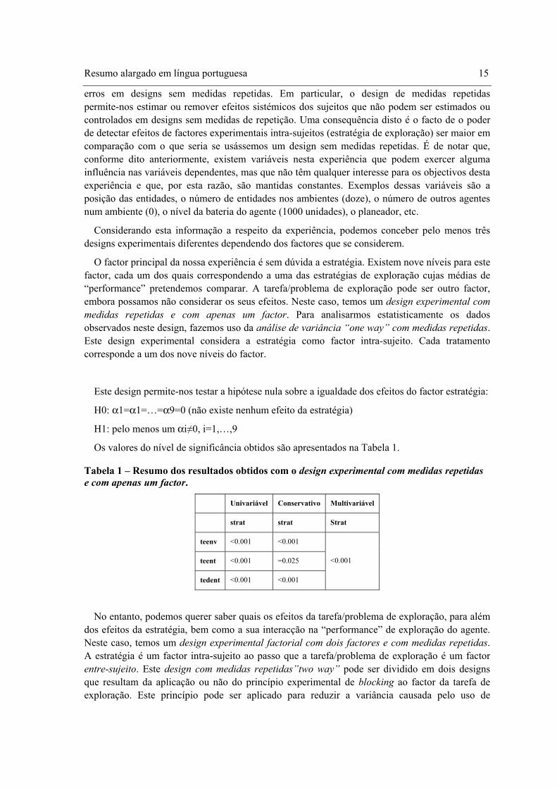
Resumo alargado em língua portuguesa 15
erros em designs sem medidas repetidas. Em particular, o design de medidas repetidas permite-nos estimar ou remover efeitos sistémicos dos sujeitos que não podem ser estimados ou controlados em designs sem medidas de repetição. Uma consequência disto é o facto de o poder de detectar efeitos de factores experimentais intra-sujeitos (estratégia de exploração) ser maior em comparação com o que seria se usássemos um design sem medidas repetidas. É de notar que, conforme dito anteriormente, existem variáveis nesta experiência que podem exercer alguma influência nas variáveis dependentes, mas que não têm qualquer interesse para os objectivos desta experiência e que, por esta razão, são mantidas constantes. Exemplos dessas variáveis são a posição das entidades, o número de entidades nos ambientes (doze), o número de outros agentes num ambiente (0), o nível da bateria do agente (1000 unidades), o planeador, etc.
Considerando esta informação a respeito da experiência, podemos conceber pelo menos três designs experimentais diferentes dependendo dos factores que se considerem.
O factor principal da nossa experiência é sem dúvida a estratégia. Existem nove níveis para este factor, cada um dos quais correspondendo a uma das estratégias de exploração cujas médias de “performance” pretendemos comparar. A tarefa/problema de exploração pode ser outro factor, embora possamos não considerar os seus efeitos. Neste caso, temos um design experimental com medidas repetidas e com apenas um factor. Para analisarmos estatisticamente os dados observados neste design, fazemos uso da análise de variância “one way” com medidas repetidas. Este design experimental considera a estratégia como factor intra-sujeito. Cada tratamento corresponde a um dos nove níveis do factor.
Este design permite-nos testar a hipótese nula sobre a igualdade dos efeitos do factor estratégia:
H0: α1=α1=…=α9=0 (não existe nenhum efeito da estratégia)
H1: pelo menos um αi≠0, i=1,…,9
Os valores do nível de significância obtidos são apresentados na Tabela 1.
Tabela 1 – Resumo dos resultados obtidos com o design experimental com medidas repetidas e com apenas um factor.
Univariável Conservativo Multivariável
strat strat Strat
teenv <0.001 <0.001
teent <0.001 =0.025
tedent <0.001 <0.001
<0.001
No entanto, podemos querer saber quais os efeitos da tarefa/problema de exploração, para além dos efeitos da estratégia, bem como a sua interacção na “performance” de exploração do agente. Neste caso, temos um design experimental factorial com dois factores e com medidas repetidas. A estratégia é um factor intra-sujeito ao passo que a tarefa/problema de exploração é um factor entre-sujeito. Este design com medidas repetidas”two way” pode ser dividido em dois designs que resultam da aplicação ou não do princípio experimental de blocking ao factor da tarefa de exploração. Este princípio pode ser aplicado para reduzir a variância causada pelo uso de
16 Resumo alargado em língua portuguesa
ambientes com diferentes complexidades ou diferentes amplitudes do campo de visão. Neste caso, estas variáveis podem ser consideradas como factores nuisance. Daqui resultam dois possíveis designs factoriais com medidas repetidas e com dois factores: design com medidas repetidas em que o problema/tarefa é um factor (chamado one-line-per-level setup - sem blocking) e design com medidas repetidas com blocking (a complexidade do ambiente ou o campo de visão podem ser usados para agrupar os sujeitos – problemas/tarefas de exploração). Consideramos este último tipo de design com blocking, que por sua vez pode ser divido em outros dois: design com medidas repetidas com três blocos de tarefas/problemas (a variável complexidade do ambiente é usada para agrupar os sujeitos - problemas/tarefas de exploração - em três grupos: ambientes de baixa, média e elevada complexidade) e design com medidas repetidas com dois blocos de tarefas/problemas de exploração (a variável campo de visão é usada para agrupar os sujeitos em dois grupos: campo de visão curto e longo).
Estes designs factoriais com medidas repetidas e com dois factores, sendo a um deles aplicado o princípio de blocking, permitem-nos testar a hipótese nula sobre a igualdade dos efeitos do factor estratégia:
H0: α1=α1=…=α9=0 (não existe nenhum efeito da estratégia)
H1: pelo menos um αi≠0 , i=1,…,9
Além disso, estes tipos de design permitem-nos testar a hipótese nula sobre a igualdade dos efeitos do factor que divide o problema/tarefa em categorias – complexidade do ambiente no primeiro tipo de design, ou campo de visão no segundo tipo de design:
H0: βj=0 , para todos os j (não existe nenhum efeito da categoria do problema/tarefa)
H1: pelo menos um βj≠0
Por fim, permitem-nos determinar se a estratégia ou a categoria do problema/tarefa interagem:
H0: (αβ)ij=0 , para todos os i,j (não existe efeito de interacção)
H1: pelo menos um (αβ)ij≠0
Por outras palavras, estes designs factoriais com blocking permitem-nos responder a três questões: (a) qual o efeito da estratégia?; (b) qual o efeito da categoria do problema/tarefa (complexidade do ambiente ou campo de visão)?; e (c) estas duas variáveis interagem, i.e., o efeito da estratégia depende da categoria do problema?
Os valores do nível de significância obtidos são apresentados na Tabela 2 e Tabela 3.
A estratégia é indubitavelmente um factor fixo. No entanto, para que os resultados sejam generalizados a todos os problemas de exploração, poderemos seleccioná-los aleatoriamente de uma população de problemas de exploração. Neste caso temos um terceiro tipo de design com dois factores, um fixo e outro aleatório. Este design é semelhante ao anterior. Assim, considera-se a estratégia como factor intra-sujeito e o problema/tarefa como factor entre-sujeito. Ao contrário do design anterior, este último factor é aleatório porque os problemas/tarefas considerados são apenas representativos de uma classe infinita de problemas/tarefas para os quais queremos generalizar os resultados. O princípio de blocking é usado com os mesmos objectivos de redução da variância, mas neste caso só faz sentido ser a complexidade do ambiente a variável de agrupamento, pois o campo de visão assume apenas dois valores e, portanto, é uma variável fixa, inviabilizando a aleatoriedade da escolha. O factor problema/tarefa é, desta forma, “aninhado” no
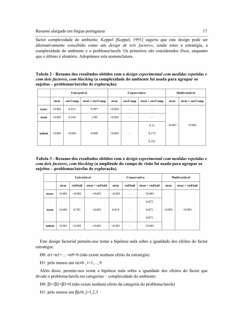
Resumo alargado em língua portuguesa 17
factor complexidade do ambiente. Keppel [Keppel, 1991] sugeriu que este design pode ser alternativamente concebido como um design de três factores, sendo estes a estratégia, a complexidade do ambiente e o problema/tarefa. Os primeiros são considerados fixos, enquanto que o último é aleatório. Adoptámos esta nomenclatura.
Tabela 2 - Resumo dos resultados obtidos com o design experimental com medidas repetidas e com dois factores, com blocking (a complexidade do ambiente foi usada para agrupar os sujeitos – problemas/tarefas de exploração).
Univariável Conservativo Multivariável
strat envComp strat × envComp strat envComp strat × envComp strat strat × envComp
teenv <0.001 0.823 0.997 <0.001 - -
teent <0.001 0.144 1.00 <0.001 - -
tedent <0.001 <0.001 0.048 <0.001 -
0.21
0.175
0.181
<0.001 <0.001
Tabela 3 - Resumo dos resultados obtidos com o design experimental com medidas repetidas e com dois factores, com blocking (a amplitude do campo de visão foi usada para agrupar os sujeitos – problemas/tarefas de exploração).
Univariável Conservativo Multivariável
strat visField strat × visField strat visField strat × visField strat strat × visField
teenv <0.001 <0.001 <0.001 <0.001 - <0.001
teent <0.001 0.781 <0.001 0.019 -
0.072
0.071
0.071
tedent <0.001 <0.001 <0.001 <0.001 - <0.001
<0.001 <0.001
Este design factorial permite-nos testar a hipótese nula sobre a igualdade dos efeitos do factor estratégia:
H0: α1=α1=…=α9=0 (não existe nenhum efeito da estratégia)
H1: pelo menos um αi≠0 , i=1,…,9
Além disso, permite-nos testar a hipótese nula sobre a igualdade dos efeitos do factor que divide o problema/tarefa em categorias – complexidade do ambiente:
H0: β1=β2=β3=0 (não existe nenhum efeito da categoria do problema/tarefa)
H1: pelo menos um βj≠0, j=1,2,3
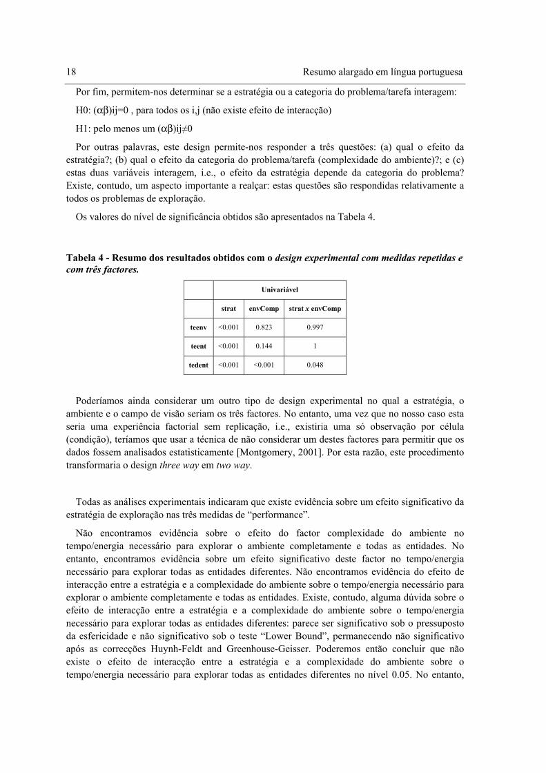
18 Resumo alargado em língua portuguesa
Por fim, permitem-nos determinar se a estratégia ou a categoria do problema/tarefa interagem:
H0: (αβ)ij=0 , para todos os i,j (não existe efeito de interacção)
H1: pelo menos um (αβ)ij≠0
Por outras palavras, este design permite-nos responder a três questões: (a) qual o efeito da estratégia?; (b) qual o efeito da categoria do problema/tarefa (complexidade do ambiente)?; e (c) estas duas variáveis interagem, i.e., o efeito da estratégia depende da categoria do problema? Existe, contudo, um aspecto importante a realçar: estas questões são respondidas relativamente a todos os problemas de exploração.
Os valores do nível de significância obtidos são apresentados na Tabela 4.
Tabela 4 - Resumo dos resultados obtidos com o design experimental com medidas repetidas e com três factores.
Univariável
strat envComp strat x envComp
teenv <0.001 0.823 0.997
teent <0.001 0.144 1
tedent <0.001 <0.001 0.048
Poderíamos ainda considerar um outro tipo de design experimental no qual a estratégia, o ambiente e o campo de visão seriam os três factores. No entanto, uma vez que no nosso caso esta seria uma experiência factorial sem replicação, i.e., existiria uma só observação por célula (condição), teríamos que usar a técnica de não considerar um destes factores para permitir que os dados fossem analisados estatisticamente [Montgomery, 2001]. Por esta razão, este procedimento transformaria o design three way em two way.
Todas as análises experimentais indicaram que existe evidência sobre um efeito significativo da estratégia de exploração nas três medidas de “performance”.
Não encontramos evidência sobre o efeito do factor complexidade do ambiente no tempo/energia necessário para explorar o ambiente completamente e todas as entidades. No entanto, encontramos evidência sobre um efeito significativo deste factor no tempo/energia necessário para explorar todas as entidades diferentes. Não encontramos evidência do efeito de interacção entre a estratégia e a complexidade do ambiente sobre o tempo/energia necessário para explorar o ambiente completamente e todas as entidades. Existe, contudo, alguma dúvida sobre o efeito de interacção entre a estratégia e a complexidade do ambiente sobre o tempo/energia necessário para explorar todas as entidades diferentes: parece ser significativo sob o pressuposto da esfericidade e não significativo sob o teste “Lower Bound”, permanecendo não significativo após as correcções Huynh-Feldt and Greenhouse-Geisser. Poderemos então concluir que não existe o efeito de interacção entre a estratégia e a complexidade do ambiente sobre o tempo/energia necessário para explorar todas as entidades diferentes no nível 0.05. No entanto,
Resumo alargado em língua portuguesa 19
estas conclusões são alteradas pelos testes multivariável que indicam uma interacção significativa entre estratégia e complexidade do ambiente sobre o tempo/energia necessário para explorar todas as entidades diferentes. O design three way indica também a existência deste efeito de interacção.
Encontramos um efeito significativo da amplitude do campo de visão no tempo/energia necessário para explorar todo o ambiente e todas as entidades diferentes, mas parece não existir tal efeito no tempo/energia necessário para explorar todas as entidades. Encontramos também evidência sobre o efeito de interacção entre a estratégia e a amplitude do campo de visão sobre tempo/energia necessário para explorar todo o ambiente. Existe, contudo, alguma dúvida sobre este efeito de interacção sobre o tempo/energia necessário para explorar todas as entidades: o teste foi significativo sob o pressuposto da esfericidade e não significativo sob o teste “Lower Bound”, permanecendo não significativo após as correcções Huynh-Feldt e Greenhouse-Geisser. Podemos assim concluir que não existe este efeito de interacção sobre o tempo/energia necessário para explorar todas as entidades no nível 0.05, mas existe tal efeito no nível 0.071. Estas conclusões são, no entanto, alteradas pelos testes multivariável que indicam a existência deste efeito de interacção. Nesta perspectiva, pode dizer-se que o efeito da estratégia é de certa forma controlado pela amplitude do campo de visão.
As estratégias que têm em conta a fome, quer isoladamente ou combinada com a curiosidade e a surpresa, apresentam melhor prestação que as restantes que têm em conta a surpresa e/ou a curiosidade.
A estratégia baseada na fome é a que requer menos tempo/energia porque o agente visita os destinos (entidades ou células fronteira) que estão mais perto do local em que se encontra, evitando assim a travessia de longas distâncias como acontece com outras estratégias. Esta estratégia é, no entanto, de pouco valor porque não tem em conta as características das entidades ou regiões, dependendo somente das posições das entidades. Para ambientes com entidades diferentes, mas com iguais localizações, a eficiência é a mesma. Esta estratégia pode ter piores prestações que outras se o objectivo for visitar as entidades diferentes de um ambiente o mais rápido possível. De facto, isto poderá acontecer se as entidades diferentes se localizarem nas últimas posições a serem visitadas.
A estratégia baseada na curiosidade faz com que o agente seleccione para visita as entidades e células fronteira que se estima maximizarem a novidade e entropia. São estas as entidades e células fronteira que proporcionam mais informação. No entanto, estas entidades e células fronteira não são frequentemente aquelas que estão mais perto, fazendo com que o agente se desloque por vezes grandes distâncias para obter o que ele espera ser uma elevada quantidade de informação nova. Os trajectos do agente são por esta razão erráticos e por isso mais morosos.
A estratégia baseada na surpresa faz com que o agente se desloque para entidades que contenham algo inesperado e que por esta razão provoquem surpresa. Esta estratégia relaciona-se bastante com a baseada na curiosidade, uma vez que ambas conduzem o agente a seleccionar destinos que proporcionem novidade e entropia. Existem contudo diferenças. Por exemplo, se a função de uma entidade tem elevada entropia com dez ou vinte funções equiprováveis, a curiosidade é elevada, mas a surpresa é nula. Para provocar surpresa, uma entidade ou região deverá, portanto, conter entropia, mas também se deverá verificar a condição de que os eventos não sejam equiprováveis. Além disso, quando existe baixa entropia (por exemplo, quando existem várias funções possíveis para uma entidade em que uma delas tem uma elevada probabilidade), a curiosidade é baixa mas a surpresa esperada é alta. Assim, esta estratégia motiva o agente a
20 Resumo alargado em língua portuguesa
deslocar-se para entidades de que se espera obter informação inesperada e não somente informação nova (esta é também forçosamente inesperada). Neste ponto, a curiosidade e a surpresa são semelhantes. Outra diferença importante entre estas duas estratégias é a de as células fronteira poderem causar uma curiosidade positiva, mas assume-se que não causam surpresa. Assim, embora ao usar estas duas estratégias o agente se comporte de maneira diferente, a “performance” é bastante similar e os trajectos de exploração, de certa forma erráticos, indicam que atravessa distâncias longas e desnecessárias que têm um forte impacto negativo na sua eficiência.
Quando a curiosidade e a surpresa são tidas em conta de forma independente ou combinadas com a fome, as trajectórias erráticas dão lugar a outras mais ordenadas e por isso a maior eficiência. De facto, a motivação para visitar entidades ou regiões longínquas que causam curiosidade ou de que se espera causar surpresa é refreada pela fome que se espera sentir nesses destinos. O resultado são estratégias que favorecem delicadamente entidades ou células fronteira que não estão demasiado longe, que causam uma considerável curiosidade e/ou de que se espera causar uma considerável surpresa.
Finalmente, uma outra experiência permitiu avaliar o processo de construção de mapas sem explorar o ambiente (não é permitido ao agente sair da posição inicial), i.e., baseando-se somente no conhecimento inicial que é dado ao agente ou que este adquiriu previamente ao explorar ambientes similares. Com o objectivo de determinar eventuais efeitos de diferentes níveis de conhecimento e da complexidade do ambiente na qualidade dos mapas construídos, o agente é colocado em vários ambientes de três tipos diferentes de complexidade (baixa, média e alta), cada vez com um nível de memória diferente. Concluiu-se que quanto maior o conhecimento, melhor a qualidade dos mapas e que quanto maior a complexidade do ambiente menor a qualidade dos mapas. Concluiu-se também que com uma memória de, por exemplo, quatro ou cinco elementos consegue-se reduzir para metade a inconsistência inicial do mapa. Este dado levanta uma outra questão de investigação relativamente aos resultados da experiência anterior: será que colocando o agente com conhecimento inicial adquirido noutros ambientes similares não se conseguem melhores “performances”? Tudo parece indicar que sim. É que os resultados da experiência anterior dependem muito da fiabilidade do processo de construção de mapas baseado na geração de expectativas. Se este processo for impreciso, os resultados serão deturpados porque o cálculo da surpresa esperada e da curiosidade basear-se-ão em dados incorrectos.
1.5 Conclusões
Nesta tese, estudámos o problema da exploração de ambientes desconhecidos que contêm entidades por agentes afectivos. O objectivo destes agentes afectivos exploradores é duplo: (i) aquisição e armazenamento em memória de mapas do ambiente – mapas métricos – nos quais as células ocupadas pelas entidades presentes no ambiente são representadas; (ii) construção de modelos dessas entidades. Examinámos o problema através de simulações devido às várias vantagens que esta abordagem oferece nomeadamente eficiência, maior controlo e melhor focalização da investigação. Esta abordagem de usar simulações só é possível porque as simplificações que fizemos não aparentam influenciar o valor dos resultados. Com esta abordagem da simulação em vista, desenvolvemos uma ferramenta para construir sistemas multi-agente que compreendam agentes afectivos e depois, com base nesta ferramenta, desenvolvemos uma aplicação para a exploração de ambientes desconhecidos, muito embora outras potenciais aplicações existam. Esta aplicação é um ambiente multi-agente simulado no
Resumo alargado em língua portuguesa 21
qual, para além de agentes inanimados (objectos), existem agentes exploradores interagindo de uma forma simples e cujo objectivo é explorar o ambiente, mapeando-o, analisando-o, estudando-o e avaliando-o.
As componentes da arquitectura que determinam o comportamento de exploração de um agente são os tipos de objectivos, os planos, os sentimentos e os desejos básicos. O agente possui objectivos para visitar entidades, regiões e sítios onde pode recarregar a sua bateria. Com base em estudos da Psicologia, o comportamento de exploração de um agente tem sido descrito desde há muito tempo pela ideia de que os organismos respondem à novidade e à mudança no ambiente que habitam quando não têm necessidades básicas (fome, sede, etc.). Se a novidade e mudança não estão presentes no ambiente, eles têm tendência para a procurar. Outras variáveis como a incerteza e conflito têm sido apontadas como determinantes do comportamento exploratório. A curiosidade/interesse é activada pela novidade, mudança e incerteza, enquanto que a surpresa é outro aspecto que é activada pela novidade, mudança e conflito. Isto explica porque confinámos as motivações básicas à fome mínima, ganho de informação máximo (redução da curiosidade) e surpresa máxima, e aos sentimentos correspondentes de fome, curiosidade, e surpresa. Cada um dos desejos básicos faz com que o sentimento correspondente seja maximizado ou reduzido. Os desejos básicos de fome mínima, ganho de informação máximo (redução da curiosidade), e surpresa máxima, direccionam o agente a minimizar o sentimento de fome, a maximizar o sentimento de surpresa e a reduzir o sentimento de curiosidade. O desejo de redução da curiosidade não significa que o agente não gosta de sentir curiosidade. Significa sim que o agente deseja executar acções que lhe façam sentir o máximo de curiosidade antes da sua execução, e, portanto, que conduzam a uma maximização da aquisição de informação após a sua execução e, consequentemente, a uma maximização da redução da curiosidade. A intensidade destes sentimentos é, assim, de primordial importância para calcular o grau de satisfação dos desejos básicos. Para a fome mínima e surpresa máxima, o grau de satisfação é dado pela fome e surpresa estimadas para depois da execução da acção, respectivamente, enquanto que para o ganho de informação máximo, é dado pela curiosidade sentida antes da execução da acção (a curiosidade é assim vista como o ganho de informação esperado).
O ciclo de raciocínio/tomada de decisão de um agente pode ser descrito resumidamente da seguinte forma. Cada agente, num determinado instante, analisa o ambiente à procura de entidades e calcula o estado actual do mundo (localização, estrutura e função dessas entidades) baseando-se na informação sensorial e na geração de expectativas para a informação em falta. O resultado deste passo é um conjunto de casos de entidades, cada um descrevendo uma entidade percepcionada. Depois, a memória de episódios e o mapa métrico são actualizados com base nesses casos de entidades. Então, novos objectivos do tipo visitEntity são gerados para cada entidade não visitada que se encontre no campo de visão com base nas tarefas-objectivo de planos do passado. Além disso, um objectivo do tipo visitLoc é gerado para cada célula fronteira [Yamauchi, 1998] (um outro tipo de objectivo é rechargeBattery). Os objectivos são então ordenados de acordo com a sua Utilidade Esperada [S. Russell & Norvig, 1995] que é calculada com base na contribuição do seu cumprimento para a satisfação dos desejos básicos. O primeiro objectivo da lista ordenada, i.e., o objectivo com maior Utilidade Esperada é considerado como intenção e um plano que foi previamente gerado para o seu cumprimento é executado.
Foram feitas três experiências principais. Uma conduziu à obtenção e avaliação de um modelo para a surpresa, outra consistiu no estudo dos efeitos na estratégia de exploração dos desejos básicos e correspondentes sentimentos, da complexidade do ambiente e da amplitude do campo de
22 Resumo alargado em língua portuguesa
visão, e outra consistiu na avaliação do processo de mapeamento usado pelo agente. Os resultados permitem concluir que o modelo computacional da surpresa é satisfatório, que a exploração de ambientes pode ser robusta e eficientemente realizada por agentes afectivos, e que, quanto maior a informação em memória e menor a complexidade do ambiente, melhores as estimativas feitas pelo agente na construção de mapas.
A próxima secção descreve detalhadamente as principais contribuições científicas desta tese, ao passo que a subsequente apresenta as limitações e questões não respondidas mais relevantes e identifica eventuais rumos de investigação para que se possam ultrapassar essas limitações e para que se possam encontrar respostas para essas questões.
1.5.1 Contribuições Científicas
As principais contribuições desta tese são:
• Exploração direccionada por afecto. A maioria das estratégias de exploração descritas na literatura assentam no cálculo da quantidade de informação a adquirir, considerando algumas também o custo de aquisição dessa informação. A nossa estratégia de exploração tem em conta estes aspectos, mas segue uma abordagem que tem como referência a forma como os humanos exploram, i.e., consideramos que o que leva um agente a adquirir o máximo de informação a um baixo custo reside na intensidade das motivações para reduzir a zero o sentimento de fome, maximizar a informação a adquirir (estimada pela intensidade do sentimento de curiosidade/interesse antes da aquisição da informação), e maximizar o sentimento de surpresa. São estas as motivações para reduzir ou maximizar sentimentos que conduzem o comportamento de um agente explorador. Por outras palavras, em vez de maximizarmos a quantidade de informação e minimizar o custo da sua aquisição, a nossa abordagem reside na maximização das motivações, sendo que as intensidades da surpresa e curiosidade são tidas como positivas, ao passo que a intensidade da fome é tida como negativa. Desta forma, privilegia-se indirectamente a selecção de acções que conduzam à aquisição de informação a baixo custo.
• Mapas tridimensionais de entidades. Os mapas desempenham um papel primordial em qualquer abordagem para a exploração de ambientes, ou não fossem eles o mecanismo de representação desses ambientes. Os mapas baseados em grelhas (grelhas de ocupação) são usados frequentemente. Nós propomos uma variante destes mapas chamada mapas de entidades. Estes são grelhas de ocupação diferentes nas quais cada célula <x,y,z> contém informação sobre quais as entidades que podem ocupá-la e respectivas probabilidades de isso acontecer. Este tipo de mapas resulta do facto de considerarmos que o objectivo da exploração de ambientes não é só o mapeamento do terreno, mas principalmente a aquisição de modelos das entidades que os habitam. Isto advém de uma outra diferença da nossa abordagem de exploração relativamente à maioria das outras abordagens: nós consideramos os ambientes como conjuntos de entidades. Esta perspectiva parece ser adequada para dar resposta ao desafio proporcionado pelos ambientes dinâmicos tridimensionais ao permitir manter a informação das posições das entidades. Ao contrário da maioria das abordagens, nós consideramos ambientes tridimensionais representáveis em mapas tridimensionais. Estes apresentam vantagens numa grande variedade de aplicações. Por exemplo, os arquitectos podem usar modelos tridimensionais para a
Resumo alargado em língua portuguesa 23
esquematização através de tecnologias de realidade virtual. Equipas de emergência, como os bombeiros, podem usar modelos tridimensionais para estudar a melhor forma de actuação em locais perigosos. Estes modelos tridimensionais são obviamente úteis para robots que operem em ambientes urbanos.
• Modelo computacional da surpresa. Propomos um modelo computacional para a surpresa que se baseia em modelos da Psicologia nos quais se defende que a surpresa é causada pelo inesperado. Um aspecto importante deste modelo computacional é o de não atribuir surpresa ao evento mais esperado de um conjunto de eventos.
• Incorporação de sentimentos numa arquitectura do tipo BDI. Ao propormos uma arquitectura do tipo BDI com qualidades mentais adicionais como os sentimentos e os desejos básicos, cumprimos o objectivo de estender a arquitectura BDI clássica.
• Uma abordagem para a definição da personalidade dos agentes. A Utilidade Esperada é uma função matemática que avalia os estados do mundo em termos da sua relevância positiva e negativa para os desejos básicos. É uma combinação de várias funções de Utilidade, uma para cada desejo básico. De acordo com a perspectiva pluralista da motivação [Havercamp & Reiss, 2003; McDougall, 1908; Reiss, 2000; Schwartz, 1992; B. Weiner, 1980], os desejos básicos contribuem para a definição da personalidade nos humanos. Essa função representa, no nosso caso, a aversão à fome, o gosto pela surpresa e pelo ganho de informação. A contribuição destas funções de Utilidade para a função da Utilidade Esperada global pode ser configurada, o que permite definir a personalidade dos agentes, dando por exemplo mais peso à fome, etc.
• Um modelo para a geração de expectativas. Infelizmente o mundo real não é claro para os agentes. Estes raramente têm acesso a todo o ambiente, principalmente porque as componentes de percepção e compreensão do ambiente são incompletas e incorrectas. É de facto demasiado difícil obter toda a informação de um ambiente complexo e dinâmico e é bastante provável que a informação acessível sofra distorções. No entanto, uma vez que o sucesso dos agentes depende muito da completude da informação sobre o estado do mundo, os agentes têm de seguir mecanismos alternativos para construir bons modelos do mundo, mesmo e especialmente quando este mundo é incerto. Propomos um modelo Bayesiano para a geração de suposições e expectativas para preencher lacunas na informação resultante da observação do mundo. Este modelo assenta em estudos de várias áreas, como a Psicologia, Ciências Cognitivas, e Etologia, que sugerem que os humanos e, no geral, os animais costumam ultrapassar esta limitação através da geração de suposições ou expectativas.
• Um processo de mapeamento tridimensional baseado na geração de expectativas. A maioria das abordagens de mapeamento são aplicadas a ambientes bidimensionais. No entanto, tal como foi dito anteriormente, os mapas tridimensionais podem ser úteis em múltiplas aplicações. Nesses domínios de aplicação, é de todo o interesse existirem métodos que possam gerar modelos tridimensionais a um baixo custo e com o mínimo de intervenção humana. Neste sentido, propomos uma técnica probabilística de mapeamento bastante simples para estes ambientes. Esta técnica assenta numa negociação entre o modelo de geração de expectativas anteriormente descrito e exploração do ambiente.
• ProCHiP (“Probabilistic, Case-based, Hierarchical task-network Planning”). Quando se pretendem aplicar sistemas de planeamento clássico ao mundo real, depressa se descobre
24 Resumo alargado em língua portuguesa
que os pressupostos em que assentam esses sistemas são bastante limitativos. Na verdade, cada um desses pressupostos leva o planeador a ignorar aspectos relevantes da maioria dos domínios de planeamento reais. O mundo real é, de facto, caracterizado pela presença de incerteza sob diversas formas. Para ultrapassar estas limitações, têm sido desenvolvidos diversos planeadores probabilísticos. No entanto, alguns planos no mundo real têm um formato hierárquico. Este aspecto motivou o aparecimento da técnica de planeamento com “Hierarchical Task-Networks” que consiste na aplicação de esquemas/métodos de redução para gerar uma hierarquia de tarefas. Contudo, o desenvolvimento de conjuntos de métodos que permitam a geração de todos os planos para muitas das aplicações reais demonstrou ser impraticável. O planeamento baseado em casos é uma técnica bastante prometedora para resolver este problema. Esta tese inclui a descrição de um planeador, chamado ProCHiP, que combina as técnicas de planeamento baseado em casos, planeamento com “Hierarchical Task-Networks” e planeamento probabilístico.
• Um ferramenta multi-agente baseada em afecto. Os agentes inteligentes são um novo paradigma para o desenvolvimento de software. Este novo paradigma de programação, também chamado programação orientada a agentes (um outro termo é computação baseada em agentes), parece ser apropriado para se lidar com certos domínios, oferecendo uma variedade de benefícios em comparação com outros paradigmas de programação como a programação orientada a objectos. Um considerável número de linguagens ou ferramentas têm sido propostas para permitir que as aplicações baseadas em agentes sejam projectadas e construídas facilmente. Nesta tese apresentamos o AMAS (“Affect-based Multi-Agent System”), um sistema multi-agente baseado nas ideias da computação afectiva e também em ideias do modelo BDI. Este sistema foi usado como plataforma para desenvolver a aplicação para a exploração de ambientes desconhecidos por agentes afectivos. O AMAS foi desenvolvido para ser usado como uma ferramenta para o desenvolvimento de aplicações baseadas em agentes. No entanto, encontra-se ainda numa versão preliminar. Por enquanto, é apenas um protótipo que precisa de melhoramentos e avaliação experimental. A versão actual é apropriada para aplicações nas quais as entidades (agentes) estão distribuídas num ambiente físico. É o caso da exploração de ambientes desconhecidos que é a única aplicação desenvolvida com o AMAS até ao momento. Exemplos de outras aplicações potenciais são o controlo de tráfico aéreo e logística de transportes (UM Translog).
Outros aspectos que também caracterizam esta tese são:
• Avaliação da qualidade dos mapas. Os mapas construídos pelos agentes exploradores devem ser avaliados para permitir tirar conclusões sobre a sua “performance”. Propomos uma abordagem que consiste em comparar os mapas construídos com aqueles que deviam ser construídos se os agentes fossem ideais, i.e., com os mapas que representam correcta e completamente o ambiente. Em experimentação com simulações isso pode ser facilmente conseguido através de um método que compara célula a célula dois mapas, contando as diferenças entre eles.
• Modelo computacional da fome. Este modelo é bastante simples, reflectindo a necessidade de uma fonte de energia por parte de um agente. A fome é expressa
Resumo alargado em língua portuguesa 25
simplesmente pela diferença entre a capacidade máxima de energia que um agente pode armazenar e a que tem num determinado momento.
• Geração autónoma e ordenamento de objectivos. Para que os agentes sejam totalmente autónomos, têm de ser capazes de gerar os seus próprios objectivos. Além disso, quando existem múltiplos objectivos simultaneamente, é difícil conseguir atingi-los simultaneamente. Assim, os agentes devem ser capazes de os ordenar de acordo com uma determinada regra de ordenamento. Propomos um algoritmo para gerar e ordenar os objectivos autonomamente. A fase de geração baseia-se na adaptação de objectivos de planos anteriores ao estado actual do mundo conforme percepcionado pelos sensores do agente. O ordenamento dos objectivos é feito tendo em conta a Utilidade Esperada calculada para cada objectivo.
1.5.2 Trabalho Futuro
O trabalho apresentado nesta tese é apenas um passo no longo caminho que há para percorrer no estudo do uso de agentes afectivos para desempenharem tarefas como a exploração de ambientes desconhecidos. Contudo, pensamos que esta tese proporcionou uns alicerces sólidos para um importante e interessante tópico da área de agentes autónomos e sistemas multi-agente. Embora esta tese proporcione uma demonstração prometedora do benefício e influência das emoções e motivações na exploração de ambientes desconhecidos, levanta contudo uma série de questões que deixámos sem resposta, deixando portanto espaço para trabalho futuro em várias áreas. De facto, tal como qualquer outro trabalho de investigação, não será surpreendente que levante mais questões do que aquelas que responde. Como afirma Bertrand Russell [B. Russell, 1959], “o que é importante não é tanto as respostas que são dadas, mas sim as questões que são colocadas”. Algumas destas questões e trabalho futuro são listadas de seguida:
• A generalidade do AMAS baseia-se principalmente na especificação do mundo, dos agentes, e dos planos disponibilizados aos agentes. As primeiras duas especificações não requerem o desenvolvimento de código em qualquer linguagem de programação. No entanto, a última exige a implementação de tarefas primitivas em C++. Até ao momento, os módulos dos desejos básicos e dos sentimentos encontram-se confinados ao conjunto de motivações que, de acordo com estudos da Psicologia e Neurociência, são essenciais para a exploração. De igual modo, as tarefas primitivas dos planos estão limitadas àquelas que são necessárias à exploração. A extensão desta plataforma de modo a que possa ser usada para desenvolver outras aplicações requer a extensão desses módulos, a implementação de outra tarefas primitivas em C++, e a extensão do módulo de geração de objectivos de forma a que outros objectivos possam ser gerados mediante a aplicação de estratégias de adaptação diferentes da substituição, ou permitindo que os agentes aceitem objectivos dados por outros agentes. Em suma, outras emoções, tais como o medo, a fúria, etc., e outras necessidades devem ser modeladas. No que diz respeito às tarefas primitivas, elas estão até ao momento confinadas à PTRANS, ATTEND e INGEST, que são baseadas nos actos primitivos de Schank [Schank, 1972]. Acreditamos que é possível lidar com outras aplicações através da implementação de todos os actos primitivos de Schank. Este seria um importante contributo para se conseguir a generalidade do AMAS, uma vez que se todos eles estiverem implementados, a especificação de uma aplicação não dependeria do desenvolvimento de código em C++. No entanto, só poderemos chegar a conclusões sobre este aspecto quando tivermos em mãos outras aplicações. A extensão
26 Resumo alargado em língua portuguesa
do módulo responsável pela geração autónoma e ordenamento de objectivos (ver pormenores mais à frente) baseia-se principalmente na consideração de outras estratégias de adaptação.
• A memória dos agentes beneficiaria da existência de mapas qualitativos/topológicos em simultâneo com os já existentes mapas métricos. Mapas métricos e qualitativos exibem vantagens e desvantagens ortogonais. Contrariamente aos mapas métricos, os qualitativos não contêm informação geométrica ou métrica, mas somente as noções de proximidade e disposição geográfica. Os mapas topológicos são representações mais eficientes para ambientes estruturados (por exemplo, edifícios), nos quais lugares distintos são frequentes (por exemplo, corredores, portas). O agente navega localmente entre lugares e, por isso, erros de movimentação não se acumulam globalmente como acontece nos mapas métricos onde existe um único sistema de coordenadas global. Ao invés, em ambientes não estruturados, nos quais o reconhecimento dos lugares é mais complexo, um robot que use somente informação topológica para se localizar pode facilmente desnortear-se. Assim, é lógico considerar a combinação das duas abordagens para se tirar partido das vantagens de ambas. Isso permite que a representação em mapas beneficie da eficiência dos mapas topológicos e da consistência e acuidade espacial dos mapas métricos.
• Na versão actual do AMAS, um agente não gera a representação analógica dos objectos a partir da proposicional e vice-versa [Kosslyn, 1980, 1985; Kosslyn et al., 1988]. No entanto, esta conversão é necessária se quisermos “transportar” os agentes para o mundo físico real.
• O modelo actual da surpresa pressupõe que esta é causada por entidades. Uma extensão deste modelo é necessária para lidar com eventos (conflito entre expectativas - incorporadas na versão actual em acções probabilísticas - e eventos futuros). De facto, a surpresa não é só causada por entidades físicas, mas também pelo conflito entre expectativas e qualquer informação adquirida do ambiente. Uma vez que as expectativas podem ser geradas também para, por exemplo, acções, o modelo actual da surpresa é certamente incompleto.
• Implementação da acção PTRANS usando uma variante determinista de iteração do valor, um algoritmo de programação dinâmica bastante popular [Bellman, 1957; Howard, 1960]. Esta é a abordagem seguida por [Anguelov et al., 2002; Biswas et al., 2002].
• Seria interessante estudar a inclusão de comportamento reactivo, combinando-o com o deliberativo (já existente), dando origem a uma arquitectura híbrida. Esta talvez seja a melhor arquitectura para agentes. Um agente com tal arquitectura possui duas componentes: uma que permite ao agente planear e decidir o que fazer usando uma abordagem simbólica; e outra que permite ao agente reagir a eventos externos de uma forma rápida e simples. Poderemos ainda considerar outras componentes, tais como raciocínio reflexivo ou meta-raciocínio, que permitam ao agente auto-avaliar os seus processos internos ao raciocinar sobre o seu próprio raciocínio e informação interna.
• A versão actual do AMAS inclui um algoritmo para permitir aos agentes a geração e ordenamento de objectivos. Este algoritmo pode ser melhorado no sentido de permitir ultrapassar algumas das suas limitações como por exemplo a impossibilidade de um agente suspender tarefas que está a executar (os planos são rígidos, não sendo permitido
Resumo alargado em língua portuguesa 27
ao agente colocar em espera uma tarefa que está a realizar para executar outra(s)) e a resolução de conflitos entre tarefas de vários agentes.
• Tornar mais eficiente o processo de decisão que se baseia no cálculo da Utilidade Esperada de uma tarefa. Existem alguns trabalhos cujas ideias podem vir a ser aproveitadas tais como a Teoria do Marcador Somático [Damásio, 1994] e a Teoria da Prospecção [Kahneman & Tversky, 1979].
• Incorporação de técnicas de negociação, colaboração e coordenação no AMAS de forma a permitir desenvolver uma técnica de planeamento multi-agente para a qual a versão actual do ProCHiP está consideravelmente preparada, ao permitir a determinação do identificador do agente que executa determinada tarefa.
• Evolução do AMAS para uma linguagem de programação orientada a agentes que permita desenvolver várias aplicações em diversos domínios como por exemplo na exploração da “World Wide Web”, bases de dados, controlo de tráfego aéreo, etc.
• Incorporação do software de um agente num robot, o que deve envolver a consideração de métodos para o problema da localização e mapeamento simultâneo (SLAM) tais como o EM [Burgard et al., 1999; Liu et al., 2001; McLachlan & Krishnan, 1997] e inclusão de um modelo de reconhecimento de padrões como, por exemplo, [Margaritis & Thrun, 1998]).
• Investigação de técnicas de cooperação e colaboração entre agentes exploradores.
• O AMAS é apropriado para lidar com ambientes dinâmicos. No entanto, este aspecto ainda não foi explorado, pelo que se apresenta como um desafio importante a ter em consideração.

29
Chapter 1 Introduction
his chapter introduces the subject of this thesis. We commence by presenting an initial motivation, followed by the thesis statement or research question and an account of how the research question will be addressed. Subsequently, we describe the main contributions
of our thesis. Finally, we present the organisation of this document.
1.1 Motivation
Science is still far from knowing how the human mind functions. One of the most intricate issues is the relationship between emotion and rationality. For many years, it was assumed that emotions are obstacles to intelligence. Since Plato, most philosophers have drawn a sharp line between reason and emotion, assuming that emotions interfere with rationality and have nothing to contribute to good reasoning. In his dialogue, the Phaedrus, Plato compared the rational part of the soul to a charioteer who must control his steeds, which correspond to the emotional parts of the soul [Plato, 1961]. Today, scientists are often taken as the paragons of rationality, and rational thought is generally assumed to be independent of emotional thinking. This traditional view on the nature of rationality has proposed that emotions and reason do not mix at all. For a human being to act rationally, he should not allow emotions to intrude in his reasoning processes. Research in neuroscience, however, has recently provided biological evidence indicating quite the contrary, showing that emotions play a fundamental role in perception, learning, attention, memory, and particularly planning and decision-making, as well as other abilities and mechanisms we tend to associate with basic rational and intelligent behaviour. In particular, recent studies of patients with lesions of the prefrontal cortex suggest a critical role for emotions in decision-making [Bechara et al., 1997; Churchland, 1996; Damásio, 1994]. Although the patients studied can perform well on a variety of intelligence and memory tests, when faced with real-life situations they seem to be unable to make good decisions. Apparently, these patients lack intuitive abilities, which, as many researchers think, may be based on memories of past emotions. These findings motivated Damásio and colleagues to suggest that human reasoning and decision-making involves several mechanisms at different levels, extending from those that regulate basic body functions, to those that deal with more cognitive control of complex strategies. An interesting and novel point of this view is that reasoning also depends on emotions and the feelings accompanying them.
The evolutionary consideration of emotion has contributed to understand its role in rational thought and decision-making. This role of emotion in the cognitive processes is considered just as another contribution to the main functions of emotion on humans: survival and well-being. Actually, survival and well-being depend on the decisions made during a lifespan. Wrong decisions may lead us to bad situations or even death. Thus, emotions are not obstacles to rationality, nor even harmless luxuries, but instead vital to intelligence.
If a human agent efforts lead him/her to attain an intended goal he/she tend to evaluate this outcome positively, and if his/her actions are thwarted the resulting emotion tends to be negative [Carver & Scheier, 1990]. Emotions are thus taken as rewards or punishments. Humans often do
T
30 Chapter 1. Introduction
things because they anticipate that they will make them feel better in some way (e.g., [Thayer et al., 1994]). According to simple principles of reinforcement, humans are more likely to repeat actions that had pleasant affective consequences in the past. But hedonism of this kind cannot account for all varieties of motivational phenomena. Opposed to those theories of hedonism and neo-hedonism [W. Cox & Klinger, 2004; Mellers, 2000; Zeelenberg et al., 2000], there is another theory or class of theories for the motivational effect of emotion on decision-making and action called emotion-specific action impulses theory [Frijda, 1994; Lazarus, 1991; B. Weiner, 2005]. These defend that there are emotion specific action tendencies for separate emotions (e.g., to flee or avoid danger in case of fear, to attack in case of anger, to help in case of pity, to make up for in case of guilt). Hedonism assumes the existence of a basic desire while emotion-specific action impulses theory assumes a pluralist view of motivation [Havercamp & Reiss, 2003; McDougall, 1908; Reiss, 2000; Schwartz, 1992; B. Weiner, 1980] by defending the existence of various basic desires (e.g., curiosity, power, hedonism, etc.). However, some theorists believe that the pleasure principle is indirectly at work even in these cases.
Motivation and emotion are thus highly intertwined and it is not always easy to establish clear boundaries between them. Emotion and motivation both depend on the relationship between the organism and its environment. Generally, motivation is defined as factors that cause an organism to behave in a certain way at a certain time. Motivation is more related with goal generation and action, while emotion is concerned with evaluative aspects of the relation of an agent with its environment. In the case of emotion, the emphasis is on how the situation makes the person feel. In the case of motivation, it is how the individual acts with respect to the situation that is of interest [Kuhl, 1986].
One of the features that characterize human beings is the tendency to explore the unknown parts of the environments they inhabit. Although exploration has existed as long as human beings, its peak is seen as being during the Age of Exploration, a period from the early 15th century and continuing into the early 17th century, when European navigators traveled around the world discovering new worlds and cultures. These big endeavours, together with the exploration of the outer space, the planets and satellites of our solar system today, are remarkable examples of the exploratory spirit of humankind. There are no limits for human exploration: from inhospitable volcanoes, mountains or oceans, to hostile planets such as Mars, and satellites such as Titan and the Moon, human beings are always trying to know more about their environment in spite of its adversity.
But what motivates this exploratory behaviour? James’ “selective attention” [James, 1890], Freud’s “cathexis” [Freud, 1938], and McDougall’s “curiosity instinct” [McDougall, 1908] are fundamental concepts concerning the relationship between motivation and exploratory behaviour. This exploratory behaviour has for a long time been expressed by the idea that organisms respond to the novelty and change in the environment they inhabit in the absence of known drives (thirst, hunger, etc.), and if novelty and change is not present in the environment, organisms tend to seek it. Evidence for this behaviour in a variety of species was provided by a number of authors [Lester, 1969]. In human beings, this kind of behaviour is already present in infants even in the first hours of life, as documented by a number of researchers who have studied selective attention in infants which is a simple form of exploratory behaviour. Infants prefer certain visual patterns over others. They do not treat with equal importance the multitude of stimuli. They explore the environment with their eyes, gazing at the more interesting objects which are those that provide novel stimuli. Some of the early researchers who showed that organisms tend to explore novel
Chapter 1. Introduction 31
objects or places in the absence of any known drives, called it the exploratory drive [Butler, 1953, 1954, 1957, 1958; Montegomery, 1952, 1953, 1954, 1955]. Among the investigators that have adopted the ideas of McDougall about curiosity are Berlyne [Berlyne, 1950] and Shand [Shand, 1914]. For these authors, curiosity is the psychological construct that has been closely related with this kind of behaviour. Considering that curiosity was innate and that it could also be acquired, Berlyne [Berlyne, 1950] argues that novel stimulus elicits curiosity, which diminishes with continued exposure to the stimulus. In later work [Berlyne, 1955, 1960, 1967], Berlyne elaborated and extended his early theory of curiosity. In addition to novelty, other variables such as change, surprisingness, complexity, uncertainty, incongruity and conflict also determine this kind of behaviour related to exploratory and investigative activities. Sharing similar ideas with Berlyne and McDougall, Shand [Shand, 1914] defined curiosity as a primary emotion consisting of a simple impulse to know, which controls and sustains the attention and provokes the body movements that allow one to acquire information about an object. These approaches are closely related to the emotion concept of interest-excitement proposed by the differential emotions theory to account for exploration, adventure, problem solving, creativity and the acquisition of skills and competencies in the absence of known drives [Izard, 1977, 1991]. In fact, the terms curiosity and interest are used more or less as synonyms, for instance, by Berlyne. Nunnally and Lemond [Nunnally & Lemond, 1973] carried out a series of experiments on the effects of novelty and complexity on visual exploration. They concluded that information conflict and novelty elicit and hold attention.
In conclusion, there is no doubt that novelty elicits curiosity/interest which is the psychological construct that accounts for exploratory behaviour. However, novelty seems to be insufficient to explain all exploratory behaviour. In addition to it, other variables such as change, surprisingness, complexity, uncertainty, incongruity and conflict also determine exploratory behaviour. Some of these variables elicit surprise, another psychological construct that also accounts for exploratory behaviour. If we also consider the recent advances in neuroscience that indicate that emotion influences the cognitive tasks of humans, and particularly planning and decision-making [Adolphs et al., 1996; Bechara et al., 1997; Damásio, 1994], exploration of unknown environments, as a decision-making process, is thereby influenced by emotion. Thus, ultimately, we may consider that there is a multitude of motivations and emotions behind the exploratory behaviour.
We may also relate exploration to creative evaluation. In fact, surprisingness and related concepts such as unpredictability or unexpectedness have been pointed out as relevant characteristics of a creative product, in addition to other commonly noted features such as novelty, originality, interestingness and appropriateness (also defined as usefulness, aesthetic value, rightness, etc.) [Boden, 1992, 1995; Jackson & Messick, 1967; Koestler, 1964; Lubart, 1994; Macedo, 1998; MacKinnon, 1962; Moorman & Ram, 1994; Ritchie, 2001; Saunders & Gero, 2001]. Furthermore, Boden argued that there is a distinction between mere novelty and creativity [Boden, 1995]. In her opinion, that distinction resides on the fact that creative products are not only novel but also unpredictable, unexpected and therefore surprising. According to Boden, unpredictability is the essence of creativity: creative products amaze us, shock us and delight us mainly because they are unexpected or unpredictable. The nature of the link between surprise and creativity is very strong. Surprise is usually considered as a property of a creative product, i.e., almost every creative product causes surprise at least the first time it is perceived. This means that the exploration of environments populated with objects may involve a kind of creative evaluation of those objects in that those that elicit more surprise, which are original, valuable, and different are those that amaze, shock and delight us and therefore are those that are
32 Chapter 1. Introduction
more interesting, getting our attention and probably provoking actions, i.e., visits in order examine them.
The human mind seems to be paradoxically unbounded. In order to extend their capabilities to deal easily with adverse situations or problems, humans were able to build systems, so-called artificial agents, that attempt to do intelligently similar things as they do or even better: accept percepts from the environment and generate actions correctly. This is paradoxical because it is simultaneous a proof of the ingenious aspect of human mind for going beyond itself but also a proof of the self awareness of its limitations to deal with certain situations or at least to deal with those situations easily. Attempting to understand and build those intelligent agents is the goal of the field of Artificial Intelligence (AI). Obviously, those agents do not (yet) possess the sensors, effectors and the mind of human beings, but instead cameras, robotic arms, software, etc. Yet, those agents exhibit forms of perception, forms of reasoning and decision-making, and forms of acting. Although they cannot do all the things humans do, perhaps they can do other sorts of things better than humans. To date, almost with no exception, all the capabilities of humans have been explored by AI and related fields such as Multi-Agent Systems, Robotics, or Distributed Artificial Intelligence, including, unsurprisingly, exploration of unknown environments.
Exploration of unknown environments by artificial agents (usually mobile robots) has, in fact, been an active field of research. Exploration may be defined as the process of selecting and executing actions so that the maximal knowledge of the environment is acquired. The result is the acquisition of models of the physical environment. So, exploration of unknown environments involves map-building but it is not confined to this process. Actually, this kind of exploration can be considered as two distinct topics. First, the agent or robot has to interpret the findings of its sensors so as to make accurate deductions about the state of its environment. This is the problem of map-building. This mapping problem itself has several aspects that have been studied intensively in the past. Among the most important aspects are the localization of the vehicle during mapping and the acquisition of appropriate models of the environment. The accuracy of the map depends on these factors. This fundamental problem in mobile robotics is called Simultaneous Localization and Mapping (SLAM) and is defined as a kind of chicken-and-egg problem as follows: while a robot navigates in an unknown environment, it must incrementally build a map of its surroundings and, at the same time, localize itself within the built map. The second but not less important aspect of exploration of unknown environments is that the agent or robot has to select its viewpoints so that the sensory measurements contain new and useful information. This is the problem of exploration itself. It involves guiding a vehicle in such a way that it covers the environment with its sensors. The accuracy of the map also depends on this choice of view-points during exploration.
Unfortunately, exploring unknown environments requires resources from agents such as time and power. There is a trade-off between the amount of knowledge acquired and the cost to acquire it. The goal of an explorer is to get the maximum knowledge of the environment at the minimum cost (e.g., minimum time and/or power). Several techniques have been proposed and tested either in simulated and real, indoor and outdoor environments, using single or multiple agents. The exploration domains include planetary exploration (e.g., Mars, Titan or lunar exploration), the search for meteorites in Antarctica, underwater mapping, volcano exploration, map-building of interiors, etc. The main advantage of using artificial agents in those domains instead of humans is that most of them are extreme environments making their exploration a dangerous task for human agents. However, the autonomy of agents still needs to be improved, as happens for instance in
Chapter 1. Introduction 33
planetary exploration which is still too human dependent (the plans are determined by a human operator as well as the interesting points to visit). Moreover, there is still much to be done especially in dynamic environments such as those mentioned above. Apart from the aspect of danger, real environments also contain objects. For example, office environments possess chairs, doors, garbage cans, etc., cities are comprised of many different kinds of buildings (houses, offices, hospitals, churches, etc.), as well as other objects such as cars. Many of these objects are non-stationary, that is, their locations may change over time. This observation motivates research on a new generation of mapping algorithms, which represent environments as collections of objects. At a minimum, such object models would enable a robot to track changes in the environment. For example, a cleaning robot entering an office at night might realize that a garbage can has moved from one location to another. It might do so without the need to learn a model of this garbage can from scratch, as would be necessary with existing robot mapping techniques. Object representations offer a second, important advantage, which is due to the fact that many environments possess large collections of objects of the same type. For example, most office chairs are examples of the same generic chair and therefore look alike, as do most doors, garbage cans, and so on. As these examples suggest, attributes of objects are shared by entire classes of objects, and understanding the nature of object classes is of significant interest to mobile robotics. In particular, algorithms that learn properties of object classes would be able to transfer learned parameters (e.g., appearance, motion parameters) from one object to another in the same class. This would have a profound impact on the accuracy of object models, and the speed at which such models can be acquired. If, for example, a cleaning robot enters a room it has never visited before, it might realize that a specific object in the room possesses the same visual appearance of other objects seen in other rooms (e.g., chairs). The robot would then be able to acquire a map of this object much faster. It would also enable the robot to predict properties of this newly seen object, such as the fact that a chair is non-stationary, without ever seeing this specific object move.
As mentioned above, emotion is essential for survival, well-being and communication in humans because, among other functions, it plays a central role in cognitive activities such as decision-making, planning and creativity. So, the question is why don’t artificial agents take advantage of emotions as humans do? What can emotional artificial agents do better than those that are not based on emotion? What can emotion offer to artificial agents? Certainly, not all the advantages that humans may benefit from are applicable to artificial agents. However, we are able to consider a number of situations in which we can see the emotional advantage such as in text-to-speech systems (by giving more intonation to speech), and in areas such as entertainment, preventive medicine, helping autistic people, in artificial pets, personalised agents that can act on the behalf of someone by selecting news, music, etc., according to someone’s mood, consumer feedback by measuring the emotions of consumers when dealing with a specific product, etc. Such applications require the abilities to recognise, express and experience emotions. Although research in AI has almost neglected the significant role of emotion in reasoning, this has already been addressed to some extent in present computational models of emotion (e.g., [Bates, 1994; Botelho & Coelho, 1998; Dias & Paiva, 2005; Elliott, 1992; Macedo & Cardoso, 2001a, 2001b; Maes, 1995; Oliveira & Sarmento, 2003; Ortony et al., 1988; Paiva et al., 2004; Pfeifer, 1988; Picard, 1997; Reilly, 1996; Schmidhuber, 1991]). This means some of those applications in which emotion may be advantageous are already implemented (e.g., artificial pets that are able to express emotions, emotion in text-to-speech systems, etc.) and hence they no longer only belong
34 Chapter 1. Introduction
anymore to science fiction, although they may require further improvements. Yet, other applications still belong to the realms of science fiction such as the computer HAL [Clarke, 1997].
In the specific case of the exploration of unknown environments, it might be useful to take emotions into consideration in the process. As far as we know there is almost no work explicitly using emotions in this kind of task. We may consider that a few studies on exploration implicitly consider rudimentary forms of some motivations. For instance, when a few studies in the field of exploration make use of mathematical formulas that evaluate the parts of the environment that contain most information for the agent or evaluate the cost of acquiring it, they are, to some extent, modelling rudimentary forms, for instance, of interest or curiosity/interest and hunger, respectively. They are actually considering variables such as novelty, uncertainty, difference or change, which are, according to psychological studies, at the foundation of the process of elicitation of curiosity/interest.
In order to accomplish the task of building artificial agents that act and think like humans [S. Russell & Norvig, 1995], we should be able to give an agent the ability to explore unknown environments, in a human-like fashion, in addition to other human features. Furthermore, given the evidence from psychology and neuroscience that emotion plays a central role in cognitive abilities such as decision-making and planning, and considering that exploration involves decision-making, it is reasonable to consider that emotion and motivation influence that activity. We might dream of a robot exploring Mars or any other inhospitable planet, avoiding dangerous situations because it can experience fear, selecting the interesting things to visit because it can experience surprise and curiosity or some sort of interest, remembering to recharge batteries because it can feel hunger, etc. In addition, we might think of such a robot mapping the environment and building models of the objects it visits and analyzes so that they can be used in the future, not only to facilitate exploration, but also to provide better ways to survive and promote well-being. Obviously, in this thesis we can’t go to this extreme, but we may make a modest attempt to be one of the forerunners. Thus, we have developed a multi-agent system in which agents are affective in that they exhibit explicit models of emotions which play an important role in motivation. Besides the module of feelings which incorporates the models of emotions, other important modules are basic desires (basic motivations/motives), memory and reasoning. This latter module includes a sequence decision-maker, i.e., a planner. Although this platform has other potential applications, in this thesis, we use it to study the problem of exploring unknown environments populated with entities (objects and other agents) by autonomous, affective agents. Hence, using this platform we built a multi-agent environment in which, in addition to inanimate entities (objects), there are also animate agents interacting in a simple way and whose goal is to explore the environment, mapping, analyzing, studying and evaluating it.
1.2 Thesis Statement/Research Question
This thesis asserts that exploration of unknown environments populated with entities can be robustly and efficiently performed by affective agents. We investigate the role of some emotions and motivations on the performance of this task. We also examine the influence on those emotions and motivations, and consequently on exploration performance, of other aspects/variables of the agents and multi-agent system, such as the agents’ amplitude of the visual field, memory size and diversity of the memory contents as well as environment size and diversity.
Chapter 1. Introduction 35
1.3 Approach
In this thesis, we study the problem of exploring unknown environments populated with entities by affective autonomous agents. These agents are affective as they incorporate explicit models of affects, a broad term commonly used to all the kind of emotion, which play an important role in their motivations.
In this kind of work with multi-agent environments, one has two distinct approaches: using a simulated or a real environment. Some researchers build softbots and then use them in a simulated environment to test theories and algorithms. Others choose to build real world robots and run them on real world environments. It was necessary to choose between these two approaches.
Simulation has advantages. For example, one can see the results of an algorithm much more quickly using softbots in simulated environments than robots in real environments. The researcher is able to do experiments without the constraints of time and expense associated with using a real robot. In addition, simulations allow the researcher to focus more tightly on the precise aspect of the problem in which he or she is interested. If for example the research is centred on path planning there may be little value in worrying about the mechanical engineering problems of building a physical robot. Moreover, the researcher has more control over the variables of the system involved in the experiments.
But simulated environments have also a few disadvantages. To build a softbot that model a real robot the researcher has to abstract the essential features of the robot being modelled. This abstraction necessarily involves some degree of simplification. In mobile robotics this is most often noticeable in the modelling of sensors. Simulated sensors are most of the times different from real sensors. Although research based on such simplifications may well produce useful results, there is always the danger that in the simplification process one has ignored a vital property of the robot so that the results will not be valid when tested on a real robot. Therefore, simulation is a good approach if all the variables that influence the results in real world are captured by the computer model. We chose to use simulations for the advantages just mentioned above and because the simplifications (presented below in this section) that we made do not seem to influence the results. For instance, we made the assumption that the agents know their localization precisely (e.g., by using GPS) because this is not relevant to test the influence of emotion and motivation in exploration.
We have developed a multi-agent system comprising affective agents. Although we foresee a rather broad potential for this multi-agent system (as we will see in Chapter 6 and throughout the thesis, this depends mainly on the kind of basic desires, feelings, goals and plans installed in the memory of the agents), in this thesis we examine the ability of the affective agents to explore unknown environments. Therefore, we are not exactly applying the multi-agent system to any of the problems to which they are commonly applied such as process control, entertainment, or eComerce, but instead to the problem of exploring unknown environments, and, more precisely, to its simulation. Domains in which this ability is required include the exploration of inhospitable geographic regions, such as planets, by mobile robots. Another example is the World Wide Web.
Taking the multi-agent system as a platform, we developed a simulated environment in which, in addition to inanimate entities (objects), there are agents interacting in a simple way whose goal is to explore the environment. In doing so, they analyze, study and evaluate it and build its map.
36 Chapter 1. Introduction
We adopted the approach of considering agents as acting and thinking like humans [S. Russell & Norvig, 1995] and took the main ideas of the Belief-Desire-Intention (BDI) architecture to guide our architecture. Note, however, that we did not implement the BDI logic. In our platform, the architecture of an agent includes the following modules: sensors, memory/beliefs (for entities, plans, and maps of the environment), basic desires (basic motivations/motives), desires/goals, intentions, feelings, and reasoning. The key components that determine the exhibition of the exploratory behaviour in an agent are the kind of basic desires, feelings, goals and plans with which the agent is equipped. In our case, and according to the studies mentioned above, the agent is equipped in advance with the basic desires for minimal hunger, maximal information gain (reduce curiosity), and maximal surprise. Each one of these basic desires drives the agent to reduce or to maximize a particular feeling. The desire for minimal hunger, maximal information gain and maximal surprise directs the agent, respectively, to reduce the feeling of hunger, to reduce the feeling of curiosity (by maximizing information gain) and to maximize the feeling of surprise. It is important to note that the desire to reduce curiosity does not mean that the agent dislike curiosity. Instead, it means the agent desires selecting actions that maximize curiosity before performing them, because after executing them it is expected that they maximize information gain and therefore that they maximize the reduction of curiosity. The intensity of these feelings is, therefore, important to compute the degree of satisfaction of the basic desires. For the desires of minimal hunger and maximal surprise it is given by the expected intensities of the feelings of hunger and surprise, respectively, after performing an action, while for the desire of maximal information gain it is given by the intensity of the feeling of curiosity before performing the action (this is the expected information gain). The memory of agents is setup with goals and plans for visiting entities that populate the environment, regions of the environment and for going to places where the agent can recharge its battery. These are the goals and plans whose execution may lead to satisfy the basic desires with which the agent is equipped in advance for the purpose of exploration. The next paragraphs explain in more detail the modules of the architecture as well as their relationships.
The memory of an agent stores information (beliefs) about the world. This information includes the configuration of the surrounding world such as the position of the entities (objects and other animated agents) that inhabit it, the description of these entities themselves, and the descriptions of plans executed by those entities. The information is stored in several memory components. There is a metric (grid-based) map to spatially model the surrounding physical environment of the agent. Descriptions of entities (physical structure and function) and plans are stored both in the episodic memory and in the semantic memory.
Following the pluralist view of motivation [Havercamp & Reiss, 2003; McDougall, 1908; Reiss, 2000; Schwartz, 1992; B. Weiner, 1980], the module of basic desires (basic motivations/motives) contains a set of basic desires that drive the behaviour of the agent. Taking into account the studies about the motivations of exploratory behaviour described in the previous section, we considered, as noted above, the following basic desires: the desire for minimal hunger, maximal information gain (reduce curiosity), and maximal surprise. The desire for minimal hunger and for maximal information gain (reduce curiosity) are among the 16 basic desires proposed by Reiss [Reiss, 2000]. These basic desires are represented in a mathematical function, the Utility Function that evaluates states of the environment in terms of the positive and negative relevance for the basic desires. This function obeys the Maximum Expected Utility (MEU) principle [S. Russell & Norvig, 1995]. This Utility Function is a combination of the Utility Functions of each desire. It represents, in our case, the aversion against hunger and the like of
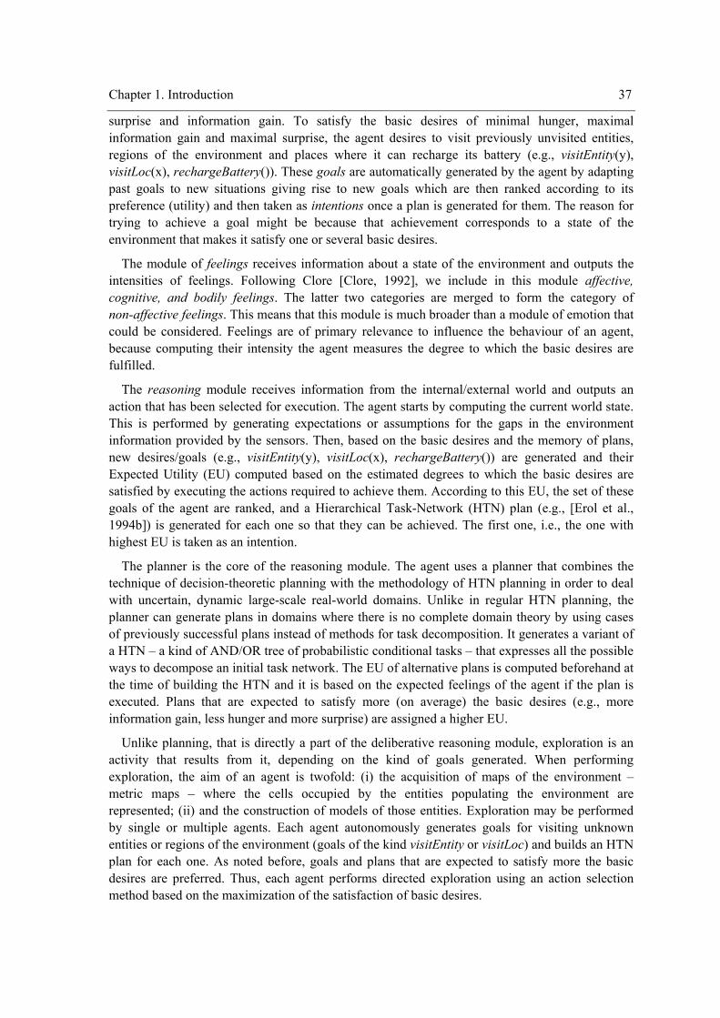
Chapter 1. Introduction 37
surprise and information gain. To satisfy the basic desires of minimal hunger, maximal information gain and maximal surprise, the agent desires to visit previously unvisited entities, regions of the environment and places where it can recharge its battery (e.g., visitEntity(y), visitLoc(x), rechargeBattery()). These goals are automatically generated by the agent by adapting past goals to new situations giving rise to new goals which are then ranked according to its preference (utility) and then taken as intentions once a plan is generated for them. The reason for trying to achieve a goal might be because that achievement corresponds to a state of the environment that makes it satisfy one or several basic desires.
The module of feelings receives information about a state of the environment and outputs the intensities of feelings. Following Clore [Clore, 1992], we include in this module affective, cognitive, and bodily feelings. The latter two categories are merged to form the category of non-affective feelings. This means that this module is much broader than a module of emotion that could be considered. Feelings are of primary relevance to influence the behaviour of an agent, because computing their intensity the agent measures the degree to which the basic desires are fulfilled.
The reasoning module receives information from the internal/external world and outputs an action that has been selected for execution. The agent starts by computing the current world state. This is performed by generating expectations or assumptions for the gaps in the environment information provided by the sensors. Then, based on the basic desires and the memory of plans, new desires/goals (e.g., visitEntity(y), visitLoc(x), rechargeBattery()) are generated and their Expected Utility (EU) computed based on the estimated degrees to which the basic desires are satisfied by executing the actions required to achieve them. According to this EU, the set of these goals of the agent are ranked, and a Hierarchical Task-Network (HTN) plan (e.g., [Erol et al., 1994b]) is generated for each one so that they can be achieved. The first one, i.e., the one with highest EU is taken as an intention.
The planner is the core of the reasoning module. The agent uses a planner that combines the technique of decision-theoretic planning with the methodology of HTN planning in order to deal with uncertain, dynamic large-scale real-world domains. Unlike in regular HTN planning, the planner can generate plans in domains where there is no complete domain theory by using cases of previously successful plans instead of methods for task decomposition. It generates a variant of a HTN – a kind of AND/OR tree of probabilistic conditional tasks – that expresses all the possible ways to decompose an initial task network. The EU of alternative plans is computed beforehand at the time of building the HTN and it is based on the expected feelings of the agent if the plan is executed. Plans that are expected to satisfy more (on average) the basic desires (e.g., more information gain, less hunger and more surprise) are assigned a higher EU.
Unlike planning, that is directly a part of the deliberative reasoning module, exploration is an activity that results from it, depending on the kind of goals generated. When performing exploration, the aim of an agent is twofold: (i) the acquisition of maps of the environment – metric maps – where the cells occupied by the entities populating the environment are represented; (ii) and the construction of models of those entities. Exploration may be performed by single or multiple agents. Each agent autonomously generates goals for visiting unknown entities or regions of the environment (goals of the kind visitEntity or visitLoc) and builds an HTN plan for each one. As noted before, goals and plans that are expected to satisfy more the basic desires are preferred. Thus, each agent performs directed exploration using an action selection method based on the maximization of the satisfaction of basic desires.
38 Chapter 1. Introduction
Having selected the simulation approach, we have made several assumptions that we think do not interfere with the purposes of this thesis, as follows:
• We confine the list of emotions and motivations to those that have been suggested as being closely related with exploratory behaviour in humans. That is, we consider only the feelings of surprise, curiosity/interest, and hunger, and the basic desires of minimal hunger, maximal information gain and maximal surprise;
• We do not address the components of emotional recognition and expression, restricting the model to the elicitation of emotions;
• We do not address the problem of recognizing aspects such as shapes of the objects or shapes of parts of them in a given environment. In the sequel we will assume that the robot can recognize some sets of shapes in objects and proceed to design algorithms based on this ability;
• We assume that the agents know their location precisely. Hence we avoid the SLAM problem, and particularly the localization problem since mapping is to some extent addressed by us;
• We assume that the agents possess ideal sensors, i.e., what is captured by a sensor is free of noise.
In order to confirm the hypothesis of this thesis that exploration of unknown environments populated with entities can be robustly performed by affective agents, we did a few experimental procedures.
First, we defined how exploration is evaluated. Following the research performed by others working on the problem of exploring unknown environments, there are two common dimensions for evaluating it: efficiency and effectiveness. Efficiency may be measured by the amount of knowledge acquired from the environment per unit of time. An efficient explorer acquires maximal knowledge in a minimal time. An agent that is able to acquire more knowledge in a time t1 is more efficient than another agent that acquires the same knowledge in a time t2>t1, which means that, from another point of view, for the same time t3, the former agent is able to acquire more knowledge than the latter. On the other hand, effectiveness is related to acquiring the information of a finite environment correctly and completely. An effective explorer is able to explore the entire environment. An effective agent is more efficient than another if it explores the entire environment before the other. In our approach, knowledge is measured in three complementary but related dimensions: the amount of the occupancy map acquired, the number and the diversity of models of entities acquired. These three dimensions are profoundly related since, for the same environment, the more models of entities acquired, the higher the probability of having acquired more information about the occupancy map. Another important aspect to take into account in the evaluation of exploration is that it is a two step process, involving the selection of viewpoints so that the sensory measurements contain new and useful information, and the interpretation of the findings of the sensors so as to make accurate deductions about the state of the environment. The first step prepares the second. It is of primary importance for the efficiency and effectiveness of an exploration strategy. Selecting the viewpoints that provide maximum information at a low cost (energy or time) enables an efficient exploration task. On the other hand those viewpoints should be selected so that all the information of the environment is acquired.
Chapter 1. Introduction 39
The map building step is more concerned with effectiveness, although it also influences efficiency. In fact, although it might involve more or less time to interpret the information provided by the sensors, this seems to have much less weight on efficiency, in comparison to the time taken to travel from place to place. On the contrary, the effectiveness of the exploration depends on the accuracy of the interpretation of the information provided by the sensors. Wrong interpretations may lead to inaccurate maps which means a partial failure in exploration. So, an evaluation of any exploration should take into account these distinct steps.
Second, in order to know whether affective agents can perform exploration efficiently and effectively, we did not confine to running an affective agent and measure its performance. Instead, we compared its performance with ordinary agents (i.e., non-affective agents). Furthermore, we went further and study what variables influence its behaviour, i.e., which affective components make it perform better. We therefore compared different exploration strategies. In our case, we compared the strategies resulting from the combination of surprise, curiosity and hunger.
Third, to guarantee that this comparison is valid, the agents should have good models of curiosity, surprise and hunger. We therefore ensured that their computational models are faithful to those of humans. This means that the computational models of surprise, curiosity and hunger should be valid models by accurately capturing the features of human models.
Finally, to test the robustness of affective agents when performing exploration, we tested them in several environments of different complexities, with different visual ranges.
In order to test the approach adopted in this thesis for exploring unknown environments, which relies on using affective agents, we experimentally investigated the relationship between the variables of the system, i.e., between variables that correspond to several aspects of affective agents such as emotions, motivations, memory size and diversity, etc., as well as variables that represent features of the environment such as environment size and diversity and (dependent) variables describing features of the exploration of unknown environments, such as efficiency and effectiveness (map quality). As a research project, this process was conducted starting by an exploratory data analysis which has led to a causal model involving the variables of the system and subsequently by confirmatory experiments in order to verify the hypothesis generated in the exploratory experiment [P. Cohen, 1995]. This experimentation follows the research performed by others working on the problem of exploring unknown environments. In fact, various researchers have tested, both in simulated and real world environments, different approaches to exploring unknown environments by changing some features of the system, such as the environment configuration and complexity, the number of agents, and their exploration strategies.
1.4 Scientific Contribution
The main contributions of this thesis are:
• Affect-directed exploration. Most of exploration strategies proposed in the literature rely on information gain and a few of them also consider the cost of acquiring knowledge. Our exploration strategy also takes into account these features but in a human-like fashion, i.e., we consider that the variables that lead an agent to acquire maximal knowledge at minimal cost reside in affect, i.e., in emotion and motivation. Surprise, curiosity/interest, and hunger are the constructs that drive the behaviour of the agents. In other words, instead of directly maximizing knowledge gain and minimizing cost, our approach relies
40 Chapter 1. Introduction
on making the agent to move to places in which it expects feeling minimal hunger, maximal surprise and maximize information gain (maximizes the reduction of the feeling of curiosity). In this sense, our approach seems to be broader than most of the approaches presented in the related literature so far.
• Three-dimensional entity maps. Maps cannot be neglected in any approach to exploration of unknown environments. They constitute the way the environment is represented as it is continuously explored. Grid-based metric maps (occupancy grids) are extensively used to deal with this problem. We propose a variant of this kind of map called entity maps. These are represented by a slightly different occupancy grid in which each cell <x,y,z> is associated to a set of pairs that indicate the entities that may occupy that cell and the respective probability. This kind of map results from the features that characterize our exploration task, namely that it is not confined to terrain mapping but also and mainly to acquiring models of the entities that populate the environment. This stems from another chief difference to most approaches to exploration: we consider the environment as a collection of entities. This view of environments seems to be suitable to respond to the challenge of three-dimensional dynamic environments by keeping track of the changes of the positions of entities. In contrast to most of the approaches, we deal with three-dimensional environments. In fact, maps in our approach are three-dimensional maps. Three-dimensional maps are useful for a range of applications. For example, architects and building managers may use three-dimensional models for design and utility studies using virtual reality technology. Emergency crews, such as fire fighters, could utilize three-dimensional models for planning how to best operate at a hazardous site. Three-dimensional models are also useful for robots operating in urban environments. Finally, accurate three-dimensional models could be a great supplement to the video game industry, especially if the model complexity is low enough for real-time virtual reality rendering.
• Computational model of surprise. We propose a computational model of surprise that relies on psychological models of surprise which maintain that surprise is elicited by unexpectedness. The model captures this idea and incorporates it in the computation of the intensity of surprise. Another feature, for example, is that the most expected event in a set of them does not cause surprise.
• Computational model of curiosity/interest. In contrast to surprise, there are already a few computational models to account for curiosity/interest. We propose our own, based on the idea that novelty and uncertainty elicit curiosity/interest.
• Incorporation of feelings into a BDI-like architecture. By proposing a BDI-like architecture with additional mentalistic qualities such as feelings and basic desires, we achieved the goal of extending the classic BDI architecture.
• An approach for defining agent’s personality. The EU function is a mathematical function that evaluates states of the environment in terms of the positive and negative relevance for the basic desires. It is a combination of the Utility Functions of the basic desires. According to the pluralist view of motivation [Havercamp & Reiss, 2003; McDougall, 1908; Reiss, 2000; Schwartz, 1992; B. Weiner, 1980], basic desires define the personality of humans. It represents, in our case, the aversion against hunger and the like of surprise and information gain. The contribution of these Utility Functions to the EU function can
Chapter 1. Introduction 41
be weighed, which means we can configure the personality of the agents by giving, for instance, more weight to curiosity than to hunger, etc.
• A model for the generation of expectations. Unfortunately, the real world is not crystal clear to agents. Agents almost never have access to the whole environment, mainly because of the incompleteness and incorrectness of their perceptual and understanding components. In fact, it is too much work to obtain all the information from a complex and dynamic world, and it is quite likely that the accessible information suffers distortions. Nevertheless, since the success of agents depends heavily on the completeness of the information of the state of the world, they have to pursue alternatives in order to construct good models of the world, even (and especially) when this is uncertain. We propose a Bayesian model for the generation of assumptions or expectations to fill in gaps in the present observational information. Our model is motivated by studies that are provided from various areas, such as psychology, cognitive science, and ethology, which suggest that humans and, in general, animals attempt to overcome this limitation through the generation of assumptions or expectations.
• A three-dimensional map-building process based on the generation of expectations. Most previous map-building approaches are applied to two-dimensional environments. As has already been described, three-dimensional maps are useful for a range of applications. In all of those application domains, there is a need for methods that can generate three-dimensional models at a low cost, and with minimum human intervention. We propose a straightforward probabilistic map-building technique for three-dimensional maps. This relies on the trade-off between exploitation and exploration. The exploitation relies on the model for the generation of expectations which enables the agent to make use of previously acquired knowledge about entities to generate assumptions/expectations for the entities that are visible, but not yet explored and therefore with missing information.
• A multi-agent tool. Intelligent agents are a new paradigm for developing software applications. This new paradigm of programming, also called agent-oriented programming (agent-based computing is another common term), seems to be appropriate to deal with certain kinds of domains, offering a variety of benefits in comparison to other programming paradigms such as object-oriented programming. A considerable number of languages or tools have been proposed so that agent-based applications can be designed and built easily. We introduce AMAS (Affect-based Multi-Agent System), a multi-agent system based on the notion of affect and also on ideas of the BDI model, that was used as a platform to develop the application for the exploration of unknown environments by affective agents. AMAS was developed to be used as a framework for building agent-based applications in general. Yet, AMAS is still in a preliminary version. For now it is simply a prototype needing further improvements and experimental evaluation. The current version is suitable for applications in which the entities (agents) are distributed in a physical environment. This is the case of the domain of the exploration of unknown environments which is the only application developed with AMAS up to date. Examples of other potential applications are air traffic control, and transportation logistics (UM Translog).
• Case-based, decision-theoretic, HTN planning. When we want to apply classical planning systems to problems that occur in uncertain, dynamic environments such as the real
42 Chapter 1. Introduction
world, we find that the assumptions they make can be severely limiting. Actually, each one of these assumptions leads the planner agent to ignore relevant aspects of most real world planning domains. In fact, the real world is characterized by the presence of uncertainty in different forms. In order to overcome these limitations, various probabilistic planning systems (decision-theoretic planners) have been developed. However, many planning decisions made in the real world are done in a hierarchical manner. This motivated the development of the HTN planning technique, which relies on the application of reduction schemas (methods) to generate a hierarchy of tasks. However, for many real-world applications, developing a collection of methods that completely models plan generation has been found to be unfeasible. Case-based planning is a promising technique to overcome this problem. This thesis includes the description of a planner, called ProCHiP (Probabilistic, Case-based Hierarchical Planning), which combines ideas from case-based planning, HTN planning, and decision-theoretic planning to deal with all these problems. It involves learning actions and their utility value.
Other aspects that also characterize this thesis are:
• Map quality evaluation. The maps built by the explorer agents must be assessed so that conclusions can be drawn with respect to their performance. We propose an approach that consists in comparing the maps built with those that should be built if the agent were an ideal agent, i.e., with a map that correctly represents the environment. In simulation experiments this can be easily achieved by comparing the maps cell by cell, counting the differences between them.
• Computational model of hunger. This model is quite simple, reflecting the need of an energy source by an agent. This is simply expressed by the difference between the total amount of energy that an agent can store and the amount of energy that is available at a given time.
• Autonomous generation and ranking of goals. In order to be fully autonomous, agents must be able to generate their own goals. Besides, when there are multiple goals occurring at the same time, it is impossible to accomplish them simultaneously. Therefore, agents should be able to prioritize them according to some ranking rule. We propose an algorithm to generate and rank goals autonomously. The generation phase is based on adapting goals from past plans to the entities that are within the agent’s sensors range. Prioritization is achieved by taking into account the EU computed for each goal.
1.5 Thesis Structure
The next chapter begins the examination of the problem of exploring unknown environments by affective agents by reviewing the work done in the related areas to date. At least seven areas are covered which reflects the wide range of subjects which had to be examined in order to deal with this problem. We divide those areas into two main categories: those that are central to this thesis and to which this thesis has a more direct contribution; and those areas to which this thesis does not have such a direct contribution but, because they are used frequently throughout the text, their central concepts must be presented in order to make this thesis more easy to read. The first areas are: agents and multi-agent systems, emotion and motivation, exploration of unknown
Chapter 1. Introduction 43
environments and the central area of this thesis, resulting from the combination of the previous three, which is the exploration of unknown environments by affective agents. Among the latter areas we present a review of knowledge representation, planning under uncertainty in dynamic environments (decision-theoretic planning), HTN planning, and creativity.
Chapter 3 introduces the prototype of the multi-agent system. This presentation is made from a general perspective. Hence, illustrative examples may not belong solely to the problem of exploration. When appropriate, examples from domains other than the exploration of unknown environments are given. The architecture of affective agents is described, including their modules such as sensors, memory (for entities, plans, and maps of the environment), goals and intentions, basic desires, feelings, and reasoning. Subsequently, the application of that affective-based multi-agent system to the problem of exploring unknown environments is presented. It includes a description of the exploration strategy as well as an illustrative example of it.
Chapter 4 describes the evaluation of our approach to the problem of exploring unknown environments. This evaluation involves the evaluation of aspects of the main processing modules of the architecture of agents that influence the exploration of unknown environments, especially the modules of basic desires and feelings.
Chapter 5 describes the evaluation of the work presented in this thesis by comparing it with other related studies.
Finally, in Chapter 6, we conclude with a summary of our contributions to the central areas of this thesis and describe some problems and issues that remain for future work.

45
Chapter 2 Background
his thesis is about affective agents that exhibit the ability to explore unknown environments. We build on ideas and concepts developed in the fields of agents and multi-agent systems as well as on affective computing (emotion and motivation) and
exploration of unknown environments. Other related areas include knowledge representation, planning under uncertainty in dynamic environments, hierarchical task-network planning, and creativity. Recent advances in psychology and neuroscience recognize the influence of emotion and motivation on reasoning, decision-making, and planning. This influence has been taken into account in several agent-based systems. In fact, the attribute of personality has been ascribed to agents, considered as almost as important as any other property such as reasoning (e.g., [Etzioni & Weld, 1995]).
In this chapter, we start our examination of the problem of exploring unknown environments by affective agents by reviewing the work done in related areas to date. Since, our thesis builds primarily on the fields of exploration, affective computing, and agents and multi-agent systems, we begin by reviewing each one of these fields independently. Firstly, we consider the field of agents and multi-agent systems, secondly, we shift to affective computing, and then we delve into exploration. Subsequently, we address the subject that joins together these primary fields, i.e., the subject of exploring unknown environments with affective agents. Finally, in order to understand our thesis, we briefly introduce, in a single section, the other specific fields that are also closely related but not central to our thesis. Such secondary areas are: knowledge representation, planning under uncertainty, hierarchical-task-network planning, and creativity. Although our work provides a contribution to these areas, mainly to hierarchical-task network planning, planning under uncertainty, and creativity, we decided not to include in this thesis any kind of evaluation of the parts of our work related to these areas, since this is not the goal of this thesis. Instead, the work that we did is used as a supporting tool. Hence, we decided not to incorporate an extensive description of these areas because they are not central to the subject of this thesis, however, we think some description is essential in that it provides an introduction to the terminology and ideas that are frequently used throughout this thesis.
2.1 Agents and Multi-Agent Systems
2.1.1 Agent: Definition and Taxonomies
The concept of agent was first introduced a few decades ago [Hewitt, 1977; McCarthy, 1959]. At the present time there are several other terms that are used such as intelligent agents, software agents and autonomous agents. The term agent is elusive. If we take a look at the most relevant papers on the subject, we verify that there is no universal definition of the term agent. Instead there is a myriad of definitions (see [Bradshaw, 1997; Franklin & Graesser, 1997; Luck & d’ Inverno, 2001]). To avoid introducing here an endless list of definitions, we present just a few of them that generically capture the idea of an agent. According to Wooldridge and Jennings [Wooldridge, 2001; Wooldridge & Jennings, 1995b], “an agent is a computer system that is
T
46 Chapter 2. Background
situated in some environment, and that is capable of autonomous action in this environment in order to meet its design objectives”. Franklin and Graesser [Franklin & Graesser, 1997] consider an agent as “a system situated within and part of an environment that senses that environment and acts on it, over time, in pursuit of its own agenda and so as to effect what it senses in the future”. Another generic definition is proposed by Russell and Norvig [S. Russell & Norvig, 1995]: “an agent is anything that can be viewed as perceiving its environment through sensors and acting upon that environment through effectors”. More definitions may be found in [Franklin & Graesser, 1997].
However, perhaps the most appropriate approach to define the term agent has been to characterize it according to certain aspects, i.e., describing the attributes that it must possess. Wooldridge and Jennings [Wooldridge & Jennings, 1995b] distinguish between weak and strong notions of agency. The former is less controversial and conceptualizes an agent as exhibiting the following list of properties:
• Autonomy: the ability to operate independently, i.e., to make its own decisions without the intervention of humans or others;
• Social ability: the ability to interact by negotiation and cooperation with other agents;
• Reactivity: the ability to perceive and respond to changes in the environment;
• Proactiveness: the ability to exhibit goal-directed behaviour by taking the initiative.
The strong notion of agency is much more controversial, although it is well accepted by researchers working in AI. According to this notion, in addition to the properties of the weak notion, agents are characterised by other attributes that belong to humans. Hence, in addition to autonomy, social ability, reactivity, and proactiveness, agents possess explicit mentalistic qualities such as knowledge, belief, intention, and obligation [Shoham, 1993], or even emotion (e.g., [Bates, 1994; Wright, 1997]).
Based on the works described in [P. Cohen et al., 1994; Etzioni et al., 1993; Etzioni & Weld, 1994; Knoblock & Arens, 1994], Etzioni and Weld [Etzioni & Weld, 1995] listed the following set of characteristics that agents are expected to exhibit:
• Autonomy, including goal-oriented, collaborative, flexible and self-starting behaviour;
• Temporal continuity: an agent is a running process, not a transitory or an ephemera event;
• Character: the property of possessing a credible personality or emotional state;
• Communication: the ability to communicate with other agents, including humans;
• Adaptability: the ability to learn and improve with experience;
• Mobility: the ability to transport itself from one place to another;
Several researchers have attempted not only to describe the attributes that agents should possess, but also distribute agents into classes or categories, i.e., they have proposed taxonomies for agents, according to the attributes they exhibit. Agents sharing similar attributes fall into the same class. The different classes result from the various combinations of the attributes that agents might possess. Examples of those classes are mobile agents, interface agents, information agents, etc. Thus, what defines a class or category of agents is the set of attributes that characterises it. This approach lists the attributes of restricted classes of agents instead of the general class of
Chapter 2. Background 47
agents. We present, as an example, the taxonomy of agents proposed in [Nwana, 1996; Nwana & Ndumu, 1997] as well as the attributes that are taken into account to classify agents. Other well known taxonomies have been proposed by Gilbert and colleagues [D. Gilbert et al., 1995], Moulin and Chaib-draa [Moulin & Chaib-draa, 1996], Franklin and Graesser [Franklin & Graesser, 1997], and Müller [Müller, 1998].
Nwana and Ndumu [Nwana, 1996; Nwana & Ndumu, 1997] suggest a typology for agents based on the following dimensions:
• Mobility: static or mobile;
• Thinking/behaviour paradigm: deliberative or reactive;
• Autonomy, cooperation and learning (these were considered the three primary attributes that agents should possess);
• Role: information or internet;
• Number of agent philosophies combined: hybrid or non hybrid;
• Versatile, trustworthiness, temporal continuity, ability to fail gracefully, and mentalistic attitudes such as beliefs, desires, intentions or even emotions (these were considered the secondary attributes).
According to Nwana, the combination of these dimensions gives rise to multiple categories of agents, such as static deliberative collaborative agents, mobile reactive collaborative agents, etc. However, because some of those categories do not exist in practice, he confined the list to the following categories:
• Collaborative agents;
• Interface agents;
• Mobile agents;
• Information/internet agents;
• Reactive agents;
• Hybrid agents;
• Smart agents.
2.1.2 Agent Architectures
Besides knowing both the attributes that characterise agents and the different types of agents that exist, it is important to know how agents are built, which are their constituent component modules and how these modules fit together and interact. Three main approaches have been proposed [Wooldridge & Jennings, 1995a, 1995b]: deliberative architectures, reactive architectures, and hybrid architectures. The first is also known as the symbolic AI paradigm or classical approach, assuming that the agent possesses an explicit, internal, symbolic model of the environment, employing logical or pseudo-logical reasoning in order to decide what actions to perform. On the contrary, the second approach does not assume that agents have symbolic models, while their behaviour is characterised by responding to the stimulus provided by the present state of the environment. The third approach, a combination of the previous two, attempt to involve both
48 Chapter 2. Background
reaction and deliberation in an effort to adopt the best of each approach. We now describe in more detail each one of these approaches, providing some examples.
The deliberative architecture has been extensively addressed by symbolic AI researchers. These researchers have long assumed that planning is an essential component of any artificial agent. Whether based on the forerunner STRIPS [Fikes & Nilsson, 1971] or on any other more recent approaches to planning such as those combining decision theory and utility theory (decision-theoretic planning) [Blythe, 1999a] or relying on hierarchical techniques [Erol et al., 1994b], various AI planning systems have been used as the primary component of artificial agents.
Besides AI planning, different deliberative architectures have been proposed based on the attitudes of belief, desire and intention [Bratman et al., 1988; A. Rao & Georgeff, 1991, 1995]. Examples of those architectures are IRMA [Bratman et al., 1988] and GRATE* [Jennings, 1993]. Based on a widely respected theory of rational action [Bratman et al., 1988], the BDI model of rational agency relies on giving primacy to beliefs, desires, and intentions in rational action. It is therefore a quite intuitive model that is based on practical reasoning – the process of reasoning that humans use everyday when deciding moment by moment which action to perform next. As in humans, a BDI agent has beliefs, i.e., information about the world, desires, i.e., states of the world that it prefers and wishes to happen, and intentions, i.e., the subset of the desired states of the environment the agent is committed to achieving.
However, the symbolic paradigm has generated a host of difficult problems which look insoluble in general. Examples of these problems are complexity (some problems, such as the planning task mentioned above, require algorithms of considerable complexity), and difficulty in solving some problems which people seem to manage easily (such as representing common sense knowledge). In order to overcome these difficulties, an alternative architecture for building intelligent agents has been proposed, called reactive architecture. Based on the findings of ethological research, Brooks [Brooks, 1985, 1986] argued that instead of building complex agents in simple worlds, we should follow the evolutionary path and start building simple agents that are able to bring fast, specific behaviours to bear in order to survive in the world much like animals do. The architecture that he proposed, called the subsumption architecture, is built in layers. Each layer gives the system a set of pre-wired behaviours. The higher levels build upon the lower levels to create more complex behaviours. The behaviour of the system as a whole is the result of many interacting simple behaviours. The layers operate asynchronously. The layers of the subsumption architecture are composed of networks of finite state machines augmented with timers called augmented finite state machines. The timers enable state changes after pre-programmed periods of time. Each augmented finite state machine has an input and output signal. When the input of an augmented finite state machine exceeds a predetermined threshold, the behaviour of that augmented finite state machine is activated (i.e., the output is activated). The inputs of augmented finite state machines come from sensors or other augmented finite state machines. The outputs of augmented finite state machines are sent to the agent’s actuators or to the inputs of other augmented finite state machines. Each augmented finite state machine also accepts a suppression signal and an inhibition signal. A suppression signal overrides the normal input signal. An inhibition signal causes output to be completely inhibited. These signals allow behaviours to override each other so that the system can produce coherent behaviour. The use of augmented finite state machines results in a tight coupling of perception and action, producing the highly reactive response characteristic of subsumption systems. However, all patterns of behaviour in
Chapter 2. Background 49
these systems are pre-wired. Augmented finite state machines are the only units of processing in the architecture. Thus, there are no symbols. Several additional extensions [Mataric, 1992] have been proposed to pure reactive subsumption systems. These extensions are also known as behaviour-based architectures. Capabilities of behaviour-based systems include landmark detection and map building, learning to walk, collective behaviours with homogeneous agents, group learning with homogeneous agents, and heterogeneous agents. A number of key features result from this architecture: no explicit knowledge representation is used; behaviour is distributed rather than centralized; response to stimuli is reflexive – the perception-action sequence is not modulated by cognitive deliberation; the agents are organized in a bottom-up fashion (thus, complex behaviours are fashioned from the combination of simpler, underlying ones); agents are extremely simple in terms of the amount of computation they need to do. Other examples of reactive architectures are those proposed in [Agre & Chapman, 1987; Chapman & Agre, 1986; Kaelbling & Rosenschein, 1990].
Various researchers defend the notion that the best architecture to build agents is that of combining the deliberative and reactive ones. An agent with such architecture exhibits two components: one that enables the agent to plan or decide what to do in a more complex fashion based on symbols; another that enables the agent to react to external events in a faster and simpler way. Examples of this kind of architecture are TouringMachines [Ferguson, 1992] and InterRRaP [Müller, 1997].
Recently, researchers such as Minsky [Minsky, 2000, 2006] and Sloman and colleagues [Sloman et al., 1994] have defended an architecture for agents that incorporates reactive and deliberative components in addition to other components such as reflexive reasoning or meta-management which, broadly speaking, involves reasoning about the internal information and reasoning processes which implies the existence of self monitoring and self evaluation functions.
Russel and Norvig [S. Russell & Norvig, 1995] distinguish four main types of agent designs/structures: simple reflex agents; agents that keep track of the world; goal-based agents; and utility-based agents. Simple reflex-agents correspond to the above mentioned reactive architecture, while agents that keep track of the world, goal-based agents, and utility-based agents correspond to two different kinds of deliberative architectures. In reflex-agents the decisions are pre-computed. Goal-based agents are much more evolved, flexible agents in comparison with reflexive agents. They employ reasoning about the desires of the agent. Utility-based agents decide what to do based on an evaluation of the outcomes of their actions. The alternative world states resulting from their possible actions are compared and the action that leads to the world state that provides higher happiness to the agent is preferred.
A closely related approach has been presented by Wooldridge [Wooldridge, 2001] in order to identify abstract architectures for intelligent agents. He also distinguishes between purely reactive agents, agents with state, and well as expressing the relevance of utility functions to the decision-making process of an agent.
2.1.3 Agent Environments
Agents cannot be dissociated from the environment they inhabit. Environments can be classified according to the following aspects [S. Russell & Norvig, 1995]: accessible versus inaccessible, deterministic versus nondeterministic, episodic versus non-episodic, static versus dynamic, and discrete versus continuous.
50 Chapter 2. Background
An environment is classified as accessible if the agent’s sensors perceive the complete state of the environment, otherwise it is inaccessible. In a deterministic environment, and contrary to what happens in a nondeterministic environment, the next state of the environment is completely determined by the current state and the actions selected by the agents. The category of episodic environment relies on the notion of episode. Each episode consists of the agent perceiving and then acting. In an episodic environment, as opposed to non-episodic environment, the agent need not think ahead because episodes are independent from each other, which means an agent’s action depends just on the episode itself and never on the actions performed in previous episodes. While an agent is making a decision, the environment may or may not change. In the former case the environment is classified as dynamic while in the latter case it is called static. In a discrete environment there is a limited number of distinct, clearly defined perceptions and actions, while in a continuous environment there is an immeasurable number of choices for action and perception.
2.1.4 Multi-Agent Systems: definition and taxonomies
When more than one agent (whatever the properties or architecture they have) are put together in an environment (no matter what properties it has), interacting with one another, the result is called a multi-agent system [Weiss, 1999; Wooldridge, 2001]. This interaction implies that additional capabilities are required by agents, in addition to those already exhibited by the individual agents such as planning, learning, etc. In fact, the interaction between agents requires abilities such as cooperation, coordination and negotiation. Moreover, the capabilities of learning or planning may also be different in order to adapt to the social aspect of the environment.
Decker [Decker, 1987] presents a taxonomy for the field of distributed artificial intelligence based on the following dimensions:
• Agent granularity (coarse versus fine);
• Heterogeneity of agent knowledge (redundant versus specialised);
• Methods of distributing control (benevolent versus competitive, team versus hierarchical, static versus shifting roles);
• Communication possibilities (blackboard versus messages, high-level versus low-level, content).
From an application perspective, Parunak [Parunak, 1996] argues that the most important characteristics of a multi-agent system are:
• System function;
• Agent architecture (degree of heterogeneity, deliberative versus reactive);
• System architecture (communication, protocols, and human involvement).
Stone and Veloso [Stone & Veloso, 1997] present a taxonomy for multi-agent systems along the following agent aspects: degree of heterogeneity and degree of communication. The three combinations of these dimensions give rise to the classification of multi-agent systems as homogeneous non-communicating agents, heterogeneous non-communicating agents, and heterogeneous communicating agents.
Chapter 2. Background 51
Logan [Logan, 1998] outlines a classification scheme for agent-based systems along the following dimensions: the features of the environment in which the agent system is embedded, the types of actions it can perform, and the kinds of goals and beliefs that can be attributed to it.
Other overviews of distributed artificial intelligence and multi-agent systems are, for instance, [Bond & Gasser, 1988; Vlassis, 2003].
2.1.5 Agent and Multi-Agent Systems Applications
Today, multi-agent systems have already been applied to a wide range of domains. Two main types of agent applications have been distinguished: those in which agents are decision-makers, i.e., they are implemented to act instead of or to advice humans (decision making is placed in the hands of agents), or as simulation tools, i.e., they are implemented in order to provide a better understanding of a certain system. Another common approach to divide agent applications is that of distinguishing between single-agent and multi-agent systems [Wooldridge, 2001]. Whatever the type of application, its implementation is based on the key abstraction of agent rather than procedures, abstract data types or objects. Nowadays, intelligent agents are a new paradigm for developing software applications [Jennings, 2001; Wooldridge, 1998, 2001]. This new paradigm of programming, also called agent-oriented programming (agent-based computing is another common term) [Shoham, 1990, 1993] seems to be appropriate to deal with certain kinds of domains, offering a variety of benefits in comparison to other programming paradigms such as object-oriented programming, expert systems or distributed computing. Those domains to which they are more suitable include problems that are inherently (physically or geographically, or even in terms of time) distributed, where independent processes can be clearly distinguished, or those requiring the interconnection and inter-operation of multiple autonomous systems. The usefulness and benefits of multi-agent systems are clearly claimed in [Jennings & Wooldridge, 1997; Stone & Veloso, 1997].
A considerable number of languages or tools have been proposed so that agent-based applications can be designed and built easily. Among them, we may refer to AGENT0 [Shoham, 1993], PLACA [Thomas, 1993], PRS [Georgeff & Ingrand, 1989; Georgeff & Lansky, 1987; K. Myers, 1997] and all the latter BDI-based multi-agent tool, which in a way or another are based on PRS, such as JACK [Busetta et al., 1999; Howden et al., 2001], dMARS [d’Inverno et al., 1997], AgentSpeak [Bordini et al., 2002; Bordini & Moreira, 2004; A. Rao, 1996], JADEX [Pokahr et al., 2005], SPARK [Morley & Myers, 2004], and 3APL [Dastani et al., 2003] languages. A more comprehensive description of these and other agent-oriented programming languages can be found in [Badjonski, 2003; Nwana & Wooldridge, 1996; Wooldridge & Jennings, 1995a]. Besides these tools, methodologies to support the analysis and design of agent-based systems have also been developed [Iglesias et al., 1998; Wooldridge, 2001] such as GAIA [Wooldridge et al., 1999, 2000], and the AAII [Kinny et al., 1996] which relies on the PRS-based BDI technology [Georgeff & Lansky, 1987] and dMARS system [d’Inverno et al., 1997]. As a complement to these tools, various studies have been made so that the development of an agent-based system is successfully performed [Wooldridge & Jennings, 1998, 1999].
Regarding the type of domain application, agents have been applied in a huge variety of areas such as workflow and business process control, manufacturing and traffic control, information retrieval and management, electronic commerce, social simulation, air traffic control, air-combat modelling, patient monitoring, health care, games, interactive theatre and cinema [Jennings et al.,
52 Chapter 2. Background
1998; Jennings & Wooldridge, 1997; Luck et al., 2003; Parunak, 1999; Wooldridge, 2001]. However, more application domains are expected to be covered in the next few years. A few of the most prominent applications in the above mentioned domains are considered below. Our aim is not to make a complete survey, but instead to present representative examples which are historically significant in those above mentioned domains. Other applications of the extensive list are presented in conference proceedings (e.g., of the International Joint Conference on Autonomous Agents and Multi-Agent Systems [Dignum et al., 2005; Gini & Ishida, 2002; Jennings & Tambe, 2004; Nakashima et al., 2006; Wooldridge & Rosenschein, 2003]), and journals (e.g., Autonomous Agents and Multi-Agent Systems – e.g., [Wooldridge & Sycara, 2006]) of the area.
ARCHON [Jennings, 1996b], a software platform for building multi-agent systems, is perhaps the best known agent-based process control system that has been applied in different domains, including electricity transportation management and particle accelerator control.
In manufacturing, applications have addressed areas of configuration design of manufacturing products, collaborative design, scheduling and controlling manufacturing operations, controlling a manufacturing robot, and determining production sequences for a factory. YAMS [Parunak, 1987] is an agent-based system whose goal is to efficiently manage the production process at the various factories belonging to a single company. Each one of these factories and each one of its components is represented by an agent.
Currently undergoing field trials at Sydney airport, OASIS [Ljunberg & Lucas, 1992] is an air-traffic control system implemented using the AII methodology [Kinny et al., 1996] relying on PRS-based BDI technology [Georgeff & Lansky, 1987] and dMARS system [d’Inverno et al., 1997]. Its aim is to assist an air-traffic controller in managing the flow of aircraft at an airport, offering estimates of aircraft arrival times, monitoring aircraft progress against previously derived estimates, informing the air-traffic controller of any errors, and finding the optimal sequence in which to land the aircraft. To do that, each aircraft that enters Sydney airspace and the various air-traffic controller systems are represented by an agent.
The complex problem of information overload, resulting from the large amount of information that is available nowadays in information repositories such as databases, e-mails or the Web, requires effective solutions. These solutions are, broadly speaking, information filtering, so that only the relevant information is provided, and information gathering, by effectively and efficiently selecting the information that meets our requirements. Agents have been widely proposed as a suitable approach to implementing these solutions. To do so, agents may be used to search the information repositories, acting on behalf of some user. There are already a few applications based on these ideas, such as MAXIMS, NewT [Maes, 1994] and Zuno Digital Library (ZDL) [Jennings & Wooldridge, 1997]. MAXIMS is an electronic mail filtering agent that learns to prioritize, delete, forward, sort, and archive mail messages on behalf of a user. The agent monitors the user and uses the actions the user makes as a lesson on what to do. Depending upon threshold limits that are constantly updated, MAXIMS will guess what the user will do. Upon surpassing a degree of certainty, it will start to suggest to the user what to do. NewT is an Internet news filtering program that takes, as input, a stream of Usenet news articles, and gives, as output, a subset of these articles that is recommended for the user to read. The user gives NewT examples of articles that would and would not be read, and NewT will then retrieve articles. The user then gives feedback about the articles, and thus NewT will then be trained further on which articles to retrieve and which articles not to retrieve. NewT retrieves words of interest from an article by performing a full-text analysis using the vector space model for documents. The ZDL system is a
Chapter 2. Background 53
multi-agent system that enables a user to obtain a single, coherent view of incoherent, disorganized data sources such as the World Wide Web. Agents in ZDL play one of three roles: consumer – represents end users of the system, who can be thought of as consuming information; producer – represents content providers who own the information that customers consume; and, facilitator – mapping between consumers and producers. Consumer agents in the system are responsible for representing the user’s interests. They maintain models of users, and use these models to assist them, by proactively providing information they require, and shielding them from information that is not of interest. ZDL thus acts both as an information filter and an information gatherer.
Although it is still not fully autonomous, an increasing amount of trade is being undertaken by agents in eCommerce, and there are already several interesting applications. Kasbah [Chavez & Maes, 1996], a simple electronic marketplace in which agents buy and sell goods, is one of them. Another is Jango [Doorenbos et al., 1997], a personal shopping assistant able to search on-line stores for product availability and price information.
In workflow and business process management, the aim is to automate the processes of a business, ensuring that a document flow is maintained and managed within an organization. Developed for British Telecom, ADEPT [Jennings, 1996a] is an example of an agent-based workflow management system, aimed at providing customers with a quote for the installation of a network that satisfies the customer’s requirements. In ADEPT, agents were created for the British Telecom departments that are involved in this activity, namely the Customers Service, Design, Surveyor, and Legal departments. In addition, an agent was also created for each person in those departments. ADEPT uses an architecture that has been developed in the GRAETE* [Jennings, 1993] and ARCHON [Jennings, 1996b] projects.
Guardian [Hayes-Roth et al., 1995] is one of the earliest and perhaps the best known system in patient monitoring. Developed for Surgical Intensive Care Units, it manages patient care. Other examples of more recent applications of agent-based systems in medicine are described in [Cortés et al., 2002; Moreno, ; Shankararaman, 2000].
In entertainment and leisure, agents have an obvious role in computer games, interactive theater and cinema, and virtual environments. These domains are characterized by involving animated characters, which can obviously be represented by agents. Hence, it is no surprise that agents have been used to develop computer games such as the highly successful Quake [idSoftware] or Creatures [Gameware], which provides a rich, simulated environment containing a number of synthetic agents that a user can interact with in real-time. Several other applications of agent-based techniques to computer games are described in [Wavish & Graham, 1996]. Agents have also been used in cinema to play out roles analogous to those played by real, human actors, such as in Titanic [Cameron, 1997]. More recently, the Massive agent system [MassiveSoftware], the premier used for generating crowd-related visual effects and character animation, was used to achieve visually impressive battle-scenes in the second of the Lord of the Rings film trilogy, The Two Towers [Walsh et al., 2002]. Although the battle scene was broadly predetermined, the movement and action of each individual character is controlled by perceiving and responding to the artificial environment and to other characters. Finally, the development of believable agents has been investigated in order to construct simulated worlds consisting of synthetic characters that have human-like behaviour. The aim is to give users the experience of living in those worlds interacting with those synthetic characters and not merely watching them. The OZ project [Bates, 1994] is a nice example of this kind of agent-based application in which agents exhibit an
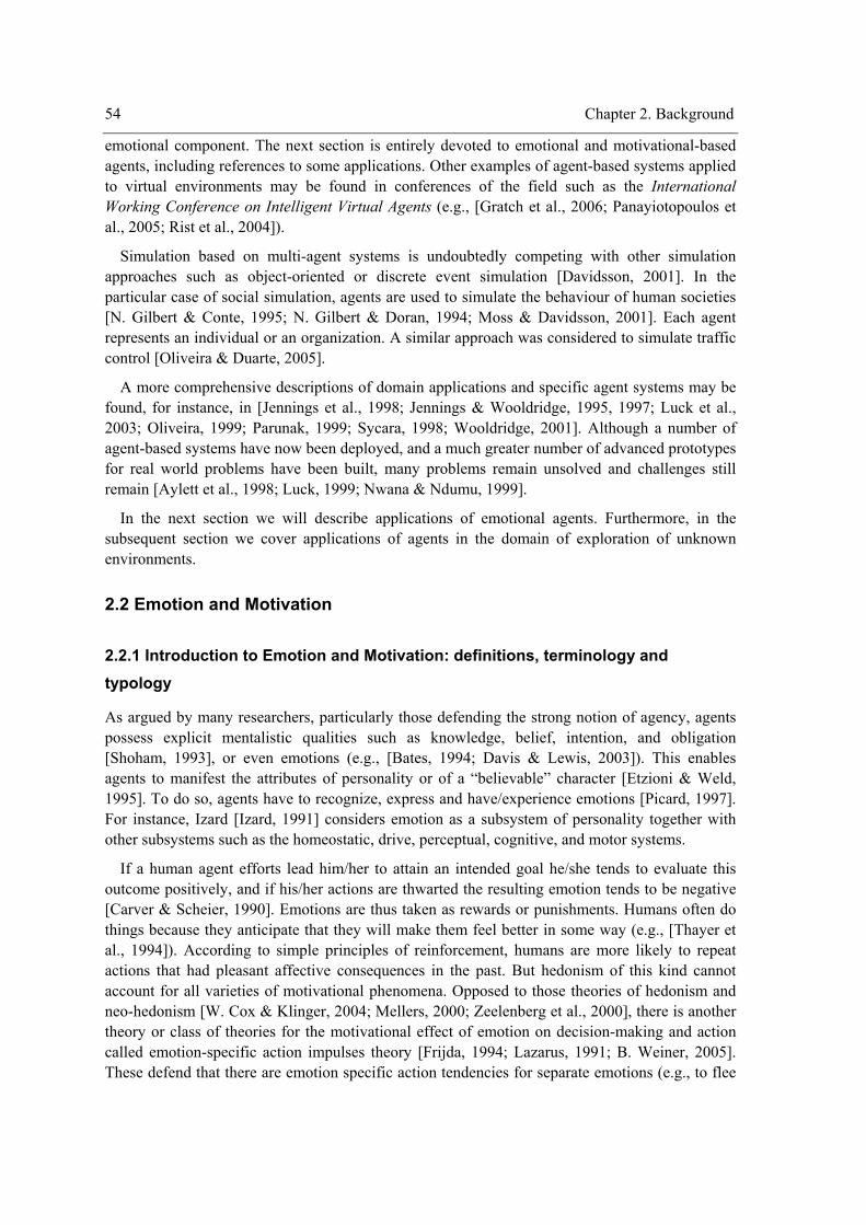
54 Chapter 2. Background
emotional component. The next section is entirely devoted to emotional and motivational-based agents, including references to some applications. Other examples of agent-based systems applied to virtual environments may be found in conferences of the field such as the International Working Conference on Intelligent Virtual Agents (e.g., [Gratch et al., 2006; Panayiotopoulos et al., 2005; Rist et al., 2004]).
Simulation based on multi-agent systems is undoubtedly competing with other simulation approaches such as object-oriented or discrete event simulation [Davidsson, 2001]. In the particular case of social simulation, agents are used to simulate the behaviour of human societies [N. Gilbert & Conte, 1995; N. Gilbert & Doran, 1994; Moss & Davidsson, 2001]. Each agent represents an individual or an organization. A similar approach was considered to simulate traffic control [Oliveira & Duarte, 2005].
A more comprehensive descriptions of domain applications and specific agent systems may be found, for instance, in [Jennings et al., 1998; Jennings & Wooldridge, 1995, 1997; Luck et al., 2003; Oliveira, 1999; Parunak, 1999; Sycara, 1998; Wooldridge, 2001]. Although a number of agent-based systems have now been deployed, and a much greater number of advanced prototypes for real world problems have been built, many problems remain unsolved and challenges still remain [Aylett et al., 1998; Luck, 1999; Nwana & Ndumu, 1999].
In the next section we will describe applications of emotional agents. Furthermore, in the subsequent section we cover applications of agents in the domain of exploration of unknown environments.
2.2 Emotion and Motivation
2.2.1 Introduction to Emotion and Motivation: definitions, terminology and typology
As argued by many researchers, particularly those defending the strong notion of agency, agents possess explicit mentalistic qualities such as knowledge, belief, intention, and obligation [Shoham, 1993], or even emotions (e.g., [Bates, 1994; Davis & Lewis, 2003]). This enables agents to manifest the attributes of personality or of a “believable” character [Etzioni & Weld, 1995]. To do so, agents have to recognize, express and have/experience emotions [Picard, 1997]. For instance, Izard [Izard, 1991] considers emotion as a subsystem of personality together with other subsystems such as the homeostatic, drive, perceptual, cognitive, and motor systems.
If a human agent efforts lead him/her to attain an intended goal he/she tends to evaluate this outcome positively, and if his/her actions are thwarted the resulting emotion tends to be negative [Carver & Scheier, 1990]. Emotions are thus taken as rewards or punishments. Humans often do things because they anticipate that they will make them feel better in some way (e.g., [Thayer et al., 1994]). According to simple principles of reinforcement, humans are more likely to repeat actions that had pleasant affective consequences in the past. But hedonism of this kind cannot account for all varieties of motivational phenomena. Opposed to those theories of hedonism and neo-hedonism [W. Cox & Klinger, 2004; Mellers, 2000; Zeelenberg et al., 2000], there is another theory or class of theories for the motivational effect of emotion on decision-making and action called emotion-specific action impulses theory [Frijda, 1994; Lazarus, 1991; B. Weiner, 2005]. These defend that there are emotion specific action tendencies for separate emotions (e.g., to flee
Chapter 2. Background 55
or avoid danger in case of fear, to attack in case of anger, to help in case of pity, to make up for in case of guilt). Hedonism assumes the existence of a basic desire while emotion-specific action impulses theory assumes a pluralist view of motivation [Havercamp & Reiss, 2003; McDougall, 1908; Reiss, 2000; Schwartz, 1992; B. Weiner, 1980] by defending the existence of various basic desires (e.g., curiosity, power, hedonism, etc.). However, some theorists believe that the pleasure principle is indirectly at work even in these cases.
Motivation and emotion are thus highly intertwined and it is not always easy to establish clear boundaries between them. Emotion and motivation both depend on the relationship between the organism and its environment. Generally, motivation is defined as factors that cause an organism to behave in a certain way at a certain time. Motivation is more related with goal generation and action, while emotion is concerned with evaluative aspects of the relation of an agent with its environment. In the case of emotion, the emphasis is on how the situation makes the person feel. In the case of motivation, it is how the individual acts with respect to the situation that is of interest [Kuhl, 1986].
Among the many possible ways of classifying human mental functions, one of the most widely accepted (e.g., [Hilgard, 1980]) defines three separate areas of cognition (thinking), affect (feeling), and conation (willing). Emotion is one of the most important and thoroughly explored forms of affect, and motivation is essentially related to conation.
In order to clarify further this tangled relation between motivation and emotion, we present the typology of motivation proposed by Izard [Izard, 1977, 1991]. He defined motivation as involving some stimulus that influences behaviour. He identified the following types of motivation: reflexes, instincts, drives, and emotions. Reflexes are automatic responses that require no evaluation or appraisal of the stimulus, i.e., no decision is made about how to behave (e.g., the eye blink produced when an object approaches the face; pupil dilation). Instincts involve hormonal changes within the body as well as some appraisal or judgement (e.g., the first flight of a swift). Drives are the physiological, survival needs basic to all animal life (e.g., hunger, thirst, comfort or pain avoidance, sex). Emotion is experienced as a feeling that motivates, organizes, and guides perception, thought, and action (e.g., fear, love, interest, happiness, etc.).
Other terms related to the notions of emotion and motivation are emotional state, emotional expression, emotional experience, feelings, drives, and mood. An emotional state refers to the mental and physical state of someone who has an emotion. Since it is of internal nature, the emotional state cannot be directly observed by someone else, but it may be inferred, for instance, from the expression of emotions. The term of emotional expression refers to what is revealed to others, voluntarily or not. Usually, when one experiences an emotion the emotional expression produced is involuntary and provides clues that others may observe to guess his/her emotional state. Emotional experience refers to everything one consciously perceives of the emotional state. This term is sometimes related with the term feelings. However, the concept of feeling is generally more related with sensations. Drives are, according to Izard, another important subsystem of personality and also an important kind of the motivational system. Generally, drives are internal conditions or impulses that activate behaviour to reduce a need and restore homeostasis. Mood is commonly associated with a long term affective state (hours, days or longer) in opposition to emotion which lasts, according to psychologists, at most, a few minutes.
Various authors claim the existence of basic, fundamental or primary emotions, although there is no consensus on which emotions meet the criteria to be classified as such. For instance,
56 Chapter 2. Background
according to Izard the list of the basic emotions includes those that have the following properties: distinct and specific neural substrates, distinct and specific configuration of facial movements or facial expression, distinct and specific feelings that achieve awareness, that are derived through evolutionary-biological processes, and have organizing and motivational properties that serve adaptive functions. Izard considers that the emotions that exhibit these properties are interest, enjoyment, surprise, sadness, anger, disgust, contempt, and fear. For Ekman [Ekman, 1992] the underlying factor that characterizes fundamental emotions is that they have universal facial expressions. For this author, anger, disgust, fear, joy, sadness and surprise are classified as fundamental emotions. For the list of fundamental emotions considered by other authors see [Ortony et al., 1988], pp 27.
Emotions have been considered as positive or negative according to their desirable or undesirable consequences. However, there are emotions that could be either positive or negative. This is the case of surprise, whose consequences, depending on the situation that elicits it, are either negative or positive. For instance, when someone is confronted with an unexpected event that also causes fear, the resulting feelings are negative, while the contrary happens when the unexpected event does not elicit fear but rather happiness. This means that surprise is not itself negative or positive but instead neutral. What is positive or negative is the event [Reisenzein, 2000b].
In order to characterise an emotion, there are several aspects that should be known such as its neurophysiology, its expression, its causes, its phenomenology, and its functions. Among these, neurophysiology, expression, and phenomenology are widely accepted as the three main components of emotion [Izard, 1991]. Neurophysiology refers to the body changes that accompany emotion. Expression is concerned with the distinct facial, vocal, gestual and bodily configuration that is associated to an emotion. Finally, phenomenology pertains to the subjective experience of that emotion, i.e., the feelings that are attached to an emotion. Izard describes basic emotions individually in terms of those aspects.
2.2.2 Emotion Theories
Although, a lot of research has been done about emotion and motivation, there are too many questions lacking a consensual answer. In fact, there are no clear answers to questions such as “How are emotions induced?”, “Are emotions physical or cognitive?”, “How are they caused?”, “Why do they exist?”, “How does someone recognize the emotional state of another person?”, and even “What is the definition of emotion?”, or “What are motivations?”. Philosophers, psychologists, neuroscientists, ethologists, biologists, and recently AI researchers, have attempted to answer these questions which just proves that this is a very complex, multidisciplinary phenomenon. The result is a myriad of emotion theories (for an overview see [Buck, 1984; Frijda, 1986; Lazarus, 1991; Mandler, 1984; Plutchik & Kellerman, 1980-1990; Strongman, 1998]). For instance, Strongman categorized those emotion theories according to the particular facets they emphasize, which are mainly: phenomenological, physiological, behavioural, cognitive, developmental, social, and clinical. Phenomenological theories are primarily concerned with the nature of emotional experience. Behavioural theories focus on what is directly observable and measurable, regarding emotion as a response rather than a state of the organism. Physiological theories rest on the belief that emotions have a biological base, focusing on finding the substrate of emotion in the central and peripheral nervous system, as well as in the endocrine system. Cognitive theories stress that emotion is related to cognition and particularly that emotions are to
Chapter 2. Background 57
do with evaluations, focusing on the nature and functioning of the process of appraisal. Developmental theories state that emotion has to be dealt with from the viewpoint of change, mainly throughout the life span of an entity. Social theories conceptualize emotion as a social phenomenon, focusing on the matter of emotional expression and recognition amongst other social interactions. Clinical theories link psychopathologies to emotional dysfunction, and thus emotion is seen as playing a central role in mental disorders. In addition to these categories of theories, Strongman also describes, from a historical perspective, the earliest emotion theories that are the background of current theories. Also, a reference is made to theories defended outside psychology. Phenomenological theories are too incomplete because they only account for the subjective aspect of emotion. Behavioural theories are currently almost inactive, mainly because they are too limited, leaving many aspects of emotion unexplained. Physiological theories are far more complete, explaining various aspects of the emotion phenomena. Cognitive theories form a very large group of emotion theories. In fact, almost all theories of emotion relate it with cognition. These theories are very complex and complete, covering many aspects of emotion. Social and clinical theories are not particularly impressive. Because of their completeness, the cognitive and physiological theories are the most relevant categories of emotion. They complete each other by emphasizing two different but complementary facets of emotion: the physical and the mental component.
2.2.3 Origins and Functions of Emotion and Motivation
The origins and functions of emotions and motivations can be explained from an evolutionary perspective. This constitutes the psycho-evolutionary theory of emotion [Plutchik, 1980a, 1980b, 1980c]. Motivations, in the broad sense that encompasses emotions, emerged and changed during the course of evolution. This is also the claim of Darwin’s [Darwin, 1965] evolutionary theory which states that emotions are a by-product of evolutionary history. The first organisms had a very rudimentary motivational system, obviously with no cognitive appraisal. However, they were able to survive by using simple approach and avoidance reactions such as those required to approach nutritive substances and to avoid toxic substances. These ideas were incorporated into the theory of motivation proposed by Freud [Freud, 1938] in the form of pleasure (approach) and pain (avoidance) principle. So, it is easy to understand why the basic motivations such as reflexes, instincts and drives (e.g., hunger, thirst, pain avoidance, sex, and elimination of body waste) emerged somehow in the species. They are necessary for survival and physical well-being. Although reflexes and instincts are rigid and stimulus dependent, they provide ways of responding and adapting to a limited set of environment situations [Izard, 1991]. However, they are almost not present in human beings. Exceptions are for instance the eye blink. The basic drives enables animals, for instance, to find food, water, shelter, maintain the species, and to eliminate waste products.
However, as our ancestors became more complex, a period of maturation and learning was required for the offspring to become able to forage and fend for themselves. During the majority of that period of complete dependence of the offspring, a strong motivation is required not only to keep the caregiver (usually the mother) near the offspring but also vice-versa. Such strong motivations could not be so basic, such as reflexes, instincts or drives, but instead what is called emotions, such as love. So, a clear reason of why emotions emerged is the mother-infant bond, which can be proved by noting that such a bond may exist for a long period or permanently
58 Chapter 2. Background
[Ainsworth et al., 1978; Shiller et al., 1986]. Therefore, there is no doubt that one of the functions of emotion is to insure social bonding between infant and caregiver [Izard, 1991].
Another reason why emotions emerged is to ensure a means of communication between infant and mother and facilitate communication between adults [Izard, 1991]. In fact, numerous studies of emotional development show that before the infant speaks, it informs the caregivers about its internal state such as feeling pain or hunger through the physical expression of emotions such as distress. Another example of the repertoire of signals that the child possesses is, for instance, the expression of interest/joy or anger when it is involved positively with the environment or is frustrated, respectively.
Further reasons and functions of emotion come from psychological and neuroscience research over the past decades, which suggests that emotions play a critical role in decision-making, action and performance, by influencing a variety of cognitive processes (e.g., attention [Izard, 1991; Meyer et al., 1997; Ortony & Partridge, 1987; Reisenzein, 2000b], planning [Gratch, 1999], etc.). On the one hand, recent research in neuroscience [Damásio, 1994; LeDoux, 1996] supports the idea of the importance of emotions in reasoning and decision-making. For instance, results from recent studies of patients with lesions of the prefrontal cortex suggest an important role of emotions in decision-making. On the other hand, there are a few theories in psychology relating emotion to decision-making and action [Andrade, 2005; Loewenstein & Lerner, 2003]. For instance, in the specific case of emotions, as outlined by [Reisenzein, 1996], within the context of the belief-desire theories of action (the dominant class of theories in today’s motivation psychology) it can be suggested that emotions are action goals, that emotions are, or include action tendencies, that emotions are, or include goal-desires, and that emotions are mental states that generate goal-desires.
It seems that this role of emotions in cognitive processes, such as decision-making, has a primary reason, survival and well-being, as happens with basic motivations [Damásio, 1994]. As complex organisms begin to live in complex environments, basic motivations such as drives or instincts do not seem sufficient to guarantee survival. In such environments such as those inhabited by humans nowadays, hunting or running away from predators are not anymore the important activities that we recognize from archaeology or history. In general, they are not as necessary as they were for our ancestors. For instance, we now go to the supermarket to buy meat instead of hunting for it. However, there are now different forms of hunting, different predators in the complex human society. Today, we need to decide or plan our personal and social actions so that we can survive in such a complex human society. According to Damásio, emotions play a central role in these new strategies of survival just as drives or instincts did for our ancestors and still do for us, functioning as survival mechanisms. The way this happens is explained by his Somatic-Marker Hypothesis which states that that decisions that are made in circumstances, whose outcome could be potentially harmful or advantageous, and are similar to previous experience, induce a somatic response used to mark future outcomes. When the situation arises again the somatic marker will signal the danger or advantage. Thus, when a negative somatic marker is linked to a particular negative future outcome it serves as an alarm signal that tells us to avoid that particular course of action. If instead, a positive somatic marker is linked to a positive outcome, it becomes an incentive to make that particular choice.
The adaptive function of these somatic markers of emotional reactions (good and bad) is to help us simplify decisions by quickly eliminating some courses of action from consideration (because they are connected to bad situations). Without these somatic markers, we do not learn to avoid
Chapter 2. Background 59
bad situations, we cannot simplify our decision processes (by winnowing down choice sets to a manageable size) and exhibit indecision.
In summary, the main functions of emotions and motivations may be reduced to: communication, survival and well-being. However, each emotion and motivation individually has its specific functions. As examples, we will examine some of those emotions and their functions. The functions of other motivations such as drives are more easily perceived (thirst signals the need for water, hunger the need for food, etc.).
Interest/curiosity played a central role in the evolution of human beings, serving adaptive functions developed over the course of humankind’s existence. It influences learning by supporting investigation, exploration, and creativity.
Anger played a critical role in coping with some of the challenges and dangers which occurred during the evolution of human beings, and thereby it was essential for survival of the species. In fact, anger mobilizes energy for action, making individuals more capable of defending themselves.
Disgust enables individuals to reject distasteful and potentially dangerous substances even in the absence of sensations of taste or odor. In evolution, disgust probably helped motivate animals to maintain an environment and their own body in sufficiently sanitary conditions for their health and to prevent them, for instance, from eating spoiled food.
The primary function of fear is perhaps to motivate cognition and action that lead to safety and security. Fear enables individuals to protect themselves from dangerous situations.
Joy is a reward for an experiment. It usually comes after the accomplishment of a goal.
Surprise plays an important role in cognitive activities, especially in attention focusing and learning (e.g., [Izard, 1977, 1991; Meyer et al., 1997; Ortony & Partridge, 1987; Reisenzein, 2000b]. According to Meyer and colleagues (e.g., [Meyer et al., 1997]), surprise has two main functions, informational and motivational, that together promote both immediate adaptive actions to a surprising event and the prediction, control and effective dealings with future occurrences of the same event.
2.2.4 Affective Artificial Agents
In the previous section, we described the main functions of emotion for human beings. As we saw, the main advantages are: communication, survival and well being. The role of emotions in cognitive processes such as planning or decision-making is essential for this achievement. So, we may ask the question of “Why don’t agents take similar advantages from emotion?” [Cañamero, 1998]. As mentioned above, an affirmative answer to this question is argued by many researchers, particularly those defending the strong notion of agency (e.g., [Bates, 1994; Shoham, 1993]). They do so because this enables agents to manifest the attributes of personality or of a “believable” character [Etzioni & Weld, 1995]. The ascription of affective features to agents gives rise to terms such as emotional agents, believable agents [Bates, 1994], motivational agents, affective agents, or affective computers [Picard, 1997]. Mainly based on the recent advances in psychology and neuroscience mentioned above, such agents are expected to plan, decide, learn or reason better than those that do not take advantage of emotions. Although the field is in an initial phase, several applications have already been appointed to affective agents. Some of those applications are entirely new, appearing only with the advent of emotional agents because they
60 Chapter 2. Background
can only be conceived with the concept of agents with affective abilities, while others constitute simply a different approach of dealing with problems that, up to now, were solved ignoring the influence of emotion on cognitive abilities. Some of those applications are still science fiction while others are already implemented. Among the former is, for instance, a computer such as HAL [Clarke, 1997]. Among presently existing emotion-based systems we may find the Tok architecture developed in the Oz project [Bates, 1994; Reilly, 1996]. We will now take a closer look at these and other related systems that incorporate models of affect. Our objective is not to survey all the work done in this area but simply to give representative examples of emotion-based computer systems. Other examples of these systems may be found in proceedings of the conferences of the area such as the First International Conference on Affective Computing & Intelligent Interaction [Tao et al., 2005], the International Conference on Intelligent Virtual Agents (e.g., [Gratch et al., 2006; Panayiotopoulos et al., 2005; Rist et al., 2004]), the annual AISB Convention symposia (e.g., [Aylett & Canãmero, 2002; Canãmero, 2005; Johnson, 2001, 2004]), the AAAI Fall Symposia (e.g., [Canãmero, 2001]), and the Affective Computing Workshop of the Portuguese International Conference on Artificial Intelligence [Paiva et al., 2005]. Those systems can be organized into three main groups: those systems that recognize emotions, those that express emotions, and those that generate or synthesize emotions. The first and the second group can be merged into a single one, because most of the systems that recognize emotions also address the issue of expressing emotions. Most of the emotion-based computer systems are about generating or synthesizing emotions and about the influence of emotions on cognitive processes such as decision-making.
Ekman and Friesen [Ekman & Friesen, 1977] developed a theory, called Facial Action Coding System, for associating expressions, and more precisely the muscular movements used to generate them, to a number of discrete categories of emotions. Essa and Pentland [Essa & Pentland, 1997] augmented this system to non-local spatial patterns and to include time components. The result is a system that is able to recognize facial expressions from video. It relies on information about facial shape and physical knowledge of facial muscles. For faster recognition, they developed another model [Essa & Pentland, 1995] which is not based on physical information but rather on templates of facial motion energy. Yacoob and Davis [Yacoob & Davis] also developed a model for facial expression recognition based on templates of motion energy, although their method is slightly different in that they consider combinations of templates and sub-templates (e.g., just for the mouth or eye area).
Recognition of emotions is not confined to facial expression. There has been previous work on emotional expression recognition from speech and from physiological information. For instance, Vyzas and Picard [Vyzas & Picard, 1999] developed a method, based on physiological data collected from an actress, for offline and online recognition of the emotional state of a person deliberately expressing one of eight emotions. The recognition method relies on a set of features extracted from physiological signals (electromyogram, blood pressure, skin conductivity, and respiration) measured from the surface of the skin of the person expressing emotion.
One of the most remarkable works that addresses the expression of emotions is that of Breazel and Scassellati [Breazeal, 1999; Breazeal & Scassellati, 1999]. They developed Kismet as a test bed for learning social interactions in situations involving an infant (the robot) and her caretaker (a human). Kismet is a head with active stereo vision and configurable facial features – eyelids, ears, eyebrows, and a mouth. Humans can interact with it either by direct, face-to-face exchange or by showing it a toy. Kismet is able to successfully negotiate the caregiver into presenting the
Chapter 2. Background 61
robot with toys when it is bored, and to engage in face to face exchange when it is lonely. The caregiver instinctively responds to the robot’s affective state to promote its well being – presenting the robot with pleasing stimuli, avoiding the presentation of noxious stimuli, and taking care not to overwhelm nor under-stimulate the robot. Perception, attention, internal drives, emotions, and motor skills are integrated in Kismet’s software architecture to provide social interactions. Kismet performs a variety of proto-social responses (affective, exploratory, protective and regulatory responses) by means of various natural social cues such as gaze direction, posture, and facial displays. These facial displays include expressions analogous to happiness, sadness, surprise, boredom, anger, calm, displeasure, fear, and interest. These nine different facial expressions are used to manipulate its human caretaker into satisfying its internal drives – a social drive, a stimulation drive, and a fatigue drive. These drives and emotions form together the motivation system of Kismet. The robot’s emotions are a result of its affective state. The affective state of the robot is represented as a point along three dimensions: arousal (i.e. high, neutral, or low), valence (i.e. positive, neutral, or negative), and stance (i.e. open, neutral, or closed). The affective state is computed by summing up contributions from the drives and behaviours. The proto-social responses enable the adult to interpret kismet’s actions as intentional. In Kismet, low-level perceptual inputs are combined with high-level influences from motivations and habituation effects by the attention system.
Thrun and colleagues [Schulte et al., 1999; Thrun et al., 1999] developed Minerva, a mobile robot that gives guided tours to visitors of the Smithsonian’s Museum of American History. Minerva displays emotional states – neutral, happy, sad, and angry – using a caricaturized face and simple speech. Although the emotions are not an integral part of the robot’s architecture, the emotional states arise as a consequence of travel-related interaction (e.g., anger results from its inability to move due to the presence of people), and their expression aims at affecting this interaction towards achieving the robot’s goals – travelling from one exhibit to the next one, holding people’s attention when describing an exhibit, and attracting people to participate in a new tour.
Feelix [Cañamero & Fredslund, 2000] is a humanoid-looking LEGO robot capable of displaying several emotional expressions in response to direct physical contact. Inspired by psychological theories about emotions in humans, Feelix implements two complementary emotion models, one concerning the “universal” facial expressions of basic emotions, and the other postulating a principle for emotion activation based on general stimulation patterns that Cañamero and Fredslund associate to discrete basic emotions. They characterize emotions in terms of the continuous dimensions of valence and arousal. They confined the set of emotions modelled to those proposed by Ekman [Ekman, 1992] as basic emotions (with the exception of disgust): anger, disgust, fear, happiness, sadness, and surprise. Interaction with Feelix is only through tactile stimulation on the feet, causing the touch sensors to be pressed. To distinguish between different kinds of stimuli, they use duration and frequency of presses. Information about presses is analyzed in terms of duration and frequency, and based on this analysis, a message encoding Feelix’ current emotional state and its intensity are used to control the face.
One of the most common approaches to synthesize emotions is of a cognitive kind. Many of these approaches rely on the so-called Ortony, Collins, and Clore’s (OCC) model [Ortony et al., 1988] which, although it is not a computational model, is very popular in the field of AI because it is suitable for implementation in computers. A central idea in this model is that emotions are reactions involving valence. The overall structure of the OCC model is based on grouping
62 Chapter 2. Background
emotions by their eliciting conditions: events, agents, and objects. Events are simply people’s interpretations of things that happened; objects are also a very straightforward level of perception; and agents are both human and non-human beings, as well as inanimate objects or abstractions such as institutions. Therefore, the OCC model proposes that emotions are the results of three types of subjective appraisals: the appraisal of the pleasingness of events with respect to the agent’s goals; the appraisal of the approval of the actions of the agent or another agent with respect to a set of standards for behaviour; and, the appraisal of the liking of objects with respect to the attitudes of the agent. Based on types of emotions, the structure of the OCC model has three main ramifications, corresponding to the three types of subjective appraisals, or, in other words, to the three ways people react to the world. The first ramification relates to emotions which arise from aspects of objects such as liking, disliking, etc. This constitutes the single class in this branch, namely the one called attraction which includes the emotions love and hate. The second branch is concerned with emotions that are related to consequences of events with respect to the person who experiences the emotion or with respect to some other person. As a reaction to them, one can be pleased, displeased, etc. This gives rise to a further division of this branch into another two branches: one concerned with the consequences of events to the person who experiences the emotion, and another related to the consequences of events to some other person. This latter branch includes the class fortunes-of-others that includes the following emotions: happy-for, resentment, gloating, and pity. The first two correspond to desirable consequences of events for others, while the latter two refer to undesirable consequences of events for others. The branch concerned with the consequences of events to the person who experiences the emotion includes a further division with respect to the prospect of an event. This prospect may be relevant or not. In the first case the class of well-being emotions is constituted by, including emotional terms such as joy, distress, sadness, happiness, or unhappiness. They reflect upon one’s well-being, and are simply default cases of being pleased or displeased. In the latter case, the class of prospect-based emotions is constituted which includes the emotions of hope and fear. However, four additional emotions are also considered to result from reacting to the prospect of positive and negative events, namely satisfaction, fears-confirmed, disappointment, and relief. The first two arise when the prospect of a positive or negative event is believed to have been confirmed, while the latter two arise when the prospect of a positive or negative event is believed to have been disconfirmed. The third branch of the structure is related to agents. It also has only one class, namely the attribution class, comprising the following emotions: pride, shame, reproach, admiration. Another additional class of emotions can be referred to as compound class. It is called wellbeing/attribution compound and it involves the emotions of gratification, remorse, gratitude, and anger.
The OCC model has been very popular in AI, and used, for instance, in the Affective Reasoner [Elliott, 1992, 1993, 1994; Elliott & Siegle, 1993], the Tok architecture developed in the Oz project [Bates, 1994; Reilly, 1996], and [Dias & Paiva, 2005].
In the Affective Reasoner, Elliot and Siegle simulate simple worlds populated with agents capable of responding emotionally. Agents are given unique pseudo-personalities modelled as both a set of appraisal frames representing their individual goals, principles, preferences, and moods, and as a set of channels for the expression of emotions. Combinations of appraisal frames are used to create agents’ interpretations of situations that occur in the simulation. These interpretations, in turn, can be characterized by the simulator in terms of the eliciting conditions for emotions. As a result, in some cases agents have emotions which then may be expressed in ways that are observable by other agents, and as new simulation events which might perturb
Chapter 2. Background 63
future situations. Additionally, agents use a case-based heuristic classification system to reason about the emotions of other agents, and to build representations of those other agents’ personalities that will help them to predict and explain future emotional episodes involving those observed agents.
Gratch [Gratch, 1999] proposes a model of cognitive appraisal called plan-based appraisal. This model relies indirectly on the OCC theory of cognitive appraisal in that it re-implements Elliott’s construal theory, which, as described above, is in turn a computational account of the OCC theory of cognitive appraisal. In construal theory, events are matched against knowledge structures called construal frames. These frames evaluate events against an agent’s goals, social standards (norms of behaviour), and preferences (the appealingness of domain objects). Construal frames make two determinations. First they assess if the event is of relevance to the agent. If so, they extract several high-level features of the event that are later used to assess the emotional response. Collectively, these features are referred to as an emotion eliciting condition relation. Plan-based appraisal departs somewhat from the spirit of construal theory, specifically in the handling of events. Construal theory centers appraisal on events and uses the construal frames to derive the relationship between events and goals. In contrast, plan-based appraisal centers appraisals on goals and uses the planner’s domain-independent threat detection processes to determine the significance of events to goals. To implement the appraisal scheme, Gratch provides definitions for each of the emotion eliciting conditions in terms of syntactic features of the current plans in working memory. Gratch associates an appraisal frame with each goal in the plan structure. Emotion eliciting conditions describe properties of each goal such as the agent that owns it, and its desirable or undesirable disposition.
The Oz project [Bates, 1992, 1994; Bates et al., 1992; Loyall & Bates, 1991; Mateas, 2002; Reilly, 1996; Reilly & Bates, 1992] at the Carnegie Mellon School of Computer Science is developing technology for high quality interactive fiction and virtual realities. The goal is to provide users with the experience of living in dramatically interesting micro-worlds that include emotional agents. An Oz world comprises a simulated physical environment, the agents that live in the environment, a user interface and its associated theory of presentation and style, and a theory of drama, which plans and controls the overall flow of events in the world. In order to provide users with the experience of living in dramatically interesting micro-worlds the users of the system have to suspend their disbelief when interacting with an Oz world. This is achieved by making the agents that populate these worlds look real in a number of ways such as: displaying competent action in the world, reaction to a changing environment, goal-directed behaviour, appropriate emotions, individual personality traits, social skills, language skills, and some degree of intelligent inferring about the world around them. These capabilities are partially divided into the various communicating components or subsystems of the agent architecture, called Tok [Bates et al., 1992], developed in the Oz project. For instance, goal-reactivity is handled by the subsystem called Hap [Loyall & Bates, 1991], while Em subsystem [Reilly, 1996; Reilly & Bates, 1992] handles most of the emotional and social aspects of the agents’ behaviour. Em’s model of emotion is based largely on the OCC cognitive model of emotion and has demonstrated some ability to produce reasonable emotional behaviour for Oz agents. Em can also model simple social relationships between agents, how these relationships change over time, and how these relationships interact with emotion and behaviour.
In spite of the extensive implementation of the OCC model, an alternative cognitive model has been recently proposed by Roseman and colleagues [Roseman, 1991; Roseman et al., 1996;
64 Chapter 2. Background
Roseman et al., 1990] which likewise seems to be easy to implement in computers. This new appraisal theory relies on the categorization of the appraisals people make about events that cause emotions. The six appraisals that give rise to seventeen emotions are: unexpectedness which elicits surprise; motivational state and situational state, i.e., whether the agent aims to get a reward (appetitive motive) or to avoid a punishment (aversive motive), and whether the situation fits the agent’s motive (situations consistent with getting a reward elicit joy; situations consistent with not getting punishment cause relief; situations inconsistent with getting a reward produce sadness; situations inconsistent with not getting punishment produce distress; probability, i.e., whether the outcome is certain or uncertain (hope and fear are elicited by uncertainty); control potential, i.e., whether the agent is able to control a negative event (frustration or disgust may arise); problem type, i.e., whether an event is negative because it hinders a goal (this gives rise to frustration) or because it is simply intrinsically negative (this gives rise to disgust); agency, i.e., events are caused by other agents (elicits liking-love, dislike, anger, or contempt) or by the self (elicits pride, regret, guilt, or shame).
Another usual approach to synthesize emotions is of a physical kind. This corresponds to considering low-level non-cognitive aspects as the basis for the generation of emotions. We have already described examples of synthesizing emotions using this approach when we described Feelix and Kismet above. Another work, also from Cañamero, uses physiological parameters to model emotions, too [Cañamero, 1997]. In this work, Cañamero investigated some aspects in which emotions can affect the behaviour of artificial creatures. These inhabit a two-dimensional world, the Gridland, and they are endowed with motivational states and a set of basic emotions. She distinguishes between motivations and emotions. Motivations constitute the basic mechanism that regulates the stability of the creature’s internal state necessary for survival, adaptation, and autonomy, driving behaviour selection. On the other hand, emotions contribute to maintaining this stability acting as a second order mechanism on top of motives. Creatures consist of three types of elements: a set of physical attributes such as hardness, brightness, the amount of organic matter, etc., a set of physiological variables that define their bodily state, and a collection of agents of different sorts. The set of basic emotions are modelled by some of those agents.
Among other works that follow this physiological mechanisms to generate emotions we may find Velásquez’s work [Velásquez, 1997, 1998a, 1998b, 1999] which relies on similar foundations to those followed in [Breazeal & Velásquez, 1998]. Velásquez developed Cathexis, a distributed, computational model for the dynamic nature of different affective phenomena, such as emotions, moods, and temperaments, and their influence on the behaviour of synthetic autonomous agents. Cathexis was later extended to a computational model of emotion-decision-making. Like in [Breazeal & Velásquez, 1998], emotions, moods, and temperaments are modelled in Cathexis as a network composed of especial emotional systems similar to Minsky’s “proto-specialist” agents. Each of these proto-specialists represents a specific emotion family such as fear or disgust. Within each proto-specialist, different sensors monitor both external (e.g., events in the environment) and internal (e.g., drive levels, feedback from sensorimotor processes) stimuli for the existence of the appropriate conditions that would elicit the emotion represented by that particular proto-specialist. These sensors are arranged into four different groups: neural, sensorimotor, motivational, and cognitive. These sensors represent different kinds of both cognitive and non-cognitive emotion activation systems. Input from these sensors either increases or decreases the intensity of the emotion proto-specialist to which they belong. Associated with each proto-specialist are two threshold values. The first threshold controls the activation of the emotion. That is, once the intensity goes above this threshold, the emotion proto-specialist
Chapter 2. Background 65
releases its output signal to other emotion proto-specialists, and to the behaviour system which in turn selects an appropriate behaviour according to the state of these emotional systems. The second threshold specifies the level of saturation for that emotion proto-specialist. This is consistent with real life emotional systems in which levels of arousal will not exceed certain limits. Another important element associated with an emotion proto-specialist is a decay function which controls the duration of the emotion episode. All of these emotion proto-specialists run in parallel and are constantly updating their intensities. In Cathexis and in its further emotion-based decision-making extension, the behaviours are directed, in the majority of cases, towards satisfying needs and interacting with humans. Examples of such behaviours include approach-person, play, request-attention, and avoid-obstacle. The behaviour is accompanied by a facial expression, body posture, and vocal expression. In order to test the Cathexis model, he created two synthetic agents, one called Simón representing a young child, and another called Yuppy which is an emotional pet robot.
This work of Velázquez as well as that of Cañamero [Cañamero, 1997], also described above, are also examples of the extensive list of works that explore the influence of emotion on cognitive processes. In this case emotion is a bias mechanism that directs behaviour and decision-making. Others examples are the works described in [Frijda, 1986; Kitano, 1995; Pfeifer, 1988].
The Cognition and Affect project [Beaudoin, 1994; Scheutz et al., 2000; Sloman, 1998; Sloman & Logan, 1999; Wright, 1997; Wright et al., 1996] at Birmingham University proposes that for certain purposes it is useful if the deliberative processes in which internal actions are performed can be monitored, evaluated and possibly modified. Accordingly, they argue that, in addition to the reactive and deliberative layers commonly seen in several hybrid agents’ architectures, a further layer, called meta-management, is useful, for instance, to monitor deliberative processes and detect that certain strategies are more effective than others. Thereby, the resulting architecture, called CogAff, divides the agent’s cognitive system into three interacting layers corresponding to the reactive, deliberative and meta-management reasoning mechanisms. All these layers receive appropriate sensory input using perceptual mechanisms and each one processes information at different levels of abstraction, besides all of them being able to generate action. Each layer serves a particular purpose in the overall architecture, but layers can also influence one another. This tripartite division provides support for the following three types of emotions: primary emotions, such as fear, that are triggered within reactive mechanisms; secondary emotions, such as shame, that are triggered in the deliberative layer; and, tertiary emotions, such as adoration or humiliation, that involve the meta-management layer, though they may be initiated elsewhere. This architecture has been the basis for developing a range of systems using the SimAgent Toolkit [Sloman & Logan, 1999].
In spite of the emotion-based systems just described above that are already a reality, there are several challenges that should be overcome in order to successfully build agents that recognize, express and experience emotions. Picard proposes features that are required to consider that a computer is able to recognize, express and experience emotions. According to Picard, in order to recognize emotions a computer should (a) receive a variety of input signals such as voice, hand gestures, etc.; (b) based on pattern recognition techniques, perform feature extraction and classification on these signals; (c) based on knowledge about how emotions are generated and expressed, predict underlying emotion; (d) get information about the individual such as his/her personal goals, etc., in order to recognize his/her emotions in an efficient and effective manner; (e) based on the emotional state of the computer, be able to recognize ambiguous emotions; (f)
66 Chapter 2. Background
output the names or descriptions of the recognized emotions. On the other hand, expressing emotions requires that computers: (a) receive instructions from its emotion generation module or from someone else about the emotion(s) to express; (b) have two alternative ways for activation of emotional expression: intentional (triggered by a deliberative decision) or spontaneous; (c) the affective state of the computer and the affective expression should influence each other; (d) the expression of the present affective state should be easier than any other affective states; (e) the relevant social norms determine when, where and how the computer expresses emotions; (f) output of the emotional expression which may comprise visible or vocal signals such as synthetic voice, animated face, gestures, etc. Finally, a computer can be said to experience emotion if it possesses the following five components exhibited by a healthy human emotional system: (a) it has behaviour that appears to arise from emotions; (b) it has fast primary emotional responses to certain inputs; (c) it can cognitively generate emotions; (d) it can experience emotions, including cognitive awareness, physiological awareness and subjective feelings; (e) there should be an interaction between emotions and the other cognitive and physical components such as memory, perception, decision-making, learning, goals, attention, planning, prioritizing, etc.
The issue concerning whether or not computers can feel is open to much discussion. Accepting this, one might say that computers are not human beings and there are a lot of differences that justify the reasoning which suggests it is inappropriate to incorporate human-like emotions in computers. Perhaps it would be more appropriate to make them express and have variations of human emotions or even totally different emotions that can only happen in computers. These and other questions are, at present, being discussed in the field of emotion. Another issue that has activated an intensive discussion is the ethical matter of providing computers with emotions.
2.3 Exploration of Unknown Environments
2.3.1 Human Exploratory Behaviour
One of the features that characterize human beings is the tendency to explore the unknown parts of the environments they inhabit. Although exploration has existed as long as human beings, its peak is seen as being during the Age of Exploration, a period from the early 15th century and continuing into the early 17th century, when European navigators traveled around the world discovering new worlds and cultures. These big endeavours, together with the exploration of the outer space, the planets and satellites of our solar system today, are remarkable examples of the exploratory spirit of humankind. There are no limits for human exploration: from inhospitable volcanoes, mountains or oceans, to hostile planets such as Mars, and satellites such as Titan and the Moon, human beings are always trying to know more about their environment in spite of its adversity. But what motivates this exploratory behaviour? James’ “selective attention” [James, 1890], Freud’s “cathexis” [Freud, 1938], and McDougall’s “curiosity instinct” [McDougall, 1908] are fundamental concepts concerning the relationship between motivation and exploratory behaviour. This exploratory behaviour has for a long time been expressed by the idea that organisms respond to the novelty and change in the environment they inhabit in the absence of known drives (thirst, hunger, etc.), and if novelty and change is not present in the environment, organisms tend to seek it. Evidence for this behaviour in a variety of species was provided by a number of authors [Lester, 1969]. In human beings, this kind of behaviour is already present in infants even in the first hours of life, as documented by a number of researchers who have studied selective attention in infants which is a simple form of exploratory behaviour. Infants prefer
Chapter 2. Background 67
certain visual patterns over others. They do not treat with equal importance the multitude of stimuli. They explore the environment with their eyes, gazing at the more interesting objects which are those that provide novel stimuli. Some of the early researchers who showed that organisms tend to explore novel objects or places in the absence of any known drives, called it the exploratory drive [Butler, 1953, 1954, 1957, 1958; Montegomery, 1952, 1953, 1954, 1955]. Among the investigators that have adopted the ideas of McDougall about curiosity are Berlyne [Berlyne, 1950] and Shand [Shand, 1914]. For these authors, curiosity is the psychological construct that has been closely related with this kind of behaviour. Considering that curiosity was innate and that it could also be acquired, Berlyne [Berlyne, 1950] argues that novel stimulus elicits curiosity, which diminishes with continued exposure to the stimulus. In later work [Berlyne, 1955, 1960, 1967], Berlyne elaborated and extended his early theory of curiosity. In addition to novelty, other variables such as change, surprisingness, complexity, uncertainty, incongruity and conflict also determine this kind of behaviour related to exploratory and investigative activities. Sharing similar ideas with Berlyne and McDougall, Shand [Shand, 1914] defined curiosity as a primary emotion consisting of a simple impulse to know, which controls and sustains the attention and provokes the body movements that allow one to acquire information about an object. These approaches are closely related to the emotion concept of interest-excitement proposed by the differential emotions theory to account for exploration, adventure, problem solving, creativity and the acquisition of skills and competencies in the absence of known drives [Izard, 1977, 1991]. In fact, the terms curiosity and interest are used more or less as synonyms, for instance, by Berlyne. Nunnally and Lemond [Nunnally & Lemond, 1973] carried out a series of experiments on the effects of novelty and complexity on visual exploration. They concluded that information conflict and novelty elicit and hold attention. In conclusion, there is no doubt that novelty elicits curiosity/interest which is the psychological construct that accounts for exploratory behaviour. However, novelty seems to be insufficient to explain all exploratory behaviour. In addition to it, other variables such as change, surprisingness, complexity, uncertainty, incongruity and conflict also determine exploratory behaviour. Some of these variables elicit surprise, another psychological construct that also accounts for exploratory behaviour. If we also consider the recent advances in neuroscience that indicate that emotion influences the cognitive tasks of humans, and particularly planning and decision-making [Adolphs et al., 1996; Bechara et al., 1997; Damásio, 1994], exploration of unknown environments, as a decision-making process, is thereby influenced by emotion. Thus, ultimately, we may consider that there is a multitude of motivations and emotions behind the exploratory behaviour.
2.3.2 Exploration of Unknown Environments by Artificial Agents
As defended by many researchers, learning is a crucial capability of intelligent agents [Alonso et al., 2001; Etzioni & Weld, 1995; Huhns & Singh, 1998; S. Russell & Norvig, 1995]. In order to be intelligent, agents have to autonomously and independently make decisions. That is, it is impossible for the agent designer to foresee all the situations that an agent might encounter and to program it with the decisions to make in those situations. Therefore, agents have to adapt and learn from their interaction with the environment they inhabit. They have to learn to behave optimally. In most cases, they probably have to build good models of the world so that those models can be helpful to improve their performance. Learning research has been mostly independent of agent research and only recently it has been connected with agents and multi-agent systems [Huhns & Weiss, 1998; Imam, 1996; Sen, 1996; Weiss, 1997, 1998; Weiss & Sen, 1996].
68 Chapter 2. Background
Approaches to learning may further be divided into two main categories: passive and active learning [Thrun, 1995].
In the passive learning paradigm, a learner is a pure observer, learning only through observing its environment. A stream of training data is generated by the environment according to some unknown probability distribution. Examples of passive learning tasks are the clustering, classification, or prediction of future data. Passive learning techniques can be subdivided into order-free and order-sensitive approaches. Order-free approaches rest on the assumption that the temporal order in which the training data arrives does not matter for the task to be learned. It is assumed that the training examples are generated independently according to a stationary probability distribution. The majority of machine learning approaches fall into this category. For example, unsupervised learning usually aims at characterizing the underlying probability distribution or grouping the data, while supervised learning is concerned with approximating an unknown target function (conditional probability) from a set of observed input-output examples. On the other hand, in order-sensitive approaches temporal order of the training data carries information relevant to the learning task. This happens, for instance, when consecutive training examples are conditionally dependent on each other, and learning about these dependencies is crucial for the success of the learner. Time series prediction and speech recognition are examples for order-sensitive learning domains.
In the active learning paradigm, the learner interacts with its environment, i.e., the learner possesses the ability to execute actions during learning, which have an impact on the generation of training data. This way, it can, to a certain extent, control what it learns. An important challenge is the decision of what actions a learner should perform to maximize learning results. Like passive learning, active learning can also be split into order-free and order-sensitive cases. Like order-free passive learning, order-free active learning rests on the assumption that the temporal order in which the training data arrives does not matter for the task to be learned which means that, in this particular case, it relies on the assumption that what is observed in the environment depends only upon the most recently executed action. Perhaps the best-known approach of this kind is learning by queries, which is characterised by the fact that the available actions are queries for values of an unknown target function. The environment provides immediate responses (answers) to these queries. On the contrary, in order-sensitive active learning, temporal order of the training data carries information relevant to the learning task, which means that observations may depend on the sequence of actions performed by the learner. In fact, actions influence the state of the environment, and the state of the environment determines what the learner observes. For example, approaches to learning optimal control (like airplane control, or game playing) fall into this category.
Exploration might be defined as the process of selecting actions in active learning. In order to learn efficiently, an agent should execute actions that are more informative for the learning task, i.e., actions whose outcomes are expected to provide more knowledge should be preferred. In fact, most of the approaches employ an action selection process that relies on the principle of knowledge gain maximization. However, the heuristics used to estimate knowledge gain differs. Several exploration techniques have been proposed [Thrun, 1992a, 1992b, 1995]. Since they are somewhat ad hoc, the effectiveness of these exploration techniques depends on the kind of environments and learning tasks at hand. Although those exploration techniques may be applied to active learning in general, they were primarily inspired by the literature of reinforcement
Chapter 2. Background 69
learning and neural nets [Thrun, 1992a, 1995]. So, before introducing them, we will examine the field of reinforcement learning.
Reinforcement learning [Dietterich, 1997; Kaelbling et al., 1996; Sutton & Barto, 1998] is an area of machine learning which addresses how an autonomous agent can learn long-term successful behaviour through interaction with its environment. The term “reinforcement learning” has its roots in behavioural psychology, in particular in Pavlovian models of reward learning in animals. Reinforcement learning might be defined as the problem confronting an agent that must learn behaviour through trial-and-error interactions with a dynamic environment. It differs from the more well studied problem of supervised learning, in that the learner is not given input-output samples of the desired behaviour. Rather, the learner is only supplied scalar feedback regarding the appropriateness of the actions, after they have been carried out. A procedure or rule π for choosing each action a given state s is called the policy of the learner, and it can be formalized as a function a = π(s). Hence, a policy is the agent’s decision-making function that maps states to action. The goal of reinforcement learning algorithms is to compute the optimal policy which maximizes some long-run measure of reinforcement. However, in order to find the optimal policy, it is necessary to prove that every off-policy action leads to expected results that are worse than the actions of the optimal policy. This is where exploration plays its role. In this situation, it is essential to explore alternative actions to determine whether they are worse (or better) than the actions of the optimal policy. The strategy of always taking the action that appears to be optimal based on the current value function is called the pure exploitation strategy. It has been shown that pure exploitation strategy does not always find the optimal policy. Hence, online reinforcement learning algorithms must balance exploitation with exploration. This is one of the challenges that arises in reinforcement learning and not in other kinds of learning: the trade-off between exploration and exploitation. To obtain a lot of reward, a reinforcement learning agent must prefer actions that it has tried in the past and found to be effective in producing reward. But to discover such actions it has to try actions that it has not selected before. The agent has to exploit what it already knows in order to obtain reward, but it also has to explore in order to make better action selections in the future. The dilemma is that neither exploitation nor exploration can be pursued exclusively without failing at the task. The agent must try a variety of actions and progressively favour those that appear to be best. Earlier theoretical research on the efficiency of exploration in this context of reinforcement learning and control learning [Thrun, 1992a, 1992b] indicate the importance of the exploration strategy for the efficiency of learning control.
Exploration strategies have been grouped into two main categories: undirected and directed exploration [Thrun, 1992a, 1992b, 1995]. Strategies belonging to the former group, such as random walk exploration, Boltzman distributed exploration, and semi-uniform distributed exploration use no exploration-specific knowledge and ensure exploration by merging randomness into action selection. In random walk exploration actions are generated randomly with uniform probability distribution, regardless of expected exploration costs or rewards. Boltzmann distributions and semi-uniform distributions provide ways to combine random exploration with exploitation. These distributions explore by flipping coins, but the likelihood of individual actions is determined by the task-specific exploitation utility. In Boltzmann distributions, the likelihood of picking an action is exponentially weighted by its utility, and in semi-uniform distributions the action with the largest utility has a distinct high probability of being executed. On the contrary, strategies belonging to the latter group of directed-exploration, such as counter-based exploration, counter-based exploration with decay, error-based exploration, and recency-based exploration, rely heavily on exploration specific-knowledge for guiding the
70 Chapter 2. Background
learning process. Counter-based exploration evaluates states on the basis of how often they occurred. Actions leading to states that occurred least are preferred. Counter-based exploration with decay extends the previous strategy by taking into account the information of when a state occurred. The more recent an occurrence of a state, the more the occurrence contributes to the counter value of that state. Error-based exploration is another extension of counter-based exploration by memorizing the latest change of the utility estimation of each state. The strategy prefers actions leading to states whose utility value has recently changed most. Recency-based exploration prefers actions leading to states which occurred less recently.
Reinforcement learning is the kind of learning where only parts of the environment have to be known in order to perform optimally. In fact, in this case the task is to learn control/behaviour, and therefore exploring parts of the state space that are irrelevant for task learning control is undesired. On the contrary, if the learning task is not control/behaviour but rather the construction of a map or world model as happens in exploration of unknown environments by mobile robots, the learning goal is not to find the optimal policy, but instead to acquire the physical map of the surrounding unknown environment. These models of the environment are revealed to be essential for carrying out tasks such as planning and navigation. To build such maps, the agent has to select actions to move to locations in the environment where the agent can gain knowledge through the senses. So, exploration of unknown environments may be divided into two steps: selection of viewpoints in which the sensors may capture new and useful information about the environment, and interpretation of that environment information provided by the sensors at those viewpoints. The former step is usually called the exploration step. Several exploration strategies have been proposed to improve the effectiveness and efficiency of the process. The latter step is commonly referred to as map-building. Likewise, several methodologies have been proposed for this step. Before introducing exploration strategies and map-building algorithms, let us present the frameworks used to represent the environment which underlie both steps.
The acquisition of a map or model of the environment cannot be performed without a way of representing the environment. A wide variety of types of world models or maps have been proposed. They may be split into two main categories: metric maps (also referred to as occupancy grids or grid-based maps) (e.g., [Borenstein & Koren, 1991; Moravec, 1988; Moravec & Elfes, 1985]) and qualitative maps (also referred as topological maps) (e.g., [Engelson & McDermott, 1992; Kortenkamp & Weymouth, 1994; Kuipers & Byun, 1991]). For a survey about mapping and other possible classifications (e.g., feature-based maps such as volumetric and elevation maps, polygons, etc.) of the types of maps see [Leal, 2003; Lee, 1996; Thrun, 2002b].
Metric maps are grids (two-dimensional or three-dimensional) with each cell of the grid representing some amount of space in the real world: each grid-cell in the map has an occupancy value attached, which measures the robot’s subjective belief whether or not its center can be moved to the center of that cell (i.e., the occupancy map models the configuration space of the robot).
Qualitative maps are generally represented as graphs, where nodes represent distinctive places or landmarks (e.g., corridors, doorways, etc.) and arcs that join nodes represent direct paths between places.
Metric and qualitative maps exhibit orthogonal strengths and weaknesses. Contrary to metric maps, qualitative maps contain no geometric or metric information, but only the notions of proximity and order. Topological maps are more efficient representations for structured
Chapter 2. Background 71
environments (e.g., buildings), where distinctive places (e.g., corridors, doorways, etc.) are more frequent. The agent navigates locally between places and therefore movement errors do not accumulate globally as happens in metric maps, where there is a single, global coordinate system. Conversely, in unstructured environments, where place recognition is more complex, a robot using purely topological information for localization, can easily become lost. In this kind of environment the metric-based approach proves to be better because the agent usually has the opportunity to realign itself with the global coordinate system that defines the metric map. Qualitative maps are also more compact in that they represent only interesting places and not the entire environment and therefore facilitate fast planning. On the other hand, metric maps are easier to learn. So, it is reasonable that efforts have been made to combine both approaches so that the strengths of both representations can be used. This enables the map representation to benefit, for instance, from the efficiency of topological maps, and from the spatial consistency and accuracy of metric maps. Examples of those hybrid approaches are [Chatila & Laumond, 1985; Choset & Nagatani, 2001; Simhon & Dudek, 1998; Thrun, 1998; Thrun, Bücken et al., 1998].
With respect to map-building, the following major paradigms have been considered [Thrun, 2002b]: Kalman filter techniques, approaches based on Dempster’s expectation maximization algorithm, occupancy grid techniques, and techniques for learning object models. All algorithms in robotic mapping share the same mathematical foundation: they are all probabilistic and versions of Bayes filters. This stems from the fact that mapping is characterized by uncertainty and sensor noise. Kalman filter techniques estimate the map and the robot location. The resulting maps usually describe the location of landmarks, or significant features in the environment, although recent extensions exist that represent environments by large numbers of raw range measurements. Approaches based on Dempster’s expectation maximization address the problem of determining whether sensor measurement recorded at different points in time correspond to the same physical entity in the real world. Object mapping seeks to identify objects in the environment, which may correspond to ceilings, walls, doors that might be open or closed, of furniture and other objects that move.
In order to be accomplished successfully, exploration has not only to guarantee the acquisition of knowledge of the entire environment but also to do that efficiently: the problem is to minimize the time needed to explore the entire environment. With this aim, several exploration strategies have been proposed for single agents (e.g., [Choset & Nagatani, 2001; Dudek et al., 1991; Edlinger & von Puttkamer, 1994; González-Bãnos et al., 1999; Kuipers & Byun, 1991; Moorehead et al., 2001; Stentz, 1994; Taylor & Kriegman, 1993; Thrun, 1993; Thrun et al., 2005; Yamauchi et al., 1999]), mostly following a greed strategy to acquire unknown terrain. Furthermore, there is a serious amount of theoretical work providing a mathematical analysis of the complexity of exploration strategies, including comparisons for single robots (e.g., [Albers & Henzinger, 2000; Albers et al., 2002; Deng et al., 1991; Deng & Papadimitriou, 1998; Koenig, Tovey et al., 2001; Lumelsky et al., 1990; N. Rao et al., 1993]). The multi-agent approach to exploration has been examined by, e.g., [Berhault et al., 2003; Billard et al., 2000; Burgard et al., 2000; Burgard et al., 2002; Burgard et al., 2005; W. Cohen, 1996; Grabowski et al., 2003; Koenig, Szymanski et al., 2001; Rekleitis et al., 2001a; Roy & Dudek, 1997, 2001; Simmons et al., 2000; Yamauchi, 1998].
To develop an exploration strategy one could be motivated by earlier research on exploration in the context of reinforcement learning [Thrun, 1992a]. Theoretical results on the efficiency of exploration indicate the importance of the exploration strategy for the amount of knowledge
72 Chapter 2. Background
gained, and for the efficiency of learning control in general. It has been shown that for certain hard deterministic environments that an autonomous robot can be confronted with, exploration strategies such as “random walk” result in an expected learning time that scales at least exponentially with the number of states the environment can take [Whitehead, 1991]. In contrast, more thoughtful exploration techniques, such as “go to the least explored location” have been shown to reduce the complexity to a small polynomial function in the size of the state space [Koenig, 1992; Thrun, 1992a]. While these results may be theoretically significant, their relevance and implications for practical research in robot exploration are unclear. This is because the best known worst-case bounds for the complexity of exploration are still too large to be of any practical meaning, given the complexity of environments and state spaces faced by a robot acting in the real world. Furthermore, the theoretical results ignore the ability of mobile robots to gain knowledge by sensing their environment, which allows the robots to make predictions for neighbouring locations. Such predictions, of course, may drastically reduce the number of exploration steps. However, the intuition behind the theoretical results carries over to mobile robot domains. An efficiently exploring robot should not explore by selecting actions randomly. Instead, it should actively move to poorly explored parts of the environment, in order to maximize knowledge gain. Most of the exploration strategies follow this principle. Almost all of them have some model that keeps track of how well the environment is explored, and then, based on this knowledge, the robot is moved to poorly explored regions.
Exploration strategies may be classified into categories according to the features they exhibit. For instance, Lee [Lee, 1996] identifies the following four categories into which the existing exploration strategies may fall: human control, reactive control, approaching the unknown, and optimal search. The human control category refers to those strategies in which the selection of the view points is made by a remote human operator whose decisions are transmitted to the agent and then executed by it. The reactive control category includes those strategies that involve a reactive algorithm to control the agent during the map-building task. The category of approaching the unknown comprises those strategies in which the agent chooses to move to those regions of its environment about which it knows least. Associated to the task of terrain acquisition, the strategies that fall into the category of optimal search, assume that the agent possesses ideal sensors and rely on a mathematical analysis of the problem of finding all objects in the agent’s environment, minimizing the length of the path travelled by the robot during exploration.
Moorehead and colleagues [Moorehead et al., 2001] propose a different classification for exploration strategies, based on the level of consideration of environment information. He suggests the following five categories: patterned search, human goal selection, active vision, find new terrain, and autonomous exploration.
Pattern search strategies are based on a previously defined path, commonly with a raster pattern and less frequently with a spiral pattern (e.g., [Shillcutt et al., 1999]), to cover the environment. Most of the strategies that fall into this category are almost environment independent as they do not take into account the environment information. Furthermore, some of those strategies require that the map of the environment be given at the start of the exploration task [Choset & Pingon, 1997; Zelinsky et al., 1993], while others are able to adapt to the environment to a certain degree (for instance, changing the predefined path so that obstacles that are detected are avoided [Acar & Choset, 2000; Cao et al., 1988; Hert et al., 1996]).
Human goal selection category is quite similar to Lee’s category of human control. In fact, strategies that fall into this category center the decision-making process on a human, who decides
Chapter 2. Background 73
where the agent should move to and thus agents that use these strategies are not completely autonomous. Moorehead includes in this category the strategy used by Sojourner on planet Mars [Mishkin et al., 1998] and path planners such as those described in [Bresina & Washington, 2000; Brumitt & Stentz, 1998; Estlin et al., 2001; Laubach et al., 1998; Stentz, ; Volpe et al., 2001].
Active vision strategies create a model of the environment and then plan the next sensor view to maximize the expected improvement in the model fit to the data. Although they consider the amount of information to be collected, they usually do not take into account the costs to achieve it. Moreover, they are restricted to simple environments such as those involving polygonal objects. The strategies described in [Maver & Bajcsy, 1993; Whaite & Ferrie, 1995] are included in this category.
Dividing the environment into two parts, the seen and unseen parts, the strategies belonging to the category of finding new terrain usually make the agent move to the closest unseen part [Yamauchi et al., 1998, 1999]. Among other strategies that fall in this category, there are those that consider the amount of unseen terrain to select the place where to go and also the costs of reaching it [Simmons et al., 2000], although, most of these approaches do not consider the cost.
Finally, the autonomous exploration category includes those strategies that are totally autonomous, i.e., the agent that uses those strategies is able, by itself, to decide where to go, considering the information to be gained. Examples of those approaches are described in [Elfes, 1995; Estlin et al., 1999; Thrun et al., 2000; Thrun, Fox et al., 1998].
In spite of the classification of exploration strategies mentioned above, we may also identify the following set of key features to characterize the approaches to exploration of unknown environments: domain application, type of environment (indoor versus outdoor, dynamic versus static), type of map/world model (metric, topological or hybrid, two-dimensional versus three-dimensional), degree of autonomy (human controlled versus autonomous), thinking paradigm (reactive, deliberative or hybrid), method for movement selection (whether the information gain is considered or not, whether the costs are considered or not), and kind of testing approach (simulation and/or real). In the case of multi-agent approaches we consider in addition the multi-agent techniques (cooperation, collaboration, whether communication is used), and aspects of the multi-agent architecture (properties such as heterogeneous versus homogenous, or centralized versus decentralized architecture). Some of these dimensions are common to those of agent classifications presented in Section 2.1. We will now describe examples of approaches to exploration in the light of these dimensions (the summary of this survey is presented later in Table 2-1 and on Table 2-2 for single and multi-agent approaches, respectively). For the sake of the organization of the presentation of these approaches, we will start by those focusing on single agents and then on those that rely on recent advances in multi-agent techniques, such as coordination and collaboration, that have lead to the more powerful exploration strategies that have been proposed for teams of agents.
Albers and colleagues [Albers & Henzinger, 1997, 2000; Albers et al., 2002] study the exploration problem where a robot has to construct a complete map of an unknown environment using a path that is as short as possible. The environment is populated with obstacles modelled by simple polygons. They concentrate on combinatorial aspects of the exploration problem rather than on geometric features. They assume that the environment is modelled by a directed, strongly connected graph. In this sense, the robot’s task is to visit all nodes and edges of the graph using the minimum number of edge traversals and determine a map, i.e., the adjacency matrix of the
74 Chapter 2. Background
graph. The robot visits an edge when it traverses the edge. A node or edge is explored when it is visited for the first time. The exploration algorithm tries to explore new edges that have not been visited so far. That is, starting at some visited node x with unvisited outgoing edges, the robot explores new edges until it gets stuck at a node y, i.e., it reaches y on an unvisited incoming edge and y has no unvisited outgoing edge. Since the robot is not allowed to traverse edges in the reverse direction, an adversary can always force the robot to visit unvisited nodes until it finally gets stuck at a visited node. The robot then relocates, using visited edges, to some visited node z with unexplored outgoing edges and continues the exploration. The algorithm tries to minimize the total number of edges traversed during all relocations.
The work described in [Awerbuch et al., 1999; Betke et al., 1995] studies the problem of piecemeal learning of an unknown environment with rectangular obstacles which is modelled as an undirected graph. The robot’s goal is to learn a complete map of its environment while satisfying the piecemeal constraint that learning must be done a piece at a time, with the robot returning to the starting point after each learning phase. The authors argue that it may be best to organize the learning into phases, allowing the robot to return to the start position before it breaks down (highly probable in dangerous environments) or runs out of power. To ensure that the agent can reach any node in the graph and then get back to the start node, they assume the robot may traverse (2+α)R edges in one exploration phase, where α> 0 is some constant and R is the radius of the graph (the maximum of all shortest path distances between the start position and any node of the graph). The algorithm relies on the classical breath first search algorithm so that the robot does not move much further away from the start position than the distance from that start position to the unvisited node nearest to that start position. The authors also address the related problem of searching a graph for a particular distinguished location or treasure. They state that if this treasure is likely to be near the start position, then the robot should explore in a breath first search manner.
The work described in [Anguelov et al., 2002; Biswas et al., 2002] is more related to map-building itself than to exploration. Viewing environments as collections of objects, the authors present an algorithm for learning object models of non-stationary objects found in office-type environments. Their algorithm relies on the fact that many objects found in office environments look alike (e.g., chairs, trash bins). The algorithm involves a two-level hierarchical representation, the object template level at the top (a set of shape templates), and the physical object level (a set of shape models of concrete objects) at the bottom. This means the hierarchy model links individual objects with generic shape templates of object classes. Each object or template is represented by an occupancy grid map. The key difference between object models and templates is that each object model corresponds to exactly one object in the world, whereas a template may correspond to more than one object. Thereby, the algorithm, an instance of the popular EM algorithm [McLachlan & Krishnan, 1997], identifies classes of objects, in addition to learning plain object models. It learns shape models of individual object classes, from multiple snapshots of non-stationary objects of the same type, extracted from occupancy grid maps acquired at different points in time. By learning shape models of object types, in addition to shape models of individual objects, this approach is able to generalize across different object models, as long as they model objects of the same type.
Choset and colleagues [Choset & Burdick, 2000; Choset & Nagatani, 2001; Choset & Pingon, 1997; Choset et al., 2000] present an incremental procedure of constructing roadmaps of unknown environments. These roadmaps are geometric structures, in the form of a network of one-dimensional curves, that concisely represents the salient geometry of a robot’s environment
Chapter 2. Background 75
(its topology) and that a robot uses to plan a path between two points in an environment. The key connection between roadmaps and exploration is that, if the robot knows the roadmap then it knows the environment, i.e., if the robot constructs the roadmap, then it has effectively explored the environment. In this sense, exploration is seen as terrain mapping. In their work they focus on a roadmap, called a hierarchical generalized Voronoi graph. They present an incremental construction procedure of the hierarchical generalized Voronoi graph that requires only local distance sensor measurements. The algorithm uses distance information to numerically construct the hierarchical generalized Voronoi graph edges. Since sensors provide distance measurements, the numerical procedure readily uses raw sensor data to generate a small portion of a hierarchical generalized Voronoi graph edge. The robot then moves along this portion, and the procedure is repeated to generate the next segment. This incremental construction technique, therefore, automatically interleaves sensing with motion. The robot traces an edge until it reaches a node in the hierarchical generalized Voronoi graph, at which point it branches out to explore all edges emanating from that node. When all nodes have no unexplored directions (and all cycles have been traversed), the algorithm finishes.
Deng and colleagues [Deng et al., 1991, 1997; Deng & Papadimitriou, 1998] consider the problem confronting a robot that has to explore an unknown room populated with polygonal obstacles. The goal of the robot is to learn its environment by making it possible that all points on the perimeter of the walls and of the obstacles must be visible from some point on the path. The efficiency of such an exploration task is given by the ratio of the expected effort (distance traversed) divided by the optimum amount of effort (i.e., the distance traversed if the robot knew in advance the environment). They present a competitive strategy by bounding this ratio by a constant.
González-Bãnos and colleagues [González-Bãnos & Latombe, 2002; González-Bãnos et al., 1999] investigate safe and efficient map-building strategies for a mobile robot with imperfect control and sensing. In the implementation, a robot equipped with a range sensor builds a polygonal map (layout) of a previously unknown indoor environment. The robot explores the environment and builds the map concurrently by patching together the local models acquired by the sensor into a global map. To build accurate models, it is crucial that the robot localizes itself precisely relative to previous sensing locations and integrates the information collected during navigation into the map (the so-called simultaneous localization and map building problem). They introduce the concept of a safe region, defined as the largest region that is guaranteed to be free of obstacles given the sensor readings made so far. Based on this concept they propose a next-best view algorithm to guide the robot through a series of good positions, where “good” refers to the expected amount and quality of the information that will be revealed at each new location. More precisely, at each iteration, the algorithm updates the map by computing the union of the safe region built so far with the local safe region generated at the new position. The new safe region is then used to select the next sensing position. To compute this position, the next-best view algorithm first generates a set of potential candidates. Next, it evaluates each candidate according to the expected gain of information that will be sensed at this position, the overlap necessary between the two partial environment maps (to ensure good alignment), and the motion cost required to move to the new position. This algorithm guarantees safe navigation despite an incomplete knowledge of the environment and sensor limitations (e.g., in range and incidence), and ensures sufficient overlap between each new local model and the current map, in order to allow registration of successive views even given the positioning uncertainties inherent to mobile robots.
76 Chapter 2. Background
The work presented in [Koenig, Tovey et al., 2001; Tovey & Koenig, 2003] describes a greedy mapping method of unknown environments. The robot has to map an initially unknown (they assume that the robot has no initial knowledge of the topology of the map), finite, undirected graph G = (V;E). The robot begins at some designated start vertex. When the robot is at a vertex v, it learns the vertices adjacent to v (that is, the vertices connected to vertex v by an edge), and can identify these vertices when it observes them again at a later point in time. The greedy mapping method they propose employs the basic principle of always moving the robot from its current location on the shortest path towards the closest location that is of interest, i.e., that it has not visited or observed yet (that is, unscanned – a vertex is unscanned if the greedy mapping agent has not yet learned all edges incident to it, or all vertices that the edges lead to) or it is informative (a vertex is informative if the agent can gain information about the graph when being in that vertex). This process is repeated until the terrain is mapped. The authors assume that the sensors provide information only about its close vicinity. They also make the assumptions that the robot is omni-directional, point-sized, equipped with only a radial short-distance sensor, and capable of error-free motion and sensing. The sensors onboard the robot uniquely identify its location and the neighbouring unobstructed locations. The authors argue that this assumption is realistic if the locations look sufficiently different or if the robot has GPS or a similar localization method available.
Kuipers and Byun [Kuipers, 1996; Kuipers & Byun, 1991] developed a qualitative method for robot exploration, mapping, and navigation in large-scale spatial environments, which are defined as environments whose structure is at a much larger scale than the sensory horizon of the robot. The method, which relies on the spatial semantic hierarchy [Kuipers, 2000], may be briefly described as follows: location-specific control algorithms are dynamically selected to control the robot’s interaction with its environment; these algorithms define distinctive places and paths, which are linked to form a topological network description; finally, geometric knowledge is included onto the elements of the network. The exploration strategy may be summarized in the following steps: from a place, move into an open direction; select a trajectory control strategy which describes how a robot can follow the link connecting two distinctive places (e.g., following the midline of a corridor) and follow a path; detect a neighbourhood; select a distinctive measure (sensory function that enables distinguishing features by which a place becomes locally distinctive), and begin the hill-climbing strategy (to move to the point where some distinctiveness measure has its local maximum value); and, reach a local maximum that defines being at another distinctive place. The topological model, in which nodes correspond to distinctive places and arcs correspond to travel paths, is built as a side-effect of executing these steps. During exploration, the robot uses an exploration agenda to keep information about where and in which direction it should explore further to complete the map. For instance, if (Place1;Direction1) is in the exploration agenda, it means that a robot has previously visited Place1 and left it in some direction(s) other than Direction1. Therefore, in order to delete (Place1;Direction1) from the exploration agenda, the robot should either visit Place1 and leave in the direction Direction1, or return to Place1 from the direction opposite to Direction1.
Lee and Recce [Lee, 1996; Lee & Recce, 1994] study the map-building and exploration capabilities of a mobile robot. Two types of fully metric maps are used: a feature-based map which describes the environment as a list of line and point features, and a grid-based map of the free space. The former is used mainly for localization, while the latter is used for path planning. They define a quality metric so that the maps built can be assessed. They tested and compared a set of exploration strategies that vary in the extent to which the developing map is used to guide
Chapter 2. Background 77
the exploratory movements. Thus, those strategies range from those which ignore the map completely and that are purely reactive, such as “wall-following” and “longest lines”, to those that make extensive use of the developing map to focus attention on the unexamined parts of the environment such as “supervised wall-following” and mainly “free-space boundaries”. “Wall-following” consists of two stages. First, the robot approaches the nearest object that it can detect. Then a repetitive process of scan, turn and move actions is executed so that the robot maintains an ideal distance from the nearest object. This strategy leads the robot to fall into traps, re-examine known objects, and repeat fruitless examinations. The “supervised wall-following” strategy overcomes these limitations since, in addition to following the boundaries of the objects as happens in “wall-following”, the robot takes into account the developing map to detect those inefficient behaviours. Like “wall-following”, “longest lines” strategy is totally reactive and was motivated by the human behaviour exhibited when exploring an environment. In fact, humans head into open regions of space instead of staying close to one of the walls. This was implemented by making the robot scan the environment and then head in the direction of the longest reading. After encountering an obstacle, the process is repeated. It has been proved that map quality could be increased rapidly in the early stages of exploration by performing this algorithm. In the “free-space boundaries”, the robot approaches the interesting regions of the environment. Interesting regions are defined as those free cells that are next to unknown cells of the map.
Leonard and Feder [Leonard & Feder, 2000] consider the scenario of an autonomous underwater vehicle using forward-looking sonar to perform concurrent mapping and localization in an environment consisting of point-like features. The vehicle senses features in the environment through range and bearing measurements. These measurements are used to create a map of the environment and concurrently to localize the vehicle. The algorithm divides the environment into multiple globally-referenced sub-map regions. Sub-map regions overlap slightly to prevent excessive map switching. If the vehicle travels into an area for which no sub-map exists, a new sub-map is created. If the vehicle travels into a previously visited region, then the earliest created sub-map containing the current estimated vehicle location is retrieved and either cross-map relocation or cross-map updating is performed.
Moorehead and colleagues [Moorehead, 2001; Moorehead et al., 1999; Moorehead et al., 2001] present an exploration technique which takes into account the amount of information that can be gained from taking sensor readings as well as the cost of collecting this information. More precisely, the approach considers multiple metrics of information simultaneously, such as finding new terrain and identifying rock type, as it explores and these information metrics can be easily changed to perform new and different exploration tasks. Besides, they are expressed in the same units which means that these values can be added up to get a total expected information gain for a location without the need for many heuristically determined relation constants. The methodology considers the costs, such as driving, sensing and planning times, associated with collecting the information. Likewise, to avoid the need for heuristic unit conversions, the same units are used for all the costs. Exploration plans are produced which maximize the utility, information gain minus exploration costs, to the exploring robot. The technique was applied to two exploration problems: creating traversability maps and exploring cliffs. The authors argue that this technique is suitable for handling complex exploration tasks, such as searching for water, in the form of ice, on the Moon or signs of life on Mars. The map is a grid. Each cell in the map contains two vectors: a vector of cell properties or attributes and a vector of expected information gains. The vector of attributes includes the height (maximum height that the robot has perceived in the cell),
78 Chapter 2. Background
reachability (denotes the probability that a cell is reachable), traversability (represents how easy or safe it is for the robot to occupy the cell), and probability of cliff (binary attribute denoting the probability that a cell is part of a cliff). The vector of expected information gains has one element for each metric of information being considered by the explorer. Each element represents the expected amount of information to be gained, over the entire sensor footprint area, by taking a sensor reading in the cell for a particular information metric. The total expected information to be gained by taking a sensor reading in the cell is the sum of the expected information gained from each information metric. Five information metrics are included. The frontier information metric indicates how much unseen terrain the explorer can expect to see. This information metric is used to attract the robot explorer to the boundary of its known and unknown world and fill in the blank spots in its map. The increase certainty weighted by the traversability information metric rewards the explorer for increasing the density of sensor readings in a cell and thus increasing the height certainty. The reachability information metric rewards the robot for going to places which will most strongly impact on its knowledge of reachability. The viewing cliff faces information metric rewards the robot for seeing the face of a cliff. The lower elevations information metric rewards the robot for travelling to cells that have a lower elevation than the cell currently occupied by the robot. The behaviour of the explorer and the exploration task it performs is determined by the composition of these two vectors. Changing the elements of the attribute vector changes what information the explorer records about the environment. Changing the information gain vector changes the metrics used by the explorer to determine what is interesting. The application to other exploration tasks requires an adequate construction of the attribute and information gain vectors in the explorer’s map. There are two main planning algorithms: greedy planning and random walk. The former algorithm plans to the first sensor reading, i.e., it chooses the cell with the maximum utility. The latter generates a random number between 0 and 1. If the random number was less than or equal to the total expected information gain then the robot takes a sensor reading. If not, the robot moves randomly to an adjacent cell (each cell has equal probability except the previous cell occupied by the robot which has zero probability).
Sim and Dudek [Sim, 1998, 2004; Sim & Dudek, 1998, 1999] developed a non-heuristic framework for autonomous exploration that is both domain and sensor independent. The framework is based on information theory: the robot is directed to acquire sensor readings from places where the ability of the map to predict the world is weakest, i.e., the robot is directed to move to the place that is globally optimal for data collection. The goal is to maximize certainty about the world, i.e., to optimize the robot’s knowledge or information about the world. In order to penalize actions that require the robot to travel long distances, the cost of executing an action is taken into account to select the optimal action. Hence, the utility of an action depends on the expected reduction of entropy that it may lead to and it is penalized by the cost of performing it. The occupancy grid is initialized to 0.5 everywhere, indicating the state of no information. Exploration is performed by first identifying a set of candidate poses which are eligible for exploration (those which are reachable considering the current occupancy grid). This occupancy grid is used to simulate the probability density function of a simulated sonar scan at each position. The pose whose sonar probability density function has highest entropy is selected as the optimal pose from which to take the next scan.
Another work closely related to that of Sim is the work of MacKay [MacKay, 1992a, 1992b]. By exploiting Shannon’s entropy, MacKay shows that the optimal place from which to take the next sample observation is where the prediction of an observation is least certain.
Chapter 2. Background 79
Whaite and Ferrie [Whaite, 1998; Whaite & Ferrie, 1994] employ MacKay’s framework in their work for the purpose of obtaining object models. According to them, the optimal place from which to take an observation is that which maximizes prediction variance, i.e., the agent is directed to take sensor readings as it climbs the uncertainty gradient.
In solving the object recognition problem, Arbel and Ferrie [Arbel, 2000; Arbel & Ferrie, 1999] also follow an information theoretical approach in that the sensor readings are directed to places which maximize the expected reduction in entropy of the probability distribution over possible object classes.
Roy and colleagues [Roy et al., 1999; Roy & Dudek, 1997, 2001; Roy & Thrun, 1999] also apply information theory for the purpose of robot navigation, by defining an objective function for navigating to a goal position in a known world that is simultaneously intended to minimize the entropy of the probability density function defining the pose of the robot. The result is a tendency to direct the robot along the boundaries of obstacles, where the certainty of the robot’s pose can be improved.
Stachniss and Burgard [Stachniss & Burgard, 2003, 2005] introduce a new probabilistic way to represent the belief of the robot about the state of the environment. They called it coverage maps. In contrast to occupancy grids, in which each cell is considered as either occupied or free, coverage maps represent in each cell of a given discretization a posterior about the amount this cell is covered by an object. The main motivation for coverage maps is the fact that some environments contain, for instance, walls that are not parallel to the x or y axis of the grid. Representing these objects requires the presence of grid cells which are only partly covered. Coverage maps deal with this problem by storing a posterior about its coverage for each cell. Coverage values range from 0 to 1. Whereas a coverage of 1 means that the cell is fully occupied, an empty cell has a coverage of 0. Since the robot usually does not know the true coverage of a grid cell, it maintains a probabilistic belief about the coverage of each cell. This probabilistic belief is given by a histogram over possible coverage values. More precisely, a histogram is associated to each grid cell, in which each bin contains the probability that the corresponding grid cell has that particular coverage. They also present a sensor model that allows the robot to appropriately update a coverage map upon sensory input and describe how coverage maps can be used to realize a decision-theoretic approach to exploration of unknown environments. The exploration strategy adopted for selecting the most favourable position from which to perform the next measurement to retrieve new information about its environment relies on the following aspects: the uncertainty of the robot in the map should be as small as possible, and the number of measurements to be incorporated as well as the distance travelled should be minimized. The uncertainty in the state of a particular cell is given by computing the entropy of the posterior for that cell. They present four strategies for choosing an appropriate position. One of those strategies drives the robot to the closest location at which the robot can gather information about a cell. Another strategy considers the expected information gain that can be obtained about the environment at a specific view-point, i.e., the change of entropy introduced by incorporating the measurement obtained at that location into the map. Yet another strategy restricts the search for potential vantage points, as performed by the previous strategy, to a local window until this has been explored, so that the distance travelled by the robot is minimized. Finally, another strategy combines the first and the second strategy. The simulation runs indicate that the strategy combining the maximum uncertainty reduction and the distance to be travelled yields the best trade-off between the number of necessary measurements and the length of the resulting paths.

80 Chapter 2. Background
Table 2-1 – Key features of some works on single agent exploration of unknown environments.
Aut
hors
Dom
ain
appl
icat
ion
Typ
e of
Env
iron
men
t (I
- Ind
oor;
O –
O
utdo
or)
Typ
e of
map
/ w
orld
mod
el
Deg
ree
of a
uton
omy
(A
– A
uton
omou
s ;
NA
– N
on-
auto
nom
ous)
Thi
nkin
g pa
radi
gm
(D –
Del
iber
ativ
e;
R –
Rea
ctiv
e)
Met
hod
for
mov
emen
t se
lect
ion
Tes
t (S
– Si
mul
atio
n;
R –
Rea
l)
Albers Terrain mapping I/O Graph-based metric map (Adjacency matrix)
A D/R Move to unvisited edges S
Awerbuch Terrain mapping I/O Graph-based metric map (Adjacency matrix)
A D/R Piecemeal exploration/move to unvisited edges
Anguelov Object models I Metric map A D Choset Terrain mapping I/O Topologic map A R González-Bãnos
Terrain mapping I Metric map A expected gain of information and cost
Koenig Terrain mapping I/O Metric/Topological maps
A R Information gain (interesting vertices)
S/F
Kuipers
Terrain mapping I/O Topological map (some metric information)
A D Based on an exploration agenda and a state-event diagram involving: moving to open spaces, detecting the neighbourhood, selecting trajectory control laws, and finding distinctive places
S
Leonard Terrain mapping (underwater)
O feature-based metric map
A Predefined S/F
Lee Buildings mapping
I Metric map A D/R Reactive and information gain
Moorehead Terrain mapping, searching for life, water
O Metric map A D Combination of multiple information metrics including cost
S/F
Sim Terrain mapping I/O Metric map A D Maximization of expected
entropy reduction and minimization of cost
S
Arbel
Object recognition
I/O A D Maximization of expected reduction in entropy probability distribution over possible object classes
S
Roy Navigation I/O Metric map A D Minimize the entropy of the
probability density function defining the pose of the robot
S
Whaite Object models construction
Maximization of expected entropy reduction
MacKay Mapping Maximization of expected entropy reduction
Stachniss
Terrain mapping I/O Metric map (Coverage maps)
A D Maximization of expected entropy reduction and minimization of travel distance
S
Thrun Terrain mapping I Occupancy grid (metric map)
A D Move to low confidence regions
S/R
Thrun, 1993 3-D Terrain mapping
I/O 3-D map A/NA D Move to free space R
Taylor Search of recognizable targets/landmarks
Topological map A Move to unexplored landmark S/R
Macedo Terrain mapping and object models
I/O Metric map (entities) A D Affect-based (Maximization of feelings resulting from the satisfaction of basic desires)
S
Chapter 2. Background 81
Thrun [Thrun, 1993] describes COLUMBUS, an autonomous mobile robot, whose goal is to explore and model unknown, static environments, while avoiding collisions with obstacles. It employs an instance-based learning technique that generalizes from a finite set of examples/experiences (location associated to sensor measurements) to arbitrary new positions based on two neural networks for modelling the environment, one for sensor interpretation and another for confidence assessment. These networks encode the specific characteristics of the sensors as well as those of typical environments of a mobile robot, thus capturing knowledge independent of any particular environment the robot might face. The sensor interpretation network maps a single experience to an estimation of reward (regions which the robot can physically not enter are labelled with negative reward), i.e., distance measurements from the sonar sensor are mapped to expected reward (generalized occupancy). The confidence network maps a single experience to a scalar in [0; 1]. Once trained, these networks enable the robot to transfer knowledge from previously explored environments to new environments. Experiences are remembered explicitly. In addition, COLUMBUS makes use of an anytime planner based on dynamic programming for planning low-cost paths to poorly explored areas. This means exploration is achieved by navigating to low confidence regions. More precisely, a real-valued exploration utility is associated to each grid point in the discretized model that represents the environment. Initially, the exploration utility of each cell is set to the negative cumulative confidence (sum of the confidences of those data points that are close enough to the cell). This cumulative confidence is a straightforward measure to estimate the utility of exploring a location. The lower this cumulative confidence is, the less explored the cell is and the higher the (initial) exploration utility of the cell is, and vice versa. All grid points are then repeatedly updated according to the maximum exploration utility of their neighbours on the grid.
Recently, there has been an increase in research on acquiring three-dimensional maps. Thrun and colleagues [Thrun et al., 2000; Thrun et al., 2005] describe a robot capable of autonomously exploring abandoned mines. However, the exploration involves following, what is essentially, a straight corridor with a slight bend to the right, which is significantly simpler than the general exploration problem of exploring many different hallways. Thrun and colleagues [Liu et al., 2001; Thrun et al., 2000] present a novel algorithm that combines ideas from the EM approach. The basic idea is to combine the idea of posterior estimation, a key element of the EM-based approach, with that of incremental map construction using maximum likelihood estimators, a key element of other incremental approaches. Most of the approaches, however, assume that the environment is static during the data-acquisition phase. Hähnel and colleagues [Hähnel et al., 2001; Hähnel et al., 2002; Hähnel, Schulz et al., 2003; Hähnel, Triebel et al., 2003] consider the problem of creating maps with mobile robots in populated environments. Their approach uses a probabilistic method to track multiple people and to incorporate the estimates of the tracking technique into the mapping process. The technique was tested for generating two-dimensional and three-dimensional maps.
Taylor and Kriegman [Taylor & Kriegman, 1993, 1998] consider the problem of exploring an unknown environment by a mobile robot equipped with a visual recognition system in search of one or more recognizable targets. The exploration algorithm is based on a representation of environments containing visual landmarks called the boundary place graph. The boundary place graph records the set of recognizable objects (landmarks) that are visible from the boundary of each configuration space obstacle. The exploration algorithm constructs the boundary place graph incrementally from sensor data. The robot is able to circumnavigate all of the obstacles that contain landmarks. The exploration algorithm causes the robot to perform a tour of the boundary
82 Chapter 2. Background
place graph of the environment where visiting a node in the place graph corresponds to circumnavigating the boundary of that obstacle. A landmark in the environment is considered explored if the robot has circumnavigated the configuration space obstacle that encloses that landmark. The algorithm assumes that at the beginning of the exploration, the robot can see at least one landmark from its current position. After selecting an unexplored landmark, a path is planned through an explored part of the boundary place graph to the region where that landmark is visible. Then, the robot approaches it and circumnavigates the boundary that contains it. Finally, the robot records any observed landmarks and updates the place graph. Once the robot has completely explored an environment, it can use the constructed representation to carry out further navigation tasks.
We will now turn to the multi-agent approach to exploration.
Amat and colleagues [Amat et al., 1997] developed a system constituted by a set of low cost, small autonomous vehicles that cooperatively explore unknown environments by using a master-multislave exploration strategy. Following a classical line of insect robots, these autonomous vehicles obtain partial information about the environment during their exploration runs and afterwards they supply it to a master robot that, in turn, is able to compute the most plausible map (position of walls and obstacles).. Each vehicle is provided with two kinds of sensors: infra-red proximity sensors for environment data acquisition, and a relatively accurate odometric system for the estimation of the vehicle position during its run. The vehicles have a partially random moving behaviour: they turn 45º randomly and every time they detect an obstacle, although a specific turn direction is not equally probable for all robots which makes them display different behaviour. They can also share environment information when they meet, which enables the master to get the information, not only from the vehicles that successfully return after an exploratory run, but also from those that cannot return, provided that they have encountered vehicles that have safely returned. When the master receives the information from the slaves, a two step, fuzzy-based map generation algorithm is applied. The first step comprises the fusion and completion of the map perceived by each robotic ant, taking into account that the same robotic ant can observe more than one portion of the same wall, and the second step consists in a global fusion and completion of the maps perceived by several team members.
The work presented by Bender and Slonim [Bender & Slonim, 1994] focuses on the coordination of two robots. They theoretically analyze the complexity of exploring strongly-connected directed graphs with two robots.
Burgard and colleagues [Burgard et al., 2000; Burgard et al., 2002; Burgard et al., 2005] consider the problem of collaborative exploration of an unknown environment by multiple robots. Instead of greedily guiding every robot to the closest unexplored area (frontier cell [Yamauchi, 1997], i.e., an already explored cell which is an immediate neighbour of an unexplored cell), their algorithm explicitly coordinates the robots so that no two robots choose to visit the same target position or to visit a position that is in the visibility area of the other. This means it tries to maximize overall utility by minimizing the potential for overlap in information gain amongst the various robots. The algorithm simultaneously considers the utility of frontier cells and the cost for reaching these cells. The cost of reaching the current frontier cells is determined by computing the optimal path from the current position of the robot to all frontier cells based on a deterministic variant of value iteration, a popular dynamic programming algorithm [Bellman, 1957; Howard, 1960]. The utility of a frontier cell is computed based on the expected visibility area of robots. Initially, the utility is set to 1 for all frontier cells. Whenever a target point is selected for a robot,
Chapter 2. Background 83
the expected visible area of that robot when it arrives there is computed and the utility of the adjacent points in distance d is reduced according to their visibility probability. The visibility probability of a cell in a certain distance d is the probability that the robot’s sensors cover objects at distance d. This is computed based on the number of times the sensors of the robot covered cells at distance d in the past. Therefore, the utility of a target location depends on the probability that this location is visible from target locations assigned to other robots. Coordination is achieved by trading off the utilities and the cost and by reducing the utilities according to the number of robots that are already heading towards a specific area. They demonstrate that the coordination technique, relying on assigning different target locations to the robots of the team, significantly reduces the exploration time compared to other approaches, such as those of Yamauchi [Yamauchi, 1998] and Singh and Fujimura [Singh & Fujimura, 1993] which are characterized by an uncoordinated exploration and more precisely by robots greedily approaching the closest unexplored part of the map although they share a joint map.
Simmons and colleagues [Simmons et al., 2000] extended the approach presented in [Burgard et al., 2000] by distributing the computation to a large extent, and by using a more sophisticated notion of expected information gain that takes current map knowledge and the robots’ individual capabilities into account. The individual robots construct “bids”, which describe their estimates of the expected information gain and costs of travelling to various locations. A central executive receives the bids and assigns tasks in an attempt to maximize overall utility, while trying to minimize overlap in coverage by the robots. In both cases, the majority of the computation is done in a distributed fashion, by the individual robots, and the centralized modules combine and coordinate information in an efficient way. This approach enables the robots’ “bids” to be calculated in parallel, which facilitates scaling to larger numbers of robots and enables the robots to construct bids based on their own capabilities (sensor range, travel costs, etc.). Moreover, this allows for more subtle types of coordination, for example, allowing the robots to remain near one another if the map shows that they are separated by a solid wall.
Berhault and colleagues [Berhault et al., 2003] study how to coordinate a team of mobile robots visiting a number of given targets in partially unknown terrain. Their approach is based on combinatorial auctions, where robots bid on bundles of targets rather than on single targets as commonly happens in bidding strategies for exploring unknown environments (e.g., [Simmons et al., 2000]). The idea is to take into account synergies between the targets in order to optimize exploration. Different combinatorial bidding strategies, such as bidding on all bundles with no more than n targets, and bidding on all bundles that contain only one or two targets, are proposed and their performance is compared with each other, as well as to single item auctions and an optimal centralized mechanism. The auctioneer is a virtual agent who has sole responsibility for holding auctions and determining their winners but has no other knowledge and cannot control the robots. Initially, no robot owns any targets. Whenever a robot visits a target or gains more information about the terrain, it shares this information with the other robots and the auctioneer starts a new auction that contains all targets that have not yet been visited. Simulation results achieved with a multi-robot simulator, called TeamBots, indicate that combinatorial auctions generally lead to significantly superior team performance than single item auctions and generate very good results compared to an optimal centralized mechanism.
Billard and colleagues [Billard et al., 2000] investigate the influence of communication, of learning, and of the number of robots in the task of mapping the locations of objects in a dynamic environment. The investigation is performed through simulation, physical implementation, and
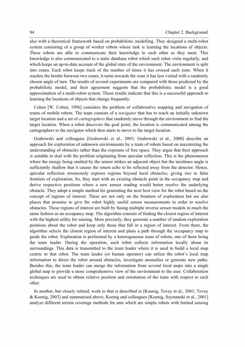
84 Chapter 2. Background
also with a theoretical framework based on probabilistic modelling. They designed a multi-robot system consisting of a group of worker robots whose task is learning the locations of objects. These robots are able to communicate their knowledge to each other as they meet. This knowledge is also communicated to a static database robot which each robot visits regularly, and which keeps an up-to-date account of the global state of the environment. The environment is split into zones. Each robot keeps track of the number of times it has crossed each zone. When it reaches the border between two zones, it turns towards the zone it has less visited with a randomly chosen angle of turn. The results of several experiments are compared with those predicted by the probabilistic model, and their agreement suggests that the probabilistic model is a good approximation of a multi-robot system. Those results indicate that this is a successful approach to learning the locations of objects that change frequently.
Cohen [W. Cohen, 1996] considers the problem of collaborative mapping and navigation of teams of mobile robots. The team consists of a navigator that has to reach an initially unknown target location and a set of cartographers that randomly move through the environment to find the target location. When a robot discovers the goal point, the location is communicated among the cartographers to the navigator which then starts to move to the target location.
Grabowski and colleagues [Grabowski et al., 2003; Grabowski et al., 2000] describe an approach for exploration of unknown environments by a team of robots based on maximizing the understanding of obstacles rather than the exposure of free space. They argue that their approach is suitable to deal with the problem originating from specular reflection. This is the phenomenon where the energy being emitted by the sensor strikes an adjacent object but the incidence angle is sufficiently shallow that it causes the return echo to be reflected away from the detector. Hence, specular reflection erroneously exposes regions beyond local obstacles, giving rise to false frontiers of exploration. So, they start with an existing obstacle point in the occupancy map and derive respective positions where a new sensor reading would better resolve the underlying obstacle. They adopt a simple method for generating the next best view for the robot based on the concept of regions of interest. These are not only on the frontiers of exploration but are also places that promise to give the robot highly useful sensor measurements in order to resolve obstacles. These regions of interest are built by fusing multiple inverse sensor models in much the same fashion as an occupancy map. The algorithm consists of finding the closest region of interest with the highest utility for sensing. More precisely, they generate a number of random exploration positions about the robot and keep only those that fall in a region of interest. From there, the algorithm selects the closest region of interest and plans a path through the occupancy map to guide the robot. Exploration is performed by a heterogeneous team of robots, one of them being the team leader. During the operation, each robot collects information locally about its surroundings. This data is transmitted to the team leader where it is used to build a local map centric to that robot. The team leader (or human operator) can utilize the robot’s local map information to direct the robot around obstacles, investigate anomalies or generate new paths. Besides this, the team leader can merge the information from several local maps into a single global map to provide a more comprehensive view of the environment to the user. Collaboration techniques are used to obtain relative position and orientation of the team with respect to each other.
In another, but closely related, work to that is described in [Koenig, Tovey et al., 2001; Tovey & Koenig, 2003] and summarised above, Koenig and colleagues [Koenig, Szymanski et al., 2001] analyze different terrain coverage methods for ants which are simple robots with limited sensing
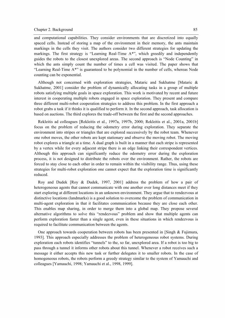
Chapter 2. Background 85
and computational capabilities. They consider environments that are discretized into equally spaced cells. Instead of storing a map of the environment in their memory, the ants maintain markings in the cells they visit. The authors consider two different strategies for updating the markings. The first strategy is “Learning Real-Time A*”, which greedily and independently guides the robots to the closest unexplored areas. The second approach is “Node Counting” in which the ants simply count the number of times a cell was visited. The paper shows that “Learning Real-Time A*” is guaranteed to be polynomial in the number of cells, whereas Node counting can be exponential.
Although not concerned with exploration strategies, Mataric and Sukhatme [Mataric & Sukhatme, 2001] consider the problem of dynamically allocating tasks in a group of multiple robots satisfying multiple goals in space exploration. This work is motivated by recent and future interest in cooperating multiple robots engaged in space exploration. They present and compare three different multi-robot cooperation strategies to address this problem. In the first approach a robot grabs a task if it thinks it is qualified to perform it. In the second approach, task allocation is based on auctions. The third explores the trade-off between the first and the second approaches.
Rekleitis ad colleagues [Rekleitis et al., 1997a, 1997b, 2000; Rekleitis et al., 2001a, 2001b] focus on the problem of reducing the odometry error during exploration. They separate the environment into stripes or triangles that are explored successively by the robot team. Whenever one robot moves, the other robots are kept stationary and observe the moving robot. The moving robot explores a triangle at a time. A dual graph is built in a manner that each stripe is represented by a vertex while for every adjacent stripe there is an edge linking their correspondent vertices. Although this approach can significantly reduce the odometry error during the exploration process, it is not designed to distribute the robots over the environment. Rather, the robots are forced to stay close to each other in order to remain within the visibility range. Thus, using these strategies for multi-robot exploration one cannot expect that the exploration time is significantly reduced.
Roy and Dudek [Roy & Dudek, 1997, 2001] address the problem of how a pair of heterogeneous agents that cannot communicate with one another over long distances meet if they start exploring at different locations in an unknown environment. They argue that to rendezvous at distinctive locations (landmarks) is a good solution to overcome the problem of communication in multi-agent exploration in that it facilitates communication because they are close each other. This enables map sharing, in order to merge them into a global map. They propose several alternative algorithms to solve this “rendezvous” problem and show that multiple agents can perform exploration faster than a single agent, even in these situations in which rendezvous is required to facilitate communication between the agents.
One approach towards cooperation between robots has been presented in [Singh & Fujimura, 1993]. This approach especially addresses the problem of heterogeneous robot systems. During exploration each robots identifies “tunnels” to the, so far, unexplored area. If a robot is too big to pass through a tunnel it informs other robots about this tunnel. Whenever a robot receives such a message it either accepts this new task or further delegates it to smaller robots. In the case of homogeneous robots, the robots perform a greedy strategy similar to the system of Yamauchi and colleagues [Yamauchi, 1998; Yamauchi et al., 1998, 1999].
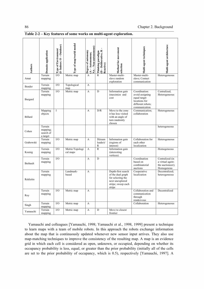
86 Chapter 2. Background
Table 2-2 – Key features of some works on multi-agent exploration. A
utho
rs
Dom
ain
appl
icat
ion
Typ
e of
Env
iron
men
t (I
- Ind
oor;
O –
Out
door
)
Typ
e of
map
/wor
ld m
odel
Deg
ree
of a
uton
omy
(A –
Aut
onom
ous;
N
A –
Non
-aut
onom
ous)
T
hink
ing
para
digm
(D
– D
elib
erat
ive;
R –
R
eact
ive)
Met
hod
for
mov
emen
t se
lect
ion
Mul
ti-ag
ent t
echn
ique
s
Mul
ti-ag
ent a
rchi
tect
ure
Amat Terrain mapping
I/O Metric map A R Master-multi-slave random exploration
Master-multi-slave; Contact communication
Heterogeneous
Bender Terrain mapping
I/O Topological map
A
Burgard
Terrain mapping
I/O Metric map A D Information gain (maximize and cost
Coordination: avoid assigning equal target locations for different robots; communication
Centralized, Heterogeneous
Billard
Mapping objects
I A D/R Move to the zone it has less visited with an angle of turn randomly chosen
Communication; collaboration
Heterogeneous
Cohen
Terrain mapping; search of a target
heterogeneous
Grabowski Terrain mapping
I/O Metric map A D(team leader)/R
Information gain (regions of interest)
Collaboration for each other localization
Heterogeneous
Koenig Terrain mapping
I/O Metric/Topological maps
A R Information gain (interesting vertices)
Homogeneous
Berhault
Terrain mapping
I/O A D Coordination based on combinatorial auctions
Centralized (in a virtual agent- the auctioneer); Homogenous
Rekleitis
Terrain mapping
Landmark-based
A Depth-first search of the dual graph for selecting the next unexplored stripe; sweep each stripe
Cooperative localization
Decentralized; heterogeneous
Roy
Terrain mapping
I/O Metric map A Collaboration and communication through rendezvous
Decentralized
Singh Terrain mapping
I/O Metric map A Collaboration Heterogeneous
Yamauchi Terrain mapping
I/O Metric map A D Move to closest frontier
Yamauchi and colleagues [Yamauchi, 1998; Yamauchi et al., 1998, 1999] present a technique to learn maps with a team of mobile robots. In this approach the robots exchange information about the map that is continuously updated whenever new sensor input arrives. They also use map-matching techniques to improve the consistency of the resulting map. A map is an evidence grid in which each cell is considered as open, unknown, or occupied, depending on whether its occupancy probability is less, equal, or greater than the prior probability (initially all of the cells are set to the prior probability of occupancy, which is 0.5), respectively [Yamauchi, 1997]. A
Chapter 2. Background 87
process analogous to edge detection and region extraction in computer vision is used to find the boundaries between open space and unknown space. Any open cell adjacent to an unknown cell is labelled a frontier edge cell. Adjacent edge cells are grouped into frontier regions. Any frontier region above a certain minimum size (roughly the size of the robot) is considered a frontier. Once frontiers have been detected within a particular evidence grid, all robots follow a greedy strategy and move to the closest frontier cell. The path planner uses a depth-first search on the grid, starting at the robot’s current cell and attempting to take the shortest obstacle-free path to the cell containing the goal location.
2.4 Exploration of Unknown Environments with Affective Agents
As described in Section 2.3.1, the relationship between exploration of unknown environments and emotion or motivation has not been ignored in fields such as Psychology, Ethology, or Neuroscience. However, as far as we know, there are almost no computational works in AI and robotics explicitly relating affective agents with exploration of unknown environments. Among the exceptions are the following works: [Whaite, 1998], [Breazeal, 1999; Breazeal & Scassellati, 1999], [Blanchard & Cañamero, 2006], [Oliveira & Sarmento, 2002], and [Velásquez, 1997, 1998a, 1998b, 1999]. For instance, Kismet [Breazeal, 1999; Breazeal & Scassellati, 1999] exhibits the proto-social response of exploration by searching for desired visual stimuli. Exploratory responses allow the “caregiver” to attribute curiosity, interest, and desires to the robot. Kismet possesses an attention system that enables it to select perceptual stimuli. Velásquez included in the drive system of his agents drives such as curiosity and also two other drives closely related to hunger, namely fatigue and “BatteryRegulation”. He also included surprise in the emotional system and related it to variables such as novelty, anticipatory expectancy, and other issues that have been considered essential components of a general attention system, including orienting to sensory stimuli, executive functions such as the detection of target events, and maintenance of a general “alert” state. Typical behavioural responses controlled by this system include look-around, orient-to-[stimulus], and look-at-[stimulus]. Anyway, neither of these latter two works addresses map-building nor considers exploration seriously, i.e., as a necessary step towards map-building.
However, we might consider that other works implicitly include rudimentary forms of some motivations and emotions and relate them to exploration. For instance, when a few works in the field of exploration make use of mathematical formulas that evaluate the parts of the environment that contain more information for the agent or that evaluate the cost of acquiring it, they are, to some extent, modelling in the agent rudimentary forms, for instance, of interest, curiosity, or hunger. They are actually considering variables such as novelty, difference, uncertainty, or change which are, according to emotion theorists, the basis of the process of elicitation of those feelings. However, by doing so, those works are not following the approach of building artificial agents that act and think like humans [S. Russell & Norvig, 1995]. Further, none of those works considers the influence of unpredictability, unexpectedness, or surprinsingness on exploration.
2.5 Other Related Fields
In the course of the research study undertaken in the context of this thesis, namely in the construction of a multi-agent system, we used concepts from knowledge representation and reasoning theories, especially from the artificial intelligence fields of case-based reasoning, as
88 Chapter 2. Background
well as planning, specifically hierarchical task network and decision-theoretic planning. The contribution of our work to these areas is not directly in the scope of this thesis. However, the importance of this section and subsections to the understanding of subsequent chapters cannot be understated. In order to describe our work thoroughly, it was important to present the parts of it that involve techniques from those areas, which logically include concepts and terminology typical of them. Moreover, as mentioned earlier in Section 1.1, we have discovered a close relationship between the exploration of unknown environments and the evaluation of creative products. Therefore, in addition to these areas, the field of creativity, especially creative evaluation, must be discussed.
Hence, this section includes an introduction to other fields that are required to understand this thesis, although they are not as central as exploration of unknown environments, emotion and motivation, or even agents and multi-agent systems. We start with knowledge representation, then we shift to planning under uncertainty in dynamic environments, subsequently we focus on the planning technique of hierarchical task-network planning, and finally we devote a few words to creativity.
2.5.1 Knowledge Representation
How the human mind represents the world is one of the questions that has been challenging cognitive science in its various perspectives for centuries, from psychologists, philosophers, linguists, neuroscientists, and more recently AI researchers. The uncertain and controversial ideas generated around this subject matter corroborate the lack of certain knowledge existing on the subject. However, knowledge representation plays a central and essential role in intelligent agents, and consequently when modelling them, as for example, in reasoning, problem solving, and thinking.
The world comes into the human mind through the sensory system: humans see, feel, hear, taste, and smell. The sensory world is somewhat transformed and represented in the mind, into what is called mental representation or knowledge representation of the world in the mind. People have knowledge of the visual appearance of a house, the feel of objects (e.g., ice is cold), taste (e.g., sugar is sweet), odors (e.g., the odor of a perfume), and sounds. Moreover, people know what a bird is. Finally, people know skills that are difficult to express to others in any way but showing them (e.g., how to ride a bicycle).
The knowledge represented in the mind is of different sorts. However, it is reasonable to classify it into a small number of categories. This has not been a consensual task, giving rise to different taxonomies of approaches to knowledge representation. Some of those taxonomies are presented as follows.
Rumelhart and Norman [Rumelhardt & Norman, 1985] distinguish between a represented world and a representing world. The represented world corresponds to the external real world. The representing world must mirror some aspects of the represented world. Rumelhart and Norman distinguish three main families of representational systems: the propositionally based systems in which knowledge is represented as a set of discrete symbols or propositions, so that concepts are represented by formal statements; the analogical based systems in which the correspondence between the represented world and the representing world is as direct as possible; and, procedural based systems in which knowledge is represented in terms of active processes or procedures.
Chapter 2. Background 89
Stillings and colleagues [Stillings et al., 1989] maintain a taxonomy similar to that of [Rumelhardt & Norman, 1985], distinguishing between propositional, analogical (imagery) and procedural knowledge. In addition, Stillings and colleagues group propositional and analogical knowledge into declarative knowledge as opposed to procedural knowledge. Declarative knowledge refers to the static, fact-like nature of representations, while procedural knowledge concerns the processes that operate on that factual knowledge.
Eysenck and Keane [Eysenck & Keane, 1991] define knowledge as the information that is represented mentally in a format and structured or organized in some manner. With respect to the format of knowledge they consider internal mental representations, as opposed to external (non-mental) representations (pictorial or diagrammatic based representations such as maps, pictures, etc., and linguistic based representations such as stories, etc.), from two main perspectives: symbolic and distributed representations. Symbolic representations comprise both propositional and analogical (visual, auditory, olfactory, gustatory, tactile, or kinetic image) representations. Distributed representations are linked to a connectionist approach to representing the world. Regarding the organization of knowledge, Eysenck and Keane suggest that there are two main kinds of knowledge organization: simple and complex organisation. Simple organization refers to how different entities can be grouped together under a common concept (object concepts) and also to relational concepts like “hit”, “buy”, “give”, etc. On the contrary, complex organization refers to how large groups of concepts (events and sequence of events – plans) are structured and used. Schemata, frames, MOPS and TOPS (described below) are examples of these complex knowledge structures.
Sharing aspects with the previous taxonomies, McNamara [McNamara, 1994] proposed a taxonomy in which the primary division occurs between declarative and procedural knowledge. Declarative knowledge is the kind of knowledge that can be verbalized, visualized or declared in some manner, while procedural knowledge corresponds to skills, cognitive operations or knowledge of how to do things that can be represented by production rules. McNamara suggests two ways for representing declarative knowledge: analogical and symbolic representations. Analogical representations preserve properties of objects and events in an intrinsic manner, i.e., the representational system has the same inherent constraints as the system being represented (e.g., a bird is represented by its image). Analogical representations are related to all the senses like visual, spatial, auditory, olfactory, gustatory, tactile, and motor. On the other hand, in symbolic representations, meanings or ideas are represented in propositions, each one having a relation and arguments (e.g., heavier(A,B) expresses the idea that an object A outweighs an object B). Propositions are the smallest units of knowledge that can stand as an assertion and that can be true or false. In propositional representations details are not covered. According to complexity, McNamara distinguishes between simple and complex knowledge representations. Simple knowledge representations, comprising the analogical, symbolic, and procedural representations, are the components of complex knowledge representations such as concepts, schemata, cognitive maps and mental models (described below).
In short, there seems to be a consensual distinction between three main kinds of knowledge representations: analogical, propositional, and procedural. Also, declarative knowledge is commonly distinguished from procedural knowledge. Declarative knowledge can be represented by analogical and propositional (symbolic) representations. There is also some consensus on splitting simple knowledge representations from complex knowledge representations. We will
90 Chapter 2. Background
now take a look at the mental constructs or frameworks proposed to model knowledge representation in humans and extensively used in computers.
Regarding analogical representation systems, most of the research has focused on visual imagery rather than on, for instance, auditory or olfactory imagery. One of the most remarkable works on visual imagery is by Kosslyn [Kosslyn, 1980, 1985]. Relying on the cathode ray tube metaphor, the basic idea of Kosslyn’s theory is that there are two fundamental kinds of representations of image information: surface and deep representation. The former corresponds to the visual image itself, while the latter refers to some sort of propositional representation from which the image can be generated. Kosslyn has also buttressed the evidence that spatial memories are of an analogical kind by showing that images of objects and of collections of objects are scanned in similar ways. Moreover, Kosslyn and colleagues [Kosslyn et al., 1988] as well as McNamara and colleagues [McNamara et al., 1992] have contributed by considering that temporal-order information is encoded in metric representations. That is, spatial memories encode not only the places occupied by objects but also when that happened. From this point of view, routes through the environment can be defined as temporally ordered sequences of scenes. This knowledge structure about the physical environment that is acquired and used, generally without concentrated effort, to find and follow routes from one place to another, and to store and use the relative positions of places, is often called the cognitive map [Kuipers, 1978, 1996, 2000, 2003; Kuipers & Byun, 1991]. An alternative formalism for analogical representation, called mental models, has been proposed by Johnson-Laird [Johnson-Laird, 1985].
With respect to procedural representations, production systems [Newell, 1973] are perhaps the most important formalism. This corresponds to if-then or condition-action statements. The action of a production is executed whenever the condition side of the production holds.
The simplest of the propositional representation systems is semantic features or attributes in which concepts are represented by a weighted set of features or attributes. Frege [Frege, 1952] distinguishes two aspects of a concept: the intension, i.e., the set of attributes which define what it is to be a member of the concept; and, the extension, i.e., the set of entities that are members of the concept. From this point of view, the intension of, for instance, the concept “bachelor” comprises the following attributes: male, unmarried, and adult. The extension of this concept includes the pope, all priests, etc. Particularly related to this approach are the ideas of Wittgenstein [Wittgenstein, 1953] who observed that concepts that are part of the natural world, such as bird, orange, chair, car, etc., are polymorphic. That is, their instances may be categorized in a variety of ways, and it is not possible to come up with a useful classical definition, in terms of a set of necessary and sufficient features, for such concepts. An answer to this problem is to represent a concept extensionally, defined by its set of instances or cases.
Resulting from an effort to overcome the drawbacks of semantic features, the model proposed by Smith and colleagues [Smith et al., 1974] led to the separation of features into two types: defining features and characteristic features. While defining features are essential features of a category or concept, characteristic features are not necessary for the definition of a concept. For instance, “has feathers” is a defining feature for the concept “bird”, whereas “can fly” is a characteristic feature. In fact, all birds have feathers, but even though most of them can fly this is not a universal feature of birds.
However, these approaches deal only with object concepts. Therefore, it becomes necessary to represent relations between concepts. Semantic networks [Quillian, 1966] were proposed with this
Chapter 2. Background 91
goal. They are directed, labelled graphs comprising a set of nodes interrelated by relations. Concepts are represented by nodes and their meaning is given by the relations it has with other concepts. One of the properties of semantic networks is inheritance, allowed by the relations “isa” and “subset”. For instance, “a isa b” means that the concept a is an instance of the concept b, while “a subset b” means that the concept a is a subset of the concept b. A drawback of semantic networks is that they became clumsy and unwieldy when they become large.
Besides object concepts, there was the need to represent relational concepts such as “hit”, “bounce”, “collide”, etc. Although several approaches were proposed to deal with these kinds of concepts, most of them based on a propositional representation of the meaning of a relation, perhaps the most remarkable approach was proposed by Schank [Schank, 1972]. Called conceptual dependency, this approach proposed a representation for the knowledge contained in language. The goals of such representation were: it should be unique and unambiguous; it must express the meaning of a sentence in any language; it must be language independent; two different sentences with the same meaning must have the same representation; and, similar concepts must have the same representation. To achieve these goals Schank proposed that the core meaning of verbs may be reduced to 12 to 15 conceptual primitives, called primitive acts (e.g., ATRANS – transfer of possession, PTRANS – physical transfer from one location to another, etc.). A relational concept is represented by a schema with four variables: actor, act, object, and direction. These variables may be filled with a value. For instance, the act variable may be instantiated with one of the primitive acts such as ATRANS, PTRANS, etc. The actor refers to the subject that is responsible for the act, while the object is the direct object of the act. Each primitive act can be used to characterise many relations. For instance, ATRANS (transfer of possession) could be “receive”, “take”, “buy”, and “sell”.
Semantic features deal only with word meaning while semantic networks and conceptual dependency include lexical and semantic knowledge. All these approaches try to represent knowledge in a single format. However, there was the need to focus on higher units of knowledge, so called supra-sentential knowledge. Minsky, Schank, and Rumelhart started the search of a solution for this problem suggesting very similar representation formalisms. Minsky [Minsky, 1975] proposed a formalism called frames, Schank [Schank & Abelson, 1977] proposed another formalism called scripts (further elaborated into MOPs [Schank, 1982]), and Rumelhart and colleagues [Rumelhardt, 1980; Rumelhardt & Norman, 1985; Rumelhardt & Ortony, 1977] still another formalism called schemata. Although they have different names, they are aimed at the same goal: to structure knowledge into higher-order representational units.
The concept of schema comes from Bartlett [Bartlett, 1932] and Piaget [Piaget, 1952]. However, the idea was not well accepted and only later did the idea become more widely used. Schemata are data structures for representing the generic concepts stored in memory. There are schemata for generalised concepts of objects, situations, events, sequence of events, action and sequences of actions, etc. They have been used to account for our ability to make inferences in complex situations, to make default assumptions about unmentioned aspects of situations, and to generate predictions about what is likely to occur in the future. Rumelhart and Ortony [Rumelhardt & Ortony, 1977] list various features of schemata as follows. First, schemata have variables. Besides a constant part that represents the characteristics of a concept which are always true in all examples of the concept (e.g., the number of legs – four – for the concept “dog”), a schema has a variable part (e.g., the colour or size of the concept “dog”). Variables of this part have default values, i.e., there is information about what values to assume for variables when the
92 Chapter 2. Background
incoming information is unspecified. Second, schemata can embedded one within another. A schema is a configuration of sub-schemata, and so on. For instance, the schema of the “human body” consists of the schemata for the “head”, the “trunk”, the “arms”, and the “legs”. In turn, the schema for “head” comprises the schemata of the “eyes”, the “mouth”, etc. Some schemata are assumed to be primitive or undecomposable. Third, schemata represent knowledge at all levels of abstraction from ideologies and cultures to word meaning and sentential knowledge. Fourth, schemata represent knowledge rather than definitions. Schemata exist for semantic and episodic knowledge [Tulving, 1972]. These terms are attributed to Tulving, who agues that the episodic memory stores information about temporally dated episodes or events, and temporally spatial relations among these events, while semantic memory stores information necessary for language such as the meaning of words, rules to manipulate them, etc. For instance, the schema for the concept “bird” contains the definition of a bird (has feathers, can fly, etc.), facts and relationships about birds (e.g., what they eat, where they live, etc.), and our own experience with birds (e.g., knowledge about a particular bird that we saw recently, etc.). The first two kinds of knowledge about birds are referred to as semantic knowledge, while the third kind of knowledge is referred to as episodic knowledge. Finally, the fifth feature of schemata concerns viewing them as active processes that evaluate its appropriateness when input information is acquired.
Script theory and its successor, dynamic memory theory [Schank, 1982, 1986] (including the notions of MOPs and TOPs which are more elaborated notions than scripts), are a variant of schemata that have been proposed to characterise people’s knowledge of commonplace event sequences such as going to a restaurant. With this dynamic memory theory, Schank also contributed to enlarging the list of categories of memory such as long-term, short-term, auditory memory, etc., by distinguishing the following three types of knowledge in his dynamic memory theory: particular situations or experiences of particular events (e.g., the knowledge about going to a restaurant last Tuesday); generalized events, i.e., general information about situations that is obtained from abstracting the common features or losing the details of those situations that have been experienced numerous times (e.g., healthcare assistants wear white uniforms); and, plan-like information (e.g., information about going to a restaurant). The first kind of knowledge is stored in what Schank called event memory, the second kind of knowledge is stored in situational memory, and the third kind of knowledge is stored in intentional memory.
The taxonomies described above, as well as other works, yield various dualities, some of which are very controversial such as analogical versus propositional (symbolic) representations, procedural versus declarative, semantic versus episodic memory, and event versus situational versus intentional memory. Closely related to Schank’s categorization of memory is Cohen’s proposal [G. Cohen, 1989] of the existence of various types of contents in memory such as plans and actions, places, objects or events, faces, etc. These contents require different models and conceptual frameworks to represent them in memory. Hence there is a memory for plans and actions, a memory for places, etc.
These knowledge representation formalisms allow an agent to possess a model of the world. The process of making the right decision by agents depends heavily on the quality of such a model of the environment that surrounds them. Unfortunately, the real world is not crystal clear to agents. Agents almost never have access to the whole environment, mainly because of the incompleteness and incorrectness of their perceptual and understanding components. In fact, it is too much work to obtain all the information from a complex and dynamic world, and it is quite
Chapter 2. Background 93
likely that the accessible information suffers distortions. Nevertheless, since the success of agents depends heavily on the completeness of the information of the state of the world, they have to pursue alternatives to construct good models of the world even (and especially) when this is uncertain. According to psychologists, cognitive scientists and ethologists [Kline, 1999; Piaget, 1952], humans and, in general, animals attempt to overcome this limitation through the generation of assumptions or expectations1 to fill in gaps in the present observational information. Note, however, that not all those expectations generated to fill in gaps in the present observational information are made explicit. However, the reasoning of the agent may be improved if its model of the world contains also a good model of future worlds. In this case, the process cannot be confined to filling in gaps in the information provided by perception because there is no information at all of those worlds. In order to overcome this limitation, agents also exhibit the ability to make predictions about future states of the world taking into account the present world and inference processes.
Gärdenfors [Gärdenfors, 1994] defends the idea that expectations are defeasible beliefs that are necessary to everyday reasoning. With respect to their cognitive origins, Gärdenfors argues that they are much like summaries of previous experiences. Thus, he suggests that they are the result of inductive reasoning. This is particularly related with Schank’s theory of dynamic memory. According to Schank, although a MOPs serve to organize our experiences that have been gathered from different episodes into sensible units organized around essential similarities, their main purpose is to provide expectations that enable the prediction of future events on the basis of previously encountered, structurally similar events.
When the missing information, either of the present state of the world or of the future states of the world, becomes known to the agent, there might be an inconsistency or conflict between it and the assumptions or expectations that the agent has. As defended by Reisenzein [Reisenzein, 2000b], Gärdenfors [Gärdenfors, 1994], Ortony and Partridge [Ortony & Partridge, 1987], etc., the result of this inconsistency gives rise to surprise. It also gives rise to the process of updating beliefs, called belief revision (e.g., [Gärdenfors, 1992]), which may be briefly described as a mechanism for changing repositories of information in the light of new information. These mechanisms can be used to incorporate new information into a knowledge container without compromising its integrity. If the new information to be incorporated is consistent with the knowledge stored in memory then this process is straightforward: simply add the new information. On the other hand, if the new information contradicts the knowledge stored in memory then great care must be exercised otherwise the introduction of an inconsistency will compromise the integrity of the knowledge base. In order to incorporate new information which is inconsistent with the knowledge base, the agent must decide what information it is prepared to give up. Belief revision attempts to model decisions concerning modifications to a knowledge repository. The guiding principles are that the changes should be both rational and minimal in some sense. Three main kinds of belief changes may be distinguished: expansion, revision, and contraction [Gärdenfors, 1992].
Case-based reasoning, in the context of artificial intelligence, is a problem solving and learning paradigm that relies on reusing the specific knowledge of previous and similar experiences or concrete problem situations (so-called cases or episodes) to solve a new problem [Aamodt & 1 Although some authors use the terms assumption and expectation as synonyms, there are authors that make a
distinction between them defending that an expectation has to do with future world states while assumptions are related to the current world state.
94 Chapter 2. Background
Plaza, 1994; Kolodner, 1993]. Hence, a case or episode may be defined as a particular, previously experienced situation, which has been captured and learned so that it can be reused to solve future problems. A case-base or memory of cases is the storage structure that holds cases. Case-based reasoning is supported by the evidence that people use case-based reasoning in their daily reasoning. It is rooted in works such as that of Schank [Schank, 1982] on dynamic memory and the central role that the remembering of earlier situations (episodes or cases) and situation patterns (scripts, MOPs) has in problem solving and learning, and Gentner [Gentner, 1983] on analogical reasoning. Apart from this, case-based reasoning is also based on other works within philosophy and psychology such as those of Tulving [Tulving, 1972] or Wittgenstein [Wittgenstein, 1953] on theories of concept formation, problem solving and experiential learning,
A new problem is solved by retrieving the most similar past case(s), reusing or adapting the information contained in this(these) case(s), revising or evaluating the solution based on reusing the previous case(s), and retaining or learning the new case by storing it in the existing case-base [Aamodt & Plaza, 1994; Kolodner, 1993]. Four main processes are therefore involved in the case-based reasoning cycle: retrieval, reuse, revision and retention. Together with these processes, case representation constitutes the primary features of case-based reasoning.
Case representation refers to the contents of a case, the structure of the case, and the organization and indexing of cases in memory so that an effective retrieval and reuse is guaranteed. The need to keep to a minimum the knowledge engineering effort required to construct case libraries, and the need for efficiency are the two main reasons to use simple case representations in some case-based reasoning systems. These simple case representations usually comprise two unstructured sets of attribute-value pairs or case features: the problem and the solution features [Gebhardt et al., 1997]. There is no description of the relationships or constraints between the features of a case. Moreover, these simple case representations are characterised by having a low number of indexed features [Watson & Perera, 1997]. The retrieval simply involves the standard nearest neighbour algorithm.
However, the construction of case-based reasoning systems in complex real-world domains critically requires complex case representations. Case-based reasoning systems for these domains are usually characterised by having a large problem space. As described by Watson and Perera [Watson & Perera, 1997], and Leake [Leake, 1996], the larger the problem space is, the more likely the case coverage is lower, and so, the more likely the case matching is poorer. Consequently, the system may propose distant and less useful solutions, which will require more adaptive effort.
Hierarchical-structured representations of cases [Macedo et al., 1996; Watson & Perera, 1997] aid overcoming the drawback of large problem space as they provide the implementation of the divide and conquer approach, offering the ability to treat subparts of cases as fully-fledged cases. This way they enable solving complex problems by re-composition of sub-solutions [Maher & Zhang, 1991]: a large problem (or a large goal) is divided into several smaller sub-problems (sub-goals), which can be independently solved using case-based reasoning. This means that the problem space may be broken into sub-problem spaces, each one having less features than the higher level problem space. The benefit of considering cases as a set of pieces, called snippets [Redmond, 1990], instead of monolithic entities, can improve the results of a case-based reasoning system in that solutions of problems may result from the contribution of multiple cases. Therefore, they make it possible to minimise the problems that appear when using parts of
Chapter 2. Background 95
multiple monolithic cases, particularly, the considerable effort taken to find the useful parts in them.
Graph-structured case representations, comprising objects and relations among them, are a suitable approach to dealing with the complex case representation problem, since they permit the ability to express the relations between any two objects in a case, they permit the variation of the set of relations used in different cases, they permit the continuous addition of new relations to the set of relations used in a continuously updated case library, and they permit the implementation of both hierarchical and non-hierarchical case decomposition. Consequently, they provide a more flexible and higher expressive power than attribute-value representations. However, they have the problem of requiring complex retrieval mechanisms (e.g., a structure similarity is usually needed) that causes significant computational costs and a hard case acquisition task. This is the main reason why some case-based reasoning systems have used representations that fall between graph-structured and unstructured representations.
2.5.2 Planning under Uncertainty in Dynamic Environments: Probabilistic and Decision-Theoretic Planning
Planning is defined as the process of finding a course of action which should be executed to achieve some goal. The so-called classical planning problem is usually defined by three aspects: description of the initial state of the world, description of the agent’s goal, and description of the set of actions that can be performed (domain theory). The initial state is usually specified by giving a list of facts that hold true in it, and the goal description is usually a logical sentence using a subset of the facts as terms. Actions are usually described in terms of preconditions and effects where the precondition of an operator is a logical sentence describing the states in which the operator can legally be applied, and the effects describe the changes that will be brought about in a state if the operator is applied. Following STRIPS [Fikes & Nilsson, 1971], the effects are usually represented as a list of facts to be deleted from the current state and a list of facts to be added.
Until recently, classical planning has been ruled by a number of problematic simplifying assumptions, notably the following [Pollack & Horty, 1999]:
• The planning agent is omniscient, i.e., it knows all the relevant facts about its environment;
• The actions that the agent can perform have definite outcomes, i.e., they are deterministic;
• The goals presented to the agent are categorical, i.e., they are either achieved or not and there is no notion of partial satisfaction;
• The agent is the only source of change in the environment, i.e., there are neither exogenous events nor other agents;
• The goals presented to the agent remain unchanged throughout the process of planning and execution;
• The actions that the agent can perform have neither temporal extent nor fixed times of occurrence.
96 Chapter 2. Background
While these systems represent significant technical achievements, when we want to apply them to problems that occur in uncertain, dynamic environments such as the real world, we find that these assumptions they make can be severely limiting. Each one these assumptions leads the planner agent to ignore relevant aspects of most real world planning domains. In fact, the real world is characterized by the presence of uncertainty in different manners. Unfortunately, the real world is not crystal clear to agents. Agents almost never have access to the whole environment, mainly because of the incompleteness and incorrectness of their perceptual and understanding components. Actually, it is too much work to obtain all the information from a complex and dynamic world, and it is quite likely that the accessible information suffers distortions. Besides, the environment can change while the planner agent is deliberating, especially because other agents may be changing the world through exogenous events that are not completely known or predictable. Finally, the outcomes of actions taken in the domain may be nondeterministic, and finally the goals of the agent may change over time perhaps unpredictably. These sources of uncertainty make the planning task harder. So, in these domains where actions may have several outcomes, a plan may consequently also have different possible outcomes, or, more appropriately, there are actually different alternative courses of action, each one with a specific probability value of achieving the goals to a certain degree. Hence, some of those alternative outcomes may be more valuable than others. Especial techniques are required to evaluate them. The benefits of executing a plan must be weighed against the costs. They must balance the potential of some plan achieving a goal state against the risk of producing an undesirable state and against the cost of performing the plan. This is particularly useful to prevent the agent suffering the consequences of undesired states of the world that may be achieved by executing the plan.
Decision theory [Luce & Raiffa, 1957] provides an attractive framework for weighing the strengths and weaknesses of a particular course of action. Resulting from the combination of utility theory and probability theory [S. Russell & Norvig, 1995; Shafer & Pearl, 1990], decision theory provides artificial agents with processes to make “right” decisions. It relies on the expected-utility maximization approach founded by von Neumann and Morgenstern [von Neumann & Morgenstern, 1944] and extended by Savage [Savage, 1953]. It is presumed that for every decision-maker there exists some real-valued function u, defined on the relevant set X of outcomes x1,x2,…xn, such that if one available action a results in probabilities pi over the outcomes xi (for i=1,…,n) and another available action b results in probabilities qi over the same outcomes, then the decision-maker (strictly) prefers action a to action b if, and only if, the statistically expected value of this utility function u is greater under a than under b. Formally, the criterion for choosing a is thus ∑∑ >
iii
iii xuqxup )()( .
Hence, the process is reduced to a problem of expectation formation and maximization. The decision-maker is thus assumed to behave as if he correctly assigned probabilities to relevant random events and chose an action that maximized the expected value of his resulting utility.
However, decision theory is certainly not a framework to build a plan with high EU. It can just provide a way to evaluate plans, but not build them. So merging it with AI planning was required to accomplish the goal of planning under uncertainty. The result is a technique called decision-theoretic planning [Blythe, 1998, 1999a, 1999b]. Several decision-theoretic planning approaches have been proposed and used successfully, some based on the extension of classical planning and others on Markov-Decision Processes (see [Blythe, 1999a; Boutilier et al., 1995; Littman & Majercik, 1997] for a survey). Unsurprisingly, these approaches result from relaxing
Chapter 2. Background 97
some of the overly strong assumptions of the classical planning paradigm. Not all the approaches address relaxing all the assumptions. Several planning features had to be modified and others introduced as described as follows.
In an uncertain world, high-utility plans created in advance may need to have some actions that are conditional on future observations. Planning agents must be able to make observations of their domain during execution in order to use conditional plans, removing the need to assume omniscience (first assumption) [Collins & Pryor, 1995; Peot & Smith, 1992].
In order to eliminate the assumption of deterministic actions (second assumption), it is necessary to represent uncertain actions. To do that, one has to represent various alternative outcomes and their probabilities, conditional on the state. Providing a richer representation of action inevitably makes the planning problem harder, and planners must use a representation that expresses the different outcomes as concisely as possible while still being fully expressive [Blythe, 1998; Haddawy & Doan, 1994; Kushmerick et al., 1994, 1995; Younes, 2003].
Some planners relax the binary measure of goal achievement (third assumption) to allow partial satisfaction of goals [Haddawy & Doan, 1994; Williamson & Hanks, 1994]. Besides this, one must compute or estimate the EU of a plan. For the degenerate case, this is simply the probability of success.
The assumption of static environment (fourth and fifth assumptions) has been relaxed by using techniques that rely on folding exogenous changes into the predicted outcomes of actions [Blythe, 1998; Hanks et al., 1996]. This is also the approach used in the Markov-Decision Process framework [Boutilier et al., 1995]. Another approach, often called reactive planning or plan execution systems [Firby, 1994] addresses run time system behaviour and relies on low level behaviours that are responsive to changes in the world.
Particularly, the assumption of static goals has been relaxed in works on deliberation scheduling which involves techniques for deciding which goals to attend to and when [Dean & Boddy, 1988].
Finally, there has been recent work on developing planners that reason about rich temporal constraints [Bacchus & Kabanza, 1996] and hence do away with the sixth assumption.
In short, in most of these probabilistic or decision-theoretic planning frameworks, actions are usually probabilistic conditional actions, preferences over the outcomes of the actions are expressed in terms of a utility function, and plans are evaluated in terms of their EU. The main goal is to find the plan or set of plans that maximizes an EU function [S. Russell & Norvig, 1995], i.e., to find the optimal plan. However, this might be a computationally complex task. It is usually not feasible to search the entire space of plans to find the MEU plan. Indeed, computing the EU of a single plan can be prohibitively expensive because the number of possible outcomes can grow very large. So, in order to avoid specifying the value of each possible outcome, compact ways for specifying utilities as well as actions have to be found, and the interaction between them has to be considered. These constitute the main issues and challenges that have to be confronted in order to create such probabilistic, decision-theoretic planners that are able to deal with uncertainty.
2.5.3 HTN Planning
In the context of planning, a task network is a collection of tasks that need to be carried out, together with constraints on the order in which tasks can be performed, the way variables are
98 Chapter 2. Background
instantiated, and what literals must be true before or after each task is performed. Task networks are clearly represented by a graph in which nodes represent tasks and edges represent ordering relations between tasks.
HTN planning [Erol et al., 1994a, 1994b; Erol, Hendler, & Nau, 1995; Erol, Hendler, Nau et al., 1995] is a planning methodology that solves planning problems, specified by a set of tasks that need to be performed (the initial task network) in addition to an initial state like that of classical planning, by recursively decomposing high-level tasks into simpler subtasks until tasks that can be directly executed are reached (so-called primitive tasks). This means that, unlike in action-based (also called STRIPS-like) planning [Fikes & Nilsson, 1971], there are two main types of actions in HTN planning: primitive tasks (also called operators or primitive actions) and non-primitive tasks (also called compound, decomposable, or abstract tasks). Primitive tasks are atomic or non-decomposable tasks or concrete actions that can be executed directly by the planning agent. Non-primitive tasks cannot be executed directly, because they represent activities that may involve performing several other tasks. The description of a planning domain includes a set of operators similar to those of classical planning, and also a set of methods. These methods provided by the domain theory indicate how the non-primitive tasks are decomposed into subtasks. A method associates a non-primitive task a with a task network t. It states that one way to accomplish the non-primitive task a is to achieve all the tasks in the task network t without violating the constraints in t. For each non-primitive task there may be more than one method. Each method is associated with various constraints that limit the applicability of the method to certain conditions and define the relations between the subtasks of the method. Methods result from the structured planning knowledge available in a domain. For example, in a travel planning domain, we might have the knowledge that one can reach a destination by either “taking a plane” or by “taking a train”. We may also know that “taking a plane” in turn involves “making a reservation”, “buying a ticket”, “taking a cab to the airport”, “getting on the plane”, etc. In such a situation, we can consider “taking a plane” as a non-primitive task (which cannot be directly executed by the agent). This abstract task can then be reduced to a plan fragment consisting of other non-primitive or primitive tasks (in this case: “making a reservation”, “buying a ticket”, “going to the airport”, and “getting on the plane”). This way, if there are some high-level problems with the “taking a plane” action and other goals (e.g., there is not going to be enough money to take a plane as well as pay the rent), we can resolve them before we work on low level details such as getting to the airport.
In summary, HTN planning takes a partial plan p containing tasks (it might include primitive tasks in addition to non-primitive tasks), picks an abstract task t, and for each method (reduction schema) that can be used to reduce t, a refinement of p is generated with t replaced by the subtasks of the method. This basic HTN planning procedure is outlined in the following steps (adapted from [Erol, Hendler, & Nau, 1995]):
1. Input a planning problem p.
2. If p contains only primitive tasks, then resolve the conflicts in p and return the result. If the conflicts cannot be resolved, return failure.
3. Choose a non-primitive task t in p.
4. Choose an expansion for t.
5. Replace t with the expansion.
Chapter 2. Background 99
6. Use critics to find the interactions among the tasks in p, and suggest ways to handle them.
7. Apply one of the ways suggested in step 6.
8. Go to step 2.
The task network resulting from the application of HTN planning to an initial task network exhibits a hierarchical configuration and hence it is called HTN. This HTN is therefore a set of tasks with temporal and hierarchical constraints between them. When the initial task network comprises a single root task, the resulting HTN has the structure of a tree.
HTN planning is suitable for many real world planning domains since many planning decisions made in the real world are done in a hierarchical manner. Besides, reduction schemas (methods) are readily available in those domains. A number of HTN planning systems have been developed and applied to real world domains such as those described in [Clement et al., 2001; Dix et al., 2001; Dix et al., 2002; Erol et al., 1994b; Ilghami et al., 2002; Lotem & Nau, 2000; Lotem et al., 1999; Mukkamalla & Muñoz-Avila, 2002; Muñoz-Avila, Aha et al., 2000; Muñoz-Avila, Aha et al., 2001; Muñoz-Avila, Dix et al., 2000; Muñoz-Avila, Gupta et al., 2001; Nau et al., 2003; Nau et al., 2001; Tsuneto, 1999; Tsuneto et al., 1997; Xu & Munõz-Avila, 2003].
However, for many real-world applications, developing a collection of methods that completely models plan generation has been found to be unfeasible. There are several factors that limit the development of methods. In particular, domain experts find method representation, which includes variables, difficult to use. In addition, identifying and formulating suitable preconditions is also difficult. In order to overcome this limitation, [Muñoz-Avila, Aha et al., 2001] use a case-based HTN planning algorithm, in which cases are instances of methods. Learning hierarchical plans or HTNs is still rarely addressed by the machine learning community, although there are a few exceptions. Garland and colleagues [Garland et al., 2001] infer task models from annotated examples, i.e., through demonstration by a domain expert. [Ilghami et al., 2002] describe a planning system that learns the HTN methods incrementally under supervision of an expert. They present a general formal framework for learning HTN methods, and a supervised learning algorithm, named CaMeL, based on this formalism. van Lent and Laird [van Lent & Laird, 1999] used a learning-by-observation technique which involves extracting knowledge from observations of an expert performing a task and generalizes this knowledge into a hierarchy of rules. Xu and Muñoz [Xu & Munõz-Avila, 2003] use an algorithm that gathers and generalizes information on how domain experts solve HTN planning problems.
Even though HTN planning is used more in practical applications, most studies in AI planning have been done in the action-based planning framework. However, HTN planning is provably more expressive than STRIPS-style planning [Erol, Hendler, & Nau, 1995]. There are a lot of differences between these two planning formalisms. The primary difference is in what they plan for, and how they plan for it. In STRIPS-style planning, the objective is to find a sequence of actions that will bring the world to a state that satisfies certain conditions or attainment goals. Planning proceeds by finding operators that have the desired effects, and by making the preconditions of those operators into sub-goals. In contrast, HTN planners search for plans that accomplish task networks, which can include things other than just attainment goals. Further, they plan via task decomposition and conflict resolution.
100 Chapter 2. Background
2.5.4 Creativity
Creativity is a controversial, mysterious and somehow frightening subject matter. Very few dare to try to clearly explain the challenge of clarifying the creative phenomenon. Artists and scientists rarely know how their creative ideas come about. They usually ta1k about “flashes of insight”, “inspirational moments”, “sudden ideas that pop into their heads” and mention intuition and inspiration (like the Muses) as the unique explanation. Psychologists, sociologists, philosophers, etc. cannot tell us much more about it either. Although some progress has been achieved in the study of creativity, it still is a mystery, judging by the many contradictory and incomplete theories about it. Innumerable questions still do not have concrete, objective and consensual answers: What is creativity?, What is the nature of the creative process?, Is it fruit of inspiration or is it just like other ordinary processes?, Is it conscious or unconscious?, What are the properties that characterise a creative product?, How should creativity be evaluated?, etc. This is one of the reasons why so many people claim that there will never be a scientific theory of creativity. However, the course of creativity studies tells us that this is not so. In spite of these many unanswered questions, some progress has been made, judging by the considerable amount of theories, among which there are a few that generate consensus.
In the literature, two main concepts are referred to as related to the act of creation: to bring into existence something original which did not exist before (the exnhilo definition); and to give an original form of existence to something that already exists. However, everybody seems to agree that no one can originate new things out of nothing.
In spite of the diversity of opinions with respect to the nature of creativity, it is reasonable to consider that there are four main approaches to research as suggested by Mooney [Mooney, 1963] and Stein [Stein, 1969]. According to these authors, there are four different but interrelated approaches to creativity: the creative environment, i.e., the environment where the creation happens; the creative product, i.e., the product of creating; the creative process, i.e., the process of creating; and the creative person, i.e., the person who is creative. This idea of considering creativity as a four-part phenomenon has been generally accepted by the majority of the authors in the field (see for instance [Glover et al., 1989; Sternberg, 1988]). Nonetheless, the creative process and the creative product perspectives are the most addressed in the literature. When all of these approaches are considered, one is assuming that creativity is considered as an activity (process), as a product, as a feature of the personality and that happens in a place or context. These different four approaches are deeply connected and to some extent they complement each other. We will now focus on the creative product perspective, since this is the one which this thesis and particularly exploration of unknown environments is more related to.
From the point of view of the product (one of the four main facets of creativity), surprise and related concepts such as unpredictability or unexpectedness have been pointed out as being relevant characteristics of a creative product, in addition to other commonly referred to features such as novelty, originality, interestingness and appropriateness (also defined as usefulness, aesthetic value, rightness, etc.) [Boden, 1992, 1995; Jackson & Messick, 1967; Koestler, 1964; Lubart, 1994; Macedo, 1998; MacKinnon, 1962; Moorman & Ram, 1994; Ritchie, 2001; Saunders & Gero, 2001]. Furthermore, Boden argued that there is a distinction between mere novelty and creativity [Boden, 1995]. In her opinion, that distinction resides in the fact that creative products are not only novel but also unpredictable, unexpected and therefore surprising. According to Boden, unpredictability is the essence of creativity: creative products amaze us, shock us and delight us mainly because they are unexpected or unpredictable. The nature of the

Chapter 2. Background 101
link between surprise and creativity is very strong. Surprise is usually considered as a property of a creative product, i.e., almost every creative product causes surprise, at least at the first time it is perceived.
Schank and Cleary [Schank & Cleary, 1995], and Boden [Boden, 1992, 1994] distinguish two types of perspectives in the evaluation of a creative product: the individual and the society. They claim that, for example, in the case of an individual that discovers the Theory of Relativity today, without having heard about it previously, if the perspective is himself then he may be considered creative, but non creative if the perspective is the society. In this first case, the individual is p-creative, but not h-creative [Boden, 1992].

103
Chapter 3 The Exploration of Unknown Environments by Affective Agents
xploration gathers information about the unknown. Exploration of unknown environments by artificial agents (usually mobile robots) has been an active research field in recent years. The exploration domains include planetary exploration (e.g., Mars or lunar
exploration), the search for meteorites in Antarctica, volcano exploration, map-building of interiors, etc. The main advantage of using artificial agents in those domains instead of humans is that most of them are extreme environments making exploration a dangerous task for human agents. However, there is still much to be done, especially in dynamic environments such as those real environments mentioned above. Those real environments consist of objects. For example, office environments possess chairs, doors, garbage cans, etc., cities comprise different kinds of buildings (houses, offices, hospitals, churches, etc.), as well as other objects such as cars, etc. Many of these objects are non-stationary, that is, their locations may change over time. This observation has motivated research on a new generation of mapping algorithms, which represent environments as collections of objects. Moreover, the autonomy of agents still needs to be improved, as happens, for instance, in planetary exploration which is still too human dependent [Bresina et al., 1999; Washington et al., 1999]. The plans are determined by a human operator as well as the interesting points to visit and communicated to the robots. Besides, tele-operation is impractical at longer distances, and therefore some level of autonomous operation is necessary for planetary robots deployed beyond our moon. Several exploration techniques have been proposed and tested either in simulated and real, indoor and outdoor environments, using single or multiple agents. In human beings, exploration has been closely connected with motivation and emotion. This relationship between exploration and motivation has been defended for a long time in the realms of Psychology and Ethology. Therefore, a reasonable approach is to model artificial agent’s exploration on that of humans, i.e., in a human-like fashion by assigning artificial agents mentalistic qualities such as emotion and motivation, beliefs, intentions, and desires. In fact, there is one primary reason for taking the way humans explore the environment as a reference: the problem of modelling exploration in humans has already been successfully solved by millions of years of evolution. Yet, in general, a lot of barriers have been found to incorporating models of emotion in artificial agents. Research in AI has almost completely ignored this significant role of emotions in reasoning, and only recently was this issue taken seriously, mainly because of the recent advances in neuroscience, which have indicated that cognitive tasks of humans, and particularly planning and decision-making, are influenced by emotion [Adolphs et al., 1996; Bechara et al., 1997; Churchland, 1996; Damásio, 1994; LeDoux, 1996]. Since exploration is a decision-making process, these results further support the thesis which links exploration to emotion and motivation.
In this chapter we describe an approach, based on affect, to the problem of exploring unknown environments by agents. We start by introducing AMAS, a multi-agent system based on the notion of affect and on ideas of the BDI model, that was used as a platform to develop the application for the exploration of unknown environments with affective agents. Primary relevance is given to the architecture of an affective agent. Although AMAS is presented from a generic perspective, illustrative examples are given for the particular case of the domain of the exploration
E

104 Chapter 3. The Exploration of Unknown Environments by Affective Agents
of unknown environments throughout its description. Then, we present the exploration strategy. Finally, we illustrate this strategy with an example.
3.1 A Multi-Agent System Composed of Affective Agents
Throughout its history, software engineering has developed an increasingly powerful array of tools with which to tackle the complexity of software systems. The most significant improvements in software engineering have come about through the introduction of powerful abstractions with which to manage the inherent complexity of software such as object-oriented programming. However, object-orientation fails to provide an adequate set of concepts and mechanisms for modelling complex systems. For such systems, objects are insufficient means of abstraction. This explains the most recent addition to software engineering of the notion of the intelligent agent which, unlike an object, is a self-contained problem solving system capable of autonomous, reactive, pro-active, and social behaviour. Based on this abstraction tool of agent, agent-based computing (agent-oriented programming/agent-oriented software engineering/agent-based systems) is a promising approach to developing a range of complex, usually distributed, software systems. Such complex software systems are appropriately developed as a collection of interacting, autonomous agents, i.e., as a multi-agent system.
This section describes AMAS, a multi-agent system based on the notion of affect and the BDI model. The next subsection provides an overview of AMAS, paying especial attention to the specification of the multi-agent system. The subsequent section presents the kind of environment agents can inhabit. Finally, the architecture adopted for the agents of this agent-based tool is described.
3.1.1 Overview of the Affect-based Multi-Agent System
AMAS was developed to be used as a framework for building agent-based applications in general. However, AMAS is still only in a preliminary version. For now it is simply a prototype needing further improvements and experimental evaluation (see Section 6.2). The current version is suitable for applications in which the entities (agents) are distributed in a physical environment. This is the case of the domain of exploration of unknown environments, which is the only application developed with AMAS up to date. This application is described later in this chapter. Examples of other potential applications are air traffic control, and transportation logistics (UM Translog). To extend this platform to other kinds of applications, features such as the sensors have to be extended or adapted to the requirements of such applications. For now, we focus on the agent-based platform used to develop the application of exploration of unknown environments.
As an agent-based system tool, AMAS requires the specification of the environment as well as of the agents that inhabit it. During this process it is supposed that developers describe the agents, namely their motivations, feelings, plans, goals, and actions, as well as the environment they inhabit, namely the objects and respective locations in it. The tools provided to specify the settings of the multi-agent system are still very rudimentary, lacking, for instance, a compiler. AMAS is prepared to deal with dynamic and uncertain environments. It is a homogeneous multi-agent system in the sense that all the agents are of the same type, sharing the same architecture, although converting it to a heterogeneous architecture seems to be a straightforward process. However, together with these agents, the environment can also be populated with objects. If we ultimately consider that these objects are a kind of inanimate agents, then in this case the
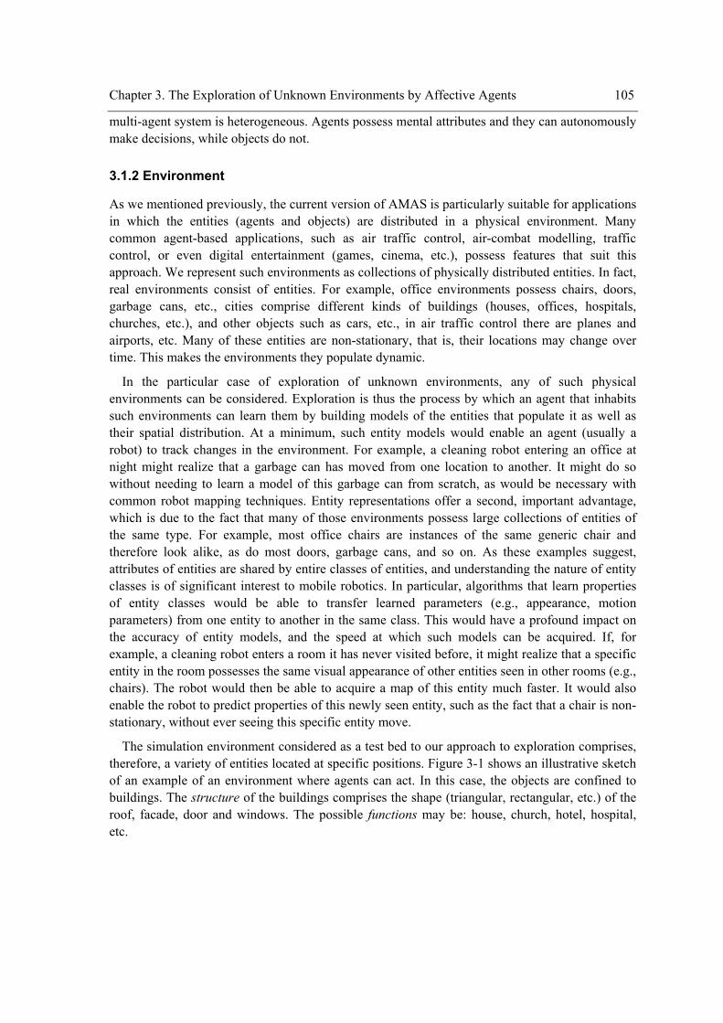
Chapter 3. The Exploration of Unknown Environments by Affective Agents 105
multi-agent system is heterogeneous. Agents possess mental attributes and they can autonomously make decisions, while objects do not.
3.1.2 Environment
As we mentioned previously, the current version of AMAS is particularly suitable for applications in which the entities (agents and objects) are distributed in a physical environment. Many common agent-based applications, such as air traffic control, air-combat modelling, traffic control, or even digital entertainment (games, cinema, etc.), possess features that suit this approach. We represent such environments as collections of physically distributed entities. In fact, real environments consist of entities. For example, office environments possess chairs, doors, garbage cans, etc., cities comprise different kinds of buildings (houses, offices, hospitals, churches, etc.), and other objects such as cars, etc., in air traffic control there are planes and airports, etc. Many of these entities are non-stationary, that is, their locations may change over time. This makes the environments they populate dynamic.
In the particular case of exploration of unknown environments, any of such physical environments can be considered. Exploration is thus the process by which an agent that inhabits such environments can learn them by building models of the entities that populate it as well as their spatial distribution. At a minimum, such entity models would enable an agent (usually a robot) to track changes in the environment. For example, a cleaning robot entering an office at night might realize that a garbage can has moved from one location to another. It might do so without needing to learn a model of this garbage can from scratch, as would be necessary with common robot mapping techniques. Entity representations offer a second, important advantage, which is due to the fact that many of those environments possess large collections of entities of the same type. For example, most office chairs are instances of the same generic chair and therefore look alike, as do most doors, garbage cans, and so on. As these examples suggest, attributes of entities are shared by entire classes of entities, and understanding the nature of entity classes is of significant interest to mobile robotics. In particular, algorithms that learn properties of entity classes would be able to transfer learned parameters (e.g., appearance, motion parameters) from one entity to another in the same class. This would have a profound impact on the accuracy of entity models, and the speed at which such models can be acquired. If, for example, a cleaning robot enters a room it has never visited before, it might realize that a specific entity in the room possesses the same visual appearance of other entities seen in other rooms (e.g., chairs). The robot would then be able to acquire a map of this entity much faster. It would also enable the robot to predict properties of this newly seen entity, such as the fact that a chair is non-stationary, without ever seeing this specific entity move.
The simulation environment considered as a test bed to our approach to exploration comprises, therefore, a variety of entities located at specific positions. Figure 3-1 shows an illustrative sketch of an example of an environment where agents can act. In this case, the objects are confined to buildings. The structure of the buildings comprises the shape (triangular, rectangular, etc.) of the roof, facade, door and windows. The possible functions may be: house, church, hotel, hospital, etc.
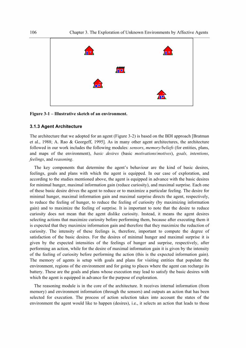
106 Chapter 3. The Exploration of Unknown Environments by Affective Agents
Figure 3-1 – Illustrative sketch of an environment.
3.1.3 Agent Architecture
The architecture that we adopted for an agent (Figure 3-2) is based on the BDI approach [Bratman et al., 1988; A. Rao & Georgeff, 1995]. As in many other agent architectures, the architecture followed in our work includes the following modules: sensors, memory/beliefs (for entities, plans, and maps of the environment), basic desires (basic motivations/motives), goals, intentions, feelings, and reasoning.
The key components that determine the agent’s behaviour are the kind of basic desires, feelings, goals and plans with which the agent is equipped. In our case of exploration, and according to the studies mentioned above, the agent is equipped in advance with the basic desires for minimal hunger, maximal information gain (reduce curiosity), and maximal surprise. Each one of these basic desire drives the agent to reduce or to maximize a particular feeling. The desire for minimal hunger, maximal information gain and maximal surprise directs the agent, respectively, to reduce the feeling of hunger, to reduce the feeling of curiosity (by maximizing information gain) and to maximize the feeling of surprise. It is important to note that the desire to reduce curiosity does not mean that the agent dislike curiosity. Instead, it means the agent desires selecting actions that maximize curiosity before performing them, because after executing them it is expected that they maximize information gain and therefore that they maximize the reduction of curiosity. The intensity of these feelings is, therefore, important to compute the degree of satisfaction of the basic desires. For the desires of minimal hunger and maximal surprise it is given by the expected intensities of the feelings of hunger and surprise, respectively, after performing an action, while for the desire of maximal information gain it is given by the intensity of the feeling of curiosity before performing the action (this is the expected information gain). The memory of agents is setup with goals and plans for visiting entities that populate the environment, regions of the environment and for going to places where the agent can recharge its battery. These are the goals and plans whose execution may lead to satisfy the basic desires with which the agent is equipped in advance for the purpose of exploration.
The reasoning module is in the core of the architecture. It receives internal information (from memory) and environment information (through the sensors) and outputs an action that has been selected for execution. The process of action selection takes into account the states of the environment the agent would like to happen (desires), i.e., it selects an action that leads to those
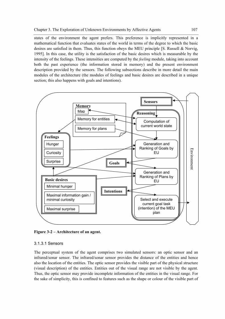
Chapter 3. The Exploration of Unknown Environments by Affective Agents 107
states of the environment the agent prefers. This preference is implicitly represented in a mathematical function that evaluates states of the world in terms of the degree to which the basic desires are satisfied in them. Thus, this function obeys the MEU principle [S. Russell & Norvig, 1995]. In this case, the utility is the satisfaction of the basic desires which is measurable by the intensity of the feelings. These intensities are computed by the feeling module, taking into account both the past experience (the information stored in memory) and the present environment description provided by the sensors. The following subsections describe in more detail the main modules of the architecture (the modules of feelings and basic desires are described in a unique section; this also happens with goals and intentions).
Figure 3-2 – Architecture of an agent.
3.1.3.1 Sensors
The perceptual system of the agent comprises two simulated sensors: an optic sensor and an infrared/sonar sensor. The infrared/sonar sensor provides the distance of the entities and hence also the location of the entities. The optic sensor provides the visible part of the physical structure (visual description) of the entities. Entities out of the visual range are not visible by the agent. Thus, the optic sensor may provide incomplete information of the entities in the visual range. For the sake of simplicity, this is confined to features such as the shape or colour of the visible part of
Memory for entities
Generation and Ranking of Goals by
EU
Sensors
Memory for plans
Memory
Hunger
Feelings
Computation of current world state
Generation and Ranking of Plans by
EU
Select and execute current goal task
(intention) of the MEU plan
Reasoning
Minimal hunger
Maximal information gain / minimal curiosity
Maximal surprise
Map
Intentions
Goals
Environment
Surprise
Curiosity
Basic desires
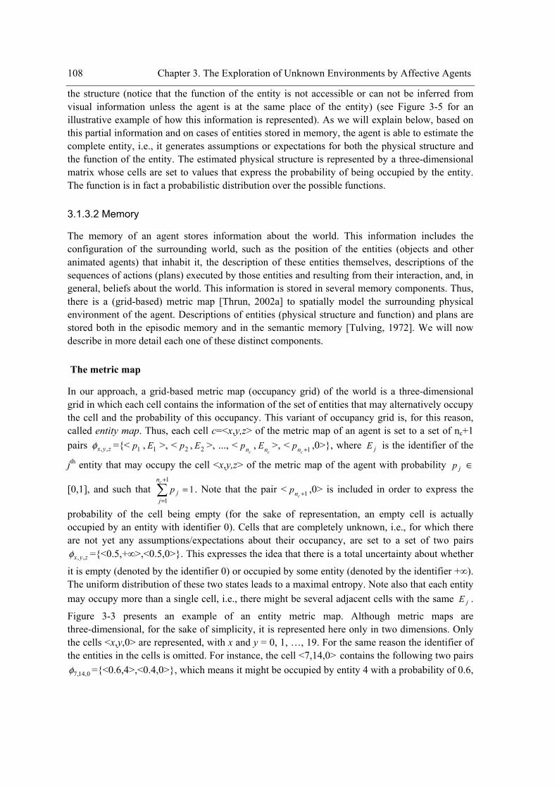
108 Chapter 3. The Exploration of Unknown Environments by Affective Agents
the structure (notice that the function of the entity is not accessible or can not be inferred from visual information unless the agent is at the same place of the entity) (see Figure 3-5 for an illustrative example of how this information is represented). As we will explain below, based on this partial information and on cases of entities stored in memory, the agent is able to estimate the complete entity, i.e., it generates assumptions or expectations for both the physical structure and the function of the entity. The estimated physical structure is represented by a three-dimensional matrix whose cells are set to values that express the probability of being occupied by the entity. The function is in fact a probabilistic distribution over the possible functions.
3.1.3.2 Memory
The memory of an agent stores information about the world. This information includes the configuration of the surrounding world, such as the position of the entities (objects and other animated agents) that inhabit it, the description of these entities themselves, descriptions of the sequences of actions (plans) executed by those entities and resulting from their interaction, and, in general, beliefs about the world. This information is stored in several memory components. Thus, there is a (grid-based) metric map [Thrun, 2002a] to spatially model the surrounding physical environment of the agent. Descriptions of entities (physical structure and function) and plans are stored both in the episodic memory and in the semantic memory [Tulving, 1972]. We will now describe in more detail each one of these distinct components.
The metric map
In our approach, a grid-based metric map (occupancy grid) of the world is a three-dimensional grid in which each cell contains the information of the set of entities that may alternatively occupy the cell and the probability of this occupancy. This variant of occupancy grid is, for this reason, called entity map. Thus, each cell c=<x,y,z> of the metric map of an agent is set to a set of nc+1 pairs zyx ,,φ ={< 1p , 1E >, < 2p , 2E >, ..., <
cnp ,cnE >, < 1+cnp ,0>}, where jE is the identifier of the
jth entity that may occupy the cell <x,y,z> of the metric map of the agent with probability jp ∈
[0,1], and such that ∑+
==
1
11
cn
jjp . Note that the pair < 1+cnp ,0> is included in order to express the
probability of the cell being empty (for the sake of representation, an empty cell is actually occupied by an entity with identifier 0). Cells that are completely unknown, i.e., for which there are not yet any assumptions/expectations about their occupancy, are set to a set of two pairs
zyx ,,φ ={<0.5,+∞>,<0.5,0>}. This expresses the idea that there is a total uncertainty about whether
it is empty (denoted by the identifier 0) or occupied by some entity (denoted by the identifier +∞). The uniform distribution of these two states leads to a maximal entropy. Note also that each entity may occupy more than a single cell, i.e., there might be several adjacent cells with the same jE .
Figure 3-3 presents an example of an entity metric map. Although metric maps are three-dimensional, for the sake of simplicity, it is represented here only in two dimensions. Only the cells <x,y,0> are represented, with x and y = 0, 1, …, 19. For the same reason the identifier of the entities in the cells is omitted. For instance, the cell <7,14,0> contains the following two pairs
0,14,7φ ={<0.6,4>,<0.4,0>}, which means it might be occupied by entity 4 with a probability of 0.6,
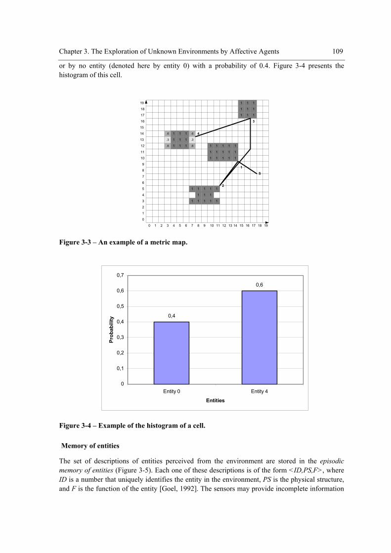
Chapter 3. The Exploration of Unknown Environments by Affective Agents 109
or by no entity (denoted here by entity 0) with a probability of 0.4. Figure 3-4 presents the histogram of this cell.
1 11
1 1 1
11111
1 1
0 1 2 3 4 5 6 7 8 9 10 11 12 13 14 15 16 17 18 19
0
1
2
3
4
5
6
7
8
9
10
11
12
13
14
15
16
17
18
19
1 11
1 1 1
11111
1 1
1 1
1 11
1 1 1
111
1 11
1 1 1
111
.6
.3
.6
.6.6
.3
S
1
2
3
4
Figure 3-3 – An example of a metric map.
0,4
0,6
0
0,1
0,2
0,3
0,4
0,5
0,6
0,7
Entity 0 Entity 4
Entities
Prob
abili
ty
Figure 3-4 – Example of the histogram of a cell.
Memory of entities
The set of descriptions of entities perceived from the environment are stored in the episodic memory of entities (Figure 3-5). Each one of these descriptions is of the form <ID,PS,F>, where ID is a number that uniquely identifies the entity in the environment, PS is the physical structure, and F is the function of the entity [Goel, 1992]. The sensors may provide incomplete information
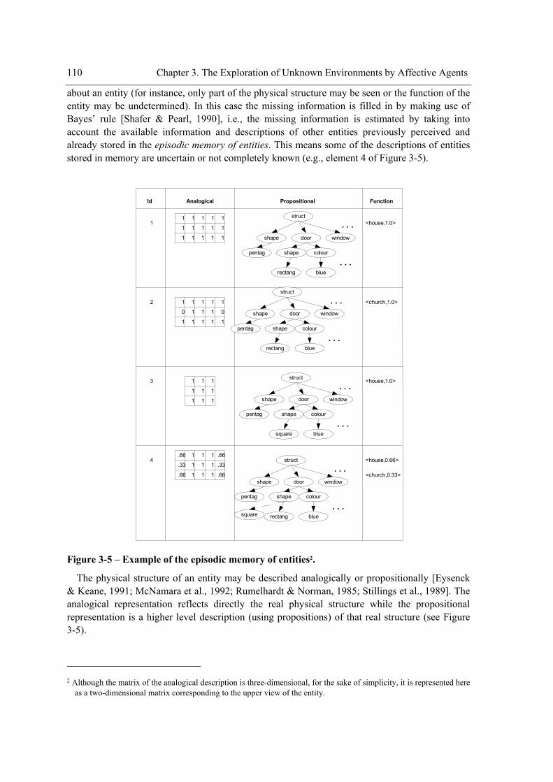
110 Chapter 3. The Exploration of Unknown Environments by Affective Agents
about an entity (for instance, only part of the physical structure may be seen or the function of the entity may be undetermined). In this case the missing information is filled in by making use of Bayes’ rule [Shafer & Pearl, 1990], i.e., the missing information is estimated by taking into account the available information and descriptions of other entities previously perceived and already stored in the episodic memory of entities. This means some of the descriptions of entities stored in memory are uncertain or not completely known (e.g., element 4 of Figure 3-5).
<house,1.0>
shape
. . .door window
shape
rectang
colour
blue. . .
pentag
struct
Id Analogical
1
1
1
1 1 1
1 1 1
1 1 11
1
1
Propositional Function
1
shape
. . .door window
shape
square
colour
blue. . .
pentag
struct
<church,1.0>2 1
0
1
1 1 1
1 1 1
1 1 11
1
0
1 1 1
1 1 1
1 1 1
shape
. . .door window
shape
rectang
colour
blue. . .
pentag
struct
<house,1.0>3
.66
.33
.66
1 1 1
1 1 1
1 1 1.66
.66
.33
shape
. . .door window
shape
rectang
colour
blue. . .
pentag
struct
square
<house,0.66>
<church,0.33>
4
Figure 3-5 – Example of the episodic memory of entities2.
The physical structure of an entity may be described analogically or propositionally [Eysenck & Keane, 1991; McNamara et al., 1992; Rumelhardt & Norman, 1985; Stillings et al., 1989]. The analogical representation reflects directly the real physical structure while the propositional representation is a higher level description (using propositions) of that real structure (see Figure 3-5).
2 Although the matrix of the analogical description is three-dimensional, for the sake of simplicity, it is represented here
as a two-dimensional matrix corresponding to the upper view of the entity.
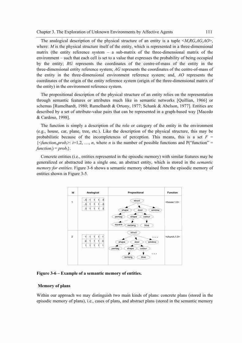
Chapter 3. The Exploration of Unknown Environments by Affective Agents 111
The analogical description of the physical structure of an entity is a tuple <M,RG,AG,AO>, where: M is the physical structure itself of the entity, which is represented in a three-dimensional matrix (the entity reference system – a sub-matrix of the three-dimensional matrix of the environment – such that each cell is set to a value that expresses the probability of being occupied by the entity; RG represents the coordinates of the centre-of-mass of the entity in the three-dimensional entity reference system; AG represents the coordinates of the centre-of-mass of the entity in the three-dimensional environment reference system; and, AO represents the coordinates of the origin of the entity reference system (origin of the three-dimensional matrix of the entity) in the environment reference system.
The propositional description of the physical structure of an entity relies on the representation through semantic features or attributes much like in semantic networks [Quillian, 1966] or schemas [Rumelhardt, 1980; Rumelhardt & Ortony, 1977; Schank & Abelson, 1977]. Entities are described by a set of attribute-value pairs that can be represented in a graph-based way [Macedo & Cardoso, 1998].
The function is simply a description of the role or category of the entity in the environment (e.g., house, car, plane, tree, etc.). Like the description of the physical structure, this may be probabilistic because of the incompleteness of perception. This means, this is a set F = {<functioni,probi>: i=1,2, …, n, where n is the number of possible functions and P(“function” = functioni) = probi}.
Concrete entities (i.e., entities represented in the episodic memory) with similar features may be generalized or abstracted into a single one, an abstract entity, which is stored in the semantic memory for entities. Figure 3-6 shows a semantic memory obtained from the episodic memory of entities shown in Figure 3-5.
<house,1.0>
Id Analogical
.5
.5
.5
1 1 1
1 1 1
1 1 1.5
.5
.5
Propositional Function
1
<church,1.0>2 1
0
1
1 1 1
1 1 1
1 1 11
1
0 shape
. . .door window
shape
rectang
colour
blue. . .
pentag
struct
shape door window
shape
rectang
colour
blue
pentag
struct
square
Figure 3-6 – Example of a semantic memory of entities.
Memory of plans
Within our approach we may distinguish two main kinds of plans: concrete plans (stored in the episodic memory of plans), i.e., cases of plans, and abstract plans (stored in the semantic memory
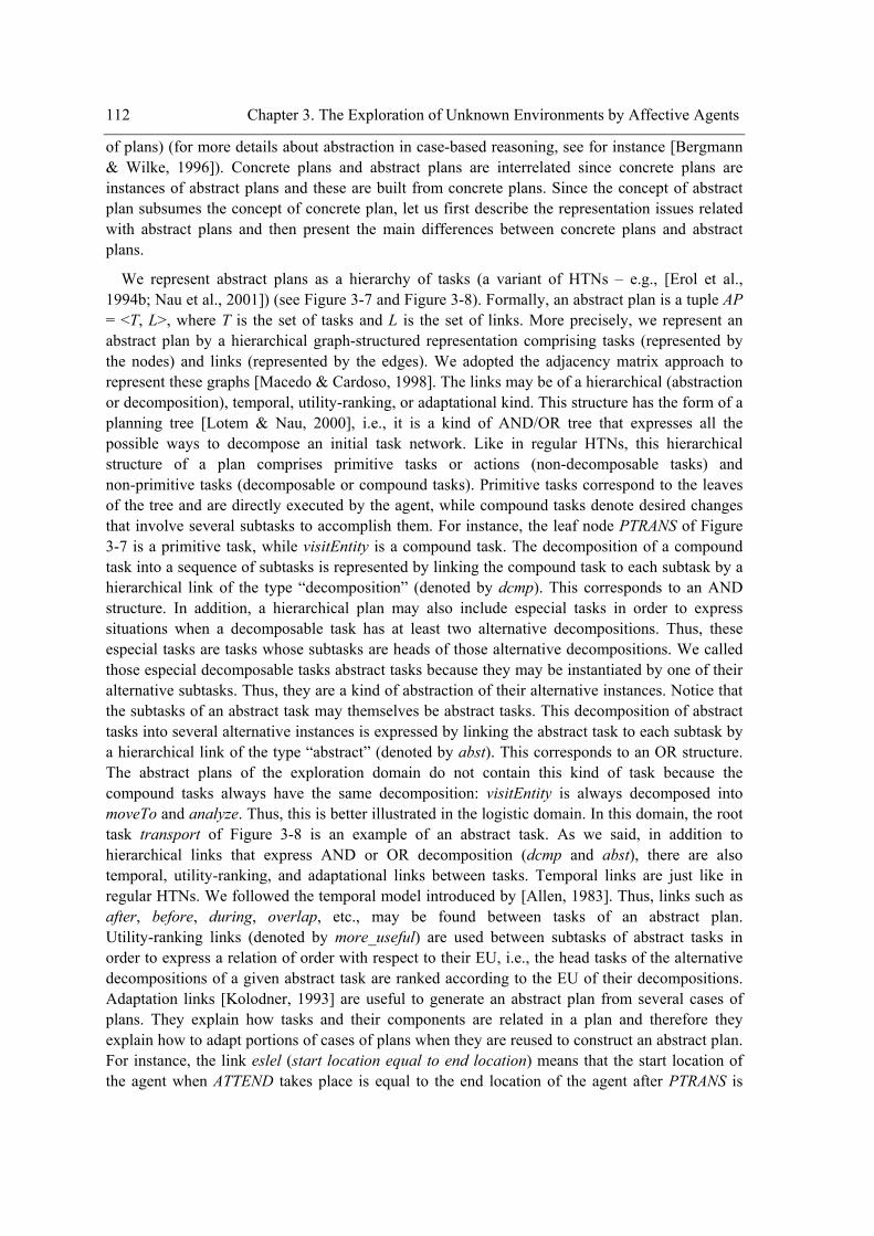
112 Chapter 3. The Exploration of Unknown Environments by Affective Agents
of plans) (for more details about abstraction in case-based reasoning, see for instance [Bergmann & Wilke, 1996]). Concrete plans and abstract plans are interrelated since concrete plans are instances of abstract plans and these are built from concrete plans. Since the concept of abstract plan subsumes the concept of concrete plan, let us first describe the representation issues related with abstract plans and then present the main differences between concrete plans and abstract plans.
We represent abstract plans as a hierarchy of tasks (a variant of HTNs – e.g., [Erol et al., 1994b; Nau et al., 2001]) (see Figure 3-7 and Figure 3-8). Formally, an abstract plan is a tuple AP = <T, L>, where T is the set of tasks and L is the set of links. More precisely, we represent an abstract plan by a hierarchical graph-structured representation comprising tasks (represented by the nodes) and links (represented by the edges). We adopted the adjacency matrix approach to represent these graphs [Macedo & Cardoso, 1998]. The links may be of a hierarchical (abstraction or decomposition), temporal, utility-ranking, or adaptational kind. This structure has the form of a planning tree [Lotem & Nau, 2000], i.e., it is a kind of AND/OR tree that expresses all the possible ways to decompose an initial task network. Like in regular HTNs, this hierarchical structure of a plan comprises primitive tasks or actions (non-decomposable tasks) and non-primitive tasks (decomposable or compound tasks). Primitive tasks correspond to the leaves of the tree and are directly executed by the agent, while compound tasks denote desired changes that involve several subtasks to accomplish them. For instance, the leaf node PTRANS of Figure 3-7 is a primitive task, while visitEntity is a compound task. The decomposition of a compound task into a sequence of subtasks is represented by linking the compound task to each subtask by a hierarchical link of the type “decomposition” (denoted by dcmp). This corresponds to an AND structure. In addition, a hierarchical plan may also include especial tasks in order to express situations when a decomposable task has at least two alternative decompositions. Thus, these especial tasks are tasks whose subtasks are heads of those alternative decompositions. We called those especial decomposable tasks abstract tasks because they may be instantiated by one of their alternative subtasks. Thus, they are a kind of abstraction of their alternative instances. Notice that the subtasks of an abstract task may themselves be abstract tasks. This decomposition of abstract tasks into several alternative instances is expressed by linking the abstract task to each subtask by a hierarchical link of the type “abstract” (denoted by abst). This corresponds to an OR structure. The abstract plans of the exploration domain do not contain this kind of task because the compound tasks always have the same decomposition: visitEntity is always decomposed into moveTo and analyze. Thus, this is better illustrated in the logistic domain. In this domain, the root task transport of Figure 3-8 is an example of an abstract task. As we said, in addition to hierarchical links that express AND or OR decomposition (dcmp and abst), there are also temporal, utility-ranking, and adaptational links between tasks. Temporal links are just like in regular HTNs. We followed the temporal model introduced by [Allen, 1983]. Thus, links such as after, before, during, overlap, etc., may be found between tasks of an abstract plan. Utility-ranking links (denoted by more_useful) are used between subtasks of abstract tasks in order to express a relation of order with respect to their EU, i.e., the head tasks of the alternative decompositions of a given abstract task are ranked according to the EU of their decompositions. Adaptation links [Kolodner, 1993] are useful to generate an abstract plan from several cases of plans. They explain how tasks and their components are related in a plan and therefore they explain how to adapt portions of cases of plans when they are reused to construct an abstract plan. For instance, the link eslel (start location equal to end location) means that the start location of the agent when ATTEND takes place is equal to the end location of the agent after PTRANS is
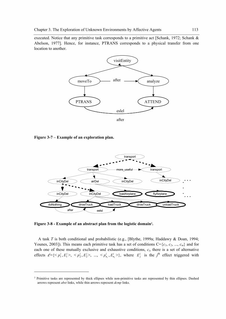
Chapter 3. The Exploration of Unknown Environments by Affective Agents 113
executed. Notice that any primitive task corresponds to a primitive act [Schank, 1972; Schank & Abelson, 1977]. Hence, for instance, PTRANS corresponds to a physical transfer from one location to another.
Figure 3-7 – Example of an exploration plan.
transport
transport transport
inCityDel airDel inCityDel inCityDel
flyAirplaneloadAirplaneinCityDel inCityDel
doNothing driveTruck loadTruck driveTruck unloadTruck
. . .
.
.
.
. . .
after
more_useful
eelsl
Figure 3-8 - Example of an abstract plan from the logistic domain3.
A task T is both conditional and probabilistic (e.g., [Blythe, 1999a; Haddawy & Doan, 1994; Younes, 2003]). This means each primitive task has a set of conditions C={c1, c2, ..., cm} and for each one of these mutually exclusive and exhaustive conditions, ci, there is a set of alternative effects εi={< ip1 , iE1 >, < ip2 , iE2 >, ..., < i
nip , i
niE >}, where i
jE is the jth effect triggered with
3 Primitive tasks are represented by thick ellipses while non-primitive tasks are represented by thin ellipses. Dashed
arrows represent abst links, while thin arrows represent dcmp links.
visitEntity
moveTo analyze
PTRANS ATTEND
eslel
after
after
114 Chapter 3. The Exploration of Unknown Environments by Affective Agents
probability ijp ∈ [0,1] by condition ci (i.e., i
jiij pcEP =)|( ), and such that ∑
==
in
j
ijp
11. Figure 3-9
presents the generic structure of a task. The probabilities of conditions are represented in that structure although we assume that conditions are independent of tasks, i.e., P(ci|T)=P(ci). The main reason for this is to emphasize that the EU of a task, in addition to the probability of effects, depends on the probability of conditions too. In addition to conditions and effects, a task has other information components. Formally, a task (primitive or not) may be defined as follows.
Definition 1. A task is a tuple <PS, ID, TT, AID, DO, IO, ST, ET, SL, EL, PR, A, EP, EU, P>, where:
• PS is the set of preconditions that should be satisfied so that the task can be executed;
• ID is the task’s identifier, i.e., an integer that uniquely identifies the task in a plan;
• TT is the task category (e.g., driveTruck, transport);
• AID is the identifier of the agent that is responsible for the execution of the task4;
• DO is the direct object of the task, i.e., the identifier of the entity that was subjected to the task directly (e.g., for a task of type “driveTruck”, the direct object is the object – its identifier – to be driven; for a task of type “transport”, the direct object is the entity that is transported – for instance, a package);
• IO is the indirect object of the task, i.e., the answer to the question “To whom?” (e.g., for a task of type “give”, the indirect object is the entity that receives the entity (the direct object) that is given – for instance, the person who receives the money);
• ST is the scheduled start time of the task;
• ET is the scheduled end time of the task,
• SL is the start location of the agent that is responsible for executing the task;
• EL is the end location of the agent that is responsible for executiing the task;
• PR is a Boolean value that is true when the task is primitive;
• A is a Boolean value that is true when the task is abstract (for primitive tasks it is always false);
• EP is the set of alternative probabilistic conditional effects of the task, i.e., EP = {<ci,εi>: 1=< i <=m};
• EU is the EU of the task;
• P is the probability of the task (this has always the value 1 for every task except the heads of alternative decompositions of an abstract task as will be explained below).
4 Notice that our planning formalism is suitable for multi-agent planning, i.e., the structure of the plans allows them to
be built so they may be executed by a team of agents.
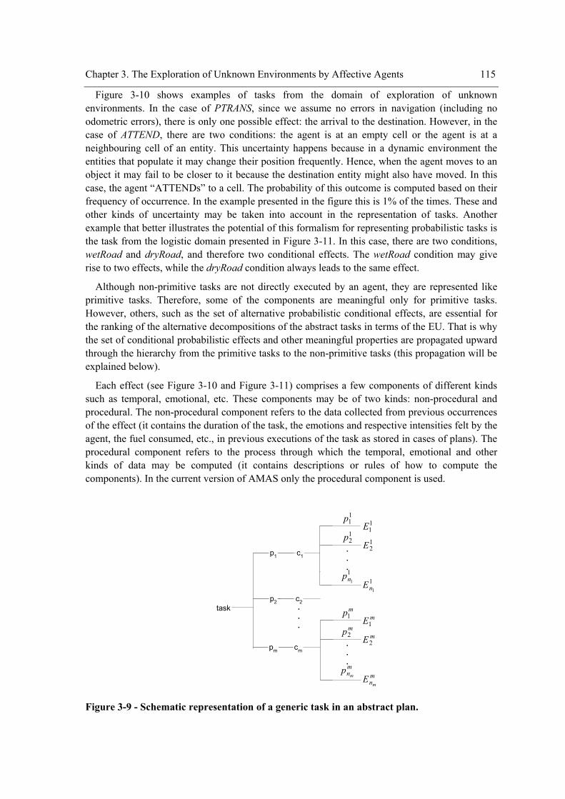
Chapter 3. The Exploration of Unknown Environments by Affective Agents 115
Figure 3-10 shows examples of tasks from the domain of exploration of unknown environments. In the case of PTRANS, since we assume no errors in navigation (including no odometric errors), there is only one possible effect: the arrival to the destination. However, in the case of ATTEND, there are two conditions: the agent is at an empty cell or the agent is at a neighbouring cell of an entity. This uncertainty happens because in a dynamic environment the entities that populate it may change their position frequently. Hence, when the agent moves to an object it may fail to be closer to it because the destination entity might also have moved. In this case, the agent “ATTENDs” to a cell. The probability of this outcome is computed based on their frequency of occurrence. In the example presented in the figure this is 1% of the times. These and other kinds of uncertainty may be taken into account in the representation of tasks. Another example that better illustrates the potential of this formalism for representing probabilistic tasks is the task from the logistic domain presented in Figure 3-11. In this case, there are two conditions, wetRoad and dryRoad, and therefore two conditional effects. The wetRoad condition may give rise to two effects, while the dryRoad condition always leads to the same effect.
Although non-primitive tasks are not directly executed by an agent, they are represented like primitive tasks. Therefore, some of the components are meaningful only for primitive tasks. However, others, such as the set of alternative probabilistic conditional effects, are essential for the ranking of the alternative decompositions of the abstract tasks in terms of the EU. That is why the set of conditional probabilistic effects and other meaningful properties are propagated upward through the hierarchy from the primitive tasks to the non-primitive tasks (this propagation will be explained below).
Each effect (see Figure 3-10 and Figure 3-11) comprises a few components of different kinds such as temporal, emotional, etc. These components may be of two kinds: non-procedural and procedural. The non-procedural component refers to the data collected from previous occurrences of the effect (it contains the duration of the task, the emotions and respective intensities felt by the agent, the fuel consumed, etc., in previous executions of the task as stored in cases of plans). The procedural component refers to the process through which the temporal, emotional and other kinds of data may be computed (it contains descriptions or rules of how to compute the components). In the current version of AMAS only the procedural component is used.
c1...
c2
cm...
task
p1
p2
pm
.
.
.
11p12p
11np
11E12E
11nE
mp1
mp2
mnm
p
mE1
mE2
mnm
E
Figure 3-9 - Schematic representation of a generic task in an abstract plan.
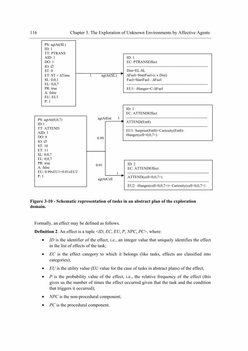
116 Chapter 3. The Exploration of Unknown Environments by Affective Agents
Figure 3-10 - Schematic representation of tasks in an abstract plan of the exploration domain.
Formally, an effect may be defined as follows.
Definition 2. An effect is a tuple <ID, EC, EU, P, NPC, PC>, where:
• ID is the identifier of the effect, i.e., an integer value that uniquely identifies the effect in the list of effects of the task;
• EC is the effect category to which it belongs (like tasks, effects are classified into categories);
• EU is the utility value (EU value for the case of tasks in abstract plans) of the effect;
• P is the probability value of the effect, i.e., the relative frequency of the effect (this gives us the number of times the effect occurred given that the task and the condition that triggers it occurred);
• NPC is the non-procedural component;
• PC is the procedural component.
PS: agtAt(SL) ID: 1 TT: PTRANS AID: 1 DO: 1 IO: ∅ ST: 0 ET: ST + ∆Time SL: 0,0,1 EL: 0,0,7 PR: true A: false EU: EU1 P: 1
agtAt(SL) 1
PS: agtAt(0,0,7) ID:1 TT: ATTEND AID: 1 DO: 8 IO: ∅ ST: 10 ET: 11 SL: 0,0,7 EL: 0,0,7 PR: true A: false EU: 0.99xEU1+0.01xEU2 P: 1
ID: 1 EC: ATTENDEffect ----------------------------------------------------------------- ATTEND(Ent8) ----------------------------------------------------------------- EU1: Surprise(Ent8)+Curiosity(Ent8)-Hunger(cell<0,0,7>)
0.99
agtAtEnt
ID: 2 EC: ATTENDEffect ----------------------------------------------------------------- ATTEND(cell<0,0,7>) ----------------------------------------------------------------- EU2: -Hunger(cell<0,0,7>)+ Curiosity(cell<0,0,7>)
agtAtCell
0.01
ID: 1 EC: PTRANSEffect ----------------------------------------------------------------- Dist=EL-SL ∆Fuel=StartFuel-(c x Dist) Fuel=StartFuel - ∆Fuel ----------------------------------------------------------------- EU1: -Hunger=C-∆Fuel
1
1
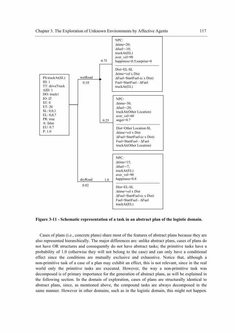
Chapter 3. The Exploration of Unknown Environments by Affective Agents 117
Figure 3-11 - Schematic representation of a task in an abstract plan of the logistic domain.
Cases of plans (i.e., concrete plans) share most of the features of abstract plans because they are also represented hierarchically. The major differences are: unlike abstract plans, cases of plans do not have OR structures and consequently do not have abstract tasks; the primitive tasks have a probability of 1.0 (otherwise they will not belong to the case) and can only have a conditional effect since the conditions are mutually exclusive and exhaustive. Notice that, although a non-primitive task of a case of a plan may exhibit an effect, this is not relevant, since in the real world only the primitive tasks are executed. However, the way a non-primitive task was decomposed is of primary importance for the generation of abstract plans, as will be explained in the following section. In the domain of exploration, cases of plans are structurally identical to abstract plans, since, as mentioned above, the compound tasks are always decomposed in the same manner. However in other domains, such as in the logistic domain, this might not happen.
wetRoad 0.18
PS:truckAt(SL) ID: 1 TT: driveTruck AID: 1 DO: truck1 IO: ∅ ST: 0 ET: 20 SL: 0,0,1 EL: 0,0,7 PR: true A: false EU: 0.7 P: 1.0
0.82 dryRoad
NPC: ∆time=20; ∆fuel=-10; truckAt(EL) aver_vel=90 happiness=0.5;surprise=0 ------------------------------------- Dist=EL-SL ∆time=vel x Dist ∆Fuel=StartFuel-(c x Dist) Fuel=StartFuel - ∆Fuel truckAt(EL)
0.75
NPC: ∆time=30; ∆fuel=-20; truckAt(Other Location) aver_vel=60 anger=0.7 ------------------------------------- Dist=Other Location-SL ∆time=vel x Dist ∆Fuel=StartFuel-(c x Dist) Fuel=StartFuel - ∆Fuel truckAt(Other Location)
0.25
NPC: ∆time=15; ∆fuel=-7; truckAt(EL) aver_vel=90 happiness=0.8 ------------------------------------- Dist=EL-SL ∆time=vel x Dist ∆Fuel=StartFuel-(c x Dist) Fuel=StartFuel - ∆Fuel truckAt(EL)
1.0
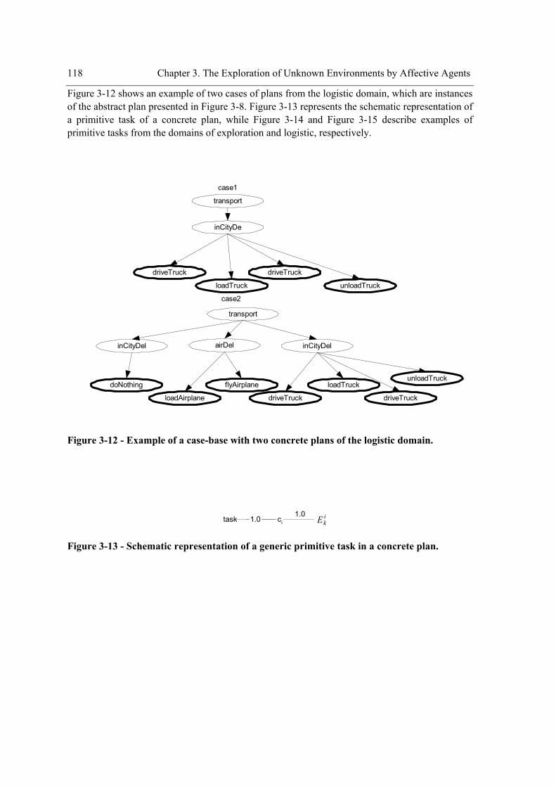
118 Chapter 3. The Exploration of Unknown Environments by Affective Agents
Figure 3-12 shows an example of two cases of plans from the logistic domain, which are instances of the abstract plan presented in Figure 3-8. Figure 3-13 represents the schematic representation of a primitive task of a concrete plan, while Figure 3-14 and Figure 3-15 describe examples of primitive tasks from the domains of exploration and logistic, respectively.
transport
inCityDel airDel inCityDel
doNothing flyAirplane
loadAirplane driveTruck
loadTruck
driveTruck
unloadTruck
case2
case1
transport
inCityDe
driveTruck
loadTruck
driveTruck
unloadTruck
Figure 3-12 - Example of a case-base with two concrete plans of the logistic domain.
task ci1.0 ikE
1.0
Figure 3-13 - Schematic representation of a generic primitive task in a concrete plan.
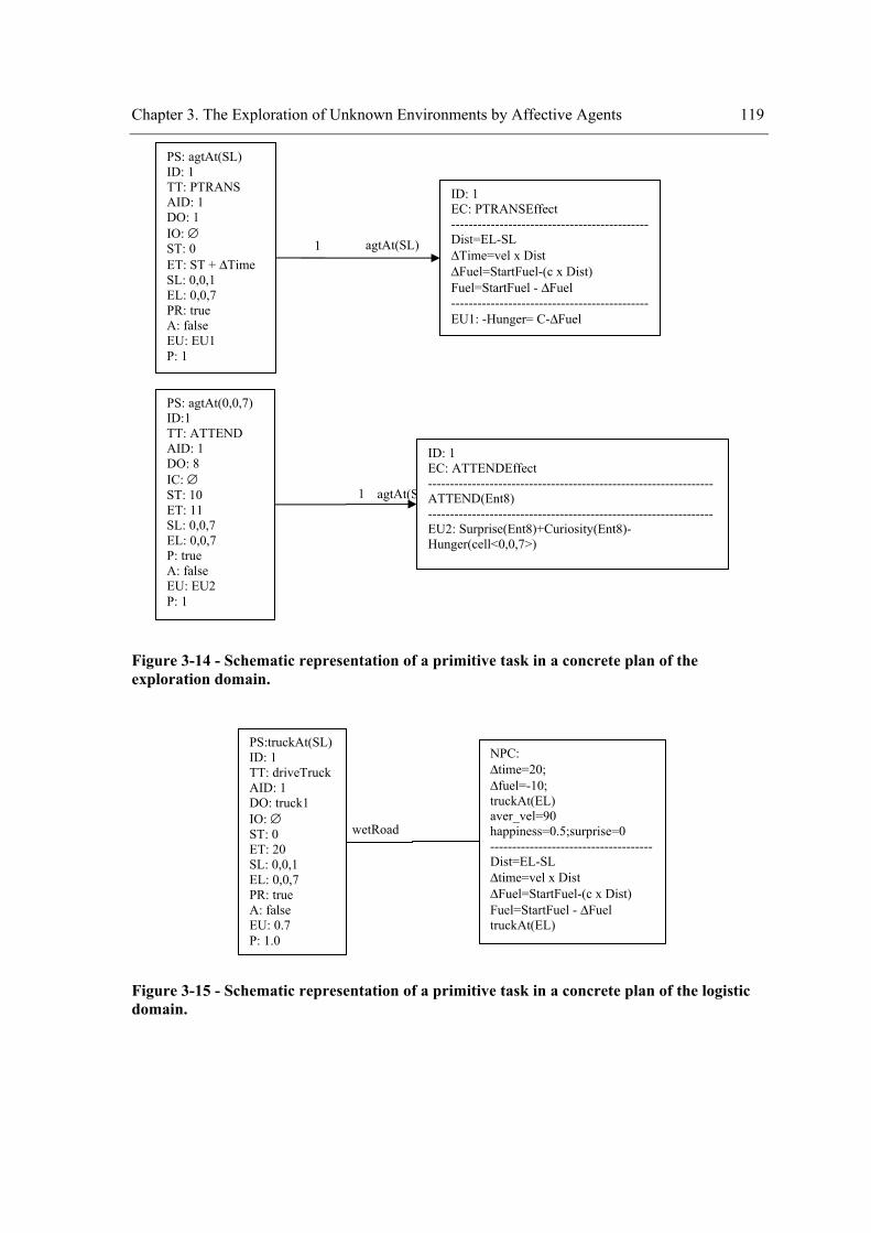
Chapter 3. The Exploration of Unknown Environments by Affective Agents 119
Figure 3-14 - Schematic representation of a primitive task in a concrete plan of the exploration domain.
Figure 3-15 - Schematic representation of a primitive task in a concrete plan of the logistic domain.
wetRoad
PS:truckAt(SL) ID: 1 TT: driveTruck AID: 1 DO: truck1 IO: ∅ ST: 0 ET: 20 SL: 0,0,1 EL: 0,0,7 PR: true A: false EU: 0.7 P: 1.0
NPC: ∆time=20; ∆fuel=-10; truckAt(EL) aver_vel=90 happiness=0.5;surprise=0 ------------------------------------- Dist=EL-SL ∆time=vel x Dist ∆Fuel=StartFuel-(c x Dist) Fuel=StartFuel - ∆Fuel truckAt(EL)
PS: agtAt(SL) ID: 1 TT: PTRANS AID: 1 DO: 1 IO: ∅ ST: 0 ET: ST + ∆Time SL: 0,0,1 EL: 0,0,7 PR: true A: false EU: EU1 P: 1
ID: 1 EC: PTRANSEffect --------------------------------------------- Dist=EL-SL ∆Time=vel x Dist ∆Fuel=StartFuel-(c x Dist) Fuel=StartFuel - ∆Fuel --------------------------------------------- EU1: -Hunger= C-∆Fuel
agtAt(SL) 1
PS: agtAt(0,0,7) ID:1 TT: ATTEND AID: 1 DO: 8 IC: ∅ ST: 10 ET: 11 SL: 0,0,7 EL: 0,0,7 P: true A: false EU: EU2 P: 1
1 agtAt(SL)
ID: 1 EC: ATTENDEffect ----------------------------------------------------------------- ATTEND(Ent8) ----------------------------------------------------------------- EU2: Surprise(Ent8)+Curiosity(Ent8)-Hunger(cell<0,0,7>)
120 Chapter 3. The Exploration of Unknown Environments by Affective Agents
3.1.3.3 Basic Desires and Feelings
Following the pluralist view of motivation [Havercamp & Reiss, 2003; McDougall, 1908; Reiss, 2000; Schwartz, 1992; B. Weiner, 1980], the module of basic desires (basic motivations/motives) contains a set of basic desires that drive the behaviour of the agent. Taking into account the studies about the motivations of exploratory behaviour described in Sections 2.3 and 2.4, we considered the following basic desires: the desires for minimal hunger, maximal information gain (reduce curiosity), and maximal surprise. The desire for minimal hunger and for maximal information gain (reduce curiosity) are among the sixteen basic desires proposed by Reiss [Reiss, 2000]. These basic desires are represented in a mathematical function that evaluates states of the environment in terms of the positive and negative relevance for the basic desires. This function obeys the MEU principle [S. Russell & Norvig, 1995] (see Section 3.1.3.5 - Generation and Management of the Agent’s Goals). This Utility Function is a combination of the Utility Functions of each desire. It represents, in our case, the aversion against hunger and the like of surprise and information gain. To satisfy the basic desires of minimal hunger, maximal information gain and maximal surprise, in the case of exploration, the agent desires to visit previously unvisited entities, regions of the environment and places where it can recharge its battery (e.g., visitEntity(y), visitLoc(x), rechargeBattery()) (see Section 3.1.3.5 - Generation and Management of the Agent’s Goals). These goals are automatically generated by the agent by adapting past goals to new situations giving rise to new goals which are then ranked according to its preference (utility) and then taken as intentions once a plan is generated for them. The reason for trying to achieve a goal might be because that achievement corresponds to a state of the environment that makes it satisfy one or several basic desires.
Each one of these basic desire drives the agent to reduce or to maximize a particular feeling. The desire for minimal hunger, maximal information gain and maximal surprise directs the agent, respectively, to reduce the feeling of hunger, to reduce the feeling of curiosity (by maximizing information gain) and to maximize the feeling of surprise. It is important to note that the desire to reduce curiosity does not mean that the agent dislike curiosity. Instead, it means the agent desires selecting actions that maximize curiosity before performing them, because after executing them it is expected that they maximize information gain and therefore that they maximize the reduction of curiosity. The intensity of these feelings is, therefore, important to compute the degree of satisfaction of the basic desires. For the desires of minimal hunger and maximal surprise it is given by the expected intensities of the feelings of hunger and surprise, respectively, after performing an action, while for the desire of maximal information gain it is given by the intensity of the feeling of curiosity before performing the action (this is the expected information gain). The intensity of these feelings is the output of the module of feelings based on the information about a state of the environment. Following Clore [Clore, 1992], we include in this module affective, cognitive, and bodily feelings. The latter two categories are merged to form the category of non-affective feelings. This means that this module is much broader than a module of emotion that could be considered. Feelings are of primary relevance to influence the behaviour of an agent, because computing their intensity the agent measures the degree to which the basic desires are fulfilled. In this thesis, this module is confined to the feelings that are related with some variables that are directly involved in exploratory behaviour (see Sections 2.3 and 2.4): surprise (elicited by unexpectedness), curiosity (elicited by novelty and uncertainty), and hunger (reflects the need for an energy source). The next subsections describe in detail the models adopted for these feelings.
Chapter 3. The Exploration of Unknown Environments by Affective Agents 121
Surprise
Our model of surprise is mainly based on Ortony and Partridge’s proposals [Ortony & Partridge, 1987] and on Meyer, Reisenzein, and Schützwohl’s model [Meyer et al., 1997; Reisenzein, 2000a, 2000b, 2001]. We will now give an overview of these models and then explain our computational model by comparing it with these two models.
Background Models
Although Ortony and Partridge agree with Meyer, Reisenzein, and Schützwohl (and also with other authors) that surprise is caused by events that are commonsensically called unexpected, they proposed that unexpectedness covers two cases. First, surprise results when prior expectations regarding an event are disconfirmed, i.e., surprise sometimes results from expectation failure. Second, however, surprise can also be caused by events for which expectations were never computed. That is, according to Ortony and Partridge, there are situations in which one is surprised although one had no explicit expectations (either conscious or unconscious) regarding the surprising event. Ortony and Partridge also proposed that surprisingness is an important variable in artificial intelligence systems, particularly in attention and learning.
In more detail, Ortony and Partridge’s model of surprise assumes a system (or agent) with an episodic and semantic propositional memory whose elements may be immutable (propositions that are believed to be always true) or typical (propositions that are believed to be usually, but not always true).The system receives an input proposition which activates some elements of that memory.
Furthermore they distinguish between practically deducible propositions and practically non-deducible propositions. Practically deducible propositions comprise the propositions that are explicitly represented in memory, as well as those that can be inferred from them by a few simple deductions. Hence, practically deducible propositions are that subset of formally deducible propositions that do not require many complex inferences. Furthermore, practically deducible propositions may be actively or passively deduced in a particular context. In the former case, their content corresponds to actively expected or predicted events; in the latter case, to passively expected (assumed) events.
Based on these assumptions, Ortony and Partridge propose that surprise results when the system encounters a conflict or inconsistency between an input proposition and pre-existing representations or representations computed “after the fact”. More precisely, surprise results in three situations (Table 3-1 presents the correspondent range of values): (i) active expectation failure: here, surprise results from a conflict or inconsistency between the input proposition and an active prediction or expectation; (ii) passive expectation failure (or assumption failure): here, surprise results from a conflict or inconsistency between the input proposition and what the agent implicitly knows or believes (passive expectations or assumptions); and (iii) unanticipated incongruities or deviations from norms: here, surprise results from a conflict or inconsistency between the input proposition (which in this case is a practically non-deducible proposition) and what, after the fact, may be judged to be normal or usual (cf. [Kahneman & Miller, 1986]), that is, between the input proposition and practically deducible propositions (immutable or typical) that are suggested by the unexpected fact. Note that, in this case, prior to the unexpected event there are no explicit expectations (passive or active) with which the input proposition could conflict.
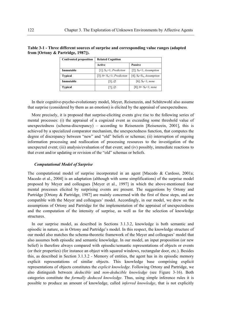
122 Chapter 3. The Exploration of Unknown Environments by Affective Agents
Table 3-1 - Three different sources of surprise and corresponding value ranges (adapted from [Ortony & Partridge, 1987]).
Related Cognition Confronted proposition
Active Passive
Immutable [1]; SA=1; Prediction [2]; SP=1; Assumption
Typical [3]; 0< SA<1; Prediction [4]; SP<SA; Assumption
Immutable [5]; ∅ [6]; SP=1; none
Typical [7]; ∅ [8]; 0< SP<1; none
In their cognitive-psycho-evolutionary model, Meyer, Reisenzein, and Schützwohl also assume that surprise (considered by them as an emotion) is elicited by the appraisal of unexpectedness.
More precisely, it is proposed that surprise-eliciting events give rise to the following series of mental processes: (i) the appraisal of a cognized event as exceeding some threshold value of unexpectedness (schema-discrepancy) – according to Reisenzein [Reisenzein, 2001], this is achieved by a specialized comparator mechanism, the unexpectedness function, that computes the degree of discrepancy between “new” and “old” beliefs or schemas; (ii) interruption of ongoing information processing and reallocation of processing resources to the investigation of the unexpected event; (iii) analysis/evaluation of that event; and (iv) possibly, immediate reactions to that event and/or updating or revision of the “old” schemas or beliefs.
Computational Model of Surprise
The computational model of surprise incorporated in an agent [Macedo & Cardoso, 2001a; Macedo et al., 2004] is an adaptation (although with some simplifications) of the surprise model proposed by Meyer and colleagues [Meyer et al., 1997] in which the above-mentioned four mental processes elicited by surprising events are present. The suggestions by Ortony and Partridge [Ortony & Partridge, 1987] are mainly concerned with the first of these steps, and are compatible with the Meyer and colleagues’ model. Accordingly, in our model, we drew on the assumptions of Ortony and Partridge for the implementation of the appraisal of unexpectedness and the computation of the intensity of surprise, as well as for the selection of knowledge structures.
In our surprise model, as described in Sections 3.1.3.2, knowledge is both semantic and episodic in nature, as in Ortony and Partridge’s model. In this respect, the knowledge structure of our model also matches the schema-theoretic framework of the Meyer and colleagues’ model that also assumes both episodic and semantic knowledge. In our model, an input proposition (or new belief) is therefore always compared with episodic/semantic representations of objects or events (or their properties) (for instance an object with squared windows, rectangular door, etc.). Besides this, as described in Section 3.1.3.2 - Memory of entities, the agent has in its episodic memory explicit representations of similar objects. This knowledge base comprising explicit representations of objects constitutes the explicit knowledge. Following Ortony and Partridge, we also distinguish between deducible and non-deducible knowledge (see Figure 3-16). Both categories constitute the formally deduced knowledge. Thus, using simple inference rules it is possible to produce an amount of knowledge, called inferred knowledge, that is not explicitly
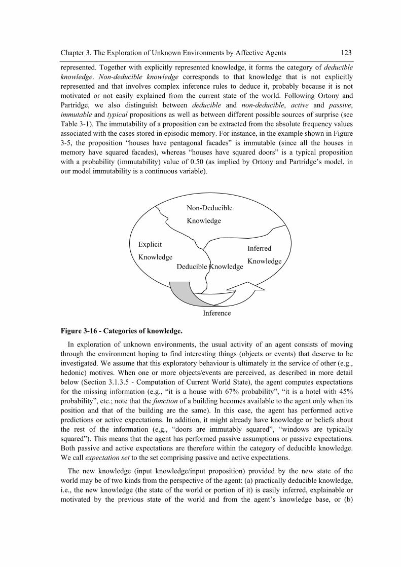
Chapter 3. The Exploration of Unknown Environments by Affective Agents 123
represented. Together with explicitly represented knowledge, it forms the category of deducible knowledge. Non-deducible knowledge corresponds to that knowledge that is not explicitly represented and that involves complex inference rules to deduce it, probably because it is not motivated or not easily explained from the current state of the world. Following Ortony and Partridge, we also distinguish between deducible and non-deducible, active and passive, immutable and typical propositions as well as between different possible sources of surprise (see Table 3-1). The immutability of a proposition can be extracted from the absolute frequency values associated with the cases stored in episodic memory. For instance, in the example shown in Figure 3-5, the proposition “houses have pentagonal facades” is immutable (since all the houses in memory have squared facades), whereas “houses have squared doors” is a typical proposition with a probability (immutability) value of 0.50 (as implied by Ortony and Partridge’s model, in our model immutability is a continuous variable).
Figure 3-16 - Categories of knowledge.
In exploration of unknown environments, the usual activity of an agent consists of moving through the environment hoping to find interesting things (objects or events) that deserve to be investigated. We assume that this exploratory behaviour is ultimately in the service of other (e.g., hedonic) motives. When one or more objects/events are perceived, as described in more detail below (Section 3.1.3.5 - Computation of Current World State), the agent computes expectations for the missing information (e.g., “it is a house with 67% probability”, “it is a hotel with 45% probability”, etc.; note that the function of a building becomes available to the agent only when its position and that of the building are the same). In this case, the agent has performed active predictions or active expectations. In addition, it might already have knowledge or beliefs about the rest of the information (e.g., “doors are immutably squared”, “windows are typically squared”). This means that the agent has performed passive assumptions or passive expectations. Both passive and active expectations are therefore within the category of deducible knowledge. We call expectation set to the set comprising passive and active expectations.
The new knowledge (input knowledge/input proposition) provided by the new state of the world may be of two kinds from the perspective of the agent: (a) practically deducible knowledge, i.e., the new knowledge (the state of the world or portion of it) is easily inferred, explainable or motivated by the previous state of the world and from the agent’s knowledge base, or (b)
Explicit
Knowledge Inferred
Knowledge
Non-Deducible
Knowledge
Inference
Deducible Knowledge
124 Chapter 3. The Exploration of Unknown Environments by Affective Agents
non-deducible knowledge, i.e., the new knowledge is hardly inferred, unexplainable or not motivated by the previous state of the world and from the agent’s knowledge base. In the former case, (a), another two major situations may happen: (a1) there is a conflict between that new knowledge and the practically deduced knowledge of the agent (active and passive expectations), or (a2) there is no conflict at all. In the former case, (a1), the degree of the conflict is assessed and the respective reaction is performed such as the elicitation of surprise [Macedo & Cardoso, 2001a; Macedo et al., 2004]. In situation (b), there is no conflict between the input knowledge and expectations because there are no expectations at all. Notice that the input knowledge of situation (b) describes a state of the world or part of it that is non-deducible to the agent and therefore it is impossible for the agent to have expectations for it. However, after the fact (after that unpredictable or practically non-deducible state of the world) it is possible to evaluate its deviation from the norm or the usual. Thus, in contrary to situation (a1), the conflict or inconsistency happens after the fact and is related to practically deducible knowledge that it suggests. The different surprise-eliciting situations distinguished by Ortony and Partridge are thus dealt with in our model in the following way. As said above, when an agent perceives an object, it first computes expectations (deducible, active expectations) for missing information (e.g., “it is a hotel with 45% probability”). If, after having visited that object, the agent detects that the object is different from what was expected (e.g., if it is a post office), the agent is surprised because its active expectations conflict with the input proposition (note that, in our model, belief conflicts may be partial as well as total). This is thus an example of the first source of surprise distinguished by Ortony and Partridge. In contrast, when an agent perceives an aspect or part of an object with particular properties (e.g., a building with a window of a circular shape) that were not actively predicted, it may still be able to infer that it expected something (e.g., a rectangular-shaped window with, 45% probability, a square-shaped window with 67%, etc.). This is an example of a deducible, passive expectation: although the expectation was not present before the agent perceived the object, it was inferred after the object had been perceived. This case is therefore an example of the second source of surprise distinguished by Ortony and Partridge, where an input proposition conflicts with an agent’s passive expectations. Finally, when an agent perceives an object with a completely new part (e.g., a building with no facade), it has neither an active nor a passive expectation available. The reason is that, because there are no objects of this kind (e.g., buildings with no facade) stored in the agent’s memory, the agent cannot predict that such objects might be encountered. The perception of an object with a completely new part is thus an example of a non-deducible proposition. This is an example of the third source of surprise distinguished by Ortony and Partridge: there is a conflict between the input proposition (e.g., “the house has no facade”) and what after the fact is judged to be normal or usual (e.g., “buildings have a facade”).
On the basis of the available information (e.g., the visible structure of an object) and the computed expectations (e.g., predictions for the function of an object), the agent then determines the computation of the degree of conflict and the computation of the intensity of surprise that may be caused by the object/event (these computations, which correspond to the “appraisal of unexpectedness” in the Meyer and colleagues’ model, are described in more detail below). Subsequently, the object/event with the maximum estimated surprise is selected to be visited and investigated5. This corresponds to the “interruption of ongoing activity” and the “reallocation of
5 We are assuming here a decision-making process completely dependent on surprise. However, as we will describe
later, this process may also take into account other variables.
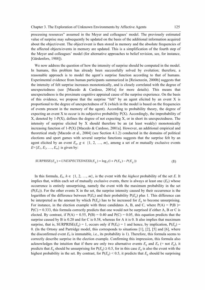
Chapter 3. The Exploration of Unknown Environments by Affective Agents 125
processing resources” assumed in the Meyer and colleagues’ model. The previously estimated value of surprise may subsequently be updated on the basis of the additional information acquired about the object/event. The object/event is then stored in memory and the absolute frequencies of the affected objects/events in memory are updated. This is a simplification of the fourth step of the Meyer and colleagues’ model (for alternative approaches to belief revision, see, for instance, [Gärdenfors, 1988]).
We now address the question of how the intensity of surprise should be computed in the model. In humans, this problem has already been successfully solved by evolution; therefore, a reasonable approach is to model the agent’s surprise function according to that of humans. Experimental evidence from human participants summarized in [Reisenzein, 2000b] suggests that the intensity of felt surprise increases monotonically, and is closely correlated with the degree of unexpectedness (see [Macedo & Cardoso, 2001a] for more details). This means that unexpectedness is the proximate cognitive appraisal cause of the surprise experience. On the basis of this evidence, we propose that the surprise “felt” by an agent elicited by an event X is proportional to the degree of unexpectedness of X (which in the model is based on the frequencies of events present in the memory of the agent). According to probability theory, the degree of expecting an event X to occur is its subjective probability P(X). Accordingly, the improbability of X, denoted by 1-P(X), defines the degree of not expecting X, or in short its unexpectedness. The intensity of surprise elicited by X should therefore be an (at least weakly) monotonically increasing function of 1-P(X) [Macedo & Cardoso, 2001a]. However, an additional empirical and theoretical study [Macedo et al., 2004] (see Section 4.1.2) conducted in the domains of political elections and sport games with several surprise functions suggests that the surprise felt by an agent elicited by an event Eg, g ∈ {1, 2, …, m}, among a set of m mutually exclusive events E={E1, E2, …, Em} is given by:
))()(1(log)()( 2 ghgg EPEPENESSUNEXPECTEDESURPRISE −+== (1)
In this formula, Eh, h ∈ {1, 2, …, m}, is the event with the highest probability of the set E. It implies that, within each set of mutually exclusive events, there is always at least one (Eh) whose occurrence is entirely unsurprising, namely the event with the maximum probability in the set (P(Eh)). For the other events X in the set, the surprise intensity caused by their occurrence is the logarithm of the difference between P(Eh) and their probability P(Eg) plus 1. This difference can be interpreted as the amount by which P(Eg) has to be increased for Eg to become unsurprising. For instance, in the election example with three candidates A, B, and C, where P(A) = P(B )= P(C) = 0.333, this formula correctly predicts that one would not be surprised if either A, B or C is elected. By contrast, if P(A) = 0.55, P(B) = 0.40 and P(C) = 0.05, this equation predicts that the surprise caused by B is 0.20 and for C is 0.58, whereas for A it is 0. It also implies that maximum surprise, that is, SURPRISE(Eg) = 1, occurs only if P(Eh) = 1 and hence, by implication, P(Eg) = 0. (In the Ortony and Partridge model, this corresponds to situations [1], [2], [5] and [6], where the disconfirmed event Eh is immutable, i.e., its probability is 1). Therefore, this formula seems to correctly describe surprise in the election example. Confirming this impression, this formula also acknowledges the intuition that if there are only two alternative events Eg and Eh (= not Eg), it predicts that Eg should be unsurprising for P(Eg) ≥ 0.5, for in this case Eg is also the event with the highest probability in the set. By contrast, for P(Eg) < 0.5, it predicts that Eg should be surprising
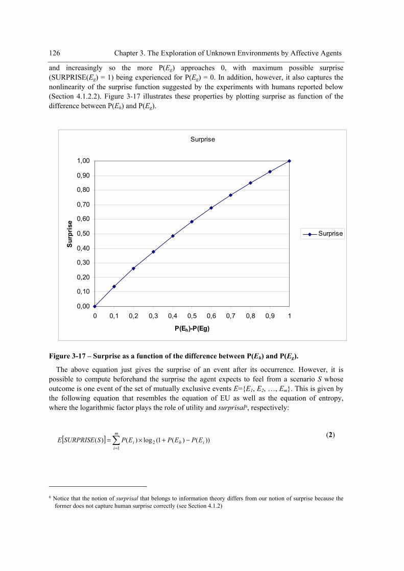
126 Chapter 3. The Exploration of Unknown Environments by Affective Agents
and increasingly so the more P(Eg) approaches 0, with maximum possible surprise (SURPRISE(Eg) = 1) being experienced for P(Eg) = 0. In addition, however, it also captures the nonlinearity of the surprise function suggested by the experiments with humans reported below (Section 4.1.2.2). Figure 3-17 illustrates these properties by plotting surprise as function of the difference between P(Eh) and P(Eg).
Surprise
0,00
0,10
0,20
0,30
0,40
0,50
0,60
0,70
0,80
0,90
1,00
0 0,1 0,2 0,3 0,4 0,5 0,6 0,7 0,8 0,9 1
P(Eh)-P(Eg)
Sur
pris
e
Surprise
Figure 3-17 – Surprise as a function of the difference between P(Eh) and P(Eg).
The above equation just gives the surprise of an event after its occurrence. However, it is possible to compute beforehand the surprise the agent expects to feel from a scenario S whose outcome is one event of the set of mutually exclusive events E={E1, E2, …, Em}. This is given by the following equation that resembles the equation of EU as well as the equation of entropy, where the logarithmic factor plays the role of utility and surprisal6, respectively:
[ ] ∑=
−+×=m
iihi EPEPEPSSURPRISEE
12 ))()(1(log)()(
(2)
6 Notice that the notion of surprisal that belongs to information theory differs from our notion of surprise because the
former does not capture human surprise correctly (see Section 4.1.2)
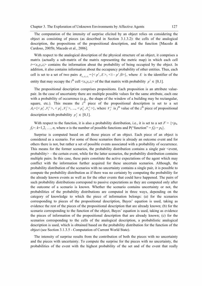
Chapter 3. The Exploration of Unknown Environments by Affective Agents 127
The computation of the intensity of surprise elicited by an object relies on considering the object as consisting of pieces (as described in Section 3.1.3.2): the cells of the analogical description, the propositions of the propositional description, and the function [Macedo & Cardoso, 2005b; Macedo et al., 2006].
With respect to the analogical description of the physical structure of an object, it comprises a matrix (actually a sub-matrix of the matrix representing the metric map) in which each cell i=<xi,yi,zi> contains the information about the probability of being occupied by the object. In addition, it also contains information about the occupancy probability of other entities. Thus, each cell is set to a set of two pairs
iii zyx ,,φ ={< ip , E >, < ip−1 ,0>}, where E is the identifier of the
entity that may occupy the ith cell <xi,yi,zi> of the that matrix with probability ip ∈ [0,1].
The propositional description comprises propositions. Each proposition is an attribute value-pair. In the case of uncertainty there are multiple possible values for the same attribute, each one with a probability of occurrence (e.g., the shape of the window of a building may be rectangular, square, etc.). This means the zth piece of the propositional description is set to a set Az={< zp1 , zV1 >, < zp2 , zV2 >, ..., < z
rzp , z
rzV >}, where z
jV is jth value of the zth piece of propositional
description with probability zjp ∈ [0,1].
With respect to the function, it is also a probability distribution, i.e., it is set to a set F = {<pk, fk>: k=1,2, …, n, where n is the number of possible functions and P(“function” = fk) = pk}.
Surprise is computed based on all those pieces of an object. Each piece of an object is considered as a scenario. For some of those scenarios there is already an outcome event and for others there is not, but rather a set of possible events associated with a probability of occurrence. This means for the former scenarios, the probability distribution contains a single pair <event, probability> – the certain event, while for the latter scenarios, the probability distribution contains multiple pairs. In this case, these pairs constitute the active expectations of the agent which may conflict with the information further acquired for these uncertain scenarios. Although, the probability distribution of the scenarios with no uncertainty contains a single pair, it is possible to compute the probability distribution as if there was no certainty by computing the probability for the already known events as well as for the other events that could have happened. The pairs of such probability distributions correspond to passive expectations as they are computed only after the outcome of a scenario is known. Whether the scenario contains uncertainty or not, the probabilities of the probability distributions are computed in three ways, depending on the category of knowledge to which the piece of information belongs: (a) for the scenarios corresponding to pieces of the propositional description, Bayes’ equation is used, taking as evidence the rest of the pieces of the propositional description that are already known; (b) for the scenario corresponding to the function of the object, Bayes’ equation is used, taking as evidence the pieces of information of the propositional description that are already known; (c) for the scenarios corresponding to the cells of the analogical description, a probabilistic analogical description is used, which is obtained based on the probability distribution for the function of the object (see Section 3.1.3.5 - Computation of Current World State).
The intensity of surprise results from the contribution of both the pieces with no uncertainty and the pieces with uncertainty. To compute the surprise for the pieces with no uncertainty, the probabilities of the event with the highest probability of the set and of the event that really
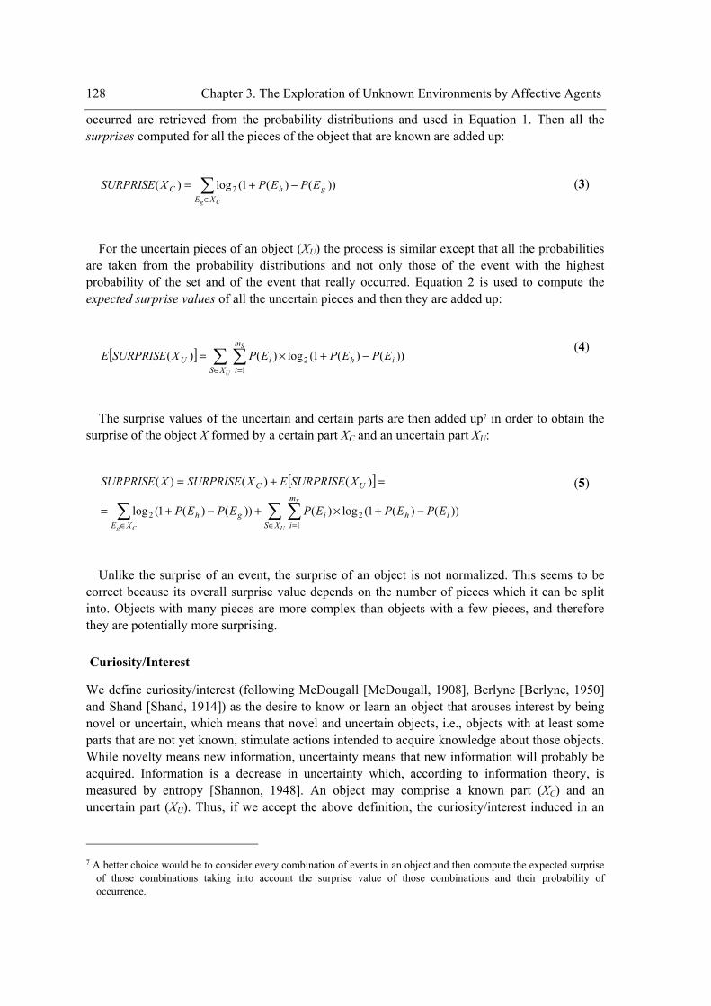
128 Chapter 3. The Exploration of Unknown Environments by Affective Agents
occurred are retrieved from the probability distributions and used in Equation 1. Then all the surprises computed for all the pieces of the object that are known are added up:
∑∈
−+=Cg XE
ghC EPEPXSURPRISE ))()(1(log)( 2 (3)
For the uncertain pieces of an object (XU) the process is similar except that all the probabilities are taken from the probability distributions and not only those of the event with the highest probability of the set and of the event that really occurred. Equation 2 is used to compute the expected surprise values of all the uncertain pieces and then they are added up:
[ ] ∑ ∑∈ =
−+×=U
S
XS
m
iihiU EPEPEPXSURPRISEE
12 ))()(1(log)()(
(4)
The surprise values of the uncertain and certain parts are then added up7 in order to obtain the surprise of the object X formed by a certain part XC and an uncertain part XU:
[ ]
∑ ∑∑∈ =∈
−+×+−+=
=+=
U
S
Cg XS
m
iihi
XEgh
UC
EPEPEPEPEP
XSURPRISEEXSURPRISEXSURPRISE
122 ))()(1(log)())()(1(log
)()()(
(5)
Unlike the surprise of an event, the surprise of an object is not normalized. This seems to be correct because its overall surprise value depends on the number of pieces which it can be split into. Objects with many pieces are more complex than objects with a few pieces, and therefore they are potentially more surprising.
Curiosity/Interest
We define curiosity/interest (following McDougall [McDougall, 1908], Berlyne [Berlyne, 1950] and Shand [Shand, 1914]) as the desire to know or learn an object that arouses interest by being novel or uncertain, which means that novel and uncertain objects, i.e., objects with at least some parts that are not yet known, stimulate actions intended to acquire knowledge about those objects. While novelty means new information, uncertainty means that new information will probably be acquired. Information is a decrease in uncertainty which, according to information theory, is measured by entropy [Shannon, 1948]. An object may comprise a known part (XC) and an uncertain part (XU). Thus, if we accept the above definition, the curiosity/interest induced in an
7 A better choice would be to consider every combination of events in an object and then compute the expected surprise
of those combinations taking into account the surprise value of those combinations and their probability of occurrence.
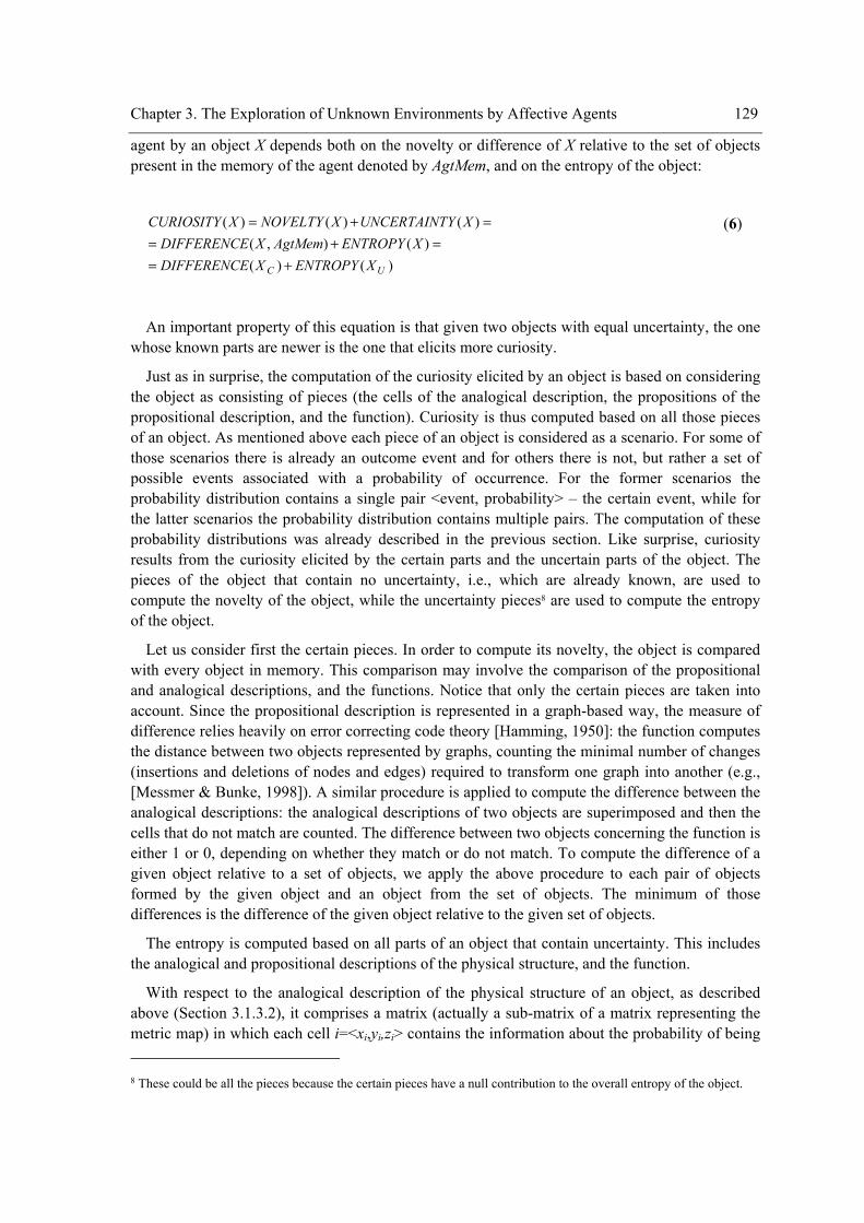
Chapter 3. The Exploration of Unknown Environments by Affective Agents 129
agent by an object X depends both on the novelty or difference of X relative to the set of objects present in the memory of the agent denoted by AgtMem, and on the entropy of the object:
)()()(),(
)()()(
UC XENTROPYXDIFFERENCEXENTROPYAgtMemXDIFFERENCE
XYUNCERTAINTXNOVELTYXCURIOSITY
+==+=
=+=
(6)
An important property of this equation is that given two objects with equal uncertainty, the one whose known parts are newer is the one that elicits more curiosity.
Just as in surprise, the computation of the curiosity elicited by an object is based on considering the object as consisting of pieces (the cells of the analogical description, the propositions of the propositional description, and the function). Curiosity is thus computed based on all those pieces of an object. As mentioned above each piece of an object is considered as a scenario. For some of those scenarios there is already an outcome event and for others there is not, but rather a set of possible events associated with a probability of occurrence. For the former scenarios the probability distribution contains a single pair <event, probability> – the certain event, while for the latter scenarios the probability distribution contains multiple pairs. The computation of these probability distributions was already described in the previous section. Like surprise, curiosity results from the curiosity elicited by the certain parts and the uncertain parts of the object. The pieces of the object that contain no uncertainty, i.e., which are already known, are used to compute the novelty of the object, while the uncertainty pieces8 are used to compute the entropy of the object.
Let us consider first the certain pieces. In order to compute its novelty, the object is compared with every object in memory. This comparison may involve the comparison of the propositional and analogical descriptions, and the functions. Notice that only the certain pieces are taken into account. Since the propositional description is represented in a graph-based way, the measure of difference relies heavily on error correcting code theory [Hamming, 1950]: the function computes the distance between two objects represented by graphs, counting the minimal number of changes (insertions and deletions of nodes and edges) required to transform one graph into another (e.g., [Messmer & Bunke, 1998]). A similar procedure is applied to compute the difference between the analogical descriptions: the analogical descriptions of two objects are superimposed and then the cells that do not match are counted. The difference between two objects concerning the function is either 1 or 0, depending on whether they match or do not match. To compute the difference of a given object relative to a set of objects, we apply the above procedure to each pair of objects formed by the given object and an object from the set of objects. The minimum of those differences is the difference of the given object relative to the given set of objects.
The entropy is computed based on all parts of an object that contain uncertainty. This includes the analogical and propositional descriptions of the physical structure, and the function.
With respect to the analogical description of the physical structure of an object, as described above (Section 3.1.3.2), it comprises a matrix (actually a sub-matrix of a matrix representing the metric map) in which each cell i=<xi,yi,zi> contains the information about the probability of being 8 These could be all the pieces because the certain pieces have a null contribution to the overall entropy of the object.
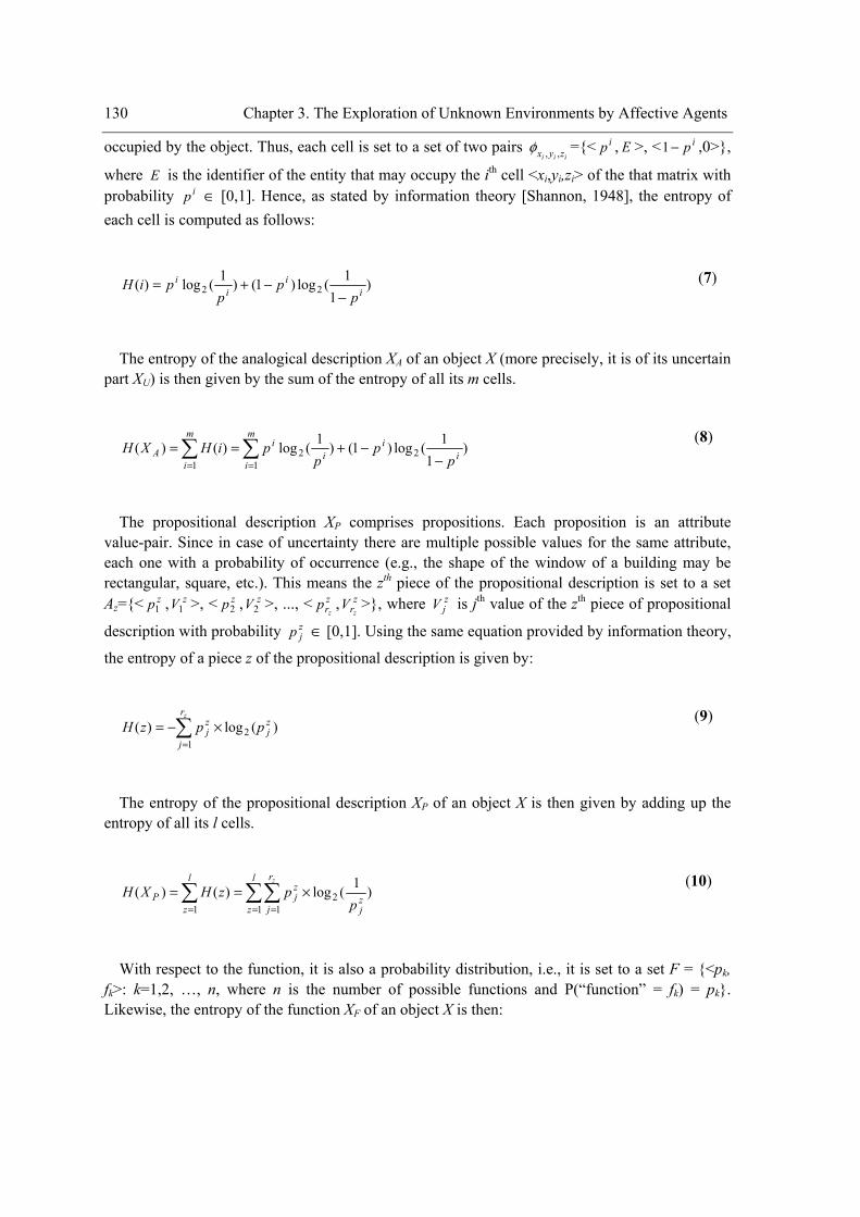
130 Chapter 3. The Exploration of Unknown Environments by Affective Agents
occupied by the object. Thus, each cell is set to a set of two pairs iii zyx ,,φ ={< ip , E >, < ip−1 ,0>},
where E is the identifier of the entity that may occupy the ith cell <xi,yi,zi> of the that matrix with probability ip ∈ [0,1]. Hence, as stated by information theory [Shannon, 1948], the entropy of each cell is computed as follows:
)1
1(log)1()1(log)( 22 ii
ii
pp
ppiH
−−+= (7)
The entropy of the analogical description XA of an object X (more precisely, it is of its uncertain part XU) is then given by the sum of the entropy of all its m cells.
∑∑== −
−+==m
ii
ii
im
iA p
pp
piHXH1
221
)1
1(log)1()1(log)()( (8)
The propositional description XP comprises propositions. Each proposition is an attribute value-pair. Since in case of uncertainty there are multiple possible values for the same attribute, each one with a probability of occurrence (e.g., the shape of the window of a building may be rectangular, square, etc.). This means the zth piece of the propositional description is set to a set Az={< zp1 , zV1 >, < zp2 , zV2 >, ..., < z
rzp , z
rzV >}, where z
jV is jth value of the zth piece of propositional
description with probability zjp ∈ [0,1]. Using the same equation provided by information theory,
the entropy of a piece z of the propositional description is given by:
)(log)(1
2zj
r
j
zj ppzH
z
∑=
×−= (9)
The entropy of the propositional description XP of an object X is then given by adding up the entropy of all its l cells.
∑∑∑= ==
×==l
zzj
r
j
zj
l
zP p
pzHXHz
1 12
1)1(log)()(
(10)
With respect to the function, it is also a probability distribution, i.e., it is set to a set F = {<pk, fk>: k=1,2, …, n, where n is the number of possible functions and P(“function” = fk) = pk}. Likewise, the entropy of the function XF of an object X is then:
Chapter 3. The Exploration of Unknown Environments by Affective Agents 131
)(log)(1
2 k
n
KkF ppXH ∑
=×−=
(11)
The entropy of an object X may be computed by adding up the entropies of its propositional and analogical description plus the entropy of its function:
)1(log)1(log)1
1(log)1()1(log
)()()()(
12
1 12
122
k
n
Kk
l
zzj
r
j
zj
m
ii
ii
i
FPA
pp
pp
pp
pp
XHXHXHXHz
∑∑∑∑== ==
×+×+−
−+=
=++=
(12)
Computed by the above equation, curiosity is not normalized. This seems to be correct because objects with many novel and uncertain pieces potentially provide more information than objects with a few pieces, and therefore they elicit more curiosity.
Hunger
Hunger is defined as the need for a source of energy. Given the capacity C of the storage of that source (C=1, i.e., C=100%), and L the amount of energy left (0 ≤ L ≤ C), the hunger elicited in an agent is computed as follows:
)()( LCAgtHUNGER −−= (13)
The function hunger is already normalized, since C=1 and 0 ≤ L ≤ C, which implies that 0 ≤ C-L ≤ 1.
3.1.3.4 Goals and Intentions
Desires are states of the environment the agent would like to happen, i.e., they correspond to those states of the environment the agent prefers. This preference is implicitly represented in a mathematical function that evaluates states of the environment in terms of the degree of satisfaction of the basic desires which, as noted before, drive the agent to reduce or to maximize feelings. This function obeys the MEU principle [S. Russell & Norvig, 1995]. The agent always prefers those states that maximize or reduce certain feelings. Goals may be understood as something that an agent wants or has to do. These might be automatically generated by the agent (see Section 3.1.3.5 - Generation and Management of the Agent’s Goals). The reason for trying to achieve a goal might be because that achievement corresponds to a state of the environment that makes it satisfy the basic desires. Thus, goals may be thought of as a subset of the agent’s desires [Huhns & Singh, 1998].
To satisfy the basic desires of minimal hunger, maximal information gain and maximal surprise, the agent desires to visit previously unvisited entities, regions of the environment and places where it can recharge its battery. This means that, in the particular case of exploration,
132 Chapter 3. The Exploration of Unknown Environments by Affective Agents
agents may possess three kinds of goals: visitEntity(X), visitLoc(Y), and rechargeBattery. This happens because the memory of the agents is seeded with plans to achieve these goal tasks. Notice that if plans for other goal tasks are given to the memory of the agents, then they are able to deal with those other goals. However, for our exploration strategy those visitEntity(X), visitLoc(Y), and rechargeBattery suffice. The first is concerned with the goal of visiting an entity of the environment, the second refers to the goal of visiting a location where there is no entity, and finally the third concerns the goal of going to the place where there is a source of energy to recharge batteries. These goals are automatically generated by the agent by adapting past goals to new situations giving rise to new goals which are then ranked according to its preference (utility) and then taken as intentions once a plan is generated for them.
3.1.3.5 Reasoning
The reasoning module receives information from the internal/external world and outputs an action that has been selected for execution. This is actually a sequential decision-making process, as opposed to single decision-making, in that not only a single decision is made but rather a sequence of decisions, i.e., the computation of a sequence of decisions involves several single decision-making processes, bearing in mind that each one belongs to a sequence. We will now explain this process in detail.
Figure 3-18 presents the algorithm for the reasoning cycle of the agent, including the management of goals, planning, and execution. The main principle of decision-making is kept: the agent receives percepts and generates an action. The first of the steps is concerned with getting percepts. The second is the computation of the current world state. This is performed by generating expectations or assumptions, based on the knowledge stored in memory, for the gaps of the environment information provided by the sensors. Since the agent knows its position precisely, there is no need for generating assumption/expectations for its current position. The agent has a queue of goal tasks (goals) ranked by their priority (i.e., EU). The first of the ranking is the goal/intention that is under achievement. Once one goal is achieved, it is removed from the queue and the way it was achieved could be learned for future reuse by simply storing its plan in memory as a case. However, for instance, external events or objects may give rise to new goals. This is the next step of the reasoning/decision-making process: the generation of new goals, computation of their EU and insertion in the queue of goals according to their priority (i.e., their EU). Though, if the queue was empty before this step and no new goals are generated in this step, the queue remains empty. In this case there is nothing to reason or decide about and consequently no action is returned. However, the most likely situation is that the queue is not empty either before or after the step of generating new goals. If the first goal of the queue is still the same, then proceed with its execution. However, the addition of new goals may have caused changes in the ranking of the goals in the queue because a new goal may be more expected useful than some old goals. Thus, the first goal may now be different from the previous first goal. In this case the old first goal is said to be suspended. Thus, a plan is required for this new first goal in queue, which will be from now on or until its achievement the current goal. That plan could be built or retrieved from memory (if there is one – remember that this current goal may be previously suspended or even previously achieved in the past). Anyway, the plan is executed and the next primitive task (action) is returned.
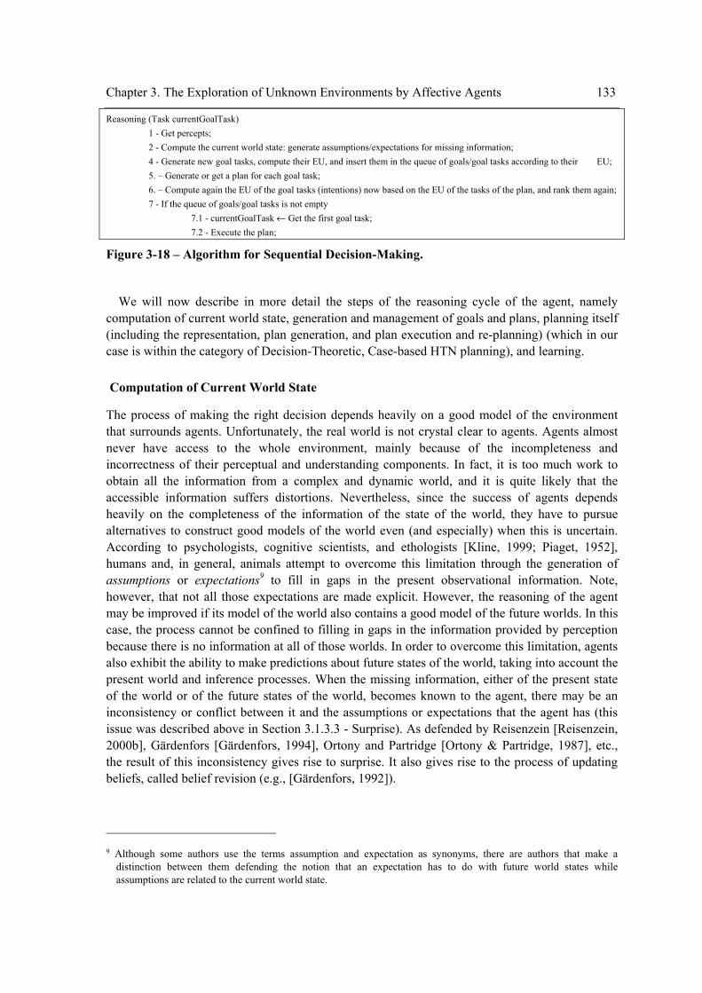
Chapter 3. The Exploration of Unknown Environments by Affective Agents 133
Reasoning (Task currentGoalTask) 1 - Get percepts; 2 - Compute the current world state: generate assumptions/expectations for missing information; 4 - Generate new goal tasks, compute their EU, and insert them in the queue of goals/goal tasks according to their EU; 5. – Generate or get a plan for each goal task; 6. – Compute again the EU of the goal tasks (intentions) now based on the EU of the tasks of the plan, and rank them again; 7 - If the queue of goals/goal tasks is not empty 7.1 - currentGoalTask ← Get the first goal task; 7.2 - Execute the plan;
Figure 3-18 – Algorithm for Sequential Decision-Making.
We will now describe in more detail the steps of the reasoning cycle of the agent, namely computation of current world state, generation and management of goals and plans, planning itself (including the representation, plan generation, and plan execution and re-planning) (which in our case is within the category of Decision-Theoretic, Case-based HTN planning), and learning.
Computation of Current World State
The process of making the right decision depends heavily on a good model of the environment that surrounds agents. Unfortunately, the real world is not crystal clear to agents. Agents almost never have access to the whole environment, mainly because of the incompleteness and incorrectness of their perceptual and understanding components. In fact, it is too much work to obtain all the information from a complex and dynamic world, and it is quite likely that the accessible information suffers distortions. Nevertheless, since the success of agents depends heavily on the completeness of the information of the state of the world, they have to pursue alternatives to construct good models of the world even (and especially) when this is uncertain. According to psychologists, cognitive scientists, and ethologists [Kline, 1999; Piaget, 1952], humans and, in general, animals attempt to overcome this limitation through the generation of assumptions or expectations9 to fill in gaps in the present observational information. Note, however, that not all those expectations are made explicit. However, the reasoning of the agent may be improved if its model of the world also contains a good model of the future worlds. In this case, the process cannot be confined to filling in gaps in the information provided by perception because there is no information at all of those worlds. In order to overcome this limitation, agents also exhibit the ability to make predictions about future states of the world, taking into account the present world and inference processes. When the missing information, either of the present state of the world or of the future states of the world, becomes known to the agent, there may be an inconsistency or conflict between it and the assumptions or expectations that the agent has (this issue was described above in Section 3.1.3.3 - Surprise). As defended by Reisenzein [Reisenzein, 2000b], Gärdenfors [Gärdenfors, 1994], Ortony and Partridge [Ortony & Partridge, 1987], etc., the result of this inconsistency gives rise to surprise. It also gives rise to the process of updating beliefs, called belief revision (e.g., [Gärdenfors, 1992]).
9 Although some authors use the terms assumption and expectation as synonyms, there are authors that make a
distinction between them defending the notion that an expectation has to do with future world states while assumptions are related to the current world state.
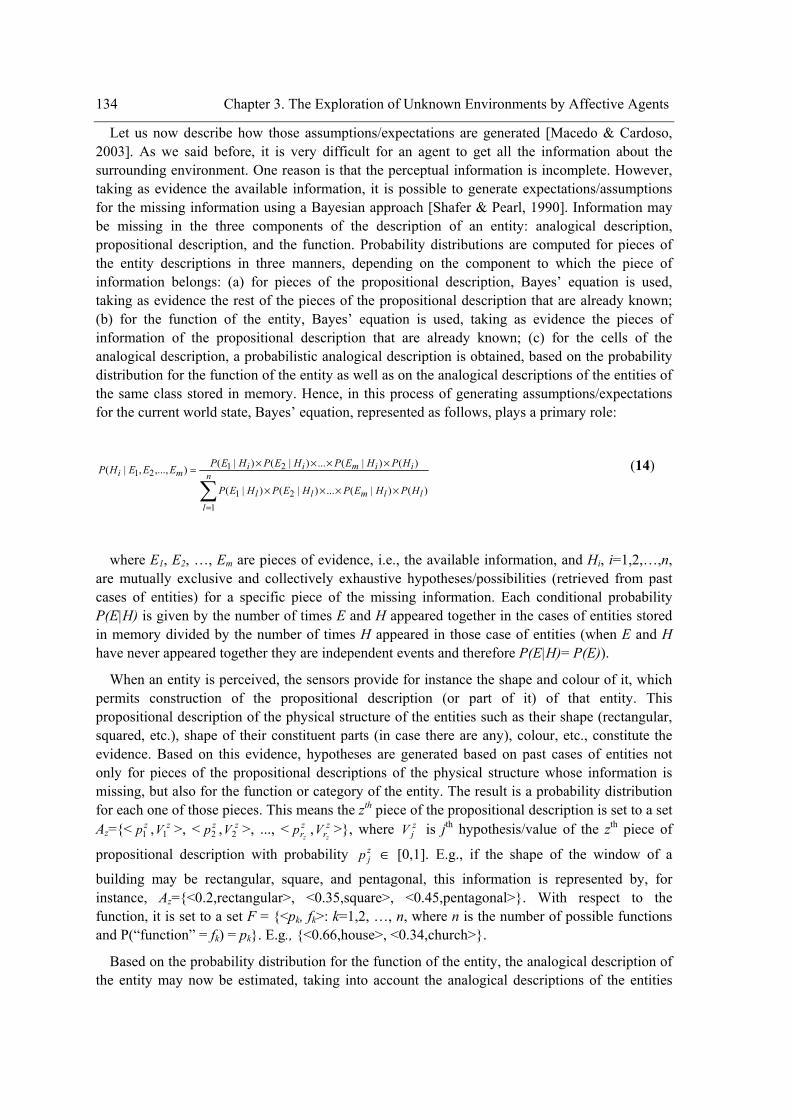
134 Chapter 3. The Exploration of Unknown Environments by Affective Agents
Let us now describe how those assumptions/expectations are generated [Macedo & Cardoso, 2003]. As we said before, it is very difficult for an agent to get all the information about the surrounding environment. One reason is that the perceptual information is incomplete. However, taking as evidence the available information, it is possible to generate expectations/assumptions for the missing information using a Bayesian approach [Shafer & Pearl, 1990]. Information may be missing in the three components of the description of an entity: analogical description, propositional description, and the function. Probability distributions are computed for pieces of the entity descriptions in three manners, depending on the component to which the piece of information belongs: (a) for pieces of the propositional description, Bayes’ equation is used, taking as evidence the rest of the pieces of the propositional description that are already known; (b) for the function of the entity, Bayes’ equation is used, taking as evidence the pieces of information of the propositional description that are already known; (c) for the cells of the analogical description, a probabilistic analogical description is obtained, based on the probability distribution for the function of the entity as well as on the analogical descriptions of the entities of the same class stored in memory. Hence, in this process of generating assumptions/expectations for the current world state, Bayes’ equation, represented as follows, plays a primary role:
∑=
××××
××××= n
lllmll
iimiimi
HPHEPHEPHEP
HPHEPHEPHEPEEEHP
121
2121
)()|(...)|()|(
)()|(...)|()|(),...,,|( (14)
where E1, E2, …, Em are pieces of evidence, i.e., the available information, and Hi, i=1,2,…,n, are mutually exclusive and collectively exhaustive hypotheses/possibilities (retrieved from past cases of entities) for a specific piece of the missing information. Each conditional probability P(E|H) is given by the number of times E and H appeared together in the cases of entities stored in memory divided by the number of times H appeared in those case of entities (when E and H have never appeared together they are independent events and therefore P(E|H)= P(E)).
When an entity is perceived, the sensors provide for instance the shape and colour of it, which permits construction of the propositional description (or part of it) of that entity. This propositional description of the physical structure of the entities such as their shape (rectangular, squared, etc.), shape of their constituent parts (in case there are any), colour, etc., constitute the evidence. Based on this evidence, hypotheses are generated based on past cases of entities not only for pieces of the propositional descriptions of the physical structure whose information is missing, but also for the function or category of the entity. The result is a probability distribution for each one of those pieces. This means the zth piece of the propositional description is set to a set Az={< zp1 , zV1 >, < zp2 , zV2 >, ..., < z
rzp , z
rzV >}, where z
jV is jth hypothesis/value of the zth piece of
propositional description with probability zjp ∈ [0,1]. E.g., if the shape of the window of a
building may be rectangular, square, and pentagonal, this information is represented by, for instance, Az={<0.2,rectangular>, <0.35,square>, <0.45,pentagonal>}. With respect to the function, it is set to a set F = {<pk, fk>: k=1,2, …, n, where n is the number of possible functions and P(“function” = fk) = pk}. E.g., {<0.66,house>, <0.34,church>}.
Based on the probability distribution for the function of the entity, the analogical description of the entity may now be estimated, taking into account the analogical descriptions of the entities
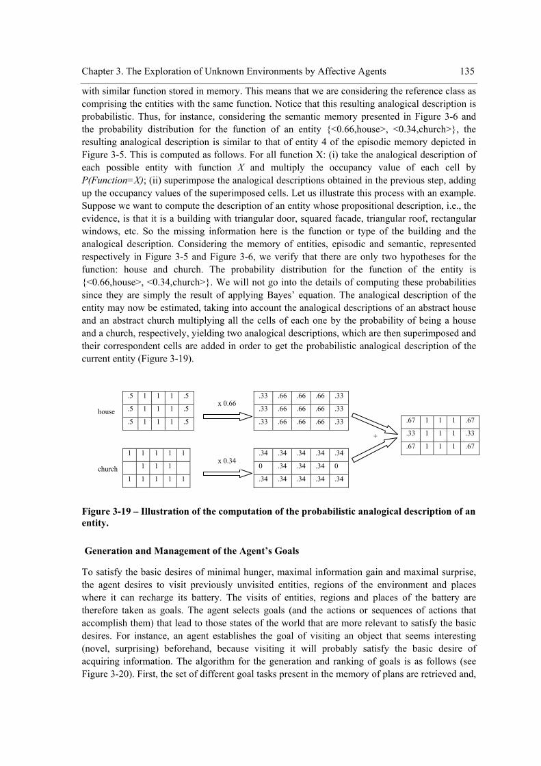
Chapter 3. The Exploration of Unknown Environments by Affective Agents 135
with similar function stored in memory. This means that we are considering the reference class as comprising the entities with the same function. Notice that this resulting analogical description is probabilistic. Thus, for instance, considering the semantic memory presented in Figure 3-6 and the probability distribution for the function of an entity {<0.66,house>, <0.34,church>}, the resulting analogical description is similar to that of entity 4 of the episodic memory depicted in Figure 3-5. This is computed as follows. For all function X: (i) take the analogical description of each possible entity with function X and multiply the occupancy value of each cell by P(Function=X); (ii) superimpose the analogical descriptions obtained in the previous step, adding up the occupancy values of the superimposed cells. Let us illustrate this process with an example. Suppose we want to compute the description of an entity whose propositional description, i.e., the evidence, is that it is a building with triangular door, squared facade, triangular roof, rectangular windows, etc. So the missing information here is the function or type of the building and the analogical description. Considering the memory of entities, episodic and semantic, represented respectively in Figure 3-5 and Figure 3-6, we verify that there are only two hypotheses for the function: house and church. The probability distribution for the function of the entity is {<0.66,house>, <0.34,church>}. We will not go into the details of computing these probabilities since they are simply the result of applying Bayes’ equation. The analogical description of the entity may now be estimated, taking into account the analogical descriptions of an abstract house and an abstract church multiplying all the cells of each one by the probability of being a house and a church, respectively, yielding two analogical descriptions, which are then superimposed and their correspondent cells are added in order to get the probabilistic analogical description of the current entity (Figure 3-19).
Figure 3-19 – Illustration of the computation of the probabilistic analogical description of an entity.
Generation and Management of the Agent’s Goals
To satisfy the basic desires of minimal hunger, maximal information gain and maximal surprise, the agent desires to visit previously unvisited entities, regions of the environment and places where it can recharge its battery. The visits of entities, regions and places of the battery are therefore taken as goals. The agent selects goals (and the actions or sequences of actions that accomplish them) that lead to those states of the world that are more relevant to satisfy the basic desires. For instance, an agent establishes the goal of visiting an object that seems interesting (novel, surprising) beforehand, because visiting it will probably satisfy the basic desire of acquiring information. The algorithm for the generation and ranking of goals is as follows (see Figure 3-20). First, the set of different goal tasks present in the memory of plans are retrieved and,
.5 1 1 1 .5
.5 1 1 1 .5
.5 1 1 1 .5 house
church
1 1 1 1 1
1 1 1
1 1 1 1 1
.34 .34 .34 .34 .34
0 .34 .34 .34 0
.34 .34 .34 .34 .34
.33 .66 .66 .66 .33
.33 .66 .66 .66 .33
.33 .66 .66 .66 .33
x 0.66
x 0.34
+
.67 1 1 1 .67
.33 1 1 1 .33
.67 1 1 1 .67
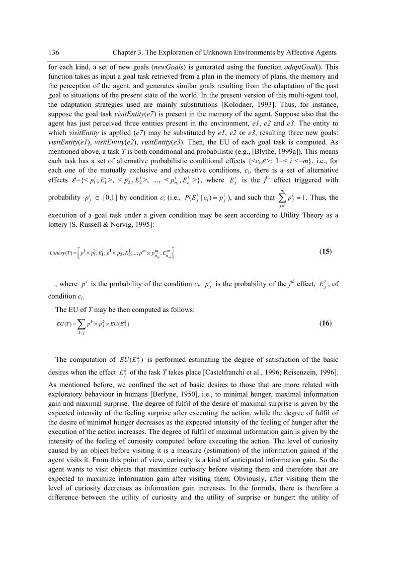
136 Chapter 3. The Exploration of Unknown Environments by Affective Agents
for each kind, a set of new goals (newGoals) is generated using the function adaptGoal(). This function takes as input a goal task retrieved from a plan in the memory of plans, the memory and the perception of the agent, and generates similar goals resulting from the adaptation of the past goal to situations of the present state of the world. In the present version of this multi-agent tool, the adaptation strategies used are mainly substitutions [Kolodner, 1993]. Thus, for instance, suppose the goal task visitEntity(e7) is present in the memory of the agent. Suppose also that the agent has just perceived three entities present in the environment, e1, e2 and e3. The entity to which visitEntity is applied (e7) may be substituted by e1, e2 or e3, resulting three new goals: visitEntity(e1), visitEntity(e2), visitEntity(e3). Then, the EU of each goal task is computed. As mentioned above, a task T is both conditional and probabilistic (e.g., [Blythe, 1999a]). This means each task has a set of alternative probabilistic conditional effects {<ci,εi>: 1=< i <=m}, i.e., for each one of the mutually exclusive and exhaustive conditions, ci, there is a set of alternative effects εi={< ip1 , iE1 >, < ip2 , iE2 >, ..., < i
nip , i
niE >}, where i
jE is the jth effect triggered with
probability ijp ∈ [0,1] by condition ci (i.e., i
jiij pcEP =)|( ), and such that ∑
==
in
j
ijp
11. Thus, the
execution of a goal task under a given condition may be seen according to Utility Theory as a lottery [S. Russell & Norvig, 1995]:
⎥⎦⎤
⎢⎣⎡ ×××= m
nmn
mmm
EppEppEppTLottery ,;...;,;,)( 12
12
111
11
1 (15)
, where ip is the probability of the condition ci, ijp is the probability of the jth effect, i
jE , of
condition ci.
The EU of T may be then computed as follows:
∑ ××=jk
kj
kj
k EEUppTEU,
)()(
(16)
The computation of )( kjEEU is performed estimating the degree of satisfaction of the basic
desires when the effect kjE of the task T takes place [Castelfranchi et al., 1996; Reisenzein, 1996].
As mentioned before, we confined the set of basic desires to those that are more related with exploratory behaviour in humans [Berlyne, 1950], i.e., to minimal hunger, maximal information gain and maximal surprise. The degree of fulfil of the desire of maximal surprise is given by the expected intensity of the feeling surprise after executing the action, while the degree of fulfil of the desire of minimal hunger decreases as the expected intensity of the feeling of hunger after the execution of the action increases. The degree of fulfil of maximal information gain is given by the intensity of the feeling of curiosity computed before executing the action. The level of curiosity caused by an object before visiting it is a measure (estimation) of the information gained if the agent visits it. From this point of view, curiosity is a kind of anticipated information gain. So the agent wants to visit objects that maximize curiosity before visiting them and therefore that are expected to maximize information gain after visiting them. Obviously, after visiting them the level of curiosity decreases as information gain increases. In the formula, there is therefore a difference between the utility of curiosity and the utility of surprise or hunger: the utility of
Chapter 3. The Exploration of Unknown Environments by Affective Agents 137
curiosity is indeed the anticipated information gain, while the utility of surprise and hunger is itself the anticipated surprise and hunger, respectively. After visiting an object, the level of curiosity of this object is null, while surprise and hunger may not. Thus, the intensities of surprise, curiosity and hunger felt by the agent when the effect takes place are estimated based on the procedural component of the effect, i.e., on the information available in the effect about the changes produced in the world. Another choice that is not in the scope of this thesis is performing these computations based on the non-procedural component (somatic markers [Damásio, 1994]), i.e., on the intensities of feelings felt in past occurrences of the effect of the task.
The generic function )( kjEEU is used to compute the EU of the effect k
jE as follows:
∑ ×=i
kjdi
kj EUEEU
i)()( α (17)
where αi is the weight of basic desire di, with i ∈ ℵ.
For the particular application of exploration of unknown environments, this function is as follows:
)()()(
)()()()(
321
321
kj
kj
kj
kjhunger
kjcuriosity
kjsurprise
kj
EHungerECuriosityESurprise
EUEUEUEEU
×+×+×=
=×+×+×=
ααα
ααα
(18)
, where, α3 = 1 and αi (i≠3) may be defined as follows:
⎩⎨⎧
⇐>−+⇐
=otherwise
DAgtHUNGERCi 0
0)(1α (19)
, where D is the amount of energy necessary to go from the end location of goal task T to the closest place where energy could be recharged, and C is the maximum amount of energy that could be stored by the agent. The functions )( k
jESurprise , )( kjECuriosity , and )( k
jEHunger are
replaced by the functions of surprise, curiosity, and hunger defined above (Section 3.1.3.3) and applied to the resulting state of the world when the effect k
jE takes place. Which parts of the state of the world they are applied to is determined in the definition of each action. For instance for the case of task ATTEND they are applied to the entity or the cell visited. In the first case, it is restricted to surprise and curiosity, while in the second case only the function hunger is used. The definition of the task PTRANS determines that surprise and curiosity are not applied to a path. However, this could be addressed in a future version of the system since certain paths elicit more surprise and curiosity than others. In contrast, hunger depends directly on the distance of the path.
This dependence of the parameters αi (i≠3) on the hunger of the agent partially models the results of Berlyne’s experiments (e.g., [Berlyne, 1950]) that have shown that in the absence of (or despite) known drives, humans tend to explore and investigate their environment as well as seek stimulation. In fact, surprise and curiosity are taken into account to compute the EU of a task only when there is enough energy to go from the end location of goal task T to the closest place where an energy source could be found. Otherwise, only hunger is taken into account for the EU of tasks
138 Chapter 3. The Exploration of Unknown Environments by Affective Agents
and further ranking. This means that in this situation (when hunger is above a specific threshold), the goal of rechargeBattery has the highest EU=0 (which is actually because the expected hunger is 0 after executing it). In the other situations (hunger below a specific threshold), hunger plays the role of a negative reward decreasing the utility of a task by the percentage of energy needed after the task is completed. Thus, the further the distance to the location after the execution of a task, the more energy is required and the less utility of that task.
Algorithm generateRankGoals(newRankedGoals) Output: newRankedGoals – the set of ranked goals newGoals ← ∅ setPastGoals ← {x: x is a goal task belonging to some plan in memory} for each goal in setPastGoals do adaptationGoal←adaptGoal(goal,agtMemory,agtPercepts) newGoals ← newGoals ∪ adaptationGoals end for each for each T in newGoals do
∑ ××=jk
kj
kj
k EEUppTEU,
)()(
insert(T,,newRankedGoals) end for each return newRankedGoals end
Figure 3-20 – Algorithm for the generation and ranking of goals.
Decision-Theoretic, Case-Based, HTN Planning
As we said before, the decision-making process may involve the construction of a plan for each goal and then the execution of it. This is the competence of the planner, called ProCHiP, a planner that combines case-based reasoning with the techniques of decision-theoretic planning and HTN planning in order to deal with uncertain, dynamic large-scale real-world domains [Macedo & Cardoso, 2004a, 2004b]. We describe first how a plan is constructed and finally how it is executed and revised (replanned). The description is illustrated with examples taken from the logistics domain [Andrews et al., 1995]. This domain was designed especially to fulfil the clear need for planning benchmarks with matching complexity to evaluate features and capabilities of planning systems. This domain seems to be more appropriate to illustrate the capabilities of ProCHiP than the domain of exploration of unknown environments. In fact, as described above, this domain contains far simpler plans.
Plan Generation
Since the planner is used by an agent that is part of a multi-agent environment, the agent should have the information of the initial state of the environment in memory in order to solve a planning problem. This comprises a three-dimensional metric map of the environment in which inanimate and other animate agents are spatially represented. Figure 3-21 presents an example of such an initial state of the environment. It comprises: one truck (truck1) located at coordinates (11,0,0); three packages, pk1, pk2 and pk3, located at, respectively, (10,3,0), (4,3,0), and (8,0,0); and one plane located at the airport with coordinates (2,1,0).
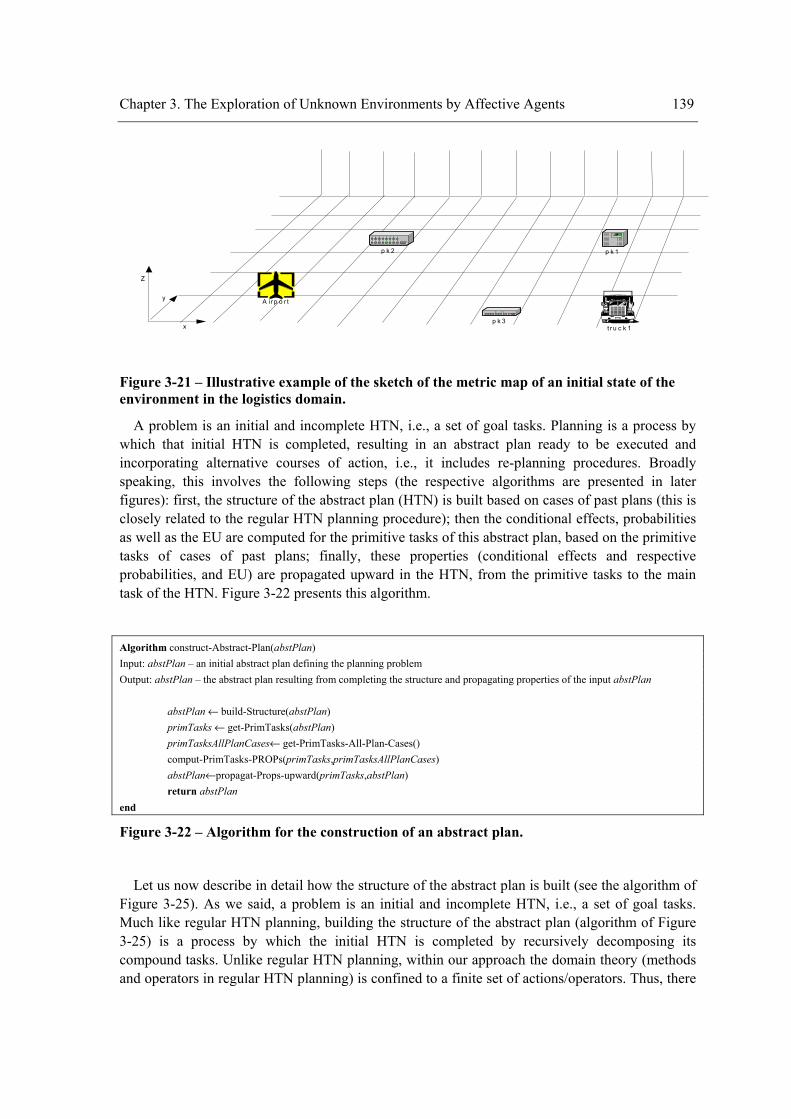
Chapter 3. The Exploration of Unknown Environments by Affective Agents 139
p k 1p k 2
p k 3
A ir p o r t
t r u c k 1
Z
y
x
Figure 3-21 – Illustrative example of the sketch of the metric map of an initial state of the environment in the logistics domain.
A problem is an initial and incomplete HTN, i.e., a set of goal tasks. Planning is a process by which that initial HTN is completed, resulting in an abstract plan ready to be executed and incorporating alternative courses of action, i.e., it includes re-planning procedures. Broadly speaking, this involves the following steps (the respective algorithms are presented in later figures): first, the structure of the abstract plan (HTN) is built based on cases of past plans (this is closely related to the regular HTN planning procedure); then the conditional effects, probabilities as well as the EU are computed for the primitive tasks of this abstract plan, based on the primitive tasks of cases of past plans; finally, these properties (conditional effects and respective probabilities, and EU) are propagated upward in the HTN, from the primitive tasks to the main task of the HTN. Figure 3-22 presents this algorithm.
Algorithm construct-Abstract-Plan(abstPlan) Input: abstPlan – an initial abstract plan defining the planning problem Output: abstPlan – the abstract plan resulting from completing the structure and propagating properties of the input abstPlan abstPlan ← build-Structure(abstPlan) primTasks ← get-PrimTasks(abstPlan) primTasksAllPlanCases← get-PrimTasks-All-Plan-Cases() comput-PrimTasks-PROPs(primTasks,primTasksAllPlanCases) abstPlan←propagat-Props-upward(primTasks,abstPlan) return abstPlan end
Figure 3-22 – Algorithm for the construction of an abstract plan.
Let us now describe in detail how the structure of the abstract plan is built (see the algorithm of Figure 3-25). As we said, a problem is an initial and incomplete HTN, i.e., a set of goal tasks. Much like regular HTN planning, building the structure of the abstract plan (algorithm of Figure 3-25) is a process by which the initial HTN is completed by recursively decomposing its compound tasks. Unlike regular HTN planning, within our approach the domain theory (methods and operators in regular HTN planning) is confined to a finite set of actions/operators. Thus, there
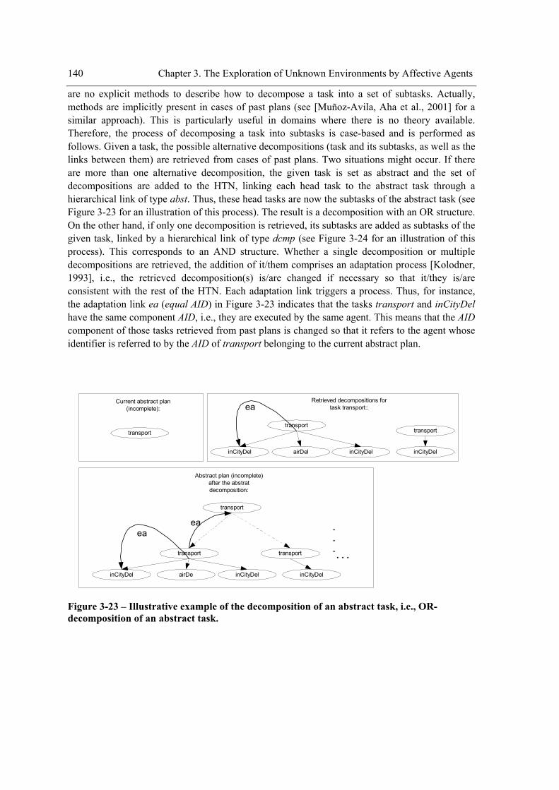
140 Chapter 3. The Exploration of Unknown Environments by Affective Agents
are no explicit methods to describe how to decompose a task into a set of subtasks. Actually, methods are implicitly present in cases of past plans (see [Muñoz-Avila, Aha et al., 2001] for a similar approach). This is particularly useful in domains where there is no theory available. Therefore, the process of decomposing a task into subtasks is case-based and is performed as follows. Given a task, the possible alternative decompositions (task and its subtasks, as well as the links between them) are retrieved from cases of past plans. Two situations might occur. If there are more than one alternative decomposition, the given task is set as abstract and the set of decompositions are added to the HTN, linking each head task to the abstract task through a hierarchical link of type abst. Thus, these head tasks are now the subtasks of the abstract task (see Figure 3-23 for an illustration of this process). The result is a decomposition with an OR structure. On the other hand, if only one decomposition is retrieved, its subtasks are added as subtasks of the given task, linked by a hierarchical link of type dcmp (see Figure 3-24 for an illustration of this process). This corresponds to an AND structure. Whether a single decomposition or multiple decompositions are retrieved, the addition of it/them comprises an adaptation process [Kolodner, 1993], i.e., the retrieved decomposition(s) is/are changed if necessary so that it/they is/are consistent with the rest of the HTN. Each adaptation link triggers a process. Thus, for instance, the adaptation link ea (equal AID) in Figure 3-23 indicates that the tasks transport and inCityDel have the same component AID, i.e., they are executed by the same agent. This means that the AID component of those tasks retrieved from past plans is changed so that it refers to the agent whose identifier is referred to by the AID of transport belonging to the current abstract plan.
Retrieved decompositions fortask transport::
Current abstract plan(incomplete):
transporttransport
inCityDel airDel inCityDel
transport
inCityDel
Abstract plan (incomplete)after the abstratdecomposition:
transport
transport
inCityDel airDe inCityDel
transport
inCityDel
. . .
.
.
.
ea
ea
ea
Figure 3-23 – Illustrative example of the decomposition of an abstract task, i.e., OR-decomposition of an abstract task.
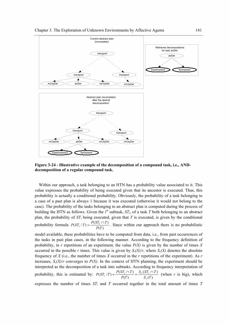
Chapter 3. The Exploration of Unknown Environments by Affective Agents 141
Retrieved decompositionsfor task airDel:
Current abstract plan(incomplete):
Abstract plan (incomplete)after the abstratdecomposition:
transport
transport
inCityDel airDel inCityDel
transport
inCityDel
airDel
flyAirplaneloadAirplane
transport
transport
inCityDel airDel inCityDel
transport
inCityDel
flyAirplaneloadAirplane()
Figure 3-24 - Illustrative example of the decomposition of a compound task, i.e., AND-decomposition of a regular compound task.
Within our approach, a task belonging to an HTN has a probability value associated to it. This value expresses the probability of being executed given that its ancestor is executed. Thus, this probability is actually a conditional probability. Obviously, the probability of a task belonging to a case of a past plan is always 1 because it was executed (otherwise it would not belong to the case). The probability of the tasks belonging to an abstract plan is computed during the process of building the HTN as follows. Given the ith subtask, STi, of a task T both belonging to an abstract plan, the probability of STi being executed, given that T is executed, is given by the conditional
probability formula )(
)()/(
TPTSTP
TSTP ii
∩= . Since within our approach there is no probabilistic
model available, these probabilities have to be computed from data, i.e., from past occurrences of the tasks in past plan cases, in the following manner. According to the frequency definition of probability, in r repetitions of an experiment, the value P(X) is given by the number of times X occurred in the possible r times. This value is given by Sr(X)/r, where Sr(X) denotes the absolute frequency of X (i.e., the number of times X occurred in the r repetitions of the experiment). As r increases, Sr(X)/r converges to P(X). In the context of HTN planning, the experiment should be interpreted as the decomposition of a task into subtasks. According to frequency interpretation of
probability, this is estimated by: )(
)()(
)()/(
TSTSTS
TPTSTP
TSTPr
irii
∩=
∩= (when r is big), which
expresses the number of times STi and T occurred together in the total amount of times T
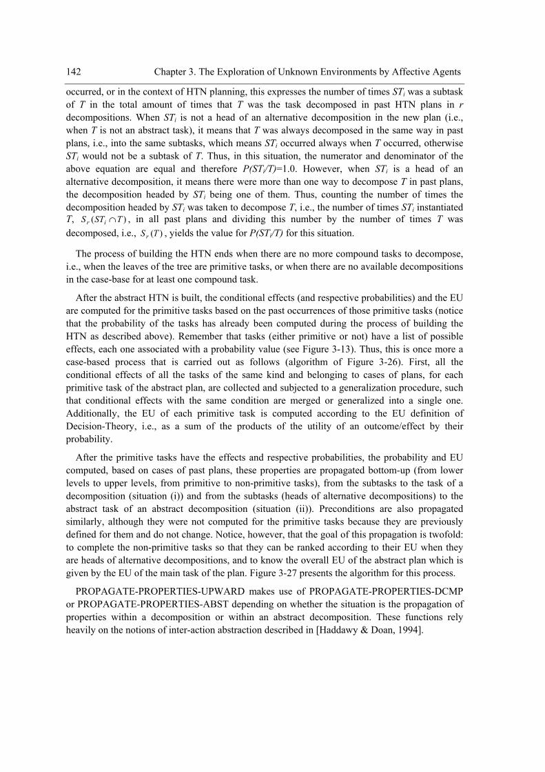
142 Chapter 3. The Exploration of Unknown Environments by Affective Agents
occurred, or in the context of HTN planning, this expresses the number of times STi was a subtask of T in the total amount of times that T was the task decomposed in past HTN plans in r decompositions. When STi is not a head of an alternative decomposition in the new plan (i.e., when T is not an abstract task), it means that T was always decomposed in the same way in past plans, i.e., into the same subtasks, which means STi occurred always when T occurred, otherwise STi would not be a subtask of T. Thus, in this situation, the numerator and denominator of the above equation are equal and therefore P(STi/T)=1.0. However, when STi is a head of an alternative decomposition, it means there were more than one way to decompose T in past plans, the decomposition headed by STi being one of them. Thus, counting the number of times the decomposition headed by STi was taken to decompose T, i.e., the number of times STi instantiated T, )( TSTS ir ∩ , in all past plans and dividing this number by the number of times T was decomposed, i.e., )(TSr , yields the value for P(STi/T) for this situation.
The process of building the HTN ends when there are no more compound tasks to decompose, i.e., when the leaves of the tree are primitive tasks, or when there are no available decompositions in the case-base for at least one compound task.
After the abstract HTN is built, the conditional effects (and respective probabilities) and the EU are computed for the primitive tasks based on the past occurrences of those primitive tasks (notice that the probability of the tasks has already been computed during the process of building the HTN as described above). Remember that tasks (either primitive or not) have a list of possible effects, each one associated with a probability value (see Figure 3-13). Thus, this is once more a case-based process that is carried out as follows (algorithm of Figure 3-26). First, all the conditional effects of all the tasks of the same kind and belonging to cases of plans, for each primitive task of the abstract plan, are collected and subjected to a generalization procedure, such that conditional effects with the same condition are merged or generalized into a single one. Additionally, the EU of each primitive task is computed according to the EU definition of Decision-Theory, i.e., as a sum of the products of the utility of an outcome/effect by their probability.
After the primitive tasks have the effects and respective probabilities, the probability and EU computed, based on cases of past plans, these properties are propagated bottom-up (from lower levels to upper levels, from primitive to non-primitive tasks), from the subtasks to the task of a decomposition (situation (i)) and from the subtasks (heads of alternative decompositions) to the abstract task of an abstract decomposition (situation (ii)). Preconditions are also propagated similarly, although they were not computed for the primitive tasks because they are previously defined for them and do not change. Notice, however, that the goal of this propagation is twofold: to complete the non-primitive tasks so that they can be ranked according to their EU when they are heads of alternative decompositions, and to know the overall EU of the abstract plan which is given by the EU of the main task of the plan. Figure 3-27 presents the algorithm for this process.
PROPAGATE-PROPERTIES-UPWARD makes use of PROPAGATE-PROPERTIES-DCMP or PROPAGATE-PROPERTIES-ABST depending on whether the situation is the propagation of properties within a decomposition or within an abstract decomposition. These functions rely heavily on the notions of inter-action abstraction described in [Haddawy & Doan, 1994].
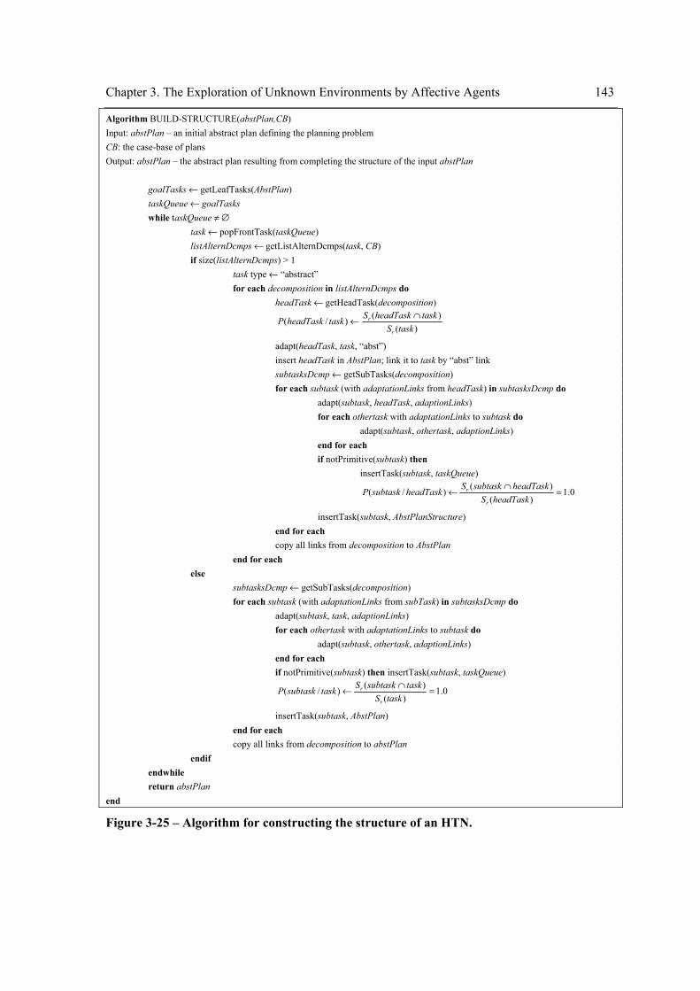
Chapter 3. The Exploration of Unknown Environments by Affective Agents 143
Algorithm BUILD-STRUCTURE(abstPlan,CB) Input: abstPlan – an initial abstract plan defining the planning problem CB: the case-base of plans Output: abstPlan – the abstract plan resulting from completing the structure of the input abstPlan goalTasks ← getLeafTasks(AbstPlan) taskQueue ← goalTasks while taskQueue ≠ ∅ task ← popFrontTask(taskQueue) listAlternDcmps ← getListAlternDcmps(task, CB) if size(listAlternDcmps) > 1 task type ← “abstract” for each decomposition in listAlternDcmps do headTask ← getHeadTask(decomposition)
)()()/(
taskStaskheadTaskStaskheadTaskP
r
r ∩←
adapt(headTask, task, “abst”) insert headTask in AbstPlan; link it to task by “abst” link subtasksDcmp ← getSubTasks(decomposition) for each subtask (with adaptationLinks from headTask) in subtasksDcmp do adapt(subtask, headTask, adaptionLinks) for each othertask with adaptationLinks to subtask do adapt(subtask, othertask, adaptionLinks) end for each if notPrimitive(subtask) then insertTask(subtask, taskQueue)
0.1
)()()/( =∩←
headTaskSheadTasksubtaskSheadTasksubtaskP
r
r
insertTask(subtask, AbstPlanStructure) end for each copy all links from decomposition to AbstPlan end for each else subtasksDcmp ← getSubTasks(decomposition) for each subtask (with adaptationLinks from subTask) in subtasksDcmp do adapt(subtask, task, adaptionLinks) for each othertask with adaptationLinks to subtask do adapt(subtask, othertask, adaptionLinks) end for each if notPrimitive(subtask) then insertTask(subtask, taskQueue)
0.1
)()()/( =∩←
taskStasksubtaskStasksubtaskP
r
r
insertTask(subtask, AbstPlan) end for each copy all links from decomposition to abstPlan endif endwhile return abstPlan end
Figure 3-25 – Algorithm for constructing the structure of an HTN.
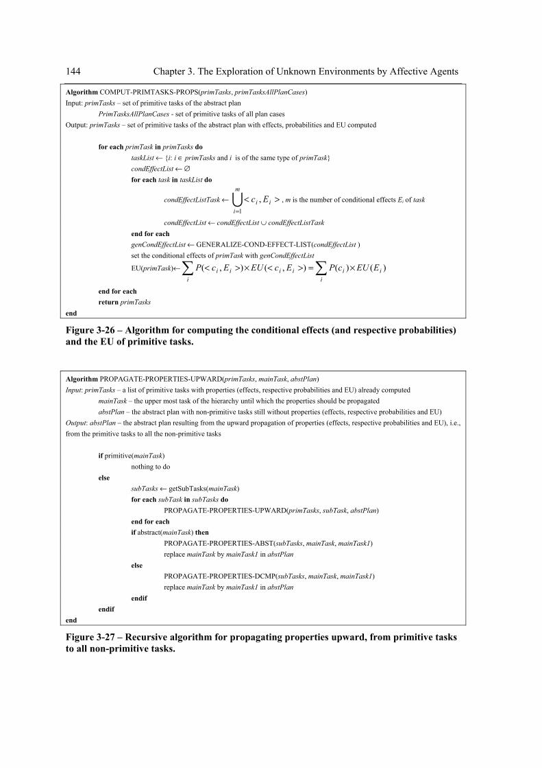
144 Chapter 3. The Exploration of Unknown Environments by Affective Agents
Algorithm COMPUT-PRIMTASKS-PROPS(primTasks, primTasksAllPlanCases) Input: primTasks – set of primitive tasks of the abstract plan PrimTasksAllPlanCases - set of primitive tasks of all plan cases Output: primTasks – set of primitive tasks of the abstract plan with effects, probabilities and EU computed for each primTask in primTasks do taskList ← {i: i ∈ primTasks and i is of the same type of primTask} condEffectList ← ∅ for each task in taskList do
condEffectListTask ← Um
iii Ec
1
,=
>< , m is the number of conditional effects Ei of task
condEffectList ← condEffectList ∪ condEffectListTask end for each genCondEffectList ← GENERALIZE-COND-EFFECT-LIST(condEffectList ) set the conditional effects of primTask with genCondEffectList
EU(primTask)← )()(),(),( ii
iiii
ii EEUcPEcEUEcP ×=><×>< ∑∑
end for each return primTasks end
Figure 3-26 – Algorithm for computing the conditional effects (and respective probabilities) and the EU of primitive tasks.
Algorithm PROPAGATE-PROPERTIES-UPWARD(primTasks, mainTask, abstPlan) Input: primTasks – a list of primitive tasks with properties (effects, respective probabilities and EU) already computed mainTask – the upper most task of the hierarchy until which the properties should be propagated abstPlan – the abstract plan with non-primitive tasks still without properties (effects, respective probabilities and EU) Output: abstPlan – the abstract plan resulting from the upward propagation of properties (effects, respective probabilities and EU), i.e., from the primitive tasks to all the non-primitive tasks if primitive(mainTask) nothing to do else subTasks ← getSubTasks(mainTask) for each subTask in subTasks do PROPAGATE-PROPERTIES-UPWARD(primTasks, subTask, abstPlan) end for each if abstract(mainTask) then PROPAGATE-PROPERTIES-ABST(subTasks, mainTask, mainTask1) replace mainTask by mainTask1 in abstPlan else PROPAGATE-PROPERTIES-DCMP(subTasks, mainTask, mainTask1) replace mainTask by mainTask1 in abstPlan endif endif end
Figure 3-27 – Recursive algorithm for propagating properties upward, from primitive tasks to all non-primitive tasks.
Chapter 3. The Exploration of Unknown Environments by Affective Agents 145
In situation (ii), when all the subtasks (heads of alternative decompositions) of an abstract task have the effects and respective probabilities, the probability and EU computed, a link of the kind more_useful is established between them so that they are ranked according to their EU. The main reason of this ranking is to establish a preference between them for the instantiation of the abstract task. Thus, the most EU alternative decomposition instantiates the abstract task. When there is an execution failure of one of the primitive actions that is hierarchically dependent on this decomposition, the next most EU alternative decomposition instantiates the abstract task.
Plan Execution an Re-planning
Finding the optimal plan in ProCHiP consists simply of traversing the abstract plan, selecting the most EU subtask of an abstract task. Given a previously constructed abstract plan, its execution is a continuous process that involves the following two steps: selection of an action, and execution of the selected action.
Learning
As described in the previous section, executing a plan corresponds to an instantiation of an abstract plan. After a plan is executed, the instantiation that was actually executed is stored in memory for future reuse. In addition, the abstract plan is also stored in memory. This way, it might be useful in the future since it might avoid the unnecessary process of generating it again.
3.2 Affect-based Exploration of Unknown Environments
Throughout the description of the multi-agent system, we presented and illustrated most of the aspects of the application developed for the domain of exploration of unknown environments, especially those concerned with the architecture of agents such as: how the agents represent the environment, the entities that populate the environment, the motivational and emotional makeup, goals, plans, how these goals and plans are generated, how the agents generate assumptions/expectations for the current world state, and in general how the agents make decisions. We called this application A-EUNE (Affect-based Exploration of UNknown Environments). The description of how the explorer agents make decisions and behaves, i.e., how the exploratory behaviour comes up, is still missing. This will be addressed in the present and the following section.
The goal of exploration is twofold: (i) acquisition of maps of the environment – metric maps – to be stored in memory and where the cells occupied by the entities that populate that environment are represented; (ii) construction of models of those entities. Each agent is continuously performing the reasoning algorithm. Thus, each agent at a given time senses the environment to look for entities and compute the current world state (location, structure and function of those entities) based on the sensorial information and on the generation of expectations for the missing information. Then, a goal of kind visitEntity is generated for each unvisited entity (including those within the visual range and also those out of this range that were previously perceived but not yet visited). In addition, a goal of the kind visitLoc is generated for all the frontier cells [Yamauchi, 1998]. Then, these goals are then inserted in the ranked list of goals which might already contain previous goals generated in the past but not yet accomplished.
146 Chapter 3. The Exploration of Unknown Environments by Affective Agents
This list of goals is ranked according to the EU of the goals, which is computed, based on the intensities of feelings predicted as explained above.
3.3 A Running Session
We ran an agent in a simulated environment populated with several buildings (their functions were for instance, house, church, hotel, etc.; for the sake of simplicity, their descriptions were related with the shapes of their structure: rectangular, square, etc.). Figure 3-28 presents the simulated environment and the path taken by the agent to explore it. The agent started at location 0, with an empty memory of entities, but with a single case of a past plan for visiting entities. At this location its visual field included objects E1 and E2, located respectively at locations 1 and 2. Then the agent generated goals for visiting them by adapting the goal visitEntity of the previous plan stored in memory. The resulting goals are: visitEntity(E1) and visitEntity(E2). E1 and E2 are entirely new for the agent (remember that the agent started with an empty memory of entities). Therefore, the surprise and curiosity that they may elicit when visited is maximum. However, E1 is closer, so the hunger that may be felt when the agent is at location 1 is lower than in location 2. Hence, the agent ranks the goals as follows: visitEntity(E1) followed by visitEntity(E2). A plan is generated for the first goal. After its execution, the agent is at location 1 with a complete description of E1 stored in memory as a case (case 1 of the episodic memory of Figure 3-5) and an incomplete description of E2 (because it has not been visited yet and therefore it is not completely known – at least the function is still undetermined). In addition, the goal visitEntity(E1) is deleted from the queue of goals. At location 1, the agent perceives E2 and E3 (E1 is also perceived, but it has just been visited). The agent generates the goal visitEntity(E3) for visiting E3. Notice that visitEntity(E2) is still in the queue of goals. E3 is similar to the previously visited E1 and therefore it feels now a low curiosity and it predicts feeling a low intensity of surprise when visiting it. Besides, hunger is expected to be higher in location 3 than in 2 (the place for recharging the battery is location 0). So, the goals are ranked as follows: visitEntity(E2) followed by visitEntity(E3). Once again, a plan is generated for visitEntity(E2) and then executed. The result is the completion of the description of E2 (case 2 of the episodic memory of Figure 3-5). At location 2, the agent perceives E4, in addition to E3. E4 is similar to both E1 and E2. However, its EU is lower than that of E3 mainly because the agent expects a higher hunger in location 4 than in 3. Thus, E3 is visited. At this time, the agent has the episodic memory of Figure 3-5. An interesting behaviour is observed later when the agent has to select between visiting E11 and E12, which are exactly equal to E1 and E2, respectively, and at similar distances (E11 is slightly closer to location 0). Therefore, it might be expected that the agent would visit E11. However, this time the agent ranks the goals as follows: visitEntity(E12) and visitEntity(E11). This is because the agent has now more cases describing entities similar to E11 than to E12. Therefore, E12 is expected to elicit more surprise than E11, and hence the EU of visiting E12 is higher than that of visiting E11.

Chapter 3. The Exploration of Unknown Environments by Affective Agents 147
1
2
3
411
12
010
Figure 3-28 – A running session.

149
Chapter 4 Experimental Evaluation
xperimental evaluation of works on the exploration of unknown environments usually comprises two components: simulation tests and field tests. Simulation tests involve building softbots and then using them in a simulated environment to test theories and
algorithms. Field tests require building real world robots and running them in real world environments. As we mentioned in Section 1.3, we decided to confine the experimental evaluation to the simulation approach. The main reason that lead us to make this decision is that the hypothesis we are testing in our thesis does not necessarily require field tests, although, just as any other claims related with real world application, field tests would provide a more complete evaluation of our thesis. Besides, any field test of our approach would require a larger project involving modules of pattern recognition, etc. This would necessarily involve people from other research fields. We do not reject this kind of evaluation. On the contrary, we would like to do it in the future. Conversely, simulation tests almost only offer us advantages: we can see the results of our approach much more quickly using softbots in simulated environments than robots in real environments; the research is almost independent from the constraints of time and expenses that are usually associated with using real robots; and, we could focus more specifically on the precise aspect of the problem which we were interested in. Hence, in conclusion, and considering that there would not be relevant advantages of field tests for our purposes but almost only disadvantages, and that simulation tests provide us various advantages, we decided to perform only simulation tests. To do that, we had to guarantee that the majority of the disadvantages of simulation tests were avoided, given that, to build softbots as models of real robots, we had to abstract the essential features of the robots being modelled, i.e., we had to make some simplifications especially in the modelling of sensors. This was accomplished by ensuring that the variables that influence the results in the real world are captured by the computer model, and that the simplifications that we made do not discard part of those variables. For instance, we made the assumption that the agents know their localization precisely, for example by using GPS, because this is not relevant to test the influence of emotion and motivations on exploration.
The hypothesis of this thesis is that exploration of unknown environments populated with entities can be robustly and efficiently performed by affective agents. If we want to confirm this hypothesis, there are a few experimental procedures we should do.
First, we should define how exploration is evaluated. Following the research performed by others working on the problem of exploring unknown environments, there are two common dimensions for evaluating it: efficiency and effectiveness. Efficiency may be measured by the amount of knowledge acquired from the environment per unit of time. An agent that is able to acquire more knowledge in a time t1 is more efficient than another agent that acquires the same knowledge in a time t2>t1, which means that, from another point of view, for the same time t3, the former agent is able to acquire more knowledge than the latter. On the other hand, effectiveness is related to acquiring the information of a finite environment correctly and completely. An effective explorer is able to explore the entire environment. An effective agent is more efficient than another if it explores the entire environment before the other. In our approach, knowledge is measured in three complementary but related dimensions: the amount of the
E
150 Chapter 4. Experimental Evaluation
occupancy map acquired, the number and the diversity of models of entities acquired. These three dimensions are profoundly related since, for the same environment, the more models of entities acquired, the higher the probability of having acquired more information about the occupancy map. Remember that the analogical description of the entities is used to build the occupancy map. Another important aspect to take into account in the evaluation of exploration is that it is a two step process, involving the selection of viewpoints so that the sensory measurements contain new and useful information, and the interpretation of the findings of the sensors so as to make accurate deductions about the state of the environment. The first step prepares the second. It is of primary importance for the efficiency and effectiveness of an exploration strategy. Selecting the viewpoints that provide maximum information at a low cost (energy or time) enables an efficient exploration task. On the other hand those viewpoints should be selected so that all the information of the environment is acquired. The map building step is more concerned with effectiveness, although it also influences efficiency. In fact, although it might involve more or less time to interpret the information provided by the sensors, this seems to have much less weight on efficiency, in comparison to the time taken to travel from place to place. On the contrary, the effectiveness of the exploration depends on the accuracy of the interpretation of the information provided by the sensors. Wrong interpretations may lead to inaccurate maps which means a partial failure in exploration. So, an evaluation of any exploration should take into account these distinct steps.
Second, in order to know whether affective agents can perform exploration efficiently and effectively, we should not be confined to running an affective agent and measure its performance. Instead, we should compare its performance with ordinary agents (i.e., non affective agents). Furthermore, we should go further and study what variables influence its behaviour, i.e., which affective components make it perform better. We should therefore compare different exploration strategies. In our case, we should compare the strategies resulting from the combination of surprise, curiosity and hunger.
Third, to be valid, this comparison should rely on good models of curiosity, surprise and hunger. We should therefore ensure that their computational models are faithful to those of humans. This means that the computational models of surprise, curiosity and hunger should be valid models by accurately capturing the features of human models.
Finally, if we want to test the robustness of affective agents when performing exploration, we should test them with different amplitudes of the visual field in several environments of different complexities.
We performed three experiments to address these issues.
Experiment I addresses the third issue. However, we decided not to evaluate the computational model of curiosity nor that of hunger because they truly reflect the psychological theories which assign them a simple linearity. Actually, curiosity is usually equated with novelty and uncertainty, and hunger with the physiological need of an energy source. Novelty is peacefully computed by difference and uncertainty by entropy. The problem is with the complexity of the surprise model which seems to be non linear, according to some psychological theories. Therefore we tested the validity of the computational model of surprise.
Experiment II is the main experiment of the thesis that confirms the hypothesis. It addresses the first, the second and the last issue. The first issue is addressed concerning only to the efficiency of the exploration strategy. It tests whether affective agents can perform better or as better as
Chapter 4. Experimental Evaluation 151
ordinary agents. Moreover, it addresses the issue of determining which strategy is better and therefore it tests the influence of surprise, curiosity and hunger on the exploratory behaviour of the affective agent (second issue). This experiment also tests the robustness of the affect-based approach by assessing this influence in several environments (third issue). Besides considering the parameter of the exploration strategy and environment complexity, we also take into account the amplitude of the visual field of the agent.
Experiment III addresses the first issue related with exploration effectiveness. While Experiment II is more concerned with the step related with the selection of viewpoints, i.e., with the exploration strategy, Experiment III addresses the evaluation of the map-building process which relies on the generation of assumptions. Therefore, we assess its main advantage, which is the possibility of building maps by exploiting the knowledge acquired in previous exploration phases in the same or in other environments rather than by actually exploring the environment. This process depends on the contents of the memory, namely on the memory of entities. We test this influence as well as that of the environment complexity. However, it was not our intention to study the influence of affect on this exploration stage, but mainly to reach conclusions about its accuracy. The goal was to know whether the model for generating expectations can estimate accurately the entities of the environment based on incomplete information of them. This is important because the selection of viewpoints relies on these estimated entities. If they are too different from real entities, the computation of estimated feelings might be wrong and therefore the results of Experiment II may be invalid.
Not all aspects of the affective agents were tested. This is the case of the planner. This variable of the system was kept constant, i.e., the same planner was used in all the exploration sessions. However, it is obvious that the performance of exploration depends on the planner efficiency and effectiveness whose extensive evaluation is beyond the scope of this thesis. Besides, since the planner is constant, i.e., it is always the same planner, the corresponding variable that represents the planner is constant and hence does not interfere with the exploration task. The only involvement of the planner is in the ranking of goals which is affected by the component for autonomous generation and ranking of goals. According to the algorithm in Figure 3-18, a plan for a given goal could even not be generated if there is already one in memory. So, if we have to test the planner we should do it concerning the adaptation of plans. Anyway, a preliminary evaluation of this planner may be found in [Macedo & Cardoso, 2004a, 2004b]. Another part of the reasoning module that is constant is the module for autonomous generation and ranking of goals [Macedo & Cardoso, 2004d].
In conclusion, besides evaluating the computational model of surprise [Macedo & Cardoso, 2001a; Macedo et al., 2004], we also evaluate the following relationships between the variables of our approach (Figure 4-1): the role of surprise, curiosity and hunger (the strategy) on the performance of the exploration of environments populated with entities [Macedo & Cardoso, 2004c]; the role of environment complexity and amplitude of the visual field on the performance of the exploration of environments populated with entities; the sensitivity of the strategy to the environment complexity and visual field, and vice-versa, i.e., whether the influence of the strategy on time/energy required for exploring an environment depends on or is controlled or “gated” by the environment complexity and by the visual field, and vice-versa; the role of the size and to some extent of the diversity of the memory of entities on map-building by exploitation [Macedo & Cardoso, 2004e, 2005a]; and, the role of the environment complexity on map-building by exploitation. Any exploration task depends on the environment where it is performed. Therefore,
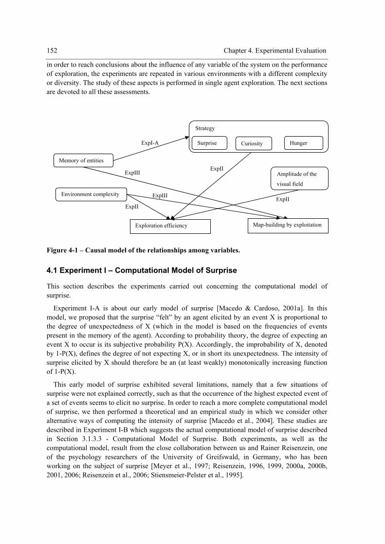
152 Chapter 4. Experimental Evaluation
in order to reach conclusions about the influence of any variable of the system on the performance of exploration, the experiments are repeated in various environments with a different complexity or diversity. The study of these aspects is performed in single agent exploration. The next sections are devoted to all these assessments.
Figure 4-1 – Causal model of the relationships among variables.
4.1 Experiment I – Computational Model of Surprise
This section describes the experiments carried out concerning the computational model of surprise.
Experiment I-A is about our early model of surprise [Macedo & Cardoso, 2001a]. In this model, we proposed that the surprise “felt” by an agent elicited by an event X is proportional to the degree of unexpectedness of X (which in the model is based on the frequencies of events present in the memory of the agent). According to probability theory, the degree of expecting an event X to occur is its subjective probability P(X). Accordingly, the improbability of X, denoted by 1-P(X), defines the degree of not expecting X, or in short its unexpectedness. The intensity of surprise elicited by X should therefore be an (at least weakly) monotonically increasing function of 1-P(X).
This early model of surprise exhibited several limitations, namely that a few situations of surprise were not explained correctly, such as that the occurrence of the highest expected event of a set of events seems to elicit no surprise. In order to reach a more complete computational model of surprise, we then performed a theoretical and an empirical study in which we consider other alternative ways of computing the intensity of surprise [Macedo et al., 2004]. These studies are described in Experiment I-B which suggests the actual computational model of surprise described in Section 3.1.3.3 - Computational Model of Surprise. Both experiments, as well as the computational model, result from the close collaboration between us and Rainer Reisenzein, one of the psychology researchers of the University of Greifswald, in Germany, who has been working on the subject of surprise [Meyer et al., 1997; Reisenzein, 1996, 1999, 2000a, 2000b, 2001, 2006; Reisenzein et al., 2006; Stiensmeier-Pelster et al., 1995].
Memory of entities
Environment complexity
Exploration efficiency
Amplitude of the
visual field
Strategy
ExpIII
ExpIII
ExpII
ExpI-A
ExpII ExpII
Hunger Surprise Curiosity
Map-building by exploitation
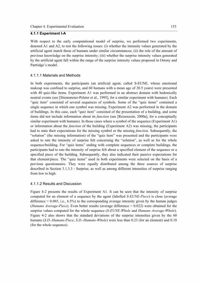
Chapter 4. Experimental Evaluation 153
4.1.1 Experiment I-A
With respect to the early computational model of surprise, we performed two experiments, denoted A1 and A2, to test the following issues: (i) whether the intensity values generated by the artificial agent match those of humans under similar circumstances; (ii) the role of the amount of previous knowledge on the surprise intensity; (iii) whether the surprise intensity values generated by the artificial agent fall within the range of the surprise intensity values proposed in Ortony and Partridge’s model.
4.1.1.1 Materials and Methods
In both experiments, the participants (an artificial agent, called S-EUNE, whose emotional makeup was confined to surprise, and 60 humans with a mean age of 20.5 years) were presented with 40 quiz-like items. Experiment A1 was performed in an abstract domain with hedonically neutral events (see [Stiensmeier-Pelster et al., 1995], for a similar experiment with humans). Each “quiz item” consisted of several sequences of symbols. Some of the “quiz items” contained a single sequence in which one symbol was missing. Experiment A2 was performed in the domain of buildings. In this case, each “quiz item” consisted of the presentation of a building, and some items did not include information about its function (see [Reisenzein, 2000a], for a conceptually similar experiment with humans). In those cases where a symbol of the sequence (Experiment A1) or information about the function of the building (Experiment A2) was missing, the participants had to state their expectations for the missing symbol or the missing function. Subsequently, the “solution” (the missing information) of the “quiz item” was presented and the participants were asked to rate the intensity of surprise felt concerning the “solution”, as well as for the whole sequence/building. For “quiz items” ending with complete sequences or complete buildings, the participants had to rate the intensity of surprise felt about a specified element of the sequence or a specified piece of the building. Subsequently, they also indicated their passive expectations for that element/piece. The “quiz items” used in both experiments were selected on the basis of a previous questionnaire. They were equally distributed among the three sources of surprise described in Section 3.1.3.3 - Surprise, as well as among different intensities of surprise ranging from low to high.
4.1.1.2 Results and Discussion
Figure 4-2 presents the results of Experiment A1. It can be seen that the intensity of surprise computed for an element of a sequence by the agent (labelled S-EUNE-Piece) is close (average difference = 0.065, i.e., 6.5%) to the corresponding average intensity given by the human judges (Humans Average-Piece). Even better results (average difference = 0.022) were obtained for the surprise values computed for the whole sequence (S-EUNE-Whole and Humans Average-Whole). Figure 4-2 also shows that the standard deviations of the surprise intensities given by the 60 humans (S.D.-Humans-Piece, S.D.-Humans-Whole) were less than 0.23 (for an element) and 0.18 (for the whole sequence).
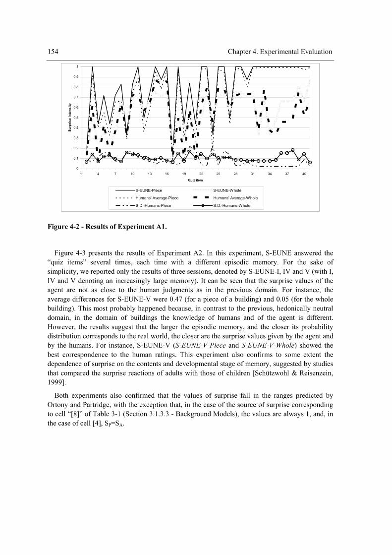
154 Chapter 4. Experimental Evaluation
0
0,1
0,2
0,3
0,4
0,5
0,6
0,7
0,8
0,9
1
1 4 7 10 13 16 19 22 25 28 31 34 37 40
Quiz item
Surp
rise
inte
nsity
S-EUNE-Piece S-EUNE-Whole
Humans' Average-Piece Humans' Average-Whole
S.D.-Humans-Piece S.D.-Humans-Whole
Figure 4-2 - Results of Experiment A1.
Figure 4-3 presents the results of Experiment A2. In this experiment, S-EUNE answered the “quiz items” several times, each time with a different episodic memory. For the sake of simplicity, we reported only the results of three sessions, denoted by S-EUNE-I, IV and V (with I, IV and V denoting an increasingly large memory). It can be seen that the surprise values of the agent are not as close to the human judgments as in the previous domain. For instance, the average differences for S-EUNE-V were 0.47 (for a piece of a building) and 0.05 (for the whole building). This most probably happened because, in contrast to the previous, hedonically neutral domain, in the domain of buildings the knowledge of humans and of the agent is different. However, the results suggest that the larger the episodic memory, and the closer its probability distribution corresponds to the real world, the closer are the surprise values given by the agent and by the humans. For instance, S-EUNE-V (S-EUNE-V-Piece and S-EUNE-V-Whole) showed the best correspondence to the human ratings. This experiment also confirms to some extent the dependence of surprise on the contents and developmental stage of memory, suggested by studies that compared the surprise reactions of adults with those of children [Schützwohl & Reisenzein, 1999].
Both experiments also confirmed that the values of surprise fall in the ranges predicted by Ortony and Partridge, with the exception that, in the case of the source of surprise corresponding to cell “[8]” of Table 3-1 (Section 3.1.3.3 - Background Models), the values are always 1, and, in the case of cell [4], SP=SA.
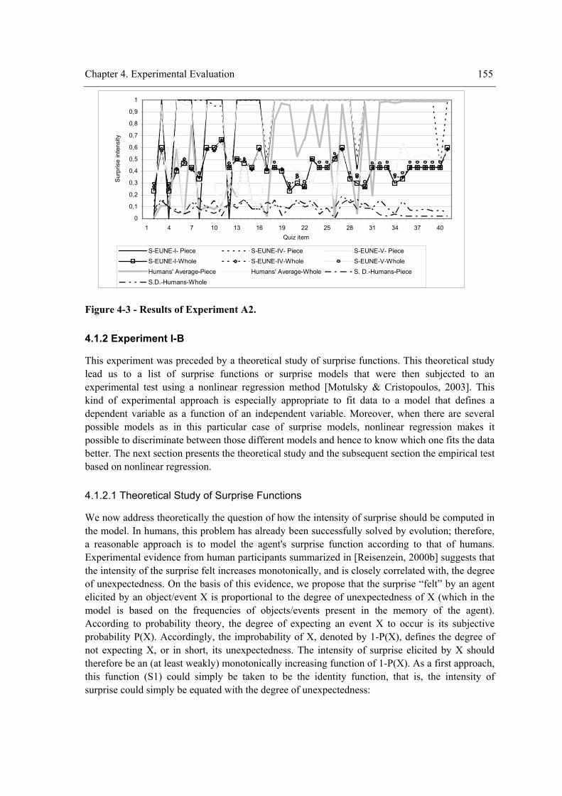
Chapter 4. Experimental Evaluation 155
0
0,1
0,2
0,3
0,4
0,5
0,6
0,7
0,8
0,9
1
1 4 7 10 13 16 19 22 25 28 31 34 37 40Quiz item
Sur
pris
e in
tens
ity
S-EUNE-I- Piece S-EUNE-IV- Piece S-EUNE-V- PieceS-EUNE-I-Whole S-EUNE-IV-Whole S-EUNE-V-WholeHumans' Average-Piece Humans' Average-Whole S. D.-Humans-PieceS.D.-Humans-Whole
Figure 4-3 - Results of Experiment A2.
4.1.2 Experiment I-B
This experiment was preceded by a theoretical study of surprise functions. This theoretical study lead us to a list of surprise functions or surprise models that were then subjected to an experimental test using a nonlinear regression method [Motulsky & Cristopoulos, 2003]. This kind of experimental approach is especially appropriate to fit data to a model that defines a dependent variable as a function of an independent variable. Moreover, when there are several possible models as in this particular case of surprise models, nonlinear regression makes it possible to discriminate between those different models and hence to know which one fits the data better. The next section presents the theoretical study and the subsequent section the empirical test based on nonlinear regression.
4.1.2.1 Theoretical Study of Surprise Functions
We now address theoretically the question of how the intensity of surprise should be computed in the model. In humans, this problem has already been successfully solved by evolution; therefore, a reasonable approach is to model the agent's surprise function according to that of humans. Experimental evidence from human participants summarized in [Reisenzein, 2000b] suggests that the intensity of the surprise felt increases monotonically, and is closely correlated with, the degree of unexpectedness. On the basis of this evidence, we propose that the surprise “felt” by an agent elicited by an object/event X is proportional to the degree of unexpectedness of X (which in the model is based on the frequencies of objects/events present in the memory of the agent). According to probability theory, the degree of expecting an event X to occur is its subjective probability P(X). Accordingly, the improbability of X, denoted by 1-P(X), defines the degree of not expecting X, or in short, its unexpectedness. The intensity of surprise elicited by X should therefore be an (at least weakly) monotonically increasing function of 1-P(X). As a first approach, this function (S1) could simply be taken to be the identity function, that is, the intensity of surprise could simply be equated with the degree of unexpectedness:
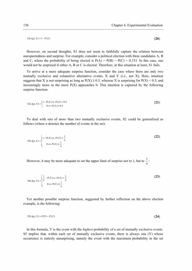
156 Chapter 4. Experimental Evaluation
)(1),(1 XPXAgtS −= (20)
However, on second thoughts, S1 does not seem to faithfully capture the relation between unexpectedness and surprise. For example, consider a political election with three candidates A, B and C, where the probability of being elected is P(A) = P(B) = P(C) = 0.333. In this case, one would not be surprised if either A, B or C is elected. Therefore, in this situation at least, S1 fails.
To arrive at a more adequate surprise function, consider the case where there are only two mutually exclusive and exhaustive alternative events, X and Y (i.e., not X). Here, intuition suggests that X is not surprising as long as P(X) ≥ 0.5, whereas X is surprising for P(X) < 0.5, and increasingly more so the more P(X) approaches 0. This intuition is captured by the following surprise function:
⎩⎨⎧
≥⇐<⇐−
=5.0)(0
5.0)()(1),(2
XPXPXP
XAgtS
(21)
To deal with sets of more than two mutually exclusive events, S2 could be generalized as follows (where n denotes the number of events in the set):
⎪⎪⎩
⎪⎪⎨
⎧
≥⇐
<⇐−=
nXP
nXPXP
XAgtS 1)(0
1)()(1),(3
(22)
However, it may be more adequate to set the upper limit of surprise not to 1, but to n1 :
⎪⎪⎩
⎪⎪⎨
⎧
≥⇐
<⇐−=
nXP
nXPXP
nXAgtS 1)(0
1)()(
1
),(4
(23)
Yet another possible surprise function, suggested by further reflection on the above election example, is the following:
)()(),(5 XPYPXAgtS −= (24)
In this formula, Y is the event with the highest probability of a set of mutually exclusive events. S5 implies that, within each set of mutually exclusive events, there is always one (Y) whose occurrence is entirely unsurprising, namely the event with the maximum probability in the set
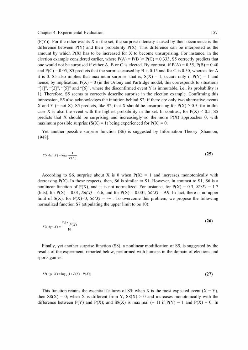
Chapter 4. Experimental Evaluation 157
(P(Y)). For the other events X in the set, the surprise intensity caused by their occurrence is the difference between P(Y) and their probability P(X). This difference can be interpreted as the amount by which P(X) has to be increased for X to become unsurprising. For instance, in the election example considered earlier, where P(A) = P(B )= P(C) = 0.333, S5 correctly predicts that one would not be surprised if either A, B or C is elected. By contrast, if P(A) = 0.55, P(B) = 0.40 and P(C) = 0.05, S5 predicts that the surprise caused by B is 0.15 and for C is 0.50, whereas for A it is 0. S5 also implies that maximum surprise, that is, S(X) = 1, occurs only if P(Y) = 1 and hence, by implication, P(X) = 0 (in the Ortony and Partridge model, this corresponds to situations “[1]”, “[2]”, “[5]” and “[6]”, where the disconfirmed event Y is immutable, i.e., its probability is 1). Therefore, S5 seems to correctly describe surprise in the election example. Confirming this impression, S5 also acknowledges the intuition behind S2: if there are only two alternative events X and Y (= not X), S5 predicts, like S2, that X should be unsurprising for P(X) ≥ 0.5, for in this case X is also the event with the highest probability in the set. In contrast, for P(X) < 0.5, S5 predicts that X should be surprising and increasingly so the more P(X) approaches 0, with maximum possible surprise (S(X) = 1) being experienced for P(X) = 0.
Yet another possible surprise function (S6) is suggested by Information Theory [Shannon, 1948]:
)(1log),(6 2 XP
XAgtS =
(25)
According to S6, surprise about X is 0 when P(X) = 1 and increases monotonically with decreasing P(X). In these respects, then, S6 is similar to S1. However, in contrast to S1, S6 is a nonlinear function of P(X), and it is not normalized. For instance, for P(X) = 0.3, S6(X) = 1.7 (bits), for P(X) = 0.01, S6(X) = 6.6, and for P(X) = 0.001, S6(X) = 9.9. In fact, there is no upper limit of S(X): for P(X)=0, S6(X) = +∝. To overcome this problem, we propose the following normalized function S7 (stipulating the upper limit to be 10):
10)(
1log),(7
2 XPXAgtS =
(26)
Finally, yet another surprise function (S8), a nonlinear modification of S5, is suggested by the results of the experiment, reported below, performed with humans in the domain of elections and sports games:
))()(1(log),(8 2 XPYPXAgtS −+= (27)
This function retains the essential features of S5: when X is the most expected event (X = Y), then S8(X) = 0; when X is different from Y, S8(X) > 0 and increases monotonically with the difference between P(Y) and P(X); and S8(X) is maximal (= 1) if P(Y) = 1 and P(X) = 0. In
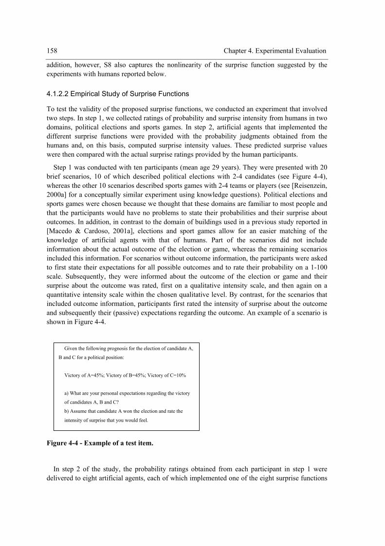
158 Chapter 4. Experimental Evaluation
addition, however, S8 also captures the nonlinearity of the surprise function suggested by the experiments with humans reported below.
4.1.2.2 Empirical Study of Surprise Functions
To test the validity of the proposed surprise functions, we conducted an experiment that involved two steps. In step 1, we collected ratings of probability and surprise intensity from humans in two domains, political elections and sports games. In step 2, artificial agents that implemented the different surprise functions were provided with the probability judgments obtained from the humans and, on this basis, computed surprise intensity values. These predicted surprise values were then compared with the actual surprise ratings provided by the human participants.
Step 1 was conducted with ten participants (mean age 29 years). They were presented with 20 brief scenarios, 10 of which described political elections with 2-4 candidates (see Figure 4-4), whereas the other 10 scenarios described sports games with 2-4 teams or players (see [Reisenzein, 2000a] for a conceptually similar experiment using knowledge questions). Political elections and sports games were chosen because we thought that these domains are familiar to most people and that the participants would have no problems to state their probabilities and their surprise about outcomes. In addition, in contrast to the domain of buildings used in a previous study reported in [Macedo & Cardoso, 2001a], elections and sport games allow for an easier matching of the knowledge of artificial agents with that of humans. Part of the scenarios did not include information about the actual outcome of the election or game, whereas the remaining scenarios included this information. For scenarios without outcome information, the participants were asked to first state their expectations for all possible outcomes and to rate their probability on a 1-100 scale. Subsequently, they were informed about the outcome of the election or game and their surprise about the outcome was rated, first on a qualitative intensity scale, and then again on a quantitative intensity scale within the chosen qualitative level. By contrast, for the scenarios that included outcome information, participants first rated the intensity of surprise about the outcome and subsequently their (passive) expectations regarding the outcome. An example of a scenario is shown in Figure 4-4.
Figure 4-4 - Example of a test item.
In step 2 of the study, the probability ratings obtained from each participant in step 1 were delivered to eight artificial agents, each of which implemented one of the eight surprise functions
Given the following prognosis for the election of candidate A,
B and C for a political position:
Victory of A=45%; Victory of B=45%; Victory of C=10%
a) What are your personal expectations regarding the victory
of candidates A, B and C?
b) Assume that candidate A won the election and rate the
intensity of surprise that you would feel.
Chapter 4. Experimental Evaluation 159
S1-S8 described earlier. Using these functions, the agents computed surprise intensity values from the probabilities. These predicted surprise values were then compared with the surprise ratings of the humans obtained in step 1.
The data obtained in the first step of the experiment suggested two qualitative conclusions. First, the occurrence of the most expected event of the set of mutually exclusive and exhaustive events did not elicit surprise in humans. For example, when the expectations for the election of three political candidates A, B and C were P(A) = 0.55, P(B) = 0.40, and P(C) = 0.05, the participants felt no surprise about the election of candidate A. This was also true when two or more candidates had equal maximal probabilities. For example, when P(A) = 0.40, P(B) = 0.40 and P(C) = 0.20, participants were not surprised when either A or B was elected. Second, beyond the point of zero surprise, the surprise function appeared to be nonlinear. For example, relatively high surprise was indicated when candidate C won the elections in both of the above situations, although it was still higher for P(C) = 0.05 than for P(C) = 0.20.
To compare the surprise values generated by the artificial agents and the surprise ratings provided by the human judges, the following fit indices were used: the root mean squared difference, the mean absolute difference, and the Pearson correlation. The results of these comparisons are shown in Table 4-1, separately for the 10 participants (H1, …, H10) and for six of the eight artificial agents (A1,…,A8) (the surprise functions S6 and S7 were not included because they have a different range to the human ratings and therefore computation of the absolute and squared differences is not meaningful). It can be seen from Table 4-1 that, regardless of which fit index is used, agent A8 (which implemented surprise function S8) was the one with the best fit to the human ratings: it had on average, the lowest root mean squared differences (Ms= 0.10), the lowest absolute differences (Md= 0.06), and the highest correlation to these ratings (Mr= 0.98). A8 was closely followed by A5 (Ms = 0.21; Md = 0.08; Mr = 0.97), whereas agents A1 and A2 had the comparatively worst fit values (for instance, A1 had Ms = 0.35; Md = 0.26; Mr = 0.81). The main reason for the bad performance of A1 was apparently that it failed in the case of the occurrence of the most expected event of the set: A1 still predicts a positive surprise value (1-P(X)) for this case, whereas humans do not feel surprised by the occurrence of this event. However, in other situations, A1 performed well.
In conclusion, the empirical study of the surprise functions suggests ))()(1(log)(8 2 XPYPXS −+= as the most appropriate surprise function for the domains of
political elections and sport games, although S5 (the linear counterpart of S8) is a very close contender. However, before more definitive conclusions can be drawn, additional tests need to be performed in other domains, as well as with yet other possible surprise functions (e.g., [Shackle, 1969]).
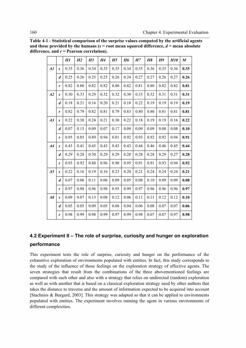
160 Chapter 4. Experimental Evaluation
Table 4-1 - Statistical comparison of the surprise values computed by the artificial agents and those provided by the humans (s = root mean squared difference, d = mean absolute difference, and r = Pearson correlation).
H1 H2 H3 H4 H5 H6 H7 H8 H9 H10 M
s 0.35 0.36 0.34 0.35 0.35 0.34 0.35 0.36 0.35 0.36 0.35
d 0.25 0.26 0.25 0.25 0.26 0.24 0.27 0.27 0.26 0.27 0.26
A1
r 0.82 0.80 0.82 0.82 0.80 0.82 0.81 0.80 0.82 0.82 0.81
s 0.30 0.33 0.29 0.32 0.32 0.30 0.33 0.32 0.31 0.31 0.31
d 0.18 0.21 0.16 0.20 0.21 0.18 0.22 0.19 0.19 0.19 0.19
A2
r 0.82 0.79 0.82 0.81 0.79 0.83 0.80 0.80 0.81 0.81 0.81
s 0.22 0.30 0.24 0.21 0.30 0.22 0.18 0.19 0.19 0.16 0.22
d 0.07 0.15 0.09 0.07 0.17 0.09 0.09 0.09 0.08 0.08 0.10
A3
r 0.95 0.85 0.89 0.94 0.81 0.92 0.93 0.92 0.92 0.94 0.91
s 0.43 0.41 0.45 0.43 0.43 0.43 0.44 0.46 0.46 0.45 0.44
d 0.29 0.28 0.30 0.29 0.29 0.28 0.28 0.28 0.29 0.27 0.28
A4
r 0.93 0.92 0.88 0.96 0.90 0.95 0.91 0.91 0.93 0.94 0.92
s 0.22 0.16 0.19 0.16 0.23 0.20 0.21 0.24 0.24 0.24 0.21
d 0.07 0.06 0.11 0.06 0.09 0.05 0.08 0.10 0.09 0.09 0.08
A5
r 0.97 0.98 0.96 0.98 0.95 0.99 0.97 0.96 0.96 0.96 0.97
s 0.09 0.07 0.13 0.08 0.12 0.06 0.11 0.13 0.12 0.12 0.10
d 0.05 0.05 0.09 0.05 0.08 0.04 0.06 0.08 0.07 0.07 0.06
A8
r 0.98 0.99 0.98 0.99 0.97 0.99 0.98 0.07 0.07 0.97 0.98
4.2 Experiment II – The role of surprise, curiosity and hunger on exploration performance
This experiment tests the role of surprise, curiosity and hunger on the performance of the exhaustive exploration of environments populated with entities. In fact, this study corresponds to the study of the influence of those feelings on the exploration strategy of affective agents. The seven strategies that result from the combinations of the three abovementioned feelings are compared with each other and also with a strategy that relies on undirected (random) exploration as well as with another that is based on a classical exploration strategy used by other authors that takes the distance to traverse and the amount of information expected to be acquired into account [Stachniss & Burgard, 2003]. This strategy was adapted so that it can be applied to environments populated with entities. The experiment involves running the agent in various environments of different complexities.
Chapter 4. Experimental Evaluation 161
As we mentioned above, the performance of exploring unknown environments populated with entities may be measured in terms of efficiency and effectiveness. Efficiency may be measured in terms of the amount of knowledge acquired in a period of time. This amount of knowledge may be measured by the number of entities visited (i.e., the number or percentage of entity models acquired) and/or by the number or percentage of different entities acquired (i.e., the number or percentage of different entity models acquired) (notice that two distinct entities may be totally equal except for the identifier). Another way to measure the amount of knowledge obtained could be based on the amount (for instance, number or percentage of known cells) of the occupancy map acquired or, from a different perspective, the inconsistency between the map built and the real map. In conclusion, we opted to report here these three different ways of measuring the amount of knowledge acquired which are: the amount (number or percentage of known cells) of the occupancy map acquired, the number of entities visited (i.e., the number or percentage of entity models acquired), the number or percentage of different entities acquired (i.e., the number or percentage of different entity models acquired). Since the simplifications that we made in our simulations ensure that the agents acquire the map with no errors when they explore the environment exhaustively, i.e., the occupancy map and the real map are fully consistent after exploring the whole environment whatever the strategy considered, the difference relies solely on the time elapsed and energy consumed to perform such exploration task. So, in this case of the full exploration of an environment, performance may be measured by computing the time elapsed and the energy required to complete the exploration of the environment, i.e., to acquire all the knowledge of the environment. In order to simplify the experiment we consider that the agent consumes a unit of energy per unit of time, which enables us to merge these two variables into a single one: exploration performance (more specifically: exploration efficiency). Furthermore, the agent consumes a unit of energy per cell traversed. Considering that we have three different ways of measuring the amount of knowledge acquired, performance may be measured by computing the time elapsed and the energy required to acquire completely the occupancy map (time elapsed and the energy required to get information about all the cells of an environment), the time elapsed and the energy required to visit all the entities (time elapsed and the energy required to acquire all entity models of an environment), and the time elapsed and the energy required to visit all different entities (time elapsed and the energy required to acquire all different entity models of an environment). These are the dependent variables (or response variables) of the experiment. This is, therefore, a multivariate study.
One of those strategies used by the agent, strategy 9, is based on the distance to be travelled by the agent and the expected information gain which is defined by the entropy [Stachniss & Burgard, 2003]. This is the classical strategy used by other authors. Eight of these strategies result from considering the combinations of the parameters of Equation 18. The possible combinations of these parameters and the correspondent strategies are presented in Table 4-2. With strategy 1, the agent performs undirected exploration (random) [Thrun, 1992a]. With strategy 2, the agent performs directed exploration based solely on hunger. With strategy 3 it performs directed exploration based solely on curiosity. With strategy 4, the agent performs directed exploration based on curiosity/interest and hunger. With strategy 5, the agent performs directed exploration based only on surprise. With strategy 6, it performs directed exploration based on surprise and hunger. With strategy 7, it performs directed exploration based on surprise and curiosity. With strategy 8, it performs directed exploration based on surprise, curiosity, and hunger.
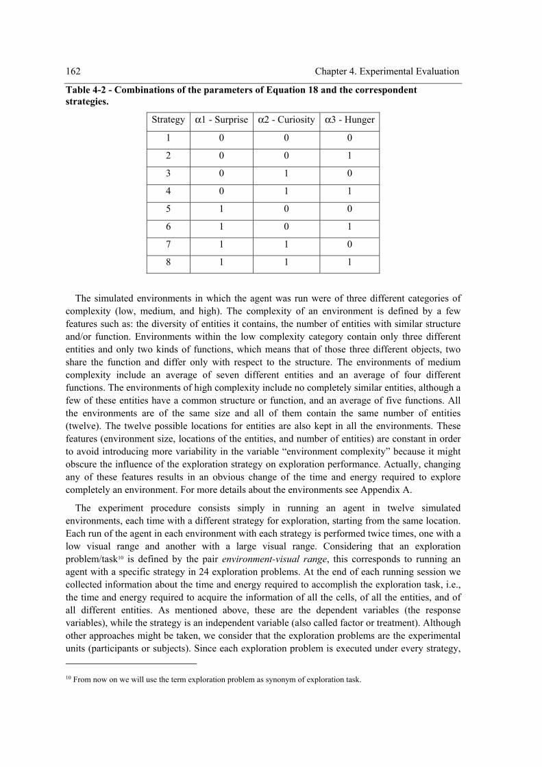
162 Chapter 4. Experimental Evaluation
Table 4-2 - Combinations of the parameters of Equation 18 and the correspondent strategies.
Strategy α1 - Surprise α2 - Curiosity α3 - Hunger
1 0 0 0
2 0 0 1
3 0 1 0
4 0 1 1
5 1 0 0
6 1 0 1
7 1 1 0
8 1 1 1
The simulated environments in which the agent was run were of three different categories of complexity (low, medium, and high). The complexity of an environment is defined by a few features such as: the diversity of entities it contains, the number of entities with similar structure and/or function. Environments within the low complexity category contain only three different entities and only two kinds of functions, which means that of those three different objects, two share the function and differ only with respect to the structure. The environments of medium complexity include an average of seven different entities and an average of four different functions. The environments of high complexity include no completely similar entities, although a few of these entities have a common structure or function, and an average of five functions. All the environments are of the same size and all of them contain the same number of entities (twelve). The twelve possible locations for entities are also kept in all the environments. These features (environment size, locations of the entities, and number of entities) are constant in order to avoid introducing more variability in the variable “environment complexity” because it might obscure the influence of the exploration strategy on exploration performance. Actually, changing any of these features results in an obvious change of the time and energy required to explore completely an environment. For more details about the environments see Appendix A.
The experiment procedure consists simply in running an agent in twelve simulated environments, each time with a different strategy for exploration, starting from the same location. Each run of the agent in each environment with each strategy is performed twice times, one with a low visual range and another with a large visual range. Considering that an exploration problem/task10 is defined by the pair environment-visual range, this corresponds to running an agent with a specific strategy in 24 exploration problems. At the end of each running session we collected information about the time and energy required to accomplish the exploration task, i.e., the time and energy required to acquire the information of all the cells, of all the entities, and of all different entities. As mentioned above, these are the dependent variables (the response variables), while the strategy is an independent variable (also called factor or treatment). Although other approaches might be taken, we consider that the exploration problems are the experimental units (participants or subjects). Since each exploration problem is executed under every strategy, 10 From now on we will use the term exploration problem as synonym of exploration task.
Chapter 4. Experimental Evaluation 163
i.e., each participant gets each of the treatments or conditions of the independent variable(s) or levels of the factor(s), this is a repeated measures experimental design (also called within subjects experimental design). Repeated measures designs allow us to obtain a lot of information from a relatively small number of subjects by gathering several pieces of data from each subject [P. Cohen, 1995; D. Cox & Reid, 2000; Dowdy et al., 2004; Mason et al., 2003; Montgomery, 2001; Murphy & Myors, 2004; I. Weiner, 2003]. All other things being equal, there is less random variability in a set of repeated measures than in a set of independent measures, each obtained from a different subject. Furthermore, repeated measures designs allow us to take advantage of the fact that the mean of several correlated observations is a more reliable piece of information about a subject than a single observation, which is all we would have in a between-subjects experimental design. Finally, repeated measures designs allow for the identification and removal of sources of variance in scores that are treated as error in a between-subject design. In particular, repeated measures designs allow for estimation and removal of systematic subject effects that cannot be estimated or controlled in typical between-subject designs. A consequence of this is that the power to detect the effects of within-subjects experimental factors (in our case confined to the strategy) is increased compared with testing in a between-subjects design. It is worth of notice that, as mentioned before, there are variables in this experiment that may exert some influence on the response variables, but for purposes of this experiment these are not of interest and are held at a specific level such as: location of the entities (for the purpose of this experiment we decided to perform all experimental runs holding the location of the entities constant), number of entities in the environment (twelve), number of other agents in the environment (0), battery level (1000 units), the planner, etc.
Considering this experiment information, we might conceive at least three different experimental designs depending on the factors considered.
The main factor of our experiment is the strategy. There are nine levels for this factor, each one corresponding to one of the different strategies whose means we want to compare. The exploration problem may be another factor, although we may not consider its effects. In this case, we have a one factor with repeated measures experimental design (described in Section 4.2.1). In order to statistically analyse the observed data produced by those runs of the agent using different exploration strategies in different environments, we make use of the one way analysis of variance with repeated measures.
However, we may want to know the effects of the problem in addition to the effects of the strategy as well as the effects of their interaction on the exploration performance of the agent. In this case, we have a two factor factorial experimental design with repeated measures. This two way repeated measure design may in turn be split into the following two slightly different designs depending on whether or not the blocking experimental principle is applied to the exploration problem factor. This principle may be applied in order to reduce the variance caused by the use of environments with different complexities or by the different visual ranges considered. In this case these variables may be considered as nuisance factors. This yields the following slightly different two factor factorial repeated measures designs: repeated measures design with the problem as a factor (the one-line-per-level setup - without blocking), repeated measures design with blocking (the environment complexity or the visual range might be used to group the subjects – exploration problems) (described in Section 4.2.2).
The strategy is undoubtedly a fixed factor. However, in order to generalize the results to all the exploration problems we might choose them randomly from a population of exploration problems.
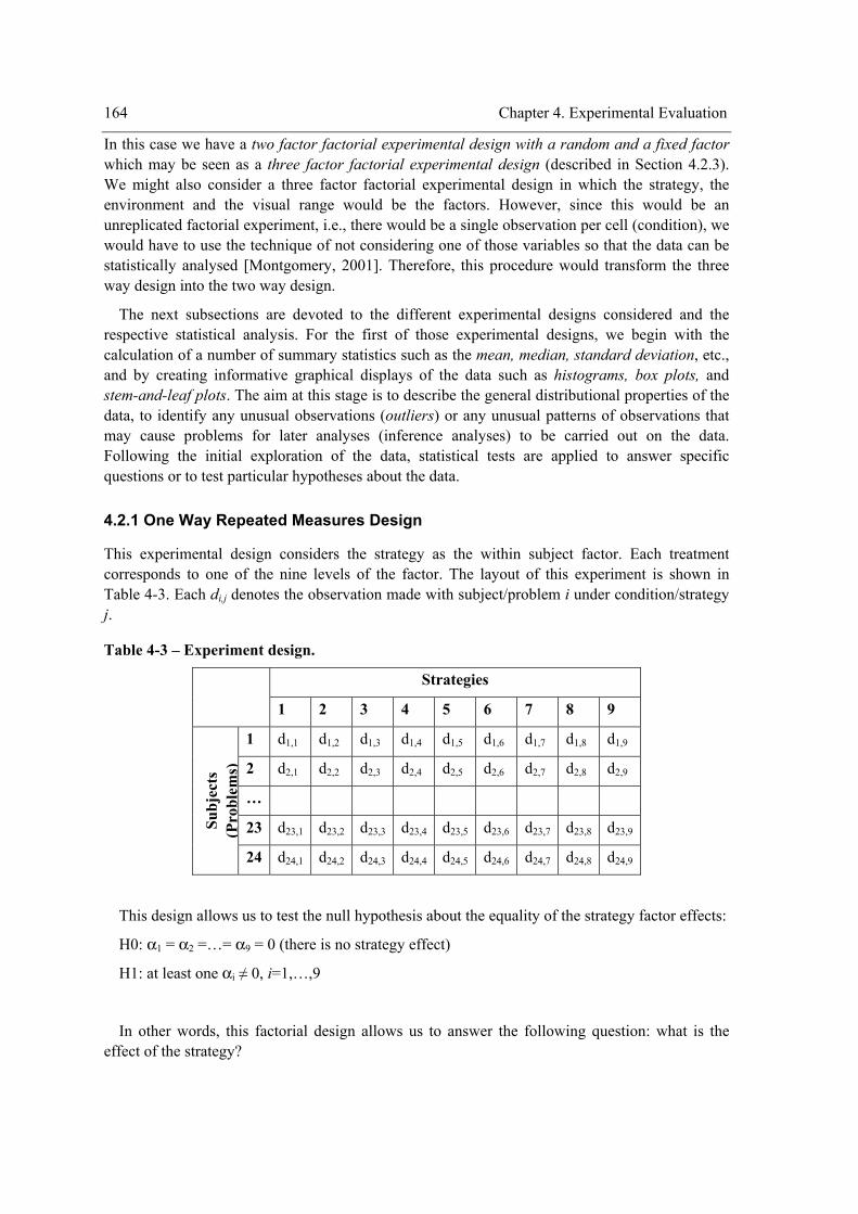
164 Chapter 4. Experimental Evaluation
In this case we have a two factor factorial experimental design with a random and a fixed factor which may be seen as a three factor factorial experimental design (described in Section 4.2.3). We might also consider a three factor factorial experimental design in which the strategy, the environment and the visual range would be the factors. However, since this would be an unreplicated factorial experiment, i.e., there would be a single observation per cell (condition), we would have to use the technique of not considering one of those variables so that the data can be statistically analysed [Montgomery, 2001]. Therefore, this procedure would transform the three way design into the two way design.
The next subsections are devoted to the different experimental designs considered and the respective statistical analysis. For the first of those experimental designs, we begin with the calculation of a number of summary statistics such as the mean, median, standard deviation, etc., and by creating informative graphical displays of the data such as histograms, box plots, and stem-and-leaf plots. The aim at this stage is to describe the general distributional properties of the data, to identify any unusual observations (outliers) or any unusual patterns of observations that may cause problems for later analyses (inference analyses) to be carried out on the data. Following the initial exploration of the data, statistical tests are applied to answer specific questions or to test particular hypotheses about the data.
4.2.1 One Way Repeated Measures Design
This experimental design considers the strategy as the within subject factor. Each treatment corresponds to one of the nine levels of the factor. The layout of this experiment is shown in Table 4-3. Each di,j denotes the observation made with subject/problem i under condition/strategy j.
Table 4-3 – Experiment design.
Strategies
1 2 3 4 5 6 7 8 9
1 d1,1 d1,2 d1,3 d1,4 d1,5 d1,6 d1,7 d1,8 d1,9
2 d2,1 d2,2 d2,3 d2,4 d2,5 d2,6 d2,7 d2,8 d2,9
…
23 d23,1 d23,2 d23,3 d23,4 d23,5 d23,6 d23,7 d23,8 d23,9 Subj
ects
(P
robl
ems)
24 d24,1 d24,2 d24,3 d24,4 d24,5 d24,6 d24,7 d24,8 d24,9
This design allows us to test the null hypothesis about the equality of the strategy factor effects:
H0: α1 = α2 =…= α9 = 0 (there is no strategy effect)
H1: at least one αi ≠ 0, i=1,…,9
In other words, this factorial design allows us to answer the following question: what is the effect of the strategy?
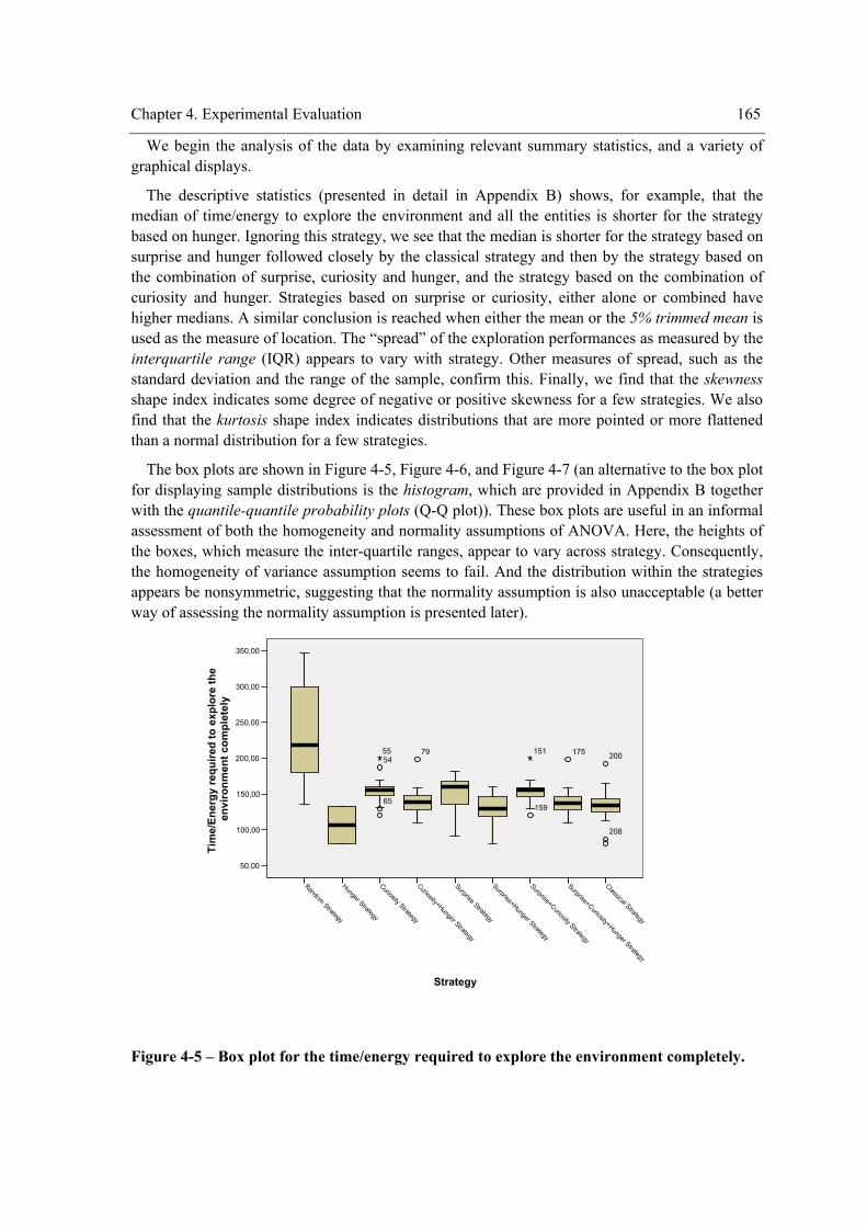
Chapter 4. Experimental Evaluation 165
We begin the analysis of the data by examining relevant summary statistics, and a variety of graphical displays.
The descriptive statistics (presented in detail in Appendix B) shows, for example, that the median of time/energy to explore the environment and all the entities is shorter for the strategy based on hunger. Ignoring this strategy, we see that the median is shorter for the strategy based on surprise and hunger followed closely by the classical strategy and then by the strategy based on the combination of surprise, curiosity and hunger, and the strategy based on the combination of curiosity and hunger. Strategies based on surprise or curiosity, either alone or combined have higher medians. A similar conclusion is reached when either the mean or the 5% trimmed mean is used as the measure of location. The “spread” of the exploration performances as measured by the interquartile range (IQR) appears to vary with strategy. Other measures of spread, such as the standard deviation and the range of the sample, confirm this. Finally, we find that the skewness shape index indicates some degree of negative or positive skewness for a few strategies. We also find that the kurtosis shape index indicates distributions that are more pointed or more flattened than a normal distribution for a few strategies.
The box plots are shown in Figure 4-5, Figure 4-6, and Figure 4-7 (an alternative to the box plot for displaying sample distributions is the histogram, which are provided in Appendix B together with the quantile-quantile probability plots (Q-Q plot)). These box plots are useful in an informal assessment of both the homogeneity and normality assumptions of ANOVA. Here, the heights of the boxes, which measure the inter-quartile ranges, appear to vary across strategy. Consequently, the homogeneity of variance assumption seems to fail. And the distribution within the strategies appears be nonsymmetric, suggesting that the normality assumption is also unacceptable (a better way of assessing the normality assumption is presented later).
Classical Strategy
Surprise+Curiosity+Hunger Strategy
Surprise+Curiosity Strategy
Surprise+Hunger Strategy
Surprise Strategy
Curiosity+Hunger Strategy
Curiosity Strategy
Hunger Strategy
Random Strategy
Strategy
350,00
300,00
250,00
200,00
150,00
100,00
50,00
Tim
e/En
ergy
requ
ired
to e
xplo
re th
een
viro
nmen
t com
plet
ely
200
208
175
159
7954
65
15155
Figure 4-5 – Box plot for the time/energy required to explore the environment completely.
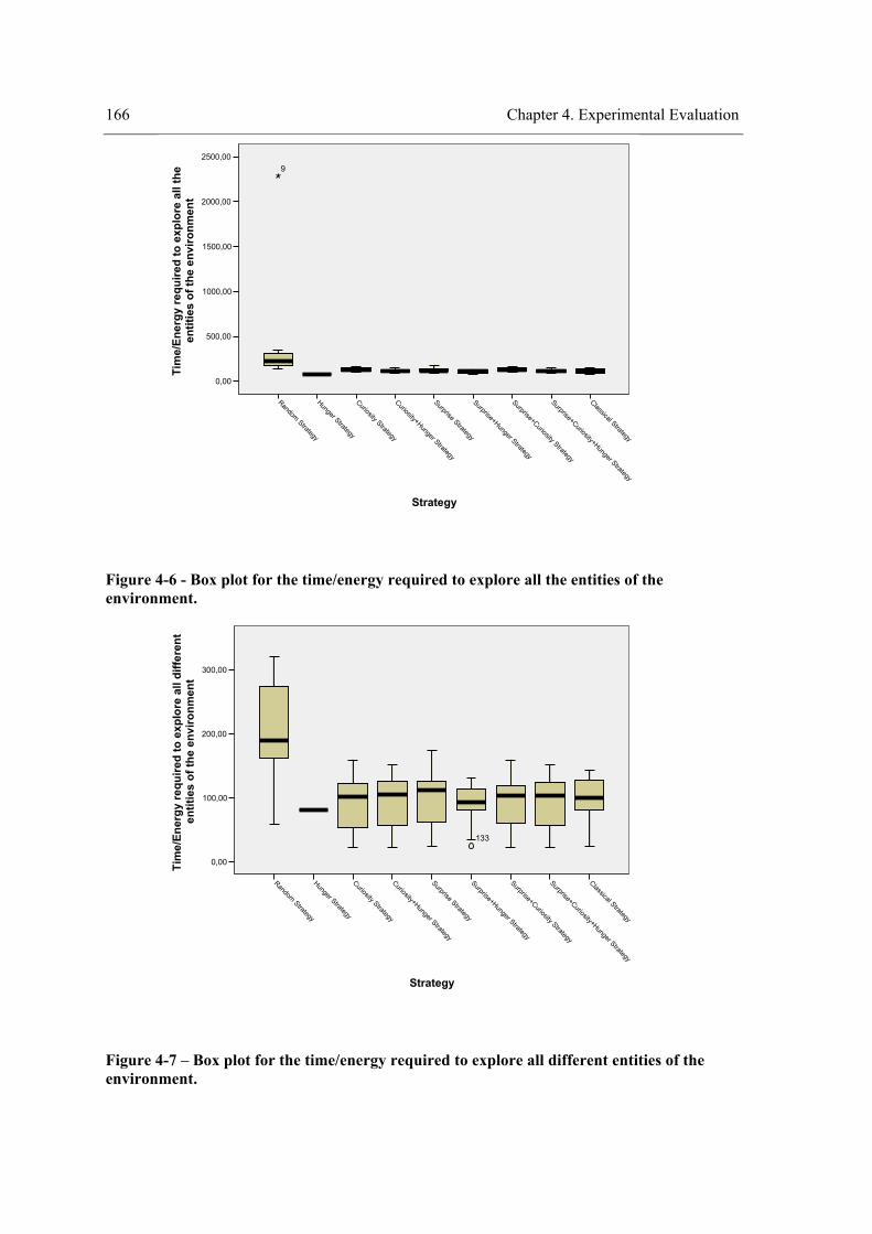
166 Chapter 4. Experimental Evaluation
Classical Strategy
Surprise+Curiosity+Hunger Strategy
Surprise+Curiosity Strategy
Surprise+Hunger Strategy
Surprise Strategy
Curiosity+Hunger Strategy
Curiosity Strategy
Hunger Strategy
Random Strategy
Strategy
2500,00
2000,00
1500,00
1000,00
500,00
0,00
Tim
e/En
ergy
requ
ired
to e
xplo
re a
ll th
een
titie
s of
the
envi
ronm
ent
9
Figure 4-6 - Box plot for the time/energy required to explore all the entities of the environment.
Classical Strategy
Surprise+Curiosity+Hunger Strategy
Surprise+Curiosity Strategy
Surprise+Hunger Strategy
Surprise Strategy
Curiosity+Hunger Strategy
Curiosity Strategy
Hunger Strategy
Random Strategy
Strategy
300,00
200,00
100,00
0,00Tim
e/En
ergy
requ
ired
to e
xplo
re a
ll di
ffere
nten
titie
s of
the
envi
ronm
ent
133
Figure 4-7 – Box plot for the time/energy required to explore all different entities of the environment.
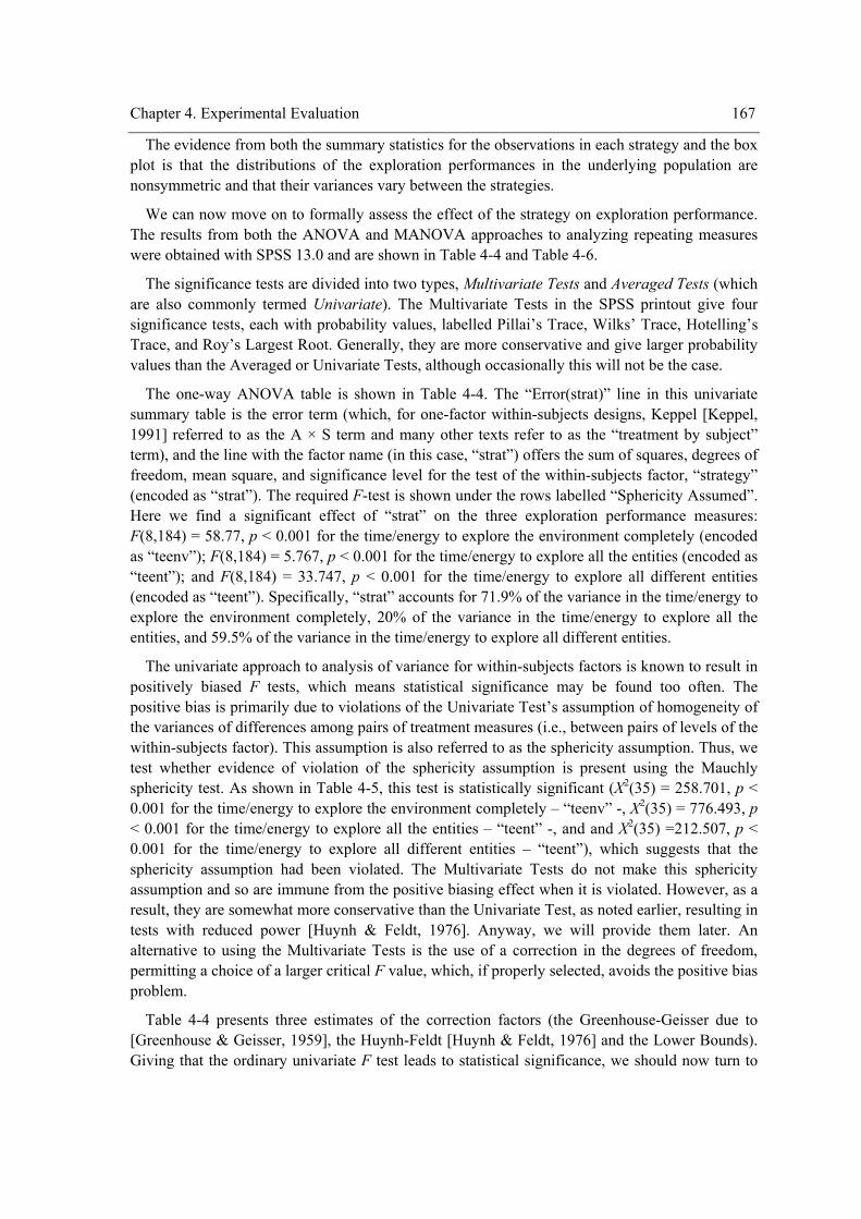
Chapter 4. Experimental Evaluation 167
The evidence from both the summary statistics for the observations in each strategy and the box plot is that the distributions of the exploration performances in the underlying population are nonsymmetric and that their variances vary between the strategies.
We can now move on to formally assess the effect of the strategy on exploration performance. The results from both the ANOVA and MANOVA approaches to analyzing repeating measures were obtained with SPSS 13.0 and are shown in Table 4-4 and Table 4-6.
The significance tests are divided into two types, Multivariate Tests and Averaged Tests (which are also commonly termed Univariate). The Multivariate Tests in the SPSS printout give four significance tests, each with probability values, labelled Pillai’s Trace, Wilks’ Trace, Hotelling’s Trace, and Roy’s Largest Root. Generally, they are more conservative and give larger probability values than the Averaged or Univariate Tests, although occasionally this will not be the case.
The one-way ANOVA table is shown in Table 4-4. The “Error(strat)” line in this univariate summary table is the error term (which, for one-factor within-subjects designs, Keppel [Keppel, 1991] referred to as the A × S term and many other texts refer to as the “treatment by subject” term), and the line with the factor name (in this case, “strat”) offers the sum of squares, degrees of freedom, mean square, and significance level for the test of the within-subjects factor, “strategy” (encoded as “strat”). The required F-test is shown under the rows labelled “Sphericity Assumed”. Here we find a significant effect of “strat” on the three exploration performance measures: F(8,184) = 58.77, p < 0.001 for the time/energy to explore the environment completely (encoded as “teenv”); F(8,184) = 5.767, p < 0.001 for the time/energy to explore all the entities (encoded as “teent”); and F(8,184) = 33.747, p < 0.001 for the time/energy to explore all different entities (encoded as “teent”). Specifically, “strat” accounts for 71.9% of the variance in the time/energy to explore the environment completely, 20% of the variance in the time/energy to explore all the entities, and 59.5% of the variance in the time/energy to explore all different entities.
The univariate approach to analysis of variance for within-subjects factors is known to result in positively biased F tests, which means statistical significance may be found too often. The positive bias is primarily due to violations of the Univariate Test’s assumption of homogeneity of the variances of differences among pairs of treatment measures (i.e., between pairs of levels of the within-subjects factor). This assumption is also referred to as the sphericity assumption. Thus, we test whether evidence of violation of the sphericity assumption is present using the Mauchly sphericity test. As shown in Table 4-5, this test is statistically significant (X2(35) = 258.701, p < 0.001 for the time/energy to explore the environment completely – “teenv” -, X2(35) = 776.493, p < 0.001 for the time/energy to explore all the entities – “teent” -, and and X2(35) =212.507, p < 0.001 for the time/energy to explore all different entities – “teent”), which suggests that the sphericity assumption had been violated. The Multivariate Tests do not make this sphericity assumption and so are immune from the positive biasing effect when it is violated. However, as a result, they are somewhat more conservative than the Univariate Test, as noted earlier, resulting in tests with reduced power [Huynh & Feldt, 1976]. Anyway, we will provide them later. An alternative to using the Multivariate Tests is the use of a correction in the degrees of freedom, permitting a choice of a larger critical F value, which, if properly selected, avoids the positive bias problem.
Table 4-4 presents three estimates of the correction factors (the Greenhouse-Geisser due to [Greenhouse & Geisser, 1959], the Huynh-Feldt [Huynh & Feldt, 1976] and the Lower Bounds). Giving that the ordinary univariate F test leads to statistical significance, we should now turn to
168 Chapter 4. Experimental Evaluation
one of these more conservative (likely too conservative) tests. Following the procedure suggested for instance by [Keppel, 1991; J. Myers, 1979], we turn to the Lower Bound test. The within subject effect that tested significant under the assumption of sphericity remain significant with this test (see Table 4-4 under the rows “Lower-bound”): F(1.00, 23.00) = 58.77, p < 0.001 for the time/energy to explore the environment completely, F(1.00, 23.00) = 5.767, p = 0.025 for the time/energy to explore all the entities, and F(1.00, 23.00) = 33.747, p < 0.001 for the time/energy to explore all different entities. Giving this statistical significance, we need not to use the other two conservative tests. Anyway, the within subject effect that tested significant under the assumption of sphericity and with the Lower Bound test remain highly significant even after these corrections: using Huynh-Feldt correction factor, F(1.647, 37.874) = 58.77, p < 0.001 for the time/energy to explore the environment completely, F(1.013, 23.291) = 5.767, p = 0.024 for the time/energy to explore all the entities, and F(2.409, 55.406) = 33.747, p < 0.001 for the time/energy to explore all different entities; using Greenhouse-Geisser correction factor, F(1.555, 35.759) = 58.77, p < 0.001 for the time/energy to explore the environment, F(1.011, 23.256) = 5.767, p = 0.024 for the time/energy to explore all the entities, and F(2.174, 49.996) = 33.747, p < 0.001 for the time/energy to explore all different entities.
The Multivariate Tests are shown in Table 4-6. As noted earlier, these give four commonly used significance tests labelled Pillai’s Trace, Wilks’ Trace, Hotelling’s Trace, and Roy’s Largest Root. The results for testing the main effect of “strat” are identical to those obtained from the univariate ANOVA model: the four tests of significance for the strategy effect given by the Multivariate Tests, Pillai’s Trace (value = 0.944; F(24.00, 552.00)=10.565, p < 0.001), Wilks’ Lambda (value = 0.218; F(24.00, 528.457) = 15.219, p < 0.001), Hotelling’s Trace (value = 2.847; F(24.00, 542.00) = 21.429, p < 0.001), and Roy’s Largest Root (value = 2.556; F(8.00,184.00) = 58.787, p < 0.001), indicate that the strategy has a significant effect. The Partial Eta Squared values for strategy show that it explains quite a lot of variation in exploration performance.
All the analyses reported above have established that the exploration performance is affected by the strategy. Therefore we reject the null hypothesis. The F test tell us only if all the group means are roughly equal or if there are some significant differences among them. In the latter case, it does not tell us which groups are different from which other groups. Therefore, we now undertake further tests to determine which particular group means differ. Since we have no prior hypotheses about the group differences and we are simply exploring the data to ascertain which group differences are driving the significance of the overall F test, we conducted post hoc comparisons. The resulting multiple comparison output for the strategy factor is shown in Table 4-7, Table 4-8, and Table 4-9. For each comparison type and pair of groups (strategies), the Pairwise Comparisons table provides an estimate of the difference in means and the p-value from a statistical test of zero group difference (in parentheses). Additional information, such as the standard error of that estimator and a confidence interval for the mean difference, is provided by the original table presented in Appendix B.
The profile plots (Figure 4-8, Figure 4-9, and Figure 4-10) show the model-estimated means for the nine strategies. Together with the multiple comparison output, the plots provide us the following results. As it can be seen strategy 1 (random) is significantly (p < 0.001) the worst strategy considering the three exploration performance measures (time/energy to explore the environment completely, time/energy to explore all the entities, and the time/energy to explore all different entities). On the contrary, strategy 2 (hunger-based) is significantly (p < 0.001) the best

Chapter 4. Experimental Evaluation 169
strategy considering the three exploration performance measures. However, as we will note later, this strategy depends heavily on the position of the entities in the environment (this factor was kept constant in our experiment).
Table 4-4 - Univariate ANOVA tables for testing the main effects of the within-subject factor (strategy) on the exploration performance.
Univariate Tests
Source Measure Type III Sum of Squares df Mean
Square F Sig. Partial
Eta Squared
Noncent. Parameter
Observed Power(a)
Sphericity Assumed 252678.317 8 31584.790 58.770 0.000 0.719 470.159 1.000
Greenhouse-Geisser 252678.317 1.555 162521.447 58.770 0.000 0.719 91.372 1.000
Huynh-Feldt 252678.317 1.647 153446.105 58.770 0.000 0.719 96.776 1.000
teenv
Lower-bound 252678.317 1.000 252678.317 58.770 0.000 0.719 58.770 1.000
Sphericity Assumed 950894.351 8 118861.794 5.767 0.000 0.200 46.138 1.000
Greenhouse-Geisser 950894.351 1.011 940422.587 5.767 0.024 0.200 5.831 0.637
Huynh-Feldt 950894.351 1.013 939006.521 5.767 0.024 0.200 5.840 0.637
teent
Lower-bound 950894.351 1.000 950894.351 5.767 0.025 0.200 5.767 0.633
Sphericity Assumed 282320.236 8 35290.029 33.747 0.000 0.595 269.977 1.000
Greenhouse-Geisser 282320.236 2.174 129878.039 33.747 0.000 0.595 73.357 1.000
Huynh-Feldt 282320.236 2.409 117195.996 33.747 0.000 0.595 81.295 1.000
strat
tedent
Lower-bound 282320.236 1.000 282320.236 33.747 0.000 0.595 33.747 1.000
Sphericity Assumed 98887.417 184 537.432
Greenhouse-Geisser 98887.417 35.759 2765.387
Huynh-Feldt 98887.417 37.874 2610.965
teenv
Lower-bound 98887.417 23.000 4299.453
Sphericity Assumed 3792198.038 184 20609.772
Greenhouse-Geisser 3792198.038 23.256 163062.448
Huynh-Feldt 3792198.038 23.291 162816.912
teent
Lower-bound 3792198.038 23.000 164878.176
Sphericity Assumed 192412.496 184 1045.720
Greenhouse-Geisser 192412.496 49.996 3848.568
Huynh-Feldt 192412.496 55.406 3472.771
Error(strat)
tedent
Lower-bound 192412.496 23.000 8365.761 a Computed using alpha = 0.05
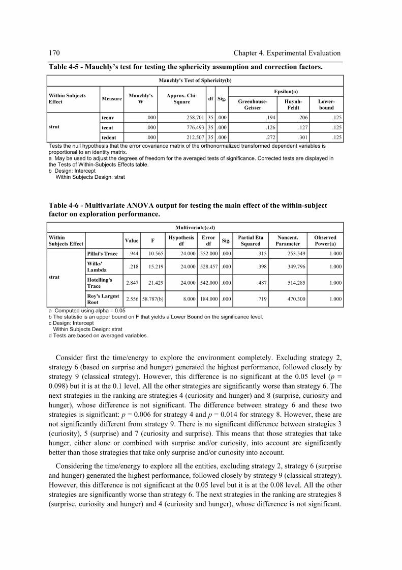
170 Chapter 4. Experimental Evaluation
Table 4-5 - Mauchly’s test for testing the sphericity assumption and correction factors.
Mauchly's Test of Sphericity(b)
Epsilon(a) Within Subjects Effect Measure Mauchly's
W Approx. Chi-
Square df Sig. Greenhouse-Geisser
Huynh-Feldt
Lower-bound
teenv .000 258.701 35 .000 .194 .206 .125
teent .000 776.493 35 .000 .126 .127 .125strat
tedent .000 212.507 35 .000 .272 .301 .125Tests the null hypothesis that the error covariance matrix of the orthonormalized transformed dependent variables is proportional to an identity matrix. a May be used to adjust the degrees of freedom for the averaged tests of significance. Corrected tests are displayed in the Tests of Within-Subjects Effects table. b Design: Intercept
Within Subjects Design: strat
Table 4-6 - Multivariate ANOVA output for testing the main effect of the within-subject factor on exploration performance.
Multivariate(c.d)
Within Subjects Effect Value F Hypothesis
df Error
df Sig. Partial Eta Squared
Noncent. Parameter
Observed Power(a)
Pillai's Trace .944 10.565 24.000 552.000 .000 .315 253.549 1.000
Wilks' Lambda .218 15.219 24.000 528.457 .000 .398 349.796 1.000
Hotelling's Trace 2.847 21.429 24.000 542.000 .000 .487 514.285 1.000
strat
Roy's Largest Root 2.556 58.787(b) 8.000 184.000 .000 .719 470.300 1.000
a Computed using alpha = 0.05 b The statistic is an upper bound on F that yields a Lower Bound on the significance level. c Design: Intercept Within Subjects Design: strat d Tests are based on averaged variables.
Consider first the time/energy to explore the environment completely. Excluding strategy 2, strategy 6 (based on surprise and hunger) generated the highest performance, followed closely by strategy 9 (classical strategy). However, this difference is no significant at the 0.05 level (p = 0.098) but it is at the 0.1 level. All the other strategies are significantly worse than strategy 6. The next strategies in the ranking are strategies 4 (curiosity and hunger) and 8 (surprise, curiosity and hunger), whose difference is not significant. The difference between strategy 6 and these two strategies is significant: p = 0.006 for strategy 4 and p = 0.014 for strategy 8. However, these are not significantly different from strategy 9. There is no significant difference between strategies 3 (curiosity), 5 (surprise) and 7 (curiosity and surprise). This means that those strategies that take hunger, either alone or combined with surprise and/or curiosity, into account are significantly better than those strategies that take only surprise and/or curiosity into account.
Considering the time/energy to explore all the entities, excluding strategy 2, strategy 6 (surprise and hunger) generated the highest performance, followed closely by strategy 9 (classical strategy). However, this difference is not significant at the 0.05 level but it is at the 0.08 level. All the other strategies are significantly worse than strategy 6. The next strategies in the ranking are strategies 8 (surprise, curiosity and hunger) and 4 (curiosity and hunger), whose difference is not significant.
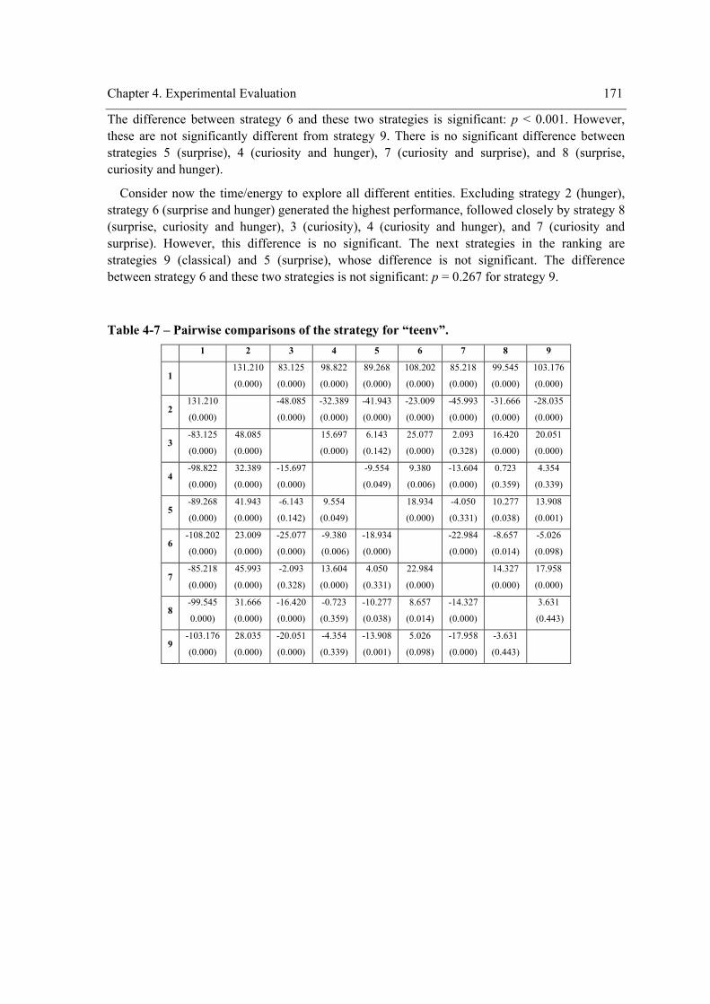
Chapter 4. Experimental Evaluation 171
The difference between strategy 6 and these two strategies is significant: p < 0.001. However, these are not significantly different from strategy 9. There is no significant difference between strategies 5 (surprise), 4 (curiosity and hunger), 7 (curiosity and surprise), and 8 (surprise, curiosity and hunger).
Consider now the time/energy to explore all different entities. Excluding strategy 2 (hunger), strategy 6 (surprise and hunger) generated the highest performance, followed closely by strategy 8 (surprise, curiosity and hunger), 3 (curiosity), 4 (curiosity and hunger), and 7 (curiosity and surprise). However, this difference is no significant. The next strategies in the ranking are strategies 9 (classical) and 5 (surprise), whose difference is not significant. The difference between strategy 6 and these two strategies is not significant: p = 0.267 for strategy 9.
Table 4-7 – Pairwise comparisons of the strategy for “teenv”. 1 2 3 4 5 6 7 8 9
1 131.210
(0.000)
83.125
(0.000)
98.822
(0.000)
89.268
(0.000)
108.202
(0.000)
85.218
(0.000)
99.545
(0.000)
103.176
(0.000)
2 131.210
(0.000)
-48.085
(0.000)
-32.389
(0.000)
-41.943
(0.000)
-23.009
(0.000)
-45.993
(0.000)
-31.666
(0.000)
-28.035
(0.000)
3 -83.125
(0.000)
48.085
(0.000)
15.697
(0.000)
6.143
(0.142)
25.077
(0.000)
2.093
(0.328)
16.420
(0.000)
20.051
(0.000)
4 -98.822
(0.000)
32.389
(0.000)
-15.697
(0.000)
-9.554
(0.049)
9.380
(0.006)
-13.604
(0.000)
0.723
(0.359)
4.354
(0.339)
5 -89.268
(0.000)
41.943
(0.000)
-6.143
(0.142)
9.554
(0.049)
18.934
(0.000)
-4.050
(0.331)
10.277
(0.038)
13.908
(0.001)
6 -108.202
(0.000)
23.009
(0.000)
-25.077
(0.000)
-9.380
(0.006)
-18.934
(0.000)
-22.984
(0.000)
-8.657
(0.014)
-5.026
(0.098)
7 -85.218
(0.000)
45.993
(0.000)
-2.093
(0.328)
13.604
(0.000)
4.050
(0.331)
22.984
(0.000)
14.327
(0.000)
17.958
(0.000)
8 -99.545
0.000)
31.666
(0.000)
-16.420
(0.000)
-0.723
(0.359)
-10.277
(0.038)
8.657
(0.014)
-14.327
(0.000)
3.631
(0.443)
9 -103.176
(0.000)
28.035
(0.000)
-20.051
(0.000)
-4.354
(0.339)
-13.908
(0.001)
5.026
(0.098)
-17.958
(0.000)
-3.631
(0.443)
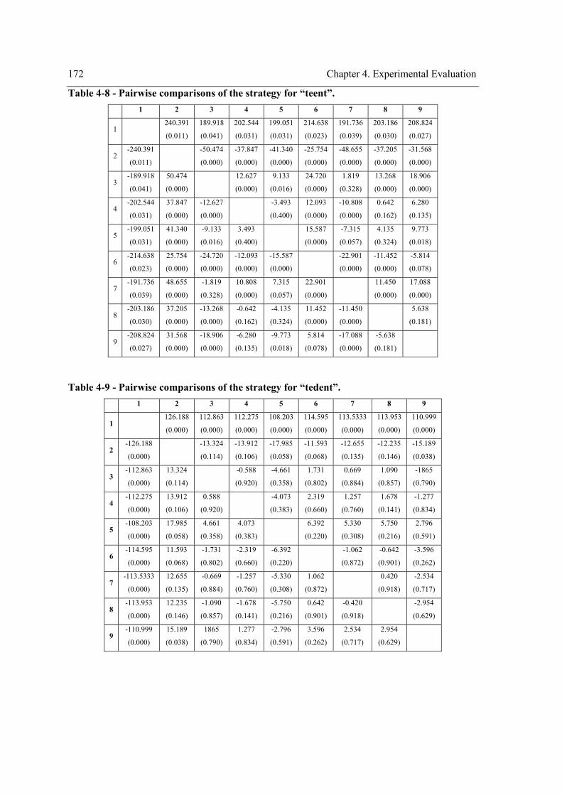
172 Chapter 4. Experimental Evaluation
Table 4-8 - Pairwise comparisons of the strategy for “teent”. 1 2 3 4 5 6 7 8 9
1 240.391
(0.011)
189.918
(0.041)
202.544
(0.031)
199.051
(0.031)
214.638
(0.023)
191.736
(0.039)
203.186
(0.030)
208.824
(0.027)
2 -240.391
(0.011)
-50.474
(0.000)
-37.847
(0.000)
-41.340
(0.000)
-25.754
(0.000)
-48.655
(0.000)
-37.205
(0.000)
-31.568
(0.000)
3 -189.918
(0.041)
50.474
(0.000)
12.627
(0.000)
9.133
(0.016)
24.720
(0.000)
1.819
(0.328)
13.268
(0.000)
18.906
(0.000)
4 -202.544
(0.031)
37.847
(0.000)
-12.627
(0.000)
-3.493
(0.400)
12.093
(0.000)
-10.808
(0.000)
0.642
(0.162)
6.280
(0.135)
5 -199.051
(0.031)
41.340
(0.000)
-9.133
(0.016)
3.493
(0.400)
15.587
(0.000)
-7.315
(0.057)
4.135
(0.324)
9.773
(0.018)
6 -214.638
(0.023)
25.754
(0.000)
-24.720
(0.000)
-12.093
(0.000)
-15.587
(0.000)
-22.901
(0.000)
-11.452
(0.000)
-5.814
(0.078)
7 -191.736
(0.039)
48.655
(0.000)
-1.819
(0.328)
10.808
(0.000)
7.315
(0.057)
22.901
(0.000)
11.450
(0.000)
17.088
(0.000)
8 -203.186
(0.030)
37.205
(0.000)
-13.268
(0.000)
-0.642
(0.162)
-4.135
(0.324)
11.452
(0.000)
-11.450
(0.000)
5.638
(0.181)
9 -208.824
(0.027)
31.568
(0.000)
-18.906
(0.000)
-6.280
(0.135)
-9.773
(0.018)
5.814
(0.078)
-17.088
(0.000)
-5.638
(0.181)
Table 4-9 - Pairwise comparisons of the strategy for “tedent”. 1 2 3 4 5 6 7 8 9
1 126.188
(0.000)
112.863
(0.000)
112.275
(0.000)
108.203
(0.000)
114.595
(0.000)
113.5333
(0.000)
113.953
(0.000)
110.999
(0.000)
2 -126.188
(0.000)
-13.324
(0.114)
-13.912
(0.106)
-17.985
(0.058)
-11.593
(0.068)
-12.655
(0.135)
-12.235
(0.146)
-15.189
(0.038)
3 -112.863
(0.000)
13.324
(0.114)
-0.588
(0.920)
-4.661
(0.358)
1.731
(0.802)
0.669
(0.884)
1.090
(0.857)
-1865
(0.790)
4 -112.275
(0.000)
13.912
(0.106)
0.588
(0.920)
-4.073
(0.383)
2.319
(0.660)
1.257
(0.760)
1.678
(0.141)
-1.277
(0.834)
5 -108.203
(0.000)
17.985
(0.058)
4.661
(0.358)
4.073
(0.383)
6.392
(0.220)
5.330
(0.308)
5.750
(0.216)
2.796
(0.591)
6 -114.595
(0.000)
11.593
(0.068)
-1.731
(0.802)
-2.319
(0.660)
-6.392
(0.220)
-1.062
(0.872)
-0.642
(0.901)
-3.596
(0.262)
7 -113.5333
(0.000)
12.655
(0.135)
-0.669
(0.884)
-1.257
(0.760)
-5.330
(0.308)
1.062
(0.872)
0.420
(0.918)
-2.534
(0.717)
8 -113.953
(0.000)
12.235
(0.146)
-1.090
(0.857)
-1.678
(0.141)
-5.750
(0.216)
0.642
(0.901)
-0.420
(0.918)
-2.954
(0.629)
9 -110.999
(0.000)
15.189
(0.038)
1865
(0.790)
1.277
(0.834)
-2.796
(0.591)
3.596
(0.262)
2.534
(0.717)
2.954
(0.629)
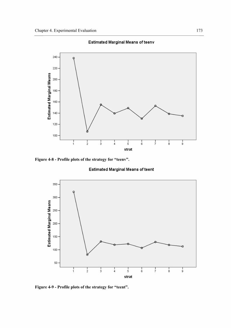
Chapter 4. Experimental Evaluation 173
Figure 4-8 - Profile plots of the strategy for “teenv”.
Figure 4-9 - Profile plots of the strategy for “teent”.
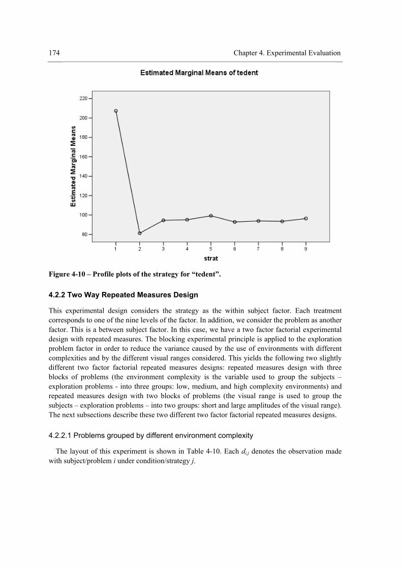
174 Chapter 4. Experimental Evaluation
Figure 4-10 – Profile plots of the strategy for “tedent”.
4.2.2 Two Way Repeated Measures Design
This experimental design considers the strategy as the within subject factor. Each treatment corresponds to one of the nine levels of the factor. In addition, we consider the problem as another factor. This is a between subject factor. In this case, we have a two factor factorial experimental design with repeated measures. The blocking experimental principle is applied to the exploration problem factor in order to reduce the variance caused by the use of environments with different complexities and by the different visual ranges considered. This yields the following two slightly different two factor factorial repeated measures designs: repeated measures design with three blocks of problems (the environment complexity is the variable used to group the subjects – exploration problems - into three groups: low, medium, and high complexity environments) and repeated measures design with two blocks of problems (the visual range is used to group the subjects – exploration problems – into two groups: short and large amplitudes of the visual range). The next subsections describe these two different two factor factorial repeated measures designs.
4.2.2.1 Problems grouped by different environment complexity
The layout of this experiment is shown in Table 4-10. Each di,j denotes the observation made with subject/problem i under condition/strategy j.
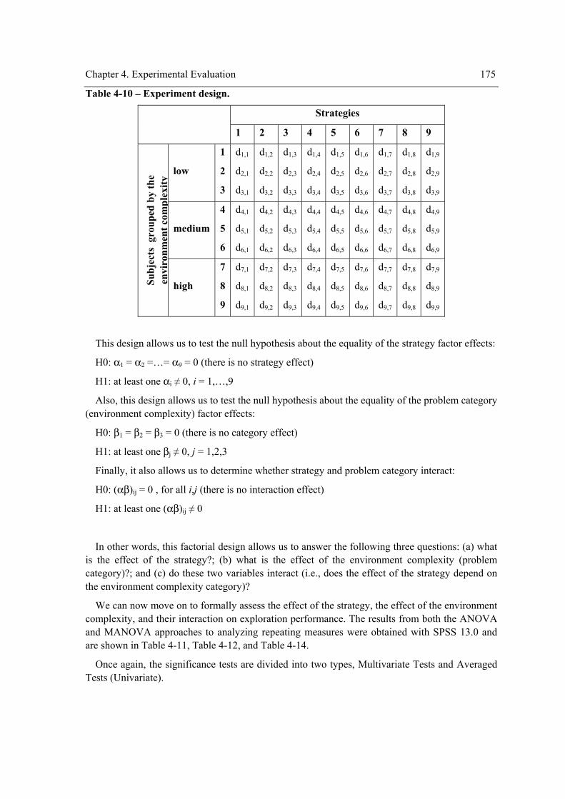
Chapter 4. Experimental Evaluation 175
Table 4-10 – Experiment design.
Strategies
1 2 3 4 5 6 7 8 9
low
1
2
3
d1,1
d2,1
d3,1
d1,2
d2,2
d3,2
d1,3
d2,3
d3,3
d1,4
d2,4
d3,4
d1,5
d2,5
d3,5
d1,6
d2,6
d3,6
d1,7
d2,7
d3,7
d1,8
d2,8
d3,8
d1,9
d2,9
d3,9
medium
4
5
6
d4,1
d5,1
d6,1
d4,2
d5,2
d6,2
d4,3
d5,3
d6,3
d4,4
d5,4
d6,4
d4,5
d5,5
d6,5
d4,6
d5,6
d6,6
d4,7
d5,7
d6,7
d4,8
d5,8
d6,8
d4,9
d5,9
d6,9
Subj
ects
gro
uped
by
the
envi
ronm
ent c
ompl
exity
high
7
8
9
d7,1
d8,1
d9,1
d7,2
d8,2
d9,2
d7,3
d8,3
d9,3
d7,4
d8,4
d9,4
d7,5
d8,5
d9,5
d7,6
d8,6
d9,6
d7,7
d8,7
d9,7
d7,8
d8,8
d9,8
d7,9
d8,9
d9,9
This design allows us to test the null hypothesis about the equality of the strategy factor effects:
H0: α1 = α2 =…= α9 = 0 (there is no strategy effect)
H1: at least one αi ≠ 0, i = 1,…,9
Also, this design allows us to test the null hypothesis about the equality of the problem category (environment complexity) factor effects:
H0: β1 = β2 = β3 = 0 (there is no category effect)
H1: at least one βj ≠ 0, j = 1,2,3
Finally, it also allows us to determine whether strategy and problem category interact:
H0: (αβ)ij = 0 , for all i,j (there is no interaction effect)
H1: at least one (αβ)ij ≠ 0
In other words, this factorial design allows us to answer the following three questions: (a) what is the effect of the strategy?; (b) what is the effect of the environment complexity (problem category)?; and (c) do these two variables interact (i.e., does the effect of the strategy depend on the environment complexity category)?
We can now move on to formally assess the effect of the strategy, the effect of the environment complexity, and their interaction on exploration performance. The results from both the ANOVA and MANOVA approaches to analyzing repeating measures were obtained with SPSS 13.0 and are shown in Table 4-11, Table 4-12, and Table 4-14.
Once again, the significance tests are divided into two types, Multivariate Tests and Averaged Tests (Univariate).

176 Chapter 4. Experimental Evaluation
The one-way ANOVA table for testing our single between-subject factor “environment complexity” (“envComp”) is shown in Table 4-11. We do not find a significant main effect of the environment complexity factor both on the time/energy to explore the environment completely (encoded as “teenv”) (F(2, 15) = 0.197, p = 0.823), and on the time/energy to explore all the entities (“teent”) (F(2, 15) = 2.207, p = 0.144). Specifically, the environment complexity group accounts for 2.6% of the variance in the time/energy to explore the environment completely and for 22.7% of the variance in the time/energy to explore all the entities; averaged over the nine strategies, exploration times for the complete environment and all the entities do not differ between the three environment complexity groups. However, we find a significant main effect of the environment complexity factor on the time/energy to explore all different entities (encoded as “tedent”) (F(2, 15) = 157.875, p < 0.001). Specifically, the environment complexity group accounts for 95.5% of the variance in the time/energy to explore all different entities.
Table 4-11 - ANOVA table for testing the main effect of the between-subject factor environment complexity (variable “envComp”) on exploration performance (variables “teenv”, “teent”, and “tedent”).
Tests of Between-Subjects Effects Transformed Variable: Average
Source Measure Type III Sum of Squares df Mean
Square F Sig. Partial Eta Squared
Noncent. Parameter
Observed Power(a)
teenv 3607668.081 1 3607668.081 1004.601 0.000 0.985 1004.601 1.000
teent 2688996.451 1 2688996.451 6564.152 0.000 0.998 6564.152 1.000Intercept
tedent 1729663.603 1 1729663.603 3115.725 0.000 0.995 3115.725 1.000
teenv 1414.218 2 707.109 0.197 0.823 0.026 0.394 0.075
teent 1808.504 2 904.252 2.207 0.144 0.227 4.415 0.380envComp
tedent 175285.467 2 87642.734 157.875 0.000 0.955 315.750 1.000
teenv 53867.189 15 3591.146
teent 6144.731 15 409.649 Error
tedent 8327.101 15 555.140 a Computed using alpha = 0.05
The within-subjects parts are included in the “Tests of Within-Subjects Effects” table under the rows labelled “Sphericity Assumed” (Table 4-12). Variability in the exploration times can be due to a main effect of the strategy (variable “strat”) or an interaction between the strategy and the between-subject factor group. As a result, F-tests are constructed that compare variability due to these sources against within-subjects error variability in this model. We find a main effect of the strategy on the three exploration performance measures: F(8, 120) = 41.403, p < 0.001 for the time/energy to explore the environment completely, F(8, 120) = 36.376, p < 0.001 for the time/energy to explore all the entities, and F(8, 120) = 25.050, p < 0.001 for the time/energy to explore all different entities. Specifically, the strategy accounts for 73.4% of the variance in the time/energy to explore the environment completely, 70.8% of the variance in the time/energy to explore all the entities, and for 62.5% of the variance in the time/energy to explore all different entities. We find evidence for the two-way interaction involving “envComp” and “strat” on the time/energy to explore all different entities (F(16, 120) = 1.738, p = 0.048), but no evidence for the two-way interaction involving “envComp” and “strat” on the other two exploration performance measures (F(16, 120) = 0.276, p = 0.997 for the time/energy to explore the environment completely, and F(16, 120) = 0.160, p = 1.00 for the time/energy to explore all the
Chapter 4. Experimental Evaluation 177
entities). Specifically, “envComp” and “strat” accounts for 18.8% of the variance in the time/energy to explore all different entities.
We test whether evidence of violation of the sphericity assumption is present using the Mauchly Sphericity Test. As shown in Table 4-13, this test is statistically significant (X2(35) = 174.578, p < 0.001 for the time/energy to explore the environment completely – “teenv” -, X2(35) = 242.371, p < 0.001 for the time/energy to explore all the entities – “teent” -, and X2(35) = 202.068, p < 0.001 for the time/energy to explore all different entities – “tedent”), which suggests that the sphericity assumption had been violated. As in the previous experimental design, we have two ways to deal with this violation: the use of the Multivariate Tests and the use of a correction in the degrees of freedom. Table 4-12 presents the three estimates of the correction factors (Greenhouse-Geisser, Huynh-Feld, and the Lower Bounds). Giving that the ordinary univariate F test leads to statistical significance of the strategy on the three exploration performance measures, we should now turn to one of these more conservative tests. We turn to the Lower Bound test. The within subject effect that tested significant under the assumption of sphericity remain significant with this test (see Table 4-12 under the rows “Lower-bound”, for the three exploration performance measures): F(1.00, 15.00) = 41.403, p < 0.001 for the time/energy to explore the environment completely, F(1.00, 15.00) = 36.376, p < 0.001 for the time/energy to explore all the entities, and F(1.00, 15.00) = 25.050, p < 0.001 for the time/energy to explore all different entities. Giving this statistical significance, we need not to use the other two conservative tests. Anyway, the within subject effect that tested significant under the assumption of sphericity and with the Lower Bound test remain highly significant even after these corrections. For instance, for the time/energy to explore the environment completely: using Huynh-Feldt correction factor, F(1.665, 24.974) = 41.403, p < 0.001; using Greenhouse-Geisser correction factor, F(1.372, 20.575) = 41.403, p < 0.001.
Giving that the ordinary univariate F test leads to statistical significance of the interaction effect “strat” × “envComp” on “tedent”, we should now turn to one of the more conservative tests. We turn to the Lower Bound test. The interaction effect involving the within subject effect that tested significant under the assumption of sphericity does not remain significant with the Lower Bound test (see Table 4-12 under the rows “Lower-bound”, for the measure time/energy to explore all different entities of the environment, under the row “strat * envComp”): F(2.00, 15.00) = 1.738, p = 0.21. The two tests contradict each other, that is, the uncorrected (positively biased) test yields statistical significance and the conservative (negatively biased) test does not. Therefore, the more specific epsilon correction in the degrees of freedom is made, substituting either the Greenhouse-Geisser or Huynh-Feldt epsilon estimate in place of the Lower Bound epsilon. The use of one of these estimates, besides being likely to yield higher degrees of freedom than the Lower Bound, should yield degrees of freedom for the unbiased F distribution, the distribution that is more likely to represent the true degrees of freedom created by the extent of the violation of the assumption. The new degrees of freedom obtained with one of the estimates should then be used to select a new critical F value, with which a final statistical decision is made. The interaction effect “strat” and “envComp” that tested significant under the assumption of sphericity and no significant under the Lower Bound test remain no significant after these corrections: using Huynh-Feldt correction factor, F(3.634, 27.258) = 1.738, p = 0.175; using Greenhouse-Geisser correction factor, F(2.953, 22.146) = 1.738, p < 0.189. Therefore we conclude that there is no effect of “strat” × “envComp” on “tedent”.

178 Chapter 4. Experimental Evaluation
Table 4-12 - Univariate ANOVA tables for testing the main effects of and interactions involving the within-subject factor (strategy) on exploration performance.
Univariate Tests
Source Measure Type III Sum of Squares
df Mean Square F Sig. Partial Eta
Squared Noncent.
Parameter Observed Power(a)
Sphericity Assumed 204960.674 8 25620.084 41.403 0.000 0.734 331.224 1.000
Greenhouse-Geisser 204960.674 1.372 149422.828 41.403 0.000 0.734 56.792 1.000
Huynh-Feldt 204960.674 1.665 123104.192 41.403 0.000 0.734 68.933 1.000
teenv
Lower-bound 204960.674 1.000 204960.674 41.403 0.000 0.734 41.403 1.000
Sphericity Assumed 292815.084 8 36601.885 36.376 0.000 0.708 291.006 1.000
Greenhouse-Geisser 292815.084 1.199 244168.048 36.376 0.000 0.708 43.623 1.000
Huynh-Feldt 292815.084 1.419 206321.923 36.376 0.000 0.708 51.625 1.000
teent
Lower-bound 292815.084 1.000 292815.084 36.376 0.000 0.708 36.376 1.000
Sphericity Assumed 208948.522 8 26118.565 25.050 0.000 0.625 200.398 1.000
Greenhouse-Geisser 208948.522 1.476 141526.940 25.050 0.000 0.625 36.983 1.000
Huynh-Feldt 208948.522 1.817 114984.459 25.050 0.000 0.625 45.520 1.000
strat
tedent
Lower-bound 208948.522 1.000 208948.522 25.050 0.000 0.625 25.050 0.997
Sphericity Assumed 2734.845 16 170.928 0.276 0.997 0.036 4.420 0.173
Greenhouse-Geisser 2734.845 2.743 996.894 0.276 0.825 0.036 0.758 0.093
Huynh-Feldt 2734.845 3.330 821.306 0.276 0.861 0.036 0.920 0.097
teenv
Lower-bound 2734.845 2.000 1367.423 0.276 0.762 0.036 0.552 0.086
Sphericity Assumed 2569.744 16 160.609 0.160 1.000 0.021 2.554 0.113
Greenhouse-Geisser 2569.744 2.398 1071.409 0.160 0.887 0.021 0.383 0.072
Huynh-Feldt 2569.744 2.838 905.340 0.160 0.914 0.021 0.453 0.074
teent
Lower-bound 2569.744 2.000 1284.872 0.160 0.854 .021 0.319 0.070
Sphericity Assumed 28988.137 16 1811.759 1.738 0.048 0.188 27.802 0.913
Greenhouse-Geisser 28988.137 2.953 9817.256 1.738 0.189 0.188 5.131 0.387
Huynh-Feldt 28988.137 3.634 7976.092 1.738 0.175 0.188 6.315 0.440
strat * envComp
tedent
Lower-bound 28988.137 2.000 14494.068 1.738 0.210 0.188 3.475 0.307a Computed using alpha = 0.05
(continues in the next page)

Chapter 4. Experimental Evaluation 179
Table 4-12 (cont.) - Univariate ANOVA tables for testing the main effects of and interactions involving the within-subject factor (strategy) on exploration performance.
Univariate Tests
Source Measure Type III Sum of Squares
df Mean Square F Sig. Partial Eta
Squared Noncent.
Parameter Observed Power(a)
Sphericity Assumed 74255.799 120 618.798
Greenhouse-Geisser 74255.799 20.575 3608.989
Huynh-Feldt 74255.799 24.974 2973.318
teenv
Lower-bound 74255.799 15.000 4950.387
Sphericity Assumed 120746.016 120 1006.217
Greenhouse-Geisser 120746.016 17.989 6712.386
Huynh-Feldt 120746.016 21.288 5671.964
teent
Lower-bound 120746.016 15.000 8049.734
Sphericity Assumed 125120.181 120 1042.668
Greenhouse-Geisser 125120.181 22.146 5649.837
Huynh-Feldt 125120.181 27.258 4590.246
Error(strat)
tedent
Lower-bound 125120.181 15.000 8341.345 a Computed using alpha = 0.05
Table 4-13 - Mauchly’s test for testing the sphericity assumption and correction factors.
Mauchly's Test of Sphericity(b)
Epsilon(a) Within Subjects Effect Measure Mauchly's
W Approx. Chi-
Square df Sig. Greenhouse-Geisser
Huynh-Feldt
Lower-bound
teenv 0.000 174.578 35 0.000 0.171 0.208 0.125
teent 0.000 242.371 35 0.000 0.150 0.177 0.125strat
tedent 0.000 202.068 35 0.000 0.185 0.227 0.125Tests the null hypothesis that the error covariance matrix of the orthonormalized transformed dependent variables is proportional to an identity matrix. a May be used to adjust the degrees of freedom for the averaged tests of significance. Corrected tests are displayed in the Tests of Within-Subjects Effects table. b Design: Intercept+envComp
Within Subjects Design: strat The Multivariate Tests are shown in Table 4-14. As noted earlier, these give four commonly
used significance tests labelled Pillai’s Trace, Wilks’ Trace, Hotelling’s Trace, and Roy’s Largest Root. The results for testing the main effect of “strat” and the interaction “strat” × “envComp” are identical to those obtained from the univariate ANOVA model: the four tests of significance for the strategy effect given by the Multivariate Tests, Pillai’s Trace (value = 1.151, F(24.00, 360.00) = 9.331, p < 0.001), Wilks’ Lambda (value = 0.162, F(24.00, 342.837) = 12.453, p < 0.001), Hotelling’s Trace (value = 3.397, F(24.00,350.00) = 16.511, p < 0.001), and Roy’s Largest Root (value = 2.856, F(8.00, 120.00) = 42.847, p < 0.001), indicate that the strategy has a significant effect. The large Partial Eta Squared values for the strategy show that it explains quite a lot of
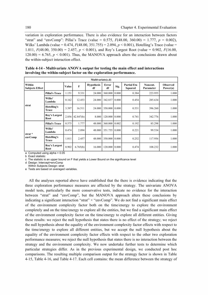
180 Chapter 4. Experimental Evaluation
variation in exploration performance. There is also evidence for an interaction between factors “strat” and “envComp”: Pillai’s Trace (value = 0.575, F(48.00, 360.00) = 1.777, p = 0.002), Wilks’ Lambda (value = 0.474, F(48.00, 351.755) = 2.094, p < 0.001), Hotelling’s Trace (value = 1.011, F(48.00, 350.00) = 2.457, p < 0.001), and Roy’s Largest Root (value = 0.902, F(16.00, 120.00) = 6.765, p < 0.001). Thus, the MANOVA approach alters the conclusions drawn about the within-subject interaction effect.
Table 4-14 - Multivariate ANOVA output for testing the main effect and interactions involving the within-subject factor on the exploration performance.
Multivariate(c.d)
Within Subjects Effect Value F Hypothesis
df Error
df Sig. Partial Eta Squared
Noncent. Parameter
Observed Power(a)
Pillai's Trace 1.151 9.331 24.000 360.000 0.000 0.384 223.955 1.000
Wilks' Lambda 0.162 12.453 24.000 342.837 0.000 0.454 285.634 1.000
Hotelling's Trace 3.397 16.511 24.000 350.000 0.000 0.531 396.260 1.000
strat
Roy's Largest Root 2.856 42.847(b) 8.000 120.000 0.000 0.741 342.776 1.000
Pillai's Trace 0.575 1.777 48.000 360.000 0.002 0.192 85.298 1.000
Wilks' Lambda 0.474 2.094 48.000 351.755 0.000 0.221 99.534 1.000
Hotelling's Trace 1.011 2.457 48.000 350.000 0.000 0.252 117.956 1.000
strat * envComp
Roy's Largest Root 0.902 6.765(b) 16.000 120.000 0.000 0.474 108.232 1.000
a Computed using alpha = 0.05 b Exact statistic c The statistic is an upper bound on F that yields a Lower Bound on the significance level d Design: Intercept+envComp Within Subjects Design: strat e Tests are based on averaged variables.
All the analyses reported above have established that the there is evidence indicating that the three exploration performance measures are affected by the strategy. The univariate ANOVA model tests, particularly the more conservative tests, indicate no evidence for the interaction between “strat” and “envComp”, but the MANOVA approach alters these conclusions by indicating a significant interaction “strat” × “envComp”. We do not find a significant main effect of the environment complexity factor both on the time/energy to explore the environment completely and on the time/energy to explore all the entities, but we find a significant main effect of the environment complexity factor on the time/energy to explore all different entities. Giving these results: we reject the null hypothesis that states there is no effect of the strategy; we reject the null hypothesis about the equality of the environment complexity factor effects with respect to the time/energy to explore all different entities, but we accept the null hypothesis about the equality of the environment complexity factor effects with respect to the other two exploration performance measures; we reject the null hypothesis that states there is no interaction between the strategy and the environment complexity. We now undertake further tests to determine which particular strategies differ. As in the previous experimental design, we conducted post hoc comparisons. The resulting multiple comparison output for the strategy factor is shown in Table 4-15, Table 4-16, and Table 4-17. Each cell contains: the mean difference between the strategy of

Chapter 4. Experimental Evaluation 181
the row and the strategy of the column; and, the respective p-value (enclosed in parentheses). The mean difference is significant at the 0.05 level. Additional information, such as the standard error of that estimator and a confidence interval for the mean difference, is provided by the original table presented in Appendix B.
The profile plots (Figure 4-11, Figure 4-12, Figure 4-13, Figure 4-14, Figure 4-15, Figure 4-16, Figure 4-17, Figure 4-18, Figure 4-19, Figure 4-20, Figure 4-21, and Figure 4-22) show the model-estimated means for the nine strategies. Together with the multiple comparison output, the plots provide us similar results to those reached with the one-way repeated measures experimental design with respect to the strategy. The profile plots also indicate that there is no clear significant interaction “strat” × “envComp” (it seems to happen only for a group of strategies), as well as that there is a significant effect of “envComp” only on the time/energy to explore all different entities (this is also confirmed by the pairwise comparisons of “envComp” presented in Table 4-18).
Table 4-15 – Pairwise comparisons of the strategy for “teenv”. 1 2 3 4 5 6 7 8 9
1 135.687
(0.000)
89.863
(0.000)
104.117
(0.000)
92.614
(0.000)
112.496
(0.000)
92.653
(0.000)
105.081
(0.000)
109.066
(0.000)
2 -135.687
(0.000)
-45.824
(0.000)
-31.571
(0.000)
-43.073
(0.000)
-23.191
(0.000)
-43.034
(0.000)
-30.607
(0.000)
-26.622
(0.000)
3 -89.863
(0.000)
45.824
(0.000)
14.254
(0.001)
2.751
(0.479)
22.633
(0.000)
2.791
(0.333)
15.218
(0.001)
4.949
(0.236)
4 -104.117
(0.000)
31.571
(0.000)
-14.254
(0.001)
-11.503
(0.028)
8.379
(0.012)
-11.463
(0.002)
.964
(0.368)
4.949
(0.236)
5 -92.614
(0.000)
43.073
(0.000)
-2.751
(0.479)
11.503
(0.028)
19.882
(0.001)
.039
(0.993)
12.467
(0.024)
16.452
(0.001)
6 -112.496
(0.000)
23.191
(0.000)
-22.633
(0.000)
-8.379
(0.012)
-19.882
(0.001)
-19.843
(0.000)
-7.416
(0.038)
-3.431
(0.297)
7 -92.653
(0.000)
43.034
(0.000)
-2.791
(0.333)
11.463
(0.002)
-0.039
(0.993)
19.843
(0.000)
12.427
(0.002)
16.412
(0.001)
8 -105.081
(0.000)
30.607
(0.000)
-15.218
(0.001)
-0.964
(0.368)
-12.467
(0.024)
7.416
(0.038)
-12.427
(0.002)
3.985
(0.390)
9 -109.066
(0.000)
26.622
(0.000)
-19.203
(0.000)
-4.949
(0.236)
-16.452
(0.001)
3.431
(0.297)
-16.412
(0.001)
-3.985
(0.390)
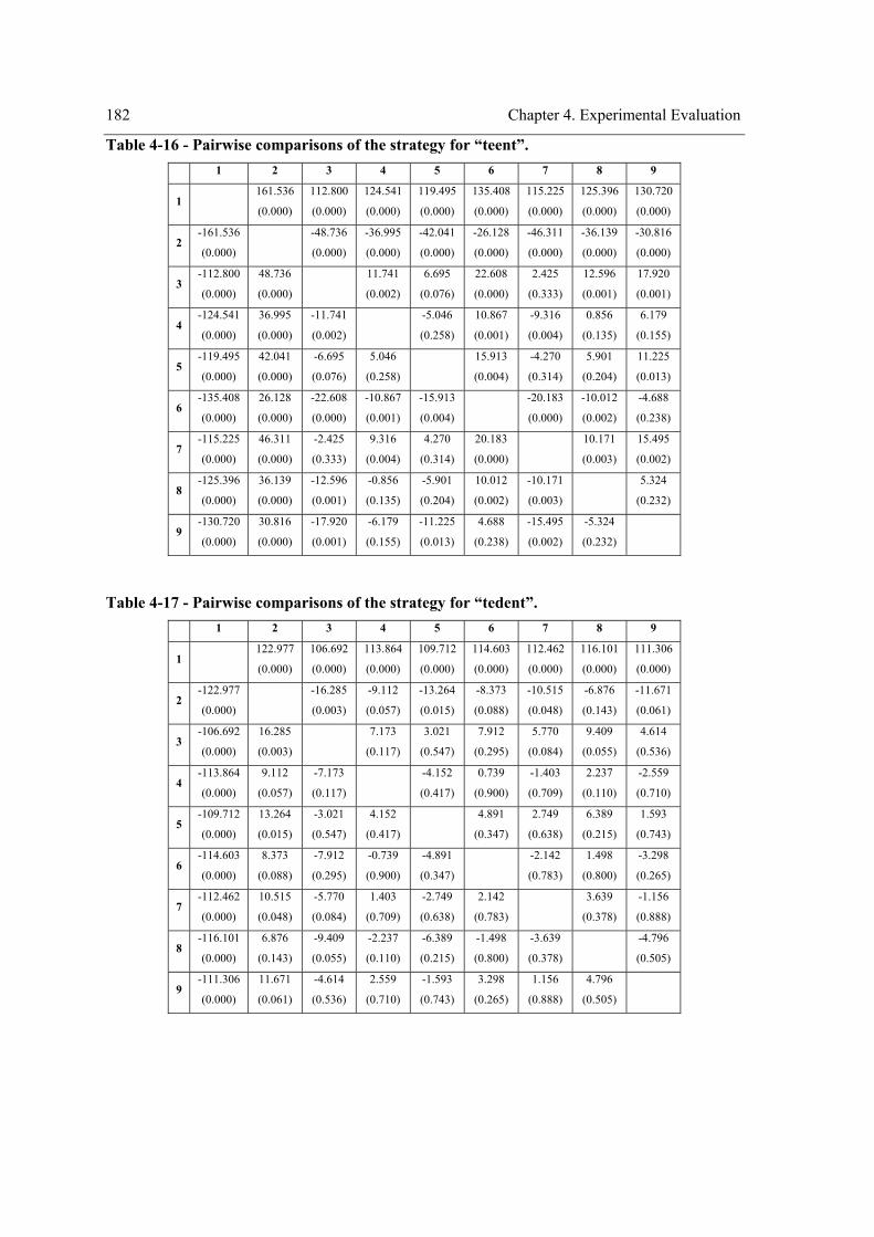
182 Chapter 4. Experimental Evaluation
Table 4-16 - Pairwise comparisons of the strategy for “teent”. 1 2 3 4 5 6 7 8 9
1 161.536
(0.000)
112.800
(0.000)
124.541
(0.000)
119.495
(0.000)
135.408
(0.000)
115.225
(0.000)
125.396
(0.000)
130.720
(0.000)
2 -161.536
(0.000)
-48.736
(0.000)
-36.995
(0.000)
-42.041
(0.000)
-26.128
(0.000)
-46.311
(0.000)
-36.139
(0.000)
-30.816
(0.000)
3 -112.800
(0.000)
48.736
(0.000)
11.741
(0.002)
6.695
(0.076)
22.608
(0.000)
2.425
(0.333)
12.596
(0.001)
17.920
(0.001)
4 -124.541
(0.000)
36.995
(0.000)
-11.741
(0.002)
-5.046
(0.258)
10.867
(0.001)
-9.316
(0.004)
0.856
(0.135)
6.179
(0.155)
5 -119.495
(0.000)
42.041
(0.000)
-6.695
(0.076)
5.046
(0.258)
15.913
(0.004)
-4.270
(0.314)
5.901
(0.204)
11.225
(0.013)
6 -135.408
(0.000)
26.128
(0.000)
-22.608
(0.000)
-10.867
(0.001)
-15.913
(0.004)
-20.183
(0.000)
-10.012
(0.002)
-4.688
(0.238)
7 -115.225
(0.000)
46.311
(0.000)
-2.425
(0.333)
9.316
(0.004)
4.270
(0.314)
20.183
(0.000)
10.171
(0.003)
15.495
(0.002)
8 -125.396
(0.000)
36.139
(0.000)
-12.596
(0.001)
-0.856
(0.135)
-5.901
(0.204)
10.012
(0.002)
-10.171
(0.003)
5.324
(0.232)
9 -130.720
(0.000)
30.816
(0.000)
-17.920
(0.001)
-6.179
(0.155)
-11.225
(0.013)
4.688
(0.238)
-15.495
(0.002)
-5.324
(0.232)
Table 4-17 - Pairwise comparisons of the strategy for “tedent”. 1 2 3 4 5 6 7 8 9
1 122.977
(0.000)
106.692
(0.000)
113.864
(0.000)
109.712
(0.000)
114.603
(0.000)
112.462
(0.000)
116.101
(0.000)
111.306
(0.000)
2 -122.977
(0.000)
-16.285
(0.003)
-9.112
(0.057)
-13.264
(0.015)
-8.373
(0.088)
-10.515
(0.048)
-6.876
(0.143)
-11.671
(0.061)
3 -106.692
(0.000)
16.285
(0.003)
7.173
(0.117)
3.021
(0.547)
7.912
(0.295)
5.770
(0.084)
9.409
(0.055)
4.614
(0.536)
4 -113.864
(0.000)
9.112
(0.057)
-7.173
(0.117)
-4.152
(0.417)
0.739
(0.900)
-1.403
(0.709)
2.237
(0.110)
-2.559
(0.710)
5 -109.712
(0.000)
13.264
(0.015)
-3.021
(0.547)
4.152
(0.417)
4.891
(0.347)
2.749
(0.638)
6.389
(0.215)
1.593
(0.743)
6 -114.603
(0.000)
8.373
(0.088)
-7.912
(0.295)
-0.739
(0.900)
-4.891
(0.347)
-2.142
(0.783)
1.498
(0.800)
-3.298
(0.265)
7 -112.462
(0.000)
10.515
(0.048)
-5.770
(0.084)
1.403
(0.709)
-2.749
(0.638)
2.142
(0.783)
3.639
(0.378)
-1.156
(0.888)
8 -116.101
(0.000)
6.876
(0.143)
-9.409
(0.055)
-2.237
(0.110)
-6.389
(0.215)
-1.498
(0.800)
-3.639
(0.378)
-4.796
(0.505)
9 -111.306
(0.000)
11.671
(0.061)
-4.614
(0.536)
2.559
(0.710)
-1.593
(0.743)
3.298
(0.265)
1.156
(0.888)
4.796
(0.505)

Chapter 4. Experimental Evaluation 183
Table 4-18 – Pairwise comparisons of the environment complexity.
Pairwise Comparisons
95% Confidence Interval for Difference(a) Measure (I) Environment
Complexity (J) Environment Complexity
Mean Difference (I-J)
Std. Error Sig.(a)
Lower Bound Upper Bound
Medium -1.556 11.533 0.894 -26.138 23.025Low
High -6.899 11.533 0.559 -31.481 17.682
Low 1.556 11.533 0.894 -23.025 26.138Medium
High -5.343 11.533 0.650 -29.924 19.239
Low 6.899 11.533 0.559 -17.682 31.481
teenv
High Medium 5.343 11.533 0.650 -19.239 29.924
Medium -2.017 3.895 0.612 -10.319 6.285Low
High -7.878 3.895 0.061 -16.180 0.425
Low 2.017 3.895 0.612 -6.285 10.319Medium
High -5.861 3.895 0.153 -14.163 2.442
Low 7.878 3.895 0.061 -0.425 16.180
teent
High Medium 5.861 3.895 0.153 -2.442 14.163
Medium -61.452(*) 4.534 0.000 -71.117 -51.788Low
High -75.856(*) 4.534 0.000 -85.521 -66.192
Low 61.452(*) 4.534 0.000 51.788 71.117Medium
High -14.404(*) 4.534 0.006 -24.069 -4.739
Low 75.856(*) 4.534 0.000 66.192 85.521
tedent
High Medium 14.404(*) 4.534 0.006 4.739 24.069
Based on estimated marginal means * The mean difference is significant at the 0.05 level. a Adjustment for multiple comparisons: Least Significant Difference (equivalent to no adjustments).
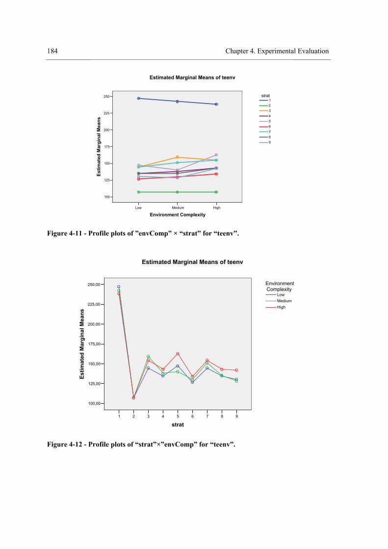
184 Chapter 4. Experimental Evaluation
HighMediumLow
Environment Complexity
250
225
200
175
150
125
100
Estim
ated
Mar
gina
l Mea
ns
987654321
strat
Estimated Marginal Means of teenv
Figure 4-11 - Profile plots of ”envComp” × “strat” for “teenv”.
987654321
strat
250,00
225,00
200,00
175,00
150,00
125,00
100,00
Estim
ated
Mar
gina
l Mea
ns
HighMediumLow
EnvironmentComplexity
Estimated Marginal Means of teenv
Figure 4-12 - Profile plots of “strat”×”envComp” for “teenv”.
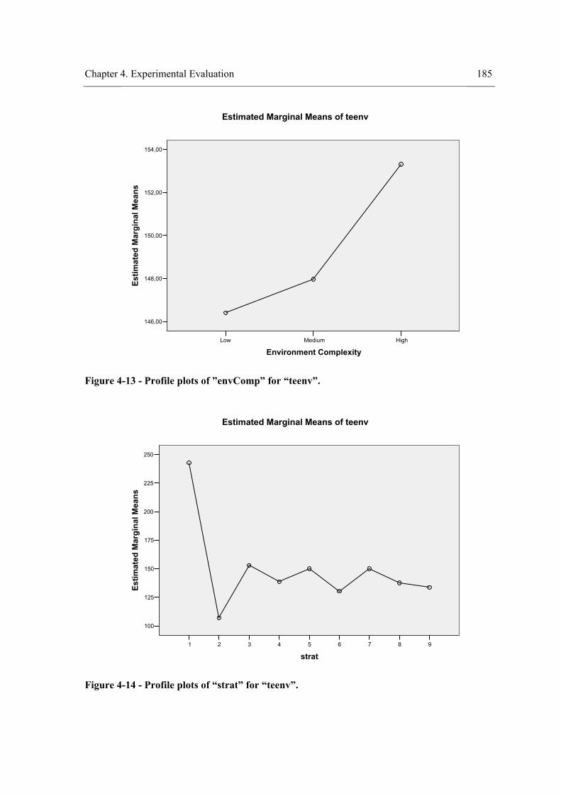
Chapter 4. Experimental Evaluation 185
HighMediumLow
Environment Complexity
154,00
152,00
150,00
148,00
146,00
Estim
ated
Mar
gina
l Mea
ns
Estimated Marginal Means of teenv
Figure 4-13 - Profile plots of ”envComp” for “teenv”.
987654321
strat
250
225
200
175
150
125
100
Estim
ated
Mar
gina
l Mea
ns
Estimated Marginal Means of teenv
Figure 4-14 - Profile plots of “strat” for “teenv”.
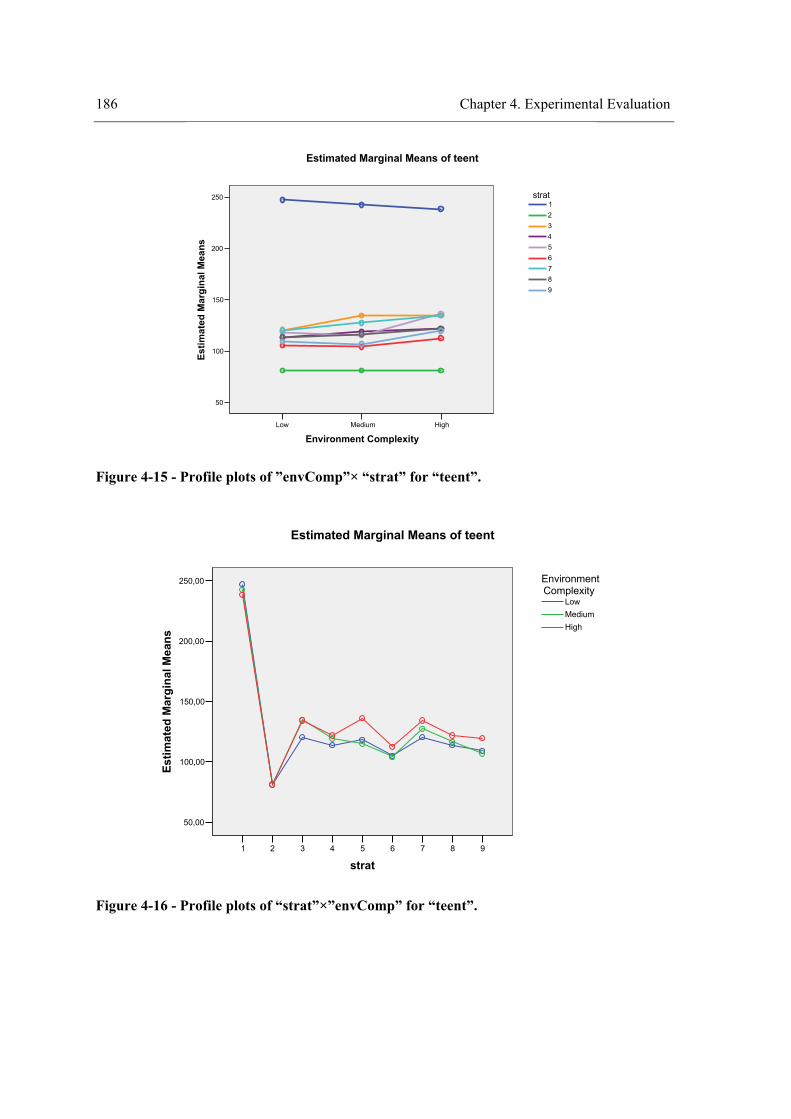
186 Chapter 4. Experimental Evaluation
HighMediumLow
Environment Complexity
250
200
150
100
50
Estim
ated
Mar
gina
l Mea
ns
987654321
strat
Estimated Marginal Means of teent
Figure 4-15 - Profile plots of ”envComp”× “strat” for “teent”.
987654321
strat
250,00
200,00
150,00
100,00
50,00
Estim
ated
Mar
gina
l Mea
ns
HighMediumLow
EnvironmentComplexity
Estimated Marginal Means of teent
Figure 4-16 - Profile plots of “strat”×”envComp” for “teent”.
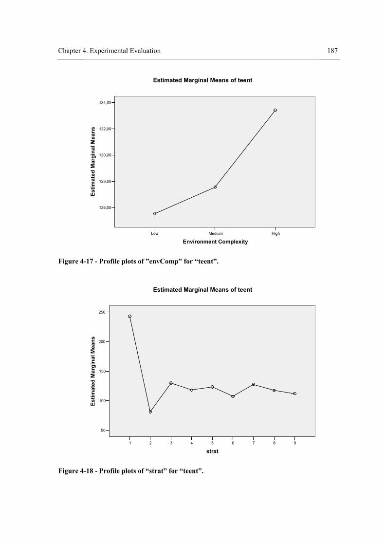
Chapter 4. Experimental Evaluation 187
HighMediumLow
Environment Complexity
134,00
132,00
130,00
128,00
126,00
Estim
ated
Mar
gina
l Mea
ns
Estimated Marginal Means of teent
Figure 4-17 - Profile plots of ”envComp” for “teent”.
987654321
strat
250
200
150
100
50
Estim
ated
Mar
gina
l Mea
ns
Estimated Marginal Means of teent
Figure 4-18 - Profile plots of “strat” for “teent”.
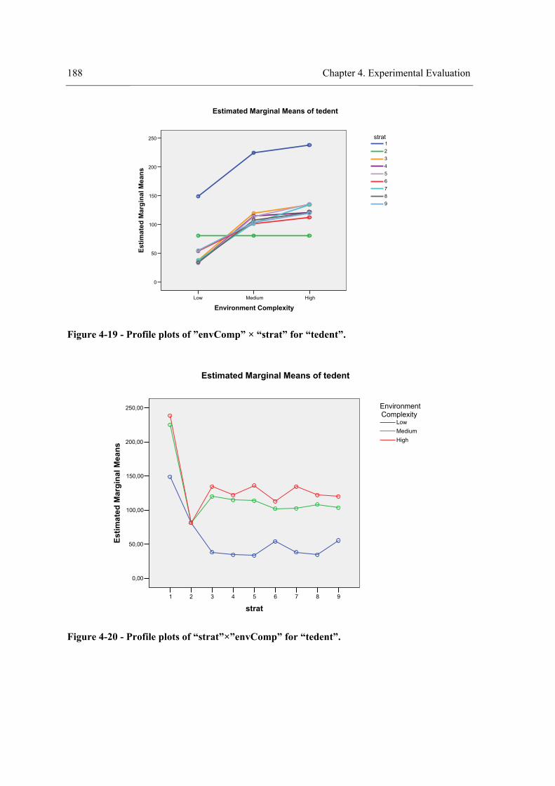
188 Chapter 4. Experimental Evaluation
HighMediumLow
Environment Complexity
250
200
150
100
50
0
Estim
ated
Mar
gina
l Mea
ns
987654321
strat
Estimated Marginal Means of tedent
Figure 4-19 - Profile plots of ”envComp” × “strat” for “tedent”.
987654321
strat
250,00
200,00
150,00
100,00
50,00
0,00
Estim
ated
Mar
gina
l Mea
ns
HighMediumLow
EnvironmentComplexity
Estimated Marginal Means of tedent
Figure 4-20 - Profile plots of “strat”×”envComp” for “tedent”.
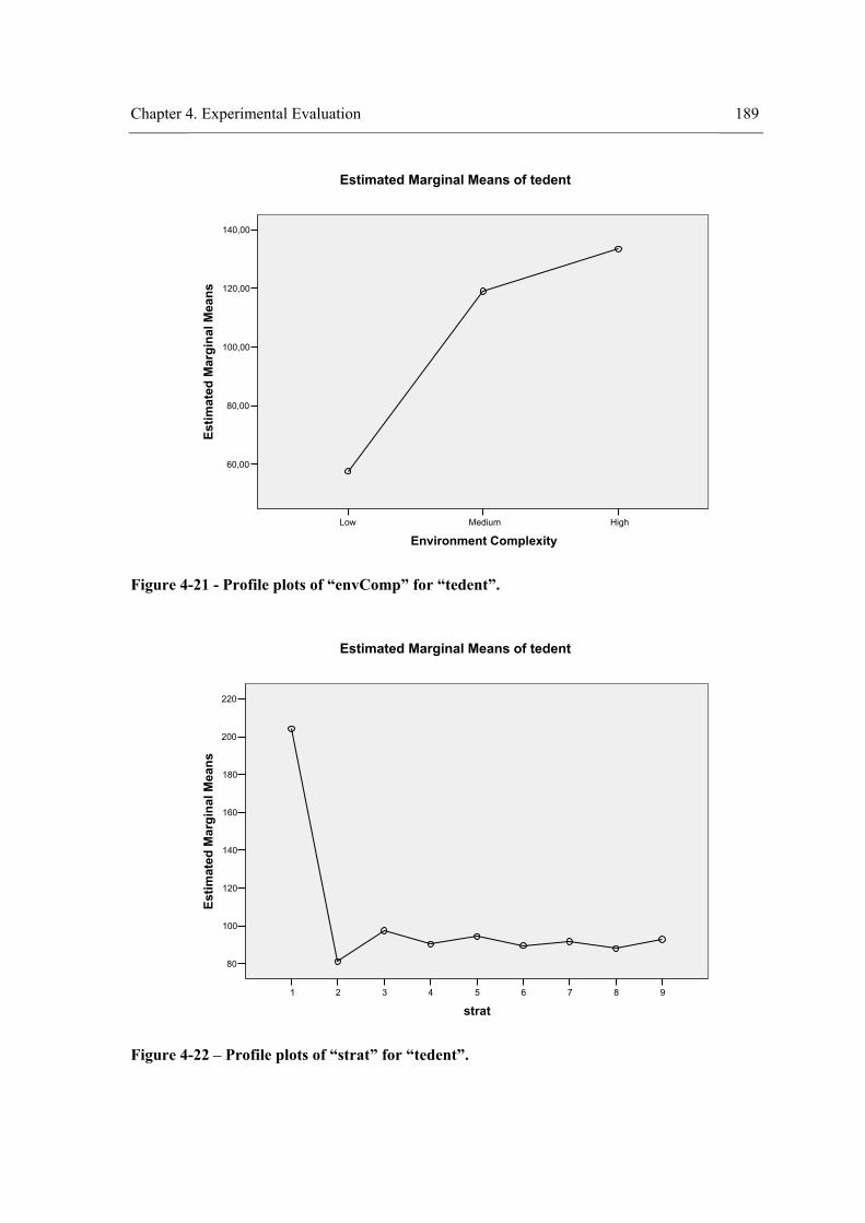
Chapter 4. Experimental Evaluation 189
HighMediumLow
Environment Complexity
140,00
120,00
100,00
80,00
60,00
Estim
ated
Mar
gina
l Mea
ns
Estimated Marginal Means of tedent
Figure 4-21 - Profile plots of “envComp” for “tedent”.
987654321
strat
220
200
180
160
140
120
100
80
Estim
ated
Mar
gina
l Mea
ns
Estimated Marginal Means of tedent
Figure 4-22 – Profile plots of “strat” for “tedent”.
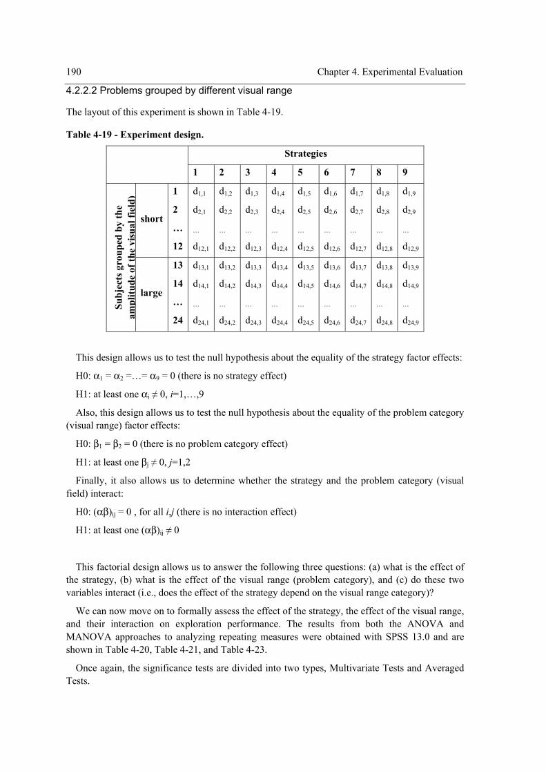
190 Chapter 4. Experimental Evaluation
4.2.2.2 Problems grouped by different visual range
The layout of this experiment is shown in Table 4-19.
Table 4-19 - Experiment design.
Strategies
1 2 3 4 5 6 7 8 9
short
1
2
…
12
d1,1
d2,1
…
d12,1
d1,2
d2,2
…
d12,2
d1,3
d2,3
…
d12,3
d1,4
d2,4
…
d12,4
d1,5
d2,5
…
d12,5
d1,6
d2,6
…
d12,6
d1,7
d2,7
…
d12,7
d1,8
d2,8
…
d12,8
d1,9
d2,9
…
d12,9
Subj
ects
gro
uped
by
the
ampl
itude
of t
he v
isua
l fie
ld)
large
13
14
…
24
d13,1
d14,1
…
d24,1
d13,2
d14,2
…
d24,2
d13,3
d14,3
…
d24,3
d13,4
d14,4
…
d24,4
d13,5
d14,5
…
d24,5
d13,6
d14,6
…
d24,6
d13,7
d14,7
…
d24,7
d13,8
d14,8
…
d24,8
d13,9
d14,9
…
d24,9
This design allows us to test the null hypothesis about the equality of the strategy factor effects:
H0: α1 = α2 =…= α9 = 0 (there is no strategy effect)
H1: at least one αi ≠ 0, i=1,…,9
Also, this design allows us to test the null hypothesis about the equality of the problem category (visual range) factor effects:
H0: β1 = β2 = 0 (there is no problem category effect)
H1: at least one βj ≠ 0, j=1,2
Finally, it also allows us to determine whether the strategy and the problem category (visual field) interact:
H0: (αβ)ij = 0 , for all i,j (there is no interaction effect)
H1: at least one (αβ)ij ≠ 0
This factorial design allows us to answer the following three questions: (a) what is the effect of the strategy, (b) what is the effect of the visual range (problem category), and (c) do these two variables interact (i.e., does the effect of the strategy depend on the visual range category)?
We can now move on to formally assess the effect of the strategy, the effect of the visual range, and their interaction on exploration performance. The results from both the ANOVA and MANOVA approaches to analyzing repeating measures were obtained with SPSS 13.0 and are shown in Table 4-20, Table 4-21, and Table 4-23.
Once again, the significance tests are divided into two types, Multivariate Tests and Averaged Tests.

Chapter 4. Experimental Evaluation 191
The one-way ANOVA table for testing our single between-subject factor “amplitude of the visual field” (variable “visField”), is shown in Table 4-20. We find a significant main effect of “visField” factor on the time/energy to explore the environment completely (“teenv”) (F(1, 22) = 119.534, p < 0.001), but no effect both on the time/energy to explore all the entities (“teent”) (F(1, 22) = 0.577, p = 0.445) and on the time/energy to explore all different entities (“tedent”) (F(1, 22) = 0.080, p = 0.781). Specifically, the visual field accounts for 84.5% of the variance in the time/energy to explore the environment completely, for 2.6% of the variance in the time/energy to explore all the entities, and for 0.4% of the variance in the time/energy to explore all different entities; averaged over the nine strategies, time/energy to explore all the entities and all different entities does not differ between the two visual ranges.
Table 4-20 - ANOVA table for testing the main effect of the between-subject factor “amplitude of the visual field” (variable “visField”) on exploration performance (variables “teenv”, “teent”, and “tedent”).
Tests of Between-Subjects Effects Transformed Variable: Average
Source Measure Type III Sum of Squares df Mean
Square F Sig. Partial Eta Squared
Noncent. Parameter
Observed Power(a)
teenv 4829711.339 1 4829711.339 8081.078 0.000 0.997 8081.078 1.000
teent 4127188.402 1 4127188.402 232.800 0.000 0.914 232.800 1.000Intercept
tedent 2426823.362 1 2426823.362 273.672 0.000 0.926 273.672 1.000
teenv 71440.137 1 71440.137 119.534 0.000 0.845 119.534 1.000
teent 10235.517 1 10235.517 0.577 0.455 0.026 0.577 0.112visField
tedent 705.540 1 705.540 0.080 0.781 0.004 0.080 0.058
teenv 13148.449 22 597.657
teent 390025.786 22 17728.445 Error
tedent 195087.693 22 8867.622 a Computed using alpha = 0.05
The within-subjects parts are included in the “Tests of Within-Subjects Effects” table under the rows labelled “Sphericity Assumed” (Table 4-21). Variability in the exploration times can be due to a main effect of strategy (“strat”) or an interaction between “strat” and the between-subject factor visual range (“visField”). As a result, F-tests are constructed that compare variability due to these sources against within-subjects error variability in this model. We find a main effect of the strategy on the three exploration performance measures: the time/energy to explore the environment completely (F(8, 176) = 147.260, p < 0.001), the time/energy to explore all the entities (F(8, 176) = 6.414, p < 0.001), and the time/energy to explore all different entities (F(8, 176) = 78.408, p < 0.001). Specifically, the strategy accounts for 87% of the variance in the time/energy to explore the environment completely, for 22.6% of the variance in the time/energy to explore all the entities, and for 78.1% of the variance in the time/energy to explore all different entities. We also find evidence for the two-way interaction involving “visField” and “strat” also on the three exploration performance measures: the time/energy to explore the environment completely (F(8, 176) = 35.631, p < 0.001), the time/energy to explore all the entities (F(8, 176) = 3.579, p = 0.001), and the time/energy to explore all different entities (F(8, 176) = 31.438, p < 0.001). The interaction accounts for 61.8% of the variance in the time/energy to explore the environment completely, for 14.0% of the variance in the time/energy to explore all the entities, and for 58.8% of the variance in the time/energy to explore all different entities.

192 Chapter 4. Experimental Evaluation
Table 4-21 - Univariate ANOVA tables for testing the main effects of and interactions involving the within-subject factor (strategy) on the exploration performance.
Univariate Tests
Source Measure Type III Sum of Squares Df Mean
Square F Sig. Partial
Eta Squared
Noncent. Parameter
Observed Power(a)
Sphericity Assumed 252678.317 8 31584.790 147.260 0.000 0.870 1178.079 1.000
Greenhouse-Geisser 252678.317 3.361 75174.791 147.260 0.000 0.870 494.971 1.000
Huynh-Feldt 252678.317 4.221 59866.204 147.260 0.000 0.870 621.542 1.000
teenv
Lower-bound 252678.317 1.000 252678.317 147.260 0.000 0.870 147.260 1.000
Sphericity Assumed 950894.351 8 118861.794 6.414 0.000 0.226 51.311 1.000
Greenhouse-Geisser 950894.351 1.011 940558.219 6.414 0.019 0.226 6.484 0.681
Huynh-Feldt 950894.351 1.061 896449.901 6.414 0.017 0.226 6.803 0.696
teent
Lower-bound 950894.351 1.000 950894.351 6.414 0.019 0.226 6.414 0.678
Sphericity Assumed 282320.236 8 35290.029 78.408 0.000 0.781 627.264 1.000
Greenhouse-Geisser 282320.236 3.919 72032.823 78.408 0.000 0.781 307.307 1.000
Huynh-Feldt 282320.236 5.092 55445.638 78.408 0.000 0.781 399.241 1.000
strat
tedent
Lower-bound 282320.236 1.000 282320.236 78.408 0.000 0.781 78.408 1.000
Sphericity Assumed 61138.346 8 7642.293 35.631 0.000 0.618 285.049 1.000
Greenhouse-Geisser 61138.346 3.361 18189.382 35.631 0.000 0.618 119.764 1.000
Huynh-Feldt 61138.346 4.221 14485.298 35.631 0.000 0.618 150.389 1.000
teenv
Lower-bound 61138.346 1.000 61138.346 35.631 0.000 0.618 35.631 1.000
Sphericity Assumed 530599.793 8 66324.974 3.579 0.001 0.140 28.632 0.981
Greenhouse-Geisser 530599.793 1.011 524832.224 3.579 0.071 0.140 3.618 0.443
Huynh-Feldt 530599.793 1.061 500219.748 3.579 0.069 0.140 3.796 0.454
teent
Lower-bound 530599.793 1.000 530599.793 3.579 0.072 0.140 3.579 0.440
Sphericity Assumed 113198.059 8 14149.757 31.438 0.000 0.588 251.505 1.000
Greenhouse-Geisser 113198.059 3.919 28882.010 31.438 0.000 0.588 123.217 1.000
Huynh-Feldt 113198.059 5.092 22231.274 31.438 0.000 0.588 160.078 1.000
strat * visField
tedent
Lower-bound 113198.059 1.000 113198.059 31.438 0.000 0.588 31.438 1.000
(continues in the next page)
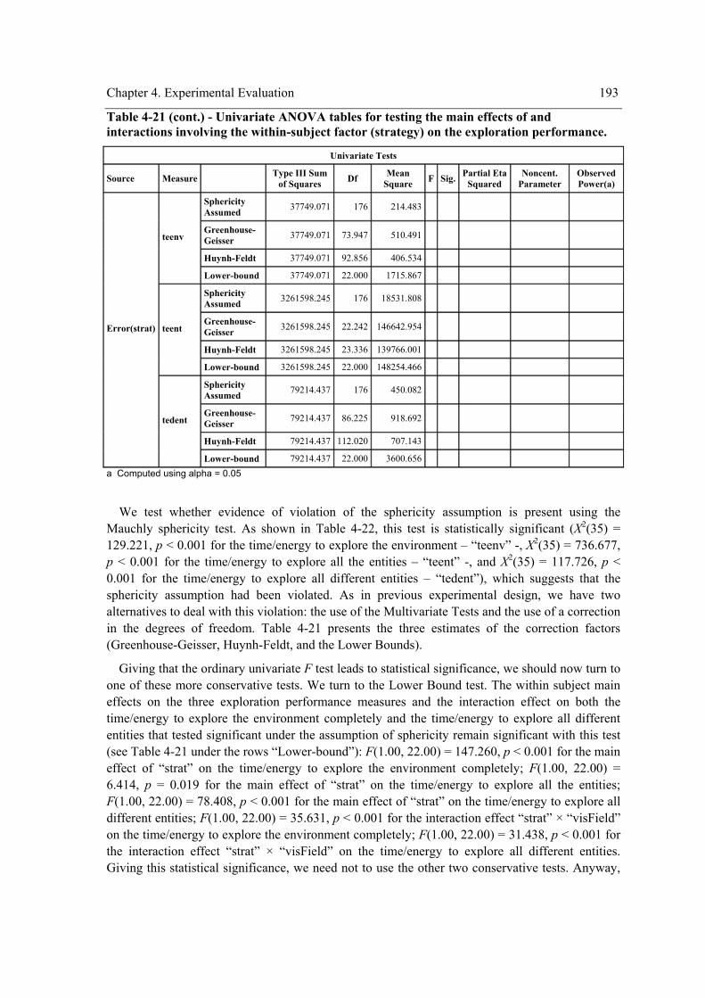
Chapter 4. Experimental Evaluation 193
Table 4-21 (cont.) - Univariate ANOVA tables for testing the main effects of and interactions involving the within-subject factor (strategy) on the exploration performance.
Univariate Tests
Source Measure Type III Sum of Squares Df Mean
Square F Sig. Partial Eta Squared
Noncent. Parameter
Observed Power(a)
Sphericity Assumed 37749.071 176 214.483
Greenhouse-Geisser 37749.071 73.947 510.491
Huynh-Feldt 37749.071 92.856 406.534
teenv
Lower-bound 37749.071 22.000 1715.867
Sphericity Assumed 3261598.245 176 18531.808
Greenhouse-Geisser 3261598.245 22.242 146642.954
Huynh-Feldt 3261598.245 23.336 139766.001
teent
Lower-bound 3261598.245 22.000 148254.466
Sphericity Assumed 79214.437 176 450.082
Greenhouse-Geisser 79214.437 86.225 918.692
Huynh-Feldt 79214.437 112.020 707.143
Error(strat)
tedent
Lower-bound 79214.437 22.000 3600.656 a Computed using alpha = 0.05
We test whether evidence of violation of the sphericity assumption is present using the Mauchly sphericity test. As shown in Table 4-22, this test is statistically significant (X2(35) = 129.221, p < 0.001 for the time/energy to explore the environment – “teenv” -, X2(35) = 736.677, p < 0.001 for the time/energy to explore all the entities – “teent” -, and X2(35) = 117.726, p < 0.001 for the time/energy to explore all different entities – “tedent”), which suggests that the sphericity assumption had been violated. As in previous experimental design, we have two alternatives to deal with this violation: the use of the Multivariate Tests and the use of a correction in the degrees of freedom. Table 4-21 presents the three estimates of the correction factors (Greenhouse-Geisser, Huynh-Feldt, and the Lower Bounds).
Giving that the ordinary univariate F test leads to statistical significance, we should now turn to one of these more conservative tests. We turn to the Lower Bound test. The within subject main effects on the three exploration performance measures and the interaction effect on both the time/energy to explore the environment completely and the time/energy to explore all different entities that tested significant under the assumption of sphericity remain significant with this test (see Table 4-21 under the rows “Lower-bound”): F(1.00, 22.00) = 147.260, p < 0.001 for the main effect of “strat” on the time/energy to explore the environment completely; F(1.00, 22.00) = 6.414, p = 0.019 for the main effect of “strat” on the time/energy to explore all the entities; F(1.00, 22.00) = 78.408, p < 0.001 for the main effect of “strat” on the time/energy to explore all different entities; F(1.00, 22.00) = 35.631, p < 0.001 for the interaction effect “strat” × “visField” on the time/energy to explore the environment completely; F(1.00, 22.00) = 31.438, p < 0.001 for the interaction effect “strat” × “visField” on the time/energy to explore all different entities. Giving this statistical significance, we need not to use the other two conservative tests. Anyway,
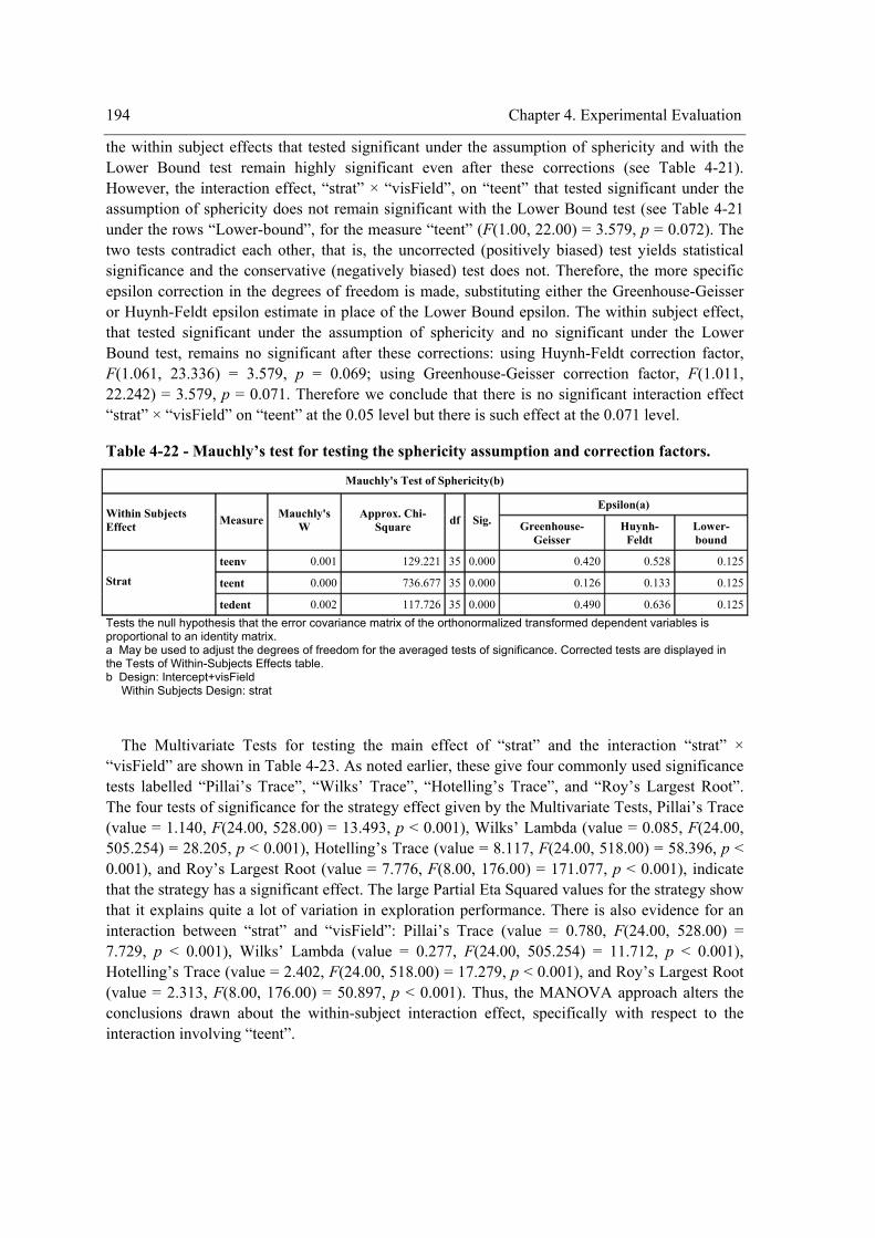
194 Chapter 4. Experimental Evaluation
the within subject effects that tested significant under the assumption of sphericity and with the Lower Bound test remain highly significant even after these corrections (see Table 4-21). However, the interaction effect, “strat” × “visField”, on “teent” that tested significant under the assumption of sphericity does not remain significant with the Lower Bound test (see Table 4-21 under the rows “Lower-bound”, for the measure “teent” (F(1.00, 22.00) = 3.579, p = 0.072). The two tests contradict each other, that is, the uncorrected (positively biased) test yields statistical significance and the conservative (negatively biased) test does not. Therefore, the more specific epsilon correction in the degrees of freedom is made, substituting either the Greenhouse-Geisser or Huynh-Feldt epsilon estimate in place of the Lower Bound epsilon. The within subject effect, that tested significant under the assumption of sphericity and no significant under the Lower Bound test, remains no significant after these corrections: using Huynh-Feldt correction factor, F(1.061, 23.336) = 3.579, p = 0.069; using Greenhouse-Geisser correction factor, F(1.011, 22.242) = 3.579, p = 0.071. Therefore we conclude that there is no significant interaction effect “strat” × “visField” on “teent” at the 0.05 level but there is such effect at the 0.071 level.
Table 4-22 - Mauchly’s test for testing the sphericity assumption and correction factors.
Mauchly's Test of Sphericity(b)
Epsilon(a) Within Subjects Effect Measure Mauchly's
W Approx. Chi-
Square df Sig. Greenhouse-Geisser
Huynh-Feldt
Lower-bound
teenv 0.001 129.221 35 0.000 0.420 0.528 0.125
teent 0.000 736.677 35 0.000 0.126 0.133 0.125Strat
tedent 0.002 117.726 35 0.000 0.490 0.636 0.125Tests the null hypothesis that the error covariance matrix of the orthonormalized transformed dependent variables is proportional to an identity matrix. a May be used to adjust the degrees of freedom for the averaged tests of significance. Corrected tests are displayed in the Tests of Within-Subjects Effects table. b Design: Intercept+visField
Within Subjects Design: strat
The Multivariate Tests for testing the main effect of “strat” and the interaction “strat” × “visField” are shown in Table 4-23. As noted earlier, these give four commonly used significance tests labelled “Pillai’s Trace”, “Wilks’ Trace”, “Hotelling’s Trace”, and “Roy’s Largest Root”. The four tests of significance for the strategy effect given by the Multivariate Tests, Pillai’s Trace (value = 1.140, F(24.00, 528.00) = 13.493, p < 0.001), Wilks’ Lambda (value = 0.085, F(24.00, 505.254) = 28.205, p < 0.001), Hotelling’s Trace (value = 8.117, F(24.00, 518.00) = 58.396, p < 0.001), and Roy’s Largest Root (value = 7.776, F(8.00, 176.00) = 171.077, p < 0.001), indicate that the strategy has a significant effect. The large Partial Eta Squared values for the strategy show that it explains quite a lot of variation in exploration performance. There is also evidence for an interaction between “strat” and “visField”: Pillai’s Trace (value = 0.780, F(24.00, 528.00) = 7.729, p < 0.001), Wilks’ Lambda (value = 0.277, F(24.00, 505.254) = 11.712, p < 0.001), Hotelling’s Trace (value = 2.402, F(24.00, 518.00) = 17.279, p < 0.001), and Roy’s Largest Root (value = 2.313, F(8.00, 176.00) = 50.897, p < 0.001). Thus, the MANOVA approach alters the conclusions drawn about the within-subject interaction effect, specifically with respect to the interaction involving “teent”.
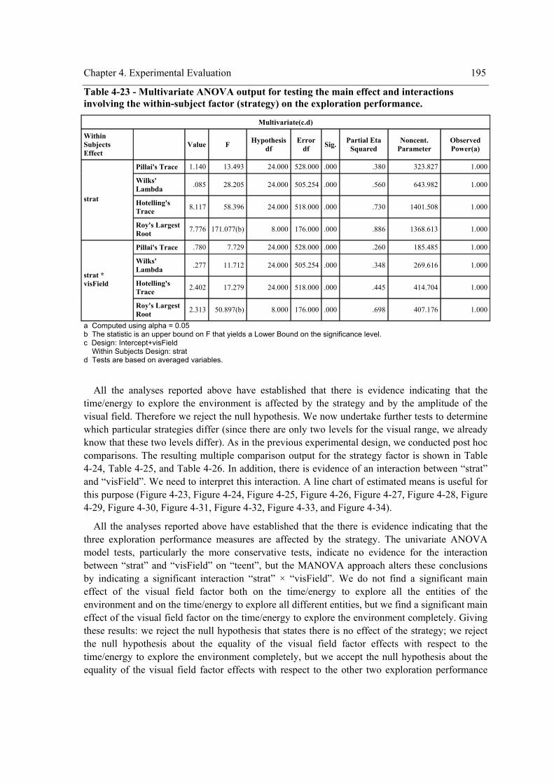
Chapter 4. Experimental Evaluation 195
Table 4-23 - Multivariate ANOVA output for testing the main effect and interactions involving the within-subject factor (strategy) on the exploration performance.
Multivariate(c.d)
Within Subjects Effect
Value F Hypothesis df
Error df Sig. Partial Eta
Squared Noncent.
Parameter Observed Power(a)
Pillai's Trace 1.140 13.493 24.000 528.000 .000 .380 323.827 1.000
Wilks' Lambda .085 28.205 24.000 505.254 .000 .560 643.982 1.000
Hotelling's Trace 8.117 58.396 24.000 518.000 .000 .730 1401.508 1.000
strat
Roy's Largest Root 7.776 171.077(b) 8.000 176.000 .000 .886 1368.613 1.000
Pillai's Trace .780 7.729 24.000 528.000 .000 .260 185.485 1.000
Wilks' Lambda .277 11.712 24.000 505.254 .000 .348 269.616 1.000
Hotelling's Trace 2.402 17.279 24.000 518.000 .000 .445 414.704 1.000
strat * visField
Roy's Largest Root 2.313 50.897(b) 8.000 176.000 .000 .698 407.176 1.000
a Computed using alpha = 0.05 b The statistic is an upper bound on F that yields a Lower Bound on the significance level. c Design: Intercept+visField Within Subjects Design: strat d Tests are based on averaged variables.
All the analyses reported above have established that there is evidence indicating that the time/energy to explore the environment is affected by the strategy and by the amplitude of the visual field. Therefore we reject the null hypothesis. We now undertake further tests to determine which particular strategies differ (since there are only two levels for the visual range, we already know that these two levels differ). As in the previous experimental design, we conducted post hoc comparisons. The resulting multiple comparison output for the strategy factor is shown in Table 4-24, Table 4-25, and Table 4-26. In addition, there is evidence of an interaction between “strat” and “visField”. We need to interpret this interaction. A line chart of estimated means is useful for this purpose (Figure 4-23, Figure 4-24, Figure 4-25, Figure 4-26, Figure 4-27, Figure 4-28, Figure 4-29, Figure 4-30, Figure 4-31, Figure 4-32, Figure 4-33, and Figure 4-34).
All the analyses reported above have established that the there is evidence indicating that the three exploration performance measures are affected by the strategy. The univariate ANOVA model tests, particularly the more conservative tests, indicate no evidence for the interaction between “strat” and “visField” on “teent”, but the MANOVA approach alters these conclusions by indicating a significant interaction “strat” × “visField”. We do not find a significant main effect of the visual field factor both on the time/energy to explore all the entities of the environment and on the time/energy to explore all different entities, but we find a significant main effect of the visual field factor on the time/energy to explore the environment completely. Giving these results: we reject the null hypothesis that states there is no effect of the strategy; we reject the null hypothesis about the equality of the visual field factor effects with respect to the time/energy to explore the environment completely, but we accept the null hypothesis about the equality of the visual field factor effects with respect to the other two exploration performance
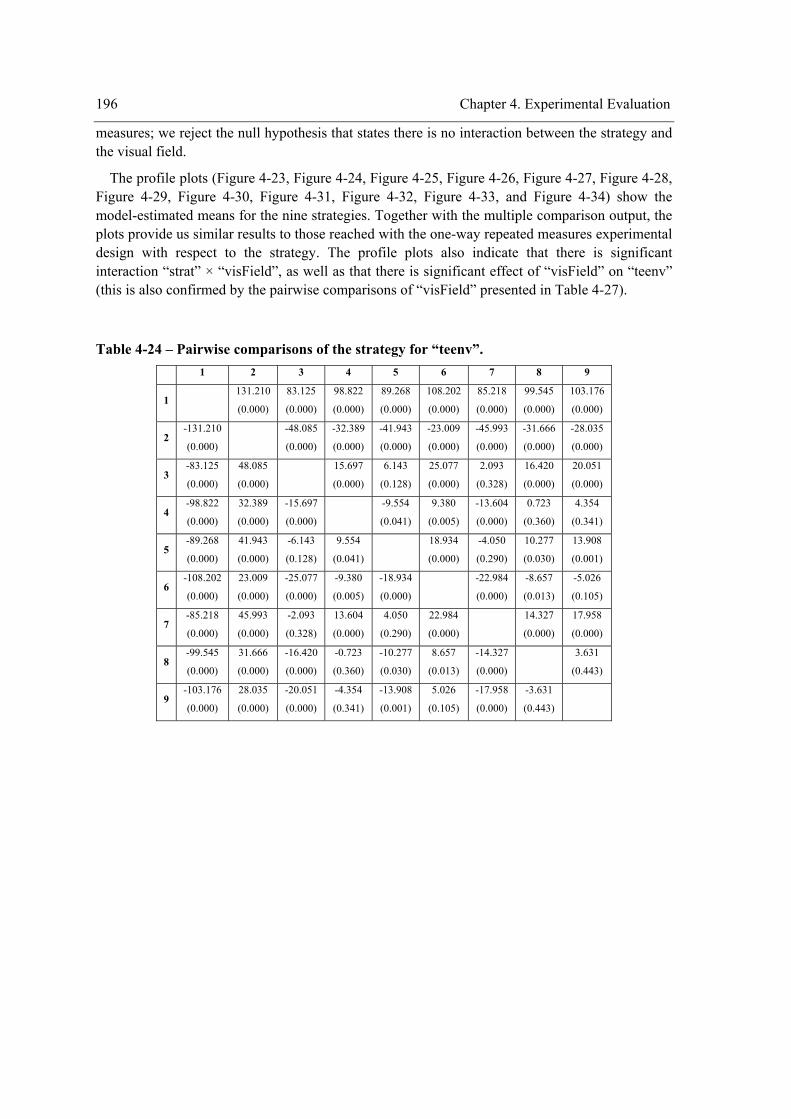
196 Chapter 4. Experimental Evaluation
measures; we reject the null hypothesis that states there is no interaction between the strategy and the visual field.
The profile plots (Figure 4-23, Figure 4-24, Figure 4-25, Figure 4-26, Figure 4-27, Figure 4-28, Figure 4-29, Figure 4-30, Figure 4-31, Figure 4-32, Figure 4-33, and Figure 4-34) show the model-estimated means for the nine strategies. Together with the multiple comparison output, the plots provide us similar results to those reached with the one-way repeated measures experimental design with respect to the strategy. The profile plots also indicate that there is significant interaction “strat” × “visField”, as well as that there is significant effect of “visField” on “teenv” (this is also confirmed by the pairwise comparisons of “visField” presented in Table 4-27).
Table 4-24 – Pairwise comparisons of the strategy for “teenv”. 1 2 3 4 5 6 7 8 9
1 131.210
(0.000)
83.125
(0.000)
98.822
(0.000)
89.268
(0.000)
108.202
(0.000)
85.218
(0.000)
99.545
(0.000)
103.176
(0.000)
2 -131.210
(0.000)
-48.085
(0.000)
-32.389
(0.000)
-41.943
(0.000)
-23.009
(0.000)
-45.993
(0.000)
-31.666
(0.000)
-28.035
(0.000)
3 -83.125
(0.000)
48.085
(0.000)
15.697
(0.000)
6.143
(0.128)
25.077
(0.000)
2.093
(0.328)
16.420
(0.000)
20.051
(0.000)
4 -98.822
(0.000)
32.389
(0.000)
-15.697
(0.000)
-9.554
(0.041)
9.380
(0.005)
-13.604
(0.000)
0.723
(0.360)
4.354
(0.341)
5 -89.268
(0.000)
41.943
(0.000)
-6.143
(0.128)
9.554
(0.041)
18.934
(0.000)
-4.050
(0.290)
10.277
(0.030)
13.908
(0.001)
6 -108.202
(0.000)
23.009
(0.000)
-25.077
(0.000)
-9.380
(0.005)
-18.934
(0.000)
-22.984
(0.000)
-8.657
(0.013)
-5.026
(0.105)
7 -85.218
(0.000)
45.993
(0.000)
-2.093
(0.328)
13.604
(0.000)
4.050
(0.290)
22.984
(0.000)
14.327
(0.000)
17.958
(0.000)
8 -99.545
(0.000)
31.666
(0.000)
-16.420
(0.000)
-0.723
(0.360)
-10.277
(0.030)
8.657
(0.013)
-14.327
(0.000)
3.631
(0.443)
9 -103.176
(0.000)
28.035
(0.000)
-20.051
(0.000)
-4.354
(0.341)
-13.908
(0.001)
5.026
(0.105)
-17.958
(0.000)
-3.631
(0.443)
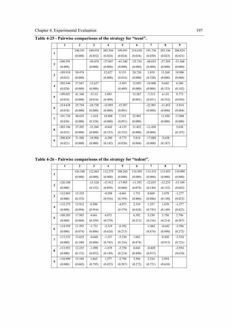
Chapter 4. Experimental Evaluation 197
Table 4-25 - Pairwise comparisons of the strategy for “teent”. 1 2 3 4 5 6 7 8 9
1 240.391
(0.008)
189.918
(0.032)
202.544
(0.024)
199.051
(0.024)
214.638
(0.018)
191.736
(0.030)
203.186
(0.023)
208.824
(0.021)
2 -240.391
(0.008)
-50.474
(0.000)
-37.847
(0.000)
-41.340
(0.000)
-25.754
(0.000)
-48.655
(0.000)
-37.205
(0.000)
-31.568
(0.000)
3 -189.918
(0.032)
50.474
(0.000)
12.627
(0.000)
9.133
(0.016)
24.720
(0.000)
1.819
(0.328)
13.268
(0.000)
18.906
(0.000)
4 -202.544
(0.024)
37.847
(0.000)
-12.627
(0.000)
-3.493
(0.409)
12.093
(0.000)
-10.808
(0.000)
0.642
(0.153)
6.280
(0.142)
5 -199.051
(0.024)
41.340
(0.000)
-9.133
(0.016)
3.493
(0.409)
15.587
(0.001)
-7.315
(0.051)
4.135
(0.332)
9.773
(0.020)
6 -214.638
(0.018)
25.754
(0.000)
-24.720
(0.000)
-12.093
(0.000)
-15.587
(0.001)
-22.901
(0.000)
-11.452
(0.000)
-5.814
(0.084)
7 -191.736
(0.030)
48.655
(0.000)
-1.819
(0.328)
10.808
(0.000)
7.315
(0.051)
22.901
(0.000)
11.450
(0.000)
17.088
(0.000)
8 -203.186
(0.023)
37.205
(0.000)
-13.268
(0.000)
-0.642
(0.153)
-4.135
(0.332)
11.452
(0.000)
-11.450
(0.000)
5.638
(0.187)
9 -208.824
(0.021)
31.568
(0.000)
-18.906
(0.000)
-6.280
(0.142)
-9.773
(0.020)
5.814
(0.084)
-17.088
(0.000)
-5.638
(0.187)
Table 4-26 - Pairwise comparisons of the strategy for “tedent”. 1 2 3 4 5 6 7 8 9
1 126.188
(0.000)
112.863
(0.000)
112.275
(0.000)
108.203
(0.000)
114.595
(0.000)
113.533
(0.000)
113.953
(0.000)
110.999
(0.000)
2 -126.188
(0.000)
-13.324
(0.152)
-13.912
(0.094)
-17.985
(0.060)
-11.593
(0.074)
-12.655
(0.140)
-12.235
(0.132)
-15.189
(0.042)
3 -112.863
(0.000)
13.324
(0.152)
-0.588
(0.916)
-4.661
(0.359)
1.731
(0.806)
0.669
(0.886)
1.678
(0.149)
-1.277
(0.823)
4 -112.275
(0.000)
13.912
(0.094)
0.588
(0.916)
-4.073
(0.379)
2.319
(0.624)
1.257
(0.743)
1.678
(0.149)
-1.277
(0.823)
5 -108.203
(0.000)
17.985
(0.060)
4.661
(0.359)
4.073
(0.379)
6.392
(0.213)
5.330
(0.316)
5.750
(0.214)
2.796
(0.587)
6 -114.595
(0.000)
11.593
(0.074)
-1.731
(0.806)
-2.319
(0.624)
-6.392
(0.213)
-1.062
(0.874)
-0.642
(0.890)
-3.596
(0.272)
7 -113.533
(0.000)
12.655
(0.140)
-0.669
(0.886)
-1.257
(0.743)
-5.330
(0.316)
1.062
(0.874)
0.420
(0.913)
-2.534
(0.721)
8 -113.953
(0.000)
12.235
(0.132)
-1.090
(0.852)
-1.678
(0.149)
-5.750
(0.214)
0.642
(0.890)
-0.420
(0.913)
-2.954
(0.610)
9 -110.999
(0.000)
15.189
(0.042)
1.865
(0.795)
1.277
(0.823)
-2.796
(0.587)
3.596
(0.272)
2.534
(0.721)
2.954
(0.610)
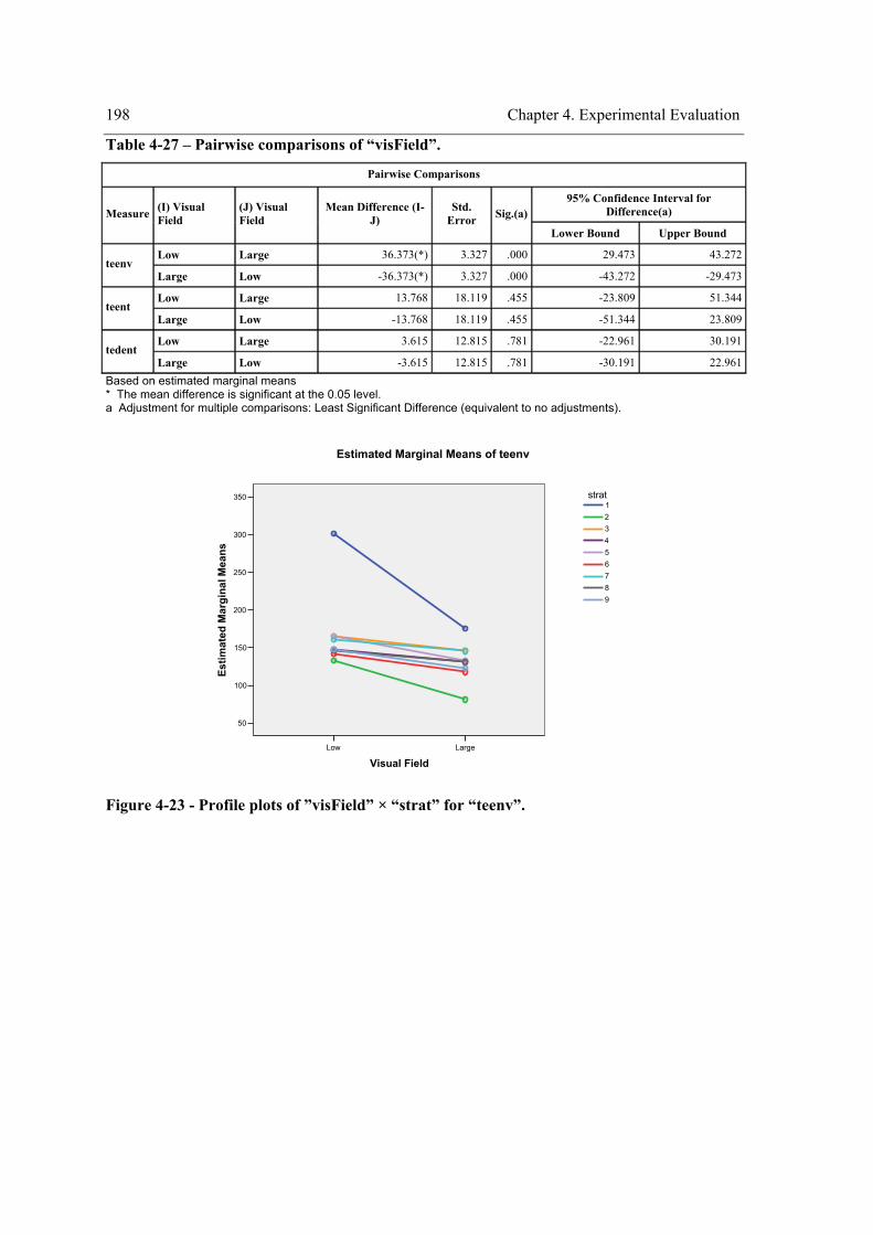
198 Chapter 4. Experimental Evaluation
Table 4-27 – Pairwise comparisons of “visField”.
Pairwise Comparisons
95% Confidence Interval for Difference(a) Measure (I) Visual
Field (J) Visual Field
Mean Difference (I-J)
Std. Error Sig.(a)
Lower Bound Upper Bound
Low Large 36.373(*) 3.327 .000 29.473 43.272teenv
Large Low -36.373(*) 3.327 .000 -43.272 -29.473
Low Large 13.768 18.119 .455 -23.809 51.344teent
Large Low -13.768 18.119 .455 -51.344 23.809
Low Large 3.615 12.815 .781 -22.961 30.191tedent
Large Low -3.615 12.815 .781 -30.191 22.961Based on estimated marginal means * The mean difference is significant at the 0.05 level. a Adjustment for multiple comparisons: Least Significant Difference (equivalent to no adjustments).
LargeLow
Visual Field
350
300
250
200
150
100
50
Estim
ated
Mar
gina
l Mea
ns
987654321
strat
Estimated Marginal Means of teenv
Figure 4-23 - Profile plots of ”visField” × “strat” for “teenv”.
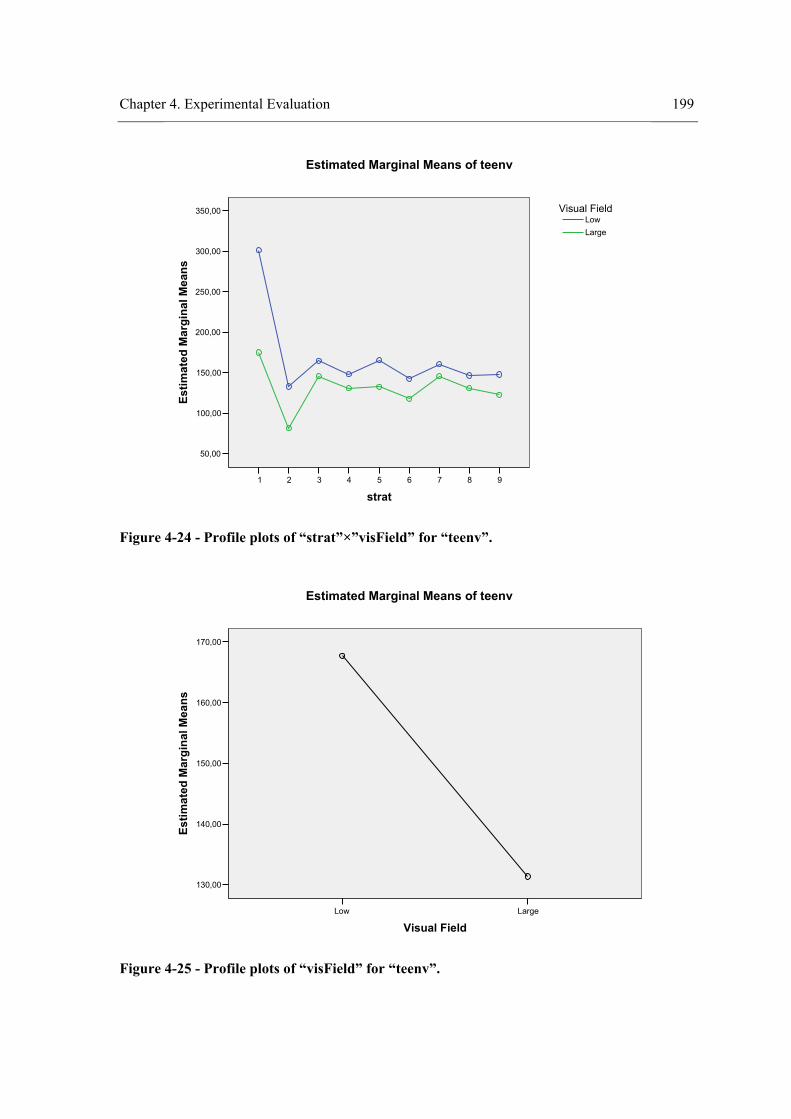
Chapter 4. Experimental Evaluation 199
987654321
strat
350,00
300,00
250,00
200,00
150,00
100,00
50,00
Estim
ated
Mar
gina
l Mea
ns
LargeLow
Visual Field
Estimated Marginal Means of teenv
Figure 4-24 - Profile plots of “strat”×”visField” for “teenv”.
LargeLow
Visual Field
170,00
160,00
150,00
140,00
130,00
Estim
ated
Mar
gina
l Mea
ns
Estimated Marginal Means of teenv
Figure 4-25 - Profile plots of “visField” for “teenv”.
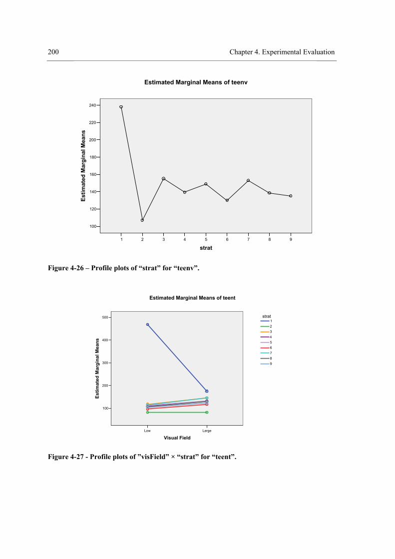
200 Chapter 4. Experimental Evaluation
987654321
strat
240
220
200
180
160
140
120
100
Estim
ated
Mar
gina
l Mea
nsEstimated Marginal Means of teenv
Figure 4-26 – Profile plots of “strat” for “teenv”.
LargeLow
Visual Field
500
400
300
200
100
Estim
ated
Mar
gina
l Mea
ns
987654321
strat
Estimated Marginal Means of teent
Figure 4-27 - Profile plots of ”visField” × “strat” for “teent”.
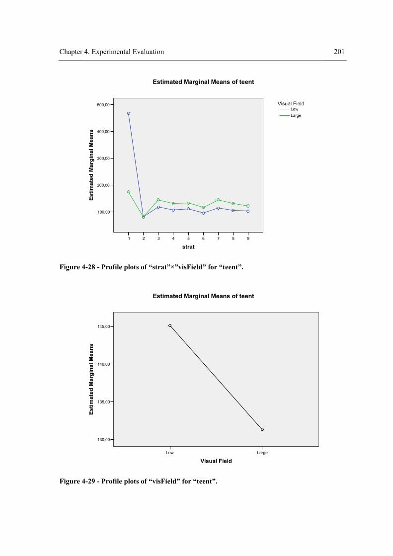
Chapter 4. Experimental Evaluation 201
987654321
strat
500,00
400,00
300,00
200,00
100,00
Estim
ated
Mar
gina
l Mea
ns
LargeLow
Visual Field
Estimated Marginal Means of teent
Figure 4-28 - Profile plots of “strat”×”visField” for “teent”.
LargeLow
Visual Field
145,00
140,00
135,00
130,00
Estim
ated
Mar
gina
l Mea
ns
Estimated Marginal Means of teent
Figure 4-29 - Profile plots of “visField” for “teent”.
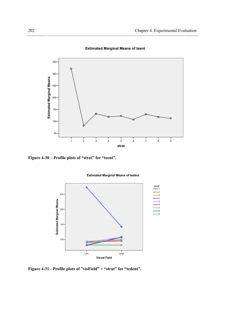
202 Chapter 4. Experimental Evaluation
987654321
strat
350
300
250
200
150
100
50
Estim
ated
Mar
gina
l Mea
nsEstimated Marginal Means of teent
Figure 4-30 – Profile plots of “strat” for “teent”.
LargeLow
Visual Field
250
200
150
100
Estim
ated
Mar
gina
l Mea
ns
987654321
strat
Estimated Marginal Means of tedent
Figure 4-31 - Profile plots of ”visField” × “strat” for “tedent”.
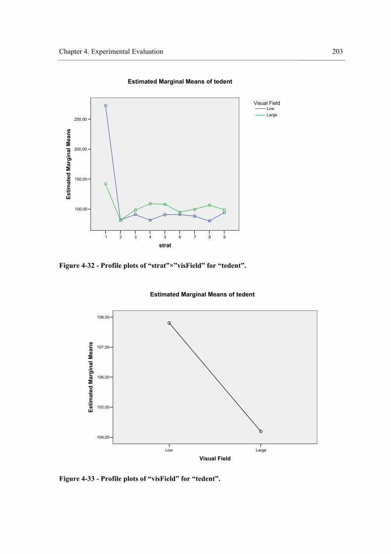
Chapter 4. Experimental Evaluation 203
987654321
strat
250,00
200,00
150,00
100,00
Estim
ated
Mar
gina
l Mea
ns
LargeLow
Visual Field
Estimated Marginal Means of tedent
Figure 4-32 - Profile plots of “strat”×”visField” for “tedent”.
LargeLow
Visual Field
108,00
107,00
106,00
105,00
104,00
Estim
ated
Mar
gina
l Mea
ns
Estimated Marginal Means of tedent
Figure 4-33 - Profile plots of “visField” for “tedent”.
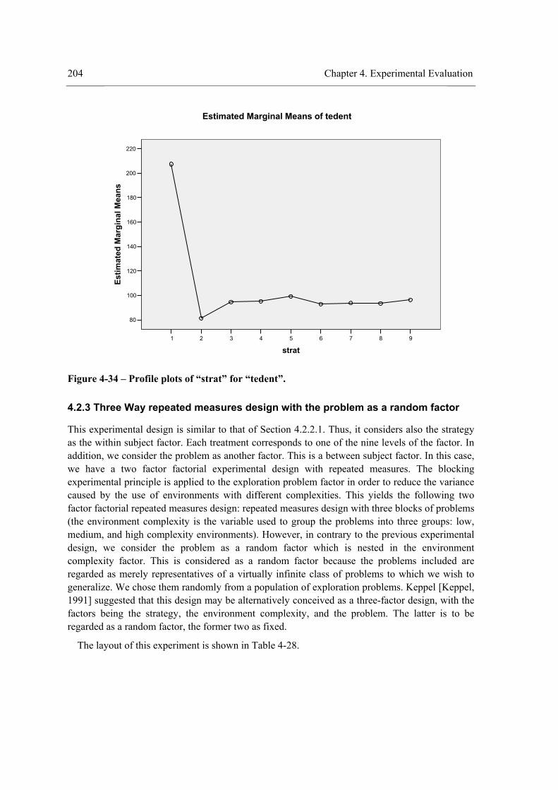
204 Chapter 4. Experimental Evaluation
987654321
strat
220
200
180
160
140
120
100
80
Estim
ated
Mar
gina
l Mea
nsEstimated Marginal Means of tedent
Figure 4-34 – Profile plots of “strat” for “tedent”.
4.2.3 Three Way repeated measures design with the problem as a random factor
This experimental design is similar to that of Section 4.2.2.1. Thus, it considers also the strategy as the within subject factor. Each treatment corresponds to one of the nine levels of the factor. In addition, we consider the problem as another factor. This is a between subject factor. In this case, we have a two factor factorial experimental design with repeated measures. The blocking experimental principle is applied to the exploration problem factor in order to reduce the variance caused by the use of environments with different complexities. This yields the following two factor factorial repeated measures design: repeated measures design with three blocks of problems (the environment complexity is the variable used to group the problems into three groups: low, medium, and high complexity environments). However, in contrary to the previous experimental design, we consider the problem as a random factor which is nested in the environment complexity factor. This is considered as a random factor because the problems included are regarded as merely representatives of a virtually infinite class of problems to which we wish to generalize. We chose them randomly from a population of exploration problems. Keppel [Keppel, 1991] suggested that this design may be alternatively conceived as a three-factor design, with the factors being the strategy, the environment complexity, and the problem. The latter is to be regarded as a random factor, the former two as fixed.
The layout of this experiment is shown in Table 4-28.
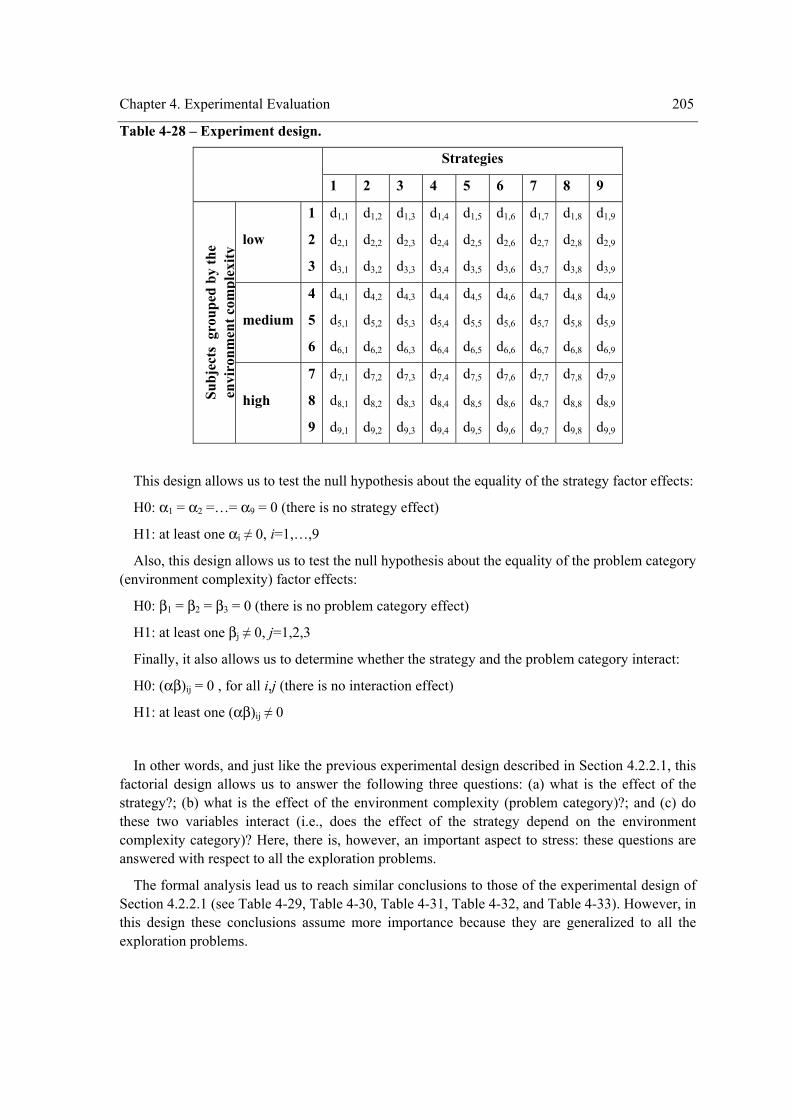
Chapter 4. Experimental Evaluation 205
Table 4-28 – Experiment design.
Strategies
1 2 3 4 5 6 7 8 9
low
1
2
3
d1,1
d2,1
d3,1
d1,2
d2,2
d3,2
d1,3
d2,3
d3,3
d1,4
d2,4
d3,4
d1,5
d2,5
d3,5
d1,6
d2,6
d3,6
d1,7
d2,7
d3,7
d1,8
d2,8
d3,8
d1,9
d2,9
d3,9
medium
4
5
6
d4,1
d5,1
d6,1
d4,2
d5,2
d6,2
d4,3
d5,3
d6,3
d4,4
d5,4
d6,4
d4,5
d5,5
d6,5
d4,6
d5,6
d6,6
d4,7
d5,7
d6,7
d4,8
d5,8
d6,8
d4,9
d5,9
d6,9
Subj
ects
gro
uped
by
the
envi
ronm
ent c
ompl
exity
high
7
8
9
d7,1
d8,1
d9,1
d7,2
d8,2
d9,2
d7,3
d8,3
d9,3
d7,4
d8,4
d9,4
d7,5
d8,5
d9,5
d7,6
d8,6
d9,6
d7,7
d8,7
d9,7
d7,8
d8,8
d9,8
d7,9
d8,9
d9,9
This design allows us to test the null hypothesis about the equality of the strategy factor effects:
H0: α1 = α2 =…= α9 = 0 (there is no strategy effect)
H1: at least one αi ≠ 0, i=1,…,9
Also, this design allows us to test the null hypothesis about the equality of the problem category (environment complexity) factor effects:
H0: β1 = β2 = β3 = 0 (there is no problem category effect)
H1: at least one βj ≠ 0, j=1,2,3
Finally, it also allows us to determine whether the strategy and the problem category interact:
H0: (αβ)ij = 0 , for all i,j (there is no interaction effect)
H1: at least one (αβ)ij ≠ 0
In other words, and just like the previous experimental design described in Section 4.2.2.1, this factorial design allows us to answer the following three questions: (a) what is the effect of the strategy?; (b) what is the effect of the environment complexity (problem category)?; and (c) do these two variables interact (i.e., does the effect of the strategy depend on the environment complexity category)? Here, there is, however, an important aspect to stress: these questions are answered with respect to all the exploration problems.
The formal analysis lead us to reach similar conclusions to those of the experimental design of Section 4.2.2.1 (see Table 4-29, Table 4-30, Table 4-31, Table 4-32, and Table 4-33). However, in this design these conclusions assume more importance because they are generalized to all the exploration problems.

206 Chapter 4. Experimental Evaluation
Table 4-29 - Tests of Between-Subjects Effects.
Tests of Between-Subjects Effects Dependent Variable: Time/Energy required to explore the environment completely
Source Type III Sum of Squares df Mean
Square F Sig. Partial Eta Squared
Noncent. Parameter
Observed Power(a)
Hypothesis 3607668.081 1 3607668.081 1004.601 0.000 0.985 1004.601 1.000Intercept
Error 53867.189 15 3591.146(b)
Hypothesis 204960.674 8 25620.084 41.403 0.000 0.734 331.224 1.000strat
Error 74255.799 120 618.798(c)
Hypothesis 1414.218 2 707.109 0.197 0.823 0.026 0.394 0.075envComp
Error 53867.189 15 3591.146(b)
Hypothesis 2734.845 16 170.928 0.276 0.997 0.036 4.420 0.173strat * envComp Error 74255.799 120 618.798(c)
Hypothesis 53867.189 15 3591.146 5.803 0.000 0.420 87.051 1.000envComp * problem Error 74255.799 120 618.798(c)
Tests of Between-Subjects Effects
Dependent Variable: Time/Energy required to explore all the entities of the environment
Source Type III Sum of Squares df Mean
Square F Sig. Partial Eta Squared
Noncent. Parameter
Observed Power(a)
Hypothesis 2688996.451 1 2688996.451 6564.152 0.000 0.998 6564.152 1.000Intercept
Error 6144.731 15 409.649(b)
Hypothesis 292815.084 8 36601.885 36.376 0.000 0.708 291.006 1.000strat
Error 120746.016 120 1006.217(c)
Hypothesis 1808.504 2 904.252 2.207 0.144 0.227 4.415 0.380envComp
Error 6144.731 15 409.649(b)
Hypothesis 2569.744 16 160.609 0.160 1.000 0.021 2.554 0.113strat * envComp Error 120746.016 120 1006.217(c)
Hypothesis 6144.731 15 409.649 0.407 0.975 0.048 6.107 0.245envComp * problem Error 120746.016 120 1006.217(c)
Tests of Between-Subjects Effects
Dependent Variable: Time/Energy required to explore all different entities of the environment
Source Type III Sum of Squares df Mean
Square F Sig. Partial Eta Squared
Noncent. Parameter
Observed Power(a)
Hypothesis 1729663.603 1 1729663.603 3115.725 0.000 0.995 3115.725 1.000Intercept
Error 8327.101 15 555.140(b)
Hypothesis 208948.522 8 26118.565 25.050 0.000 0.625 200.398 1.000strat
Error 125120.181 120 1042.668(c)
Hypothesis 175285.467 2 87642.734 157.875 0.000 0.955 315.750 1.000envComp
Error 8327.101 15 555.140(b)
Hypothesis 28988.137 16 1811.759 1.738 0.048 0.188 27.802 0.913strat * envComp Error 125120.181 120 1042.668(c)
Hypothesis 8327.101 15 555.140 0.532 0.918 0.062 7.986 0.325envComp * problem Error 125120.181 120 1042.668(c) a Computed using alpha = 0.05 b MS(envComp * Problem) c MS(Error)
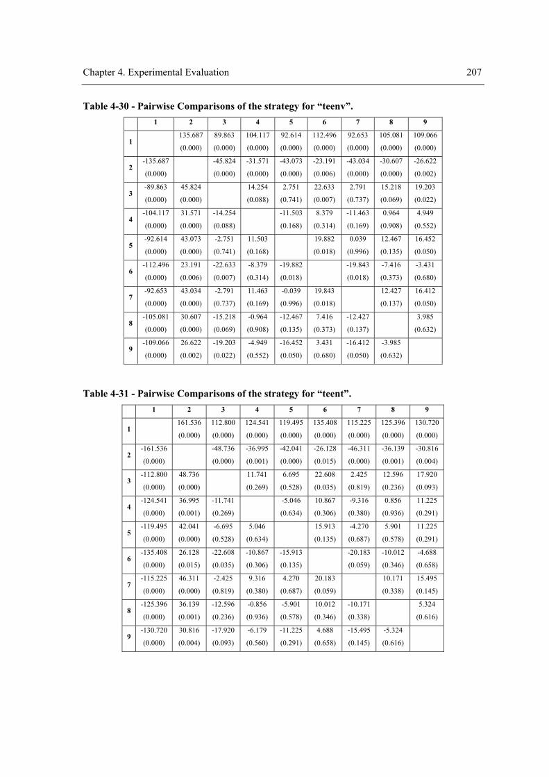
Chapter 4. Experimental Evaluation 207
Table 4-30 - Pairwise Comparisons of the strategy for “teenv”. 1 2 3 4 5 6 7 8 9
1 135.687
(0.000)
89.863
(0.000)
104.117
(0.000)
92.614
(0.000)
112.496
(0.000)
92.653
(0.000)
105.081
(0.000)
109.066
(0.000)
2 -135.687
(0.000)
-45.824
(0.000)
-31.571
(0.000)
-43.073
(0.000)
-23.191
(0.006)
-43.034
(0.000)
-30.607
(0.000)
-26.622
(0.002)
3 -89.863
(0.000)
45.824
(0.000)
14.254
(0.088)
2.751
(0.741)
22.633
(0.007)
2.791
(0.737)
15.218
(0.069)
19.203
(0.022)
4 -104.117
(0.000)
31.571
(0.000)
-14.254
(0.088)
-11.503
(0.168)
8.379
(0.314)
-11.463
(0.169)
0.964
(0.908)
4.949
(0.552)
5 -92.614
(0.000)
43.073
(0.000)
-2.751
(0.741)
11.503
(0.168)
19.882
(0.018)
0.039
(0.996)
12.467
(0.135)
16.452
(0.050)
6 -112.496
(0.000)
23.191
(0.006)
-22.633
(0.007)
-8.379
(0.314)
-19.882
(0.018)
-19.843
(0.018)
-7.416
(0.373)
-3.431
(0.680)
7 -92.653
(0.000)
43.034
(0.000)
-2.791
(0.737)
11.463
(0.169)
-0.039
(0.996)
19.843
(0.018)
12.427
(0.137)
16.412
(0.050)
8 -105.081
(0.000)
30.607
(0.000)
-15.218
(0.069)
-0.964
(0.908)
-12.467
(0.135)
7.416
(0.373)
-12.427
(0.137)
3.985
(0.632)
9 -109.066
(0.000)
26.622
(0.002)
-19.203
(0.022)
-4.949
(0.552)
-16.452
(0.050)
3.431
(0.680)
-16.412
(0.050)
-3.985
(0.632)
Table 4-31 - Pairwise Comparisons of the strategy for “teent”. 1 2 3 4 5 6 7 8 9
1 161.536
(0.000)
112.800
(0.000)
124.541
(0.000)
119.495
(0.000)
135.408
(0.000)
115.225
(0.000)
125.396
(0.000)
130.720
(0.000)
2 -161.536
(0.000)
-48.736
(0.000)
-36.995
(0.001)
-42.041
(0.000)
-26.128
(0.015)
-46.311
(0.000)
-36.139
(0.001)
-30.816
(0.004)
3 -112.800
(0.000)
48.736
(0.000)
11.741
(0.269)
6.695
(0.528)
22.608
(0.035)
2.425
(0.819)
12.596
(0.236)
17.920
(0.093)
4 -124.541
(0.000)
36.995
(0.001)
-11.741
(0.269)
-5.046
(0.634)
10.867
(0.306)
-9.316
(0.380)
0.856
(0.936)
11.225
(0.291)
5 -119.495
(0.000)
42.041
(0.000)
-6.695
(0.528)
5.046
(0.634)
15.913
(0.135)
-4.270
(0.687)
5.901
(0.578)
11.225
(0.291)
6 -135.408
(0.000)
26.128
(0.015)
-22.608
(0.035)
-10.867
(0.306)
-15.913
(0.135)
-20.183
(0.059)
-10.012
(0.346)
-4.688
(0.658)
7 -115.225
(0.000)
46.311
(0.000)
-2.425
(0.819)
9.316
(0.380)
4.270
(0.687)
20.183
(0.059)
10.171
(0.338)
15.495
(0.145)
8 -125.396
(0.000)
36.139
(0.001)
-12.596
(0.236)
-0.856
(0.936)
-5.901
(0.578)
10.012
(0.346)
-10.171
(0.338)
5.324
(0.616)
9 -130.720
(0.000)
30.816
(0.004)
-17.920
(0.093)
-6.179
(0.560)
-11.225
(0.291)
4.688
(0.658)
-15.495
(0.145)
-5.324
(0.616)
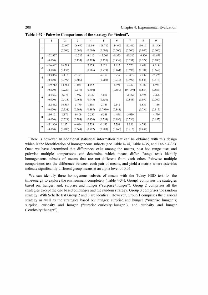
208 Chapter 4. Experimental Evaluation
Table 4-32 - Pairwise Comparisons of the strategy for “tedent”. 1 2 3 4 5 6 7 8 9
1 122.977
(0.000)
106.692
(0.000)
113.864
(0.000)
109.712
(0.000)
114.603
(0.000)
112.462
(0.000)
116.101
(0.000)
111.306
(0.000)
2 -122.977
(0.000)
-16.285
(0.133)
-9.112
(0.399)
-13.264
(0.220)
-8.373
(0.438)
-10.515
(0.331)
-6.876
(0.524)
-11.671
(0.280)
3 -106.692
(0.000)
16.285
(0.133)
7.173
(0.506)
3.021
(0.779)
7.912
(0.464)
5.770
(0.593)
9.409
(0.384)
4.614
(0.669)
4 -113.864
(0.000)
9.112
(0.399)
-7.173
(0.506)
-4.152
(0.700)
0.739
(0.945)
-1.403
(0.897)
2.237
(0.836)
-2.559
(0.812)
5 -109.712
(0.000)
13.264
(0.220)
-3.021
(0.779)
4.152
(0.700)
4.891
(0.650)
2.749
(0.7999)
6.389
(0.554)
1.593
(0.883)
6 -114.603
(0.000)
8.373
(0.438)
-7.912
(0.464)
-0.739
(0.945)
-4.891
(0.650)
-2.142
(0.843)
1.498
(0.890)
-3.298
(0.760)
7 -112.462
(0.000)
10.515
(0.331)
-5.770
(0.593)
1.403
(0.897)
-2.749
(0.7999)
2.142
(0.843)
3.639
(0.736)
-1.156
(0.915)
8 -116.101
(0.000)
6.876
(0.524)
-9.409
(0.384)
-2.237
(0.836)
-6.389
(0.554)
-1.498
(0.890)
-3.639
(0.736)
-4.796
(0.657)
9 -111.306
(0.000)
11.671
(0.280)
-4.614
(0.669)
2.559
(0.812)
-1.593
(0.883)
3.298
(0.760)
1.156
(0.915)
4.796
(0.657)
There is however an additional statistical information that can be obtained with this design
which is the identification of homogeneous subsets (see Table 4-34, Table 4-35, and Table 4-36). Once we have determined that differences exist among the means, post hoc range tests and pairwise multiple comparisons can determine which means differ. Range tests identify homogeneous subsets of means that are not different from each other. Pairwise multiple comparisons test the difference between each pair of means, and yield a matrix where asterisks indicate significantly different group means at an alpha level of 0.05.
We can identify three homogenous subsets of means with the Tukey HSD test for the time/energy to explore the environment completely (Table 4-34). Group1 comprises the strategies based on: hunger; and, surprise and hunger (“surprise+hunger”). Group 2 comprises all the strategies except the one based on hunger and the random strategy. Group 3 comprises the random strategy. With Scheffe test Group 2 and 3 are identical. However, Group 1 comprises the classical strategy as well as the strategies based on: hunger; surprise and hunger (“surprise+hunger”); surprise, curiosity and hunger (“surprise+curiosity+hunger”); and curiosity and hunger (“curiosity+hunger”).

Chapter 4. Experimental Evaluation 209
Table 4-33 - Pairwise Comparisons for the environment complexity.
Pairwise Comparisons Dependent Variable: Time/Energy required to explore the environment completely
95% Confidence Interval for Difference(a) (I) Environment
Complexity (J) Environment Complexity
Mean Difference (I-J)
Std. Error Sig.(a)
Lower Bound Upper Bound
Medium -1.556(b.c) 4.787 0.746 -11.035 7.922Low
High -6.899(b.c) 4.787 0.152 -16.378 2.579
Low 1.556(b.c) 4.787 0.746 -7.922 11.035Medium
High -5.343(b.c) 4.787 0.267 -14.821 4.136
Low 6.899(b.c) 4.787 0.152 -2.579 16.378High
Medium 5.343(b.c) 4.787 0.267 -4.136 14.821
Pairwise Comparisons Dependent Variable: Time/Energy required to explore all the entities of the environment
95% Confidence Interval for Difference(a) (I) Environment
Complexity (J) Environment Complexity
Mean Difference (I-J)
Std. Error Sig.(a)
Lower Bound Upper Bound
Medium -2.017(b.c) 6.105 0.742 -14.104 10.070Low
High -7.878(b.c) 6.105 0.199 -19.964 4.209
Low 2.017(b.c) 6.105 0.742 -10.070 14.104Medium
High -5.861(b.c) 6.105 0.339 -17.948 6.226
Low 7.878(b.c) 6.105 0.199 -4.209 19.964High
Medium 5.861(b.c) 6.105 0.339 -6.226 17.948
Pairwise Comparisons Dependent Variable: Time/Energy required to explore all different entities of the environment
95% Confidence Interval for Difference(a) (I) Environment
Complexity (J) Environment Complexity
Mean Difference (I-J)
Std. Error Sig.(a)
Lower Bound Upper Bound
Medium -61.452(*.b.c) 6.214 0.000 -73.756 -49.149Low
High -75.856(*.b.c) 6.214 0.000 -88.160 -63.553
Low 61.452(*.b.c) 6.214 0.000 49.149 73.756Medium
High -14.404(*.b.c) 6.214 0.022 -26.708 -2.100
Low 75.856(*.b.c) 6.214 0.000 63.553 88.160High
Medium 14.404(*.b.c) 6.214 0.022 2.100 26.708Based on estimated marginal means a Adjustment for multiple comparisons: Least Significant Difference (equivalent to no adjustments). b An estimate of the modified population marginal mean (I). c An estimate of the modified population marginal mean (J).
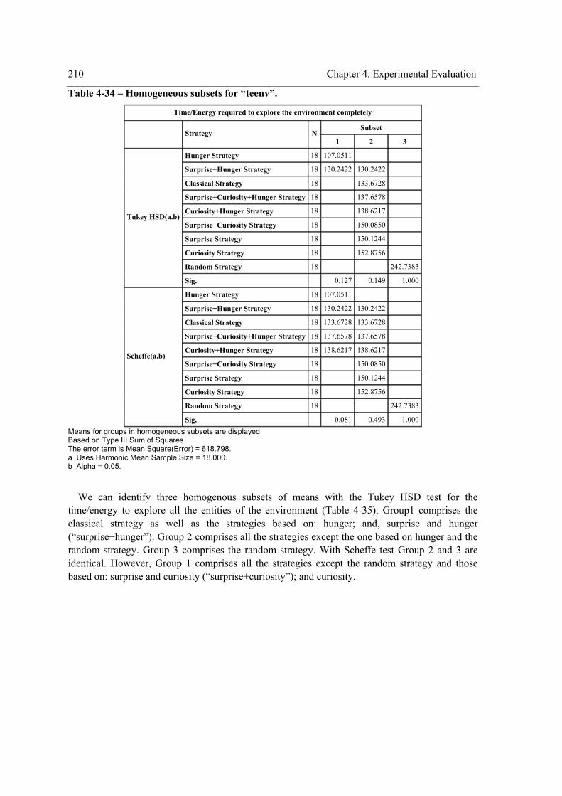
210 Chapter 4. Experimental Evaluation
Table 4-34 – Homogeneous subsets for “teenv”.
Time/Energy required to explore the environment completely
Subset Strategy N
1 2 3
Hunger Strategy 18 107.0511
Surprise+Hunger Strategy 18 130.2422 130.2422
Classical Strategy 18 133.6728
Surprise+Curiosity+Hunger Strategy 18 137.6578
Curiosity+Hunger Strategy 18 138.6217
Surprise+Curiosity Strategy 18 150.0850
Surprise Strategy 18 150.1244
Curiosity Strategy 18 152.8756
Random Strategy 18 242.7383
Tukey HSD(a.b)
Sig. 0.127 0.149 1.000
Hunger Strategy 18 107.0511
Surprise+Hunger Strategy 18 130.2422 130.2422
Classical Strategy 18 133.6728 133.6728
Surprise+Curiosity+Hunger Strategy 18 137.6578 137.6578
Curiosity+Hunger Strategy 18 138.6217 138.6217
Surprise+Curiosity Strategy 18 150.0850
Surprise Strategy 18 150.1244
Curiosity Strategy 18 152.8756
Random Strategy 18 242.7383
Scheffe(a.b)
Sig. 0.081 0.493 1.000 Means for groups in homogeneous subsets are displayed. Based on Type III Sum of Squares The error term is Mean Square(Error) = 618.798. a Uses Harmonic Mean Sample Size = 18.000. b Alpha = 0.05.
We can identify three homogenous subsets of means with the Tukey HSD test for the time/energy to explore all the entities of the environment (Table 4-35). Group1 comprises the classical strategy as well as the strategies based on: hunger; and, surprise and hunger (“surprise+hunger”). Group 2 comprises all the strategies except the one based on hunger and the random strategy. Group 3 comprises the random strategy. With Scheffe test Group 2 and 3 are identical. However, Group 1 comprises all the strategies except the random strategy and those based on: surprise and curiosity (“surprise+curiosity”); and curiosity.

Chapter 4. Experimental Evaluation 211
Table 4-35 - Homogeneous subsets for “teent”.
Time/Energy required to explore all the entities of the environment
Subset Strategy N
1 2 3
Hunger Strategy 18 81.2028
Surprise+Hunger Strategy 18 107.3306 107.3306
Classical Strategy 18 112.0183 112.0183
Surprise+Curiosity+Hunger Strategy 18 117.3422
Curiosity+Hunger Strategy 18 118.1978
Surprise Strategy 18 123.2433
Surprise+Curiosity Strategy 18 127.5133
Curiosity Strategy 18 129.9383
Random Strategy 18 242.7383
Tukey HSD(a.b)
Sig. 0.096 0.453 1.000
Hunger Strategy 18 81.2028
Surprise+Hunger Strategy 18 107.3306 107.3306
Classical Strategy 18 112.0183 112.0183
Surprise+Curiosity+Hunger Strategy 18 117.3422 117.3422
Curiosity+Hunger Strategy 18 118.1978 118.1978
Surprise Strategy 18 123.2433 123.2433
Surprise+Curiosity Strategy 18 127.5133
Curiosity Strategy 18 129.9383
Random Strategy 18 242.7383
Scheffe(a.b)
Sig. 0.055 0.800 1.000 Means for groups in homogeneous subsets are displayed. Based on Type III Sum of Squares The error term is Mean Square(Error) = 1006.217. a Uses Harmonic Mean Sample Size = 18.000. b Alpha = 0.05.
We can identify two homogenous subsets of means both with the Tukey HSD and the Scheffe tests for the time/energy to explore all different entities of the environment (Table 4-36). Group1 comprises the all the strategies except the random strategy which is the single strategy that forms Group2.

212 Chapter 4. Experimental Evaluation
Table 4-36 - Homogeneous subsets for “tedent”.
Time/Energy required to explore all different entities of the environment
Subset Strategy N
1 2
Hunger Strategy 18 81.2100
Surprise+Curiosity+Hunger Strategy 18 88.0856
Surprise+Hunger Strategy 18 89.5833
Curiosity+Hunger Strategy 18 90.3222
Surprise+Curiosity Strategy 18 91.7250
Classical Strategy 18 92.8811
Surprise Strategy 18 94.4744
Curiosity Strategy 18 97.4950
Random Strategy 18 204.1867
Tukey HSD(a.b)
Sig. 0.847 1.000
Hunger Strategy 18 81.2100
Surprise+Curiosity+Hunger Strategy 18 88.0856
Surprise+Hunger Strategy 18 89.5833
Curiosity+Hunger Strategy 18 90.3222
Surprise+Curiosity Strategy 18 91.7250
Classical Strategy 18 92.8811
Surprise Strategy 18 94.4744
Curiosity Strategy 18 97.4950
Random Strategy 18 204.1867
Scheffe(a.b)
Sig. 0.969 1.000 Means for groups in homogeneous subsets are displayed. Based on Type III Sum of Squares The error term is Mean Square(Error) = 1042.668. a Uses Harmonic Mean Sample Size = 18.000. b Alpha = 0.05.
4.2.4 Summary of Results
We begin with the summary of the results reached with the one way repeated measures experimental design. With the univariate approach, we find a significant effect of “strat” on the three exploration performance measures: F(8,184) = 58.77, p < 0.001 for the time/energy to explore the environment completely (encoded as “teenv”); F(8,184) = 5.77, p < 0.001 for the time/energy to explore all the entities (encoded as “teent”); and F(8,184) = 33.747, p < 0.001 for the time/energy to explore all different entities (encoded as “teent”). Specifically, “strat” accounts for 71.9% of the variance in the time/energy to explore the environment completely, 20% of the variance in the time/energy to explore all the entities, and 59.5% of the variance in the time/energy to explore all different entities.
The within subject effect, “strat”, that tested significant under the assumption of sphericity remains significant with the tests based on correction factors (Lower Bound): F(1.00, 23.00) = 58.77, p < 0.001 for the time/energy to explore the environment completely, F(1.00, 23.00) = 5.767, p = 0.025 for the time/energy to explore all the entities, and F(1.00, 23.00) = 33.747, p < 0.001 for the time/energy to explore all different entities.
Chapter 4. Experimental Evaluation 213
The Multivariate Test results for testing the main effect of “strat” are identical to those obtained from the univariate ANOVA model: the four tests of significance for the strategy effect given by the Multivariate Tests, Pillai’s Trace (value = 0.944; F(24.00, 552.00)=10.565, p < 0.001), Wilks’ Lambda (value = 0.218; F(24.00, 528.457) = 15.219, p < 0.001), Hotelling’s Trace (value = 2.847; F(24.00, 542.00) = 21.429, p < 0.001), and Roy’s Largest Root (value = 2.556; F(8.00,184.00) = 58.787, p < 0.001), indicate that the strategy has a significant effect.
All the analyses reported above have established that the exploration performance is affected by the strategy. Therefore we reject the null hypothesis. The F test tell us only if all the group means are roughly equal or if there are some significant differences among them. In the latter case, it does not tell us which groups are different from which other groups. Therefore, we undertake further tests to determine which particular group means differ. Since we has no prior hypotheses about the group differences and we are simply exploring the data to ascertain which group differences are driving the significance of the overall F test, we conducted post hoc comparisons.
Together with the multiple comparison output, the plots provide us the following results. Strategy 1 (random) is significantly (p < 0.001) the worst strategy considering the three exploration performance measures (time/energy to explore the environment completely, time/energy to explore all the entities and the time/energy to explore all different entities). On the contrary, strategy 2 (hunger-based) is significantly (p < 0.001) the best strategy considering the three exploration performance measures. However, this strategy depends heavily on the position of the entities in the environment (this factor was kept constant in our experiment).
Consider first the time/energy to explore the environment completely. Excluding strategy 2, strategy 6 (based on surprise and hunger) generated the highest performance, followed closely by strategy 9 (classical strategy). However, this difference is no significant at the 0.05 level (p = 0.098) but it is at the 0.1 level. All the other strategies are significantly worse than strategy 6. The next strategies in the ranking are strategies 4 (curiosity and hunger) and 8 (surprise, curiosity, and hunger), whose difference is not significant. The difference between strategy 6 and these two strategies is significant: p = 0.006 for strategy 4 and p = 0.014 for strategy 8. However, these are not significantly different from strategy 9. There is no significant difference between strategies 3 (curiosity), 5 (surprise), and 7 (curiosity and surprise). This means that those strategies that take hunger, either alone or combined with surprise and/or curiosity, into account are significantly better than those strategies that take only surprise and/or curiosity into account.
Considering the time/energy to explore all the entities, and, excluding strategy 2, strategy 6 (surprise and hunger) generated the highest performance, followed closely by strategy 9 (classical strategy). However, this difference is not significant at the 0.05 level but it is at the 0.08 level. All the other strategies are significantly worse than strategy 6. The next strategies in the ranking are strategies 8 (surprise, curiosity and hunger) and 4 (curiosity and hunger), whose difference is not significant. The difference between strategy 6 and these two strategies is significant: p < 0.001. However, these are not significantly different from strategy 9. There is no significant difference between strategies 5 (surprise), 4 (curiosity and hunger), 7 (curiosity and surprise), and 8 (surprise, curiosity and hunger).
Consider now the time/energy to explore all different entities. Excluding strategy 2 (hunger), strategy 6 (surprise and hunger) generated the highest performance, followed closely by strategy 8 (surprise and curiosity), 3 (curiosity), 4 (curiosity and hunger), and 7 (curiosity and surprise). However, this difference is no significant. The next strategies in the ranking are strategies 9
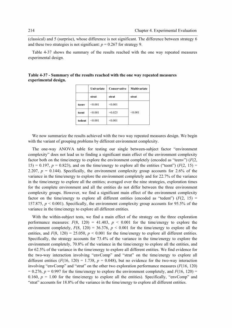
214 Chapter 4. Experimental Evaluation
(classical) and 5 (surprise), whose difference is not significant. The difference between strategy 6 and these two strategies is not significant: p = 0.267 for strategy 9.
Table 4-37 shows the summary of the results reached with the one way repeated measures experimental design.
Table 4-37 - Summary of the results reached with the one way repeated measures experimental design.
Univariate Conservative Multivariate
strat strat strat
teenv <0.001 <0.001
teent <0.001 =0.025
tedent <0.001 <0.001
<0.001
We now summarize the results achieved with the two way repeated measures design. We begin with the variant of grouping problems by different environment complexity.
The one-way ANOVA table for testing our single between-subject factor “environment complexity” does not lead us to finding a significant main effect of the environment complexity factor both on the time/energy to explore the environment completely (encoded as “teenv”) (F(2, 15) = 0.197, p = 0.823), and on the time/energy to explore all the entities (“teent”) (F(2, 15) = 2.207, p = 0.144). Specifically, the environment complexity group accounts for 2.6% of the variance in the time/energy to explore the environment completely and for 22.7% of the variance in the time/energy to explore all the entities; averaged over the nine strategies, exploration times for the complete environment and all the entities do not differ between the three environment complexity groups. However, we find a significant main effect of the environment complexity factor on the time/energy to explore all different entities (encoded as “tedent”) (F(2, 15) = 157.875, p < 0.001). Specifically, the environment complexity group accounts for 95.5% of the variance in the time/energy to explore all different entities.
With the within-subject tests, we find a main effect of the strategy on the three exploration performance measures: F(8, 120) = 41.403, p < 0.001 for the time/energy to explore the environment completely, F(8, 120) = 36.376, p < 0.001 for the time/energy to explore all the entities, and F(8, 120) = 25.050, p < 0.001 for the time/energy to explore all different entities. Specifically, the strategy accounts for 73.4% of the variance in the time/energy to explore the environment completely, 70.8% of the variance in the time/energy to explore all the entities, and for 62.5% of the variance in the time/energy to explore all different entities. We find evidence for the two-way interaction involving “envComp” and “strat” on the time/energy to explore all different entities (F(16, 120) = 1.738, p = 0.048), but no evidence for the two-way interaction involving “envComp” and “strat” on the other two exploration performance measures (F(16, 120) = 0.276, p = 0.997 for the time/energy to explore the environment completely, and F(16, 120) = 0.160, p = 1.00 for the time/energy to explore all the entities). Specifically, “envComp” and “strat” accounts for 18.8% of the variance in the time/energy to explore all different entities.
Chapter 4. Experimental Evaluation 215
The within subject effect that tested significant under the assumption of sphericity remain significant with the test based on correction factors (Lower Bound): F(1.00, 15.00) = 41.403, p < 0.001 for the time/energy to explore the environment completely, F(1.00, 15.00) = 36.376, p < 0.001 for the time/energy to explore all the entities, and F(1.00, 15.00) = 25.050, p < 0.001 for the time/energy to explore all different entities. Giving this statistical significance, we need not to use the other two conservative tests.
The interaction effect involving the within subject effect, “strat” × “envComp” on “tedent”, that tested significant under the assumption of sphericity does not remain significant with the Lower Bound Test: F(2.00, 15.00) = 1.738, p = 0.21. The two tests contradict each other, that is, the uncorrected (positively biased) test yields statistical significance and the conservative (negatively biased) test does not. Therefore, the more specific epsilon correction in the degrees of freedom is made, substituting either the Greenhouse-Geisser or Huynh-Feldt epsilon estimate in place of the Lower Bound epsilon. The interaction effect “strat” and “envComp” that tested significant under the assumption of sphericity and no significant under the Lower Bound test remain no significant after these corrections: using Huynh-Feldt correction factor, F(3.634, 27.258) = 1.738, p = 0.175; using Greenhouse-Geisser correction factor, F(2.953, 22.146) = 1.738, p < 0.189. Therefore we conclude that there is no effect of “strat” × “envComp” on “tedent”.
The Multivariate Test results for testing the main effect of “strat” and the interaction “strat” × “envComp” are identical to those obtained from the univariate ANOVA model: the four tests of significance for the strategy effect given by the Multivariate Tests, Pillai’s Trace (value = 1.151, F(24.00, 360.00) = 9.331, p < 0.001), Wilks’ Lambda (value = 0.162, F(24.00, 342.837) = 12.453, p < 0.001), Hotelling’s Trace (value = 3.397, F(24.00, 350.00) = 16.511, p < 0.001), and Roy’s Largest Root (value = 2.856, F(8.00, 120.00) = 42.847, p < 0.001), indicate that the strategy has a significant effect. The large Partial Eta Squared values for the strategy show that it explains quite a lot of variation in exploration performance. There is also evidence for an interaction between factors “strat” and “envComp”: Pillai’s Trace (value = 0.575, F(48.00, 360.00) = 1.777, p = 0.002), Wilks’ Lambda (value = 0.474, F(48.00, 351.755) = 2.094, p < 0.001), Hotelling’s Trace (value = 1.011, F(48.00, 350.00) = 2.457, p < 0.001), and Roy’s Largest Root (value = 0.902, F(16.00, 120.00) = 6.765, p < 0.001). Thus, the MANOVA approach alters the conclusions drawn about the within-subject interaction effect.
All these analyses establish that the there is evidence indicating that the three exploration performance measures are affected by the strategy. The univariate ANOVA model tests, particularly the more conservative tests, indicate no evidence for the interaction between “strat” and “envComp”, but the MANOVA approach alters these conclusions by indicating a significant interaction “strat” × “envComp”. We do not find a significant main effect of the environment complexity factor both on the time/energy to explore the environment completely and on the time/energy to explore all the entities, but we find a significant main effect of the environment complexity factor on the time/energy to explore all different entities. Giving these results: we reject the null hypothesis that states there is no effect of the strategy; we reject the null hypothesis about the equality of the environment complexity factor effects with respect to the time/energy to explore all different entities, but we accept the null hypothesis about the equality of the environment complexity factor effects with respect to the other two exploration performance measures; we reject the null hypothesis that states there is no interaction between the strategy and the environment complexity.
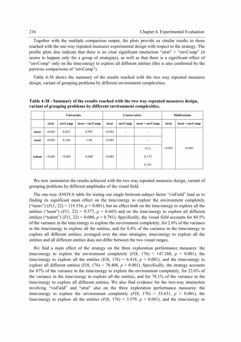
216 Chapter 4. Experimental Evaluation
Together with the multiple comparison output, the plots provide us similar results to those reached with the one-way repeated measures experimental design with respect to the strategy. The profile plots also indicate that there is no clear significant interaction “strat” × “envComp” (it seems to happen only for a group of strategies), as well as that there is a significant effect of “envComp” only on the time/energy to explore all different entities (this is also confirmed by the pairwise comparisons of “envComp”).
Table 4-38 shows the summary of the results reached with the two way repeated measures design, variant of grouping problems by different environment complexities.
Table 4-38 - Summary of the results reached with the two way repeated measures design, variant of grouping problems by different environment complexities.
Univariate Conservative Multivariate
strat envComp strat × envComp strat envComp strat × envComp strat strat × envComp
teenv <0.001 0.823 0.997 <0.001 - -
teent <0.001 0.144 1.00 <0.001 - -
tedent <0.001 <0.001 0.048 <0.001 -
0.21
0.175
0.181
<0.001 <0.001
We now summarize the results achieved with the two way repeated measures design, variant of grouping problems by different amplitudes of the visual field.
The one-way ANOVA table for testing our single between-subject factor “visField” lead us to finding its significant main effect on the time/energy to explore the environment completely (“teenv”) (F(1, 22) = 119.534, p < 0.001), but no effect both on the time/energy to explore all the entities (“teent”) (F(1, 22) = 0.577, p = 0.445) and on the time/energy to explore all different entities (“tedent”) (F(1, 22) = 0.080, p = 0.781). Specifically, the visual field accounts for 84.5% of the variance in the time/energy to explore the environment completely, for 2.6% of the variance in the time/energy to explore all the entities, and for 0.4% of the variance in the time/energy to explore all different entities; averaged over the nine strategies, time/energy to explore all the entities and all different entities does not differ between the two visual ranges.
We find a main effect of the strategy on the three exploration performance measures: the time/energy to explore the environment completely (F(8, 176) = 147.260, p < 0.001), the time/energy to explore all the entities (F(8, 176) = 6.414, p < 0.001), and the time/energy to explore all different entities (F(8, 176) = 78.408, p < 0.001). Specifically, the strategy accounts for 87% of the variance in the time/energy to explore the environment completely, for 22.6% of the variance in the time/energy to explore all the entities, and for 78.1% of the variance in the time/energy to explore all different entities. We also find evidence for the two-way interaction involving “visField” and “strat” also on the three exploration performance measures: the time/energy to explore the environment completely (F(8, 176) = 35.631, p < 0.001), the time/energy to explore all the entities (F(8, 176) = 3.579, p = 0.001), and the time/energy to
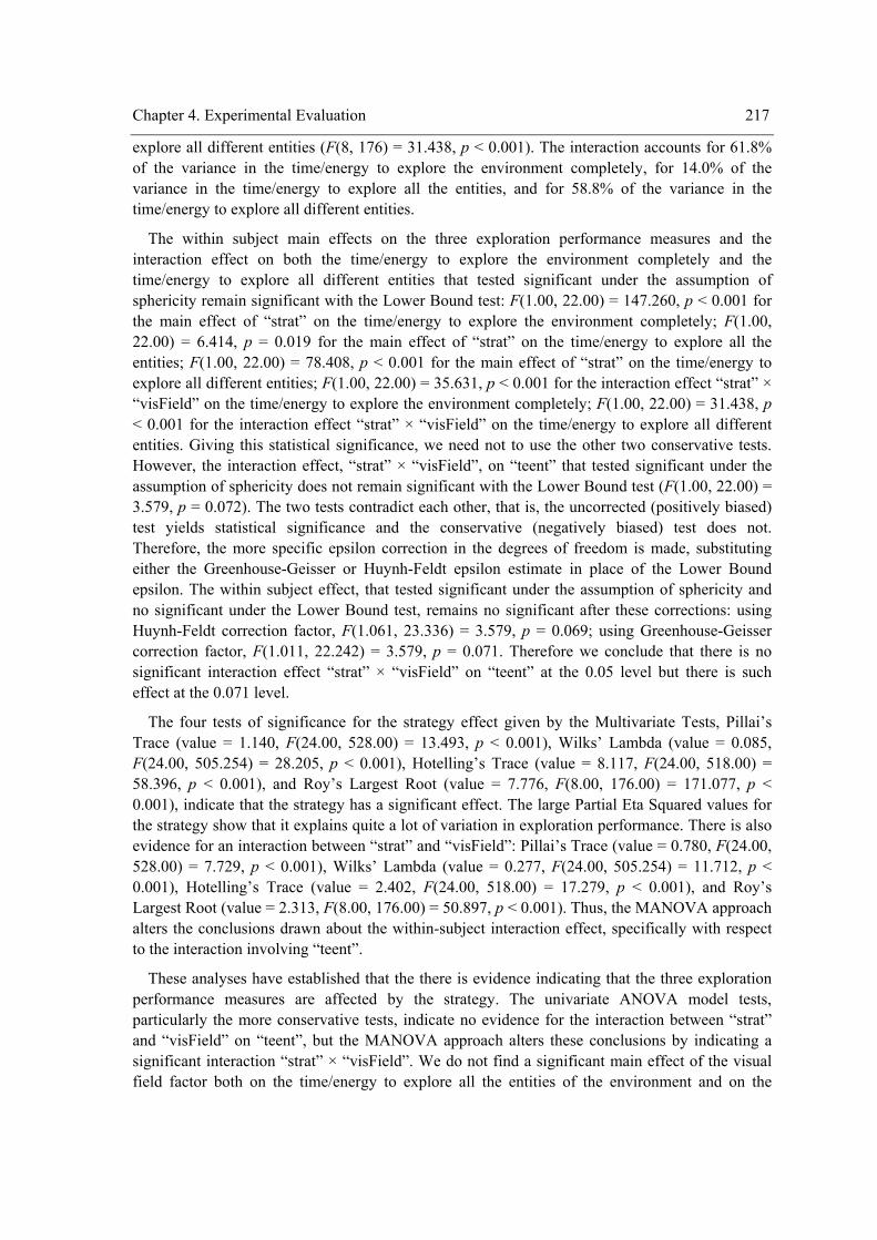
Chapter 4. Experimental Evaluation 217
explore all different entities (F(8, 176) = 31.438, p < 0.001). The interaction accounts for 61.8% of the variance in the time/energy to explore the environment completely, for 14.0% of the variance in the time/energy to explore all the entities, and for 58.8% of the variance in the time/energy to explore all different entities.
The within subject main effects on the three exploration performance measures and the interaction effect on both the time/energy to explore the environment completely and the time/energy to explore all different entities that tested significant under the assumption of sphericity remain significant with the Lower Bound test: F(1.00, 22.00) = 147.260, p < 0.001 for the main effect of “strat” on the time/energy to explore the environment completely; F(1.00, 22.00) = 6.414, p = 0.019 for the main effect of “strat” on the time/energy to explore all the entities; F(1.00, 22.00) = 78.408, p < 0.001 for the main effect of “strat” on the time/energy to explore all different entities; F(1.00, 22.00) = 35.631, p < 0.001 for the interaction effect “strat” × “visField” on the time/energy to explore the environment completely; F(1.00, 22.00) = 31.438, p < 0.001 for the interaction effect “strat” × “visField” on the time/energy to explore all different entities. Giving this statistical significance, we need not to use the other two conservative tests. However, the interaction effect, “strat” × “visField”, on “teent” that tested significant under the assumption of sphericity does not remain significant with the Lower Bound test (F(1.00, 22.00) = 3.579, p = 0.072). The two tests contradict each other, that is, the uncorrected (positively biased) test yields statistical significance and the conservative (negatively biased) test does not. Therefore, the more specific epsilon correction in the degrees of freedom is made, substituting either the Greenhouse-Geisser or Huynh-Feldt epsilon estimate in place of the Lower Bound epsilon. The within subject effect, that tested significant under the assumption of sphericity and no significant under the Lower Bound test, remains no significant after these corrections: using Huynh-Feldt correction factor, F(1.061, 23.336) = 3.579, p = 0.069; using Greenhouse-Geisser correction factor, F(1.011, 22.242) = 3.579, p = 0.071. Therefore we conclude that there is no significant interaction effect “strat” × “visField” on “teent” at the 0.05 level but there is such effect at the 0.071 level.
The four tests of significance for the strategy effect given by the Multivariate Tests, Pillai’s Trace (value = 1.140, F(24.00, 528.00) = 13.493, p < 0.001), Wilks’ Lambda (value = 0.085, F(24.00, 505.254) = 28.205, p < 0.001), Hotelling’s Trace (value = 8.117, F(24.00, 518.00) = 58.396, p < 0.001), and Roy’s Largest Root (value = 7.776, F(8.00, 176.00) = 171.077, p < 0.001), indicate that the strategy has a significant effect. The large Partial Eta Squared values for the strategy show that it explains quite a lot of variation in exploration performance. There is also evidence for an interaction between “strat” and “visField”: Pillai’s Trace (value = 0.780, F(24.00, 528.00) = 7.729, p < 0.001), Wilks’ Lambda (value = 0.277, F(24.00, 505.254) = 11.712, p < 0.001), Hotelling’s Trace (value = 2.402, F(24.00, 518.00) = 17.279, p < 0.001), and Roy’s Largest Root (value = 2.313, F(8.00, 176.00) = 50.897, p < 0.001). Thus, the MANOVA approach alters the conclusions drawn about the within-subject interaction effect, specifically with respect to the interaction involving “teent”.
These analyses have established that the there is evidence indicating that the three exploration performance measures are affected by the strategy. The univariate ANOVA model tests, particularly the more conservative tests, indicate no evidence for the interaction between “strat” and “visField” on “teent”, but the MANOVA approach alters these conclusions by indicating a significant interaction “strat” × “visField”. We do not find a significant main effect of the visual field factor both on the time/energy to explore all the entities of the environment and on the
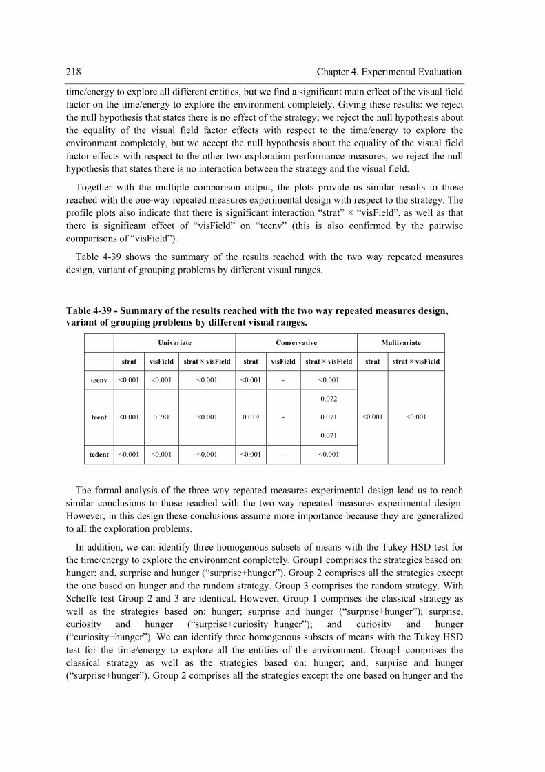
218 Chapter 4. Experimental Evaluation
time/energy to explore all different entities, but we find a significant main effect of the visual field factor on the time/energy to explore the environment completely. Giving these results: we reject the null hypothesis that states there is no effect of the strategy; we reject the null hypothesis about the equality of the visual field factor effects with respect to the time/energy to explore the environment completely, but we accept the null hypothesis about the equality of the visual field factor effects with respect to the other two exploration performance measures; we reject the null hypothesis that states there is no interaction between the strategy and the visual field.
Together with the multiple comparison output, the plots provide us similar results to those reached with the one-way repeated measures experimental design with respect to the strategy. The profile plots also indicate that there is significant interaction “strat” × “visField”, as well as that there is significant effect of “visField” on “teenv” (this is also confirmed by the pairwise comparisons of “visField”).
Table 4-39 shows the summary of the results reached with the two way repeated measures design, variant of grouping problems by different visual ranges.
Table 4-39 - Summary of the results reached with the two way repeated measures design, variant of grouping problems by different visual ranges.
Univariate Conservative Multivariate
strat visField strat × visField strat visField strat × visField strat strat × visField
teenv <0.001 <0.001 <0.001 <0.001 - <0.001
teent <0.001 0.781 <0.001 0.019 -
0.072
0.071
0.071
tedent <0.001 <0.001 <0.001 <0.001 - <0.001
<0.001 <0.001
The formal analysis of the three way repeated measures experimental design lead us to reach similar conclusions to those reached with the two way repeated measures experimental design. However, in this design these conclusions assume more importance because they are generalized to all the exploration problems.
In addition, we can identify three homogenous subsets of means with the Tukey HSD test for the time/energy to explore the environment completely. Group1 comprises the strategies based on: hunger; and, surprise and hunger (“surprise+hunger”). Group 2 comprises all the strategies except the one based on hunger and the random strategy. Group 3 comprises the random strategy. With Scheffe test Group 2 and 3 are identical. However, Group 1 comprises the classical strategy as well as the strategies based on: hunger; surprise and hunger (“surprise+hunger”); surprise, curiosity and hunger (“surprise+curiosity+hunger”); and curiosity and hunger (“curiosity+hunger”). We can identify three homogenous subsets of means with the Tukey HSD test for the time/energy to explore all the entities of the environment. Group1 comprises the classical strategy as well as the strategies based on: hunger; and, surprise and hunger (“surprise+hunger”). Group 2 comprises all the strategies except the one based on hunger and the
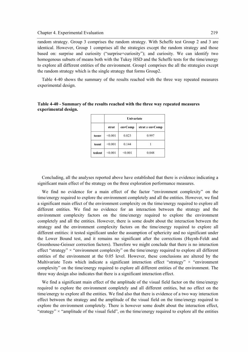
Chapter 4. Experimental Evaluation 219
random strategy. Group 3 comprises the random strategy. With Scheffe test Group 2 and 3 are identical. However, Group 1 comprises all the strategies except the random strategy and those based on: surprise and curiosity (“surprise+curiosity”); and curiosity. We can identify two homogenous subsets of means both with the Tukey HSD and the Scheffe tests for the time/energy to explore all different entities of the environment. Group1 comprises the all the strategies except the random strategy which is the single strategy that forms Group2.
Table 4-40 shows the summary of the results reached with the three way repeated measures experimental design.
Table 4-40 - Summary of the results reached with the three way repeated measures experimental design.
Univariate
strat envComp strat x envComp
teenv <0.001 0.823 0.997
teent <0.001 0.144 1
tedent <0.001 <0.001 0.048
Concluding, all the analyses reported above have established that there is evidence indicating a significant main effect of the strategy on the three exploration performance measures.
We find no evidence for a main effect of the factor “environment complexity” on the time/energy required to explore the environment completely and all the entities. However, we find a significant main effect of the environment complexity on the time/energy required to explore all different entities. We find no evidence for an interaction between the strategy and the environment complexity factors on the time/energy required to explore the environment completely and all the entities. However, there is some doubt about the interaction between the strategy and the environment complexity factors on the time/energy required to explore all different entities: it tested significant under the assumption of sphericity and no significant under the Lower Bound test, and it remains no significant after the corrections (Huynh-Feldt and Greenhouse-Geisser correction factors). Therefore we might conclude that there is no interaction effect “strategy” × “environment complexity” on the time/energy required to explore all different entities of the environment at the 0.05 level. However, these conclusions are altered by the Multivariate Tests which indicate a significant interaction effect “strategy” × “environment complexity” on the time/energy required to explore all different entities of the environment. The three way design also indicates that there is a significant interaction effect.
We find a significant main effect of the amplitude of the visual field factor on the time/energy required to explore the environment completely and all different entities, but no effect on the time/energy to explore all the entities. We find also that there is evidence of a two way interaction effect between the strategy and the amplitude of the visual field on the time/energy required to explore the environment completely. There is however some doubt about the interaction effect, “strategy” × “amplitude of the visual field”, on the time/energy required to explore all the entities
220 Chapter 4. Experimental Evaluation
of the environment: it tested significant under the assumption of sphericity and no significant under the Lower Bound test, and it remains no significant after the corrections (Huynh-Feldt and Greenhouse-Geisser correction factors). Therefore we might conclude that there is no interaction effect “strategy” × “amplitude of the visual field” on the time/energy required to explore all the entities of the environment at the 0.05 level but there is such effect at the 0.071 level. However, these conclusions are altered by the Multivariate Tests which indicate a significant interaction effect “strategy” × “amplitude of the visual field” on the time/energy required to explore all the entities of the environment. The influence of the strategy is to some extent controlled by the amplitude of the visual field.
With respect to the time/energy to explore the environment completely, excluding strategy 2, strategy 6 (based on surprise and hunger) generated the highest performance, followed closely by strategy 9 (classical strategy). However, this difference is no significant at the 0.05 level (p = 0.098) but it is at the 0.1 level. All the other strategies are significantly worse than strategy 6. The next strategies in the ranking are strategies 4 (curiosity and hunger) and 8 (surprise, curiosity and hunger), whose difference is not significant. The difference between strategy 6 and these two strategies is significant: p = 0.006 for strategy 4 and p = 0.014 for strategy 8. However, these are not significantly different from strategy 9. There is no significant difference between strategies 3 (curiosity), 5 (surprise) and 7 (curiosity and surprise). This means that those strategies that take hunger, either alone or combined with surprise and/or curiosity, into account are significantly better than those strategies that take only surprise and/or curiosity into account. Whatever the values of “envComp” or “visField”, this ranking is more or less maintained. Note, however, that with environments of higher complexity or with a low visual field, the performances are usually worse.
Concerning the time/energy required to explore all the entities of the environment, excluding strategy 2, strategy 6 (surprise and hunger) generated the highest performance, followed closely by strategy 9 (classical strategy). However, this difference is not significant at the 0.05 level but it is at the 0.08 level. All the other strategies are significantly worse than strategy 6. The next strategies in the ranking are strategies 8 (surprise, curiosity and hunger) and 4 (curiosity and hunger), whose difference is not significant. The difference between strategy 6 and these two strategies is significant: p < 0.001. However, these are not significantly different from strategy 9. There is no significant difference between strategies 5 (surprise), 4 (curiosity and hunger), 7 (curiosity and surprise), and 8 (surprise, curiosity and hunger). As with “teenv”, we should note, however, that with environments of higher complexity or with a high visual field, the performances are usually worse, but this ranking is in general kept.
Finally, concerning the time/energy required to explore all different entities of the environment, excluding strategy 2 (hunger), strategy 6 (surprise and hunger) generated the highest performance, followed closely by strategy 8 (surprise, curiosity and hunger), 3 (curiosity), 4 (curiosity and hunger), and 7 (curiosity and surprise). However, this difference is no significant. The next strategies in the ranking are strategies 9 (classical) and 5 (surprise), whose difference is not significant. The difference between strategy 6 and these two strategies is not significant: p = 0.267 for strategy 9. On the contrary to the previous performance measures (“teenv” and “teent”), the ranking of the strategies varies with the category of “envComp” or “visField”. For instance, strategies 3, 4, 5, 7 and 8 outperform significantly the other strategies when “envComp” is low. Another curious result is that strategies 4 and 8 are the best strategies when “visField” is low and the worst when “visField” is large. Note that, as with “teent”, and in contrary to “teenv”, best
Chapter 4. Experimental Evaluation 221
results are achieved with a low “visField”, and that, as with “teent” and “teenv”, best results are achieved with a low “envComp”.
4.2.5 Discussion
As mentioned above this experiment shows that the strategy that takes hunger into account requires less time and energy to explore the whole of the environment. This happens because an agent that uses this strategy computes beforehand the expected hunger it may feel at the destination locations (either closer to an entity or at a frontier cell). The agent then selects the destination location that minimizes hunger. By doing this, it selects those destination locations that are closer to it and, by navigating through the environment with this principle in mind, it avoids traversing long distances, as happens with other strategies, and therefore explores the entire environment efficiently. However, this strategy is deterministic given that the location of the entities is constant. It does not take into account the characteristics of the places to visit.
The strategy that takes curiosity into account leads the agent to select entities or frontier cells that are expected to maximize novelty and entropy for visits. These are the entities or frontier cells that are expected to provide most information. However, these entities or frontier cells are frequently not the closest ones and therefore the agent sometimes traverses long distances to obtain what it expects to be the highest information gain. By exploring the environment with this strategy, the agent wastes much time taking routes that are sometimes erratic and therefore it does not outperform the other strategies.
The strategy that takes surprise into account makes the agent move to entities that are expected to elicit surprise by containing something unexpected. This strategy is related with the one that takes curiosity into account because entities whose parts that are not already known are new and with higher entropy and are therefore eligible to elicit surprise. However, there are a few differences. For instance, if the function of an entity has high entropy with ten or twenty equally probable functions, the curiosity is high but surprise is 0. So, in order to have a positive value for the expected surprise there must be entropy but also that the events are not equally probable. Moreover, when there is a low entropy (e.g., when there are several possible functions for an entity and one of them has a high probability) the curiosity is low but the expected surprise is high. So, the strategy that takes surprise into account motivates the agent to move to entities that are expected to provide unexpected information rather than solely new information. On the other hand the known parts of the entities (the parts with no entropy) elicit surprise and curiosity if they contain new information (new information is unexpected). In this point curiosity and surprise are quite similar. Another major difference between the surprise-based strategy and the curiosity-based strategy is that while frontier cells may have a positive expected curiosity, we assume that they do not elicit surprise. So, although when the agent makes use of the surprise-based strategy it behaves differently from when it makes use of the curiosity-based strategy, the performance is quite similar and its, to some extent erratic, exploration paths indicate that it traverses unnecessarily long distances which has negative effects on its efficiency.
However, when surprise or curiosity, jointly or independently, are taken into account together with hunger, the erratic paths are replaced by ordered exploration paths and hence to a significant increase in efficiency. In fact, the motivation to visit entities or frontier cells that are expected to elicit curiosity and/or surprise but that are far away from the location of the agent is restrained by the hunger that is expected to be felt at those destination locations. When curiosity and surprise
222 Chapter 4. Experimental Evaluation
are taken into account together with hunger, the result is a strategy that nicely favours entities or frontier cells that are not too far away and that are expected to elicit a considerable intensity of curiosity and surprise. The performance of this strategy usually does not outperform the other two closer strategies that take curiosity and hunger, and surprise and hunger, into account, respectively. This happens because the restraining role of hunger, i.e., the weight of hunger, is reduced in that strategy (it is one of three feelings while in the other two strategies it is one of two feelings).
The difference between the strategy based on curiosity and hunger and that based on surprise and hunger may be explained by the fact that the intensities of surprise are lower than the intensities of curiosity. Therefore, the restrained effect of hunger is higher in the former than in the latter strategy. This also explains why the classical strategy usually outperforms the strategies based on curiosity and hunger and on curiosity, surprise and hunger. All of them take into account the distance, but values for the entropy computed by the classical strategy are lower than the curiosty values, because curiosity also takes into account the novelty in addition to entropy.
Giving this, we can logically understand the results above which indicate that the strategy has a significant effect on exploration performance.
We may understand better the significant effect of the amplitude of the visual field on “teenv”, “teent” and “tedent” if we take a look at the exploration paths (see Appendix C). When the “visField” is large enough so that the agent can access the whole environment, the agent does not have to visit frontier cells, but instead solely entities. Once it finishes visiting all the entities, it knows the whole environment because its sensors captured already all the information of the whole environment. Therefore, the “teenv” is lower when the “visField” is large. This is responsible for the significant effect of the amplitude of the visual field on “teenv”. When the agent has a large visual field, it can see not only the entities that are closer but also those entities that are far. Then, and especially when hunger is not taken into account, sometimes it selects for visiting entities that are far which has a negative effect on the “teent” and “tedent”.
When the environment is of higher complexity, there are more different entities. These are usually dispersed and therefore the agent has to follow erratic paths to visit all the entities. This explains the higher “teenv”, “teent” and “tedent” when “envComp” is high. However, concerning “tedent”, there is an additional effect: since higher complexity environments have more different entities than lower complexity environments it is obvious that an agent usually takes more time to visit all different entities in the former environments than in the latter.
4.3 Experiment III –Map-building by exploiting the knowledge in memory
We conducted an experiment to assess the influence of the size of memory and of the environment complexity on map-building by exploitation. Furthermore, this experiment enables us to study the trade-off between map-building by exploitation and map-building by exploration. A good approach to evaluate a map-building approach is by comparing the map built with the ideal map, i.e., with the map that should have been built. In the case of simulation, these two maps are known which facilitates this evaluation process. So, with this end, we let an agent explore various environments with different degrees of complexity. This process was repeated various times (twelve), each time with a larger memory. The key issue of this experiment is that the agent had such a minimum time limit to explore the environment that it could not leave the starting location, i.e., the agent only had time to sense the world and generate expectations about it.
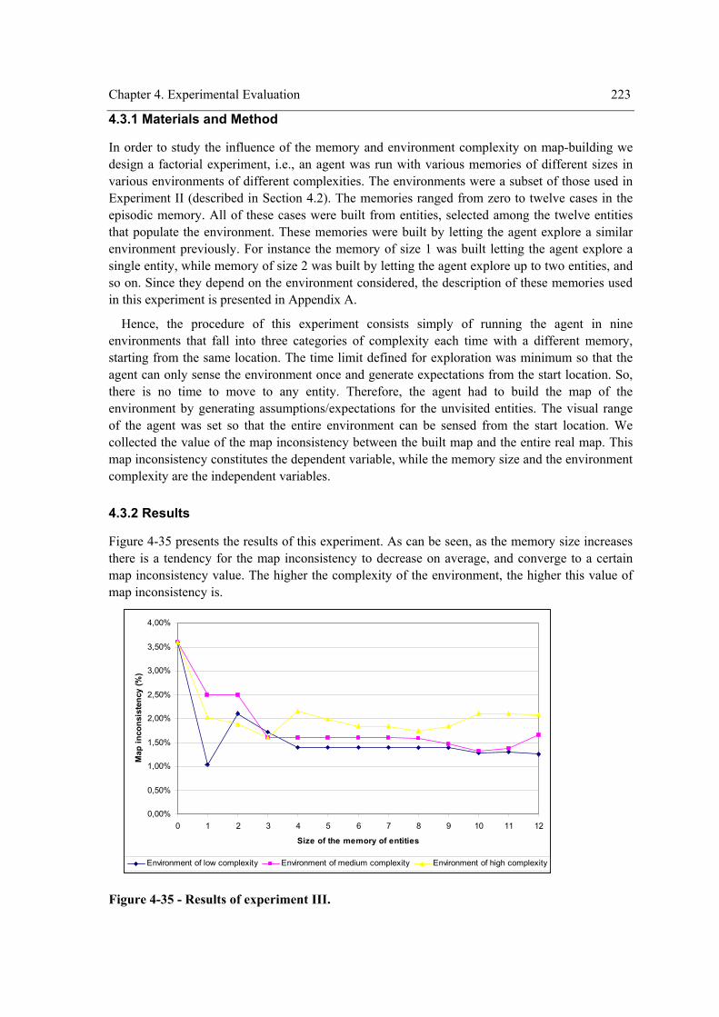
Chapter 4. Experimental Evaluation 223
4.3.1 Materials and Method
In order to study the influence of the memory and environment complexity on map-building we design a factorial experiment, i.e., an agent was run with various memories of different sizes in various environments of different complexities. The environments were a subset of those used in Experiment II (described in Section 4.2). The memories ranged from zero to twelve cases in the episodic memory. All of these cases were built from entities, selected among the twelve entities that populate the environment. These memories were built by letting the agent explore a similar environment previously. For instance the memory of size 1 was built letting the agent explore a single entity, while memory of size 2 was built by letting the agent explore up to two entities, and so on. Since they depend on the environment considered, the description of these memories used in this experiment is presented in Appendix A.
Hence, the procedure of this experiment consists simply of running the agent in nine environments that fall into three categories of complexity each time with a different memory, starting from the same location. The time limit defined for exploration was minimum so that the agent can only sense the environment once and generate expectations from the start location. So, there is no time to move to any entity. Therefore, the agent had to build the map of the environment by generating assumptions/expectations for the unvisited entities. The visual range of the agent was set so that the entire environment can be sensed from the start location. We collected the value of the map inconsistency between the built map and the entire real map. This map inconsistency constitutes the dependent variable, while the memory size and the environment complexity are the independent variables.
4.3.2 Results
Figure 4-35 presents the results of this experiment. As can be seen, as the memory size increases there is a tendency for the map inconsistency to decrease on average, and converge to a certain map inconsistency value. The higher the complexity of the environment, the higher this value of map inconsistency is.
0,00%
0,50%
1,00%
1,50%
2,00%
2,50%
3,00%
3,50%
4,00%
0 1 2 3 4 5 6 7 8 9 10 11 12
Size of the memory of entities
Map
inco
nsis
tenc
y (%
)
Environment of low complexity Environment of medium complexity Environment of high complexity
Figure 4-35 - Results of experiment III.
224 Chapter 4. Experimental Evaluation
4.3.3 Discussion
The results reported above show that the higher the complexity of the environment, the higher the map inconsistency. Higher complexity means higher diversity, and therefore it is harder for the agent to predict the reality accurately. There is much more uncertainty in such environments in that there is more diversity of entities than in low complexity environments. As the complexity increases the probability of finding any two similar entities decreases. In low complexity environments, this is, therefore, an easier task.
The results also show the influence of the memory size on map inconsistency. On average, the higher the memory size, the lower the map inconsistency. This happens because the higher the memory size the higher the knowledge about the entities present in the environment. This means that the probability distribution of the entities present in the memory approaches that of the environment as the memory size increases, and therefore the expectations generated are closer to reality. However, this is not linear, because sometimes the addition of a case may make the two probability distributions diverge slightly. However, the tendency is to converge. This is quite analogous to the theory of big numbers. Notice that with memories of size 4 or 5 the map inconsistency is almost optimal. In fact, the addition of seven or eight episodes to those memories results in an insignificant improvement in map inconsistency.
Considering these results we may infer the advantages and disadvantages of map-building by exploiting the knowledge acquired in previous training explorations. The main advantage of this map learning process is that it requires less time and less energy than that of involving a complete exploration of the environment. In fact, the agent does not have to explore all the regions of the environment, such as the invisible side of the entities, since it is able to predict that inaccessible information. The disadvantage of this approach is that the learned maps may be more inconsistent than those learned from an exhaustive exploration of the environment. However, this inconsistency can be decreased by incorporating a memory with a probability distribution that approaches that of the environment.
This experiment raises another research question concerning Experiment II: whether the results won’t be better for the affective strategies if the agent starts with a wealthy memory of entities previously acquired by training in similar environments.
225
Chapter 5 Related Work
ur work draws upon several areas as described in Chapter 2. It integrates multiple aspects from agents and multi-agent systems, emotion and motivation, exploration of unknown environments, knowledge representation, probabilistic planning, HTN planning, and
creativity. Thereby, various studies from these areas need to be compared with our work so that we can assess its position and importance to these areas. In this chapter we make that comparison. Our goal is not to survey the most representative work done in those areas (this was to some extent included in Chapter 2) but rather to simply make a comparison to those representative studies by stressing the main differences and similarities. This comparison is organized according to each one of the referred areas.
5.1 Autonomous Agents and Multi-Agent Systems
In our approach, agents have their own world model, their goals that they try to achieve, and they use plans to achieve them. In this sense the architecture of our agents is of a deliberative kind. Many other works adopt this architecture for agents, especially those within the traditional field of AI.
Our agents are assigned mentalistic qualities such as beliefs, desires, intentions, emotion and motivation, in addition to autonomy, social ability, reactivity and proactiveness. Considering Wooldridge and Jennings’ distinction between a weak and strong notion of agency [Wooldridge & Jennings, 1995b], we are among many others who put forward the latter notion. Other closely related works are, for instance, [Bates, 1994; Shoham, 1993; Wright, 1997] (others that assign emotion and motivation to agents are described in the next section).
Relying on this strong notion of agency, we would like to mention, in particular, the forerunner BDI-based multi-agent tool PRS [Georgeff & Ingrand, 1989; Georgeff & Lansky, 1987; K. Myers, 1997] and all the latter BDI-based multi-agent tool, which in a way or another are based on PRS, such as JACK [Busetta et al., 1999; Howden et al., 2001], dMARS [d’Inverno et al., 1997], AgentSpeak [Bordini et al., 2002; Bordini & Moreira, 2004; A. Rao, 1996], JADEX [Pokahr et al., 2005], SPARK [Morley & Myers, 2004], and 3APL [Dastani et al., 2003]. For instance, JACK intelligent agents are autonomous software components that have explicit goals to achieve or events to handle (desires). To describe how they should go about achieving these desires, these agents are programmed with a set of plans. Each plan describes how to achieve a goal under varying circumstances. Set to work, the agent pursues its given desires, adopting the appropriate plans (intentions) according to its current set of data (beliefs) about the state of the world. This combination of desires and beliefs initiating context-sensitive intentional behaviour is part of what characterizes a BDI agent. AMAS also relies on the BDI model. Therefore, it shares many characteristics of the above mentioned tools. However, we do not incorporate this model so closely. There are also beliefs, desires and intentions. Desires (or goals) are generated from previous goals of the plans presented in memory. These goals are evaluated and ranked in terms of how they contribute to satisfy the basic desires [Reiss, 2000; Schwartz, 1992] which are represented in an EU function. The goal that maximizes this function is taken as an intention and
O
226 Chapter 5. Related Work
the plan generated for it is executed. Other closely related multi-agent languages and tools that also assign mentalistic qualities to agents include the forerunners AGENT0 [Shoham, 1993] and PLACA [Thomas, 1993].
5.2 Emotion and Motivation
Our work has similarities to that of Breazel and Scassellati [Breazeal, 1999; Breazeal & Scassellati, 1999] in that Kismet exhibits the proto-social response of exploration by searching for desired visual stimuli. Exploratory responses allow the “caregiver” to attribute curiosity, interest, and desires to the robot. Kismet possesses an attention system that enables it to select perceptual stimuli. As in our approach, the motivational system of Kismet includes emotions and drives, although, contrarily to our model, emotions are modelled along three dimensions, valence, arousal and stance, while we consider solely valence and arousal.
Cañamero [Cañamero, 1997] has also developed a synthetic environment, the Gridland, inhabited by entities. However, unlike us, she considers three different types of entities: living beings, food and water sources, and inanimate objects. Like our agents, living beings are endowed with motivations and emotions. While we rely on a cognitive approach for modelling emotions, Cañamero uses physiological parameters. In addition to these physiological variables that define their body state, creatures also possess physical attributes such as hardness, brightness, amount of organic matter, etc., and a collection of agents, among which some of them model emotions. This latter property of creatures means that they are seen as a society of agents [Minsky, 1985]. This is definitely a different approach from ours. But, as in our approach, the behaviour of the creatures is controlled by motivation in that their behaviour is selected in order to satisfy some drive.
The Cathexis computational model of emotion and its further emotion-based decision-making extension [Velásquez, 1997, 1998a, 1998b, 1999] are particularly close to our approach in that the decisions of what to do next are influenced by drives and emotions. Behaviours are activated mainly to satisfy drives. In addition, positive and negative emotional memories are created when the agent interacts with people. This corresponds to some extent to somatic markers associated to particular situations that influence the selection of future behaviours so that negative outcomes are avoided. Besides this similarity with our approach, Velásquez included drives such as curiosity and also two other drives closely related to hunger, namely fatigue and “BatteryRegulation”. He also included surprise in the emotional system and related it to variables such as novelty, anticipatory expectancy, and other issues that have been considered essential components of a general attention system, including orienting to sensory stimuli, executive functions such as the detection of target events, and maintenance of a general “alert” state. Typical behavioural responses controlled by this system include look-around, orient-to-[stimulus], and look-at-[stimulus]. In addition, the detection of sudden, unexpected stimuli might also mediate more reflex-like responses such as an acoustic startle reflex. However, Velásquez’s model is much richer than ours in terms of the number of drives and emotions considered, although this can be explained by the different goals of both works.
One of the most closely related systems is the Affective Reasoner of Elliot [Elliott, 1992], a platform for modelling the interactions between multiple agents operating in an environment. This is also one of the goals of our platform. In addition, the Affective Reasoner and AMAS also share the feature of reasoning about the emotions and emotion induced actions. However, the Affective Reasoner is much broader with respect to the emotional component. It includes the twenty-two
Chapter 5. Related Work 227
emotion types of the OCC model plus two additional emotions: love and hate. Although our platform predicts the inclusion of all these emotions, in the current version, the feeling makeup of agents is confined to surprise, curiosity/interest, and hunger.
The Oz project [Bates, 1992, 1994; Bates et al., 1992; Loyall & Bates, 1991; Reilly, 1996; Reilly & Bates, 1992] and especially the Tok architecture also shares a few features with our work. Although with a different purpose, both works are about simulated environments populated with agents which exhibit some capabilities, especially an emotional makeup. However, like the Affective Reasoner, Em, the subsystem of Tok that handles emotion, is based on the OCC model and therefore is far more general than the AMAS counterpart module of feelings. The Hap, and particularly, the handling of goals is also similar to the AMAS counterpart module of goals. Hap supports multiple active goals and multiple plans for each goal. The architecture automatically chooses which goal to pursue and how to pursue it by examining the most current perceived state of the world and the internal state of the agent. In particular, high-level goals are expanded to primitive acts incrementally at execution-time by choosing appropriate plans and their component sub-goals.
Our work has also similarities with those studies about building agents with personality which is closely related to the concept of believable agents. For instance, in [Oliveira & Sarmento, 2002] an agent is endowed with an emotion-based mechanism that strongly influences its own decision-making process. There is a particular set of emotional parameters, which comprise the “Sensibility Factors of Emotional Valence Functions”, the “Decay Rate of Emotional Accumulator” and the “Memory Threshold Levels”. Each combination of those parameters gives rise to a specific personality. This is similar to our approach in which we also consider parameters (in our case these are the basic desires: minimal hunger, maximal surprise, and maximal information gain) whose combination also defines a specific personality for an agent. Oliveira and Sarmento also consider the emotional mechanism of curiosity which is responsible for the exploratory behaviour of their agents. Dias and Paiva [Dias & Paiva, 2005] used a different approach to define the personality of agents based on the OCC model which shares some parameters of Oliveira and Sarmento’s approach. An agent personality is defined by: a set of goals; a set of emotional reaction rules; the character’s action tendencies; emotional thresholds and decay rates for each of the 22 emotion types defined in the OCC model.
Like Pereira and colleagues [Pereira et al., 2006b; Pereira et al., 2005] we are also pursing the goal of incorporating emotion into the BDI architecture. Pereira and colleagues’ approach to extend the classic BDI architecture relies on the addition of three new components: the “Sensing and Perception Manager”, the “Effective Capabilities and Effective Resources revision function“ and the “Emotional State Manager” (which may be based on the model proposed in [Oliveira & Sarmento, 2003]). In our architecture, we also have a similar sensing and perception module. We could also make a correspondence between our feelings module and the Emotional State Manager in that both comprise a set of emotions which are linked to the tasks the agent has to perform. However, our model differs in that we consider feelings, comprising affective and non-affective feelings, including for instance the feeling of hunger which is not an emotion. Besides, we don’t consider a decay rate which is undoubtedly a realistic property that should be taken into account. The Capability module corresponds somehow to ours memory component of plans. We can also consider that the battery level of our agents corresponds to the Resources module. However, the work of Pereira and colleagues is formal [Pereira et al., 2006a] while ours is informal. Besides these differences and similarities, it is worth of noticing that there is a module in our architecture
228 Chapter 5. Related Work
that is not considered in the classic BDI architecture (at least directly). This is the module of basic desires. Note that we consider the existence of desires (goals) which are different from basic desires.
The ultimate goal of Gratch [Gratch, 1999] is to use an understanding of emotional appraisal to guide planning in useful ways. The plan-based view that Gratch proposes allows appraisals to influence plan construction as well as immediate action selection. For example, a planner could be guided to focus its planning effort on goals that elicit the strongest appraisals. One can alter the balance between plan generation and plan execution by being more or less eager to execute steps in a plan before completely reasoning through their consequences. We also associated emotion to planning in similar ways, enabling the planner agent to select courses of action that provide higher utility in the sense of maximizing and/or reducing feelings for the agent. Among other differences between both approaches we stress that Gratch draws upon classical planning while we do not.
With respect to the cognitive appraisal of emotions, it is worth noticing that our model differs from the OCC model in that this does not include surprise. However, our model of surprise is consistent with Roseman’s [Roseman, 1991; Roseman et al., 1996; Roseman et al., 1990] model of emotion and Meyer, Reisenzein, and Schützwohl’s [Meyer et al., 1997] model of surprise by considering the appraisal of unexpectedness as the proximate cause of surprise. It is also compatible with Ortony and Patridge’s [Ortony & Partridge, 1987] ideas about surprisingness. There other computational models of surprise such as [Baldi, 2004; Castelfranchi & Lorini, 2003; Itti & Baldi, 2004; Lorini & Castelfranchi, 2004, 2006; Peters, 1998]. Lorini and Castelfranchi define two main kinds of surprise in the context of the BDI model: mismatch-based surprise and astonishment. They also consider the existence of explicit and implicit expectations. Contrary to us, they propose a formal logic of beliefs and probabilities (similar to [Halpern, 2003]) in order to integrate a formal model of surprise and a formal model of belief change. These models are closely related with those about belief revision (e.g., [Gärdenfors, 1988]). Balsi and Itti [Baldi, 2004; Itti & Baldi, 2004] claim that surprise is function of the distance between prior probabilities and posterior probabilities obtained after conditioning on a set of perceived data. Peters’ computational model of surprise [Peters, 1998] is implemented in a computer vision system and focuses on the detection of unexpected movements.
5.3 Exploration of Unknown Environments
The dependence of the parameters αi (i≠3) on the hunger of the agent in Equation 18 partially models the results of Berlyne’s experiments (e.g., [Berlyne, 1950]) that have shown that, in the absence of (or despite) known drives, humans tend to explore and investigate their environment as well as seek stimulation. Actually, surprise and curiosity are taken into account to compute the EU of a task only when there is enough energy to go from the end location of goal task T to the closest place where an energy source could be found. Otherwise, only hunger is taken into account for the EU of tasks and further ranking. This means that in this situation (when hunger is above a specific threshold), only the goal of rechargeBattery has an EU > 0. In the other situations (hunger below a specific threshold), hunger plays the role of a negative reward decreasing the utility of a task by the percentage of energy needed after the task is completed. Thus, the further the distance to the location after the execution of a task, the more energy required and therefore the less utility of that task. This is related with piecemeal exploration and therefore with the exploration approaches described in [Albers & Henzinger, 1997, 2000; Albers et al., 2002; Awerbuch et al., 1999; Betke et al., 1995], although we assume that the location for
Chapter 5. Related Work 229
recharging energy could be anywhere and not only the starting position. Besides, the agent does not have to return every time to the recharging place but rather only when the agent is forced to stop with no energy to continue the exploration of the environment if it performs the next task that it is committed to accomplish.
In our approach we consider environments as collections of non-stationary objects. This is an assumption that also underlies the work of Anguelov and colleagues [Anguelov et al., 2002; Biswas et al., 2002]. In fact, like Anguelov and colleagues’ work we also learn high level shape representations (templates in their terminology, semantic entities in ours) from several occurrences of the same type of object represented by an occupancy grid map. However, unlike them, we go beyond the occupancy grid/analogical representation of objects since object representations include the function of objects in our approach. Another difference to their work is that in our approach the physical component is represented both in a propositional and in an analogical way.
Our approach is close to the work of Taylor and Kriegman [Taylor & Kriegman, 1993, 1998] in that the agents are assumed to be equipped with a visual recognition system able to recognize features of the obstacles or entities that populate the environment. In our approach these features are the shapes of objects, or of their constituent parts, or even their colour.
Like Burgard et al. [Burgard et al., 2000; Burgard et al., 2002] we also take into account the cost and the utility of visiting a specific frontier cell. However, in addition to frontier cells, our agents may also have as target points cells in the neighbourhood of entities. This is actually one of main differences to their work resulting from our consideration of environments as collections of objects. Another chief difference is that our approach is confined to simulation while theirs comprises both simulations and real environments with real robots. Concerning the basis of exploration, we also use similar metric maps.
Our work is particularly related with those of Sim and Dudek [Sim, 1998, 2004; Sim & Dudek, 1998, 1999], Arbel and Ferrie [Arbel, 2000; Arbel & Ferrie, 1999], Whaite and Ferrie [Whaite, 1998; Whaite & Ferrie, 1994, 1995], Stachniss and Burgard [Stachniss & Burgard, 2003], and MacKay [MacKay, 1992a, 1992b], in that the selection of the actions is based on the maximization of the expected reduction in entropy. In fact, by considering the model of curiosity/interest as capturing the variable of uncertainty in addition to novelty, our agents are directed to move to entities or places of the environment where there is more uncertainty. This way, the agents are directed to maximize information gain, since wherever there is more uncertainty an agent can expect to get more information.
One of the experiments performed to study the influence of curiosity/interest, surprise and hunger, either individually or combined, leads us to results which are similar to those achieved by Stachniss and Burgard [Stachniss & Burgard, 2003] in that the combination of curiosity and hunger enables the agent to visit more entities and acquire more entity models. Their strategy, that combines the maximization of the reduction of the entropy (the curiosity/interest counterpart of their approach) and takes into account the travel distance (the hunger counterpart of their approach), achieved in a similar way the best results (measured in terms of the number of measurements and travel distance).
Like Yamauchi [Yamauchi, 1997, 1998; Yamauchi et al., 1998] we also consider exploring frontier cells. By making the agents take into account the paths that elicit less hunger, we are to some extent choosing to visit those frontier cells that are closer to the agent. However, our agents’
230 Chapter 5. Related Work
exploration behaviour is not confined to frontier cells, but also includes the entities that populate the environment. Therefore the targets of exploration actions are, in addition to frontier cells, entities, and the location for recharging energy.
In conclusion, most of the exploration strategies rely, in some way, on information gain. Either by selecting the frontier cells [Yamauchi, 1997] which have higher expected visible range, or the positions where a new sensor reading would better resolve the underlying obstacle, or the locations with maximal entropy, etc., the maximization of knowledge gain is a consensual method. However, some approaches consider also the cost of travelling to the target positions. Our approach considers both. However, we follow a human-like approach in that both the variables of information gain, namely novelty, uncertainty, unexpectedness and surprisingness, and energy cost are incorporated in the motivational system of the agents. Instead of maximizing directly knowledge gain and minimizing cost, our approach relies on maximizing surprise, maximizing the reduction of curiosity, and minimizing hunger. In this sense, our approach seems to be broader. Besides, in contrast to most of the approaches (the exceptions are [Anguelov et al., 2002; Biswas et al., 2002; Thrun, 1993]) our exploration task is not confined to terrain mapping but also and mainly to acquiring models of the entities that populate the environment. This stems from another chief difference to most of the approaches: we consider the environment as a collection of entities. This perspective of environments seems to be suitable to respond to the challenge of three-dimensional dynamic environments by keeping track of the changes of the positions of entities. In contrast to most of the approaches (the exceptions are [Hähnel et al., 2001; Hähnel et al., 2002; Hähnel, Schulz et al., 2003; Hähnel, Triebel et al., 2003; Liu et al., 2001; Thrun et al., 2000; Thrun et al., 2005]), we deal with three-dimensional environments. In fact, maps in our approach are three-dimensional maps. These are represented by a slightly different occupancy grid in which, in contrast to other approaches, each cell <x,y,z> is set to a set of pairs that indicate the entities that may occupy that cell and respective probability.
5.4 Knowledge Representation
Knowledge representation in our approach follows works such as those of Cohen [G. Cohen, 1989] and Schank [Schank, 1982, 1986; Schank & Abelson, 1977] in that information about the world is stored in several memory components such as the memory for entities (description of these entities), the memory for plans (descriptions of the sequences of actions – plans – executed by those entities and resulting from their interaction), and the metric map (configuration of the surrounding world such as the position of the entities – objects and other animated agents – that inhabit it). The first and second components exist in two forms: episodic and semantic. In this manner, knowledge representation is similar to the work of Tulving [Tulving, 1972]. Our approach also captures features of Schank’s dynamic memory theory by distinguishing particular situations or experiences of particular events from generalized events, as well as the idea of obtaining these generalized events from abstracting the common features or losing the details of those situations that have been experienced numerous times. Besides, our knowledge representation approach for entities draws upon the taxonomies of Rumelhardt and Norman [Rumelhardt & Norman, 1985], Stillings and colleagues [Stillings et al., 1989], Eysenck and Keane [Eysenck & Keane, 1991], and McNamara [McNamara, 1994] in that it involves propositional and analogical facets. The physical structure of the entities is represented directly, in addition to a graph-based representation of their high level description, in a way that resembles schemata [Rumelhardt, 1980; Rumelhardt & Norman, 1985; Rumelhardt & Ortony, 1977] and
Chapter 5. Related Work 231
similar representation formalisms (frames [Minsky, 1975], and scripts [Schank & Abelson, 1977] – further elaborated into MOPs [Schank, 1982]). By considering these two facets for the representation of entities, our work is related to Kosslyn’s theory [Kosslyn, 1980, 1985]. In fact, Kosslyn considered two fundamental kinds of representations of image information: surface and deep representation. The former corresponds to the visual image itself, while the latter refers to some sort of propositional representation from which the image can be generated. The difference is that in our approach the analogical representation is not generated from the propositional counterpart, although that could be possible.
In our approach, one of the main purposes of the knowledge stored in memory is to provide assumptions and expectations to fill in gaps in the present observational information and to predict future world states. This is also one of the functions of MOPs [Schank, 1982] and schemata [Rumelhardt & Ortony, 1977]. In fact, MOPs serve to organize our experiences that have been gathered from different episodes into sensible units organized around essential similarities and their main purpose is to provide expectations that enable the prediction of future events on the basis of previously encountered structurally similar events. On the other hand, according to Rumelhardt and Ortony [Rumelhardt & Ortony, 1977], schemata are used to account for our ability to make inferences in complex situations, to make default assumptions about unmentioned aspects of situations, and to generate predictions about what is likely to occur in the future. Defending the notion that expectations are defeasible beliefs that are necessary to everyday reasoning, Gärdenfors [Gärdenfors, 1994] argues, with respect to their cognitive origins, that they may be much like summaries of previous experiences.
The propositional description of entities, either episodic or semantic, is represented in a graph-based way. This kind of graph-structured representation is a suitable approach to dealing with the problem of complex case representation since they provide a more flexible and higher expressive power than attribute-value representations. Other works that use this kind of representation for cases or episodes may be found in [Gebhardt et al., 1997; Watson & Perera, 1997].
5.5 Planning
Our work is closely related to HTN planning. This methodology has been extensively used in planning systems such as UMCP [Erol et al., 1994b], SHOP and SHOP2 [Nau et al., 2003]. Unlike these planners, our planner, ProCHiP, does not use methods as part of the domain theory for task decomposition, but instead uses methods that are implicitly included in cases that describe previous planning problem solving experiences. SiN [Muñoz-Avila, Aha et al., 2001] also uses a case-based HTN planning algorithm, in which cases are instances of methods.
Learning hierarchical plans or HTNs is still rarely addressed by the machine learning community, although there are a few exceptions. Garland and colleagues [Garland et al., 2001] infer task models from annotated examples, i.e., through demonstration by a domain expert. van Lent and Laird [van Lent & Laird, 1999] used a learning-by-observation technique which involves extracting knowledge from observations of an expert performing a task and generalizes this knowledge to a hierarchy of rules. Xu and Muñoz [Xu & Munõz-Avila, 2003] use an algorithm that gathers and generalizes information on how domain experts solve HTN planning problems.
232 Chapter 5. Related Work
Among decision-theoretic planners, DRIPS [Haddawy & Doan, 1994] is probably the most closely related to ProCHiP. In fact, DRIPS shares a similar representation approach for abstract plans (an abstraction/decomposition hierarchy) and for actions. Besides, it also returns the optimal plan according to a given utility function. However, in contrast to DRIPS, in ProCHiP the variant of an HTN that represents abstract plans is automatically built from cases and not given as input for the planning problem. Besides, it includes temporal, utility ranking and adaptation links, in addition to decomposition links. Another major difference is that, in ProCHiP, the EU of tasks and of alternative plans is computed when the abstract plan is built, while in DRIPS this occurs when the optimal plan is searched. In ProCHiP, there is the possibility of computing the EU of tasks based on the non-procedural component of their effects, which avoids some additional computations at the cost of being less accurate. Moreover, finding the optimal plan in ProCHiP consists simply in traversing the HTN with backtracking (or re-planning) points located at the subtasks of an abstract task. In ProCHiP the propagation of properties upward in the hierarchy is similar to the approach taken in DRIPS for abstracting actions [Haddawy & Doan, 1994]. A propagation of properties in the planning tree, bottom-up and left-to-right, is also used in GraphHTN [Lotem & Nau, 2000] in order to improve the search algorithm.
5.6 Creative Evaluation
We consider the perspective that exploration of environments populated with objects may involve a kind of creative evaluation of those objects in that those that elicit more surprise, that are novel, and original are those that amaze us, shock us and delight us and therefore are those that are more interesting, catch our attention and probably incite visits to them in order to get to know them better. In this sense, we may find some work in the literature that is related with ours concerning the aspect of creative evaluation. Among them we may consider the works of Tang and Gero [Tang & Gero, 2002] and, particularly, Saunders and Gero [Saunders & Gero, 2001].
Tang and Gero [Tang & Gero, 2002] propose a cognitive method to measure potential creativity in designing. Its connection to our work is in the assessment of novelty and unpredictability which are also considered by us regarding the evaluation of objects. However, they also consider value.
Of particular interest to our work is that of Saunders and Gero who developed a computational model consisting of agents that can assess the interestingness of artworks by seeking novelty in them. Each agent is equipped with an evolutionary art system that enables it to generate genetic artworks. The agent then assesses each artwork generated in terms of novelty and in order to obtain the degree of its interestingness. Those interesting artworks generated (from the point of view of the generator) may be exposed to other agents for peer review. The agents exhibit a form of curious behaviour in that they select those artworks that incite learning them. Saunders and Gero consider that interesting artworks are not those that are too similar nor too different to an agent’s previous experiences, but rather those that fall between this interval. This means that they use a subjective measure of interestingness which relies on a measure of novelty or unexpectedness, whose computation is based on the previous experience of agents. We also consider this subjective aspect of interest/curiosity. However, unlike Saunders and Gero, we consider that interesting objects are those that are novel and contain uncertainty regardless of whether they are too similar or too different. By considering uncertainty and novelty we endow the agents with the ability to look for objects that may enrich their memory after studying them. In

Chapter 5. Related Work 233
contrast to their approach in which they equate unexpectedness to novelty, we consider unexpectedness as part of the model of surprise.

235
Chapter 6 Conclusions
n this thesis, we study the problem of the exploration of unknown environments populated with entities by affective autonomous agents. The goal of these agents is twofold: (i) the acquisition of maps of the environment – metric maps – to be stored in memory, where the
cells occupied by the entities that populate that environment are represented; (ii) the construction of models of those entities. We examine this problem through simulations because of the various advantages this approach offers, mainly efficiency, more control and easy focus of the research. Besides, the simulation approach can be used because the simplifications that we made do not influence the value of the results. To this end, we have developed a framework to build multi-agent systems comprising affective agents and then, based on this platform, we developed an application for the exploration of unknown environments (although it might have other potential applications). This application is a simulated multi-agent environment in which, in addition to inanimate agents (objects), there are explorer agents interacting in a simple way, whose goal is to explore the environment, while mapping, analyzing, studying and evaluating it.
Our approach to building artificial agents is that of assigning agents mentalistic qualities such as feelings, basic desires, memory/beliefs, desires/goals, intentions. Therefore, we are close to the view of agents as acting and thinking like humans. The inclusion of affect in the agent architecture is supported by the psychological and neuroscience research over the past decades which suggests that emotions and, in general, motivations play a critical role in decision-making, action and reasoning, by influencing a variety of cognitive processes (e.g., attention, perception, planning, etc.). Therefore, by relying on an affective component plus ideas from the BDI architecture, the architecture of an agent reflects this primacy of affect, beliefs, desires and intentions, including the following modules: sensors, memory/beliefs (for entities, plans, and maps of the environment), desires/goals, intentions, basic desires (basic motivations/motives), feelings, and reasoning.
The key components that determine the exhibition of the exploratory behaviour in an agent are the kind of basic desires, feelings, goals and plans with which the agent is equipped. According to solid, psychological experimental evidence, exploratory behaviour has for a long time been expressed by the idea that organisms respond to novelty and change in the environment they inhabit, in the absence of known drives (thirst, hunger, etc.), and if novelty and change are not present in the environment, organisms tend to seek them. In addition, other variables such as surprisingness, uncertainty, or conflict have also been claimed to determine exploratory behaviour. Curiosity/interest is the psychological construct that is elicited by novelty, change, and uncertainty, while surprise is another psychological construct that is elicited by novelty, change, and conflict. This explains why the agent is equipped in advance with the basic desires for minimal hunger, maximal information gain (reduce curiosity), and maximal surprise. Each one of these basic desires drives the agent to reduce or to maximize a particular feeling. The desire for minimal hunger, maximal information gain and maximal surprise directs the agent, respectively, to reduce the feeling of hunger, to reduce the feeling of curiosity (by maximizing information gain) and to maximize the feeling of surprise. It is important to note that the desire to reduce curiosity does not mean that the agent dislike curiosity. Instead, it means the agent desires
I
236 Chapter 6. Conclusions
selecting actions that maximize curiosity before performing them, because after executing them it is expected that they maximize information gain and therefore that they maximize the reduction of curiosity. The intensity of these feelings is, therefore, important to compute the degree of satisfaction of the basic desires. For the basic desires of minimal hunger and maximal surprise it is given by the expected intensities of the feelings of hunger and surprise, respectively, after performing an action, while for the desire of maximal information gain it is given by the intensity of the feeling of curiosity before performing the action (this is the expected information gain).
The memory of agents is setup with goals and decision-theoretic, HTN plans for visiting entities that populate the environment, regions of the environment, and for going to places where the agent can recharge its battery. These are the goals and plans whose execution may lead to satisfy the basic desires with which the agent is equipped in advance for the purpose of exploration. In addition to a memory for plans, the agents also possess a memory for entities which comprises both analogical and propositional knowledge representations. The analogical representations of entities are also included in the map of the environment.
The reasoning cycle of an agent may be briefly described as follows. Each agent, at a given time, senses the environment to look for entities and compute the current world state (location, structure and function of those entities) based on the sensorial information and on the generation of expectations or assumptions for the gaps in the environment information provided by the sensors. The result is a set of cases of entities, each one describing an entity that was perceived. Then, the episodic memory and metric map are updated based on these episodic entities. To satisfy the basic desires of minimal hunger, maximal information gain and maximal surprise, the agent desires to visit previously unvisited entities, regions of the environment, and places where it can recharge its battery. Therefore, new goals of the kind visitEntity are generated for each unvisited entity within the visual range based on the goal tasks of past plans. In addition, a goal of the kind visitLoc is generated for some frontier cells, and another goal of the kind rechargeBattery is generated for recharging battery. These goals are automatically generated by the agent by adapting past goals to new situations giving rise to new goals which are then ranked according to its preference, i.e., its EU. The EU function is a mathematical function that evaluates states of the environment in terms of the positive and negative relevance for the basic desires. This function obeys the MEU principle. It is a combination of the Utility Functions of each basic desire. It represents, in our case, the aversion against hunger and the like of surprise and information gain. The positive or negative relevance for the basic desires (the degree of satisfaction of the basic desires) is given by the intensity of the feelings that are reduced or maximized. As said above, for the basic desires of minimal hunger and maximal surprise it is given by the expected intensities of the feelings of hunger and surprise, respectively, after achieving a goal, while for the desire of maximal information gain it is given by the intensity of the feeling of curiosity before achieving the goal. According to this EU, the set of these goals of the agent are ranked, and a HTN plan is generated for each one of them so that they can be achieved. The first one, i.e., the one with highest EU is taken as an intention.
In order to test the approach followed in this thesis to the exploration of unknown environments by affective agents, we experimentally investigated the relationship between the dependent and independent variables of the system. The independent variables correspond to various aspects of affective agents such as emotions, motivations, memory size and diversity, etc., as well as to features of the environment such as the size and diversity of the environment. Dependent variables describe features of the problem of exploring unknown environments, such as efficiency
Chapter 6. Conclusions 237
and effectiveness (map quality). As a research project, this process was conducted starting by an exploratory data analysis which has led to a causal model involving the variables of the system and subsequently by confirmatory experiments in order to verify the hypothesis generated in the exploratory experiment [P. Cohen, 1995].
The hypothesis of this thesis is that exploration of unknown environments populated with entities can be robustly and efficiently performed by affective agents. In order to confirm this hypothesis, we did a few experimental procedures.
First, we defined how exploration is evaluated. Following the research performed by others working on the problem of exploring unknown environments, there are two common dimensions for evaluating it: efficiency and effectiveness. Efficiency may be measured by the amount of knowledge acquired from the environment per unit of time. An agent that is able to acquire more knowledge in a time t1 is more efficient than another agent that acquires the same knowledge in a time t2>t1, which means that, from another point of view, for the same time t3, the former agent is able to acquire more knowledge than the latter. On the other hand, effectiveness is related to acquiring the information of a finite environment correctly and completely. An effective explorer is able to explore the entire environment. An effective agent is more efficient than another if it explores the entire environment before the other. In our approach, knowledge is measured in three complementary but related dimensions: the amount of the occupancy map acquired, the number and the diversity of models of entities acquired. These three dimensions are profoundly related since, for the same environment, the more models of entities acquired, the higher the probability of having acquired more information about the occupancy map. Remember that the analogical description of the entities is used to build the occupancy map. Another important aspect to take into account in the evaluation of exploration is that it is a two step process, involving the selection of viewpoints so that the sensory measurements contain new and useful information, and the interpretation of the findings of the sensors so as to make accurate deductions about the state of the environment. The first step prepares the second. It is of primary importance for the efficiency and effectiveness of an exploration strategy. Selecting the viewpoints that provide maximum information at a low cost (energy or time) enables an efficient exploration task. On the other hand those viewpoints should be selected so that all the information of the environment is acquired. The map building step is more concerned with effectiveness, although it also influences efficiency. In fact, although it might involve more or less time to interpret the information provided by the sensors, this seems to have much less weight on efficiency, in comparison to the time taken to travel from place to place. On the contrary, the effectiveness of the exploration depends on the accuracy of the interpretation of the information provided by the sensors. Wrong interpretations may lead to inaccurate maps which means a partial failure in exploration. So, an evaluation of any exploration should take into account these distinct steps.
Second, in order to know whether affective agents can perform exploration efficiently and effectively, we didn’t confine to running an affective agent and measure its performance. Instead, we compared its performance with ordinary agents (i.e., non affective agents). Furthermore, we went further and studied what variables influence its behaviour, i.e., which affective components make it perform better. To this end, we compared different exploration strategies. In our case, we compared the strategies resulting from the combination of surprise, curiosity and hunger.
Third, to be valid, this comparison should rely on good models of curiosity, surprise and hunger. We therefore ensured that their computational models are faithful to those of humans.
238 Chapter 6. Conclusions
This means that the computational models of surprise, curiosity and hunger should be valid models by accurately capturing the features of human models.
Finally, in order to test the robustness of affective agents when performing exploration, we tested them with different amplitudes of the visual field in several environments of different complexities.
We performed three experiments to address these issues.
Experiment I addresses the third issue. However, we decided not to evaluate the computational model of curiosity nor that of hunger because they truly reflect the psychological theories which assign them a simple linearity. Actually, curiosity is usually equated with novelty and uncertainty, and hunger with the physiological need of an energy source. Novelty is peacefully computed by difference and uncertainty by entropy. The problem is with the complexity of the surprise model which seems to be non linear, according to some psychological theories. Therefore we tested the validity of the computational model of surprise.
Experiment II is the main experiment of the thesis that confirms the hypothesis. It addresses the first, the second and the last issue. The first issue is addressed concerning only to the efficiency of the exploration strategy. It tests whether affective agents can perform better or as better as ordinary agents. Moreover, it addresses the issue of determining which strategy is better and therefore it tests the influence of surprise, curiosity and hunger on the exploratory behaviour of the affective agent (second issue). This experiment also tests the robustness of the affect-based approach by assessing this influence in several environments (third issue). Besides considering the parameter of the exploration strategy and environment complexity, we also take into account the amplitude of the visual field of the agent.
Experiment III addresses the first issue related with exploration effectiveness. While Experiment II is more concerned with the step related with the selection of viewpoints, i.e., with the exploration strategy, Experiment III addresses the evaluation of the map-building process which relies on the generation of assumptions. Therefore, we assess its main advantage, which is the possibility of building maps by exploiting the knowledge acquired in previous exploration phases in the same or in other environments rather than by actually exploring the environment. This process depends on the contents of the memory, namely on the memory of entities. We tested this influence as well as that of the environment complexity. However, it was not our intention to study the influence of affect on this exploration stage, but mainly to reach conclusions about its accuracy. The goal was to know whether the model for generating expectations can estimate accurately the entities of the environment based on incomplete information of them. This is important because the selection of viewpoints relies on these estimated entities. If they are too different from real entities, the computation of estimated feelings might be wrong and therefore the results of Experiment II may be invalid.
In summary, besides evaluating the computational model of surprise [Macedo & Cardoso, 2001a; Macedo et al., 2004], we also evaluated the following relationships between the variables of our approach (Figure 4-1): the role of surprise, curiosity and hunger (the strategy) on the performance of the exploration of environments populated with entities [Macedo & Cardoso, 2004c]; the role of environment complexity and amplitude of the visual field on the performance of the exploration of environments populated with entities; the sensitivity of the strategy to the environment complexity and visual field, and vice-versa, i.e., whether the influence of the strategy on time/energy required for exploring an environment depends on or is controlled or “gated” by
Chapter 6. Conclusions 239
the environment complexity and by the visual field, and vice versa; the role of the size and to some extent of the diversity of the memory of entities on map-building by exploitation [Macedo & Cardoso, 2004e, 2005a]; and, the role of the environment complexity on map-building by exploitation. Any exploration task depends on the environment where it is performed. Therefore, in order to reach conclusions about the influence of any variable of the system on the performance of exploration, the experiments were repeated in various environments with a different complexity or diversity. The study of these aspects was performed in single agent exploration. The next paragraphs are devoted to the results of all these assessments.
Our early model of surprise [Macedo & Cardoso, 2001a] proposed that the surprise “felt” by an agent elicited by an event X is proportional to the degree of unexpectedness of X (which in the model is based on the frequencies of events present in the memory of the agent). According to probability theory, the degree of expecting an event X to occur is its subjective probability P(X). Accordingly, the improbability of X, denoted by 1-P(X), defines the degree of not expecting X, or in short its unexpectedness. The intensity of surprise elicited by X should therefore be an (at least weakly) monotonically increasing function of 1-P(X). In two experiments (experiments A1 and A2 of Experiment I-A), in which we tested whether the intensity values of surprise generated by an artificial agent with this computational model of surprise match those of humans under similar circumstances, when answering a quiz in an abstract domain with hedonically neutral events (with sequences of symbols) and in the domain of buildings, we found a strong evidence about the appropriateness of this model. Concerning the abstract domain with hedonically neutral events, the intensity of surprise computed for an element of a sequence by the agent is close (average difference = 0.065, i.e., 6.5%) to the corresponding average intensity given by the human judges. Even better results (average difference = 0.022, i.e., 2.2%) were obtained for the surprise values computed for the whole sequence. However, concerning the domain of buildings, the surprise values of the agent are not as close to the human judgments as in the hedonically neutral domain. For instance, the average differences were at least 0.47 (for a piece of a building) and 0.05 (for the whole building).
This early model of surprise exhibited several limitations, namely that a few situations of surprise were not explained correctly, such as that the occurrence of the highest expected event of a set of events seems to elicit no surprise. In order to reach a more complete computational model of surprise, we then performed a theoretical and an empirical study, in Experiment I-B, in which we consider other alternative ways of computing the intensity of surprise [Macedo et al., 2004]. These studies performed in the domains of political elections and sport games suggest
))()(1(log)(8 2 XPYPXS −+= as the most appropriate surprise function, at least for the domains of political elections and sport games.
The summary of the results of Experiment II are presented in the following paragraphs.
All the analyses have established that there is evidence indicating a significant main effect of the strategy on the three exploration performance measures.
We find no evidence for a main effect of the factor “environment complexity” on the time/energy required to explore the environment completely and all the entities. However, we find a significant main effect of the environment complexity on the time/energy required to explore all different entities. We find no evidence for an interaction between the strategy and the environment complexity factors on the time/energy required to explore the environment completely and all the entities. However, there is some doubt about the interaction between the
240 Chapter 6. Conclusions
strategy and the environment complexity factors on the time/energy required to explore all different entities: it tested significant under the assumption of sphericity and no significant under the Lower Bound test, and it remains no significant after the corrections (Huynh-Feldt and Greenhouse-Geisser correction factors). Therefore we might conclude that there is no interaction effect “strategy” × “environment complexity” on the time/energy required to explore all different entities of the environment at the 0.05 level. However, these conclusions are altered by the Multivariate Tests which indicate a significant interaction effect “strategy” × “environment complexity” on the time/energy required to explore all different entities of the environment. The three way design also indicates that there is a significant interaction effect.
We find a significant main effect of the amplitude of the visual field factor on the time/energy required to explore the environment completely and all different entities, but no effect on the time/energy to explore all the entities. We find also that there is evidence of a two way interaction effect between the strategy and the amplitude of the visual field on the time/energy required to explore the environment completely. There is however some doubt about the interaction effect, “strategy” × “amplitude of the visual field”, on the time/energy required to explore all the entities of the environment: it tested significant under the assumption of sphericity and no significant under the Lower Bound test, and it remains no significant after the corrections (Huynh-Feldt and Greenhouse-Geisser correction factors). Therefore we might conclude that there is no interaction effect “strategy” × “amplitude of the visual field” on the time/energy required to explore all the entities of the environment at the 0.05 level but there is such effect at the 0.071 level. However, these conclusions are altered by the Multivariate Tests which indicate a significant interaction effect “strategy” × “amplitude of the visual field” on the time/energy required to explore all the entities of the environment. The influence of the strategy is to some extent controlled by the amplitude of the visual field.
With respect to the time/energy to explore the environment completely, excluding strategy 2, strategy 6 (based on surprise and hunger) generated the highest performance, followed closely by strategy 9 (classical strategy). However, this difference is no significant at the 0.05 level (p = 0.098) but it is at the 0.1 level. All the other strategies are significantly worse than strategy 6. The next strategies in the ranking are strategies 4 (curiosity and hunger) and 8 (surprise, curiosity and hunger), whose difference is not significant. The difference between strategy 6 and these two strategies is significant: p = 0.006 for strategy 4 and p = 0.014 for strategy 8. However, these are not significantly different from strategy 9. There is no significant difference between strategies 3 (curiosity), 5 (surprise) and 7 (curiosity and surprise). This means that those strategies that take hunger, either alone or combined with surprise and/or curiosity, into account are significantly better than those strategies that take only surprise and/or curiosity into account. Whatever the values of “envComp” or “visField”, this ranking is more or less maintained. Note, however, that with environments of higher complexity or with a low visual field, the performances are usually worse.
Concerning the time/energy required to explore all the entities of the environment, excluding strategy 2, strategy 6 (surprise and hunger) generated the highest performance, followed closely by strategy 9 (classical strategy). However, this difference is not significant at the 0.05 level but it is at the 0.08 level. All the other strategies are significantly worse than strategy 6. The next strategies in the ranking are strategies 8 (surprise, curiosity and hunger) and 4 (curiosity and hunger), whose difference is not significant. The difference between strategy 6 and these two strategies is significant: p < 0.001. However, these are not significantly different from strategy 9.
Chapter 6. Conclusions 241
There is no significant difference between strategies 5 (surprise), 4 (curiosity and hunger), 7 (curiosity and surprise), and 8 (surprise, curiosity and hunger). As with “teenv”, we should note, however, that with environments of higher complexity or with a high visual field, the performances are usually worse, but this ranking is in general kept.
Finally, concerning the time/energy required to explore all different entities of the environment, excluding strategy 2 (hunger), strategy 6 (surprise and hunger) generated the highest performance, followed closely by strategy 8 (surprise, curiosity and hunger), 3 (curiosity), 4 (curiosity and hunger), and 7 (curiosity and surprise). However, this difference is no significant. The next strategies in the ranking are strategies 9 (classical) and 5 (surprise), whose difference is not significant. The difference between strategy 6 and these two strategies is not significant: p = 0.267 for strategy 9. On the contrary to the previous performance measures (“teenv” and “teent”), the ranking of the strategies varies with the category of “envComp” or “visField”. For instance, strategies 3, 4, 5, 7 and 8 outperform significantly the other strategies when “envComp” is low. Another curious result is that strategies 4 and 8 are the best strategies when “visField” is low and the worst when “visField” is large. Note that, as with “teent”, and in contrary to “teenv”, best results are achieved with a low “visField”, and that, as with “teent” and “teenv”, best results are achieved with a low “envComp”.
As mentioned above this experiment shows that the strategy that takes hunger into account requires less time and energy to explore the whole of the environment. This happens because an agent that uses this strategy computes beforehand the expected hunger it may feel at the destination locations (either closer to an entity or at a frontier cell). The agent then selects the destination location that minimizes hunger. By doing this, it selects those destination locations that are closer to it and by navigating through the environment with this principle in mind it avoids traversing long distances, as happens with other strategies, and therefore explores the entire environment efficiently. However, this strategy is deterministic given that the location of the entities is constant. It does not take into account the characteristics of the places to visit.
The strategy that takes curiosity into account leads the agent to select entities or frontier cells that are expected to maximize novelty and entropy for visits. These are the entities or frontier cells that are expected to provide most information. However, these entities or frontier cells are frequently not the closest ones and therefore the agent sometimes traverses long distances to obtain what it expects to be the highest information gain. By exploring the environment with this strategy, the agent wastes much time taking routes that are sometimes erratic and therefore it does not outperform the other strategies.
The strategy that takes surprise into account makes the agent move to entities that are expected to elicit surprise by containing something unexpected. This strategy is related with the one that takes curiosity into account because entities whose parts that are not already known are new and with higher entropy and are therefore eligible to elicit surprise. However, there are a few differences. For instance, if the function of an entity has high entropy with ten or twenty equally probable functions, the curiosity is high but surprise is 0. So, in order to have a positive value for the expected surprise there must be entropy but also that the events are not equally probable. Moreover, when there is a low entropy (e.g., when there are several possible functions for an entity and one of them has a high probability) the curiosity is low but the expected surprise is high. So, the strategy that takes surprise into account motivates the agent to move to entities that are expected to provide unexpected information rather than solely new information. On the other hand the known parts of the entities (the parts with no entropy) elicit surprise and curiosity if they
242 Chapter 6. Conclusions
contain new information (new information is unexpected). In this point curiosity and surprise are quite similar. Another major difference between the surprise-based strategy and the curiosity-based strategy is that while frontier cells may have a positive expected curiosity, we assume that they do not elicit surprise. So, although when the agent makes use of the surprise-based strategy it behaves differently from when it makes use of the curiosity-based strategy, the performance is quite similar and its, to some extent erratic, exploration paths indicate that it traverses unnecessarily long distances which has negative effects on its efficiency.
However, when surprise or curiosity, jointly or independently, are taken into account together with hunger, the erratic paths are replaced by ordered exploration paths and hence to a significant increase in efficiency. In fact, the motivation to visit entities or frontier cells that are expected to elicit curiosity and/or surprise but that are far away from the location of the agent is restrained by the hunger that is expected to be felt at those destination locations. When curiosity and surprise are taken into account together with hunger, the result is a strategy that nicely favours entities or frontier cells that are not too far away and that are expected to elicit a considerable intensity of curiosity and surprise. The performance of this strategy usually does not outperform the other two closer strategies that take curiosity and hunger, and surprise and hunger, into account, respectively. This happens because the restraining role of hunger, i.e., the weight of hunger, is reduced in that strategy (it is one of three feelings while in the other two strategies it is one of two feelings).
The difference between the strategy based on curiosity and hunger and that based on surprise and hunger may be explained by the fact that the intensities of surprise are lower than the intensities of curiosity. Therefore, the restrained effect of hunger is higher in the former than in the latter strategy. This also explains why the classical strategy usually outperforms the strategies based on curiosity and hunger and on curiosity, surprise and hunger. All of them take into account the distance, but the values for the entropy computed by the classical strategy are lower than the curiosty values, because curiosity also takes into account the novelty in addition to entropy.
Giving this, we can logically understand the results above which indicate that the strategy has a significant effect on exploration performance.
We may understand better the significant effect of the amplitude of the visual field on “teenv”, “teent” and “tedent” if we take a look at the exploration paths (see Appendix C). When the “visField” is large enough so that the agent can access the whole environment, the agent does not have to visit frontier cells, but instead solely entities. Once it finishes visiting all the entities, it knows the whole environment because its sensors captured already all the information of the whole environment. Therefore, the “teenv” is lower when the “visField” is large. This is responsible for the significant effect of the amplitude of the visual field on “teenv”. When the agent has a large visual field, it can see not only the entities that are closer but also those entities that are far. Then, and especially when hunger is not taken into account, sometimes it selects for visiting entities that are far which has a negative effect on the “teent” and “tedent”.
When the environment is of higher complexity, there are more different entities. These are usually dispersed and therefore the agent has to follow erratic paths to visit all the entities. This explains the higher “teenv”, “teent” and “tedent” when “envComp” is high. However, concerning “tedent”, there is an additional effect: since higher complexity environments have more different entities than lower complexity environments it is obvious that an agent usually takes more time to visit all different entities in the former environments than in the latter.
Chapter 6. Conclusions 243
Finally, in Experiment III, we concluded that as the memory size increases there is a tendency for the map inconsistency to decrease on average, and converge to a certain map inconsistency value. The results show that the higher the complexity of the environment, the higher the map inconsistency. Higher complexity means higher diversity, and therefore it is harder for the agent to predict the reality accurately. There is much more uncertainty in such environments in that there is more diversity of entities than in low complexity environments. As the complexity increases the probability of finding any two similar entities decreases. In low complexity environments, this is, therefore, an easier task.
The results of Experiment III also show the influence of the memory size on map inconsistency. On average, the higher the memory size, the lower the map inconsistency. This happens because the higher the memory size, the higher the knowledge about the entities present in the environment. This means that the probability distribution of the entities present in the memory approaches that of the environment as the memory size increases, and therefore the expectations generated are closer to reality. However, this is not linear, because sometimes the addition of a case may make the two probability distributions diverge slightly. However, the tendency is to converge. This is quite analogous to the theory of big numbers. Notice that with memories of size 4 or 5 the map inconsistency is almost optimal. In fact, the addition of 7 or 8 episodes to those memories results in an insignificant improvement in map inconsistency.
Considering these results, we may infer the advantages and disadvantages of map-building by exploiting the knowledge acquired in previous training explorations. The main advantage of this map learning process is that it requires less time and less energy than that of involving a complete exploration of the environment. In fact, the agent does not have to explore all the regions of the environment, such as the invisible side of the entities, since it is able to predict that inaccessible information. The disadvantage of this approach is that the learned maps may be more inconsistent than those learned from an exhaustive exploration of the environment. However, this inconsistency can be decreased by incorporating a memory with a probability distribution that approaches that of the environment.
This experiment raises another research question concerning Experiment II: whether the results won’t be better for the affective strategies if the agent starts with a wealthy memory of entities previously acquired by training in similar environments.
The next section details the main contributions of this thesis, while the subsequent section presents the limitations and questions left unanswered by this thesis, and outlines future directions for research so that those unanswered questions may be addressed and those limitations may be overcome.
6.1 Contributions
The main contributions of this thesis are:
• Affect-directed exploration. Most of exploration strategies proposed in the literature rely on information gain and a few of them also consider the cost of acquiring knowledge. Our exploration strategy also takes into account these features but in a human-like fashion, i.e., we consider that the variables that lead an agent to acquire maximal knowledge at minimal cost reside in affect, i.e., in emotion and motivation. Surprise, curiosity/interest,
244 Chapter 6. Conclusions
and hunger are the constructs that drive the behaviour of the agents. In other words, instead of directly maximizing knowledge gain and minimizing cost, our approach relies on making the agent to move to places in which it expects feeling minimal hunger, maximal surprise and maximize information gain (maximizes the reduction of the feeling of curiosity). In this sense, our approach seems to be broader than most of the approaches presented in the related literature so far.
• Three-dimensional entity maps. Maps cannot be neglected in any approach to exploration of unknown environments. They constitute the way the environment is represented as it is continuously explored. Grid-based metric maps (occupancy grids) are extensively used to deal with this problem. We propose a variant of this kind of map called entity maps. These are represented by a slightly different occupancy grid in which each cell <x,y,z> is associated to a set of pairs that indicate the entities that may occupy that cell and the respective probability. This kind of map results from the features that characterize our exploration task, namely that it is not confined to terrain mapping but also and mainly to acquiring models of the entities that populate the environment. This stems from another chief difference to most approaches to exploration: we consider the environment as a collection of entities. This view of environments seems to be suitable to respond to the challenge of three-dimensional dynamic environments by keeping track of the changes of the positions of entities. In contrast to most of the approaches, we deal with three-dimensional environments. In fact, maps in our approach are three-dimensional maps. Three-dimensional maps are useful for a range of applications. For example, architects and building managers may use three-dimensional models for design and utility studies using virtual reality technology. Emergency crews, such as fire fighters, could utilize three-dimensional models for planning how to best operate at a hazardous site. Three-dimensional models are also useful for robots operating in urban environments. Finally, accurate three-dimensional models could be a great supplement to the video game industry, especially if the model complexity is low enough for real-time virtual reality rendering.
• Computational model of surprise. We propose a computational model of surprise that relies on psychological models of surprise which maintain that surprise is elicited by unexpectedness. The model captures this idea and incorporates it in the computation of the intensity of surprise. Another feature, for example, is that the most expected event in a set of them does not cause surprise.
• Computational model of curiosity/interest. In contrast to surprise, there are already a few computational models to account for curiosity/interest. We propose our own, based on the idea that novelty and uncertainty elicit curiosity/interest.
• Incorporation of feelings into a BDI-like architecture. By proposing a BDI-like architecture with additional mentalistic qualities such as feelings and basic desires, we achieved the goal of extending the classic BDI architecture.
• An approach for defining agent’s personality. The EU function is a mathematical function that evaluates states of the environment in terms of the positive and negative relevance for the basic desires. It is a combination of the Utility Functions of the basic desires. According to the pluralist view of motivation [Havercamp & Reiss, 2003; McDougall, 1908; Reiss, 2000; Schwartz, 1992; B. Weiner, 1980], these define the personality of
Chapter 6. Conclusions 245
humans. It represents, in our case, the aversion against hunger and the like of surprise and information gain. The contribution of these Utility Functions to the EU function can be weighed, which means we can configure the personality of the agents by giving, for instance, more weight to curiosity than to hunger, etc.
• A model for the generation of expectations. Unfortunately, the real world is not crystal clear to agents. Agents almost never have access to the whole environment, mainly because of the incompleteness and incorrectness of their perceptual and understanding components. In fact, it is too much work to obtain all the information from a complex and dynamic world, and it is quite likely that the accessible information suffers distortions. Nevertheless, since the success of agents depends heavily on the completeness of the information of the state of the world, they have to pursue alternatives in order to construct good models of the world, even (and specially) when this is uncertain. We propose a Bayesian model for the generation of assumptions or expectations to fill in gaps in the present observational information. Our model is motivated by studies that are provided from various areas, such as psychology, cognitive science, and ethology, which suggest that humans and, in general, animals attempt to overcome this limitation through the generation of assumptions or expectations.
• A three-dimensional map-building process based on the generation of expectations. Most previous map-building approaches are applied to two-dimensional environments. As has already been described, three-dimensional maps are useful for a range of applications. In all of those application domains, there is a need for methods that can generate three-dimensional models at a low cost, and with minimum human intervention. We propose a straightforward probabilistic map-building technique for three-dimensional maps. This relies on the trade-off between exploitation and exploration. The exploitation relies on the model for the generation of expectations which enables the agent to make use of previously acquired knowledge about entities to generate assumptions/expectations for the entities that are visible, but not yet explored and therefore with missing information.
• A multi-agent tool. Intelligent agents are a new paradigm for developing software applications. This new paradigm of programming, also called agent-oriented programming (agent-based computing is another common term), seems to be appropriate to deal with certain kinds of domains, offering a variety of benefits in comparison to other programming paradigms such as object-oriented programming. A considerable number of languages or tools have been proposed so that agent-based applications can be designed and built easily. We introduce AMAS, a multi-agent system based on the notion of affect and also on ideas of the BDI model, that was used as a platform to develop the application for the exploration of unknown environments by affective agents. AMAS was developed to be used as a framework for building agent-based applications in general. Yet, AMAS is still in a preliminary version. For now it is simply a prototype needing further improvements and experimental evaluation. The current version is suitable for applications in which the entities (agents) are distributed in a physical environment. This is the case of the domain of the exploration of unknown environments which is the only application developed with AMAS up to date. Examples of other potential applications are air traffic control, and transportation logistics (UM Translog).
246 Chapter 6. Conclusions
• Case-based, decision-theoretic, HTN planning. When we want to apply classical planning systems to problems that occur in uncertain, dynamic environments such as the real world, we find that the assumptions they make can be severely limiting. Actually, each one of these assumptions leads the planner agent to ignore relevant aspects of most real world planning domains. In fact, the real world is characterized by the presence of uncertainty in different forms. In order to overcome these limitations, various probabilistic planning systems (decision-theoretic planners) have been developed. However, many planning decisions made in the real world are done in a hierarchical manner. This motivated the development of the HTN planning technique, which relies on the application of reduction schemas (methods) to generate a hierarchy of tasks. However, for many real-world applications, developing a collection of methods that completely models plan generation has been found to be unfeasible. Case-based planning is a promising technique to overcome this problem. This thesis includes the description of a planner, called ProCHiP, that combines ideas from case-based planning, HTN planning, and decision-theoretic planning to deal with all these problems. It involves learning actions and their utility value.
Other aspects that also characterize this thesis are:
• Map quality evaluation. The maps built by the explorer agents must be assessed so that conclusions can be drawn with respect to their performance. We propose an approach that consists in comparing the maps built with those that should be built if the agent were an ideal agent, i.e., with a map that correctly represents the environment. In simulation experiments this can be easily achieved by comparing the maps cell by cell, counting the differences between them.
• Computational model of hunger. This model is quite simple, reflecting the need of an energy source by an agent. This is simply expressed by the difference between the total amount of energy that an agent can store and the amount of energy that is available at a given time.
• Autonomous generation and ranking of goals. In order to be fully autonomous, agents must be able to generate their own goals. Besides, when there are multiple goals occurring at the same time, it is impossible to accomplish them simultaneously. Therefore, agents should be able to prioritize them according to some ranking rule. We propose an algorithm to generate and rank goals autonomously. The generation phase is based on adapting goals from past plans to the entities that are within the agent’s sensors range. Prioritization is achieved by taking into account the EU computed for each goal.
6.2 Future Work
The work presented in this thesis is but a step on the long road to examining the use of affective agents to perform tasks such as exploring unknown environments. Yet, the thesis has provided a solid foundation for an exciting and important topic for autonomous agents and multi-agent systems. While it gives a promising demonstration of the benefit and influence of emotions and motivations on the exploration of unknown environments, it raises a number of questions we have left unanswered and leaves room for further work in many areas. In fact, as any other research
Chapter 6. Conclusions 247
work, it should be no surprise that it raises many more questions than it answers. As Bertrand Russell [B. Russell, 1959] states, “what is important is not so much the answers that are given, but rather the questions that are asked”. Some of those questions and further work are listed below.
• The generality of AMAS relies mainly on a specification of the world, of the agents, and the plans available for the agents. The first two specifications do not require developing code in any specific programming language. However, the latter specification – of plans – requires implementing the primitive tasks in C++. Up to date the modules of basic desires and feelings are confined to the set of basic desires and feelings that are essential to exploration. Likewise, the primitive actions of the plans are confined to those required by exploration. Extending this platform so that it can be used to develop other applications requires the extension of the modules of basic desires and feelings, the implementation in C++ of other primitive tasks, and the extension of the module of autonomous generation of goals so that other goals could be generated by making use of adaptation strategies other than substitution, or by permitting agents to accept goals from other agents. Therefore, other feelings should be modelled such as fear, anger, etc. With respect to the primitive actions, they are now confined to PTRANS, ATTEND, and INGEST, which are based on the primitive acts of Schank [Schank, 1972]. We believe it is possible to deal with other applications by implementing all the primitive acts of Schank. This would be an important contribution to the generality of AMAS, since if all of them were implemented, the specification of an application would not depend on C++ code. However, only by considering other concrete applications can definite conclusions be drawn. The extension of the module responsible for the autonomous generation and ranking of goals (addressed in another item below) relies mainly on considering other adaptation strategies.
• The memory of the agents would benefit from considering qualitative/topological maps in addition to the already considered metric maps. Metric and qualitative maps exhibit orthogonal strengths and weaknesses. Contrarily to metric maps, qualitative maps contain no geometric or metric information, but only the notions of proximity and order. Topological maps are more efficient representations for structured environments (e.g., buildings), where distinctive places (e.g., corridors, doorways, etc.) are more frequent. The agent navigates locally between places and therefore movement errors do not accumulate globally as happens in metric maps where there is a single, global coordinate system. Conversely, in unstructured environments, where place recognition is more complex, a robot using purely topological information for localization, can easily become lost. So, it is reasonable to consider the combination of both approaches so that the strengths of both representations can be used. This enables the map representation to benefit, for instance, from the efficiency of topological maps, and from the spatial consistency and accuracy of metric maps.
• In the current version of AMAS the agent is abstracted of the generation of the analogical representation from the propositional counterpart and vice-versa [Kosslyn, 1980, 1985; Kosslyn et al., 1988]. However, this conversion is required so that agents can be embodied in the physical world.
• The present model of surprise assumes that surprise is elicited by entities. An extension of this model of surprise to deal with events (conflict between future events and the expectations for them – incorporated already in probabilistic actions) is required. In fact,
248 Chapter 6. Conclusions
surprise is not only elicited by entities, but also by a conflict between expectations and the information acquired from the environment. Since expectations may also be created, for instance, for actions, the present model of surprise is certainly not complete.
• Implement PTRANS using a deterministic variant of value iteration, a popular dynamic programming algorithm [Bellman, 1957; Howard, 1960]. This is an approach followed by [Anguelov et al., 2002; Biswas et al., 2002].
• It would be interesting to study the inclusion of reactive behaviour giving rise to a hybrid architecture. Perhaps the best architecture for building agents is that of combining the deliberative and reactive ones. An agent with such architecture exhibits two components: one that enables the agent to plan or decide what to do in a more complex fashion based on symbols; another that enables the agent to react to external events in a faster and simpler way. In addition, we might also consider other components such as reflective reasoning or meta-management which would enable agents to exhibit self monitoring and self evaluation by reasoning about the internal information and reasoning processes.
• The current version of AMAS includes an algorithm for autonomously generating and ranking of goals. The algorithm for generating goals relies on reusing past goals and adapting them to the present state of the environment. The adaptation strategies are confined to substitution. Therefore, in order to make AMAS more general, additional adaptation strategies should be considered. Moreover, the ranking of goals should be more dynamic, i.e., it should be possible to generate goals during the execution of another goal and rearrange them continuously. The current version of AMAS includes agents that exhibit a simple decision-making process that involves, among other limitations, the fact that after a goal task is selected and a plan generated for it, it is not permitted, until that plan is completely executed, that other goal tasks may be generated and force the suspension of that goal task under achievement. So, further studies should be performed to assess the benefits and drawbacks of such new decision-making process. This requires additional work concerning the suspension of goals. In order to be suitable for multi-agent planning, AMAS should include processes for resolving conflicts between goals.
• In the current version of ProCHiP, probabilities and effects of the tasks of an abstract plan are learnt from tasks of past plans. ProCHiP also predicts the possibility of computing the EU of the tasks based on a non-procedural component. By taking into account the non-procedural component of the effects, we avoid the computations of the intensities of the feelings. In fact, by doing so, we are taking into account their intensities in previous occurrences of the tasks and respective effects. This emotional/motivational information collected from previous occurrences of a task is similar to Damásio’s somatic marker [Damásio, 1994]. For this reason, tasks should be called somatically-marked tasks. When a task is about to occur again, the planning agent may compute its EU based on this data. In fact, this seems to be faster than the alternative approach of estimating the emotions that a task may elicit based on the values of the variables of the state of the world such as the time duration, fuel consumed, etc. This is part of our ongoing work, and although most of the technique is already implemented it requires tests. This approach also requires that unsuccessful plans should be stored in an especial place of the episodic memory reserved for failure cases. These would be essential in order to update the probabilities of the effects of the primitive tasks. Not considering them might generate high probabilities for positive effects and low probabilities for negative effects of the primitive tasks. This
Chapter 6. Conclusions 249
may distort reality since some tasks that lead to unpleasant effects would be considered more useful than they really are.
• The structure of the tasks of the plans, mainly the inclusion of the identifier of the agent that executes the task, enables multi-agent planning. However, multi-agent planning is far more complex than single agent planning, as multi-agent planning requires robust techniques to resolve conflicts and to make the plans sound. This issue is related with incorporating sophisticated negotiation, collaboration and coordination techniques in AMAS.
• AMAS is a prototype of a multi-agent tool. This multi-agent system may evolve to an agent-oriented programming language that could be used to generate more easily various applications in various domains. We highlight a few of these in the following item. To design and implement a new programming language powerful enough to be used in commercial software implementation requires far more resources than a Ph.D. project can afford. Hence, further improvements are necessary, such as the improvement of the collaboration, coordination, and negotiation capabilities of agents, as well as a more user-friendly specification of the settings of the components of the multi-agent system (environment, agents of the system, plans). Amongst the required tools that should be provided are:
ο An agent definition editor for describing agents (memory, basic desires, feelings, goals, and plans);
ο A plan definition editor for describing plans (including a task/action description editor for describing the attributes of tasks);
ο Visualization tools to collect information on agent activity, interpret it and display various aspects in real-time. To this end, the following tools should be included:
� A society viewer that shows all known agents, their organizational relationships and the messages they exchange. This challenge may be met using computer graphic tools such as OpenGL;
� A reports tool that shows the society-wide decomposition/distribution of active tasks and the execution states of the various tasks;
� A statistics tool that displays individual agent and society-wide statistics in a variety of formats;
� An agent viewer that enables the internal states of agents to be observed and monitored;
� A control tool that is used to review and/or modify the internal states of individual agents remotely;
• Using such a multi-agent tool, a broad number of applications might be developed (it depends on changing the environment, the goals/plans from the memory of the agents, and the further improvements required to make the tool more general as described in a previous item) such as:
250 Chapter 6. Conclusions
ο Exploration of the Web (in this case the agent that represents someone models the emotions of the individual, selecting the web pages that are potentially more interesting for him/her by being more surprising, novel and uncertain). In this case the agent acts on behalf of an individual, acting as an information gathering system, but richer in the sense that it is acting proactively. This application is analogous to the application considered in this thesis.
ο Exploration of data bases (similar to the previous item, by changing the environment from the web to a data base).
ο Air traffic control, and traffic control
• This thesis is about software agents inhabiting a simulated physical environment. However, by making a few modifications the softbots may be embodied, i.e., the software may be incorporated in a robot in a physical environment, and therefore field tests might be performed. This is actually one the requirements to fully assess the application developed. To this end, further improvements are necessary:
ο Incorporating SLAM. Mapping is already addressed to some extent, but a method to localize the robot in the map that allows us to relax the assumption of knowing the position of the agent (notice that it is assumed that agents use GPS). Several methods have already been developed so far, such as EM [Burgard et al., 1999; Liu et al., 2001; McLachlan & Krishnan, 1997].
ο Incorporation of a model of pattern recognition (for instance [Margaritis & Thrun, 1998]) so that the shape of the entities can be recognized and the propositional description be generated autonomously (for now this is abstracted from the agents since it is performed by the model of the environment)
• In addition to exploration, we have been working on the production of creative products. This is not exactly future work because we have been developing this investigative direction in parallel with the research described in this thesis. When performing creatively, an agent generates goals for the creation of novel, original and valuable entities (goals of the kind createObj) and builds a plan for each one. Just as in exploration, goals and plans that are expected to reduce or maximize particular feelings are preferred. Feelings such as surprise and curiosity that capture variables such as unexpectedness, or novelty and uncertainty, respectively, are hence important for creativity
• More research is required in cooperation and coordination methods for the exploration of unknown environments.
• AMAS is suitable for dealing with dynamic environments. However, we have not yet explored this feature when developing the application of the exploration of unknown environments described in this thesis. So, a future research direction may be the extension of the current application to deal with exploration of unknown, three-dimensional, dynamic environments, which is one of the hardest challenges within the exploration domain.
251
Bibliography
[Aamodt & Plaza, 1994] Aamodt, A., & Plaza, E. (1994). Case-based reasoning: foundational
issues, Methodological variations, and system approaches. AI Communications, 7(1), 39-59.
[Acar & Choset, 2000] Acar, E., & Choset, H. (2000). Critical point sensing in unknown
environments. In Proceedings of the 2000 IEEE International Conference on Robotics and
Automation, pp. 3803-3810, San Francisco, CA, USA.
[Adolphs et al., 1996] Adolphs, R., Tranel, D., Bechara, A., Damasio, H., & Damasio, A. (1996).
Neuropsychological approaches to reasoning and decision-making. In A. Damasio, H.
Damasio & Y. Christen (Eds.), Neurobiology of Decision-Making (pp. 157–179). Berlin:
Springer.
[Agre & Chapman, 1987] Agre, P., & Chapman, D. (1987). PENGI: an implementation of a
theory of activity. In Proceedings of the Sixth National Conference on Artificial Intelligence,
pp. 268–272, Seattle, WA, USA.
[Ainsworth et al., 1978] Ainsworth, M., Blehar, M., Waters, E., & Wall, S. (1978). Patterns of
attachement: a psychological study of the strange situation. Hillsdale, NJ: Erlbaum.
[Albers & Henzinger, 1997] Albers, S., & Henzinger, M. (1997). Exploring unknown
environments (Technical Report No. 1997-014). Palo Alto, CA: Digital - Systems Research
Center.
[Albers & Henzinger, 2000] Albers, S., & Henzinger, M. (2000). Exploring unknown
environments. SIAM Journal on Computing, 29(4), 1164–1188.
[Albers et al., 2002] Albers, S., Kursawe, K., & Schuierer, S. (2002). Exploring unknown
environments with obstacles. Algorithmica, 32, 123-143.
[Allen, 1983] Allen, J. (1983). Maintaining knowledge about temporal intervals. Communications
of the ACM, 26(11), 832-843.
[Alonso et al., 2001] Alonso, E., d’Inverno, M., Kudenko, D., Luck, M., & Noble, J. (2001).
Learning in multi-agent systems. Knowledge Engineering Review, 16(3), 277-284.
[Amat et al., 1997] Amat, J., Màntaras, R., & Sierra, C. (1997). Cooperative autonomous low-cost
robots for exploring unknown environments. In Proceedings of the 4th International
Symposium on Experimental Robotics IV, pp. 40-49, Stanford, CA, USA.
[Andrade, 2005] Andrade, E. B. (2005). Behavioral consequences of affect: combining evaluative
and regulatory mechanisms. Journal of Consumer Research, 32(3), 355-362.
252 Bibliography
[Andrews et al., 1995] Andrews, S., Kettler, B., Erol, K., & Hendler, J. (1995). UM Translog: a
planning domain for the development and benchmarking of planning systems (Tecnnical
Report No. TR 95-60). College Park, MD: University of Maryland.
[Anguelov et al., 2002] Anguelov, D., Biswas, R., Koller, D., Limketkai, B., Sanner, S., & Thrun,
S. (2002). Learning hierarchical object maps of non-Stationary environments with mobile
robots. In Proceedings of the 17th Annual Conference on Uncertainty in Artificial Intelligence,
pp. 10-17, Alberta,Canada.
[Arbel, 2000] Arbel, T. (2000). Active object recognition conditioned by probabilistic evidence
and entropy maps. McGill University, Montréal.
[Arbel & Ferrie, 1999] Arbel, T., & Ferrie, F. (1999). Viewpoint selection by navigation through
entropy maps. In Proceedings of the Seventh IEEE International Conference on Computer
Vision, pp. 248-254, Kerkyra, Corfu, Greece.
[Awerbuch et al., 1999] Awerbuch, B., Betke, M., Rivest, R., & Singh, M. (1999). Piecemeal
graph exploration by a mobile robot. Information and Computation, 152(2), 155-172.
[Aylett et al., 1998] Aylett, R., Brazier, F., Jennings, N., Luck, M., Nwana, H., & Preist, C.
(1998). Agent systems and applications. Knowledge Engineering Review, 13(3), 303–308.
[Aylett & Canãmero, 2002] Aylett, R., & Canãmero, L. (Eds.). (2002). AISB-02 Symposium on
Animating Expressive Characters for Social Interactions. Brighton, UK: AISB Press.
[Bacchus & Kabanza, 1996] Bacchus, F., & Kabanza, F. (1996). Planning for temporally
extended goals. In Proceedings of the 13th National Conference on Artificial Intelligence, pp.
1215–1222, Portland, Oregon, USA.
[Badjonski, 2003] Badjonski, M. (2003). Adaptable Java Agents (AJA) – a tool for programming
of multi-agent systems. Unpublished PhD Thesis, Univerzitet u Novom Sadu Prirodno, Novi
Sad.
[Baldi, 2004] Baldi, P. (2004). Surprise: a shortcut for attention? In L. Itti, G. Rees & J. Tsotsos
(Eds.), Neurobiology of Attention (pp. 24-28). San Diego, CA, USA: Elsevier Science.
[Bartlett, 1932] Bartlett, F. (1932). Remembering: a study in experimental and social psychology.
Cambridge, MA: Cambridge University Press.
[Bates, 1992] Bates, J. (1992). Virtual reality, art, and entertainment. Presence: The Journal of
Teleoperators and Virtual Environments, 1(1), 133-138.
Bibliography 253
[Bates, 1994] Bates, J. (1994). The role of emotion in believable agents. Communications of the
ACM, 37(7), 122-125.
[Bates et al., 1992] Bates, J., Loyall, A., & Reilly, S. (1992). Integrating reactivity, goals, and
emotion in a broad agent. In Proceedings of the Fourteenth Annual Conference of the
Cognitive Science Society, Bloomington, IN.
[Beaudoin, 1994] Beaudoin, L. (1994). Goal processing in autonomous agents. Unpublished PhD
thesis, University of Birmingham, Birmingham.
[Bechara et al., 1997] Bechara, A., Damásio, H., Tranel, D., & Damásio, A. (1997). Deciding
advantageously before knowing the advantageous strategy. Science, 275, 1293-1295.
[Bellman, 1957] Bellman, R. (1957). Dynamic programming. Princeton, NJ: Princeton University
Press.
[Bender & Slonim, 1994] Bender, M., & Slonim, D. (1994). The power of team exploration: two
robots can learn unlabeled directed graphs. In Proceedings of the 35th Annual Symposium on
Foundations of Computer Science, pp. 75–85, Santa Fe, New Mexico, USA.
[Bergmann & Wilke, 1996] Bergmann, R., & Wilke, W. (1996). On the role of abstraction in
case-based reasoning. In Advances in Case-Based Reasoning - Proceedings of the Third
European Workshop on Case-Based Reasoning, pp. 28-43, Lausanne, Switzerland.
[Berhault et al., 2003] Berhault, M., Huang, Y., Keskinocak, P., Koenig, S., Elmaghraby, W.,
Griffin, P., & Kleywegt, A. (2003). Robot exploration with combinatorial auctions. In
Proceedings of the International Conference on Intelligent Robots and Systems, pp. 1957-
1962, Las Vegas, Nevada, USA.
[Berlyne, 1950] Berlyne, D. (1950). Novelty and curiosity as determinants of exploratory
behavior. British Journal of Psychology, 41(1), 68-80.
[Berlyne, 1955] Berlyne, D. (1955). The arousal and satiation of perceptual curiosity in the rat.
Journal of Comparative and Physiological Psychology, 48, 238-246.
[Berlyne, 1960] Berlyne, D. (1960). Conflict, arousal and curiosity. New York: McGraw-Hill.
[Berlyne, 1967] Berlyne, D. (1967). Arousal and reinforcement. In Nebraska Symposium on
Motivation, pp. 1-110, Lincoln, Nebraska.
[Betke et al., 1995] Betke, M., Rivest, R., & Singh, M. (1995). Piecemeal learning of an unknown
environment. Machine Learning Journal, 18(2/3), 1-24.
254 Bibliography
[Billard et al., 2000] Billard, A., Ijspeert, A., & Martinoli, A. (2000). A multi-robot system for
adaptive exploration of a fast changing environment: probabilistic modelling and experimental
study. Connection Science, 11(3/4), 357–377.
[Biswas et al., 2002] Biswas, R., Limketkai, B., Sanner, S., & Thrun, S. (2002). Towards object
mapping in non-stationary environments with mobile robots. In Proceedings of the Conference
on Intelligent Robots and Systems, pp. 1014–1019, Lausanne, Switzerland.
[Blanchard & Cañamero, 2006] Blanchard, A., & Cañamero, L. (2006). Modulation of
exploratory behavior for adaptation to the context. In Biologically Inspired Robotics (Biro-net)
in AISB’06: Adaptation in Artificial and Biological Systems, pp. 131–139, Brighton, UK.
[Blythe, 1998] Blythe, J. (1998). Planning under uncertainty in dynamic domains. Unpublished
PhD, Carnegie Mellon University, Pittsburg, PA.
[Blythe, 1999a] Blythe, J. (1999a). Decision-theoretic planning. AI Magazine, 20(2), 37-54.
[Blythe, 1999b] Blythe, J. (1999b). An overview of planning under uncertainty. AI Magazine,
20(2), 37-54.
[Boden, 1992] Boden, M. (1992). The creative mind: myths and mechanisms. New York: Basic
Books.
[Boden, 1994] Boden, M. (1994). Creativity and computers. In T. Dartnall (Ed.), Artificial
intelligence and creativity (pp. 3-26). Dordrecht, Netherlands: Kluwer Academic Publishers.
[Boden, 1995] Boden, M. (1995). Creativity and unpredictability. Stanford Humanities Review,
4(2), 123-139.
[Bond & Gasser, 1988] Bond, A., & Gasser, L. (1988). An analysis of problems and research in
DAI. In A. Bond & L. Gasser (Eds.), Readings in Distributed Artificial Intelligence (pp. 3-35).
San Mateo, CA: Morgan Kaufmann Publishers.
[Bordini et al., 2002] Bordini, R., Bazzan, A., Jannone, R., Basso, D., Vicari, R., & Lesser, V.
(2002). AgentSpeak(XL): efficient intention selection in BDI agents via decision-theoretic task
scheduling. In Proceedings of the First International Joint Conference on Autonomous Agents
and Multiagent Systems, pp. 1294–1302, Bologna, Italy.
[Bordini & Moreira, 2004] Bordini, R., & Moreira, A. (2004). Proving BDI properties of agent
oriented programming languages: The asymmetry thesis principles in AgentSpeak(L). Annals
of Mathematics and Artificial Intelligence, 42(1-3), 197-226.
Bibliography 255
[Borenstein & Koren, 1991] Borenstein, J., & Koren, Y. (1991). The vector field histogram – fast
obstacle avoidance for mobile robots. IEEE Journal of Robotics and Automation, 7(3), 278–
288.
[Botelho & Coelho, 1998] Botelho, L., & Coelho, L. (1998). Artificial autonomous agents with
artificial emotions. In Proceedings of the Second International Conference on Autonomous
Agents, pp. 449-450, Minneapolis, Minnesota, USA.
[Boutilier et al., 1995] Boutilier, C., Dean, T., & Hanks, S. (1995). Planning under uncertainty:
structural assumptions and computational leverage. In M. Ghallab & A. Milani (Eds.), New
Directions in AI Planning (pp. 157–172). Assissi, Italy: IOS Press.
[Bradshaw, 1997] Bradshaw, J. (1997). An introduction to software agents. In J. Bradshaw (Ed.),
Software agents (pp. 3-46). Cambridge, MA: MIT Press.
[Bratman et al., 1988] Bratman, M., Israel, D., & Pollack, M. (1988). Plans and resource-bounded
practical reasoning. Computational Intelligence, 4(4), 349–355.
[Breazeal, 1999] Breazeal, C. (1999). Robot in society: friend or appliance? In Proceedings of the
Workshop on Emotion-Based Agent Architectures, pp. 18-26, Seattle, WA, USA.
[Breazeal & Scassellati, 1999] Breazeal, C., & Scassellati, B. (1999). How to build robots that
make friends and influence people. In Proceedings of the IEEE/RSJ International Conference
on Intelligent Robots and Systems, pp. 858–863, Kyongju, Korea.
[Breazeal & Velásquez, 1998] Breazeal, C., & Velásquez, J. (1998). Toward teaching a robot
"infant" using emotive communication acts. In Proceedings of 1998 Simulation of Adaptive
Behavior - Workshop on Socially Situated Intelligence, pp. 25-40, Zurich, Switzerland.
[Bresina et al., 1999] Bresina, J., Dorais, G., Golden, K., Smith, D., & Washington, R. (1999).
Autonomous rovers for human exploration of Mars. In Proceedings of the Mars Society
Founding Convention, Boulder, Colorado.
[Bresina & Washington, 2000] Bresina, J., & Washington, R. (2000). Expected utility
distributions for flexible, contingent execution. In Proceedings of the AAAI-2000 Workshop:
Representation Issues for Real-World Planning Systems, Austin, TX.
[Brooks, 1985] Brooks, R. (1985). A robust layered control system for a mobile robot (Technical
Report No. AI Memo 864): Artificial Intelligence Laboratory, Massachusetts Institute of
Technology.
256 Bibliography
[Brooks, 1986] Brooks, R. (1986). A robust layered control system for a mobile robot. IEEE
Journal of Robotics and Automation, 2(1), 14-23.
[Brumitt & Stentz, 1998] Brumitt, B., & Stentz, A. (1998). GRAMMPS: A Generalized Mission
Planner for Multiple Mobile Robots in Unstructured Environments. In Proceedings of the
IEEE International Conference on Robotics and Automation, pp. 1564–1571, Leuven,
Belgium.
[Buck, 1984] Buck, R. (1984). The communication of emotion. London: Guilford Press.
[Burgard et al., 1999] Burgard, W., Fox, D., Jans, H., Matenar, C., & Thrun, S. (1999). Sonar-
based mapping with mobile robots using EM. In Proceedings of the International Conference
on Machine Learning, pp. 67-76, Bled, Slovenia.
[Burgard et al., 2000] Burgard, W., Fox, D., Moors, M., Simmons, R., & Thrun, S. (2000).
Collaborative multi-robot exploration. In Proceedings of the IEEE International Conference
on Robotics and Automation, pp. 476-481, San Francisco, CA, USA.
[Burgard et al., 2002] Burgard, W., Moors, M., & Schneider, F. (2002). Collaborative exploration
of unknown environments with teams of mobile robots. In M. Beetz, J. Hertzberg, M. Ghallab
& M. Pollack (Eds.), Advances in plan-based control of robotic agents (Vol. 2466). Berlin:
Springer Verlag.
[Burgard et al., 2005] Burgard, W., Moors, M., Stachniss, C., & Schneider, F. (2005).
Coordinated multi-robot exploration. IEEE Transactions on Robotics and Automation, 21(3),
376-378.
[Busetta et al., 1999] Busetta, P., Rönnquist, R., Hodgson, A., & Lucas, A. (1999). Jack
intelligent agents - components for intelligent agents in java. AgentLink News Letter, 2, 2-5.
[Butler, 1953] Butler, R. (1953). Discrimination learning by rhesus monkeys to visual exploration
motivation. Journal of Comparative and Physiological Psychology, 46(2), 95-98.
[Butler, 1954] Butler, R. (1954). Incentive conditions which influence visual exploration. Journal
of Experimental Psychology, 48, 19-23.
[Butler, 1957] Butler, R. (1957). The effect of deprivation of visual incentives on visual-
exploration motivation in monkeys. Journal of Comparative and Physiological Psychology,
50, 177-179.
[Butler, 1958] Butler, R. (1958). The differential effect of visual and auditory incentives on the
performance of monkeys. American Journal of Psychology, 71, 591-593.
Bibliography 257
[Cameron, 1997] Cameron, J. (Writer) (1997). Titanic.
[Cañamero, 1997] Cañamero, D. (1997). A hormonal model of emotions for behavior control. In
Proceedings of the 4th European Conference on Artificial Life, Brighton, UK.
[Cañamero, 1998] Cañamero, D. (1998). Issues in the design of emotional agents. In Emotional
and Intelligent: The Tangled Knot of Cognition. Papers from the 1998 AAAI Fall Symposium.
Technical Report FS-98-03, pp. 49-54, Orlando, Florida, USA.
[Cañamero & Fredslund, 2000] Cañamero, D., & Fredslund, J. (2000). How does it feel?
Emotional interaction with a humanoid LEGO robot. In Socially Intelligent Agents: The
Human in the Loop. Papers from the AAAI 2000 Fall Symposium, pp. 23-28, North Falmouth,
MA, USA.
[Canãmero, 2001] Canãmero, L. (Ed.). (2001). Emotional and Intelligent II: The Tangled Knot of
Social Cognition - Papers from the 2001 AAAI Fall Symposium (Technical Report FS-01-02).
Menlo Park, CA: AAAI Press.
[Canãmero, 2005] Canãmero, L. (Ed.). (2005). AISB-04 Symposium on Agents that Want and
Like: Motivational and Emotional Roots of Cognition and Action. Brighton, UK: AISB Press.
[Cao et al., 1988] Cao, Y., Huang, Y., & Hall, E. (1988). Region filling operations with random
obstacle avoidance for mobile robots. Journal of Robotic Systems, 5(2), 87-102.
[Carver & Scheier, 1990] Carver, C. S., & Scheier, M. F. (1990). Origins and functions of
positive and negative affect: A control-process view. Psychological Review, 97, 19-35.
[Castelfranchi et al., 1996] Castelfranchi, C., Conte, R., Miceli, M., & Poggi, I. (1996). Emotions
and goals. In B. Kokinov (Ed.), Perspectives on Cognitive Science (pp. 131-145). Sofia: New
Bulgarian University.
[Castelfranchi & Lorini, 2003] Castelfranchi, C., & Lorini, E. (2003). Cognitive anatomy and
functions of expectations. In Proceedings of IJCAI’03 Workshop on Cognitive Modeling of
Agents and Multi-Agent Interactions, Acapulco, Mexico.
[Chapman & Agre, 1986] Chapman, D., & Agre, P. (1986). Abstract reasoning as emergent from
concrete activity. In Proceedings of the 1986 Workshop on Reasoning About Actions and
Plans, Timberline, Oregon, USA.
[Chatila & Laumond, 1985] Chatila, R., & Laumond, J. (1985). Position referencing and
consistent world modeling for mobile robots. In Proceedings of the IEEE International
Conference on Robotics and Automation, pp. 138-145, Birmingham, U.K.
258 Bibliography
[Chavez & Maes, 1996] Chavez, A., & Maes, P. (1996). Kasbah: An agent marketplace for
buying and selling goods. In Proceedings of First International Conference on the Practical
Application of Intelligent Agents and Multi-Agent Systems, pp. 75-90, London.
[Choset & Burdick, 2000] Choset, H., & Burdick, J. (2000). Sensor-based exploration: the
hierarchical generalized voronoi graph. The International Journal of Robotics Research, 19(2),
96-125.
[Choset & Nagatani, 2001] Choset, H., & Nagatani, K. (2001). Topological Simultaneous
Localization and Mapping (SLAM): toward exact localization without explicit localization.
IEEE Transactions on Robotics and Automation, 17(2), 125-137.
[Choset & Pingon, 1997] Choset, H., & Pingon, P. (1997). Coverage path planning: the
boustrophedon cellular decomposition. In International Conference on Field and Service
Robotics, Canberra, Australia.
[Choset et al., 2000] Choset, H., Walker, S., & Eiamsa-Ard, K. (2000). Sensor-based exploration:
incremental construction of the hierarchical generalized voronoi graph. The International
Journal of Robotics Research, 19(2), 126-148.
[Churchland, 1996] Churchland, P. (1996). Feeling reasons. In A. Damasio, H. Damasio & Y.
Christen (Eds.), Neurobiology of Decision-Making (pp. 181-199). Berlin: Springer.
[Clarke, 1997] Clarke, A. (1997). 2010: Odyssay two. London: HarperCollinsPubkishers.
[Clement et al., 2001] Clement, B., Barrett, A., Rabideau, G., & Durfee, E. (2001). Using
abstraction in planning and scheduling. In Proceedings of the Sixth European Conference on
Planning, Toledo, Spain.
[Clore, 1992] Clore, G. (1992). Cognitive phenomenology: Feelings and the construction of
judgment. In L. Martin & A. Tesser (Eds.), The Construction of Social Judgments (pp. 133-
163). Hillsdale, NJ: Lawrence Erlbaum Associates.
[Cohen, 1989] Cohen, G. (1989). Memory in the real world. London: Lawrence Erlbaum
Associates.
[Cohen, 1995] Cohen, P. (1995). Empirical methods for artificial intelligence. Cambridge, MA:
MIT Press.
[Cohen et al., 1994] Cohen, P., Cheyer, A., Wang, M., & Baeg, S. (1994). An open agent
architecture. In Working Notes of the AAAI Spring Symposium: Software Agents, pp. 1-8,
Stanford, CA, USA.
Bibliography 259
[Cohen, 1996] Cohen, W. (1996). Adaptive mapping and navigation by teams of simple robots.
Robotics and Autonomous Systems, 18, 411–434.
[Collins & Pryor, 1995] Collins, G., & Pryor, L. (1995). Planning under uncertainty: some key
issues. In Proceedings of the 14th International Joint Conference on Artificial Intelligence, pp.
1567-1573, Montréal, Québec, Canada.
[Cortés et al., 2002] Cortés, U., Fox, J., & Moreno, A. (Eds.). (2002). Proceedings of the
Workshop on Agent Applications in Health Care - 15th European Conference on Artificial
Intelligence.
[Cox & Reid, 2000] Cox, D., & Reid, N. (2000). The theory of the design of experiments. New
York: Chapman & Hall/CRC.
[Cox & Klinger, 2004] Cox, W., & Klinger, E. (2004). Handbook of motivational counseling.
Chichester, UK: Wiley.
[d’Inverno et al., 1997] d’Inverno, M., Kinny, D., Luck, M., & Wooldridge, M. (1997). A formal
specification of dMARS. In Intelligent Agents IV: Proceedings of the Fourth International
Workshop on Agent Theories, Architectures and Languages, pp. 155–176, Providence, Rhode
Island, USA.
[Damásio, 1994] Damásio, A. (1994). Descartes'error: emotion, reason and the human brain.
New York: Grosset/Putnam Books.
[Darwin, 1965] Darwin, C. (1965). The expression of emotion in man and animals. Chicago:
University of Chicago Press.
[Dastani et al., 2003] Dastani, M., de Boer, F., Dignum, F., & Meyer, J. (2003). Programming
agent deliberation – an approach illustrated using the 3APL language. In Proceedings of the
Second International Joint Conference on Autonomous Agents & Multiagent Systems, pp. 97-
104, Melbourne, Australia.
[Davidsson, 2001] Davidsson, P. (2001). Multi agent based simulation: beyond social simulation.
In Multiagent-based simulation (Vol. 1979, pp. 97-107). Berlin: Springer.
[Davis & Lewis, 2003] Davis, D., & Lewis, S. (2003). Computational models of emotion for
autonomy and reasoning. Informatica (Slovenia), 27(2), 157-164.
[Dean & Boddy, 1988] Dean, T., & Boddy, M. (1988). An analysis of time-dependent planning.
In Proceedings of the 7th National Conference on Artificial Intelligence, pp. 49-54, St. Paul,
Minnesota, USA.
260 Bibliography
[Decker, 1987] Decker, K. (1987). Distributed problem solving: A survey. IEEE Transactions on
Systems, Man, and Cybernetics, 17(5), 729–740.
[Deng et al., 1991] Deng, X., Kameda, T., & Papadimitriou, C. (1991). How to learn in an
unknown environment. In Proceedings of the 32nd Symposium on the Foundations of
Computer Science, pp. 298–303, Cesky Krumlov, Czech Republic.
[Deng et al., 1997] Deng, X., Kameda, T., & Papadimitriou, C. (1997). How to learn in an
unknown environment I: The rectilinear case (Technical Report No. CS-93-04). York, UK:
Department of Computer Science, York University.
[Deng & Papadimitriou, 1998] Deng, X., & Papadimitriou, C. (1998). How to learn in an
unknown environment: The rectilinear case. Journal of the ACM, 45(2), 215–245.
[Dias & Paiva, 2005] Dias, J., & Paiva, A. (2005). Feeling and reasoning: a computational model
for emotional agents. In Proceedings of 12th Portuguese Conference on Artificial Intelligence
- Affective Computing Workshop, pp. 127-140, Covilhã, Portugal.
[Dietterich, 1997] Dietterich, T. (1997). Machine-learning research - four current directions. AI
Magazine, 18(4), 97-136.
[Dignum et al., 2005] Dignum, F., Dignum, V., Koenig, S., Kraus, S., Singh, M., & Wooldridge,
M. (Eds.). (2005). Proceedings of the Fourth International Joint Conference on Autonomous
Agents and Multi-Agent Systems. New York: ACM Press.
[Dix et al., 2001] Dix, J., Munõz-Avila, H., & Nau, D. (2001). IMPACTing SHOP: putting an AI
planner into a multi-agent environment. Annals of Mathematics and Artificial Intelligence,
37(4), 381-407.
[Dix et al., 2002] Dix, J., Munõz-Avila, H., Nau, D., & Zhang, L. (2002). Planning in a multi-
agent environment: theory and practice. In Proceedings of the Firts International Joint
Conference on Autonomous Agents and Multi-Agent Systems, pp. 944-945, Bologna, Italy.
[Doorenbos et al., 1997] Doorenbos, R., Etzioni, O., & Weld, D. (1997). A scaleable comparison-
shoping agent for the world wide web. In Proceedings of the 1st International Conference on
Autonomous Agents, pp. 39-48, Marina del Rey, California, USA.
[Dowdy et al., 2004] Dowdy, S., Weardon, S., & Chilko, D. (2004). Statistics for research.
Hoboken, NJ: John Wiley & Sons, Inc.
[Dudek et al., 1991] Dudek, G., Jenkin, M., Milios, E., & Wilkes, D. (1991). Robotic exploration
as graph construction. IEEE Transactions on Robotics and Automation, 7(6), 859–865.
Bibliography 261
[Edlinger & von Puttkamer, 1994] Edlinger, T., & von Puttkamer, E. (1994). Exploration of an
indoor-environment by an autonomous mobile robot. In Proceedings of the IEEE/RSJ
International Conference on Intelligent Robots and Systems, pp. 1278-1284, Munich,
Germany.
[Ekman, 1992] Ekman, P. (1992). An argument for basic emotions. In N. L. Stein & K. Oatley
(Eds.), Basic Emotions (pp. 169-200). Hove, UK: Lawrence Erlbaum.
[Ekman & Friesen, 1977] Ekman, P., & Friesen, W. (1977). Facial action coding system. Palo
Alto, CA: Consulting Psychologists Press.
[Elfes, 1995] Elfes, A. (1995). Robot navigation: integrating perception, environmental
constraints and task execution within a probabilistic framework. In L. Dorst, M. van
Lambalgen & F. Voorbraak (Eds.), Reasoning with Uncertainty in Robotics (pp. 93-130).
Berlin: Springer.
[Elliott, 1992] Elliott, C. (1992). The affective reasoner: a process model of emotions in a multi-
agent system. Unpublished Ph.D., Northwestern University, Chicago, USA.
[Elliott, 1993] Elliott, C. (1993). Using the affective reasoner to support social simulations. In
Proceedings of the Thirteenth International Joint Conference on Artificial Intelligence, pp.
194-200, Chambéry, France.
[Elliott, 1994] Elliott, C. (1994). Research problems in the use of a shallow artificial intelligence
model of personality and emotion. In Proceedings of the Twelfth National Conference of
Artificial Intelligence, pp. 9-15, Seattle, Washington, USA.
[Elliott & Siegle, 1993] Elliott, C., & Siegle, G. (1993). Variables influencing the intensity of
simulated affective states. In Proceedings of the Spring Symposium on Reasoning about
Mental States: Formal Theories and Applications, pp. 58-67, College Park, MD, USA.
[Engelson & McDermott, 1992] Engelson, S., & McDermott, D. (1992). Error correction in
mobile robot map learning. In Proceedings of the IEEE International Conference on Robotics
and Automation, pp. 2555–2560, Washington, DC, USA.
[Erol et al., 1994a] Erol, K., Hendler, J., & Nau, D. (1994a). HTN planning: complexity and
expressivity. In Proceedings of the Twelfth National Conference on Artificial Intelligence, pp.
1123-1128, Seattle, Washington, USA.
262 Bibliography
[Erol et al., 1994b] Erol, K., Hendler, J., & Nau, D. (1994b). UMCP: A sound and complete
procedure for hierarchical task-network planning. In Proceedings of the International
Conference on AI Planning Systems, pp. 249-254, Chicago, Illinois, USA.
[Erol et al., 1995] Erol, K., Hendler, J., & Nau, D. (1995). Semantics for hierarchical task-
network planning (No. ISR-TR-95-9): Institute for Systems Research - University of
Maryland.
[Erol et al., 1995] Erol, K., Hendler, J., Nau, D., & Tsuneto, R. (1995). A critical look at critics in
HTN planning. In Proceedings of the Thirteenth International Joint Conference on Artificial
Intelligence, pp. 1592-1598, Montréal, Québec, Canada.
[Essa & Pentland, 1995] Essa, I., & Pentland, A. (1995). Facial expression recognition using a
dynamic model and motion energy. In Proceedings of the IEEE International Conference on
Computer Vision, pp. 360-367, Boston, MA, USA.
[Essa & Pentland, 1997] Essa, I., & Pentland, A. (1997). Coding, analysis, interpretation and
recognition of facial expressions. IEEE Transactions on Pattern Analysis and Machine
Intelligence, 19(7), 757-763.
[Estlin et al., 1999] Estlin, T., Gray, A., Mann, T., Rabideau, G., Castano, R., Chien, S., &
Mjolsness, E. (1999). An integrated system for multi-rover scientific exploration. In
Proceedings of the Sixteenth National Conference on Artificial Intelligence, pp. 613-620,
Orlando, Florida, USA.
[Estlin et al., 2001] Estlin, T., Volpe, R., Nesnas, I., Mutz, D., Fisher, F., Engelhardt, B., & Chien,
S. (2001). Decision-making in a robotic architecture for autonomy. In International
Symposium on Artificial Intelligence, Robotics and Automation in Space, Montreal, Canada.
[Etzioni et al., 1993] Etzioni, O., Lesh, N., & Segal, I. (1993). Building softbots for UNIX
(preliminary report ) (Technical Report No. 93-09-01): University of Washington.
[Etzioni & Weld, 1994] Etzioni, O., & Weld, D. (1994). A softbot-based interface to the internet.
Communications of the ACM, 37(7), 72-76.
[Etzioni & Weld, 1995] Etzioni, O., & Weld, D. (1995). Intelligent agents on the internet: fact,
fiction, and forecast. IEEE Expert, 10(4), 44-49.
[Eysenck & Keane, 1991] Eysenck, M., & Keane, M. (1991). Cognitive psychology. London:
Lawrence Erlbaum Associates.
Bibliography 263
[Ferguson, 1992] Ferguson, I. (1992). TouringMachines: an architecture for dynamic, rational,
mobile agents. Unpublished PhD, University of Cambridge, Clare Hall, UK.
[Fikes & Nilsson, 1971] Fikes, R., & Nilsson, N. (1971). STRIPS: A new approach to the
application of theorem proving to problem solving. Artificial Intelligence, 5(2), 189-208.
[Firby, 1994] Firby, R. (1994). Task networks for controlling continuous processes: issues in
reactive planning. In Proceedings of the Second International Conference on Artificial
Intelligence Planning Systems, pp. 49-54, Chicago, Illinois, USA.
[Franklin & Graesser, 1997] Franklin, S., & Graesser, A. (1997). Is it an agent, or just a program?:
A taxonomy for autonomous agents. In Intelligent Agents III: Proceedings of the Third
International Workshop on Agent Theories, Architectures, and Languages, pp. 21–35,
Budapest, Hungary.
[Frege, 1952] Frege, G. (1952). On sense and reference. In P. Geach & M. Black (Eds.),
Translations from the Philosoohical Writings of Gottlob Frege (pp. 56-78). Oxford, UK: Basil
Blackwell.
[Freud, 1938] Freud, S. (1938). The basic writings of Sigmund Freud. New York: Random House.
[Frijda, 1986] Frijda, N. (1986). The emotions. Cambridge, UK: Cambridge University Press.
[Frijda, 1994] Frijda, N. (1994). Emotions are functional, most of the time. In P. Ekman & R. J.
Davidson (Eds.), The nature of emotion (pp. 112-136). NY: Oxford University Press.
[Gameware] Gameware.Creatures, from http://www.gamewaredevelopment.co.uk
[Gärdenfors, 1988] Gärdenfors, P. (1988). Knowledge in flux: Modeling the dynamics of epistemic
states. Cambridge, MA: Bradford Books.
[Gärdenfors, 1992] Gärdenfors, P. (1992). Belief revision: An introduction. In P. Gärdenfors
(Ed.), Belief Revision (pp. 1-20). Cambridge, UK: Cambridge University Press.
[Gärdenfors, 1994] Gärdenfors, P. (1994). The role of expectations in reasoning. In M. Masuch &
L. Polos (Eds.), Knowledge Representation and Reasoning Under Uncertainty (pp. 1-16).
Berlin: Springer-Verlag.
[Garland et al., 2001] Garland, A., Ryall, K., & Rich, C. (2001). Learning hierarchical task
models by defining and refining examples. In Proceedings of the First International
Conference on Knwoledge Capture, pp. 44-51, Victoria, Canada.
264 Bibliography
[Gebhardt et al., 1997] Gebhardt, F., Voß, A., Gräther, W., & Schmidt-Beltz, B. (1997).
Reasoning with complex cases. Norwell, MA: Kluwer Academic Publishers.
[Gentner, 1983] Gentner, D. (1983). Structure Mapping - A Theoretical Framework for Analogy.
Cognitive Science, 7, 155-170.
[Georgeff & Ingrand, 1989] Georgeff, M., & Ingrand, F. (1989). Decision-making in an
embedded reasoning system. In Proceedings of the 11th International Joint Conference on
Artificial Intelligence, pp. 972-978, Detroit, Michigan, USA.
[Georgeff & Lansky, 1987] Georgeff, M., & Lansky, A. (1987). Reactive reasoning and planning.
In Proceedings of the 6th National Conference on Artificial Intelligence, pp. 677–682, Seattle,
WA, USA.
[Gilbert et al., 1995] Gilbert, D., Aparicio, M., Atkinson, B., Brady, S., Ciccarino, J., Grosof, B.,
O’Connor, P., Osisek, D., Pritko, S., Spagna, R., & Wilson, L. (1995). IBM intelligent agent
strategy. New York: IBM Corporation.
[Gilbert & Conte, 1995] Gilbert, N., & Conte, R. (Eds.). (1995). Artificial societies: the computer
simulation of social life. London: University College of London.
[Gilbert & Doran, 1994] Gilbert, N., & Doran, J. (Eds.). (1994). Simulating societies. London:
University College of London.
[Gini & Ishida, 2002] Gini, M., & Ishida, T. (Eds.). (2002). Proceedings of the First International
Joint Conference on Autonomous Agents and Multi-Agent Systems. New York: ACM Press.
[Glover et al., 1989] Glover, J., Ronning, R., & Reynolds, C. (Eds.). (1989). Handbook of
creativity. New York: Plenum Press.
[Goel, 1992] Goel, A. (1992). Representation of design functions in experience-based design. In
D. Brown, M. Walderon & H. Yosnikawa (Eds.), Intelligent Computer Aided Design.
Cambridge, MA: Elsevier Science.
[González-Bãnos & Latombe, 2002] González-Bãnos, H., & Latombe, J. (2002). Navigation
strategies for exploring indoor environments. International Journal of Robotics Research,
21(10-11), 829-848.
[González-Bãnos et al., 1999] González-Bãnos, H., Mao, E., Latombe, J., Murali, T., & Efrat, A.
(1999). Planning robot motion strategies for efficient model construction. In Proceedings of
the International Symposium on Robotics Research, pp. 345–352, Lorne, Victoria, Australia.
Bibliography 265
[Grabowski et al., 2003] Grabowski, R., Khosla, P., & Choset, H. (2003). Autonomous
exploration via regions of interest. In Proceedings of the 2003 IEEE/RSJ Intl. Conference on
Intelligent Robots and Systems, pp. 1691-1696, Las Vegas, USA.
[Grabowski et al., 2000] Grabowski, R., Navarro-Serment, L., Paredis, C., & Khosla, P. (2000).
Heterogeneous teams of modular robots for mapping and exploration. Journal of Autonomous
Robots, 8(3), 293–308.
[Gratch, 1999] Gratch, J. (1999). Why you should buy an emotional planner. In Proceedings of
the Workshop on Emotion-based Agent Architectures - Third International Conference on
Autonomous Agents, pp. 53-60, Seattle, Washington, USA.
[Gratch et al., 2006] Gratch, J., Young, M., Aylett, R., Ballin, D., & Olivier, D. (Eds.). (2006).
Proceedings of the 6th International Working Conference on Intelligent Virtual Agents (Vol.
4133). Berlin: Springer.
[Greenhouse & Geisser, 1959] Greenhouse, S., & Geisser, S. (1959). On the methods in the
analysis of profile data. Psychometrika, 24, 95-112.
[Haddawy & Doan, 1994] Haddawy, P., & Doan, A. (1994). Abstracting probabilistic actions. In
Proceedings of the Tenth Conference on Uncertainty in Artificial Intelligence, pp. 270-277,
Seattle, Washington, USA.
[Hähnel et al., 2001] Hähnel, D., Burgard, W., & Thrun, S. (2001). Learning compact 3D models
of indoor and outdoor environments with a mobile robot. Robotics and Autonomous Systems,
44(1), 15-27.
[Hähnel et al., 2002] Hähnel, D., Schulz, D., & Burgard, W. (2002). Map building with mobile
robots in populated environments. In Proceedings of the IEEE/RSJ International Conference
on Intelligent Robots and Systems, pp. 496-501, Lausanne, Switzerland.
[Hähnel et al., 2003] Hähnel, D., Schulz, D., & Burgard, W. (2003). Mobile robot mapping in
populated environments. Advanced Robotics, 17(7), 579-597.
[Hähnel et al., 2003] Hähnel, D., Triebel, R., Burgard, W., & Thrun, S. (2003). Map building with
mobile robots in dynamic environments. In Proceedings of the International Conference on
Robotics and Automation, pp. 1557-1563, Taipei, Taiwan.
[Halpern, 2003] Halpern, J. (2003). Reasoning about uncertainty. Cambridge, MA: MIT Press.
[Hamming, 1950] Hamming, R. (1950). Error Detecting and Error Correcting Codes. The Bell
System Technical Journal, 26(2), 147-160.
266 Bibliography
[Hanks et al., 1996] Hanks, S., Madigan, P., & Gavrin, J. (1996). Probabilistic temporal reasoning
with endogenous change. In Proceedings of the 11th Conference on Uncertainty in Artificial
Intelligence, pp. 245-254, Portland, Oregon, USA.
[Havercamp & Reiss, 2003] Havercamp, S. M., & Reiss, S. (2003). A comprehensive assessment
of human strivings: test–retest reliability and validity of the Reiss Profile. Journal of
Personality Assessment, 81, 123– 132.
[Hayes-Roth et al., 1995] Hayes-Roth, B., Hewett, M., Waashington, R., Hewett, R., & Seiver, A.
(1995). Distributing intelligence within an individual. In L. Gasser & M. Huhns (Eds.),
Distributed AI (Vol. II, pp. 385-412). San Mateo, CA: Morgan Kaufmann Publishers, Inc.
[Hert et al., 1996] Hert, S., Tiwari, S., & Lumelsky, V. (1996). A terrain-covering algorithm for
an AUV. Autonomous Robots, 3, 91-119.
[Hewitt, 1977] Hewitt, C. (1977). Viewing control structures as patterns of passing messages.
Artificial Intelligence, 8(3), 323-364.
[Hilgard, 1980] Hilgard, E. R. (1980). The trilogy of mind: cognition, affection, and conation.
Journal of the History of the Behavioral Sciences, 16, 107-117.
[Howard, 1960] Howard, R. (1960). Dynamic programming and Markov Processes. Cambridge,
MA: MIT Press.
[Howden et al., 2001] Howden, N., Rönnquist, R., Hodgson, A., & Lucas, A. (2001). JACK
intelligent agents - Summary of an agent infrastructure. In Proceedings of the Second
International Workshop on Infrastructure for Agents - 5th International Conference on
Autonomous Agents, Montreal, Quebec, Canada.
[Huhns & Singh, 1998] Huhns, M., & Singh, M. (1998). Cognitive agents. IEEE Internet
Computing, 2(6), 87-89.
[Huhns & Weiss, 1998] Huhns, M., & Weiss, G. (Eds.). (1998). Special Issue on Multiagent
Learning - Machine Learning Journal (Vol. 33).
[Huynh & Feldt, 1976] Huynh, H., & Feldt, L. (1976). Estimates of the correction for degrees of
freedom for sample data in randomised block and split-plot designs. Journal of Educational
Statistics, 1, 69–82.
[idSoftware] idSoftware.Quake, from http://www.idsoftware.com/games/quake/quake4/
Bibliography 267
[Iglesias et al., 1998] Iglesias, C., Garijo, M., & González, J. (1998). A survey of agent-oriented
methologies. In Intelligent agents V - Proceedings of the Fifth International Workshop on
Agents Theories, Architectures, and Languages, pp. 185-198, Paris, France.
[Ilghami et al., 2002] Ilghami, O., Nau, D., Muñoz-Avila, H., & Aha, D. (2002). CaMeL:
Learning methods for HTN planning. In Proceedings of the Sixth International Conference on
AI Planning and Scheduling, pp. 168-178, Toulouse, France.
[Imam, 1996] Imam, I. (Ed.). (1996). Proceedings of the AAAI Workshop on Intelligent Adaptive
Agents. Menlo Park, CA: AAAI Press.
[Itti & Baldi, 2004] Itti, L., & Baldi, P. (2004). A surprising theory of attention. In Proceedings of
IEEE Workshop on Applied Imagery and Pattern Recognition.
[Izard, 1977] Izard, C. (1977). Human emotions. New York: Plenum Press.
[Izard, 1991] Izard, C. (1991). The psychology of emotions. New York: Plenum Press.
[Jackson & Messick, 1967] Jackson, P., & Messick, S. (1967). The person, the product, and the
response: Conceptual problems in the assessment of creativity. In J. Kagan (Ed.), Creativity
and learning (pp. 1-19). Boston: Houghton Mifflin.
[James, 1890] James, W. (1890). The principles of psychology. New York: Holt.
[Jennings, 1993] Jennings, N. (1993). Specification and implementation of a belief desire joint-
intention architecture for collaborative problem solving. Journal of Intelligent and
Cooperative Information Systems, 2(3), 289-318.
[Jennings, 1996a] Jennings, N. (1996a). Agent-based business process management. Journal of
Cooperative Information Systems, 5(2-3), 105-130.
[Jennings, 1996b] Jennings, N. (1996b). Using ARCHON to develop real-world DAI applications
for electricity transportation management and particle acceleration control. IEEE Expert,
11(6), 60-88.
[Jennings, 2001] Jennings, N. (2001). An agent-based approach for building complex software
systems. Communications of the ACM, 44(4), 35-41.
[Jennings et al., 1998] Jennings, N., Sycara, K., & Wooldridge, M. (1998). A roadmap of agent
research and development. Autonomous Agents and Multi-Agent Systems, 1, 7-38.
268 Bibliography
[Jennings & Tambe, 2004] Jennings, N., & Tambe, M. (Eds.). (2004). Proceedings of the Third
International Joint Conference on Autonomous Agents and Multi-Agent Systems. Washington,
DC, USA: IEEE Computer Society.
[Jennings & Wooldridge, 1995] Jennings, N., & Wooldridge, M. (1995). Aplying agent
technology. Applied Artificial Intelligence: An International Journal, 9(4), 351-361.
[Jennings & Wooldridge, 1997] Jennings, N., & Wooldridge, M. (Eds.). (1997). Agent
technology: foundations, applications, and markets. Berlin: Springer.
[Johnson, 2001] Johnson, C. (Ed.). (2001). Proceedings of the AISB'01 Symposium on Emotion,
Cognition and Affective Computing. Brighton, UK: AISB Press.
[Johnson, 2004] Johnson, C. (Ed.). (2004). AISB-04 Symposium on Emotion, cognition, and
affective computing. Brighton, UK: AISB Press.
[Johnson-Laird, 1985] Johnson-Laird, P. (1985). Mental models. In A. Aitkenhead & J. Slack
(Eds.), Issues in Cognitive Modelling (pp. 81-99). London: Lawrence Erlbaum Associates.
[Kaelbling et al., 1996] Kaelbling, L., Littman, M., & Moore, A. (1996). Reinforcement learning:
a survey. Journal of Artificial Intelligence Research, 4, 237–285.
[Kaelbling & Rosenschein, 1990] Kaelbling, L., & Rosenschein, S. (1990). Action and planning
in embedded agents. In P. Maes (Ed.), Designing Autonomous Agents (pp. 35–48). Cambridge,
MA: MIT Press.
[Kahneman & Miller, 1986] Kahneman, D., & Miller, D. (1986). Norm theory: comparing reality
to its alternatives. Psychological Review, 93, 136-153.
[Kahneman & Tversky, 1979] Kahneman, D., & Tversky, A. (1979). Prospect theory: an analysis
of decision under risk. Econometrica, 47(2), 263-292.
[Keppel, 1991] Keppel, G. (1991). Design and analysis: A researcher’s handbook (3rd ed.).
Englewood Cliffs, NJ: Prentice-Hall.
[Kinny et al., 1996] Kinny, D., Georgeff, M., & Rao, A. (1996). A methodology and modelling
technique for systems of BDI agents. In Agents Breaking Away: Proceedings of the 7th
European Workshop on Modelling Autonomous Agents in a Multi-Agent World, pp. 56-71,
Eindhoven, The Netherlands.
[Kitano, 1995] Kitano, H. (1995). A model for hormonal modulation of learning. In Proceedings
of the Fourteenth International Joint Conference on Artificial Intelligence, pp. 532-538,
Montréal, Québec, Canada.
Bibliography 269
[Kline, 1999] Kline, C. (1999). Observation-based expectation generation and response for
behavior-based artificial creatures. Unpublished MSc Thesis, Massachusetts Institute of
Technology, Cambridge, USA.
[Knoblock & Arens, 1994] Knoblock, C., & Arens, Y. (1994). An architecture for information
retrieval agents. In Working Notes of the AAAI Spring Symposium: Software Agents, pp. 49-56,
Stanford, CA, USA.
[Koenig, 1992] Koenig, S. (1992). The complexity of real-time search (Technical Report No.
CMU-CS-92-145). Pittsburg, PA: Carnegie Mellon University.
[Koenig et al., 2001] Koenig, S., Szymanski, B., & Liu, Y. (2001). Efficient and inefficient ant
coverage methods. Annals of Mathematics and Artificial Intelligence, 31(1-4), 41-76.
[Koenig et al., 2001] Koenig, S., Tovey, C., & Halliburton, W. (2001). Greedy mapping of terrain.
In Proceedings of the IEEE International Conference on Robotics and Automation, pp. 3594-
3599, Seoul, Korea.
[Koestler, 1964] Koestler, A. (1964). The act of creation. London: Hutchinson.
[Kolodner, 1993] Kolodner, J. (1993). Case-Based Reasoning. San Mateo, CA: Morgan-
Kaufmann.
[Kortenkamp & Weymouth, 1994] Kortenkamp, D., & Weymouth, T. (1994). Topological
mapping for mobile robots using a combination of sonar and vision sensing. In Proceedings of
the Twelfth National Conference on Artificial Intelligence, pp. 979–984, Seattle, Washington,
USA.
[Kosslyn, 1980] Kosslyn, S. (1980). Image and mind. Cambridge, MA: Harvard University Press.
[Kosslyn, 1985] Kosslyn, S. (1985). The medium and the message in mental imagery: a theory. In
A. Aitkenhead & J. Slack (Eds.), Issues in Cognitive Modelling (pp. 63-80). London:
Lawrence Erlbaum Associates.
[Kosslyn et al., 1988] Kosslyn, S., Cave, C., Provost, D., & von Gierke, S. (1988). Sequential
processes in image generation. Cognitive Psychology, 20, 319-343.
[Kuhl, 1986] Kuhl, J. (1986). Motivation and information processing: A new look at decision
making, dynamic change, and action control. In R. M. Sorrentino & E. T. Higgins (Eds.),
Handbook of motivation and cognition: Foundations of social behavior (pp. 404-434).
Chichester, UK: Wiley.
[Kuipers, 1978] Kuipers, B. (1978). Modeling spatial knowledge. Cognitive Science, 2, 129-153.
270 Bibliography
[Kuipers, 1996] Kuipers, B. (1996). A hierarchy of qualitative representations for space. In
Working Papers of the Tenth International Workshop on Qualitative Reasoning about Physical
Systems, Stanford, CA.
[Kuipers, 2000] Kuipers, B. (2000). The spatial semantic hierarchy. AI Journal, 119(1-2), 191-
233.
[Kuipers, 2003] Kuipers, B. (2003). The skeleton in the cognitive map. Environment and
Behaviour, 35(1), 81-106.
[Kuipers & Byun, 1991] Kuipers, B., & Byun, Y. (1991). A robot exploration and mapping
strategy based on a semantic hierarchy of spatial representations. Robotics and Autonomous
Systems, 8, 47-63.
[Kushmerick et al., 1994] Kushmerick, N., Hanks, S., & Weld, D. (1994). An algorithm for
probabilistic least-commitment planning. In Proceedings of the Twelfth National Conference
on Artificial Intelligence, pp. 1073-1078, Seattle, Washington, USA.
[Kushmerick et al., 1995] Kushmerick, N., Hanks, S., & Weld, D. (1995). An algorithm for
probabilistic planning. Artificial Intelligence, 76(1-2), 239-286.
[Laubach et al., 1998] Laubach, S., Burdick, J., & Matthies, L. (1998). An autonomous path
planner implemented on the Rocky 7 Prototype Microrover. In Proceedings of the 1998 IEEE
International Conference on Robotics and Automation, pp. 292-297, Leuven, Belgium.
[Lazarus, 1991] Lazarus, R. (1991). Emotion and adaptation. New York: Oxford University
Press.
[Leake, 1996] Leake, D. (1996). CBR in context: the present and future. In D. Leake (Ed.), Case-
Based Reasoning – Experiences, Lessons, & Future Directions (pp. 3-30). Menlo Park, CA,
Cambridge, MA: AAAI Press/MIT Press.
[Leal, 2003] Leal, J. (2003). Stochastic environment representation. Unpublished PhD, University
of Sydney, Sydney.
[LeDoux, 1996] LeDoux, J. (1996). The emotional brain. New York: Simon and Schuster.
[Lee, 1996] Lee, D. (1996). The map-building and exploration strategies of a simple, sonar-
equipped mobile robot; an experimental, quantitative evaluation. Unpublished PhD,
University College of London, London.
[Lee & Recce, 1994] Lee, D., & Recce, M. (1994). Quantitative evaluation of the exploration
strategies of a mobile robot. International Journal of Robotics Research, 16(4), 413-447.
Bibliography 271
[Leonard & Feder, 2000] Leonard, J., & Feder, H. (2000). A computationally efficient method for
large-scale concurrent mapping and localization. In Proceedings of the Ninth International
Symposium on Robotics Research, pp. 169-176, Snowbird, Utah, USA.
[Lester, 1969] Lester, D. (1969). Explorations in exploration. New York: Van Nostrand Reinhold.
[Littman & Majercik, 1997] Littman, M., & Majercik, S. (1997). Large-scale planning under
uncertainty: a survey. In Proceedings of the Workshop on Planning and Scheduling for Space,
pp. 1-8, Embassy Suites, Oxnard, CA.
[Liu et al., 2001] Liu, Y., Emery, R., Chakrabarti, D., Burgard, W., & Thrun, S. (2001). Using
EM to learn 3D models of indoor environments with mobile robots. In Proceedings of the
Eighteenth International Conference on Machine Learning, pp. 329-336, Williams College,
Williamstown, MA, USA.
[Ljunberg & Lucas, 1992] Ljunberg, M., & Lucas, A. (1992). The OASIS air traffic management
system. In Proceedings of the 2nd Pacific Rim International Conference on Artificial
Intelligence, Seoul, Korea.
[Loewenstein & Lerner, 2003] Loewenstein, G., & Lerner, J. (2003). The role of affect in decision
making. In R. J. Davidson, K. R. Scherer & H. H. Goldsmith (Eds.), Handbook of affective
sciences (pp. 619-642). Oxford, UK: Oxford University Press.
[Logan, 1998] Logan, B. (1998). Classifying agent systems. In B. Logan & J. Baxter (Eds.),
Proceedings of the Workshop on Software Tools for Developing Agents - Fifteenth National
Conference on Artificial Intelligence (pp. 11-21). Madison, Wisconsin, USA: AAAI Press.
[Lorini & Castelfranchi, 2004] Lorini, E., & Castelfranchi, C. (2004). The role of epistemic
actions in expectations. In Proceedings of the Second Workshop of Anticipatory Behavior in
Adaptive Learning Systems, pp. 62-71, Los Angels, USA.
[Lorini & Castelfranchi, 2006] Lorini, E., & Castelfranchi, C. (2006). The unexpected aspects of
Surprise. International Journal of Pattern Recognition and Artificial Intelligence, 20(6), 817-
835.
[Lotem & Nau, 2000] Lotem, A., & Nau, D. (2000). New advances in GraphHTN: Identifying
independent subproblems in large HTN domains. In Proceedings of the Fifth International
Conference on Artificial Intelligence Planning Systems, pp. 206-215, Breckenridge, Colorado,
USA.
272 Bibliography
[Lotem et al., 1999] Lotem, A., Nau, D., & Hendler, J. (1999). Using planning graphs for solving
HTN planning problems. In Proceedings of the Sixteenth National Conference on Artificial
Intelligence, pp. 534-540, Orlando, Florida, USA.
[Loyall & Bates, 1991] Loyall, A., & Bates, J. (1991). Hap - a reactive, adaptive architecture for
agents (Technical Report No. CMU-CS-91-147). Pittsburg, PA: School of Computer Science,
Carnegie Mellon University.
[Lubart, 1994] Lubart, T. (1994). Creativity. In R. Sternberg (Ed.), Thinking and Problem
Solving. San Diego, CA: Academic Press.
[Luce & Raiffa, 1957] Luce, R., & Raiffa, H. (1957). Games and decisions: introduction and
critical survey. New York: John Wiley & Sons.
[Luck, 1999] Luck, M. (1999). From definition to deployment: what next for agent-based
systems. Knowledge Engineering Review, 14(2), 119-124.
[Luck & d’ Inverno, 2001] Luck, M., & d’ Inverno, M. (2001). A conceptual framework for agent
definition and development. The Computer Journal, 44(1), 1-20.
[Luck et al., 2003] Luck, M., McBurney, P., & Preist, C. (2003). Agent technology: enabling next
generation computing - a roadmap for agent-based computing. Southampton, UK: AgentLink
II, the European Network of Excellence for Agent-Based Computing.
[Lumelsky et al., 1990] Lumelsky, S., Mukhopadhyay, S., & Sun, K. (1990). Dynamic path
planning in sensor-based terrain acquisition. IEEE Transactions on Robotics and Automation,
6(4), 462–472.
[Macedo, 1998] Macedo, L. (1998). A model for creative problem solving based on divergent
production of solutions. In Proceedings of the 13th European Conference on Artificial
Intelligence, pp. 100-101, Brighton, UK.
[Macedo & Cardoso, 1998] Macedo, L., & Cardoso, A. (1998, September, 1998). Nested-graph
structured representations for cases. In Advances in Case-Based Reasoning - Proceedings of
the 4th European Workshop on Case-Based Reasoning, pp. 1-12, Dublin, Ireland.
[Macedo & Cardoso, 2001a] Macedo, L., & Cardoso, A. (2001a). Modelling forms of surprise in
an artificial agent. In Proceedings of the 23rd Annual Conference of the Cognitive Science
Society, pp. 588-593, Edinburgh, Scotland, UK.
Bibliography 273
[Macedo & Cardoso, 2001b] Macedo, L., & Cardoso, A. (2001b). SC-EUNE - Surprise/Curiosity-
based Exploration of Uncertain and Unknown Environments. In Proceedings of the AISB'01
Symposium on Emotion, Cognition and Affective Computing, pp. 73-81, York, UK.
[Macedo & Cardoso, 2003] Macedo, L., & Cardoso, A. (2003). A model for generating
expectations: the bridge between memory and surprise. In Proceedings of the 3rd Workshop
on Creative Systems: Approaches to Creativity in AI and Cognitive Science, International
Joint Conference on Artificial Intelligence, pp. 3-11, Acapulco, Mexico.
[Macedo & Cardoso, 2004a] Macedo, L., & Cardoso, A. (2004a). Case-based, decision-theoretic,
HTN planning. In Advances in Case-Based Reasoning: Proceedings of the 7th European
Conference on Case-Based Reasoning, pp. 257-271, Madrid, Spain.
[Macedo & Cardoso, 2004b] Macedo, L., & Cardoso, A. (2004b). Emotional-based planning. In
Proceedings of the AISB'04 Symposium on Emotion, Cognition, and Affective Computing, pp.
36-45, Leeds, UK.
[Macedo & Cardoso, 2004c] Macedo, L., & Cardoso, A. (2004c). Exploration of unknown
environments with motivational agents. In Proceedings of the Third International Joint
Conference on Autonomous Agents and Multiagent Systems, pp. 328 - 335, New York.
[Macedo & Cardoso, 2004d] Macedo, L., & Cardoso, A. (2004d). A motivation-based approach
for Autonomous generation and ranking of goals in artificial agents. In Proceedings of the
AISB'04 Fourth Symposium on Adaptive Agents and Multi-Agent Systems, pp. 113-118, Leeds,
UK.
[Macedo & Cardoso, 2004e] Macedo, L., & Cardoso, A. (2004e). Using CBR in the exploration
of unknown environments with an autonomous agent. In P. Calero & P. Funk (Eds.), Advances
in Case-Based Reasoning: Proceedings of the 7th European Conference on Case-Based
Reasoning (pp. 272-286). Madrid, Spain: Springer.
[Macedo & Cardoso, 2005a] Macedo, L., & Cardoso, A. (2005a). Building maps from incomplete
environment information: a cognitive approach based on the generation of expectations. In
Proceedings of 5th IFAC/EURON Symposium on Intelligent Autonomous Vehicles, Lisbon,
Portugal.
[Macedo & Cardoso, 2005b] Macedo, L., & Cardoso, A. (2005b). The role of surprise, curiosity
and hunger on the exploration of unknown environments. In Proceedings of the 12th
Portuguese Conference on Artificial Intelligence, Covilhã, Portugal.
274 Bibliography
[Macedo et al., 2006] Macedo, L., Cardoso, A., & Reisenzein, R. (2006). A surprise-based agent.
In Proceedings of the 18th European Meeting on Cybernetics and Systems Research, pp. 583-
588, Vienna, Austria.
[Macedo et al., 1996] Macedo, L., Pereira, F. C., Grilo, C., & Cardoso, A. (1996). Plans as
structured networks of hierarchically and temporally related case pieces. In Advances in Case-
Based Reasoning - Proceedings of the Third European Workshop on Case-Based Reasoning,
pp. 234-248, Lausanne, Switzerland.
[Macedo et al., 2004] Macedo, L., Reisenzein, R., & Cardoso, A. (2004). Modeling forms of
surprise in artificial agents: empirical and theoretical study of surprise functions. In
Proceedings of the 26th Annual Conference of the Cognitive Science Society, pp. 873-878,
Chicago, Illinois, USA.
[MacKay, 1992a] MacKay, D. (1992a). Bayesian interpolation. Neural Computation, 4(3), 415-
447.
[MacKay, 1992b] MacKay, D. (1992b). Information-based objective functions for active data
selection. Neural Computation, 4(4), 590-604.
[MacKinnon, 1962] MacKinnon, D. (1962). The nature of nurture of creative talent. American
Psychologist, 17, 484-495.
[Maes, 1994] Maes, P. (1994). Agents that reduce work and information overload.
Communications of the ACM, 37(2), 30-40.
[Maes, 1995] Maes, P. (1995). Artificial life meets entertainment: lifelike autonomous agents.
Communications of the ACM. Special Issue on Novel Applications of AI, 38(11), 108-114.
[Maher & Zhang, 1991] Maher, M., & Zhang, D. (1991). CADSYN: using case and
decomposition knowledge for design sinthesis. In J. Gero (Ed.), Artificial Intelligence in
Design (pp. 137-150). Oxford, UK: Butterworth-Heinmann.
[Mandler, 1984] Mandler, G. (1984). Mind and body: psychology of emotion and stress. New
York: W. W. Norton & Company.
[Margaritis & Thrun, 1998] Margaritis, D., & Thrun, S. (1998). Learning to locate an object in 3D
space from a sequence of camera images. In Proceedings of the International Conference on
Machine Learning, pp. 332-340, Madison, Wisconson, USA.
[Mason et al., 2003] Mason, R., Gunst, R., & Hess, J. (2003). Statistical design and analysis of
experiments - with applications to engineering and science. Hoboken, NJ: John Wiley & Sons.
Bibliography 275
[MassiveSoftware] MassiveSoftware.Massive Software, from http://www.massivesoftware.com/
[Mataric, 1992] Mataric, M. (1992). Integration of representation into goal-driven behaviour-
based robots. IEEE Transactions on Robotics and Automation, 8(3), 304-312.
[Mataric & Sukhatme, 2001] Mataric, M., & Sukhatme, G. (2001). Task-allocation and
coordination of multiple robots for planetary exploration. In Proceedings of the 10th
International Conference on Advanced Robotics (pp. 61-70). Buda, Hungary.
[Mateas, 2002] Mateas, M. (2002). Interactive drama, art, and artificial intelligence. Unpublished
PhD Thesis, Carnegie Mellon University, Pittsburg, PA.
[Maver & Bajcsy, 1993] Maver, J., & Bajcsy, R. (1993). Occlusions as guide for planning the
next view. IEEE Transactions on Pattern Analysis and Machine Intelligence, 15(5), 417-433.
[McCarthy, 1959] McCarthy, J. (1959). Programs with common sense. In Proceedings of the
Symposium of the National Physics Laboratory - Mechanization of Thought Processes, pp. 77–
84, London.
[McDougall, 1908] McDougall, W. (1908). An introduction to social psychology. London:
Methuen.
[McLachlan & Krishnan, 1997] McLachlan, G., & Krishnan, T. (1997). The EM algorithm and
extensions. New York: Wiley.
[McNamara, 1994] McNamara, T. (1994). Knowledge representation. In R. Sternberg (Ed.),
Thinking and Problem Solving (pp. 81-117). London: Academic Press.
[McNamara et al., 1992] McNamara, T., Halpin, J., & Hardy, J. (1992). Spatial and temporal
contributions to the structure of spatial memory. Journal of Experimental Psychology:
Learning, Memory and Cognition, 18, 555-564.
[Mellers, 2000] Mellers, B. A. (2000). Choice and the relative pleasure of consequences.
Psychological Bulletin, 126, 910-924.
[Messmer & Bunke, 1998] Messmer, B., & Bunke, H. (1998). A new algorithm for error-tolerant
subgraph isomorphism detection. IEEE Transactions on Pattern Analysis and Machine
Intelligence, 20(5), 493-504.
[Meyer et al., 1997] Meyer, W., Reisenzein, R., & Schützwohl, A. (1997). Towards a process
analysis of emotions: the case of surprise. Motivation and Emotion, 21, 251-274.
276 Bibliography
[Minsky, 1975] Minsky, M. (1975). A framework for representing knowledge. In P. Winston
(Ed.), The Psychology of Computer Vision (pp. 211-277). New York: McGraw-Hill.
[Minsky, 1985] Minsky, M. (1985). The society of mind. New York: Simon & Schuster.
[Minsky, 2000] Minsky, M. (2000). Future models for mind-machines. In Proceedings of AISB
2000 Symposium on How to Design a Functioning Mind, pp. 124-129, Birmingham, UK.
[Minsky, 2006] Minsky, M. (2006). The emotion machine: commonsense thinking, artificial
intelligence, and the future of the human mind. New York: Simon & Schuster.
[Mishkin et al., 1998] Mishkin, A., Morrison, J., Nguyen, T., Stone, H., Cooper, B., & Wilcox, B.
(1998). Experiences with operations and autonomy of the Mars Pathfinder Microrover. In
Proceedings of the IEEE Aerospace Conference, Aspen, CO, USA.
[Montegomery, 1952] Montegomery, K. (1952). A test of two explanations of spontaneous
alternation. Journal of Comparative and Physiological Psychology, 45, 287-293.
[Montegomery, 1953] Montegomery, K. (1953). Exploratory behaviour as a function of
"similarity" of stimulus situations. Journal of Comparative and Physiological Psychology, 46,
126-133.
[Montegomery, 1954] Montegomery, K. (1954). The role of exploratory drive in learning. Journal
of Comparative and Physiological Psychology, 47, 60-64.
[Montegomery, 1955] Montegomery, K. (1955). The relation between fear induced by novel
stimulation and exploratory behaviour. Journal of Comparative and Physiological Psychology,
48, 225-228.
[Montgomery, 2001] Montgomery, D. (2001). Design and analysis of experiments (5th ed.). New
York: John Wiley & Sons.
[Mooney, 1963] Mooney, R. (1963). A conceptual model for integrating four approaches to the
identification of creative talent. In C. Taylor & F. Barron (Eds.), Scientific creativity: Its
recognition and development (pp. 331-340). New York: Wiley.
[Moorehead, 2001] Moorehead, S. (2001). Autonomous surface exploration for mobile robots.
Unpublished PhD, Carnegie Mellon University, Pittsburg, PA.
[Moorehead et al., 1999] Moorehead, S., Simmons, R., Apostolopoulos, D., & Whittaker, W.
(1999). Autonomous navigation field results of a planetary analog robot in Antarctica. In
International Symposium on Artificial Intelligence, Robotics and Automation in Space,
Noordwijk, Holland.
Bibliography 277
[Moorehead et al., 2001] Moorehead, S., Simmons, R., & Whittaker, W. L. (2001). Autonomous
exploration using multiple sources of information. In Proceedings of the 2001 IEEE
International Conference on Robotics and Automation, pp. 3098-3103, Seoul, Korea.
[Moorman & Ram, 1994] Moorman, K., & Ram, A. (1994). A model of creative understanding.
In Proceedings of the Twelfth National Conference on Artificial Intelligence, pp. 74-79,
Seattle, WA, USA.
[Moravec, 1988] Moravec, H. (1988). Sensor fusion in certainty grids for mobile robots. AI
Magazine, 9(2), 61-74.
[Moravec & Elfes, 1985] Moravec, H., & Elfes, A. (1985). High resolution maps from wide angle
sonar. In Proceedings of the IEEE International Conference on Robotics and Automation, pp.
116-121, St. Louis, MO, USA.
[Moreno, 2003] Moreno, A. (2003). Agents applied in health care - guest-editorial. AI
Communications, 16(3), 135-137.
[Morley & Myers, 2004] Morley, D., & Myers, K. (2004). The SPARK agent framework. In
Proceedings of the Third International Joint Conference on Autonomous Agents and
Multiagent Systems, pp. 714–721, Standford, California, USA.
[Moss & Davidsson, 2001] Moss, S., & Davidsson, P. (Eds.). (2001). Multi-agent-based
simulation (Vol. 1979). Berlin: Springer.
[Motulsky & Cristopoulos, 2003] Motulsky, H., & Cristopoulos, A. (2003). Fitting models to
biological data using linear and nonlinear regression. A pratical guide to curve fitting. San
Diego, CA: GraphPad Software, Inc.
[Moulin & Chaib-draa, 1996] Moulin, B., & Chaib-draa, B. (1996). An overview of distributed
artificial intelligence. In G. O’Hare & N. Jennings (Eds.), Foundations of Distributed Artificial
Intelligence (pp. 3–55). New York: John Wiley & Sons.
[Mukkamalla & Muñoz-Avila, 2002] Mukkamalla, S., & Muñoz-Avila, H. (2002). Case
acquisition in a project planning environment. In Advances in Case-Based Reasoning,
Proceedings of the 6th EuropeanConference on Case-Based Reasoning, pp. 264-277,
Aberdeen, Scotland, UK.
[Müller, 1997] Müller, J. (1997). A cooperation model for autonomous agents. In J. Müller, M.
Wooldridge & N. Jennings (Eds.), Intelligent Agents III (Vol. 1193, pp. 245-260). Berlin:
Springer.
278 Bibliography
[Müller, 1998] Müller, J. (1998). Architectures and applications of intelligent agents: A survey.
Knowledge Engineering Review, 13(4), 353–380.
[Muñoz-Avila et al., 2000] Muñoz-Avila, H., Aha, D., Breslow, L., Nau, D., & Weber, R. (2000).
Integrating conversational case retrieval with generative planning. In Advances in Case-Based
Reasoning - Proceedings of the 5th European Workshop on Case-Based Reasoning, pp. 210-
221, Trento, Italy.
[Muñoz-Avila et al., 2001] Muñoz-Avila, H., Aha, D., Nau, D., Breslow, L., Weber, R., & Yamal,
F. (2001). SiN: integrating case-based reasoning with task decomposition. In Proceedings of
the Seventeenth International Joint Conference on Artificial Intelligence (IJCAI-2001), pp.
999-1004, Seattle, WA.
[Muñoz-Avila et al., 2000] Muñoz-Avila, H., Dix, J., & Nau, D. (2000). IMPACTing SHOP:
foundations for integrating HTN planning and multi-agency (Technical Report No. CS-TR-
4100,). College Park, MD, USA: Computer Science Department, University of Maryland.
[Muñoz-Avila et al., 2001] Muñoz-Avila, H., Gupta, K., Aha, D., & Nau, D. (2001). Knowledge-
based project planning. In Knowledge Management and Organizational Memories: Papers
from the IJCAI Workshop, Seattle, Washington, USA.
[Murphy & Myors, 2004] Murphy, K., & Myors, B. (2004). Statistical Power Analysis - A Simple
and General Model for Traditional and Modern Hypothesis Tests. Mahwah, N.J.: Lawrence
Erlbaum Associates.
[Myers, 1979] Myers, J. (1979). Fundamentals of experimental design (3rd ed.). Boston: Allyn &
Bacon.
[Myers, 1997] Myers, K. (1997). User guide for the procedural reasoning system (Tech Report).
Menlo Park, CA: Artificial Intelligence Center, SRI International.
[Nakashima et al., 2006] Nakashima, H., Wellman, M., Weiss, G., & Stone, P. (Eds.). (2006).
Proceedings of the Fifth International Joint Conference on Autonomous Agents and Multi-
Agent Systems. New York: ACM Press.
[Nau et al., 2003] Nau, D., Au, T., Ilghami, O., Kuter, U., Murdock, W., Wu, D., & Yaman, F.
(2003). SHOP2: An HTN planning system. Journal of Artificial Intelligence Research,
20(December 2003), 379-404.
Bibliography 279
[Nau et al., 2001] Nau, D., Muñoz-Avila, H., Cao, Y., Lotem, A., & Mitchell, S. (2001). Total-
order planning with partially ordered subtasks. In Proceedings of the Seventeenth International
Joint Conference on Artificial Intelligence, pp. 425-430, Seattle, WA, USA.
[Newell, 1973] Newell, A. (1973). Production systems: models of control structures. In W. Chase
(Ed.), Visual Information Processing (pp. 463-525). New York: Academic Press.
[Nunnally & Lemond, 1973] Nunnally, J., & Lemond, L. (1973). Exploratory behaviour and
human development. Advances in Child Development and Behaviour, 8, 59-107.
[Nwana, 1996] Nwana, H. (1996). Software agents: an overview. Knowledge Engineering Review,
11(3), 205-244.
[Nwana & Ndumu, 1997] Nwana, H., & Ndumu, D. (1997). An introduction to agent technology.
In S. Nwana & N. Azarmi (Eds.), Software Agents and Soft Computing: Towards Enhancing
Machine Intelligence (pp. 3-26). Berlin: Springer.
[Nwana & Ndumu, 1999] Nwana, H., & Ndumu, D. (1999). A perspective on software agents
research. Knowledge Engineering Review, 14(2), 1-18.
[Nwana & Wooldridge, 1996] Nwana, H., & Wooldridge, M. (1996). Software agent
technologies. BT Technology Journal, 14(4), 68-78.
[Oliveira, 1999] Oliveira, E. (1999). Applications of intelligent agent-based systems. In
Proceedings of the 4º Simpósio Brasileiro de Automação Inteligente, S. Paulo, Brazil.
[Oliveira & Duarte, 2005] Oliveira, E., & Duarte, N. (2005). Making way for emergency vehicles.
In Proceedings of the European Simulation and Modelling Conference, pp. 128-135, Oporto,
Portugal.
[Oliveira & Sarmento, 2002] Oliveira, E., & Sarmento, L. (2002). Emotional valence-based
mechanisms and agent personality. In Advances in Artificial Intelligence - Proceedings of the
XVI Brazilian Symposium on Artificial Intelligence, pp. 152-162, Porto de Galinhas/Recife,
Brazil.
[Oliveira & Sarmento, 2003] Oliveira, E., & Sarmento, L. (2003). Emotional advantage for
adaptability and autonomy. In Proceedings of the International Conference on Autonomous
Agents and Multiagent Systems, pp. 305 - 312, Melbourne, Australia.
[Ortony et al., 1988] Ortony, A., Clore, G., & Collins, A. (1988). The cognitive structure of
emotions. New York: Cambridge University Press.
280 Bibliography
[Ortony & Partridge, 1987] Ortony, A., & Partridge, D. (1987). Surprisingness and expectation
failure: what's the difference? In Proceedings of the 10th International Joint Conference on
Artificial Intelligence, pp. 106-108, Milan, Italy.
[Paiva et al., 2004] Paiva, A., Dias, J., Sobral, D., Aylett, R., Sobreperez, P., Woods, S., Zoll, C.,
& Hall, L. (2004). Caring for agents and agents that care: building empathic relations with
synthetic agents. In Proceedings of the Third International Joint Conference on Autonomous
Agents and Multiagent Systems, pp. 194-201, New York.
[Paiva et al., 2005] Paiva, A., Martinho, C., & Oliveira, E. (2005). Introduction. In Proceedings of
the 12th Portuguese Conference on Artificial Intelligence, pp. 101, Covilhã, Portugal.
[Panayiotopoulos et al., 2005] Panayiotopoulos, T., Gratch, J., Aylett, R., Ballin, D., Olivier, P.,
& Rist, T. (Eds.). (2005). Proceedings of the 5th International Working Conference on
Intelligent Virtual Agents (Vol. 3661). Berlin: Springer.
[Parunak, 1987] Parunak, H. (1987). Manufacturing experience with the contract net. In M. Huhns
(Ed.), Distributed AI (pp. 285-310). London: Pitman.
[Parunak, 1996] Parunak, H. (1996). Applications of distributed artificial intelligence in industry.
In G. O’Hare & N. Jennings (Eds.), Foundations of Distributed Artificial Intelligence (pp.
139–164). New York: Wiley Interscience.
[Parunak, 1999] Parunak, H. (1999). Industrial and practical applications of DAI. In G. Weiβ
(Ed.), Multi-Agent Systems (pp. 377-421). Cambridge, MA: MIT Press.
[Peot & Smith, 1992] Peot, M., & Smith, D. (1992). Conditional nonlinear planning. In
Proceedings of the First International Conference on AI Planning Systems, pp. 189-197,
College Park, MD.
[Pereira et al., 2006a] Pereira, D., Oliveira, E., & Moreira, N. (2006a). Modelling emotional BDI
agents. In Proceedings of the Workshop on Formal Approaches to Multi-Agent Systems -
European Conference on Artificial Intelligence, pp. 47-62, Riva del Garda, Italy.
[Pereira et al., 2006b] Pereira, D., Oliveira, E., & Moreira, N. (2006b). Towards an architecture
for emotional BDI agents (Technical Report No. DCC-2005-09). Oporto: Faculty of Sciences
of the University of Oporto.
[Pereira et al., 2005] Pereira, D., Oliveira, E., Moreira, N., & Sarmento, L. (2005). Towards an
architecture for emotional BDI agents. In Proceedings of the Twelfth Portuguese Conference
on Artificial Intelligence, pp. 40–47, Covilhã, Portugal.
Bibliography 281
[Peters, 1998] Peters, M. (1998). Towards artificial forms of intelligence, creativity, and surprise.
In Proceedings of the Twentieth Annual Conference of the Cognitive Science Society, pp. 836-
841, Madison, Wisconsin, USA.
[Pfeifer, 1988] Pfeifer, P. (1988). Artificial intelligence models of emotion. In V. Hamilton, G.
Bower & N. Frijda (Eds.), Cognitive Perspectives of Emotion and Motivation (pp. 287-320).
Netherlands: Kluwer.
[Piaget, 1952] Piaget, J. (1952). The origins of intelligence in children (M. Cook, Trans.). New
York: International Universities Press.
[Picard, 1997] Picard, R. (1997). Affective computing. Cambridge, MA: MIT Press.
[Plato, 1961] Plato. (1961). The collected dialogues. Princeton: Princeton University Press.
[Plutchik, 1980a] Plutchik, R. (1980a). Emotion in the context of evolution. In R. Plutchik (Ed.),
Emotion: a psychoevolutionary synthesis (pp. 119-127). New York: Harper & Row.
[Plutchik, 1980b] Plutchik, R. (1980b). Emotion: a psychoevolutionary synthesis. New York:
Harper & Row.
[Plutchik, 1980c] Plutchik, R. (1980c). A general psychoevolutionary theory of emotion. In R.
Plutchik & H. Kellerman (Eds.), Emotion theory, research, and experience (Vol. 1, pp. 119-
127). New York: Academic Press.
[Plutchik & Kellerman, 1980-1990] Plutchik, R., & Kellerman, H. (Eds.). (1980-1990). Emotion
theory, research, and experience (Vol. 1-5). New York: Academic Press.
[Pokahr et al., 2005] Pokahr, A., Braubach, L., & Lamersdorf, W. (2005). A flexible BDI
architecture supporting extensibility. In Proceedings of the IEEE/WIC/ACM International
Conference on Intelligent Agent Technology, pp. 379–385, Compiègne, France.
[Pollack & Horty, 1999] Pollack, M., & Horty, J. (1999). There's more to life than making plans:
plan management in dynamic, multi-agent environments. AI Magazine, 20(4), 71-83.
[Quillian, 1966] Quillian, M. (1966). Semantic memory. Unpublished PhD Thesis, Carnegie
Institute of Technology, Pittsburg, PA.
[Rao, 1996] Rao, A. (1996). AgentSpeak(L): BDI agents speak out in a logical computable
language. In Agents Breaking Away, 7th European Workshop on Modelling Autonomous
Agents in a Multi-Agent World, pp. 42–55, Eindhoven, The Netherlands.
282 Bibliography
[Rao & Georgeff, 1991] Rao, A., & Georgeff, M. (1991). Modeling rational agents within a BDI-
architecture. In Proceedings of the 2nd International Conference on Principles of Knowledge
Representation and Reasoning, pp. 473–484, Cambridge, MA, USA.
[Rao & Georgeff, 1995] Rao, A., & Georgeff, M. (1995). BDI agents: from theory to practice. In
Proceedings of the First International Conference on Multiagent Systems, pp. 312-319, San
Francisco, CA, USA.
[Rao et al., 1993] Rao, N., Hareti, S., Shi, W., & Iyengar., S. (1993). Robot navigation in
unknown terrains: Introductory survey of non-heuristic algorithms (Technical Report No.
ORNL/TM-12410). Oak Ridge: National Laboratory.
[Redmond, 1990] Redmond, M. (1990). Distributed cases for case-based reasoning; facilitating
use of multiple cases. In Proceedings of the Eighteenth National Conference on Artificial
Intelligence, pp. 304–309, Boston, MA, USA.
[Reilly, 1996] Reilly, W. (1996). Believable social and emotional agents. Unpublished PhD
Thesis, School of Computer Science, Carnegie Mellon University, Pittsburg, PA.
[Reilly & Bates, 1992] Reilly, W., & Bates, J. (1992). Building emotional agents (Technical
Report). Pittsburg, PA: School of Computer Science, Carnegie Mellon University.
[Reisenzein, 1996] Reisenzein, R. (1996). Emotional action generation. In W. Battmann & S.
Dutke (Eds.), Processes of the molar regulation of behavior. Lengerich: Pabst Science
Publishers.
[Reisenzein, 1999] Reisenzein, R. (1999). A theory of emotions as metarepresentational states of
mind. Personality and Social Psychology Reviews.
[Reisenzein, 2000a] Reisenzein, R. (2000a). Exploring the strength of association between the
components of emotion syndromes: The case of surprise. Cognition and Emotion, 14, 1-38.
[Reisenzein, 2000b] Reisenzein, R. (2000b). The subjective experience of surprise. In H. Bless &
J. Forgas (Eds.), The message within: The role of subjective experience in social cognition and
behavior. Philadelphia, PA: Psychology Press.
[Reisenzein, 2001] Reisenzein, R. (2001). Appraisal processes conceptualized from a schema-
theoretic perspective: Contributions to a process analysis of emotions. In K. Scherer, A. Schorr
& T. Johnstone (Eds.), Appraisal processes in emotion: Theory, Methods, Research (pp. 187-
201). Oxford: Oxford University Press.
Bibliography 283
[Reisenzein, 2006] Reisenzein, R. (2006). Emotions as metarepresentational states of mind. In
Proceedings of the 18th European Meeting on Cybernetics and Systems Research, pp. 649-
653, Vienna.
[Reisenzein et al., 2006] Reisenzein, R., Bördgen, S., Holtbernd, T., & Matz, D. (2006). Evidence
for strong dissociation between emotion and facial displays: The case of surprise. Journal of
Personality and Social Psychology, 91, 295-315.
[Reiss, 2000] Reiss, S. (2000). Who am I? The 16 basic desires that motivate our actions and
define our personalities. New York: Berkley Books.
[Rekleitis et al., 1997a] Rekleitis, I., Dudek, G., & Milios, E. (1997a). Multi-robot exploration of
an unknown environment, efficiently reducing the odometry error. In Proceedings of the
Fifteenth International Joint Conference on Artificial Intelligence, pp. 1340-1345, Nagoya,
Japan.
[Rekleitis et al., 1997b] Rekleitis, I., Dudek, G., & Milios, E. (1997b). Reducing odometry error
through cooperating robots during the exploration of an unknown world. In Proceedings of the
Fifth IASTED International Conference Robotics and Manufacturing, pp. 250-255, Cancun,
Mexico.
[Rekleitis et al., 2000] Rekleitis, I., Dudek, G., & Milios, E. (2000). Graph-based exploration
using multiple robots. In Proceedings of the 5th International Symposium on Distributed
Autonomous Robotic Systems, pp. 241-250, Knoxville, Tennessee, USA.
[Rekleitis et al., 2001a] Rekleitis, I., Sim, R., Dudek, G., & Milios, E. (2001a). Collaborative
exploration for map construction. In IEEE International Symposium on Computational
Intelligence in Robotics and Automation, pp. 296-301, Alberta, Canada.
[Rekleitis et al., 2001b] Rekleitis, I., Sim, R., Dudek, G., & Milios, E. (2001b). Collaborative
exploration for the construction of visual maps. In Proceedings of the IEEE/RSJ International
Conference on Intelligent Robots and Systems, pp. 1269-1274, Maui, Hawaii, USA.
[Rist et al., 2004] Rist, T., Aylett, R., Ballin, D., & Rickel, J. (Eds.). (2004). Proceedings of the
4th International Working Conference on Intelligent Virtual Agents (Vol. 2792). Berlin:
Springer.
[Ritchie, 2001] Ritchie, G. (2001). Assessing creativity. In Proceedings of the AISB'01
Symposium on Artificial Intelligence and Creativity in Arts and Science, pp. 3-11, York, UK.
284 Bibliography
[Roseman, 1991] Roseman, I. (1991). Appraisal determinants of discrete emotions. Cognition and
Emotion, 5(3), 161-200.
[Roseman et al., 1996] Roseman, I., Antoniou, A., & Jose, P. (1996). Appraisal determinants of
emotions: constructing a more accurate and comprehensive theory. Cognition and Emotion,
10(3), 241-277.
[Roseman et al., 1990] Roseman, I., Spindel, M., & Jose, P. (1990). Appraisals of emotion-
eliciting events: testing a theory of discrete emotions. Journal of Personality and Social
Psychology, 59(5), 899-915.
[Roy et al., 1999] Roy, N., Burgard, W., Fox, D., & Thrun, S. (1999). Coastal navigation - mobile
robot navigation with uncertainty in dynamic environments. In Proceedings of the IEEE
Conference on Robotics and Automation, pp. 35-40, Detroit, MI, USA.
[Roy & Dudek, 1997] Roy, N., & Dudek, G. (1997). Learning to rendezvous during multi-agent
exploration. In Proceedings of the European Workshop on Learning Robots, Brighton, UK.
[Roy & Dudek, 2001] Roy, N., & Dudek, G. (2001). Collaborative robot exploration and
rendezvous: algorithms, performance bounds and observations. Journal of Autonomous
Robots, 11(2), 117–136.
[Roy & Thrun, 1999] Roy, N., & Thrun, S. (1999). Coastal navigation - robot motion with
uncertainty. Advances in Neural Processing Systems, 12, 1043-1049.
[Rumelhardt, 1980] Rumelhardt, D. (1980). Schemata: the basic building blocks of cognition. In
R. Spiro, B. Bruce & W. Brewer (Eds.), Theoretical Issues in Reading Comprehension (pp.
33-58). Hillsdale, NJ: Lawrence Erlbaum Associates.
[Rumelhardt & Norman, 1985] Rumelhardt, D., & Norman, D. (1985). Representation of
knowledge. In A. Aitkenhead & J. Slack (Eds.), Issues in Cognitive Modelling (pp. 15-62).
London: Lawrence Erlbaum Associates.
[Rumelhardt & Ortony, 1977] Rumelhardt, D., & Ortony, A. (1977). The representation of
knowledge in memory. In R. Anderson, Spiro, R. & W. Montague (Eds.), Schooling and the
Acquisition of Knowledge (pp. 99-135). Hillsdale, NJ: Lawrence Erlbaum Associates.
[Russell, 1959] Russell, B. (1959). Wisdom of the West: A historical survey of western
philosophy. London: Macdonald.
[Russell & Norvig, 1995] Russell, S., & Norvig, P. (1995). Artificial intelligence - a modern
approach. Englewood Cliffs, NJ: Prentice Hall.
Bibliography 285
[Saunders & Gero, 2001] Saunders, R., & Gero, J. (2001). The digital clockwork muse: a
computational model of aesthetic evolution. In Proceedings of the AISB'01 Symposium on
Artificial Intelligience and Creativity in Arts and Science, pp. 12-21, York, UK.
[Savage, 1953] Savage, L. (1953). The foundations of statistics. New York: John Wiley & Sons.
[Schank, 1972] Schank, R. (1972). Conceptual dependency: a theory of natural language
understanding. Cognitive Psychology, 3, 552-631.
[Schank, 1982] Schank, R. (1982). Dynamic memory. Cambridge, MA: Cambridge University
Press.
[Schank, 1986] Schank, R. (1986). Explanation patterns: understanding mechanicaly and
creatively. Hillsdale, NJ: Lawrence Erlbaum Associates.
[Schank & Abelson, 1977] Schank, R., & Abelson, R. (1977). Scripts, plans, goals and
understanding. Hillsdale, NJ: Lawrence Erlbaum Associates.
[Schank & Cleary, 1995] Schank, R., & Cleary, C. (1995). Making machines creative. In S.
Smith, T. Ward & R. Finke (Eds.), The creative cognition approach (pp. 229-247).
Cambridge, MA: MIT Press.
[Scheutz et al., 2000] Scheutz, M., Sloman, A., & Logan, B. (2000). Emotional states and realistic
agent behaviour. In Proceedings GAME-ON 2000, London.
[Schmidhuber, 1991] Schmidhuber, J. (1991). Curious model-building control systems. In
Proceedings of the International Conference on Neural Networks, pp. 1458-1463, Singapore.
[Schulte et al., 1999] Schulte, J., Rosenberg, C., & Thrun, S. (1999). Spontaneous, short-term
interaction with mobile robots in public places. In Proceedings of the IEEE International
Conference on Robotics and Automation, pp. 658-663, Detroit, Michigan, USA.
[Schützwohl & Reisenzein, 1999] Schützwohl, A., & Reisenzein, R. (1999). Children's and adults'
reactions to a schema-discrepant event: A developmental analysis of surprise. International
Journal of Behavioral Development, 23, 37-62.
[Schwartz, 1992] Schwartz, S. H. (1992). Universals in the content and structure of values:
Theoretical advances and empirical tests in 20 countries. In M. P. Zanna (Ed.), Advances in
experimental social psychology (Vol. 25, pp. 1-65). NY: Academic Press.
[Sen, 1996] Sen, S. (Ed.). (1996). Proceedings of the AAAI Spring Symposium on Adaptation,
Coevolution and Learning in Multiagent Systems. Stanford, CA, USA: AAAI Press.
286 Bibliography
[Shackle, 1969] Shackle, G. (1969). Decision, order and time in human affairs (2 ed.).
Cambridge, UK: Cambridge University Press.
[Shafer & Pearl, 1990] Shafer, G., & Pearl, J. (Eds.). (1990). Readings in uncertain reasoning.
Palo Alto, CA: Morgan Kaufmann.
[Shand, 1914] Shand, A. (1914). The foundations of character. London: Macmillan.
[Shankararaman, 2000] Shankararaman, V. (Ed.). (2000). Proceedings of the Workshop on Agents
in Health Care - 4th International Conference on Autonomous Agents. Boston, MA, USA.
[Shannon, 1948] Shannon, C. (1948). A mathematical theory of communication. Bell System
Technical Journal, 27, 379-423 and 623-656.
[Shillcutt et al., 1999] Shillcutt, K., Apostolopoulos, D., & Whittaker, W. (1999). Patterned search
planning and testing for the robotic antarctic meteorite search. In Meeting on Robotics and
Remote Systems for the Nuclear Industry, Pittsburgh, PA.
[Shiller et al., 1986] Shiller, V., Izard, C., & Hembree, E. (1986). Patterns of emotion expression
during separation in the strange-situation procedure. Developmental Psychology, 22, 378-382.
[Shoham, 1990] Shoham, Y. (1990). Agent-oriented programming (No. STAN–CS–1335–90).
Stanford, CA: Computer Science Department, Stanford University.
[Shoham, 1993] Shoham, Y. (1993). Agent-oriented programming. Artificial Intelligence, 60(1),
51-92.
[Sim, 1998] Sim, R. (1998). Mobile robot localization from learned landmarks. Unpublished MSc
Thesis, McGill University, Montréal.
[Sim, 2004] Sim, R. (2004). On visual maps and their automatic construction. McGill University,
Montreal, Quebec, Canada.
[Sim & Dudek, 1998] Sim, R., & Dudek, G. (1998). Mobile robot localization from learned
landmarks. In Proceedings of the IEEE/RSJ Conference on Intelligent Robots and Systems, pp.
1060-1065, Victoria, Canada.
[Sim & Dudek, 1999] Sim, R., & Dudek, G. (1999). Learning and evaluating visual features for
pose estimation. In Proceedings of the Seventh IEEE International Conference on Computer
Vision, pp. 1217-1222, Kerkyra, Greece.
Bibliography 287
[Simhon & Dudek, 1998] Simhon, S., & Dudek, G. (1998). A global topological map formed by
local metric maps. In Proceedings of the IEEE/RSJ International Conference on Intelligent
Robotics and Systems, pp. 1708–1714, Victoria, Canada.
[Simmons et al., 2000] Simmons, R., Apfelbaum, D., Burgard, W., Fox, D., Moors, M., Thrun, S.,
& Younes, H. (2000). Coordination for multi-robot exploration and mapping. In Proceedings
of the Seventeenth National Conference on Artificial Intelligence, pp. 852-858, Austin, Texas,
USA.
[Singh & Fujimura, 1993] Singh, K., & Fujimura, K. (1993). Map making by cooperating mobile
robots. In Proceedings of the IEEE International Conference on Robotics and Automation, pp.
254–259, Atlanta, Georgia, USA.
[Sloman, 1998] Sloman, A. (1998). Damásio, Descartes, alarms and meta-management. In
Proceedings of the IEEE International Conference on Systems, Man, and Cybernetics, pp.
2652–2657, San Diego, CA, USA.
[Sloman et al., 1994] Sloman, A., Beaudoin, L., & Wright, I. (1994). Computational modeling of
motive management processes. In Proceedings of the Conference of the International Society
for Research in Emotions, pp. 344-348, Cambridge, UK.
[Sloman & Logan, 1999] Sloman, A., & Logan, B. (1999). Building cognitively rich agents using
the SimAgent toolkit. Communications of the Association of Computing Machinery, 42(3), 71–
77.
[Smith et al., 1974] Smith, E., Shoben, E., & Rips, L. (1974). Structure and process in semantic
memory: a feature model for semantic decisions. Psychological Review, 81, 214-241.
[Stachniss & Burgard, 2003] Stachniss, C., & Burgard, W. (2003). Exploring unknown
environments with mobile robots using coverage maps. In Proceedings of the Eighteenth
International Joint Conference on Artificial Intelligence, pp. 1127-1132, Acapulco, Mexico.
[Stachniss & Burgard, 2005] Stachniss, C., & Burgard, W. (2005). Mobile robot mapping and
localization in non-static environments. In Proceedings of the Twentieth National Conference
on Artificial Intelligence, pp. 1324-1329, Pittsburgh, Pennsylvania, USA.
[Stein, 1969] Stein, M. I. (1969). Creativity. In E. F. Borgatta & W. W. Lambert (Eds.),
Handbook of personality theory and research (pp. 900-942). Chicago: Rand McNally.
288 Bibliography
[Stentz, 1994] Stentz, A. (1994). Optimal and efficient path planning for partially-known
environments. In Proceedings of the IEEE International Conference on Robotics and
Automation, pp. 3310–3317, San Diego, CA, USA.
[Stentz, 1995] Stentz, A. (1995). The focussed D* algorithm for real-time replanning. In
Proceedings of the Fourteenth International Joint Conference on Artificial Intelligence, pp.
1652-1659, Montréal, Québec, Canada.
[Sternberg, 1988] Sternberg, R. (Ed.). (1988). The nature of creativity. New York: Cambridge
University Press.
[Stiensmeier-Pelster et al., 1995] Stiensmeier-Pelster, J., Martini, A., & Reisenzein, R. (1995).
The role of surprise in the attribution process. Cognition and Emotion, 9, 5-31.
[Stillings et al., 1989] Stillings, N., Feinstein, M., Garfield, J., Rissland, E., Rosenbaum, D.,
Weisler, S., & Baker-Ward, L. (1989). Cognitive science. Cambridge, MA: MIT Press.
[Stone & Veloso, 1997] Stone, P., & Veloso, M. (1997). Multiagent systems: a survey from a
machine learning perspective (Technical Report No. CMU-CS-97-193). Pittsburg, PA, USA:
School of Computer Science Carnegie Mellon University.
[Strongman, 1998] Strongman. (1998). The psychology of emotions - Theories of emotion in
perspective (4 ed.). Chichester, UK: John Wiley & Sons.
[Sutton & Barto, 1998] Sutton, R., & Barto, A. (1998). Reinforcement learning: an introduction.
Cambridge, MA: MIT Press.
[Sycara, 1998] Sycara, K. (1998). Multiagent systems. Artificial Intelligence Magazine, 19(2), 79-
92.
[Tang & Gero, 2002] Tang, H., & Gero, J. (2002). A cognitive method to measure potential
creativity in designing. In Proceedings of the ECAI'02 Workshop of Creative Systems:
Approaches to Creativity in AI and Cognitive Science, pp. 47-54, Lyon, France.
[Tao et al., 2005] Tao, J., Tan, T., & Picard, R. (Eds.). (2005). Proceedings of the the First
International Conference on Affective Computing & Intelligent Interaction (Vol. 3784).
Berlin: Springer.
[Taylor & Kriegman, 1993] Taylor, C., & Kriegman, D. J. (1993). Exploration strategies for
mobile robots. In Proceedings of the IEEE International Conference on Robotics and
Automation, pp. 248–253, Atlanta, Georgia, USA.
Bibliography 289
[Taylor & Kriegman, 1998] Taylor, C., & Kriegman, D. J. (1998). Vision-based motion planning
and exploration algorithms for mobile robots. IEEE Transactions on Robotics and Automation,
14(3), 417-427.
[Thayer et al., 1994] Thayer, R. E., Newman, J. R., & McClain, T. M. (1994). Self-regulation of
mood: Strategies for changing a bad mood, raising energy, and reducing tension. Journal of
Personality and Social Psychology, 67, 910-925.
[Thomas, 1993] Thomas, S. (1993). PLACA, an agent oriented programming language.
Unpublished PhD, Stanford University, Stanford, CA.
[Thrun, 1992a] Thrun, S. (1992a). Efficient exploration in reinforcement learning (No. CMU-CS-
92-102). Pittsburgh, PA: Carnegie Mellon University, Computer Science Department.
[Thrun, 1992b] Thrun, S. (1992b). The role of exploration in learning control. In D. White & D.
Sofge (Eds.), Handbook of Intelligent Control: Neural, Fuzzy and Adaptive Approaches (pp.
527-559). New York: Van Nostrand Reinhold.
[Thrun, 1993] Thrun, S. (1993). Exploration and model building in mobile robot domains. In
Proceedings of the International Conference on Neural Networks, pp. 175--180, San
Francisco, CA.
[Thrun, 1995] Thrun, S. (1995). Exploration in active learning. In M. Arbib (Ed.), Handbook of
Brain Science and Neural Networks (pp. 381–384). Cambridge, MA: MIT Press.
[Thrun, 1998] Thrun, S. (1998). Learning metric-topological maps for indoor mobile robot
navigation. Artificial Intelligence, 99(1), 21–71.
[Thrun, 2002a] Thrun, S. (2002a). Robotic mapping: a survey. In G. Lakemeyer & B. Nebel
(Eds.), Exploring Artificial Intelligence in the New Millenium (pp. 1-35). San Francisco, CA:
Morgan Kaufmann Publishers, Inc.
[Thrun, 2002b] Thrun, S. (2002b). Robotic mapping: a survey (Tech Report No. CMU-CS-02-
111). Pittsburg, PA: School of Computer Science, Carnegie Mellon University.
[Thrun et al., 1999] Thrun, S., Bennewitz, M., Burgard, W., Cremers, A., Dellaert, F., Fox, D.,
Hähnel, D., Rosenberg, C., Roy, N., Schulte, J., & Schulz, D. (1999). MINERVA: A second
generation mobile tour-guide robot. In Proceedings of the IEEE International Conference on
Robotics and Automation, pp. 1999-2005, Detroit, MI, USA.
290 Bibliography
[Thrun et al., 1998] Thrun, S., Bücken, A., Burgard, W., Fox, D., Fröhlinghaus, T., Hennig, D.,
Hofmann, T., Krell, M., & Schmidt, T. (1998). Map learning and high-speed navigation in
RHINO. In D. Kortenkamp, R. Bonasso & R. Murphy (Eds.), AI-based Mobile Robots: Case
studies of successful robot systems (pp. 21-52). Cambridge, MA: MIT Press.
[Thrun et al., 2000] Thrun, S., Burgard, W., & Fox, D. (2000). A real-time algorithm for mobile
robot mapping with applications to multi-robot and 3D mapping. In Proceedings of the 2000
IEEE International Conference on Robotics and Automation, pp. 321-328, San Francisco, CA,
USA.
[Thrun et al., 1998] Thrun, S., Fox, D., & Burgard, W. (1998). Probabilistic mapping of an
environment by a mobile robot. In Proceedings of the 1998 IEEE International Conference on
Robotics and Automation, pp. 1546-1551, Leuven, Belgium.
[Thrun et al., 2005] Thrun, S., Thayer, S., Whittaker, W., Baker, C., Burgard, W., Ferguson, D.,
Hähnel, D., Montemerlo, M., Morris, A., Omohundro, Z., & Reverte, C. (2005). Autonomous
exploration and mapping of abandoned mines. IEEE Robotics and Automation Magazine,
11(4), 79-91.
[Tovey & Koenig, 2003] Tovey, C., & Koenig, S. (2003). Improved analysis of greedy mapping.
In Proceedings of the IEEE International Conference on Intelligent Robots and Systems, pp.
3251-3257, Edmonton, Alberta, Canada.
[Tsuneto, 1999] Tsuneto, R. (1999). Efficient refinement strategies for HTN planning.
Unpublished PhD, University of Maryland, College Park, MD.
[Tsuneto et al., 1997] Tsuneto, R., Nau, D., & Hendler, J. (1997). Plan-refinement strategies and
search-space size. In Proceedings of the European Conference on Planning, pp. 414-426,
Toulouse, France.
[Tulving, 1972] Tulving, E. (1972). Episodic and semantic memory. In E. Tulving & W.
Donaldson (Eds.), Organization of Memory (pp. 381-403). New York: Academic Press.
[van Lent & Laird, 1999] van Lent, M., & Laird, J. (1999). Learning hierarchical performance
knowledge by observation. In Proceedings of the Sixteenth International Conference on
Machine Learning, pp. 229-238, Bled, Slovenia.
[Velásquez, 1997] Velásquez, J. (1997). Modeling emotions and other motivations in synthetic
agents. In Proceedings of the Fourteenth National Conference on Artificial Intelligence, pp.
10-15, Providence, Rhode Island.
Bibliography 291
[Velásquez, 1998a] Velásquez, J. (1998a). Modeling emotion-based decision-making. In
Proceedings of the AAAI Fall Symposium Emotional and Intelligent: The Tangled Knot of
Cognition, pp. 164-169, Orlando, Florida, USA.
[Velásquez, 1998b] Velásquez, J. (1998b). When robots weep: emotional memories and decision-
making. In Proceedings of the Fifteenth National Conference on Artificial Intelligence, pp. 70-
75, Madison, Wisconsin, USA.
[Velásquez, 1999] Velásquez, J. (1999). From affect programs to higher cognitive emotions: an
emotion-based control approach. In Proceedings of the Workshop on Emotion-Based Agent
Architectures, pp. 119-125, Seattle, WA, USA.
[Vlassis, 2003] Vlassis, N. (2003). A concise introduction to multiagent systems and distributed
AI. Amsterdam: University of Amsterdam.
[Volpe et al., 2001] Volpe, R., Nesnas, I., Estlin, T., Mutz, D., Petras, R., & Das, H. (2001). The
CLARAty architecture for robotic autonomy. In Proceedings of the 2001 IEEE Aerospace
Conference, pp. 121-132, Big Sky, Montana.
[von Neumann & Morgenstern, 1944] von Neumann, J., & Morgenstern, O. (1944). Theory of
games and economic behavior (3 ed.). Princeton: Princeton University Press.
[Vyzas & Picard, 1999] Vyzas, E., & Picard, R. (1999). Offline and online recognition of emotion
expression from physiological data. In Proceedings of the Workshop on Emotion-Based
Archetectures - Third International Conference on Autonomous Agents, pp. 135-142, Seattle,
WA.
[Walsh et al., 2002] Walsh, F., Boyens, P., Sinclair, S., & Jackson, P. (Writer), & P. Jackson
(Director) (2002). The lord of the rings - the two towers.
[Washington et al., 1999] Washington, R., Bresina, J., Smith, D., Anderson, C., & Smith, T.
(1999). Autonomous rovers for Mars exploration. In Proceedings of the 1999 IEEE Aerospace
Conference, Aspen, CO, USA.
[Watson & Perera, 1997] Watson, I., & Perera, S. (1997). The evaluation of a hierarchical case
representation using context guided retrieval. In Case-Based Reasoning Research and
Development - Proceedings of the International Conference on Case-Based Reasoning, pp.
255-266, Providence, Rhode Island.
292 Bibliography
[Wavish & Graham, 1996] Wavish, P., & Graham, M. (1996). A situated action approach to
implementing characters in computer games. International Journal of Applied Artificial
Intelligence, 10(1), 53-74.
[Weiner, 1980] Weiner, B. (1980). Human motivation. New York: Holt, Rinehart & Winston.
[Weiner, 2005] Weiner, B. (2005). Social motivation, justice, and the moral emotions: an
attributional approach. Mahwah, NJ, USA: Lawrence Erlbaum Associates.
[Weiner, 2003] Weiner, I. (2003). Handbook of psychology - Research Methods in Psychology
(Vol. 2). Hoboken, NJ: John Wiley & Sons, Inc.
[Weiss, 1997] Weiss, G. (1997). Distributed artificial intelligence meets machine learning (Vol.
1221). Berlin: Springer.
[Weiss, 1999] Weiss, G. (1999). Multiagent systems. A modern approach to Distributed Artificial
Intelligence. Cambridge, MA: MIT Press.
[Weiss, 1998] Weiss, G. (Ed.). (1998). Special Issue on Learning in Distributed Artificial
Intelligence Systems - Journal of Experimental and Theoretical Artificial Intelligence (Vol.
10).
[Weiss & Sen, 1996] Weiss, G., & Sen, S. (Eds.). (1996). Adaption and learning in multiagent
systems (Vol. 1042). Berlin: Springer.
[Whaite, 1998] Whaite, P. (1998). A curious machine for autonomous visual exploration.
Unpublished PhD Thesis, McGill University, Montréal.
[Whaite & Ferrie, 1994] Whaite, P., & Ferrie, F. (1994). Autonomous exploration: driven by
uncertainty. In Proceedings of the Conference on Computer Vision and Pattern Recognition,
pp. 339-346, Seattle, WA, USA.
[Whaite & Ferrie, 1995] Whaite, P., & Ferrie, F. (1995). Autonomous exploration: driven by
uncertainty. IEEE Transactions on Pattern Analysis and Machine Intelligence, 19(3), 193-205.
[Whitehead, 1991] Whitehead, S. (1991). A study of cooperative mechanisms for faster
reinforcement learning (Technical Report No. 365). Rochester, NY: University of Rochester,
Computer Science Department.
[Williamson & Hanks, 1994] Williamson, M., & Hanks, S. (1994). Optimal planning with a goal-
directed utility model. In Proceedings of the Second International Conference on Artificial
Intelligence Planning Systems, pp. 176-181, Menlo Park, CA.
Bibliography 293
[Wittgenstein, 1953] Wittgenstein, L. (1953). Philosophical investigations. Oxford, UK: Basil
Blackwell.
[Wooldridge, 1998] Wooldridge, M. (1998). Agents and software engineering. AI*IA Notizie,
XI(3), 31-37.
[Wooldridge, 2001] Wooldridge, M. (2001). An introduction to multiagent systems. West Sussex:
John Wiley & Sons.
[Wooldridge & Jennings, 1995a] Wooldridge, M., & Jennings, N. (1995a). Agent theories,
architectures, and languages: a survey. In Intelligent Agents: ECAI-94 Workshop on Agent
Theories, Architectures, and Languages, pp. 1-39, Amsterdam, the Netherlands.
[Wooldridge & Jennings, 1995b] Wooldridge, M., & Jennings, N. (1995b). Intelligent agents:
theory and practice. Engineering Review, 10(2), 115-152.
[Wooldridge & Jennings, 1998] Wooldridge, M., & Jennings, N. (1998). Pitfalls of agent-oriented
development. In Proceedings of the 2nd International Conference on Autonomous Agents, pp.
385-391, Minneapolis/Saint Paul, Minnesota, USA.
[Wooldridge & Jennings, 1999] Wooldridge, M., & Jennings, N. (1999). Software engineering
with agents: pitfalls and pratfalls. IEEE Internet Computing, 3(5), 20-27.
[Wooldridge et al., 1999] Wooldridge, M., Jennings, N., & Kinny, D. (1999). A methodology for
agent-oriented analysis and design. In Proceedings of the 3rd International Conference on
Autonomous Agents, pp. 69-76, Seattle, WA, USA.
[Wooldridge et al., 2000] Wooldridge, M., Jennings, N., & Kinny, D. (2000). The GAIA
methodology for agent-oriented analysis and design. Autonomous Agents and Multi-Agent
Systems, 3, 285-312.
[Wooldridge & Rosenschein, 2003] Wooldridge, M., & Rosenschein, J. (Eds.). (2003).
Proceedings of the Second International Joint Conference on Autonomous Agents and Multi-
Agent Systems. New York: ACM Press.
[Wooldridge & Sycara, 2006] Wooldridge, M., & Sycara, K. (Eds.). (2006). Autonomous Agents
and Multi-Agent Systems. Norwell, MA: Springer.
[Wright, 1997] Wright, I. (1997). Emotional agents. Unpublished PhD, University of
Birmingham, Birmingham.
[Wright et al., 1996] Wright, I., Sloman, A., & Beaudoin, L. (1996). Towards a design-based
analysis of emotional episodes. Philosophy Psychiatry and Psychology, 3(2), 101–126.
294 Bibliography
[Xu & Munõz-Avila, 2003] Xu, K., & Munõz-Avila, H. (2003). CBM-Gen+: An algorithm for
reducing case base inconsistencies in hierarchical and incomplete domains. In Proceedings of
the International Conference on Case-Based Reasoning, pp. 665-678, Trondheim, Norway.
[Yacoob & Davis, 1996] Yacoob, Y., & Davis, L. (1996). Recognizing human facial expressions
from log image sequences using optical flow. IEEE Transactions on Pattern Analysis and
Machine Intelligence, 18(6), 636-642.
[Yamauchi, 1997] Yamauchi, B. (1997). A frontier-based approach for autonomous exploration.
In Proceedings of the 1997 IEEE International Symposium on Computational Intelligence in
Robotics and Automation, pp. 146-151, Monterey, California, USA.
[Yamauchi, 1998] Yamauchi, B. (1998). Frontier-based exploration using multiple robots. In
Proceedings of the Second International Conference on Autonomous Agents, pp. 47–53,
Minneapolis, MN, USA.
[Yamauchi et al., 1998] Yamauchi, B., Schultz, A., & Adams, W. (1998). Mobile robot
exploration and map-building with continuous localization. In Proceedings of the 1998 IEEE
International Conference on Robotics and Automation, pp. 3715-3720, Leuven, Belgium.
[Yamauchi et al., 1999] Yamauchi, B., Schultz, A., & Adams, W. (1999). Integrating exploration
and localization for mobile robots. Adaptive Systems, 7(2), 217-230.
[Younes, 2003] Younes, H. (2003). Extending PDDL to model stochastic decision processes. In
Proceedings of the Workshop on PDDL - Thirteenth International Conference on Automated
Planning and Scheduling, Trento, Italy.
[Zeelenberg et al., 2000] Zeelenberg, M., van Dijk, W. W., Manstead, A. S. R., & van der Pligt, J.
(2000). On bad decisions and disconfirmed expectancies: The psychology of regret and
disappointment. Cognition and Emotion, 14, 521-541.
[Zelinsky et al., 1993] Zelinsky, A., Jarvis, R., Byrne, J., & Yuta, S. (1993). Planning paths of
complete coverage of an unstructured environment by a mobile robot. In Proceedings of
International Conference on Advanced Robotics, pp. 533-538, Tokyo, Japan.
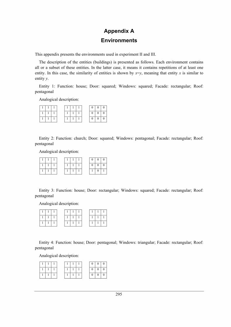
295
Appendix A Environments
This appendix presents the environments used in experiment II and III.
The description of the entities (buildings) is presented as follows. Each environment contains all or a subset of these entities. In the latter case, it means it contains repetitions of at least one entity. In this case, the similarity of entities is shown by x=y, meaning that entity x is similar to entity y.
Entity 1: Function: house; Door: squared; Windows: squared; Facade: rectangular; Roof: pentagonal
Analogical description:
Entity 2: Function: church; Door: squared; Windows: pentagonal; Facade: rectangular; Roof: pentagonal
Analogical description:
Entity 3: Function: house; Door: rectangular; Windows: squared; Facade: rectangular; Roof: pentagonal
Analogical description:
Entity 4: Function: house; Door: pentagonal; Windows: triangular; Facade: rectangular; Roof: pentagonal
Analogical description:
1 1 1
1 1 1
1 1 1
1 1 1
1 1 1
1 1 1
0 0 0
0 0 0
0 0 0
1 1 1
1 1 1
1 1 1
1 1 1
1 1 1
1 1 1
1 1 1
1 1 1
1 1 1
1 1 1
1 1 1
1 1 1
1 1 1
1 1 1
1 1 1
0 0 0
0 0 0
1 0 1
1 1 1
1 1 1
1 1 1
1 1 1
1 1 1
1 1 1
0 0 0
0 0 0
0 0 0
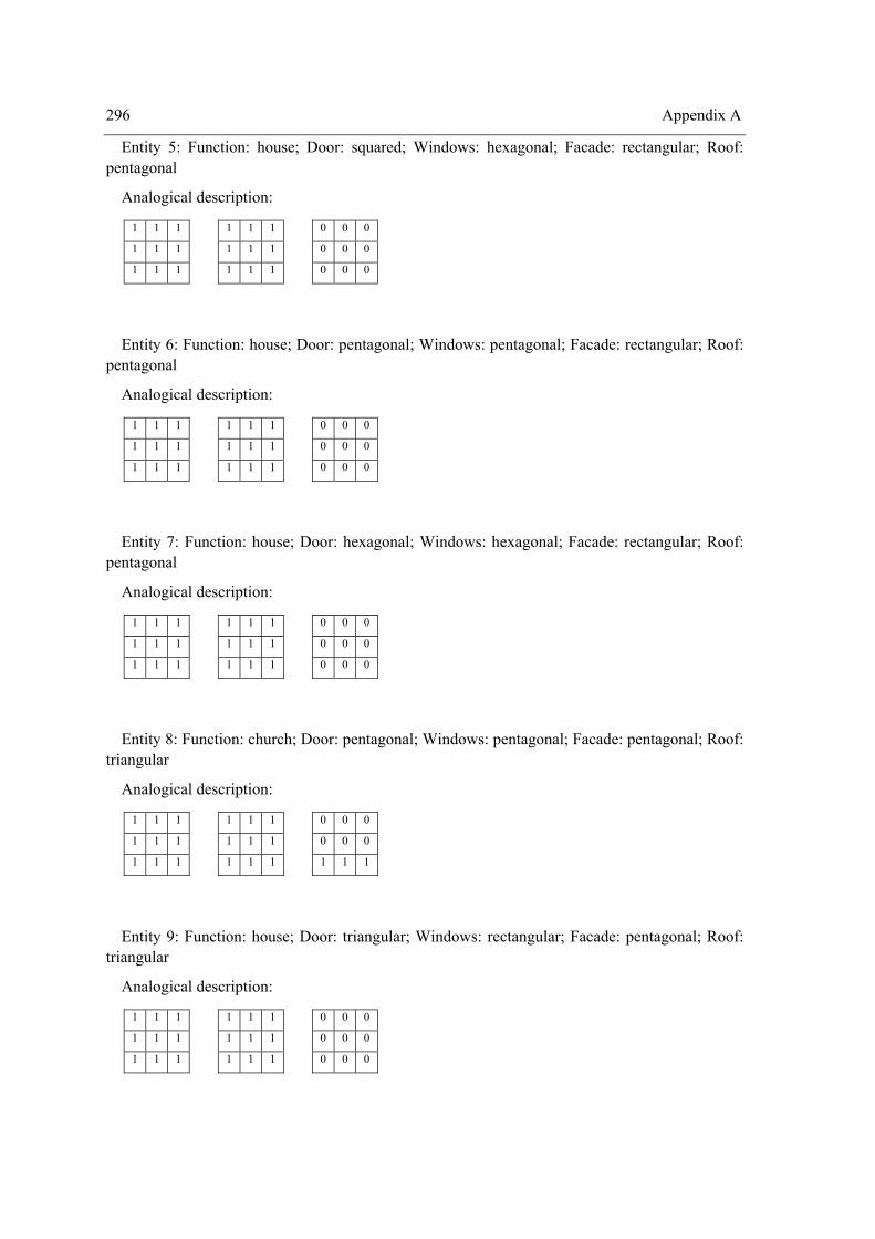
296 Appendix A
Entity 5: Function: house; Door: squared; Windows: hexagonal; Facade: rectangular; Roof: pentagonal
Analogical description:
Entity 6: Function: house; Door: pentagonal; Windows: pentagonal; Facade: rectangular; Roof: pentagonal
Analogical description:
Entity 7: Function: house; Door: hexagonal; Windows: hexagonal; Facade: rectangular; Roof: pentagonal
Analogical description:
Entity 8: Function: church; Door: pentagonal; Windows: pentagonal; Facade: pentagonal; Roof: triangular
Analogical description:
Entity 9: Function: house; Door: triangular; Windows: rectangular; Facade: pentagonal; Roof: triangular
Analogical description:
1 1 1
1 1 1
1 1 1
1 1 1
1 1 1
1 1 1
0 0 0
0 0 0
0 0 0
1 1 1
1 1 1
1 1 1
1 1 1
1 1 1
1 1 1
0 0 0
0 0 0
1 1 1
1 1 1
1 1 1
1 1 1
1 1 1
1 1 1
1 1 1
0 0 0
0 0 0
0 0 0
1 1 1
1 1 1
1 1 1
1 1 1
1 1 1
1 1 1
0 0 0
0 0 0
0 0 0
1 1 1
1 1 1
1 1 1
1 1 1
1 1 1
1 1 1
0 0 0
0 0 0
0 0 0
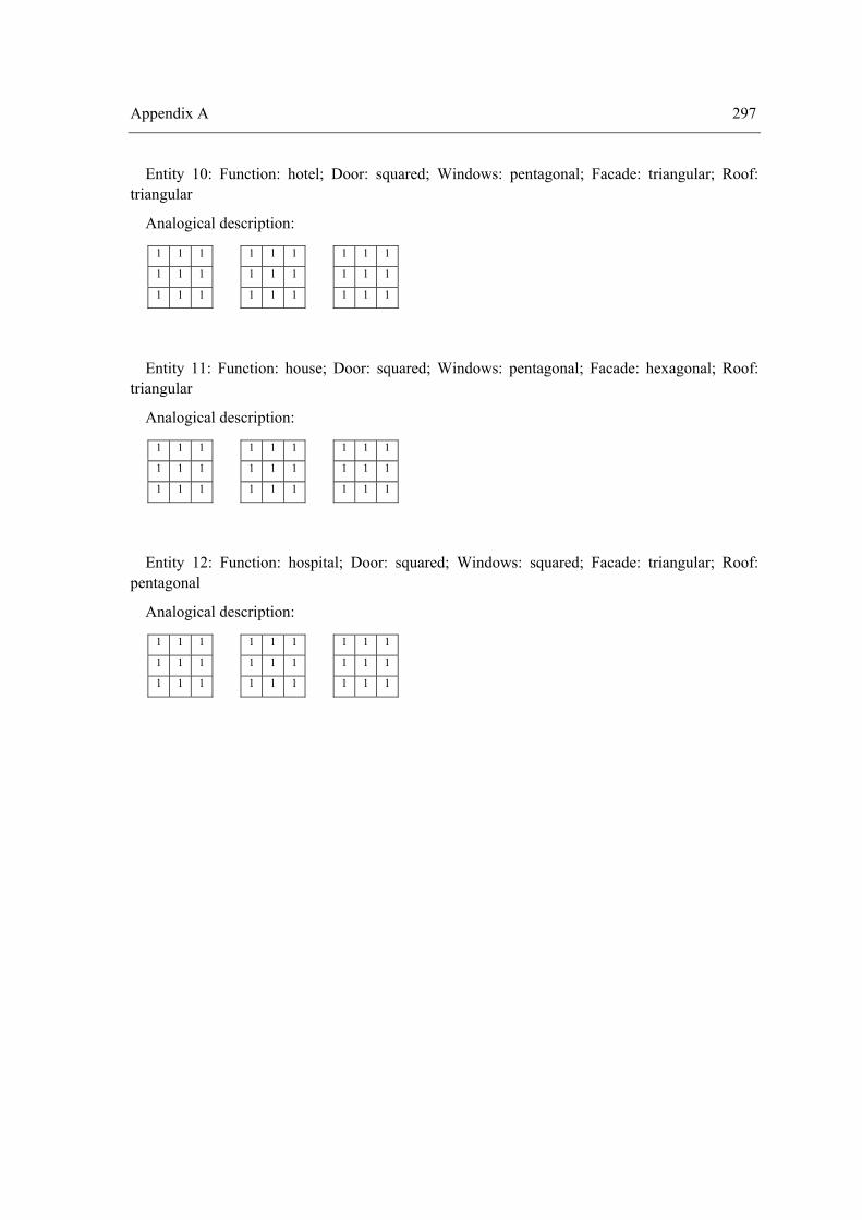
Appendix A 297
Entity 10: Function: hotel; Door: squared; Windows: pentagonal; Facade: triangular; Roof: triangular
Analogical description:
Entity 11: Function: house; Door: squared; Windows: pentagonal; Facade: hexagonal; Roof: triangular
Analogical description:
Entity 12: Function: hospital; Door: squared; Windows: squared; Facade: triangular; Roof: pentagonal
Analogical description:
1 1 1
1 1 1
1 1 1
1 1 1
1 1 1
1 1 1
1 1 1
1 1 1
1 1 1
1 1 1
1 1 1
1 1 1
1 1 1
1 1 1
1 1 1
1 1 1
1 1 1
1 1 1
1 1 1
1 1 1
1 1 1
1 1 1
1 1 1
1 1 1
1 1 1
1 1 1
1 1 1
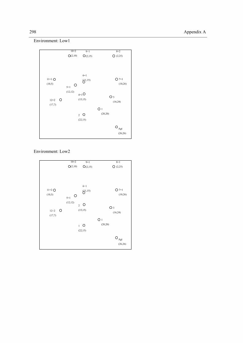
298 Appendix A
Environment: Low1
Environment: Low2
10=2
(2,10) 9=1
(2,15) 8=1
(2,25)
6=1
(11,15) 11=2
(10,5) 7=1
(10,26) 5=1
(12,12)
12=2
(17,7)
2
(15,15)
1
(20,20)
3
(16,24)
1
(22,15)
Agt
(26,26)
10=2
(2,10) 9=1
(2,15) 8=2
(2,25)
6=1
(11,15) 11=1
(10,5) 7=1
(10,26) 5=1
(12,12)
12=2
(17,7)
4=1
(15,15)
1
(20,20)
3
(16,24)
2
(22,15)
Agt
(26,26)
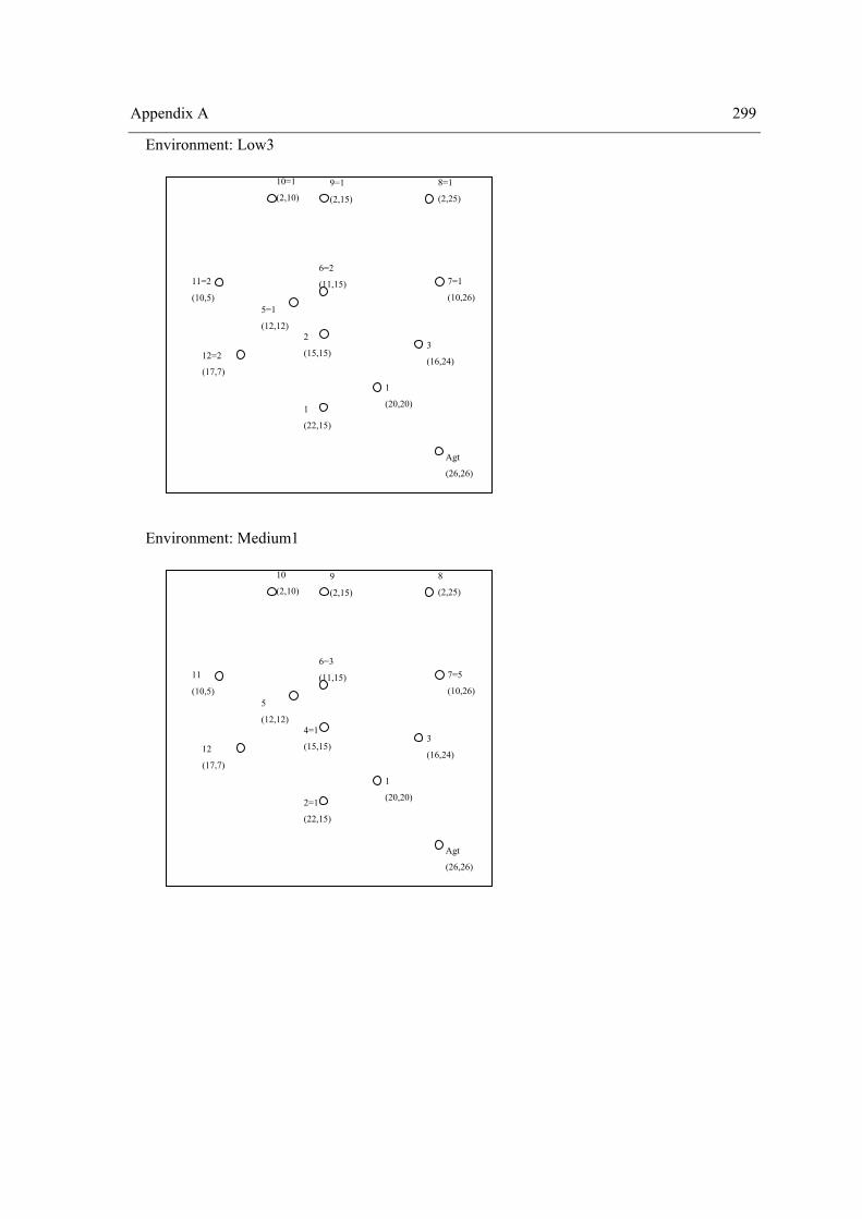
Appendix A 299
Environment: Low3
Environment: Medium1
10
(2,10) 9
(2,15) 8
(2,25)
6=3
(11,15) 11
(10,5) 7=5
(10,26) 5
(12,12)
12
(17,7)
4=1
(15,15)
1
(20,20)
3
(16,24)
2=1
(22,15)
Agt
(26,26)
10=1
(2,10) 9=1
(2,15) 8=1
(2,25)
6=2
(11,15) 11=2
(10,5) 7=1
(10,26) 5=1
(12,12)
12=2
(17,7)
2
(15,15)
1
(20,20)
3
(16,24)
1
(22,15)
Agt
(26,26)
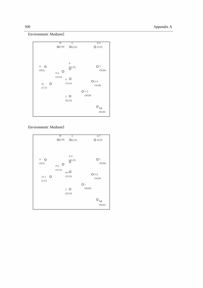
300 Appendix A
Environment: Medium2
Environment: Medium3
10
(2,10) 9
(2,15) 8=7
(2,25)
6=2
(11,15) 11
(10,5) 7
(10,26) 5=2
(12,12)
12=1
(17,7)
4=1
(15,15)
1
(20,20)
3=2
(16,24)
2
(22,15)
Agt
(26,26)
10
(2,10) 9
(2,15) 8=2
(2,25)
6
(11,15) 11
(10,5) 7
(10,26) 5=4
(12,12)
12
(17,7)
4
(15,15)
1=2
(20,20)
3=2
(16,24)
2
(22,15)
Agt
(26,26)
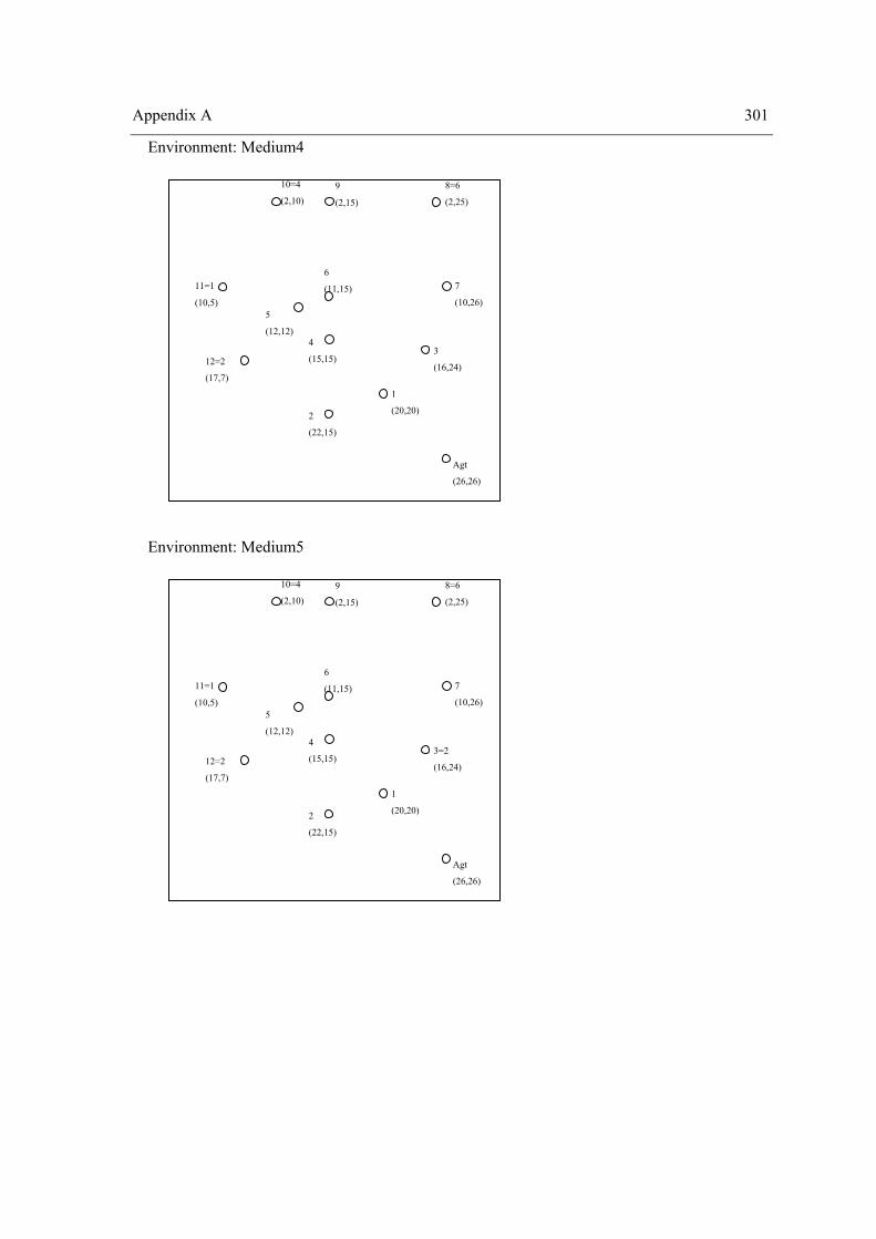
Appendix A 301
Environment: Medium4
Environment: Medium5
10=4
(2,10) 9
(2,15) 8=6
(2,25)
6
(11,15) 11=1
(10,5) 7
(10,26) 5
(12,12)
12=2
(17,7)
4
(15,15)
1
(20,20)
3=2
(16,24)
2
(22,15)
Agt
(26,26)
10=4
(2,10) 9
(2,15) 8=6
(2,25)
6
(11,15) 11=1
(10,5) 7
(10,26) 5
(12,12)
12=2
(17,7)
4
(15,15)
1
(20,20)
3
(16,24)
2
(22,15)
Agt
(26,26)
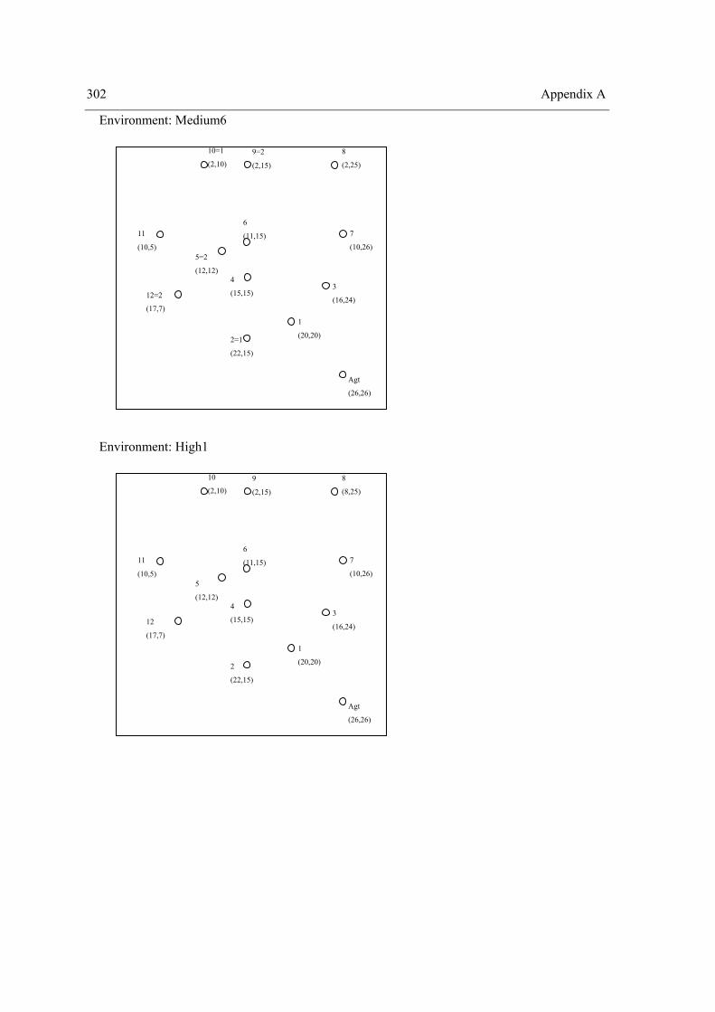
302 Appendix A
Environment: Medium6
Environment: High1
10
(2,10) 9
(2,15) 8
(8,25)
6
(11,15) 11
(10,5) 7
(10,26) 5
(12,12)
12
(17,7)
4
(15,15)
1
(20,20)
3
(16,24)
2
(22,15)
Agt
(26,26)
10=1
(2,10) 9=2
(2,15) 8
(2,25)
6
(11,15) 11
(10,5) 7
(10,26) 5=2
(12,12)
12=2
(17,7)
4
(15,15)
1
(20,20)
3
(16,24)
2=1
(22,15)
Agt
(26,26)
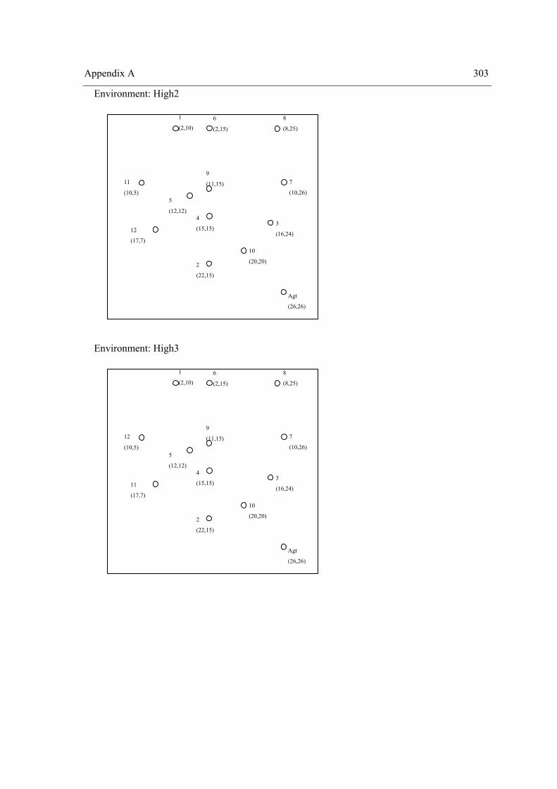
Appendix A 303
Environment: High2
Environment: High3
1
(2,10) 6
(2,15) 8
(8,25)
9
(11,15) 12
(10,5) 7
(10,26) 5
(12,12)
11
(17,7)
4
(15,15)
10
(20,20)
3
(16,24)
2
(22,15)
Agt
(26,26)
1
(2,10) 6
(2,15) 8
(8,25)
9
(11,15) 11
(10,5) 7
(10,26) 5
(12,12)
12
(17,7)
4
(15,15)
10
(20,20)
3
(16,24)
2
(22,15)
Agt
(26,26)


305
Appendix B SPSS outputs of Experiment II
This appendix presents the SPSS outputs of Experiment II. Because of the extension of these outputs, the contents of this appendix are included in the CD attached to this thesis.

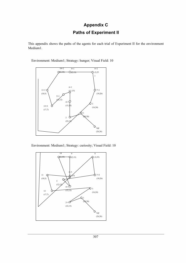
307
Appendix C Paths of Experiment II
This appendix shows the paths of the agents for each trial of Experiment II for the environment Medium1.
Environment: Medium1; Strategy: hunger; Visual Field: 10
Environment: Medium1; Strategy: curiosity; Visual Field: 10
10
(2,10) 9
(2,15) 8
(2,25)
6=3
(11,15) 11
(10,5) 7=5
(10,26) 5
(12,12)
12
(17,7)
4=1
(15,15)
1
(20,20)
3
(16,24)
2=1
(22,15)
Agt
(26,26)
10=2
(2,10) 9=1
(2,15) 8=2
(2,25
)
6=1
(11,15) 11=1
(10,5) 7=1
(10,26) 5=1
(12,12)
12=2
(17,7)
4=1
(15,15)
1
(20,20)
3
(16,24)
2
(22,15)
Agt
(26,26)
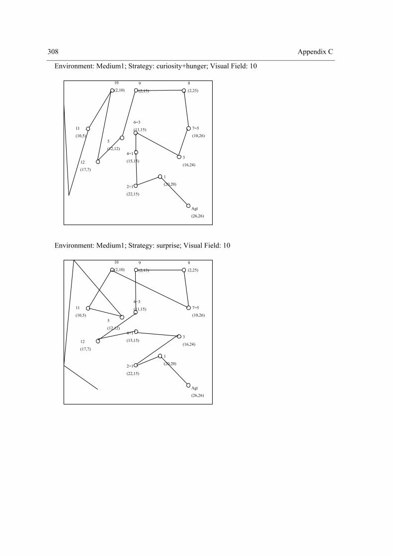
308 Appendix C
Environment: Medium1; Strategy: curiosity+hunger; Visual Field: 10
Environment: Medium1; Strategy: surprise; Visual Field: 10
10
(2,10) 9
(2,15) 8
(2,25)
6=3
(11,15) 11
(10,5) 7=5
(10,26) 5
(12,12)
12
(17,7)
4=1
(15,15)
1
(20,20)
3
(16,24)
2=1
(22,15)
Agt
(26,26)
10
(2,10) 9
(2,15) 8
(2,25)
6=3
(11,15) 11
(10,5) 7=5
(10,26) 5
(12,12)
12
(17,7)
4=1
(15,15)
1
(20,20)
3
(16,24)
2=1
(22,15)
Agt
(26,26)
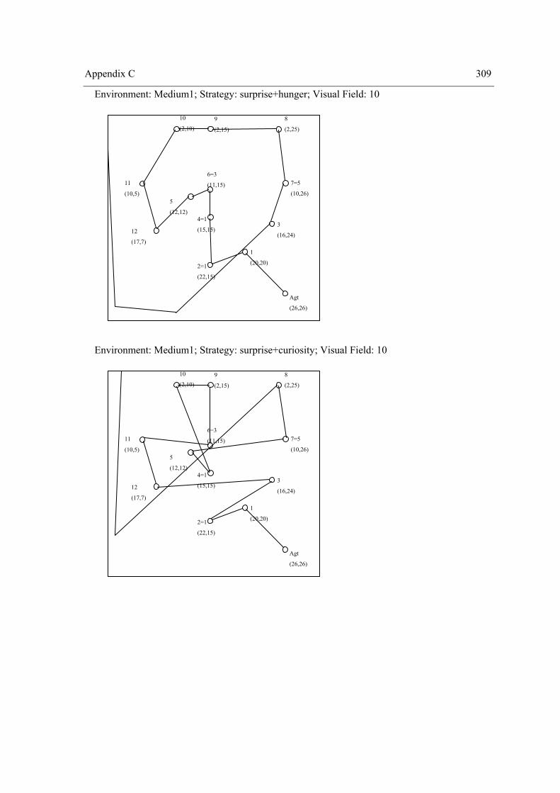
Appendix C 309
Environment: Medium1; Strategy: surprise+hunger; Visual Field: 10
Environment: Medium1; Strategy: surprise+curiosity; Visual Field: 10
10
(2,10) 9
(2,15) 8
(2,25)
6=3
(11,15) 11
(10,5) 7=5
(10,26) 5
(12,12)
12
(17,7)
4=1
(15,15)
1
(20,20)
3
(16,24)
2=1
(22,15)
Agt
(26,26)
10
(2,10) 9
(2,15) 8
(2,25)
6=3
(11,15) 11
(10,5) 7=5
(10,26) 5
(12,12)
12
(17,7)
4=1
(15,15)
1
(20,20)
3
(16,24)
2=1
(22,15)
Agt
(26,26)
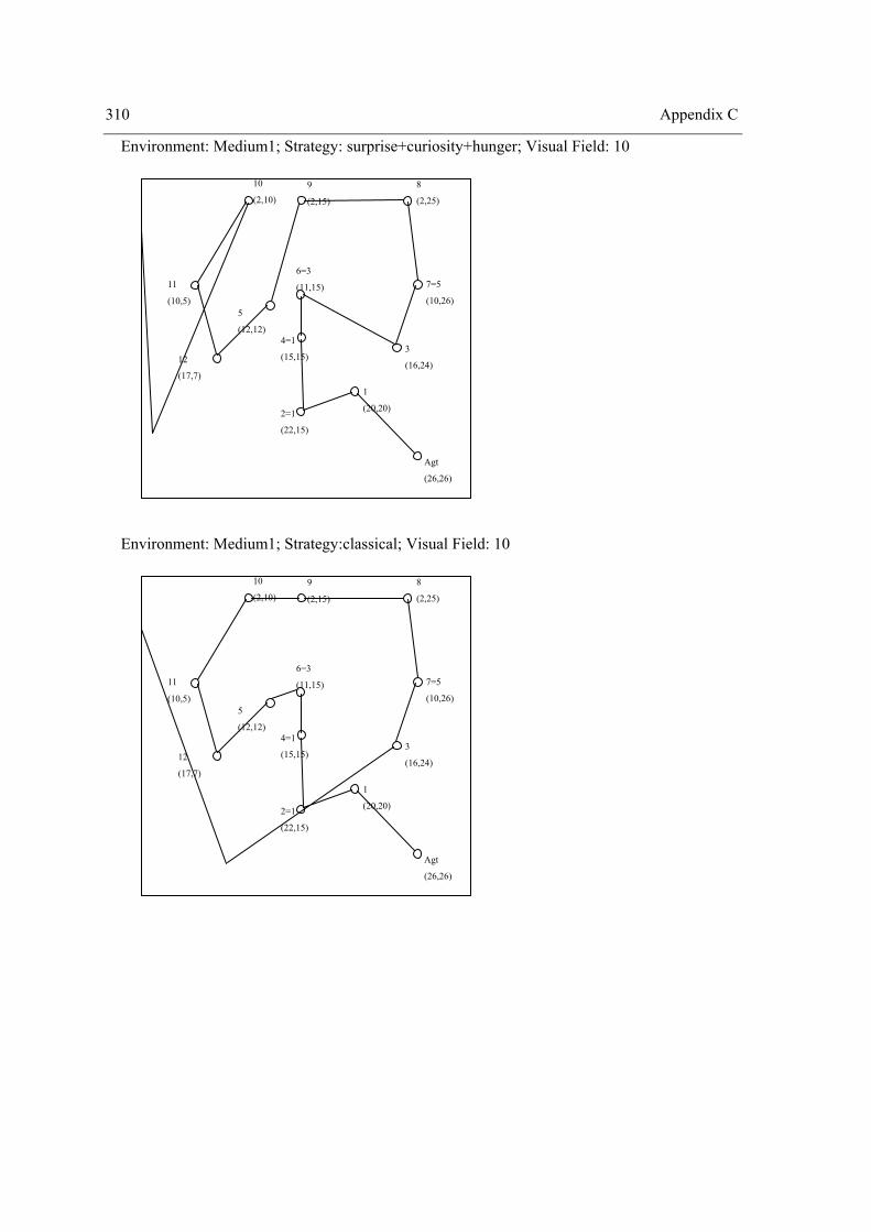
310 Appendix C
Environment: Medium1; Strategy: surprise+curiosity+hunger; Visual Field: 10
Environment: Medium1; Strategy:classical; Visual Field: 10
10
(2,10) 9
(2,15) 8
(2,25)
6=3
(11,15) 11
(10,5) 7=5
(10,26) 5
(12,12)
12
(17,7)
4=1
(15,15)
1
(20,20)
3
(16,24)
2=1
(22,15)
Agt
(26,26)
10
(2,10) 9
(2,15) 8
(2,25)
6=3
(11,15) 11
(10,5) 7=5
(10,26) 5
(12,12)
12
(17,7)
4=1
(15,15)
1
(20,20)
3
(16,24)
2=1
(22,15)
Agt
(26,26)
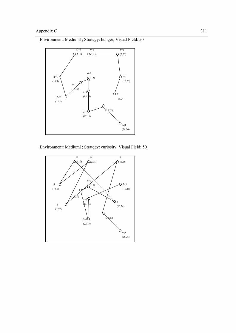
Appendix C 311
Environment: Medium1; Strategy: hunger; Visual Field: 50
Environment: Medium1; Strategy: curiosity; Visual Field: 50
10
(2,10) 9
(2,15) 8
(2,25)
6=3
(11,15) 11
(10,5) 7=5
(10,26) 5
(12,12)
12
(17,7)
4=1
(15,15)
1
(20,20)
3
(16,24)
2=1
(22,15)
Agt
(26,26)
10=2
(2,10) 9=1
(2,15) 8=2
(2,25)
6=1
(11,15) 11=1
(10,5) 7=1
(10,26) 5=1
(12,12)
12=2
(17,7)
4=1
(15,15)
1
(20,20)
3
(16,24)
2
(22,15)
Agt
(26,26)
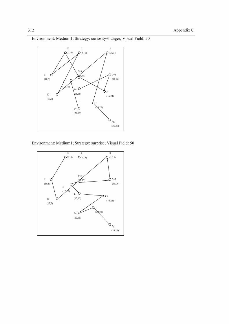
312 Appendix C
Environment: Medium1; Strategy: curiosity+hunger; Visual Field: 50
Environment: Medium1; Strategy: surprise; Visual Field: 50
10
(2,10) 9
(2,15) 8
(2,25)
6=3
(11,15) 11
(10,5) 7=5
(10,26) 5
(12,12)
12
(17,7)
4=1
(15,15)
1
(20,20)
3
(16,24)
2=1
(22,15)
Agt
(26,26)
10
(2,10) 9
(2,15) 8
(2,25)
6=3
(11,15) 11
(10,5) 7=5
(10,26) 5
(12,12)
12
(17,7)
4=1
(15,15)
1
(20,20)
3
(16,24)
2=1
(22,15)
Agt
(26,26)
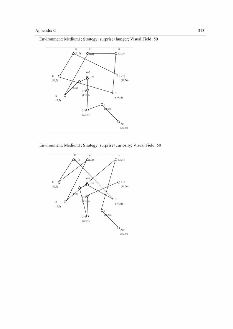
Appendix C 313
Environment: Medium1; Strategy: surprise+hunger; Visual Field: 50
Environment: Medium1; Strategy: surprise+curiosity; Visual Field: 50
10
(2,10) 9
(2,15) 8
(2,25)
6=3
(11,15) 11
(10,5) 7=5
(10,26) 5
(12,12)
12
(17,7)
4=1
(15,15)
1
(20,20)
3
(16,24)
2=1
(22,15)
Agt
(26,26)
10
(2,10) 9
(2,15) 8
(2,25)
6=3
(11,15) 11
(10,5) 7=5
(10,26) 5
(12,12)
12
(17,7)
4=1
(15,15)
1
(20,20)
3
(16,24)
2=1
(22,15)
Agt
(26,26)
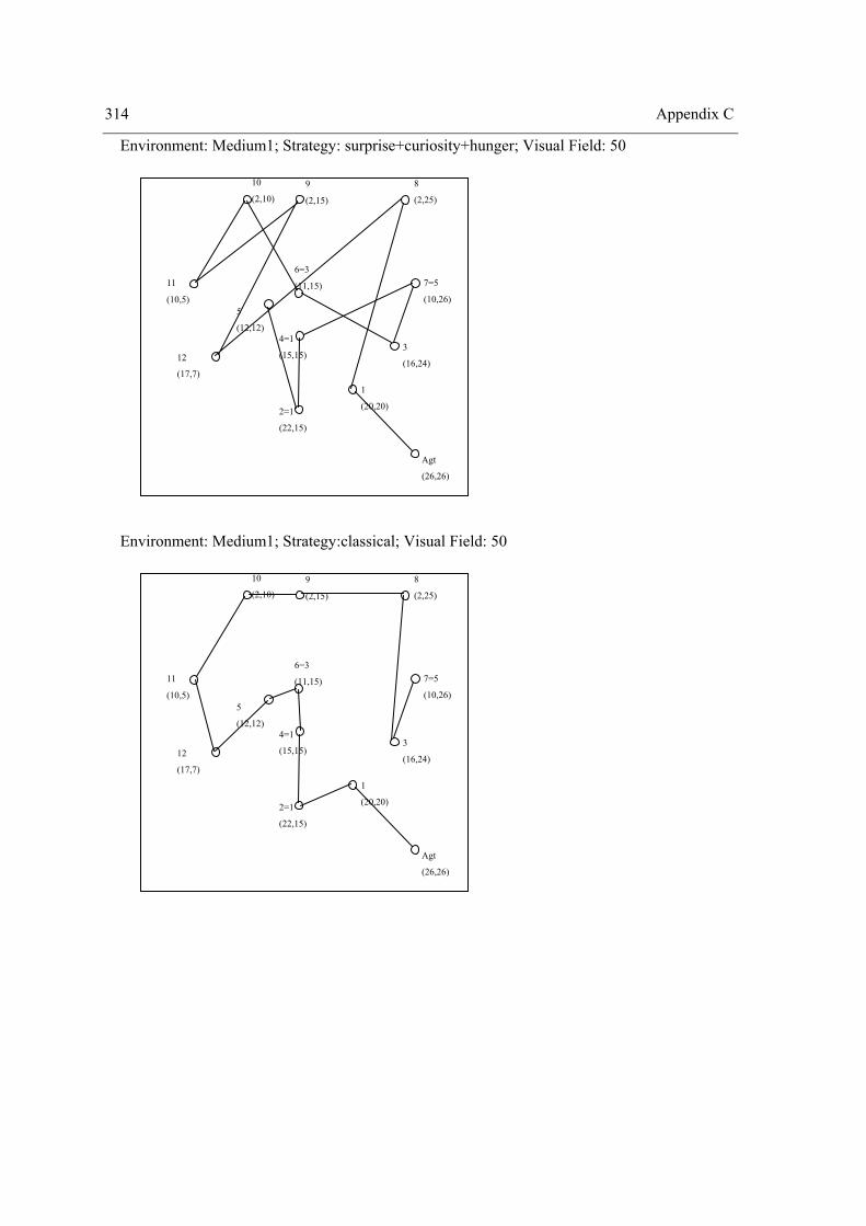
314 Appendix C
Environment: Medium1; Strategy: surprise+curiosity+hunger; Visual Field: 50
Environment: Medium1; Strategy:classical; Visual Field: 50
10
(2,10) 9
(2,15) 8
(2,25)
6=3
(11,15) 11
(10,5) 7=5
(10,26) 5
(12,12)
12
(17,7)
4=1
(15,15)
1
(20,20)
3
(16,24)
2=1
(22,15)
Agt
(26,26)
10
(2,10) 9
(2,15) 8
(2,25)
6=3
(11,15) 11
(10,5) 7=5
(10,26) 5
(12,12)
12
(17,7)
4=1
(15,15)
1
(20,20)
3
(16,24)
2=1
(22,15)
Agt
(26,26)