dynamic robot walking on unknown terrain - mediatum

Technische Universität München

TUM School of Engineering and Design

Dynamic Robot Walking on Unknown Terrain:

Stabilization and Multi-Contact Control of Biped Robots

in Uncertain Environments

Felix Simon Sygulla

Vollständiger Abdruck der von der TUM School of Engineering and Design der Technischen Universität

München zur Erlangung eines

Doktors der Ingenieurwissenschaften (Dr.-Ing.)

genehmigten Dissertation.

Vorsitz: Prof. Dr.-Ing. Boris Lohmann

Prüfer*innen der Dissertation:

1. Prof. dr.ir. Daniel J. Rixen

2. Prof. Abderrahmane Kheddar

Die Dissertation wurde am 24. Juni 2021 bei der Technischen Universität München eingereicht und durch

die TUM School of Engineering and Design am 29. November 2021 angenommen.

Abstract

The main advantage of anthropomorphic robots is their adaptability to environments builtfor humans. For walking robots, robustness to uneven terrain is essential to exploit theseadvantages. Although current approaches often use the full multi-body dynamics, the exe-cuted motions over uneven terrain are often only quasi-static, i.e., correspondingly slow. Thisthesis deals with reduced control approaches to answer which level of detail of the models isnecessary for dynamic walking over uneven ground.

In this thesis, a tactile sensor prototype for measuring contact surfaces is proposed and ex-perimentally evaluated. Also, this work proposes contributions for balance control strategiesthat consider the robot’s structural eigenfrequencies and centroidal dynamics. Furthermore,force-control concepts for contacts with the environment are presented, which exhibit robuststability to uncertain mechanical contact properties. On the one hand, the approaches tol-erate uncertainty in the timing, stiffness, and geometry of the contacts. On the other hand,they also adapt to unexpected parameters based on the measured contact surface and contactforces. Both hand and foot contacts are considered to support multi-contact locomotion onrugged terrain. Other parts of this thesis deal with software modules and architectures forbiped robots and a hardware layer design. In addition, a machine-learning-based tool forintelligent robot system testing is presented.

All methods are evaluated on the bipedal robot LOLA both for normal walking and multi-contact locomotion experiments. The results show high robustness to undetected uneventerrain, unknown ground-height changes, and unexpectedly soft ground using the proposedcontrol schemes with reduced dynamic models. The achieved walking speed on unevenand soft terrain is significantly higher than for state-of-the-art bipeds. Moreover, the resultsshow that high-quality hardware and software/hardware integration in humanoid roboticsare essential to achieve high overall system performance.

Acknowledgments

This thesis results from my research work at the Chair of Applied Mechanics, Technical Uni-versity of Munich between 2015 and 2021. I want to express my gratitude to the many peoplewho supported, inspired, and assisted me during the project.

First of all, I thank my supervisor Prof. dr. ir. Daniel Rixen for his trust and for giving methe great opportunity of working on LOLA. I am grateful for the freedom he gave me in myresearch and his constant interest and support. The good working atmosphere at the Chair ismainly due to his uncomplicated and cooperative working style.

During my time at the Chair, I have worked with many highly talented and motivatedindividuals. The very collegial and friendly spirit was a true enrichment. I want to thank allcolleagues for their support, the numerous professional and personal conversations, and thefriendships that extended well beyond life at university.

I was lucky to work with and learn from three generations of LOLA Ph.D. students duringmy time. I’ll never forget the fruitful discussions, various hours in the lab, and the ups anddowns of the project we have experienced together. It is virtually impossible to work alone ona machine as complex as LOLA, which is why I am particularly grateful for the ever-reliablesupport of the LOLA team members. My thanks go to Robert Wittmann, Arne-ChristophHildebrandt, Daniel Wahrmann, Philipp Seiwald, Nora-Sophie Staufenberg and Moritz Sat-tler. Special thanks are devoted to Philipp Seiwald, with whom I spent most of the timemaintaining and improving LOLA. This thesis is unthinkable without his support and greatcommitment to the project. This is also the place to thank the German Research Foundation(DFG) for funding the project "Adaptive Walking through Multi-Contact Stabilization", grant#407378162; it also supported the research presented in this thesis.

I want to thank Christoph Schütz, Tobias Berninger, and Felix Ellensohn from the Chair’srobotics research group for the fruitful discussions and joint research. Furthermore, I amgrateful to my mentor Thomas Buschmann, who always had time for technical discussionson LOLA and beyond.

The electrical and mechanical workshops at the Chair are especially valuable for the pro-duction and maintenance of robots. I want to thank Georg Mayr and Andreas Köstler fordesigning numerous electronic components, laying and repairing many cables, and alwaysbeing ready to help with electrical problems of any kind. I further thank Georg König forbuilding the great and challenging walls and terrain boards used in this thesis and SimonGerer for manufacturing the required spare parts.

Numerous student projects supported the research of the LOLA project. I want to thank allof my students for the commitment to the project and the fruitful scientific discourse. Finally,I would like to thank Philipp, Moritz, Nora-Sophie, and Kira for proofreading this thesis andgiving valuable advice.

Contents

Glossary xi

1 Introduction 1

1.1 State of the Art: An Overview . . . . . . . . . . . . . . . . . . . . . . . . . . . . . . . 21.2 Objectives and Outline . . . . . . . . . . . . . . . . . . . . . . . . . . . . . . . . . . . 71.3 Notation and Videos . . . . . . . . . . . . . . . . . . . . . . . . . . . . . . . . . . . . . 8

2 Platform Mechatronics 9

2.1 Mechatronic Design Overview . . . . . . . . . . . . . . . . . . . . . . . . . . . . . . . 92.1.1 Design Revisions of LOLA . . . . . . . . . . . . . . . . . . . . . . . . . . . . . 92.1.2 Current Design . . . . . . . . . . . . . . . . . . . . . . . . . . . . . . . . . . . . 11

2.2 EtherCAT-based Real-Time Hardware Layer . . . . . . . . . . . . . . . . . . . . . . 152.2.1 Software Architecture . . . . . . . . . . . . . . . . . . . . . . . . . . . . . . . 162.2.2 Software Integration and Timing . . . . . . . . . . . . . . . . . . . . . . . . 192.2.3 Communication with the Bus Slaves . . . . . . . . . . . . . . . . . . . . . . 202.2.4 System Performance . . . . . . . . . . . . . . . . . . . . . . . . . . . . . . . . 212.2.5 Related Work . . . . . . . . . . . . . . . . . . . . . . . . . . . . . . . . . . . . . 22

2.3 A Flexible and Low-Cost Tactile Sensor for Robots . . . . . . . . . . . . . . . . . . 242.3.1 Design Overview . . . . . . . . . . . . . . . . . . . . . . . . . . . . . . . . . . 252.3.2 Sensor Prototypes . . . . . . . . . . . . . . . . . . . . . . . . . . . . . . . . . . 262.3.3 Experimental Results . . . . . . . . . . . . . . . . . . . . . . . . . . . . . . . . 272.3.4 Related Work . . . . . . . . . . . . . . . . . . . . . . . . . . . . . . . . . . . . . 312.3.5 Discussion & Summary . . . . . . . . . . . . . . . . . . . . . . . . . . . . . . 32

2.4 A Tactile Foot Design . . . . . . . . . . . . . . . . . . . . . . . . . . . . . . . . . . . . 332.4.1 Mechanical Concept . . . . . . . . . . . . . . . . . . . . . . . . . . . . . . . . 342.4.2 Sensor Concept and Contact Material . . . . . . . . . . . . . . . . . . . . . 342.4.3 Design Proposal . . . . . . . . . . . . . . . . . . . . . . . . . . . . . . . . . . . 352.4.4 Related Work . . . . . . . . . . . . . . . . . . . . . . . . . . . . . . . . . . . . . 36

2.5 Chapter Summary . . . . . . . . . . . . . . . . . . . . . . . . . . . . . . . . . . . . . . 36

3 Real-Time Walking Control 39

3.1 The Dynamics of Biped Robots . . . . . . . . . . . . . . . . . . . . . . . . . . . . . . 393.1.1 Feasibility of Motions . . . . . . . . . . . . . . . . . . . . . . . . . . . . . . . . 403.1.2 Stability of Motions . . . . . . . . . . . . . . . . . . . . . . . . . . . . . . . . . 42

3.2 Control Structure Overview . . . . . . . . . . . . . . . . . . . . . . . . . . . . . . . . 443.3 Previous Work on LOLA . . . . . . . . . . . . . . . . . . . . . . . . . . . . . . . . . . . 463.4 Frames of Reference and Task-Space Definition . . . . . . . . . . . . . . . . . . . . 47

3.4.1 Frames of Reference . . . . . . . . . . . . . . . . . . . . . . . . . . . . . . . . 483.4.2 Task-Space Definition . . . . . . . . . . . . . . . . . . . . . . . . . . . . . . . 483.4.3 Task-Space Trajectory Modification . . . . . . . . . . . . . . . . . . . . . . . 50

3.5 Walking Pattern Generation . . . . . . . . . . . . . . . . . . . . . . . . . . . . . . . . 51

vii

viii Contents

3.6 Sensor Data Preprocessing . . . . . . . . . . . . . . . . . . . . . . . . . . . . . . . . . 533.6.1 Floating-Base Inclination . . . . . . . . . . . . . . . . . . . . . . . . . . . . . 533.6.2 Contact Transition Detection . . . . . . . . . . . . . . . . . . . . . . . . . . . 543.6.3 Force Control Activation . . . . . . . . . . . . . . . . . . . . . . . . . . . . . . 56

3.7 Reactive Trajectory Adaptation . . . . . . . . . . . . . . . . . . . . . . . . . . . . . . 583.7.1 Early Contact Reflex . . . . . . . . . . . . . . . . . . . . . . . . . . . . . . . . 583.7.2 Swing Foot Adaptation . . . . . . . . . . . . . . . . . . . . . . . . . . . . . . . 62

3.8 Feedback Stabilization . . . . . . . . . . . . . . . . . . . . . . . . . . . . . . . . . . . . 633.8.1 Control System Plants . . . . . . . . . . . . . . . . . . . . . . . . . . . . . . . 643.8.2 Onboard Plant Estimation . . . . . . . . . . . . . . . . . . . . . . . . . . . . . 64

3.9 Inverse and Direct Kinematics . . . . . . . . . . . . . . . . . . . . . . . . . . . . . . . 663.10 Chapter Summary . . . . . . . . . . . . . . . . . . . . . . . . . . . . . . . . . . . . . . 68

4 Balance Control 69

4.1 Previous Work on LOLA . . . . . . . . . . . . . . . . . . . . . . . . . . . . . . . . . . . 694.2 Inclination Control . . . . . . . . . . . . . . . . . . . . . . . . . . . . . . . . . . . . . . 70

4.2.1 Basic Control Scheme . . . . . . . . . . . . . . . . . . . . . . . . . . . . . . . 714.2.2 The Effect of Structural Resonances on Inclination Control . . . . . . . . 724.2.3 Filter-Based Resonance Rejection . . . . . . . . . . . . . . . . . . . . . . . . 734.2.4 Time-Domain Passivity Control . . . . . . . . . . . . . . . . . . . . . . . . . 754.2.5 Experimental Comparison . . . . . . . . . . . . . . . . . . . . . . . . . . . . . 764.2.6 Discussion in the Context of Related Work . . . . . . . . . . . . . . . . . . 77

4.3 Optimal Contact Wrench Distribution . . . . . . . . . . . . . . . . . . . . . . . . . . 804.3.1 Prerequisites . . . . . . . . . . . . . . . . . . . . . . . . . . . . . . . . . . . . . 804.3.2 Problem Formulation . . . . . . . . . . . . . . . . . . . . . . . . . . . . . . . . 824.3.3 Implementation . . . . . . . . . . . . . . . . . . . . . . . . . . . . . . . . . . . 834.3.4 Experimental Comparison . . . . . . . . . . . . . . . . . . . . . . . . . . . . . 844.3.5 Discussion in the Context of Related Work . . . . . . . . . . . . . . . . . . 85

4.4 Vertical Center of Mass Tracking . . . . . . . . . . . . . . . . . . . . . . . . . . . . . 864.5 Vertical Center of Mass Acceleration . . . . . . . . . . . . . . . . . . . . . . . . . . . 87

4.5.1 Control Approach . . . . . . . . . . . . . . . . . . . . . . . . . . . . . . . . . . 884.5.2 Late-Contact Foot Acceleration . . . . . . . . . . . . . . . . . . . . . . . . . . 904.5.3 Experimental Validation . . . . . . . . . . . . . . . . . . . . . . . . . . . . . . 904.5.4 Discussion in the Context of Related Work . . . . . . . . . . . . . . . . . . 92

4.6 Chapter Summary . . . . . . . . . . . . . . . . . . . . . . . . . . . . . . . . . . . . . . 95

5 Contact Force Control 97

5.1 Previous Work on LOLA . . . . . . . . . . . . . . . . . . . . . . . . . . . . . . . . . . . 975.2 Ground Reaction Force Control . . . . . . . . . . . . . . . . . . . . . . . . . . . . . . 98

5.2.1 Explicit Contact Model in Task-Space . . . . . . . . . . . . . . . . . . . . . . 985.2.2 Influences from Unilateral Contact Dynamics . . . . . . . . . . . . . . . . 1025.2.3 Robust Hybrid Force/Motion Control Approach . . . . . . . . . . . . . . . 1045.2.4 Robust Stability Analysis . . . . . . . . . . . . . . . . . . . . . . . . . . . . . 1055.2.5 Extension via Lag Reduction . . . . . . . . . . . . . . . . . . . . . . . . . . . 1075.2.6 Time-Integration and Tuning . . . . . . . . . . . . . . . . . . . . . . . . . . . 1085.2.7 Experimental Validation . . . . . . . . . . . . . . . . . . . . . . . . . . . . . . 1105.2.8 Discussion in the Context of Related Work . . . . . . . . . . . . . . . . . . 111

5.3 Sensor-Based Contact Model Updating . . . . . . . . . . . . . . . . . . . . . . . . . 1125.3.1 Control Concept . . . . . . . . . . . . . . . . . . . . . . . . . . . . . . . . . . . 1125.3.2 Contact Surface Estimation . . . . . . . . . . . . . . . . . . . . . . . . . . . . 1135.3.3 Limitations & Implementation . . . . . . . . . . . . . . . . . . . . . . . . . . 115

Contents ix

5.3.4 Experimental Validation . . . . . . . . . . . . . . . . . . . . . . . . . . . . . . 1155.3.5 Discussion in the Context of Related Work . . . . . . . . . . . . . . . . . . 1185.3.6 Contact Surface Estimation using a Tactile Foot Sole . . . . . . . . . . . . 119

5.4 Adaptive Contact Force Control . . . . . . . . . . . . . . . . . . . . . . . . . . . . . . 1205.4.1 Reference Model . . . . . . . . . . . . . . . . . . . . . . . . . . . . . . . . . . 1205.4.2 Uncertain Plant Description . . . . . . . . . . . . . . . . . . . . . . . . . . . 1225.4.3 Adaptive Control Law . . . . . . . . . . . . . . . . . . . . . . . . . . . . . . . 1235.4.4 Adaptive Control with Sensor-Based Contact Model Updating . . . . . . 1245.4.5 Experimental Validation . . . . . . . . . . . . . . . . . . . . . . . . . . . . . . 1255.4.6 Discussion in the Context of Related Work . . . . . . . . . . . . . . . . . . 128

5.5 Multi-Contact Force Control . . . . . . . . . . . . . . . . . . . . . . . . . . . . . . . . 1305.5.1 Control Approach . . . . . . . . . . . . . . . . . . . . . . . . . . . . . . . . . . 1305.5.2 Experimental Validation . . . . . . . . . . . . . . . . . . . . . . . . . . . . . . 1315.5.3 Discussion in the Context of Related Work . . . . . . . . . . . . . . . . . . 132

5.6 Chapter Summary . . . . . . . . . . . . . . . . . . . . . . . . . . . . . . . . . . . . . . 133

6 Software Architecture and System Testing 135

6.1 Previous Work on LOLA . . . . . . . . . . . . . . . . . . . . . . . . . . . . . . . . . . . 1366.2 The Broccoli Library . . . . . . . . . . . . . . . . . . . . . . . . . . . . . . . . . . . . . 1376.3 Stabilization and Inverse Kinematics Application . . . . . . . . . . . . . . . . . . . 1396.4 Further Software Enhancements . . . . . . . . . . . . . . . . . . . . . . . . . . . . . 1416.5 Learning the Noise of Failure: NoisyTest . . . . . . . . . . . . . . . . . . . . . . . . 142

6.5.1 Simulation Environment and Dataset . . . . . . . . . . . . . . . . . . . . . 1436.5.2 Noise-Related Feature-Extraction . . . . . . . . . . . . . . . . . . . . . . . . 1436.5.3 Failure Symptoms and Scenarios . . . . . . . . . . . . . . . . . . . . . . . . 1446.5.4 Signal Preprocessing . . . . . . . . . . . . . . . . . . . . . . . . . . . . . . . . 1466.5.5 Classification via Support Vector Machine . . . . . . . . . . . . . . . . . . . 1496.5.6 Results . . . . . . . . . . . . . . . . . . . . . . . . . . . . . . . . . . . . . . . . . 1506.5.7 Discussion in the Context of Related Work . . . . . . . . . . . . . . . . . . 152

6.6 Chapter Summary . . . . . . . . . . . . . . . . . . . . . . . . . . . . . . . . . . . . . . 153

7 Performance Evaluation 155

7.1 Inclined Uneven Terrain . . . . . . . . . . . . . . . . . . . . . . . . . . . . . . . . . . 1557.2 Ground Height Changes . . . . . . . . . . . . . . . . . . . . . . . . . . . . . . . . . . 1567.3 Hard and Soft Ground . . . . . . . . . . . . . . . . . . . . . . . . . . . . . . . . . . . . 1577.4 Multi-Contact Balancing . . . . . . . . . . . . . . . . . . . . . . . . . . . . . . . . . . 1587.5 Discussion . . . . . . . . . . . . . . . . . . . . . . . . . . . . . . . . . . . . . . . . . . . 1597.6 Chapter Summary . . . . . . . . . . . . . . . . . . . . . . . . . . . . . . . . . . . . . . 162

8 Closure 163

8.1 Contributions of this Thesis . . . . . . . . . . . . . . . . . . . . . . . . . . . . . . . . 1638.2 Conclusions . . . . . . . . . . . . . . . . . . . . . . . . . . . . . . . . . . . . . . . . . . 1648.3 Recommendations for Future Work . . . . . . . . . . . . . . . . . . . . . . . . . . . 167

A Notation and Fundamentals 171

A.1 Frames of Reference . . . . . . . . . . . . . . . . . . . . . . . . . . . . . . . . . . . . . 171A.2 Rotations in 3D . . . . . . . . . . . . . . . . . . . . . . . . . . . . . . . . . . . . . . . . 171A.3 Digital Filter Implementations . . . . . . . . . . . . . . . . . . . . . . . . . . . . . . . 175A.4 Task-Space Operators . . . . . . . . . . . . . . . . . . . . . . . . . . . . . . . . . . . . 176A.5 Control Schemes . . . . . . . . . . . . . . . . . . . . . . . . . . . . . . . . . . . . . . . 177

x Contents

B Joint Control Settings & Bus Topology 179

C Identified Plants 183

D Manufacturing Steps Tactile Sensor 187

Bibliography 191

Co-authored Publications 215

Supervised Student Theses 217

Glossary

Acronyms

SVM Support Vector MachineFT Force/TorqueCoM Center of MassIMU Inertial Measurement UnitCAN Controller Area NetworkZMP Zero Moment PointFZMP Fictious Zero Moment PointFRI Foot Rotation IndicatorDoF Degree of FreedomADC Analog-to-digital converterTCP Tool Center PointZRAM Zero Rate of Angular MomentumCMP Centroidal Moment PivotLIPM Linear Inverted Pendulum ModelCoP Center of PressureDCM Divergent Component of MotionBoS Base of SupportFoR Frame of ReferenceQP Quadratic ProgramDSCB Distributed Sensor Control BoardWPG Walking Pattern GeneratorSIK Stabilization and Inverse KinematicsRF Right FootLF Left FootRH Right HandLH Left HandB Base (Feet, Torso, Head)FB Floating BaseASC Automatic Supervisory ControlIK Inverse KinematicsDK Direct KinematicsJ JointsDARPA Defense Advanced Research Projects AgencyDRC DARPA Robotics ChallengeMPC Model Predictive ControlDDP Differential Dynamic ProgrammingMIMO Multiple-Input Multiple-OutputMRAC Model-Reference Adaptive Control

xi

xii Glossary

SDO Service Data ObjectPDO Process Data ObjectAPI Application Programming InterfacePSD Power Spectral DensityPC Passivity ControllerCAD Computer Aided DesignVHIP Variable-Height Inverted PendulumRMS Root Mean SquareHWL Hardware LayerCI Continuous IntegrationPWM Pulse-Width ModulationFFT Fast Fourier TransformRBF Radial Basis FunctionDCT Discrete Cosine TransformC-SVC C Support Vector ClassificationEC EtherCATDC Distributed ClocksROS Robot Operating SystemYARP Yet Another Robot PlatformCP Capture PointPCB Printed Circuit Board

Symbols

kr i, j Position vector from i to j written in k FoR

kωi, j Angular velocity of j relative to i written in k FoR

jϑ j,i Rotation vector describing the frame rotation from i to j

jAi Frame-transforming rotation matrix from FoR i to FoR j

j s i Frame-transforming quaternion from FoR i to FoR j in vectorial formq Configuration-space vectorJ Jacobian matrixe x 3D unit vector along the x-axise y 3D unit vector along the y-axisez 3D unit vector along the z-axisg Gravity constantn Current time step: t = n∆tcontΛ

P Total wrench on the robot at point P

λP A wrench consisting of forces and torques, e.g. λP =

F

T P

at point P

F Force vectorT P Torque vector at point P

ξ Task-space selection factor ξ ∈ [0, 1]; a 1 denotes the hand position is in task-spaceξ All task-space selection factors [ξRH,ξLH]

T

x Task-space vector; upper case indicates the complete vector, lower case a subvectorv Absolute task-space velocity; upper case indicates the complete vector, lower case

a subvectorI ′ FoR, which differs from I only in rotations around Iz. The I ′x axis always points in

walking direction of the robot

Indices xiii

I Real world inertial frame of referenceW Ideal world inertial FoRU Upper-body attached FoRE Generic end-effector FoR, see e

C(s) Laplace transformation of a linear controllerP(s) Laplace transformation of a linear plantU Contact model matrixS Binary selection vector or matrixγ A load factor γ ∈ [0, 1], γRF + γLF = 1γ All load factors γe as vectorβ A control-mode blending factor β ∈ [0,1]; a value of 1 means force-controlledβ All control-mode blending factors β e as vector

I ′ϑIMU IMU-based rotation vector I ′ϑI ′,U for frame rotation from I ′ to U , written in I ′

UωIMU IMU-based angular velocity UωI ,U for frame rotation from I to U , written in U

UϑFB Rotation vector Uϑid,m for floating-base frame rotation of measured U to ideal U ,written in U

UωFB Angular velocity UωI ′,W for floating-base frame rotation from I ′ to W , written in U

ε Early contact state ε ∈ 0, 1ε All early contact states εe as vectorι Late contact state ι ∈ 0,1ι All late contact states ιe as vectorκ Actual contact factor κ ∈ 0, 1κ All actual contact factors κe as vectorG Feedback control gainχ Binary contact state data from discrete switches (one vector element per pad) or

tactile sensor (binary matrix)D Torque and friction limit matrixne Contact surface normal for an end effector e in the end-effector FoRN Contact surface normals for all end effectors [nRF,nLF,nRH,nLH]

Indices

(·)id An ideal (planned) quantity(·)ad A quantity already modified by the trajectory adaptation module, see Figure 3.1(·)bl A quantity already modified by the balance control module, see Figure 3.1(·)d A desired quantity(·)e A quantity related to end effector e = RF, LF, LH, RH(·)e A quantity related to the associated end effector of e. For the right hand, this is the

left hand. For the left foot, this is the right foot, ...(·) f A quantity related to a foot f = RF, LF(·)h A quantity related to a hand h= RH, LH(·)m A measured quantity(·)∗ An optimal quantity(·)cont A quantity related to the main control cycle(·)bus A quantity related to the bus update cycle(·)ref A quantity describing a reference

xiv Glossary

Operators

(·) Tilde operator, see Equation (A.7)wrap Wraps the given rotation vector to the range [−π,π), see Appendix A.2⊙ Element-wise product (Hadamard / Schur product)(·) Element-wise inverse of a matrix or vector (Hadamard inverse)(·)# The Moore-Penrose pseudoinverse of a matrixddt Discrete-time derivative, see Appendix A.3int Discrete-time integrator, see Appendix A.3lpf1 First-order low pass, see Appendix A.3lpf2 Second-order low pass, see Appendix A.3notch Notch filter, see Appendix A.3rotMat Transforms quaternion to rotation matrix, see Equation (A.20)⊗ Hamiltonian product of two quaternions, see Equation (A.11)quat Converts a rotation vector to a corresponding quaternion, see Equation (A.23)rotVec Converts a quaternion to a corresponding rotation vector, see Equation (A.23)diag Diagonal matrix from vectordeltaX Calculates the difference between two task-space vectors, see Appendix A.4modify End effector task-space modifier, see Appendix A.4modifyAll Apply modify to multiple end effectors in a chain, see Section 3.4.3hybridCtl Hybrid control scheme taking (β ,u, x) as arguments, see Equation (A.40)posCtl Position control scheme taking (u, x) as arguments, see Equation (A.39)intA Integrator for vectors in moving FoR, see Equation (3.12)(·)∗ Quaternion conjugate(·) Absolute derivative for quantities in a moving FoR, E

r i= E r i + Eωi × E r i

Chapter 1

Introduction

Since the industrial revolution, the importance of machines for human society has continu-ously increased. The first industrial machines drastically changed the economy and humansociety of that time, although these machines were relatively simple and well specialized ona particular problem or purpose. In the 1950s, the first industrial robots, i.e., programmablemulti-purpose manipulators, were developed. Today, industrial robots automate the produc-tion of a large amount of high-tech goods. These robots are, when compared to humans, stillvery specialized in their specific tasks. Most notably, the robots, in most cases, are not mobilebut are fixed in a very controlled environment and perform mostly repetitive tasks.

Mobility drastically increases robotic systems’ complexity and leads to a new range ofapplications in complex non-industrial scenarios. Today, wheels are the preferred way oflocomotion for robots in warehouses [170, 191], service robots [276], or cleaning robots athome. Still, wheeled robots may fail to overcome stairs, high obstacles, or uneven terrain — arestriction that does not hold for legged robots. Hybrids between legged and wheeled robotscombine both worlds’ strengths at the cost of higher system complexity [22, 148]. While theuse of four-legged robots is — due to the higher stability — in most cases beneficial, nar-row environments require biped robots with a smaller footprint. With their anthropomorphicdesign, biped robots are also ideal for the operation in environments built for humans. Theinitially high costs for humanoid robots favor applications that put high physical or psycho-logical stress on humans. The list of applications is potentially huge, ranging from disasterrecovery, search and rescue, inspection and monitoring of machinery in a dangerous environ-ment to health- and elderly care. Moreover, the technology behind these robots can push thedevelopment of active prostheses or exoskeletons.

The unilateral contact between the robot’s feet and the ground and the discrete stepsused for continuous locomotion make bipedal walking challenging. The most significantproblem is not the formulation of a comprehensive mathematical model for the involvedphysics. Instead, it is a problem of computational power to generate valid solutions in real-time and identify all the required parameters — some are hard to measure. One commonapproach is the use of a specific model in conjunction with a comprehensive optimizationproblem. While this strategy is elegant and generalizing from a mathematical perspective,its performance depends on the model’s accuracy, and its optimization parameters are oftensensitive to the targeted robotic hardware. A different approach — which is used throughoutthis thesis — is based on reduced models and simple control policies, which are easy to relatewith physical effects and may be ported to different robots using only minimal informationon the system characteristics. This approach further explains why a specific control policyhas benefits in certain situations, which may show links to human walking strategies.

There has been considerable research on the dynamics and control of biped walkingrobots since the development of the first biped in 1973 [149]. Nevertheless, biped robotsare still not competitive compared to wheeled robots, mostly because of their limited robust-ness on uneven or undetected terrain. Typically, the environment is perceived by camerasor similar sensors on the robot. Safe footholds are then computed based on a generated

1

2 1 Introduction

environment model [77, 93, 114, 146, 213, 317]. Disturbances and model inaccuracies aretypically mitigated via feedback control loops. Still, uneven terrains are only traversed atlow walking speeds [77, 146, 156, 195, 257, 277, 330] to keep the perception errors lowand maintain stability. However, the machines must perform motions at a speed comparableto humans to be competitive — even in the presence of disturbances or unexpected uneventerrain.

This work attempts to identify control policies to improve the stabilization of biped robotson undetected, uneven terrain without using visual information on the terrain. It furthertries to generate an understanding of why specific methods work and how they compare todifferent approaches. The thesis further deals with robot balancing in multi-contact scenarios,i.e., when the feet and arms are used for stabilization. In the following, an overview of thestate of art is given, and the objectives and outline of this thesis are described.

1.1 State of the Art: An Overview

Due to the vast field of biped robot research, only works most relevant to this thesis’s scopeare summarized in the following. A comprehensive literature survey on work related to theproposed methods is part of the thesis’s corresponding chapters. For a more in-depth reviewof vision-based planning and navigation for biped robots, refer to [111, 318].

Waseda University The first biped robot WABOT-1 was developed at Waseda University in1973 [149]. Since then, several impressive humanoid robots have been developed at theuniversity’s Humanoid Robotics Institute HRI. The latest biped WABIAN-2R [220] is able towalk over soft ground [104] at a walking speed of 0.22 m/s and realizes a quite human-likegait pattern with heel-strike and toe-off motions [221]. The robot is able to use slipperyground for quicker turning on the spot [102]. Recent research deals with developing human-inspired control of a running robot [224, 225].

Tokyo University - Jouhou System Kougaku Laboratory (JSK) At the JSK laboratory ofthe Tokyo University, several biped robots were developed, including the humanoids H6 andH7 [212, 218]. These robots reached a high level of autonomy and enabled early work ononline 3D vision and motion planning for bipeds [133]. More recently, bipeds with water-cooled high-performance electrical drives were developed at JSK [131, 310]. These machinesshowed an impressive performance for step recovery in case of external disturbances al-though having position-controlled joints [311]. The team later founded the company SCHAFTInc. to participate in the DARPA Robotics Challenge (DARPA) 2013 [58, 128] and won thefirst round of the "Trials" before being acquired by Google. The used robot was based onUrata and Nakanishi’s work, who pronounced the importance of high-performance hardwarefor humanoid robots [128]. Recent work investigates the use of joint torque control withoutdedicated torque sensors [288] and robot control in multi-contact scenarios [116].

Humanoid Robotics Project / AIST The Humanoid Robotics Project (HRP) is a joint projectof Japan’s National Institute of Advanced Industrial Science and Technology (AIST), severaluniversities, and Japanese industry partners. The general aim of the project is the develop-ment of domestic helper robots. Since 1998, several humanoid robots have been developedin the scope of the project [6, 134, 141–144] with the HRP-5P being the latest prototype[145]. At AIST, ground-breaking research on the stabilization of biped robots based on theZero Moment Point (ZMP) was conducted [136, 137, 214]. Furthermore, adjustments to

1.1 State of the Art: An Overview 3

the ZMP trajectories [203, 216] combined with ground force control, and early-/late-contactstrategies [201] enabled HRP robots to walk over uneven ground (±2 cm) at walking speedsup to 0.31 m/s. The used control schemes support partial contacts with the feet when the Baseof Support (BoS) — often called support polygon due to the common approximation via poly-gons — is known beforehand [204]. Recent research with HRP-5P focuses on multi-contactplanning of arm contacts [171].

Honda The Honda Motor Company is one of the pioneers in biped robot research. It initi-ated research on domestic robots in 1986 and developed several biped robots in total secrecy[117]. The first publicly released prototype P2 already used ZMP and ground reaction forcecontrol and was able to walk on flat surfaces and stairs [115]. The gained experience with P2and the smaller P3 resulted in the development of the biped ASIMO in 2002 [253]. ASIMOwas continuously improved and is able to walk, hop, and run at a speed of 2.8 m/s [302].A later developed experimental humanoid robot based on ASIMO is able to switch betweendifferent gait schemes dynamically in the presence of external disturbances [140]. Hondapublished few papers on ASIMO’s control algorithms [140, 300–303], which, however, donot fully disclose the secrets behind ASIMO’s hardware and software design. Nevertheless,Honda’s approaches greatly shaped the design of humanoid robots worldwide.

Later work concentrated on the development of a legged robot for disaster response[332]. Recently, Honda published work on a mechanical leg design, which renders the me-chanical properties of a biped close to those of a spring-loaded inverted pendulum, potentiallysimplifying control effort for biped walking [272].

KAIST / Seoul National University The Korea Institute of Science and Technology (KAIST)developed several humanoid robots from KHR-1 over KHR-3 (Hubo) [231] to Hubo-2 [107].The robots are able to walk over uneven terrain (±4 mm) at speeds < 0.2 m/s [156] and runwith a short flight phase [48]. For walking and running, the BoS of the feet overlap inforward direction, which allows to use a static stability criterion for motion planning. KAISTwon the finals of the DRC [58] with the robot DRC-Hubo+ [12], which can switch to wheeledlocomotion to overcome debris. The Hubo robots were commercialized and are sold by theKorean Rainbow Robotics company [249].

The Seoul National University participated at the DRC Finals with their robot THORMANG[159] with a focus on the driving and manipulation tasks. Recent work deals with balancecontrol of a biped with torque-controlled joints [176] and detecting partial contacts in uneventerrain by active exploration [177]. The motions are executed quasi-statically.

German Aerospace Center (DLR) The German Aerospace Center presented its first bipedrobot in 2010 [227]. The mechanical design is based on the DLR lightweight robot arm[7], enabling torque control at the joint level. The DLR Biped was later extended to the fullhumanoid robot TORO with 25 torque-controllable joints and two position-controlled joints[70].

The balance control scheme is based on impedance control for the Center of Mass (CoM)position [226]. Computed net wrenches from the CoM- and posture impedance controllerare distributed to the feet; the desired joint torques are computed via inverse dynamics.The approach was later extended to multi-contact scenarios [106]. It showed impressivecompliance of the robot in various balancing tasks while the robot stood in one place. Thecontrol approach was, however, not applied to walking. The walking control of TORO is basedon the related concepts of Capture Point (CP) — a point where a robot can step to come torest — [241] and the Divergent Component of Motion (DCM) [301], which were extendedto arbitrary CoM height trajectories [67]. Although having torque-controllable joints, TORO

4 1 Introduction

was at first only walking based on joint position control with the DCM control scheme [69]due to stability problems [66]. Static walking — the feet overlap in forward direction — ontorque-level was achieved later using a specialized combination of a rate limiter and filter[66]. It is unclear if the observed limiting structural vibrations are caused by methodologicallimitations or hardware and integration limitations. Recent work achieved dynamic walkingof TORO at a speed of 0.37 m/s using joint torque control by extending the passivity-basedbalance control scheme with DCM tracking [195]. TORO is able to walk over grass at awalking speed of 0.15 m/s and can traverse a soft mattress with 0.05 m/s [195].

Centre National de la Recherche Scientifique (CNRS) The CNRS operates a Joint Robot-ics Laboratory (JRL) with Japan’s research institute AIST, using the HRP robot platform. TheJRL lab’s research focus is the generation of complex motion plans for multi-contact scenar-ios [29, 30, 71, 178]. The methods facilitate the use of complex models and constraint sets,leading to planning times in the range of minutes [29] or hours [178]. More recent researchis directed towards real-time capability, describing a combination of stabilization methodsfor stair climbing [43], or real-time static balancing in multi-contact scenarios [254]. Experi-ments with HRP-4 to walk on gravel with a soft sole have been conducted in [228]. The robotquasi-statically walks over the uneven ground at a speed of 0.011 m/s.

Italian Institute of Technology (IIT) Several biped robots have been developed at theItalian Institute of Technology [179, 198, 306], some of them containing serial elastic actua-tors with a relatively low intrinsic stiffness [179, 306]. The WALK-MAN robot can overcomeuneven terrain based on visual data [146]. Only a single footstep is located on rough ter-rain, and the walking speed is unspecified; an approximation from the attached video yields≈ 0.2 m/s. The contact with the uneven terrain significantly disturbs the robot’s state. Ex-periments without prior knowledge on the environment or vision-based data have not beenconducted to this author’s best knowledge.

Boston Dynamics In 1979, Marc Raibert started with his research on one-legged hoppingmachines to study legged locomotion fundamentals. The pneumatically driven machineswith a low leg-to-base mass ratio were able to hop and locomote in 3D using relatively simplecontrol structures [246]. Raibert further argues “that the trotting quadruped is like a biped,that a biped is like a one-legged machine, and that control of one-legged machines is asolved problem.” [246, p. 22]. Conceptually, the approach is related to the control of theinstantaneous CP [241]. By defining a Virtual Leg, the control schemes were later transferredto the control of a quadruped [247, 248].

In 1992, Raibert founded the company Boston Dynamics Inc. to build the hydraulicallypowered quadruped BigDog with funding from Defense Advanced Research Projects Agency(DARPA). The machine uses control based on the virtual leg concept and is able to traverseuneven terrain carrying high payloads [245]. From 2009 to 2012, the company developedthe bipeds PETProto and PETMAN based on hardware and control of BigDog [208]. Thesemachines are able to walk at a speed of up to 1.96 m/s on flat ground. Later, the Atlas seriesextended the capabilities of PETMAN with arms to make contact with the environment or bal-ance using angular momentum control [207]. The Atlas robots are able to cross challengingterrain at high walking speeds and were provided as a platform to teams participating in theDRC [58].

There is no substantial information on the control schemes used by Boston Dynamics tocontrol these machines. One supposed big advantage to other machines is the high totalmass of the robots (95-182 kg) in conjunction with the very powerful hydraulically actuatedlegs, which make these robots particularly well suited for stabilization by step modification.

1.1 State of the Art: An Overview 5

For safety reasons, these robots’ hydraulic actuation does not seem suitable for a broaderrange of applications, though. Boston Dynamics’ first commercially available product — thequadruped Spot — is electrically actuated [27]. In 2016, Boston Dynamics revealed the nextgeneration Atlas. To date, only videos of executed motions are available [26].

Massachusetts Institute of Technology (MIT) / Institute for Human and Machine Cogni-

tion (IHMC) At MIT, a team of researchers worked on a control framework for biped robotsbased on a hierarchy of Quadratic Programs (QPs) [169]. A motion planner QP computesvalid footholds and trajectories based on visual information with a computation time in therange of several minutes. A second, real-time capable QP then tracks the plan while con-sidering constraints and the robot’s dynamics [168]. Experiments are carried out on BostonDynamic’s Atlas platform, which was provided to several US institutes, and universities inthe context of the DRC [58]. The QP based framework is tested for visual-guided walkingon uneven terrain. The terrain-blind traversal of uneven terrain has — to the author’s bestknowledge — not been tested.

In 2006, Pratt, Carff, Drakunov, and Goswami [241] described the concept of the CP —the point a robot needs to step to bring its orbital energy to zero — for the stabilization ofbiped robots. The approach was experimentally validated on the Yobotics-IHMC robot [242],is equivalent to the Divergent Component of Motion approach used in the Honda robots [299,301], and uses a linear model for the robot’s dynamics.

In the context of the DRC, a team from IHMC and MIT developed a control frameworkbased on CP and momentum control [166]. The instantaneous CP is used to generate theCoM trajectories and the desired momentum rate of change. A subsequent QP solves for thejoint accelerations and contact wrenches using the relation between centroidal momentumand wrenches on the robot. The QP combines wrench distribution, momentum control, andmotion tasks in one problem, which is solved in real-time. Experimental results with Atlaswalking over undetected rubble were shown. The walking speed is not specified; analysis ofthe photos of the experiment indicate an approximate speed of 0.2 m/s over the undetecteduneven terrain [166]. By combining the momentum-based controller with a Center of Pres-sure (CoP) based contact estimator, IHMC’s Atlas is able to balance on partial/line contacts[324]. Recent work includes disturbance rejection by step modification [91] and footstepplanning for uneven terrain based on visual data [93].

Oregon State / Agility Robotics The semi-passive biped robot ATRIAS was developed atthe Oregon State University in 2016 to study the application of the biomechanically inspiredspring-mass model. The robot is equipped with two point-feet, and most of its weight islocated in the upper body. This enables ATRIAS to walk in 3D with relatively simple heuristicsfor the next step location [125].

Jonathan Hurst and Damion Shelton later founded the robotics spin-off Agility Roboticsto commercialize the research on ATRIAS with the biped Cassie [4]. Cassie has no upperbody, and each of its legs is driven by five actuated and two passive degrees of freedom.Just as ATRIAS, it uses four-bar linkage mechanisms with leaf springs for the passive jointsand is technically walking on its toes with a small support area. The advanced mechanicaldesign lumps most of the mass in its upper body and enables the control of Cassie with simpleheuristics [87]. While Cassie can go upstairs quite well, it is unclear if going down is possiblewith its inverted knee kinematics. Agility Robotics has recently announced a new productDigit, which has a full torso, perception, and arms to manipulate objects [4]. It uses the sameleg kinematics as Cassie with larger feet. The arms have four Degrees of Freedom (DoFs)each and are used to hold an object by clamping it between the two arms (no fingers).

6 1 Introduction

Others At Carnegie Mellon University, Stephens and Atkeson [283] worked on push recov-ery and momentum-based balancing of compliant robots [284]. The methods were exper-imentally validated by applying external disturbances on a Sarcos Primus hydraulic robotstanding on flat ground. On the same hardware, Herzog, Righetti, Grimminger, Pastor, andSchaal [108] from the Max Planck Institute for Intelligent Systems demonstrated the effec-tiveness of cascaded QPs for the implementation of a similar momentum-based controller.The approach considers a full set of physical constraints and the robot’s full centroidal dy-namics while still being fast enough for a 1 kHz control loop. Experimental validation iscarried out in several balancing scenarios while the robot stands still.

For participation in the DRC Finals, the humanoid robot ESCHER was built at VirginiaTech [122]. The robot with torque-controlled joints is able to overcome undetected unevenand soft terrain at a walking speed of 0.075 m/s.

Quadrupeds The control of quadruped robots poses, in general, very similar problems com-pared to biped robot control. Some differences to biped robots are the point feet, a largersupport area, and a drastically smaller leg-to-base mass ratio. Notable research quadrupedsare ANYmal [126] from the ETH Zürich, MIT’s Cheetah [61, 210, 230] and Mini-Cheetah[150], and HyQ [268] from the IIT. At ETH Zürich, methods based on Model Predictive Con-trol with the full dynamics of the robot are used on ANYmal for disturbance rejection [78]or walking on soft ground [90]. Current research with the Mini Cheetah is about the ex-traction of simple heuristics from offline optimizations to reduce the computational powerrequired on the robot and simplify parameter tuning [23]. At IIT, current research dealswith quadruped locomotion over terrain with different compliance using a contact-consistentwhole-body control scheme [75].

Quadrupeds are increasingly commercially available, e.g., Spot from Boston Dynamics[27], ANYmal from ANYbotics [10], or the A1 from Unitree Robotics [309].

Chair for Applied Mechanics - Technical University of Munich In the 1990s, the six-legged robot Max and eight-legged robot Moritz were designed at the Chair for Applied Me-chanics using a control design based on neurobiological findings [236]. The first biped robotJOHNNIE was able to autonomously walk over known obstacles using onboard navigationand reached a maximum speed of 0.66 m/s on flat ground [186, 187]. The experience withJOHNNIE led to the design of its successor LOLA [189], which was presented to the gen-eral public in 2010. LOLA was shown to reach a maximum walking speed of 0.93 m/s onflat ground [36] and overcome simple undetected obstacles of several centimeters in height[35]. Furthermore, real-time autonomous navigation methods [112], and step modificationsfor disturbance rejection in the presence of obstacles [114, 328] were investigated on thisplatform. The LOLA biped has been continuously improved over the years and is the hard-ware used for this thesis’s investigations.

Summary There are some remarkable particularities when looking at the state of the art inthe field of biped robots: First, most high-performance bipeds are either designed by com-panies or private research institutes. Consequently, one could reason that system integrationand the particularly time-consuming hardware design seem to influence system performancesignificantly. On the other hand, the control schemes and their complexity are incrediblydiverse in biped robot control. Lacking hardware performance or integration may, in somecases, be compensated with more complex control algorithms. Different approaches are sel-dom evaluated on the same hardware, making it hard to separate problems related to thecore nature of bipedal walking from problems caused by poor hardware performance or sys-

1.2 Objectives and Outline 7

tem integration. Third, most control approaches use dynamic models, but the experimentalvalidations often show quasi-static motions only.

1.2 Objectives and Outline

The goal of this thesis is to improve the robustness of fast biped walking over undetecteduneven terrain with contributions to the following biped walking research areas:

• proprioceptive contact sensors,

• hardware and software integration,

• balance and multi-contact force control algorithms.

The dynamics and state of contacts play an essential role in the control of biped walkingrobots. It is difficult to create precise models of the contacts made between the robot and theground, making the measurement of contact information especially valuable for control.

Enhanced hardware and software integration improves the robot’s overall performanceand reduces the coupling between effects caused by unsatisfactory system performance andeffects caused by the control schemes. This author hypothesizes that the higher performanceof the robot on hardware and software level enables less complicated control schemes; itsweakest part always limits the whole system’s performance. This work tries to answer howfar the limits of robustness can be pushed using elementary control policies with reduced dy-namic models, making hardware and software integration especially important. The balanceand force control algorithms proposed in this thesis

• rely on fast feedback loops with reduced dynamical models,

• are local in time (non-predictive) and therefore efficient,

• do not require vision-based or other prior knowledge on the environment,

• support stabilization in multi-contact situations, i.e., with additional use of the robot’shands,

• also work at relatively high walking speeds ≥ 0.5 m/s.

The approaches do not require a full multi-body dynamics model of the biped. Because iden-tifying a precise multi-body model is time-consuming, this requirement reduces the overallengineering effort for the application to a robot. Time-locality ensures efficiency and makesit easy to use the approaches in global optimal control schemes on higher control-levels, e.g.,[328].

The developed algorithms are experimentally tested on the biped robot LOLA in severaluneven terrain scenarios. In all experiments, the control software assumes perfectly flatground. To evaluate the control algorithms’ performance in the context of high uncertainty,the robot’s vision system is not used. Nevertheless, the approaches described in this thesismay be combined with a vision-based planner, which reduces the terrain uncertainties to theperception errors of the vision system.

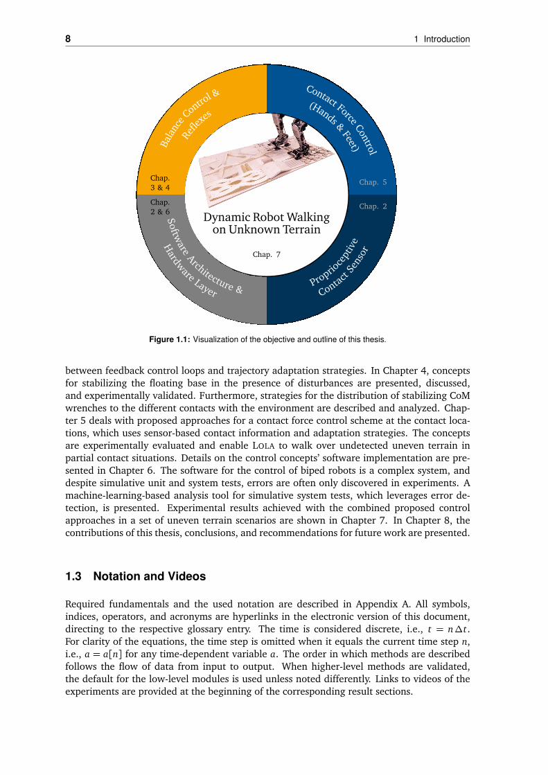
The outline of this thesis is visualized in Figure 1.1. In Chapter 2, an overview of thehardware platform LOLA is given first. Furthermore, the proposed hardware control architec-ture and tactile contact sensor are described and experimentally evaluated. Chapter 3 givesan overview of the planning and control approach of LOLA and deals with the connection

8 1 Introduction

Bala

nce Con

trol &

Refle

xes

Chap.3 & 4

Contact ForceControl

(Hands &Feet)

Chap. 5

Software

Architecture &

Hardw

are Layer

Chap.2 & 6

Proprio

cept

ive

Contact Se

nsor

Chap. 2

Dynamic Robot Walkingon Unknown Terrain

Chap. 7

Figure 1.1: Visualization of the objective and outline of this thesis.

between feedback control loops and trajectory adaptation strategies. In Chapter 4, conceptsfor stabilizing the floating base in the presence of disturbances are presented, discussed,and experimentally validated. Furthermore, strategies for the distribution of stabilizing CoMwrenches to the different contacts with the environment are described and analyzed. Chap-ter 5 deals with proposed approaches for a contact force control scheme at the contact loca-tions, which uses sensor-based contact information and adaptation strategies. The conceptsare experimentally evaluated and enable LOLA to walk over undetected uneven terrain inpartial contact situations. Details on the control concepts’ software implementation are pre-sented in Chapter 6. The software for the control of biped robots is a complex system, anddespite simulative unit and system tests, errors are often only discovered in experiments. Amachine-learning-based analysis tool for simulative system tests, which leverages error de-tection, is presented. Experimental results achieved with the combined proposed controlapproaches in a set of uneven terrain scenarios are shown in Chapter 7. In Chapter 8, thecontributions of this thesis, conclusions, and recommendations for future work are presented.

1.3 Notation and Videos

Required fundamentals and the used notation are described in Appendix A. All symbols,indices, operators, and acronyms are hyperlinks in the electronic version of this document,directing to the respective glossary entry. The time is considered discrete, i.e., t = n∆t.For clarity of the equations, the time step is omitted when it equals the current time step n,i.e., a = a[n] for any time-dependent variable a. The order in which methods are describedfollows the flow of data from input to output. When higher-level methods are validated,the default for the low-level modules is used unless noted differently. Links to videos of theexperiments are provided at the beginning of the corresponding result sections.

Chapter 2

Platform Mechatronics

This chapter describes the platform mechatronics of the humanoid robot LOLA, i.e., everypiece of platform-specific software, electronics, and hardware required to move the robot’sjoints and read its state. This includes the low-level software for joint control, communication,and data pre-/post-processing. The interface to the control software is defined by the Hard-ware Layer (HWL), which provides general data interfaces to the high-level control softwaremodules.

The platform mechatronics is extremely important for the whole robotic system’s perfor-mance: All high-level modules, i.e., the Walking Pattern Generator (WPG) and Stabilizationand Inverse Kinematics (SIK), rely on the performance of this combined piece of hardwareand software. If seen as a cascaded structure, it becomes clear that the platform mecha-tronics must meet the highest requirements for update rates, latency, safety, and reliability.This chapter presents the proposed hardware control architecture for improved hardwareintegration and a tactile sensor concept for biped robots.

2.1 Mechatronic Design Overview

This section gives a short overview of the different design revisions of LOLA and describes thecurrent design. Note that the original design is only described in detail where necessary forthe understanding of later improvements.

2.1.1 Design Revisions of LOLA

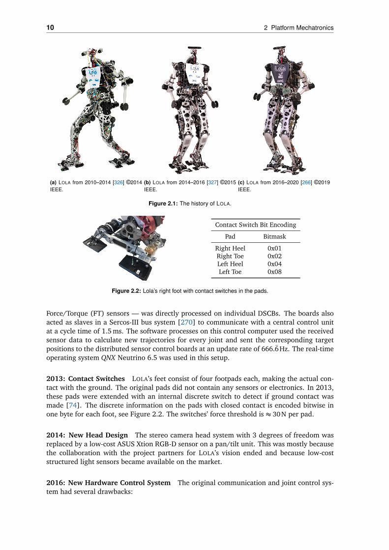
Since its first stable design in 2010, several improvements were made to the mechatronicarchitecture of LOLA, see Figure 2.1. In the following, the changes leading to different hard-ware revisions and corresponding lessons learned are briefly summarized.

2010: Original Design The original mechatronic design of the humanoid robot LOLA [33,81, 188] is shown in Figure 2.1a. By that time, the robot was equipped with a stereo camerahead from a project partner with 3 degrees of freedom [39]. This resulted in a total of 25degrees of freedom for the whole robot. Due to the high computational load, the vision dataprocessing was done on computers in an external rack. However, the trajectory generationand control already ran on a central control unit on LOLA’s back.

The communication and actuation structure of LOLA consisted of 9 Distributed SensorControl Boards (DSCBs) [80]. Each board could control up to three joints via dedicated ElmoMotion Control servo drives [65], which were connected to a DSCB via a Controller AreaNetwork (CAN) bus. Sensor data from the joint encoders was read in; target positions forthe joints were sent to the servo drives. Additional sensor data — for example from the

9

10 2 Platform Mechatronics

(a) LOLA from 2010–2014 [326] ©2014

IEEE.

(b) LOLA from 2014–2016 [327] ©2015

IEEE.

(c) LOLA from 2016–2020 [266] ©2019

IEEE.

Figure 2.1: The history of LOLA.

Contact Switch Bit Encoding

Pad Bitmask

Right Heel 0x01Right Toe 0x02Left Heel 0x04Left Toe 0x08

Figure 2.2: Lola’s right foot with contact switches in the pads.

Force/Torque (FT) sensors — was directly processed on individual DSCBs. The boards alsoacted as slaves in a Sercos-III bus system [270] to communicate with a central control unitat a cycle time of 1.5 ms. The software processes on this control computer used the receivedsensor data to calculate new trajectories for every joint and sent the corresponding targetpositions to the distributed sensor control boards at an update rate of 666.6 Hz. The real-timeoperating system QNX Neutrino 6.5 was used in this setup.

2013: Contact Switches LOLA’s feet consist of four footpads each, making the actual con-tact with the ground. The original pads did not contain any sensors or electronics. In 2013,these pads were extended with an internal discrete switch to detect if ground contact wasmade [74]. The discrete information on the pads with closed contact is encoded bitwise inone byte for each foot, see Figure 2.2. The switches’ force threshold is ≈ 30 N per pad.

2014: New Head Design The stereo camera head system with 3 degrees of freedom wasreplaced by a low-cost ASUS Xtion RGB-D sensor on a pan/tilt unit. This was mostly becausethe collaboration with the project partners for LOLA’s vision ended and because low-coststructured light sensors became available on the market.

2016: New Hardware Control System The original communication and joint control sys-tem had several drawbacks:

2.1 Mechatronic Design Overview 11

• Unnecessary Complexity: The design of the DSCBs was very complex. This complexitywas built to enable advanced distributed control concepts — concepts that were neverimplemented.

• Lacking Reliability: Probably due to their high complexity, the control boards wereunreliable. After a certain time of operation, the boards repeatably failed to boot-upand needed to be replaced. This process was repeated until the circuit components wereno longer available. The problems with hardware and software caused much downtimeof the robot and made it hard to concentrate on developing new methods.

• Low Control Bandwidth: Although equipped with an Ethernet-based Sercos-III bus,the servo drives were still connected via CAN to the DSCBs. The update cycle timewas limited to 1.5 ms. Furthermore, the joints’ position control loop was closed onthe control boards and over the CAN. This led to additional latencies and jitter in thecontrol loop timing.

Based on the experiences with the original control system, a new design was created. Further-more, the real-time operating system was upgraded to QNX Neutrino 6.6. The new hardwarecontrol system’s detailed design and characteristics are described in Section 2.2 of this thesis.

2020: Redesigned Upper Body and Arms Earlier versions of LOLA used the arms only forcompensating the angular momentum of the feet during walking. In the context of a newDFG research project1, LOLA’s arms were redesigned to enable balancing in multi-contactscenarios. By adding one degree of freedom to each arm, the kinematically reachable spacewas extended. Also, FT sensors were added to the hands to enable feedback control of handcontact forces [267]. Hand contacts are made via spherical end effectors with rubber coating.Note that only unilateral multi-contact scenarios are considered.

The weak connection between the lower- and upper body in LOLA’s original design causedstructural resonances near the mounting point of the Inertial Measurement Unit (IMU). Thismechanical design flaw limited the balancing controller’s bandwidth and is discussed in [16].The upper body has thus been redesigned with the intent to shift the structural eigenfrequen-cies to higher values. A comparison of the eigenfrequencies of both designs can be found in[17].

Additional hardware enhancements include increased computational power of the on-board computers and an updated vision system. A comprehensive in-detail description of allchanges is presented in [267].

2020: New Foot-Sole Material The compliant material on the footpads was replaced witha two-layer design. The inner layer is made of the compliant shoe material Nora Lunasoft SLW(6mm) to absorb impacts with the ground. The compliance of this material is additionallyimportant for the design of the contact force control, see Chapter 5. The outer layer is madeof the shoe-sole material Nora Astral Crepe (1.8mm) and provides the necessary rigidity forcontacts with rough surfaces. Furthermore, this layer provides an excellent static frictioncoefficient µ= 0.8 [285].

2.1.2 Current Design

The humanoid robot platform LOLA is 1.76 m tall, weighs approximately 67 kg, and is ac-tuated by 26 electric joint drives. The kinematic structure is shown in Figure 2.3. LOLA isequipped with an active toe joint, which allows to rotate the forefoot separately.

1German Research Foundation, grant number 407378162


Figure 2.3: The design of LOLA and its kinematic structure at the time of writing. The current design features 26

DoFs and a redesign of the upper body / the arms.

Drive Modules Every joint drive module consists of a brushless DC motor, encoders, anda servo drive for decentralized and fast control of joint position and velocity. The servodrives are commercial Gold Line drives from Elmo Motion Control [64]. The distributed jointcontrol architecture enables high local sample rates with 20 kHz for the current feedback, and10 kHz for velocity and position. The servo controller implements a PPI cascade and uses theincremental encoder on motor-side for position and velocity feedback.

Most drive modules are equipped with stiff high-ratio Harmonic Drive transmission gears.An exception are the ankle and knee joints: The knee joint is designed as linear actuatorvia planetary roller screws; the ankle joints are actuated via a parallel kinematics using twospatial slider crank mechanisms and belt drives. All joints are back-drivable. Every drivemodule is equipped with an incremental encoder on motor side and an absolute encoder onjoint side, i.e., after the gearbox or linear actuator kinematics. The schematics of a typicaldrive module is shown in Figure 2.4. Details on the joint drive properties are described inAppendix B. Information on the mechanical design of the drive modules can be found in[188].

Sensors The robot is equipped with the commercial IMU iVRU-FC-C167 from iMAR Navi-gation [129]. The device is mounted at the torso of the robot. It contains three fibre-opticgyroscopes, three Micro-Electro-Mechanical accelerometers, and a micro controller for inter-nal sensor data fusion, temperature correction, and communication. The system provides theorientation, its derivative, and the linear accelerations via CAN at a data rate of 200 Hz.

LOLA is further equipped with custom 6-axis FT sensors at the feet, because there are —to date — no commercial sensors available on the market, which combine the requirementsof low weight and size with the high torque specifications (±120 Nm,1000 N, overload-safe).Measurement data is supplied via CAN at a data rate of 1 kHz. Details on the mechanicaldesign are described in [188]. Efforts for a redesign of the sensor have been made to increasethe accuracy and bandwidth while keeping the low weight of 400 g [237].

2.1 Mechatronic Design Overview 13

Joint Drive Module

Servo Drive

Elmo Motion Control

Gold Line Drive

(Whistle / Guitar)

Joint Actuator

Absolute Rotary Encoder

Heidenhain

ECI1100 / ECI1300

16 / 17 bits

EnDat 2.1

Incremental Encoder

magnetic

11520 counts / rev.

(4000 for toe joints)

Harmonic Drive gearbox

optical limit switch

3-phase brushless DC motor

11 different sizes/packages

Co

ntr

oE

the

rCA

T B

us

EtherCAT

80 V

mo

tor

vo

ltag

e24 V

op

era

tin

g v

olt

ag

e

Figure 2.4: Simplified schematics for a typical joint drive module of LOLA.

The hands of LOLA feature FTE-AXIA80-DUAL SI-200-8/SI-500-20 6-axis FT sensors fromSchunk GmbH & Co. KG with a maximum contact force of 900 N and a maximum contactmoment of 20 Nm. These AXIA FT sensors are directly connected to the EtherCAT (EC) busand support a maximum update rate of 4 kHz.

Onboard Computing & Communication The distributed servo drives and sensors commu-nicate via EC [73] with LOLA’s central control computer, see Figure 2.5. This control unit,which is located at the back of the robot, runs the real-time operating system QNX Neutrino7.0 and executes all computations required to plan and control the motion of the humanoid.The onboard computer is built from an Advantech AIMB-276 mainboard with an Intel i7-8700hexa-core CPU and 32 GB RAM. A second onboard computer at the front, with identical spec-ifications, but additional Nvidia Quadro P2000 graphics card, runs a standard linux distribu-tion and is connected to the control unit via Gigabit Ethernet. This vision processing unit andthe connected Intel RealSense cameras at LOLA’s head are not used throughout this thesis.

The EC bus topology is based on three lines — one for each arm and one for the rest ofthe slaves. The separated lines for the arms are necessary due to missing second ports onthe commercial FT sensors of the arms. CAN-based data is integrated via a CAN-EC gateway[72] with 1 Mbit/s bandwidth. The EC bus runs with an update frequency of 4 kHz and usesthe Distributed Clocks feature of the EC technology. In Table B.4, a detailed description ofthe bus topology is presented.

Power Network LOLA does not have an onboard power supply; it is operated tethered witha 24 V supply line for the electric components, and a 80 V supply line for the motors (excepthead joints). The power supplies are located in a nearby rack.


Onboard Hardware Overview

Ethernet

EtherCAT@4kHz

Control PCCore [email protected] RAM

Neutrino RTOS 7.0

Vision PCCore [email protected] RAMNvidia Quadro P2000

Linux Ubuntu

USB

Intel RealSense D435/T265

CAN Gateway

1 Mbit/s

Head / Leg Joint 1

Motor + Servo Drive + Sensors

Left Arm Joint 1


Head / Leg Joint 18


EtherCAT Junction

IMU

iMAR NavigationiVRU-FC-C167

CAN

Left Arm Joint 4


Right Arm Joint 1


Right Arm Joint 4


EtherCAT EtherCAT

FTS Right Arm

Schunk AXIA80

... ... ...

FTS Left Foot

FTS Right Foot

FTS Left Arm

Schunk AXIA80

EtherCAT

Oper

ator

PC

Ethernet

Figure 2.5: Overview on the computing and communication components onboard of LOLA.

2.2 EtherCAT-based Real-Time Hardware Layer 15

Operator Commands Both onboard computers are connected to an operator PC via GigabitEthernet. The connection is used to send high-level control commands and parameters to thesoftware running on the control unit via a publish–subscribe system. Furthermore, logfilesand executables are transferred via Ethernet to the onboard computers.

Hardware Layer Application The Hardware Layer Application runs the HWL in the soft-ware architecture of LOLA. It is responsible for all low-level communication and safety mea-sures, handles hardware errors, implements device abstractions to represent their state, andprovides a shared-memory based sensor and target data interface to the high-level controlmodules. The module is further described in the following section.

2.2 EtherCAT-based Real-Time Hardware Layer

The content in this section haspreviously been published in [296]©2018 IEEE.

The following section describes the proposed EC-based hardware control software for LOLA

to improve hardware integration and overall performance. This control software is respon-sible for executing and controlling target motions for the robot. Furthermore, sensor data iscollected and sent to the higher-level planning and stabilization modules of the robot. Theperformance, i.e., control bandwidth and latency, of this hardware-near control structure isessential because it represents the inner control loop for all higher-level software and, there-fore, directly limits the overall system’s performance. The key features of the new hardwarecontrol system design are — in the order of priority:

• Reliability: More commercial components and less hardware-near custom code. Byreducing the complexity and deploying widely used technology, the risk of failure isminimized.

• Bandwidth: The EC field-bus technology and commercial servo-drives with high localupdate rates allow high bandwidth of the hardware control system. The control loopand all involved software components are designed for hard real-time constraints withlow communication latency and low jitter, i.e., a low standard deviation of the controlloop update rate. The communication system allows update rates > 1 kHz.

• Compatibility: The EC technology is a wide-spread standard and allows easy integra-tion of many commercial sensors and actors in the future.

• Portability: The hardware layer tries to be as generic as possible. It implements areal-time bus middleware to decouple the field-bus characteristics from those of theconnected devices and the higher-level modules. This makes it easier to change tech-nologies (devices or the bus itself) in the future.

In the following, the components of the real-time capable HWL are described. This in-cludes data pre-/post-processing, the real-time bus middleware, device drivers, and safetymeasures. Subsequently, the software’s performance, the EC bus, and the overall system areanalyzed. Parts of the HWL code are available open-source, see Chapter 6.


HardwareLayer

DeviceAbstractions

CAN Gateway

IMU

FT Sensorsat the Feet

FT Sensorsat the Hands

Elmo DriveGroup Drives 1-26

Preprocessor

Joint Model

Target DataExtrapolation

Joint Feedfor-ward Control

Safety Checks

Real-TimeRequirements

Limited Track-ing Error

Plausible FTSensor Data

State Machine

Interfaces

Data Logging

Calibration Data

Publish–SubscribeSystem

Shared MemoryWPG/SIK

FieldbusDriver

Real-Time Bus Middleware

⟲ 250µs

SIK/WPG

Hardware

Figure 2.6: Overview of the architecture of the HWL application with major components.

2.2.1 Software Architecture

An overview of the HWL’s software components is visualized in Figure 2.6.

Interfaces and Data Preprocessing The HWL receives target data from high-level robotcontrol processes and, at the same time, sends sensor data to these processes. The commu-nication is done via a synchronized shared memory interface [33]. All higher-level moduleswait for new sensor data from the HWL, generate new target data, and finally copy it to theshared memory region. This means the HWL defines the timing of all software processes —including the high-level modules. While the HWL blocks the robot control processes untilnew sensor data is ready, the HWL itself is never blocked to ensure high timing accuracy andsafety. Instead, it always uses the newest available target data in the shared memory region.

With the new EC bus system, communication cycle times as fast as ∆tbus = 250µs canbe attained for LOLA. However, the high-level control modules typically can, because ofthe computational complexity of the control algorithms, not keep up with these low cycletimes. Therefore, the HWL publishes sensor data just every nth bus cycle to trigger high-levelmodule execution at the higher control cycle time ∆tcont = n∆tbus. The last target data in theshared memory region is linearly extrapolated for all minor bus cycles Cm = i | i mod n = 0based on the target data gradients (e.g. velocities).

In addition, target and sensor data preprocessing includes converting motor to joint an-gles and vice-versa and converting raw sensor data to physical units. These conversionsinclude the resolution of the knee- and ankle-joint kinematics with a non-constant gear ra-tio. Moreover, a feed-forward control strategy on velocity-level is implemented to further


reduce joint position tracking errors [296]. The technique uses a learned feed-forward gainto compensate for typical velocity-dependent position errors, e.g., caused by friction.

Parameters and operator commands are received via network using a publish–subscribesystem. The robot’s kinematics can be calibrated using a specialized calibration rig. The HWLstores relevant joint calibration data, which is used when homing the joint drives.

State Machine and Safety The HWL contains a state machine to represent the state ofthe communication bus and all attached devices. If a device is entering an invalid or unsafestate or experiencing communication errors, the software tries to bring the robot to a safehalt. Once the machine is in such a fault state, the operator has to explicitly acknowledgecontinued operation before the joint drives can be reactivated.

Also, safety checks are part of the data preprocessor. When FT sensor data is not plausibleor the tracking error on a joint is above a specified limit, the HWL state machine assumesa fault and puts all devices in a safe state. Also, every sensor data frame sent to SIK/WPGcarries a working counter number, which increases every cycle. The working counter fromthe sensor data is sent as part of the planner data from WPG to SIK, and as part of the targetdata from SIK back to the HWL. For every sensor data frame sent to the higher-level moduleswith a certain working counter, the HWL expects a target data frame from SIK with exactlythe same working counter in the next cycle. If the counters do not match, either SIK or WPGwere too slow and violated the real-time requirements. A working counter mismatch doestrigger a fault when it happens at two consequent cycles.

Real-Time Bus Middleware To abstract the communication between nodes in a Fieldbus,two common CANopen [40] definitions are used: Process Data Objects (PDOs) and ServiceData Objects (SDOs). These concepts are also widely used in modern Fieldbus technologysuch as EC and define the name, type, and size of objects, which can be received from and/orsent to a slave. PDOs define data objects, which are cyclically sent and received in real-time;SDOs are used for asynchronous communication based on a request-response pattern and dotypically not meet hard real-time constraints. Furthermore, the following definition of theFieldbus’ state based on the EC standard is used in the middleware:

• Init: Initial state of a slave.

• Pre-Op: Initialization done; SDO but no PDO communication yet.

• Safe-Op: PDO data is exchanged; PDO output data is not yet applied, i.e., physicaloutputs remain in a safe state.

• Op: PDO data is exchanged; PDO output data is applied on the slave, i.e., physicaloutputs are changed according to the PDO.

In the following, a new approach to decouple the Fieldbus communication from the applica-tion software is proposed. A middleware software layer makes the bus completely transpar-ent for the application software. It makes device-specific implementations, e.g., interpretingsensor data or abstracting the device’s state, independent from the Fieldbus protocol andimplementation. This has advantages in handling the software (and system) complexity andimproves maintainability and safety. The core idea behind the abstraction is the proposal ofBus Variables to make PDOs and SDOs available to the HWL application. Basically, a Bus Vari-able is an instance of a special class representing a variable of a certain predefined primitivedata type (int, float, char, etc.); it may be used as any standard variable in the applicationcode. However, the Bus Variable can be linked to a PDO of a slave by telling the middle-ware the name and slave identifier of the PDO object. The Bus Variable then serves as a


Slave2.actPosSlave2.trgtPos

...

Slave 2

Slave1.actPosSlave1.trgtPos

...

Slave 1

Master

Fieldbus Driver

Middleware

BusUInt32<BusOutput> desPosition;BusUInt32<BusInput> actPosition;...linkPDOVar("Slave1.trgtPos", desPosition);linkPDOVar("Slave1.actPos", actPosition);

...

void process() // All processing takes place here,// triggered by Middleware each Cycle...// Set desired position on slave 1desPosition = 234; // Bus Variables arethread-safe

Device Abstraction

Bus Description File

...

00 10 45 69 5A

3F C3 A3 EA 00

00 00 ...

PDO Map

Figure 2.7: The proposed middleware decouples the device abstraction layer (application software) from the

Fieldbus driver and Fieldbus type by using Bus Variables. These variables are linked to PDOs in the PDO map via

the name and type information in the bus description file. Adapted from [296] ©2018 IEEE.

fully transparent representation of the distributed slave objects. If an Output Bus Variable’svalue is changed, the middleware automatically sends the new data to the correspondingslave. Equivalently, the data in Input Bus Variables is updated every time new PDO data isreceived from the bus slaves. Bus Variables are thread-safe and implement an automateddata-type checking during run time. Furthermore, Bus Variables can be used for SDO-basedcommunication. The concept is visualized in Figure 2.7.

The middleware software layer defines an abstract data interface to the Fieldbus driver,which then translates changes in the PDO/SDO data to data packets on the bus. Note thatone can use different implementations for different Fieldbus types or driver implementationswithout changing code on the device abstraction or application side. For LOLA, a commercialEC master stack is used as Fieldbus driver [3]. The connection between the Bus Variables inthe application code and the variables on the slaves is made through the respective slave andvariable names defined in the EC Network Information File (ENI), which is the bus descriptionfile for EC.

The framework for Bus Variables is available open-source as part of a header-only C++

library, see Section 6.2.

Device Abstraction Layer On top of the middleware layer, all devices on the bus are repre-sented by device abstraction classes. The class instances map the internal logic and physicalbehavior of the slaves to the software. The device abstraction classes are derived from ageneral BusDevice class provided by the middleware, which makes the use of Bus Variablesin these implementations straightforward.

For LOLA, there are device classes for the Elmo Motion Control servo drives, the CANgateway, the IMU, and the FT sensors. Every device class implements a state-machine, spe-cialized error handling and provides an Application Programming Interface (API) to controlthe corresponding device. For example, the FT sensor device class provides methods that re-turn the current force and torque readings; the servo drive device class accordingly providesmethods to change the joint controllers’ set points. These API methods are called from thedata processing module of the HWL, see Section 2.2.1. Some common device abstractionimplementations based on Bus Variables are available open-source, see Section 6.2.


Bus Cycle ⟲∆tbus ...

Timing .. waitForNextCycle...

EtherCAT ... RX copyRX copyTX sendFrames mailbox waitForTimingEvent...

Main ... getTargets waitForDataReady... process publishSensorData generalTasks ..

2µs

signalTimingEvent

signalNextCycle signalDataReady

1 3 5 7 9 12

2 8

4 6 10 11 13 14

Figure 2.8: Timing and synchronization of the three main threads in the HWL. The timing thread unblocks with

∆tbus. Orange sections describe CPU-time used by the QNX Neutrino scheduler. The sections are described in

Tables 2.1 and 2.2. The figure is to scale with the given legend. Adapted from [296] ©2018 IEEE.

ID Name Description

1 waitForTimingEvent Wait for an event from the timing thread2 signalNextCycle Unblocks the main thread3 RX Process the frames received in the last cycle (EC stack)5 copyRX Copy incoming data from the EC stack to the Bus Variables7 copyTX Copy outgoing data from the Bus Variables to the EC stack8 signalDataReady Signal main thread new incoming data is available and Output Bus Variables

may be modified9 sendFrames Queue cyclic EC frames to be sent on the bus12

mailbox Send acyclic frames and execute administrative tasks of the EC stack

Table 2.1: Execution sections called in the EC-thread of the HWL. Adapted from [296] ©2018 IEEE.

2.2.2 Software Integration and Timing

The HWL contains both the device abstraction layer and the middleware. It spawns severalchild threads for the bus communication, logging, operator interfaces, and inter-process com-munication with the other two control framework processes (SIK/WPG). The main threadruns the data processing, the state machine, and error handling in a cyclic loop, see Sec-tion 2.2.1. It is synchronized to a higher-priority EC-thread to ensure minimum latency ofinput and output data. Within the EC-thread, methods of the bus middleware and the ECmaster stack are executed. This includes copying data between the Bus Variables and theactual EC PDO map and sending all cyclic and acyclic EC frames. To keep the timing be-tween consecutive EC cycles precise, a separate timing task with the highest priority is usedto trigger the EC-thread execution.

In Figure 2.8, the timing and synchronization of the three threads is shown. All importantexecution sections of the EC- and main thread are described in Tables 2.1 and 2.2. Aparticularity of the approach is the interleaving of sections that access the same Bus Variables.Section 4 and 7 both operate on the target data Bus Variables and, in theory, simultaneousaccess may occur when section 4 has a higher execution time than section 3 and 5. AlthoughBus Variables are thread-safe, the process data may become invalid when data in differentBus Variables of the same device becomes inconsistent. There is more sensor data than targetdata to process in practice, at least for humanoid robots. This means section 5 very likelyhas a higher execution time — more Bus Variables need to be processed — than section 4.This concept seems unsafe at first, but it reduces the latency of the whole control loop —i.e., from sensor data over the high-level modules to target data on the devices — by one buscycle ∆tbus. Furthermore, the execution times are deterministic and can be analyzed by highprecision measurements with a trace logging tool to prove the concept’s viability.


ID Name Description

4 getTargets Get new target values from high-level control modules (if available)6 waitForDataReady Block the thread until new input/output data has been processed in EC-thread10 process Process raw input data in Device Abstractions11 publishSensorData Push processed input data to shared memory. This triggers a new calculation of

target data in the high-level modules and is skipped for all minor bus cycles Cm

13 generalTasks Executes state-machine logic, error handling, and communication with the op-erator computer

14

waitForNextCycle Blocks the thread until the EC Cycle Time has elapsed

Table 2.2: Execution sections called in the main thread of the HWL. Adapted from [296] ©2018 IEEE.

BusEvents

Hardware DriverEvents

sendFrames() sendFrames() sendFrames() sendFrames()∆tbus

Sync0 Sync0 Sync0 Sync0

Global Shift

∆tshift

Slave Input

Latch

∆tlatch

Slave Output valid

∆tset

tpublishSensorData()

updateTargets()

publishSensorData()∆tcont

Input Delay

∆tin

Output Delay

∆tout

Figure 2.9: Visualizes the input- (∆t in) and output delay (∆tout) for slave input and output data in the HWL. All

slaves and the master are synchronized to the Sync0 event of the EC distributed clocks functionality. The control

delays depend on the settings for the distributed clocks master synchronization (∆tshift), and the slave’s input

data latch (∆t latch) / output set (∆tset) delays. The visualization is simplified to a bus with identical slaves and

∆tcont = 2∆tbus.

2.2.3 Communication with the Bus Slaves

The slaves in an EC bus are organized in a logical ring — independently from the physicaltopology of the slaves. When an EC frame with new data is sent from the bus master, it passesevery slave and is finally sent back to the master by the last logical slave. Each slave readsand writes data to the EC frame while passing the device, i.e., “on the fly”. This enables shortdelays, resulting in low minimum cycle times, and avoids collisions by design. Furthermore,bandwidth usage is optimized as input- and output data belonging to different slaves mayshare the same space in the EC frame. Due to the logical ring and the propagation delays ofthe physical transport medium, however, an EC frame passes every slave at a different time.This means that the slaves’ input- and output data is not synchronized and may represent thesystem’s state at different points in time. To overcome this problem, master and slaves can besynchronized with the EC Distributed Clocks (DC) functionality. The synchronization of themaster operates in BusShift mode, i.e., the time of the slaves is changed depending on thetiming of the bus master. All slaves and the master are synchronized to a global-in-time eventcalled Sync0, see Figure 2.9. The Sync0 event is shifted relative to the sendFrames() operationof the bus master with the Global Shift Time ∆tshift. The hardware driver’s input- (∆tin) andoutput delay (∆tout) depends on the slave time required for latching/processing a measuredinput ∆tlatch, the slave time required to set an output value ∆tset, the bus cycle time ∆tbus,and the global shift time ∆tshift. Note that for a bus with identical slaves, ∆tlatch >∆tshift and∆tin >∆tbus holds.

The global shift time ∆tshift is subject to tuning. It needs to be as low as possible toreduce the output delay ∆tout and as high as required to allow all slaves to receive the EC


Quantity Mean or normvalue

Standarddeviation

Data Source

Input PDO data size 822 bytes - ENIOutput PDO data size 526 bytes - ENITotal PDO data size 1348 bytes - ENIEC datagram size 974 bytes - ENIGlobal Shift ∆tshift 140µs - -

Propagation Delay 114µs 6µs Wireshark measurementMinimum input data delay ∆tin,min ∆tbus + 35µs n.a. traceloggerMinimum output data delay ∆tout,min ∆tshift + 20.5µs n.a. traceloggerMinimum total control latency ∆tin,min+∆tout,min+

∆tcont − 56µsn.a. tracelogger

Bus cycle time ∆tbus 249.3µs 2.69µs High Performance Event TimerMaster Sync0 Timing Error 147 ns 840 ns master stackSlaves Sync0 Timing Error 1.5 ns 94 ns master stack

Table 2.3: Parameters and performance quantities for the HWL and the EC bus system.

frame before the scheduled Sync0 event. This means the propagation delay of the EC frameto the last logical slave defines the absolute minimum for the global shift time. To optimizethe global shift time, the propagation delay is measured using an Ethernet switch betweenthe master and the first slave and a connected measurement computer with the open-sourcesoftware Wireshark [305]. The time delay between the outgoing (coming from the master)and incoming EC datagram belonging to one bus cycle is a conservative measurement of thepropagation delay. Additional latencies from the switch and the measurement computer areadded. The mean value of the propagation delay over a period of ≈ 13 seconds is 114µs witha standard deviation of 6µs. For robust operation, the global shift time is set to 140µs.

2.2.4 System Performance

The performance of the HWL in terms of data processing and communication is evaluatedin the following. For all further tests, the bus runs at an update rate ∆tbus = 250µs, with ahigh-level control update rate ∆tcont = 1 ms. Higher bus update rates are not possible withthe current control unit’s hardware. The limited accuracy of the real-time clock does notallow BusShift operation of the DC at higher update rates. The parameters and measuredperformance values are summarized in Table 2.3.

The system’s software-side performance is measured on the real-time control unit usingQNX Neutrino’s trace logging features. This enables to get precise information on the timingof individual program sections. The exact execution times for all code sections in one ECbus cycle are visualized in Figure 2.8. Furthermore, these measurements are the basis forthe calculation of the input- and output data delay. The installed joint drive modules donot provide information on the actual latch- ∆tlatch or set-delays ∆tset via the slave’s objectdictionary. Therefore, only the minimum delays, usually only a few microseconds less thanthe actual ones, can be calculated from the trace logging data.

For the chosen bus cycle time, the total latency caused by the hardware control system isonly 389.5µs. The total control latency, including the high-level control modules’ computa-tion time, results in 1389.5µs.

The timing error of the global Sync0 events on the master and the slaves — the system issynchronized via the DC feature — is measured by the master stack; statistical informationon the error is given in Table 2.3. In 99.99 % of the time, the error of the master timing isless than 1.4 % of the bus cycle time. The timing of the slaves is even more accurate.


The accuracy of the timing thread (bus cycle time) is measured online with a high-precision CPU-internal timer. As the bus cycle is the data source for all high-level controlmodules, errors in this timing primarily affect the correctness of these modules’ calculations.Relative to the control module cycle time ∆tcont = 1000µs, the error is less than 1.2 % in99.99 % of the time.

Additional data on the performance of the joint controllers itself can be found in [296].

2.2.5 Related Work

In the following, the proposed hardware control system is discussed in the context of relatedwork. First, real-time software frameworks in the context of robotics are compared withthe proposed real-time bus middleware. Second, the achieved performance of the combinedhardware and software concept is benchmarked to state-of-the-art robots.

Software Frameworks Commonly used frameworks for the control of robots, e.g., the Ro-bot Operating System (ROS) [244] or Yet Another Robot Platform (YARP) [197], do in gen-eral not support hard real-time constraints. While this is not a problem for high-level com-munication and planning, the frameworks are not suited for low-level motion control. UsingROS or YARP in such a context is, of course, possible but will introduce jitter in the timing ofthe control loops and unnecessarily limit the minimum reachable sample time.

To mitigate this problem, several (not so commonly used) frameworks provide real-timecapable communication. The OpenRTM-aist Software supports real-time control threads, pro-vides a graphical user interface for the design and connection of components, and uses codegeneration to speed up the development process [9]. Unfortunately, the timing and inter-nal latency of the software framework are not analyzed. Compared to the hardware controlsystem presented in this work, OpenRTM-aist provides a more general software generationapproach for robots.

Another robot platform software, XBotCore, provides a lightweight shared-memory-basedcommunication structure directly connected to an open-source EC master stack implemen-tation [205]. The interface between the EC bus, the device abstractions, and high-levelsoftware is defined by typical robot devices, such as joints, IMU, and FT sensors and not onPDO/SDO level. Data showing the control period for the robot WALK-MAN using XBotCoreis presented in [205]. While the control period is below the target of 1 ms, there is significantjitter in the timing.

To the author’s best knowledge, the concept of Bus Variables has not been presented inliterature so far. In contrast to related work, the interface between the communication busand the device implementations is at variable-level, effectively separating device-specific codefrom the bus technology and master implementation. Despite this fine-grained interface, thepresented hardware layer concept supports hard real-time requirements and minimal controlloop latency.

Hardware Layer Performance Although modern real-time bus technologies have beenavailable for quite some time, only a few humanoids are equipped with high-performancecommunication systems. In contrast to distributed control systems with a digital bus com-munication system, central control concepts were used, e.g., in the Honda humanoid robot[115], HRP-2 [141], or Wabian-2 [220]. All sensors and actuators are directly attached toI/O interface boards in the central control computer in these architectures. As an advantage,high update rates are possible as no communication bus is needed. However, the system’scomplexity is high, as all peripheral sensors and actuators must be connected directly to the


central control unit. Due to their high complexity, centralized systems are more error-pronethan distributed systems, where some error checking and handling are already executed onintelligent distributed slaves. With decentralized control concepts, parts of the computa-tional effort can be off-loaded to the intelligent actuator controls. This also allows for veryhigh update rates of the local control cycles (e.g., 20 kHz current control).

Because of its easiness and reliability, CAN is a prevalent technique for communication indistributed control systems of humanoid robots. It is used in popular robots such as the HRProbots version 3 and 4 [142, 144], Hubo-2 [48] and the iCub [198] to send and receive datato and from the distributed joint controllers. However, the maximum bandwidth of CAN isrelatively low (1 Mbit/s) and communication is only partially deterministic (for high prioritymessages). Therefore, multiple CAN networks are used in parallel for robots with a highnumber of DoFs. Still, the maximum achievable update rates for joint-controller set-pointsare considerably low. The DRC-Hubo uses CAN for communication and is limited to a controlrate of 200 Hz [333]. With the use of four parallel CAN-Buses, CHIMP reaches an update rateof 500 Hz [282]. Also, the CAN protocol does not allow to compensate for the transmissiondelays, i.e., allow synchronous execution of commands on the distributed joint controllers.

Several different approaches were used in literature to overcome the drawbacks of CAN.[310] proposes the use of multiple RS422 connections with an effective data rate of 6 Mbitsper connection and a central control system with ART Linux operating system. However, itis unclear what kind of protocol and media access control is used in the daisy-chain setupof the RS422 interface. In [6], a real-time communication system based on the Ethernetprotocol is developed for the HRP-3P (prototype). It uses a custom protocol to link severalbus nodes, which operate an ART-Linux real-time operating system. While originally designedto replace the unreliable central control system of the HRP-2, the AIST group later switchedto CAN for the final HRP-3 humanoid “to improve reliability and maintenance of the system”.[142, p.2476]. PETMAN [208] uses a modified CAN bus to reach an update frequency of1 kHz, details have however not been published so far. Unfortunately, there is only littleinformation on the hardware of ATLAS (1 kHz update rate) [169] and no information onthe inner structure of Honda’s ASIMO. For the robot TORO [70], a Sercos-II bus with abandwidth of up to 16 Mbit/s is used. Although this enables a 1 kHz control rate, the bitratewould probably not allow for much higher update rates. The former hardware design of thehumanoid robot LOLA, see Section 2.1.1, used a Sercos-III bus based on 100 Mbit/s-Ethernet[81]. However, the distributed I/O boards and interfaces to the actual joint drives were in-house made and complex. As this introduces another source of errors, the reliability of thewhole solution was limited.

For the design of newer robots, the EC bus became increasingly popular, as it is fast, reli-able, and widely-used. In-house-made electronics are often used for the actual joint control,and fault handling in such systems [83, 139], which may reduce such solutions’ reliabilityand persistence. Furthermore, often non-real-time capable software frameworks are com-bined with the EC technology, giving away its advantages of low communication delays [83].The latency of the communication or the control loop is in general not analyzed.

The RoboSimian robot from the Jet Propulsion Laboratory features a similar hardwarestructure using an EC bus and the same commercial joint servo drives [147]. The controlloop runs at 1 kHz on a non-real-time operating system. There is no data given on the la-tencies of the control loop. The biped robot TALOS from PAL Robotics uses an EC bus forits communication network with update rates beyond 1 kHz. The hardware layer interfaceis based on a ROS node, and there is no data given on the latency of the communication orcontrol loop [280]. The recently presented robots HRP-5P [145], and CENTAURO [148] usean EC network. There is no information given on the used control rates or latency.

Compared to the systems found in literature, the proposed control architecture operates


Figure 2.10: Picture of the proposed tactile sensor (prototype C) [291] ©2017 IEEE.

at an update rate of 4 kHz. The system has explicitly been designed and evaluated for lowcontrol loop latency. The approach uses reliable and available hardware modules. The onlyother example found in literature specifies a 2 ms latency at a 1 kHz bus update rate for thehumanoid robot TORO [70]. However, it is not specified how the latency is measured andwhat is included in the value. The total control latency of the proposed architecture currentlyis < 1.4ms, which is mostly limited by the high-level control modules.

2.3 A Flexible and Low-Cost Tactile Sensor for Robots

The content in this section is publishedin [291] ©2017 IEEE.

While today’s industrial robots present potential harm and are thus caged with safety fences,the next generation of robots will have to provide intrinsic safety without external mea-sures. This paradigm change enables operation in human environments, and an expansionof robotic applications is expected, e.g., to health-care and service robotics or human-robotcooperation. In these scenarios, the robots must handle unstructured, unknown, or changingenvironments, requiring them to safely interact with the environment or detect contacts ifthey occur.

There are many approaches to achieve safe motion planning for robots in human-centeredenvironments. Typically, these use visual information, prior knowledge on the environment,or FT sensors, e.g., in the robot’s joints. However, these methods generally do not performwell when the line of sight is obscured or objects with unknown mechanical properties are en-countered. The common use of FT sensors provides only limited information on the pressuredistribution, i.e., the contact location and surface. Moreover, contacts with the environmentare generally avoided. The sense of touch is crucial to explore unknown and unstructuredenvironments, as contacts with the environment can be accurately detected and localized.

In the following, the development of a tactile sensor for robots is described. It uses aset of tactile pixels — commonly called taxels — to sense the pressure on a sensor surface.Three different designs are analyzed and compared. The final design, see Figure 2.10, isselected based on experimental results. The sensor is generally suitable for a wide rangeof applications, not only for humanoid robots. The presented designs are motivated by theexperience gained from preliminary studies [100].

2.3 A Flexible and Low-Cost Tactile Sensor for Robots 25

2.3.1 Design Overview

In this section, the design criteria, and materials for the proposed sensor are described.

Design Goals The tactile sensor requirements are defined with several use cases in mind:First, tactile sensing on robotic fingers with a high spatial resolution (2–3 mm). Second,a flexible tactile skin may cover a humanoid robot’s whole body to detect collisions withthe environment and the precise contact location. Third, a tactile foot sole on the feet of ahumanoid robot to detect the contact state. Based on these applications, the design goalsfor the tactile sensor are defined. The tactile skin has been developed due to the lack ofcommercial alternatives which meet the following resulting base requirements for a roboticapplication:

• High spatial resolution

• High resolution and linearity of a calibrated taxel (for spatial interpolation)

• Mechanical robustness and flexibility

• Low cost

• Easy to replicate

• High update rates ≥ 1 kHz, low mass, and low energy consumption

The main objective of the sensor is to detect accurate positions of contacts on the sensorsurface. Interpolation algorithms may be used on the pressure readings to improve the overallspatial resolution for a given amount of taxels. Interpolation requires an acceptable accuracyand linearity of the sensed pressure on each taxel. Any calibration of the sensor shouldbe easy and ideally only be carried out once. For good integration on arbitrarily shapedsurfaces, the material must be flexible, and it must be possible to customize the shape andspatial resolution of the sensor. Further essential requirements are low cost and the ability toreplicate the sensor element with commonly available tools and materials. This enables theuse of the sensor concept as a tool in research projects.

General Concept and Materials The selection of the materials largely influences confor-mance with the requirements. In the following, the general concept and materials are mo-tivated and described. The sensor is based on the piezoresistive effect, enabling the mea-surement of both static and dynamic pressures. If pressure is applied to such a piezoresistivematerial, its electrical resistance decreases. The resistance is measured via conductive elec-trodes on both sides of the sensor layer. Many taxels are arranged next to each other toachieve a high spatial resolution. In order to keep the number of necessary connecting wireslow, the commonly-known matrix structure is used. All electrodes on a vertical line are con-nected to one wire, and all electrodes on a horizontal line are connected to another commonwire. Each taxel’s resistance in the matrix can be measured by selecting the right combinationof vertical and horizontal wires.

Based on the design goals, the sensor design should consist of commonly available andlow-priced materials. Retail prices are used to estimate the overall costs. The search led to thechoice of Velostat™ 4540 EVA Copolymer (≈ 50€/m2), which is produced by 3M and consistsof a polymeric foil (11µm thickness) impregnated with carbon black. While this material isintended for the packaging of electrostatic-sensitive devices, it is known for its piezoresistivity.For the electrodes, which also serve as connecting wires, a commonly available stainless steelthread (2-ply and 3-ply) at costs of ≈ 0.26€/m is used. An outer protection layer is made of acotton fabric (≈ 3€/m2), or neoprene2(≈ 25€/m2).

2SEDO Chemicals Neoprene LS, 2 mm thickness


Prototype Description Drawbacks

Similar to prototype A, but with a silicone cast instead of the neo-prene cover

High pressure thresholdsHigh bending radius

Similar to prototype B, but laminated with insulating foil insteadof the neoprene cover

Air between the contactsHigh bending radius

Similar to prototype C, but with the threads directly attached tothe polymer using an adhesive foil and neoprene cover

Difficult to manufacture

Table 2.4: A list of earlier design prototypes and their drawbacks [291] ©2017 IEEE.

Upper Thread

Lower Thread

Piezoresistive Polymer Neoprene

Insulation

Figure 2.11: Assembly of the sensor prototypes A and B with neoprene cover. For prototype B, the adhesive

insulation layer is not present and all layers are sewed together on the border [291] ©2017 IEEE.

2.3.2 Sensor Prototypes

Based on the selected materials, several prototypes for the overall sensor element assemblywere built and evaluated. This section describes the three best designs concerning the ac-curacy, manufacturability, and low force thresholds. All other tested prototypes and theirdrawbacks are described shortly in Table 2.4.

Woven Matrix with Glued Neoprene Cover (A) The structural composition of this pro-totype is depicted in Figure 2.11 for a 3 × 3 taxels matrix. Stainless steel threads (3-ply)are woven into the polymeric foil to build a grid. Shimojo, Namiki, Ishikawa, Makino, andMabuchi [271] previously used this technique for a silicone-rubber-based matrix. Each verti-cal and horizontal thread intersects at exactly one point, where one of the threads is on theupper side of the polymer and the other on the lower side. On the left side of Figure 2.11,one taxel on the matrix is magnified. The sewing process is carried out manually. The sensorelement is wrapped in a neoprene cover to protect it from mechanical damage. The coveris glued to the inner layers using a silicone-based adhesive3 to preserve its flexibility. Beforethe cover is glued, a thin and flexible adhesive insulating foil is attached to the polymer toprotect the electrical contacts from the silicone adhesive, which may break the electrical con-tact between the polymeric foil and the stainless steel thread. This design allows a bendingradius rA ≈ 10 mm. The radius is determined by clamping two ends of the sensor togetherand measuring the resulting radius in the middle of the patch.

3Dow Corning 3140 MIL-A-46146 RTV


ConductiveThread

NormalThread

Piezoresistive Polymer

Fabric

Optional Neoprene

Figure 2.12: Assembly of the sensor prototype C with machine-sewed matrix and fabric cover [291] ©2017 IEEE.

Woven Matrix with Hand-Sewed Neoprene Cover (B) This prototype is similar to proto-type A. Instead of gluing the neoprene cover, all layers are sewed together manually on thesensor patch’s outer rim. Thus, there are no adhesive tangential forces between the singlelayers, even if the sensor is bent or deformed in any way. Without adhesive, the insulationlayer is not necessary, and a lower bending radius rB ≈ 6 mm is reached.

Machine-Sewed Matrix with Fabric Cover (C) The assembly of prototype C is depictedin Figure 2.12 for a 4 × 4 taxels matrix. In this case, the conductive threads are machine-sewed into the protective cotton fabric using a lockstitch with a normal sewing thread and astainless steel thread (2-ply). The non-conductive thread electrically insulates the polymer /steel thread from the environment; the conductive thread is accessible only from the innersides of the fabrics, touching the polymer. All layers are machine-sewed together at the outerrim of the sensor patch. The result is a very flexible sensor prototype. Due to the machine-based sewing process, higher spatial resolutions and accuracies can be reached comparedto prototypes A and B. Furthermore, this prototype can be cut to fit arbitrary shapes aftermanufacturing, as long as the conductive threads can be connected. The taxels’ positioncan be designed arbitrarily (curves or other shapes) and even non-uniformly throughout thepatch. The sewing process is easy and fast. Due to the higher robustness of the sensing layers,it is unnecessary to wrap the elements with neoprene. However, an additional neoprene layermay be sewed to the bottom of the sensor patch to achieve mechanical compliance. Thisprototype allows a bending radius of rC ≈ 5mm.

2.3.3 Experimental Results

https://youtu.be/HLdVkaF9ZR4/

The proposed concepts are evaluated on three different prototypes with a matrix size of6 × 6 taxels and 7 mm taxel distance. Analyzed metrics are the accuracy of the pressuremeasurement and the threshold for the detection of contacts. Prototype C is measured withthe additional neoprene layer at the bottom.

Calibration Model A calibration model is identified to reconstruct a corresponding pres-sure value from the resistance of a taxel. Due to the nature of the piezoresistive effect, the



relation between resistance and pressure is highly nonlinear. The following equations wereconsidered possible candidates for the sensor’s calibration:

p = a exp (b R) (2.1)

p = a exp (b R) + c exp (d R) (2.2)

p = a R2 + b R+ c, (2.3)

with the sensed pressure p, the resistance R and the parameters a, b, c, d. Experimental resultsshow the lowest fitting errors for model Equation (2.2). This model is used in two differentways to describe the sensor behavior:

Distinct Model The distinct model uses a separate parameter set for each taxel, which leadsto the highest accuracy but requires taxel-wise calibration.

Universal Model The universal model uses only one parameter set for all taxels. As all tax-els have slightly different properties, higher errors occur. However, this significantly reducesthe calibration effort to the measurement of one taxel. Different units of the same sensortype may even use a single parameter set. In the following, the universal model is generatedfrom a measurement on all taxels. However, the concept can similarly be applied by usingmeasurements from a few taxels only.

Test Setup The test bench for the prototypes consists of a manual force test stand IMADAHV-500N II combined with a Sauter FL-20 force gauge, see Figure 2.13. The reference forcesensor accuracy is ±0.05 N, with a resolution of 0.01 N. The flat circular test probe has acontact area of Ap = 3.0cm2. A custom electronics board with a voltage divider and severalanalog multiplexers converts the taxels’ resistance to a voltage signal. The row and columnare selected via the address lines of the used multiplexer modules. The output voltage re-flects the resistance of the selected taxel. A scanning algorithm is implemented on a dataacquisition system to read the complete matrix taxel-per-taxel with a sample time of 0.001 sper taxel. The update rate for data from the entire sensor is relatively low with ≈ 28 Hz.However, this is a limitation of the test setup readout electronics and not the sensor itself.

Evaluation of the Sensor Patches First, a single taxel is loaded with a continuously in-creasing pressure until 33.33 kPa (10 N) are reached. Then, the force is decreased to zero.The corresponding taxel’s resistance is measured during the whole process, which is repeatedfor each taxel on the matrix. Figure 2.13 shows the result for one taxel of prototype A. Forlow loads, the resistance of the taxel increases unexpectedly. This effect has been previouslydescribed in [287] and is caused by the different elasticity of the stainless steel thread andthe piezoresistive polymeric foil. When pressure is applied on a taxel, the steel thread witha higher elastic modulus is deformed less than the polymeric foil (and neoprene). Conse-quently, the contacting steel threads lift off the foil, and the contact resistance increases. Asa result, pressures below a specific pressure threshold (pth) cannot be detected reliably. Thepressure value at the first drop below the unloaded resistance value is defined as pth, seeFigure 2.13.

The original intention behind prototype B is less influence from tangential forces whenthe whole sensor is bent or placed on a curved surface. However, without the adhesive,the thread-lifting effect is also clearly reduced, and lower pressures can be detected. Ashorizontal movement between the layers is no longer constrained, the viscoelastic materialsmay deform horizontally, which possibly reduces the vertical deformation and, therefore, thelift-off of the steel threads.


0 10 20 30 40 50 60 70

Time [s]

5

6

7

8

Res

ista

nce

[kΩ

]

0

10

20

30

Pres

sure

[kPa

]

pth

Figure 2.13: On the left: the used IMADA HV-500N II test stand with Sauter FL-20 force gauge, tactile skin, and

multiplexer electronics board. On the right: Resistance and reference pressure over time for a taxel of prototype

A.

A B C

Pressure threshold max(pth) [kPa] 27.9 3.9 0.7Distinct model error median emed,dist [kPa] 0.5 0.5 0.3Distinct model standard deviation σ15,dist [Ω] 552 344 286Universal model error median emed,univ [kPa] 4.1 2.7 1.5

Table 2.5: Pressure thresholds and model errors for all prototypes.

For prototype C, even lower minimum pressures are reached. On the one hand, thismay again result from the loose coupling between the layers. On the other hand, the steelthread is sewed into the fabrics with significantly higher thread tensions. Thus, the steelthreads are additionally constrained in their movements, making the combined fabrics lessinhomogeneous. Presumably, the elastic modulus of the combined fabrics (cotton & steelthreads) better matches the polymer’s elastic modulus, effectively reducing the lift-off effect.Therefore, prototype C is selected as the final prototype and is considered in the following ex-periments. The maximum pressure threshold values max(pth) over all taxels of the prototypesare summarized in Table 2.5.

Calibration and Pressure Resolution Calibration curves are identified from the measure-ments described above to reconstruct pressure signals from each taxel’s resistance. For eachtaxel, 17 data points (reference pressure and resistance) between 0.5 kPa and 33 kPa are se-lected from one data set (pressure increase over time). Data points with a resistance valueabove the unloaded resistance of the taxel are discarded. Via nonlinear least-squares, theparameters for each taxel’s distinct calibration model are identified from this data.

The median of each parameter over all taxel-distinct models builds the universal modelfor all taxels. This procedure results in a fit, which may have higher errors for outliers than anew least-squares fit over all data points but has lower errors for most taxels (typical taxels).Moreover, a subset of all taxel measurements generally leads to the same universal model,which reduces the calibration effort.

Results on the calibration models of the prototypes are shown in Table 2.5. The analysisuses the absolute error between the distinct model and the data points for each taxel. Themedian of all these errors emed,dist is quite low for all three prototypes. The standard devi-


2 4 6 8 10 120

10

20

30

40

Resistance [kΩ]

Pres

sure

[kPa

]data pointsdistinct modeluniversal model

(a)

0 5 10 15 20 25 300

20

40

60

80

Time [s]

Pres

sure

[kPa

]

referencedistinct modeluniversal model

(b)

Figure 2.14: (a) Data points as well as distinct models and universal model of prototype C. For the measurement

of the data points, the pressure is increased step by step. (b) Comparison of reference and sensed pressure for

distinct and universal model of prototype C. Adapted from [291] ©2017 IEEE.

Typical Taxel [kPa] Worst Taxel [kPa]max(edist) max(euniv) max(edist) max(euniv)

0 - 5 kPa 0.9 1.0 1.4 1.65 - 10 kPa 2.2 2.4 3.7 4.710 - 20 kPa 4.4 4.8 7.9 11.820 - 40 kPa 9.9 10.9 14.4 24.8

Table 2.6: Maximum errors between sensor value and reference pressure for a typical and for the worst taxel of

prototype C.

ation σ15,dist of the resistance value at 15 kPa indicates the extent of differences between aprototype’s taxels in the calibration curves. The distinct calibration models of prototype Adiffer more from each other than those of prototype B. The lowest value for σ15,dist is reachedwith prototype C. This also reflects in the median model error for a universal parameter set,emed,univ, where prototype C is best.

The data points for every taxel, the distinct models, and the universal model over all taxelsfor prototype C are shown in Figure 2.14a. Due to the nonlinear response of the material,the universal model’s error is best at low pressures with increasing (absolute) uncertainty forhigher pressures.

Figure 2.14b shows the sensed pressure signal with distinct- and universal model for pro-totype C on a typical taxel, i.e., a taxel with a parameter set near the median of all taxels.Note that this is based on a measurement that is not part of the calibration data and con-tains different loading speeds and loads (0–74 kPa) significantly above the calibration range(0–33 kPa). Especially for low pressures, the sensor values represent meaningful informa-tion about the intensity of contact with the environment. Besides, there is no significantdependency on the loading speed, and the calibration model also yields reasonably accurateestimates outside the calibration range. The maximum sensor errors for a typical and for theworst taxel of prototype C are shown in Table 2.6. Using the universal model with just onefit function still provides low sensor errors. However, sensor errors can be higher for singleoutlier taxels.


2 4 6 8 10

100

101

Resistance [kΩ]

Pres

sure

[kPa

]Measurement 1Measurement 2Measurement 3

(a)

12

34

56

23

45

60

5

10

Row

s

Columns

Pres

sure

[kPa

]

(b)

Figure 2.15: (a) Hysteresis of prototype C. Note that the upper end of the hysteresis curve is rounded and not a

sharp edge due to superimposed drift effects of the material for constant pressure [291] ©2017 IEEE. (b) Sensor

output of prototype C for a four-point load.

Hysteresis and Drift Several load cycles at different maximum pressure were applied toone taxel of prototype C to analyze the piezoresistive material’s hysteresis effects. The resultof the measurements is shown in Figure 2.15a. There is a significant hysteresis effect, espe-cially for higher pressures > 15 kPa. The sensor model may be extended to include differentcalibration curves for loading and unloading the taxels if required for the targeted purpose.For the applications described in this thesis, the effect is only of minor importance becausethe tactile sensor data is typically only used during foot loading.

Prototype C is loaded with a weight to ensure constant loads to analyze the drift overtime. The median drift (of all taxels) of the sensed pressure is 0.26 kPa/s. The drift effectreduces the absolute accuracy for long-time static loads. However, the effect is equal for alltaxels (standard deviation of 0.08 kPa/s), i.e., spatial localization of contacts is still accurate.

Spatial Resolution In general, the spatial resolution is defined by the number of taxels perarea and the taxels’ arrangement on the sensor surface. Depending on the skills of the workerwho sews the steel threads into the fabric, high resolutions < 5 mm can be achieved. An ex-ample of a sensor output of prototype C for a four-point contact is shown in Figure 2.15b.A video of the sensor output for the tactile prototype C at different loads and contact sce-narios is available at https://youtu.be/HLdVkaF9ZR4/. For some applications, interpolationmethods with adequate models may be used to enhance the spatial resolution of the sensoroutput. Both the four-point load example in Figure 2.15b and the video show some crosstalkbetween the taxels. A further analysis of the effect and the resulting spatial resolution hasbeen conducted by Hirschmann [118].

2.3.4 Related Work

Tactile sensing has been of increasing scientific interest in the last years. Numerous tac-tile sensor skins have been proposed [41, 262, 308]. Work has been done in the field ofmulti-modal and modular tactile skins [57, 199] and on the problems of electric wiring andscalability [14, 320]. However, these tactile sensors are stiff, and their application to arbi-trarily shaped geometries is limited. Therefore, several 3D-shaped sensor elements have been



designed [31, 164]. While these sensors can be manufactured to fit arbitrary shapes, theyare not inherently flexible. A flexible sensor simplifies integration and allows adaptation toany form of external contact. A completely flexible, multi-modal skin based on a capacitivemeasurement principle is proposed in [120] — the design yields high accuracy and low cost.However, the spatial resolution may be limited. In [19, 32, 123] the taxels are also based onlarger contact areas. While these sensors provide excellent results for specific applications,the theoretically reachable spatial resolution is limited.

Micro-mechanical taxels or a matrix structure of the connecting wires are used to reachhigher spatial resolutions [49, 63, 158, 174, 234, 286]. Most of these designs are based onflexible Printed Circuit Boards (PCBs) or injection-molded elastomers. Either the structure iscomplex, or the manufacturing process targets high volumes. For low volumes and custompieces, as needed in, e.g., research labs, manufacturing effort, and costs are usually high.

Some flexible sensor designs described in the literature are easy to reproduce. In [307], arobust and low-cost tactile skin is proposed, based on a capacitive measurement principle. Ingeneral, this design can be built quickly without the need for special machinery. However, itrequires a dedicated circuit for each taxel, which complicates the overall design. Although thesensor could be made flexible, no flexible version has been published so far to the author’sknowledge. [154] presents an approach based on a screen-printed piezoresistive ink anda flexible PCB. It is unclear how accurate the pressure measurements are and how easythe manufacturing process is. Another approach is based on electrical wires stitched intopiezoresistive rubber [271]. The design is easy to build and flexible. There are, however, nodetails on the accuracy of the sensor patch given.

Recently, after the publication of the presented design in [291], Kim, Vu, and Kim [155]proposed a single layer piezoresistive tactile sensor based on woven fabric with a mixture ofcarbon-impregnated conductive yarn and standard wool yarn. The sensor is flexible, easy tobuild, and its design enables a high spatial resolution. The sensor is experimentally evalu-ated for pressures up to 1000 kPa. The sensitivity at low pressures has not been analyzed. In[173], a promising design based on a tactile matrix is proposed. It consists of carbon-black-filled silicone and conductive fabric. Manufacturing is easy given the mix of carbon-blackand silicone is known. The sensor’s accuracy is high; however, it is unclear if higher spatialresolutions can be reached easily. Another approach is presented in [269], based on conduc-tive ink on a PET film. While this sensor is easy to manufacture, only discrete pressure valuesare detected. In [223], a highly scalable tactile skin is presented, based on photo-reflectorscovered by urethane foam. The design is low-cost and relatively easy to build, but the photoreflector size limits the spatial resolution. Another approach based on a piezoresistive foiland a fabric-based conductive matrix is proposed in [59]. In contrast to the work presented,the sensor consists of more layers, and its spatial resolution is limited by the large conductivefabric rows and columns. Day, Penaloza, Santos, and Killpack [59] additionally proposedmethods to mitigate crosstalk effects between taxels.

The proposed sensor concept is especially targeted to low-cost, flexibility, and a simplemanufacturing process. Its primary application is detecting the contact points or the contactarea and not the precise reconstruction of contact forces.

2.3.5 Discussion & Summary

In the evaluation, prototype C (Figure 2.12), which is made out of a cotton fabric andmachine-sewed steel threads, showed the lowest threshold pressure and highest accuracy.Prototypes A and B (Figure 2.11) can be made by hand, but the manufacturing effort is highfor large areas and accuracies are lower. As prototype C only requires a sewing machineand can be easily manufactured, it is selected as the final prototype. The sensor patch has a

2.4 A Tactile Foot Design 33

maximum activation threshold (over all taxels) of only 0.7 kPa, which is significantly belowthe values found in literature. The thresholds for comparable flexible sensors are 10–20 kPain [286], 15 kPa in [234], 15.8–158 kPa in [63] as well as ≈ 3–4 kPa in [32].

The relationship between the sensor accuracy and the number of taxels was not evalu-ated; however, similar results for a higher number of taxels are expected. Furthermore, theinfluence of parameters such as the polymeric foil’s thickness, the thread tension, and thick-ness was not analyzed. Even better designs may be reached with further experiments in thisdirection. Although larger contact areas are generally possible, the matrix design results ina high wiring effort for a high number of taxels compared to decentralized approaches, e.g.,[199] (which do, however, not support high spatial resolutions).

The calibration model with distinct parameter sets leads to low errors in the sensed pres-sure as it considers local differences between the taxels. A universal calibration model gen-erated from all distinct models leads to almost the same accuracy for a typical taxel on thesensor patch. The universal model may be general enough for a group of sensor patches with-out or with a very simple re-calibration per sensor. The detected hysteresis leads to errors forhigher pressures. An extended inverse hysteresis model might improve this. Furthermore,the sensor values drift over time. As the drift is equal for all taxels, localization of the contactareas should not be affected. In general, the sensor is more suitable for measuring contactpoints and the contact area than for accurate contact forces.

With the described properties, this sensor fits general tactile sensing applications in ro-botics. Due to the low force threshold, it may be used for collision detection or even on arobotic hand’s fingertips. The sensor is made of widely available and low-cost materials andcan be manufactured with low effort. Due to the high flexibility, a bending radius of 5mm isfeasible. The material costs are 60− 100€/m2, depending on the spatial resolution. Despitethe low-cost design, pressure sensing on the taxels is accurate in the range of 0–40 kPa usinga simple calibration model. Pressures of up to 70 kPa can be detected reliably. As the sensorpatch consists of fabric with stainless steel threads, the spatial resolution can be customized,and the sensor may be cut to arbitrary shapes.

The manufacturing process for an exemplary sensor patch is shown in Appendix D. Fur-ther work dealing with data extraction from a tactile sensor of this type is presented in [118].Moreover, a comprehensive model of the tactile sensor considering hysteresis, drift, nonlin-earity, and taxel crosstalk is described in [250].

2.4 A Tactile Foot Design

Biped robots typically sense the ground reaction forces and use these measurements in bal-ance control concepts. In some cases, joint torque sensors are used; in other cases, 6D FTsensors are attached to the end effectors — hands and arms — of the robot. Generally, onlythe resulting ground reaction forces are measured and not the pressure distribution of thecontact. However, especially in partial ground contact situations, the knowledge of the pre-cise contact area helps to improve humanoid robots’ balancing capabilities. In the following,a foot design for LOLA with an integrated tactile sensor array is presented. Besides the inte-gration of the sensor, proposed mechanical improvements for the traversal of uneven terrainare described. The design is a prototype proposal, which has not been integrated on LOLA

yet.


Figure 2.16: Pad-based foot design with contact switches and the coarse design (blue) for the new toe and heel

element from side and bottom view.

2.4.1 Mechanical Concept

The original foot concept for LOLA consists of four footpads making contact with the envi-ronment, see Figure 2.2 — a design going back to the feet of its predecessor JOHNNIE [33].This approach allows a lightweight design of the foot and reduces the leg’s effective inertia,thus enabling faster walking. The pads are covered with a compliant, thin material to absorbshocks from impacts; the normal stiffness of one pad (with compliant material) is relativelyhigh with approx. 80 N/mm [85] to enable contact force control at high bandwidth. In thepresence of small and high objects, this design may lead to unwanted contact points betweenthe four pads.

A schematic comparison of the original and proposed mechanical foot design is shownin Figure 2.16. The active toe joint is kept, and the foot is separated in a closed toe- andheel element. Alternative actuation possibilities for the toe joint, which reduce the leg’sinertia, were investigated in [172]. The solutions are, however, very complex and requirecomprehensive changes to the robot’s leg design. Thus, the toe actuator is kept in place, andonly the axis of the toe joint is shifted forward to the middle of the toe element to provideequal torque reserves in both directions. When standing on the toe element only, it shouldnot make a difference for the toe joint torque requirements wether the robot stands on thefront or rear edge of the element. Furthermore, the width of the foot is reduced to makewalking in narrower environments possible.

2.4.2 Sensor Concept and Contact Material

For the contact sensor array, the tactile sensor described in Section 2.3 is used. Hirschmann[118] successfully evaluated its suitability for the detection, parametrization, and classifica-tion of individual contacting objects. Furthermore, the convex BoS can be calculated fromthe tactile sensor data.

A separate sensor patch is used for the toe and heel area; both sensors feature a resolutionof 1 taxel/cm2, resulting in 8× 14 and 20× 14 taxels per patch, see Appendix D. The conductivethreads are connected to separate row and column multiplexers for each patch, which in turnroute the sensor signals to a PCB with the Infineon XMC4300 microcontroller, see Figure 2.17.Both sensor patches are scanned taxel-by-taxel and simultaneously by the two Analog-to-digital converters (ADCs) of the microcontroller. The raw resistance values for all taxels arethen sent to the control computer via EC.

2.4 A Tactile Foot Design 35

Multiplexer

Toe Sensor

Heel Sensor

Mu

ltip

lexe

r A

D

A

D

Cortex M4

EtherCAT

GPIO

Infineon XMC4300

Figure 2.17: Proposed wiring diagram for the readout electronics of the tactile sensor arrays of toe and heel

element.

Contact element

Tactile sensor

Compliant element

Aluminum plate

Figure 2.18: Proposed composition of the different foot sole layers.

On the one hand, the tactile sensor patches must be protected from wear and sharp objectson the ground. On the other hand, the sensor should be as close as possible to the ground toavoid the spatial distribution of ground pressure to a larger sensor patch surface. A structureconsisting of four layers is proposed to resolve this conflict of objectives as far as possible,see Figure 2.18. The sensor is protected by a hard contact layer, while a thicker layer overthe sensor ensures compliance. Only materials withstanding the high loads occurring fromwalking over uneven terrain are used. A detailed analysis of several mechanical designs forthe foot sole layers is described in [285].

2.4.3 Design Proposal

A drawing of the foot sole prototype with two tactile sensor elements — one for the pad andone for the heel — is depicted in Figure 2.19. The design is inspired by the preliminary worksdeveloped in [285]. The compliant sole-layer is intended to be glued to the aluminum platewith an universal leather glue adhesive. The tactile sensor sits in a small pouch of the compli-ant material and is loosely clamped by the contact element (not shown) to avoid tangentialstresses on the sensor fabric. The design uses an early form of multiplexer electronics boardsat the foot’s side, where the individual sensor wires are connected. The isolated row andcolumn line wires are routed through small drill holes in the aluminum plate and connectedto the multiplexer boards. In this early prototype, the clamping bars and multiplexer boardsstand over the foot’s support boundary. Future designs may integrate parts of the wiring inthe sole layers. The foot also contains the regular FT sensor, which is more accurate in mea-suring the total ground reaction forces than the tactile skin. The electronics board with aninterface to the EC bus is located at the heel.


clamping bar toe joint FT sensorinterfaceto ankle

electronicsboard

sole layers clamping barmultiplexers

sensor wireconnector

Figure 2.19: Computer Aided Design (CAD) drawing of the tactile foot sole prototype proposal. The sole is

attached to the ankle via the interface at the FT sensor.

2.4.4 Related Work

A tactile foot sole on a humanoid robot was first proposed by Kinoshita, Kimura, and Shimojo[161] in 2003. The approach used a conductive rubber between row and column electrodesforming 14×24 taxels and was used to measure the actual CoP [162]. A similar design for theH7 humanoid based on a conductive rubber pad and a PCB board with 32× 32 (3.3 taxel/cm2)taxels is described in [298]. In [76], a flexible foot sole with integrated capacitive sensorpatches is proposed to retrieve proximity data in different foot areas.

The presented approaches concentrate on designing the sensor foot sole and not on con-trol schemes using the additional data. In many cases [161, 162, 298] only the calculationof the actual CoP from the pressure data is described. However, the used sensing techniquescan generally not keep up with the precision and accuracy of FT sensors — either in the jointsor the end effectors. The use of the contact area is not discussed.

In [252], the multi-modal tactile skin described in [199] is used on the foot sole of ahumanoid robot. It is shown that actual CoP and the support BoS can be estimated fromthe measurements of the 42 taxels (0.15 taxel/cm2) per foot. Furthermore, the contact area atthe initial touchdown is used to decide if the contact is safe; when the area is below a fixedthreshold, the footstep location is changed. The movements are executed quasi-statically.

Compared to related work, the proposed tactile foot design is specifically targeting themeasurement of the contact area rather than performing a second measurement of the con-tact forces, which are anyway acquired from the FT sensor in each foot. The contact areainformation can, especially for dynamic walking on uneven terrain with unplanned partialcontacts, significantly increase the contact force controllers’ performance, see Chapter 5. Thecontact area data is primarily of interest in the first 100 ms after initial contact, which justifiesthe high readout sample rate and related engineering effort.

2.5 Chapter Summary

This chapter gives an overview on the hardware of the biped robot platform LOLA. Further-more, a hardware control software based on the new concept of Bus Variables is proposed.Although the hardware-near software is designed for maximum flexibility, special emphasisis put on low latency and a high update rate of 4 kHz. All higher-level control modules de-

2.5 Chapter Summary 37

scribed in the following chapters rely on the performance of the low-level hardware control,which makes it especially important for the operation of the whole system.

An easy-to-manufacture fabric tactile sensor design is proposed and analysed experimen-tally. It may generally be used for a wide range of applications where contacts and theirlocations must be traced on an arbitrary surface. This information can, for example, be usedto avoid collisions with obstacles in real-time, see [261, 294].

To improve the performance of contact control methods described in this thesis, a footdesign prototype with integrated tactile fabric is proposed. The concept aims to provide ac-curate information on the actual contact surface with the ground. Control schemes describedin Chapter 5 are able to use this data to improve the robot’s robustness to unexpected contactconditions.

Chapter 3

Real-Time Walking Control

The following chapter briefly discusses the dynamic properties of biped robots and conse-quent implications for their control. Furthermore, it gives an overview of LOLA’s planning andcontrol schemes. It sets the different control modules into context and draws the connectionbetween the high-level and low-level control modules. Important frames of reference and thetask-space definition are discussed. Besides, an overview of the WPG used throughout thisthesis is given. In addition, this chapter describes strategies for the event-based adaptationof trajectories. It also presents a method to identify relevant control system plants using onlyonboard sensors and actors. The proposed control structure supports multi-contact scenarios,i.e., intended support with the feet and at least one hand.

3.1 The Dynamics of Biped Robots

A high number of degrees of freedom is characteristic for the dynamics of humanoid robots.Furthermore, these machines are not fixed to their environment but are standing on theground with unilateral contact. The nature of bipedal walking requires to make and breakcontact with the environment in a rhythmic pattern, combining discrete events with contin-uous dynamics. The control of biped robots has been (and continues to be) a research topicfor several decades because of these special properties of the involved dynamics.

To illustrate the implications on the control of such systems, let us write the equations ofmotions for a biped with n joint coordinates qJ ∈ Rn, and the additional DoFs qU ∈ R6, whichdefine the orientation and position of the upper body in the world:

M(q) q + h(q , q) =

0

τJ

+

J T

FB,RF

J TJ,RF

λRF +

J T

FB,LF

J TJ,LF

λLF (3.1)

with

q =

qU

qJ

=

qFB + qU ,d

qJ

M =

MFB MFBJ

MFBJ MJ

h =

hFB

hJ

. (3.2)

M denotes the mass matrix, and h contains the gyroscopic, centrifugal and gravitationalforces on the robot. The right-hand side consists of the joint actuator torques τJ, and thecontact wrenches (forces, torques) for the right (λRF) and left (λLF) foot, which are projectedto the coordinates q via corresponding Jacobians. The floating-base DoFs qFB are definedto be the delta between the actual upper-body pose qU and the desired pose qU ,d

1. Forsimplicity, qU ,d = const. is further assumed in this section.

1The precise definition of qFB and qU is not required for the following considerations, but it is assumed thattheir choice does not lead to singularities in practice.

39

40 3 Real-Time Walking Control

Equation (3.1) shows the underactuation of the system: Only qJ can directly be influencedby the actuator torques τJ. This limitation is especially problematic because qFB containsDoFs with unstable (labile) dynamics. Even when sufficient friction in the ground plane isassumed, rotations around the edges of the feet in the sagittal and frontal plane are labile.When there is low friction, even more floating-base components require stabilization.

One indirect possibility for the floating-base stabilization is the induction of inertial forcevia the acceleration of joints. This becomes clearer when the floating-base dynamics arewritten for position-controlled joints. In this case, the control inputs are desired joint anglesqJ,d, and it is assumed that the decentralized joint control achieves qJ ≈ qJ,d:

MFB qFB + hFB = −MFBJ qJ,d + J TFB,RF λRF(qJ,d) + J T

FB,LF λLF(qJ,d)︸︷︷︸

ΛFB

(3.3)

The right hand side of Equation (3.3) describes the wrench ΛFB acting on the floating-basedynamics. The term −MFBJ qJ,d describes a linear dependency of ΛFB on the desired acceler-ations of the joints, which may be used to stabilize the robot’s floating base.

A second and more powerful possibility concerning control input limitations is the controlof the external contact forces, which act on the dynamics of the floating-base DoFs, see thelast two terms of the right hand side of Equation (3.3). The corresponding Jacobians JFB,RF,JFB,LF typically are full rank for surface contact (at least one foot must be on the ground).Furthermore, the robot’s desired configuration qJ,d influences the contact wrenches whenthe contact is compliant, which is valid for all real-world contacts. The contact wrenches arelimited by the unilateral contact to the ground, which complicates the control of the floating-base dynamics.

The control of dynamic systems described by Equation (3.3) involves the generation oftrajectories for the robot’s joints, which consider the discrete nature of footsteps, are feasiblewith the unilateral contact constraints including friction, and stabilize the underactuatedfloating-base dynamics.

3.1.1 Feasibility of Motions

The unilateral contact between the ground and the feet is one of the essential constraints inbiped walking. In combination with the unilateral contact restrictions, the discrete footholdslead to a changing BoS for the robot in the ground plane. A planned motion (floating baseand joints) for a biped robot is considered feasible when it is dynamically consistent with theunilateral contact constraints. In this case, the underactuated floating-base DoFs experiencezero acceleration when the joint motion is applied to an arbitrary (often reduced) dynamicsmodel.

Feasibility does not guarantee the motion’s stability because it does not consider a possiblydisturbed state of the robot with nonzero floating-base angular momentum [240], nor doesit necessarily consider an exact dynamical model of the robot. Feasibility is required for abiped’s stability in the static case (no movement). However, feasibility is not required fora biped’s stability in general because a motion can be stable even if it does not result inthe planned floating-base motion (there are multiple valid solutions). Still, from a controlperspective, it does not make sense to violate the feasibility criterion deliberately because thisincreases the uncertainty in the system due to a (higher) deviation of the floating-base DoFsfrom their expected trajectories.

The Zero Moment Point The ZMP was proposed over 50 years ago and is defined as thatpoint on the ground within the BoS of the feet, at which the total moment of inertial and grav-

3.1 The Dynamics of Biped Robots 41

itational forces has no component along the horizontal axes [314]. Differently phrased, theexistence of the ZMP (within the BoS) means that the forces corresponding to a dynamic mo-tion of the biped are compatible with the unilateral contact constraint under the assumptionof sufficient friction. Note that the direction of allowed unilateral forces is only implicitlyconsidered because, by definition of the ZMP, only forces in one of the two directions arepossible. When used as a synthesis tool, the direction of ground-reaction forces is defineda priori. When used for the analysis of motions, an additional check for the vertical forcecomponent is required.

Vukobratovic and Borovac [314] term the system “dynamically balanced” when the ZMPexists. Furthermore, the ZMP always coincides with the CoP on the ground; the CoP is,however, not automatically the ZMP, because the latter may not exist. Vukobratovic andBorovac [314] develop the ZMP equations from the dynamics of the foot only, with the resultof an undesired foot rotation when the ZMP does not exist. This description is commonlyused, e.g., for the FRI [88]. Still, this definition makes it hard to differentiate betweenundesired and intentional rotations of the foot. The meaning of the ZMP becomes clearerwhen the robot is considered as one system with all gravitational and inertial forces beingwritten at one point (the CoM for example) and the ground-reaction forces described inthe ground plane. With this description, it becomes clear that a non-existing ZMP doeslead to a rotational acceleration of the whole robot around the edge of the foot. Becausethis rotation is not contained in the bodies’ intentional (planned) motion, it shows up as afloating-base rotation in the model. Consequently, when the ZMP exists, the floating-baseangular acceleration is zero (for the used dynamics model). This logic matches the definitionof feasibility above and makes it a suitable criterion for synthesizing biped walking motions.

Strictly speaking, the ZMP is only defined for contacts in one ground plane. However, theconcept may be ported to foot locations on different heights or uneven terrain [256].

A typical trajectory synthesis method for bipeds is the ZMP trajectory: the contact forcesare defined by a specified ZMP trajectory, which automatically ensures compatibility with theunilateral contact. Usually, the ZMP trajectory is generated first, then a compatible CoM mo-tion is calculated using the system’s dynamics or a reduced-order model. In theory, the ZMPtrajectory can be designed arbitrarily, and this method does not impose limitations beyondthe constraints of the unilateral contact. The distances between the ZMP and the edges ofthe BoS describe margins of the contact forces to the infeasibility of the planned motion. Themargins limit the foot torque reserves, which might be needed by a balance controller relativeto the system’s nominal motion. Thus, it is advisable to keep these margins high, althoughthey are not (directly) related to the system’s stability.

The ZMP criterion is fundamental and only related to the feasibility of planned motions.In particular, it does not enforce a zero rate of angular momentum on the total system dy-namics nor does it consider friction limitations. Besides, measurements of human walking ona flat ground show a margin of the ZMP trajectory to the BoS [238], similar to the standardgait synthesis method for LOLA.

The Fictious Zero Moment Point / Foot Rotation Indicator To detect if the currentlyexecuted motion is compatible with the BoS, Goswami [88] proposed the Foot Rotation Indi-cator (FRI). Vukobratovic and Borovac [314] term this point the Fictious Zero Moment Point(FZMP). It is defined identically to the ZMP, except that it may leave the BoS. Complianceof a motion with the contact constraints can not be evaluated using the contact forces be-cause the CoP can not leave the support and a location on the edge of the BoS is indifferentconcerning feasibility. The FZMP needs to be calculated from the biped’s motion to evaluateif the current motion is valid. If its location is within the BoS (including the edges), theunilateral constraint is met.


Friction Cone The description of the contact via the ZMP assumes sufficient friction in thehorizontal ground plane. To lift this limitation, the additional constraint

||F t || ≤ µ||F n|| (3.4)

for the tangential F t and normal F n total ground reaction force must be considered. Thislimits the direction of the total ground reaction force to a friction cone at the ZMP/CoPdescribed by the friction coefficient µ.

Because of the nonlinearity of the constraint Equation (3.4), the friction cone is oftenapproximated using polyhedra, or more specifically regular pyramids [119, 166, 169]. Thisallows the description of valid forces via a set of linear basis vectors and makes related opti-mization problems convex [166, 169]. For multiple contacts in different planes, volumetricfriction polyhedrons are used to define the feasible range of forces on the robot [2, 11].

Note that the consideration of friction coefficients in the generation of biped robot trajec-tories may cause drawbacks. It is generally difficult to know the exact mechanical propertiesof the environment beforehand. When the believed friction coefficients are lower than theactual ones, conservative (slow) movements result from the constraints, making the applica-tion of biped robots unappealing. Therefore, choosing relatively high values by default andtreating unexpected slipping as disturbance seems to be a better alternative.

3.1.2 Stability of Motions

The generation of motions for biped robots, which lead to a dynamically stable gait, is akey problem in biped robotics. The motions must be compatible with the contact constraintsand stabilize the unstable parts of the underactuated floating-base dynamics. They mustmatch discrete footsteps constrained by the environment and kinematic capabilities of therobot. In the following, several approaches for trajectory generation and stability criteria aresummarized. Note that some of the techniques may be combined to improve balancing indifferent scenarios.

Hybrid Zero Dynamics / Virtual Constraints Westervelt, Grizzle, and Koditschek [322]proposed an interesting framework for generating asymptotically stable motions for bipedrobots. The control concept is based on a set of holonomic constraints parametrized by thestate of the robot. These position-based constraints are used to define the desired motionsof the robot. They are called virtual constraints because they are enforced by controllersacting on the actuated DoFs of the robot. Instead of explicitly generating trajectories for thejoints over time, the approach looks for parameters of the virtual constraints (between joints)leading to stable walking.

By choosing corresponding system outputs for the dynamics, which are zero when theconstraints are fulfilled, control loops for the virtual constraints can be designed with low ef-fort. Having the system outputs driven to zero via these controllers, only the (internal) zerodynamics of the robot determines the overall system’s stability. The zero dynamics are thesystem’s internal dynamics, which are not visible on the output (in the constraints). Becausebipeds are a hybrid system with discrete and continuous states, it is called hybrid zero dynam-ics in this case. An offline optimization problem on the parameters of the virtual constraintsis used to achieve stable zero dynamics. This concept has been successfully applied to a seriesof semi-passive bipeds [87, 229, 279]. The approach has, to the author’s knowledge, onlybeen applied to robots with small (point) feet. The application to different walking scenar-ios (speed, step parameters) requires the generation of a gait library with different virtualconstraint parametrizations.

3.1 The Dynamics of Biped Robots 43

Zero Rate of Angular Momentum / Centroidal Moment Pivot Goswami and Kallem [89]introduce the concept of the Zero Rate of Angular Momentum (ZRAM) point as a stabilitycriterion for biped robots. The ZRAM is the point on the ground surface where the totalground reaction force would have to act to reach a zero rate of change of the biped’s totalangular momentum [89]. In an independent investigation, Popovic, Goswami, and Herr[238] describe the same point as Centroidal Moment Pivot (CMP). When a biped falls, thedistance between ZRAM/CMP and the CoP increases, effectively leading to a high angularmomentum. However, the criterion of a zero rate of angular momentum is stringent for thegeneration of biped robot trajectories. A motion with a non-zero rate of angular momentummay still be stable, e.g., for a periodic and symmetric modulation. The difference to theZMP is that the ZRAM enforces zero rate of the total angular momentum of the robot, whilethe ZMP only enforces that the directions of qFB corresponding to the sagittal and frontalinclinations are zero for a certain considered dynamics.

Reference Trajectory Modification A prevalent method for controlling biped robots is thegeneration of feasible — not necessarily stable — reference trajectories for the CoM andthe contact forces. A subsequent stabilization module then uses sensor data to balance therobot by modifying the reference. The generation of reference trajectories is generally acomplex problem with a high number of effects and parameters to consider. Using an op-timization problem for the generation, many relations can be considered exactly [29, 169,178]. However, this also requires the knowledge of often uncertain parameters, and leads tohigh computation times in the range of minutes or hours. Moreover, the high dimensionalityof the search space may trap the optimizers in local minima, leading to often counterintu-itive solutions. To achieve higher autonomy of the machine, the planner must be real-timecapable, i.e., have a planning time lower than one footstep duration. These online plannerstypically use simplified models for the robot’s dynamics; in most cases, the Linear InvertedPendulum Model (LIPM) is used [50, 99, 136, 202]. In some cases, the model is extended todirectly describe dynamic effects of the torso and leg motion [37, 241, 266, 301]. The CoMtrajectory is usually obtained by solving the dynamic model for a predefined ZMP referencetrajectory. This typically involves approximating the solution or modifying the ZMP, as theunderlying problem is overdetermined [37, 136, 266].

The stabilization of the reference trajectories is done via feedback loops. There are threedifferent basic mechanisms to balance a biped robot. Two of them are continuous and di-rectly visible in Equation (3.3): (1) modifying the contact wrench, (2) accelerating the CoM.The third mechanism is discrete: (3) a modification of the BoS, i.e., modifying the next foot-step location. While this is the most efficient approach, it is constrained by kinematic limits,obstacles, and the robot’s stepping speed. The first two mechanisms are related since theacceleration of the CoM changes the contact forces and vice versa. The third one can beinterpreted as a change in the feasible contact wrench. Most control approaches stabilizethe upper-body orientation or position of the CoM via contact forces [38, 135, 166, 187,201, 300]. For robots with torque-controlled joints, this usually requires control of the CoMposition based on the robot’s estimated state [106, 127, 166, 175]. In contrast, additionalforce control feedback based on FT sensor data is usually needed for robots with position-controlled joints to track desired ground reaction forces [38, 86, 201]. An acceleration ofthe CoM is typically applied when the contact forces are saturated [166, 303]. Step modifi-cations based on heuristics are described by [303]. Further stabilization schemes based on amodification of the next footstep location are described in the following paragraphs.

Capturability Pratt, Carff, Drakunov, and Goswami [241] introduced the concept of theCapture Point (CP) — the point a robot needs to step to bring its orbital energy to zero.


When multiple CPs are possible — and kinematically reachable — the set of these points iscalled Capture Region. For the calculation of CPs, the robot is modeled as a linear invertedpendulum with additional rotational inertia in the sagittal plane. The ability to bring therobot’s orbital energy to zero within N footsteps is called N -step Capturability. This approachis used as a stability criterion and control scheme for step recovery [203, 242].

The CP concept is equivalent to the 2D Divergent Component of Motion (DCM) describedearlier by Takenaka [299] and Takenaka, Matsumoto, and Yoshiike [301]. The main ideabehind this approach is the separation of the CoM dynamics in a stable (convergent) andunstable (divergent) component. A stable gait trajectory for the CoM is obtained by specifyingthe divergent component dynamics. The method has later been extended to 3D with arbitrarytrajectories for the CoM height [67]. The DCM-based CoM planner framework described in[68] was successfully implemented on different robots traversing various terrain [166, 195].The concept exploits the linearity of the floating-base CoM dynamics of the robot. However,it does not directly include dynamic effects caused by the acceleration of the legs and arms.Furthermore, a zero rate of angular momentum is assumed in the planning process, limitingthe set of possible motions (see above).

Model Prediction Due to the nonlinear dynamics, Model Predictive Control (MPC) schemesare often used for the stabilization of biped robots. Nishiwaki and Kagami [214] and Tajima,Honda, and Suga [297] facilitate a high frequency replanning of the CoM trajectories basedon the LIPM. Wieber [323] extends ZMP preview control [136] to linear model predictivecontrol to generate optimal CoM trajectories online. Stephens and Atkeson [283] use linearMPC to calculate step modifications in case of disturbances on the robot. Urata et al. [311]combine fast replanning with an optimal preview controller for the LIPM to determine footstep locations and foot step timing online, achieving impressing disturbance rejection. TheMPC concept is also used for step recovery with nonlinear reduced dynamic models [328].With advances in computational power and by using parallelization techniques, MPC con-sidering the full whole-body dynamics and constraints was successfully deployed to a biped[163] and quadruped [78]. Both implementations are based on Differential Dynamic Pro-gramming (DDP).

MPC schemes do not consider the effect of unforeseen mechanical properties of the envi-ronment or obstacles which were not detected by a vision system. Therefore, these conceptsmust be paired with performant local control schemes to increase disturbance rejection onuneven terrain.

3.2 Control Structure Overview

Figure 3.1 visualizes the hierarchical control structure of LOLA’s walking controller. An opera-tor sends high-level user commands via a network to the WPG. The operator interface allowsthe execution of pre-defined walking sequences or the control of the robot via joystick. Usinga reduced dynamic model of the robot, the WPG module calculates an ideal walking patternwith trajectories X id, V id for the center of mass, all four end effectors, and the correspondingideal ground reaction wrench ΛCoM

id = [F Tid, T T

id]T at the CoM2. In addition, the information on

the desired contact states γid (open/closed in a continuous fashion) is generated by the WPG.The trajectories are ideal in the sense of being calculated from a reduced dynamic model andnot considering a possibly disturbed state of the robot. Vision-based data on the environmentis the only sensory information used by the WPG module.

2Due to the task-space definition and the planner’s internals, the CoM is a natural choice.

3.2 Control Structure Overview 45

High-Level User Commands

Walking Pattern Generator (WPG)

Trajectory Adaptation

Stabilization &Inverse Kinematics (SIK)

Balance Control

Wrench Distribution

Contact ForceControl

Inverse KinematicsDirect

KinematicsSensor Data

Preprocessing

Hardware Layer (HWL)

Joint Controllers & Robot

1

2

3

4

5

6 109

7

8

⟲ event-based

⟲ 1ms

⟲ 250µs

⟲ 100µs position/velocity

50µs current

X id, V idΛCoMid ,γid

Xad, VadΛCoMid ,γad

Xbl, VblΛCoMbl ,γad

Xbl, Vblλe,d

Xd, Vd

qJ,d, qJ,d

λe,m, β e, χ e,m

UϑFB, UωFB, κ

β , ε, ι

γid

Figure 3.1: Overview of the hierarchical walking controller with signal flow and simplified control loops.


The generated plan contains several footsteps and always ends with a safe state for therobot. The (re-)planning of the walking pattern is triggered event-based, e.g., by a newtarget position or commanded velocity; however, the currently executed step is not changedto ensure smooth trajectories.

All planned task-space trajectories are evaluated and sent to the SIK module every∆tcont =

500µs via a shared memory interface. The primary purpose of SIK is the compensation ofinaccuracies in the model and the environment and the mitigation of a caused disturbed stateby modifying the ideal task-space trajectories from the WPG module.

The reactive trajectory adaptation module is designed for the mitigation of discrete events,such as unexpected impacts on the environment. It uses contact event data of early contactsε, and late contacts ι. Furthermore, the currently executed control mode (force or posi-tion), stored in β e for every end effector e, is utilized. A subsequent balance control modulemodifies the desired contact wrench and the CoM trajectories to reject disturbances on themeasured floating-base inclination UϑFB, and angular velocity UωFB of the robot. A verticalCoM acceleration module additionally uses the actual contact factors κ.

The resulting total desired wrench ΛCoMbl is distributed to specific end-effector wrenches

λe,d for each end effector e. The resulting desired wrenches for each end effector are thenfed into corresponding contact force controller instances. These modules track the desiredcontact wrenches based on the measured forces λm and contact state χ e,m by modificationof the task-space trajectories. These final trajectories Xd, Vd are passed to a velocity-levelInverse Kinematics (IK) before being sent to the hardware control software via a sharedmemory interface.

This work deals with continuous and local control schemes. The inclination UϑFB andinclination rate UωFB of the floating base are used as quality factors to quantify the perfor-mance of different control schemes regarding the stability of the system. The goal of alldescribed stabilization schemes is the minimization of these deviations. The floating baseinclination is measured via the IMU using the torso’s known inclination relative to the base,see Section 3.6.1.

3.3 Previous Work on LOLA

This section briefly summarizes relevant previous work on LOLA in the context of this chapter.More detailed comparisons are part of the corresponding chapters dealing with individualcontrol submodules. The hierarchical control structure for LOLA has been proposed in [33]and is adopted for this work. The original planner used a collocation approach with cubicsplines to generate CoM trajectories for the robot [37]. A subsequent inertial stabilizationand force control method modified the planned trajectories in the presence of disturbances[38]. The wrench distribution to the two feet used a heuristic, which does not consideradditional hand contacts with the environment. An angular momentum compensation innullspace (mainly using the arms) was proposed in [264].

Later work on LOLA deals with the generation and optimization of stepping motions overpreviously unseen but detected obstacles [109, 113] and the navigation in the presence of ob-stacles [112]. Furthermore, a vertical torso trajectory generation for LOLA based on an opti-mization problem was investigated in [110]. Due to the integration of a simplified kinematicrobot model, the approach enabled the successful execution of dynamic stepping motionsnear the kinematic limits of LOLA. In terms of disturbance rejection, a reduced nonlinearmodel was used for step recovery in a model-predictive-control fashion [327, 328]. The cor-responding control module was located between the planner and stabilization module, withan update rate of 50 Hz. These global approaches are not used in the scope of this thesis.

3.4 Frames of Reference and Task-Space Definition 47

Frames of Reference and Task-Space Definition Based on the experience with JOHNNIE,a jumping reference frame was used to describe task-space trajectories [33]. The framewas inertial on the current stance leg position, which simplifies calculating an ideal walkingpattern. This approach required additional variables for the biped’s location in the world,especially for vision-related implementations.

The end-effector trajectories were defined relative to the CoM position, which was definedin the jumping reference frame. The orientation of the torso and the feet were describedin a custom angle representation proposed by LÖFFLER [33]. While these representationsallow the independent description of two of the three rotations, their use makes a purposivemodification of foot orientations complicated.

Note that the CoM position was part of the task-space for the used IK solution. Further-more, the arm joints were entirely in the nullspace, determined only by secondary objectives,e.g., angular momentum compensation and the CoM location.

Event-Based Walking Control Event-based walking is motivated by how many animalsand humans adapt their walking patterns once contact with the environment occurs. TheWPG of LOLA was previously enhanced to enable event-based transitions from single-supportto double-support phase [35]. These transitions are necessary when the robot steps on anundetected obstacle — leading to an early contact of the swing foot. The findings indicatethat keeping the original step timing is beneficial because this extends the practical double-support phase in the presence of such disturbances. The transitions were implemented via anadditional impact state, in which the trajectory of the swing foot was replanned to accomplisha premature halt of the swing foot.

However, practical experience with this algorithm revealed several drawbacks: (1) Thealgorithm is implemented in the WPG — and not in the generally faster SIK module. Thisleads to additional delays until the changed trajectory becomes effective. Furthermore, aparametrized implementation in the form of a curve makes the implementation more com-plicated than necessary. (2) After the early-contact impact on the obstacle, the swing footmoves too far away from the new ground, effectively leading to a subsequent late-contactsituation. Thus, a different method for early-contact situations (which still keeps the originalstep timing) is proposed in this chapter.

3.4 Frames of Reference and Task-Space Definition

In general, there are many possible valid choices for the components used in the task-spacedefinition and their respective Frames of Reference (FoRs). Compared to previous work onLOLA, the end effectors’ motions and the CoM are described relative to a fixed (non-jumping)FoR. This simplifies calculations in the SIK module and gives a more intuitive description ofthe motions. In contrast to previous work on LOLA, double-precision floating-point arithmeticis used. Thus, the numeric error caused by an accumulation of large values in the task-spaceentries is no (longer) significant relative to the machine’s total accuracy. Furthermore, thelocation of the reference FoR can be reset from time to time to avoid numerical inaccuracies.Internally, the WPG still uses a jumping reference frame, which significantly simplifies theplanning effort for feasible trajectories.


I x

I z

W x

W z

U x

Uz

Figure 3.2: On the left: the end-effector FoRs for LOLA with visualization of x - (red), y- (green), and z-axis (blue).

On the right: Visualization of inertial FoR I , the ideal-world FoR W , and the upper-body FoR U .

3.4.1 Frames of Reference

The planned trajectories from the WPG are described in the world FoR W . This frame isinertial in the ideal world of the WPG; its z-axis points upwards. The origin of the FoR islocated on the ground level; the exact location, however, is not essential. The planner hasno notion of a possibly disturbed state of the robot and the planned trajectories are alwaysexpressed in W . However, the actual robot state may be disturbed, and W is thus not areal inertial FoR. For example, when the robot tilts, W rotates with respect to the real-worldinertial frame I . The definition of I allows SIK to differentiate between trajectories for theideal world and the robot’s actual orientation. The transformation between I and W equalsthe floating-base DoFs introduced in Section 3.1.

Another important FoR, the upper body frame U , is fixed to the torso body of LOLA. Itsz-axis faces upwards when the upper body is vertical, its x-axis is directed forwards. Theframe is attached to the torso body’s origin; only its orientation is relevant. A visualizationof the FoRs is depicted in Figure 3.2. The additional intermediate FoR I ′ differs from I in arotation around its z-axis; the I ′x -axis and the projection of the Ux -axis onto the I ′x , I ′y planeare parallel. This FoR is required for the representation of yaw-free orientations measured bythe IMU, see Section 3.6.1.

Each end effector (feet, hands) has a body-attached frame E = RF, LF, LH, RH, seeFigure 3.2. The frames are located at the respective Tool Center Point (TCP) of the endeffector. For the feet, this is the geometric center of the toe contact surface on ground-level;the z-axis is orthogonal to the contact surface and faces upwards, the x-axis points in forwardwalking direction. For the hands, the TCP is located in the geometric middle of the contactsphere.

3.4.2 Task-Space Definition

The components used for the task-space definition of LOLA are summarized in Table 3.1. Therotation vectors are a form of angle-axis representation and can be transformed from andto quaternion descriptions, see Appendix A. Using this parametrization instead of quater-

3.4 Frames of Reference and Task-Space Definition 49

Symbol Description

W r W ,CoM Position (x, y, z) of the CoM relative to the world FoR in the world FoR

WϑW ,U Rotation vector from upper body FoR to world FoR

W r W ,RF Position (x, y, z) of the right foot TCP relative to the world FoR in the world FoR

WϑW ,RF Rotation vector from right foot end effector FoR to the world FoRϕRT Right toe angle

W r W ,LF Position (x, y, z) of the left foot TCP relative to the world FoR in the world FoR

WϑW ,LF Rotation vector from left foot end effector FoR to the world FoRϕLT Left toe angleϕP Head pan angleϕT Head tilt angle

W r W ,RH Position (x, y, z) of the right hand TCP relative to the world FoR in the world FoR

W r W ,LH Position (x, y, z) of the left hand TCP relative to the world FoR in the world FoR

Table 3.1: Components of the task-space definition of LOLA.

nion coefficients in the task-space simplifies the modification of orientations in the controlapproaches and reduces the task-space size.

Using the described components, the following three task-space vectors are defined. Theposition of the base — that is the upper body and the legs — is described by

W x TB :=

W r TW ,CoM Wϑ

TW ,U W r T

W ,RF WϑTW ,RF ϕRT W r T

W ,LF WϑTW ,LF ϕLT ϕP ϕT

,

(3.5)

with the corresponding absolute velocity using angular velocities and not ϑ =ω:

W v TB :=

W r TW ,CoM Wω

TW ,U W r T

W ,RF WωTW ,RF ϕRT W r T

W ,LF WωTW ,LF ϕLT ϕP ϕT

.

(3.6)

Additionally, separate vectors for the two hands h = LH,RH are defined:

W x h := W r W ,h, W vh := W r W ,h, (3.7)

E x h := E r W ,h, E vh := E

r W ,h . (3.8)

Via the selection factors ξ, the task priorities in the IK can be changed online. A value ofξ = 1 denotes the position of a hand can be specified in task-space, while ξ = 0 makes thearms available for secondary objectives, see Section 3.9. Depending on the task-space choice,the number of redundant DoFs changes, see Table 3.2. The complete task-space vector isdescribed by

X T :=

W x TB W x T

RH W x TLH

∈ R28. (3.9)

Task-Space Choice Task-Space Size Redundant DoFs

Base 22 10One Arm & Base 25 7Both Arms & Base 28 4

Table 3.2: The task-space size and redundancy for the different selectable task-space choices. LOLA has 26

mechanical DoFs plus 6 unactuated DoFs for the floating base.


The position and orientation of the feet are key for the stabilization and control of the robot.For convenience, the 6D pose of a foot f = LF,RF is additionally described with

W x Tf

:=

W r TW , f Wϑ

TW , f

, W v Tf

:=

W r TW , f Wω

TW , f

, (3.10)

E x Tf

:=

E r TW , f Eϑ

TW , f

, E v Tf

:=h

E

r

T

W , f EωTW , f

i

. (3.11)

3.4.3 Task-Space Trajectory Modification

Reference trajectories from the planner need to be modified to stabilize the robot in uneventerrain. For example, several control modules modify the pose of the feet relative to an inputtask-space vector, see Figure 3.1. In this section, several operators and helper algorithms aredefined, which are used for the purpose of modifying a reference trajectory online.

Different task-space vectors must not be added directly due to the description of footorientations via the coupled 3D rotation vector. Thus, the operators modifyRF, modifyLF areintroduced to define the superposition of a task-space trajectory X , V with a differential foottrajectory ∆x f ,∆v f , see Appendix A.4. The alias W modify f , E modify f are used to describethe operators for modifying the trajectory of a foot f in world or end-effector FoR. Modifiersfor the hand positions of LOLA are defined analogously to modifyRH, modifyLH, with the alias

W modifyh, E modifyh. Algorithm 1 describes a cascade to modify all specified end effectorsusing a specified expression for the modifications.

Function (X ′, V ′) = FoR modifyAllSet(X , V, expression)

(X ′, V ′)← (X , V);for all i in Set do

(X ′, V ′)← FoR modifyi(X′, V ′, expressioni);

end

end

Algorithm 1: Applies the modify operator to a set of end effectors by chaining the calls tothe operator.

Time-Integration Helpers Instantaneous velocities need to be integrated to translationalor rotational delta modifications before being added to a reference trajectory. By default, thediscrete-time integrator int() described in Appendix A.3 is used for integration from t0 = 0 sto current time t = n∆tcont. In some cases, the modifying (absolute) velocities are describedin moving FoRs, for example the end-effector FoR. However, when the requested velocitiesare zero, the modifications stored in the integral should be constant in an inertial FoR, not amoving one. Thus, the velocities are transformed to an inertial FoR before integration. Forthis purpose, the special integrator

intA: Rk ×Rk×k→ Rk

(z, A) 7→ AT [n] int(A[n] z[n]) (3.12)

takes a time-dependent transformation matrix A for this purpose. The result of the integratoris, however, always returned in the FoR of the input vector z. The transformation matrixusually is based on the reference trajectory the module wants to modify. Note that thisspecial measure is not a question of mathematical correctness but a question of modificationpolicy. Either the modification is constant in the moving FoR or in the inertial FoR for zerovelocity.

3.5 Walking Pattern Generation 51

0

0.02

0.04

0.06

0.08

0.1

2.7 2.8 2.9 3 3.1 3.2 3.3 3.4 3.5 3.60

0.5

1

Foot

Posi

tion

[m]

Load

Fact

or[0

-1]

t [s]

e xT

W r W,RF

ezT

W r W,RF

γRF

Figure 3.3: Typical foot trajectory for one step of the right foot on flat ground, with a step duration of 0.8 s.

3.5 Walking Pattern Generation

This section gives an overview of the WPG (1 in Figure 3.1) used for experiments in thisthesis. The WPG’s design is outside of this thesis’s scope3, and details on the implementationare consequently only given where necessary to understand the overall system. For an in-depth explanation of the planner, refer to [33, 266]. The WPG is currently being extended togenerate feasible trajectories for multi-contact scenarios, i.e., when additional hand contactsare required. In the following, only the sequence of stages for the generation of standardwalking patterns is described.

Stage 1: Foot Step Locations, Foot Trajectories, and Load Factors In the first stage, thefootstep locations are determined. Based on a user-commanded target location and a mapof the environment — typically acquired by a vision system — footstep locations may beautonomously planned [112]. In the context of this thesis, however, only fixed sequences offootsteps with predefined timing and step lengths4 are used, see Figure 3.3. Correspondingcollision-free foot trajectories are planned via a heuristic using fifth-order polynomials forparametrization [266]. Toe joint rotation is used to increase the margins to the kinematiclimits for large steps. In addition, the load factors γid = [γRF, γLF, γRH, γLH]

T are plannedaccording to the planned contact state. The factors indicate the fraction of the maximumcontact wrench capability of an end effector, which may be used by contact force control togenerate the desired total CoM wrenches and stabilize the robot. Typical trajectories for thefoot and the corresponding load factor are depicted in Figure 3.3.

Stage 2: ZMP Trajectory The WPG plans a piecewise linear ZMP trajectory with predefinedmargin to the edges of the BoS, see Figure 3.4. This solution minimizes the change of theZMP over time and thus makes the resulting contact forces easier to track by contact forcecontrol [37]. The ZMP trajectory is traversed with constant velocity, except for the first andlast step [266]. Note that this trajectory is just one possible solution, which works wellwith the proposed control schemes and leads to smooth walking. The ZMP-based planninggenerally allows arbitrary walking gaits as it is just related to feasibility of the motion, seeSection 3.1.1.

3LOLA’s latest WPG has been developed by Philipp Seiwald.4The step length is the distance between the left and right foot when taking a step. In contrast, the stride

length is the distance a foot travels before touching the ground again.


Figure 3.4: Typical ZMP trajectory (red) with the BoS (yellow), foot trajectories (green, blue), and resulting CoM

trajectory (grey) for LOLA.

Stage 3: CoM Trajectory As proposed in [33], the WPG uses a three-mass model — onemass for the torso, and one for each leg — as reduced dynamic model for the biped. Com-pared to the commonly-used linear inverted pendulum model, this additionally takes the dy-namics of swing foot accelerations into account. Another advantage is that the vertical CoMtrajectory can be defined arbitrarily. Based on the model, the linear- and angular momentump, L

CoMat the CoM may be written as

p = F +mg (3.13)

LCoM= L

CoMRF + L

CoMLF + L

CoMTorso = T (3.14)

ΛCoMid =

F

T

(3.15)

with the mass of the robot m, and the contact forces F and torques T on the CoM. Theangular momentum for the reduced dynamics model can be split into parts for the torso andthe foot masses. The first two components of T are already known from the planned ZMPtrajectory. Furthermore, the vertical components of p and L

CoMTorso are specified by the desired

vertical CoM trajectory and the desired torso rotation around the vertical axis, respectively.The previously planned foot trajectories completely define L

CoMRF and L

CoMLF . This leaves the

horizontal motion of the torso mass (and therefore the CoM), and the vertical componentof T as unknowns to be determined. Using all known entities, the equations of motionsbecome two linear ordinary differential equations, which form a boundary value problemtogether with boundary conditions for the start and end of the robot’s motion. The problemis overdetermined and its solution is approximated by a collocation method with quinticsplines. More details can be found in [266].

The solution for a CoM trajectory is run iteratively to consider kinematic limits properly.Based on a simplified kinematic model, the desired vertical torso trajectory is changed ineach iteration when kinematic limits are violated. This method is generally not active in theexperiments conducted as part of this thesis unless noted differently.

Multi-Contact For improved robustness, the WPG module can use additional hand contactsin challenging scenarios. This involves selecting a suitable support point, planning feasible

3.6 Sensor Data Preprocessing 53

Parameter Value Note

Step Time 0.8 s Time between two double-support phasesStep Length 0.4 m Distance between two steps (half the stride length)Step Height 7 cmMean Torso Velocity 0.5 m/s

Table 3.3: The default walking pattern gait parameters used for experiments in this thesis.

hand trajectories, and determining the timing for a transition to contact control and viceversa. Moreover, the planner may decide to explicitly consider a certain contact force at thehands when calculating the CoM trajectory, which results in leaning against the support. Asan ultimate goal, the planner should use vision-based data to generate an environment modelfor an autonomous generation of trajectories. In its current preliminary state, the WPG usespredefined hand positions and timings without vision-based data in the loop.

Interface to SIK At every control-module time step ∆tcont, the WPG evaluates the plannedtrajectories for the current time and sends the result to SIK via shared memory. The data con-tains the complete task-space vector X , the ideal contact wrench ΛCoM

id from Equation (3.15),the load factors γid, task-space selection factors ξ, and surface normals N for the end effec-tors:

WPGdata =

X V WΛCoMid γid ξ N

. (3.16)

The contact normals for the feet always point along the Ez axis; for the hands, the normalsare based on the environment model.

Default Gait Parameters The default gait parameters used for all experiments in this thesis— unless noted differently — are described in Table 3.3.

3.6 Sensor Data Preprocessing

In the following, essential parts of the sensor data preprocessing module (10 in Figure 3.1)are described. Further parts of this module are described in Chapter 5 along with the data-consuming modules.

3.6.1 Floating-Base Inclination

The floating-base inclination is defined by the rotations in the sagittal and frontal planebetween the ideal world FoR W and the inertial frame I , see Section 3.4. In general, thistransformation can be obtained when the planned (ideal) and the actual orientation of anyrobot body is known, see Section 3.1. For LOLA, the IMU is located at the torso, and thefloating-base inclination is consequently calculated from this body’s orientation.

The IMU provides roll-pitch-yaw data for the transformation from the IMU-fixed frameU to the inertial frame I and the corresponding angular velocity UωIMU = UωI ,Um

(index mfor measured). The roll and pitch angles are automatically initialized via the gravity fieldwhen the sensor is switched on. The yaw angle, however, is set to zero in an unknowninitial pose of the robot and it is not required for the stabilization of the robot’s floating base.


Consequently, the yaw measurements are not used for the calculation of the floating-baseinclination, assuming the robot always follows the desired (planned) yaw orientation.

Based on the measured roll and pitch angles, setting yaw to zero, the rotation vector

I ′ϑIMU = I ′ϑI ′,Umis calculated. To retrieve a full transformation to the inertial FoR, the desired

yaw transformation I s I ′ is multiplied to the left:

I sUm= I s I ′⊗quat(I ′ϑIMU). (3.17)

The pure yaw transformation I s I ′ is calculated from the angle between the vectors e x anddiag([1, 1, 0])W AU id

e x using planned entities only. The floating-base inclination is then cal-culated from the actual orientation I sUm

and the ideal (planned) orientation W sU id. The

angular velocity of the floating base results from the actual and the planned entities UωIMU,and WωW ,U id

, respectively:

UϑFB = wrap

rotVec

W sU id

∗⊗I sUm

(3.18)

UωFB = UωIMU − rotMat(W sU id)T WωW ,U id

. (3.19)

The wrap() operator shifts the rotation vector to the smallest representation to get the short-est angle between the two orientations.

3.6.2 Contact Transition Detection

The ideal timing of contacts with the environment is determined by the planned load factorsγid. Disturbances of the robot’s state and undetected terrain properties, however, changethe actual contact timing. The purpose of this preprocessing step is the detection of contacttransitions on the end effectors using FT sensor data and discrete contact state data χm fromcontact switches (see Section 2.1.1) or a tactile sensor (see Section 2.4). The sole use ofFT sensor data may lead to false positives when the sensors experience high accelerations(finding a force threshold is difficult).

Actual Contact Factors The actual contact factor κe ∈ [0, 1] for an end effector e describesthe actual contact state (1.0 closed, 0.0 open). The input data for the generation of thesefactors is discrete, i.e., non-smooth, but κe is used to activate or deactivate the output ofvelocity-level controllers continuously. The factors must be C1 smooth to achieve finite de-sired accelerations from the control laws’ output. Thus, the discrete states are rate limitedwith δκ and low-pass filtered, see Algorithm 2.

Early Contacts An early contact occurs when the contact on an end effector closes earlierthan expected from the ideal plan. The algorithm to detect an early contact event on anarbitrary end effector is described in Algorithm 3. A combination of FT data and measuredcontact states from contact switches or a tactile foot sole is used. By using a force thresh-old Fec,th,e for the activation, minor contact-timing imperfections are tolerated; without thisthreshold, almost every step would be classified as being early, e.g., due to slight floating-baseinclinations. The detection logic can equally be used for hand contacts with the environment,using a different parameterization for the contact force thresholds. Theoretically, the algo-rithm works with data acquired solely from the FT sensors. However, the combination of datafrom the contact switches and the FT sensors makes the algorithm robust to wrong sensorreadings from either sensor type. The early contact state ends when the desired load on theend effector becomes non-zero, and the contact force controller is completely activated.


input : Contact force norm Fe = ||λe,m||, measured binary contact state χ e,mfor end effector e, sample time ∆tcont

output : Actual contact factor κe

initial state: linFactor← 0;

contactClosed← ||χ e,m||> 0 || Fe > Fc,th,e;if contactClosed then

changeRate← δκ;else

changeRate←−δκ;end

linFactor← linFactor+ changeRate∆tcont ;linFactor←max(min(1.0, linFactor), 0.0);κe← lpf1(T = 0.003 s, linFactor);

Algorithm 2: The algorithm to generate a C1 smooth actual contact factor κe from rawsensor data χ e,m for end effector e. The measured input contact state is acquired fromdiscrete contact switches or a tactile skin. A typical parametrization is Fc,th, f = 200 N,Fc,th,h = 10 N, δκ =

10.02 s . For the implementation of lpf1 refer to Appendix A.3.

input : Contact force norm Fe = ||λe,m||, contactClosed from Algorithm 2, idealload γe, force control activation factor from the last time stepβ e[n− 1], see Algorithm 5, sample time ∆tcont

output : Early contact state εe

initial state: plannedAirTime← 0;

if !εe then

if contactClosed && γe == 0 && Fe > Fec,th,e && plannedAirTime > ∆tε,dead then

εe← 1;end

else if γe > 0 && β e[n− 1]> 0.99 then

εe← 0;end

if γe > 0 then

plannedAirTime← 0;end

plannedAirTime← plannedAirTime+∆tcont;

Algorithm 3: The algorithm to detect an early contact for an end effector. A typicalparametrization is Fec,th, f = 100N, Fec,th,h = 100N, ∆tε,dead = 0.3 s.


Late Contacts A late contact of an end effector happens when the contact of an end effectorcloses significantly later than ideally planned via γe. The algorithm to detect a late contact isdepicted in Algorithm 4.

input : contactClosed from Algorithm 2, ideal load γe, sample time ∆tcontoutput : Late contact state ιeinitial state: contactDelay← 0;

if !ιe then

if !contactClosed && γe > 0 then

contactDelay← contactDelay + ∆tcont;else

contactDelay← 0.0end

if contactDelay > ∆tι,dead thenιe← 1

end

else if contactClosed || γe == 0 then

ιe← 0;contactDelay← 0.0

end

Algorithm 4: The algorithm to detect a late contact for an end effector. A typicalparametrization for the feet is ∆tι,dead = 0.12 s.

3.6.3 Force Control Activation

An end effector may either be position-controlled (adhering to the planned reference trajec-tories), or force-controlled (when in contact with the environment). The nature of bipedwalking requires to repeatedly switch between these control modes. A force-controlled endeffector corresponds to a force control activation factor β = 1, while position-control modemeans β = 0. This control mode blending factor β e for an end effector e is generated fromthe algorithm depicted in Algorithm 5.

Generally speaking, the force control mode is turned on when there is a planned loadon the respective end effector. In the case of early contact, the end effector is immediatelyswitched to force control. In the case of late contact, it seems rational to keep the oppositefoot (the swing foot) in force-controlled mode until the late contact situation is over (theplanned stance foot made contact). Because the swing foot can not break contact with theenvironment as long as the planned stance foot is in the air, this would otherwise lead tocontact with the environment in position-controlled mode, reducing the ability to stabilizethe robot. The control mode factors are changed linearly over time with the specified ratelimits and processed by a subsequent low-pass filter to ensure C1 smoothness. This is requiredto have C2 smoothness of the control approaches using the activation factors in their controllaws, see Chapter 5.


input : Early contact states ε, late contact states ι, ideal loads γ, sample time∆tcont

output : Force control activation factors βinitial state: lateContactActivation← 0;

for all end effectors e do

if γe > 0 then

changeRate← δβ ,e;else

changeRate←−δβ ,e;end

/* Immediate increase on early contact */

if εe > 0 then

linBetae← 1.0;changeRate← 0;

end

linBetae← linBetae + changeRate∆tcont ;linBetae←max(min(1.0, linBetae), 0.0);

end

/* Keep swing foot force-controlled when stance foot contact is

late */

if ιRF || ιLF then

lateContactActivation← 1.0;changeRate← 0.0;

elsechangeRate←−δβ ,lc

end

lateContactActivation← lateContactActivation+ changeRate∆t;lateContactActivation←max(lateContactActivation, 0.0);with swing foot as f

linBeta f ←max(linBeta f , lateContactActivation);end

for all end effectors e do

β e← lpf1(T = 0.003s, linBetae);end

Algorithm 5: The algorithm to generate C1 smooth force control activation factors. Atypical parametrization is δβ , f =

10.03 s , δβ ,h =

10.06 s , δβ ,lc =

10.1 s .


3.7 Reactive Trajectory Adaptation

Parts of this section have previouslybeen published in [292].

This section describes the trajectory adaptation module (2 in Figure 3.1), which modifies theplanned reference trajectories based on discrete events and desired quantities. The moduledoes not close (continuous) feedback loops using sensor data, but includes strategic feedfor-ward approaches.

3.7.1 Early Contact Reflex

In order to achieve precise tracking of the end-effector trajectories — this is especially im-portant for stepping over obstacles [114] or avoiding arm collisions with the environment— high-gain position control loops are required. On LOLA, the distributed joint controllersensure the positional tracking of the desired joint trajectories. However, when the swing foothits an undetected obstacle, the nonzero impact velocity causes high contact forces and dis-turbs the robot’s state. In the following, an approach to mitigate the influence of such earlycontacts is presented, which preserves the quality of the end effectors’ positional tracking.The strategy does not require re-planning of the CoM, or end-effector trajectories; instead, itreactively modifies the currently planned trajectories to minimize the impact on the system.

Feed-forward Control In the following, the control approach is described for early contactson the feet. The methodology is equally applied to the robot’s hands.

In an early-contact situation, the swing foot still has a (planned) non-zero velocity, whenit hits the ground. The general idea is to reduce these planned velocities v e,id as fast aspossible using event-triggered feed-forward control. The following velocity is added to theideal trajectories of an early contact end effector:

W∆v e,ec = lpf2(T = 0.003 s, d = 1.0, −εe,a W v e,id). (3.20)

The second-order low-pass filter is used to ensure C2 smooth trajectories and limit the band-width of the feedforward controller to match limitations imposed by the robot’s hardware. Ituses critical damping to reduce overshoot of the foot (away from the obstacle). For the filterimplementation, refer to Appendix A.3. The activation factor εe,a is set to 1.0 in the case of anearly-contact, and is ramped-down linearly when the early contact situation is over to slowlyreturn to the original foot velocities:

εe,a =max

εe, 1.0−n∑

nlastEC,e

δε,a∆tcont

!

. (3.21)

The variable nlastEC,e denotes the last time step εe > 0 held. The maximum rate of changeis typically parametrized with δε,a =

10.1 s . Ideally, this method reaches W∆v e,ec = −W v e,id

shortly after the beginning of the early-contact situation, which means full compensation ofthe planned ideal foot velocities. The time-constant T of the low-pass filter determines thebuild-up time of the feed-forward approach (99 % in 5T) and can be used to tune the speedof adaptation. The activation factor, planned, and adapted vertical velocity on an impacting

3.7 Reactive Trajectory Adaptation 59

−0.5

−0.4

−0.3

−0.2

−0.1

0

0.1

−0.1 −0.05 0 0.05 0.1 0.15 0.2 0.250

1

Foot

Velo

city

[m/s]

Fact

orε

f,a

[0-1

]

t − tec [s]

ε f ,a

W rW, f ,id,z

W rW, f ,ad,z

Figure 3.5: Activation factor (dashed black), planned vertical foot velocity (orange), and resulting adapted vertical

foot velocity (blue) in an exemplary early-contact scenario at time tec .

foot are visualized in Figure 3.5. The ideal task-space trajectories are modified with theintegrated velocity, which yields the adapted task-space trajectories:

W∆v ′e,ec[n] = posCtl(W∆v e,ec , (1− β e)(1− εe)W∆x ′e,ec[n− 1]) (3.22)

W∆x ′e,ec = int(W∆v ′e,ec) (3.23)

X ′ad, V ′ad

= W modifyAlle

X id, V id, W∆x ′e,ec , W∆v ′e,ec

. (3.24)

The position controller (see Appendix A.5), which drives the modifications back to zero, isactive when the end effector control mode is position control and there is no early contactsituation. Note that the integration of rotational velocities in Equation (3.23) is only approx-imative, see Appendix A.2.

Contact Transition The feed-forward control described above operates in the position do-main to reduce the velocities of the end effectors as fast as possible. In parallel, feedbackcontrol of the contact forces is activated on the impacting end effector, see Section 3.6.3. Theplanned load on the end effector, however, is still zero. In order to keep the (early) contactat the end effector, and to avoid subsequent late contact situations, the planned load factor isincreased to a low value γec. Algorithm 6 describes the adaptation strategy. Note that the sumof the load factors of both feet is always 1, while the hand load factors are not constrained.This is expected by the wrench distribution heuristics, see Section 4.1. Figure 3.6 visualizesthe resulting ideal load γid and adapted load γad on the impacting foot.

Validation In Sygulla and Rixen [292], an earlier version of the early contact reflex hasbeen validated and compared with LOLA’s original approach [35] on LOLA 2020 (fig. 2.1c).Compared to the strategy described above, [292] uses a different task-space definition andleaves tangential impact velocities uncompensated. Unfortunately, due to software and hard-ware incompatibilities, a fair comparison of the strategy described above with the method in[35] is no longer possible on recent LOLA hardware.

Nevertheless, the current strategy is evaluated on the newest hardware concerning floating-base inclination and vertical contact forces on the impacting foot. The results of all threevariants are depicted in Figures 3.7 and 3.8. For best comparability with the older results,the vertical CoM acceleration method described in Section 4.5 is activated with reduced gainGCoM = 0.26.


input : Early contact states ε, ideal loads γidoutput : Adapted loads γadinitial state: ∆γe← 0 for all e;

γad← γid;for all end effectors e do

if εe > 0 then

∆γe←∆γe +δγ,ec γec∆t;∆γe←min(∆γe,γec);

else if γid,e > γec then

∆γe← 0;end

if ∆γe > 0 then

γad,e =max(γad,e,∆γe);if e is foot then

// The load of the opposite foot is reduced

γad,e← 1.0− γad,e;end

end

end

Algorithm 6: The algorithm to adapt the load on an end effector for an early contactsituation. A typical parametrization is γec = 0.05, δγ,ec =

10.05 s .

0

0.2

0.4

0.6

0.8

1

−0.1 0 0.1 0.2 0.3 0.4

Fact

or,L

oad

[0-1

]

t − tec [s]

β γid γad

Figure 3.6: Force control activation factor β (blue), and the planned γid (black) and adapted γad (orange) load for

the impacting foot of an early contact at time tec .

3.7 Reactive Trajectory Adaptation 61

−4−3−2−1

01234

−2 −1.5 −1 −0.5 0 0.5 1 1.5 2Fo

rwar

dIn

clin

atio

nUϑ

FB,y

[°]

t − tec [s]

prevnewer

current

Figure 3.7: Experimental early-contact scenario with an undetected, 4-cm-high wooden board on LOLA 2020

(fig. 2.1c) [292]. The graph on the right shows the sagittal floating base inclination in an early-contact situation

for the previous (prev [35]), newer method (newer [292]), and strategy described above (current). Note that the

results for the current method are evaluated on LOLA 2021 (fig. 2.3), while the older approaches were tested on

LOLA 2020 (fig. 2.1c).

In the experimental test scenario, LOLA walks in the direction of an unknown, 4 cm highundetected obstacle with the gait parameters described in Table 3.3. The earlier implementa-tion of the method has been compared to the previous method of Buschmann, Ewald, Ulbrich,and Büschges [35] for an early-contact situation on LOLA 2020 (fig. 2.1c) [292]. The newerearly-contact method provides a reduced impact-induced change in sagittal torso inclinationfrom 3.1 to 1.2 , see Figure 3.7. The change in frontal torso inclination is similarly reducedfrom 3.7 to 1.6 . The impact forces decrease faster, and the "bouncing" of the foot is reduced— i.e., the second force peak is smaller, see Figure 3.8.

The method proposed above is an extension of the work in [292], uses a different task-space representation, and is also able to compensate tangential impact velocities of the feet.The results of an experiment in the same early-contact scenario, see Figures 3.7 and 3.8,proof the effectiveness against early contact situations. However, due to different walkinggait parameters and hardware changes, it is impossible to isolate the effects of the tangentialvelocity compensation. Nevertheless, simulations with a multi-body model of LOLA haveshown a benefit of the algorithm’s extension.

Related Work An early-contact concept is essential for robots with position-controlled jointsand the resulting high, intrinsic stiffness. There are several ways to mitigate the impact effectsof the swing foot on uneven terrain, e.g., the modification of the joint controller gains basedon the gait cycle timing [101, 218] or the activation of a ground reaction force controller oncethe swing foot is in contact [201]. Another strategy is implementing reflexive heuristics thatchange the vertical trajectory of the swing foot when an early contact occurs — i.e., whenthe vertical contact forces exceed a certain threshold [124, 135]. Other approaches trigger areplanning of the gait-cycle trajectories once an early contact occurs [35] or combine a fastwalking-pattern regeneration with heuristics to stop the swing-foot upon early contact [215].While these global approaches certainly have the ability to consider a reduced dynamicsmodel of the system in the updated trajectories, the latency from an early-contact event toan actual change in trajectories is usually about 20 ms — this may lead to high impact forcesfor fast walking on uneven ground. Therefore, the proposed method is restricted to maintainthe original trajectory plan and to modify the swing-foot trajectory based on the combinationof a reflexive heuristic with force control at a latency of ∆tcont. Furthermore, findings withthe early-contact method [35] previously used on LOLA indicate that maintaining the original


−200

0

200

400

600

800

1000

1200

−0.05 0 0.05 0.1 0.15 0.2 0.25 0.3

Con

tact

Forc

eF

z[N

]

t − tec [s]

currentprev

newer

Figure 3.8: Right foot’s vertical contact forces in an early-contact situation for the previous (prev [35]), newer

(newer [292]) and current method (current). Note that the results for the current method are evaluated on LOLA

2021 (fig. 2.3), while the older approaches were tested on LOLA 2020 (fig. 2.1c). For the time right after the impact,

no data is available for prev and newer as the FT sensor did not provide data at high loads due to a hardware

issue by that time.

step timing is beneficial, as this extends the effective double-support phase in the presence ofsuch disturbances. The combination of force control and reflexes has already been describedin [101, 156]. In contrast to related work, the approach at hand includes an additionalmodification of the planned load on the impacting foot. This avoids bouncing effects of theimpacting foot just after the early-contact event and allows for higher impact velocities.

3.7.2 Swing Foot Adaptation

When the robot steps on undetected uneven terrain, the early contact reflex stops the footimmediately and switches to contact-controlled mode. Both footholds are now located ondifferent heights, which raises the question of which height the next swing foot should be setin such a case.

Ground Plane Matching Within this thesis, the following strategy is pursued: After anearly- oder late contact, the next swing foot is set on exactly the same height as the currentstance foot (which initially hit the uneven terrain). To implement this policy, the verticaldeviations of both feet to the ideal planned trajectories are calculated from direct kinematics.The required modification of a foot height then results from the negative deviation of theopposite foot:

W∆z f ,plane = −ezT

W r W , f ,id −W r W , f

. (3.25)

Note that this compensation is also required for level ground, because small deviations of thefoot positions — caused by contact force or balance control, see Chapter 5 — otherwise leadto imperfect contact timing.

Footsole Deformation Compensation At the planning stage, infinite stiffness of the groundcontact is assumed when foot trajectories are generated. The foot sole of LOLA consistsof a flexible material, though, and the limited bandwidth of joint position control leads toadditional compliance. Due to the deformation of the stance foot, the swing foot hits the

3.8 Feedback Stabilization 63

ground too early, causing a non-smooth gait or disturbed state of the robot. Therefore, acorresponding additional modification

W∆zdeform =m g

cfoot, (3.26)

with the robot mass m, gravity constant g, and the total stiffness of one foot cfoot, is calculated.The value of cfoot is determined experimentally.

Time-Integration & Discussion Both modifications are applied to the height of the cur-rently position-controlled foot (swing foot), tracked by a position controller:

W∆z f [n] = posCtl(−W∆zcm[n− 1]

Ts f ,decay, (1.0− β f ) (W∆z f [n− 1]−W∆z f ,plane −W∆zdeform)),

(3.27)

where W∆z f [n−1] is the integrated modification from the last time step. The common modeof the modification of both feet

W∆zcm =1

2(W∆zLF +W∆zRF) (3.28)

decays to zero with time-constant Ts f ,decay = 0.2 s to avoid building a vertical offset on bothfeet, for example, when repeated early contacts occur. The calculated velocities are integratedand added to the adapted task-space vector:

W∆z f = int(W∆z f ) (3.29)

(Xad, Vad) = W modifyAll f

X ′ad, V ′ad,

ez

0

W∆z f ,

ez

0

W∆z f

. (3.30)

In words, this algorithm adds the vertical deviations of the stance foot inversely to the swingfoot’s trajectory, and the swing foot height is increased by the estimated deformation of thestance foot.

The presented swing foot adaptation method strongly depends on the chosen task-spacedefinition. In some cases, this logic might not be explicitly necessary to generate the samepolicy. In general, the topic of swing foot placement in the context of known unknownuncertainty (there is a known uncertainty but not a quantified one) is rarely discussed inthe literature. Most concepts avoid to explicitly model uncertainties in the perception ofthe environment and the consequences caused by undetected obstacles. Wahrmann et al.[315] show that an overestimation of the ground height leads to a smaller disturbance ofLOLA than an underestimation, which justifies the chosen policy. However, such analysis isstrongly dependent on the type of robot and control mechanisms, making it difficult to findgenerally valid policies for such cases.

3.8 Feedback Stabilization

The planned, adapted trajectories describe feasible but not necessarily stable motions for thebiped robot. In this thesis’s scope, the robot is stabilized using three continuous, cascadedfeedback control loops. The outer loop modifies the desired total contact wrenches to drivethe floating-base inclination UϑFB of the robot to zero (see Chapter 4). The inner loops arecontact wrench feedback for each end effector (see Chapter 5) and a method to adapt theCoM trajectory to match the current contact wrenches (see Chapter 4). In the following, allrelevant control plants for the design of the feedback control loops are introduced.


3.8.1 Control System Plants

Figure 3.9 visualizes the feedback loops as a connection of transfer functions. Several sim-plifications must be made to describe the control system in this form. First, the system islinearized, i.e., the transfer functions depend on the robot’s pose. Second, only the footcontacts are considered in this analysis. Furthermore, symmetry of the right and left foot’sdynamics is assumed. All transfer functions describe the system in a settled state, i.e., whencontacts are either fully closed or fully open, and the robot is in a standing pose. Althoughthe unknown plants describe the system’s dynamics only for a particular state, their structureat different operating points gives hints on the contained uncertainty, which is used to de-sign robust feedback laws in the following chapters. The plants contain valuable informationon the dynamics of actuators and sensors and the structural dynamics of the robot’s bod-ies. Because the structural eigenfrequencies of lightweight robots can easily — even whenhigh stiffness is a primary design goal — be in the operating range of feedback controllers(1–20 Hz) [15, 16], the plant data must either be used to drive mechanical design decisions[267] or for the design of robust control loops. The mechanical design of LOLA’s torso hasalready been improved to shift the first eigenfrequencies to higher values, see Section 2.1.1.In the following chapters, the identified plant data is used to further increase the bandwidthof control loops under structural eigenfrequencies’ influence.

3.8.2 Onboard Plant Estimation

The identification of the unknown plants in Figure 3.9 is made on LOLA using only onboardsensors and actuators. This approach does not require additional hardware for the identifi-cation. It automatically includes sensor and actuator characteristics in the identified plants.The identification must, due to the coupling of the Multiple-Input Multiple-Output (MIMO)plants / controllers, be done open-loop, i.e., with deactivated CoM and contact controllersCCoM(s) = 0, C contact(s) = 0, see Section 4.5 and chapter 5. Otherwise, it can not be guaran-teed that only one input of the plants is excited at a time because the controllers themselvesmay connect different plant inputs via their loops.

All task-space measures are described on velocity-level to avoid errors caused by slightdifferences in the robot’s pose. A periodic excitation is added to the controller output. Byobserving the respective system output, the plant transfer function can be identified [183]. Inthe described case, two different identification input locations (see Figure 3.9) are sufficientto identify all unknown plants. Only one component of one excitation input is used at a time.For the identification of Pcontact(s), only one foot is excited via u1. Pstructure(s) is identifiedby simultaneous, in-phase excitation of both feet (via u1). The third plant PCoM(s) is excitedvia the additional input u2. A superposition of multiple sine waves is used for the excitationof the system. Compared to the commonly used chirp signal, single frequencies are excitedfor a longer time, which reduces the influence of sensor noise and the transient states of thesystem (for example, caused by friction in the joint actuators). A further advantage is theprecise control of the energy brought in for a certain frequency range. Compared to a chirpsignal, the system is not excited at frequencies outside the specified band [183]. This comesat the price of higher measurement effort and lower frequency resolution. The sine wavesuse Schroeder phases to minimize the crest factor — i.e., overlapping peaks — of the signal[260]. Table 3.4 lists the excited frequency ranges.

System identification is conducted in the robot’s standing pose (see Figure 3.2), once indouble support and once in single support on the left foot. Based on the periodograms ofrecorded input and output signals for an unknown plant, a transfer function is estimated forevery pose and frequency range using the Matlab Signal Processing Toolbox [304].

3.8 Feedback Stabilization 65

Cbl(s)

PΛCoM→λ(s)

C contact(s)

u1

Pcontact(s)

Pλ→ΛCoM(s)

Pstructure(s)

CCoM(s)

u2

PCoM(s)

ΛCoMbl

λ f ,d

+

+ +

v f ,d

λ f ,m

+

ΛCoMm

+

+

+

W r W,CoM

+

−−

UϑFB

Pbl(s)

Pλ(s)

Figure 3.9: Simplified representation of the feedback control loops in the frequency domain. Transfer functions

with white background are designed in the following chapters; blocks with gray background depend on the robot’s

structural and multi-body dynamics, and the contacts with the environment. Triangle blocks describe the wrench

distribution and its inverse, see Section 4.3. There are two excitation inputs u1, u2 for the system. C bl(s) denotes

the transfer function of the inclination controller, see Section 4.2. C contact(s) and Pcontact(s) denote the transfer

function of a contact force controller and its plant, respectively, see Section 5.2. CCoM(s) and PCoM(s) describe

the CoM acceleration controller and its respective plant, see Section 4.5. The loop of the inclination controller is

closed via the plant Pstructure(s) from total wrenches at the CoM to the floating-base inclination.


Frequency Range [Hz] Nr. of Sine Waves Frequency Resolution [Hz]

0.5–5 31 0.155–10 31 0.1710–15 31 0.1715–20 31 0.1720–25 31 0.1725–30 31 0.1730–40 31 0.3340–50 31 0.33

Table 3.4: The frequency range and number of sine waves for the system identification. The system’s response

to the excitation in each line is recorded separately.

A Hann window is used to reduce leakage effects. The resulting discrete transfer functionsamples at the excitation frequencies are then merged to an estimated transfer function overthe excitation frequency range.

The identification technique has been cross-validated with a modal analysis of LOLA,showing a good match of structural eigenfrequencies and the identified plant’s resonances[16]. The concept may be used to compare different hardware revisions of one robot or dif-ferent robots in terms of their structural eigenfrequencies. Given no changes are necessaryon the hardware, the identification can be carried out rather quickly. In contrast to a modalanalysis with external excitation and sensors, the system’s structural modes can, however,not be identified. Initial experiments with this technique on LOLA were conducted by [184].

3.9 Inverse and Direct Kinematics

The desired task-space trajectories from the feedback module (Xd, Vd) are fed into a localIK scheme based on Automatic Supervisory Control (ASC) [180]. This IK module (6 in Fig-ure 3.1) calculates the solution of the optimization problem

min1

2q T q +αN

∂ H∂ q

Tq (3.31)

subject to v − Jq = 0, (3.32)

i.e., the joint velocities q and the additional objective function H are locally minimized subjectto the constraints of the robot’s kinematics described by the task-space jacobian J [34]. Theproblem is solved [206] via the generalized (pseudo) inverse

J# = J T

J J T−1

(3.33)

using the relations

q = J#vd,eff −αN

I − J#J ∂ H∂ q

T(3.34)

v d,eff = vd + GIK∆x . (3.35)

The desired joint angles q are obtained from q via numerical integration. In order to elim-inate numerical error ∆x , the desired task-space velocity vd is extended by a compensatorwith gain GIK.

3.9 Inverse and Direct Kinematics 67

Direct Kinematics The actual robot state x is obtained via a recursive Direct Kinematics(DK) implementation (for details see [33]), which is based on the output of the IK q T

d=

q T

U ,d q TJ,d

— not the measured joint configuration of the robot. This makes the DK dataless prone to noise; tracking errors of the joints are not considered, which implicitly assumesperfect tracking. The desired pose for the upper body qU ,d is a by-product of the IK due toall quantities in the task-space being defined relative to W . The DK module (9 in Figure 3.1)provides position and velocity data of the task-space, position and velocity data of all robotbodies, and the Jacobians required for the calculation of IK.

Secondary Objectives The specification of the cost function H allows the exploitation of therobot’s redundancy with respect to the chosen task-space definition to meet secondary controlobjectives. For LOLA, cost terms for a comfort pose, joint limit- and self-collision avoidance,and the minimization of the robot’s total vertical angular momentum are considered.

The comfort pose and joint limit avoidance terms are based on the robot’s current joint-space configuration, keeping the pose away from joint limits and close to a preferred con-figuration. Self-collision avoidance is based on distance calculations between predeterminedbodies of the robot, mostly the elbows and hips. The vertical angular momentum compen-sation uses a full dynamics model of the robot to determine the angular momentum causedby the base (feet, hips, torso). Corresponding cost gradients on unconstrained bodies (thearms) are then used to approximately compensate the base-induced angular momentum. Formore details on the secondary objective methods, refer to [34, 263, 264].

Task-Space Blending For standard walking, the exact position of the robot’s hands is irrel-evant, leaving the pose of the arms fully available for the realization of secondary objectives.In the case of a planned contact between the hand and the environment (multi-contact),however, the task-space hand trajectories must be tracked exactly to avoid collisions with theenvironment and allow precise end-effector force control. The task-space definition needs tobe changed online to achieve this behavior with the used velocity-level IK.

One possibility is the use of hierarchical IK algorithms, treating xB as the highest prioritytask, and xRH, x LH as the lower priority tasks. Individual hand position tasks may be blendedout using smooth blending factors [151]. The implementation of a corresponding IK scheme,however, does either not provide exact tracking of lower-priority tasks [47] or is computa-tionally expensive and prone to algorithmic singularities (when subtasks become orthogonal)[151, 275].

A different possibility is to change the task-space definition online, sometimes also termedtask-space or nullspace switching. Exchanging the pseudoinverses of different task-spacedefinitions, however, leads to discontinuities in the solution [192]. Interpolations in task-space selectively nullify regions of the Jacobians and task-space vectors [192]. Additionalcoupling matrices need to be computed to ensure smoothness in the joint-space during thecontinuous blending process.

A more straightforward solution, using interpolation in joint-space, is described by Anand Lee [8]. A modified version of this approach is used for the multi-contact IK solution inthe SIK module. The continuous task-space selection factors ξ define if a corresponding handend effector is in the task-space or not, see Section 3.4.2. The factors must be C1 smooth toachieve C2 smooth joint trajectories because they are multiplied to the joint velocities, whichrequire C1 smoothness.


Based on the four different task-space combinations

Sv =

v1 = W vB, v2 =

W vB

W vRH

, v3 =

W vB

W vLH

, v4 =

W vB

W vRH

W vLH

, (3.36)

separate IK solutions are defined:

qn,d = J#n vn,d,eff −αN

I − J#n Jn

∂ H∂ q

TJn =

∂ vn

∂ q(3.37)

vn,d,eff = vn,d + GIK∆x n ∀ n= 1,2, 3,4. (3.38)

The task-space error for the base vector must be calculated via the separate operator deltaXB

to correctly consider the orientations:

∆x 1 = deltaXB(W x B,d, W xB) ∆x 2 =

∆x 1

W xRH,d −W xRH

(3.39)

∆x 3 =

∆x 1

W x LH,d −W x LH

∆x 4 =

∆x 2

W x LH,d −W x LH

(3.40)

The four IK solutions represent the possible extremes that may occur when the ξ factorsare chosen to their maximum or minimum. Solutions in between are calculated via bilinearinterpolation in the joint-space:

qd =

4∑

n=1

wnqn,d, (3.41)

with the weighing factors

w1 = (1− ξRH)(1− ξLH) w2 = ξRH(1− ξLH) (3.42)

w3 = ξLH(1− ξRH) w4 = ξLH ξRH. (3.43)

All four IK solutions must be calculated for this algorithm to work. However, the imple-mentations of the individual IKs are numerically efficient, see Chapter 6. Note that only thedesired mechanical joint trajectories qJ,d, qJ,d — a subspace of qd — are sent to the HWL, seeEquation (3.2).

3.10 Chapter Summary

This chapter introduces the concepts of feasibility and stability in the context of biped robotresearch. Furthermore, an overview of the proposed control framework of LOLA and previousconcepts is given. The chapter describes the chosen frames of reference, the task space, andIK algorithm. The utilized WPG module is explained as far as necessary for the experimentsconducted in this thesis.

Further, algorithms for sensor data preprocessing and reactive trajectory adaptations aredescribed. These approaches deal with the contact timing imperfections that occur in thecontext of uneven and unknown terrain. The reactive concepts enable the robot to deal withunexpected closing of contacts even at high impact speeds. Induced disturbances on thefloating base can be mitigated effectively.

Also, applying an onboard system identification concept to acquire the robot’s essentialcontrol plants is described. This chapter’s concepts and definitions are essential prerequisitesfor developing stabilization methods described in the following chapters.

Chapter 4

Balance Control

Parts of this chapter have previouslybeen published in [292].

This chapter deals with concepts to stabilize the floating-base dynamics of a biped robot inthe presence of disturbances or uneven terrain. The methods modify the adapted trajectoryXad and the total desired contact wrench on the CoM ΛCoM

d (3 in Figure 3.1). Furthermore,a concept for the distribution of the total wrench to multiple end effectors in contact isdescribed in this chapter (4 in Figure 3.1). The resulting desired wrenches λd for every endeffector and the modified position trajectories Xbl describe the interface to the contact forcecontrollers presented in Chapter 5.

The balance controller’s primary goal is to stabilize the planned trajectories by counteract-ing deviations of the CoM location in an inertial FoR. In this work, the measured floating-baseinclination between the planner’s ideal world W and the actual inertial FoR I is used to bal-ance the robot’s state. The corresponding control approach for inclinations in the frontaland sagittal plane is covered in Section 4.2. A further balance strategy involving an addi-tional vertical acceleration of the CoM is treated in Section 4.5. This chapter investigatesthe relationship between the balance control performance and structural resonances of therobot. Different approaches to mitigate parasitic effects from mechanical vibrations are im-plemented and compared experimentally. All presented balance concepts do not change thefootstep locations or gait pattern and can thus be easily combined with obstacle avoidancealgorithms.


The original balance controller used for LOLA is proposed in [33] and uses a PD-type ap-proach to calculate modifications of the torque acting on the CoM:

∆TCoMx = KP,x ∆ϕx + KD,x ∆ϕx (4.1)

∆TCoMy = KP,y∆ϕy + KD,y∆ϕy , (4.2)

where ∆ϕ describes the difference between desired and measured inclinations of the torsousing a special representation of rotations introduced by Löffler [185]. The special angle def-inition allows an independent representation of inclinations in the sagittal (ϕx) and frontalplane (ϕy). In addition, vertical deviations of the CoM are regulated via modification of thetotal vertical contact force

∆FCoMz = KP,z ez

T (W r W ,CoM,id −W r W ,CoM) + KD,z ezT (W r W ,CoM,id −W r W ,CoM) (4.3)

69

70 4 Balance Control

to avoid drifting effects caused by inaccuracies or modeling errors when the feet are force-controlled. Typically, the derivative term was inactive with KD,z = 0. The equations in thissection originate from [33, p. 95] and are adapted to the notation used in this thesis.

Wrench Distribution The previous wrench distribution for LOLA uses a heuristic based onthe planned load factors γ for the feet. Buschmann [33] proposes to maximize the use ofnormal forces due to the foot torques being limited by the size of the feet. The heuristicuses the planned load factors and a modification of the normal forces ∆Fz,stab to calculate thecontact wrenches for both feet:

W FRF = γRF W Fbl + ez∆Fz,stab (4.4)

W FLF = γLF W Fbl − ez∆Fz,stab (4.5)

W T feet = W Tbl −W rCoM,RF ×W FRF −W rCoM,LF ×W FLF (4.6)

W TRF = γRF W T feet (4.7)

W TLF = γLF W T feet. (4.8)

To calculate the normal force modification, the desired total torque component perpendicularto the connecting line of the feet (TCPs) in the ground plane is considered. ∆Fz,stab is chosento realize this torque component (minimizing the foot torques) under the constraint of theunilateral contact and a maximum admissible normal force Fz,max = γ f 2mg for foot f , wherem is the robot’s total mass. The approach does not consider hand contacts. For details on theconcept refer to [33]. Typical planned load factors are depicted in Figure 3.3. The originalmethod was later extended to restrict the normal force modifications keeping a minimumnormal force of 30 N per foot [292]. This extension helps to keep the feet in contact at anytime, reducing the probability of late contacts.

Event-Based Walking Control For late-contact situations, the extension of the single sup-port by horizontal acceleration of the CoM has been proposed for LOLA [316]. However, thisconcept requires an additional modification of the footstep locations to match the modifiedhorizontal CoM trajectory. It is shown in the following that a vertical acceleration of theCoM can effectively be used on late-contact scenarios without having to modify the footsteplocations.

4.2 Inclination Control

The stabilization of the rotational floating-base DoFs, i.e., the inclination in the sagittal andthe frontal plane, is the primary aim of the controller described in this section. Its lineariza-tion corresponds to the transfer function Cbl(s) in Figure 3.9, which defines the outer loop ofthe feedback control system.

The floating-base rotation vector UϑFB and its angular velocity UωFB are measured indi-rectly via the difference between the planned orientation of the torso in the planner’s worldFoR and the actual rotation vector obtained from the IMU at the torso, see Section 3.6.1.The control scheme is motivated from the corresponding floating-base dynamics in Equa-tion (3.3):

Mϑx y U ϑFB,x y + hϑx y= −Mϑx y ,J qJ,d + U TCoM

x y , (4.9)

where UϑFB,x y = [1, 1, 0]T UϑFB ∈ R2 denotes the floating-base inclination in the sagittal andfrontal plane of the upper-body FoR, U TCoM

x y the corresponding commanded contact torques

4.2 Inclination Control 71

I x

I z

U x

Uz

m,θx ,θyUϑFB,y

Figure 4.1: Illustration of the simplified floating-base dynamics in the sagittal plane used to derive an inclination

controller. A single mass at the location of the CoM with rotational inertia is considered. The y-component of the

floating-base inclination in the upper-body FoR is defined by UϑFB,y .

at the CoM, and Mϑx y, hϑx y

describe the system dynamics. Note that UϑFB,x y is a rotationvector and the x- and y-components of this vector thus equal the projected angles in thefrontal and sagittal plane respectively. The total torque on the system can be separated in theideal (planned) torques U TCoM

x y,id and a modification U∆TCoMx y . The same applies to the desired

joint accelerations qJ,d, which yields:

Mϑx y U ϑFB,x y + hϑx y= −Mϑx y ,J∆qJ,d −Mϑx y ,J qJ,d,id + U TCoM

x y,id + U∆TCoMx y . (4.10)

Assuming sufficient accuracy of the reduced planning model in the WPG,

U TCoMx y,id −Mϑx y ,J qJ,d,id ≈ 0 (4.11)

holds since the planner does not intentionally create a non-zero floating-base inclination1.In addition, Mϑx y ,J∆qJ,d ≈ 0 is assumed, i.e., the influence of joint accelerations caused bytrajectory modifications of the ideal plan are treated as disturbances on the system. If further

U x and U y describe main axes of inertia, the full floating-base dynamics reduces to separate(nonlinear) inverted pendulum models:

θx x 00 θy y

CoM

U ϑFB,x y −mgl

sin(UϑFB,x)

sin(UϑFB,y)

= U∆TCoMx y , (4.12)

with the rotational inertia θx x , θy y , the robot’s mass m, and the shortest distance l betweenthe CoM and the pivot of the inclination (the TCP in the ground plane), see Figure 4.1.

4.2.1 Basic Control Scheme

The control objective is to minimize the floating-base inclination ϑFB,x y following a prede-fined second-order dynamics:

ζv⊙ζv⊙U ϑFB,x y + 2d v⊙ζv⊙U ϑFB,x y + UϑFB,x y = 0, (4.13)

1The floating-base inclination is defined as the difference between the planner’s ideal world and the actualinertial FoR. Thus, differences are caused by errors in the planner’s model and external disturbances.


with time constant and damping vectors ζv, d v. By solving Equation (4.13) for U ϑFB,x y andinserting into Equation (4.12), a PD-type controller with nonlinear compensation of gravity

U∆TCoMx y =

θx x

θy y

CoM

⊙

−ζv⊙ζv⊙UϑFB,x y − 2d v⊙ζv⊙U ϑFB,x y

−mgl

sin(UϑFB,x)

sin(UϑFB,y)

(4.14)

is obtained. Introducing the gain vectors

Gv =

θx x

θy y

CoM

⊙ζv⊙ζv Gω = 2

θx x

θy y

CoM

⊙d v⊙ζv , (4.15)

and using the relation2U ϑFB,x y ≈ UωFB,x y simplifies the control law to

U∆TCoMx y = −Gv⊙UϑFB,x y −Gω⊙UωFB,x y −mgl

sin(UϑFB,x)

sin(UϑFB,y)

. (4.16)

For the distance l, the planned (ideal) vertical height of the CoM relative to the ground(TCPs) is used. The inclination controller directly modifies the ideal total CoM wrench to

WΛCoMbl = WΛ

CoMid +

0

W AU

U∆TCoMx y

0

=

W FCoMid

W TCoMid +W AU

U∆TCoMx y

0

︸︷︷︸

W TCoMbl

, (4.17)

with W AU calculated from the desired orientation of the upper body FoR. The approach isa PD-type control scheme with additional gravity compensation, which is commonly usedin related work, see [104, 226] for example. Compared to the previous implementation onLOLA, the nonlinear compensation of gravitational torques is added.

4.2.2 The Effect of Structural Resonances on Inclination Control

The plant of the inclination controller depends on the wrench distribution (Section 4.3), thecontact force controller (Chapter 5), the actual contact, and the mechanical structure of therobot between the feet and the mounting of the IMU at the torso, see Figures 3.1 and 3.9.The control cascade requires the inclination controller to have significantly slower open-loopdynamics than the inner contact force control loop to preserve stability. Due to uncertaintyin the properties of the contact, the gains Gv and Gω must be chosen carefully.

However, experience with LOLA has shown that the mechanical robot structure’s flexibil-ity imposes a far more significant performance limitation. The discrete nature of footstepsexcites the system’s mechanical eigenfrequencies, causing vibrations of the IMU mounting.Primarily via the sensed angular velocities, UωFB,x y , the vibrations are fed into the controlloop and strongly limit the maximum value for Gω. The relation between the mechani-cal eigenfrequencies of the structure and resonances observed in IMU measurements wasconfirmed with an experimental modal analysis of LOLA [16]. A redesign of LOLA’s torsointended to increase the structural eigenfrequencies with a stiffer design to reduce their im-pacts on the control loops [267]. However, it is generally difficult to significantly improvethe eigenfrequencies as the reachable specific modulus is limited; only an increase of theeigenfrequencies by ≈ 2Hz has been achieved [17].

2For this 2D case, the assumption holds for small angles tan(UϑFB,x y)≈ UϑFB,x y , see [273].


Frequency [Hz] Sharpness Q Damping d

9.3 1.17 0.135317.5 2.2 0.022730.0 3.77 0.04194

Table 4.1: Notch filter parameters for the inclination controller.

To analyze the effects of the structure on the inclination control loop, the estimated trans-fer function Pstructure(s) from desired torques at the CoM to the floating-base inclination isused, see Section 3.8.1. The combined open-loop transfer function for inclination controlEquation (4.16) and the estimated plant is depicted in Figure 4.2. For the raw plant transferfunction estimates, see Appendix C.

The floating-base modes of the system are located at low frequencies < 3 Hz and needto be stabilized by the inclination controller. Especially in the x direction, the phase dropssignificantly at 3 Hz. Thus, the resonances above 9 Hz require relatively low inclination con-troller gains to preserve closed-loop stability. However, this reduces the crossover frequencyand disturbance rejection for the critical range around the floating-base eigenfrequencies. Inthe following, several methods for the suppression of structural resonances are described andcompared.

4.2.3 Filter-Based Resonance Rejection

One approach to deal with the structural resonances is to shape the open-loop transfer func-tion using frequency-domain filters. Two approaches with different filter types are consideredin the following. The first approach uses the low pass filter lpf2(T = 1

2π7.0Hz , d = 0.65) (Ap-pendix A.3) to attenuate all significant resonances above 7 Hz. The design effort for this filteris low. However, it creates an additional phase shift in the low-frequency ranges, limiting thecrossover frequency.

The second approach is based on three notch filters (Appendix A.3) for the highest eigen-frequencies and a second-order low pass lpf2(T = 1

2π26.0 Hz , d = 0.65) with 26 Hz cutoff fre-quency. In contrast to the low pass, the notches affect the open-loop transfer function only inthe resonances’ vicinity. However, the robot’s structural resonances likely depend on its pose,which changes during walking. The antiresonances of the notches must, therefore, be chosenwide enough to tolerate these uncertainties. Unfortunately, plant identification in differentposes is difficult, and the choice of parameters is thus solely based on experience. An advan-tage is that the eigenfrequencies are linearly dependent on the square root of the stiffnessper mass, which causes low sensitivity to mass (inertia) changes at higher frequencies. Also,the small differences between eigenfrequencies of the old and revamped torso design [17,267], and similar results for robot manipulators [15] indicate low sensitivity of the eigenfre-quencies to changes of the robot’s pose. However, the eigenfrequencies might — dependingon the pose — be either visible in the x- or y direction of the inclination control plant. Thus,the same filters are used for both directions. The parameters for the notch filters are listed inTable 4.1.

Both approaches’ filter transfer functions are depicted in Figure 4.3. The floating-baseangles UϑFB,x y and angular velocities UωFB,x y are calculated from IMU data, which uses afiber-optic gyroscope and physically measures velocities. Due to internal filter mechanismsof the IMU and the low amplitude of vibrations, resonances are only visible in the angularvelocity signal and not the integrated angles themselves. Thus, the filters are applied to theangular velocity signals only.


−30−25−20−15−10−5

05

1015

1 10

Mag

nit

ud

e[d

B]

Frequency [Hz]

x y

−270

−180

−90

0

90

1 10

Phas

e[°

]

Frequency [Hz]

x y

0

0.2

0.4

0.6

0.8

1

1 10

Coh

eren

ce

Frequency [Hz]

x y

Figure 4.2: Estimated transfer function for the open loop of the inclination controller, consisting of the plant

Pstructure(s) and the controller Equation (4.16) for Gv = 700 Nm/rad

1 1T

, Gω = 175 Nms/rad

1 1T

. Both

rotational directions around the x - and y-axis are depicted. The closed-loop dynamics of the contact controller is

considered ideal (neglected).


−40

−30

−20

−10

0

10

1 10

Mag

nit

ud

e[d

B]

Frequency [Hz]

lowPassnotch + lowPass

−180

−135

−90

−45

0

45

1 10

Phas

e[°

]

Frequency [Hz]

lowPassnotch + lowPass

Figure 4.3: Transfer function of the low and notch filter approaches to suppress structural resonances in the

inclination control loop. The filters are applied on the floating-base angular velocities of both directions.

4.2.4 Time-Domain Passivity Control

A system is passive if and only if the energy flowing into the system is at all times greaterthan the energy flowing out of the system, i.e., the system does not generate energy. In thefollowing, mechanical one-port systems with input u and output y are considered, whereuT y > 0 indicates energy is flowing into the system. This leads to the following condition forpassivity:

t∫

0

u(τ)T y(τ)dτ+ E0 ≥ 0, ∀t ≥ 0, (4.18)

where u, y is a force/velocity port pair, and E0 the initially stored energy. Passivity is a suf-ficient condition for stability of both linear and nonlinear systems. For physical systems, acollocated input–output pair satisfying Equation (4.18) must exist due to energy conserva-tion.

The concept of passivity is transferred to the inclination controller in the presence ofunmodeled structural dynamics. The power port between controller and plant is defined bythe desired torque at the CoM U TCoM

bl,x yand the corresponding velocity of the floating-base

UωFB,x y . The control law Equation (4.16) may be interpreted as a spring–damper system,and is, therefore, always passive with respect to this power port. However, the controlledrobot is not necessarily passive because the power port is not a collocated input–output pair:the desired torques from the controller output do not act at the IMU but the feet. This meansthe structural resonances may “generate” energy, which leads to the observed instability ofthe inclination controller.

Hannaford and Ryu [98] proposed the concept of a time-domain Passivity Controller (PC),which observes a system’s energy ports and adds additional damping on the ports whenenergy is generated. The concept wraps the original system with a new power port, for whichthe system is passive, see Figure 4.4. The approach is, for example, used in teleoperation orhaptic interaction tasks where unknown and varying time-delays occur, because these arechallenging to model. The method is purely based on energy considerations and does notrequire any information on the plant’s inner structure. The inclination control plant followsa force-to-velocity causality, and thus a parallel PC is used [98].


PlantPassivity

ControllerInclinationController

U TCoMbl,x y

UωFB,x y

U TCoMbl,x y

Uω′FB,x y

Figure 4.4: Total network of the control loop. The time-domain passivity controller exposes the new passive port

(U T CoMbl,x y , Uω

′FB,x y ) to the inclination controller by adding damping.

The power port of the system is observed with a passivity observer, which updates thestored energy estimate Eob in every time-step n. The inclination controller is fed with theupdated angular velocity

Uω′FB,x y = UωFB,x y +α U TCoM

bl,x y, (4.19)

with the time-varying damping factor α > 0. The required damping is calculated from theobserved energy of the system:

α=

min

−Eob

||TCoMbl,x y||2 , αmax

for Eob < 0

0 for Eob ≥ 0(4.20)

with a maximum damping factor αmax > 0. The energy estimate for the system is given by

Eob[n] =min(Eob[n− 1] +∆tcont E[n], Emax) (4.21)

with the power flow

E[n] = U TCoMbl,x y[n]T UωFB,x y[n]

︸︷︷︸

E1

+(Gω⊙Uω′FB,x y[n− 1])T Uω

′FB,x y[n− 1]

︸︷︷︸

E2

(4.22)

+α[n− 1] ||TCoMbl,x y[n]||2

︸︷︷︸

E3

.

E1 describes the power flow at the plant’s port. E2 considers the known power dissipationof the inclination controller, which depends on the velocity in the last step and the gainfor angular velocities. Without this term, power dissipated in the inclination controller andflowing out of the plant would lead to an increase in damping. E3 considers the dissipationgenerated by the PC in the last time step. The maximum energy the system may generateover a contiguous set of time-steps before the PC adds damping to the port is defined by Emax.

4.2.5 Experimental Comparison

Experiments on LOLA are conducted to analyze and compare the performance of the twofilter-based and the passivity-based approach. In the test setup, the robot is commanded tostep in place with inclination control gains Gv = 700 Nm/rad

1 1T

, Gω = 175 Nms/rad

1 1T

,which lead to significant amplification of the structural resonances in the control loop. Thereference controller and the PC use an additional prefilter lpf2(T = 1

2π26.0 Hz , d = 0.65) with26 Hz cutoff frequency to attenuate high-frequency noise. The PC is parametrized withEmax = 0, and αmax = 0.003 rad/Nms.


−160

−140

−120

−100

−80

−60

−40

1 10

PSD

ofω

FB,x

[log(r

ad2 /

Hz)

dB

]

Frequency [Hz]

reflow pass

notchespc

Figure 4.5: Power Spectral Density (PSD) of the floating-base angular velocity signal for different vibration damp-

ing strategies in a walking experiment with LOLA.

In the standard pose, the structural resonances are dominant in the rotations around thex-axis, see Figure 4.2. Thus, only this direction is considered in the following. Figure 4.5shows the PSD of the measured floating-base angular velocity around the x-axis for all threecontrollers and the reference. Especially the high peak of vibrations at 17 Hz in the referenceis effectively reduced by all three approaches. The low-pass filter and the notch filters yieldcomparable results over the whole frequency range. The results for the PC are close; how-ever, it does not reach the same vibration suppression level with the used parametrization.Significant differences between the filter-based approaches and the passivity-based approachare only visible in the floating-base inclination, see Figure 4.6. With the PC but otherwiseidentical parameters of the inclination controller, significantly higher oscillations of the ro-bot’s floating-base occur. In fact, the disturbance rejection gets even worse for higher valuesof αmax. A variation of this parameter has shown that the PC is not Pareto optimal withrespect to floating-base inclination and vibration suppression.

4.2.6 Discussion in the Context of Related Work

The Relation to DCM Tracking Control A common approach to balance biped robots isthe DCM, see also Section 3.1.2. The concept can be used to generate a reference trajectoryfor the CoM. Furthermore, DCM tracking control provides a control scheme to track thistrajectory based on sensor data. For the tracking control, the CoM reference trajectory fromany planner may be used.

In the following, the extension of the DCM to 3D is considered [67]. For the approach,point feet are assumed, and the robot is approximated with a single point mass. Due to thepoint-mass model, a zero rate of angular momentum is assumed.

The DCM approach uses the fact that it is not required to consider the second-order dy-namics of the CoM to track its position in space. Instead, the DCM ζ with time constant b isintroduced:

ζ = r W ,CoM + b r W ,CoM . (4.23)


−4

−3

−2

−1

0

1

2

3

4

0 1 2 3 4 5 6

Incl

inat

ion

Uϑ

FB,x

[°]

t [s]

reflow pass

notchespc

Figure 4.6: Floating-base inclination of LOLA in the frontal plane for walking on the spot with different vibration

damping controllers. Interestingly, good vibration damping with the PC leads to worse stabilization of the floating

base’s unstable dynamics. In contrast, the filter-based methods produce similar results.

With this substitution, the tracking task simplifies to the first-order dynamics of ζ as it isknown that r W ,CoM follows ζ with stable dynamics. The variable b is a design parameterrelated to the (average) height of the CoM above ground. Based on these considerations, theDCM tracking controller

FCoM =m

b2(r W ,CoM + bζd − ζ+ k b(ζd − ζ)) (4.24)

calculates the force on the CoM that tracks a reference DCM trajectory ζd using the robot’smass m and a control gain k [67].

Re-substituting Equation (4.23) into Equation (4.24) yields

FCoM = mr W ,CoM︸︷︷︸

FCoM ,id

+m

b

k(r W ,CoM ,d − r W ,CoM ) + (1+ kb)(r W ,CoM ,d − r W ,CoM )

, (4.25)

which is basically a PD-type controller on the CoM position and velocity, with feedforwardterm FCoM ,id for the planned contact forces. In contrast, the balance controller describedin Section 4.2 tracks the floating-base inclination of the robot, i.e., an angular difference tothe planned reference. Naturally, the CoM position error and the floating-base inclinationare related, although not necessarily linearly. A further difference is the zero rate of angularmomentum assumption from the DCM tracking controller — the desired ground reactionforces always point to the CoM. In contrast, the concept from Section 4.2 does only usetorques at the CoM to balance the robot and track the reference trajectory. It assumes thatrotational disturbances rather than translational ones cause deviations of the CoM trajectory.

In [43], for example, the DCM tracking controller is used to modify a planned ZMP loca-tion. In general, this leads to additional torque around the CoM, i.e., it violates the zero rateof angular momentum assumption of the DCM formulation. The approach is a viable solutionfrom a control perspective, though, and even closer to the implementation from Section 4.2.In this case, the only difference is the approximation of a rotational disturbance via the errorin the CoM location.


Structural Resonance Rejection The greatest advantage of the PC approach — not re-quiring any knowledge on the plant — is also its greatest disadvantage. Operating in thetime-domain, the PC damps all frequencies equally, including those belonging to the float-ing base’s unstable modes. A closer look at Equations (4.16) and (4.19) shows that the PCeffectively reduces the absolute value of the angular velocity fed into the inclination con-troller when it adds damping. Experiments have shown that a reduction of the dampinggain (Gω = 114 Nms/rad

1 1T

) for the reference (just prefilter) leads to a similar behavior ofthe system concerning the inclinations. Nevertheless, the PC provides better damping of thestructural resonances than just reducing the gains of the reference controller. The conceptof the time-domain PC originates in teleoperation, where time-varying plants with deadtimesare common. Of course, the approach does work for other plants and can passivate a systemwithout further knowledge of the inner workings. This simplicity, however, comes at the priceof a reduced tracking performance of the closed loop. Typical robot plants do not contain sig-nificant deadtimes3 and are not per se time-varying but depend on the robot’s configuration.The results show that even for the moving structural eigenfrequencies, loop shaping via notchfilters provides a better overall performance.

There is no related work on analyzing time-domain passivity control for vibration sup-pression on biped robots to the author’s best knowledge. The technique has, however, beenapplied for different purposes in the field. Kim, Lee, Ryu, and Kim [160] use a PC for alanding force control of a biped robot. In [105], the approach is used for a compliant balancecontroller of a biped to make the system robust to soft and moving ground. In contrast tothe acceleration-level (torque-based) contact control in [105], the force control approachespresented in Chapter 5 provide robust stability via velocity-level feedback; an additional pas-sivation is not required.

Both the low-pass and the notch-based variants seem adequate solutions to deal with thestructural resonances. Because the notches lead to less phase shift at low frequencies andthe variation of the eigenfrequencies seems unproblematic, they are the preferred approachused in this thesis. Notch filters are a standard way in the literature to suppress mechanicalvibrations [243]. In contrast to phase-based vibration canceling techniques, the notch filterscan be applied to non-collocated control loops (as is the case here). For all subsequent experi-ments in this thesis, the new default values Gv = 725 Nm/rad

1 1T

, Gω = 250 Nms/rad

1 1T

are used for the parametrization of the inclination controller.In [13], the filter-based methods are compared to a model-based state observer with an

optimal controller. The work assumes the structural dynamics are known beforehand andevaluates the approaches on a simulation model that considers some flexibility in LOLA’sstructures. Interestingly, the differences in the achieved performance are minor, while thedesign- and tuning effort for the model-based approaches are significantly higher.

There are only a few publications on vibration suppression on humanoid robots. In [138],a model of structural resonances is identified from estimated transfer functions and usedto design a vibration-damping controller based on observer design. However, this requiresidentifying state-space (or other whitebox) plant models from the transfer function data,which requires high effort, especially for MIMO systems. In contrast, the notch filters can bedesigned right from the raw transfer function data. Another example of vibration dampingis described by [157] and uses an additional accelerometer to damp vibrations. In [329], afeedforward control method is used to suppress vibrations of flexible robot parts.

Although structural vibrations seem to limit robots’ performance in many cases, only afew publications explicitly deal with this problem. This may also be because the effects of

3The sample frequency is usually a lot faster than the dynamics of the robot. The dynamics are dominated bythe inertia of the joint drive modules (high gear ratio) and the robot’s links. Friction effects can effectively bemitigated by appropriate design of the joint-level control loops.


the structure on these complex systems are not fully understood. For example, the oscillationproblems reported in [66] may be caused by the robot’s structure, and it might be neces-sary to reveal the propagation paths of the vibrations to facilitate effective countermeasures.When structural resonances are not explicitly considered in the control loop design, theyare often suppressed by choosing suboptimal parameters for observers or control loop gains,making the closed loops slower than necessary. Also, to the author’s best knowledge, the onlypublication describing an experimental modal analysis of a humanoid deals with LOLA [16,17]. These tests are essential to prove that the structure causes the resonances identified inthe control loops.

4.3 Optimal Contact Wrench Distribution

The desired contact wrench ΛCoMbl from the inclination controller is realized by contact force

controllers, one for each end effector, see Chapter 5. When multiple end effectors (feet,hands) are in contact with the environment, the distribution of wrenches to the individualcontact controllers becomes redundant. In previous work on LOLA, the wrench distributionto the feet in the double support phase is achieved via a heuristic, see Section 4.1. However,hand contacts are not considered by this method. In the following, an optimization-basedapproach is presented, which enables multi-contact with the hands and feet, and considers(different) friction at the end effectors. To make the algorithm computationally efficient andcompatible with hard real-time requirements, the problem is formulated as a convex QP.The wrench distribution module is part of the inclination control loop and its linearization isdepicted with triangle blocks in Figure 3.9.

4.3.1 Prerequisites

The constraint of limited friction sets a relation between the tangential forces on an endeffector E F e,t , the friction coefficient µe, and force E F e,n normal to the contact surface:

||E F e,t || ≤ µe||E F e,n||. (4.26)

Unfortunately, Equation (4.26) is a nonlinear relation and must be linearized first to obtaina convex problem. The friction cone is commonly approximated via regular pyramids [119,166, 169]. Based on the contact surface normal ne and the friction coefficient µe, a set ofp unit basis vectors be,i ∈ R3, i = 1, ..., p is calculated for each end effector. The surfacenormals N from the WPG are used to generate the basis vectors. These vectors geometricallyapproximate the friction cone, i.e., the set of possible force directions compatible with thefriction constraint, see Figure 4.7a. The contact force vector is then given by

E F e =

p∑

i=1E be,i ϕe,i , (4.27)

where ϕe,i > 0 denote the coordinates in the new basis. The relation can be written inmatrix-vector form, which yields the more compact formulation

E F e = EBeφe, (4.28)

with EBe ∈ R3×p, φe ∈ Rp. The matrix EBe is calculated from the contact normal and frictioncoefficient of an end effector and is defined in the corresponding end-effector FoR.

4.3 Optimal Contact Wrench Distribution 81

be,1

be,2be,3

be,4

ne

F e

(a) Friction cone and linearized representation with p = 4basis vectors of a regular pyramid.

E x

E y

dx ,min

dx ,max

dy

rµ

(b) Foot geometry distances and friction radius used for the

foot torque contraint, exemplarily shown for LOLA’s feet.

Figure 4.7: Friction cone model and foot geometry variables used in the unilateral contact constraints.

In order to be able to limit the contact forces in the QP, a relation for the normal contactforces as a function of the ϕe,i coordinates is required. The normal force component for anend effector is

Fe,n = EneT

E F e = EneT

p∑

i=1E be,i ϕe,i =

p∑

i=1Ene

TE be,i

︸︷︷︸

cos(atan(µe))

ϕe,i =1

Æ

1+µ2e

p∑

i=1

ϕe,i . (4.29)

Due to the hands’ spherical geometry, only point contacts with the environment are assumed,and no additional torques are considered at the hand end effectors. The position of a hand’scontact point relative to the world FoR is denoted W r W ,h,c and results from the contact surfacenormal, the geometry of the hand, and the location of the hand’s TCP.

Additional contact torques can be realized with the feet, which must be considered in theoptimization problem. The unilateral contact poses constraints on the maximum achievablecontact torques, depending on the current normal (Ez direction) contact force. The torquese x

TE T f , e y

TE T f in the ground plane additionally depend on the foot’s length and width.

The torque ezT

E T f around the foot plane normal is further limited by the friction coefficientand the effective friction radius

rµ =1

A

∫∫

S

ri(x , y)dSi (4.30)

|ezT

E T f | ≤ rµµ f EezT

E F f , (4.31)

where A is the area of the foot and ri(x , y) denotes the radius to a surface element i relative tothe origin in the foot plane. Note that this limitation is a common approximation — the yawtorque limit generally depends on the CoP location and the tangential forces [44]. However,the effect of this simplification is assumed to be low, because the yaw torques are not activelycontrolled and already defined by the planned WPG motion. Further, the friction coefficientor radius may simply be reduced for a stricter limit. Figure 4.7b illustrates the geometryparameters and the friction radius of LOLA’s foot. The planned contact surface, i.e., eitherfull contact of the whole foot or the toe segment is used for the calculation of the geometryparameters. The latter case is only relevant for walking on LOLA’s toes, e.g. for stair climbing.


The unilateral contact constraint on a foot torque E T f is then described with

ED f ,min E F f ≤ E T f ≤ ED f ,max E F f , (4.32)

where the matrices

ED f ,min =

−dy

−dx ,min−rµµ f

ezT

ED f ,max =

dy

dx ,maxrµµ f

ezT (4.33)

contain the relevant geometry and friction parameters. This representation is relatively com-pact in comparison to the use of multiple point contacts per foot. However, it is limited torectangularly shaped feet.

4.3.2 Problem Formulation

The state vector of the optimization problem is given by

ZT =

φTRF φT

LF φTRH φT

LH E T TRF E T T

LF

. (4.34)

The static QP which finds an optimal Z∗ is defined to:

minZ

∑

f =RF,LF

φTf EBT

f H F EB f φ f + E T Tf H T E T f

(4.35)

+∑

h=RH,LH

φTh EBT

h HH EBhφh

(regularization) (4.36)

+F Tres H F,res F res + T T

res H T,res T res (constraint residuals) (4.37)

with

F res =W Fbl −∑

e=RF,LF,RH,LH

W AE EBeφe

(desired force) (4.38)

T res =W TCoMbl −

∑

f =RF,LF

W AE E T f +W r W , f W AE EB f φ f

(4.39)

−∑

h=RH,LH

W r W ,h,c W AE EBhφh

(desired torque)

subject to

ϕe,i ≥0 ∀e = RF,LF,RH,LH, i = 1, .., p (friction cone) (4.40)

γad,e Fe,n,min ≤Fe,n ≤ Fe,n,max γad,e ∀e = RF,LF,RH,LH (force limits) (4.41)

ED f ,min EB f φ f ≤E T f ≤ ED f ,max EB f φ f ∀ f = RF,LF (torque limits) (4.42)

The cost Term (4.35) describes quadratic costs in the contact forces and torques of the feet,which may be weighted via the diagonal matrices H F , H T . Similarly, Term (4.36) describescosts for the hand contact forces with diagonal weighing matrix HH . Further, a deviationfrom the desired forces and torques is penalized via the diagonal matrices H F,res, and H T,resrespectively. Typically, the entries of these matrices are set to high values to ensure theresidual forces and torques only become nonzero when no other solution to the wrenchdistribution problem exists.

Constraint Equation (4.40) enforces the unilateral contact with the environment. Equa-tion (4.41) limits the normal contact forces to an admissible range [Fe,n,min, Fe,n,max] andensures end effectors are not considered when the respective load γad,e is zero (no planned


contact). This allows a smooth transition between single- and double support phase, forexample. Equation (4.42) limits the contact torques at the feet, refer to Equations (4.32)and (4.33).

The main objective of the wrench distribution problem is encoded in Equations (4.38)and (4.39). The sum of all contact forces — transformed to the world FoR via W AE — shouldequal the desired total forces from the inclination controller, see Equation (4.38). Analo-gously, the total torque at the CoM should match the desired torque, see Equation (4.39).The residuals of these soft constraints are minimized with high cost values to ensure theseconstraints are seldomly violated.

The optimization problem is solved once every time step without reuse of data from theprevious run. Due to the convexity, a proper choice of cost values leads to a smooth optimalstate Z∗ over time given all input variables to the problem are smooth. Due to the inequalityconstraints, only C0 smoothness may be reached. The desired contact wrenches for the endeffectors result from the optimal state vector:

λ f ,d =φT

f ∗ EBTf E T f ∗

Tλh,d =

φTh∗ EBT

h0T

. (4.43)

4.3.3 Implementation

The linearized friction cone is parametrized with p = 4 for application of the wrench dis-tribution on LOLA. The friction radius is approximated with the mean value of the radii tothe four pads’ center. Given that there is significant uncertainty in the friction coefficient,this simplification seems valid with a view to the overall accuracy. From experiments withthe pad material, the static friction coefficient is known for different ground materials. Themaximum of these coefficients µ f = 0.8 is chosen for the feet. In contrast, the material ofthe hands does not provide much grip with µh = 0.05. The cost factors’ parametrization isreduced to three scalars for the foot forces, torques, and hand forces. Furthermore, the handforce and torque costs are scaled relatively to foot force costs based on typical ranges of thethree different quantities:

H F = h f I H T = ht

F2f ,n,typ

T2f ,typ

m2 I HH = hh

F2f ,n,typ

F2h,n,typ

I , (4.44)

with (4.45)

F f ,n,typ = 600 N T f ,typ = 100Nm Fh,n,typ = 200N. (4.46)

The residual wrench costs are set to H F,res = 5000 I , and H T,res = 50000 I . The torques containthe output of the inclination controller and should, therefore, be realized by all means withcorresponding high costs. Errors in the desired forces have less impact on the stabilization —in fact, the horizontal components are equally encoded in the desired task-space trajectories.Also, the lower costs enable the algorithm to generate the desired torques at the CoM via amodulation of the (vertical) contact forces when no other option exists. The realization ofthese forces via acceleration of masses is described in Section 4.5.

The minimum and maximum normal forces are set as follows:

F f ,n,min = 30 N F f ,n,max = 1200 N (4.47)

Fh,n,min = 10 N Fh,n,max = 400N. (4.48)

The nonzero minimum forces help to avoid altogether losing contact with the environment.Otherwise, the end effectors may drift away from the contact and lead to a late-contact


Method ωFB,z,RMS [rad/s] W eCoMTx ,RMS [Nm] W eCoM

Ty ,RMS [Nm]

Heuristic 0.1405 31.5 25.7QP, h f = 1, ht = 1 0.1416 32.9 24.0QP, h f = 10, ht = 1 0.1322 32.4 23.2

QP, h f = 20, ht = 1 0.1502 34.7 30.3QP, h f = 1, ht = 10 0.1515 32.5 26.6

Table 4.2: Experimentally identified metrics for different wrench distribution methods and parametrizations. Bold

values represent the optimum of a column.

situation when contact forces need to be applied (again). The QP is solved with a customsolver generated via CVXGEN, see [194]. The web-based tool uses C-code generation tocreate tailored solvers for convex problems. The iterations per cycle are limited to 40. Thetolerance for solver-related residuals on constraints and the duality gap are set to 1× 10−4.The problem can easily be solved under the real-time constraints of the control loop, seeSection 6.3.

4.3.4 Experimental Comparison

The optimization-based wrench distribution is experimentally compared to the previouslyused heuristics for LOLA, see Section 4.1. An early contact scenario, see Figure 3.7, is used forthe comparison of the foot-wrench distribution in the double-support phase. The vertical CoMacceleration method described in Section 4.5 is activated with reduced gain GCoM = 0.26. Thecosts for hand contact forces are consistently set to hh = 10. A validation experiment of theoptimal wrench distribution in a multi-contact scenario is described in Section 5.5.

Several measures are used for the comparison. The Root Mean Square (RMS) value of thefloating-base angular velocity around the vertical axis ωFB,z,RMS is used to quantify slippingeffects on the ground. Slipping usually occurs when the swing foot is accelerated forwards,and leads to a rotation around the vertical axis. In addition, the RMS errors between thedesired and actual torques at the CoM W eCoM

Tx ,RMS, W eCoMTy ,RMS indicate how well a wrench distri-

bution solution can be tracked by the contact force controllers. Table 4.2 contains the resultsfor the heuristic and different parametrizations of the QP.

The results show that neither the heuristic nor the QP-based wrench distribution representglobal optimums concerning the chosen metrics. The most significant difference betweenheuristic and single parametrizations of the QP approach is shown for the tracking of thetorques around the y-axis with a maximum improvement by 9.7 %. The QP-based approachhas advantages concerning slipping for some parametrizations. It is notable that the heuristicalready performs quite well given no information on the ground friction is used. The heuristichas another advantage concerning the smoothness of the resulting contact wrenches. Thetarget wrenches generated from the QP are subject to more constraints, causing kinks inthe target wrenches when a boundary is hit. An example of the desired contact wrenchesresulting from both concepts is depicted in Figure 4.8.

Both methods can be computed in real time. However, the QP-based approach is ≈45× slower than the heuristics, see Table 6.1. Nevertheless, the QP-based solution withparametrization h f = 10, ht = 1, hh = 10 is adopted for all subsequent experiments presentedin this work. A systematic advantage is the adaptability via cost function tuning. Moreover,only the QP-based solution makes multi-contact balancing possible, see Section 5.5.


0

100

200

300

400

500

600

700

2.4 2.6 2.8 3 3.2 3.4

Con

tact

Forc

es[N

]

t [s]

E Fz,d,QP E Fz,d,heu

−40−20

020406080

100120

2.4 2.6 2.8 3 3.2 3.4

Con

tact

Torq

ues

[Nm

]

t [s]

E Tx ,d,QP

E Tx ,d,heu

E Ty,d,QP

E Ty,d,heu

Figure 4.8: The right foot’s desired contact wrenches for heuristic (heu) and QP-based optimization method (QP)

with h f = 10, ht = 1, hh = 10.


There are several examples in the literature using QPs for the distribution of contact wrencheson humanoid robots, e.g. [43, 106, 166, 195]. A comparable formulation with linearizedfriction cones is described in [106]. The problem additionally considers torque limitations ofthe joints and does not describe limitations of the yaw torque (this is, however, mentionedin a later publication reusing the method [195]). Instead of regularizing the wrench costs ofhands or feet, the wrenches are weighted depending on their origin (planner, interaction task,balance controller). On LOLA, the total desired wrench is a sum of planned wrenches andthe wrenches from the inclination controller. Because the inclination controller also mitigatesmodel errors of the planner, no separate weighting is used.

In [43], another related QP formulation is introduced. The friction cone is linearizedsimilarly and considers the correct analytical relation for the yaw torque friction in contrastto the approximation used above. The QP tracks the desired wrench via a soft constraint inthe cost function, minimizes the ankle joint torques, and regularizes the normal foot forcesto a predefined load, similar to the load factors used in this work. The regularization ofnormal forces is required to achieve continuous contact forces when contacts open or close.A potential problem with this soft constraint is the parametrization of its weight. Whenchosen too low, a significant contact force may be assigned to end effectors not in contact.When chosen too high, the load factors (relative force between feet) are tracked ideally, andthe algorithm may not use variations of the load to realize torques. In contrast, force andtorque limitations are encoded as inequality constraints for the presented approach.

The wrench distribution problem is often solved as part of a bigger QP, which additionallyconsiders the centroidal dynamics [166, 169] or even solves the control problem at task-level[52]. In contrast, the approaches presented in this work stick to the principle of single re-sponsibility of a module. While this may cause suboptimal solutions, the modules can beexchanged — and more importantly — different implementations can be compared. Further-more, using the planned contact state (load factors) for the distribution is essential for thehierarchical approach’s performance. Otherwise, the contact force controller will not makean effort to close an unexpectedly open contact because the wrench distribution commandszero force. Still, using the actual load (measured) for the end effectors may have advantagesin late contact scenarios, where the current method still assigns contact wrenches to the cor-responding end effector. As a possible enhancement for future research, for example, twoproblems could be solved: one with the desired loads to calculate wrenches for end effectors


currently not in contact; another one using actual loads to optimize the use of currently con-tacting end effectors. Seemingly, the fundamental problem is to make the resultant contactforces smooth when contacts open or close.

The implementations for wrench distributions in literature are quite similar, with onlysubtle differences in the chosen cost function or constraints. There is, however, little infor-mation on the sensitivity of these approaches to the cost parameters or their performancecompared to straightforward heuristics. Notably, the results are not clearly in favor of the op-timization problem. The relatively simple heuristic already achieves quite good performance,for some parameter choices even better than the optimization-based solution. Nevertheless,the generalization of the heuristic to multiple contacts in 3D (not a single plane), i.e., handcontacts, is not straightforward. One general disadvantage of the QP implementation seemsa lacking constraint on the contact wrench change rate, which should match the maximumdynamics of the subsequent contact force controllers. Because the total performance trackingerror depends not only on the physical correctness of the desired wrenches but also on itscompatibility with the subsequent force control approaches, tuning the QP parameters can betedious (has to be done on real hardware). As a possible extension in the future, subsequentcontrol layers could communicate the current cost for realizing the contact wrenches to theupstream modules.

4.4 Vertical Center of Mass Tracking

The reference trajectory for the CoM of the robot in the world FoR is generated by the WPG,see Section 3.5. As part of the task-space description, it is considered in the IK and realizedvia the joint controllers without drift. Consequently, an additional tracking controller for theCoM position is generally not required.

However, the vertical position of the feet in the world FoR is modified by several controlmodules, for example the early contact reflex (Section 3.7.1), or the contact force controllers(Chapter 5). Because the CoM height is described relative to the same FoR, the relativeheight of the CoM above the (stance) foot changes. As a further example, consider the robotstepping on an undetected large plate from ground level. This triggers the early contactreflex, causing all subsequent footsteps to be placed on the new ground height. However, theCoM height remains on the same level, effectively being reduced relative to the new groundheight. Therefore, the vertical CoM height relative to the current stance foot must be trackedexplicitly. Additionally, the tracking controller is a prerequisite for the method explained inthe following section.

The control scheme is based on a virtual spring-damper pair between the desired andthe actual CoM height relative to the ground. This concept is passive, provides C2 smoothtrajectories, and is in the literature also used on robots with torque-controlled joints wherepositional tracking of the CoM is required, see for example [106]. The actual height of theground and its velocity are determined from the load-weighted location of both feet:

zground = ezT (γad,RF W r W ,RF + γad,LF W r W ,LF), (4.49)

zground = ezT (γad,RF W r W ,RF + γad,LF W r W ,LF). (4.50)

In the double-support phase, this is the average height of both feet. In the single-supportphase, this equals the height of the stance foot. Analogously, the same can be formulated forthe desired, planned foot locations:

zground,id = ezT (γad,RF W r W ,RF,id + γad,LF W r W ,LF,id), (4.51)

zground,id = ezT (γad,RF W r W ,RF,id + γad,LF W r W ,LF,id). (4.52)

4.5 Vertical Center of Mass Acceleration 87

The error between planned CoM height above planned ground and actual CoM height aboveactual ground is then given by

eCoM,z =

ezT

W r W ,CoM,id − zground,id

−

ezT

W r W ,CoM − zground

. (4.53)

Using this difference, its velocity, and the robot’s mass m, the accelerations on the CoMgenerated by the tracking controller result to

∆zCoM,track =1

m

K eCoM,z + D eCoM,z

, (4.54)

with the virtual stiffness K and virtual damping D. Together with an additional accelerationinput ∆zCoM,ctl (described in Section 4.5), the tracking controller output is integrated andadded to the task-space trajectories:

∆zCoM =∆zCoM,track +∆zCoM,ctl (4.55)

∆zCoM = int(∆zCoM) ∆zCoM = int(∆zCoM) (4.56)

Xbl′ = Xad + SCoM,z∆zCoM V ′bl = Vad + SCoM,z∆zCoM. (4.57)

The binary selection vector SCoM,z is defined such that

STCoM,z X = ez

TW r W,CoM. (4.58)

The choice of the parameters K, D is a tradeoff between precise tracking of the referenceon the one hand and smooth resulting contact force profiles, i.e., low accelerations, on theother hand. Precise tracking is required to avoid violations of the kinematic limits. However,abrupt changes in the CoM height might disturb the robot’s state and may cause the robotto fall. The tracking controller is primarily active when the robot steps on an undetectedobstacle, which requires to increase the CoM height relative to the new ground height. Thefact that the robot does already step on the obstacle means the tracking of the CoM height isa long-term kinematic problem. For example, a consecutive increase in ground height mightthen lead to violations of the kinematic limits. In contrast, the robot’s state may alreadybe disturbed when stepping on an undetected new ground. Thus, smooth force profiles arechosen over precise tracking of the ideal CoM height. In addition, a method presented inthe following section uses deliberate deviations from the planned trajectory to improve therobot’s balancing. Hence, the coefficients for the virtual spring–damper system are chosen torelatively low values K = 4500 N/m, D = 800Ns/m, which correspond to an eigenfrequencyof ≈ 1.3 Hz and a damping ratio of ≈ 0.73 . The damping rate must be high enough toavoid unwanted oscillations of the CoM for example on soft ground. As an alternative, alow damping can be combined with a time-domain PC approach, see [105]. The chosenparameter set keeps the desired CoM height in the long-term, and allows deviations for ashort time.

4.5 Vertical Center of Mass Acceleration

It is known that an acceleration of the robot’s masses directly causes contact forces, seeEquation (3.3). A simplified way to create such reaction forces is to accelerate all robotbodies in the same direction, i.e., accelerating the CoM. This reduces the robot’s dynamicsto a single point mass and requires only little effort to model and plan feasible accelerationtrajectories in contrast to dealing with individual joint accelerations. One possibility is thehorizontal acceleration of the CoM. Unfortunately, a modification of the horizontal location of


I x

I z

W x

W z

m

∆zCoM,∆F

∆Fz,RF∆Fz,LF

Figure 4.9: Illustration of the used dynamics model with the vertical acceleration of the CoM ∆zCoM ,∆F and the

vertical force tracking errors of the left and right foot ∆Fz,LF, ∆Fz,RF. Adapted from [295] ©2017 IEEE.

the CoM may also require a modified BoS, i.e., a change of the footstep locations. Thus, suchapproaches generally need to be combined with global footstep modification methods [114,316]. In contrast, vertical accelerations of the CoM are unproblematic when the footsteplocations are kept and are also not limited by the friction of the contact.

The method presented in the following shows that the modification of the vertical contactforces on the robot is a powerful way to improve the robot’s balancing. Because the approachmodifies the contact forces with the environment, it may also be interpreted as an extensionof a force controller. Because the modification acts on the total force of all end effectors,however, it is covered in this chapter. The general idea behind the approach has first beenpublished in Sygulla et al. [295] and has been extended in Sygulla and Rixen [292]. Forthis thesis, the method is ported to the new task-space definition. Furthermore, the influ-ence of the structural dynamics is considered, which significantly increases the approach’sperformance on LOLA. The com acceleration module is part of the inclination control loop,parallel to contact force controllers and the wrench distribution. Its linearization is describedvia CCoM(s) in Figure 3.9.

4.5.1 Control Approach

The centroidal dynamics of the robot connects the contact wrenches on the feet with theacceleration of the CoM. For translational accelerations, the dynamics can be reduced to asingle point mass, see Figure 4.9. For the calculation of CoM accelerations, only differencesof the actual (measured) contact forces F f ,m to the desired forces F f ,d are considered. Fur-thermore, the forces are expressed in the world FoR:

∆Fz, f = ezT

W AE (E F f ,d − E F f ,m). (4.59)

Errors in the contact forces occur when the contact force controllers (see Chapter 5) are un-able to track their setpoints. For example, this may occur when the end effectors’ plannedcontact state does not match the actual one or if the ground has unexpected mechanical prop-erties. From the contact force errors, a desired acceleration of the CoM is then calculated:

∆zCoM,∆F =GCoM

m(∆Fz,RF κRF +∆Fz,LF κLF), (4.60)

with additional scaling gain GCoM ∈ ]0,1]. An acceleration of the CoM only has an effect onthe contact forces of the feet in contact. Consequently, the force errors are scaled with theactual contact factors κ f ∈ [0, 1]. For the CoM controller, only foot contacts are considered.


−50−40−30−20−10

0102030

131 10

Mag

nit

ud

e[d

B]

Frequency [Hz]

−360

−270

−180

−90

0

90

180

131 10

Phas

e[°

]

Frequency [Hz]

Figure 4.10: Estimated transfer function for the open loop of the vertical acceleration controller, consisting of

estimated plant PCoM,3, controller Equation (4.60), and CoM tracker Equation (4.54) for GCoM = 1. The original

estimated plant is depicted in Figure C.4.

Frequency [Hz] Sharpness Q Damping d

12.7 1.6 0.01761815.17 1.1914 0.1327121.67 2.72 0.05806

Table 4.3: Notch filter parameters for the vertical CoM acceleration controller. The locations of the notches match

the resonance frequencies depicted in Figure 4.10. For the notch implementation refer to Appendix A.3.

As an example, consider a late contact on the right foot. Because the corresponding κRFis zero, in this case, only the force errors on the left foot are considered. Because the left footmust additionally provide the forces planned for the right foot, ∆Fz,LF < 0 and the CoM isaccelerated downwards.

Experiments with LOLA show that the control approach becomes unstable for gain valuesGCoM > 0.3. This has already been observed in Sygulla and Rixen [292], and the causehas been suspected in structural resonances of the robot. By analyzing the correspondingestimated plant PCoM, see Section 3.8.2, this assumption can be confirmed.

The open-loop transfer function for the vertical acceleration controller is depicted in Fig-ure 4.10. The critical phase is reached at ≈ 13 Hz and the three distinct resonances above thisfrequency make the control loop unstable for GCoM = 1. In accordance with the strategy forthe inclination controller, a cascade of notch filters is used on the controller output ∆zCoM,∆F

to shape the open-loop transfer function and suppress structural resonances, see Table 4.3.The output of the notch() operators is then used for the additional acceleration input∆zCoM,ctlin Equation (4.55).


4.5.2 Late-Contact Foot Acceleration

The control approach only accelerates the CoM, without changing the foot positions in theworld FoR. Consider the case of a foot being in a late contact, i.e., contact is expected butnot present. In this case, it is advantageous to accelerate the CoM and the foot not in con-tact simultaneously. This strategy reduces the time required to close the late contact andis also used in the previous implementation [292]. Due to a changed task-space definition,where the foot positions are no longer described relative to the CoM, this strategy must beimplemented explicitly compared to the implicit realization in [292]. Based on the totalcommanded CoM velocity ∆zCoM , see Equation (4.56), a vertical velocity for each foot iscalculated:

W∆z f ,acc[n] = hybridCtl(β f , (1− κ f ) min(∆zCoM, 0), W∆z f ,acc[n− 1]). (4.61)

The controller uses the hybrid control scheme described in Appendix A.5. Only velocitiesdirected to the ground are applied to the swing foot — otherwise the foot may lift off unex-pectedly and never make contact when the CoM is accelerated upwards. The modification isactive when there is no actual contact (1−κ f )> 0 and the foot is force controlled (β f > 0). Itis driven back to zero when the foot becomes position controlled with β f = 0. The resultingvelocity is integrated and added to the trajectories of the feet:

W∆z f ,acc = int(W∆z f ,acc) (4.62)

(Xbl, Vbl) = W modifyAll f

X ′bl, V ′bl,

ez

0

W∆z f ,acc,

ez

0

W∆z f ,acc

. (4.63)

This extension to the pure CoM acceleration makes the proposed method an effective way todeal with undetected changes in the ground level.

4.5.3 Experimental Validation

The effect of the vertical CoM acceleration controller on the performance of LOLA in an earlycontact scenario, see Figure 3.7, is evaluated in the following. The robot walks at a speed of0.5 m/s on an undetected board having a height of 4 cm. A comparison between the reference(no vertical CoM acceleration) and the controller with different gains GCoM is conducted. Os-cillations in the vertical contact forces are observed during single support. These oscillationsincrease for higher gains, see Figure 4.11. It is in particular interesting that the vibrationsare not dominant in the desired accelerations of the CoM controller, i.e., they are already at-tenuated by the loop-shaping filters. Also, an additional notch filter directly at the frequencyof the vibration did not change the outcome. Furthermore, the vibrations are not reducedfor lower gains of the inclination controller (see Section 4.2) or of the contact force con-trollers (see Chapter 5). Further, the vibrations are effectively damped by the contact forcecontrollers, and reduced force control gains lead to higher amplitudes.

The acceleration controller with its double integrator introduces a negative phase shiftand may theoretically cause closed-loop instability. However, the fact that the vibrations alsoexist in the reference and damping does not change significantly with higher gains indicatesa different reason. A higher gain causes higher vertical accelerations and a higher excitationof mechanical eigenfrequencies of the system. Thus, the contact force variations may simplybe caused by a strong excitation of upper-body eigenfrequencies. One should note that themechanical vibrations are barely visible on the real robot, i.e, only have a small (position)amplitude.


0

200

400

600

800

1000

1200

5.4 5.6 5.8 6 6.2 6.4 6.6

Con

tact

Forc

es[N

]

t [s]

GCoM = 0 GCoM = 1 GCoM = 0.5

Figure 4.11: Vertical contact force on the right foot after an early contact and for different CoM acceleration gains

GCoM.

−2−1.5−1−0.5

00.5

11.5

22.5

3

2 4 6 8 10 12tup tdown

Forw

ard

Incl

inat

ion

Uϑ

FB,y

[°]

t [s]

GCoM = 0 GCoM = 0.5

Figure 4.12: Forward floating-base inclination of LOLA walking over an unexpected obstacle without and with

vertical CoM acceleration.

Fortunately, the relation between the gain GCoM and the performance of the whole systemin terms of the floating-base inclination is nonlinear. For low gains already high performanceimprovements are achieved; for higher gains, the relative increase is less. Thus, a reducedgain GCoM = 0.5 already provides good performance and acceptable oscillations in the verti-cal forces, see the floating-base inclinations for stepping on and off an unexpected obstaclein Figure 4.12. This parametrization is used for all experiments in this thesis unless noteddifferently. The data shows that the concept is most beneficial when the robot walks down anunexpected negative ground height change. The forward inclination is reduced by approxi-mately 30 % compared to the reference controller. Further, using the vertical CoM accelera-tion, the disturbance on the robot is reduced faster, taking only two steps for the inclinationto return to the common pattern during straight walking. Snapshots of the motion showingthe resulting CoM trajectory are depicted in Figure 4.13. On flat ground, the method slightlyimproves the peak-to-peak value for the floating-base inclinations. Further experiments withhigher obstacles are described in Section 7.2. In these scenarios, the reference controller isno longer able to overcome the obstacles.


(a) (b) (c) (d)

Figure 4.13: Motion snapshots from initial early contact (a) to full compensation of the disturbance (d). The CoM

height is increased to a maximum in (b) to match the new ground height. In (c) the CoM is accelerated downwards

to track new ground and reduce the impact forces.


The proposed method improves the robustness of the biped to undetected terrain using twodifferent mechanisms. The first generates contact forces via the vertical acceleration of theCoM. The second reduces the duration of a late contact by tying the vertical foot movementsto the CoM accelerations of the first mechanism.

CoM Admittance Control The vertical CoM acceleration controller Equation (4.60) mustbe analyzed in combination with the CoM tracking controller Equation (4.54), which limitsthe deviations from the reference height and velocity. If one assumes for the moment that thefeet are exactly at their planned locations, an error in the CoM height can only be inducedby the acceleration controller itself, i.e., eCoM,z = −∆zCoM, see Equations (4.53) to (4.56).This simplification is merely done for the purpose of making the following lines easier todigest for the reader. The statements written in the following do hold independently of thisassumption. From Equations (4.54), (4.55) and (4.60) then follows

m∆zCoM + D∆zCoM + K∆zCoM = GCoM (∆Fz,RF κRF +∆Fz,LF κLF). (4.64)

Equation (4.64) describes an admittance controller changing the vertical CoM position basedon an error in the contact forces. Because the CoM is tracked relatively to the ground (theaverage foot height), this may equally be interpreted as admittance on the foot positionrelative to the base (CoM).

Admittance control — also known as position-based impedance control — is often utilizedto mitigate the landing impacts of the swing foot. One approach for robots with position-controlled joints is to reduce the swing leg’s joint controller gains just before anticipatedcontact [101, 218]. Alternatively, admittance control can be implemented by modifying thedesired trajectories based on FT sensor information [181, 232, 233, 257, 277]. The forcereference for this controller usually depends on a predefined [232, 233, 277] or previouslyrecorded force profile [257]. Later work extended the concept to using model-based forcereferences — i.e., the output of a ZMP controller [201]. In general, admittance control leads


to a tradeoff between impact mitigation during the landing phase and the control of thedesired forces once the foot is in safe contact with the ground. In the first case, the stiffnessshould be relatively low, while in the second case, the stiffness needs to be high to trackthe desired force profiles. In related work, this is often resolved by varying the impedanceparameters based on the gait cycle phase [181, 232, 257, 277]. Another approach is toswitch between different control concepts, e.g., admittance and position-control [103], oradmittance and computed torque control [233].

A different approach for force control on biped robots with position-controlled joints isthe direct force-control scheme [33, 86, 295], which does not impose a particular admittanceon the system but tracks a given force directly. Based on these concepts, the contact forcesat the end effectors of LOLA are controlled to track the reference force trajectories from thewrench distribution. For the vertical contact forces, the control efforts from the contact forcecontrollers and the admittance controller on the CoM in Equation (4.64) are superimposed.The proposed combination of these approaches has several advantages. The contact con-trollers precisely track the desired force trajectories primarily using relative motions betweenthe end effectors. Both the contact controllers and the CoM admittance controller react tovertical disturbances on the feet. The combination makes time-varying parameters for theadmittance controller unnecessary. Furthermore, the approaches complement each other: Inthe double-support phase, the contact controllers ensure precise vertical force tracking; in thesingle-support phase, the contact forces can only be influenced via acceleration of the CoM.

Balance Control via Vertical CoM Height Modification The method of CoM accelerationis motivated by the generation of contact forces on the feet to reduce the error to a referenceforce. This vertical reference force on the CoM is generated in the planner from a predefinedCoM height trajectory, see Figure 3.4, and a reduced dynamic model of the biped. It is notablethat the method also modifies the vertical CoM trajectory to compensate for inaccuracies inthese dynamic models, which slightly improves the balancing on flat ground.

The CoM height of bipeds typically follows a predefined trajectory and is not modified— even in the case of disturbances. Koolen, Posa, and Tedrake [165] show, however, that abiped can be balanced solely by a modification of the CoM height trajectory. The consideredcontroller is based on the orbital energy of a 2D Variable-Height Inverted Pendulum (VHIP)in simulation.

In contrast, the prevailing idea in the proposed method is to improve the tracking ofvertical forces by an acceleration of masses. The method presented in this thesis has first beenintroduced in [295] and has been extended in [292]. When the CoP reaches the borders ofthe BoS, the modulation of the vertical contact forces is the best way (not limited by friction)to induce stabilization torques on the floating base and can only be achieved by a verticalacceleration of masses (with consequently changed vertical CoM trajectory). One may arguethe vertical reference force is predefined and not modified when a disturbance acts on LOLA.However, the wrench distribution method may choose to violate the predefined forces on theCoM in favor of stabilizing torques when the end effector wrench reserves are depleted, seeSection 4.3. Furthermore, impacts on the robot’s base (especially after a late contact) directlycause vertical CoM accelerations. The results indicate that the foot does not solely land earlierin a scenario with negative ground height change, but that the resulting disturbance of therobot’s state is reduced faster to nominal.

Later, Van Hofslot, Griffin, Bertrand, and Pratt [312], described a concept of balancingvia vertical CoM accelerations applied to the biped Valkyrie. When the CoP reaches the BoS— i.e., when the feet can no longer apply torques on the ground — a bang-bang controllerapplies a vertical acceleration profile to the CoM. A disturbance rejection scenario in still-stand shows an advantage of the method compared to a reference implementation. Recently,


another approach on a biped with position-controlled joints is described in [42], which de-velops an extended DCM controller for the VHIP model to consider CoM height variations inthe desired contact forces. The linear best-effort DCM controller results from a QP, which issolved at each time step to consider the time-varying properties of the VHIP. Like the work athand, vertical admittance control on the normalized leg stiffness is applied to track the totalcontact forces on the position-controlled biped with a low gain. It is reported that highergains lead to vibrations of the system. The contact force controllers only act on the footforces’ difference and are, therefore, not superimposed to the admittance controller.

Conceptionally, control frameworks for robots with torque-controlled joints do not need togenerate accelerations from contact force errors explicitly. The problem changes from a force-control to a position-control task of the CoM. Popular control frameworks usually deployhigh-gain PD control to track a CoM reference trajectory [166, 175], which does not allowmodifications to a predefined reference trajectory. In other cases, low impedance gains areonly used for balancing in stillstand and not for walking [106, 127]. Only recently, interestingwork replaced the hard constraint on the height of the CoM with a soft constraint of the kneejoint angle [92], allowing variations of the CoM trajectory (vertical CoM accelerations).

Late Contact Strategy By moving a foot in a late contact with the same vertical velocityas the CoM, the contact controllers are supported in their effort to close these contacts asfast as possible. This significantly reduces the disturbance on the floating base in such latecontact scenarios. It enables the robot to overcome unexpected height changes of severalcentimeters, see also Section 7.2.

In [316], a late-contact strategy using horizontal accelerations of the CoM is proposed.It is based on the observation that the planned CoP is outside of the BoS in a late-contactscenario. The CoM is accelerated forwards, extending the single-support phase to reestablishfeasibility of the CoM trajectory concerning the unilateral contact. Due to the horizontalacceleration, the robot’s floating-base is not disturbed by the missing contact force. However,the effect can not be held up infinitely long, and the method primarily buys time to let thecontact controllers establish ground contact. The modification of the horizontal CoM locationgenerally requires changing the next footstep location to avoid falling forwards when the footfinally makes contact with the ground. This assumes that a change of the footstep locationis possible regarding collisions with the environment. In contrast, the vertical adaptation ofthe CoM proposed above — which is also limited to short periods due to kinematic limits— reduces the time until full contact is made and does not require additional stabilizationtechniques or an adaptation of footstep positions. Both methods may be combined to reducethe floating-base disturbance further while contact with the ground is established.

Late contacts are also investigated in [201]. The approach applies a constant verticalvelocity to a foot with late contact to reduce the duration until full contact is made. Incontrast, the presented approach is driven by differences in the actual contact forces.

Biologically Inspired Walking The concept is somehow related to biologically inspiredsemi-passive walking machines, which use a limited number of actuators and compliant ele-ments in the legs to achieve energy-efficient walking. Typically, a combination of a point masswith a spring or spring-damper pair is used to model the system’s dynamics. These machinesachieve impressing robustness to ground height changes [125, 229], are, however, restrictedto a subspace of possible motions compared to a full actuation of the joints. Findings in [21]indicate that a set of task-level priorities for a damped spring-mass system with an actuator inseries is sufficient to describe the ground reaction forces of robust and energy-aware walking.This outcome is obtained by analyzing birds’ behavior when walking over an expected (seen)obstacle. The investigations consider point feet with the spring-damper pair being aligned


with the leg. Although in this thesis, only the vertical force components are considered for theCoM acceleration, several similarities exist. The admittance on the CoM describes a virtualspring-damper pair between the CoM and the feet. Only forces deviating from the reference,however, act on this admittance. It seems possible to realize similar behavior by selectinga particular force reference related to the series actuator work in the biological model. TheCoM strategy for overcoming an unexpected obstacle, which follows from the CoM trackingcontroller, seems related to the “Energy exchange strategy” described in [21, Fig. 1., p.3787].The CoM height of LOLA is increased to keep the distance to the ground constant. However,the control scheme operates only in the vertical direction, without actually exchanging ki-netic energy to potential energy — the horizontal velocity of the CoM is kept constant, andthe actuators must spend energy to increase the CoM height. The relation to the semi-passivebiological model also further motivates the additional late contact strategy for the swing foot.When the feet are considered spring-damper pairs in the vertical direction, the swing foot isnaturally tied to the movements of the CoM.

Compared to the virtual spring-damper pair, mechanical compliances have the advantageof zero delays in response to impacts and may store energy. However, the floating-base dy-namics are relatively slow, making it possible to use virtual components for rapid prototypingof biological actuation principles. The experiments with LOLA show that the control schemesare fast enough to handle ground height changes of several centimeters.

Limitations of Vibration Suppression With the approaches described in this chapter, struc-tural resonances can effectively be decoupled from feedback loops. This means that the con-trol scheme’s stability is not affected by the mechanical structure, and the crossover frequencymay be improved. However, the mechanical structure and the damping of the eigenfrequen-cies are not changed by these concepts. Although the amplitudes may be low, structuralvibrations can still significantly affect the ground reaction forces, especially when the cor-responding eigenmodes are only slightly damped. An effective countermeasure is dampingcontrol; see the contact force controllers in Chapter 5. However, the corresponding controlloops on bipeds are not collocated with respect to the ground reaction forces, the groundproperties are subject to uncertainty, and the actuator dynamics are limited. Thus, only alimited amount of damping can be injected into the system. These observations support thedesign goal of sufficient damping in the mechanical structure and the controlled joints.

4.6 Chapter Summary

This chapter describes methods related to balancing the floating-base of a biped robot usingIMU data. It is shown that the mechanical structure of the robot has a significant influence oncorresponding control loops. Several approaches for the suppression of structural resonancesin these feedback loops are evaluated and discussed. The application of these methods en-ables a higher crossover frequency of floating-base balancing controllers, and therefore amore effective way of disturbance rejection.

The chapter further deals with techniques to distribute an overall desired contact wrenchto several end effectors of the robot. An optimization-based approach is compared with aheuristic in experiments with LOLA. The results indicate only minor differences in the twoapproaches for normal walking. In addition, a concept to use vertical accelerations of theCoM for the stabilization of the floating-base is proposed and experimentally evaluated. Onthe one hand, the method uses an acceleration of the robot’s bodies to reduce errors in thevertical contact force. On the other hand, it enables to effectively overcome late contactscenarios, i.e., an undetected decrease in ground height.


The methods described in this chapter generate modified task-space trajectories and de-sired contact wrenches for the end effectors. How the force trajectories are realized usingcontact wrench control is discussed in following chapter.

Chapter 5

Contact Force Control

Parts of this chapter have previouslybeen published in [292, 295].

The desired contact wrenches for the end effectors, which the balance controller calculates(see Chapter 4), are regulated via individual contact force controllers (5 in Figure 3.1). Thischapter introduces several control approaches designed to achieve robust, high-bandwidthcontrol of contact wrenches. A general design guideline is that the mechanical properties ofthe contact are assumed unknown and variable. Thus, the control schemes must deal withcompletely different mechanical properties while preserving stability and, ideally, the closed-loop crossover frequency. A lower bound of the contact control bandwidth is critical since thecascaded higher-level balance control loop may become unstable otherwise.

This chapter presents control strategies for the ground reaction forces, which are eitherrobust to the contact’s uncertainty or adapt to it. Experimental data and theoretical consider-ations prove the robustness of the approaches. Additional sensor data from contact sensors —or more generally a tactile foot sole, see Section 2.4 — is utilized to improve the performancewhen only parts of the foot are in contact with the environment. For this, a formulation ofan explicit contact model, which directly parametrizes the contact surface, is described first.Moreover, the chapter deals with adaptive control schemes to handle different mechanicalground properties. Finally, a contact force control scheme for the robot’s hands is presentedto enable multi-contact locomotion. The contact force control module operates as an in-ner loop of the feedback loops. Its linearized transfer function is denoted with C contact(s) inFigure 3.9.


Previous work on a hybrid position/force controller for LOLA is described in [38]. The ap-proach uses an explicit contact model, which is defined as gradient of forces/torques withrespect to motions in the configuration space:

λ f =∂ λ f

∂ qq . (5.1)

This requires the calculation of Jacobians for the contact points and an additional IK withinthe hybrid position/force controller to solve for task-space modifications. Although beingan elegant formulation in many ways, the effects of changing contact surfaces are hard toformalize for a gradient in the configuration space q .

97

98 5 Contact Force Control

5.2 Ground Reaction Force Control

The control scheme basis for ground reaction force control at the feet consists of a contactmodel and a regulator based on hybrid position/force control. Each foot has a separateindependent control instance. The components of this control approach are described in thefollowing.

5.2.1 Explicit Contact Model in Task-Space

The proposed explicit contact model describes the relation between ground reaction forcesand a foot’s corresponding movements in task space. It is parameterized with geometry in-formation on the contact surface and the mean contact stiffness of the ground. This explicitway to formulate the contact model enables the use of sensory information on the currentcontact state to improve the tracking in partial contact situations, see Section 5.3. The pro-posed model is intended for flat robot feet with or without toe elements. The following workhas — with a minor difference in formulation — previously been published in [295]. In itsoriginal form, the model was used in an inertial frame. This was mainly due to restrictionsof the task-space definition by that time. The foot-attached frame formulation shown here iscertainly more suitable to curve-walking and other scenarios with arbitrary foot orientation(ramps for example).

Choosing the force-controlled space The contact between a robot’s foot and the groundis unilateral, i.e., the robot can not pull on the ground, and three components of the contactwrench (E Tx , E Ty , E Fz) depend on friction only. These tangential friction-dependent compo-nents, whose feasibility is greatly influenced by the ground’s unknown mechanical properties,are not considered in the force control scheme. Looking at the way the WPG generates thedesired contact wrench and the motion of the center of mass, see Section 3.5, reveals thatthese tangential contact forces automatically result from the planned movement of the feet,or more precisely, the acceleration of the CoM. There is no need for an additional feedbackloop on these forces as long as there is sufficient friction; furthermore, strategies that reducethe robot’s angular momentum around its vertical axis can help avoid slipping effects [264].

The rest of the degrees of freedom of the foot, namely the torques E Tx , E Ty , and thenormal contact force E Fz are susceptible to changes of the environment, the timing of themotion, or a disturbed state of the robot. Thus, these directions are force-controlled andconsidered in the explicit contact model; all other directions remain position-controlled. Theseparation of force-controlled and position-controlled directions is done in the foot-attachedend-effector frame E.

The infinitesimal contact element The contact with the environment is approximated bya linear elastic stiffness acting on each infinitesimal element of the contact area. This equalsan infinite number of decoupled linear springs, which act on the robot’s contacting foot,Figure 5.1. The stiffness cz > 0 N/m3 of these elements can, for instance, be derived from theelasticity of the contact material E and the effective thickness d of the ground with cz = E/d.Alternatively, it may be determined experimentally by measuring the vertical stiffness of aground contact kz with a contact area A: cz = kz/A. It is assumed that all contact elements,and the TCP lie in the same plane of the foot. Within that plane, the position of each contactelement i is described via E r i = [E x i , E yi , 0]T with E x i , E yi defined in the foot-attached end-effector frame E. Considering such a contact element and an infinitesimal small pitch angle

5.2 Ground Reaction Force Control 99

E xE y

Ez

r i

TCP

Ez

E x

i

cz

δzi,αy

Eδαy

Foot Pad

Figure 5.1: LOLA’s foot with the four contact pads and the proposed contact element model in top and side view.

This visualization applies to LOLA’s foot design from 2013, see Figure 2.1b. The foot is rotated with the pitch angle

Eδαy . Adapted from [295] ©2017 IEEE.

of the foot Eδαy around the E y axis — see Figure 5.1 — the pitch-induced deformation ofthe contact element results to

δzi,αy= E x i Eδαy . (5.2)

With these differential rotations being infinitesimal small around the coordinate system’saxes, the total deformation of a contact element — depending on the roll angle Eδαx , pitchangle Eδαy , and a vertical movement of the foot EδzTCP — is then a superposition of thedeformations caused by the individual components:

δzi = E x i Eδαy − E yi Eδαx − EδzTCP, (5.3)

which yields the following differential vertical force (compressive forces are positive) forcontact element i:

δ fz,i = cz

E x i Eδαy − E yi Eδαx − EδzTCP

. (5.4)

Parameterization for arbitrary contact surfaces For an arbitrarily shaped planar contactsurface S, the resulting differential torques and forces on the foot — caused by the differentialmovements Eδαx , Eδαy , and EδzTCP — are calculated by integration over every (active)contact surface element dSi = dE x i dE yi. This yields equations for the differential torques

EδTx , EδTy , and the differential normal force EδFz:

EδTx =

∫∫

S

δ fz,i E yi dSi (5.5)

EδTy = −∫∫

S

δ fz,i E x i dSi (5.6)

EδFz =

∫∫

S

δ fz,i dSi . (5.7)


Inserting Equation (5.4) into Equation (5.5) and simplifying yields:

EδTx = cz

Eδαy

∫∫

S

E x i E yi dSi

︸︷︷︸

Ix y

−Eδαx

∫∫

S

E y2i dSi

︸︷︷︸

Ix x

−EδzTCP

∫∫

S

E yi dSi

︸︷︷︸

A rc,y

. (5.8)

The first two surface integrals can be interpreted as the second moments of area Ix y , Ix x > 0of the contact area A> 0. The third integral contains the position of the center of the contactarea rc,y in E y-direction with respect to the TCP. Equation (5.6) analogously becomes

EδTy = cz

− Eδαy

∫∫

S

E x2i dSi

︸︷︷︸

I y y

+Eδαx

∫∫

S

E yi E x i dSi

︸︷︷︸

Ix y

+EδzTCP

∫∫

S

E x i dSi

︸︷︷︸

A rc,x

, (5.9)

with the second moment of area I y y > 0 and the position of the contact surface centroid rc,x

in E x-direction. Using the same relations for the remaining term EδFz leads to the followinglinear relation between infinitesimal deformations and respective wrenches:

Eδλ f ,u =

EδTx

EδTy

EδFz

= cz

−Ix x Ix y −A rc,y

Ix y −I y y A rc,x

−A rc,y A rc,x −A

︸︷︷︸

U

Eδαx

Eδαy

EδzTCP

= U Eδx f ,u. (5.10)

The complete information on the foot’s geometry, material stiffness, the effective contact area(closed contacts), and the coupling between torques and forces is contained in the symmetricmatrix U. It describes the gradient of foot torques/forces with respect to correspondingmovements in a 3D subspace. Using a binary selection matrix S f , the relation can be writtenin the full 6D force/motion space of one foot, connecting differential wrenches Eδλ f withdifferential motions Eδx f :

Eδλ f =

EδFx

EδFy

EδFz

EδTx

EδTy

EδTz

= STf U S f

EδxTCP

Eδ yTCP

EδzTCP

Eδαx

Eδαy

Eδαz

= STf U S f Eδx f , (5.11)

with

S f =

0 0 0 1 0 00 0 0 0 1 00 0 1 0 0 0

. (5.12)

Lemma 5.2.1. The real-valued contact model matrix U defined in Equation (5.10) is negativedefinite for cz > 0, Ix x > 0, I y y > 0, A> 0.

Proof. U is negative definite, if and only if it has only negative eigenvalues. Further, it is realsymmetric and can be decomposed to

U = Q M QT , (5.13)


with the orthogonal matrix Q. M is in diagonal form and contains the eigenvalues of U onits diagonal:

M = cz

−I ′x x 0 00 −I ′y y 0

0 0 −A

. (5.14)

Geometrically, this form is obtained by rotating the coordinate axes into the second momentof the contact area’s principal axes and shifting the coordinates to the surface’s centroid.From the assumptions directly follows that U is negative definite.

The inverse contact model is given by

Eδx f ,u = U−1Eδλ f ,u (5.15)

Eδx f = STf U−1 S f Eδλ f (5.16)

U−1 =1

det(U)

I y y − Ar2c,x Ix y − Arc,x rc,y Ix y rc,x − I y y rc,y

Ix y − Arc,x rc,y Ix x − Ar2c,y Ix x rc,x − Ix y rc,y

Ix y rc,x − I y y rc,y Ix x rc,x − Ix y rc,y −1A(I

2x y − Ix x I y y)

(5.17)

det(U) = cz(I2x y − 2AIx y rc,x rc,y + AIx x r2

c,x + AI y y r2c,y − Ix x I y y).

The contact surface parameters used for LOLA are depicted in Table 5.1. The geometry pa-rameters are calculated for a full foot contact (all four pads). The stiffness is parametrized tocz = 1.9×107 N/m3 and matches the properties of LOLA’s compliant foot sole. This assumptionof infinitely stiff ground is used for all experiments conducted as part of this thesis, as themechanical properties of the environment are assumed unknown.

Limitations of the model The proposed contact model has a set of limitations, which areshortly addressed in this paragraph. First of all, the model is linear, which seems like a severerestriction for real-world applications. In the context of its use as a gradient for (adaptive)feedback control loops, however, nonlinear effects play a secondary role. The deformationsare typically small, and the control law treats deviations as disturbance, which effectivelyleads to a linear approximation of the real contact. Besides, nonlinear models generally takemore parameters, which need to be estimated for an unknown environment.

The contact model does consider the geometry of the contact surface. It does, however,not describe any contact dynamics caused by involved masses. The dynamics are separatelyconsidered because it is not only influenced by contact parameters but also the pose of therobot, see Section 5.2.2.

A further limitation of the model is the neglect of damping. There are several reasons forthis design choice: (1) The actual damping is hard to estimate. (2) A wrong estimation forthe damping may even be worse than not considering damping at all. (3) As the proposedforce control acts on velocity-level, disturbances caused by damping effects are already effec-tively mitigated. (4) Damping information is only relevant in combination with the contactdynamics, which depend on the robot’s configuration, see Section 5.2.2.

Reference Ix x [m4] I y y [m

4] Ix y [m4] A [m2] rc,x [m] rc,y [m]

One Pad centroid 8.854× 10−7 2.559× 10−6 0.0 4.25× 10−3 0.0 0.0Full Foot TCP 1.264× 10−4 3.206× 10−4 0.0 0.017 -0.096 0.0Toe Only TCP 6.318× 10−5 5.118× 10−6 0.0 8.5× 10−3 0.0 0.0

Table 5.1: Contact model parameters for a single pad, full foot contact, and toe-only contact of LOLA’s feet.


Finally, the coupling of the feet in the double-support phase is neglected, i.e., influencescaused by the other foot’s contact control are not explicitly modeled. Simulations with LOLA

have shown that a coupled contact model is less effective because this leaves less DoFs forthe contact controllers.

5.2.2 Influences from Unilateral Contact Dynamics

Unlike the static case, a foot or hand contact’s dynamic properties are only defined in con-nection with the floating-base dynamics and the structural dynamics between actuators andthe contact. This is due to the contact’s unilateralism, which requires the simultaneous con-sideration of the floating-base movement, the inertia of the connected structure, and themechanical contact properties. The resulting dynamics depend on the configuration of therobot, can include nonlinear effects, e.g., caused by friction, and are greatly influenced bythe previously unknown contact parameters. Instead of using a comprehensive model of thesystem — with partially unknown parameters — the experimentally identified contact dy-namics (see Section 3.8.2) are analyzed concerning their uncertainty in different scenarios.The examined plant Pcontact(s) also contains the actuator dynamics.

Figure 5.2 depicts experimentally identified transfer functions from vertical velocities ofone foot to the resulting vertical forces on the same foot for different configurations andcontact properties. From all directions of the full MIMO plant Pcontact(s), this is the one withthe highest uncertainty. Further plant directions are depicted in Appendix C. Several directobservations can be made from the transfer functions:

• especially the double-support plants show multiple resonance/anti-resonance pairs atlow frequencies (1–10 Hz)

• all resonances/anti-resonances are shifted to lower frequencies on soft ground, i.e.,there are no fixed eigenfrequencies observable both on soft- and hard ground

• the static gain decreases for softer ground

• there are significant differences of the plant for single and double support

Furthermore, the static gains

Pu = lims→0

S f Pcontact(s)STf U−1

full (5.18)

calculated with the assumed inverse contact model U−1full for full foot contact should theoret-

ically equal identity. However, Pu calculated from the experimental plant estimates is noteven diagonal. This can be explained with a caused floating-base inclination when the feetare excited at low frequencies. The inclination also changes the feet’s actual contact surfaceand thus the contact model matrix U. Consequently, there is an uncertainty in the parametersof U even on level ground, where full surface contact is possible. The following additionalhints are known from the structure of the contact problem:

• the contact is defined by a series connection of LOLA’s compliant foot sole and theground; the total stiffness may, therefore, only be less than the known foot sole stiffness

• the combined damping of foot sole and ground has an upper bound defined by the footsole; thus, the low damping of LOLA’s foot sole reduces the uncertainty of the totalcontact damping (ground damping must be lower to have an effect)

• for lower stiffness, the damping ratio increases for fixed damping property of a material;low-stiffness materials often have high damping.


0102030405060708090

100

1 10

Mag

nit

ud

e[l

og(N

s /m)d

B]

Frequency [Hz]

ds ds soft ss

−270

−180

−90

0

90

180

1 10

Phas

e[°

]

Frequency [Hz]

ds ds soft ss

0

0.2

0.4

0.6

0.8

1

1 10

Coh

eren

ce

Frequency [Hz]

ds ds soft ss

Figure 5.2: Estimated measured transfer functions from vertical foot velocity to vertical contact forces

−Pcontact,3,3(s) for double support (ds), double support on soft ground (ds soft), and single support (ss). In ad-

dition, a magnitude-squared coherence estimate is shown. The foot velocities and contact torques have inverted

directions (see Section 3.4.2). Thus, the transfer function to negative contact forces is shown to avoid unintuitive

phase readings. A positive phase does not violate physical consistency due to the velocity-level plant input.


2030405060708090

100110

0.1 1 10

Mag

nit

ud

e[l

og(N

s /m)d

B]

Frequency [Hz]

uncertainty modelexperiment

−180

−90

0

90

0.1 1 10

Phas

e[°

]

Frequency [Hz]

uncertainty modelexperiment

Figure 5.3: Modeled uncertainty for a variation of the double-support transfer function−Pcontact,3,3(s). The stiffness

is reduced up to a factor of 25, the damping up to a factor of 2. The plot displays a subset of all possible uncertainty

transfer function points to visualize the estimated plant uncertainty over frequency.

Combining the observations from the experiments with known clues, the uncertainty inthe contact dynamics can be modeled for a wide range of real-world contacts. The expecteduncertainty for contacts ranging to 1/25 of the foot-sole stiffness and 1/2 of its damping isshown in Figure 5.3. This uncertainty model is generated from a white-box system descrip-tion of the estimated transfer function in double support. The parameters of this system arerandomly varied according to the known constraints, which yields the set of possible transferfunctions, i.e., the uncertainty model.

The uncertainty model already shows several beneficial plant properties for a robust con-trol design. First, the infinity norm of the uncertain plant is bounded, and the supremumis located at low frequencies, where sufficient phase-reserve is available. Second, all anti-resonances and resonances are only shifted without swapping their place. Thus, the locationof the critical phase is also only shifted.

A theoretical stability analysis conducted in Section 5.2.4 supports the observations ofthese experimentally identified and stability-related properties.

5.2.3 Robust Hybrid Force/Motion Control Approach

Following the deployed IK approach, the proposed force control scheme modifies the velocityof a foot to achieve the desired contact wrench Eλ f ,d. Generally, higher-order derivatives(acceleration-level, for example) are possible, yet this reduces the reachable bandwidth intrade for smoother trajectories. Every foot has a dedicated controller, which acts indepen-dently of the other foot’s controller. Only a subspace of the full foot task-space vector — seethe contact model in Section 5.2.1 — is used for force control; the rest is motion-controlled,which makes it a hybrid force/motion control scheme [54]. Furthermore, the control modeof a foot changes from hybrid force/motion control to pure motion control at the beginningof the swing phase. This switching of control modes is based on the control mode blendingfactors β . The basic control design has previously been published in [295].

Starting from a first-order error dynamics

E e f + Gλ Ee f = 0 with Ee f = S f Eλ f ,d − S f Eλ f ,m (5.19)


in the subspace of the contact model Equation (5.10) and the scalar gain Gλ ∈ R>0, a relationfor the desired change of contact wrenches Eδλ f ,u ∈ R3 results:

Eδλ f ,u = S f Eλ f ,d + Gλ(S f Eλ f ,d − S f Eλ f ,m). (5.20)

The wrench distribution, see Section 4.3, does not provide the derivative of the desiredwrench Eλ f ,d. Thus, a discrete derivative implementation is used for the feedforward part

Eδλ f ,u = Gd ddt(Tl , S f Eλ f ,d) + Gλ(S f Eλ f ,d − S f Eλ f ,m), (5.21)

with the filter time-constant Tl > 0 and additional gain 0 < Gd < 1. This feedforward gain isrequired to limit the amplification of noise inserted from the balance controller.

From the definition of the contact model in Section 5.2.1 follows a relation betweenchanges in the contact wrenches and corresponding motion gradients of the foot. Hence, thecontrol law for the ground reaction forces follows from the combination of Equation (5.15)and Equation (5.21):

Eδv f ,u = U−1

Gd ddt(Tl , S f Eλ f ,d) + Gλ (S f Eλ f ,d − S f Eλ f ,m)

. (5.22)

For now the contact model matrix U−1 is constant and parametrized with the geometry of thetotal foot surface. Furthermore, it is assumed that U−1 contains all (static) coupling effectsbetween the individual wrench directions.

5.2.4 Robust Stability Analysis

The relatively simple approach described above provides robust stability of the contact forcecontrol loop, which is proven in the following. In this section, the work in [295] is extendedvia a robust stability analysis. Only the force-controlled subspace of the full MIMO plantPcontact(s) is considered in the following with

Pcontact,u(s) = S f Pcontact(s)STf , (5.23)

see the definition of the contact model in Equation (5.10). The other directions are notaffected by the force controller, but result from the planned position trajectories of the feet,see also Section 5.2.1. The plant of the force controller — refer to Figure 3.9 — can beseparated into an integrator, the actuator dynamics, the mechanical system, and the constantcontact model matrix U:

Pcontact,u(s) = U Pmech(s)Pact(s)1

s. (5.24)

It is assumed that the joint actuator control is asymptotically stable; the mechanical systemis a real passive system.

Lemma 5.2.2 (see [190, p.228]). Let the transfer function P(s) with static part

Ps = lims→0

P(s), (5.25)

describe an asymptotically stable time-invariant MIMO plant with equal number of inputs andoutputs k. Further let P be a closed negative feedback loop consisting of P(s) and an integralcontroller

C(s) = a K1

s(5.26)


with scalar gain a, matrix gain K ∈ Rk×k, and the complex frequency parameter s. Then, theclosed loop system

PP(s) = P(s)C(s) (I + P(s)C(s))−1 (5.27)

is asymptotically stable for an interval 0< a ≤ a+, if and only if

ReλiPs K> 0, i = 1, 2, ..., k, (5.28)

where λi are the eigenvalues of Ps K .

Proof. The lemma is proven in [190, p.228].

Theorem 5.2.3. Let

P(s) = U Pd(s)1

s(5.29)

lims→0

Pd(s) = I (5.30)

||U|| ≤ ||U+||, (5.31)

be an uncertain time-invariant MIMO plant with equal number of inputs and outputs k, asymp-totically stable dynamics Pd(s), bounded uncertain coupling matrix U ∈ Rk×k, and the complexfrequency parameter s. Further let P be a closed negative feedback loop consisting of P(s) andthe controller

C(s) = U−1 G, (5.32)

with gain G ∈ R>0 and the matrix U−1 ∈ Rk×k. Then there exists a gain value G which makesthe closed loop system P of the uncertain plant asymptotically stable, if and only if

ReλiU U−1> 0, i = 1,2, ..., k. (5.33)

This includes the special case

U U−1 = p I , (5.34)

for some 0< p < p+.

Proof. By rearranging, the plant and control law can be rewritten to

P(s)′ =U

||U|| Pd(s) (5.35)

C(s)′ = ||U||U−1 G1

s, (5.36)

without changing the open loop system P(s)C(s) = P(s)′C(s)′. From Lemma 5.2.2 immedi-ately follows asymptotic stability of the closed loop system for some ||U|| ≤ ||U+||, if and onlyif Equation (5.33) holds.

Corollary 5.2.3.1. Theorem 5.2.3 shows that there exists a gain Gλ for the control law inEquation (5.22), which makes the closed-loop with plant Equation (5.24) asymptotically stablefor any bounded contact ||U|| ≤ ||U+||, if the assumed contact geometry matches the real one,i.e., U U−1 = p I for some 0< p < p+.

This means that only an upper bound on the contact stiffness is required for robust sta-bility in the case of a known contact surface. The following considerations show that contactsurface equality is actually not required in general.


Lemma 5.2.4. The product A B of two symmetric positive definite matrices A and B has onlyreal positive eigenvalues.

Proof. B has a positive definite square root B1/2 with

B1/2 B1/2 = B, (5.37)

and the matrix B1/2 A B1/2 is consequently also positive definite. Due to similarity transfor-mation A B has the same real positive eigenvalues as the positive definite matrix B1/2 A B1/2

[18, p.256]:

A B = A B1/2 B1/2 = B−1/2 (B1/2 A B1/2)B1/2. (5.38)

Theorem 5.2.5. There exists a gain Gλ > 0 for the control law in Equation (5.22), whichmakes the closed-loop with uncertain plant Equation (5.24) asymptotically stable for all boundedcontacts ||U|| ≤ ||U+||, i.e., bounded stiffness and surface area, if U, U−1 match the structuredefined by Equations (5.10) and (5.17) with arbitrary parameters.

Proof. From Theorem 5.2.3 follows that the control loop is asymptotically stable, if and onlyif

ReλiU U−1> 0, i = 1, 2,3. (5.39)

The assumed inverse contact model U−1 uses a contact model matrix U with different pa-rameters than U. From Lemma 5.2.1 follows that −U and −U are symmetric positive definitematrices. Furthermore, the inverse of −U is again symmetric positive definite. From Lemma5.2.4 follows (−U) (−U)−1 = UU−1 has only real, positive eigenvalues.

Unfortunately, Theorem 5.2.5 can not be used to make a statement on the (asymptotic)stability when ˙U = 0, i.e., when the contact surface or stiffness changes. Nevertheless, ˙U = 0is limited to the quite short contact transition phase and the changing contact model cantherefore be considered a disturbance of the system. Furthermore, the theorems assumeasymptotic stability of the joint controllers and mechanical system.

Indeed, the described control scheme has been used extensively for LOLA [292, 295] andhas shown its robustness to uncertain terrain, including grass, asphalt, and cobblestone, seehttps://youtu.be/cNkQT2SUegE/and https://youtu.be/pmtKv8VEItY/.

5.2.5 Extension via Lag Reduction

In this section, an extension of [295] leading to increased performance is described. Thecrossover frequency of the closed loop is limited by the value of Gλ, which in turn is limitedby the intended robustness to the plant’s magnitude uncertainties (the gain scales the open-loop transfer function). The performance of the control loop can only be increased (at similarrobustness) by increasing the open-loop phase near the crossover frequency.

Lead Compensator A standard way to introduce positive phase shift is the lead compen-sator, see Figure 5.4. The positive phase-shift has its maximum between the location of thepole/zero pair of the compensator. In addition, the lead compensator amplifies higher fre-quencies to compensate magnitude roll-off. Per definition, a lead compensator introduces

https://youtu.be/cNkQT2SUegE/

https://youtu.be/pmtKv8VEItY/


0

20

40

60

0.1 1 10

Mag

nit

ud

e[d

B]

Frequency [Hz]

0.1 0.5 1.0

020406080

100

0.1 1 10

Phas

e[°

]

Frequency [Hz]

0.1 0.5 1.0

Figure 5.4: Bode diagram of a lead compensatorg s+1Tl s+1 for Tl =

12π30 Hz and different gains g.

phase lead (positive) and reduces the lag (negative phase) of a system. With a first-orderlead compensator, the force control law (Equation (5.22)) in Laplace domain changes to

C(s) =sX f ,u(s)

E f (s)= U−1 diag

Gλ s+ Gλ

Tl s+ 1

, (5.40)

with additional derivative gain Gλ ∈ R>0, and filter time constant Tl > 0. In theory, higherorder lead compensators can be used. This, however, also puts higher demands on the signal-to-noise ratio of the sensor signals. The implementation in discrete time domain with thealready described feedforward approach yields

Eδλ f ,u = Gd ddt(Tl , S f Eλ f ,d) + Gλ ddt(Tl ,S f Eλ f ,d − S f Eλ f ,m)

+ Gλ lpf1(Tl ,S f Eλ f ,d − S f Eλ f ,m), (5.41)

Eδv f ,u = U−1Eδλ f ,u. (5.42)

The value of the lead-compensator time constant Tl also depends on the noise and quanti-zation of the measured contact wrenches. Ideally, Tl is placed to get the maximum phaseshift in the critical frequency range 7–15 Hz. However, this requires very low values of Tl

with accompanying high sensor noise amplification. Experiments with different values forthe lead-compensator gain are described in Section 5.2.7.

Robust Stability Discussion The lead-compensator does not contain poles near the imagi-nary axis nor poles with positive real part. With higher gains, the corresponding poles of theclosed loop move to the left. This means Theorem 5.2.5 on the asymptotical stability of theclosed loop applies unchanged to the modified control law Equation (5.41), if and only if thegain Gλ < l+ is bounded with some l+ > 0 [190].

5.2.6 Time-Integration and Tuning

The control scheme modifies the trajectories calculated from the balance control module de-scribed in Chapter 4. For each foot f , a foot velocity modification is calculated based on a hy-brid force/motion control scheme (see Appendix A.5) and the control effort Equation (5.42):

E∆v f ,λx[n] = hybridCtl

β f , STf Eδv f ,u, E∆x f ,λx[n− 1]

, (5.43)

with the control mode blending factor β f , the contact model selection matrix S f (see Equa-tion (5.12)), and the integrated modifications from the last time step E∆x f ,λx[n − 1]. The


quantities are described in the end-effector FoR E to match the definition of the contactmodel. The time-integration of the foot’s velocity modification is done via

E∆x f ,λx =

intA

[I3 03×3] E∆v f ,λx , W AE

int

[03×3 I3] E∆v f ,λx

. (5.44)

The translational modification velocities are transformed to the W FoR before integration tokeep the modification constant in the world FoR when the orientation of the foot changes.For the rotations, the modifications are integrated in the foot-attached FoR. Note that theintegration of rotational velocities is only approximative, see Appendix A.2. Finally, the footmodifications E∆x f ,λx for both feet are applied to the input trajectories of the contact controlmodule to get

X ′d, V ′d

= E modifyAll f

Xbl, Vbl, E∆x f ,λx , E∆v f ,λx

. (5.45)

Common-Mode Rejection Equations (5.43) to (5.45) are generally sufficient to modify thetask-space trajectories based on the contact force control efforts. However, a characteristiccaused by the unilateral contact is the indifference of the contact wrenches to common verti-cal modifications of both feet in the same direction. In stillstand, the force controllers may, forinstance, set a constant vertical velocity on both feet based on model or sensor inaccuracies,which causes a drift of the robot’s pose, but does not influence the contact forces.

Although this drift is compensated by CoM tracking and inclination control (see Chap-ter 4), the time-integration of CoM tracking and contact force controllers uses different inte-grators and only the sum of the modifications is zero. Due to the large values, inaccuraciesmay occur in the final trajectories. Consequently, the contact control approach should notaccumulate vertical modifications of the feet that point in the same direction. To avoid thiseffect, the common-mode translational modification for foot f is calculated:

E∆zcm, f ,λx =ez

T

1+ β f

I3 03×3

E∆x f ,λx + β f

EAE 03×3

E∆x f ,λx

. (5.46)

This quantity is the β-weighted sum1 of the vertical modifications of both feet, representedin the FoR of foot f . It describes the share of both feet’s vertical modifications with the samesign. Consequently, the control approach should minimize this common-mode modification.To achieve this, Equation (5.43) is modified to yield

E∆v f ,λx[n] = hybridCtl

β f , STf Eδv f ,u −

E∆zcm, f ,λx[n− 1]

Tdecay

ez

03

, E∆x f ,λx[n− 1]

, (5.47)

with the common-mode decay time constant Tdecay > 0.

Tuning The parameters of the control approaches described above must be tuned experi-mentally on the real robot. At first, Gλ = 0 is used and the gain Gλ is slowly increased untila desired stability margin or response in the time domain is achieved. It is important to testthe gains during walking and with different step parameters to evaluate the performancein single- and double support and different configurations. Moreover, tuning must be doneon stiff ground to reach guaranteed stability of the gains for all ground stiffnesses. When asuitable Gλ is found, Gλ is increased until either the performance of the controller decreases,or the noise propagated to the actuators leaves acceptable ranges. The noise amplificationcan additionally be adjusted via the filter time constant Tl . The decay time constant Tdecayshould be set to relatively high values to avoid performance degradation and is chosen toTdecay = 1.0 s in this thesis.

1The weighing is imperfect as the expression is not weighted with β f to avoid division by zero, assuming β f =

1. In practice, this does not make a difference as common-mode rejection is only relevant when βLF = βRF = 1.


Gλ W eCoMTx ,RMS [Nm] W eCoM

Ty ,RMS [Nm]

0 29.7 12.90.1 28.7 10.60.15 29.6 10.70.2 29.4 10.2

0.3 30.0 10.60.4 28.6 10.3

Table 5.2: The RMS contact torque tracking errors for walking on the spot with Gλ = 24s−1 and different lead

compensator gains. Bold values represent the optimum of a column.


The contact force control scheme is experimentally evaluated on LOLA, performing measure-ments while the robot is stepping in place — standard forward walking imposes higher distur-bances on the robot and may cause timing imperfections on the contacts. The more periodicand reproducible stamping motion is chosen because only the contact controller’s perfor-mance shall be evaluated. Vertical accelerations of the CoM are deactivated with GCoM = 0 toisolate effects of the contact controllers. The gain Gλ is determined as indicated in the previ-ous section. For the feedforward term, a relatively low value Gd = 0.05 is required on LOLA

due to the numerical differentiation of wrenches calculated from IMU measurements. Highervalues propagate noise and vibrations to the force controllers and do not provide substan-tially higher performance. The filter time-constant for lead compensator and feed forwardterm is chosen to Tl =

12π20.0 Hz .

The total CoM wrench RMS tracking errors for different lead compensator gains are de-picted in Table 5.2. Small values for Gλ already reduce the tracking errors of torques aroundthe x- and y-axis by 3.4 % and 17.8 % respectively. Higher values do not further improve thetracking errors or even lead to worse results. Further, low gain values have the advantage ofreduced noise amplification. Consequently, Gλ = 24 s−1, Gλ = 0.1 is selected for the foot con-tact controllers. These values are consistently used in all experiments described in this thesis.The relatively high torque tracking error around the x-axis compared to the error around they-axis can be explained with the robot’s configuration. Timing imperfections (late contacts)primarily cause torque errors around the x-axis because the feet are aligned along the y-axiswhen stepping in place. Exemplary desired and actual contact wrenches for a foot during thestamping motion are visualized in Figure 5.5. It is noticeable that the vertical forces contain(damped) oscillations, evident in the single-support phase. These vibrations are discussed indetail in Section 4.5.

The validity of the proposed contact model has been experimentally evaluated on LOLA

2020 (fig. 2.1c) via comparison with the previous approach presented in [38]. For a defaultwalking gait with an unexpected obstacle of 4 cm height, the RMS tracking errors of thetotal CoM torque were compared. For similar target error dynamics, the method with theproposed contact model has reached a 3 % and 9 % improvement of torque tracking for x-,and y-axis, respectively. The experiment uses a different task-space definition and slightlydifferent implementation of the force control scheme than the method described above. Formore information, refer to [295]. Unfortunately, a comparison on up-to-date hardware is nolonger possible due to irreversible soft- and hardware changes. In all described experimentsin the context of this thesis, the proposed force control scheme is active. Further experimentswith this method are described in several other parts of this work, notably in Chapter 7.


0

100

200

300

400

500

600

700

1.6 1.8 2 2.2 2.4 2.6

Con

tact

Forc

es[N

]

t [s]

E Fz,d E Fz

−40

−20

0

20

40

60

80

100

1.6 1.8 2 2.2 2.4 2.6

Con

tact

Torq

ues

[Nm

]

t [s]

E Tx ,d

E Tx

E Ty,d

E Ty

Figure 5.5: Desired and actual contact wrench on the right foot for stamping on stiff ground.


Fujimoto and Kawamura [86] initially proposed using a hybrid position/force control schemefor the foot torques to track a ZMP reference. Hybrid position/force control was originallyformulated for torque-controlled manipulators [54]. The application to position-controlledrobots led to the development of hybrid position/force control with inner position-loop [274].This control scheme is deployed in a large number of position-controlled humanoid robots.[135] uses a 2-DoF force controller for the ground reaction torques. The controller mapserrors in the contact torques to the joints’ velocities and is specified as feedback filters in thefrequency domain. A similar approach with additional position constraint on the modifica-tions is described in [137]. Nishiwaki and Kagami [211] use acceleration-level feedback toattain desired ground reaction forces. A quite similar approach with additional position con-straint is described by [201]. Acceleration-level feedback typically produces smoother outputtrajectories, which are easier to follow by the joint controllers. However, that typically comesat the price of reduced closed-loop dynamics.

The velocity-level force control methods described in the literature are conceptionallysimilar to the robust control scheme described in Equation (5.21). However, none of the ap-proaches described above uses an explicit contact model. Instead, the controllers’ gains aretuned accordingly, and geometric coupling between individual directions is ignored. Further-more, explicit contact models provide the possibility to consider the exact contact geometry.Compared to the previous force control strategy [38] for LOLA, the contact surface with theground is parametrized explicitly, which enables the adaptation to partial contact control (seeSection 5.3) and an analysis of stability.

The proposed contact model was first published in 2017 [295]. In parallel, a similarcontrol approach was proposed in [228], using a velocity-level force controller with contactmodel matrix to approximate a static nonlinear footsole model. Still, this contact model isstatic and not explicitly parametrized with the contact geometry.

Although the basic velocity-level force control concepts for bipeds have often been used inmany publications, the robustness has, to the author’s best knowledge, not been investigatedconcerning contact stiffness- and contact surface uncertainties. There is, however, literatureon robust control design for torque-controlled quadrupeds [79]. Also, the work at handinvestigates the effect of an additional lead compensator on the robustness and performanceof contact force control for bipeds. Of course, the presented methods only apply to bipedrobots with position-controlled joints. A theoretical comparison of differences and similaritiesto robots with torque-controller joints is given in Section 7.5.


The robustness of the presented force controller to contacts with arbitrary mechanicalproperties is remarkable and has been proven through experiments and theoretical consider-ations. It is commonly known that such control schemes with force/position causality2 maysuffer from instability problems for very stiff contacts. However, the results show that if thetotal stiffness to the environment is limited, for example, by having a compliant elementin series, and the controller is tuned for the maximum contact stiffness, the control loop isrobust to all possible contacts. This also applies to robot manipulators, see [294].

Interestingly, some desired properties on the compliant contact material can be inferredfrom the theoretical and experimental analysis. First of all, the material should providesufficiently high internal damping, which is usually the case for softer materials. Regardingthe stiffness, the following trade-offs have to be kept in mind: On the one hand, a lowstiffness has an advantage regarding impacts with the environment. On the other hand, alow stiffness puts higher demands on sensors and actuators (required higher gains) for apredefined closed-loop crossover frequency. Due to nonlinear (sensor) effects, the stiffnessoptimization will most likely require comparisons of the closed-loop performance. Note thatthe gains must be re-tuned for different materials.

A disadvantage of the control method’s robustness is a reduced force tracking performancefor soft grounds of unknown stiffness. One possibility to reduce this tradeoff is presented inSection 5.4.

5.3 Sensor-Based Contact Model Updating

Usually, full foot contact with the environment is assumed for force-control approaches onhumanoid robots. However, in scenarios with partial contact between the robot’s feet andthe ground, the actual contact dynamics can differ. Based on the contact model and controlscheme introduced in Section 5.2, a new approach to consider the shape and location of theactual contact surface in the ground reaction force-control scheme is proposed. The generalapproach has previously been published in [292]. It is migrated to the improved force controlconcept with lead compensator and re-validated on current hardware of LOLA. Moreover, theviability of the concept in combination with a tactile foot sole is validated in simulation.

5.3.1 Control Concept

In Section 5.2, the inverse contact model matrix U−1 is considered constant, which enablesrobust stability for varying contact surfaces. However, when the actual contact surface issmaller than the foot, the performance of the controller degrades due to the lower wrenchgradient w.r.t. foot movements. Thus, the contact matrix must be time-varying with a distinctrepresentation U−1

f(t) for each foot f to mitigate these limitations. Equation (5.15) then

changes to

Eδx f ,u = U−1f (t) Eδλ f ,u. (5.48)

Differentiating this relation with respect to time yields

Eδv f ,u = U−1f (t) Eδλ f ,u +U−1

f (t) Eδλ f ,u. (5.49)

2Often also called admittance control, although strictly speaking no admittance model is used for the controlbut direct force control with arbitrary reference trajectory.

5.3 Sensor-Based Contact Model Updating 113

The first term of Equation (5.49) leads to practical problems for the controller design. De-pending on the contact transition (opening, closing), U

−1f may either be positive or negative

definite. Furthermore, there are no known limits for the matrix norm ||U−1f || (contacts may

open and close very fast), which may cause unbounded positive feedback and potential in-stability of the system. Besides, the derivative of the contact surface can not be directly mea-sured. Consequently, only feedback via the (time-dependent) inverse contact matrix itself isapplied:

Eδv f ,u = U−1f (t) Eδλ f ,u. (5.50)

The only difference to the control laws described in Section 5.2.3 is the time dependency ofU−1

f(t). In the following sections, techniques for the computation of the time-varying contact

model from sensor data are proposed.In the case of a quasi-static plant and controller with U f , U−1

fpiecewise constant, some

statements on the stability of the concept can be made. From Theorem 5.2.5 follows theexistence of a stable gain for each U−1

f(t), but the gain then also depends on the time. For all

combinations of actual and assumed contact geometry, the circular gain of the overall systemmust be below an arbitrary threshold for the controller to be stable with a constant set ofgains. As a result, U−1

f(t) must additionally be bounded with some ||U−1

f(t)||< ||U−1

f

+||. Thismeans that the assumed contact area must have a lower positive bound for robust stabilitywhen the gain is tuned for the lowest contact area. However, gain tuning is usually done forfull surface contact. To achieve robust stability for this parametrization, the more restrictivecondition ||U f (t)U

−1f(t)|| ≤ 1 must hold for U−1

f(t). In other words, this means the actual

contact surface must be less or equal to the assumed contact surface in the inverse contactmodel.

In the transient case with ˙U f = 0 and U−1f = 0, statements about the system’s stability

are difficult, as uncertain plant and controller then describe time-varying MIMO systems.However, the transitions can be considered as disturbances on the system due to their shortduration.

5.3.2 Contact Surface Estimation

For this section, the foot contact geometry is measured based on the state of the discretecontact switches located in each foot pad of LOLA, see Section 2.1.1. Vast parts of this sectionhave previously been published in [292].

Once a switch is closed, full contact of the corresponding pad with the ground is assumed.When no switch is closed, full contact at all pads of the foot is assumed (the contact modelmust be parametrized with some A > 0). The switches are far from being ideal contactindicators; they do not trigger when the foot is inclined relative to the contact surface, andthere is a certain threshold of ≈ 30 N for activation. Therefore, the raw sensor signal per footis enhanced with information from the FT sensors. Figure 5.6 shows the whole pipeline fromthe raw sensor signals to the final contact geometry matrix U−1

f(t). It is separated into several

modules, which are described next. Each foot has a separate pipeline with an independentestimation.

Contact State Enhancement This module contains several steps to improve the quality ofthe raw sensor contact state. For every foot, an enhanced contact state is calculated to get amore realistic representation of the actual contact geometry.


Pad Switches FT Sensor

ContactEstimator

CoPCalculator

GeometryCalculation

Pad Geometryand Location

Assemblyand Filtering

U−1f(t)

raw state Eλ f ,m

E rCoP, f

enhanced state

A, rc,x , rc,y , Ix x , Ix y , I y y

12

3

4

Figure 5.6: The contact geometry estimation pipeline based on discrete contact switches [292].

1 2

3 4

a) 1 Pad

d

d

1 2

3 4

b) 2 Pads

1 2

3 4

c) 3 Pads

d

d

Figure 5.7: Top-down view of the foot with its four pads [292]. Grey pads have already been detected as closed

contacts in these three exemplary states. The boundaries (red, blue) for the CoP-based enhancement of the

contact state are defined by the pad geometry and a margin d. If the location of the CoP crosses a boundary in

the direction of the corresponding arrow, the pads pointed to are treated as closed contact in the enhanced sensor

state.

First, a contact closing delay is applied to the sensor data, i.e., a contact state must beactive for a certain duration ∆td,c = 0.02 s until it is captured in the enhanced state. Thisapplies only to the initial foot contact with the environment. This logic’s main purpose is toprevent erroneously detected partial contact situations in the first milliseconds after contactdue to delayed activation of the contact switches.

Second, contacts may only close based on sensor data but not open again. This assump-tion is necessary, as the contact sensors’ discrete nature otherwise leads to instabilities causedby the permanent transition between closed and open contact states. Therefore, if a pad con-tact was closed in the past, it remains closed in the enhanced state. The enhanced state isreset to zero — i.e., no contact — in the corresponding foot’s swing phase.

Finally, the calculated position of the CoP is fused with sensor data from the contactswitches to detect contact-closing transitions faster and more reliably. Based on the full 6-axisdata from the FT sensor, the location E rCoP, f of the CoP in the foot plane is calculated. Notethat this is the CoP per foot, not the overall CoP of both feet. Sensor noise and accelerationof the foot mass can falsify the calculated E rCoP, f . Therefore the module is only active whenthe foot load is higher than 30 % of the robot’s weight.

The algorithm works with geometric margins for the current CoP and therefore requiresat least one contact sensor of the foot to have detected a contact first. The general princi-ple is simple and visualized in Figure 5.7: Once the CoP is outside the geometric region ofclosed-contact pads, some of the other pads must also be in contact. The algorithm han-


dles all permutations of the three scenario classes shown there. For classes a) and b), onlyone dimension of E rCoP is evaluated for the decision, which is a simplification for class b)scenarios (two contacts are considered closed by looking only at a single CoP coordinate).Furthermore, type c) estimation is also simplified, as it does not consider the more compli-cated actual BoS of the three closed-contact pads. The simplifications make the algorithmrobust against false data, as it tends to overestimate the contact area, which in turn leads toless aggressive contact force control. Currently, two diagonally opposite closed contacts arenot considered, i.e., the state is not enhanced based on the CoP location in this case.

Geometry Calculation & Filtering The enhanced contact state from the Contact Estimatoris used in conjunction with the known geometry and location of the footpads to calculatethe contact model’s geometry parameters. These consist of the position of the contact areacentroid (E rc,x , E rc,y), the contact area A, as well as the corresponding second moments ofarea Ix x , I y y , Ix y relative to the location of the foot’s TCP, see Section 5.2.1. When a padcontact is closed, the whole area of the pad is considered the contact area.

The contact geometry parameters are then used to actually compute the raw inverse con-tact model matrix U−1

f ,r(t) for each foot f . As the geometry information is discontinuous dueto the discrete nature of the contact switches, the raw matrix is then filtered with a second-order low-pass filter:

U−1f (t) = lpf2(T = 0.005s, d = 1.0,U−1

f ,r(t)). (5.51)

The filter is applied element-wise, i.e., every matrix element is filtered independently. Thisstep represents the end of the contact estimation process, and the resulting contact model isused for the control approach described above.

5.3.3 Limitations & Implementation

It becomes clear from the contact estimation pipeline that U−1f(t) is bounded — the smallest

assumed contact surface is one footpad. However, the delay in the contact switches maycause the assumed contact surface to be less than the actual contact surface and the condition||U f (t)U

−1f(t)|| ≤ 1 is violated. This can result in stability issues due to increased total open-

loop gain when the gains are tuned for the nominal (full) contact surface.This trade-off between high performance in the nominal and partial contact cases on the

one side, and stability on the other side, is solved with different gains for partial and fullcontact. Equation (5.50) then changes to

Eδv f ,u =

U−1full + Gp

U−1f (t)−U−1

full

Eδλ f ,u, (5.52)

with the static full contact model, the additional gain 0 < Gp < 1 and Eδλ f ,u from Equa-tion (5.41). The approach scales the difference of the inverse contact model to the fullcontact with an additional gain to make the control loop robust to delayed contact surfaceinformation. The output of Equation (5.52) is inserted into Equation (5.47) to get the com-plete contact control law.


The method is evaluated in several scenarios where the contact surface is only a part of thefull foot surface. This partial contact is not considered in the planned trajectories for the


−2−1

0123456

2 3 4 5 6 7 8 9 10

Incl

inat

ion

Uϑ

FB,x

[°]

t [s]

refnew

Figure 5.8: Experimental partial foothold scenario with an unexpected, 4-cm-high wooden board. The graph on

the right shows the frontal (left/right) floating-base inclination for walking over this obstacle at a speed of 0.5 m/s

for the reference force controller (ref) and the proposed controller with changing contact model (new). In the

reference, the robot inclines further and falls.

robot, i.e., it is unexpected. In one case, LOLA walks in the direction of an unexpected 4 cm-high obstacle at a walking speed of 0.5 m/s. The obstacle’s location is chosen to provide onlya partial foothold at the inner side of the right foot, see Figure 5.8. This setup is especiallytricky to overcome because it induces a disturbance directing away from the next stance.Even stabilization schemes via step modification may fail to compensate such a disturbancebecause this requires crossing the feet, which may be kinematically infeasible. The methodsare evaluated with activated vertical CoM acceleration using the parameters3 GCoM = 0.4,D = 600 Ns/m.

The dynamic contact model gain is set to a relatively low value Gp = 0.05. Although highervalues do not immediately cause instability problems, the contact model’s abrupt changes —caused by the contact switches’ discrete nature — lead to high accelerations of the feet.Experiments with LOLA show this reduced gain is already very effective in partial footholdscenarios. With the reference controller (constant U−1

f), LOLA fails to overcome the partial

foothold; with the proposed time-varying contact model U−1f(t), the disturbance is effectively

mitigated, see Figure 5.8. Once contact with the ground is made, the Contact Estimator gen-erates an estimate of the actual surface contact from raw contact switch data, see Figure 5.9.At the time t = 5.48 s, the partial foot contact (the left pads only) with the obstacle is estab-lished. The raw sensor values are particularly noisy, but the proposed enhanced contact stateutilizing FT sensor data provides a robust estimation. At the time t = 5.90 s, the right side ofthe foot makes contact with the ground, closing full contact of the foot. It is noteworthy thatthe contact switches do not detect this contact surface change due to the foot’s inclinationrelative to the ground. However, the enhanced state reflects this state change, as the locationof the measured CoP leaves the permitted boundaries. The time-varying contact model leadsto a higher effective feedback gain of the force controller during the partial contact. Theresulting faster reaction reduces the time required to return to a full foot contact and resultsin lower torque tracking errors, see Figure 5.10.

Various experiments of the approach in heel-only and other side-only contacts indicatesimilar behavior for all partial footholds detectable by the contact switches. More exper-iments related to partial footholds are described in Section 7.1. A comparison with the

3The default parameters given in Sections 4.4 and 4.5 were optimized later and provide even better perfor-mance.


02468

10121416

5.5 6 6.5 7 7.5 8 8.5

Det

ecte

dC

onta

ctSt

ate

t [s]

raw enhanced

Figure 5.9: The raw and enhanced contact state for the right foot in the partial foothold scenario with time-varying

contact model. The value is bit-encoded with 15 being all pad switches closed, 0 being no contact, and 12

indicating contact only on the left pads, see Section 2.1.1.

−120−100−80−60−40−20

02040

5.4 5.6 5.8 6 6.2 6.4 6.6

Torq

ue

Err

or[N

m]

t [s]

E Tx ,d,ref − E Tx ,m,ref

E Tx ,d,new − E Tx ,m,new

Figure 5.10: Torque tracking errors around the E x -axis of the right foot for a partial foothold. The reference (ref)

uses a static contact model, the new approach a time-varying contact model (new).


reference for walking on flat ground does not show significant differences. The IMU dataindicates a small reduction in the peak-to-peak inclination angles. With time-varying contactmodel, the total CoM wrench tracking errors W eCoM

Tx ,RMS, W eCoMTy ,RMS change by −2.3 % and +1.9 %

respectively. The changes are not significant with improvements for the x-axis torques andalmost equal deteriorations for the y-axis.


There has only been little research on the use of terrain information directly in the groundreaction force control to the author’s knowledge. One interesting approach uses feet withfour-point contacts and force sensors in every corner to get information on the contact geom-etry [222]. The work uses a set of foot-motion primitives — entitled environmental modes— to control the contact forces that affect the ZMP. Furthermore, a strategy for a two-pointcontact along the feet’s diagonal axis is proposed to avoid instability if the desired ZMP is onthat axis. Other work proposes two different force sensors at the center and front positionof the foot. Based on the two force sensor readings, a heuristic detects if uneven terrain ispresent and lowers the stiffness of a virtual impedance of the ankle joint [331]. The parame-ters used for the virtual impedance are predefined and switch in a digital way when uneventerrain is detected. In contrast to the work presented in this thesis, both approaches haveno direct coupling between the contact geometry information and a force control’s contactmodel.

Another approach estimates the rough terrain profile based on direct kinematics and thelocation of the center of pressure at initial touchdown [330]. The disturbed robot is drivenback to the reference trajectories using kinematic and IMU data. Also, in other work, theactual CoP is used to determine simple information on the contact state and heuristicallyadapt the motion of the robot [217]. However, it is not possible to directly measure thecontact area from the instantaneous CoP information. Nevertheless, it is possible to use anactive exploration mechanism to determine the current contact area from foot movements.This approach makes the robot ATLAS walk on partial footholds, and even line contacts [324].Naturally, the exploration of the allowable region for the CoP takes time in contrast to aninstantaneous contact surface measurement. Furthermore, the contribution focuses on theonline generation of specific trajectories for such narrow support regions. In contrast, thework at hand focuses on realizing already planned contact wrenches when an unplannedpartial foothold occurs.

There is related work on tactile foot soles for biped robots [134, 161, 162, 298], see alsoSection 2.4.4. However, contact surface information is, to the author’s best knowledge, notused for contact force control. [252] describes the use of the measured foot contact areato determine if a contact is safe. In the case of partial contact, the footstep location is re-planned. In contrast to the work at hand, the motions are executed quasi-statically, and nofeedback loop is closed over the contact surface information.

The experimental results indicate that the surface-aware force controller’s primary benefitis a significantly lower duration until full foot contact is established. Just as for all contactforce control schemes presented in this chapter, the motion of the CoM is not changed, whichrequires the realization of the contact wrenches intended for full foot contact. Consequently,the approach fails when a full surface contact can not be achieved, e.g., in the case of a veryhigh obstacle. The method can be combined with step-modification stabilization schemesto mitigate disturbances in these cases. For uneven terrain with heights in the robot’s stepheight range, the proposed method provides a significant improvement for unexpected partialcontacts. This is despite the coarse estimation of the contact surface via four discrete contact


(a)

−2

−1

0

1

2

3

4

5

6

5 6 7 8 9 10

Incl

inat

ion

Uϑ

FB,y

[°]

t [s]

reftactile

(b)

Figure 5.11: (a) Partial-contact simulation scenario with small contact surface and the virtual tactile foot. Every

red sphere corresponds to a taxel. The arrows indicate the force on the taxels. (b) Sagittal floating-base inclination

from a simulation experiment with static contact model (ref) and with contact-surface updating from tactile sensor

data (tactile). In the reference, the robot falls in this scenario.

switches. Although the contact switch data is fused with FT sensor data, the contact surfaceestimation is delayed due to the contact switches’ activation thresholds.

5.3.6 Contact Surface Estimation using a Tactile Foot Sole

A higher resolution and lower delay for the contact estimations can be achieved using a tac-tile foot sole, see Section 2.4. Compared to the discrete contact switches, the tactile sensortriggers already at low contact pressures, see Section 2.3.3, reducing the time required to de-tect the surface. A simulation model of the tactile foot sole covering nonlinearity, hysteresis,drift, and taxel-crosstalk is developed in [250]. Based on this model, simulative experimentswith a virtual tactile foot, see Figure 5.11, are conducted for LOLA.

A binary contact state is extracted via thresholding the quotient of the current resistanceto each taxel’s unloaded resistance. This provides binary contact data for every cm2 of the footsole, not only for complete footpad areas. From the binary state matrix, the contact modelparameters are calculated. Simulation results considering the full multi-body dynamics ofLOLA support the sensor’s suitability for contact surface detection. The robot overcomes theobstacle when the contact model is updated based on tactile sensor data; in the reference,the simulated LOLA falls, see Figure 5.11. However, a direct comparison with the methodusing the discrete sensors is not conducted due to a lacking realistic simulation model for thediscrete pad switches. The author expects a performance gain for contact surfaces smallerthan a single footpad. Nevertheless, the opening and closing of contacts occurs very fast,and the resulting high changes in the contact model put high torque requirements on therobot’s hardware. A limitation of the contact model change rate seems necessary even forestimations from a tactile sensor sole.

A different approach to improving the detection of contact surfaces is based on additionaldistance sensors or cameras at the feet. Based on such sensor data, the ground topology canbe detected before the contact is made, which enables in-air adaptation of the swing foottrajectory to avoid early- and late contacts. Initial experiments with foot distance sensors onLOLA in this direction are promising [258]. An additional advantage of distance sensors isthat the contact surface may be estimated beforehand without the tactile sensor’s delay.


z f ,dController

UncertainContact Dynamics

ReferenceModel

Adaptive Law

u f

−

z f ,ref

+

e f ,z

z f

G f ,s, G f ,c Contact Control

Figure 5.12: Exemplary MRAC control scheme with reference model for the closed-loop contact control of foot

f . An error between the reference state z f ,ref and the actual state z f causes an adaptation law to modify the

controller gains G f ,s, G f ,c .

5.4 Adaptive Contact Force Control

The control approach described in Section 5.3 uses the sensed contact surface to avoid degra-dation of the controller performance for partial contacts with the environment. However, thedynamics of the controller are not adapted to changing ground stiffness. Because the plantof a soft ground has a lower static gain (see Section 5.2.1), the nominal controller gains leadto degraded controller performance, i.e., lower crossover frequency of the closed loop. Astraightforward countermeasure is the direct estimation of the mechanical contact propertieswith consideration in the inverse contact model Equation (5.15). However, this requires veryaccurate information on the positions and orientations of the feet in the inertial FoR. Thisis typically difficult due to elasticities in the mechanical structures and joints, and limitedinformation on the floating-base DoFs [239].

Instead, a different approach is taken: changes of the ground stiffness are detected in-directly by comparing the contact wrench dynamics to a reference model of the nominal(stiff) closed-loop dynamics. A direct Model-Reference Adaptive Control (MRAC) schemeis deployed on each foot to adapt the control law gains when the actual contact wrenchdynamics diverge from the reference model, see Figure 5.12. The design is based on the lag-compensated contact controller described in Equation (5.41) and combined with the sensor-based model updating described in Section 5.3. The approach mainly aims at improvingcontact control — and therefore robustness of the robot — on soft ground.

5.4.1 Reference Model

The reference model defines the nominal (expected) dynamics of the closed-loop contactforce controller. It calculates a reference state z f ,ref from the desired input state z f ,d. To finda suitable reference model, the state vector z f must be defined first. The MRAC scheme isbased on time-varying full state feedback of z f , and the structure of this adaptive controllershould match the well-tested approach used in the preceding sections, i.e., Equation (5.41).

5.4 Adaptive Contact Force Control 121

−60−50−40−30−20−10

010203040

5.6 5.8 6 6.2 6.4 6.6

Con

tact

Torq

ue

[Nm

]

t [s]

E Tx E Tx ,ref

Figure 5.13: Actual contact torque around the x -axis and corresponding torque calculated from the reference

model for one step on hard ground. Note that the models do only match some time after initial contact due to

timing errors and a changing contact surface.

Thus, the following definitions for the actual and desired state are used:

z f =

Eλ f ,u

Eλ f ,u

=

lpf1(Tl , S f Eλ f ,m)

ddt(Tl , S f Eλ f ,m)

∈ R6 z f ,d =

Eλ f ,u,d

Eλ f ,u,d

=

lpf1(Tl , S f Eλ f ,d)

ddt(Tl , S f Eλ f ,d)

∈ R6,

(5.53)

with time-constant Tl from Section 5.2.7. Note that in theory, any choice of the state vectoris valid. However, the full state vector must be observable from the only measurable variable

Eλ f ,m. In this case, simple filters are used to generate the filtered contact wrench and itsderivative.

The following decoupled second-order system is chosen as reference model for the nomi-nal closed-loop dynamics of foot f :

ζn⊙ζn⊙Eλ f ,u,ref + 2dn⊙ζn⊙Eλ f ,u,ref + Eλ f ,u,ref = Eλ f ,u,d, (5.54)

where ζn ∈ R3 and dn ∈ R3 are vectors of time constants and damping factors for each direc-tion of Eλ f ,u,ref ∈ R3 respectively. The parameters of the reference model are obtained fromexperiments with the nominal controller on stiff ground and with full foot surface contact. Astate-space representation of the reference model is given by

z f ,ref =

03×3 I3

−diag(ζn⊙ζn) −2 diag(dn⊙ζn)

︸︷︷︸

Aref∈R6×6

z f ,ref +

03×3 03×3

diag(ζn⊙ζn) 03×3

︸︷︷︸

Bref∈R6×6

z f ,d, (5.55)

with zTf ,ref =

EλTf ,u,ref Eλ

T

f ,u,ref

, and (·) the element-wise (Hadamard) inverse. The refer-ence model is asymptotically stable. To parametrize the reference model, desired and actualcontact wrench measurements are acquired for LOLA walking on flat ground. Time-constantsand damping values are then chosen for a best fit between the reference model output and theactual contact wrench, resulting in the parametrization ζn =

0.01327s, 0.01327s, 0.01769sT

,

dn =

0.95, 0.9,0.4T

. The actual torque around the x-axis of the right foot and the corre-sponding torque from the reference model are depicted in Figure 5.13 for normal walking onhard ground.


5.4.2 Uncertain Plant Description

The design of the adaptive control law requires a state space description of the uncertainactuator and contact dynamics plant for a foot. For a robot with position-controlled joints,the actual foot state zT

f=x T

fv T

f

∈ R1×12, i.e., position and orientation of the foot and

their derivatives, follows the desired trajectory u f = v f ,d ∈ R6 with some dynamics:

˙z f = A z f + B u f . (5.56)

From the actual contact model U (see Section 5.2.4) follows the relation to the force-controlledcontact wrench:

Eλ f ,u =

U S f 03×6

z f . (5.57)

The dynamics matrix A ∈ R12×12 is considered unknown. A decoupled actuator dynamics4 isassumed with input matrix structure:

B =

06×6

I6

. (5.58)

Note that the system can have a maximum relative degree of two, which reduces the approx-imation of the actuator dynamics to a single pole. This restriction comes from the definitionof the system state. Higher-order models for the plant require a larger state vector withresulting high effort for the design of a state observer.

The state vector of the uncertain plant description must match the definition used for thereference model above in order to use it for an adaptive controller. In the following, thesystem is transformed to a suitable formulation. Note that the input and output of the statespace model must not match the physical ports of the system. Using the transform

z f =

U S f 03×6

03×6 U S f

︸︷︷︸

L

z f , (5.59)

the plant can be written with the state z f . Furthermore, the control input of the plant isshifted to match the output of the robust force control Equation (5.41) with inverse contactmodel U−1:

z f = L A L−1︸︷︷︸

A∈R6×6

z f + L B STf U−1

Eδλ f ,u. (5.60)

It is further known that the robust force-control feedback is linear in the gains Gλ, Gλ. Con-sequently, the system’s input is further shifted to

z f = A z f + B diag(Ξ)u f (5.61)

Eλ f ,u =

I3 03×3

z f , (5.62)

where the input matrix B ∈ R6×6 now contains the actual contact U, the inverse contactmodel U−1, and the nominal gains Gλ, Gλ:

B = L B STf U−1

I3 Gλ I3 Gλ

(5.63)

=

03×6

U U−1

I3 Gλ I3 Gλ

. (5.64)

4Due to the high gear ratios of the robot, the mass matrix of the dynamic system is diagonally dominant. Incombination with the decentralized joint controllers, the closed-loop actuator dynamics are largely decoupled.


This selection of the system input has two advantages: First, it allows the straightforward in-tegration of sensor-based contact surface data, see below. Second, the nominal state feedbackmatrices become identity matrices.

Moreover, an unknown positive definite diagonal uncertainty diag(Ξ) ∈ R6×6 is introducedto the left of uT

f=uT

f ,λ uTf ,λ

∈ R1×6. It is directly related to an uncertainty in the diagonal

entries of U U−1 — an unmatched ground stiffness, for example. The plant uncertainty may,however, also cover differences of the plant between single and double support.

5.4.3 Adaptive Control Law

In the following, an adaptive control law based on a direct MRAC scheme is derived forthe uncertain contact dynamics. In contrast to indirect MRAC, where the uncertain plantis estimated first, directly the gains of the feedback controller are adapted. The controlscheme provides asymptotic tracking of the reference model, i.e., the closed-loop dynamicsare adapted via the gains to match the reference-model dynamics. Comprehensive literatureon the subject can, for example, be found in [209]. Let the adaptive controller with time-varying gains be defined as

u f = G f ,c(t) z f +G f ,s(t) z f ,d. (5.65)

Provided there exist gains G f ,c∗ ∈ R6×6, G f ,s∗ ∈ R6×6 for the unknown A, and uncertaintydiag(Ξ) such that

A+ B diag(Ξ)G f ,c∗ = Aref (5.66)

B diag(Ξ)G f ,s∗ = Bref, (5.67)

then an adaptive control law to reach this equality with the reference model is given by

GT

f ,c = diag(Γ c) z f eTf ,z Y B (5.68)

GT

f ,s = diag(Γ s) z f ,d eTf ,z Y B (5.69)

e f ,z = z f ,ref − z f , (5.70)

where Γ c, Γ s parametrize the adaptation rates for each direction of z f , z f ,d, and Y solves theLyapunov equation

Y Aref + ATref Y = −Q (5.71)

for the reference-model state matrix Aref, and Q some positive definite matrix [209]. Theadaptation law requires the knowledge of the input matrix structure B, which, however,depends on the unknown actual contact model matrix U. Thus, a matching contact surfacewith U U−1 = pI for some p > 0 is assumed and

B ≈

03×6

I3 Gλ I3 Gλ

(5.72)

is used for the adaptation laws in Equations (5.68) and (5.69). The default (nominal) gainsare defined by

G f ,c,t0= −I6 (5.73)

G f ,s,t0= I6. (5.74)


When a foot f is switched to position control (β f = 0), its gains G f ,c, G f ,s are reset to thedefault values. This is motivated by the assumption that the ground at each footstep locationhas different mechanical properties. In addition, the adaptation of the gains is halted, whenthe normal force on the foot is below a threshold Fa,th = 40 N. This avoids adaptation whena foot is in the air or is near to break contact with the environment, because the referencemodel does not consider opening contacts.

The resulting modification of the foot velocities with feedforward term from Equation(5.41) and constant inverse contact model U−1 results to

Eδv f ,u = U−1

Gd ddt(Tl , S f Eλ f ,d) +

I3 Gλ I3 Gλ

u f

, (5.75)

which defines the contact force controller together with Equations (5.47) and (5.65).

Stability Discussion In the nominal case, the control law equals Equation (5.41) and thecorresponding statements on the control loop stability apply, see Section 5.2.4. The track-ing error between the reference state and the actual state e f ,z is asymptotically stable, ifEquations (5.66) and (5.67) hold and the actual contact surface matches the expected withU U−1 = p I for some p > 0. However, it is known that adaptive controllers may lead to insta-bility in the case of unmodeled dynamics of the plant [209]. Because the contact dynamicsplant is generally uncertain, additional measures for robust stability are taken and describedin the following.

Robust Adaptive Control The total stiffness of the ground and foot sole of the robot canonly decrease but never increase beyond the stiffness of the foot sole. In addition, there arelimits to the ground softness encountered in real-world scenarios. Consequently, the adaptedgains are limited element-wise

−Ga ≤ G f ,c,i j ≤ −Ii j (5.76)

Ii j ≤ G f ,s,i j ≤ Ga, (5.77)

with some scalar gain limit Ga > 1. For maximum robustness, the maximum gains are chosento yield marginal stability reserves for the contact force controller on stiff ground. FromTheorem 5.2.5 then follows stability for all ground stiffnesses and the allowed range of gainsunder the specified conditions.

In addition, the σ modification, a well-known method to improve the robustness of adap-tive controllers, is applied to the control scheme [130]. This basically introduces dampingparametrized via σ > 0 to the adaptive laws, which change to

GT

f ,c = diag(Γ c) z f eTf ,z Y B−σGT

f ,c (5.78)

GT

f ,s = diag(Γ s) z f ,d eTf ,z Y B−σGT

f ,s. (5.79)

In combination with the gain limits, the approach adds a higher “cost” to high gains andslowly returns to the minimal (default gains) when the deviation from the reference model issmall. However, the tracking of the reference model is no longer asymptotic. Due to the resetof the gains for every physical step, this plays a minor role compared to the higher robustnessof the system.

5.4.4 Adaptive Control with Sensor-Based Contact Model Updating

The adaptive controller is able to compensate an uncertainty of the contact plant to somedegree, whether caused by a different ground stiffness, contact surface, or robot pose. Never-theless, the sensor-based information on the contact surface is available anyway and provides


(a) (b)

Figure 5.14: Evaluation experiments for the adaptive force controller. (a) with a soft foam board and (b) with a

wooden board and a heel-only partial contact. The robot walks at the same speed of 0.5 m/s. The density of the

foam is 40 kg/m3, the compression hardness is specified to 40 % compression at 6 kPa. The uncompressed height

of the foam is 5 cm. In single support the foam is compressed to ≈ 1.5 cm height. Due to the softness of the

material, the foot pads and the FT sensor body in the middle of the foot make contact, i.e., the contact surface is

greater than just the four foot pads.

an instantaneous estimation. The combination of the approach described in Section 5.3 andthe adaptive control law is straightforward. In fact, U U−1 = I is assumed for the design ofthe adaptive laws and can only be achieved for a partial contact, if sensor-based contact datais used.

The approach described in the following is based on the estimation using the discretecontact switches of LOLA, see Section 5.3.2. Because of the coarse spatial resolution anddelay, the feedback path with time-varying contact model is again limited with the additionalgain Gp. Equation (5.75) with time-varying contact model U−1

f(t) becomes

Eδv f ,u =

U−1full + Gp

U−1f (t)−U−1

full

Gd ddt(Tl , S f Eλ f ,d) +

I3 Gλ I3 Gλ

u f

(5.80)

and is plugged into Equation (5.47) as usual. This control scheme contains all other ap-proaches described in this chapter, i.e., only the parametrization of this control structuremust be changed to reach the exact behavior of all other described methods. The conceptdeals with the plant uncertainties using different strategies. On the one hand, plant uncer-tainties are tolerated with decreased quality of control, on the other hand some uncertaintiesare compensated by adaptation without or with lower performance loss.


The adaptive force control scheme is evaluated in different experiments containing softground and partial footholds, see Figure 5.14. The adaptive law is parametrized with Γ c =

7 × 10−4

1 1 0 0 0 0T

, Γ s = 9 × 10−4

1 1 0 0 0 0T

, σ = 0.15, and Ga = 1.4.These values are found from various experiments with LOLA to have minimal adaptation onflat terrain while still providing sufficiently fast adaptation for soft ground. The adaptationrates corresponding to the lead-compensator gains are set to zero to avoid stronger amplifi-cation of noise. Further, the vertical force direction gains are not adapted because verticalforce control has only limited leverage in the single-support phase. A higher gain does not


change the dynamics significantly, leading to a fast adaptation to the maximums. High gainsin the vertical direction result in significant differences in the vertical foot trajectory, i.e, theCoM height in the single-support phase. In contrast to the method described in Section 4.5,these modifications are generated on velocity-level (not acceleration-level), i.e., without di-rect leverage on the vertical contact forces and are thus undesired.

Experiments on soft ground further revealed the force threshold for the early contactreflex (see Section 3.6.2) is too low for soft ground. The stance foot sinks into the softmaterial, which means the swing foot must also compress the ground to some extend. Whenthe force threshold is too low, a false early contact is triggered on contact buildup with thesoft material. The resulting stop of the foot motion may lead to the robot tipping over to thefront. Thus, it is increased to Fec,th, f = 200 N for the experiments in the following. The setupis also tested on stiff ground, showing no significant differences to the original lower value.The default gait parameters from Table 3.3 are used.

Static Contact Model For the evaluation on soft terrain, see Figure 5.14a, the contactmodel U−1 is static and not updated (but the adaptation is active). The RMS values ofthe torque tracking errors W eCoM

Tx ,RMS, W eCoMTy ,RMS, and the floating-base inclination UϑFB,x ,RMS,

UϑFB,y,RMS quantify the overall system performance, see Table 5.3. On stiff terrain, the resultsobtained from walking experiments are typically deterministic, i.e, repeatable. However, onthe soft terrain, already slight differences in the initial position of the robot or the obstaclelead to measurable differences in the results. Thus, several runs are conducted for everymethod; mean and maximum values are given for each set of experiments.

The results are clearly in favor of the adaptive control law when compared to the baseforce controller (Γ c = Γ s = 0). Figure 5.15 shows the gains are primarily adapted when thefoot is on soft ground — up to the maximum absolute value Ga. The adapted force-controlgains and resulting higher crossover frequency can also be observed in the floating-base incli-nation, see Figure 5.16. With the adaptive control law, the peak-to-peak inclinations aroundthe x-axis are reduced by ≈ 34 % relative to the reference; the peak-to-peak inclinationsaround the y-axis are reduced by ≈ 25 %.

Changing Contact Model The adaptive control law is further evaluated in the context ofpartial footholds, see Figure 5.14b. In this case, the actual foot surface differs from the ex-pected one, causing different dynamics than specified by the reference model. Thus, theadaptive control law is expected to have advantages in these scenarios — even withoutsensor-based contact model updating.

The adaptive controller with static, and dynamic contact model is compared to the non-adaptive variants of the base controller with static (Section 5.2.3) and dynamic (Section 5.3)contact model. The RMS values of the torque tracking errors and the floating-base inclinationare depicted in Table 5.4. Figure 5.17 shows the robot’s floating-base inclination for theconducted experiments over time.

W eCoMTx ,RMS [Nm] W eCoM

Ty ,RMS [Nm] UϑFB,x ,RMS [10−3 rad] UϑFB,y,RMS [10−3 rad]

Method mean max mean max mean max mean max

reference 43.1 43.6 40.0 41.6 25.0 25.6 22.1 23.0adaptive 39.5 40.2 38.1 41.0 21.0 21.9 18.9 21.0

Table 5.3: Comparison of tracking error results for adaptive and reference controller in the soft-board scenario.

The mean and maximum values over a set of four experiments for each method are shown.


−1.5

−1

−0.5

0

0.5

1

1.5

4 4.5 5 5.5 6 6.5 7 7.5 8 8.5

Ad

apti

veG

ain

Valu

e

t [s]

GRF,s,1,1 GRF,c,1,1 GRF,s,2,2 GRF,c,2,2

Figure 5.15: Adapted diagonal force-control gains when walking over a soft foam board with the right foot.

−5−4−3−2−1

01234

4 5 6 7 8 9 10tup tdown

Incl

inat

ion

Uϑ

FB,x

[°]

t [s]

refadapt

−2

−1

0

1

2

3

4

5

4 5 6 7 8 9 10tup tdown

Incl

inat

ion

Uϑ

FB,y

[°]

t [s]

refadapt

Figure 5.16: Floating-base inclination for walking over a soft foam board with the reference force controller and

adaptive control law.

Method W eCoMTx ,RMS [Nm] W eCoM

Ty ,RMS [Nm] UϑFB,x ,RMS [10−3 rad] UϑFB,y,RMS [10−3 rad]

reference 35.6 45.4 16.7 25.0adapt 37.6 41.8 19.1 22.3senmodel 35.4 38.9 15.3 16.9

senmodel+adapt 36.6 40.5 17.7 17.8

Table 5.4: Comparison of tracking error results in a heel-only partial contact scenario for the base controller

without (ref ) and with sensor-based contact model (senmodel), and the adaptive controller without (adapt) and

with sensor-based contact model (adapt+senmodel). Bold values represent the optimum of a column.


−2.5−2−1.5−1−0.5

00.5

11.5

22.5

4 5 6 7 8 9 10tup tdown

Incl

inat

ion

Uϑ

FB,x

[°]

t [s]

refadapt

senmodeladapt+senmodel

−2

−1

0

1

2

3

4

5

6

4 5 6 7 8 9 10tup tdown

Incl

inat

ion

Uϑ

FB,y

[°]

t [s]

refadapt

senmodeladapt+senmodel

Figure 5.17: Floating-base inclination in a heel-only partial contact scenario for the base controller without (ref )

and with sensor-based contact model (senmodel), and the adaptive controller without (adapt) and with sensor-

based contact model (adapt+senmodel).

Compared to the reference with the static contact model, the adaptive control law showsa tracking error improvement for the y-axis but a degradation for the x-axis. However,looking at the floating-base inclination around the x-axis over time reveals an offset of theinclination with similar peak-to-peak values. Nevertheless, the reference controller with thedynamic contact model clearly outperforms the adaptive controller with the static contactmodel. Moreover, it is striking that the combination of the adaptive control law and thedynamic contact model approach is worse than the reference controller with the dynamiccontact model. The time-data shows an offset for the x-axis inclinations, explaining the highRMS error values for this axis. However, the peak-to-peak inclinations in both directions arealso slightly worse when combining the two methods.


One primary goal of the proposed adaptive control law is the traversal of unknown ter-rain with arbitrary mechanical properties at constant tracking quality for desired contactwrenches. The concept is presented for bipeds with position-controlled joints, where the nec-essary outer contact control loop is robust, but degrades in performance for softer ground.Due to the collocation of sensor and actor, joint torque control loops do not suffer from thisproblem. The higher-level balance and pose tracking controllers depend on the changingcontact plant for robots with torque-controlled joints and the concept is assumed to poseadvantages there, too.

There is only little research on biped walking over soft ground. In [104], dynamic walkingover soft ground with a static-gain force controller is shown. It is unclear if the gains weretuned for rigid or soft ground. Quasi-static walking over soft terrain with torque-controlledjoints is shown in [122, 195]. In [106], balancing on soft ground is shown for a robotstanding on the spot. None of these approaches uses an adaptive control scheme for thecontact controller.


In [90], an MPC scheme for a quadruped robot is extended with frequency-shaped costfunctions to be able to tolerate soft ground, i.e., a violation of the rigid contact constraint.Further research on soft-terrain quadruped walking is presented in [75]. To the author’s bestknowledge, this is the only work actually closing a feedback loop over estimated contact pa-rameters. The compliance of the ground is explicitly estimated via the state of the quadrupedand the measured contact forces. This estimate is then fed into a contact-consistent whole-body controller to generate adapted trajectories. Further work describes the explicit detec-tion of different terrain types via visual [84], haptic [20, 28, 121, 319], or multi-sensor [152]information. The resulting terrain estimate is in some cases used to adapt high-level gait pa-rameters — e.g. step height, step width, timing — either based on heuristics [28, 84], orpre-computed cost maps [319]. In some cases, the different terrain classes needed to beknown beforehand [20, 84, 121, 152, 319].

In contrast to related work, the approach proposed in this thesis uses a reference modelinstead of an explicit estimation of the mechanical contact properties. This has the advantagethat it is not necessary to estimate the biped’s floating-base state. Furthermore, the methoddoes not change high-level gait parameters because experimental studies have shown thathumans do not significantly modify their gait parameters when walking over soft ground[104]. The presented approach has two main advantages to the state of the art: First, thecontact parameters’ implicit estimation only requires the measurement of the contact forcesand a reference model. Second, it can be combined with sensor-based contact surface datato use available parameters and estimate unknown ones.

On soft ground, the adaptive controller has a clear advantage compared to a static-gainapproach. The results further indicate the adaptation of the gains is primarily triggered onsoft ground, while a stiff ground only leads to a minimal deviation from the nominal values.While the original approach proposed in Section 5.2.3 is robust to the uncertainty of themechanical ground parameters, the adaptive control approach adapts itself to the uncertaintywith consequently higher performance of the closed-loop. The gains are only changed locallywithout threatening the stability margins of the other foot’s control loop — which may standon stiff ground. Moreover, the results show the proposed use of a reference model triggersadaptation for an unexpected ground stiffness and an unexpected contact surface.

However, the adaptive controller is worse than the reference controller when the contact-model is updated based on sensor data. The underlying cause can not be clearly concludedfrom the results. A plausible hypothesis is a mismatch between the reference model and theactual contact dynamics for partial contact surfaces. The adaptive control law does track thereference model dynamics by all means, even when the actual dynamics are advantageous.The reference controller with the sensor-based contact model may cause an error dynamicsfaster than specified by the reference model, especially with the coarse and delayed detectionof the contact surface. This deviation also leads to an adaptation of the feedback gains toreach the slower reference dynamics. However, this hypothesis can not be clearly confirmedfrom the experiments. It is generally challenging to derive cause/effect relations due tothe components’ high coupling (controller, adaptive law, reference model, contact surface).Further tests with different reference models are required to prove the hypothesis.

Although the adaptive control approach leads to slightly lower performance on stiff ground— especially with partial contact surfaces — it improves the system’s total robustness whenarbitrary stiff and soft obstacles are encountered. The general idea combines the robustnessto uncertainty (basic force control approach) with the adaptation to uncertainty, which tothe author’s best knowledge, has not been used for legged robot stabilization so far. Furtherexperiments showing this control scheme’s robustness are presented in Section 7.3.

The gains are currently reset after each step, which is a relatively conservative but robustapproach. It might be possible to use a forgetting factor and prime the gains for the next


cover with rubber coating

AXIA 80 M20 FT sensor

EtherCAT and power supply connector

Figure 5.18: LOLA’s hand with 6-axis FT sensor and spherical end effector. The cover is 3D-printed from PLA.

step with values between the default and the adapted gains of the current step. Moreover,the vertical force control gains are not adapted due to lacking correlation between the gainsand the actual dynamics for the single-support phase. However, an adaptation of these gainspurely in the double-support phase seems a reasonable extension of the algorithm.

5.5 Multi-Contact Force Control

In the context of this thesis, multi-contact control refers to using not only the feet, butalso the hands of the robot for desired contacts with the environment. Additional contactsprovide more potential to stabilize the robot’s pose in case of a disturbance or kinemati-cally/dynamically challenging movements. Each hand of LOLA is equipped with an additionalFT sensor to enable control of the contact wrenches, see Figure 5.18. Just equally to the feet,the desired wrenches for the hand contacts are calculated in the wrench distribution QP, seeSection 4.3. Note that the decision when to use a hand contact and where to place the endeffector is determined by the WPG. For the experiments described in this thesis, the loca-tions of the hands are predefined. Moreover, the hands use the same early-contact reflex andforce-control activation logic than the feet, see Chapter 3.

5.5.1 Control Approach

In order to have sufficient kinematic reserves [267], only the positions of the hands are inthe task space, while the orientation remains unspecified, see Section 3.4. The TCP of ahand is located at the geometric center of the spherical end effectors. Even for multiplecontacts on one hand, the resulting forces can always be modeled as the result of a singlepoint contact. Consequently, the contact mechanics is modeled with a 3D linear spring withconstant stiffness kh and the force control scheme is based on the approach described inSection 5.2.3:

Eδλh,u = Gd ddt(Tl , Sh Eλh,d) + Gλ,h ddt(Tl ,Sh Eλh,d − Sh Eλh,m)

+ Gλ,h lpf1(Tl ,Sh Eλh,d − Sh Eλh,m), (5.81)

with the measured Eλh,m and desired Eλh,d contact wrench for the hand. The additional gainsGλ,h, Gλ,h are defined for the hand contact controllers. All other constants are shared with

5.5 Multi-Contact Force Control 131

−100

102030405060708090

0 2 4 6 8 10

Con

tact

Forc

es[N

]t [s]

E Fy,d

E Fy

E Fz,d

E Fz

Figure 5.19: The multi-contact validation scenario (left), and the desired and actual contact forces in y and z

direction. For clarity of the plot, the x -axis forces are not shown (these components point in direction of the arm

with no significant forces).

the foot force control implementations. The velocity modification for the contact control taskresults to

Eδvh,u = −1

khEδλh,u. (5.82)

Similarly to the feet, a hybrid control scheme (see Appendix A.5) is deployed to bring themodifications back to zero when the contact opens. This results in the following total velocitymodification for a hand h:

E∆vh,λx[n] = hybridCtl

βh, Eδvh,u, E∆x h,λx[n− 1]

, (5.83)

with the control mode blending factor βh and the integrated modifications from the last timestep E∆x h,λx[n− 1]. Integration of the combined velocity is done via

E∆x h,λx = intA(E∆vh,λx , W AE). (5.84)

Finally, the modifications on both hands are applied to the task-space trajectories calculatedfrom the foot force controllers (see Section 5.2.6) to retrieve the final task-space trajectoriesfor the IK:

(Xd, Vd) = E modifyAllh

X ′d, V ′d, E∆x h,λx , E∆vh,λx

. (5.85)


Multi-contact force control is validated for an additional contact of the right hand whilethe robot stands in place, see Figure 5.19. The controller gains are tuned with the samemethodology used for the feet, resulting in Gλ,h = 5s−1, Gλ,h = 0.02. The location andtiming of the hand contact is predefined in the WPG. Once the hand is in contact, the robotis disturbed by pushing on the left shoulder in the wall’s direction. The desired and actualcontact forces on the right hand are depicted in Figure 5.19. At time t ≈ 1s the hand impactswith the wooden wall. After contact is made, the robot is pushed four times. The data showsthe desired values are reached in the steady-state case.

The closed loop’s crossover frequency is too low for the dynamics of the external pushes,resulting in significant errors in the force. Still, the actual contact forces are higher than


the desired contact forces, i.e., an increase of the force-control gain would lead to a reducedcounterforce to the disturbance. Because of the finite gain of the inclination controller (seeSection 4.2), the robot basically behaves like a spring-damper system and allows a certain in-clination. Note that this experiment also shows the consistency of the wrench distribution QP(see Section 4.3) for hand contacts. Further experiments utilizing both hands are describedin Section 7.4.


Multi-contact locomotion is currently an active field of research in the robotics community.Yet, the term “multi-contact” describes quite different matters, ranging from multiple contactson one foot to full-body contacts. In this thesis’s context, multi-contact control defines theuse of the feet and hands of LOLA to stabilize the robot in challenging environments. Inrelated work, the multi-contact problem, i.e., the calculation of feasible contact points and acontact-consistent motion for the CoM and the end effectors, is often solved by pure planningapproaches. On robots with position-controlled joints, this results in no force feedback at allby using models for the dynamics, and the contacts [45, 167]. However, these approaches arenaturally sensitive to errors in the utilized models and often require planning times betweenminutes and hours.

To overcome these problems, outer force-control loops are added to the control schemes.In [116], damping control with additional decay of the modification over time is added tocontrol the hand contact forces. The controller presented above uses the same general prin-ciple of force-feedback on velocity-level. Differences are in the additional switching betweenposition- and force-controlled hands, making a general decay term unnecessary. The ap-proach is commonly used and also applied in more recent work [254]. For robots withposition-controlled joints, this control scheme is generally considered state of the art. Theapproach in this thesis is combined with the early-contact reflex to handle impacts (see Sec-tion 3.7.1), and the extension to an adaptive controller for unexpected mechanical propertiesis straightforward, see Section 5.4.

The general approach is also used on robots with torque-controlled joints when closingthe torque-control loop on joint-level is undesired due to high sensor noise [52]. In this case,the data from additional FT sensors is fed back on velocity-level, and the ultimate desiredconfiguration is realized via inverse dynamics. The approach is validated using a simulationonly and can easily be applied to robots with position-controlled joints, practically not usingthe advantages of torque-control on joint-level. In contrast, the control framework describedin [106, 196, 321] for multi-contact of a torque-controlled robot facilitates high-bandwidthtorque control at joint-level and shows impressive compliance of the robot in these scenarios.

The experiment also validates the wrench distribution QP for use in multi-contact scenar-ios, showing the concept’s general applicability. The desired contact forces assigned to thehand are relatively low even for large external disturbances of the robot. Thus, putting lowercosts on the hand contact forces in the QP might improve the overall system performance inmulti-contact scenarios even further.

The experimental data indicate that a low bandwidth of the outer contact-force controlloops is not directly a disadvantage for robots with position-controlled joints. In this case,the robot’s arm behaves stiffer than specified by the balance controller and the wrench distri-bution QP, ultimately leading to a more aggressive rejection of an external disturbance.

The hand’s orientation is currently not considered in the force control approach, andthe TCP of the hands is located in the geometric center of the spherical end effectors. Thismeans that a hand’s angular velocity—the orientations are not in the task space—may causea non-zero contact point velocity that acts as disturbance on the force controller. As a future


extension, it might be possible to estimate the contact point location from the measuredcontact torques and the geometrical parameters of the sphere to compensate for these effects.

The hand controllers show the same robust stability to the environment’s unknown prop-erties as the ground reaction force controllers. Also, impacts on the environment are handledby the same early contact algorithm. Although the contact material of the hands is relativelystiff, impact forces can be reduced effectively. Softer hand materials could further improvethe robustness to impacts. The same principles as for the feet apply to the design of thiscompliant material, see Section 5.2.8.

5.6 Chapter Summary

This chapter proposes methods for the contact wrench control at the end effectors of thebiped. For the ground reaction forces, an explicit contact model formulation is introduced,enabling the description of contact surface and geometry. The robustness of the controlschemes to the mechanical ground parameters’ uncertainty is shown using experimental andtheoretical considerations. Furthermore, an approach for partial footholds is proposed, whichuses contact sensors at the feet to parametrize the explicit contact model online. Moreover,the chapter presents an adaptive control scheme to deal with varying mechanical ground stiff-ness, i.e., adapting to the uncertainty instead of just tolerating it. The presented approachesare key enablers for walking over uneven and unstructured terrain with arbitrary contactsurface and stiffness.

Based on the knowledge gained from the foot force controller design, control schemes forthe robot’s hands are designed to extend the stabilization to multiple hand and foot contacts.All methods are validated experimentally on LOLA.

Chapter 6

Software Architecture and System Testing

This chapter describes the control software architecture and ecosystem utilized for the de-velopment and testing of algorithms for LOLA. For software development, special emphasisis put on hard real-time constraints and full knowledge of the software’s behavior. Thus,all methods running online and onboard of the robot are implemented completely in C++.Robot software frameworks like ROS [244] or YARP [197] are not used due to the missingsupport for hard real-time constraints, see also Section 2.2.5. On the one hand, this designchoice increases the implementation effort for new methods; on the other hand, it enablesvery efficient implementations with low control latency and accurate runtime measurements.

Besides the custom control software, a specialized software ecosystem is used to developsoftware for LOLA. This includes a full multi-body dynamics simulation with a tailored con-tact model, data logging and visualization tools, and testing tools for the system to detectgaps between simulation and experiments at an early stage. The advantage of this ecosystemlies in its explicit specialization to LOLA. Especially the simulation environment lacks gen-eralizability to other robots. However, this also makes the simulation particularly efficientand accurate because no compromises need to be made. Most of the ecosystem tools arenot constrained by real-time requirements and are thus implemented in Python to reduce thedevelopment effort.

Because most of the code for LOLA is custom and the codebase is large, reusing softwareparts is especially important. To support code reuse across multiple robotic projects at TUMand worldwide, a dedicated C++ software library (broccoli) has been extracted from the refac-tored code of the LOLA project. Both broccoli and the LOLA codebase use the linear algebraC++ template library Eigen [95].

Safety is an important design goal in the context of powerful and expensive machines likeLOLA. However, too strict safety considerations, e.g., strict velocity and acceleration limits onthe joints, can greatly influence the control methods’ performance. Because LOLA is a researchplatform, the system’s safety is primarily achieved by extensive testing (in simulation) andnot by limitations on the performance.

The three control system modules WPG, SIK, HWL, and the software utilities of the de-velopment ecosystem are visualized in Figure 6.1. In the following, previous work on LOLA’ssoftware architecture is described briefly. Furthermore, the current architecture of those soft-ware modules primarily designed by this author (SIK and HWL) is presented. Please notethat many other improvements, tools, and particularly the WPG software module have beendeveloped by Philipp Seiwald and are — although not documented here — equally importantto the biped system’s operation. Finally, a learning-based system testing approach is proposedand evaluated in the context of the software development for LOLA.

135

136 6 Software Architecture and System Testing

Rob

otM

odel

and Sim

ulation

kinematics

multi-bodydynamics

sensor- andjoint-drivemodels

contactmodel

BROCCOLIreal-time

capable

roboticsalgorithms

DataVisu

aliz

atio

n

gnuplot

Testing

GoogleTest

NoisyTest

experiments

High-Level UserCommands

Walking PatternGenerator (WPG)

Stabilizationand Inverse

Kinematics (SIK)

HardwareLayer (HWL)

Figure 6.1: The LOLA software ecosystem. At the core of the LOLA codebase are the three main control modules

WPG, SIK, and HWL, which run in independent processes on the real-time operating system QNX Neutrino. The

separation of the code in different programs reduces the risk of a fault: as long as the HWL application runs, the

system can transition to a safe state should WPG or SIK crash. The main control modules utilize a robot model,

which is simultaneously used to simulate the controlled system on a Linux- or macOS-based development host.

Simulation results or experimental data may be visualized and analyzed using a custom blender (https://blender.

org) plugin and the gnuplot(http://gnuplot.info) graphing utility. Testing is done with unit and system tests via

Google Test(https://github.com/google/googletest), a proposed machine-learning system test tool Noisytest, and

real-world experiments. The open-source library broccoli [265] originates from the LOLA codebase and provides

general robotics algorithms.


The first software system for the control of LOLA was developed by Buschmann [33] in theyears 2004 to 2010. Later, new functionalities have been added by Schwienbacher [263],Favot [80], Wittmann [325], Hildebrandt [111], and Wahrmann Lockhart [318]. With thebeginning of the project dedicated to multi-contact locomotion for LOLA, it became clearthat the existing software architecture had grown too quickly over time and that necessarychanges would have been difficult to implement. Therefore, large parts of the software wereredesigned to provide the necessary flexibility for the coming years. The former softwarearchitecture and the gained knowledge on good and less good parts of the software served asa basis for this new development. Parts of the old structure still exist and were only adaptedto work with the new software system. This includes the original publish–subscribe system

https://blender.org

https://blender.org

http://gnuplot.info

https://github.com/google/googletest

6.2 The Broccoli Library 137

for parameters of the methods [33], and the complete robot model considering kinematics,electromechanical dynamics, and contacts [33, 34, 263]. The legacy code uses the customlinear algebra library matvec [278], which does not support vectorization features of modernCPUs. The library is successively replaced with Eigen. In the following, the architecture of therefactored software is presented. Furthermore, improvements to the remaining legacy codeare described briefly.

6.2 The Broccoli Library

The Beautiful Robot C++ Code Library (broccoli) is an open-source header-only library forcommon robotics algorithms [265]. This library’s development is a joint project and wasinitiated with the refactoring of several software modules for the LOLA control software.The extraction of refactored LOLA code to this project has several advantages. First, eachsoftware component in broccoli must have a stable and general public interface, which favorsthe development of reusable code1. Second, the old code was not covered by unit tests, and itwas found easier to implement tests for new code in broccoli than to add them to legacy codein the LOLA project. Third, moving common utility components from the LOLA codebaseto broccoli reduces the overall maintenance effort. broccoli can be tested and maintainedseparately from the LOLA codebase (which is then also smaller) and tends to be used by alarger userbase than the LOLA code. The library is already used for another robotics projectat TUM, reducing the overall implementation effort.

Furthermore, this author believes that the separation of code responsibilities just by ex-traction of LOLA code into broccoli alone has a positive effect on long-term development effortand code quality. Lastly, one has to add that broccoli is certainly not perfect regarding state-of-the-art code quality measures. In the end, the time in research projects is always limited,and unfortunately, the quality of code in a robotics research project is only of minor inter-est in the research community. The created modules and major contributions to individualsoftware components by this author are described briefly for the broccoli version 2.9.0 “bel-star” in the following. For an in-detail documentation of features, refer to the broccoli API(https://am.pages.gitlab.lrz.de/broccoli/).

control The control module contains algorithms related to control theory and signal pro-cessing. It defines templates to represent discrete-time signals of different data types, con-sisting of an actual value and a corresponding sample time. Standard unary and binarymathematical operators and further signal processing steps are defined for the broccoli sig-nals, which allows using these objects just as normal variables. However, the implementationof signals uses expression templates — a C++ metaprogramming technique — to define com-plex signal processing chains. The technique encodes an expression in the data type of anobject at compile time. This enables “lazy evaluation” of expressions, which avoids temporaryvariables and makes some operations more efficient.

As an example, consider the product of two scalar signals. This operation’s return value isnot another signal containing the result but an object storing the operator (product) and theoriginal operands. This signal expression is only evaluated when required by a signal sink orenforced by the user. The approach allows a user to define arbitrarily complex expressionsin a human-readable way without drawbacks on efficiency. At compile time, the expressionis basically condensed to a single statement. Expression templates are commonly used in

1In research projects, time is often a limiting factor. The development of reusable code requires higher effort,which often results in specialized pseudo modular structures. By requiring a well-defined public interface, atleast some minimum reusability level is enforced.

https://am.pages.gitlab.lrz.de/broccoli/


modern linear algebra libraries, such as Eigen [95]. broccoli signal expressions are compatiblewith Eigen. The following submodules exist:

• operators: Contains operators for signal expressions, i.e, standard unary and binaryoperators, integrators, saturators, linear faders, and more.

• sources: Contains signal sources such as deterministic gaussian noise and the multi-sine implementation used for the onboard plant estimation, see Section 3.8.2.

• feedback: Contains essential feedback control implementations.

• filters: Contains several digital filter implementations (Finite Impulse Response andInfinite Impulse Response types), including those described for the use in the proposedcontrol schemes, see Appendix A.3.

• lti: Contains discrete-time state-space representations for linear time-invariant systems.Additionally, converters from time-continuous to time-discrete representations are im-plemented in this submodule.

• kinematics: Contains efficient inverse kinematics implementations and related helpers.

core The core module contains miscellaneous utility components for mathematical opera-tions, high-precision timing, and more. This author contributed the following two compo-nents and several minor extensions to this module:

• platform: Contains a wrapper for platform-specific functions used in other parts ofbroccoli, which are related to threading and accurate timing.

• float: Contains functions to compare floating-point numbers for approximative equalityor inequality based on their units in the last place.

geometry/rotations This component implements functionality related to rotations and inparticular the operators defined in Appendix A.2. It also contains additional software com-ponents from other authors of broccoli.

hwl The hardware layer module provides a framework for real-time communication be-tween a control computer and distributed sensors or actuators of a robot. It implements thereal-time middleware described in Section 2.2 with interfaces and wrappers for the Bus Vari-able concept. It further includes device abstractions for standard devices in robotics. Themodule is still under development; it strives to provide a complete set of building blocks forthe easy integration of robot devices via different Fieldbus technologies with emphasis onreal-time requirements and flexibility.

ode/integration This module provides a set of interface declarations to integrate systemdynamics containing both time-continuous and time-discrete parts. Simulation models forrobots must contain both the time-continuous electro-mechanical dynamics and the time-discrete data processing occurring in sensors, control loops, and actuators at different sampletimes. With the defined abstract interfaces, a simulated robotic system’s components can bestructured as a tree. Each leaf node represents a single, solvable entity with time-continuousand/or time-discrete part; each branch node is a set of other nodes that are solved in apredefined order. The tree structure makes it possible to define the order of time-discreteprocesses and group entities to a bigger system using a branch node. An exemplary tree

6.3 Stabilization and Inverse Kinematics Application 139

Controlled Robot

Control Modules Virtual Robot

Joint Drives Multi-Body Dynamics Sensors

Figure 6.2: Exemplary tree structure for a solvable system (ode/integration) with time-continuous (ellipsoid), time-

discrete (rectangular), and hybrid (rounded-edge rectangular) solvable entities.

structure for the simulation of a robot is depicted in Figure 6.2.Although the current implementation only supports sequential (single-threaded) integra-

tion of entities, the concept can easily be extended to support parallel simulation of a node’schild entities by replacing the implementation for this branch node. This may, for example,be used to simulate the dynamics of the joint drive current loops in parallel. Because themechanical dynamics are significantly slower, an independent (parallel) simulation for eachjoint may be feasible without a big accuracy deficit.

The integration solver automatically finds the largest block in continuous time betweentwo discrete events from the tree data. This makes the actual integration loop smaller (it doesnot have to care about discrete events), opening up potential for automatic and manual codeoptimizations, for example, loop unrolling, vectorization or optimizations targeting branchprediction. A basic forward integration scheme is included with the interface declarations.

6.3 Stabilization and Inverse Kinematics Application

A brief overview of the SIK software architecture is visualized in Figure 6.3. SIK containsa unidirectional real-time shared memory interface for the planner data and a bidirectionalshared memory interface for the exchange of sensor and joint target data with the HWL. Also,the parameters for the methods, for example, gains, are received from the operator computervia a legacy (not real-time capable) publish–subscribe system during initialization.

The SIK module contains a finite state machine primarily for the abstraction of a faultstate and the robot’s initialization. When the operator gives the command to switch therobot’s state from idle to operational, an integrated pose planner creates simple trajectoriesfrom the joints’ current positions to the desired pose calculated via IK (the standing pose).

The control approaches are part of the SIK Module component. While the SIK Applicationis executed only on the robot’s computer, the SIK Module is also instantiated in the simulationenvironment to control a virtual LOLA. The different subcomponents contain the methodsdescribed in various sections of this thesis, see Figure 6.3 and are executed in the depictedorder from top to bottom. For the main components, the relative runtime is given in percent.

It is particularly noticeable that the computation of DK and IK together accounts for 68 %of the total SIK Module runtime. The direct kinematics module still contains a large amountof legacy code tied to LOLA’s kinematic model, which is not optimized for modern CPU vector-ization commands. Regarding the IK algorithm, 31 % of the runtime is used for the nullspacegradient calculation, i.e., mainly the collision checking. Furthermore, four different IK solu-tions need to be solved due to the bilinear interpolation between different task-space config-urations, see Section 3.9. Currently, the four IK solvers run sequentially; a parallelization ofthese operations is straightforward, though.


SIKApplication

SIK Module

InverseKinematics

IK Resolution

NullspaceGradient

Evaluation

Stabilizer

Contact WrenchController

CoM Controller

WrenchDistribution

InclinationControlTrajectory

Adaptation

Sensor DataPreprocessing

Direct Kinematics

Pose InitializationPlanner

State Machine

Interfaces

Data Logging

Publish–SubscribeSystem

Shared MemoryWPG/HWL

38 %

69 %

31 %

28 %

23 %

3 %

72 %

2 %

30 %

1 %

2 %

(3.6)

(3.7)

(4.2)

(3.9)

(3.9)

(4.3)

(4.5)

(5)

⟲ 1 ms

WPG

HWL

Figure 6.3: Simplified overview of SIK’s software architecture showing major components. The mean relative

runtimes of the modules in percent of the parent’s runtime are given where available. The runtimes are measured

with the broccoli high-precision timer for a multi-contact experiment. The numbers in brackets indicate the chapter

or section describing the corresponding methods.

6.4 Further Software Enhancements 141

Module and Variant Mean [µs] StandardDeviation [µs]

Max @99.99 %Confidence [µs]

Wrench Distribution Heuristics 1.3 0.2 2.1Wrench Distribution Optimization 57.3 7.7 87.3Contact Control Non-Adaptive 5.1 0.8 8.2Contact Control Adaptive 14.1 2.3 23.2SIK Module 322.0 17.7 391.0

Table 6.1: Measured runtimes of several modules gathered from multiple walking and multi-contact experiments

with LOLA. A data point is acquired for every control loop cycle (@1 kHz); the duration of the measurements

ranges from 12 s to 19 s. The worst values from all experiments are used and several different walking sequences

are used to compare the runtimes of specific methods. The clock resolution for the measurement is 1 ns; the delay

caused by the time measurement itself is ≈ 0.18µs — it is identified from two consecutive measurements in a

test application.

Further runtime measurements are summarized in Table 6.1. The QP-based wrench dis-tribution method is significantly slower than the simple heuristics. Also, the activation ofthe adaptive control law significantly increases the runtime for the contact force controllers.Nevertheless, the total execution time for the SIK Module is theoretically low enough for a2 kHz operation of SIK. However, the FT sensor data from the feet is currently only availableat 1 kHz and the network-attached storage does not support data-logging rates > 1kHz. Adirect EC interface for the FT sensors and local storage on the onboard computing unit ofLOLA may be used in the future to mitigate these bottlenecks.

Compared to the previous implementation, the refactored control modules and structuresoffer higher flexibility concerning future software changes or the integration of completelydifferent control architectures. The refactoring further made major required changes possi-ble in the first place, e.g., multi-contact support or the new task-space representation withrotation vectors. Special attention is devoted to the descriptive naming of components, meth-ods, and objects to make the code easier to understand. The single-responsibility principle isapplied wherever possible. The “standardization” of software modules by extraction to thebroccoli library reduces the code base’s complexity and maintenance effort.

6.4 Further Software Enhancements

The codebase has been improved in various other parts. Enhancements on the toolchain arethe transition from QNX Neutrino version 6 to version 7 with 64bit and C++14 support. More-over, the build system configuration and folder structure have been reworked, and a Continu-ous Integration (CI) pipeline with automatic tests, test coverage, and code-style checking hasbeen added. It should still be emphasized that even for research projects with small teams (2people), it makes sense to set up an extensive CI pipeline. Productivity increases in the shortterm and the long term as the code becomes more readable and tested. The alternative oftenis that researchers do not test their code and implement a rough proof of concept. While thisstrategy can be very time-effective, it comes with high long-term costs.

Simulation Environment The high-level interface of the simulation environment has beenextensively refactored. This involved removing a legacy solver structure and the replacementwith the broccoli/ode/integration design. Following the new tree definition for solvable ob-jects, the first virtual devices (simulation models for joint controllers) have been extracted


from a monolithic robot simulation class. However, further refactorings are required to re-trieve fully modular components of the simulation with loose coupling between the jointcontrollers, sensors, electrical- and mechanical systems. Individual improvements and refac-torings are listed in the following.

• Object Creation: A further effort has gone into a refactored creation interface for sim-ulation components. This enhancement enabled the definition of configurable, auto-mated system tests of the virtual LOLA. Conditions for failure or success may be definedby attaching diagnostic listener objects to a virtual LOLA instance. Heuristics on thefloating-base inclination are used, for example, to check for failure. Similarly, modifierobjects may be used to alter the simulation’s behavior, e.g., apply a virtual externalforce on the torso during the simulation.

• Contact Model: The contact with the environment is described via a set of uncoupledKelvin-Voigt elements [33]. The solver and creation code for these contact elementshas been refactored to simplify the parametric generation of contact surfaces and allowthe integration of contact points at the robot’s hands (multi-contact).

• Joint Controller Model: The virtual joint controllers’ implementation (models of thejoint drives) contains several new components to improve simulated joint tracking ac-curacy. The additional components are documented in the Elmo Gold drive user manual[64] and include an anti-windup and saturation of the Pulse-Width Modulation (PWM)voltage signal. Furthermore, the slope of a current command is additionally limitedaccording to the real drive’s implementation.

• Sensor Models: The tactile sensor model from Rainer [250] has been added. Moreover,several improvements of the IMU and FT sensor models, for example related to thesensor noise, lead to a more accurate simulation of these devices.

Utilities Regarding utilities, an important enhancement is an Eigen/matvec interface. Be-cause parts of the codebase still use the legacy linear algebra library matvec, a transparentinterface between the two libraries has been implemented. This enables a step-by-step refac-toring or replacement of legacy code components. However, the approach in many casesrequires making copies of the data due to the missing 16-byte alignment for matvec variables.Thus, it is still advisable to minimize the number of conversions by porting the legacy codecompletely to Eigen.

6.5 Learning the Noise of Failure: NoisyTest

The content in this section is publishedas preprint [293].

Experimental testing of new control algorithms for robots is often time-consuming and some-times a safety issue. However, it is common to reduce the time spent on experiments andrun simulated system tests of the robot with virtual hardware and environment. The robotcan be tested safely by simulating its movement using the full multi-body dynamics, an en-vironment model, and the actuator/sensor characteristics. Failure evaluation can either bedone by manual inspection of the simulation results or as part of automated system tests in

6.5 Learning the Noise of Failure: NoisyTest 143

combination with distinct conditions for failure or success. Based on the used simulationmodels’ granularity, the results can be pretty close to real-world observations. Nevertheless,there will undoubtedly be unmodeled effects, which require final experimental tests.

The experience gained from experiments with LOLA indicates that simulation data oftencontains clues on the robot’s code flaws. Still, these minor issues often remain undetectedin an automated or manual inspection of the data because the robot generally achieves thehigh-level goal, i.e., it does not fall or incline abnormally. The standard heuristics used forautomated testing on LOLA are not sensitive enough to detect these soft failures. However,one would immediately hear something is wrong from the robot’s noise in a correspondingreal-world experiment. Possible error causes are oscillating feedback loops, hard impactsbetween feet and the ground, or discontinuities in the desired trajectories.

Therefore, the question with which this section is concerned is: Is it possible to reliablyextract the hidden information on soft failures from simulation data to use it for automatedsystem tests?

6.5.1 Simulation Environment and Dataset

The proposed failure detection method is applied to data from LOLA’s simulation environ-ment. All data shown in the following is simulated for the 24 DoF version LOLA 2020(fig. 2.1c). An application to the current 26 DoF simulation is straightforward yet requiresthe regeneration of training and validation data.

The utilized full simulation model of LOLA considers rigid multi-body dynamics, contactswith the environment, and joint drive models — consisting of a decentralized joint controller,electrical system, motor, and gearbox [33, 80]. Furthermore, arbitrary walking sequencesand obstacles can be defined. The obstacles are, in this case, unknown to the control softwareof the humanoid. The relevant outputs from the simulation are the desired and actual jointtrajectories qJ,d, qJ,d ∈ R24, qJ, qJ ∈ R24, and the floating-base trajectories qFB, qFB ∈ R6. Thesimulation output is already validated using several heuristics to check, for example, that therobot did not fall.

6.5.2 Noise-Related Feature-Extraction

The simulation results for a biped like LOLA are high-dimensional time-series data. The pro-cessing of such data for machine learning requires high computational effort both for trainingand evaluation. To make the approach computationally efficient, the data is compressed inthe following using engineering domain knowledge. As motivated above, the real robot’snoise changes significantly when one of the soft failures occurs. Therefore, a scalar signalrelated to the robot’s radiated noise is generated from the raw simulation data. Notably, thesignal must not have a direct physical relationship with the real noise; it must only containthe same features as the robot’s sound at points in time where failures occur.

To derive this coarse approximation of the noise radiated by the virtual robot, let’s con-sider a single robot link i with rotational DoF qi. The radiated sound power of this bodydepends on the average velocity of the body’s surface ¯r [55]:

Pi(t) = ρ cσi Ai¯r 2(t), (6.1)

with the density of the air ρ, the speed of sound c, the surface area Ai and the radiationefficiency σi ∈]0,1[. In particular, the sound power depends on the squared average velocityof the oscillating surface. The simulation environment assumes rigid bodies, which means


the surface velocity only depends on the joint velocity qi and the velocity of the parent links.Because only the relative joint velocity adds unique features to the noise estimate, a body’sradiated sound power feature signal uses the relation

Pi(t) = q2i (t). (6.2)

For the total noise power feature signal over all n joints, the sum of the individual bodys isused

P(t) = ||q ||2(t), (6.3)

with q ∈ Rn. This already provides a feature signal related to the robot joints’ radiated soundpower caused by the actual movement. The scaling between the noise coming from theindividual joints is lost with this approximation. However, although the relative weighing ofthe noise sources is lost, the signal still contains features for events local in time. Besides thedata from the actual robot configuration, the sound power related to the desired movementis added to get

P(t) = ||q ||2(t) + ||qd||2(t), (6.4)

with the desired joint velocities qd ∈ Rm. This ensures that features only visible in the desiredmovement — q will in general not follow the desired qd exactly — are also part of the noisefeature signal. By assuming radial and even distribution of this sound power, the observedpressure at a large distance d to the bodies is [55]:

p(t) =

s

P(t)ρc

4πd2. (6.5)

Again, only the basic physical relation is used by removing all constants from the equationsto obtain the final noise feature signal:

p(t) =Æ

||q ||2 + ||qd||2. (6.6)

In the case of LOLA 2020 (fig. 2.1c), q = [q TJ ,q T

FB]T ∈ Rn, qd = qJ,d ∈ Rm holds for the noise

feature signal, with n= 30 , m= 24 .

6.5.3 Failure Symptoms and Scenarios

Several test scenarios are considered for the generation of training and validation data withthe robot simulation. In all those scenarios, the robot does not fall; all these tests are consid-ered successful by classical system tests. Still, the following symptoms may indicate a failurein these simulations:

• Hard impacts with the environment: Faulty trajectories of the feet may lead to impacts onthe ground - even for walking on level ground. Also, inclinations of the robot’s floatingbase can lead to unexpected early contacts (impacts) even when the inclination is lowenough to continue walking.

• Unusually high joint accelerations: Badly parametrized control systems without limita-tion of the actuating variable may lead to velocity jumps or otherwise high accelera-tions.

• Oscillations: Unstable control loops may lead to oscillations of the actuated bodies. Theamplitude of these vibrations is usually small and does not cause the robot to fall —still, it is an undesired behavior.


Nr ScenarioDescription

Intentional Defect Parameters ContainedLabels

1 Walkingstraight

- - OK

2 Curvewalking

- - OK

3–4

Walkingsideways,forward,backward,on the spot

- Variation of step sequence and stepduration

OK

5–9

Walking overanundetectedobstacle

Unexpected positive ground heightchange (obstacle)

Variation over different initial con-tact points with the obstacle (fullfoot, heel only, toe only, side only)resulting in different impact times inthe simulation data

OK, Impact,HighAcc

10 Walkingstraight

Decalibrated right ankle joint; theright foot is inclined on touchdown

0.05 rad calibration error OK, Impact

11–19

Walkingstraight

Multiple sine-wave oscillations su-perposed to the vertical task-spaceposition of the feet

Multi-sine with 1 sine/Hz, amplitude:2 mm; several experiments withdifferent frequency ranges: 20–30, 30–40, 40–50, 50–60, 60–100,100–150, 150–250, 250–350, 900–1000 Hz

Oscillations

20–21

Walkingstraight

Unexpected positive ground change(obstacle) only on left foot; leads torepeated early and late contact

Height deviation: 2 cm; variation ofstep height and step duration

Impact

22 Walkingdowna platform

Unexpected negative ground heightchange; the last step on the platformis a partial contact; causes the con-trol scheme to execute dynamic footmotions with high accelerations.

6 cm platform height HighAcc,Oscillations

23–24

Walkingstraight

Faulty FT sensor signals with 400Nforce or 30Nm torque signal jumps

- HighAcc,Oscillations

Table 6.2: The simulation scenarios and defects used for the generation of training and validation data. Intentional

defects are changes to the simulation environment that influence the robot’s performance and are not known to

the control software. In the parameter column, variations of a scenario and the corresponding parameter ranges

are described. Every variation has an individual scenario number. The last column indicates failure symptoms

(manually) annotated for a certain time-region of the data.


Based on the failure symptoms, four different labels for a block of time-domain noise fea-ture data are defined: cls = OK, Impact, HighAcc, Oscillations. The noise feature data isgenerated from simulation runs for the scenarios defined in Table 6.2.

The scenarios were designed to generate noise data for the failure symptoms in multipleways while still relating to real-world problems. The data is manually annotated in the time-domain, i.e., every time block of simulation data is linked to one label. The start and theend time of a block is set manually based on the data. The total set of 83 time-data blockscorresponds to a total of 45.7 s annotated noise signal training data, and 27.6 s annotatednoise signal validation data — both at a sample rate of fs = 10 kHz.

Note that an observed symptom can indicate a failure in one scenario but can be com-pletely valid in another. For example, in scenarios 5–9, 20–21, and 22, the impact or highaccelerations are expected, and the control algorithms react accordingly. Nevertheless, thetesting tool is trained on these features because an impact that does not happen exactlywhen an unknown obstacle is hit, may indicate a (software) failure. The interpretation ofNoisyTest’s results depending on the context of the test scenario is considered the task of ahigher-level system test software.

6.5.4 Signal Preprocessing

The preprocessing step transforms the noise feature signal in the time-domain to a meaning-ful, dense representation with preferably high relation to the failure classes. The structure ofthe preprocessing pipeline is motivated by techniques used in speech recognition systems. Inthe following, all steps of the pipeline are described. Several parameters for the preprocess-ing pipeline and classifier are introduced. Variables marked with a superscript ⋆ are subjectto a later hyper-parameter search, see Section 6.5.6; the values of all other parameters aredirectly motivated within this section.

Framing The incoming labeled noise signal blocks all have a different duration/number ofsamples. By framing the data, all blocks are transformed to the same number of samplesn f . Failure patterns in the noise signal are expected to fit in a time frame of ∆tF = 0.4 s;consequently, the frame size is set to n f = 4000 samples. Given a data block with arbitrarysize nc, the following cases exist:

(1) When nc ≥ n f , several overlapping frames of size n f are extracted using a stridelength s = 1000 samples for a sliding window. This increases the total number of trainingframes and pertubates the time-domain data by time shifts. All extracted frames share thesame label data of the original data block. Only windows of size n f are extracted, i.e., theshifted window must completely fit into the larger data block. The parameters n f and s

are set based on expert knowledge of possible data patterns and a coarse parameter search.They directly influence the size and composition of the data set and are considered fixed inthe following.

(2) When nc < n f , the block is padded with n f − nc samples at its end by reflectingthe samples at the edge value both in the direction of the time and amplitude axis, seeFigure 6.4a. This way, the padded frame is continuous at the edge points and resemblesthe original data in a repeated manner. Padding is only required during training to avoidmixing data with different failures when these failures occur in a short period. For validationdata, always a full frame is used without padding and the whole block is labeled with the


0 0.1 0.2 0.3 0.4

2.5

3

3.5

4

Time [s]

p[r

ad/s]

(a)

0 1 2 3

0

200

400

Time [s∗fft/ fs]

Freq

uen

cy[f

s/n

fft]

(b)

0 1 2 3

0

50

100

150

Time [s∗fft/ fs]

Freq

uen

cy[3

f s/n

fft]

(c)

0 1 2 3

0

50

100

150

DCT coefficient index k

Freq

uen

cy[3

f s/n

fft]

(d)

Figure 6.4: Exemplary visualization of the 4 preprocessing steps. a) shows framed time data. The data is

padded at its actual end (t = 0.2 s). b) and c) show the original and compressed spectrograms, respectively.

This visualization uses s⋆fft= 834. The colors encode low (blue) to high (yellow) values of the absolute log-scaled

magnitude [log(rad/s)]. d) shows the final DCT coefficients (before flattening). The colors encode low (blue) to high

(yellow) values of the coefficients [log(rad/s)].


OK Impact HighAcc Oscillations

0

100

200208

22 1447

129

11 1239

Fram

esof

nf

tim

e-sa

mpl

es

training datavalidation data

Figure 6.5: The used data sets and their failure symptom distribution. Note that the events of Impact and HighAcc

symptoms are usually short, thus yielding a lower number of frames.

corresponding annotation data. This is required because test input data is always processedin full frames (with unknown failure location).

This preprocessing step’s output are NT = 291 training data frames of n f time sampleseach, and NV = 191 validation data frames. The failure symptom distribution of the data setis shown in Figure 6.5.

Spectrogram Generation In the second step, the time series data is de-correlated by trans-formation to the frequency domain. This step improves the performance of downstreammachine learning approaches, which perform best for uncorrelated input data. To preserveinformation on the noise signal changes over time, a short-time Fourier transformation isperformed on every frame. The performed Fast Fourier Transform (FFT) uses nfft = 1024points with Hann window and a stride length s⋆fft, resulting in nt different transforms. TheFFT length is chosen based on the minimum resolvable frequency fmin = fs/nfft ≈ 9.8Hz —a value where typically the lowest mechanical eigenfrequencies of robots reside [16]. Theamplitudes resulting from the FFTs are used for the spectrogram, see Figure 6.4b; phase datais not used. The output of this preprocessing step is a [NT × nt × 513] training data tensorand a [NV × nt × 513] validation data tensor.

Frequency Domain Compression The resolution of the fourier transform in frequency do-main is fs/nfft ≈ 9.8Hz, which leads to nfft/2+ 1 = 513 frequency bins for the frequency range[0, fs/2]. Several tests of the whole classification architecture have shown this high resolutionto be unnecessary for the classification task. Thus, the frequency spectrum is compressed witha factor of 3 by binning the frequency samples into (nfft/2+1)/3 = 171 linear-spaced bins. Themagnitude for three original frequency bins is accumulated (summed up) into one resultingfrequency bin. This step has shown to significantly improve the accuracy on the validationdata set, as it assumably reduces overfitting the training data. The amplitudes of the spectro-gram are log-scaled after compression, see Figure 6.4c. The output of this preprocessing stepis a [NT × nt × 171] training data tensor and a [NV × nt × 171] validation data tensor.

Resolving Time-Locality The spectrogram contains information on the evolution of thefrequency spectrum over time. When using this data as input for a classical machine learn-ing approach, time locality must be considered. The input data should be independent ofthe relative time in the spectrogram where a failure event occurs. Otherwise, the flattenedspectrogram (feature or input vector) may be completely different for two identical failureevents, making it more difficult to learn a common model. Therefore, a 1D type-II Discrete


Cosine Transform (DCT) [5] in the orthogonal form is applied on every frequency row of thespectrogram:

dct: Rnt → Rnt (6.7)

xn 7→ Xn, with

X0 =1p

nt

nt−1∑

n=0

xn,

Xk =

√√ 2

nt

nt−1∑

n=0

xn cosπ

2

n+1

2

k

,

k = 1, ..., nt − 1.

This way, time-locality is resolved and the temporal evolution is stored in form of DCT coeffi-cients for every frequency bin, see Figure 6.4d. More information on DCT transforms can befound in [219]. The final preprocessing step flattens the output to a [NT × 171 nt] trainingdata tensor and a [NV × 171 nt] validation data tensor.

6.5.5 Classification via Support Vector Machine

This section describes the classification approach used to automatically learn the relationsbetween the preprocessed noise signal and the annotated failure labels. The classificationuses a classical machine learning tool, the Support Vector Machine (SVM). SVMs have theadvantage to be effective in high dimensional input spaces, even when the number of featuresin input data is higher than the size of the dataset — which is the case here. Furthermore,they are resource efficient and provide adequate training times for small datasets [259, 281].

Two-Class SVM Formulation NoisyTest uses the libsvm [46] implementation of the C Sup-port Vector Classification (C-SVC) approach [25, 53]. Given a data set of n-dimensionalvectors x i ∈ Rn, i = 1, ..., m, and corresponding binary label data y ∈ Rm, yi ∈ 1,−1, C-SVClooks for the weights w ∈ Rl and bias b by solving the following primal optimization problem[46]:

minw ,b,ξ

1

2w T w + C

m∑

i=1

ξi (6.8)

s.t. yi(wTφ(x i) + b)≥ 1− ξi , i = 1, ..., m (6.9)

ξi ≥ 0, i = 1, ..., m, (6.10)

where φ(x i) : Rn → Rl maps into the higher-dimensional space l > n, and C > 0 is a reg-ularization parameter with the constraint error variables ξi. The value of C is inverselyproportional to the l1 regularization of the weights w , which helps circumvent overfitting thetraining data. Regularization of w tries to keep the weights minimal, i.e., use a minimal setof weights to represent a decision boundary.

For a high dimensional w , it is computationally expensive or even unfeasible to solve the


problem in its primal form. Instead, the corresponding dual formulation is used [46, 53]:

maxα

− 1

2αT Qα+

m∑

i=1

αi (6.11)

s.t. y Tα= 0, (6.12)

0≤ αi ≤ C , i = 1, ..., m, (6.13)

where Q i j = yi y jK(x i , x j) = yi y jφ(x i)Tφ(x j). (6.14)

An explicit calculation of the high-dimensional vector φ(x i) is no longer necessary with thisformulation. Instead, the scalar kernel function K(x i , x j) is directly calculated from its ar-guments without explicit mapping to the l-dimensional space. Furthermore, at the optimalsolution, only a few of the Lagrangian multipliers αi are non-zero — namely those whichcorrespond to the support vectors [53]. This set of input data vectors x i defines the decisionboundaries in the input data hyperplanes.

Common choices for the kernel function are the linear kernel Klinear(x i , x j) = x Ti x j, and

the Radial Basis Function (RBF) kernel Krbf = exp

−γ⋆||x i − x j ||2

. From the solution of thedual problem and the primal-dual relationship, the decision function for classification of aninput vector x results [46]:

y = sgn

w Tφ(x ) + b

= sgn

m∑

i=1

yiαiK(x i , x ) + b

. (6.15)

Multi-Class SVM Formulation To extend the binary SVM classification to multiple classesin the data, the “one-vs-rest” approach is deployed [259]. For each class cls in the dataset, aseparate binary C-SVC is used to learn the appearance of the class in the data. The C-SVCsshare the same parameters and kernel, except for the regularization parameters Ccls, whichare set inversely proportional to the respective class frequency NT/NT,cls of the training data set:Ccls = 1/4NT/NT,clsC

⋆. The global regularization parameter C⋆ is subject to the hyperparametersearch described in Section 6.5.6.

6.5.6 Results

NoisyTest is implemented in python3. It uses scikit-learn’s [235] wrapper to libsvm [46] forthe support vector machine, and TensorFlow [1] for data preprocessing. The NoisyTest code[290] and used data set [289] are available online.

Hyperparameter Search The preprocessing pipeline and the SVM implementation have aset of hyperparameters, which need to be tuned to the data set and application for maximumperformance. These parameters are the FFT window stride length s⋆fft, the regularization pa-

rameter C⋆, and the kernel parameter γ⋆ for radial basis function kernel. The best set ofparameters maximizes all classes’ accuracy (subset accuracy) on the validation data set. It isfound with a grid search by training the SVM for every parameter combination and evaluat-ing the accuracy on the validation data set. For more details, refer to the implementation.The resulting optimal hyperparameters are shown in Table 6.3. The sensitivity of the hyper-parameters for the RBF kernel is shown in Figure 6.6.

Accuracy Evaluation The accuracy of NoisyTest is evaluated on the validation data set. Dueto the relatively low sensitivity of the hyperparameters (see Figure 6.6) and the small data


Parameter Linear kernel RBF kernel

FFT stride length s⋆fft 401 834Inv. regularization C⋆ 1.0 1.1Kernel parameter γ⋆ - 5.7× 10−4

nt 8 4SVM input vector size 1368 684

Table 6.3: Optimal hyperparameter values and terms resulting from this selection.

−50 −40 −30 −20 −10 0 10 20 30 40 5082

84

86

88

90

92

94

Variation [%]

Subs

etac

cura

cy[%

]

C∗ γ∗ s∗fft

Figure 6.6: Accuracy for a variation of one parameter from its optimal value for the RBF kernel.

set, no extra test data set is used. The results for the linear and radial basis function kernel aresummarized in Section 6.5.6. Both approaches perform well in terms of the overall detectionof failures (OK vs. rest). The RBF kernel performs best in terms of subset accuracy. However,it shows a non-zero false-negative rate for the OK class, i.e., falsely detected failures. In thefollowing, only the results of the RBF kernel variant are discussed.

The shown accuracy data and additional evaluations with reduced validation data setshow that the undetected failures are caused by the Impact symptom in scenario 21. Fur-thermore, the HighAcc events in scenario 24 are falsely detected as Impact and Oscillationssymptoms. However, the torque signal jumps induced in this scenario are hard to classify.They are closely related to the effects of an impact and certainly also lead to subsequentoscillations. In reality, it is likely that the classes only occur together or in close succession.Nevertheless, identifying the possible failure symptom (instead of just a single-class evalua-tion) may provide the user with additional hints on the failure cause.


False negative errors linear kernel 0.0 % 1.0 % 5.8 % 4.7 %False negative errors RBF kernel 0.5 % 2.6 % 6.3 % 0.0 %False positive errors linear kernel 5.8 % 5.8 % 0.0 % 0.0 %False positive errors RBF kernel 2.1 % 2.6 % 0.0 % 4.7 %

Failure detection rate linear kernel 94.2 %Failure detection rate RBF kernel 97.9 %Subset accuracy linear kernel 88.5 %Subset accuracy RBF kernel 90.6 %

Table 6.4: Achieved accuracies on the validation data set.



False negative errors 1.6 % 4.2 % 6.3 % 7.3 %False positive errors 9.4 % 7.9 % 0.0 % 2.1 %

Failure detection rate 90.6 %Subset accuracy 80.6 %

Table 6.5: Achieved RBF-kernel SVM accuracies on the validation data set with reduced noise feature signal.

Only the knee and ankle joints of both feet are used.

An additional test is conducted to evaluate if the SVM learns the concrete features ofa failure independently of the number of involved joints. For this check, a reduced noisesignal for LOLA was generated using only the knee and ankle joints of both feet. The reducednumber of involved joints results in a completely different time-domain signal. Evaluating thetrained SVM with RBF kernel on a separated validation set with the reduced noise estimatestill gives reasonable detection performance, see Table 6.5.

Runtimes The hyperparameter search takes several hours on a standard notebook com-puter. However, one training and validation run on the presented dataset takes only ≈ 8s.Checking 10 s of simulated noise data takes ≈ 4s, which makes the algorithm generally real-time capable. Furthermore, most of the runtime required for checking is related to loadingthe required libraries and not the actual evaluation of the SVM.


Typical fault detection and fault diagnosis approaches for robots focus on detecting failuresduring their use in a production environment — caused by faulty sensors or actuators [153].Common techniques for manipulators use the residual of a model-based observer on the sys-tem’s dynamics to detect and isolate actuator failures [60, 62, 313]. These methods targetthe detection of failures on a real robotic system. The detected failures are typically unrecov-erable, like a collision or actuator malfunction. For testing control methods in a simulationenvironment, these observer-based approaches are unnecessary because the state of the robotand the environment are known anyway. In contrast, the application scope and the approachfor tests with NoisyTest are different. By training a model on the robot’s expected standard be-havior and on several symptoms that might indicate soft failures (performance degradation),a statement on the quality of the robot’s performance is possible. This allows identifyingpossible performance restrictions at an early stage in the development process. For LOLA, thenormal closing of foot contacts with the environment is, for example, considered normal bythe tool. However, an abnormally strong impact in one of the steps (which may indicate asoftware flaw) is immediately recognized as outside normal parameters. Although these de-tections may in some cases be possible with simple heuristics, the automatic learning of thedefault behavior, which can also change over time, makes manual tuning of failure thresholdssuperfluous.

Vibration signals are commonly analyzed with machine learning approaches for fault diag-nosis of rotating machinery [182]. Typically, measured acceleration signals are transformedinto the frequency domain, and the levels of individual subbands are then fed into neuralnetworks or support vector machines [82, 193]. Alternative approaches use wavelet trans-form coefficients [96] or a large set of features from classical signal analysis [255] as inputdata. In contrast, the work presented here uses a simulated signal related to the virtual


system’s noise — not a vibration (acceleration) signal of a real system. Moreover, the prepro-cessing pipeline uses a short-time Fourier transformation of the estimated noise signal andcompresses the resulting spectrum instead of using individual frequency subbands.

Note that the signal that is motivated by the noise of the robot’s bodies has no direct rela-tionship with the system’s real-world noise. This is actually not necessary for the successfulapplication of NoisyTest in simulation — the signal is just used to carry features that are usu-ally also part of the real system’s acoustic noise. Because the signal is scalar and the resultsshow that also a reduced noise feature signal (from a subset of joints) still yields high failuredetection accuracy, it is assumed that a single trained model may even work for differentrobots. To prove this, further simulation tests for different robots are required.

The use of a NoisyTest model trained in simulation for experimental data for LOLA turnedout to be difficult. For a standard walking sequence, several false positives are reported.However, this is somewhat expected as experimental data contains more noise, and the modelwas not trained on this data. Nevertheless, the use of NoisyTest on experiments is technicallypossible. Still, it is unclear if a sufficiently high accuracy can be reached on real hardwaredata.

While the proposed tool works to detect simple soft failures, it is still a work in progresswith many possible extensions. First, it might be possible to run NoisyTest on several noiseestimates generated from intermediate signals in the control algorithm’s data flow to localizethe faulty code. Second, it is interesting to test its performance on noise estimates generatedfrom experimental data. A possible use case is a fully automatic system test of the actual robotsystem with a noise-based evaluation of its performance. Furthermore, the used classificationtechnique is computationally efficient, presumably allowing online real-time diagnostics ofthe robot.

6.6 Chapter Summary

This chapter describes the implementation of the methods presented in Chapters 3 to 5 andgives details on the runtime of these approaches in the real-time environment. Moreover, theecosystem for the development of software for LOLA is described, and improvements on thisecosystem contributed by this author are presented. An important part of the ecosystem isthe open-source robotics library broccoli, a by-product of code refactoring in the LOLA project.

In addition to the software ecosystem, the gap between simulation and experiment in thecontext of system testing is discussed. A machine learning tool for additional virtual systemtesting which uses a noise-related signal is proposed. The goal is the earlier detection of softfailures caused by the control software.

Chapter 7

Performance Evaluation

In the preceding chapters, individual methods were validated in repeatable and relativelysimple terrain scenarios. In contrast, the experiments presented in this chapter try to evaluatethe whole system’s performance in application-relevant complex scenarios. Primarily, therobustness of LOLA to all kinds of undetected terrain (changes) is evaluated. A discussionof existing limitations follows the presentation of several scenarios and the correspondingexperimental results. Videos of the experiments are available online and are referred to inthe corresponding sections. Note that no camera-based data nor prior information on theenvironment is used for all experiments shown in this thesis. The algorithms always assumethe ground is flat and stiff before contact is made. The default walking gait with a velocity of0.5 m/s is used for all experiments unless noted differently.

All methods are parameterized as described in the corresponding method sections. Theonly exception is the early-contact detection force threshold (see Section 3.6.2), which isretrospectively changed to the higher value Fec,th, f = 350 N. This improves the robot’s stabilityon soft ground while having no significant effect on the stiff-ground performance.

7.1 Inclined Uneven Terrain

https://youtu.be/jtG7kswtEo0

Three different test scenarios define the benchmark for inclined unexpected terrain, see Fig-ure 7.1. In the first two scenarios, the step height is parametrized to 7 cm; in the last scenario,it is set to 10 cm. The ground reaction force controllers use the sensor-based contact model.However, the adaptive control law is turned off due to the slightly negative effect on thesystem’s performance in combination with partial contacts, see Section 5.4.6. For the firstscenario (Figure 7.1a), six different runs with different orientations of the board and startingpositions were conducted. In four of these six experiments, the robot successfully traversedthe obstacles. In the two failed experiments, an obstacle is hit exactly with the middle ofa foot, i.e., none of the four footpads makes contact. Thus, the partial contact surface re-mains undetected (no contact switch triggers), resulting in a slower reaction of the forcecontrollers. In this case, the early-contact reflex further relies on FT sensor data only, whichdelays the algorithm’s activation. Over the set of successful runs, the maximum floating-baseinclinations around x- and y-axis are 5.1 ° and 5.7 °, respectively. For the second scenario(Figure 7.1b), the maximum floating-base inclinations of the robot around x- and y-axis are4.8 ° and 4.6 °, respectively. The initial drop from the platform makes no significant differ-ence concerning the floating-base inclinations. For the third scenario, again six different runsof the experiment were conducted. Again, four of the runs were successful. In each of the

155

https://youtu.be/jtG7kswtEo0

156 7 Performance Evaluation

(a) (b) (c)

Figure 7.1: The test scenarios for uneven terrain performance evaluation: (a) a wooden plate with obstacles of

maximum up to 6 cm in height, (b) a combination of a 12 cm-high platform with the wooden plate, and (c) loose

wooden boards with a total height of up to 9 cm.

two failure cases, the swing foot got stuck below one of the boards, leaving no chance for thebalance controllers to mitigate the disturbance. Over the set of successful runs, the maximumfloating-base inclinations of the robot around x- and y-axis are 6.4 ° and 4.8 °, respectively.

7.2 Ground Height Changes

https://youtu.be/DzuFXPc2U5c

The robustness of LOLA to ground height changes is already evaluated in Section 4.5 in thecontext of vertical CoM accelerations. In this section, further experiments are documentedand described briefly. In all scenarios, a step height of 7 cm is used. In the experiments,the basic control scheme for the ground reaction forces is generally used, i.e., with a staticcontact model and without adaptive control law. The extensions are not strictly necessaryin these scenarios. However, for the leg-in-hole experiment, the sensor-based contact modelis activated, which slightly improves the performance due to the partial contact with theground. Due to the relatively simple structure, the experiments are deterministic and re-peatable. The first scenario (Figure 7.2a) contains a positive and negative ground heightchange (6.7 cm). The maximum contact forces are 1292 N and the maximum floating-baseinclinations of the robot around x- and y-axis are 2.6 ° and 3.2 °, respectively. The maximuminclination occurs while walking down from the board, i.e., in the late-contact situation andnot the early-contact situation.

In the second scenario (Figure 7.2b), the order of ground height changes (6 cm) is changedto negative first and positive second (leg-in-hole). The maximum contact forces are again1292 N and the maximum floating-base inclinations of the robot around x- and y-axis are2.7 ° and 4.5 °, respectively. Again, the maximum inclinations occur at the late contact whenthe right foot touches the ground. However, the maximum contact forces are reached whenaccelerating the robot upwards and not at the immediate impact (600 N). Although theground height difference is higher in the first scenario, the maximum forward inclinationis larger for the leg-in-hole experiment. However, the CoM is still moving upwards to the

https://youtu.be/DzuFXPc2U5c

7.3 Hard and Soft Ground 157

(a) (b) (c)

Figure 7.2: The test scenarios for performance evaluation with ground height changes: (a) a wooden board with

height of 6.7 cm, (b) a leg-in-hole experiment with 6 cm height change, and (c) a drop of 9 cm from a platform.

nominal height when the late contact occurs in the first scenario, which reduces the foot’sheight above ground.

In the third scenario (Figure 7.2c), a higher negative ground height change (9 cm) isevaluated. The maximum contact forces are 1267 N and the maximum floating-base incli-nations of the robot around x- and y-axis are 2.9 ° and 6.1 °, respectively. The disturbanceon the floating-base of the robot is already significantly increased compared to the otherexperiments. Nevertheless, the robot robustly overcomes the ground-height change at thisrelatively high walking speed. Greater height differences were not tested. On the one hand,these generally seem possible; on the other hand, the platform’s height may approach therobot’s kinematic limits. This can lead to the swing foot being dragged over the platformafter the robot stepped down, effectively generating a tilting torque in forward direction.

7.3 Hard and Soft Ground

https://youtu.be/HH2a1mNmCkYhttps://youtu.be/Vzqm94bxjKI

The additional experiments described in this section show that (a) the robot is able to over-come soft ground even when multiple steps are soft, and (b) that the adaptive contact con-troller allows to traverse Parcours with soft and hard obstacles, see Figure 7.3. This showsthat the controllers’ parameters are not specifically tuned for soft or hard ground and thatthe control scheme is robust to different mechanical ground properties. For the soft foam,the step height is increased to 8 cm, and the timing of the horizontal foot motion is changedslightly1 to avoid dragging the foam sheets with the swing foot. For experiments containingrandom obstacles, the standard walking gait with 7 cm step height is sufficient. The full setof methods is active regarding contact force control, i.e., sensor-based contact model andadaptive control law. In the first scenario (Figure 7.3a), four foam sheets are placed at the

1The horizontal foot motion at lift-off is delayed by 0.05 s (lag) to produce only vertical foot motions whenthe foam is still compressed.

https://youtu.be/HH2a1mNmCkY

https://youtu.be/Vzqm94bxjKI


(a) (b) (c)

Figure 7.3: The test scenarios for performance evaluation on soft and hard ground: (a) soft foam sheets with an

uncompressed height of 5 cm, (b) randomly arranged soft and hard obstacles, and (c) disturbance rejection on soft

and hard ground.

footstep locations of the robot. The density of the foam is 40 kg/m3, the compression hardnessis specified to 40 % compression at 6kPa with a uncompressed height of 5 cm. For single sup-port the foam is compressed to ≈ 1.5cm height. Due to the softness of the material, the footpads and the FT sensor body in the middle of the foot make contact, i.e., the actual contactsurface is greater than the surface of all pads. The maximum floating-base inclinations of therobot around x- and y-axis are 4.0 ° and 2.6 °, respectively.

In the second scenario (Figure 7.3b), soft and hard obstacles are randomly placed in frontof the robot. Six different runs with different locations of the obstacles are conducted. Infour of these experiments, the robot successfully walks over the obstacles. In two cases, theswing foot gets stuck under an obstacle, and the robot falls. Over the set of successful runs,the maximum floating-base inclinations of the robot around x- and y-axis are 5.1 ° and 3.3 °,respectively.

The third test scenario involves external pushes on the robot while standing and stampingon soft or hard ground. The video footage particularly shows the modification of the verticalCoM height for large inclinations. Furthermore, the stabilization scheme’s effectiveness onsoft ground is further validated with the disturbed stamping motions on the foam sheets.

7.4 Multi-Contact Balancing

https://youtu.be/gUNZ0AmLiWU

Balancing the robot in difficult terrain using additional hand contacts is evaluated in severalscenarios, see Figure 7.4. The decision to use hands, the desired hand positions, and thetiming when to make contact with the hands are predefined in the planner. In the future,this information may originate from a camera-based system that estimates the difficulty ofthe terrain and sends corresponding data to the WPG.

In the first scenario (Figure 7.4a), the robot walks over the wooden terrain plate supportby both hands. The second footstep on the plate makes contact only with the middle of thefoot and not the foot pads. On the one hand, this prevents the contact controllers from a

https://youtu.be/gUNZ0AmLiWU

7.5 Discussion 159

(a) (b)

Figure 7.4: The test scenarios for multi-contact performance evaluation: (a) uneven terrain with additional hand

support, and (b) rolling obstacle with additional hand support.

correct estimation of the contact surface; on the other hand, the maximum foot torques arefurther limited by the smaller surface. However, the hands are in contact during this step,keeping the robot balanced. Total contact forces (vector norm) up to 440 N are measured onthe right hand, and up to 300 N on the left hand. Both hands simultaneously push on thewalls; this results from the solution of the wrench distribution QP. Due to the higher normalforces on the wall, tangential contact forces can be supported to reduce the tilt of the bipedin the sagittal plane. The maximum floating-base inclinations of the robot around x- andy-axis are 2.6 ° and 5.2 °, respectively.

In the second scenario (Figure 7.4b), LOLA steps onto a rolling wooden board, only keep-ing balance due to the additional hand support. The total contact force (vector norm) is upto 90 N per hand. The maximum floating-base inclinations of the robot around x- and y-axisare 5.2 ° and 6.5 °, respectively. The high inclination around the y-axis occurs when steppingdown from the obstacle. During the multi-contact balancing, mainly an inclination aroundthe x-axis is measured. This also explains the lower contact forces of the hands, because noforces tangential to the wall must be supported.

7.5 Discussion

The ultimate goal for biped robots is locomotion in unstructured, human-centered environ-ments. This involves high robustness to uneven terrain and unexpected disturbances. To becompetitive, the walking speed must furthermore be sufficiently high. This section discussesthe experimental outcomes of this thesis in the context of these high-level goals. Further-more, differences to robots with torque-controlled joints are discussed. For a broad overviewof state of the art, refer to Section 1.1.

Uneven Terrain and Ground Height Changes The walking experiments with LOLA onuneven terrain demonstrate the effectiveness of the balancing and stabilization methods pro-posed in this thesis. Because no terrain data from cameras or prior information is used, therobot is technically blind. Therefore, one can argue that the system could tackle even higherobstacles and completely unstructured terrain when a vision system is used in the loop toadjust footstep locations and timing. The system is mainly limited by the coarse resolution


of the contact surface detection (via the four discrete footpads), kinematic limitations of therobot, and the foot’s shape.

The footpads offer a relatively large number of interfering edges, which can get stuck onthe terrain. Also, it is not guaranteed that only the pads themselves make contact with theground on uneven terrain. Smaller obstacles can also make contact with the housing of theforce sensor between the pads. These contacts are currently not detected, and there is alsono damping of the impact by the soft sole of the pads. Moreover, due to the relatively lowheight and large contact area, the entire foot can easily get under moving obstacles and dragthem along.

In related work, unexpected uneven terrain is usually traversed quasi-statically at lowwalking speeds, i.e., 1.6 to 45 times slower than shown in this work, see Section 1.1. Fur-thermore, the uneven terrain only in one case has a similar complexity [166], i.e., the uneventerrain scenarios mostly consist of rather small (< 4cm) ground height changes with ratherlarge and flat contact surfaces. Besides the speed advantage, successful walking over movingterrain (loose wooden plates) with a biped robot has not been reported so far in the litera-ture to the author’s best knowledge. In contrast to all other robot’s performance worldwide,the hydraulically actuated Atlas from Boston Dynamics achieves high walking speeds acrossuneven terrain. Nevertheless, only video footage is available for these experiments with-out further insight into the applied methods, used assumptions and sensor systems, or priorknowledge of the environment.

The author argues that the unexpected ground-height changes (9 cm for sure) LOLA canovercome are also challenging for humans when the change is unexpected (unseen). Fur-thermore, it is realistic to have a camera-based perception of the environment with errorsless than 9 cm. Thus, the robot’s performance in the context of these disturbances seems fullysufficient for generally robust and fast biped walking over arbitrary uneven terrain. There areonly a few biped robots that can overcome unexpected height changes of this magnitude ata walking speed of ≥ 0.5 m/s, see Sections 1.1 and 4.5.4. Notable are the planar semi-passivewalkers [125, 229], which, however, have a reduced versatility of possible motions. Basedon the available literature, LOLA is the first humanoid robot with fully actuated joints to haveshown robustness to unexpected ground-height changes of this magnitude to the author’sbest knowledge.

Walking over Soft Ground The presented approaches enable LOLA to walk over hard andsoft ground with a single parametrization for the controllers. Using these algorithms, therobot can overcome soft terrain significantly faster than state-of-the-art systems. In fact,experiments in related work only reach a 2.3–10 times slower walking speed over soft ground,see Section 1.1. It is further unclear if a single configuration of the robot’s algorithms doeswork for hard and soft ground.

Limitations of LOLA’s ability to traverse soft terrain are again imposed by the foot’s designitself. Experiments have shown that for soft materials with a sink-in depth ≥ 10 cm, the foot’ssharp edges get easily stuck in the material and make the robot fall. Also, the results indicatekinematic limits of the robot play a more important role than the stabilization control. Fortu-nately, there are very few real-world examples of soft ground with a high sink-in depth thathumans (or robots) have to cross.

Multi-Contact Balancing The force control concepts deployed on LOLA’s feet can easily beadapted for additional hand contact force control. Combined with an extended wrench dis-tribution method, this enables LOLA to dynamic multi-contact locomotion on uneven terrain.Conceptionally, the extension of the robot stabilization to multiple contacts is straightforwardwith only slight modifications. However, fast dynamic multi-contact locomotion is achieved

7.5 Discussion 161

with these approaches, which is in great contrast to the slow and quasi-static motions de-scribed in literature [45, 167, 254, 321]. Even the fastest example in literature uses a contacttransition time of approximately 2 s [196] compared to 0.8 s for the multi-contact experi-ments on LOLA. Furthermore, the used WPG2 and all SIK modules run in real-time, whilestate-of-the-art multi-contact planners take several seconds to generate corresponding move-ments.

Position-Controlled Joints vs. Torque-Controlled Joints The algorithms proposed in thisthesis are designed for robots with position-controlled joints. In the last years, joint torquecontrol has gained increasing attention in the robotics community. The technology is moti-vated by safety aspects — due to the torque sensor in each joint, collisions with the environ-ment (or humans) can be detected, and the robot can react in a compliant way. However,the safety of robots does not necessarily require torque-control at the joint level [24]. Stiffobjects surround humans, and it seems unnecessary that a robot gives way compliantly whennot moving before the collision. When a robot is in motion, it must be guaranteed that thekinetic energy is limited or reduced before impact when a collision is inevitable. Provided animminent collision can be detected — for example, from drive currents or external sensors— only the gear ratio, the mass of the robot’s bodies, and the joint drives’ power determinethe impact force. Conceptionally, robots with torque-controlled joints can reach a higher per-formance for interaction tasks than robots with position-controlled joints, which require anadditional outer force-control loop.

In the context of biped walking, both positions and forces are important. On the one hand,footstep positioning must be accurate because this defines the BoS and greatly influences thedynamics of the system. On the other hand, contact wrench control must mitigate impacteffects from timing imperfections and is important for the system’s dynamics when an end ef-fector is in contact. It seems to be due to these requirements in both domains (positions andforces) that robots with torque-controlled joints so far have not shown significant benefitscompared to the less complex position-controlled ones. Apart from the many different con-trol frameworks for both approaches, the two necessary control loops for positions and forcesbasically swap places in a cascaded structure. This means that robots with torque-controlledjoints have a slower position-control loop than force-control loop to preserve stability; conse-quently, for robots with position-controlled joints, the position-control loop is faster than theforce-control loop. However, the differences are fluid, and the quality of gears, sensors, andmechanical structure introduce biases in one or the other direction.

Position-control on joint-level can be designed as collocated control when using encoderfeedback on the motor-side, allowing high closed-loop bandwidth. Of course, this leadsto imperfect tracking of positions on the joint side. However, the deviations are usuallyneglectable when the gearbox is reasonably stiff, and feedforward control approaches canbe used to improve joint-side accuracy. Force control loops must operate as an outer loop,which requires external force sensors. Also, the mechanical structures between the FT sensorand the joint motors are part of the force control loop’s plant and can limit the crossoverfrequency.

Torque-control on joint-level is usually done with a joint-side sensor to be able to detectexternal forces (safety). However, this means the inner force control loop is not collocated,and its crossover frequency depends on the gearbox’s quality. Moreover, special actuationdesigns for biped robots try to shift the heavy motors upwards using belt and roller screwmechanisms. Due to the friction in these mechanisms, errors between the actual contactforces and the forces estimated from the joint torque-sensors exist. In some cases, these

2The achievements of multi-contact planning are not part of this thesis’ contributions. For details, refer to thework of Philipp Seiwald.


effects are reduced by additional FT sensors at the end effectors, making the overall systemeven more complex. An advantage of joint torque control is the ability to measure contactforces on the humanoid’s whole body, although it is not always possible to separate theindividual contributions of multiple contact points. An outer position-control loop is requiredto track positional trajectories for CoM and the end effectors and avoid joint limits. In contrastto robots with position-controlled joints, the DK is always calculated from actual encodervalues and not the desired configuration. This puts higher demands on the quality of thesensors and state-estimation techniques to retrieve noise-free pose estimates.

As shown in this thesis, the contact force control of robots with position-controlled jointsis robust to the ground’s mechanical uncertainties. These control schemes become unstablewhen the ground is stiffer than the nominal parametrization, which is not relevant in realitydue to the foot sole’s finite stiffness. In contrast, torque-control loops directly at joint-levelcan become unstable on soft or moving ground without further measures or reduced gains[75, 106]. The observations described for soft ground in Section 5.4 are inverted in this setup:The outer position-control loop’s performance degrades on soft ground, leading to higherdeviations from the reference pose than on hard ground. Depending on the parametrization,the changes of the pose may be drastic. It may be possible to transfer the MRAC approach tothe outer position controller in these control schemes to get a uniform behavior for differentgrounds.

Each approach tends to favor either position- or force control due to the inner and outerloop location. However, both are required for biped walking, making it hard to tell if onemethod is generally better suited than the other. Both approaches strongly benefit from back-drivable joints (low friction) just like the drives on LOLA. Both approaches can be affected bystructural resonances. Thus, the related methods described in this thesis can be transferredto robots with torque-controlled joints.

The author believes that the impact of drive components and mechanical design on per-formance is underestimated. A robot with high-performance position-controlled joints mayultimately have a higher force-control bandwidth than a robot with inferior torque-controlledjoints. A fair comparison of the two control methods is only possible when done on hardwarebest suited for both approaches. To the author’s best knowledge, such a comparison has notbeen conducted yet.

7.6 Chapter Summary

This chapter contains experiments showing the achieved overall performance of LOLA on un-even terrain, soft ground, and multi-contact locomotion. In contrast to the relatively simplevalidation experiments for the individual control methods, complex scenarios are consid-ered and tested on LOLA. The biped’s newly gained abilities are compared to state of theart described in Chapter 1. Disadvantages of the current design and control schemes anddifferences to robots with torque-controlled joints are discussed. Based on the consideredexperiments, conclusions on the research topic and outlooks on future work are given inChapter 8.

Chapter 8

Closure

This chapter summarizes the work presented in this thesis. Furthermore, conclusions on thegained knowledge are given and recommendations for future work are described briefly.

8.1 Contributions of this Thesis

This thesis’s contributions are three-folded: First, hardware-near software and a tactile sen-sor/foot sole design for improved perception of the ground surface are presented. Second,control schemes for balancing biped robots on uneven terrain using foot and hand contactsare presented and experimentally evaluated. Third, software modules and tools to stabilizebipeds, generally control robots, and test robotic systems with a machine-learning approachare proposed. The contributions to these three parts are listed in the following.

Hardware-Related

• A high-performance hardware-layer implementation with particular emphasis on hardreal-time is presented. A new concept for the abstraction of bus communication isproposed and published open-source.

• Several designs for a general-purpose low-cost tactile sensor are proposed and com-pared experimentally. The accuracy of these flexible and easy-to-replicate designs isanalyzed.

• A design outlook for integrating tactile sensing into the foot sole of a humanoid robot isgiven. The design targets the instantaneous measurement of contact surfaces in partialcontact scenarios.

Control Schemes The proposed control schemes rely on simple dynamical and geometric(contact) models. Some of the required plants are identified via onboard system identifi-cation. Others require basic data, for example, the humanoid’s mass and foot design. Allcontrol policies are experimentally evaluated on LOLA.

• An improved inverse-kinematics scheme for task-space switching is presented.

• Reactive control strategies for early- and late contacts are proposed for the compensa-tion of contact timing deviations. These strategies find application for foot and handcontact control.

• Methods to compensate parasitic effects caused by structural dynamics are comparedfor inclination control schemes.

163

164 8 Closure

• A QP formulation for the wrench distribution to multiple contact locations is comparedwith an existing heuristic.

• A control concept to overcome vertical ground-height changes is proposed. The methodinduces vertical CoM-height changes from the ground-reaction forces.

• A contact force control scheme with an explicit contact model is proposed. The controlscheme’s robustness to unknown ground properties is analyzed theoretically and withsupport from experimentally identified control plants.

• The use of sensor-based foothold surface data in the contact model of the ground-reaction force controllers is proposed. The approach improves the performance in par-tial foothold scenarios. It is shown that a tactile foot sole can increase the potential ofthis method.

• An extension of the ground-reaction force controller with adaptive control law is pro-posed. The algorithm reacts to previously unknown mechanical ground properties, forexample, softer ground.

• The developed techniques for ground-reaction force control are ported to hand con-tact controllers, enabling multi-contact balancing and locomotion with dynamic contacttransitions.

Software Architecture and Ecosystem

• The software architecture for the stabilization and control of LOLA is presented as partof a greater software ecosystem. Further enhancements to the simulation environmentand development toolchain are presented. Special emphasis is put on hard real-timecapability.

• Several control-related software modules used for LOLA are published open-source aspart of the introduced broccoli library. The software is free to use and finds applicationsin other TUM robotics projects.

• A novel machine-learning-based system testing tool is presented. The approach usesnoise-related features for the detection of failures from simulation data.

The developed control algorithms significantly improve the robustness of LOLA to unde-tected uneven and soft terrain. Note that no vision-based data or prior knowledge is usedin the experiments, i.e., the robot is technically blind. In the experiments, LOLA overcomesinclined wooden terrain, loose wooden boards, ground-height changes of up to 9 cm, and amixture of soft and hard obstacles at a walking speed of 0.5 m/s. The terrain’s difficulty andthe walking speed are significantly higher than reported in state of the art. With additionalhand-contacts, LOLA can further overcome footsteps that may roll away using fast contacttransitions. Related experiments have not been reported in the literature to the author’s bestknowledge.

8.2 Conclusions

The hypothesis stated in Chapter 1 is supported by the experimental results: Although thepresented control schemes do not use the full dynamics models, the robot performs excep-tionally well on uncertain terrain. Instead of using a complex model that needs to be accurate,

8.2 Conclusions 165

the approaches deal with uncertainty by taking only a few things as well-known and adapt-ing to deviations when appropriate. Of course, full model-based control of bipeds can furtherimprove the performance. However, dealing with uncertainty in the model and the terraintypically becomes more complex for such approaches. In the following, further conclusionsdrawn from the experimental results are presented.

Hardware Performance Looking at state of the art on biped robots (see Section 1.1), onemay notice that all high-performance robots are owned and developed by companies. Thisauthor believes that this is mainly due to insufficient hardware (integration) on researchplatforms. It is particularly striking that publications on hardware or hardware-related inte-gration are not considered valuable to the community. Still, control methods based on fullmulti-body dynamics are often validated by slow quasi-static motions of a biped, which donot require considering dynamics at all.

The results shown in this thesis and the experience gained from the control schemes’ de-sign indicate the high importance of low-level control and integration. Furthermore, controlschemes should live as close to the hardware as possible, adding complexity only where nec-essary. Indeed, the control schemes must be based on sound theoretical approaches — goodintegration alone is just as unhelpful. Still, the validation and fair comparison of methodsrequire high-performance underlying control layers and hardware.

Low-Cost Tactile Sensors Experimental results with the proposed flexible, low-cost tactilesensor show the suitability of such designs to detect contact (locations) or contact surfaces,see Section 2.3. However, the attained pressure readings are not particularly accurate. Aremaining problem for a high density of taxels is the connection of sensor wires to a suitablereadout electronics. Especially for low taxel density, the proposed design can be replicatedquickly and with low effort.

Foot Design The primary reason for the failure of experiments on uneven terrain with LOLA

is related to the foot design, see Section 7.5. First, the separation in four separate pads is notideal for small obstacles or inclined terrain. Second, the flat foot pads can get caught underprotruding edges or loose objects. These results indicate the necessity of a foot redesign. Thepresented tactile foot design is a basic prototype for a new development.

Wrench Distribution A comparison of a heuristic with a QP-based solution shows surpris-ingly small differences for walking on flat ground, see Section 4.3.5. Other parts of the gen-eral control approach (contact force controllers, balance controllers) seem to have a higherimpact on the overall robot performance. Moreover, tuning of the cost function parameterscan be tedious due to the missing physical relation and the dependency on underlying controlloops in the hierarchy. Nevertheless, the wrench distribution approach is essential for multi-contact locomotion to generate contact-consistent desired wrenches for all end effectors.

Vertical CoM Acceleration Experiments with unexpected ground-height changes show sig-nificant improvements in robustness when the CoM is additionally accelerated verticallybased on the ground-reaction force tracking error, see Section 4.5.4. On the one hand, the ac-celeration of masses dynamically generates contact forces when required. On the other hand,the actual height of the CoM is adapted automatically. In contrast to horizontal CoM accel-erations, a modification of the vertical contact forces and the CoM height are independentlyfrom the BoS and the horizontal dynamics.

166 8 Closure

The control scheme resembles a virtual spring-damper pair and has relations to biome-chanical models. It may further be used to study energy-exchange mechanisms of humans1

when walking over unexpected obstacles.

Contact Force Control: Robustness to Uncertainty This thesis’s theoretical considerationsand experiments prove the proposed contact force control scheme’s high robustness to uncer-tain ground properties, see Section 5.2.4. The key to these methods’ robust stability lies in abounded stiffness of the control plant, which consists of the robot’s structure, the foot sole,and the actual ground. Especially the inherent compliance of the foot sole enables robuststability of the control loops on soft and hard ground, loose and moving wooden parts. Thus,the design of the compliant contact elements is essential for the system’s performance.

Contact Force Control: Adaptation to Uncertainty On soft terrain, or for partial footholds,the robust contact force controllers’ stability margins increase further at the cost of the closed-loop crossover frequency.

This thesis’s results show that the measured contact surface can be considered in an ex-plicit contact model to reduce these effects for partial footholds, see Section 5.3. Alreadycoarse surface measurements lead to better force tracking on uneven terrain with initialpartial contacts of the feet. Simulations have shown an even higher performance when high-resolution tactile foot soles are used.

Experiments with an adaptive control approach show similar achievements concerningthe uncertainty of unexpectedly soft ground, see Section 5.4. This approach’s critical part isa reference model, which must encode the expected force-tracking behavior on hard ground.A deviation of the closed-loop from the reference model’s dynamics leads to an adaptation ofthe control gains and avoids reducing the crossover frequency on soft ground. The methodenables LOLA to walk on mixed soft and hard obstacles at walking speeds significantly higherthan reported in the literature.

While the general robustness tolerates uncertainty in the ground properties, these addi-tional approaches can compensate the uncertainty to some extent to improve the tradeoffbetween stability and performance.

The Stiffness of Contact Elements The compliance of the elements making contact withthe environment (foot soles, hand surfaces) is important for the contact force controllers’robustness. Moreover, an optimum for these elements’ stiffness exists, which depends onthe actuator’s limitation and the quality of the measured contact forces, see Section 5.2.8.A careful choice of these materials reduces force peaks during impacts while maintaining ahigh crossover frequency of the force-control loops.

Dynamic Contact Transitions The proposed contact-force control concepts are robust todynamic and unexpected contact transitions. Experiments on uneven terrain and in multi-contact scenarios show the effectiveness of the event-based continuous switching betweenposition- and force control. Furthermore, contact-timing imperfections are compensated bythe implemented early- and late-contact reflexes.

Structural Resonances This work deals with resonances in the control loop plants causedby the flexibility of the robot’s structure or joints. It is shown that filter-based loop shaping

1When walking over an unexpected obstacle, one strategy of humans is to trade in walking speed for CoMheight to keep the CoM height over ground constant.

8.3 Recommendations for Future Work 167

effectively reduces structural dynamics effects and increases the closed-loop crossover fre-quency, see Section 4.2.6. Interestingly, this approach is sufficiently robust to the variationof eigenfrequencies for different configurations of the robot. In contrast, time-domain ap-proaches can not specifically target the structural resonance frequencies causing a generalreduction of the control bandwidth.

Nevertheless, only the amplification of measured structural resonances via the controlloops is avoided with these approaches. The results show that the corresponding bodies stillvibrate, affecting the total system’s performance, see Section 4.5.4. The amount of dampinginserted via the joint-position-, force-, and balance control loops, is limited and the oscilla-tions must be observable at the sensor locations. This leads to the conclusion that the robot’sstructure itself should be significantly damped for best performance. The results indicate thatthis may be even more important than a high stiffness.

Position-Control on Joint Level From a comparison of state of the art and the resultsshown in this thesis, one can conclude that currently, bipeds with torque-controlled joints donot show a systematic advantage to robots with position-controlled joints. Concerning bal-ancing (in multi-contact scenarios), a stiff behavior of the robot’s joints can be an advantagewhen dedicated methods for possible impacts are in place, see Section 7.4. From the discus-sion in Section 7.5 follows a strong dependency on specific hardware features. Therefore, ageneral statement is difficult, especially since biped walking requires precise control of bothposition and torques.

Software Quality and Ecosystem Two things can be concluded from work presented in thisthesis concerning software development, see Chapter 6. First, software quality is essential forlong-term research projects, and higher initial efforts usually pay off quickly. Second, com-mon robotics frameworks like ROS are not suited for all robotics applications, in particular,due to missing hard real-time capability. The experiences with LOLA show that heterogeneousecosystems with loosely-coupled modules are a lot more flexible than complete solutions,which probably will not fit all problems. In this context, small and independent research li-braries (like broccoli) can facilitate higher flexibility in the development while still being ableto share code because these can easily be used in combination with other frameworks.

Noise or Vibrations are a viable source for failure detection The early detection of soft-ware errors is essential for the effective development of new approaches for biped robots.Experiments are usually time-consuming and can put the expensive hardware at risk. The re-sults in Section 6.5 show that a signal related to the virtual noise of the robot contains clueson failure symptoms. Due to this effective compression of dimensionality, applied machine-learning techniques are computationally efficient. An advantage to heuristics is a low effortrequired to add new software failures or train new expected behavior.

8.3 Recommendations for Future Work

Minor recommendations for improvements are given in the sections of the respective meth-ods. In the following, future research topics on a broader scope are recommended. Thisincludes both topics more specifically targeted on LOLA and topics generally considered rele-vant in biped robotics.

168 8 Closure

Next-Generation Robot Structures The structural parts for biped robots must withstandhigh forces during walking or when hitting an obstacle unexpectedly. At the same time, light-weight designs are required to enable fast movements and higher walking speeds. A certaincompliance of the robot’s links is not critical as long as the structure is sufficiently damped.Future work in this direction could focus on how to specifically introduce damping into thestructural parts and joints. Possible candidates are 3D-printing or compound materials. Theresearch could be inspired from the human physiology where the load-bearing bones aresurrounded by soft tissue.

Full Centroidal Dynamics It seems particularly interesting to compare the hierarchical con-trol approach for LOLA, which already has some notion on the (vertical) centroidal dynamics,with whole-body control frameworks like [166]. This could help to extract other simple con-trol policies that arise from the consideration of centroidal dynamics. This author expectsthat a similarly constrained whole-body control approach leads to comparable results. Theapplication on LOLA requires additional work due to the missing possibilities for joint-leveltorque control [94].

Global Stabilization Schemes The presented stabilization schemes are local in time anddo not change footstep timing or locations. The methods benefit from the relatively largefoot dimensions for LOLA. Consequently, the next step is implementing a global, predictivestep recovery method on top of these control schemes. However, for accurate predictions ofthe biped’s dynamics and resulting next footstep locations, large feet are disadvantageous.With large feet, an error in the robot’s estimated state leads to a larger difference of theinitial contact point of a foot, i.e., the robot ideally should be equipped with point-feet. Apossible solution to this tradeoff between contact-force tracking performance and preciseprediction of the dynamics may be a new foot design. It is further recommended to considerthe conclusions on known foot-design issues described above.

Extended Ground-Profile Sensors State-of-the-art vision sensors usually have a pretty nar-row field of view and limited resolution in the centimeter range. In particular, a head cameracan not acquire data on the terrain directly in front of the robot. Additional sensors at the feetor legs of a biped could be used to detect the ground surface relevant for the next footstep.These concepts may be especially beneficial to predictive stabilization concepts, which needprior knowledge on the terrain below the next footstep to predict the dynamics accurately.

Hybrid Joint Control The control of biped robots requires accurate tracking of the jointpositions and the contact forces. A possible direction for future work is integrating hybridcontrol loops at joint-level or in the fast 4 kHz loop of the communication bus. Currently, theswitching between force-controlled and position-controlled directions is done in task-space.Shifting this hybrid scheme closer to the hardware can potentially increase performance.Although additional joint-torque sensors are beneficial, a hybrid implementation on LOLA

can also use motor current measurements on back-drivable joints (for example, the knee) toachieve higher-bandwidth torque control. A possible strategy could be to switch the kneesto current control before touchdown and switch back to position-control when the swingphase begins. A particular challenge is the consistency of the desired position- and torquetrajectories2 and the smooth switching between different control schemes.

2The control objectives of the individual joint controllers, which can be in position- or force control mode,must not conflict with each other or the global force-/motion targets.

8.3 Recommendations for Future Work 169

Falling Strategies All control strategies for LOLA and most other bipeds are designed toavoid falling by all means. However, also humans do fall from time to time or on extremelycomplex terrain. Advances in this field are closely related to safety concepts. Are therealternatives to shutting off the power supply when things go wrong? Which strategies can beused to reduce impact and return to a safe standing pose afterwards? The relevance of fallingstrategies is not only justified by an increased autonomy in operation but also in the possibilityto automated test and recovery. The later is a beneficial prerequisite for the fully autonomousacquisition of data sets in the context of data-driven optimization/machine-learning.

Automated Test Quality Evaluation A possible extension of the work started with NoisyTestmay be the fully automatic evaluation of the quality of a hardware experiment. Instead oflearning to detect specific failures in the data, the quality of an experiment may be linkedwith its measurement data. Based on training data, the system over time could automaticallyjudge on the performance of an experiment. The automatic evaluation is a key part for thedeployment of automatic, iterative optimizations run on real hardware (see below).

Solving Parameter Complexity Numerous parameters define the walking gait of LOLA,i.e., the step timing, the exact shape of the foot trajectories, the ZMP trajectory, and more.Furthermore, the stabilization module contains additional parameters and gains, and someparameter sets work better for specific scenarios than others.

An exciting direction for future work is how to determine these parameters and adaptthem to the current situation of the biped. One possibility is a heuristic that may, for ex-ample, use the robot’s state and vision-based semantic information of the scene to select oractivate different gait modes and control schemes. This may be implemented in the form of asupervising software module that coordinates all planning and control efforts and considerscorrelations between the modules’ methods.

As a further extension, the optimal parameters and their relation to the robot’s statemay be identified using unsupervised learning on the hardware. This approach requires theautomated evaluation of an experiment’s quality described above and is further supportedby falling strategies. From many automated tests on different terrain, the software learnsreasonable parameter choices, which makes parameter tuning superfluous. As an alternativeto a learned reward function (see above), reference models may be used to define the bipedrobot system’s desired behavior. Given that the reference-model state gradients depending onthe parameters are known (these can be evaluated in simulation), optimal parameters maybe calculated online when the actual state differs from the reference model.

Appendix A

Notation and Fundamentals

A.1 Frames of Reference

A vector quantity, like the position of a point p, r p, may be written in different FoRs. The cor-responding FoR is denoted by the left hand index of the quantity. For example, j r p describesthe vector r p measured in the j frame of reference. i r k,p = i r p − i r k denotes the vector frompoint k to point p written in frame i.

A.2 Rotations in 3D

This section summarizes the basics on rotations in 3D and quaternions. The summary doesnot claim to be complete. Relationships and operators are explained only as far as necessary;some definitions are only given implicitly. The following content is based on the correspond-ing literature [51, 56, 97, 132, 200, 251].

Rotation Matrices A rotation matrix jAi ∈ R3 defines a frame transformation from i to j

using the notation:

j r p = jAi i r p (A.1)

kAi = kA j jAi . (A.2)

By developing j Ai via finite differences

j Ai = lim∆t→0

jAi(t +∆t)− jAi(t)

∆t= lim∆t→0

jAi(t) i∆Ai − jAi(t)

∆t, (A.3)

using an infinitesimal small rotation i∆Ai, the relation to the instantaneous angular velocitybetween the frames i and j iω j,i is found. The rotation matrix i∆Ai is constructed from thesuperposition of infinitesimal small frame rotations around the unit vectors of frame i usingcos(x)≈ 1, sin(x)≈ x , and neglecting higher-order terms:

R =

1 0 00 1 −i∆α

0 i∆α 1

1 0 i∆β

0 1 0−i∆β 0 1

1 −i∆γ 0

i∆γ 1 00 0 1

(A.4)

i∆Ai =

1 −i∆γ i∆β

i∆γ 1 −i∆α

−i∆β i∆α 1

≈ R. (A.5)

171

172 A Notation and Fundamentals

Inserting Equation (A.5) into Equation (A.3) then yields

j Ai = jAi iω j,i , (A.6)

with the tilde operator being defined to

ω =

0 −ωz ωy

ωz 0 −ωx

−ωy ωx 0

∀ω ∈ R3. (A.7)

Quaternions There are several notations for quaternions. To clarify the use of quaternionsin this thesis, the notation and some basic relations are introduced in the following. The orig-inal Hamiltonian (right-handed) definition [97] is used in this thesis and defines a quaternionto

S = sw + sx i + sy j + szk ∈ H, with (A.8)

i2 = j2 = k2 = i jk = −1, (A.9)

and its vectorial form

s =

sw

s v

=

sw

sx

sy

sz

∈ R4. (A.10)

The Hamiltonian product of two quaternions is denoted with ⊗:

s⊗t =

sw tw − s Tv t v

swt v + tws v + s v × t v

= t⊗s . (A.11)

The definition of an inverse quaternion is given by

s⊗s−1 = s−1⊗s = s1 =

10

, with (A.12)

s−1 =s∗

||s ||2 =s∗

s2w + ||s v ||2

, (A.13)

and the conjugate of a quaternion

s∗ =

sw

−s v

. (A.14)

Describing Rotations with Quaternions To describe rotations in R3 with the help of unitquaternions (||s || = 1) on the unit 3-sphere S3, a notation similar to the one for rotationmatrices is used:

0

j r p

= j s i⊗

0

i r p

⊗ j s i∗ (A.15)

ks i = ks j⊗ j s i ∈ S3. (A.16)

The quaternion j s i encodes the information of a frame transformation from i to j and is aunit quaternion with || j s i ||= 1. From considerations on Equation (A.15) and Equation (A.11)

A.2 Rotations in 3D 173

with vectors describing small rotations follows that a small rotation of the frame i with angles

i∆α, i∆β , i∆γ is described by

i∆s i =

1 12 i∆α

12 i∆β

12 i∆γ

T. (A.17)

Similar to the rotation matrices, and using Equation (A.17), the quaternion time derivativeis developed using finite differences:

j s i = lim∆t→0

j s i(t +∆t)− j s i(t)

∆t= lim∆t→0

j s i(t)⊗i∆s i − j s i(t)

∆t

= lim∆t→0

j s i(t)⊗

1 12 i∆α

12 i∆β

12 i∆γ

T − s1

∆t

= lim∆t→0

j s i(t)⊗

0 12 i∆α

12 i∆β

12 i∆γ

T

∆t

= j s i⊗

012 iω j,i

. (A.18)

Using the quaternion transform Equation (A.15), Equation (A.18) can be rewritten with theangular velocity in the j frame:

j s i =

012 jω j,i

⊗ j s i . (A.19)

Relation between Quaternions and Rotation Matrices The transformations in Equations(A.1) and (A.15) show the equivalence of rotation matrices and quaternions for the descrip-tion of rotations. Both representations may be converted to each other. The following op-erator is defined to describe the conversion of a rotation-describing unit quaternion to acorresponding transformation matrix:

rotMat: S3→ R3×3

j s i 7→ jAi . (A.20)

While the composition of rotations is usually done via quaternions, the actual transformationof entities (e.g. a position vector) is done via the corresponding rotation matrix. This isdue to the fact that the multiplication of rotation matrices is less efficient than the multipli-cation of quaternions, but transformation matrices are efficient when performing the actualtransformation.

Rotation Vectors A rotation vector ϑ ∈ R is an axis-angle representation of rotations in 3D,where the angle is encoded in the length of the vector. From a rotation axis ju and angle θ j,i

for a frame rotation from i to j, the corresponding rotation vector is given by jϑ j,i = θ j,i ju.From the solutions of the differential equations (A.18), (A.19) for constant angular velocity

j s i(t) = j s i(0)⊗exp

012 iω j,i t

= exp

012 jω j,i t

⊗ j s i(0) (A.21)

also follows a direct relation between 12 jω j,i t = 1

2 jϑ j,i and a corresponding unit quaternionfor jω j,i = const.:

j s i = exp

012 jϑ j,i

and

012 jϑ j,i

= ln( j s i), (A.22)


where the exponential and natural logarithm are defined by their Taylor series. The relationbetween a rotation vector (angle-axis representation) and quaternion parameters can also bederived via the Euler-Rodrigues formula [200, pp.42].

The following operators are additionally defined to describe the direct mapping betweena rotation vector in R3 and a unit quaternion in S3:

quat: R3→ S3 rotVec: S3→ R3

ϑ 7→ exp

012ϑ

= quat(ϑ) = s s 7→ quat−1(s) = ϑ. (A.23)

Rotation vectors are a minimal but complete description of rotations in 3D. The additionaloperator wrap() takes a rotation vector ϑ and returns an equivalent representation ϑ′, wherethe norm ||ϑ′|| is wrapped to ||ϑ′|| ∈ [−π,π). When the rotation vector describes a differencebetween two orientations, this ensures always the smallest angle is returned.

From instantaneous angular velocities to orientation modifications For the control ofthe foot orientations, it is necessary to synthesize a rotation from the integration of instan-taneous angular velocities. In this thesis, the following approximative relation is used tochange the orientation of LOLA’s feet. For a modification velocity i∆ω(t) in the i frame, theapproximative rotation vector is obtained via integration:

iϑi,i′ ≈t∫

0

i∆ω(τ)dτ. (A.24)

Note that the instantaneous angular velocity i∆ω(τ) is always interpreted in the i frame, notthe i′ frame. This approximation assumes the angle between i∆ω(τ) and iϑi,i′ is small, whichis true when the axis of the angular velocity only changes slowly. The exact analytical relationbetween iϑi,i′ and i∆ω(τ) is described in [273] and is singular in certain configurations.

An alternative solution that uses a piecewise-constant angular velocity in a time-discrete,iterative scheme is based on Equation (A.21):

i s i,i′[n+ 1] = quat(i∆ω[n]∆t)⊗i s i,i′[n]. (A.25)

This algorithm calculates a modification quaternion from a small rotation vector and thequaternion of the last time-step n. Simulations with LOLA have shown neglectable differ-ences between the two solutions from Equations (A.24) and (A.25) even when walking onuneven terrain with relatively large foot inclinations. A further alternative is the numericalintegration of the quaternion parameters using Equation (A.19). However, this requires thenormalization of resulting quaternion parameters after each integration step. Due to simplic-ity and the reuse of code for the integrators, the approximative integration Equation (A.24)is used.

The orientation modification may be applied relative to a time-dependent frame i, seeAppendix A.4 for an example. Let j s i(t) be a unit quaternion describing the orientation offrame i relative to j. The orientation modification described in the i frame may then also becombined to a total orientation:

j s i′(t) = j s i(t)⊗quat(iϑi,i′). (A.26)

Note that the order of rotations must be respected, i.e., for modifications in the j frame, theorder of multiplication flips.

A.3 Digital Filter Implementations 175

A.3 Digital Filter Implementations

In the following, the implementations of several digital filters are described. These filtersfollow from their continuous-time counterpart using the bilinear (tustin) transformationmethod. The filter frequencies are not adapted (prewarped), i.e., the characteristic frequen-cies start to shift when they come close to the nyquist frequency 1

2∆tcont.

First-Order Low-Pass Filter The lpf1(T, u) with the time constant T , and input vector u isan element-wise digital implementation of the continuous-time transfer function

P1(s) =1

Ts+ 1(A.27)

with the time-discrete representation

P1(z) =∆tcont (1+ z−1)

(∆tcont + 2T ) + (∆tcont − 2T ) z−1. (A.28)

Second-Order Low-Pass Filter The lpf2(T, d, u) with the time constant T , the dampingfactor d, and input vector u is an element-wise digital implementation of the continuous-time transfer function

P2(s) =1

T2s2 + 2dTs+ 1, (A.29)


P2(z) =∆t2

cont (1+ 2z−1 + z−2)

4T2 + 4dT∆tcont +∆t2cont + (2∆t2

cont − 8T2) z−1 + (4T2 − 4dT∆tcont +∆t2cont) z

−2.

(A.30)

Discrete-Time Derivative Filter The ddt(T, u) filter with the time constant T , and inputvector u is an element-wise numeric derivative of the first-order time-discrete low-pass filterdescribed above with the time-discrete representation

Pdt(z) =(1− z−2)

(∆tcont + 2T ) + (∆tcont − 2T ) z−1. (A.31)

Discrete-Time Integrator The int(u) integrator with the input vector u is an element-wisediscrete-time forward Euler integrator defined by the transfer function

Pint(z) =∆tcont

1− z−1. (A.32)

Notch Filter The notch(T,Q, d, u) with the time constant T , the sharpness factor Q, thedamping factor d, and input vector u is an element-wise digital implementation of thecontinuous-time transfer function

Pn(s) =T2s2 + 2dTs+ 1

T2s2 + TQ s+ 1

, (A.33)


Pn(z) =Q(4T 2 + 4dT∆tcont +∆t2

cont) + (2∆t2cont − 8T 2) z−1 + (4T 2 − 4dT∆tcont +∆t2

cont) z−2

4QT 2 + 2T∆tcont +Q∆t2cont + (2Q∆t2

cont − 8QT 2) z−1 + (4QT 2 − 2T∆tcont +Q∆t2cont) z

−2.

(A.34)


A.4 Task-Space Operators

The following operators are required for the modification and comparison of task-space vec-tors. They are used in several parts of this thesis; see also Section 3.4.3. The modification ofa task-space vector is not straightforward due to the included rotation vectors. The consider-ations from Appendix A.2 on the modification of orientations are used in the following.

For the right foot, the operator for a modification of the foot trajectory in W is given by

W modifyRF : R28 ×R28 ×R6 ×R6→ R28 ×R28

(X , V , W∆x RF , W∆vRF ) 7→

W r W ,CoM

WϑW ,U

W r W ,RF + W∆r W ,RF

rotVec

quat(W∆ϑW ,RF)⊗quat(WϑW ,RF)

ϕRT

W r W ,LF

WϑW ,LF

ϕLT

ϕP

ϕT

W x RH

W x LH

,

W r W ,CoM

WωW ,U

W r W ,RF + W∆r W ,RF

WωW ,RF + W∆ωW ,RF

ϕRT

W r W ,LF

WωW ,LF

ϕLT

ϕP

ϕT

W vRH

W vLH

. (A.35)

Correspondingly, the operator for modifying the right foot trajectory in the end-effector FoRis given by

RF modifyRF : R28 ×R28 ×R6 ×R6→ R28 ×R28

(X , V , RF∆x RF , RF∆vRF ) 7→

W r W ,CoM

WϑW ,U

W r W ,RF + rotMat(quat(WϑW ,RF))RF∆r W ,RF

rotVec

quat(WϑW ,RF)⊗quat(RF∆ϑW ,RF)

ϕRT

W r W ,LF

WϑW ,LFϕLTϕPϕT

W xRH

W x LH

,

W r W ,CoM

WωW ,U

W r W ,RF + rotMat(quat(WϑW ,RF))RF∆r W ,RF

WωW ,RF + rotMat(quat(WϑW ,RF))RF∆ωW ,RFϕRT

W r W ,LF

WωW ,LFϕLTϕPϕT

W vRH

W vLH

.

(A.36)

The operators for the left foot are defined accordingly. The operator for modifying a the handtrajectory, exemplarily for the right hand, is given by

RH modifyRH : R28 ×R28 ×R3 ×R3→ R28 ×R28

(X , V , RH∆x RH , RF∆vRH) 7→

W r W ,CoM

WϑW ,U

W r W ,RF

WϑW ,RF

ϕRT

W r W ,LF

WϑW ,LF

ϕLT

ϕP

ϕT

W x RH + W ARH RH∆x RH

W x LH

,

W r W,CoM

WωW ,U

W r W,RF

WωW ,RF

ϕRT

W r W ,LF

WωW,LF

ϕLT

ϕP

ϕT

W vRH + W ARH RH∆vRH

W vLH

. (A.37)

A.5 Control Schemes 177

IK algorithms require the calculation of a difference between two task-space vectors. Forthe hand task-space vectors this is the standard subtraction. For the base vector the differenceis defined via

deltaXB : R22 ×R22→ R22

(W x B,d, W x B) 7→

W r W ,CoM,d − W r W ,CoM

wrap(rotVec(quat(WϑW ,U ,d)⊗quat(WϑW ,U )∗))

W r W ,RF,d − W r W ,RF

wrap(rotVec(quat(WϑW ,RF,d)⊗quat(WϑW ,RF)∗))

ϕRT,d −ϕRT

W r W ,LF,d − W r W ,LF

wrap(rotVec(quat(WϑW ,LF,d)⊗quat(WϑW ,LF)∗))

ϕLT,d −ϕLT

ϕP,d −ϕP

ϕT,d −ϕT

. (A.38)

A.5 Control Schemes

The following control schemes are repeatedly used in this thesis and are intended for velocity-level operation, i.e., their output and the control input u are velocities. The following func-tions are intended to make the control scheme equations in this thesis easier to read.

Both control schemes use a position control gain G x = 25 s−1. Due to the first-orderstructure of this controller, 5

Gx= 0.2 s is the time until 99 % of a static modification are com-

pensated. The value is chosen such that modifications on the feet can safely be driven backto zero until a swing foot reaches its maximum height, see Figure 3.3.

Position Control The following scheme

posCtl: Rn ×Rn→ Rn

(u, x ) 7→ u − G x x (A.39)

returns the input velocity u with superposed position controller to drive a supplied modifica-tion x back to zero.

Hybrid Control Based on a blending factor β ∈ [0,1], and a control input velocity u, thecontrol scheme

hybridCtl: R×Rn ×Rn→ Rn

(β , u, x ) 7→ β u − (1− β)G x x (A.40)

either returns u (β = 1) or returns a velocity to drive x back to zero (β = 0). The scheme isused for time-depending hybrid control of the end effectors (force/position).

Appendix B

Joint Control Settings & Bus Topology

This appendix briefly summarizes the technical details of the joint actuators, the settingsused in the decentralized control modules, and the topology of the EC bus. In Table B.1,the inverter settings used on the joint drives are shown. These settings are based on themanufacturer-specified maximums for windings and gearbox, see Table B.2. The motors are,in some cases, operated out of their specifications, due to better thermal properties of thedrive modules compared to the manufacturer’s reference design. The values were foundbased on experience and the measurement of the winding temperature, see [188].

The feedback encoder settings for the joint drive modules are summarized in Table B.3.Furthermore, the following settings are applied and saved on each joint controller:

• Single feedback, motor side, no gearbox (between encoder and motor), rotary load.

• Incremental encoder on socket 1: Quadrature encoder port B, no hall sensors.

• Absolute encoder on socket 2: EnDat 2.1 on port A with error bit mask.

• Socket 2 is auxiliary position: CA[79]=2

• General purpose settings according to Table B.3.

In Table B.4, the physical and logical connections between all EC slaves are described.

179

180 B Joint Control Settings & Bus Topology

Joints Motor Kit Type Inverter Type ContinuousCurrent [A]

PeakCurrent [A]

Max. MotorSpeed [RPM]

PolePairs

Pelvis Adduc-tionPelvis Rotation

PB K064050-8Y G-WHI15/100EE 4.67 12.0 8500 4

Hip Flexion PB K375100-4D G-GUT35/100EE 24.0 62.0 4800 6

Hip AdductionHip Rotation

PB K064075-7Y G-WHI15/100EE 5.35 16.48 8000 4

Knee Flexion PB K375050-5Y G-GUT35/100EE 13.5 32.0 5600 6

Ankle FlexionAnkle Adduc-tion

PB K064050-8Y G-WHI15/100EE 4.67 14.1 8500 4

Toe Flexion PB K044025-JY G-WHI5/100EE 1.06 4.2 8500 3

Arm Flexion PB K064050-9D G-WHI15/100EE 6.46 16.5 8000 4

Arm Rotation PB K064025-GD G-WHI10/100EE 3.2 10.21 8000 4

Arm AdductionElbow Flexion

PB K064025-GD G-WHI15/100EE 3.2 10.21 8000 4

Head Pan WI MSSI 022H-017C

G-WHI5/100EE 2.3 9.0 25500 3

Head Tilt HD RSF-5A G-WHI5/100EE 0.5 1.08 10000 4

Table B.1: Inverter settings for LOLA’s joint motors. The settings are primarily chosen based on thermal consider-

ations of the motor windings. In some cases, the overload torque of the gearbox () is the limiting factor.

Joints Drive Type TorqueMotorConstant[Nm/Arms]

Nom. WindingCurrent [Arms]

Gearbox GearRatio

Gearbox Torque[Nm]

Cont. Peak avg. peak overload

Pelvis Adduc-tionPelvis Rotation

DPB K064050-8Y

0.133 4.44 14.02 HFUC-20 100 49 82 147

Hip Flexion APB K375100-4D

0.119 19.66 62.18 CSG-32 50 140 281 497

Hip AdductionHip Rotation

B & CPB K064075-7Y

0.159 5.22 16.48 HFUC-25 100 108 157 284

Knee Flexion PB K375050-5Y 0.129 10.16 32.09 RGTF-12x5 ≤ 72 - - -

Ankle FlexionAnkle Adduc-tion

PB K064050-8Y 0.133 4.44 14.02 RGTF-8x5 ≤ 70 - - -

Toe Flexion GPB K044025-JY

0.115 0.96 3.13 CPL-14 100 11 28 54

Arm Flexion DPB K064050-9D

0.096 6.15 19.27 HFUC-20 100 49 82 147

Arm Rotation EPB K064025-GD

0.097 3.20 10.21 HFUC-20 100 49 82 147

Arm AdductionElbow Flexion

FPB K064025-GD

0.097 3.20 10.21 HFUC-17 100 39 54 110

Head Pan WI MSSI022H-017C

0.009 2.3 9.0 CSF-11 100 8.9 11 25

Head Tilt HD RSF-5A 0.013 0.5 1.08 RSF-5A 100 0.65 1.4 -

Table B.2: Manufacturer-provided motor and gearbox maximums for LOLA’s joint drives, derived from [188].

181

Joints Inc. Encoderticks/revolution

Inc. EncoderDirection (right side /left side)

Abs. EncoderResolution[bits]

Abs. EncoderDirection (right side /left side)

LimitSwitchOperation

Pelvis AdductionPelvis RotationHip FlexionHip RotationArm FlexionArm Rotation

11520 Inverted 17 Inverted GP5 Low=Inhibit

Arm Adduction 11520 Non-Inverted /Inverted

17 Non-Inverted /Inverted

GP5 Low=Inhibit

Hip Adduction 11520 Non-Inverted /Inverted

17 Non-Inverted /Inverted

GP5 Low=Inhibit

Knee Flexion 11520 Non-Inverted 17 Inverted GP5 Low=Inhibit

Ankle Flexion(outer motor)

11520 Inverted 16 Non-Inverted -

Ankle Adduction(inner motor)

11520 Inverted 16 Inverted /Non-Inverted

-

Toe Flexion 4000 Inverted 16 Non-Inverted GP5 Low=Inhibit

Elbow Flexion 11520 Non-Inverted 17 Non-Inverted GP5 Low=Inhibit

Head Pan 2000 Non-Inverted - - HomingGP5 High=FLSGP6 High=RLS

Head Tilt 2000 Non-Inverted - - HomingGP5 High=RLSGP6 High=FLS

Table B.3: Incremental (Inc.) and absolute (Abs.) encoder data for LOLA’s joint drives.

182 B Joint Control Settings & Bus Topology

Device / Joint Drive StationAddress

PhysicalParentAddress

PhysicalChildAddresses

CANGateway 1006 Master 1036EtherCAT Coupler 1036 1006 1013(Out)

1037(Ebus)EL3602 Analog Input 1037 1036 1038Junction 1038 1037 1017(X1)

1018(X2)

Arm Flexion Right 1018 1038 1019Arm Adduction Right 1019 1018 1039Arm Rotation Right 1039 1019 1022Elbow Flexion Right 1022 1039 1041Hand FTS Right 1041 1022 End

Arm Flexion Left 1017 1038 1016Arm Adduction Left 1016 1017 1040Arm Rotation Left 1040 1016 1015Head Tilt 1015 1040 1014Head Pan 1014 1015 1023Elbow Flexion Left 1023 1014 1042Hand FTS Left 1042 1023 End

Hip Flexion Right 1013 1036 1007Hip Adduction Right 1007 1013 1008Hip Rotation Right 1008 1007 1009Knee Flexion Right 1009 1008 1010Ankle Adduction Right 1010 1009 1011Ankle Flexion Right 1011 1010 1012Toe Flexion Right 1012 1011 1020

Pelvis Adduction 1020 1012 1021Pelvis Rotation 1021 1020 1024

Hip Flexion Left 1024 1021 1025Hip Rotation Left 1025 1024 1026Hip Adduction Left 1026 1025 1027Knee Flexion Left 1027 1026 1028Ankle Flexion Left 1028 1027 1029Ankle Adduction Left 1029 1028 1030Toe Flexion Left 1030 1029 End

Table B.4: EtherCAT bus topology and station addresses.

Appendix C

Identified Plants

−40−30−20−10

010203040506070

1 10Mag

nit

ud

e[l

og(N

ms /

rad)d

B]

Frequency [Hz]

ds ds soft ss

−270

−180

−90

0

90

180

1 10

Phas

e[°

]

Frequency [Hz]

ds ds soft ss

0

0.2

0.4

0.6

0.8

1

1 10

Coh

eren

ce

Frequency [Hz]

ds ds soft ss

Figure C.1: Estimated measured transfer functions from rotational foot velocity (x -axis) to contact torques (Tx )

−Pcontact,4,4(s) for double support (ds), double support on soft ground (ds soft), and single support (ss). In addi-

tion, a magnitude-squared coherence estimate is shown. The foot velocities and contact torques have inverted

directions (see Section 3.4.2). Thus, the transfer function to negative contact torques is shown to avoid unintuitive


183

184 C Identified Plants

−30−20−10

010203040506070

1 10Mag

nit

ud

e[l

og(N

ms /

rad)d

B]

Frequency [Hz]

ds ds soft ss

−270

−180

−90

0

90

180

1 10

Phas

e[°

]

Frequency [Hz]

ds ds soft ss

0

0.2

0.4

0.6

0.8

1

1 10

Coh

eren

ce

Frequency [Hz]

ds ds soft ss

Figure C.2: Estimated measured transfer functions from rotational foot velocity (y-axis) to contact torques (Ty )

−Pcontact,5,5(s) for double support (ds), double support on soft ground (ds soft), and single support (ss). In addi-

tion, a magnitude-squared coherence estimate is shown. The foot velocities and contact torques have inverted

directions (see Section 3.4.2). Thus, the transfer function to negative contact torques is shown to avoid unintuitive


185

−120

−110

−100

−90

−80

−70

−60

1 10Mag

nit

ud

e[l

og(r

ad/N

m)d

B]

Frequency [Hz]

ϑFB,x ϑFB,y

−360

−270

−180

−90

0

1 10

Phas

e[°

]

Frequency [Hz]

ϑFB,x ϑFB,y

0

0.2

0.4

0.6

0.8

1

1 10

Coh

eren

ce

Frequency [Hz]

ϑFB,x ϑFB,y

Figure C.3: Estimated transfer function Pstructure,x y(s) from torques at the CoM to the floating-base inclination

UϑFB,x y in frontal and sagittal plane, see also Section 3.8.1. The excitation is done solely via vertical contact force

variations on both feet, which yields the best coherence for both directions. For the estimation, the transfer from

torques to angular velocities is used due to higher sensitivity. The depicted transfer function, however, is already

corrected to the correct output (angles).

186 C Identified Plants

2030405060708090

100

1 10Mag

nit

ud

e[l

og(N

s /m)d

B]

Frequency [Hz]

ds ds soft

−360

−270

−180

−90

0

90

1 10

Phas

e[°

]

Frequency [Hz]

ds ds soft

0

0.2

0.4

0.6

0.8

1

1 10

Coh

eren

ce

Frequency [Hz]

ds ds soft

Figure C.4: Estimated transfer function PCoM,3(s) from vertical velocities of the CoM to the total vertical contact

forces, see also Section 3.8.1. The estimation is done in double-support (ds), once for a stiff and once for a soft

ground. From the matching resonances of both estimates one can draw the conclusion that the contact stiffness

has only a damping effect and that the resonances originate from the structure of the robot.

Appendix D

Manufacturing Steps Tactile Sensor

This appendix describes the manufacturing process for the tactile sensor (prototype C) de-scribed in Section 2.3. The following pictures show the assembly of a toe sensor patch forLOLA. The manufacturing process is mostly independent of the geometry of the sensor patch.

Materials and Tools All required materials and tools are summarized in Table D.1.

Material / Tool Requirements Article name

Fabric Thin but tear-resistant / tough cotton fabric –Stainless steel thread The stainless steel threads must be as thin as possible — other-

wise the sewing process may fail or the sensor has a low sensi-tivity. In this work, a 2-ply stainless steel thread was used.

Adafruit stainlessthin conductivethread

Standard thread This non-conductive thread must not be too thin to get mechani-cal properties near those of the stainless steel thread. A syntheticmaterial with relatively high stiffness works best.

–

Piezoresistive material – VelostatSewing machine Use a robust sewing machine — older machines made of metal,

or professional sewing machines perform way better than to-day’s consumer grade machines.

–

Sewing machine needle Use a thicker needle to get better results with the steel threads,e.g., 1mm thickness.

PN-100/16

Other tools Fixing pins, scissors, colored pencils, tape –

Table D.1: Required materials and tools for manufacturing a tactile sensor patch.

Figure D.1: Sketch of the conductive thread positions (yellow) and the overall size of the senor patch on one of

the two fabrics.

187

188 D Manufacturing Steps Tactile Sensor

Step 1 — Preparing the cotton fabric Start by sketching the sensor patch’s desired size andthe position of the conductive threads on the cotton fabric (both halves), see Figure D.1. Beaware that the three sensor layers need to be sewed together on the sensor patch’s outer rim.This fixing seam should not be too close (> 5 mm distance) to the outer taxels. Otherwise,rim taxels might become pre-tensioned and may behave differently. Cut out the two fabricpatches and make sure they are the same size and can be aligned.

Step 2 — Sewing the metal threads into the fabric Use the steel thread as the shuttle(lower) thread in the machine and the non-conductive thread as the upper one. This reducesthe wear of the steel material during the sewing process. Stitch lengths of 3 mm or higherworked well. Make sure to leave enough of the steel threads at the patch’s edges to connectthem to the electronics board later. The cotton fabric does deform a little bit due to the metalthreads’ tension — this is normal for this sensor design. If the fabric crumples too much orthe non-conductive thread ruptures, the two threads’ tension is likely too different, and oneshould select other materials. The final result of one fabric half is shown in Figure D.2.

(a) Upper side (b) Bottom side

Figure D.2: One fabric half with sewed-in steel threads.

Step 3 — Assembly of the two fabric patches Start by taping the metal threads to thecotton to avoid sewing them into the layered assembly. Use fixing pins to align the two fabricpatches on one side, see Figure D.3. Then cut out an appropriate size of the piezoresistivefoil — it will be sewed together with the other two layers and should be larger than theactual sensor size. Once the foil is aligned with the planned (marked) positions of the fixingseam on the outer edge, see Figure D.4, tape it down on one side of the cotton. Make sureto remove the tape after the sewing is finished. Fold the three layers together. Again, checkthe layers’ alignment and add more fixing pins to prevent the layers from moving during thesewing process.

Step 4 — Sewing all layers together Use a standard cotton thread to sew all three layerstogether on the sensor patch’s outer rim. Remove all tape and prepare the stainless steelwires for connection.

189

Figure D.3: Aligned fabric halves without piezoresistive layer. Fixing pins are used on the right edge of the two

layers to keep the alignment.

Figure D.4: Aligned fabric halves with piezoresistive layer.

Bibliography

[1] Abadi, M. et al. TensorFlow: Large-Scale Machine Learning on Heterogeneous Systems.2015. URL: https://www.tensorflow.org/ (visited on 04/10/2021).

[2] Abi-Farraj, F., Henze, B., Ott, C., Giordano, P. R., and Roa, M. A. “Torque-Based Bal-ancing for a Humanoid Robot Performing High-Force Interaction Tasks”. In: IEEE Ro-botics and Automation Letters 4.2 (2019), pp. 2023–2030. DOI: 10.1109/LRA.2019.2898041.

[3] Acontis Technologies EC-Master. URL: https://www.acontis.com/en/ecmaster.html(visited on 03/29/2021).

[4] Agility Robotics. Digit & Cassie. URL: https://www.agilityrobotics.com/robots (visitedon 04/26/2021).

[5] Ahmed, N., Natarajan, T., and Rao, K. R. “Discrete Cosine Transform”. In: IEEE Trans-actions on Computers C-23.1 (1974), pp. 90–93. DOI: 10.1109/T-C.1974.223784.

[6] Akachi, K. et al. “Development of humanoid robot HRP-3P”. In: Proceedings IEEE-RASInternational Conference on Humanoid Robots. 2005, pp. 50–55. DOI: 10.1109/ICHR.2005.1573544.

[7] Albu-Schäffer, A. et al. “The DLR lightweight robot: design and control concepts forrobots in human environments”. In: Industrial Robot: An International Journal 34(2007), pp. 376–385. DOI: 10.1108/01439910710774386.

[8] An, S. I. and Lee, D. “Prioritized Inverse Kinematics with Multiple Task Definitions”.In: Proceedings IEEE International Conference on Robotics and Automation. 2015,pp. 1423–1430. DOI: 10.1109/ICRA.2015.7139376.

[9] Ando, N., Suehiro, T., Kitagaki, K., Kotoku, T., and Yoon, W.-k. “RT-Middleware: Distributed Component Middleware for RT ( Robot Technology )”. In: Proceed-ings IEEE/RSJ International Conference on Intelligent Robots and Systems. 2015,pp. 3933–3938. DOI: 10.1109/IROS.2005.1545521.

[10] ANYbotics. ANYmal C. 2019. URL: https ://www.anybotics . com/anymal - legged-robot/ (visited on 04/06/2021).

[11] Audren, H. and Kheddar, A. “3-D Robust Stability Polyhedron in Multicontact”. In:IEEE Transactions on Robotics 34.2 (2018), pp. 388–403. DOI: 10.1109/TRO.2017.2786683.

[12] Bae, H., Lee, I., Jung, T., and Oh, J. H. “Walking-wheeling dual mode strategy for hu-manoid robot, DRC-HUBO+”. In: Proceedings IEEE International Conference on Intel-ligent Robots and Systems. 2016, pp. 1342–1348. DOI: 10.1109/IROS.2016.7759221.

[13] Baumann, O. “Design of a Controller to Stabilize a Biped Robot under Considerationof Structural Dynamics”. Master’s Thesis. Technical University of Munich, 2020. URL:https://mediatum.ub.tum.de/1609231.

191

https://www.tensorflow.org/

https://doi.org/10.1109/LRA.2019.2898041

https://doi.org/10.1109/LRA.2019.2898041

https://www.acontis.com/en/ecmaster.html

https://www.agilityrobotics.com/robots

https://doi.org/10.1109/T-C.1974.223784

https://doi.org/10.1109/ICHR.2005.1573544


https://doi.org/10.1108/01439910710774386

https://doi.org/10.1109/ICRA.2015.7139376

https://doi.org/10.1109/IROS.2005.1545521

https://www.anybotics.com/anymal-legged-robot/

https://www.anybotics.com/anymal-legged-robot/

https://doi.org/10.1109/TRO.2017.2786683

https://doi.org/10.1109/TRO.2017.2786683


https://mediatum.ub.tum.de/1609231

192 Bibliography

[14] Bergner, F., Mittendorfer, P., Dean-Leon, E., and Cheng, G. “Event-based signaling forreducing required data rates and processing power in a large-scale artificial roboticskin”. In: Proceedings IEEE/RSJ International Conference on Intelligent Robots and Sys-tems. 2015, pp. 2124–2129. DOI: 10.1109/IROS.2015.7353660.

[15] Berninger, T. F. C., Fuderer, S., and Rixen, D. J. “Modal Analysis of a 7 DoF SweetPepper Harvesting Robot”. In: Proceedings Topics in Modal Analysis & Testing, Volume8. Springer International Publishing, 2020, pp. 163–170. DOI: 10.1007/978-3-030-12684-1_16.

[16] Berninger, T. F. C., Sygulla, F., Fuderer, S., and Rixen, D. J. “Experimental Analysisof Structural Vibration Problems of a Biped Walking Robot”. In: Proceedings IEEEInternational Conference on Robotics and Automation (ICRA). 2020, pp. 8726–8731.DOI: 10.1109/ICRA40945.2020.9197282.

[17] Berninger, T. F. C., Seiwald, P., Sygulla, F., and Rixen, D. J. “Evaluating the Me-chanical Redesign of a Biped Walking Robot Using Experimental Modal Analysis”.In: Proceedings Topics in Modal Analysis & Testing, Society for Experimental MechanicsSeries. Ed. by Dilworth B.J., M. M. Vol. 8. 2021. DOI: 10.1007/978-3-030-75996-4_6.

[18] Bhatia, R. Matrix Analysis. Springer Science+Business Media New York, 1997. ISBN:978-1-4612-0653-8. DOI: 10.1007/978-1-4612-0653-8.

[19] Bhattacharjee, T., Jain, A., Vaish, S., Killpack, M. D., and Kemp, C. C. “Tactile Sensingover Articulated Joints with Stretchable Sensors”. In: Proceedings IEEE World HapticsConference. 2013, pp. 103–108. DOI: 10.1109/WHC.2013.6548392.

[20] Bhattacharya, S. et al. “Surface-Property Recognition with Force Sensors for StableWalking of Humanoid Robot”. In: IEEE Access 7 (2019), pp. 146443–146456. DOI:10.1109/ACCESS.2019.2945983.

[21] Birn-Jeffery, A. V. et al. “Don’t break a leg: Running birds from quail to ostrich priori-tise leg safety and economy on uneven terrain”. In: Journal of Experimental Biology217.21 (2014), pp. 3786–3796. DOI: 10.1242/jeb.102640.

[22] Bjelonic, M., Sankar, P. K., Bellicoso, C. D., Vallery, H., and Hutter, M. “Rolling inthe Deep - Hybrid Locomotion for Wheeled-Legged Robots Using Online TrajectoryOptimization”. In: IEEE Robotics and Automation Letters 5.2 (2020), pp. 3626–3633.DOI: 10.1109/LRA.2020.2979661.

[23] Bledt, G. and Kim, S. “Extracting Legged Locomotion Heuristics with RegularizedPredictive Control”. In: Proceedings IEEE International Conference on Robotics and Au-tomation. 2020, pp. 406–412. DOI: 10.1109/ICRA40945.2020.9197488.

[24] Blue Danube Robotics GmbH. AirSkin. URL: https : / / www. airskin . io (visited on03/24/2021).

[25] Boser, B. E., Guyon, I. M., and Vapnik, V. N. “A Training algorithm for optimal marginclassifiers”. In: Proceedings Proceedings of the Fifth Annual ACM Workshop on Compu-tational Learning Theory. Association for Computing Machinery, 1992, pp. 144–152.ISBN: 0-89791-497-X. DOI: 10.1145/130385.130401.

[26] Boston Dynamics. Atlas, The Next Generation. URL: https://youtu.be/rVlhMGQgDkY(visited on 03/29/2021).

[27] Boston Dynamics. Spot. URL: https://www.bostondynamics.com/spot (visited on03/29/2021).


https://doi.org/10.1007/978-3-030-12684-1_16

https://doi.org/10.1007/978-3-030-12684-1_16

https://doi.org/10.1109/ICRA40945.2020.9197282

https://doi.org/10.1007/978-3-030-75996-4_6

https://doi.org/10.1007/978-1-4612-0653-8

https://doi.org/10.1109/WHC.2013.6548392

https://doi.org/10.1109/ACCESS.2019.2945983

https://doi.org/10.1242/jeb.102640

https://doi.org/10.1109/LRA.2020.2979661


https://www.airskin.io

https://doi.org/10.1145/130385.130401

https://youtu.be/rVlhMGQgDkY

https://www.bostondynamics.com/spot

Bibliography 193

[28] Bosworth, W., Whitney, J., Kim, S., and Hogan, N. “Robot locomotion on hard and softground: Measuring stability and ground properties in-situ”. In: Proceedings IEEE In-ternational Conference on Robotics and Automation. Vol. 2016-June. 2016, pp. 3582–3589. DOI: 10.1109/ICRA.2016.7487541.

[29] Brossette, S., Vaillant, J., Keith, F., Escande, A., and Kheddar, A. “Point-cloud multi-contact planning for humanoids: Preliminary results”. In: Proceedings IEEE Conferenceon Robotics, Automation and Mechatronics. 2013, pp. 19–24. DOI: 10.1109/RAM.2013.6758553.

[30] Brossette, S. et al. “Integration of non-inclusive contacts in posture generation”. In:Proceedings IEEE International Conference on Intelligent Robots and Systems. IEEE,2014, pp. 933–938. DOI: 10.1109/IROS.2014.6942671.

[31] Büscher, G., Meier, M., Walck, G., Haschke, R., and Ritter, H. J. “Augmenting CurvedRobot Surfaces with Soft Tactile Skin”. In: Proceedings IEEE/RSJ International Confer-ence on Intelligent Robots and Systems. 2015, pp. 1514–1519. DOI: 10.1109/IROS.2015.7353568.

[32] Büscher, G. H., Kõiva, R., Schürmann, C., Haschke, R., and Ritter, H. J. “Flexible andstretchable fabric-based tactile sensor”. In: Robotics and Autonomous Systems 63.P3(2015), pp. 244–252. DOI: 10.1016/j.robot.2014.09.007.

[33] Buschmann, T. “Simulation and Control of Biped Walking Robots”. Dissertation.Technical University of Munich, 2010. ISBN: 978-3-86853-804-5. URL: http://nbn-resolving.de/urn/resolver.pl?urn:nbn:de:bvb:91-diss-20101201-997204-1-6.

[34] Buschmann, T. “Dynamics and Control of Redundant Robots”. Habilitation Thesis.Technical University of Munich, 2014. URL: http://nbn-resolving.de/urn/resolver.pl?urn:nbn:de:bvb:91-diss-20150605-1254716-1-0.

[35] Buschmann, T., Ewald, A., Ulbrich, H., and Büschges, A. “Event-Based WalkingControl - From Neurobiology to Biped Robots”. In: Proceedings IEEE/RSJ Interna-tional Conference on Intelligent Robots and Systems. 2012. DOI: 10.1109/IROS.2012.6385783.

[36] Buschmann, T., Favot, V., Lohmeier, S., Schwienbacher, M., and Ulbrich, H. “Experi-ments in Fast Biped Walking”. In: Proceedings IEEE International Conference on Mecha-tronics. IEEE, 2011, pp. 863–868. DOI: 10.1109/ICMECH.2011.5971235.

[37] Buschmann, T., Lohmeier, S., Bachmayer, M., Ulbrich, H., and Pfeiffer, F. “A Collo-cation Method for Real-Time Walking Pattern Generation”. In: Proceedings IEEE-RASInternational Conference on Humanoid Robots. 2007, pp. 1–6. DOI: 10.1109/ICHR.2007.4813841.

[38] Buschmann, T., Lohmeier, S., and Ulbrich, H. “Biped Walking Control Based on Hy-brid Position/Force Control”. In: Proceedings IEEE/RSJ International Conference onIntelligent Robots and Systems. 2009, pp. 3019–3024. DOI: 10 .1109/ IROS.2009 .5354643.

[39] Buschmann, T. et al. “Walking in Unknown Environments — a Step Towards MoreAutonomy”. In: Proceedings IEEE-RAS International Conference on Humanoid Robots.2010, pp. 237–244. DOI: 10.1109/ICHR.2010.5686338.

[40] CAN in Automation (CiA). CANopen. URL: https://www.can-cia.org/can-knowledge/canopen/canopen/ (visited on 04/10/2021).


https://doi.org/10.1109/RAM.2013.6758553

https://doi.org/10.1109/RAM.2013.6758553




https://doi.org/10.1016/j.robot.2014.09.007

http://nbn-resolving.de/urn/resolver.pl?urn:nbn:de:bvb:91-diss-20101201-997204-1-6






https://doi.org/10.1109/ICMECH.2011.5971235






https://www.can-cia.org/can-knowledge/canopen/canopen/

https://www.can-cia.org/can-knowledge/canopen/canopen/

194 Bibliography

[41] Cannata, G., Maggiali, M., Metta, G., and Sandini, G. “An embedded artificial skinfor humanoid robots”. In: Proceedings IEEE International Conference on MultisensorFusion and Integration for Intelligent Systems. 2008, pp. 434–438. DOI: 10.1109/MFI.2008.4648033.

[42] Caron, S. “Biped Stabilization by Linear Feedback of the Variable-Height InvertedPendulum Model”. In: Proceedings IEEE International Conference on Robotics and Au-tomation. 2020, pp. 9782–9788. DOI: 10.1109/ICRA40945.2020.9196715.

[43] Caron, S., Kheddar, A., and Tempier, O. “Stair climbing stabilization of the HRP-4humanoid robot using whole-body admittance control”. In: Proceedings IEEE Inter-national Conference on Robotics and Automation. 2019, pp. 277–283. DOI: 10.1109/ICRA.2019.8794348.

[44] Caron, S., Pham, Q. C., and Nakamura, Y. “Stability of surface contacts for humanoidrobots: Closed-form formulae of the Contact Wrench Cone for rectangular support ar-eas”. In: Proceedings IEEE International Conference on Robotics and Automation. 2015,pp. 5107–5112. DOI: 10.1109/ICRA.2015.7139910.

[45] Carpentier, J. and Mansard, N. “Multicontact Locomotion of Legged Robots”. In: IEEETransactions on Robotics 34.6 (2018), pp. 1441–1460. DOI: 10 .1109/TRO.2018 .2862902.

[46] Chang, C. C. and Lin, C. J. “LIBSVM: A Library for support vector machines”. In:ACM Transactions on Intelligent Systems and Technology 2.3 (2011), pp. 1–27. DOI:10.1145/1961189.1961199.

[47] Chiaverini, S. “Singularity-robust task-priority redundancy resolution for real-timekinematic control of robot manipulators”. In: IEEE Transactions on Robotics and Au-tomation 13.3 (1997), pp. 398–410. DOI: 10.1109/70.585902.

[48] Cho, B. K., Park, S. S., and Oh, J. H. “Controllers for Running in the Humanoid Ro-bot, HUBO”. In: Proceedings IEEE/RAS International Conference on Humanoid Robots.2009, pp. 385–390. DOI: 10.1109/ICHR.2009.5379574.

[49] Cho, C. and Ryuh, Y. “Fabrication of flexible tactile force sensor using conductive inkand silicon elastomer”. In: Sensors and Actuators A: Physical 237 (2016), pp. 72–80.DOI: 10.1016/j.sna.2015.10.051.

[50] Choi, Y., Kim, D., Oh, Y., and You, B. J. “Posture/Walking Control for HumanoidRobot Based on Kinematic Resolution of CoM Jacobian With Embedded Motion”. In:IEEE Transactions on Robotics 23.6 (2007), pp. 1285–1293. DOI: 10.1109/TRO.2007.904907.

[51] Chou, J. C. K. “Quaternion Kinematic and Dynamic Differential Equations”. In: IEEETransactions on Robotics and Automation 8.1 (1992), pp. 53–64. DOI: 10.1109/70.127239.

[52] Cisneros, R., Benallegue, M., Morisawa, M., and Kanehiro, F. “QP-based task-spacehybrid / parallel control for multi-contact motion in a torque-controlled humanoidrobot”. In: Proceedings IEEE-RAS International Conference on Humanoid Robots. 2019,pp. 663–670. DOI: 10.1109/Humanoids43949.2019.9035038.

[53] Cortes, C. and Vapnik, V. “Support-vector networks”. In: Machine Learning 20.3(1995), pp. 273–297. DOI: 10.1007/BF00994018.

[54] Craig, J. J. and Raibert, M. H. “A systematic method of hybrid position/force con-trol of a manipulator”. In: Proceedings IEEE Computer Society’s Third InternationalComputer Software and Applications Conference. 1979, pp. 446–451. DOI: 10.1109/CMPSAC.1979.762539.

https://doi.org/10.1109/MFI.2008.4648033

https://doi.org/10.1109/MFI.2008.4648033





https://doi.org/10.1109/TRO.2018.2862902

https://doi.org/10.1109/TRO.2018.2862902

https://doi.org/10.1145/1961189.1961199

https://doi.org/10.1109/70.585902


https://doi.org/10.1016/j.sna.2015.10.051

https://doi.org/10.1109/TRO.2007.904907

https://doi.org/10.1109/TRO.2007.904907

https://doi.org/10.1109/70.127239

https://doi.org/10.1109/70.127239

https://doi.org/10.1109/Humanoids43949.2019.9035038

https://doi.org/10.1007/BF00994018

https://doi.org/10.1109/CMPSAC.1979.762539

https://doi.org/10.1109/CMPSAC.1979.762539

Bibliography 195

[55] Cremer, L., Heckl, M., and Petersson, B. Structure-Borne Sound. Springer-Verlag BerlinHeidelberg, 2005. ISBN: 978-3-540-22696-3.

[56] Dam, E. B., Koch, M., and Lillholm, M. Quaternions, Interpolation and Animation.Tech. rep. DIKU-TR-98/5. University of Copenhagen, Department of Computer Sci-ence, 1998.

[57] Dan Stiehl, W. and Breazeal, C. “A sensitive skin for robotic companions featuringtemperature, force, and electric field sensors”. In: Proceedings IEEE/RSJ InternationalConference on Intelligent Robots and Systems. 2006, pp. 1952–1959. DOI: 10.1109/IROS.2006.282324.

[58] DARPA. DARPA Robotics Challenge. URL: https://archive.darpa.mil/roboticschallenge/(visited on 04/06/2021).

[59] Day, N., Penaloza, J., Santos, V. J., and Killpack, M. D. “Scalable fabric tactile sen-sor arrays for soft bodies”. In: Journal of Micromechanics and Microengineering 28.6(2018), pp. 1–10. DOI: 10.1088/1361-6439/aab221.

[60] De Luca, A. and Mattone, R. “An identification scheme for robot actuator faults”.In: Proceedings IEEE/RSJ International Conference on Intelligent Robots and Systems.2005, pp. 2613–2617. DOI: 10.1109/IROS.2005.1545370.

[61] Di Carlo, J., Wensing, P. M., Katz, B., Bledt, G., and Kim, S. “Dynamic Locomo-tion in the MIT Cheetah 3 Through Convex Model-Predictive Control”. In: Pro-ceedings IEEE/RSJ International Conference on Intelligent Robots and Systems. 2018,pp. 7440–7447. DOI: 10.1109/IROS.2018.8594448.

[62] Dixon, W. E., Walker, I. D., Dawson, D. M., and Hartranft, J. P. “Fault detection forrobot manipulators with parametric uncertainty: A prediction-error-based approach”.In: IEEE Transactions on Robotics and Automation 16.6 (2000), pp. 689–699. DOI:10.1109/70.897780.

[63] Duchaine, V., Lauzier, N., Baril, M., Lacasse, M.-A., and Gosselin, C. “A Flexible RobotSkin for Safe Physical Human Robot Interaction”. In: Proceedings IEEE InternationalConference on Robotics and Automation. 2009, pp. 3676–3681. DOI: 10.1109/ROBOT.2009.5152595.

[64] Elmo Servo Drives Gold Line. URL: https://www.elmomc.com/products/industrial-environment/servo-drive-gold-family/ (visited on 03/29/2021).

[65] Elmo Servo Drives SimpleIQ. URL: https://www.elmomc.com/products/industrial-environment/servo-drive-simpiq-family/ (visited on 03/29/2021).

[66] Englsberger, J., Mesesan, G., Werner, A., and Ott, C. “Torque-Based Dynamic Walking- A Long Way from Simulation to Experiment”. In: Proceedings IEEE InternationalConference on Robotics and Automation. 2018, pp. 440–447. DOI: 10.1109/ICRA.2018.8462862.

[67] Englsberger, J., Ott, C., and Albu-Schäffer, A. “Three-dimensional bipedal walkingcontrol using divergent component ofmotion”. In: Proceedings IEEE/RSJ InternationalConference on Intelligent Robots and Systems. 2013, pp. 2600–2607. DOI: 10.1109/IROS.2013.6696723.

[68] Englsberger, J., Ott, C., and Albu-Schäffer, A. “Three-Dimensional Bipedal WalkingControl Based on Divergent Component of Motion”. In: IEEE Transactions on Robotics31.2 (2015), pp. 355–368. DOI: 10.1109/TRO.2015.2405592.



https://archive.darpa.mil/roboticschallenge/

https://doi.org/10.1088/1361-6439/aab221



https://doi.org/10.1109/70.897780

https://doi.org/10.1109/ROBOT.2009.5152595


https://www.elmomc.com/products/industrial-environment/servo-drive-gold-family/

https://www.elmomc.com/products/industrial-environment/servo-drive-gold-family/

https://www.elmomc.com/products/industrial-environment/servo-drive-simpiq-family/

https://www.elmomc.com/products/industrial-environment/servo-drive-simpiq-family/





https://doi.org/10.1109/TRO.2015.2405592

196 Bibliography

[69] Englsberger, J., Ott, C., Roa, M. A., Albu-Schäffer, A., and Hirzinger, G. “Bipedal walk-ing control based on capture point dynamics”. In: Proceedings IEEE International Con-ference on Intelligent Robots and Systems. 2011, pp. 4420–4427. DOI: 10.1109/IROS.2011.6048045.

[70] Englsberger, J. et al. “Overview of the torque-controlled humanoid robot TORO”. In:Proceedings IEEE-RAS International Conference on Humanoid Robots. 2014, pp. 916–923. DOI: 10.1109/HUMANOIDS.2014.7041473.

[71] Escande, A., Kheddar, A., and Miossec, S. “Planning support contact-points for hu-manoid robots and experiments on HRP-2”. In: Proceedings IEEE International Con-ference on Intelligent Robots and Systems. 2006, pp. 2974–2979. DOI: 10.1109/IROS.2006.282154.

[72] esd electronics CAN-EtherCAT Gateway. URL: https : / / esd . eu / en / products / can -ethercat (visited on 04/06/2021).

[73] EtherCAT Technology Group. URL: https://www.ethercat.org (visited on 03/29/2021).

[74] Ewald, A., Beutler, F., and Buschmann, T. “Ground Contact Detection with Short-stroke Buttons for Biped Robots”. In: Pamm 13.1 (2013), pp. 477–478. DOI: 10 .1002/pamm.201310231.

[75] Fahmi, S. et al. “STANCE: Locomotion Adaptation over Soft Terrain”. In: IEEE Trans-actions on Robotics 36.2 (2020), pp. 443–457. DOI: 10.1109/TRO.2019.2954670.

[76] Faller, L.-M., Stetco, C., Mitterer, T., and Zangl, H. “An All-Flexible Sensing Sole ForLegged Robots”. In: Proceedings IEEE FLEPS 2019. 2019, pp. 1–3. DOI: 10 .1109/FLEPS.2019.8792287.

[77] Fallon, M. F. et al. “Continuous Humanoid Locomotion over Uneven Terrain us-ing Stereo Fusion”. In: Proceedings IEEE-RAS International Conference on HumanoidRobots. 2015, pp. 881–888. DOI: 10.1109/HUMANOIDS.2015.7363465.

[78] Farshidian, F., Jelavic, E., Satapathy, A., Giftthaler, M., and Buchli, J. “Real-Time mo-tion planning of legged robots: A model predictive control approach”. In: Proceed-ings IEEE-RAS International Conference on Humanoid Robots. 2017, pp. 577–584. DOI:10.1109/HUMANOIDS.2017.8246930.

[79] Farshidian, F., Jelavic, E., Winkler, A. W., and Buchli, J. “Robust whole-body motioncontrol of legged robots”. In: Proceedings IEEE International Conference on IntelligentRobots and Systems. 2017, pp. 4589–4596. DOI: 10.1109/IROS.2017.8206328.

[80] Favot, V. Hierarchical Joint Control of Humanoid Robots. Dissertation. Technical Uni-versity of Munich, 2016. URL: http://nbn-resolving.de/urn/resolver.pl?urn:nbn:de:bvb:91-diss-20161206-1294180-1-9.

[81] Favot, V., Buschmann, T., Schwienbacher, M., Ewald, A., and Ulbrich, H. “The Sensor-Controller Network of the Humanoid Robot LOLA”. In: Proceedings IEEE/RAS In-ternational Conference on Humanoid Robots. 2012, pp. 805–810. DOI: 10 . 1109 /HUMANOIDS.2012.6651612.

[82] Fernández-Francos, D., Marténez-Rego, D., Fontenla-Romero, O., and Alonso-Betanzos,A. “Automatic bearing fault diagnosis based on one-class m-SVM”. In: Computers andIndustrial Engineering 64.1 (2013), pp. 357–365. DOI: 10.1016/j.cie.2012.10.013.

[83] Ferrati, M. et al. “The Walk-Man Robot Software Architecture”. In: Frontiers in Robot-ics and AI 3.25 (2016). DOI: 10.3389/frobt.2016.00025.



https://doi.org/10.1109/HUMANOIDS.2014.7041473



https://esd.eu/en/products/can-ethercat

https://esd.eu/en/products/can-ethercat

https://www.ethercat.org

https://doi.org/10.1002/pamm.201310231

https://doi.org/10.1002/pamm.201310231

https://doi.org/10.1109/TRO.2019.2954670

https://doi.org/10.1109/FLEPS.2019.8792287

https://doi.org/10.1109/FLEPS.2019.8792287








https://doi.org/10.1016/j.cie.2012.10.013

https://doi.org/10.3389/frobt.2016.00025

Bibliography 197

[84] Filitchkin, P. and Byl, K. “Feature-based terrain classification for LittleDog”. In:Proceedings IEEE International Conference on Intelligent Robots and Systems. 2012,pp. 1387–1392. DOI: 10.1109/IROS.2012.6386042.

[85] Freymann, M. von. “Experimentelle Identifikation von Kontakteigenschaften der Fuß-sohle eines humanoiden Roboters”. Semester Thesis. Technical University of Munich,2018. URL: https://mediatum.ub.tum.de/1463742.

[86] Fujimoto, Y. and Kawamura, A. “Proposal of Biped Walking Control Based on Ro-bust Hybrid Position/Force control”. In: Proceedings IEEE International Conference onRobotics and Automation. 1996, pp. 2724–2730. DOI: 10.1109/ROBOT.1996.506574.

[87] Gong, Y. et al. “Feedback control of a cassie bipedal robot: Walking, standing, andriding a segway”. In: Proceedings American Control Conference. American AutomaticControl Council, 2019, pp. 4559–4566. DOI: 10.23919/acc.2019.8814833.

[88] Goswami, A. “Foot rotation indicator (FRI) point: a new gait planning tool to evaluatepostural stability of biped robots”. In: Proceedings IEEE International Conference on Ro-botics and Automation. Vol. 1. 1999, pp. 47–52. DOI: 10.1109/ROBOT.1999.769929.

[89] Goswami, A. and Kallem, V. “Rate of change of angular momentum and balancemaintenance of biped robots”. In: Proceedings IEEE International Conference on Ro-botics and Automation. Vol. 4. 2004, pp. 3785–3790. DOI: 10.1109/ROBOT.2004.1308858.

[90] Grandia, R., Farshidian, F., Dosovitskiy, A., Ranftl, R., and Hutter, M. “Frequency-Aware Model Predictive Control”. In: IEEE Robotics and Automation Letters 4.2(2019), pp. 1517–1524. DOI: 10.1109/LRA.2019.2895882.

[91] Griffin, R. J., Wiedebach, G., Bertrand, S., Leonessa, A., and Pratt, J. “Walking sta-bilization using step timing and location adjustment on the humanoid robot, Atlas”.In: Proceedings IEEE International Conference on Intelligent Robots and Systems. 2017,pp. 667–673. DOI: 10.1109/IROS.2017.8202223.

[92] Griffin, R. J., Wiedebach, G., Bertrand, S., Leonessa, A., and Pratt, J. “Straight-LegWalking Through Underconstrained Whole-Body Control”. In: Proceedings IEEE In-ternational Conference on Robotics and Automation. 2018, pp. 5747–5754. DOI: 10.1109/ICRA.2018.8460751.

[93] Griffin, R. J. et al. “Footstep Planning for Autonomous Walking over Rough Terrain”.In: Proceedings IEEE-RAS International Conference on Humanoid Robots. 2019, pp. 9–16. DOI: 10.1109/Humanoids43949.2019.9035046.

[94] Grundner, C. “Whole-Body-Momentum Control: Anwendung auf den humanoidenRoboter LOLA”. Master’s Thesis (unpublished). Technical University of Munich, 2019.

[95] Guennebaud, G., Jacob, B., et al. Eigen v3. 2010. URL: http://eigen.tuxfamily.org.

[96] Guo, S., Yang, T., Gao, W., and Zhang, C. “A novel fault diagnosis method for rotatingmachinery based on a convolutional neural network”. In: Sensors (Switzerland) 18.5(2018), pp. 1–16. DOI: 10.3390/s18051429.

[97] Hamilton, S. W. R. “LXXVIII. On quaternions; or on a new system of imaginaries inAlgebra”. In: The London, Edinburgh, and Dublin Philosophical Magazine and Journalof Science 25.169 (1844), pp. 489–495. DOI: 10.1080/14786444408645047.

[98] Hannaford, B. and Ryu, J.-H. “Time Domain Passivity Control of Haptic Interfaces”.In: Proceedings IEEE International Conference on Robotics & Automation. IEEE, 2001,pp. 1863–1869. DOI: 10.1109/ROBOT.2001.932880.




https://doi.org/10.23919/acc.2019.8814833




https://doi.org/10.1109/LRA.2019.2895882





http://eigen.tuxfamily.org

https://doi.org/10.3390/s18051429

https://doi.org/10.1080/14786444408645047


198 Bibliography

[99] Harada, K., Kajita, S., Kaneko, K., and Hirukawa, H. “An Analytical Method on Real-time Gait Planning for a Humanoid Robot”. In: Proceedings IEEE/RAS InternationalConference on Humanoid Robots. 2004, pp. 640–655. DOI: 10 .1109/ ICHR.2004 .1442676.

[100] Harder, M. “Experimentelle Untersuchung der charakteristischen Eigenschaften einertaktilen Roboter- Haut”. Bachelor’s Thesis (unpublished). Technical University of Mu-nich, 2016.

[101] Hashimoto, K. et al. “Terrain-Adaptive Control to Reduce Landing Impact Force forHuman-Carrying Biped Robot”. In: Proceedings IEEE/ASME International Conferenceon Advanced Intelligent Mechatronics. 2009, pp. 174–179. DOI: 10.1109/AIM.2009.5230020.

[102] Hashimoto, K., Yoshimura, Y., Kondo, H., Lim, H. O., and Takanishi, A. “Realization ofquick turn of biped humanoid robot by using slipping motion with both feet”. In: Pro-ceedings IEEE International Conference on Robotics and Automation. 2011, pp. 2041–2046. DOI: 10.1109/ICRA.2011.5980498.

[103] Hashimoto, K. et al. “Biped landing pattern modification method with nonlinear com-pliance control”. In: Proceedings IEEE International Conference on Robotics and Au-tomation. 2006, pp. 1213–1218. DOI: 10.1109/ROBOT.2006.1641874.

[104] Hashimoto, K. et al. “Realization of biped walking on soft ground with stabilizationcontrol based on gait analysis”. In: Proceedings IEEE/RSJ International Conference onIntelligent Robots and Systems. 2012, pp. 2064–2069. DOI: 10 .1109/ IROS.2012 .6385684.

[105] Henze, B., Balachandran, R., Roa-Garzon, M. A., Ott, C., and Albu-Schaffer, A. “Pas-sivity analysis and control of humanoid robots on movable ground”. In: IEEE Robot-ics and Automation Letters 3.4 (2018), pp. 3457–3464. DOI: 10.1109/LRA.2018.2853266.

[106] Henze, B., Roa, M. A., and Ott, C. “Passivity-based whole-body balancing for torque-controlled humanoid robots in multi-contact scenarios”. In: International Journal ofRobotics Research 35.12 (2016), pp. 1522–1543. DOI: 10.1177/0278364916653815.

[107] Heo, J.-w., Lee, I.-h., and Oh, J.-h. “Development of Humanoid Robots in HUBOLaboratory , KAIST”. In: Journal of the Robotics Society of Japan 30.4 (2012), pp. 367–371. DOI: 10.7210/jrsj.30.367.

[108] Herzog, A., Righetti, L., Grimminger, F., Pastor, P., and Schaal, S. “Balancing exper-iments on a torque-controlled humanoid with hierarchical inverse dynamics”. In:Proceedings IEEE International Conference on Intelligent Robots and Systems. 2014,pp. 981–988. DOI: 10.1109/IROS.2014.6942678.

[109] Hildebrandt, A.-C. et al. “Real-time predictive kinematic evaluation and optimizationfor biped robots”. In: Proceedings IEEE International Conference on Intelligent Robotsand Systems. 2016, pp. 5789–5796. DOI: 10.1109/IROS.2016.7759852.

[110] Hildebrandt, A. C. et al. “Torso height optimization for bipedal locomotion”. In: Inter-national Journal of Advanced Robotic Systems 15.5 (2018), pp. 1–11. DOI: 10.1177/1729881418804442.

[111] Hildebrandt, A.-C. “Autonomous Robots in Unknown and Dynamic Scenarios”. Dis-sertation. Technical University of Munich, 2018. URL: http://nbn-resolving.de/urn/resolver.pl?urn:nbn:de:bvb:91-diss-20181019-1441767-1-4.



https://doi.org/10.1109/AIM.2009.5230020

https://doi.org/10.1109/AIM.2009.5230020





https://doi.org/10.1109/LRA.2018.2853266

https://doi.org/10.1109/LRA.2018.2853266

https://doi.org/10.1177/0278364916653815

https://doi.org/10.7210/jrsj.30.367



https://doi.org/10.1177/1729881418804442

https://doi.org/10.1177/1729881418804442



Bibliography 199

[112] Hildebrandt, A.-C. et al. “Real-Time Path Planning in Unknown Environments forBipedal Robots”. In: IEEE Robotics and Automation Letters 2.4 (2017), pp. 1856–1863.DOI: 10.1109/lra.2017.2712650.

[113] Hildebrandt, A.-C. et al. “Kinematic optimization for bipedal robots: a frameworkfor real-time collision avoidance”. In: Journal of Autonomous Robots 43.5 (2019),pp. 1187–1205. DOI: 10.1007/s10514-018-9789-3.

[114] Hildebrandt, A.-C. et al. “Versatile and robust bipedal walking in unknown environ-ments: real-time collision avoidance and disturbance rejection”. In: Journal of Au-tonomous Robots 43 (2019), pp. 1957–1976. DOI: 10.1007/s10514-019-09838-3.

[115] Hirai, K., Hirose, M., Haikawa, Y., and Takenaka, T. “The Development of HondaHumanoid Robot”. In: Proceedings IEEE International Conference on Robotics and Au-tomation. 1998, pp. 1321–1326. DOI: 10.1109/ROBOT.1998.677288.

[116] Hiraoka, N. et al. “Whole-Body Control of Humanoid Robot in 3D Multi-Contact un-der Contact Wrench Constraints Including Joint Load Reduction with Self-Collisionand Internal Wrench Distribution”. In: Proceedings IEEE International Conference onIntelligent Robots and Systems. 2019, pp. 3860–3867. DOI: 10 .1109/ IROS40897 .2019.8967555.

[117] Hirose, M. and Ogawa, K. “Honda humanoid robots development”. In: Philosophi-cal transactions. Series A, Mathematical, Physical, and Engineering Sciences 365.1850(2007), pp. 11–19. DOI: 10.1098/rsta.2006.1917.

[118] Hirschmann, H. “Entwicklung einer taktilen Fußsohle für einen humanoiden Robo-ter”. Master’s Thesis. Technical University of Munich, 2017. URL: https://mediatum.ub.tum.de/1388135.

[119] Hirukawa, H. et al. “A universal stability criterion of the foot contact of legged robots -adios ZMP”. In: Proceedings IEEE International Conference on Robotics and Automation.2006, pp. 1976–1983. DOI: 10.1109/ROBOT.2006.1641995.

[120] Ho, V. A., Hirai, S., and Naraki, K. “Fabric Interface with Proximity and Tactile Sensa-tion for Human-Robot Interaction”. In: Proceedings IEEE/RSJ International Conferenceon Intelligent Robots and Systems. 2016, pp. 238–245. DOI: 10.1109/IROS.2016.7759061.

[121] Hoepflinger, M. A., Remy, C. D., Hutter, M., Haag, S., and Siegwart, R. “Haptic terrainclassification on natural terrains for legged robots”. In: Proceedings 13th InternationalConference on Climbing and Walking Robots and the Support Technologies for MobileMachines. 2010, pp. 785–792. DOI: 10.1142/9789814329927_0097.

[122] Hopkins, M. A., Griffin, R. J., Leonessa, A., Lattimer, B. Y., and Furukawa, T. “Designof a compliant bipedal walking controller for the DARPA Robotics Challenge”. In:Proceedings IEEE-RAS International Conference on Humanoid Robots. 2015, pp. 831–837. DOI: 10.1109/HUMANOIDS.2015.7363450.

[123] Hoshi, T. and Shinoda, H. “A Tactile Sensing Element for a Whole Body Robot Skin”.In: International Symposium on Robotics (2005), pp. 1–6.

[124] Huang, Q. and Nakamura, Y. “Sensory Reflex Control for Humanoid Walking”. In:IEEE Transactions on Robotics 21.5 (2005), pp. 977–984. DOI: 10.1109/TRO.2005.851381.

[125] Hubicki, C. et al. “ATRIAS: Design and validation of a tether-free 3D-capable spring-mass bipedal robot”. In: International Journal of Robotics Research 35.12 (2016),pp. 1497–1521. DOI: 10.1177/0278364916648388.

https://doi.org/10.1109/lra.2017.2712650

https://doi.org/10.1007/s10514-018-9789-3

https://doi.org/10.1007/s10514-019-09838-3


https://doi.org/10.1109/IROS40897.2019.8967555

https://doi.org/10.1109/IROS40897.2019.8967555

https://doi.org/10.1098/rsta.2006.1917






https://doi.org/10.1142/9789814329927_0097


https://doi.org/10.1109/TRO.2005.851381

https://doi.org/10.1109/TRO.2005.851381

https://doi.org/10.1177/0278364916648388

200 Bibliography

[126] Hutter, M. et al. “ANYmal - A highly mobile and dynamic quadrupedal robot”. In:Proceedings IEEE International Conference on Intelligent Robots and Systems. 2016,pp. 38–44. DOI: 10.1109/IROS.2016.7758092.

[127] Hyon, S. H. and Cheng, G. “Passivity-based Full-Body Force Control for Humanoidsand Application to Dynamic Balancing and Locomotion”. In: Proceedings IEEE Inter-national Conference on Intelligent Robots and Systems. 2006, pp. 4915–4922. DOI:10.1109/IROS.2006.282450.

[128] IEEE Spectrum. Who Is SCHAFT, the Robot Company Bought by Google and Winner ofthe DRC? URL: https://spectrum.ieee.org/automaton/robotics/humanoids/schaft-robot - company - bought - by - google - darpa - robotics - challenge - winner (visited on03/29/2021).

[129] iMAR Navigation. URL: https://www.imar-navigation.de/ (visited on 03/29/2021).

[130] Ioannou, P. A. and Kokotovic, P. V. “Instability analysis and improvement of robust-ness of adaptive control”. In: Automatica 20.5 (1984), pp. 583–594. DOI: 10.1016/0005-1098(84)90009-8.

[131] Ito, Y. et al. “Development and Verification of Life-Size Humanoid with High-OutputActuation System”. In: Proceedings IEEE International Conference on Robotics and Au-tomation. 2014, pp. 3433–3438. DOI: 10.1109/ICRA.2014.6907353.

[132] Joan Sola. Quaternion Kinematics for Error-State KF. Tech. rep. 2017. URL: https ://arxiv.org/abs/1711.02508.

[133] Kagami, S. et al. “Online 3D vision, motion planning and bipedal locomotion controlcoupling system of humanoid robot: H7”. In: Proceedings IEEE/RSJ International Con-ference on Intelligent Robots and Systems. 2002, pp. 2557–2562. DOI: 10.1109/IRDS.2002.1041655.

[134] Kagami, S. et al. “Humanoid HRP2-DHRC for autonomous and interactive behavior”.In: Robotics Research. Ed. by Thrun, S., Brooks, R., and Durrant-Whyte, H. Springer,Berlin, Heidelberg, 2007. DOI: 10.1007/978-3-540-48113-3_10.

[135] Kajita, S., Nagasaki, T., Kaneko, K., Yokoi, K., and Tanie, K. “A Running Controllerof Humanoid Biped HRP-2LR”. In: Proceedings 2005 IEEE International Conference onRobotics and Automation. 2005, pp. 616–622. DOI: 10.1109/ROBOT.2005.1570186.

[136] Kajita, S. et al. “Biped Walking Pattern Generation by using Preview Control of Zero-Moment Point”. In: Proceedings IEEE International Conference on Robotics and Automa-tion. 2003, pp. 1620–1626. DOI: 10.1109/ROBOT.2003.1241826.

[137] Kajita, S. et al. “Biped Walking Stabilization Based on Linear Inverted PendulumTracking”. In: Proceedings IEEE/RSJ International Conference on Intelligent Robots andSystems. Vol. 2. 2010, pp. 4489–4496. DOI: 10.1109/IROS.2010.5651082.

[138] Kajita, S. et al. “Vertical vibration suppression for a position controlled biped ro-bot”. In: Proceedings IEEE International Conference on Robotics and Automation. 2013,pp. 1637–1642. DOI: 10.1109/ICRA.2013.6630789.

[139] Kaminaga, H. et al. “Mechanism and Control of Whole-Body Electro-Hydrostatic Ac-tuator Driven Humanoid Robot Hydra”. In: Proceedings International Symposium onExperimental Robotics. ISER 2016. Springer Proceedings in Advanced Robotics. Ed. byKulic, D., Nakamura, Y., Khatib, O., and Venture, G. Vol. 1. Springer, Cham, 2017,pp. 656–665. DOI: 10.1007/978-3-319-50115-4_57.

[140] Kamioka, T. et al. “Push Recovery Strategy of Dynamic Gait Transition between Walk-ing, Running and Hopping”. In: International Journal of Humanoid Robotics 16.3(2019). DOI: 10.1142/S0219843619400012.



https://spectrum.ieee.org/automaton/robotics/humanoids/schaft-robot-company-bought-by-google-darpa-robotics-challenge-winner

https://spectrum.ieee.org/automaton/robotics/humanoids/schaft-robot-company-bought-by-google-darpa-robotics-challenge-winner

https://www.imar-navigation.de/

https://doi.org/10.1016/0005-1098(84)90009-8

https://doi.org/10.1016/0005-1098(84)90009-8


https://arxiv.org/abs/1711.02508


https://doi.org/10.1109/IRDS.2002.1041655


https://doi.org/10.1007/978-3-540-48113-3_10





https://doi.org/10.1007/978-3-319-50115-4_57

https://doi.org/10.1142/S0219843619400012

Bibliography 201

[141] Kaneko, K. et al. “Humanoid robot HRP-2”. In: Proceedings IEEE International Confer-ence on Robotics and Automation. 2004, pp. 1083–1090. DOI: 10.1109/ROBOT.2004.1307969.

[142] Kaneko, K., Harada, K., Kanehiro, F., Miyamori, G., and Akachi, K. “Humanoid RobotHRP-3”. In: Proceedings IEEE/RSJ International Conference on Intelligent Robots andSystems. 2008, pp. 2471–2478. DOI: 10.1109/IROS.2008.4650604.

[143] Kaneko, K. et al. “Design of prototype humanoid robotics platform for HRP”. In:Proceedings IEEE International Conference on Intelligent Robots and Systems. 2002,pp. 2431–2436. DOI: 10.1109/irds.2002.1041632.

[144] Kaneko, K. et al. “Humanoid robot HRP-4 - Humanoid robotics platform with light-weight and slim body”. In: Proceedings IEEE/RSJ International Conference on Intelli-gent Robots and Systems. 2011, pp. 4400–4407. DOI: 10.1109/IROS.2011.6094465.

[145] Kaneko, K. et al. “Humanoid robot HRP-5P: An electrically actuated humanoid robotwith high-power and wide-range joints”. In: IEEE Robotics and Automation Letters 4.2(2019), pp. 1431–1438. DOI: 10.1109/LRA.2019.2896465.

[146] Kanoulas, D. et al. “Vision-Based Foothold Contact Reasoning using Curved Sur-face Patches”. In: Proceedings IEEE-RAS International Conference on Humanoid Robots.2017, pp. 121–128. DOI: 10.1109/HUMANOIDS.2017.8239546.

[147] Karumanchi, S. et al. “Team RoboSimian: Semi-autonomous Mobile Manipulation atthe 2015 DARPA Robotics Challenge Finals”. In: Journal of Field Robotics 34.2 (2016),pp. 305–332. DOI: 10.1002/rob.21676.

[148] Kashiri, N. et al. “CENTAURO: A hybrid locomotion and high power resilient manip-ulation platform”. In: IEEE Robotics and Automation Letters 4.2 (2019), pp. 1595–1602. DOI: 10.1109/LRA.2019.2896758.

[149] Kato, I. “[Development of the Biped Robot WABOT-1]”. In: [Biomechanisms Japan] 2(1973), pp. 173–174. DOI: 10.3951/biomechanisms.2.173.

[150] Katz, B., Carlo, J. D., and Kim, S. “Mini cheetah: A Platform for Pushing the Limitsof Dynamic Quadruped Control”. In: Proceedings IEEE International Conference onRobotics and Automation. 2019, pp. 6295–6301. DOI: 10.1109/ICRA.2019.8793865.

[151] Keith, F., Wieber, P. B., Mansard, N., and Kheddar, A. “Analysis of the discontinu-ities in prioritized tasks-space control under discreet task scheduling operations”.In: Proceedings IEEE International Conference on Intelligent Robots and Systems. 2011,pp. 3887–3892. DOI: 10.1109/IROS.2011.6048309.

[152] Kertesz, C. “Rigidity-Based Surface Recognition for a Domestic Legged Robot”. In:IEEE Robotics and Automation Letters 1.1 (2016), pp. 309–315. DOI: 10.1109/LRA.2016.2519949.

[153] Khalastchi, E. and Kalech, M. “On fault detection and diagnosis in robotic systems”.In: ACM Computing Surveys 51.1 (2018), pp. 1–24. DOI: 10.1145/3146389.

[154] Kheddar, A. and Billard, A. “A Tactile Matrix for Whole-Body Humanoid Haptic Sens-ing and Safe interaction”. In: Proceedings IEEE International Conference on Roboticsand Biomimetics. 2011, pp. 1433–1438. DOI: 10.1109/ROBIO.2011.6181491.

[155] Kim, G., Vu, C. C., and Kim, J. “Single-layer pressure textile sensors withwoven con-ductive yarn circuit”. In: Applied Sciences (Switzerland) 10.8 (2020), pp. 1–10. DOI:10.3390/APP10082877.




https://doi.org/10.1109/irds.2002.1041632


https://doi.org/10.1109/LRA.2019.2896465


https://doi.org/10.1002/rob.21676

https://doi.org/10.1109/LRA.2019.2896758

https://doi.org/10.3951/biomechanisms.2.173



https://doi.org/10.1109/LRA.2016.2519949

https://doi.org/10.1109/LRA.2016.2519949

https://doi.org/10.1145/3146389

https://doi.org/10.1109/ROBIO.2011.6181491

https://doi.org/10.3390/APP10082877

202 Bibliography

[156] Kim, J. Y., Park, I. W., and Oh, J. H. “Walking Control Algorithm of Biped HumanoidRobot on Uneven and Inclined Floor”. In: Journal of Intelligent and Robotic Systems48.4 (2007), pp. 457–484. DOI: 10.1007/s10846-006-9107-8.

[157] Kim, J. Y., Lee, J., and Ho, J. H. “Experimental realization of dynamic walking fora human-riding biped robot, HUBO FX-1”. In: Advanced Robotics 21.3-4 (2007),pp. 461–484. DOI: 10.1163/156855307780132063.

[158] Kim, K. et al. “A silicon-based flexible tactile sensor for ubiquitous robot companionapplications”. In: Journal of Physics: Conference Series 34.1 (2006), pp. 399–403. DOI:10.1088/1742-6596/34/1/065.

[159] Kim, S. et al. “Approach of Team SNU to the DARPA Robotics Challenge finals”. In:Proceedings IEEE-RAS International Conference on Humanoid Robots. 2015, pp. 777–784. DOI: 10.1109/HUMANOIDS.2015.7363458.

[160] Kim, Y. D., Lee, B. J., Ryu, J. H., and Kim, J. H. “Landing force control for humanoidrobot by time-domain passivity approach”. In: IEEE Transactions on Robotics 23.6(2007), pp. 1294–1301. DOI: 10.1109/TRO.2007.906250.

[161] Kinoshita, G., Kimura, T., and Shimojo, M. “Dynamic Sensing Experiments of Reac-tion Force Distributions on the Sole of a Walking Humanoid Robot”. In: IEEE Interna-tional Conference on Intelligent Robots and Systems 2.2 (2003), pp. 1413–1418. DOI:10.1109/iros.2003.1248842.

[162] Kinoshita, G., Oota, C., Osumi, H., and Shimojo, M. “Acquisition of reaction forcedistributions for a walking humanoid robot”. In: 2004 IEEE/RSJ International Con-ference on Intelligent Robots and Systems (IROS) 4.l (2004), pp. 3859–3864. DOI:10.1109/iros.2004.1390016.

[163] Koenemann, J. et al. “Whole-body model-predictive control applied to the HRP-2 hu-manoid”. In: Proceedings IEEE International Conference on Intelligent Robots and Sys-tems. Vol. 2015-Decem. 2015, pp. 3346–3351. DOI: 10.1109/IROS.2015.7353843.

[164] Koiva, R., Zenker, M., Schürmann, C., Haschke, R., and Ritter, H. J. “A highly sen-sitive 3D-shaped tactile sensor”. In: Proceedings IEEE/ASME International Conferenceon Advanced Intelligent Mechatronics. 2013, pp. 1084–1089. DOI: 10.1109/AIM.2013.6584238.

[165] Koolen, T., Posa, M., and Tedrake, R. “Balance control using center of mass heightvariation: limitations imposed by unilateral contact”. In: Proceedings IEEE-RAS Inter-national Conference on Humanoid Robots. 2016, pp. 8–15. DOI: 10.1109/HUMANOIDS.2016.7803247.

[166] Koolen, T. et al. “Design of a Momentum-Based Control Framework and Applicationto the Humanoid Robot Atlas”. In: International Journal of Humanoid Robotics 13.1(2016). DOI: 10.1142/S0219843616500079.

[167] Kudruss, M. et al. “Optimal control for whole-body motion generation using center-of-mass dynamics for predefined multi-contact configurations”. In: Proceedings IEEE-RAS International Conference on Humanoid Robots. 2015, pp. 684–689. DOI: 10.1109/HUMANOIDS.2015.7363428.

[168] Kuindersma, S., Permenter, F., and Tedrake, R. “An efficiently solvable quadratic pro-gram for stabilizing dynamic locomotion”. In: Proceedings IEEE International Confer-ence on Robotics and Automation. 2014, pp. 2589–2594. DOI: 10.1109/ICRA.2014.6907230.

https://doi.org/10.1007/s10846-006-9107-8

https://doi.org/10.1163/156855307780132063

https://doi.org/10.1088/1742-6596/34/1/065


https://doi.org/10.1109/TRO.2007.906250

https://doi.org/10.1109/iros.2003.1248842

https://doi.org/10.1109/iros.2004.1390016


https://doi.org/10.1109/AIM.2013.6584238

https://doi.org/10.1109/AIM.2013.6584238



https://doi.org/10.1142/S0219843616500079





Bibliography 203

[169] Kuindersma, S. et al. “Optimization-based locomotion planning, estimation, and con-trol design for the atlas humanoid robot”. In: Autonomous Robots 40.3 (2015), pp. 1–27. DOI: 10.1007/s10514-015-9479-3.

[170] KUKA. The Mobile Robot KMR iiwa. URL: https://www.kuka.com/en-de/products/mobility/mobile-robots/kmr-iiwa (visited on 03/29/2021).

[171] Kumagai, I., Morisawa, M., Benallegue, M., and Kanehiro, F. “Bipedal LocomotionPlanning for a Humanoid Robot Supported by Arm Contacts Based on GeometricalFeasibility”. In: Proceedings IEEE-RAS International Conference on Humanoid Robots.2019, pp. 132–139. DOI: 10.1109/Humanoids43949.2019.9035072.

[172] Künzel, F. “Konstruktion neuartiger Fußgeometrien für einen humanoiden Laufrobo-ter”. Master’s Thesis. Technical University of Munich, 2017. URL: https://mediatum.ub.tum.de/1378389.

[173] Lacasse, M. A., Duchaine, V., and Gosselin, C. “Characterization of the Electrical Re-sistance of Carbon-Black-Filled Silicone: Application to a Flexible and StretchableRobot Skin”. In: Proceedings IEEE International Conference on Robotics and Automa-tion. 2010, pp. 4842–4848. DOI: 10.1109/ROBOT.2010.5509283.

[174] Lee, H.-K., Chang, S.-I., and Yoon, E. “A Flexible Polymer Tactile Sensor: Fabricationand Modular Expandability for Large Area Deployment”. In: Journal of Microelec-tromechanical Systems 15.6 (2006), pp. 1681–1686. DOI: 10.1109/JMEMS.2006.886021.

[175] Lee, S. H. and Goswami, A. “A momentum-based balance controller for humanoidrobots on non-level and non-stationary ground”. In: Autonomous Robots 33 (2012),pp. 399–414. DOI: 10.1007/s10514-012-9294-z.

[176] Lee, Y., Hwang, S., and Park, J. “Balancing of humanoid robot using contact force/ moment control by task-oriented whole body control framework”. In: AutonomousRobots 40.3 (2015), pp. 457–472. DOI: 10.1007/s10514-015-9509-1.

[177] Lee, Y., Lee, H., Hwang, S., and Park, J. “Terrain edge detection for biped walkingrobots using active sensing with vCoP-position hybrid control”. In: Robotics and Au-tonomous Systems 96.June (2017), pp. 41–57. DOI: 10.1016/j.robot.2017.05.011.

[178] Lengagne, S., Vaillant, J., Yoshida, E., and Kheddar, A. “Generation of whole-body op-timal dynamic multi-contact motions”. In: International Journal of Robotics Research32.9-10 (2013), pp. 1104–1119. DOI: 10.1177/0278364913478990.

[179] Li, Z., Vanderborght, B., Tsagarakis, N. G., Colasanto, L., and Caldwell, D. G. “Stabi-lization for the compliant humanoid robot COMAN exploiting intrinsic and controlledcompliance”. In: Proceedings IEEE International Conference on Robotics and Automa-tion. 2012, pp. 2000–2006. DOI: 10.1109/ICRA.2012.6224705.

[180] Liégeois, A. “Automatic Supervisory Control of the Configuration and Behavior ofMultibody Mechanisms”. In: IEEE Transactions on Systems, Man, and Cybernetics 7.12(1977), pp. 868–871. DOI: 10.1109/TSMC.1977.4309644.

[181] Lim, H. O., Setiawan, S. A., and Takanishi, A. “Balance and Impedance Control forBiped Humanoid Robot Locomotion”. In: Proceedings IEEE/RSJ International Confer-ence on Intelligent Robots and Systems. 2001, pp. 494–499. DOI: 10.1109/IROS.2001.973405.

[182] Liu, R., Yang, B., Zio, E., and Chen, X. “Artificial intelligence for fault diagnosis ofrotating machinery: A review”. In: Mechanical Systems and Signal Processing 108(2018), pp. 33–47. DOI: 10.1016/j.ymssp.2018.02.016.

https://doi.org/10.1007/s10514-015-9479-3

https://www.kuka.com/en-de/products/mobility/mobile-robots/kmr-iiwa

https://www.kuka.com/en-de/products/mobility/mobile-robots/kmr-iiwa





https://doi.org/10.1109/JMEMS.2006.886021

https://doi.org/10.1109/JMEMS.2006.886021

https://doi.org/10.1007/s10514-012-9294-z

https://doi.org/10.1007/s10514-015-9509-1

https://doi.org/10.1016/j.robot.2017.05.011

https://doi.org/10.1177/0278364913478990


https://doi.org/10.1109/TSMC.1977.4309644



https://doi.org/10.1016/j.ymssp.2018.02.016

204 Bibliography

[183] Ljung, L. System Identification: Theory for the User. Prentice Hall information andsystem sciences series. Prentice Hall PTR, 1999. ISBN: 978-0-13-656695-3.

[184] Lochner, E. “Closed-Loop Identifikation von Regelstrecken eines humanoiden Laufro-boters”. Semester Thesis (unpublished). Technical University of Munich, 2018.

[185] Löffler, K. Dynamik und Regelung einer zweibeinigen Laufmaschine. FortschrittberichteVDI, Reihe 8 1094. Düsseldorf: VDI-Verlag, 2006. ISBN: 3-18-509408-5.

[186] Löffler, K., Gienger, M., and Pfeiffer, F. “Model Based Control of a Biped Robot”. In:Proceedings 7th International Workshop on Advanced Motion Control. 2002, pp. 443–448. DOI: 10.1109/AMC.2002.1026961.

[187] Löffler, K., Gienger, M., Pfeiffer, F., and Ulbrich, H. “Sensors and Control Concept ofa Biped Robot”. In: IEEE Transactions on Industrial Electronics 51.5 (2004), pp. 972–980. DOI: 10.1109/TIE.2004.834948.

[188] Lohmeier, S. “Design and Realization of a Humanoid Robot for Fast and AutonomousBipedal Locomotion”. Dissertation. Technical University of Munich, 2010. ISBN: 978-3-86853-734-5. URL: https://mediatum.ub.tum.de/980754.

[189] Lohmeier, S., Buschmann, T., and Ulbrich, H. “System design and control of anthro-pomorphic walking Robot LOLA”. In: IEEE/ASME Transactions on Mechatronics 14.6(2009), pp. 658–666. DOI: 10.1109/TMECH.2009.2032079.

[190] Lunze, J. Regelungstechnik 2. Springer-Verlag Berlin Heidelberg, 2016. ISBN: 978-3-662-52676-7.

[191] Magazino. The Warehouse Robot Toru. URL: https://www.magazino.eu/products/toru/?lang=en (visited on 03/29/2021).

[192] Mansard, N., Remazeilles, A., and Chaumette, F. “Continuity of varying-feature-setcontrol laws”. In: IEEE Transactions on Automatic Control 54.11 (2009), pp. 2493–2505. DOI: 10.1109/TAC.2009.2031202.

[193] Martínez-Rego, D., Fontenla-Romero, O., and Alonso-Betanzos, A. “Power wind millfault detection via one-class ν-SVM vibration signal analysis”. In: Proceedings of theInternational Joint Conference on Neural Networks May 2016 (2011), pp. 511–518.DOI: 10.1109/IJCNN.2011.6033264.

[194] Mattingley, J. and Boyd, S. “CVXGEN: A code generator for embedded convex opti-mization”. In: Optimization and Engineering 13.1 (2012), pp. 1–27. DOI: 10.1007/s11081-011-9176-9. URL: www.cvxgen.com.

[195] Mesesan, G., Englsberger, J., Garofalo, G., Ott, C., and Albu-Schaffer, A. “DynamicWalking on Compliant and Uneven Terrain using DCM and Passivity-based Whole-body Control”. In: Proceedings IEEE-RAS International Conference on Humanoid Robots.2019, pp. 25–32. DOI: 10.1109/Humanoids43949.2019.9035053.

[196] Mesesan, G., Englsberger, J., Henze, B., and Ott, C. “Dynamic multi-contact tran-sitions for humanoid robots using Divergent Component of Motion”. In: Proceed-ings IEEE International Conference on Robotics and Automation. 2017, pp. 4108–4115.DOI: 10.1109/ICRA.2017.7989473.

[197] Metta, G., Fitzpatrick, P., and Natale, L. “YARP: Yet another robot platform”. In: In-ternational Journal of Advanced Robotic Systems 3.1 (2006), pp. 043–048. DOI: 10.5772/5761.

[198] Metta, G. et al. “The iCub humanoid robot: An open-systems platform for researchin cognitive development”. In: Neural Networks 23.8-9 (2010), pp. 1125–1134. DOI:10.1016/j.neunet.2010.08.010.

https://doi.org/10.1109/AMC.2002.1026961

https://doi.org/10.1109/TIE.2004.834948


https://doi.org/10.1109/TMECH.2009.2032079

https://www.magazino.eu/products/toru/?lang=en

https://www.magazino.eu/products/toru/?lang=en

https://doi.org/10.1109/TAC.2009.2031202

https://doi.org/10.1109/IJCNN.2011.6033264

https://doi.org/10.1007/s11081-011-9176-9

https://doi.org/10.1007/s11081-011-9176-9

www.cvxgen.com



https://doi.org/10.5772/5761

https://doi.org/10.5772/5761

https://doi.org/10.1016/j.neunet.2010.08.010

Bibliography 205

[199] Mittendorfer, P., Dean, E., and Cheng, G. “3D Spatial Self-organization of a ModularArtificial Skin”. In: Proceedings IEEE/RSJ International Conference on Intelligent Robotsand Systems. 2014, pp. 3969–3974. DOI: 10.1109/IROS.2014.6943120.

[200] Morais, J. P., Georgiev, S., and Sprößig, W. Real quaternionic calculus handbook. 2014.ISBN: 978-3-0348-0622-0. DOI: 10.1007/978-3-0348-0622-0.

[201] Morisawa, M., Kanehiro, F., Kaneko, K., Kajita, S., and Yokoi, K. “Reactive BipedWalking Control for a Collision of a Swinging Foot on Uneven Terrain”. In: Proceed-ings IEEE-RAS International Conference on Humanoid Robots. 2011, pp. 768–773. DOI:10.1109/Humanoids.2011.6100885.

[202] Morisawa, M. et al. “A biped pattern generation allowing immediate modificationof foot placement in real-time”. In: Proceedings IEEE-RAS International Conference onHumanoid Robots. 2006, pp. 581–586. DOI: 10.1109/ICHR.2006.321332.

[203] Morisawa, M. et al. “Balance control based on Capture Point error compensationfor biped walking on uneven terrain”. In: Proceedings IEEE-RAS International Confer-ence on Humanoid Robots. 2012, pp. 734–740. DOI: 10.1109/HUMANOIDS.2012.6651601.

[204] Morisawa, M. et al. “Biped locomotion control for uneven terrain with narrow sup-port region”. In: Proceedings IEEE/SICE International Symposium on System Integra-tion. 2014, pp. 34–39. DOI: 10.1109/SII.2014.7028007.

[205] Muratore, L. et al. “XBotCore: A real-time cross-robot software platform”. In: Proceed-ings IEEE International Conference on Robotic Computing, IRC. 2017, pp. 77–80. DOI:10.1109/IRC.2017.45.

[206] Nakamura, Y. Advanced Robotics: Redundancy and Optimization. Addison-Wesley,1991. ISBN: 978-0-201-15198-5.

[207] Nelson, G., Saunders, A., and Playter, R. “The PETMAN and Atlas Robots at BostonDynamics”. In: Humanoid Robotics: A Reference. Springer Nature B.V., 2019, pp. 169–186. DOI: 10.1007/978-94-007-6046-2_15.

[208] Nelson, G. et al. “PETMAN: A Humanoid Robot for Testing Chemical Protective Cloth-ing”. In: Journal of the Robotics Society of Japan 30.4 (2012), pp. 372–377. DOI:10.7210/jrsj.30.372.

[209] Nguyen, N. T. Model-Reference Adaptive Control. Springer International PublishingAG, 2018. ISBN: 978-3-319-56393-0. DOI: 10.1007/978-3-319-56393-0.

[210] Nguyen, Q., Powell, M. J., Katz, B., Carlo, J. D., and Kim, S. “Optimized Jumping onthe MIT Cheetah 3 robot”. In: Proceedings IEEE International Conference on Roboticsand Automation. 2019, pp. 7448–7454. DOI: 10.1109/ICRA.2019.8794449.

[211] Nishiwaki, K. and Kagami, S. “Frequent Walking Pattern Generation that Uses Esti-mated Actual Posture for Robust Walking Control”. In: Proceedings IEEE-RAS Inter-national Conference on Humanoid Robots. 2009, pp. 535–541. DOI: 10.1109/ICHR.2009.5379519.

[212] Nishiwaki, K. et al. “Design and development of research platform for perception-action integration in humanoid robot: H6”. In: Proceedings IEEE/RSJ InternationalConference on Intelligent Robots and Systems. 2000, pp. 1559–1564. DOI: 10.1109/IROS.2000.895195.

[213] Nishiwaki, K., Chestnutt, J., and Kagami, S. “Autonomous navigation of a humanoidrobot over unknown rough terrain using a laser range sensor”. In: The Interna-tional Journal of Robotics Research 31.11 (2012), pp. 1251–1262. DOI: 10 .1177/0278364912455720.


https://doi.org/10.1007/978-3-0348-0622-0

https://doi.org/10.1109/Humanoids.2011.6100885




https://doi.org/10.1109/SII.2014.7028007

https://doi.org/10.1109/IRC.2017.45

https://doi.org/10.1007/978-94-007-6046-2_15

https://doi.org/10.7210/jrsj.30.372

https://doi.org/10.1007/978-3-319-56393-0






https://doi.org/10.1177/0278364912455720

https://doi.org/10.1177/0278364912455720

206 Bibliography

[214] Nishiwaki, K. and Kagami, S. “High Frequency Walking Pattern Generation basedon Preview Control of ZMP”. In: Proceedings IEEE/RAS International Conference onHumanoid Robots. 2006, pp. 2667–2672. DOI: 10.1109/ROBOT.2006.1642104.

[215] Nishiwaki, K. and Kagami, S. “Walking Control on Uneven Terrain with Short CyclePattern Generation”. In: Proceedings IEEE/RAS International Conference on HumanoidRobots. 2007, pp. 447–453. DOI: 10.1109/ICHR.2007.4813908.

[216] Nishiwaki, K. and Kagami, S. “Strategies for Adjusting the ZMP Reference Trajectoryfor Maintaining Balance in Humanoid Walking”. In: Proceedings IEEE InternationalConference on Robotics and Automation. 2010, pp. 4230–4236. DOI: 10.1109/ROBOT.2010.5510002.

[217] Nishiwaki, K. and Kagami, S. “Trajectory Design and Control of Edge-landing Walkingof a Humanoid for Higher Adaptability to Rough Terrain”. In: Proceedings IEEE/RSJInternational Conference on Intelligent Robots and Systems. 2012, pp. 3432–3439. DOI:10.1109/IROS.2012.6386056.

[218] Nishiwaki, K., Kuffner, J., Kagami, S., Inaba, M., and Inoue, H. “The experimental hu-manoid robot H7: a research platform for autonomous behaviour.” In: PhilosophicalTransactions of the Royal Society A 365.1850 (2007), pp. 79–107. DOI: 10.1098/rsta.2006.1921.

[219] Ochoa-Dominguez, H. and Rao, K. R. Discrete Cosine Transform. Second. Milton: Tay-lor & Francis Group, 2019. ISBN: 978-1-351-39648-6.

[220] Ogura, Y. et al. “Development of a new humanoid robot WABIAN-2”. In: Proceed-ings IEEE International Conference on Robotics and Automation. 2006, pp. 76–81. DOI:10.1109/ROBOT.2006.1641164.

[221] Ogura, Y. et al. “Human-like walking with knee stretched, heel-contact and toe-offmotion by a humanoid robot”. In: Proceedings IEEE International Conference on Intel-ligent Robots and Systems. 2006, pp. 3976–3981. DOI: 10.1109/IROS.2006.281834.

[222] Ohashi, E., Sato, T., and Ohnishi, K. “Motion Control of Environmental Adaptationfor Biped Robot”. In: Proceedings 2008 International Workshop on Advanced MotionControl. 2008, pp. 306–311. DOI: 10.1109/AMC.2008.4516084.

[223] Ohmura, Y., Kuniyoshi, Y., and Nagakubo, A. “Conformable and Scalable Tactile Sen-sor Skin for Curved Surfaces”. In: Proceedings IEEE International Conference on Au-tomation and Robotics. 2006, pp. 1348–1353. DOI: 10.1109/ROBOT.2006.1641896.

[224] Otani, T. et al. “Joint mechanism that mimics elastic characteristics in human run-ning”. In: Machines 4.1 (2016). DOI: 10.3390/machines4010005.

[225] Otani, T. et al. “Upper-body control and mechanism of humanoids to compensatefor angular momentum in the yaw direction based on human running”. In: AppliedSciences (Switzerland) 8.1 (2018), pp. 1–16. DOI: 10.3390/app8010044.

[226] Ott, C., Roa, M. A., and Hirzinger, G. “Posture and Balance Control for Biped Robotsbased on Contact Force Optimization”. In: Proceedings IEEE-RAS International Con-ference on Humanoid Robots. 2011, pp. 26–33. DOI: 10 . 1109 / Humanoids . 2011 .6100882.

[227] Ott, C. et al. “Development of a biped robot with torque controlled joints”. In: Pro-ceedings IEEE-RAS International Conference on Humanoid Robots. 2010, pp. 167–173.DOI: 10.1109/ICHR.2010.5686340.










https://doi.org/10.1109/AMC.2008.4516084


https://doi.org/10.3390/machines4010005

https://doi.org/10.3390/app8010044




Bibliography 207

[228] Pajon, A., Caron, S., De Magistri, G., Miossec, S., and Kheddar, A. “Walking on gravelwith soft soles using linear inverted pendulum tracking and reaction force distribu-tion”. In: Proceedings IEEE-RAS International Conference on Humanoid Robots. 2017,pp. 432–437. DOI: 10.1109/HUMANOIDS.2017.8246909.

[229] Park, H.-W., Ramezani, A., and Grizzle, J. W. “A Finite-state Machine for Accommo-dating Unexpected Large Ground Height Variations in Bipedal Robot Walking”. In:IEEE Transactions on Robotics 29.2 (2013), pp. 331–345. DOI: 10.1109/TRO.2012.2230992.

[230] Park, H. W., Wensing, P. M., and Kim, S. “High-speed bounding with the MIT Cheetah2: Control design and experiments”. In: International Journal of Robotics Research36.2 (2017), pp. 167–192. DOI: 10.1177/0278364917694244.

[231] Park, I.-W., Kim, J.-Y., Lee, J., and Oh, J.-H. “Mechanical Design of the HumanoidRobot Platform KHR-3 (KAIST Humanoid Robot - 3: HUBO)”. In: Proceedings IEEE-RAS International Conference on Humanoid Robots. 2005, pp. 321–326. DOI: 10.1109/ICHR.2005.1573587.

[232] Park, J. H. “Impedance Control for Biped Robot Locomotion”. In: IEEE Transactionson Robotics and Automation 17.6 (2001), pp. 870–882. DOI: 10.1109/70.976014.

[233] Park, J. H. and Chung, H. “Hybrid Control for Biped Robots Using Impedance Con-trol and Computed-Torque Control”. In: Proceedings IEEE International Conference onRobotics and Automation. 1999, pp. 1365–1370. DOI: 10.1109/ROBOT.1999.772551.

[234] Park, Y.-L., Chen, B., and Wood, R. J. “Design and Fabrication of Soft Artificial SkinUsing Embedded Microchannels and Liquid Conductors”. In: IEEE Sensors Journal12.8 (2012), pp. 2711–2718. DOI: 10.1109/JSEN.2012.2200790.

[235] Pedregosa, F. et al. “Scikit-learn: Machine Learning in Python”. In: Journal of MachineLearning Research 12 (2011), pp. 2825–2830. URL: https://scikit-learn.org.

[236] Pfeiffer, F. “The TUM walking machines”. In: Philosophical Transactions of the RoyalSociety A: Mathematical, Physical and Engineering Sciences 365.1850 (2007), pp. 109–131. DOI: 10.1098/rsta.2006.1922.

[237] Pölzleitner, D. “Experimentelle Untersuchung von Halbleiter-Dehnungsmessstreifenfür den Einsatz in Kraftsensoren eines humanoiden Roboters”. Bachelor’s Thesis.Technical University of Munich, 2020. URL: https://mediatum.ub.tum.de/1593945.

[238] Popovic, M. B., Goswami, A., and Herr, H. “Ground reference points in legged lo-comotion: Definitions, biological trajectories and control implications”. In: Interna-tional Journal of Robotics Research 24.12 (2005), pp. 1013–1032. DOI: 10 .1177/0278364905058363.

[239] Praegla, P. “Walking on Soft Ground: Online Ground Stiffness Estimation for Hu-manoid Robots”. Semester Thesis (unpublished). Technical University of Munich,2019.

[240] Pratt, J. E. and Tedrake, R. “Velocity-based stability margins for fast bipedal walking”.In: Lecture Notes in Control and Information Sciences 340 (2006), pp. 299–324. DOI:10.1007/978-3-540-36119-0_14.

[241] Pratt, J., Carff, J., Drakunov, S., and Goswami, A. “Capture Point: A Step towardHumanoid Push Recovery”. In: Proceedings IEEE/RAS International Conference on Hu-manoid Robots. 2006, pp. 200–207. DOI: 10.1109/ICHR.2006.321385.

[242] Pratt, J. E. et al. “The yobotics-IHMC lower body humanoid robot”. In: Proceed-ings IEEE/RSJ International Conference on Intelligent Robots and Systems. IEEE, 2009,pp. 410–411. DOI: 10.1109/IROS.2009.5354430.


https://doi.org/10.1109/TRO.2012.2230992

https://doi.org/10.1109/TRO.2012.2230992

https://doi.org/10.1177/0278364917694244



https://doi.org/10.1109/70.976014


https://doi.org/10.1109/JSEN.2012.2200790

https://scikit-learn.org



https://doi.org/10.1177/0278364905058363

https://doi.org/10.1177/0278364905058363

https://doi.org/10.1007/978-3-540-36119-0_14



208 Bibliography

[243] Preumont, A. Vibration control of active structures. 1st ed. Springer Netherlands,1997. ISBN: 978-94-010-6385-2. DOI: 10.1007/978-94-011-5654-7.

[244] Quigley, M. et al. “ROS: an open-source Robot Operating System”. In: Proceed-ings ICRA Workshop on Open Source Software. 2009. URL: http://www.willowgarage.com/papers/ros-open-source-robot-operating-system.

[245] Raibert, M. H., Blankespoor, K., Nelson, G., and Playter, R. “BigDog, the Rough-Terrain Quadruped Robot”. In: Proceedings Proc. of the 17th World Congress The IntlFederation of Automatic Control. 2008, pp. 10822–10825. DOI: 10.3182/20080706-5-KR-1001.01833.

[246] Raibert, M. H. Legged Robots that Balance. Cambridge, Massachusetts: The MIT Press,1986. ISBN: 0-262-18117-7.

[247] Raibert, M. H. “Trotting, pacing and bounding by a quadruped robot”. In: Journal ofBiomechanics 23.SUPPL. 1 (1990), pp. 79–98. DOI: 10.1016/0021-9290(90)90043-3.

[248] Raibert, M. H., Chepponis, M., and Brown, H. B. “Running on Four Legs As ThoughThey Were One”. In: IEEE Journal on Robotics and Automation 2.2 (1986), pp. 70–82.DOI: 10.1109/JRA.1986.1087044.

[249] Rainbow Robotics. Robot Products. URL: http://www.rainbow-robotics.com/new/index.php (visited on 03/29/2021).

[250] Rainer, J. “Experimentelle Untersuchung und Modellierung des Sensorverhaltenseiner taktilen Fußsohle für humanoide Roboter”. Bachelor’s Thesis. Technical Uni-versity of Munich, 2020. URL: https://mediatum.ub.tum.de/1591539.

[251] Roberson, R. E. and Schwertassek, R. Dynamics of Multibody Systems. 1st ed. Springer-Verlag Berlin Heidelberg, 1988. ISBN: 978-3-642-86466-7. DOI: 10.1007/978-3-642-86464-3.

[252] Rogelio Guadarrama Olvera, J., Leon, E. D., Bergner, F., and Cheng, G. “PlantarTactile Feedback for Biped Balance and Locomotion on Unknown Terrain”. In: In-ternational Journal of Humanoid Robotics 17.1 (2020), pp. 1–21. DOI: 10 . 1142 /S0219843619500361.

[253] Sakagami, Y. et al. “The intelligent ASIMO: System overview and integration”. In:Proceedings IEEE/RSJ International Conference on Intelligent Robots and Systems.2002, pp. 2478–2483. DOI: 10.1109/IRDS.2002.1041641.

[254] Samadi, S., Caron, S., Tanguy, A., and Kheddar, A. “Balance of Humanoid Robots in aMix of Fixed and Sliding Multi-Contact Scenarios”. In: Proceedings IEEE InternationalConference on Robotics and Automation. 1. 2020, pp. 6590–6596. DOI: 10 .1109/ICRA40945.2020.9197253.

[255] Santos, P., Villa, L. F., Reñones, A., Bustillo, A., and Maudes, J. “An SVM-based so-lution for fault detection in wind turbines”. In: Sensors (Switzerland) 15.3 (2015),pp. 5627–5648. DOI: 10.3390/s150305627.

[256] Sardain, P. and Bessonnet, G. “Forces Acting on a Biped Robot. Center of Pressure andZero Moment Point”. In: IEEE Transactions on Systems, Man, and Cybernetics - Part A:Systems and Humans 34.5 (2004), pp. 630–637. DOI: 10.1109/TSMCA.2004.832811.

[257] Sato, T., Sakaino, S., and Ohnishi, K. “Switching Impedance Control in VerticalDirection for Biped Robot with Toe and Heel Joints on Uneven Terrain”. In: Pro-ceedings 2010 Industrial Electronics Conference. 2010. DOI: 10.1109/IECON.2010.5675437.

https://doi.org/10.1007/978-94-011-5654-7

http://www.willowgarage.com/papers/ros-open-source-robot-operating-system

http://www.willowgarage.com/papers/ros-open-source-robot-operating-system

https://doi.org/10.3182/20080706-5-KR-1001.01833

https://doi.org/10.3182/20080706-5-KR-1001.01833

https://doi.org/10.1016/0021-9290(90)90043-3

https://doi.org/10.1109/JRA.1986.1087044

http://www.rainbow-robotics.com/new/index.php

http://www.rainbow-robotics.com/new/index.php


https://doi.org/10.1007/978-3-642-86464-3

https://doi.org/10.1007/978-3-642-86464-3

https://doi.org/10.1142/S0219843619500361

https://doi.org/10.1142/S0219843619500361




https://doi.org/10.3390/s150305627

https://doi.org/10.1109/TSMCA.2004.832811

https://doi.org/10.1109/IECON.2010.5675437


Bibliography 209

[258] Sattler, M. “Sensor-Based Adaptation of Foot Trajectories for a Bipedal Robot”. Mas-ter’s Thesis (unpublished). Technical University of Munich, 2018.

[259] Schölkopf, B. and Smola, A. J. Learning with Kernels: Support Vector Machines, Reg-ularization, Optimization, and Beyond. Cambridge, Massachusetts: MIT Press, 2002.ISBN: 978-0-262-25693-3.

[260] Schroeder, M. “Synthesis of low-peak-factor signals and binary sequences with lowautocorrelation”. In: IEEE Transactions on Information Theory 16.1 (1970), pp. 85–89. DOI: 10.1109/TIT.1970.1054411.

[261] Schuetz, C., Pfaff, J., Sygulla, F., Rixen, D., and Ulbrich, H. “Motion Planning forRedundant Manipulators in Uncertain Environments based on Tactile Feedback”.In: Proceedings IEEE/RSJ International Conference on Intelligent Robots and Systems.2015, pp. 6387–6394. DOI: 10.1109/IROS.2015.7354290.

[262] Schürmann, C., Koiva, R., Haschke, R., and Ritter, H. “A modular high-speed tactilesensor for human manipulation research”. In: Proceedings IEEE World Haptics Confer-ence. 2011, pp. 339–334. DOI: 10.1109/WHC.2011.5945509.

[263] Schwienbacher, M. “Efficient Algorithms for Biped Robots”. Dissertation. TechnicalUniversity of Munich, 2013. URL: http://nbn-resolving.de/urn/resolver.pl?urn:nbn:de:bvb:91-diss-20140623-1175522-0-6.

[264] Schwienbacher, M., Buschmann, T., Lohmeier, S., Favot, V., and Ulbrich, H. “Self-collision avoidance and angular momentum compensation for a biped humanoid ro-bot”. In: Proceedings IEEE International Conference on Robotics and Automation. 2011,pp. 581–586. DOI: 10.1109/ICRA.2011.5980350.

[265] Seiwald, P. and Sygulla, F. broccoli: Beautiful Robot C++ Code Library. 2019. URL:https://gitlab.lrz.de/AM/broccoli.

[266] Seiwald, P., Sygulla, F., Staufenberg, N. S., and Rixen, D. “Quintic Spline Collocationfor Real-Time Biped Walking-Pattern Generation with variable Torso Height”. In: Pro-ceedings IEEE/RAS International Conference on Humanoid Robots. 2019, pp. 56–63.DOI: 10.1109/Humanoids43949.2019.9035076.

[267] Seiwald, P. et al. “LOLA v1.1 - An Upgrade in Hardware and Software Design forDynamic Multi-Contact Locomotion”. In: Proceedings IEEE/RAS International Confer-ence on Humanoid Robots. 2021, pp. 9–16. DOI: 10.1109/HUMANOIDS47582.2021.9555790.

[268] Semini, C. et al. “Design of HyQ -A hydraulically and electrically actuated quadrupedrobot”. In: Proceedings of the Institution of Mechanical Engineers. Part I: Journalof Systems and Control Engineering 225.6 (2011), pp. 831–849. DOI: 10 . 1177 /0959651811402275.

[269] Seo, S. et al. “Flexible Touch Sensors Made of Two Layers of Printed ConductiveFlexible Adhesives”. In: Sensors (Switzerland) 16.9 (2016), pp. 1–13. DOI: 10.3390/s16091515.

[270] Sercos III Fieldbus. URL: https://www.sercos.org/technology/ (visited on 03/29/2021).

[271] Shimojo, M., Namiki, A., Ishikawa, M., Makino, R., and Mabuchi, K. “A Tactile SensorSheet Using Pressure Conductive Rubber With Electrical-Wires Stitched Method”. In:IEEE Sensors Journal 4.5 (2004), pp. 589–596. DOI: 10.1109/JSEN.2004.833152.

[272] Shin, H., Ishikawa, T., Kamioka, T., Hosoda, K., and Yoshiike, T. “Mechanistic Prop-erties of Five-bar Parallel Mechanism for Leg Structure Based on Spring Loaded In-verted Pendulum”. In: Proceedings IEEE-RAS International Conference on HumanoidRobots. 2019, pp. 320–327. DOI: 10.1109/Humanoids43949.2019.9035071.

https://doi.org/10.1109/TIT.1970.1054411


https://doi.org/10.1109/WHC.2011.5945509




https://gitlab.lrz.de/AM/broccoli


https://doi.org/10.1109/HUMANOIDS47582.2021.9555790


https://doi.org/10.1177/0959651811402275

https://doi.org/10.1177/0959651811402275

https://doi.org/10.3390/s16091515

https://doi.org/10.3390/s16091515

https://www.sercos.org/technology/

https://doi.org/10.1109/JSEN.2004.833152


210 Bibliography

[273] Shuster, M. “The kinematic equation for the rotation vector”. In: IEEE Transactions onAerospace and Electronic Systems 29.1 (1993), pp. 263–267. DOI: 10.1109/7.249140.

[274] Siciliano, B., Sciavicco, L., Villani, L., and Oriolo, G. Robotics: Modelling, Planningand Control. Advanced Textbooks in Control and Signal Processing Series. Springer,2008. ISBN: 978-1-84996-634-4.

[275] Siciliano, B. and Slotine, J.-J. “A general framework for managing multiple tasks inhighly redundant robotic systems”. In: Proceedings Fifth International Conference onAdvanced Robotics ’Robots in Unstructured Environments. 1991, pp. 1211–1216. DOI:10.1109/ICAR.1991.240390.

[276] Softbank Robotics. The Service Robot Pepper. URL: https://www.softbankrobotics .com/emea/en/pepper (visited on 03/29/2021).

[277] Son, B. G., Kim, J. T., and Park, J. H. “Impedance Control for Biped Robot Walkingon Uneven Terrain”. In: Proceedings IEEE International Conference on Robotics andBiomimetics. 2009. DOI: 10.1109/ROBIO.2009.5420645.

[278] Sorge, K., Rossmann, T., Weidemann, H.-J., Funk, K., and Buschmann, T. matvec.Chair of Applied Mechanics, Technical University of Munich, 2009.

[279] Sreenath, K., Park, H. W., Poulakakis, I., and Grizzle, J. W. “A compliant hybrid zerodynamics controller for stable, efficient and fast bipedal walking on MABEL”. In:International Journal of Robotics Research 30.9 (2011), pp. 1170–1193. DOI: 10.1177/0278364910379882.

[280] Stasse, O. et al. “TALOS: A new humanoid research platform targeted for industrialapplications”. In: Proceedings IEEE-RAS International Conference on Humanoid Robots.2017, pp. 689–695. DOI: 10.1109/HUMANOIDS.2017.8246947.

[281] Steinwart, I. and Christmann, A. Support Vector Machines. New York: Springer, 2008.ISBN: 978-0-387-77241-7.

[282] Stentz, A. et al. “CHIMP, the CMU Highly Intelligent Mobile Platform”. In: Journal ofField Robotics 32.2 (2015), pp. 209–228. DOI: 10.1002/rob.21569.

[283] Stephens, B. J. and Atkeson, C. G. “Push Recovery by stepping for humanoid robotswith force controlled joints”. In: Proceedings IEEE/RAS International Conference onHumanoid Robots. 2010, pp. 52–59. DOI: 10.1109/ICHR.2010.5686288.

[284] Stephens, B. J. and Atkeson, C. G. “Dynamic balance force control for complianthumanoid robots”. In: Proceedings IEEE/RSJ International Conference on IntelligentRobots and Systems. 2010, pp. 1248–1255. DOI: 10.1109/IROS.2010.5648837.

[285] Sterr, S. “Entwicklung einer taktilen Fußsohle für humanoide Roboter”. Bachelor’sThesis. Technical University of Munich, 2020. URL: https://mediatum.ub.tum.de/1388135.

[286] Strohmayr, M. W., Wörn, H., and Hirzinger, G. “The DLR Artificial Skin Step I: UnitingSensitivity and Collision Tolerance”. In: Proceedings IEEE International Conference onRobotics and Automation. 2013, pp. 1012–1018. DOI: 10.1109/ICRA.2013.6630697.

[287] Strohmayr, M., Saal, H., Potdar, A., and Smagt, P. van der. “The DLR Touch SensorI : A Flexible Tactile Sensor for Robotic Hands based on a Crossed-Wire Approach”.In: Proceedings IEEE/RSJ International Conference on Intelligent Robots and Systems.2010, pp. 897–903. DOI: 10.1109/IROS.2010.5650191.

[288] Suzuki, H. et al. “Torque based stabilization control for torque sensorless humanoidrobots”. In: Proceedings IEEE-RAS International Conference on Humanoid Robots. 2017,pp. 425–431. DOI: 10.1109/HUMANOIDS.2017.8246908.

https://doi.org/10.1109/7.249140

https://doi.org/10.1109/ICAR.1991.240390

https://www.softbankrobotics.com/emea/en/pepper

https://www.softbankrobotics.com/emea/en/pepper

https://doi.org/10.1109/ROBIO.2009.5420645

https://doi.org/10.1177/0278364910379882

https://doi.org/10.1177/0278364910379882










Bibliography 211

[289] Sygulla, F. NoisyTest Dataset for Lola. 2020. URL: https : //github . com/am- lola/noisytest-data-lola.

[290] Sygulla, F. NoisyTest: Noise-Based System Test Tool. 2020. URL: https://github.com/xifle/noisytest.

[291] Sygulla, F., Ellensohn, F., Hildebrandt, A.-C., Wahrmann, D., and Rixen, D. “A Flex-ible and Low-Cost Tactile Sensor for Robotic Applications”. In: Proceedings IEEE In-ternational Conference on Advanced Intelligent Mechatronics. 2017, pp. 58–63. DOI:10.1109/AIM.2017.8013995.

[292] Sygulla, F. and Rixen, D. “A force-control scheme for biped robots to walk over un-even terrain including partial footholds”. In: International Journal of Advanced RoboticSystems 17.1 (2020), pp. 1–14. DOI: 10.1177/1729881419897472.

[293] Sygulla, F. and Rixen, D. Learning the Noise of Failure: Intelligent System Tests forRobots. 2021. arXiv: 2102.08080 [cs.RO].

[294] Sygulla, F., Schuetz, C., and Rixen, D. “Adaptive motion control in uncertain environ-ments using tactile feedback”. In: Proceedings IEEE/ASME International Conference onAdvanced Intelligent Mechatronics, AIM. 2016, pp. 1277–1284. DOI: 10.1109/AIM.2016.7576946.

[295] Sygulla, F. et al. “Hybrid Position/Force Control for Biped Robot Stabilization withIntegrated Center of Mass Dynamics”. In: Proceedings IEEE-RAS International Confer-ence on Humanoid Robots. 2017, pp. 742–748. DOI: 10.1109/HUMANOIDS.2017.8246955.

[296] Sygulla, F. et al. “An EtherCAT-Based Real-Time Control System Architecture for Hu-manoid Robots”. In: Proceedings IEEE/RAS International Conference on AutomationScience and Engineering. 2018, pp. 483–490. DOI: 10.1109/COASE.2018.8560532.

[297] Tajima, R., Honda, D., and Suga, K. “Fast Running Experiments Involving a HumanoidRobot”. In: Proceedings IEEE International Conference on Robotics and Automation.2009, pp. 1571–1576. DOI: 10.1109/ROBOT.2009.5152404.

[298] Takahashi, Y., Nishiwaki, K., Kagami, S., Mizoguchi, H., and Inoue, H. “High-speedpressure sensor grid for humanoid robot foot”. In: 2005 IEEE/RSJ International Con-ference on Intelligent Robots and Systems, IROS (2005), pp. 1097–1102. DOI: 10.1109/IROS.2005.1545126.

[299] Takenaka, T. “Gait generation system of legged mobile robot”. In: European PatentEP1671754A2 (2001).

[300] Takenaka, T., Matsumoto, T., and Yoshiike, T. “Real Time Motion Generation andControl for Biped Robot - 3rd report: Dynamics Error Compensation-”. In: Pro-ceedings IEEE/RSJ International Conference on Intelligent Robots and Systems. 2009,pp. 1594–1600. DOI: 10.1109/IROS.2009.5354542.

[301] Takenaka, T., Matsumoto, T., and Yoshiike, T. “Real Time Motion Generation andControl for Biped Robot -1st Report: Walking Gait Pattern Generation-”. In: Pro-ceedings IEEE/RSJ International Conference on Intelligent Robots and Systems. 2009,pp. 1084–1091. DOI: 10.1109/IROS.2009.5354662.

[302] Takenaka, T., Matsumoto, T., Yoshiike, T., and Shirokura, S. “Real Time Motion Gen-eration and Control for Biped Robot -2nd Report: Running Gait Pattern Generation-”.In: Proceedings IEEE/RSJ International Conference on Intelligent Robots and Systems.2009, pp. 1084–1091. DOI: 10.1109/IROS.2009.5354662.

https://github.com/am-lola/noisytest-data-lola


https://github.com/xifle/noisytest


https://doi.org/10.1109/AIM.2017.8013995

https://doi.org/10.1177/1729881419897472


https://doi.org/10.1109/AIM.2016.7576946

https://doi.org/10.1109/AIM.2016.7576946



https://doi.org/10.1109/COASE.2018.8560532







212 Bibliography

[303] Takenaka, T. et al. “Real Time Motion Generation and Control for Biped Robot -4threport: Integrated Balance Control”. In: Proceedings IEEE/RSJ International Confer-ence on Intelligent Robots and Systems. 2009, pp. 1601–1608. DOI: 10.1109/IROS.2009.5354522.

[304] The MathWorks. Matlab tfestimate(). 2020. URL: https : //mathworks . com/help/signal/ref/tfestimate.html.

[305] The Wireshark Community. Wireshark. URL: https://wireshark.org.

[306] Tsagarakis, N. G. et al. “WALK-MAN: A High-Performance Humanoid Platform forRealistic Environments”. In: Journal of Field Robotics 34.7 (2017), pp. 1225–1259.DOI: 10.1002/rob.21702.

[307] Ulmen, J. and Cutkosky, M. “A robust, Low-Cost and Low-Noise Artificial Skin forHuman-Friendly Robots”. In: Proceedings IEEE International Conference on Roboticsand Automation. 2010, pp. 4836–4841. DOI: 10.1109/ROBOT.2010.5509295.

[308] Um, D., Stankovic, B., Giles, K., Hammond, T., and Lumelsky, V. “A modularizedsensitive skin for motion planning in uncertain environments”. In: Proceedings IEEEInternational Conference on Robotics and Automation. Vol. 1. 1998. DOI: 10.1109/ROBOT.1998.676240.

[309] Unitree Robotics. A1 Quadruped. 2020. URL: https://www.unitree.com/products/a1(visited on 04/06/2021).

[310] Urata, J., Nakanishi, Y., Okada, K., and Inaba, M. “Design of High Torque and HighSpeed Leg Module for High Power Humanoid”. In: Proceedings IEEE/RSJ InternationalConference on Intelligent Robots and Systems. 2010, pp. 4497–4502. DOI: 10.1109/IROS.2010.5649683.

[311] Urata, J. et al. “Online decision of foot placement using singular LQ preview regula-tion”. In: Proceedings IEEE-RAS International Conference on Humanoid Robots. 2011,pp. 13–18. DOI: 10.1109/Humanoids.2011.6100894.

[312] Van Hofslot, B. J., Griffin, R., Bertrand, S., and Pratt, J. “Balancing using verticalcenter-of-mass motion: A 2-d analysis from model to robot”. In: IEEE Robotics andAutomation Letters 4.4 (2019), pp. 3247–3254. DOI: 10.1109/LRA.2019.2925303.

[313] Vemuri, A. T., Polycarpou, M. M., and Diakourtis, S. A. “Neural network based faultdetection in robotic manipulators”. In: IEEE Transactions on Robotics and Automation14.2 (1998), pp. 342–348. ISSN: 1042296X. DOI: 10.1109/70.681254.

[314] Vukobratovic, M. and Borovac, B. “Zero-Moment Point — Thirty Five Years of ItsLife”. In: International Journal of Humanoid Robotics 01.01 (2004), pp. 157–173.DOI: 10.1142/S0219843604000083.

[315] Wahrmann, D. et al. “Modifying the estimated ground height to mitigate error ef-fects on bipedal robot walking”. In: Proceedings IEEE International Conference on Ad-vanced Intelligent Mechatronics. IEEE, 2017, pp. 1471–1476. DOI: 10.1109/AIM.2017.8014226.

[316] Wahrmann, D. et al. “Time-variable, event-based walking control for biped robots”.In: International Journal of Advanced Robotic Systems 15.2 (2018). DOI: 10.1177/1729881418768918.

[317] Wahrmann, D. et al. “Vision-Based 3D Modeling of Unknown Dynamic Environmentsfor Real-Time Humanoid Navigation”. In: International Journal of Humanoid Robotics16.1 (2019). DOI: 10.1142/S0219843619500026.



https://mathworks.com/help/signal/ref/tfestimate.html

https://mathworks.com/help/signal/ref/tfestimate.html

https://wireshark.org





https://www.unitree.com/products/a1




https://doi.org/10.1109/LRA.2019.2925303

https://doi.org/10.1109/70.681254

https://doi.org/10.1142/S0219843604000083

https://doi.org/10.1109/AIM.2017.8014226

https://doi.org/10.1109/AIM.2017.8014226

https://doi.org/10.1177/1729881418768918

https://doi.org/10.1177/1729881418768918

https://doi.org/10.1142/S0219843619500026

Bibliography 213

[318] Wahrmann Lockhart, D. “Autonomous Robot Walking in Unknown Scenarios”. Dis-sertation. Technical University of Munich, 2018. URL: http://nbn-resolving.de/urn/resolver.pl?urn:nbn:de:bvb:91-diss-20181015-1395259-1-9.

[319] Walas, K., Kanoulas, D., and Kryczka, P. “Terrain classification and locomotion pa-rameters adaptation for humanoid robots using force/torque sensing”. In: Proceed-ings IEEE-RAS International Conference on Humanoid Robots. 2016, pp. 133–140. DOI:10.1109/HUMANOIDS.2016.7803265.

[320] Weiss, K. and Wörn, H. “Resistive Tactile Sensor Matrices using Inter-Electrode Sam-pling”. In: Proceedings IEEE Industrial Electronics Conference. 2005, pp. 1949–1954.DOI: 10.1109/IECON.2005.1569203.

[321] Werner, A. et al. “Multi-contact planning and control for a torque-controlled hu-manoid robot”. In: Proceedings IEEE International Conference on Intelligent Robots andSystems. 2016, pp. 5708–5715. DOI: 10.1109/IROS.2016.7759840.

[322] Westervelt, E. R., Grizzle, J. W., and Koditschek, D. E. “Hybrid zero dynamics of pla-nar biped walkers”. In: IEEE Transactions on Automatic Control 48.1 (2003), pp. 42–56. DOI: 10.1109/TAC.2002.806653.

[323] Wieber, P. B. “Trajectory free linear model predictive control for stable walking in thepresence of strong perturbations”. In: Proceedings Proceedings of the 2006 6th IEEE-RAS International Conference on Humanoid Robots, HUMANOIDS. 2006, pp. 137–142.DOI: 10.1109/ICHR.2006.321375.

[324] Wiedebach, G. et al. “Walking on Partial Footholds Including Line Contacts withthe Humanoid Robot Atlas”. In: Proceedings 2016 IEEE-RAS International Confer-ence on Humanoid Robots. 2016, pp. 1312–1319. DOI: 10.1109/HUMANOIDS.2016.7803439.

[325] Wittmann, R. “Robust Walking Robots in Unknown Environments”. Dissertation.Technical University of Munich, 2017. URL: http://nbn-resolving.de/urn/resolver.pl?urn:nbn:de:bvb:91-diss-20171023-1352929-1-6.

[326] Wittmann, R., Hildebrandt, A.-C., Ewald, A., and Buschmann, T. “An EstimationModel for Footstep Modifications of Biped Robots”. In: Proceedings IEEE/RSJ Inter-national Conference on Intelligent Robots and Systems. 2014, pp. 2572–2578. DOI:10.1109/IROS.2014.6942913.

[327] Wittmann, R., Hildebrandt, A.-C., Wahrmann, D., Rixen, D., and Buschmann, T. “Real– Time Nonlinear Model Predictive Footstep Optimization for Biped Robots”. In: Pro-ceedings IEEE-RAS International Conference on Humanoid Robots. 2015, pp. 711–717.DOI: 10.1109/HUMANOIDS.2015.7363432.

[328] Wittmann, R. et al. “Model-Based Predictive Bipedal Walking Stabilization”. In: Pro-ceedings IEEE-RAS International Conference on Humanoid Robots. 2016, pp. 718–724.DOI: 10.1109/HUMANOIDS.2016.7803353.

[329] Yi, J., Zhu, Q., Xiong, R., and Wu, J. “Vibration suppression based on input shapingfor biped walking”. In: Proceedings IEEE-RAS International Conference on HumanoidRobots. 2016, pp. 236–241. DOI: 10.1109/HUMANOIDS.2016.7803283.

[330] Yi, J., Zhu, Q., Xiong, R., and Wu, J. “Walking Algorithm of Humanoid Robot on Un-even Terrain with Terrain Estimation”. In: International Journal of Advanced RoboticSystems 13.1 (2016). DOI: 10.5772/62245.






https://doi.org/10.1109/TAC.2002.806653










https://doi.org/10.5772/62245

214 Bibliography

[331] Yoo, S. M., Hwang, S. W., Kim, D. H., and Park, J. H. “Biped Robot Walking onUneven Terrain Using Impedance Control and Terrain Recognition Algorithm”. In:Proceedings IEEE-RAS International Conference on Humanoid Robots. 2018, pp. 293–298. DOI: 10.1109/HUMANOIDS.2018.8624996.

[332] Yoshiike, T. et al. “Development of experimental legged robot for inspection and dis-aster response in plants”. In: Proceedings IEEE International Conference on IntelligentRobots and Systems. 2017, pp. 4869–4876. DOI: 10.1109/IROS.2017.8206364.

[333] Zucker, M. et al. “A General-purpose System for Teleoperation of the DRC-HUBOHumanoid Robot”. In: Journal of Field Robotics 32.3 (2015), pp. 336–351. DOI: 10.1002/rob.21570.





Co-authored Publications

[16] Berninger, T. F. C., Sygulla, F., Fuderer, S., and Rixen, D. J. “Experimental Analysisof Structural Vibration Problems of a Biped Walking Robot”. In: Proceedings IEEEInternational Conference on Robotics and Automation (ICRA). 2020, pp. 8726–8731.DOI: 10.1109/ICRA40945.2020.9197282.

[17] Berninger, T. F. C., Seiwald, P., Sygulla, F., and Rixen, D. J. “Evaluating the Me-chanical Redesign of a Biped Walking Robot Using Experimental Modal Analysis”.In: Proceedings Topics in Modal Analysis & Testing, Society for Experimental MechanicsSeries. Ed. by Dilworth B.J., M. M. Vol. 8. 2021. DOI: 10.1007/978-3-030-75996-4_6.

[109] Hildebrandt, A.-C. et al. “Real-time predictive kinematic evaluation and optimizationfor biped robots”. In: Proceedings IEEE International Conference on Intelligent Robotsand Systems. 2016, pp. 5789–5796. DOI: 10.1109/IROS.2016.7759852.

[110] Hildebrandt, A. C. et al. “Torso height optimization for bipedal locomotion”. In: Inter-national Journal of Advanced Robotic Systems 15.5 (2018), pp. 1–11. DOI: 10.1177/1729881418804442.

[112] Hildebrandt, A.-C. et al. “Real-Time Path Planning in Unknown Environments forBipedal Robots”. In: IEEE Robotics and Automation Letters 2.4 (2017), pp. 1856–1863.DOI: 10.1109/lra.2017.2712650.

[113] Hildebrandt, A.-C. et al. “Kinematic optimization for bipedal robots: a frameworkfor real-time collision avoidance”. In: Journal of Autonomous Robots 43.5 (2019),pp. 1187–1205. DOI: 10.1007/s10514-018-9789-3.

[114] Hildebrandt, A.-C. et al. “Versatile and robust bipedal walking in unknown environ-ments: real-time collision avoidance and disturbance rejection”. In: Journal of Au-tonomous Robots 43 (2019), pp. 1957–1976. DOI: 10.1007/s10514-019-09838-3.

[261] Schuetz, C., Pfaff, J., Sygulla, F., Rixen, D., and Ulbrich, H. “Motion Planning forRedundant Manipulators in Uncertain Environments based on Tactile Feedback”.In: Proceedings IEEE/RSJ International Conference on Intelligent Robots and Systems.2015, pp. 6387–6394. DOI: 10.1109/IROS.2015.7354290.

[265] Seiwald, P. and Sygulla, F. broccoli: Beautiful Robot C++ Code Library. 2019. URL:https://gitlab.lrz.de/AM/broccoli.

[266] Seiwald, P., Sygulla, F., Staufenberg, N. S., and Rixen, D. “Quintic Spline Collocationfor Real-Time Biped Walking-Pattern Generation with variable Torso Height”. In: Pro-ceedings IEEE/RAS International Conference on Humanoid Robots. 2019, pp. 56–63.DOI: 10.1109/Humanoids43949.2019.9035076.

[267] Seiwald, P. et al. “LOLA v1.1 - An Upgrade in Hardware and Software Design forDynamic Multi-Contact Locomotion”. In: Proceedings IEEE/RAS International Confer-ence on Humanoid Robots. 2021, pp. 9–16. DOI: 10.1109/HUMANOIDS47582.2021.9555790.

215


https://doi.org/10.1007/978-3-030-75996-4_6


https://doi.org/10.1177/1729881418804442

https://doi.org/10.1177/1729881418804442

https://doi.org/10.1109/lra.2017.2712650

https://doi.org/10.1007/s10514-018-9789-3

https://doi.org/10.1007/s10514-019-09838-3


https://gitlab.lrz.de/AM/broccoli




216 Co-authored Publications

[289] Sygulla, F. NoisyTest Dataset for Lola. 2020. URL: https : //github . com/am- lola/noisytest-data-lola.

[290] Sygulla, F. NoisyTest: Noise-Based System Test Tool. 2020. URL: https://github.com/xifle/noisytest.

[291] Sygulla, F., Ellensohn, F., Hildebrandt, A.-C., Wahrmann, D., and Rixen, D. “A Flex-ible and Low-Cost Tactile Sensor for Robotic Applications”. In: Proceedings IEEE In-ternational Conference on Advanced Intelligent Mechatronics. 2017, pp. 58–63. DOI:10.1109/AIM.2017.8013995.

[292] Sygulla, F. and Rixen, D. “A force-control scheme for biped robots to walk over un-even terrain including partial footholds”. In: International Journal of Advanced RoboticSystems 17.1 (2020), pp. 1–14. DOI: 10.1177/1729881419897472.

[293] Sygulla, F. and Rixen, D. Learning the Noise of Failure: Intelligent System Tests forRobots. 2021. arXiv: 2102.08080 [cs.RO].

[294] Sygulla, F., Schuetz, C., and Rixen, D. “Adaptive motion control in uncertain environ-ments using tactile feedback”. In: Proceedings IEEE/ASME International Conference onAdvanced Intelligent Mechatronics, AIM. 2016, pp. 1277–1284. DOI: 10.1109/AIM.2016.7576946.

[295] Sygulla, F. et al. “Hybrid Position/Force Control for Biped Robot Stabilization withIntegrated Center of Mass Dynamics”. In: Proceedings IEEE-RAS International Confer-ence on Humanoid Robots. 2017, pp. 742–748. DOI: 10.1109/HUMANOIDS.2017.8246955.

[296] Sygulla, F. et al. “An EtherCAT-Based Real-Time Control System Architecture for Hu-manoid Robots”. In: Proceedings IEEE/RAS International Conference on AutomationScience and Engineering. 2018, pp. 483–490. DOI: 10.1109/COASE.2018.8560532.

[315] Wahrmann, D. et al. “Modifying the estimated ground height to mitigate error ef-fects on bipedal robot walking”. In: Proceedings IEEE International Conference on Ad-vanced Intelligent Mechatronics. IEEE, 2017, pp. 1471–1476. DOI: 10.1109/AIM.2017.8014226.

[316] Wahrmann, D. et al. “Time-variable, event-based walking control for biped robots”.In: International Journal of Advanced Robotic Systems 15.2 (2018). DOI: 10.1177/1729881418768918.

[317] Wahrmann, D. et al. “Vision-Based 3D Modeling of Unknown Dynamic Environmentsfor Real-Time Humanoid Navigation”. In: International Journal of Humanoid Robotics16.1 (2019). DOI: 10.1142/S0219843619500026.

[328] Wittmann, R. et al. “Model-Based Predictive Bipedal Walking Stabilization”. In: Pro-ceedings IEEE-RAS International Conference on Humanoid Robots. 2016, pp. 718–724.DOI: 10.1109/HUMANOIDS.2016.7803353.





https://doi.org/10.1109/AIM.2017.8013995

https://doi.org/10.1177/1729881419897472


https://doi.org/10.1109/AIM.2016.7576946

https://doi.org/10.1109/AIM.2016.7576946



https://doi.org/10.1109/COASE.2018.8560532

https://doi.org/10.1109/AIM.2017.8014226

https://doi.org/10.1109/AIM.2017.8014226

https://doi.org/10.1177/1729881418768918

https://doi.org/10.1177/1729881418768918

https://doi.org/10.1142/S0219843619500026


Supervised Student Theses

[13] Baumann, O. “Design of a Controller to Stabilize a Biped Robot under Considerationof Structural Dynamics”. Master’s Thesis. Technical University of Munich, 2020. URL:https://mediatum.ub.tum.de/1609231.

[85] Freymann, M. von. “Experimentelle Identifikation von Kontakteigenschaften der Fuß-sohle eines humanoiden Roboters”. Semester Thesis. Technical University of Munich,2018. URL: https://mediatum.ub.tum.de/1463742.

[94] Grundner, C. “Whole-Body-Momentum Control: Anwendung auf den humanoidenRoboter LOLA”. Master’s Thesis (unpublished). Technical University of Munich, 2019.

[100] Harder, M. “Experimentelle Untersuchung der charakteristischen Eigenschaften einertaktilen Roboter- Haut”. Bachelor’s Thesis (unpublished). Technical University of Mu-nich, 2016.

[118] Hirschmann, H. “Entwicklung einer taktilen Fußsohle für einen humanoiden Robo-ter”. Master’s Thesis. Technical University of Munich, 2017. URL: https://mediatum.ub.tum.de/1388135.

[172] Künzel, F. “Konstruktion neuartiger Fußgeometrien für einen humanoiden Laufrobo-ter”. Master’s Thesis. Technical University of Munich, 2017. URL: https://mediatum.ub.tum.de/1378389.

[184] Lochner, E. “Closed-Loop Identifikation von Regelstrecken eines humanoiden Laufro-boters”. Semester Thesis (unpublished). Technical University of Munich, 2018.

[237] Pölzleitner, D. “Experimentelle Untersuchung von Halbleiter-Dehnungsmessstreifenfür den Einsatz in Kraftsensoren eines humanoiden Roboters”. Bachelor’s Thesis.Technical University of Munich, 2020. URL: https://mediatum.ub.tum.de/1593945.

[239] Praegla, P. “Walking on Soft Ground: Online Ground Stiffness Estimation for Hu-manoid Robots”. Semester Thesis (unpublished). Technical University of Munich,2019.

[250] Rainer, J. “Experimentelle Untersuchung und Modellierung des Sensorverhaltenseiner taktilen Fußsohle für humanoide Roboter”. Bachelor’s Thesis. Technical Uni-versity of Munich, 2020. URL: https://mediatum.ub.tum.de/1591539.

[258] Sattler, M. “Sensor-Based Adaptation of Foot Trajectories for a Bipedal Robot”. Mas-ter’s Thesis (unpublished). Technical University of Munich, 2018.

[285] Sterr, S. “Entwicklung einer taktilen Fußsohle für humanoide Roboter”. Bachelor’sThesis. Technical University of Munich, 2020. URL: https://mediatum.ub.tum.de/1388135.

217











dynamic robot walking on unknown terrain - mediatum

Documents