interactive terrain rendering - opus4.kobv.de
TRANSCRIPT
Interactive Terrain Rendering:Towards Realism with Procedural Models and Graphics
Hardware
Interaktive Darstellung von Landschaften:Realismus mittels prozeduraler Modelle und
Grafik-Hardware
Der Technischen Fakultät derUniversität Erlangen–Nürnberg
zur Erlangung des Grades
DOKTOR–INGENIEUR
vorgelegt von
Dipl.–Inf. Carsten Dachsbacher
Erlangen — 2006
Als Dissertation genehmigt vonder Technischen Fakultät
der Universität Erlangen–Nürnberg
Tag der Einreichung: 19.1.2006Tag der Promotion: 7.3.2006Dekan: Prof. Dr.–Ing. Alfred LeipertzBerichterstatter: Prof. Dr.–Ing. Marc Stamminger
Dr. George Drettakis
i
Abstract
The photo-realistic reproduction of natural terrains is a classical challenge in computergraphics and the interactive display of non-trivial landscapes is only possible with re-cent graphics hardware. The reasons for this are the vast amount of data due to geomet-ric detail of the terrain, vegetation and further objects, but also the inherent complexityof natural phenomena that are necessary to achieve convincing results. Realistic ter-rain rendering also has to consider the complex lighting conditions due to atmosphericscattering and further aspects such as the rendering of waterbodies and cloudscapes.
One focus of this dissertation are procedural models for terrain elevation and textur-ing. They can either be used to create completely artificial, realistic landscapes, mimicreal terrains by guiding the models with real-world data or augment acquired data withadditional procedural detail. By this, we can reproduce natural scenes with the advan-tage of a compact procedural description. Another emphasis is placed on the interactiverendering of such terrains including specifically tailored level-of-detail methods andlighting computations for terrains and rendering techniques for complex plant models.
We introduce a set of novel techniques and algorithms that address the aforemen-tioned problems and achieve results in real-time with photo-realistic image quality us-ing programmable graphics hardware. In particular, we propose new algorithms fora data-guided height field creation, realistic terrain surface texture generation, a novellevel-of-detail method for terrain rendering and hardware friendly, efficient point-basedrendering and splatting techniques. We also provide a comprehensive presentation ofunderlying theories and related work to put our work in perspective of the researcharea.

ii Abstract
iii
Contents
Abstract i
Contents iii
List of Tables vii
List of Figures ix
1 Introduction 11.1 Applications . . . . . . . . . . . . . . . . . . . . . . . . . . . . . . . . . . . . 21.2 Problem Statement . . . . . . . . . . . . . . . . . . . . . . . . . . . . . . . . 21.3 Chapter Overview . . . . . . . . . . . . . . . . . . . . . . . . . . . . . . . . 2
2 Background 52.1 Radiometry and Photometry . . . . . . . . . . . . . . . . . . . . . . . . . . . 6
2.1.1 Basic Terms . . . . . . . . . . . . . . . . . . . . . . . . . . . . . . . . 62.1.2 Tone Mapping . . . . . . . . . . . . . . . . . . . . . . . . . . . . . . . 72.1.3 BRDF and BSSRDF . . . . . . . . . . . . . . . . . . . . . . . . . . . . 82.1.4 Rendering Equation . . . . . . . . . . . . . . . . . . . . . . . . . . . 9
3 Rendering Techniques 113.1 The Graphics Pipeline . . . . . . . . . . . . . . . . . . . . . . . . . . . . . . 12
3.1.1 Geometry Processing . . . . . . . . . . . . . . . . . . . . . . . . . . . 133.1.2 Rasterization . . . . . . . . . . . . . . . . . . . . . . . . . . . . . . . 143.1.3 Per-Fragment Operations . . . . . . . . . . . . . . . . . . . . . . . . 153.1.4 Framebuffer and Textures . . . . . . . . . . . . . . . . . . . . . . . . 15
3.2 Graphics APIs . . . . . . . . . . . . . . . . . . . . . . . . . . . . . . . . . . . 163.3 Applications for Programmable Graphics Hardware . . . . . . . . . . . . . 17
4 Point-Based Rendering 194.1 Survey of Point-Based Rendering . . . . . . . . . . . . . . . . . . . . . . . . 204.2 Point-Based Rendering in this Thesis . . . . . . . . . . . . . . . . . . . . . . 21
5 Height Field Rendering with Level-of-Detail 235.1 Purpose of Level-of-Detail Rendering . . . . . . . . . . . . . . . . . . . . . 23
iv Contents
5.1.1 Triangular Irregular Networks . . . . . . . . . . . . . . . . . . . . . 235.1.2 Static Level-of-Detail . . . . . . . . . . . . . . . . . . . . . . . . . . . 245.1.3 Continuous Level-of-Detail . . . . . . . . . . . . . . . . . . . . . . . 265.1.4 Level-of-Detail on Contemporary Graphics Hardware . . . . . . . 275.1.5 Other Level-of-Detail Aspects . . . . . . . . . . . . . . . . . . . . . . 285.1.6 Future of Level-of-Detail . . . . . . . . . . . . . . . . . . . . . . . . . 28
6 Fundamentals of Procedural Modelling 296.1 Procedural Texturing and Terrain Generation . . . . . . . . . . . . . . . . . 29
6.1.1 Noise Functions . . . . . . . . . . . . . . . . . . . . . . . . . . . . . . 296.1.2 Artificial Terrain . . . . . . . . . . . . . . . . . . . . . . . . . . . . . 316.1.3 Models for Terrain Erosion . . . . . . . . . . . . . . . . . . . . . . . 326.1.4 Ground Detail . . . . . . . . . . . . . . . . . . . . . . . . . . . . . . . 34
6.2 Vegetation . . . . . . . . . . . . . . . . . . . . . . . . . . . . . . . . . . . . . 356.2.1 Creating Plant Models . . . . . . . . . . . . . . . . . . . . . . . . . . 366.2.2 Interactive Rendering of Plants . . . . . . . . . . . . . . . . . . . . . 37
6.3 Atmospheric Models . . . . . . . . . . . . . . . . . . . . . . . . . . . . . . . 376.3.1 Light Scattering . . . . . . . . . . . . . . . . . . . . . . . . . . . . . . 386.3.2 Simulation and Models . . . . . . . . . . . . . . . . . . . . . . . . . 43
6.4 Modeling and Rendering of Clouds . . . . . . . . . . . . . . . . . . . . . . 456.5 Simulating Natural Waters . . . . . . . . . . . . . . . . . . . . . . . . . . . . 47
7 Terrain Heightmaps 497.1 Procedural and Real-World Heightmaps . . . . . . . . . . . . . . . . . . . . 497.2 Augmented Procedural Detail . . . . . . . . . . . . . . . . . . . . . . . . . . 507.3 Height Field Synthesis by Non-Parametric Sampling . . . . . . . . . . . . . 51
7.3.1 Previous Work on Texture Synthesis . . . . . . . . . . . . . . . . . . 517.3.2 Texture Synthesis by Non-Parametric Sampling . . . . . . . . . . . 527.3.3 Adaptation to Height Fields . . . . . . . . . . . . . . . . . . . . . . . 537.3.4 Results and Conclusions . . . . . . . . . . . . . . . . . . . . . . . . . 56
7.4 Geometry Image Warping . . . . . . . . . . . . . . . . . . . . . . . . . . . . 587.4.1 Overview of Terrain Rendering with Geometry Images . . . . . . . 587.4.2 Geometry Image Warping . . . . . . . . . . . . . . . . . . . . . . . . 607.4.3 Applying the Procedural Model . . . . . . . . . . . . . . . . . . . . 647.4.4 Implementation and Results . . . . . . . . . . . . . . . . . . . . . . 667.4.5 Conclusions . . . . . . . . . . . . . . . . . . . . . . . . . . . . . . . . 67
8 Texturing Terrain 698.1 Procedural and Acquired Real-World Data . . . . . . . . . . . . . . . . . . 69
8.1.1 Aerial and Satellite Imagery . . . . . . . . . . . . . . . . . . . . . . . 708.1.2 Procedural Determination of Surface Appearance . . . . . . . . . . 70
8.2 Cached Procedural Textures . . . . . . . . . . . . . . . . . . . . . . . . . . . 738.2.1 Surface Layers and Attributes . . . . . . . . . . . . . . . . . . . . . . 748.2.2 Evaluation . . . . . . . . . . . . . . . . . . . . . . . . . . . . . . . . . 75
Contents v
8.2.3 Constraints and Contributions of Surface Layers . . . . . . . . . . . 778.2.4 Caching Terrain Textures . . . . . . . . . . . . . . . . . . . . . . . . 798.2.5 Further Options and Discussion . . . . . . . . . . . . . . . . . . . . 81
8.3 Mapping the Real World . . . . . . . . . . . . . . . . . . . . . . . . . . . . . 828.3.1 Acquiring the Surface Layer Description . . . . . . . . . . . . . . . 828.3.2 Conclusions and Results . . . . . . . . . . . . . . . . . . . . . . . . . 87
9 Lighting Computation for Terrains 899.1 Outdoor Lighting . . . . . . . . . . . . . . . . . . . . . . . . . . . . . . . . . 89
9.1.1 Radiance Transfer . . . . . . . . . . . . . . . . . . . . . . . . . . . . . 909.2 Numerical Solution of the Rendering Equation . . . . . . . . . . . . . . . . 939.3 Precomputed Radiance Transfer with Spherical Harmonics . . . . . . . . . 939.4 Fast Approximations for Outdoor Lighting . . . . . . . . . . . . . . . . . . 959.5 Comparison of the Approaches . . . . . . . . . . . . . . . . . . . . . . . . . 96
10 Point-Based Rendering 10110.1 Sequential Point Trees . . . . . . . . . . . . . . . . . . . . . . . . . . . . . . 102
10.1.1 The Q-Splat Algorithm . . . . . . . . . . . . . . . . . . . . . . . . . . 10210.1.2 Efficient Rendering by Sequentialization . . . . . . . . . . . . . . . 10210.1.3 Point Tree Hierarchy . . . . . . . . . . . . . . . . . . . . . . . . . . . 10410.1.4 Error Metrics . . . . . . . . . . . . . . . . . . . . . . . . . . . . . . . 10510.1.5 Recursive Rendering . . . . . . . . . . . . . . . . . . . . . . . . . . . 10610.1.6 Sequentialization . . . . . . . . . . . . . . . . . . . . . . . . . . . . . 10710.1.7 Rearrangement . . . . . . . . . . . . . . . . . . . . . . . . . . . . . . 10810.1.8 Hybrid Point-Polygon Rendering . . . . . . . . . . . . . . . . . . . . 10910.1.9 Color, Texture, and Material . . . . . . . . . . . . . . . . . . . . . . . 11010.1.10 Normal Clustering . . . . . . . . . . . . . . . . . . . . . . . . . . . . 11110.1.11 Implementation and Results . . . . . . . . . . . . . . . . . . . . . . 111
10.2 Perspective Accurate Splatting . . . . . . . . . . . . . . . . . . . . . . . . . 11410.2.1 Theory of Surface Splatting . . . . . . . . . . . . . . . . . . . . . . . 11410.2.2 Perspective Accurate Splatting and Homogeneous Coordinates . . 11810.2.3 Implementation and Results . . . . . . . . . . . . . . . . . . . . . . 12410.2.4 Rendering Sharp Features . . . . . . . . . . . . . . . . . . . . . . . . 127
10.3 Instancing Techniques for Point Primitives . . . . . . . . . . . . . . . . . . 12810.4 Proposed GPU Extension . . . . . . . . . . . . . . . . . . . . . . . . . . . . . 129
11 Conclusion 131
A Color Plates 133
Bibliography 139

vi Contents
vii
List of Tables
3.1 Direct3D versus OpenGL. . . . . . . . . . . . . . . . . . . . . . . . . . . . . 16
8.1 Surface attributes used for the texturing. . . . . . . . . . . . . . . . . . . . . 75
10.1 Rendering performance of Perspective Accurate Splatting. . . . . . . . . . 12410.2 Shader instruction slots for Perspective Accurate Splatting. . . . . . . . . . 12610.3 Performance of instancing techniques for point-based rendering. . . . . . 129

viii List of Tables
ix
List of Figures
3.1 The standard graphics pipeline. . . . . . . . . . . . . . . . . . . . . . . . . . 123.2 The geometry processing stage of the graphics pipeline. . . . . . . . . . . . 133.3 The rasterization processing stage of the graphics pipeline. . . . . . . . . . 143.4 A fragment passes several tests before it is written to the frame buffer. . . 153.5 The development of driving simulators. . . . . . . . . . . . . . . . . . . . . 173.6 Advanced rendering techniques for driving simulators. . . . . . . . . . . . 18
5.1 Representations of elevation data. . . . . . . . . . . . . . . . . . . . . . . . 245.2 The static level-of-detail technique by Koller et al. . . . . . . . . . . . . . . 255.3 Progressive meshes for terrain rendering. . . . . . . . . . . . . . . . . . . . 265.4 The continuous level-of-detail technique by Lindstrom et al. . . . . . . . . 27
6.1 Noise functions and interpolation methods. . . . . . . . . . . . . . . . . . . 306.2 Different fractal terrain models. . . . . . . . . . . . . . . . . . . . . . . . . . 336.3 Procedural generation of rocks. . . . . . . . . . . . . . . . . . . . . . . . . . 346.4 Various procedurally generated rocks. . . . . . . . . . . . . . . . . . . . . . 356.5 A complex tree model generated with Xfrog. . . . . . . . . . . . . . . . . . 366.6 Scattering of sun light penetrating the earth’s atmosphere . . . . . . . . . . 386.7 Optical lengths for molecules and aerosols through the atmosphere. . . . . 416.8 The quantities involved in computing the sky light. . . . . . . . . . . . . . 426.9 Aerial perspective consists of extinction and inscattering. . . . . . . . . . . 436.10 A comparison of two analytic skylight models. . . . . . . . . . . . . . . . . 456.11 Two real-time cloud rendering algorithms. . . . . . . . . . . . . . . . . . . 466.12 Two models for the rendering of oceanscapes. . . . . . . . . . . . . . . . . 47
7.1 Height field synthesis by non-parametric sampling. . . . . . . . . . . . . . 517.2 Filling holes in height fields by non-parametric synthesis. . . . . . . . . . . 527.3 The synthesis accounts for height field elevation and derivatives. . . . . . 537.4 Different relative weights for the derivatives during synthesis. . . . . . . . 547.5 Growing a transition between height fields of two procedural models. . . 557.6 Intermediate transition growing steps and the final rendering. . . . . . . . 567.7 Handling of detail levels . . . . . . . . . . . . . . . . . . . . . . . . . . . . . 587.8 Processing pipeline of terrain rendering with geometry warping. . . . . . 59
x List of Figures
7.9 The influence of importance on the resulting quad mesh. . . . . . . . . . . 617.10 Importance-driven warping . . . . . . . . . . . . . . . . . . . . . . . . . . . 637.11 Pseudo code for the row-wise importance driven warping . . . . . . . . . 637.12 Analysis of the warping process. . . . . . . . . . . . . . . . . . . . . . . . . 647.13 Snapshots from a flight over the Alps at about 35 frames per second . . . . 687.14 Augmented procedural detail for geometry and lighting. . . . . . . . . . . 68
8.1 Geographic input data: elevation, temperature, irradiance and rainfall. . . 728.2 A procedurally textured terrain. . . . . . . . . . . . . . . . . . . . . . . . . . 738.3 Traversal of a surface layer hierarchy. . . . . . . . . . . . . . . . . . . . . . . 748.4 Processing steps for applying a surface layer. . . . . . . . . . . . . . . . . . 768.5 Bi-Cubic interpolation uses a 4× 4 grid of input values. . . . . . . . . . . . 778.6 Surface layer constraints can be efficiently represented by hat functions. . 788.7 A texture atlas for a terrain with a hierarchical texture representation. . . . 808.8 Texture tiles overlap to guarantee a correctly filtered terrain texture. . . . . 818.9 A terrain rendered with procedural texturing in real-time. . . . . . . . . . 838.10 Real-world input data for reproducing satellite images. . . . . . . . . . . . 848.11 Color space conversions allow feasible classification of terrain surfaces. . . 858.12 The hue-saturation histogram of the satellite image. . . . . . . . . . . . . . 858.13 Distribution histograms estimated from real-world data. . . . . . . . . . . 868.14 Renderings of a region in Kazakhstan with procedural texturing. . . . . . 88
9.1 Radiance transfer on terrains. . . . . . . . . . . . . . . . . . . . . . . . . . . 929.2 Components of terrain transfer functions. . . . . . . . . . . . . . . . . . . . 959.3 Two lighting environments for the terrain lighting computation. . . . . . . 989.4 Lighting from sun and sky light in the morning. . . . . . . . . . . . . . . . 999.5 Terrain lighting with interreflected light. . . . . . . . . . . . . . . . . . . . . 999.6 Sky light illumination and discrete approximations. . . . . . . . . . . . . . 1009.7 Sky light illumination with spherical harmonics and ambient occlusion. . 100
10.1 The traversal of a Q-Splat bounding sphere hierarchy. . . . . . . . . . . . . 10310.2 The Q-Splat data structure is a bounding sphere hierarchy. . . . . . . . . . 10310.3 Continuous detail levels generated in vertex programs on the GPU. . . . . 10410.4 The perpendicular error for a disk approximation. . . . . . . . . . . . . . . 10510.5 The tangential error for a disk approximation. . . . . . . . . . . . . . . . . 10610.6 Conversion of a point tree into a Sequential Point Tree. . . . . . . . . . . . 10710.7 Vertex fronts in a Sequential Point Tree. . . . . . . . . . . . . . . . . . . . . 10910.8 Hybrid point-polygon rendering with Sequential Point Trees. . . . . . . . 11010.9 Including color into the error measure. . . . . . . . . . . . . . . . . . . . . . 11110.10 Garden of Siggraph Sculptures. . . . . . . . . . . . . . . . . . . . . . . . . 11210.11 Point-based rendering of a rock. . . . . . . . . . . . . . . . . . . . . . . . . 11310.12 Artificial terrain with shrubs and rocks. . . . . . . . . . . . . . . . . . . . . 11310.13 A texture function on a point sampled surface. . . . . . . . . . . . . . . . 115
List of Figures xi
10.14 Splatting maps reconstruction kernels into screen space. . . . . . . . . . . 11910.15 Affine approximations of projectively mapped Gaussians. . . . . . . . . . 12110.16 Hard cases for affine approximations. . . . . . . . . . . . . . . . . . . . . . 12210.17 Perspective projection of a regularly point-sampled plane. . . . . . . . . . 12310.18 A checker board rendered with perspective accurate splatting. . . . . . . 12510.19 Rendering quality with EWA splatting. . . . . . . . . . . . . . . . . . . . . 12610.20 A clip line of two point’s reconstruction kernels. . . . . . . . . . . . . . . . 12710.21 Rendering an object with sharp features created by a CSG operation. . . . 128
A.1 A terrain rendered with procedural texturing in real-time. . . . . . . . . . 134A.2 Visualization of simulations. . . . . . . . . . . . . . . . . . . . . . . . . . . . 134A.3 Color space conversions and hue-saturation histogram. . . . . . . . . . . . 135A.4 A comparison of two analytic skylight models. . . . . . . . . . . . . . . . . 135A.5 Renderings of a region in Kazakhstan with procedural texturing. . . . . . 136A.6 Garden of Siggraph Sculptures. . . . . . . . . . . . . . . . . . . . . . . . . . 137A.7 Artificial terrain with shrubs and rocks. . . . . . . . . . . . . . . . . . . . . 137

xii
1
Chapter 1
Introduction
Ever since generating synthetic images with computers was possible, scientists in com-puter graphics and artists were fascinated about the reproduction of natural, realisticscenes. A classical, although not trivial, challenge is the photorealistic rendering of –either real or artificial – outdoor scenes and terrains. This includes various elementssuch as the rendering of the terrain surfaces, waterbodies, vegetation, other objects likerocks, but also considering the complex lighting conditions due to atmospheric scatter-ing, translucency and indirect illumination.
In the past, convincing results were only possible with offline rendering algorithms.This is due to the complexity of these scenes, complex material properties and expen-sive lighting computations. The advances of scan-conversion or rasterizing graphicshardware over the last years allows to cope with increasingly complex geometry. Untilthe year 2000, the rendering, that is the creation of the synthetic image from a scenedescription of triangular meshes, light sources, viewing parameters and material prop-erties, followed a fixed process sequence, described as the rendering pipeline. Mostnotably the introduction of programmability for two pipeline stages, namely the ge-ometry processing and the rasterization, of the graphics hardware allows high qualityshading and rendering with complex material properties.
Of course this increase in performance and possibilities raises expectations of higherand more realistic image quality and scene complexity. For the creation of natural, re-alistic scenes, an explicit description is most often not practicable or obtainable and theamount of data is usually tremendous. Procedural models are a powerful and compact,yet manageable means to describe complex scenes: they can be used to enrich capturedterrain elevation data with small-scale details or generate completely new landscapes.They can also be used to create artificial plant models, model the appearance of the ter-rain surfaces, generate realistic cloudscapes, or describe the interaction of light with theearth’s atmosphere or waterbodies.
2 Chapter 1. Introduction
1.1 Applications
Terrain rendering is required for a wide range of applications and obviously interac-tivity and realism are not only desirable, but also crucial for many of them. Amongclassical applications there are vehicle or flight simulators, geographical informationsystems, visualizations of simulations and landscape architecture. With the availabilityof consumer graphics hardware also computer games – a market with great financialpower and attraction – often provide stunning interactive rendering of outdoor scenes.The increasing installation of computers and high-resolution displays in cars and thespread of navigation systems, in cars and other mobile systems, leads to the assump-tion that three dimensional terrain rendering will find its way to these devices, too. Asthe production cost plays a decisive role, these devices are not equipped with as muchcomputational power as desktop computers do and the need for algorithms specificallydesigned for interactivity becomes even more apparent.
The computational power improves steadily, but the expectations of the viewersraise, the amount of input data, e.g. elevation data acquired by satellites, grows andthe display quality and resolutions increase as well. Among others, these are reasons,why we cannot be satisfied with the current state-of-the-art, but have to improve exist-ing methods and create new algorithms to meet these requirements.
1.2 Problem Statement
In this dissertation, we introduce a set of new techniques and algorithms that addressthe procedural creation of terrain elevation data and surface appearance. We attachimportance to the guidance of these procedural models by real-world data. By this, wecan reproduce natural scenes with the advantage of the compact procedural description.
A second focus of this thesis is the interactive rendering of these partly or purelyartificial scenes. This requires an appropriate design of the developed algorithms, butalso specific rendering techniques, for example point-based rendering for vegetation.
1.3 Chapter Overview
The generation of realistic images presupposes a background of the theory of light, hu-man perception and physically based rendering which is presented in Chapter 2. Theinteractive rendering in this thesis is based on scan conversion hardware and a corre-sponding outline thereof is given in Chapter 3. In this chapter we also show the benefitsof programmable graphics hardware for driving simulator applications. Chapter 4 pro-vides a short survey of point-based rendering techniques as an alternative to classicaltriangle-based rendering. The vast research area of terrain rendering from elevationdata and of level-of-detail methods therefor is addressed in Chapter 5. As a completion,
1.3 Chapter Overview 3
a survey of procedural models for texture and terrain generation, creation of plants,modeling of cloudscapes and waterbodies and light scattering in atmospheres and flu-ids is given in Chapter 6.
Chapter 7 presents a novel method for the generation of elevation data, that repro-duces or mimics artificial or real-world input data. In this chapter we also describe anew level-of-detail method for terrain rendering which allows to augment the inputdata with procedural detail at run time.
In Chapter 8 we illustrate different ways for acquiring surface textures for terrainrendering, that is aerial or satellite imagery or procedural generation, and we describeour novel procedural method that works with and without the guidance by geographicinput data. As various widespread methods exist for the computation or approximationof outdoor terrain lighting, we provide a classification and comparison in Chapter 9.
Point-based rendering and splatting techniques for the purpose of plant and grounddetail rendering are presented in Chapter 10. We describe a method that transforms hi-erarchical data structures commonly used with point-based rendering algorithms intoa sequential representation in order to achieve efficient rendering with graphics hard-ware. The theory of high quality splatting, that is the rendering with point primitives,is explained in detail and an implementation running purely on graphics hardware isdescribed.
Chapter 11 closes this thesis drawing conclusions from the presented techniquesand algorithms, presents results, puts our work in perspective of the research area andpoints to possible future work.

4 Chapter 1. Introduction
5
Chapter 2
Background
In order to describe how light is physically represented and perceived by the humanvisual system (HVS) much of the work in computer graphics is based on results fromother fields of research, namely physics and psychophysics.
Light can be regarded from two points of view, also referred to as the wave-particledualism of light:
Wave optics interprets light as an electromagnetic wave at different frequencies. Theelectromagnetic wave consists of oscillating electric and magnetic fields perpen-dicular to each other and to the propagation direction of the light.
Particle optics describes light as a flow of photons moving at the speed of light. Photonsare particles carrying the energy of light where the amount of energy depends onthe photon’s frequency.
Throughout his work, and also most often done in computer graphics, we can abstractfrom both, wave and particle optics, and operate on the level of geometric optics or rayoptics, where macroscopic properties of light suffice to describe the interaction of lightwith objects much larger than their wavelength. It is also possible to incorporate phe-nomena like dispersion or interference caused by interaction of light with objects ofapproximately the same size as its wavelength (although these effects are explained bythe wave optics models). Light’s interaction with atoms has to be described by quan-tum mechanics, but fortunately these effects have no impact on rendering problems andcan be ignored for our purposes. For a derivation of the laws of geometric optics and anin-depth discussion see [7] and [133]. The connection between radiative transfer operat-ing on the geometric level and Maxwell’s classical equations describing electromagneticfields is presented in [144].
6 Chapter 2. Background
2.1 Radiometry and Photometry
2.1.1 Basic Terms
In this section, we give an overview on radiometry, which is the study of the propagationof electromagnetic radiation in an environment. It is built on an abstraction of lightbased on particles flowing through space. Therefore, effects like polarization of lightdo not fit into this framework but nonetheless radiometry has a solid basis in physics[52, 144] and it is required for understanding the principles in digital image synthesis.The most important quantities of radiometry are introduced in this section. In general,all of them are wavelength dependent. This is ignored for the remainder of this section,but is important to keep in mind.
Radiant Energy, denoted by Q, is the energy transported by photons measured injoules [J = Ws]. The energy of a single photon with frequency f (or wavelength λ)is Q = h f = hc
λ , where h ≈ 6.63 · 10−34 Js is the Planck constant and c is the speedof light.
Radiant Flux or Radiant Power, normally denoted by Φ = dQ/dt, is the power (totalamount of energy per unit time) passing through a region of space. It is measuredin joules per second [J/s] or watts [W]. For example, the total emission of a lightsource is described in terms of flux.
Irradiance and Radiant Exitance are measured in [W/m2] and describe the area densityof flux. The Irradiance E = dΦ/dA is the radiant flux dΦ incident at a surface dA.The term Radiosity is often used as replacement for the radiant exitance B whichdescribes the flux density leaving a surface.
Radiance is the radiant flux per solid angle and per projected unit area [W/m2sr] inci-dent or exitant at a surface point: L(x, ~ω) = d2Φ/ (cos θdAdω) with θ being theangle between surface normal and the direction ω. Vice versa the flux can also becomputed from the radiance (Ω is the hemisphere of incoming directions aroundthe surface normal): Φ =
∫
A
∫
ΩL(x, ~ω) cos θdωdA.
Intensity denoted by I = dΦ/dω is the flux density per solid angle (measured in stera-diant [sr]) and is used to describe the directional distribution of light. It is onlymeaningful for point light sources (a model commonly used in computer graph-ics), whose brightness cannot be correctly described by the radiance. Such lightsources emit radiant energy from a single point in space, where the radiance hasa singularity. An isotropic point light source with radiant power Φ has intensityI = Φ/4π · sr, as a full sphere of directions has a solid angle of 4π · sr.
Radiometry deals with the physical quantities and the propagation of electromagneticradiation in an environment, whereas photometry is the study of visible electromagneticradiation and its perception by the HVS. The luminous efficiency function defines the
2.1 Radiometry and Photometry 7
sensitivity of the human eye, which is the perceived brightness, to light of a specificwavelength. Of interest in rendering are the wavelength of light visible to humans lyingbetween approximately 370nm (bluish colors) and 730nm (reddish colors). The humaneye is most sensitive to greenish light with a wavelength of about 550nm.
Consequently, photometry provides quantities analogous to the radiometric quanti-ties by weighting wavelength with the luminous efficiency function. By this, we get theLuminous Flux, measured in lumens [lm], which is the radiant flux weighted by the lu-minous efficiency function. Accordingly the illuminance and luminosity correspond toirradiance and radiosity and are luminous flux densities measured in Lux [lx = lm/m2].
The luminance is the luminous flux density per solid angle, measured in Candela[cd = lm/m2sr = lx/sr] and therefore closely related to the radiance.
2.1.2 Tone Mapping
In the real world, the HVS often has to deal with scenes having radiance values with fiveorders of magnitudes ranging from 0.01 for darkest and 1000 for brightest parts [140].The human eye can handle this great range of brightness remarkably well as it is moresensitive to local contrast than to absolute brightness. Common computer displays arenot capable of representing very dim or bright colors. They can display only about twoorders of magnitude of brightness. As a consequence, the rendering of realistic sceneswith physically based rendering algorithms suffers from these inadequate device capa-bilities. Much work was recently spent on displaying images such that it has a closeappearance to what it would look like in reality. Tone-mapping algorithms, consider-ing properties of the HVS, have been developed which can compensate for the devicelimitations and proved to work well.
The goal of a tone-mapping algorithm is to derive a function which maps imageluminance to display luminance. When using a single monotonic function for the wholeimage this function is called global or uniform operator. More sophisticated tone-mappingalgorithms exploit the knowledge about the HVS: the human eye is more sensitive tolocal contrast than overall luminance. For this a spatially varying or local operator, notnecessarily monotonic, is applied to the image. This operator depends on the brightnessof an image’s pixel and the brightness of its spatial neighborhood.
Tone-mapping is a research topic of great interest and much improvement was madein the last years. A complete overview would go beyond the scope of this thesis andtherefore we direct the interested reader to the survey ’STAR: Tone reproduction andphysically based spectral rendering’ by Devlin et al. [43].
Recently, attempts were made in creating computer displays with a higher range ofdisplay brightness [162]. These displays can - once ready for marketing - help display-ing realistic images, but will not make tone-mapping superfluous. Prototypes of thesedisplays achieved a brightness intensity of up to 8500cd/m2, which is much comparedto typical desktop displays with approximately 300cd/m2, but still low compared toreal-world scenes: a 60-watt light bulb has a luminance of 120000cd/m2.
8 Chapter 2. Background
Blooming
In addition to tone-mapping algorithms it is possible to fool the HVS and give the im-pression that the display is brighter than it actually is. Blooming appears when a humaneye is looking at a part of an environment which is significantly brighter than surround-ing parts: it causes a blurred glow effect around the bright surface part. The origin of theeffect is not completely certain, but it is likely that the cause is light scattering withinthe human eye. We can easily simulate the effect for displaying computer generatedimages. The bloom effect is approximated by a wide support filter with a quick fall-offapplied to the final image. Very bright parts of the image will contribute to surround-ing pixels causing glow effects whereas image regions with similar brightness valueswill not be changed. The filtered image is mixed with the original image with a userdefinable weighting.
2.1.3 BRDF and BSSRDF
In order to compute the appearance of a surface, we need to specify its material proper-ties. The reflectance is the ratio between the reflected and the incoming flux, has no unitand is bounded between 0 and 1 (θ is the respective angle between incoming/outgoingdirection and the surface normal):
ρ(x) =dΦo(x)
dΦi(x)=
∫
ΩoLo(x, ~ωo) cos θodωo
∫
ΩiLi(x, ~ωi) cos θidωi
(2.1)
The bidirectional reflectance distribution function (BRDF) defines the radiance leaving apoint x of the surface in direction ~ωo incident from direction ~ωi and thus defines thereflection of light at x:
fo(x, ~ωi → ~ωo) =Lo(x, ~ωo)
Li(x, ~ωi) cos θidωi
[
1sr
]
Lo(x, ~ωo) =∫
Ωi
fo(x, ~ωi → ~ωo)Li(x, ~ωi) cos θidωi
(2.2)
A BRDF is a 6-dimensional function depending on the surface location (with potentiallyvarying surface parameters) and two directions, each with two degrees of freedom. Of-ten BRDFs are assumed constant across an object’s surface reducing its dimensionalityto four. In general BRDFs describe anisotropic surfaces, that is the reflection characteris-tics are not invariant under the rotation around the surface normal. Thus isotropic reflec-tion further reduces the dimensionality. Although BRDFs are often used in computergraphics they can only model a subset of physical effects:
• When light hits a surface it is reflected at the same location. Thus participatingmedia and effects like sub-surface scattering cannot be represented with BRDFs.
2.1 Radiometry and Photometry 9
• Phosphorescence can not be modeled: the energy of the incident light it reflectedinstantaneously and not stored and re-emitted later.
• Fluorescence can not be described as reflected light has always the same frequencyas incident light.
The bidirectional surface scattering distribution function BSSRDF is a more comprehensivedescription of light transport. It relates the outgoing radiance Lo(xo, ~ωo) at the surfacelocation xo in direction ~ωo to the incident flux:
dLo(xo, ~ωo) = S(xi, ~ωi, xo, ~ωo)dΦi(xi, ~ωi) (2.3)
The outgoing radiance is computed by integrating all the incident radiance over incom-ing directions and surfaces:
Lo(xo, ~ωo) =∫
A
∫
Ωi
S(xi, ~ωi, xo, ~ωo)Li(xi, ~ωi) cos θidωidA(xi) (2.4)
The BRDF is a special case of the BSSRDF assuming that light enters and leaves at thesame surface location, that is xo = xi.
2.1.4 Rendering Equation
The classical Rendering Equation [85] describes the illumination in a scene through anintegral representing all inter-surface reflections. Since it is based on the BRDF it sharesthe same aforementioned limitations.
Lo(x, ~ωo) = Le(x, ~ωo) +∫
Ω~n
fo(x, ~ωi → ~ωo)Li(x, ~ωi) cos θidωi (2.5)
The outgoing radiance Lo(x, ~ωo) of a surface at location x in direction ~ωo is the emittedradiance in this direction (the surface can be a light source) plus the reflected radiance.The rendering equation assumes that light is in the state of equilibrium, that is movementof scene objects happen much slower than the speed of light. Since it describes all inter-reflections and thus indirect illumination in a scene it models global illumination. Still,most interactive computer graphics algorithms are restricted to local illumination, thatis they account only for light directly arriving at surfaces from a finite number of lightsources. For this, the following simplified equation describes illumination:
Lo(x, ~ωo) = Le(x, ~ωo) +n
∑k=0
fo(x, ~ωi → ~ωo)g(x)Ik(x, ~ωi) cos θi, (2.6)
where g(x)Ik(x, ~ωi) is the incoming radiance due to the k-th light source. The geometryterm g(x) represents the fall-off of light intensity with distance but may also incorporatethe visibility of the surface location x from the light’s position.

10 Chapter 2. Background
11
Chapter 3
Rendering Techniques
There are mainly two competing rendering techniques which are used to generate im-ages using the fundamentals presented in the last chapter. The first one is ray tracingwhich was - until recently - computed by software only, as no special hardware existed[178]. An approach of quite a different nature is rasterization, which is implemented bycommon graphics hardware.
Ray Tracing
For generating images using ray tracing, rays are traced from the camera through everypixel on the viewplane and the first intersection with any surface in the scene in com-puted. For the intersection point either local illumination (see Sec. 2.1.4) is computed orglobal illumination approximated with adequate algorithms (e.g. [85, 97]).
Rasterization
Rasterization is the common approach of graphics hardware but it can of course alsobe implemented in software. Rasterization iterates over all geometric primitives (mostoften these are triangles, lines and points) and projects them, according to the currentcamera settings, onto two-dimensional screen coordinates. With scanline algorithms aradiance value for each pixel covered by the primitive is determined. Before writing it tothe frame buffer, its depth value (distance to the camera frustum near-plane) is comparedagainst previously stored depth values and the output is only written, if the comparisonyields a specific result.
For this thesis, due to its objectives, almost solely hardware assisted rasterizationwas used. Techniques based on ray tracing, e.g. Bi-directional Path Tracing [97], wereused to obtain reference solutions in order to compare them against approximating real-time algorithms.
12 Chapter 3. Rendering Techniques
GEOMETRY
PROCESSINGRASTERIZATION
PER-FRAGMENT
OPERATIONS
FRAME
BUFFERAPPLICATION
Vertices Primitives Fragments Pixels
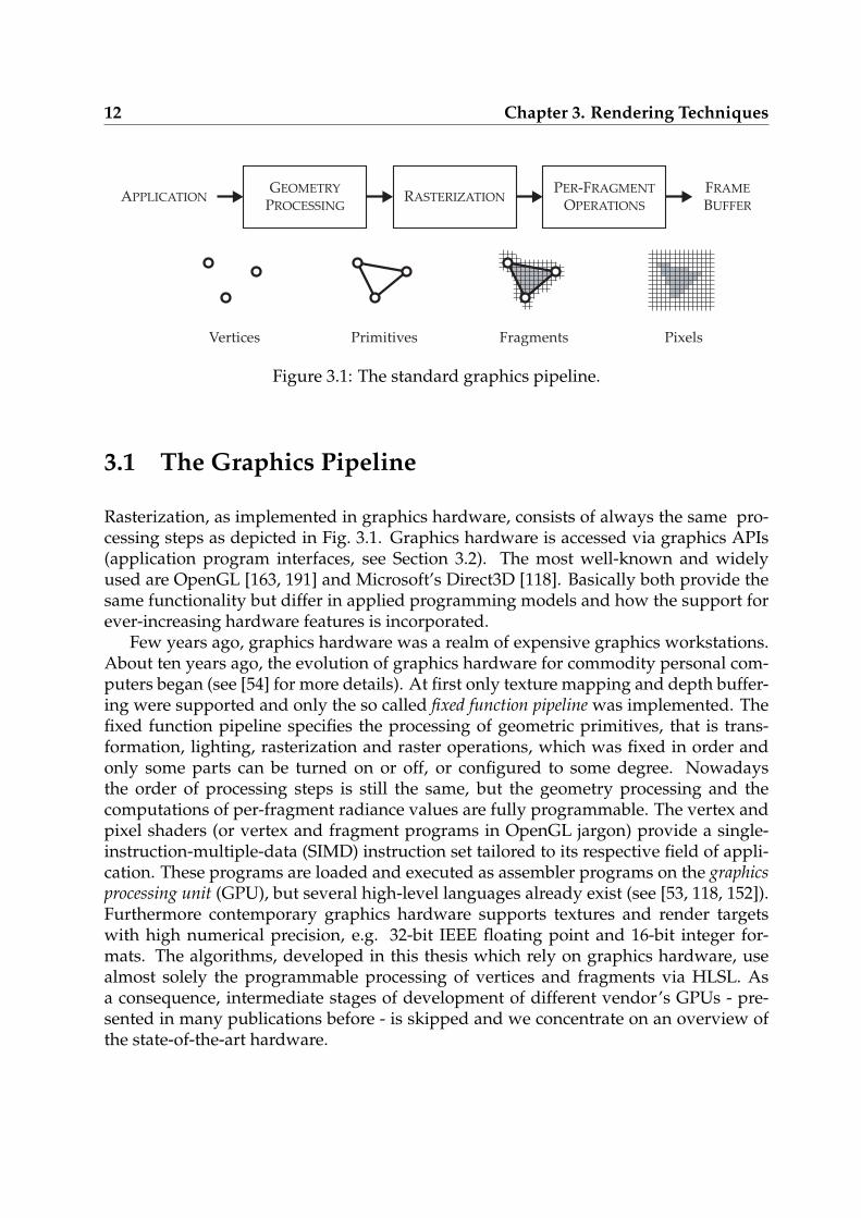
Figure 3.1: The standard graphics pipeline.
3.1 The Graphics Pipeline
Rasterization, as implemented in graphics hardware, consists of always the same pro-cessing steps as depicted in Fig. 3.1. Graphics hardware is accessed via graphics APIs(application program interfaces, see Section 3.2). The most well-known and widelyused are OpenGL [163, 191] and Microsoft’s Direct3D [118]. Basically both provide thesame functionality but differ in applied programming models and how the support forever-increasing hardware features is incorporated.
Few years ago, graphics hardware was a realm of expensive graphics workstations.About ten years ago, the evolution of graphics hardware for commodity personal com-puters began (see [54] for more details). At first only texture mapping and depth buffer-ing were supported and only the so called fixed function pipeline was implemented. Thefixed function pipeline specifies the processing of geometric primitives, that is trans-formation, lighting, rasterization and raster operations, which was fixed in order andonly some parts can be turned on or off, or configured to some degree. Nowadaysthe order of processing steps is still the same, but the geometry processing and thecomputations of per-fragment radiance values are fully programmable. The vertex andpixel shaders (or vertex and fragment programs in OpenGL jargon) provide a single-instruction-multiple-data (SIMD) instruction set tailored to its respective field of appli-cation. These programs are loaded and executed as assembler programs on the graphicsprocessing unit (GPU), but several high-level languages already exist (see [53, 118, 152]).Furthermore contemporary graphics hardware supports textures and render targetswith high numerical precision, e.g. 32-bit IEEE floating point and 16-bit integer for-mats. The algorithms, developed in this thesis which rely on graphics hardware, usealmost solely the programmable processing of vertices and fragments via HLSL. Asa consequence, intermediate stages of development of different vendor’s GPUs - pre-sented in many publications before - is skipped and we concentrate on an overview ofthe state-of-the-art hardware.
3.1 The Graphics Pipeline 13
GEOMETRY PROCESSING
LIGHTINGPRIMITIVE
ASSEMBLY
MODELING &
VIEWING
TRANSFORMATION
CLIPPING/
PROJECTIVE
TRANSFORMATION
Vertices Primitives
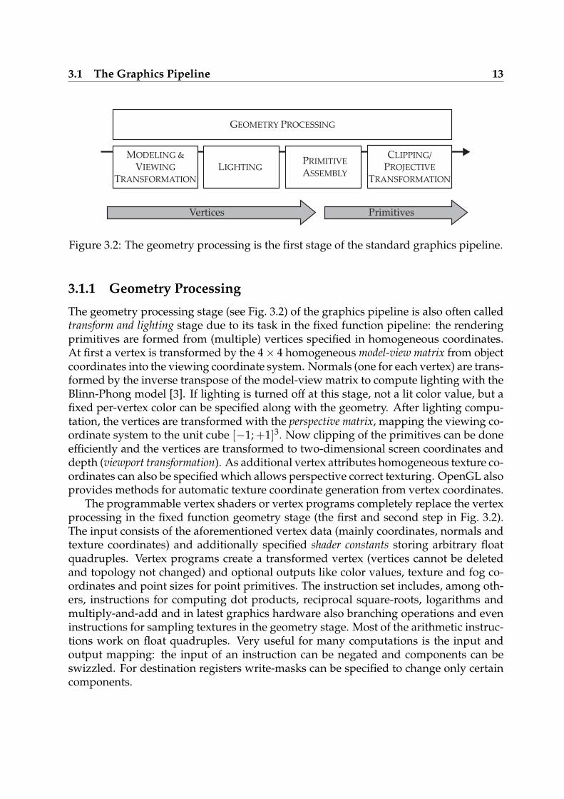
Figure 3.2: The geometry processing is the first stage of the standard graphics pipeline.
3.1.1 Geometry Processing
The geometry processing stage (see Fig. 3.2) of the graphics pipeline is also often calledtransform and lighting stage due to its task in the fixed function pipeline: the renderingprimitives are formed from (multiple) vertices specified in homogeneous coordinates.At first a vertex is transformed by the 4× 4 homogeneous model-view matrix from objectcoordinates into the viewing coordinate system. Normals (one for each vertex) are trans-formed by the inverse transpose of the model-view matrix to compute lighting with theBlinn-Phong model [3]. If lighting is turned off at this stage, not a lit color value, but afixed per-vertex color can be specified along with the geometry. After lighting compu-tation, the vertices are transformed with the perspective matrix, mapping the viewing co-ordinate system to the unit cube [−1; +1]3. Now clipping of the primitives can be doneefficiently and the vertices are transformed to two-dimensional screen coordinates anddepth (viewport transformation). As additional vertex attributes homogeneous texture co-ordinates can also be specified which allows perspective correct texturing. OpenGL alsoprovides methods for automatic texture coordinate generation from vertex coordinates.
The programmable vertex shaders or vertex programs completely replace the vertexprocessing in the fixed function geometry stage (the first and second step in Fig. 3.2).The input consists of the aforementioned vertex data (mainly coordinates, normals andtexture coordinates) and additionally specified shader constants storing arbitrary floatquadruples. Vertex programs create a transformed vertex (vertices cannot be deletedand topology not changed) and optional outputs like color values, texture and fog co-ordinates and point sizes for point primitives. The instruction set includes, among oth-ers, instructions for computing dot products, reciprocal square-roots, logarithms andmultiply-and-add and in latest graphics hardware also branching operations and eveninstructions for sampling textures in the geometry stage. Most of the arithmetic instruc-tions work on float quadruples. Very useful for many computations is the input andoutput mapping: the input of an instruction can be negated and components can beswizzled. For destination registers write-masks can be specified to change only certaincomponents.
14 Chapter 3. Rendering Techniques
RASTERIZATION
INTERPOLATION OF
VERTEX ATTRIBUTES
ACROSS TRIANGLES
SHADE PIXELS/TEXTURING
SCAN
CONVERSION
Primitives Fragments
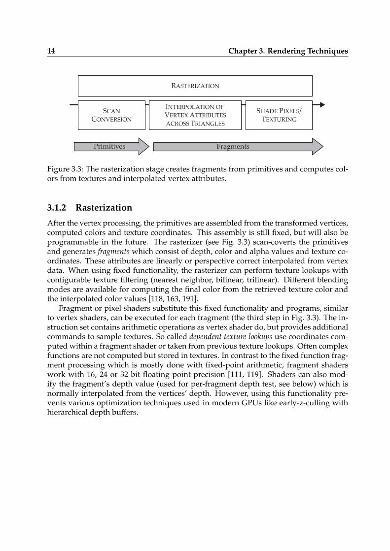
Figure 3.3: The rasterization stage creates fragments from primitives and computes col-ors from textures and interpolated vertex attributes.
3.1.2 Rasterization
After the vertex processing, the primitives are assembled from the transformed vertices,computed colors and texture coordinates. This assembly is still fixed, but will also beprogrammable in the future. The rasterizer (see Fig. 3.3) scan-coverts the primitivesand generates fragments which consist of depth, color and alpha values and texture co-ordinates. These attributes are linearly or perspective correct interpolated from vertexdata. When using fixed functionality, the rasterizer can perform texture lookups withconfigurable texture filtering (nearest neighbor, bilinear, trilinear). Different blendingmodes are available for computing the final color from the retrieved texture color andthe interpolated color values [118, 163, 191].
Fragment or pixel shaders substitute this fixed functionality and programs, similarto vertex shaders, can be executed for each fragment (the third step in Fig. 3.3). The in-struction set contains arithmetic operations as vertex shader do, but provides additionalcommands to sample textures. So called dependent texture lookups use coordinates com-puted within a fragment shader or taken from previous texture lookups. Often complexfunctions are not computed but stored in textures. In contrast to the fixed function frag-ment processing which is mostly done with fixed-point arithmetic, fragment shaderswork with 16, 24 or 32 bit floating point precision [111, 119]. Shaders can also mod-ify the fragment’s depth value (used for per-fragment depth test, see below) which isnormally interpolated from the vertices’ depth. However, using this functionality pre-vents various optimization techniques used in modern GPUs like early-z-culling withhierarchical depth buffers.
3.1 The Graphics Pipeline 15
PER-FRAGMENT OPERATIONS
Fragments
ALPHA
BLENDING
SCISSOR
TEST
ALPHA
TEST
STENCIL
TEST
DEPTH
TEST
Figure 3.4: A fragment passes several tests before it is written to the frame buffer.
3.1.3 Per-Fragment Operations
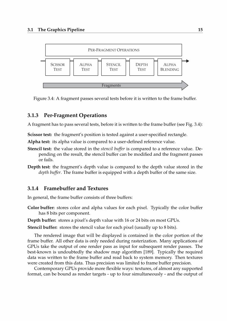
A fragment has to pass several tests, before it is written to the frame buffer (see Fig. 3.4):
Scissor test: the fragment’s position is tested against a user-specified rectangle.
Alpha test: its alpha value is compared to a user-defined reference value.
Stencil test: the value stored in the stencil buffer is compared to a reference value. De-pending on the result, the stencil buffer can be modified and the fragment passesor fails.
Depth test: the fragment’s depth value is compared to the depth value stored in thedepth buffer. The frame buffer is equipped with a depth buffer of the same size.
3.1.4 Framebuffer and Textures
In general, the frame buffer consists of three buffers:
Color buffer: stores color and alpha values for each pixel. Typically the color bufferhas 8 bits per component.
Depth buffer: stores a pixel’s depth value with 16 or 24 bits on most GPUs.
Stencil buffer: stores the stencil value for each pixel (usually up to 8 bits).
The rendered image that will be displayed is contained in the color portion of theframe buffer. All other data is only needed during rasterization. Many applications ofGPUs take the output of one render pass as input for subsequent render passes. Thebest-known is undoubtedly the shadow map algorithm [189]. Typically the requireddata was written to the frame buffer and read back to system memory. Then textureswere created from this data. Thus precision was limited to frame buffer precision.
Contemporary GPUs provide more flexible ways: textures, of almost any supportedformat, can be bound as render targets - up to four simultaneously - and the output of
16 Chapter 3. Rendering Techniques
the rasterizer is directly written to them. The precision is only limited by the textureformat and no time-consuming detour on system memory is necessary. Texture formatsrange from fixed point numbers of few bits per component to full IEEE 32 bit floatingpoint precision and 16 bit integer numbers. The only remaining restriction is, that ren-der targets have to be two-dimensional textures. When rendering to 3D textures each2D slice has to be processed separately.
3.2 Graphics APIs
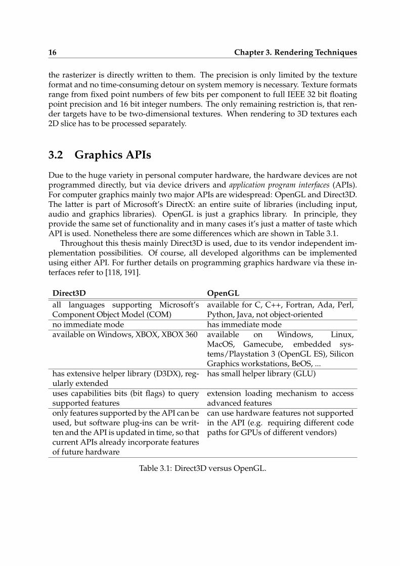
Due to the huge variety in personal computer hardware, the hardware devices are notprogrammed directly, but via device drivers and application program interfaces (APIs).For computer graphics mainly two major APIs are widespread: OpenGL and Direct3D.The latter is part of Microsoft’s DirectX: an entire suite of libraries (including input,audio and graphics libraries). OpenGL is just a graphics library. In principle, theyprovide the same set of functionality and in many cases it’s just a matter of taste whichAPI is used. Nonetheless there are some differences which are shown in Table 3.1.
Throughout this thesis mainly Direct3D is used, due to its vendor independent im-plementation possibilities. Of course, all developed algorithms can be implementedusing either API. For further details on programming graphics hardware via these in-terfaces refer to [118, 191].
Direct3D OpenGL
all languages supporting Microsoft’sComponent Object Model (COM)
available for C, C++, Fortran, Ada, Perl,Python, Java, not object-oriented
no immediate mode has immediate modeavailable on Windows, XBOX, XBOX 360 available on Windows, Linux,
MacOS, Gamecube, embedded sys-tems/Playstation 3 (OpenGL ES), SiliconGraphics workstations, BeOS, ...
has extensive helper library (D3DX), reg-ularly extended
has small helper library (GLU)
uses capabilities bits (bit flags) to querysupported features
extension loading mechanism to accessadvanced features
only features supported by the API can beused, but software plug-ins can be writ-ten and the API is updated in time, so thatcurrent APIs already incorporate featuresof future hardware
can use hardware features not supportedin the API (e.g. requiring different codepaths for GPUs of different vendors)
Table 3.1: Direct3D versus OpenGL.
3.3 Applications for Programmable Graphics Hardware 17
3.3 Applications for Programmable Graphics Hardware
The driving force behind the development of commodity graphics hardware is of coursethe mass market of computer games. There the programmability of the GPUs is exten-sively used for creating computer games with increasing scene complexity and stunningeffects. Furthermore, the flexible programmability allows to offload more and morecomputations to the graphics hardware and frees the CPU for other tasks, for examplephysic simulations, game artificial intelligence and sound or music.
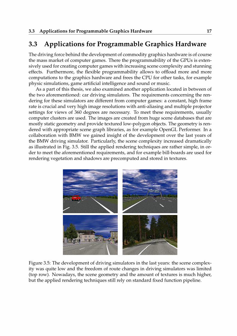
As a part of this thesis, we also examined another application located in between ofthe two aforementioned: car driving simulators. The requirements concerning the ren-dering for these simulators are different from computer games: a constant, high framerate is crucial and very high image resolutions with anti-aliasing and multiple projectorsettings for views of 360 degrees are necessary. To meet these requirements, usuallycomputer clusters are used. The images are created from huge scene databases that aremostly static geometry and provide textured low-polygon objects. The geometry is ren-dered with appropriate scene graph libraries, as for example OpenGL Performer. In acollaboration with BMW we gained insight of the development over the last years ofthe BMW driving simulator. Particularly, the scene complexity increased dramaticallyas illustrated in Fig. 3.5. Still the applied rendering techniques are rather simple, in or-der to meet the aforementioned requirements, and for example bill-boards are used forrendering vegetation and shadows are precomputed and stored in textures.
Figure 3.5: The development of driving simulators in the last years: the scene complex-ity was quite low and the freedom of route changes in driving simulators was limited(top row). Nowadays, the scene geometry and the amount of textures is much higher,but the applied rendering techniques still rely on standard fixed function pipeline.
18 Chapter 3. Rendering Techniques
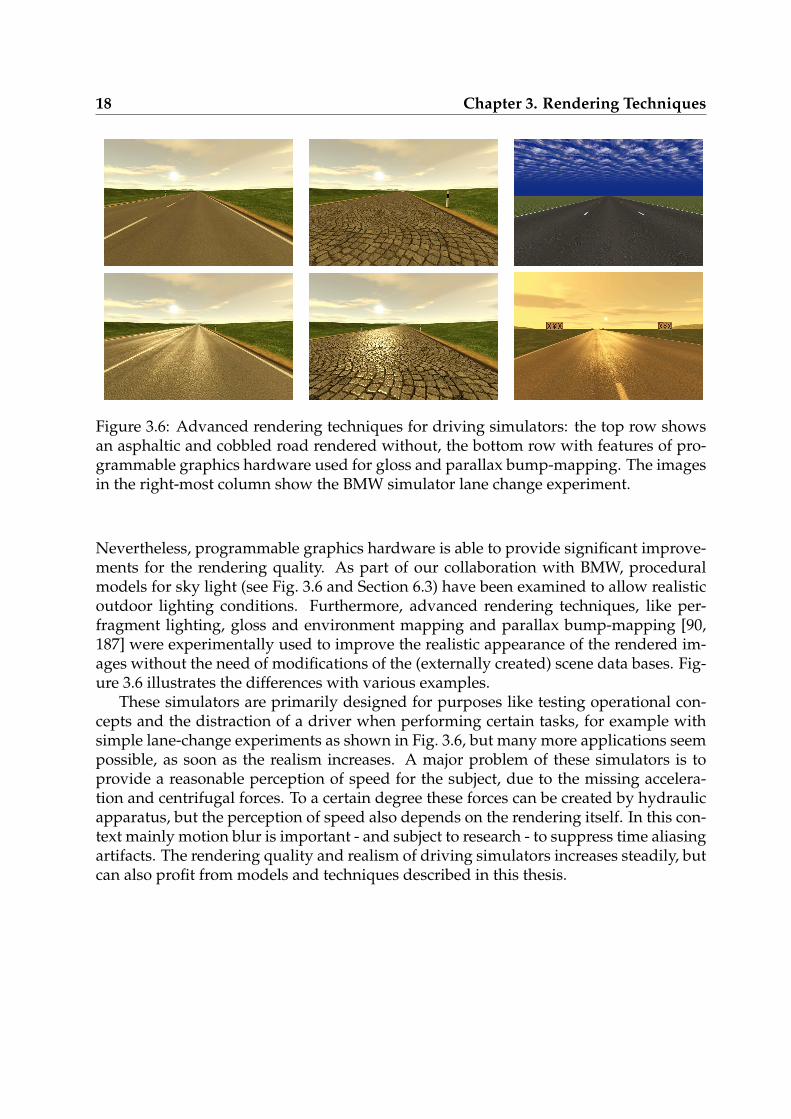
Figure 3.6: Advanced rendering techniques for driving simulators: the top row showsan asphaltic and cobbled road rendered without, the bottom row with features of pro-grammable graphics hardware used for gloss and parallax bump-mapping. The imagesin the right-most column show the BMW simulator lane change experiment.
Nevertheless, programmable graphics hardware is able to provide significant improve-ments for the rendering quality. As part of our collaboration with BMW, proceduralmodels for sky light (see Fig. 3.6 and Section 6.3) have been examined to allow realisticoutdoor lighting conditions. Furthermore, advanced rendering techniques, like per-fragment lighting, gloss and environment mapping and parallax bump-mapping [90,187] were experimentally used to improve the realistic appearance of the rendered im-ages without the need of modifications of the (externally created) scene data bases. Fig-ure 3.6 illustrates the differences with various examples.
These simulators are primarily designed for purposes like testing operational con-cepts and the distraction of a driver when performing certain tasks, for example withsimple lane-change experiments as shown in Fig. 3.6, but many more applications seempossible, as soon as the realism increases. A major problem of these simulators is toprovide a reasonable perception of speed for the subject, due to the missing accelera-tion and centrifugal forces. To a certain degree these forces can be created by hydraulicapparatus, but the perception of speed also depends on the rendering itself. In this con-text mainly motion blur is important - and subject to research - to suppress time aliasingartifacts. The rendering quality and realism of driving simulators increases steadily, butcan also profit from models and techniques described in this thesis.
19
Chapter 4
Point-Based Rendering
Although graphics hardware is primarily specialized in rendering triangles, renderingwith point primitives is an interesting alternative - especially for increasingly complexscenes consisting of a huge number of triangles. The projected area of these trianglesis often smaller than one pixel and triangle based scan-line rendering wastes times insuperfluous sub-pixel computation. Level-of-detail methods [108] try to prevent this byremoving invisible geometric detail. With triangle mesh reduction (e.g. [76, 77, 94]) suchunnecessarily small triangles can be merged to larger ones, but at the expense of signifi-cant precomputation times, large CPU load for on-the-fly re-triangulations, or poppingartifacts of discrete detail levels. Impostors (see e.g. [160]) also reduce geometry, butsuffer from similar problems. Most of these level-of-detail approaches require signifi-cant CPU computation and thus leave the enormous processing power of contemporarygraphics boards unused.
Point representations completely lack topological information, so the degree of detailcan be adapted by adding or removing points. Point-based methods have proven to beefficient not only for rendering, but also for processing and editing three dimensionalmodels [129, 132]. When using 3D scanning technologies, point-sampled surface data isgenerated that is difficult to process and edit. Instead of reconstructing triangle meshesor higher order surface representations from the acquired data, point-based methodswork directly with the point samples.
In the next section, we will give a nearly chronological survey of point based ren-dering methods. This includes approaches using software implementation or hardwareacceleration, but also different ways of generating the images from point samples. Purepoint rendering approaches concentrate on the proper selection of point samples suchthat surfaces can be rendered without holes, when point samples are represented bya fixed point size in screen space (e.g. [183]). Others initially accept holes in the im-age and fill these gaps in subsequent passes (e.g. [65]). More recent approaches, offer-ing the highest rendering quality, use splatting techniques: a surfel (see [139]), that is apoint primitive with associated size and additional attributes (normals, texture colorsetc), covers up to several pixels in screen space and its contribution to their colors iscomputed. This process can also be formulated differently: a point-sampled surface
20 Chapter 4. Point-Based Rendering
provides a non-uniformly sampled signal and during rendering, a continuous signalin image space is reconstructed. Sainz et al. [156, 157] give an overview of existingmethods and a comparison of various point based rendering and splatting methods ina single framework.
4.1 Survey of Point-Based Rendering
Levoy and Whitted [100] proposed to use points as display primitives and emphasizedthe fundamental issues of point-based rendering, that is filtering and surface reconstruc-tion. Grossman and Dally [65] used point-based rendering together with an efficientimage space surface reconstruction technique. Their approach was improved by Pfisteret al. [139] by adding a hierarchical object representation and texture filtering. Focusingon the visualization of large data sets acquired using 3D scanning, Rusinkiewicz et al.developed the Q-Splat system [154], where a bounding sphere hierarchy, constructedfrom point samples, is traversed during rendering. Every traversed node is projectedinto the image and if it has small enough image size, it is rendered as a point of constantradius and further traversal of the subtree is skipped. In [155], the Q-Splat data structureis used for streaming objects over networks. The generated point stream is a sequentialversion of the Q-Splat tree, but the rendering procedure is hierarchical and done on theCPU, so no graphics hardware acceleration is possible. Wand et al. [183] also do a hi-erarchy traversal, but the leaf nodes contain arrays of random point samples which arerendered by the GPU very efficiently. Similarly, [40, 171] precompute random point setson plant objects and sequentially render a list prefix of variable length. The two previ-ous approaches allow very fast rendering of highly irregular objects like plants, but dueto the random sampling they are less suited for connected, smooth surfaces.
Cohen et al. [22] and Chen et al. [15] present hierarchical approaches that smoothlyreplace the point clouds by the original triangles for close up views. In [21] the pointsof an object are sorted back to front by the CPU and then rendered by the GPU withoutdepth test, but with blending. A completely software-based point renderer is presentedin [12], using an octree quantization of point samples and providing a well optimizedCPU rendering method.
Whereas previous work mentioned so far mainly addresses the geometry side ofpoint rendering, that is representation, storage and submission of point sampled geom-etry, a principled analysis of the sampling issues arising in point rendering was pro-vided by Zwicker et al. [194]. His work relies on the concept of resampling filters in-troduced by Heckbert [71]. Heckbert showed how to unify a Gaussian reconstructionand band-limiting filter into a single Gaussian resampling kernel. Point rendering withGaussian resampling kernels, also called elliptical weighted average (EWA) splatting, pro-vides high image quality with anti-aliasing capabilities similar to anisotropic texturefiltering [115]. To reduce the computational complexity of EWA splatting, an approxi-mation using look-up tables has been presented by Botsch et al. [12].
Much effort has been spent on exploiting the computational power and programma-
4.2 Point-Based Rendering in this Thesis 21
bility of current graphics hardware [104, 112] to increase the performance of EWA andother splatting techniques. Ren et al. proposed to represent the resampling filter foreach point by a quadrilateral rasterized by the GPU [150]. However, this implies thedrawback of quadruplicating the geometry data sent to the GPU. When restricting tocircular reconstruction kernels and an approximation of EWA splatting, a more efficientapproach by Botsch et al. [10] based on point sprites can by used. A GPU implemen-tation of EWA splatting using point primitives was also presented by Guennebaud etal. [67]. Zwicker et al. [195] show how point primitives can be used for rasterizingsplats with exact shape, implementing EWA splatting, and handling arbitrary ellipti-cal reconstruction kernels. They formulate splatting using homogeneous coordinates,which resembles the technique described by Olano and Greer [128] for rasterizing tri-angles.
4.2 Point-Based Rendering in this Thesis
Undoubtedly point representations do not always offer advantages, but several fieldsof application exist. In this thesis, point-based rendering is used due to the simplicityof level-of-detail rendering. We use point-based rendering, where triangle meshes offerpoor performance: when rendering trees and other plants, classic triangle based level-of-detail methods fail, due to the huge number of unconnected surfaces in such models.Another application is the rendering of terrain ground detail, e.g. rocks and stones, withcontinuous levels of detail. Triangle based continuous level-of-detail methods introducean overhead that is too large for rendering a large number of instances of an object.
We propose an extension to methods using point hierarchies for rendering, like e.g.Q-Splat. The hierarchical rendering traversal can be transformed to a sequential process.We rearrange the nodes of a hierarchical point tree to a sequential list, such that allpoints that are typically selected during a hierarchical rendering traversal are denselyclustered in the list (see Section 10.1).
For high-quality rendering, we use either pure point rendering for distant geometryor high-quality splatting, as described in Section 10.2 and [195], for close views.

22 Chapter 4. Point-Based Rendering
23
Chapter 5
Height Field Rendering withLevel-of-Detail
The key component of realistic rendering of outdoor scenes is the rendering of the un-derlying terrain. Much research has been spent on this topic and the developed algo-rithms, in particular their utilization of available hardware, evolved over time. There-fore we give a brief chronological survey of decisive terrain rendering methods.
5.1 Purpose of Level-of-Detail Rendering
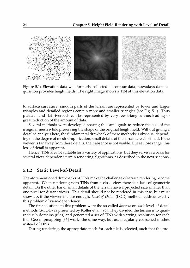
Traditionally, terrain data was collected as contour maps, but nowadays the data acqui-sition is done by airborne and satellite based scanners. Elevation data is then stored asa height map or height field: a regular two-dimensional height-matrix. Often height fieldsare given as a two-dimensional image, where the height information is represented bygray-scales or color coded.
Terrain data sets are usually very large. Even a moderate height field of size 40002
already corresponds to 32 million triangles and thus cannot be directly rendered in realtime. In practice, data sets can be much larger and even the fast advancements of graph-ics hardware cannot compensate for this. Instead, a simplified triangle mesh is gener-ated from the height field and rendered instead. Terrain rendering algorithms differ inhow they achieve this, what criteria incorporate into the mesh generation and finally,how the mesh is stored and rendered. Most of these methods rely on the fact, that thetriangle mesh generated from a height field has a simple topology. The simplification ofarbitrary 3D geometry is more complicated and not discussed here.
5.1.1 Triangular Irregular Networks
The term triangular irregular networks (often abbreviated as TINs) was introduced byFowler et al. [58] and established a basis for several subsequent methods. The regularheight field is converted into a irregular triangle mesh where the triangle count adapts
24 Chapter 5. Height Field Rendering with Level-of-Detail
Figure 5.1: Elevation data was formerly collected as contour data, nowadays data ac-quisition provides height fields. The right image shows a TIN of this elevation data.
to surface curvature: smooth parts of the terrain are represented by fewer and largertriangles and detailed regions contain more and smaller triangles (see Fig. 5.1). Thusplateaus and flat riverbeds can be represented by very few triangles thus leading togreat reduction of the amount of data.
Several methods were developed sharing the same goal: to reduce the size of theirregular mesh while preserving the shape of the original height field. Without giving adetailed analysis here, the fundamental drawback of these methods is obvious: depend-ing on the degree of mesh simplification, small details of the terrain are abolished. If theviewer is far away from these details, their absence is not visible. But at close range, thisloss of detail is apparent.
Hence, TINs are not suitable for a variety of applications, but they serve as a basis forseveral view-dependent terrain rendering algorithms, as described in the next sections.
5.1.2 Static Level-of-Detail
The aforementioned drawbacks of TINs make the challenge of terrain rendering becomeapparent. When rendering with TINs from a close view there is a lack of geometricdetail. On the other hand, small details of the terrain have a projected size smaller thanone pixel for distant views. This detail should not be rendered in this case, but mustshow up, if the viewer is close enough. Level-of-Detail (LOD) methods address exactlythis problem of view-dependency.
The first solutions to this problem were the so-called discrete or static level-of-detailmethods (S-LOD) as presented by Koller et al. [96]. They divided the terrain into quad-ratic sub-domains (tiles) and generated a set of TINs with varying resolution for eachtile. Geo-mipmapping [36] works the same way, but uses regularly coarsened meshesinstead of TINs.
During rendering, the appropriate mesh for each tile is selected, such that the pro-
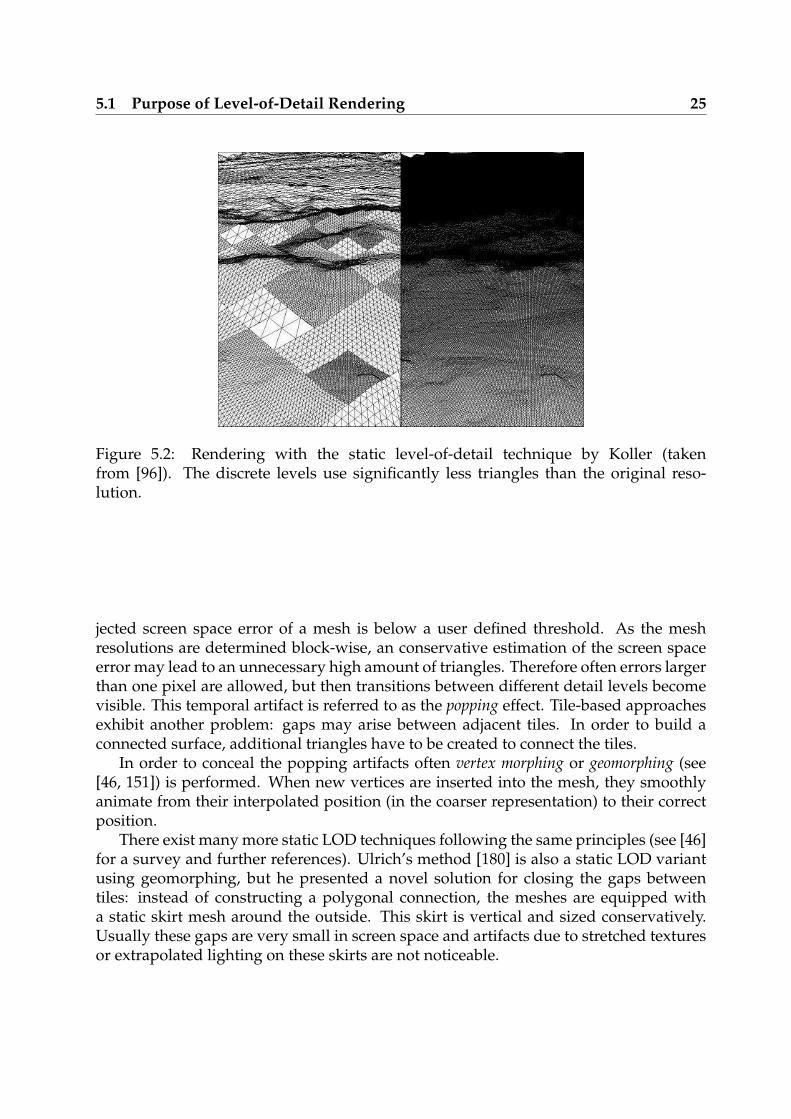
5.1 Purpose of Level-of-Detail Rendering 25
Figure 5.2: Rendering with the static level-of-detail technique by Koller (takenfrom [96]). The discrete levels use significantly less triangles than the original reso-lution.
jected screen space error of a mesh is below a user defined threshold. As the meshresolutions are determined block-wise, an conservative estimation of the screen spaceerror may lead to an unnecessary high amount of triangles. Therefore often errors largerthan one pixel are allowed, but then transitions between different detail levels becomevisible. This temporal artifact is referred to as the popping effect. Tile-based approachesexhibit another problem: gaps may arise between adjacent tiles. In order to build aconnected surface, additional triangles have to be created to connect the tiles.
In order to conceal the popping artifacts often vertex morphing or geomorphing (see[46, 151]) is performed. When new vertices are inserted into the mesh, they smoothlyanimate from their interpolated position (in the coarser representation) to their correctposition.
There exist many more static LOD techniques following the same principles (see [46]for a survey and further references). Ulrich’s method [180] is also a static LOD variantusing geomorphing, but he presented a novel solution for closing the gaps betweentiles: instead of constructing a polygonal connection, the meshes are equipped witha static skirt mesh around the outside. This skirt is vertical and sized conservatively.Usually these gaps are very small in screen space and artifacts due to stretched texturesor extrapolated lighting on these skirts are not noticeable.
26 Chapter 5. Height Field Rendering with Level-of-Detail
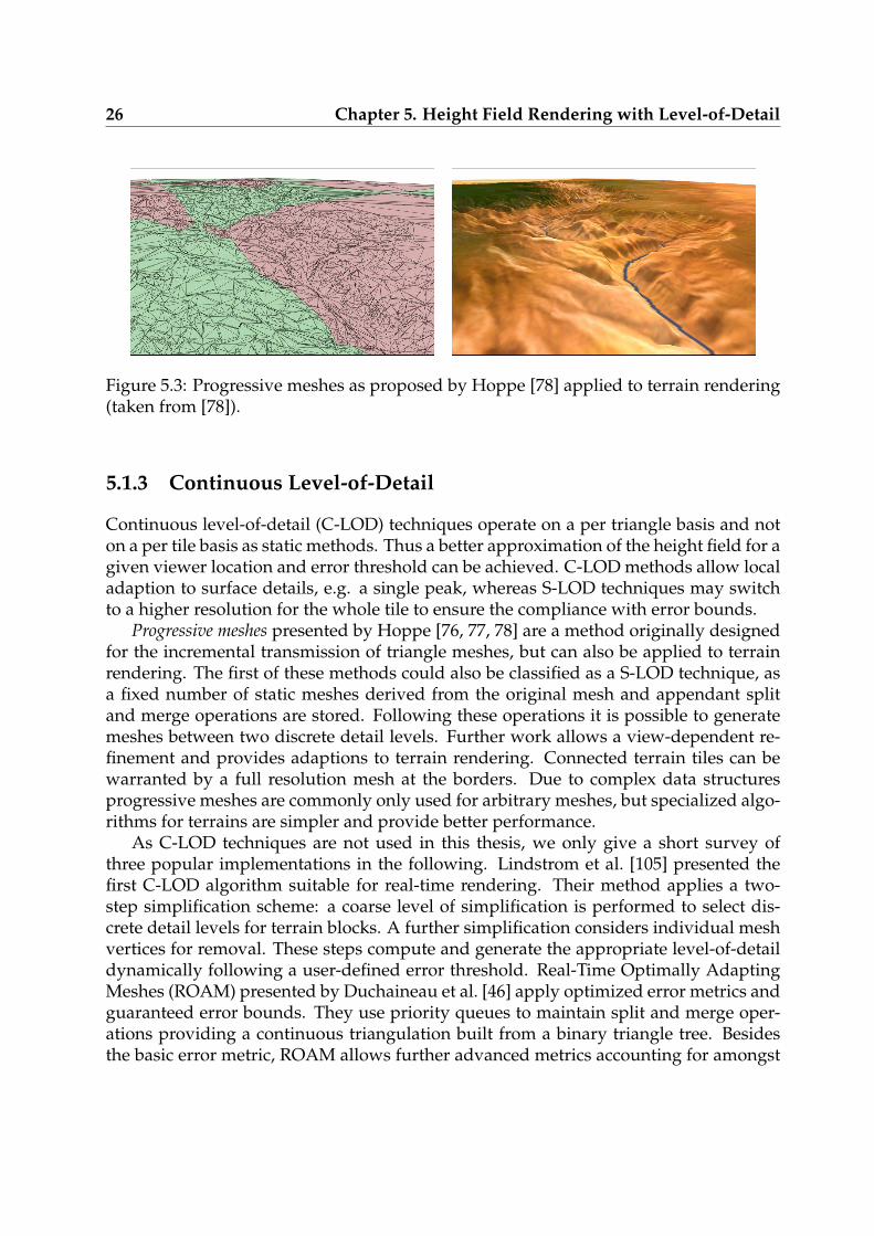
Figure 5.3: Progressive meshes as proposed by Hoppe [78] applied to terrain rendering(taken from [78]).
5.1.3 Continuous Level-of-Detail
Continuous level-of-detail (C-LOD) techniques operate on a per triangle basis and noton a per tile basis as static methods. Thus a better approximation of the height field for agiven viewer location and error threshold can be achieved. C-LOD methods allow localadaption to surface details, e.g. a single peak, whereas S-LOD techniques may switchto a higher resolution for the whole tile to ensure the compliance with error bounds.
Progressive meshes presented by Hoppe [76, 77, 78] are a method originally designedfor the incremental transmission of triangle meshes, but can also be applied to terrainrendering. The first of these methods could also be classified as a S-LOD technique, asa fixed number of static meshes derived from the original mesh and appendant splitand merge operations are stored. Following these operations it is possible to generatemeshes between two discrete detail levels. Further work allows a view-dependent re-finement and provides adaptions to terrain rendering. Connected terrain tiles can bewarranted by a full resolution mesh at the borders. Due to complex data structuresprogressive meshes are commonly only used for arbitrary meshes, but specialized algo-rithms for terrains are simpler and provide better performance.
As C-LOD techniques are not used in this thesis, we only give a short survey ofthree popular implementations in the following. Lindstrom et al. [105] presented thefirst C-LOD algorithm suitable for real-time rendering. Their method applies a two-step simplification scheme: a coarse level of simplification is performed to select dis-crete detail levels for terrain blocks. A further simplification considers individual meshvertices for removal. These steps compute and generate the appropriate level-of-detaildynamically following a user-defined error threshold. Real-Time Optimally AdaptingMeshes (ROAM) presented by Duchaineau et al. [46] apply optimized error metrics andguaranteed error bounds. They use priority queues to maintain split and merge oper-ations providing a continuous triangulation built from a binary triangle tree. Besidesthe basic error metric, ROAM allows further advanced metrics accounting for amongst
5.1 Purpose of Level-of-Detail Rendering 27
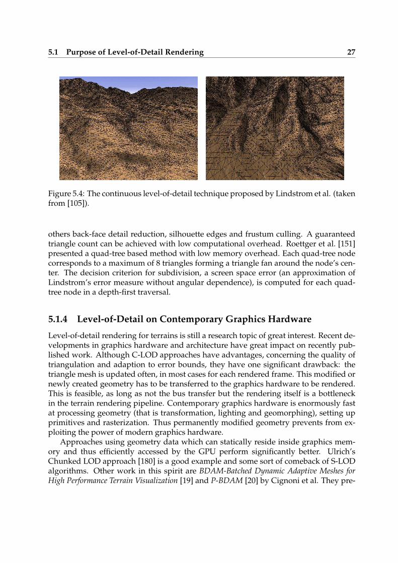
Figure 5.4: The continuous level-of-detail technique proposed by Lindstrom et al. (takenfrom [105]).
others back-face detail reduction, silhouette edges and frustum culling. A guaranteedtriangle count can be achieved with low computational overhead. Roettger et al. [151]presented a quad-tree based method with low memory overhead. Each quad-tree nodecorresponds to a maximum of 8 triangles forming a triangle fan around the node’s cen-ter. The decision criterion for subdivision, a screen space error (an approximation ofLindstrom’s error measure without angular dependence), is computed for each quad-tree node in a depth-first traversal.
5.1.4 Level-of-Detail on Contemporary Graphics Hardware
Level-of-detail rendering for terrains is still a research topic of great interest. Recent de-velopments in graphics hardware and architecture have great impact on recently pub-lished work. Although C-LOD approaches have advantages, concerning the quality oftriangulation and adaption to error bounds, they have one significant drawback: thetriangle mesh is updated often, in most cases for each rendered frame. This modified ornewly created geometry has to be transferred to the graphics hardware to be rendered.This is feasible, as long as not the bus transfer but the rendering itself is a bottleneckin the terrain rendering pipeline. Contemporary graphics hardware is enormously fastat processing geometry (that is transformation, lighting and geomorphing), setting upprimitives and rasterization. Thus permanently modified geometry prevents from ex-ploiting the power of modern graphics hardware.
Approaches using geometry data which can statically reside inside graphics mem-ory and thus efficiently accessed by the GPU perform significantly better. Ulrich’sChunked LOD approach [180] is a good example and some sort of comeback of S-LODalgorithms. Other work in this spirit are BDAM-Batched Dynamic Adaptive Meshes forHigh Performance Terrain Visualization [19] and P-BDAM [20] by Cignoni et al. They pre-
28 Chapter 5. Height Field Rendering with Level-of-Detail
compute TINs for small triangular patches off-line with high quality simplification al-gorithms for out of core rendering. A traversal algorithm selects these TINs for eachframe. Geometry Clipmaps [107] rely on a mesh simplification only based on viewingdistance. Graphics hardware is used to compute smooth transitions between fixed detaillevels and the clipmap construction allows compression of the height data. Furthermoreprocedural detail can be added during rendering. The original concept of clipmaps isrelated to texture maps (see [164] for details).
Previously mentioned techniques can be either classified as continuous or staticlevel-of-detail methods. We developed a novel technique which generates quad meshesof locally varying adapted resolution from a coarse height field on the fly. Proceduralgeometric and texture detail can be added during rendering. The triangle count is al-ways constant and the quad mesh is adapted to the terrain visible in the current viewfrustum taking back-face and occlusion culling into account. We present this work inSection 7.4.
5.1.5 Other Level-of-Detail Aspects
The level-of-detail concepts cannot only be applied to geometry, but also to other time-consuming and/or complex tasks performed during rendering. Whenever a renderedobject is distant from the viewer (that is small in screen space), blurred due to atmo-spheric conditions or the viewer does not pay attention to it (see Luebke’s work onperceptually driven simplification [109]) approximation of geometry and surface ap-pearance can be applied or textures with lower resolution can be used.
For example lighting and shadow computations are very costly involving complexvertex and fragment shaders. If less detail is required, simpler lighting equations can beapplied and accurate shadowing can be abandoned. Fragment shaders may be simpler,when e.g. bump mapping is not used for distant, blurred objects.
5.1.6 Future of Level-of-Detail
Finally, to close this brief overview over level-of-detail concepts, it is important to men-tion, that no matter how fast graphics hardware emerges, the demands regarding com-plexity and amount of input data, rendering quality and screen resolution will alwaysmake level-of-detail methods inevitable for real-time rendering. Furthermore resourcesand computation time are saved and can be used to implement sophisticated lightingmodels or physically based simulations - both are important parts for photo-realisticterrain rendering.
29
Chapter 6
Fundamentals of Procedural Modelling
The rendering of a photo-realistic virtual terrain is made up of several distinct parts: atfirst, the elevation of the terrain has to be specified to render its soil. Texturing terrainwith simple color textures is only feasible when the viewing distance is large. For closerviews, the vegetation and small features, e.g. rocks, are very important. Surfaces of wa-ter bodies, like rivers, lakes, or coastal waters, may be present and have to be renderedwith convincing coloring and reflections. For a plausible appearance of the whole scenethe properties of the surrounding atmosphere have to be taken into account. The socalled aerial perspective causes bluing and loss of contrast with distance and is vital forhuman perception of distances.
Some of the required data can be measured and acquired from real-world scenes,but most often procedural or physically based models are applied to generate the dataneeded for rendering. This chapter provides an overview and introduction to such mod-els, used during developing this thesis, and direct the interested reader to further refer-ences.
6.1 Procedural Texturing and Terrain Generation
6.1.1 Noise Functions
Many procedural models applied to create textures, artificial terrain or terrain detail,are based on an irregular primitive function called noise. One might think, that whitenoise [48] (and an approximation of it using a pseudo-random number generator) is areasonable approach. White noise has its energy distributed equally over all frequen-cies, including frequencies much higher than the Nyquist frequency of the samplingwhich is done during texture/terrain creation. To keep procedural models stable andfree from aliasing, a low-pass-filtered version of white noise is necessary.
30 Chapter 6. Fundamentals of Procedural Modelling
An ideal noise function, which takes e.g. texture coordinates as input, should meet thefollowing criteria:
• it is a repeatable pseudo-random function of its inputs.
• it has a known codomain, e.g. [−1; 1].
• it is band-limited.
• pseudo-random functions are always periodic, but the period can be made verylong and thus periodicity may be not noticeable.
• it is stationary and isotropic, that is translationally and rotationally invariant.
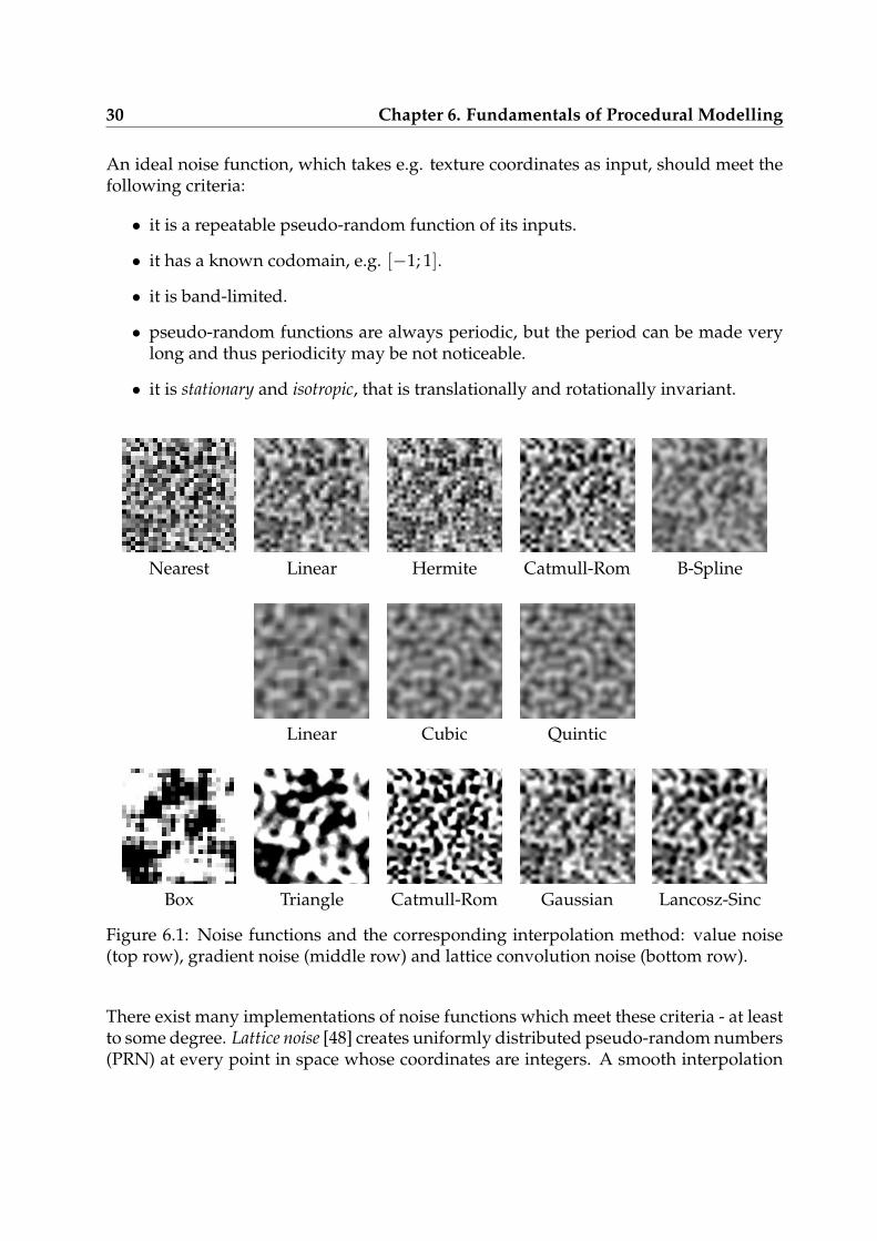
Nearest Linear Hermite Catmull-Rom B-Spline
Linear Cubic Quintic
Box Triangle Catmull-Rom Gaussian Lancosz-Sinc
Figure 6.1: Noise functions and the corresponding interpolation method: value noise(top row), gradient noise (middle row) and lattice convolution noise (bottom row).
There exist many implementations of noise functions which meet these criteria - at leastto some degree. Lattice noise [48] creates uniformly distributed pseudo-random numbers(PRN) at every point in space whose coordinates are integers. A smooth interpolation
6.1 Procedural Texturing and Terrain Generation 31
of this integer lattice provides the necessary low-pass filtering of the noise. The band-limitation of the interpolation, and thus the quality of the noise function, depends onthe interpolation scheme (see Fig. 6.1). Linear interpolation is insufficient to producessmooth noise: lattice cells are obvious and the derivative of a linearly interpolated valueis not continuous, which is obvious to the human eye. Cubic interpolation providescontinuous first and second derivatives and thus Catmull-Rom splines are widely used.Quadratic and cubic B-splines are also widespread, but they do not interpolate but ap-proximate the lattice values and may lead to a narrower oscillation range.
When noise values are stored in the integer lattice and interpolated, we speak ofvalue noise. Gradient noise generates pseudo-random gradient vectors at lattice pointsand use them to reconstruct the noise function [136, 138]. A value-gradient noise combi-nation is also often used. Unfortunately lattice noises often exhibit axis-aligned artifacts,which can be reduced by a discrete convolution technique, the so called lattice convolu-tion noise [48]. Sparse convolution noise [101, 102], and spot noise [181] provide a noisefunction not based on a regular lattice of PRNs. A comparison of various noise functionsand interpolation methods is shown in Fig. 6.1.
All of these noise functions can be evaluated implicitly: a noise value can be re-turned for any input texture coordinate. Explicit noise algorithms generate a large batchof noise values all at once. To use them in an implicit fashion, the results are stored ina table or texture. Familiar techniques in this vein are the midpoint displacement tech-nique [57] (and related [158]) and a Fourier transform based spectral synthesis [48]. Theevaluation cost of explicit methods can be well below the cost of implicit methods [159].
To generate a stochastic function with a particular power spectrum, spectral syn-thesis based on noise functions is often used. The well-known turbulence function [48]is a function of such type, with a power spectrum in which the amplitude is inverselyproportional to the frequency.
6.1.2 Artificial Terrain
The above presented functions can be used to generate procedural textures, by mappingnoise values to colors, or procedural terrains. In the latter case, height fields are gener-ated. As mentioned before, a height field is a two-dimensional array of altitude valuesat equally spaced grid points and thus there are no overhangs in such a terrain.
The fractal Brownian Motion (fBM) [48] is one of the classic approaches for generatingheight fields. It’s a generalization of the aforementioned turbulence function. The resultfor a surface point x is computed from a weighted sum of noise functions:
f BM(x) =n−1
∑i=0
N(x · Li)L−iH (6.1)
where n is the number of octaves, L is the gap between successive frequencies called lacu-narity, N(x) the value of the noise function at x, and H is the fractal increment parameter.For H = 1 and L = 2 this equals Perlin’s turbulence function. The fBM function is
32 Chapter 6. Fundamentals of Procedural Modelling
homogeneous and isotropic, that is - literally speaking - terrain generated from fBMhas the same roughness everywhere. This is of course not desirable for creating realis-tic looking terrain. Multifractals do not combine noise functions additively, as the fBMdoes, but multiplicatively. By this, the occurence of high frequencies depend on the noisevalues of lower frequencies. Note that an additional offset parameter O was added tocontrol the multifractality [48]:
M(x) =n−1
∏i=0
(
N(x · Li) + O)
L−iH (6.2)
Heterogeneous terrain models [121] were developed to create more realistic terrain byapproximating certain erosion features, e.g. talus slopes. To enforce low-lying area tobe smoother, than mountains, absolute altitude values are involved into weighting ofthe noise functions:
f0(x) = N(x) + O
fi(x) =(
N(x · Li) + O)
L−iH fi−1(x)
H(x) =n−1
∑i=0
fi(x)
(6.3)
Ebert et al. [48] present further terrain models which are all derived from the presentedmodels. Among these are the hybrid multifractal and the ridged multifractal model. Fig-ure 6.2 illustrates terrains created with these models.
6.1.3 Models for Terrain Erosion
In order to increase the realism of artificially created terrain erosion is simulated. Ero-sion happens due to thermal weathering: sediment runoff is caused by thermal shocksand parts of the soil material are deposited elsewhere depending on the local surfacegradient. Hydraulic erosion is more or less computed with sediment transport modelsapplied to height fields: water appears at certain locations (e.g. from a spring or wa-ter flow) or affects large terrain regions (due to rain) and dissolves a certain amount ofsoil. Depending on height field gradients the material is transported and deposited atanother location.
Most research of terrain erosion models for computer graphics is more or less in-spired by these simple observations. For detailed description, we direct the interestedreader to [17, 45, 92, 121, 122].
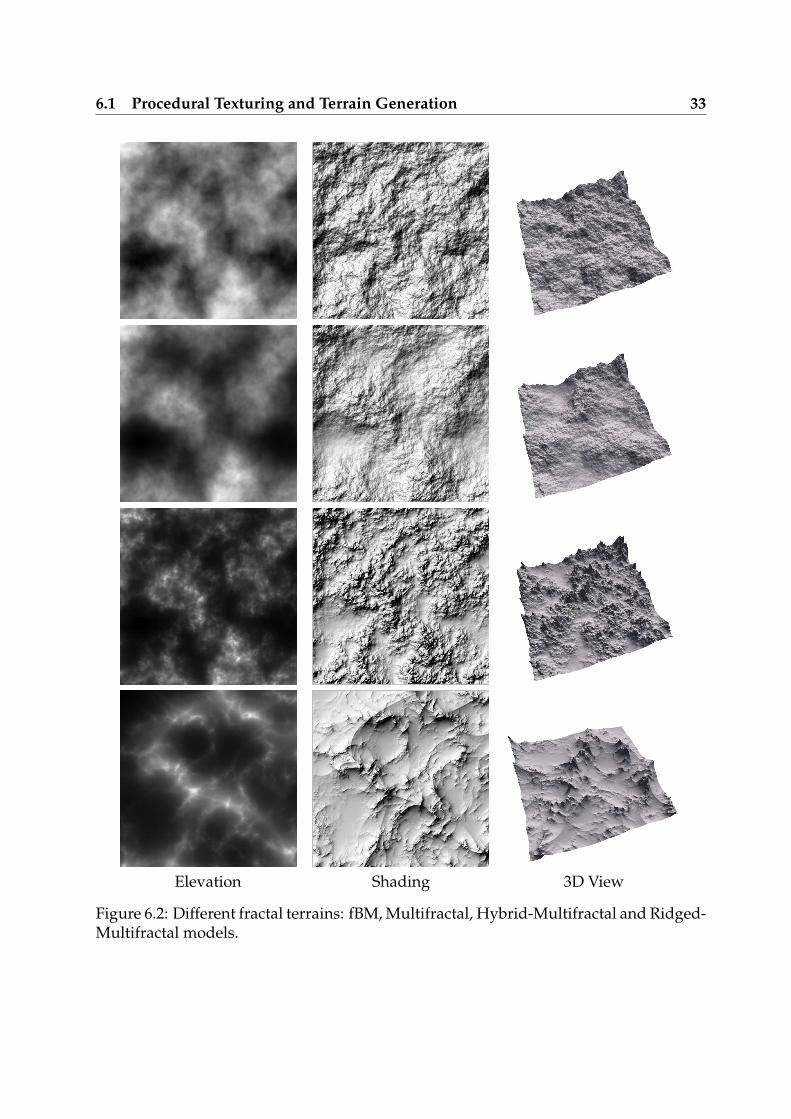
6.1 Procedural Texturing and Terrain Generation 33
Elevation Shading 3D View
Figure 6.2: Different fractal terrains: fBM, Multifractal, Hybrid-Multifractal and Ridged-Multifractal models.
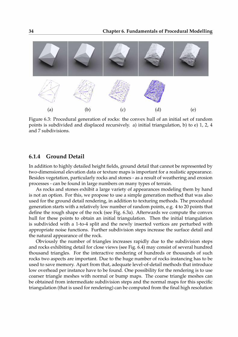
34 Chapter 6. Fundamentals of Procedural Modelling
(a) (b) (c) (d) (e)
Figure 6.3: Procedural generation of rocks: the convex hull of an initial set of randompoints is subdivided and displaced recursively. a) initial triangulation, b) to e) 1, 2, 4and 7 subdivisions.
6.1.4 Ground Detail
In addition to highly detailed height fields, ground detail that cannot be represented bytwo-dimensional elevation data or texture maps is important for a realistic appearance.Besides vegetation, particularly rocks and stones - as a result of weathering and erosionprocesses - can be found in large numbers on many types of terrain.
As rocks and stones exhibit a large variety of appearances modeling them by handis not an option. For this, we propose to use a simple generation method that was alsoused for the ground detail rendering, in addition to texturing methods. The proceduralgeneration starts with a relatively low number of random points, e.g. 4 to 20 points thatdefine the rough shape of the rock (see Fig. 6.3a). Afterwards we compute the convexhull for these points to obtain an initial triangulation. Then the initial triangulationis subdivided with a 1-to-4 split and the newly inserted vertices are perturbed withappropriate noise functions. Further subdivision steps increase the surface detail andthe natural appearance of the rock.
Obviously the number of triangles increases rapidly due to the subdivision stepsand rocks exhibiting detail for close views (see Fig. 6.4) may consist of several hundredthousand triangles. For the interactive rendering of hundreds or thousands of suchrocks two aspects are important. Due to the huge number of rocks instancing has to beused to save memory. Apart from that, adequate level-of-detail methods that introducelow overhead per instance have to be found. One possibility for the rendering is to usecoarser triangle meshes with normal or bump maps. The coarse triangle meshes canbe obtained from intermediate subdivision steps and the normal maps for this specifictriangulation (that is used for rendering) can be computed from the final high resolution
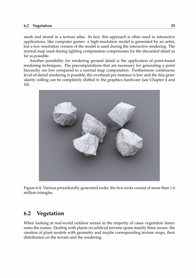
6.2 Vegetation 35
mesh and stored in a texture atlas. In fact, this approach is often used in interactiveapplications, like computer games: a high-resolution model is generated by an artist,but a low-resolution version of the model is used during the interactive rendering. Thenormal map used during lighting computation compensates for the discarded detail asfar as possible.
Another possibility for rendering ground detail is the application of point-basedrendering techniques. The precomputations that are necessary for generating a pointhierarchy are low compared to a normal map computation. Furthermore continuouslevel-of-detail rendering is possible, the overhead per instance is low and the fine gran-ularity culling can be completely shifted to the graphics hardware (see Chapter 4 and10).
Figure 6.4: Various procedurally generated rocks: the five rocks consist of more than 1.6million triangles.
6.2 Vegetation
When looking at real-world outdoor scenes in the majority of cases vegetation domi-nates the scenes. Dealing with plants on artificial terrains spans mainly three issues: thecreation of plant models with geometry and maybe corresponding texture maps, theirdistribution on the terrain and the rendering.
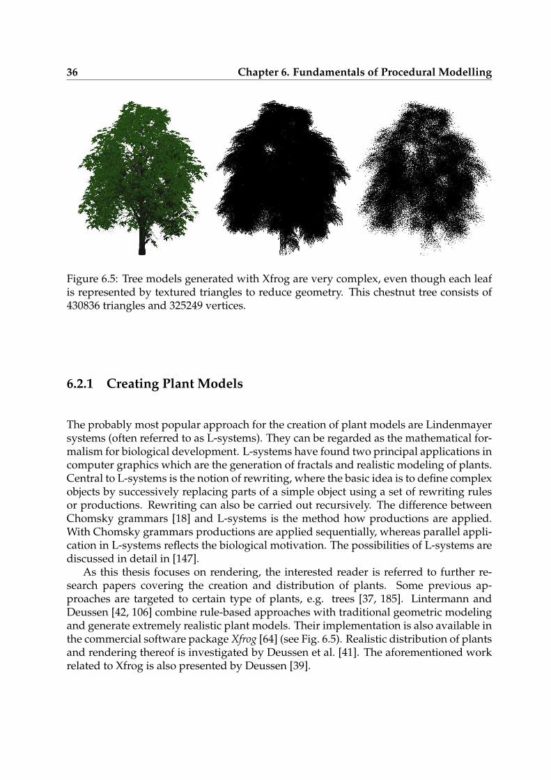
36 Chapter 6. Fundamentals of Procedural Modelling
Figure 6.5: Tree models generated with Xfrog are very complex, even though each leafis represented by textured triangles to reduce geometry. This chestnut tree consists of430836 triangles and 325249 vertices.
6.2.1 Creating Plant Models
The probably most popular approach for the creation of plant models are Lindenmayersystems (often referred to as L-systems). They can be regarded as the mathematical for-malism for biological development. L-systems have found two principal applications incomputer graphics which are the generation of fractals and realistic modeling of plants.Central to L-systems is the notion of rewriting, where the basic idea is to define complexobjects by successively replacing parts of a simple object using a set of rewriting rulesor productions. Rewriting can also be carried out recursively. The difference betweenChomsky grammars [18] and L-systems is the method how productions are applied.With Chomsky grammars productions are applied sequentially, whereas parallel appli-cation in L-systems reflects the biological motivation. The possibilities of L-systems arediscussed in detail in [147].
As this thesis focuses on rendering, the interested reader is referred to further re-search papers covering the creation and distribution of plants. Some previous ap-proaches are targeted to certain type of plants, e.g. trees [37, 185]. Lintermann andDeussen [42, 106] combine rule-based approaches with traditional geometric modelingand generate extremely realistic plant models. Their implementation is also available inthe commercial software package Xfrog [64] (see Fig. 6.5). Realistic distribution of plantsand rendering thereof is investigated by Deussen et al. [41]. The aforementioned workrelated to Xfrog is also presented by Deussen [39].
6.3 Atmospheric Models 37
6.2.2 Interactive Rendering of Plants
The rendering of realistic vegetation is a challenging task as the geometric complexityof generated plant models is extremely high and lighting computation is difficult dueto inter-reflections and sub-surface scattering effects. Classical level-of-detail (LOD)methods, e.g. as used for connected triangle meshes, cannot be applied. Behrendt etal. [2] approximate the plant models using a dynamically changing set of billboardsand to use spherical harmonics for lighting computation. The same idea is presented inby Colditz et al. [24] and additionally an overview is given on related work.
Another solution to the rendering of complex plant geometry is presented byDeussen et al. [40]. Plants are not only rendered using triangles, but also with lines andpoints as primitives. For example, distant grass blades are rendered as lines and distantleaves are replaced by points. The latter two primitives allow simple LOD schemes asproposed by Stamminger et al. [171] and Wand et al. [183]. The work on plant renderingin this thesis follows this spirit as well, using a hybrid point, line and triangle approach.
Further work on plant rendering is specialized in rendering of wide open grassprairies (Perbet et al. [134]) and forest scenes (Decaudin et al. [38]).
6.3 Atmospheric Models
The earth is surrounded by the atmosphere which is, compared to the size of the earth,relatively thin and its density decreases with distance from the earth’s surface. Thetroposphere (altitude up to 17km), where the weather happens, contains water vapor,clouds and aerosols. The next layer is the stratosphere and ranges from 17km to 50km.It includes the ozone layer (altitude 18km to 25km) which is responsible for absorptionof the ultraviolet radiation. Further atmosphere layers are the mesosphere, ionosphereand exosphere which already states the transition to outer space. For the visual appear-ance only troposphere and stratosphere are of interest. They consists of various gases,but only four make up the biggest part: Nitrogen (a decay of biological products) con-stitutes 78,09%, oxygen (from photosynthesis) constitutes 20,95%, the noble gas Argonconstitutes 0,93% and carbon dioxide 0,033% of a dry atmosphere. Other gases occuronly in low concentrations, but are fundamental for vital processes. But the atmospherealso contains water vapor and dust particles. The density and pressure of the atmo-sphere vary with altitude, but also depend on solar heating and geomagnetic activity.Most often a simple approximative model with an exponential fall off with altitude isused [114].
Sun light penetrating the earth’s atmosphere is partly absorbed, whereas molecularoxygen and ozone absorbs light in the ultraviolet range and e.g. water vapor and car-bon dioxide absorb infrared light. Apart from absorption, light is scattered once (singlescattering) or multiple times (multiple scattering) at molecules and particles and arrivesat the earth’s surface from all directions as diffuse skylight or daylight (see Fig. 6.6). Fordaylight conditions, the absorption (aside from the ozone layer) is negligible [68].
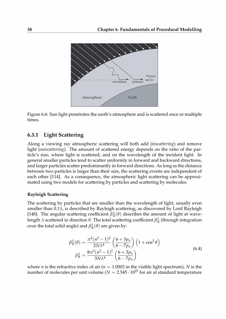
38 Chapter 6. Fundamentals of Procedural Modelling
Atmosphere Earth
secondary primary
Viewer
Figure 6.6: Sun light penetrates the earth’s atmosphere and is scattered once or multipletimes.
6.3.1 Light Scattering
Along a viewing ray atmospheric scattering will both add (inscattering) and removelight (outscattering). The amount of scattered energy depends on the ratio of the par-ticle’s size, where light is scattered, and on the wavelength of the incident light. Ingeneral smaller particles tend to scatter uniformly in forward and backward directions,and larger particles scatter predominantly in forward directions. As long as the distancebetween two particles is larger than their size, the scattering events are independent ofeach other [114]. As a consequence, the atmospheric light scattering can be approxi-mated using two models for scattering by particles and scattering by molecules.
Rayleigh Scattering
The scattering by particles that are smaller than the wavelength of light, usually evensmaller than 0.1λ, is described by Rayleigh scattering, as discovered by Lord Rayleigh[148]. The angular scattering coefficient βλ
R(θ) describes the amount of light at wave-length λ scattered in direction θ. The total scattering coefficient βλ
R (through integrationover the total solid angle) and βλ
R(θ) are given by:
βλR(θ) =
π2(n2 − 1)2
2Nλ4
(
6 + 3pn
6− 7pn
)
(
1 + cos2 θ)
βλR =
8π3(n2 − 1)2
3Nλ4
(
6 + 3pn
6− 7pn
)(6.4)
where n is the refractive index of air (n = 1.0003 in the visible light spectrum), N is thenumber of molecules per unit volume (N = 2.545 · 1025 for air at standard temperature
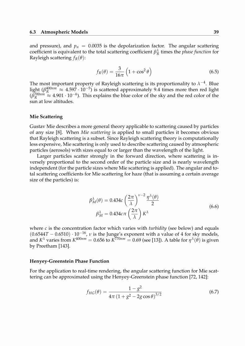
6.3 Atmospheric Models 39
and pressure), and pn = 0.0035 is the depolarization factor. The angular scatteringcoefficient is equivalent to the total scattering coefficient βλ
R times the phase function forRayleigh scattering fR(θ):
fR(θ) =3
16π
(
1 + cos2 θ)
(6.5)
The most important property of Rayleigh scattering is its proportionality to λ−4. Bluelight (β400nm
R ≈ 4.597 · 10−5) is scattered approximately 9.4 times more then red light(β700nm
R ≈ 4.901 · 10−6). This explains the blue color of the sky and the red color of thesun at low altitudes.
Mie Scattering
Gustav Mie describes a more general theory applicable to scattering caused by particlesof any size [8]. When Mie scattering is applied to small particles it becomes obviousthat Rayleigh scattering is a subset. Since Rayleigh scattering theory is computationallyless expensive, Mie scattering is only used to describe scattering caused by atmosphericparticles (aerosols) with sizes equal to or larger than the wavelength of the light.
Larger particles scatter strongly in the forward direction, where scattering is in-versely proportional to the second order of the particle size and is nearly wavelengthindependent (for the particle sizes where Mie scattering is applied). The angular and to-tal scattering coefficients for Mie scattering for haze (that is assuming a certain averagesize of the particles) is:
βλM(θ) = 0.434c
(
2π
λ
)ν−2 ηλ(θ)
2
βλM = 0.434cπ
(
2π
λ
)
Kλ
(6.6)
where c is the concentration factor which varies with turbidity (see below) and equals(0.6544T − 0.6510) · 10−16, ν is the Junge’s exponent with a value of 4 for sky models,and Kλ varies from K400nm = 0.656 to K770nm = 0.69 (see [13]). A table for ηλ(θ) is givenby Preetham [143].
Henyey-Greenstein Phase Function
For the application to real-time rendering, the angular scattering function for Mie scat-tering can be approximated using the Henyey-Greenstein phase function [72, 142]:
fHG(θ) =1− g2
4π (1 + g2 − 2g cos θ)3/2 (6.7)
40 Chapter 6. Fundamentals of Procedural Modelling
This function describes an ellipse centered at a variable focus and is primarily used dueto their mathematical simplicity than for their theoretical accuracy. Scattering predomi-nantly in forward direction is achieved by positive values for g, backward scattering bynegative values.
Turbidity and Optical Depth
The Mie scattering resulting from aerosols if often referred to as haze. Haze refers toscattering due to more than just molecules, but less than fog [114]. It is often describedby a single heuristic parameter called turbidity. Turbidity T is defined as the ratio ofthe optical thickness (or optical depth) of the haze atmosphere, which is haze particles andmolecules, to the optical thickness of the atmosphere with molecules alone:
T =tm + th
tm(6.8)
where tm is the optical depth of the molecular and th the optical depth of the haze at-mosphere. The optical depth for a given path is the integral of the scattering coefficientβ(s) along this path:
tβ =∫ s
0β(s)ds (6.9)
For optical applications turbidity is typically given for wavelengths of 550nm. Variousdefinitions of turbidity are used in other research areas, so care has to be taken of re-ported values. Turbidity can also be estimated using meteorological range. This is thedistance under daylight conditions at which contrast of a black object against the hori-zon sky is apparent. This distance is approximately the distance to the most distantvisible geographic feature. Preetham [143] presents turbidity values for different mete-orological ranges.
Skylight
The Rayleigh and Mie scattering theories are used to explain the appearance of the sky:the inscattering of blue light from the incident sun light is responsible for the typicalsky light. The variations of blue color and intensity, resulting from the phase functionof Rayleigh scattering, can be noticed on very clear days. Mie scattering causes a rapidincrease in brightness towards the sun, and increased skylight intensity and less bluishcolor towards the horizon.
In order to describe light scattering we define two more quantities. The mass of amedium with density ρ in a path of from A to B of unit cross-section is called opticalmass and given by:
mAB =∫ B
Aρ(x)dx (6.10)
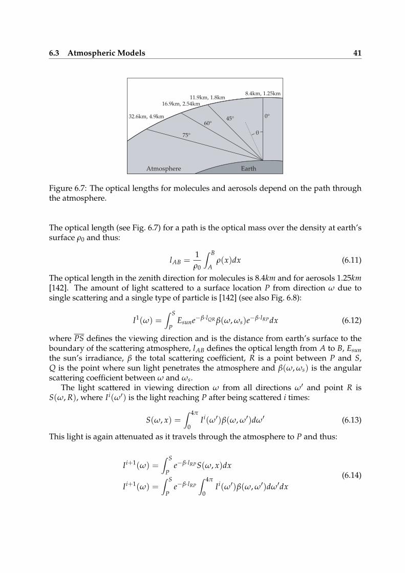
6.3 Atmospheric Models 41
Atmosphere Earth
0°45°60°
75° θ
8.4km, 1.25km11.9km, 1.8km
16.9km, 2.54km
32.6km, 4.9km
Figure 6.7: The optical lengths for molecules and aerosols depend on the path throughthe atmosphere.
The optical length (see Fig. 6.7) for a path is the optical mass over the density at earth’ssurface ρ0 and thus:
lAB =1ρ0
∫ B
Aρ(x)dx (6.11)
The optical length in the zenith direction for molecules is 8.4km and for aerosols 1.25km[142]. The amount of light scattered to a surface location P from direction ω due tosingle scattering and a single type of particle is [142] (see also Fig. 6.8):
I1(ω) =∫ S
PEsune−β·lQR β(ω, ωs)e−β·lRP dx (6.12)
where PS defines the viewing direction and is the distance from earth’s surface to theboundary of the scattering atmosphere, lAB defines the optical length from A to B, Esunthe sun’s irradiance, β the total scattering coefficient, R is a point between P and S,Q is the point where sun light penetrates the atmosphere and β(ω, ωs) is the angularscattering coefficient between ω and ωs.
The light scattered in viewing direction ω from all directions ω′ and point R isS(ω, R), where Ii(ω′) is the light reaching P after being scattered i times:
S(ω, x) =∫ 4π
0Ii(ω′)β(ω, ω′)dω′ (6.13)
This light is again attenuated as it travels through the atmosphere to P and thus:
Ii+1(ω) =∫ S
Pe−β·lRP S(ω, x)dx
Ii+1(ω) =∫ S
Pe−β·lRP
∫ 4π
0Ii(ω′)β(ω, ω′)dω′dx
(6.14)
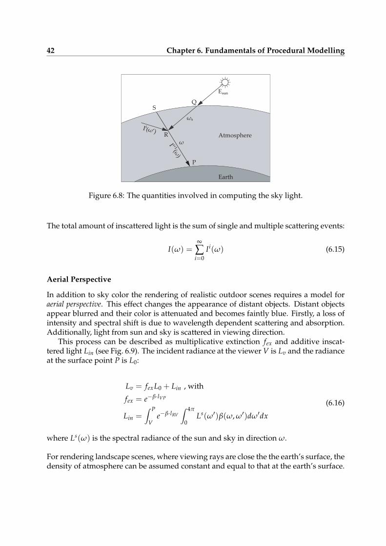
42 Chapter 6. Fundamentals of Procedural Modelling
P
SQ
R
E !"
ω
ω
I$(ω‘)
I $⁺¹(ω)
Atmosphere
Earth
Figure 6.8: The quantities involved in computing the sky light.
The total amount of inscattered light is the sum of single and multiple scattering events:
I(ω) =∞
∑i=0
Ii(ω) (6.15)
Aerial Perspective
In addition to sky color the rendering of realistic outdoor scenes requires a model foraerial perspective. This effect changes the appearance of distant objects. Distant objectsappear blurred and their color is attenuated and becomes faintly blue. Firstly, a loss ofintensity and spectral shift is due to wavelength dependent scattering and absorption.Additionally, light from sun and sky is scattered in viewing direction.
This process can be described as multiplicative extinction fex and additive inscat-tered light Lin (see Fig. 6.9). The incident radiance at the viewer V is Lv and the radianceat the surface point P is L0:
Lv = fexL0 + Lin , with
fex = e−β·lVP
Lin =∫ P
Ve−β·lRV
∫ 4π
0Ls(ω′)β(ω, ω′)dω′dx
(6.16)
where Ls(ω) is the spectral radiance of the sun and sky in direction ω.
For rendering landscape scenes, where viewing rays are close the the earth’s surface, thedensity of atmosphere can be assumed constant and equal to that at the earth’s surface.
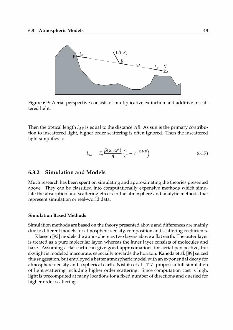
6.3 Atmospheric Models 43
PL⁰
R
L!(ω‘)
ω VL#
Figure 6.9: Aerial perspective consists of multiplicative extinction and additive inscat-tered light.
Then the optical length lAB is equal to the distance AB. As sun is the primary contribu-tion to inscattered light, higher order scattering is often ignored. Then the inscatteredlight simplifies to:
Lin = Esβ(ω, ω′)
β
(
1− e−β·VP)
(6.17)
6.3.2 Simulation and Models
Much research has been spent on simulating and approximating the theories presentedabove. They can be classified into computationally expensive methods which simu-late the absorption and scattering effects in the atmosphere and analytic methods thatrepresent simulation or real-world data.
Simulation Based Methods
Simulation methods are based on the theory presented above and differences are mainlydue to different models for atmosphere density, composition and scattering coefficients.
Klassen [93] models the atmosphere as two layers above a flat earth. The outer layeris treated as a pure molecular layer, whereas the inner layer consists of molecules andhaze. Assuming a flat earth can give good approximations for aerial perspective, butskylight is modeled inaccurate, especially towards the horizon. Kaneda et al. [89] seizedthis suggestion, but employed a better atmospheric model with an exponential decay foratmosphere density and a spherical earth. Nishita et al. [127] propose a full simulationof light scattering including higher order scattering. Since computation cost is high,light is precomputed at many locations for a fixed number of directions and queried forhigher order scattering.
44 Chapter 6. Fundamentals of Procedural Modelling
Analytic Models
Various analytic models for skylight exist. The Commission Internationale de l’Eclairage[80] adopted two models for clear and overcast sky luminance.
The clear sky model was proposed by Pokrokwski based on theory and sky mea-surements. The adopted model, improved by Kittler [142], for clear sky luminance is:
YC = YZ(0.91 + 10e−3γ + 0.45 cos2 γ)(1− e−0.32/cosθ)
(0.91 + 10e−3θs + 0.45 cos2 θs)(1− e−0.32)(6.18)
where YZ is the zenith luminance (tables can be found in [91]), θ is the angle betweenzenith and viewing direction, θs the angle between zenith and sun direction and γ theangle between sun and viewing direction.
The original model for overcast skies was proposed by Moon and Spencer and adop-ted by CIE in a simplified manner:
YOC = YZ1 + 2 cos θ
3(6.19)
The ASRC-CIE model is a linear combination of four different models and can be usedto describe different atmospheric conditions.
Apart from CIE models, Perez proposed his all weather luminance model [135]. Hismodel is based on five parameters, A to E, related to: darkening/brightening of and theluminance gradient near the horizon, the relative intensity and width of the circumsolarregion and the amount of backscattered light. This model is very flexible and able toproduce many different skies. It is given by:
YP = YZF(θ, γ)
F(0, θz), with
F(θ, γ) = (1 + AeB/ cos θ))(1 + CeDγ + E cos2 γ)
(6.20)
All of the above presented models describe sky luminance without spectral dependency.Preetham [143] (see Fig. 6.10) presented an analytical model for spectral radiance of thesky based on the model of Perez. Atmospheric conditions may vary from clear to over-cast skies using a turbidity parameter. They used Nishita’s method to compute sky-light (ignoring ground reflection and third and higher order scattering) together withan improved atmospheric model. The parameters for the Perez model where fitted tothe simulated data for sky luminance (Y) and chromaticity values x and y and spectralradiance can be obtained from these. They also presented an efficient method for com-puting aerial perspective assuming a flat earth and using a cubic polynomial to modelatmosphere density. Please note, that this model is used to compute skylight and doesnot represent the sun disc itself.
Hoffman et al. [75] (see Fig. 6.10) make simplifications in scattering theory assuminga constant density atmosphere and a viewer located on the ground. Thus optical length
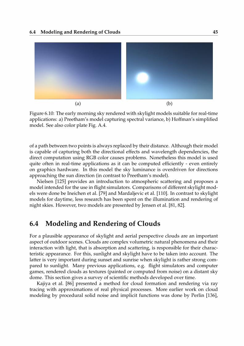
6.4 Modeling and Rendering of Clouds 45
(a) (b)
Figure 6.10: The early morning sky rendered with skylight models suitable for real-timeapplications: a) Preetham’s model capturing spectral variance, b) Hoffman’s simplifiedmodel. See also color plate Fig. A.4.
of a path between two points is always replaced by their distance. Although their modelis capable of capturing both the directional effects and wavelength dependencies, thedirect computation using RGB color causes problems. Nonetheless this model is usedquite often in real-time applications as it can be computed efficiently - even entirelyon graphics hardware. In this model the sky luminance is overdriven for directionsapproaching the sun direction (in contrast to Preetham’s model).
Nielsen [125] provides an introduction to atmospheric scattering and proposes amodel intended for the use in flight simulators. Comparisons of different skylight mod-els were done be Ineichen et al. [79] and Mardaljevic et al. [110]. In contrast to skylightmodels for daytime, less research has been spent on the illumination and rendering ofnight skies. However, two models are presented by Jensen et al. [81, 82].
6.4 Modeling and Rendering of Clouds
For a plausible appearance of skylight and aerial perspective clouds are an importantaspect of outdoor scenes. Clouds are complex volumetric natural phenomena and theirinteraction with light, that is absorption and scattering, is responsible for their charac-teristic appearance. For this, sunlight and skylight have to be taken into account. Thelatter is very important during sunset and sunrise when skylight is rather strong com-pared to sunlight. Many previous applications, e.g. flight simulators and computergames, rendered clouds as textures (painted or computed from noise) on a distant skydome. This section gives a survey of scientific methods developed over time.
Kajiya et al. [86] presented a method for cloud formation and rendering via raytracing with approximations of real physical processes. More earlier work on cloudmodeling by procedural solid noise and implicit functions was done by Perlin [136],
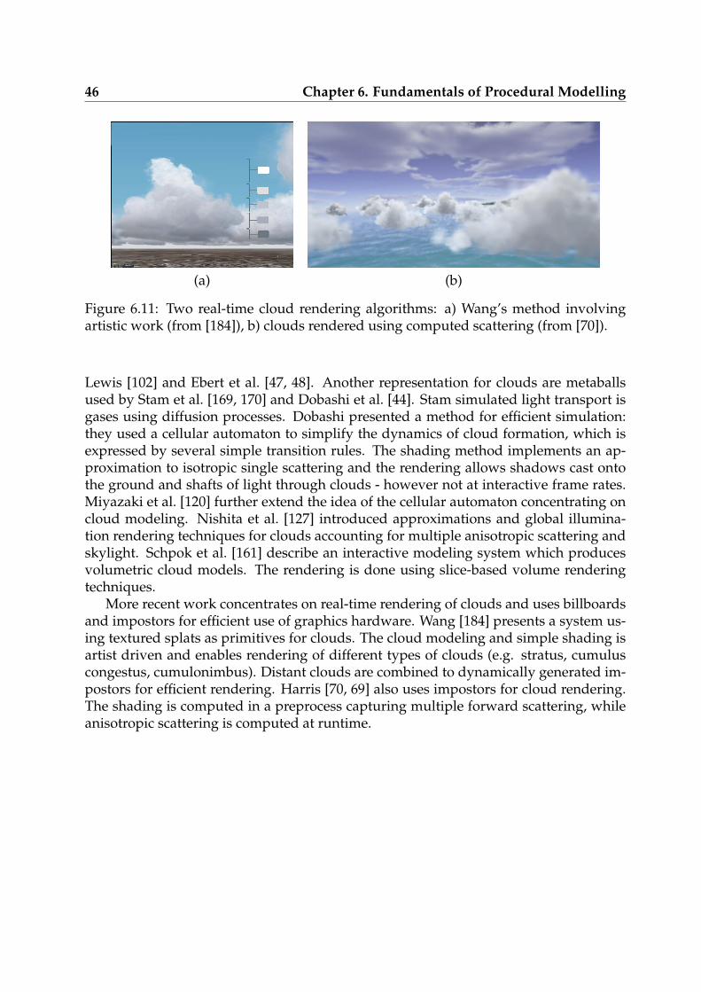
46 Chapter 6. Fundamentals of Procedural Modelling
(a) (b)
Figure 6.11: Two real-time cloud rendering algorithms: a) Wang’s method involvingartistic work (from [184]), b) clouds rendered using computed scattering (from [70]).
Lewis [102] and Ebert et al. [47, 48]. Another representation for clouds are metaballsused by Stam et al. [169, 170] and Dobashi et al. [44]. Stam simulated light transport isgases using diffusion processes. Dobashi presented a method for efficient simulation:they used a cellular automaton to simplify the dynamics of cloud formation, which isexpressed by several simple transition rules. The shading method implements an ap-proximation to isotropic single scattering and the rendering allows shadows cast ontothe ground and shafts of light through clouds - however not at interactive frame rates.Miyazaki et al. [120] further extend the idea of the cellular automaton concentrating oncloud modeling. Nishita et al. [127] introduced approximations and global illumina-tion rendering techniques for clouds accounting for multiple anisotropic scattering andskylight. Schpok et al. [161] describe an interactive modeling system which producesvolumetric cloud models. The rendering is done using slice-based volume renderingtechniques.
More recent work concentrates on real-time rendering of clouds and uses billboardsand impostors for efficient use of graphics hardware. Wang [184] presents a system us-ing textured splats as primitives for clouds. The cloud modeling and simple shading isartist driven and enables rendering of different types of clouds (e.g. stratus, cumuluscongestus, cumulonimbus). Distant clouds are combined to dynamically generated im-postors for efficient rendering. Harris [70, 69] also uses impostors for cloud rendering.The shading is computed in a preprocess capturing multiple forward scattering, whileanisotropic scattering is computed at runtime.
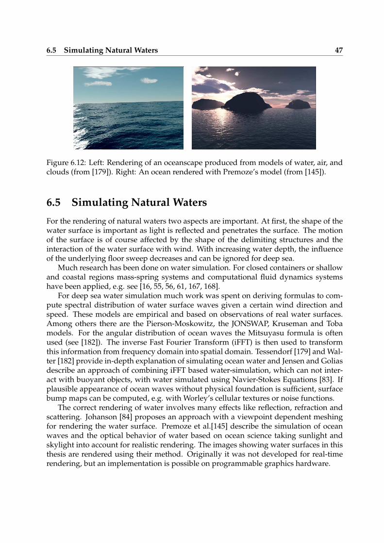
6.5 Simulating Natural Waters 47
Figure 6.12: Left: Rendering of an oceanscape produced from models of water, air, andclouds (from [179]). Right: An ocean rendered with Premoze’s model (from [145]).
6.5 Simulating Natural Waters
For the rendering of natural waters two aspects are important. At first, the shape of thewater surface is important as light is reflected and penetrates the surface. The motionof the surface is of course affected by the shape of the delimiting structures and theinteraction of the water surface with wind. With increasing water depth, the influenceof the underlying floor sweep decreases and can be ignored for deep sea.
Much research has been done on water simulation. For closed containers or shallowand coastal regions mass-spring systems and computational fluid dynamics systemshave been applied, e.g. see [16, 55, 56, 61, 167, 168].
For deep sea water simulation much work was spent on deriving formulas to com-pute spectral distribution of water surface waves given a certain wind direction andspeed. These models are empirical and based on observations of real water surfaces.Among others there are the Pierson-Moskowitz, the JONSWAP, Kruseman and Tobamodels. For the angular distribution of ocean waves the Mitsuyasu formula is oftenused (see [182]). The inverse Fast Fourier Transform (iFFT) is then used to transformthis information from frequency domain into spatial domain. Tessendorf [179] and Wal-ter [182] provide in-depth explanation of simulating ocean water and Jensen and Goliasdescribe an approach of combining iFFT based water-simulation, which can not inter-act with buoyant objects, with water simulated using Navier-Stokes Equations [83]. Ifplausible appearance of ocean waves without physical foundation is sufficient, surfacebump maps can be computed, e.g. with Worley’s cellular textures or noise functions.
The correct rendering of water involves many effects like reflection, refraction andscattering. Johanson [84] proposes an approach with a viewpoint dependent meshingfor rendering the water surface. Premoze et al.[145] describe the simulation of oceanwaves and the optical behavior of water based on ocean science taking sunlight andskylight into account for realistic rendering. The images showing water surfaces in thisthesis are rendered using their method. Originally it was not developed for real-timerendering, but an implementation is possible on programmable graphics hardware.

48 Chapter 6. Fundamentals of Procedural Modelling
49
Chapter 7
Terrain Heightmaps
The basis for terrain rendering is of course the elevation data representing the terrain’sshape and appearance. This data, typically stored as a height map, can be acquiredfrom real-world data or generated procedurally. But many approaches follow a middlecourse: real-world data is used to capture the coarse shape of the terrain while proce-dural small scale detail is added when the viewer approaches.
In this chapter we present a novel method for the generation of elevation data fromexisting height map fragments. This can be done by adapting texture synthesis by non-parametric sampling to height maps. Furthermore, we describe a level-of-detail methodfor terrain rendering that cannot be classified into previously existing categories. Itexploits the fixed topology of height maps and warps a quadrilateral mesh according tocurrent viewing parameters to fit given elevation data and adds procedural small scaledetail afterwards.
7.1 Procedural and Real-World Heightmaps
Nowadays the acquisition of elevation data is feasible due to assistance from satellitebased systems. Freely available data reaches high accuracy and the magnitude of sam-ple spacing is about 1 meter on the earth’s surface. On the one hand, this resolution isnot high enough to reproduce a realistic appearance of the terrain if the viewer is closeto the ground. Of course this is because a realistic terrain does not only consist of a sin-gle soil surface but also of vegetation, rocks and many other small features that cannotbe represented by a height map. On the other hand, the amount of data required for typ-ical viewing distances, which can be up to several kilometers, becomes tremendouslyhigh, even for those height maps that are available.
In contrast, implicit procedural models (see Section 6.1) can be evaluated on demandat arbitrary locations and the storage of the whole height map in advance is not neces-sary. Another – rarely utilized – feature of procedural models for terrain generation is,that there is no restriction to two-dimensional height fields as with satellite data. Proce-dural models are usually suited to produce a certain type of terrains, e.g. hilly valleys or
50 Chapter 7. Terrain Heightmaps
rough mountains. Although efforts were made to develop models that exhibit differentfeatures, a method for combining various models into one height map is desirable. Sucha method is presented in Section 7.3.
7.2 Augmented Procedural Detail
Obviously, real-world and procedural data are completely different starting points anda combination of both is not only possible, but also proved to work well as shown invarious works, e.g. by Losasso et al. [107].
The simplest way of integrating procedural detail into real-world data is to usebump mapping for the rendering of high-frequency detail. This is widely used to gen-erate detail that cannot be captured by the coarse geometry representation of the terrain(without increasing the triangle count for rendering). The bump mapping can eitherbe achieved with precomputed normal maps or by computing the normal pertubationper fragment. In both cases only the lighting computation is affected, but the coarsegeometric resolution remains visible to the viewer.
Modification of the real geometry is often referred to as displacement mapping. Inthe case of terrain rendering from height maps displacement mapping can be achievedmore easily than for arbitrary triangle meshes: whenever the detail of the height mapis insufficient, geometric detail, that is height values lying in between original samples,are computed. Two completely different terrain rendering approaches rely on such de-tail generation. One of them is presented in Section 7.4, the other one is the alreadymentioned work by Losasso et al. [107].
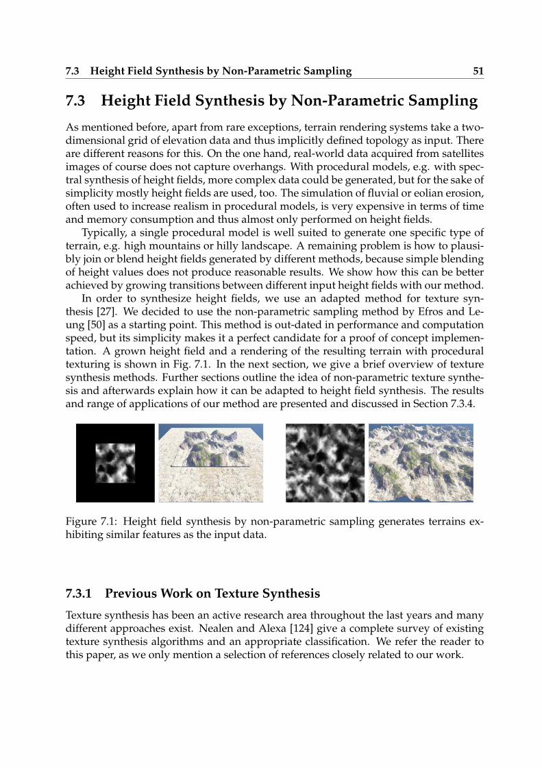
7.3 Height Field Synthesis by Non-Parametric Sampling 51
7.3 Height Field Synthesis by Non-Parametric Sampling
As mentioned before, apart from rare exceptions, terrain rendering systems take a two-dimensional grid of elevation data and thus implicitly defined topology as input. Thereare different reasons for this. On the one hand, real-world data acquired from satellitesimages of course does not capture overhangs. With procedural models, e.g. with spec-tral synthesis of height fields, more complex data could be generated, but for the sake ofsimplicity mostly height fields are used, too. The simulation of fluvial or eolian erosion,often used to increase realism in procedural models, is very expensive in terms of timeand memory consumption and thus almost only performed on height fields.
Typically, a single procedural model is well suited to generate one specific type ofterrain, e.g. high mountains or hilly landscape. A remaining problem is how to plausi-bly join or blend height fields generated by different methods, because simple blendingof height values does not produce reasonable results. We show how this can be betterachieved by growing transitions between different input height fields with our method.
In order to synthesize height fields, we use an adapted method for texture syn-thesis [27]. We decided to use the non-parametric sampling method by Efros and Le-ung [50] as a starting point. This method is out-dated in performance and computationspeed, but its simplicity makes it a perfect candidate for a proof of concept implemen-tation. A grown height field and a rendering of the resulting terrain with proceduraltexturing is shown in Fig. 7.1. In the next section, we give a brief overview of texturesynthesis methods. Further sections outline the idea of non-parametric texture synthe-sis and afterwards explain how it can be adapted to height field synthesis. The resultsand range of applications of our method are presented and discussed in Section 7.3.4.
Figure 7.1: Height field synthesis by non-parametric sampling generates terrains ex-hibiting similar features as the input data.
7.3.1 Previous Work on Texture Synthesis
Texture synthesis has been an active research area throughout the last years and manydifferent approaches exist. Nealen and Alexa [124] give a complete survey of existingtexture synthesis algorithms and an appropriate classification. We refer the reader tothis paper, as we only mention a selection of references closely related to our work.
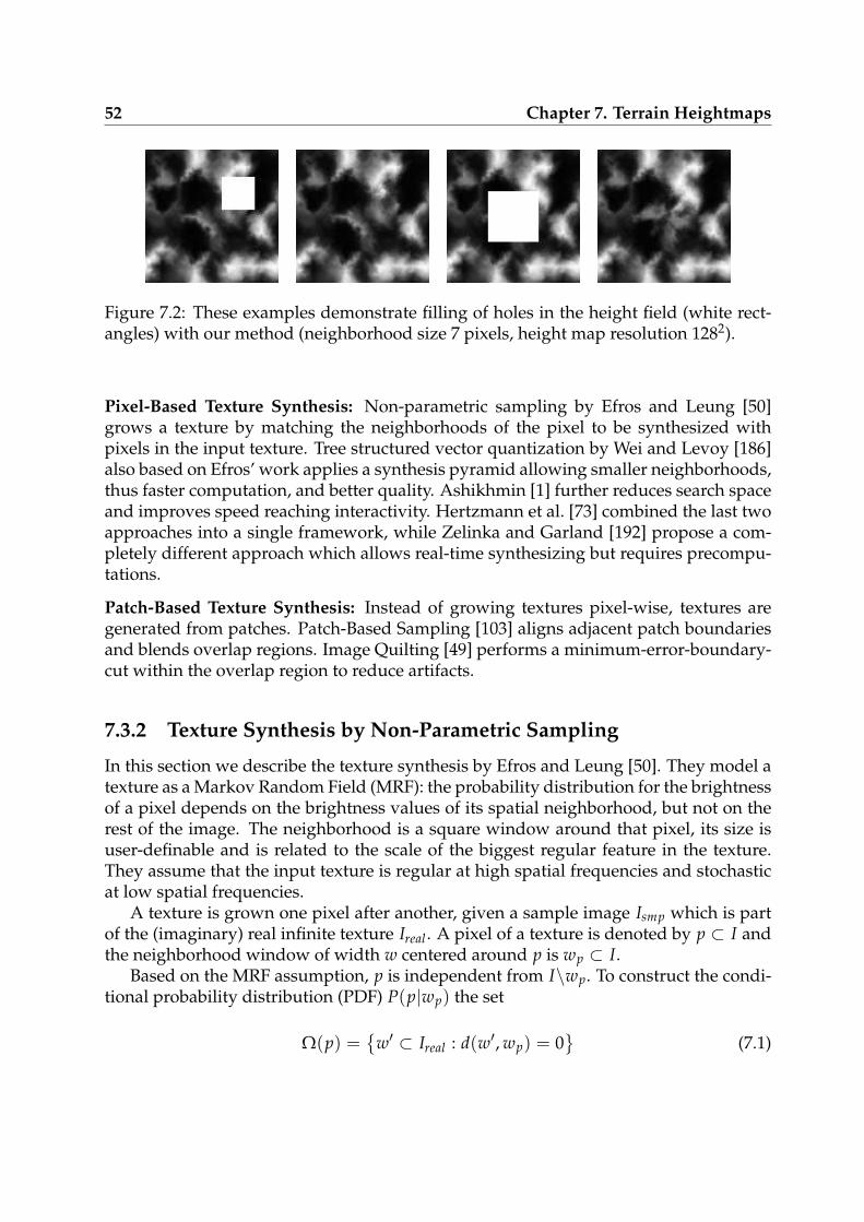
52 Chapter 7. Terrain Heightmaps
Figure 7.2: These examples demonstrate filling of holes in the height field (white rect-angles) with our method (neighborhood size 7 pixels, height map resolution 1282).
Pixel-Based Texture Synthesis: Non-parametric sampling by Efros and Leung [50]grows a texture by matching the neighborhoods of the pixel to be synthesized withpixels in the input texture. Tree structured vector quantization by Wei and Levoy [186]also based on Efros’ work applies a synthesis pyramid allowing smaller neighborhoods,thus faster computation, and better quality. Ashikhmin [1] further reduces search spaceand improves speed reaching interactivity. Hertzmann et al. [73] combined the last twoapproaches into a single framework, while Zelinka and Garland [192] propose a com-pletely different approach which allows real-time synthesizing but requires precompu-tations.
Patch-Based Texture Synthesis: Instead of growing textures pixel-wise, textures aregenerated from patches. Patch-Based Sampling [103] aligns adjacent patch boundariesand blends overlap regions. Image Quilting [49] performs a minimum-error-boundary-cut within the overlap region to reduce artifacts.
7.3.2 Texture Synthesis by Non-Parametric Sampling
In this section we describe the texture synthesis by Efros and Leung [50]. They model atexture as a Markov Random Field (MRF): the probability distribution for the brightnessof a pixel depends on the brightness values of its spatial neighborhood, but not on therest of the image. The neighborhood is a square window around that pixel, its size isuser-definable and is related to the scale of the biggest regular feature in the texture.They assume that the input texture is regular at high spatial frequencies and stochasticat low spatial frequencies.
A texture is grown one pixel after another, given a sample image Ismp which is partof the (imaginary) real infinite texture Ireal . A pixel of a texture is denoted by p ⊂ I andthe neighborhood window of width w centered around p is wp ⊂ I.
Based on the MRF assumption, p is independent from I\wp. To construct the condi-tional probability distribution (PDF) P(p|wp) the set
Ω(p) =
w′ ⊂ Ireal : d(w′, wp) = 0
(7.1)
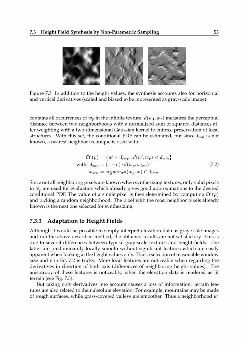
7.3 Height Field Synthesis by Non-Parametric Sampling 53
Figure 7.3: In addition to the height values, the synthesis accounts also for horizontaland vertical derivatives (scaled and biased to be represented as gray-scale image).
contains all occurrences of wp in the infinite texture. d(w1, w2) measures the perceptualdistance between two neighborhoods with a normalized sum of squared distances af-ter weighting with a two-dimensional Gaussian kernel to enforce preservation of localstructures. With this set, the conditional PDF can be estimated, but since Ireal is notknown, a nearest-neighbor technique is used with:
Ω′(p) =
w′ ⊂ Ismp : d(w′, wp) < dmin
with dmin = (1 + ǫ) · d(wp, wbest)
wbest = argminwd(wp, w) ⊂ Ismp
(7.2)
Since not all neighboring pixels are known when synthesizing textures, only valid pixelsin wp are used for evaluation which already gives good approximations to the desiredconditional PDF. The value of a single pixel is then determined by computing Ω′(p)and picking a random neighborhood. The pixel with the most neighbor pixels alreadyknown is the next one selected for synthesizing.
7.3.3 Adaptation to Height Fields
Although it would be possible to simply interpret elevation data as gray-scale imagesand run the above described method, the obtained results are not satisfactory. This isdue to several differences between typical gray-scale textures and height fields. Thelatter are predominantly locally smooth without significant features which are easilyapparent when looking at the height values only. Thus a selection of reasonable windowsize and ǫ in Eq. 7.2 is tricky. More local features are noticeable when regarding thederivatives in direction of both axis (differences of neighboring height values). Theanisotropy of these features is noticeably, when the elevation data is rendered as litterrain (see Fig. 7.3).
But taking only derivatives into account causes a loss of information: terrain fea-tures are also related to their absolute elevation. For example, mountains may be madeof rough surfaces, while grass-covered valleys are smoother. Thus a neighborhood w′
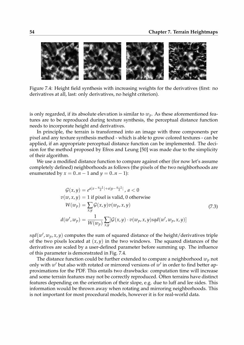
54 Chapter 7. Terrain Heightmaps
Figure 7.4: Height field synthesis with increasing weights for the derivatives (first: noderivatives at all, last: only derivatives, no height criterion).
is only regarded, if its absolute elevation is similar to wp. As these aforementioned fea-tures are to be reproduced during texture synthesis, the perceptual distance functionneeds to incorporate height and derivatives.
In principle, the terrain is transformed into an image with three components perpixel and any texture synthesis method - which is able to grow colored textures - can beapplied, if an appropriate perceptual distance function can be implemented. The deci-sion for the method proposed by Efros and Leung [50] was made due to the simplicityof their algorithm.
We use a modified distance function to compare against other (for now let’s assumecompletely defined) neighborhoods as follows (the pixels of the two neighborhoods areenumerated by x = 0..n− 1 and y = 0..n− 1):
G(x, y) = ea|x− n−12 |+a|y− n−1
2 | , a < 0v(w, x, y) = 1 if pixel is valid, 0 otherwise
W(wp) = ∑x,yG(x, y)v(wp, x, y)
d(w′, wp) =1
W(wp)∑x,y
[G(x, y) · v(wp, x, y)sqd(w′, wp, x, y)]
(7.3)
sqd(w′, wp, x, y) computes the sum of squared distance of the height/derivatives tripleof the two pixels located at (x, y) in the two windows. The squared distances of thederivatives are scaled by a user-defined parameter before summing up. The influenceof this parameter is demonstrated in Fig. 7.4.
The distance function could be further extended to compare a neighborhood wp notonly with w′ but also with rotated or mirrored versions of w′ in order to find better ap-proximations for the PDF. This entails two drawbacks: computation time will increaseand some terrain features may not be correctly reproduced. Often terrains have distinctfeatures depending on the orientation of their slope, e.g. due to luff and lee sides. Thisinformation would be thrown away when rotating and mirroring neighborhoods. Thisis not important for most procedural models, however it is for real-world data.
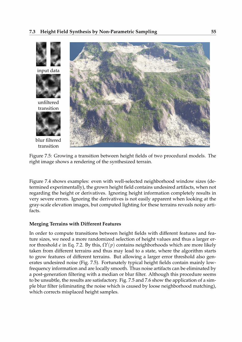
7.3 Height Field Synthesis by Non-Parametric Sampling 55
input data
unfilteredtransition
blur filteredtransition
Figure 7.5: Growing a transition between height fields of two procedural models. Theright image shows a rendering of the synthesized terrain.
Figure 7.4 shows examples: even with well-selected neighborhood window sizes (de-termined experimentally), the grown height field contains undesired artifacts, when notregarding the height or derivatives. Ignoring height information completely results invery severe errors. Ignoring the derivatives is not easily apparent when looking at thegray-scale elevation images, but computed lighting for these terrains reveals noisy arti-facts.
Merging Terrains with Different Features
In order to compute transitions between height fields with different features and fea-ture sizes, we need a more randomized selection of height values and thus a larger er-ror threshold ǫ in Eq. 7.2. By this, Ω′(p) contains neighborhoods which are more likelytaken from different terrains and thus may lead to a state, where the algorithm startsto grow features of different terrains. But allowing a larger error threshold also gen-erates undesired noise (Fig. 7.5). Fortunately typical height fields contain mainly low-frequency information and are locally smooth. Thus noise artifacts can be eliminated bya post-generation filtering with a median or blur filter. Although this procedure seemsto be unsubtle, the results are satisfactory. Fig. 7.5 and 7.6 show the application of a sim-ple blur filter (eliminating the noise which is caused by loose neighborhood matching),which corrects misplaced height samples.
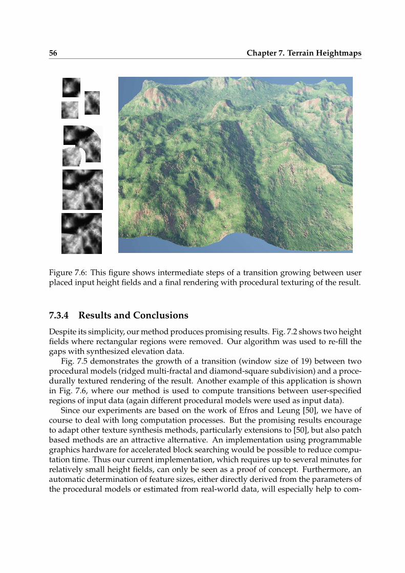
56 Chapter 7. Terrain Heightmaps
Figure 7.6: This figure shows intermediate steps of a transition growing between userplaced input height fields and a final rendering with procedural texturing of the result.
7.3.4 Results and Conclusions
Despite its simplicity, our method produces promising results. Fig. 7.2 shows two heightfields where rectangular regions were removed. Our algorithm was used to re-fill thegaps with synthesized elevation data.
Fig. 7.5 demonstrates the growth of a transition (window size of 19) between twoprocedural models (ridged multi-fractal and diamond-square subdivision) and a proce-durally textured rendering of the result. Another example of this application is shownin Fig. 7.6, where our method is used to compute transitions between user-specifiedregions of input data (again different procedural models were used as input data).
Since our experiments are based on the work of Efros and Leung [50], we have ofcourse to deal with long computation processes. But the promising results encourageto adapt other texture synthesis methods, particularly extensions to [50], but also patchbased methods are an attractive alternative. An implementation using programmablegraphics hardware for accelerated block searching would be possible to reduce compu-tation time. Thus our current implementation, which requires up to several minutes forrelatively small height fields, can only be seen as a proof of concept. Furthermore, anautomatic determination of feature sizes, either directly derived from the parameters ofthe procedural models or estimated from real-world data, will especially help to com-

7.3 Height Field Synthesis by Non-Parametric Sampling 57
pute optimal window-sizes when using the pixel-based methods. It is important to notethat all computations should be performed with sufficient accuracy, i.e. at least 16 bitsper component. We believe that a significant speed-up, but also gain in terms of qual-ity, can be achieved with other methods. This speed-up is of course required to reducecomputation time to tolerable magnitudes for high-detail elevation data.
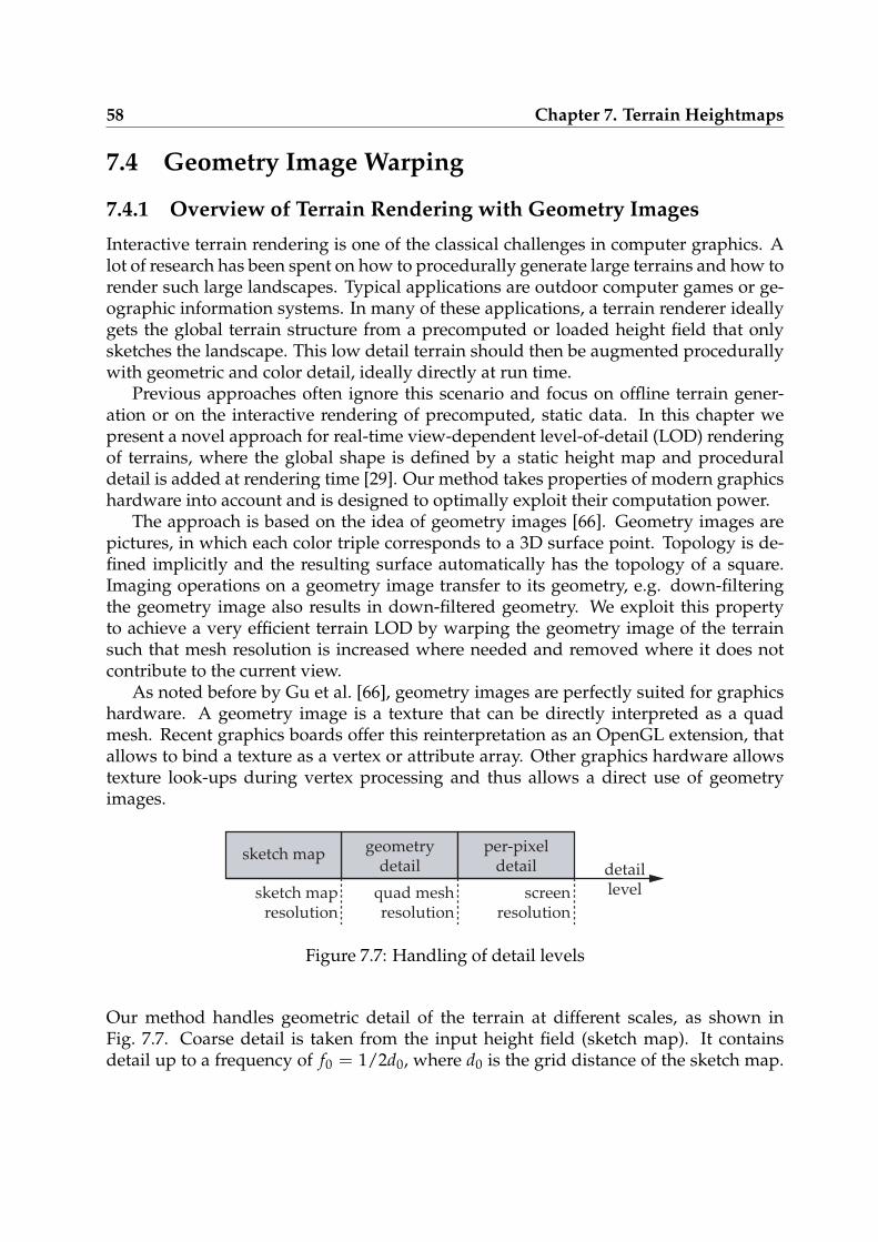
58 Chapter 7. Terrain Heightmaps
7.4 Geometry Image Warping
7.4.1 Overview of Terrain Rendering with Geometry Images
Interactive terrain rendering is one of the classical challenges in computer graphics. Alot of research has been spent on how to procedurally generate large terrains and how torender such large landscapes. Typical applications are outdoor computer games or ge-ographic information systems. In many of these applications, a terrain renderer ideallygets the global terrain structure from a precomputed or loaded height field that onlysketches the landscape. This low detail terrain should then be augmented procedurallywith geometric and color detail, ideally directly at run time.
Previous approaches often ignore this scenario and focus on offline terrain gener-ation or on the interactive rendering of precomputed, static data. In this chapter wepresent a novel approach for real-time view-dependent level-of-detail (LOD) renderingof terrains, where the global shape is defined by a static height map and proceduraldetail is added at rendering time [29]. Our method takes properties of modern graphicshardware into account and is designed to optimally exploit their computation power.
The approach is based on the idea of geometry images [66]. Geometry images arepictures, in which each color triple corresponds to a 3D surface point. Topology is de-fined implicitly and the resulting surface automatically has the topology of a square.Imaging operations on a geometry image transfer to its geometry, e.g. down-filteringthe geometry image also results in down-filtered geometry. We exploit this propertyto achieve a very efficient terrain LOD by warping the geometry image of the terrainsuch that mesh resolution is increased where needed and removed where it does notcontribute to the current view.
As noted before by Gu et al. [66], geometry images are perfectly suited for graphicshardware. A geometry image is a texture that can be directly interpreted as a quadmesh. Recent graphics boards offer this reinterpretation as an OpenGL extension, thatallows to bind a texture as a vertex or attribute array. Other graphics hardware allowstexture look-ups during vertex processing and thus allows a direct use of geometryimages.
sketch map geometrydetail
per-pixeldetail detail
levelsketch mapresolution
quad meshresolution
screenresolution
Figure 7.7: Handling of detail levels
Our method handles geometric detail of the terrain at different scales, as shown inFig. 7.7. Coarse detail is taken from the input height field (sketch map). It containsdetail up to a frequency of f0 = 1/2d0, where d0 is the grid distance of the sketch map.
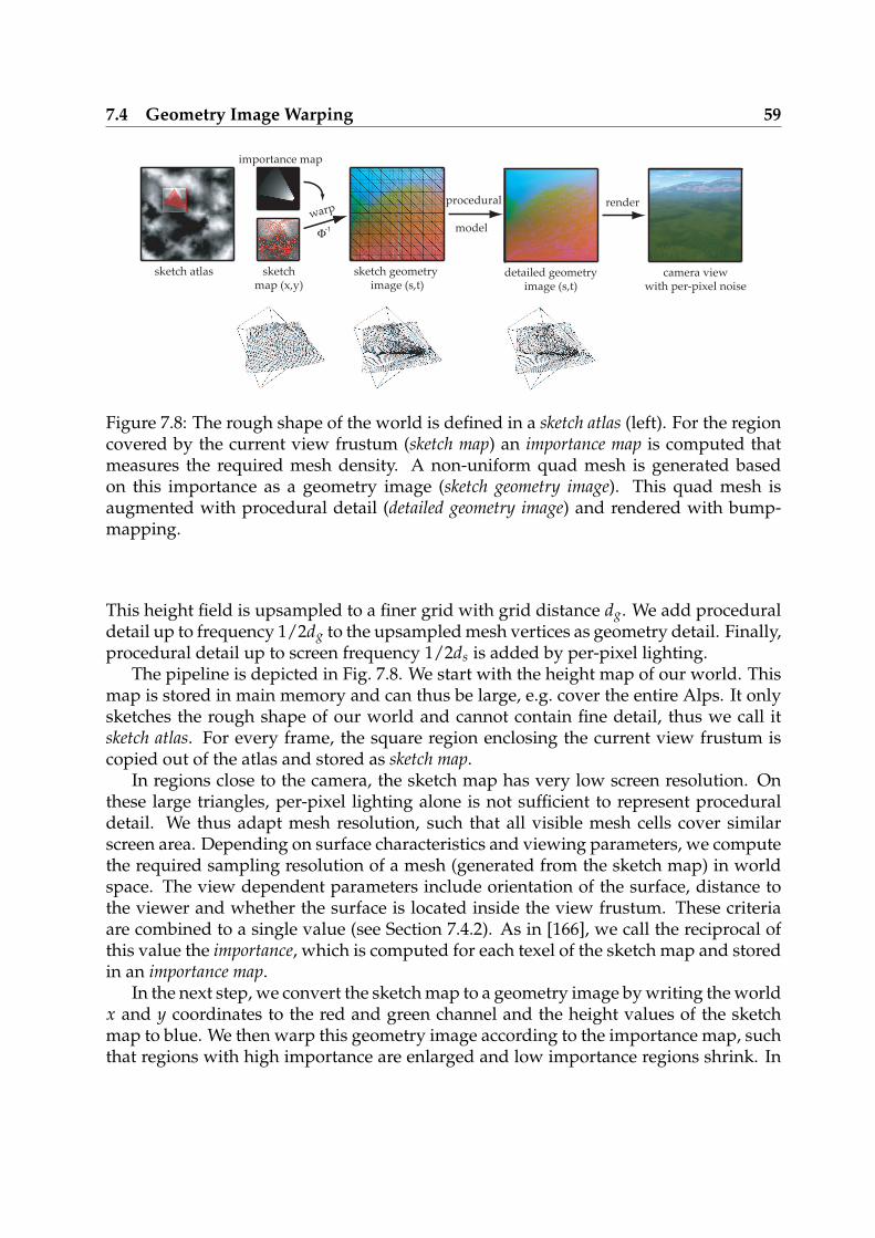
7.4 Geometry Image Warping 59
procedural
model
sketch atlas sketchmap (x,y)
sketch geometry image (s,t)
detailed geometryimage (s,t)
Φ-1
importance map
camera viewwith per-pixel noise
renderwarp
Figure 7.8: The rough shape of the world is defined in a sketch atlas (left). For the regioncovered by the current view frustum (sketch map) an importance map is computed thatmeasures the required mesh density. A non-uniform quad mesh is generated basedon this importance as a geometry image (sketch geometry image). This quad mesh isaugmented with procedural detail (detailed geometry image) and rendered with bump-mapping.
This height field is upsampled to a finer grid with grid distance dg. We add proceduraldetail up to frequency 1/2dg to the upsampled mesh vertices as geometry detail. Finally,procedural detail up to screen frequency 1/2ds is added by per-pixel lighting.
The pipeline is depicted in Fig. 7.8. We start with the height map of our world. Thismap is stored in main memory and can thus be large, e.g. cover the entire Alps. It onlysketches the rough shape of our world and cannot contain fine detail, thus we call itsketch atlas. For every frame, the square region enclosing the current view frustum iscopied out of the atlas and stored as sketch map.
In regions close to the camera, the sketch map has very low screen resolution. Onthese large triangles, per-pixel lighting alone is not sufficient to represent proceduraldetail. We thus adapt mesh resolution, such that all visible mesh cells cover similarscreen area. Depending on surface characteristics and viewing parameters, we computethe required sampling resolution of a mesh (generated from the sketch map) in worldspace. The view dependent parameters include orientation of the surface, distance tothe viewer and whether the surface is located inside the view frustum. These criteriaare combined to a single value (see Section 7.4.2). As in [166], we call the reciprocal ofthis value the importance, which is computed for each texel of the sketch map and storedin an importance map.
In the next step, we convert the sketch map to a geometry image by writing the worldx and y coordinates to the red and green channel and the height values of the sketchmap to blue. We then warp this geometry image according to the importance map, suchthat regions with high importance are enlarged and low importance regions shrink. In
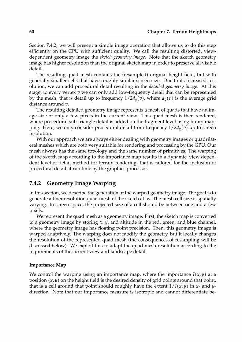
60 Chapter 7. Terrain Heightmaps
Section 7.4.2, we will present a simple image operation that allows us to do this stepefficiently on the CPU with sufficient quality. We call the resulting distorted, view-dependent geometry image the sketch geometry image. Note that the sketch geometryimage has higher resolution than the original sketch map in order to preserve all visibledetail.
The resulting quad mesh contains the (resampled) original height field, but withgenerally smaller cells that have roughly similar screen size. Due to its increased res-olution, we can add procedural detail resulting in the detailed geometry image. At thisstage, to every vertex v we can only add low-frequency detail that can be representedby the mesh, that is detail up to frequency 1/2dg(v), where dg(v) is the average griddistance around v.
The resulting detailed geometry image represents a mesh of quads that have an im-age size of only a few pixels in the current view. This quad mesh is then rendered,where procedural sub-triangle detail is added on the fragment level using bump map-ping. Here, we only consider procedural detail from frequency 1/2dg(v) up to screenresolution.
With our approach we are always either dealing with geometry images or quadrilat-eral meshes which are both very suitable for rendering and processing by the GPU. Ourmesh always has the same topology and the same number of primitives. The warpingof the sketch map according to the importance map results in a dynamic, view depen-dent level-of-detail method for terrain rendering, that is tailored for the inclusion ofprocedural detail at run time by the graphics processor.
7.4.2 Geometry Image Warping
In this section, we describe the generation of the warped geometry image. The goal is togenerate a finer resolution quad mesh of the sketch atlas. The mesh cell size is spatiallyvarying. In screen space, the projected size of a cell should be between one and a fewpixels.
We represent the quad mesh as a geometry image. First, the sketch map is convertedto a geometry image by storing x, y, and altitude in the red, green, and blue channel,where the geometry image has floating point precision. Then, this geometry image iswarped adaptively. The warping does not modify the geometry, but it locally changesthe resolution of the represented quad mesh (the consequences of resampling will bediscussed below). We exploit this to adapt the quad mesh resolution according to therequirements of the current view and landscape detail.
Importance Map
We control the warping using an importance map, where the importance I(x, y) at aposition (x, y) on the height field is the desired density of grid points around that point,that is a cell around that point should roughly have the extent 1/I(x, y) in x- and y-direction. Note that our importance measure is isotropic and cannot differentiate be-
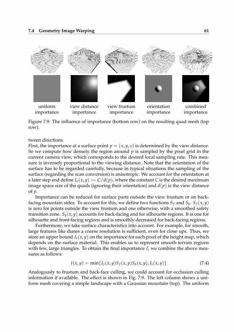
7.4 Geometry Image Warping 61
uniform view distance view frustum orientation combinedimportance importance importance importance importance
Figure 7.9: The influence of importance (bottom row) on the resulting quad mesh (toprow).
tween directions.First, the importance at a surface point p = (x, y, z) is determined by the view distance.So we compute how densely the region around p is sampled by the pixel grid in thecurrent camera view, which corresponds to the desired local sampling rate. This mea-sure is inversely proportional to the viewing distance. Note that the orientation of thesurface has to be regarded carefully, because in typical situations the sampling of thesurface (regarding the scan conversion) is anisotropic. We account for the orientation ata later step and define Iv(x, y) := C/d(p), where the constant C is the desired maximumimage space size of the quads (ignoring their orientation) and d(p) is the view distanceof p.
Importance can be reduced for surface parts outside the view frustum or on back-facing mountain sides. To account for this, we define two functions S f and Sb. S f (x, y)is zero for points outside the view frustum and one otherwise, with a smoothed safetytransition zone. Sb(x, y) accounts for back-facing and for silhouette regions. It is one forsilhouette and front-facing regions and is smoothly decreased for back-facing regions.
Furthermore, we take surface characteristics into account. For example, for smooth,large features like dunes a coarse resolution is sufficient, even for close ups. Thus, westore an upper bound Is(x, y) on the importance for each pixel of the height map, whichdepends on the surface material. This enables us to represent smooth terrain regionswith few, large triangles. To obtain the final importance I, we combine the above mea-sures as follows:
I(x, y) = minIv(x, y)S f (x, y)Sb(x, y), Is(x, y) (7.4)
Analogously to frustum and back-face culling, we could account for occlusion cullinginformation if available. The effect is shown in Fig. 7.9. The left column shows a uni-form mesh covering a simple landscape with a Gaussian mountain (top). The uniform
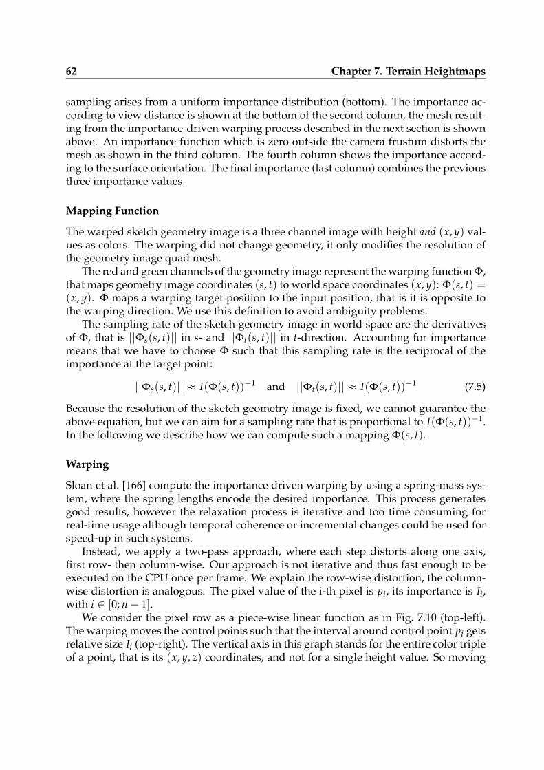
62 Chapter 7. Terrain Heightmaps
sampling arises from a uniform importance distribution (bottom). The importance ac-cording to view distance is shown at the bottom of the second column, the mesh result-ing from the importance-driven warping process described in the next section is shownabove. An importance function which is zero outside the camera frustum distorts themesh as shown in the third column. The fourth column shows the importance accord-ing to the surface orientation. The final importance (last column) combines the previousthree importance values.
Mapping Function
The warped sketch geometry image is a three channel image with height and (x, y) val-ues as colors. The warping did not change geometry, it only modifies the resolution ofthe geometry image quad mesh.
The red and green channels of the geometry image represent the warping function Φ,that maps geometry image coordinates (s, t) to world space coordinates (x, y): Φ(s, t) =(x, y). Φ maps a warping target position to the input position, that is it is opposite tothe warping direction. We use this definition to avoid ambiguity problems.
The sampling rate of the sketch geometry image in world space are the derivativesof Φ, that is ||Φs(s, t)|| in s- and ||Φt(s, t)|| in t-direction. Accounting for importancemeans that we have to choose Φ such that this sampling rate is the reciprocal of theimportance at the target point:
||Φs(s, t)|| ≈ I(Φ(s, t))−1 and ||Φt(s, t)|| ≈ I(Φ(s, t))−1 (7.5)
Because the resolution of the sketch geometry image is fixed, we cannot guarantee theabove equation, but we can aim for a sampling rate that is proportional to I(Φ(s, t))−1.In the following we describe how we can compute such a mapping Φ(s, t).
Warping
Sloan et al. [166] compute the importance driven warping by using a spring-mass sys-tem, where the spring lengths encode the desired importance. This process generatesgood results, however the relaxation process is iterative and too time consuming forreal-time usage although temporal coherence or incremental changes could be used forspeed-up in such systems.
Instead, we apply a two-pass approach, where each step distorts along one axis,first row- then column-wise. Our approach is not iterative and thus fast enough to beexecuted on the CPU once per frame. We explain the row-wise distortion, the column-wise distortion is analogous. The pixel value of the i-th pixel is pi, its importance is Ii,with i ∈ [0; n− 1].
We consider the pixel row as a piece-wise linear function as in Fig. 7.10 (top-left).The warping moves the control points such that the interval around control point pi getsrelative size Ii (top-right). The vertical axis in this graph stands for the entire color tripleof a point, that is its (x, y, z) coordinates, and not for a single height value. So moving
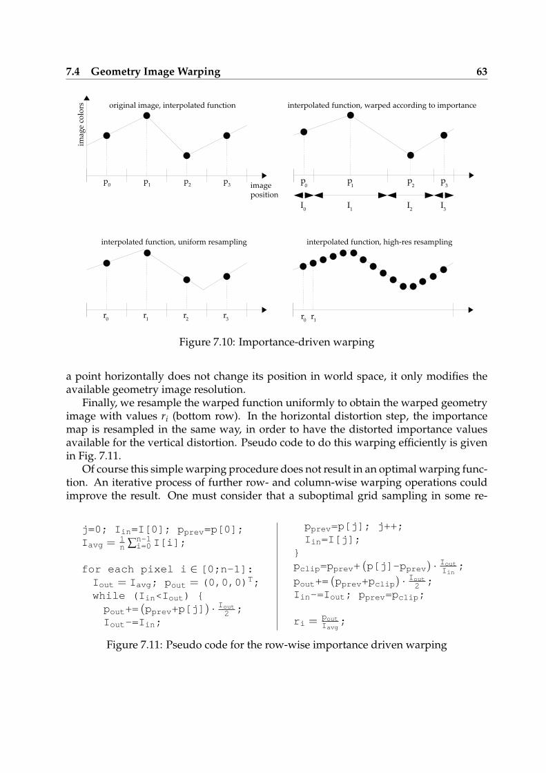
7.4 Geometry Image Warping 63
p0
p
0
p
3
p2
p1
I0
I2
I1
I3
r0
r3
r2
r1 r
0r1
original image, interpolated function
imag
e co
lors
interpolated function, uniform resampling interpolated function, high-res resampling
interpolated function, warped according to importance
imageposition
p1
p2
p3 30
Figure 7.10: Importance-driven warping
a point horizontally does not change its position in world space, it only modifies theavailable geometry image resolution.
Finally, we resample the warped function uniformly to obtain the warped geometryimage with values ri (bottom row). In the horizontal distortion step, the importancemap is resampled in the same way, in order to have the distorted importance valuesavailable for the vertical distortion. Pseudo code to do this warping efficiently is givenin Fig. 7.11.
Of course this simple warping procedure does not result in an optimal warping func-tion. An iterative process of further row- and column-wise warping operations couldimprove the result. One must consider that a suboptimal grid sampling in some re-
j=0; Iin=I[0]; pprev=p[0];Iavg = 1
n ∑n-1i=0 I[i];
for each pixel i ∈ [0;n-1]:Iout = Iavg; pout = (0,0,0)T;while (Iin<Iout) pout+= (pprev+p[j]) · Iout2 ;Iout-=Iin;
pprev=p[j]; j++;Iin=I[j];
pclip=pprev+ (p[j]-pprev) · IoutIin
;
pout+= (pprev+pclip) · Iout2 ;Iin-=Iout; pprev=pclip;
ri = poutIavg
;
Figure 7.11: Pseudo code for the row-wise importance driven warping
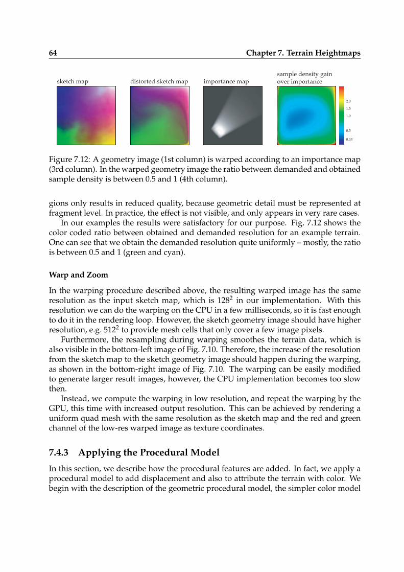
64 Chapter 7. Terrain Heightmaps
sketch map distorted sketch map importance mapsample density gainover importance
1.0
0.5
1.5
2.0
0.33
Figure 7.12: A geometry image (1st column) is warped according to an importance map(3rd column). In the warped geometry image the ratio between demanded and obtainedsample density is between 0.5 and 1 (4th column).
gions only results in reduced quality, because geometric detail must be represented atfragment level. In practice, the effect is not visible, and only appears in very rare cases.
In our examples the results were satisfactory for our purpose. Fig. 7.12 shows thecolor coded ratio between obtained and demanded resolution for an example terrain.One can see that we obtain the demanded resolution quite uniformly – mostly, the ratiois between 0.5 and 1 (green and cyan).
Warp and Zoom
In the warping procedure described above, the resulting warped image has the sameresolution as the input sketch map, which is 1282 in our implementation. With thisresolution we can do the warping on the CPU in a few milliseconds, so it is fast enoughto do it in the rendering loop. However, the sketch geometry image should have higherresolution, e.g. 5122 to provide mesh cells that only cover a few image pixels.
Furthermore, the resampling during warping smoothes the terrain data, which isalso visible in the bottom-left image of Fig. 7.10. Therefore, the increase of the resolutionfrom the sketch map to the sketch geometry image should happen during the warping,as shown in the bottom-right image of Fig. 7.10. The warping can be easily modifiedto generate larger result images, however, the CPU implementation becomes too slowthen.
Instead, we compute the warping in low resolution, and repeat the warping by theGPU, this time with increased output resolution. This can be achieved by rendering auniform quad mesh with the same resolution as the sketch map and the red and greenchannel of the low-res warped image as texture coordinates.
7.4.3 Applying the Procedural Model
In this section, we describe how the procedural features are added. In fact, we apply aprocedural model to add displacement and also to attribute the terrain with color. Webegin with the description of the geometric procedural model, the simpler color model
7.4 Geometry Image Warping 65
is then described after that.
Procedural Displacement
Procedural displacement is partly represented in the geometry of the rendered quadmesh and partly accounted for during per-pixel lighting (bump-mapping). Since theresolution of the rendered quad mesh is locally varying, we need to determine for eachquad mesh vertex, which frequency domain of the procedural detail can be representedby a vertex offset and which domain has to be accounted for in the lighting model. Thismeans that we must be able to restrict the evaluation to frequency bands.
As model for procedural detail we chose spectral synthesis of band-limited noisefunctions. Due to the better separation properties in frequency domain, we propose touse wavelet noise functions [25]. The detail is the sum of noise functions nk(x, y) (k ≥ 1)of increasing frequency and decreasing amplitude: n(x, y) = ∑
∞k=1 wknk(x, y). In our
implementation, the frequency of nk(x, y) is 2k f0. Because of this frequency doubling(lacunarity of 2), the noise functions are called octaves [48].
The procedural detail is supposed to generate features that cannot be representedin the original sketch atlas. We thus use as base frequency f1 the first noise octave thatcannot be represented in the sketch map. Thus, if d0 is the grid distance of the sketchmap, we select f1 = 1/d0.
Low frequencies of the above sum can be represented in the warped quad mesh. Theupper frequency bound varies with the quad mesh resolution, so we compute for everyquad mesh vertex (i, j) the maximum distance d(i, j) to its four direct neighbors. Ac-cording to the sampling theorem, we can represent signals up to the Nyquist frequencyof 1
2di,jaround that vertex. So, for every vertex, we calculate the split octave oi,j which
describes up to which octave k the procedural detail can be represented:
oi,j = ldd0
di,j(7.6)
All signals contained within noise octaves up to ⌊oi,j⌋ can be reconstructed with thesampling rate and should thus be added as geometric offset. Detail with higher fre-quency (and up to screen resolution) must be accounted for in lighting on a per-pixelbasis.
In order to achieve a smooth transition between procedural detail accounted for bygeometry and by bump maps, we share the contribution of n⌊oi,j⌋ between these two.This method is comparable to the way of anti-aliasing procedural models, also calledclamping and fading. It reduces aliasing to a neglible amount, provided that the fre-quency of the noise octaves is also bounded below. Otherwise, higher octaves mayalso contain low-frequency information which will only be considered during lightingcomputation but will no longer affect the geometry.In all our previous discussions, we assumed that with a sample distance of d, detail upto a frequency of 1/2d can be represented. However, this is an upper bound only, and a
66 Chapter 7. Terrain Heightmaps
faithful reconstruction is only possible for significantly smaller sample distances. If thiseffect is not considered, the procedural geometric detail is ’swimming’ over the mesh.The effect can be corrected by using more conservative estimates for the split octavein Eq. 7.6 and shifting more detail to the bump mapping. By this, we cannot avoidswimming artifacts, but reduce them to a tolerable amount.
Procedural Texturing
The procedural texturing is handled differently. First, for every pixel we determine thesurface type like snow, grass, or rock. This can be computed according to the underlyingsurface (altitude, slope, orientation) or be read from a surface type map. In order towash out the boundaries, we perturbate the surface position by a precomputed andperiodic turbulence function before we evaluate its type. According to the surface type,different color and material parameters are chosen.
Because we use precomputed, periodic turbulence textures in this stage, the fre-quency clamping is done by the mip-mapping hardware. This comes at the price ofperiodicity in the texture, which is sometimes noticeable. The costly alternative is tocompute the turbulence at rendering time.
The texturing model proposed here is a very simple model that can be evaluated atarbitrary locations on the surface. For a more complex and much more realistic terraintexturing method we the refer the reader to Chapter 8.
7.4.4 Implementation and Results
In this section we present results of an OpenGL implementation as it provides nativesupport for the render-to-vertex-array functionality (via OpenGL buffer objects exten-sions). As mentioned before, a shader model 3.0 implementation using Direct3D forrecent graphics hardware is also possible – even the warping step can then be donecompletely on the GPU as loops in shader executions are possible.
As sketch atlas we use the GTOPO30 data set of Europe. This data set of 55 MBexhibits a resolution of 30 arc seconds, which corresponds to about 700m. Out of thissketch atlas resolution, we copy a 1282 sub-image (sketch map) covered by the viewfrustum. This allows us to cover a visible range of about 90 kilometers.
Next, we calculate the view dependent importance map and compute the distortedgeometry image with the warping function in the red and green channel as describedabove. This step is done on the CPU, and requires only a few microseconds. The result-ing warping function texture and the sketch map are transferred to the GPU, where thewarping is repeated with higher target image size. Additionally, in this step the splitoctaves are computed and procedural geometry up to this level is added. The result-ing image is the detailed geometry image. The split octave value is stored in the alphachannel.In another pass, we compute the normals of this detailed geometry image and store thevertex coordinates, normals, and split octaves in a buffer in video memory. The OpenGL
7.4 Geometry Image Warping 67
buffer object extensions provide functionality to write from fragment programs intogeneralized memory blocks which can be used as textures, index or vertex arrays. Thusit is possible to use the calculated coordinates and normals as geometry information forrendering without further overhead.
Finally, the detailed geometry image is rendered as a quad mesh from the viewer’sperspective. The split octave is added as vertex attribute and interpolated over thetriangle. Procedural detail from the interpolated split octave up to screen resolution isadded using bump-mapping in a fragment program.
The main memory consumption only depends on the resolution of the sketch atlasplus temporary space in the magnitude of a few hundred kilobytes, namely for thevisible part of the map, the importance map and the warped visible low-res map (all1282).
The video memory consumption directly depends on the size of the buffer objectsused for rendering. We use two 5122 resolution buffers (storing a float quadruple foreach pixel), each 512 · 512 · 4 · 4 = 4 megabytes, and 3 p-buffers, each 512 · 512 · 4 · 4 =4 megabytes. Apart from that, the terrain surface types are stored in a simple colortexture, whose resolution depends on the input data. The memory requirements for thenoise textures are small, we used a 5122 color texture (8 bits per channels) for storingthe noise function.
In our implementation, we use a fairly low resolution sketch atlas as input, so that a1282 resolution sketch map is sufficient. This is small enough to do the importance andwarping computation on the CPU and to transfer the result to the GPU once per frame.For a higher resolution sketch atlas, a down sampled version of the sketch atlas wouldbe required for fast importance and warping computation on the CPU. This resultingwarping function can be used to generate sketch geometry images in arbitrary resolu-tion. For this, the visible part of the sketch atlas must be kept in video memory, whichcan be achieved by simple memory management.
Our terrain rendering approach can be hardly compared with previous approachesand does not fit into previous classifications. Our method is focused on proceduraldetail generation at runtime without precomputations. For displaying a given heightfield without the addition of further detail, well-known previous approaches are moreefficient (see Chapter 5 for a survey).
In Fig. 7.13 one can see snapshots of a flight towards the Alps. On a PC with a 2.4GHz Pentium and an ATI Radeon 9700 pro, we achieve very constant frame rates ofabout 35 frames per second for an image resolution of 5122. Fig. 7.14 shows how ourprocedural model augments the original height field.
7.4.5 Conclusions
This approach for view dependent level-of-detail terrain rendering requires almost noprecalculation and very small storage cost as a consequence of the application of pro-cedural models. The rendering using quadrilateral meshes enables high performance
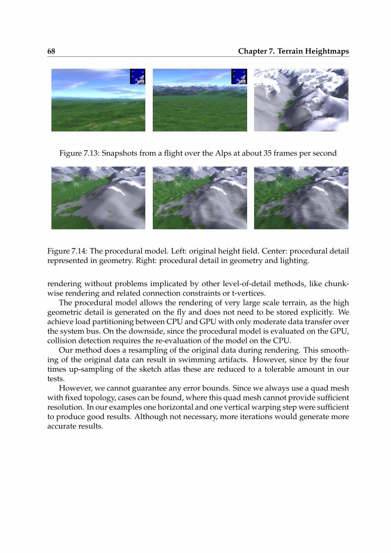
68 Chapter 7. Terrain Heightmaps
Figure 7.13: Snapshots from a flight over the Alps at about 35 frames per second
Figure 7.14: The procedural model. Left: original height field. Center: procedural detailrepresented in geometry. Right: procedural detail in geometry and lighting.
rendering without problems implicated by other level-of-detail methods, like chunk-wise rendering and related connection constraints or t-vertices.
The procedural model allows the rendering of very large scale terrain, as the highgeometric detail is generated on the fly and does not need to be stored explicitly. Weachieve load partitioning between CPU and GPU with only moderate data transfer overthe system bus. On the downside, since the procedural model is evaluated on the GPU,collision detection requires the re-evaluation of the model on the CPU.
Our method does a resampling of the original data during rendering. This smooth-ing of the original data can result in swimming artifacts. However, since by the fourtimes up-sampling of the sketch atlas these are reduced to a tolerable amount in ourtests.
However, we cannot guarantee any error bounds. Since we always use a quad meshwith fixed topology, cases can be found, where this quad mesh cannot provide sufficientresolution. In our examples one horizontal and one vertical warping step were sufficientto produce good results. Although not necessary, more iterations would generate moreaccurate results.
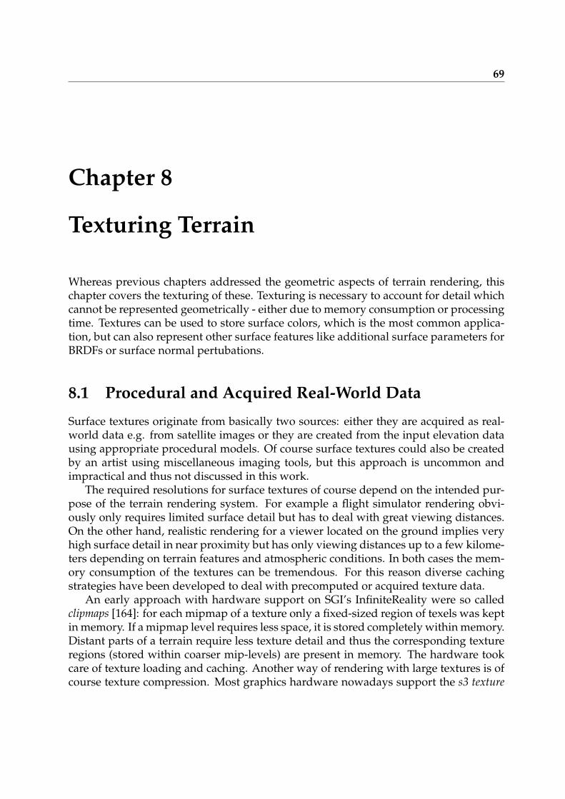
69
Chapter 8
Texturing Terrain
Whereas previous chapters addressed the geometric aspects of terrain rendering, thischapter covers the texturing of these. Texturing is necessary to account for detail whichcannot be represented geometrically - either due to memory consumption or processingtime. Textures can be used to store surface colors, which is the most common applica-tion, but can also represent other surface features like additional surface parameters forBRDFs or surface normal pertubations.
8.1 Procedural and Acquired Real-World Data
Surface textures originate from basically two sources: either they are acquired as real-world data e.g. from satellite images or they are created from the input elevation datausing appropriate procedural models. Of course surface textures could also be createdby an artist using miscellaneous imaging tools, but this approach is uncommon andimpractical and thus not discussed in this work.
The required resolutions for surface textures of course depend on the intended pur-pose of the terrain rendering system. For example a flight simulator rendering obvi-ously only requires limited surface detail but has to deal with great viewing distances.On the other hand, realistic rendering for a viewer located on the ground implies veryhigh surface detail in near proximity but has only viewing distances up to a few kilome-ters depending on terrain features and atmospheric conditions. In both cases the mem-ory consumption of the textures can be tremendous. For this reason diverse cachingstrategies have been developed to deal with precomputed or acquired texture data.
An early approach with hardware support on SGI’s InfiniteReality were so calledclipmaps [164]: for each mipmap of a texture only a fixed-sized region of texels was keptin memory. If a mipmap level requires less space, it is stored completely within memory.Distant parts of a terrain require less texture detail and thus the corresponding textureregions (stored within coarser mip-levels) are present in memory. The hardware tookcare of texture loading and caching. Another way of rendering with large textures is ofcourse texture compression. Most graphics hardware nowadays support the s3 texture
70 Chapter 8. Texturing Terrain
compression (see e.g. [118]) that works on separate pixel-blocks and reduces the memoryconsumption of a texture by a factor of 4 to 6. It allows quick decompression duringrendering and saves on-chip bandwidth required for texture transfer.
Other solutions to this problem are solved on the software side using adequatecaching or paging strategies. Typically the large terrain texture is represented by aquadtree-like data structure and the required texture resolution for each visible nodeis determined and the appropriate texture is loaded or generated. Various approachesfollowing this technique exist and among others see Blow [5, 6] and Ulrich [180]. Ourwork presented in this chapter also uses a similar spatial subdivision scheme.
8.1.1 Aerial and Satellite Imagery
Aerial imagery is the easiest way to acquire terrain surface textures. Unfortunately,these aerial photos often lack georegistration and have a non-uniform warping due toperspective and effects caused by terrain elevation. For this, the photos have to bewarped to match a georeferenced bases. For very small areas, even the practice of kiteaerial photography might work.
Nowadays, the most feasible way to acquire surface textures for a larger terrain re-gion is the use of satellite images. Usually, satellites take photographs not only but alsoin the human-visible light spectra. For example, the LandSat 7 satellite captures imageswith 7 wavelength intervals between 0.45µm and 2.35µm. The ASTER (Advanced Air-borne Thermal Emission and Reflection Radiometer) provides low-cost imagery with 14wavelength bands and elevation data with a resolution from 15m to 90m. The IKONOSsatellite is the first commercial satellite with a 1-meter accurate remote sensing. Ler-oux [99] provides a list of the status, capabilities and availability of data from varioussatellites. Premoze et al. [146] propose methods for classifying surface types and forremoving shading and shadowing artifacts from aerial imagery. By this, images of theterrain for variable times of day can be rendered.
8.1.2 Procedural Determination of Surface Appearance
In various settings, it is not possible to use acquired real-world data for terrain render-ing. It may be that the texture resolution is too low for close-up views, that the imagesinclude human housing or agriculture although undisturbed, natural scenes are to berendered. For this, procedural models can be used to compute textures.
Previously used texturing models, e.g. in computer games and other interactive ap-plications, usually use very simple models. Procedurally precomputed low-resolutiontexture maps combined with detail or bump maps are not sufficient for a plausible ap-pearance of soil, especially due to the visible repetitions. Although Wang tiles [23] cansolve this problem they require a set of precomputed texture tiles and cannot accountfor varying terrain features, like steep slopes and plains. Precomputing procedural tex-tures at high resolution requires paging and caching algorithms, but even those have
8.1 Procedural and Acquired Real-World Data 71
their limitations. Widely used in games was the so called texture splatting, that is com-positing of a terrain texture by blending a set of tileable textures (e.g. for rock, sand andgrass surfaces) in the frame-buffer (see Bloom [4] for details).
To solve this problem, a procedural model is required that can be computed effi-ciently and at different resolutions and accounts for terrain input data. We present sucha model in Section 8.2 and show how it can be implemented on graphics hardware (seealso [30]).
Integration of Geographic Input-Data into Procedural Models
Apart from efficient computation, the quality of a procedural model depends mainly onthe realism it achieves. Most procedural models used so far account for terrain eleva-tion and slope (e.g. the Terragen [51] model), but it is also possible to include furtherparameters. Among others these are temperature, solar radiation, rainfall and primarywind direction and strength. These quantities can either be acquired from appropriategaging stations or computed by simulations (see Fig. 8.1).
First of all, we use the procedural texture model presented in Section 8.2 to representall types of surfaces and all smaller features like grass and scrub. That is, vegetation ordifferent surface materials are represented by computed color textures only. To accountfor additional data it is important to know how it influences the appearance of surfacetypes. We refer the interested reader to physical geography and biogeography textbooks(e.g. [116, 141]) and present a collected summary of aspects that proved to be decisive.
The appearance of plants in general depends on few parameters: they require a cer-tain amount of solar radiation for photosynthesis, sufficient water supply and an ade-quate soil to strike roots. The sunshine duration can be computed for a given terrainand location on the earth, provided that an average cloud cover can be assumed. Com-puting the irradiation for a surface location from the solar constant (the amount of energyreceived at the top of the earth’s atmosphere, 1368W/m2) is explained by Stickler [176].Concerning the availability of water, it is important to note that it does not depend solelyon direct rainfall, but also on subterranean streams that are hard to simulate. The rain-fall distribution mainly depends on large-scale terrain features. In general, the amountof rainfall increases with altitude, because airmasses cool down when ascending andcannot keep the evaporated water. On very high mountains, even a maximum heightof rainfall can be noticed. For lower terrains, the most important aspect is the rainfall’shadowing’ from mountains in the main wind direction.
Procedural models for height field generation or real world elevation data usuallydo not exhibit soil type information. For this, the distribution of soil materials is usu-ally computed within the procedural texturing model assuming that e.g. rocky surfacesappear at steep slopes. Our model is constructed such that one surface type is the pre-condition for the existence of another: for example, a surface type representing fertilesediments is the precondition for grass and other plants to appear.
For the distribution of soil materials mainly altitude and slope criteria are consid-ered. Additional information can be acquired from erosion simulation to determine
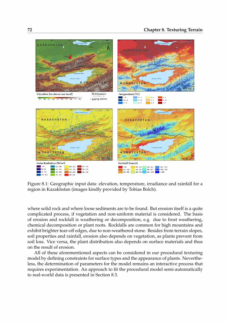
72 Chapter 8. Texturing Terrain
Figure 8.1: Geographic input data: elevation, temperature, irradiance and rainfall for aregion in Kazakhstan (images kindly provided by Tobias Bolch).
where solid rock and where loose sediments are to be found. But erosion itself is a quitecomplicated process, if vegetation and non-uniform material is considered. The basisof erosion and rockfall is weathering or decomposition, e.g. due to frost weathering,chemical decomposition or plant roots. Rockfalls are common for high mountains andexhibit brighter tear-off edges, due to non-weathered stone. Besides from terrain slopes,soil properties and rainfall, erosion also depends on vegetation, as plants prevent fromsoil loss. Vice versa, the plant distribution also depends on surface materials and thuson the result of erosion.
All of these aforementioned aspects can be considered in our procedural texturingmodel by defining constraints for surface types and the appearance of plants. Neverthe-less, the determination of parameters for the model remains an interactive process thatrequires experimentation. An approach to fit the procedural model semi-automaticallyto real-world data is presented in Section 8.3.
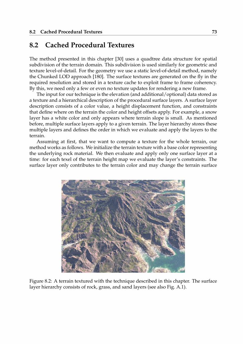
8.2 Cached Procedural Textures 73
8.2 Cached Procedural Textures
The method presented in this chapter [30] uses a quadtree data structure for spatialsubdivision of the terrain domain. This subdivision is used similarly for geometric andtexture level-of-detail. For the geometry we use a static level-of-detail method, namelythe Chunked LOD approach [180]. The surface textures are generated on the fly in therequired resolution and stored in a texture cache to exploit frame to frame coherency.By this, we need only a few or even no texture updates for rendering a new frame.
The input for our technique is the elevation (and additional/optional) data stored asa texture and a hierarchical description of the procedural surface layers. A surface layerdescription consists of a color value, a height displacement function, and constraintsthat define where on the terrain the color and height offsets apply. For example, a snowlayer has a white color and only appears where terrain slope is small. As mentionedbefore, multiple surface layers apply to a given terrain. The layer hierarchy stores thesemultiple layers and defines the order in which we evaluate and apply the layers to theterrain.
Assuming at first, that we want to compute a texture for the whole terrain, ourmethod works as follows. We initialize the terrain texture with a base color representingthe underlying rock material. We then evaluate and apply only one surface layer at atime: for each texel of the terrain height map we evaluate the layer’s constraints. Thesurface layer only contributes to the terrain color and may change the terrain surface
Figure 8.2: A terrain textured with the technique described in this chapter. The surfacelayer hierarchy consists of rock, grass, and sand layers (see also Fig. A.1).
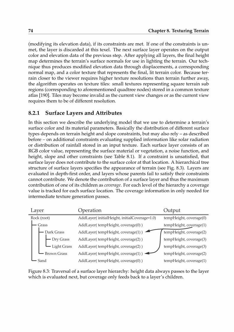
74 Chapter 8. Texturing Terrain
(modifying its elevation data), if its constraints are met. If one of the constraints is un-met, the layer is discarded at this texel. The next surface layer operates on the outputcolor and elevation data of the previous step. After applying all layers, the final heightmap determines the terrain’s surface normals for use in lighting the terrain. Our tech-nique thus produces modified elevation data through displacements, a correspondingnormal map, and a color texture that represents the final, lit terrain color. Because ter-rain closer to the viewer requires higher texture resolutions than terrain further away,the algorithm operates on texture tiles: small textures representing square terrain subregions (corresponding to aforementioned quadtree nodes) stored in a common textureatlas [190]. Tiles may become invalid as the current view changes or as the current viewrequires them to be of different resolution.
8.2.1 Surface Layers and Attributes
In this section we describe the underlying model that we use to determine a terrain’ssurface color and its material parameters. Basically the distribution of different surfacetypes depends on terrain height and slope constraints, but may also rely – as describedbefore – on additional constraints evaluating supplied information like solar radiationor distribution of rainfall stored in an input texture. Each surface layer consists of anRGB color value, representing the surface material or vegetation, a noise function, andheight, slope and other constraints (see Table 8.1). If a constraint is unsatisfied, thatsurface layer does not contribute to the surface color at that location. A hierarchical treestructure of surface layers specifies the appearance of terrain (see Fig. 8.3). Layers areevaluated in depth-first order, and layers whose parents fail to satisfy their constraintscannot contribute. We denote the contribution of a surface layer and thus the maximumcontribution of one of its children as coverage. For each level of the hierarchy a coveragevalue is tracked for each surface location. The coverage information in only needed forintermediate texture generation passes.
Rock (root)
Grass
Dark Grass
Dry Grass
Light Grass
Sand
AddLayer( initialHeight, initialCoverage=1.0)
AddLayer( tempHeight, coverage(0) )
tempHeight, coverage(0)
tempHeight, coverage(1)
AddLayer( tempHeight, coverage(1) )
AddLayer( tempHeight, coverage(2) )
AddLayer( tempHeight, coverage(2) )
AddLayer( tempHeight, coverage(0) )
tempHeight, coverage(2)
tempHeight, coverage(3)
tempHeight, coverage(3)
tempHeight, coverage(1)
Brown Grass AddLayer( tempHeight, coverage(1) ) tempHeight, coverage(2)
Layer Operation Output
Figure 8.3: Traversal of a surface layer hierarchy: height data always passes to the layerwhich is evaluated next, but coverage only feeds back to a layer’s children.
8.2 Cached Procedural Textures 75
surface attribute descriptionbumpiness or roughness BS roughness of the terrain, achieved by adding
noise to the elevation data, where the surfacelayer contributes
surface color RGBS RGB color of surface materialnoise function N(x) noise values in the range [0;1) used for modify-
ing (multiplicatively) the result of the constraintcomputations
coverage/fractal noise cS, nS these scalar values are used to bias and scale thenoise values before constraint modification
minimum and maximumvalue and fuzziness for al-titude, slope, rainfall, so-lar radiation etc.
Cn,min,Cn,max,Cn, f
defines boundaries for the appearance of thesurface layer including a fuzziness region,where the surface layer may appear, but less no-ticeable or likely
Table 8.1: Surface attributes used for the texturing.
8.2.2 Evaluation
Instead of evaluating the entire terrain once at a fixed resolution, the quadtree subdivi-sion allows a texture computation for multiple square subdomains. Each tile guaran-tees constant sampling of the input height field, as the input is upsampled isotropicallyand uniformly. Texture tiles and intermediate data for evaluating surface layers areoff-screen render targets. We describe how to manage these various render targets ef-ficiently in Section 8.2.4 below. Figure 8.4 shows the inputs and outputs of rendering asurface layer.
The surface layers are evaluated in depth-first order. The root node is special in thatit has no constraints: the base material of the terrain is present everywhere. The inputto the root node is the original terrain elevation data.
As a surface layer can modify height values it affects the distribution of the subse-quent layers. The height output of one surface layer is the height input for the nextsurface layer. Coverage, on the other hand, is only propagated to a layer’s children.Figure 8.3 illustrates an example traversal of a simple surface layer hierarchy.
In general, the render target texture resolution is much higher than the resolutionof the original elevation data. Thus, height values are typically interpolated. Becausewe compute normals and shading from the elevation data, simple linear interpolationof the elevation data results in piecewise linear patches and thus causes undesirableartifacts. To avoid these artifacts we use cubic B-spline interpolation instead. Whilethis type of interpolation is costly, we only require it when processing the root node.All subsequent surface layers operate at the same texture resolution as the root node’soutput height map.
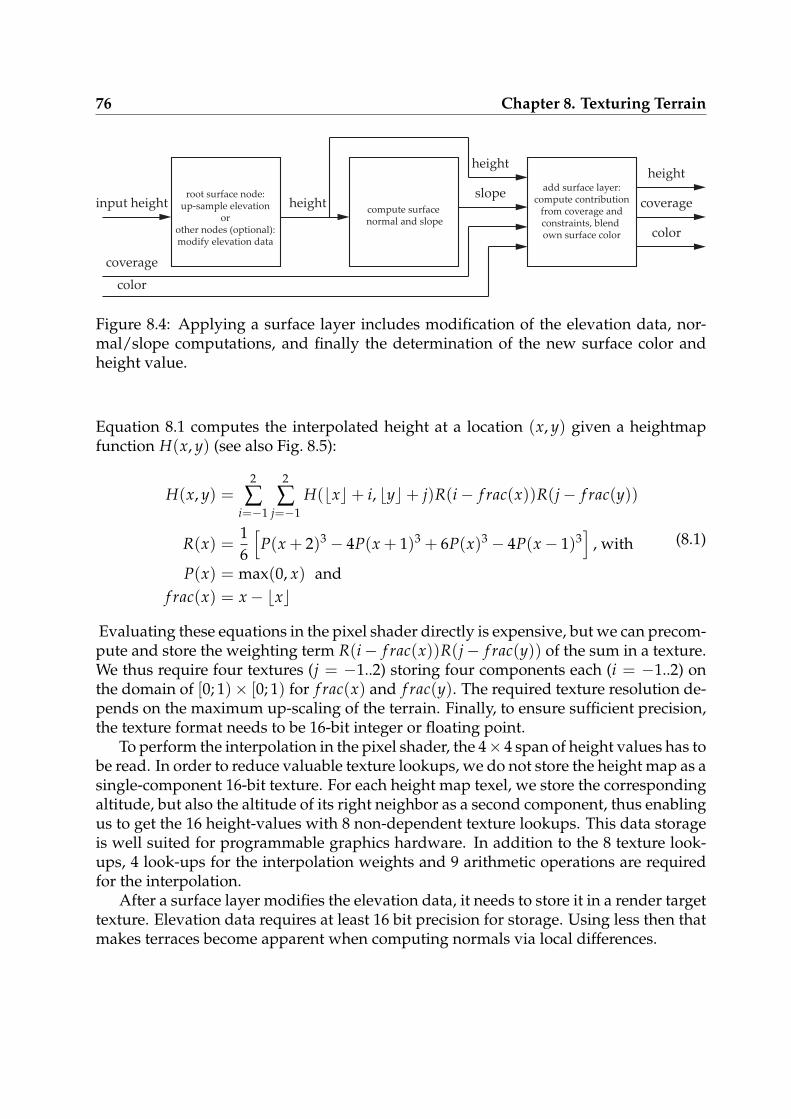
76 Chapter 8. Texturing Terrain
height
slope
coverage
add surface layer:compute contribution
from coverage andconstraints, blend own surface color
height
coverage
color
color
input height heightroot surface node:
up-sample elevationor
other nodes (optional):modify elevation data
compute surface normal and slope
Figure 8.4: Applying a surface layer includes modification of the elevation data, nor-mal/slope computations, and finally the determination of the new surface color andheight value.
Equation 8.1 computes the interpolated height at a location (x, y) given a heightmapfunction H(x, y) (see also Fig. 8.5):
H(x, y) =2
∑i=−1
2
∑j=−1
H(⌊x⌋+ i, ⌊y⌋+ j)R(i− f rac(x))R(j− f rac(y))
R(x) =16
[
P(x + 2)3 − 4P(x + 1)3 + 6P(x)3 − 4P(x− 1)3]
, with
P(x) = max(0, x) andf rac(x) = x− ⌊x⌋
(8.1)
Evaluating these equations in the pixel shader directly is expensive, but we can precom-pute and store the weighting term R(i− f rac(x))R(j− f rac(y)) of the sum in a texture.We thus require four textures (j = −1..2) storing four components each (i = −1..2) onthe domain of [0; 1)× [0; 1) for f rac(x) and f rac(y). The required texture resolution de-pends on the maximum up-scaling of the terrain. Finally, to ensure sufficient precision,the texture format needs to be 16-bit integer or floating point.
To perform the interpolation in the pixel shader, the 4× 4 span of height values has tobe read. In order to reduce valuable texture lookups, we do not store the height map as asingle-component 16-bit texture. For each height map texel, we store the correspondingaltitude, but also the altitude of its right neighbor as a second component, thus enablingus to get the 16 height-values with 8 non-dependent texture lookups. This data storageis well suited for programmable graphics hardware. In addition to the 8 texture look-ups, 4 look-ups for the interpolation weights and 9 arithmetic operations are requiredfor the interpolation.
After a surface layer modifies the elevation data, it needs to store it in a render targettexture. Elevation data requires at least 16 bit precision for storage. Using less then thatmakes terraces become apparent when computing normals via local differences.
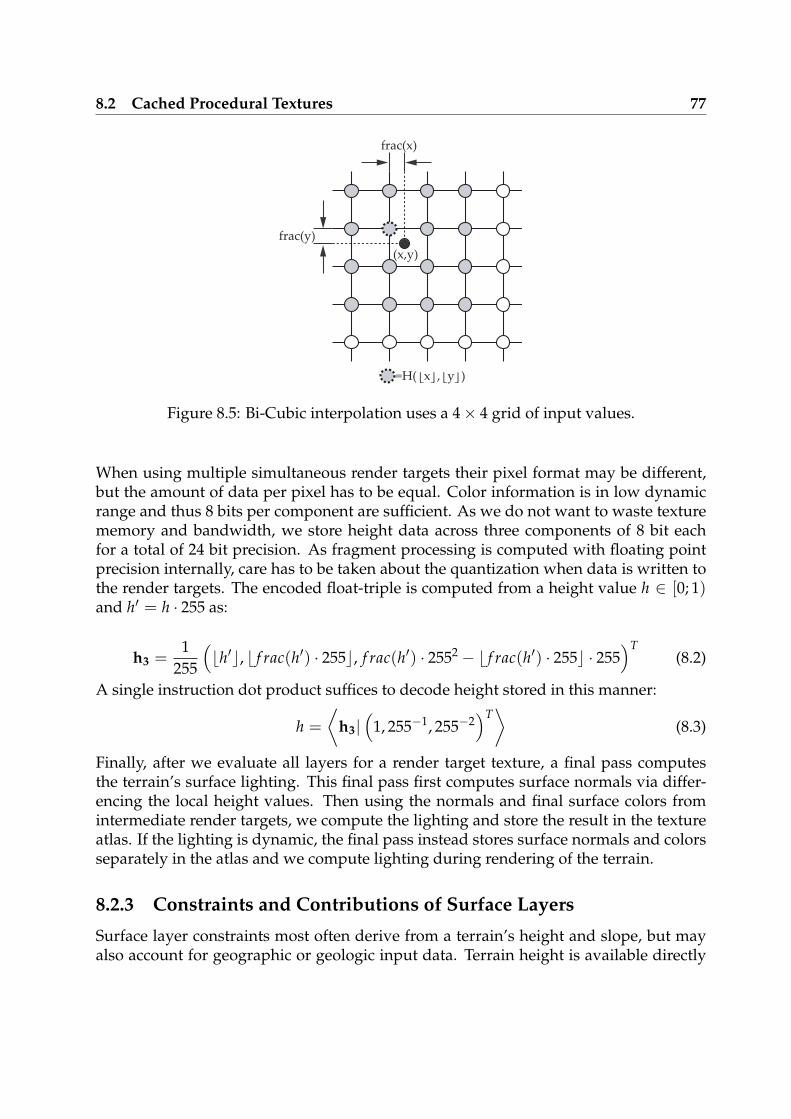
8.2 Cached Procedural Textures 77
frac(x)
frac(y)
(x,y)
=H( x , y )
Figure 8.5: Bi-Cubic interpolation uses a 4× 4 grid of input values.
When using multiple simultaneous render targets their pixel format may be different,but the amount of data per pixel has to be equal. Color information is in low dynamicrange and thus 8 bits per component are sufficient. As we do not want to waste texturememory and bandwidth, we store height data across three components of 8 bit eachfor a total of 24 bit precision. As fragment processing is computed with floating pointprecision internally, care has to be taken about the quantization when data is written tothe render targets. The encoded float-triple is computed from a height value h ∈ [0; 1)and h′ = h · 255 as:
h3 =1
255
(
⌊h′⌋, ⌊ f rac(h′) · 255⌋, f rac(h′) · 2552 − ⌊ f rac(h′) · 255⌋ · 255)T
(8.2)
A single instruction dot product suffices to decode height stored in this manner:
h =
⟨
h3|(
1, 255−1, 255−2)T⟩
(8.3)
Finally, after we evaluate all layers for a render target texture, a final pass computesthe terrain’s surface lighting. This final pass first computes surface normals via differ-encing the local height values. Then using the normals and final surface colors fromintermediate render targets, we compute the lighting and store the result in the textureatlas. If the lighting is dynamic, the final pass instead stores surface normals and colorsseparately in the atlas and we compute lighting during rendering of the terrain.
8.2.3 Constraints and Contributions of Surface Layers
Surface layer constraints most often derive from a terrain’s height and slope, but mayalso account for geographic or geologic input data. Terrain height is available directly
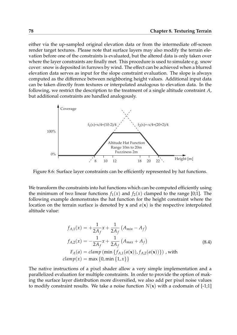
78 Chapter 8. Texturing Terrain
either via the up-sampled original elevation data or from the intermediate off-screenrender target textures. Please note that surface layers may also modify the terrain ele-vation before one of the constraints is evaluated, but the altered data is only taken overwhere the layer constraints are finally met. This procedure is used to simulate e.g. snowcover: snow is deposited in furrows by wind. The effect can be achieved when a blurredelevation data serves as input for the slope constraint evaluation. The slope is alwayscomputed as the difference between neighboring height values. Additional input datacan be taken directly from textures or interpolated analogous to elevation data. In thefollowing, we restrict the description to the treatment of a single altitude constraint A,but additional constraints are handled analogously.
Height [m]108 12 18 20 22
Coverage
0%
100%
Altitude Hat FunctionRange 10m to 20m
Fuzziness 2m
f2(x)=-x/4+(20+2)/4f1(x)=x/4+(10-2)/4
Figure 8.6: Surface layer constraints can be efficiently represented by hat functions.
We transform the constraints into hat functions which can be computed efficiently usingthe minimum of two linear functions f1(x) and f2(x) clamped to the range [0;1]. Thefollowing example demonstrates the hat function for the height constraint where thelocation on the terrain surface is denoted by x and a(x) is the respective interpolatedaltitude value:
fA,1(x) = +1
2A fx +
12A f
(
Amin − A f)
fA,2(x) = − 12A f
x +1
2A f
(
Amax + A f)
FA(a) = clamp (min fA,1(a(x)), fA,2(a(x))) , withclamp(x) = max 0, min 1, x
(8.4)
The native instructions of a pixel shader allow a very simple implementation and aparallelized evaluation for multiple constraints. In order to provide the option of mak-ing the surface layer distribution more diversified, we also add per pixel noise valuesto modify constraint results. We take a noise function N(x) with a codomain of [-1;1]
8.2 Cached Procedural Textures 79
which can be precomputed and stored as a texture. The contribution C of a surface layer,also referred to as coverage is then computed from all constraint functions (denoted byFi here), where n is the number of constraints:
C(x) = clamp
(
[cs + nsN(x)]n−1
∏i=0
Fi(x)
)
(8.5)
Since the surface appearance is represented by a hierarchy of surface layers, we haveto take the coverage from parent surface nodes CP into account, this gives us the finalcoverage CS:
CS(x) = C(x)CP(x) (8.6)
Finally, we can determine the output color and height values. On the latter we canoptionally apply a displacement DS(x) representing surface layer characteristics, e.g.bumps or cracks:
RGB(x) = (1− CS(x))RGBin(x) + CS(x)RGBS(x)
a′(x) = a(x) + CS(x)BSDS(x)(8.7)
8.2.4 Caching Terrain Textures
Our texturing method is meant to be combined with level-of-detail algorithms workingwith square sub-domains. Thus we can account for varying geometric and texture detailfor each sub-domain independently. Creating a unique texture for each of these sub-domains causes many render-target changes during the computation of the texturesand many texture switches during rendering. To avoid these state changes, we packtextures into a few large texture atlases (see [190] for details). For static lighting, or veryslow changes, we store terrain colors in the atlases. To enable dynamic lighting, normalmaps are stored within the atlas, too. To ensure tight and easy packing of textures, werestrict our texture dimensions for the sub-domains to powers of two.
All other textures, e.g. storing per-pixel coverage, are only needed during computa-tion of the terrain textures and have the same resolution as a single texture of the atlas.
Managing the Texture Atlas
We render the terrain using a Chunk-LOD [180] approach, where a quad-tree dividesthe height map into a hierarchy of sub-domains.
For a given view we select appropriate sub-domains such that:
• the geometric error is below a user-defined threshold
• the required texture size for this chunk – to capture enough detail – is not too large(we target medium sized textures of approx. 1282 texels)
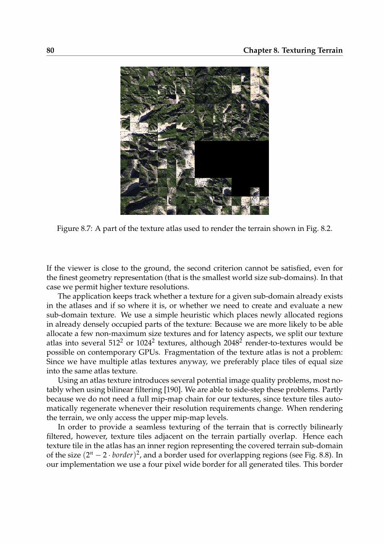
80 Chapter 8. Texturing Terrain
Figure 8.7: A part of the texture atlas used to render the terrain shown in Fig. 8.2.
If the viewer is close to the ground, the second criterion cannot be satisfied, even forthe finest geometry representation (that is the smallest world size sub-domains). In thatcase we permit higher texture resolutions.
The application keeps track whether a texture for a given sub-domain already existsin the atlases and if so where it is, or whether we need to create and evaluate a newsub-domain texture. We use a simple heuristic which places newly allocated regionsin already densely occupied parts of the texture: Because we are more likely to be ableallocate a few non-maximum size textures and for latency aspects, we split our textureatlas into several 5122 or 10242 textures, although 20482 render-to-textures would bepossible on contemporary GPUs. Fragmentation of the texture atlas is not a problem:Since we have multiple atlas textures anyway, we preferably place tiles of equal sizeinto the same atlas texture.
Using an atlas texture introduces several potential image quality problems, most no-tably when using bilinear filtering [190]. We are able to side-step these problems. Partlybecause we do not need a full mip-map chain for our textures, since texture tiles auto-matically regenerate whenever their resolution requirements change. When renderingthe terrain, we only access the upper mip-map levels.
In order to provide a seamless texturing of the terrain that is correctly bilinearlyfiltered, however, texture tiles adjacent on the terrain partially overlap. Hence eachtexture tile in the atlas has an inner region representing the covered terrain sub-domainof the size (2n − 2 · border)2, and a border used for overlapping regions (see Fig. 8.8). Inour implementation we use a four pixel wide border for all generated tiles. This border
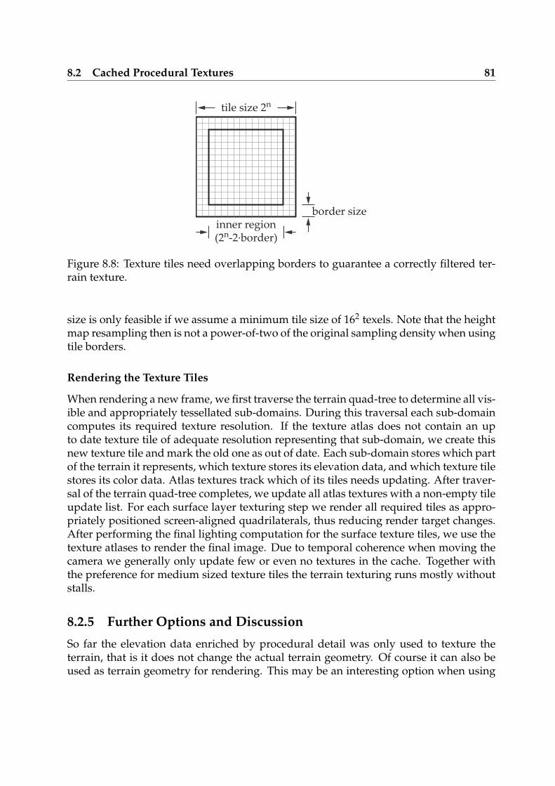
8.2 Cached Procedural Textures 81
tile size 2n
border sizeinner region(2n-2·border)
Figure 8.8: Texture tiles need overlapping borders to guarantee a correctly filtered ter-rain texture.
size is only feasible if we assume a minimum tile size of 162 texels. Note that the heightmap resampling then is not a power-of-two of the original sampling density when usingtile borders.
Rendering the Texture Tiles
When rendering a new frame, we first traverse the terrain quad-tree to determine all vis-ible and appropriately tessellated sub-domains. During this traversal each sub-domaincomputes its required texture resolution. If the texture atlas does not contain an upto date texture tile of adequate resolution representing that sub-domain, we create thisnew texture tile and mark the old one as out of date. Each sub-domain stores which partof the terrain it represents, which texture stores its elevation data, and which texture tilestores its color data. Atlas textures track which of its tiles needs updating. After traver-sal of the terrain quad-tree completes, we update all atlas textures with a non-empty tileupdate list. For each surface layer texturing step we render all required tiles as appro-priately positioned screen-aligned quadrilaterals, thus reducing render target changes.After performing the final lighting computation for the surface texture tiles, we use thetexture atlases to render the final image. Due to temporal coherence when moving thecamera we generally only update few or even no textures in the cache. Together withthe preference for medium sized texture tiles the terrain texturing runs mostly withoutstalls.
8.2.5 Further Options and Discussion
So far the elevation data enriched by procedural detail was only used to texture theterrain, that is it does not change the actual terrain geometry. Of course it can also beused as terrain geometry for rendering. This may be an interesting option when using
82 Chapter 8. Texturing Terrain
coarse input-height fields or if high geometric detail is desired.Texturing terrain based on slope constraints in screen-space mostly suffers from sam-
pling problems: the input data is filtered accordingly, but the filtering is linear andwould only be correct for example for color values - that is filtered slope values maycause completely different texturing. Of course our approach has to deal with theseproblems, too, because the elevation data is sampled at different rates, enriched withprocedural detail and then afterwards the slope is computed. By using a texture atlas,this problem is pushed further away, because it contains textures computed in worldspace at a higher resolution and later in screen space the filtering is applied to colorvalues. Enough precision for the cubic B-spline interpolation during up sampling of theelevation data is crucial. A lack of precision causes artifacts within the height valuesand consequently wrong slopes, and thus wrong texturing.
When using level-of-detail methods with geomorphing, it is insufficient to rely onlyon the computed geometric error for selecting terrain chunks for rendering. Texturetile resolution is equally important. Thus, texture resolution errors also influence selec-tion of geometric resolution. We therefore suggest obtaining the geomorph factor bymultiplying the geometric and texture errors.
Using slope and height constraints for procedural texturing of terrains has been usedbefore in simpler or non-realtime methods. By employing texture atlases and cachingof texture tiles, it is possible to render highly detailed terrain and generate procedu-rally enriched elevation data on contemporary GPUs. More examples of our method,together with a model for skylight and aerial perspective [143] and for water render-ing [145] rendered in realtime are shown in Fig. 8.9.
8.3 Mapping the Real World
In this section we describe a method to estimate surface layer constraints and propertiesfor the procedural texturing method from real-world data, that is satellite color images,elevation and further geographic data. For this, we need registered input data as shownin Figure 8.10. Once a surface layer description is constructed from real-world data, wecan render arbitrary views of the input terrain or images from other terrain parts forwhich elevation and (maybe simulated) geographic data, but no color images, exists.
8.3.1 Acquiring the Surface Layer Description
Several processing steps are involved to acquire the surface layer description. These arepresented in chronological order in the following sections. To capture the complexity ofnature, we do not represent the surface layer constraints by simple hat functions, but byarbitrary constraint functions. These functions are acquired by sampling the real-worlddata and stored for a later evaluation.
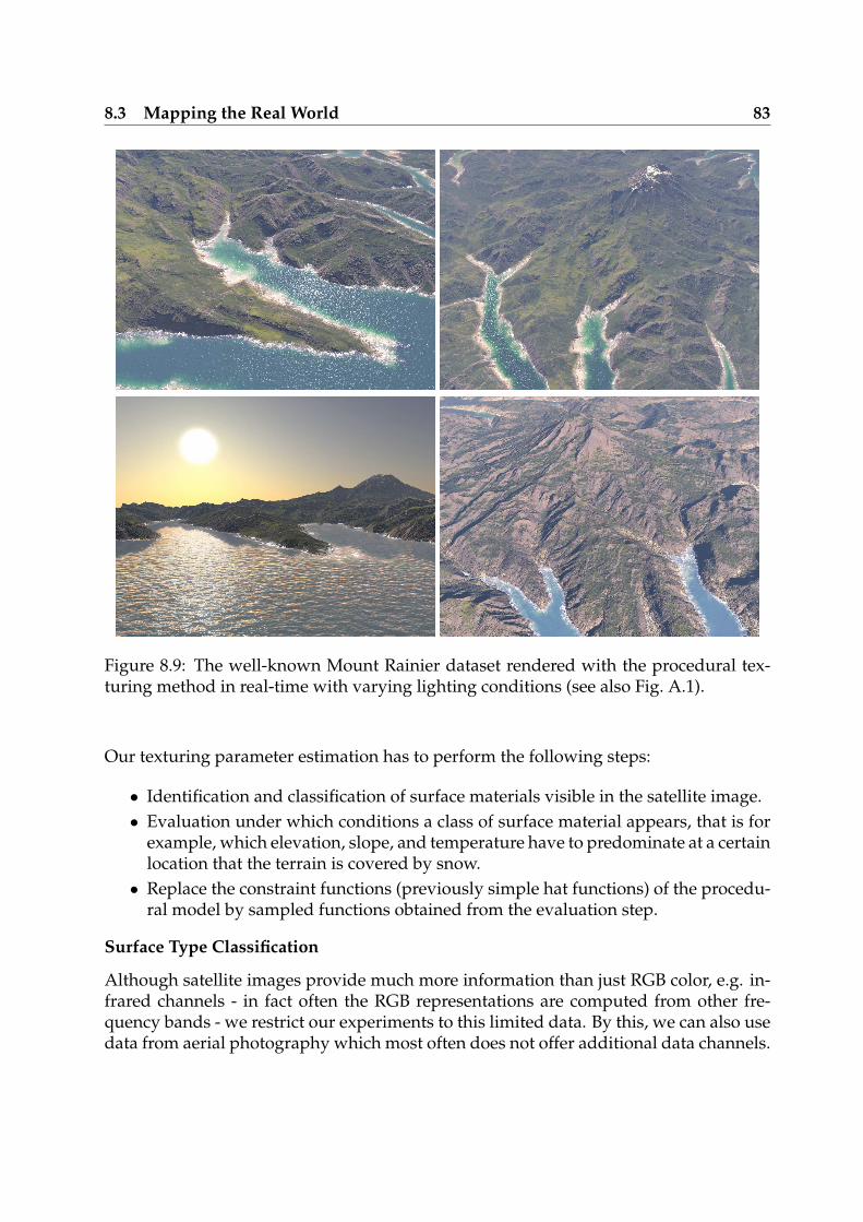
8.3 Mapping the Real World 83
Figure 8.9: The well-known Mount Rainier dataset rendered with the procedural tex-turing method in real-time with varying lighting conditions (see also Fig. A.1).
Our texturing parameter estimation has to perform the following steps:
• Identification and classification of surface materials visible in the satellite image.• Evaluation under which conditions a class of surface material appears, that is for
example, which elevation, slope, and temperature have to predominate at a certainlocation that the terrain is covered by snow.• Replace the constraint functions (previously simple hat functions) of the procedu-
ral model by sampled functions obtained from the evaluation step.
Surface Type Classification
Although satellite images provide much more information than just RGB color, e.g. in-frared channels - in fact often the RGB representations are computed from other fre-quency bands - we restrict our experiments to this limited data. By this, we can also usedata from aerial photography which most often does not offer additional data channels.
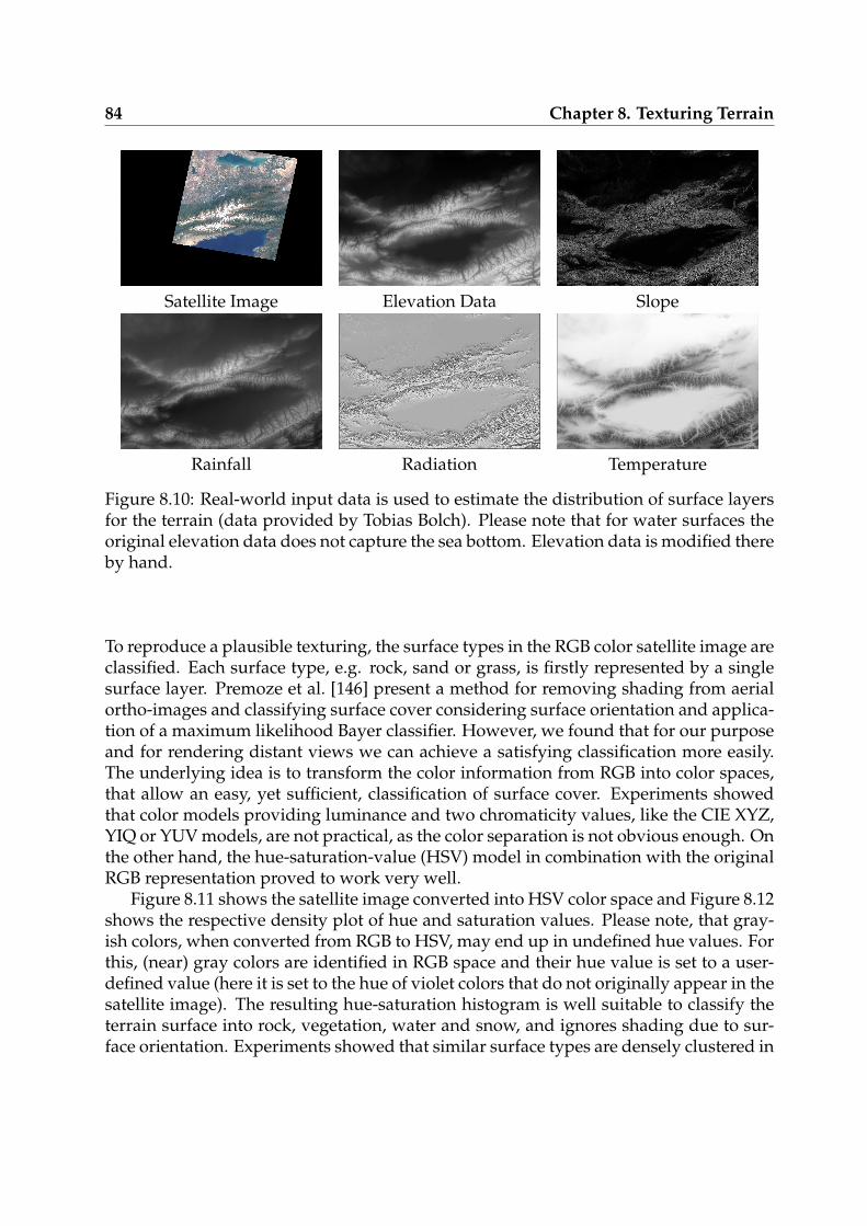
84 Chapter 8. Texturing Terrain
Satellite Image Elevation Data Slope
Rainfall Radiation Temperature
Figure 8.10: Real-world input data is used to estimate the distribution of surface layersfor the terrain (data provided by Tobias Bolch). Please note that for water surfaces theoriginal elevation data does not capture the sea bottom. Elevation data is modified thereby hand.
To reproduce a plausible texturing, the surface types in the RGB color satellite image areclassified. Each surface type, e.g. rock, sand or grass, is firstly represented by a singlesurface layer. Premoze et al. [146] present a method for removing shading from aerialortho-images and classifying surface cover considering surface orientation and applica-tion of a maximum likelihood Bayer classifier. However, we found that for our purposeand for rendering distant views we can achieve a satisfying classification more easily.The underlying idea is to transform the color information from RGB into color spaces,that allow an easy, yet sufficient, classification of surface cover. Experiments showedthat color models providing luminance and two chromaticity values, like the CIE XYZ,YIQ or YUV models, are not practical, as the color separation is not obvious enough. Onthe other hand, the hue-saturation-value (HSV) model in combination with the originalRGB representation proved to work very well.
Figure 8.11 shows the satellite image converted into HSV color space and Figure 8.12shows the respective density plot of hue and saturation values. Please note, that gray-ish colors, when converted from RGB to HSV, may end up in undefined hue values. Forthis, (near) gray colors are identified in RGB space and their hue value is set to a user-defined value (here it is set to the hue of violet colors that do not originally appear in thesatellite image). The resulting hue-saturation histogram is well suitable to classify theterrain surface into rock, vegetation, water and snow, and ignores shading due to sur-face orientation. Experiments showed that similar surface types are densely clustered in
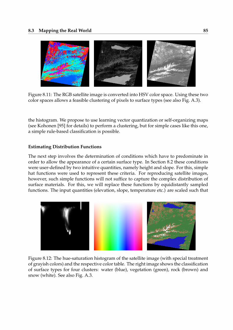
8.3 Mapping the Real World 85
Figure 8.11: The RGB satellite image is converted into HSV color space. Using these twocolor spaces allows a feasible clustering of pixels to surface types (see also Fig. A.3).
the histogram. We propose to use learning vector quantization or self-organizing maps(see Kohonen [95] for details) to perform a clustering, but for simple cases like this one,a simple rule-based classification is possible.
Estimating Distribution Functions
The next step involves the determination of conditions which have to predominate inorder to allow the appearance of a certain surface type. In Section 8.2 these conditionswere user-defined by two intuitive quantities, namely height and slope. For this, simplehat functions were used to represent these criteria. For reproducing satellite images,however, such simple functions will not suffice to capture the complex distribution ofsurface materials. For this, we will replace these functions by equidistantly sampledfunctions. The input quantities (elevation, slope, temperature etc.) are scaled such that
Figure 8.12: The hue-saturation histogram of the satellite image (with special treatmentof grayish colors) and the respective color table. The right image shows the classificationof surface types for four clusters: water (blue), vegetation (green), rock (brown) andsnow (white). See also Fig. A.3.
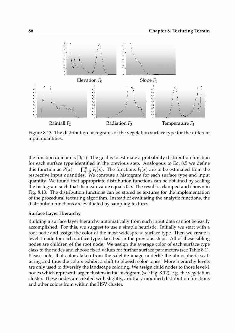
86 Chapter 8. Texturing Terrain
Elevation F0 Slope F1
Rainfall F2 Radiation F3 Temperature F4
Figure 8.13: The distribution histograms of the vegetation surface type for the differentinput quantities.
the function domain is [0; 1). The goal is to estimate a probability distribution functionfor each surface type identified in the previous step. Analogous to Eq. 8.5 we definethis function as P(x) = ∏
n−1i=0 Fi(x). The functions Fi(x) are to be estimated from the
respective input quantities. We compute a histogram for each surface type and inputquantity. We found that appropriate distribution functions can be obtained by scalingthe histogram such that its mean value equals 0.5. The result is clamped and shown inFig. 8.13. The distribution functions can be stored as textures for the implementationof the procedural texturing algorithm. Instead of evaluating the analytic functions, thedistribution functions are evaluated by sampling textures.
Surface Layer Hierarchy
Building a surface layer hierarchy automatically from such input data cannot be easilyaccomplished. For this, we suggest to use a simple heuristic. Initially we start with aroot node and assign the color of the most widespread surface type. Then we create alevel-1 node for each surface type classified in the previous steps. All of these siblingnodes are children of the root node. We assign the average color of each surface typeclass to the nodes and choose fixed values for further surface parameters (see Table 8.1).Please note, that colors taken from the satellite image underlie the atmospheric scat-tering and thus the colors exhibit a shift to blueish color tones. More hierarchy levelsare only used to diversify the landscape coloring. We assign child nodes to those level-1nodes which represent larger clusters in the histogram (see Fig. 8.12), e.g. the vegetationcluster. These nodes are created with slightly, arbitrary modified distribution functionsand other colors from within the HSV cluster.
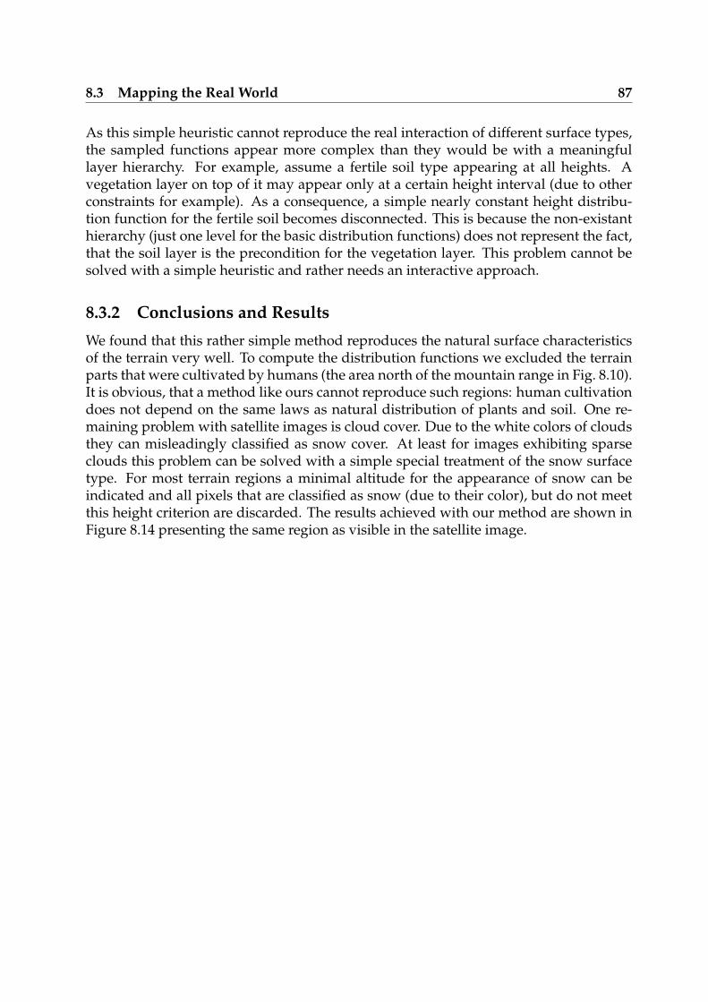
8.3 Mapping the Real World 87
As this simple heuristic cannot reproduce the real interaction of different surface types,the sampled functions appear more complex than they would be with a meaningfullayer hierarchy. For example, assume a fertile soil type appearing at all heights. Avegetation layer on top of it may appear only at a certain height interval (due to otherconstraints for example). As a consequence, a simple nearly constant height distribu-tion function for the fertile soil becomes disconnected. This is because the non-existanthierarchy (just one level for the basic distribution functions) does not represent the fact,that the soil layer is the precondition for the vegetation layer. This problem cannot besolved with a simple heuristic and rather needs an interactive approach.
8.3.2 Conclusions and Results
We found that this rather simple method reproduces the natural surface characteristicsof the terrain very well. To compute the distribution functions we excluded the terrainparts that were cultivated by humans (the area north of the mountain range in Fig. 8.10).It is obvious, that a method like ours cannot reproduce such regions: human cultivationdoes not depend on the same laws as natural distribution of plants and soil. One re-maining problem with satellite images is cloud cover. Due to the white colors of cloudsthey can misleadingly classified as snow cover. At least for images exhibiting sparseclouds this problem can be solved with a simple special treatment of the snow surfacetype. For most terrain regions a minimal altitude for the appearance of snow can beindicated and all pixels that are classified as snow (due to their color), but do not meetthis height criterion are discarded. The results achieved with our method are shown inFigure 8.14 presenting the same region as visible in the satellite image.
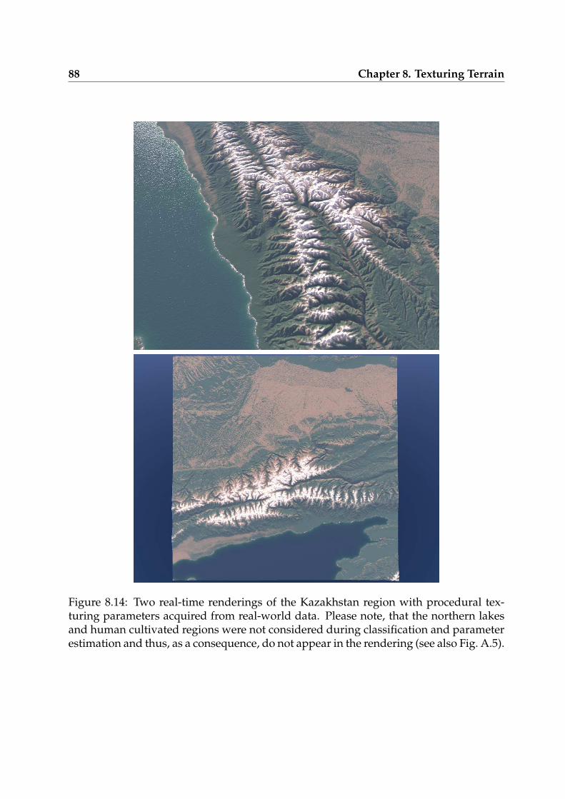
88 Chapter 8. Texturing Terrain
Figure 8.14: Two real-time renderings of the Kazakhstan region with procedural tex-turing parameters acquired from real-world data. Please note, that the northern lakesand human cultivated regions were not considered during classification and parameterestimation and thus, as a consequence, do not appear in the rendering (see also Fig. A.5).
89
Chapter 9
Lighting Computation for Terrains
Previous chapters presented methods and algorithms that allow the rendering of com-plex outdoor scenes in terms of geometric and texture detail. Another important partfor the visual complexity and the appeal of terrains is their lighting.
For static lighting conditions we can precompute an accurate lighting solution, e.g.based on the atmospheric models presented in Section 6.3. In this chapter we describethe outdoor lighting situation, the problems arising when computing physically basedsolutions for dynamic lighting conditions, and compare different approaches to thisproblem.
9.1 Outdoor Lighting
The light incident on the earth’s surface is a result of a complex interaction of sun lightand the molecules and aerosols in the earth’s atmosphere. The theory of this light scat-tering is presented in Section 6.3.
To characterize the outdoor lighting situation we distinguish between direct illumi-nation caused by the sun and sky light, and indirect illumination due to reflected lightfrom terrain surfaces. We can make further distinctions on the direct illumination: it isreasonable for the rendering process to handle bright direct sun light and blueish scat-tered sky light separately - although both originate from the sun itself. According toHoffman et al. [74] this approach is not only suitable for daylight, but also for nightlighting conditions.
The sun is very distant from the earth (about 149.6× 10⁶km) and thus can be treatedas a directional light source without introducing noticeable errors. But due to its size,it cannot be regarded as a point light source. For a viewer on the earth, the sun has anangular diameter of about 0.5 degrees (in astronomy the size of objects in the sky is oftenmeasured in terms of the angular diameter as seen from earth, rather than their actualsize). As a consequence, the shadows caused by direct sun light exhibit soft edges.
The sky light, actually scattered sun light, is – in terms of rendering – a hemispher-ical light source with varying (over time and area) color and intensity of the emitted
90 Chapter 9. Lighting Computation for Terrains
light. It has most visual impact in shadowed regions where direct sun light does notpredominate the lighting.
The indirect illumination is a subtle effect for outdoor terrain rendering and its con-tribution to the radiance reflected from the terrain is relatively low. However, for com-puter generated images subtle effects like this (or plausible approximations thereof)help to increase the realism.
In the following, we present a formulation of the terrain lighting situation. Theseparation of sun and sky light is used in Sections 9.3 and 9.4 to achieve reasonablereal-time capable methods for terrain rendering.
9.1.1 Radiance Transfer
The Rendering Equation (see Section 2.1.4 and [85]) describes the light transport in a sceneand is based on the BRDF:
Lo(x, ~ωo) = Le(x, ~ωo) +∫
Ω ~nx
fo(x, ~ωi → ~ωo)Li(x, ~ωi) cos θidωi (9.1)
where the surface normal at a point x is denoted by ~nx and cos θi = 〈~nx, ωi〉. We can as-sume that all terrain surfaces exhibit Lambertian reflection properties, that is the BRDFis direction independent:
fo(x, ~ωi → ~ωo) =ρ(x)
π, (9.2)
where ρ(x) ∈ [0; 1] is the diffuse reflectivity. By this, we get the radiosity equation:
Lo(x, ~ωo) = Le(x, ~ωo) +ρ(x)
π
∫
Ω ~nx
Li(x, ~ωi) cos θidωi (9.3)
As terrains usually do not emit light, we can omit the corresponding term Le.
Diffuse Shadowed Radiance Transfer
The simplest interesting case for terrain rendering is local illumination from an environ-mental light, that is:
Li(x, ~ωi) = Lenv(x, ~ωi) (9.4)
Please note that we obtain the environmental light from light probes or models for sunand sky light and Lenv already includes inscattered light along the path to x. Further-more, we define the transfer function for diffuse radiance transfer Td,x(~ωi):
Td,x(~ωi) =1π〈~nx, ~ωi〉 (9.5)
To account for shadowing, we integrate the hemispherical visibility term V to obtain thediffuse shadowed transfer function. If a ray originating from x in direction ~ωi intersects
9.1 Outdoor Lighting 91
the terrain then V(x, ~ωi) = 0, otherwise V(x, ~ωi) = 1:
Tx(~ωi) =1π〈~nx, ~ωi〉V(x, ~ωi) (9.6)
For the outgoing radiance we get:
Lo(x) = ρ(x)∫
Ω ~nx
Tx(~ωi)Lenv(x, ~ωi)dωi (9.7)
The surface reflectivity ρ(x) is usually not integrated in the transfer function to decouplelighting computation from surface color. Material properties are often stored as surfacetextures.
Radiance Transfer with Interreflections
The aforementioned simple transfer function directly computes the outgoing radiancefrom the environmental lighting, surface orientation and the visibility term. Basicallya local illumination is computed, however with shadowing. If we account for inter-reflections from diffuse surfaces, Eq. 9.7 has to be extended, as not only environmentallighting (for directions with V(x, ~ωi) = 1), but also incoming radiance from other sur-faces (V(x, ~ωi) = 0) contribute to the outgoing radiance Lo(x, ~ωo). We account only forsuch surface locations x′ = ray(x, ~ωi)
1 , if 〈~nx, ~ωi〉 ≥ 02.
Lo(x) =ρ(x)∫
Ω ~nx
1π〈~nx, ~ωi〉V(x, ~ωi)Lenv(x, ~ωi)dωi+
ρ(x)∫
Ω ~nx
1π〈~nx, ~ωi〉 (1−V(x, ~ωi)) Lo(ray(x, ~ωi))dωi
(9.8)
This integral equation can be solved numerically by iteration. For this, we begin withthe computation of the first summand for all surface points x:
L(0)o (x) = ρ(x)
∫
Ω ~nx
1π〈~nx, ~ωi〉V(x, ~ωi)Lenv(x, ~ωi)dωi (9.9)
Further summands are computed in subsequent iterations, each relying on the resultsof the previous iteration:
L(k)o (x) = ρ(x)
∫
Ω ~nx
1π〈~nx, ~ωi〉 (1−V(x, ~ωi)) L(k−1)
o (ray(x, ~ωi)) dωi, k = 1, 2, ..., K
(9.10)
1x′ is the intersection of the ray originating from x in direction ~ωi and the terrain surface. Such anintersection point does not always exist and special handling of these cases is necessary – this is ignoredhere for notational simplicity, as V(x, ~ωi) = 1 in these cases and thus the corresponding terms do notcontribute to the result.
2for notational simplicity this is ignored here
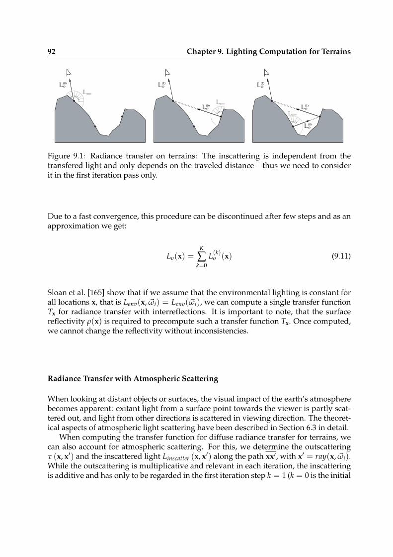
92 Chapter 9. Lighting Computation for Terrains
L⁽⁰⁾o
L !"
L⁽¹⁾o
L !"L⁽⁰⁾o
L⁽²⁾o
L !"
L⁽¹⁾o
L⁽⁰⁾o
Figure 9.1: Radiance transfer on terrains: The inscattering is independent from thetransfered light and only depends on the traveled distance – thus we need to considerit in the first iteration pass only.
Due to a fast convergence, this procedure can be discontinued after few steps and as anapproximation we get:
Lo(x) =K
∑k=0
L(k)o (x) (9.11)
Sloan et al. [165] show that if we assume that the environmental lighting is constant forall locations x, that is Lenv(x, ~ωi) = Lenv(~ωi), we can compute a single transfer functionTx for radiance transfer with interreflections. It is important to note, that the surfacereflectivity ρ(x) is required to precompute such a transfer function Tx. Once computed,we cannot change the reflectivity without inconsistencies.
Radiance Transfer with Atmospheric Scattering
When looking at distant objects or surfaces, the visual impact of the earth’s atmospherebecomes apparent: exitant light from a surface point towards the viewer is partly scat-tered out, and light from other directions is scattered in viewing direction. The theoret-ical aspects of atmospheric light scattering have been described in Section 6.3 in detail.
When computing the transfer function for diffuse radiance transfer for terrains, wecan also account for atmospheric scattering. For this, we determine the outscatteringτ (x, x′) and the inscattered light Linscatter (x, x′) along the path xx′, with x′ = ray(x, ~ωi).While the outscattering is multiplicative and relevant in each iteration, the inscatteringis additive and has only to be regarded in the first iteration step k = 1 (k = 0 is the initial

9.2 Numerical Solution of the Rendering Equation 93
step, see Eq. 9.9 and Fig. 9.1):
L(1)o (x) = ρ(x)
∫
Ω ~nx
1π〈~nx, ~ωi〉 (1−V(x, ~ωi))
[
τ(
x, x′)
L(0)o(
x′)
+ Linscatter(
x, x′)
]
dωi
L(k)o (x) = ρ(x)
∫
Ω ~nx
1π〈~nx, ~ωi〉 (1−V(x, ~ωi))
[
τ(
x, x′)
L(k−1)o
(
x′)
]
dωi, k = 2, 3, ..., K
(9.12)
As we can see, it is possible to account for atmospheric effects when computing the ra-diance transfer. The precomputation of a corresponding transfer function however, isnot reasonable: the result depends on the atmospheric conditions, time of day and geo-graphic location of the terrain and thus the environmental lighting cannot be changed,that is a separation of Tx and Lenv for the lighting computation is not possible.
9.2 Numerical Solution of the Rendering Equation
The rendering equation and its simplifications for terrain rendering, as presented inthe last section, can be solved numerically by Monte Carlo ray tracing methods, e.g.bi-directional ray tracing [14] and distributed ray tracing [26].
Both of these methods are not suitable for real-time rendering on contemporaryhardware. Nonetheless, they can be used to compute reference solutions for a com-parison with fast, approximating methods. Our reference images were computed withdistributed ray tracing and are presented in Section 9.5.
9.3 Precomputed Radiance Transfer with Spherical Har-
monics
The spherical harmonics (SH) [62, 165] form an orthogonal basis over a sphere, compara-ble to the Fourier transform over a 1D circle. Using the parameterization (assuming aunit-sphere S):
s = (x, y, z)T = (sin θ cos φ, sin θ sin φ, cos θ)T (9.13)
the basis functions are defined as:
Yml (θ, φ) = Km
l P|m|l (cos θ) eimφ, l ∈ N, − l ≤ m ≤ l (9.14)
94 Chapter 9. Lighting Computation for Terrains
where l is the band index. Lower bands represent low-frequency basis functions. P|m|lare the Legendre polynomials and Km
l the normalization constants:
Kml =
√
(2l + 1)
4π
(l − |m|)!(l + |m|)!
Pml (x) =
x (2l − 1) Pml−1 − (l + m− 1) Pm
l−2
l −m
Pmm (x) = (−1)m (2m− 1)!!
(
√
1− x2)m
Pmm+1(x) = x (2m + 1) Pm
m
(9.15)
Using the following transformation, a real-valued basis can be derived from the above,complex basis:
yml =
√2ℜ(Ym
l ) =√
2 Kml Pm
l (cos θ) cos(mφ), if m > 0√2ℑ(Ym
l ) =√
2 Kml P−m
l (cos θ) sin(−mφ), if m < 0Y0
l = K0l P0
l (cos θ), if m = 0
(9.16)
Scalar functions can be projected into the SH basis and reconstructed from the coeffi-cients of the basis functions. Low-frequency functions can be accurately reconstructedwith few SH bands. Increasingly higher numbers of basis functions provide better re-construction of high-frequency functions which become band-limited when using fewSH bands. When projecting discontinuous functions into the SH basis the Gibbs phe-nomenon may occur. Possible ways to reduce these ’ringing’ artifacts are discussed byNavarra et al. [123].
For low-frequency lighting environments, as the sky light for example, the transferfunction and environmental light can be compactly represented by spherical harmon-ics. The advantage of a SH representation of the lighting environment is that the hemi-spherical lighting integral can be replaced by a dot-product of SH coefficients. As thesefunctions are defined on the surface of a sphere, we extend the transfer function in orderto replace the hemispherical integral Ω by an integral over the whole sphere S:
T′x(~ωi) = Tx(~ωi) χΩ(~ωi) =
Tx(~ωi), if ~ωi ∈ Ω, that is 〈~nx, ~ωi〉 ≥ 00, otherwise
Lo(x, ~ωo) = ρ(x)∫
ST′x(~ωi)Lenv(x, ~ωi)dωi
(9.17)
Another possibility would be to use hemispherical basis functions [59] which offer thesame advantages as spherical harmonics, but are directly applicable to hemisphericaldata representations. For terrains and other static objects the transfer function and itsSH-projection can be precomputed and stored as surface attribute per-vertex or in a tex-ture atlas. Furthermore we can assume that Lenv is nearly constant for large regions of
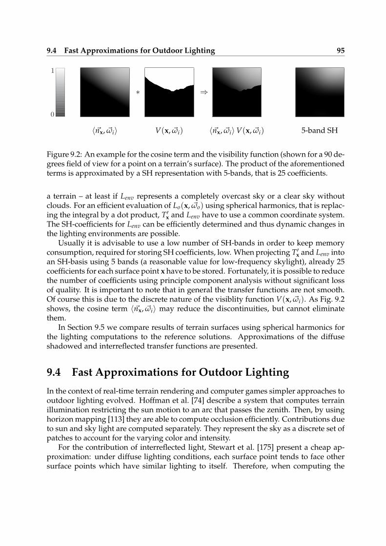
9.4 Fast Approximations for Outdoor Lighting 95
1
0
∗ ⇒
〈~nx, ~ωi〉 V(x, ~ωi) 〈~nx, ~ωi〉V(x, ~ωi) 5-band SH
Figure 9.2: An example for the cosine term and the visibility function (shown for a 90 de-grees field of view for a point on a terrain’s surface). The product of the aforementionedterms is approximated by a SH representation with 5-bands, that is 25 coefficients.
a terrain – at least if Lenv represents a completely overcast sky or a clear sky withoutclouds. For an efficient evaluation of Lo(x, ~ωo) using spherical harmonics, that is replac-ing the integral by a dot product, T′x and Lenv have to use a common coordinate system.The SH-coefficients for Lenv can be efficiently determined and thus dynamic changes inthe lighting environments are possible.
Usually it is advisable to use a low number of SH-bands in order to keep memoryconsumption, required for storing SH coefficients, low. When projecting T′x and Lenv intoan SH-basis using 5 bands (a reasonable value for low-frequency skylight), already 25coefficients for each surface point x have to be stored. Fortunately, it is possible to reducethe number of coefficients using principle component analysis without significant lossof quality. It is important to note that in general the transfer functions are not smooth.Of course this is due to the discrete nature of the visiblity function V(x, ~ωi). As Fig. 9.2shows, the cosine term 〈~nx, ~ωi〉 may reduce the discontinuities, but cannot eliminatethem.
In Section 9.5 we compare results of terrain surfaces using spherical harmonics forthe lighting computations to the reference solutions. Approximations of the diffuseshadowed and interreflected transfer functions are presented.
9.4 Fast Approximations for Outdoor Lighting
In the context of real-time terrain rendering and computer games simpler approaches tooutdoor lighting evolved. Hoffman et al. [74] describe a system that computes terrainillumination restricting the sun motion to an arc that passes the zenith. Then, by usinghorizon mapping [113] they are able to compute occlusion efficiently. Contributions dueto sun and sky light are computed separately. They represent the sky as a discrete set ofpatches to account for the varying color and intensity.
For the contribution of interreflected light, Stewart et al. [175] present a cheap ap-proximation: under diffuse lighting conditions, each surface point tends to face othersurface points which have similar lighting to itself. Therefore, when computing the
96 Chapter 9. Lighting Computation for Terrains
lighting for a surface point, we can assume that other visible surface points exhibit sim-ilar radiance. This yields to a closed-form expression for light interreflections [175].Stewart [174] used this approach for terrain lighting and the approximation errors havebeen measured and shown to be small.
A far more rigorous approach for real-time applications is using ambient occlu-sion [98] for terrain lighting. The sky is assumed to have constant color Lsky and foreach surface location an occlusion term O is precomputed:
O(x) = 1− 1π
∫
Ω ~nx
V(x, ~ωi) 〈~nx, ωi〉 dωi (9.18)
The lighting computation simplifies to:
Lo(x) = Vsun(x, ~ωi) 〈~nx, ~ωi〉 Lsun(x, ~ωi) + O(x)Lsky (9.19)
where Vsun(x, ~ωi) is the occlusion of the sun that can be computed by using any shadowalgorithm, e.g. shadow mapping [189]. Note that in this setting, a further simplificationis made as the volume expansion of the sun is ignored. Together with the ambientocclusion method often bent normals are used for the lighting computation: the surfacenormals are bent in the direction of least occlusion.
9.5 Comparison of the Approaches
The aforementioned approximations and simplified assumptions for the outdoor light-ing computation are necessary to achieve real-time rendering speed with contemporarygraphics hardware. In this section we present solutions computed with the differentmodels and compare results under different lighting conditions. All images are gener-ated assuming a pure white, diffuse surface. For rendering the final images, the reflec-tivity of the surfaces has to be taken into account for direct and indirect lighting.
The first setting is a autumn morning sky (see Fig. 9.3, top). The sun light is notcompletely overwhelming the sky light and the latter exhibits strong variation in colorand intensity. Thus it is suitable to identify weaknesses of an approximation concerningdirectional dependencies. The second lighting environment is a summer noon sky (seeFig. 9.3, bottom). We computed the spectral radiance and intensity using Preethamsanalytic model (see Section 6.3 for details).
Figure 9.4 shows a reference solution (without interreflections) for the morning skyenvironment and spherical harmonics approximations with different number of bands.When using few bands, spherical harmonics are not able to reproduce hard edges be-tween shadowed and non-shadowed regions without an occurrence of the Gibbs phe-nomenon. Appropriate filtering reduces artifacts but increases the angular distributionof the sun light enormously. For sky light only, exhibiting only low-frequency lighting,the spherical harmonics proved to be well suited and few bands are sufficient for a quiteaccurate representation (see Fig. 9.7).
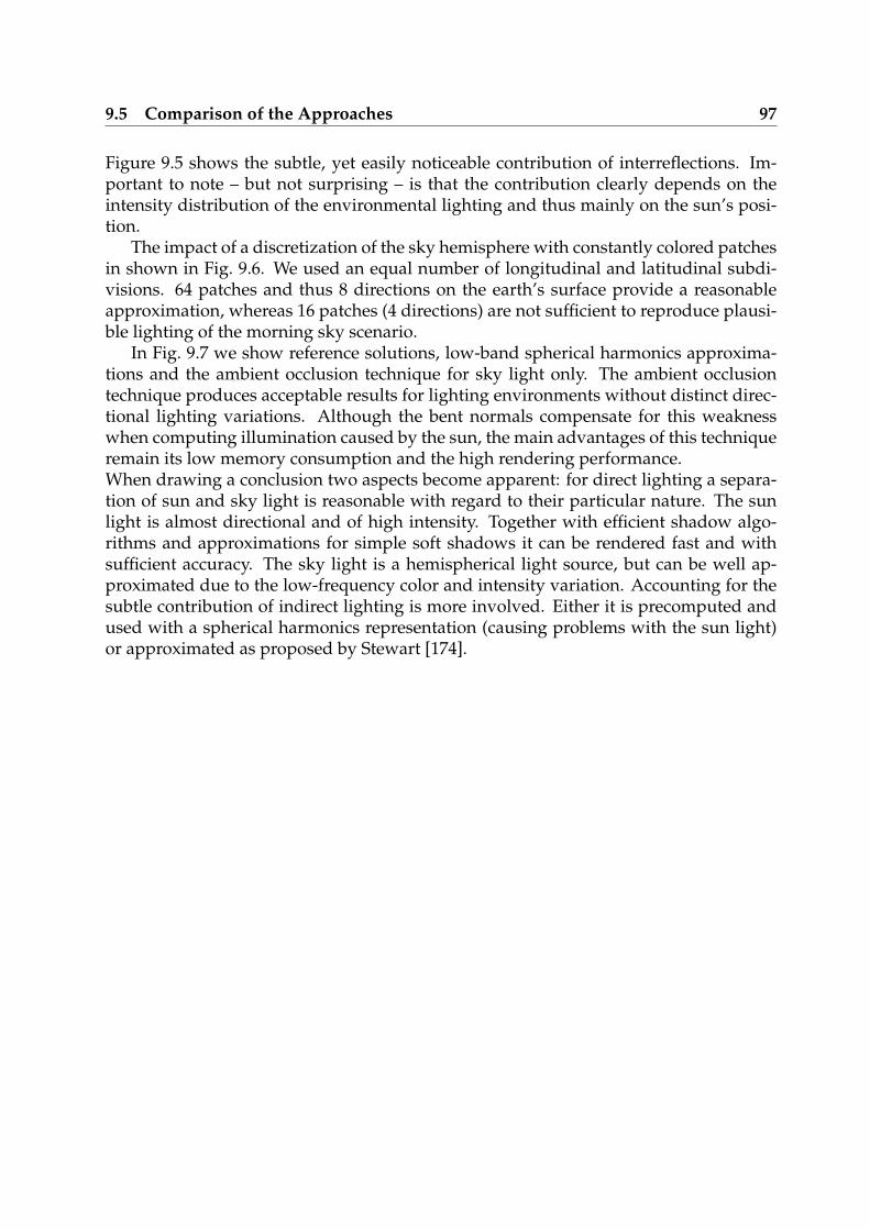
9.5 Comparison of the Approaches 97
Figure 9.5 shows the subtle, yet easily noticeable contribution of interreflections. Im-portant to note – but not surprising – is that the contribution clearly depends on theintensity distribution of the environmental lighting and thus mainly on the sun’s posi-tion.
The impact of a discretization of the sky hemisphere with constantly colored patchesin shown in Fig. 9.6. We used an equal number of longitudinal and latitudinal subdi-visions. 64 patches and thus 8 directions on the earth’s surface provide a reasonableapproximation, whereas 16 patches (4 directions) are not sufficient to reproduce plausi-ble lighting of the morning sky scenario.
In Fig. 9.7 we show reference solutions, low-band spherical harmonics approxima-tions and the ambient occlusion technique for sky light only. The ambient occlusiontechnique produces acceptable results for lighting environments without distinct direc-tional lighting variations. Although the bent normals compensate for this weaknesswhen computing illumination caused by the sun, the main advantages of this techniqueremain its low memory consumption and the high rendering performance.When drawing a conclusion two aspects become apparent: for direct lighting a separa-tion of sun and sky light is reasonable with regard to their particular nature. The sunlight is almost directional and of high intensity. Together with efficient shadow algo-rithms and approximations for simple soft shadows it can be rendered fast and withsufficient accuracy. The sky light is a hemispherical light source, but can be well ap-proximated due to the low-frequency color and intensity variation. Accounting for thesubtle contribution of indirect lighting is more involved. Either it is precomputed andused with a spherical harmonics representation (causing problems with the sun light)or approximated as proposed by Stewart [174].
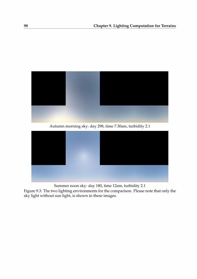
98 Chapter 9. Lighting Computation for Terrains
Autumn morning sky: day 298, time 7.30am, turbidity 2.1
Summer noon sky: day 180, time 12am, turbidity 2.1Figure 9.3: The two lighting environments for the comparison. Please note that only thesky light without sun light, is shown in these images.
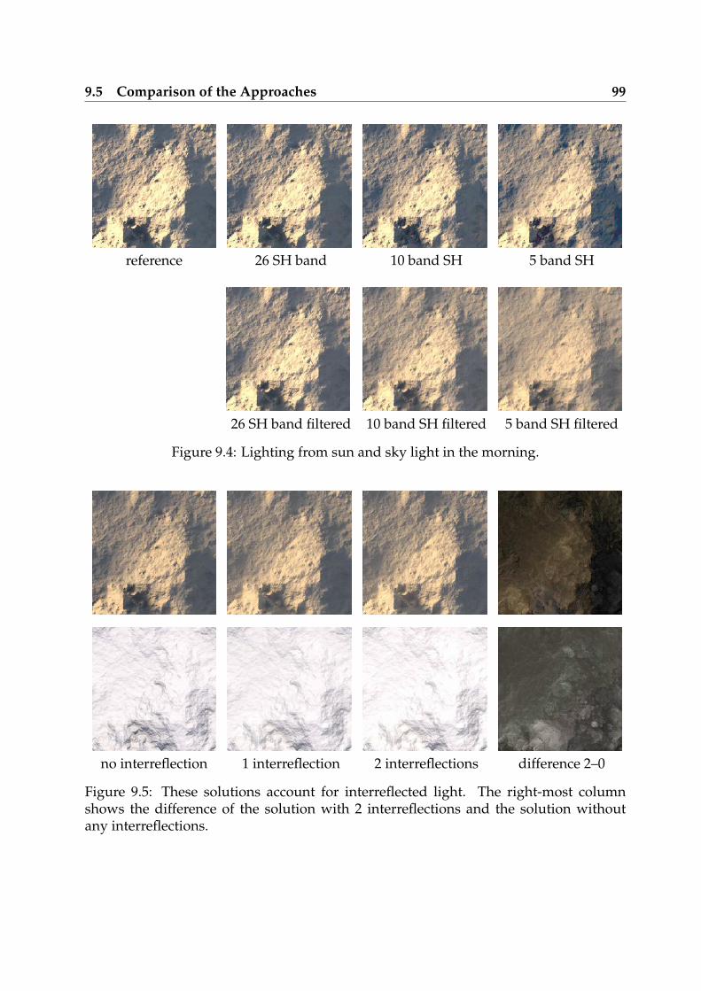
9.5 Comparison of the Approaches 99
reference 26 SH band 10 band SH 5 band SH
26 SH band filtered 10 band SH filtered 5 band SH filtered
Figure 9.4: Lighting from sun and sky light in the morning.
no interreflection 1 interreflection 2 interreflections difference 2–0
Figure 9.5: These solutions account for interreflected light. The right-most columnshows the difference of the solution with 2 interreflections and the solution withoutany interreflections.
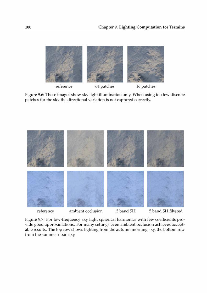
100 Chapter 9. Lighting Computation for Terrains
reference 64 patches 16 patches
Figure 9.6: These images show sky light illumination only. When using too few discretepatches for the sky the directional variation is not captured correctly.
reference ambient occlusion 5 band SH 5 band SH filtered
Figure 9.7: For low-frequency sky light spherical harmonics with few coefficients pro-vide good approximations. For many settings even ambient occlusion achieves accept-able results. The top row shows lighting from the autumn morning sky, the bottom rowfrom the summer noon sky.
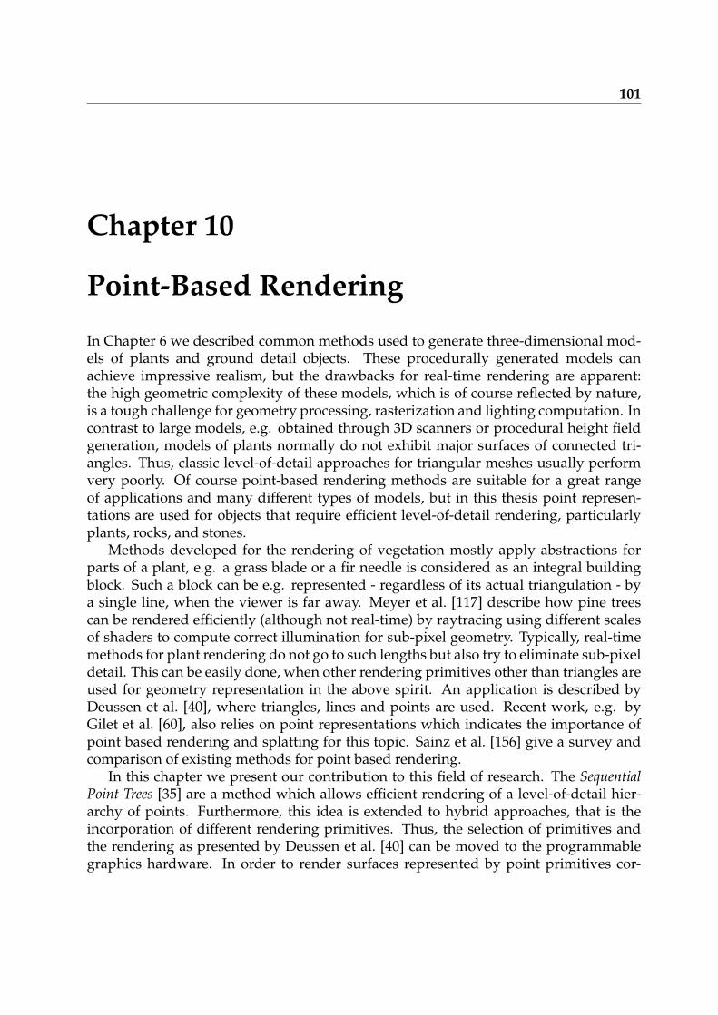
101
Chapter 10
Point-Based Rendering
In Chapter 6 we described common methods used to generate three-dimensional mod-els of plants and ground detail objects. These procedurally generated models canachieve impressive realism, but the drawbacks for real-time rendering are apparent:the high geometric complexity of these models, which is of course reflected by nature,is a tough challenge for geometry processing, rasterization and lighting computation. Incontrast to large models, e.g. obtained through 3D scanners or procedural height fieldgeneration, models of plants normally do not exhibit major surfaces of connected tri-angles. Thus, classic level-of-detail approaches for triangular meshes usually performvery poorly. Of course point-based rendering methods are suitable for a great rangeof applications and many different types of models, but in this thesis point represen-tations are used for objects that require efficient level-of-detail rendering, particularlyplants, rocks, and stones.
Methods developed for the rendering of vegetation mostly apply abstractions forparts of a plant, e.g. a grass blade or a fir needle is considered as an integral buildingblock. Such a block can be e.g. represented - regardless of its actual triangulation - bya single line, when the viewer is far away. Meyer et al. [117] describe how pine treescan be rendered efficiently (although not real-time) by raytracing using different scalesof shaders to compute correct illumination for sub-pixel geometry. Typically, real-timemethods for plant rendering do not go to such lengths but also try to eliminate sub-pixeldetail. This can be easily done, when other rendering primitives other than triangles areused for geometry representation in the above spirit. An application is described byDeussen et al. [40], where triangles, lines and points are used. Recent work, e.g. byGilet et al. [60], also relies on point representations which indicates the importance ofpoint based rendering and splatting for this topic. Sainz et al. [156] give a survey andcomparison of existing methods for point based rendering.
In this chapter we present our contribution to this field of research. The SequentialPoint Trees [35] are a method which allows efficient rendering of a level-of-detail hier-archy of points. Furthermore, this idea is extended to hybrid approaches, that is theincorporation of different rendering primitives. Thus, the selection of primitives andthe rendering as presented by Deussen et al. [40] can be moved to the programmablegraphics hardware. In order to render surfaces represented by point primitives cor-
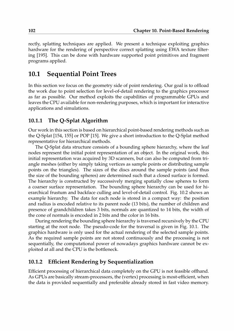
102 Chapter 10. Point-Based Rendering
rectly, splatting techniques are applied. We present a technique exploiting graphicshardware for the rendering of perspective correct splatting using EWA texture filter-ing [195]. This can be done with hardware supported point primitives and fragmentprograms applied.
10.1 Sequential Point Trees
In this section we focus on the geometry side of point rendering. Our goal is to offloadthe work due to point selection for level-of-detail rendering to the graphics processoras far as possible. Our method exploits the capabilities of programmable GPUs andleaves the CPU available for non-rendering purposes, which is important for interactiveapplications and simulations.
10.1.1 The Q-Splat Algorithm
Our work in this section is based on hierarchical point-based rendering methods such asthe Q-Splat [154, 155] or POP [15]. We give a short introduction to the Q-Splat methodrepresentative for hierarchical methods.
The Q-Splat data structure consists of a bounding sphere hierarchy, where the leafnodes represent the initial point representation of an object. In the original work, thisinitial representation was acquired by 3D scanners, but can also be computed from tri-angle meshes (either by simply taking vertices as sample points or distributing samplepoints on the triangles). The sizes of the discs around the sample points (and thusthe size of the bounding spheres) are determined such that a closed surface is formed.The hierarchy is constructed by successively merging spatially close spheres to forma coarser surface representation. The bounding sphere hierarchy can be used for hi-erarchical frustum and backface culling and level-of-detail control. Fig. 10.2 shows anexample hierarchy. The data for each node is stored in a compact way: the positionand radius is encoded relative to its parent node (13 bits), the number of children andpresence of grandchildren takes 3 bits, normals are quantized to 14 bits, the width ofthe cone of normals is encoded in 2 bits and the color in 16 bits.
During rendering the bounding sphere hierarchy is traversed recursively by the CPUstarting at the root node. The pseudo-code for the traversal is given in Fig. 10.1. Thegraphics hardware is only used for the actual rendering of the selected sample points.As the required sample points are not stored continuously and the processing is notsequentially, the computational power of nowadays graphics hardware cannot be ex-ploited at all and the CPU is the bottleneck.
10.1.2 Efficient Rendering by Sequentialization
Efficient processing of hierarchical data completely on the GPU is not feasible offhand.As GPUs are basically stream-processors, the (vertex) processing is most-efficient, whenthe data is provided sequentially and preferable already stored in fast video memory.
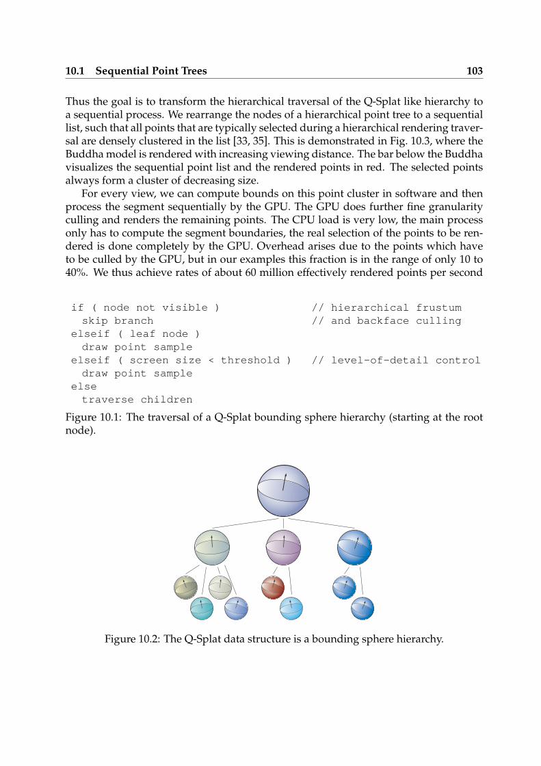
10.1 Sequential Point Trees 103
Thus the goal is to transform the hierarchical traversal of the Q-Splat like hierarchy toa sequential process. We rearrange the nodes of a hierarchical point tree to a sequentiallist, such that all points that are typically selected during a hierarchical rendering traver-sal are densely clustered in the list [33, 35]. This is demonstrated in Fig. 10.3, where theBuddha model is rendered with increasing viewing distance. The bar below the Buddhavisualizes the sequential point list and the rendered points in red. The selected pointsalways form a cluster of decreasing size.
For every view, we can compute bounds on this point cluster in software and thenprocess the segment sequentially by the GPU. The GPU does further fine granularityculling and renders the remaining points. The CPU load is very low, the main processonly has to compute the segment boundaries, the real selection of the points to be ren-dered is done completely by the GPU. Overhead arises due to the points which haveto be culled by the GPU, but in our examples this fraction is in the range of only 10 to40%. We thus achieve rates of about 60 million effectively rendered points per second
if ( node not visible )skip branch
elseif ( leaf node )draw point sample
elseif ( screen size < threshold )draw point sample
elsetraverse children
// hierarchical frustum// and backface culling
// level-of-detail control
Figure 10.1: The traversal of a Q-Splat bounding sphere hierarchy (starting at the rootnode).
Figure 10.2: The Q-Splat data structure is a bounding sphere hierarchy.
104 Chapter 10. Point-Based Rendering
on a Radeon 9700 and about 80 million on a GeForce 6800 GT, in each case with verylow CPU load.As mentioned above, the Sequential Point Trees (SPTs) are also based on a point tree hi-erarchy. We first describe our point tree hierarchy and its hierarchical rendering traver-sal, in order to define notation and to explain extensions. After that, we can introducethe Sequential Point Tree data structure and its efficient rendering by the graphics pro-cessor. We then add extensions that help to improve performance even further.
Note that our scenes are sets of objects. For each of the objects, a Sequential PointTree as described in the following is generated. With instancing, the same point tree canbe rendered at different locations. This simple scene structure reflects the necessities oftypical interactive applications like games or rendering of outdoor scenes for example.The goal is to render each visible object at a level of detail which is an optimal balancefor the current point of view.
10.1.3 Point Tree Hierarchy
Every node in our point tree hierarchy represents a part of the object. It stores a cen-ter point p and an average normal n. For now, we consider objects of uniform color,extensions for colored and textured point clouds are later described in Section 10.1.9.Furthermore, every node stores a diameter d of a bounding sphere around p for therepresented object part. An inner node in the hierarchy represents the union of all itschildren, so the diameter monotonically increases when going up the hierarchy. The leafpoints should be uniformly distributed over the object, so that the leaves’ diameters areroughly equal.
We begin with a set of uniformly distributed point samples on the object, whichare inserted into an octree. The octree represents the point hierarchy. Position and
Figure 10.3: Continuous detail levels of a Buddha generated in a vertex program on theGPU. The colors denote the LOD level used and the bars describe the selected amount ofpoints selected for the GPU (top row) and the average CPU load required for rendering(bottom row, taken from [35]).
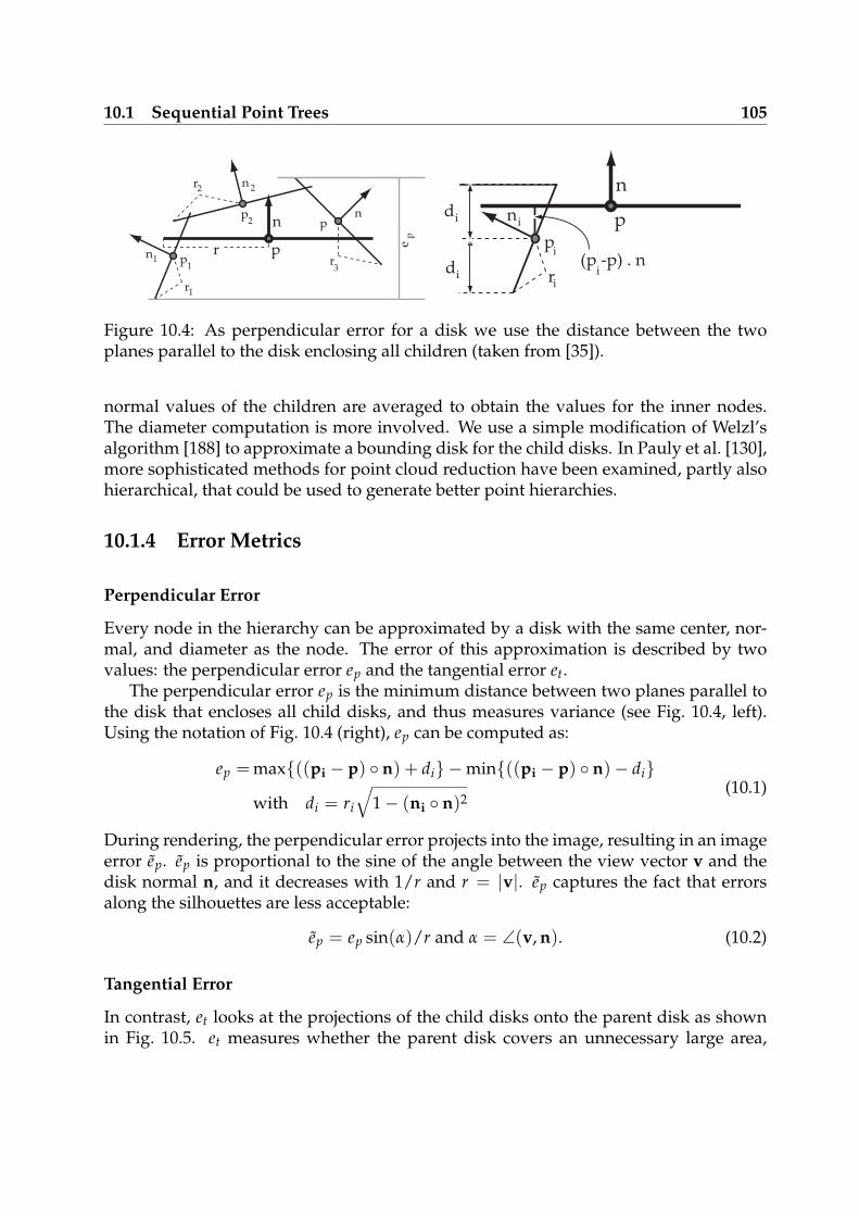
10.1 Sequential Point Trees 105
p1
2p
n1
n 2
pn
1r
2r
3r
p
n
r ep
pi
ni
ir
p
n
(p -p) . ni
id
id
Figure 10.4: As perpendicular error for a disk we use the distance between the twoplanes parallel to the disk enclosing all children (taken from [35]).
normal values of the children are averaged to obtain the values for the inner nodes.The diameter computation is more involved. We use a simple modification of Welzl’salgorithm [188] to approximate a bounding disk for the child disks. In Pauly et al. [130],more sophisticated methods for point cloud reduction have been examined, partly alsohierarchical, that could be used to generate better point hierarchies.
10.1.4 Error Metrics
Perpendicular Error
Every node in the hierarchy can be approximated by a disk with the same center, nor-mal, and diameter as the node. The error of this approximation is described by twovalues: the perpendicular error ep and the tangential error et.
The perpendicular error ep is the minimum distance between two planes parallel tothe disk that encloses all child disks, and thus measures variance (see Fig. 10.4, left).Using the notation of Fig. 10.4 (right), ep can be computed as:
ep = max((pi − p) n) + di −min((pi − p) n)− di
with di = ri
√
1− (ni n)2(10.1)
During rendering, the perpendicular error projects into the image, resulting in an imageerror ep. ep is proportional to the sine of the angle between the view vector v and thedisk normal n, and it decreases with 1/r and r = |v|. ep captures the fact that errorsalong the silhouettes are less acceptable:
ep = ep sin(α)/r and α = ∠(v, n). (10.2)
Tangential Error
In contrast, et looks at the projections of the child disks onto the parent disk as shownin Fig. 10.5. et measures whether the parent disk covers an unnecessary large area,
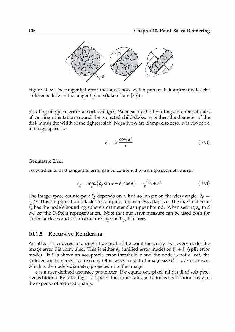
106 Chapter 10. Point-Based Rendering
e =0t
et
et
Figure 10.5: The tangential error measures how well a parent disk approximates thechildren’s disks in the tangent plane (taken from [35]).
resulting in typical errors at surface edges. We measure this by fitting a number of slabsof varying orientation around the projected child disks. et is then the diameter of thedisk minus the width of the tightest slab. Negative et are clamped to zero. et is projectedto image space as:
et = etcos(α)
r(10.3)
Geometric Error
Perpendicular and tangential error can be combined to a single geometric error
eg = maxαep sin α + et cos α =
√
e2p + e2
t (10.4)
The image space counterpart eg depends on r, but no longer on the view angle: eg =eg/r. This simplification is faster to compute, but also less adaptive. The maximal erroreg has the node’s bounding sphere’s diameter d as upper bound. When setting eg to dwe get the Q-Splat representation. Note that our error measure can be used both forclosed surfaces and for unstructured geometry, like trees.
10.1.5 Recursive Rendering
An object is rendered in a depth traversal of the point hierarchy. For every node, theimage error e is computed. This is either eg (unified error mode) or ep + et (split errormode). If e is above an acceptable error threshold ǫ and the node is not a leaf, thechildren are traversed recursively. Otherwise, a splat of image size d = d/r is drawn,which is the node’s diameter, projected onto the image.
ǫ is a user defined accuracy parameter. If ǫ equals one pixel, all detail of sub-pixelsize is hidden. By selecting ǫ > 1 pixel, the frame-rate can be increased continuously, atthe expense of reduced quality.
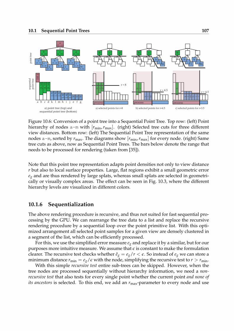
10.1 Sequential Point Trees 107
a) selected points for r=8 b) selected points for r=4.5 c) selected points for r=3.5
po
int
tree
seq
uen
tial
po
int
tree
ml
ji
b
h k
r = 8
b c d
ml
b c
k
a b c d
[5..1
0]
[10.
.]
[4..1
0]
[3..1
0]
[..5
]
[..4
]
[..3
]
m[0...5]
l[0...5]j
[0...4]
i[0...4]g
[0...3]
f[0...3]
a[10...oo]
b[3...10]
c[4...10]
d[5...10]
e[0...3]
h[0...4]
k[0...5]
a) point tree (top) andsequential point tree (bo!om)
b c d
[..5
]
[..5
]
[..4
]
[..4
]
[..3
]
[..3
]
k l m h i j e f g
r = 4.5
b c
k l m
r = 4.5
b
k l m h i j
process processprocess
b c
kk ll m
b
k l m h i j
b c d
Figure 10.6: Conversion of a point tree into a Sequential Point Tree. Top row: (left) Pointhierarchy of nodes a-m with [rmin, rmax]. (right) Selected tree cuts for three differentview distances. Bottom row: (left) The Sequential Point Tree representation of the samenodes a-m, sorted by rmax. The diagrams show [rmin, rmax] for every node. (right) Sametree cuts as above, now as Sequential Point Trees. The bars below denote the range thatneeds to be processed for rendering (taken from [35]).
Note that this point tree representation adapts point densities not only to view distancer but also to local surface properties. Large, flat regions exhibit a small geometric erroreg and are thus rendered by large splats, whereas small splats are selected in geometri-cally or visually complex areas. The effect can be seen in Fig. 10.3, where the differenthierarchy levels are visualized in different colors.
10.1.6 Sequentialization
The above rendering procedure is recursive, and thus not suited for fast sequential pro-cessing by the GPU. We can rearrange the tree data to a list and replace the recursiverendering procedure by a sequential loop over the point primitive list. With this opti-mized arrangement all selected point samples for a given view are densely clustered ina segment of the list, which can be efficiently processed.
For this, we use the simplified error measure eg and replace it by a similar, but for ourpurposes more intuitive measure. We assume that ǫ is constant to make the formulationclearer. The recursive test checks whether eg = eg/r < ǫ. So instead of eg we can store aminimum distance rmin = eg/ǫ with the node, simplifying the recursive test to r > rmin.
With this simple recursive test entire sub-trees can be skipped. However, when thetree nodes are processed sequentially without hierarchy information, we need a non-recursive test that also tests for every single point whether the current point and none ofits ancestors is selected. To this end, we add an rmax-parameter to every node and use
108 Chapter 10. Point-Based Rendering
r ∈ [rmin, rmax] as non-recursive test. Intuitively, we test with the upper bound whetherthe view distance is so large that one of the ancestors will be selected for rendering; thermax test thus replaces the recursive skip.
A first attempt for the selection of rmax is to use rmin of the direct parent or infinityfor the root node. So when going up the hierarchy the intervals don’t overlap and notboth a node and its children are selected. Examples with a simple point hierarchy andthe node fronts selected by different values for r are shown in the top row of Fig. 10.6.
The above approach works when r is constant for the entire tree. But if we recomputer for all nodes, it can happen for a node that r is just below rmin, but due to the differentr for the children also above some children’s rmax, resulting in holes in the rendering.We can account for this by adding an interval overlap as big as the point distance. Thisoverlap ensures that no holes appear, but it also means that for some nodes both, thenode and some of its children are selected. This results in overdraw and slightly reducedperformance, but we did not experience visible artifacts from it.
10.1.7 Rearrangement
After transforming the recursive test to a simple distance interval test, we store the pointtree nodes as a non-hierarchical list, which is processed sequentially. At this step, the[rmin, rmax]-test allows for a very efficient optimization: by sorting the list for descendingrmax, we can easily restrict the computation to a prefix of the list. Consider the bottomrow of Fig. 10.6. The leftmost column shows a simple point tree (top) and its sequentialcounterpart, sorted for rmax (bottom). In the bottom row, one can see the list pointsselected by a certain r. For r = 8, only the first four points can contribute, because forall later points rmax < r. For smaller r, this boundary moves to the right.
However, for finite objects r is not constant. The effect is shown in Fig. 10.7. For con-stant r (left column), r defines a front in the point tree. In the Sequential Point Tree list,this front cuts the list into two halves. If r varies, the resulting vertex front is enclosedby the vertex fronts defined by minr and maxr. In the list, this results in a fuzzyzone, where points are partially selected.
Thus the algorithm is as follows. First, a lower bound on r is computed from abounding volume of the object. We then search the first list entry with rmax ≤ minrby a binary search. The beginning of the list up to this entry is passed to the GPU.For every point, the GPU computes r and does the [rmin, rmax] test in a vertex program.Points that pass the test are rendered using splat size d, which is also computed bythe vertex program; points that fail the test are culled by moving them to infinity. Thecorresponding vertex program is very simple, the culling and point size computation isdone in a few instructions.
With this simple approach, we efficiently combine coarse and fine granularity culling.The CPU does a first efficient preculling for rmax by selecting i and then passes the entiresegment [0, i] to the GPU (coarse granularity). The GPU processes the segment sequen-tially at maximum efficiency and also does the fine granularity culling. The percentage
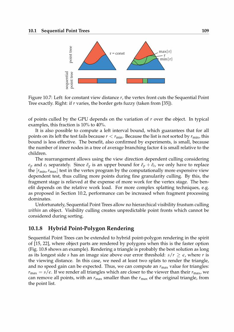
10.1 Sequential Point Trees 109
r = const max
minr
po
int
tree
seq
uen
tial
po
int
tree
r
r
Figure 10.7: Left: for constant view distance r, the vertex front cuts the Sequential PointTree exactly. Right: if r varies, the border gets fuzzy (taken from [35]).
of points culled by the GPU depends on the variation of r over the object. In typicalexamples, this fraction is 10% to 40%.
It is also possible to compute a left interval bound, which guarantees that for allpoints on its left the test fails because r < rmin. Because the list is not sorted by rmin, thisbound is less effective. The benefit, also confirmed by experiments, is small, becausethe number of inner nodes in a tree of average branching factor 4 is small relative to thechildren.
The rearrangement allows using the view direction dependent culling consideringep and et separately. Since eg is an upper bound for ep + et, we only have to replacethe [rmin, rmax] test in the vertex program by the computationally more expensive viewdependent test, thus culling more points during fine granularity culling. By this, thefragment stage is relieved at the expense of more work for the vertex stage. The ben-efit depends on the relative work load. For more complex splatting techniques, e.g.as proposed in Section 10.2, performance can be increased when fragment processingdominates.
Unfortunately, Sequential Point Trees allow no hierarchical visibility frustum cullingwithin an object. Visibility culling creates unpredictable point fronts which cannot beconsidered during sorting.
10.1.8 Hybrid Point-Polygon Rendering
Sequential Point Trees can be extended to hybrid point-polygon rendering in the spiritof [15, 22], where object parts are rendered by polygons when this is the faster option(Fig. 10.8 shows an example). Rendering a triangle is probably the best solution as longas its longest side s has an image size above our error threshold: s/r ≥ ǫ, where r isthe viewing distance. In this case, we need at least two splats to render the triangle,and no speed gain can be expected. Thus, we can compute an rmax value for triangles:rmax = s/ǫ. If we render all triangles which are closer to the viewer than their rmax, wecan remove all points, with an rmax smaller than the rmax of the original triangle, fromthe point list.
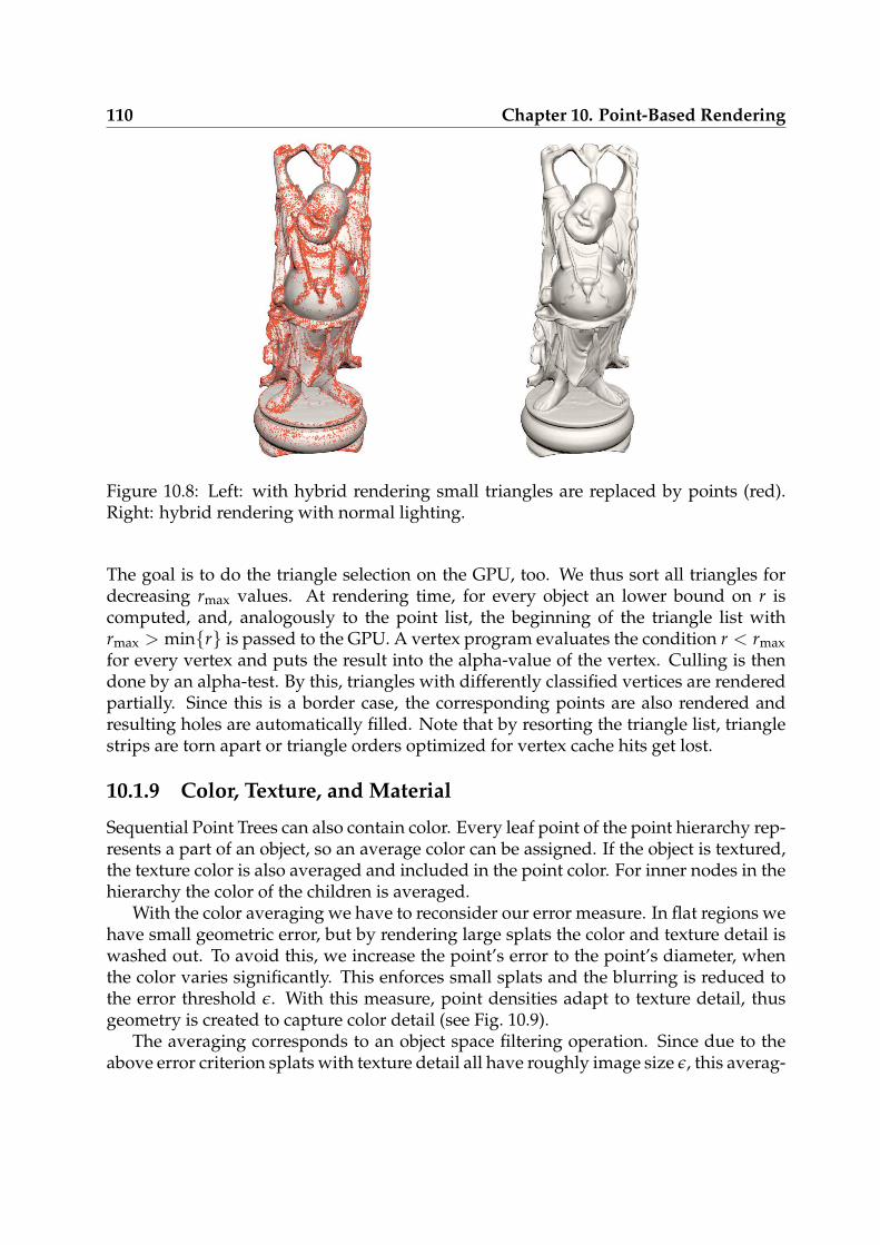
110 Chapter 10. Point-Based Rendering
Figure 10.8: Left: with hybrid rendering small triangles are replaced by points (red).Right: hybrid rendering with normal lighting.
The goal is to do the triangle selection on the GPU, too. We thus sort all triangles fordecreasing rmax values. At rendering time, for every object an lower bound on r iscomputed, and, analogously to the point list, the beginning of the triangle list withrmax > minr is passed to the GPU. A vertex program evaluates the condition r < rmaxfor every vertex and puts the result into the alpha-value of the vertex. Culling is thendone by an alpha-test. By this, triangles with differently classified vertices are renderedpartially. Since this is a border case, the corresponding points are also rendered andresulting holes are automatically filled. Note that by resorting the triangle list, trianglestrips are torn apart or triangle orders optimized for vertex cache hits get lost.
10.1.9 Color, Texture, and Material
Sequential Point Trees can also contain color. Every leaf point of the point hierarchy rep-resents a part of an object, so an average color can be assigned. If the object is textured,the texture color is also averaged and included in the point color. For inner nodes in thehierarchy the color of the children is averaged.
With the color averaging we have to reconsider our error measure. In flat regions wehave small geometric error, but by rendering large splats the color and texture detail iswashed out. To avoid this, we increase the point’s error to the point’s diameter, whenthe color varies significantly. This enforces small splats and the blurring is reduced tothe error threshold ǫ. With this measure, point densities adapt to texture detail, thusgeometry is created to capture color detail (see Fig. 10.9).
The averaging corresponds to an object space filtering operation. Since due to theabove error criterion splats with texture detail all have roughly image size ǫ, this averag-
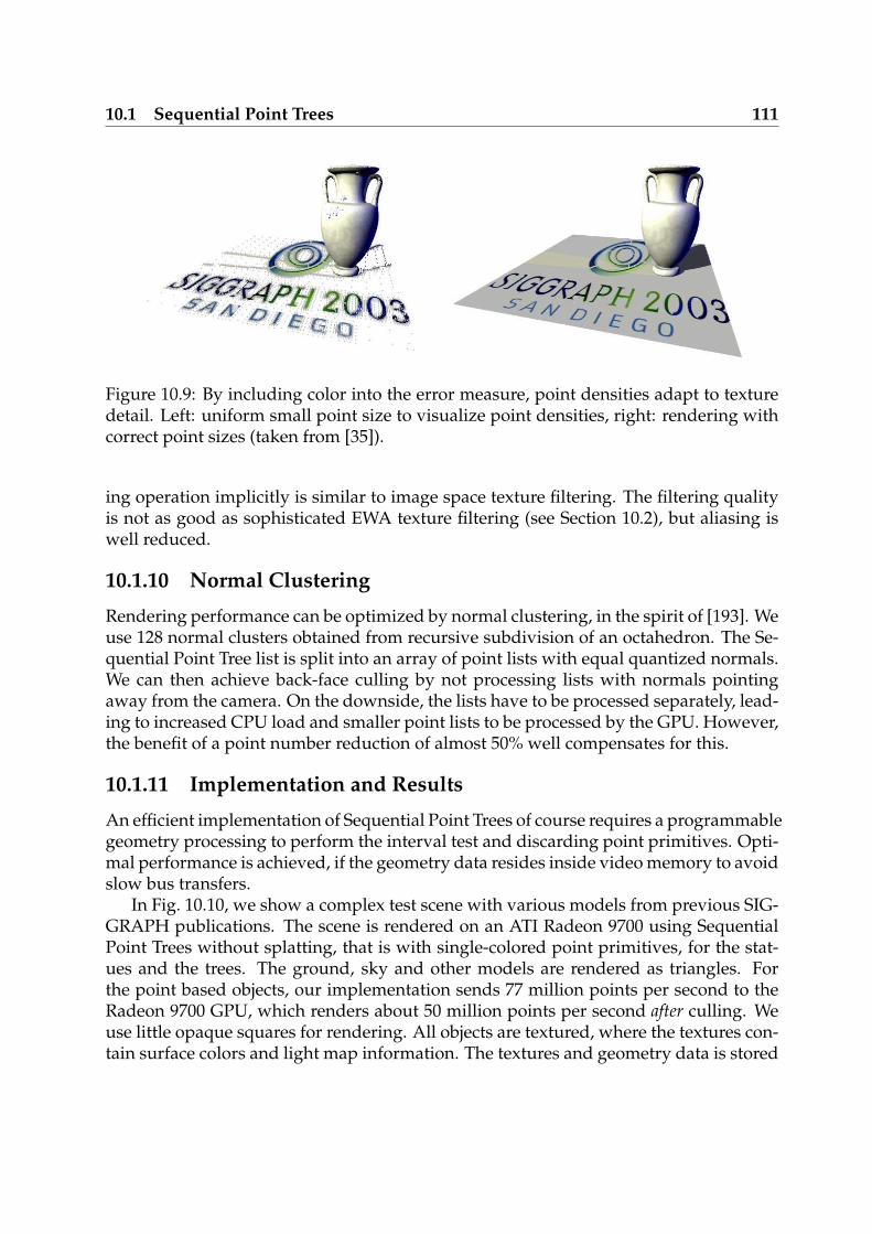
10.1 Sequential Point Trees 111
Figure 10.9: By including color into the error measure, point densities adapt to texturedetail. Left: uniform small point size to visualize point densities, right: rendering withcorrect point sizes (taken from [35]).
ing operation implicitly is similar to image space texture filtering. The filtering qualityis not as good as sophisticated EWA texture filtering (see Section 10.2), but aliasing iswell reduced.
10.1.10 Normal Clustering
Rendering performance can be optimized by normal clustering, in the spirit of [193]. Weuse 128 normal clusters obtained from recursive subdivision of an octahedron. The Se-quential Point Tree list is split into an array of point lists with equal quantized normals.We can then achieve back-face culling by not processing lists with normals pointingaway from the camera. On the downside, the lists have to be processed separately, lead-ing to increased CPU load and smaller point lists to be processed by the GPU. However,the benefit of a point number reduction of almost 50% well compensates for this.
10.1.11 Implementation and Results
An efficient implementation of Sequential Point Trees of course requires a programmablegeometry processing to perform the interval test and discarding point primitives. Opti-mal performance is achieved, if the geometry data resides inside video memory to avoidslow bus transfers.
In Fig. 10.10, we show a complex test scene with various models from previous SIG-GRAPH publications. The scene is rendered on an ATI Radeon 9700 using SequentialPoint Trees without splatting, that is with single-colored point primitives, for the stat-ues and the trees. The ground, sky and other models are rendered as triangles. Forthe point based objects, our implementation sends 77 million points per second to theRadeon 9700 GPU, which renders about 50 million points per second after culling. Weuse little opaque squares for rendering. All objects are textured, where the textures con-tain surface colors and light map information. The textures and geometry data is stored
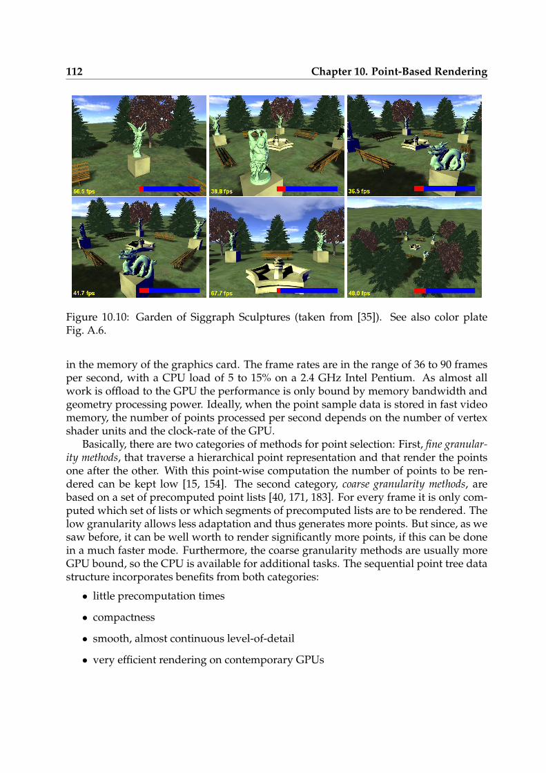
112 Chapter 10. Point-Based Rendering
Figure 10.10: Garden of Siggraph Sculptures (taken from [35]). See also color plateFig. A.6.
in the memory of the graphics card. The frame rates are in the range of 36 to 90 framesper second, with a CPU load of 5 to 15% on a 2.4 GHz Intel Pentium. As almost allwork is offload to the GPU the performance is only bound by memory bandwidth andgeometry processing power. Ideally, when the point sample data is stored in fast videomemory, the number of points processed per second depends on the number of vertexshader units and the clock-rate of the GPU.
Basically, there are two categories of methods for point selection: First, fine granular-ity methods, that traverse a hierarchical point representation and that render the pointsone after the other. With this point-wise computation the number of points to be ren-dered can be kept low [15, 154]. The second category, coarse granularity methods, arebased on a set of precomputed point lists [40, 171, 183]. For every frame it is only com-puted which set of lists or which segments of precomputed lists are to be rendered. Thelow granularity allows less adaptation and thus generates more points. But since, as wesaw before, it can be well worth to render significantly more points, if this can be donein a much faster mode. Furthermore, the coarse granularity methods are usually moreGPU bound, so the CPU is available for additional tasks. The sequential point tree datastructure incorporates benefits from both categories:
• little precomputation times
• compactness
• smooth, almost continuous level-of-detail
• very efficient rendering on contemporary GPUs
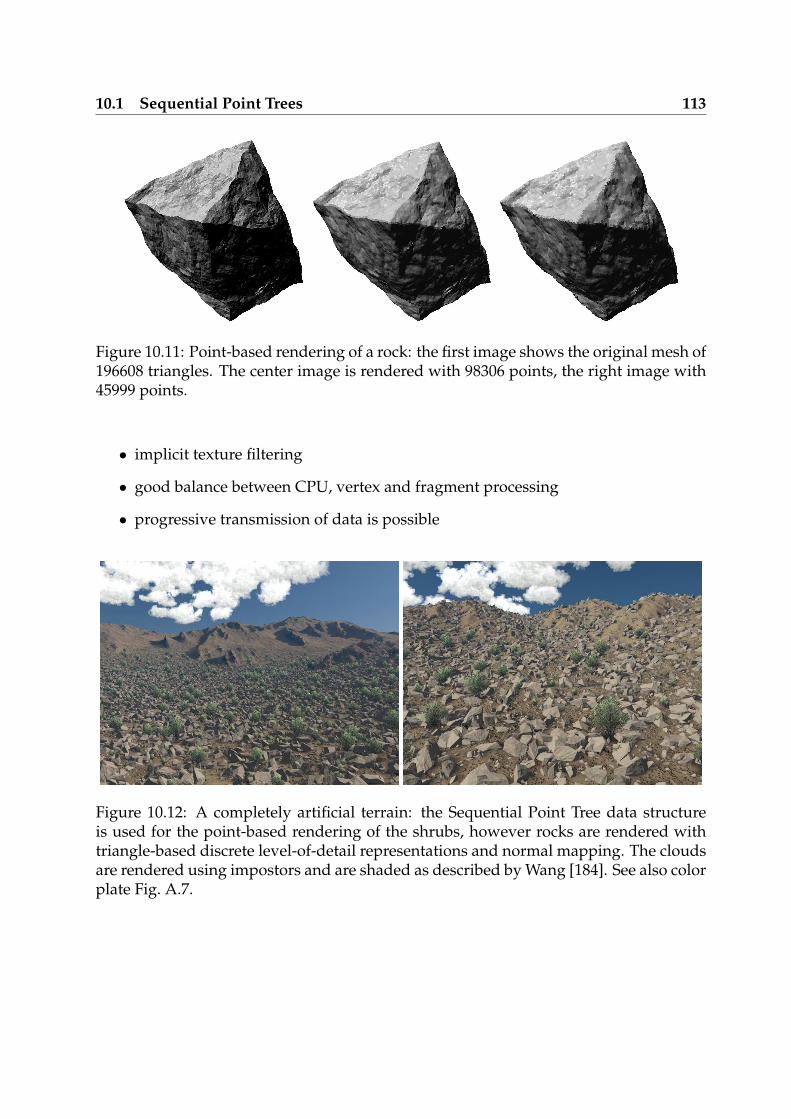
10.1 Sequential Point Trees 113
Figure 10.11: Point-based rendering of a rock: the first image shows the original mesh of196608 triangles. The center image is rendered with 98306 points, the right image with45999 points.
• implicit texture filtering
• good balance between CPU, vertex and fragment processing
• progressive transmission of data is possible
Figure 10.12: A completely artificial terrain: the Sequential Point Tree data structureis used for the point-based rendering of the shrubs, however rocks are rendered withtriangle-based discrete level-of-detail representations and normal mapping. The cloudsare rendered using impostors and are shaded as described by Wang [184]. See also colorplate Fig. A.7.
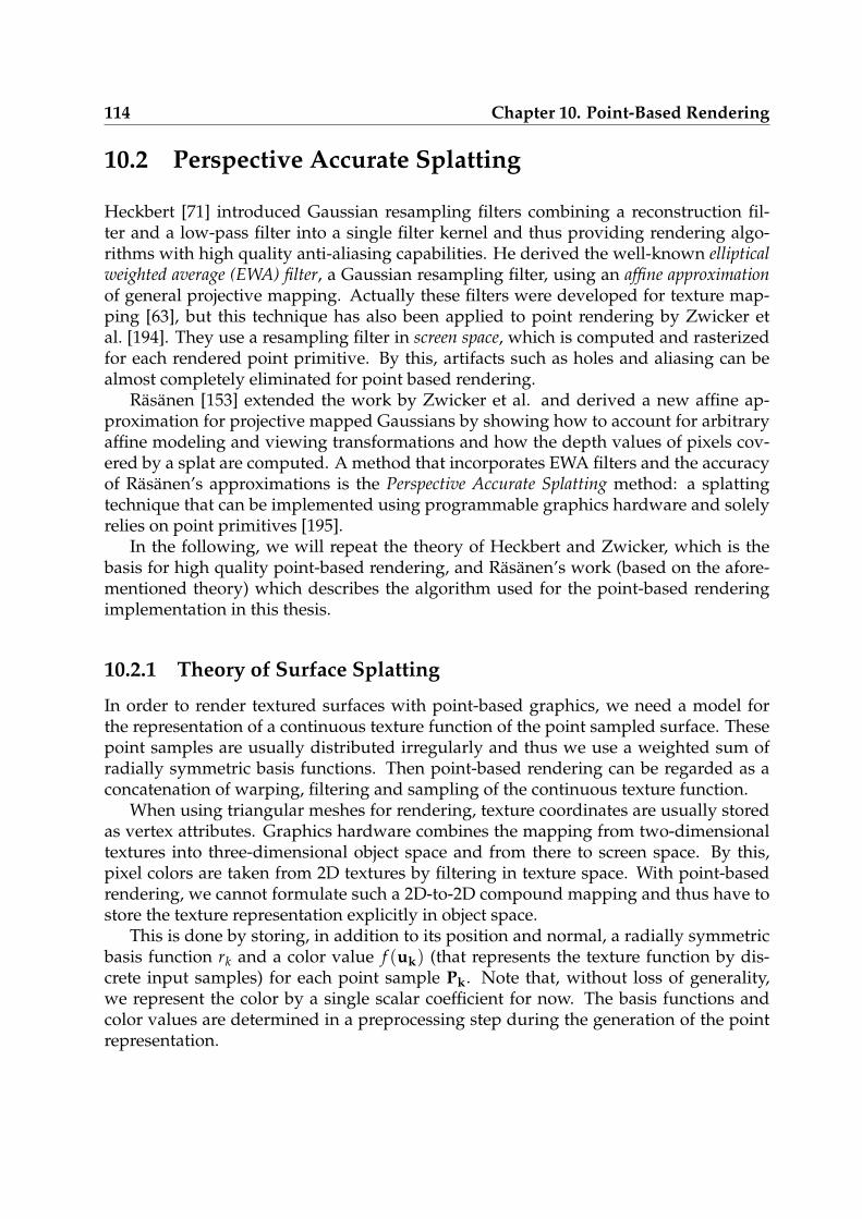
114 Chapter 10. Point-Based Rendering
10.2 Perspective Accurate Splatting
Heckbert [71] introduced Gaussian resampling filters combining a reconstruction fil-ter and a low-pass filter into a single filter kernel and thus providing rendering algo-rithms with high quality anti-aliasing capabilities. He derived the well-known ellipticalweighted average (EWA) filter, a Gaussian resampling filter, using an affine approximationof general projective mapping. Actually these filters were developed for texture map-ping [63], but this technique has also been applied to point rendering by Zwicker etal. [194]. They use a resampling filter in screen space, which is computed and rasterizedfor each rendered point primitive. By this, artifacts such as holes and aliasing can bealmost completely eliminated for point based rendering.
Räsänen [153] extended the work by Zwicker et al. and derived a new affine ap-proximation for projective mapped Gaussians by showing how to account for arbitraryaffine modeling and viewing transformations and how the depth values of pixels cov-ered by a splat are computed. A method that incorporates EWA filters and the accuracyof Räsänen’s approximations is the Perspective Accurate Splatting method: a splattingtechnique that can be implemented using programmable graphics hardware and solelyrelies on point primitives [195].
In the following, we will repeat the theory of Heckbert and Zwicker, which is thebasis for high quality point-based rendering, and Räsänen’s work (based on the afore-mentioned theory) which describes the algorithm used for the point-based renderingimplementation in this thesis.
10.2.1 Theory of Surface Splatting
In order to render textured surfaces with point-based graphics, we need a model forthe representation of a continuous texture function of the point sampled surface. Thesepoint samples are usually distributed irregularly and thus we use a weighted sum ofradially symmetric basis functions. Then point-based rendering can be regarded as aconcatenation of warping, filtering and sampling of the continuous texture function.
When using triangular meshes for rendering, texture coordinates are usually storedas vertex attributes. Graphics hardware combines the mapping from two-dimensionaltextures into three-dimensional object space and from there to screen space. By this,pixel colors are taken from 2D textures by filtering in texture space. With point-basedrendering, we cannot formulate such a 2D-to-2D compound mapping and thus have tostore the texture representation explicitly in object space.
This is done by storing, in addition to its position and normal, a radially symmetricbasis function rk and a color value f (uk) (that represents the texture function by dis-crete input samples) for each point sample Pk. Note that, without loss of generality,we represent the color by a single scalar coefficient for now. The basis functions andcolor values are determined in a preprocessing step during the generation of the pointrepresentation.
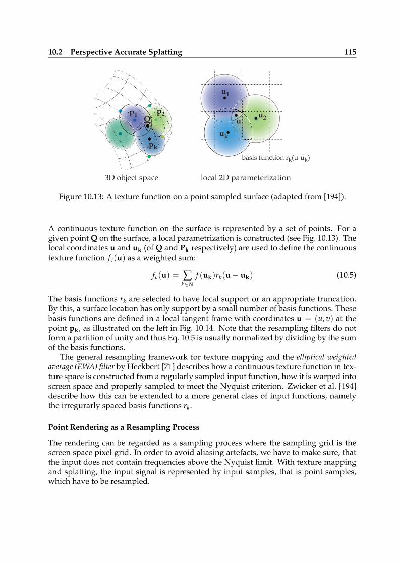
10.2 Perspective Accurate Splatting 115
p1
3D object space
basis function rk(u-uk)
pk
p2Q
u1
u2
uk
u
local 2D parameterization
Figure 10.13: A texture function on a point sampled surface (adapted from [194]).
A continuous texture function on the surface is represented by a set of points. For agiven point Q on the surface, a local parametrization is constructed (see Fig. 10.13). Thelocal coordinates u and uk (of Q and Pk respectively) are used to define the continuoustexture function fc(u) as a weighted sum:
fc(u) = ∑k∈N
f (uk)rk(u− uk) (10.5)
The basis functions rk are selected to have local support or an appropriate truncation.By this, a surface location has only support by a small number of basis functions. Thesebasis functions are defined in a local tangent frame with coordinates u = (u, v) at thepoint pk, as illustrated on the left in Fig. 10.14. Note that the resampling filters do notform a partition of unity and thus Eq. 10.5 is usually normalized by dividing by the sumof the basis functions.
The general resampling framework for texture mapping and the elliptical weightedaverage (EWA) filter by Heckbert [71] describes how a continuous texture function in tex-ture space is constructed from a regularly sampled input function, how it is warped intoscreen space and properly sampled to meet the Nyquist criterion. Zwicker et al. [194]describe how this can be extended to a more general class of input functions, namelythe irregurarly spaced basis functions rk.
Point Rendering as a Resampling Process
The rendering can be regarded as a sampling process where the sampling grid is thescreen space pixel grid. In order to avoid aliasing artefacts, we have to make sure, thatthe input does not contain frequencies above the Nyquist limit. With texture mappingand splatting, the input signal is represented by input samples, that is point samples,which have to be resampled.
116 Chapter 10. Point-Based Rendering
This resampling involves the reconstruction of a continuous representation with an ap-propriate reconstruction filter that is used to transform the continuous representationfrom input space to screen space and to band-limit the mapped representation. Thisis finally sampled to obtain a discrete output signal. In the case of splatting the inputspace is the object space, where point samples and basis functions are defined.
The continuous input signal is given in Eq. 10.5. The mapping from object to screenspace is denoted by x = m(u) = Mu : R
2 → R2. Note that M is a 3 × 3 matrix
describing a projective mapping. The continuous input texture function is then warpedinto screen space ( denotes function concatenation):
gc(x) = ( fc m−1)(x) = fc(M−1x) (10.6)
The screen space signal is band-limited using a prefilter h, giving us the continuousoutput function g′c(x) (⊗ denotes convolution):
g′c(x) = gc(x)⊗ h(x) =∫
R2gc(t)h(x− t)dt (10.7)
The continuous output function is multiplied with an impulse train i(x) to obtain thediscrete output samples x0:
g(x) = g′c(x)i(x), with i(x) =∞
∑n=−∞
δ(x− nT) (10.8)
Expanding the formula for g′c(x), we get:
g′c(x) =∫
R2gc(t)h(x− t)dt
=∫
R2fc(m−1(t))h(x− t)dt
=∫
R2h(x− t) ∑
k∈Nf (uk)rk(m−1(t)− uk)dt
= ∑k∈N
f (uk)ρ(x, uk)
(10.9)
whereρ(x, uk) =
∫
R2h(x− t)rk(m−1(t)− uk)dt (10.10)
is the resampling kernel or resampling filter. The observation from Eq. 10.9 is, that wecan first warp and filter each basis function individually (by reconstructing the resam-pling kernels) and accumulate the contributions of these kernels in screen space. Thisapproach is called surface splatting [194].
We substitute uk in Eq. 10.10, as the mapping of uk into screen space can be ex-pressed by xk = m(uk):
ρ(x, xk) =∫
R2h(x− t)rk(m−1(t)−m−1(xk))dt (10.11)
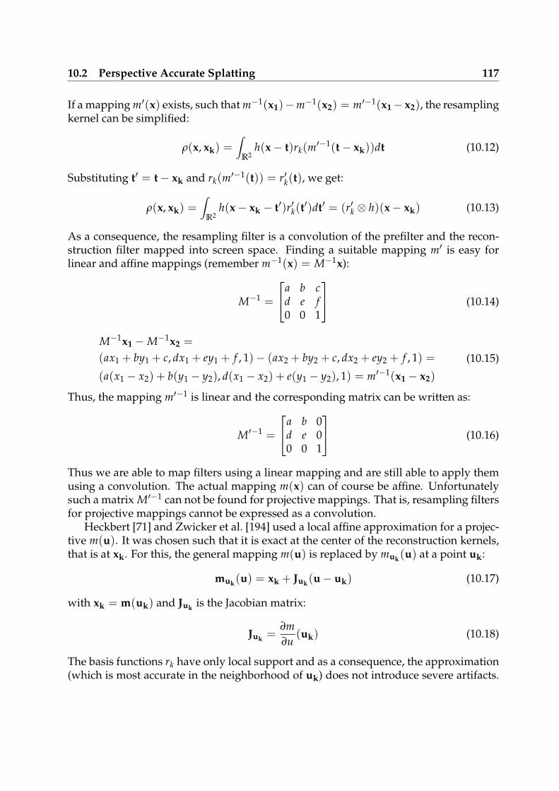
10.2 Perspective Accurate Splatting 117
If a mapping m′(x) exists, such that m−1(x1)−m−1(x2) = m′−1(x1− x2), the resamplingkernel can be simplified:
ρ(x, xk) =∫
R2h(x− t)rk(m′−1(t− xk))dt (10.12)
Substituting t′ = t− xk and rk(m′−1(t)) = r′k(t), we get:
ρ(x, xk) =∫
R2h(x− xk − t′)r′k(t′)dt′ = (r′k ⊗ h)(x− xk) (10.13)
As a consequence, the resampling filter is a convolution of the prefilter and the recon-struction filter mapped into screen space. Finding a suitable mapping m′ is easy forlinear and affine mappings (remember m−1(x) = M−1x):
M−1 =
a b cd e f0 0 1
(10.14)
M−1x1 −M−1x2 =
(ax1 + by1 + c, dx1 + ey1 + f , 1)− (ax2 + by2 + c, dx2 + ey2 + f , 1) =
(a(x1 − x2) + b(y1 − y2), d(x1 − x2) + e(y1 − y2), 1) = m′−1(x1 − x2)
(10.15)
Thus, the mapping m′−1 is linear and the corresponding matrix can be written as:
M′−1 =
a b 0d e 00 0 1
(10.16)
Thus we are able to map filters using a linear mapping and are still able to apply themusing a convolution. The actual mapping m(x) can of course be affine. Unfortunatelysuch a matrix M′−1 can not be found for projective mappings. That is, resampling filtersfor projective mappings cannot be expressed as a convolution.
Heckbert [71] and Zwicker et al. [194] used a local affine approximation for a projec-tive m(u). It was chosen such that it is exact at the center of the reconstruction kernels,that is at xk. For this, the general mapping m(u) is replaced by muk
(u) at a point uk:
muk(u) = xk + Juk
(u− uk) (10.17)
with xk = m(uk) and Jukis the Jacobian matrix:
Juk=
∂m∂u
(uk) (10.18)
The basis functions rk have only local support and as a consequence, the approximation(which is most accurate in the neighborhood of uk) does not introduce severe artifacts.
118 Chapter 10. Point-Based Rendering
However, choosing the approximation such that it is exact at the center of the recon-struction kernels causes incorrect splat shapes in screen space. Thus we will show inSection 10.2.2, how an affine mapping can be computed such that the projective map-ping of a splat’s contour is achieved. Although the splat shape is then computed exactly,the resampling kernel is still based on an affine approximation of the perspective pro-jection.
When using the affine approximation for the resampling kernel ρ(x, uk) (Eq. 10.13),we get:
ρ(x, xk) = (r′k ⊗ h)(x−muk(uk)) (10.19)
and because for linear mappings the Jacobian of the mapping is the mapping matrixitself:
r′k(t) = rk(m′−1(t)) = rk(J−1uk
t) (10.20)
To derive a practical resampling filter, Heckbert chose Gaussians for both reconstructionand low-pass filters, as Gaussians are closed under affine mappings and convolutions.A 2D elliptical Gaussian, with a 2× 2 variance matrix V, is defined as
GV(x) =|V−1|1/2
2πe−
12 xV−1xT
, (10.21)
where |V| is the determinant of V and x is a 1 × 2 row vector. We denote Gaussianreconstruction and low-pass filters by rk = GRk and h = GH. If projective mappingsof such filters are approximated by affine mappings, the resampling filter is again aGaussian [71]. For the reconstruction kernel in screen space r′k we get:
r′k(x) =1
|R′k|1/2GR′k(x), (10.22)
with a new variance matrix R′k whose computation is presented in Section 10.2.2. Thevariance matrix H of the low-pass filter is typically an identity matrix. The resamplingfilter is then given by
ρ(x, xk) =1
|R′k|1/2GR′k+H(x). (10.23)
This derived formular is called the EWA resampling filter. More details on its derivationcan be found in [71, 194].
10.2.2 Perspective Accurate Splatting and Homogeneous Coordinates
Similar to previous techniques, the Perspective Accurate Splatting approach is basedon Gaussian resampling filters as in Equation 10.23. In contrast to previous techniques,where the splat shape is determined by an affine approximation, it provides perspec-tive correct splat shapes. The underlying theory as described by Räsänen [153] is based
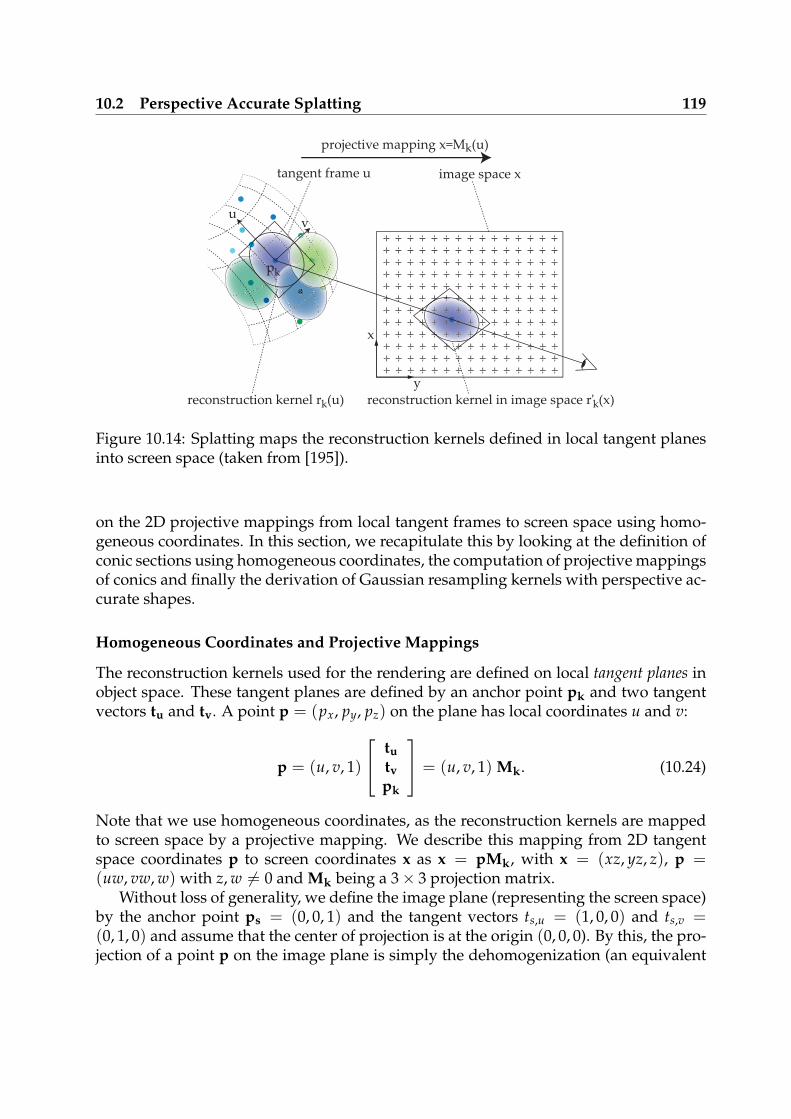
10.2 Perspective Accurate Splatting 119
y
x
image space xtangent frame u
uv
pk
reconstruction kernel rk(u)
projective mapping x=Mk(u)
reconstruction kernel in image space r'k(x)
Figure 10.14: Splatting maps the reconstruction kernels defined in local tangent planesinto screen space (taken from [195]).
on the 2D projective mappings from local tangent frames to screen space using homo-geneous coordinates. In this section, we recapitulate this by looking at the definition ofconic sections using homogeneous coordinates, the computation of projective mappingsof conics and finally the derivation of Gaussian resampling kernels with perspective ac-curate shapes.
Homogeneous Coordinates and Projective Mappings
The reconstruction kernels used for the rendering are defined on local tangent planes inobject space. These tangent planes are defined by an anchor point pk and two tangentvectors tu and tv. A point p = (px, py, pz) on the plane has local coordinates u and v:
p = (u, v, 1)
tu
tv
pk
= (u, v, 1) Mk. (10.24)
Note that we use homogeneous coordinates, as the reconstruction kernels are mappedto screen space by a projective mapping. We describe this mapping from 2D tangentspace coordinates p to screen coordinates x as x = pMk, with x = (xz, yz, z), p =(uw, vw, w) with z, w 6= 0 and Mk being a 3× 3 projection matrix.
Without loss of generality, we define the image plane (representing the screen space)by the anchor point ps = (0, 0, 1) and the tangent vectors ts,u = (1, 0, 0) and ts,v =(0, 1, 0) and assume that the center of projection is at the origin (0, 0, 0). By this, the pro-jection of a point p on the image plane is simply the dehomogenization (an equivalent
120 Chapter 10. Point-Based Rendering
interpretation is that Mk in Eq. 10.24 is a projective mapping matrix):
(x, y, 1) =
(
px
pz,
py
pz, 1)
. (10.25)
Implicit Conics in Homogeneous Coordinates
Conics are important for perspective accurate splatting as the isocontours of Gaussiankernels are ellipses, that is special cases of general conics. A general conic in implicitform is given by:
φ(x, y) = Ax2 + 2Bxy + Cy2 + 2Dx + 2Ey− F = 0 (10.26)
In implicit form, all scalar multiples of Eq. 10.26 are equivalent and we assume thatA ≥ 0. The discriminant of a general conic is ∆ = AC − B2. If ∆ > 0 it describes anellipse, a parabola if ∆ = 0 and a hyperbola if ∆ < 0. A point is inside the conic ifφ(x, y) < 0, outside if φ(x, y) > 0 and on the conic if φ(x, y) = 0. By using homogeneouscoordinates a general conic can be written in matrix form:
xQhxT = 0 , with Qh =
A B DB C ED E −F
(10.27)
If D = E = 0, we speak of a central conic, that is its center is at the origin. Central conicsare often referred to as canonical conic and can also be expressed in matrix form with theconic matrix Q:
Ax2 + 2Bxy + Cy2 = F
xQxT = F, with Q =
[
A BB C
]
(10.28)
Any general conic can be transformed into a central conic. For this, we formulate thegeneral conic with the center offset to xt = (xt, yt):
A(x + xt)2 + 2B(x + xt)(y + yt) + C(y + yt)
2 + 2D(x + xt) + 2E(y + yt)− F = 0
To compute xt, the terms of the first degree of x and y have to equal zero and solvingthe resulting system of two equations gives1:
xt = (xt, yt) =
(
BE− CD∆
,BD− AE
∆
)
. (10.29)
1For parabolas with a determinant of ∆ = 0, the center is at infinity.
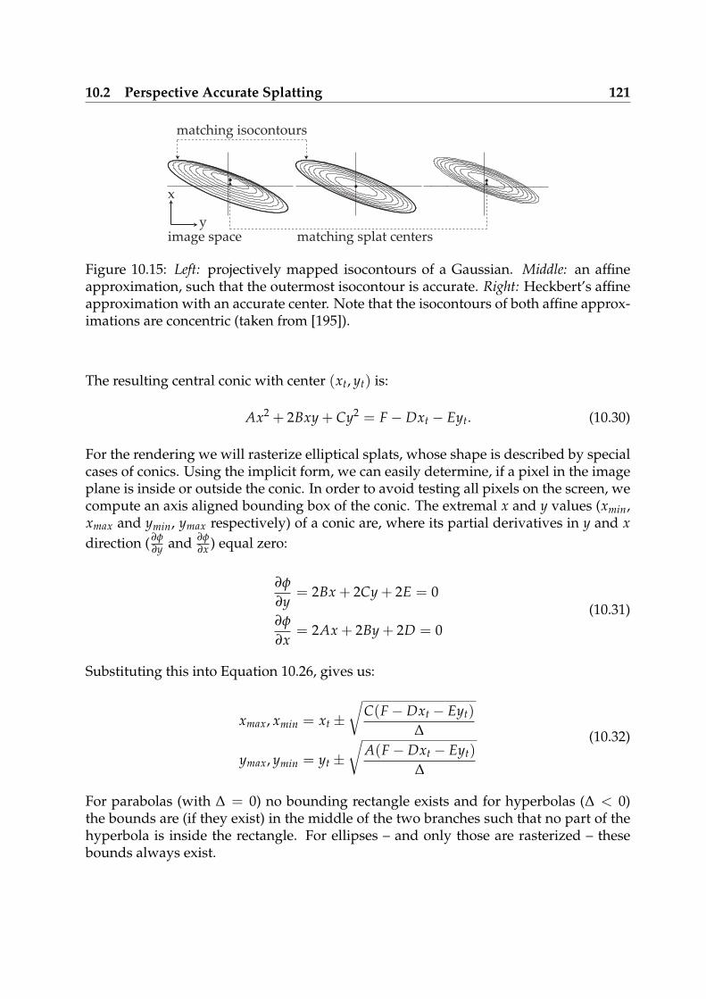
10.2 Perspective Accurate Splatting 121
x
matching isocontours
matching splat centersy
image space
Figure 10.15: Left: projectively mapped isocontours of a Gaussian. Middle: an affineapproximation, such that the outermost isocontour is accurate. Right: Heckbert’s affineapproximation with an accurate center. Note that the isocontours of both affine approx-imations are concentric (taken from [195]).
The resulting central conic with center (xt, yt) is:
Ax2 + 2Bxy + Cy2 = F− Dxt − Eyt. (10.30)
For the rendering we will rasterize elliptical splats, whose shape is described by specialcases of conics. Using the implicit form, we can easily determine, if a pixel in the imageplane is inside or outside the conic. In order to avoid testing all pixels on the screen, wecompute an axis aligned bounding box of the conic. The extremal x and y values (xmin,xmax and ymin, ymax respectively) of a conic are, where its partial derivatives in y and xdirection (∂φ
∂y and ∂φ∂x ) equal zero:
∂φ
∂y= 2Bx + 2Cy + 2E = 0
∂φ
∂x= 2Ax + 2By + 2D = 0
(10.31)
Substituting this into Equation 10.26, gives us:
xmax, xmin = xt ±√
C(F− Dxt − Eyt)
∆
ymax, ymin = yt ±√
A(F− Dxt − Eyt)
∆
(10.32)
For parabolas (with ∆ = 0) no bounding rectangle exists and for hyperbolas (∆ < 0)the bounds are (if they exist) in the middle of the two branches such that no part of thehyperbola is inside the rectangle. For ellipses – and only those are rasterized – thesebounds always exist.
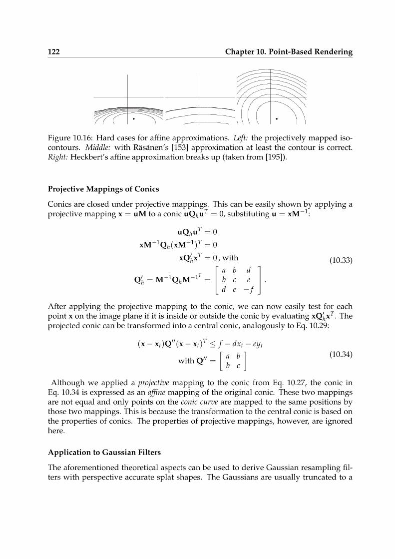
122 Chapter 10. Point-Based Rendering
Figure 10.16: Hard cases for affine approximations. Left: the projectively mapped iso-contours. Middle: with Räsänen’s [153] approximation at least the contour is correct.Right: Heckbert’s affine approximation breaks up (taken from [195]).
Projective Mappings of Conics
Conics are closed under projective mappings. This can be easily shown by applying aprojective mapping x = uM to a conic uQhuT = 0, substituting u = xM−1:
uQhuT = 0
xM−1Qh(xM−1)T = 0
xQ′hxT = 0 , with
Q′h = M−1QhM−1T=
a b db c ed e − f
.
(10.33)
After applying the projective mapping to the conic, we can now easily test for eachpoint x on the image plane if it is inside or outside the conic by evaluating xQ′hxT. Theprojected conic can be transformed into a central conic, analogously to Eq. 10.29:
(x− xt)Q′′(x− xt)T ≤ f − dxt − eyt
with Q′′ =[
a bb c
]
(10.34)
Although we applied a projective mapping to the conic from Eq. 10.27, the conic inEq. 10.34 is expressed as an affine mapping of the original conic. These two mappingsare not equal and only points on the conic curve are mapped to the same positions bythose two mappings. This is because the transformation to the central conic is based onthe properties of conics. The properties of projective mappings, however, are ignoredhere.
Application to Gaussian Filters
The aforementioned theoretical aspects can be used to derive Gaussian resampling fil-ters with perspective accurate splat shapes. The Gaussians are usually truncated to a
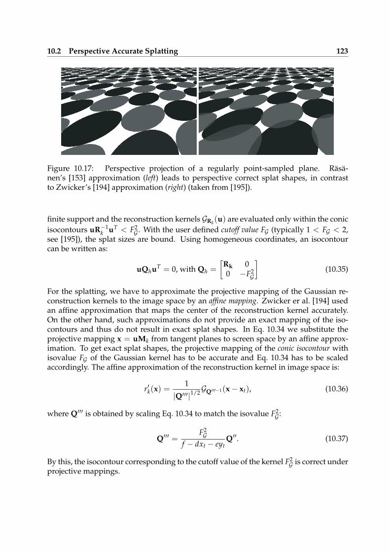
10.2 Perspective Accurate Splatting 123
Figure 10.17: Perspective projection of a regularly point-sampled plane. Räsä-nen’s [153] approximation (left) leads to perspective correct splat shapes, in contrastto Zwicker’s [194] approximation (right) (taken from [195]).
finite support and the reconstruction kernels GRk(u) are evaluated only within the conicisocontours uR−1
k uT < F2G . With the user defined cutoff value FG (typically 1 < FG < 2,
see [195]), the splat sizes are bound. Using homogeneous coordinates, an isocontourcan be written as:
uQhuT = 0, with Qh =
[
Rk 00 −F2
G
]
(10.35)
For the splatting, we have to approximate the projective mapping of the Gaussian re-construction kernels to the image space by an affine mapping. Zwicker er al. [194] usedan affine approximation that maps the center of the reconstruction kernel accurately.On the other hand, such approximations do not provide an exact mapping of the iso-contours and thus do not result in exact splat shapes. In Eq. 10.34 we substitute theprojective mapping x = uMk from tangent planes to screen space by an affine approx-imation. To get exact splat shapes, the projective mapping of the conic isocontour withisovalue FG of the Gaussian kernel has to be accurate and Eq. 10.34 has to be scaledaccordingly. The affine approximation of the reconstruction kernel in image space is:
r′k(x) =1
|Q′′′|1/2GQ′′′−1(x− xt), (10.36)
where Q′′′ is obtained by scaling Eq. 10.34 to match the isovalue F2G :
Q′′′ =F2G
f − dxt − eytQ′′. (10.37)
By this, the isocontour corresponding to the cutoff value of the kernel F2G is correct under
projective mappings.
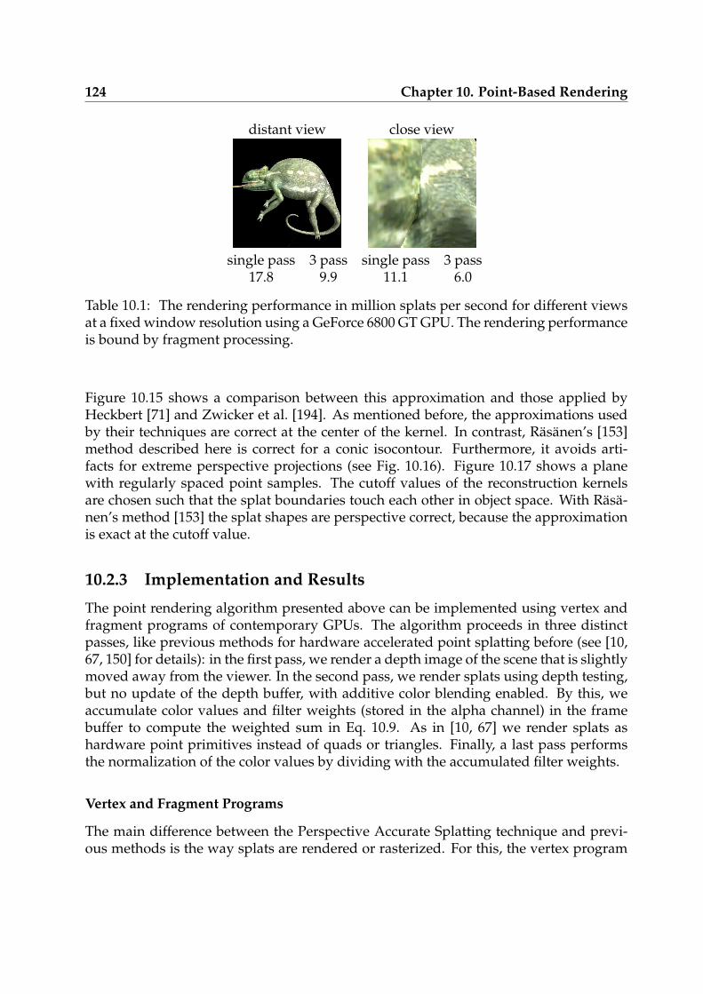
124 Chapter 10. Point-Based Rendering
distant view close view
single pass 3 pass single pass 3 pass17.8 9.9 11.1 6.0
Table 10.1: The rendering performance in million splats per second for different viewsat a fixed window resolution using a GeForce 6800 GT GPU. The rendering performanceis bound by fragment processing.
Figure 10.15 shows a comparison between this approximation and those applied byHeckbert [71] and Zwicker et al. [194]. As mentioned before, the approximations usedby their techniques are correct at the center of the kernel. In contrast, Räsänen’s [153]method described here is correct for a conic isocontour. Furthermore, it avoids arti-facts for extreme perspective projections (see Fig. 10.16). Figure 10.17 shows a planewith regularly spaced point samples. The cutoff values of the reconstruction kernelsare chosen such that the splat boundaries touch each other in object space. With Räsä-nen’s method [153] the splat shapes are perspective correct, because the approximationis exact at the cutoff value.
10.2.3 Implementation and Results
The point rendering algorithm presented above can be implemented using vertex andfragment programs of contemporary GPUs. The algorithm proceeds in three distinctpasses, like previous methods for hardware accelerated point splatting before (see [10,67, 150] for details): in the first pass, we render a depth image of the scene that is slightlymoved away from the viewer. In the second pass, we render splats using depth testing,but no update of the depth buffer, with additive color blending enabled. By this, weaccumulate color values and filter weights (stored in the alpha channel) in the framebuffer to compute the weighted sum in Eq. 10.9. As in [10, 67] we render splats ashardware point primitives instead of quads or triangles. Finally, a last pass performsthe normalization of the color values by dividing with the accumulated filter weights.
Vertex and Fragment Programs
The main difference between the Perspective Accurate Splatting technique and previ-ous methods is the way splats are rendered or rasterized. For this, the vertex program
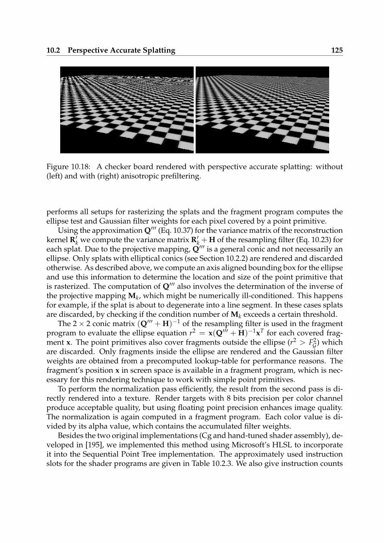
10.2 Perspective Accurate Splatting 125
Figure 10.18: A checker board rendered with perspective accurate splatting: without(left) and with (right) anisotropic prefiltering.
performs all setups for rasterizing the splats and the fragment program computes theellipse test and Gaussian filter weights for each pixel covered by a point primitive.
Using the approximation Q′′′ (Eq. 10.37) for the variance matrix of the reconstructionkernel R′k we compute the variance matrix R′k + H of the resampling filter (Eq. 10.23) foreach splat. Due to the projective mapping, Q′′′ is a general conic and not necessarily anellipse. Only splats with elliptical conics (see Section 10.2.2) are rendered and discardedotherwise. As described above, we compute an axis aligned bounding box for the ellipseand use this information to determine the location and size of the point primitive thatis rasterized. The computation of Q′′′ also involves the determination of the inverse ofthe projective mapping Mk, which might be numerically ill-conditioned. This happensfor example, if the splat is about to degenerate into a line segment. In these cases splatsare discarded, by checking if the condition number of Mk exceeds a certain threshold.
The 2× 2 conic matrix (Q′′′ + H)−1 of the resampling filter is used in the fragmentprogram to evaluate the ellipse equation r2 = x(Q′′′ + H)−1xT for each covered frag-ment x. The point primitives also cover fragments outside the ellipse (r2 > F2
G) whichare discarded. Only fragments inside the ellipse are rendered and the Gaussian filterweights are obtained from a precomputed lookup-table for performance reasons. Thefragment’s position x in screen space is available in a fragment program, which is nec-essary for this rendering technique to work with simple point primitives.
To perform the normalization pass efficiently, the result from the second pass is di-rectly rendered into a texture. Render targets with 8 bits precision per color channelproduce acceptable quality, but using floating point precision enhances image quality.The normalization is again computed in a fragment program. Each color value is di-vided by its alpha value, which contains the accumulated filter weights.
Besides the two original implementations (Cg and hand-tuned shader assembly), de-veloped in [195], we implemented this method using Microsoft’s HLSL to incorporateit into the Sequential Point Tree implementation. The approximately used instructionslots for the shader programs are given in Table 10.2.3. We also give instruction counts
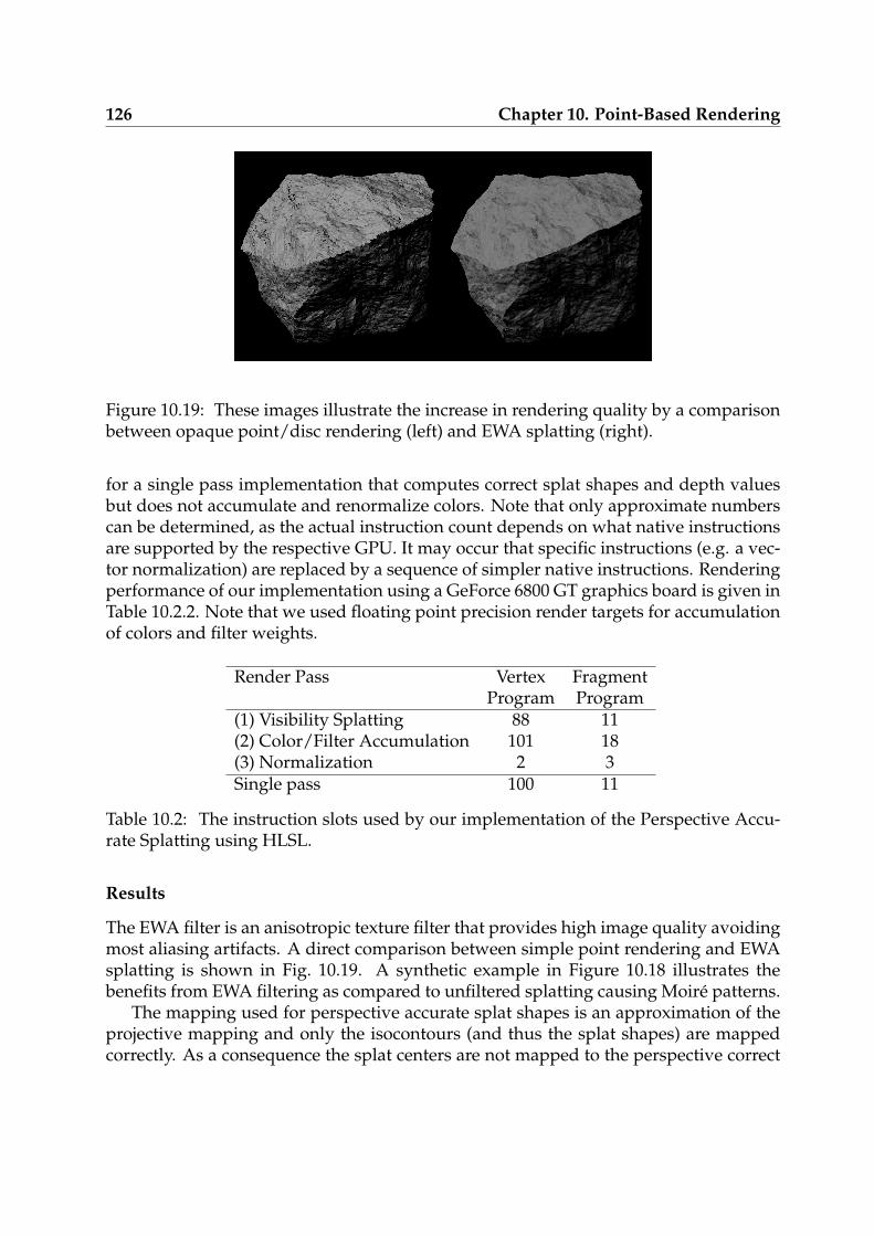
126 Chapter 10. Point-Based Rendering
Figure 10.19: These images illustrate the increase in rendering quality by a comparisonbetween opaque point/disc rendering (left) and EWA splatting (right).
for a single pass implementation that computes correct splat shapes and depth valuesbut does not accumulate and renormalize colors. Note that only approximate numberscan be determined, as the actual instruction count depends on what native instructionsare supported by the respective GPU. It may occur that specific instructions (e.g. a vec-tor normalization) are replaced by a sequence of simpler native instructions. Renderingperformance of our implementation using a GeForce 6800 GT graphics board is given inTable 10.2.2. Note that we used floating point precision render targets for accumulationof colors and filter weights.
Render Pass Vertex FragmentProgram Program
(1) Visibility Splatting 88 11(2) Color/Filter Accumulation 101 18(3) Normalization 2 3Single pass 100 11
Table 10.2: The instruction slots used by our implementation of the Perspective Accu-rate Splatting using HLSL.
Results
The EWA filter is an anisotropic texture filter that provides high image quality avoidingmost aliasing artifacts. A direct comparison between simple point rendering and EWAsplatting is shown in Fig. 10.19. A synthetic example in Figure 10.18 illustrates thebenefits from EWA filtering as compared to unfiltered splatting causing Moiré patterns.
The mapping used for perspective accurate splat shapes is an approximation of theprojective mapping and only the isocontours (and thus the splat shapes) are mappedcorrectly. As a consequence the splat centers are not mapped to the perspective correct
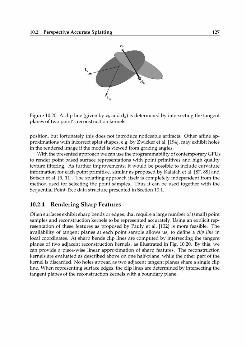
10.2 Perspective Accurate Splatting 127
ch
dh
tv
tu
Figure 10.20: A clip line (given by ch and dh) is determined by intersecting the tangentplanes of two point’s reconstruction kernels.
position, but fortunately this does not introduce noticeable artifacts. Other affine ap-proximations with incorrect splat shapes, e.g. by Zwicker et al. [194], may exhibit holesin the rendered image if the model is viewed from grazing angles.
With the presented approach we can use the programmability of contemporary GPUsto render point based surface representations with point primitives and high qualitytexture filtering. As further improvements, it would be possible to include curvatureinformation for each point primitive, similar as proposed by Kalaiah et al. [87, 88] andBotsch et al. [9, 11]. The splatting approach itself is completely independent from themethod used for selecting the point samples. Thus it can be used together with theSequential Point Tree data structure presented in Section 10.1.
10.2.4 Rendering Sharp Features
Often surfaces exhibit sharp bends or edges, that require a large number of (small) pointsamples and reconstruction kernels to be represented accurately. Using an explicit rep-resentation of these features as proposed by Pauly et al. [132] is more feasible. Theavailability of tangent planes at each point sample allows us, to define a clip line inlocal coordinates. At sharp bends clip lines are computed by intersecting the tangentplanes of two adjacent reconstruction kernels, as illustrated in Fig. 10.20. By this, wecan provide a piece-wise linear approximation of sharp features. The reconstructionkernels are evaluated as described above on one half-plane, while the other part of thekernel is discarded. No holes appear, as two adjacent tangent planes share a single clipline. When representing surface edges, the clip lines are determined by intersecting thetangent planes of the reconstruction kernels with a boundary plane.
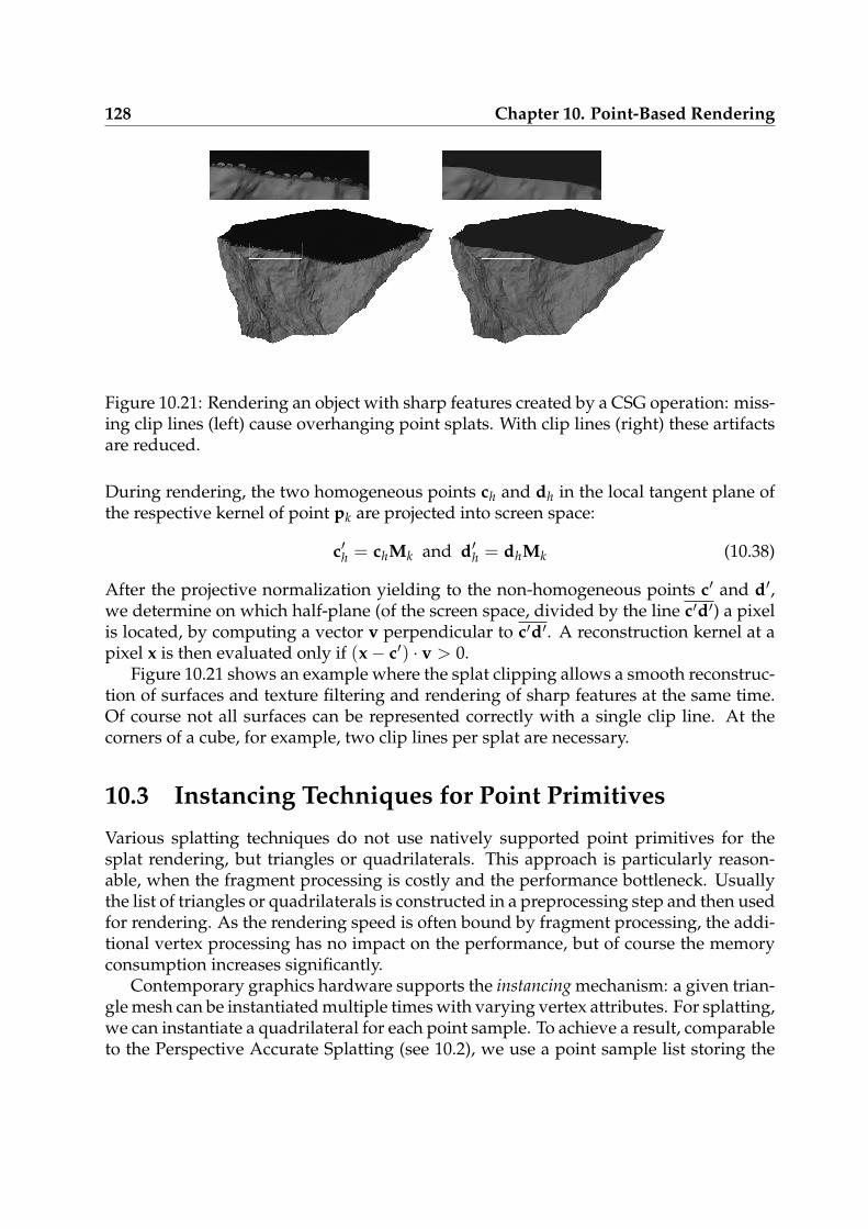
128 Chapter 10. Point-Based Rendering
Figure 10.21: Rendering an object with sharp features created by a CSG operation: miss-ing clip lines (left) cause overhanging point splats. With clip lines (right) these artifactsare reduced.
During rendering, the two homogeneous points ch and dh in the local tangent plane ofthe respective kernel of point pk are projected into screen space:
c′h = chMk and d′h = dhMk (10.38)
After the projective normalization yielding to the non-homogeneous points c′ and d′,we determine on which half-plane (of the screen space, divided by the line c′d′) a pixelis located, by computing a vector v perpendicular to c′d′. A reconstruction kernel at apixel x is then evaluated only if (x− c′) · v > 0.
Figure 10.21 shows an example where the splat clipping allows a smooth reconstruc-tion of surfaces and texture filtering and rendering of sharp features at the same time.Of course not all surfaces can be represented correctly with a single clip line. At thecorners of a cube, for example, two clip lines per splat are necessary.
10.3 Instancing Techniques for Point Primitives
Various splatting techniques do not use natively supported point primitives for thesplat rendering, but triangles or quadrilaterals. This approach is particularly reason-able, when the fragment processing is costly and the performance bottleneck. Usuallythe list of triangles or quadrilaterals is constructed in a preprocessing step and then usedfor rendering. As the rendering speed is often bound by fragment processing, the addi-tional vertex processing has no impact on the performance, but of course the memoryconsumption increases significantly.
Contemporary graphics hardware supports the instancing mechanism: a given trian-gle mesh can be instantiated multiple times with varying vertex attributes. For splatting,we can instantiate a quadrilateral for each point sample. To achieve a result, comparableto the Perspective Accurate Splatting (see 10.2), we use a point sample list storing the
10.4 Proposed GPU Extension 129
position, the tangent frame and the surface color. A quadrilateral (to be instantiated)consists of four vertices with coordinates (0, 0), (1, 0), (1, 1), (0, 1) that are used to placethe quadrilateral in object space in the tangent plane of a point sample and as texturecoordinates (see below). The positioning of the quadrilateral is done by a vertex shaderwhich takes the vertex coordinates and point sample data as input. The texture coordi-nates are used to access reconstruction kernels stored in textures. The built-in featuresof the GPU take care of the perspective correct mapping of the point splat and the fil-ter kernel. This method can be easily integrated into existing implementations: onlyfew API calls have to be changed to render with instancing and the representation ofthe quadrilateral has to be integrated. The required vertex and fragment programs arecompact and far less complicated than for a Perspective Accurate Splatting implemen-tation.
Unfortunately, experiments showed that instancing – at least with contemporaryhardware/driver combinations – introduces a per-instance overhead which is particu-larly noticeable when many instances of small meshes are created, as it is the case forpoint splatting. A comparison of instancing, quadruplication and Perspective AccurateSplatting approaches is given in Table 10.3. Please note, that for each splatting methoda three pass method, that is visibility splatting, accumulation and normalization, is per-formed.
Splatting Method FPS Vertices ProcessedPerspective Accurate Splatting 50.0 NQuadruplication 97.8 2 · 3 · N(2 triangles per splat) reduces to 4 · N due to vertex cachingInstancing 29.7 2 · 3 · N(2 triangles per splat) reduces to 4 · N due to vertex caching
Table 10.3: Rendering a close view of an object with N = 101.685 splats, such that eachwindow pixel at a resolution of 5122 is covered. The results in frames per second (FPS)were measured using a GeForce 6800 GT graphics board.
10.4 Proposed GPU Extension
As also noted by others [194], the accumulation with splatting techniques requires adepth buffer test with tolerance. This can be circumvented by a two-pass renderingapproach. But even then blending is difficult, because it still requires an additional, finalrenormalization pass. These problems could be avoided by an interleaved blending anddepth test. Our proposed depth/blending mode combines a source fragment with color,alpha, and depth (Cs,As,zs) with destination values (Cd,Ad,zd) as follows:
130 Chapter 10. Point-Based Rendering
if (zs < zd - zfuzzy)Cd = Cs; Ad = As; zd = zs;
else if (zs < zd + zfuzzy)Cd = (Ad*Cd + As*Cs)/(Ad+As); Ad += As;
endif
zfuzzy defines the fuzziness of the test. If the source fragment is within the fuzzydepth range of the destination fragment, their weighted sum is computed and immedi-ately renormalized. This would solve the fuzzy depth test and blending problems andthus high quality splatting techniques can be obtained in a single render pass. Up tonow, three passes are required to achieve comparable results: at first a visibility splattingpass captures the scene geometry (as seen by the viewer) in the depth buffer. After-wards, the splats’ weighted contribution is accumulated and finally a renormalizationpass is necessary, because the splatting resampling filters do not form a partition ofunity [195].
131
Chapter 11
Conclusion
Based on a comprehensive overview of previous and related work this thesis presentsnovel algorithms for the creation and interactive, photo-realistic rendering of – artificialor reproduced – terrains with the aid of procedural models. Two major aspects of ren-dering natural scenes have been examined further: First, methods for the generation,rendering, texturing and approximate lighting of terrain height fields were presented.Second, two algorithms for efficient and high-quality point-based rendering were pre-sented and used for the rendering of vegetation and ground detail.
Our work on height fields can be summarized as follows:
• Using methods similar to non-parametric sampling [27], we can synthesize newterrain height fields guided by procedural or captured input data, compute tran-sitions between different landscapes and are able to plausibly combine differentprocedural models.
• A novel level-of-detail algorithm [29] for the view-dependent rendering of heightfields takes a coarse terrain shape from a height field as input data and augmentsit with procedurally generated geometric and color detail and run time. This ap-proach is well suited for graphics hardware and uses warped geometry images asrepresentation for the terrain mesh.
• Texturing of terrains is very important for a realistic appearance. Our method [30]is able to produce high-resolution textures and is suitable for real-time applica-tions. The procedural model is controlled by very few intuitive parameters, partic-ularly height and slope distribution of surface types, and is thus easily applicable.
• We improved our procedural model and examined, how the procedurally com-puted surface appearance can be guided to reproduce the terrain appearance takenfrom satellite images. For this, we incorporated further geographic input data inaddition to elevation data, namely rainfall, solar radiation, and temperature.
• The outdoor lighting scenario is, due to the atmospheric scattering and large view-ing distances, very different from indoor scenes. For this reason, we examined and
132 Chapter 11. Conclusion
compared different approximations of varying complexity for the lighting of ter-rains.
In order to render vegetation and ground detail efficiently and with high renderingquality point-based rendering approaches have been applied and the geometry pro-cessing and rasterization steps have been examined:
• Point-based rendering proved to be an interesting alternative to classical triangle-based rendering, particularly for highly detailed objects. Point representationscompletely lack topological information, so the degree of detail can be adaptedby adding or removing points. Our Sequential Point Tree method [33, 35] is able tooffload almost all work for the level-of-detail computations efficiently to the GPU.
• Point representations provide a non-uniformly sampled signal and during render-ing, a continuous signal in image space has to be reconstructed. Elliptical weightedaverage (EWA) splatting ensures efficient and high-quality rendering with pointprimitives by using Gaussian reconstruction filters [195].
The further development of the terrain rendering system includes the incorporation ofour work on interactive rendering of complex material properties and global illumina-tion effects:
• Many natural objects consist of translucent material and computing the light trans-port within the object is important for a realistic rendering [28].
• For dynamic objects appropriate shadows have to be computed, e.g. with shadowmaps, and Perspective Shadow Maps address the sampling problems that arise forhuge outdoor scenes when using shadow maps [172, 173].
• The lighting cannot be precomputed for dynamic scenes, but direct and one-bounceindirect light can be computed and approximated in real-time [31, 32, 34].
Although photo-realistic terrain rendering is a classical challenge in computer graphics,it will certainly remain a fascinating research area for a long time. The results thatcan be obtained now are already very convincing, but the overwhelming complexity ofnature and all the subtle, yet important details and aspects still provide much room forimprovements and future research.

133
Appendix A
Color Plates
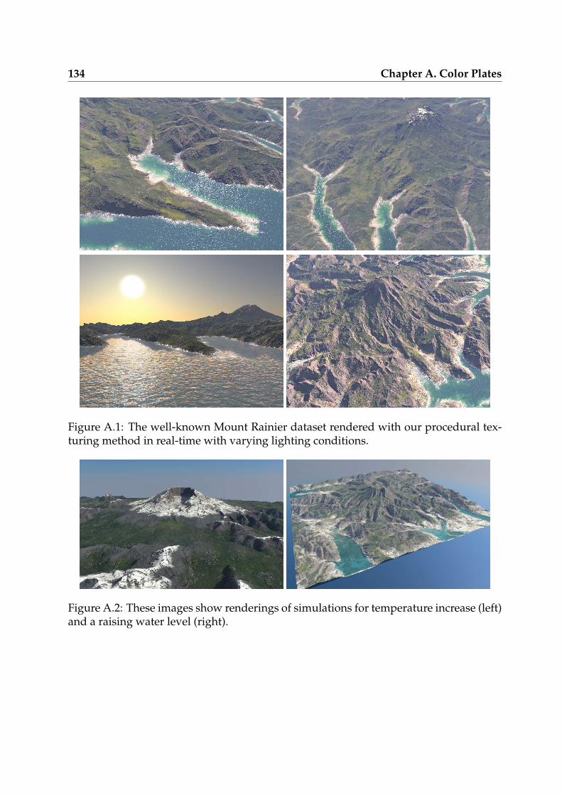
134 Chapter A. Color Plates
Figure A.1: The well-known Mount Rainier dataset rendered with our procedural tex-turing method in real-time with varying lighting conditions.
Figure A.2: These images show renderings of simulations for temperature increase (left)and a raising water level (right).
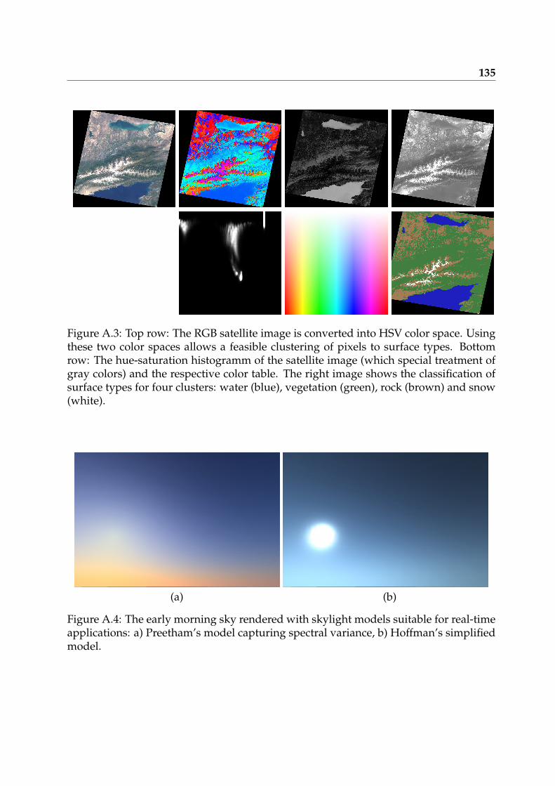
135
Figure A.3: Top row: The RGB satellite image is converted into HSV color space. Usingthese two color spaces allows a feasible clustering of pixels to surface types. Bottomrow: The hue-saturation histogramm of the satellite image (which special treatment ofgray colors) and the respective color table. The right image shows the classification ofsurface types for four clusters: water (blue), vegetation (green), rock (brown) and snow(white).
(a) (b)
Figure A.4: The early morning sky rendered with skylight models suitable for real-timeapplications: a) Preetham’s model capturing spectral variance, b) Hoffman’s simplifiedmodel.
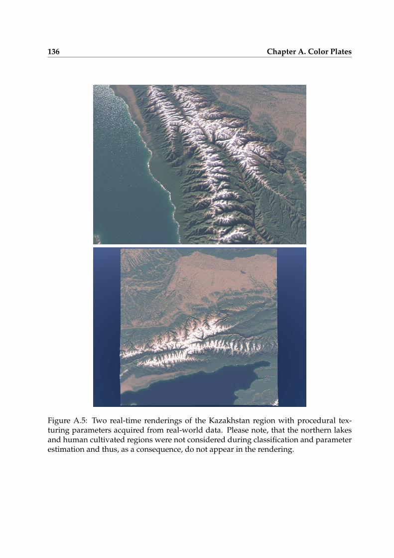
136 Chapter A. Color Plates
Figure A.5: Two real-time renderings of the Kazakhstan region with procedural tex-turing parameters acquired from real-world data. Please note, that the northern lakesand human cultivated regions were not considered during classification and parameterestimation and thus, as a consequence, do not appear in the rendering.
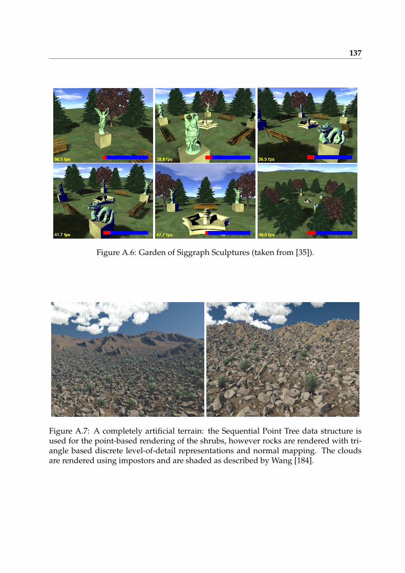
137
Figure A.6: Garden of Siggraph Sculptures (taken from [35]).
Figure A.7: A completely artificial terrain: the Sequential Point Tree data structure isused for the point-based rendering of the shrubs, however rocks are rendered with tri-angle based discrete level-of-detail representations and normal mapping. The cloudsare rendered using impostors and are shaded as described by Wang [184].

138
139
Bibliography
[1] ASHIKHMIN, M. Synthesizing natural textures. In Symposium on Interactive 3D Graphics(2001), pp. 217–226.
[2] BEHRENDT, S., COLDITZ, C., FRANZKE, O., J., K., AND DEUSSEN, O. Realistic real-timerendering of landscapes using billboard clouds. In Proceedings of the Eurographics 2005Conference (2005).
[3] BLINN, J. F. Models of light reflection for computer synthesized pictures. In SIGGRAPH’77: Proceedings of the 4th annual conference on Computer graphics and interactive techniques(New York, NY, USA, 1977), ACM Press, pp. 192–198.
[4] BLOOM, C. Terrain Texture Compositing by Blending in the Frame-Buffer. Available onlineat http://www.cbloom.com/3d/techdocs/splatting.txt (2000).
[5] BLOW, J. Implementing a Texture Caching System. Game Developers Magazine (April 1998).
[6] BLOW, J. Terrain Rendering at High Levels of Detail. Available online athttp://number-none.com/blow/papers/terrain_rendering.pdf (2000).
[7] BORN, M., AND WOLF, E. Principles of Optics, 6th ed. Pergamon Press, Oxford, 1993.
[8] BORN, M., AND WOLF, E. Diffraction by a Conducting Sphere; Theory of Mie. In Principlesof Optics: Electromagnetic Theory of Propagation, Interference, and Diffraction of Light (1999),Cambridge University Press, pp. 633–644.
[9] BOTSCH, M., HORNUNG, A., ZWICKER, M., AND KOBBELT, L. High-Quality SurfaceSplatting on Today’s GPUs. In Eurographics Symposium on Point-Based Graphics (2005).
[10] BOTSCH, M., AND KOBBELT, L. High-quality point-based rendering on modern GPUs. InPacific Graphics 2003 (2003), pp. 335–442.
[11] BOTSCH, M., SPERNAT, M., AND KOBBELT, L. Phong Splatting. In Eurographics Symposiumon Point-Based Graphics (2004).
[12] BOTSCH, M., WIRATANAYA, A., AND KOBBELT, L. Efficient high quality rendering ofpoint sampled geometry. In Rendering Techniques 2002 (Proc. Eurographics Workshop onRendering) (2002).
[13] BULLRICH, K. Scattered Radiation in the Atmosphere. In Advances in Geophysics 10 (1964),Academic Press.
140 Bibliography
[14] CHATTOPADHYAY, S., AND FUJIMOTO, A. Bi-directional ray tracing. In CG International’87 on Computer graphics 1987 (New York, NY, USA, 1987), Springer-Verlag New York, Inc.,pp. 335–343.
[15] CHEN, B., AND NGUYEN, M. X. POP: a hybrid point and polygon rendering system forlarge data. In IEEE Visualization 2001 (October 2001), pp. 45–52.
[16] CHEN, J. X., DA VITORIA LOBO, N., HUGHES, C. E., AND MOSHELL, J. Real-Time FluidSimulation in a Dynamic Virtual Environment. In IEEE Computer Graphics and Application(May 1997), pp. 52–61.
[17] CHIBA, N., MURAOKA, K., AND FUJITA, K. An erosion model based on velocity fields forthe visual simulation of mountain scenery. Journal of Visualization and Computer Animation9, 4 (1998), pp. 185–194.
[18] CHOMSKY, N. Syntactic Structures. Mouton and Co, The Hague, 1957.
[19] CIGNONI, P., GANOVELLI, F., GOBBETTI, E., MARTON, F., PONCHIO, F., AND SCOPIGNO,R. BDAM – Batched Dynamic Adaptive Meshes for High Performance Terrain Visualiza-tion. Computer Graphics Forum 22, 3 (September 2003), pp. 505–514.
[20] CIGNONI, P., GANOVELLI, F., GOBBETTI, E., MARTON, F., PONCHIO, F., AND SCOPIGNO,R. Planet–Sized Batched Dynamic Adaptive Meshes (P-BDAM). In Proceedings IEEE Vi-sualization (Conference held in Seattle, WA, USA, October 2003), IEEE Computer SocietyPress, pp. 147–155.
[21] COCONU, L., AND HEGE, H.-C. Hardware-Accelerated Point-Based Rendering of Com-plex Scenes. In Rendering Techniques 2002 (Proc. Eurographics Workshop on Rendering) (2002),pp. 41–51.
[22] COHEN, J. D., ALIAGA, D. G., AND ZHANG, W. Hybrid simplification: combining multi-resolution polygon and point rendering. In IEEE Visualization 2001 (October 2001), pp. 37–44.
[23] COHEN, M. F., SHADE, J., HILLER, S., AND DEUSSEN, O. Wang tiles for image and texturegeneration. ACM Transactions on Graphics 22, 3 (2003), pp. 287–294.
[24] COLDITZ, C., COCONU, L., DEUSSEN, O., AND HEGE, H. Real-time Rendering of Com-plex Photorealistic Landscapes Using Hybrid Level-of-Detail Approaches. In Real-time vi-sualization and participation, 6th International Conference for Information Technologies in Land-scape Architecture (June 2005).
[25] COOK, R. L., AND DEROSE, T. Wavelet noise. ACM Transactions on Graphics 24, 3 (2005),pp. 803–811.
[26] COOK, R. L., PORTER, T., AND CARPENTER, L. Distributed ray tracing. In SIGGRAPH’84: Proceedings of the 11th annual conference on Computer graphics and interactive techniques(New York, NY, USA, 1984), ACM Press, pp. 137–145.
Bibliography 141
[27] DACHSBACHER, C., MEYER, M., AND STAMMINGER, M. Heightfield Synthesis by Non-Parametric Sampling. In Vision, Modeling and Visualization 2005 (2005), Akademische Ver-lagsgesellschaft Aka, pp. 297–302.
[28] DACHSBACHER, C., AND STAMMINGER, M. Translucent shadow maps. In EGRW ’03: Pro-ceedings of the 14th Eurographics workshop on Rendering (Aire-la-Ville, Switzerland, Switzer-land, 2003), Eurographics Association, pp. 197–201.
[29] DACHSBACHER, C., AND STAMMINGER, M. Rendering Procedural Terrain by GeometryImage Warping. In Rendering Techniques 2004 (Proceedings of the Eurographics Symposium onRendering) (2004), Eurographics Association, pp. 103–107.
[30] DACHSBACHER, C., AND STAMMINGER, M. Cached Procedural Textures for Terrain Ren-dering. In Shader X4 (2005), Charles River Media.
[31] DACHSBACHER, C., AND STAMMINGER, M. Interactive Indirect Illumination. In ShaderX4 (2005), Charles River Media.
[32] DACHSBACHER, C., AND STAMMINGER, M. Reflective shadow maps. In SI3D ’05: Pro-ceedings of the 2005 symposium on Interactive 3D graphics and games (New York, NY, USA,2005), ACM Press, pp. 203–231.
[33] DACHSBACHER, C., AND STAMMINGER, M. Sequential Point Trees. In Point Based Graphics(2006), Morgan Kaufman/Elsevier, to appear.
[34] DACHSBACHER, C., AND STAMMINGER, M. Splatting Indirect Illumination. In SI3D ’06:Proceedings of the 2006 symposium on Interactive 3D graphics and games (New York, NY, USA,2006), ACM Press, to appear.
[35] DACHSBACHER, C., VOGELGSANG, C., AND STAMMINGER, M. Sequential Point Trees. InProceedings of ACM SIGGRAPH 2003 (2003), ACM Press, pp. 657–662.
[36] DE BOER, W. Fast Terrain Rendering Using Geometrical MipMapping. Available online athttp://www.flipcode.com/tutorials/tut_geomipmaps.shtml (2000).
[37] DE REFFYE, P., EDELIN, C., FRANCON, J., JAEGER, M., AND PUECH, C. Plant mod-els faithful to botanical structure and development. SIGGRAPH Computer Graphics 22, 4(1988), pp. 151–158.
[38] DECAUDIN, P., AND NEYRET, F. Rendering Forest Scenes in Real-Time. In RenderingTechniques ’04 (Eurographics Symposium on Rendering) (June 2004), pp. 93–102.
[39] DEUSSEN, O. Computergenerierte Pflanzen. Springer, 2003.
[40] DEUSSEN, O., COLDITZ, C., STAMMINGER, M., AND DRETTAKIS, G. Interactive visual-ization of complex plant ecosystems. In VIS ’02: Proceedings of the conference on Visualization’02 (Washington, DC, USA, 2002), IEEE Computer Society, pp. 219–226.
[41] DEUSSEN, O., HANRAHAN, P., LINTERMANN, B., MECH, R., PHARR, M., AND
PRUSINKIEWICZ, P. Realistic modeling and rendering of plant ecosystems. In SIGGRAPH’98: Proceedings of the 25th annual conference on Computer graphics and interactive techniques(New York, NY, USA, 1998), ACM Press, pp. 275–286.
142 Bibliography
[42] DEUSSEN, O., AND LINTERMANN, B. A modeling method and user interface for creatingplants. In Proceedings of the conference on Graphics interface ’97 (Toronto, Ont., Canada,Canada, 1997), Canadian Information Processing Society, pp. 189–197.
[43] DEVLIN, K., CHALMERS, A., WILKIE, A., AND PURGATHOFER, W. STAR: Tone Repro-duction and Physically Based Spectral Rendering. In State of the Art Reports, Eurographics2002 (September 2002), D. Fellner and R. Scopignio, Eds., The Eurographics Association,pp. 101–123.
[44] DOBASHI, Y., KANEDA, K., YAMASHITA, H., OKITA, T., AND NISHITA, T. A simple,efficient method for realistic animation of clouds. In SIGGRAPH ’00: Proceedings of the27th annual conference on Computer graphics and interactive techniques (New York, NY, USA,2000), ACM Press/Addison-Wesley Publishing Co., pp. 19–28.
[45] DORSEY, J., EDELMAN, A., JENSEN, H. W., LEGAKIS, J., AND PEDERSEN, H. K. Model-ing and rendering of weathered stone. In SIGGRAPH ’99: Proceedings of the 26th annualconference on Computer graphics and interactive techniques (New York, NY, USA, 1999), ACMPress/Addison-Wesley Publishing Co., pp. 225–234.
[46] DUCHAINEAU, M., WOLINSKY, M., SIGETI, D. E., MILLER, M. C., ALDRICH, C., AND
MINEEV-WEINSTEIN, M. B. ROAMing terrain: real-time optimally adapting meshes. InVIS ’97: Proceedings of the 8th conference on Visualization ’97 (Los Alamitos, CA, USA, 1997),IEEE Computer Society Press, pp. 81–88.
[47] EBERT, D. S. Volumetric modeling with implicit functions: a cloud is born. In SIGGRAPH’97: ACM SIGGRAPH 97 Visual Proceedings: The art and interdisciplinary programs of SIG-GRAPH ’97 (New York, NY, USA, 1997), ACM Press, p. 147.
[48] EBERT, D. S., MUSGRAVE, F. K., PEACHEY, D., PERLIN, K., AND WORLEY, S. Texturingand Modeling: A Procedural Approach. Morgan Kaufmann Publishers Inc., San Francisco,CA, USA, 2002.
[49] EFROS, A. A., AND FREEMAN, W. T. Image quilting for texture synthesis and transfer. InSIGGRAPH ’01: Proceedings of the 28th annual conference on Computer graphics and interactivetechniques (New York, NY, USA, 2001), ACM Press, pp. 341–346.
[50] EFROS, A. A., AND LEUNG, T. K. Texture Synthesis by Non-parametric Sampling. InICCV (2) (1999), pp. 1033–1038.
[51] FAIRCLOUGH, M. Terragen v0.9 (Software). Available online from Planetside Software athttp://www.planetside.co.uk (2005).
[52] FANTE, R. L. Relationship between radiative-transport theory and Maxwell’s equationsin dielectric media. Journal of the Optical Society of America 71(4) (1981), pp. 460–468.
[53] FERNANDO, R., AND KILGARD, M. J. The Cg Tutorial: The Definitive Guide to ProgrammableReal-Time Graphics. Addison–Wesley Professional, February 2003.
[54] FERNANDO, R., AND ZELLER, C. Programming Graphics Hardware, Tutorial of ACMSIGGRAPH 2005 Symposium on Interactive 3D Graphics and Games. Available online athttp://developer.nvidia.com.
Bibliography 143
[55] FOSTER, N., AND METAXAS, D. Realistic Animation of Liquids. In Graphical Models andImage Processing, 58(5) (1996), pp. 471–483.
[56] FOSTER, N., AND METAXAS, D. Controlling Fluid Animation. In Proceeding of the ComputerGraphics International (CGIŠ97) (1997).
[57] FOURNIER, A., FUSSELL, D., AND CARPENTER, L. Computer rendering of stochasticmodels. Commun. ACM 25, 6 (1982), pp. 371–384.
[58] FOWLER, R. J., AND LITTLE, J. J. Automatic extraction of Irregular Network digital terrainmodels. In SIGGRAPH ’79: Proceedings of the 6th annual conference on Computer graphics andinteractive techniques (New York, NY, USA, 1979), ACM Press, pp. 199–207.
[59] GAUTRON, P., KRIVÁNEK, J., PATTANAIK, S. N., AND BOUATOUCH, K. A Novel Hemi-spherical Basis for Accurate and Efficient Rendering. In Eurographics Symposium on Ren-dering (erscheint) (June 2004), pp. 321–330.
[60] GILET, G., MEYER, A., AND NEYRET, F. Point-based rendering of trees. In EurographicsWorkshop on Natural Phenomena (2005), P. P. E. Galin, Ed.
[61] GOMEZ, M. Interactive Simulation of Water Surfaces. In Game Programming Gems (Rock-land, MA, USA, 2000), Charles River Media.
[62] GREEN, R. Spherical Harmonic Lighting: The Gritty Details. In Proceedings of the GameDevelopers Conference (2003).
[63] GREENE, N., AND HECKBERT, P. Creating Raster Omnimax Images From Multiple Per-spective Views Using the Elliptical Weighted Average Filter. IEEE CG & A 6, 6 (1986), pp.21–27.
[64] GREENWORKS ORGANIC–SOFTWARE. Xfrog, http://www.xfrog.com, 2005.
[65] GROSSMAN, J. P., AND DALLY, W. J. Point Sample Rendering. In Rendering Techniques ’98(July 1998), pp. 181–192.
[66] GU, X., GORTLER, S. J., AND HOPPE, H. Geometry Images. ACM Transactions on Graphics(Proc. SIGGRAPH 2002) 21, 3 (July 2002), pp. 355–361.
[67] GUENNEBAUD, G., AND PAULIN, M. Efficient screen space approach for hardware ac-celerated surfel rendering. In Vision, Modeling and Visualization, Munich (November 2003),pp. 1–10.
[68] HALTRIN, V. I. A real-time algorithm for atmospheric corrections of airborne remoteoptical measurements above the ocean. In Proceedings of the Second International AirborneRemote Sensing Conference and Exhibition, volume III (1996), pp. 63–72.
[69] HARRIS, M. J. Real-Time Cloud Simulation and Rendering. PhD thesis, Chapel Hill, NC,USA, 2003.
[70] HARRIS, M. J., AND LASTRA, A. Real-Time Cloud Rendering. Tech. rep., University ofNorth Carolina at Chapel Hill, NC, USA, 2001.
144 Bibliography
[71] HECKBERT, P. Fundamentals of Texture Mapping and Image Warping. MSc thesis, Uni-versity of California, Berkeley, June 1989.
[72] HENYEY, L., AND GREENSTEIN, J. Diffuse reflection in the Galaxy. In Astrophysical Journal93:70 (1941).
[73] HERTZMANN, A., JACOBS, C. E., OLIVER, N., CURLESS, B., AND SALESIN, D. H. ImageAnalogies. In SIGGRAPH 2001, Computer Graphics Proceedings (2001), E. Fiume, Ed., ACMPress / ACM SIGGRAPH, pp. 327–340.
[74] HOFFMAN, N., AND MITCHELL, K. Methods for Dynamic, Photorealistic Terrain Light-ing. In Game Programming Gems 3 (Rockland, MA, USA, 2002), Charles River Media.
[75] HOFFMAN, N., AND PREETHAM, A. Rendering outdoor light scattering in real time. InGame Developers Conference (2002).
[76] HOPPE, H. Progressive Meshes. In Computer Graphics (Annual Conference Series) (1996),vol. 30, pp. 99–108.
[77] HOPPE, H. View-dependent refinement of progressive meshes. In SIGGRAPH ’97: Pro-ceedings of the 24th annual conference on Computer graphics and interactive techniques (NewYork, NY, USA, 1997), ACM Press/Addison-Wesley Publishing Co., pp. 189–198.
[78] HOPPE, H. Smooth view-dependent level-of-detail control and its application to terrainrendering. In VIS ’98: Proceedings of the conference on Visualization ’98 (Los Alamitos, CA,USA, 1998), IEEE Computer Society Press, pp. 35–42.
[79] INEICHEN, P., MOLINEAUX, B., AND PEREZ, R. Sky luminance data validation: Compar-ison of seven models with four data banks. In Solar Energy 52, 4 (1994), pp. 337–346.
[80] INTERNATIONAL COMMISSION ON ILLUMINATION. Spatial distribution of daylight - lu-minance distributions of various reference skies. CIE-110-1994 (1994).
[81] JENSEN, H., PREMOZE, S., SHIRLEY, P., THOMPSON, W., FERWERDA, J., AND STARK,M. Night rendering. In Tech. Rep. UUCS-00-016 (August 2000), Computer Science Dept.,University of Utah.
[82] JENSEN, H. W., DURAND, F., DORSEY, J., STARK, M. M., SHIRLEY, P., AND PREMOZE,S. A physically-based night sky model. In SIGGRAPH ’01: Proceedings of the 28th annualconference on Computer graphics and interactive techniques (New York, NY, USA, 2001), ACMPress, pp. 399–408.
[83] JENSEN, L. S., AND GOLIAS, R. Deep-Water Animation and Rendering. In GamasutraArticle, http://www.gamasutra.com/gdce/2001/jensen/jensen_04.htm (September 2001).
[84] JOHANSON, C. Real-time water rendering - introducing the projected grid concept. MScthesis, Lund University, Sweden, March 2004.
[85] KAJIYA, J. T. The rendering equation. In Computer Graphics (SIGGRAPH ’86 proceedings)(Aug. 1986), pp. 143–150.
Bibliography 145
[86] KAJIYA, J. T., AND HERZEN, B. P. V. Ray tracing volume densities. In SIGGRAPH ’84:Proceedings of the 11th annual conference on Computer graphics and interactive techniques (NewYork, NY, USA, 1984), ACM Press, pp. 165–174.
[87] KALAIAH, A., AND VARSHNEY, A. Differential Point Rendering. In Proceedings of the12th Eurographics Workshop on Rendering Techniques (London, UK, 2001), Springer-Verlag,pp. 139–150.
[88] KALAIAH, A., AND VARSHNEY, A. Modeling and rendering points with local geometry.IEEE Transactions on Visualization and Computer Graphics 9, 1 (January 2003), pp. 30–42.
[89] KANEDA, K., OKAMOTO, T., NAKAMAE, E., AND NISHITA, T. Photorealistic image syn-thesis for outdoor scenery under various atmospheric conditions. The Visual Computer 7,5&6 (1991), pp. 247–258.
[90] KANEKO, T., TAKAHEI, T., INAMI, M., KAWAKAMI, N., YANAGIDA, Y., MAEDA, T., AND
TACHI, S. Detailed shape representation with parallax mapping. In In Proceedings of theICAT 2001 (2001), pp. 205–208.
[91] KAUFMAN, J. The Illumination Engineering Society Lighting Handbook, Reference Volume.Waverly Press, 1984.
[92] KELLEY, A. D., MALIN, M. C., AND NIELSON, G. M. Terrain simulation using a modelof stream erosion. In SIGGRAPH ’88: Proceedings of the 15th annual conference on Computergraphics and interactive techniques (New York, NY, USA, 1988), ACM Press, pp. 263–268.
[93] KLASSEN, R. Modeling the effect of the atmosphere on light. In ACM Transactions onGraphics 6 (1987), pp. 215–237.
[94] KLEIN, R., LIEBICH, G., AND STRASSER, W. Mesh Reduction with Error Control. In IEEEVisualization ’96 (October 1996), pp. 311–318.
[95] KOHONEN, T. Self-Organizing Maps, 3rd ed. Springer, Berlin, Germany, 2001.
[96] KOLLER, D., LINDSTROM, P., RIBARSKY, W., HODGES, L. F., FAUST, N., AND TURNER, G.Virtual GIS: A Real-Time 3D Geographic Information System. In VIS ’95: Proceedings of the6th conference on Visualization ’95 (Washington, DC, USA, 1995), IEEE Computer Society,p. 94.
[97] LAFORTUNE, E. P., AND WILLEMS, Y. D. Bi-directional Path Tracing. In Proceedings ofThird International Conference on Computational Graphics and Visualization Techniques (Com-pugraphics ’93) (Alvor, Portugal, 1993), H. P. Santo, Ed., pp. 145–153.
[98] LANDIS, H. Production-Ready Global Illumination. Siggraph Course Notes #16 (2002).
[99] LEROUX, A. Alex’s Remote Sensing Imagery Summary Table. Available online athttp://homepage.mac.com/alexandreleroux/arsist (2005).
[100] LEVOY, M., AND WHITTED, T. The Use of Points as a Display Primitive. Tech. rep., Univ.of North Carolina at Chapel Hill, 1985.
146 Bibliography
[101] LEWIS, J.-P. Texture synthesis for digital painting. In SIGGRAPH ’84: Proceedings of the11th annual conference on Computer graphics and interactive techniques (New York, NY, USA,1984), ACM Press, pp. 245–252.
[102] LEWIS, J. P. Algorithms for solid noise synthesis. In SIGGRAPH ’89: Proceedings of the16th annual conference on Computer graphics and interactive techniques (New York, NY, USA,1989), ACM Press, pp. 263–270.
[103] LIANG, L., LIU, C., XU, Y.-Q., GUO, B., AND SHUM, H.-Y. Real-time texture synthesisby patch-based sampling. ACM Transactions on Graphics 20, 3 (2001), pp. 127–150.
[104] LINDHOLM, E., KILGARD, M., AND MORETON, H. A user-programmable vertex engine.In SIGGRAPH 2001 (2001), pp. 149–158.
[105] LINDSTROM, P., KOLLER, D., RIBARSKY, W., HODGES, L. F., FAUST, N., AND TURNER,G. A. Real-time, continuous level of detail rendering of height fields. In SIGGRAPH ’96:Proceedings of the 23rd annual conference on Computer graphics and interactive techniques (NewYork, NY, USA, 1996), ACM Press, pp. 109–118.
[106] LINTERMANN, B., AND DEUSSEN, O. Interactive Modeling of Plants. IEEE ComputerGraphic Applications 19, 1 (1999), pp. 56–65.
[107] LOSASSO, F., AND HOPPE, H. Geometry clipmaps: terrain rendering using nested regulargrids. ACM Transactions on Graphics 23, 3 (2004), pp. 769–776.
[108] LUEBKE, D., WATSON, B., COHEN, J. D., REDDY, M., AND VARSHNEY, A. Level of Detailfor 3D Graphics. Elsevier Science Inc., New York, NY, USA, 2002.
[109] LUEBKE, D. P., AND HALLEN, B. Perceptually-Driven Simplification for Interactive Ren-dering. In Proceedings of the 12th Eurographics Workshop on Rendering Techniques (London,UK, 2001), Springer-Verlag, pp. 223–234.
[110] MARDALJEVIC, J. Daylight Simulation: Validation, Sky Models and Daylight Coefficients. PhDthesis, De Montfort University Leicester, December 1999.
[111] MARK, B. Hardware Shading Language Course: NVIDIA Programmable Graphics Tech-nology. In SIGGRAPH Course Notes (July 2002).
[112] MARK, W. R., GLANVILLE, R. S., AKELEY, K., AND KILGARD, M. J. Cg: A System forProgramming Graphics Hardware in a C-like Language. In SIGGRAPH 2003 (2003).
[113] MAX, N. L. Horizon mapping: shadows for bump-mapped surfaces. The Visual Computer4, 2 (1988), pp. 109–117.
[114] MCCARTNEY, E. J. Optics of the Atmosphere, second ed. Wiley publication, 1976.
[115] MCCORMACK, J., PERRY, R., FARKAS, K., AND JOUPPI, N. Feline: fast elliptical lines foranisotropic texture mapping. In SIGGRAPH 1999 (1999), pp. 243–250.
[116] MCKNIGHT, T. L., AND HESS, D. Physical Geography: A Landscape Appreciation, 8th edition.Pearson Prentice Hall, San Francisco, CA, USA, 2005.
Bibliography 147
[117] MEYER, A., AND NEYRET, F. Multiscale Shaders for the Efficient Realistic Rendering ofPine-Trees. In Graphics Interface (May 2000), pp. 137–144.
[118] MICROSOFT CORPORATION. DirectX 9.0 SDK, 2002, November 2002.
[119] MITCHELL, J. Radeon 9700 Shading, ATI Technologies Inc., July 2002.
[120] MIYAZAKI, R., YOSHIDA, S., NISHITA, T., AND DOBASHI, Y. A Method for ModelingClouds Based on Atmospheric Fluid Dynamics. In PG ’01: Proceedings of the 9th PacificConference on Computer Graphics and Applications (Washington, DC, USA, 2001), IEEE Com-puter Society, p. 363.
[121] MUSGRAVE, F. K., KOLB, C. E., AND MACE, R. S. The synthesis and rendering of erodedfractal terrains. In SIGGRAPH ’89: Proceedings of the 16th annual conference on Computergraphics and interactive techniques (New York, NY, USA, 1989), ACM Press, pp. 41–50.
[122] NAGASHIMA, K. Computer generation of eroded valley and mountain terrains. In TheVisual Computer (Jan. 1988), vol. 13, pp. 456–464.
[123] NAVARRA, A., STERN, W. F., AND MIYAKODA, K. Reduction of the Gibbs Oscillation inSpectral Model Simulations. Journal of Climate 7, 8 (Aug. 1994), pp. 1169–1183.
[124] NEALEN, A., AND ALEXA, M. Hybrid texture synthesis. In EGRW ’03: Proceedings ofthe 14th Eurographics workshop on Rendering (Aire-la-Ville, Switzerland, Switzerland, 2003),Eurographics Association, pp. 97–105.
[125] NIELSEN, R. S. Real Time Rendering of Atmospheric Scattering Effects for Flight Sim-ulators. MSc thesis, Informatics and Mathematical Modelling, Technical University ofDenmark, DTU, Richard Petersens Plads, Building 321, DK-2800 Kgs. Lyngby, 2003. Su-pervisor: Niels Jørgen Christensen.
[126] NISHITA, T., DOBASHI, Y., KANEDA, K., AND YAMASHITA, H. Display Method of theSky Color Taking into Account Multiple Scattering. In Proceedings of Pacific Graphics ’96(1996), pp. 117–132.
[127] NISHITA, T., DOBASHI, Y., AND NAKAMAE, E. Display of clouds taking into accountmultiple anisotropic scattering and sky light. In SIGGRAPH ’96: Proceedings of the 23rdannual conference on Computer graphics and interactive techniques (New York, NY, USA, 1996),ACM Press, pp. 379–386.
[128] OLANO, M., AND GREER, T. Triangle scan conversion using 2d homogeneous coordi-nates. In SIGGRAPH/Eurographics Workshop on Graphics Hardware 1997 (1997), pp. 89–96.
[129] PAULY, M., AND GROSS, M. Spectral processing of point-sampled geometry. In SIG-GRAPH ’01: Proceedings of the 28th annual conference on Computer graphics and interactivetechniques (New York, NY, USA, 2001), ACM Press, pp. 379–386.
[130] PAULY, M., GROSS, M., AND KOBBELT, L. Efficient Simplification of Point-Sampled Sur-faces. In Proc. IEEE Visualization 2002 (2002).
148 Bibliography
[131] PAULY, M., KEISER, R., AND GROSS, M. Multi-scale feature extraction on point-sampledsurfaces. In Eurographics 2003 (2003), pp. 281–289.
[132] PAULY, M., KEISER, R., KOBBELT, L., AND GROSS, M. Shape modeling with point-sampled geometry. In SIGGRAPH 2003 (2003), pp. 641–650.
[133] PEDROTTI, F., AND PEDROTTI, L. Introduction to Optics, second ed. Prentice Hall, 1993.
[134] PERBET, F., AND CANI, M.-P. Animating prairies in real-time. In SI3D ’01: Proceedingsof the 2001 symposium on Interactive 3D graphics (New York, NY, USA, 2001), ACM Press,pp. 103–110.
[135] PEREZ, R., SEALS, R., AND MICHALSKY, J. All-weather model for sky luminancedistribution-preliminary configuration and validation. In Solar Energy 50, 3 (1993),pp. 235–245.
[136] PERLIN, K. An Image Synthesizer. In Proceedings of the 12th annual conference on Computergraphics and interactive techniques (July 1985), vol. 19(3), pp. 287–296.
[137] PERLIN, K. Improving noise. In SIGGRAPH ’02: Proceedings of the 29th annual conferenceon Computer graphics and interactive techniques (New York, NY, USA, 2002), ACM Press,pp. 681–682.
[138] PERLIN, K., AND HOFFERT, E. M. Hypertexture. In SIGGRAPH ’89: Proceedings of the16th annual conference on Computer graphics and interactive techniques (New York, NY, USA,1989), ACM Press, pp. 253–262.
[139] PFISTER, H., ZWICKER, M., VAN BAAR, J., AND GROSS, M. Surfels: Surface Elementsas Rendering Primitives. In Proceedings of ACM SIGGRAPH 2000 (July 2000), ComputerGraphics Proceedings, pp. 335–342.
[140] PHARR, M., AND HUMPHREYS, G. Physically Based Rendering: From Theory to Implementa-tion. Morgan Kaufmann Publishers Inc., San Francisco, CA, USA, 2004.
[141] PIDWIRNY, M. Fundamentals of Physical Geography - Online Textbook. Available onlineat http://www.physicalgeography.net (2005).
[142] PREETHAM, A. Modeling Skylight and Aerial Perspective. In Course notes of the SIG-GRAPH 2003 conference (2003).
[143] PREETHAM, A. J., SHIRLEY, P., AND SMITS, B. A practical analytic model for daylight. InSIGGRAPH ’99: Proceedings of the 26th annual conference on Computer graphics and interac-tive techniques (New York, NY, USA, 1999), ACM Press/Addison-Wesley Publishing Co.,pp. 91–100.
[144] PREISENDORFER, R. W. Radiative Transfer on Discrete Spaces. Pergamon Press, Oxford,1965.
[145] PREMOZE, S., AND ASHIKHMIN, M. Rendering Natural Waters. In PG ’00: Proceedingsof the 8th Pacific Conference on Computer Graphics and Applications (Washington, DC, USA,2000), IEEE Computer Society, p. 23.
Bibliography 149
[146] PREMOZE, S., THOMPSON, W. B., AND SHIRLEY, P. Geospecific Rendering of AlpineTerrain. In Rendering Techniques (1999), pp. 107–118.
[147] PRUSINKIEWICZ, P., AND LINDENMAYER, A. The algorithmic beauty of plants. Springer-Verlag New York, Inc., New York, NY, USA, 1996.
[148] RAYLEIGH, L. On the scattering of light by small particles. In Philosophical Magazine 41(1871), pp. 447–451.
[149] RECK, F., DACHSBACHER, C., STAMMINGER, M., GROSSO, R., AND GREINER, G. Real-time Isosurface Extraction with Graphics Hardware. In Eurographics 2004, Short Presenta-tions and Interactive Demos (2004), INRIA and Eurographics Association, pp. 33–36.
[150] REN, L., PFISTER, H., AND ZWICKER, M. Object Space EWA Surface Splatting: A Hard-ware Accelerated Approach to High Quality Point Rendering. Computer Graphics Forum(Proc. EUROGRAPHICS 2002 3, 21 (2002), pp. 461–470.
[151] ROETTGER, S., HEIDRICH, W., SLUSALLEK, P., AND SEIDEL, H.-P. Real-Time Genera-tion of Continuous Levels of Detail for Height Fields. In Procceedings of WSCG ’98 (1998),pp. 315–322.
[152] ROST, R., KESSENICH, J., AND BALDWIN, D. The OpenGL Shading Language. Addison–Wesley, Amsterdam, April 2004.
[153] RÄSÄNEN, J. Surface Splatting: Theory, Extensions and Implementation. MSc thesis,Helsinki University of Technology, Finland, May 2002.
[154] RUSINKIEWICZ, S., AND LEVOY, M. QSplat: A Multiresolution Point Rendering Systemfor Large Meshes. In Proceedings of ACM SIGGRAPH 2000 (July 2000), Computer GraphicsProceedings, pp. 343–352.
[155] RUSINKIEWICZ, S., AND LEVOY, M. Streaming QSplat: A Viewer for Networked Visual-ization of Large, Dense Models. In 2001 ACM Symposium on Interactive 3D Graphics (March2001), pp. 63–68.
[156] SAINZ, M., AND PAJAROLA, R. Point-based rendering techniques. Computers & Graphics28, 6 (2004), pp. 869–879.
[157] SAINZ M., P. R., AND R., L. Points Reloaded: Point-Based Rendering Revisited. InProceedings of the EG Symposium on Point-Based Graphics (2004), pp. 121–128.
[158] SAUPE, D. Random fractals in image synthesis. In Fractals and Chaos (New York, 1991),Springer-Verlag.
[159] SAUPE, D., AND JUERGENS, H. Point Evaluation of Multi-Variable Random Fractals. InVisualisierung in Mathematik und Naturissenschaft – Bremer Computergraphik Tage 1988 (Hei-delberg, 1989), Springer-Verlag.
[160] SCHAUFLER, G., AND STÜRZLINGER, W. A Three Dimensional Image Cache for VirtualReality. Computer Graphics Forum 15, 3 (August 1996), pp. 227–236.
150 Bibliography
[161] SCHPOK, J., SIMONS, J., EBERT, D. S., AND HANSEN, C. A real-time cloud mod-eling, rendering, and animation system. In SCA ’03: Proceedings of the 2003 ACMSIGGRAPH/Eurographics symposium on Computer animation (Aire-la-Ville, Switzerland,Switzerland, 2003), Eurographics Association, pp. 160–166.
[162] SEETZEN, H., HEIDRICH, W., STUERZLINGER, W., WARD, G., WHITEHEAD, L., TRENTA-COSTE, M., GHOSH, A., AND VOROZCOVS, A. High Dynamic Range Display Systems. InProc. of SIGGRAPH ’04 (Special issue of ACM Transactions on Graphics) (Aug. 2004).
[163] SEGAL, M., AND AKELEY, K. The OpenGL Graphics System: A Specification (Version1.2.1), 1999.
[164] SGI OPENGL PERFORMER. Using Clip Textures. Available online athttp://www.sgi.com/products/software/performer/whitepapers.html.
[165] SLOAN, P.-P., KAUTZ, J., AND SNYDER, J. Precomputed Radiance Transfer for Real-Time Rendering in Dynamic, Low-Frequency Lighting Environments. ACM Transactionson Graphics 21, 3 (July 2002), pp. 527–536.
[166] SLOAN, P.-P. J., WEINSTEIN, D. M., AND BREDERSON, J. D. Importance Driven TextureCoordinate Optimization. Computer Graphics Forum 17, 3 (1998), pp. 97–104.
[167] STAM, J. Stable fluids. In SIGGRAPH ’99: Proceedings of the 26th annual conference on Com-puter graphics and interactive techniques (New York, NY, USA, 1999), ACM Press/Addison-Wesley Publishing Co., pp. 121–128.
[168] STAM, J. Real-Time Fluid Dynamics for Games. In Game Developers Conference (2003).
[169] STAM, J., AND FIUME, E. A Multiple-Scale Stochastic Modelling Primitive. In Proceedingsof Graphics Interface ’91 (June 1991), pp. 24–31.
[170] STAM, J., AND FIUME, E. Depiction of Fire and Other Gaseous Phenomena Using Diffu-sion Processes. In SIGGRAPH 95 Conference Proceedings, Annual Conference Series (August1995), pp. 129–136.
[171] STAMMINGER, M., AND DRETTAKIS, G. Interactive Sampling and Rendering for Complexand Procedural Geometry. In Proceedings of the 12th Eurographics Workshop on RenderingTechniques (London, UK, 2001), Springer-Verlag, pp. 151–162.
[172] STAMMINGER, M., DRETTAKIS, G., AND DACHSBACHER, C. Perspective Shadow Maps.In Game Programming Gems 4 (2004), Charles River Media.
[173] STAMMINGER, M., DRETTAKIS, G., AND DACHSBACHER, C. Perspektivische ShadowMaps. In Spiele Programmierung Gems 4 (2004), Hanser Verlag.
[174] STEWART, A. J. Fast Horizon Computation at All Points of a Terrain With Visibility andShading Applications. IEEE Transactions on Visualization and Computer Graphics 4, 1 (1998),pp. 82–93.
Bibliography 151
[175] STEWART, A. J., AND LANGER, M. S. Towards Accurate Recovery of Shape from Shadingunder Diffuse Lighting. In CVPR ’96: Proceedings of the 1996 Conference on Computer Visionand Pattern Recognition (CVPR ’96) (Washington, DC, USA, 1996), IEEE Computer Society,p. 411.
[176] STICKLER, G. Solar Radiation and the Earth System. Available online athttp://edmall.gsfc.nasa.gov/inv99Project.Site/Pages/science-briefs ←/ed-stickler/ed-irradiance.html (1999).
[177] SUSSNER, G., DACHSBACHER, C., AND STAMMINGER, M. Hexagonal LOD for Interac-tive Terrain Rendering. In Vision, Modeling and Visualization 2005 (2005), AkademischeVerlagsgesellschaft Aka, pp. 437–444.
[178] SVEN WOOP, J. S., AND SLUSALLEK, P. RPU: A Programmable Ray Processing Unit forRealtime Ray Tracing. In Proceedings of ACM SIGGRAPH 2005 (July 2005).
[179] TESSENDORF, J. Simulating Ocean Water. In SIGGRAPH 2004 Course Notes (2004).
[180] ULRICH, T. ’Super-size it! Scaling up to Massive Virtual Worlds’ course at SIGGRAPH2002. Available online at http://tulrich.com/geekstuff/chunklod.html (2002).
[181] VAN WIJK, J. J. Spot noise texture synthesis for data visualization. In SIGGRAPH ’91:Proceedings of the 18th annual conference on Computer graphics and interactive techniques (NewYork, NY, USA, 1991), ACM Press, pp. 309–318.
[182] WALTER, B. Erweiterung und Verbesserung eines strahlenphysikalischen Ansatzes zurSimulierung der Globalstrahlung und ihre Anwendung bei der Visualisierung windbe-wegter Wasseroberflaechen, Diplomarbeit, July 1996.
[183] WAND, M., FISCHER, M., PETER, I., AUF DER HEIDE, F. M., AND STRASSER, W. Therandomized z-buffer algorithm: interactive rendering of highly complex scenes. In SIG-GRAPH ’01: Proceedings of the 28th annual conference on Computer graphics and interactivetechniques (New York, NY, USA, 2001), ACM Press, pp. 361–370.
[184] WANG, N. Realistic and Fast Cloud Rendering. In Journal of graphics tools, 9(3) (2004),pp. 21–40.
[185] WEBER, J., AND PENN, J. Creation and rendering of realistic trees. In SIGGRAPH ’95:Proceedings of the 22nd annual conference on Computer graphics and interactive techniques (NewYork, NY, USA, 1995), ACM Press, pp. 119–128.
[186] WEI, L.-Y., AND LEVOY, M. Fast texture synthesis using tree-structured vector quantiza-tion. In SIGGRAPH ’00: Proceedings of the 27th annual conference on Computer graphics andinteractive techniques (New York, NY, USA, 2000), ACM Press/Addison-Wesley PublishingCo., pp. 479–488.
[187] WELSH, T. Parallax Mapping. In Shader X3 (2004), Charles River Media.
[188] WELZL, E. Smallest enclosing disks (balls and ellipsoids). In New Results and New Trendsin Computer Science, H. Maurer, Ed., vol. 555 of Lecture Notes Computer Science. Springer-Verlag, 1991, pp. 359–370.
152 Bibliography
[189] WILLIAMS, L. Casting curved shadows on curved surfaces. In SIGGRAPH ’78: Proceedingsof the 5th annual conference on Computer graphics and interactive techniques (New York, NY,USA, 1978), ACM Press, pp. 270–274.
[190] WLOKA, M. Improved Batching via Texture Atlases. In Shader X3: Advanced Renderingwith DirectX and OpenGL (2005), Charles River Media, pp. 155–167.
[191] WOO, M., NEIDER, J., DAVIS, T., AND SHREINER, D. OpenGL Programming Guide,third ed. Addison–Wesley, 1999.
[192] ZELINKA, S., AND GARLAND, M. Towards real-time texture synthesis with the jumpmap. In EGRW ’02: Proceedings of the 13th Eurographics workshop on Rendering (Aire-la-Ville,Switzerland, Switzerland, 2002), Eurographics Association, pp. 99–104.
[193] ZHANG, H., AND III, K. E. H. Fast Backface Culling Using Normal Masks. In Symposiumon Interactive 3D Graphics (1997), pp. 103–106, 189.
[194] ZWICKER, M., PFISTER, H., VAN BAAR, J., AND GROSS, M. Surface Splatting. In Proceed-ings of ACM SIGGRAPH 2001 (August 2001), Computer Graphics Proceedings, pp. 371–378.
[195] ZWICKER, M., RÄSÄNEN, J., BOTSCH, M., DACHSBACHER, C., AND PAULY, M. Perspec-tive accurate splatting. In GI ’04: Proceedings of the 2004 conference on Graphics interface(School of Computer Science, University of Waterloo, Waterloo, Ontario, Canada, 2004),Canadian Human-Computer Communications Society, pp. 247–254.

Interaktive Darstellung von Landschaften:Realismus mittels prozeduraler Modelle und
Grafik-Hardware
154 Zusammenfassung
Zusammenfassung
Die Reproduktion von natürlichen Landschaften in photo-realistischer Qualität ist eineder klassischen Herausforderungen in der Computergrafik und die interaktive Darstel-lung von nicht-trivialen Landschaften ist nur mit moderner Grafik-Hardware möglich.Die Gründe hierfür sind die gewaltigen Datenmengen, die aus dem geometrischen De-tail der Landschaft, der Vegetation und weiteren Objekten resultieren, aber auch dieinhärente Komplexität der natürlichen Phänomene, die simuliert werden müssen, umüberzeugende Resultate zu erhalten. Realistische Landschaftsdarstellung muss u.a. dieaufwändige Beleuchtungssituation aufgrund von atmospärischer Streuung und andereAspekte, wie z.B. die Darstellung von Gewässern und Wolkenformationen, berücksich-tigen.
Einer der Schwerpunkte dieser Dissertation liegt auf prozeduralen Modellen fürLandschaftsniveaus und -texturierung. Diese können entweder verwendet werden, umvollkommen künstliche, aber realistische Landschaften zu erzeugen, um reale Land-schaften nachzuahmen, indem die Modelle reale Daten nachbilden, oder um erfasstereale Datensätze mit zusätzlichem prozeduralen Detail anzureichern. Dadurch ist esmöglich, natürliche Szenen mit dem Vorteil einer kompakten, prozeduralen Beschrei-bung zu reproduzieren. Ein weiterer Schwerpunkt wurde auf die interaktive Darstel-lung dieser Landschaften gesetzt, wobei spezielle Detaillierungsgrad Methoden undBeleuchtungsberechnungen für Landschaften und Rendering Techniken für komplexePflanzenmodelle und Bodendetail zum Einsatz kommen.
Dazu stellen wir neue Techniken und Algorithmen vor, die die oben genannten Pro-bleme angehen und photo-realistische Bilder mittels programmierbarer Grafik-Hard-ware in Echtzeit erreichen. Insbesondere schlagen wir neue Algorithmen vor: Für diedatengerichtete Erzeugung von Höhenfeldern; für die Erstellung realistischer Oberflä-chentexturen; für eine neuartige Detaillierungsgrad Methode zur Landschaftsdarstel-lung und effiziente Methoden für punktbasiertes Rendering und Splatting. Eine um-fassende Beschreibung der zugrundeliegenden Theorien und zugehörigen Arbeiten er-laubt eine Einordnung dieser Arbeit in das entsprechende Forschungsgebiet.
155
Inhaltsverzeichnis
Zusammenfassung i
Inhaltsverzeichnis v
Tabellenverzeichnis vii
Abbildungsverzeichnis xi
1 Einleitung 11.1 Anwendungen . . . . . . . . . . . . . . . . . . . . . . . . . . . . . . . . . . . 21.2 Problemstellung . . . . . . . . . . . . . . . . . . . . . . . . . . . . . . . . . . 21.3 Kapitelübersicht . . . . . . . . . . . . . . . . . . . . . . . . . . . . . . . . . . 2
2 Hintergrung 52.1 Radiometrie und Photometrie . . . . . . . . . . . . . . . . . . . . . . . . . . 6
2.1.1 Definitionen . . . . . . . . . . . . . . . . . . . . . . . . . . . . . . . . 62.1.2 Farbton Abbildung . . . . . . . . . . . . . . . . . . . . . . . . . . . . 72.1.3 BRDF und BSSRDF . . . . . . . . . . . . . . . . . . . . . . . . . . . . 82.1.4 Die Rendering Gleichung . . . . . . . . . . . . . . . . . . . . . . . . 9
3 Bildgebende Verfahren 113.1 Grafik Verarbeitungsschritte . . . . . . . . . . . . . . . . . . . . . . . . . . . 12
3.1.1 Geometrieverarbeitung . . . . . . . . . . . . . . . . . . . . . . . . . 133.1.2 Rasterisierung . . . . . . . . . . . . . . . . . . . . . . . . . . . . . . . 143.1.3 Fragment Operationen . . . . . . . . . . . . . . . . . . . . . . . . . . 153.1.4 Bildspeicher und Texturen . . . . . . . . . . . . . . . . . . . . . . . . 15
3.2 Grafik Programmierschnittstellen . . . . . . . . . . . . . . . . . . . . . . . . 163.3 Anwendungen für programmierbare Grafik-Hardware . . . . . . . . . . . 17
4 Punkt-Basiertes Rendering 194.1 Überblick über Punkt-Basiertes Rendering . . . . . . . . . . . . . . . . . . . 204.2 Punkt-Basiertes Rendering in dieser Arbeit . . . . . . . . . . . . . . . . . . 21
5 Darstellung von Höhenfeldern mit Detaillierungsgrad 235.1 Zweck von variierendem Detaillierungsgrad . . . . . . . . . . . . . . . . . 23
156 Inhaltsverzeichnis
5.1.1 Irreguläre Netzwerke aus Dreiecken . . . . . . . . . . . . . . . . . . 235.1.2 Statische Detailstufen . . . . . . . . . . . . . . . . . . . . . . . . . . 245.1.3 Kontinuierliches Detail . . . . . . . . . . . . . . . . . . . . . . . . . . 265.1.4 Darstellung mit Detaillierungsgrad und aktueller Grafik-Hardware 275.1.5 Weitere Aspekte bei Rendering mit Detaillierungsgrad . . . . . . . 285.1.6 Die Zukunft von Darstellung mit Detaillierungsgrad . . . . . . . . 28
6 Grundlagen der prozeduralen Modellierung 296.1 Prozedurale Texturierung und Landschaftserzeugung . . . . . . . . . . . . 29
6.1.1 Rausch Funktionen . . . . . . . . . . . . . . . . . . . . . . . . . . . . 296.1.2 Künstliche Landschaften . . . . . . . . . . . . . . . . . . . . . . . . . 316.1.3 Modelle für Landschaftserosion . . . . . . . . . . . . . . . . . . . . 326.1.4 Boden Detail . . . . . . . . . . . . . . . . . . . . . . . . . . . . . . . . 34
6.2 Vegetation . . . . . . . . . . . . . . . . . . . . . . . . . . . . . . . . . . . . . 356.2.1 Erstellen von Planzenmodellen . . . . . . . . . . . . . . . . . . . . . 366.2.2 Interaktive Darstellung von Pflanzen . . . . . . . . . . . . . . . . . 37
6.3 Modelle für Atmosphären . . . . . . . . . . . . . . . . . . . . . . . . . . . . 376.3.1 Theorie der Lichtstreuung . . . . . . . . . . . . . . . . . . . . . . . . 386.3.2 Simulation und Modelle . . . . . . . . . . . . . . . . . . . . . . . . . 43
6.4 Modellierung und Darstellung von Wolken . . . . . . . . . . . . . . . . . . 456.5 Simulation von natürlichen Gewässern . . . . . . . . . . . . . . . . . . . . 47
7 Landschafts-Höhenfelder 497.1 Prozedurale und reale Höhenfelder . . . . . . . . . . . . . . . . . . . . . . . 497.2 Höhenfelder angereichert mit prozeduralem Detail . . . . . . . . . . . . . 507.3 Synthese von Höhenfeldern durch nicht-parametrisches Abtasten . . . . . 51
7.3.1 Vorarbeiten im Bereich der Textur-Synthese . . . . . . . . . . . . . . 517.3.2 Textur-Synthese durch nicht-parametrisches Abtasten . . . . . . . . 527.3.3 Anpassung an Höhenfelder . . . . . . . . . . . . . . . . . . . . . . . 537.3.4 Ergebnisse und Schlussfolgerungen . . . . . . . . . . . . . . . . . . 56
7.4 Geometry Image Warping . . . . . . . . . . . . . . . . . . . . . . . . . . . . 587.4.1 Überblick über Landschaftsdarstellung mit Geometry Images . . . 587.4.2 Verzerren von Geometry Images . . . . . . . . . . . . . . . . . . . . 607.4.3 Anwenden des prozeduralen Modells . . . . . . . . . . . . . . . . . 647.4.4 Implementation und Ergebnisse . . . . . . . . . . . . . . . . . . . . 667.4.5 Schlussfolgerungen . . . . . . . . . . . . . . . . . . . . . . . . . . . . 67
8 Texturierung von Landschaften 698.1 Prozedurale und akquirierte reale Daten . . . . . . . . . . . . . . . . . . . . 69
8.1.1 Luft- und Satellitenbilder . . . . . . . . . . . . . . . . . . . . . . . . 708.1.2 Prozedurale Bestimmung der Oberflächenbeschaffenheit . . . . . . 70
8.2 Zwischengespeicherte prozedurale Texturen . . . . . . . . . . . . . . . . . 738.2.1 Oberflächenschichten und -attribute . . . . . . . . . . . . . . . . . . 748.2.2 Auswertung . . . . . . . . . . . . . . . . . . . . . . . . . . . . . . . . 75
Inhaltsverzeichnis 157
8.2.3 Bedingungen und Beiträge der Oberflächenschichten . . . . . . . . 778.2.4 Zwischenspeicherung der Landschaftstexturen . . . . . . . . . . . . 798.2.5 Weitere Möglichkeiten und Diskussion . . . . . . . . . . . . . . . . 81
8.3 Nachbilden realer Landschaften . . . . . . . . . . . . . . . . . . . . . . . . . 828.3.1 Ermitteln einer Oberflächenbeschreibung . . . . . . . . . . . . . . . 828.3.2 Ausblick und Ergebnisse . . . . . . . . . . . . . . . . . . . . . . . . 87
9 Beleuchtungsberechnung für Landschaften 899.1 Beleuchtungssituation im Freien . . . . . . . . . . . . . . . . . . . . . . . . 89
9.1.1 Strahlungstransfer . . . . . . . . . . . . . . . . . . . . . . . . . . . . 909.2 Numerische Lösung der Rendering Gleichung . . . . . . . . . . . . . . . . 939.3 Vorberechneter Strahlungstransfer mit Kugelflächenfunktionen . . . . . . 939.4 Schnelle Approximationen für Beleuchtung im Freien . . . . . . . . . . . . 959.5 Vergleich der verschiedenen Ansätze . . . . . . . . . . . . . . . . . . . . . . 96
10 Punkt-Basierte Darstellung 10110.1 Sequentielle Punktbäume . . . . . . . . . . . . . . . . . . . . . . . . . . . . 102
10.1.1 Der Q-Splat Algorithmus . . . . . . . . . . . . . . . . . . . . . . . . 10210.1.2 Effizientes Rendering durch Sequentialisierung . . . . . . . . . . . 10210.1.3 Punkt-Baum Hierarchien . . . . . . . . . . . . . . . . . . . . . . . . 10410.1.4 Fehlermaße . . . . . . . . . . . . . . . . . . . . . . . . . . . . . . . . 10510.1.5 Rekursives Rendering . . . . . . . . . . . . . . . . . . . . . . . . . . 10610.1.6 Sequentialisierung . . . . . . . . . . . . . . . . . . . . . . . . . . . . 10710.1.7 Sortierung der Punkte . . . . . . . . . . . . . . . . . . . . . . . . . . 10810.1.8 Hybrides Punkt-Polygon Rendering . . . . . . . . . . . . . . . . . . 10910.1.9 Oberflächenfarbe, Texturen und Material . . . . . . . . . . . . . . . 11010.1.10 Normalen Clustering . . . . . . . . . . . . . . . . . . . . . . . . . . 11110.1.11 Implementation und Ergebnisse . . . . . . . . . . . . . . . . . . . . 111
10.2 Perspektivisch akkurates Splatting . . . . . . . . . . . . . . . . . . . . . . . 11410.2.1 Theorie des Oberflächen-Splatting . . . . . . . . . . . . . . . . . . . 11410.2.2 Perspektivisch korrektes Splatting mit homogenen Koordinaten . . 11810.2.3 Implementation und Ergebnisse . . . . . . . . . . . . . . . . . . . . 12410.2.4 Rendering von scharfen Kanten . . . . . . . . . . . . . . . . . . . . 127
10.3 Instantiierung von Punkt-Primitiven . . . . . . . . . . . . . . . . . . . . . . 12810.4 Erweiterungsvorschlag für Grafik-Hardware . . . . . . . . . . . . . . . . . 129
11 Schlussfolgerungen 131
A Farbbilder 133
Literaturverzeichnis 139
158 Einleitung
Einleitung
Seit die Erzeugung synthetischer Bilder mittels Rechnern möglich ist, waren Wissen-schaftler und Grafikkünstler von der Reproduktion natürlicher und realistischer Szenenfasziniert. Eine klassische, aber nicht triviale Problemstellung ist die photorealistischeDarstellung von realen oder auch künstlichen Landschaften. Hierfür sind eine Vielzahlvon Elementen wichtig, unter anderem die Darstellung der Terrainoberfläche, von Ge-wässern, Vegetation und anderen Objekten, wie zum Beispiel Felsen. Aber auch diekomplexe Beleuchtungssituation durch atmosphärische Streuung, Lichtdurchlässigkeitnatürlicher Materialien und indirekte Beleuchtung sind wichtige Komponenten.
In der Vergangenheit waren überzeugende Resultate nur mit aufwendigen, nicht-echtzeitfähigen Algorithmen erreichbar. Die Gründe hierfür liegen in der Komplexi-tät der Szene, der komplexen Materialeigenschaften und den aufwendigen Beleuch-tungsberechnungen. Die Fortschritte der Rasterisierungs-Grafik-Hardware in den letz-ten Jahren erlaubt es, Szenen mit zunehmend komplexer Geometrie zu verarbeiten.Bis etwa zum Jahr 2000 folgte der Rendering-Vorgang, also die Erzeugung des syn-thetischen Bildes aus einer Szenenbeschreibung bestehend aus Dreiecksnetzten, Licht-quellen, Betrachter- und Materialparameter, einem starren Ablauf, bezeichnet als dieRendering-Pipeline. Vor allem der Einführung der Programmierbarkeit zweier Verar-beitungsschritte dieser Pipeline, nämlich der Geometrieverarbeitung und der Rasteri-sierung, ist es zu verdanken, dass mit solcher Grafik-Hardware nun Bilder mit quali-tativ hochwertigen Schattierungsberechnungen und komplexen Materialeigenschaftenberechnet werden können.
Natürlich steigen durch die Erhöhung der Leistungsfähigkeit und Zunahme an Mög-lichkeiten auch die Erwartungen bezüglich der Bildqualität, der realistischen Darstel-lung und der Szenenkomplexität. Für die Erzeugung natürlicher und realistischer Sze-nen ist eine explizite Beschreibung oft nicht praktikabel oder erhältlich und die Daten-mengen sind dabei enorm. Prozedurale Modelle stellen eine mächtige und gleichzeitigkompakte Beschreibung komplexer Szenen dar: Sie können erfasste Landschaften mitDetails versehen oder vollkommen neue, virtuelle Landschaften erschaffen. Man kannsie aber auch verwenden, um künstliche Pflanzen zu erzeugen, um die Oberflächenbe-schaffenheit von Landschaften zu bestimmen, um realistische Wolkenformationen zuberechnen oder um die Interaktion von Licht mit der Erdatmosphäre und Gewässernzu beschreiben.
Einleitung 159
Anwendungen
Landschaftsdarstellungen werden für eine Reihe von Anwendungen benötigt und In-teraktivität und Realismus sind nicht nur wünschenswert, sondern in viele Fällen auchnotwendig. Die klassischen Einsatzgebiete sind unter anderem Fahr- und Flugsimu-latoren, geographische Informationssysteme, Visualisierungen von Simulationen undLandschaftsplanung. Mit der Verfügbarkeit von erschwinglicher Grafik-Hardware zäh-len dazu auch Computer-Spiele – ein attraktiver und finanzstarker Markt – die oft-mals erstaunliche, interaktive Darstellung von Außenszenen darbieten. Der zunehmen-de Einbau von Rechnern und hochauflösenden Anzeigen in Fahrzeugen und die Ver-breitung von Navigationssystemen, sowohl in Fahrzeugen als auch andere mobile Sys-teme, lässt vermuten, dass drei-dimensionale Landschaftsdarstellungen auch ihren Wegdorthin finden werden. Da die Produktionskosten dort eine große Rolle spielen, sinddiese Geräte nicht mit einer Rechenleistung ausgestattet, die Desktop-Systemen eben-bürtig ist und der Bedarf an Algorithmen, die speziell für Interaktivität ausgelegt sind,wird umso deutlicher.
Die Rechenleistung der Systeme nimmt ständig weiter zu, allerdings steigen die Er-wartungen der Betrachter, die Datenmengen, z.B. Höhendaten von Satellitenaufnah-men, und die Qualität und Auflösung der Bildschirme ebenso. Dies sind unter ande-rem Gründe, weshalb man nicht auf dem aktuellen Stand der Technik beharren kann,sondern bestehende Methoden ständig verbessern und neue Algorithmen entwickelnmuss, um diesen Anforderungen gerecht zu werden.
Problemstellung
In dieser Disseration stellen wir eine Reihe von neuartigen Techniken und Algorithmenvor, die die prozedurale Erzeugung von Landschaften und deren Oberflächenbeschaf-fenheit behandeln. Großer Wert wurde dabei darauf gelegt, dass diese prozeduralenModelle durch reale Daten gesteuert werden können. So ist es möglich, natürliche Sze-nen mit den Vorteilen einer kompakten prozeduralen Beschreibung zu reproduzieren.
Ein weiterer Schwerpunkt dieser Arbeit ist die interaktive Darstellung der teilweiseoder vollkommen künstlichen Landschaftsszenen. Hierfür ist ein entsprechender Ent-wurf von geeigneten Algorithmen Voraussetzung – aber auch spezielle Rendering Tech-niken, wie punktbasiertes Rendering für Vegetation und Bodendetail.
Kapitelübersicht
Die Erzeugung realistischer Bilder setzt Kenntnisse über die Theorie des Lichts, dermenschlichen Wahrnehmung und physikalisch-basiertem Rendering voraus, die in Ka-pitel 2 vorgestellt werden. Das interaktive Rendering in dieser Disseration basiert auf
160 Einleitung
dem Einsatz von Rasterisierings-Grafik-Hardware und ein Überblick über dieses The-ma befindet sich in Kapitel 3, wo anhand des Beispiels eines Fahrsimulators die Vorteileprogrammierbarer Grafik-Hardware aufgezeigt werden. Kapitel 4 beinhaltet eine kur-ze Übersicht über punktbasierte Rendering-Techniken, die eine Alternative zum klas-sischen dreiecksbasierten Rendering darstellen. Das große Forschungsfeld der Land-schaftsdarstellung von Höhendaten und von Detaillierungsgrad-Methoden wird in Ka-pitel 5 behandelt. Zur Vervollständigung der vorhergehenden und zugehörigen Arbei-ten schliesst Kapitel 6 mit einem Überblick über prozedurale Modelle für Textur- undLandschaftsgenerierung, Erzeugung von Pflanzen, Modellierung von Wolken und Ge-wässern und Modellen zur Beschreibung von Lichtstreuung in Atmosphären und Flüs-sigkeiten.
Kapitel 7 beschreibt eine neue Methode für die Erzeugung von Höhendaten, wobeisowohl künstliche, als auch reale Eingabedaten nachgeahmt werden. Weiterhin wird indiesem Kapitel eine neue Detaillierungsgrad-Methode für die Landschaftsdarstellungvorgestellt, die es ermöglicht, Höhenfelder während der Laufzeit mit prozeduralem De-tail anzureichern.
In Kapitel 8 beschreiben wir verschiedene Methoden, um Oberflächentexturen fürdie Landschaftsdarsellung zu akquirieren und neben Luft- und Satelliten-Bildern stehtvor allem die prozedurale Erzeugung von Texturen zur Verfügung. Hierzu stellen wirunsere prozedurale Methode vor, die es erlaubt Oberflächentexturen mit und ohne Steue-rung durch geographische Eingabedaten zu generieren. Die wichtigsten einer Vielzahlvon Methoden zur Approximation der Landschaftsbeleuchtung werden in Kapitel 9klassifiziert und verglichen.
Punktbasiertes Rendering und Splatting Techniken werden zum Zweck der Darstel-lung von Vegetation und Bodendetail in Kapitel 10 vorgestellt. Wir beschreiben dabei ei-ne Methode, die hierarchische Datenstrukturen, wie sie oft bei punktbasierten Algorith-men Verwendung finden, in eine sequentielle Darstellung überführt. Diese erlaubt eineeffiziente Verarbeitung durch die Grafik-Hardware. Die Theorie von hoch-qualitativemSplatting, dem Rendering mit Punktprimitiven, wird dort detalliert beschrieben undein Algorithmus hierzu, der vollständig durch die Grafik-Hardware abgearbeitet wer-den kann, wird vorgestellt.
Kapitel 11 schliesst diese Arbeit, fasst die Ergebnisse der Techniken und Algorith-men dieser Arbeit zusammen, zieht Schlussfolgerungen, ordnet diese Arbeit in das For-schungsgebiet ein und zeigt mögliche zukünftige Arbeiten auf diesem Gebiet auf.
Schlussfolgerungen 161
Schlussfolgerungen
Auf der Grundlage eines umfassenden Überblicks über vorhergehende und zugehörigeArbeiten, beschreibt diese Dissertation neue Algorithmen für die Erzeugung und dieinteraktive, photo-realistische Darstellung von künstlichen und reproduzierten Land-schaften unter Zuhilfenahme von prozeduralen Modellen. Zwei wichtige Aspekte derDarstellung natürlicher Szenen wurden genauer untersucht: Zum einen wurden Metho-den zur Erzeugung, Darstellung, Texturierung und approximativen Beleuchtung vonLandschafts-Höhenfeldern aufgezeigt. Zum anderen wurden zwei Algorithmen für ef-fiziente punkt-basierte Darstellung präsentiert und im Hinblick auf die Darstellung vonVegetation und Bodendetail untersucht.
Unsere Arbeiten bezüglich Höhenfelder können wie folgt zusammengefasst werden:
• Methoden ähnlich dem nicht-parametrischen Abtasten von Texturen [27] ermög-lichen es, neue Höhenfelder, geleitet durch prozedurale oder erfasste Eingabeda-ten, zu synthetisieren, Übergänge zwischen verschiedenen Landschaftstypen zuberechnen und unterschiedliche, prozedurale Modelle zu kombinieren.
• Ein neuartiger Algorithmus für die Darstellung von Höhenfeldern mit blickpunkt-abhängigem Detailgrad [29] arbeitet mit einer groben Landschaftsinformation auseinem Höhenfeld und ergänzt sie während der Laufzeit mit prozedural erzeug-ten Geometrischen- und Farbdetails. Dieser Ansatz ist gut für Grafik-Hardwaregeeignet und verwendet verzerrte Geometry Images als Repräsentation für das Git-ternetz der Landschaft.
• Die Texturierung von Landschaften ist sehr wichtig, um einen realistischen Ein-druck zu vermitteln. Unsere Methode [30] ist in der Lage hochaufgelöste Texturenzu erzeugen und kann in Echtzeit-Anwendungen eingesetzt werden. Das proze-durale Modell wird mittels weniger, intuitiver Parameter – im Wesentlichen fürHöhen- und Steigungsverteilung – kontrolliert und kann daher einfach eingesetztwerden.
• Weiterhin haben wir die prozedurale Texturierung flexibilisiert und untersucht,wie die Berechnung gesteuert werden kann, damit ein vorgegebenes Aussehen,z.B. von Satellitenbildern, reproduziert werden kann. Hierzu wurden zusätzlichzu den Höhenfeldern weitere geographische Daten, nämlich Niederschlag, Son-neneinstrahlung und Temperatur, herangezogen.

162 Schlussfolgerungen
• Das Beleuchtungsszenario im Freien unterscheidet sich, aufgrund von atmosphä-rischer Streuung und großer Entfernungen, sehr von der Situation in geschlos-senen Räumen. Aus diesem Grund wurden verschiedene Approximationen fürdie Beleuchtungsberechnung auf Landschaften mit unterschiedlicher Komplexi-tät untersucht.
Für die effiziente Darstellung von Vegetation und Bodendetail mit hoher Darstellungs-qualität wurden punktbasierte Techniken verwendet, wozu die Geometrieverarbeitungund Rasterisierung untersucht wurden:
• Punkt-basierte Darstellung hat sich als interessante Alternative zur klassischenDreiecks-basierten Darstellung, vor allem für sehr komplexe Objekte, erwiesen.Punkt-Repräsentationen besitzen keinerlei Topologie-Information und der Detail-grad kann deshalb einfach durch Hinzufügen oder Entfernen von Punkten ange-passt werden. Unsere Sequential Point Tree Methode [33, 35] ist in der Lage, diedamit verbundenen Aufgaben effizient und nahezu vollständig auf die Grafik-Hardware zu übertragen.
• Punkt-Repräsentationen stellen eine nicht-uniforme Abtastung von Oberflächendar und für deren Darstellung wird ein kontinuierliches Signal im Bildraum re-konstruiert. So genanntes Elliptical Weighted Average (EWA) Splatting erfüllt die-se Aufgabe und erlaubt effiziente Darstellung bei gleichzeitig hoher Qualität fürPunkt-Repräsentationen mittels Gauss’scher Rekonstruktions-Filter [195].
Die zukünftige Entwicklung des beschriebenen Systems zur Landschafts-Darstellungumfasst die Integration unserer Arbeiten auf dem Gebiet der interaktiven Darstellungkomplexer Materialeigenschaften und globaler Beleuchtungseffekte:
• Viele natürliche Objekte bestehen aus (teilweise) lichtdurchlässigem Material unddie Berechnungen des Lichttransport im Inneren der Objekte trägt maßgeblich zurrealistischen Darstellung bei [28].
• Für dynamische Objekte ist die Berechnung entsprechender Schatten notwendig,was z.B. mittels Shadow Maps erfolgen kann. Perspektivische Shadow Maps lösen Pro-bleme, die auftreten, wenn solche bildbasierten Verfahren für große Außenszenenverwendet werden [172, 173].
• Beleuchtung kann nicht für dynamische Szenen vorberechnet werden – allerdingskann direkte und einfach-reflektierte, indirekte Beleuchtung in Echtzeit berechnetbzw. approximiert werden [31, 32, 34].
Obwohl die photo-realistische Darstellung von Landschaften eine der klassischen Her-ausforderungen der Computer-Grafik ist, wird diese Aufgabe sicher noch lange ein fas-zinierendes Forschungsgebiet darstellen. Die Ergebnisse, die wir heute schon erzielenkönnen, sind bereits sehr überzeugend, aber die überwältigende Komplexität der Naturund die vielen subtilen, aber wichtigen Details und Aspekte bieten noch viel Raum fürVerbesserungen und zukünftige Forschung.
Lebenslauf
NAME: Dachsbacher
VORNAME: Carsten Gerhard
GEBURTSDATUM: 01.12.1976
GEBURTSORT: Neuendettelsau
STAATSANGEHÖRIGKEIT: deutsch
FAMILIENSTAND: ledig
1983–1987 Grundschule Heilsbronn
1987–1996 Platen–Gymnasium Ansbach
1996 Abitur
1996–1997 Bundeswehr
1997–2002 Studium der Informatik
an der Universität Erlangen–Nürnberg
2002 Diplom mit Arbeit über
Punktbasiertes Rendering mit moderner Grafik-Hardware
1998 Studentische Hilfskraft
am Lehrstuhl für Graphische Datenverarbeitung
2001–2002 Studentische Hilfskraft
am Lehrstuhl für Physiologie
seit 2002 Wissenschaftlicher Mitarbeiter
am Lehrstuhl für Graphische Datenverarbeitung
unter anderem im Rahmen des von der DFG geförder-
ten Projektes ’VisProMo’ (interaktive Visualisierung
prozeduraler Modelle)
