Takustrasse 7D-14195 Berlin-Dahlem

GermanyZuse Institute Berlin

TIMO BERTHOLD, GREGOR HENDEL, ANDTHORSTEN KOCH

The Three Phases of MIP Solving

The work for this article has been conducted within the Research Campus MODAL funded by the German Federal Ministry of Education and Research (fund number05M14ZAM). The work was supported by the ICT COST Action TD1207 Mathematical Optimization in the Decision Support Systems for Efficient and Robust EnergyNetworks. The research was supported by a Google Faculty Research Award.

ZIB Report 16-78 (December 2016)

Zuse Institute BerlinTakustrasse 7D-14195 Berlin-Dahlem

Telefon: 030-84185-0Telefax: 030-84185-125

e-mail: bibliothek@zib.deURL: http://www.zib.de

ZIB-Report (Print) ISSN 1438-0064ZIB-Report (Internet) ISSN 2192-7782

The Three Phases of MIP Solving

Timo Berthold∗

Gregor Hendel†

Thorsten Koch‡

December 30, 2016

Modern MIP solvers employ dozens of auxiliary algorithmic components to sup-port the branch-and-bound search in finding and improving primal solutions and instrengthening the dual bound. Typically, all components are tuned to minimize theaverage running time to prove optimality. In this article, we take a different look atthe run of a MIP solver. We argue that the solution process consists of three differentphases, namely achieving feasibility, improving the incumbent solution, and provingoptimality. We first show that the entire solving process can be improved by adaptingthe search strategy with respect to the phase-specific aims using different control tun-ings. Afterwards, we provide criteria to predict the transition between the individualphases and evaluate the performance impact of altering the algorithmic behavior of theMIP solver SCIP at the predicted phase transition points.

1 IntroductionMixed-integer programming (MIP) formulations are a valuable modeling tool for manydecision problems from industry and economic areas. One of the reasons is the avail-ability of powerful, commercial and non-commercial MIP solving software such asCBC [12], FICO XPRESS [34], GUROBI [17], IBM ILOG CPLEX [15], and SCIP [30,1]. All of them employ an LP-based branch-and-bound [24] that solves a series of LP-relaxations obtained by branching on the integer variables with fractional LP solutionvalues. A typical situation for branch-and-bound is that an optimal solution is foundlong before the proof of optimality is given and that a first feasible solution is foundlong before the optimal solution.

The idea of this paper is to partition the solution process into three solving phases,which we name after the specific goal which should be achieved during this phase:First, the solver tries to find a feasible solution during the feasibility phase. Duringthe subsequent improvement phase, a sequence of solutions with improving objectiveis generated until the incumbent solution is eventually optimal. During the remainingproof phase, the search aims at proving optimality. Two questions must be answered∗Fair Isaac Germany GmbH, Takustraße 7, 14195 Berlin, Germany, timoberthold@fico.com†Zuse Institute Berlin, Takustr. 7, 14195 Berlin, Germany, hendel@zib.de‡Queen Mary University of London, School of Mathematical Sciences, koch@zib.de

1

to obtain an adaptive solver that dynamically tunes its behavior w.r.t. different solvingphases: How should the solver detect the transition between the improvement and theproof phase and how should it react on the phase transitions?

We mainly focus on the first question and present heuristic criteria for decidingwhether a given incumbent solution is already optimal. Such criteria cannot be ex-pected to be exact because the decision problem of proving whether a given solution isoptimal is still N P-complete in general. Concerning the second question, we buildupon the results of [19] for chosing adequate parameter tunings for each phase. Ourcomputational results evaluate the impact of altering the solver settings at the predictedphase transition points.

The paper is organized as follows: In Section 2, we give an overview of previouswork on prediction for search algorithms. In Section 3, we briefly introduce mixed-integer programs and important components of modern MIP solving software. Further-more, we give a rough classification of the different components regarding the primaland dual progress of the solution process. We formalize the solving phases describedabove in Section 4 and discuss computational aspects of the different phases. The maincontribution of this paper are heuristic criteria for deciding when the solver should stopsearching for better solutions and concentrate on proving optimality. We present twosuch heuristic criteria that take into account global information of the search progressin Section 5. Finally, we present two computational studies to evaluate the accuracy ofthe heuristic criteria and their benefits when used inside an adaptive solver in Section 6.

2 Related workIt has been suggested to use different node selection and branching rules as long as nofeasible solution has been found during a MIP solve, see [27]. In the notation that weintroduce in Section 4, this could be seen as a 2-phase approach, switching branchingparameters at the first phase transition.

The exponential nature of the branch-and-bound procedure has motivated researchon early estimates of final search attributes such as the search tree size, the total amountof time, or the optimal objective value of the given problem. Most previous contribu-tions have been made in the area of tree size prediction, mostly for general searchtrees. An application inside branch-and-bound is particularly challenging because thechanging primal bound results in occasional pruning of huge parts of the search tree.Knuth [21] suggested to average the individual predictions of repeated random probesdown the search tree as an unbiased estimate of the search tree size. A generalizationof Knuth’s method by Chen [13] introduced the use of stratifiers in order to reducethe variance of the estimate. The concept of stratifiers is also referred to as type sys-tem [25, 26, 35]. Chen’s stratified sampling traverses a partial search tree in breadth-first order. Both Knuth and Chen discuss an additional difficulty of branch-and-boundalgorithms for tree size prediction: the absence of knowledge about the optimal objec-tive value of the problem at hand.

Recently, Lelis et al. [25, 26] suggested several extensions to stratified search. Thefirst, a two-step stratified sampling, constructs a set of stratified search trees in themanner of Chen’s [13] and then simulates a depth-first search to only visit nodes from

2

the previously sampled trees. To better cope with a decreasing objective when newincumbent solutions are found, the authors [25] store additional objective informationin the form of histograms. This is inspired by the use of histograms for tree size pre-dictions by Burns et al. [11] in the context of iterative deepening in general searchtrees. The second approach by Lelis et al. [26] is called retentive stratified sampling.It uses auxiliary data on solution paths gathered during previous probes to model morecorrect pruning behavior of the actual search algorithm. Retentive stratified samplingproduces predictions of similar quality without the exhaustive memory requirements ofthe two-step stratified search [25].

The weighted backtrack estimate by Kilby et al. [20] is an online method for binarysearch trees explored by depth first search. For each probe down the tree until a leafnode at depth d is reached, the estimate for the size of the tree considering only thissingle probe is 2d+1− 1, while the probability of reaching this particular leaf by ran-domly choosing whether to go left or right at every depth is 2−d . Kilby et al. combinethis into a weighted mean

n = ∑d∈D

2−d(2d+1−1)∑p 2−d

over the multiset of reached branching depths D before the algorithm backtracks.Cornuéjols et al. [14] present an online method for tree-size prediction that uses

some features of the shape of the partially explored tree to model a shape function forthe whole search tree.

Clearly, every estimate for the final search tree size can be used to extrapolate theremaining solving time until termination, and vice versa. Hence, previous predictionmethods for the end of the solution process estimate the end of the third phase inthe terminology of Section 4. Estimated solution times or search tree sizes can beused for ranking different algorithms for the same problem, e.g., by running severalalgorithms in parallel for a limited amount of time (a so-called racing ramp-up [31])and afterwards continuing the search with the algorithm that yielded the smallest treesize estimate. All methods are based on partial information of a search tree of theproblem and designed to be early available.

The transition heuristics that we propose in Section 5 are different in that theyattempt to recognize the point in time when the incumbent solution is optimal, whichcan happen long before the end of the solution process. Another difference is thattransition heuristics are used to adapt the solver behavior directly during the search.

3 Mixed-integer programming and solving componentsA mixed-integer program (MIP) is an optimization problem that minimizes a linearobjective function subject to linear constraints over real- and integer-valued variables.Let n,m ∈ N, l,u ∈ Qn ∪{−∞,∞}n denote lower and upper bounds for the variables.Let A∈Qm×n be a rational matrix, b∈Qm, and c∈Qn. Let further I ∪C be a partitionof {1, . . . ,n}. We call C and I the continuous and integer variables, respectively. A

3

mixed-integer program (MIP) is a minimization problem of the form

copt := inf{cTx : x ∈Qn, Ax≤ b, l ≤ x≤ u, x j ∈ Z ∀ j ∈I }.

A vector y ∈ Qn is called a (feasible) solution for a MIP P, if it satisfies all linearconstraints, bound requirements, and integrality restrictions of P. A solution yopt thatsatisfies cTyopt = copt is called optimal. A MIP with no integrality restrictions I = /0 iscalled a linear program (LP). The LP-relaxation of a MIP P is defined by dropping theintegrality restrictions. By solving its LP-relaxation to optimality, we obtain a lowerbound on the optimal objective of P.

The idea of branch-and-bound [24] is simple, yet effective: an optimization prob-lem is recursively split into smaller subproblems, thereby creating a search tree andimplicitly enumerating all potential assignments of the integer variables. The task ofbranching is to successively divide the given problem instance into smaller subprob-lems until the individual subproblems are easy to solve. Each node of the search treerepresents one of the subproblems. The unprocessed subproblems are referred to as thenode frontier [22]. The intention of bounding is to avoid the complete enumeration. Ifa subproblem’s dual bound is greater than or equal to the primal bound given by thebest solution found so far (the incumbent), that subproblem can be pruned. For MIPs,dual bounds are calculated by solving the subproblem’s LP relaxation.

In modern MIP solvers such as SCIP or XPRESS, the basic branch-and-boundmethod is enhanced by various auxiliary algorithms with the purpose of improvingthe primal or dual convergence of the branch-and-bound method. We call such algo-rithms solving components. Among the most important types of solving componentsare

1. Branching rules: A branching rule represents a scoring mechanism to rank dif-ferent alternatives how to split the current (sub-)problem further to enforce theLP-relaxation in the created child nodes. For an overview on MIP branchingrules, see [4].

2. Node selection rules: A node selection rule determines the choice of the nextopen node from the search tree. Classical node selection rules include depth-first, breadth-first, best-bound and best-estimate [6].

3. Presolving: Presolving transforms the given problem instance into an equivalentinstance that is (hopefully) easier to solve. Presolving removes redundant con-straints or variables and strengthens the LP relaxation by exploiting integralityinformation. For more details on presolving, see [16].

4. Cutting plane separation Cutting planes separate the current LP relaxation solu-tion from the convex hull of the solutions of the MIP. For an overview of com-putationally useful cutting plane techniques, see [28].

5. Primal heuristics Primal heuristics are auxiliary algorithms aimed at providingfeasible solutions early during search. They can be classified based on the tech-niques they apply into rounding, propagation, diving and large neighborhoodsearch heuristics, see [3]. For a recent overview of primal heuristics in MIP andMINLP solvers, see [8].

4

The integration and execution of MIP solver components inside of a completesolver such as SCIP [30] influences the overall solver performance. Clearly, someof the components mainly affect the primal bound, while others mainly contribute tothe dual bound development. As a consequence, special settings for individual solvingphases should put different emphases on each of the components.

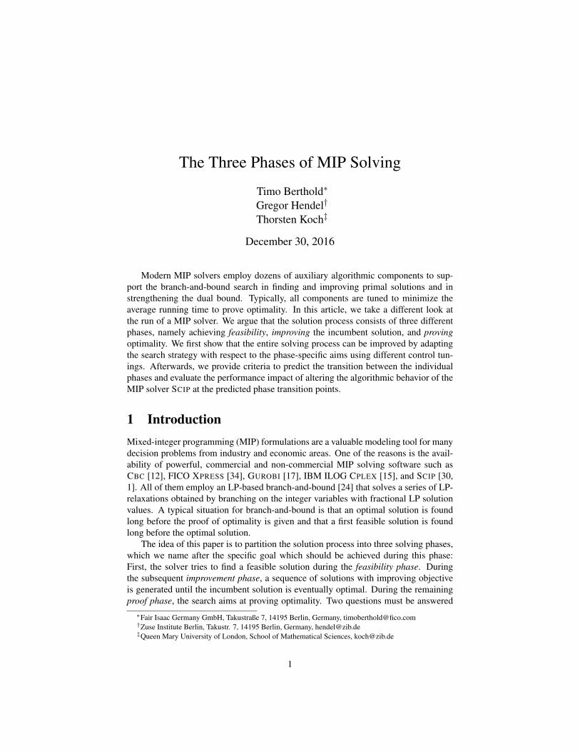
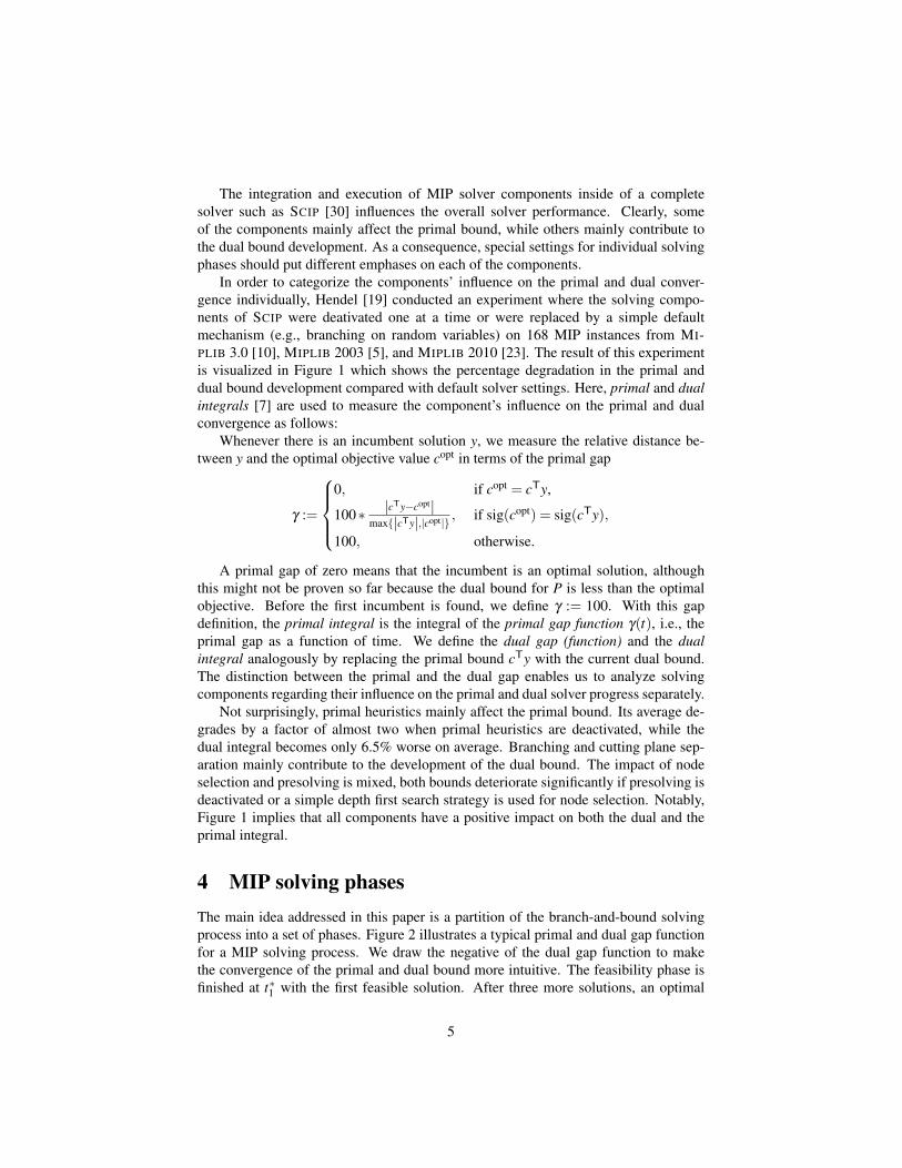
In order to categorize the components’ influence on the primal and dual conver-gence individually, Hendel [19] conducted an experiment where the solving compo-nents of SCIP were deativated one at a time or were replaced by a simple defaultmechanism (e.g., branching on random variables) on 168 MIP instances from MI-PLIB 3.0 [10], MIPLIB 2003 [5], and MIPLIB 2010 [23]. The result of this experimentis visualized in Figure 1 which shows the percentage degradation in the primal anddual bound development compared with default solver settings. Here, primal and dualintegrals [7] are used to measure the component’s influence on the primal and dualconvergence as follows:

Whenever there is an incumbent solution y, we measure the relative distance be-tween y and the optimal objective value copt in terms of the primal gap

γ :=

0, if copt = cTy,

100∗ |cTy−copt|max{|cTy|,|copt|} , if sig(copt) = sig(cTy),

100, otherwise.

A primal gap of zero means that the incumbent is an optimal solution, althoughthis might not be proven so far because the dual bound for P is less than the optimalobjective. Before the first incumbent is found, we define γ := 100. With this gapdefinition, the primal integral is the integral of the primal gap function γ(t), i.e., theprimal gap as a function of time. We define the dual gap (function) and the dualintegral analogously by replacing the primal bound cTy with the current dual bound.The distinction between the primal and the dual gap enables us to analyze solvingcomponents regarding their influence on the primal and dual solver progress separately.

Not surprisingly, primal heuristics mainly affect the primal bound. Its average de-grades by a factor of almost two when primal heuristics are deactivated, while thedual integral becomes only 6.5% worse on average. Branching and cutting plane sep-aration mainly contribute to the development of the dual bound. The impact of nodeselection and presolving is mixed, both bounds deteriorate significantly if presolving isdeactivated or a simple depth first search strategy is used for node selection. Notably,Figure 1 implies that all components have a positive impact on both the dual and theprimal integral.

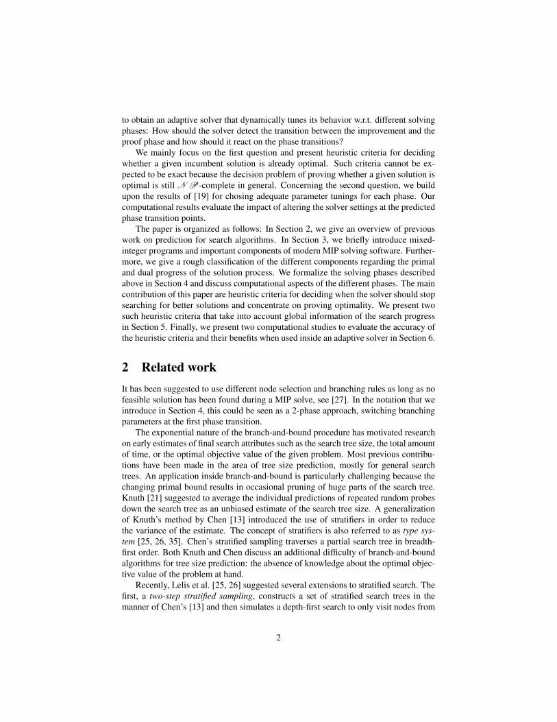
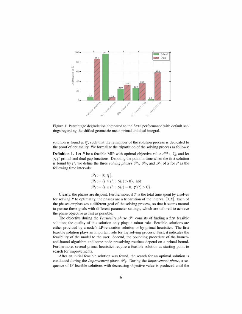
4 MIP solving phasesThe main idea addressed in this paper is a partition of the branch-and-bound solvingprocess into a set of phases. Figure 2 illustrates a typical primal and dual gap functionfor a MIP solving process. We draw the negative of the dual gap function to makethe convergence of the primal and dual bound more intuitive. The feasibility phase isfinished at t∗1 with the first feasible solution. After three more solutions, an optimal

5

random

branch

noheuristics

dfsnode

sel

nopresolving

noseparation

0

20

40

60

80

100

Deg

rad

atio

nin

%

6.8

97.1

24.0 25.9

2.8

86.4

6.5

32.836.0

58.5

Primal

Dual

Figure 1: Percentage degradation compared to the SCIP performance with default set-tings regarding the shifted geometric mean primal and dual integral.

solution is found at t∗2 , such that the remainder of the solution process is dedicated tothe proof of optimality. We formalize the tripartition of the solving process as follows:

Definition 1. Let P be a feasible MIP with optimal objective value copt ∈ Q, and letγ,γ∗ primal and dual gap functions. Denoting the point in time when the first solutionis found by t∗1 , we define the three solving phases P1, P2, and P3 of S for P as thefollowing time intervals:

P1 := [0, t∗1 [ ,P2 := {t ≥ t∗1 : γ(t)> 0}, andP3 := {t ≥ t∗1 : γ(t) = 0, γ

∗(t)> 0}.

Clearly, the phases are disjoint. Furthermore, if T is the total time spent by a solverfor solving P to optimality, the phases are a tripartition of the interval [0,T ]. Each ofthe phases emphasizes a different goal of the solving process, so that it seems naturalto pursue these goals with different parameter settings, which are tailored to achievethe phase objective as fast as possible.

The objective during the Feasibility phase P1 consists of finding a first feasiblesolution; the quality of this solution only plays a minor role. Feasible solutions areeither provided by a node’s LP-relaxation solution or by primal heuristics. The firstfeasible solution plays an important role for the solving process: First, it indicates thefeasibility of the model to the user. Second, the bounding procedure of the branch-and-bound algorithm and some node presolving routines depend on a primal bound.Furthermore, several primal heuristics require a feasible solution as starting point tosearch for improvements.

After an initial feasible solution was found, the search for an optimal solution isconducted during the Improvement phase P2. During the Improvement phase, a se-quence of IP-feasible solutions with decreasing objective value is produced until the

6

−40

−20

0

20

40

0 t∗1 t∗2 T

Time(sec.)

Gap

Primal GapNeg. Dual Gap

Figure 2: Solving phases of a MIP solution process with phase transition points t∗1 andt∗2

solver eventually finds an optimal solution. For users of MIP solving software, this isoften the most important phase. In many practical applications, MIP models are not re-quired to be solved to proven optimality, reaching a small optimality gap is consideredsufficient [7]. The reasons for this are threefold: there might be strict running timelimitations, the models often are too large to complete the search and the input dataitself might only be based on estimates.

The remaining time, which we call the Proof phase P3, is spent on proving theoptimality of the incumbent solution. Such a proof requires the full exploration of theremaining search tree until there are no more open nodes with dual bound lower thanthe optimal primal objective value.

It is possible for both the Improvement phase and the Proof phase to be empty. Ifthe first feasible solution is also an optimal one, then P2 = /0; similarly, if the bestpossible dual bound is found before an incumbent with this optimal objective valueis found, then P3 = /0. In the special case that the MIP is a pure feasibility problem(c = 0), both the Improvement phase and Proof phase are empty. For the test set whichwe use for our computational experiments in Section 6, only one of 161 instances isa pure feasibility problem. Further, 11 instances have an empty Improvement phaseand 34 instances have an empty or almost empty Proof phase, their union being 40instances. Hence, it applies for a majority of 75 % of our test cases that the solvingprocess is indeed partitioned into three nonempty phases by Definition 1.

We refer to the two points in time that mark the boundaries between the phases as

7

phase transitions. More precisely, we call t∗1 the first phase transition, and we definethe second phase transition as

t∗2 := supP1∪P2.

The recognition of the second phase transition t∗2 after the Improvement phase requiresknowledge about the optimality of the current incumbent prior to the termination ofthe solving process. If P3 6= /0, the decision problem of proving that there exists nosolution better than y(t∗2 ) for our input MIP P remains to be solved. This problem isco-N P-complete in general.

In the next section, we address the problem of how to heuristically estimate thesecond phase transition during the solving process.

5 Two phase transition heuristicsIf P3 6= /0, the detection of t∗2 requires knowledge of the optimal solution value. In thissection, we present two heuristic criteria to estimate the second phase transition pointt∗2 without knowledge of the optimal solution value. These phase transition heuristicswill be used to switch to settings for the Proof phase when the criteria indicate that thecurrent incumbent is optimal.

We present two phase transition heuristics based on a property called node estima-tion [6] of all nodes in the node frontier. The node estimation constitutes an estimateof the objective value of the best attainable solution of a node.

More formally, let FP := { j ∈ I : (yP) j /∈ Z} be the set of fractional variablesof an LP solution yP at node P. For j ∈ FP, we define f−P ( j) := (yP) j − b(yP) jcand f+P ( j) := d(yP) je− (yP) j the down- and up-fractionality, respectively, of j. For abranching direction ∗ ∈ {+,−}, we denote by Ψ∗j the average gain per unit fraction-ality over all prior branchings on j in direction ∗. We estimate the objective gain inbranching direction ∗ by the pseudo-costs [6] Ψ∗j · f ∗P( j).

Apart from their use in the selection of the best candidate for branching, pseudo-costs can also be applied to estimate the best solution attainable from a node P. There-fore, we denote by

ΨminP ( j) := min{Ψ−j · f−P ( j),Ψ+

j · f+P ( j)}

the estimated minimum cost to make variable j ∈I integer.

Definition 2 (Node estimation [6]). The node estimation for a node P for which theLP-relaxation has been solved is given by the formula

cP = cTyP + ∑j∈FP

ΨminP ( j).

The rationale behind Definition 2 is to independently consider an estimate of mak-ing each fractional variable j ∈FP integer. In the following, we will be mainly inter-ested in node estimations of open nodes, for which no LP relaxation has been solvedso far. In order to determine an estimate of an open node Q, we simply subtract the

8

contribution of the branching variable and direction that led to the creation of Q. Let Qbe the child of another node P after branching upwards on j ∈FP. An initial estimateof Q can be calculated via

cQ = cP−ΨminP ( j)+Ψ

+j · f+P ( j),

thereby extending Definition 2 to open search nodes.The node estimation does not account for a possible interplay between variables.

This observation makes cP likely to overestimate the actual integer objective valuecopt

P of the best attainable solution from the subtree rooted at P. It is, on the otherhand, also possible to underestimate copt

P . Another important aspect concerns a possibledegeneracy of the LP-relaxation: Whenever there exist different optima to the node LP-relaxation, they might lead to different estimates.

5.1 The best-estimate transitionWe call the minimum node estimation among the set of open nodes Q,

cminQ = min{cQ : Q ∈Q}

the best-estimate. The best-estimate is used as primary criterion for the default nodeselection in SCIP and is one possible estimate of the optimal objective value of a givenMIP, for other possible estimates, we refer to [33]. As our first phase transition heuris-tic, we propose to switch to the Proof phase when the best-estimate exceeds the incum-bent objective:

testim2 := min

{t ≥ t∗1 : cTy(t)≤ cmin

Q (t)}

(1)

Note that by requiring t ≥ t∗1 , we make sure that there is indeed an incumbent solution.

5.2 The rank-1 transitionWith an increasing number of explored branch-and-bound nodes, it intuitively becomesless and less likely to encounter a solution better than the current incumbent. Yet, everyunprocessed node Q ∈Q has the potential to contain a better solution in the subtreeunderneath.

Definition 3. Let S be the search tree after termination, and define dQ as depth andcopt

Q as the (integer) optimal objective value for every node Q ∈ S (or ∞ if there is nofeasible solution for Q). We define the rank rgQ of Q as

rgQ :=∣∣∣{Q′ ∈ S : dQ′ = dQ,c

optQ′ < copt

Q }∣∣∣+1.

The rank rgQ represents the minimum position of node Q in any list PdQ thatcontains all nodes at depth dQ in nondecreasing order of their optimal solution. Theroot node P0 trivially has a rank of 1, because it is the only node at depth 0. Indeed, if Swere known in advance, the rank is defined in such a way that an optimal solution can

9

be found by following a path of nodes of rank 1, starting at the root node. If the solvingprocess has not uncovered an optimal solution yet, there exists a node of rank 1 amongthe open nodes Q. Note, however, that there may even be nodes of rank 1 present inthe node frontier although the current incumbent is already optimal.

The second phase transition heuristic is based on the definition ( 3) of node ranks.As for the best-estimate transition, we use the node estimation (cf. Definition 2) to cir-cumvent the absence of true knowledge about best solutions in the unexplored subtrees.We impose a partial order relation ≺ on the nodes of the search tree S:

Q′ ≺ Q ⇔ Q′ was processed before Q dQ′ = dQ, ∀Q′ 6= Q ∈ S.

With this partial order relation, we define the set of rank-1 nodes

Qrank-1 := {Q ∈Q : cQ ≤ inf{cQ′ : Q′ ∈ S,Q′ ≺ Q}} (2)

as the set of all open nodes with a node estimation at least as good as the best evaluatednode at the same depth. Note that Qrank-1 may become empty much earlier than Q,i.e., prior to the termination of the search, as soon as a single node with small nodeestimation has been processed at every depth of the current tree.

Using the following rank-1 transition, we assume that the current incumbent isoptimal when Qrank-1 becomes empty:

trank-12 := min{t ≥ t∗1 : Qrank-1(t) = /0}. (3)

If there is an open node Q at a depth dQ which was not yet explored by the solvingprocess, it holds that Q ∈Qrank-1 since

cQ ≤ inf{cQ′ : Q′ ∈ S,Q′ ≺ Q}= inf /0 = ∞.

The main difference between the best-estimate and the rank-1 transitions is thatthe rank-1 transition does not directly compare incumbent solution objectives and nodeestimations. On the one hand, it is an intuitive restriction to only compare nodes of thesame depth because node estimations can be assumed to gain precision with increasingdepth. Furthermore, it has a computational benefit because our update procedure onlyneeds to compare newly inserted open nodes with other open nodes at the same depth.

For every depth d, we keep track of the minimum node estimate at this particulardepth so far, including feasible nodes, i.e. subproblems with feasible LP-relaxationsolutions. Every time a node is branched on, its two children are inserted in an arrayQd of open nodes at their depth d. Qd is sorted in nondecreasing order of the nodeestimations of the nodes. In order to keep the set Qrank-1 updated, we store for everydepth the best-estimate over all nodes already processed, which we update every timea node Q ∈Qrank-1 was selected to be explored next.

6 Computational resultsIn this section, we first evaluate the potential of the two proposed transitions used withdefault settings. Second, we show how the use of the proposed transitions togetherwith phase-specific solver settings affects the solution process.

10

6.1 Accuracy of the proposed phase transitionsIn this section, we analyze the accuracy of the proposed phase transition heuristics fromSection 5. We based our implementation on SCIP [1] 3.1.0 together with SoPlex [32]2.0 as LP-solver. All computations were performed on a cluster of 32 computers. Eachcomputer runs with a 64bit Intel Xeon X5672 CPUs at 3.20 GHz with 12 MB cacheand 48 GB main memory. The operating system was Ubuntu 14.4. A gcc compiler wasused in version 4.8.2. Hyperthreading and Turboboost were disabled. We ran only onejob per computer in order to minimize the random noise in the measured running timethat might be caused by cache-misses if multiple processes share common resources.

As test library, we use a combined library of MIPLIB 3 [10], MIPLIB 2003 [5],and MIPLIB 2010 [23] after the removal of three infeasible instances. In addition, weexcluded the four instances for which, by the time of this writing, the optimal objectivevalue was unknown, so that it is not possible to determine the actual phase transitiont∗2 . On the remaining 161 instances we ran SCIP with default settings and a time limitof 2h. We record the solving time in seconds after which a transition criterion wasreached for the first time. Before we start checking the transition criteria, we requirethe search to explore at least 50 branch-and-bound nodes for the node frontier to bemeaningfully initialized.

It is noteworthy that the node estimations in SCIP are not updated dynamicallytogether with the pseudo-costs due to running-time considerations, i.e., all nodes keeptheir initial estimation during the entire time they are in the node queue, although morerecent pseudo-cost information on the variables might be available.

The goal of this experiment is to compare the proposed transition points with theactual second phase transition t∗2 . It may happen that t∗2 > 2h, i.e., an optimal solutionis not found within the time limit, or a transition criterion is not met. Therefore, wefirst consider instances for which the solver finished the improvement phase within thetime limit and at least one of the transition criteria was met.

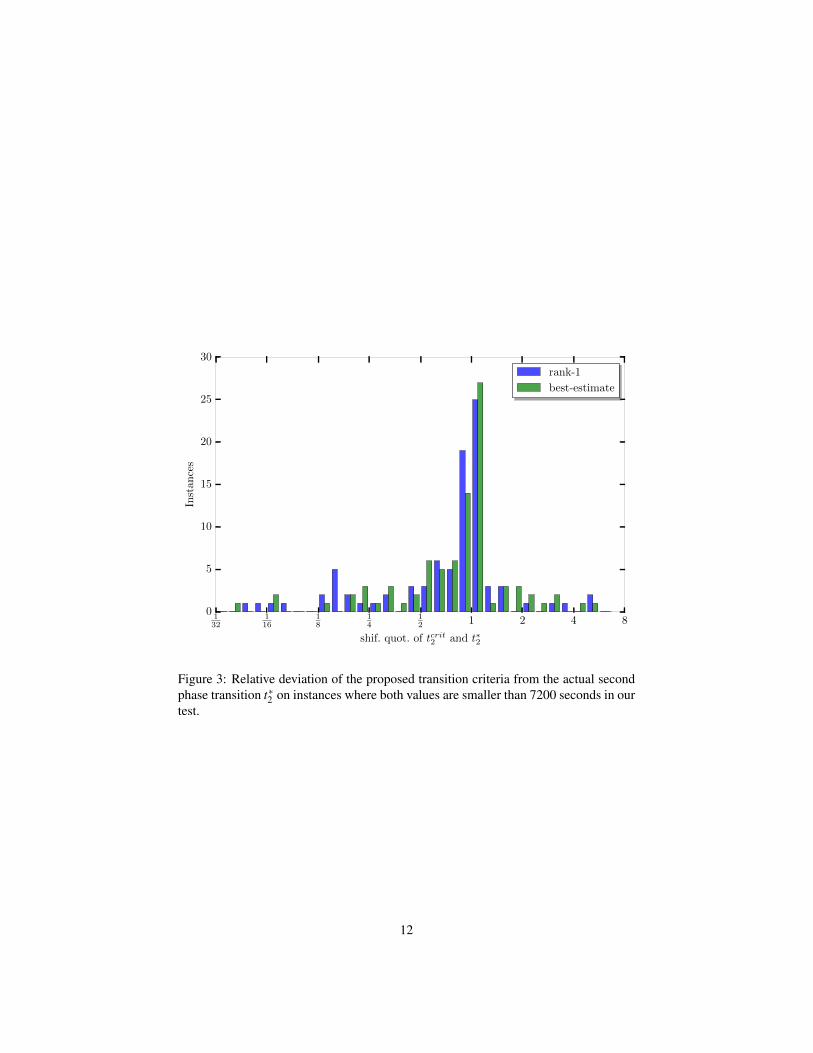
We compare the relative difference between the two points in time by means of theirshifted quotient (tcrit

2 + τ)/(t∗2 + τ) using a shift of τ = 10 seconds. The use of a shiftvalue compensates for very large or small quotients caused by numbers that are closeto one and hence also shifts our attention to harder instances. A shifted quotient largerthan one for an instance means that a phase transition heuristic correctly classifies anoptimal incumbent solution. A quotient smaller than one, however, is encountered forinstances where the transition criterion was met during the Improvement phase.

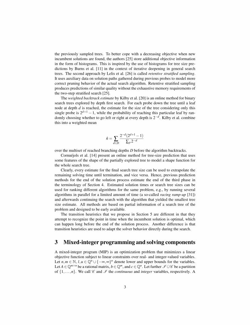
We present Figure 3 to compare the true second phase transition t∗2 and the phasetransition tcrit

2 that we recorded for the phase transitions. The histogram uses a bin widthof 0.25 on the logarithm of the shifted quotients. The two bins around one thereforedenote the time span shortly before or after t∗2 . We do not show instances which couldbe solved during the root node. Out of the remaining 147 instances, SCIP finds optimalsolutions for 117. The rank-1 and the best-estimate criterion are reached for 91 and93 of these instances, respectively. Note that the both rank-1 and the best-estimatetransitions are trivially met whenever there is no open node left in the tree, i.e., afterthe search was completed.

We see in the figure that the bars for both transitions are centered around one, therank-1 transition with 44 instances and the best-estimate transition with 41 instances.

11

132

116

18

14

12 1 2 4 8

shif. quot. of tcrit2 and t∗2

0

5

10

15

20

25

30

Inst

ance

s

rank-1

best-estimate

Figure 3: Relative deviation of the proposed transition criteria from the actual secondphase transition t∗2 on instances where both values are smaller than 7200 seconds in ourtest.

12

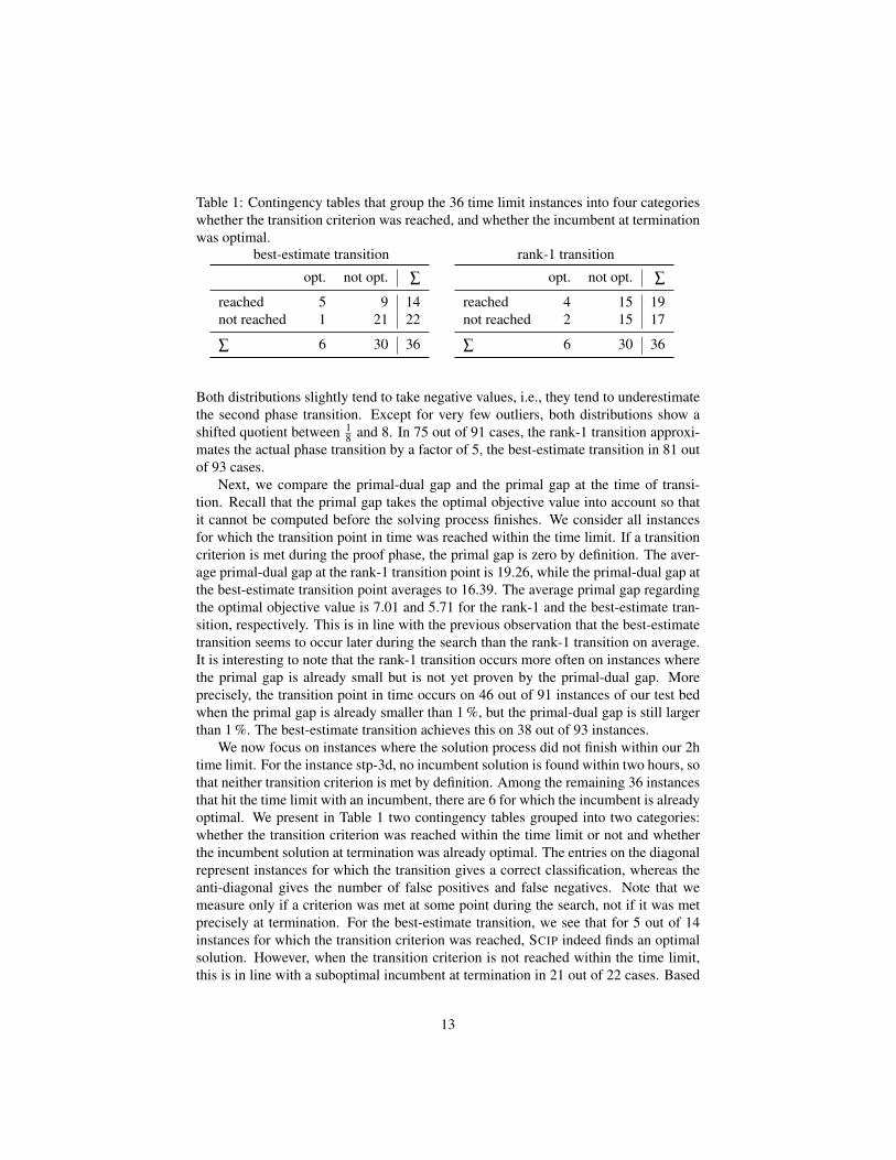
Table 1: Contingency tables that group the 36 time limit instances into four categorieswhether the transition criterion was reached, and whether the incumbent at terminationwas optimal.

best-estimate transition rank-1 transition

opt. not opt. ∑

reached 5 9 14not reached 1 21 22

∑ 6 30 36

opt. not opt. ∑

reached 4 15 19not reached 2 15 17

∑ 6 30 36

Both distributions slightly tend to take negative values, i.e., they tend to underestimatethe second phase transition. Except for very few outliers, both distributions show ashifted quotient between 1

8 and 8. In 75 out of 91 cases, the rank-1 transition approxi-mates the actual phase transition by a factor of 5, the best-estimate transition in 81 outof 93 cases.

Next, we compare the primal-dual gap and the primal gap at the time of transi-tion. Recall that the primal gap takes the optimal objective value into account so thatit cannot be computed before the solving process finishes. We consider all instancesfor which the transition point in time was reached within the time limit. If a transitioncriterion is met during the proof phase, the primal gap is zero by definition. The aver-age primal-dual gap at the rank-1 transition point is 19.26, while the primal-dual gap atthe best-estimate transition point averages to 16.39. The average primal gap regardingthe optimal objective value is 7.01 and 5.71 for the rank-1 and the best-estimate tran-sition, respectively. This is in line with the previous observation that the best-estimatetransition seems to occur later during the search than the rank-1 transition on average.It is interesting to note that the rank-1 transition occurs more often on instances wherethe primal gap is already small but is not yet proven by the primal-dual gap. Moreprecisely, the transition point in time occurs on 46 out of 91 instances of our test bedwhen the primal gap is already smaller than 1 %, but the primal-dual gap is still largerthan 1 %. The best-estimate transition achieves this on 38 out of 93 instances.

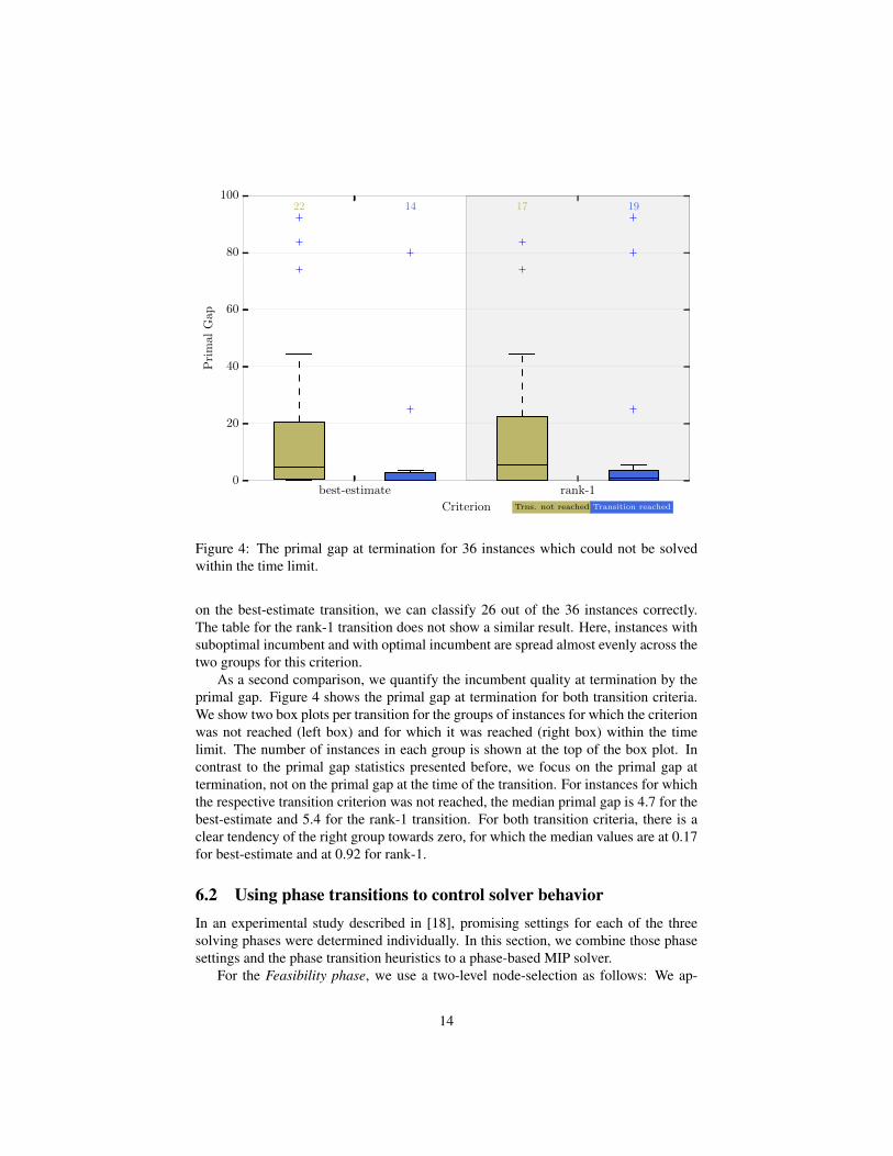
We now focus on instances where the solution process did not finish within our 2htime limit. For the instance stp-3d, no incumbent solution is found within two hours, sothat neither transition criterion is met by definition. Among the remaining 36 instancesthat hit the time limit with an incumbent, there are 6 for which the incumbent is alreadyoptimal. We present in Table 1 two contingency tables grouped into two categories:whether the transition criterion was reached within the time limit or not and whetherthe incumbent solution at termination was already optimal. The entries on the diagonalrepresent instances for which the transition gives a correct classification, whereas theanti-diagonal gives the number of false positives and false negatives. Note that wemeasure only if a criterion was met at some point during the search, not if it was metprecisely at termination. For the best-estimate transition, we see that for 5 out of 14instances for which the transition criterion was reached, SCIP indeed finds an optimalsolution. However, when the transition criterion is not reached within the time limit,this is in line with a suboptimal incumbent at termination in 21 out of 22 cases. Based

13

best-estimate rank-1

Criterion

0

20

40

60

80

100P

rim

alG

ap22 14 17 19

Trns. not reached Transition reached

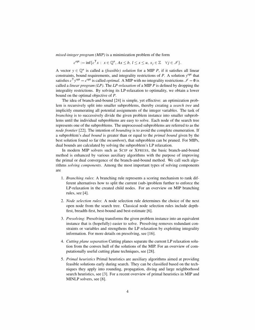
Figure 4: The primal gap at termination for 36 instances which could not be solvedwithin the time limit.

on the best-estimate transition, we can classify 26 out of the 36 instances correctly.The table for the rank-1 transition does not show a similar result. Here, instances withsuboptimal incumbent and with optimal incumbent are spread almost evenly across thetwo groups for this criterion.

As a second comparison, we quantify the incumbent quality at termination by theprimal gap. Figure 4 shows the primal gap at termination for both transition criteria.We show two box plots per transition for the groups of instances for which the criterionwas not reached (left box) and for which it was reached (right box) within the timelimit. The number of instances in each group is shown at the top of the box plot. Incontrast to the primal gap statistics presented before, we focus on the primal gap attermination, not on the primal gap at the time of the transition. For instances for whichthe respective transition criterion was not reached, the median primal gap is 4.7 for thebest-estimate and 5.4 for the rank-1 transition. For both transition criteria, there is aclear tendency of the right group towards zero, for which the median values are at 0.17for best-estimate and at 0.92 for rank-1.

6.2 Using phase transitions to control solver behaviorIn an experimental study described in [18], promising settings for each of the threesolving phases were determined individually. In this section, we combine those phasesettings and the phase transition heuristics to a phase-based MIP solver.

For the Feasibility phase, we use a two-level node-selection as follows: We ap-

14

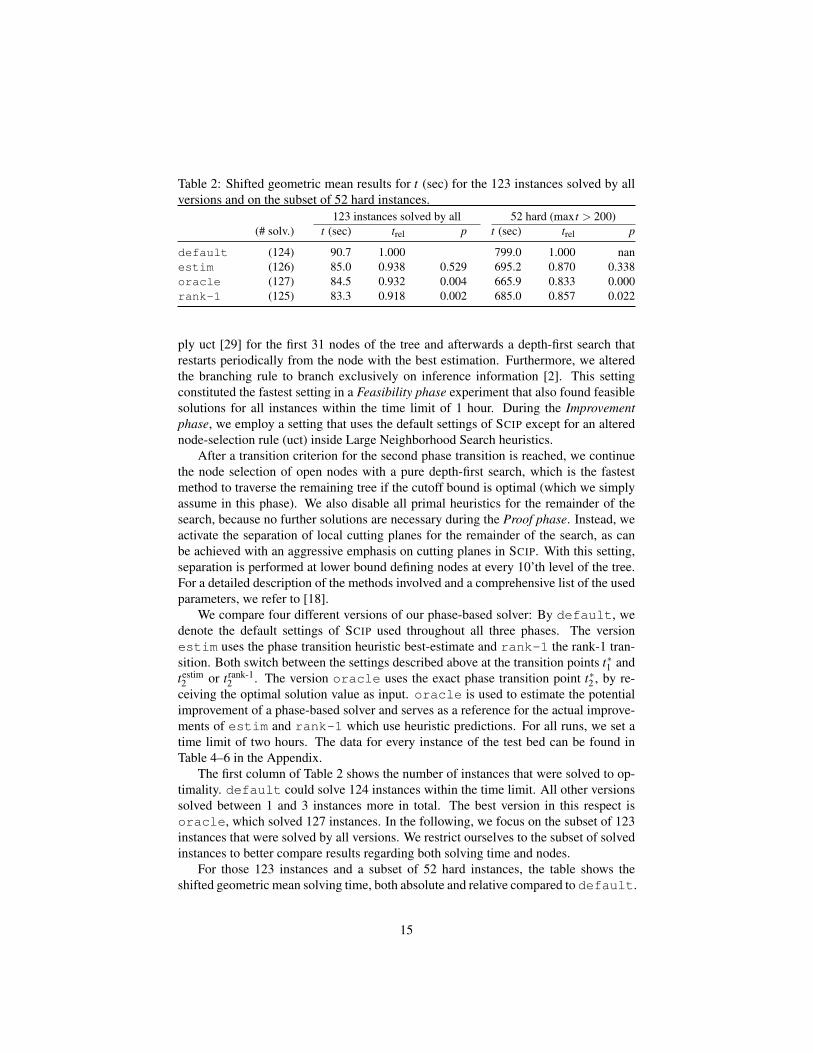
Table 2: Shifted geometric mean results for t (sec) for the 123 instances solved by allversions and on the subset of 52 hard instances.

123 instances solved by all 52 hard (max t > 200)(# solv.) t (sec) trel p t (sec) trel p

default (124) 90.7 1.000 799.0 1.000 nanestim (126) 85.0 0.938 0.529 695.2 0.870 0.338oracle (127) 84.5 0.932 0.004 665.9 0.833 0.000rank-1 (125) 83.3 0.918 0.002 685.0 0.857 0.022

ply uct [29] for the first 31 nodes of the tree and afterwards a depth-first search thatrestarts periodically from the node with the best estimation. Furthermore, we alteredthe branching rule to branch exclusively on inference information [2]. This settingconstituted the fastest setting in a Feasibility phase experiment that also found feasiblesolutions for all instances within the time limit of 1 hour. During the Improvementphase, we employ a setting that uses the default settings of SCIP except for an alterednode-selection rule (uct) inside Large Neighborhood Search heuristics.

After a transition criterion for the second phase transition is reached, we continuethe node selection of open nodes with a pure depth-first search, which is the fastestmethod to traverse the remaining tree if the cutoff bound is optimal (which we simplyassume in this phase). We also disable all primal heuristics for the remainder of thesearch, because no further solutions are necessary during the Proof phase. Instead, weactivate the separation of local cutting planes for the remainder of the search, as canbe achieved with an aggressive emphasis on cutting planes in SCIP. With this setting,separation is performed at lower bound defining nodes at every 10’th level of the tree.For a detailed description of the methods involved and a comprehensive list of the usedparameters, we refer to [18].

We compare four different versions of our phase-based solver: By default, wedenote the default settings of SCIP used throughout all three phases. The versionestim uses the phase transition heuristic best-estimate and rank-1 the rank-1 tran-sition. Both switch between the settings described above at the transition points t∗1 andtestim2 or trank-1

2 . The version oracle uses the exact phase transition point t∗2 , by re-ceiving the optimal solution value as input. oracle is used to estimate the potentialimprovement of a phase-based solver and serves as a reference for the actual improve-ments of estim and rank-1 which use heuristic predictions. For all runs, we set atime limit of two hours. The data for every instance of the test bed can be found inTable 4–6 in the Appendix.

The first column of Table 2 shows the number of instances that were solved to op-timality. default could solve 124 instances within the time limit. All other versionssolved between 1 and 3 instances more in total. The best version in this respect isoracle, which solved 127 instances. In the following, we focus on the subset of 123instances that were solved by all versions. We restrict ourselves to the subset of solvedinstances to better compare results regarding both solving time and nodes.

For those 123 instances and a subset of 52 hard instances, the table shows theshifted geometric mean solving time, both absolute and relative compared to default.

15

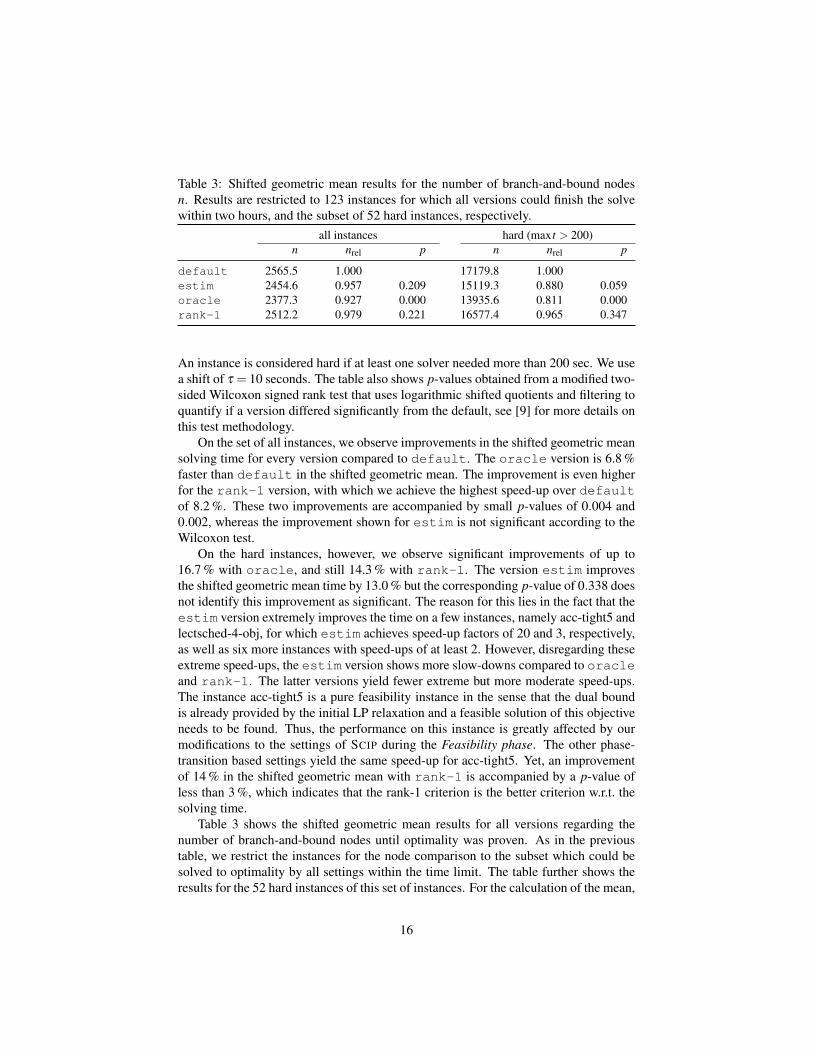
Table 3: Shifted geometric mean results for the number of branch-and-bound nodesn. Results are restricted to 123 instances for which all versions could finish the solvewithin two hours, and the subset of 52 hard instances, respectively.

all instances hard (max t > 200)n nrel p n nrel p

default 2565.5 1.000 17179.8 1.000estim 2454.6 0.957 0.209 15119.3 0.880 0.059oracle 2377.3 0.927 0.000 13935.6 0.811 0.000rank-1 2512.2 0.979 0.221 16577.4 0.965 0.347

An instance is considered hard if at least one solver needed more than 200 sec. We usea shift of τ = 10 seconds. The table also shows p-values obtained from a modified two-sided Wilcoxon signed rank test that uses logarithmic shifted quotients and filtering toquantify if a version differed significantly from the default, see [9] for more details onthis test methodology.

On the set of all instances, we observe improvements in the shifted geometric meansolving time for every version compared to default. The oracle version is 6.8 %faster than default in the shifted geometric mean. The improvement is even higherfor the rank-1 version, with which we achieve the highest speed-up over defaultof 8.2 %. These two improvements are accompanied by small p-values of 0.004 and0.002, whereas the improvement shown for estim is not significant according to theWilcoxon test.

On the hard instances, however, we observe significant improvements of up to16.7 % with oracle, and still 14.3 % with rank-1. The version estim improvesthe shifted geometric mean time by 13.0 % but the corresponding p-value of 0.338 doesnot identify this improvement as significant. The reason for this lies in the fact that theestim version extremely improves the time on a few instances, namely acc-tight5 andlectsched-4-obj, for which estim achieves speed-up factors of 20 and 3, respectively,as well as six more instances with speed-ups of at least 2. However, disregarding theseextreme speed-ups, the estim version shows more slow-downs compared to oracleand rank-1. The latter versions yield fewer extreme but more moderate speed-ups.The instance acc-tight5 is a pure feasibility instance in the sense that the dual boundis already provided by the initial LP relaxation and a feasible solution of this objectiveneeds to be found. Thus, the performance on this instance is greatly affected by ourmodifications to the settings of SCIP during the Feasibility phase. The other phase-transition based settings yield the same speed-up for acc-tight5. Yet, an improvementof 14 % in the shifted geometric mean with rank-1 is accompanied by a p-value ofless than 3 %, which indicates that the rank-1 criterion is the better criterion w.r.t. thesolving time.

Table 3 shows the shifted geometric mean results for all versions regarding thenumber of branch-and-bound nodes until optimality was proven. As in the previoustable, we restrict the instances for the node comparison to the subset which could besolved to optimality by all settings within the time limit. The table further shows theresults for the 52 hard instances of this set of instances. For the calculation of the mean,

16

we use a shift of 100 nodes. The setting oracle significantly improves the overallshifted geometric mean of default by 7.3 % and by 18.9 % on the hard instances.For the criteria estim and rank-1, the obtained node reductions amount to 4.3 %and 2.1 %, respectively. In this case, however, the p-column does not indicate either ofthe improvements as significant. The split into easy and hard instances attributes theobserved reductions mainly to the hard instances, where estim shows an improvementof 12 % compared to default.

Our experiments in the previous section revealed that estim transitions occur laterduring the search than rank-1-transitions which makes estim a more conservativetransition criterion. While it achieves a good performance w.r.t. overall running time,rank-1 performs even better, in particular when taking the statistic significance of theresults into account. In the previous section, we saw that rank-1 has a tendency tounderestimate the point of phase transition. We interpret our results such that switchingsettings shortly before the second phase transition, i.e. when the solver is about to findthe optimal solution, is sufficient, if not preferable, to improve performance. The factthat only one of the two transition heuristics achieves a significant time speed-up showsthat the speed-up cannot be attributed only to the changes to the Feasibility phase,during which all three versions that employ phase-based settings have exactly the samebehavior.

Using the rank-1 phase transition, we obtain a solving time improvement that issimilar to the improvement obtained with oracle. Comparing the results for anoracle-based phase transition and the phase-transition criteria that we introduced, weconclude that the rank-1 transition is sufficient in practice to achieve a solving-timeperformance similar to what can be obtained in principle if we could determine thephase transition exactly.

7 ConclusionIn this article, we discussed the partition of a MIP solving process into three phases:feasibility, improvement, and proof. Each of them benefits from different algorithmiccomponents. We introduced and empirically analyzed two criteria to predict the tran-sition between the improvement and the proof phase: the best-estimate transition andthe rank-1 transition.

We showed that a phase-based version of the MIP solver SCIP, using the rank-1 transition, improves SCIP’s mean running time by 8 % on general MIP instances,and 14 % on hard instances, while simultaneously reducing the number of branch-and-bound nodes. Hence, our computational experiments provide evidence that thoseeasy-to-evaluate criteria correlate sufficiently well with the actual, hard-to-detect phasetransition to make use of this approach in practice.

Acknowledgement(s)The work for this article has been conducted within the Research Campus MODALfunded by the German Federal Ministry of Education and Research (fund number

17

05M14ZAM). The work was supported by the ICT COST Action TD1207 Mathe-matical Optimization in the Decision Support Systems for Efficient and Robust EnergyNetworks. The research was supported by a Google Faculty Research Award.

References[1] T. Achterberg, SCIP: Solving constraint integer programs, Mathematical Pro-

gramming Computation 1 (2009), pp. 1–41.

[2] T. Achterberg and T. Berthold, Hybrid Branching, in Integration of AI and ORTechniques in Constraint Programming for Combinatorial Optimization Prob-lems, 6th International Conference, CPAIOR 2009, Lecture Notes in ComputerScience, Vol. 5547, Springer, 2009, pp. 309–311.

[3] T. Achterberg, T. Berthold, and G. Hendel, Rounding and Propagation Heuris-tics for Mixed Integer Programming, in Operations Research Proceedings 2011,Springer Berlin Heidelberg, 2012, pp. 71–76.

[4] T. Achterberg, T. Koch, and A. Martin, Branching rules revisited, OperationsResearch Letters 33 (2004), pp. 42–54.

[5] T. Achterberg, T. Koch, and A. Martin, MIPLIB 2003, Operations Research Let-ters 34 (2006), pp. 1–12.

[6] M. Bénichou, J.M. Gauthier, P. Girodet, G. Hentges, G. Ribière, and O. Vin-cent, Experiments in mixed-integer programming, Mathematical Programming 1(1971), pp. 76–94.

[7] T. Berthold, Measuring the impact of primal heuristics, Operations Research Let-ters 41 (2013), pp. 611–614.

[8] T. Berthold, Heuristic algorithms in global MINLP solvers, Ph.D. diss., Technis-che Universität Berlin, 2014.

[9] T. Berthold, G. Gamrath, and D. Salvagnin, Cloud branching, Presentationslides from Mixed Integer Programming Workshop at Ohio State University.https://mip2014.engineering.osu.edu/sites/mip2014.engineering.osu.edu/files/uploads/Berthold_MIP2014_Cloud.pdf (2014).

[10] R.E. Bixby, S. Ceria, C.M. McZeal, and M.W. Savelsbergh, An updated mixedinteger programming library: MIPLIB 3.0, Optima 58 (1998), pp. 12–15.

[11] E. Burns and W. Ruml, Iterative-deepening search with on-line tree size predic-tion, Annals of Mathematics and Artificial Intelligence 69 (2013), pp. 183–205,Available at http://dx.doi.org/10.1007/s10472-013-9347-9.

[12] COIN-OR branch-and-cut MIP solver (2016), https://projects.coin-or.org/Cbc.

18

[13] P.C. Chen, Heuristic sampling: A method for predicting the performance of treesearching programs, SIAM Journal on Computing 21 (1992), pp. 295–315, Avail-able at http://dx.doi.org/10.1137/0221022.

[14] G. Cornuéjols, M. Karamanov, and Y. Li, Early estimates of the size of branch-and-bound trees, INFORMS Journal on Computing 18 (2006), pp. 86–96, Avail-able at http://dx.doi.org/10.1287/ijoc.1040.0107.

[15] IBM ILOG CPLEX Optimizer (2016), http://www-01.ibm.com/software/integration/optimization/cplex-optimizer/.

[16] G. Gamrath, T. Koch, A. Martin, M. Miltenberger, and D. Weninger, Progress inpresolving for mixed integer programming, Mathematical Programming Compu-tation 7 (2015), pp. 367–398.

[17] GUROBI Optimizer (2016), http://www.gurobi.com/products/gurobi-optimizer/gurobi-overview.

[18] G. Hendel, Empirical analysis of solving phases in mixed integer programming,Master thesis, Technische Universität Berlin (2014).

[19] G. Hendel, Enhancing MIP Branching Decisions by Using the Sample Varianceof Pseudo Costs, in Integration of AI and OR Techniques in Constraint Program-ming, Vol. 9075, in press, 2015, pp. 199 – 214.

[20] P. Kilby, J.K. Slaney, S. Thiébaux, and T. Walsh, Estimating Search Tree Size, inAAAI, AAAI Press, 2006, pp. 1014–1019.

[21] D.E. Knuth, Estimating the efficiency of backtrack programs., Tech. Rep., Stan-ford University, Stanford, CA, USA, 1974.

[22] T. Koch, A. Martin, and M.E. Pfetsch, Progress in academic computational in-teger programming, in Facets of Combinatorial Optimization, M. Jünger and G.Reinelt, eds., Springer, 2013, pp. 483–506.

[23] T. Koch, T. Achterberg, E. Andersen, O. Bastert, T. Berthold, R.E. Bixby, E.Danna, G. Gamrath, A.M. Gleixner, S. Heinz, A. Lodi, H. Mittelmann, T.Ralphs, D. Salvagnin, D.E. Steffy, and K. Wolter, MIPLIB 2010, Mathemat-ical Programming Computation 3 (2011), pp. 103–163, Available at http://dx.doi.org/10.1007/s12532-011-0025-9.

[24] A.H. Land and A.G. Doig, An automatic method of solving discrete programmingproblems, Econometrica 28 (1960), pp. 497–520.

[25] L.H.S. Lelis, L. Otten, and R. Dechter, Predicting the Size of Depth-first Branch and Bound Search Trees, in Proceedings of the Twenty-ThirdInternational Joint Conference on Artificial Intelligence, IJCAI ’13, Bei-jing, China, Available at http://dl.acm.org/citation.cfm?id=2540128.2540215, AAAI Press, 2013, pp. 594–600.

19

[26] L.H.S. Lelis, L. Otten, and R. Dechter, Memory-Efficient Tree Size Prediction forDepth-First Search in Graphical Models, in Principles and Practice of ConstraintProgramming - 20th International Conference, CP 2014, Lyon, France, Septem-ber 8-12, 2014. Proceedings, Available at http://dx.doi.org/10.1007/978-3-319-10428-7_36, 2014, pp. 481–496.

[27] J.T. Linderoth and M.W.P. Savelsbergh, A computational study of search strate-gies for mixed integer programming, INFORMS Journal on Computing 11(1999), pp. 173–187.

[28] H. Marchand, A. Martin, R. Weismantel, and L.A. Wolsey, Cutting planes ininteger and mixed integer programming, Discrete Applied Mathematics 123/124(2002), pp. 391–440.

[29] A. Sabharwal, H. Samulowitz, and C. Reddy, Guiding Combinatorial Opti-mization with UCT., in CPAIOR, Lecture Notes in Computer Science, Vol.7298, Available at http://dblp.uni-trier.de/db/conf/cpaior/cpaior2012.html#SabharwalSR12, Springer, 2012, pp. 356–361.

[30] SCIP, SCIP. Solving Constraint Integer Programs., http://scip.zib.de/(2016).

[31] Y. Shinano, T. Achterberg, T. Berthold, S. Heinz, and T. Koch, ParaSCIP – aparallel extension of SCIP, in Competence in High Performance Computing 2010,Springer, 2012, pp. 135–148.

[32] SoPlex. An open source LP solver implementing the revised simplex algorithm.,http://soplex.zib.de/ (2016).

[33] D.T. Wojtaszek and J.W. Chinneck, Faster mip solutions via new node selectionrules, Computers & Operations Research 37 (2010), pp. 1544–1556.

[34] Xpress, FICO Xpress-Optimizer (2016), http://www.fico.com/en/Products/DMTools/xpress-overview/Pages/Xpress-Optimizer.aspx.

[35] U. Zahavi, A. Felner, N. Burch, and R.C. Holte, Predicting the performance ofida* using conditional distributions, J. Artif. Intell. Res. (JAIR) 37 (2010), pp.41–83, Available at http://dx.doi.org/10.1613/jair.2890.

20

Appendix

21

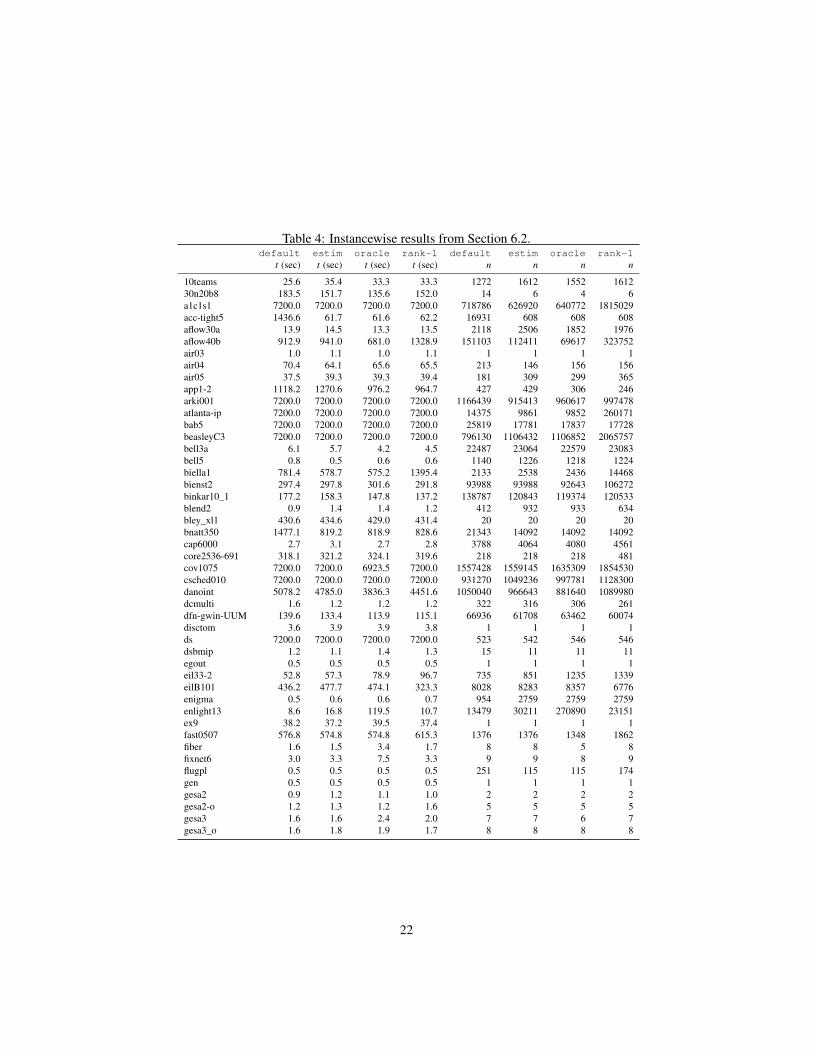
Table 4: Instancewise results from Section 6.2.default estim oracle rank-1 default estim oracle rank-1

t (sec) t (sec) t (sec) t (sec) n n n n

10teams 25.6 35.4 33.3 33.3 1272 1612 1552 161230n20b8 183.5 151.7 135.6 152.0 14 6 4 6a1c1s1 7200.0 7200.0 7200.0 7200.0 718786 626920 640772 1815029acc-tight5 1436.6 61.7 61.6 62.2 16931 608 608 608aflow30a 13.9 14.5 13.3 13.5 2118 2506 1852 1976aflow40b 912.9 941.0 681.0 1328.9 151103 112411 69617 323752air03 1.0 1.1 1.0 1.1 1 1 1 1air04 70.4 64.1 65.6 65.5 213 146 156 156air05 37.5 39.3 39.3 39.4 181 309 299 365app1-2 1118.2 1270.6 976.2 964.7 427 429 306 246arki001 7200.0 7200.0 7200.0 7200.0 1166439 915413 960617 997478atlanta-ip 7200.0 7200.0 7200.0 7200.0 14375 9861 9852 260171bab5 7200.0 7200.0 7200.0 7200.0 25819 17781 17837 17728beasleyC3 7200.0 7200.0 7200.0 7200.0 796130 1106432 1106852 2065757bell3a 6.1 5.7 4.2 4.5 22487 23064 22579 23083bell5 0.8 0.5 0.6 0.6 1140 1226 1218 1224biella1 781.4 578.7 575.2 1395.4 2133 2538 2436 14468bienst2 297.4 297.8 301.6 291.8 93988 93988 92643 106272binkar10_1 177.2 158.3 147.8 137.2 138787 120843 119374 120533blend2 0.9 1.4 1.4 1.2 412 932 933 634bley_xl1 430.6 434.6 429.0 431.4 20 20 20 20bnatt350 1477.1 819.2 818.9 828.6 21343 14092 14092 14092cap6000 2.7 3.1 2.7 2.8 3788 4064 4080 4561core2536-691 318.1 321.2 324.1 319.6 218 218 218 481cov1075 7200.0 7200.0 6923.5 7200.0 1557428 1559145 1635309 1854530csched010 7200.0 7200.0 7200.0 7200.0 931270 1049236 997781 1128300danoint 5078.2 4785.0 3836.3 4451.6 1050040 966643 881640 1089980dcmulti 1.6 1.2 1.2 1.2 322 316 306 261dfn-gwin-UUM 139.6 133.4 113.9 115.1 66936 61708 63462 60074disctom 3.6 3.9 3.9 3.8 1 1 1 1ds 7200.0 7200.0 7200.0 7200.0 523 542 546 546dsbmip 1.2 1.1 1.4 1.3 15 11 11 11egout 0.5 0.5 0.5 0.5 1 1 1 1eil33-2 52.8 57.3 78.9 96.7 735 851 1235 1339eilB101 436.2 477.7 474.1 323.3 8028 8283 8357 6776enigma 0.5 0.6 0.6 0.7 954 2759 2759 2759enlight13 8.6 16.8 119.5 10.7 13479 30211 270890 23151ex9 38.2 37.2 39.5 37.4 1 1 1 1fast0507 576.8 574.8 574.8 615.3 1376 1376 1348 1862fiber 1.6 1.5 3.4 1.7 8 8 5 8fixnet6 3.0 3.3 7.5 3.3 9 9 8 9flugpl 0.5 0.5 0.5 0.5 251 115 115 174gen 0.5 0.5 0.5 0.5 1 1 1 1gesa2 0.9 1.2 1.1 1.0 2 2 2 2gesa2-o 1.2 1.3 1.2 1.6 5 5 5 5gesa3 1.6 1.6 2.4 2.0 7 7 6 7gesa3_o 1.6 1.8 1.9 1.7 8 8 8 8

22

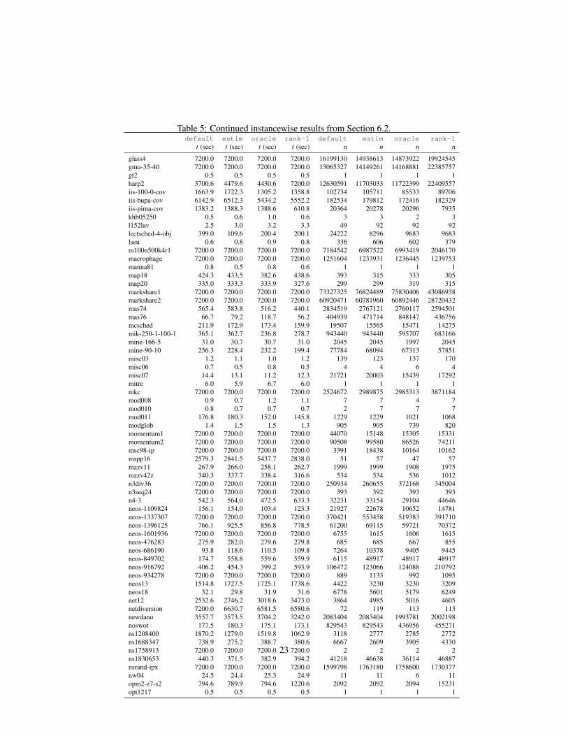
Table 5: Continued instancewise results from Section 6.2.default estim oracle rank-1 default estim oracle rank-1

t (sec) t (sec) t (sec) t (sec) n n n n

glass4 7200.0 7200.0 7200.0 7200.0 16199130 14938613 14873922 19924545gmu-35-40 7200.0 7200.0 7200.0 7200.0 13065327 14149261 14168881 22385757gt2 0.5 0.5 0.5 0.5 1 1 1 1harp2 3700.6 4479.6 4430.6 7200.0 12630591 11703033 11722399 22409557iis-100-0-cov 1663.9 1722.3 1305.2 1358.8 102734 105711 85533 89706iis-bupa-cov 6142.9 6512.3 5434.2 5552.2 182534 179812 172416 182329iis-pima-cov 1383.2 1388.3 1388.6 610.8 20364 20278 20296 7935khb05250 0.5 0.6 1.0 0.6 3 3 2 3l152lav 2.5 3.0 3.2 3.3 49 92 92 92lectsched-4-obj 399.0 109.6 200.4 200.1 24222 8296 9683 9683lseu 0.6 0.8 0.9 0.8 336 606 602 379m100n500k4r1 7200.0 7200.0 7200.0 7200.0 7184542 6987522 6993419 2046170macrophage 7200.0 7200.0 7200.0 7200.0 1251604 1233931 1236445 1239753manna81 0.8 0.5 0.8 0.6 1 1 1 1map18 424.3 433.5 382.6 438.6 393 315 333 305map20 335.0 333.3 333.9 327.6 299 299 319 315markshare1 7200.0 7200.0 7200.0 7200.0 73327325 76824489 75830406 43086938markshare2 7200.0 7200.0 7200.0 7200.0 60920471 60781960 60892446 28720432mas74 565.4 583.8 516.2 440.1 2834519 2767121 2760117 2594501mas76 66.7 79.2 118.7 56.2 404939 471714 848147 436756mcsched 211.9 172.9 173.4 159.9 19507 15565 15471 14275mik-250-1-100-1 365.1 362.7 236.8 278.7 943440 943440 595707 683166mine-166-5 31.0 30.7 30.7 31.0 2045 2045 1997 2045mine-90-10 256.3 228.4 232.2 199.4 77784 68094 67313 57851misc03 1.2 1.1 1.0 1.2 139 123 137 170misc06 0.7 0.5 0.8 0.5 4 4 6 4misc07 14.4 13.1 11.2 12.3 21721 20003 15439 17292mitre 6.0 5.9 6.7 6.0 1 1 1 1mkc 7200.0 7200.0 7200.0 7200.0 2524672 2989875 2985313 3871184mod008 0.9 0.7 1.2 1.1 7 7 4 7mod010 0.8 0.7 0.7 0.7 2 7 7 7mod011 176.8 180.3 152.0 145.8 1229 1229 1021 1068modglob 1.4 1.5 1.5 1.3 905 905 739 820momentum1 7200.0 7200.0 7200.0 7200.0 44070 15148 15305 15331momentum2 7200.0 7200.0 7200.0 7200.0 90508 99580 86526 74211msc98-ip 7200.0 7200.0 7200.0 7200.0 3391 18438 10164 10162mspp16 2579.3 2841.5 5437.7 2838.0 51 57 47 57mzzv11 267.9 266.0 258.1 262.7 1999 1999 1908 1975mzzv42z 340.3 337.7 338.4 316.6 534 534 536 1012n3div36 7200.0 7200.0 7200.0 7200.0 250934 260655 372168 345004n3seq24 7200.0 7200.0 7200.0 7200.0 393 392 393 393n4-3 542.3 564.0 472.5 633.3 32231 33154 29104 44646neos-1109824 156.1 154.0 103.4 123.3 21927 22678 10652 14781neos-1337307 7200.0 7200.0 7200.0 7200.0 370421 553458 519383 391710neos-1396125 766.1 925.5 856.8 778.5 61200 69115 59721 70372neos-1601936 7200.0 7200.0 7200.0 7200.0 6755 1615 1606 1615neos-476283 275.9 282.0 279.6 279.8 685 685 667 855neos-686190 93.8 118.6 110.5 109.8 7264 10378 9405 9445neos-849702 174.7 558.8 559.6 559.9 6115 48917 48917 48917neos-916792 406.2 454.3 399.2 593.9 106472 123066 124088 210792neos-934278 7200.0 7200.0 7200.0 7200.0 889 1133 992 1095neos13 1514.8 1727.5 1725.1 1738.6 4422 3230 3230 3209neos18 32.1 29.8 31.9 31.6 6778 5601 5179 6249net12 2532.6 2746.2 3018.6 3473.0 3864 4985 5016 4605netdiversion 7200.0 6630.7 6581.5 6580.6 72 119 113 113newdano 3557.7 3573.5 3704.2 3242.0 2083404 2083404 1993781 2002198noswot 177.5 180.3 175.1 173.1 829543 829543 436956 455271ns1208400 1870.2 1279.0 1519.8 1062.9 3118 2777 2785 2772ns1688347 738.9 275.2 388.7 380.6 6667 2609 3905 4330ns1758913 7200.0 7200.0 7200.0 7200.0 2 2 2 2ns1830653 440.3 371.5 382.9 394.2 41218 46638 36114 46887nsrand-ipx 7200.0 7200.0 7200.0 7200.0 1599798 1763180 1758600 1730377nw04 24.5 24.4 25.3 24.9 11 11 6 11opm2-z7-s2 794.6 789.9 794.6 1220.6 2092 2092 2094 15231opt1217 0.5 0.5 0.5 0.5 1 1 1 1

23

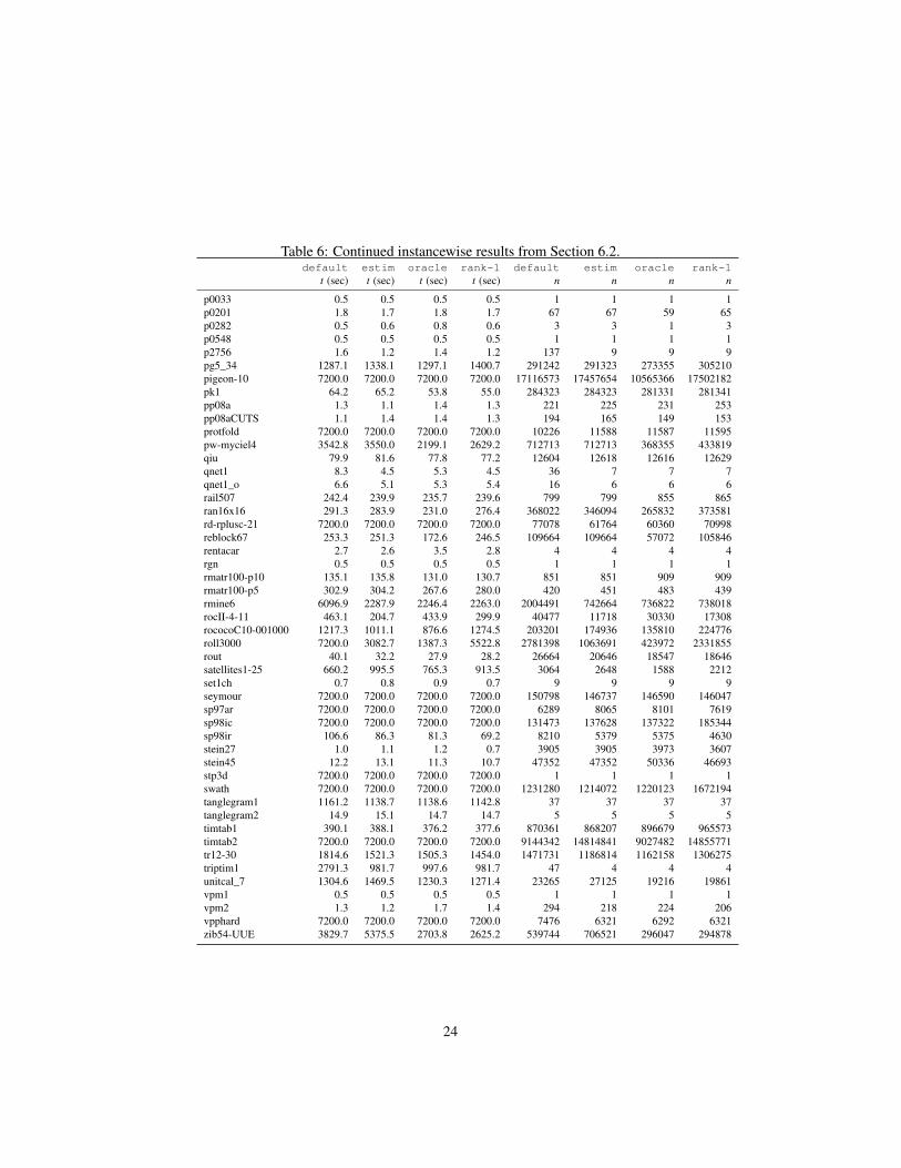
Table 6: Continued instancewise results from Section 6.2.default estim oracle rank-1 default estim oracle rank-1

t (sec) t (sec) t (sec) t (sec) n n n n

p0033 0.5 0.5 0.5 0.5 1 1 1 1p0201 1.8 1.7 1.8 1.7 67 67 59 65p0282 0.5 0.6 0.8 0.6 3 3 1 3p0548 0.5 0.5 0.5 0.5 1 1 1 1p2756 1.6 1.2 1.4 1.2 137 9 9 9pg5_34 1287.1 1338.1 1297.1 1400.7 291242 291323 273355 305210pigeon-10 7200.0 7200.0 7200.0 7200.0 17116573 17457654 10565366 17502182pk1 64.2 65.2 53.8 55.0 284323 284323 281331 281341pp08a 1.3 1.1 1.4 1.3 221 225 231 253pp08aCUTS 1.1 1.4 1.4 1.3 194 165 149 153protfold 7200.0 7200.0 7200.0 7200.0 10226 11588 11587 11595pw-myciel4 3542.8 3550.0 2199.1 2629.2 712713 712713 368355 433819qiu 79.9 81.6 77.8 77.2 12604 12618 12616 12629qnet1 8.3 4.5 5.3 4.5 36 7 7 7qnet1_o 6.6 5.1 5.3 5.4 16 6 6 6rail507 242.4 239.9 235.7 239.6 799 799 855 865ran16x16 291.3 283.9 231.0 276.4 368022 346094 265832 373581rd-rplusc-21 7200.0 7200.0 7200.0 7200.0 77078 61764 60360 70998reblock67 253.3 251.3 172.6 246.5 109664 109664 57072 105846rentacar 2.7 2.6 3.5 2.8 4 4 4 4rgn 0.5 0.5 0.5 0.5 1 1 1 1rmatr100-p10 135.1 135.8 131.0 130.7 851 851 909 909rmatr100-p5 302.9 304.2 267.6 280.0 420 451 483 439rmine6 6096.9 2287.9 2246.4 2263.0 2004491 742664 736822 738018rocII-4-11 463.1 204.7 433.9 299.9 40477 11718 30330 17308rococoC10-001000 1217.3 1011.1 876.6 1274.5 203201 174936 135810 224776roll3000 7200.0 3082.7 1387.3 5522.8 2781398 1063691 423972 2331855rout 40.1 32.2 27.9 28.2 26664 20646 18547 18646satellites1-25 660.2 995.5 765.3 913.5 3064 2648 1588 2212set1ch 0.7 0.8 0.9 0.7 9 9 9 9seymour 7200.0 7200.0 7200.0 7200.0 150798 146737 146590 146047sp97ar 7200.0 7200.0 7200.0 7200.0 6289 8065 8101 7619sp98ic 7200.0 7200.0 7200.0 7200.0 131473 137628 137322 185344sp98ir 106.6 86.3 81.3 69.2 8210 5379 5375 4630stein27 1.0 1.1 1.2 0.7 3905 3905 3973 3607stein45 12.2 13.1 11.3 10.7 47352 47352 50336 46693stp3d 7200.0 7200.0 7200.0 7200.0 1 1 1 1swath 7200.0 7200.0 7200.0 7200.0 1231280 1214072 1220123 1672194tanglegram1 1161.2 1138.7 1138.6 1142.8 37 37 37 37tanglegram2 14.9 15.1 14.7 14.7 5 5 5 5timtab1 390.1 388.1 376.2 377.6 870361 868207 896679 965573timtab2 7200.0 7200.0 7200.0 7200.0 9144342 14814841 9027482 14855771tr12-30 1814.6 1521.3 1505.3 1454.0 1471731 1186814 1162158 1306275triptim1 2791.3 981.7 997.6 981.7 47 4 4 4unitcal_7 1304.6 1469.5 1230.3 1271.4 23265 27125 19216 19861vpm1 0.5 0.5 0.5 0.5 1 1 1 1vpm2 1.3 1.2 1.7 1.4 294 218 224 206vpphard 7200.0 7200.0 7200.0 7200.0 7476 6321 6292 6321zib54-UUE 3829.7 5375.5 2703.8 2625.2 539744 706521 296047 294878

24