Intl. Trans. in Op. Res. 00 (2013) 1–11DOI: 10.1111/itor.12034

INTERNATIONALTRANSACTIONS

IN OPERATIONALRESEARCH

MIP-and-refine matheuristic for smart grid energymanagement

Matteo Fischetti, Giorgio Sartor and Arrigo Zanette

DEI, University of Padova, via Gradenigo 6/A, 35131 Padova, ItalyE-mail: matteo.fischetti@unipd.it [Fischetti]; gio.srt@gmail.com [Sartor]; zanettea@gmail.com [Zanette]

Received 13 December 2012; accepted 22 May 2013

Abstract

In the past years, we have witnessed an increasing interest in smart buildings, in particular for optimal energymanagement, renewable energy sources, and smart appliances. In this paper, we investigate the problem ofscheduling smart appliance operation in a given time horizon with a set of energy sources and accumulators.Appliance operation is modeled in terms of uninterruptible sequential phases with a given power demand,with the goal of minimizing the energy bill fulfilling duration, energy, and user preference constraints. Amixed-integer linear programming (MIP) model and greedy heuristic algorithm are given, which are used ina synergic way. We show how a general purpose (off-the-shelf) MIP-refining procedure can be effectively usedfor improving, in short computing time, the quality of the solutions provided by the initial greedy heuristic.Computational results confirm the viability of the overall approach, in terms of both solution quality andspeed.

Keywords: matheuristics; mixed-integer programming; refinement heuristics; energy management; smart houses

1. Prologue

Many successful matheuristic schemes use a black-box mixed integer linear programming (MIP)solver to generate high-quality heuristic solutions for difficult optimization problems. The hall-mark of this approach is the availability of an (possibly incomplete) MIP model, and an externalmetascheme that iteratively solves sub-MIPs obtained by introducing invalid constraints (e.g., vari-able fixings) defining “interesting” neighborhoods of certain solutions. The goal of the approach isto iteratively refine the incumbent solution, producing a sequence of improved feasible solutions inshort (or, at least, acceptable) computing times. The above solution-refinement approach is com-pletely general, that is, it can in principle be applied to the original MIP without the need of ad hocadaptations.

C© 2013 The Authors.International Transactions in Operational Research C© 2013 International Federation of Operational Research SocietiesPublished by John Wiley & Sons Ltd, 9600 Garsington Road, Oxford, OX4 2DQ, UK and 350 Main St, Malden, MA02148,USA.

2 M. Fischetti et al. / Intl. Trans. in Op. Res. 00 (2013) 1–11

The evolutionary “polishing method” of Rothberg (2007) is an example of a general MIP-refinement procedure. This method implements an evolutionary metaheuristic to be applied atselected nodes of a branch-and-bound tree. A fixed-size population of feasible solutions is main-tained. Iteratively, two or more “parent” solutions are combined with the aim of creating a new“son” member of the population. This is done by fixing all variables whose value coincides in theparent solutions and heuristically solving the resulting sub-MIP by invoking an external MIP solverfor a limited number of branch-and-bound nodes. Diversification is guaranteed by performing aclassical mutation operation that consists in (i) selecting at random a seed solution in the population,(ii) fixing at random some of its variables, and (iii) heuristically solving the resulting sub-MIP.

Interesting enough for practitioners, an off-the-shelf implementation of the polishing heuristicis available in some commercial MIP solvers, hence it can be readily used. In very difficult cases,however, the approach based on general MIP refinement is not successful, and one tends to designad hoc matheuristics that exploit the structure of the problem. As a matter of fact, the main issuewith the general approach is the lack of good (or even feasible) solutions to refine. In this context,one can argue that ad hoc heuristics and general MIP-refinement procedures are complementary toeach other; the former being typically able to find feasible solutions very quickly, whereas the lattercan exploit the underlying MIP model to improve them by reaching a quality degree that is difficultto attain otherwise.

In this paper, we show how the application of above scheme can lead to a very effective overallheuristic even in case a very simple greedy is used to feed an off-the-shelf general MIP-refinementmodule. The resulting “MIP-and-refine” approach is exemplified and tested in the context of smartgrid energy management whose underlying MIP models turn out to be very difficult to solve withoutthe hints provided by an external heuristic.

Although we cannot claim deep theoretical contributions, we hope that this paper can be used asa case study by researchers and practitioners working in the field of matheuristics, and the simplicityof the MIP-and-refine approach will make it one of the first options to be tried when approachinga new problem.

2. Introduction

Energy optimization is attracting a great interest among researchers as long as new “smarter”infrastructures and devices are going to replace the traditional ones. The most popular scenarioinvolves a new concept of electrical grid, the “smart grid” that allows to convey a two-way flowof electricity and information between central generators and customers (Fang et al., 2012). Smartgrid benefits are fully exploited only if the grid endpoints, home appliances for example, are smartas well. Smart appliances are able to exchange data with the grid, such as dynamic energy pricesand grid status. Along with user preferences, this information can be used to optimally manage theenergy demand in order to reduce the customer energy bill and prevent major blackouts. A commonway of addressing the demand side energy management problem is by solving a scheduling probleminvolving multiple appliances with different operational constraints, user preferences, renewableenergy sources, and batteries.

MIP models from the literature allow an effective mathematical formulation of the appliancescheduling problem. Barbato et al. (2011) also consider photovoltaic (PV) energy, and a linearized

C© 2013 The Authors.International Transactions in Operational Research C© 2013 International Federation of Operational Research Societies

M. Fischetti et al. / Intl. Trans. in Op. Res. 00 (2013) 1–11 3

description of battery charge states is presented. Sou et al. (2011) provide a detailed MIP formulationof appliance power profiles and operations, and model appliance operations as a set of sequentialuninterruptible phases with variable interphase delays. Other authors have investigated variantsof the appliance scheduling problem—Hatami and Pedram (2010) by considering the interactionamong different users, Zhang et al. (2011) by considering a so-called microgrid, and Agnetis et al.(2011) by addressing additional thermal comfort constraints.

As far as the solution of appliance scheduling problem is concerned, Carpentieri et al. (2012)propose a Linear Programming (LP) rounding heuristic for solving the appliance scheduling problemwith the goal of minimizing the maximum peak energy of multiple houses. Taking into account thereal parameters, Barbato and Carpentieri (2012) use different heuristics to address the problem ofonline schedule recovering an off-line schedule.

The rest of the paper is organized as follows. In Sections 3 and 4, we describe only two ingredientsof our recipe: the MIP model and a simple greedy heuristic, respectively. Computational results arethen presented in Section 5, while some conclusions are drawn in Section 6. The present work isbased on the dissertation of the second author (Sartor, 2012).

3. Our MIP model

Following Sou et al. (2011), we model appliance operations as a set of sequential uninterruptibleenergy phases, each of which uses a total amount of given electric energy. For example, typicalwashing machine phases are prewash, wash, rinse, and spinning. The set of phases is also called the“power profile” of the appliance.

Depending on the appliance, phase duration may vary, as long as there is an interphase delay (e.g.,the spinning of the washing machine must start within 10 minutes of the rinsing being finished).The total energy given for a phase can be evenly distributed over time, or it may vary. We model thelatter case with per-phase bounds on the instantaneous power consumption. Besides the intrinsicoperational constraints, we allow the user to specify preferences for the time interval in which anappliance should run (e.g., start the washing machine between 4:00 p.m. and 6:00 p.m.).

Following Barbato et al. (2011), we have modeled three classes of energy sources: power grid,domestic renewable energy, and accumulators (batteries). The power grid advertises the maximumamount of available energy (peak power) for each time instant. Note that this peak power can bedifferent from the actual user contract maximum power. In fact, a common feature in the smart gridparadigm is to dynamically advertise (i.e., broadcast) the peak power depending on the grid state, inorder to let users adjust their demands for preventing more dangerous power outages. Along withthe peak power, the cost of energy also changes with time. For example, in the Italian market itcan vary between two values depending on the time of the day and day of the week. More dynamicpower grids allow for a finer grain price adjustment (hourly or less).

Domestic renewable energy sources provide free energy but with a limited availability. For example,the performance of a PV plant depends on geographical position, weather conditions, and time.Accumulators allow to store energy (from grid or other sources) when energy price is low, anduse it later when energy price is higher. This feature represents an important degree of freedomas far as optimization is concerned. Our model only deals with batteries, viewed as direct electricenergy accumulators; however, it can trivially be extended to other types of energy accumulators

C© 2013 The Authors.International Transactions in Operational Research C© 2013 International Federation of Operational Research Societies

4 M. Fischetti et al. / Intl. Trans. in Op. Res. 00 (2013) 1–11

(e.g., boilers for thermic energy). Finally, the optimization goal is to minimize the total energy costby finding a proper allocation of all appliance phases.

Given two integers a and b, let [a, b] denote the discrete set {a, a+ 1, . . . , b}. We discretize thescheduling time horizon into m uniform time slots, indexed by k ∈ [1, m]. The phases for eachappliance i ∈ [1, N] are denoted by j ∈ [1, ni]. To simplify notation, in what follows, we write ∀i, jinstead of ∀i ∈ [1, N], j ∈ [1, ni], and ∀k instead of ∀k ∈ [1, m].

In our model, non-negative continuous variables pki j represent the energy assigned to phase j of

appliance i during time slot k. The typical unit for pki j is Watt (W) per time slot (energy). With

binary variables xki j , sk

i j , and tki j , we model the allocation of a time slot k for phase j of appliance i.

In particular, xki j = 1 iff phase j of appliance i is allocated in time slot k. Variable sk

i j jumps from 0to 1 right after the last time slot of where the phase j of appliance i is allocated, and is defined bythe equations

xk−1i j − xk

i j ≤ ski j ∀ i, j,∀k ∈ [2, m], (1a)

sk−1i j ≤ sk

i j ∀ i, j,∀k ∈ [2, m]. (1b)

Instead, tki j is 1 iff there is an interphase delay between phase j − 1 and j in time slot k, and is

defined as

tki j = sk

i( j−1) −(xk

i j + ski j

) ∀i, k,∀ j ∈ [2, ni].

Figure 1 illustrates the meaning of the above variables in a simple case of an appliance with twophases: the first phase is allocated between 2 and 6 hours, and the second between 14 and 16 hours(the day being divided into 12 time slots).

Our model also uses non-negative continuous variables zk and yk to represent the amount of totalenergy sold and bought in each time slot k, respectively. Then, if ck and gk denote the input cost ofbought and sold electricity during time slot k, respectively, our MIP model calls for

z = minm∑

k=1

(ckyk − gkzk) (2)

subject to the following constraints.Phase energy: It ensures that the energy allocated during phase j of appliance i meets the given

phase total energy Ei j

m∑

k=1

pki j = Ei j ∀ i, j. (3)

Energy bounds: It ensures that the energy allocated in phase j for appliance i in any time slot kbelongs to the allowed range [ Pi j, Pi j ]

Pi j xki j ≤ pk

i j ≤ Pi j xki j ∀ i, j,∀k. (4)

C© 2013 The Authors.International Transactions in Operational Research C© 2013 International Federation of Operational Research Societies

M. Fischetti et al. / Intl. Trans. in Op. Res. 00 (2013) 1–11 5

Fig. 1. Example of binary variables xki j , sk

i j , and tki j .

Power safety: It guarantees that the total energy assigned in time slot k does not exceed the peakpower limit

yk ≤ Pkpeak ∀ k, (5)

where Pkpeak is the peak limit of slot k; this constraint can also be used to model additional unsched-

uled power demands that reduce the available grid energy in time slot k.Energy phase duration:

T i j ≤m∑

k=1

xki j ≤ T i j ∀ i, j, (6)

where T i j and T i j represent, respectively, the lower and upper bounds on the number of time slotsto allocate for phase j of appliance i.Uninterruptible phase: These constraints ensure that all time slots of phase j are allocated contigu-ously (i.e., when an energy phase starts, it must finish without interruptions).

xki j + sk

i j ≤ 1 ∀ i, j, k. (7)

Recall that ski j is 0 before the last time slot allocated for phase j and appliance i, and becomes 1

afterwards 1a until the end 1b. Thus, constraint 7 prevents the variable xki j to be 1 after the last-phase

time slot.

C© 2013 The Authors.International Transactions in Operational Research C© 2013 International Federation of Operational Research Societies

6 M. Fischetti et al. / Intl. Trans. in Op. Res. 00 (2013) 1–11

Sequential processing: Previous energy phase must end before a new one starts

xki j ≤ sk

i( j−1) ∀ i, k, ∀ j ∈ [2, ni]. (8)

Interphase delay duration:

Di j ≤m∑

k=1

tki j ≤ Di j ∀ i, ∀ j ∈ [2, ni], (9)

where Di j and Di j are the minimum and maximum number of time slots between phases j − 1 andj of the appliance i.User time preferences: Disable phase allocation of appliance i in the given time slots

xki j ≤ T Pk

i ∀ i, j, k, (10)

where T Pki is equal to 0 iff phase j of appliance i cannot be allocated in time slot k.

In order to model batteries behavior, we need two extra binary variables wkc and wk

d , where wkc is

equal to 1 if the battery is charging in time slot k and 0 otherwise, while wkd is equal to 1 if the battery

is discharging in time slot k and 0 otherwise. Moreover, with the non-negative continuous variablesvk

c and vkd , we describe the charge and discharge rates, respectively, that is the amount of energy that

is charged/discharged in time slot k. The total accumulated energy in time slot k is described by thenon-negative continuous variable ek.Battery usage constraint: The battery cannot charge and discharge at the same time.

wkc + wk

d ≤ 1 ∀ k. (11)

Battery charge/discharge rate bounds:

vkc ≤ vmax

c wkc ∀ k (12a)

vkd ≤ vmax

d wkd ∀ k, (12b)

where vmaxc and vmax

d denote the maximum charge and discharge rates, respectively.Battery energy function: This is linearization of the actual charge/discharge curves

ek = ek−1 + ηcvkc − ηd vk

d ∀ k, (13)

where ηc and ηd are, respectively, the charging and discharging efficiency.Battery capacity bounds: These are used to limit the energy stored in the battery

γ min ≤ ek ≤ γ max ∀ k, (14)

where γ max and γ min represent the maximum capacity and minimum energy safety value (required,e.g., by lithium batteries).Balancing constraint: It balances between produced and consumed energy

yk + πk + vkd = zk +

N∑

i=1

ni∑

j=1

pki j + vk

c ∀ k, (15)

where πk is the sum of the renewable domestic power sources contribution in time slot k.

C© 2013 The Authors.International Transactions in Operational Research C© 2013 International Federation of Operational Research Societies

M. Fischetti et al. / Intl. Trans. in Op. Res. 00 (2013) 1–11 7

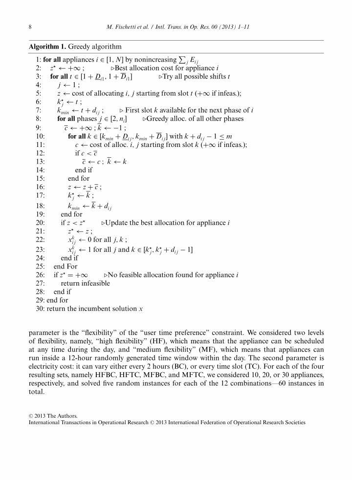
4. A greedy algorithm

In this section, we describe a heuristic greedy algorithm for finding good feasible solutions ofthe described problem, which we apply in a multistart fashion. According to a greedy policy, thealgorithm schedule appliances in decreasing priority—once an appliance has been scheduled, itcannot be changed, and all other appliances are allocated on top of the current partial solution.In the first application of the greedy, we use energy requirements as appliance priorities. In thesubsequent runs, the priority vector is shifted to generate different solutions. For each appliance, welook for a feasible allocation of its phases according to the following rules. We consider a simplified(more restricted) version of the problem, where the duration di j (say) of each phase is minimumbetween T i j and �Ei j/Pi j�, and bounds 4 become pk

i j = xki jEi j/di j for all k.

Accordingly, every phase has a constant duration and energy consumption, and can be scheduledin the time slots interval [1, m− dmin

i ], where dmini =∑ni

j=1 di j represents the minimum duration of acomplete appliance power profile (i.e., without phase delays). To be more specific, once a phase hasbeen allocated, we look for all possible allocations of the next phase in the range given by [Di j, Di j ],see 9, and select the most profitable one. Our allocation procedure enforces the user preferences ontime slots 10 and three other constraints: power safety 5, uninterruptible phase 7, and sequentialprocessing 8.

A pseudocode of our heuristic is given in Algorithm 1. We have an external loop (starting afterline 1) where appliances i are scheduled one after the other. For each appliance i, we consider allpossible “shifts” t for the starting slot of the first phase (line 3), and then consider a straightforwardgreedy (lines 8–19) to find the best starting slot k�

j of all other phases j. Variable kmin gives the firstslot k currently available for allocation: it is initialized at line 7 after the allocation of the first phase,then it is updated at line 18 after the allocation of each new phase.

Recall that we consider a simplified phase allocation whose duration di j is a constant, so the “costof allocating i, j starting from slot k” at lines 5 and 11 refers to the solution with xh

i j = 1 for allh ∈ [k, k+ di j − 1], and also takes user preferences into account.

When all possible shifts t have been tried, z� gives the cost of the (heuristically) best assignment forall phases of i, the corresponding solution being stored in the incumbent x. At line 27, if no feasiblephase allocation was found for appliance i (case z� = +∞), the overall problem is heuristicallyconsidered to be infeasible and the greedy is aborted—although this situation can occur if theconstraints are very tight, it never occurred in our tests.

According to time complexity, the most time-consuming step is the cost evaluation at line 11,which takes O(dmax) time, where dmax = maxi j di j . This step is executed, for each appliance i andeach shift t, at most nmaxDmax times, where nmax = maxi ni and Dmax = maxi j{Di j −Di j + 1 : j ≥ 2}.As we have N appliances i and O(m) possible shifts t, the overall time complexity of our heuristicis O(NnmaxDmaxdmaxm).

5. Computational results

In our tests, we considered a time horizon of 24 hours, subdivided in 96 time slots of 15 min-utes each. Experiments were grouped into four sets according to two main parameters. The first

C© 2013 The Authors.International Transactions in Operational Research C© 2013 International Federation of Operational Research Societies

8 M. Fischetti et al. / Intl. Trans. in Op. Res. 00 (2013) 1–11

Algorithm 1. Greedy algorithm

1: for all appliances i ∈ [1, N] by nonincreasing∑

j Ei j2: z�←+∞ ; �Best allocation cost for appliance i3: for all t ∈ [1+Di1, 1+Di1] �Try all possible shifts t4: j ← 1 ;5: z← cost of allocating i, j starting from slot t (+∞ if infeas.);6: k�

j ← t ;7: kmin ← t + di j ; � First slot k available for the next phase of i8: for all phases j ∈ [2, ni] �Greedy alloc. of all other phases9: c←+∞ ; k←−1 ;10: for all k ∈ [kmin +Di j, kmin +Di j ] with k+ di j − 1 ≤ m11: c← cost of alloc. i, j starting from slot k (+∞ if infeas.);12: if c < c13: c← c ; k← k14: end if15: end for16: z← z+ c ;17: k�

j ← k ;

18: kmin ← k+ di j19: end for20: if z < z� �Update the best allocation for appliance i21: z�← z ;22: xk

i j ← 0 for all j, k ;23: xk

i j ← 1 for all j and k ∈ [k�j, k�

j + di j − 1]24: end if25: end For26: if z� = +∞ �No feasible allocation found for appliance i27: return infeasible28: end if29: end for30: return the incumbent solution x

parameter is the “flexibility” of the “user time preference” constraint. We considered two levelsof flexibility, namely, “high flexibility” (HF), which means that the appliance can be scheduledat any time during the day, and “medium flexibility” (MF), which means that appliances canrun inside a 12-hour randomly generated time window within the day. The second parameter iselectricity cost: it can vary either every 2 hours (BC), or every time slot (TC). For each of the fourresulting sets, namely HFBC, HFTC, MFBC, and MFTC, we considered 10, 20, or 30 appliances,respectively, and solved five random instances for each of the 12 combinations—60 instances intotal.

C© 2013 The Authors.International Transactions in Operational Research C© 2013 International Federation of Operational Research Societies

M. Fischetti et al. / Intl. Trans. in Op. Res. 00 (2013) 1–11 9

A constant price of the sold PV energy was considered, which was equal to half of the minimumcost of the bought energy. All the other model parameters were taken from uniform randomdistributions: ck ∈ [2, 4], j ∈ [2, 5], Ei j ∈ [400, 800], Pi j ∈ [50, 80], Pi j ∈ [400, 800], T i j ∈ [1, 2], T i j ∈[3, 5], and Pk

peak ∈ [2400, 2600]. For all appliances i, we set Di j = 0 for all j, and Di j ∈ [4, 6] (if j ≥ 2)or Di j = m−∑

t dit (if j = 1).We considered a single renewable PV power source whose provided energy is sampled from a

Gaussian distribution N (μ, σ ) with mean μ = 52 (1:00 p.m., the period of maximum productionat the latitude of Italy), standard deviation σ = 10, and maximum value of 1250 W per timeslot. The considered battery has a capacity γ max = 500 W per time slot and charge/discharge ratesvmax

c = vmaxd = 50 W per time slot, with efficiencies ηc = ηd = 1.

We compared four different solution approaches, all run in single-thread mode:

� Greedy-alone: Our stand-alone greedy algorithm without multistart enhancement.� Greedy: Our greedy algorithm applied N times by starting from the N possible shifts of the

initial priority vector, taking the best solution found and storing the others.� CPLEX: The state-of-the-art IBM ILOG CPLEX MIP 12.4 solver used as a black box, with its

default setting, stopped as soon as the first feasible solution is found.� CPLEX + Polish: CPLEX’s polishing refining heuristic (Rothberg, 2007) applied immediately

after the root node and for a total of 10 nodes (all cuts disabled), when starting from the feasiblesolution found by the previous CPLEX algorithm.

� Greedy + Polish: Our proposed MIP-and-refine scheme, that is, the previousCPLEX + Polish algorithm but starting from the list of all feasible solutions found byGreedy.

Note that the last three methods also return a lower bound on the optimal value hence, as abyproduct, they can provide a proof of optimality in some (easy) cases. This is true, in particular,when the root–node lower bound is very tight and the method starts with an (almost) optimalGreedy solution, meaning that just few branching nodes need to be explored.

According to Table 1, Greedy + Polish outperforms its competitors. As expected, Greedy-alone is always able to provide feasible solutions in very short computing times. In spite of itsgreedy nature, the solution quality is fair in many cases, in particular in the easiest scenarios wherethe greedy solution often turns out to be optimal. Nevertheless, for more difficult scenarios, there isroom for big improvements—also because of the contribution of batteries that are exploited by theMIP model but not by the greedy.

As to CPLEX, it has a great difficulty even in finding its first feasible solution—a task thattakes a huge amount of time in the difficult cases. Significantly improved solutions are found byCPLEX + Polish, thus confirming the effectiveness of this heuristic. However, the full power ofMIP refinement is only exploited when Greedy + Polish comes into play. This is due to twomain factors: the speed of the greedy and the fact that several diversified solutions are passed to thepolishing method.

Of course, we cannot claim that Greedy + Polish would outperform more sophisticatedheuristic approaches from the literature on similar problems—for that, much more extensive com-putational comparisons would be needed. However, we believe our computational results support

C© 2013 The Authors.International Transactions in Operational Research C© 2013 International Federation of Operational Research Societies

10 M. Fischetti et al. / Intl. Trans. in Op. Res. 00 (2013) 1–11

Table 1Percentage cost increase (% Incr) with respect to the Greedy-alone algorithm, and computing time (in CPU seconds);a negative increase corresponds to a better solution w.r.t. Greedy-alone

Greedy CPLEX CPLEX + Polish Greedy + Polish

Set % Incr % STD Time % Incr % STD Time % Incr % STD Time % Incr % STD Time

HFBC 10 0.0 5 0.0 0.5 252.9 193.4 56.8 72.7 2 95.6 94.9 0.0 5 0.0 0.6HFBC 20 −0.5 0.5 2.4 50.2 80.4 3,054.4 13.4 41.2 3,223.2 −9.4 4.8 262.0HFBC 30 −0.6 0.5 6.4 1.8 4.7 9,585.8 −5.1 3.4 9,966.5 −6.1 1 3.2 310.2HFTC 10 0.0 5 0.0 0.4 94.0 129.2 49.0 47.0 4 94.1 83.4 0.0 5 0.0 0.6HFTC 20 −1.7 1.2 2.3 58.0 49.9 2,213.0 −1.4 21.3 2,387.4 −22.2 1 1.8 154.7HFTC 30 −0.6 0.3 6.6 −12.3 1.4 46,439.1 −19.0 2.6 46,904.7 −21.2 1 2.5 617.7MFBC 10 0.0 5 0.0 0.3 157.3 1 146.7 5.2 38.8 2 51.4 15.4 0.0 5 0.0 1.3MFBC 20 −3.0 2.2 1.5 160.1 45.9 35.2 24.4 24.2 90.0 −13.8 7.8 100.8MFBC 30 −0.8 0.5 3.7 44.4 11.5 65.1 0.7 8.3 164.5 −11.7 1 4.5 67.4MFTC 10 0.0 5 0.0 0.3 159.9 89.5 5.6 33.5 1 24.8 18.8 0.0 5 0.0 1.5MFTC 20 −1.2 1.2 1.5 54.8 21.8 52.5 −8.4 13.6 114.2 −23.5 1 2.6 54.6MFTC 30 −1.0 0.3 3.7 16.2 24.8 117.8 −14.0 6.1 232.7 −22.0 1.6 112.0

The reported values are arithmetic means over five random instances. Column % STD gives the percentage standard deviationof cost increase. Computing times for Greedy-alone are just negligible. Superscript k means proven optimality for k of fiveinstances (proof of optimality, when available, being obtained by any of the exact methods).

the message of this paper—sound matheuristics can be built around a simple greedy and an off-the-shelf MIP-refinement procedure.

6. Conclusions

A simple MIP-and-refine matheuristic framework has been addressed, where a greedy heuristic isused to trigger a general purpose MIP-refinement procedure. Computational results on a smartgrid energy management problem have been presented, showing that the method produces soundresults.

The approach is based on two ingredients: an initial heuristic and MIP model. The heuristic neednot be very effective, as its role is just to initialize a pool of feasible solutions—the more diversifiedthe better. The MIP model itself need not be very sophisticated, as it is automatically resized by thegeneral purpose MIP-refinement procedure. Nevertheless, the combination of the two can be muchmore effective than the sum of its parts, in the sense that the two modules work in a highly synergicway and can produce outcomes whose solution quality can only be matched by sophisticated ad hocheuristics.

Future research on the topic will hopefully confirm the viability of the approach on other classesof very difficult problems.

Acknowledgments

The research of the first author was supported by the “Progetto di Ateneo” on “ComputationalInteger Programming” of the University of Padova and by MiUR, Italy (PRIN project “IntegratedApproaches to Discrete and Nonlinear Optimization”).

C© 2013 The Authors.International Transactions in Operational Research C© 2013 International Federation of Operational Research Societies

M. Fischetti et al. / Intl. Trans. in Op. Res. 00 (2013) 1–11 11

References

Agnetis, A., Dellino, G., Detti, P., Innocenti, G., De Pascale, G., Vicino, A., 2011. Appliance operation schedulingfor electricity consumption optimization. 50th IEEE Conference on Decision and Control and European ControlConference (CDC-ECC), December 12–15, Orlando, FL, pp. 5899–5904.

Barbato, A., Capone, A., Carello, G., Delfanti, M., Merlo, M., Zaminga, A., 2011. House energy demand optimization insingle and multi-user scenarios. 2nd IEEE International Conference on Smart Grid Communications, SmartGridComm’11, Brussels, Belgium, October.

Barbato, A., Carpentieri, G., 2012. Model and algorithms for the real time management of residential electricity demand.IEEE International Conference and Exhibition, ENERGYCON ’12, Florence, Italy, September.

Carpentieri, G., Carello, G., Amaldi, E., 2012. Optimization models for residential energy load management. Atti delleGiornate AIRO, Vietri.

Fang, X., Misra, S., Xue, G., , 2012. Smart grid—the new and improved power grid: a survey. IEEE CommunicationsSurveys and Tutorials (COMST), 14, 944–980.

Hatami, S., Pedram, M., 2010. Minimizing the electricity bill of cooperative users under a quasi-dynamic pricing model.SmartGridComm(tm)10, pp. 421–426.

Rothberg, E., 2007. An evolutionary algorithm for polishing mixed integer programming solutions. INFORMS Journalon Computing, 19, 4, 534–541.

Sartor, G., 2012. Optimal scheduling of smart home appliances using mixed-integer linear programming. Master’s thesis,DEI, University of Padova.

Sou, K.C., Weimer, J., Sandberg, H., Johansson, K.H., 2011. Scheduling smart home appliances using mixed integer linearprogramming. 50th IEEE Conference on Decision and Control and European Control Conference (CDC-ECC),December 12–15, Orlando, FL, pp. 5144–5149.

Zhang, D., Papageorgiou, L.G., Samsatli, N.J., Shah, N., 2011. Optimal scheduling of smart homes energy consumptionwith microgrid. ENERGY 2011, The First International Conference on Smart Grids, Green Communications andIT Energy-aware Technologies, pp. 70–75.

C© 2013 The Authors.International Transactions in Operational Research C© 2013 International Federation of Operational Research Societies