Correlation Analysis of Spatial Time SeriesDatasets: A Filter-and-Re�ne Approa hPusheng Zhang?, Yan Huang, Shashi Shekhar??, and Vipin Kumar??Computer S ien e & Engineering Department, University of Minnesota,200 Union Street SE, Minneapolis, MN 55455, U.S.A.[pusheng|huangyan|shekhar|kumar℄� s.umn.eduAbstra t. A spatial time series dataset is a olle tion of time series,ea h referen ing a lo ation in a ommon spatial framework. Correlationanalysis is often used to identify pairs of potentially intera ting elementsfrom the ross produ t of two spatial time series datasets. However, the omputational ost of orrelation analysis is very high when the dimen-sion of the time series and the number of lo ations in the spatial frame-works are large. The key ontribution of this paper is the use of spatialauto orrelation among spatial neighboring time series to redu e ompu-tational ost. A �lter-and-re�ne algorithm based on oning, i.e. groupingof lo ations, is proposed to redu e the ost of orrelation analysis over apair of spatial time series datasets. Cone-level orrelation omputation an be used to eliminate (�lter out) a large number of element pairs whose orrelation is learly below (or above) a given threshold. Element pair orrelation needs to be omputed for remaining pairs. Using experimen-tal studies with Earth s ien e datasets, we show that the �lter-and-re�neapproa h an save a large fra tion of the omputational ost, parti ularlywhen the minimal orrelation threshold is high.

1 Introdu tionSpatio-temporal data mining [14, 16, 15, 17, 13, 7℄ is important in many appli- ation domains su h as epidemiology, e ology, limatology, or ensus statisti s,where datasets whi h are spatio-temporal in nature are routinely olle ted. Thedevelopment of eÆ ient tools [1, 4, 8, 10, 11℄ to explore these datasets, the fo usof this work, is ru ial to organizations whi h make de isions based on largespatio-temporal datasets.A spatial framework [19℄ onsists of a olle tion of lo ations and a neighborrelationship. A time series is a sequen e of observations taken sequentially in? The onta t author. Email: pusheng� s.umn.edu. Tel: 1-612-626-7515?? This work was partially supported by NASA grant No. NCC 2 1231 and by ArmyHigh Performan e Computing Resear h Center ontra t number DAAD19-01-2-0014. The ontent of this work does not ne essarily re e t the position or poli yof the government and no oÆ ial endorsement should be inferred. AHPCRC andMinnesota Super omputer Institute provided a ess to omputing fa ilities.

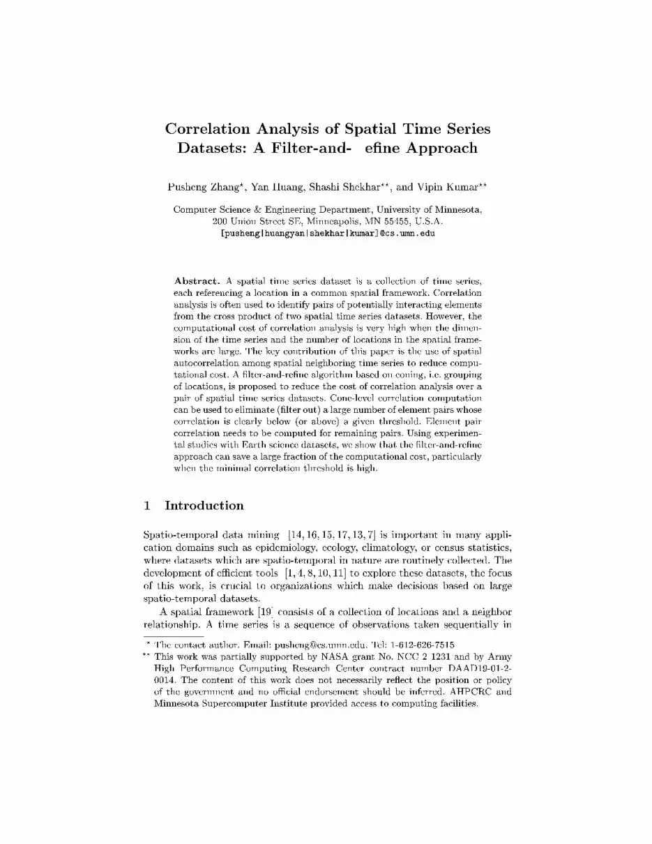
time [2℄. A spatial time series dataset is a olle tion of time series, ea h refer-en ing a lo ation in a ommon spatial framework. For example, the olle tionof global daily temperature measurements for the last 10 years is a spatial timeseries dataset over a degree-by-degree latitude-longitude grid spatial frameworkon the surfa e of the Earth.D 1

1D 2

1

D1

D 3

1D 4

1

D2

D 2

2

D 1

2

D 2

1D 1

2

t t

t

t

t

t t

tFig. 1. An Illustration of the Correlation Analysis of Two Spatial Time Series DatasetsCorrelation analysis is important to identify potentially intera ting pairs oftime series a ross two spatial time series datasets. A strongly orrelated pair oftime series indi ates potential movement in one series when the other time seriesmoves. For example, El Nino, the anomalous warming of the eastern tropi alregion of the Pa i� , has been linked to limate phenomena su h as droughtsin Australia and heavy rainfall along the Eastern oast of South Ameri a [18℄.Fig. 1 illustrates the orrelation analysis of two spatial time series datasets D1and D2. D1 has 4 spatial lo ations and D2 has 2 spatial lo ations. The rossprodu t of D1 and D2 has 8 pairs of lo ations. A highly orrelated pair, i.e.(D12,D21), is identi�ed from the orrelation analysis of the ross produ t of thetwo datasets.However, a orrelation analysis a ross two spatial time series datasets is om-putationally expensive when the dimension of the time series and number oflo ations in the spa es are large. The omputational ost an be redu ed by re-du ing time series dimensionality or redu ing the number of time series pairs tobe tested, or both. Time series dimensionality redu tion te hniques in lude dis- rete Fourier transformation [1℄, dis rete wavelet transformation [4℄, and singularve tor de omposition [6℄.The number of pairs of time series an be redu ed by a one-based �lter-and-re�ne approa h whi h groups together similar time series within ea h dataset.A �lter-and-re�ne approa h has two logi al phases. The �ltering phase groupssimilar time series as ones in ea h dataset and al ulates the entroids andboundaries of ea h one. These one parameters allow omputation of the upperand lower bounds of the orrelations between the time series pairs a ross ones.Many All-True and All-False time series pairs an be eliminated at the one levelto redu e the set of time series pairs to be tested by the re�nement phase. Wepropose to exploit an interesting property of spatial time series datasets, namelyspatial auto- orrelation [5℄, whi h provides a omputationally eÆ ient method todetermine ones. Experiments with Earth s ien e data [12℄ show that the �lter-and-re�ne approa h an save a large fra tion of omputational ost, espe ially

when the minimal orrelation threshold is high. To the best of our knowledge,this is the �rst paper exploiting spatial auto- orrelation among time series atnearby lo ations to redu e the omputational ost of orrelation analysis over apair of spatial time series datasets.S ope and Outline: In this paper, the omputation saving methods fo us onredu tion of the time series pairs to be tested. Methods based on non-spatialproperties (e.g. time-series power spe trum [1, 4, 6℄) are beyond the s ope of thepaper and will be addressed in future work.The rest of the paper is organized as follows. In Se tion 2, the basi on eptsand lemmas related to one boundaries are provided. Se tion 3 proposes our�lter-and-re�ne algorithm, and the experimental design and results are presentedin Se tion 4. We summarize our work and dis uss future dire tions in Se tion 5.2 Basi Con eptsIn this se tion, we introdu e the basi on epts of orrelation al ulation andthe multi-dimensional unit sphere formed by normalized time series. We de�nethe one on ept in the multi-dimensional unit sphere and prove two lemmas tobound the orrelation of pairs of time series from two ones.2.1 Correlation and Test of Signi� an e of CorrelationLet x = hx1; x2; : : : ; xmi and y = hy1; y2; : : : ; ymi be two time series of lengthm. The orrelation oeÆ ient [3℄ of the two time series is de�ned as: orr(x; y) = 1m� 1 mXi=1(xi � x�x )� (yi � y�y ) = bx� bywhere x = Pmi=1 xim , y = Pmi=1 yim , �x = qPmi=1(xi�x)2m�1 , �y = qPmi=1(yi�x)2m�1 , bxi =1pm�1 xi�x�x , byi = 1pm�1 yi�y�y , bx = hbx1; bx2; : : : ; bxmi, and by = hby1; by2; : : : ; bymi.A simple method to test the null hypothesis that the produ t moment or-relation oeÆ ient is zero an be obtained using a Student's t-test [3℄ on the tstatisti as follows: t = pm� 2 rp1�r2 , where r is the orrelation oeÆ ient be-tween the two time series. The freedom degree of the above test is m� 2. Usingthis we an �nd a p � value or �nd the riti al value for a test at a spe i�edlevel of signi� an e. For a dataset with larger length m, we an adopt Fisher'sZ-test [3℄ as follows: Z = 12 log 1+r1�r , where r is the orrelation oeÆ ient betweenthe two time series. The orrelation threshold an be determined for a given timeseries length and on�den e level2.2 Multi-dimensional Sphere Stru tureIn this subse tion, we dis uss the multi-dimensional unit sphere representationof time series. The orrelation of a pair of time series is related to the osinemeasure between their unit ve tor representations in the unit sphere.

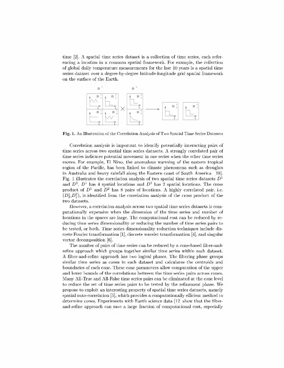
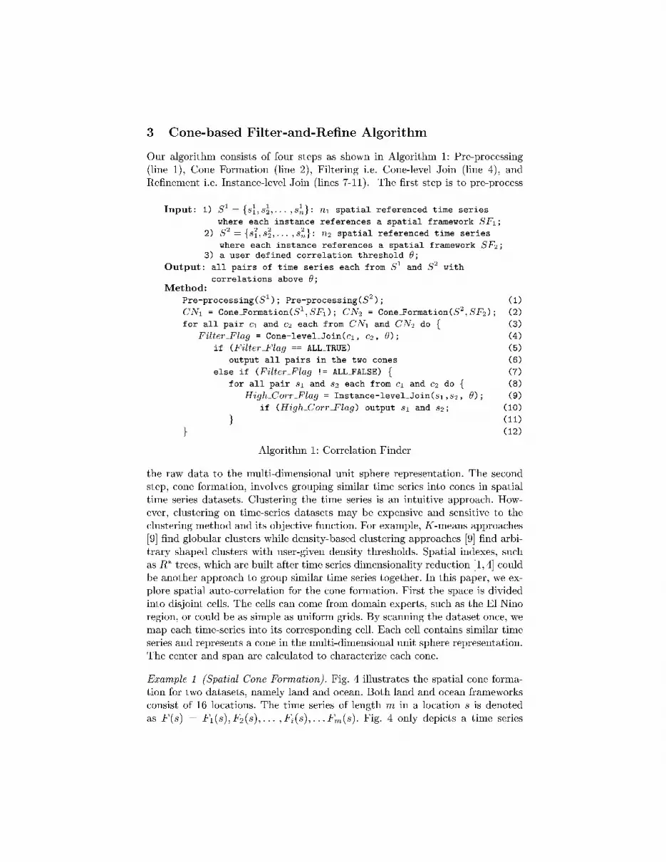
Fa t 1 (Multi-dimensional Unit Sphere Representation) Let x =hx1; x2; : : : ; xmi and y = hy1; y2; : : : ; ymi be two time series of length m. Let bxi =1pm�1 xi�x�x , byi = 1pm�1 yi�y�y , bx = hbx1; bx2; : : : ; bxmi, and by = hby1; by2; : : : ; bymi.Then bx and by are lo ated on the surfa e of a multi-dimensional unit sphere and orr(x; y) = bx� by = os(\(bx; by)) where \(bx; by) is the angle of bx and by in [0; 180Æ℄in the multi-dimensional unit sphere .Be ause the sum of the bxi2 is equal to 1:Pmi=1 bxi2 =Pmi=1( 1pm�1 xi�xrPmi=1(xi�x)2m�1 )2= 1, bx is lo ated in the multi-dimensional unit sphere. Similarly, by is also lo atedin the multi-dimensional unit sphere. Based on the de�nition of orr(x; y), wehave orr(x; y) = bx� by = os(\(bx; by)).Fa t 2 (Correlation and Cosine) Given two time series x and y and auser spe i�ed minimal orrelation threshold � where 0 < � � 1, j orr(x; y)j =j os(\(bx; by))j � � if and only if 0 � \(bx; by) � �a or 180Æ� �a � \(bx; by) � 180Æ,where �a = ar os(�).

Angle

Co

rre

latio

n

arccos(θ)

θ

−θ

180°− arccos(θ)

0

0°180°

1

−1 Fig. 2. Cosine Value vs. CentralAngle

φ

y’x’

360 -

(c)

(b)

(a)

x’ y’φ

γmin

γmax

min

maxγ

γ

O

Cone Cone

δ

Q2

2 Q

1

P2C1C

1 2

P

maxγ

min

1

γ

maxγ

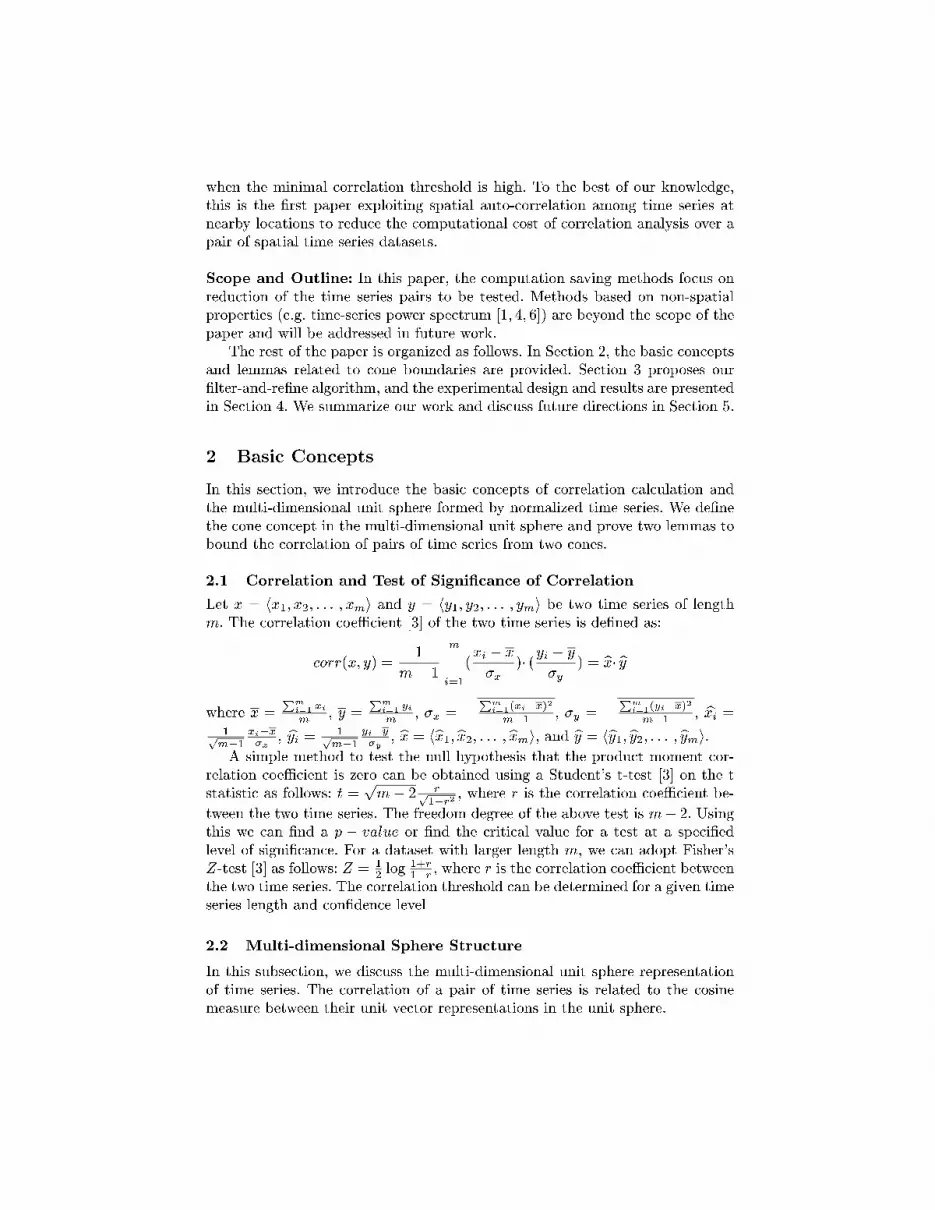
Fig. 3. Angle of Time Series in Two Spheri alConesFig. 2 shows that j orr(x; y)j = j os(\(bx; by))j falls in the range of [�; 1℄or [�1;��℄ if and only if \(bx; by) falls in the range of [0; ar os(�)℄ or [180Æ �ar os(�); 180Æ℄.The orrelation of two time series is dire tly related to the angle between thetwo time series in the multi-dimensional unit sphere. Finding pairs of time serieswith an absolute value of orrelation above the user given minimal orrelationthreshold � is equivalent to �nding pairs of time series bx and by on the unit multi-dimensional sphere with an angle in the range of [0, �a℄ or [180Æ � �a; 180Æ℄.2.3 Cone and Correlation between a Pair of ConesThis subse tion formally de�nes the on ept of one and proves two lemmas tobound the orrelations of pairs of time series from two ones. The user spe i�ed

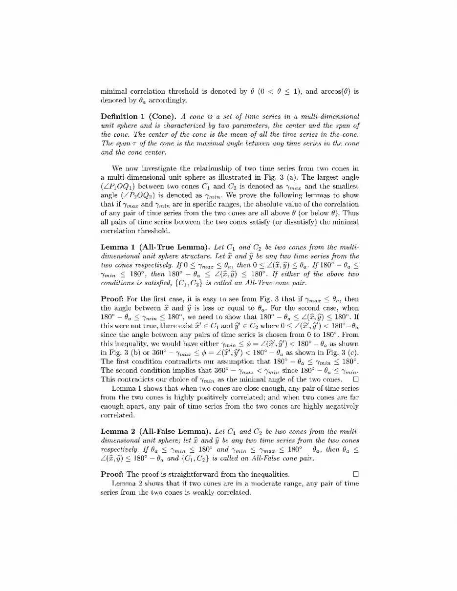
minimal orrelation threshold is denoted by � (0 < � � 1), and ar os(�) isdenoted by �a a ordingly.De�nition 1 (Cone). A one is a set of time series in a multi-dimensionalunit sphere and is hara terized by two parameters, the enter and the span ofthe one. The enter of the one is the mean of all the time series in the one.The span � of the one is the maximal angle between any time series in the oneand the one enter.We now investigate the relationship of two time series from two ones ina multi-dimensional unit sphere as illustrated in Fig. 3 (a). The largest angle(\P1OQ1) between two ones C1 and C2 is denoted as max and the smallestangle (\P2OQ2) is denoted as min. We prove the following lemmas to showthat if max and min are in spe i� ranges, the absolute value of the orrelationof any pair of time series from the two ones are all above � (or below �). Thusall pairs of time series between the two ones satisfy (or dissatisfy) the minimal orrelation threshold.Lemma 1 (All-True Lemma). Let C1 and C2 be two ones from the multi-dimensional unit sphere stru ture. Let bx and by be any two time series from thetwo ones respe tively. If 0 � max � �a, then 0 � \(bx; by) � �a. If 180Æ � �a � min � 180Æ, then 180Æ � �a � \(bx; by) � 180Æ. If either of the above two onditions is satis�ed, fC1; C2g is alled an All-True one pair.Proof: For the �rst ase, it is easy to see from Fig. 3 that if max � �a, thenthe angle between bx and by is less or equal to �a. For the se ond ase, when180Æ � �a � min � 180Æ, we need to show that 180Æ � �a � \(bx; by) � 180Æ. Ifthis were not true, there exist bx0 2 C1 and by0 2 C2 where 0 � \(bx0; by0) < 180Æ��asin e the angle between any pairs of time series is hosen from 0 to 180Æ. Fromthis inequality, we would have either min � � = \(bx0; by0) < 180Æ� �a as shownin Fig. 3 (b) or 360Æ � max � � = \(bx0; by0) < 180Æ � �a as shown in Fig. 3 ( ).The �rst ondition ontradi ts our assumption that 180Æ � �a � min � 180Æ.The se ond ondition implies that 360Æ � max < min sin e 180Æ � �a � min.This ontradi ts our hoi e of min as the minimal angle of the two ones. �Lemma 1 shows that when two ones are lose enough, any pair of time seriesfrom the two ones is highly positively orrelated; and when two ones are farenough apart, any pair of time series from the two ones are highly negatively orrelated.Lemma 2 (All-False Lemma). Let C1 and C2 be two ones from the multi-dimensional unit sphere; let bx and by be any two time series from the two onesrespe tively. If �a � min � 180Æ and min � max � 180Æ � �a, then �a �\(bx; by) � 180Æ � �a and fC1; C2g is alled an All-False one pair.Proof: The proof is straightforward from the inequalities. �Lemma 2 shows that if two ones are in a moderate range, any pair of timeseries from the two ones is weakly orrelated.

3 Cone-based Filter-and-Re�ne AlgorithmOur algorithm onsists of four steps as shown in Algorithm 1: Pre-pro essing(line 1), Cone Formation (line 2), Filtering i.e. Cone-level Join (line 4), andRe�nement i.e. Instan e-level Join (lines 7-11). The �rst step is to pre-pro essInput: 1) S1 = fs11; s12; : : : ; s1ng: n1 spatial referen ed time serieswhere ea h instan e referen es a spatial framework SF1;2) S2 = fs21; s22; : : : ; s2ng: n2 spatial referen ed time serieswhere ea h instan e referen es a spatial framework SF2;3) a user defined orrelation threshold �;Output: all pairs of time series ea h from S1 and S2 with orrelations above �;Method:Pre-pro essing(S1); Pre-pro essing(S2); (1)CN1 = Cone Formation(S1 ; SF1); CN2 = Cone Formation(S2 ; SF2); (2)for all pair 1 and 2 ea h from CN1 and CN2 do f (3)Filter F lag = Cone-level Join( 1, 2, �); (4)if (Filter F lag == ALL TRUE) (5)output all pairs in the two ones (6)else if (Filter F lag != ALL FALSE) f (7)for all pair s1 and s2 ea h from 1 and 2 do f (8)High Corr F lag = Instan e-level Join(s1,s2, �); (9)if (High Corr F lag) output s1 and s2; (10)g (11)g (12)Algorithm 1: Correlation Finderthe raw data to the multi-dimensional unit sphere representation. The se ondstep, one formation, involves grouping similar time series into ones in spatialtime series datasets. Clustering the time series is an intuitive approa h. How-ever, lustering on time-series datasets may be expensive and sensitive to the lustering method and its obje tive fun tion. For example, K-means approa hes[9℄ �nd globular lusters while density-based lustering approa hes [9℄ �nd arbi-trary shaped lusters with user-given density thresholds. Spatial indexes, su has R� trees, whi h are built after time series dimensionality redu tion [1, 4℄ ouldbe another approa h to group similar time series together. In this paper, we ex-plore spatial auto- orrelation for the one formation. First the spa e is dividedinto disjoint ells. The ells an ome from domain experts, su h as the El Ninoregion, or ould be as simple as uniform grids. By s anning the dataset on e, wemap ea h time-series into its orresponding ell. Ea h ell ontains similar timeseries and represents a one in the multi-dimensional unit sphere representation.The enter and span are al ulated to hara terize ea h one.Example 1 (Spatial Cone Formation). Fig. 4 illustrates the spatial one forma-tion for two datasets, namely land and o ean. Both land and o ean frameworks onsist of 16 lo ations. The time series of length m in a lo ation s is denotedas F (s) = F1(s); F2(s); : : : ; Fi(s); : : : Fm(s). Fig. 4 only depi ts a time series

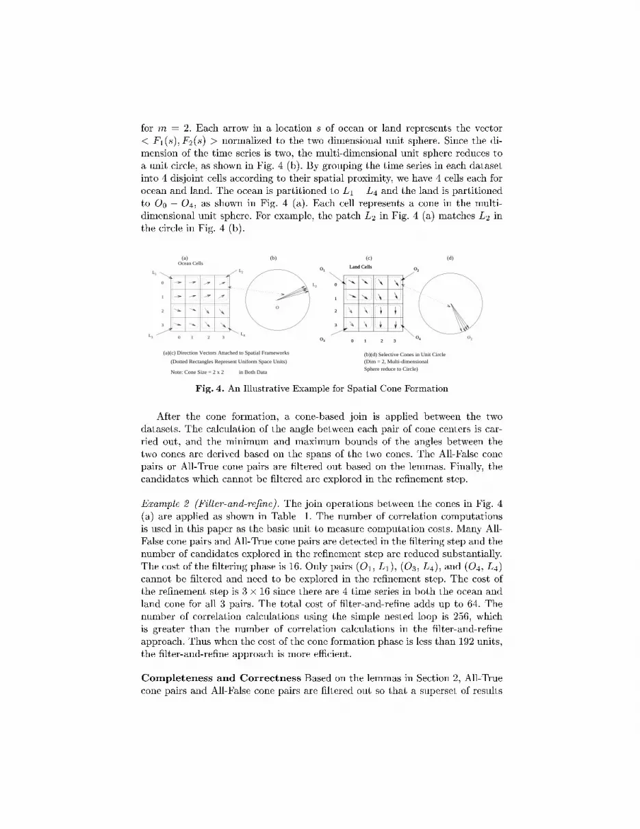
for m = 2. Ea h arrow in a lo ation s of o ean or land represents the ve tor< F1(s); F2(s) > normalized to the two dimensional unit sphere. Sin e the di-mension of the time series is two, the multi-dimensional unit sphere redu es toa unit ir le, as shown in Fig. 4 (b). By grouping the time series in ea h datasetinto 4 disjoint ells a ording to their spatial proximity, we have 4 ells ea h foro ean and land. The o ean is partitioned to L1�L4 and the land is partitionedto O0 � O4, as shown in Fig. 4 (a). Ea h ell represents a one in the multi-dimensional unit sphere. For example, the pat h L2 in Fig. 4 (a) mat hes L2 inthe ir le in Fig. 4 (b).(c)(b)(a)

Note: Cone Size = 2 x 2Sphere reduce to Circle)

(b)(d) Selective Cones in Unit Circle

(d)

in Both Data

L

L2L1

L3

L

O

2

4

Ocean Cells

0

1

2

3

0 1 2 3

Land Cells

0

1

2

3

0 1 2 3

O2

O4O3

O1 O2

O4

O1

O3O2

Land Cells

0

1

2

3

0 1 2 3

(Dim = 2, Multi-dimensional(Dotted Rectangles Represent Uniform Space Units)

(a)(c) Direction Vectors Attached to Spatial Frameworks

Fig. 4. An Illustrative Example for Spatial Cone FormationAfter the one formation, a one-based join is applied between the twodatasets. The al ulation of the angle between ea h pair of one enters is ar-ried out, and the minimum and maximum bounds of the angles between thetwo ones are derived based on the spans of the two ones. The All-False onepairs or All-True one pairs are �ltered out based on the lemmas. Finally, the andidates whi h annot be �ltered are explored in the re�nement step.Example 2 (Filter-and-re�ne). The join operations between the ones in Fig. 4(a) are applied as shown in Table 1. The number of orrelation omputationsis used in this paper as the basi unit to measure omputation osts. Many All-False one pairs and All-True one pairs are dete ted in the �ltering step and thenumber of andidates explored in the re�nement step are redu ed substantially.The ost of the �ltering phase is 16. Only pairs (O1, L1), (O3, L4), and (O4, L4) annot be �ltered and need to be explored in the re�nement step. The ost ofthe re�nement step is 3� 16 sin e there are 4 time series in both the o ean andland one for all 3 pairs. The total ost of �lter-and-re�ne adds up to 64. Thenumber of orrelation al ulations using the simple nested loop is 256, whi his greater than the number of orrelation al ulations in the �lter-and-re�neapproa h. Thus when the ost of the one formation phase is less than 192 units,the �lter-and-re�ne approa h is more eÆ ient.Completeness and Corre tness Based on the lemmas in Se tion 2, All-True one pairs and All-False one pairs are �ltered out so that a superset of results

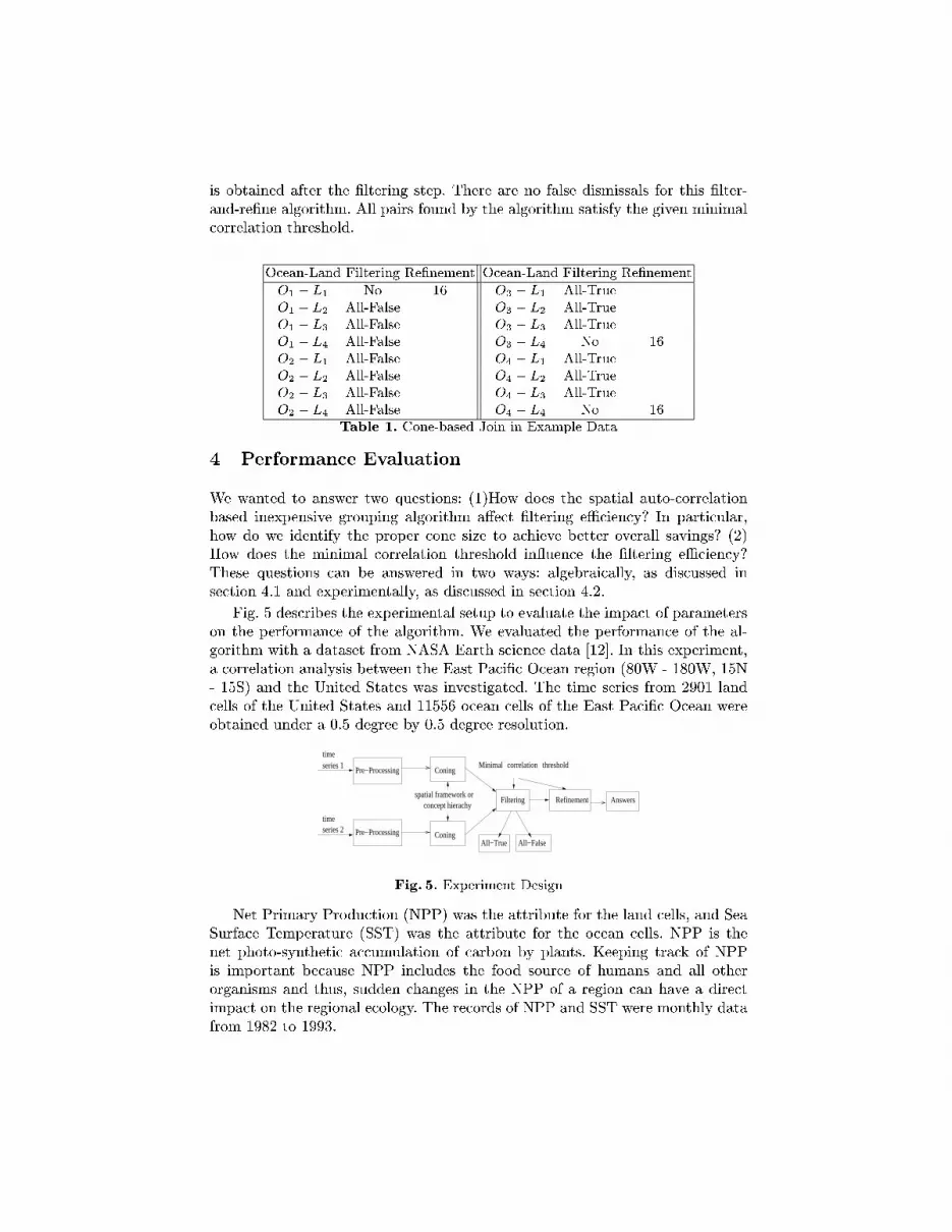
is obtained after the �ltering step. There are no false dismissals for this �lter-and-re�ne algorithm. All pairs found by the algorithm satisfy the given minimal orrelation threshold.O ean-Land Filtering Re�nement O ean-Land Filtering Re�nementO1 � L1 No 16 O3 � L1 All-TrueO1 � L2 All-False O3 � L2 All-TrueO1 � L3 All-False O3 � L3 All-TrueO1 � L4 All-False O3 � L4 No 16O2 � L1 All-False O4 � L1 All-TrueO2 � L2 All-False O4 � L2 All-TrueO2 � L3 All-False O4 � L3 All-TrueO2 � L4 All-False O4 � L4 No 16Table 1. Cone-based Join in Example Data4 Performan e EvaluationWe wanted to answer two questions: (1)How does the spatial auto- orrelationbased inexpensive grouping algorithm a�e t �ltering eÆ ien y? In parti ular,how do we identify the proper one size to a hieve better overall savings? (2)How does the minimal orrelation threshold in uen e the �ltering eÆ ien y?These questions an be answered in two ways: algebrai ally, as dis ussed inse tion 4.1 and experimentally, as dis ussed in se tion 4.2.Fig. 5 des ribes the experimental setup to evaluate the impa t of parameterson the performan e of the algorithm. We evaluated the performan e of the al-gorithm with a dataset from NASA Earth s ien e data [12℄. In this experiment,a orrelation analysis between the East Pa i� O ean region (80W - 180W, 15N- 15S) and the United States was investigated. The time series from 2901 land ells of the United States and 11556 o ean ells of the East Pa i� O ean wereobtained under a 0.5 degree by 0.5 degree resolution.Pre−Processing

Pre−Processing Coning

Coning

Answers

thresholdcorrelationtimeseries 1

timeseries 2

spatial framework orconcept hierachy

Refinement

All−False

Filtering

All−True

Minimal

Fig. 5. Experiment DesignNet Primary Produ tion (NPP) was the attribute for the land ells, and SeaSurfa e Temperature (SST) was the attribute for the o ean ells. NPP is thenet photo-syntheti a umulation of arbon by plants. Keeping tra k of NPPis important be ause NPP in ludes the food sour e of humans and all otherorganisms and thus, sudden hanges in the NPP of a region an have a dire timpa t on the regional e ology. The re ords of NPP and SST were monthly datafrom 1982 to 1993.

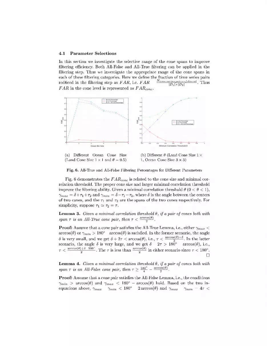
4.1 Parameter Sele tionsIn this se tion we investigate the sele tive range of the one spans to improve�ltering eÆ ien y. Both All-False and All-True �ltering an be applied in the�ltering step. Thus we investigate the appropriate range of the one spans inea h of these �ltering ategories. Here we de�ne the fra tion of time series pairsredu ed in the �ltering step as FAR, i.e. FAR = Ntime series pairs�filteredjD1j�jD2j . ThusFAR in the one level is represented as FAR one.

1 2 3 4 5 60

0.1

0.2

0.3

0.4

0.5

0.6

0.7

0.8

Ocean Bin Size

FAR

cone

All−Out PercentageAll−In PercentageAll−In + All−Out Percentage

(a) Di�erent O ean Cone Size(Land Cone Size 1� 1 and � = 0:5)0.2 0.3 0.4 0.5 0.6 0.7 0.8 0.9 10

0.1

0.2

0.3

0.4

0.5

0.6

0.7

0.8

0.9

1

Minmum Correlation Threshold θ

FAR co

ne

All−Out PercentageAll−In PercentageAll−In + All−Out Percentage

(b) Di�erent � (Land Cone Size 1�1, O ean Cone Size 3� 3)Fig. 6. All-True and All-False Filtering Per entages for Di�erent ParametersFig. 6 demonstrates the FAR one is related to the one size and minimal or-relation threshold. The proper one size and larger minimal orrelation thresholdimprove the �ltering ability. Given a minimal orrelation threshold � (0 < � < 1), max = Æ+�1+�2 and min = Æ��1��2, where Æ is the angle between the entersof two ones, and the �1 and �2 are the spans of the two ones respe tively. Forsimpli ity, suppose �1 ' �2 = � .Lemma 3. Given a minimal orrelation threshold �, if a pair of ones both withspan � is an All-True one pair, then � < ar os(�)2 .Proof: Assume that a one pair satis�es the All-True Lemma, i.e., either max <ar os(�) or min > 180Æ�ar os(�) is satis�ed. In the former s enario, the angleÆ is very small, and we get Æ + 2� < ar os(�), i.e., � < ar os(�)�Æ2 . In the latters enario, the angle Æ is very large, and we get Æ � 2� > 180Æ � ar os(�), i.e.,� < ar os(�)+Æ�180Æ2 . The � is less than ar os(�)2 in either s enario sin e � < 180Æ.�Lemma 4. Given a minimal orrelation threshold �, if a pair of ones both withspan � is an All-False one pair, then � � 180Æ4 � ar os(�)2 .Proof: Assume that a one pair satis�es the All-False Lemma, i.e., the onditions min > ar os(�) and max < 180Æ � ar os(�) hold. Based on the two in-equations above, max � min < 180Æ � 2 ar os(�) and max � min = 4� <

180Æ � 2 ar os(�) are true. Thus when the All-False lemma is satis�ed, � <180Æ4 � ar os(�)2 . �The range of � is related to the minimal orrelation thresholds. In this ap-pli ation domain, the pairs with absolute orrelations over 0.3 are interestingto the domain experts. As shown in Fig. 6, All-False �ltering provides stronger�ltering than All-True �ltering for almost all values of one sizes and orrelationthresholds. Thus we hoose the one span � for maximizing All-False �ltering onditions. The value of ar os(�) is less than 72:5Æ for � 2 (0:3; 1℄, so the onespan � should not be greater than 180Æ4 � ar os(�)2 = 8:75Æ.4.2 Experimental ResultsExperiment 1: E�e t of Coning The purpose of the �rst experiment was to eval-uate under what oning sizes the savings from �ltering outweighs the overhead.When the one is small, the time series in the one are relatively homogeneous,resulting in a small one span � . Although it may result in more All-False andAll-True pairs of ones, su h one formation in urs more �ltering overhead be- ause the number of ones is substantially in reased and the number of �lteredinstan es in ea h All-False or All-True pair is small. When the one is large,the value of the one span � is large, resulting in a de rease in the number ofAll-False and All-True pairs. The e�e ts of the All-False and All-True �lteringin the given data are investigated.Experiment 2: E�e t of Minimal Correlation Thresholds In this experiment, weevaluated the performan e of the �ltering algorithm when the minimal orre-lation threshold is hanged. Various minimal orrelation thresholds were testedand the trends of �ltering eÆ ien y were identi�ed with the hange of minimal orrelation thresholds.E�e t of Coning This se tion des ribes a group of experiments arried outto show the net savings of the algorithm for di�erent one sizes. For simpli ity,we only hanged the one size for one dataset. A ording to the analysis of theprevious se tion, the land one size is �xed at 1 � 1. We arried out a series ofexperiments using the �xed minimal orrelation threshold, the �xed land onesize, and various o ean one sizes. The minimal orrelation threshold � was �xedat 0.5. Fig. 7 (a) shows the net savings as a per entage of the omputational ost of the nested loop join algorithm for di�erent o ean one sizes. The x-axisrepresents the di�erent one sizes ranging from 1 � 1 to 6 � 6, and the y-axisrepresents the net savings in omputational ost as a per entage of the ostsusing the simple nested loop join algorithm. The net savings range from 40per ent to 62 per ent.E�e t of Minimal Correlation Thresholds In this experiment, we investi-gated the e�e ts of minimal orrelation threshold � on the savings in omputation ost for orrelation analysis. The land and o ean one sizes were �xed at 1 � 1and 3�3 respe tively, and a series of experiments was arried out for di�erent �s.

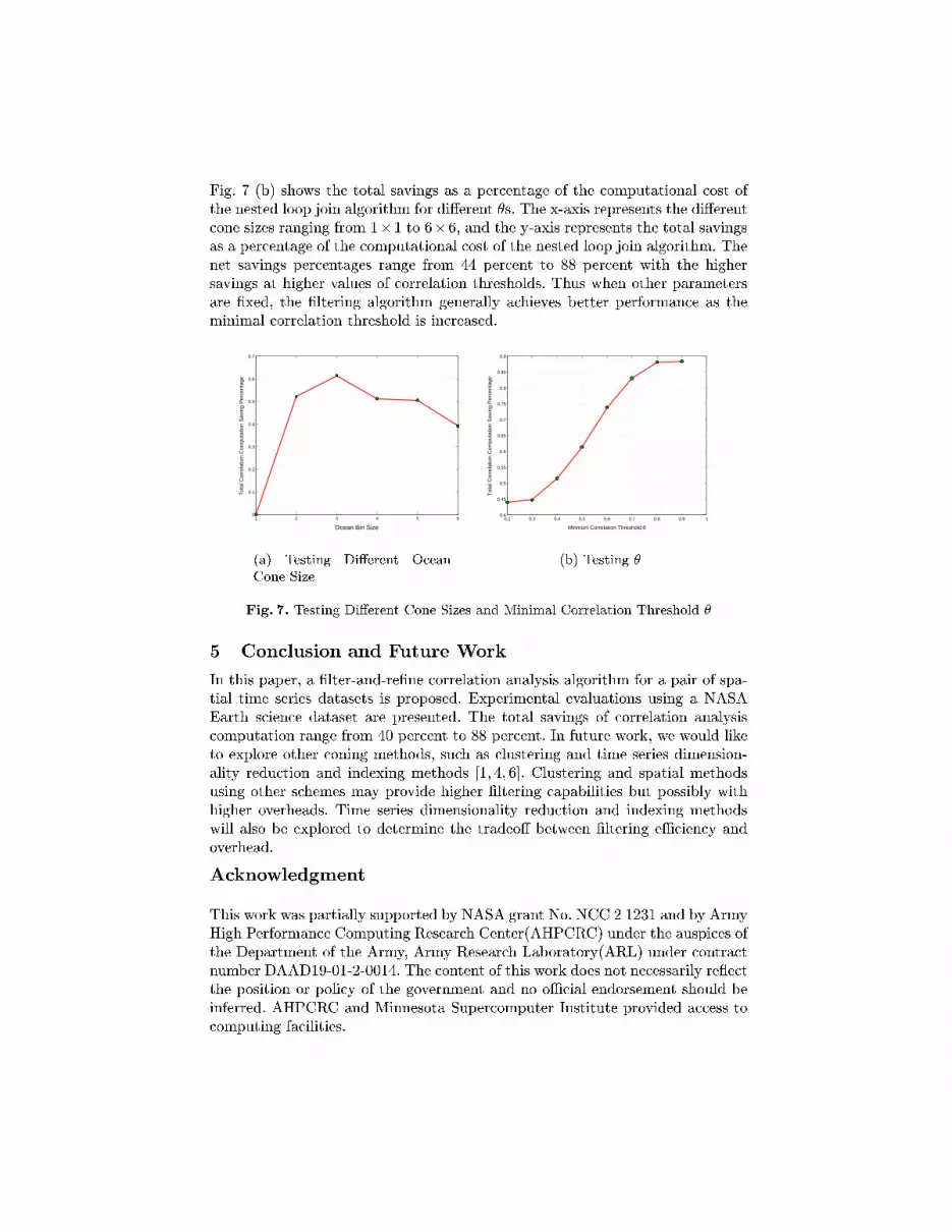
Fig. 7 (b) shows the total savings as a per entage of the omputational ost ofthe nested loop join algorithm for di�erent �s. The x-axis represents the di�erent one sizes ranging from 1�1 to 6�6, and the y-axis represents the total savingsas a per entage of the omputational ost of the nested loop join algorithm. Thenet savings per entages range from 44 per ent to 88 per ent with the highersavings at higher values of orrelation thresholds. Thus when other parametersare �xed, the �ltering algorithm generally a hieves better performan e as theminimal orrelation threshold is in reased.

1 2 3 4 5 60

0.1

0.2

0.3

0.4

0.5

0.6

0.7

Ocean Bin Size

Tot

al C

orre

latio

n C

ompu

tatio

n S

avin

g P

erce

ntag

e

(a) Testing Di�erent O eanCone Size0.2 0.3 0.4 0.5 0.6 0.7 0.8 0.9 1

0.4

0.45

0.5

0.55

0.6

0.65

0.7

0.75

0.8

0.85

0.9

Minmum Correlation Threshold θ

Tot

al C

orre

latio

n C

ompu

tatio

n S

avin

g P

erce

ntag

e

(b) Testing �Fig. 7. Testing Di�erent Cone Sizes and Minimal Correlation Threshold �5 Con lusion and Future WorkIn this paper, a �lter-and-re�ne orrelation analysis algorithm for a pair of spa-tial time series datasets is proposed. Experimental evaluations using a NASAEarth s ien e dataset are presented. The total savings of orrelation analysis omputation range from 40 per ent to 88 per ent. In future work, we would liketo explore other oning methods, su h as lustering and time series dimension-ality redu tion and indexing methods [1, 4, 6℄. Clustering and spatial methodsusing other s hemes may provide higher �ltering apabilities but possibly withhigher overheads. Time series dimensionality redu tion and indexing methodswill also be explored to determine the tradeo� between �ltering eÆ ien y andoverhead.A knowledgmentThis work was partially supported by NASA grant No. NCC 2 1231 and by ArmyHigh Performan e Computing Resear h Center(AHPCRC) under the auspi es ofthe Department of the Army, Army Resear h Laboratory(ARL) under ontra tnumber DAAD19-01-2-0014. The ontent of this work does not ne essarily re e tthe position or poli y of the government and no oÆ ial endorsement should beinferred. AHPCRC and Minnesota Super omputer Institute provided a ess to omputing fa ilities.

We are parti ularly grateful to NASA Ames Resear h Center ollaborators C.Potter and S. Klooster for their helpful omments and valuable dis ussions. Wewould also like to express our thanks to Kim Ko�olt for improving the readabilityof this paper.Referen es1. R. Agrawal, C. Faloutsos, and A. Swami. EÆ ient Similarity Sear h In Sequen eDatabases. In Pro . of the 4th Int'l Conferen e of Foundations of Data Organiza-tion and Algorithms, 1993.2. G. Box, G. Jenkins, and G. Reinsel. Time Series Analysis: Fore asting and Control.Prenti e Hall, 1994.3. B.W. Lindgren. Statisti al Theory (Fourth Edition). Chapman-Hall, 1998.4. K. Chan and A. W. Fu. EÆ ient Time Series Mat hing by Wavelets. In Pro . ofthe 15th ICDE, 1999.5. N. Cressie. Statisti s for Spatial Data. John Wiley and Sons, 1991.6. Christos Faloutsos. Sear hing Multimedia Databases By Content. Kluwer A ademi Publishers, 1996.7. R. Grossman, C. Kamath, P. Kegelmeyer, V. Kumar, and R. Namburu, editors.Data Mining for S ienti� and Engineering Appli ations. Kluwer A ademi Pub-lishers, 2001.8. D. Gunopulos and G. Das. Time Series Similarity Measures and Time SeriesIndexing. SIGMOD Re ord, 30(2):624{624, 2001.9. J. Han and M. Kamber. Data Mining: Con epts and Te hniques. Morgan Kauf-mann Publishers, 2000.10. E. Keogh and M. Pazzani. An Indexing S heme for Fast Similarity Sear h inLarge Time Series Databases. In Pro . of 11th Int'l Conferen e on S ienti� andStatisti al Database Management, 1999.11. Y. Moon, K. Whang, and W. Han. A Subsequen e Mat hing Method in Time-Series Databases Based on Generalized Windows. In Pro . of ACM SIGMOD,Madison, WI, 2002.12. C. Potter, S. Klooster, and V. Brooks. Inter-annual Variability in Terrestrial NetPrimary Produ tion: Exploration of Trends and Controls on Regional to GlobalS ales. E osystems, 2(1):36{48, 1999.13. J. Roddi k and K. Hornsby. Temporal, Spatial, and Spatio-Temporal Data Mining.In First Int'l Workshop on Temporal, Spatial and Spatio-Temporal Data Mining,2000.14. S. Shekhar and S. Chawla. Spatial Databases: A Tour. Prenti e Hall, 2002.15. S. Shekhar, S. Chawla, S. Ravada, A. Fetterer, X. Liu, and C.T. Lu. Spatialdatabases: A omplishments and resear h needs. IEEE Transa tions on Knowledgeand Data Engineering, 11(1):45{55, 1999.16. M. Steinba h, P. Tan, V. Kumar, C. Potter, S. Klooster, and A. Torregrosa. DataMining for the Dis overy of O ean Climate Indi es. In Pro of the Fifth Workshopon S ienti� Data Mining, 2002.17. P. Tan, M. Steinba h, V. Kumar, C. Potter, S. Klooster, and A. Torregrosa. FindingSpatio-Temporal Patterns in Earth S ien e Data. In KDD 2001 Workshop onTemporal Data Mining, 2001.18. G. H. Taylor. Impa ts of the El Nio/Southern Os illation on the Pa i� Northwest.http://www.o s.orst.edu/reports/enso pnw.html.19. Mi hael F. Worboys. GIS - A Computing Perspe tive. Taylor and Fran is, 1995.