Single and Parallel Machine Capacitated Lotsizing and Scheduling: NewIterative MIP-based Neighborhood Search Heuristics

Ross J.W. James∗,a,1, Bernardo Almada-Lobob

aDepartment of Management, University of Canterbury, Private Bag 4800, Christchurch, 8140, New ZealandbFaculdade de Engenharia da Universidade do Porto, Porto, Portugal

Abstract

We propose a general-purpose heuristic approach combining metaheuristics and Mixed Integer Program-

ming to find high quality solutions to the challenging single- and parallel-machine capacitated lotsizing and

scheduling problem with sequence-dependent setup times and costs. Commercial solvers fail to solve even

medium-sized instances of this NP-hard problem, therefore heuristics are required to find competitive solu-

tions. We develop construction, improvement and search heuristics all based on MIP formulations. We then

compare the performance of these heuristics with those of two metaheuristics and other MIP-based heuris-

tics that have been proposed in the literature, and to a state-of-the-art commercial solver. A comprehensive

set of computational experiments shows the effectiveness and efficiency of the main approach, a stochastic

MIP-based local search heuristic, in solving medium to large size problems. Our solution procedures are

quite flexible and may easily be adapted to cope with model extensions or to address different optimization

problems that arise in practice.

Key words: CLSD-PM, sequence-dependent setup, Mixed Integer Programming, relax-and-fix, local

search, metaheuristic, parallel-machine

1. Introduction

The aim of this paper is to develop a range of mathematical programming-based heuristics to solve

complex lotsizing and scheduling problems. The techniques developed here are employed to solve a specific

problem, but could be easily generalized to other variants of lotsizing and scheduling problems and even

other problems outside this domain.

Our motivation is to solve the single-machine capacitated lotsizing and scheduling problem with sequence-

dependent setup times and costs, and to generalize this to the parallel-machine case that arises in many

industrial applications. This single-stage problem is an extension of the pure capacitated lotsizing problem

(CLSP – Bitran and Yanasse [7]) and of the CLSD proposed by Haase [13], which only addresses one

∗Corresponding authorEmail addresses: ross.james@canterbury.ac.nz (Ross J.W. James), almada.lobo@fe.up.pt (Bernardo Almada-Lobo)

1Tel: +64 3 364 2987 Ext 7015, Fax: +64 3 364 2020

Preprint submitted to Elsevier February 6, 2011

machine and no setup times, as we consider an allocation dimension with multiple parallel machines and a

sequencing dimension with sequence-dependent setups. In their review of capacitated lot-sizing extensions,

Quadt and Kuhn [19] denote this problem as CLSD for single-machine and CLSD-PM for parallel-machines.

CLSD is considered to be a big-bucket problem, as several products/setups may be produced/performed per

period. The practical relevance of parallel machine lotsizing and extensions is supported by examples of its

application in various industries such as pharmaceutical, chemical, electronics, food, tile manufacturing, tire

industry, injection molding, the alloy foundry industry and multi-layer-ceramics (Jans [15] and Quadt and

Kuhn [19]). Naturally, the extension to parallel machines enlarges the planning problem, making it much

harder to solve as the product-to-machine assignment has to be tackled. Despite its applicability, the amount

of research on these problems and correlated variants is small, mainly due to its inherent complexity (Clark

et al. [9]). The same conclusion is drawn by Zhu and Wilhelm [22], who state that, despite the significant role

of combined lotsizing and scheduling in the effective utilization of limited resources in different production

systems, most research has focused on the single-machine configuration. Research on other configurations is

sparse.

We consider N products to be manufactured on M different capacitated machines over a discrete planning

horizon of T periods. Due to the sequence-dependency of setups in a product changeover, lot sizing and

sequencing are simultaneously tackled. The objective is to find a strategy that satisfies demands without

backlogging and minimizes both setup and holding costs. The computational complexity of the resulting

mixed integer programming (MIP) model (the underlying problem is NP-hard) makes the use of efficient

heuristic strategies mandatory for solving large real-world instances. State-of-the-art optimization engines

either fail to generate feasible solutions to this problem or take a prohibitively large amount of computation

time, even in the single-machine setting (see Almada-Lobo and James [2]).

A variety of algorithms have been developed to tackle this area. Buschkhl et al. [8] classifies solution

approaches to dynamic capacitated big-bucket lotsizing problems into five major categories. The spectrum

ranges from mathematical programming heuristics, lagrangean heuristics and decomposition and aggregation

heuristics, to metaheuristics and greedy heuristics. Most of the research to date considers either approximate

approaches or optimization models, however research into combining heuristics and optimization has recently

started to emerge (Framinan and Pastor [12]). Almada-Lobo and James [2] solved the single-machine CLSD

(CLSD-SM) by integrating a big-bucket lotsizing and scheduling model and a batching scheduling model

(converting lots into jobs) and developed two neighborhood-based search algorithms, based on Tabu Search

(TS) and Variable Neighborhood Search (VNS).

It is acknowledged by the community that the time to solve lotsizing and scheduling problems is heavily

dependent upon the instances being solved. Nevertheless, there is a need for more realistic random instances

for these problems based on real-world cases, especially for the multi-machine setting (Clark et al. [9]). In

this paper, we propose a problem generator with new features that allows us to conduct computational

2

experiments on a set of diverse data. To the best of our knowledge, previous literature has dealt with

capacity of a time period being proportional to the demand of the time period. We investigate removing

this assumption. In addition we introduce two parameters, machine balancing and machine loading, that

control the product-machine assignment matrix.

Here we focus our attention on new mathematical programming-based heuristics and metaheuristics that

are flexible and could easily be adapted to cope with model extensions or to address different optimization

problems that arise in practice, as they are problem- and constraint-independent. Naturally, we only explore

parts of the solution space, and therefore we are not able to prove optimality.

The so-called progressive interval heuristics (such as the relax-and-fix heuristic and internally rolling

schedule heuristics) solve the overall MIP problem as a sequence of partially relaxed MIPs (thus reducing

the number of binary variables to be treated simultaneously), always starting from the first period on a

forward shifting move (Federgruen et al. [10]). The setup variables are progressively fixed at their optimal

values obtained in earlier iterations. Different variants of this class of solution approach allow a trade-off

between optimality and run-time. Beraldi et al. [6] and Ferreira et al. [11] recently applied relax-and-fix

variants successfully to different lotsizing and scheduling problems. These are all construction-heuristics

that provide initial solutions. Pochet and Wolsey [17] describe an improvement heuristic similar to the

relax-and-fix heuristic, which they called ‘exchange’. The decomposition scheme for the integer variables

is the same as before, but it differs from the relax-and-fix heuristic in that it does not relax the binary

setup variables in the subproblems. At each step the integer variables are fixed at their best value found

in the previous iterations, except for a limited set of integer variables that are related to the subproblem

at hand and are restricted to take integer values. The next iteration deals with a new subproblem with a

different subset of integer variables to be optimized. Note that when the last partition is solved, and in case a

better solution is found, this exchange procedure can be repeated (i.e., each subproblem may be solved more

than once) until a local optimum is reached. Naturally, this procedure needs to be given a feasible starting

solution. The same approach is used in Sahling et al. [20] and Helber and Sahling [14] for the multi-level

CLSP, where the authors called it the fix-and-optimize heuristic.

All the aforementioned MIP-based approaches are deterministic, which may lead to a poor local optimum

for hard instances of a problem. We develop a stochastic MIP-based local search improvement heuristic that

tries to improve any given feasible solution. The key idea is to solve a series of subMIPs randomly selected

in an iterative exchange algorithm. The probability of selecting each subMIP is based on two factors: the

frequency and the recency of the subMIP being selected. To move the search out of a local minimum,

we borrow well-known diversification mechanisms from local search metaheuristics, and we use different

neighborhoods based on the original MIP. This novel procedure combines features of exact enumeration

methods (branch-and-bound) with approximate procedures (local search). According to Puchinger and Raidl

[18], our approach fits into the category of an integrative combination of exact algorithms and metaheuristics,

3

as the former is incorporated in the latter. Though this heuristic cannot guarantee the solution’s optimality,

however we hope to obtain quasi-optimal solutions in a reasonable amount of CPU time. To produce a feasible

solution from scratch, we rely on a construction heuristic based on the general relax-and-fix framework. Our

results will be compared with those obtained with the exchange heuristic of Pochet and Wolsey [17] or the

fix-and-optimize heuristic of Sahling et al. [20], the VNS and TS metaheuristics of Almada-Lobo and James

[2] and, finally, the CPLEX commercial solver.

The remainder of the paper is organized as follows: Section 2 introduces the formulation for the parallel

machine capacitated lotsizing and scheduling (CLSD-PM). Section 3 is devoted to the Iterative MIP-based

Neighborhood Search Heuristic, presenting its general decomposition idea and main ingredients. Section 4

provides computational evidence that demonstrates the superiority of this approach and finally, Section 5

draws some conclusions from this work and suggests directions for future research.

2. CLSD-PM Model Formulation

In this paper we study the parallel machine capacitated lotsizing and scheduling problem with sequence

dependent setups (CLSD-PM) of which the single machine problem (CLSD-SM) is a special case. We consider

a planning interval with t = 1, . . . , T periods and i, j = 1, . . . , N products processed on m = 1, . . . ,M

machines. We use the notation [K] to refer to the set {1, 2, . . . , K}. As usual, dit denotes the demand of

product i in period t, smij and cmij the time and cost incurred when a setup occurs from product i to

product j on machine m respectively, hi the cost of carrying one unit of inventory of product i from one

period to the next, pmi the processing time of one unit of product i on machine m and Cmt the capacity of

machine m available in period t. In addition, Gmit is an upper bound on the production quantity of product

i in period t to machine m. Ami indicates which machines are able to produce which products. Ami is set

to one if machine m is able to produce product i, or zero otherwise.

The following decision variables are used: Xmit refers to the quantity of product i produced in period t

on machine m, Iit the inventory level of product i at the end of period t and Vmit an auxiliary variable that

assigns product i on machine m in period t. The larger Vmit is, the later the product i is scheduled in period

t on machine m, assuring that each machine is only set up for one product at any given time.

In addition, the following 0/1 decision variables are defined: Tmijt equals one if a setup occurs from

product i to product j on machine m in period t, and Ymit equals one if the machine m is set up for product

i at the beginning of period t. The CLSD-PM model below is a generalization of the CLSD-SM introduced

in Almada-Lobo et al. [3]:

4

min∑m

∑

i

∑

j

∑t

cmij · Tmijt+∑

i

∑t

hi · Iit (1)

Ii(t−1) +∑m

Xmit − dit =Iit i ∈ [N ], t ∈ [T ] (2)

Ii0 =0 i ∈ [N ] (3)∑

i

pmi ·Xmit +∑

i

∑

j

smij · Tmijt ≤Cmt m ∈ [M ], t ∈ [T ] (4)

Xmit ≤Gmit · (∑

j

Tmjit + Ymit)m ∈ [M ], i ∈ [N ],

t ∈ [T ](5)

Ymi(t+1) +∑

j

Tmijt =Ymit +∑

j

Tmjit m ∈ [M ], i ∈ [N ], t ∈ [T ] (6)

∑

i

Ymit =1 m ∈ [M ], t ∈ [T ] (7)

Vmit + N · Tmijt − (N − 1)−N · Ymjt ≤Vmjt

m ∈ [M ], i ∈ [N ],

j ∈ [N ] \ {i}, t ∈ [T ](8)

∑t

Xmit ≤GmitAmi m ∈ [M ], i ∈ [N ] (9)

(Xmit, Iit) ≥ 0, (Tmijt, Ymit) ∈{0, 1}, Xmit ∈ Z, Vmit ∈ R (10)

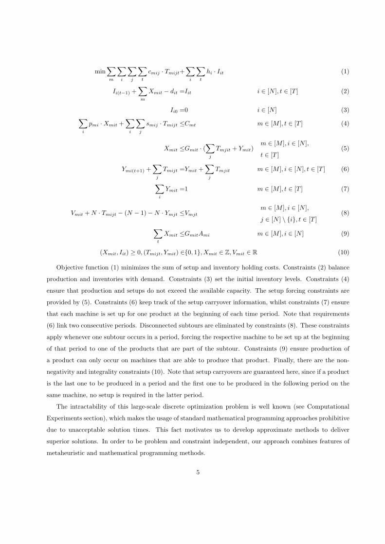
Objective function (1) minimizes the sum of setup and inventory holding costs. Constraints (2) balance

production and inventories with demand. Constraints (3) set the initial inventory levels. Constraints (4)

ensure that production and setups do not exceed the available capacity. The setup forcing constraints are

provided by (5). Constraints (6) keep track of the setup carryover information, whilst constraints (7) ensure

that each machine is set up for one product at the beginning of each time period. Note that requirements

(6) link two consecutive periods. Disconnected subtours are eliminated by constraints (8). These constraints

apply whenever one subtour occurs in a period, forcing the respective machine to be set up at the beginning

of that period to one of the products that are part of the subtour. Constraints (9) ensure production of

a product can only occur on machines that are able to produce that product. Finally, there are the non-

negativity and integrality constraints (10). Note that setup carryovers are guaranteed here, since if a product

is the last one to be produced in a period and the first one to be produced in the following period on the

same machine, no setup is required in the latter period.

The intractability of this large-scale discrete optimization problem is well known (see Computational

Experiments section), which makes the usage of standard mathematical programming approaches prohibitive

due to unacceptable solution times. This fact motivates us to develop approximate methods to deliver

superior solutions. In order to be problem and constraint independent, our approach combines features of

metaheuristic and mathematical programming methods.

5

3. Iterative MIP-Based Neighborhood Search

3.1. Basic Idea of the Decomposition Scheme

The number of integer variables in the CLSD-PM model (N2 ·M ·T +2 ·N ·T ·M) determines most of the

computational burden. The techniques we use to solve the CLSD-PM problem are based on decomposing

the original problem into subsets that can be solved more easily by a MIP in an iterative fashion. As the

number of integer variables in each subproblem is significantly smaller than that of the original problem,

the solution times to solve each one to optimality is very small. In order to do this we assume we already

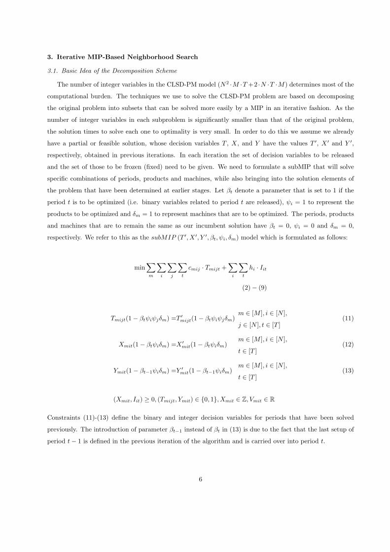
have a partial or feasible solution, whose decision variables T , X, and Y have the values T ′, X ′ and Y ′,

respectively, obtained in previous iterations. In each iteration the set of decision variables to be released

and the set of those to be frozen (fixed) need to be given. We need to formulate a subMIP that will solve

specific combinations of periods, products and machines, while also bringing into the solution elements of

the problem that have been determined at earlier stages. Let βt denote a parameter that is set to 1 if the

period t is to be optimized (i.e. binary variables related to period t are released), ψi = 1 to represent the

products to be optimized and δm = 1 to represent machines that are to be optimized. The periods, products

and machines that are to remain the same as our incumbent solution have βt = 0, ψi = 0 and δm = 0,

respectively. We refer to this as the subMIP (T ′, X ′, Y ′, βt, ψi, δm) model which is formulated as follows:

min∑m

∑

i

∑

j

∑t

cmij · Tmijt +∑

i

∑t

hi · Iit

(2)− (9)

Tmijt(1− βtψiψjδm) =T ′mijt(1− βtψiψjδm)m ∈ [M ], i ∈ [N ],

j ∈ [N ], t ∈ [T ](11)

Xmit(1− βtψiδm) =X ′mit(1− βtψiδm)

m ∈ [M ], i ∈ [N ],

t ∈ [T ](12)

Ymit(1− βt−1ψiδm) =Y ′mit(1− βt−1ψiδm)

m ∈ [M ], i ∈ [N ],

t ∈ [T ](13)

(Xmit, Iit) ≥ 0, (Tmijt, Ymit) ∈ {0, 1}, Xmit ∈ Z, Vmit ∈ R

Constraints (11)-(13) define the binary and integer decision variables for periods that have been solved

previously. The introduction of parameter βt−1 instead of βt in (13) is due to the fact that the last setup of

period t− 1 is defined in the previous iteration of the algorithm and is carried over into period t.

6

3.2. MIP-Based Construction Heuristic

In order to create an initial solution to the CLSD-PM problem instance we use a procedure based on the

well known relax-and-fix framework (Pochet and Wolsey [17]).

The relax-and-fix (RF) framework decomposes a large-scale MIP into a number of smaller partially

relaxed MIP subproblems, which are solved in sequence. Naturally, the way the original MIP is partitioned

defines the solution quality of the RF heuristic and the computational burden. Each subproblem should

entail a small enough number of integer variables to be quickly and optimally solved using exact methods.

Due to the structure of the original MIP, we rely on a time-stage partition, which is a rolling horizon

approach. The planning horizon is typically partitioned into non-overlapping intervals (e.g., Stadtler [21],

Araujo et al. [4] and Ferreira et al. [11]). A shift forward strategy solves a sequence of sub-MIPs (one per

time interval), each dealing with a subset of the integer variable set of the overall problem. The other

subsets are either relaxed or removed (i.e., periods beyond the end of the current interval are not included)

depending on the simplification strategy. As this heuristic progresses, the integer variables (and, depending

on the freezing strategy, also the continuous variables) are permanently fixed to their current values. The

schedule is completed at the last iteration.

The RF heuristic can be parameterized in many ways. Our design is based on the results published by

Merce and Fontan [16] and Absi and Kedad-Sidhoum [1]. Let γ be the number of periods whose decisions

variables were determined in the previous iterations but are to be re-solved, and w be the number of periods

to be solved at each iteration, i.e. the time intervals overlap by γ periods between iterations. It is implied here

that both parameters are constant throughout the algorithm. Note that γ allows us to smooth the heuristic

solution by creating some overlap between successive planning intervals. Let tik and tfk denote the initial

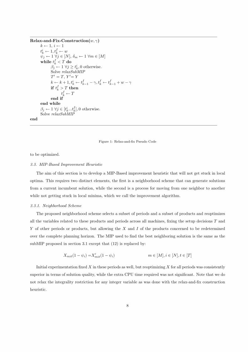
and final periods of the interval at step k. The RF pseudo code is described in Figure 1. The relaxSubMIP

denotes the relaxed version of subMIP (T ′, X ′, Y ′, βt, ψi, δm) subproblem to be solved at iteration k of the

heuristic, where the sub-set of variables T and Y up to period tik−1 are fixed, the sub-set from period tik up

to tfk are restricted to be integer, and each other period’s integer variables are relaxed to being real numbers.

This is essentially the subMIP model outlined in Section 3.1, except that equation (12) is removed and

(Tmijt, Ymit) ∈ {0, 1}∀t ≤ tfk ,∈ R otherwise (i.e. the integrality constraints are relaxed). According to the

definition of RF, βt is set to one for every t greater than or equal to tik, and ψi and δm are set to one for

every product and machine, respectively.

Note that w − γ defines the length of the anticipation horizon at each iteration and, consequently,

the number of iterations of the heuristic. Recall that our formulation keeps track of the setup carryover

information, knowing the product that the machine is ready to process at the beginning of each time period.

The motivation for using w > 1 and γ > 0 (with γ < w) comes from the setup carryover information. With

a γ = 0, blocks do not overlap and therefore the product the machine is set up for at the beginning of the

block is fixed at the previous iteration. This therefore affects the production sequence of the current block

7

Relax-and-Fix-Construction(w, γ)k ← 1, i ← 1tik ← 1, tfk ← wψj ← 1 ∀j ∈ [N ], δm ← 1 ∀m ∈ [M ]while tfk < T do

βj ← 1 ∀j ≥ tik, 0 otherwise.Solve relaxSubMIPT ′ = T , Y ′= Y

k ← k + 1, tik ← tfk−1 − γ, tfk ← tfk−1 + w − γ

if tfk > T thentfk ← T

end ifend whileβj ← 1 ∀j ∈ [tik...tfk ], 0 otherwise.Solve relaxSubMIP

end

Figure 1: Relax-and-fix Pseudo Code

to be optimized.

3.3. MIP-Based Improvement Heuristic

The aim of this section is to develop a MIP-Based improvement heuristic that will not get stuck in local

optima. This requires two distinct elements, the first is a neighborhood scheme that can generate solutions

from a current incumbent solution, while the second is a process for moving from one neighbor to another

while not getting stuck in local minima, which we call the improvement algorithm.

3.3.1. Neighborhood Scheme

The proposed neighborhood scheme selects a subset of periods and a subset of products and reoptimizes

all the variables related to these products and periods across all machines, fixing the setup decisions T and

Y of other periods or products, but allowing the X and I of the products concerned to be redetermined

over the complete planning horizon. The MIP used to find the best neighboring solution is the same as the

subMIP proposed in section 3.1 except that (12) is replaced by:

Xmit(1− ψi) =X ′mit(1− ψi) m ∈ [M ], i ∈ [N ], t ∈ [T ]

Initial experimentation fixed X in these periods as well, but reoptimizing X for all periods was consistently

superior in terms of solution quality, while the extra CPU time required was not significant. Note that we do

not relax the integrality restriction for any integer variable as was done with the relax-and-fix construction

heuristic.

8

3.3.2. Improvement Algorithm

The proposed improvement heuristic has two phases: a local search phase and a neighborhood modifica-

tion phase.

The local search phase is based on solving the neighborhood with all products (i.e. ψi = 1∀i ∈ [N ]),

all machines and a selected number of contiguous periods. Initially, the probability of selecting a particular

period is the same. However, as periods are selected, the probability of that period being selected again is

reduced. Two factors are used to determine the probability of selection of a period: the frequency and the

recency. The more frequently a period has been used in a neighborhood (given by the number of runs the

respective period was selected), and the more recently it has been used (given by the number of iterations

passed since the last selection of that period), the lower the probability of selection, which is proportional to

a weighted average of these two factors. The search also keeps track of which period combinations have been

solved without any improvement in the solution quality. A period will not be selected if it has already been

used and the current objective value was obtained (providing a form of short-term memory which speeds up

the solution procedure). If all period combinations have been tried and there has been no improvement in

the solution, then a local minimum has been found and this phase of the improvement algorithm ends. Of

course the algorithm will also terminate if the maximum CPU time is exceeded. We refer to the heuristic

which just uses this phase of the improvement algorithm the Product Quantity(X) Period (P) heuristic (H)

or XPH.

The second phase, the neighborhood modification phase, is similar to Variable Neighborhood Search

(VNS) in that it uses a different neighborhood to move the search out of a local minimum. Unlike the

shaking step of VNS, however, the move from the second neighborhood will always be an improvement from

the incumbent solution due to using a MIP optimizer to generate the best neighbor. In a similar manner

to VNS, once a new solution is found the search reverts to the original neighborhood and proceeds to find

another local minimum using the original neighborhood scheme, in our case the XPH local search.

The local minima are created because the sequences and the product quantities of all products are only

optimized over a given small number of periods. Therefore, in order to break this source of local minima, we

need to consider the sequencing of a product over a greater number of periods. The alternative neighborhood

scheme limits the number of products while considering a larger number of periods than that of XPH, the

size of which is determined by the user. In this phase we try to find a better solution by randomly selecting

different combinations of products and periods. The selection is biased to those periods and products that

have not been chosen as often. Once a better solution is found, the search switches back to the XPH

neighborhood and completes another local search from that point. If a better solution is not found within a

predefined number of iterations (determined by a parameter), then the search is terminated. We also limit

the time an iteration can take in order to ensure that, if a difficult combination of periods and products

is selected, not all the available search time is consumed by evaluating one move. The user must therefore

9

specify the number of products and periods to evaluate in a move, the maximum iteration time, the number

of non-improving iterations to complete before exiting and the maximum time for the search overall.

The heuristic, composed of the two phases described above, we call Iterative Neighborhood Search or

INS.

4. Computational Experiments

We perform computational experiments on an extensive set of instances that reflects different character-

istics of real-world cases found in practice. It is well known that the complexity of these problems is highly

dependent on the settings to be considered. In the next sections the results are categorized into four sets:

single and multi-machine environments, and instances with or without machine capacity variations. We aim

to investigate the impact of the overall capacity of a time period not being proportional to the net demand

of that period; such a feature is common in the process industries (such as glass container, beverages and

textiles).

4.1. Problem Instance Generation

The problem instances used in the following computational experiments are based on the approach of

Almada-Lobo et al. [3]. Elements of each problem instance are generated from a uniform distribution and

then rounded to the nearest integer, or calculated from elements that were generated this way. The ranges

used for the elements are as follows:

• Setup Times between 5 and 10 time units, and Setup Costs are proportional to the setup time by a

specified factor (Cost of Setup per unit of time, θ).

• Holding costs between 2 and 9 penalty units per period.

• Demand between 40 and 59 units per period.

• Period Capacity is proportional to the total demand in that period as defined by a parameter (Capacity

Utilization per period, Cut): Ct =∑

i dit/Cut.

• Processing time for one unit = one unit of time.

As in Almada-Lobo et al. [3], the following problem parameters were varied in order to create different

problem types:

• Number of Products, N , Number of Periods, T , Capacity Utilization per period, Cut, and Cost of

Setup per unit of time, θ

In order to control for the amount of capacity variation we also introduce another parameter CutV ar,

which works in conjunction with Cut. When capacity variation is introduced, Cut becomes the target

10

utilization for the overall problem instance as before and we ensure that the cumulative capacity utilization

for all periods never exceeds this value (otherwise the problem would not be feasible, as backlogging is not

permitted). The new parameter CutV ar represents and controls the maximum total allowed variation from

Cut, so the actual capacity utilization can vary. The variation is then randomly allocated to the periods.

To ensure that the variation is spread between the periods, a maximum of half of this total can be allocated

to any one period in the first half of the planning horizon. Note that if CutV ar equals zero, then there is

no capacity variation and the problem instances generated are the same as in Almada-Lobo et al. [3].

To allow for multi-machine problem instances, besides the parameter M for the number of machines,

we introduce two further parameters to generate the 0/1 assignment matrix data, Ami, which specifies if a

product can be produced or not on a given machine. These new parameters are the probability of an extra

machine being able to produce the same product, MProb, and the maximum percentage difference in the

number of jobs that can be processed on different machines, MBal. In the case where MProb equals one,

each machine can process every product (i.e. identical machines).

Each type of instance can therefore be characterized by the parameters M , N , T , Cut, CutV ar, θ,

MProb and MBal. Clearly if M = 1 then MProb and MBal are redundant.

The problem instances used in this research can be downloaded at

http://www.mang.canterbury.ac.nz/people/rjames/

4.2. Algorithms Tested

We rely on the following abbreviations to represent the algorithms that were used to test some or all of

the problem instances:

• XPHOC: five-step construction heuristic of Almada-Lobo et al. [3] then the XPH local search; the

construction heuristic contains several forward and backward steps that place feasibility over optimality

to find feasible solutions efficiently. The aim is to compare the effectiveness of the improvement heuristic

given different initial solutions.

• XPHRF: relax-and-fix construction heuristic then the XPH local search;

• TS : the Tabu search of Almada-Lobo and James [2];

• VNS : the Variable Neighborhood Search of Almada-Lobo and James [2];

• FOHRF9: relax-and-fix construction heuristic then a fix-and-optimize (or exchange) improvement

heuristic with a MIP solution tolerance of 10−9;

• CPLEX: branch-and-cut performed by Parallel CPLEX on the original CLSD-PM model;

• INSRF: the MIP-based Iterative Neighborhood Search heuristic starting with a relax-and-fix construc-

tion heuristic.

11

The Relax-and-Fix heuristic requires two parameters, namely the width of the interval w and the number

of overlapping periods γ. Preliminary empirical analysis pointed to the following choice of values: w = 2 and

γ = 1. For each relaxSubMIP we have set a time limit of 3600/K seconds, where K = d(T − w)/(w − γ)e+1

denotes the total number of iterations, and a relative MIP gap tolerance of 0.5%.

For the fix-and-optimize (exchange) heuristic, the best option was to consider a step (width) of two

periods. At the K = d(T − w)/we + 1-th iteration, the exchange procedure is repeated if a better solution

is found. The maximum time was set at one hour. For a detailed description of this algorithm the reader is

referred to Sahling et al. [20].

For our MIP Improvement heuristic, XPH local search, there are four parameters: the number of periods

to solve at a time, the weights for recency and frequency for the probability calculation, and the maximum

time allowed per iteration. The number of periods to solve at a time was set at two, as larger values slowed

the solving time considerably. Preliminary testing showed that the weights appeared to have little influence

on the performance of the search so we arbitrarily set these to 0.5 and 0.2 respectively for recency and

frequency.

Finally, for the INS, the alternative neighborhood used to shake the incumbent solution considers a

different number of products and periods to evaluate in a move, depending on the size of the problem.

For 25 and 15 product problems, 16 and 10 products respectively are considered. For 15, 10 and 5 period

problems 10, 10 and 5 periods respectively are considered. If not stated otherwise, the maximum iteration

time is set at 1800 seconds and the number of non-improving iterations to complete before exiting is set at

100. As with all the other searches the maximum time for the search overall is set at one hour.

4.3. Single Machine Experiments with No Capacity Variation

Twenty four different problem types were created from the combinations of the following parameters:

N ∈ {15, 25}, P ∈ {5, 10, 15}, Cut ∈ {0.6, 0.8}, θ ∈ {50, 100}. Of course M = 1 and CutV ar = 0 in all of

these instances. In each case 10 different instances were generated, creating a total of 240 instances to be

solved.

To evaluate the quality of these heuristics, we use the lower bound generation procedure described in

Almada-Lobo et al. [3], which essentially strengthens the CLSD-PM formulation with the (l, S) cuts that

are introduced with the separation algorithm of Barany et al. [5]. These computational experiments were

performed on a Pentium T7700 CPU running at 2.4 GHz with 2GB of random access memory. On this

system, Parallel CPLEX 11.1 was used as the mixed integer programming solver, while the algorithms were

coded in Visual C++ .NET 2005.

The problems solved here are a subset of the problems that were solved in Almada-Lobo and James [2]

using Tabu Search and Variable Neighborhood Search. Almada-Lobo and James [2] used similar hardware

to what we used here, and therefore we can compare the quality of the solutions between the different

techniques and the CPU times required to obtain these solutions.

12

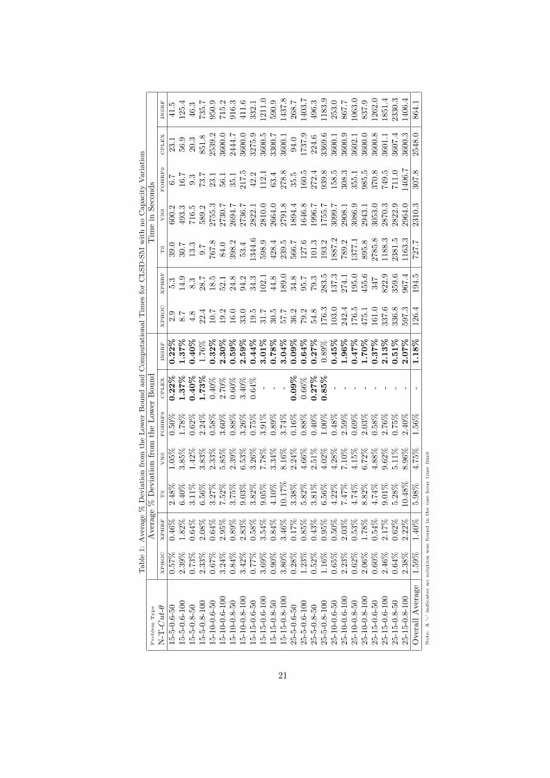
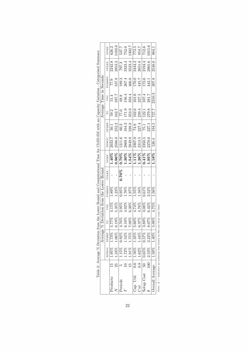
Table 1 presents the computational results of the different algorithms proposed in this paper and Table

2 summarizes these results by grouping instances by the number products (N), the number of periods (T ),

capacity utilization values (Cut), and setup cost per unit of time (θ).

The results clearly show that all linear programming (LP)-based heuristics, including Fix-and-Optimize,

outperformed the TS and VNS metaheuristics in every problem type. In all cases the LP heuristics not only

obtain higher quality solutions but also do so in less time. Overall, however, the technique that consistently

found the best solutions was the INSRF heuristic, producing the best average result for 22 of the 24 problem

types studied here. By design the INSRF will always dominate XPHRF, as the first phase of INSRF is

a local search using the XPH neighborhood scheme. Therefore the improvement made by the alternative

neighborhood scheme incorporated into INS can be measured as the difference between the results from

XPHRF and INSRF. On average we can see that the effect of this neighborhood scheme was to produce a

0.22% improvement in the average solution quality at a cost of, on average, 669.6 seconds. This improvement

to time ratio is very small - however as the MIP heuristics are producing high quality solutions in the first

place, large gains cannot be expected.

The relax-and-fix initial solution provides some performance benefits, as can be seen by comparing the

XPHOC with XPHRF, however these differences are rather small and therefore we may conclude that these

LP-based heuristics are reasonably insensitive to the starting point provided.

Table 2 generally shows that the larger the number of periods, the higher the deviation from the lower

bound. This is not surprising as these problems are larger in size and therefore it is more difficult to search

the solution space. Nevertheless, the quality of the solution seems to be independent of the number of

products and the capacity utilization factor. Table 2 also shows that there is a significant difference in the

average deviation from the lower bound, being for all LP-based heuristics between 3.2 and 4.7 times larger

when the setup cost per unit of time, θ, is 100, compared to when it is 50 - which suggests that problems

with higher setup costs are more difficult to solve.

4.4. Single Machine Experiments With Capacity Variation

To test single machine problems with capacity variation, we use the same set of problem types used in

Section 4.3, however for each instance CutV ar was set at 0.5. The instances were then solved using the best

heuristics we found in Section 4.3, namely XPHRF, INSRF and FOHRF9. For these experiments and the

remaining experiments in this paper we used an Intel Quad-Core Q9550 processor running at 2.83GHz with

3Gb RAM and CPLEX 12.1 mixed integer programming solver. The results are given in Table 3 while the

results grouped by number of products (N), number of periods (T ), capacity utilization values (Cut), and

setup cost per unit of time (θ) are provided in Table 4.

13

From these tables we notice that the introduction of capacity variation has produced results that are

very similar to the results for instances without capacity variation. The ranking of the solution techniques

is the same, with INSRF providing the best results followed by XPHRF and FOHRF9, however the change

in the deviations from the lower bound are quite different for the different techniques. When we compare

these results with the results for instances without capacity variation, the average lower bound deviation

for INSRF drops by 0.02% (a 1.9% drop), while the XPHRF increases by 0.15% (a 8.6% increase) while

the FOHRF9 increases by 0.58% (a 37.2% increase). The solution times also vary considerably with the

CPU time for INSRF increasing 1316.5 seconds (152.4% increase), XPHRF decreasing 105.7 seconds (54.3%

decrease) and FOHRF decreasing 242.3 seconds (78.7% decrease). By comparing the average deviation from

the lower bound in Tables 1 and 3 we see that some deviations increased and others decreased for each of the

techniques, and there was no specific problem type characteristic that could be used to predict this change.

Generally, however, we can see that the two local search procedures (XPHRF and FOHRF9) produced

poorer results in less time, which indicates that the local minima that they converged to was not as deep for

instances with capacity variation as compared to instances without capacity variation. The neighborhood

structure used by FOHRF9 is smaller and therefore the local minima are shallower than those local minima

found by XPHRF, which has a slightly larger neighborhood scheme. The fact that the INSRF procedure,

which is able to break out of local minima, was able to find better and better solutions (indicated by the long

running time) shows that there were a large number of local minima than needed to be navigated around.

These results suggest that the introduction of capacity variation changes the landscape of the search

space with the introduction of more local minima, therefore making the terrain rougher and therefore harder

to search. In this environment local search techniques will generally not perform as well as their performance

will be highly dependent on the starting point used. The number of local minima can be reduced by using

more general neighborhood structures and therefore those local search procedures with larger neighborhoods

will generally perform better in this type of environment. Using metaheuristics is likely to more beneficial in

this type of environment as they will be able to negotiate the increased number of local minima introduced

by the capacity variation.

4.5. Multiple Machines with No Capacity Variation

In order to generate problem instances we used, as a base, a mid-sized problem instance with 15 products,

10 periods and 80% capacity utilization. We then tried different perturbations of M , N , T , Cut, θ, MProb

and MBal. For each combination 10 instances were generated. The average results are presented in Table 5

while an analysis of the effect on parameter changes is provided in Table 6. Note that all instances have

a 3600 second time limit, however run times may be longer as any MIP started within this time limit are

14

allowed to finish. The fix-and-optimize heuristic (FOHRF9) has a 3600/K second sub-MIP time limit, while

the INSRF heuristic has a 600 second XPH sub-MIP time limit. CPLEX could not find solutions to these

problem instances within the one hour time limit, however it was used to calculate a lower bound that was

based on a plant-location reformulation of our model which is known to produce tighter bounds.

The results in Table 5 show that the best overall technique, in terms of average deviation from the lower

bound, was the XPHRF heuristic followed by the INSRF heuristic and lastly the FOHRF9. This reverses

the ranking for XPHRF and INSRF that was observed for the single machine problems. The reason for this

change in ranking is due to the 600 second time limit placed on the XPH subMIP in the INS heuristic. As we

can see by the CPU times in Table 5, the XPHRF took on average 2207.3 seconds to run to completion, well

in excess of the subMIP time limit. As a result the solutions obtained from INSRF are of a lower quality,

however the average solution times for INSRF are nearly half that of XPHRF. The time taken to solve the

XPHRF is strongly related to the number of machines in the problem instance, as can be seen in the huge

increase in CPU time taken between solving two and three machine problem instances in Table 6. This

suggests that within the XPH framework the number of machines, as well as periods and products, need to

be limited so that its performance is not unduly affected by when the number of machines increases in the

problem instance.

FOHRF9 is the fastest of all three heuristics by a large margin, however it does have the largest deviation

from the average lower bound. As with the other two techniques, adding machines to the problem does

increase the computational burden considerably. Even with its speed FOHRF9 found the lowest average

deviation from the lower bound for one of the larger problem types. This problem type was very difficult to

solve, as illustrated by XPHRF taking an average of over 7600 seconds, hence the smaller neighborhood of

FOHRF9 was able to quickly move to better solutions and converge to a local minima.

If we compare the average lower bound deviations in Tables 1 and 5 we see that the deviations for the

multi-machine problems are more than 5% higher than the deviations we obtained for the single machine

problem, which could indicate one of two things: either the problem is much more difficult to solve with the

introduction of more machines, or the lower bound procedure is not as tight for the multi-machine problem.

This trend can also be observed in Table 6 where problem instances with three machines had between 4.5%

- 6.0% more lower bound deviation than those problem instances with two machines.

Referring to Table 6, we can gain some further insights into this problem and these heuristics. Inter-

estingly increasing the number of products reduces the deviations from the lower bound, however this does

not mean the problem is easier as the time taken to solve these problems does increase considerably. If the

number of periods increases, the problem expands linearly in terms of its variables and we would expect

there to be an increase in average lower bound deviation and time, and this is what we observe in the data in

Table 6. Increasing Capacity utilization and setup costs both have a similar effect. Regarding the influence

of the assignment matrix data Ami, smaller changes are observed when we consider changing the balance

15

of jobs across the machines (given by MBal), but they become more expressive when the total number of

possible job-machine allocations is modified. Clearly, when moving MProb from 60% to 80%, the problem

becomes harder as the solution space is expanded.

4.6. Multiple Machines with Capacity Variation

For the Multiple Machines problem with Capacity Variation the same set of problem instances solved in

Section 4.5 were generated with a CutV ar = 0.5. Once again these instances were solved using the XPHRF,

INSRF and FOHRF9 heuristics. The results for these instances are detailed in Table 7, while an analysis of

the changes in problem instance parameters is presented in Table 8.

We see from Table 7 that, as we observed in the instances without capacity variation, XPHRF is the best

performing heuristic followed by INSRF and finally FOHRF9. The reason for XPHRF outperforming INSRF

is once again due to the restricted subMIP time as discussed in Section 4.5. XPHRF requires the most

CPU time and FOHRF9 the least, however here the difference in average time required between XPHRF

and INSRF is just 11% compared to 85% for instances without capacity variation. This is due primarily to

XPHRF average CPU time required dropping significantly as the INSRF times are fairly comparable.

In comparison to the Multi-Machine instances without capacity variation we note that adding capacity

variation does not affect the average lower bound deviations significantly, however in all cases the average

has actually dropped with the introduction of capacity variation unlike the single machine instances where

there was a mix of changes. If we compare the CPU times we find that introducing capacity variation has,

surprisingly, decreased them as well. A possible explanation for this is that capacity variation can narrow

down the possible alternative schedules for those periods where capacity is reduced, and in a multi-machine

setting these constraints become even tighter. It is important here to note that the results for the multi-

machine problem may be at a different level of quality to the single machine problems discussed in the

previous section. Here the multi-machine lower bound deviations are on average in the 6-7% range, whereas

for the single machine data these were in the 1-2% range. Therefore adding capacity variation to a multi-

machine problem may produce different behavior than for a single machine. In this case capacity variation

appears to have made it easier to find good areas of the search space and therefore good solutions. In terms

of finding an optimal solution, however, we predict that adding capacity variation will still increase the

roughness of the search landscape and therefore increase the difficulty of finding the exact optimal solution

as we observed with the results from the single machine data.

Table 8 shows similar lower bound deviation patterns to the results for instances without capacity vari-

ation presented in Table 6. The CPU times, however, are different - demonstrating the fact that instances

16

with capacity variation, no matter what the changes are, tend to be solved more quickly than those without

capacity variation. Again, by allowing jobs to be processed on more machines (MProb increasing from 60%

to 80%), the average lower bound deviation tends to increase independently of capacity variation, while

MBal makes very little difference to the performance.

When we analyze the performance of the heuristics by problem type, we see that the best heuristic for

each problem class is almost exactly the same for problems with capacity variation as those for the problems

without capacity variation, with the exception of problem type 2-20-10-0.8-0.5-100-80-20. For problem type

3-15-10-0.8-0.5-50-80-20 it is clear that XPHRF tended to become stuck in local minima which both INSRF

and FOHRF9 are able to get out of or avoid altogether. This particular class was the only one where XPHRF

performed considerably worse than the other techniques, however it does demonstrate the importance of the

heuristic being able to climb out of local minima.

5. Conclusions

In this paper we introduced a novel Mixed Integer Programming (MIP) based Iterative Neighborhood

Search heuristic (INSRF) to solve the Capacitated Lot Sizing and Scheduling problem with sequence depen-

dent setup times and costs in single and multi-machine settings. The algorithm is composed of two steps:

a local search phase to intensify the search and a neighborhood modification phase, in order to break out

of local minima. INSRF essentially solves a series of biased selected subMIPs of different dimensions in an

iterative fashion, therefore combining features of exact enumeration methods with approximate procedures.

We showed with extensive computational experiments on a number of very difficult large-size instances

that INSRF outperforms default CPLEX 12.1 and other approaches reported in the literature in terms

of quality and often in running times, such as pure meta-heuristics and other MIP-based heuristics (e.g.

fix-and-optimize or exchange).

Our findings also indicate that with higher setup costs per unit of setup time, the problem instances

become more difficult to solve for all the heuristics, but INSRF is not as adversely affected as the other

solution procedures. For problems involving more than one machine, INSRF can still be used in an effective

way. However, it must be noted that the limits on solving time play an important role in determining the

quality of the solutions produced. The inclusion of the capacity variation feature produces different results

whether we are facing single-machine or multi-machine settings. For the case of INSRF, the results are

slightly better with the variation of capacity, but the running times vary significantly. Nevertheless, and

based on the output of the other heuristics, we may infer that, when compared to problems without capacity

variation, the number of local optima increases with this characteristic. With regards to the assignment

17

matrix, the number of machines a job may be allocated to appears to influence the performance of multi-

machine problems, but the impact of balancing the jobs between machines seems negligible.

This work raised several issues, which remain as interesting and challenging topics for future research.

Firstly, INSRF finds local optima, but not necessarily global optima. It incorporates a simple mechanism

to escape local minima, however other more sophisticated techniques may provide more efficient ways of

crossing barriers in the solution space typology. Secondly, all the partitions considered in INSRF are based

on the product and/or period dimensions, but not on the machines, i.e., each subMIP takes into account

all the machines simultaneously. Naturally, these heuristics could be extended to select in each iteration a

subset of machines. This generalization is straightforward; the way the sets of binary variables should be

partitioned (here and in other types of problems – e.g. in the multi-level setting, the decomposition may

be carried out by the levels of the bill-of-materials) needs to be investigated. Finally, it seems promising to

devise a partition-based heuristic that throughout the search is able to dynamically change the dimensions of

the partition (number of products, periods and machines) based on the performance of the algorithm (MIP

gap and computational time to solve each iteration until optimality).

6. Acknowledgments

The authors would like to thank the two anonymous referees whose feedback helped improve the overall

quality of this paper.

References

[1] N. Absi and S. Kedad-Sidhoum. MIP-based heuristics for multi-item capacitated lot-sizing problem

with setup times and shortage costs. Rairo-Operations Research, 41(2):171–192, 2007.

[2] B. Almada-Lobo and R. James. Neighbourhood search metaheuristics for capacitated lotsizing with

sequence-dependent setups. International Journal of Production Research, 48(3):861–878, 2010.

[3] B. Almada-Lobo, D. Klabjan, M. A. Carravilla, and J. F. Oliveira. Single machine multi-product

capacitated lotsizing with sequence-dependent setups. International Journal of Production Research,

45(20):4873–4894, 2007.

[4] S. Araujo, N. Arenales, and A. R. Clark. Lot sizing and furnace scheduling in small foundries. Computers

and Operations Research, 35(3):916–932, 2008.

[5] I. Barany, T. J. Vanroy, and L. A. Wolsey. Strong formulations for multi-item capacitated lot sizing.

Management Science, 30(10):1255–1261, 1984.

18

[6] P. Beraldi, G. Ghiani, A. Grieco, and E. Guerriero. Rolling-horizon and fix-and-relax heuristics for the

parallel machine lot-sizing and scheduling problem with sequence-dependent set-up costs. Computers

and Operations Research, 35(11):3644–3656, 2008.

[7] G. Bitran and H. Yanasse. Computational complexity of the capacitated lot size problem. Management

Science, 28(10):1174–1186, 1982.

[8] L. Buschkhl, F. Sahling, S. Helber, and H. Tempelmeier. Dynamic capacitated lotsizing - a classification

and review of the literature on “big bucket” problems. OR Spectrum, 32:231–261, 2010.

[9] A. R. Clark, B. Almada-Lobo, and C. Almeder. Editorial on lotsizing and scheduling: industrial

extensions and research opportunities. Accepted for publication in International Journal of Production

Research, 2010.

[10] A. Federgruen, J. Meissner, and M. Tzur. Progressive interval heuristics for multi-item capacitated

lot-sizing problems. Operations Research, 55(3):490–502, 2007.

[11] D. Ferreira, R. Morabito, and S. Rangel. Solution approaches for the soft drink integrated production

lot sizing and scheduling problem. European Journal of Operational Research, 196:697–706, 2009.

[12] J. M. Framinan and R. Pastor. A proposal for a hybrid meta-strategy for combinatorial optimization

problems. Journal of Heuristics, 14(4):375–390, 2008.

[13] K. Haase. Capacitated lot-sizing with sequence dependent setup costs. Operations Research Spektrum,

18:51–59, 1996.

[14] S. Helber and F. Sahling. A fix-and-optimize approach for the multi-level capacitated lot sizing problem.

International Journal of Production Economics, 123:247–256, 2010.

[15] R. Jans. Solving lot-sizing problems on parallel identical machines using symmetry-breaking constraints.

Informs Journal on Computing, 21(1):123–136, 2009.

[16] C. Merce and G. Fontan. MIP-based heuristics for capacitated lotsizing problems. International Journal

of Production Economics, 85(1):97–111, 2003.

[17] Y. Pochet and L. A. Wolsey. Production Planning by Mixed Integer Programming. Springer Series in

Operations Research and Financial Engineering. Springer, New York, 2006.

[18] J. Puchinger and G. R. Raidl. Combining metaheuristics and exact algorithms in combinatorial opti-

mization: A survey and classification. In Artificial Intelligence and Knowledge Engineering Applications:

a Bioinspired Approach, Pt 2, Proceedings, volume 3562 of Lecture Notes in Computer Science, pages

41–53. 2005.

19

[19] D. Quadt and H. Kuhn. Capacitated lot-sizing wih extensions: a review. 4OR, 6:61–83, 2008.

[20] F. Sahling, L. Buschkhl, H. Tempelmeier, and S. Helber. Solving a multi-level capacitated lot sizing

problem with multi-period setup carry-over via a fix-and-optimize heuristic. Computers and Operations

Research, 36(9):2546–2553, 2009.

[21] H. Stadtler. Multilevel lot sizing with setup times and multiple constrained resources: Internally rolling

schedules with lot-sizing windows. Operations Research, 51(3):487–502, 2003.

[22] X. Y. Zhu and W. E. Wilhelm. Scheduling and lot sizing with sequence-dependent setup: A literature

review. IIE Transactions, 38(11):987–1007, 2006.

20

Table

1:

Aver

age

%D

evia

tion

from

the

Low

erB

ound

and

Com

puta

tionalT

imes

for

CLSD

-SM

wit

hno

Capaci

tyV

ari

ati

on

Pro

ble

mType

Aver

age

%D

evia

tion

from

the

Low

erB

ound

Tim

ein

Sec

onds

N-T

-Cut-

θX

PH

OC

XPH

RF

TS

VN

SFO

HR

F9

CPLEX

INSR

FX

PH

OC

XPH

RF

TS

VN

SFO

HR

F9

CPLEX

INSR

F

15-5

-0.6

-50

0.5

7%

0.4

6%

2.4

8%

1.0

5%

0.5

0%

0.2

2%

0.2

2%

2.9

5.3

39.0

600.2

6.7

23.1

41.5

15-5

-0.6

-100

2.3

9%

1.8

2%

6.4

0%

3.8

5%

1.7

8%

1.3

7%

1.3

7%

8.7

14.9

30.7

493.3

16.7

56.9

125.4

15-5

-0.8

-50

0.7

3%

0.6

4%

3.1

1%

1.4

2%

0.6

2%

0.4

0%

0.4

0%

4.8

8.3

13.3

716.5

9.3

20.3

46.3

15-5

-0.8

-100

2.3

3%

2.0

8%

6.5

6%

3.8

3%

2.2

4%

1.7

3%

1.7

6%

22.4

28.7

9.7

589.2

73.7

851.8

735.7

15-1

0-0

.6-5

00.6

7%

0.6

4%

3.2

7%

2.3

3%

0.5

8%

0.4

0%

0.3

2%

10.7

18.5

767.8

2755.3

23.1

2539.2

950.9

15-1

0-0

.6-1

00

3.2

4%

2.9

5%

7.5

2%

5.8

5%

3.6

0%

2.7

0%

2.3

0%

19.2

52.1

84.0

2730.7

56.1

3600.0

715.2

15-1

0-0

.8-5

00.8

4%

0.8

9%

3.7

5%

2.3

9%

0.8

8%

0.6

0%

0.5

9%

16.0

24.8

398.2

2694.7

35.1

2444.7

916.3

15-1

0-0

.8-1

00

3.4

2%

2.8

3%

9.0

3%

6.5

3%

3.2

6%

3.4

0%

2.5

9%

33.0

94.2

53.4

2736.7

217.5

3600.0

411.6

15-1

5-0

.6-5

00.7

7%

0.5

8%

3.8

2%

3.2

6%

0.7

5%

0.6

4%

0.4

4%

19.5

34.3

1344.6

2822.1

42.2

3275.9

332.1

15-1

5-0

.6-1

00

3.6

9%

3.5

4%

9.0

5%

7.7

8%

3.9

1%

-3.0

1%

31.7

102.1

598.9

2810.0

112.1

3600.5

1211.0

15-1

5-0

.8-5

00.9

0%

0.8

4%

4.1

0%

3.3

4%

0.8

9%

-0.7

8%

30.5

44.8

428.4

2664.0

63.4

3300.7

590.9

15-1

5-0

.8-1

00

3.8

0%

3.4

6%

10.1

7%

8.1

6%

3.7

4%

-3.0

4%

57.7

189.0

239.5

2791.8

278.8

3600.1

1437.8

25-5

-0.6

-50

0.2

8%

0.1

7%

3.3

8%

2.2

4%

0.1

6%

0.0

9%

0.0

9%

36.2

34.8

566.7

1894.4

35.5

94.0

268.7

25-5

-0.6

-100

1.2

3%

0.8

5%

5.8

2%

4.6

6%

0.8

8%

0.6

6%

0.6

4%

79.2

95.7

127.6

1646.8

160.5

1737.9

1403.7

25-5

-0.8

-50

0.5

2%

0.4

3%

3.8

1%

2.5

1%

0.4

0%

0.2

7%

0.2

7%

54.8

79.3

101.3

1996.7

272.4

224.6

496.3

25-5

-0.8

-100

1.1

6%

0.9

5%

6.5

6%

4.0

2%

1.0

0%

0.8

5%

0.8

9%

176.3

283.5

193.2

1755.7

939.8

3369.6

1183.9

25-1

0-0

.6-5

00.6

5%

0.5

0%

4.2

2%

4.2

8%

0.4

8%

-0.4

5%

103.0

137.3

1887.2

3099.7

158.5

3600.1

253.0

25-1

0-0

.6-1

00

2.2

3%

2.0

3%

7.4

7%

7.1

0%

2.5

9%

-1.9

6%

242.4

274.1

789.2

2908.1

308.3

3600.9

867.7

25-1

0-0

.8-5

00.6

2%

0.5

3%

4.7

4%

4.1

5%

0.6

9%

-0.4

7%

176.5

195.0

1377.1

3086.9

355.1

3602.1

1063.0

25-1

0-0

.8-1

00

2.0

6%

1.7

8%

8.8

2%

6.7

2%

2.0

3%

-1.7

0%

475.1

455.6

895.8

2943.1

985.5

3600.0

837.9

25-1

5-0

.6-5

00.6

0%

0.5

4%

4.7

4%

4.8

8%

0.5

8%

-0.3

7%

161.0

347

2785.8

3053.0

370.8

3600.8

1262.0

25-1

5-0

.6-1

00

2.4

6%

2.1

7%

9.0

1%

9.6

2%

2.7

6%

-2.1

3%

337.6

822.9

1188.3

2870.3

749.5

3601.1

1851.4

25-1

5-0

.8-5

00.6

4%

0.6

2%

5.2

8%

5.1

1%

0.7

5%

-0.5

1%

336.8

359.6

2381.5

2822.9

711.0

3607.4

2330.3

25-1

5-0

.8-1

00

2.3

8%

2.2

2%

10.4

8%

8.9

6%

2.4

0%

-2.0

7%

597.3

967.4

1163.3

2964.0

1406.7

3600.3

1406.4

Over

all

Aver

age

1.5

9%

1.4

0%

5.9

8%

4.7

5%

1.5

6%

-1.1

8%

126.4

194.5

727.7

2310.3

307.8

2548.0

864.1

Note

:A

‘-’in

dic

ate

sno

solu

tion

was

found

inth

eone

hour

tim

elim

it

21

Table

2:

Aver

age

%D

evia

tion

from

the

Low

erB

ound

and

Com

puta

tionalT

ime

for

CLSD

-SM

wit

hno

Capaci

tyV

ari

ati

on

-C

ate

gori

sed

Sum

mary

Aver

age

%D

evia

tion

from

the

Low

erB

ound

Aver

age

Tim

ein

Sec

onds

XPH

OC

XPH

RF

TS

VN

SFO

HR

F9

CPLEX

INSR

FX

PH

OC

XPH

RF

TS

VN

SFO

HR

F9

CPLEX

INSR

F

Pro

duct

s15

1.9

5%

1.7

3%

5.7

7%

4.1

5%

1.8

9%

-1.4

0%

2033.7

50.1

59.2

51.4

77.9

2242.8

626.2

N25

1.2

4%

1.0

6%

6.1

9%

5.3

5%

1.2

3%

-0.9

6%

2586.8

252.2

342.7

337.7

537.8

2853.2

1102.0

Per

iods

51.1

5%

0.9

2%

4.7

6%

2.9

5%

0.9

5%

0.7

0%

0.7

0%

1211.6

60.3

77.0

68.8

189.3

797.3

537.7

T10

1.7

2%

1.5

2%

6.1

0%

4.9

2%

1.7

6%

-1.3

0%

2869.4

164.3

171.9

156.4

267.4

3323.4

752.0

15

1.9

1%

1.7

5%

7.0

8%

6.3

9%

1.9

7%

-1.5

4%

2849.8

228.8

353.9

358.4

466.8

3523.4

1302.7

Cap.

Uti

l.0.6

1.5

6%

1.3

5%

5.6

0%

4.7

4%

1.5

5%

-1.1

1%

2307.0

74.8

162.6

161.6

170.0

2444.2

773.5

Cut

0.8

1.6

2%

1.4

4%

6.3

7%

4.7

6%

1.5

8%

-1.2

6%

2313.5

227.4

239.4

227.5

445.7

2651.8

954.7

Set

up

Cost

50

0.6

5%

0.5

7%

3.8

9%

3.0

8%

0.6

1%

-0.4

1%

2350.5

75.1

122.1

107.4

173.6

2194.4

712.6

θ100

2.5

3%

2.2

2%

8.0

7%

6.4

2%

2.5

2%

-1.9

5%

2270.0

227.1

279.8

281.7

442.1

2901.6

1015.6

Over

all

Aver

age

1.5

9%

1.4

0%

5.9

8%

4.7

5%

1.5

6%

-1.1

8%

126.4

194.5

727.7

2310.3

307.8

2548.0

864.1

Note

:A

‘-’in

dic

ate

sno

solu

tion

was

found

inth

eone

hour

tim

elim

it

22

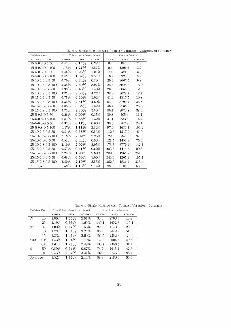
Table 3: Single-Machine with Capacity Variation - Categorized Summary

Problem Type Ave. % Dev. from Lower Bound Ave. Time in Seconds

N-T-Cut-CutV ar-θ XPHRF INSRF FOHRF9 XPHRF INSRF FOHRF9

15-5-0.6-0.5-50 0.42% 0.14% 0.38% 6.4 494.4 2.215-5-0.6-0.5-100 1.75% 1.27% 2.57% 9.3 1309.7 3.215-5-0.8-0.5-50 0.46% 0.28% 1.01% 7.6 538.0 3.015-5-0.8-0.5-100 2.43% 1.68% 3.54% 10.9 3224.5 5.815-10-0.6-0.5-50 0.70% 0.24% 0.89% 20.4 3667.5 9.815-10-0.6-0.5-100 3.58% 2.60% 3.97% 28.5 3624.6 16.015-10-0.8-0.5-50 0.98% 0.48% 1.48% 23.8 3650.0 12.515-10-0.8-0.5-100 3.23% 3.06% 4.77% 38.0 3628.7 18.715-15-0.6-0.5-50 0.75% 0.20% 1.02% 41.4 1817.5 19.815-15-0.6-0.5-100 3.34% 2.51% 4.69% 64.9 3799.4 35.815-15-0.8-0.5-50 0.88% 0.35% 1.52% 46.4 2763.6 25.815-15-0.8-0.5-100 3.73% 3.20% 5.50% 80.7 3982.8 38.425-5-0.6-0.5-50 0.26% 0.09% 0.35% 30.8 505.4 11.125-5-0.6-0.5-100 0.87% 0.66% 1.32% 37.1 833.6 14.425-5-0.8-0.5-50 0.37% 0.17% 0.63% 38.6 587.9 24.125-5-0.8-0.5-100 1.47% 1.11% 2.82% 97.6 1631.1 100.225-10-0.6-0.5-50 0.51% 0.38% 0.53% 112.6 1247.9 41.025-10-0.6-0.5-100 2.18% 2.02% 2.25% 122.8 3342.8 97.025-10-0.8-0.5-50 0.52% 0.44% 0.98% 121.5 1458.9 75.425-10-0.8-0.5-100 2.10% 2.02% 3.05% 173.5 3770.4 142.125-15-0.6-0.5-50 0.57% 0.41% 0.62% 203.6 1444.5 90.825-15-0.6-0.5-100 2.23% 1.90% 2.89% 209.3 1968.2 254.325-15-0.8-0.5-50 0.68% 0.50% 1.00% 243.6 1205.9 195.125-15-0.8-0.5-100 2.50% 2.19% 3.55% 362.0 1836.4 335.4

Average 1.52% 1.16% 2.14% 88.8 2180.6 65.5

Table 4: Single-Machine with Capacity Variation - Summary

Problem Type Ave. % Dev. from Lower Bound Ave. Time in Seconds

XPHRF INSRF FOHRF9 XPHRF INSRF FOHRF9

N 15 1.86% 1.33% 2.61% 31.5 2708.4 15.925 1.19% 0.99% 1.66% 146.1 1652.8 115.1

T 5 1.00% 0.67% 1.58% 29.8 1140.6 20.510 1.73% 1.41% 2.24% 80.1 3048.9 51.615 1.83% 1.41% 2.60% 156.5 2352.3 124.4

Cut 0.6 1.43% 1.04% 1.79% 73.9 2004.6 49.60.8 1.61% 1.29% 2.49% 103.7 2356.5 81.4

θ 50 0.59% 0.31% 0.87% 74.7 1615.1 42.6100 2.45% 2.02% 3.41% 102.9 2746.0 88.4

Average 1.52% 1.16% 2.14% 88.8 2180.6 65.5

23

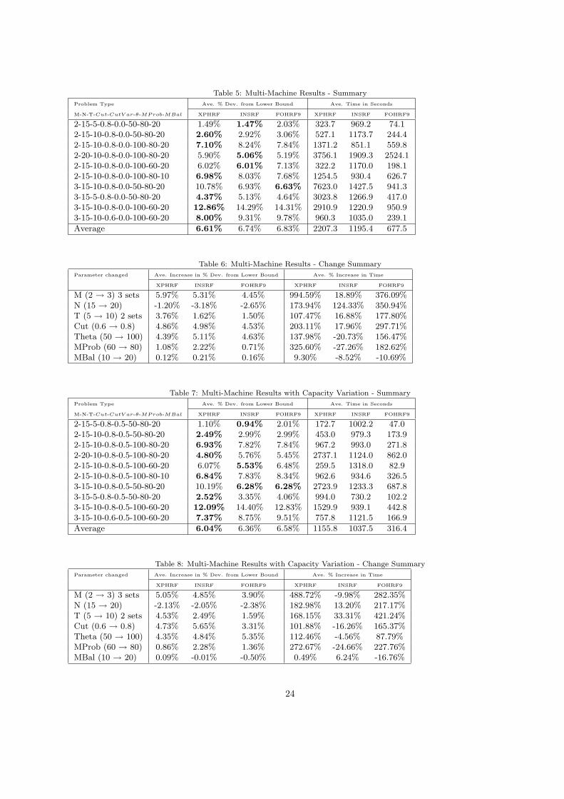
Table 5: Multi-Machine Results - Summary

Problem Type Ave. % Dev. from Lower Bound Ave. Time in Seconds

M-N-T-Cut-CutV ar-θ-MP rob-MBal XPHRF INSRF FOHRF9 XPHRF INSRF FOHRF9

2-15-5-0.8-0.0-50-80-20 1.49% 1.47% 2.03% 323.7 969.2 74.12-15-10-0.8-0.0-50-80-20 2.60% 2.92% 3.06% 527.1 1173.7 244.42-15-10-0.8-0.0-100-80-20 7.10% 8.24% 7.84% 1371.2 851.1 559.82-20-10-0.8-0.0-100-80-20 5.90% 5.06% 5.19% 3756.1 1909.3 2524.12-15-10-0.8-0.0-100-60-20 6.02% 6.01% 7.13% 322.2 1170.0 198.12-15-10-0.8-0.0-100-80-10 6.98% 8.03% 7.68% 1254.5 930.4 626.73-15-10-0.8-0.0-50-80-20 10.78% 6.93% 6.63% 7623.0 1427.5 941.33-15-5-0.8-0.0-50-80-20 4.37% 5.13% 4.64% 3023.8 1266.9 417.03-15-10-0.8-0.0-100-60-20 12.86% 14.29% 14.31% 2910.9 1220.9 950.93-15-10-0.6-0.0-100-60-20 8.00% 9.31% 9.78% 960.3 1035.0 239.1

Average 6.61% 6.74% 6.83% 2207.3 1195.4 677.5

Table 6: Multi-Machine Results - Change Summary

Parameter changed Ave. Increase in % Dev. from Lower Bound Ave. % Increase in Time

XPHRF INSRF FOHRF9 XPHRF INSRF FOHRF9

M (2 → 3) 3 sets 5.97% 5.31% 4.45% 994.59% 18.89% 376.09%N (15 → 20) -1.20% -3.18% -2.65% 173.94% 124.33% 350.94%T (5 → 10) 2 sets 3.76% 1.62% 1.50% 107.47% 16.88% 177.80%Cut (0.6 → 0.8) 4.86% 4.98% 4.53% 203.11% 17.96% 297.71%Theta (50 → 100) 4.39% 5.11% 4.63% 137.98% -20.73% 156.47%MProb (60 → 80) 1.08% 2.22% 0.71% 325.60% -27.26% 182.62%MBal (10 → 20) 0.12% 0.21% 0.16% 9.30% -8.52% -10.69%

Table 7: Multi-Machine Results with Capacity Variation - Summary

Problem Type Ave. % Dev. from Lower Bound Ave. Time in Seconds

M-N-T-Cut-CutV ar-θ-MP rob-MBal XPHRF INSRF FOHRF9 XPHRF INSRF FOHRF9

2-15-5-0.8-0.5-50-80-20 1.10% 0.94% 2.01% 172.7 1002.2 47.02-15-10-0.8-0.5-50-80-20 2.49% 2.99% 2.99% 453.0 979.3 173.92-15-10-0.8-0.5-100-80-20 6.93% 7.82% 7.84% 967.2 993.0 271.82-20-10-0.8-0.5-100-80-20 4.80% 5.76% 5.45% 2737.1 1124.0 862.02-15-10-0.8-0.5-100-60-20 6.07% 5.53% 6.48% 259.5 1318.0 82.92-15-10-0.8-0.5-100-80-10 6.84% 7.83% 8.34% 962.6 934.6 326.53-15-10-0.8-0.5-50-80-20 10.19% 6.28% 6.28% 2723.9 1233.3 687.83-15-5-0.8-0.5-50-80-20 2.52% 3.35% 4.06% 994.0 730.2 102.23-15-10-0.8-0.5-100-60-20 12.09% 14.40% 12.83% 1529.9 939.1 442.83-15-10-0.6-0.5-100-60-20 7.37% 8.75% 9.51% 757.8 1121.5 166.9

Average 6.04% 6.36% 6.58% 1155.8 1037.5 316.4

Table 8: Multi-Machine Results with Capacity Variation - Change Summary

Parameter changed Ave. Increase in % Dev. from Lower Bound Ave. % Increase in Time

XPHRF INSRF FOHRF9 XPHRF INSRF FOHRF9

M (2 → 3) 3 sets 5.05% 4.85% 3.90% 488.72% -9.98% 282.35%N (15 → 20) -2.13% -2.05% -2.38% 182.98% 13.20% 217.17%T (5 → 10) 2 sets 4.53% 2.49% 1.59% 168.15% 33.31% 421.24%Cut (0.6 → 0.8) 4.73% 5.65% 3.31% 101.88% -16.26% 165.37%Theta (50 → 100) 4.35% 4.84% 5.35% 112.46% -4.56% 87.79%MProb (60 → 80) 0.86% 2.28% 1.36% 272.67% -24.66% 227.76%MBal (10 → 20) 0.09% -0.01% -0.50% 0.49% 6.24% -16.76%

24