the 2004 december 26 indian ocean tsunami impact on sri lanka: cascade modelling from ocean to city...

Geophys. J. Int. (2009) 177, 1080–1090 doi: 10.1111/j.1365-246X.2009.04106.xG

JISei

smol

ogy

The 2004 December 26 Indian Ocean tsunami impact on Sri Lanka:cascade modelling from ocean to city scales

B. Poisson, M. Garcin and R. PedrerosBRGM, Land Use Planning and Natural Hazards, Orleans, France. E-mail: [email protected]

Accepted 2009 January 7. Received 2009 January 6; in original form 2008 July 4

S U M M A R YThe 2004 December 26 Indian Ocean tsunami severely hit Sri Lanka. Although it was not inthe direct path of the initial tsunami waves, the western coast was struck by diffracted wavesthat caused much damage. The numerical model GEOWAVE is used to compute tsunamigeneration, propagation and inundation from the earthquake source to the Sri Lankan coast. Anested grid system is constructed to increase the resolution until Galle Bay, on the southwesterncoast, where a 20 m-grid is used. The six nested topobathymetric grids are interpolated fromETOPO2 and high resolution data, at sea as onshore. Simulation results are compared withtsunami height data from National Oceanic and Atmospheric Administration (NOAA; US) andGeological Survey & Mines Bureau (GSMB; Sri Lanka). When the grid resolution increases,the discrepancy between the model and the data remains, on average, good, whereas its spreadincreases. We then conclude that the order of magnitude of the tsunami height is consistent fromthe 180 m-resolution grid, but the spatial imprecision is too high to locally predict reliablewater heights. Nevertheless, the comparison between computed time-series of sea surfaceelevation at the Colombo tide station and tide-gauge data shows a very good agreement asboth amplitude, and arrival time of the first wave are well reproduced. When focusing onshore,the modelled inundation limit is compared with the limit measured in the field. With its a priorisetup, computed inundation spreads much farther behind the field limit. We then integrate moreaccurate nearshore conditions into the model. Non-linear shallow water equations are choseninstead of fully non-linear Boussinesq equations; the bottom friction on land is increased to amuch higher value than at sea; the buildings cover and the low tide conditions are taken intoaccount in the DEM. The resulting high resolution simulation agrees better with field data,even if discrepancies are still locally observed in places of DEM imprecision and in a rivervalley. This simulation, however, demonstrates that taking into account nearshore and onshorefeatures may significantly improve tsunami impact assessment.

Key words: Tsunamis; Indian Ocean.

1 I N T RO D U C T I O N

The 2004 December 26 Sumatra–Andaman earthquake was oneof the most disastrous recorded earthquakes, due, in part, to itslarge magnitude, M w between 9.1 and 9.3 (Ammon et al. 2005;Park et al. 2005; Stein & Okal 2005). The earthquake generated atsunami, which propagated through the Indian Ocean and causedextreme inundation and destruction along the surroundings coasts(Chanson 2005). The resulting death toll is estimated to be between200 000 and 300 000. The most devastated country was Indonesia,as it lies near the subduction zone where the earthquake occurred,but the tsunami also severely struck Sri Lanka, where more than30 000 people were killed (Liu et al. 2005; Goff et al. 2006;Inoue et al. 2007). The tsunami hit the island because it was onthe main propagation axis, and then diffracted around it, so that thesouthwestern zone was as greatly damaged as the eastern zone.

Since 2005, numerous studies have attempted to model thetsunami propagation: some focused on the seismic source to dis-criminate between inverted slip distributions (Pietrzak et al. 2007)or to directly invert the slip distribution (Grilli et al. 2007; Piatanesi& Lorito 2007; Sladen & Hebert 2008); others attempted to modelthe tsunami impact on local targets like Thailand or the MascareneIslands (Ioualalen et al. 2007; Hebert et al. 2007); and one studyexamined the propagation of the tsunami over the entire world andthe spatial transport of energy in all oceans (Kowalik et al. 2007).

The potential influence of nearshore propagation effects on localtsunami height at the shoreline and onshore is well known. Mosttsunami models, however, only operate on rough bathymetric data(Dao & Tkalich 2007; Geist et al. 2007; Ioualalen et al. 2007).The difficulty is to obtain high resolution data and to handle thewhole extent of tsunami propagation, for example, with an irregularmesh or a nested system (Pietrzak et al. 2007; Hebert et al. 2007).

1080 C© 2009 The Authors

Journal compilation C© 2009 RAS

by guest on April 28, 2016

http://gji.oxfordjournals.org/D

ownloaded from

http://gji.oxfordjournals.org/

Numerical modelling of 2004 Tsunami: focus on Sri Lanka 1081

Without such accurate data, numerical modelling may only computetsunami amplitude at sea and cannot appraise the tsunami impacton the coasts (Geist et al. 2007).

In this study, we extend the global model of Grilli et al. (2007),with focus on the impact on southwestern Sri Lanka. We built asimulation chain to increase the resolution of the tsunami calculationin this area. Along the process, computed tsunami heights on SriLanka shore are compared with several sets of observations. The laststep of the simulation chain is a focus on the Bay of Galle. There,model results are compared with field data of inundation limits. Atthis stage, we run several calculations with different options andparameters in order to refine the model so that it agrees, as well aspossible, with the data.

2 N U M E R I C A L M O D E L L I N G

2.1 Tsunami model

In this study, we used the tsunami generation, propagation and in-undation model GEOWAVE (Watts et al. 2003). The initial tsunami(surface water deformation and velocity) is computed from thevertical displacements of seafloor produced by an elastic disloca-tion simulating the earthquake (Okada 1985). Then, propagationand inundation of tsunami waves are computed with FUNWAVE, amodel based on fully non-linear Boussinesq equations, accountingfor frequency dispersion (Wei et al. 1995). The methodology ofGEOWAVE is described in Grilli et al. (2007).

2.2 Nesting system

The aim is to compute tsunami waves until they reach the Sri Lankancoast. In a first stage, the most important thing is to describe thetsunami wavelength well, which is related to the source characteris-tics. For an earthquake-generated tsunami, the wavelength generallyreaches a few hundred kilometres if the concerned fault is long. Forthe 2004 Sumatra earthquake, the wavelength is estimated, fromthe first wave measured by the Jason-1 satellite altimeter, as around500–600 km (Gower 2005). The spatial resolution of the computa-tional grid must be chosen according to this wavelength. In our case,a grid resolution of a few kilometres is enough to model tsunamipropagation across the deep part of the Indian Ocean. However,when the tsunami comes near the coast, its wavelength decreasesdue to the decreasing depth, so that the resolution of the com-putational grid must increase. As GEOWAVE can solve tsunamipropagation only on a regular square grid, we had to implement asystem of nested grids. Considering the layout of the affected zone,a one-way nested scheme appears to be appropriate. Such systemsare commonly used in tsunami modelling with non-linear shallowwater equations (Koshimura & Mofjeld 2001; Titov et al. 2005),but this approach was not previously applied to Boussinesq-typemodels. In such a one-way nested grid scheme, wave propagation isfirst computed on the entire domain of the coarse grid. Information(velocity and water height) are extracted from the coarse grid sim-ulation at the boundaries of the included fine grid and then used forthe calculation on the fine grid. Information are not returned to thecoarse grid from the fine one. Indeed, in the case of the December2004 tsunami, the waves propagate in one preferential direction,they enter the Sri Lanka region and then exit without coming backagain. The trapped waves are fully computed in the finer grids. Itappears that some waves are reflected by the Maldives and thencome back towards Sri Lanka, but the simulation shows that they

Table 1. Mesh and domain size for the six nested grids used in thisstudy.

Name of Mesh size Domain Time step(sub)grid simulation (m) size (s)

S0 4860 677 × 663 8.57S1 1620 751 × 814 2.27S2 540 682 × 1006 0.79S3 180 739 × 637 0.28S4 60 829 × 454 0.15S5 20 445 × 520 0.10

have a negligible amplitude compared with direct and trapped waves(see Fig. 3). In practice, a first complete run is performed on gridof δx 0-uniform spacing, during which water height and velocitiesare recorded at the limits of a second domain included within thefirst. Then, these conditions are interpolated on the limits of sec-ond domain, according to the chosen nested grid resolution δx 1 <

δx 0 and used to compute through a new run more accurate tsunamipropagation on this finer grid.

In our simulations, we chose to use a nested ratio of 3, so thatδx 1 = δx 0/3. As we intend to reach a local scale around the Bayof Galle in Sri Lanka, the nesting process is iterated as needed. Theresolution of all grids composing the nesting system are reported inTable 1. The first three simulations comprise the whole of Sri Lanka(Fig. 1). The last three are centred on the southwestern part of theisland and then on the Bay of Galle.

2.3 Source parameters

The source parameters are taken from Grilli et al. (2007), whoadjusted a five-segment fault model to satellite track records andsome tide gauge data around the most devastasted part of the IndianOcean coasts. We also use the same time sequence spanning 1200 s,which could be debated as it largely exceeds measured ruptureduration (Ammon et al. 2005; Ni et al. 2005; Park et al. 2005). Grilliet al. (2007) defend their choice by referring to rising time effects,low shear-wave speed in the accretionary prism and since othertsunami modelling also assumed reduced rupture speed (e.g. Fujii& Satake 2007).

2.4 Outputs

The output of each calculation consists of time-series of griddedsea surface elevation (SSE), maximum SSE on the domain (zmax)and, eventually, time-series of SSE at selected points taken as nu-merical gauges. The time-series results are important as they helpto constrain the arrival time of the tsunami at the shore, and theyalso enable tsunami period estimation.

3 DATA U S E D I N T H I S S T U DY

3.1 Bathymetric and topographic data

Bathymetric grids are derived from several data sets of variousresolutions.

The first grid S0 is derived from the ETOPO2 data set (U.S.Department of Commerce & Atmospheric Administration 2006).ETOPO2 is made from several data sources, mainly, satellitealtimetry and has a 2′ × 2′ spatial resolution.

C© 2009 The Authors, GJI, 177, 1080–1090




ownloaded from


1082 B. Poisson, M. Garcin and R. Pedreros

Figure 1. Location of the six nested grids used in our simulation chain (coordinates are in Mercator projection).

Figure 2. Bathymetric data points around the southwestern Sri Lankancoast.

A loose data set of sounding points on the complete Sri Lankamargin was provided by the DEOCOM project (Delimitation ofthe Outer Edge of the Continental Margin of Sri Lanka under theUNCLOS; Fig. 2). Nearshore detailed bathymetric profiles wereprovided by the Coastal Conservation Department (CCD), but onlya few kilometres along north of Galle. Around Galle Bay andWeligama Bay, fine resolution data were provided by the NationalHydrographic Office (NHO) of Sri Lanka (Garcin et al. 2007). Thesedata have been checked and corrected before computing topobathy-metric grids at various resolutions up to 20 m (Garcin et al. 2007,2008).

Topography is needed to model inundation and tsunami reflec-tion when the tsunami hits the coast. It, thus, mainly plays a rolein high-resolution simulations, that is S4 and S5. We used a finetopographical data set on a 3–4-km wide coastal strip, where themain part is below 10 m elevation. A 20 m specific DEM was inter-polated from the Survey Department of Sri Lanka data (elevationpoints and contour lines) and covers the coastal strip from Beruwalato Weligama Bay (thus covering the extent of S4 extent; Garcin et al.2007). Another DEM made by the United Nations University (UNU)from a 1 : 5000 map digitizing and kinematic GPS data covers theGalle urban area with a 5 m resolution. Both these DEMs helpedto build S4 and S5 topographical grids through subsampling. Else-where, SRTM elevation data with a 3′ ′ × 3′ ′ resolution are used buthave almost no influence on the tsunami calculation. Because of

their limited extent, fine topographical data are integrated only inS3 and subsequent grids.

We use the Mercator projection to build a nesting system of sixrectangular uniform grids from topobathymetric data with spatialresolutions from 4860 to 20 m (Table 1).

3.2 Tsunami observation data: tsunami heightand inundation

As in the NOAA data set, what we call here ‘tsunami height’ mayrefer to the maximum elevation reached by the water either at sea(in case of tide gauges) or onshore (when talking about run-up).

Tsunami height data sets from several sources were used in thisstudy. We first retrieved NOAA data (http://www.ngdc.noaa.gov/hazard/tsu.shtml), which is well spatially distributed data for theentire global domain of calculation. NOAA data for Sri Lanka areused to particularly check S0 to S2 simulations. When focusing onsouthern Sri Lanka (S2 and S3), we use GSMB data collected inthe field a few days after the tsunami disaster (2004 December 30;Siriwardana et al. 2005).

Then, when zooming on the Bay of Galle, we resorted to NOAAdata because the GSMB data are too sparse in this zone (S4).

The nearest tide gauge to our zone of interest is located atColombo, around the middle of the western coast of Sri Lanka.This tide gauge recorded the first half of the tsunami wave but thenmalfunctioned. This record, however, is precious, as it precisely in-dicates the time of tsunami arrival and the height of the first wave(2.1 m), even if the arriving wave at Colombo had been somewhatdisturbed and weakened when moving around half the island.

Around Galle, we have the maximum inundation limits as itwas estimated, interpretated and localized by GPS in the field fromwitnesses testimonies (Garcin et al. 2007). This field inundationlimit (FIL) extends from Weligama Bay in the south to Beruwala inthe north, so that the S4 domain is entirely covered.

Topographic data on simulations S0–S2 are derived only fromSRTM data set, inducing a higher shore relief in the main partof southwestern Sri Lanka. Because of this artefact, the simulatedtsunami at these resolutions cannot inundate the coastal zone as itshould. In consequence, a lot of points that were actually inundatedare modelled as always dry. This happens also on the S3–S5 grids,probably because of imprecision in data localization and/or in topo-graphical modelling. For this reason, we relocalized data points foreach simulation within a 1-pixel radius for S0 and S1 and 2-pixelradius for S2–S4 in such a way that we can test an average agree-ment with NOAA data, regardless of details. At the same time, wecompare data at its original location with the result, as a control.

C© 2009 The Authors, GJI, 177, 1080–1090




ownloaded from



4 R E S U LT S

All simulations compute tsunami propagation and inundation until5 hr 40 min after the beginning of rupture, corresponding to at least2 hr 30 min after the first tsunami impact on Sri Lanka.

In the following, a parallel between model results and data isdrawn and discussed simulation after simulation.

4.1 First simulations: S0 and S1

The simulation of tsunami propagation throughout the Indian Oceanfrom Sumatra to the Maldives distinctly reproduces two major re-flections of tsunami waves (Fig. 3). The first obstacle hit by thetsunami is Sri Lanka. Here, diffraction and reflection of the waveoccur at the same moment. The diffracted wave rolls around theisland and runs along the shore until it is on the western part. Thereflected wave moved radially away around the island. The sec-ond obstacle was the Maldives, at the southwest of southern India.There was some diffraction on the atoll islands, but the first andhighest wave was also reflected from the archipelago and movedback, mostly northeastwards. When looking in detail at the simula-tion in the area between Sri Lanka and Maldives, the waves reflectedby the Maldives archipelago are clearly visible in the open sea, notbecause of their amplitude but because the open sea is no longerdisturbed by direct incident waves (Fig. 3). As the reflected wavefront propagates towards the Sri Lankan shore, their contribution tosimulated wave height appears completely dwarfed by the trappedwaves coming from diffraction along the southern coast. In a realsystem, however, the dissipation of trapped waves should have beenmore efficient, so that the reflected waves may have contributedsomewhat to the latest waves impacting southwestern Sri Lanka,about 2.5 hr after the first wave struck.

Watts et al. (2005) made the initial simulation, from which Grilliet al. (2007) elaborated their source model, and they already com-pared the simulated propagation of the tsunami with available satel-lite altimetry track records on a domain similar to our S0. Theyfound that salient features of the Jason-1 satellite transect werereproduced, although details differ somewhat.

S0 and S1 outputs were compared with 24 tsunami heights re-ported by NOAA and slightly relocalized by us in southern Indiaand all around Sri Lanka (Fig. 4 and Table 2). The average ratio of

Figure 3. Shaded relief map of sea surface height 4 hr after the earthquake(S0). White arrows indicate the first wave reflected from Sri Lanka, whereasblack ones mark the wave reflected from the Maldives.

Figure 4. Maximal SSE (m) on S1 grid (1620 m resolution), with NOAApoints for checking S0 and S1 results around Sri Lanka.

zmax to measured tsunami heights for both simulations, R0 and R1,amount to 62 and 88 per cent, respectively. As it could be expected,the average of tsunami heights at shore appears to be underestimatedwhen the resolution of the calculation grid is too coarse. The lackof accurate data at shallow depth indeed prevents accounting for theamplification of the wave, where the wavelength greatly decreases.The wave height at the shore may then appear much lower than itshould. The fact that R1 is higher than R0 is consistent with theimprovement of calculation when the resolution is increased. Thefact that R1 is lower than 100 per cent suggests that S1 resolution(1620 m) is still too poor for modelling tsunami impact on shore-lines. We note, however, that the difference between data and S1results is larger around southern India than around Sri Lanka. Thisis likely due to the integration of DEOCOM data around Sri Lankacoast in the S1 bathymetric grid. Sri Lanka is surrounded by a con-tinental shelf about 20-km wide in average, which is already quitewell described at the S1 resolution.

The polarity of the first wave is positive at each point of Table 2,as was observed on tide-gauge data throughout the S1 domain(Nagarajan et al. 2006). The polarity is directly determined bythe source mechanism, but it is important to check that diffractionalong the Sri Lankan coast is correctly modelled and does not alterthe shape of tsunami waves with respect to observations.

We observe that in the northern part of Sri Lanka, a coastalsegment was saved from tsunami impact, thanks to two bathymet-ric thresholds located on both sides (Fig. 4). Just opposite, thecorresponding coast segment in India was similarly saved. Boththresholds standing in the way of the tsunami efficiently stopped thewaves. This result of the modelling is consistent with inundationextent observed in northern Sri Lanka (Wijetunge 2006).

4.2 Intermediate simulations: S2 and S3

S2 is the last simulation stage comprising the whole of Sri Lanka. Itshows more clearly than S1 how the whole eastern coast of the islandis severely impacted by the tsunami, with probable far-penetratinginundation. On the western side, the most harshly affected zone liessouth of Colombo. This part of the coast was reached by diffractedwaves having hit the eastern coast and also later by waves reflectedfrom the Maldives.

C© 2009 The Authors, GJI, 177, 1080–1090




ownloaded from



Table 2. NOAA check points for S0 and S1, in southern India (IN) and Sri Lanka (SL).

Point Loc. Designation H t Z0max R0 (per cent) Z1

max R1 (per cent)

1 IN Arcattuthurai/ Veddarayan 4.2 2.4 58 2.9 682 IN Kalapakkom, Tamil Nadu 4.9 2.4 48 3.9 793 IN Kochi, Kerala 0.8 0.7 81 1.1 1315 IN Nagapattinum, Tamil Nadu 5.8 4.0 70 3.8 667 IN Periakalapet, Tamil Nadu 6.3 4.2 66 4.9 778 IN Pulicat, Tamil Nadu 5.0 1.7 35 1.5 3010 IN Tarangambadi, Tamil Nadu 5.1 4.4 88 3.5 6922 SL Eva Hotel, Tangalle 7.5 3.3 45 5.1 6823 SL Rathgama/Doanduwa 4.5 2.6 58 4.9 10824 SL Mahaseelawa Beach, Yala 8.4 4.4 52 7.5 8925 SL Berawala 6.0 3.1 51 4.3 7226 SL Maratuwa 5.5 2.9 53 5.7 10327 SL Pottuvil 9.0 4.7 52 7.9 8828 SL Uswettakeiyawa 2.6 2.5 98 2.8 10729 SL Vennapuwa North 1.8 0.9 52 1.3 7230 SL Karativu 7.0 3.6 52 4.9 7131 SL Kalkudah 7.0 5.7 81 6.5 9332 SL China Bay Ferry 3.3 1.8 53 5.9 17933 SL Irrakkakandi 4.0 2.3 57 4.0 100

Note: H t is tsunami height reported by NOAA, Z0max and Z1

max are maximum SSE respectively for S0 andS1, and R0 and R1 are corresponding ratio of Zmax to H t.

Figure 5. Tide-gauge data at Colombo superimposed on the correspondingtime-series extracted from S2 results.

As S2 grid includes Colombo, we put a numerical gauge at thelocation of the tide-gauge in the harbour. Fig. 5 shows the compar-ison between detided sea level data and the model results. Data areonly available for the first 20 min of the tsunami demonstration atColombo, corresponding to the sea surface rise and subsequent fall.Although Colombo lies across the island with respect to the sidefacing the tsunami, the model result agrees well with the rise and isonly a bit shifted during the fall. Both arrival time and maximumamplitude of this first wave are very well reproduced. This con-sistency confirms the model validity, even in calculating diffractedwaves evolution.

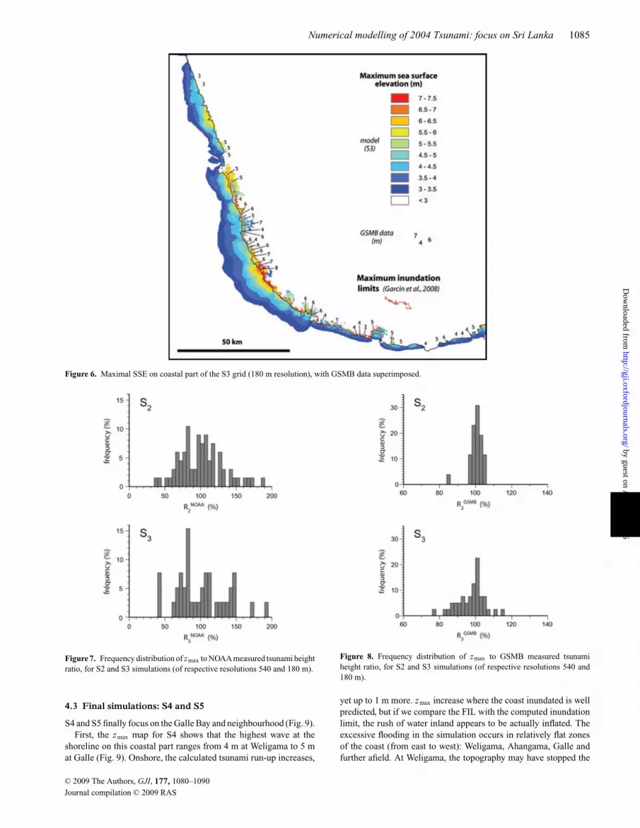
S3 focuses on the affected southwestern coast, refining thebathymetry description above 1000 m depth (Fig. 6). S2 and S3results are compared with NOAA tsunami height data on their re-spective domains (67 points on S2 domain, 39 points on S3 do-main). With relocalized gauges, average ratio of zmax to measuredtsunami heights, R2 and R3, are 101 and 100 per cent, respec-tively. At original gauge points that are inundated in the modelsimulations, these ratios are 106 per cent and 104 per cent. Theseaverage values are very satisfying and suggest that although ap-parently coarse, S2 and S3 resolutions are appropriate for properlymodelling tsunami impact. Nevertheless, plots of frequency distri-bution of RNOAA

2 and RNOAA3 show that the dispersion of model–data

discrepancy increases with increasing resolution (Fig. 7). As S3 do-main is included in the S2 domain, this trend may actually mean thatthe discrepancy is higher in the S3 zone than in the other parts of S2,that is to say, the rest of Sri Lanka. The S3 zone is actually withinthe only part of Sri Lanka that was severely hit not by direct wavesbut by diffracted ones. This specific context may probably causelarger discrepancy between data and model results. The realisticaverage R3 however suggest that the discrepancy is mainly spatial,and that in some places, high and low values are just inverted. Aszmax quite varies along the coastal part of S3, this hypothesis seemsrather plausible.

Model results were also compared with GSMB tsunami heightdata (Siriwardana et al. 2005). We rejected the data points thatwere not inundated during the simulation. Some of the selected71 points were relocalized within a 3-pixel radius (for most ofthem, at a less than 1-pixel distance from the original location).As GSMB data covers the entire south part of Sri Lanka and notonly the S3 domain, we compare them to S3 results when possible(Fig. 6), otherwise with S2 results. Resulting zmax to measuredtsunami height ratio is plotted on Fig. 8. The agreement between theselected GSMB data and the model result is good in both simulations

S2 and S3, as the average ratios RGSMB2 and RGSMB

3 are 100 and97 per cent, respectively. Both distributions are clearly tighter thanin the comparison with NOAA data. Once more, they confirm thatthe S2 simulation already computes a realistic tsunami impact interms of maximum SSE at the shoreline.

On Fig. 6 the FIL measured by Garcin et al. (2008) is also plotted.This limit is clearly overestimated by the model in many placeswhere the computed tsunami penetrates further 3 km.

The zmax map for S3 exhibits a patch of run-up higher than 7 mon a section of the coastline (red spot on the Fig. 6). This is theplace where a train was swept off by the tsunami in Pereliya,killing more than 1500 people. The calculated inundation limitthere agrees quite well with data. When looking at the DEM, wesee that a topographical bank stops the tsunami penetration, con-trary to other locations where the model calculates too great aninundation.

C© 2009 The Authors, GJI, 177, 1080–1090




ownloaded from



Figure 6. Maximal SSE on coastal part of the S3 grid (180 m resolution), with GSMB data superimposed.

Figure 7. Frequency distribution of zmax to NOAA measured tsunami heightratio, for S2 and S3 simulations (of respective resolutions 540 and 180 m).

4.3 Final simulations: S4 and S5

S4 and S5 finally focus on the Galle Bay and neighbourhood (Fig. 9).First, the zmax map for S4 shows that the highest wave at the

shoreline on this coastal part ranges from 4 m at Weligama to 5 mat Galle (Fig. 9). Onshore, the calculated tsunami run-up increases,

Figure 8. Frequency distribution of zmax to GSMB measured tsunamiheight ratio, for S2 and S3 simulations (of respective resolutions 540 and180 m).

yet up to 1 m more. zmax increase where the coast inundated is wellpredicted, but if we compare the FIL with the computed inundationlimit, the rush of water inland appears to be actually inflated. Theexcessive flooding in the simulation occurs in relatively flat zonesof the coast (from east to west): Weligama, Ahangama, Galle andfurther afield. At Weligama, the topography may have stopped the

C© 2009 The Authors, GJI, 177, 1080–1090




ownloaded from



Figure 9. Maximal SSE on the S4 grid (60 m resolution), with NOAA points around Galle. White crosses indicate the NOAA data locations.

Figure 10. Frequency distribution of computed zmax to NOAA measuredtsunami height ratio, for S4 simulation (of resolution 60 m).

real tsunami, whereas the DEM is too flat to have the same stoppingeffect. At Ahangama, the inundated zone behind the FIL corre-sponds almost exactly to the Koggala Lake, which is described asland in the DEM because of its positive elevation. At Galle, a flatzone on the back of the town is inundated during the simulation,although it stayed dry in reality. This takes place in the S5 zone, so itwill be discussed later. The 5-m elevation contour for the used DEMis plotted on Fig. 9 for indication. The frontal part of the contour linematches remarkably well with the computed inundation limit. Thisagreement suggests that in our simulations, the only way to stopthe tsunami propagation even onshore is a topographic bank. In thecase of such a powerful tsunami, energy dissipation in FUNWAVEis insufficient to stop inundation within a 1–1.5 km wide coastalstrip, as it should.

zmax results are compared with the 17 NOAA data points forthe S4 domain. With relocalization, the average ratio of zmax tomeasured tsunami height R4 amounts to 106 per cent, whereas the11 original points that are inundated in S4 exhibit a similar ratioat 105 per cent. This result seems quite consistent, but it must benoted that the dispersion in R4 is even worse than for S3 (Fig. 10).

The S5 simulation on a 20-m resolution grid intends to refine thecalculation on the Bay of Galle. One can first note that the tsunamimagnitude computed in S3 over the Galle Bay does not change in S4and S5 (Fig. 11). S3 appears to be adequate for computing tsunami

heights at the shoreline, as it clearly improves the tsunami propa-gation model when water depth gradually decreases in this zone.Then, S4 and S5 improve the precision of the result and slightlyimprove the calculation of inundation limit, but the spatial distribu-tion of tsunami height does not change any more. The stabilisationof tsunami height with increasing resolution validates the simula-tion chain, as we are certain not to miss the amplification effect atshallow depth near the coast.

Instantaneous sea surface height profiles are extracted from S3,S4 and S5 outputs across Galle Bay and until computed inundationlimit (Fig. 12). They confirm the same amplitude and shape oftsunami waves whatever the simulation. S4 and S5 are particularlyconcordant, except for minor details on shore.

We extracted the SSE time-series at a numerical gauge corre-sponding to the SL19 NOAA point, at the Bay entrance (Fig. 13).This time-series indicates that the highest wave at Galle was the sec-ond. This result is consistent with eye witness testimonies (Garcinet al. 2007). In addition, we can observe on this graph that sub-sequent waves are still significant, as they exceed half the highestwave. This could be due to the influence of waves that were re-flected back from the Maldives. These waves indeed came back tothe southwestern coast of Sri Lanka around 1hr 50 min after the firstarrival, but the numerical gauge signal shows that they only had anegligible effect on the SSE (Fig. 13). The wave sequence couldalso have been influenced by trapped waves.

As was noted already in previous simulations, the computed in-undation limit outruns by far the FIL (Fig. 11). We then tried to im-prove the final computation of tsunami propagation and inundationby taking into account the following previously ignored considera-tions:

(1) In simulations S0–S4, we chose in FUNWAVE to use fullynon-linear Boussinesq equations from Wei et al. (1995). It maybe, however, better to use the non-linear shallow water equations(NLSWE) option for the S5 domain, as it is physically more appro-priate for very shallow water. The wavelength indeed remains veryhigh as the depth greatly decreases, so that the depth to wavelengthratio is very small nearshore, thus allowing to use NLSWE.

(2) The bottom friction coefficient had been set as its defaultvalue, 0.0025. As this value is much lower than the rough surface

C© 2009 The Authors, GJI, 177, 1080–1090




ownloaded from



Figure 11. S2–S5 maximal computed SSE on S5 around Galle. Coastline and 5 m contour are extracted from the S5 topobathymetric grid. The dashed linesindicate the track of the Fig. 12 profiles.

Figure 12. Instantaneous SSE profiles through Galle Bay and the town, atthe maximum of the first and second wave (see location on the Fig. 11).Three profiles are extracted for each wave from S3, S4 and S5 outputs, forcomparison. The topographical profile is also reported from the S5 grid.

Figure 13. SSE time-series at the SL19 numerical gauge, off the Galle Fort(simulation S5).

onshore, we try to consider a more realistic bottom friction coef-ficient on the topography. 0.2–0.3 bottom friction coefficients areassigned to coral reefs contexts (Lugo-Fernandez et al. 1998; Loweet al. 2005). Besides, this coefficient may reach 0.1–0.2 when esti-mated on rough bed during storm events (Trembanis et al. 2004).

C© 2009 The Authors, GJI, 177, 1080–1090




ownloaded from



We then tested several bottom friction values on land: 0.1, 0.2 and0.5.

(3) Inundation, wave-breaking and stopping of tsunami wavesdepend on obstacles in its way. At Galle, the seafront consists ofmany, often connected, buildings rather high compared with theincoming waves. Thanks to the Geographic Information Systemfor Coastal Hazards in Sri Lanka project, we have available high-resolution vectorized data for buildings, which had been extractedfrom maps and data of the Survey Department of Sri Lanka (Garcinet al. 2007, 2008). Topographical data used until then representedonly a digital terrain model, so that the buildings cover will help torefine the S5 topographical grid into an approximate digital surfacemodel. Although the pixel size exceeds most of buildings length,elevation is noteably raised in areas with many connected buildings.As individual building heights were unknown, uniform heights of 3and 8 m were tested.

(4) The tide had not been taken into account until now, as it hasonly an influence close to the shore. The tsunami indeed arrivedon the western coast of Sri Lanka just at low tide. To take thisfactor into account, we added 0.4 m to our topobathymetric grid,corresponding to the 0.4 m negative amplitude of the consideredtide.

We made serial test simulations by modifying underlined param-eters first one by one, then by combining several effects at once.The aim is to move the computed inundation limit as near to the FILas possible. To better assess the difference between the model resultand inundation data, we now consider maximal water height on land(hmax

w ) instead of zmax. hmaxw is computed by subtracting the positive

topography from zmax. Fig. 14 shows maps of hmaxw in four of the

performed tests. In the default simulation (test 0), hmaxw appears to

Figure 14. Maximal water height map for four S5 simulation tests with modified parameters.

exceed 4 m until 2 km beyond the FIL, where the computed inunda-tion limit lies. When choosing NLSWE option (test 1), hmax

w dropsby 1 m against test 0 almost everywhere. In test 2, we resume test 1settings by adding the buildings cover to the initial DEM. A uniformheight of 3 m was first imposed, which corresponds mostly to resi-dential sector, behind the seafront. Then we chose another uniformheight of 8 m, to represent the high buildings on the seafront (withat least three levels for the main part). Both options lead to almostthe same hmax

w map, except that buildings get submerged for a 3 mheight and not for a 8 m height. Anyway, hmax

w in test 2 seems to bemarkedly reduced behind the FIL. Inundation still extends too far,but where hmax

w had reached 3 m in test 0, it is now restricted to anaverage value of 1 m. As we add a high bottom friction coefficientin test 3, two changes in hmax

w are perceptible: first, hmaxw decreases

when moving away from the FIL because of enhanced friction; andsecond, the strip of hmax

w of more than 3 m along the seafront appearsto be paradoxically wider than in test 2. The reason for this is thatenhanced friction does not allow the incoming mass of water tospread as greatly as for a very low friction. The waves then do notflow quickly away after having ran over the first seafront buildings.

The ultimate test on S5 simulation consists of combining togetherNLSWE, 8 m buildings cover, high bottom friction coefficient of0.5 and the 0.4 m tidal shift of the DEM (Fig. 15). The resultinginundation limit is now consistent with the FIL in many places,in the west of the domain and in the east of Galle Bay. Places ofremaining discrepancy may be interpreted one by one. A points ona river valley, where the high bottom friction coefficient artificiallyprevents the propagation of tsunami flow as it should overrun theriver. B indicates a very flat area that is too low to actually stopthe flow propagation (2 m elevation on almost the whole dark blue

C© 2009 The Authors, GJI, 177, 1080–1090




ownloaded from



Figure 15. Maximal water height map for the last test on the S5 simulation.Black arrows and letters indicate places where the discrepancy betweenmodel and FIL is larger.

zone). At last, topographical data at Unawatuna (C) exhibits muchsteeper slopes than the actual topography, so, that it does not allowthe water flow to reach the FIL. It must be noted that in the last test,calculated inundation limit steps aside the 5-m contour line morethan in any other simulation, whereas it comes closer to the FIL.This assessment suggests that by default, the modelled tsunami flowon land only stops when a topographical obstacle is in its way.

5 C O N C LU S I O N

The 2004 December 26 tsunami severely impacted the coast of SriLanka. To numerically model this impact, it has been necessary toimplement a nesting grid system, with six nested grids of increasingresolution. From 4860 to 540 m mesh size, the nesting processsupports the improvement of tsunami propagation calculation asit approaches the coast. Then, from 180 m to 20 m mesh sizes,increasing resolution helps mostly to refine the model at sea and toimprove the tsunami processes at the shoreline and onshore.

Successive nested simulations are checked with several distinctdata sets. Maximum water elevation is compared with NOAAtsunami height data in simulations S0–S4. The model results areconsistent, on average, with these NOAA data, for simulations S2–S4. However, when the spatial resolution of calculation increases,the distribution of model-data difference also increases, showinggrowing spatial dispersion. The observed discrepancy may likelybe due to the lack of detailed bathymetric and/or topographical datathat may induce very localized effects. Another tsunami height dataset helps to check the model consistency. GSMB data are comparedwith S2 and S3 results in the southern part of Sri Lanka. Whilesome data points are neglected because the modelled tsunami doesnot reach them, the comparison between data and model results atthe remaining points leads to a good agreement. In case of NOAAdata, as for GSMB data, we had to relocalized data points within a1 km radius before making the comparison. The same comparisonbetween S4 model results and NOAA data leads us to require a sim-ilar relocalization. Considering this technique, we can conclude thatthe model is only consistent in average. This is not surprising, asthe tsunami evolution and run-up depend a lot on very local detailslike buildings, structures and ground roughness. Results must thenbe considered by sector, not by punctual values.

Apart from tsunami height data, we used tide-gauge data fromthe Colombo station to check arrival time and height of the firsttsunami wave on the western coast. The time-series of SSE at thispoint agrees very well with available measurements. This agreementis important in confirming that the model succeeds in calculatingthe tsunami wave diffraction along an about 300 km-long coastalsegment before it reaches Colombo.

The last simulation, S5, has a pixel size of 20 m and focuses onGalle Bay. As too few tsunami height data are available at this place,S5 model results are tested from the inundation point of view. Themaximum inundation limit is taken from field work of Garcin et al.(2008). It concerns mainly the S5 domain. As the computed limitextends far beyond the FIL, we try to improve the description ofhigh resolution context and processes by changing some parametersand inputs in the model. We computed test simulations by takinginto account NLSWE theory for very shallow water propagation inthe Bay, much higher bottom friction onshore than at sea, buildingscover and tidal shift of elevation. A last test with all changes togethershows a much better concordance between the resulting inundationlimit and the FIL. The remaining discrepancy is located in placeswhere the DEM seems to be distorted, or in a river valley wherethe local water is not taken into account by the model. The focusof the tsunami model on a small high resolution domain brings outthe great importance of taking into account detailed characteristicsof the coast, otherwise the computed tsunami may be significantlyoverestimated.

A C K N OW L E D G M E N T S

This study was funded by BRGM research projects. Philip Watts(Applied Fluids Engineering, Inc.) provided the initial GEOWAVEcode version that we modified and used in this work. The authorsare very grateful to the GSMB team for their useful help in fieldinvestigations and for providing tsunami heights data. They thankthe University of Hawai’i Sea Level Center for making availabletide-gauge data from the Colombo sea level station. John Douglasand Thomas Dewez helped to improve the English of the manuscript.Two anonymous reviewers provided useful comments that helpedus to improve the quality of the manuscript.

R E F E R E N C E S

Ammon, C.J. et al., 2005. Rupture process of the 2004 Sumatra–Andamanearthquake, Science, 308, 1133–1139.

Chanson, H., 2005. Le Tsunami du 26 decembre 2004 : un phenomenehydraulique d’ampleur internationale. Premiers constats, La HouilleBlanche, 2, 25–32.

Dao, M.H. & Tkalich, P., 2007. Tsunami propagation modelling – a sensi-tivity study, Nat. Hazards Earth Syst. Sci., 6, 741–754.

Fujii, Y. & Satake, K., 2007. Tsunami source of the 2004 Sumatra–Andamanearthquake inferred from tide gauge and satellite data, Bull. seism. Soc.Am., 97(1A), S192–207.

Garcin, M. et al., 2007. A geographic information system for coastalhazards—application to a pilot site in Sri Lanka (Final Report), OpenFile Report BRGM - RP-55553-FR.

Garcin, M. et al., 2008. Integrated approach for coastal hazards and risks inSri Lanka, Nat. Hazards Earth Syst. Sci., 8, 577–586.

Geist, E.L., Titov, V.V., Arcas, D., Pollitz, F.F. & Bilek, S.L., 2007. Implica-tions of the 26 December 2004 Sumatra–Andaman earthquake on tsunamiforecast and assessment models for Great Subduction-Zone earthquakes,Bull. seism. Soc. Am., 97(1A), S249–270.

C© 2009 The Authors, GJI, 177, 1080–1090




ownloaded from



Goff, J. et al., 2006. Sri Lanka field survey after the December 2004 IndianOcean Tsunami, Earthq. Spectra, 22, S155–S172.

Gower, J., 2005. Jason 1 detects the 26 December 2004 Tsunami, EOS,Trans. Am. geophys. Un., 86, 37–38.

Grilli, S.T., Ioualalen, M., Asavanant, J., Shi, F., Kirby, J. & Watts, P.,2007. Source constraints and model simulation of the December 26, 2004Indian Ocean ssunami, J. Waterway Port Coastal Ocean Eng., 133, 414–428.

Hebert, H., Sladen, A. & Schindele, F., 2007. Numerical Modeling of theGreat 2004 Indian Ocean Tsunami: focus on the Mascarene Islands, Bull.seism. Soc. Am., 97(1A), S208–222.

Inoue, S., Wijeyewickrema, A., Matsumoto, H., Miura, H., Gunaratna, P.,Madurapperuma, M. & Sekiguchi, T., 2007. Field survey of tsunami ef-fects in Sri Lanka due to the Sumatra–Andaman earthquake of December26, 2004, Pure appl. Geophys., 164, 395–411.

Ioualalen, M., Asavanant, J., Kaewbanjak, N., Grilli, S.T., Kirby, J.T. &Watts, P., 2007. Modeling the 26 December 2004 Indian Ocean tsunami;case study of impact in Thailand, J. geophys. Res., 112, C07024.

Koshimura, S. & Mofjeld, H.O., 2001. Inundation modeling of localtsunamis in Puget Sound, Washington, due to potential earthquakes, inProceedings of the International Tsunami Symposium, Seattle, pp. 861–873.

Kowalik, Z., Knight, W., Logan, T. & Whitmore, P., 2007. The Tsunamiof 26 December, 2004: Numerical modeling and energy considerations,Pure appl. Geophys., 164, 379–393.

Liu, P.L.F. et al., 2005. Observations by the International Tsunami SurveyTeam in Sri Lanka, Science, 308, 1595.

Lowe, R.J., Falter, J.L., Bandet, M.D., Pawlak, G., Atkinson, M.J., Moni-smith, S.G. & Koseff, J.R., 2005. Spectral wave dissipation over a barrierreef, J. geophys. Res., 110, C04001.

Lugo-Fernandez, A., Roberts, H.H., Wiseman Jr, W.J. & Carter, B.L., 1998.Water level and currents of tidal and infragravity periods at Tague Reef,St. Croix (USVI), Coral Reefs, 17, 343–349.

Nagarajan, B. et al., 2006. The Great Tsunami of 26 December 2004: adescription based on tide-gauge data from the Indian subcontinent andsurrounding areas, Earth Planets Space, 58, 211–215.

Ni, S., Kanamori, H. & Helmberger, D., 2005. Energy radiation from theSumatra earthquake, Nature, 434, 582.

Okada, Y., 1985. Surface deformation due to shear and tensile faults in ahalf-space, Bull. seism. Soc. Am., 75, 1135–1154.

Park, J. et al., 2005. Earth’s free oscillations excited by the 26 December2004 Sumatra–Andaman earthquake, Science, 308, 1139–1144.

Piatanesi, A. & Lorito, S., 2007. Rupture process of the 2004 Sumatra–Andaman earthquake from tsunami waveform inversion, Bull. seism. Soc.Am., 97(1A), S223–S231.

Pietrzak, J. et al., 2007. Defining the source region of the Indian Oceantsunami from GPS, altimeters, tide gauges and tsunami models, Earthplanet. Sci. Lett., 261, 49–64.

Siriwardana, C.H.E.R., Weerawarnakula, S., Mudunkotuwa, S.M.A.T.B. &Preme, W.K.B.N., 2005. Final report on the tsunami mapping program(TMP) conducted in the Eastern, Southern and Western coastal regionsin Sri Lanka, Tech. rep., GSMB.

Sladen, A. & Hebert, H., 2008. On the use of satellite altimetry to infer theearthquake rupture characteristics: application to the 2004 Sumatra event,Geophys. J. Int., 172, 707–714.

Stein, S. & Okal, E.A., 2005. Speed and size of the Sumatra earthquake,Nature, 434, 581–582.

Titov, V.V., Gonzalez, F.I., Bernard, E.N., Eble, M.C., Mofjeld, H.O., New-man, J.C. & Venturato, A.J., 2005. Real-time tsunami forecasting: chal-lenges and solutions, Nat. Hazards, 35, 35–41.

Trembanis, A.C., Wright, L.D., Friedrichs, C.T., Green, M.O. & Hume, T.,2004. The effects of spatially complex inner shelf roughness on boundarylayer turbulence and current and wave friction: Tairua embayment, NewZealand, Continent. Shelf Res., 24, 1549–1571.

U.S. Department of Commerce, N.O. & Atmospheric Administration, N.G.D.C., 2006. 2-minute Gridded Global Relief Data (ETOPO2v2).

Watts, P., Grilli, S.T., Kirby, J.T., Fryer, G.J. & Tappin, D.R., 2003. Landslidetsunami case studies using a Boussinesq model and a fully nonlineartsunami generation model, Nat. Hazards Earth Syst. Sci., 3, 391–402.

Watts, P., Ioualalen, M., Grilli, S.T., Shi, F. & Kirby, J.T., 2005. Numericalsimulation of the December 26, 2004 Indian Ocean ssunami using ahigher-order Boussinesq model, in Proceedings of the 5th InternationalConference on Ocean Wave Measurement and Analysis, WAVES 2005,Madrid, Spain, 2005 July 3–7.

Wei, G., Kirby, J., Grilli, S. & Subramanya, R., 1995. A fully nonlinearBoussinesq model for surface waves, I: highly nonlinear, unsteady waves,J. Fluid Mech., 294, 71–92.

Wijetunge, J.J., 2006. Tsunami on 26 december 2004 : spatial distributionof tsunami height and the extent of inundation in Sri Lanka, Sci. TsunamiHazards, 24, 225–239.

C© 2009 The Authors, GJI, 177, 1080–1090




ownloaded from


the 2004 december 26 indian ocean tsunami impact on sri lanka: cascade modelling from ocean to city...

Documents