tsunami warning system - scholarly commons
TRANSCRIPT
Dissertations and Theses
8-2016
Tsunami Warning System Tsunami Warning System
Amay Vijay Desai
Follow this and additional works at: https://commons.erau.edu/edt
Part of the Oceanography and Atmospheric Sciences and Meteorology Commons
Scholarly Commons Citation Scholarly Commons Citation Desai, Amay Vijay, "Tsunami Warning System" (2016). Dissertations and Theses. 298. https://commons.erau.edu/edt/298
This Thesis - Open Access is brought to you for free and open access by Scholarly Commons. It has been accepted for inclusion in Dissertations and Theses by an authorized administrator of Scholarly Commons. For more information, please contact [email protected].
i
Tsunami Warning System
A Thesis
Submitted to the Faculty
of Embry-Riddle Aeronautical University
by
Amay Vijay Desai
In Partial Fulfillment of the
Requirements for the Degree
of
Master of Science in Electrical and Computer Engineering
August 2016
Embry-Riddle Aeronautical University
Daytona Beach, Florida

iii
Acknowledgments
First I would like to thank my thesis advisers Dr. Ilteris Demirkiran, Dr. Andre
Ludu, and Dr. Tianyu Yang at Embry Riddle Aeronautical University. They have
all always been available to help me solve all queries in my research and writing
work. They steered me in the right direction to ensure successful completion.
Finally, I would like to express gratitude to my family for providing for giving
me immense support and continuous encouragement throughout my studies. This
accomplishment would not have been possible without them. Thank you.
iv
ABSTRACT
The effects of a tsunami on a coastline can be devastating. In an attempt to
mitigate the damages caused by tsunamis, and to provide coastal communities
with evacuation alerts, it is essential to have early warning systems installed
offshore. Tsunami early warning systems can detect the formation of tsunami
waves long before they reach shore, providing coastal communities with
information about the strength of an incoming tsunami.
Since providing accurate information about oceanic wave patterns is
absolutely necessary to forecast the magnitude of a tsunami as it forms, the focus
of this research is to develop a novel approach which will predict the height and
velocity of a tsunami long before it makes landfall. The research comprises of a
mathematical study of how the objects under water appear would appear to any
observer outside. Also included in the research is study of water surface
regeneration techniques. The investigators believe that the proposed approach
will provide unprecedented detail and accuracy to help forecast the magnitude of
forming tsunami waves. This research will lay the groundwork for the next
tsunami early warning system, which will continue to save lives in coastal
communities around the world.
v
Table of Contents
Chapter 1: Introduction ....................................................................................................... 1
1.1 Background .......................................................................................................... 1
1.2 Goals and Objectives ............................................................................................ 2
1.3 Thesis Outline ...................................................................................................... 4
Chapter 2: Literature Review .............................................................................................. 5
2.1 History of Water Wave Research. ............................................................................. 5
2.2 Various approaches to Surface Wave and Image Reconstruction. ............................ 8
Chapter 3: Mathematical approach to estimate object position ........................................ 10
3.1 Object viewed in still water ..................................................................................... 10
3.1.1 Calculate the x component of X’ ..................................................................... 12
3.1.2 Calculate the y component of X’ ..................................................................... 14
3.1.3 Image formed on the lens ................................................................................. 15
3.2 Water surface at an angle with the normal .............................................................. 16
3.2.1 Calculate the y component of X’ ..................................................................... 16
Chapter 4: Graphical Representation of derived equations .............................................. 20
4.1 Case 1: [Water height h = 50 cm, Camera at 300 cm] ............................................ 20
4.2 Case 2: [Water height h = 100 cm, Camera at 300 cm] .......................................... 22
4.3 Case 3: [Water height h = 150 cm, Camera at 300 cm] .......................................... 24
4.4 Case 4: [Water height h = 250 cm, Camera at 300 cm] .......................................... 26
4.5 Case 5: [Object Distance = 50 cm, Camera at 300 cm] .......................................... 28
Chapter 5: Summary and conclusion ................................................................................ 30
Conclusion ........................................................................................................................ 44
Future Work ...................................................................................................................... 47
References ......................................................................................................................... 48
Appendix A Snell’s Law .................................................................................................... A
Appendix B Matlab Codes .................................................................................................. C
Appendix C Mathematica Simulation And Theory ............................................................ F
vi
Table of Figures
Figure 1: Camera Setup over Water Tank ...........................................................................2
Figure 2: Side view of camera setup ....................................................................................3
Figure 3: Object view by the camera .................................................................................10
Figure 4: To calculate X component ..................................................................................12
Figure 5: Water Surface at an angle with the normal. .......................................................13
Figure 6: Plot of angle α’ v/s Change in object position [Case 1] .....................................20
Figure 7: Plot of angle β’ v/s Change in object position. [Case 1] ....................................21
Figure 8: Plot of Virtual Height of X’ v/s Change in object position [Case 1] .................21
Figure 9: Plot of angle α’ v/s Change in object position [Case 2] .....................................22
Figure 10: Plot of angle β’ v/s Change in object position. [Case 2] ..................................23
Figure 11: Plot of Virtual Height of X’ v/s Change in object position [Case 2] ...............23
Figure 12: Plot of angle α’ v/s Change in object position [Case 3] ...................................24
Figure 13: Plot of angle β’ v/s Change in object position. [Case 3] ..................................25
Figure 14: Plot of Virtual Height of X’ v/s Change in object position [Case 3] ...............25
Figure 15: Plot of angle α’ v/s Change in object position [Case 4] ...................................26
Figure 16: Plot of angle β’ v/s Change in object position. [Case 4] ..................................27
Figure 17: Plot of Virtual Height of X’ v/s Change in object position [Case 4] ...............27
Figure 18: Plot of angle α’ v/s Change in water height. ..................................................28
Figure 19: Plot of angle β’ v/s Change in water height .....................................................29
Figure 20: Plot of Virtual Height of X’ v/s Change in Water height .................................29
Figure 21: : Diagram of vectors for the full 3-dimensional calculations. ..........................30
Figure 22: Sine wave Generator .......................................................................................38
Figure 23: Grid placement inside the tank .........................................................................38
Figure 24: Waves captured using high speed camera. .......................................................39
Figure 25: Overhead view of the waves moving over the grid ..........................................39
Figure 26: Height measured using oscilloscope ................................................................40
Figure 27: Comparison of heights using numerical method rapid camera and level
gauges. ...............................................................................................................................40
Figure 28: Irregular waves compared using the three listed methods ...............................41
Figure 29: Y component Vs Water height .........................................................................43
vii
Figure 30: The Predicted result Using Mathematica .........................................................44
Figure 31: Image of a coin with no water………………………………………………..46
Figure 32: Image of a coin with 1 inch water……………………………………………46
1
Chapter 1: Introduction
In this chapter, the overview of the thesis research will be covered. It includes some
background on wave study, purpose of the thesis and its organization.
1.1 Background
Nature and its forces will continue impacting and affecting all living and non-living
aspects of the earth. Some of these godly phenomenon are water-waves, wind-waves
and the interactions between the air and the sea. The study of this subject has its
applications not only in science but in engineering as well. The off-shore and floating
platforms require structural engineers to study the stability and impact of the wave
forces on the platform. Enhancing current ship designs requires naval engineers to have
knowledge of water waves. Marine biologists are interested in learning how gas and
mineral transfer takes place between the two surfaces and its effect on marine life.
Hence the study of free-surface flows, which are complex and not yet fully understood
rouse a lot of interest among people of varied backgrounds.
The investigators study of water waves begins with the initial assumption that the
change in height of water leads to changes in the magnification and apparent distortion
of objects under water. The study tries to correlate magnification and water height thus
helping the investigators predict the water height while comparing magnification to
two consecutive images. This research could help judge the size of any waves which
will be the stepping stone towards the tsunami warning system.
2
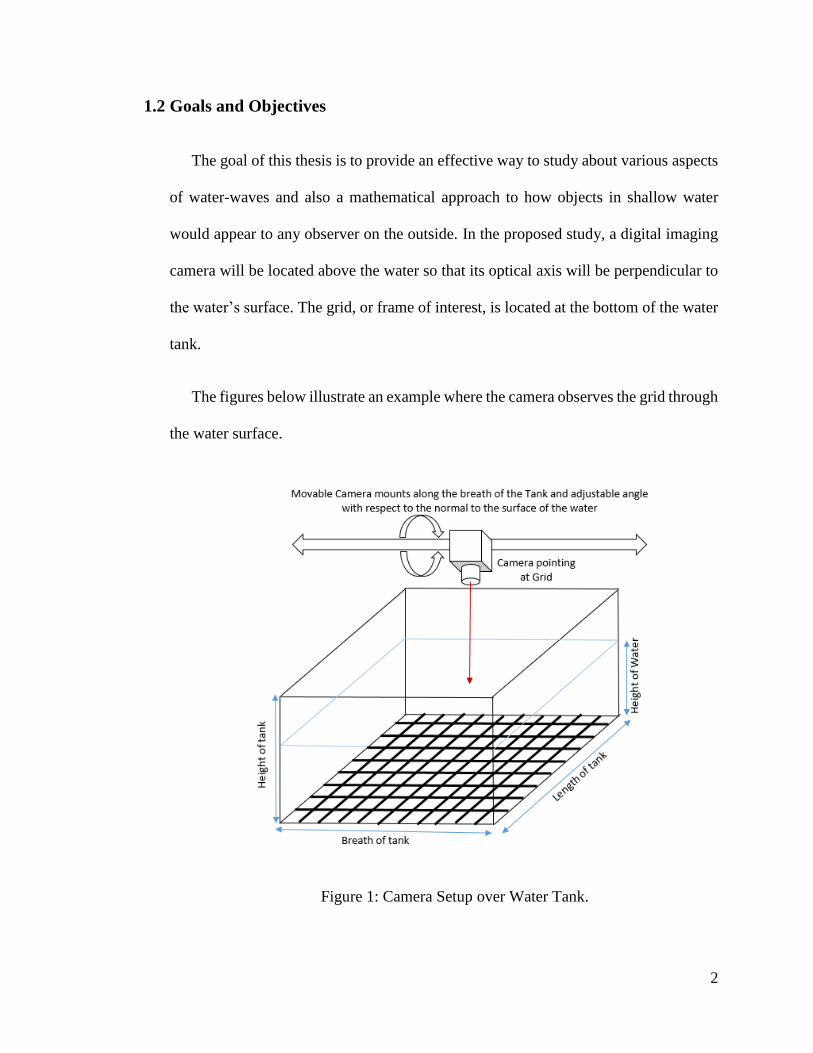
1.2 Goals and Objectives
The goal of this thesis is to provide an effective way to study about various aspects
of water-waves and also a mathematical approach to how objects in shallow water
would appear to any observer on the outside. In the proposed study, a digital imaging
camera will be located above the water so that its optical axis will be perpendicular to
the water’s surface. The grid, or frame of interest, is located at the bottom of the water
tank.
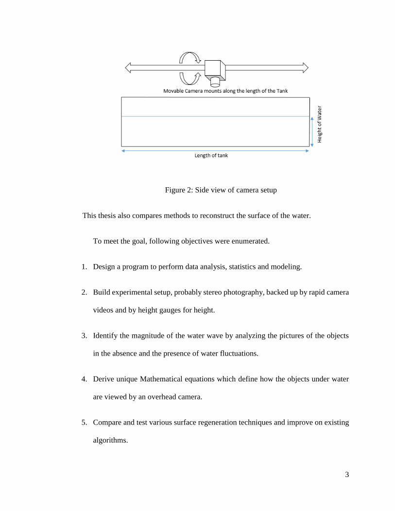
The figures below illustrate an example where the camera observes the grid through
the water surface.
Figure 1: Camera Setup over Water Tank.
3
Figure 2: Side view of camera setup
This thesis also compares methods to reconstruct the surface of the water.
To meet the goal, following objectives were enumerated.
1. Design a program to perform data analysis, statistics and modeling.
2. Build experimental setup, probably stereo photography, backed up by rapid camera
videos and by height gauges for height.
3. Identify the magnitude of the water wave by analyzing the pictures of the objects
in the absence and the presence of water fluctuations.
4. Derive unique Mathematical equations which define how the objects under water
are viewed by an overhead camera.
5. Compare and test various surface regeneration techniques and improve on existing
algorithms.
4
1.3 Thesis Outline
In the following chapters of the report, the proposed study is detailed.
Chapter 2 includes literature review to discuss initial study and different aspects of
water wave theory.
Chapter 3 has detailed derivations of the researcher’s mathematical approach
towards how an object under water is viewed through a camera lens versus how the
object actually appears.
Chapter 4 is a graphical representation of the mathematical equations derived and
its comparision to previous assumptions.
Chapter 5 covers the conclusions and results.
5
Chapter 2: Literature Review
This chapter will focus on all the literature needed for the Research. It will discuss
the initial study of water waves and varied approaches to surface reconstruction algorithms.
2.1 History of Water Wave Research.
To begin the study on water waves, the researchers will review on the
origins of this theory before the 20th century which was done extensively in Craik
(2004). Sir Isaac Newton (1687) first attempted to devise a theory of water-waves,
whose work was followed by Gravesande (1721) and Charles Bossut (1786), while the
equations of hydrodynamics were derived by Euler (1757a, 1757b, 1761).
Wave motion was reexamined by Laplace and posed the general initial value
problem in Laplace (1799). Lagrange (1781, 1786) derived linearized governing
equations for small-amplitude waves and obtained the solution in the limiting case of
long plane waves in shallow water.
The first exact nonlinear solution for waves of finite amplitude in deep water was
given by Gerstner (1802). Young (1821) wrote extensively on tides, but briefly on
waves. In 1818 and 1827 Cauchy-Poisson analysis was presented, and although
Dalmedico (1988) highlighted errors in the fundamental equations, it is one of the most
important contributions in the mathematical theory of initial-value problems.
Vince (1798), a British scientist, published on Hydrodynamics. Pratt (1836) had
brief section on the equations of inviscid flow. Green, Kelland, airy and Earnshaw
published on water waves during the following years. Kelland’s (1844) analysis
considered the wave-motion in a fluid of finite depth, on the hypothesis of parallel
sections considering long waves in shallow water, what is now called the Stokes
6
frequency correction. Kelland's study of waves in canals with non-rectangular cross
sections is also noteworthy. Earnshaw (1847) began with an intro for solitary waves
and arrived at the results for horizontal velocity and water depth for the wave speed.
Eventually, Rayleigh derived the correct approximate solution, retaining both
dispersion and nonlinearity and further observed that Earnshaw's solution is not
irrotational.
Although Airy's (1841, 1845) main focus of interest was tidal phenomena, he also
wrote a substantial section on the Theory of Waves in Canals in 1841 and an Account
of Experiments on Waves in 1845. Much of the work is original and concerned with
modelling observed or observable phenomena. Airy gave the now-standard linear
theory for plane waves and his theory gives very good approximate prediction of water
waves but it is not applicable to predict steep waves and non-linear waves observed in
the oceans.
The first person to put forward almost all the previous work in one place including
his work describing linear mathematical models governing water waves and the
analytical theory for wind-waves was Sir Horace Lamb (1930). The possibility that
separation of the airflow might occur at each wave crest and produce a region of low
velocity and low pressure downwind of the crest was pointed out by Jeffreys (1924b,
1924a, 1925). Thus there would be a difference in pressure between upwind and
downwind faces of the wave able to transfer energy from the wind to the wind-waves.
However, the generally observed rate of growth of wind-waves is lower than Jeffreys
(1924b) calculation.
7
Seminal work on shear flow theory on the generation of surface waves by wind was
presented by John Miles (1957) with certain assumptions in shear flow theory such as
air flow is assumed to be inviscid, incompressible and has some specified mean shear
flow in the absence of waves. The disturbances in the air flow induced by the surface
waves are assumed to be two dimensional and small enough so that the equations of
motion are linearized. The turbulent fluctuations which must be present to maintain the
mean shear flow are neglected in the perturbation equations. The assumption is that the
water is inviscid, incompressible, irrotational and has small surface slopes along with
no mean drift currents. Furthermore, the wave speed is assumed to be unaltered by any
push by the wind and the wind speed is considered low compared to the wave speed.
All the above assumptions leads to inappropriate energy extraction and
subsequently underestimate the wave growth due to wind-wave interaction. The theory
is found to under-predict the wave growth rate by a factor of 8 to 10 on comparing with
fieldwork studies by Snyder & Cox (1966), Barnett & Wilkerson (1967) and laboratory
studies by Bole & Hsu (1969). The resonance model of Phillips (1957) includes direct
action of turbulent pressure fluctuations on the water surface but neglects any
interactions between wave field and pressure field. It is an uncoupled model in the
sense that the response is assumed to be independent from excitation and the wind
profile over the waves is assumed to be logarithmic.
Moreover, the theory by Phillips (1957) relies on turbulent pressure fluctuations to
provide a random force acting onto the wave surface, ensuring wind-to-wave energy
transfer and leading to a linear increase in wave amplitude in time. However, most of
the researchers have found this assumption invalid in real ocean measurements. This
8
proves that distribution of stress on the surface is a function of the pressure field and
also the coupled instability mechanism. Kinsman (1965) has done detailed analysis
about the effect of resonant wave and shear flow and has written extensively about the
combined model (resonance and shear flow) and the nonlinear wind-wave model for
surface waves.
2.2 Various approaches to Surface Wave and Image Reconstruction.
Surface reconstruction has now been a widely researched subject and its primary
purpose is to study the wave structure. The researchers have presented a brief study of
surface reconstruction with the idea of comparing images distorted by water waves to
its reconstructed images thus giving an approximate idea of the water surface shape
and features. Thus the below study would point out various researches conducted in
image recovery, image reconstruction and surface reconstruction.
The main approach to surface reconstruction has been to extract the shape of water
surfaces from images of water [10, 11, 12, 13].This work done by those in the computer
vision community as well as those in oceanography sought to take advantage of waters
optical properties to reconstruct a surface. Techniques developed to utilize water’s
refractivity to reconstruct a surface have had much more success than those using the
reflectivity property of water [9, 10].
Any transparent object moving above a certain surface causes distortion in the
appearance of the lower surface due to refraction at its surface. Most refraction
methods use a single viewpoint and assume an orthographic projection [13, 15, 16].
Murase (1992) [5, 13] describes an algorithm to reconstruct the surface shape of the
non-rigid transparent object from the apparent motion of the observed pattern. He has
9
achieved this by extracting the optical flow sequence of consecutive images of the
distorted surface, averaging their trajectory thus calculating the surface normal and
reconstructing the surface. This method shares certain similarities with another method
called shape from motion. Two major difference between these two methods is
(1) The latter involves 3-D structure reconstruction using movements of several
points on the object based on an assumption of rigidity [6].
(2)Murase’s algorithm uses points on the refracted images rather than points on the
object.
The drawbacks of Murase’s algorithm was the accuracy of the extraction of optical
flow impacted the final result. Also, his method requires a relatively distant camera to
minimize projection distortion.
Morris [14] avoids certain assumptions and inaccuracies of previous methods by
using stereo cameras to capture images of a pattern refracted through water. His
research builds on work that utilizes refractive distortion as well as stereo
reconstruction research. His system was based upon finding individual points on the
water surface.
10
Chapter 3: Mathematical approach to estimate object position
In this section, the investigators derive the measurement technique in detail and
compare it to theoretical results.
3.1 Object viewed in still water
The investigators have set up the experiment as shown in the figure below.
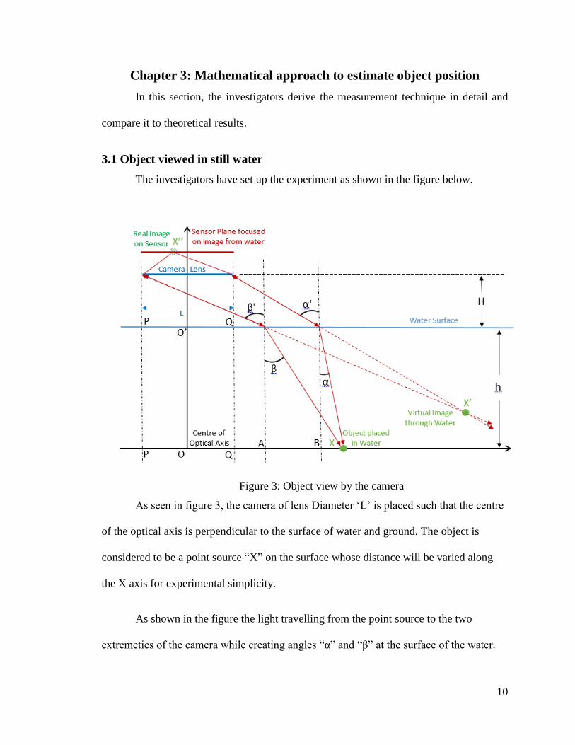
Figure 3: Object view by the camera
As seen in figure 3, the camera of lens Diameter ‘L’ is placed such that the centre
of the optical axis is perpendicular to the surface of water and ground. The object is
considered to be a point source “X” on the surface whose distance will be varied along
the X axis for experimental simplicity.
As shown in the figure the light travelling from the point source to the two
extremeties of the camera while creating angles “α” and “β” at the surface of the water.
11
Thus, due to Snell’s law (Appendix A), the angles “α” and “β” will get diffracted
and form “α’ ” and “β’ ” as the rays of light reach the camera. Due to refraction across
water, the virtual image is seen at point “X’ “.
Given Distance of object ‘X’ from the Centre of optical axis ‘O’, we calculate the
angles by which light gets refracted as it reaches the lens
From figure 1, we calculate the two angles ‘α’ and ‘β’ with respect to the ‘x’:
𝑥 = 𝑋𝐵 + 𝐵𝐴 + 𝐴𝑄 + 𝑄𝑂 eq. (1)
‘x’ in terms or angle ‘α’
Using trigonometric properties eq. (1) can be re-written as:
𝑥 = ℎ ∗ tan(𝛼) + 𝐻 ∗ tan(𝛼′) +𝐿
2 eq. (2)
Snell’s Law, n1sinθ1 = n2sinθ2, is used to calculate…. (Appendix A))
Using Snell’s Law, the visual displacement of the object in water was calculated in
this manner:
𝑛 ∗ sin(𝛼) = sin (𝛼′) eq. (3)
𝑥 = ℎ ∗ tan(𝛼) + 𝐻 ∗sin(𝛼′)
cos(𝛼′)+𝐿
2 eq. (4)
Substituting eq. (3) in eq. (4)
𝑥 = ℎ ∗ tan(𝛼) + 𝐻 ∗sin(𝛼)
√1−𝑛2𝑠𝑖𝑛2 (α))+𝐿
2 eq. (5)
12
Similarly for ‘x’ in terms of angle ‘β’
𝑥 = ℎ ∗ tan(𝛽) + 𝐻 ∗sin𝛽
√1−𝑛2 𝑠𝑖𝑛2(β))−𝐿
2 eq. (6)
3.1.1 Calculate the x component of X’
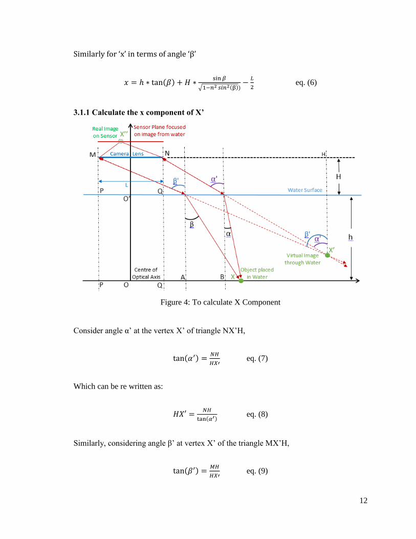
Figure 4: To calculate X Component
Consider angle α’ at the vertex X’ of triangle NX’H,
tan(𝛼′) =𝑁𝐻
𝐻𝑋′ eq. (7)
Which can be re written as:
𝐻𝑋′ =𝑁𝐻
tan(𝛼′) eq. (8)
Similarly, considering angle β’ at vertex X’ of the triangle MX’H,
tan(𝛽′) =𝑀𝐻
𝐻𝑋′ eq. (9)
13
But MH = MN+ NH As seen in figure 2,
Hence, tan(𝛽′) =𝑀𝑁+𝑁𝐻
𝐻𝑋′ eq. (10)
But MN = L,
Thus eq. 10 can be re written as
tan(𝛽′) =𝐿+𝑁𝐻
𝐻𝑋′ eq. (11)
Now substituting the value of HX’ from Eq. (8) in eq. (11),
We get,
tan(𝛽′) =𝐿+𝑁𝐻𝑁𝐻
tan(𝛼′)
i.e.
tan(𝛽′) =𝐿+𝑁𝐻
𝑁𝐻∗ tan(𝛼′) eq. (12)
Simplifying and equating in terms of NH, we have:
𝑁𝐻 =𝐿∗tan(𝛼′)
tan(𝛽′)− tan(𝛼′) eq. (13)
From figure we can see that X component of X’ is 𝑁𝐻 + 𝐿
2
Therefore,
𝑋 𝑐𝑜𝑚𝑝𝑜𝑛𝑒𝑛𝑡 𝑜𝑓 𝑋′ =𝐿∗tan(𝛼′)
tan(𝛽′)− tan(𝛼′)+𝐿
2 eq. (14)
14
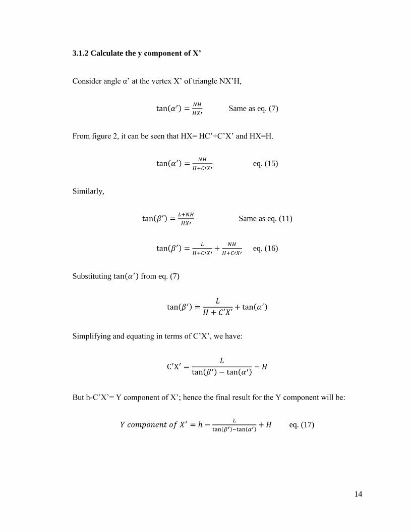
3.1.2 Calculate the y component of X’
Consider angle α’ at the vertex X’ of triangle NX’H,
tan(𝛼′) =𝑁𝐻
𝐻𝑋′ Same as eq. (7)
From figure 2, it can be seen that HX= HC’+C’X’ and HX=H.
tan(𝛼′) =𝑁𝐻
𝐻+𝐶′𝑋′ eq. (15)
Similarly,
tan(𝛽′) =𝐿+𝑁𝐻
𝐻𝑋′ Same as eq. (11)
tan(𝛽′) =𝐿
𝐻+𝐶′𝑋′+
𝑁𝐻
𝐻+𝐶′𝑋′ eq. (16)
Substituting tan(𝛼′) from eq. (7)
tan(𝛽′) =𝐿
𝐻 + 𝐶′𝑋′+ tan(𝛼′)
Simplifying and equating in terms of C’X’, we have:
C′X′ =𝐿
tan(𝛽′) − tan(𝛼′)− 𝐻
But h-C’X’= Y component of X’; hence the final result for the Y component will be:
𝑌 𝑐𝑜𝑚𝑝𝑜𝑛𝑒𝑛𝑡 𝑜𝑓 𝑋′ = ℎ −𝐿
tan(𝛽′)−tan(𝛼′)+ 𝐻 eq. (17)
15
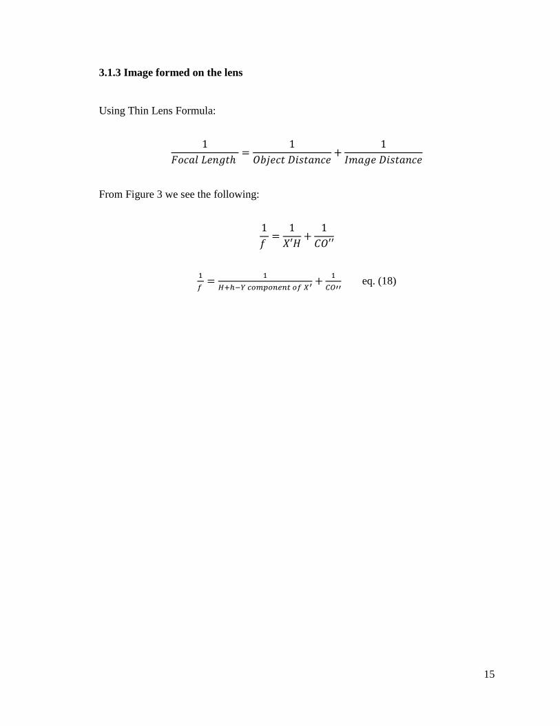
3.1.3 Image formed on the lens
Using Thin Lens Formula:
1
𝐹𝑜𝑐𝑎𝑙 𝐿𝑒𝑛𝑔𝑡ℎ =
1
𝑂𝑏𝑗𝑒𝑐𝑡 𝐷𝑖𝑠𝑡𝑎𝑛𝑐𝑒+
1
𝐼𝑚𝑎𝑔𝑒 𝐷𝑖𝑠𝑡𝑎𝑛𝑐𝑒
From Figure 3 we see the following:
1
𝑓 =
1
𝑋′𝐻+
1
𝐶𝑂′′
1
𝑓 =
1
𝐻+ℎ−𝑌 𝑐𝑜𝑚𝑝𝑜𝑛𝑒𝑛𝑡 𝑜𝑓 𝑋′+
1
𝐶𝑂′′ eq. (18)
16
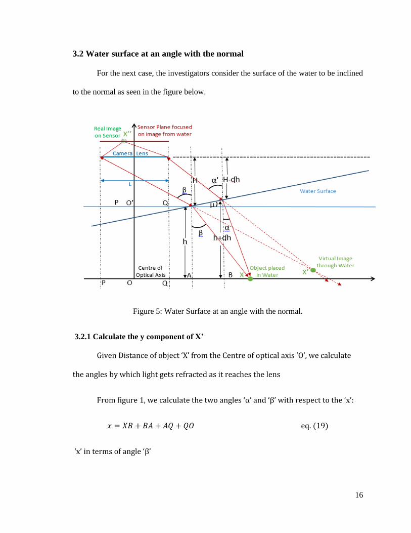
3.2 Water surface at an angle with the normal
For the next case, the investigators consider the surface of the water to be inclined
to the normal as seen in the figure below.
Figure 5: Water Surface at an angle with the normal.
3.2.1 Calculate the y component of X’
Given Distance of object ‘X’ from the Centre of optical axis ‘O’, we calculate
the angles by which light gets refracted as it reaches the lens
From figure 1, we calculate the two angles ‘α’ and ‘β’ with respect to the ‘x’:
𝑥 = 𝑋𝐵 + 𝐵𝐴 + 𝐴𝑄 + 𝑄𝑂 eq. (19)
‘x’ in terms of angle ‘β’
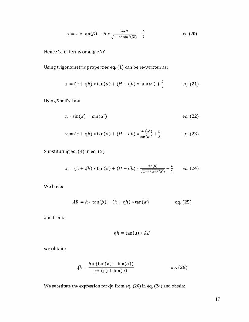
17
𝑥 = ℎ ∗ tan(𝛽) + 𝐻 ∗sin𝛽
√1−𝑛2 𝑠𝑖𝑛2(β))−𝐿
2 eq.(20)
Hence ‘x’ in terms or angle ‘α’
Using trigonometric properties eq. (1) can be re-written as:
𝑥 = (ℎ + ʠℎ) ∗ tan(𝛼) + (𝐻 − ʠℎ) ∗ tan(𝛼′) +𝐿
2 eq. (21)
Using Snell’s Law
𝑛 ∗ sin(𝛼) = sin (𝛼′) eq. (22)
𝑥 = (ℎ + ʠℎ) ∗ tan(𝛼) + (𝐻 − ʠℎ) ∗sin(𝛼′)
cos(𝛼′)+𝐿
2 eq. (23)
Substituting eq. (4) in eq. (5)
𝑥 = (ℎ + ʠℎ) ∗ tan(𝛼) + (𝐻 − ʠℎ) ∗sin(α)
√1−𝑛2𝑠𝑖𝑛2 (α))+𝐿
2 eq. (24)
We have:
𝐴𝐵 = ℎ ∗ tan(𝛽) − (ℎ + ʠℎ) ∗ tan(𝛼) eq. (25)
and from:
ʠℎ = tan(µ) ∗ 𝐴𝐵
we obtain:
ʠℎ =ℎ ∗ (tan(𝛽) − tan(𝛼))
cot(µ) + tan(𝛼) 𝑒𝑞. (26)
We substitute the expression for ʠℎ from eq. (26) in eq. (24) and obtain:
18
𝑥 = (ℎ +ℎ∗(tan(𝛽)−tan(𝛼))
cot(µ)+tan(𝛼)) ∗ tan(𝛼) + (𝐻 −
ℎ∗(tan(𝛽)−tan(𝛼))
cot(µ)+tan(𝛼)) ∗
sin(α)
√1−𝑛2𝑠𝑖𝑛2 (α))+𝐿
2
eq. (27)
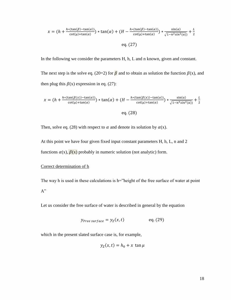
In the following we consider the parameters H, h, L and n known, given and constant.
The next step is the solve eq. (20=2) for 𝛽 and to obtain as solution the function 𝛽(x), and
then plug this 𝛽(x) expression in eq. (27):
𝑥 = (ℎ +ℎ∗(tan(𝛽(𝑥))−tan(𝛼))
cot(µ)+tan(𝛼)) ∗ tan(𝛼) + (𝐻 −
ℎ∗(tan(𝛽(𝑥))−tan(𝛼))
cot(µ)+tan(𝛼)) ∗
sin(α)
√1−𝑛2𝑠𝑖𝑛2 (α))+𝐿
2
eq. (28)
Then, solve eq. (28) with respect to 𝛼 and denote its solution by 𝛼(x).
At this point we have four given fixed input constant parameters H, h, L, n and 2
functions 𝛼(x), 𝛽(x) probably in numeric solution (not analytic) form.
Correct determination of h
The way h is used in these calculations is h=”height of the free surface of water at point
A”
Let us consider the free surface of water is described in general by the equation
𝑦𝐹𝑟𝑒𝑒 𝑠𝑢𝑟𝑓𝑎𝑐𝑒 = 𝑦𝛴(𝑥, 𝑡) eq. (29)
which in the present slated surface case is, for example,
𝑦𝛴(𝑥, 𝑡) = ℎ0 + 𝑥 tan 𝜇
19
where ℎ0 is the height of water right under the center of the lenses, at origin x=0. It
implies we have to use in all equations above, instead of the constant h, the solution h(x)
of the equation:
ℎ → 𝑦𝛴(𝑥𝐴, 𝑡) = ℎ = ℎ0 + 𝑥𝐴 tan 𝜇 =ℎ0 + 𝑂𝐴 tan 𝜇
By solving the equation above we have
ℎ → ℎ(𝑥) =(ℎ0 + 𝑥 tan 𝜇) tan𝛽
1 + tan 𝜇 tan𝛽
This observation completely changes the expressions in eqs. (20, 28). Namely we have:
𝑥 =(ℎ0+𝑥 tan𝜇) tan𝛽
1+tan𝜇 tan𝛽∗ tan(𝛽) + 𝐻 ∗
sin𝛽
√1−𝑛2 𝑠𝑖𝑛2(β))−𝐿
2 eq.(30)
and
𝑥 =(ℎ0+𝑥 tan𝜇) tan𝛽(𝑥)
1+tan𝜇 tan𝛽(𝑥)(1 +
tan(𝛽(𝑥))−tan(𝛼)
cot(µ)+tan(𝛼)) ∗ tan(𝛼) + (𝐻 −
(ℎ0+𝑥 tan𝜇) tan𝛽(𝑥)
1+tan𝜇 tan𝛽(𝑥)
tan(𝛽(𝑥))−tan(𝛼)
cot(µ)+tan(𝛼)) ∗
sin(α)
√1−𝑛2𝑠𝑖𝑛2 (α))+𝐿
2 eq. (31)
20
Chapter 4: Graphical Representation of derived equations
In this chapter, the investigators implement the derived functions graphically and
compare its results to the initial findings for various cases.
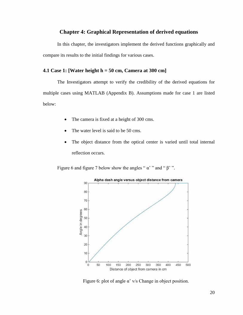
4.1 Case 1: [Water height h = 50 cm, Camera at 300 cm]
The Investigators attempt to verify the credibility of the derived equations for
multiple cases using MATLAB (Appendix B). Assumptions made for case 1 are listed
below:
The camera is fixed at a height of 300 cms.
The water level is said to be 50 cms.
The object distance from the optical center is varied until total internal
reflection occurs.
Figure 6 and figure 7 below show the angles “ α’ ” and “ β’ ”.
Figure 6: plot of angle α’ v/s Change in object position.
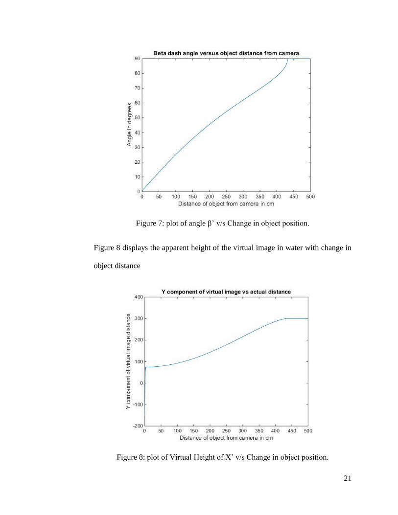
21
Figure 7: plot of angle β’ v/s Change in object position.
Figure 8 displays the apparent height of the virtual image in water with change in
object distance
Figure 8: plot of Virtual Height of X’ v/s Change in object position.
22
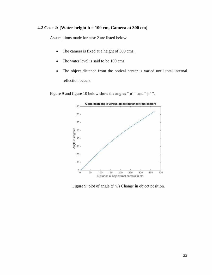
4.2 Case 2: [Water height h = 100 cm, Camera at 300 cm]
Assumptions made for case 2 are listed below:
The camera is fixed at a height of 300 cms.
The water level is said to be 100 cms.
The object distance from the optical center is varied until total internal
reflection occurs.
Figure 9 and figure 10 below show the angles “ α’ ” and “ β’ ”.
Figure 9: plot of angle α’ v/s Change in object position.
23
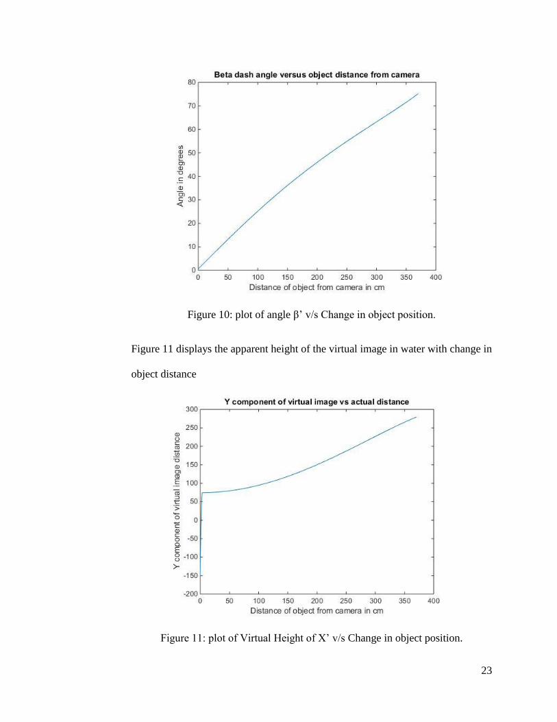
Figure 10: plot of angle β’ v/s Change in object position.
Figure 11 displays the apparent height of the virtual image in water with change in
object distance
Figure 11: plot of Virtual Height of X’ v/s Change in object position.
24
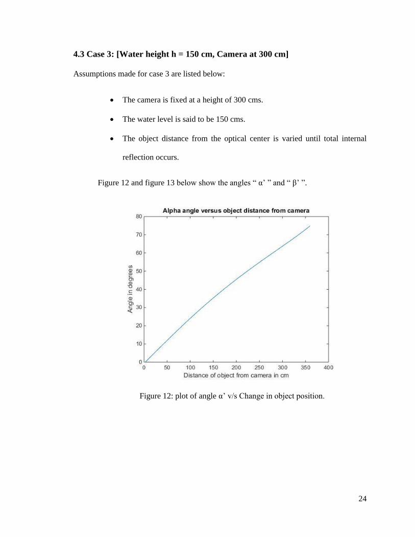
4.3 Case 3: [Water height h = 150 cm, Camera at 300 cm]
Assumptions made for case 3 are listed below:
The camera is fixed at a height of 300 cms.
The water level is said to be 150 cms.
The object distance from the optical center is varied until total internal
reflection occurs.
Figure 12 and figure 13 below show the angles “ α’ ” and “ β’ ”.
Figure 12: plot of angle α’ v/s Change in object position.
25
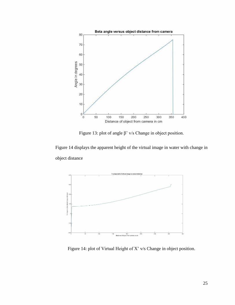
Figure 13: plot of angle β’ v/s Change in object position.
Figure 14 displays the apparent height of the virtual image in water with change in
object distance
Figure 14: plot of Virtual Height of X’ v/s Change in object position.
26
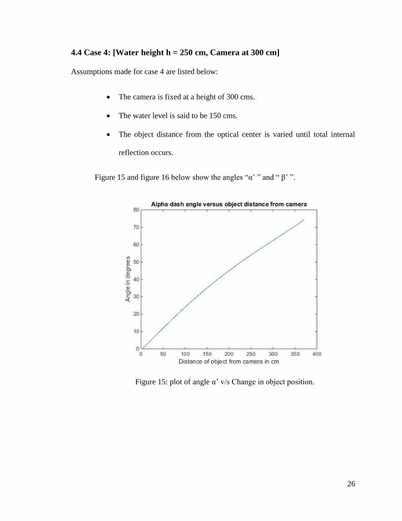
4.4 Case 4: [Water height h = 250 cm, Camera at 300 cm]
Assumptions made for case 4 are listed below:
The camera is fixed at a height of 300 cms.
The water level is said to be 150 cms.
The object distance from the optical center is varied until total internal
reflection occurs.
Figure 15 and figure 16 below show the angles “α’ ” and “ β’ ”.
Figure 15: plot of angle α’ v/s Change in object position.
27
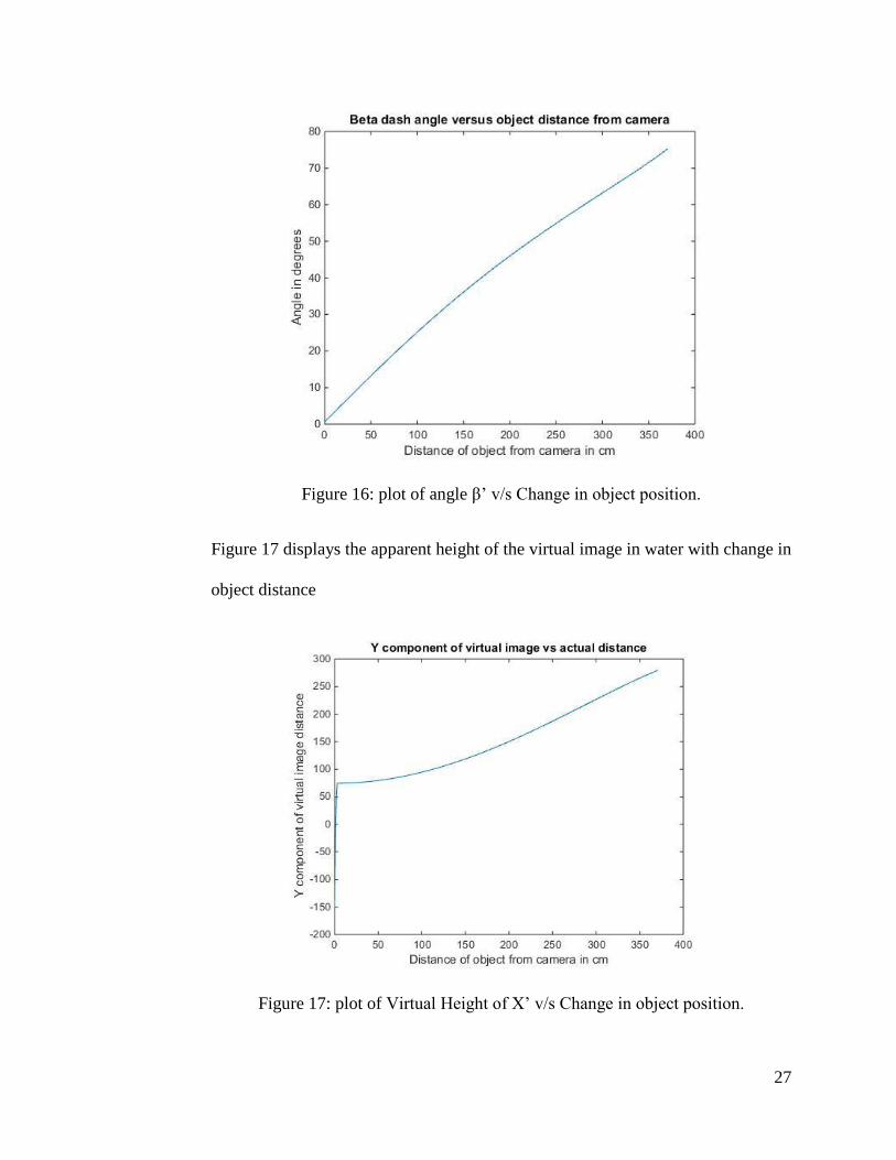
Figure 16: plot of angle β’ v/s Change in object position.
Figure 17 displays the apparent height of the virtual image in water with change in
object distance
Figure 17: plot of Virtual Height of X’ v/s Change in object position.
28
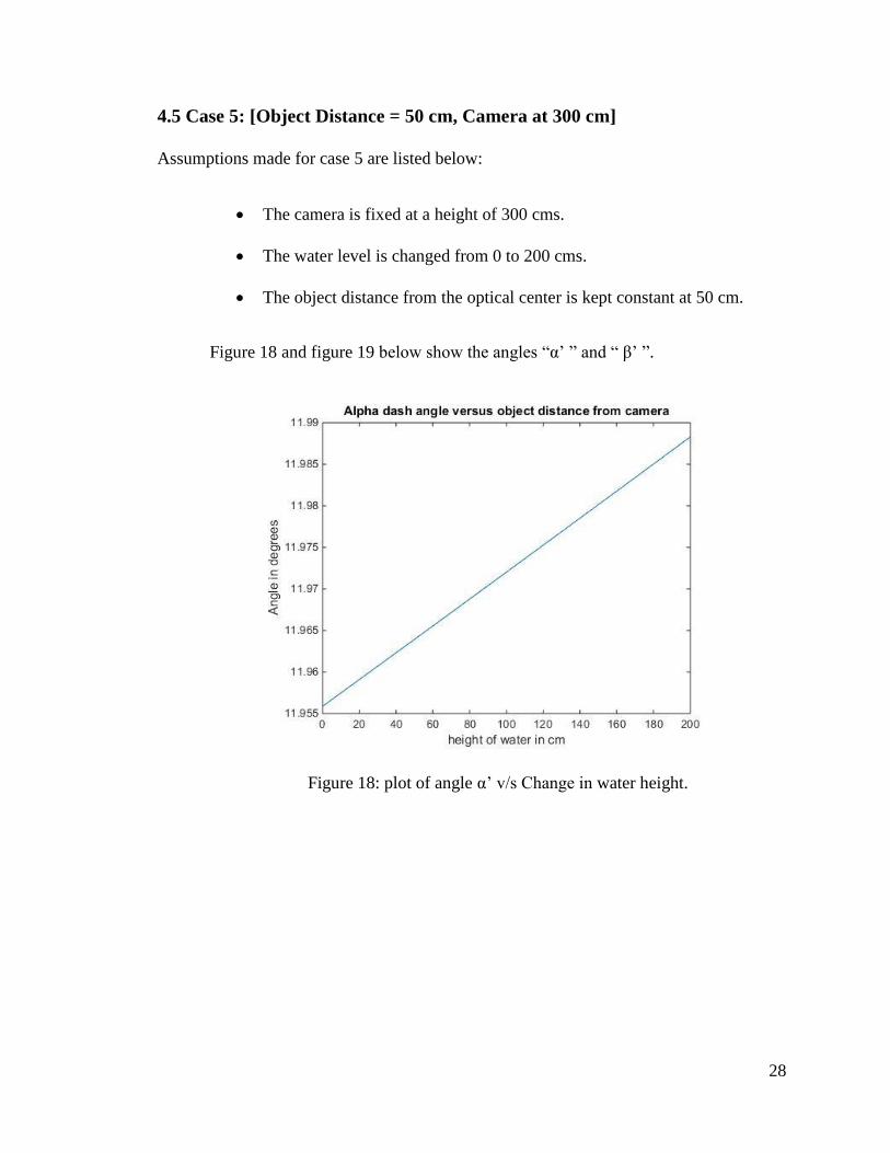
4.5 Case 5: [Object Distance = 50 cm, Camera at 300 cm]
Assumptions made for case 5 are listed below:
The camera is fixed at a height of 300 cms.
The water level is changed from 0 to 200 cms.
The object distance from the optical center is kept constant at 50 cm.
Figure 18 and figure 19 below show the angles “α’ ” and “ β’ ”.
Figure 18: plot of angle α’ v/s Change in water height.
29
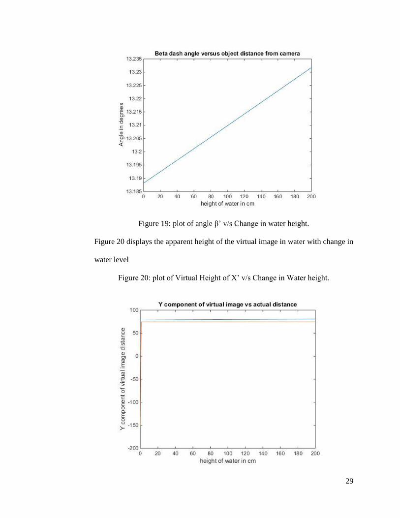
Figure 19: plot of angle β’ v/s Change in water height.
Figure 20 displays the apparent height of the virtual image in water with change in
water level
Figure 20: plot of Virtual Height of X’ v/s Change in Water height.
30
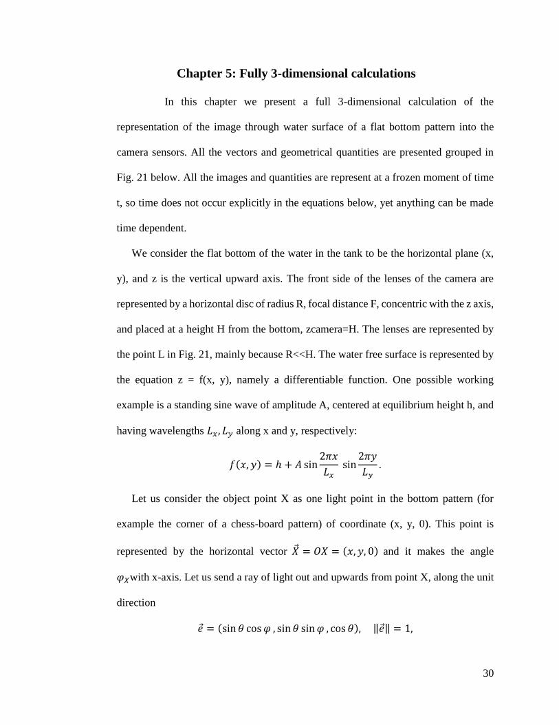
Chapter 5: Fully 3-dimensional calculations
In this chapter we present a full 3-dimensional calculation of the
representation of the image through water surface of a flat bottom pattern into the
camera sensors. All the vectors and geometrical quantities are presented grouped in
Fig. 21 below. All the images and quantities are represent at a frozen moment of time
t, so time does not occur explicitly in the equations below, yet anything can be made
time dependent.
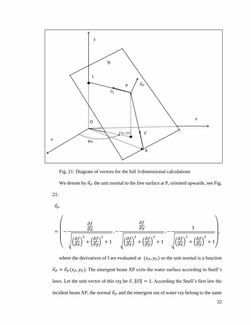
We consider the flat bottom of the water in the tank to be the horizontal plane (x,
y), and z is the vertical upward axis. The front side of the lenses of the camera are
represented by a horizontal disc of radius R, focal distance F, concentric with the z axis,
and placed at a height H from the bottom, zcamera=H. The lenses are represented by
the point L in Fig. 21, mainly because R<<H. The water free surface is represented by
the equation z = f(x, y), namely a differentiable function. One possible working
example is a standing sine wave of amplitude A, centered at equilibrium height h, and
having wavelengths 𝐿𝑥, 𝐿𝑦 along x and y, respectively:
𝑓(𝑥, 𝑦) = ℎ + 𝐴 sin2𝜋𝑥
𝐿𝑥 sin
2𝜋𝑦
𝐿𝑦.
Let us consider the object point X as one light point in the bottom pattern (for
example the corner of a chess-board pattern) of coordinate (x, y, 0). This point is
represented by the horizontal vector �⃗� = 𝑂𝑋 = (𝑥, 𝑦, 0) and it makes the angle
𝜑𝑋with x-axis. Let us send a ray of light out and upwards from point X, along the unit
direction
𝑒 = (sin 𝜃 cos𝜑 , sin 𝜃 sin𝜑 , cos 𝜃), ‖𝑒‖ = 1,
31
where 0 ≤ 𝜃 ≤𝜋
2, 0 ≤ 𝜑 ≤ 2𝜋 are the polar angles measured from z-axis and x-
axis, respectively, see Fig. 21. This emergent ray intersects the free water surface at a
point P (see Fig. 21) represented by the vector �⃗⃗� = 𝑋𝑃 = (𝑥𝑃, 𝑦𝑃, 𝑓(𝑥𝑃, 𝑦𝑃)). Note that
𝑥𝑃 ≠ 𝑥, 𝑦𝑃 ≠ 𝑦 because the projection of point P on the bottom does not coincide with
X. In order to obtain the coordinates of P we write this vector beginning from origin to
X and then along the emergent ray unit vector 𝑒, that is
�⃗⃗� = �⃗� + 𝜆𝑒,
where 𝜆 is a parameter given by the solution of the equation:
𝜆 cos 𝜃 = 𝑓(𝑥 + 𝜆 sin 𝜃 cos𝜑, 𝑦 + 𝜆 sin 𝜃 sin𝜑),
which is the condition for the emergent beam to intersect the water surface at point
P. From now we denote the solution of the transcendental equation above by 𝜆1
because this solution depends on the independent parameters of the problem, that is
𝜆1 = 𝜆1(𝑥, 𝑦, 𝜃, 𝜑) . This equation can be solved only numerically, even for the
simplest surfaces. With 𝜆1 thus calculated we can write the expressions of the
coordinates of point P:
{
𝑥𝑃 = 𝑥 + 𝜆1 sin 𝜃 cos𝜑𝑦𝑃 = 𝑦 + 𝜆1 sin 𝜃 sin 𝜑
𝑧𝑃 = 𝑓(𝑥𝑃, 𝑦𝑃)
32
Fig. 21: Diagram of vectors for the full 3-dimensional calculations
We denote by �⃗⃗�𝑃 the unit normal to the free surface at P, oriented upwards, see Fig.
21:
�⃗⃗�𝑃
=
(
−
𝜕𝑓𝜕𝑥
√(𝜕𝑓𝜕𝑥)2
+ (𝜕𝑓𝜕𝑦)2
+ 1
,−
𝜕𝑓𝜕𝑦
√(𝜕𝑓𝜕𝑥)2
+ (𝜕𝑓𝜕𝑦)2
+ 1
,−1
√(𝜕𝑓𝜕𝑥)2
+ (𝜕𝑓𝜕𝑦)2
+ 1)
,
where the derivatives of f are evaluated at (𝑥𝑃, 𝑦𝑃) so the unit normal is a function
�⃗⃗�𝑃 = �⃗⃗�𝑃(𝑥𝑃, 𝑦𝑃). The emergent beam XP exits the water surface according to Snell’s
laws. Let the unit vector of this ray be �⃗�, ‖�⃗�‖ = 1. According the Snell’s first law the
incident beam XP, the normal �⃗⃗�𝑃 and the emergent out of water ray belong to the same
33
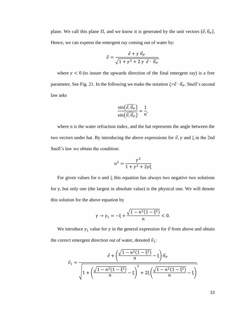
plane. We call this plane Π, and we know it is generated by the unit vectors {𝑒, �⃗⃗�𝑃}.
Hence, we can express the emergent ray coming out of water by:
�⃗� =𝑒 + 𝛾 �⃗⃗�𝑃
√1 + 𝛾2 + 2 𝛾 𝑒 ∙ �⃗⃗�𝑃,
where 𝛾 < 0 (to insure the upwards direction of the final emergent ray) is a free
parameter, See Fig. 21. In the following we make the notation ξ=𝑒 ∙ �⃗⃗�𝑃. Snell’s second
law asks
sin(𝑒, �⃗⃗��̂�)
sin(�⃗�, �⃗⃗��̂�)=1
𝑛,
where n is the water refraction index, and the hat represents the angle between the
two vectors under hat. By introducing the above expressions for �⃗�, 𝛾 and ξ in the 2nd
Snell’s law we obtain the condition:
𝑛2 =𝛾2
1 + 𝛾2 + 2𝛾ξ
For given values for n and ξ this equation has always two negative two solutions
for 𝛾, but only one (the largest in absolute value) is the physical one. We will denote
this solution for the above equation by
𝛾 → 𝛾1 = −ξ +√1 − 𝑛2(1 − ξ2)
𝑛< 0.
We introduce 𝛾1 value for 𝛾 in the general expression for �⃗� from above and obtain
the correct emergent direction out of water, denoted �⃗�1:
�⃗�1 =
𝑒 + (√1 − 𝑛2(1 − ξ2)
𝑛 − ξ) �⃗⃗�𝑃
√1 + (√1 − 𝑛2(1 − ξ2)
𝑛 − ξ)
2
+ 2ξ(√1 − 𝑛2(1 − ξ2)
𝑛 − ξ)
,
34
with �⃗�1 still normalized.
This unit vector �⃗�1 should be extended to the lens point, L, see Fig. 21.So we are
going to multiply this unit vector with an arbitrary parameter 𝜇, and determine the
value of this parameter from the condition:
(�⃗⃗� + 𝜇�⃗�1)𝑧 = 𝐻,
that is the z-component of the vector OX+XP+PL=OL is the height of the lens.
There is an additional condition which will determine the angles 𝜃, 𝜑of the initial
bottom emergent ray to end into the lens, namely:
[(�⃗⃗� + 𝜇�⃗�1)𝑥]2
+ [(�⃗⃗� + 𝜇�⃗�1)𝑦]2
≤ 𝑅,
That is the final emergent ray PL must collide the inside of the disk of radius R,
which represents the front lenses of the camera. We will use this inequality to obtain
the domain of variation of the angles 𝜃, 𝜑 emerging from X such that the rays will enter
the lenses. In optic this locus is called the caustic surface of point X through the water
refracting medium, see Burkhard (1973).
By introducing the expression of �⃗⃗�, and �⃗�1 in the vertical matching condition
(�⃗⃗� + 𝜇�⃗�1)𝑧 = 𝐻, we obtain the final value of parameter 𝜇 which we call 𝜇1;
𝜇1 =(𝐻 − 𝜆1 cos 𝜃)√1 + 𝛾12 + 2 𝛾1 ξ
cos 𝜃 +𝛾1
√(𝜕𝑓𝜕𝑥)2
+ (𝜕𝑓𝜕𝑦)2
+ 1
,
where the derivatives of f are again calculated at (𝑥𝑃, 𝑦𝑃) , 𝜆1 is the solution
described above, and ξ has the same signification of dot product. In Fig. 21 we present
all the vectors 𝑒, 𝑋𝑃 = 𝜆1𝑒, �⃗⃗�𝑃, and 𝜇1�⃗�1 described above, all belonging to the same
35
plane 𝛱. The sequence of vectors OX+XP+PL take the origin into the bottom pattern
reference point X, to the impact with water point P, and out of water to the lens L.
The procedure in the following consists in 2 steps.
Step 1. Given (x,y) we calculate all the parameters in the system, namely
{𝑥𝑃, 𝑦𝑃,, 𝜆1, 𝜉, 𝛾1, 𝜇1} for these x, y and in general for all values of the angles 𝜃, 𝜑.
Next, solve the “center equation”
{(�⃗⃗� + 𝜇�⃗�1)𝑥 = 0
(�⃗⃗� + 𝜇�⃗�1)𝑦 = 0,
This equation requests that the final emergent ray P to arrive into the center of the
lens L of coordinates (0, 0, H). These two equations, highly nonlinear and
transcendental can be solved only numerically and will provide those values (denoted
𝜃𝐿 , 𝜑𝐿) for the angles 𝜃, 𝜑 for which the ray generated at X ends up at center of L.
These two equations have the following explicit forms:
{
𝑥 + 𝜆1 sin 𝜃𝐿 cos𝜑𝐿 +𝜇1
√1 + 𝛾12 + 2 𝛾1 ξ
(
sin 𝜃𝐿 cos𝜑𝐿 − 𝛾1𝜕𝑓𝜕𝑥
√(𝜕𝑓𝜕𝑥)2
+ (𝜕𝑓𝜕𝑦)2
+ 1)
= 0,
𝑦 + 𝜆1 sin 𝜃𝐿 sin𝜑𝐿+𝜇1
√1 + 𝛾12 + 2 𝛾1 ξ
(
sin 𝜃𝐿 sin𝜑𝐿 − 𝛾1𝜕𝑓𝜕𝑦
√(𝜕𝑓𝜕𝑥)2
+ (𝜕𝑓𝜕𝑦)2
+ 1)
= 0
Step 2. Having the central ray PL into the center of the lens, we rely on the
smallness of the lens radius compared to the heights of lens and water, and to the mean
values of the bottom patterns, that is 𝑅 ≪ ℎ, 𝐻, 𝐿𝑥, 𝐿𝑦. Under this “geometrical optics”
36
approximation we consider that the rest of the rays entering into the lens are just
infinitesimal variations 𝛿𝜃, 𝛿𝜑 around 𝜃𝐿 , 𝜑𝐿 respectively.
Coming back to the last level of calculations, we need to take the final emergent
ray PL and pass it through the lens onto the camera sensor plane. We assume that the
camera sensor plane is also horizontal, centered at z-axis and we overlap on it the same
x, y coordinates. According to the same “geometric optics” approximation we assume
that the final images of pattern points X will be projected onto the focal plane of the
camera, so we neglect at this point the fuzziness generated by miss-focusing. The ray
PL enters the lenses at an angle 𝛷 made with the z-axis given by cos𝛷 = |(�⃗�1)𝑧|. This
expression arises from the dot product between the unit vector �⃗�1 and the z-axis unit
vector.
The “central ray” enters the lens at the center (0,0,H) of the lens at angle 𝛷, emerges
through the lens at the same angle (geometric optics approximation) and intersects the
focal plane at a point Q. This Q point has its z-coordinate 𝑄𝑧 = 𝐻 + 𝐹 (placed in the
focal plane) and it is placed at a distance 𝜌 from the z-axis. The PL ray is in the vertical
plane Π that makes the angle 𝜑𝑃with the x-axis, see Fig. 21.The ray exits the lens at
the same angle 𝜑𝑃 with the x-axis, and ends at point Q. So the position of point Q is
diametric opposed from point P, in the focal plane on a circle of radius 𝜌. Let
(𝑥𝐼 , 𝑦𝐼 , 𝐻 + 𝐹) be the coordinates of Q (label I as in image). We have:
{𝑥𝐼 = 𝜌 cos𝜑𝐿𝑦𝐼 = −𝜌 sin𝜑𝐿
with 𝜌 given from triangle similarity:
𝜌 = 𝐹√1 − [(�⃗�1)𝑧]2
|(�⃗�1)𝑧|.
37
Gathering all these expressions in a final equation we have the position of the image
of source object point X, onto the camera sensor in the focal plane given by:
{
𝑥𝐼 = 𝐹
√1 − [(�⃗�1)𝑧]2
|(�⃗�1)𝑧|
𝑥𝑃
√(𝑥𝑃)2 + (𝑦𝑃)2
𝑦𝐼 = −𝐹√1 − [(�⃗�1)𝑧]2
|(�⃗�1)𝑧|
𝑦𝑃
√(𝑥𝑃)2 + (𝑦𝑃)2
These last equations represent the final result of this fully 3-dimensional model.
Namely, from an object point X at the bottom, we calculate all the parameters such that
the final emergent ray PL arrives at the center of the lenses, that is find 𝜃𝐿and 𝜑𝐿. The
image of the point X is given by the above final equations, in the focal plane, Next step,
we differentiate the above equations with respect to 𝜃, 𝜑, and λ and linearize them to
the first order of differentiation around the center values 𝜃𝐿and 𝜑𝐿. To do this we have
to perform an intermediate step: differentiate the equation for 𝜆1 (see it above):
𝜆 cos 𝜃 = 𝑓(𝑥 + 𝜆 sin 𝜃 cos𝜑, 𝑦 + 𝜆 sin 𝜃 sin𝜑),
with respect to 𝜃, 𝜑, and λ and find a relation between the derivatives 𝛿λ
𝛿𝜃, and
𝛿λ
𝛿𝜑. Next, we substitute the 𝜆 derivatives in the linearized expression for 𝑥𝐼 , 𝑦𝐼 and
transform the above equalities in the inequality [(�⃗⃗� + 𝜇�⃗�1)𝑥]2
+ [(�⃗⃗� + 𝜇�⃗�1)𝑦]2
≤ 𝑅.
This inequality will set the limiting values to 𝛿𝜃, 𝛿𝜑. This will give the maximal cone
of light emerging from X which is completely absorbed by the lens. The differentials
𝑑𝑥𝐼 , 𝑑𝑦𝐼 will provide the size and shape of the spot of light into which the object point
X is mapped.
We performed all these calculations for the test sine wave function presented at the
beginning of this section. We evaluate the position of the image points 𝑥𝐼 , 𝑦𝐼 in the
38
focal plane based on the above calculations. Then we performed experiments in the
wave tank and generate similar sine wave and take snap shots of their image in the
camera. Finally we compared the calculations with the experiment and obtain a
satisfactory result.
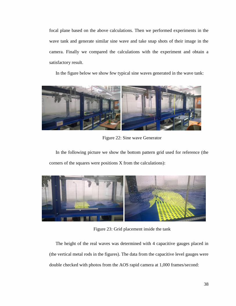
In the figure below we show few typical sine waves generated in the wave tank:
Figure 22: Sine wave Generator
In the following picture we show the bottom pattern grid used for reference (the
corners of the squares were positions X from the calculations):
Figure 23: Grid placement inside the tank
The height of the real waves was determined with 4 capacitive gauges placed in
(the vertical metal rods in the figures). The data from the capacitive level gauges were
double checked with photos from the AOS rapid camera at 1,000 frames/second:
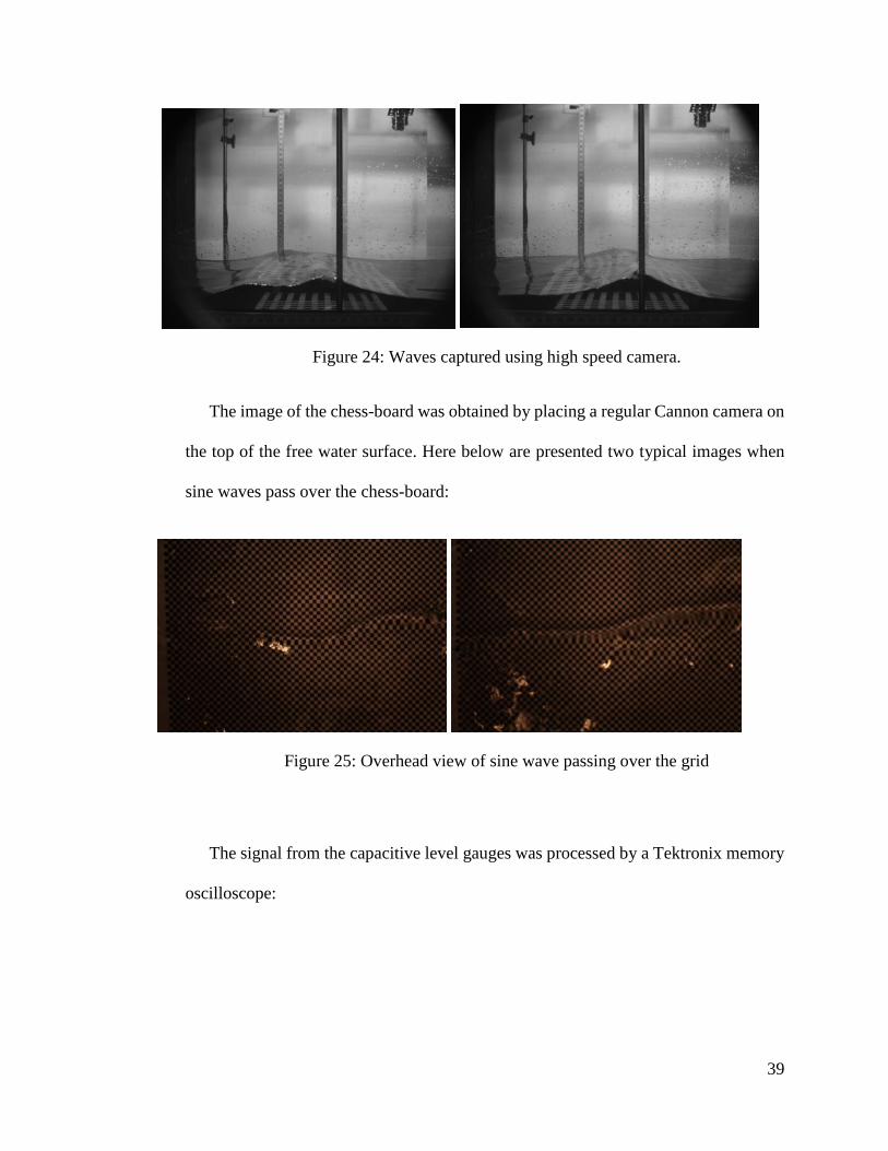
39
Figure 24: Waves captured using high speed camera.
The image of the chess-board was obtained by placing a regular Cannon camera on
the top of the free water surface. Here below are presented two typical images when
sine waves pass over the chess-board:
Figure 25: Overhead view of sine wave passing over the grid
The signal from the capacitive level gauges was processed by a Tektronix memory
oscilloscope:
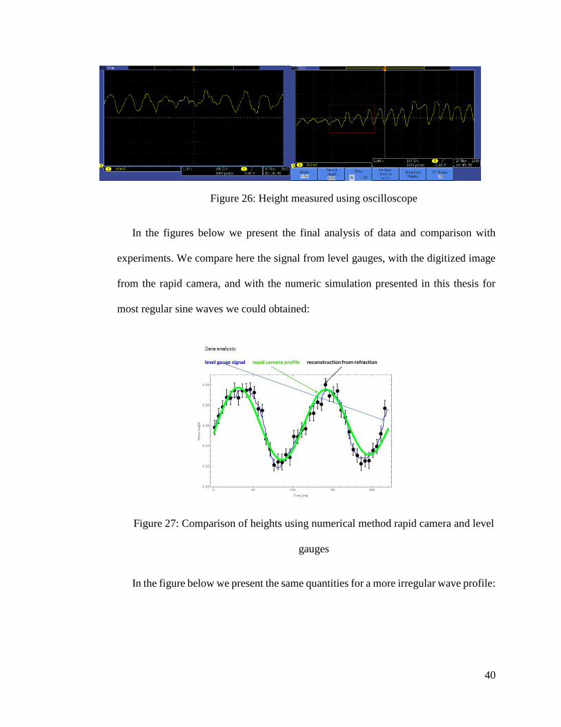
40
Figure 26: Height measured using oscilloscope
In the figures below we present the final analysis of data and comparison with
experiments. We compare here the signal from level gauges, with the digitized image
from the rapid camera, and with the numeric simulation presented in this thesis for
most regular sine waves we could obtained:
Figure 27: Comparison of heights using numerical method rapid camera and level
gauges
In the figure below we present the same quantities for a more irregular wave profile:
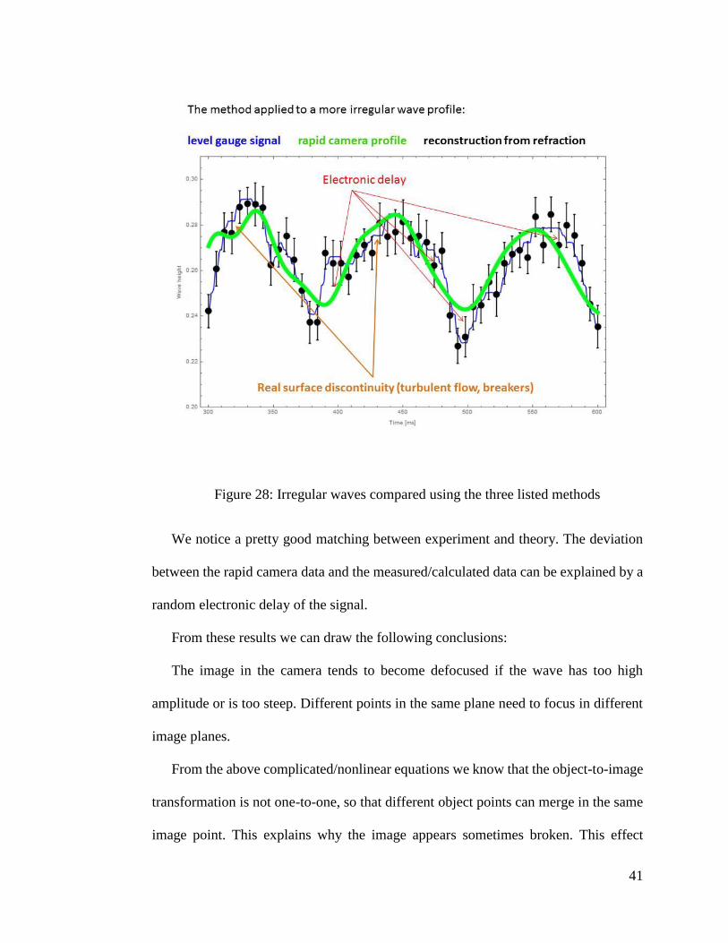
41
Figure 28: Irregular waves compared using the three listed methods
We notice a pretty good matching between experiment and theory. The deviation
between the rapid camera data and the measured/calculated data can be explained by a
random electronic delay of the signal.
From these results we can draw the following conclusions:
The image in the camera tends to become defocused if the wave has too high
amplitude or is too steep. Different points in the same plane need to focus in different
image planes.
From the above complicated/nonlinear equations we know that the object-to-image
transformation is not one-to-one, so that different object points can merge in the same
image point. This explains why the image appears sometimes broken. This effect
42
happens when the height of the waves is too large, or the camera too close and the
geometric optic approximation is not valid anymore.
Illumination should be carefully chosen to eliminate all parasite reflections on wavy
water surface that cannot be predicted from horizontal surface.
The system always needs at least one level gauges to measure the average height of
the wave at one point.
The major advantages of our method are 2: It is fully 3-dimensional procedure, and
it is able to reconstruct the wave field simultaneously over all the investigated area,
hence it may render good data for tsunami prevention. In addition our method is easy
to calibrate and to use.
43
Chapter 6: Summary and conclusion
The investigators begin the research with the concept that an object under water
will change in magnification with change in the height of the water in which the object is
placed when observed by a camera or observer outside water.
The study led to the derivation of a novel equation to calculate the apparent height
of an object with the change in water levels or change in the distance of the object from
the center of origin of the camera.
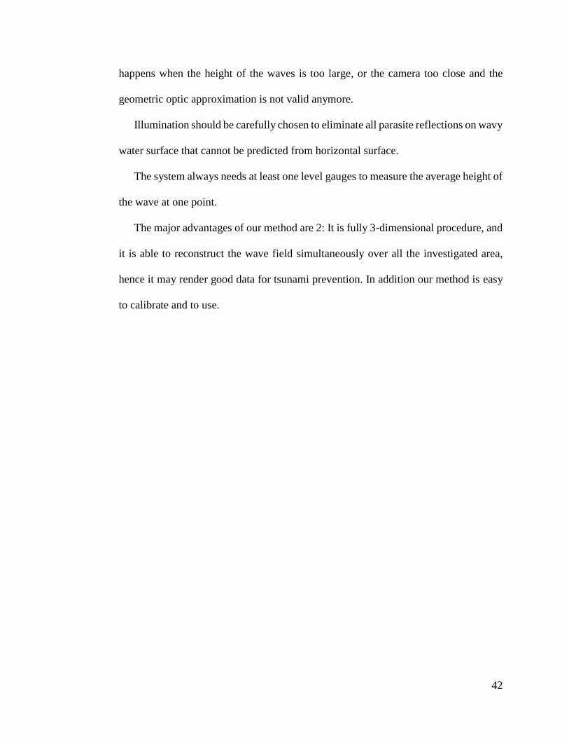
The equations were simulated in MATLAB for various test cases and the results
obtained were in section 4 and compare them to the initial results obtained using
Mathematica Appendix C.
Figure 29: Y component Vs Water height.
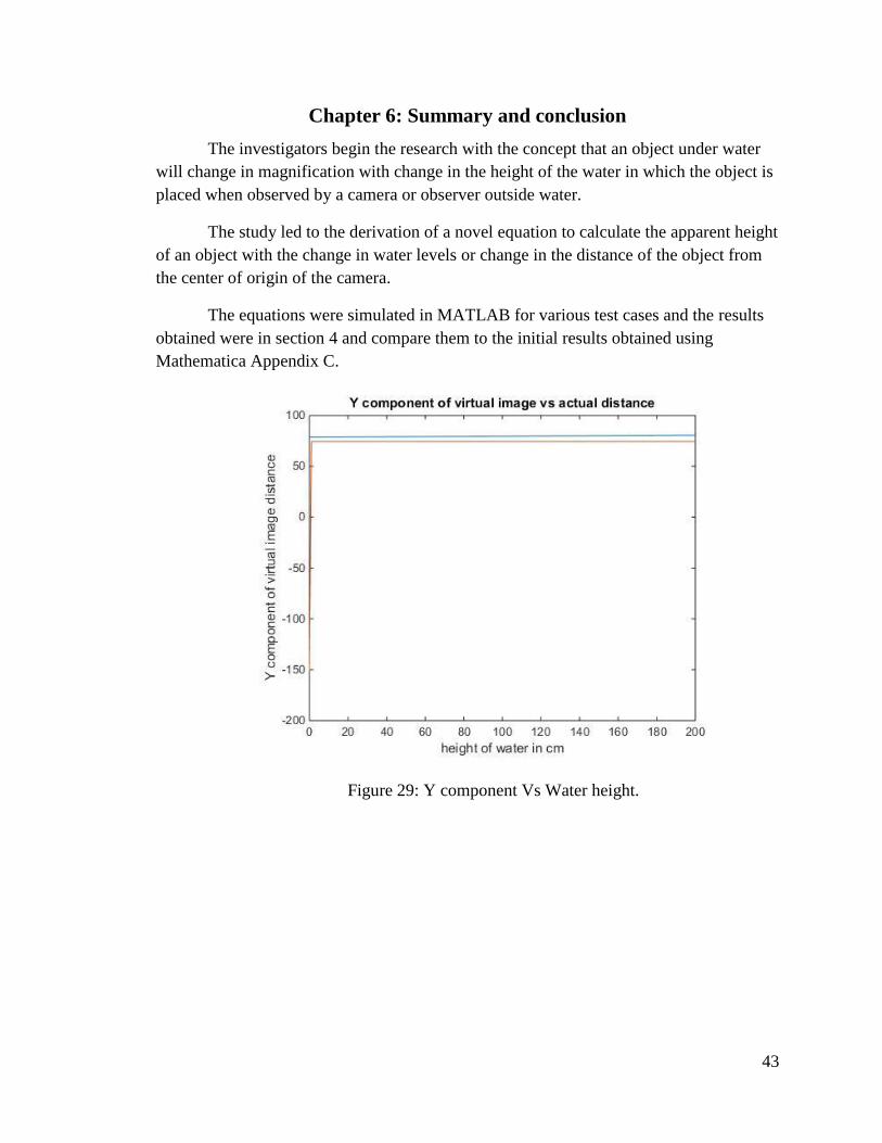
44
Figure 30: The Predicted result Using Mathematica [Appendix C]
It is seen from the above figures that the change in water height leads to the apparent
change in height of the object. This can be identified as apparent magnification of the object
thus confirming that change in water height impacts the magnification of objects seen in
water.
The same is seen when the water is slightly inclined to the steady surface as seen
in section 3.2. These concepts can be used to further the study of water waves thus a
stepping stone to Tsunami warning system.
Another concept to measure the height of water by comparing images distorted by
water to the restored and reconstructed images is mentioned. Hence a brief study is done
in reconstruction of images under water.
Conclusion
The main purpose of the research is to express the relation of water height to
magnification of objects under water. The relation derived is than tested at different cases
to further strengthen the argument that change in water height leads to apparent change in
magnification of the object under water to a certain extent.
45
This research is a stepping stone to building a fool-proof tsunami warning system which
could help save thousands of lives and mitigate dame caused by tsunamis.
At the beginning, the task first at hand was to check the delay the images were
captured simultaneously between the two stereo cameras. The physical setup was
constructed fairly quickly and testing can be done smoothly. Next the investigators clicked
images to have a practical idea of whether the images under water have any apparent
magnification with increase in water height. Though the images showed magnification on
physical calculation, implementing an initial software program to calculate it for various
water heights had a serious drawback.
Firstly, on adding every inch of water in the tank, the images were extremely distorted due
to the following reasons:
The distortion from images due to water increased exponentially with every inch
of water added.
After about 5 inches of water, without an external source of light the image was
impossible to capture since the object would be extremely darkened to get any
useful info out of it.
The use of external lights was suggested but due to the refractive and reflective
properly of water, it could add only a few more inches to the water before image
distortion.
The suggestion of image restoration and correction was suggested to than further
process the distorted images and compare magnification, but image correction let
to change in the original image characteristics which would affect the comparison
of magnification significantly since the change is very minute.
Hence the calculation for magnification was done physically as shown in images below.
46
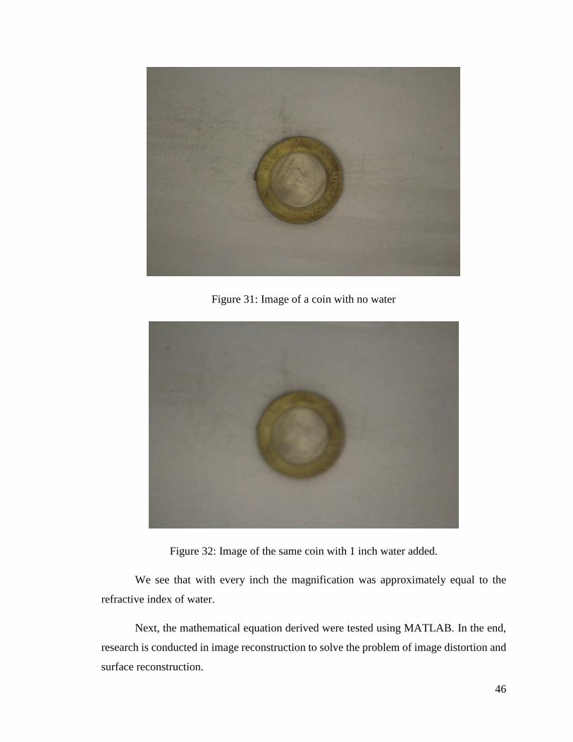
Figure 31: Image of a coin with no water
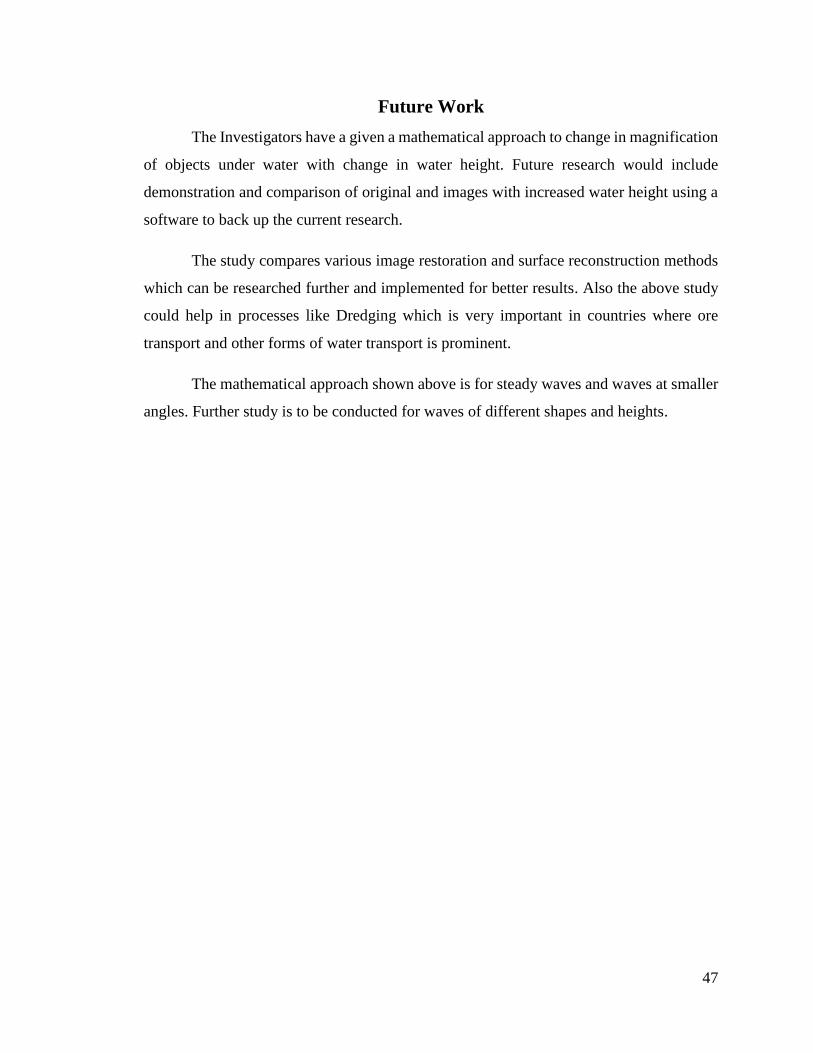
Figure 32: Image of the same coin with 1 inch water added.
We see that with every inch the magnification was approximately equal to the
refractive index of water.
Next, the mathematical equation derived were tested using MATLAB. In the end,
research is conducted in image reconstruction to solve the problem of image distortion and
surface reconstruction.
47
Future Work
The Investigators have a given a mathematical approach to change in magnification
of objects under water with change in water height. Future research would include
demonstration and comparison of original and images with increased water height using a
software to back up the current research.
The study compares various image restoration and surface reconstruction methods
which can be researched further and implemented for better results. Also the above study
could help in processes like Dredging which is very important in countries where ore
transport and other forms of water transport is prominent.
The mathematical approach shown above is for steady waves and waves at smaller
angles. Further study is to be conducted for waves of different shapes and heights.
48
References
[1] Yuandong Tian and Srinivasa G. Narasimhan, "Seeing through Water: Image
Restoration using Model-based Tracking". Proc. of IEEE International Conference of
Computer Vision (ICCV), Oct, 2009.
[2]Douglas Enright, Ronald Fedkiw, Joel Ferziger, and Ian Mitchell. A hybrid particle
level set method for improved interface capturing. In Proceedings of SIGGRAPH 2002,
ACM Press / ACM SIGGRAPH, 2002.
[3]Nick Foster and Ronald Fedkiw. Practical animation of liquids. In Proceedings of
SIGGRAPH 2001, ACM Press / ACM SIGGRAPH, pages 23–30, 2001.
[4] Nick Foster and Dimitri Metaxas. Realistic animation of liquids. In Graphical models
and image processing, 1995.
[5] H. Murase, Surface Shape Reconstruction of a Nonrigid Transparent Object Using
Refraction and Motion. IEEE Transactions on Pattern Analysis and Machine Intelligence,
Vol. 14, No. 10, Oct 1992
[6] S.Ullman, The Interpretation of Visual Motion. Cambridge, MA: MIT press,1979.
[7] Michael Kass and Gavin Miller. Rapid, stable fluid dynamics for computer graphics.
In Proceedings of SIGGRAPH 1990, ACM Press / ACM SIGGRAPH, pages 49–55,
1990.
[8]D. Peachy. Modeling waves and surf. In Proceedings of SIGGRAPH 1986, ACM
Press / ACM SIGGRAPH, pages 65–74, 1986.
[9]Bernd J¨ahne, Jochen Klinke, and Stefan Waas. Imaging of short ocean wind waves: a
critical review. Journal of Optical Society of America, 11(8):2197–2209, 1994.
[10]Bernd J¨ahne, Jochen Klinke, Peter Geissler, and Frank Hering. Image sequence
analysis of ocean wind waves. In Proceedings of the International Seminar on Imaging in
Transport Processes, 1992.
[11]O.H. Shemdin. Measurement of short surface waves with stereophotography. In
Engineering in the Ocean Environment. Conference Proceedings, pages 568–571, 1990.
[12]Xin Zhang and Charles Cox. Measuring the two-dimensional structure of a wavy
water surface optically: A surface gradient detector. Experiments in Fluids, Springer
Verlag, 17:225–237, 1994.
[13]Hiroshi Murase. Shape reconstruction of an undulating transparent object. In Proc.
IEEE Intl. Conf. Computer Vision, pages 313–317, 1990.
49
[14]Nigel Jed Wesley Morris. Image-based Water Surface Reconstruction with
Refractive Stereo, Graduate Department of Computer Science, University of Toronto,
2004
[15]W. C. Keller and B. L. Gotwols. Two-dimensional optical measurement of wave
slope. Applied Optics, 22(22):3476–3478, 1983.
[16]J.M. Daida, D. Lund, C. Wolf, G.A. Meadows, K. Schroeder, J. Vesecky,
D.R.Lyzenga, B.C. Hannan, and R.R. Bertram. Measuring topography of small-
scalewater surface waves. In Geoscience and Remote Sensing Symposium.
ConferenceProceedings, volume 3, pages 1881–1883, 1995.
[17] Ludu, Andrei, Final.Laser, Daytona Beach, FL, Embry-Riddle Aeronautical
University. 2012
[18] Nejad, Sh. Mohammed and M. H. Haji Mirsaeidi, Altitude Measurement using Laser
Beam Reflected from Water Surface, Iranian Journal of Electrical & Electronic
Engineering. 2005
[19]Ladyada, Photoconductive Cells,
http://www.ladyada.net/media/sensors/APP_PhotocellIntroduction.pdf. 2012
[20] NOAA, Triaxys Directional Wave Buoy for Nearshore Wave Measurements – Test
and Evaluation Plan, http://tidesandcurrents.noaa.gov/publications/techrpt38.pdf. 2003
[21] Burkhard, D. G., and Shealy, D. L., Flux density for ray propagation in geometrical
optics, Optical Society of America, 63, 3 (1973) 299-304.
A
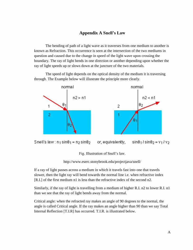
Appendix A Snell’s Law
The bending of path of a light wave as it traverses from one medium to another is
known as Refraction. This occurrence is seen at the intersection of the two mediums in
question and caused due to the change in speed of the light wave upon crossing the
boundary. The ray of light bends in one direction or another depending upon whether the
ray of light speeds up or slows down at the juncture of the two materials.
The speed of light depends on the optical density of the medium it is traversing
through. The Example below will illustrate the principle more clearly.
Fig. Illustration of Snell’s law.
http://www.eserc.stonybrook.edu/projectjava/snell/
If a ray of light passes across a medium in which it travels fast into one that travels
slower, then the light ray will bend towards the normal line i.e. when refractive index
[R.I.] of the first medium n1 is less than the refractive index of the second n2.
Similarly, if the ray of light is travelling from a medium of higher R.I. n2 to lower R.I. n1
than we see that the ray of light bends away from the normal.
Critical angle: when the refracted ray makes an angle of 90 degrees to the normal, the
angle is called Critical angle. If the ray makes an angle higher than 90 than we say Total
Internal Reflection [T.I.R] has occurred. T.I.R. is illustrated below.
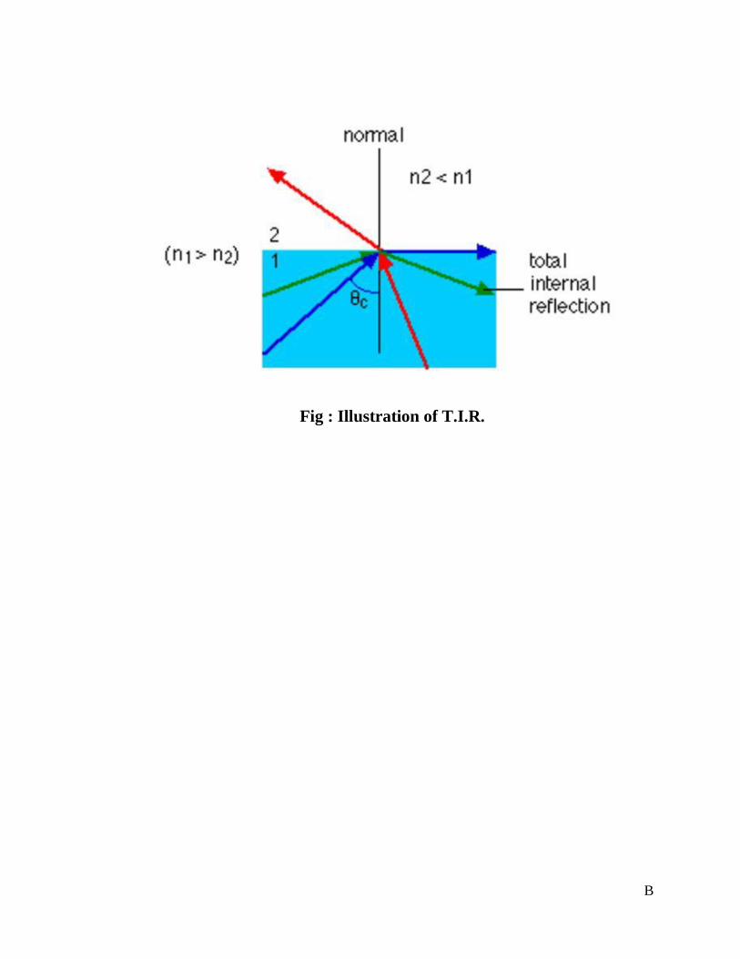
B
Fig : Illustration of T.I.R.
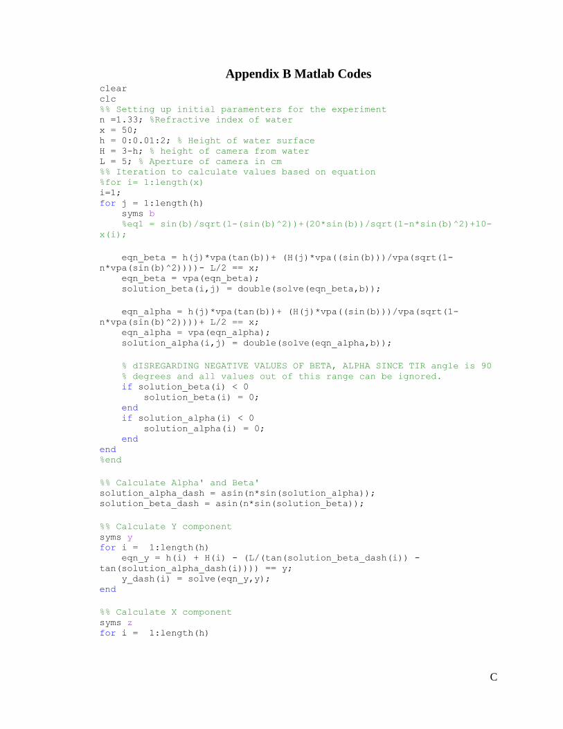
C
Appendix B Matlab Codes clear clc %% Setting up initial paramenters for the experiment n =1.33; %Refractive index of water x = 50; h = 0:0.01:2; % Height of water surface H = 3-h; % height of camera from water L = 5; % Aperture of camera in cm %% Iteration to calculate values based on equation %for i= 1:length(x) i=1; for j = 1:length(h) syms b %eq1 = sin(b)/sqrt(1-(sin(b)^2))+(20*sin(b))/sqrt(1-n*sin(b)^2)+10-
x(i);
eqn_beta = h(j)*vpa(tan(b))+ (H(j)*vpa((sin(b)))/vpa(sqrt(1-
n*vpa(sin(b)^2))))- L/2 == x; eqn_beta = vpa(eqn_beta); solution_beta(i,j) = double(solve(eqn_beta,b));
eqn_alpha = h(j)*vpa(tan(b))+ (H(j)*vpa((sin(b)))/vpa(sqrt(1-
n*vpa(sin(b)^2))))+ L/2 == x; eqn_alpha = vpa(eqn_alpha); solution_alpha(i,j) = double(solve(eqn_alpha,b));
% dISREGARDING NEGATIVE VALUES OF BETA, ALPHA SINCE TIR angle is 90 % degrees and all values out of this range can be ignored. if solution_beta(i) < 0 solution_beta(i) = 0; end if solution_alpha(i) < 0 solution_alpha(i) = 0; end end %end
%% Calculate Alpha' and Beta' solution_alpha_dash = asin(n*sin(solution_alpha)); solution_beta_dash = asin(n*sin(solution_beta));
%% Calculate Y component syms y for i = 1:length(h) eqn_y = h(i) + H(i) - (L/(tan(solution_beta_dash(i)) -
tan(solution_alpha_dash(i)))) == y; y_dash(i) = solve(eqn_y,y); end
%% Calculate X component syms z for i = 1:length(h)
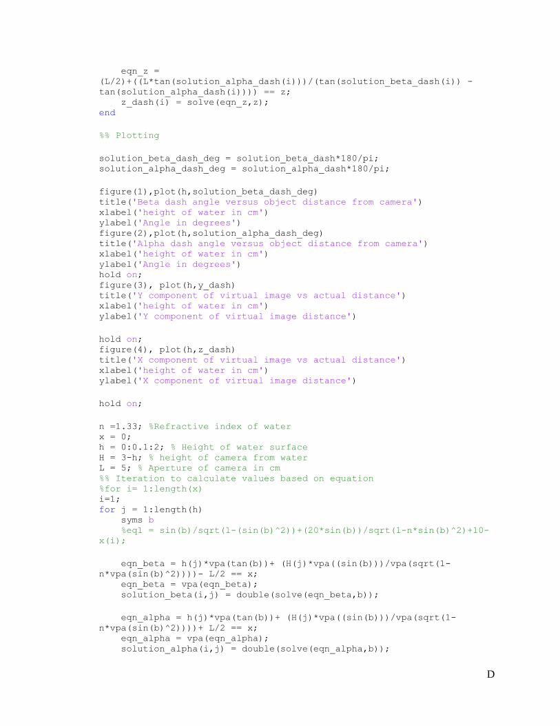
D
eqn_z =
(L/2)+((L*tan(solution_alpha_dash(i)))/(tan(solution_beta_dash(i)) -
tan(solution_alpha_dash(i)))) == z; z_dash(i) = solve(eqn_z,z); end
%% Plotting
solution_beta_dash_deg = solution_beta_dash*180/pi; solution_alpha_dash_deg = solution_alpha_dash*180/pi;
figure(1),plot(h,solution_beta_dash_deg) title('Beta dash angle versus object distance from camera') xlabel('height of water in cm') ylabel('Angle in degrees') figure(2),plot(h,solution_alpha_dash_deg) title('Alpha dash angle versus object distance from camera') xlabel('height of water in cm') ylabel('Angle in degrees') hold on; figure(3), plot(h,y_dash) title('Y component of virtual image vs actual distance') xlabel('height of water in cm') ylabel('Y component of virtual image distance')
hold on; figure(4), plot(h,z_dash) title('X component of virtual image vs actual distance') xlabel('height of water in cm') ylabel('X component of virtual image distance')
hold on;
n =1.33; %Refractive index of water x = 0; h = 0:0.1:2; % Height of water surface H = 3-h; % height of camera from water L = 5; % Aperture of camera in cm %% Iteration to calculate values based on equation %for i= 1:length(x) i=1; for j = 1:length(h) syms b %eq1 = sin(b)/sqrt(1-(sin(b)^2))+(20*sin(b))/sqrt(1-n*sin(b)^2)+10-
x(i);
eqn_beta = h(j)*vpa(tan(b))+ (H(j)*vpa((sin(b)))/vpa(sqrt(1-
n*vpa(sin(b)^2))))- L/2 == x; eqn_beta = vpa(eqn_beta); solution_beta(i,j) = double(solve(eqn_beta,b));
eqn_alpha = h(j)*vpa(tan(b))+ (H(j)*vpa((sin(b)))/vpa(sqrt(1-
n*vpa(sin(b)^2))))+ L/2 == x; eqn_alpha = vpa(eqn_alpha); solution_alpha(i,j) = double(solve(eqn_alpha,b));
E
% dISREGARDING NEGATIVE VALUES OF BETA, ALPHA SINCE TIR angle is 90 % degrees and all values out of this range can be ignored. if solution_beta(i) < 0 solution_beta(i) = 0; end if solution_alpha(i) < 0 solution_alpha(i) = 0; end end %end
%% Calculate Alpha' and Beta' solution_alpha_dash = asin(n*sin(solution_alpha)); solution_beta_dash = asin(n*sin(solution_beta));
%% Calculate Y component syms y for i = 1:length(h) eqn_y = h(i) + H(i) - (L/(tan(solution_beta_dash(i)) -
tan(solution_alpha_dash(i)))) == y; y_dash(i) = solve(eqn_y,y); end
%% Calculate X component syms z for i = 1:length(h) eqn_z =
(L/2)+((L*tan(solution_alpha_dash(i)))/(tan(solution_beta_dash(i)) -
tan(solution_alpha_dash(i)))) == z; z_dash(i) = solve(eqn_z,z); end
hold on; figure(3), plot(h,y_dash) title('Y component of virtual image vs actual distance') xlabel('height of water in cm') ylabel('Y component of virtual image distance')
hold on; figure(4), plot(h,z_dash) title('X component of virtual image vs actual distance') xlabel('height of water in cm') ylabel('X component of virtual image distance')
hold on;
F
Appendix C Mathematica Simulation And Theory
Calculations:
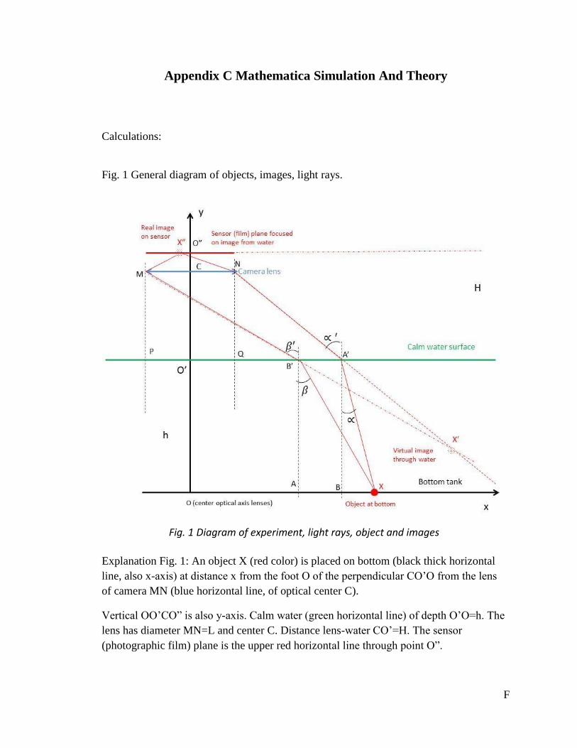
Fig. 1 General diagram of objects, images, light rays.
Fig. 1 Diagram of experiment, light rays, object and images
Explanation Fig. 1: An object X (red color) is placed on bottom (black thick horizontal
line, also x-axis) at distance x from the foot O of the perpendicular CO’O from the lens
of camera MN (blue horizontal line, of optical center C).
Vertical OO’CO” is also y-axis. Calm water (green horizontal line) of depth O’O=h. The
lens has diameter MN=L and center C. Distance lens-water CO’=H. The sensor
(photographic film) plane is the upper red horizontal line through point O”.
G
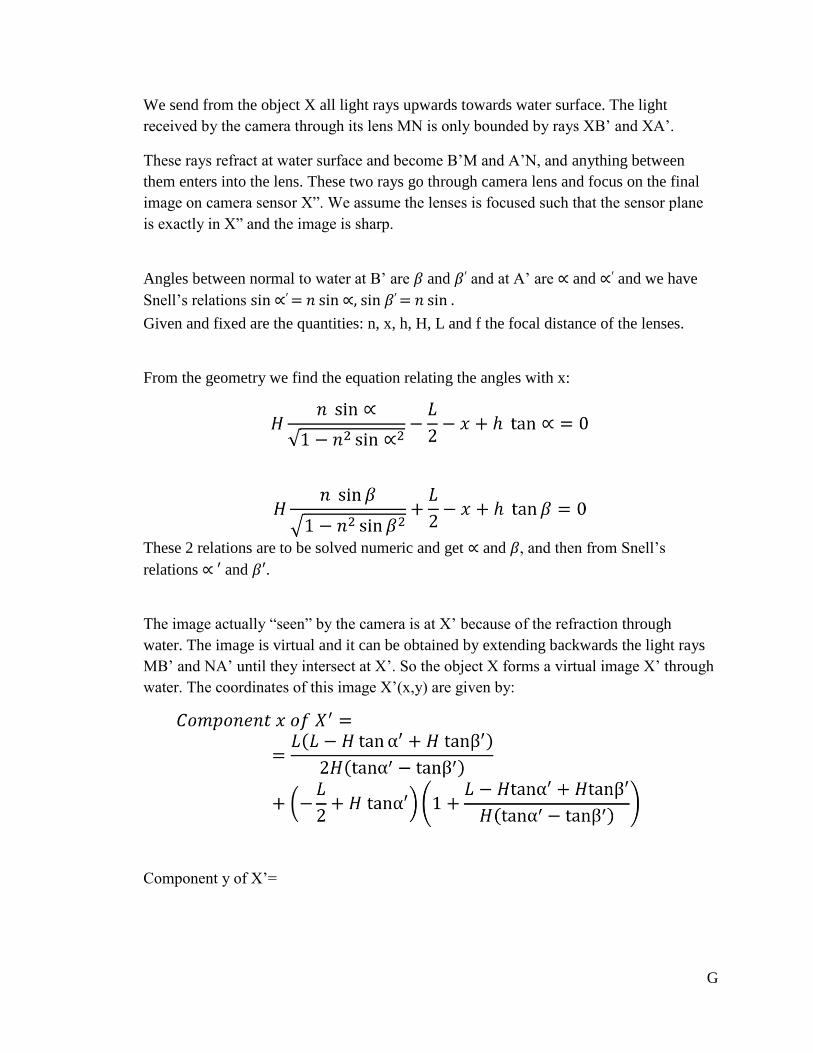
We send from the object X all light rays upwards towards water surface. The light
received by the camera through its lens MN is only bounded by rays XB’ and XA’.
These rays refract at water surface and become B’M and A’N, and anything between
them enters into the lens. These two rays go through camera lens and focus on the final
image on camera sensor X”. We assume the lenses is focused such that the sensor plane
is exactly in X” and the image is sharp.
Angles between normal to water at B’ are 𝛽 and 𝛽′ and at A’ are ∝ and ∝′ and we have
Snell’s relations sin ∝′ = 𝑛 sin ∝, sin 𝛽′ = 𝑛 sin .
Given and fixed are the quantities: n, x, h, H, L and f the focal distance of the lenses.
From the geometry we find the equation relating the angles with x:
These 2 relations are to be solved numeric and get ∝ and 𝛽, and then from Snell’s
relations ∝ ′ and 𝛽′.
The image actually “seen” by the camera is at X’ because of the refraction through
water. The image is virtual and it can be obtained by extending backwards the light rays
MB’ and NA’ until they intersect at X’. So the object X forms a virtual image X’ through
water. The coordinates of this image X’(x,y) are given by:
Component y of X’=
H
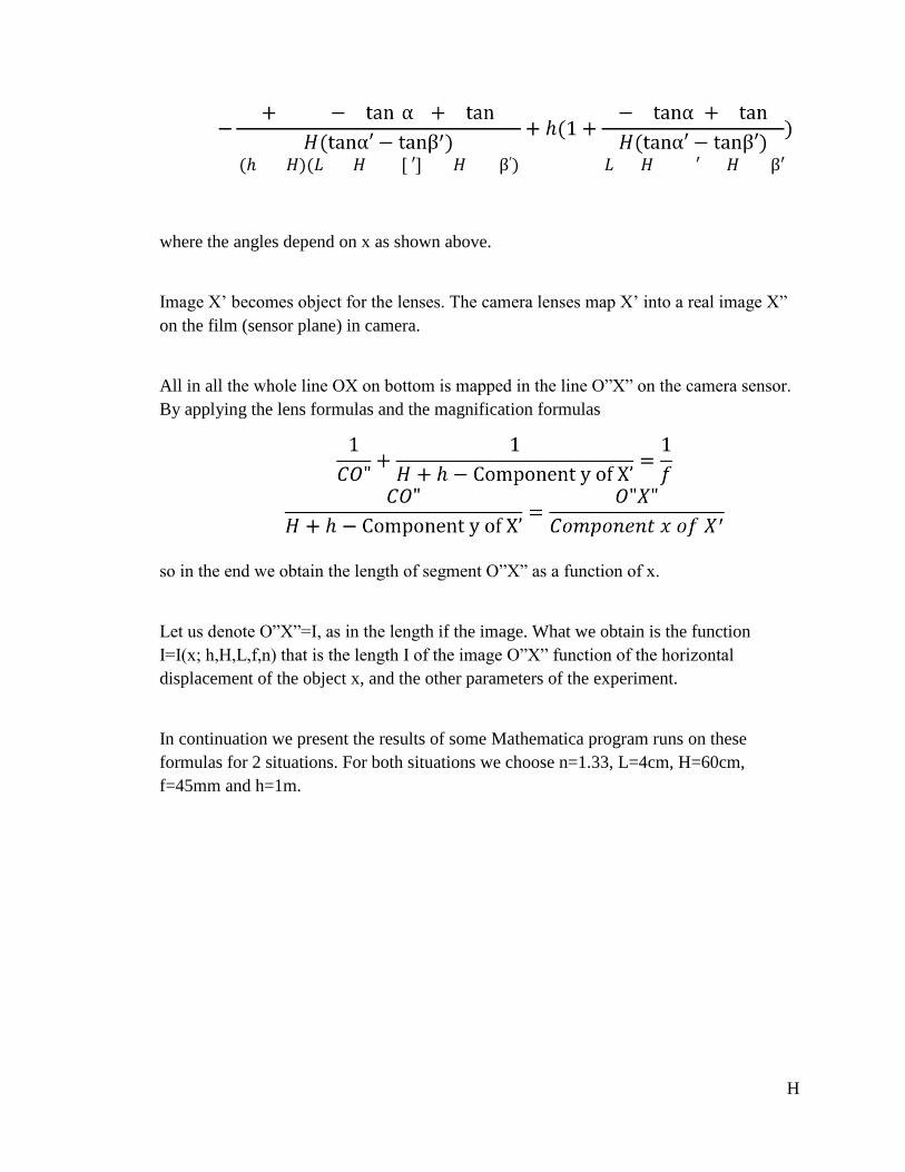
(ℎ 𝐻)(𝐿 𝐻 [ ′] 𝐻 β′) 𝐿 𝐻 ′ 𝐻 β′
where the angles depend on x as shown above.
Image X’ becomes object for the lenses. The camera lenses map X’ into a real image X”
on the film (sensor plane) in camera.
All in all the whole line OX on bottom is mapped in the line O”X” on the camera sensor.
By applying the lens formulas and the magnification formulas
so in the end we obtain the length of segment O”X” as a function of x.
Let us denote O”X”=I, as in the length if the image. What we obtain is the function
I=I(x; h,H,L,f,n) that is the length I of the image O”X” function of the horizontal
displacement of the object x, and the other parameters of the experiment.
In continuation we present the results of some Mathematica program runs on these
formulas for 2 situations. For both situations we choose n=1.33, L=4cm, H=60cm,
f=45mm and h=1m.
I
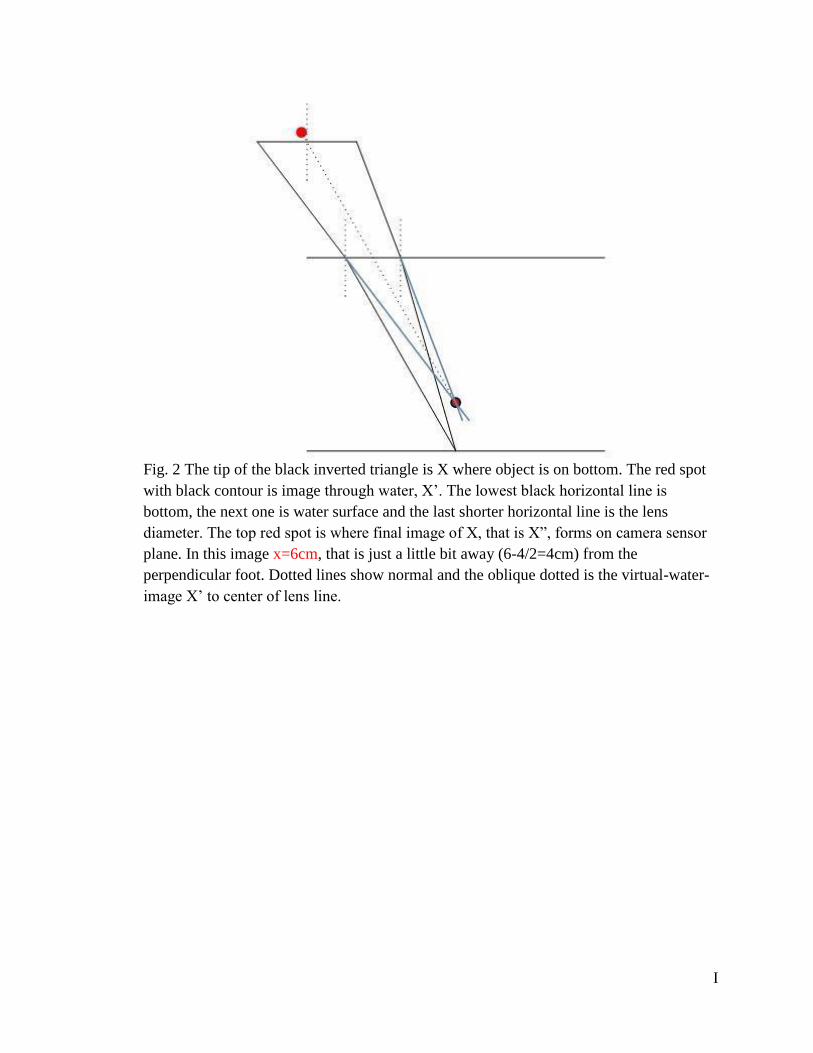
Fig. 2 The tip of the black inverted triangle is X where object is on bottom. The red spot
with black contour is image through water, X’. The lowest black horizontal line is
bottom, the next one is water surface and the last shorter horizontal line is the lens
diameter. The top red spot is where final image of X, that is X”, forms on camera sensor
plane. In this image x=6cm, that is just a little bit away (6-4/2=4cm) from the
perpendicular foot. Dotted lines show normal and the oblique dotted is the virtual-water-
image X’ to center of lens line.
J
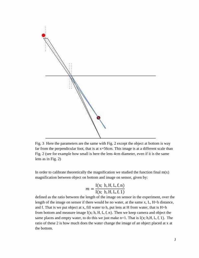
Fig. 3 Here the parameters are the same with Fig. 2 except the object at bottom is way
far from the perpendicular foot, that is at x=56cm. This image is at a different scale than
Fig. 2 (see for example how small is here the lens 4cm diameter, even if it is the same
lens as in Fig. 2)
In order to calibrate theoretically the magnification we studied the function final m(x)
magnification between object on bottom and image on sensor, given by:
defined as the ratio between the length of the image on sensor in the experiment, over the
length of the image on sensor if there would be no water, at the same x, L, H+h distance,
and f. That is we put object at x, fill water to h, put lens at H from water, that is H+h
from bottom and measure image I(x; h, H, L, f, n). Then we keep camera and object the
same places and empty water, to do this we just make n=1. That is I(x; h,H, L, f, 1). The
ratio of these 2 is how much does the water change the image of an object placed at x at
the bottom.
K
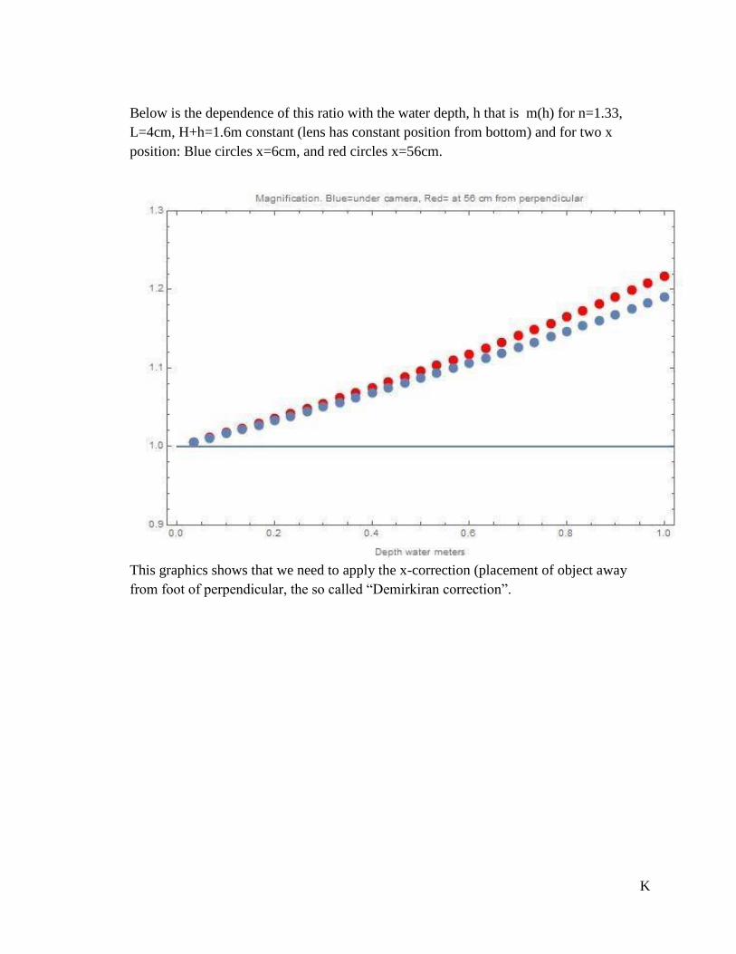
Below is the dependence of this ratio with the water depth, h that is m(h) for n=1.33,
L=4cm, H+h=1.6m constant (lens has constant position from bottom) and for two x
position: Blue circles x=6cm, and red circles x=56cm.
This graphics shows that we need to apply the x-correction (placement of object away
from foot of perpendicular, the so called “Demirkiran correction”.