Technology shocks and aggregate fluctuations

in an estimated hybrid RBC model∗

Jim MalleyUniversity of Glasgow and CESifo

Ulrich Woitek

University of Zurich and CESifo

April 14, 2009

Abstract

This paper contributes to the on-going empirical debate regardingthe role of the RBC model and in particular of technology shocks in ex-plaining aggregate fluctuations. To this end we estimate the model’sposterior density using Markov-Chain Monte-Carlo (MCMC) meth-ods. Within this framework we extend Ireland’s (2001, 2004) hybridestimation approach to allow for a vector autoregressive moving aver-age (VARMA) process to describe the movements and co-movementsof the model’s errors not explained by the basic RBC model. Theresults of marginal likelihood ratio tests reveal that the more generalmodel of the errors significantly improves the model’s fit relative tothe VAR and AR alternatives. Moreover, despite setting the RBCmodel a more difficult task under the VARMA specification, our anal-ysis, based on forecast error and spectral decompositions, suggeststhat the RBC model is still capable of explaining a significant fractionof the observed variation in macroeconomic aggregates in the post-warU.S. economy.

Keywords: Real Business Cycle, Bayesian estimation, VARMA errorsJEL codes: C11, C52, E32

∗We would like to thank seminar participants at the Department of Economics, Uni-versity of Glasgow for helpful comments and suggestions. The usual disclaimer applies.

1

1 Introduction

The role of technology shocks as a leading determinant of business cyclescontinues to be a heated debate over their ability to explain the observedvariation of macroeconomic aggregates in the postwar US economy. While anumber of authors as early as Eichenbaum (1991) and more recently Ireland(2004) and Chari et al. (2007a), acknowledge a large degree of uncertaintyassociated with these estimates, they do not rule out the possibility thattechnology may still have an important role to play.

For example, Eichenbaum (1991 p. 608) states, “What the data areactually telling us is that, while technology shocks almost certainly playsome role in generating the business cycle, there is an enormous amount ofuncertainty about just what percent of aggregate fluctuations they actuallydo account for. The answer could be 70% as Kydland and Prescott (1989)[1991] claim, but the data contain almost no evidence against either the viewthat the answer is really 5% or that the answer is really 200%”.

In a similar vein, when reviewing the results from a vast range of stud-ies based on calibration and econometric estimation,1 Chari et al. (2007ap. 39) argue, “The message we get from these and related studies in thebusiness cycle literature is that a plausible case can be made that in theUS data, technology shocks account for essentially any value between zeroand 100% of output variance. Put differently, when the US data are viewedthrough the lens of the growth model, dismissing any estimate in this rangeis unreasonable”.

Ireland’s (2004) findings however, are less pessimistic than both Eichen-baum (1991) and Chari et al. (2007). He remarks, “Even if the true fractionof output variation explained by the real business cycle model is two stan-dard errors less than the point estimate of 90%, for instance, that fractionremains greater than 60%” (Ireland 2004, p. 1213).

In sharp contrast, a series of influential studies by Galı (1999), Galı andRabanal (2005) and Francis and Ramey (2005), are far less circumspect intheir view regarding the usefulness of the basic RBC model as a frameworkin which to study business cycles. For example, Francis and Ramey (2005,p. 1380) proclaim that “the original technology-driven real business cyclehypothesis does appear to be dead”. These studies arrive at their conclusionsvia a differenced structural vector autoregressive (DSVAR) model using USdata and find, contrary to the predictions of the standard RBC model, that

1The econometric studies referred to by Chari et al. (2007a) include those using bothgeneralized method of moments (GMM) and maximum likelihood (ML) methods to esti-mate an RBC model as well as studies based on structural vector autoregressions (SVAR)employing long-run restrictions.

2

hours worked falls in response to a positive technology shock. They also findthat technology shocks do not generally play a prominent role in accountingfor the variance of output.

Despite the clear messages arising from the DSVAR studies, the findingsby Christiano et al. (2003) and more recently by Chari et al. (2007a) suggestthat perhaps these results are not robust. For example, Christiano et al.

(2003), using an SVAR specified in levels (LSVAR), are able to reverse theimpulse response results of the DSVAR studies. Chari et al. (2007a) takean even stronger position and suggest that the findings of both specificationsof the SVAR should be viewed with some suspicion since they suffer fromlag-truncation bias. Instead they argue that an alternative SVAR approachbased on the work of Sims (1989) and Cogley and Nason (1995) as well as thebusiness cycle accounting approach of Chari et al. (2007b) are potentiallymore fruitful methods for appealing to the data to help develop businesscycle theory.

In contrast to the SVAR method, which relies only loosely on economictheory, another strand of the literature views the RBC model’s equilibriumconditions and their associated “cross-equation restrictions” as a likelihoodfunction which can be maximized (see, e.g. Sargent (1989)).2 A recent set ofstudies in the likelihood estimation literature which are particularly relevantfor our work are by Ireland (2001, 2004) who proposes a hybrid approachto model estimation. This method is motivated by the desire to avoid theproblem of stochastic singularity due to the presence of only one source ofuncertainty in the basic RBC model. To this end Ireland builds directly onthe work of Sargent (1989), Altug (1989), McGrattan (1994), Hall (1996)and McGrattan et al. (1997) by also adding scalar AR(1) errors to theobservation equations of the state-space representation of the RBC model.However in contrast to these authors, he further allows for cross-equationcorrelation between these errors using a VAR(1) structure.3

Ireland convincingly argues, “The method takes as its starting point afully-specifed DSGE model, but also admits that while this model may bepowerful enough to account for and explain many key features of the US data,it remains too stylized to possibly capture all of the dynamics that can be

2Ruge-Murcia (2007) provides an excellent overview of this literature and extensive ref-erences relating to classical and Bayesian estimation of both linear and nonlinear dynamicequilibrium models.

3Solving the stochastic singularity problem associated with maximum likelihood es-timation of the linearized model can also be tackled by introducing structural shocksuntil the number of shocks is equal to the number of observables in the model (see, e.g.Bencivenga (1992), Ireland (1997, 2001a,b, 2002), DeJong et al. (2000a,b), Kim (2000),Schorfheide (2000), Smets and Wouters (2003) and Bouakez et al. (2005)).

3

found in the data. Hence, it augments the DSGE model so that its residuals– meaning the movements in the data that the theory cannot explain – aredescribed by a VAR, making estimation, hypothesis testing, and forecastingfeasible” (Ireland 2004, p. 1206). He goes on to state that while the residualsmay account for measurement errors, “... they can also be interpreted moreliberally as capturing all of the movements and co-movements in the datathat the real business cycle model, because of its elegance and simplicity,cannot explain” (Ireland 2004, p. 1206).

With a view to contributing to the still clearly open question regardingthe role of the technology-driven RBC model in explaining aggregate fluc-tuations, we apply and extend the Ireland (2001, 2004) hybrid approach tomodel estimation. Consistent with Ireland’s objective to reconcile the lim-ited dynamics in the RBC model with the data, we extend his method toallow for a VARMA(1,1) representation of the residuals. Since a stationaryVARMA(1,1) has both infinite VAR and VMA representations, it allows for amuch richer representation of the dynamic interactions between the residuals.Accounting for these can lead to improvements in model fit to the historicaldata and hence more accurate predictions for the various diagnostics usedto asses the explanatory power of the RBC model, e.g. forecast error andspectral decompositions. Realizing these potential gains is clearly critical inlight of the objectives of this paper.

In contrast to Ireland (2001, 2004), we do not employ classical maximumlikelihood methods to obtain parameter estimates for the competing mod-els we consider but instead use simulation methods pioneered in dynamicmacroeconomics by DeJong et al. (2000a,b). Given that Ireland’s approachmakes use of prior information when estimating the likelihood function, sim-ulation methods are a natural extension since they provide a framework forformally incorporating both parameter and model uncertainty.

Our main findings are: (i) the VARMA(1,1) specification of the errorssignificantly improves the basic RBC model’s fit to the historical data relativeto the VAR(1) and AR(1) alternatives; (ii) despite setting the RBC model amore difficult task under the VARMA(1,1) specification, technological shocksare still capable of explaining a significant share of the observed variation inoutput and its components over shorter- and longer-forecast horizons as wellas hours at shorter horizons; (iii) the RBC model generally does a relativelybetter job at matching low and high frequency cyclical movements in thedata than at the traditional business cycles ranges; and (iv) the degree ofuncertainty associated with the explanatory power of the RBC model muchdiscussed in the literature is perhaps overstated since we find that estimatedposterior distributions for the forecast error and spectral decompositions tobe quite concentrated.

4

2 Basic RBC Model

Following is a brief sketch of the structure and approximate solution of aprototypical RBC model (see Hansen (1985)). This model or simple varia-tions thereof are frequently used when developing and illustrating alternativesolution and estimation procedures (for examples of the later see, e.g. Ruge-Murcia (2007), Ireland (2001, 2004) and Dejong et al. (2000b)).

Given that the model and its solution are well known, the main purposeof this section is simply to fix ideas, notation and variable definitions whichwill be used in the estimation and analysis which follows. Moreover, sinceone of our objectives is to extend Ireland’s method, we will use the exactvariant of the Hansen (1985) model employed in Ireland (2004) to facilitatetransparent comparability.4 Accordingly, we leave out many of the detailswhich can be found in Ireland (2004) and cross-reference these as requiredbelow.

2.1 Households

The representative household maximizes expected discounted lifetime utility

max{Ct,Ht}

∞

t=0

E0

∞∑

t=0

βt [ln (Ct) − γHt] , β ∈ (0, 1), γ > 0 (1)

where E0 is the conditional expectations operator; Ct is consumption at timet, Ht is hours worked, β is the discount factor and γ is a parameter governingthe linearity of hours.

The household faces the following budget constraint in every period

rtKt + wtHt + Πt = Ct + It (2)

where Kt is the quantity of physical capital at the beginning of period t; rt isthe rental rate of capital; wt is the wage rate of labour; Πt is the household’sshare of profits of the representative firm; and It is investment.

Capital accumulates according to the standard evolution equation

Kt+1 = It + (1 − δ)Kt, δ ∈ (0, 1) (3)

where δ is the constant rate of depreciation.

4Consistent with this choice we also use the US data employed in Ireland (2004), seewww2.bc.edu/~irelandp/. Note that the quarterly observation period is 1948:1-2002:2.

5

2.2 Firms

The representative firm produces a consumption good, Yt and maximizes(from t = 0...∞) as series of static profit functions

Πt = Yt − rtKt − wtHt (4)

subject to a series of technology constraints

Yt = AtKθt

(ηtHt

)1−θ, θ ∈ (0, 1), η > 1 (5)

where At is Hick’s neutral technological progress, θ is the productivity ofprivate capital and η is the gross rate of labour-augmenting technologicalprogress.

2.3 Aggregate resource constraint and technology

In each period t = 0, 1, 2, ... the goods market clearing condition holds, i.e.

Yt = Ct + It. (6)

Finally, the exogenous first-order stochastic Markov process for technol-ogy, At is given by

At+1 = A(1−ρ)Aρt eεt+1, ρ ∈ (0, 1) (7)

εt ∼ N(0, σ2ε)

where ρ is an AR(1) parameter and σ2ε is the constant variance of the stochas-

tic errors, εt.

2.4 Equilibrium conditions and model solution

Given the above setup the representative household chooses {Yt, Ct, It, Ht,Kt+1}

∞t=0 to maximize utility (for given K0, A0) subject to (3, 5, 6, 7) and

the firm chooses {Ht, Kt+1}∞t=0 to maximize profits subject to (5); yielding

a set of non-stationary equilibrium allocations.5 The linearized stationary

5See Ireland (2004, p. 1208) for the explicit form of these conditions.

6

representation of these for all t = 0, 1, 2, ... is given by:

yt = at + θkt + (1 − θ)ht

at = ρat−1 + εt

(η/β − 1 + δ)yt = [(η/β − 1 + δ) − θ(η − 1 + δ)] ct + θ(η − 1 + δ)it

ηkt+1 = (1 − δ)kt + (η − 1 + δ)i (8)

ct + ht = yt

−η

βct = −

η

βEtct+1 +

(η

β− 1 + δ

)Etyt+1 −

(η

β− 1 + δ

)kt+1

where yt = Yt/ηt , ct

= Ct/ηt , it = It/ηt , kt = Kt/ηt , ht ≡ Ht, at ≡ At andfor any stationary variable xt, xt = ln

(xt

x

). Finally, non-time subscripted

variables, x, refer to deterministic steady-state values.6

The policy functions comprising the solution of the above linear systemof stochastic difference equations can be written in state-space form as

yt =(lzk lzx

) (ktat

)

(ktat

)=

(lkk lkx0 ρ

) (kt−1

at−1

)+

(01

)ǫt

or

yt = Zαt; (9)

αt = Tαt−1 + Gǫt.

where yt =(

yt ct ht

)′

and the elements of Z and T contain convolutions

the model’s structural parameters.

3 Econometric Setup

In this section we first provide some motivation for the more flexible errorstructure we propose. We then add AR(1), VAR(1) and VARMA(1,1) er-rors to (9) and derive the models’ corresponding likelihood functions. Toobtain the latter we employ the Kalman filter given that the capital stock,technology, and the various measurement/specification errors are treated asunobservables.

6Again, see Ireland (2004, p. 1221) for the details of the unique steady-state equilib-rium.

7

3.1 Motivation for VARMA structure

Consider the following decomposition of a vector of measured data, ymt intothe part captured by a structural economic model, yst , and another vectornot captured by the model, ǫt:

ymt = yst + ǫt. (10)

In other words, the non-structural component, ǫt, consisting of measure-ment and specification errors represents an unobservable wedge between themeasured data and the structural model. In contrast to Chari et al. (2007b),we do not give the wedge a structural interpretation, but instead follow, e.g.Sargent (1989) and Ireland (2004) and as a first step use a AR(1)/VAR(1)structure for ǫt

7:

ymt = yst + ǫt

ǫt = ι1ǫt−1 + ζt (11)

(1 − ι1L) ǫt = ζt.

Let’s next assume that the dynamic structure of the wedge can be ap-proximated by a more general VARMA(1,1) process

ymt = yst + ǫt

ǫt = φǫt−1 + ζt + ϑζt−1 (12)

φ(L)ǫt = ϑ (L) ζt.

If the filter θ(L) is stable and invertible, the VARMA(1,1) process rep-resents a more flexible and parsimonious representation of a VAR(∞) orVMA(∞) process (see, e.g. Lutkepohl (1991, p. 220-223)), i.e.

ϑ (L)−1φ(L)ǫt = ζt

ι(L)ǫt = ζt (13)(1 − ι1L − ι2L

2 − ...)ǫt = ζt.

This structure precludes the so called lag-truncation bias problem associatedwith approximating infinite order VARs with finite order representations. Aspointed out in the introduction, allowing for a more general representationof the dynamic interactions between the errors can lead to improvements inmodel fit and hence more accurate predictions for the various diagnostic usedto asses the explanatory power of the RBC model.

7Note that when the variance covariance matrix of ζt and ρ1 are diagonal, the AR(1)structure maintains.

8

3.2 AR(1)/VAR(1) setup

Adding an n-dimensional VAR(1) measurement/specification error, i.e. ηt =Vηt−1 + νt, to (9) as in Ireland (2001, 2004) yields the following state-spacerepresentation

yt = Zαt + ηt =(Z In

)︸ ︷︷ ︸

Z

(αtηt

)

︸ ︷︷ ︸αt

(14)

(αtηt

)

︸ ︷︷ ︸αt

=

(T 00 V

)

︸ ︷︷ ︸T

(αt−1

ηt−1

)

︸ ︷︷ ︸αt−1

+

(G 00 In

) (ǫtνt

)

︸ ︷︷ ︸ζt∼N(0,Σ)

.

Using the VAR(1) representation, an extension to a finite VAR(p) errorstructure is also straightforward (see, Lutkepohl 1991, p. 11). Also note thatwhen the matrices V and Σ are diagonal, the AR(1) specification maintains(see, e.g. Sargent (1989)).

3.3 VARMA(1,1) setup

As pointed out above, if stable and invertible, the VARMA(1,1) specifi-cation allows us to generalize the finite VAR(p) errors to a VAR(∞) orVMA(∞) structure thus yielding a much richer representation of the dy-namic interactions between the errors. For the VARMA(1,1) case, i.e.ηt = Vηt−1 + Mνt−1 + νt, the state-space representation in (9) becomes

yt =(Z H

)

Z

αtηtνt

αt

(15)

αtηtνt

αt

=

T 0 00 J 00 0 0

︸ ︷︷ ︸T

αt−1

ηt−1

νt−1

︸ ︷︷ ︸αt−1

+

(G 00 R

) (ǫtνt

)

︸ ︷︷ ︸ζt∼N(0,Σ)

where

J =

(V M0 0

)R =

(IKIK

)H =

(IK 0

).

3.4 Kalman filter

For given initial estimates of the state vector, a0, i.e. a0 = E (α0) and thecovariance matrix, P0, the filter consists of the following steps:

9

1. prediction step

at|t−1 = Tat−1,

Pt|t−1 = TPt−1T′ + Σ. (16)

2. updating step

υt = yt − Zat|t−1;

Ft = ZPt|t−1Z′;

Kt = TPt|t−1Z′F−1

t ; (17)

at = Tat|t−1 + Ktυt;

Pt =(T − KtZ

)Pt|t−1

(T −KtZ

)′

+ Σ

where υt are the model’s forecast errors. The remaining vector and matriceshave either been defined above or, in the case of Ft and Kt, are simplytransformations of previously defined matrices.8

3.5 Likelihood function and estimation algorithm

We are now in a position to write the model’s likelihood function as

p(yt,t=1 , ...,T |ψ) =

T∏

t=1

(2π)−0.5n |Ft|−0.5 exp

(−0.5υ′

tF−1t υt

)(18)

where ψ is the vector of model parameters to be estimated and n is thenumber of measurement equations. We estimate ψ using the random walkMetropolis-Hastings algorithm (see e.g., Chib and Greenberg (1995)), settingthe number of simulations to S = 60, 000 with a burn-in of 10, 000. We drawa new realization of ψ according to

ψ1 = ψ0 + ξ, ξ ∼ N(0,Ξ), (19)

where Ξ is the proposal variance-covariance matrix. A draw ψ1 is acceptedif

a ≥ u, u ∼ U(0, 1),

a (ψ1,ψ0) = min

(p(yt,t=1 , ...,T |ψ1)p(ψ1)

p(yt,t=1 , ...,T |ψ0)p(ψ0), 1

), (20)

where p(ψ) is the prior distribution given in Table 1.

8See Hamilton (1994) or Harvey (1992) for further details regarding the Kalman filter.

10

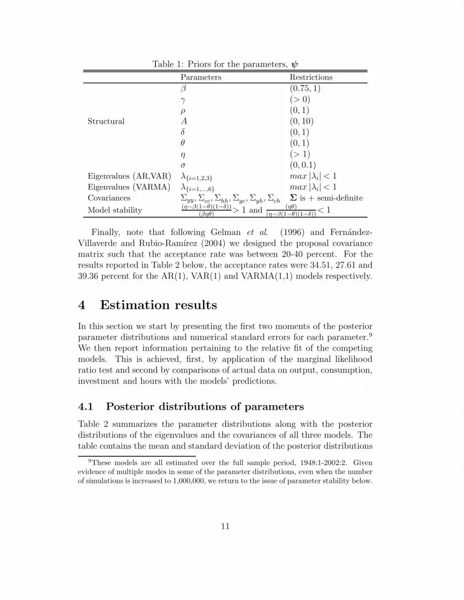
Table 1: Priors for the parameters, ψ

Parameters Restrictions

β (0.75, 1)γ (> 0)ρ (0, 1)

Structural A (0, 10)δ (0, 1)θ (0, 1)η (> 1)σ (0, 0.1)

Eigenvalues (AR,VAR) λ{i=1,2,3} max |λi|< 1Eigenvalues (VARMA) λ{i=1,...,6} max |λi|< 1Covariances Σyy, Σcc, Σhh, Σyc, Σyh, Σch Σ is + semi-definite

Model stability(η−β(1−θ)(1−δ))

(βηθ)> 1 and

(ηθ)(η−β(1−θ)(1−δ))

< 1

Finally, note that following Gelman et al. (1996) and Fernandez-Villaverde and Rubio-Ramırez (2004) we designed the proposal covariancematrix such that the acceptance rate was between 20-40 percent. For theresults reported in Table 2 below, the acceptance rates were 34.51, 27.61 and39.36 percent for the AR(1), VAR(1) and VARMA(1,1) models respectively.

4 Estimation results

In this section we start by presenting the first two moments of the posteriorparameter distributions and numerical standard errors for each parameter.9

We then report information pertaining to the relative fit of the competingmodels. This is achieved, first, by application of the marginal likelihoodratio test and second by comparisons of actual data on output, consumption,investment and hours with the models’ predictions.

4.1 Posterior distributions of parameters

Table 2 summarizes the parameter distributions along with the posteriordistributions of the eigenvalues and the covariances of all three models. Thetable contains the mean and standard deviation of the posterior distributions

9These models are all estimated over the full sample period, 1948:1-2002:2. Givenevidence of multiple modes in some of the parameter distributions, even when the numberof simulations is increased to 1,000,000, we return to the issue of parameter stability below.

11

of the parameters along with a measure of estimation accuracy based onnumerical standard errors, NSE (see, e.g. Geweke (1992)).10

It is first useful to contextualize the size of the means of the structuralparameters reported in Table 2 with the estimated parameters in Ireland(2004). For example, conditioning of a fixed value of β = 0.99 and δ =0.025, Ireland estimated the following values using maximum likelihood: [γ =0.0045; ρ = 0.9987; A = 5.1847; θ = 0.2292; η = 1.0051; σe = 0.0056]. Whileit reassuring that our results are so similar to Ireland’s, it is not entirelyunexpected given that we estimate the same model with the same data.

It is next of interest to note that our estimates of the structural parame-ters remain very stable across the three models with the most relative move-ment occurring for the trend, η, and the variance of technology parameters,σe. This stability is again perhaps not surprising since there is no change inthe RBC part of the model across the three estimations. In contrast, we seesubstantial change in the modes of the eigenvalues in the AR/VAR/VARMAmatrices and the covariances as we move from the restrictive to the generalmodel of the errors. It remains to be seen, in the next subsection, if account-ing for the movements and co-movements of the errors in this way implies abetter fit for the VARMA(1,1) model.

If we now turn to the spread of these distributions, it is again informa-tive to present our results in the context of the literature. Here we cannotrely on the Ireland study given the different approaches we apply to estima-tion. However, the recent study by Fernandez-Villaverde and Rubio-Ramırez(2005) includes a Bayesian estimation of a linearized RBC model and reportsstandard deviations that are roughly the same order of magnitude but gen-erally larger. The fact that our distributions are even tighter is most likelydue to the fact that we explicitly model the errors with varying degress ofstructure whereas they employ a simple additive error term in their mea-surement system. But, of course, some of these dissimilarities could also bedue to differences, for example, in model structure, data used, de-trendingmethods, etc..11

Finally, examination of the numerical standard errors as a share of themeans of the posteriors reveals that our estimates are generally quite precise.The most accurate block appears to be the structural one, followed by the

covariance and eigenvalue blocks. The largest values of

(NSE

|ψi|× 100

)for

10Note that the ratio reported in the Table 2 is in percent terms, i.e. NSE

|ψi|× 100.

11As in Ireland (2004), we estimate and detrend simultaneously, since η is part of theparameter vector (see Section 2.4).

12

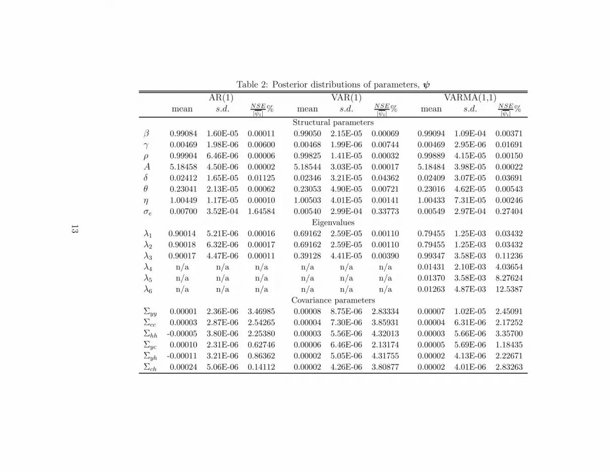
Table 2: Posterior distributions of parameters, ψ

AR(1) VAR(1) VARMA(1,1)mean s.d. NSE

|ψi|% mean s.d. NSE

|ψi|% mean s.d. NSE

|ψi|%

Structural parameters

β 0.99084 1.60E-05 0.00011 0.99050 2.15E-05 0.00069 0.99094 1.09E-04 0.00371

γ 0.00469 1.98E-06 0.00600 0.00468 1.99E-06 0.00744 0.00469 2.95E-06 0.01691

ρ 0.99904 6.46E-06 0.00006 0.99825 1.41E-05 0.00032 0.99889 4.15E-05 0.00150

A 5.18458 4.50E-06 0.00002 5.18544 3.03E-05 0.00017 5.18484 3.98E-05 0.00022

δ 0.02412 1.65E-05 0.01125 0.02346 3.21E-05 0.04362 0.02409 3.07E-05 0.03691

θ 0.23041 2.13E-05 0.00062 0.23053 4.90E-05 0.00721 0.23016 4.62E-05 0.00543

η 1.00449 1.17E-05 0.00010 1.00503 4.01E-05 0.00141 1.00433 7.31E-05 0.00246

σe 0.00700 3.52E-04 1.64584 0.00540 2.99E-04 0.33773 0.00549 2.97E-04 0.27404

Eigenvalues

λ1 0.90014 5.21E-06 0.00016 0.69162 2.59E-05 0.00110 0.79455 1.25E-03 0.03432

λ2 0.90018 6.32E-06 0.00017 0.69162 2.59E-05 0.00110 0.79455 1.25E-03 0.03432

λ3 0.90017 4.47E-06 0.00011 0.39128 4.41E-05 0.00390 0.99347 3.58E-03 0.11236

λ4 n/a n/a n/a n/a n/a n/a 0.01431 2.10E-03 4.03654

λ5 n/a n/a n/a n/a n/a n/a 0.01370 3.58E-03 8.27624

λ6 n/a n/a n/a n/a n/a n/a 0.01263 4.87E-03 12.5387

Covariance parameters

Σyy 0.00001 2.36E-06 3.46985 0.00008 8.75E-06 2.83334 0.00007 1.02E-05 2.45091

Σcc 0.00003 2.87E-06 2.54265 0.00004 7.30E-06 3.85931 0.00004 6.31E-06 2.17252

Σhh -0.00005 3.80E-06 2.25380 0.00003 5.56E-06 4.32013 0.00003 5.66E-06 3.35700

Σyc 0.00010 2.31E-06 0.62746 0.00006 6.46E-06 2.13174 0.00005 5.69E-06 1.18435

Σyh -0.00011 3.21E-06 0.86362 0.00002 5.05E-06 4.31755 0.00002 4.13E-06 2.22671

Σch 0.00024 5.06E-06 0.14112 0.00002 4.26E-06 3.80877 0.00002 4.01E-06 2.83263

13

each block respectively, are 0.27, 3.36 and 12.54 percent.12

4.2 Model comparison

To compare the fit of alternative specifications for the error block, we followChib and Jeliazkov (2001) and calculate Bayes factors based on marginallikelihoods obtained from the simulated parameter realizations. Let Mj , j =1, 2, 3 denote the AR(1), VAR(1), and VARMA(1,1) models respectively.The Bayes factors for comparing model j and k are given by the ratio of thetwo marginal likelihoods for Mj and Mk,

BFjk =p(y|Mj)

p(y|Mk). (21)

The marginal likelihood identity follows from Bayes’ formula:

p(ψj|y, Mj) =p(y|ψj , Mj)p(ψj |Mj)

p(y|Mj)

p(y|Mj) =p(y|ψj , Mj)p(ψj |Mj)

p(ψj |y, Mj), j = 1, 2, 3.

(22)

Calculated at e.g. the mean of the posterior density ψ⋆j , the logarithm of the

marginal likelihood is

ln p(y|Mj) = ln p(y|ψ⋆j , Mj) + ln p(ψ⋆|Mj) − ln p(ψ⋆

j |y, Mj).

To compute the marginal likelihood, we need to find p(ψ⋆j |y, Mj). We

next denote the candidate generating density for the move from ψ to ψ′

as q(ψ′|ψ,y). The acceptance probability is given as

p(ψ⋆|ψ,y) =α(ψ⋆|ψ,y)q(ψ⋆|ψ,y)

α(ψ⋆|ψ,y) = min

(1,

f(y|ψ⋆)p(ψ⋆)

f(y|ψ)p(ψ)

q(ψ|ψ⋆,y)

q(ψ⋆|ψ,y)

).

(23)

Integratingp(ψ⋆|ψ,y)p(ψ|y) = p(ψ|ψ⋆,y)p(ψ⋆|y) (24)

over ψ, we obtain

p(ψ⋆|y) =

∫α(ψ⋆|ψ,y)q(ψ⋆|ψ,y)p(ψ|y)dψ∫

α(ψ|ψ⋆,y)q(ψ|ψ⋆,y)dψ(25)

12Note that our most inaccurate estimate is of a similar magnitude to others describedin the literature, e.g. Dejong et al. (2000) reports a value of 11 percent for their leastaccurate estimate.

14

which is a ratio of two expected values

p(ψ⋆|y) =E(α(ψ⋆|ψ,y)q(ψ⋆|ψ,y))

E(α(ψ|ψ⋆,y))(26)

that can be estimated as

p(ψ⋆|y) =1S

∑Ss=1 α(ψ⋆|ψs,y)q(ψ⋆|ψs,y)

1J

∑Jj=1 α(ψj |ψ

⋆,y)(27)

where ψs are realizations of ψ from the posterior distribution and ψj aredraws from the candidate generating density conditional on ψ⋆. Substitutingp(ψ⋆|y) into the logarithm of the marginal likelihood identity gives

ln p(y|Mj) = ln p(y|ψ⋆j , Mj) + ln p(ψ⋆|Mj) − ln p(ψ⋆

j |y, Mj). (28)

Table 3 below reports the results of the logmarginal likelihood differencetest, using (21) and (28), for our three models of interest. An intuitiveinterpretation is provided by Fernandez-Villaverde and Rubio-Ramırez (2005,p. 907-908) who state “Another way to think about the marginal likelihoodis as a measure of the ability of the model to forecast within sample.” To aidthe interpretation regarding the size of the gains in relative fit, Fernandez-Villaverde and Rubio-Ramırez (2005, p. 902) further remark “A good wayto read this number is to use Jeffreys’ (1961) rule: if one hypothesis is morethan 100 times more likely than the other, the evidence is decisive in itsfavour. This translates into differences in logmarginal likelihoods of 4.6 orhigher”. Given that all of the differences reported in Table 3 are greater than4.6, we can conclude that the VARMA(1,1) is far more likely to accuratelypredict the historical data than the VAR(1) and AR(1) alternatives.

Table 3: Differences inlogmarginal likelihoods

VAR(1) VARMA(1,1)

AR(1) 210.79 234.20VAR(1) n/a 23.40

4.3 RBC model versus error system fit

In light of the above results regarding overall model fit, it is also informativeto examine the models’ ability to predict the individual measured series underconsideration. Moreover since a hybrid estimation approach is employed itis also useful to decompose the predictions provided by the RBC versus themeasurement/specification error block.

15

To implement this, first recall the VAR(1) measurement error setup inequation (14).13 By simulating smoothed states αt and ηt using the posteriormeans of the model parameters, we arrive at data predictions from the RBCand the error blocks of the model.14 Next, for each model (AR(1), VAR(1)and VARMA(1,1)) and each component part (RBC and error system), wesimulate 1000 replications of the technology shock and the shocks to theerror system, respectively. To obtain the predictions of the RBC block, themeasurement equation in (14) becomes

yRBCt = Zαt (29)

with the predictions for the error system given by

yESt = ηt (30)

where ydatat = yRBCt + yESt .The within-sample forecasts of (29) and (30) for the measured data across

the three models are contained in Figure 1 below which plots the actual logdeviations for the measured variables against the predictions of the RBCversus the error blocks of the model. These provide an idea of the relativeability of the competing blocks to predict within-sample movements of thedata. The first point to note in Figure 1 is that as we move from the AR(1)model of the errors to the more general models, the fit of the RBC modelworsens as the error models take on a more prominent predictive role. It isalso interesting to note that the RBC model does a poor job at predictinghours for all models, especially from around 1980.

Thus it appears that ignoring the dynamic interactions in the errors leadsto a overly optimistic view regarding the ability of the RBC model to replicatethe logged deviations data (except of course for hours). It remains to be seenbelow how the more general models of the errors affect the RBC model’sability to explain the observed variation in each of these aggregates.

13The procedure for the VARMA(1,1) measurement error is equivalent.14The smoothing step of the Kalman filter starts with the last updated state aT and

the last covariance matrix PT , and runs the Kalman filter backwards, as described inHamilton (1994, p. 394-397) or Harvey (1992, p. 154-155 ).

16

Figu

re1:

Model

Fit

-D

eviation

s

1950 1960 1970 1980 1990 2000−0.1

−0.05

0

0.05

0.1

0.15

0.2

0.25

0.3Output

Date

y

1950 1960 1970 1980 1990 2000−0.05

0

0.05

0.1

0.15

0.2

0.25

Consumption

Date

c

1950 1960 1970 1980 1990 2000−0.4

−0.2

0

0.2

0.4

0.6Investment

Date

i

1950 1960 1970 1980 1990 2000−0.1

−0.05

0

0.05

0.1

0.15

0.2

0.25Hours

Date

AR

h

1950 1960 1970 1980 1990 2000−0.1

−0.05

0

0.05

0.1

0.15

0.2

0.25

0.3Output

Date

y

1950 1960 1970 1980 1990 2000−0.05

0

0.05

0.1

0.15

0.2

0.25

Consumption

Date

c

1950 1960 1970 1980 1990 2000−0.4

−0.2

0

0.2

0.4

0.6Investment

Date

i

1950 1960 1970 1980 1990 2000−0.1

−0.05

0

0.05

0.1

0.15

0.2

0.25Hours

Date

VAR

h

1950 1960 1970 1980 1990 2000−0.1

−0.05

0

0.05

0.1

0.15

0.2

0.25

0.3Output

Date

y

1950 1960 1970 1980 1990 2000−0.05

0

0.05

0.1

0.15

0.2

0.25

0.3Consumption

Date

c

1950 1960 1970 1980 1990 2000−0.4

−0.2

0

0.2

0.4

0.6Investment

Date

i

1950 1960 1970 1980 1990 2000−0.1

−0.05

0

0.05

0.1

0.15

0.2

0.25Hours

Date

VARMA

h

Data

RBC Block

Error Block

17

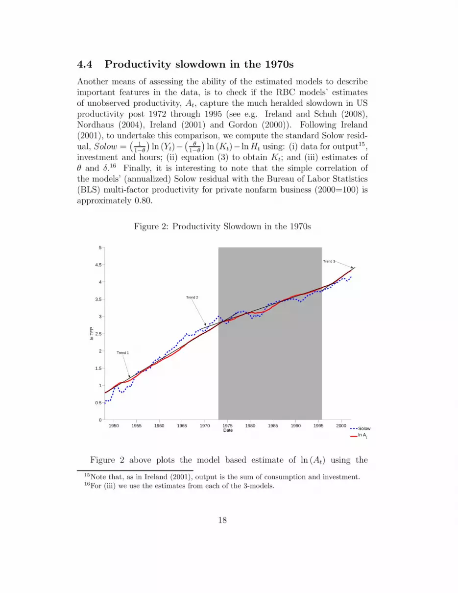
4.4 Productivity slowdown in the 1970s

Another means of assessing the ability of the estimated models to describeimportant features in the data, is to check if the RBC models’ estimatesof unobserved productivity, At, capture the much heralded slowdown in USproductivity post 1972 through 1995 (see e.g. Ireland and Schuh (2008),Nordhaus (2004), Ireland (2001) and Gordon (2000)). Following Ireland(2001), to undertake this comparison, we compute the standard Solow resid-ual, Solow =

(1

1−θ

)ln (Yt)−

(θ

1−θ

)ln (Kt)− ln Ht using: (i) data for output15,

investment and hours; (ii) equation (3) to obtain Kt; and (iii) estimates ofθ and δ.16 Finally, it is interesting to note that the simple correlation ofthe models’ (annualized) Solow residual with the Bureau of Labor Statistics(BLS) multi-factor productivity for private nonfarm business (2000=100) isapproximately 0.80.

Figure 2: Productivity Slowdown in the 1970s

1950 1955 1960 1965 1970 1975 1980 1985 1990 1995 20000

0.5

1

1.5

2

2.5

3

3.5

4

4.5

5

Date

ln T

FP

Solowln A

t

Trend 1

Trend 2

Trend 3

Figure 2 above plots the model based estimate of ln (At) using the

15Note that, as in Ireland (2001), output is the sum of consumption and investment.16For (iii) we use the estimates from each of the 3-models.

18

VARMA(1,1) model against the Solow residual.17 The gray shaded areacorresponds with the time period generally associated with the productivityslowdown between the early 1970s to the mid-1990s. In addition to theseplots we also draw three trend lines through the estimates of the hybridRBC model to show the extent to which the models predictions capture theproductivity slowdown. This figure shows that while the model is able toapproximately match the long swings in the Solow residual, its has a hardertime matching its cyclical variability. Thus, despite the model’s predictionsfor productivity being somewhat smoother than the Solow residual, the hy-brid RBC model does appear to do a reasonable job at picking up the trendchanges in TFP much documented in the productivity literature.18

5 Explanatory power of the RBC model

We next turn to an assessment of the RBC model’s ability to explain theobserved variation in the measured data. To this end, we first undertakeforecast error decompositions (FEDs) which allow us to split the contempo-raneous and the k-step-ahead forecast error variances of the measured vari-ables into the portions explained by shocks to technology and shocks to theerror system. The latter, as Ireland (2004, p. 1213) points out, “...pick upthe combined effects of shocks, including monetary and fiscal policy shocks,not present in the real business cycle model”. Thus, in the context of thehybrid setup, the RBC model faces a more difficult task since more shockshave been added to explain the variation in the measured data. In the lightof the objectives of this paper and the findings of the last section, we areespecially interested to discover the extent to which the RBC model’s pre-dictions, based on calibration and other estimation studies, are robust tothe inclusion of these new shocks. Finally we employ multivariate spectralmethods to further evaluate the explanatory power of the RBC model atalternative business cycle frequencies.19 Analogous to the FEDs, we will cal-culate the proportion of the variance of our measured data explained by thevariance of the technology shocks.

17Since the model based estimates of ln (At) are quite similar, we only present the modelwith VARMA(1,1) errors here.

18Also note that a similar picture emerges when the annualized model estimates arecompared with the BLS annual estimates of multifactor productivity.

19See Watson (1993) for a univariate spectral analysis of the cyclical properties of acalibrated stochastic RBC model.

19

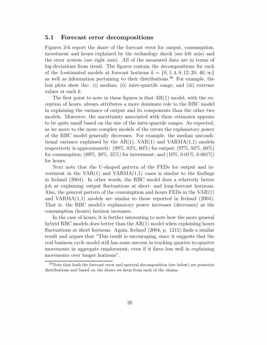
5.1 Forecast error decompositions

Figures 3-6 report the share of the forecast error for output, consumption,investment and hours explained by the technology shock (see left axis) andthe error system (see right axis). All of the measured data are in terms oflog-deviations from trend. The figures contain the decompositions for eachof the 3-estimated models at forecast horizons k = {0, 1, 4, 8, 12, 20, 40,∞}as well as information pertaining to their distributions.20 For example, thebox plots show the: (i) median; (ii) inter-quartile range; and (iii) extremevalues at each k.

The first point to note in these figures is that AR(1) model, with the ex-ception of hours, always attributes a more dominate role to the RBC modelin explaining the variance of output and its components than the other twomodels. Moreover, the uncertainty associated with these estimates appearsto be quite small based on the size of the inter-quartile ranges. As expected,as we move to the more complex models of the errors the explanatory powerof the RBC model generally decreases. For example, the median uncondi-tional variance explained by the AR(1), VAR(1) and VARMA(1,1) modelsrespectively is approximately: (99%, 82%, 60%) for output; (97%, 92%, 68%)for consumption; (89%, 38%, 35%) for investment; and (10%, 0.01%, 0.001%)for hours.

Next note that the U-shaped pattern of the FEDs for output and in-vestment in the VAR(1) and VARMA(1,1) cases is similar to the findingsin Ireland (2004). In other words, the RBC model does a relatively betterjob at explaining output fluctuations at short- and long-forecast horizons.Also, the general pattern of the consumption and hours FEDs in the VAR(1)and VARMA(1,1) models are similar to those reported in Ireland (2004).That is, the RBC model’s explanatory power increases (decreases) as theconsumption (hours) horizon increases.

In the case of hours, it is further interesting to note how the more generalhybrid RBC models does better than the AR(1) model when explaining hoursfluctuations at short horizons. Again, Ireland (2004, p. 1215) finds a similarresult and argues that “This result is encouraging, since it suggests that thereal business cycle model still has some success in tracking quarter-to-quartermovements in aggregate employment, even if it fares less well in explainingmovements over longer horizons”.

20Note that both the forecast error and spectral decomposition (see below) are posteriordistributions and based on the draws we keep from each of the chains.

20

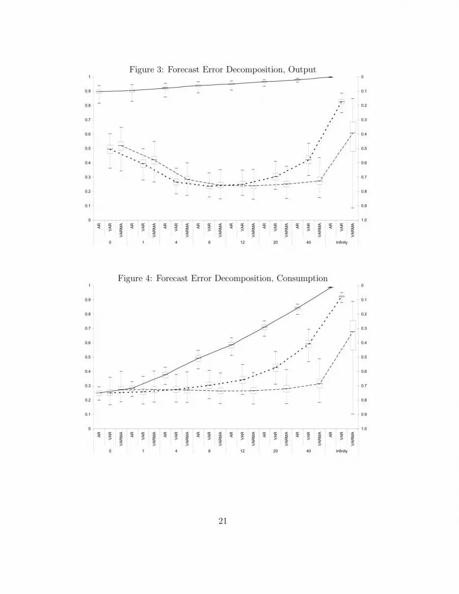
Figure 3: Forecast Error Decomposition, Output

0

0.1

0.2

0.3

0.4

0.5

0.6

0.7

0.8

0.9

1

AR

VAR

VARMA

AR

VAR

VARMA

AR

VAR

VARMA

AR

VAR

VARMA

AR

VAR

VARMA

AR

VAR

VARMA

AR

VAR

VARMA

AR

VAR

VARMA

0 1 4 8 12 20 40 Infinity

1.0

0.9

0.8

0.7

0.6

0.5

0.4

0.3

0.2

0.1

0

Figure 4: Forecast Error Decomposition, Consumption

0

0.1

0.2

0.3

0.4

0.5

0.6

0.7

0.8

0.9

1

AR

VAR

VARMA

AR

VAR

VARMA

AR

VAR

VARMA

AR

VAR

VARMA

AR

VAR

VARMA

AR

VAR

VARMA

AR

VAR

VARMA

AR

VAR

VARMA

0 1 4 8 12 20 40 Infinity

1.0

0.9

0.8

0.7

0.6

0.5

0.4

0.3

0.2

0.1

0

21

Figure 5: Forecast Error Decomposition, Investment

0

0.1

0.2

0.3

0.4

0.5

0.6

0.7

0.8

0.9

1

AR

VAR

VARMA

AR

VAR

VARMA

AR

VAR

VARMA

AR

VAR

VARMA

AR

VAR

VARMA

AR

VAR

VARMA

AR

VAR

VARMA

AR

VAR

VARMA

0 1 4 8 12 20 40 Infinity

1.0

0.9

0.8

0.7

0.6

0.5

0.4

0.3

0.2

0.1

0

Figure 6: Forecast Error Decomposition, Hours

0

0.1

0.2

0.3

0.4

0.5

0.6

0.7

0.8

0.9

1

AR

VAR

VARMA

AR

VAR

VARMA

AR

VAR

VARMA

AR

VAR

VARMA

AR

VAR

VARMA

AR

VAR

VARMA

AR

VAR

VARMA

AR

VAR

VARMA

0 1 4 8 12 20 40 Infinity

1.0

0.9

0.8

0.7

0.6

0.5

0.4

0.3

0.2

0.1

0

To place the size of the FEDs in context it is useful to take into ac-count that they are similar to R2s in simple regression analysis and that log-deviations data are employed when calculating them. In simple regression

22

analysis, using de-trended data, if the proportion of total variance explainedis roughly 40% or greater then, ceteris paribus, this would be considered areasonably good fit. Thus, it appears that the RBC model, even in the pres-ence of VARMA(1,1) errors is still capable of explaining a non-trivial shareof aggregate fluctuations. Moreover, given that the various distributions ofthe FEDs are generally quite concentrated, there appears to be much moreroom for optimism regarding the degree of uncertainty associated with theexplanatory power of the RBC model than is expressed by some authors citedin the introduction.

5.2 Spectral decompositions

To next compare the explanatory power of the three RBC models over differ-ent business cycle ranges, we use the means of the posterior parameter distri-butions and the state space representation to calculate the spectral densitymatrices. Because of the autoregressive structure, it is straightforward tocalculate the spectral density matrix for the transition equation system:21

αt = Tαt−1 + ζt, ζt ∼ N(0,Σ)

Fα(ω) =1

2πT(ω)−1ΣT (ω)−⋆ ; ω ∈ [−π, π].

where T(ω) is the Fourier transform of the matrix lag polynomial T(L) =

I − TL.22 Once the matrix Fα(ω) is calculated, the measurement equationcan be used to obtain the spectral density matrix for yt and αt, t = 1, . . . , T :

Fy,c,h,α(ω) = ZFα (ω) Z′; ω ∈ [−π, π]. (31)

Since the elements of the vector yt are output, consumption, and hours,the spectral density matrix containing also investment can be derived as

Fi,y,c,h,α(ω) =

(X 0

I

)Fy,c,h,α(ω)

(X 0

I

)′

; ω ∈ [−π, π],

where

X =

1 0 0y

ı− cı

00 1 00 0 1

.

21See e.g. Priestley (1981) and Hamilton (1994, Ch. 6) for a textbook treatment ofspectral analysis.

22L is the backshift operator; the superscript ‘⋆’ denotes the complex conjugate trans-pose.

23

The measure presented in Table 4 below is “explained variance”, derivedfrom squared coherency (sc). Squared coherency assesses the degree of linearrelationship between cyclical components of two series Xt and Yt , frequencyby frequency. It is defined as

sc(ω) =|fyx(ω)|2

fx(ω)fy(ω); 0 ≤ sc(ω) ≤ 1, (32)

where fx(ω) is the spectrum of the series Xt from the diagonal of the spectraldensity matrix F(ω), and fyx(ω) is the cross-spectrum for Yt and Xt, the rel-evant off-diagonal element of F(ω). Using this expression, we can decomposefy(ω) into and explained and an unexplained part. Integrating it over thefrequency band [−π, π] gives

∫ π

−π

fy(ω)dω

︸ ︷︷ ︸γy(0)

=

∫ π

−π

sc(ω)fy(ω)dω

︸ ︷︷ ︸“explained”variance

+

∫ π

−π

fu(ω)dω. (33)

The first term on the right in equation (33) is the product of squaredcoherency between Xt and Yt and the spectrum of Yt; and the second termis white noise. This equality holds for every frequency band [ω1, ω2]. Com-paring the area under the spectrum of the explained component to the areaunder Y ’s (i.e. output, consumption, investment and hours) spectrum in afrequency interval [ω1, ω2] yields a measure of the explanatory power of X(i.e. technology shocks), analogous to a partial R2 in the time domain.23

Table 4 contains the results of the spectral decompositions, i.e. the meansand standard deviations (in brackets) of the posterior distribution of the spec-tral measures. These measures are reported over the high and low frequencyranges (i.e. 2-quarters to 3-years and 10 to infinity years respectively) andthe classical business cycle ranges (i.e. 3-5, 5–7 and 7-10 years).24

23See A’Hearn and Woitek (2001) for a detailed discussion.24Note that the results of a univariate spectral analysis are consistent with the findings

of Watson (2003). In particular, we find that the RBC model, irrespective of the errormodel employed, does a very good job at matching the low frequency movements in thedata for output and its components. For high frequency movements, the model spectrafor output provide the relatively best match to the data spectra. In contrast, the modelspectra are significantly different from the data spectra for the traditional business cycleranges for all measured variables (i.e. y, c, i, h). Further details relating to the univariateresults are available upon request from the authors.

24

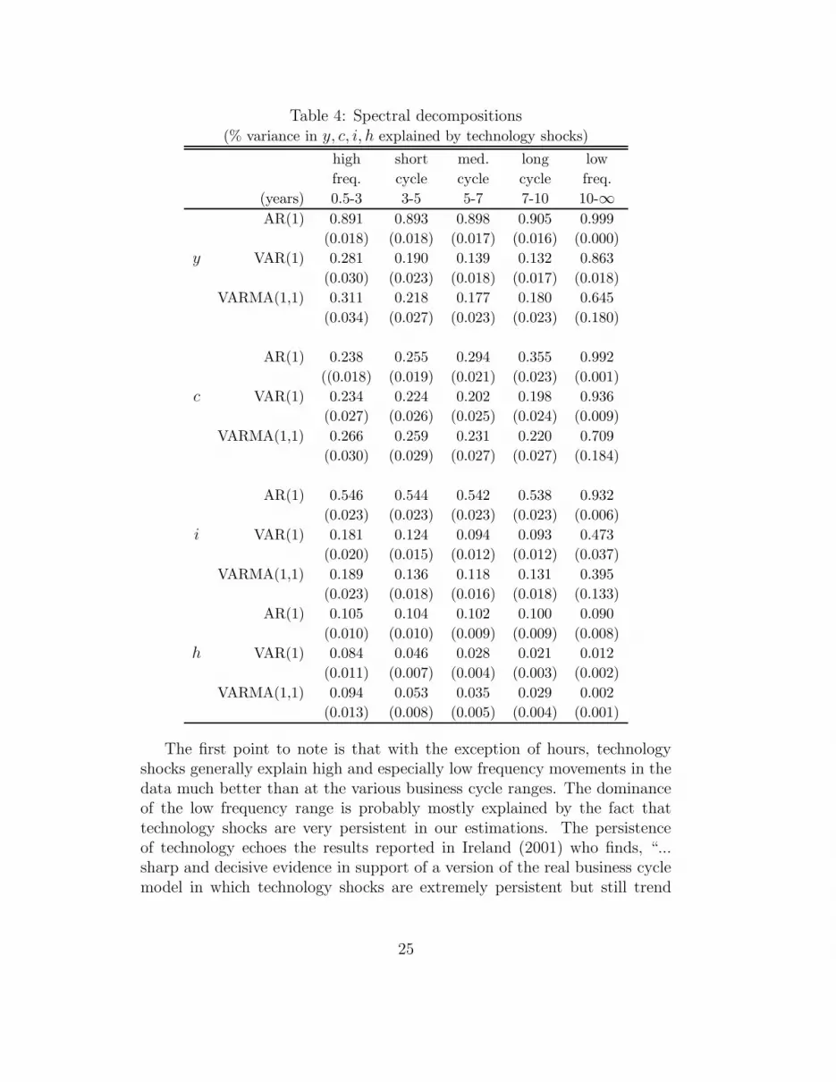
Table 4: Spectral decompositions(% variance in y, c, i, h explained by technology shocks)

high short med. long low

freq. cycle cycle cycle freq.

(years) 0.5-3 3-5 5-7 7-10 10-∞AR(1) 0.891 0.893 0.898 0.905 0.999

(0.018) (0.018) (0.017) (0.016) (0.000)

y VAR(1) 0.281 0.190 0.139 0.132 0.863

(0.030) (0.023) (0.018) (0.017) (0.018)

VARMA(1,1) 0.311 0.218 0.177 0.180 0.645

(0.034) (0.027) (0.023) (0.023) (0.180)

AR(1) 0.238 0.255 0.294 0.355 0.992

((0.018) (0.019) (0.021) (0.023) (0.001)

c VAR(1) 0.234 0.224 0.202 0.198 0.936

(0.027) (0.026) (0.025) (0.024) (0.009)

VARMA(1,1) 0.266 0.259 0.231 0.220 0.709

(0.030) (0.029) (0.027) (0.027) (0.184)

AR(1) 0.546 0.544 0.542 0.538 0.932

(0.023) (0.023) (0.023) (0.023) (0.006)

i VAR(1) 0.181 0.124 0.094 0.093 0.473

(0.020) (0.015) (0.012) (0.012) (0.037)

VARMA(1,1) 0.189 0.136 0.118 0.131 0.395

(0.023) (0.018) (0.016) (0.018) (0.133)

AR(1) 0.105 0.104 0.102 0.100 0.090

(0.010) (0.010) (0.009) (0.009) (0.008)

h VAR(1) 0.084 0.046 0.028 0.021 0.012

(0.011) (0.007) (0.004) (0.003) (0.002)

VARMA(1,1) 0.094 0.053 0.035 0.029 0.002

(0.013) (0.008) (0.005) (0.004) (0.001)

The first point to note is that with the exception of hours, technologyshocks generally explain high and especially low frequency movements in thedata much better than at the various business cycle ranges. The dominanceof the low frequency range is probably mostly explained by the fact thattechnology shocks are very persistent in our estimations. The persistenceof technology echoes the results reported in Ireland (2001) who finds, “...sharp and decisive evidence in support of a version of the real business cyclemodel in which technology shocks are extremely persistent but still trend

25

stationary” (Ireland 2001, p.705).25 In this context, based on evidence fromforecast error decompositions, he also draws attention to the fact that “...anincrease in the persistence of technology shocks helps the model to explainthe behavior of output and consumption even as it hurts the model’s abilityto explain the behavior of investment and hours worked” (Ireland, 2001, p.718). This rank ordering also appears to generally hold for the spectral resultsreported in Table 4, especially for the VAR(1) and VARMA(1,1) models.

Complimentary to our forecast error decomposition results, the findings inTable 4 also suggest that adding more complicated error structures generallyweakens the explanatory power of the RBC model. This holds uniformly aswe move from the AR(1) to the VAR(1)/VARMA(1,1) specifications. In con-trast, as we move from the VAR(1) to the VARMA(1,1), explanatory powerappears to increase again. But based on the size of the standard deviationsreported in Table 4, the posterior distributions overlap considerably.

6 Parameter stability

Given the evidence of multimodal posterior parameter distributions raisedin section 4, suggesting parameter instability, we next examine this issuefurther for the VARMA(1,1) specification. To place this topic in context,Ireland (2004 p. 1216) states, “Across the board, the tests reject the nullhypothesis of parameter stability. Evidently, important changes have takenplace in the postwar US economy that neither the real business cycle modelnor the hybrid model’s residuals can fully account for. These test results echoand extend the previous findings from Stock and Watson (1996), who recordevidence of widespread instability in parameters in VAR models estimatedwith postwar US data.”

To test for parameter stability, we adopt the 1980 breakpoint used inIreland (2004) and in each step of the estimation algorithm, draw two re-alisations of the parameter vector. The first one is active in the period1948:1-1979:4 and the second one in the period 1980:1-2002:2. These twoparameter vectors allow for structural breaks in both the economic and mea-surement/specification error blocks of the model. The likelihood is based onthe entire period, and the prior for the parameter vector is calculated from

25Its worth pointing out that using the estimation methods employed here we found thatthe data supported the highly persistent trend stationary to difference stationary specifi-cation of productivity. Strictly speaking, the data preferred trend stationary productivityin the Hansen model to the alternative which included difference stationary productivityand production re-specified as Yt = Kθ

t (AtHt)1−θ

(see Appendix). For further details onwhy permanent changes in productivity must be modelled in labour augmenting form, seeKing et al. (1988 pp. 199-200) and additional references therein.

26

the priors of the two realisations. The results of applying the logmarginallikelihood difference test to the split-sample relative to the full-sample modelyields a value of 735.99 indicating a far better fit for the fomer. In otherwords the data strongly prefer two sets of parameter estimates to one indi-cating, as others have found, that there has indeed been structural changethroughout this period.

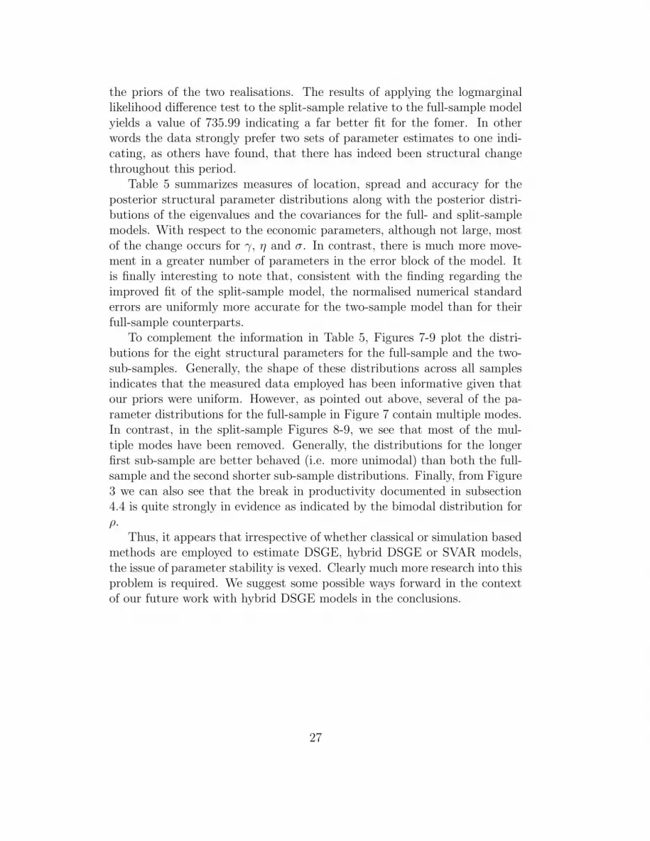
Table 5 summarizes measures of location, spread and accuracy for theposterior structural parameter distributions along with the posterior distri-butions of the eigenvalues and the covariances for the full- and split-samplemodels. With respect to the economic parameters, although not large, mostof the change occurs for γ, η and σ. In contrast, there is much more move-ment in a greater number of parameters in the error block of the model. Itis finally interesting to note that, consistent with the finding regarding theimproved fit of the split-sample model, the normalised numerical standarderrors are uniformly more accurate for the two-sample model than for theirfull-sample counterparts.

To complement the information in Table 5, Figures 7-9 plot the distri-butions for the eight structural parameters for the full-sample and the two-sub-samples. Generally, the shape of these distributions across all samplesindicates that the measured data employed has been informative given thatour priors were uniform. However, as pointed out above, several of the pa-rameter distributions for the full-sample in Figure 7 contain multiple modes.In contrast, in the split-sample Figures 8-9, we see that most of the mul-tiple modes have been removed. Generally, the distributions for the longerfirst sub-sample are better behaved (i.e. more unimodal) than both the full-sample and the second shorter sub-sample distributions. Finally, from Figure3 we can also see that the break in productivity documented in subsection4.4 is quite strongly in evidence as indicated by the bimodal distribution forρ.

Thus, it appears that irrespective of whether classical or simulation basedmethods are employed to estimate DSGE, hybrid DSGE or SVAR models,the issue of parameter stability is vexed. Clearly much more research into thisproblem is required. We suggest some possible ways forward in the contextof our future work with hybrid DSGE models in the conclusions.

27

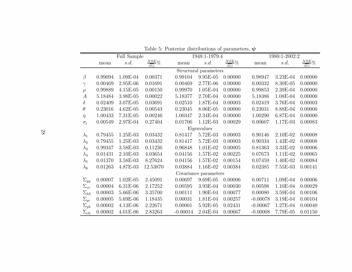
Table 5: Posterior distributions of parameters, ψ

Full Sample 1948:1-1979:4 1980:1-2002:2mean s.d. NSE

|ψi|% mean s.d. NSE

|ψi|% mean s.d. NSE

|ψi|%

Structural parameters

β 0.99094 1.09E-04 0.00371 0.99104 9.95E-05 0.00000 0.98947 3.23E-04 0.00000γ 0.00469 2.95E-06 0.01691 0.00469 2.77E-06 0.00000 0.00332 8.30E-05 0.00000ρ 0.99889 4.15E-05 0.00150 0.99970 1.05E-04 0.00000 0.99853 2.39E-04 0.00000A 5.18484 3.98E-05 0.00022 5.18377 2.70E-04 0.00000 5.18386 1.08E-04 0.00000δ 0.02409 3.07E-05 0.03691 0.02510 1.87E-04 0.00003 0.02419 3.76E-04 0.00003θ 0.23016 4.62E-05 0.00543 0.23045 8.06E-05 0.00000 0.23031 8.88E-04 0.00000η 1.00433 7.31E-05 0.00246 1.00347 2.34E-04 0.00000 1.00290 6.87E-04 0.00000σǫ 0.00549 2.97E-04 0.27404 0.01706 1.12E-03 0.00029 0.00607 1.17E-03 0.00083

Eigenvalues

λ1 0.79455 1.25E-03 0.03432 0.81417 5.72E-03 0.00003 0.90146 2.10E-02 0.00008λ2 0.79455 1.25E-03 0.03432 0.81417 5.72E-03 0.00003 0.90334 1.43E-02 0.00008λ3 0.99347 3.58E-03 0.11236 0.96848 1.01E-02 0.00005 0.81363 3.33E-02 0.00006λ4 0.01431 2.10E-03 4.03654 0.04156 1.57E-02 0.00225 0.07673 1.11E-02 0.00065λ5 0.01370 3.58E-03 8.27624 0.04156 1.57E-02 0.00154 0.07459 1.40E-02 0.00084λ6 0.01263 4.87E-03 12.53870 0.03884 1.16E-02 0.00384 0.02385 7.55E-03 0.00141

Covariance parameters

Σyy 0.00007 1.02E-05 2.45091 0.00697 9.69E-05 0.00006 0.00711 1.09E-04 0.00006Σcc 0.00004 6.31E-06 2.17252 0.00595 3.93E-04 0.00030 0.00598 1.10E-04 0.00029Σhh 0.00003 5.66E-06 3.35700 0.00111 1.90E-04 0.00077 0.00080 3.59E-04 0.00106Σyc 0.00005 5.69E-06 1.18435 0.00031 1.81E-04 0.00257 -0.00078 3.19E-04 0.00104Σyh 0.00002 4.13E-06 2.22671 0.00001 5.92E-05 0.02431 -0.00067 1.27E-04 0.00040Σch 0.00002 4.01E-06 2.83263 -0.00014 2.04E-04 0.00667 -0.00008 7.79E-05 0.01150

28

Figure 7: Posterior Distributions (Structural Parameters), Full Sample

0.971 0.972 0.973 0.974 0.9750

500

1000β

Parameter Value

PD

F

4.44 4.46 4.48 4.5

x 10−3

0

5

10x 10

4 γ

Parameter Value

PD

F

0.99 0.995 10

100

200

300

400ρ

Parameter Value

PD

F

5.15 5.155 5.16 5.1650

50

100

150

200A

Parameter Value

PD

F

0.046 0.048 0.05 0.0520

500

1000

1500

2000δ

Parameter Value

PD

F

0.266 0.268 0.27 0.272 0.2740

500

1000θ

Parameter Value

PD

F

1.004 1.005 1.006 1.0070

500

1000

1500

2000η

Parameter Value

PD

F

1 2 3 4

x 10−5

0

0.5

1

1.5

2x 10

5 σε

Parameter Value

PD

F

29

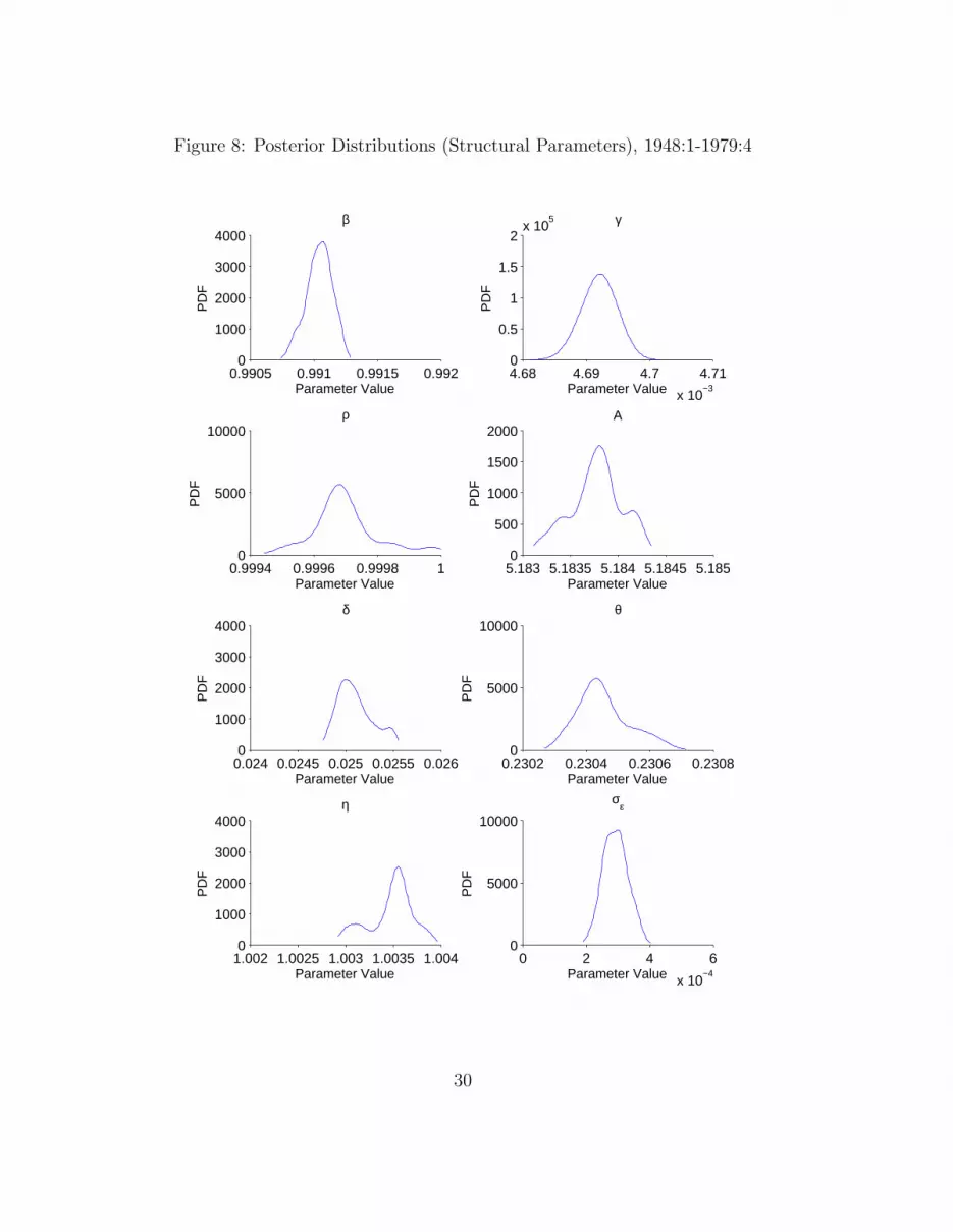
Figure 8: Posterior Distributions (Structural Parameters), 1948:1-1979:4

0.9905 0.991 0.9915 0.9920

1000

2000

3000

4000β

Parameter Value

PD

F

4.68 4.69 4.7 4.71

x 10−3

0

0.5

1

1.5

2x 10

5 γ

Parameter Value

PD

F

0.9994 0.9996 0.9998 10

5000

10000ρ

Parameter Value

PD

F

5.183 5.1835 5.184 5.1845 5.1850

500

1000

1500

2000A

Parameter Value

PD

F

0.024 0.0245 0.025 0.0255 0.0260

1000

2000

3000

4000δ

Parameter Value

PD

F

0.2302 0.2304 0.2306 0.23080

5000

10000θ

Parameter Value

PD

F

1.002 1.0025 1.003 1.0035 1.0040

1000

2000

3000

4000η

Parameter Value

PD

F

0 2 4 6

x 10−4

0

5000

10000

σε

Parameter Value

PD

F

30

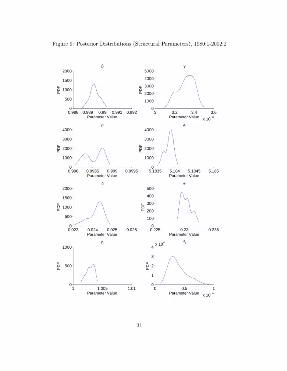
Figure 9: Posterior Distributions (Structural Parameters), 1980:1-2002:2

0.988 0.989 0.99 0.991 0.9920

500

1000

1500

2000β

Parameter Value

PD

F

3 3.2 3.4 3.6

x 10−3

0

1000

2000

3000

4000

5000γ

Parameter Value

PD

F

0.998 0.9985 0.999 0.99950

1000

2000

3000

4000ρ

Parameter Value

PD

F

5.1835 5.184 5.1845 5.1850

1000

2000

3000

4000A

Parameter Value

PD

F

0.023 0.024 0.025 0.0260

500

1000

1500

2000δ

Parameter Value

PD

F

0.225 0.23 0.2350

100

200

300

400

500θ

Parameter Value

PD

F

1 1.005 1.010

500

1000η

Parameter Value

PD

F

0 0.5 1

x 10−4

0

1

2

3

4x 10

4 σε

Parameter Value

PD

F

31

7 Conclusions and Future Work

This paper has attempted to contribute to the on-going empirical debateregarding the role of the RBC model and in particular of technology shocksin explaining aggregate fluctuations. To this end we have extended Ireland’s(2001, 2004) hybrid estimation approach to allow for a VARMA(1,1) pro-cess to describe the movements and co-movements of the model’s errors notexplained by the basic RBC model.

Our main findings are: (i) the VARMA(1,1) specification of the errorssignificantly improves the basic RBC model’s fit to the historical data relativeto the VAR(1) and AR(1) alternatives; (ii) despite setting the RBC model amore difficult task under the VARMA(1,1) specification, technological shocksare still capable of explaining a significant share of the observed variation inoutput and its components over shorter- and longer-forecast horizons as wellas hours at shorter horizons; (iii) the RBC model generally does a relativelybetter job at matching low and high frequency cyclical movements in thedata than at the traditional business cycles ranges; and (iv) the degree ofuncertainty associated with the explanatory power of the RBC model muchdiscussed in the literature is perhaps overstated since we find that estimatedposterior distributions for the forecast error and spectral decompositions tobe quite concentrated.

In future research we plan to further examine the issue of structuralstability in a split sample setting but also in the context of time-varyingparameters. We would argue that the former is more appropriate for themodel’s structural parameters, unless of course non-constant structural pa-rameters are part of the theoretical model. On the other hand, varyingparameters might usefully be employed to pick up structural change in thea-theoretical VAR(MA) block of the model. Recent successful examples us-ing time-varying parameters in a VAR context include the research of Cogleyand Sargent (2005) and Primiceri (2005). Another possible extension wouldbe to modify the basic RBC model to allow for endogenous growth in hu-man capital but still retaining the exogenous process driving productivity inthe goods sector. In addition, if an analogous exogenous process is addedto the human capital production function, then the relative contributions ofthe competing productivity processes to explaining the observed variationin macroeconomic aggregates could be quantitatively assessed. Given thatour conclusions regarding the usefulness of the basic RBC model are moreoptimistic than many in the literature, we think these are issues well worthexploring.

32

8 Appendix

Equations (34)− (36) contain the stationary decentralised competitive equi-librium, exogenous process for technology and the steady-state respec-tively required to re-estimate the RBC model assuming permanent technicalchange:26

gyt syt =

(skt

)θ(satht)

1−θ

1 =(rct + rit

)

skt+1 =(1 − δ)skt

sat+ rits

yt+1 (34)

γrctht = (1 − θ)

1

rct= βEt

{θsyt+1

rct+1skt+1

+1 − δ

gyt+1rct+1

}

Etsyt+1 =

syt gyt

sat

sat = ηeεt ; (35)

gy = η

ri =βθ (η − 1 + δ)

η − β (1 − δ)

rc = 1 −βθ (η − 1 + δ)

η − β (1 − δ)

h =(1 − θ)

γ[1 − βθ(η−1+δ)

η−β(1−δ)

] (36)

sy =

(ηβθ

η − β (1 − δ)

) θ1−θ

h (η)θ

θ−1

sk =

(ηβθ

η − β (1 − δ)

) 1

1−θ

h (η)θ

θ−1

where syt = Yt−1

At−1, gyt = Yt

Yt−1, rct = Ct

Yt, rit = It

Yt, ht ≡ Ht ≡, skt = Kt

At−1, and

sat = At

At−1. Analogous to our calculations in section 2, to prepare the model for

estimation, we log-linearise (34) and (35) around (36) and solve the resultingsystem for the model’s policy functions in state-space form.

26Note that the non-stationary equilibrium conditions are the same as reported in Ireland(2004, p. 1208) except the alternative production function set out in footnote 25 is usedhere.

33

References

[1] A’Hearn, B. and U. Woitek. (2001). More international evidence on thehistorical properties of business cycles, Journal of Monetary Economics,47, 321-346.

[2] Altug, S. (1989). Time-to-build and aggregate fluctuations: some newevidence, International Economic Review, 30, 889-920.

[3] Bencivenga, V. (1992). An econometric study of hours and output vari-ation with preference shocks, International Economic Review, 33, 449-471.

[4] Bouakez, H., Cardia, E. and F. Ruge-Murcia (2005). Habit formationand the persistence of monetary shocks, Journal of Monetary Economics,52, 1073-1088.

[5] Chari, V., Kehoe, P. and E. McGrattan (2007a). Are structural VARswith long-run restrictions useful in developing business cycle theory?Federal Reserve Bank of Minneapolis, Research Department Staff Re-port 364.

[6] Chari, V., Kehoe, P. and E. McGrattan (2007b). Business cycle account-ing, Econometrica, 75, 781-836.

[7] Chib, S. and I. Jeliazkov (2001). Marginal likelihood from theMetropolis-Hastings output, Journal of the American Statistical Asso-ciation, 96, 270-281.

[8] Chib, S. and Greenberg, E. (1995). Understanding the Metropolis-Hastings algorithm, American Statistician, 49, 327-335.

[9] Christiano, L., Eichenbaum, M. and R. Vigfusson (2003). What happensafter a technology shock? NBER Working Paper, 9819.

[10] Christiano, L. (1988). Why does inventory investment fluctuate somuch? Journal of Monetary Economics, 21, 247-280.

[11] Cogley, T. and T. Sargent (2005). Drifts and Volatilities: MonetaryPolicies and Outcomes in the Post WWII US, Review of Economic,Dynamics, 8, 262-302.

[12] Cogley, T. and Nason, J. (1995). Output dynamics in real-business-cyclemodels, American Economic Review, 85, 492-511.

34

[13] DeJong, D., Ingram, B. and C. Whiteman (2000a). Keynesian impulsesversus Solow residuals: identifying sources of business cycle fluctuations,Journal of Applied Econometrics, 15, 311–329.

[14] DeJong, D., Ingram, B. and C. Whiteman (2000b). A Bayesian approachto dynamic macroeconomics, Journal of Econometrics, 98, 203-223.

[15] Eichenbaum, M. (1991). Real business-cycle theory: wisdom or whimsy?Journal of Economic Dynamics and Control, 15, 607-626.

[16] Fernandez-Villaverde, J. and J. Rubio-Ramırez (2004), Comparing dy-namic equilibrium models to data: a Bayesian approach, Journal ofEconometrics, 123, 153–187.

[17] Fernandez-Villaverde, J. and J. Rubio-Ramırez (2005), Estimating dy-namic equilibrium economies: linear versus nonlinear likelihood, Journalof Applied Econometrics, 20, 891-910.

[18] Francis, N. and V. Ramey (2005). Is the technology-driven real busi-ness cycle hypothesis dead? Shocks and aggregate fluctuations revisited,Journal of Monetary Economics, 52, 1379-1399.

[19] Galı, G. (1999). Technology, employment, and the business cycle: dotechnology shocks explain aggregate fluctuations?, American EconomicReview, 89, 249-271.

[20] Galı, J. and P. Rabanal (2005). Technology shocks and aggregate fluc-tuations: how well does the RBC model fit postwar U.S. data? NBERMacroeconomics Annual 2004, (ed) M. Gertler and K. Rogoff, 225-88,Cambridge, Mass.: MIT Press.

[21] Gelman, A., Roberts, G., and W. Gilks (1996). Efficient Metropolisjumping rules. In: Berger, J.O., Bernado, J.M., David, A.P., Smith,A.F.M. (Eds.), Bayesian Statistics, Vol. 5. Oxford University Press, Ox-ford, pp. 599–607.

[22] Geweke (1992). Evaluating the accuracy of sampling-based approachesto the calculation of posterior moments. In: Bernardo, J.M., Berger,J.O., Dawid, A.P., Smith, A.F.M. (Eds.), Bayesian Statistics, Vol. 4.Oxford University Press, Oxford, 169–193 (with discussion).

[23] Gordon, R. (2000). Interpreting the “one big wave” in U.S. long-termproductivity growth, NBER Working Paper 7752, Cambridge, MA.

35

[24] Greenberg, E. (2008). Introduction to Bayesian Econometrics, Cam-bridge University Press, New York.

[25] Hall, G. (1996). Overtime effort, and the propagation of business cycleshocks, Journal of Monetary Economics, 38, 139-160.

[26] Hamilton (1994). Time Series Analysis, Princeton University Press,Princeton, New Jersey.

[27] Hansen, G. (1985). Indivisible labor and the business cycle. Journal ofMonetary Economics 16, 309-327.

[28] Harvey, A. (1992). Forecasting, Structural Time Series Models and theKalman Filter, Cambridge University Press.

[29] Ireland, P. (1997). A small structural, quarterly model for monetary pol-icy evaluation. Carnegie-Rochester Conference Series on Public Policy,47,83-108.

[30] Ireland, P. (2001a). Money’s role in the monetary business cycle, NBERWorking Paper 8115, Mass.

[31] Ireland, P. (2001b). Sticky-price models of the business cycle: specifica-tion and stability, Journal of Monetary Economics, 47, 3-18.

[32] Ireland, P. (2001c). Technology shocks and the business cycle: an em-pirical investigation, Journal of Economic Dynamics and Control, 25,703-719.

[33] Ireland, P. (2002). Endogenous money or sticky prices? NBER WorkingPaper 9390, Cambridge, Mass.

[34] Ireland, P. (2004). A method for taking models to the data, Journal ofEconomic Dynamics and Control, 24, 1205-1226.

[35] Ireland, P. (2008). Productivity and US macroeconomic performance:Interpreting the past and predicting the future with a two-sector realbusiness cycle model, Review of Economic Dynamics, 11, 473-92.

[36] Kim, J. (2000). Constructing and estimating a realistic optimizing modelof monetary policy, Journal of Monetary Economics, 45, 329-359.

[37] King, R., Plosser, C., and S. Rebelo (1988). Production, growth andbusiness cycles: I. the basic neoclassical model model, Journal of Mon-etary Economics, 21, 195-232.

36

[38] Lutkepohl, H. (1991). Introduction to Multiple Time Series Analysis,Springer.

[39] McGrattan, E. (1994). The macroeconomic effects of distortionary tax-ation, Journal of Monetary Economics, 33, 573-601.

[40] McGrattan, E., Rogerson, R. and R. Wright (1997). An equilibriummodel of the business cycle with household production and fiscal policy,International Economic Review, 38, 267-290.

[41] Nordhaus, W. (2004). Retrospective on the 1970s productivity slow-down, NBER Working Paper 10950.

[42] Priestley, M. (1981). Spectral Analysis and Time Series. Academic Press,London.

[43] Primiceri, G. (2005). Time varying structural vector autoregressions andmonetary policy, The Review of Economic Studies, 72, 821–852.

[44] Ruge-Murcia, F. (2007). Methods to estimate dynamic stochastic gen-eral equilibrium models, Journal of Economic Dynamics and Control,31, 2599-2636.

[45] Sargent, T. (1989). Two models of measurements and the investmentaccelerator, Journal of Political Economy, 97, 251-287.

[46] Schorfheide, F. (2000). Loss function-based evaluation of DSGE models,Journal of Applied Econometrics, 15, 645-670.

[47] Sims, C. (1989). Models and their uses, American Journal of AgriculturalEconomics, 71, 489-494.

[48] Smets, F. and R. Wouters (2003). An estimated stochastic dynamicgeneral equilibrium model for the euro area, Journal of the EuropeanEconomic Association, 1, 1123-1175.

[49] Stock, J. and M. Watston (1996). Evidence on structural instability inmacroeconomic time series relations, Journal of Business and EconomicStatistics, 14, 11-30.

[50] Watson, M. (1993). Measures of fit for calibrated models, Journal ofPolitical Economy, 101, 1011-41.

37