Growth and Shocks: evidence from ruralEthiopia

Stefan DerconCSAE, Department of Economics and Jesus College, Oxford

Stefan.Dercon@economics.ox.ac.uk

November 2, 2003

Abstract

Using panel data from villages in rural Ethiopia, the paper studies thedeterminants of consumption growth (1989-97), based on a microgrowthmodel, controlling for heterogeneity. Consumption grew substantially, butwith diverse experiences across villages and individuals. A key focus is onwhether shocks affect growth. Rainfall shocks have a substantial impacton consumption growth, and its impact presists for many years. Therealso appears to be a significant, persistent growth impact from the large-scale famine in the 1980s, as well as substantial externalities from thepresence of road infrastructure. The findings related to the persistenteffects of rainfall shocks and the famine crisis imply that welfare lossesdue to the lack of insurance and protection measures are well beyond thewelfare cost of short term consumption fluctuations.

JEL Classification: I32, O12, Q12Paper prepared for a conference at the International Monetary Fund,

May 2002. I am grateful for useful comments from Jan Willem Gun-ning, Cathy Pattillo, Martin Ravallion and seminar participants at Ox-ford, WIDER/UNU and the World Bank. All errors are mine.

1 IntroductionThe study of the poor people’s impediments to escape poverty remains at thecore of development economics. This paper discusses the determinants of growthin living standards in a number of rural communities in Ethiopia between 1989and 1997. The focus is on the role of shocks, such as drought and famine, onpoverty persistence, as well as on identifying the correlates of welfare improve-ments.Inspired by the standard growth literature, the paper uses household panel

data covering 1989 to 1997 and six villages across the country to study ruralconsumption growth in this period using a linearised empirical growth model.The focus is on the impact of shocks, and more specifically on persistent effects

1

of rainfall shocks on growth. The results suggest that idiosyncratic and com-mon shocks had substantial contemporaneous impact. Especially better rainfallcontributed to the observed growth. We also test for persistence of the effects ofpast shocks. We find that there is evidence of some persistence - lagged rainfallshocks matter for current growth. Furthermore, indicators of the severity ofthe famine in 1984-85 are significant to explain growth in the 1990s, furthersuggesting persistence. Finally, road infrastructure is a source of divergence ingrowth experience across households and communities.The study of growth in developing countries using micro-level household

data is not common, largely because suitable panel data sets are missing toembark on such work. Deininger and Okidi [2003] and Gunning et al. [2000]look into the determinants of growth in Ugandan and Zimbabwean panel data.As part of a number of papers using data from rural China, Ravallion and Jalan[1996] use a framework inspired by both the Solow model and the endogenousgrowth literature to investigate sources of divergence and convergence betweenregions. In further work using the household level data from their panel (e.g.Jalan and Ravalllion [1997, 1998, 2002]), divergence due to spatial factors isexplicitly tested for and discovered, suggesting spatial poverty traps. This paperdraws inspiration from their approach by explicitly disentangling communityand individual effects. It goes beyond their approach by focusing explicitly onthe impact of uninsured risk on household outcomes.It is well documented that households and individuals in developing countries

use different strategies to cope with risk, including self-insurance via savings,informal insurance mechanisms or income portfolio adjustments towards loweroverall risk in their activities. Literature surveys suggest that these mechanismstypically only succeed in partial insurance (Morduch [1995], Townsend [1995]).Given that households are generally ’fluctuation averse’, the resulting fluctua-tions in consumption and other welfare outcomes imply a loss of welfare due touninsured risk. However, beyond this transient impact on welfare, there mayalso be a ’chronic’ impact from uninsured risk, i.e. persistent or even permanenteffects on levels and growth rates of income linked to uninsured risk. In partic-ular, one can distinguish two effects. First, an ex-ante or behavioural impact:uninsured risk implies that it is optimal to avoid profitable but risky opportu-nities. Households may diversify, enter into low risk but low return activitiesor invest in low risk assets, all at the expense of mean returns. Second, an ex-post impact, after a ’bad’ state has materialised: the lack of insurance againstsuch a shock implies that human, physical or social capital may be lost reduc-ing access to profitable opportunities. In short, uninsured risk may be a causeof poverty. Several theoretical models of poverty traps and persistence havebeen developed whereby temporary events affect long-term outcomes (Banerjeeand Newman [1993], Acemoglu and Zilibotti [1997]). A number of empiricalstudies [e.g. Rosenzweig and Binswanger [1993], Rosenzweig and Wolpin [1993],Morduch[1995]) find evidence consistent with permanent effects linked to risk.There is also evidence from studies focusing on health and educational outcomesconsistent with permanent impacts of shocks such as drought (Alderman et al.[2001], Hoddinott and Kinsey [2001]). A few recent studies investigate the im-

2

pact of risk on growth using household data. Jalan and Ravallion [2002a] andLokshin and Ravallion [2001] test the idea of shock-induced poverty trap, bytesting for whether the transition dynamics after a shock are convex; they donot find evidence of a transition to a low-outcome equilibrium but the recoveryafter a shock in income is nevertheless slow. Elbers et al.[2003], using data fromZimbabwe, calibrate and simulate a household optimal growth model allowingfor both ex-ante and ex-post responses to risk, allowing them to quantify thelosses linked to uninsured risk, which proved substantial in their data set.This paper uses a reduced-form econometric approach to test for the impact

of uninsured risk. Measured recent and past shocks are directly introduced inthe regressions, and their cumulative impact is quantified. This is similar tothe study of persistence in macroeconomic series. Campbell and Mankiw [1987]investigate persistence in the log of GNP, i.e. whether shocks continue to havean effect ’for a long time into the future’. Formally, they estimate the growthin GNP as stationary autoregressive moving average process. Their persistencemeasure is based on cumulative impact of past shocks on the level of GNP. Thisis not the same as testing for the existence of a ’poverty trap’ in the sense of theinvestigation of the threshold, below which there is a tendency to be trapped inpermanently low income, from which no escape is possible except for by largepositive shocks. Persistence within the time period of the data does not excludepermanent effects, but does not imply them either.Ethiopia is an obvious setting to study the impact of uninsured risk. About

85 percent of the population lives in rural areas and virtually all rural house-holds are dependent on rainfed agriculture as the basis for their livelihoods.Drought are recurrent events, while high incidence of pests, as well as animaland human disease affect their livelihoods as well. Insurance and asset marketsare functioning relatively poorly, while safety nets, even though present andwidespread, are not able to credibly guarantee support when needed (Jayne etal. [2002], Dercon and Krishnan [2003]). The data set used is relatively small -only 342 households with complete information for the core parts of the analy-sis. It implies that some care will have to be taken to interpret the findings; thepaper may however give insights and suggestions on how to study these issues inother contexts and on larger data sets. Furthermore, the information availableis relatively comprehensive: there are data on events, shocks and experiencesover the survey period as well data collected using longer-term recall - includingon experiences during the (by far largest recent) famine in the mid-1980s.The sample is not a random sample of rural communities in Ethiopia, but

they were initially selected since they had suffered from the drought in themid-1980s, which had developed into a large scale famine due to the civil warand other political factors. During the 1990s, growth rates in GDP picked upconsiderably, with GDP per capita growing by about 14 percent between 1990and 1997 (the study period). While the economic reform taking place in thisperiod is likely to have been a necessary condition for this growth experience,it begs the question whether these growth rates should not be largely viewedas recoveries from earlier shocks. Indeed, it took until about 1996 for GDP percapita to surpass levels reached in the early 1980s, before the war, famine and

3

repressive politics plunged Ethiopia into the crisis of the late 1980s. Further-more, growth rates fluctuated considerably as well in the 1990s. In the surveyvillages, the issue of recovery and weather induced growth may even be moreimportant. Consumption growth was well beyond national levels in the 1990s,implying impressive poverty reductions (Dercon and Krishnan [2002]). How-ever, since the villages were chosen because the famine had strong effects, thequestion of recovery and differential effects across households and villages dur-ing this recovery becomes crucial to understanding of the long-term impact ofthis type of crisis..In the next section, I present the theoretical and empirical framework used.

It is based on the standard ’informal’ empirical growth model, drawing inspi-ration from both Mankiw et al. [1992] and endogenous growth theory, e.g.Romer [1986], and introduce into this framework our approach to the study ofpersistence. A number of testable hypotheses are derived. In section 3, thecontext and data are presented. In section 4, the econometric specifications arediscussed and the estimates are presented are presented in section 5. Section 6concludes.

2 Theoretical and empirical frameworkThe framework used is a standard empirical growth model, allowing for tran-sitional dynamics, inspired by Mankiw et al. [1992]. In this model, growthrates are negatively related to initial levels of income, as well as related to anumber of variables determining initial efficiency and the steady state, includinginvestment rates in human and physical capital. In the context of panel dataon per worker incomes of N households i (i = 1, ...N) across periods t, yit, thisempirical model can be written as (see e.g. Islam [1995]):

ln yit − ln yit−1 = α+ β ln yit−1 + δZit + γXi + uit (1)

in which Zit are time-varying and Xi fixed characteristics of the household,for example determining savings rates or investment in human capital, while αis a common source of growth across households, and uit is a transitory errorterm with mean zero. There are numerous reasons why one should be carefulin applying this framework to any context, given the theoretical and empiricalassumptions implied by this model (for example, see the reviews by Temple[1999] or Durlauf and Quah [1998]). Still, one could use this framework as astarting point. A standard question is whether there is conditional convergencein the household data: a negative estimate for β would suggest convergence,allowing for underlying differences in the steady state. A relevant question inthis respect is at which level this convergence is occurring: within or betweenvillages. Equation (1) can be rewritten as:

ln yit − ln yit−1 = α+ β(ln yit−1 − ln yit−1) + β1 ln yit−1 + δZit + γXi + uit (2)

4

in which yit−1 is the average per worker income in a community. A rejec-tion of the null hypothesis of β1 = β would suggest that convergence within andacross villages is occurring at different speeds. Of course, the growth theoreticalliterature is far richer than implied by this discussion. In different endogenousgrowth models, convergence may not exist. For example, models such as Romer[1986] imply that overall, inputs exhibit increasing returns to scale, so that capi-tal levels (and by implication, output levels) may be positively related to growthlevels. Ravallion and Jalan [1996] exploit this in the context of a convergencetest, by distinguishing regional versus household initial levels of capital. A pos-itive estimate for β1, for example, would suggest divergence related to externaleffects from community wealth levels. Unpacking these effects further allows amore careful discussion of the role of different types of initial conditions in thisrespect. For example, let us define ki as (a vector of) household level capitalper worker and hv village level capital, such as infrastructure or mean levels ofhousehold capital per worker. Let us write the relationship as in (2), but nowin terms of capital goods as1:

ln yit − ln yit−1 = α+ ζ ln kit−1 + η lnhvt−1 + δZit + γXi + uit (3)

Although in the Solow model growth rates will be decreasing in the level ofa each production factor, the specification in (3) allows growth rates to beincreasing functions of the endowment of some factors and decreasing of someother factors, as in some endogenous growth models.Shocks have no explicit role to play in this formulation, even though it is

generally acknowledged that shocks, e.g. due to climate, could be an appropriatejustification to introduce a stationary error term. One way of interpreting thiseffect is that initial efficiency (the technological coefficient in the underlyingproduction function) may be influenced by period-specific conditions (Temple[1999]). An important shortcoming of such approach is that it is assumed thatthere is no persistence in the impact of shocks. An alternative route would be tointroduce information about shocks directly in (1) to (3). To do so, and againreferring back to the Cobb-Douglas technology assumptions as in the Solowmodel, let us assume that there is multiplicative risk, affecting the technologicalcoefficient. Let us call the value of this source of risk at t Sit, which could bethought of as rainfall or a measure of health status in this particular period.This risk could be idiosyncratic or common. It is then possible to introduce riskinto equations (1) to (3), both as controls for shocks in growth rates, as well asto investigate whether there is any tendency of persistence in relation to shocks.No further distributional assumptions about these shocks need to be imposed.A positive impact from positive current shocks (changes in the log of S) wouldbe expected.We can also attempt to assess whether there is any persistence in shocks:

do shocks in the period preceding the one for which we measure growth still

1Given Cobb-Douglas production technology defined over capital, labour and human cap-ital, and constant returns to scale, as in the original Solow model, then (3) follows directly,from (2), and γ and η can be derived from the parameters of the production function and β.

5

affect current growth? The notion of persistence used is similar to the presenceof a distributed lag on shock terms (e.g. Campbell and Mankiw [1987]. Ifthese past shocks matter, then persistence has been identified. Finally, addingindicators of serious shocks substantial time before the measurement of thegrowth rates would allow us to a further form of persistence. They are capturedby Fit−τ , measures of serious events that have occurred at t− τ . In particular,we will introduce indicators of the impact of the famine of the mid-1980s onthe household, which occurred several years before the beginning of the dataperiod. If these shocks still affect growth a decade later, this would be a furthersign of persistence. Persistence of shocks on growth and levels of income is notthe same as identifying whether there is ever any recovery from these shocks interms of outcome levels. Still, if these shocks have persistent effects on growth,the least that can be concluded is that these households would actually take along time to recover from them, after first diverging. The presence of permanentshocks cannot be tested using this linear model - i.e. whether the steady stateis permanently affected (see e.g. Jalan and Ravallion [2002]). A general modelto investigate determinants of growth in reduced form regression could then bewritten as:

ln yit − ln yit−1 = α+ ζ ln kit−1 + η lnhvt−1 + θ(lnSit − lnSit−1)+λ(lnSit−1 − lnSit−2) + δZit + γXi + ϕFit−τ + uit(4)

In this formulation it is assumed that all cross-sectional variation in growthrates is captured by initial capital and by shocks, but specifically allowing forsome other sources of heterogeneity across households. The econometric modelbelow will take this up again.

3 DataThe data used in this paper is from six communities in rural Ethiopia. Ineach village, a random sample was selected, yielding information on about 350households (the attrition rate between 1989 and 1994 was about 3 percent,between 1994 and 1997 only about 2 percent)2. The villages are located in thecentral and southern part of the country. In 1989, the war made it impossibleto survey any northern villages. Nevertheless, the villages combine a varietyof characteristics, common to rural Ethiopia. Four of the villages are cerealgrowing villages, one is in a coffee/enset area and one grows mainly sorghum buthas been experiencing the rapid expansion of chat (a valuable, aphetamine-likedrug). All but one are not too far from towns, but only half have an all-weatherroad. The villages were initially selected to study the crisis and recovery from

2It is worthwhile to comment on the definition of the household used in these 8 years. Thehousehold was considered the same if the head of the household was unchanged, while if thehead had died or left the household, the household was considered the same if the currenthousehold head acknowledged that the household (in the local meaning of the term) was thesame as in the previous round.

6

drought and famine in the mid-1980s (Webb et al. [1992]). Details on the surveyare in Dercon and Krishnan [1998] and in Dercon [2002].The households in the survey are virtually all involved in agriculture. Almost

all have access to land, although with important differences in quality and acrossvillages. On average, about half their income is derived from crops, the rest fromlivestock and off-farm activities. Most of the off-farm activities (such as sellinghome-made drinks or dungcakes) are closely linked to the agricultural activities.Alternatives are collecting firewood, making charcoal and weaving.In this paper, I use data from 1989 and from the revisits during four rounds

in 1994-97. Growth is measured using the growth rates in food consumption.Non-food consumption data were not collected in 1989 in all communities, sothe analysis had to limit itself largely to food consumption - its implication forthe analysis will be discussed below. Calorie intake data and a smaller dataseton total consumption (using only four villages) are used to test the robustnessof the results. Data are reported in per adult equivalent and in real terms, inprices of 1994. The food price deflator and any other price data used in thisstudy are based on separate price surveys conducted by the survey team and bythe Central Statistical Authority. The procedures used are discussed in Derconand Krishnan [1998]. Nutritional equivalence scales specific for East-Africa wereused to control for household size and composition. Since food consumption isunlikely to be characterised by economies of scale, no further scaling is used(Deaton [1997]).The underlying questionnaire was based on a one-week recall of food con-

sumption, from own sources, purchased or from gifts. Seasonal analysis usingthe panel revealed rather large seasonal fluctuations in consumption, seeminglylinked to price and labour demand fluctuations (Dercon and Krishnan [2000a]and [2000b]). Therefore, the data used for the analysis in this paper for foodconsumption in 1994/95 are for food consumption levels in the same season aswhen the data had been collected in 1989. Consequently, only one observationof the three possible data points collected during the 1994/95 rounds is used.The data for 1997 are matched to those of 1994/95 in a similar way. The resultwas three observations on food consumption (1989, 1994/5 and 1997) and twogrowth rates for each households.Table 1 reports average real food consumption per adult for each village.

The table suggests substantial growth in mean per adult food consumptionin this period: the average household level growth rate in the sample (i.e theaverage of household level growth rates) is equivalent to more than 12 percentper year. There are nevertheless substantial differences between villages. Inall but one village, growth was above national growth rates. In another paper,we studied poverty, and the data revealed substantial poverty declines as well,but again with substantial differences between villages (Dercon and Krishnan[2002]). In that paper, it is also shown that the choice of the data sources for thedeflators matter for the exact magnitude of the results, but not for the overalland relatively patterns involved.These declines are surprisingly high and they definitely do not square with

the overall impressions of rural Ethiopia in this period. In general, an improve-

7

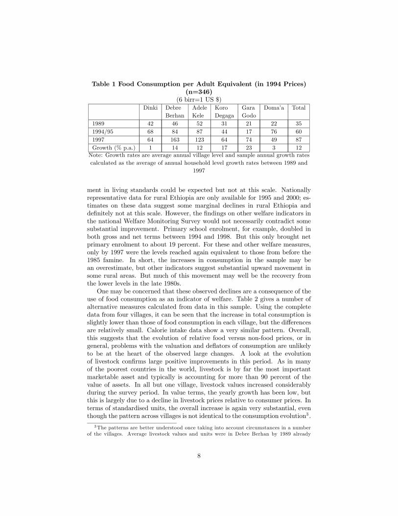
Table 1 Food Consumption per Adult Equivalent (in 1994 Prices)(n=346)

(6 birr=1 US $)Dinki Debre Adele Koro Gara Doma’a Total

Berhan Kele Degaga Godo1989 42 46 52 31 21 22 351994/95 68 84 87 44 17 76 601997 64 163 123 64 74 49 87Growth (% p.a.) 1 14 12 17 23 3 12Note: Growth rates are average annual village level and sample annual growth ratescalculated as the average of annual household level growth rates between 1989 and

1997

ment in living standards could be expected but not at this scale. Nationallyrepresentative data for rural Ethiopia are only available for 1995 and 2000; es-timates on these data suggest some marginal declines in rural Ethiopia anddefinitely not at this scale. However, the findings on other welfare indicators inthe national Welfare Monitoring Survey would not necessarily contradict somesubstantial improvement. Primary school enrolment, for example, doubled inboth gross and net terms between 1994 and 1998. But this only brought netprimary enrolment to about 19 percent. For these and other welfare measures,only by 1997 were the levels reached again equivalent to those from before the1985 famine. In short, the increases in consumption in the sample may bean overestimate, but other indicators suggest substantial upward movement insome rural areas. But much of this movement may well be the recovery fromthe lower levels in the late 1980s.One may be concerned that these observed declines are a consequence of the

use of food consumption as an indicator of welfare. Table 2 gives a number ofalternative measures calculated from data in this sample. Using the completedata from four villages, it can be seen that the increase in total consumption isslightly lower than those of food consumption in each village, but the differencesare relatively small. Calorie intake data show a very similar pattern. Overall,this suggests that the evolution of relative food versus non-food prices, or ingeneral, problems with the valuation and deflators of consumption are unlikelyto be at the heart of the observed large changes. A look at the evolutionof livestock confirms large positive improvements in this period. As in manyof the poorest countries in the world, livestock is by far the most importantmarketable asset and typically is accounting for more than 90 percent of thevalue of assets. In all but one village, livestock values increased considerablyduring the survey period. In value terms, the yearly growth has been low, butthis is largely due to a decline in livestock prices relative to consumer prices. Interms of standardised units, the overall increase is again very substantial, eventhough the pattern across villages is not identical to the consumption evolution3.

3The patterns are better understood once taking into account circumstances in a numberof the villages. Average livestock values and units were in Debre Berhan by 1989 already

8

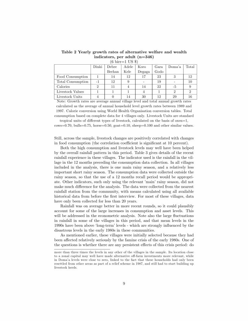
Table 2 Yearly growth rates of alternative welfare and wealthindicators, per adult (n=346)

(6 birr=1 US $)Dinki Debre Adele Koro Gara Doma’a Total

Berhan Kele Degaga GodoFood Consumption 1 14 12 17 23 3 12Total Consumption -1 12 9 - 19 - 10Calories 2 11 4 14 22 -5 9Livestock Values 1 1 1 4 1 2 2Livestock Units 4 0 14 30 12 29 16Note: Growth rates are average annual village level and total annual growth ratescalculated as the average of annual household level growth rates between 1989 and1997. Calorie conversion using World Health Organisation conversion tables. Totalconsumption based on complete data for 4 villages only. Livestock Units are standardtropical units of different types of livestock, calculated on the basis of oxen=1,

cows=0.70, bulls=0.75, horse=0.50, goat=0.10, sheep=0.100 and other similar values.

Still, across the sample, livestock changes are positively correlated with changesin food consumption (the correlation coefficient is significant at 10 percent).Both the high consumption and livestock levels may well have been helped

by the overall rainfall pattern in this period. Table 3 gives details of the recentrainfall experience in these villages. The indicator used is the rainfall in the vil-lage in the 12 months preceding the consumption data collection. In all villagesincluded in the analysis, there is one main rainy season, and a relatively lessimportant short rainy season. The consumption data were collected outside therainy season, so that the use of a 12 months recall period would be appropri-ate. Other indicators, such only using the relevant ’main’ rainy season, did notmake much difference for the analysis. The data were collected from the nearestrainfall station from the community, with means calculated using all availablehistorical data from before the first interview. For most of these villages, datahave only been collected for less than 20 years.Rainfall was on average better in more recent rounds, so it could plausibly

account for some of the large increases in consumption and asset levels. Thiswill be addressed in the econometric analysis. Note also the large fluctuationsin rainfall in some of the villages in this period, and that mean levels in the1990s have been above ‘long-term’ levels - which are strongly influenced by thedisastrous levels in the early 1980s in these communities.As mentioned earlier, these villages were initially selected because they had

been affected relatively seriously by the famine crisis of the early 1980s. One ofthe questions is whether there are any persistent effects of this crisis period: do

more than three times the levels in any other of the villages in the sample. Its location closeto a zonal capital may well have made alternative off-farm investments more relevant, whilein Doma’a levels were close to zero, linked to the fact that these households had only beenresettled from other areas as part of a relief scheme in 1987, and still had to start building uplivestock herds.

9

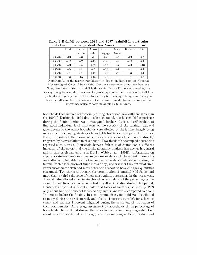
Table 3 Rainfall between 1989 and 1997 (rainfall in particularperiod as a percentage deviation from the long term mean)

Dinki Debre Adele Koro Gara Doma’a TotalBerhan Kele Degaga Godo

1988-89 -13 +6 -7 +2 +5 -13 +21993-94 +16 +7 +13 -19 -8 +16 +41996-97 -23 +4 +52 +32 +7 -23 +101985-89 +5 -1 +5 +16 +7 -6 +41990-94 -6 -2 +17 +21 -7 +6 +41994-97 +6 -15 +18 +48 +9 -2 +8

Note:Rainfall in the nearest rainfall station, based on data from the NationalMeteorological Office, Addis Ababa. Data are percentage deviations from the’long-term’ mean. Yearly rainfall is the rainfall in the 12 months preceding the

survey. Long term rainfall data are the percentage deviation of average rainfall in aparticular five year period, relative to the long term average. Long term average isbased on all available observations of the relevant rainfall station before the first

interview, typically covering about 15 to 20 years.

households that suffered substantially during this period have different growth inthe 1990s? During the 1994 data collection round, the households’ experienceduring the famine period was investigated further. It is non-self evident tofind good individual level indicators of the severity of the famine. Table 4gives details on the extent households were affected by the famine, largely usingindicators of the coping strategies households had to use to cope with the crisis.First, it reports whether households experienced a serious loss of wealth directlytriggered by harvest failure in this period. Two-thirds of the sampled householdsreported such a crisis. Household harvest failure is of course not a sufficientindicator of the severity of the crisis, as famine analysis has shown in generaland in this particular case (Sen [1981], Webb et al. [1992]). Information oncoping strategies provides some suggestive evidence of the extent householdswere affected..The table reports the number of meals households had during thefamine (with a local norm of three meals a day) and whether they cut meal sizes.Fewer meals were taken and most households report to have cut back quantitiesconsumed. Two thirds also report the consumption of unusual wild foods, andmore than a third sold some of their most valued possessions in the worst year.The data also allowed an estimate (based on recall data) of the percentage of thevalue of their livestock households had to sell or that died during this period.Households reported substantial sales and losses of livestock, so that by 1989only about half the households owned any significant levels, compared to about75 percent before the famine. In some communities, food aid was distributedto many during the crisis period, and about 11 percent even left for a feedingcamp, and another 7 percent migrated during the crisis out of the region oftheir communities. An average assessment by households of the percentage ofhouseholds that suffered during the crisis in each community suggested thatabout two-thirds suffered on average, with less suffering in Debre Berhan and

10

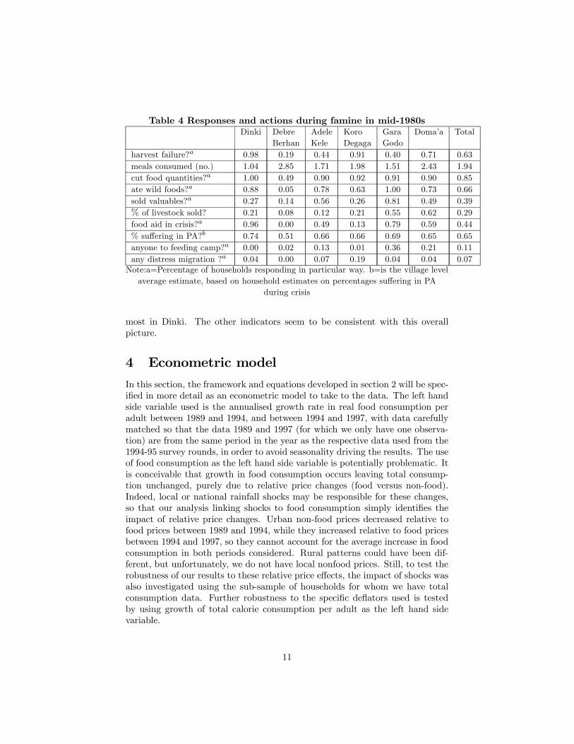
Table 4 Responses and actions during famine in mid-1980sDinki Debre Adele Koro Gara Doma’a Total

Berhan Kele Degaga Godoharvest failure?a 0.98 0.19 0.44 0.91 0.40 0.71 0.63meals consumed (no.) 1.04 2.85 1.71 1.98 1.51 2.43 1.94cut food quantities?a 1.00 0.49 0.90 0.92 0.91 0.90 0.85ate wild foods?a 0.88 0.05 0.78 0.63 1.00 0.73 0.66sold valuables?a 0.27 0.14 0.56 0.26 0.81 0.49 0.39% of livestock sold? 0.21 0.08 0.12 0.21 0.55 0.62 0.29food aid in crisis?a 0.96 0.00 0.49 0.13 0.79 0.59 0.44% suffering in PA?b 0.74 0.51 0.66 0.66 0.69 0.65 0.65anyone to feeding camp?a 0.00 0.02 0.13 0.01 0.36 0.21 0.11any distress migration ?a 0.04 0.00 0.07 0.19 0.04 0.04 0.07Note:a=Percentage of households responding in particular way. b=is the village levelaverage estimate, based on household estimates on percentages suffering in PA

during crisis

most in Dinki. The other indicators seem to be consistent with this overallpicture.

4 Econometric modelIn this section, the framework and equations developed in section 2 will be spec-ified in more detail as an econometric model to take to the data. The left handside variable used is the annualised growth rate in real food consumption peradult between 1989 and 1994, and between 1994 and 1997, with data carefullymatched so that the data 1989 and 1997 (for which we only have one observa-tion) are from the same period in the year as the respective data used from the1994-95 survey rounds, in order to avoid seasonality driving the results. The useof food consumption as the left hand side variable is potentially problematic. Itis conceivable that growth in food consumption occurs leaving total consump-tion unchanged, purely due to relative price changes (food versus non-food).Indeed, local or national rainfall shocks may be responsible for these changes,so that our analysis linking shocks to food consumption simply identifies theimpact of relative price changes. Urban non-food prices decreased relative tofood prices between 1989 and 1994, while they increased relative to food pricesbetween 1994 and 1997, so they cannot account for the average increase in foodconsumption in both periods considered. Rural patterns could have been dif-ferent, but unfortunately, we do not have local nonfood prices. Still, to test therobustness of our results to these relative price effects, the impact of shocks wasalso investigated using the sub-sample of households for whom we have totalconsumption data. Further robustness to the specific deflators used is testedby using growth of total calorie consumption per adult as the left hand sidevariable.

11

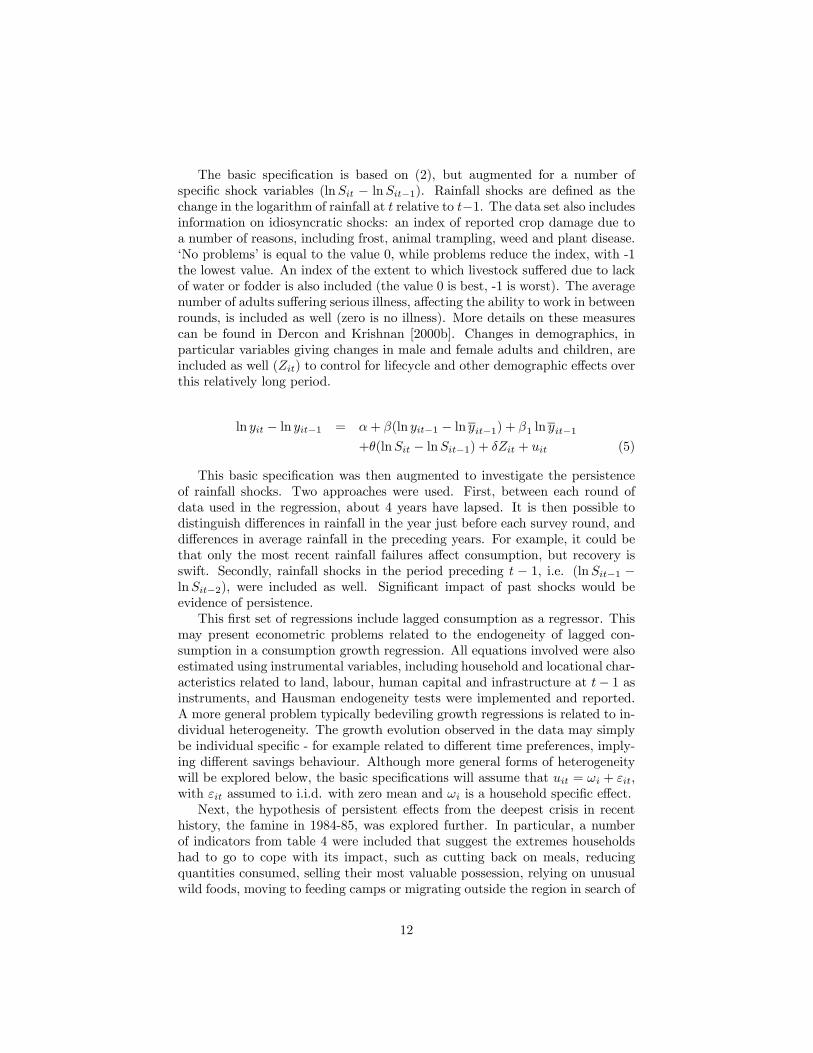
The basic specification is based on (2), but augmented for a number ofspecific shock variables (lnSit − lnSit−1). Rainfall shocks are defined as thechange in the logarithm of rainfall at t relative to t−1. The data set also includesinformation on idiosyncratic shocks: an index of reported crop damage due toa number of reasons, including frost, animal trampling, weed and plant disease.‘No problems’ is equal to the value 0, while problems reduce the index, with -1the lowest value. An index of the extent to which livestock suffered due to lackof water or fodder is also included (the value 0 is best, -1 is worst). The averagenumber of adults suffering serious illness, affecting the ability to work in betweenrounds, is included as well (zero is no illness). More details on these measurescan be found in Dercon and Krishnan [2000b]. Changes in demographics, inparticular variables giving changes in male and female adults and children, areincluded as well (Zit) to control for lifecycle and other demographic effects overthis relatively long period.

ln yit − ln yit−1 = α+ β(ln yit−1 − ln yit−1) + β1 ln yit−1+θ(lnSit − lnSit−1) + δZit + uit (5)

This basic specification was then augmented to investigate the persistenceof rainfall shocks. Two approaches were used. First, between each round ofdata used in the regression, about 4 years have lapsed. It is then possible todistinguish differences in rainfall in the year just before each survey round, anddifferences in average rainfall in the preceding years. For example, it could bethat only the most recent rainfall failures affect consumption, but recovery isswift. Secondly, rainfall shocks in the period preceding t − 1, i.e. (lnSit−1 −lnSit−2), were included as well. Significant impact of past shocks would beevidence of persistence.This first set of regressions include lagged consumption as a regressor. This

may present econometric problems related to the endogeneity of lagged con-sumption in a consumption growth regression. All equations involved were alsoestimated using instrumental variables, including household and locational char-acteristics related to land, labour, human capital and infrastructure at t− 1 asinstruments, and Hausman endogeneity tests were implemented and reported.A more general problem typically bedeviling growth regressions is related to in-dividual heterogeneity. The growth evolution observed in the data may simplybe individual specific - for example related to different time preferences, imply-ing different savings behaviour. Although more general forms of heterogeneitywill be explored below, the basic specifications will assume that uit = ωi + εit,with εit assumed to i.i.d. with zero mean and ωi is a household specific effect.Next, the hypothesis of persistent effects from the deepest crisis in recent

history, the famine in 1984-85, was explored further. In particular, a numberof indicators from table 4 were included that suggest the extremes householdshad to go to cope with its impact, such as cutting back on meals, reducingquantities consumed, selling their most valuable possession, relying on unusualwild foods, moving to feeding camps or migrating outside the region in search of

12

food. Basic correlation analysis between these variables showed that they wereall correlated, which may well lead to multicollinearity problems. Preliminaryanalysis using these variables highlighted these problems so a simple index wasconstructed providing an average of these six indicators4.Finally, the lagged household and village level consumption variables were

unpacked further, as in (3) and (4). In line with standard empirical growthmodel approaches, variables measuring capital goods suitable for accumulationand the underlying technology are relevant. The data set contains three vari-ables that could be most relevant in this context: livestock, the standard assetfor accumulation in this rural economy, which, in per capita terms, may or maynot be liable to decreasing returns; education levels (average years of educationof adults in the household), providing scope for increasing returns, for examplelinked to the ability to innovate and a geographical variable capturing whetherthere was a road connecting the village, relevant given the general poor roadinfrastructure in Ethiopia. Work in China using micro-growth models has foundevidence in favour positive externalities from roads as well as positive growth ef-fects from household level education (Jalan and Ravallion [2002]), but De Vreyeret al. [2003]) did not find a significant effect for either in Peru. Deiniger andOkidi [2002] find evidence of the impact of community level infrastructure and ofhousehold level education on growth in their data, but only in a model withoutany control for heterogeneity. Limitations in the data from 1989 do not allow usto test the impact of other geographical variables. For example, both the Peruand the China study find evidence on the impact of health related variables(prevalence of particular diseases and the presence of health centres in the caseof Peru, and the presence of medical personnel in the case of China), but thiscould not be tested in the Ethiopia data. Other variables are less relevant forthe period under consideration. For example, Jalan and Ravallion [2002] findevidence of the impact of farm assets and of initial fertiliser use at the com-munity level positively affecting growth, while Gunning et al. [2000] identifyproductivity increases linked to modern input use and extension as the mostimportant source of growth in their Zimbabwe panel. In Ethiopia, the use ofmodern inputs was hardly relevant in the communities studied by 1989, eventhough during the second half of the 1990s they become again more important5.The variables related to the 1984 famine and, since no new roads were build

in this period, road infrastructure are time-invariant in this model. A standardfixed effects estimator would wipe out these effects, even though they are ofinterest. Assuming that all time-invariant and time-varying variables are alluncorrelated with the fixed effect would allow the estimation by random effects,but this is an extreme assumption, unlikely to be met in this data set. The

4 In this index, all ’yes/no’ variables were simply given 1 if the strategy was used, and zeroif not. If the household reduced meals from 3 to 1, 1 was added, while if it reduced to 2meals, 0.5 was added. The simple average of these six values was then used as an index of theseverity of the crisis.

5The work on Zimbabwe also highlighted the relevance of land holdings for growth, butgiven that in Ethiopia all land is state-owned and in the period considered was liable torepeated redistribution, the scope for investing in larger farm size was non-existent, justifyingthe use of livestock as the key asset for understanding accumulation.

13

econometric analysis explores three alternative ways of allowing a fixed effect,correlated with variables of interest, to be present, but still identifying time-invariant variables. The first method involves estimating a model using thefixed effects (within) estimator, but with initial levels of consumption unpackedusing time variant variables (levels at t − 1 of the average years of educationper adult and the level of livestock holdings per adult), and fixed effects. Thefixed effects were then regressed on a series of time-invariant variables, provid-ing suggestive evidence of the impact of roads and of the famine on growth inthe 1990s. Secondly, the Hausman-Taylor model (Hausman and Taylor [1981])is used. This involves partitioning the time-invariant and time-varying vectorof variables in two groups each, of which one group of variables is assumed tobe uncorrelated with the fixed effect. The orthogonality assumptions providethen enough restrictions for a method of moments procedure. The partitioningassumptions are strong, but in the approach below all demographic variablesand the illness shocks were included as endogenous time-varying variables, andthe extent to which drastic coping strategies had to be used and (in the rel-evant version of the econometric model) the presence of a road were treatedas endogenous time-invariant variables. Furthermore, depending on the versionof the model, lagged consumption at the village and household level, or initiallevels of livestock and education, and the presence of a road, are also treated asendogenous. All agricultural and rainfall shocks are treated as exogenous, whilewhether there was a harvest failure in 1984, the estimate of the proportion ofthe community that suffered substantially and the pre-famine levels of livestockwere used as further instruments for the extent drastic household-level copingstrategies had to be used. As a third alternative, the Jalan-Ravallion (Jalan andRavallion, [2002]) estimator that allows for some time-varying heterogeneity wasused to check the robustness of the results (see also Holtz-Eakin et al. [1988]).This estimator relies on a decomposition of the error term as uit = ρtωi + εit,with εit assumed to i.i.d. with zero mean, ωi is a household specific effect and ρtare exogenous shocks, whose impact on the household is modified by ωi.Quasi-differencing techniques can then be used to obtain estimates of parameters ofinterest, except for the household specific effect. To illustrate the procedure,consider a simplified version of (3), but with the error term allowing for a fixedeffect multiplied by a time-varying shifter.

∆ ln yit = α+ γ0 ln kit−1 + δZit + γXi + ρtωi + εit (6)

Defining rt = ρt/ρt−1, then lagging and premultiplying (6) with rt, andsubtracting it from (5) gives a quasi-differenced equation in which the fixedeffects ωi have been removed, but in which δ can be identified provided rt 6= 1.

∆ ln yit = α(1− rt) + rt∆ ln yit−1 + γ0 ln kit−1 − rtγ0 ln kit−2 +

δZit − rtδZit−1 + γ(1− rt)Xi + εit − rtεit−1 (7)

which can be estimated by imposing the relevant restrictions on the followingequation:

14

∆ ln yit = at+bt∆ ln yit−1+c ln kit−1+dt ln kit−2+eZit+ftZit−1+gtXi+vit (8)

All the parameters can be recovered from this equation (except for the levelof the household specific effect ωi) since rt is the only cause of time-varying co-efficients in this model. With three rounds of data (i.e. two growth rates), as inour data set, the procedure can just be implemented. The model was estimatedusing restricted maximum likelihood estimation, imposing the cross-equationsrestrictions. In principle, the GMM procedure as in Jalan and Ravallion (2002)or in De Vreyer et al. (2002) would be most efficient, but the current proceduregives consistent estimators.It is not self-evident to test whether the restriction that the fixed effects

are time-invariant after all (θt = θ).Standard chi-squared asymptotic tests arenot appropriate, since under the null rt = 1, the parameters associated with theconstant and the time-invariant variables are not identified. Jalan and Ravallion(2002) proceed by using a test suggested by Godfrey (1988), but, as they noteas well, the power of this test will be weak in small samples such as the oneused in this paper. As a consequence, the different procedures are not testedagainst each other, but just presented as cumulative evidence using differentassumptions regarding the role of heterogeneity in explaining the present results.

5 Estimation resultsTables 5, 6, 7 and 8 present the results from testing the hypotheses against thedata. Table 5 first focuses on the basic specification, presenting a fixed effectsestimator of the growth in food consumption on initial levels of household andvillage consumption, and a set of common and idiosyncratic shock variables.Note that the regressions control for changes in demographic variables. The firstcolumn points to higher growth rates in richer villages, but lower growth ratesfor richer individual households. Overall, the coefficients point to a process ofconvergence within villages, but for a given initial consumption level, householdsexperience a higher growth rate in richer than in poorer villages (i.e. village witha higher initial mean level of consumption)6. Rainfall shocks clearly matter anda ten percent decline in rainfall reduces food consumption by about five percent.There is some evidence of non-rainfall shocks also mattering. The impact ofshocks is robust to the use of other welfare outcome measures. Using the fourcommunities with complete total consumption data, the impact of a rainfallshock is smaller at about three percent for a ten percent decline in rainfall7 .

6Referring to equation (1) above, the estimates here suggest β = −0.319 and β1 = −0.106,and β1 is significantly different from zero at less than one percent, i.e. there is a significantlydifferent effect across than within villages.

7The total consumption regression suggests divergence between communities. However,with only a small number of communities included in this regression, the power of the estimatesrelated to community level variables is obviously small, and overall, the issue of divergenceand convergence between communities has to be interpreted with caution.

15

This may suggest that some but not all impact of the rainfall shock is in factthe consequence of relative price changes: at higher rainfall levels, possiblylocally declining food prices relative to nonfood prices, increases food relativeto nonfood consumption, and vice versa. But the fact that total consumptionin real terms responds to rainfall shocks suggests also that the results are notexplained by just a relative price effect. Finally, column 3, using calorie intakedata, suggests also that the sensitivity to rain and other effects are not drivenby the choice of deflators - the effects are similar to using the growth in thevalue of food consumption in real terms.All these specifications were estimated using instruments for lagged con-

sumption (i.e. assets and infrastructure at t − 1). A Hausman test for endo-geneity could never reject the assumption of exogeneity. Similarly, using laggedcharacteristics (at t − 2) and using twice lagged consumption as instrumentssimilarly showed that exogeneity of lagged consumption could not be rejected8.As a consequence, I only report the uninstrumented regressions - in any case,the estimated coefficients were qualitatively very similar (which is of coursewhat the Hausman test systematically investigated, by comparing the actualestimated coefficients using 2SLS and OLS).To investigate persistence, the specification in column (1) in table 5 has

been expanded in column (5) in table 6, disentangling rainfall in the 12 monthsrelevant for the particular level of consumption, and the preceding years withinthe period during which growth has been observed. For example, to explaingrowth between 1994 and 1997, the change in rainfall in the 12 months beforethese years has been entered seperately from average rainfall change in theperiod 1994-96 compared to 1989-92. As column (4) shows, there is some signof persistence: rainfall changes in the beginning of the period of observationhas a significant impact on outcome changes, beyond the effect from changes inthe most recent levels rainfall. A ten percent decrease in rainfall several yearsago still has an impact of about 3 percent on food consumption. There is alsoevidence of persistence over longer periods. To test this, lagged rainfall wasintroduced, for example, rainfall in the years before 1994 was used to explaingrowth between 1994 and 1997. Column (5) shows that a ten percent decline inlagged rainfall reduces food consumption by 1.6 percent: rainfall shocks have apersistent effect, lasting many years.Tables 7 and 8 explore the impact of unpacking village and household level

effects using specific community and household level variables, in particular live-stock and education, as well as the presence of road infrastructure. Furthermore,the impact of the severity of the famine in the mid-1980s on growth in the 1990sis explored using the index of dependence on ’extreme’ coping mechanisms inthis period, based on six indicators as described before. Since the severity ofthe famine index and the presence of road infrastructure are time-invariant vari-ables, a simple fixed effects estimation cannot illuminate matters. As discussedbefore, three different approaches have been used. They are reported in tables

8Note that when using two laggs, the regressions were reduced to a cross-section estimateof growth rates between 1994 and 1997, using values in 1989 as instruments, so that no fixedeffects could be used.

16

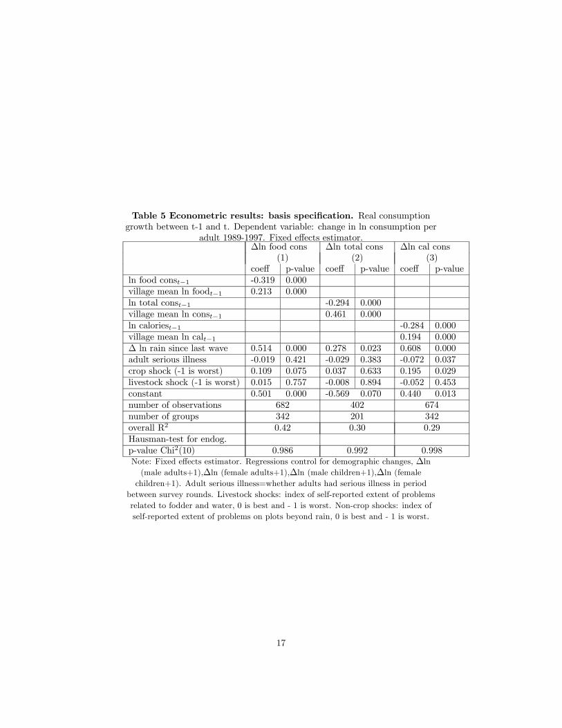
Table 5 Econometric results: basis specification. Real consumptiongrowth between t-1 and t. Dependent variable: change in ln consumption per

adult 1989-1997. Fixed effects estimator.∆ln food cons ∆ln total cons ∆ln cal cons

(1) (2) (3)coeff p-value coeff p-value coeff p-value

ln food const−1 -0.319 0.000village mean ln foodt−1 0.213 0.000ln total const−1 -0.294 0.000village mean ln const−1 0.461 0.000ln caloriest−1 -0.284 0.000village mean ln calt−1 0.194 0.000∆ ln rain since last wave 0.514 0.000 0.278 0.023 0.608 0.000adult serious illness -0.019 0.421 -0.029 0.383 -0.072 0.037crop shock (-1 is worst) 0.109 0.075 0.037 0.633 0.195 0.029livestock shock (-1 is worst) 0.015 0.757 -0.008 0.894 -0.052 0.453constant 0.501 0.000 -0.569 0.070 0.440 0.013number of observations 682 402 674number of groups 342 201 342overall R2 0.42 0.30 0.29Hausman-test for endog.p-value Chi2(10) 0.986 0.992 0.998Note: Fixed effects estimator. Regressions control for demographic changes, ∆ln(male adults+1),∆ln (female adults+1),∆ln (male children+1),∆ln (femalechildren+1). Adult serious illness=whether adults had serious illness in period

between survey rounds. Livestock shocks: index of self-reported extent of problemsrelated to fodder and water, 0 is best and - 1 is worst. Non-crop shocks: index ofself-reported extent of problems on plots beyond rain, 0 is best and - 1 is worst.

17

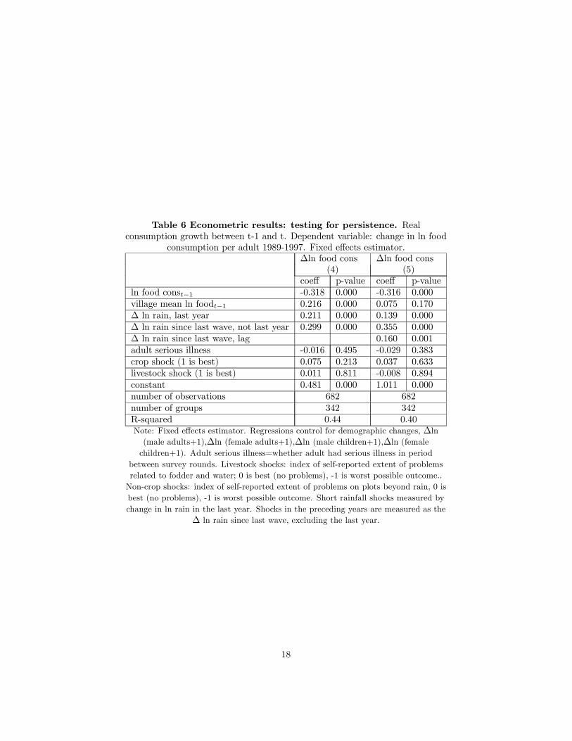
Table 6 Econometric results: testing for persistence. Realconsumption growth between t-1 and t. Dependent variable: change in ln food

consumption per adult 1989-1997. Fixed effects estimator.∆ln food cons ∆ln food cons

(4) (5)coeff p-value coeff p-value

ln food const−1 -0.318 0.000 -0.316 0.000village mean ln foodt−1 0.216 0.000 0.075 0.170∆ ln rain, last year 0.211 0.000 0.139 0.000∆ ln rain since last wave, not last year 0.299 0.000 0.355 0.000∆ ln rain since last wave, lag 0.160 0.001adult serious illness -0.016 0.495 -0.029 0.383crop shock (1 is best) 0.075 0.213 0.037 0.633livestock shock (1 is best) 0.011 0.811 -0.008 0.894constant 0.481 0.000 1.011 0.000number of observations 682 682number of groups 342 342R-squared 0.44 0.40Note: Fixed effects estimator. Regressions control for demographic changes, ∆ln(male adults+1),∆ln (female adults+1),∆ln (male children+1),∆ln (femalechildren+1). Adult serious illness=whether adult had serious illness in period

between survey rounds. Livestock shocks: index of self-reported extent of problemsrelated to fodder and water; 0 is best (no problems), -1 is worst possible outcome..Non-crop shocks: index of self-reported extent of problems on plots beyond rain, 0 isbest (no problems), -1 is worst possible outcome. Short rainfall shocks measured bychange in ln rain in the last year. Shocks in the preceding years are measured as the

∆ ln rain since last wave, excluding the last year.

18

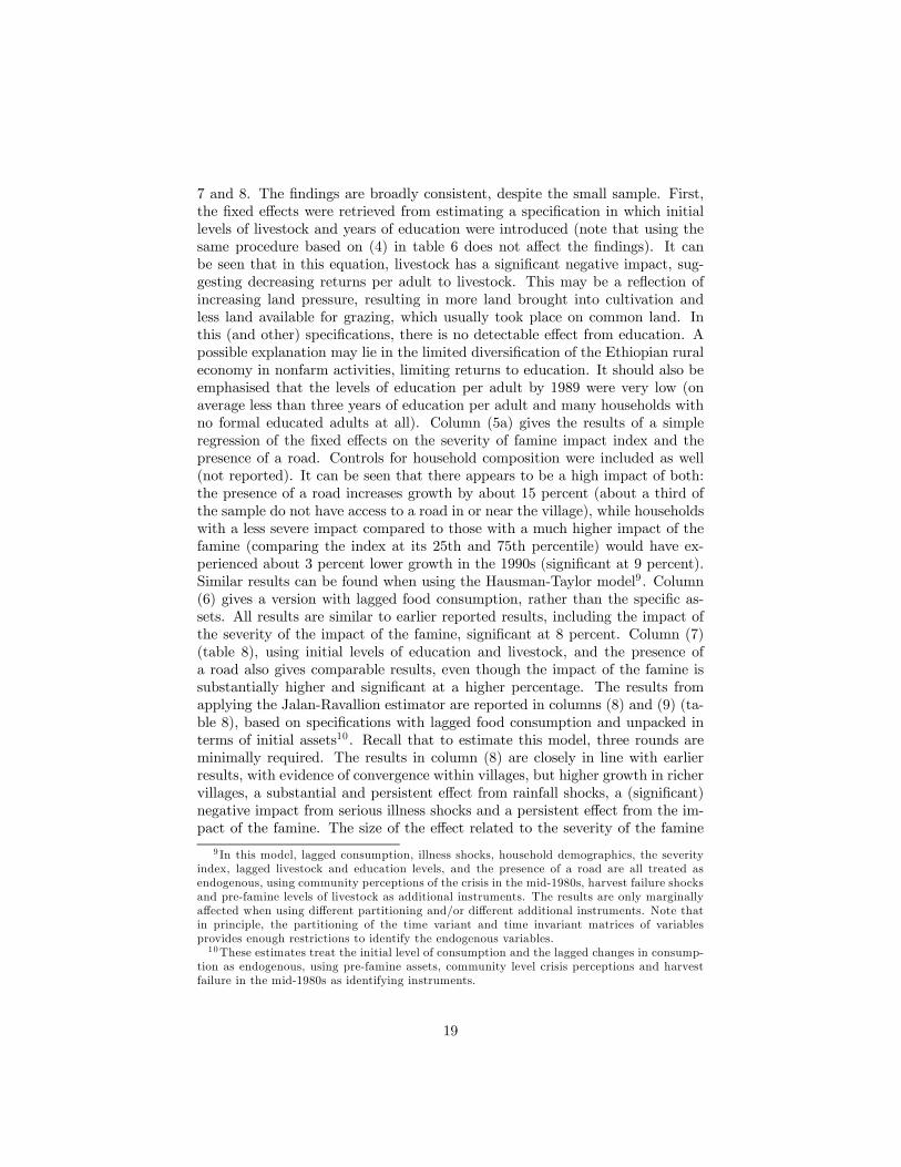
7 and 8. The findings are broadly consistent, despite the small sample. First,the fixed effects were retrieved from estimating a specification in which initiallevels of livestock and years of education were introduced (note that using thesame procedure based on (4) in table 6 does not affect the findings). It canbe seen that in this equation, livestock has a significant negative impact, sug-gesting decreasing returns per adult to livestock. This may be a reflection ofincreasing land pressure, resulting in more land brought into cultivation andless land available for grazing, which usually took place on common land. Inthis (and other) specifications, there is no detectable effect from education. Apossible explanation may lie in the limited diversification of the Ethiopian ruraleconomy in nonfarm activities, limiting returns to education. It should also beemphasised that the levels of education per adult by 1989 were very low (onaverage less than three years of education per adult and many households withno formal educated adults at all). Column (5a) gives the results of a simpleregression of the fixed effects on the severity of famine impact index and thepresence of a road. Controls for household composition were included as well(not reported). It can be seen that there appears to be a high impact of both:the presence of a road increases growth by about 15 percent (about a third ofthe sample do not have access to a road in or near the village), while householdswith a less severe impact compared to those with a much higher impact of thefamine (comparing the index at its 25th and 75th percentile) would have ex-perienced about 3 percent lower growth in the 1990s (significant at 9 percent).Similar results can be found when using the Hausman-Taylor model9 . Column(6) gives a version with lagged food consumption, rather than the specific as-sets. All results are similar to earlier reported results, including the impact ofthe severity of the impact of the famine, significant at 8 percent. Column (7)(table 8), using initial levels of education and livestock, and the presence ofa road also gives comparable results, even though the impact of the famine issubstantially higher and significant at a higher percentage. The results fromapplying the Jalan-Ravallion estimator are reported in columns (8) and (9) (ta-ble 8), based on specifications with lagged food consumption and unpacked interms of initial assets10 . Recall that to estimate this model, three rounds areminimally required. The results in column (8) are closely in line with earlierresults, with evidence of convergence within villages, but higher growth in richervillages, a substantial and persistent effect from rainfall shocks, a (significant)negative impact from serious illness shocks and a persistent effect from the im-pact of the famine. The size of the effect related to the severity of the famine

9 In this model, lagged consumption, illness shocks, household demographics, the severityindex, lagged livestock and education levels, and the presence of a road are all treated asendogenous, using community perceptions of the crisis in the mid-1980s, harvest failure shocksand pre-famine levels of livestock as additional instruments. The results are only marginallyaffected when using different partitioning and/or different additional instruments. Note thatin principle, the partitioning of the time variant and time invariant matrices of variablesprovides enough restrictions to identify the endogenous variables.10These estimates treat the initial level of consumption and the lagged changes in consump-

tion as endogenous, using pre-famine assets, community level crisis perceptions and harvestfailure in the mid-1980s as identifying instruments.

19

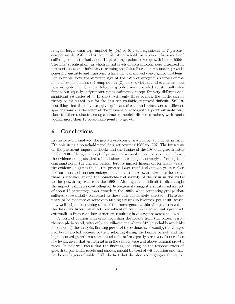
is again larger than e.g. implied by (5a) or (6), and significant at 7 percent:comparing the 25th and 75 percentile of households in terms of the severity ofsuffering, the latter had about 16 percentage points lower growth in the 1990s.The final specification, in which initial levels of consumption were unpacked interms of assets and infrastructure using the Jalan-Ravallion estimator, providegenerally unstable and imprecise estimates, and showed convergence problems.For example, note the different sign of the ratio of exogenous shifters of thefixed effects in column (9) compared to (8). In (9), virtually all coefficients arenow insignificant. Slightly different specifications provided substantially dif-ferent, but equally insignificant point estimates, except for very different andsignificant estimates of r. In short, with only three rounds, the model can intheory be estimated, but for the data set available, it proved difficult. Still, itis striking that the only strongly significant effect - and robust across differentspecifications - is the effect of the presence of roads,with a point estimate veryclose to other estimates using alternative models discussed before, with roadsadding more than 15 percentage points to growth.

6 ConclusionsIn this paper, I analysed the growth experience in a number of villages in ruralEthiopia using a household panel data set covering 1989 to 1997. The focus wason the persistent impact of shocks and the famine of the 1980s on growth ratesin the 1990s. Using a concept of persistence as used in macroeconomic analysis,the evidence suggests that rainfall shocks are not just strongly affecting foodconsumption in the current period, but its impact lingers on for many years:the evidence suggests that a ten percent lower rainfall about 4-5 years earlierhad an impact of one percentage point on current growth rates. Furthermore,there is evidence linking the household-level severity of the crisis in the 1980sto the growth experience in the 1990s. Although it is difficult to disentanglethe impact, estimates controlling for heterogeneity suggest a substantial impactof about 16 percentage lower growth in the 1990s, when comparing groups thatsuffered substantially compared to those only moderately affected. There ap-pears to be evidence of some diminishing returns to livestock per adult, whichmay well help in explaining some of the convergence within villages observed inthe data. No discernible effect from education could be detected, but significantexternalities from road infrastructure, resulting in divergence across villages.A word of caution is in order regarding the results from this paper. First,

the sample is small, with only six villages and about 342 households availablefor (most of) the analysis, limiting power of the estimates. Secondly, the villageshad been selected because of their suffering during the famine period, and thehigh observed growth rates are bound to be at least partly a recovery from earlierlow levels, given that growth rates in the sample were well above national growthrates. It may well mean that the findings, including on the responsiveness ofgrowth to particular assets and shocks, should be treated with caution and maynot be easily generalisable. Still, the fact that the observed high growth may be

20

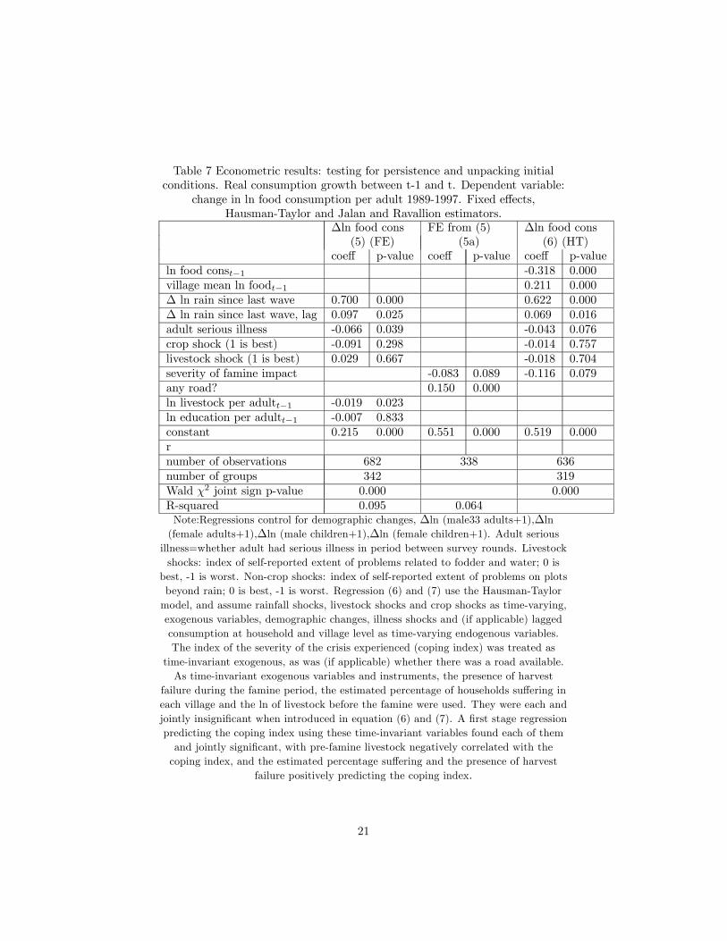
Table 7 Econometric results: testing for persistence and unpacking initialconditions. Real consumption growth between t-1 and t. Dependent variable:

change in ln food consumption per adult 1989-1997. Fixed effects,Hausman-Taylor and Jalan and Ravallion estimators.

∆ln food cons FE from (5) ∆ln food cons(5) (FE) (5a) (6) (HT)

coeff p-value coeff p-value coeff p-valueln food const−1 -0.318 0.000village mean ln foodt−1 0.211 0.000∆ ln rain since last wave 0.700 0.000 0.622 0.000∆ ln rain since last wave, lag 0.097 0.025 0.069 0.016adult serious illness -0.066 0.039 -0.043 0.076crop shock (1 is best) -0.091 0.298 -0.014 0.757livestock shock (1 is best) 0.029 0.667 -0.018 0.704severity of famine impact -0.083 0.089 -0.116 0.079any road? 0.150 0.000ln livestock per adultt−1 -0.019 0.023ln education per adultt−1 -0.007 0.833constant 0.215 0.000 0.551 0.000 0.519 0.000rnumber of observations 682 338 636number of groups 342 319Wald χ2 joint sign p-value 0.000 0.000R-squared 0.095 0.064Note:Regressions control for demographic changes, ∆ln (male33 adults+1),∆ln(female adults+1),∆ln (male children+1),∆ln (female children+1). Adult seriousillness=whether adult had serious illness in period between survey rounds. Livestockshocks: index of self-reported extent of problems related to fodder and water; 0 isbest, -1 is worst. Non-crop shocks: index of self-reported extent of problems on plotsbeyond rain; 0 is best, -1 is worst. Regression (6) and (7) use the Hausman-Taylormodel, and assume rainfall shocks, livestock shocks and crop shocks as time-varying,exogenous variables, demographic changes, illness shocks and (if applicable) laggedconsumption at household and village level as time-varying endogenous variables.The index of the severity of the crisis experienced (coping index) was treated as

time-invariant exogenous, as was (if applicable) whether there was a road available.As time-invariant exogenous variables and instruments, the presence of harvest

failure during the famine period, the estimated percentage of households suffering ineach village and the ln of livestock before the famine were used. They were each andjointly insignificant when introduced in equation (6) and (7). A first stage regressionpredicting the coping index using these time-invariant variables found each of themand jointly significant, with pre-famine livestock negatively correlated with thecoping index, and the estimated percentage suffering and the presence of harvest

failure positively predicting the coping index.

21

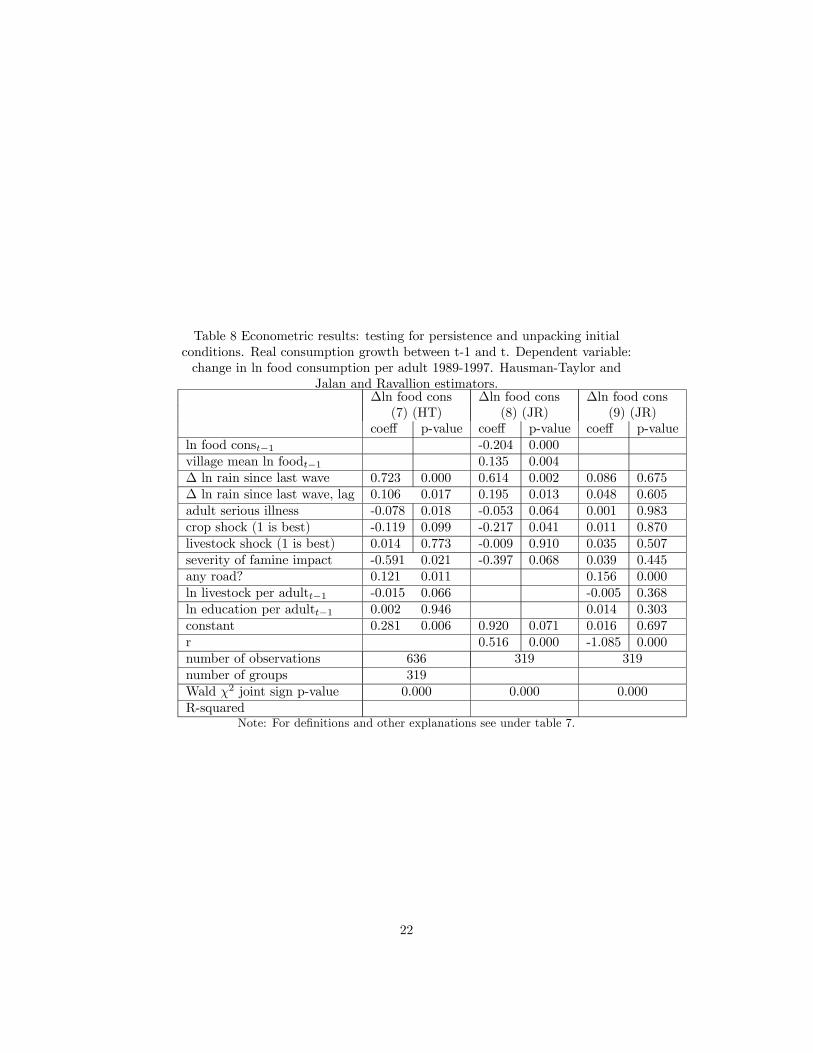
Table 8 Econometric results: testing for persistence and unpacking initialconditions. Real consumption growth between t-1 and t. Dependent variable:change in ln food consumption per adult 1989-1997. Hausman-Taylor and

Jalan and Ravallion estimators.∆ln food cons ∆ln food cons ∆ln food cons

(7) (HT) (8) (JR) (9) (JR)coeff p-value coeff p-value coeff p-value

ln food const−1 -0.204 0.000village mean ln foodt−1 0.135 0.004∆ ln rain since last wave 0.723 0.000 0.614 0.002 0.086 0.675∆ ln rain since last wave, lag 0.106 0.017 0.195 0.013 0.048 0.605adult serious illness -0.078 0.018 -0.053 0.064 0.001 0.983crop shock (1 is best) -0.119 0.099 -0.217 0.041 0.011 0.870livestock shock (1 is best) 0.014 0.773 -0.009 0.910 0.035 0.507severity of famine impact -0.591 0.021 -0.397 0.068 0.039 0.445any road? 0.121 0.011 0.156 0.000ln livestock per adultt−1 -0.015 0.066 -0.005 0.368ln education per adultt−1 0.002 0.946 0.014 0.303constant 0.281 0.006 0.920 0.071 0.016 0.697r 0.516 0.000 -1.085 0.000number of observations 636 319 319number of groups 319Wald χ2 joint sign p-value 0.000 0.000 0.000R-squared

Note: For definitions and other explanations see under table 7.

22

partly a recovery is interesting as well, since it then lasted about 10 years forhouseholds to recover from the famine crisis - in line with a long persistence ofthe consequences of shocks.This analysis does not allow us to fully understand the actual processes

involved. Evidence in Dercon and Krishnan [1996], looking at income portfoliosin 1989 in this data set, found evidence of households sorting themselves intogroups in which basic farming is combined with either low return, low risk or lowentry cost activities on the one hand (weaving, firewood collection, dungcakesand charcoal production), and farming combined with more lucrative off-farmactivities or livestock products related activities. Both risk considerations as wellas entry constraints (the need to have skills or capital) appear to explain thissorting behaviour. Those entering into the low return activities are typicallylocated in the more remote areas, or had extremely low livestock and otherasset levels by 1989, partly linked to asset losses during the famine period. Theevidence in the current paper is consistent with this process, since it would haveresulted in lower returns to some groups compared to others, affecting growthsubsequently. More work on the actual activity and asset portfolio behaviour,for example in line with Rosenzweig and Binswanger [1993], could shed morelight on whether this is indeed the process involved.If anything, this paper shows that risk and shocks may well be an important

cause of poverty persistence. The evidence presented here suggests that moreprotection, in the form of ex-ante insurance and post-shock safety nets wouldhave substantial returns, not just in terms of the short run welfare gains, butalso in terms of subsequent growth.

References[1] Acemoglu D. and F. Zilibotti, [1997],”Was Prometheus Unbound by

Chance? Risk, Diversification and Growth”, Journal of Political Economy,vol 105, pp. 709-751.

[2] Alderman, H., Behrman, J., Lavy, V. and Menon, R. [2001]. ’Child Healthand School Enrollment: A Longitudinal Analysis’. Journal of Human Re-sources, Vol. 36, pp. 185-205.

[3] Banerjee, A. and A.Newman [1993], ”Occupational Choice and the Processof Development”, Journal of Political Economy, vol.101, no.2, pp.274-298.

[4] Campbell, J.Y. and G.N.Mankiw [1987], ”Are Output Fluctuations Tran-sitory”, Quarterly Journal of Economics, vol.102, no.4, pp.857-880.

[5] Deaton, A., [1997], The Analysis of Household Surveys: a MicroeconometricApproach to Development Policy, Washington D.C. and Baltimore: TheWorld Bank and Johns Hopkins University Press.

23

[6] Deiniger, K. and K.Okidi. [2003] ”Growth and poverty reduction in Uganda,1992-2000: panel data evidence”, Development Policy Review, vol.21, no.4,pp.481-509.

[7] Dercon, S. [1995], ”On Market Integration and Liberalisation : Methodand Application to Ethiopia”, Journal of Development Studies, October,pp.112-143.

[8] Dercon, S. and P.Krishnan [1996], ”Income Portfolios in Rural Ethiopiaand Tanzania: Choices and Constraints”, Journal of Development Studies,Vol.32, No.6, 850—75.

[9] Dercon, S. and P. Krishnan [1998], ”Changes in Poverty in RuralEthiopia 1989-1995: Measurement, Robustness Tests and Decomposition”,CSAE Working Paper Series WPS 98.7, Centre for the Study of AfricanEconomies, Oxford

[10] Dercon, S. and P.Krishnan [2000a], ”Vulnerability, seasonality and povertyin Ethiopia”, Journal of Development Studies vol.36, no.6., pp.25-53

[11] Dercon, S. and P.Krishnan [2000b], ”In Sickness and in Health: Risk-Sharing in rural Ethiopia”, Journal of Political Economy, vol.108 (4): 688—727.

[12] Dercon, S. and P.Krishnan [2002], ”Changes in poverty in villages in ru-ral Ethiopia: 1989-95”, in A.Booth and P.Mosley (eds) The New PovertyStrategies, Palgrave MacMillan, Basingstoke.

[13] Dercon, S. and P.Krishnan [2003], ”Risk-sharing and public transfers”, Eco-nomic Journal, 113, 486 (March): C86-C94.

[14] Dercon, S. [2002], The Impact of Economic Reforms on Rural Householdsin Ethiopia: a study from 1989 to 1995, Washington D.C.: The WorldBank.

[15] Durlauf, S. and Quah, D. [1998], The new empirics of economic growth.CEP discussion paper no. 384 Prepared for the Handbook of Macroeco-nomics.

[16] Elbers, C., J.W.Gunning and B.Kinsey [2003], ”Growth and Risk: Method-ology and Micro Evidence”, Free University Amsterdam, mimeo.

[17] Godfrey, L.G.[1988], Misspecification Tests in Econometrics, Cambridge:Cambridge University Press.

[18] Gunning, J.W., J.Hoddinott, B. Kinsey and T.Owens, [2000], ”Revisitingforever gained: Income dynamics in the resettlement areas of Zimbabwe,1983-1997” Journal of Development Studies, 2000, vol. 36, pp. 131-154.

[19] Hoddinott, J. and Kinsey, B. [2001]. ’Child health in the time of drought.’Oxford Bulletin of Economics and Statistics, 2001, vol. 63, pp. 409-436.

24

[20] Holtz-Eakin, D., W. Newey and H.Rosen [1988], ”Estimating vector au-toregressions with panel data”, Econometrica, vol.56, pp1371-1395.

[21] Islam, N. [1995], ”Growth Empirics: A Panel Data Approach”, QuarterlyJournal of Economics, vol.110, no.4, pp.1127-1170.

[22] Jalan, J. and M.Ravallion [2002], ”Geographic Poverty Traps? A MicroModel of Consumption Growth in Rural China”, Journal of Applied Econo-metrics, vol.17, pp.329-346.

[23] Jalan, J. and M.Ravallion [2002a], ”Household Income Dynamics in Ru-ral China”, forthcoming in: S.Dercon, Insurance against Poverty, Oxford:Oxford University Press.

[24] Jalan, J. and M.Ravallion [1998], ”Are There Dynamic Gains from a Poor-Area Development Program?”, Journal of Public Economics,Vol.67 No. 1,pp. 65-86..

[25] Jalan, J. and M.Ravallion [1997], ”Spatial Poverty Traps?”, Policy ResearchWorking Paper Series,1862, December

[26] Jayne, T.S., J.Strauss, T.Yamano and D.Molla [2002], ”Targeting of foodaid in rural Ethiopia: chronic need or inertia?”, Journal of DevelopmentEconomics, vol.68, pp.247-288.

[27] Lokshin, M. and M.Ravallion, M., [2001]. ”Short-Lived Shocks with Long-Lived Impacts? Household Income Dynamics in a Transition Economy,”Papers 2459, World Bank - Country Economics Department

[28] Mankiw, N.G., D.Romer and D.N.Weil [1992], ”A Contribution to theEmpirics of Economic Growth”, Quarterly Journal of Economics, vol.107,pp.409-437.

[29] Morduch, J. [1995], ”Income smoothing and consumption smoothing”,Journal of Economic Perspectives, vol.9 (3), pp.103-114

[30] Ravallion, M. and J. Jalan [1996], ”Growth Divergence due to Spatial Ex-ternalities”, Economics Letters ,Vol. 53 No. 2, pp. 227-232

[31] Romer, P. [1986], ”Increasing returns and long-run growth”, Journal ofPolitical Economy, vol.94, pp.1002-1037.

[32] Rosenzweig, M. and H.Binswanger [1993], ”Wealth, weather risk and thecomposition and profitability of agricultural investments”, Economic Jour-nal, vol.103: 56-78.

[33] Rosenzweig, M. and K.Wolpin [1993], ”Credit market constraints, con-sumption smoothing and the accumulation of durable production assetsin low-income countries: investments in bullocks in India”, Journal of Po-litical Economy ; vol.101, no.2, pp.223-244.

25

[34] Sen , A. [1981], Poverty and Famine, Oxford: Oxford University Press.

[35] Temple, J. [1999], ”The new growth evidence”, Journal of Economic Lit-erature, 37(1), March, 112-156.

[36] Townsend, R. [1995],”Consumption insurance: An evaluation of risk-bearing systems in low income economies”, Journal of Economic Perspec-tives, 2, (Summer), pp. pp. 83-102.

[37] Webb, P., J. von Braun and Y.Yohannes, [1992], ”Famine in Ethiopia: Pol-icy Implication of Coping Failure at National and Household Levels”, Re-search Report no.92, International Food Policy Research Institute, Wash-ington D.C.

26