teaching and assessing reasoning about variability (special section)

Statistics EducationResearch Journal

Volume 4 Number 1 May 2005

Editors

Flavia JolliffeIddo Gal

Assistant Editor

Christine Reading

Associate Editors

Andrej BlejecJoan B. GarfieldJohn HarrawayM. Gabriella OttavianiLionel Pereira-MendozaMaxine PfannkuchMokaeane PolakiDave PrattErnesto SanchezRichard L. ScheafferGilberte SchuytenJane Watson

International Association for Statistical Educationhttp://www.stat.auckland.ac.nz/~iase

International Statistical Institutehttp://www.cbs.nl/isi

Statistics Education Research Journal

SERJ is a peer-reviewed electronic journal of the International Association for Statistical Education(IASE) and the International Statistical Institute (ISI). SERJ is published twice a year and is free.

SERJ aims to advance research-based knowledge that can help to improve the teaching, learning, andunderstanding of statistics or probability at all educational levels and in both formal (classroom-based) and informal (out-of-classroom) contexts. Such research may examine, for example, cognitive,motivational, attitudinal, curricular, teaching-related, technology-related, organizational, or societalfactors and processes that are related to the development and understanding of stochastic knowledge.In addition, research may focus on how people use or apply statistical and probabilistic informationand ideas, broadly viewed.

The Journal encourages the submission of quality papers related to the above goals, such as reports oforiginal research (both quantitative and qualitative), integrative and critical reviews of researchliterature, analyses of research-based theoretical and methodological models, and other types ofpapers described in full in the Guidelines for Authors. All papers are reviewed internally by anAssociate Editor or Editor, and are blind-reviewed by at least two external referees. Contributions inEnglish are recommended. Contributions in French and Spanish will also be considered. A submittedpaper must not have been published before or be under consideration for publication elsewhere.

Further information and guidelines for authors are available at: http://www.stat.auckland.ac.nz/serj

Submissions

Manuscripts must be submitted by email, as an attached Word document. Manuscripts submittedbefore 1 November 2005 should be sent to co-editor Flavia Jolliffe <[email protected]>.Manuscripts submitted after 1 November 2005 should be sent to co-editor Iddo Gal<[email protected]>. These files should be produced using the Template available online. Fulldetails regarding submission are given in the Guidelines for Authors on the Journal’s Web page:http://www.stat.auckland.ac.nz/serj

© International Association for Statistical Education (IASE/ISI), May, 2005

Publication: IASE/ISI, Voorgurg, The NetherlandsTechnical Production: University of New England, Armidale, NSW, Australia

ISSN: 1570-1824

International Association for Statistical Education

President: Gilberte Schuyten ( Belgium)President-Elect: Allan Rosman (United States of America)Past- President: Chris Wild (New Zealand)Vice-Presidents: Andrej Blejec (Slovenia), John Harraway (New Zealand), Christine Reading

(Australia), Michiko Watanabe (Japan), Larry Weldon (Canada)

SERJ EDITORIAL BOARD

Editors

Flavia R. Jolliffe, Institute of Mathematics, Statistics and Actuarial Science, University of Kent,Canterbury, Kent, CT2 7NF, United Kingdom. Email: [email protected]

Iddo Gal, Department of Human Services, University of Haifa, Eshkol Tower, Room 718, Haifa31905, Israel. Email: [email protected]

Assistant Editor

Christine Reading, SiMERR National Centre, Faculty of Education, Health and Professional Studies,University of New England, Armidale, NSW 2351, Australia. Email: [email protected]

Associate Editors

Andrej Blejec, National Institute of Biology, Vecna pot 111 POB 141, SI-1000 Ljubljana, Slovenia.Email: [email protected]

Joan B. Garfield, Educational Psychology, 315 Burton Hall, 178 Pillsbury Drive, S.E., Minneapolis,MN 55455, USA. Email: [email protected]

John Harraway, Dept of Mathematics and Statistics, University of Otago, P.O.Box 56, Dunedin, NewZealand. Email: [email protected]

M. Gabriella Ottaviani, Dipartimento di Statistica Probabilitá e Statistiche Applicate, Universitá degliStudi di Roma “La Sapienza”, P.le Aldo Moro, 5, 00185, Rome, Italy. Email:[email protected]

Lionel Pereira-Mendoza, National Institute of Education, Nanyang Technological University, 1Nanyang Walk, Singapore 637616. Email: [email protected]

Maxine Pfannkuch, Mathematics Education Unit, Department of Mathematics, The University ofAuckland, Private Bag 92019, Auckland, New Zealand. Email: [email protected]

Mokaeane Polaki, School of Education, National University of Lesotho, P.O. Box Roma 180,Lesotho. Email: [email protected]

Dave Pratt, Centre for New Technologies Research in Education, Institute of Education, University ofWarwick, Coventry CV4 7AL, United Kingdom. Email: [email protected]

Ernesto Sanchez, Joaquín Romo # 68 – 9, Col. Miguel Hidalgo; Del. Tlalpan, 14260 México D. F.Email: [email protected]

Richard L. Scheaffer, Department of Statistics, University of Florida, 907 NW 21 Terrace,Gainesville, FL 32603, USA. Email: [email protected]

Gilberte Schuyten, Faculty of Psychology and Educational Sciences, Ghent University, H. Dunantlaan1, B-9000 Gent, Belgium. Email: [email protected]

Jane Watson, University of Tasmania, Private Bag 66, Hobart, Tasmania 7001, Australia. Email:[email protected]

1

TABLE OF CONTENTS

Editorial 2

New Associate Editors 4

Call for Nominations for New Co-Editor 5

Call for Papers: Reasoning about Distributions 6

Linda Collins and Kathleen MittagEffect of Calculator Technology on Student Achievement in an IntroductoryStatistics Course

7

Elena C. Papanastasiou

Factor Structure of the “Attitudes Toward Research” Scale 16

Special Section: Reasoning about VariationGuest Editors: Joan Garfield and Dani Ben-Zvi

Katie Makar and Jere Confrey

“Variation Talks”: Articulating Meaning in Statistics 27

Bob delMas and Yan Liu

Exploring Students’ Conceptions of the Standard Deviation 55

Maxine Pfannkuch (Invited)

Thinking Tools and Variation 83

Joan Garfield and Dani Ben-Zvi (Invited)

A Framework for Teaching and Assessing Reasoning about Variability 92

Past IASE Conferences 100

Other Past Conferences 104

Forthcoming IASE Conferences 105

Other Forthcoming Conferences 108

2

EDITORIAL1

SERJ is in its fourth year of operation and it is clear that it is now well established as the researchjournal of the International Association for Statistical Education (IASE). The flow of newmanuscripts, as well as their breadth, are increasing, and represent the growing interest in researchand in new knowledge that can inform practice in statistics education. That said, many areas ofimportance for statistics education are underrepresented in current research, such as: learning aboutassociations and correlations, learning advanced topics such as regression or inference testing, the linkbetween knowledge of probability and learning of statistical inference, students’ ability to apply andtransfer knowledge to out-of-school situations which require activation of statistical understanding, orfactors that affect and programs that can improve adults’ understanding of real-world statisticalmessages and arguments.

The selected examples given above are far from being exhaustive; they are provided merely toillustrate the range of research areas that have a potential to contribute to improvement of statisticslearning, teaching, and application by people in different educational, cultural and functional contexts.We encourage researchers and educators from diverse disciplines to collaborate, and to considerexpanding and extending research plans, in order to address the research and practice needs of theinternational statistics education community.

This issue contains six papers, four of which appear in a special section on research on variation,which extends the special issue we published in November 2004 on that topic. We thank JoanGarfield and Dani Ben Zvi, who were the Guest Editors both for the former special issue as well asfor the special section in the current issue, for their work and initiative regarding this important area.

The four papers on variation include two refereed research papers (Makar & Confrey; delMas &Liu) and two invited discussion papers (Garfield & Ben-Zvi; Pfannkuch). Katie Makar and JereConfrey examine how prospective secondary mathematics and science teachers understand andarticulate notions of variation as they compare two distributions. Bob delMas and Yan Liu examinestudents’ understanding of the standard deviation, and the impact of using a customized computerapplet, on their reasoning about the link between spread and center. Maxine Pfannkuch discussesbroad implications of the empirical papers on reasoning about variation published in the November2004 special issue, with an emphasis on the role of tools in students’ learning and in future research,and the link between learning about variation and broader aspects of the statistical enquiry cycle. JoanGarfield and Dani Ben-Zvi further extend their reflection based on the empirical papers on reasoningabout variation, by pointing to a model that can inform instruction, assessment, and future research.This issue also includes two regular research papers. Linda Brant Collins and Kathleen Mittag dealwith the use of calculators in teaching statistics and their paper fills an important gap in the literature.Elena Papanastasiou describes a scale developed to measure “attitudes towards research” of collegestudents, thus adding to the literature that so far has focused more on attitudes and beliefs regardingstatistics.

We now turn to a brief report of changes and future plans at SERJ.

First, we plan a special issue on research on “learning and teaching of reasoning aboutdistributions” for November 2006. A preliminary announcement was circulated a few months ago,and a more detailed Call for Papers appears later in this issue. The deadline for submissions is 1November 2005. Interested authors are asked to submit a letter of intent and to follow the guidelinesin the Call for Papers.

Second, there have been some recent changes to our editorial board. Three associate editors havedeparted, Carmen Batanero, Annie Morin, and Chris Wild. We thank all three for the many

Statistics Education Research Journal, 4(1), 2-3, http://www.stat.auckland.ac.nz/serj


3

contributions they have made to the development of SERJ while serving on the board. Carmen was afounding Editor and was instrumental in the transition from the former Statistical Education ResearchNewsletter. Chris was also involved with SERJ from the start and Annie joined soon after. Chris,while president of IASE, developed the Association’s web pages and SERJ’s web page is naturallypart of that site. We welcome two new associate editors, Gilberte Schuyten from Belgium, andErnesto Sanchez from Mexico. Biographical notes for both are given on the next page.

Third, Flavia Jolliffe’s four-year term as co-editor ends on 31 December 2005. The search for anew co-editor is progressing, following a procedure recently formalised by the IASE Executive. A 3-person search committee is being formed, consisting of a member of the IASE Executive (chair)appointed by the IASE president, the continuing co-editor, and a member-at-large of IASE who isneither on the IASE Executive nor on the SERJ editorial board. A Call for Nominations is publishedlater in this issue as well as on the IASE website under ‘Publications’.

Fourth, we continue updating the guidelines for authors and other SERJ documentation. Weexpect the revised guidelines to be available in July 2005 and encourage prospective authors toexamine these materials and follow them in future submissions. We take this opportunity to expressour gratitude to Chris Reading, SERJ’s Assistant Editor, for the many hours she puts in, and the careshe takes, in producing SERJ to a high professional standard.

Finally, now that plans are well underway for ICOTS7 in 2006 and for many other conferenceswhere research papers in statistics education are presented, we would like to remind prospectiveauthors to be attentive to “prior publication” or “duplicate publication” policies which differentjournals apply. Like many journals, SERJ’s policy is that papers already published, i.e., available forwide public consumption via the Internet or other electronic or printed means, cannot be accepted forconsideration by SERJ. In the case of submissions based on papers previously published inconference proceedings, whether in print or electronically, we expect that submitted papers will besubstantially different or expanded. This usually does not present a problem as many conferencestypically pose a limit on word/page count, so what is published is limited in scope from the outset.The upshot is that authors have to strategize in advance what selected portions they submit forpublication in conference proceedings and what additional materials, results, analyses, anddiscussions will be added and be exclusive to manuscripts submitted for journal consideration andreview. As will be explained in our revised guidelines, authors will be expected to declare uponsubmission if a paper or a portion of it was previously published in any form. Authors are encouragedto consult the editors in advance if doubts exist as to what constitutes prior publication, in order tomaximize the match of author intentions and journal expectations, and make sure authors find asuitable outlet for their research work.

In closing, we reiterate our conviction that the Journal is supposed to serve a diverse andexpanding community of practitioners and researchers interested in statistics education and learning indiverse fields and contexts. We thus encourage all readers of SERJ to send us comments andsuggestions regarding the journal, its scope, papers it publishes, and ideas for future plans.

IDDO GAL AND FLAVIA JOLLIFFE

4

NEW ASSOCIATE EDITORS2

SERJ welcomes the following new Associate Editors, who have joined the Editorial Board for a3-year appointment 2005-2007.

Ernesto Sanchez has a Ph. D. in Mathematics Education with a further background inmathematics. He is a Researcher at the Center for Research and Advanced Studies of ‘InstitutoPolitécnico Nacional’ in Mexico. His research interests have focused on topics of teaching andlearning of probability such as stochastic independence, conditional probability, and relationshipsbetween probabilistic thinking and technology. He has published numerous research articles instatistics education in the Spanish language. Recently he was a coauthor with Carmen Batanero of achapter ‘What is the nature of high school student’s conceptions and misconceptions aboutprobability?’ in the book by Graham Jones (2005) on research and teaching of probability in schools.

Gilberte Schuyten is Professor and Head of the Department of Data Analysis at the Faculty ofPsychology and Educational Sciences at Ghent University, Belgium. She teaches data analysis andempirical research methods at the Faculty. Her Ph.D. is in Mathematics from Ghent University(1971). As a young researcher she started ‘new math’ experiments in the late sixties, and later herresearch interests centered on technology and the school curriculum. She introduced Logo inBelgium, organized training courses for Flemish teachers, and directed projects of the Flemishgovernment aimed at using ICT in statistics courses at universities. At the European level she hasorganized international meetings and conferences about information technologies at school. Herprimary interest is the influence of cognitive and affective characteristics and the use of electronictechnologies on statistics learning of students in the social sciences.

Statistics Education Research Journal, 4(1), 4, http://www.stat.auckland.ac.nz/serj


5

CALL FOR NOMINATIONS FOR NEW CO-EDITOR:STATISTICS EDUCATION RESEARCH JOURNAL3

The International Association for Statistical Education (IASE) is starting a search for the next co-editor of Statistics Education Research Journal (SERJ), its peer-reviewed electronic journal. The neweditor will serve a four-year term starting Jan 1, 2006, replacing Flavia Jolliffe (U. of Kent, UK), whowill end her four-year tenure in Dec 2005. The new editor will join Iddo Gal (U. of Haifa, Israel), thecontinuing co-editor until Dec 2007.

SERJ was established in 2002 by IASE to advance research-based knowledge that can help toimprove the teaching, learning, and understanding of statistics or probability at all educational levelsand in both formal and informal contexts. The breadth and scope of manuscripts submitted to SERJare increasing and represent the growing interest in research and in new knowledge that can informpractice in statistics education. The SERJ organization includes two co-editors who serve for 4 years(one is replaced every two years), an Assistant Editor in charge of copy-editing and production, andan Editorial Board presently comprised of 12 Associate Editors from 10 countries. SERJ issues andmaterials are published on the IASE website, presently hosted by the University of Auckland (NZ).The journal maintains autonomy regarding content and process, although some activities arecoordinated with IASE and its parent organization and co-publisher, the International StatisticalInstitute (ISI). All journal activities are conducted electronically. Board members meet during keyinternational conferences such as ICOTS or ISI. SERJ is a virtual organization and it operates on thebasis of voluntary work by all board members and editors.

The co-editors are responsible for overall management of all journal operations, determine thecomposition of the Editorial Board and the reviewer pool, initiate and conduct communication withprospective authors, reviewers, associate editors, and external stakeholders, and manage peer-reviewand editorial processes. The co-editors are expected to establish editorial policies, set scholarly andquality expectations, and uphold acceptance criteria regarding manuscripts. The co-editors shouldhave a forward-looking vision and initiate new features and structures, if needed in consultation withBoard members and others, so as to enable SERJ to respond to the evolving knowledge needs in thedynamic area of statistics education. Overall, the co-editors should lead the journal to make animportant contribution to research and practice in statistics education.

The qualified individual will have a research and practice background of relevance to statisticseducation, possess the skill to work with prospective contributors in a supportive yet critical spirit,and be able to maintain and strengthen international professional networks of authors and reviewersand enhance the Journal’s reputation and impact.

The search process and how to apply

IASE encourages both nominations of suitable candidates and self-nominations from interestedindividuals. All nominations and self-nominations will be considered by the Search Committee, whichcan also propose additional nominees. Candidates or self-nominees will be asked to prepare a briefstatement describing their vision for continuing the growth and development of the Journal, alongwith a statement of their qualifications for the position, and an academic vita or professional resume.Candidates might also be asked to respond to additional questions by the search committee.

For more information about the search process, or to submit a nomination, please contact theChair of the Search Committee, Chris Wild, (U. of Auckland. NZ): <[email protected]>.Questions about the practicalities of the editorship can be sent to either the continuing co-editor, IddoGal <[email protected]> or to the departing co-editor, Flavia Jolliffe:<[email protected]>. Nominations should be submitted as soon as possible, preferably not laterthan July 15, 2005. The editorial change is expected to occur January 1, 2006.



6

CALL FOR PAPERS: REASONING ABOUT DISTRIBUTIONS4

The Statistics Education Research Journal (SERJ), a journal of the International Association forStatistical Education (IASE), is planning a special issue for November 2006, focused on research onreasoning about distributions. Submission Deadline: November 1, 2005.

The aim of the special issue is to advance the current state of research-based knowledge about thelearning and teaching of reasoning about distributions, and to contribute to future research and toresearch-based practice in this area. Little research, whether qualitative or quantitative, has beenpublished to date in this area, despite “distribution” being a foundational topic in statistics and one ofthe underpinnings of statistical literacy. Many research challenges exist, such as regarding knowledgeof students and educators in diverse contexts of learning distribution-related ideas (e.g., K-12, tertiary,workplace), effective curricular materials and tools, or methods for documenting knowledge ormeasuring performance on tasks that require understanding of distributions.

Examples for relevant topics for research-oriented papers include (but are not limited to):

• How students or adults understand distributions, or make use of information aboutdistributions, whether as a stand alone topic or in relation to reasoning about other statisticaltopics or tasks (e.g., involving variation, statistical inference, probability),

• How technological tools are utilized by learners to generate representations or improvethinking about distributions,

• What developmental trajectories exist, e.g., in acquisition of informal and formal knowledgeabout distributions, in learning to represent distributions, in proficiency in interpretinginformation or displays about distributions,

• How students interpret information regarding distributions when generated by technology orother means, and how these interpretations can be improved,

• What misconceptions and difficulties can be seen when students or adults think about or workwith information about distributions, and what may be their origins,

• How does learners’ knowledge of distributions, or difficulties they encounter in this regard,contribute to or impede their behavior and thinking when coping with tasks involving othertopics in statistics and probability,

• Knowledge and perspectives of educators involved in teaching about distributions,

• The relative efficacy of teaching approaches or curricular materials that can promote theunderstanding of distributions or their use in various tasks,

• Innovative assessment approaches and research methodologies in this area.

Manuscripts will be limited to a maximum of 8500 words of body text (not counting abstract,tables and graphs, references, appendices). Shorter, concise papers are preferred. Manuscripts will bereviewed following SERJ’s regular double-blind refereeing process. Guest Editors of this specialissue will be Maxine Pfannkuch (University of Auckland, New Zealand) and Chris Reading(University of New England, Australia).

Interested authors are asked to send a letter of intent with details of the planned paper, or anyqueries, to Iddo Gal, SERJ co-editor, at: <[email protected]>. Manuscripts must be submittedby November 1, 2005 to the same address, using the SERJ Author Guidelines and Template found on:<www.stat.auckland.ac.nz/serj>. (Please be advised that the Author Guidelines and Template will beupdated in July 2005.)



7

EFFECT OF CALCULATOR TECHNOLOGYON STUDENT ACHIEVEMENT

IN AN INTRODUCTORY STATISTICS COURSE5

LINDA BRANT COLLINSUniversity of Chicago

[email protected]

KATHLEEN CAGE MITTAGUniversity of Texas at San Antonio

[email protected]

SUMMARY

We report on a study of the relationship between calculator technology and student learning intwo introductory statistics class sections taught by the same instructor at the University of Texasat San Antonio. At the introduction of hypothesis testing and confidence intervals, one classsection (A) was given graphing calculators capable of inferential statistics to use for a few weeks.At the same time, the other class section (B) was given non-inferential graphing calculators. Datawere collected on all test grades and daily quiz grades for both class sections. The students wereallowed to use the inferential calculators on only the examination covering hypothesis tests andconfidence intervals and on the final examination. Both sections received the same tests. Wefound that although use of the calculator with inferential capabilities is associated with improvedscores on the inferential examination, the improvement is not significant once we adjust forperformance on previous tests. Still, we note that on final examination questions specificallyutilizing the calculator inference functions, the two classes perform similarly. In fact, both classeshad trouble with “calculations” while at the same time answering “concept” questions fairlywell. The inferential calculator did not appear to give students any clear advantage ordisadvantage in their performance on examinations.

Keywords: Statistics education research; Introductory statistics; Graphing calculator; Inferentialcalculator; Student achievement

1. INTRODUCTION

Since calculators with inferential statistics capabilities came on the market in January, 1996, it hasbecome evident that statistics educators need to analyze the effectiveness of the new hand-heldtechnology. It is interesting to note that many statistics instructors at our university were not aware ofthese calculators and this may also be true at many other universities.

We studied the effect of calculator technology on student achievement in two introductorystatistics class sections taught by one of the authors in autumn, 1998, at a large public urbanuniversity in the United States. At the introduction of the topics of hypothesis testing and confidenceintervals, one class section (Class A) was given inferential calculators to use for a few weeks. At thesame time, the other class section (Class B) was given older calculators without inferentialcapabilities. Other than this difference in calculators, the two groups were treated as similarly aspossible.



8

In this paper, we first review the current literature on technology in the statistics (andmathematics) classroom and then proceed to an analysis of the data collected from our own study.

2. BACKGROUND: COMPUTERS

Many efforts are being made to enhance the learning experiences for students in introductorystatistics courses (Cobb, 1993; Garfield, 1995; Gnanadesikan, Scheaffer, Watkins, & Witmer, 1997).Technology is influencing the teaching and learning of statistics. Gilchrist (1986) suggested thatcomputers should be utilized to teach concepts and methods and that number crunching should be de-emphasized. Singer and Willet (1990) asserted that since the advent of computers, artificial data setsare no longer needed. David Moore (1992) suggested that calculation and graphics be automated asmuch as possible. Hogg (1992), Neter (1989) and Pirie (1989) wrote that the use of computers inundergraduate statistics classrooms is very important. A computer-based instructional strategy shouldbe used either for managing large data sets or for generating simulations to illustrate probabilityconcepts (Mittag & Eltinge, 1998).

Moore wrote in Moore, Cobb, Garfield, and Meeker (1995) that

The nature of both statistical research and statistical practice has changed dramatically underthe impact of technology. Our teaching has certainly changed as well --- but what strikes me ishow little it has changed. The computing revolution has changed neither the nature of teachingnor our productivity as teachers. (p. 250)

Moore goes on to suggest that some reasons for educators being slow to change may be: “ourcosts have risen much faster than incomes or inflation; we see no need to change; we have an outdatedorganizational structure; and there is little internal incentive to change” (p. 251).

3. BACKGROUND: CALCULATORS

The advent of calculator technology has influenced the teaching of mathematics in a profoundway (Dunham & Dick, 1994; Demana & Waits, 1990; Fey & Good, 1985). Several research studieshave documented the benefits of calculator use in the mathematics classroom (Campbell & Stewart,1993; Carlson, 1995; Dunham, 1993; Dunham, 1996; Graham & Thomas, 2000; Harvey, Waits, &Demana, 1995; Hembree & Dessart, 1986; Hennessy, Fung, & Scanlon, 2001; Quesada & Maxwell,1994). Research has not focused on the use of calculator technology in the statistics classroom. Therehave been a few papers published which discuss graphing calculators in statistics. Rinaman (1998)discussed changes that had been made in basic statistics courses at his university. The TI-83 graphingcalculator was recommended for the students to purchase but it was determined that all studentsshould be required to purchase this or no calculator should be allowed at all. Garfield (1995, p.31)wrote that “calculators and computers should be used to help students visualize and explore data, notjust to follow algorithms to predetermined ends.” A sample lesson using the TI-80 calculator based onmodeling and simulation was discussed by Graham (1996a). Binomial graph and Poisson graphprograms for the TI-82 were presented and demonstrated by Francis (1997). Statistical features of theTI-83 and TI-92 were discussed by Graham (1996b). Since there has been little, if any, research onthe effect of graphing calculators on conceptual understanding in introductory statistics, the authorsdecided to conduct the study described in this paper.

4. EXPLANATION OF CALCULATORS USED IN THE STUDY

Statistics students have used the scientific calculator for the past two decades. With theintroduction of the graphing calculator about ten years ago, basic descriptive statistics and graphingwere automated. One or two variable data sets (n < 100) could be entered in the calculator then:

9

descriptive statistics, such as the mean and standard deviation, calculated; graphs such as histogramand scatterplot, displayed; and some regression equations, such as linear, exponential, ln, log, powerand inverse, could be calculated. In our study, a graphing calculator with the above capabilities wasfurnished to Class B.

Class A received a graphing calculator with inferential statistics capabilities. At the time ofwriting, Casio, Sharp and Texas Instruments offer these calculators for less than $100 in the USA.These calculators have many sophisticated statistical capabilities that include inferential statistics suchas hypothesis testing, confidence interval calculations, and one-way analysis of variance.

5. WHY USE THE GRAPHING CALCULATOR?

There are several reasons to use the advanced graphing calculator in an introductory statisticscourse. The major reasons are access and economics (Kemp, Kissane, & Bradley, 1998). For aninvestment of less than $100, a student has access to technology at home and in the classroom at alltimes. A student can do homework and take examinations using the calculator, which is difficult to dowith a computer. Many students already own a calculator, especially if they are recent high schoolgraduates. The Advanced Placement examinations in Calculus and Statistics require the use of agraphing calculator. The high school mathematics curriculum has included the incorporation ofcalculator technology for several years. Of course, the calculator does not have all the capabilities ofcomputer software packages. Data set size and analyses are limited and printing results is not as easy.However, the calculator is a useful tool and teaching aid for introductory statistics.

6. BASIC METHODOLOGY OF THE STUDY

Class A consisted of 22 individuals who completed one section of an introductory statistics courseand were provided with a calculator capable of inferential statistics. Class B was 47 individuals whocompleted another section of the same introductory statistics course with the same instructor. Thesestudents were also provided with a calculator, but without the facility for direct inferential statistics.Students enrolled in either Class A or Class B on their own, with no knowledge of the existence of thestudy. Students in both sections of the course were told that they were being asked to use thecalculator in an effort to assess its effectiveness and all students used the calculators on the analyzedexaminations. The instructor used the non-inferential calculator overhead while lecturing to bothsections. Students were expected to show all the traditional calculations on the inferentialexamination. The teacher demonstrated the inferential capabilities of the calculator in Class A and didnot discuss the inferential capabilities in Class B. Both classes had instruction on other similarstatistical capabilities of the two calculator models. The students from each class did not meet or worktogether to discuss instruction. During examinations, the teacher made sure that the correct calculatorswere being used. She did not allow the inferential calculator to be used in Class B. The finalexamination was 2 hours and 45 minutes long and all the problems were compulsory. Both classsections had the same examination though there were four different forms. (See the appendix for anexample question with answers.) Every effort was made to keep the experience and evaluation of thetwo groups as similar as possible.

As an example of the difference in capabilities of the two calculators, consider the exercise ofconstructing a confidence interval for a proportion, p. Students using the inferential calculator wouldsimply input the confidence level, number of observed successes, and total sample size. Then, thecalculator reports an estimate and confidence interval for p. Students using non-inferential calculatorswould need to first calculate the sample proportion, estimate the standard error, find the appropriate z-value to create the margin of error, and then find the two endpoints of the confidence interval.

For a hypothesis test on a proportion, p, students using the inferential calculator would input thenull hypothesis, number of observed successes, total sample size, and type of tail for the test. Then,the calculator reports the test statistic and the p-value for the test. Students using the non-inferentialcalculators would need to first calculate the sample proportion, estimate the standard error, create the

10

test statistic, and then look up the critical value and p-value for the test. One sample inferenceproblem from the final examination with answers is given in the appendix.

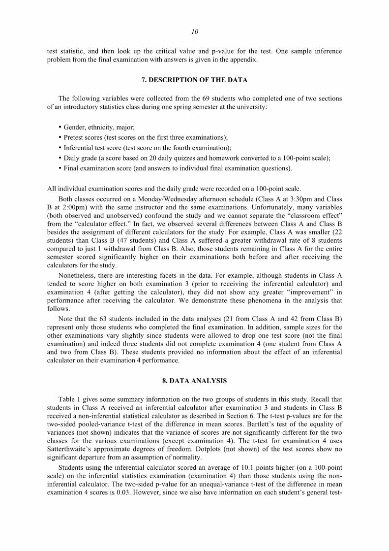
7. DESCRIPTION OF THE DATA

The following variables were collected from the 69 students who completed one of two sectionsof an introductory statistics class during one spring semester at the university:

• Gender, ethnicity, major;

• Pretest scores (test scores on the first three examinations);

• Inferential test score (test score on the fourth examination);

• Daily grade (a score based on 20 daily quizzes and homework converted to a 100-point scale);

• Final examination score (and answers to individual final examination questions).

All individual examination scores and the daily grade were recorded on a 100-point scale.

Both classes occurred on a Monday/Wednesday afternoon schedule (Class A at 3:30pm and ClassB at 2:00pm) with the same instructor and the same examinations. Unfortunately, many variables(both observed and unobserved) confound the study and we cannot separate the “classroom effect”from the “calculator effect.” In fact, we observed several differences between Class A and Class Bbesides the assignment of different calculators for the study. For example, Class A was smaller (22students) than Class B (47 students) and Class A suffered a greater withdrawal rate of 8 studentscompared to just 1 withdrawal from Class B. Also, those students remaining in Class A for the entiresemester scored significantly higher on their examinations both before and after receiving thecalculators for the study.

Nonetheless, there are interesting facets in the data. For example, although students in Class Atended to score higher on both examination 3 (prior to receiving the inferential calculator) andexamination 4 (after getting the calculator), they did not show any greater “improvement” inperformance after receiving the calculator. We demonstrate these phenomena in the analysis thatfollows.

Note that the 63 students included in the data analyses (21 from Class A and 42 from Class B)represent only those students who completed the final examination. In addition, sample sizes for theother examinations vary slightly since students were allowed to drop one test score (not the finalexamination) and indeed three students did not complete examination 4 (one student from Class Aand two from Class B). These students provided no information about the effect of an inferentialcalculator on their examination 4 performance.

8. DATA ANALYSIS

Table 1 gives some summary information on the two groups of students in this study. Recall thatstudents in Class A received an inferential calculator after examination 3 and students in Class Breceived a non-inferential statistical calculator as described in Section 6. The t-test p-values are for thetwo-sided pooled-variance t-test of the difference in mean scores. Bartlett’s test of the equality ofvariances (not shown) indicates that the variance of scores are not significantly different for the twoclasses for the various examinations (except examination 4). The t-test for examination 4 usesSatterthwaite’s approximate degrees of freedom. Dotplots (not shown) of the test scores show nosignificant departure from an assumption of normality.

Students using the inferential calculator scored an average of 10.1 points higher (on a 100-pointscale) on the inferential statistics examination (examination 4) than those students using the non-inferential calculator. The two-sided p-value for an unequal-variance t-test of the difference in meanexamination 4 scores is 0.03. However, since we also have information on each student’s general test-

11

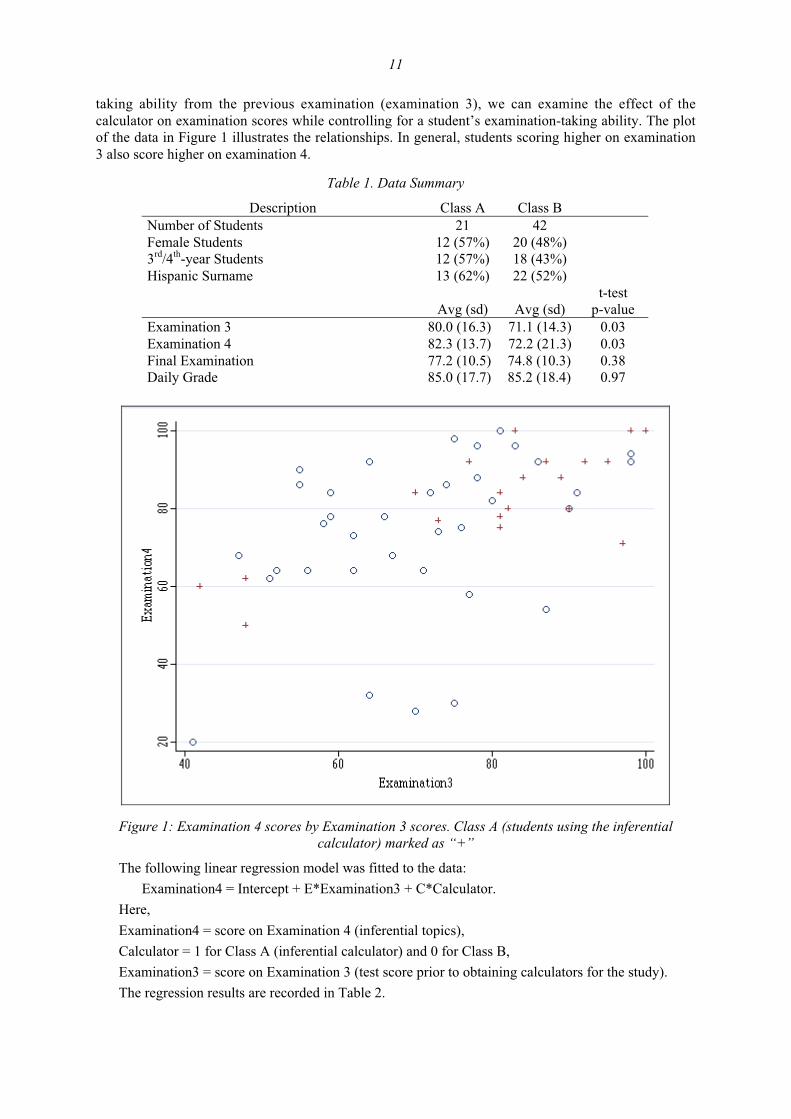
taking ability from the previous examination (examination 3), we can examine the effect of thecalculator on examination scores while controlling for a student’s examination-taking ability. The plotof the data in Figure 1 illustrates the relationships. In general, students scoring higher on examination3 also score higher on examination 4.

Table 1. Data Summary

Description Class A Class BNumber of Students 21 42Female Students 12 (57%) 20 (48%)3rd/4th-year Students 12 (57%) 18 (43%)Hispanic Surname 13 (62%) 22 (52%)

t-testAvg (sd) Avg (sd) p-value

Examination 3 80.0 (16.3) 71.1 (14.3) 0.03Examination 4 82.3 (13.7) 72.2 (21.3) 0.03Final Examination 77.2 (10.5) 74.8 (10.3) 0.38Daily Grade 85.0 (17.7) 85.2 (18.4) 0.97

Figure 1: Examination 4 scores by Examination 3 scores. Class A (students using the inferentialcalculator) marked as “+”

The following linear regression model was fitted to the data:

Examination4 = Intercept + E*Examination3 + C*Calculator.

Here,

Examination4 = score on Examination 4 (inferential topics),

Calculator = 1 for Class A (inferential calculator) and 0 for Class B,

Examination3 = score on Examination 3 (test score prior to obtaining calculators for the study).

The regression results are recorded in Table 2.

12

Table 2. Least squares regression results to estimate calculator effect while adjusting for priorexamination scores

Dependent Variable: examination4Coefficient Parameter

EstimateStandard

ErrorT for Ho:

Parameter=0P-Value:Prob > |T|

Intercept 33.640 12.210 2.76 0.008E (Examination3) 0.608 0.146 4.17 0.000C (Calculator) 2.690 4.716 0.57 0.571

R-Square = 28.34%

The examination 3 scores are, as expected, a strongly significant predictor of the averageexamination 4 score (p-value < 0.0001). However, once the model is adjusted for this measure ofexamination performance (examination 3 score), the type of calculator used is not at all statistically(or practically) significantly related to performance on the inferential statistics examination(examination 4). A similar analysis with the final examination score as the response variable indicatesno significant difference between the two groups of students either conditionally (adjusting forprevious scores on examination 3) or unconditionally (as already seen in Table 1 where the p-valuefor a t-test of the difference in average final examination scores was 0.38).

We should point out that, generally, there is a lot of variability in these data and even theexamination 3 scores only account for about 28% of the variability in examination 4 scores whenusing the linear regression model fit in Table 2. The relationship between examination 3 andexamination 4 scores appears fairly linear for both groups, but there is a lot of scatter in the data. Aplot of the residuals does not indicate the presence of a non-linear pattern.

To look further for any effect of the inferential calculator, we took a deeper look at students’performance on specific examination questions. See, for example, the sample final examinationquestion in the Appendix. In this question, Parts I, II, and V could be considered conceptual and III,IV, and VI calculations (with some overlap). We found that both classes had trouble with the“calculations” while at the same time answering “concept” questions fairly well.

9. DISCUSSION AND CONCLUSIONS

In general, we observed no difference between the two groups of students in their performance onexaminations on inferential topics in an introductory statistics course. In particular, use of aninferential calculator that performs many of the intermediate steps for calculating confidence intervalsand p-values does not appear to be related to student performance. The study size was small and thedesign did not allow for the separation of the “calculator effect” from the “classroom effect” (aconfounding factor). However, it is interesting to note that although Class A generally performedbetter on examinations prior to receiving inferential calculators for the study, these same students didnot perform significantly or practically better on inference topics after using the calculator. Theinferential calculator did not appear to give students any clear advantage (or disadvantage) in theirperformance on examinations. This study suggests that use of the inferential calculator needs to beexplored further as a benefit for student-learning in an introductory statistics courses. We encourageothers who may teach within an infrastructure that could allow a randomized experiment to completea study and share their results.

Of course, if the inferential calculator is required in an introductory statistics course, the instructorwould be able to spend much less time on computation and more time on gathering and analyzingreal-world data. Indeed, as classroom computer use has changed how statistics has been taught duringthe last 20 years (as computers have changed the practice of statistics), inferential calculators can alsochange how introductory statistics is taught.

13

ACKNOWLEDGEMENTS

This research was completed at the University of Texas at San Antonio.

REFERENCES

Campbell, P., & Stewart, E.L. (1993). Calculators and computers. In R. Jensen (Ed.), Early ChildhoodMathematics, NCTM Research Interpretation Project (pp. 251-268). New York: MacmillanPublishing Company.

Carlson, M. P. (1995). A successful transition to a calculator integrated college algebra curriculum:Clues, surveys, and trends. In P. Bogack (Managing Ed.), E. D. Fife, & L. Husch (Eds.),Proceedings of the Seventh Annual International Conference on Technology in CollegiateMathematics (pp. 73-77). Reading, MA: Addison-Wesley Publishing Group.

Cobb, G. W. (1993). Reconsidering statistics education: A National Science Foundation conference,Journal of Statistics Education, 1(1). [Online: www.amstat.org/publications/jse]

Demana, F., & Waits, B. K. (1990). Implementing the Standards: The role of technology in teachingmathematics, Mathematics Teacher, 83, 27-31.

Dunham, P. H. (1993). Does using calculators work? the jury is almost in. UME Trends, 5(2), 8-9.

Dunham, P. H. (1996). Looking for trends: What’s new in graphing calculator research? In P. Bogack(Managing Ed.), E. D. Fife, & L. Husch (Eds.), Proceedings of the Eighth Annual InternationalConference on Technology in Collegiate Mathematics (pp. 120-124). Reading, MA: AddisonWesley Publishing Company.

Dunham, P. H., & Dick, T. P. (1994). Research on graphing calculators. Mathematics Teacher, 87,440-445.

Fey, J. T., & Good, R. A. (1985). Rethinking the sequence and priorities of high school mathematicscurricula. In C. R. Hirsch & J. Zweng (Eds.), The secondary school mathematics curriculum,1985 yearbook (pp. 43-2). Reston, VA: National Council of Teachers of Mathematics.

Francis, B. (1997). Graphs of binomial and Poisson distributions on a graphical calculator. TeachingStatistics, 19(1), 24-25.

Garfield, J. (1995). How students learn statistics. International Statistical Review, 63(1), 25-34.

Gilchrist, W. (1986). Teaching statistics to the rest of humanity. In R. Davidson & J. Swift (Eds.),Proceedings of the Second International Conference on Teaching Statistics (pp. 494-497).Victoria, British Columbia, Canada: University of Victoria Conference Services.

Gnanadesikan, M., Scheaffer, R. L., Watkins, A. E., & Witmer, J. R. (1997). An activity-basedstatistics course. Journal of Statistics Education, 5(2).

Graham, A. (1996a). Following form with a graphic calculator. Teaching Statistics, 18(2), 52-55.

Graham, A. (1996b). The TI-83 and TI-92 calculators. Teaching Statistics, 18(3), 94-95.

Graham, A. T., & Thomas, M. O. J. (2000). Building a versatile understanding of algebraic variableswith a graphic calculator. Educational Studies in Mathematics, 41(3), 265-282.

Harvey, J. G., Waits, B. K., & Demana, F. D. (1995). The influence of technology on the teaching andlearning of algebra. Journal of Mathematical Behavior, 14, 75-109.

Hembree, R., & Dessart, D. J. (1986). Effects of hand-held calculators in precollege mathematicseducation: A meta-analysis. Journal for Research in Mathematics Education, 17, 83-89.

Hennesey, S., Fung, P., & Scanlon, E. (2001). The role of the graphic calculator in mediatinggraphing activity. Education in Science and Technology, 32, 267-290.

Hogg, R.V. (1992). Towards lean and lively courses in statistics. In F. Gordon & S. Gordon (Eds.),Statistics in the twenty-first century [MAA Notes No. 26] (pp. 3-13). Washington, DC:Mathematical Association of America.

14

Kemp, M., Kissane, B., & Bradley, J. (1998). Learning undergraduate statistics: The role of thegraphics calculator. In B. Parker (Ed.), Proceedings of the International Conference on theTeaching of Mathematics (pp. 176-178). Reading, MA: John Wiley and Sons, Inc.

Mittag, K. C., & Eltinge, E. (1998). Topics coverage in statistics courses: A national Delphi study.Research in the Schools, 5(1), 53-60.

Moore, D. S. (1992). Teaching statistics as a respectable subject. In F. Gordon, & S. Gordon (Eds.),Statistics in the Twenty-First Century [MAA Notes, No. 26] (pp. 14-25). Washington, DC:Mathematical Association of America.

Moore, D. S., Cobb, G. W., Garfield, J., & Meeker, W. (1995). Statistics education fin de siecle. TheAmerican Statistician, 49(3), 250-260.

Neter, J. (1989). Undergraduate statistics service courses in the years ahead. In J. Bolinger & R.Brookmejer (Eds.), American Statistical Association, 1989 Proceedings of the Section onStatistical Education (pp. 29-31). Alexandria, VA: American Statistical Association.

Pirie, W. R. (1989). Undergraduate statistics programs: Challenges for the 1990’s. In J. Bolinger & R.Brookmejer (Eds.), American Statistical Association 1989 Proceedings of the Section onStatistical Education (pp. 32-33). Alexandria, VA: American Statistical Association.

Quesada, A. R., & Maxwell, M. E. (1994). The effects of using graphing calculators to enhancecollege students’ performance in precalculus. Educational Studies in Mathematics, 27, 205-215.

Rinaman, W. C. (1998). Revising a basic statistics course, Journal of Statistics Education, 6(2).[Online: www.amstat.org/publications/jse]

Singer, J. D., & Willet, J. B. (1990). Improving the teaching of applied statistics: Putting the data backinto data analysis. The American Statistician, 44(3), 223-230.

LINDA BRANT COLLINS

Department of Statistics

University of Chicago

5734 S. University Ave

Chicago, IL 60637

United States of America

15

APPENDIX: FINAL EXAMINATION INFERENCE QUESTION WITH ANSWERSA statistics professor surveys 60 students and finds that 12 are left-handed. Use a 0.05 level of significance

to test the claim that these students come from a population in which the percentage of left-handed people isgreater than 10%.

Part I: What is the correct null and alternative?

a) H0: p ≤ 0.10 H1: p > 0.10

b) H0: p > 0.10 H1: p ≤ 0.10

c) H0: p = 0.10 H1: p ≠ 0.10

d) H0: p ≠ 0.10 H1: p = 0.10

e) none of these

Answer: a) H0: p ≤ 0.10 H1: p > 0.10

Part II: Which of the following is true?

a) This is a two-tailed test.

b) This is a left-tailed test.

c) This is a right-tailed test.

Answer: c) This is a right-tailed test.

Part III: What is the test statistic?

a) -1.94

b) -2.58

c) 2.58

d) 1.94

e) none of these

Answer: c) 2.58

Part IV: What is the critical value?

a) 1.645

b) 2.575

c) 1.96

d) none of these

Answer: a) 1.645

Part V: What is the conclusion?

a) There is not sufficient evidence to reject the claim

that the proportion is more than 0.10.

b) There is not sufficient evidence to support the claim


c) There is sufficient evidence to reject the claim


d) There is sufficient evidence to support the claim


e) none of these

Answer: d) There is sufficient evidence to support the

claim that the proportion is more than 0.10.

Part VI: What is the p-value for this problem?

a) 0.0049

b) 0.4951

c) 0.4738

d) 0.0262

e) none of these

Answer: a) 0.0049

16

FACTOR STRUCTURE OF THE“ATTITUDES TOWARD RESEARCH” SCALE6

ELENA C. PAPANASTASIOUIntercollege, [email protected]

SUMMARY

Students at the undergraduate level usually tend to view research methods courses negatively.However, an understanding of these attitudes is necessary to help instructors facilitate thelearning of research for their students, by enabling them to create more positive attitudes towardsuch courses. The aim of this study is to describe the development of an “attitudes towardresearch” scale and verify the dimensions of attitudes toward research among undergraduatestudents enrolled in introductory research courses. The basic hypothesis of this research study isthat the concept of attitudes is multidimensional in nature. The sample of the study consisted of226 students who had completed a research methods course. Based on a factor analysis, fivefactors of student attitudes toward research were identified. These were the factors of usefulnessof research, anxiety, affect indicating positive feelings about research, life relevancy of researchto the students’ daily lives, and difficulty of research.

Keywords: Statistics education research; Research methods; Quantitative research attitudes;Scale development; Factor structure; Attitudes toward research; Psychometrics

1. THEORETICAL FRAMEWORK

Students at the undergraduate university level, typically tend to view research-related courses withnegative attitudes and feelings. These negative attitudes have been documented in numerous studiesfor a number of years in relation to courses in research, statistics and mathematics (Adams &Holcomb, 1986; Elmore & Vasu, 1980; Wise, 1985). One of the main problems of these negativeattitudes is that they have been found to serve as obstacles to learning (Wise, 1985; Waters, Martelli,Zakrajsek, & Popovich, 1988). In turn, these negative attitudes have been found to be associated withpoor performance in such courses (Elmore, & Lewis, 1991; Woelke, 1991; Zeidner, 1991). Causalmodels, however, suggest that attitudes are actually mediators between past performance and futureachievement (Meece, Wigfield, & Eccles, 1990).

Prior research studies have found that negative attitudes toward a course (e.g., mathematics) havebeen found to explain a significant portion of the variance in student learning (Ma, 1995). In turn,these attitudes influence the amount of effort one is willing to expend on learning a subject, whichalso influences the selection of more advanced courses in similar areas (e.g., research and statisticscourses) beyond those of minimum requirements. Therefore, assessing students’ attitudes toward aresearch methods course is important in order to enable instructors to develop instructional techniquesleading to more positive attitudes toward the subject (Waters et al., 1988).

In a 1980 study, Roberts and Bilderback (1980) found that most students who take statistics arequite anxious. Once this preponderance of negative attitudes was revealed, many more surveyinstruments designed to measure university students’ attitudes toward statistics were developed(Dauphinee, Schau, & Stevens, 1997; Zeidner, 1991). One such instrument is the Survey of ‘AttitudesTowards Statistics’ (Schau et al., 1995), which is comprised of four dimensions, those of affect,cognitive competence, value, and attitudes about the difficulty of statistics. Another instrument



17

created for the same purpose was that of Attitudes Toward Statistics (Wise, 1985), which wasdesigned to measure two separate domains, student attitudes toward the course they were enrolled in,and student attitudes toward the usefulness of statistics in their field of study. The Statistical AnxietyRating Scale (Cruise et al., 1985) was designed to measure the value of statistics, the interpretation ofstatistical information, test anxiety, cognitive skills in statistics, fear of approaching the instructor andfear of statistics. Other similar instruments included the Statistics Attitude Survey (Roberts &Bilderback, 1980), and the Statistics Anxiety Inventory (Zeidner, 1991).

However, although a number of instruments that measure attitudes toward statistics already exist,they all differ in content and configuration (Dauphinee, 1993). For example, although someinstruments represent attitudes as a construct with six factors, others regard it as a unidimensionalconstruct which hypothesizes that no meaningful domains exist within attitudes (Roberts &Bilderback, 1980). The identification of the factors that form the structure of the student attitudestoward a research methods course may bear important theoretical and practical implications,especially due to the fact that this has never been examined before. For example, by identifying thesesubscales of attitudes, research methods instructors may include themselves in the process of learningresearch from a different angle. By using these domains, instructors may facilitate the learning ofresearch for their students, by enabling them to create more positive attitudes toward such courses.Therefore, the central aims of this study are to explore the multidimensional factor structure of the“Attitudes Toward Research” scale (ATR) and to examine its psychometric properties. Thisquestionnaire was developed by the author of this paper in the Fall of 2002, and the original versionconsisted of 56 items that were created on a Likert type scale. Based on the analysis of thepsychometric properties of this questionnaire that is presented in this paper, further refinements of thequestionnaire have been completed, and are presented in section 3. Although the questionnaire wasadministered in Greek, a translated version of the questionnaire is presented in English in theAppendix.

2. METHOD

2.1. SAMPLE

The data for this study were collected from students who had completed a compulsory andintroductory undergraduate course in ‘Methodology of Educational Research’ at the University ofCyprus. All the students in the sample were enrolled in the elementary or kindergarten educationmajor. This major is considered of very high esteem in Cyprus, and only the highest ability studentsare accepted into this major. Students from no other majors were obtained from the University sinceresearch methods courses are only required for students in the elementary and kindergarten educationmajor. The target population for this study included all students who had completed this course in aperiod of three years. This population would have consisted of about 450 students. Among the 226students who took part in the study, 98 (43.4%) completed the questionnaire on the last day of theirresearch methods course, while the remaining 56.6% also answered the questionnaire on the last dayof the semester, although they had completed the course one to four semesters earlier. Of the total 226students in the sample, 15.6% were male and the remaining 84.4% were female. Although there was adisproportionate number of females in the study, this was because there are generally more femalethan male students that choose to major in elementary or kindergarten education in Cyprus, and thebreakdown is not dissimilar to that usually holding in the group majoring in these subjects.

Of the complete sample, 36.9% were sophomores, 34.2% were juniors and 28.9% were seniors.All students who had attended the classes from which the data were collected, responded to thequestionnaire, and no non-responses were encountered.

The students were also asked to indicate their self reported level of socioeconomic status (SES),as well as the overall level of their parents’ education. Both questions were closed option questions,where the students had to select among four options (very high, high, average and low). In terms ofSES, only one student indicated that their level of SES was very high. There were 84.4% of thestudents that indicated that their SES level was average, 12.8% who indicated that their SES was high,

18

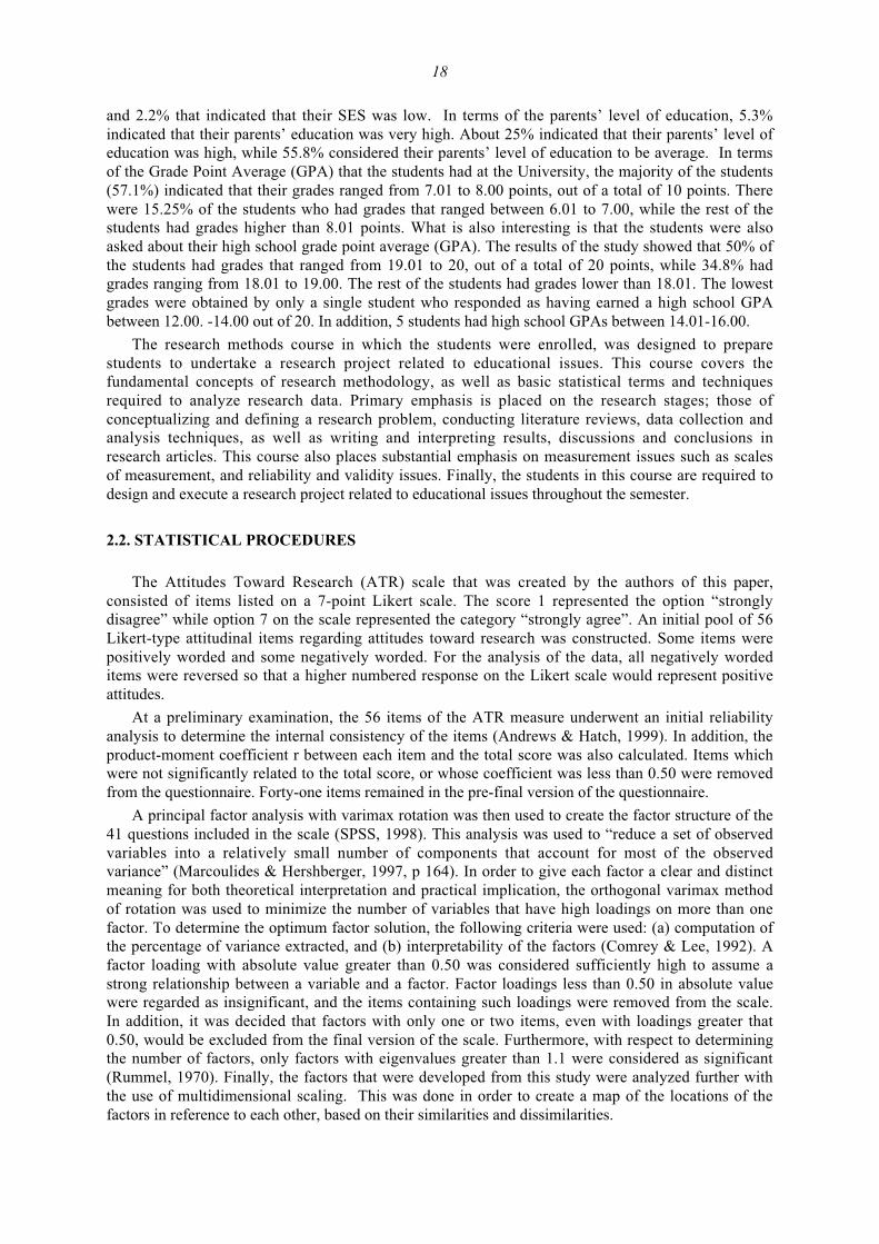
and 2.2% that indicated that their SES was low. In terms of the parents’ level of education, 5.3%indicated that their parents’ education was very high. About 25% indicated that their parents’ level ofeducation was high, while 55.8% considered their parents’ level of education to be average. In termsof the Grade Point Average (GPA) that the students had at the University, the majority of the students(57.1%) indicated that their grades ranged from 7.01 to 8.00 points, out of a total of 10 points. Therewere 15.25% of the students who had grades that ranged between 6.01 to 7.00, while the rest of thestudents had grades higher than 8.01 points. What is also interesting is that the students were alsoasked about their high school grade point average (GPA). The results of the study showed that 50% ofthe students had grades that ranged from 19.01 to 20, out of a total of 20 points, while 34.8% hadgrades ranging from 18.01 to 19.00. The rest of the students had grades lower than 18.01. The lowestgrades were obtained by only a single student who responded as having earned a high school GPAbetween 12.00. -14.00 out of 20. In addition, 5 students had high school GPAs between 14.01-16.00.

The research methods course in which the students were enrolled, was designed to preparestudents to undertake a research project related to educational issues. This course covers thefundamental concepts of research methodology, as well as basic statistical terms and techniquesrequired to analyze research data. Primary emphasis is placed on the research stages; those ofconceptualizing and defining a research problem, conducting literature reviews, data collection andanalysis techniques, as well as writing and interpreting results, discussions and conclusions inresearch articles. This course also places substantial emphasis on measurement issues such as scalesof measurement, and reliability and validity issues. Finally, the students in this course are required todesign and execute a research project related to educational issues throughout the semester.

2.2. STATISTICAL PROCEDURES

The Attitudes Toward Research (ATR) scale that was created by the authors of this paper,consisted of items listed on a 7-point Likert scale. The score 1 represented the option “stronglydisagree” while option 7 on the scale represented the category “strongly agree”. An initial pool of 56Likert-type attitudinal items regarding attitudes toward research was constructed. Some items werepositively worded and some negatively worded. For the analysis of the data, all negatively wordeditems were reversed so that a higher numbered response on the Likert scale would represent positiveattitudes.

At a preliminary examination, the 56 items of the ATR measure underwent an initial reliabilityanalysis to determine the internal consistency of the items (Andrews & Hatch, 1999). In addition, theproduct-moment coefficient r between each item and the total score was also calculated. Items whichwere not significantly related to the total score, or whose coefficient was less than 0.50 were removedfrom the questionnaire. Forty-one items remained in the pre-final version of the questionnaire.

A principal factor analysis with varimax rotation was then used to create the factor structure of the41 questions included in the scale (SPSS, 1998). This analysis was used to “reduce a set of observedvariables into a relatively small number of components that account for most of the observedvariance” (Marcoulides & Hershberger, 1997, p 164). In order to give each factor a clear and distinctmeaning for both theoretical interpretation and practical implication, the orthogonal varimax methodof rotation was used to minimize the number of variables that have high loadings on more than onefactor. To determine the optimum factor solution, the following criteria were used: (a) computation ofthe percentage of variance extracted, and (b) interpretability of the factors (Comrey & Lee, 1992). Afactor loading with absolute value greater than 0.50 was considered sufficiently high to assume astrong relationship between a variable and a factor. Factor loadings less than 0.50 in absolute valuewere regarded as insignificant, and the items containing such loadings were removed from the scale.In addition, it was decided that factors with only one or two items, even with loadings greater that0.50, would be excluded from the final version of the scale. Furthermore, with respect to determiningthe number of factors, only factors with eigenvalues greater than 1.1 were considered as significant(Rummel, 1970). Finally, the factors that were developed from this study were analyzed further withthe use of multidimensional scaling. This was done in order to create a map of the locations of thefactors in reference to each other, based on their similarities and dissimilarities.

19

3. RESULTS

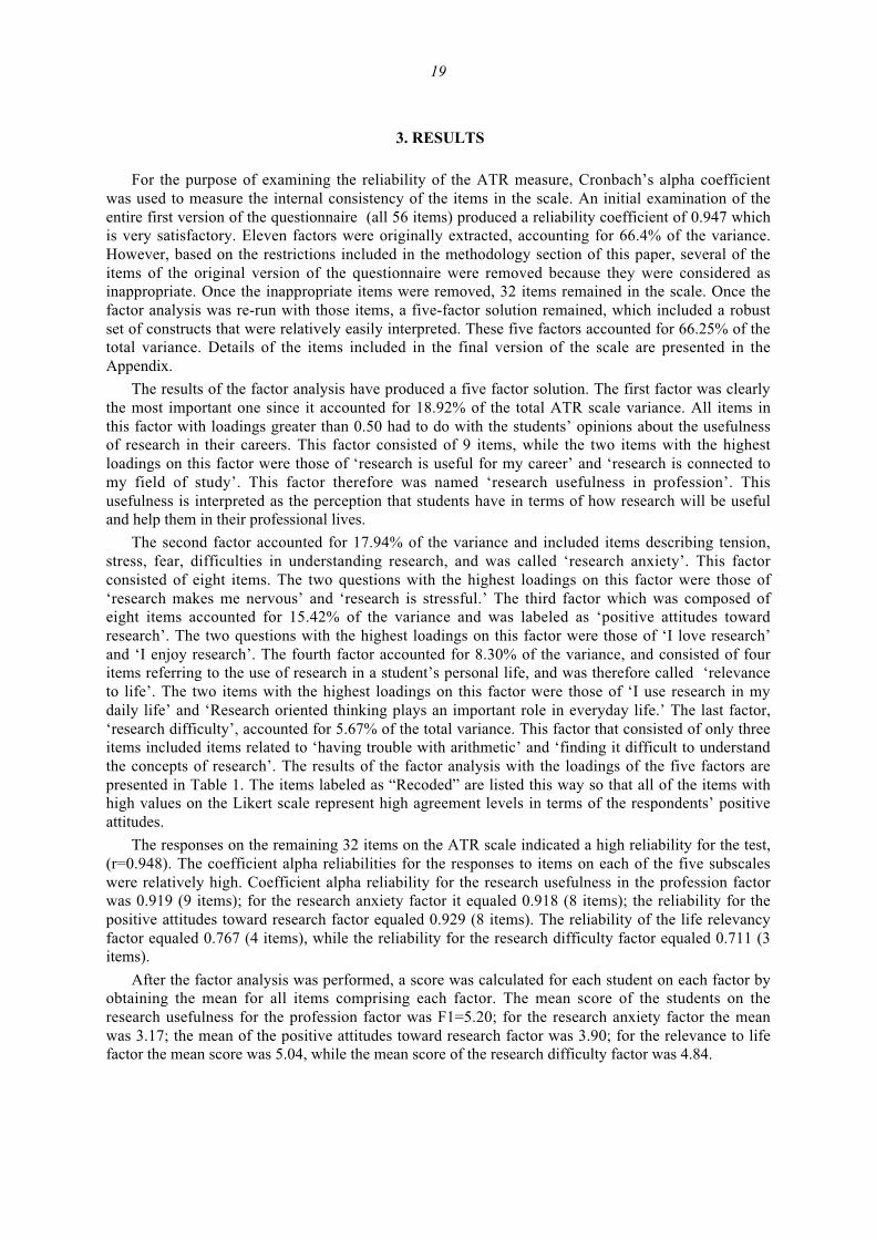
For the purpose of examining the reliability of the ATR measure, Cronbach’s alpha coefficientwas used to measure the internal consistency of the items in the scale. An initial examination of theentire first version of the questionnaire (all 56 items) produced a reliability coefficient of 0.947 whichis very satisfactory. Eleven factors were originally extracted, accounting for 66.4% of the variance.However, based on the restrictions included in the methodology section of this paper, several of theitems of the original version of the questionnaire were removed because they were considered asinappropriate. Once the inappropriate items were removed, 32 items remained in the scale. Once thefactor analysis was re-run with those items, a five-factor solution remained, which included a robustset of constructs that were relatively easily interpreted. These five factors accounted for 66.25% of thetotal variance. Details of the items included in the final version of the scale are presented in theAppendix.

The results of the factor analysis have produced a five factor solution. The first factor was clearlythe most important one since it accounted for 18.92% of the total ATR scale variance. All items inthis factor with loadings greater than 0.50 had to do with the students’ opinions about the usefulnessof research in their careers. This factor consisted of 9 items, while the two items with the highestloadings on this factor were those of ‘research is useful for my career’ and ‘research is connected tomy field of study’. This factor therefore was named ‘research usefulness in profession’. Thisusefulness is interpreted as the perception that students have in terms of how research will be usefuland help them in their professional lives.

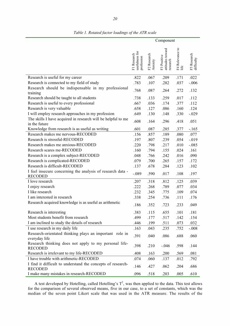
The second factor accounted for 17.94% of the variance and included items describing tension,stress, fear, difficulties in understanding research, and was called ‘research anxiety’. This factorconsisted of eight items. The two questions with the highest loadings on this factor were those of‘research makes me nervous’ and ‘research is stressful.’ The third factor which was composed ofeight items accounted for 15.42% of the variance and was labeled as ‘positive attitudes towardresearch’. The two questions with the highest loadings on this factor were those of ‘I love research’and ‘I enjoy research’. The fourth factor accounted for 8.30% of the variance, and consisted of fouritems referring to the use of research in a student’s personal life, and was therefore called ‘relevanceto life’. The two items with the highest loadings on this factor were those of ‘I use research in mydaily life’ and ‘Research oriented thinking plays an important role in everyday life.’ The last factor,‘research difficulty’, accounted for 5.67% of the total variance. This factor that consisted of only threeitems included items related to ‘having trouble with arithmetic’ and ‘finding it difficult to understandthe concepts of research’. The results of the factor analysis with the loadings of the five factors arepresented in Table 1. The items labeled as “Recoded” are listed this way so that all of the items withhigh values on the Likert scale represent high agreement levels in terms of the respondents’ positiveattitudes.

The responses on the remaining 32 items on the ATR scale indicated a high reliability for the test,(r=0.948). The coefficient alpha reliabilities for the responses to items on each of the five subscaleswere relatively high. Coefficient alpha reliability for the research usefulness in the profession factorwas 0.919 (9 items); for the research anxiety factor it equaled 0.918 (8 items); the reliability for thepositive attitudes toward research factor equaled 0.929 (8 items). The reliability of the life relevancyfactor equaled 0.767 (4 items), while the reliability for the research difficulty factor equaled 0.711 (3items).

After the factor analysis was performed, a score was calculated for each student on each factor byobtaining the mean for all items comprising each factor. The mean score of the students on theresearch usefulness for the profession factor was F1=5.20; for the research anxiety factor the meanwas 3.17; the mean of the positive attitudes toward research factor was 3.90; for the relevance to lifefactor the mean score was 5.04, while the mean score of the research difficulty factor was 4.84.

20

Table 1. Rotated factor loadings of the ATR scale

Component

F1 R

esea

rch

usef

ulne

ss f

orpr

ofes

sion

F2 R

esea

rch

Anx

iety

F3 P

ositi

veat

titud

es to

war

dre

sear

ch

F4 R

elev

ance

tolif

e

F5 R

esea

rch

diff

icul

ty

Research is useful for my career .822 .067 .209 .171 .022Research is connected to my field of study .783 .107 .282 .037 -.006Research should be indispensable in my professionaltraining

.768 .087 .264 .272 .132

Research should be taught to all students .738 .133 .259 .017 .112Research is useful to every professional .667 .036 .174 .377 .112Research is very valuable .658 .127 .086 .160 .124I will employ research approaches in my profession .649 .130 .148 .330 -.029The skills I have acquired in research will be helpful to mein the future

.608 .164 .296 .418 .051

Knowledge from research is as useful as writing .601 .087 .285 .377 -.165Research makes me nervous-RECODED .156 .857 .189 .080 .077Research is stressful-RECODED .197 .807 .239 .054 -.019Research makes me anxious-RECODED .220 .798 .217 .010 -.085Research scares me-RECODED .160 .794 .155 .024 .161Research is a complex subject-RECODED .048 .766 .242 .016 .090Research is complicated-RECODED .079 .700 .265 .157 .172Research is difficult-RECODED .137 .678 .284 .123 .102I feel insecure concerning the analysis of research data -RECODED

-.089 .590 .017 .108 .197

I love research .207 .318 .812 .125 .039I enjoy research .222 .268 .789 .077 .034I like research .232 .345 .775 .109 .074I am interested in research .338 .254 .736 .111 .176Research acquired knowledge is as useful as arithmetic

.186 .352 .723 .233 .049

Research is interesting .383 .115 .655 .101 .181Most students benefit from research .499 .177 .517 .142 .154I am inclined to study the details of research .446 .199 .511 .073 .032I use research in my daily life .163 .043 .235 .752 -.008Research-orientated thinking plays an important role ineveryday life

.391 .040 .086 .688 .060

Research thinking does not apply to my personal life-RECODED

.398 .210 -.046 .598 .144

Research is irrelevant to my life-RECODED .408 .163 .200 .569 .081I have trouble with arithmetic-RECODED .074 .060 .137 .012 .792I find it difficult to understand the concepts of research-RECODED

.146 .427 .062 .204 .686

I make many mistakes in research-RECODED .096 .518 .203 .005 .610

A test developed by Hotelling, called Hotelling’s T2, was then applied to the data. This test allowsfor the comparison of several observed means, five in our case, to a set of constants, which was themedian of the seven point Likert scale that was used in the ATR measure. The results of the

21

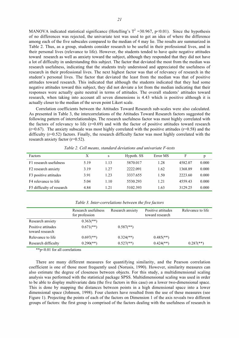
MANOVA indicated statistical significance (Hotelling’s T2 =30.967, p<0.01). Since the hypothesisof no differences was rejected, the univariate test was used to get an idea of where the differenceamong each of the five subscales compared to the median of 4 may lie. The results are summarized inTable 2. Thus, as a group, students consider research to be useful in their professional lives, and intheir personal lives (relevance to life). However, the students tended to have quite negative attitudestoward research as well as anxiety toward the subject, although they responded that they did not havea lot of difficulty in understanding this subject. The factor that deviated the most from the median wasresearch usefulness, indicating that the students truly understood and appreciated the usefulness ofresearch in their professional lives. The next highest factor was that of relevancy of research in thestudent’s personal lives. The factor that deviated the least from the median was that of positiveattitudes toward research. This indicated that although the students indicated that they had somenegative attitudes toward this subject, they did not deviate a lot from the median indicating that theirresponses were actually quite neutral in terms of attitudes. The overall students’ attitudes towardresearch, when taking into account all seven dimensions is 4.43 which is positive although it isactually closer to the median of the seven point Likert scale.

Correlation coefficients between the Attitudes Toward Research sub-scales were also calculated.As presented in Table 3, the intercorrelations of the Attitudes Toward Research factors suggested thefollowing pattern of interrelationships. The research usefulness factor was most highly correlated withthe factors of relevancy to life (r=0.69) and with the factor of positive attitudes toward research(r=0.67). The anxiety subscale was most highly correlated with the positive attitudes (r=0.58) and thedifficulty (r=0.52) factors. Finally, the research difficulty factor was most highly correlated with theresearch anxiety factor (r=0.52).

Table 2. Cell means, standard deviations and univariate F-tests

Factors X s Hypoth. SS Error MS F p

F1 research usefulness 5.19 1.13 5870.017 1.28 4582.07 0.000

F2 research anxiety 3.19 1.27 2222.091 1.62 1368.89 0.000

F3 positive attitudes 3.91 1.23 3337.655 1.50 2223.60 0.000

F4 relevance to life 5.04 1.10 5530.293 1.21 4559.43 0.000

F5 difficulty of research 4.84 1.21 5102.393 1.63 3129.25 0.000

Table 3. Inter-correlations between the five factors

Research usefulnessfor profession

Research anxiety Positive attitudestoward research

Relevance to life

Research anxiety 0.363(**)

Positive attitudestoward research

0.671(**) 0.587(**)

Relevance to life 0.697(**) 0.324(**) 0.485(**)

Research difficulty 0.290(**) 0.527(**) 0.424(**) 0.287(**)

**p<0.01 for all correlations

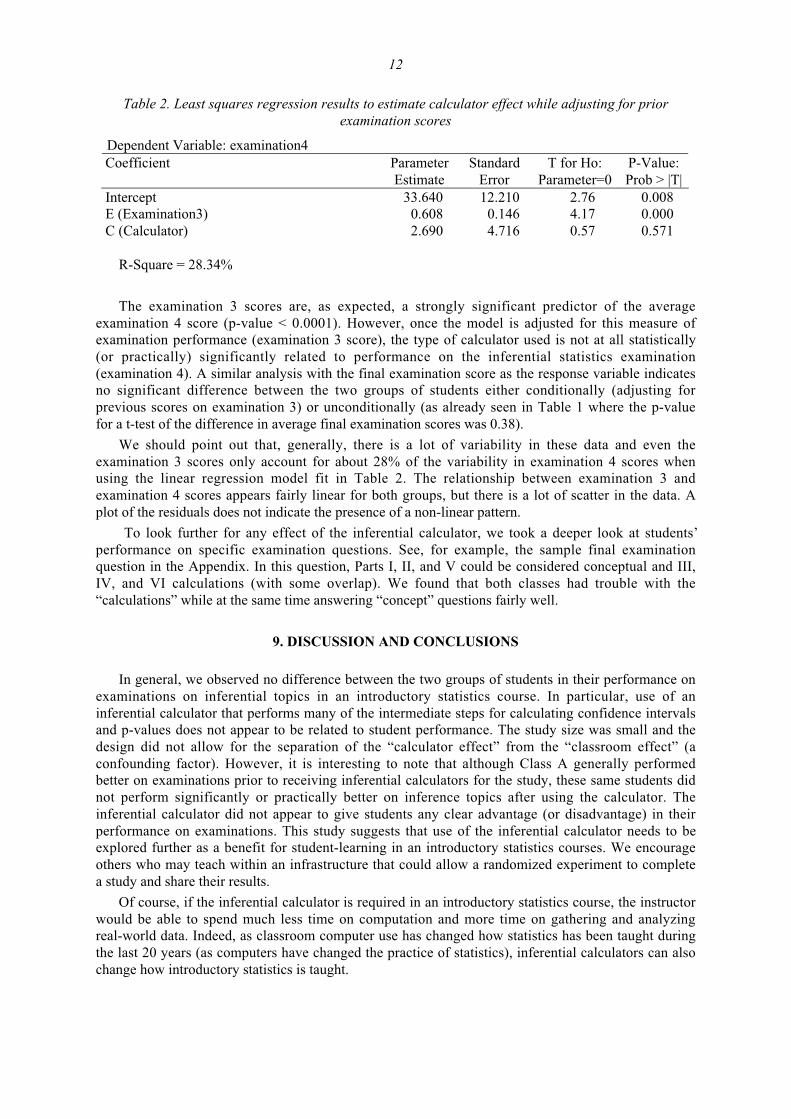
There are many different measures for quantifying similarity, and the Pearson correlationcoefficient is one of those most frequently used (Norusis, 1990). However, similarity measures canalso estimate the degree of closeness between objects. For this study, a multidimensional scalinganalysis was performed with the statistical package SPSS. Multidimensional scaling was used in orderto be able to display multivariate data (the five factors in this case) on a lower two-dimensional space.This is done by mapping the distances between points in a high dimensional space into a lowerdimensional space (Johnson, 1998). Four clusters have resulted from the use of these measures (seeFigure 1). Projecting the points of each of the factors on Dimension 1 of the axis reveals two differentgroups of factors: the first group is comprised of the factors dealing with the usefulness of research in

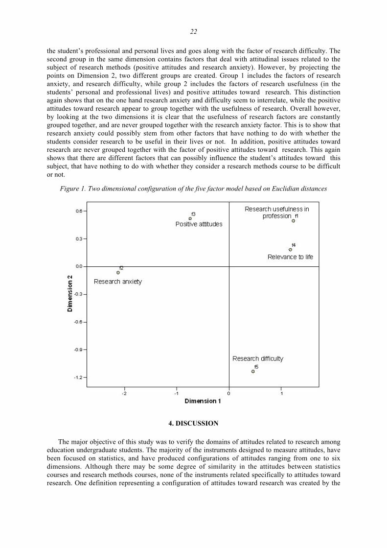
22

the student’s professional and personal lives and goes along with the factor of research difficulty. Thesecond group in the same dimension contains factors that deal with attitudinal issues related to thesubject of research methods (positive attitudes and research anxiety). However, by projecting thepoints on Dimension 2, two different groups are created. Group 1 includes the factors of researchanxiety, and research difficulty, while group 2 includes the factors of research usefulness (in thestudents’ personal and professional lives) and positive attitudes toward research. This distinctionagain shows that on the one hand research anxiety and difficulty seem to interrelate, while the positiveattitudes toward research appear to group together with the usefulness of research. Overall however,by looking at the two dimensions it is clear that the usefulness of research factors are constantlygrouped together, and are never grouped together with the research anxiety factor. This is to show thatresearch anxiety could possibly stem from other factors that have nothing to do with whether thestudents consider research to be useful in their lives or not. In addition, positive attitudes towardresearch are never grouped together with the factor of positive attitudes toward research. This againshows that there are different factors that can possibly influence the student’s attitudes toward thissubject, that have nothing to do with whether they consider a research methods course to be difficultor not.

Figure 1. Two dimensional configuration of the five factor model based on Euclidian distances

4. DISCUSSION

The major objective of this study was to verify the domains of attitudes related to research amongeducation undergraduate students. The majority of the instruments designed to measure attitudes, havebeen focused on statistics, and have produced configurations of attitudes ranging from one to sixdimensions. Although there may be some degree of similarity in the attitudes between statisticscourses and research methods courses, none of the instruments related specifically to attitudes towardresearch. One definition representing a configuration of attitudes toward research was created by the

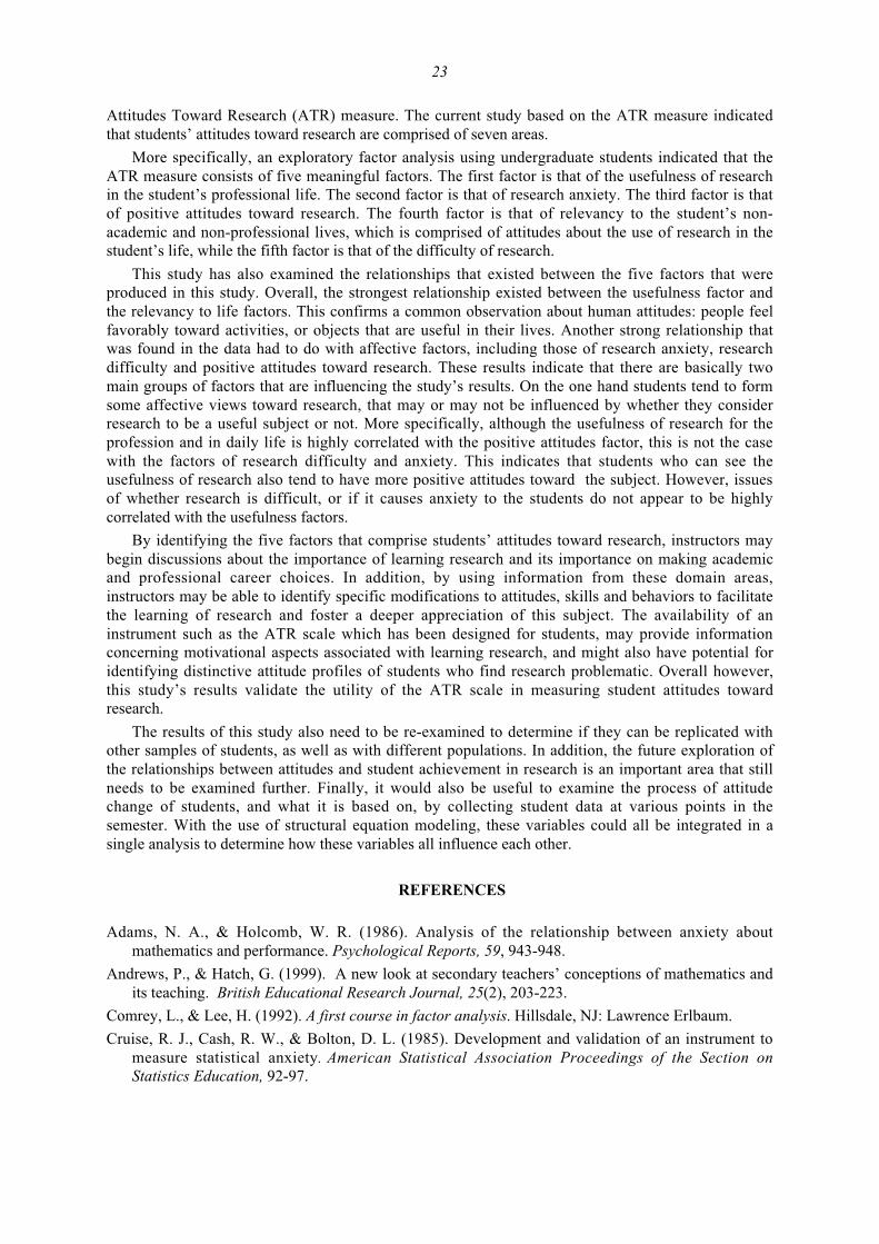
23

Attitudes Toward Research (ATR) measure. The current study based on the ATR measure indicatedthat students’ attitudes toward research are comprised of seven areas.

More specifically, an exploratory factor analysis using undergraduate students indicated that theATR measure consists of five meaningful factors. The first factor is that of the usefulness of researchin the student’s professional life. The second factor is that of research anxiety. The third factor is thatof positive attitudes toward research. The fourth factor is that of relevancy to the student’s non-academic and non-professional lives, which is comprised of attitudes about the use of research in thestudent’s life, while the fifth factor is that of the difficulty of research.

This study has also examined the relationships that existed between the five factors that wereproduced in this study. Overall, the strongest relationship existed between the usefulness factor andthe relevancy to life factors. This confirms a common observation about human attitudes: people feelfavorably toward activities, or objects that are useful in their lives. Another strong relationship thatwas found in the data had to do with affective factors, including those of research anxiety, researchdifficulty and positive attitudes toward research. These results indicate that there are basically twomain groups of factors that are influencing the study’s results. On the one hand students tend to formsome affective views toward research, that may or may not be influenced by whether they considerresearch to be a useful subject or not. More specifically, although the usefulness of research for theprofession and in daily life is highly correlated with the positive attitudes factor, this is not the casewith the factors of research difficulty and anxiety. This indicates that students who can see theusefulness of research also tend to have more positive attitudes toward the subject. However, issuesof whether research is difficult, or if it causes anxiety to the students do not appear to be highlycorrelated with the usefulness factors.

By identifying the five factors that comprise students’ attitudes toward research, instructors maybegin discussions about the importance of learning research and its importance on making academicand professional career choices. In addition, by using information from these domain areas,instructors may be able to identify specific modifications to attitudes, skills and behaviors to facilitatethe learning of research and foster a deeper appreciation of this subject. The availability of aninstrument such as the ATR scale which has been designed for students, may provide informationconcerning motivational aspects associated with learning research, and might also have potential foridentifying distinctive attitude profiles of students who find research problematic. Overall however,this study’s results validate the utility of the ATR scale in measuring student attitudes towardresearch.

The results of this study also need to be re-examined to determine if they can be replicated withother samples of students, as well as with different populations. In addition, the future exploration ofthe relationships between attitudes and student achievement in research is an important area that stillneeds to be examined further. Finally, it would also be useful to examine the process of attitudechange of students, and what it is based on, by collecting student data at various points in thesemester. With the use of structural equation modeling, these variables could all be integrated in asingle analysis to determine how these variables all influence each other.

REFERENCES

Adams, N. A., & Holcomb, W. R. (1986). Analysis of the relationship between anxiety aboutmathematics and performance. Psychological Reports, 59, 943-948.

Andrews, P., & Hatch, G. (1999). A new look at secondary teachers’ conceptions of mathematics andits teaching. British Educational Research Journal, 25(2), 203-223.

Comrey, L., & Lee, H. (1992). A first course in factor analysis. Hillsdale, NJ: Lawrence Erlbaum.

Cruise, R. J., Cash, R. W., & Bolton, D. L. (1985). Development and validation of an instrument tomeasure statistical anxiety. American Statistical Association Proceedings of the Section onStatistics Education, 92-97.

24

Dauphinee, T. L. (1993). The factor structure and gender factor invariance of an instrument to assessadult attitudes toward statistics. Unpublished doctoral dissertation, The University of NewMexico, Albuquerque, New Mexico.

Dauphinee, T. L., Schau, C., & Stevens, J. J. (1997). Survey of attitudes toward statistics: Factorstructure and factorial invariance for women and men. Structural Equation Modeling, 4(2), 129-141.

Elmore, P. B., & Vasu, E. S. (1980). Relationship between selected variables and statisticsachievement: Building a theoretical model. Journal of Educational Psychology, 46, 215-222.

Elmore, P. B., & Lewis, E. L. (1991, April). Statistics and computer attitudes and achievement ofstudents enrolled in applied statistics: Effect of computer laboratory. Paper presented at theannual meeting of the American Educational Research Association, Chicago, IL.

Johnson, D. E. (1998). Applied multivariate methods for data analysis. Pacific Grove, CA: DuxburyPress.

Ma, X. (1995). Factor structure of attitudes toward mathematics among high, average, and lowachieving high school senior students in the Dominican Republic. Focus on Learning Problems inMathematics, 17(4), 20-35.

Marcoulides, G. A., & Hershberger, S. L. (1997). Multivariate statistical methods: A first course.Mahwah, NJ: Lawrence Erlbaum Associates Publishers.

Meece, J. L., Wigfield, A., & Eccles, J. S. (1990). Predictors of math anxiety and its influence onyoung adolescents’ course enrollment intentions and performance in mathematics. Journal ofEducational Psychology, 82, 60-70.

Norusis, M. J. (1990). SPSS: Statistical data analysis. Chicago: SPSS Inc.

Roberts, D. M., & Bilderback, E. W. (1980). Reliability and validity of a statistics attitude survey.Educational and Psychological Measurement, 40, 235-238.

Rummel, R. J. (1970). Applied factor analysis. Evanston: Northwestern University Press.

Schau, C., Stevens, J., Dauphinee, T. L., & Del Vecchio, A. D. (1995). The development andvalidation of attitudes towards statistics. Educational and Psychological Measurement, 55(5),868-875.

SPSS, Inc. (1998). SPSS Base 8.0: Applications guide. Chicago, IL: Author.

Waters, L. K., Martelli, T. A., Zakrajsek, T., & Popovich, P. M. (1988). Attitudes toward statistics:An evaluation of multiple measures. Educational and Psychological Methods, 48, 513-516.

Wise, S. L. (1985) The development and validation of a scale measuring attitudes toward statistics.Educational and Psychological Measurement, 45, 401-405.

Woelke, P. L. (1991, April). An examination of the factor structure of Wise’s attitude toward statisticsscale. Paper presented at the annual meeting of the American Educational Research Association,Chicago, IL.

Zeidner, M. (1991). Statistics and mathematics anxiety in social science students: Some interestingparallels. British Journal of Educational Psychology, 61, 319-328.

ELENA C. PAPANASTASIOU

Intercollege, Cyprus

Mourouzi 7, #402

1055 Nicosia

Cyprus

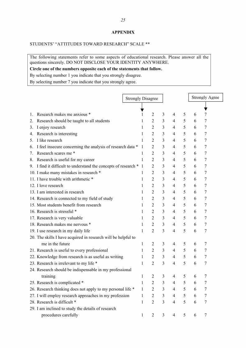
25

APPENDIX

STUDENTS’ “ATTITUDES TOWARD RESEARCH” SCALE **

The following statements refer to some aspects of educational research. Please answer all thequestions sincerely. DO NOT DISCLOSE YOUR IDENTITY ANYWHERE.

Circle one of the numbers opposite each of the statements that follow.

By selecting number 1 you indicate that you strongly disagree.

By selecting number 7 you indicate that you strongly agree.

1. Research makes me anxious * 1 2 3 4 5 6 7

2. Research should be taught to all students 1 2 3 4 5 6 7

3. I enjoy research 1 2 3 4 5 6 7

4. Research is interesting 1 2 3 4 5 6 7

5. I like research 1 2 3 4 5 6 7

6. I feel insecure concerning the analysis of research data * 1 2 3 4 5 6 7

7. Research scares me * 1 2 3 4 5 6 7

8. Research is useful for my career 1 2 3 4 5 6 7

9. I find it difficult to understand the concepts of research * 1 2 3 4 5 6 7

10. I make many mistakes in research * 1 2 3 4 5 6 7

11. I have trouble with arithmetic * 1 2 3 4 5 6 7

12. I love research 1 2 3 4 5 6 7

13. I am interested in research 1 2 3 4 5 6 7

14. Research is connected to my field of study 1 2 3 4 5 6 7

15. Most students benefit from research 1 2 3 4 5 6 7

16. Research is stressful * 1 2 3 4 5 6 7

17. Research is very valuable 1 2 3 4 5 6 7

18. Research makes me nervous * 1 2 3 4 5 6 7

19. I use research in my daily life 1 2 3 4 5 6 7

20. The skills I have acquired in research will be helpful to

me in the future 1 2 3 4 5 6 7

21. Research is useful to every professional 1 2 3 4 5 6 7

22. Knowledge from research is as useful as writing 1 2 3 4 5 6 7

23. Research is irrelevant to my life * 1 2 3 4 5 6 7

24. Research should be indispensable in my professional

training 1 2 3 4 5 6 7

25. Research is complicated * 1 2 3 4 5 6 7

26. Research thinking does not apply to my personal life * 1 2 3 4 5 6 7

27. I will employ research approaches in my profession 1 2 3 4 5 6 7

28. Research is difficult * 1 2 3 4 5 6 7

29. I am inclined to study the details of research

procedures carefully 1 2 3 4 5 6 7

Strongly AgreeStrongly Disagree

26

30. Research is pleasant 1 2 3 4 5 6 7

31. Research-orientated thinking plays an important

role in my daily life 1 2 3 4 5 6 7

32. Research is a complex subject * 1 2 3 4 5 6 7

* The items with an asterisk are items whose direction has been changed in the analysis.

** This version of the questionnaire has been translated to English from Greek.

27

“VARIATION-TALK”: ARTICULATING MEANING IN STATISTICS7

KATIE MAKARUniversity of Queensland, Australia

[email protected]

JERE CONFREYWashington University in St. Louis, U.S.A.

[email protected]

SUMMARY

Little is known about the way that teachers articulate notions of variation in their own words. Thestudy reported here was conducted with 17 prospective secondary math and science teachersenrolled in a preservice teacher education course which engaged them in statistical inquiry oftesting data. This qualitative study examines how these preservice teachers articulated notions ofvariation as they compared two distributions. Although the teachers made use of standardstatistical language, they also expressed rich views of variation through nonstandardterminology. This paper details the statistical language used by the prospective teachers,categorizing both standard and nonstandard expressions. Their nonstandard language revealedstrong relationships between expressions of variation and expressions of distribution.Implications and the benefits of nonstandard language in statistics are outlined.

Keywords: Statistical reasoning; Statistics education; Reasoning about variation and distribution;Mathematics education; Teacher education; Nonstandard language

Do not let calculations override common sense.

Moore & McCabe (1993, p. 121)

1. INTRODUCTION

Recently, researchers in statistics education have been calling for greater emphasis in schools ondeveloping students’ conceptions of variation (Moore, 1990; Shaughnessy, Watson, Moritz, &Reading, 1999; Pfannkuch & Begg, 2004). In addition, they argue that too much instruction instatistics has focused on performing statistical operations rather than developing students’ thinkingabout what makes sense. One approach to sense-making is through encouraging learners to expresstheir ideas in their own words (Noss & Hoyles, 1996). Russell and Mokros (1990) documentedteachers’ statistical thinking by attending to their ways of describing data using nonstandard statisticallanguage. Other research has also revealed that learners often articulate concepts of variation usingnonstandard language (e.g., Bakker, 2004; Reading, 2004); however these studies have notsystematically looked at ways that learners express notions of variation. Even less is known abouthow teachers express concepts of variation.

In other qualitative studies, we examined preservice secondary mathematics and science teachers’experiences making sense of data as they conducted technology-based investigations (Confrey,Makar, & Kazak, 2004; Makar, 2004; Makar & Confrey, submitted). This paper reports on anexploratory study of preservice teachers’ use of standard and nonstandard statistical language whendiscussing notions of variation. Below we first review the background for the present study, including



28

the conceptualization of variation, prior research on teachers’ and students’ knowledge of variation,and research needs regarding meaning construction and language use in statistics education.

2. REASONING ABOUT VARIATION

Although variation is a central component of understanding statistics, little is known about howchildren (and even less about how teachers) reason with, conceptualize, learn about, and expressnotions of variation. This section begins with a conceptual analysis of variation, then looks at recentresearch on developing teachers’ conceptions of variation, and finally turns to recent work on middleschool students’ reasoning in this area.

2.1. VARIATION AS A CONCEPTUAL ENTITY

Most uses of the term “variation” in research studies are taken to have a self-evident, commonsense meaning, and leave it undefined. Variation is closely linked to the concepts of variable anduncertainty. It is often regarded as a measurement of the amount that data deviate from a measure ofcenter, such as with the interquartile range or standard deviation. Variation encompasses more than ameasure, although measuring variation is an important component in data analysis. In consideringvariation, one must consider not just what it is (its definition or formula), or how to use it as a tool(related procedures), but also why it is useful within a context (purpose).

In simple terms, variation is the quality of an entity (a variable) to vary, including variation due touncertainty. “Uncertainty and variability are closely related: because there is variability, we live inuncertainty, and because not everything is determined or certain, there is variability” (Bakker, 2004,p. 14). While no one expects all five year-old children to be the same height, there is often difficultyunderstanding the extent to which children’s height vary, and that the variability of their heights is amixture of explained factors (e.g., the parents’ heights, nutrition) and chance or unexplained factors.

In this paper, we will not distinguish between reasoning about variability and reasoning aboutvariation, although Reading and Shaughnessy’s (2004, p. 202) definition of variation distinguishes itfrom variability:

The term variability will be taken to mean the [varying] characteristic of the entity that isobservable, and the term variation to mean the describing or measuring of that characteristic.Consequently, the following discourse, relating to “reasoning about variation,” will deal withthe cognitive processes involved in describing the observed phenomenon in situations thatexhibit variability, or the propensity for change.

We would argue that developing the concept of variation, beyond just an acknowledgement of itsexistence, requires some understanding of distribution. In examining a variable in a data set, one isoften interested in uncovering patterns in the variability of the data (Bakker, 2004), for example byrepresenting the ordered values of the variable in a graph. The distribution, then, becomes a visualrepresentation of the data’s variation and understanding learners’ concept of variation becomesclosely linked to understanding their concept of distribution. A key goal in developing students’reasoning about distributions is assisting them in seeing a distribution as an aggregate with its owncharacteristics (such as its shape or its mean) rather than thinking of a distribution as a collection ofindividual points (Hancock, Kaput, & Goldsmith, 1992; Konold & Higgins, 2002; Marshall, Makar,& Kazak, 2002; Bakker, 2004).

In thinking about what the notion of distribution entails, one might think of the associatedmeasures, properties, or characteristics of a distribution—for example, its mean, shape, outliers, orstandard deviation. These entities in isolation, however, do not capture the desired concept and canaggravate the focus on individual points. In addition, they lack the idea that we want to capture adistribution of something. Pfannkuch, Budgett, Parsonage, and Horring (2004) cautioned that studentsoften focus on characteristics of a distribution, but forget to focus on the meaning of the distribution

29

within the context of the problem. In comparing distributions, for example, they suggested thatstudents should first look at the distributions and compare centers, spread, and anything noteworthy,but then should be asked to draw an evidence-based conclusion, using probabilistic rather thandeterministic language, based on their observations.

2.2. TEACHERS’ REASONING ABOUT VARIATION

Teachers’ mind-set and conceptions about data have been of great concern in the researchcommunity for over a decade (Hawkins, 1990; Shaughnessy, 1992). Despite this, Shaughnessy (2001)reports, “[I am] not aware of any research studies that have dealt specifically with teachers’conceptions of variability, although in our work teaching statistics courses for middle school andsecondary school mathematics teachers we have evidence that many teachers have a knowledge gapabout the role and importance of variability.”

Three very recent research projects have focused specifically on teachers’ notions of variation anddistribution. Hammerman and Rubin (2004) report on a study of a two-year professional developmentproject that gave secondary teachers an opportunity to analyze data with a new data visualization tool.The software Tinkerplots™ (Konold & Miller, 2004) allows learners to create their own datarepresentations through sorting, ordering, and stacking data. They found that teachers did not chooseto use measures of center in comparing distributions even though those measures were readilyavailable in the software, but rather chose to compare groups by comparing slices and subsets ofdistributions to support compelling arguments with data. In addition, Hammerman and Rubin notedthat teachers were dissatisfied with representations such as histograms and box plots that would hidethe detail of the underlying distribution. From their study, we can begin to see the potential that newvisualization tools have for helping teachers to construct their own meaning of statistical concepts.

In another study, Canada (2004) created a framework to investigate prospective elementaryteachers’ expectation, display, and interpretation of variation within three statistical contexts: repeatedsampling, data distributions, and probability outcomes. His study took place in a preservicemathematics course developed to build the teachers’ content knowledge of probability and statisticsthrough activities that emphasized hands-on experiments involving chance and computer-generateddata simulations. Canada’s study found that initially, although the prospective teachers had a goodsense of center, they found it difficult to predict realistic spreads in distributions from collected dataor produced from random sampling and probability experiments. Their predictions for underlyingdistributions included expectations of way too little variation, overly extreme variation, orunrealistically symmetrical distributions. In addition, many of the teachers took an initial stance that‘anything goes’ in random experiments and felt that they could therefore make no judgment about thedistribution of outcomes. After the course, the teachers demonstrated stronger intuitions aboutvariation - their predictions were much more realistic and their expectation of variation morebalanced. In addition, the teachers’ descriptions of distributions were more rich and robust in theirrecognition of variation and distribution as an important concept, for example by referencing how thedistributions were clustered, spread, concentrated, or distributed. Canada’s study hints at a potentiallink between the elements that teachers focus on when describing distributions and their intuitionabout variation and uncertainty in data.

In previous research on statistical inquiry with practicing middle school teachers, we found thatteachers, like their students, often begin examining data distributions by focusing on individual points(Confrey & Makar, 2002). Yet in a meaningful context (e.g., student test scores), the teachers in ourstudy constructed a need for examining variation in a distribution by initiating a discussion of how thedistribution of students’ abilities affected their choice of instructional strategies. We noticed,however, that when the teachers did not adequately construct more complex concepts, like samplingdistributions, they would tend to use statistical tools mechanically, without carefully examining theirrelationship to the data (Makar & Confrey, 2004).

In summary, although much concern has been expressed about the over-emphasis on proceduresin teaching statistics, the studies described above highlight some important ways to improve whatShaughnessy (1992) calls teachers’ lack of intuition about stochastics. The main ideas these studies

30

bring out is that teachers themselves need to learn statistical concepts in an environment much like theone recommended for students – one that is active, technology-rich, involving authentic data, andoffering plenty of opportunities to build their conceptions through experiences with data. Particularsabout how teachers build these conceptions still needs further research.

2.3. STUDENTS’ REASONING ABOUT VARIATION

It is useful to briefly review research on students’ development of concepts of variation, as it mayprovide insight into potential ways to build teachers’ conceptions of variation. First, teachersfrequently possess similar reasoning to their students (Hammerman & Rubin, 2004; McClain, 2002).Second, understanding students’ conceptions of variation can help teachers to plan instruction.Finally, the research in this area has uncovered new insights into students’ intuitions about variationwithout formal procedures and terminology. These insights may provide ideas for new methods ofprofessional development for teachers.

A common thread in the research on teaching concepts of variation and distribution is arecommendation to focus not only on the characteristics of distributions, but on their purpose. A well-documented approach to this is through comparing groups (see for example, Cobb, 1999; Watson &Moritz, 1999; Biehler, 1997; Makar & Confrey, 2004; Hammerman & Rubin, 2004). Pfannkuch et al.(2004) found that the descriptions of distributions given by secondary students sometimes includedcharacteristics of the distribution that were disconnected from the context or meaning of the problem.For example, when taking note of the variability of the data, half of the students compared the ranges,which was not relevant to their question, and most of the students focused on comparing measures ofcenter or extremes. Pfannkuch and her colleagues hypothesized that the instruction the studentsreceived focused not on drawing meaningful conclusions, but rather on comparing features of the boxplot. They recommended that instruction concentrate not on how to compare centers, but why oneshould do so. Reading and Shaughnessy (2004) also found that tasks which asked students not just fordescriptive information but also for explanations offered greater possibilities for insight into students'reasoning about variation.

In developing students’ conception of statistics, Konold and Pollatsek (2002) argue that “thecentral idea should be that of searching for a signal and that the idea of distribution comes into betterfocus when it is viewed as the ‘distribution around’ a signal” (p. 262). Bakker and Gravemeijer (2004)on the other hand hold that “reasoning with shapes forms the basis for reasoning about distributions”(p. 149). By developing a lens of seeing the distribution as an entity, one can then look at statisticalmeasures as characteristics of the distribution rather than as calculations from individual points(Bakker, 2004).

Bakker (2004; Bakker & Gravemeijer, 2004) also found that with Cobb’s Minitool software andan innovative learning trajectory he was able to encourage his middle school students to think aboutvariation and towards a distribution-view of data. Initial discussions with students focused on themiddle “bump” of the distribution, but later the “bump” came to represent the whole distribution.Konold and his colleagues (2002), who studied middle school students, emphasized that in problemsolving with data, the middle bump was a frequently identified portion of a mound-shapeddistribution, and termed this central bump a modal clump. Bakker (2004) also found that rather thanjust focusing on the central region of a distribution, students also tend to divide distributions into threecategories: low, middle, and high. Hammerman and Rubin (2004) saw the teachers in their study takea similar tactic in comparing distributions. These findings may indicate that dividing distributions intothree pieces may be a more natural way for students to examine a distribution than by dividing it intofour sections, as in the box plot.

The studies reported above suggest that if learners are provided with relevant contexts, concreteexperiences, complex tasks, adequate time and support, and appropriate tools to build statisticalconcepts, then their understanding appears to be much more robust. One notable common feature ofthese studies is that they developed learners’ notions of variation through constructing a purpose forvariation, often building on the learners’ own language for describing and interpreting what they wereseeing.

31

3. CONCEPT DEVELOPMENT

Below we briefly discuss some aspects of how learners construct meaning of data as well asissues surrounding the use of learners’ everyday or nontechnical terminology. These issues affectedthe design of the present study and the lens we used to interpret prospective teachers’ articulation ofvariation. The need to refer both to standard statistical terminology and to nonstandard ornontechnical statistical terminology arises because one cannot assume that if a respondent can repeatthe definition of a concept, she has necessarily assimilated this concept. For example, although astudent may be taught the concept and formula for standard variation and can even use this term aspart of class discourse, this does not imply that they are “seeing” variation in what is being measured.

3.1. CONSTRUCTING MEANING

Because students are frequently taught definitions and procedures without first developing theirown intuition and meaning about the concepts underlying them, premature instruction of formalterminology and rules can inhibit students’ own sense-making (Flyvbjerg, 2001; Schoenfeld, 1991;Boaler, 1997). Formal mathematical procedures, terminology, and symbolism are critical fordeveloping advanced levels of mathematical understanding in that they can provide efficient paths toproblem-solving, focus attention on particular aspects of a problem, and open new levels ofunderstanding of the concepts represented by the terms or symbols. However, the emphasis must beon building meaning, not simply assuming that standard procedures or terms can themselves carry themeanings of underlying concepts.

Shaughnessy (1992) notes that students’ and teachers’ lack of intuition about stochastics is acritical barrier to improved teaching and learning in statistics. Fischbein’s (1987) description ofintuition matches well with the kind of thinking that we believed should be developed in teachers.

Intuitions are always the product of personal experience, of the personal involvement of theindividual in a certain practical or theoretical activity. Only when striving to cope activelywith certain situations does one need such global, anticipatory, apparently self-consistentrepresentations. The development of … intuitions implies, then, didactical situations in whichthe student is asked to evaluate, to conjecture, to predict, to devise, and check solutions. Inorder to develop new, correct probabilistic intuitions, for instance, it is necessary to createsituations in which the student has to cope, practically, with uncertain events (p. 213, italics inoriginal).

For building intuition, Fischbein further argues that the role of visualization “is so important that veryoften intuitive knowledge is identified with visual representations” (p. 103). Insight can also be gainedinto learners’ sense-making by focusing on how they use their own words to explain relationships,constructs, and processes (Noss & Hoyles, 1996). One might infer from these last three quotes thatintuition in statistics is built through the development of visualization, articulation, and representationof data distributions within personally compelling contexts. Intuition about variation, then, may befostered through a lens of “seeing variation” (Watkins, Scheaffer, & Cobb, 2003, p. 10), or Moore’s(1990) acknowledgement of the omnipresence of variation. These insights may be gained throughattending to students’ own words for describing what they are seeing. These words are often lesstechnical and contain elements of nonstandard language.

3.2. NONSTANDARD LANGUAGE USE

Noss and Hoyles (1996) state that focusing on mathematical meaning moves us to consider howlearners express mathematics rather than how they learn it. The difference is in the locus of theconcept. If we focus on how students learn statistics, it implies that statistical concepts areontologically fixed and that the goal of learning is to impart a priori knowledge from teacher to

32

student. However, by turning that around to foster learners’ dynamic conceptions of statisticalconcepts, we acknowledge that these concepts are not passively received, but rather are actively andsocially constructed by the individual.

Developing understanding oftentimes requires the use of nonstandard terminology. Unfortunately,when students do use their own language to make meaning, teachers often do not recognizenonstandard ways of talking (Lemke, 1990). Biehler (1997) attributes some of the difficulty incommunicating and understanding relationships in data to the lack of formal language we have indescribing distributions beyond the level of statistical summaries:

The description and interpretation of statistical graphs and other results is also a difficultproblem for interviewers and teachers. We must be more careful in developing a language forthis purpose and becoming aware of the difficulties inherent in relating different systems ofrepresentation. Often, diagrams involve expressing relations of relations between numbers. Anadequate verbalization is difficult to achieve and the precise wording of it is often critical.There are profound problems to overcome in interpreting and verbally describing statisticalgraphs and tables that are related to the limited expressability of complex quantitative relationsby means of common language (p. 176).

Biehler’s work implies that the current focus on statistical summaries in describing distributions isinadequate and that research needs to be improved in the area of developing statistical language forinterpreting more robust relationships in data.

4. DESIGN AND METHODOLOGY

4.1. APPROACH

This exploratory study was designed to gain insight into the ways that prospective secondarymathematics and science teachers express or discuss notions of variation when engaged in apurposeful statistical task. Based on the literature reviewed, it was anticipated that respondents willuse standard or conventional descriptions and terms, as well as nonstandard descriptions and informallanguage, and the goal of the study was to document the different types of language used.Respondents were interviewed twice using an identical task, in the first and last week of a fifteen-week preservice course on assessment, which included an embedded component of exploratory dataanalysis. The task given during the interview asked teachers to compare two distributions of datarelevant to the context of teaching, in terms of the relative improvement in test scores of two groupsof students.

Although interviews were conducted at the beginning and end of the course, the purpose of thestudy was not to evaluate the effectiveness of the course or to compare performance before and afterinstruction. Some comparisons will be made of language use before and after the course, but given thesmall number of respondents, these comparisons should be interpreted with caution. The primaryinterest was in categorizing and describing the language respondents use to describe variation in thedata. Any change that may have occurred in respondents’ language use simply enriched and extendedthe range of responses available for analysis.

4.2. SUBJECTS

The respondents for the study were secondary mathematics and science preservice teachers at alarge university in the southern United States enrolled in an innovative one-semester undergraduatecourse on assessment designed and taught by the authors (Confrey et al., 2004). Twenty-two studentsbegan the course, but four withdrew from the course before the end of the semester. In addition, somedata from one subject was lost due to technical malfunction, leaving seventeen subjects with acomplete set of data. The seventeen subjects ranged in age from 19 to 42, with ten students of

33

traditional college age (19-22), five aged 23-29, and two students over 30 years of age. Of these, threewere male and fourteen female, nine were mathematics majors and eight were science majors(predominantly biology). About 60% of the class was Anglo, with the remaining students being ofHispanic and African-American ancestry. The students had varying backgrounds in statistics: eighthad not previously studied statistics, while five had previously taken a traditional university-basedstatistics course either in the mathematics department or in a social science department. Theremaining four had not taken a formal course, but had previous experience in statistics as a topic inone of their mathematics or science courses.

4.3. SETTING

The study took place at the beginning and end of a one-semester course that integrated ideas ofassessment, data analysis, equity, and inquiry—themes identified as critical but missing frompreservice education (National Research Council, 1999; 2000; 2001). The purpose of the course wasto give the preservice teachers some background in classroom and high-stakes assessment, developtheir statistical reasoning, gain experience using technological tools to interpret student assessmentresults, and to introduce them to issues of equity through examining data. In the final month of thecourse, the prospective teachers conducted their own data-based inquiry into an issue of equity inassessment.

The prospective teachers were guided through several investigations that built an atmosphere ofinterpretation of data rather than the development of formal theoretical foundations. The inclusion ofthe dynamic statistical software Fathom™ (Finzer, 2001) was critical as a learning tool rather than atraditional statistical package aimed at statisticians and statistics students. The statistical content of thecourse was comprised of an overview of data graphing (histograms, box plots, dot plots), descriptivestatistics (mean, median, standard deviation, interquartile range, distribution shapes), linear regression(association, correlation, least-squares, residuals), and a brief introduction to sampling distributionsand inference (through building of simulations). The statistical content was developed as a set of toolsto gain insight into data rather than as isolated topics.

4.4. INTERVIEW TASK AND PROCEDURE

Respondents were interviewed by the first author during the first and last week of the course,using the same task in both interviews. Most interviews lasted between ten and twenty minutes. Thetask was set in the context of an urban middle school trying to determine the effectiveness of asemester-long mathematics remediation program (called ‘Enrichment’) for eighth-grade (13-14 yearsold) students considered in need of extra help preparing for the state exam given each spring. Todecide if the Enrichment program was working, the school compared student scores from theirseventh grade state exam score in mathematics to their scores on a practice test given near the end ofeighth grade. Respondents were shown a pair of dot plots (Figure 1) of authentic data taken fromstudents in an Enrichment class (upper distribution) and a regular eighth grade class (lowerdistribution). Respondents were asked initially to compare the relative improvement of students in thetwo groups, and then were probed if their responses needed clarification. It is important to note thatthe data in Figure 1 represent the change (difference) in scores between the two assessments, i.e.numbers on the x-axis are positive when scores improved, and negative when scores declined. (Datapoints in red (shaded dots) highlighted those students classified as economically disadvantaged; thiswas used for another question in the interview related to equity but not pertinent for this study.)

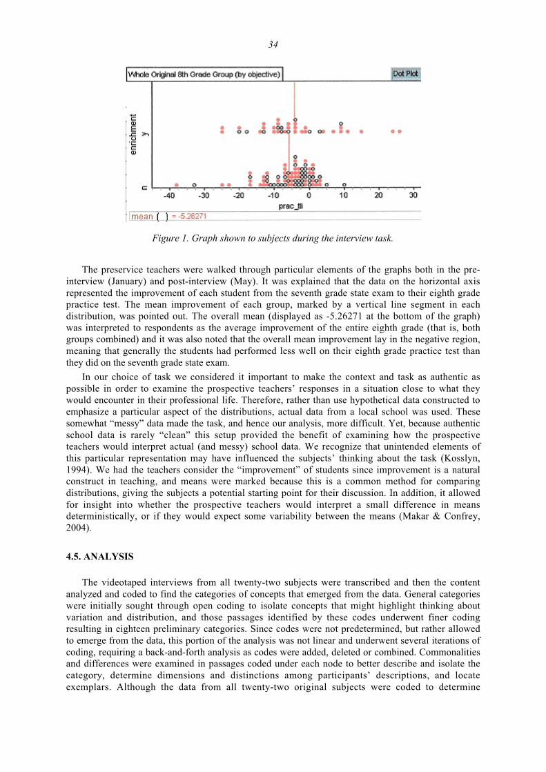
34

Figure 1. Graph shown to subjects during the interview task.

The preservice teachers were walked through particular elements of the graphs both in the pre-interview (January) and post-interview (May). It was explained that the data on the horizontal axisrepresented the improvement of each student from the seventh grade state exam to their eighth gradepractice test. The mean improvement of each group, marked by a vertical line segment in eachdistribution, was pointed out. The overall mean (displayed as -5.26271 at the bottom of the graph)was interpreted to respondents as the average improvement of the entire eighth grade (that is, bothgroups combined) and it was also noted that the overall mean improvement lay in the negative region,meaning that generally the students had performed less well on their eighth grade practice test thanthey did on the seventh grade state exam.

In our choice of task we considered it important to make the context and task as authentic aspossible in order to examine the prospective teachers’ responses in a situation close to what theywould encounter in their professional life. Therefore, rather than use hypothetical data constructed toemphasize a particular aspect of the distributions, actual data from a local school was used. Thesesomewhat “messy” data made the task, and hence our analysis, more difficult. Yet, because authenticschool data is rarely “clean” this setup provided the benefit of examining how the prospectiveteachers would interpret actual (and messy) school data. We recognize that unintended elements ofthis particular representation may have influenced the subjects’ thinking about the task (Kosslyn,1994). We had the teachers consider the “improvement” of students since improvement is a naturalconstruct in teaching, and means were marked because this is a common method for comparingdistributions, giving the subjects a potential starting point for their discussion. In addition, it allowedfor insight into whether the prospective teachers would interpret a small difference in meansdeterministically, or if they would expect some variability between the means (Makar & Confrey,2004).

4.5. ANALYSIS

The videotaped interviews from all twenty-two subjects were transcribed and then the contentanalyzed and coded to find the categories of concepts that emerged from the data. General categorieswere initially sought through open coding to isolate concepts that might highlight thinking aboutvariation and distribution, and those passages identified by these codes underwent finer codingresulting in eighteen preliminary categories. Since codes were not predetermined, but rather allowedto emerge from the data, this portion of the analysis was not linear and underwent several iterations ofcoding, requiring a back-and-forth analysis as codes were added, deleted or combined. Commonalitiesand differences were examined in passages coded under each node to better describe and isolate thecategory, determine dimensions and distinctions among participants’ descriptions, and locateexemplars. Although the data from all twenty-two original subjects were coded to determine

35

categories, dimensions, and exemplars, only the seventeen subjects with complete data sets (both pre-and post-interviews) were used in quantitative descriptions.

5. RESULTS

In this section we first overview key categories of standard terms and concepts that therespondents, prospective teachers, used when comparing distributions. Next, categories ofnonstandard language and terms are described, referring to two separate but overlapping areas:variation (e.g., spread) and distribution (e.g., low-middle-high, modal clumps). We later refer to thesetwo types of non-standard categories as “variation-talk”. Finally, relationships found within andbetween the categories of standard and nonstandard language categories will be summarized. Asexplained, the primary goal of the study is to provide a rich description of prospective teachers’language when discussing variation; hence, the information from the January and May interviews isusually combined. Changes in respondents’ articulations from the first interview to the interviewconducted after the course are noted as well but should be interpreted with caution in light of thesmall number of respondents and other factors noted later.

5.1. STANDARD STATISTICAL LANGUAGE

This subsection describes the conventional statistical language used by the respondents. Table 1summarizes the percentage of respondents articulating each category of standard statistical terms anddescriptions in their responses. As can be seen in the table, multiple types of standard expressionswere used by respondents (i.e., percentages sum to more than 100%) and overall, nearly every subjectincluded at least one type of standard statistical description in their response (94% in January and allrespondents in May). Most respondents included the proportion (or number) improved or the mean intheir descriptions and the inclusion of standard statistical terms in their responses increased in allcategories by the end of the course.

Table 1. Percentage of respondents using standard statistical language (N=17)

Category January May

Proportion or number improved 59% 65%

Mean 53% 88%

Maximum/Minimum 29% 41%

Sample size 18% 47%

Outliers 18% 41%

Range 12% 47%

Shape (e.g., skewed, bell-shaped) 12% 35%

Standard deviation 0% 12%

Overall 94% 100%

Proportion or number improvedThe most common comparison the respondents made in January was through reporting on the

students in each group whose scores improved or dropped, with three respondents describingimprovement as the sole element in their comparison. The prevalence of discussing improvement isnot surprising given that the data in the task measured the improvement of students’ scores.

In most cases, respondents split the groups into two—improved or not improved—as exemplifiedby Hope (all names are pseudonyms):

Hope: Some people have improved. A lot of people. (Jan)

36

In May, mention of the proportion of students improving persisted in the respondents’comparisons of distributions. The respondents were more likely to quantify their descriptions andnone of them relied on proportions as their sole piece of statistical evidence.

Charmagne: There seem to be, like a split between, um, those who improved and those dropped,like, sort of, off the 50-50 split. (May)

One could argue that a focus on the proportion of students who improved does not necessarily implythat respondents are visualizing the variation in the data, nor seeing the distribution as an aggregate.

MeansOnly about half of the respondents interviewed used the average in their descriptions in January,

despite the fact that the means for each group were marked on the figure and also pointed out by theinterviewer when describing the task. Use of the mean in comparing the distributions ranged from abrief mention to a major focus of their discussion. For example, two of those who mentioned themean did not use any other statistical descriptions to compare the distributions:

Mark: Well, it looks to me like, uh, the group that did the Enrichment program overall has abetter, uh, improvement even though it’s not really even- [an improvement].

I: Okay. … And what are you basing that on?

Mark: Uh, cause you. I think you said that this line was the mean? … So, uh, I was lookingat that. (Jan)

José: It seems about even. I mean, they didn’t decrease by that much, compared to the other[group]. … I don’t even know what that would be, a point between their mean andtheir mean? (Jan)

In previous work (Makar & Confrey, 2004), the authors noticed that while some respondents hada deterministic view of measures, others indicated some tolerance for variability in means, as did tworespondents in this study who recognized the effect a small sample could have on the variability of themean. The first excerpt below comes from Angela, a teacher with no formal training in statistics,whereas the second teacher, Janet, was a post-graduate student with a strong background in statistics.

Angela: Um, well, it’s, I guess, obvious, I guess that. As this group [Enrichment], they didimprove more, just I mean, because their average is better. But it’s not a hugedramatic difference. … I mean, there’s not as many in the Enrichment program [as thenon-Enrichment] and they did improve more, but yet, I mean, I mean out of a smallergroup of number. So their mean, I mean, comes from a smaller group. … I mean, ifthere were more kids, their average might have been different. (Jan)

Janet: So the Enrichment class did have a higher mean improvement, higher averageimprovement, uh, but they had a smaller class. Um, I don’t know what else you wantme to tell you about it.

I: You said they had a smaller class, is that going to have any-

Janet: A smaller sample size can throw things off.

I: How’s that?

37

Janet: (laughs) Um. The, with a, a larger population the outliers have less of an effect on the,on the means than in a smaller sample. So it doesn’t, um, I don’t remember how tosay it, it doesn’t, uh, even things out as much. (Jan)

Janet’s initial statement “I don’t know what else you want me to tell you about it” may imply thatshe saw a difference in the means, but little else worth discussing. Kathleen, who had also used somestatistics before in science, recalled comparing means there:

Kathleen: The mean [Enrichment] was a little bit higher than the, the group who didn’t, whodidn’t take the Enrichment class. And I don’t know if that would be statisticallyhigher, but-

I: What do you mean, ‘statistically higher’?

Kathleen: Like if you, if you ran statistics on it. Like a t-test or something.

When pressed further, Kathleen went on to explain in more detail:

Kathleen: If you, um, if you normalize the data, and um, brought them in together. In fact, onceyou normalize it for the number of students in this case [Enrichment group] versus thenumber of students in this case [non-Enrichment group] and brought them, like, closertogether for the, for the number of students, and normalized it, then I think thedifference [in the means] wouldn’t be as great. (Jan)

Although through further probing she was unable to articulate what she meant by “normalize thedata”, it seems likely that Kathleen was referring to the dependence of sample size on key outcomesof the Central Limit Theorem to compare means with sampling distributions. In the May interviews atthe end of the course, nearly all of the respondents mentioned the means, often with more specificity:

Anne: Well, it looks like the students in the Enrichment class, on average, um, improved, ordidn’t decline as much as the ones in the regular class. Um.

I: And what are you basing that on?

Anne: The means. Uh, the regular class is down by negative, uh, seven, six, minus six. Andthe Enrichment on average is at minus, um, is that three? (May)

While mean and percentage improvement are important considerations when determining theeffectiveness of a class targeted to help students improve their test scores, our hope was that therespondents would do more than just reduce the data and compare means or percentage improvementas their sole method in determining how well the Enrichment program may have worked. Instead, wesought a more robust understanding of the context and an examination of the whole distribution indescribing their comparisons.

Outliers and Extreme ValuesAnother common notion in comparing the relative improvement of each group described by the

respondents at the beginning of the course arose through examination of outliers and extreme values.For example,

Andre: Well, it seems like with a few outliers here and a few outliers here, they’re prettysimilar, um, in terms of how much they changed. (Jan)

38

Andre had previously studied statistics. The descriptions by other students in the course with nostatistics background were less precise:

Gabriela: There’s only, like these two out here that have actually, like, greatly intenselyimproved. (Jan)

Gabriela focused on not just the criterion of whether students improved, but qualified it with byhow much, suggesting that she was seeing the upper values of the distribution and not just whether ornot students improved. Note that Andre and Gabriela are not focusing on individual points, but on aset of values at the high or low portion of the graph (e.g., those who “greatly intensely improved”).

ShapeThe interview task likely did not illicit a need to formally describe the shape of the distributions

(e.g., skewed, normal), so their summary here is brief. Traditional shape descriptions were unlikely inJanuary and only somewhat more common in May:

Christine: The non-Enrichment group seems to be skewed to the left. Uh, which means that anyoutliers that they do have are in the way negative region. Um. The Enrichment groupseems to be more normal. It’s slightly skewed to the right, but not quite. (May)

Standard DeviationNo one in January and only two of the subjects in May made any mention of standard deviation, a

traditional measure of variation, despite the fact that it was discussed in class and included in ahomework assignment. In one of these cases, a teacher mentioned standard deviation, but not for anyparticular argument except to state its relative size in each distribution:

José: Probably the standard deviation is going to be, like, really large on this [Enrichment],compared to that [non-Enrichment], because this is pretty spread out pretty far. (May)

Another prospective teacher indicated that she knew the term, but implied that she did not see it asuseful in comparing the relative improvement of the students in the Enrichment program with thosewho were not, stating a few minutes into her interview:

Charmagne: Um. Yeah. There is more variation in the Enrichment class. This seems to be kind ofmound-shaped also. So. I mean. Probably like 65% is in one standard deviation,[laughs] I’m just babbling now. Did I answer the question yet? (May)

From these, the only two examples of the subjects mentioning standard deviation, it would appearthat the notion of standard deviation as a measure of variation did not hold much meaning for therespondents. Both of these excerpts pair the use of standard deviation with other less standardexpressions that described the variation (“pretty spread out”) or shape (“more variation” vs. “kind ofmound-shaped”). This may imply that these less conventional descriptions of variation aided them inmaking meaning of standard deviation.

RangeIt was often difficult to tease out notions of variability from descriptions of measures of variation,

particularly when the respondents used terms like “range”. Ten respondents used the word “range”during the interviews (2 in January and 8 in May, with no respondents in common). In almost everycase, their use of it was linked to notions of either measure or location (an interval).

39

Carmen: The Enrichment class definitely had a better performance since most people areconcentrated in this area, whereas you have a wider range and even a very goodamount of points that they improved on. … I think it is working, yeah. Because youhave a just wider range, whereas everyone was kind of close in on their improvementhere. Uh. With the wider range, um, I would say it’s working at least for some of thestudents. Because in the non-Enrichment, no one seemed to improve that much. …Because there’s not a range here [the upper portion of the scale]. (Jan)

Carmen’s use of the word “range” four times in this passage communicates range as an interval ofvalues in the distribution rather than as a measure. First, she contrasted “wider range” with“concentrated in this area” and “close in … here” giving the impression that she was expressing thatthe data were spanning a greater part of the scale at a particular location. Next, her suggestion that thewider range implied it was “working at least for some of the students” indicates that it was located inthe upper part of the scale, unlike the data for the non-Enrichment group where she said “there’s not arange here [the upper portion of the scale].” Brian also used the term “range” to indicate the scale:

Brian: It seems pretty evenly distributed across the whole scoring range. (Jan)

In the May interviews, the use of “range” was more common than in January, even though itwasn’t a term we made use of formally in the class. In almost every case, the term “range” eithermeant an interval, as in the case of Carmen and Brian above, or a measure, like April:

April: The distribution, um, like the lowest the scores in the distri-, the length of thedistribution, see this one starts, it’s. [pause] … This one is about negative, almostnegative forty, I’d say. And this one goes up to ten. So, that’s about 50. And thisone’s about negative 25 and this one’s right about 25, a little more, so that’s about 50.So, I guess the range is about the same. (May)

Gabriela: There’s a lot less of them improving in the Enrichment program, but it’s still betterthat they go off by about five or ten points … then for them to have gone off by fortyor twenty. Still kind of in this range. (May)

April’s use of the term range is more numeric whereas Gabriela’s use appears to indicate asegment of the scale. One difficulty may be that in school mathematics, the term “range” is usuallyrelated to a function and defined as a set, almost always an interval on the real number line. Instatistics, however, the term “range” is a measure—the absolute difference between the minimumvalue of a distribution and the maximum value. By using the same term to indicate a set and ameasure, we begin to see where the distinction between objects and measures become murky instatistics. In school, the distinction between a geometric object (like a polygon), a measure of it (itsarea or perimeter), and a non-numerical attribute or categorization of it (closed or convex) is madeclear. In teaching statistics, we have not emphasized a clear distinction between an object (e.g. adistribution), a measure of it (its mean or interquartile range), and an attribute (e.g. its shape). Thismay cause some problems for students trying to make sense of statistical concepts.

5.2. NONSTANDARD STATISTICAL LANGUAGE

This subsection documents the phrases used by the respondents to articulate statistical conceptswhich could not be categorized as standard statistical terminology. Two dimensions of nonstandardstatistical language emerged from the observations made by the respondents (Table 2): spread anddistribution chunks. Nonstandard statistical phrases were categorized into one of these two categories(i.e., they were mutually exclusive), however the dimensions of spread and distribution, as we will

40

show in subsection 5.3, were related. Similar to the results of the use of standard statistical languagein the previous subsection, many respondents included both types of nonstandard statisticaldescriptions (i.e. percentages sum to more than 100%). As can be seen in Table 2, most respondents(53%) included some mention of distribution chunks in their interviews in January and this percentageincreased somewhat in May. Although few respondents (35%) discussed the spread of the data in theJanuary interviews, this percentage increased markedly in May. Overall, in both the January and Mayinterviews, the majority of respondents included some kind of nonstandard statistical language in theirresponses and this percentage increased from the beginning to the end of the course.

Table 2. Percentage of subjects making observations intwo dimensions of nonstandard language (N=17)

Dimensions January May

Spread 35% 59%

Distribution chunks 53% 65%

Overall 59% 76%

Expressions of variation: Clustered and spread outHere we will document the nonstandard statistical language used by respondents in the interviews

that capture their articulation of variation. Their words encompassed a diverse range of language, butthe concepts they articulated were fairly similar.

Some respondents used the word clustered to describe the relative improvement of each group,like Andre and Margaret, both older college students with previous statistical experience:

Andre: I don’t know what to make of this, actually, because as far as, like, it seems to me tosupport little difference between the Enrichment group and the other group. Because.Um. Both groups are kind of clustered around the same area. (Jan)

Margaret: [The non-Enrichment data] are more clustered. So where there’s little improvement,at least it’s consistent. This [Enrichment] doesn’t feel consistent. First impression.

I: And you’re basing this on?

Margaret: The clustering versus, it’s like some students reacted really well to this, and somedidn’t. But it’s more spread out than this grouping. (Jan)

Andre’s use of the term “clustered” highlights his observation that the location of the modalclump in the two distributions overlapped. On the other hand, Margaret’s initial description of“clustered” is paired with a notion of consistency, a concept closely related to variability (Cobb,1999). She goes on to include it in contrast to being “more spread out”, a phrase commonly associatedwith variation (Canada, 2004; Bakker, 2004; Reading, 2004). Five other respondents made use of thephrase “spread out” during the interviews. A few excerpts are given below.

Brian: It seems to be pretty evenly distributed across the whole scoring range. Like fromabout 30 to [negative] 25, it appears pretty evenly spread out. (Jan)

Janet: They seem pretty evenly distributed, … fairly evenly spread out. (Jan)

April: This distribution is more skewed to the left and this one is more evenly spread out …more of an even distribution. (May)

41

The respondents who used the phrase “spread out” also accompanied it with the word evenly.They may be expressing that the data were dispersed fairly equally throughout the scale of thedistribution, particularly given its common pairing with the phrase evenly distributed or evendistribution in all three cases above. This context gives spread out a meaning related to the shape ofthe distribution, particularly given the contrast April made between skewed left and evenly spread out.Carmen’s description below gives the phrase a similar meaning:

Carmen: It’s more spread out, the distribution in the Enrichment program, and they’re reallykind of clumped, um, in the non-Enrichment program. (May)

Given this interpretation, we turn back to and expand Margaret’s excerpt to re-examine her use ofthe phrase spread out contrasted with clustered, which is similar to Carmen’s clumped above:

Margaret: It’s interesting that this is not, that this is not, um, this is much more spread out thanthis group, so. I mean, first impressions. … These are more clustered. So wherethere’s little to no improvement, at least it’s consistent. This doesn’t feel consistent.First impression.

I: And you’re basing that on?

Margaret: The clustering versus, it’s like some students reacted really well to this, and somedidn’t. But it’s more spread out than this grouping. Is, am I saying that okay? (Jan)

The term spread out in all these cases appeared to point to an attribute of the distribution akin toshape; we would argue that clustered and clumped, phrases that accompanied spread out, could alsobe attributes that describe the shape of the distribution, similar to Konold and his colleagues’ (2002)notion of modal clump.

How is the spread related to spread out? Given their similarity, how does its use as a nouncompare with its use as an adjective?

Carmen: If you were just to, you know, break the distribution in half. Kind of based on the, thescale, or the spread of it, it just seems that, you know, the same amount of studentsdid not improve in both. (May)

Here, Carmen indicates that she is using the noun the spread as an indication of length by herpairing of the spread with the scale. Rachel, in her interview in May, first compared the means of theEnrichment and non-Enrichment groups, then turned to the range, and finally, below, finishes theinterview by discussing the way the distribution looked:

Rachel: It’s more clumped, down there in the non-Enrichment. And kind of more evenlydistributed. [Points to Enrichment] … Let’s see. Range and spread. That’s what Ialways first look at. And then average. (May)

Margaret: [The Enrichment distribution] has a much wider spread or distribution than this group[non-Enrichment]. (May)

In all three of these cases—the only ones where spread is used as a noun—Carmen, Rachel, andMargaret convey a meaning of spread as a visual (rather than numerical) attribute of a distribution.Rachel uses the word spread to categorize her description of two contrasting terms more clumped andmore evenly distributed. Note that she also distinguishes her notion of spread as different than range(as a measure), which she discussed earlier in the interview. Margaret directly pairs the word spread

42

with its apparent synonym distribution, although she likely was using the word distribution in a morecolloquial sense.

Another phrase that conveyed similar meaning to spread was scattered, as used by threerespondents:

I: The first thing I want you to do is just to look at those two and compare the two interms of their relative improvement or non-improvement. We’re trying to determine ifthe program is working.

Hope: Well, it’s doing something.

I: What do you mean?

Hope: I mean, they’re more scattered across, these guys. … It’s helping a little.

I: Okay. And you’re basing that on?

Hope: On. Well, there’s more grouped right here. … But you have guys spanning all theway out to here, so it’s helping. … It’s helping, it’s scattering them more, it seems.Instead of them all having, so grouped together. (Jan)

Hope’s descriptions are akin to those we heard above with phrases like spread out and clustered andclumped. Janet’s and Anne’s uses were similar:

Janet: There’s Economically Disadvantaged kids pretty much scattered throughout bothgraphs. (May)

Anne: I mean these are all kind of scattered out almost evenly. Whereas these are morebunched up together. (May)

If we substitute scattered with spread out above, notice how the meaning doesn’t appear tochange. Also note Anne’s contrast of scattered out with bunched up. One more pairing may also beincluded here:

June: It seems that the people that weren’t in the Enrichment seems to be all gathered fromthe zero and the negative side compared to the people that were in the Enrichmentprogram because this is kind of dispersed off and this is like, gathered in the center.(Jan)

From these excerpts, we can collect a set of terms under the umbrella spread that indicate similarnotions: spread out, scattered, evenly distributed, dispersed. Antonyms include clumped, grouped,bunched up, clustered, gathered. Three other terms, concentrated, tight, and close in, appeared tooinfrequently to compare, but conjectured to be similar. Note that many of the respondents’ articulationof variation accompanied or integrated distribution shape, argued by Bakker (2004) to be a key entrypoint for understanding variation. The next section will look at language the respondents used todescribe distribution – what we call distribution chunks, or context-relevant distribution subsets.

Expressions of distribution: Meaningful chunksThis subsection will tackle the second dimension of nonstandard statistical language used by the

prospective teachers in the study: observations regarding the distribution. Although our goal in thestudy was to investigate the way the prospective teachers articulated notions of variation, we foundthat many of their observations relating to the distribution were also rich with notions of variation. Inthis subsection, we will discuss three particular kinds of observations of the distribution emerged fromthe data: triads, modal clumps, and distribution chunks.

43

Triads. Although describing the data by the number or percentage who improved was verycommon, not all of the respondents used this criterion to split the distribution into two categories:improvement and non-improvement. Other respondents partitioned each distribution intotriads—improving, not improving, and “about the same”—as Maria and Chloe did in January:

Maria: Well the people who weren’t in the Enrichment program they did score lower, and theone in the Enrichment program, their scores are kind of varied—some of them didimprove, others stayed about the same, and some decreased. … The ones who didn’ttake [Enrichment] basically stayed the same. There was no real improvement. There’smaybe, maybe a few that did, but not so many. While in the Enrichment, there was alot that did improve. (Jan)

Chloe: Well, uh, it seems like the people that aren’t in the Enrichment program, they’restaying the same or even getting worse off at, with the next test. But the people in theEnrichment program it looks like, it looks like it’s evened out. Like you have somedoing better, some doing worse, and some on the same level. There’s a little bit moredoing worse, but you still got those few that are still doing better. (Jan)

Here, Maria and Chloe partitioned the distribution into three categories: those who improved,those who “stayed about the same” and those whose scores decreased. This seems to indicate that theysaw more than just the students who scored above and below an absolute cut point of zero (asdescribed in section 5.1) and that the demarcation between improving and not was more blurred.Their decision to split the distribution into triads (“some doing better, some doing worse, and some onthe same level”) is consistent with Bakker’s (2004) finding that students often naturally divide thedistribution into three pieces – low, middle, and high. Viewing the distribution in three pieces is oneway that the respondents may have simplified the complexity of the data. This supports work byKosslyn (1994) who argues that the mind is able to hold no more than about four perceptual units inmind at one time.

Modal clumps. Beyond recognition of the distribution into three chunks–low, middle, andhigh–several of the respondents focused specifically on the middle portion of the distribution, seeingwhat Konold et al. (2002) refer to as the modal clump:

To summarize their data, students tended to use a ‘modal clump,’ a range of data in the heart ofa distribution of values. These clumps appear to allow students to express simultaneously whatis average and how variable the data are. (p. 1).

A diverse set of expressions indicating awareness of a modal clump emerged from several of therespondents’ responses:

Chloe: It seems like the most, the bulk of them are right at zero. (Jan)

Janet: [The Economically Disadvantaged students] seem pretty evenly distributed. I mean,from this bottom group here, they, the two kids with the highest scores are notEconomically Disadvantaged, but that’s just a, they don’t have that muchimprovement above the others, above the main group. (Jan)

Hope: It’s kind of flip-flopped the big chunk of this one is on this side, the big chunk of thisone is on this side. (Jan)

Gabriela: The majority of the ones that took Enrichment anyways are still more in the middle.[pause] Or they stayed the same, or they got worse, so I would say that just it’s not aneffective program. (Jan)

44

The use of terms like the bulk of them, the main group, the big chunk, and the majority, by theserespondents all indicate an awareness of a modal clump. In addition, Gabriela’s observation that thedistributions overlapped factored into her decision about whether she thought the Enrichment programwas effective. This suggests that she may have been expecting a more distinct division between thetwo groups if, in fact, the Enrichment program was working. Gabriela seemed to be basing much ofher tendency to split the distribution into three groups by focusing on the scale (position relative tozero) rather than on the notion of Bakker’s (2004) low-middle-high. This perspective changed in herMay interview as she added an additional caveat to her description:

Gabriela: If the, if the mean will tell you, that give or, give or take five points [of a drop], thatthat’s ‘normal’ or ‘usual’ for them, that then that’s not cause to think that ‘well,they’re not improving’ or the program’s not working – if they stay around those[negative] five points. (May)

Gabriela’s decision about whether the Enrichment program was working changed from herJanuary to May interview based on her interpretation of the middle clump. In January, she indicatedthat the program wasn’t working because the middle clump overlapped with the non-Enrichmentgroup, and its location being below zero meant most of the students hadn’t improved. In May,however, she argued that because a five-point drop was typical for the eighth graders as a whole, youcould not use the fact that it was negative to argue against the success of the Enrichment program.Notice that she is using the middle clump here as a description of the average of the group. The notionof this clump persisted for others as well in May and its frequency increased, as evidenced by April:

April: The majority of their sample size is on the right side of the mean. Um. And I’d saythis is about even, maybe a little more on the opposi-, on the left side of the mean.(May)

Mention of proportion or number improved was very common in the respondents’ reports incomparing the improvement of each group (more common than reports of average), and many of therespondents who compared the two groups based on proportion of improvement also saw a majorityor main group clump; this may indicate that modal clumps are strong primitive notions of variationand distribution. The fact that almost all of the respondents used some sort of criterion to separateeach distribution (into either two or three groups) also implies that modal clumps may be a usefulstarting point to motivate a more distributional view.

Distribution chunks. Not all of the respondents who described distribution chunks did so with themodal clump or as a way to split the group into low-middle-high. Several of the respondentsexamined a different meaningful subset of the distribution, most typically a handful of students whoimproved the most:

Anne: It looks like a few students responded really well to the Enrichment class andimproved their scores a lot. … [And] for this, these, this student in particular, but allof these [pointing to a group of high improvers], the Enrichment program worked. Iwould say that. (Jan)

Carmen: It just seems like the majority of them didn’t improve very much. … You still havethese way up here—not just the fact that they, that these two improved so much [twohighest in Enrichment]—but you have several that went way beyond the average, youknow, they went beyond the majority that, of the improvement here. (Jan)

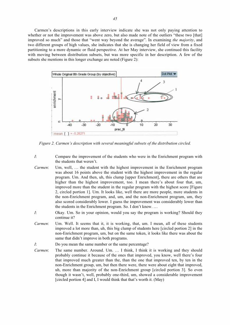
45

Carmen’s descriptions in this early interview indicate she was not only paying attention towhether or not the improvement was above zero, but also made note of the outliers “these two [that]improved so much” and those that “went way beyond the average”. In examining the majority, andtwo different groups of high values, she indicates that she is changing her field of view from a fixedpartitioning to a more dynamic or fluid perspective. At her May interview, she continued this facilitywith moving between distribution subsets, but was more specific in her description. A few of thesubsets she mentions in this longer exchange are noted (Figure 2):

Figure 2. Carmen’s description with several meaningful subsets of the distribution circled.

I: Compare the improvement of the students who were in the Enrichment program withthe students that weren’t.

Carmen: Um, well, … the student with the highest improvement in the Enrichment programwas about 16 points above the student with the highest improvement in the regularprogram. Um. And then, uh, this clump [upper Enrichment], there are others that arehigher than the highest improvement, too. I mean there’s about four that, um,improved more than the student in the regular program with the highest score [Figure2, circled portion 1]. Um. It looks like, well there are more people, more students inthe non-Enrichment program, and, um, and the non-Enrichment program, um, theyalso scored considerably lower. I guess the improvement was considerably lower thanthe students in the Enrichment program. So. I don’t know. …

I: Okay. Um. So in your opinion, would you say the program is working? Should theycontinue it?

Carmen: Um. Well. It seems that it, it is working, that, um. I mean, all of these studentsimproved a lot more than, uh, this big clump of students here [circled portion 2] in thenon-Enrichment program, um, but on the same token, it looks like there was about thesame that didn’t improve in both programs.

I: Do you mean the same number or the same percentage?

Carmen: The same number. Around. Um. … I think, I think it is working and they shouldprobably continue it because of the ones that improved, you know, well there’s fourthat improved much greater than the, than the one that improved ten, by ten in thenon-Enrichment group, um, but then there were, there were about eight that improved,uh, more than majority of the non-Enrichment group [circled portion 3]. So eventhough it wasn’t, well, probably one-third, um, showed a considerable improvement[circled portion 4] and I, I would think that that’s worth it. (May)

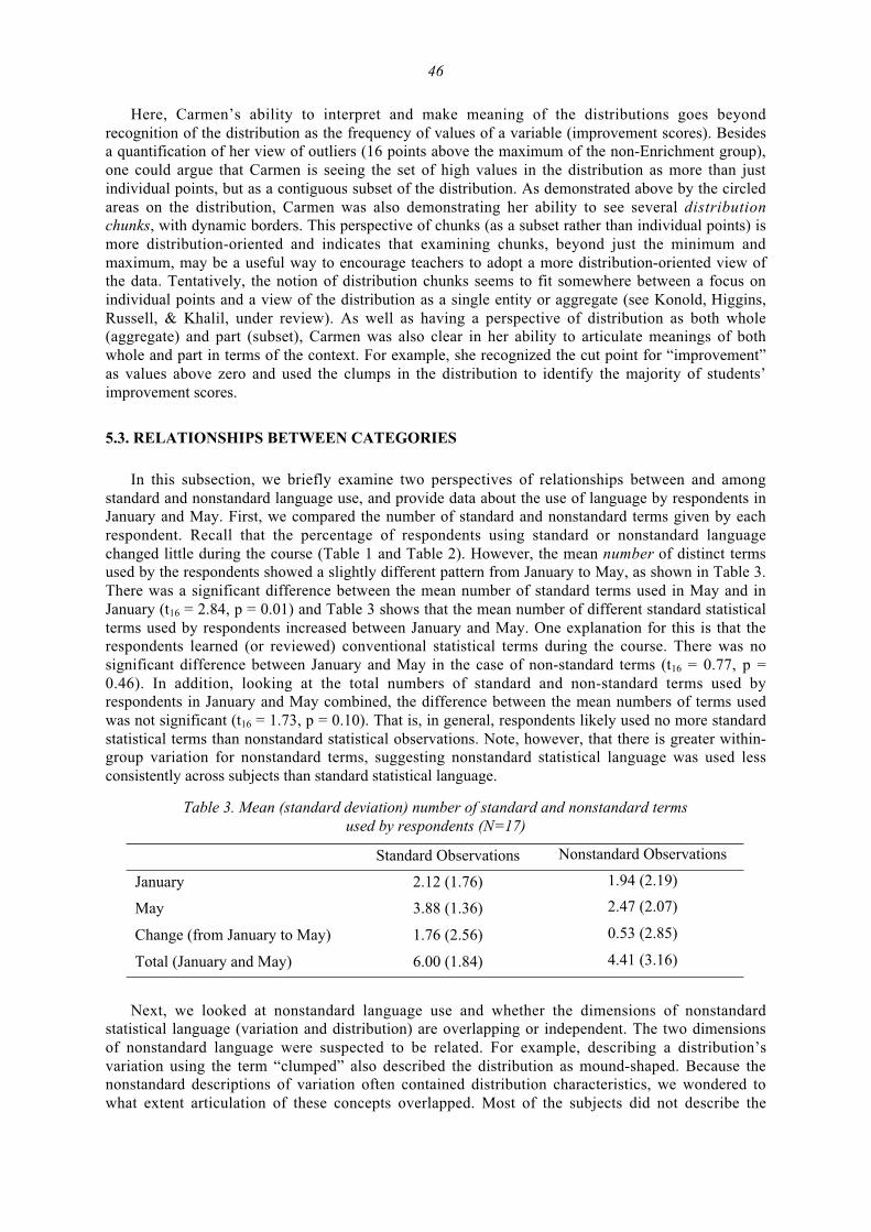
46

Here, Carmen’s ability to interpret and make meaning of the distributions goes beyondrecognition of the distribution as the frequency of values of a variable (improvement scores). Besidesa quantification of her view of outliers (16 points above the maximum of the non-Enrichment group),one could argue that Carmen is seeing the set of high values in the distribution as more than justindividual points, but as a contiguous subset of the distribution. As demonstrated above by the circledareas on the distribution, Carmen was also demonstrating her ability to see several distributionchunks, with dynamic borders. This perspective of chunks (as a subset rather than individual points) ismore distribution-oriented and indicates that examining chunks, beyond just the minimum andmaximum, may be a useful way to encourage teachers to adopt a more distribution-oriented view ofthe data. Tentatively, the notion of distribution chunks seems to fit somewhere between a focus onindividual points and a view of the distribution as a single entity or aggregate (see Konold, Higgins,Russell, & Khalil, under review). As well as having a perspective of distribution as both whole(aggregate) and part (subset), Carmen was also clear in her ability to articulate meanings of bothwhole and part in terms of the context. For example, she recognized the cut point for “improvement”as values above zero and used the clumps in the distribution to identify the majority of students’improvement scores.

5.3. RELATIONSHIPS BETWEEN CATEGORIES

In this subsection, we briefly examine two perspectives of relationships between and amongstandard and nonstandard language use, and provide data about the use of language by respondents inJanuary and May. First, we compared the number of standard and nonstandard terms given by eachrespondent. Recall that the percentage of respondents using standard or nonstandard languagechanged little during the course (Table 1 and Table 2). However, the mean number of distinct termsused by the respondents showed a slightly different pattern from January to May, as shown in Table 3.There was a significant difference between the mean number of standard terms used in May and inJanuary (t16 = 2.84, p = 0.01) and Table 3 shows that the mean number of different standard statisticalterms used by respondents increased between January and May. One explanation for this is that therespondents learned (or reviewed) conventional statistical terms during the course. There was nosignificant difference between January and May in the case of non-standard terms (t16 = 0.77, p =0.46). In addition, looking at the total numbers of standard and non-standard terms used byrespondents in January and May combined, the difference between the mean numbers of terms usedwas not significant (t16 = 1.73, p = 0.10). That is, in general, respondents likely used no more standardstatistical terms than nonstandard statistical observations. Note, however, that there is greater within-group variation for nonstandard terms, suggesting nonstandard statistical language was used lessconsistently across subjects than standard statistical language.

Table 3. Mean (standard deviation) number of standard and nonstandard termsused by respondents (N=17)

Standard Observations Nonstandard Observations

January 2.12 (1.76) 1.94 (2.19)

May 3.88 (1.36) 2.47 (2.07)

Change (from January to May) 1.76 (2.56) 0.53 (2.85)

Total (January and May) 6.00 (1.84) 4.41 (3.16)

Next, we looked at nonstandard language use and whether the dimensions of nonstandardstatistical language (variation and distribution) are overlapping or independent. The two dimensionsof nonstandard language were suspected to be related. For example, describing a distribution’svariation using the term “clumped” also described the distribution as mound-shaped. Because thenonstandard descriptions of variation often contained distribution characteristics, we wondered towhat extent articulation of these concepts overlapped. Most of the subjects did not describe the

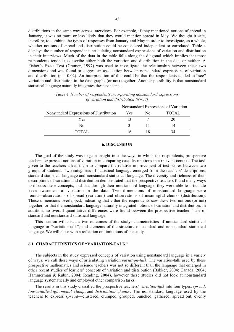
47

distributions in the same way across interviews. For example, if they mentioned notions of spread inJanuary, it was no more or less likely that they would mention spread in May. We thought it safe,therefore, to combine the types of responses from January and May in order to investigate, as a whole,whether notions of spread and distribution could be considered independent or correlated. Table 4displays the number of respondents articulating nonstandard expressions of variation and distributionin their interviews. Much of the data in the table falls along the diagonal which implies that mostrespondents tended to describe either both the variation and distribution in the data or neither. AFisher’s Exact Test (Cramer, 1997) was used to investigate the relationship between these twodimensions and was found to suggest an association between nonstandard expressions of variationand distribution (p = 0.02). An interpretation of this could be that the respondents tended to “see”variation and distribution in the data graphs (or not) together. Another possibility is that nonstandardstatistical language naturally integrates these concepts.

Table 4. Number of respondents incorporating nonstandard expressionsof variation and distribution (N=34)

Nonstandard Expressions of Variation

Nonstandard Expressions of Distribution Yes No TOTAL

Yes 13 7 20

No 3 11 14

TOTAL 16 18 34

6. DISCUSSION

The goal of the study was to gain insight into the ways in which the respondents, prospectiveteachers, expressed notions of variation in comparing data distributions in a relevant context. The taskgiven to the teachers asked them to compare the relative improvement of test scores between twogroups of students. Two categories of statistical language emerged from the teachers’ descriptions:standard statistical language and nonstandard statistical language. The diversity and richness of theirdescriptions of variation and distribution demonstrated that the prospective teachers found many waysto discuss these concepts, and that through their nonstandard language, they were able to articulatekeen awareness of variation in the data. Two dimensions of nonstandard language werefound—observations of spread (variation) and observations of meaningful chunks (distribution).These dimensions overlapped, indicating that either the respondents saw these two notions (or not)together, or that the nonstandard language naturally integrated notions of variation and distribution. Inaddition, no overall quantitative differences were found between the prospective teachers’ use ofstandard and nonstandard statistical language.

This section will discuss two outcomes of the study: characteristics of nonstandard statisticallanguage or “variation-talk”, and elements of the structure of standard and nonstandard statisticallanguage. We will close with a reflection on limitations of the study.

6.1. CHARACTERISTICS OF “VARIATION-TALK”

The subjects in the study expressed concepts of variation using nonstandard language in a varietyof ways; we call these ways of articulating variation variation-talk. The variation-talk used by theseprospective mathematics and science teachers was not so different than the language that emerged inother recent studies of learners’ concepts of variation and distribution (Bakker, 2004; Canada, 2004;Hammerman & Rubin, 2004; Reading, 2004), however these studies did not look at nonstandardlanguage systematically and employed other comparison tasks.

The results in this study classified the prospective teachers’ variation-talk into four types: spread,low-middle-high, modal clump, and distribution chunks. The nonstandard language used by theteachers to express spread—clustered, clumped, grouped, bunched, gathered, spread out, evenly

48

distributed, scattered, dispersed—all past participles, highlighted their attention to more spatialaspects of the distribution. These terms took on a meaning that implied attention to variation as acharacteristic of shape rather than as a measure. This is consistent with Bakker’s (2004) description ofshape as a pattern of variability. In contrast, concepts of variation in conventional statistical languageare articulated by terms like range or standard deviation, both of which are measures.

The other three types of “variation-talk”, all nouns, focused on aspects of the variability of thedata which required the prospective teachers to partition the distribution and examine a subset, orchunk of the distribution. Similar to Hammerman and Rubin’s (2004) teachers, the prospectiveteachers in this study simplified the complexity of the data’s variability by partitioning them into binsand comparing slices of data, in this case three slices: low-middle-high. Although simple, this is amore variation-oriented perspective than responses that took into account only the proportion ornumber of students who improved on the test. This approach is consistent with the findings of Bakker(2004), who argued that partitioning distributions into triads may be more intuitive than the moreconventional partitioning into four, as in the box plot. The awareness of learners’ tendency to simplifythe complexity of the data into low-middle-high bins motivated the creators of Tinkerplots (Konold &Miller, 2004) to include the “hat plot” (Konold, 2002) in the software, a representation where userscan partition the data into thirds based on the range, the average or standard deviation, the percentageof points, or a visual perspective of the data.

In some excerpts, teachers argued that the overlap of the middle slices was evidence that theEnrichment class was not effective. The focus on the modal clump (Konold et al., 2002) in data hasbeen a consistent finding across several studies of both students and teachers, reinforcing both theintuitive nature of seeing variability through slices-in-thirds, and recognizing the potential of using thenotion of a modal clump to encourage learners to move from a focus of individual points towards afocus on the aggregate of a distribution. Having a lens of a distribution as an aggregate, as opposed toa set of individual points, allows for concepts such as center to be thought of as a characteristic of thedistribution rather than as a calculation derived from individual points (Bakker, 2004). In addition,locating a modal clump allows the learner to simultaneously express their visualization of the centerand spread of the data (Konold et al., 2002), again highlighting its relational nature.

Finally, the use of other meaningful chunks by several of the prospective teachers demonstratedtheir ability to focus on the variability of the data by examining particular subsets of the distribution.This category contained responses as simple as comparing the outliers of one distribution to the“majority” of the other. A more complex visualization of distribution subsets was articulated byCarmen who used several different distribution subsets, with dynamic borders, as evidence for theeffectiveness of the Enrichment program. Her facility to fluidly manipulate borders of these subsetshighlighted her ability to visualize variation in the data. In addition, each of her meaningful chunkswas tied back to the context of the problem, indicating that she was able to use them to make meaningof the situation. Although Konold and Bakker have encouraged the conceptualization of a distributionas an aggregate, the articulation of distribution chunks by these teachers suggests that they arethinking of distribution chunks as mini-aggregates of the data. Kosslyn (1994) argues that our mindsand eyes work together to actively group input into perceptual units that ascribe meaning. We wouldargue that in articulating subsets of the distribution, the prospective teachers are communicating theperceptual units they are seeing in the data.

The three perspectives of seeing partial distributions—triads, modal clump, and distributionchunks—indicate that there are more than just the two perspectives of distribution that are usuallydiscussed in the literature: single points and aggregate. This third perspective—partial distributions or“mini-aggregates”—deserves further research to investigate the strength of its link to statisticalthinking about distributions. This study has highlighted that prospective teachers may use descriptionsof partial distributions not only to articulate rich views of variation, but also to use these distributionchunks in meaningful ways that could not be captured using conventional statistical terminology.Even though we classified expressions of variation separately from notions of distribution, thisseparation was somewhat artificial in that all four types of “variation-talk” expressed a relationshipbetween variation and distribution.

49

6.2. THE STRUCTURE OF STANDARD AND NONSTANDARD STATISTICALLANGUAGE

The nonstandard language used by the prospective teachers by its very nature integrates theimportant statistical ideas of variation and distribution, capturing and implying cognitive relationshipsbetween notions of center, dispersion, and shape. In contrast, the standard statistical language used bythe prospective teachers was by its very nature less relational, with a tendency to express importantideas in statistics as conceptually separate. Terms such as mean, standard deviation, and skeweddistribution describe the center, dispersion, and shape of a distribution but they do so in isolation. Theoveruse of this standard terminology, at least early in learning statistical concepts, may encouragelearners to maintain a perspective that statistical concepts are isolated “bits” of knowledge rather thaninformation that can provide insight into relationships in the data. Several difficulties of learningstatistics that are documented in research are consistent with a perspective of statistics as isolatedfacts. For example, seeing data as a set of isolated points rather than developing a “propensityperspective” (Konold, Pollatsek, Well, & Gagnon, 1997), lack of intuition in stochastics(Shaughnessy, 1992), or focusing instruction on calculations, isolated procedures, and graphcharacteristics in statistics instead of on drawing meaningful conclusions from data (Pfannkuch et al.,2004) may all be reinforced by the overuse (too much, too soon) of conventional statistical language.

The process of integrating rather than separating concepts in statistics has been shown to be aproductive avenue for developing statistical thinking and reasoning (Konold et al., 2002; Konold &Pollatsek, 2002; Bakker, 2004). This does not imply that one should “teach” nonstandard statisticallanguage as a means to encourage the development of students’ intuition about statistics, but rather toencourage their sense-making by acknowledging and encouraging learners’ own language. Had weacknowledged only conventional terms in our search for their articulation of variation, we would havelost many opportunities to gain insight into their thinking. For example, only two preservice teachersused the term “standard deviation” in their comparisons, and it can be argued that neither one usedthis concept to articulate meaning about variation.

An important lesson we learned in trying to categorize the preservice teachers’ descriptions washow difficult it was to separate their observations of variation and distribution. For example, whenApril described the shape of one distribution (“skewed to the left”), she compared its shape with thespread of the other distribution (“evenly spread out”). Using the teachers’ words, we could see thatdescribing data as clumped or spread out said as much about the distribution of the data as it didabout its variation. It was not surprising, therefore, when the responses in the two dimensions ofnonstandard language (variation and distribution) were found to be correlated.

6.3. LIMITATIONS OF THE STUDY

Although we believe that the results of this study communicate a powerful message about theopportunities of listening to learners’ nonstandard statistical language, several limitations of the studymust be acknowledged.

• Population. The subjects in the study were prospective secondary mathematics and scienceteachers and the study is not directly generalizable beyond that population. While many of theresults may seem to transfer to other groups (for example, practicing teachers), more researchwould need to be conducted in order to corroborate these results with other populations.

• Particulars of the task. The setting may have had strong influences on the responses that theprospective teachers gave during their interviews. Although the data were authentic, the taskwas not as it did not emerge from the teachers’ own desire to know. Therefore, it is possiblethat the responses given by the prospective teachers may have mirrored an expectation of whatthey thought the researchers wanted them to say, particularly since the researchers were alsotheir course instructors and the interviews were conducted as part of the course assessment.

• Particulars of the graphic. Elements of the graph could elicit responses that may differ withslight modifications. Recall, for example, that the means were marked on the figure andexplicitly pointed out to the subjects at the beginning of the task. By drawing specific attention

50

to the means, we may have been tacitly communicating that the means should have beenattended to in addition to or even instead of the prospective teachers’ own way of comparingthe two groups. The results of the Hammerman and Rubin (2004) study, for example, noted thatthe teachers in their study were not interested in using means to compare distributions butinvented their own ways of making meaning of comparisons in the problems they werediscussing.

• Irregularities in questioning. In a few of the interviews, the interviewer did not explicitly askfor a decision to be made regarding the effectiveness of the Enrichment program. This meantthat comparisons could not be made systematically regarding the prospective teachers’ use ofevidence towards a decision, which could have elicited richer responses.

• Generalizations about the course. Given the unique nature of the course which the prospectiveteachers undertook, the study was not designed to make generalizations about the effectivenessof such a course in developing learners’ statistical reasoning. Many of the compelling elementsused in the course and the task were developed from local problems in the implementation ofstandardized testing. Instead, the study was designed to focus on variation-related language thatpreservice teachers use at different stages or levels of learning about statistics. Other reports ofthe larger research study communicate elements of the course that may have had an impact onthe prospective teachers’ thinking and learning (Confrey et al., 2004; Makar & Confrey,submitted; Makar, 2004).

7. CONCLUSION AND IMPLICATIONS

This study was built on pioneering work by researchers at TERC who first studied teachers’nonstandard statistical language (e.g., Russell & Mokros, 1990), and shows the breadth and depth ofnonstandard language used by prospective teachers to describe variation. It follows that teachers needto learn to recognize and value “variation-talk” as a vehicle for students to express meaningfulconcepts of variation and distribution. This study has contributed to our understanding that preserviceteachers majoring in math and science often articulate meaning in statistics through the use of lessconventional terminology. Other research studies have shown that school children do so as well (e.g.,Bakker, 2004; Reading, 2004; Konold et al., 2002). These studies have begun to articulate rich andproductive learning trajectories to move students towards a more distribution-oriented view of data.

Although the preservice teachers in this study were using nonstandard statistical language, theconcepts they are discussing are far from simplistic and need to be acknowledged as statisticalconcepts. Not recognizing nonstandard statistical language can have two pernicious effects. For one,we miss opportunities to gain insight students’ statistical thinking. Noss and Hoyles (1996) explainthe benefits of attending to students’ articulation for creating mathematical meaning: “It is thisarticulation which offers some purchase on what the learner is thinking, and it is in the process ofarticulation that a learner can create mathematics and simultaneously reveal this act of creation to anobserver” (p. 54, italics in original). Gaining insight into student thinking, therefore, is not the onlybenefit from attending to nonstandard statistical language. Noss and Hoyles also argue that throughthe process of articulation, students have opportunities to create meaning. Sense-making in statisticsis an ultimate goal that is often neglected by more traditional learning environments. Valuing thediversity of students’ “variation-talk” and listening to student voice (Confrey, 1998) may encourageteachers to shift from the typically procedure-focused statistics courses towards a focus on sense-making. This is an issue of equity if we are to acknowledge the diversity of students’ ideas rather thanjust cover the content and label those who don’t talk statistically as being unable to do so.

The other problematic effect of neglecting students’ nonstandard statistical language is the tacitmessage that is communicated that statistics can only be understood by those who can use properstatistical talk. Lemke (1990) argues that the formal dialogue of science communicates a mystique ofscience as being much more complex and difficult than other subjects, requiring that we defer ourown ideas to those of ‘experts’. By doing so, Lemke argues

51

The language of classroom science sets up a pervasive and false opposition between a world ofobjective, authoritative, impersonal, humorless scientific fact and the ordinary, personal world ofhuman uncertainties, judgments, values, and interests … many of the unwritten rules about howwe are supposed to talk science make it seem that way (p. 129).

Although Lemke here is talking about science, the situation in statistics is isomorphic. Countlessstudents complain that statistics (which they call “sadistics”) is not understandable to ordinaryhumans and lacks a connection to sense-making. By communicating statistics as accessible only toexperts and geniuses, we are reinforcing a notion of statistics as a gatekeeper to powerful insightsabout the world, alienating students and denying opportunity to those who do lack the confidence intheir ability to make sense of statistics.

Three major benefits come out of teachers’ use of their own, nonstandard statistical terminologyin describing, interpreting, and comparing distributions. First, they are using words that hold meaningfor them and that convey their own conceptions of variation. In the constructivist perspective,knowledge is not conveyed through language but must be abstracted through experience. Nonstandardlanguage carries a subjective flavor that reminds us of this. Through interaction with others, thissubjectivity becomes intersubjective—one’s meaning is not identical to another’s, but through furtherexplanation, our meanings become more compatible with the language of our peers (von Glasersfeld,1991). Second, everyday uses of language are more accessible to a wide variety of students, allowingmultiple points of entry to statistical concepts while encouraging teachers to be more sensitive tohearing rich conceptions of variation in students’ voice (Confrey, 1998), words that may allowstudents easier access to class discussions. This is a more equitable, more inclusive stance; one that iscontrary to the conception of mathematics (or statistics) as a gatekeeper. Third, if the goal is toprovide students with experiences that will provide them with a more distribution-oriented view ofdata, then nonstandard statistical language that emerges from making meaning of statistical conceptsmay help to orient students (and their teachers!) towards this perspective. Describing a distribution as“more clumped in the center” conveys a more distribution-oriented perspective in language thanstating, say, standard deviation or range to compare its dispersion.

The results of this study are not meant to downplay the importance of using conventional termsand measures in comparing groups. On the contrary, these are very important tools. Our hope is thatteachers do not emphasize simply summarizing or reducing the data with conventional measures tomake overly simplistic comparisons as we have seen schools do in examining test data (Confrey &Makar, 2005), but rather seek insights into the context the data represent through richer views thatinclude notions of distribution and variation. Further research is needed to gain insight into howteachers understand concepts of variation and distribution, as well as to document how teacherssupport their students’ emerging statistical understanding.

ACKNOWLEDGEMENTS

This research was funded by the National (U.S.) Science Foundation under their Collaborative forExcellence in Teacher Preparation program (DUE-9953187). The authors are grateful to NSF for itsfinancial support and to the UTeach program at the University of Texas for their support in this study.The authors wish to thank the organizers of SRTL-3 for their permission and encouragement to makethese results available to a broader audience, and also appreciated the feedback offered by our SRTLcolleagues. The authors would also like to thank the reviewers who provided constructive, thoughtful,and extensive feedback on earlier drafts of this paper. Insightful and tenacious feedback from IddoGal, going beyond his role as editor of SERJ, greatly improved the final version.

52

REFERENCES

Bakker, A. (2004). Design research in statistics education: On symbolizing and computer tools.Published Doctoral dissertation. Utrecht, The Netherlands: Freudenthal Institute. [Online:www.stat.auckland.ac.nz/~iase/publications/dissertations/dissertations.php]

Bakker, A., & Gravemeijer, K. P. E. (2004). Learning to reason about distribution. In D. Ben-Zvi & J.Garfield (Eds.), The challenge of developing statistical literacy, reasoning, and thinking (pp. 147-168). Dordrecht, the Netherlands: Kluwer Academic Publishers.

Biehler, R. (1997). Student’s difficulties in practicing computer-supported data analysis: Somehypothetical generalizations from results of two exploratory studies. In J. Garfield & G. Burrill(Eds.), Research on the role of technology in teaching and learning statistics (pp. 169-190).Voorburg, The Netherlands: International Statistics Institute.

Boaler, J. (1997). Experiencing school mathematics: Teaching styles, sex, and setting. Buckingham:Open University Press.

Canada, D. (2004). Preservice teachers’ understanding of variation. Unpublished doctoraldissertation, Portland State University, Portland, Oregon (USA). [Online:www.stat.auckland.ac.nz/~iase/publications/dissertations/dissertations.php]

Cobb, P. (1999). Individual and collective mathematical development: The case of statistical dataanalysis. Mathematical Thinking and Learning, 1(1), 5-43.

Confrey, J. (1998). Voice and perspective: Hearing epistemological innovation in students’ words. InM. Larochelle, N. Bednarz, & J. Garrison (Eds.), Constructivism and education (pp. 104-120).New York, N.Y.: Cambridge University Press.

Confrey, J., & Makar, K. (2002). Developing secondary teachers’ statistical inquiry throughimmersion in high-stakes accountability data. In D. S. Mewborn, P. Sztajn, D. Y. White, H. G.Wiegel, R. L. Bryant, & K. Nooney (Eds.), Proceedings of the Twenty-fourth Annual Meeting ofthe North American Chapter of the International Group for the Psychology of MathematicsEducation (PME-NA), Athens, GA, (Vol. 3, pp. 1267-1279). Columbus, OH: ERIC Clearinghouse,Mathematics and Environment Education.

Confrey, J., & Makar, K. (2005). Critiquing and improving the use of data from high-stakes tests withthe aid of dynamic statistics software. In C. Dede, J. Honan, & L. Peters (Eds.), Scaling up forsuccess: Lessons from technology-based educational improvement (pp. 198-226). Cambridge,MA: Harvard College of Education.

Confrey, J., Makar, K., & Kazak, S. (2004). Undertaking data analysis of student outcomes asprofessional development for teachers. International Reviews on Mathematical Education(Zentralblatt für Didaktik der Mathematik), 36(1), 32-40.

Cramer, D. (1997). Basic statistics for social research. London: Routledge.

Finzer, W. (2001). Fathom! (Version 1.16) [Computer Software]. Emeryville, CA: Key CurriculumPress.

Fischbein, E. (1987). Intuition in mathematics and science: An educational approach. Dordrecht, TheNetherlands: D. Reidel Publishing Company.

Flyvbjerg, B. (2001). Making social science matter: Why social inquiry fails and how it can succeedagain. Cambridge, UK: Cambridge University Press.

Hammerman, J., & Rubin, A. (2004). Strategies for managing statistical complexity with newsoftware tools. Statistics Education Research Journal, 3(2), 17-41. [Online:www.stat.auckland.ac.nz/serj]

Hancock, C., Kaput, J. J., & Goldsmith, L. T. (1992). Authentic inquiry into data: Critical barriers toclassroom implementation. Educational Psychologist, 27(3), 337-364.

Hawkins, A. (Ed.). (1990). Teaching teachers to teach statistics. Voorburg, The Netherlands:International Statistics Institute.

Konold, C. (2002). “Hat Plots? ” Unpublished manuscript, University of Massachusetts, Amherst.

53

Konold, C., & Higgins, T. (2002). Highlights of related research. In S. J. Russell, D. Schifter, & V.Bastable, Developing mathematical ideas: Working with data, (pp. 165-201). Parsippany, NJ:Dale Seymour Publications.

Konold, C., Higgins, T., Russell, S. J., & Khalil, K. (submitted). Data seen through different lenses.Journal for Research in Mathematics Education.

Konold, C., & Miller, C. (2004). Tinkerplots (Version 1.0) [Computer Software]. Emeryville, CA:Key Curriculum Press.

Konold, C., & Pollatsek, A. (2002). Data analysis as the search for signals in noisy processes. Journalfor Research in Mathematics Education, 33(4), 259-289.

Konold, C., Pollatsek, A., Well, A., & Gagnon, A. (1997). Students analyzing data: research ofcritical barriers. In J. Garfield & G. Burrill (Eds.), Research on the role of technology in teachingand learning statistics (pp. 151-167). Voorburg, The Netherlands: International StatisticsInstitute.

Konold, C., Robinson, A., Khalil, K., Pollatsek, A., Well, A., Wing, R., & Mayr, S. (2002). Students’use of modal clumps to summarize data. In B. Phillips (Ed.), Proceedings of the SixthInternational Conference on Teaching Statistics, Cape Town, South Africa [CD-ROM]. Voorburg,The Netherlands: International Statistical Institute.

Kosslyn, S. (1994). Elements of graph design. New York: W. H. Freeman and Company.

Lemke, J. (1990). Talking science: Language, learning, and values. Norwood, NJ: Ablex Publishing.

Makar, K. (2004). Developing statistical inquiry: Prospective secondary mathematics and scienceteachers’ investigations of equity and fairness through analysis of accountability data.Unpublished Doctoral dissertation, University of Texas at Austin (USA). [Online:www.stat.auckland.ac.nz/~iase/publications/dissertations/dissertations.php]

Makar, K., & Confrey, J. (submitted). Modeling fairness in student achievement in mathematics usingstatistical software by preservice secondary teachers. ICMI Study Volume 14: Applications andmodeling in mathematics education.

Makar, K., & Confrey, J. (2004). Secondary teachers’ reasoning about comparing two groups. In D.Ben-Zvi & J. Garfield (Eds.), The challenges of developing statistical literacy, reasoning, andthinking (pp. 353-373). Dordrecht, the Netherlands: Kluwer Academic Publishers.

Marshall, J., Makar, K., & Kazak, S. (2002). Young urban students’ conceptions of data uses,representation, and analysis. In D. S. Mewborn, P. Sztajn, D. Y. White, H. G. Wiegel, R. L.Bryant, & K. Nooney (Eds.), Proceedings of the Twenty-fourth Annual Meeting of the NorthAmerican Chapter of the International Group for the Psychology of Mathematics Education(PME-NA), Athens, GA, (Vol. 3, pp. 1293-1304). Columbus, OH: ERIC Clearinghouse,Mathematics and Environment Education.

McClain, K. (2002). Supporting teachers’ understanding of statistical data analysis: Learningtrajectories as tools for change. In B. Phillips (Ed.), Proceedings of the Sixth InternationalConference on Teaching Statistics, Cape Town, South Africa [CD-ROM]. Voorburg, TheNetherlands: International Statistical Institute.

Moore, D. (1990). Uncertainty. In L. A. Steen (Ed.), On the shoulders of giants (pp. 95-137).Washington, D.C.: Academy Press.

Moore, D., & McCabe, G. (1993). Introduction to the practice of statistics (2nd ed.). New York:Freeman.

National Research Council (1999). High stakes: Testing for tracking, promotion, and graduation.Heubert, J. P., & Hauser, R. M. (Eds.), Washington, D.C.: National Academy Press.

National Research Council (2000). Inquiry and the National Science Education Standards: A guidefor teaching and learning. Washington, D.C.: National Academy Press.

National Research Council (2001). Knowing what students know. Washington, D.C.: NationalAcademy Press.

54

Noss, R., & Hoyles, C. (1996). Windows on mathematical meanings: Learning cultures andcomputers. Dordrecht, The Netherlands: Kluwer Academic Publishers.

Pfannkuch, M., & Begg, A. (2004). The school statistics curriculum: Statistics and probabilityeducation literature review. Mathematics Curriculum Reference Group Report to the Ministry ofEducation. Auckland, New Zealand.

Pfannkuch, M., Budgett, S., Parsonage, R., & Horring, J. (2004). Comparison of data plots: Building apedagogical framework. Paper presented at the Tenth International Congress on MathematicsEducation (ICME-10), Copenhagen, Denmark, 4-11 July.

Reading, C. (2004). Student description of variation while working with weather data. StatisticsEducation Research Journal, 3(2), 84-105. [Online: www.stat.auckland.ac.nz/serj]

Reading, C., & Shaughnessy, J. M. (2004). Reasoning about variation. In D. Ben-Zvi & J. Garfield(Eds.), The challenge of developing statistical literacy, reasoning and thinking (pp. 201-226).Dordrecht, The Netherlands: Kluwer Academic Publishers.

Russell, S. J., & Mokros, J. R. (1990). What’s typical: Teacher’s descriptions of data. Paper presentedat the Annual Meeting of the American Educational Research Association, Boston, MA.

Schoenfeld, A. (1991). On mathematics as sense-making: An informal attack on the unfortunatedivorce of formal and informal mathematics. In J. Voss, D. Perkins, & J. Segal (Eds.), Informalreasoning and education (pp. 311-343). Hillsdale, NJ: Lawrence Erlbaum Associates.

Shaughnessy, J. M. (1992). Research in probability and statistics: Reflections and directions. In D. A.Grouws (Ed.), Handbook of research on mathematics teaching and learning (pp. 465-494). NewYork: MacMillan.

Shaughnessy, J. M. (2001). Draft of grant proposal sent to the National Science Foundation.

Shaughnessy, J. M., Watson, J., Moritz, J., & Reading, C. (1999, April). School mathematicsstudents’ acknowledgement of statistical variation. In C. Maher (Chair), There’s More to Life thanCenters. Presession Research Symposium, 77th Annual National Council of Teachers ofMathematics Conference, San Francisco, CA.

von Glasersfeld, E. (Ed.) (1991). Radical constructivism in mathematics education. Dordrecht, theNetherlands: Kluwer Academic Publisher.

Watkins, A. E., Scheaffer, R., & Cobb, G. (2003). Statistics in action: Understanding a world of data.Emeryville, CA: Key Curriculum Press.

Watson, J., & Moritz, J. B. (1999). The beginning of statistical inference: Comparing two data sets.Educational Studies in Mathematics, 37, 145-168.

KATIE MAKAR

School of Education, Social Sciences Bldg

University of Queensland

Brisbane, Queensland 4072

Australia

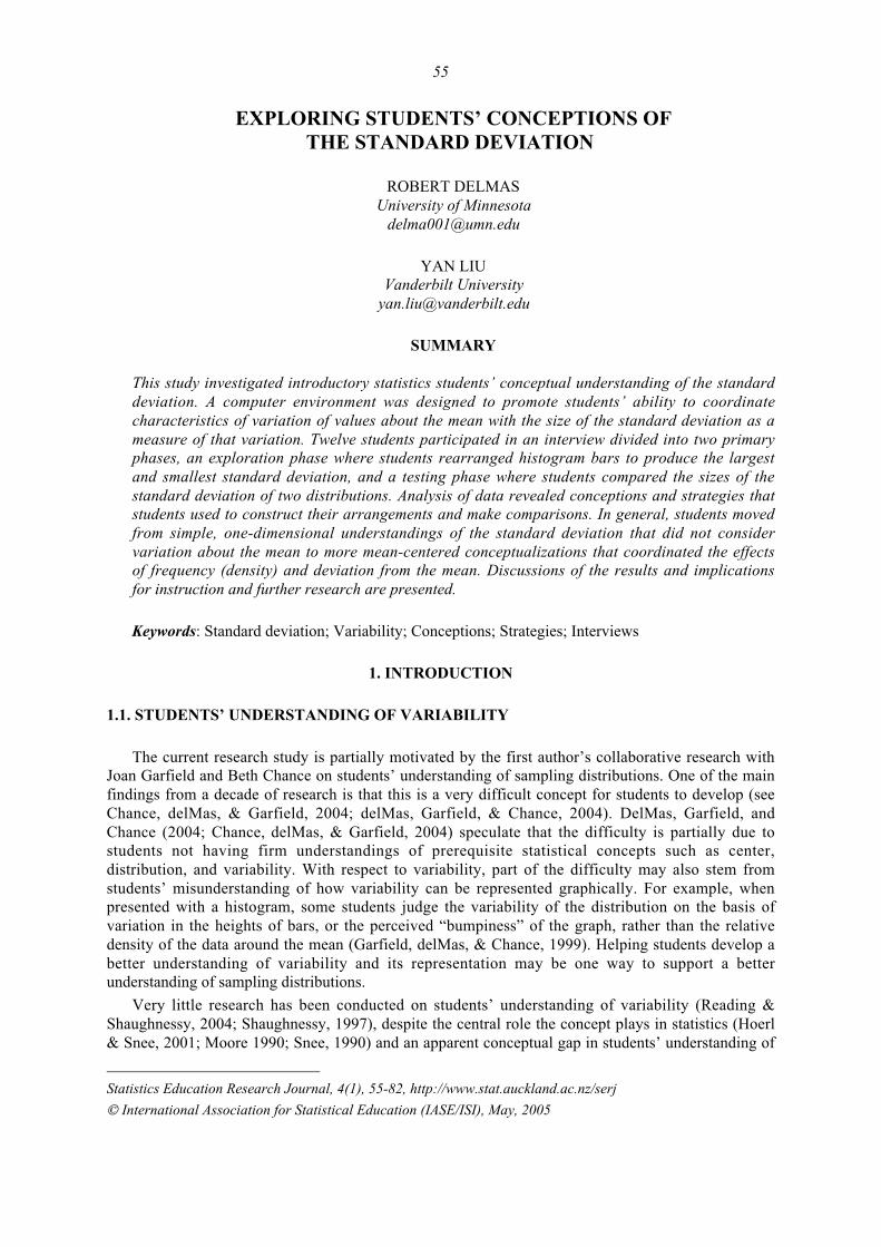
55

EXPLORING STUDENTS’ CONCEPTIONS OFTHE STANDARD DEVIATION8

ROBERT DELMASUniversity of Minnesota

[email protected]

YAN LIUVanderbilt University

[email protected]

SUMMARY

This study investigated introductory statistics students’ conceptual understanding of the standarddeviation. A computer environment was designed to promote students’ ability to coordinatecharacteristics of variation of values about the mean with the size of the standard deviation as ameasure of that variation. Twelve students participated in an interview divided into two primaryphases, an exploration phase where students rearranged histogram bars to produce the largestand smallest standard deviation, and a testing phase where students compared the sizes of thestandard deviation of two distributions. Analysis of data revealed conceptions and strategies thatstudents used to construct their arrangements and make comparisons. In general, students movedfrom simple, one-dimensional understandings of the standard deviation that did not considervariation about the mean to more mean-centered conceptualizations that coordinated the effectsof frequency (density) and deviation from the mean. Discussions of the results and implicationsfor instruction and further research are presented.

Keywords: Standard deviation; Variability; Conceptions; Strategies; Interviews

1. INTRODUCTION

1.1. STUDENTS’ UNDERSTANDING OF VARIABILITY

The current research study is partially motivated by the first author’s collaborative research withJoan Garfield and Beth Chance on students’ understanding of sampling distributions. One of the mainfindings from a decade of research is that this is a very difficult concept for students to develop (seeChance, delMas, & Garfield, 2004; delMas, Garfield, & Chance, 2004). DelMas, Garfield, andChance (2004; Chance, delMas, & Garfield, 2004) speculate that the difficulty is partially due tostudents not having firm understandings of prerequisite statistical concepts such as center,distribution, and variability. With respect to variability, part of the difficulty may also stem fromstudents’ misunderstanding of how variability can be represented graphically. For example, whenpresented with a histogram, some students judge the variability of the distribution on the basis ofvariation in the heights of bars, or the perceived “bumpiness” of the graph, rather than the relativedensity of the data around the mean (Garfield, delMas, & Chance, 1999). Helping students develop abetter understanding of variability and its representation may be one way to support a betterunderstanding of sampling distributions.

Very little research has been conducted on students’ understanding of variability (Reading &Shaughnessy, 2004; Shaughnessy, 1997), despite the central role the concept plays in statistics (Hoerl& Snee, 2001; Moore 1990; Snee, 1990) and an apparent conceptual gap in students’ understanding of



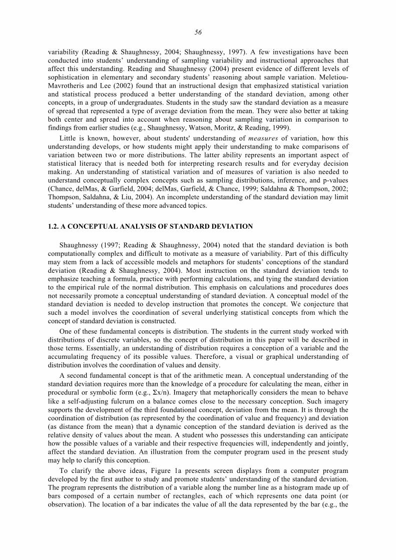
56

variability (Reading & Shaughnessy, 2004; Shaughnessy, 1997). A few investigations have beenconducted into students’ understanding of sampling variability and instructional approaches thataffect this understanding. Reading and Shaughnessy (2004) present evidence of different levels ofsophistication in elementary and secondary students’ reasoning about sample variation. Meletiou-Mavrotheris and Lee (2002) found that an instructional design that emphasized statistical variationand statistical process produced a better understanding of the standard deviation, among otherconcepts, in a group of undergraduates. Students in the study saw the standard deviation as a measureof spread that represented a type of average deviation from the mean. They were also better at takingboth center and spread into account when reasoning about sampling variation in comparison tofindings from earlier studies (e.g., Shaughnessy, Watson, Moritz, & Reading, 1999).

Little is known, however, about students' understanding of measures of variation, how thisunderstanding develops, or how students might apply their understanding to make comparisons ofvariation between two or more distributions. The latter ability represents an important aspect ofstatistical literacy that is needed both for interpreting research results and for everyday decisionmaking. An understanding of statistical variation and of measures of variation is also needed tounderstand conceptually complex concepts such as sampling distributions, inference, and p-values(Chance, delMas, & Garfield, 2004; delMas, Garfield, & Chance, 1999; Saldahna & Thompson, 2002;Thompson, Saldahna, & Liu, 2004). An incomplete understanding of the standard deviation may limitstudents’ understanding of these more advanced topics.

1.2. A CONCEPTUAL ANALYSIS OF STANDARD DEVIATION

Shaughnessy (1997; Reading & Shaughnessy, 2004) noted that the standard deviation is bothcomputationally complex and difficult to motivate as a measure of variability. Part of this difficultymay stem from a lack of accessible models and metaphors for students’ conceptions of the standarddeviation (Reading & Shaughnessy, 2004). Most instruction on the standard deviation tends toemphasize teaching a formula, practice with performing calculations, and tying the standard deviationto the empirical rule of the normal distribution. This emphasis on calculations and procedures doesnot necessarily promote a conceptual understanding of standard deviation. A conceptual model of thestandard deviation is needed to develop instruction that promotes the concept. We conjecture thatsuch a model involves the coordination of several underlying statistical concepts from which theconcept of standard deviation is constructed.

One of these fundamental concepts is distribution. The students in the current study worked withdistributions of discrete variables, so the concept of distribution in this paper will be described inthose terms. Essentially, an understanding of distribution requires a conception of a variable and theaccumulating frequency of its possible values. Therefore, a visual or graphical understanding ofdistribution involves the coordination of values and density.

A second fundamental concept is that of the arithmetic mean. A conceptual understanding of thestandard deviation requires more than the knowledge of a procedure for calculating the mean, either inprocedural or symbolic form (e.g., Σx/n). Imagery that metaphorically considers the mean to behavelike a self-adjusting fulcrum on a balance comes close to the necessary conception. Such imagerysupports the development of the third foundational concept, deviation from the mean. It is through thecoordination of distribution (as represented by the coordination of value and frequency) and deviation(as distance from the mean) that a dynamic conception of the standard deviation is derived as therelative density of values about the mean. A student who possesses this understanding can anticipatehow the possible values of a variable and their respective frequencies will, independently and jointly,affect the standard deviation. An illustration from the computer program used in the present studymay help to clarify this conception.

To clarify the above ideas, Figure 1a presents screen displays from a computer programdeveloped by the first author to study and promote students’ understanding of the standard deviation.The program represents the distribution of a variable along the number line as a histogram made up ofbars composed of a certain number of rectangles, each of which represents one data point (orobservation). The location of a bar indicates the value of all the data represented by the bar (e.g., the

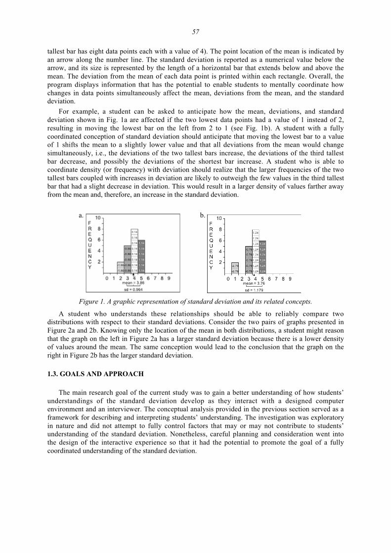
57

tallest bar has eight data points each with a value of 4). The point location of the mean is indicated byan arrow along the number line. The standard deviation is reported as a numerical value below thearrow, and its size is represented by the length of a horizontal bar that extends below and above themean. The deviation from the mean of each data point is printed within each rectangle. Overall, theprogram displays information that has the potential to enable students to mentally coordinate howchanges in data points simultaneously affect the mean, deviations from the mean, and the standarddeviation.

For example, a student can be asked to anticipate how the mean, deviations, and standarddeviation shown in Fig. 1a are affected if the two lowest data points had a value of 1 instead of 2,resulting in moving the lowest bar on the left from 2 to 1 (see Fig. 1b). A student with a fullycoordinated conception of standard deviation should anticipate that moving the lowest bar to a valueof 1 shifts the mean to a slightly lower value and that all deviations from the mean would changesimultaneously, i.e., the deviations of the two tallest bars increase, the deviations of the third tallestbar decrease, and possibly the deviations of the shortest bar increase. A student who is able tocoordinate density (or frequency) with deviation should realize that the larger frequencies of the twotallest bars coupled with increases in deviation are likely to outweigh the few values in the third tallestbar that had a slight decrease in deviation. This would result in a larger density of values farther awayfrom the mean and, therefore, an increase in the standard deviation.

a. b.

Figure 1. A graphic representation of standard deviation and its related concepts.

A student who understands these relationships should be able to reliably compare twodistributions with respect to their standard deviations. Consider the two pairs of graphs presented inFigure 2a and 2b. Knowing only the location of the mean in both distributions, a student might reasonthat the graph on the left in Figure 2a has a larger standard deviation because there is a lower densityof values around the mean. The same conception would lead to the conclusion that the graph on theright in Figure 2b has the larger standard deviation.

1.3. GOALS AND APPROACH

The main research goal of the current study was to gain a better understanding of how students’understandings of the standard deviation develop as they interact with a designed computerenvironment and an interviewer. The conceptual analysis provided in the previous section served as aframework for describing and interpreting students’ understanding. The investigation was exploratoryin nature and did not attempt to fully control factors that may or may not contribute to students’understanding of the standard deviation. Nonetheless, careful planning and consideration went intothe design of the interactive experience so that it had the potential to promote the goal of a fullycoordinated understanding of the standard deviation.

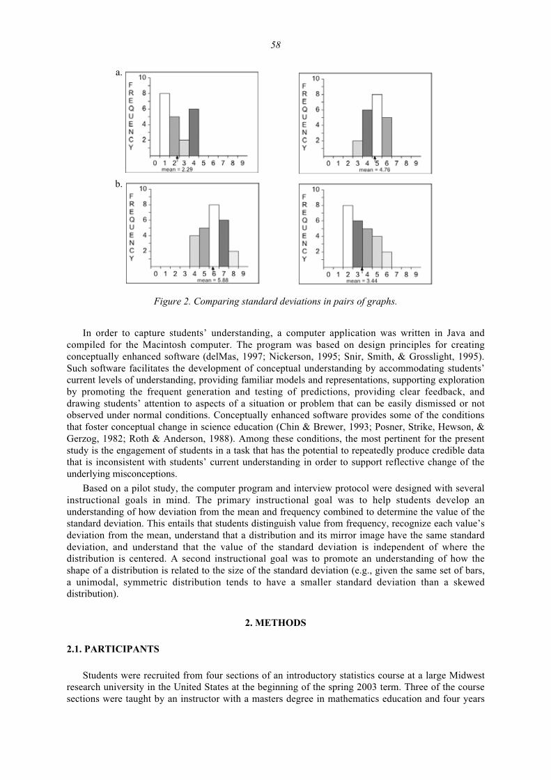
58

a.

b.

Figure 2. Comparing standard deviations in pairs of graphs.

In order to capture students’ understanding, a computer application was written in Java andcompiled for the Macintosh computer. The program was based on design principles for creatingconceptually enhanced software (delMas, 1997; Nickerson, 1995; Snir, Smith, & Grosslight, 1995).Such software facilitates the development of conceptual understanding by accommodating students’current levels of understanding, providing familiar models and representations, supporting explorationby promoting the frequent generation and testing of predictions, providing clear feedback, anddrawing students’ attention to aspects of a situation or problem that can be easily dismissed or notobserved under normal conditions. Conceptually enhanced software provides some of the conditionsthat foster conceptual change in science education (Chin & Brewer, 1993; Posner, Strike, Hewson, &Gerzog, 1982; Roth & Anderson, 1988). Among these conditions, the most pertinent for the presentstudy is the engagement of students in a task that has the potential to repeatedly produce credible datathat is inconsistent with students’ current understanding in order to support reflective change of theunderlying misconceptions.

Based on a pilot study, the computer program and interview protocol were designed with severalinstructional goals in mind. The primary instructional goal was to help students develop anunderstanding of how deviation from the mean and frequency combined to determine the value of thestandard deviation. This entails that students distinguish value from frequency, recognize each value’sdeviation from the mean, understand that a distribution and its mirror image have the same standarddeviation, and understand that the value of the standard deviation is independent of where thedistribution is centered. A second instructional goal was to promote an understanding of how theshape of a distribution is related to the size of the standard deviation (e.g., given the same set of bars,a unimodal, symmetric distribution tends to have a smaller standard deviation than a skeweddistribution).

2. METHODS

2.1. PARTICIPANTS

Students were recruited from four sections of an introductory statistics course at a large Midwestresearch university in the United States at the beginning of the spring 2003 term. Three of the coursesections were taught by an instructor with a masters degree in mathematics education and four years

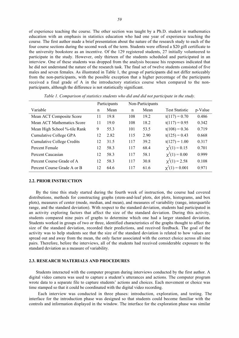
59

of experience teaching the course. The other section was taught by a Ph.D. student in mathematicseducation with an emphasis in statistics education who had one year of experience teaching thecourse. The first author made a brief presentation about the nature of the research study to each of thefour course sections during the second week of the term. Students were offered a $20 gift certificate tothe university bookstore as an incentive. Of the 129 registered students, 27 initially volunteered toparticipate in the study. However, only thirteen of the students scheduled and participated in aninterview. One of these students was dropped from the analysis because his responses indicated thathe did not understand the nature of the research task. The final set of twelve students consisted of fivemales and seven females. As illustrated in Table 1, the group of participants did not differ noticeablyfrom the non-participants, with the possible exception that a higher percentage of the participantsreceived a final grade of A in the introductory statistics course when compared to the non-participants, although the difference is not statistically significant.

Table 1. Comparison of statistics students who did and did not participate in the study.

Variable

Participants

n Mean

Non-Participants

n Mean Test Statistic p-Value

Mean ACT Composite Score 11 19.8 108 19.2 t(117) = 0.70 0.486

Mean ACT Mathematics Score 11 19.0 108 18.2 t(117) = 0.95 0.342

Mean High School %-tile Rank 9 55.3 101 53.5 t(108) = 0.36 0.719

Cumulative College GPA 12 2.82 115 2.90 t(125) = 0.43 0.668

Cumulative College Credits 12 31.5 117 39.2 t(127) = 1.00 0.317

Percent Female 12 58.3 117 68.4 χ2(1) = 0.15 0.701

Percent Caucasian 12 58.3 117 58.1 χ2(1) = 0.00 0.999

Percent Course Grade of A 12 58.3 117 30.8 χ2(1) = 2.58 0.108

Percent Course Grade A or B 12 64.6 117 61.6 χ2(1) = 0.001 0.971

2.2. PRIOR INSTRUCTION

By the time this study started during the fourth week of instruction, the course had covereddistributions, methods for constructing graphs (stem-and-leaf plots, dot plots, histograms, and boxplots), measures of center (mode, median, and mean), and measures of variability (range, interquartilerange, and the standard deviation). With respect to the standard deviation, students had participated inan activity exploring factors that affect the size of the standard deviation. During this activity,students compared nine pairs of graphs to determine which one had a larger standard deviation.Students worked in groups of two or three, identified characteristics of the graphs thought to affect thesize of the standard deviation, recorded their predictions, and received feedback. The goal of theactivity was to help students see that the size of the standard deviation is related to how values arespread out and away from the mean, the only factor associated with the correct choice across all ninepairs. Therefore, before the interviews, all of the students had received considerable exposure to thestandard deviation as a measure of variability.

2.3. RESEARCH MATERIALS AND PROCEDURES

Students interacted with the computer program during interviews conducted by the first author. Adigital video camera was used to capture a student’s utterances and actions. The computer programwrote data to a separate file to capture students’ actions and choices. Each movement or choice wastime stamped so that it could be coordinated with the digital video recording.

Each interview was conducted in three phases: introduction, exploration, and testing. Theinterface for the introduction phase was designed so that students could become familiar with thecontrols and information displayed in the window. The interface for the exploration phase was similar

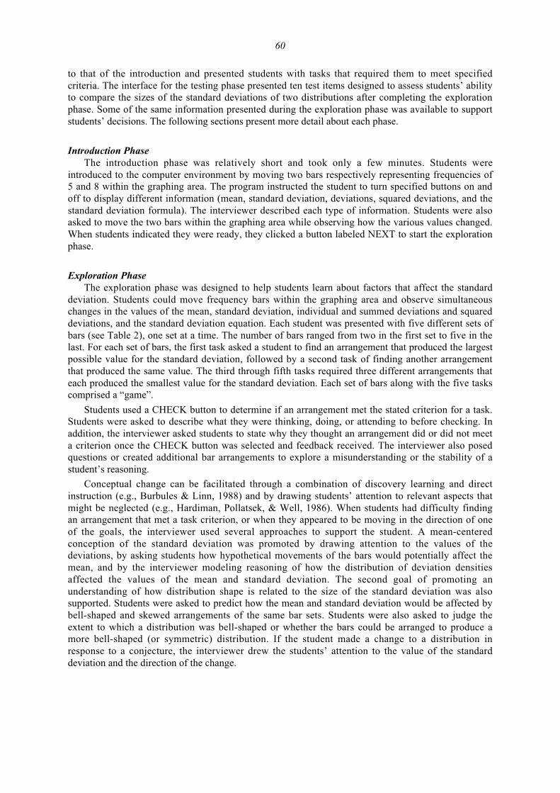
60

to that of the introduction and presented students with tasks that required them to meet specifiedcriteria. The interface for the testing phase presented ten test items designed to assess students’ abilityto compare the sizes of the standard deviations of two distributions after completing the explorationphase. Some of the same information presented during the exploration phase was available to supportstudents’ decisions. The following sections present more detail about each phase.

Introduction PhaseThe introduction phase was relatively short and took only a few minutes. Students were

introduced to the computer environment by moving two bars respectively representing frequencies of5 and 8 within the graphing area. The program instructed the student to turn specified buttons on andoff to display different information (mean, standard deviation, deviations, squared deviations, and thestandard deviation formula). The interviewer described each type of information. Students were alsoasked to move the two bars within the graphing area while observing how the various values changed.When students indicated they were ready, they clicked a button labeled NEXT to start the explorationphase.

Exploration PhaseThe exploration phase was designed to help students learn about factors that affect the standard

deviation. Students could move frequency bars within the graphing area and observe simultaneouschanges in the values of the mean, standard deviation, individual and summed deviations and squareddeviations, and the standard deviation equation. Each student was presented with five different sets ofbars (see Table 2), one set at a time. The number of bars ranged from two in the first set to five in thelast. For each set of bars, the first task asked a student to find an arrangement that produced the largestpossible value for the standard deviation, followed by a second task of finding another arrangementthat produced the same value. The third through fifth tasks required three different arrangements thateach produced the smallest value for the standard deviation. Each set of bars along with the five taskscomprised a “game”.

Students used a CHECK button to determine if an arrangement met the stated criterion for a task.Students were asked to describe what they were thinking, doing, or attending to before checking. Inaddition, the interviewer asked students to state why they thought an arrangement did or did not meeta criterion once the CHECK button was selected and feedback received. The interviewer also posedquestions or created additional bar arrangements to explore a misunderstanding or the stability of astudent’s reasoning.

Conceptual change can be facilitated through a combination of discovery learning and directinstruction (e.g., Burbules & Linn, 1988) and by drawing students’ attention to relevant aspects thatmight be neglected (e.g., Hardiman, Pollatsek, & Well, 1986). When students had difficulty findingan arrangement that met a task criterion, or when they appeared to be moving in the direction of oneof the goals, the interviewer used several approaches to support the student. A mean-centeredconception of the standard deviation was promoted by drawing attention to the values of thedeviations, by asking students how hypothetical movements of the bars would potentially affect themean, and by the interviewer modeling reasoning of how the distribution of deviation densitiesaffected the values of the mean and standard deviation. The second goal of promoting anunderstanding of how distribution shape is related to the size of the standard deviation was alsosupported. Students were asked to predict how the mean and standard deviation would be affected bybell-shaped and skewed arrangements of the same bar sets. Students were also asked to judge theextent to which a distribution was bell-shaped or whether the bars could be arranged to produce amore bell-shaped (or symmetric) distribution. If the student made a change to a distribution inresponse to a conjecture, the interviewer drew the students’ attention to the value of the standarddeviation and the direction of the change.

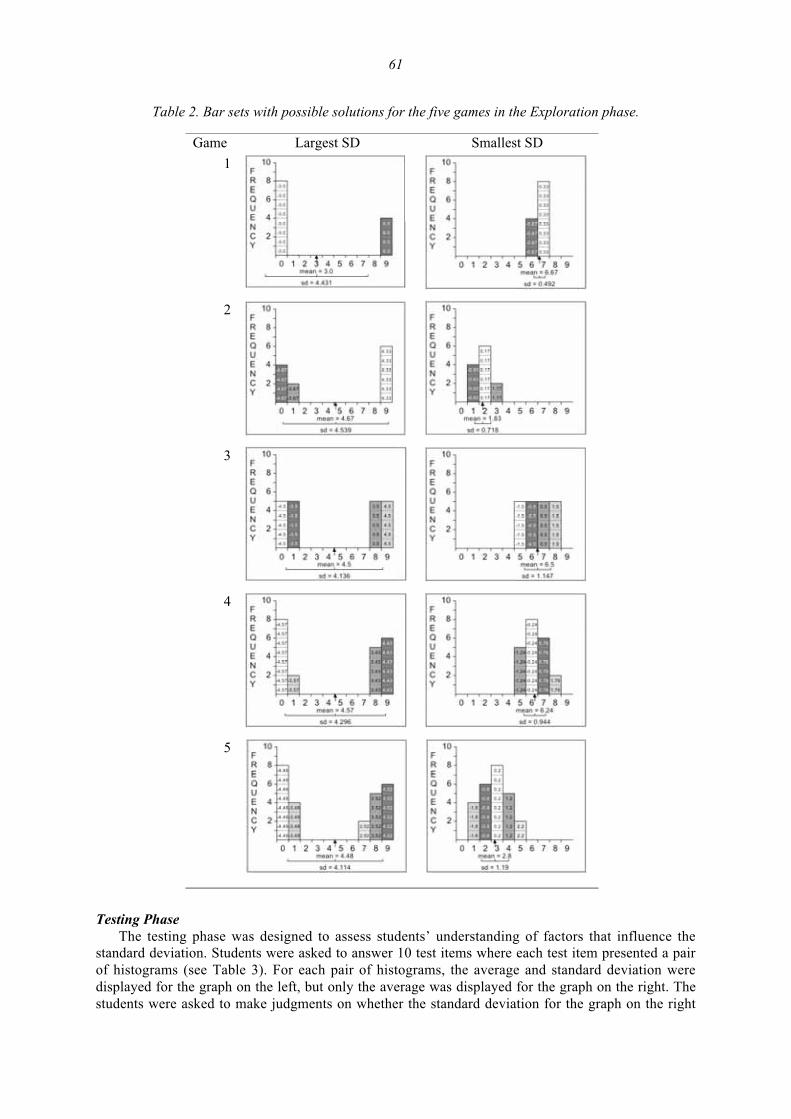
61

Table 2. Bar sets with possible solutions for the five games in the Exploration phase.

Game Largest SD Smallest SD

1

2

3

4

5

Testing PhaseThe testing phase was designed to assess students’ understanding of factors that influence the

standard deviation. Students were asked to answer 10 test items where each test item presented a pairof histograms (see Table 3). For each pair of histograms, the average and standard deviation weredisplayed for the graph on the left, but only the average was displayed for the graph on the right. Thestudents were asked to make judgments on whether the standard deviation for the graph on the right

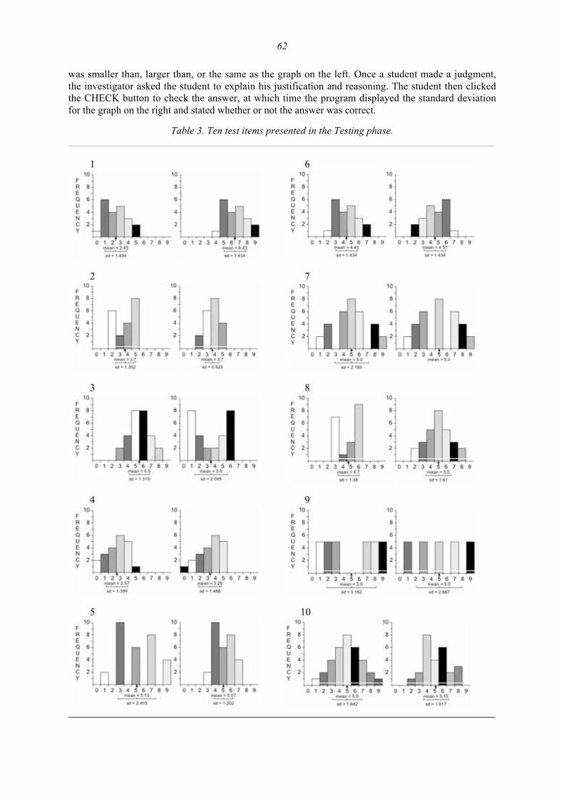
62

was smaller than, larger than, or the same as the graph on the left. Once a student made a judgment,the investigator asked the student to explain his justification and reasoning. The student then clickedthe CHECK button to check the answer, at which time the program displayed the standard deviationfor the graph on the right and stated whether or not the answer was correct.

Table 3. Ten test items presented in the Testing phase.

1 6

2 7

3 8

4 9

5 10

63

The test items were based on the two stated goals of the study. None of the bar sets were identicalto the sets of bars presented during the exploration phase. Each pair of graphs in test items 1 through 7had identical bars placed in different arrangements. Test item 1 required students to recognize thatboth graphs had the same bar arrangement in different locations, whereas students had to recognizethat one distribution was the mirror image of the other in test item 6. Test item 4 was specificallydesigned to see if students understood that given the same frequencies and range, a distribution with astronger skew tended to have a larger standard deviation. Test items 2 and 3 tested students’sensitivity to the density of values around the mean. Test items 5 and 7 were similar in this respect,however the bars in both graphs were in the same order. These latter two items were designed toidentify students who might attend only to the order of the bars and not to the relative density ofdeviations from the mean. The pair of graphs in test items 8, 9, and 10 did not have identical bars andalso had a different number of values represented in each graph. In a pilot study, some studentsinitially thought that evenly spacing the bars across the full range of the number scale would producethe largest value for the standard deviation. This misunderstanding was tested directly by test item 9,although this thinking could also be used to answer test item 5.

Test items 8 and 10 were designed to challenge the belief that a perfectly symmetric and bell-shaped distribution will always have a smaller standard deviation. Students were expected to findthese items more difficult than the others. For both test items, each graph had characteristics thatindicated it could have either the smaller or larger standard deviation of the pair. For example, in testitem 8, the U-shaped graph on the left appeared to have less density about the mean while the graphon the right was perfectly symmetric with apparently a large portion of the density centered aroundthe mean. Based on this, a student might have reasoned that the graph on the right had the smallerstandard deviation. However, the graph on the left had a smaller range and represented a smallernumber of values. Both of these characteristics made it possible for the graph on the left to haverelatively more density around the mean than the graph on the right (which was the case). Areasonable response to test items 8 and 10 would have been that both standard deviations (or thevariances) needed to be calculated to determine how they differ. The program provided the sum ofsquared deviations for both graphs to support these calculations.

3. RESULTS

3.1. EXPLORATION PHASE

The transcript analysis of the exploration phase focused on categorizing and describing thejustifications students presented when asked why they expected an arrangement to satisfy a taskcriterion (e.g., the largest possible standard deviation). These justifications were taken to represent thestudents’ conceptual understandings of the standard deviation as they developed during the interview.While some students appeared to start the interview with a fairly sophisticated understanding offactors that affect the standard deviation, most students started with a very simple, rule orientedapproach.

Eleven broad categories of justifications were identified with the following labels (in alphabeticalorder): Balance, Bell-Shaped, Big Mean, Contiguous, Equally Spread Out, Far Away, Guess andCheck, Location, Mean in the Middle, Mirror Image, and More Bars in the Middle. Each justificationis described and illustrated in more detail in the subsequent sections. This section is organized in fivesubsections: Justifications for arrangements intended to produce the largest standard deviation (task 1)are presented first, followed by justifications for arrangements intended to produce the smalleststandard deviation (task 3), and then justifications for arrangements intended to produce the samestandard deviation (tasks 2, 4, and 5). These subsections are followed by a general discussion ofstudents who began to coordinate conceptions about the standard deviation, and a final section thatsummarizes the findings from the exploration phase.

Graphs of students’ bar arrangements are presented to illustrate excerpts from student interviews.Each bar in the software program was presented in a different color, however, the bars presented inthe figures are in gray tones. Table 4 presents a legend for the bar colors.

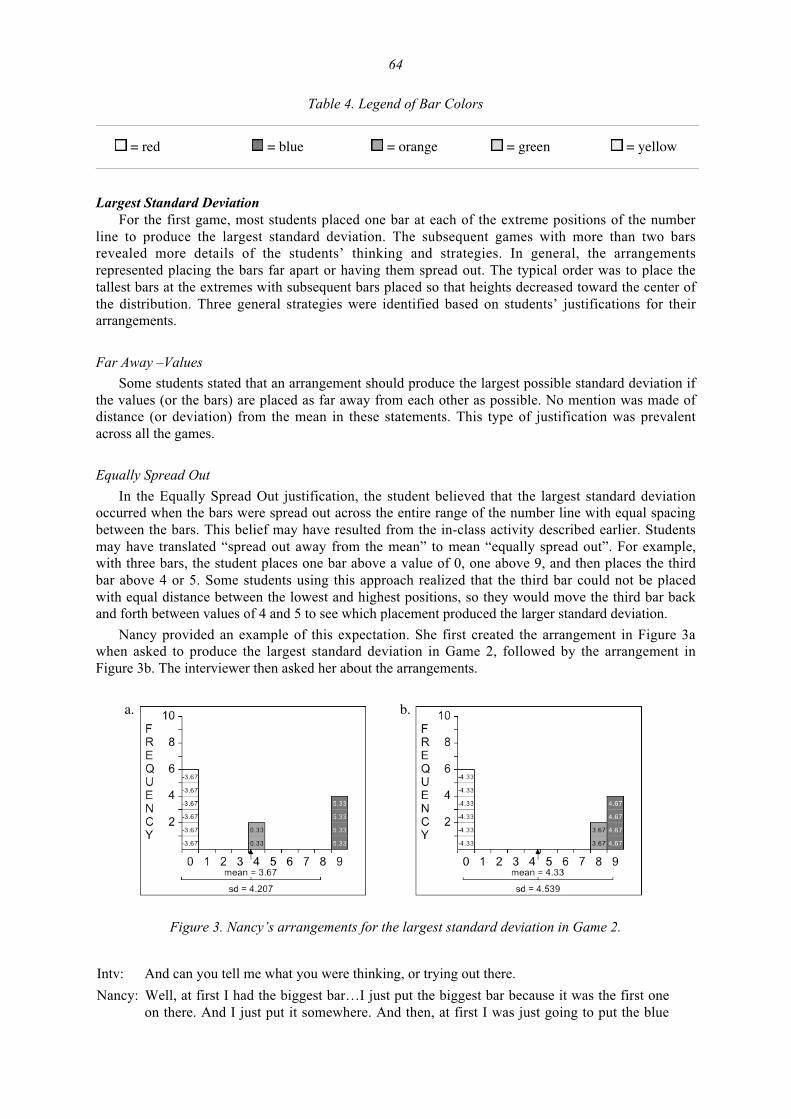
64

Table 4. Legend of Bar Colors

= red = blue = orange = green = yellow

Largest Standard DeviationFor the first game, most students placed one bar at each of the extreme positions of the number

line to produce the largest standard deviation. The subsequent games with more than two barsrevealed more details of the students’ thinking and strategies. In general, the arrangementsrepresented placing the bars far apart or having them spread out. The typical order was to place thetallest bars at the extremes with subsequent bars placed so that heights decreased toward the center ofthe distribution. Three general strategies were identified based on students’ justifications for theirarrangements.

Far Away –Values

Some students stated that an arrangement should produce the largest possible standard deviation ifthe values (or the bars) are placed as far away from each other as possible. No mention was made ofdistance (or deviation) from the mean in these statements. This type of justification was prevalentacross all the games.

Equally Spread Out

In the Equally Spread Out justification, the student believed that the largest standard deviationoccurred when the bars were spread out across the entire range of the number line with equal spacingbetween the bars. This belief may have resulted from the in-class activity described earlier. Studentsmay have translated “spread out away from the mean” to mean “equally spread out”. For example,with three bars, the student places one bar above a value of 0, one above 9, and then places the thirdbar above 4 or 5. Some students using this approach realized that the third bar could not be placedwith equal distance between the lowest and highest positions, so they would move the third bar backand forth between values of 4 and 5 to see which placement produced the larger standard deviation.

Nancy provided an example of this expectation. She first created the arrangement in Figure 3awhen asked to produce the largest standard deviation in Game 2, followed by the arrangement inFigure 3b. The interviewer then asked her about the arrangements.

a. b.

Figure 3. Nancy’s arrangements for the largest standard deviation in Game 2.

Intv: And can you tell me what you were thinking, or trying out there.

Nancy: Well, at first I had the biggest bar…I just put the biggest bar because it was the first oneon there. And I just put it somewhere. And then, at first I was just going to put the blue

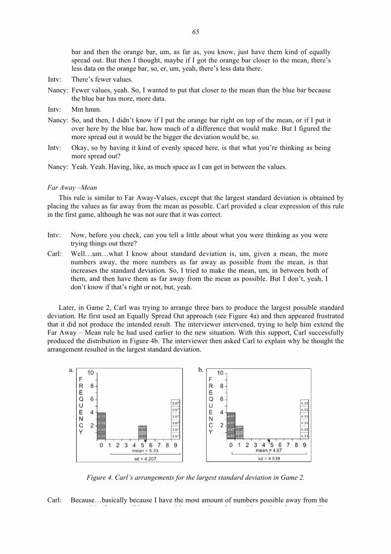
65

bar and then the orange bar, um, as far as, you know, just have them kind of equallyspread out. But then I thought, maybe if I got the orange bar closer to the mean, there’sless data on the orange bar, so, er, um, yeah, there’s less data there.

Intv: There’s fewer values.

Nancy: Fewer values, yeah. So, I wanted to put that closer to the mean than the blue bar becausethe blue bar has more, more data.

Intv: Mm hmm.

Nancy: So, and then, I didn’t know if I put the orange bar right on top of the mean, or if I put itover here by the blue bar, how much of a difference that would make. But I figured themore spread out it would be the bigger the deviation would be, so.

Intv: Okay, so by having it kind of evenly spaced here, is that what you’re thinking as beingmore spread out?

Nancy: Yeah. Yeah. Having, like, as much space as I can get in between the values.

Far Away –Mean

This rule is similar to Far Away-Values, except that the largest standard deviation is obtained byplacing the values as far away from the mean as possible. Carl provided a clear expression of this rulein the first game, although he was not sure that it was correct.

Intv: Now, before you check, can you tell a little about what you were thinking as you weretrying things out there?

Carl: Well…um…what I know about standard deviation is, um, given a mean, the morenumbers away, the more numbers as far away as possible from the mean, is thatincreases the standard deviation. So, I tried to make the mean, um, in between both ofthem, and then have them as far away from the mean as possible. But I don’t, yeah, Idon’t know if that’s right or not, but, yeah.

Later, in Game 2, Carl was trying to arrange three bars to produce the largest possible standarddeviation. He first used an Equally Spread Out approach (see Figure 4a) and then appeared frustratedthat it did not produce the intended result. The interviewer intervened, trying to help him extend theFar Away – Mean rule he had used earlier to the new situation. With this support, Carl successfullyproduced the distribution in Figure 4b. The interviewer then asked Carl to explain why he thought thearrangement resulted in the largest standard deviation.

a. b.

Figure 4. Carl’s arrangements for the largest standard deviation in Game 2.

Carl: Because…basically because I have the most amount of numbers possible away from theU b if I I h b h bi h h ll

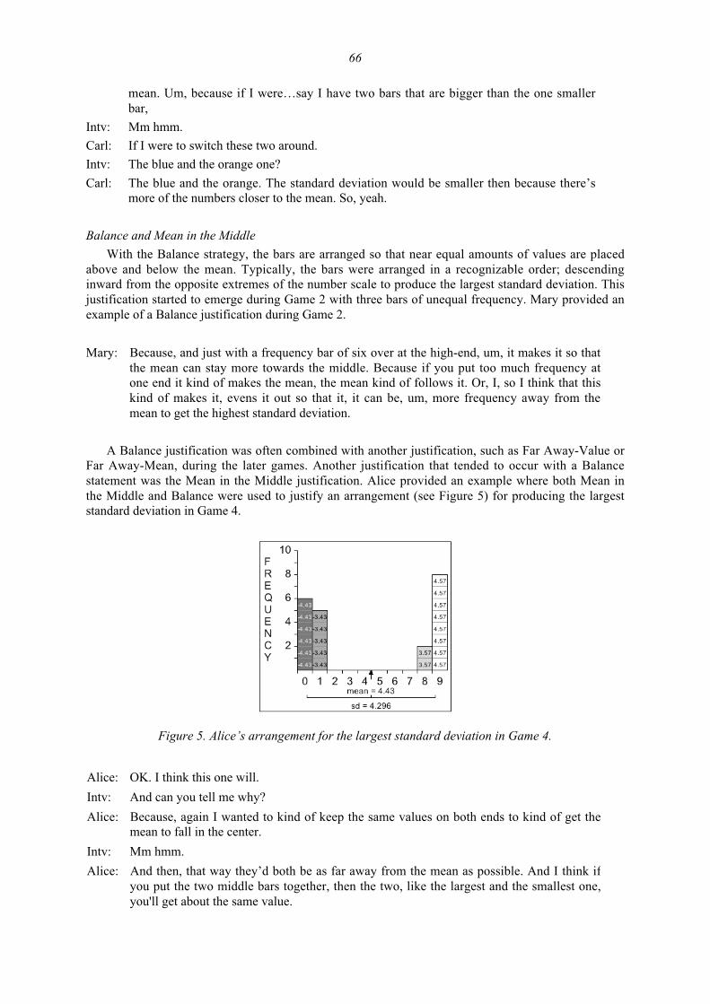
66

mean. Um, because if I were…say I have two bars that are bigger than the one smallerbar,

Intv: Mm hmm.

Carl: If I were to switch these two around.

Intv: The blue and the orange one?

Carl: The blue and the orange. The standard deviation would be smaller then because there’smore of the numbers closer to the mean. So, yeah.

Balance and Mean in the Middle

With the Balance strategy, the bars are arranged so that near equal amounts of values are placedabove and below the mean. Typically, the bars were arranged in a recognizable order; descendinginward from the opposite extremes of the number scale to produce the largest standard deviation. Thisjustification started to emerge during Game 2 with three bars of unequal frequency. Mary provided anexample of a Balance justification during Game 2.

Mary: Because, and just with a frequency bar of six over at the high-end, um, it makes it so thatthe mean can stay more towards the middle. Because if you put too much frequency atone end it kind of makes the mean, the mean kind of follows it. Or, I, so I think that thiskind of makes it, evens it out so that it, it can be, um, more frequency away from themean to get the highest standard deviation.

A Balance justification was often combined with another justification, such as Far Away-Value orFar Away-Mean, during the later games. Another justification that tended to occur with a Balancestatement was the Mean in the Middle justification. Alice provided an example where both Mean inthe Middle and Balance were used to justify an arrangement (see Figure 5) for producing the largeststandard deviation in Game 4.

Figure 5. Alice’s arrangement for the largest standard deviation in Game 4.

Alice: OK. I think this one will.

Intv: And can you tell me why?

Alice: Because, again I wanted to kind of keep the same values on both ends to kind of get themean to fall in the center.

Intv: Mm hmm.

Alice: And then, that way they’d both be as far away from the mean as possible. And I think ifyou put the two middle bars together, then the two, like the largest and the smallest one,you'll get about the same value.

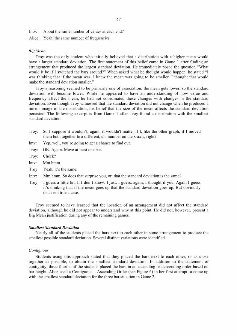
67

Intv: About the same number of values at each end?

Alice: Yeah, the same number of frequencies.

Big Mean

Troy was the only student who initially believed that a distribution with a higher mean wouldhave a larger standard deviation. The first statement of this belief came in Game 1 after finding anarrangement that produced the largest standard deviation. He immediately posed the question “Whatwould it be if I switched the bars around?” When asked what he thought would happen, he stated “Iwas thinking that if the mean was, I knew the mean was going to be smaller. I thought that wouldmake the standard deviation smaller.”

Troy’s reasoning seemed to be primarily one of association: the mean gets lower, so the standarddeviation will become lower. While he appeared to have an understanding of how value andfrequency affect the mean, he had not coordinated these changes with changes in the standarddeviation. Even though Troy witnessed that the standard deviation did not change when he produced amirror image of the distribution, his belief that the size of the mean affects the standard deviationpersisted. The following excerpt is from Game 1 after Troy found a distribution with the smalleststandard deviation.

Troy: So I suppose it wouldn’t, again, it wouldn't matter if I, like the other graph, if I movedthem both together to a different, uh, number on the x-axis, right?

Intv: Yep, well, you’re going to get a chance to find out.

Troy: OK. Again. Move at least one bar.

Troy: Check?

Intv: Mm hmm.

Troy: Yeah, it’s the same.

Intv: Mm hmm. So does that surprise you, or, that the standard deviation is the same?

Troy: I guess a little bit. I, I don’t know. I just, I guess, again, I thought if you. Again I guessit’s thinking that if the mean goes up that the standard deviation goes up. But obviouslythat's not true a case.

Troy seemed to have learned that the location of an arrangement did not affect the standarddeviation, although he did not appear to understand why at this point. He did not, however, present aBig Mean justification during any of the remaining games.

Smallest Standard DeviationNearly all of the students placed the bars next to each other in some arrangement to produce the

smallest possible standard deviation. Several distinct variations were identified.

Contiguous

Students using this approach stated that they placed the bars next to each other, or as closetogether as possible, to obtain the smallest standard deviation. In addition to the statement ofcontiguity, three-fourths of the students placed the bars in an ascending or descending order based onbar height. Alice used a Contiguous – Ascending Order (see Figure 6) in her first attempt to come upwith the smallest standard deviation for the three bar situation in Game 2.

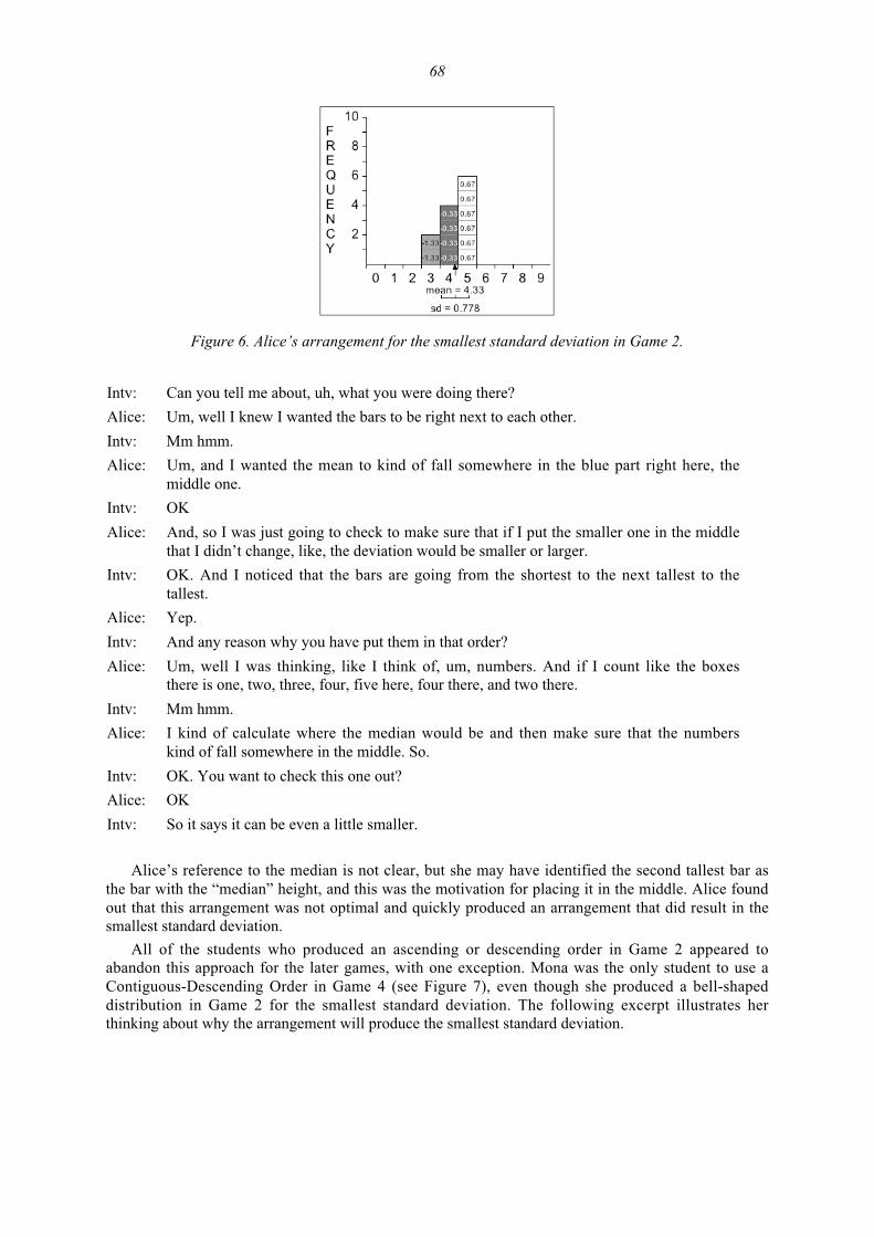
68

Figure 6. Alice’s arrangement for the smallest standard deviation in Game 2.

Intv: Can you tell me about, uh, what you were doing there?

Alice: Um, well I knew I wanted the bars to be right next to each other.

Intv: Mm hmm.

Alice: Um, and I wanted the mean to kind of fall somewhere in the blue part right here, themiddle one.

Intv: OK

Alice: And, so I was just going to check to make sure that if I put the smaller one in the middlethat I didn’t change, like, the deviation would be smaller or larger.

Intv: OK. And I noticed that the bars are going from the shortest to the next tallest to thetallest.

Alice: Yep.

Intv: And any reason why you have put them in that order?

Alice: Um, well I was thinking, like I think of, um, numbers. And if I count like the boxesthere is one, two, three, four, five here, four there, and two there.

Intv: Mm hmm.

Alice: I kind of calculate where the median would be and then make sure that the numberskind of fall somewhere in the middle. So.

Intv: OK. You want to check this one out?

Alice: OK

Intv: So it says it can be even a little smaller.

Alice’s reference to the median is not clear, but she may have identified the second tallest bar asthe bar with the “median” height, and this was the motivation for placing it in the middle. Alice foundout that this arrangement was not optimal and quickly produced an arrangement that did result in thesmallest standard deviation.

All of the students who produced an ascending or descending order in Game 2 appeared toabandon this approach for the later games, with one exception. Mona was the only student to use aContiguous-Descending Order in Game 4 (see Figure 7), even though she produced a bell-shapeddistribution in Game 2 for the smallest standard deviation. The following excerpt illustrates herthinking about why the arrangement will produce the smallest standard deviation.

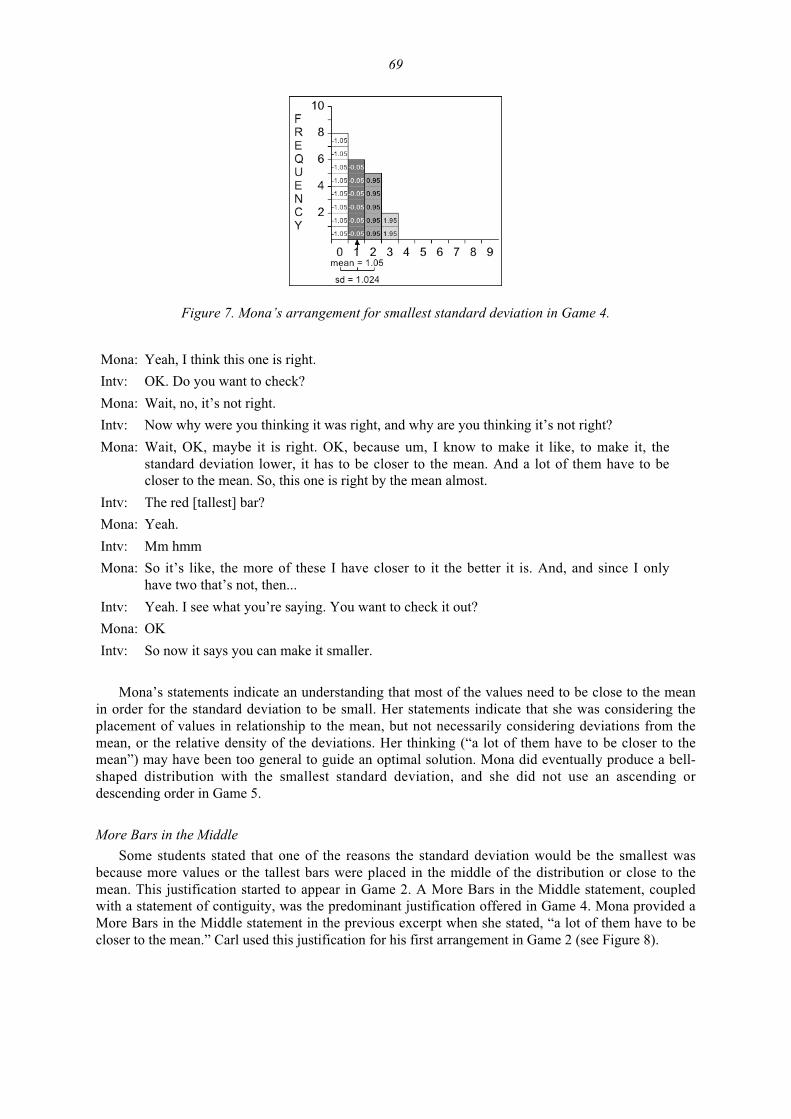
69

Figure 7. Mona’s arrangement for smallest standard deviation in Game 4.

Mona: Yeah, I think this one is right.

Intv: OK. Do you want to check?

Mona: Wait, no, it’s not right.

Intv: Now why were you thinking it was right, and why are you thinking it’s not right?

Mona: Wait, OK, maybe it is right. OK, because um, I know to make it like, to make it, thestandard deviation lower, it has to be closer to the mean. And a lot of them have to becloser to the mean. So, this one is right by the mean almost.

Intv: The red [tallest] bar?

Mona: Yeah.

Intv: Mm hmm

Mona: So it’s like, the more of these I have closer to it the better it is. And, and since I onlyhave two that’s not, then...

Intv: Yeah. I see what you’re saying. You want to check it out?

Mona: OK

Intv: So now it says you can make it smaller.

Mona’s statements indicate an understanding that most of the values need to be close to the meanin order for the standard deviation to be small. Her statements indicate that she was considering theplacement of values in relationship to the mean, but not necessarily considering deviations from themean, or the relative density of the deviations. Her thinking (“a lot of them have to be closer to themean”) may have been too general to guide an optimal solution. Mona did eventually produce a bell-shaped distribution with the smallest standard deviation, and she did not use an ascending ordescending order in Game 5.

More Bars in the Middle

Some students stated that one of the reasons the standard deviation would be the smallest wasbecause more values or the tallest bars were placed in the middle of the distribution or close to themean. This justification started to appear in Game 2. A More Bars in the Middle statement, coupledwith a statement of contiguity, was the predominant justification offered in Game 4. Mona provided aMore Bars in the Middle statement in the previous excerpt when she stated, “a lot of them have to becloser to the mean.” Carl used this justification for his first arrangement in Game 2 (see Figure 8).

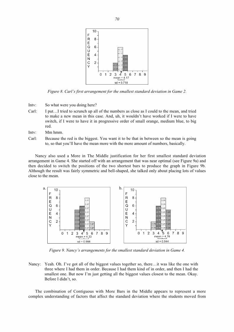
70

Figure 8. Carl’s first arrangement for the smallest standard deviation in Game 2.

Intv: So what were you doing here?

Carl: I put…I tried to scrunch up all of the numbers as close as I could to the mean, and triedto make a new mean in this case. And, uh, it wouldn’t have worked if I were to haveswitch, if I were to have it in progressive order of small orange, medium blue, to bigred.

Intv: Mm hmm.

Carl: Because the red is the biggest. You want it to be that in between so the mean is goingto, so that you’ll have the mean more with the more amount of numbers, basically.

Nancy also used a More in The Middle justification for her first smallest standard deviationarrangement in Game 4. She started off with an arrangement that was near optimal (see Figure 9a) andthen decided to switch the positions of the two shortest bars to produce the graph in Figure 9b.Although the result was fairly symmetric and bell-shaped, she talked only about placing lots of valuesclose to the mean.

a. b.

Figure 9. Nancy’s arrangements for the smallest standard deviation in Game 4.

Nancy: Yeah. Oh. I’ve got all of the biggest values together so, there…it was like the one withthree where I had them in order. Because I had them kind of in order, and then I had thesmallest one. But now I’m just getting all the biggest values closest to the mean. Okay.Before I didn’t, so.

The combination of Contiguous with More Bars in the Middle appears to represent a morecomplex understanding of factors that affect the standard deviation where the students moved from

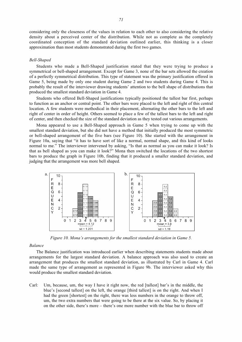
71

considering only the closeness of the values in relation to each other to also considering the relativedensity about a perceived center of the distribution. While not as complete as the completelycoordinated conception of the standard deviation outlined earlier, this thinking is a closerapproximation than most students demonstrated during the first two games.

Bell-Shaped

Students who made a Bell-Shaped justification stated that they were trying to produce asymmetrical or bell-shaped arrangement. Except for Game 3, none of the bar sets allowed the creationof a perfectly symmetrical distribution. This type of statement was the primary justification offered inGame 5, being made by only one student during Game 2 and two students during Game 4. This isprobably the result of the interviewer drawing students’ attention to the bell shape of distributions thatproduced the smallest standard deviation in Game 4.

Students who offered Bell-Shaped justifications typically positioned the tallest bar first, perhapsto function as an anchor or central point. The other bars were placed to the left and right of this centrallocation. A few students were methodical in their placement, alternating the other bars to the left andright of center in order of height. Others seemed to place a few of the tallest bars to the left and rightof center, and then checked the size of the standard deviation as they tested out various arrangements.

Mona appeared to use a Bell-Shaped approach in Game 5 when trying to come up with thesmallest standard deviation, but she did not have a method that initially produced the most symmetricor bell-shaped arrangement of the five bars (see Figure 10). She started with the arrangement inFigure 10a, saying that “it has to have sort of like a normal, normal shape, and this kind of looksnormal to me.” The interviewer intervened by asking, “Is that as normal as you can make it look? Isthat as bell shaped as you can make it look?” Mona then switched the locations of the two shortestbars to produce the graph in Figure 10b, finding that it produced a smaller standard deviation, andjudging that the arrangement was more bell shaped.

a. b.

Figure 10. Mona’s arrangements for the smallest standard deviation in Game 5.

Balance

The Balance justification was introduced earlier when describing statements students made aboutarrangements for the largest standard deviation. A balance approach was also used to create anarrangement that produces the smallest standard deviation, as illustrated by Carl in Game 4. Carlmade the same type of arrangement as represented in Figure 9b. The interviewer asked why thiswould produce the smallest standard deviation.

Carl: Um, because, um, the way I have it right now, the red [tallest] bar’s in the middle, theblue’s [second tallest] on the left, the orange [third tallest] is on the right. And when Ihad the green [shortest] on the right, there was less numbers in the orange to throw off,um, the two extra numbers that were going to be there at the six value. So, by placing iton the other side, there’s more – there’s one more number with the blue bar to throw off

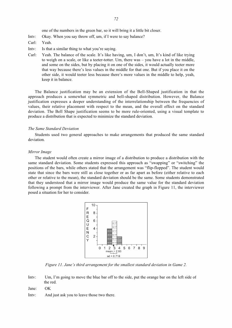
72

one of the numbers in the green bar, so it will bring it a little bit closer.

Intv: Okay. When you say throw off, um, if I were to say balance?

Carl: Yeah.

Intv: Is that a similar thing to what you’re saying.

Carl: Yeah. The balance of the scale. It’s like having, um, I don’t, um, It’s kind of like tryingto weigh on a scale, or like a teeter-totter. Um, there was – you have a lot in the middle,and some on the sides, but by placing it on one of the sides, it would actually teeter morethat way because there’s less values in the middle for that one. But if you place it on theother side, it would teeter less because there’s more values in the middle to help, yeah,keep it in balance.

The Balance justification may be an extension of the Bell-Shaped justification in that theapproach produces a somewhat symmetric and bell-shaped distribution. However, the Balancejustification expresses a deeper understanding of the interrelationship between the frequencies ofvalues, their relative placement with respect to the mean, and the overall effect on the standarddeviation. The Bell Shape justification seems to be more rule-oriented, using a visual template toproduce a distribution that is expected to minimize the standard deviation.

The Same Standard Deviation

Students used two general approaches to make arrangements that produced the same standarddeviation.

Mirror Image

The student would often create a mirror image of a distribution to produce a distribution with thesame standard deviation. Some students expressed this approach as “swapping” or “switching” thepositions of the bars, while others stated that the arrangement was “flip-flopped”. The student wouldstate that since the bars were still as close together or as far apart as before (either relative to eachother or relative to the mean), the standard deviation should be the same. Some students demonstratedthat they understood that a mirror image would produce the same value for the standard deviationfollowing a prompt from the interviewer. After Jane created the graph in Figure 11, the interviewerposed a situation for her to consider.

Figure 11. Jane’s third arrangement for the smallest standard deviation in Game 2.

Intv: Um, I’m going to move the blue bar off to the side, put the orange bar on the left side ofthe red.

Jane: OK

Intv: And just ask you to leave those two there.

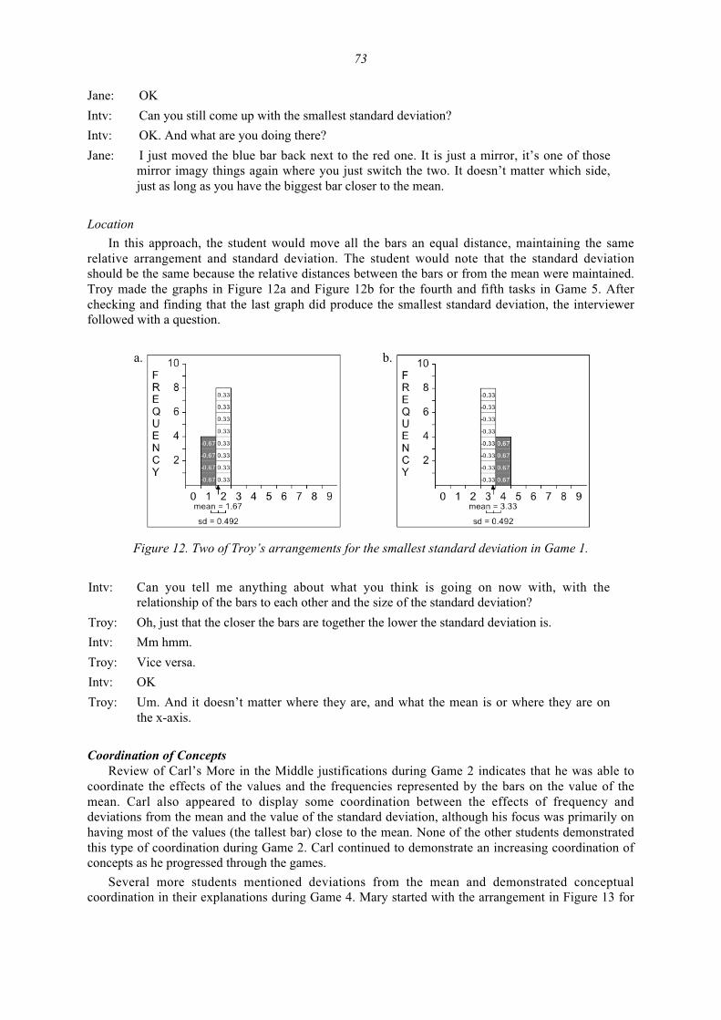
73

Jane: OK

Intv: Can you still come up with the smallest standard deviation?

Intv: OK. And what are you doing there?

Jane: I just moved the blue bar back next to the red one. It is just a mirror, it’s one of thosemirror imagy things again where you just switch the two. It doesn’t matter which side,just as long as you have the biggest bar closer to the mean.

Location

In this approach, the student would move all the bars an equal distance, maintaining the samerelative arrangement and standard deviation. The student would note that the standard deviationshould be the same because the relative distances between the bars or from the mean were maintained.Troy made the graphs in Figure 12a and Figure 12b for the fourth and fifth tasks in Game 5. Afterchecking and finding that the last graph did produce the smallest standard deviation, the interviewerfollowed with a question.

a. b.

Figure 12. Two of Troy’s arrangements for the smallest standard deviation in Game 1.

Intv: Can you tell me anything about what you think is going on now with, with therelationship of the bars to each other and the size of the standard deviation?

Troy: Oh, just that the closer the bars are together the lower the standard deviation is.

Intv: Mm hmm.

Troy: Vice versa.

Intv: OK

Troy: Um. And it doesn’t matter where they are, and what the mean is or where they are onthe x-axis.

Coordination of ConceptsReview of Carl’s More in the Middle justifications during Game 2 indicates that he was able to

coordinate the effects of the values and the frequencies represented by the bars on the value of themean. Carl also appeared to display some coordination between the effects of frequency anddeviations from the mean and the value of the standard deviation, although his focus was primarily onhaving most of the values (the tallest bar) close to the mean. None of the other students demonstratedthis type of coordination during Game 2. Carl continued to demonstrate an increasing coordination ofconcepts as he progressed through the games.

Several more students mentioned deviations from the mean and demonstrated conceptualcoordination in their explanations during Game 4. Mary started with the arrangement in Figure 13 for

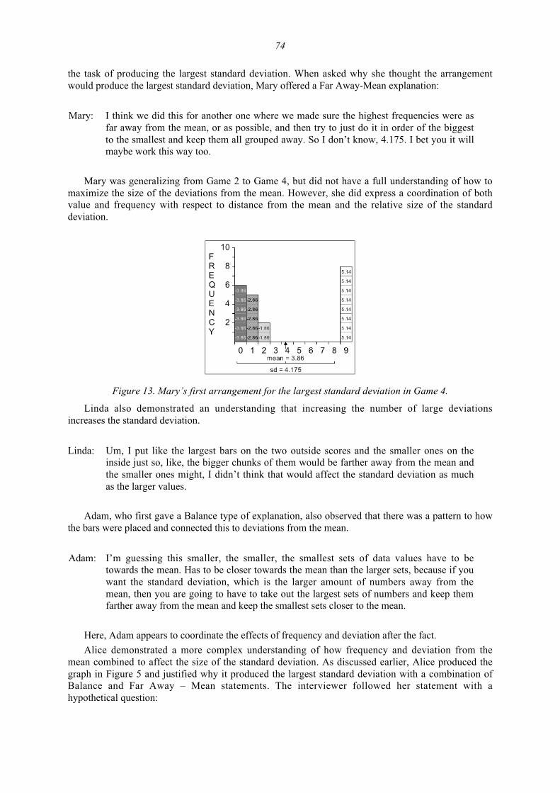
74

the task of producing the largest standard deviation. When asked why she thought the arrangementwould produce the largest standard deviation, Mary offered a Far Away-Mean explanation:

Mary: I think we did this for another one where we made sure the highest frequencies were asfar away from the mean, or as possible, and then try to just do it in order of the biggestto the smallest and keep them all grouped away. So I don’t know, 4.175. I bet you it willmaybe work this way too.

Mary was generalizing from Game 2 to Game 4, but did not have a full understanding of how tomaximize the size of the deviations from the mean. However, she did express a coordination of bothvalue and frequency with respect to distance from the mean and the relative size of the standarddeviation.

Figure 13. Mary’s first arrangement for the largest standard deviation in Game 4.

Linda also demonstrated an understanding that increasing the number of large deviationsincreases the standard deviation.

Linda: Um, I put like the largest bars on the two outside scores and the smaller ones on theinside just so, like, the bigger chunks of them would be farther away from the mean andthe smaller ones might, I didn’t think that would affect the standard deviation as muchas the larger values.

Adam, who first gave a Balance type of explanation, also observed that there was a pattern to howthe bars were placed and connected this to deviations from the mean.

Adam: I’m guessing this smaller, the smaller, the smallest sets of data values have to betowards the mean. Has to be closer towards the mean than the larger sets, because if youwant the standard deviation, which is the larger amount of numbers away from themean, then you are going to have to take out the largest sets of numbers and keep themfarther away from the mean and keep the smallest sets closer to the mean.

Here, Adam appears to coordinate the effects of frequency and deviation after the fact.

Alice demonstrated a more complex understanding of how frequency and deviation from themean combined to affect the size of the standard deviation. As discussed earlier, Alice produced thegraph in Figure 5 and justified why it produced the largest standard deviation with a combination ofBalance and Far Away – Mean statements. The interviewer followed her statement with ahypothetical question:

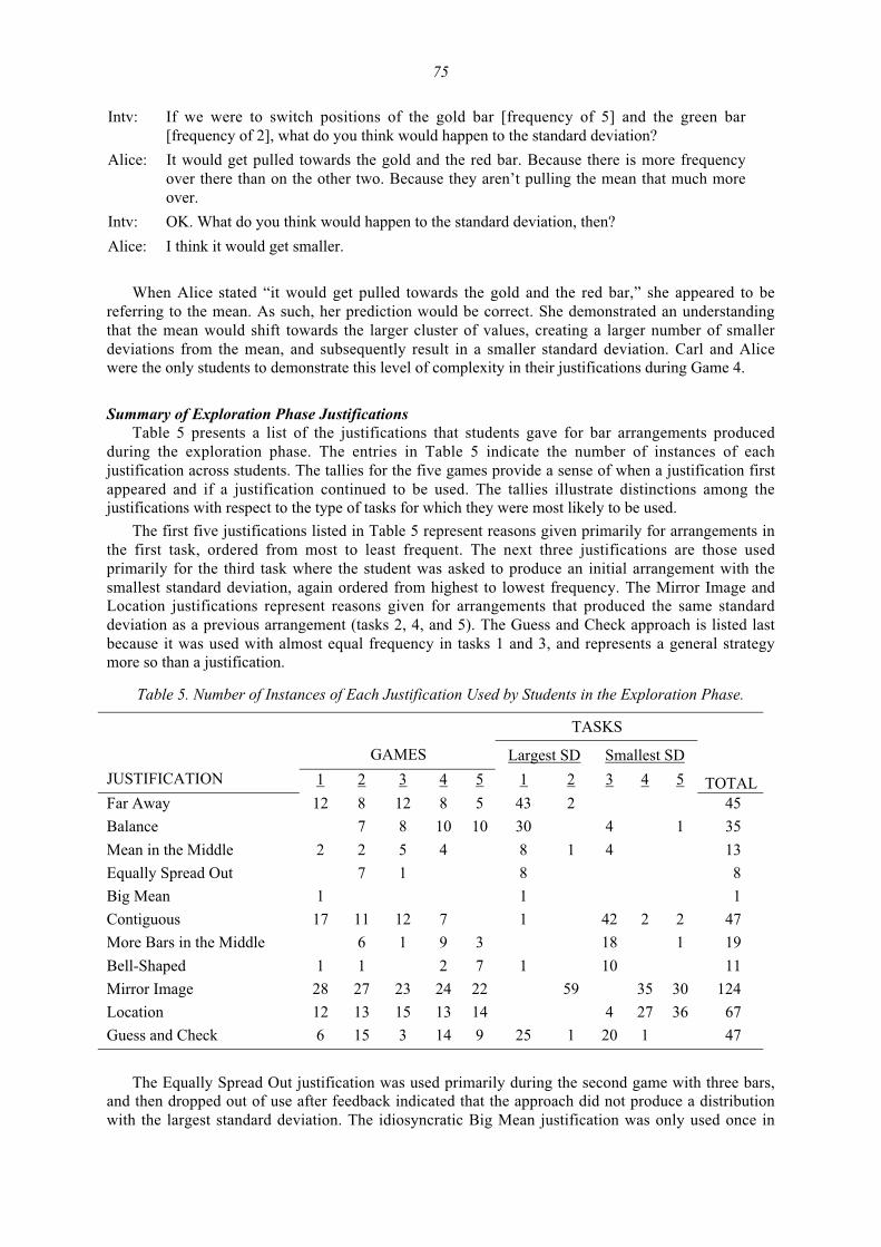
75

Intv: If we were to switch positions of the gold bar [frequency of 5] and the green bar[frequency of 2], what do you think would happen to the standard deviation?

Alice: It would get pulled towards the gold and the red bar. Because there is more frequencyover there than on the other two. Because they aren’t pulling the mean that much moreover.

Intv: OK. What do you think would happen to the standard deviation, then?

Alice: I think it would get smaller.

When Alice stated “it would get pulled towards the gold and the red bar,” she appeared to bereferring to the mean. As such, her prediction would be correct. She demonstrated an understandingthat the mean would shift towards the larger cluster of values, creating a larger number of smallerdeviations from the mean, and subsequently result in a smaller standard deviation. Carl and Alicewere the only students to demonstrate this level of complexity in their justifications during Game 4.

Summary of Exploration Phase JustificationsTable 5 presents a list of the justifications that students gave for bar arrangements produced

during the exploration phase. The entries in Table 5 indicate the number of instances of eachjustification across students. The tallies for the five games provide a sense of when a justification firstappeared and if a justification continued to be used. The tallies illustrate distinctions among thejustifications with respect to the type of tasks for which they were most likely to be used.

The first five justifications listed in Table 5 represent reasons given primarily for arrangements inthe first task, ordered from most to least frequent. The next three justifications are those usedprimarily for the third task where the student was asked to produce an initial arrangement with thesmallest standard deviation, again ordered from highest to lowest frequency. The Mirror Image andLocation justifications represent reasons given for arrangements that produced the same standarddeviation as a previous arrangement (tasks 2, 4, and 5). The Guess and Check approach is listed lastbecause it was used with almost equal frequency in tasks 1 and 3, and represents a general strategymore so than a justification.

Table 5. Number of Instances of Each Justification Used by Students in the Exploration Phase.

TASKS

GAMES Largest SD Smallest SD

JUSTIFICATION 1 2 3 4 5 1 2 3 4 5 TOTALFar Away 12 8 12 8 5 43 2 45

Balance 7 8 10 10 30 4 1 35

Mean in the Middle 2 2 5 4 8 1 4 13

Equally Spread Out 7 1 8 8

Big Mean 1 1 1

Contiguous 17 11 12 7 1 42 2 2 47

More Bars in the Middle 6 1 9 3 18 1 19

Bell-Shaped 1 1 2 7 1 10 11

Mirror Image 28 27 23 24 22 59 35 30 124

Location 12 13 15 13 14 4 27 36 67

Guess and Check 6 15 3 14 9 25 1 20 1 47

The Equally Spread Out justification was used primarily during the second game with three bars,and then dropped out of use after feedback indicated that the approach did not produce a distributionwith the largest standard deviation. The idiosyncratic Big Mean justification was only used once in

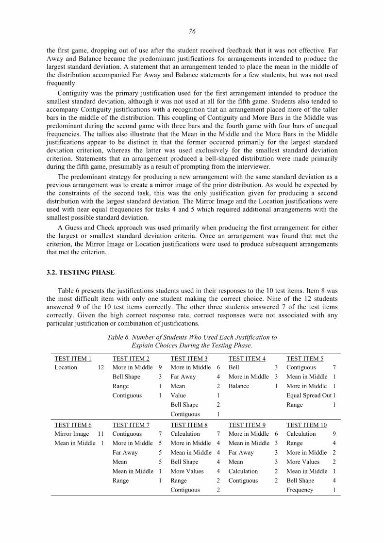
76

the first game, dropping out of use after the student received feedback that it was not effective. FarAway and Balance became the predominant justifications for arrangements intended to produce thelargest standard deviation. A statement that an arrangement tended to place the mean in the middle ofthe distribution accompanied Far Away and Balance statements for a few students, but was not usedfrequently.

Contiguity was the primary justification used for the first arrangement intended to produce thesmallest standard deviation, although it was not used at all for the fifth game. Students also tended toaccompany Contiguity justifications with a recognition that an arrangement placed more of the tallerbars in the middle of the distribution. This coupling of Contiguity and More Bars in the Middle waspredominant during the second game with three bars and the fourth game with four bars of unequalfrequencies. The tallies also illustrate that the Mean in the Middle and the More Bars in the Middlejustifications appear to be distinct in that the former occurred primarily for the largest standarddeviation criterion, whereas the latter was used exclusively for the smallest standard deviationcriterion. Statements that an arrangement produced a bell-shaped distribution were made primarilyduring the fifth game, presumably as a result of prompting from the interviewer.

The predominant strategy for producing a new arrangement with the same standard deviation as aprevious arrangement was to create a mirror image of the prior distribution. As would be expected bythe constraints of the second task, this was the only justification given for producing a seconddistribution with the largest standard deviation. The Mirror Image and the Location justifications wereused with near equal frequencies for tasks 4 and 5 which required additional arrangements with thesmallest possible standard deviation.

A Guess and Check approach was used primarily when producing the first arrangement for eitherthe largest or smallest standard deviation criteria. Once an arrangement was found that met thecriterion, the Mirror Image or Location justifications were used to produce subsequent arrangementsthat met the criterion.

3.2. TESTING PHASE

Table 6 presents the justifications students used in their responses to the 10 test items. Item 8 wasthe most difficult item with only one student making the correct choice. Nine of the 12 studentsanswered 9 of the 10 test items correctly. The other three students answered 7 of the test itemscorrectly. Given the high correct response rate, correct responses were not associated with anyparticular justification or combination of justifications.

Table 6. Number of Students Who Used Each Justification toExplain Choices During the Testing Phase.

TEST ITEM 1 TEST ITEM 2 TEST ITEM 3 TEST ITEM 4 TEST ITEM 5Location 12 More in Middle 9

Bell Shape 3

Range 1

Contiguous 1

More in Middle 6

Far Away 4

Mean 2

Value 1

Bell Shape 2

Contiguous 1

Bell 3

More in Middle 3

Balance 1

Contiguous 7

Mean in Middle 1

More in Middle 1

Equal Spread Out 1

Range 1

TEST ITEM 6 TEST ITEM 7 TEST ITEM 8 TEST ITEM 9 TEST ITEM 10Mirror Image 11

Mean in Middle 1

Contiguous 7

More in Middle 5

Far Away 5

Mean 5

Mean in Middle 1

Range 1

Calculation 7

More in Middle 4

Mean in Middle 4

Bell Shape 4

More Values 4

Range 2

Contiguous 2

More in Middle 6

Mean in Middle 3

Far Away 3

Mean 3

Calculation 2

Contiguous 2

Calculation 9

Range 4

More in Middle 2

More Values 2

Mean in Middle 1

Bell Shape 4

Frequency 1

77

Students’ justifications for their responses tended to be similar to those identified during theexploration phase, and tended to reflect relevant characteristics of the graphs. For example, allstudents indicated that the two graphs had the same standard deviation for the first test item, notingthat the arrangements were the same but in different locations. Most of the students’ justifications fortest items 2 and 3 were More in the Middle statements, although test item 3 also prompted Far Awayjustifications, probably because the graph on the right was U-shaped. For test item 6, studentsrecognized that one graph was the mirror image of the other and that the standard deviations were thesame. Almost all of the students gave a Mirror Image justification for their choice in item 6.

Students found test item 4 a little more difficult than the first three tests. Most noted that the onlydifference between the two graphs was the placement of the black (shortest bar). Only about half ofthe students provided a justification for their responses, which tended to be either that the graph on theleft was more bell-shaped, or that it had more values in the middle or around the mean compared tothe graph on the right. A few students stated that the left-hand graph was more skewed.

Two students (Adam and Lora) judged incorrectly that the graph on the left would have a smallerstandard deviation in test item 4. Adam noted the different location of the black bar in both graphs,but did not offer any other justification for his response. Adam did not demonstrate a consistentunderstanding of how frequency and deviation from the mean combined to affect the standarddeviation during the exploration phase, which was evidenced by his extensive use of a Guess andCheck approach. Item 4 may have proven difficult due to this lack of understanding. Lora alsodisplayed Guess and Check behavior during the exploration phase, but not to the same extent asAdam. Lora’s justification was actually a description of each graph’s characteristics and did notcompare the two graphs on features that would determine how the standard deviations differed. Whenasked how the graph on the right compared to the graph on the left, Lora responded, “That, well that’skind of the same thing as this one, but this one is, um, the smallest one is on the end instead, andalong with the other one.” No other justifications were offered before checking.

The difficulty with test item 4 may have resulted from the nature of the tasks during theexploration phase. The tasks required solutions that had some degree of symmetry and did not requirestudents to produce skewed distributions, although skewed distributions were often generated andchecked before an optimal distribution was found for the third task. The arrangements produced forthe largest standard deviation were U-shaped, with a large gap through the middle, while the optimalarrangements for the smallest distribution were bell- or mound-shaped. This experience during theexploration phase probably facilitated the comparison in test items 2 and 3, but did not necessarilyprovide experience directly related to the comparison needed to solve test item 4. Nonetheless, themajority of the students correctly identified the graph on the right as having a larger standarddeviation.

The first four test items involved graphs with contiguous bar placement, so that test item 5provided the first test of sensitivity to gaps between the bars. Almost all of the students’ justificationsfor test item 5 involved statements of contiguity. A few students noted that the range was wider in theleft-hand graph so that the graph on the right should have a smaller standard deviation given that thebars were the same and in the same order in both graphs. One of these students noted that the barswere equally spread out for the graph on the left, although the emphasis was on the wider range. Twostudents, Adam and Jeff, appeared to ignore the gaps between bars in the left-hand graph andresponded that the two graphs would have the same standard deviation, suggesting that shape was themain feature they considered in their decisions and an insensitivity to spread or deviation from themean.

Test item 7 also tested students’ understanding of how gaps affected the standard deviation,although in a more subtle way. All students answered test item 7 correctly, using arguments ofcontiguity and more values in the middle for the left-hand distribution as the reason why the right-hand distribution would have a larger standard deviation. Some students also noted that the right-handdistribution had relatively more values away from the mean. Test item 9 also presented gaps in thetwo distributions and challenged the misconception that having the bars evenly or equally spacedproduces a large standard deviation. All students answered test item 9 correctly and offered

78

justifications similar to those used in test item 7, indicating that the initial misconception representedby the Equally Spread Out justification had been overcome by those who first displayed it.

Test items 8 and 10 were designed to challenge the idea that perfectly symmetric, bell-shapeddistributions always have the smaller standard deviation. For test item 8, all but one of the studentsincorrectly stated that the graph on the right would have a smaller standard deviation. Linda answeredcorrectly that the symmetric, bell-shaped graph would have a larger standard deviation. Her reasoningwas that “there are more bars. There, um, even though like I think they are clumped pretty well,there’s still, um, a higher frequency and so, there’s three more, so because of like the extra threethere’s going to be more like room for deviation just because there’s more added values.” Otherstudents noted that there were more bars or values in the graph on the right, or that it had a largerrange, but still selected the smaller option as an answer. Students tended to note the bell-shape or theperception that more values were in the middle of the right-hand distribution compared to the one onthe left as reasons for their responses.

After students checked their answers to item 8 and found out they were incorrect, the interviewerattempted to guide their attention to the ambiguity that stemmed from a comparison of characteristicsbetween the two graphs. Attention was drawn to the differences in the number of values and therange, pointing out that while the bell shape suggested the right-hand graph would have a smallerstandard deviation, the larger range made it possible for it to have a larger standard deviation, and thedifferent number of values (or bars) presented a different situation than was presented either duringthe exploration phase or in the previous tests. The interviewer suggested that ambiguous situationsmight require calculation of the standard deviations, and demonstrated how the information providedby the program could be used to do so.

When students came to test item 10, they were more likely to note the difference in the number ofbars or values between the two graphs and resort to calculating the standard deviation for the graph onthe right. Nine of the students came to a correct decision predominantly through calculation. Two ofthe students (Troy and Jane) initially predicted the graph on the right to have a larger standarddeviation, but then noted the discrepancy in range or number of values, calculated the standarddeviation, and changed their decisions. Three students (Jeff, Lora, and Linda) did not performcalculations and incorrectly responded that the right-hand graph would have a larger standarddeviation. Because Linda correctly answered test item 8, she did not receive the same guidance fromthe interviewer as the other students, which may account for her incorrect response on test item 10.

4. DISCUSSION

While some research on students’ understanding of statistical variability has been conducted, littleis known about students’ understanding of measures of variability, such as the standard deviation,how that understanding develops, and effective ways to support that development. The study reportedhere was an attempt to address this lack of information. An exploratory research design was used thatemployed a multi-phase interview protocol where students interacted with a computer environmentdesigned to help them coordinate underlying concepts that are foundational to an understanding of thestandard deviation. The primary instructional goal was to help students develop an understanding ofhow deviation from the mean and frequency combined to determine the value of the standarddeviation. The primary research goal was to develop a better understanding of students thinking aboutthe standard deviation, both after classroom instruction on the concept, and as the concept wasdeveloped and elaborated. What has the study contributed with respect to both of these goals? Toaddress this question, a brief critique of some aspects of the research design is offered, followed by adiscussion of implications for instruction and future research.

4.1. LIMITATIONS

Definitive statements about the necessity of the instructional design features cannot be made dueto the exploratory nature of the investigation. Other approaches may be more optimal and efficient atpromoting students’ conceptual understanding of the standard deviation. For example, the series of

79

games was designed so that the complexity of the bar arrangements increased incrementally. This wasexpected to facilitate attending to the various factors that affect the standard deviation andcoordination of their simultaneous contributions. However, the incremental increase may not benecessary. The use of several four bar and five bar games may be just as effective in eliciting studentsjustifications and, at the same time, may provide sufficient feedback over a series of games topromote an integrated understanding. It may also be just as effective to describe these relationships tostudents, perhaps introducing one relationship among factors at a time, building up the complexity ofthe description in steps, and presenting graphical examples as illustrations for each step.

Students’ justifications for their responses to the test items were based on comparisons of relevantcharacteristics of the histograms and were similar to their justifications expressed during theexploration phase. However, it cannot be firmly established that these justifications were learned ordeveloped during the interview. An independent assessment of the characteristics of histogramsstudents attend to and the type of justifications they give prior to interacting with the computerenvironment would have been helpful in revealing students’ prior knowledge and conceptions.

The situation presented in the computer environment was artificial, although none of the studentsindicated that this was a problem or produced any difficulty. Nonetheless, a more realistic situationmight provide the same type of feedback and support conceptual development while promotingreasoning with real data. The process of building up a distribution, one data value at a time, may bemore effective at promoting distributional reasoning and thinking (see Bakker, 2004). For example,values from a real data set could be presented one at a time, and the student could be asked toanticipate the effect on the mean, deviations, and standard deviation of adding the next value to thedistribution.

4.2. IMPLICATIONS FOR RESEARCH AND INSTRUCTION

The ensemble of justifications, strategies, and concepts found in this study indicate that studentsin an introductory statistics course form a variety of ideas as they are first learning about the standarddeviation. Some of these ideas, such as the Contiguous, Range, Mean in the Middle, and Far Away-Values rules, capture some relevant aspects of variation and the standard deviation, but may representa cursory and fragmented level of understanding. Others such as the Far Away-Mean, Balance, MoreValues in the Middle, and Bell-Shaped rules, represent much closer approximations to an integratedunderstanding. There are still other ideas, notably the prevalent Equally Spread Out rule and theidiosyncratic Big Mean rule, that are inconsistent with a coherent conception of the standarddeviation. Some students also demonstrated an ability to coordinate the effects of several operationson the value of the standard deviation, an indication of a more integrated conception.

To what extent did students achieve a fully coordinated conceptualization of the standarddeviation through interaction with the computer program and the interviewer? Only one student, Troy,appeared to have a prior belief that the location of the mean was directly related to the size of thestandard deviation, but he readily used mirror images and moving distributions to new locations toproduce arrangements with the same standard deviation by the third game. Interaction with thecomputer environment also appeared effective in changing the conception of students who presentedthe Equally Spread Out justification early in the interview. By the end of the exploration phase, all ofthe students appeared to have understood that the mirror image of a distribution conserved the valueof the standard deviation. They also demonstrated the understanding that the relative, and notabsolute, location of the bars determined the standard deviation.

Only a few students provided justifications by the end of the exploration phase that approached afully coordinated conception of how frequency and deviation from the mean combine to influence thevalue of the standard deviation. Students’ arrangements and justifications initially indicated anunderstanding that a large number of values needed to cluster around the mean to produce a relativelysmall standard deviation, while larger numbers of values needed to be placed far from the mean, inboth directions, to produce a relatively large standard deviation. Students’ justifications became morecomplex as the number of bars increased. More students made references to the distribution of valuesrelative to the mean, indicating an awareness of deviation. They also tended to combine earlier

80

justifications, such as presenting both Balance and Far Away arguments to justify a distribution forthe largest standard deviation, or combining Contiguity and More in the Middle arguments for why adistribution should have the smallest standard deviation. Therefore, while many students did not havea fully coordinated understanding by the end of the exploration phase, most had developed parts ofthis conceptualization and began to coordinate some of the concepts.

Most of the students used a rule-based approach to compare variability across distributions insteadof reasoning from a conceptual representation of the standard deviation. Even among the studentswith apparently richer representations, their explanations during the testing phase were usually basedon finding a single distinguishing characteristic between the two distributions rather than reasoningabout the size of the standard deviation through a conception that reflected how density wasdistributed around the mean in each distribution. This suggests that students tend to take a rule-based,pattern recognition approach when comparing distributions. If this is the case, two questions need tobe addressed. What type of experiences are required to move students from a rule-based approach to amore integrated understanding that can be generalized to a variety of contexts? In addition to theinteractive experience presented in the current study, do students need additional support to reflect onthe relationships between the different factors and to attend to and coordinate the related changes?

A pattern-recognition, rule-based approach is consistent with a goal of finding the right answer bynoting characteristics that differentiate one arrangement from another and noting the correspondencewith the size of the standard deviation. This orientation was supported by the design of the software inthat the value of the standard deviation was always available and there were no consequences for anarrangement that did not meet a criterion. This may have overemphasized the need to be “correct”instead of promoting the exploration and reflection needed to develop an understanding of factors thataffect the standard deviation. Is there a way to modify the task so there is less emphasis on a correctsolution and more emphasis on exploring the relationships among the factors that affect the standarddeviation? One possibility is to modify the software so that the mean and standard deviation are notautomatically revealed. This might promote reflection and result in less Guess and Check behavior.

The interviewer attempted to extend students’ conceptual understanding by trying to draw theirattention to relevant aspects of the distributions, and by modeling the desired conceptualunderstanding. The software was designed to help students identify factors that affect the standarddeviation. The software and interview were not designed with the promotion of model building inmind. A model eliciting approach may be more likely to produce the “system-as-a-whole” thinking(Lesh & Carmona, 2003) that is needed for a fully coordinated conception of the standard deviation,and to allow students to develop a more integrated representational system (Lehrer & Schauble,2003), rather than a collection of separate and potentially conflicting rules.

Several changes to the program could be introduced to support model building and study how itaffects understanding of the standard deviation. The software currently draws attention to a single barrather than visually emphasizing how characteristics change simultaneously. A second display abovethe graphing area of the histogram that presents horizontal deviation bars colored to match thecorresponding vertical frequency bar colors may facilitate coordination of simultaneous changes invalues, the mean, deviations, and the standard deviation. The interview protocol would also needmodification to include model eliciting prompts and probes. This can be done through elicitingconjectures from students about how changes to arrangements will affect the value of the mean anddeviations, and how these changes subsequently affect the standard deviation, promoting acoordination of the concepts and a relational structure that models their mutual effects. This contrastswith the current protocol where the interviewer modeled the thinking and reasoning for the studentrather than supporting students to produce their own conjectures and test their implications.

ACKNOWLEDGMENTS

The authors would like to thank three anonymous reviewers and the editor for their careful andthoughtful reviews of earlier versions of this manuscript.

81

REFERENCES

Bakker, A. (2004). Design research in statistics education: On symbolizing and computer tools.(Doctoral dissertation, Utrecht University). Utrecht: CD-β Press.

Bubules, N. C., & Linn, M. C. (1988). Response to contradiction: Scientific reasoning duringadolescence. Journal of Educational Psychology, 80, 67-75.

Chance, B., delMas, R., & Garfield, J. (2004). Reasoning about sampling distributions. In D. Ben-Zvi& J. Garfield (Eds.), The challenge of developing statistical literacy, reasoning, and thinking (pp.295-323). Dordrecht, The Netherlands: Kluwer Academic Publishers.

Chin, C. A., & Brewer, W. F. (1993). The role of anomalous data in knowledge acquisition: Atheoretical framework and implications for science instruction. Review of Educational Research,63(1), 1-49.

delMas, R. (1997). A framework for the development of software for teaching statistical concepts. InJ. B. Garfield & G. Burril (Eds.), Research on the role of technology in teaching and learningstatistics: Proceedings of the 1996 International Association of Statistics Education (IASE) RoundTable Conference (pp. 85-99). Voorburg, The Netherlands: International Statistical Institute.

delMas, R., Garfield, J., & Chance, B. (1999). A model of classroom research in action: Developingsimulation activities to improve students’ statistical reasoning. Journal of Statistics Education,7(3). [Online: www.amstat.org/publications/jse]

delMas, R., Garfield, J., & Chance, B. (2004). Using assessment to study the development ofstudents’ reasoning about sampling distributions. Paper presented at the Annual Meeting of theAmerican Educational Research Association, April 13, San Diego, CA. [Online:www.gen.umn.edu/faculty_staff/delmas/AERA_2004_samp_dist.pdf]

Garfield, J., delMas, R., & Chance, B. (1999). The role of assessment in research on teaching andlearning statistics. Paper presented at the Annual Meeting of the American Educational ResearchAssociation, Montreal.

Hardiman, P., Pollatsek, A., & Well, A. D. (1986). Learning to understand the balance beam.Cognition and Instruction, 3, 63-86.

Hoerl, R., & Snee, R. D. (2001). Statistical thinking: Improving business performance. DuxburyPress: Pacific Grove, CA.

Lehrer, R., & Schauble, L. (2003). Origins and evolution of model-based reasoning in mathematicsand science. In R. Lesh & H. M. Doerr (Eds.), Beyond constructivism: Models and modelingperspectives on mathematics problem solving, learning, and teaching (pp. 59-70). Mahwah, NJ:Lawrence Erlbaum.

Lesh, R., & Carmona, G. (2003). Piagetian conceptual systems and models for mathematizingeveryday experiences. In R. Lesh & H. M. Doerr (Eds.), Beyond constructivism: Models andmodeling perspectives on mathematics problem solving, learning, and teaching (pp. 71-96).Mahwah, NJ: Lawrence Erlbaum.

Meletiou-Mavrotheris, M., & Lee, C. (2002). Teaching students the stochastic nature of statisticalconcepts in an introductory statistics course. Statistics Education Research Journal, 1(2), 22-37.[Online: www.stat.auckland.ac.nz/serj/]

Moore, D.S. (1990). Uncertainty. In L. Steen (Ed.), On the shoulders of giants. Washington, DC:National Academy Press.

Nickerson, R. S. (1995). Can technology help teach for understanding? In D. N. Perkins, J. L.Schwartz, M. M. West, & M. S. Wiske (Eds.), Software goes to school: Teaching forunderstanding with new technologies (pp. 7-22). New York: Oxford University Press.

Posner, G. J., Strike, K. A., Hewson, P. W., & Gertzog, W. A. (1982). Accommodation of a scientificconception: Toward a theory of conceptual change. Science Education, 66(2), 211-227.

Reading, C., & Shaughnessy, J. M. (2004). Reasoning about variation. In D. Ben-Zvi & J. Garfield(Eds.), The challenge of developing statistical literacy, reasoning, and thinking (pp. 201-226).Dordrecht, The Netherlands: Kluwer Academic Publishers.

82

Roth, K., & Anderson, C. (1988). Promoting conceptual change learning from science textbooks. In P.Ramsden (Ed.), Improving learning: New perspectives (pp. 109-141). London: Kogan Page.

Saldahna, L. A., & Thompson, P. W. (2002). Conceptions of sample and their relationship tostatistical inference. Educational Studies in Mathematics, 51(3), 257-270.

Shaughnessy, J. M. (1997). Missed opportunities in research on the teaching and learning of data andchance. In F. Bidulph & K. Carr (Eds.), Proceedings of the Twentieth Annual Conference of theMathematics Education Research Group of Australasia (pp. 6-22). Rotorua, N.Z.: University ofWaikata.

Shaughnessy, J. M., Watson, J., Moritz, J., & Reading, C. (1999, April). School mathematicsstudents’ acknowledgment of statistical variation. In C. Maher (Chair), There’s More to Life thanCenters. Presession Research Symposium, 77th Annual National Council of Teachers ofMathematics Conference, San Francisco, CA.

Snee, R. (1990). Statistical thinking and its contribution to quality. The American Statistician, 44,116-121.

Snir, J., Smith, C., & Grosslight, L. (1995). Conceptually enhanced simulations: A computer tool forscience teaching. In D. N. Perkins, J. L. Schwartz, M. M. West, & M. S. Wiske (Eds.), Softwaregoes to school: Teaching for understanding with new technologies (pp. 106-129). New York:Oxford University Press.

Thompson, P. W., Saldahna, L. A., & Liu, Y. (2004). Why statistical inference is hard to understand.Paper presented at the Annual Meeting of the American Educational Research Association, SanDiego, CA.

ROBERT DELMAS

University of Minnesota

354 Appleby Hall

128 Pleasant Street SE

Minneapolis, MN 55455

USA

83

THINKING TOOLS AND VARIATION9

MAXINE PFANNKUCHThe University of Auckland, New Zealand

[email protected]

Editor’s note: This article is a discussion of and reaction to five papers which appeared in the SERJspecial issue 3(2) published in November 2004, on Research on Reasoning about Variation andVariability. These include four refereed papers reporting original research, by Hammerman andRubin, Ben-Zvi, Bakker, and Reading, and Gould’s invited paper providing a statistician’s view ofvariation and its analysis. For brevity, these papers will be referenced here only by author names,without the year of publication.

SUMMARY

This article discusses five papers focused on “Research on Reasoning about Variation andVariability”, by Hammerman and Rubin, Ben-Zvi, Bakker, Reading, and Gould, which appearedin a special issue of the Statistics Education Research Journal (No. 3(2) November 2004). Threeissues emerged from these papers. First, there is a link between the types of tools that students useand the type of reasoning about variation that is observed. Second, students’ reasoning aboutvariation is interconnected to all parts of the statistical investigation cycle. Third, learning toreason about variation with tools and to understand phenomena are two elements that should bereflected in teaching. The discussion points to the need to expand instruction to include bothexploratory data analysis and classical inference approaches and points to directions for futureresearch.

Keywords: Statistics education; Variation; Reasoning; Thinking tools; Statistical investigation;Exploratory data analysis

1. INTRODUCTION

The five papers in the SERJ November 2004 special issue on reasoning about variation andvariability not only open a window into an exciting new research area but also give an excellentinsight into current research on developing cognitive and pedagogical theories. The opportunity toread how statisticians, teachers, and students reason about variation proved to be interesting andthought–provoking. Each of the papers gives its own unique perspective into and interpretation ofreasoning about variation, whereas when considering the five papers as a whole the research onvariation reasoning becomes more than the sum of all these findings. It then becomes a challenge toexplicate and to extract some themes and issues about variation from all the papers.

Variation lies at the heart of statistical enquiry and is one of the “big ideas” that should underpinstatistical teaching (Moore, 1990; Gal & Garfield, 1997). Consideration of the effects of variationinfluences all thinking and reasoning through every stage of the empirical enquiry cycle – problem,plan, data, analysis, and conclusion (Pfannkuch & Wild, 2004). Thinking about variation starts fromnoticing variation in a real situation, the problem. It influences the strategies that are adopted in theplanning and data collection stages, for example by introducing planned variation into data productionthrough the use of randomization or reducing known sources of variability. In the analysis and

9Statistics Education Research Journal, 4(1), 83-91, http://www.stat.auckland.ac.nz/serj© International Association for Statistical Education (IASE/ISI), May, 2005

84

conclusion stages the presence of variation determines how perceived patterns might be characterizedand acted upon.

Research on how students might develop skills to reason about variation and variabilitythroughout the empirical enquiry cycle has been limited (Shaughnessy, 1997). Further, althoughvariation is a core concept in statistics, teaching has not focused on enculturating students intovariation-type thinking and reasoning approaches. Much needs to be learnt about how to cultivate anddevelop this type of reasoning in students. The November 2004 of SERJ will be seen as a landmarkspecial issue in establishing some beginning foundations for such a knowledge base, and is followedby additional papers on the same topic in the current issue.

With the juxtaposition of a statistician’s (Gould’s) view of how he deals with and reasons aboutvariation, and the views of statistics education researchers of how students and teachers reason aboutvariation (Bakker; Ben-Zvi; Hammerman & Rubin; Reading), many interesting avenues for enquiryare suggested. One noticeable feature of the five papers is the different thinking tools used by thestatistician and students and teachers for the analysis of the data, such as graphs, tables of data, ordiagrams. I view these as “thinking tools” because they are more than mere external representations;for example, in the analysis stage they allow the statistician and students to interrogate the data, toextract information contained in the data, and to think and reason with the data. Another noticeablefeature is that the focus is on the variation in the analysis stage of the empirical enquiry cycle. Ideallyteaching and learning data analysis should always be situated within the full empirical enquiry cycle.While specific grade levels may focus on developing particular statistical concepts, the overall cycleof enquiry should always be part of the teaching approach, otherwise students’ thinking and reasoningcan become disconnected (Pfannkuch & Wild, 2003). These two noticeable features raise two mainissues. First, about the relationship between tools and the types of reasoning that they encourage orpermit and second, about how reasoning about variation is interconnected to all parts of the enquirycycle.

What strikes me most, however, from the juxtaposition of the statistician paper and educationresearch papers, is the contrast in the purposes of investigating data. The nature of the analyses thatthe students are doing seems to me to be leading towards the future enculturation of students intoclassical inference. In comparison, the statistician’s focus, in the statistical case studies described, ismore about modeling variation to arrive at insights about underlying data-generated mechanisms. Thethinking is less structured, more wide-ranging, and draws on many knowledge sources. Gould’s focusis on modeling variation for the purposes of explanation (Lead-Level case study) and prediction(UCLA Rain, Drinking Trends and Chipmunk case studies). This Exploratory Data Analysis (EDA)approach (cf., Tukey, 1977; Shaughnessy, Garfield, & Greer, 1996), whose main aim is modeling andunderstanding phenomena, is in stark contrast to the simple estimation of parameters of populationsfrom samples, which underscores most of current statistics education.

In light of the above, three main issues are addressed in this paper: the thinking tools used fordisplaying variation for analysis and the type of reasoning observed; the need to consider howreasoning about variation involves the whole empirical enquiry cycle; and the need to extend thestatistics curriculum to include analytic or non-confirmatory situations. Questions will be raised inresponse to the papers and possible directions for future research will be explored.

2. THINKING TOOLS IN THE ANALYSIS STAGE

The five papers use a range of thinking tools in the analysis stage of the empirical enquiry cycle,such as tabular graphs, graphs, tables of data, and diagrammatic representations, to aid students’reasoning about variation. This section will examine what each paper presents in this regard, reflecton the findings about students’ reasoning, and raise questions about the first main issue – possibleinterconnections between the tools used and the reasoning observed.

Hammerman and Rubin describe how teachers used a new dynamic data visualization tool(TinkerplotsTM) to divide distributions into slices and consequently compared frequencies andpercentages within these slices to make inferences. This tool, which I will call the tabular graphapproach, is an integration of table and graph features. The type of thinking observed was slice-wise

85

comparison across groups, which tended to ignore the distribution as a whole (see also Cobb,McClain, & Gravemeijer, 2003). According to Hammerman and Rubin, teachers were viewing thedata from a classifier perspective, through their focus on comparing frequencies of particular attributevalues within and between data sets, rather than seeing the data sets as a whole, a pre-cursor stage foraggregate-based reasoning. They argue that this new tool engendered and made visible thinking thathad previously lain dormant or invisible, since the teachers’ slice-wise comparison reasoning seemedto be an extension of pair-wise comparison reasoning that other researchers have documented (e.g.,Moritz, 2000), whereby students compare two individual cases. The tool provided the means to dividethe data up, but reasoning about variability also requires detecting patterns in the whole distribution.Is this new integrated tabular graph tool helping or hindering understanding? If the visible frequencycount bars or unorganized dots in the bins were concealed by a bar graph in this tool, would theteachers’ thinking change? Did this tool produce cognitive overload in the teachers with one of theconsequences being subgroup or bin reasoning? Or has this tool opened up completely new ways ofreasoning about variation?

Ben-Zvi gives a thorough insight into how two students grappled with variability within andbetween two distributions. The students built up their inferential reasoning by being introduced to asequence of tools throughout the learning process, namely frequency table, percentage table,statistical measures, graph. This is a tables plus graph approach. Ben-Zvi’s approach is to let thestudents focus and think with one tool at a time. First, with the table, the students were scaffolded tonotice the variation and then formulate a hypothesis. To justify their hypothesis they argued with atable of percentages where slice-wise comparisons were made, as well as range comparisonsinvolving variation within and between two sets of data in table format. The introduction of statisticalmeasures seemed to produce few new steps in their thinking. The production of a series comparisongraph by the students induced pairwise comparison of the bars, which led to seeing the pattern in thevariation and to articulating a trend. Ben-Zvi gets his students to think with the table but otherresearch (e.g., Pfannkuch & Rubick, 2002) shows students do not necessarily do this since the table isperceived as a means to organize data for graphing, not as a tool to think with. Did using the table aidthe students’ thinking? Was the percentage table a necessary precursor to their thinking with graphs?Did these students integrate the percentage table and graph into their thinking or did the thinkingremain separated? How should the teacher integrate statistical measures into their graphicalreasoning? Should thinking tools be introduced in a sequential way?

Bakker, who deals with sample distributions and “grows” them to population distributions, has apurely graphical or diagrammatic reasoning approach. The students described the variability inpredicted sample data distributions, comparing their predictions to real sample data sets. The focus ison transitioning students’ informal language and notions to statistical language and notions and ontransitioning the students from seeing variability in data plots to seeing variability in continuousdistributions. The aim is to stay away from the data and foster the notion and concept of distributionby discussing averages and spread in relation to shape. An important part of using these graphicaltools for reasoning is the role of reflection and the role of the teacher in facilitating students’conceptions. However, Bakker is not sure whether students recognized that there was more variabilityin small samples. What patterns were students conceiving within the variability of small samples?How did they integrate into their reasoning the sample distributions with the population distribution?If the students were given a population distribution and asked to take a sample of size 10 from it whatwould their predicted sample distribution look like?

Reading reports that her students did not use graphic tools for reasoning but rather used tables ofdata. The students noticed the variation, and looked for and detected patterns in the data. This is anatural human response, since all humans tend to see patterns even if none exist (Wild & Pfannkuch,1999) and to find causal connections (e.g., Watson, Collis, Callingham, & Moritz, 1995). Readingdistinguishes a hierarchy of reasoning from qualitative to quantitative. In the qualitative responses thestudents noticed and acknowledged the variation, whereas at the quantitative level there wereemergent ideas of measuring and quantifying the variation such as reasoning with the minima,maxima, ranges, and notions of deviation. Yet, the teacher did not scaffold Reading’s students’reasoning and few students chose to use graphs (with which they were familiar). What were thecharacteristics of the data table that induced students not to change the data to another representation?

86

In contrast, Gould, the statistician, uses multiple graphs and models as his thinking tools andkeeps re-organizing the data to draw out the information contained in the variation. This is thetransnumerative type of thinking promoted by Wild and Pfannkuch (1999). He chips away at theunexplained variation to gain more information about patterns in the data and about underlying factorsthat may be sources of variation in the realistic situations examined. He has a data detective approach– searching for patterns and trends, causes, and explanations for the variation.

These studies suggest that there is a link between the thinking tools used and the reasoningobserved in the students or teachers studied. This raises the question as to what tools or sequence oftools will aid students or teachers to conceive both statistical patterns and deviations from thosepatterns. Prompting students to use multiple models or graphs, multiple ways of seeing andarticulating patterns, would seem to be one solution suggested by this research. We do not know,however, how students or teachers link and interconnect their reasoning across tools or how the toolsaffect, limit, or empower their thinking.

With the above in mind, it is useful to look more broadly at the notion of a thinking tool. Inmathematics education research, there is wide recognition that thinking tools or representations doaffect students’ thinking. Mesquita (1998) observes how the role and nature of the externalrepresentation in geometry affects students’ thinking. She identifies external representations as havingtwo roles, descriptive and heuristical. The descriptive representation “illustrates multiple relationshipsand properties involved in the problem without suggesting solution procedures” (p. 191) whereas theheuristical representation “acts as a support for intuition, suggesting transformations that lead to asolution” (p. 191). In another study, Hegedus and Kaput (2004) argue that their dynamic connectiverepresentations for algebra activities accounted for significant gains in student performance, whichprovides further evidence of a link between students’ thinking and the thinking tool employed.Mesquita believes that external representations are relevant elements in cognitive theory. In fact,Thomas (2004) reports that there is no coherent cognitive theory on the role and nature of externalrepresentations.

Fischbein (1987, p. 125) states that thinking tools or models are useful for the learner to gainaccess to an understanding of a concept. For productive reasoning the tool must “constitute anintervening device between the intellectually inaccessible and the intellectually acceptable andmanipulable.” He warns, however, that the properties inherent in the tool may lead to an imperfectmediator and hence can cause incomplete or incorrect interpretations. In the light of what Fischbein issaying the results from the empirical investigations reviewed here suggest that some statisticalthinking tools developed by statisticians may be considered as imperfect thinking mediums and maylead to misinterpretation. One avenue to overcome such misinterpretations is for the teacher andlearner to become aware of these intuitive obstacles. Another avenue to pursue is that advocated byFischbein (1987, p. 191): “to create fundamentally new representations.” Therefore statisticseducators and statisticians may need to reassess the existing thinking tools in the discipline andperhaps create new thinking tools that are more closely aligned to human reasoning, an approachtaken by the TinkerplotsTM software creators Konold and Miller (2004).

3. VARIATION AND THE EMPIRICAL ENQUIRY CYCLE

Statistical investigations are conducted to expand contextual knowledge and to improveunderstanding of situations, as well as to solve data-based problems. In reporting on statisticalinvestigations, usually the problem and the measures taken are defined, the method of data collectionis explained, and the main results are communicated. It is important, however, to ask how muchinformation is provided to learners about the context from which data emerged, and what role doescontextual information have. Gould, the statistician, briefly gives details of where his four sets of datahave come from, how data were collected and how measurements were taken. For the reader thisallows extra thinking tools for understanding his data and findings. This raises the issue as to whetherlack of such information might inhibit or prevent students’ thinking from reaching an optimal level.This type of information feeds into the analysis and conclusions parts of the cycle. In order todemonstrate how seeking explanations for the variation is grounded in the empirical enquiry cycle,

87

questions will be raised below about the sources of the data for each of the statistics education papers.These remarks do not assume that these aspects were neglected in the four classroom studies; rather,they aim to raise the second main issue about considering how students’ reasoning about variation isinterconnected with the whole enquiry cycle.

Ben-Zvi analysed reactions to a task which asked students to compare the lengths of Israeli andAmerican last names. Information that might help an analysis would be: Where did these names comefrom? What parts of the respective countries? What grades were the two classes selected? What yearwere they collected? Bakker states that the teacher used real data sets about the weights of groups ofchildren. Were they eighth graders from another Dutch school? Did the school have the same socio-economic level, same ethnicity as the students’ school? Were the weights of one gender or bothgenders? How accurate were the data collected—self-report or actual weighting with a scale?

Hammerman and Rubin ask their teachers to compare homework hours studied by students at twoschools. Before comparing the data it would be helpful to know the following: Were the students thesame age? How were the data collected – recall of number of hours for one particular week, diaryover one week, or was it students’ perception of how much homework they usually did each week?Were the two schools similar in ethnicity, socio-economic level? Were both genders included? Was arandom sample taken from each school or were particular classes selected? Reading has studentsanalyse real weather data from the students’ town. She has a three-year census of data but eachstudent is given a sample of one month’s rainfall and later on – in another teaching segment – onemonth’s temperature data to comment on. Questions that need to be considered are: How were thesedata measured? Were they averages from a number of weather stations or from one weather station?In what parts of the town were these measurements taken? How is a wet day defined in that area?What is the difference between a “wet” day and a “showery” day and how is this information capturedin the rainfall measurement? What range of temperatures is considered best for outdoor activities?

The variation that is considered and dealt with in the first two stages of the empirical cycle,problem and plan, should be part of the information or story that is presented to students. One couldargue that there would be too much information for students to grasp, hence there should be a balancebetween providing enough background information to inform the analysis and enable students toengage with their data, versus providing no information, which may leave teachers wondering whystudents did not consider certain questions. Hammerman and Rubin notice that the analyses appearedto be context dependent. Their teachers seemed to reach an aggregate perspective with the AIDS dataand one wonders whether the teachers were given or had more background information about thedata.

All the above issues about the problem and plan stages may well have been discussed with theclasses but the statistician included his story in his paper while the researchers left their stories outand the question is why? Is it just that their focus was different when writing their papers? Or isteaching different from the practitioner way of doing data analysis? Or should teaching incorporatemore of the statisticians’ practice into their teaching? Whatever the answer, research that exploresstudents’ reasoning about variation with and without the investigative cycle information may provideinsights into pedagogical practice and students’ cognition.

A secondary but related issue to the above discussion is that the thinking tools used bystatisticians and hence statistics educators tend to be tools for the analysis stage of the empiricalenquiry cycle. Wild and Pfannkuch (1999), however, argue that new thinking tools need to be createdand used for the other stages of the cycle. The quality management field has created thinking tools forthe enquiry cycle such as Joiner’s (1994) seven-step process for projects, which gives lists of criticalquestions and diagrams to prompt, stimulate, and trigger thinking. Quality management definesstatistics in terms of variation, and hence variation underpins all its thinking tools. Such tools aresuccessfully used in the quality management field and there seems to be no reason why the statisticsdiscipline and statistics education researchers should not adapt and expand these tools for the generalfield (see Section 4 of Wild & Pfannkuch, 1999).

88

4. PURPOSE OF THE STATISTICS CURRICULUM

The third main issue raised upon reading the five papers is that the nature of the analyses seems tobe leading students towards a classical inference perspective. This raises the question about thepurposes of the thinking tools that were used by the students. EDA and classical inference should betwo major strands of statistical investigation in a modern curriculum. It was W. E. Deming in 1953who first raised the distinction between what he termed enumerative and analytic studies.Enumerative studies are concerned with describing the current situation and inference is limited to thepopulation or process sampled. Current statistics education curricula seem to me to be geared towardsformal statistical inference and the carrying out of tests to determine information about the populationfrom the sample data. Causal thinking or seeking explanations or making predictions for phenomenaare inadvertently discouraged in such an approach, as probabilistic thinking is a key outcome.Analytic studies involve using data from current processes or populations for understanding andseeking explanations for observed phenomena in order to control or predict the future behavior ofprocesses or populations. It is the measuring and modeling of variation for these purposes as well asexplaining and dealing with it that Wild and Pfannkuch (1999) considered important. Gould, thestatistician, demonstrates such an approach in his case studies as he attempts to learn more about realworld situations through interacting and interrogating the data and to provide some possible solutions(e.g., the identification of chipmunk families).

The differentiation between analytic and enumerative studies suggests a dual approach toreasoning about variation. Consideration of variation should allow for the seeking of explanations,looking for causes, making predictions, or improving processes. Yet at the same time awareness thatnot all variation can be explained should be raised. That is, there is a need to determine whether theobserved differences in sample data reflect the underlying differences in populations, the explainedsystematic variation, or are due to sampling variability—the unexplained variation statisticians chooseto model as random variation. An analytic approach involves learning more about observedphenomena. Each statistics education paper is now considered to raise questions about what thestudents might have learnt when they interacted with their data if they were afforded an EDAperspective. Again, these remarks do not assume that the EDA perspective was not adopted. Rather,the issue raised is the need to query how teaching could adopt both EDA and classical inferenceapproaches.

In Ben-Zvi’s students’ conceptions of variability in data, they used their contextual knowledge torealize that a source of variation was in the structure of the two languages. This interaction betweendata and context enabled them to continue to believe that there was a difference between the two setsof data. What did his students learn about the real world situation? Perhaps they became aware thatEnglish surnames are usually longer than Israeli surnames a fact that they had not considered before.Ben-Zvi mentioned that the sources of variation were cultural, historical, and hereditary but he did notseem to explore these ideas with his students.

Bakker’s students, when reasoning about the shape of a weight distribution, used their contextualknowledge of weight to explain the type of variability they would expect. Bakker’s students were notusing actual data when discussing a graph shape for weight; rather, they used “everyday data” that arecollected as one operates in the daily environment. They were interrogating data that had not beencollected in a planned way. Tversky and Kahneman (1982), Snee (1999), and Pfannkuch and Wild(2004) believed it was possible to have a statistical perspective and understand variation when notbeing able to collect data. What these students were learning was how to reason about variation usingtheir contextual knowledge. Contextually they learned that weight has a positively skeweddistribution, that is, for the Dutch eighth graders population, weights which are much greater thanaverage are more common than weights which are much smaller than average.

Reading facilitates her students to make predictions about future behavior, by requiring studentsto look at one month of weather data and to argue whether that particular month would or would notbe a good time to hold a youth festival. Her students were at the stage of noticing variability withinthe data and arguing verbally with scant summarization and modeling of data. It seemed that thestudents were relying on their experience of the context or their “everyday” data that they had

89

collected on the weather and not the information in the data. This raises another question as to how dostudents learn when to argue by referring to or using the given data, their “everyday” data, or both?What did her students learn about the real world situation? Presumably they learnt about variabilitypresent in the weather during one month. Sources of variation such as the season, year, and datacollection method could be considered for further exploration of the data as well as wondering if theytook the same month of data in different years whether they would detect similar patterns in the data.From the classical inference perspective the students could consider that they had a sample from apopulation. Hence, with these weather data both an EDA and classical inference approach could beadopted.

Hammerman and Rubin describe teachers comparing slices when making decisions about whetherthere was a difference between groups. The teachers reduced the variability in the data by continuallybreaking up the data into categories. In particular, when comparing hours of homework studiedbetween two groups, the teachers argued with a subgroup of the data to state that Amherst studentsstudied more homework than the Holyoke students. If these hours of homework studied wereconsidered, then hypothetically the next step would be to seek an explanation for the variationbetween the two schools. If there was a belief or research evidence that hours of homework werelinked to improved performance, a specific improvement in the Holyoke system, based on theexplanation of the variation, could be implemented in order to raise the level of homework hours perweek. Another question about homework hours was to consider whether the difference was real orwhether it was due to sampling variation. Herein lays the duality of classical inference and EDA.Assuming that the number of homework hours was real data and that the teachers knew the schoolsand students since they explained the upper end variation by commenting on “lifestyle”, what didthese teachers learn about the real situation? When they looked at the “typical student” and foundAmherst students did more homework there seemed to be no explanation for this source of variation.It was not clear whether this finding was a revelation to the teachers or a confirmation of what theyalready knew.

5. CONCLUSIONS AND FURTHER RESEARCH

Variation is at the core of statistical thinking (Moore, 1990) and the research papers reviewed arebeginning to uncover how variation reasoning might be integrated into and revealed within thestatistics discipline. The task for the students and teachers who participated in the studies reviewedwas noticing and distinguishing variability within and between distributions in many forms, such as:

• tabular graphs which can be an integration of information represented as frequencies,percentages, unorganized dots, or count bars;

• graphs which can be dot plots, continuous distributions, or series comparison graphs;

• tables which can contain raw data, frequencies, or percentages.

The question remains about how to enculturate students into reasoning about variation with avariety of analysis thinking tools, as well as into focusing on learning more about observedphenomena. Perhaps Gould provides an avenue for consideration when he states that confirmatoryanalysis should be de-emphasized and more attention paid to the noise.

Overall, the five papers examined here will contribute greatly towards variation reasoningbecoming an integral part of statistics students’ experience and thought. The juxtaposition of thesepapers raised three key issues which have been the focus of this discussion.

The first key issue is the link between the types of tools students were exposed to and the type ofreasoning about variation that was observed. Future research should explore how representationsaffect, limit, or empower students’ thinking; particularly as statistics learning may requirerepresentations that suggest multiple ways of transforming and reorganizing data in order to seek outthe information contained in the data. For example, the integrated tabular graph representation doesnot exist as a conventional statistics tool. Therefore research could explore whether the tools actually

90

assist in enculturating students towards reasoning with conventional statistical thinking tools. Acomparison of students’ reasoning about variability between the Hammerman and Rubin integratedapproach and the Ben-Zvi sequential approach is another possible research avenue. Furthermore, theintegrated tabular graph representation that was explored by Hammerman and Rubin has not featuredin mathematics education research (Thomas, 2004) and therefore statistics education research shouldbe able to make a contribution to cognitive theories on external representations.

The second key issue is the grounding of students’ reasoning about variation within the wholeenquiry cycle. Research should not only explore students’ reasoning about variation and variabilitywithin and between each stage but also consider how the reasoning is connected to the overall cycle.Researchers could also develop thinking tools for all parts of the empirical enquiry cycle and thenexplore how students reason about variation using these tools.

The third key issue is the need to extend teaching approaches and the curriculum towards an EDAperspective. Herein a tension arises in two goals for learning: learning to use a tool to reason aboutvariation; and reasoning about variation to understand a phenomenon. Thinking of sources ofvariability and then re-organizing the data to produce more distributions to reason with is part of theprocess. Reasoning about variation involves the interrogation of the data and requires the interplaybetween context and the variation in data. The context can be general knowledge about the subjectarea, knowledge of how the data were collected, how the measures were defined, or the “everyday”data that one collects. Reasoning about variation also involves detecting patterns through the interplaybetween the centre or trend and the variation. All the data interrogated by these students could haveled to them understanding and learning more about an observed phenomenon. Unlocking the story inthe data requires both an analytic EDA and an enumerative classical inference approach. Futureresearch needs to consider how students can be enculturated into both ways of reasoning and inparticular examine how students reason about variation for the purposes of explanation andprediction.

REFERENCES

Cobb, P., McClain, K., & Gravemeijer, K. (2003). Learning about statistical covariation. Cognitionand Instruction, 21(1), 1–78.

Fischbein, E. (1987). Intuition in Science and Mathematics. Dordrecht, The Netherlands: Reidel.

Gal, I., & Garfield, J. (1997). Curricular goals and assessment challenges in statistics education. In I.Gal & J. Garfield (Eds.), The assessment challenge in statistics education (pp. 1–13). Amsterdam:IOS Press.

Hegedus, S., & Kaput, J. (2004). An introduction to the profound potential of connected algebraactivities: Issues of representation, engagement and pedagogy. In M. Hoines & A. Fuglestad(Eds.), Proceedings of the 28th Conference of the International Group for the Psychology ofMathematics Education (Vol. 3, pp. 129-136). Bergen, Norway: Bergen University College.

Konold, C., & Miller, C. (2004). TinkerplotsTM Dynamic Data Explorations. Emeryville, CA: KeyCurriculum Press.

Joiner, B. (1994). Fourth generation management. New York: McGraw-Hill Inc.

Mesquita, A. (1998). On conceptual obstacles linked with external representation in geometry.Journal of Mathematical Behavior, 17(2), 183-195.

Moore, D. (1990). Uncertainty. In L. Steen (Ed.), On the shoulders of giants: New approaches tonumeracy (pp. 95-137). Washington, D.C.: National Academy Press.

Moritz, J. B. (2000). Graphical representations of statistical associations by upper primary students. InJ. Bana & A. Chapman (Eds.), Mathematics education beyond 2000: Proceedings of the Twenty-third Annual Conference of the Mathematics Education Research Group of Australasia (Vol. 2,pp. 440-447). Sydney: MERGA.

Pfannkuch, M., & Rubick, A. (2002). An exploration of students’ statistical thinking with given data.Statistics Education Research Journal, 1(2), 4–21. [Online: www.stat.auckland.ac.nz/serj]

91

Pfannkuch, M., & Wild, C. J. (2003). Statistical thinking: How can we develop it? In Bulletin of theInternational Statistical Institute 54th Session Proceedings, Berlin, 2003 [CD-ROM]. Voorburg,The Netherlands: International Statistical Institute.

Pfannkuch, M., & Wild, C. (2004). Towards an understanding of statistical thinking. In D. Ben-Zvi &J. Garfield (Eds.), The challenge of developing statistical literacy, reasoning, and thinking (pp.17-46). Dordrecht, The Netherlands: Kluwer Academic Publishers.

Shaughnessy, J. M. (1997). Missed opportunities in research on the teaching and learning of chanceand data. In F. Biddulph & K. Carr (Eds.), People in mathematics education: Proceedings of theTwentieth Annual Conference of the Mathematics Education Research Group of Australasia (Vol.1, pp. 6-22). Sydney: MERGA.

Shaughnessy, J. M., Garfield, J., & Greer, B. (1996). Data handling. In A. Bishop, K. Clements, C.Keitel, J. Kilpatrick, & C. Laborde (Eds.), International handbook of mathematics education(Part1, pp. 205–237). Dordrecht, The Netherlands: Kluwer Academic Publishers.

Snee, R. (1999.) Discussion: development and use of statistical thinking; a new era. InternationalStatistical Review, 67(3), 255–258.

Thomas, M. (2004). Personal communication, 14 October 2004, Auckland, New Zealand.

Tukey, J. (1977). Exploratory data analysis. Reading, MA: Addison-Wesley.

Tversky, A., & Kahneman, D. (1982). Judgment under uncertainty: Heuristics and biases. In D.Kahneman, P. Slovic, & A. Tversky (Eds.), Judgment under uncertainty: Heuristics and biases(pp. 3–20). New York: Press Syndicate of the University of Cambridge. (Originally published inScience, 185(1974), 1124–1131)

Watson, J., Collis, K., Callingham, R., & Moritz, J. (1995). A model for assessing higher orderthinking in statistics. Educational Research and Evaluation, 1, 247-275.

Wild, C. J., & Pfannkuch, M. (1999). Statistical thinking in empirical enquiry (with discussion).International Statistical Review, 67(3), 223-265.

MAXINE PFANNKUCH

Department of Statistics

The University of Auckland

Private Bag 92019

Auckland

New Zealand

92

A FRAMEWORK FOR TEACHING AND ASSESSINGREASONING ABOUT VARIABILITY10

JOAN GARFIELDUniversity of Minnesota

[email protected]

DANI BEN-ZVIUniversity of Haifa

[email protected]

SUMMARY

This article is a discussion of and reaction to two collections of papers on research on Reasoningabout Variation: Five papers appeared in November 2004 in a Special Issue 3(2) of the StatisticsEducation Research Journal (by Hammerman and Rubin, Ben-Zvi, Bakker, Reading, and Gould),and three papers appear in a Special Section on the same topic in the present issue (by Makarand Confrey, delMas and Liu, and Pfannkuch). These papers show that understanding ofvariability is much more complex and difficult to achieve than prior literature has led us tobelieve. Based on these papers and other pertinent literature, the present paper, written by theGuest Editors, outlines seven components that are part of a comprehensive epistemological modelof the ideas that comprise a deep understanding of variability: Developing intuitive ideas ofvariability, describing and representing variability, using variability to make comparisons,recognizing variability in special types of distributions, identifying patterns of variability in fittingmodels, using variability to predict random samples or outcomes, and considering variability aspart of statistical thinking. With regard to each component, possible instructional goals as well astypes of assessment tasks that can be used in research and teaching contexts are illustrated. Theconceptual model presented can inform the design and alignment of teaching and assessment, aswell as help in planning research and in organizing results from prior and future research onreasoning about variability.

Keywords: Variability; Variation; Learning and teaching statistics; Assessment; Statisticscurriculum; Statistics education; Reasoning and thinking; Deep understanding

1. INTRODUCTION

Variability is at the heart of statistics and is the fundamental component of statistical thinking(Pfannkuch, 1997; Pfannkuch & Wild, 2004; Shaughnessy, 1997). Variability is what makes decisionsin the face of uncertainty so difficult. Variability is what makes statistics so challenging andinteresting and allows us to interpret, model and make predictions from data (Gould, 2004).Therefore, variability should be repeatedly integrated, revisited and highlighted in statisticscurriculum and instruction (e.g., Moore, 1990). Moore (1992, p. 426) extends this notion of thecentrality of variation by stating that “pupils in the future will bring away from their schooling astructure of thought that whispers ‘variation matters’.” Variability should be centrally emphasizedfrom the earliest grades (in formal and informal activities and discussions) through high school andthe introductory college course. Suggestions for how this should be done and evaluated are the focusof this paper.

Statistics Education Research Journal, 4(1), 92-99, http://www.stat.auckland.ac.nz/serj© International Association for Statistical Education (IASE/ISI), May, 2005

93

This article discusses and extends ideas appearing in two collections of papers on research onReasoning about Variation. Five papers appeared in the November 2004 special issue of the StatisticsEducation Research Journal (Hammerman & Rubin, Ben-Zvi, Bakker, Reading, Gould), and threepapers appear in the Special Section on the same topic in the present issue (Makar & Confrey, delMas& Liu, Pfannkuch). These two collections of papers overall provide us with a strong case thatunderstanding of variability is much more complex and difficult than prior literature suggests. Forexample, even college students or teachers, examined in some of the studies, demonstrate diverseintuitions, misconceptions, and incomplete or shallow understanding (Hammerman & Rubin, 2004;delMas & Liu, 2005; Makar & Confrey, 2005). Shaughnessy, Watson, Moritz, and Reading (1999)have similarly found a lack of clear growth in students’ conceptions of variability for a particular task.A full and complete understanding of variability means developing a cognitive model that includesseveral components and their connections, and using this model to reason about variability in differentcontexts.

The two collections of papers present general ideas regarding ways for teaching and assessmentrelated to knowledge of variability, but have not examined in much detail bridges to practice, in theform of specific instructional goals and assessment methods. Hence, building from the foundations ofthe collected set of issues these papers discussed, as well as from our own work, in this paper wesuggest an epistemological model and associated actions and behaviors that would be demonstratedwhen students reason about variability as they encounter data in solving statistical problems. In thefollowing sections, we offer a preliminary but extensive set of ideas both regarding instructionaltopics as well as regarding assessment tools associated with the model of reasoning about variability,and close with a discussion of implications of the suggested model for practice and future research.

2. DEVELOPING DEEP UNDERSTANDING OF VARIABILITY

In this section, we outline the components of an epistemological model that consists of a set ofideas loosely grouped into seven overlapping categories or areas. These areas can be viewed asbuilding blocks for constructing “deep understanding” of the complex concept of variability. A deepunderstanding means that instead of being able to recite only fragmented pieces of information,students develop relatively systematic, integrated or holistic understandings. Mastery is demonstratedby their success in producing new knowledge by discovering relationships, solving new problems,constructing explanations, and drawing conclusions. Deep understanding is robust, reflective, i.e.,includes awareness of own boundaries, of limits of applicability, and also operable, i.e., can be used tosolve real problems. It is characterized by its breadth, by knowing the concept components and theirconnections, and most importantly, by knowing what is important and what is less important orirrelevant. Deep understanding is similar to “conceptual understanding” and to Skemp’s “relationalunderstanding”, as opposed to “procedural understanding” (Skemp, 1976). Conceptual understandingsimilarly implies knowledge of the idea, and how it relates to already acquired ideas. It also requiresan understanding of the contexts within which the idea is applicable, as well as its limitations. Itenables a person to apply and adapt an idea flexibly to new situations rather than just followinglearned procedures in familiar situations.

Below we present key ideas in each of the seven areas of knowledge of variability:

1. Developing intuitive ideas of variability• Recognizing that variability is everywhere (the omnipresence of variability; Moore, 1990,

1997). Individuals vary on many characteristics, and repeated measurements on the samecharacteristic are variable. Both qualitative and quantitative variables reveal variability ofdata.

• Some things vary just a little, some vary a lot.

• We can try to understand why things vary: By thinking about and examining the variables wecan try to explain the different reasons and sources for variability.

• Variability is a general or global characteristic of a data set. It involves considering data as anentity, rather than as individual points or as a combination of center and extreme values.

94

2. Describing and representing variability• Graphs of data show how things vary and may reveal patterns to help us focus on global

features of distributions and identify the signal in the noise.

• Different graphs may reveal different aspects of the variability in a data set so it is importantto study more than a single graph of a data set.

• We can use one number to represent a global feature (such as variability) of the distribution.

• Different numerical summaries tell us different things about the spread of a data set. Forexample, the Range tells us the overall spread from highest to lowest value, while theStandard Deviation (SD) tells us the typical spread from the mean. The Interquartile Range(IQR) tells us the spread of the middle half of a distribution.

• While the IQR and SD tell us about variability of data, they are most useful for interpretingvariability when we also know the related measure of center (mean for SD, median for IQR)as well as the general shape of the distribution.

• Measures of variability and center (as long as we consider them together) are more or lessinformative for different types of distribution. For example, the mean and SD tell us usefulinformation about symmetric distributions, in particular, the normal distribution. For skeweddistributions, the median and IQR are more useful summaries.

3. Using variability to make comparisons• When making comparisons of two or more data sets, examining their graphs on the same

scale allows us to compare the variability and speculate about why there are differences in thedata sets.

• It is helpful to use global summaries of spread and center when comparing groups, rather thencomparing individual data points or ‘slices’ of the graphs.

• It is important to examine both the variability within a group (looking at how the data varywithin one or more data sets) and the variability between groups (the variability of measuresused to summarize and compare data sets), and distinguish between these two types ofvariability.

4. Recognizing variability in special types of distributions• In a normal distribution, the mean and SD provide useful and specific information about

variability. For example, if we know the SD in addition to the mean, we can determine thepercentage of data within one, two, and three Standard Deviations of the mean. We can alsouse the mean and SD to estimate the high and low values of the distribution and the Range.

• There is variability in a bivariate data distribution, and we need to consider the variability ofboth variables as well as the variability for y values given individual values of x.

• The variability of a bivariate data set (covariation) may reveal a relationship between thevariables and whether we might predict values of one variable (y) for values of the other (x).

5. Identifying patterns of variability in fitting models• There is variability involved in fitting models and judging the fit of models (e.g., fitting the

normal curve to a distribution of data, or fitting a straight line to a scatterplot of bivariatedata).

• The variability of the deviations from the model (residuals) can tell us about the how well themodel fits the data.

• Data may sometimes be reorganized and transformed to better reveal patterns or fit a model.

95

6. Using variability to predict random samples or outcomes• Samples vary in some predictable ways, based on sample size and the population from which

they are drawn and how they are drawn. If we have random samples the variability can bemore readily explained and described.

• Larger samples have more variability than smaller samples, when randomly drawn from thesame population. However, sample statistics from the larger samples vary less than statisticsfrom smaller samples.

• There is variability in outcomes of chance events. We can predict and describe the variabilityfor random variables.

• In some situations we can link the variability in samples to variability in outcomes, makingpredictions or statistical inferences.

7. Considering variability as part of statistical thinking• In statistical investigations, we always need to begin with examining and discussing the

variability of data.

• Data production is designed with variation in mind. Aware of sources of uncontrolledvariation, we avoid self-selected samples, insist on comparison in experimental studies, andintroduce planned variation into data production by use of randomization (Moore, 1990).

• In statistical analysis we try to explain variation by seeking the systematic effects behind therandom variability of individuals and measurements (Moore, 1990).

• The ideas listed above are all part of statistical thinking, and come into play when exploringdata and solving statistical problems (Wild & Pfannkuch, 1999).

While the ideas described above may seem like a list for a curriculum or syllabus of introductorystatistics courses, we point out that in each area, the idea of variability is to be highlighted, discussedand emphasized. This list of increasingly sophisticated ideas offers: (1) the ways in which this body ofknowledge can be structured so that it can be most readily grasped by the learner, (2) an effectivesequences in which to present material related to variability, (3) a plan for revisiting variability asstudents progress through the statistics curriculum, and (4) a scaffold on which to build new levels ofdeep understanding of variability. Supported by theories of constructivist learning (e.g., Bruner, 1973;Cowan 1995), our belief is that progress in students’ construction of meanings is not linear but rathercomplex and is better captured by the image of spiral progression. Therefore, ideas related tovariability must be constantly revisited along the statistics curriculum from different points of view,context and levels of abstraction, to create a complex web of interconnections among them. Animportant part of building this complex knowledge is assessing where students are in developing theirdeep understanding and reasoning about variability, which is discussed in the next section.

3. ASSESSING STUDENTS’ REASONING ABOUT VARIABILITY

Most traditional assessments regarding knowledge of variability focus on knowledge ofdefinitions, calculations, and simple interpretations of standard measures of dispersion (e.g.,computing and interpreting the Range, SD, and IQR). On the other hand, alternative assessmentsfocus on intuitions, conceptual understanding, and reasoning about the connections betweenvariability and other concepts such as center and shape. Most innovative assessment tasks in this areahave been developed by researchers, as illustrated in the papers in these special issues. However, evensuch studies lack detailed discussions of how to assess students’ knowledge and reasoning aboutvariability. The ways students’ knowledge has been revealed or evaluated in the two collections ofstudies on reasoning about variability is primarily through extended data investigation activities ortasks, and through open-ended survey questions. While these are found beneficial for researchpurposes, they are not as useful as assessment tasks to provide practical evaluation feedback toteachers and students in real classroom situations, in which time and teacher resources are limited.

96

It is essential to coordinate the desired learning outcomes in either research or classroom workwith ways to assess these aspects of conceptual understanding (Wiggins & McTighe, 1999).Acknowledging that traditional methods of assessing understanding of variability have focusedmostly on definitions, calculations, and simple interpretations of measures of spread, we reflected onthe tasks used in the research articles reviewed and on their implications, as well as examined priorliterature (e.g., Ben-Zvi & Garfield, 2004). This provided us with a basis for suggesting a broaderarray of assessment items to be used for evaluating students’ reasoning about the complex concept ofvariability. In designing assessments that are aligned to instructional goals, we see a need to developassessment items that involve a real or realistic context in order to motivate students and encouragethem to use their informal knowledge of variability. Below we provide suggestions for developingassessment items, using real or realistic data, to evaluate student understanding of the many aspects ofunderstanding variability. This list is organized in terms of the seven areas listed earlier in whichstudents are expected to develop some knowledge or intuitions related to variability.

1. Assessment - Developing intuitive ideas of variability• Items that provide descriptions of variables or raw data sets (e.g., the ages of children in a

grade school, or the height of these children) and asking students to describe variability orshape of distribution.

• Items that ask students to make predictions about data sets that are not provided (e.g., if thestudents in this class were given a very easy test, what would you predict for the expectedgraph and expected variability of the test scores?).

• Given a context, students are asked to think of ways to decrease the variability of a variable(e.g., measurements of one students’ jump).

• Items that ask students to compare two or more graphs and reason about which one wouldhave larger or smaller measures of variability (e.g., Range or Standard Deviation).

2. Assessment - Describing and representing variability• Items that provide a graph and summary measures, and ask students to interpret it and write a

description of the variability for each variable.

• Items that ask students to choose appropriate measures of variability for particulardistributions (e.g., IQR for skewed distribution) and select measure of center that areappropriate (e.g., median with IQR, mean with SD).

• Items that provide a data set with an outlier that ask students to analyze the effect of differentmeasures of spread if the outlier is removed. Or, given a data set without an outlier, askingstudents what effect adding an outlier will have on measures of variability.

• Items that ask students to draw graphs of distributions for data sets with given center andspread.

3. Assessment - Using variability to make comparisons• Items that present two or more graphs and ask students to make a comparison either to see if

an intervention has made a difference or to see if intact groups differ. For example, askingstudents to compare two graphs to determine which one of two medicines is more effective intreating a disease, or whether there is a difference in length of first names for boys and girls ina class.

• Items that ask students which graph shows less (or more) variability, where they have tocoordinate shape, center, and different measures of spread.

4. Assessment - Recognizing variability in special types of distributions• Items that provide the mean and standard deviation for a data set that has a normal

distribution and students are asked to use these to draw graphs showing the spread of the data.

97

• Items that provide a scatterplot for a specific bivariate data set and students have to considerif values are outliers for either the x or y variables or for both.

• Items that provide graphs of bivariate data sets where students are asked to determine if thevariability in one variable (y) can be explained by the variability in the other variable (x).

5. Assessment - Identifying patterns of variability in fitting models• Items that ask students to determine if a set of data appear normal, or if a bivariate plot

suggests a linear relationship, based on scatter from a fitted line.

6. Assessment - Using variability to predict random samples or outcomes• Items that provide students choices of sample statistics (e.g., proportions) from a specified

population (e.g., colored candies) for a given sample size and ask which sequence of statisticsis most plausible.

• Items that ask students to predict one or more samples of data from a given population.

• Items that ask students which outcome is most likely as a result of a random experiment whenall outcomes are equally likely (e.g., different sequences of colors of candies)

• Items that ask students to make conjectures about a sample statistic given the variability ofpossible sample means.

7. Assessment - Considering variability as part of statistical thinking• Items that give students a problem to investigate along with a data set, that requires them to

graph, describe, and explain the variability in solving the problem.

• Items that allow students to carry out the steps of a statistical investigation, revealing if andhow the students consider the variability of the data.

We suggest that teachers and researchers develop items along the lines suggested in the above list,embedding the tasks in contexts that provide real or realistic situations to engage students in reasoningabout variability and to reveal their cognitive understanding of this concept. Such tasks will enhancestudents’ ability to negotiate the complex and multifaceted meanings of variability suggested above.The results of these assessments should provide detailed pictures of what students understand orpartially understand and how they reason about the many aspects of variability as they learn statisticsand carry out exploratory data investigations. In the summary comments below we focus mainly oninstructional implications of our deliberations.

4. IMPLICATIONS

We have enjoyed reading and reflecting on the rich collection of papers in the two special issues.As guest editors of these special issues we chose to extend the discussion to how we might build onthe implications of the research papers in terms of teaching, curriculum, and assessing reasoningabout variability. We hope that teachers of statistics at all levels will build on the results of thesestudies, finding and using good and rich data sets and contexts that motivate students to describeinterpret, and reason about variability.

We proposed in this paper a model of statistical ideas that are part of a deep and multifacetedunderstanding and reasoning about variability. This epistemological model suggests a sequence ofseven increasingly sophisticated areas of variability knowledge. This model can serve to guide andorganize results from prior and future research. It can help educators and curriculum developers toplan and design instruction and assessment that aim at achieving deep understanding of variability, inthe spirit of Perkins’ (1993) “teaching and learning for understanding.” We believe it is important tospend ample time on each area, with many examples in rich contexts. Variability should be centrallyemphasized throughout the statistics curriculum, from the earliest grades (in formal and informalactivities and discussions) through high school and the introductory college course. The areas of the

98

model should be revisited often, making explicit the interconnections among them as well as theconnections with other statistical “big ideas” (Garfield & Ben-Zvi, 2004).

Challenging students to reason about variability will require data sets in which variability isrevealed in interesting ways, and lead students to make and test conjectures. We encourage teachers toconduct discussions on sources of variability and what leads to the variability in a data set rather thanmerely collecting data to analyze in graphs and summary measures, or presenting data to besummarized in this way. Activities and discussions that reveal the different aspects and uses ofvariability can begin in the early grade levels and should be repeatedly included as students progressin their study of statistics. In this way, intuitive, informal notions of variability can gradually be usedto construct more formal and complex understanding of variability.

As pointed out in the discussion by Pfannkuch (2005, this issue) and by others (e.g., Garfield &Burrill, 1997), technological tools should play an important role both in developing students’reasoning about variability as well as in helping to make their reasoning visible to teachers andresearchers. We recommend the careful use of appropriate technological tools to facilitate conceptualdevelopment and reasoning, and to assist in assessing and evaluating students’ learning (e.g., Ben-Zvi,2000). It seems clear from the studies in these special issues that reflection is an important componentof these activities as well, and that students should be encouraged to communicate their learning andunderstanding in increasingly appropriate statistical language. We hope that assessments will becreated and shared with teachers and researchers that carefully evaluate students’ knowledge andreasoning about variability so that we may measure students’ achievement of this important learningoutcome. Finally, we emphasize the critical need for future research focused on the development of adeep understanding of variability and how such an understanding may be advanced over time andthrough the careful integration of curriculum, technology and assessment.

REFERENCES

Bakker, A. (2004). Reasoning about shape as a pattern in variability. Statistics Education ResearchJournal, 3(2), 64-83. [Online: www.stat.auckland.ac.nz/serj]

Ben-Zvi, D. (2000). Towards understanding the role of technological tools in statistical learning.Mathematical Thinking and Learning, 2(1&2), 127-155.

Ben-Zvi, D. (2004). Reasoning about variability in comparing distributions. Statistics EducationResearch Journal, 3(2), 42-63. [Online: www.stat.auckland.ac.nz/serj]

Ben-Zvi, D., & Garfield, J. B. (Eds.) (2004). The challenge of developing statistical literacy,reasoning, and thinking. Dordrecht, the Netherlands: Kluwer Academic Publishers.

Bruner, J. (1973). Going beyond the information given. New York: Norton.

Cowan, D. A. (1995). Rhythms of learning: Patterns that bridge individuals and organizations.Journal of Management Inquiry, 4(3), 222-246.

DelMas, R., & Liu, Y. (2005). Exploring students’ conceptions of the standard deviation. StatisticsEducation Research Journal, 4(1), 55-82. [Online: www.stat.auckland.ac.nz/serj]

Garfield, J., & Ben-Zvi, D. (2004). Research on statistical literacy, reasoning, and thinking: issues,challenges, and implications. In D. Ben-Zvi & J. Garfield (Eds.), The challenge of developingstatistical literacy, reasoning, and thinking (pp. 397-409). Dordrecht, the Netherlands: KluwerAcademic Publishers.

Garfield, J., & Burrill, G. (Eds.) (1997). Research on the role of technology in teaching and learningstatistics. Voorburg, The Netherlands: International Statistical Institute.

Gould, R. (2004). Variability: One statistician’s view. Statistics Education Research Journal, 3(2), 7-16. [Online: www.stat.auckland.ac.nz/serj]

Hammerman, J., & Rubin, A. (2004). Strategies for managing statistical complexity with newsoftware tools. Statistics Education Research Journal, 3(2), 17-41. [Online:www.stat.auckland.ac.nz/serj]

99

Makar, K., & Confrey, J. (2005). “Variation-talk”: Articulating meaning in statistics. StatisticsEducation Research Journal, 4(1), 27-54. [Online: www.stat.auckland.ac.nz/serj]

Moore, D. (1990). Uncertainty. In L. Steen (Ed.), On the shoulders of giants: New approaches tonumeracy (pp. 95–137). Washington, DC: National Academy Press.

Moore, D. (1992). Teaching statistics as a respectable subject. In F. Gordon & S. Gordon (Eds.),Statistics for the twenty-first century. MAA Notes, no. 26 (pp. 14-25). Washington, DC:Mathematical Association of America.

Moore, D. (1997). New pedagogy and new content: The case of statistics. International StatisticalReview, 65, 123-165.

Perkins, D. (1993). An apple for education: Teaching and learning for understanding. AmericanEducator, 17(3), 8, 28-35.

Pfannkuch, M. (1997). Statistical thinking: One statistician’s perspective. In F. Biddulph & K. Carr(Eds.), People in mathematics education (Proceedings of the 20th annual conference of theMathematics Education Research Group of Australasia) (pp. 406-413). Rotorua, New Zealand:MERGA.

Pfannkuch, M., & Wild, C. (2004). Towards an understanding of statistical thinking. In D. Ben-Zvi &J. Garfield (Eds.), The challenge of developing statistical literacy, reasoning, and thinking, (pp.17-46). Dordrecht, the Netherlands: Kluwer Academic Publishers.

Pfannkuch, M. (2005). Thinking tools and variation. Statistics Education Research Journal, 4(1), 83-91. [Online: www.stat.auckland.ac.nz/serj]

Reading, C. (2004). Student description of variation while working with weather data. StatisticsEducation Research Journal, 3(2), 84-105. [Online: www.stat.auckland.ac.nz/serj]

Shaughnessy, J. M. (1997). Missed opportunities in research on the teaching and learning of data andchance. In F. Biddulph & K. Carr (Eds.), People in mathematics education (Proceedings of the20th annual conference of the Mathematics Education Research Group of Australasia) (pp. 6-22).Rotorua, New Zealand: MERGA.

Shaughnessy, J. M., Watson, J., Moritz, J., & Reading, C. (1999, April). School mathematicsstudents’ acknowledgement of statistical variation. In C. Maher (Chair), There’s More to Life thanCenters. Presession Research Symposium, 77th Annual National Council of Teachers ofMathematics Conference, San Francisco, CA.

Skemp, R. R. (1976). Relational understanding and instrumental understanding. MathematicsTeaching, 77, 20-26.

Wiggins, G., & McTighe, J. (1999). Understanding by design. Alexandria, VA: Association forSupervision and Curriculum Development.

Wild, C., & Pfannkuch, M. (1999). Statistical thinking in empirical enquiry (with discussion).International Statistical Review, 67(3), 223-265.

JOAN GARFIELD

University of Minnesota

315 Burton Hall

178 Pillsbury Drive, S.E.

Minneapolis, MN 55455, USA

100

PAST IASE CONFERENCES11

1. IASE SATELLITE CONFERENCE - STATISTICS EDUCATION AND THECOMMUNICATION OF STATISTICS

Sydney, Australia, April 4-5, 2005

The conference was organized by the IASE and the Victorian Branch of the Statistical Society ofAustralia and jointly chaired by Brian Phillips, [email protected] and Kay Lipson,[email protected]. Below is the listing of sessions and presented papers. Papers (in PDF format)are available at www.stat.auckland.ac.nz/~iase/publications.php?show=14.

Session I - Keynote Speaker

• To tell the truth: What we know about lie detectionStephen Fienberg

Session II - Writing Reports of Statistical Studies

• The implications introducing report writing into an introductory statistics subjectKay Lipson, Sue Kokonis

• Helping students find their statistical voicesHelen MacGillivray

• There’s more to statistics than computation - Teaching students how to communicatestatistical resultsRoxy Peck

• An approach to report writing in statistics coursesGlenda Francis

• Teaching students to write about statisticsMike Forster, David P. Smith, Christopher J. Wild

• Enabling students to communicate statistical findingsTania Prvan, Judith Ascione

Session III - Role of Graphics in Communication of Statistics

• Interval estimates for statistical communication: Problems and possible solutionsGeoff Cumming, Fiona Fidler

• Using Amos Graphics to enhance the understanding and communication of multipleregressionEverarda Cunningham, Wei C. Wang

• GraphartiHilary Green

• Visualising data with dynamic graphics in ExcelHarold Henderson

• Enhancing effective communication of statistical analysis to non-statistical audiencesPeter Martin

• From data to graphs to words, but where are the models?K. Larry Weldon

Statistics Education Research Journal, 4(1), 100-110, http://www.stat.auckland.ac.nz/serj© International Association for Statistical Education (IASE/ISI), May, 2005

101

Session IV - Outreach to Public and Schools

• Statistics and the mediaWayne Smith

• The role of national statistics institutions in the use and understanding of official statisticsin the compulsory education sectorGareth McGuinness, Lesliey Hooper

• Data analysis or how high school students “read” statisticsSylvain Vermette, Linda Gattuso, Marc Bourdeau

• Communicating student performance data to school teachersPhilip Holmes-Smith

• Pilot study into the use and usefulness of instant messaging within an educational contextRachel Cunliffe

• Distance learning: New frontiers for solving old problemsGianfranco Galmacci, Anna Maria Milito

• Helping students to communicate statistics betterNeville Davies, Doreen Connor

Session V - Understanding the Language of Statistics

• Servicing students communicating ideas about statisticsPeter Petocz, Anna Reid

• How important are communication skills for “good” statistics students? - An internationalperspectiveSue Gordon

• University-level data analysis courses with the emphasis on understanding andcommunication of statistics - A ten years action research projectKatrin Niglas, Kairi Osula

• Statistical prevarication: Telling half truths using statisticsMilo Schield

2. THE 2005 SESSION OF THE INTERNATIONALSTATISTICAL INSTITUTE, ISI-55Sydney, Australia, April 5-12, 2005

1.1 IASE ACTIVITIES AT THE ISI-55

IASE organized a wide and varied list of topics at the 55th Session of the International StatisticalInstitute for Invited Paper Meetings, both alone and in conjunction with other ISI sections andCommittes. The Chair of IASE Programme was Chris Wild, [email protected]. Below is thelisting of the Invited Paper Meetings, organizers and presented papers. Papers (in PDF format) areavailable at www.stat.auckland.ac.nz/~iase/publications.php?show=13

IPM 45 Reasoning about Variation. Christine Reading, [email protected]

• From acknowledging to modelling: Tertiary students’ consideration of variationJackie Reid, Chris Reading

• Some aspects of reasoning about variabilityBernard Harris

• Statistical thinking from a practitioner’s perspectiveAloke Phatak, Geoff Robinson

102

IPM 46 The use of Simulation in Statistics Education. Andrej Blejec, [email protected]

• Modern introductory statistics using simulation and data analysisLarry Weldon

• Using Excel to generate empirical sampling distributionsRodney Carr, Scott Salzman

• Statistical simulations in the webJuha Puranen

IPM 47 Teaching Statistics Online. Larry Weldon, [email protected]

• Learning statistics teaching in higher education using online and distance methodsNeville Davies, Vic Barnett

• Preparing secondary teachers to teach statistics: A distance education modelRoxy Peck, Robert Gould

• E-learning for statistics education at Korea National Open UniversityTae Rim Lee

IPM 48 Statistics for Life: What are the Statistical Ideas or Skills that Matter most and why? ChrisWild, [email protected]

Panel participants:Nick Fisher, Denise Lievesley, Milo Schield, Stephen Stigler, Niels Keiding

IPM 49 Research in Statistical Education. Kay Lipson, [email protected] / Maria Ottaviani,[email protected]

• An assessment of computer-based learning methodology in teaching in an introductorystatistics hybrid coursePaul Fields, Patti Collins

• Potential uses of longitudinal analyses to investigate statistics education outcomesSharleen Forbes, Teimuraz Beridze

• Teaching confidence intervals: Problems and potential solutionsGeoff Cumming, Fiona Fidler

• Student opinions and expectations vs. reality of grading: Use of cluster profiling instatistics educationMojca Bavdaz-Kveder, Irena Ograjensek

IPM 50 Quality Assurance in Statistics Education. Matthew Regan, [email protected]

• Quality assurance in statistics education: From departmental self-evaluation toaccreditationAbbas Bazargan

• The role of statistical education in developing graduate qualitiesBrenton Dansie

• Criteria, standards and assessment in statistical educationHelen MacGillivray

103

IPM 51 Promotion of Statistical Literacy among Students. Pilar Guzman, [email protected]

• The role of official statistics agencies in the promotion of statistical literacy amongstudentsFrederick W. H. Ho

• Co-operation with educational institutions: A strategic challenge for statistical agenciesReija Helenius

• Policies and tools to make OECD statistics more visible and accessibleEnrico Giovannini, Russell Penlington, Lars Thygese

IPM 52 Using History of Statistics to Enhance the Teaching of Statistics. (IASE & ChristiaanHuygens Com. on the History of Statistics) Carol J. Blumberg, [email protected]

• Probability and statistics ideas in the classroom - Lessons from historyDavid Bellhouse

• Taking the fear out of data analysis: Case for history lessons in statistics coursesIrena Ograjensek

• Teaching probability via its history: Reflections on a case studyDavid Vere-Jones

IPM 63 Educating the Media on how best to Report Statistics. Jacob Ryten, [email protected]

• Introduction to media and official statisticsJacob Ryten

• Panel presentations and floor discussionPeter Harper, Ross Gittens, Tim Colebatch, Frederick W. H. Ho, Beat Hulliger

IPM 81 Ethical Standards in Statistics Education. (IASE & ISI Committee on Professional Ethics)Mary A. Gray, [email protected]

• Making a difference, not faking a difference - Learning And Using What's Good And FairIn BiostatisticsDavid Goddard

• The client-consultant relationship in medical research: The role of a professionalstatistician in the research teamNora Donaldson, Mary Gray

• Official statistics and statistical ethics: Selected issuesWilliam Seltzer

IPM 83 Challenges in the Teaching of Survey Sampling. (IASS & IASE) Wilton de Oliveira Bussab,[email protected]

• Balancing statistical theory, sampling concepts, and practicality in the teaching of surveysamplingColm O'Muircheartaigh

• Teaching environment for survey sampling based on a textbook and its web extensionRisto Lehtonen

• Teaching sampling in a government statistical agency: The Canadian experienceJack Gambino, Hew Gough

104

OTHER PAST CONFERENCES

1. ASIAN TECHNOLOGY CONFERENCE IN MATHEMATICS 2004Singapore, December 13-17, 2004

The conference program (with links to abstracts) of the Asian Technology Conference inMathematics on the theme Technology in Mathematics: Engaging Learners, Empowering Teachersand Enabling Research is available at

www.atcminc.com/mConferences/ATCM04/TentativeConferenceProgram.htmlConference web page: www.atcminc.com/mConferences/ATCM04/

2. CONGRESS OF THE EUROPEAN SOCIETY FOR RESEARCH IN MATHEMATICSEDUCATION, CERME-4

Sant Feliu de Guíxols, Spain, February 17-21, 2005

The Fourth Congress of the European Society for Research in Mathematics Education (CERME)was held in Sant Feliu de Guíxols, Spain, from 17 to 21 February, 2005. Presented papers (in PDFformat) are available at http://cerme4.crm.es/5.htm.

Of special interest are papers presented in Group 5: Stochastic Thinking (subjects includeepistemological and educational issues, pupils cognitive processes and difficulties, and curriculumissues), organized by Dave Pratt (e-mail: [email protected]), Rolf Biehler, Maria GabriellaOttaviani, and Maria Meletiou. The papers presented in Group 5 can be found atcerme4.crm.es/Papers%20definitius/5/wg5listofpapers.htm

105

FORTHCOMING IASE CONFERENCES

1. SRTL-4 THE FOURTH INTERNATIONAL RESEARCH FORUM ON STATISTICALREASONING, THINKING AND LITERACY

Auckland, New Zealand, July 2-7, 2005

The Fourth International Research Forum on Statistical Reasoning, Thinking, and Literacy, is tobe hosted by the Department of Statistics, The University of Auckland, New Zealand, July 2–7, 2005.This gathering offers an opportunity for a small, interdisciplinary group of researchers from aroundthe world to meet for a few days to share their work, discuss important issues, and initiatecollaborative projects. Having emerged from the three previous forums, the topic and focus of SRTL-4 will be Reasoning about Distribution. The Forum is co-chaired by Dani Ben-Zvi (University ofHaifa, Israel) and Joan Garfield (University of Minnesota, USA), co-organized by Maxine Pfannkuchand Chris Wild (The University of Auckland, New Zealand), and planned by a prestigiousinternational advisory committee.

Based on the SRTL tradition, we plan to keep the number of participants small to facilitate aworking research forum. There are three possible roles for participants in this Forum. The first role isto present current research on reasoning about distribution, the second is to discuss and react toresearch presentations, while the third is to be a small group moderator, which is ideal for doctoralstudents who are not yet ready to present research but want to participate. Participants will bestrongly encouraged to use videotape and written transcripts of students in classroom and interviewsettings to provide illustrations of what the researchers are learning about how students reason aboutdistribution. As with the previous SRTL Research Forums, we encourage the participation of youngpromising scholars. One outcome of the Forum will be a publication summarizing the work presented,discussions conducted, and issues emerging from this gathering.

The SRTL-4 Research Forum organizers invite anyone interested in participating in this forum tocontact them as soon as possible. More information from Maxine Pfannkuch,[email protected]. Web site: www.stat.auckland.ac.nz/srtl4/

2. ICOTS-7: WORKING COOPERATIVELY INSTATISTICS EDUCATION

Salvador (Bahia), Brazil, July 2-7, 2006

The International Association for Statistical Education(IASE) and the International Statistical Institute (ISI) areorganizing the Seventh International Conference on TeachingStatistics (ICOTS-7) which will be hosted by the BrazilianStatistical Association (ABE) in Salvador (Bahia), Brazil, July2-7, 2006.

The major aim of ICOTS-7 is to provide the opportunityfor people from around the world who are involved in

statistics education to exchange ideas and experiences, to discuss the latest developments in teachingstatistics and to expand their network of statistical educators. The conference theme emphasises theidea of cooperation, which is natural and beneficial for those involved in the different aspects ofstatistics education at all levels.

2.1. CALL FOR PAPERS

Statistics educators, statisticians, teachers and educators at large are invited to contribute to thescientific programme. Types of contribution include invited papers, contributed papers and posters.No person may author more than one Invited Paper at the conference, although the same person canbe co-author of more than one paper, provided each paper is presented by a different person.

106

Voluntary refereeing procedures will be implemented for ICOTS7. Details of how to preparemanuscripts, the refereeing process and final submission arrangements will be announced later.

Invited Papers

Invited Paper Sessions are organized within 9 different Conference Topics 1 to 9. The list ofTopic and Sessions themes, with email contact for Session Organisers is available at the ICOTS-7web site at www.maths.otago.ac.nz/icots7, under “Scientific Programme”.

Contributed Papers

Contributed paper sessions will be arranged in a variety of areas. Those interested in submitting acontributed paper should contact either Joachim Engel ([email protected]) or AlanMacLean ([email protected]) before September 1, 2005.

Posters

Those interested in submitting a poster should contact Celi Lopes ([email protected]) beforeFebruary, 1, 2006.

Special Interest Group MeetingsThese are meetings of Special Interest Groups of people who are interested in exchanging and

discussing experiences and/ or projects concerning a well-defined theme of common interest.Proposals to hold a SIG Meeting specifically oriented to reinforce Latin American statistics educationcooperation in a particular theme are especially welcome. In this case the organisers may decide tohold the meeting in Portuguese and Spanish language. Individuals or groups may submit proposals toestablish a Special Interest Group to Carmen Batanero at ([email protected]).

2.2. TOPICS AND TOPIC CONVENORSTopic 1. Working Cooperatively in Statistics Education. Lisbeth Cordani, [email protected] and Mike

Shaughnessy, [email protected]

Topic 2. Statistics Education at the School Level. Dani Ben-Zvi, [email protected] and LionelPereira, [email protected]

Topic 3. Statistics Education at the Post Secondary Level. Martha Aliaga, [email protected] andElisabeth Svensson, [email protected]

Topic 4. Statistics Education/Training and the Workplace. Pedro Silva, [email protected] andPilar Martín, [email protected]

Topic 5. Statistics Education and the Wider Society. Brian Phillips, [email protected] Phillips Boland, [email protected]

Topic 6. Research in Statistics Education. Chris Reading, [email protected] and MaxinePfannkuch, [email protected]

Topic 7. Technology in Statistics Education. Andrej Blejec, [email protected] and Cliff Konold,[email protected]

Topic 8. Other Determinants and Developments in Statistics Education. Theodore Chadjipadelis,[email protected] and Beverley Carlson, [email protected]

Topic 9. An International Perspective on Statistics Education. Delia North, [email protected] andAna Silvia Haedo, [email protected]

Topic 10. Contributed Papers. Joachim Engel, [email protected] and AlanMcLean, [email protected]

Topic 11. Posters. Celi Espasandín López, [email protected]

2.3. ORGANISERSLocal Organisers

Pedro Alberto Morettin, (Chair; [email protected]), Lisbeth K. Cordani ([email protected]), CléliaMaria C. Toloi ([email protected]), Wilton de Oliveira Bussab ([email protected]), Pedro Silva([email protected]).

107

IPC Executive

Carmen Batanero (Chair, [email protected]), Susan Starkings (Programme Chair,[email protected]), Allan Rossman and Beth Chance (Editors of Proceedings;[email protected]; [email protected]), John Harraway (Scientific Secretary:[email protected]), Lisbeth Cordani (Local organisers representative; [email protected]).

More information is available from the ICOTS-7 web site at www.maths.otago.ac.nz/icots7 orfrom the ICOTS IPC Chair Carmen Batanero ([email protected]), the Programme Chair SusanStarkings ([email protected]) and the Scientific Secretary John Harraway([email protected]).

3. THE 2007 SESSION OF THE INTERNATIONALSTATISTICAL INSTITUTE, ISI-56

Lisboa, Portugal, August 22 – 29, 2007

The 56th Session of the International Statistical Institute (ISI) will beheld in Lisboa, Portugal. Preliminary information can be found atwww.tziranda.com/isi2007/

108

OTHER FORTHCOMING CONFERENCES

1. UNITED STATES CONFERENCE ON TEACHING STATISTICS, USCOTS

Columbus, OH, USA, May 19-21, 2005

The first United States Conference on Teaching Statistics (USCOTS) will be held on May 19-21,2005 at the Ohio State University in Columbus, Ohio, hosted by CAUSE, the Consortium for theAdvancement of Undergraduate Statistics Education. USCOTS is an active, hands-on workingconference for teachers of Statistics at the undergraduate level, in any discipline or type of institution,including high school teachers of AP Statistics. USCOTS will feature spotlight sessions, plenarytalks, and working breakout sessions in three major areas: curriculum, pedagogy, and research. Lotsof good resources for each of these areas will be provided in a fun and active atmosphere, whereeveryone will be invited to be involved. The theme of the 2005 USCOTS is “Building Connectionsfor Undergraduate Statistics Teaching” and will focus on ways that we can share teaching ideas,develop working relationships, and identify areas for future collaborations and projects at our owninstitutions. USCOTS is partially funded by The Ohio State University Department of Statistics andits College of Mathematical and Physical Sciences. For more information about USCOTS, pleasecontact Deborah Rumsey, USCOTS program chair at [email protected]. Web site:www.causeweb.org/uscots/

2. INTERNATIONAL CONFERENCE ON MATHEMATICAL MODELLING ANDAPPLICATIONS, ICTMA 12

London, United Kingdom, July 10-14, 2005

Mathematical modelling and applications, the transition, freely between real world problems andmathematical representations of such problems, is an enduring and important feature of industry,business and commerce. Teaching mathematical modelling, through tasks, projects investigations andapplications embedded in courses and of mathematics itself through applications helps learners tounderstand relationships between real world problems and mathematical models. The 12thInternational Conference on Mathematical Modelling and Applications (ICTMA12) will be hosted bythe School of Engineering and Mathematical Sciences City of London, Sir John Cass BusinessSchool, London, UK. This conference brings together international experts in a variety of fields andfrom different sectors to consider: modelling in business and industry, evaluating effectiveness,pedagogic issues for learning, applicability at different levels, research: education and practice,innovative practices and transitions to expert practice. More information from Chris Haines,[email protected]. Web site: www.city.ac.uk/conted/reseach/ictma12/index.htm

3. PSYCHOLOGY OF MATHEMATICS EDUCATION, PME-29Melbourne, Australia, July 10-15, 2005

The PME-29 conference will be held on July 10-15, 2005 in Melbourne, Australia. Moreinformation from Helen Chick, [email protected].

Web site: staff.edfac.unimelb.edu.au/~chick/PME29/

4. THE 25TH EUROPEAN MEETING OF STATISTICIANS, EMS 2005Oslo, Norway, July 24-28, 2005

The meeting will cover all areas of methodological, applied and computational statistics,probability theory and applied probability. There will be 8 special lecturers, 23 ordinary invitedsessions and one invited discussion session. The scientific programme is broad, with ample space forapplications; invited speakers and sessions have been chosen with the specific aim to appeal to a wide

109

audience and will bridge between theory and practice, inference and stochastic models. The meetingis organised jointly by the University of Oslo and the Norwegian Computing Center. For furtherinformation contact email to [email protected] or visit the web site: www.ems2005.no

5. BEYOND THE FORMULA IXRochester, NY, USA, August 4-5, 2005

Beyond The Formula is an annual two-day, summer conference designed to promote excellence inteaching introductory statistics. Whether participants come from the high school, two-year or four-year college setting, they can expect to hear speakers who will provide them with new ideas andtechniques that will make their classrooms more effective statistics learning centers. In organizingBTF conferences four major areas of teaching concern have been identified: the curriculum, thetechniques and methodologies, the ever-changing technology, and real world applications. Each yearone of these topic areas is chosen to serve as a common thread to draw together all the presentations -with 20 to 25 large-group, small-group and workshop sessions, all of the four topic areas find theirway into each conference. Come with us each summer on a trip Beyond The Formula to see howexciting, thought provoking and inspiring the teaching of statistics can really be. For moreinformat ion con tac t Rober t Johnson , [email protected]. Web site:www.monroecc.edu/go/beyondtheformula/

6. JOINT STATISTICAL MEETINGS, JSM 2005Minneapolis, MN, USA, August 7-11, 2005

JSM (the Joint Statistical Meetings) is the largest gathering of statisticians held in North America.It is held jointly with the American Statistical Association, the International Biometric Society(ENAR and WNAR), the Institute of Mathematical Statistics, and the Statistical Society of Canada.Attended by over 4000 people, activities of the meeting include oral presentations, panel sessions,poster presentations, continuing education courses, exhibit hall (with state-of-the-art statisticalproducts and opportunities), placement service, society and section business meetings, committeemeetings, social activities, and networking opportunities. Minneapolis is the host city for JSM 2005and offers a wide range of possibilities for sharing time with friends and colleagues. For information,contact Elaine Powell, [email protected] or phone toll-free (800) 308-8943. Web site:www.amstat.org/meetings/jsm/2005/

7. INTERNATIONAL CONFERENCE OF THE MATHEMATICS EDUCATION INTO THE21ST CENTURY PROJECT: “REFORM, REVOLUTION AND PARADIGM SHIFTS IN

MATHEMATICS EDUCATION”Johor Bharu, Malaysia, November 25-December 1, 2005

The conference will be organized in Johor Bharu, Malaysia, close to Singapore and in the heart ofTropical South East Asia. Mercifully this part of Malaysia was unaffected by the tragic earthquakeand tidal wave at the end of 2004. The time and place were chosen to encourage teachers andmathematics educators from around the world to communicate with each other about the challenges ofReform, Revolution and Paradigm Shifts in Mathematics Education. The Malaysia Conference isorganised by the Mathematics Education into the 21st Century Project - an international educationalinitiative whose coordinators are Dr. Alan Rogerson (Poland) and Professor Fayez Mina (Egypt).Since its inception in 1986, the Mathematics Education into the 21st Century Project has receivedsupport and funding from many educational bodies and institutions throughout the world. In 1992UNESCO published our Project Handbook “Moving Into the 21st Century” as Volume 8 in theUNESCO series Studies In Mathematics Education.

The Mathematics Education into the 21st Century Project is dedicated to the improvement ofmathematics education world-wide through the publication and dissemination of innovative ideas.

110

Many prominent mathematics educators have supported and contributed to the project, including thelate Hans Freudental, Andrejs Dunkels and Hilary Shuard, as well as Bruce Meserve and MarilynSuydam, Alan Osborne and Margaret Kasten, Mogens Niss, Tibor Nemetz, Ubi D’Ambrosio, BrianWilson, Tatsuro Miwa, Henry Pollack, Werner Blum, Roberto Baldino, Waclaw Zawadowski, andmany others throughout the world. For further conference details email to Alan Rogerson,[email protected]. Website: math.unipa.it/~grim/21_malasya_2005.doc

8. ASIAN TECHNOLOGY CONFERENCE IN MATHEMATICS, ATCM2005Cheong-Ju, South Korea, December 12-16, 2005

The 10th Annual conference of Asian Technology Council in Mathematics (ATCM) on the themeEnriching Technology in Enhancing Mathematics for All is hosted by the Korea National Universityof Education in Cheong-Ju, South Korea. The aim of this conference is to provide a forum foreducators, researchers, teachers and experts in exchanging information regarding enrichingtechnology to enhance mathematics learning, teaching and research at all levels. English is the officiallanguage of the conference. The conference will cover a broad range of topics on the application anduse of technology in Mathematics research and teaching. More information: Professor Hee-chan Lew,[email protected]. Website: www.atcminc.com/mConferences/ATCM05/

teaching and assessing reasoning about variability (special section)

Documents