TAG UNIT M2.2

Base Year Demand Matrix Development

May 2020

Department for Transport

Transport Analysis Guidance (TAG)

https://www.gov.uk/transport-analysis-guidance-tag

This TAG unit is guidance for the MODELLING PRACTITIONER

Technical queries and comments on this TAG unit should be referred to:

Transport Appraisal and Strategic Modelling (TASM) Division Department for Transport Zone 2/25 Great Minster House 33 Horseferry Road London SW1P 4DR tasm@dft.gov.uk

Contents

1 Introduction 1

1.1 Background to Matrix Development Guidance 1 1.2 The Importance of Base Year Matrices 1 1.3 Scope of this Unit 1 1.4 Structure of this Unit 2

2 Purpose of Base Year Demand Matrix 3

2.1 Modelling Objectives 3 2.2 Demand Matrix Requirements 3

3 Planning the Matrix Development Process 5

3.1 Introduction 5 3.2 Matrix Development Process 5 3.3 Making a Matrix Development Plan 7

4 Data Assembly 9

4.1 Introduction 9 4.2 Sources and Quality of Data for Matrix Development 9 4.3 New Data Collection 11 4.4 Expansion and Verification of Data 14 4.5 Establishing Insights from the Data 15 4.6 Suitability for Planned Use 16

5 Matrix Development Process 17

5.1 Introduction 17 5.2 Synthetic Matrices 17 5.3 Combining Data Sources 22 5.4 Matrices for Variable Demand and Assignment Models 26

6 Matrix Verification and Refinement 27

6.1 Introduction 27 6.2 Verification Checks 27 6.3 Matrix Adjustments 32 6.4 Matrix Validation 34

References 35

Appendix A Glossary of Terms 36

Appendix B Considerations for Specific Data Sources 38

Appendix C Notional Data Flow Diagram Developed in Planning Stage 55

Appendix D Alternative Structures of Traditional Models 56

Appendix E Sampling Error of Estimated Trips from Surveys 60

Appendix F Matrix Development Reporting 61

TAG unit M2.2 Base Year Demand Matrix Development

1 Introduction

1.1 Background to Matrix Development Guidance

1.1.1 The aim of this unit is to provide guidance for modelling practitioners on developing demand

matrices for the modelled base year. The unit describes the methods used for gathering matrix data,

treatment of the data, and the combining of data from different sources to develop and explain the

quality of base year demand matrices.

1.1.2 The unit starts by emphasising the importance of careful planning prior to starting the process of

matrix development, and the need for ongoing review and refinement of the plan throughout the

process.

1.1.3 This unit is intended to guide practitioners in using best practice and following sound principles in

developing base year matrices by describing generic data sources, methods, and management

issues that are important to note during the development of base year demand matrices. It is not the

purpose of this unit to be prescriptive about using specific methods and data sources for the

purpose of matrix development. It is intended to be used flexibly and proportionately, and alternative

methods can be applied, provided that the resulting demand matrices are shown to be suitable for

the intended modelling purpose.

1.1.4 It is important that the content of this unit is used together with the advice provided in TAG units

M3.1 and M3.2 on trip matrix calibration and validation, which together form the guidance on base

year demand matrix development.

1.2 The Importance of Base Year Matrices

1.2.1 Base year demand matrices are a fundamental component of incremental transport models, where

a forecast change to a base condition is used to establish future travel patterns. Therefore,

acceptable replication of movements and travel patterns in the base year is a key modelling

requirement on which the suitability of model forecasting is dependent.

1.2.2 The foundation for developing base year matrices should be careful planning from the outset and

designing of a suitable data collation process.

1.2.3 Matrix development reporting is expected, which explains how the matrix has been developed, how

plans evolved during the process, the key lessons learned, and strengths and risks of using the

resulting matrices. The recommended structure of the matrix development report is provided in

Appendix F. Furthermore, the overall matrix development report and source data should be

documented within the Appraisal Specification Report (ASR).

1.3 Scope of this Unit

1.3.1 This unit includes advice on developing highway and public transport base year demand matrices

suitable for incremental models.

1.3.2 This unit excludes advice on the following topics for which no guidance is currently available and

are subjects for future developments of TAG:

• developing matrices for freight

• developing matrices for active mode demand

• trip end models

• activity based models

• aviation models

Page 1

TAG unit M2.2 Base Year Demand Matrix Development

1.3.3 This unit is a companion to the following TAG Units:

• M1.2 – Data Sources and Surveys

• M2.1 – Variable Demand Modelling

• M3.1 – Highway Assignment Modelling

• M3.2 – Public Transport Assignment Modelling

1.4 Structure of this Unit

1.4.1 After this introductory section, this unit is divided into five following sections.

1.4.2 Section 2 sets out the purpose of base year matrix development, addressing the following topics:

• model objectives and the requirements for the base year demand matrices

• key considerations in defining the detailed specification of the base year demand matrices

1.4.3 Section 3 contains advice on planning the matrix development process. It includes:

• a description of key stages in the matrix development process

• key considerations in developing the matrix development plan

1.4.4 Section 4 explains the process of assembling data for matrix development. It first introduces various

sources of data for matrix development and considerations that should be given to new data

collection, and then sets out the principles for expanding and verifying the data and establishing key

insights from it.

1.4.5 Section 5 provides general guidance on the matrix development process. It includes the following

topics:

• the role of synthetic matrices and methods for developing them

• principles of combining different data sources

• different requirements that assignment and demand models impose on base year matrices

1.4.6 Section 6 contains advice on matrix verification and how to use the evidence from this to refine

developed matrices to ensure they are suitable for their planned use.

1.4.7 A glossary of the terms used in this unit can be found in Appendix A.

1.4.8 Appendix B contains advice on the considerations and principles to draw on when specific data

sources are used to develop base year matrices.

1.4.9 Appendix C provides an example of the data flow diagram that is expected to be developed in the

matrix development planning stage and refined throughout the matrix development process.

1.4.10 Appendix D describes alternative structures of transport models, including differences between trip

and tour-based models, and origin-destination (O/D) and production/attraction (P/A) matrices.

1.4.11 Appendix E provides guidance on estimating sampling error for trip estimates from survey data.

1.4.12 Appendix F recommends the overall structure and contents of the matrix development report.

Page 2

TAG unit M2.2 Base Year Demand Matrix Development

2 Purpose of Base Year Demand Matrix

2.1 Modelling Objectives

2.1.1 Conventional transport models include both demand and supply model components, both of which

impose requirements on base year matrices that may be different in terms of units and

segmentation of demand.

2.1.2 The overall approach to transport modelling is explained in TAG unit M1.1, with guidance on

demand modelling in TAG unit M2.1, highway assignment models in TAG unit M3.1 and public

transport assignment in TAG unit M3.2.

2.1.3 The base year demand matrix is a fundamental element of the transport models used for scheme

appraisal, in particular where incremental modelling approaches are used to forecast demand by

applying a forecast change to a base matrix. Sections 2.2 to 2.5 of the Department’s technical report

on matrix building (Arup, 2016) provides a general overview of demand matrices and their role in

incremental modelling, Figure 3 in this report shows alternative incremental model structure types,

and TAG unit M2.1 explains the use of incremental modelling and different approaches to pivoting.

2.1.4 Incremental modelling requires the base year demand matrices to provide a realistic representation

of travel patterns, which is validated through acceptable demonstration of observed travel patterns

and levels of link flows when they are assigned to a network. Consequently, it is normal practice for

model developers to apply methods that explicitly use observed information on demand patterns in

the development of base year matrices.

2.1.5 Whilst the primary purpose of this unit is to provide guidance for the development of base year

demand matrices used in incremental modelling, some of the principles set out may be applied to

other types of modelling.

2.2 Demand Matrix Requirements

2.2.1 The following sets out the key considerations in defining the detailed specification of the base year

demand matrices. This will inform the overall matrix development plan and the specification of data

requirements, which are discussed in sections 3 and 4 respectively.

Matrix Dimensions

2.2.2 Transport models should represent temporal variations in travel demands and conditions. This is

achieved in many areas by representing a neutral weekday by peak, interpeak, and off-peak

periods. However, there can be instances where a particular period (e.g. weekends or holiday

periods) is of interest, for example in regions with relatively high levels of tourism.

2.2.3 Base matrices should be established representing average demand for the defined periods to

achieve the intended purpose of the model. This has a direct consequence on the time period

specified for data collection, and the choice of any existing data source to be used for matrix

development. The proposed method and potential source data should be discussed and agreed

before matrix development begins, and documented within the Appraisal Specification Report.

2.2.4 Transport models represent a number of distinct trip purposes, modes, vehicle types, demand

segments and time periods which need to be reflected in demand matrices and associated data

collection.

2.2.5 TAG unit M3.1, section 2.5 provides advice on the time period requirements of highway assignment

models. TAG unit M1.1 provides detailed advice on defining the number and definition of trip

purposes and person type segments. TAG unit M3.1, section 2 provides guidance on how user

classes in the assignment models should be defined.

Page 3

TAG unit M2.2 Base Year Demand Matrix Development

2.2.6 It is also important to define the model zoning structure prior to specifying the data requirements and

methodology for matrix development, as the data and method used will influence the spatial accuracy

of the matrices. TAG unit M3.1, section 2 and TAG unit M3.2, section 1 provide detailed guidance on

defining the zoning system for highway and public transport models, respectively. This includes the

importance of the zoning system with reference to matrices.

2.2.7 It must be noted that the accuracy of demand estimates at individual matrix cell level is expected to

be the lowest, with this increasing as estimates are aggregated across more cells. Whilst demand

estimates are prepared for the zone pairs in the model, transport model outputs are usually used at

an aggregate level where greater accuracy is expected (e.g. sectoral movements, trip ends, or

modelled link flows). Some errors in the demand data are related to spatial resolution, and they

become proportionately smaller when the data is used at a more aggregate level.

Matrix Structure

2.2.8 Having understood the dimensions required for the base year matrices there are also questions

about the data structure as matrices may represent tours or individual trips. TAG unit M2.1, section

2.5 describes these and Appendix D to this unit provides further details on trip and tour-based

models.

2.2.9 Matrices may also be expressed in production/attraction (P/A) or origin-destination (O/D) terms. The

former is the expected form for demand modelling whilst the latter is used for assignment purposes

(see Appendix B of TAG unit M1.1 for the definitions of O/D and P/A). Appendix D to this unit gives

a detailed description and numerical examples of P/A and O/D formats in the context of demand

matrices, and how to convert P/A to O/D and vice-versa). In general, adopting the data structures

identified for the demand model will allow consistent interpretation to establish origin-destination

matrices for assignment modelling.

Matrix Units

2.2.10 A highway assignment model requires demand matrices to be available in vehicle or Passenger Car

Units (PCUs), representing both personal and freight movements. Public transport or active mode

assignment models usually require person demand matrices. The segmentation of demand models

is usually based on person trips.

Verification of Matrix Requirements

2.2.11 Once the specification of the base year matrices is defined, based on model objectives, it should

also be determined how achievement of the defined objectives will be demonstrated. This is done in

principle through the definition of a series of verification tests, designed to illustrate how the

developed demand matrices satisfy the defined objectives.

Page 4

TAG unit M2.2 Base Year Demand Matrix Development

3 Planning the Matrix Development Process

3.1 Introduction

3.1.1 Developing demand matrices is a complex and resource-intensive task. It carries significant risk

because it draws on a variety of data sets, each with their own strengths and weaknesses, some of

which are only exposed through the matrix development process. Careful planning of the matrix

development approach is essential to use resources efficiently and to minimise the risks.

3.1.2 This section provides advice on planning the base year matrix development process. This includes a

description of some of the key choices that should be made, and points that should be considered.

3.2 Matrix Development Process

3.2.1 Matrices are often developed from numerous data sources as it is unlikely that a single data source

will meet all the requirements. All data have limitations and potential biases that need to be

addressed. The task of matrix development includes bringing together information and insights from

different data sources, existing models, or synthesised demand measures through a carefully

structured approach.

3.2.2 The process of demand matrix development can be divided into five stages, as shown in Figure 1.

These are:

• planning

• assembling data

• developing matrices

• refining matrices

• ongoing verification of matrices

Page 5

TAG unit M2.2 Base Year Demand Matrix Development

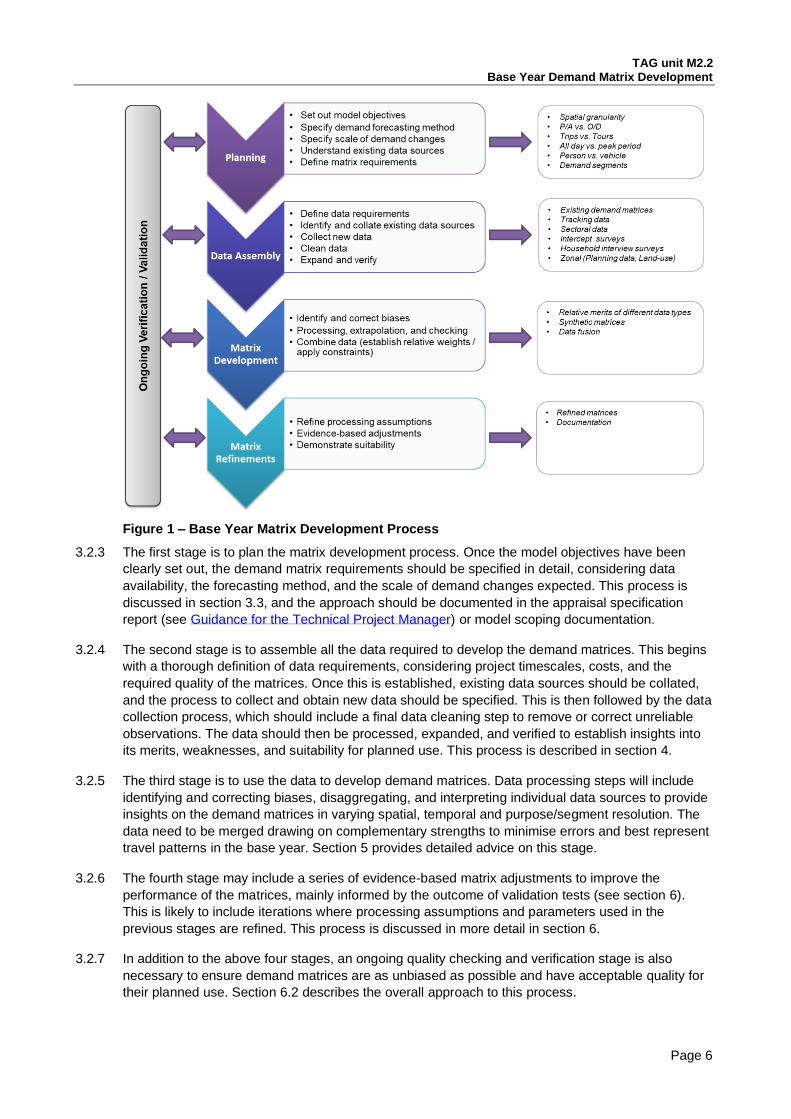
Figure 1 – Base Year Matrix Development Process

3.2.3 The first stage is to plan the matrix development process. Once the model objectives have been

clearly set out, the demand matrix requirements should be specified in detail, considering data

availability, the forecasting method, and the scale of demand changes expected. This process is

discussed in section 3.3, and the approach should be documented in the appraisal specification

report (see Guidance for the Technical Project Manager) or model scoping documentation.

3.2.4 The second stage is to assemble all the data required to develop the demand matrices. This begins

with a thorough definition of data requirements, considering project timescales, costs, and the

required quality of the matrices. Once this is established, existing data sources should be collated,

and the process to collect and obtain new data should be specified. This is then followed by the data

collection process, which should include a final data cleaning step to remove or correct unreliable

observations. The data should then be processed, expanded, and verified to establish insights into

its merits, weaknesses, and suitability for planned use. This process is described in section 4.

3.2.5 The third stage is to use the data to develop demand matrices. Data processing steps will include

identifying and correcting biases, disaggregating, and interpreting individual data sources to provide

insights on the demand matrices in varying spatial, temporal and purpose/segment resolution. The

data need to be merged drawing on complementary strengths to minimise errors and best represent

travel patterns in the base year. Section 5 provides detailed advice on this stage.

3.2.6 The fourth stage may include a series of evidence-based matrix adjustments to improve the

performance of the matrices, mainly informed by the outcome of validation tests (see section 6).

This is likely to include iterations where processing assumptions and parameters used in the

previous stages are refined. This process is discussed in more detail in section 6.

3.2.7 In addition to the above four stages, an ongoing quality checking and verification stage is also

necessary to ensure demand matrices are as unbiased as possible and have acceptable quality for

their planned use. Section 6.2 describes the overall approach to this process.

Page 6

TAG unit M2.2 Base Year Demand Matrix Development

3.3 Making a Matrix Development Plan

3.3.1 In general, whilst the overall methodology to develop matrices should be specified by model

developers from the outset, matrix development planning should be an iterative, flexible, and

dynamic process that allows for testing of data sources and exploring different options, and the plan

will evolve as data limitations are identified and addressed. The evolution of the matrix development

plan over time should be used by model developers to report the quality of the data, their reasoning,

and their resulting confidence in the matrices.

3.3.2 The following aspects of matrix development should be considered for inclusion in the plan:

• objectives – what are the expected outputs from the matrix development task

• existing data sources – what they are, their credibility and accuracy, and how they can be used

to reduce data collection costs and timescales

• gaps in the data – what are the requirements for additional data collection

• investigation – are the data biased or inconsistent, and can these be remedied

• approach – what methods can be used to bring together all complementary data sources

• checking and review – how should processing of the data and the outcome be verified and

validated

3.3.3 There are three factors that will influence planning the most appropriate approach to matrix

development:

• the purpose of the transport model – considering network performance in the short term may

call for a different approach than long term multimodal urban strategy planning

• characteristics of the source data – while some data sources are most directly interpreted as

origin-destination information for individual trips, some naturally explain tours and are more

easily associated with planning data

• the importance of the forecast demand changes – these may arise from future land use plans

or from variable demand responses

3.3.4 TAG unit M1.1 provides general guidance on the rationale for modelling and forecasting, and the

considerations for defining the overall structure of the model, linked to specific model objectives.

Setting out clear base year matrix objectives derived from the model purposes from the outset can

help to identify key risks in the matrix development process and a suitably proportionate approach.

One of the considerations in developing the suitable approach is the possibility that planning

requirements change over time. Sometimes applying remedial measures on a simpler approach are

more difficult than simplification of a more comprehensive approach. Guidance for the Technical

Project Manager provides further advice on proportionality and appropriateness of the modelling

approach.

3.3.5 When base year matrices are required for long term strategic planning and variable demand

responses are considered important1, matrices should be developed in P/A or tour form for home-

based trip purposes. In these circumstances, synthetic matrices form an important part of the matrix

development process by providing consistency between trip ends and detailed land use and

demographic data (see sections 5.2 and 5.3 for detailed advice on synthetic matrix development

and data fusion, respectively). Where matrices are intended for short term planning over a small

1 See TAG unit M2.1, section 2 for relevant advice on when demand responses may not need to be modelled

Page 7

TAG unit M2.2 Base Year Demand Matrix Development

area and demand changes are not expected, an O/D trip-based approach may be most efficient,

unless data better suit the representation of demand at P/A level.

3.3.6 Once the purpose of the model and the requirements imposed on base year demand matrices have

been set out, existing data sources should be identified and their overall suitability for use in the

matrix development process should be considered. These could include a range of different data

types, including existing demand matrices (see section 4.2 for a detailed description of these).

3.3.7 The quality of the existing data sources should be carefully reviewed. The intention of this review is

to identify:

• the extent to which the detail required for the matrix development process can be identified

• the nature of any data cleaning and processing steps already undertaken

• errors and biases in the data sources, including the age of data

3.3.8 It is good practice to prepare a quality statement for each data source before use, recording2:

• the provenance of a data source – ownership and history

• availability and transparency of reports or metadata to describe the data

• what is known and unknown about the collection or processing steps

• definitional issues that might impact on compatibility with other sources

• issues of bias that are known or suspected, the size and direction of any bias, and how these

have been treated

• spatial and age inconsistencies of the data and their treatment

• overview of suitability of the data and their impact on the model for the intended purpose

3.3.9 It should then be established how different data sources are planned to be used (an example is

provided in Appendix C). This process could include discarding some of the data sources (either

elements of it or the entire data source) that are not considered fit for purpose during the review

process, for example due to age of data, excessive expansion and sampling error for the intended

purpose, or large biases that cannot be corrected appropriately.

3.3.10 Another intended outcome of this process is to identify gaps in the data, which will be used as the

basis for specifying new data collection.

3.3.11 Sometimes the characteristics of the data can shape specific elements of the matrix development

approach, without changing the main objectives. If a demand data source with some desired

properties is already available, it is appropriate to consider how best to use it in defining the

approach to minimise the combined data collection and base matrix development costs.

3.3.12 Depending on the data source and specific stage in the matrix development process, different

quality checks and validation tests are expected to be undertaken throughout the process.

Assumptions and processes to interpret the data may be updated progressively (see section 6 for

detailed advice). In developing the plan for matrix development, it is important to consider the

approach to validation and identify any requirements, including data sources to be used and

methods to be applied.

2 Arup (2016), Provision of Technical Advice and Support for Matrix development Guidance.

Page 8

TAG unit M2.2 Base Year Demand Matrix Development

3.3.13 It is important to consider resilience in the matrix development plan. It should consider the risks

associated with data limitations and be flexible enough to accommodate possible refinements in the

approach when the suitability of data is fully understood (see section 4.6).

4 Data Assembly

4.1 Introduction

4.1.1 This section provides advice on stage two of the matrix development process, as shown in Figure 1.

It introduces the main data types that may be used for matrix development, provides generic advice

on collecting new data, as well as checking and expanding the data for use in matrix development. It

then sets out data processing principles for establishing key insights to understand strengths and

weaknesses and to review suitability for its planned use.

4.1.2 The key principles that should be applied to all data types are set out in this section. Appendix B

provides more detailed complementary guidance and considerations in relation to specific data

sources, which should be referred to in addition to this section.

4.1.3 It must be noted that the specific data sources referred to and discussed in this section and

Appendix B do not cover all data types or sources that can be used to develop demand matrices.

These are data sources most commonly used to date. Other emerging or new data sources may

exist and may be used for demand matrix development, so long as the principles set out in this

section and other parts of this unit, as well as those in TAG unit M1.1 and TAG unit M1.2 are

followed, and the data sources are shown to be suitable for the planned use.

4.2 Sources and Quality of Data for Matrix Development

4.2.1 Different types of data may be used for development and validation of base year demand matrices.

These include both conventional and emerging data sources, and generally fall into the following

categories:

• matrix data (i.e. O/D or P/A data)

• zonal data

• traffic and passenger count data

Matrix Data

4.2.2 These are data sources which directly provide information on person or vehicle journeys, including

their start and end locations (for either part of or whole of the journey) at some spatial granularity,

and may provide other characteristics of the travellers and their journeys.

4.2.3 Data sources of this type can generally be divided into the following specific groups:

• Existing demand matrices – these are matrices available from previous studies, developed to

serve a particular purpose

• Tracking data – examples include GPS tracking, Mobile Network Data (MND), and connections

through Wi-fi hotspots

• Sectoral data – examples of these include Automatic Number Plate Recognition (ANPR) or

manually recorded data, public transport ticket data, or Bluetooth data

• Intercept Surveys – for highway demand, Roadside Interview (RSI) and Car Park Surveys are

example data sources of this type. For public transport demand, examples include on-board

passenger interviews, or passenger interviews at stops, station entries, or rail platforms

Page 9

TAG unit M2.2 Base Year Demand Matrix Development

• Household Interview Surveys – examples include National Travel Survey (NTS) and London

Travel Demand Survey (LTDS)

4.2.4 Table 1 provides an overview of the key strengths and weaknesses associated with different data

types in the context of matrix development. It should be noted that the advice set out in this table is

generic and associated with the most commonly used data sources for each data type, and is

provided as a guide only. Specific data sources may have other strengths and weaknesses not

included in this table, some of which are discussed further in Appendix B.

Table 1 Key Strengths and Weaknesses of various Matrix Data Types

Data Type Key Strengths Possible Weaknesses

Existing Demand

Matrices

no new data collection costs, limited

processing time required.

Potential value in representing

external demand drawn from a

larger regional model into a local

model

age of data, lack of adequate

understanding on quality, different

spatial geography requiring processing

assumptions (weaknesses could vary

depending on provenance and level of

available documentation)

Tracking Data potentially large sample size, wide

geographical coverage, capturing

day-to-day variability in travel

patterns

sample error and errors from

interpretative algorithms require

interpretation, current MND does not

include short trips and cannot provide

fine spatial resolution, privacy filters

limiting the detail, cost (depending on

the source), detailed segmentation,

current GPS sources contain only

small samples of individuals with

associated bias and expansion issues

Sectoral Data potentially high sample rate,

providing information on vehicle type

(age, emissions)

both ticketing data to station or stage

and ANPR/Bluetooth to large sectors

require interpretation to zones,

biases from expansion, detailed

segmentation

Intercept Surveys ability to provide a detailed picture of

the travel patterns and choices of

interviewees, including origin,

destination, home and work

locations, vehicle type, occupancy,

and route choice

potentially labour intensive, time

consuming and expensive, practical

limitations associated with undertaking

surveys, lack of day-to-day variability

in the data, potential for response bias

due to annoyance or lack of

knowledge, limited geographical

coverage, limits on the sample size,

and accordingly, spatial accuracy of

data

Household

Interview Surveys

ability to provide a rich and

comprehensive picture of multi-

modal travel and activity patterns by

residents within a study area

developing spatially detailed demand

matrices directly from this data is not

generally practical due to typically

small sample sizes, response bias,

and cost.

Zonal Data

4.2.5 Zonal data refer to demographic or land-use information that is used to support the development of

trip end models, which are used directly (e.g. to generate synthetic matrices) or indirectly (e.g. as

zonal or sectoral constraints) in the process of demand matrix development.

Page 10

TAG unit M2.2 Base Year Demand Matrix Development

4.2.6 TAG unit M1.2 introduces the National Trip End Model (NTEM). It includes forecasts of population,

households, workforce and jobs over 30 years which are used in a series of models that forecast

population, employment, car ownership, trip ends and traffic growth by Middle Layer Super Output

Area (MSOA). The NTEM data set can be viewed using the TEMPro (Trip End Model Presentation

Program) software. TEMPro estimates of trip ends at any level below aggregate regions (e.g.

MSOA, district, or county level) are subject to uncertainty and should not be used as constraints in

matrix development process without verification and possible adjustments (see paragraph 5.2.22 for

further advice on how trip ends may be adjusted).

4.2.7 For direct use in matrix development, trip rate information estimated from household survey data

should be considered instead to underpin trip end estimates at zone level (see paragraph 5.2.22).

More granular level, and potentially more accurate, planning data than that within TEMPro can also

be obtained from population estimates provided by ONS and from local planning databases. The

latter can be developed through engagement with local planning authorities that will hold data at a

more disaggregated level.

Traffic and Passenger Count Data

4.2.8 In demand matrix development, traffic and passenger counts may be collected for a range of

purposes, including:

• expanding new data sources (e.g. RSI, public transport intercept survey, ANPR, or Bluetooth

data)

• re-expanding old data sources

• refining developed demand matrices

• validating performance of matrices

4.2.9 TAG unit M1.2 includes a discussion on data accuracy, and the 95% confidence intervals that

should be assumed for different types of surveys and vehicle types. However, the intervals provided

are only indicative, and the modellers should not use these as default ranges. They should instead

calculate respective 95% confidence intervals from the surveyed data where possible.

4.3 New Data Collection

4.3.1 TAG unit M1.2, section 2 describes existing data sources, whilst section 3 provides general

guidance on conducting bespoke surveys for individual study requirements. These include data

sources used for demand matrix development, as well as the key considerations in carrying out

traffic count surveys. The extent of traffic surveys or passenger counts should be dictated by the

coverage and purpose of the transport model.

4.3.2 In terms of matrix data, the key considerations that should be given when specifying new data

collection include:

• data collection period

• sample rate

• how representative the collected sample is of travel made by total population

• definitional consistency of various journey characteristics with other data sources

• spatial coverage,

• requirements on demand segmentation and representation of distinct trip purposes

• the potential for the survey method to disrupt travel patterns

Page 11

TAG unit M2.2 Base Year Demand Matrix Development

• data privacy

4.3.3 The following provides general advice and key principles that should be considered in the data

collection process. More detailed advice specific to collecting the most common matrix data sources

is provided in Appendix B.

Data Collection Period

4.3.4 The period over which data should be collected is important. This generally depends on the purpose

of the transport model (see paragraph 2.2.2). For typical purposes, TAG unit M1.2 specifies that

highway surveys should be carried out during a ‘neutral’, or representative, month avoiding main and local holiday periods, local school holidays and half terms, and other abnormal traffic periods.

However, there can be instances where a particular period (e.g. weekends or school holidays) is of

interest, for example in regions with relatively high levels of seasonal tourism.

4.3.5 Another important consideration is the number of days over which data is collected. In principle, by

including a greater number of days in the survey period has the desirable advantage of capturing

day-to-day variability, and consequently reducing sampling error of trip estimates. As set out in

Table 1, this is partly a feature of specific data sources, where some data sources such as MND

have this specific advantage, providing the opportunity of collecting data over a longer period

compared with, for example, intercept surveys where this has substantial implications on survey

costs.

Sample Size and Rate

4.3.6 Most data will be collected as a sample which will be a source of statistical error in the data. While

some data sources may provide a large volume of data, it may be sourced from a small proportion

of individuals. Careful consideration should be given to the sampling error and the implications for its

use (see Appendix E for further details). In many cases it may be concluded that the data is too

sparse to be used directly and is best interpreted at more aggregate levels than required for the final

matrices, which may be achieved by using the data to estimate parameters for statistical models. A

common approach is to aggregate the data to spatial sectors, across time periods, or over trip

purposes and segments.

4.3.7 For some data sources there will be a judgement required balancing the additional accuracy or

resolution provided by a larger sample against the data collection time and costs.

Errors and Biases in the Data

4.3.8 All data sources will include errors and bias. Within this unit, errors generally refer to statistical

errors, which are the difference between the estimated and the true value of a quantity. They tend to

be randomly distributed and are expected to have no overall net effect across all observations in the

data. Conversely, biases refer to systematic differences between the estimates and true values,

which are linked with some characteristics of the data and tend to move the estimates towards a

specific direction with a certain magnitude.

4.3.9 Both errors and biases are directly influenced by the data collection and sampling methodology (as

well as expansion and processing methods). These include measurement errors, caused by

equipment calibration and malfunctions or human errors, which could lead to biases, outliers, or

partial view of the data. The data collection methodology should carefully consider these. Any

residual large errors or biases should then be addressed during the data expansion and processing

steps.

4.3.10 The survey design should consider how the data will be used, and what margin of error would be

acceptable. For example, trip rates are most reliable at all-day level. It may therefore be preferable

to collect and use the data at longer periods (e.g. all-day for household survey data or tracking data

or 12 hour or longer period for intercept surveys) to develop spatially detailed matrices, and then to

Page 12

TAG unit M2.2 Base Year Demand Matrix Development

use appropriate data and methods to disaggregate to individual time periods, rather than rely

directly on trip end estimates by time period.

Definitional Consistencies

4.3.11 A common feature of different data sources is the definitional differences between them. As

discussed earlier, the matrix development task often involves combining multiple data sources, and

therefore it is important to ensure that their interpretation is consistent. A common example of this is

vehicle type definitions between manually classified counts (which relate to visible characteristics of

the vehicles) and number plate surveys (where the data is derived from vehicle licencing

databases).

4.3.12 Some differences may relate to the nature of the data, such as whether the data describe vehicles

or individuals. Appropriate expansion of the data should address variations in the source sampled

(such as individuals, travel groups, or devices carried by the travellers). Some definitional

differences are a consequence of how questions are designed in the data collection (for example

distinguishing tours, journeys or stages or trips, or the definition of traveller segmentation and

journey purpose), or how raw information is aggregated and categorised by time period, spatial

geography, trip purpose, etc.

Spatial Coverage

4.3.13 As explained further in Appendix B many data sources will only provide insight on a subset of the

travel demand. Intercept surveys will be limited to the modes being intercepted and to the spatial

location of the surveys undertaken, and journeys that do not pass through survey locations will not

be observed.

4.3.14 The movements for which data are not observed must be identified. These limitations must be

reflected in the processes applied to develop the matrices from the individual sources. However,

care should also be taken in reporting aggregate insights from partial data as these will not be

representative of total travel represented in the trip matrices.

Requirements on Demand Segmentation

4.3.15 One of the key limitations of some data types, as noted in Table 1, is lack of information on detailed

demand segmentation. For example, MND algorithms may distinguish commuting and possibly

education purposes, but not business-related purposes or, with sufficient confidence, user

segmentation, or ANPR data distinguish vehicle types and emissions but provide no insight on travel

purpose. In these circumstances, other data sources should be identified to provide the information

required to distinguish demand segments.

Possible Travel Disruptions

4.3.16 Depending on the type of data being collected, the data collection process may disrupt travel

patterns, for example, when RSI surveys are undertaken. Before intrusive surveys are

commissioned, the extent to which they could disrupt or affect travellers should be considered,

together with the safety of the surveyors and the travellers. The survey planning should consider

and mitigate such risks.

Data Privacy

4.3.17 It is important that legal and ethical issues including data privacy are considered during the data

collection process. Generally, the UK’s Data Protection Act 2018 which incorporates the EU’s General Data Protection Regulation (GDPR), applies to personally identifiable data, which includes

surveys that record names and addresses or vehicle licence plate numbers, or to tracking data that

includes electronic device identifiers. Anonymization and aggregation methods can be applied to

ensure data cannot be traced back to individuals. Personally identifiable data should only be

retained for the period over which it is justified for the purpose for which it was collected.

Page 13

TAG unit M2.2 Base Year Demand Matrix Development

4.4 Expansion and Verification of Data

4.4.1 The matrix data collated for demand matrix development usually represent a sample of trips, and

require factoring to represent total travel. This process is referred to as data expansion.

4.4.2 Initial quality checking and data cleaning processes are required prior to the expansion of the data.

The purpose of these are to identify and remove evident errors and outliers (unless they are valid

observations) in the data. Checking should be structured to give reasonable confidence in the

quality of the data. Common methods include:

• error checking, for example, that the data is credible and survey responses follow coding

frameworks

• logic checking to consider the plausibility of observations, for example, that a sequence of trips

does not have gaps, or no anomalous values exist that are often a sign of measurement errors

• range checking to confirm that survey data fall within predetermined ranges, for example, a car

as a vehicle type should have a maximum occupancy of 8 persons to include people carriers

• visualisations of the raw data, for examples that movements observed at an intercept survey

site have origins and destinations that could plausibly route through the site

• cross-checking for consistency of data sources, for example that traffic count estimates for

the same section of the road derived from two data sources are consistent

• statistical methods to look at the variability of observations and identify potential outliers (due

to measurement errors or similar) beyond reasonable ranges

4.4.3 Suitability of existing data sources (including existing matrices) for use in the matrix development

should be considered, taking into account the:

• age of the data

• extent to which population, land-use, and transport network has changed

• availability of documentation that describes how the data have been collected and processed

4.4.4 Practitioners should establish evidence on scale of changes to land use and demographic

characteristics, transport networks, and travel patterns, with more attention given to the key

movements in the model internal area, and use this evidence to assess the validity of ‘old’ data sources and their suitability for the intended use(s) of the model to judge their suitability for those

use(s). Former guidance (withdrawn sections of the Design Manual for Roads and Bridges)

indicated that models should not be used without justification where the source data is more than

five years old when used for detailed scheme appraisal because there might be significant changes

to the travel patterns and traffic level. This simple threshold should not be used, as there can be

significant changes that would make the use of more recent data inappropriate or there may have

been little change and older data may be acceptable. Changes such as the closure or opening of a

major retail centre or major transport infrastructure such as a new bypass would be expected to

result in the need to collect and use more recent data.

4.4.5 Model development and scheme appraisal can require considerable time, to the point that the data

to which the model has been developed and calibrated has aged. TAG guidance on the

Proportionate Update Process should be applied to judge the merits of updating transport models.

In most circumstances where the model data was collected a few years before forecasts produced

by the model are used to appraise the merits of a scheme, it would be reasonable to make efforts to

demonstrate what potential changes have occurred in recent land use and travel patterns that could

affect the model in some way (as described above). Where changes are moderate in scale, it is

Page 14

TAG unit M2.2 Base Year Demand Matrix Development

proportionate to document this evidence in reporting of model development or forecasts used for

scheme appraisal to explain associated model uncertainty.

4.4.6 When existing matrices form one of the potential data sources, documentation should exist detailing

the data sources and the process used to develop these, and their strengths and weaknesses.

4.4.7 Data quality may vary between attributes within a data set. For example, completion of postal

address locations in surveys will vary, and a particular risk is for partial addresses to be

misinterpreted. It may be appropriate to develop methods to distribute partial data spatially, or

indeed to discard records where there is incomplete information. In the latter case consideration

should be given to how the data is used and it may be that both the full sample can be used in some

ways (where the data attributes are sufficiently reliable) and a smaller subset of the data is used for

other purposes. If so the data would need to be expanded separately for the different purposes.

4.4.8 The expansion method should be designed specifically for the source data. As explained further in

Appendix B for specific data sources, the expansion factors should be calculated by comparing a

subset of journeys, or individuals, with total number of journeys or individuals that the subset

represents. The population of journeys or individuals that the data are expanded to will usually be

sourced from count data or from population estimates from ONS census data.

4.4.9 While it will be desirable to use small subsets to ensure that sampling errors do not distort the

pattern of travel represented, care is required that the individual subsets contain a large enough

sample so that the expansion does not apply undue weight to a small number of observations.

4.4.10 The expansion process must ensure that it introduces no bias particularly when there are demand

segments in the sample that have large differences in travel patterns. This should be achieved by

verifying that for any subset of trips, the sample taken is an unbiased representation of total trips

that the subset is taken from. If any biases are found, they should be addressed by:

• correcting them directly in the sample if the source of bias is known

• using separate expansion factors by demand segments having large differences in travel

patterns, where reliable information is available to establish these

4.4.11 The expanded data is expected to provide an unbiased insight of travel demand in the base year.

Data quality checks and verification tests should be undertaken to identify if the data include any

large errors or gross biases. In principle, this may be achieved by comparing various insights (e.g.

number and pattern of trips, demand segmentation, trip symmetry) with other data sources.

Comparisons should reflect the statistical properties of the estimates (see section 6.2 and Table 2

for more details).

4.4.12 When this process shows that the expanded data still includes large biases, the sources of these

should be identified and the data cleaning and expansion processes should be refined to correct

these when possible. Alternatively, the matrix development process (described in section 5) should

include specific steps to adequately address these. If biases are found to be too large and with

unknown sources, the data should be discarded from use in the matrix development process.

4.5 Establishing Insights from the Data

4.5.1 Prior to developing demand matrices, an initial analysis of data should be undertaken to establish

key insights and fully understand the strengths and weaknesses of the data sources. This is

particularly important when emerging and new data sources are used, where statistical properties of

the data, specific errors and biases, and methods to address them are less understood and

established. The following aspects should be considered:

• spatial resolution

• temporal resolution

Page 15

TAG unit M2.2 Base Year Demand Matrix Development

• travel mode and vehicle type resolution

• demand segmentation

• purpose

• spatial coverage

4.5.2 One of the key requirements is to establish the spatial level at which the data should be used. Some

errors in the demand data are related to spatial resolution, and they become larger when the data is

used at a more disaggregate level. For example, it is good practice to use intercept survey data at

sector level to reduce sampling error, whilst MND should be expanded and processed at a spatial

resolution that moderates errors from misallocation of trips to zones (see section B.3 in Appendix B

for more details).

4.5.3 The temporal level at which to use the data should also be established. This is partly related to the

sample size in the data, and partly related to the wider model requirements. For example, it should

be established whether the sample size allows using the data at time period level for any given

spatial resolution.

4.5.4 Another important requirement is to establish the definition of various matrix segments within the

data, and the consistency of definitions between different data sources used for matrix development.

For example, time period definitions within NTEM are based on the end time of journeys, whilst

intercept surveys and traffic count data provide direct information on the time at which the journey is

intercepted. Any definitional inconsistency between data sources should be clearly defined and

addressed later during the matrix development process.

4.5.5 Some data sources may lack some demand segmentation (e.g. MND, ANPR), or certain

movements may not be fully represented in some demand data sources (e.g. short trips in MND, or

unobserved movements in RSI surveys). The extent to which these limitations exist in the data

should be fully understood. Appendix B provides further advice on some of the data source specific

limitations and methods to address them.

4.5.6 It is important to fully establish the spatial coverage of the data, that is which journeys are included

in the data depending on their start / end points with respect to the defined area of detailed

modelling, rest of the fully modelled area, and external area (see TAG unit 3.1, section 2.2 for a

detailed definition of these). For example, matrices developed from intercept surveys are only

expected to include movements that traverse defined screenlines for data processing.

4.6 Suitability for Planned Use

4.6.1 Once the strengths and weaknesses of the data are identified, and sources and the extent of

various errors and biases are understood, the suitability of data sources for their planned used

should be reviewed.

4.6.2 Depending on the intended quality of the demand matrices and insights established from the

available data sources, any requirement for further data collection should be reviewed.

4.6.3 Using the evidence established from the data, the planned matrix development process (discussed

in section 3) should be revisited and revised, if necessary, to accommodate data limitations.

Page 16

TAG unit M2.2 Base Year Demand Matrix Development

5 Matrix Development Process

5.1 Introduction

5.1.1 This section provides advice on how different data sources could be combined in a practical way to

establish the best representation of travel patterns in the base year. The principles set out in this

section are generic and should be followed. However, choices may be made by modelling

practitioners on the sources of data and detailed processing methods.

5.2 Synthetic Matrices

Background

5.2.1 Synthetic matrices play a key role in developing base year matrices when they are combined with

other observed information to fill in gaps and address limitations of other data sources.

5.2.2 Furthermore, methods used to develop synthetic matrices often result in the desirable property of

consistency between trip ends and detailed land use and demographic data. This is a key

requirement for forecasting using strategic models, where a non-uniform growth is forecast, linked

with trip productions, and sometimes trip attractions. For this reason and to provide a suitable basis

for forecasting, synthetic matrices should be developed at P/A level for home-based trip purposes

when they are intended for use in base year matrix development for strategic models.

5.2.3 In the context of demand matrix development, synthetic matrices are defined as estimated travel

demand matrices based on some estimated statistical model. Independent data will usually include

zone-to-zone travel costs and the statistical models will be fitted to reproduce aggregate insights.

5.2.4 It is possible to develop statistical models that draw on all of the insights to establish demand

matrices. The Department’s technical report on matrix building (Arup, 2016) identifies a number of

practical limitations. In this guidance therefore for practical purposes ‘synthetic’ matrices are defined as an estimate of travel demand that would typically be calibrated using aggregate insights from

some of the data sources, used as ‘constraints’ in the calibration process. In their simplest form,

these include zonal trip ends and an estimate of the Trip Cost Distribution (TCD), derived from

survey data.

5.2.5 Synthetic matrices constructed in this way often include large uncertainty and errors in representing

trip distribution. Therefore, they should not be used as the single source of data in developing base

year demand matrices, unless these relatively large errors are sufficient to satisfy the study

objectives.

5.2.6 Methods can be applied to enhance the quality of the matrices by introducing into them further

observed information on trip patterns from other sources. This can be either through the synthetic

matrix calibration process3, or through combining the synthetic data with other data sources at a

later stage (i.e. data fusion).

5.2.7 The data fusion methods discussed in section 5.3 treat ‘synthetic data’ equivalently to other data sources with their inherent strengths and weaknesses. The advantage of synthetic matrices is that

they provide data at cell level, often for the entire matrix. Weaknesses reflect the errors in the

statistical models, which typically have relatively large errors in trip patterns.

5.2.8 In practice, two types of models have been used commonly to synthesise trips, which are

destination choice models (discussed in paragraph 5.2.16) and gravity models (discussed in

paragraphs 5.2.17 and 5.2.18). The same principle is applied regardless of model type, where

aggregate travel behaviour is determined by total trip ends and cost of travel.

3 For a practical example, see Psarras et al., 2017

Page 17

TAG unit M2.2 Base Year Demand Matrix Development

Strengths and Weaknesses of Synthetic Matrices

5.2.9 The key strength of synthetic matrices lies in representing the link with detailed population and land-

use information. They include suitable constraints such as daily trip production rates by purpose,

ensuring that the issue of matrix scaling is reasonable across the entire matrix, even when new data

is introduced through a data fusion process.

5.2.10 Another important merit of synthetic matrices is their completeness, as the methods used tend to

result in an estimate of demand in each cell in the matrix.

5.2.11 However, synthetic matrices are widely known to include large errors. There is limited evidence on

the scale of these errors or an approach to quantify the combined errors. These include a

combination of sampling error in the observed TCD, gravity modelling errors, and errors in trip end

models.

5.2.12 The zonal trip ends, used as constraints, will include errors that, depending on the source of data

used to derive trip ends, may partly relate to trip rates not reflecting spatial variations, and partly

relate to reliability of planning data.

5.2.13 Synthetic matrices also tend to be weaker in representing trip attractions compared with trip

productions. Zonal trip end estimates for public transport trips may not reflect the link between trip

rates and accessibility (see paragraph 5.2.23 for more details).

5.2.14 Errors in the distribution models are expected to contribute significantly to the overall uncertainty in

the trip distribution produced by synthetic matrices. These are mainly explained by the following

factors:

• aggregate TCDs produced by the synthetic matrices do not fully reflect the large variations in trip

patterns between different area types, person types, or time periods

• the target TCDs created for the calibration of distribution models includes sampling errors and

potential underlying biases

Calibration Process

5.2.15 In principle, model parameters should be calibrated so that an observed TCD is closely replicated,

whilst satisfying particular constraints.

5.2.16 The most commonly used destination choice model uses a logit function, which is described in

Appendix D, section D.5 and Appendix E, section E.5 of TAG unit M2.1. Maximum Likelihood

Estimation (MLE) or similar techniques may be used to estimate parameters of the utility functions,

using trip information collected at individual level. Several statistical packages exist that include

modules to estimate parameters of logit models using MLE method4.

5.2.17 Gravity models assume that the interaction between two zones declines with increasing impedance

(distance, cost and/or time of travel), but is positively correlated with the amount of trip activity at

each zone. The rate of decline of the interaction is represented by a ‘deterrence’ function, which is

calibrated so that the resulting TCD closely matches the TCD obtained from the surveyed data.

5.2.18 The mathematical specification of gravity model is described in detail in various transport modelling

textbooks5. Figure 2 shows the main steps in developing a simple synthetic matrix (i.e. without any

inter-sector constraints) using gravity modelling approach, for any given travel mode and demand

segment.

4 Examples include Biogeme, Nlogit, and STATA 5 For example, see Ortuzar and Willumsen, 2011.

Page 18

TAG unit M2.2 Base Year Demand Matrix Development

Figure 2 – Overview of Synthetic Matrix Development Process

5.2.19 At a minimum, the following set of inputs are required for the calibration of a gravity model for a

given travel mode:

• an estimate of zonal trip ends

• a target (observed) TCD

• an estimate of travel cost (expressed as time, distance, or generalised costs) between each zone

pair

5.2.20 The trip ends provide an estimate of the absolute travel demand for each zone in the model and it is

important that they accurately reflect the type and scale of land use in each zone. For example, the

planning data underpinning trip ends should clearly distinguish zones which include spatial land use

types such as hospitals or shopping centres from other zones.

5.2.21 TEMPro outputs provide a potential source of data for trip end estimates, particularly if model zones

and NTEM segmentation are compatible. Where there is particular value in applying trip end

functions at a zonal level, such as in land use transport interaction models, CTripEnd (the trip end

model program) allows practitioners to prepare trip end forecasts for a set of user-defined zones. It

may be possible to update zonal population and land-use data within NTEM, if more reliable local

information is available (see paragraph 4.2.7). This will ensure that the trip ends generated by the

software reflect the underlying land use of each zone in detail.

5.2.22 However, the key limitation of TEMPro lacking representation of spatial variation in trip rates

underpinning trip end estimates (see paragraphs 4.2.6 and 4.2.7) should be considered. TEMPro

trip ends must be reviewed at a local level for the possibility that any variation in number of trips

between urban areas within the NTEM area types is not represented sufficiently. Where the model

covers a sufficiently large area a direct comparison is possible using NTS data. In many cases it will

not be proportionate to undertake the data collection necessary to establish local trip rates, in which

Page 19

TAG unit M2.2 Base Year Demand Matrix Development

case an aggregate comparison of assigned flows and count data at cordon / screenline or even area

level can provide evidence to adjust base year trip rates.

5.2.23 Another important limitation of NTEM trip rates for developing base year demand matrices is related

to the missing link between mobility and accessibility. The trip rates underpinning NTEM trip ends

are estimated at an aggregate spatial level and do not vary between areas with varying access to

public transport services. As a result, NTEM trip ends for public transport generally tend to be

underestimated for areas of high public transport accessibility and vice versa.

5.2.24 Alternatively, practitioners may develop their own bespoke trip end models if more reliable estimates

of trip rates and detailed population and land-use information are available from local surveys or

other sources.

5.2.25 The TCDs should be created by grouping trip records into some defined cost bands, and calculating

the proportion of trips within each cost band. It is also important to use appropriate cost bands. They

should not be so aggregate as to hide significant differences within cost bands, but should be

sufficiently aggregated to minimise errors in the estimated costs for trips in the underlying data

sources.

5.2.26 The target TCD should be created from the observed evidence, for example, National Travel Survey

(NTS), a local household interview survey, or the RSI data. This should be prepared separately for

each demand segment for which a synthetic matrix is being developed, and should have a

consistent definition with the matrices in terms of trip purposes, time periods, spatial coverage,

directionality of trips, the range of trips lengths represented, and the definition of travel costs. For

example, RSI data should be used with care as the survey does not capture all movements,

accordingly, the fit of the TCD should be tested only for the trip movements which are fully observed

in the RSI survey, to ensure consistency between observed and modelled TCDs. Other observed

sources such as NTS may be used to test the fit of the model for the movements not observed by

the RSI survey.

5.2.27 The target TCD should exclude external-external movements because these zones are spatially

aggregate. Therefore, travel costs associated with movements between them are unlikely to be

reliable. However, trips produced in the model internal area with an external attraction should be

included in the calibration because the integrity of the trip rates depends on the possibilities for

journeys with an internal end to be made to or from external zones, and this assumption is

particularly important near the boundary of the study area.

5.2.28 A measure of intra-zonal costs should be estimated. It is common to assume a value based on the

cost to adjacent zones. Some models for example adopt half the lowest inter-zonal cost, often

imposing a cap that maintains costs at or below mean trip distances for large zones. Other

alternative methods may be considered when better assumptions can be established. Further

advice on calculating intra-zonal costs is given in Appendix A to TAG unit M2.1.

5.2.29 Any measure of travel cost (e.g. distance, cost, generalised cost) can be used for the purpose of

gravity model calibration. The following factors should be considered in deciding what cost measure

should be used:

• availability of information on the distribution of cost by demand segment

• intended use of synthetic matrices

• availability of direct data on cost

• consistency of different cost components (e.g. when they are used to calculate generalised cost)

5.2.30 An estimate of travel cost for each zone pair may be obtained from a network model. Ideally, a network

model is fully developed and calibrated before it is used to derive travel costs for the purpose of gravity

model calibration. However, in reality, network and matrix development tasks are undertaken in

Page 20

TAG unit M2.2 Base Year Demand Matrix Development

parallel due to project costs and timescales. In these circumstances, preference should be given to

the methods that draw directly on other available data (e.g. observed network speed, distance, or

journey time data from independent sources or data from an existing network from an earlier version

of the model) rather than those that could imply the need for iterations (skimmed time or distance

matrices). The latter methods need iterations between matrix development and assignments, hence

imposing a potential risk to timescales as well as an added complexity to the process.

5.2.31 For the calibration of the deterrence function, it is usually necessary to use a representation of TCD

produced from internal zones only to test the model fit. This is to ensure that the constructed TCD

based on distances between model zones is realistic and consistent with observed TCD. The fitted

function is then applied to movements between all model zones.

5.2.32 The parameters of the gravity model should be estimated through an optimisation process, where a

search algorithm is used to find a set of parameters which minimise the squared error between the

synthesised and observed distributions, described as below:

where

• 𝑇𝑐𝑜𝑏𝑠 is the number of observed (target) trips in trip cost band 𝑐

𝑠𝑦𝑛 • 𝑇𝑐 is the number of synthesised trips in trip cost band 𝑐

5.2.33 There are certain techniques that can be used in the calibration process to reduce statistical errors

and increase the reliability of synthesised movements. These should be considered carefully, taking

into account the intended use of synthetic matrices. Some of these considerations include:

• use of observed sector constraints - also referred to as k-factors, these are reliable estimates

of sector-sector movements, obtained from survey data, which can be used in the calibration

process as an additional set of constraints. See Feldman et al. (2012) for the theoretical

description and an applied example of using k-factors in the gravity model calibration process to

improve the performance of synthetic matrices

• use of multiple target TCDs – these intend to reflect significant variation in trip lengths and

patterns between different geographical areas (e.g. urban vs. rural). See Psarras et al. (2017) for

an example of using these in the gravity model calibration process and the evidence on the

improvement that this method can provide to the overall synthetic matrix performance

• type of deterrence function – depending on the characteristics of the observed TCDs, an

alternative functional form of the gravity model may provide better predictive performance and

overall fit to the target distribution6

Verification and Diagnostic Testing

5.2.34 The validity of the developed synthetic matrices should be verified by assessing how well the

modelled TCDs fit the target distribution, separately for each matrix segment. Graphical presentation

of TCDs is a powerful means of expressing strengths and weaknesses in both comparisons and any

unusual features in observed data, therefore, this should form part of the model calibration

diagnostic tests.

5.2.35 Where possible, the 95% confidence interval of trip proportions in each trip cost band in the target

TCD should be calculated and used in interpreting the goodness of fit of the model. For nearly all

the distribution curve, the modelled trip proportions are expected to be within the 95% confidence

interval of the observed proportions. The same banding used to create the target TCD should be

6 For example, see Feldman et al., 2012.

Page 21

TAG unit M2.2 Base Year Demand Matrix Development

used for this diagnostic test (see paragraph 5.2.25). Given the asymmetric nature of TCDs, use of

formal non-parametric statistical tests (e.g. Kolmogorov–Smirnov test7) may also be considered.

5.2.36 When trip distance is not used directly to establish the TCD and calibrate gravity models, it is

recommended that the Trip Length Distribution (TLD) of the developed matrices are also compared

with the observed TLDs, using the same principles set out above. This particularly verifies the

alignment of modelled long distance trips to the evidence from the observed data.

5.2.37 It is also good practice to compare modelled and observed average trip costs for each segment. The

modelled value should be within the expected statistical error (e.g. 95% confidence interval) of the

observed average values. It is however important to note that this test is not definitive and should

only be used as a guide, since the 95% confidence intervals may be affected by issues associated

with short trips, intra-zonal trips, or trips to/from special land use types (e.g. hospitals, universities).

5.2.38 The analysis of TCD should be based on an estimate of network distance or generalised costs.

Crow-fly distances should not be used (or if used, they must be aligned with verification data

definitions).

5.2.39 For external-external movements not subject to model calibration, a subsequent check should be

made that the resulting patterns of estimated external movements is realistic. When these

movements are sourced from an external model, the consistency of two data sources being

combined must be ensured (see paragraph 5.2.27 for further advice on treating external trips in the

calibration process).

5.2.40 Noting the expected uncertainty and lack of evidence for verification, resulting sector-to-sector

movements provide insights on aggregate travel patterns. The credibility of these movements

should be reviewed based on comparisons with other available evidence (e.g. patterns derived from

existing models or aggregate count data). Any systematic variation or outliers in the sector-to-sector

movements compared should be further investigated to identify possible sources of discrepancies.

Where necessary, the matrix development process should be refined to correct for any significant

bias in inputs or processing errors.

5.2.41 Where possible, some initial assignment of matrices onto an existing network and comparison of

modelled flows with total traffic at aggregate level should be considered.

5.2.42 When observed sector constraints (or k-factors) are used in the matrix development process (see

5.2.33), the effect of applying these should be reviewed and reported. A comparison of matrix

performance before and after applying these constraints will demonstrate the added confidence in

the matrices.

5.3 Combining Data Sources

Background

5.3.1 As discussed in paragraph 3.2.1, it is unlikely that a single source of matrix data can be identified

and used to develop base year demand matrices, hence, different data sources should be usually

considered as complementary.

5.3.2 Many of the data sources only provide partially-observed movements or estimates of trips that

should be used at certain spatial granularity and segmentation, reflecting statistical accuracy of the

underlying data. Therefore, processes are required to infill, merge, constrain, disaggregate, or

segment data sources using complementary data sets to address these limitations. These

processes are referred to as ‘data fusion’.

7 This is a statistical test to examine whether the distribution of a variable (e.g. trip length) is the same in two independent data sets. The test is sensitive to differences in median, dispersion, skewness, and other metrics of the distributions being compared. Standard statistical packages such as SPSS and R can be used to run a Kolmogorov– Smirnov test on two sample data, and the basic theory can be found in various statistical textbooks.

Page 22

TAG unit M2.2 Base Year Demand Matrix Development

5.3.3 In this context, the methods described in paragraph 5.2.31 to improve the quality and performance

of synthetic matrices through specifying and calibrating a ‘hybrid’ gravity model8 are also classified

as data fusion.

5.3.4 Prior to combining data sources, checks should be undertaken to ensure that the observed data is

not ‘lumpy’ (for example, when the sampling or other data errors are too large at cell level). In principle, the issue of lumpy data is often a symptom of using the data at a more detailed level

(spatially or across demand segments) than it should be used, as supported by the sample size and

statistical properties of the data. Practitioners should therefore first establish the appropriate level at

which the data should be used, based on the acceptable error of trips estimates (Appendix E

describes the principles of estimating sampling error from matrix data). The aggregate trip estimates

should then be further disaggregated using other data sources and methods discussed below.

Methods of Combining Data Sources

5.3.5 As discussed earlier, matrices constructed from observed data sources are usually partial, as they

only include representation of some movements. For example, RSI data or public transport intercept

surveys do not include trips not directly surveyed (e.g. intra cordon trips, trips external to the study

area, or trips on public transport services that were not surveyed). Similarly, MND-based demand

matrices are expected to lack representation of short trips, or trips external to the study area.

Therefore, processes are required to infill movements not fully included in some data sources.

5.3.6 Standard statistical theory explains the benefits of combining different estimates of a quantity to

improve the accuracy of estimates and to reduce the uncertainty. Where separate data sources can

be processed to establish demand matrices, application of standard statistical methods, or data

fusion, is appropriate to merge two or more matrices to obtain a more accurate representation of

base year demand patterns.

5.3.7 Methods adopted to combine data sources should consider the merging of data at matrix cell level

with the imposition of constraints. Examples of imposing constraints (i.e. zonal trip ends or k-

factors) in developing synthetic matrices were also discussed in section 5.2.

5.3.8 Insights from the source data should be applied at a spatial and segmentation level for which they

are statistically sufficiently reliable (see Appendix E for advice on estimating accuracy of estimates

from survey data). This may equivalently be considered as a process to disaggregate matrices

from the aggregate level or imposing consistent adjustment to the parts of the matrices related to

the aggregate insight. This may apply to the spatial resolution with the source data being more

aggregate than model zones, purpose and segmentation granularity (e.g. an area-based trip rate

adjustment factor applied to a group of zones comprising the same area). Similarly, a process may

be needed to split demand matrices from an aggregate definition of time of day (e.g. all-day or 12-

hour) into more detailed time periods.

Data Fusion Principles

5.3.9 The process of combining data sources in principle should be based on statistical accuracy of those

data based on sampling theory, reflecting correlation in data sources between matrix cells. Section

4.4 of the Department’s technical report on matrix building (Arup, 2016) describes in detail some of

the methods that can be used to merge two matrices. Commercial software tools include capabilities

to combine trip matrices (by application of weights at a cell level) and to apply sector and trip end

constraints based on some existing methods such as three-dimensional balancing, Furness and

Fratar Procedures.

5.3.10 The following key principles should be followed by model developers when merging two or more

data sources, irrespective of the method used:

8 Hybrid gravity model refers to gravity models that include additional parameters to allow for simultaneous calibration of multiple deterrence functions taking account of varying TCDs or allowing for inclusion of additional constraints.

Page 23

TAG unit M2.2 Base Year Demand Matrix Development

• data sources must be as unbiased as possible and consistent (both in terms of demand matrix

definitions and in trip estimates) before merging

• the relative accuracy of the data sources must be considered for each cell, or a group of matrix

cells

• consideration should be given to the types of errors in each data source i.e. some of the errors

are size related and are reduced through aggregation

• in validation against independent data, standards expected should reflect errors in the data

5.3.11 Data fusion to merge data sources contains a selection of the following tasks (not necessarily in the

order specified):

• identification and definition of constraints

• establishing relative confidence in different demand data

• merging matrices at cell level for a defined zoning system

• imposing constraints

5.3.12 When using multiple data sources, the different processing and expansion methods designed

specifically for the sources of data will lead to different trip totals, which need to be reconciled using

data ‘constraints’ before they are merged. Constraints are aggregate estimates of demand,

established both from interpretation of the matrices and their source data and from complementary

data sources, which are judged to be statistically reliable. Examples of these include aggregate trip

rates estimated from survey data, zonal/sectoral trip ends, or inter-sector trip totals from RSI data.

5.3.13 Constraints should be defined on the basis of their statistical accuracy and relatively high

confidence, however, they will still be subject to statistical error and uncertainty. Therefore,

constraints should be used within their statistical accuracy (i.e. 95% confidence intervals of the

estimates). Where it is not possible to express data errors in statistical terms, the analyst must

explain their interpretation to justify the constraints imposed.

5.3.14 Merging two or more matrices requires a relative measure of confidence, or ‘weight’, to be

established for each corresponding matrix, and these are required separately for each cell in the

matrices to be merged. Where the accuracy of different data sources is known or could be

quantified, the best practice is to use the ‘index of dispersion’9 associated with each matrix to merge

the matrices with the objective of minimising the coefficient of variation of the merged cell value.

5.3.15 Use of aggregate constraints at sector level should be considered during the matrix merging

process to ensure that the resulting cell values in the merged matrices do not distort observed

patterns and trip totals at aggregate level, and the matrices remain consistent with evidence from

the observed data.

5.3.16 Appendix B1 of the Department’s technical report on matrix building (Arup, 2016) summarises the

theoretical specification of merging data from different sources based on indices of dispersion in

such a way as to minimise the coefficient of variation of the combined cell value.

5.3.17 In practice there may be no statistical model to estimate the error for one or more of the data

sources either due to commercial confidentiality on the data processing (for example mobile network

data) or due to complexity of the error form (for example gravity models). This means that it is

sometimes necessary to adopt a process in which ‘precision’ is defined in relative terms drawing on

the judgement and experience of the analyst10. For example, comparison of modelled flows from two

9 The index of dispersion is defined as the ratio of the variance (σ2) to the mean (μ) 10 An example of this approach was used in developing EDMOND matrices. See Davies et al., 2018 for further details.

Page 24

TAG unit M2.2 Base Year Demand Matrix Development

or more matrices against observed counts could provide insights on the relative confidence in the

matrices, or relatively lower confidence should be given to older data to compensate for their age.

5.3.18 There may be circumstances where for a group of cells in the matrices (i.e. a particular movement),

confidence in one source of data is substantially greater than other sources. In these circumstances

and for practical purposes, information from this source of data may be used directly as a constraint

in the data fusion process.

5.3.19 Another key consideration is the spatial and segmentation level at which data sources should be

merged. These should be determined based on consistency of definitions between data sources

and statistical reliability of the data.

5.3.20 When spatial disaggregation of matrices is required, this should in principle ensure that zonal trip

ends will remain consistent with land-use and demographic characteristics, and the relationship

between travel demand and cost is reflected reasonably following the disaggregation process. For

example, use of zonal data such as population and employment data may be sufficient if

disaggregation is from one sector to two zones, however, in the case of large scale disaggregation

(e.g. from one sector to several zones), an existing or synthetic matrix that retains the demand / cost

relationship should be considered to provide disaggregation factors.

5.3.21 Depending on the data fusion method used, a common step in some matrix development tasks is

the process needed to segment the demand into more detailed group of journeys or travellers (e.g.

travel modes, journey purposes, travellers’ income bands). In principle, the segmentation process

must ensure that:

• demand segments at each production / attraction or origin / destination reflect the diversity in the

land-use, trip rates, and planning data

• the segmented matrices reflect the differences in trip length distribution by demand segments, as

supported by the evidence provided by complementary data

5.3.22 Specifically, use of factors at trip end or zone level without accounting for variations by trip distance

should be avoided as it does not reflect the variation in demand between segments by trip distance,

introducing biases to the disaggregate matrices.

5.3.23 Where a disaggregation process is required to split matrices from an aggregate definition of time of

day (e.g. all-day or 12-hr) into more disaggregate definitions (e.g. peak periods or peak hours), any

significant variation in time of day factors between different demand segments, journey

characteristics (e.g. trip distance), or geographical areas must be accounted for. This may be

achieved by sourcing and applying factors that vary spatially and between demand segments and

trip purposes.

5.3.24 On many occasions, data sources used to develop matrices include information on trip times. When

applicable, it is most desirable to use this information directly to derive time of day factors.

Consideration should be given to the spatial level at which these factors are calculated and applied

to ensure a reasonable statistical accuracy is achieved. There may be occasions where

complementary data sources (e.g. NTS or local household surveys) may be required to derive

detailed time of day factors.

5.3.25 Once the definition of time of day information in the data sources used to develop matrices is clearly

established (as set out in paragraph 4.5.4) and time period requirements of demand and assignment

models are understood, it is important to consider how journeys are allocated to time periods in the

matrix development process11 and whether any consideration is needed to address possible

definitional inconsistencies.

11 Some of the most common definitions are based on start time, end time, or midpoint of the journeys

Page 25

TAG unit M2.2 Base Year Demand Matrix Development

5.3.26 It is important to undertake appropriate verification tests after each data fusion step to ensure that

the pattern of demand by time of day, demand segment, and geography in the resulting matrices is

unbiased and consistent with available reliable evidence (see section 6.2 for more details).

5.4 Matrices for Variable Demand and Assignment Models

5.4.1 As noted earlier, when variable demand modelling is used, demand matrices must be developed in

P/A format for home-based trip purposes, to retain the link with demographic and land-use

information. This is because demand matrices need to indicate the production and attraction end of

trips or tours to associate model responses with land-use changes.

5.4.2 Many observed matrix data sources include information on directionality for home-based trips (that

is, from-home versus to-home) or the stage (outward or return leg) on a simple tour. When this is

the case, this information should be retained throughout the matrix development process and used

to convert between P/A and O/D format.

5.4.3 The segmentation of demand models is usually defined based on person types. A highway

assignment model requires demand matrices to be in vehicle or PCU units. Public transport

assignment models require person trip matrices. Therefore, except when only vehicle trip matrices

are required, the matrix development process should include processes to convert between vehicles

and person trips and to address any differences in purpose and segmentation represented in

demand and assignment models.

5.4.4 Many demand models do not distinguish car driver from passengers, therefore car occupancy

factors are often required to convert matrices from persons to vehicles. Car occupancy is generally

expected to vary by factors such as trip purpose, travel time, trip distance, and area type. TAG unit

M2.1 provides advice on the use of car occupancy factors to convert demand into vehicles, and

Data Book Table A1.3.3 gives default values by trip purpose and time period. When local data is

available, they may be used to investigate whether these factors are consistent with local evidence,

and whether they vary by factors such as trip distance and time of day.

5.4.5 The method used for the time period allocation of long distance journeys, and in particular how

these are defined, should be carefully considered and established. For instance, a trip may start in

the off-peak period but may reach the model area of interest in the peak period. The method defined

should take into consideration the purpose of the model and seek consistency as much as possible

between resulting matrices and other model components such as traffic counts.

Page 26

TAG unit M2.2 Base Year Demand Matrix Development

6 Matrix Verification and Refinement

6.1 Introduction

6.1.1 This section provides advice on how to undertake matrix refinements and how to establish the

evidence that informs this process.

6.1.2 As shown in Figure 1, an ongoing quality checking and verification process is necessary to ensure

demand matrices are as unbiased as possible and have acceptable quality for their planned use.

Therefore, a set of verification tests should be defined at the beginning of the matrix development

task and undertaken progressively throughout the task.

6.1.3 It is likely that, following certain matrix development steps, these tests suggest biases in the

emerging matrices, or inconsistencies between data sources. Therefore, a key step in the matrix

development process is iterative checking and refinement of assumptions and processes. This may

be accompanied by evidence-based and justifiable adjustments to improve the matrices.

6.1.4 Reporting of the matrix development process should document the matrix verification and

refinement steps and demonstrate how matrix adjustments responding to the findings from the

verification tests progressively improve the overall performance of the base year demand matrices.

6.1.5 The verification tests described in this section should be undertaken progressively as more data

sources are introduced to the process, and in particular they should be repeated pre and post Matrix

Estimation process (see paragraph 6.3.11), and the results should be documented in the matrix

development report (see Appendix F). Practitioners should use the outcome of these tests to explain

the changes introduced to the matrices after each step and verify the credibility of their impact in the

report.

6.2 Verification Checks

Approach to Matrix Verification

6.2.1 It is not (currently) possible to observe fully and accurately all travel demand, and the errors

associated with the available data sources and data processing methods are complex. Confidence

that a matrix is a fair reflection of typical/average conditions for a given base year and locality must

be established through consideration of statistically based comparisons that are mindful of

errors/limitations of the data being used to assess the base year matrices. In this regard, the general

structure (travel patterns) of the matrices and selected aggregated indicators of trip numbers (such

as zonal trip productions and attraction numbers, inter sector movements and trip length

distributions) provide the key means of establishing confidence in base year matrices.

6.2.2 TAG units M3.1 and M3.2 set out validation tests based on comparisons of assigned and counted

vehicles / passengers across complete screenlines and cordons. Whilst these tests are necessary,

they do not fully examine the structure of the matrices and variation in travel patterns at a

disaggregate spatial level. There is evidence suggesting that alternative matrices developed from

different data sources and methods could equally satisfy the validation criteria and have consistent

aggregate trip patterns but result in substantial differences when used to forecast scheme benefits,

largely explained by differences in trip patterns at disaggregate spatial level (Stanness et al., 2018).

Therefore, there is a need to undertake a set of comprehensive verification tests to fully examine the

structure and statistical properties of the matrices, that is the ‘shape’ of the constructed matrices. This is even more important when emerging data sources are used to develop demand matrices,

where the statistical properties of the data and their biases are less well understood, and the testing

can help practitioners better understand the data quality.

6.2.3 Verification tests should be undertaken throughout the matrix development process in order to:

• identify errors and biases in the matrices and their magnitude

Page 27

TAG unit M2.2 Base Year Demand Matrix Development

• verify that these have been addressed sufficiently in the matrix development process, and the

final matrices are, as far as is reasonably possible, an unbiased representation of travel demand

in the base year

6.2.4 The main purpose of matrix verification is to explain the quality of the developed matrices and the

fidelity of the source data. It should be used as a tool to assess the consistency between different

data sources and highlight areas of weakness within the matrices.

6.2.5 In principle, this is achieved by comparing various aspects of the demand matrices with other

complementary data sets, considering the statistical properties of the estimates being compared. In

most cases, there will be insufficient data to use some for independent verification. There is merit in

drawing on all available data sources to better establish base year travel patterns and develop

demand matrices. Progressive comparisons undertaken between data sources as they are drawn

into the emerging matrices provides independent verification in the insights they provide and hence

confidence in the suitability of the matrices. Where there are inconsistencies these should be

investigated.

6.2.6 Uncertainty in the base year demand matrices can have serious implications for economic forecasts.

Therefore, documentation carefully explaining the verification and use of the source data is

necessary to help interpret and complement information provided by the verification tests. Building

on the existing evidence, Table 2 summarises key measures of demand that should be verified,

where applicable, and data sources that could be used to provide observed values for

benchmarking.

6.2.7 In undertaking verification tests, it is important to consider limitations, completeness, and definitional

inconsistencies between data sources from which insights are drawn (see notes below Table 2).

The following describes the key principles that should be considered when verification tests are

undertaken. Specific considerations for different data sources are discussed in Appendix B.

Page 28

TAG unit M2.2 Base Year Demand Matrix Development

Table 2 Matrix Elements and Insights from the Data subject to Verification Checks

Matrix

element

Insights from the

data

Example data sources to

provide observed

metricsa

Diagnostic analysis

Number of

trips

Trip rates NTSb, other household

surveysb, MNDc

Comparison of mean values

Trip ends NTEM, bespoke trip end

models, MNDc

Comparison of trip end

estimates

Pattern of trips Trip Length

Distribution (TLD) NTSb, other household

surveysb, intercept

surveysc, MNDc

Comparison of mean and

standard deviation,

Comparison of distributions

Distribution of trips Census JTW (commuting)e,

intercept surveysb, existing

validated models, MNDc

Regression / correlation

analysis (scatter plots)f

Distribution of trip

ends NTEM, bespoke trip end

models

Regression / correlation

analysis (scatter plots)

Inter-sector trips ANPR/Bluetooth, PT

ticketing data, household

surveysb, intercept surveysb

Comparison of total trips

Demand

segmentation

Mode shares NTSb / NTEM, other

household surveysb

Comparison of proportions

Purpose split NTSb / NTEM, other

household surveysb,

intercept surveysb

Comparison of proportions

Time period split NTSb / NTEM, other

household surveysb, traffic /

passenger counts, MNDc

Comparison of proportions Visual comparison of daily

profile

Matrix

symmetry

Inter-sector trips ANPR/Bluetooth,

household surveysb, MNDc

Comparison of total trips

Directionality of

trips

household surveysb, , MNDc Regression / correlation

analysis (scatter plots)

Modelled

demand

Vehicle /

passenger flows

Traffic / passenger counts Percent difference with

screenline counts

Notes: a) there may be other new/emerging data sources that can be used for verification b) subject to potential under-reporting / response bias c) subject to under-reporting of short trips, e.g. by comparing only longer trip totals d) partial representation of trips e) aged and subject to definitional inconsistencies and associated bias with other data sources f) with care not to obscure variation as matrix cells may span a large range of values

Number of Trips

6.2.8 It must be verified that the matrices have the expected number of trips in different levels of

granularity and demand segments. Trip production numbers must be consistent with individual zonal

population numbers, and trip attraction numbers should align with the zonal distribution of land use.

The following key considerations should be noted:

• this test should be undertaken after individual data sources are expanded (this is a key test to

verify the expansion process, which should be refined if biases are found)

Page 29

TAG unit M2.2 Base Year Demand Matrix Development

• the spatial granularity used to compare the data should be used to demonstrate that data is

being used at a level of aggregation they can reliably support

• the measures compared should have consistent definitions and be comparable (for example,

when matrices are partial, allowance must be made for the missing trips)

• biases, such as the typical under-reporting of discretionary and active mode trips in household

travel surveys, should be considered when interpreting results

Pattern of Trips

6.2.9 Verification of trip patterns is mainly intended to identify any gross errors or biases in overall trip

patterns that must be corrected, and they do not necessarily validate the local distribution of trips.

This is because the sample size in the observed data is often not large enough to allow a detailed

estimate of trip distribution to be obtained at a disaggregate spatial level. A comparison of modelled

vehicle or passenger flows with screenline counts may provide further validation of local trip patterns

(see paragraph 6.2.18).

6.2.10 The following considerations should be noted when tests are undertaken to verify TLDs for different

demand segments in the matrices:

• the creation of TLD should be ideally based on an estimate of network distance

• definition of trips in the matrix and the observed source should be consistent in terms of trip

purposes, segments, and directionality. The same subset of movements should be selected for

comparison

• appropriate distance bands should be used. These should not be so aggregate as to hide

significant differences within distance bands, but should be sufficiently aggregated to moderate

sampling errors in the distribution of trips in the underlying data sources12

6.2.11 The extent to which the distribution of trips between zones / sectors can be verified may be limited,

reflecting availability and accuracy of corresponding observed data. When insights from existing

models are used to verify trip distribution, differences between the geographical definition of model

internal areas or the base years should be considered when the results are interpreted, and due

consideration given to areas where there have been changes to land use or transport networks.

6.2.12 Regardless of the source of data for comparison, the following considerations are noteworthy:

• a scatter plot comparing inter-sector movements may be used to investigate their correlation,

and to identify outliers for further investigations

• the uncertainty in the observed measure of trip distribution should be considered carefully when

comparison results are interpreted. Comparisons should be made between estimates with

sensible confidence interval

• large values, representing trips between large / external zones, should not normally dominate the

analysis

• the comparison should be applied to inter-sector movements that are fully represented in both

data sources

6.2.13 In developing synthetic matrices, trip ends are used directly as zonal constraints. However, when

matrices are developed from other data sources (e.g. MND), a comparison of expanded trip ends

12 Often, distance bands of 2-3 km have been used for creation of TLDs. Exceptions are trip purposes or segments with small proportion of trips, where more aggregate distance bands (e.g. 5 km) may be used. Sometimes using exponentially scaled distance bands (as opposed to evenly spaced distance bands) can help better identify biases in longer trips, or use of shorter distance bands may be appropriate for short distance trips.

Page 30

TAG unit M2.2 Base Year Demand Matrix Development

with estimated trip ends from trip end models would verify the process by which trips are allocated to

different zones or sectors. In general, these should be correlated strongly, hence this is a key

verification test to identify any misallocation of trips between zones or local bias in trip estimates.

6.2.14 The following points should be considered when a comparison of trip ends is undertaken:

• a scatter plot comparing zonal trip ends should be used to investigate the correlation (i.e. R2) and

identify large outliers

• the focus of the analysis should be the model internal area with large values excluded from the

analysis and investigated separately

• the trip end estimates being compared should be consistent and take account of any movements

that are not fully represented in the data (e.g. short trips in MND)

• in using estimates from trip end models, more confidence should normally be given to trip

productions than trip attractions

Demand Segmentation

6.2.15 The verification of demand segmentation within the matrices seeks to verify:

• the consistency of the segmentation that exists in the assembled data with external evidence

• the detailed segmentation process applied through a data fusion process, where applicable

6.2.16 In undertaking this test, it is important to consider consistency of segment definitions between the

data sources being compared. For example, allocation of journeys to time periods should use the

same principles, or trips should be assigned to modes based on the same rules. When there are

differences, the implication of these on interpreting the outcome of this test should be considered.

Matrix Symmetry

6.2.17 The symmetry of the matrices should be checked throughout the matrix development process. Two

aspects of matrix symmetry should be checked:

• trip directionality – across a whole day, the number of outbound and return trips for model zones

across all purposes should be strongly correlated, with relatively weaker correlation for individual

purposes

• matrix symmetry at sector level – the total number of daily trips between aggregate sectors (e.g.

counties or regions) is expected to be consistent when they are compared across all trip

purposes

Modelled Demand

6.2.18 Checking of modelled flows is a key test of matrix performance that can verify both the number and

distribution of trips, when used together with the other verification tests described. For the purpose

of this test, an assignment procedure can be used as a convenient way to sum trip volumes across

complete screenlines and cordons. There are however practical complications that should be

considered and addressed:

• prior to any segmentation process, matrices may not be in an assignable format, they may

represent person trips across aggregate demand segments and may not be available by time

period and at disaggregate model zone level. Therefore, processes used to express O/D

matrices suitable for assignment may also need to start from simplified assumptions and be

progressively refined

Page 31

TAG unit M2.2 Base Year Demand Matrix Development

• this test requires a network model to be used for the assignment, which is likely to be also being

developed. Comparisons can also identify network coding errors which may be mitigated, in part,

by using longer screenlines initially and refining in later stages of the matrix development

process

• studying the results at all-day / 12-hour level in the initial tests (through applying aggregate

factors to modelled flows / counts in each assignment time period) before moving to time periods

• traffic counts taken in congested conditions may not provide indicators of demand over ‘short’

periods. The definition of ‘short’ will vary but can extend for three hours or more in large

conurbations

6.2.19 Prior to this test and as part of the overall model development process, a series of cordons and

screenlines should be defined and used in the process of matrix verification and refinement based

on count data. TAG units M3.1 and M3.2 include further advice on the definition of cordons and

screenlines used for trip matrix calibration and validation.

Statistical Tests and Acceptance Criteria

6.2.20 In principle, the statistical errors in the measures being compared should be considered in

undertaking verification tests. When mean values are compared, where possible, 95% confidence

intervals should be calculated and used to identify whether differences are beyond the statistical

uncertainty in the data. This, for example, can be applied to the calculation of average trip rates, trip

lengths, and trip proportions between segments.

6.2.21 Particular attention should be given to sample size when data is used to estimate various demand

measures. Estimates based on low sample size have large uncertainty and therefore use of them for

direct comparison should be avoided13. Instead, use of scatter plots or regression analysis may be

considered in these circumstances.

6.2.22 When trip length distributions are compared, as well as a visual comparison to identify main outliers,

use of formal non-parametric statistical tests (e.g. Kolmogorov–Smirnov test) may be considered.

6.2.23 In testing assigned flows against observed counts, TAG units M3.1 and M3.2 set out flow criteria at

screenline level for highway (i.e. ±5%) and public transport (i.e. ±15%) matrices, respectively. These

are recommended criteria for the final base year matrices. Modelled flows from the interim versions

of the matrices when they have been subject to limited refinements to reduce additional errors in the

data are expected to produce larger differences with count data at screenline level. The differences

are then expected to reduce throughout the matrix refinement process, although it is unlikely that the

data available for matrix development will be sufficient to reduce data errors in the matrices to these

levels.

6.2.24 Another useful test is checking for consistency in the outcome of verification tests across different

broad regions of a study area. A reasonable level of consistency in comparisons/test results across

geographical areas provides helpful grounds for consistency of trip estimates in the entire matrix.

6.3 Matrix Adjustments

Evidence-based Matrix Adjustments

6.3.1 When the verification tests described in Table 2 identify issues, investigation is required to

understand the source of the issues found and define methods to address them. These may include

13 For example, when using NTS data, the Department advises that for estimates of households, individuals and vehicles, unweighted samples of under 100 should not be used, while samples of under 300 should be used cautiously. For trip and stage estimates, even more caution should be exercised: samples of under 300 should not be used, whilst samples of under 1,000 should be used cautiously.

Page 32

TAG unit M2.2 Base Year Demand Matrix Development

using the data sources currently used for matrix development in a different way or using insights

from a new data source not used previously in the matrix development process.

6.3.2 It is strongly advised to start the adjustment process by reviewing all processing steps and refining

them, where necessary, based on available evidence. This will ensure that a robust, consistent, and

structured approach is followed throughout the matrix development process.

6.3.3 In establishing trip estimates from surveyed data or using constraints in the data fusion process, it

was discussed that usually these are also estimated quantities, and hence subject to statistical

errors. It is therefore not good practice to freeze and retain surveyed cells during matrix

development as if they are specially trusted without thorough justification. Variations within statistical

accuracy of trip estimates may be allowed.

6.3.4 The verification process may suggest that the matrices are lumpy, particularly if they are produced

from data with low sample rates (and correspondingly large expansion factors). This will suggest

that a particular data source has been used at an inappropriately disaggregate level and it should be

used in a more aggregate way, with more reliance on synthetic estimates for fine level zonal

disaggregate data (see paragraph 5.3.4).

Use of Count Data for Matrix Refinements

6.3.5 As discussed earlier, there is merit in drawing on all available data sources to better establish base

year travel patterns in developing demand matrices, which includes count data. The crucial point is

to ensure it is used to inform interpretation of data, not merely as a constraint.

6.3.6 In principle, counts can be a valuable data source, particularly if they have been collected recently

and the data collection methodology is designed in such a way to take into account day-to-day

variation and limit sampling error in the observed flows. TAG unit M1.2, section 3.3 provides further

advice on accuracy of count data, although consideration should also be given to model routeing

errors particularly for shorter screenlines.

6.3.7 Before count data is used to refine demand matrices, they should be aggregated spatially across

cordons or screenlines, as this reduces the uncertainty in the data as well as the effect of any

routeing errors in the assignment models.

6.3.8 Use of count data to refine matrices must be through a staged approach. In the first instance, they

should be used as an independent source of data for verification (see paragraph 6.2.18). This

provides valuable insights on the existence of any systematic or localised errors in the matrices.

6.3.9 Issues identified should then be investigated by revisiting source data and the assumptions

underpinning matrix development steps. Processes and assumptions should be refined through a

set of evidence-based matrix adjustments to address the issues identified. The reasoning behind

these adjustments should be properly explained and documented.

6.3.10 Count data can also provide various insights for use in matrix development process. For example,

they can provide valuable information on vehicle splits or demand variability by time of day at

detailed geographical level, which may be used to refine matrix segmentation process.

6.3.11 A more aggressive use of count data as constraints to adjust matrices is usually referred to as the

Matrix Estimation (ME) process. The approach to using ME is detailed in section 8 of TAG unit M3.1

for highway matrices. The principles of ME apply equally to public transport and changes to the prior

matrix brought about by matrix estimation should be monitored in the same way as for highway

assignments. In TAG unit M3.1, use of ME to refine matrices is sometimes referred to as ‘matrix calibration’, nevertheless, it is important to consider this process as part of the overall matrix

development process, and in particular part of the matrix refinement stage discussed in this section,

rather than a separate stage following the development of base year matrices.

Page 33

TAG unit M2.2 Base Year Demand Matrix Development

6.3.12 ME should not be used to only achieve the flow validation criteria at the expense of significantly

changing the demand matrix patterns. The ME process can be used as a tool to initially establish

any inconsistency in the pattern of demand between the matrices and the count data that should be

investigated (see paragraph 6.3.9).

6.3.13 A staged approach to using ME should be considered, where a subset of count data is used

progressively to refine the matrices, and the performance of matrices are validated after each stage

of matrix refinement. The matrix performance should be reported separately for those screenlines

used to refine the matrices and those which have remained independent from matrix development

and refinement process. This is a key test as it provides an independent assessment of the quality

of flows that have not been constrained to count data in the final matrices (due to unavailability of

the data).

6.4 Matrix Validation

6.4.1 Table 1 in TAG unit M3.1 includes validation criteria and explains the interpretation of validation

guidelines for highway matrices. Similarly, section 6 in TAG unit M3.2 provides suggested guidelines

for validation of public transport matrices. In both units, validation of trip matrices involves

comparisons of assigned and counted vehicles / passengers across complete screenlines and

cordons.

6.4.2 The comparisons should be presented separately (a) where data were used to inform matrix

development, (b) for screenlines used as constraints in matrix estimation, and (c) screenlines used

for independent validation. As noted in paragraph 6.3.8, use of count data to refine matrices should

be through a staged approach, therefore, there may be a need to report the flow validation results at

different stages of the matrix development, showing independence at an earlier stage and

explaining the extent of change as the data is incorporated.

6.4.3 As noted in TAG units M3.1 and M3.2, the purpose of this assessment is to explain the confidence

that can be placed on the model outputs, and it should not be interpreted as a target that the model

should be constrained to achieve. Where models do not achieve the guidelines the practitioners

should review the assumptions and quality of data used to develop the matrices. The influence of

count data on output matrices should be determined by considerations of the precision of the count

data. Methods to impose counts as constraints should not be applied just to improve base year link

flow validation. Instead, in reporting the practitioners should discuss the likely reasons the model

does not reproduce observed traffic volumes to these tolerances, including errors in the observed

data, and provide advice on limitations or uncertainties that should be considered when using the

models.

Page 34

TAG unit M2.2 Base Year Demand Matrix Development

References

Feldman, O., Forero-Matrinez, J., Coombe, D. (2012). Alternative Gravity Modelling Approaches for Trip Matrix Synthesis, proceedings of the European Transport Conference, Glasgow, 2012.

Catapult (2016). Utilising Mobile Network Data for Transport Modelling Recommendations Paper. Department for Transport.

Technical Consistency Group (TCG) (2015). Technical Consulting Group Discussion Note on Regional Model Matrix Development: Consistent Approach Towards using Provisional Data. Highways England.

Arup (2016). Provision of Technical Advice and Support for Matrix development Guidance

Tolouei, R. (2017). Trip Matrix Development using Mobile Phone Data: What Have We Learnt so far and What Are the Key Principles to Follow?. Proceedings of the European Transport Conference, Barcelona.

Davies, A., Rutherford, S., Beech, T., Hanson, P., Tolouei, R., Wroe, C., Neffendorf, H., (2018). Project EDMOND - Estimating Demand from Mobile Network Data in London. European Transport Conference, Dublin.

Psarras, S., Prince, R., Tolouei, R, and Tolofari, S. (2017). A Hybrid Gravity Modelling Approach For Trip Matrix Synthesis. Proceedings of the European Transport Conference, Barcelona.

Stanness, I., Psarras, S., Tolofari, S. (2018). Trip Matrix Development: Impact of adopted approach

on forecast scheme user benefits. Proceedings of the European Transport Conference, Dublin.

Ortuzar, J.D., Willumsen, L.G., Modelling Transport, 4th Edition, March 2011.

Mackley B., Van Vuren T. (2017), How to enhance Automatic Number Plate Recognition surveys when deriving travel patterns – the value of simulation, Scottish Transport Application Research

Clarke P., Davidson P.W., van Vuren T. (2004), Building OD Matrices from a Wide Variety of Data Sources – Example of the West Midlands Strategic Transport Model.

Page 35

Data fusion: Processes to infill, merge, constrain, or disaggregate data

sources, using complementary data set.

Demand matrix: Demand matrix, also referred to as trip matrix in this unit and

other companion units, is a matrix of people movements

between defined geographical zones.

Expansion: The matrix data collated for demand matrix development

usually represents a sample of trips, and hence requires

weighting to represent total travel. This process is referred to

as data expansion.

Gravity model: A model of trip distribution that assumes the interaction

between two zones declines with increasing impedance

(distance, cost and/or time of travel), but is positively

correlated with the amount of trip activity at each zone.

Matrix estimation: The adjustment of prior trip matrices so that, when

assigned, the resulting flows accord more closely with counts

used as constraints in the process.

Matrix validation: The process to examine the suitability of final matrices by

comparing modelled flows and observed count data

Matrix verification: The process to examine the structure and statistical

properties of the matrices to confirm that they are unbiased

and have acceptable quality for the planned use.

Observed data: Information collected directly from travellers and their

journeys.

Prior trip matrix: The trip matrix prior to the application of matrix estimation

process.

Synthetic matrix: Estimated travel demand matrices based on some estimated

statistical model. Independent data will usually include zone-

zone travel costs and the statistical models will be fitted to

reproduce aggregate insights.

Tour: Any round trip, starting and finishing at home, and may

contain stops at several different destinations.

Trip: A movement by an individual from one location to perform an

activity at a different location, allocated between two zones, or

within a single zone.

TAG unit M2.2 Base Year Demand Matrix Development

Glossary of Terms

Data bias: Systematic differences between the estimates and true values

which are linked with some characteristics of the data and

tend to move the estimates towards a specific direction with a

certain magnitude.

Data error: Statistical errors, defined as the difference between the

estimated value and the true value of a quantity. They are

randomly distributed and expected to have no overall net

effect across all observations in the data.

Page 36

TAG unit M2.2 Base Year Demand Matrix Development

Trip end: Total number of trips starting or ending at a particular zone or

sector.

Trip origin / destination: The starting point of a trip is the trip origin and the ending

point of a trip is the trip destination.

Trip production / attraction: The home end of a home-based trip is the trip production and

the non-home end of a home-based trip is the trip attraction.

Page 37

TAG unit M2.2 Base Year Demand Matrix Development

Considerations for Specific Data Sources

B.1 Introduction

B.1.1 This appendix provides detailed advice on the strengths and weaknesses of specific data sources,

and considerations that should be taken into account when they are used for the purpose of base

year matrix development.

B.1.2 It should be noted that the content of this appendix is supplementary and must be used by model

developers together with the principles and guidelines set out in the main body of this unit to

develop base year demand matrices.

B.1.3 Irrespective of their source, all data have strengths and weaknesses. Figure B.1 illustrates the

nature of questions, or attributes, of source data that should be examined to help interpret the

relative weight or importance that may be attached to different data sources and help interpret the

quality of the demand matrices derived from the data sources. Where certain attributes of the data

imply higher level of uncertainty (e.g. older age, definitional inconsistencies, or lack of sufficient

documentation), these together with any treatment of data to address these should be fully

explained in the matrix development report.

Figure B.1 – Considering Data Quality

B.1.4 The specific data sources referenced in this appendix are:

• roadside interviews (RSI)

• public transport intercept surveys

• mobile network data (MND)

• automatic number plate recognition (ANPR) data

• household interviews (HI)

• vehicle tracking origin-destination data

• census Journey to Work data

B.1.5 Workplace interview surveys may also be used to provide information on individual characteristics of

employees and their journeys to work, that could complement other data sources in developing trip

Page 38

TAG unit M2.2 Base Year Demand Matrix Development

matrices. These should be expanded using total employment data, with consideration to the nature

of workplaces sampled. The principles of using these are similar to those for RSI and HI surveys,

discussed later in this appendix.

B.2 Roadside Interview Data

Strengths and Weaknesses

B.2.1 Roadside interview (RSI) intercept surveys have been used as the traditional source of data to build

highway demand matrices. Whilst RSI have historical significance, there are various significant

limitations associated with their use, which should be accounted for during the matrix build process.

B.2.2 RSI surveys can provide a detailed picture of the travel patterns and choices of interviewees,

including origin, destination, vehicle type, trip purpose, occupancy, mode and route choice. RSI

surveys are labour intensive, time consuming and expensive and there are many practical

limitations to consider:

• only one direction of travel is usually sampled (critical movements should be observed in both

directions by surveying alternate cordons or screenlines in opposite directions and where this is

not possible, then interviews may have to be carried out in both directions at some other

locations)

• limits on the sample size (generally ~10% and significantly less for goods vehicles)

• at congested sites, where self-completion postcards are sometimes distributed instead of

conducting interviews, sample rates tend to be even lower than the above and response may be

biased, e.g. by purpose

• traffic diverting around congestion caused by the RSI where messages are broadcast on the

radio or internet, or where satellite navigation devices are used

• risk of temporary or complete abandonment of RSI surveys if they cause significant congestion

• restrictions on where and when the surveys can be conducted

• the agreement and permission of Highways England or local highway authorities and the police

are necessary

• temporary Traffic Orders (TTO) may be required in some instances, for example to suspend

parking or to permit the use of bus lanes by all vehicles, which can add significant time to the

planning phase

• perceived nuisance factor by the interviewees and potential disruption caused to traffic, local

householders and businesses

• sampling error, for example data provides a single day snapshot and does not capture day-to-

day variation in traffic patterns and volumes

• mechanical / human error

• reversibility of assumptions to create non-interview direction matrices

• age of data

• seasonal variation

Page 39

TAG unit M2.2 Base Year Demand Matrix Development

Survey Design and Data Collection Considerations

B.2.3 Highways England can provide detailed advice on planning and conducting roadside interview data

including advice regarding the question of estimating the sample size needed to give results to the

level of accuracy required.

B.2.4 A standard set of questions is typically included in a roadside interview survey as illustrated in an

example survey in the guidance. When designing the RSI questionnaire practitioners also have the

opportunity to include tailored questions in order to gather data specific to a project, study area or

individual site as required. The number of questions should be kept to a minimum in order to keep

interview durations as short as possible, meaning that the best possible sample rate will be

achieved.

B.2.5 RSI surveys are associated with several practical issues related to the types of roads on which data

can be collected. They cannot be conducted on motorways, and on some all-purpose roads carrying

high volumes of traffic. Furthermore, they can create significant disruption to local traffic and result

in long queues on the day of the survey. As traffic and congestion levels rise it is becoming more

difficult to find suitable sites where it is safe and feasible to conduct such surveys.

Data Expansion and Processing Considerations

B.2.6 The Department’s technical report on matrix building (Arup, 2016) provides an overview of the

process of building trip matrices from RSI surveys, which is replicated in Figure B.2 below.

Figure B.2 – Overview of Matrix Building Process from RSI Surveys

Page 40

TAG unit M2.2 Base Year Demand Matrix Development

B.2.7 The common practice used to expand intercept surveys is based on applying link-based expansion

factors, calculated by comparing surveyed trips with typical traffic volumes. Typical traffic volumes

should be calculated based on a minimum of a fortnight of Automatic Traffic Counts (ATC) data and

should exclude days affected by the RSI. Advice on the expansion of RSI data is included within

Highway’s England’s guidance.

This guidance sets out a process of expansion of observed data as follows: B.2.8

• segment observed trip records into model time periods. A balance between shorter time periods

that better reflect diurnal variations in journey purpose, and holding large enough samples within

periods, with particular consideration needed if data collection was suspended

• goods vehicle expansion may be carried out across a wider time period due to typically lower

sample sizes

• expand vehicle types per period based on volumetric and classified data (noting that car journey

purpose data will not be available from counts)

B.2.9 Once interview direction matrices have been created the unobserved non-interview direction may be

created by transposing observations and time periods and cautiously considering:

• observed flows per vehicle type in the non-interview direction

• journey purpose variations in the time period being considered

B.2.10 Data used to transpose time periods may be obtained through an additional question on the RSI

questionnaire about time of the outbound or return journey, where applicable. In the absence of

such data practitioners may derive relationships from local data or from NTS to estimate the

proportion of trips outbound to returning by purpose in different time periods. NTS data to convert

P/A to O/D by period is available in TEMPro software and may be used as a default way to achieve

this conversion.

These methods are set out within a paper by Clarke, Davidson and van Vuren (2004). The principles

set out assist practitioners with expansion, treatment of errors and handling of double counting

where multiple intercept survey sites capture the same observed movement, the consideration of

screenlines (particularly in peri-urban locations) where a vehicle may route across the screenline

more than once and combination of data from on and off ramps from motorways where mainline

surveys are not possible.

Vehicles intercepted at RSI sites are a sample of all vehicles passing through the site. The

derivation of estimates of trips from the sample of interviews and the associated sampling errors is

as follows.

For a defined period 𝑇𝑎𝑠 represents the estimate of trips with property ‘a’ (where, for example, ‘a’

represents a cell of the trip matrix for a specific purpose) at survey site ‘s’, thus:

B.2.11

B.2.12

B.2.13

Where:

• 𝑡𝑎𝑠 is the number of trips in the sample with property ‘a’

• Ns is the population (count of vehicles)

• ns is the number of trips comprising the sample

B.2.14 Note, Ns/ns is the sampling factor. The variance of 𝑇𝑠𝑎 is:

Page 41

TAG unit M2.2 Base Year Demand Matrix Development

B.2.15 As well as the sample error, it is also important to consider the error associated with quality of the

count data and with transposition of RSI records.

B.2.16 Contributing to the work documented by Clarke et al, 2004, a review of errors was undertaken in

1993, led by Russell Harris of the then HETA division of DfT. This defines the error as comprising a

sampling error, a term related to the count (non-sampling term), and a product term. The product

term represents the effect of uncertainties in the count on sample expansion and, given that it is of

smaller magnitude is judged to be negligible.

B.2.17 Drawing on information available on the variability of counts, and assuming that the errors follow the

Poisson distribution, as is typically observed and would be expected on theoretical grounds for

counts, the non-sampling error term was defined by DfT as follows:

Where:

• 𝛾 is the coefficient of variation (i.e. and indicator of scale of non-sampling error)

• 𝐹 represents the degree of independence between individual ‘cells’ that are accumulated to the

count. (Strictly errors for individual matrix cells might be correlated. However, the interpretation

of the errors for individual matrix cells implicitly assumes independence, i.e. F=1, an area where

the research undertaken did not conclude)

B.2.18 The 1993 DfT review concluded that the magnitude of error to be expected from different sources as

shown in Table B.1 below. Values quoted in the table represent the square of the coefficient of

variation (𝛾2) in line with the term input to the equation used to calculate the variance in paragraph

B.2.17 and are added to estimate the total variance.

Table B.1: Error sources and their corresponding coefficient of variation

𝜸𝟐 Source Error source

2.5 0.5

Where interviews are factored to MCC Where interviews factored to (2 week) ATC

Count accuracy

1 0.5 0

Where flow is based on 1 day count Based on a 1 week count Based on 2+ week’s data

Day-to-day variability

1.5

0

If using national / regional data to factor count to average weekday If factoring is based on local data

Systematic Local variations in weekday flows

2.5

0

If using national / regional data to convert count to a different month If not factoring or factoring using local data

Systematic local seasonal/ monthly variations

6 (per year) 0

If factoring using national / regional growth rates If factoring using local data

Growth over time

10 5 0

If interviews are transposed If transposed records are constrained to count In survey direction

Transposing

B.2.19 As a numerical example, suppose that an interview was undertaken with both MCC and two-week

ATC counts, but required seasonal adjustment using regional rather than site specific factors.

Suppose further that interview sampled 100 individuals (n) in the given period and counted 1000

vehicles (N). Suppose that 2 of the sampled individuals travelled between the origin and destination

comprising the matrix cell.

• Expanding the sample (paragraph B.2.13) we can estimate that the demand in the matrix cell (T)

was 20 trips [2*1000/100].

• The sample variance (paragraph B.2.14) was 178 [(1000-100)/100/(100-1)*20*(100-2)].

Page 42

TAG unit M2.2 Base Year Demand Matrix Development

• Count and seasonal variance (paragraph B.2.17) was 60 [20*(0.5+2.5)].

• With the combined variance of 238 [178+60].

B.2.20 A further issue to consider is the potential for over-counting as a result of “Wiggly Trips” (where the selected route happens to cross a cordon more than once), including the impact of routings via

motorways. For trips that originate in sector A and have a destination in sector B, movements of the

trip across the cordon are treated as being either ‘positive’ (going from sector A to sector B) or ‘negative’ (going from sector B to sector A). In principle the second positive count should be cancelled out by the preceding negative one. This also applies to trips that access and egress a

motorway within the same sector, which represents the trip leaving and re-entering the same sector.

B.2.21 Care must be taken when cleaning data to ensure negative trips are not incorrectly identified as

being errors, particularly when interviews are undertaken in the negative direction.

B.2.22 Because only a proportion of trips are observed, it may be that for a particular O/D pair where there

is a "wiggly" route, there are more negative direction trips than positive. If no action were taken, this

could result in negative cell estimates. The recommended approach is to accumulate positive and

negative values separately, setting net negative estimates to zero, and factoring down the positive

estimates for all trips between the same origin and destination sectors, so as to maintain the sector-

to-sector trip totals and avoid bias.

B.2.23 A cordon system is required to combine RSI data from multiple survey sites into trip matrices.

Practitioners are required to define a specification of which screenline segments should be used for

estimating movements from each sector-to-sector movement. The principle is to maximise the

amount of interview data used to estimate trips, and, where possible, develop “watertight” cordons. It is very unlikely that the first specification used will be the best and therefore effort is required to

alter the specification in order to achieve the best possible match against observations.

B.2.24 Movements (and variances) are added across the independent survey sites comprising a single

screenline or cordon. Where movements cross two or more screenlines the individual estimates

must be combined. Weighting according to their relative confidence (which is inversely proportionate

to the variances) is a common approach, however, where the two data sets are of a consistent

quality (i.e. with similar sample rate and count data quality) then a simple average would be

acceptable.

B.3 Public Transport Intercept Surveys

Data Strengths and Weaknesses

B.3.1 Traveller intercept surveys are a common source used to build public transport (PT) demand

matrices. These include on-board passenger interviews, or interviews conducted at stops, station

entries, or on rail platforms.

B.3.2 As is the case for highway data, PT matrix information is typically required on a P/A basis where

demand modelling is to be undertaken. A limitation for this type of data is noted due to the limited

standardisation, guidance and consistency of practice for PT data historically.

B.3.3 The National Rail Travel Survey (NRTS) is a survey of passenger trips on the national rail system in

Great Britain on weekdays outside school holidays. It was carried out for the London area as part of

the London Area Travel Survey (LATS) in 2001 and throughout the rest of Great Britain in 2004 and

2005. Unfortunately, significant changes have occurred in the ticket type mix since the survey was

carried out and the data is now very old.

B.3.4 There is no nationally available matrix data of bus or coach movements. At a more local level, some

operators do undertake surveys, for example TfL undertakes its continuous RODS/BODS rail and

bus passenger monitoring data. This kind of data is also collected regularly through passenger

Page 43

TAG unit M2.2 Base Year Demand Matrix Development

surveys in regions throughout Great Britain, for example in Manchester and Newcastle, which

records origin, destination, purpose and mode for public transport journeys.

B.3.5 Data from public transport surveys sometimes provides information only about stop-to-stop or

station-to-station movements, but not full information about true O/D or P/A end of journeys. In these

cases complementary data that describes the access and egress parts of the journey needs to be

analysed. Common approaches are to disaggregate the stop-to-stop data between the zones within

the catchment areas of the stops and stations, reflecting zonal planning data and access/egress

distances.

Data Collection Considerations

B.3.6 PT interviews are difficult to undertake successfully. Factors such as achieving full coverage,

sample control and expansion can be problematic. Issues of coverage, definitions,

representativeness and bias in all sources are to be considered carefully. Other particular

considerations include:

• sampling methods for on-vehicle surveys and the associated expansion, which should be linked

to boarding counts

• constraints from surveying on board crowded services

• biases related to waiting time from station and stop based surveys, in particular in sampling

passengers transferring between services (meaning that passengers with longer connection

times would be more likely to have time to respond to the survey than passengers who are

rushing to catch their connecting service)

B.3.7 TAG unit M1.2 provides information on conducting public transport intercept surveys that could be

used for demand matrix development. These include principles of undertaking on-board, at-stop, or

at-station surveys. They could be based on face-to-face interviews or self-completion

questionnaires. Table 2 in TAG unit M1.2 sets out the advantages and disadvantages of these

survey methods.

Data Expansion and Processing Considerations

B.3.8 The principles of data expansion in PT intercept surveys are similar to RSI surveys, in that a sample

of interviews needs to be factored to match passenger counts. TAG unit M1.2 provides guidance on

the merits of at stop and on vehicle public transport survey methods and potential sources of bias.

Bias for on vehicle surveys relates to the greater likelihood of sampling passengers on longer

journeys, which can be addressed by expanding the data based on counts at the boarding station or

stop. However, where sample sizes are low for individual stops and periods the expansion factors

should be reviewed. It may be appropriate to aggregate adjacent stops or periods to mitigate large

variations in the survey sample rate. For at stop surveys, passengers making irregular journeys or

transferring may dwell at the stop longer and thus be more likely to be sampled. Whilst weightings

can be developed to compensate for this sampling bias, complementary evidence may be

necessary to establish these weightings or for validation.

B.3.9 Further biases can be introduced by interviewers sampling groups rather than individuals. Where

this occurs, care should be taken to account for group sizes as part of the expansion to passenger

counts.

B.3.10 Processing of the survey data typically includes the following steps:

• data checking and cleaning

• expansion to counts in both the survey and reverse direction by stop, direction and time period

Page 44

TAG unit M2.2 Base Year Demand Matrix Development

B.4 Public Transport Ticketing Data

Data Strengths and Weaknesses

B.4.1 Public transport operators maintain records of tickets sold. The format and definition of ticketing data

may vary between operators. Public transport ticketing data includes information about

concessionary and non-concessionary fares, but no other information on which to base

segmentation. The ticketing data therefore needs to be factored using information from another

source, such as interview data. It also provides information only in relation to a particular leg of a

journey and no information on ultimate origin or destination.

B.4.2 For rail journeys the LENNON ticketing data is recorded in a consistent format across the various

franchise operators across Great Britain. This provides information on origin and destination stations

and fare types. However, some bus operators only record fare stages, rather than the specific

alighting stop. Where there is a flat fare no alighting information is available from ticketing data.

B.4.3 Certain travel may be excluded from ticketing data (for example metropolitan area journeys may not

be part of the LENNON ticketing data), or travel using smartcards and paper based tickets may be

recorded separately. Some data relates to individual modes or journey stages of a multimodal

journey whilst other data can represent a combination of journey stages. Care is therefore required

to ensure that the definition is understood together with any exclusions or biases that will need to be

addressed by complementary data sources.

Data Collection Considerations

B.4.4 Public transport data that provides full coverage of services within the study area is often difficult to

obtain due the commercial sensitivity of the data. Data is often released at the discretion of

operators. In many cases the data obtained will therefore not cover all public transport operators

within the study area.

Data Expansion and Processing Considerations

B.4.5 Processing of public transport ticketing data usually involves a number of considerations.

• The alighting stop may need to be imputed, particularly for bus journeys. This may be inferred

from consideration of planning data and from the pattern of boarding for journeys in the reverse

direction using the service.

• Where data records season ticket purchases an estimate of the number of journeys made on the

days represented by the model may need to be made, which may require complementary survey

data.

• The data may include segmentation around fare concessions and is likely to differentiate some

ticket types that may be useful evidence for the model. Nevertheless, it is likely that

complementary survey data will be required to disaggregate demand between the different travel

purposes and segments represented in the model.

• The data typically needs to be disaggregated by purpose/segment from other data sources such

as intercept surveys. Segmentation of public transport demand by car availability is an important

consideration in multi-modal models. A trip is defined as ‘car available’ if the person could have

used a car for that trip on that day at that time but chose not to. Simplistic use of car ownership

as a proxy for car availability is too crude in most circumstances.

• In some instances, the data only records individual stages of a journey. Where journeys involve

interchanges, care needs to be taken to combine trip stages in order to reflect full journeys from

start to end station or stop. In these instances, inferences will be required, based on evidence on

transfer locations and of the propensity to transfer from complementary local data.

Page 45

TAG unit M2.2 Base Year Demand Matrix Development

• Ticketing data do not include information on the access and egress journey to and from the

station or stop. A gravity model representing the distribution of access distances and the zonal

distribution of land use may be applied to infer these stages to impute end to end zonal journeys.

• NTS describes complete journeys and can be analysed to estimate relationships describing

access leg distribution and travel purpose, but care should be taken to consider any particular

local characteristics which may result in local differences from such national average

characteristics.

B.5 Mobile Network Data

B.5.1 Using Mobile Network Data (MND) to understand travel patterns and develop demand matrices is

an emerging technique. The characteristics of the data and the approach to its use is thus most

likely to evolve as more matrix development studies and projects are conducted. The following

advice is based on the current experience and understanding of the data, and their strengths and

weaknesses.

Data Strengths and Weaknesses

B.5.2 Despite some matrix data sources being more established, MND offers additional attributes that are

typically lacking in these data sources. These include:

• larger sample size

• wider geographical coverage

• capturing day-to-day variability in travel patterns

B.5.3 However, given that data collected by Mobile Network Operators (MNOs) are not designed

specifically for transport modelling purposes, a number of limitations and uncertainties have been

identified in the use of MND for trip matrix development14, the most important of which are

summarised below:

• definition of a single journey or trip

• identification of mode and vehicle type

• identification of some trip purposes

• detection of short trips

• spatial resolution and zone allocation

• bias in use of mobile phones by different traveller types

• expansion of the mobile phone data sample

• rounding or masking of small values

Data Collection Considerations

B.5.4 The data collection process of MND firstly requires an understanding of the data supplied by the

MNOs. Key aspects of the data to be understood include the range and type of data collected,

networks being probed, sample per day, historical data availability, data bias, and any data privacy

restrictions (Catapult, 2016). This should be followed by a detailed data specification by model

developers, which should ideally include an open dialogue with MNOs.

14 For example, see TCG, 2015; Tolouei, 2017.

Page 46

TAG unit M2.2 Base Year Demand Matrix Development

B.5.5 The key considerations that should be given to MND data specification and data request are

consistent with those associated with other matrix data sources, as set out in section 4.3. An

important feature of MND, assuming the data is collected over three months or more, is the ability to

capture day-to-day variability15.

Possible Matrix Errors and Biases

B.5.6 Errors and biases associated with the process of developing demand matrices from MND are

divided into three main categories16:

• sampling error

• expansion error and bias

• processing error and bias

B.5.7 Sampling error relates to the sample size, which is the market share of MNOs. It is possible to

quantify sampling error in the estimated zonal trips using information on the day-to-day variability in

trips and the sample size (see Appendix E for further details).

B.5.8 MND expansion factors are affected by the errors in both planning data and the reliability of the

inferred home location of mobile phone users. These combined errors are difficult to quantify. To

ensure the expanded matrices are relatively unbiased, the following three factors should be

considered:

• spatial variation in MNO market share

• accuracy of allocated home locations to zones

• sample bias arising from mobility differences between mobile phone sample and the population

B.5.9 In particular, variation in trip rates and trip lengths is correlated with variation in mobile phone

ownership and usage amongst certain population segments. Individual groups who tend to have

more access to mobile phones (irrespective of the operator) are also more likely to drive and to

travel longer distances, and the key contributing factors to this correlation are age and income. The

likely outcome of this correlation is a bias in the mobile phone sample towards higher trip rates and

longer trip distances, however, the evidence available on this is limited and not sufficient for reliable

measurement of this bias (see paragraph B.5.15 for further advice on this issue).

B.5.10 MND matrices are usually produced through a series of rules and assumptions to impute various

aspects of travel demand from a series of mobile phone events. These include detection of trips,

identification of trip ends, imputation of trip purposes and mode, and definition of trip times. The

underlying rules and assumptions used for these will result in errors of unknown size and

characteristics. The algorithms applied are proprietary and the combined errors of this type are

therefore unknown. Furthermore, depending on the methodology used, any ‘infilling’ of matrix values

which are too small to be reported due to privacy rules will include a level of error and could

potentially bias the overall trip pattern in the matrix or affect its suitability.

B.5.11 Various MND limitations and biases should be fully understood and properly addressed by transport

modelling practitioners during the matrix development process (often through a data fusion process

discussed in section 5.3), otherwise the following may exist in the developed matrices:

• bias towards higher trip rates and longer trip distances (due to variation in trip rates and trip lengths being correlated with variation in mobile phone ownership and usage, see paragraph B.5.9)

15 In building EDMOND matrices for Transport for London, for example, MND data was collected covering a period of 3 months. 16 See Tolouei, 2017 for more details

Page 47

TAG unit M2.2 Base Year Demand Matrix Development

• bias in the allocation of trips to modes and purposes, particularly for shorter trips (largely due to rule-based methods used to infer this information)

• mis-allocation of trips to zones due to limited spatial accuracy of the data (it is particularly important to check this in coastal and estuarial locations where such an issue can result in large errors in the assignment results)

• under-representation of trips making shorter stops at destination due to lower dwell times (e.g. impacts on drop-off trips such as school drop-offs)

• under-detection of short trips, particularly in rural areas with relatively poorer mobile network coverage

• under-detection of, or missing trips made by international visitors

Data Expansion and Processing to Develop Matrices

B.5.12 Figure B.3 shows the main stages of trip matrix development from mobile network data.

Development of initial matrices requires access to detailed mobile network event data, therefore, it is

usually led by the MNOs. These initial matrices however lack various requirements and

segmentations and will be subject to biases that should be corrected by transport modelling

practitioners through further significant processing steps.

Figure B.3 – Overview of MND Data Processing Steps for Base Year Demand Matrix Development

B.5.13 The processing of mobile network data by MNOs includes implementing rules to infer some trip

purposes. This is primarily based on the inferred home and work location of mobile phone users,

which is based on regular overnight and weekday dwells. This enables a distinction to be made

between home-based and non-home-based trips. It is also possible to identify commuting trips and

distinguish them from other trips, as well as trips’ directionality (i.e. from-home vs. to-home). There

have been some attempts more recently to distinguish education trips from commutes based on an

analysis of the seasonality of these trips (see Davies et al., 2018).

Page 48

TAG unit M2.2 Base Year Demand Matrix Development

B.5.14 In practice, the expansion of MND matrices normally involves applying single expansion factors at

an appropriate geographical area size, calculated by comparing inferred home locations with

population estimates. The spatial disaggregation level chosen should account for variation in the

market share of the MND across the modelling area, but also should ensure that the chosen zones

are large enough for the inferred home location to be identified reliably. Therefore, a trade-off must

be made between these requirements to determine the size of the zones where data should be

expanded and further processed. Zonal allocation errors arise in part from the accuracy with which

MNOs can allocate events using a cell mast geography, and partly from data processing errors

arising from mapping of the cell mast geography to the model zone boundaries. A scatter plot

comparison of implied trip ends can help identify errors and some MNOs may also provide an

indicator of the processing accuracy. Outliers with lower precision should be investigated.

B.5.15 The issue related to mobility differences between mobile phone sample and the population

discussed in paragraph B.5.9 should ideally be addressed during the expansion of MND sample by

allowing expansion factors to vary between age and income groups17. Where this information is not

available for the MND sample, or cannot be inferred reliably, the scale of any potential bias in trip

rates and trip lengths in the expanded matrices should be investigated, and correction factors

should be established and applied accordingly. In principle, the correction factors can be

established by estimating average trip rates and TLD for the mobile phone users and comparing

these with the expected values from the population. The differences between these provide an

indication of the scale of mis-representation of the number of trips and distance travelled in the MND

sample.

B.5.16 As discussed in paragraphs B.5.3 and B.5.11, the rules and processes applied by MNOs are subject

to uncertainty and potential biases, and the matrices usually lack segmentation. They therefore

require significant further processing before they can be used as final base year matrices to support

transport modelling. Figure B.4 shows suggested processing steps when MND is used to develop

base year demand matrices. The following sets out the key principles and considerations that

should be taken into account in undertaking these steps.

Figure B.4 – Suggested Steps to using Mobile Network Data in Matrix Development

B.5.17 Ideally, there should be a mutual collaboration and direct dialogue between the MNO analysts and

transport modellers responsible for developing trip matrices to ensure that the processing

undertaken by the MNO includes the necessary measures to satisfy requirements of the matrices

and addresses potential biases throughout the MND data processing as far as possible. This is

particularly important in understanding sources of any bias, which play a key role in defining the

method to address them.

17 This method was applied to expand MND in building EDMOND matrices for TfL.

Page 49

TAG unit M2.2 Base Year Demand Matrix Development

B.5.18 In the first instance, a thorough set of verification tests should be undertaken (see section 6.2) to

evaluate the overall quality of the matrices produced by the MNOs. Depending on the findings, any

issues should be addressed by either refining the assumptions used by the MNO to process MND

data, or through further processing of the matrices to address the identified data limitations.

B.5.19 It was explained in paragraph B.5.11 that the spatial accuracy of MND is limited and the size of the

geographical zones at which the data is expanded and processed should be determined during the

expansion process. However, model developers should verify whether expanded MND matrices still

include residual errors in the allocation of trips to some zones. The verification test related to the

distribution of trip ends can be used for this purpose (see paragraph 6.2.13). Aggregation of zones

and re-expansion of the data may need to be considered before the matrices are further processed,

as suggested in Figure B.4.

B.5.20 Accordingly, MND matrices should be generated at a spatial level at which they are judged to be

most reliable, and this is likely to be more aggregate than the zoning system defined for the

transport model. The MND zoning system should be determined ideally though discussions with the

MNO, aiming to gain confidence on the allocation of MND trip ends to the defined zones.

Established trip ends from the MND and estimated trip ends from the trip end models should be

highly correlated, providing further confidence that any errors resulting from mis-allocation of trips to

MND zones are reasonably small. Any large differences should be investigated, and the MND

zoning system should be refined if necessary. A spatial disaggregation process may be needed to

convert MND matrices to the transport model zoning system (see paragraph 5.3.20 for detailed

advice).

B.5.21 The verification tests examining number of trips in the matrices (see Table 2) may show that

matrices have biases in trip rates. Ideally, these should be addressed by correcting the source of

bias, and during the processing and expansion of the MND data. Sometimes it may be difficult to

reliably identify the exact source of bias, in which case adjustments may be applied using aggregate

constraints reliably estimated using other data sources (e.g. HI surveys).

B.5.22 Processing of data by MNOs could include inferring transport modes. MNOs use a number of

analysis techniques for initial mode detection, including (Catapult, 2016):

• analysis of the spatial events created during the observed journeys to see if they match a

particular rail or road route

• analysis of the temporal pattern of events generated during the observed journeys to establish

the maximum, and average speed

• analysis of clusters of events seen by multiple handsets at the same time and place – these

clusters are generally indicative of rail travel, as multiple handsets travelling in the same train

create clusters of events

B.5.23 Depending on the geography and trip distance, these methods do not always produce a satisfactory

outcome18. This is more challenging for detecting bus, LGV, and HGV trips (as compared to rail

trips), and relatively few active mode trips are long enough to detect. More complex techniques for

mode / vehicle type allocation may, therefore, be required, often using secondary data sources.

B.5.24 Preferably, a probabilistic approach should be used where trips from each cell in the matrix are

allocated to different modes and vehicle types proportionally, reflecting differences in trip length,

routeing, land-use, and other various factors. These mode or vehicle type probabilities could be

estimated either by calibrating a statistical model (or a classifier)19 or using information from existing

mode-specific demand matrices.

18 for example, this was one of the findings from the verification of MND data undertaken by the Technical Consistency Group within the development of Regional Traffic Models for Highways England. 19 this approach was successfully implemented in developing EDMOND matrices for London, see Davies et al., 2018.

Page 50

TAG unit M2.2 Base Year Demand Matrix Development

B.5.25 Other known issues associated with MND matrices include missing short distance trips, lack of

detailed demand segmentation, and the need for spatial disaggregation. These should be

addressed using data fusion methods and principles described in section 5.3 of this unit.

B.6 ANPR Data

Data Strengths and Weaknesses

B.6.1 ANPR cameras have automated a traditionally manual, labour-intensive process of understanding

travel patterns by recognising and matching number plates. ANPR cameras may be configured to

form a cordon (or set of cordons). Number plates can be matched as vehicles cross each cordon to

yield a matrix of movements between camera locations indicating directionality and journey times

(based on time stamps). Combining ANPR with other data sources may yield other opportunities,

including:

• the capture of all road vehicle trips in the survey area as an input to highway matrices (although

it should be noted that short trips with both trip ends within the ANPR cordon would not be

captured)

• observed detailed travel patterns at higher resolution than available using traditional data

collection methods through the ability to identify detailed vehicle type, lane occupancy

• the capture of trips that may be difficult to identify using other means, but which may have

significant impact, such as drop-offs at bus and rail stations, airports, and schools

• the classification of vehicles by size – car, LGV and HGV – and by Euro emissions standards

B.6.2 However, there are limits to the information available from an ANPR survey:

• number plates can be recognised and matched only where cameras are installed. Therefore,

ANPR surveys are unlikely to provide detailed geographical granularity to build full prior matrices

• trip purpose and true origin and destination outside of the defined cordon is not known, so the

trip chain cannot be related to any zonal data

• the capture rate (ratio of number plates identified to traffic volume) depends on the orientation of

the cameras, the road, weather, vehicle volumes and vehicle spacing, where one vehicle may

block the registration plate of another. This means that the data needs to be expanded.

Data Collection Considerations

B.6.3 Camera locations must be carefully considered when planning an ANPR survey in order to ensure

that a ‘watertight’ cordon is set up around the area of interest. As such, ANPR surveys tend to be suitable for local area models and less so for regional models with wider coverage areas.

B.6.4 Traffic survey companies usually provide data on the number of matched number plate records at

each camera location as an output from the surveys. The data provided usually also includes

information about when each number plate was recorded as passing the various camera locations.

This provides some insight into trip chains.

B.6.5 An ANPR survey is typically conducted over a full day or sometimes even multiple days. Therefore,

the data collected will contain many records where the same number plate passes cameras several

hours apart. Given the typically small size of study areas for ANPR surveys this would indicate that

the vehicle has stopped and that the two consecutive cameras in such instance were not passed on

the same journey.

B.6.6 An important consideration is therefore the maximum time that should be allowed between cameras

in the matching process in order to define a trip. This should be long enough to allow for vehicles to

Page 51

TAG unit M2.2 Base Year Demand Matrix Development

complete their journey through the study area allowing for peak congestion, but on the other hand

should be short enough to ensure that trip ends are captured.

Data Expansion and Processing Considerations

B.6.7 A common problem regarding ANPR surveys is caused by imperfect sample rates, where a

proportion of passing number plates are missed at each camera. Typical sample rates with ANPR

surveys are between 80% and 95%. There are also known issues of matching in ANPR data due to

commonly misread characters (eg I and 1, O and 0, etc.) and rules should be applied in processing

to account for these.

B.6.8 A correction is therefore required in order to ensure that the ANPR is representative of general

travel patterns and volumes. One such correction is discussed in a paper by Mackley and Van

Vuren (2017). This introduced a method to address the problem through a simple simulation of the

ANPR capturing process, mapping the effects of imperfect sample rates on the origin-destination

distribution derived from the survey outputs. This simulation approach used showed that imperfect

sample rates affect not only the volume of trips but also the distribution of trips. They further used

the simulation approach to design and test a correction method, demonstrated to be successful in

reducing the impacts of less than perfect sample rates, infilling trip volume where necessary.

B.7 Household Interview Data

Data Strengths and Weaknesses

B.7.1 Apart from existing Household Interview (HI) surveys such as NTS or LTDS, the matrix development

task could include specification and collection of a HI survey. Such a local survey potentially

provides a complete representation of multi-modal travel that includes information on various

mobility aspects of the travellers originating within the sampled area. Commercial travel is not

normally captured by HI surveys.

B.7.2 HI surveys can provide a rich and comprehensive picture of travel by residents within a study area,

including walking and cycling. The travel data is usually collected by means of travel diaries,

typically for a defined day or sometimes week. Outputs from these surveys can be segmented by

the key variables of household type, person type, trip purpose, mode and time period, and provide

essential information for synthetic models.

B.7.3 HI surveys are normally carried out face to face by trained interviewers, which makes them

expensive, and likely to be confined to major urban areas, though with emerging survey methods

using the internet this could change. It is also recognised that development of meaningful trip

matrices directly from household surveys is not generally practical due to the small sample sizes

that are achievable within reasonable budgets. This applies particularly to the less frequent and

longer distance movements. Response bias in HI surveys is an important consideration, although

there are established correction methods.

B.7.4 Sampling is the process of drawing a representative set from a population with the intention of using

the characteristics of this set to describe the population as a whole. Sampling error is the variation in

the estimation of the characteristics of the whole population that could arise from measurements

based upon one or more samples drawn independently from the population. The variation due to

sampling can be estimated if reasonable assumptions are made about the way in which the sample

is drawn.

B.7.5 Sampling errors arise in traffic appraisals because most of the data upon which the models are

based are sampled data. Household interviews usually cover only a small percentage of the total

households in an area and this is then taken as being representative of the total travel.

B.7.6 HI surveys are therefore mainly used to complement information collected from other sources, for

purposes such as detailed segmentation, verification, calibration of trip end models, or refinement of

matrices built from other data sources.

Page 52

TAG unit M2.2 Base Year Demand Matrix Development

Data Collection Considerations

B.7.7 As stated earlier, it is not usually practical to build demand matrices directly from HI surveys, mainly

due to the requirements it would impose on sample size, and its associated costs. They are

therefore usually specified to serve multiple purposes in developing transport models (for example,

demand model estimation or for the calibration of gravity models against trip length / cost distribution

data), rather than used as the primary source of data for demand matrix development.

B.7.8 Before designing the survey, it is therefore important to carefully define the specific objectives from

a matrix development perspective and ensure that the survey method and sample size is designed

in such a way that these objectives are met. For example, unless a survey has been designed

specifically for the development of a public transport model, it is unlikely to be able to provide

information about ticket type (e.g. travel card) or fare type (e.g. concessionary).

Data Expansion and Processing Considerations

B.7.9 Both household interview and intercept surveys are also likely to contain biases and errors that need

to be accounted for. These may include sampling error, day-to-day variation in flows and travel

patterns, mechanical or human errors in data collection process, age of data, and seasonal

variations.

B.7.10 Should the sample be sufficiently large, appropriate tabulation of the expanded survey responses

would establish an initial trip matrix, although consideration should be given to adjusting for

response bias, where discretionary travel can be underreported. However, in most instances, the

sample is unlikely to be large enough to generate meaningful estimates at a cell level and

considerable aggregation to sectors, over time periods and purposes is likely to be necessary to

establish estimates of demand with confidence intervals of 10% or less. Appendix E describes how

the accuracy of trip estimates can be quantified based on survey sample size.

B.7.11 In some instances, more aggregate tabulations will be used to calibrate synthetic models or supply

disaggregation factors to complement other data sources.

B.8 Vehicle Tracking O/D Data

Data Strengths and Weaknesses

B.8.1 Trafficmaster is an example of a GPS-sourced vehicle tracking data set, which provides information

on vehicle movements between Census Output Areas. Trip ends are defined by switching on and off

the vehicle ignition. Other similar GPS sourced data sets are available from other providers,

however Trafficmaster is referenced specifically as the Department for Transport holds a license for

Trafficmaster data.

B.8.2 Trafficmaster journey records are split by vehicle class but provide no information about journey

purpose segmentation. As it is O/D data, it also excludes information about the home-end of trips,

which would be required for the development of a P/A matrix.

B.8.3 Whilst Trafficmaster data can provide valuable information about link-based journey times to assist

with the calibration and validation of highway assignments, the O/D data available from it is not

typically used due to low sample rates and inherent biases within the data meaning that trip patterns

extracted from it in isolation would not be representative of general patterns.

Data Collection Considerations

B.8.4 The Trafficmaster data set is updated monthly and is available from the Department for Transport.

Before requesting Trafficmaster data, the spatial and temporal spread of data must be carefully

considered.

Data Expansion and Processing Considerations

Page 53

TAG unit M2.2 Base Year Demand Matrix Development

B.8.5 In general, the use of Trafficmaster O/D data is likely to lead to a very ‘lumpy’ representation of trip patterns, although this depends in part on the granularity of the zone system used.

B.8.6 Currently, sample rates for cars and HGVs are generally very low, whilst those for light goods

vehicles are typically higher. It is however noted that this position is likely to change as increased

telematics and connected/autonomous vehicle data comes on stream.

B.8.7 It is not recommended to develop car demand matrices from Trafficmaster O/D data due to the

inherent biases and lack of a credible approach to correct these appropriately. Even LGV

movements should be treated with caution due to their relatively low sample rates compared to

other data sources. The data may only be used to derive LGV travel patterns at a spatially

aggregate level, where estimation errors tend to be smaller. Current sample rate for HGVs is not

sufficiently large to enable use of Trafficmaster as the primary source of trip data for HGV matrix

development.

B.8.8 However, there may be situations in which valuable data can be obtained from Trafficmaster data,

for example to derive patterns of LGV movements or to supplement potentially low HGV sample

rates at RSI sites. However, even for this purpose the data should not be used without verification.

Considering limited availability of trip data sources for freight in general, other data sources such as

traffic counts, ANPR surveys, RSI data, or land use data may be used for the purpose of verification.

The verification exercise should include comparing trip length distribution of LGV trips from

Trafficmaster data with the evidence established from ANPR, RSI, or available van surveys, and

comparing recorded trip ends with trip ends estimated from planning data.

B.9 Census Journey to Work Data

B.9.1 The main strength of Census Journey to Work (JTW) data is the sample size. The data was a

complete representation of population at the time of survey, which was last conducted in 2011.

B.9.2 JTW data provides some insights into the distribution of commuting trips. However, there are

fundamental definitional inconsistencies with how commuting trips are usually defined in other data

sources for transport modelling purposes. JTW matrices are constructed based on individuals’

responses to questions about the address of their home and main workplace, and their usual mode

of travel, rather than the actual commuting trips they have made on a typical weekday or travel

week.

B.9.3 Therefore, the data does not represent average weekday commuting trips, as they do not account

for people not travelling to work on a typical weekday for a variety of reasons (e.g. illness, annual

leave, working from home, etc). Allowances could be made for the average number of days

employees are absent from work due to these reasons, however, these may vary between

professions, individuals, and areas, and information on such variabilities are limited. Therefore,

methods to correct for these discrepancies introduce uncertainty.

B.9.4 Another key limitation of JTW is the age of the data. Significant changes are expected to have

occurred since the time of survey in people’s home and work locations and their commuting travel

behaviour. This limitation will be overcome in the first few years after data from the next Census,

planned for 2021 in England and Wales, becomes available, but will gradually become a limitation

again as the years progress.

B.9.5 Therefore, JTW data should be used with care and only to derive insights on commuting trip

patterns. The data provides very limited insight on travel patterns for other trip purposes, for

example, they may provide insight on the variation in relative trip production rates for public

transport, which, with care, can be used as proxy for accessibility and applied to other purposes.

Page 54

TAG unit M2.2 Base Year Demand Matrix Development

Notional Data Flow Diagram Developed in Planning Stage

C.1.1 Figure C.1 shows an example of the type of data flow diagram that is expected to be developed

during the specification and planning stage of matrix development, illustrating what data sources

would be used and how they would link. As the matrix development process evolves, more details

about the data sources and the methods will become clear, and accordingly this flowchart can be

further developed to include more details. The matrix development report should explain how

different data sets have been used to develop the trip matrices.

Figure C.1 – Notional Data Flow Diagram Developed in Planning Stage

C.1.2 In this specific example, the overall approach is planned to use different data sources to assemble

synthetic car, public transport, and freight matrices. Freight matrices are used to exclude freight

demand from MND matrices, the resulting non-freight MND matrices are then combined with other

data sources to develop final matrices through a data fusion process including infilling, merging,

disaggregation, and refinements (using principles set out in section 5.3 and Appendix B.5 of this

guidance).

Page 55

TAG unit M2.2 Base Year Demand Matrix Development

Alternative Structures of Traditional Models

D.1 Trip-based versus Tour-based Models

D.1.1 A fundamental choice in model development, with a direct impact on the matrix development

approach and data sources, is between trip-based and tour-based models as outlined in TAG unit

M2.1. This section describes trip-based and tour-based models, their advantages and

disadvantages, and modelling and forecasting considerations associated with these.

D.1.2 Trips (movements between two zones) are classified by mode, journey purpose and segment

(attributes of the traveller such as car availability) There is a further convention of distinguishing

person trips between home-based (HB) and non-home-based (NHB) purposes.

D.1.3 A tour is a series of linked trips returning to the original point of departure and tour-based models

offer the possibility of modelling trip chains, thus dealing with NHB (as well as other forms of tour). In

practice, simpler tour-based models represent only a primary attraction, i.e. linking outward from

home and return to home paired trips, and separately representing NHB trips.

D.1.4 From diary surveys (e.g. London Area Travel Survey, National Travel Survey) it is known that at

least 70% of all tours are simple tours, and for some trip purposes the percentage is even higher. Of

those tours that do contain NHB trips, the majority contain only one, so that they form triangular

tours. Whether working with tours or trips, treatment of NHB movements as separate trips remains a

weakness. Based on analysis of the National Travel Survey, NHB trips are about 15% of all trips.

D.1.5 An advantage of tour-based modelling is that modal constraints can be handled properly – this is

primarily an issue of accounting for car movements (if the car is moved from the home, it must

usually be returned. In addition, few car NHB trips are made unless a car has been used for the

prior leg).

D.1.6 Unlike trips which are found in the same time period in which they are produced, a tour that consists

of two trips has both an outgoing and a returning time period that may not be the same (the

returning time period is normally no earlier than the outgoing one).

D.1.7 Therefore, in a simple example where four time periods are assumed within a day (i.e. AM peak

period, inter-peak period, PM peak period, and off-peak period), and the day “begins” at 7 in the morning, with no, “returning next day” trips assumed, the following 10 tour matrices are required to fully represent demand across the four time periods:

• tours beginning and returning in the AM peak period

• tours outgoing in the AM peak period and returning in the inter-peak period

• tours outgoing in the AM peak period and returning in the PM peak period

• tours outgoing in the AM peak period and returning in the off-peak period

• tours beginning and returning in the inter-peak period

• tours outgoing in the inter-peak period and returning in the PM peak period

• tours outgoing in the inter-peak period and returning in the off-peak period

• tours beginning and returning in the PM peak period

• tours outgoing in the PM peak period and returning in the off-peak period

• tours beginning and returning in the off-peak period

Page 56

TAG unit M2.2 Base Year Demand Matrix Development

D.1.8 In this example, a full set of 16 matrices are required if the demand is to be allowed to return in an

earlier time period (allowing for a return the following day for example).

D.2 Production/Attraction (P/A) versus Origin-Destination (O/D)

D.2.1 This section includes a detailed description, and numerical examples of P/A and O/D formats in the

context of demand matrices, and how to convert from P/A to O/D format and vice-versa. In addition,

Appendix B of TAG unit M1.1 includes the P/A definition of trip ends, which is summarised below.

D.2.2 The distinction between the P/A matrix form that is recommended for demand models and the O/D

form for assignment models is worth emphasising. For matrices to be sensitive to land use changes,

including sociodemographic change, they need to indicate the home end of trips (the most important

source of the production of trip making). In addition, a realistic representation of destination choice

(or ‘distribution’) can only be achieved on a P/A basis.

D.2.3 But it is the O/D matrices used for assignment that form the basis of current model validation,

typically by comparing with traffic or passenger counts, which are directional and usually contain no

P/A intelligence. It is relatively easy to transform P/A matrices to O/D form. However, in this process

the P/A information is often lost and it is then much more difficult to relate any subsequent O/D

matrix adjustments made in order to improve validation (generally through ME) back to the

underlying P/A form.

D.2.4 Current practice by some modelling practitioners is to apply demand changes for a future year to the

post-ME O/D form, with only a crude link to the underlying P/A form that should be used for forecast

demand studies. In this way, the performance of the model in reflecting traveller behaviour under

future conditions can be seriously weakened.

D.2.5 The full range of demand responses (in particular, trip generation and the modelling of destination

choice) can only be modelled sensibly on a P/A (or tour) basis. However, when we consider the

impact on the network, and move to the assignment, we transform to an O/D basis, because for

network analysis it is irrelevant for any particular movement which zone is the production and which

is the attraction, as the direction of travel is the issue.

D.2.6 Figure D.1 shows a proposed practical approach to use the ME results to further update the

developed P/A matrices. This process is expected to apply the matrix adjustments at O/D level,

brought about by the ME process, back to P/A matrices, whilst retaining the desired statistical

properties of the developed P/A matrices.

D.2.7 A comparison of P/A and O/D matrices is illustrated in Figure D.2. To convert from O/D to P/A

format in trip-based models, a matrix of from-home factors, generated from the observed data, is

required. The P/A matrix can be described as:

where 𝑃𝐴𝑖𝑗 is demand associated with row 𝑖 and column 𝑗 in P/A format, 𝑂𝐷𝑖𝑗 is demand associated with row 𝑖 and column 𝑗 in O/D format, 𝑓ℎ𝑖𝑗 is a matrix of from-home factors in O/D format. Note the

transpose on the second term.

D.2.8 To convert to O/D format, the P/A matrix needs to be allocated between outward and return

movements and transposed for the return movement. Therefore, a second set of from-home factors

are required, in P/A format. It is important to note that these cannot be generated solely using the

from-home factors in O/D format, but require the original O/D matrix as well, as described below:

Page 57

TAG unit M2.2 Base Year Demand Matrix Development

where 𝐹𝐻𝑖𝑗 is from-home factors associated with row 𝑖 and column 𝑗 in P/A format. Note the

transpose on the second term in the denominator. The conversion from P/A to O/D format is then

described by the following:

Note the transpose on the second term.

D.2.9 As stated earlier and demonstrated by these equations, retaining the directionality information

throughout the matrix development process and processing the matrices for each direction

separately where possible is highly desirable, as it makes conversion between O/D and P/A

straightforward. Figure D.2 illustrates the distinction between P/A and O/D matrix formats. As

shown, the trip totals over the P/A and O/D matrices (all-day, single mode and purpose) will be

identical, although allowances can be incorporated where there is asymmetry.

D.2.10 While some models will include time period choice within the demand model, in which case this

allocation will already have been done, typically the time period allocations are held fixed (see TAG

unit M2.1, section 4.8 for a discussion of time of day choice).

Figure D.1 – A Proposed Approach to using ME to Improve the P/A Matrices

Page 58

TAG unit M2.2 Base Year Demand Matrix Development

There are two alternative formats for transport demand matrices, and the distinction is of major importance. The Origin-Destination format relates to trips starting in zone i and ending in zone j, and thus indicating the direction of travel:

Destination zone

Origin zone

1 2 … N

1

2

…

N

By contrast, the Production/Attraction format relates to trips produced in zone i and attracted to zone j. An alternative formulation is the tour, which is a chain of linked trips beginning and ending at the zone of production. In most cases the zone of production is taken as the zone of residence, although some work-related journeys can be produced from the zone of workplace:

Attraction zone

Production zone

1 2 … N

1

2

…

N

To see the difference, consider the following simple two zone example. Zone 1 has 10,000 residents who all work in zone 2, and zone 2 has 1,000 residents who all work in zone 1. Each person travels once to work and back in a day. The total daily volume of travel can thus be represented as:

Attraction zone

Productio

1 2 Total

1 20,000

n zone 2 2,000

Total 22,000

Destination zone

Origin

1 2 Total

1 11,000

zone 2 11,000

Total 22,000

O-D matrices when taken over a whole day tend to be symmetric. This is not true of P/Amatrices. The totals are the same, but the distribution over cells is quite different. It is the P/Aform that allows trip making to be linked to zonal information (e.g. land uses, demographics).

Figure D.2 – Comparison of O/D and P/A Matrices (Source: Arup, 2016)

Page 59

TAG unit M2.2 Base Year Demand Matrix Development

Sampling Error of Estimated Trips from Surveys

E.1.1 In general, sampling error of expanded trips from a sample trip data set (e.g. RSI survey or MND

sample) produced in a given zone depends on the sample size and day-to-day variation in trip

numbers in the sample.

E.1.2 Provided that number of trips is reasonably large (say greater than 100), so that it could be assumed

to be normally distributed, a 95% confidence interval (𝐶𝐼) is calculated as:

where 𝐷 is the average number of expanded trips within a given number of days (e.g. one month)

and 𝑉(𝐷) is the variance of expanded trips.

E.1.3 Therefore, the 95% Confidence Interval, represented as percentage error (𝐸), can be expressed as:

where 𝐶𝑉𝐷 is the Coefficient of Variation of expanded trips.

E.1.4 𝐸 can be used to indicate level of statistical accuracy of the estimate 𝐷. A level of desired statistical

accuracy can be established and used to inform size of a survey before the survey takes place, or to

determine the spatial level at which the trip estimates should be established and used (e.g. using

trip samples at a more aggregate level increases the sample size and reduces variability in the data,

hence reduces 𝐸)

E.1.5 In practice, expanded trips (𝐷) are usually calculated as:

where 𝑑 is number of trips in the sample and 𝑠 is the expansion factor.

E.1.6 The error in 𝐷 depends on the variability in both 𝑑 and 𝑠. The variance of 𝐷 (𝑉(𝐷)), i.e. variance of a

product of two variables, required to calculate error (𝐸), is given by:

E.1.7 Alternatively, the above equation can be expressed based on coefficient of variation, as below

E.1.8 From this, the key unknown parameters are the coefficient of variation of the trips in the sample

(𝐶𝑉𝑑) and the coefficient of variation of the expansion factor (𝐶𝑉𝑠). Depending on the source of

survey data used to derive trip estimates, or when the survey has not taken place yet, it may not be

feasible to explicitly quantify some of these variabilities. When this is the case, an estimate should

be made, at best based on a previous or similar survey, or based on the professional judgement if

no other information is available (for example, see paragraph B.2.18).

Page 60

TAG unit M2.2 Base Year Demand Matrix Development

Matrix Development Reporting

F.1.1 The recommended structure of the base year matrix development reporting is set out below. The

recommended approach is to incorporate this into the structure of the Local Model Validation Report

as shown in Appendix F.3 of TAG unit 3.1 (or into equivalent model reporting applicable to other

modes).

1 Introduction

2 Purpose of Base Year Demand Matrices

2.1 Model Objectives

2.2 Specification of Base Year Matrices

3 Overall Approach to Matrix Development

3.1 Methodology Outline

3.2 Data Requirements

4 Data Assembly

4.1 Existing Data Sources

4.2 New Data Collection

4.3 Data Processing and Expansion

4.4 Data Verification

4.5 Insights from the Data

5 Matrix Development Process

5.1 Synthetic Matrices

5.2 Combining Data Sources

5.3 Matrices for Assignment and Demand Models

6 Matrix Verification and Refinements

6.1 Verification Checks and Matrix Adjustments

6.2 Matrix Refinements using Count Data

6.3 Assessment of Fitness for Purpose

Page 61