expressed sequence tag clustering using commercial gaming hardware
TRANSCRIPT
Expressed Sequence Tag Clustering using Commercial
Gaming Hardware
by
Charl van Deventer
DISSERTATION
submitted for partial fulfilment of the requirementsfor the degree
MAGISTER INGENERIAE
inELECTRICAL AND ELECTRONIC ENGINEERING SCIENCE
in the
FACULTY OF ENGINEERING AND THE BUILT ENVIRONMENT
at the
UNIVERSITY OF JOHANNESBURG
STUDY LEADERS: Willem A. Clarke & Scott Hazelhurst
October 14, 2013

Contents
Contents i
List of Symbols and Abbreviations vii
List of Figures ix
List of Tables xi
1 Objective/Scope 1
1.1 Introduction . . . . . . . . . . . . . . . . . . . . . . . . . . . . . . . . . . . 1
1.2 Problem Statement . . . . . . . . . . . . . . . . . . . . . . . . . . . . . . . 2
1.3 Research Questions . . . . . . . . . . . . . . . . . . . . . . . . . . . . . . . 3
1.4 Objective . . . . . . . . . . . . . . . . . . . . . . . . . . . . . . . . . . . . 3
1.5 Scope . . . . . . . . . . . . . . . . . . . . . . . . . . . . . . . . . . . . . . 4
1.6 Contributions . . . . . . . . . . . . . . . . . . . . . . . . . . . . . . . . . . 4
1.7 Overview . . . . . . . . . . . . . . . . . . . . . . . . . . . . . . . . . . . . . 5
2 Literature - Bioinformatics Theory and Algorithm Overview 7
2.1 Introduction . . . . . . . . . . . . . . . . . . . . . . . . . . . . . . . . . . . 7
2.2 Bioinformatics Theory . . . . . . . . . . . . . . . . . . . . . . . . . . . . . 7
2.3 Dataset Characteristics and Error Classification . . . . . . . . . . . . . . . 12
2.3.1 Alphabet (A,C,G,T,N) . . . . . . . . . . . . . . . . . . . . . . . . . 12
2.3.2 Read Length . . . . . . . . . . . . . . . . . . . . . . . . . . . . . . 12
2.3.3 Orientation . . . . . . . . . . . . . . . . . . . . . . . . . . . . . . . 12
2.3.4 Redundancy(Coverage) . . . . . . . . . . . . . . . . . . . . . . . . . 12
2.3.5 Quantity . . . . . . . . . . . . . . . . . . . . . . . . . . . . . . . . . 13
2.3.6 Quality . . . . . . . . . . . . . . . . . . . . . . . . . . . . . . . . . 13
2.3.7 Reverse Complement . . . . . . . . . . . . . . . . . . . . . . . . . . 13
2.3.8 Forward Reverse Constraints . . . . . . . . . . . . . . . . . . . . . . 13
i
ii Contents
2.3.9 Lane Tracking Errors . . . . . . . . . . . . . . . . . . . . . . . . . . 14
2.3.10 Gene Expression Differences . . . . . . . . . . . . . . . . . . . . . . 14
2.3.11 Low-Complexity Regions and Repeats . . . . . . . . . . . . . . . . 14
2.3.12 Masking . . . . . . . . . . . . . . . . . . . . . . . . . . . . . . . . . 14
2.3.13 Alternative Splicing . . . . . . . . . . . . . . . . . . . . . . . . . . . 14
2.3.14 Single Nucleotide Polymorphism(SNPs) . . . . . . . . . . . . . . . . 14
2.3.15 Base Calling Errors . . . . . . . . . . . . . . . . . . . . . . . . . . . 15
2.3.16 Vector or Primer Contamination . . . . . . . . . . . . . . . . . . . . 15
2.3.17 Chimera . . . . . . . . . . . . . . . . . . . . . . . . . . . . . . . . . 15
2.3.18 Cellular RNA contamination . . . . . . . . . . . . . . . . . . . . . . 15
2.4 Bioinformatics Literature Study . . . . . . . . . . . . . . . . . . . . . . . . 15
2.4.1 Bioinformatics History . . . . . . . . . . . . . . . . . . . . . . . . . 15
2.4.2 Expressed Sequence Tags History . . . . . . . . . . . . . . . . . . . 17
2.4.3 Rise of GPGPU in High Performance Computing . . . . . . . . . . 18
2.4.4 GPUs in Bioinformatics . . . . . . . . . . . . . . . . . . . . . . . . 19
2.5 Data Representation Overview . . . . . . . . . . . . . . . . . . . . . . . . . 21
2.5.1 FASTA File Format . . . . . . . . . . . . . . . . . . . . . . . . . . . 21
2.5.2 Compression . . . . . . . . . . . . . . . . . . . . . . . . . . . . . . . 21
4-bit Compression . . . . . . . . . . . . . . . . . . . . . . . . . . . . 23
2-bit Compression . . . . . . . . . . . . . . . . . . . . . . . . . . . . 23
2.6 Algorithm Types Overview . . . . . . . . . . . . . . . . . . . . . . . . . . . 23
2.6.1 Distance Based Algorithms . . . . . . . . . . . . . . . . . . . . . . . 23
2.6.2 Alignment Algorithms . . . . . . . . . . . . . . . . . . . . . . . . . 24
2.6.3 Database Algorithms . . . . . . . . . . . . . . . . . . . . . . . . . . 25
2.6.4 Heuristics . . . . . . . . . . . . . . . . . . . . . . . . . . . . . . . . 25
2.7 Conclusion . . . . . . . . . . . . . . . . . . . . . . . . . . . . . . . . . . . . 25
3 Theory - GPU Theory Study 27
3.1 Introduction . . . . . . . . . . . . . . . . . . . . . . . . . . . . . . . . . . . 27
3.2 GPU Introduction . . . . . . . . . . . . . . . . . . . . . . . . . . . . . . . . 27
3.3 General Theory . . . . . . . . . . . . . . . . . . . . . . . . . . . . . . . . . 29
3.4 CUDA API . . . . . . . . . . . . . . . . . . . . . . . . . . . . . . . . . . . 30
3.4.1 Introduction to the CUDA API . . . . . . . . . . . . . . . . . . . . 30
3.4.2 CUDA Compute Capabilities . . . . . . . . . . . . . . . . . . . . . 30
3.4.3 GPU Memory . . . . . . . . . . . . . . . . . . . . . . . . . . . . . . 31
Registers . . . . . . . . . . . . . . . . . . . . . . . . . . . . . . . . . 33
Contents iii
Shared memory . . . . . . . . . . . . . . . . . . . . . . . . . . . . . 33
Global memory . . . . . . . . . . . . . . . . . . . . . . . . . . . . . 34
Local Memory . . . . . . . . . . . . . . . . . . . . . . . . . . . . . . 34
Texture memory . . . . . . . . . . . . . . . . . . . . . . . . . . . . 34
Constant memory . . . . . . . . . . . . . . . . . . . . . . . . . . . . 35
3.4.4 CUDA Parallelism . . . . . . . . . . . . . . . . . . . . . . . . . . . 35
Job level Parallelism . . . . . . . . . . . . . . . . . . . . . . . . . . 36
Block level Parallelism . . . . . . . . . . . . . . . . . . . . . . . . . 37
Thread Level Parallelism . . . . . . . . . . . . . . . . . . . . . . . . 38
Instruction Level Parallelism . . . . . . . . . . . . . . . . . . . . . . 40
3.5 Conclusion . . . . . . . . . . . . . . . . . . . . . . . . . . . . . . . . . . . . 40
4 Experimental Design 43
4.1 Introduction . . . . . . . . . . . . . . . . . . . . . . . . . . . . . . . . . . . 43
4.2 Assumptions and Experimental Framework . . . . . . . . . . . . . . . . . . 44
4.2.1 Common Assumptions . . . . . . . . . . . . . . . . . . . . . . . . . 44
Scalability of CPU Cores . . . . . . . . . . . . . . . . . . . . . . . . 44
CPU speed has a negligible effect on GPU computation . . . . . . . 44
Operating systems have a negligible effect on performance . . . . . 44
4.2.2 Experimental Concerns . . . . . . . . . . . . . . . . . . . . . . . . . 45
Fair Comparison . . . . . . . . . . . . . . . . . . . . . . . . . . . . 45
Sensitivity and Correctness . . . . . . . . . . . . . . . . . . . . . . 45
Differing Hardware . . . . . . . . . . . . . . . . . . . . . . . . . . . 46
4.2.3 Experimental Setup . . . . . . . . . . . . . . . . . . . . . . . . . . . 46
Test PC Platform . . . . . . . . . . . . . . . . . . . . . . . . . . . . 46
4.2.4 Theory and Metrics . . . . . . . . . . . . . . . . . . . . . . . . . . . 46
Timing Methodology . . . . . . . . . . . . . . . . . . . . . . . . . . 46
GFLOPS . . . . . . . . . . . . . . . . . . . . . . . . . . . . . . . . 47
Jaccard Index . . . . . . . . . . . . . . . . . . . . . . . . . . . . . . 47
Sensitivity Index . . . . . . . . . . . . . . . . . . . . . . . . . . . . 48
CUDA Occupancy . . . . . . . . . . . . . . . . . . . . . . . . . . . 49
4.3 Dataset Descriptions . . . . . . . . . . . . . . . . . . . . . . . . . . . . . . 49
4.3.1 Arabidopsis . . . . . . . . . . . . . . . . . . . . . . . . . . . . . . . 50
4.3.2 SANBI 10000 . . . . . . . . . . . . . . . . . . . . . . . . . . . . . . 50
4.3.3 Public Cotton . . . . . . . . . . . . . . . . . . . . . . . . . . . . . . 50
4.3.4 C-Series . . . . . . . . . . . . . . . . . . . . . . . . . . . . . . . . . 50
iv Contents
4.3.5 Mouse Curated . . . . . . . . . . . . . . . . . . . . . . . . . . . . . 50
4.4 Overview of Experiments . . . . . . . . . . . . . . . . . . . . . . . . . . . . 51
4.5 Investigation 1: Theoretical Performance and Cost Evaluation . . . . . . . 51
4.5.1 Aim . . . . . . . . . . . . . . . . . . . . . . . . . . . . . . . . . . . 51
4.5.2 Background . . . . . . . . . . . . . . . . . . . . . . . . . . . . . . . 51
4.5.3 Method . . . . . . . . . . . . . . . . . . . . . . . . . . . . . . . . . 52
4.5.4 Expected Outcome . . . . . . . . . . . . . . . . . . . . . . . . . . . 52
4.6 Experiment 1: Sensitivity Comparison . . . . . . . . . . . . . . . . . . . . 52
4.6.1 Aim . . . . . . . . . . . . . . . . . . . . . . . . . . . . . . . . . . . 52
4.6.2 Background . . . . . . . . . . . . . . . . . . . . . . . . . . . . . . . 52
4.6.3 Method . . . . . . . . . . . . . . . . . . . . . . . . . . . . . . . . . 53
4.6.4 Expected Outcome . . . . . . . . . . . . . . . . . . . . . . . . . . . 53
4.7 Experiment 2: Performance Benchmarking . . . . . . . . . . . . . . . . . . 53
4.7.1 Aim . . . . . . . . . . . . . . . . . . . . . . . . . . . . . . . . . . . 53
4.7.2 Background . . . . . . . . . . . . . . . . . . . . . . . . . . . . . . . 53
4.7.3 Method . . . . . . . . . . . . . . . . . . . . . . . . . . . . . . . . . 54
4.7.4 Expected Outcome . . . . . . . . . . . . . . . . . . . . . . . . . . . 54
4.8 Experiment 3: Dataset scaling tests . . . . . . . . . . . . . . . . . . . . . . 54
4.8.1 Aim . . . . . . . . . . . . . . . . . . . . . . . . . . . . . . . . . . . 54
4.8.2 Background . . . . . . . . . . . . . . . . . . . . . . . . . . . . . . . 54
4.8.3 Method . . . . . . . . . . . . . . . . . . . . . . . . . . . . . . . . . 55
4.8.4 Expected Outcome . . . . . . . . . . . . . . . . . . . . . . . . . . . 55
4.9 Experiment 4: Profiling Analysis . . . . . . . . . . . . . . . . . . . . . . . 55
4.9.1 Aim . . . . . . . . . . . . . . . . . . . . . . . . . . . . . . . . . . . 55
4.9.2 Background . . . . . . . . . . . . . . . . . . . . . . . . . . . . . . . 56
4.9.3 Method . . . . . . . . . . . . . . . . . . . . . . . . . . . . . . . . . 56
4.9.4 Expected Outcome . . . . . . . . . . . . . . . . . . . . . . . . . . . 57
4.10 Conclusion . . . . . . . . . . . . . . . . . . . . . . . . . . . . . . . . . . . . 57
5 Selection of Algorithms 59
5.1 Introduction . . . . . . . . . . . . . . . . . . . . . . . . . . . . . . . . . . . 59
5.2 Selection Criteria . . . . . . . . . . . . . . . . . . . . . . . . . . . . . . . . 59
5.2.1 Large-scale Parallelizability . . . . . . . . . . . . . . . . . . . . . . 60
5.2.2 Data Independence . . . . . . . . . . . . . . . . . . . . . . . . . . . 60
5.2.3 Random seeks . . . . . . . . . . . . . . . . . . . . . . . . . . . . . . 60
5.2.4 Computation Size . . . . . . . . . . . . . . . . . . . . . . . . . . . . 61
Contents v
5.2.5 Division into smaller tasks . . . . . . . . . . . . . . . . . . . . . . . 61
5.2.6 Simplicity and Established algorithms . . . . . . . . . . . . . . . . . 61
5.2.7 Sensitivity . . . . . . . . . . . . . . . . . . . . . . . . . . . . . . . . 61
5.3 Data Structures . . . . . . . . . . . . . . . . . . . . . . . . . . . . . . . . . 62
5.3.1 File Structure . . . . . . . . . . . . . . . . . . . . . . . . . . . . . . 62
5.3.2 Memory Structure . . . . . . . . . . . . . . . . . . . . . . . . . . . 62
5.3.3 Job Data Structure . . . . . . . . . . . . . . . . . . . . . . . . . . . 63
5.3.4 Results Data Structure . . . . . . . . . . . . . . . . . . . . . . . . . 64
5.3.5 Output Structure . . . . . . . . . . . . . . . . . . . . . . . . . . . . 65
5.4 Program Structure . . . . . . . . . . . . . . . . . . . . . . . . . . . . . . . 65
5.4.1 Basic Program Structure . . . . . . . . . . . . . . . . . . . . . . . . 66
5.4.2 Parallel Program Structure . . . . . . . . . . . . . . . . . . . . . . . 67
5.5 Heuristics Selection . . . . . . . . . . . . . . . . . . . . . . . . . . . . . . . 68
5.5.1 Common word heuristics . . . . . . . . . . . . . . . . . . . . . . . . 68
Common n-word Heuristic . . . . . . . . . . . . . . . . . . . . . . . 68
t/v-word Heuristic . . . . . . . . . . . . . . . . . . . . . . . . . . . 68
u/v-sample Heuristic . . . . . . . . . . . . . . . . . . . . . . . . . . 69
Chained Heuristic . . . . . . . . . . . . . . . . . . . . . . . . . . . . 69
5.5.2 Suffix Arrays . . . . . . . . . . . . . . . . . . . . . . . . . . . . . . 70
5.6 Comparison Algorithm Selection . . . . . . . . . . . . . . . . . . . . . . . . 71
5.6.1 Simple Comparison . . . . . . . . . . . . . . . . . . . . . . . . . . . 71
5.6.2 FFT Based . . . . . . . . . . . . . . . . . . . . . . . . . . . . . . . 72
5.6.3 d2 distance . . . . . . . . . . . . . . . . . . . . . . . . . . . . . . . . 73
5.6.4 Levenshtein Edit Distance . . . . . . . . . . . . . . . . . . . . . . . 74
5.6.5 Smith-Waterman . . . . . . . . . . . . . . . . . . . . . . . . . . . . 75
5.6.6 Modified Smith-Waterman . . . . . . . . . . . . . . . . . . . . . . . 77
5.7 Comparison . . . . . . . . . . . . . . . . . . . . . . . . . . . . . . . . . . . 78
5.8 Conclusion . . . . . . . . . . . . . . . . . . . . . . . . . . . . . . . . . . . . 80
5.8.1 Program Structure . . . . . . . . . . . . . . . . . . . . . . . . . . . 80
5.8.2 Heuristics . . . . . . . . . . . . . . . . . . . . . . . . . . . . . . . . 80
5.8.3 Comparison Algorithm . . . . . . . . . . . . . . . . . . . . . . . . . 81
6 Implementation and Issues 83
6.1 Introduction . . . . . . . . . . . . . . . . . . . . . . . . . . . . . . . . . . . 83
6.2 Program Implementation . . . . . . . . . . . . . . . . . . . . . . . . . . . . 83
6.3 Detailed Program Structure . . . . . . . . . . . . . . . . . . . . . . . . . . 83
vi Contents
6.3.1 Job Division . . . . . . . . . . . . . . . . . . . . . . . . . . . . . . . 83
6.3.2 Memory management and paging . . . . . . . . . . . . . . . . . . . 85
6.4 Detailed Heuristics Algoritms . . . . . . . . . . . . . . . . . . . . . . . . . 87
6.4.1 Word Count . . . . . . . . . . . . . . . . . . . . . . . . . . . . . . . 88
6.4.2 u/v-sample Heuristic . . . . . . . . . . . . . . . . . . . . . . . . . . 90
6.4.3 t/v-word Heuristic . . . . . . . . . . . . . . . . . . . . . . . . . . . 91
6.5 Detailed Comparison Algoritms . . . . . . . . . . . . . . . . . . . . . . . . 93
6.5.1 d2-Algorithm . . . . . . . . . . . . . . . . . . . . . . . . . . . . . . 93
6.5.2 Cumulative Smith-Waterman Distance . . . . . . . . . . . . . . . . 94
6.6 Conclusion and summary of concerns . . . . . . . . . . . . . . . . . . . . . 95
7 Results and Analysis 97
7.1 Introduction . . . . . . . . . . . . . . . . . . . . . . . . . . . . . . . . . . . 97
7.2 Investigation 1: Theoretical Performance and Cost Evaluation . . . . . . . 98
7.3 Experiment 1: Sensitivity Comparison . . . . . . . . . . . . . . . . . . . . 98
7.4 Experiment 2: Performance Benchmarking . . . . . . . . . . . . . . . . . . 100
7.5 Experiment 3: Dataset scaling tests . . . . . . . . . . . . . . . . . . . . . . 100
7.6 Experiment 4: Profiling Analysis . . . . . . . . . . . . . . . . . . . . . . . 102
7.7 Critical Analysis . . . . . . . . . . . . . . . . . . . . . . . . . . . . . . . . 104
7.7.1 Multiple Threads . . . . . . . . . . . . . . . . . . . . . . . . . . . . 105
7.7.2 Concurrent Execution . . . . . . . . . . . . . . . . . . . . . . . . . 105
7.7.3 Sequences Data Size . . . . . . . . . . . . . . . . . . . . . . . . . . 105
7.7.4 Random Reads . . . . . . . . . . . . . . . . . . . . . . . . . . . . . 105
7.7.5 Branching . . . . . . . . . . . . . . . . . . . . . . . . . . . . . . . . 106
7.8 Conclusion . . . . . . . . . . . . . . . . . . . . . . . . . . . . . . . . . . . . 106
8 Conclusion and Further Work 107
8.1 Summary . . . . . . . . . . . . . . . . . . . . . . . . . . . . . . . . . . . . 107
8.2 Research Question Resolution . . . . . . . . . . . . . . . . . . . . . . . . . 108
8.3 Further Work . . . . . . . . . . . . . . . . . . . . . . . . . . . . . . . . . . 109
8.3.1 Faster Heuristics . . . . . . . . . . . . . . . . . . . . . . . . . . . . 109
8.3.2 Multiple GPU . . . . . . . . . . . . . . . . . . . . . . . . . . . . . . 109
8.3.3 CPU Concurrent Use . . . . . . . . . . . . . . . . . . . . . . . . . . 109
8.4 Conclusion . . . . . . . . . . . . . . . . . . . . . . . . . . . . . . . . . . . . 110
Bibliography 111
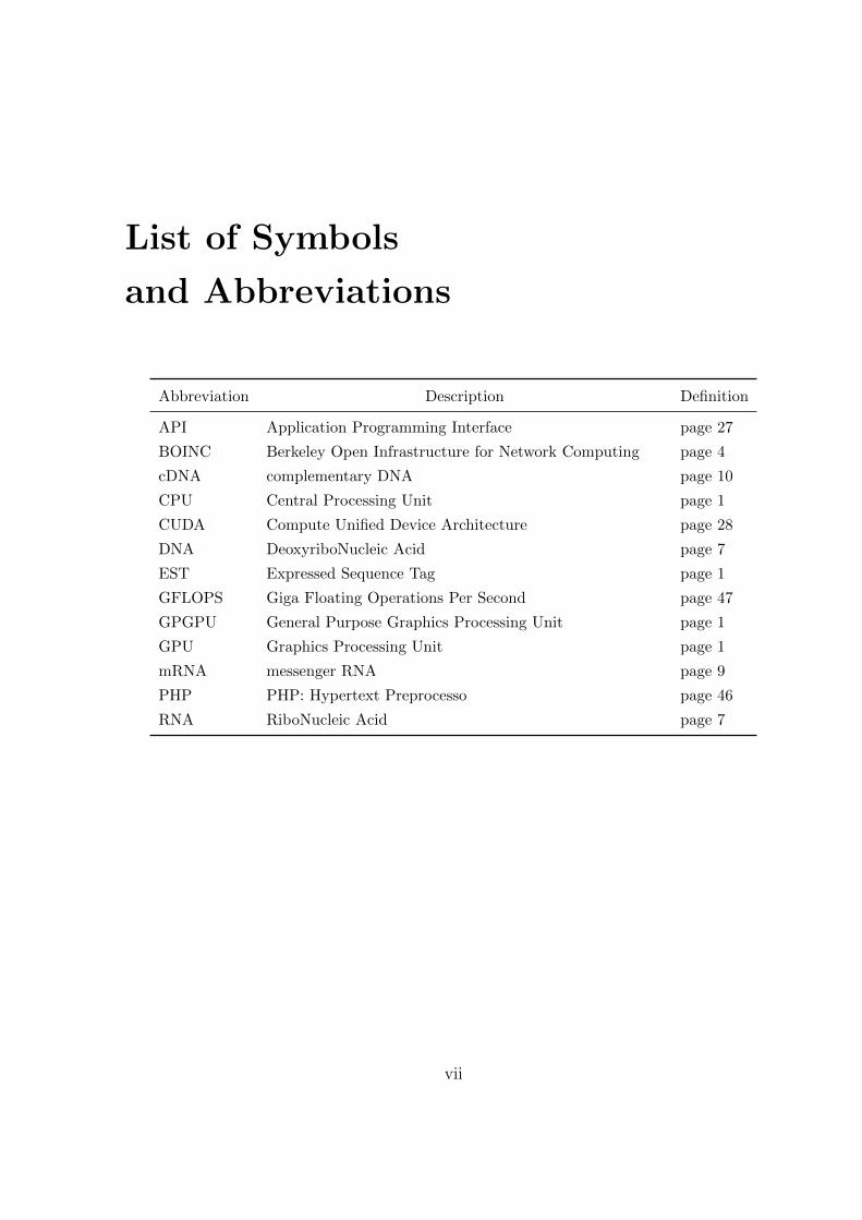
List of Symbols
and Abbreviations
Abbreviation Description Definition
API Application Programming Interface page 27
BOINC Berkeley Open Infrastructure for Network Computing page 4
cDNA complementary DNA page 10
CPU Central Processing Unit page 1
CUDA Compute Unified Device Architecture page 28
DNA DeoxyriboNucleic Acid page 7
EST Expressed Sequence Tag page 1
GFLOPS Giga Floating Operations Per Second page 47
GPGPU General Purpose Graphics Processing Unit page 1
GPU Graphics Processing Unit page 1
mRNA messenger RNA page 9
PHP PHP: Hypertext Preprocesso page 46
RNA RiboNucleic Acid page 7
vii

List of Figures
2.1 The 5 Common Nucleotides [1] . . . . . . . . . . . . . . . . . . . . . . . . . . 8
2.2 DNA Chemical Structure . . . . . . . . . . . . . . . . . . . . . . . . . . . . . . 8
3.1 The GPU devotes more transistors to data processing [2] . . . . . . . . . . . . 28
3.2 CUDA Memory Model [2] . . . . . . . . . . . . . . . . . . . . . . . . . . . . . 32
3.3 CUDA Grid of Thread Blocks [2] . . . . . . . . . . . . . . . . . . . . . . . . . 36
3.4 CUDA Block Scheduling [2] . . . . . . . . . . . . . . . . . . . . . . . . . . . . 37
5.1 Visualization of the dataset as a collection of EST sequences . . . . . . . . . . 62
5.2 Many-to-Many comparison between 6 elements . . . . . . . . . . . . . . . . . 63
5.3 Many-to-many comparison between 6 elements in grid format . . . . . . . . . 64
5.4 Many-to-many comparisons of 8 elements divided into 3 seperate 4 by 4 sized
jobs . . . . . . . . . . . . . . . . . . . . . . . . . . . . . . . . . . . . . . . . . 64
5.5 Basic Program Structure . . . . . . . . . . . . . . . . . . . . . . . . . . . . . . 66
5.6 Parallel Program Structure . . . . . . . . . . . . . . . . . . . . . . . . . . . . . 67
5.7 Comparison of Cumulative Score versus default Smith-Waterman scoring . . . 78
6.1 Detailed Program Structure . . . . . . . . . . . . . . . . . . . . . . . . . . . . 84
6.2 Word Count table . . . . . . . . . . . . . . . . . . . . . . . . . . . . . . . . . . 88
7.1 Performance on the Arabidopsis data set for different sized subsets of the data 101
7.2 Ratio of performance of GPUcluster and wcdest with dataset size . . . . . . . 101
7.3 Kernel execution time plot (time is in micro-seconds) . . . . . . . . . . . . . . 104
ix

List of Tables
2.1 Characters and meanings for FASTA sequences . . . . . . . . . . . . . . . . . 22
3.1 Comparison of various CUDA Capabilities [2] . . . . . . . . . . . . . . . . . . 31
3.2 Summary of Memory Types available to CUDA Programmers . . . . . . . . . 32
3.3 Optimal Maximums for 2.x Compute Capability GPUs for different block sizes 39
3.4 Optimal Maximums for 1.3 Compute Capability GPUs for different block sizes 39
5.1 66% Similarity Substitution Matrix . . . . . . . . . . . . . . . . . . . . . . . . 76
5.2 Alignment matrix between ’GATTCGTTA’ and ’GGATCGTA’ . . . . . . . . 76
5.3 Comparison of the various algorithms introduced in this chapter . . . . . . . . 79
6.1 Comparison of Word Count kernels memory use for different k-lengths . . . . 89
7.1 Price and performance comparison of various hardware . . . . . . . . . . . . . 98
7.2 Performance comparison between different datasets . . . . . . . . . . . . . . . 99
7.3 Timing profiling results for the 10K dataset (≈ 10K ESTs) . . . . . . . . . . . 102
7.4 Timing profiling results for the A032 dataset (≈ 70K ESTs) . . . . . . . . . . 103
xi

List of Algorithms
1 Instruction Level Parallelism Example . . . . . . . . . . . . . . . . . . . . 40
2 CPU-side Program Structure . . . . . . . . . . . . . . . . . . . . . . . . . . 85
3 Word Count kernel . . . . . . . . . . . . . . . . . . . . . . . . . . . . . . . 88
4 Word Presence kernel . . . . . . . . . . . . . . . . . . . . . . . . . . . . . . 89
5 u/v - Sample Heuristic Kernel . . . . . . . . . . . . . . . . . . . . . . . . . 90
6 t/v - Word Heuristic Kernel . . . . . . . . . . . . . . . . . . . . . . . . . . 92
xiii

Chapter 1
Objective/Scope
1.1 Introduction
Bioinformatics is one of the most rapidly advancing sciences today. It is a scientific
domain that attempts to apply modern computing and information technologies to the
field of biology, the study of life itself and involves documenting and analysing genetics,
proteins, viruses, bacteria and cancer as well as hereditary traits and diseases, as well as
researching cures and treatments for whole ranges of health threats.
The growth of bioinformatics and developments, both theoretical and experimental
in biology, can largely be linked to the IT explosion which gives the field more powerful
processing options with much cheaper solutions, limited only by the steady yet significant
improvements as promised by Moore’s Law [3].
This IT explosion has also caused significant advances due to the high consumer de-
mand region of computer graphics hardware, or GPUs (Graphics Processing Units). The
consumer demand has actually managed to advance GPUs far faster than classical CPUs
(Central Processing Units), outpacing CPU performance improvements by a large margin.
As of early 2010, the fastest available PC processor(Intel Core i7 980 XE) has a theoret-
ical performance of 107.55 GFLOPS [4], while GPUs with TFLOPS (1000 GFLOPS) of
performance have been commercially available since 2008 (ATI HD4800).
While typically used only for graphical rendering, modern innovations have greatly
increased GPU flexibility and has given rise to the field of GPGPU (General Purpose
GPU) which allows graphics processors to be applied to non-graphics applications.
By utilizing GPU processing power to solve bioinformatics problems, the field can the-
oretically be boosted once again, increasing the amount of computational power available
to scientists by an order of magnitude or more.
1
2 Chapter 1. Objective/Scope
This document will primarily deal with the possibility of utilizing GPUs in the prob-
lem of EST (Expressed Sequence Tag) clustering, chosen due to its high data volume,
complexity and overlap with other bioinformatics problems such as sequence reassembly.
1.2 Problem Statement
It is proposed that GPUs are appropriate and useful for bioinformatics problems, specif-
ically in the domain of clustering of EST sequences.
There are many possible advantages to implementing any computationally intensive
algorithm on the GPU, such as large speed-ups and reduced costs. Improvements for
ported applications have reported 1.16×-431× speed-ups over CPU implementations [5].
The problems where GPU computation are normally applied and where it achieves
high performance usually involve high volumes of structured numerical data, intense but
predictable processing with significant spatial locality in memory reads and little branch-
ing.
Bioinformatics makes use of a large set of computer algorithms, including but not
limited to string manipulation, database search and manipulation, molecular physics sim-
ulation and graph theory, all algorithms not known for their strength on the GPU. EST
clustering, a string manipulation problem, was selected specifically for this dissertation
due to its importance in many bioinformatics applications, yet perceived unsuitability to
the GPU pipeline.
Many factors count against efficient bioinformatics algorithm implementation on the
GPU such as very large datasets compared to GPU memory (a gigabyte or more is not
uncommon for a dataset), the dissimilarity between string operations required for bioin-
formatics and the native graphics pipeline which is specialised for numerical data, un-
desirability of branching statements and the parallelizability requirements of the ported
algorithms.
Some of these disadvantages can be mitigated by performing part of the processing on
the GPU and part on the CPU, utilizing each architecture to its strength.
1.3. Research Questions 3
1.3 Research Questions
This thesis will seek to address the following questions:
1. Is GPGPU a practical computing platform for bioinformatics algorithms?
2. Can existing bioinformatics algorithms be practically ported to GPGPU?
3. Is the cost of GPGPU competitive with classical CPU computing?
4. Is the performance of GPGPU competitive with classical CPU computing?
1.4 Objective
The objective of this thesis is to answer the posed research questions. To do so, the
following approaches will be used:
1. The specifications of bioinformatics algorithms are dependent on the highly spe-
cialized nature of the biological data it is designed to process. Proper research is
required to understand the unique demands, constraints and limits of the domain.
Research is required on the GPGPU platform and its strengths and weaknesses.
This can indicate whether GPGPU would be a good match for the requirements of
bioinformatics algorithms and data.
Research of previous GPGPU implementations in the bioinformatics field should
serve to provide evidence either supporting or rejecting its practicality.
2. The best way to prove the practicality of porting a bioinformatics algorithm is to
perform such a port as part of the project.
The suitability of prospective algorithms to port should be researched with chal-
lenges identified.
3. Analysis of the cost of GPGPU is performed by identifying the commercial cost of
both GPU and CPU platforms.
The advertised GFLOPS of both platforms can be compared to its cost, from which
the cost per GFLOP of both can be computed and compared.
4. The advertised GFLOPs is not always representative of real-world performance. In
order to measure this benchmark tests need to be run on CPU and GPU implemen-
tations of the same algorithm.
4 Chapter 1. Objective/Scope
1.5 Scope
Due to the open nature of the research questions, the scope of this project will be limited
to the domain of EST clustering.
EST clustering is a well-researched topic dealing with sequence comparisons. It in-
volves high volumes of relatively short sequences and is related to genome identification,
an important process in bioinformatics.
Though the domain of EST clustering is not representative of all bioinformatics prob-
lems, it is a relatively simple processing step for short nucleotide sequences and should
lend insight into the use of GPGPU in sequence reassembly.
The clustering algorithm picked depends on the algorithm’s suitability to the GPU
work-flow, its scalability to large datasets and its ability to parallelise over multiple
threads. It is not expected that a simple software port of the most common modern
algorithm will result in the ideal performance, so research is likely to find another algo-
rithm that is known and proven and best suited to parallelisation.
The project is not meant to research and develop an entirely new clustering algorithm,
but to merely adapt an existing proven one to a different platform.
The project will deal with the clustering stage only and only mention the reassembly
stage where the clustering stage can improve the reassembly stage, either by increasing
speed or by reducing errors and improving quality.
This project will not deal with the EST cleaning phase and assumes a dataset that
has already been pre-processed by the base caller.
This project will not deal with repeat masking.
1.6 Contributions
During the course of this project significant research was done on GPU Cluster Computing
for the purpose of scaling up to multiple PCs and GPUs. Many possible solutions exist,
but eventually BOINC was chosen.
BOINC (Berkeley Open Infrastructure for Network Computing) is a distributed grid
middleware platform. This means that it hosts distributed applications and provides
client and server software to allow new desktop grid computers to be added to a project
with a minimum of configuration [6]. This allows a whole office of computers, all outfitted
with GPUs, to contribute to a computing task without the need of special or dedicated
1.7. Overview 5
hardware. All the PCs used in this manner can still serve as normal desktop computers
for everyday use.
The project was initially developed with BOINC support in mind and the feasibility
study was submitted and accepted at the SATNAC 2010 conference [7], but time con-
straints has prevented the development of full support for the BOINC framework in the
final application.
1.7 Overview
The remainder of this document is organised as follows:
• Chapter 2 - Literature - Bioinformatics Theory and Algorithm Overview
– Brief introduction and literature study of bioinformatics, ESTs and an expla-
nation of why clustering ESTs is important for reassembly.
– Characteristics of EST Datasets and explanation of terms from a data analysis
standpoint.
– Brief history of bioinformatics and the important advances that resulted in our
current level of understanding of ESTs and their processing.
– Brief history of contributions GPUs have made in bioinformatics.
– Explanation of the FASTA file format, used to store ESTs.
– Introduction of the categories of GPU algorithms under review in this disser-
tation.
• Chapter 3 - Literature - GPU Literature Study
– An introduction to GPU computing, its strengths and its limitations.
– Introduces and explains the theory surrounding parallelism on the GPU.
– Introduction to the CUDA programming language including:
∗ Compute capabilities of different generations of GPU.
∗ Explanation of GPU memory types.
∗ Different types of parallelism offered by GPUs.
6 Chapter 1. Objective/Scope
• Chapter 4 - Experimental Design
– Common terms and measurement metrics are explained.
– Experimental assumptions enumerated.
– Datasets used for experimentation is listed and introduced.
– Individual tests and experiments explained in detail.
– Expected results are proposed.
• Chapter 5 - Selection of Algorithms
– Selection Criteria is listed and explained.
– Expected data, memory and program structures are introduced.
– Individual algorithms for use with heuristics are introduced and their strengths
and limitations are provided.
– Individual comparison algorithms are introduced, and their strengths and lim-
itations are provided.
– Proposed algorithms are compared and specific ones selected for GPU imple-
mentation.
• Chapter 6 - Implementation and Issues
– Implementation details surrounding program structure and memory manage-
ment is provided.
– Details on the implementation of individual kernels is provided.
– Issues with implementation are discussed.
– Implementation concerns are listed, including the shortcomings of parallelizing
algorithms originally meant for the CPU.
• Chapter 7 - Results and Analysis
– Experiments proposed in Chapter 4 are executed and its results provided.
– Critical analysis of experiments are discussed.
• Chapter 8 - Conclusion and Further Work
– Summary of the project is presented.
– Areas where further work can be performed are identified.
– Conclusion of work provided.
Chapter 2
Literature - Bioinformatics Theory
and Algorithm Overview
2.1 Introduction
This chapter provides basic introductory knowledge of the bioinformatics theory and terms
used both in the field and throughout the rest of the thesis. This is not meant to be a
comprehensive introduction to the bioinformatics field as a whole, but should be sufficient
to understand the problem and the solutions provided by this document.
A literature study is included that gives a basic overview of both the history of EST
bioinformatics processing and the contributions of GPU computation in the bioinformatics
field in general. Many of these references are used as an inspiration to this thesis, forming
the body of knowledge that this thesis intends to contribute to.
Finally, a higher level survey of the algorithms and processes used in EST comparison
and processing is introduced, which will be analysed more thoroughly in a later chapter.
2.2 Bioinformatics Theory
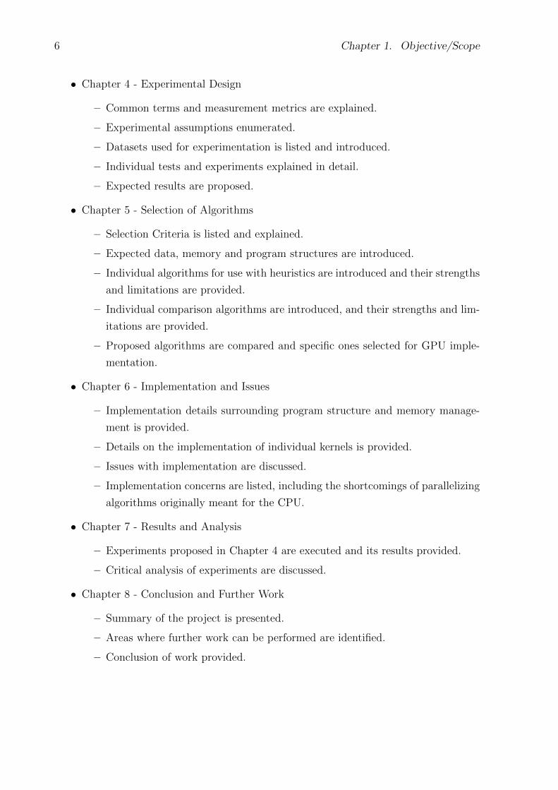
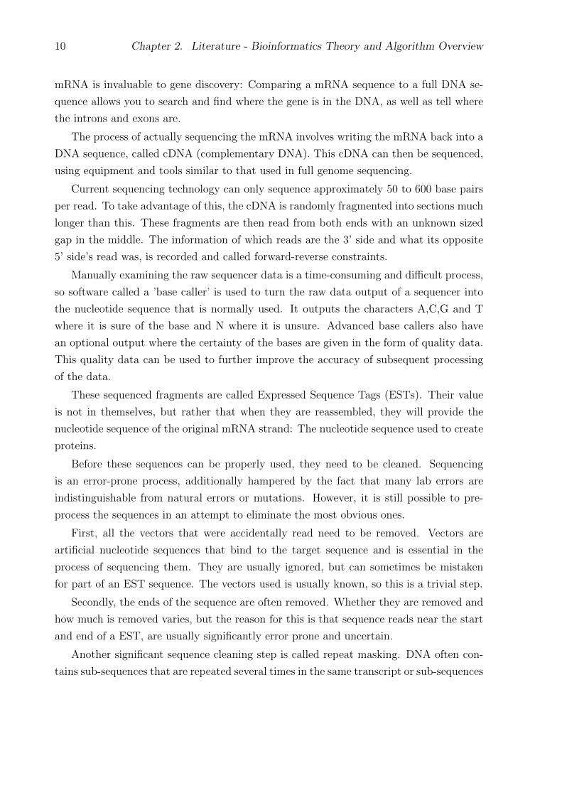
A nucleotide is the most basic building block of the nucleic acid macromolecules found
in any living species, the best known of which are DNA (DeoxyriboNucleic Acid) and
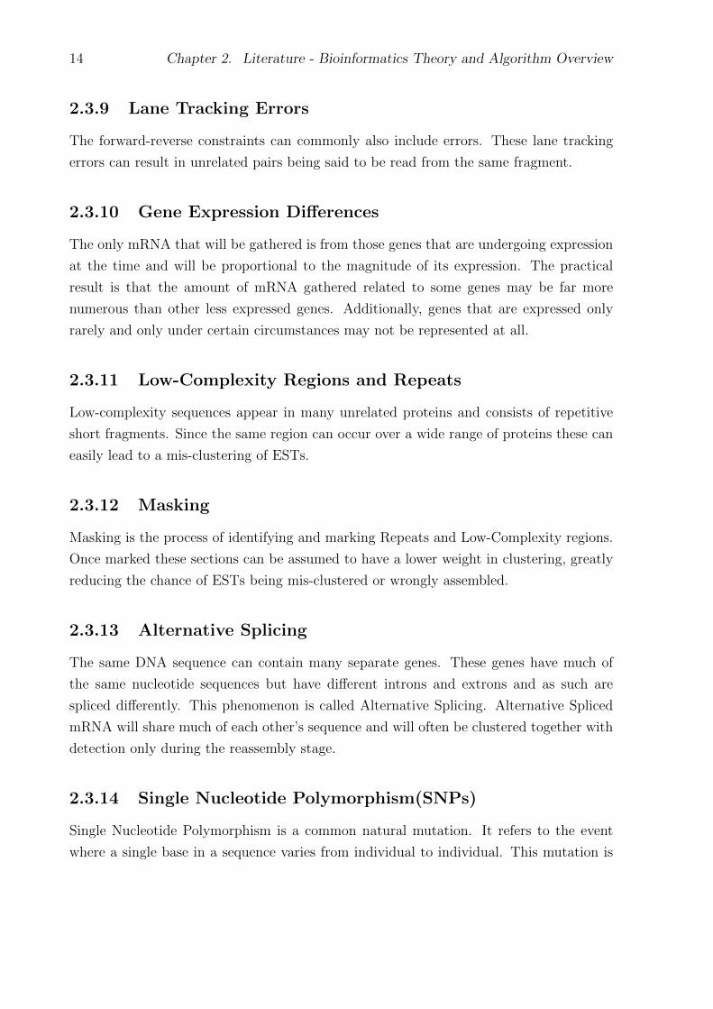
RNA (RiboNucleic Acid). There are 5 common nucleotides that this paper will deal with.
These nucleotides are Adenine (A), Guanine (G), Cytosine (C), Thymine (T) and Uracil
(U). Uracil is only found in RNA while Thymine is found only in DNA. The information
that these two represent can be considered equivalent.
7
8 Chapter 2. Literature - Bioinformatics Theory and Algorithm Overview
Figure 2.1: The 5 Common Nucleotides [1]
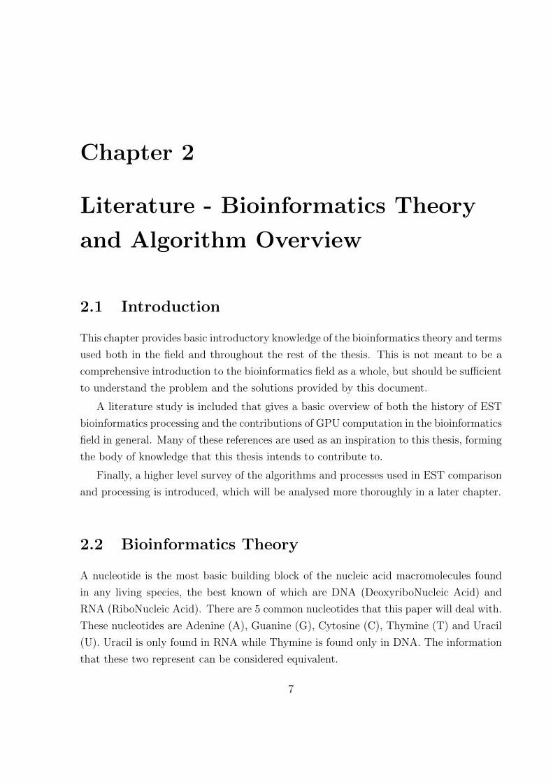
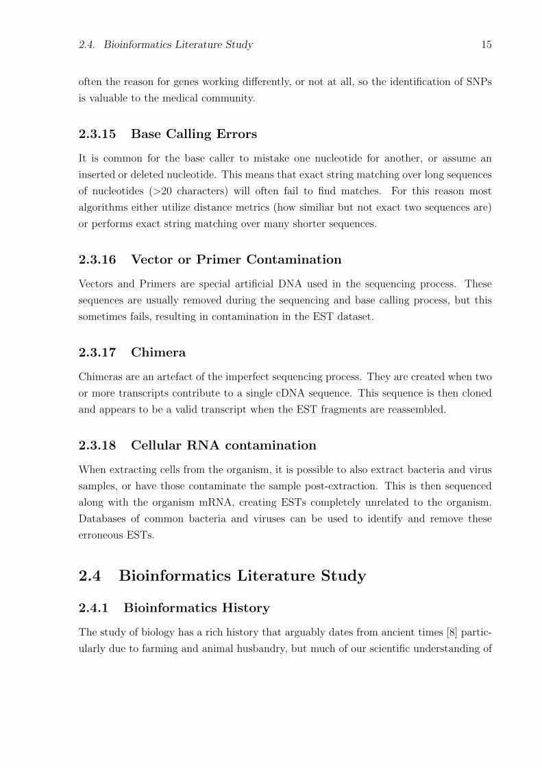
Figure 2.2: DNA Chemical Structure
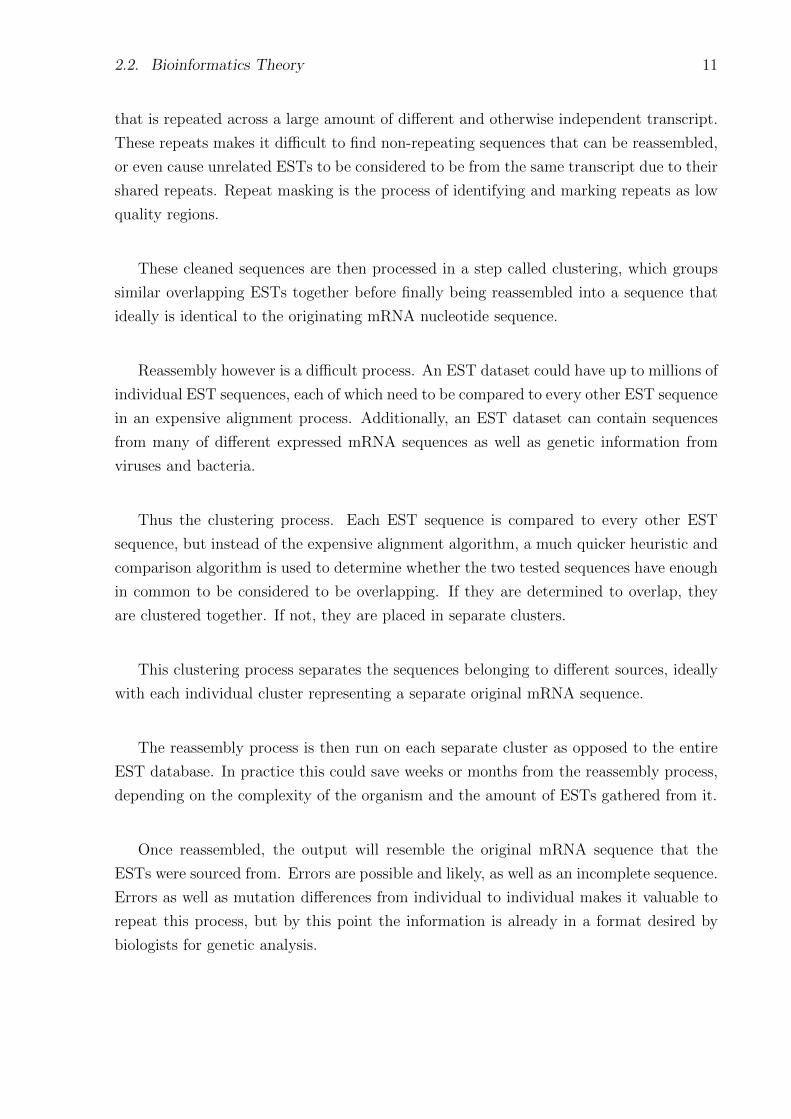
Every nucleotide base bonds natu-
rally with one other nucleotide base (Fig-
ure 2.2). Adenine bonds with Thymine
and Guanine bonds with Cytosine. Two
nucleotides bonded like this is usually re-
ferred to as a base pair. Base pairs in
DNA and RNA form sequences. Every
base pair additionally has a direction, in-
dicated by the layout of the sugars on
the base pair. The 3’ side of a base pair
can only link with the 5’ of another base
pair to form long chains. This terminol-
ogy is used to indicate the direction of a
sequence.
By convention, sequences are usually
written from the 5’ end to the 3’. The
characters A,G,C,T are used to refer to
the different nucleotides, Adenine, Gua-
nine, Cytosine and Thymine. In addition, the character N refers to an unknown low
quality read that could be any of the 4 bases. When needed, the character ’-’ could also
refer to an undetermined gap in the sequence. These 6 characters will be used throughout
the paper to represent nucleotide sequences.
The famous double helix shape of DNA occurs to two strands of nucleotides, connected
2.2. Bioinformatics Theory 9
as base pairs running in opposite directions to one another. It is important to note that
the following two sequences are equivalent and represent the same subsequence of DNA:
5’ end - ACTGGC - 3’ end
3’ end - TGACCG - 5’ end
If both sides are read from 5’ to 3’, the sequences are simply written as:
ACTGGC
GCCAGT
These are called complementary sequences.
The term base pairs (bps) also refers to the length of such sequences, with a kilobases
(kbps) being equal to a thousand base pairs of RNA or DNA and mega base pairs (Mbps)
being equal to a million base pairs. The above units only refer to double stranded bonded
base pairs. The single stranded equivalent unit of length is Nucleotides (nts). This paper
will however not make this distinction and use the unit bps in all indications of nucleotide
sequence length.
A gene is unit of heredity in living organisms and is encoded in a sequence of DNA.
They determine the growth and maintenance of cells, how they divide and how and when
they die. They determine features such as eye colour, hair colour, blood type. Genes
define every characteristic of every DNA carrying living species.
Genes, as they are coded in DNA, consist of sequences of alternating coding nucleotide
sequences (exons) and non-coding nucleotide sequences (introns). During gene expression,
these genes are transcribed to RNA sequences and the introns spliced out, leaving only a
sequence of the coding exons.
Sometimes these resulting sequences are used in cellular processes, but the interest in
this paper is the subset of RNA called mRNA (messenger RNA), that transport codon
sequences to the ribosomes, which are cellular factories that create proteins from these
sequences.
A codon is a sequence of 3 nucleotides that refer to a specific amino acid, the building
block of proteins. Though there are 64 possible codons (sequence of 3 nucleotides, resulting
in 34 permutations), there are only 20 amino acids. Most of the amino acids have many
redundant codons that they can be translated from.
At any time, many gene expressions will be occurring in any cell simultaneously. Scien-
tists however can extract this mixture of mRNA strands before they reach the Ribosomes.
10 Chapter 2. Literature - Bioinformatics Theory and Algorithm Overview
mRNA is invaluable to gene discovery: Comparing a mRNA sequence to a full DNA se-
quence allows you to search and find where the gene is in the DNA, as well as tell where
the introns and exons are.
The process of actually sequencing the mRNA involves writing the mRNA back into a
DNA sequence, called cDNA (complementary DNA). This cDNA can then be sequenced,
using equipment and tools similar to that used in full genome sequencing.
Current sequencing technology can only sequence approximately 50 to 600 base pairs
per read. To take advantage of this, the cDNA is randomly fragmented into sections much
longer than this. These fragments are then read from both ends with an unknown sized
gap in the middle. The information of which reads are the 3’ side and what its opposite
5’ side’s read was, is recorded and called forward-reverse constraints.
Manually examining the raw sequencer data is a time-consuming and difficult process,
so software called a ’base caller’ is used to turn the raw data output of a sequencer into
the nucleotide sequence that is normally used. It outputs the characters A,C,G and T
where it is sure of the base and N where it is unsure. Advanced base callers also have
an optional output where the certainty of the bases are given in the form of quality data.
This quality data can be used to further improve the accuracy of subsequent processing
of the data.
These sequenced fragments are called Expressed Sequence Tags (ESTs). Their value
is not in themselves, but rather that when they are reassembled, they will provide the
nucleotide sequence of the original mRNA strand: The nucleotide sequence used to create
proteins.
Before these sequences can be properly used, they need to be cleaned. Sequencing
is an error-prone process, additionally hampered by the fact that many lab errors are
indistinguishable from natural errors or mutations. However, it is still possible to pre-
process the sequences in an attempt to eliminate the most obvious ones.
First, all the vectors that were accidentally read need to be removed. Vectors are
artificial nucleotide sequences that bind to the target sequence and is essential in the
process of sequencing them. They are usually ignored, but can sometimes be mistaken
for part of an EST sequence. The vectors used is usually known, so this is a trivial step.
Secondly, the ends of the sequence are often removed. Whether they are removed and
how much is removed varies, but the reason for this is that sequence reads near the start
and end of a EST, are usually significantly error prone and uncertain.
Another significant sequence cleaning step is called repeat masking. DNA often con-
tains sub-sequences that are repeated several times in the same transcript or sub-sequences
2.2. Bioinformatics Theory 11
that is repeated across a large amount of different and otherwise independent transcript.
These repeats makes it difficult to find non-repeating sequences that can be reassembled,
or even cause unrelated ESTs to be considered to be from the same transcript due to their
shared repeats. Repeat masking is the process of identifying and marking repeats as low
quality regions.
These cleaned sequences are then processed in a step called clustering, which groups
similar overlapping ESTs together before finally being reassembled into a sequence that
ideally is identical to the originating mRNA nucleotide sequence.
Reassembly however is a difficult process. An EST dataset could have up to millions of
individual EST sequences, each of which need to be compared to every other EST sequence
in an expensive alignment process. Additionally, an EST dataset can contain sequences
from many of different expressed mRNA sequences as well as genetic information from
viruses and bacteria.
Thus the clustering process. Each EST sequence is compared to every other EST
sequence, but instead of the expensive alignment algorithm, a much quicker heuristic and
comparison algorithm is used to determine whether the two tested sequences have enough
in common to be considered to be overlapping. If they are determined to overlap, they
are clustered together. If not, they are placed in separate clusters.
This clustering process separates the sequences belonging to different sources, ideally
with each individual cluster representing a separate original mRNA sequence.
The reassembly process is then run on each separate cluster as opposed to the entire
EST database. In practice this could save weeks or months from the reassembly process,
depending on the complexity of the organism and the amount of ESTs gathered from it.
Once reassembled, the output will resemble the original mRNA sequence that the
ESTs were sourced from. Errors are possible and likely, as well as an incomplete sequence.
Errors as well as mutation differences from individual to individual makes it valuable to
repeat this process, but by this point the information is already in a format desired by
biologists for genetic analysis.
12 Chapter 2. Literature - Bioinformatics Theory and Algorithm Overview
2.3 Dataset Characteristics and Error Classification
2.3.1 Alphabet (A,C,G,T,N)
EST files contain sequences made from 5 characters:
A - Adenine
G - Guanine
C - Cytosine
T - Thymine
N - Unsure, could be any nucleotide
The last character (N) only occurs with low quality reads when the base caller is
uncertain.
2.3.2 Read Length
Read length is an indication of the expected amount of characters in every EST. Depend-
ing on the sequencing hardware this can be as long as 600 or as short as 40. Since errors
are most likely to occur on the ends of the reads, it is common for the ends to be trimmed,
reducing the final read length used in clustering and reassembly.
2.3.3 Orientation
Sequences have a natural direction. By convention nucleotide sequences are written from
the 5’ end to the 3’. This refers to which of the carbon atoms in a nucleotide base the
next one is bonded to, something that can be sensed by the sequencing hardware.
2.3.4 Redundancy(Coverage)
The estimated coverage suggests the amount of times any single base is represented in
an EST dataset. A coverage of 3x for instance means that any base has been read three
times and appears in three ESTs. This is only an estimation however, and may differ
based on gene expression and random chance.
The amount of coverage aimed for is dependent on the sequence read length. Short
read ESTs may need coverage as high as 8x or 16x to be reassembled correctly, while
some long reads may be reassembled with as low coverage as 3x.
2.3. Dataset Characteristics and Error Classification 13
2.3.5 Quantity
The high amount of redundancy results in an incredible amount of data. A 5 000 base
pair mRNA read with 8x coverage means 40 000 characters that need to be stored. A
complex enough organism with large amount of mRNA expressed at once can easily create
millions of individual ESTs requiring gigabytes of storage.
2.3.6 Quality
Quality data is an optional output from base calling software. Quality data refers to the
certainty of the base caller that the base read is in fact the correct one. Quality usually
starts low near the start of a read sequence and degrades again near the end of a read,
resulting in it being common practice to clip the ends of a sequence.
High quality bases can still be erroneous, but low quality bases have a greater chance
of such.
2.3.7 Reverse Complement
DNA consists of two nucleotide sequences bonded together and running in opposite di-
rections, wrapped around in a double helix shape. Adenine bonds with Thymine and
Guanine bonds with Cytosine. Both sequences represent the same information however,
and as such they are called the reverse compliment of one another. To illustrate:
5’ end - ACTGGC - 3’ end
3’ end - TGACCG - 5’ end
If both sides are read from 5’ to 3’, the sequences are simply written as:
ACTGGC
GCCAGT
2.3.8 Forward Reverse Constraints
Some sequencing hardware tracks reads from both ends of a cDNA fragment. With this
information two reads can be paired, with knowledge that one sequence is on the 3’ or
5’ of the other. This information means that these two sequences should be clustered
together, and helps with erroneous reassembly.
14 Chapter 2. Literature - Bioinformatics Theory and Algorithm Overview
2.3.9 Lane Tracking Errors
The forward-reverse constraints can commonly also include errors. These lane tracking
errors can result in unrelated pairs being said to be read from the same fragment.
2.3.10 Gene Expression Differences
The only mRNA that will be gathered is from those genes that are undergoing expression
at the time and will be proportional to the magnitude of its expression. The practical
result is that the amount of mRNA gathered related to some genes may be far more
numerous than other less expressed genes. Additionally, genes that are expressed only
rarely and only under certain circumstances may not be represented at all.
2.3.11 Low-Complexity Regions and Repeats
Low-complexity sequences appear in many unrelated proteins and consists of repetitive
short fragments. Since the same region can occur over a wide range of proteins these can
easily lead to a mis-clustering of ESTs.
2.3.12 Masking
Masking is the process of identifying and marking Repeats and Low-Complexity regions.
Once marked these sections can be assumed to have a lower weight in clustering, greatly
reducing the chance of ESTs being mis-clustered or wrongly assembled.
2.3.13 Alternative Splicing
The same DNA sequence can contain many separate genes. These genes have much of
the same nucleotide sequences but have different introns and extrons and as such are
spliced differently. This phenomenon is called Alternative Splicing. Alternative Spliced
mRNA will share much of each other’s sequence and will often be clustered together with
detection only during the reassembly stage.
2.3.14 Single Nucleotide Polymorphism(SNPs)
Single Nucleotide Polymorphism is a common natural mutation. It refers to the event
where a single base in a sequence varies from individual to individual. This mutation is
2.4. Bioinformatics Literature Study 15
often the reason for genes working differently, or not at all, so the identification of SNPs
is valuable to the medical community.
2.3.15 Base Calling Errors
It is common for the base caller to mistake one nucleotide for another, or assume an
inserted or deleted nucleotide. This means that exact string matching over long sequences
of nucleotides (>20 characters) will often fail to find matches. For this reason most
algorithms either utilize distance metrics (how similiar but not exact two sequences are)
or performs exact string matching over many shorter sequences.
2.3.16 Vector or Primer Contamination
Vectors and Primers are special artificial DNA used in the sequencing process. These
sequences are usually removed during the sequencing and base calling process, but this
sometimes fails, resulting in contamination in the EST dataset.
2.3.17 Chimera
Chimeras are an artefact of the imperfect sequencing process. They are created when two
or more transcripts contribute to a single cDNA sequence. This sequence is then cloned
and appears to be a valid transcript when the EST fragments are reassembled.
2.3.18 Cellular RNA contamination
When extracting cells from the organism, it is possible to also extract bacteria and virus
samples, or have those contaminate the sample post-extraction. This is then sequenced
along with the organism mRNA, creating ESTs completely unrelated to the organism.
Databases of common bacteria and viruses can be used to identify and remove these
erroneous ESTs.
2.4 Bioinformatics Literature Study
2.4.1 Bioinformatics History
The study of biology has a rich history that arguably dates from ancient times [8] partic-
ularly due to farming and animal husbandry, but much of our scientific understanding of
16 Chapter 2. Literature - Bioinformatics Theory and Algorithm Overview
biology comes from more recent discoveries. Modern understanding of biology owes much
to the discoveries made in the 19th century, even if the significance of many of them only
became apparent later.
Today proteins are widely known as the building blocks of life, but the term itself
only first appeared in a letter written by Gerardus Johannes Mulder in 1838 [9]. Though
he initially believed that there was only a single common large type of protein, recent
estimates suggest that the human body produces up to 84 000 different proteins [10].
Gregor Mendel is credited with the idea of genes as a unit of heredity due to the work
he published in 1865 which deals with his studies on controlled breeding of pea plants
and the propagation of traits along family lines [11, 12]. The importance of his work was
not recognised when it was first published, but its rediscovery in the 1900s led to it being
considered the foundation of modern genetic studies.
Charles Darwin’s famous ‘On the Origin of the Species’ was poorly received when it
was published in 1859 even if it is today recognised as absolutely essential in explaining
the biodiversity of species on Earth [13]. Though it sought to explain evolution through
survival of the fittest and sexual selection, the mechanism for heredity was not yet known.
Thomas Hunt Morgan, though initially critical of Darwin’s theory of evolution, used
fruit flies to replicate Gregor Mendel’s experiments. His experiments in 1910 and onward
both confirmed Gregor Mendel’s work and led to understanding of the importance of sex
chromosones in genetics, as well as a greater understanding of how genes are inherited
between generations [14].
DNA was isolated for the first time by Friedrich Miescher in 1869 during experiments
to determine the chemical composition of cells [15]. DNA is now recognised as the the
mechanism by which genes are encoded, stored and propagated.
The field of bioinformatics emerges from the overlap of biology studies and digital
computing which begins with the invention of the first digital computers in 1940s. It is
only in the 1970s [16] that the field gained prevalence due to the rise in availability of
the personal computer, allowing individual researchers without large budgets to digitally
analyse their data.
The mid-1900s saw incredible advances in our understanding of biology, including
the discovery of the structure of DNA [17, 18], the encoding of genetic information for
proteins [19] and understanding of the information content of DNA [20]. Simultaneously
new theories of computing and informatics was being developed [21].
Based on and building on these advances, 1970s saw the beginning of radical new
methods to analyse the information content of DNA and the formulation of the first
2.4. Bioinformatics Literature Study 17
sequence alignment algorithms [22, 23, 24, 25, 26, 27, 28] and the wide-spread use of
molecular data in evolutionary studies [29].
By the mid-1970s the theory and practice of sequence alignment was well understood
which resulted in increased activity and innovation in the latter half of the decade, a
key part being the establishment of standards used in the archiving and distribution of
protein sequences and protein structure information [30, 31, 32].
The availability of public databases in the 1980s [33, 34] and the increasing rate of
generation of molecular sequencing data in that decade [35] led to key advances such as the
formulation of the Smith-Waterman algorithm [36] and the FASTA family of algorithms
for database searching [37, 38].
Advances in hardware also occurred more rapidly and this included the use of dedicated
parallel hardware to more efficiently process this flood of data [39, 40, 41, 42, 43, 44].
Though ARPANET, the forbear of the internet existed since the late 1960s, it is only
in the 1990s when the internet as we know it started becoming more publicly available
that the bioinformatics data available to researchers dramatically increased [45]. Before
this point access to databases such as Genbank [34] was limited and distributed mostly
through CD-rom discs [31].
Additionally new algorithms and tool-kits such as BLAST [46] became available that
further improved on the processing that can be done with the available data.
In 1990 the Human Genome Project was started with the stated goal of providing a
complete high-quality sequence of human genomic DNA to the research community as a
publicly available resource [47]. Though well-funded, the complexity of this endeavour
meant that this effort only provided a working draft of the human genome in 2001 [48]
and was only completed in 2003 [49, 50].
2.4.2 Expressed Sequence Tags History
Before the Human Genome Project began, there were debates about the need for large
scale DNA sequencing since the sequencing of ESTs would allow identification of all of the
important gene coding regions of DNA. EST sequencing proved to be a cheaper technique
which sequences only expressed genes, allowing useful genes to be identified for medical
and research use far ahead of the 12 to 15 year estimation for the completion of the Human
Genome Project.
It was then estimated that only 3% of the information content of DNA contained
coding sequences for genes and the sequencing of these regions should take priority [51].
18 Chapter 2. Literature - Bioinformatics Theory and Algorithm Overview
Though whole-DNA sequencing was eventually used to map the human genome, far
ahead of schedule due to novel new methods, sequencing and analysis of ESTs remain an
important tool to cheaply discover novel genes in a wide array of species [52].
Several software programs have been developed before to deal with the problem of
EST clustering and reassembly. Most of them have roots in DNA shotgun sequencing,
but since the data structure and the algorithms are similar the applications can often be
adapted to be able to deal with EST data as well. What follows is some of the more
notable EST clustering/reassembly programs.
One of the best known early genome assembly programs is called PHRAP [53]. PHRAP
is part of a suite of programs that was originally designed for whole-sequence shotgun se-
quencing of DNA, but has since been adapted and used in EST assembly [54].
CAP3 [55], another well known DNA sequence assembly program, has also since been
used for EST assembly. It operates by finding all possible overlaps quickly using a BLAST-
like method, then Smith-Waterman alignment is used to align the overlaps and generate
contigs (set of overlapping DNA segments) and the final assembly. CAP3 is known to
have fewer errors than PHRAP when assembling EST data [54].
CAP3 was not originally designed for EST sequences however, so a tool called TGI
Clustering Tool [56, 52] was developed, intended to cluster sequences, greatly decreasing
the time needed for CAP3 to reassemble the sequences.
Two notable programs that have been developed purely for the purpose of clustering
EST sequences is PaCE [57], which uses a maximal common substring algorithm to find
overlaps, and d2 cluster [58], which uses a common words method to detect similiarity.
More recently, the wcdest [59] application has been developed which is based on
d2 cluster, utilizing aggressive heuristics to improve the speed performance significantly,
while having a negligible impact on the clustering accuracy. This tool only clusters the
sequences however, so a second tool is required to reassemble them. The focus on the
effectiveness of effective heuristics by wcdest served as as the groundwork and source for
the heuristics employed in this project.
2.4.3 Rise of GPGPU in High Performance Computing
The prominence of the GPU on the non-graphical field is a relatively new occurrence,
with some of the earliest papers in the field happening during the 1990s. During this
time period GPUs were still generally limited to graphics related problems, resulting in
most GPGPU programs of the era being rendering or image manipulation projects such
as real-time textures [60], image-composition [61] and video flow detection [62].
2.4. Bioinformatics Literature Study 19
The 1990s also saw one of the first non-graphics or visualisation related problems solved
using GPU computing, namely using clever rendering techniques to compute Neural Net-
works [63], which both highlights the limitations of early GPUs as well the inventiveness
of researchers to challenge them.
It is not until 2001 and the release of the first GPU with programmable shaders (the
Geforce 3) that general purpose programming on the GPU really took off with Ray Tracing
[64, 65], cellular automata [66, 67], sorting [68, 69] n-body simulations [70] and fluid flow
simulations [71].
Though these applications impressively use the power of GPUs they are still limited
to programmable shaders and programming APIs designed greatly for graphics orientated
problems. Some efforts have been made to negate these disadvantages through middle-
ware APIs that provide these graphics APIs in a more domain-neutral stream computing
format, such as BrookGPU [72, 73] or Sh (later Rapidmind) [74, 73], but it is only with
the release of CUDA in 2007 that the GPGPU computing field greatly expanded. CUDA
was developed by Ian Buck, the developer of BrookGPU, and backed by nVidia, a man-
ufacturer of GPUs. CUDA allows programming of GPUs on a very low level as opposed
to simply being a middle-ware API. CUDA is described in more detail in Chapter 3.
GPGPU has recently entered the public eye due to the publicity of the GPU clients
of the SETI@home [75, 76] and Folding@home [77, 78] projects, both of which allow the
general public to use spare GPU cycles to help solve huge scientific problems (the search
for intelligent life and protein folding simulation respectively) that traditionally requires
huge and expensive supercomputers. These projects have proven to be monumental in
raising public awareness of the computational power that GPUs can provide.
2.4.4 GPUs in Bioinformatics
Before the release of CUDA (a development language for GPUs), there were a number
of bioinformatics projects utilizing GPGPU, usually through using the OpenGL API
and modelling the data as images. These include GPU implementations of the Smith-
Waterman algorithm [79, 80], inference of evolutionary trees from DNA Sequence data
[81] and fast exact string matching [82]. These generally reported favourable speed-ups
as high as 35x compared to CPU-only implementations. These improvements serve as
evidence of the value that GPGPU computing can provide to the bioinformatics field.
After the release of CUDA, many new bioinformatics applications have become avail-
able [83] due to the increased flexibility of general purpose APIs. Most common are new
CUDA Smith-Waterman implementations such as SWcuda [84], CUDASW++ [85] and
20 Chapter 2. Literature - Bioinformatics Theory and Algorithm Overview
more [86, 87, 88]. These Smith-Waterman implementations are evidence of the importance
this specific algorithm has in bioinformatics computing and has aided in the development
of the custom implementation that is used in this project (See Section 5.6.6).
A large number of CUDA bioinformatics applications of various descriptions have been
developed, including genetic database searching though exact string matching such as
GPU-HMMER [89] and MUMmerGPU [90], several projects dealing with medical imaging
[91, 92, 93], a protein blast implementation [94] as well as the well known Folding@home
project [77, 78].
MUMmerGPU [90] is an interesting project since it addresses the issue of low memory
on GPUs (as little as 256MB) and large datasets. It allows high-throughput sequence
alignment of a set of queries to a reference database by transforming that database into
a suffix tree, a technique that allows for fast exact string matching, but requires a large
amount of memory to function. Through aggressive optimization of the data-structures
and subdivision of the suffix tree and the queries, MUMmerGPU pages different subsets
of the task in and out of GPU memory. Even with this overhead, MUMmerGPU still
reports 3.5 times faster performance than the C implementation. MUMmerGPU 2.0 [95]
reports 13x improvement over the C implementation largely though further memory and
data structure optimization.
More recently projects based on OpenCL, a more platform independent API than
CUDA, have begun to appear. To date however, CUDA is known to have better perfor-
mance than OpenCL [96], though this might change as time passes and newer GPUs and
improved drivers are released.
Bioinformatics toolkits such as Unipro UGENE [97] provide an extensive set of tools
for manipulating sequence data, alignment and assembly in a visual manner while fully
utilizing either a local CUDA-capable GPU or a remote one. This integrated approach
is valuable to scientists since every tool will work well with one another while providing
convenience in setup and configuration. As toolkits such as this is developed and mature
further, it is expected that GPU computing will become more common in laboratories
around the world.
2.5. Data Representation Overview 21
2.5 Data Representation Overview
2.5.1 FASTA File Format
The industry standard data format to represent and transfer genetic data is called the
FASTA file format [98]. This file format is human-readable and flexible, capable of storing
both nucleotide sequence data and amino acid sequence data.
The FASTA file format supports a large number of characters for both nucleotide and
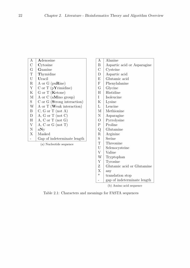
amino acid sequences, shown in Table 2.1. Of these we will only use the 5 basic characters
for nucleotide sequences: A, C, G, T and N. The table is included for completeness and
the additional characters is not used in this project or the experimental datasets.
An example of this file format is presented here, from the SANBI10000 dataset:
>T30671 g612769 | T30671 CLONE_LIB: Human Eye. LEN: 319 b.p. FILE
gbest3.seq 5-PRIME DEFN: EST20487 Homo sapiens cDNA 5’ end
ATGATAATGAAAGACTCTCGAAAGTTGAAAAAGCTAGACAGCTAAGAGAACAAGTGAATG
ACCTCTTTAGTCGGAAATTTGGTGAAGCTATTGGTATGGGTTTTCCTGTGAAAGTTCCCT
ACAGGAAAATCACAATTAACCCTGGCTGTNTGGTGGTTGATGGCATGCCCCCGGGGGTGT
CCTTCAAAGCCCCCAGCTACCTGGAAATCAGCTCCATGAGAAGGATCTTAGACTCTGCCG
AGTTTATCAAATTCACGGTCATTAGACCATTTCCAGGACTTGTGAATTAANAACCAGCTG
GTTGATCAGAGTGAGTCAG
This entry begins with a header, identified by the starting > character. The header
includes information such as its unique code, its source, clone data and other annotation.
Following this header is the actual sequence. When encoding nucleotide data this is
usually the 4 base characters, A, C, G and T, as well as the character N, which represents
an unknown base.
2.5.2 Compression
The disadvantage of the above FASTA data format is that it is not very memory efficient.
To improve on this and store the sequences in memory using less memory, compression
can be used.
In contrast to ASCII, which has character mappings for all 256 possibilities of a 8-bit
byte, nucleotide sequences only have an alphabet of 5 characters(A, C, G, T, N). Since
not all 8-bits of a byte is needed to represent a nucleotide, the data can be compressed by
22 Chapter 2. Literature - Bioinformatics Theory and Algorithm Overview
A AdenosineC CytosineG GuanineT ThymidineU UracilR A or G (puRine)Y C or T (pYrimidine)K G or T (Ketone)M A or C (aMino group)S C or G (Strong interaction)W A or T (Weak interaction)B C, G or T (not A)D A, G or T (not C)H A, C or T (not G)V A, C or G (not T)N aNyX Masked- Gap of indeterminate length
(a) Nucleotide sequence
A AlanineB Aspartic acid or AsparagineC CysteineD Aspartic acidE Glutamic acidF PhenylalanineG GlycineH HistidineI IsoleucineK LysineL LeucineM MethionineN AsparagineO PyrrolysineP ProlineQ GlutamineR ArginineS SerineT ThreonineU SelenocysteineV ValineW TryptophanY TyrosineZ Glutamic acid or GlutamineX any* translation stop- gap of indeterminate length
(b) Amino acid sequence
Table 2.1: Characters and meanings for FASTA sequences
2.6. Algorithm Types Overview 23
having a single byte represent multiple nucleotides, a technique called data packing. Com-
pression has an advantage in reducing the memory footprint of an application, and in the
case of GPGPU might present speed advantages due to less data having to be transferred
to and from GPU and host memory. Compression though increases the computational
complexity of an algorithm, so choosing the right compression is often a speed/memory
tradeoff. Two compression schemes are given below:
4-bit Compression
This compression is achieved by assigning every nucleotide its own bit. While it does not
have as good compression as a 2-bit compression scheme, it does have a speed advantage in
that comparisons are quick bit operations. Individual nucleotides are represented by mak-
ing the bit that they represent 1 and all other bits 0, while the N character, representing
a match for any nucleotide, is indicated by making all 4 bits 1.
This scheme allows 2 nucleotides to be packed into a single byte, potentially halving
the amount of memory needed for the application without requiring a computationally
expensive decompression algorithm.
2-bit Compression
The 5th character, N, referring to a wildcard that can match to any of the other 4, can be
removed by assigning it a random nucleotide. The resulting 4 character alphabet can be
represented in 2 bits, allowing 4 nucleotides to be stored in a single byte. This is the best
practical compression available, though it does increase the computational complexity of
decompression somewhat.
2.6 Algorithm Types Overview
This section details the various classes of algorithms of concern to this research. In
Chapter 5 specific examples will be given and considered.
2.6.1 Distance Based Algorithms
Distance based algorithms is the term used to refer to algorithms that compares two
sequences pairwise, then provides a single value as an output that represents how similar
the two sequences are.
24 Chapter 2. Literature - Bioinformatics Theory and Algorithm Overview
These sequences can be of any length and might only have a small subsection in
common with one another. It is considered advantageous if the algorithm scores match-
ing continuous regions more than two sequences with shorter matching regions spread
throughout.
2.6.2 Alignment Algorithms
Alignment algorithms have a lot in common with Distance algorithms. In a nutshell
the goal of alignment algorithms is to add insertions, deletions and substitutions to the
two sequences in an attempt to minimize their distances. This alignment provides a
visual representation of the similarity between two sequences and is an important tool in
bioinformatics.
Alignment algorithms are usually much more expensive than simple distance algo-
rithms due to the more information it presents, but there has been work done to properly
parallelize this class of algorithms which makes it interesting in this study.
While alignment is not expressly used in EST Clustering, the algorithms and de-
velopments in alignment can potentially be used to provide a higher quality distance
measurement.
As an example of alignment, consider the following two sequences:
Sequence 1: GATTCGTTA
Sequence 2: GGATCGTA
If these sequences are pairwise aligned to result in the minimum distance it would look
like the following:
Sequence 1: -GATTCGTTA
Sequence 2: GGAT-CGT-A
where the ’-’ character represents gaps and the bolded characters are characters that
match in both sequences.
In addition to providing an optimal alignment, alignment algorithms often also provide
a distance measurement of this final alignment.
The simplest metric for distance between two aligned sequences is called the Leven-
shtein edit distance. Using this metric every ’error’, whether it is an insertion, deletion
or substitution increases the score by 1. The goal is the minimize this distance.
For the two example aligned sequences above, their Levenshtein edit distance would
be 3.
2.7. Conclusion 25
2.6.3 Database Algorithms
Database algorithms are algorithms that instead of processing a multitude of short se-
quences pairwise to each other, instead compare a single sequence against either one large
sequence (a gene against an entire genome of a creature), or a single sequence against a
preprocessed database of sequences.
These algorithms are usually characterised by the introduction of database indices or
by representing the sequences as a fingerprint rather than the raw sequence to facilitate
faster searches.
Database algorithms usually involve an expensive preprocessing stage which provides
an output which can be reused multiple times and a quick search and comparison.
2.6.4 Heuristics
Heuristics can be any class of algorithm that provides much faster comparison than other
algorithms in its class, usually by optimizations that greatly reduce accuracy. Due to this
loss of accuracy their output is usually characterised by a binary pass or fail result and
is rarely used alone, with the failing comparisons rejected as potential matches and the
pass matches passed on to other algorithms for more exhaustive comparison.
The best heuristics are typically the ones which have a low false positive rate, thus
rejecting the fewest actually similar pairs, and a high true negative rate, rejecting a large
number of unrelated sequence pairs.
Heuristics serve as a valuable component of an EST clustering program due to mas-
sively decreasing the expensive number of computations needed for larger datasets.
2.7 Conclusion
In this chapter a basic primer to bioinformatics in general and EST clustering in specific
is provided. Basic terms used throughout this document is given and the basic classes of
algorithms that will be considered are explained.
This chapter also includes a short history of relevant bioinformatics algorithms and
a description of how modern GPGPU advances have been introduced and changed the
field.
This chapter is meant to provide basic groundwork of understanding for engineers
who are not familiar with bioinformatics and biology. These descriptions and theory are
not meant to be comprehensive since that would be outside the scope of this document.

26 Chapter 2. Literature - Bioinformatics Theory and Algorithm Overview
Since the information provided is only applicable to this project, it is advised that fur-
ther research be done on the subjects introduced rather than using this document as a
comprehensive authority on the subject of bioinformatics.
The next chapter provides a groundwork to the GPGPU field, introducing both con-
cepts and information on GPU’s requirements and limitations when applied to the bioin-
formatics field.
Chapter 3
Theory - GPU Theory Study
3.1 Introduction
In this chapter a brief introduction to the state of GPGPU (General Purpose Graphics
Processing Units) is provided, providing context for the selection of CUDA as the API
(Application Programming Interface) of choice for this project.
The theory of the different ways in which GPUs can provide parallelism to an appli-
cation is explored and the capabilities and limits of different generation NVidia GPUs is
provided.
3.2 GPU Introduction
A rapidly advancing technology within IT has been computer graphics. Constant de-
mand of higher quality, better and more flexible processing and a large market for GPUs
(Graphics Processing Units) has resulted in GPUs computing ability advancing faster
than that of classical CPUs (Central Processing Units). While CPUs have been steadily
keeping to Moore’s Law (stating that the amount of transistors that can be placed on an
integrated circuit roughly doubles every two years [3]), GPUs have been outpacing this
law [99].
The GPUs’ advantage over CPUs are their specialized design using massive multi-
threading to utilize a large number of cores and hide global memory latency [5]. While it
is commonplace for commercial CPUs at the time of writing to reach six cores, the newly
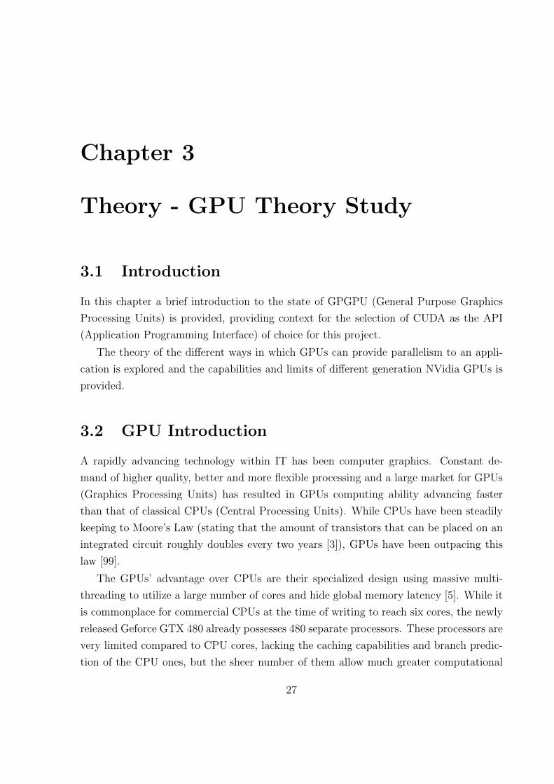
released Geforce GTX 480 already possesses 480 separate processors. These processors are
very limited compared to CPU cores, lacking the caching capabilities and branch predic-
tion of the CPU ones, but the sheer number of them allow much greater computational
27
28 Chapter 3. Theory - GPU Theory Study
Figure 3.1: The GPU devotes more transistors to data processing [2]
throughput. Market demands have also resulted in GPUs becoming more flexible and
improved programmability.
GPUs are capable of operating on large amounts of data simultaneously, equivalent to
a thread per datum on the CPU. This design makes it a good platform for parrelizable
algorithms, but the requirement that there is a minimum amount of inter-thread commu-
nication and the undefined order of completion of these threads makes GPUs unsuitable
for many complex and serial algorithms [5].
The field of GPGPU is the domain where these more flexible GPUs are applied to
non-graphics related problems. It started with the introduction of programmable shaders,
where these non-graphics problems were represented as graphics elements such as pixels,
vertices and textures. Though the theoretical and practical performance gain was great,
the format the data and the problem had to be presented in, as well as the required
expertise of the implementer, limited the number of problems the GPU could easily be
used to solve [100].
Languages and APIs are designed to apply the GPU to problems without first having to
format the non-graphics problem in a graphics format, has mitigated these disadvantages
in recent years. It is true however that best performance is reached when the problems
most closely resemble graphics problems.
Early APIs such as BrookGPU [72, 73] or Sh (later Rapidmind) [74, 73], though
instumental in the early shaping of the GPGPU field, does not enjoy the widespread
GPU Vendor support that later APIs do.
3.3. General Theory 29
Among the modern and widely supported APIs are CUDA (Compute Unified Device
Architecture), developed by NVidia for its range of commercial GPUs and publically
released in 2004, OpenCL, developed initially by Apple Inc. in 2008 but supported by a
wide range of hardware vendors and DirectCompute, an API developed by Microsoft as
part of its DirectX11 API released in 2009.
Of these well-supported APIs, both OpenCL and DirectCompute are recent inno-
vations. DirectCompute is available only to the Windows platform, which makes it
unsuitable for Linux or Unix-based operating systems which are common in research.
OpenCL has not yet been properly implemented across all platforms and suffers from
performance problems [96], though these concerns are expected to be eliminated with
time. For this project I have decided to use CUDA as my API of choice due to its
maturity and widespread use in existing bioinformatics research.
CUDA is based on the C programming language [2]. It extends the language with new
keywords, but otherwise should be familiar to anyone who has programmed in C before.
It is important to note that when programming in any GPGPU API that a distinction
must be made between the host (CPU side) and GPU side, since they have non-shared
memory and different functions may execute on either one. It becomes even more complex
in multi-GPU situations where each GPU is explicitly managed.
3.3 General Theory
Attempting to use the GPU as a CPU (single pieces of data processed, one after another)
will leave the GPU severely underutilized and will result in sub-optimal performance [2].
In order to fully utilize the GPU, the data to be processed must be sufficiently large
and capable of being processed in parallel. There is a non-trivial overhead for copying
data to and from GPU memory, but when dealing with streaming data this can be easily
hidden by concurrently processing data already on the GPU and copying over the next
set of data simultaneously [100].
Of note is the lack of memory on the GPU. Host-side CPU computation can make
use of 64-bit addressable RAM, potentially up to 8TB worth and can page memory
to disk, using hard drive space as temporary storage. The GPU has far more modest
memory amounts, from under a gigabyte for most commercial GPUs up to 4GB on some
professional hardware models available to date(2010). This is not an issue for small
problems where the entire dataset can fit into a few hundred megabytes, but realistic
applications can utilize datasets of sizes measured in terabytes or even petabytes. In
30 Chapter 3. Theory - GPU Theory Study
addition GPUs host several different types of memory, each requiring proper management
in order to fully optimize performance. For this, data streaming and explicit memory
management is essential to performance in applications utilizing large data sources.
A noted disadvantage of GPUs compared to CPUs is the fact that GPUs are stream-
lined for 32-bit floating point numbers, not integers or 64-bit floating point numbers.
While 64-bit applications are supported on modern GPUs, computation will suffer re-
duced performance.
3.4 CUDA API
3.4.1 Introduction to the CUDA API
CUDA is a GPU API developed by NVidia Corporation that allows developers low level
programming ability on NVidia GPUs by programming in ‘C for CUDA’, which is the
standard C programming language with a number of extensions and restrictions [2].
This allows developers to use the computational ability of NVidia GPUs without
having to refactor the logic and data in a format that suits the graphics pipeline, widely
increasing the potential applications of GPU hardware.
Since February 2007 when the first CUDA SDK was made public, various language
bindings and wrappers for a wide variety of programming languages have been devel-
oped, including Fortran, Java and Python. For this implementation though we will limit
ourselves to ‘C for CUDA’ and C++.
CUDA also provides various libraries built on top of CUDA to provide specialized
high performance mathematical functions: CUFFT [101] provides high performance Fast
Fourier Transforms, CUBLAS [102] is a library for linear algebra functions, CUSPARSE
[103] is a library containing functions for handling sparse matrices and CURAND [104] fo-
cusses on the generation of high quality pseudorandom numbers. None of these additional
libraries will be used in this project however.
3.4.2 CUDA Compute Capabilities
The CUDA Programming Guide [2] provides table 3.1, the technical specifications of the
various CUDA capable GPUs available at the moment.
In addition to improving specifications, newer CUDA compute capability GPUs also
provide additional features not available in previous versions. For example, compute
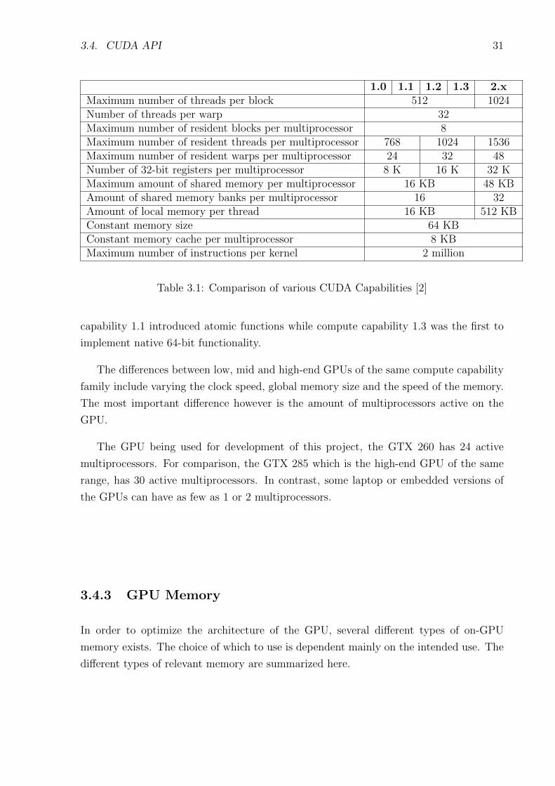
3.4. CUDA API 31
1.0 1.1 1.2 1.3 2.xMaximum number of threads per block 512 1024Number of threads per warp 32Maximum number of resident blocks per multiprocessor 8Maximum number of resident threads per multiprocessor 768 1024 1536Maximum number of resident warps per multiprocessor 24 32 48Number of 32-bit registers per multiprocessor 8 K 16 K 32 KMaximum amount of shared memory per multiprocessor 16 KB 48 KBAmount of shared memory banks per multiprocessor 16 32Amount of local memory per thread 16 KB 512 KBConstant memory size 64 KBConstant memory cache per multiprocessor 8 KBMaximum number of instructions per kernel 2 million
Table 3.1: Comparison of various CUDA Capabilities [2]
capability 1.1 introduced atomic functions while compute capability 1.3 was the first to
implement native 64-bit functionality.
The differences between low, mid and high-end GPUs of the same compute capability
family include varying the clock speed, global memory size and the speed of the memory.
The most important difference however is the amount of multiprocessors active on the
GPU.
The GPU being used for development of this project, the GTX 260 has 24 active
multiprocessors. For comparison, the GTX 285 which is the high-end GPU of the same
range, has 30 active multiprocessors. In contrast, some laptop or embedded versions of
the GPUs can have as few as 1 or 2 multiprocessors.
3.4.3 GPU Memory
In order to optimize the architecture of the GPU, several different types of on-GPU
memory exists. The choice of which to use is dependent mainly on the intended use. The
different types of relevant memory are summarized here.
32 Chapter 3. Theory - GPU Theory Study
Figure 3.2: CUDA Memory Model [2]
Type Speed Size Access Cached Scope
Registers Very Fast Very Limited Read/Write No Thread
Local Memory Very Slow Limited Read/Write No Thread
Shared Memory Fast Limited Read/Write No Block
Constant Memory Very Fast Limited Read Yes Global
Global Memory Very Slow Large Read/Write No Global
Texture Memory Slow Large Read/Write Yes Global
Table 3.2: Summary of Memory Types available to CUDA Programmers
Unlike CPUs, CUDA capable GPUs do not rely on cache to obtain their high per-
formance. Instead of relying on increasing the response time of memory reads through
expensive cache optimization, GPUs instead focus on high throughput. Though this re-
sults in slow and unresponsive memory access, larger reads performed by multiple blocks
and threads concurrently can allow a huge amount of data to be read and processed at
the same time.
3.4. CUDA API 33
Global memory reads can take up to hundreds of cycles, so proper use of the different
types of memory is needed for optimal performance of a CUDA application.
Registers
The fastest memory available to a kernel, but also the most limited in size. Every block
has a limited number of registers (32K 32-bit registers on a 2.x compute capability GPU)
that is divided between all active threads on a block. Blocks with fewer threads will
provide more registers per thread, but might suffer performance issues due to the reduced
parallelism employed.
Every variable created in a kernel is a register and it is important to learn to find
ways to minimize the number of registers an application uses to maximize the number of
concurrent threads allowed on a block.
When optimizing a kernel it is important to test the effects your choice of registers has
and whether to offload some to shared memory or even to use registers instead of shared
memory in other cases.
Shared memory
Shared memory is a section of on-multiprocessor temporary memory that is shared among
all threads within a warp. This shared memory is much faster than global memory though
slower than registers and can be used for temporary storage of data during computation.
Since even 2.x Compute Capability GPUs have only 48 KB to work with (16 KB for
earlier GPUs), this memory space needs to be well managed.
In addition all data of all threads within a block are accessible to one another. This
means that shared memory can be used as a form of inter-thread communication and
data sharing. This property of shared memory allows many algorithms to utilize gather
and scatter operations.
Though fast, shared memory accesses should still be designed to avoid bank conflicts
where multiple threads attempt to access the same section of memory. In worst case
scenario this can lead to a 16× degradation in shared memory performance if these accesses
have to be serialized for each thread instead of occurring simultaneously. More information
on bank conflicts can be found in the CUDA programming manual [2].
34 Chapter 3. Theory - GPU Theory Study
Global memory
Global memory is the main GPU memory with the largest size but also slowest access
times. This is most likely where the input data your kernel will use will be stored and
where the results of your computation will be written, so proper management of global
memory is important for optimal performance. The global memory capacity of individual
GPUs vary, usually between 256 MB to 4 GB, but is usually shown on its packaging.
When accessing global memory, the accessing threads are blocked, allowing non-
waiting threads access to the GPU multiprocessor. When the memory access is completed
these threads are unblocked and allowed to continue processing. If enough threads with
enough workload is provided then memory access latency can be completely hidden.
Since the memory latency can be hidden, memory throughput becomes much more
important and can be improved through a method known as coalescing. If a half-warp
of threads (16 sequential threads) all access sequential 64 or 128 bytes of memory then
the memory accesses can be combined into a single transaction [2]. Uncoalesced random
reads can be many times slower since several 64 bytes reads will need to be queued one
after another which severely limits the ability for the GPU to hide memory latency.
Local Memory
In memory diagrams, local memory is often indicated as being close to individual threads.
This indicates simply that local memory is private to that thread and cannot be accessed
by any other thread. In regards to performance local memory is about equal to that of
global memory since in reality local memory is simply an abstraction of global memory.
Local memory is automatically allocated by the compiler if the registers available to
the kernel is not enough. This automatic assignment is often one of the reasons for sub-par
performance and should be minimized whenever possible.
Local memory use should be minimized by algorithm improvements that reduce the
number of registers needed in the kernel or by using shared memory to store data instead
of registers.
Texture memory
Texture memory is usually used to store textures, large images that GPUs render with.
This is stored on global memory, but by marking the memory as read-only texture memory
allows various features to become available.
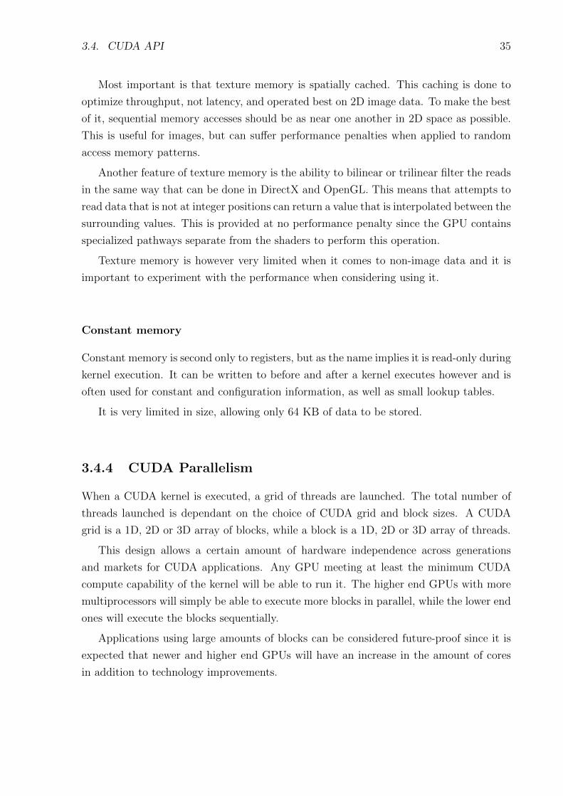
3.4. CUDA API 35
Most important is that texture memory is spatially cached. This caching is done to
optimize throughput, not latency, and operated best on 2D image data. To make the best
of it, sequential memory accesses should be as near one another in 2D space as possible.
This is useful for images, but can suffer performance penalties when applied to random
access memory patterns.
Another feature of texture memory is the ability to bilinear or trilinear filter the reads
in the same way that can be done in DirectX and OpenGL. This means that attempts to
read data that is not at integer positions can return a value that is interpolated between the
surrounding values. This is provided at no performance penalty since the GPU contains
specialized pathways separate from the shaders to perform this operation.
Texture memory is however very limited when it comes to non-image data and it is
important to experiment with the performance when considering using it.
Constant memory
Constant memory is second only to registers, but as the name implies it is read-only during
kernel execution. It can be written to before and after a kernel executes however and is
often used for constant and configuration information, as well as small lookup tables.
It is very limited in size, allowing only 64 KB of data to be stored.
3.4.4 CUDA Parallelism
When a CUDA kernel is executed, a grid of threads are launched. The total number of
threads launched is dependant on the choice of CUDA grid and block sizes. A CUDA
grid is a 1D, 2D or 3D array of blocks, while a block is a 1D, 2D or 3D array of threads.
This design allows a certain amount of hardware independence across generations
and markets for CUDA applications. Any GPU meeting at least the minimum CUDA
compute capability of the kernel will be able to run it. The higher end GPUs with more
multiprocessors will simply be able to execute more blocks in parallel, while the lower end
ones will execute the blocks sequentially.
Applications using large amounts of blocks can be considered future-proof since it is
expected that newer and higher end GPUs will have an increase in the amount of cores
in addition to technology improvements.
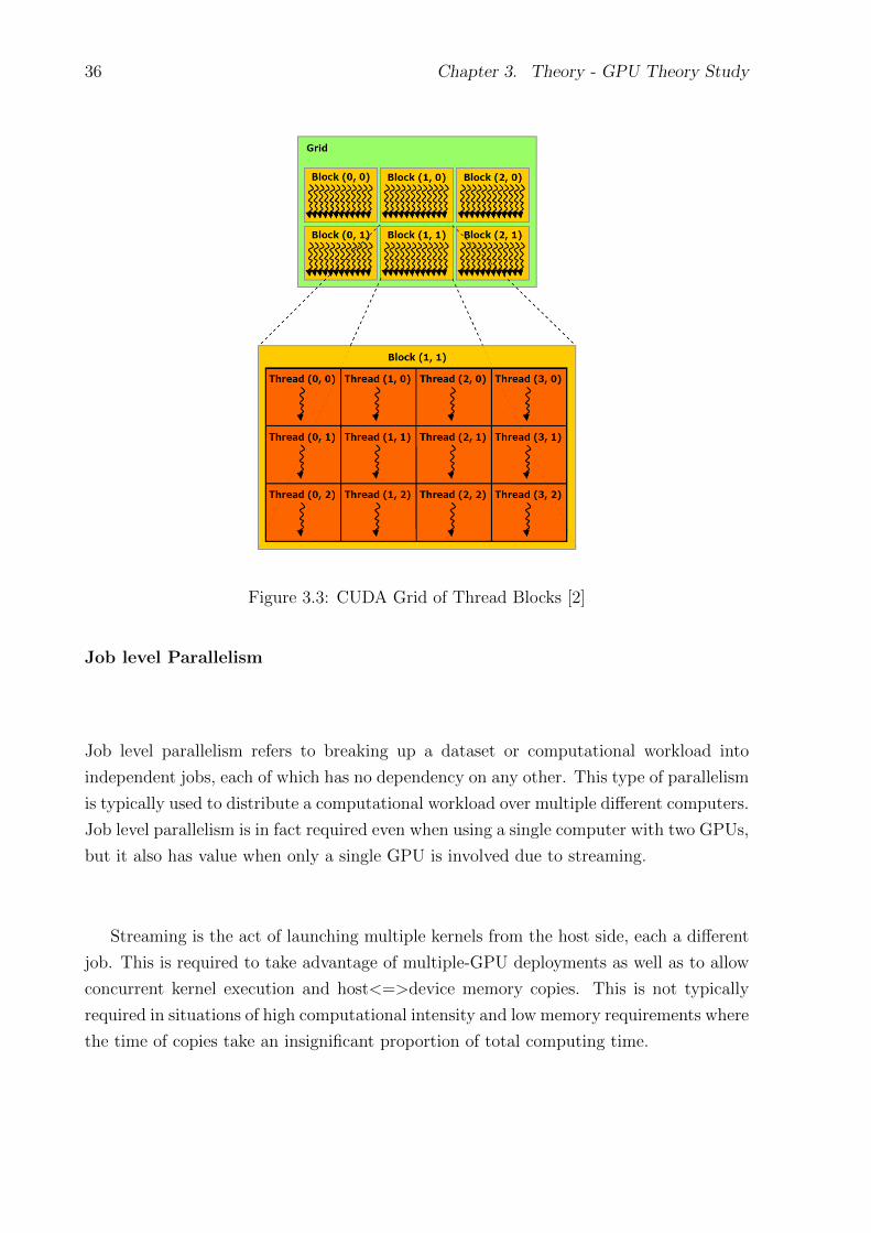
36 Chapter 3. Theory - GPU Theory Study
Figure 3.3: CUDA Grid of Thread Blocks [2]
Job level Parallelism
Job level parallelism refers to breaking up a dataset or computational workload into
independent jobs, each of which has no dependency on any other. This type of parallelism
is typically used to distribute a computational workload over multiple different computers.
Job level parallelism is in fact required even when using a single computer with two GPUs,
but it also has value when only a single GPU is involved due to streaming.
Streaming is the act of launching multiple kernels from the host side, each a different
job. This is required to take advantage of multiple-GPU deployments as well as to allow
concurrent kernel execution and host<=>device memory copies. This is not typically
required in situations of high computational intensity and low memory requirements where
the time of copies take an insignificant proportion of total computing time.
3.4. CUDA API 37
Block level Parallelism
Block level Parallelism is the scalable method used by CUDA to distribute the workload
across multiple independent multi-processors, regardless of the number of actual multi-
processors on the GPU. There is little communication between blocks and the blocks
can be executed in any order. This necessitates that no block has data dependencies
on any other block. Block level parallelism thus shares much of the same requirements
and limitations of job level parallelism, differing only in the fact that blocks are launches
simultaneously on the same GPU on a single GPU. If some sort of synchronization is
needed, multiple kernel calls are advised.
Figure 3.4: CUDA Block Scheduling [2]
The size of the grid, i.e. the total number of blocks launched by the kernel is not
a critical variable for performance beyond the requirement that enough blocks need to
be launched at once so that every multiprocessor has several blocks queued at once,
preventing under-utilization of the GPU. Attempts to experiment with block sizes has
shown a small performance increase if the number of blocks is a multiple of the amount
of multiprocessors, but the effect was relatively minor.
If the algorithm is not reliant on a set number of blocks, the grid size could be tailored
at runtime to a multiple of the number of multiprocessors reported by the GPU. If all
blocks take equal time to complete, this will allow for the most efficient allocation of
resources to the problem.
38 Chapter 3. Theory - GPU Theory Study
Thread Level Parallelism
Unlike blocks, threads do have the ability to synchronize and communicate between them-
selves. Though not necessary to use, threads have shared memory that is available and
readable by all threads in a block. This shared memory can be used as a user-managed
cache, shared data for inter-thread communication as well as individual temporary stor-
age. All threads are executed in warps, a group of 32 threads that proceed in lock-step
with each other. This lock-step behaviour makes branches that diverge within a warp
expensive [105].
The number of threads in a block is even more of a critical variable for maximum
throughput than the choice of grid size. Threads are executed in warps of size 32, so
selecting a thread size that is not a multiple of 32 is strongly discouraged.
When selecting a block size, it is important to maximize what is called occupancy.
Occupancy is the percentage of cores active per multiprocessor. Though each multipro-
cessor only executes one warp at a time, it is capable of storing multiple warps, called
resident warps, at once.
Instructions such as loading from global or shared memory can take many cycles to
complete. Since shared and global reads are not cached, every thread needs to wait
the full amount of time to load data from memory. Instead of implementing caching to
combat this effect, GPUs simply switch to another warp when such blocking operations are
reached and continues execution while the blocked warp finishes its memory read. In this
way memory latencies can be hidden with concurrent execution, rather than eliminated.
Texture memory is the one form of global memory that is cached, but in keeping with this
model, it is cached to reduce memory bandwidth usage rather than latency. A cached
texture memory read has the same latency as an uncached read.
By making sure the occupancy is as high as possible, the GPU is given many more
warps to switch to while others are busy, reducing any downtime where there is no available
warps available to execute.
Table 3.3 and Table 3.4 shows how the choice of threads per block can affect the
maximum possible occupancy and the availability of resurces such as shared memory and
registers for different generations of GPU.
Important to note is the fact that total register count and total shared memory are
limited per multiprocessor. If a kernel uses more than the maximum available, less blocks
will be resident than otherwise for this kernel, resulting in reduced occupancy.
Even with full occupancy the memory accesses of some very memory heavy kernels
might still not be sufficiently hidden. In other cases where the kernel is more computa-
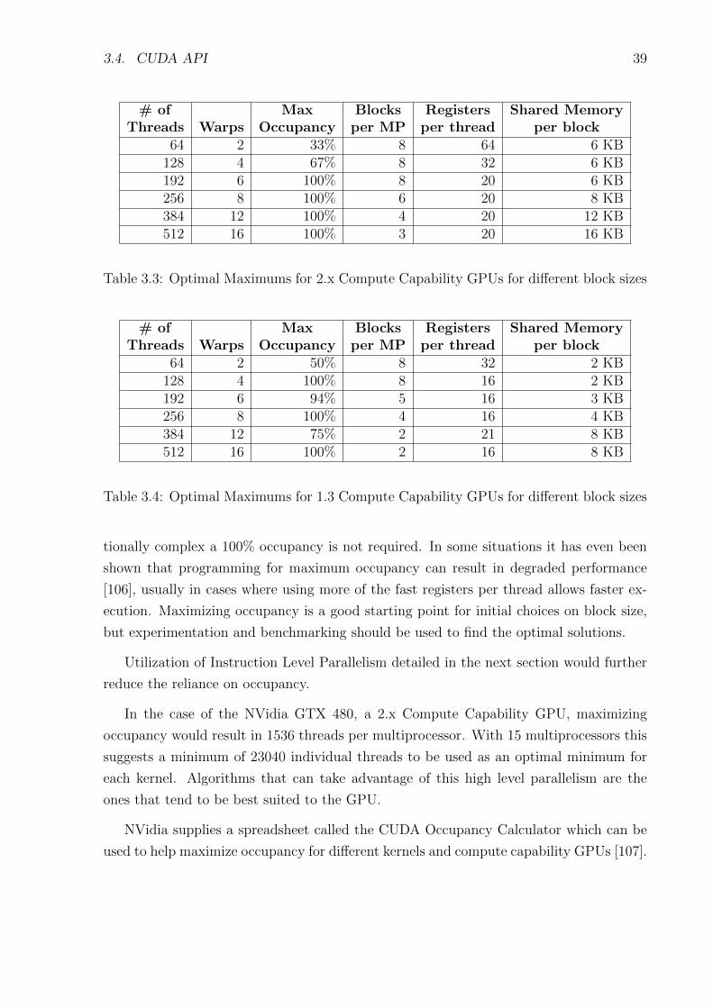
3.4. CUDA API 39
# of Max Blocks Registers Shared MemoryThreads Warps Occupancy per MP per thread per block
64 2 33% 8 64 6 KB128 4 67% 8 32 6 KB192 6 100% 8 20 6 KB256 8 100% 6 20 8 KB384 12 100% 4 20 12 KB512 16 100% 3 20 16 KB
Table 3.3: Optimal Maximums for 2.x Compute Capability GPUs for different block sizes
# of Max Blocks Registers Shared MemoryThreads Warps Occupancy per MP per thread per block
64 2 50% 8 32 2 KB128 4 100% 8 16 2 KB192 6 94% 5 16 3 KB256 8 100% 4 16 4 KB384 12 75% 2 21 8 KB512 16 100% 2 16 8 KB
Table 3.4: Optimal Maximums for 1.3 Compute Capability GPUs for different block sizes
tionally complex a 100% occupancy is not required. In some situations it has even been
shown that programming for maximum occupancy can result in degraded performance
[106], usually in cases where using more of the fast registers per thread allows faster ex-
ecution. Maximizing occupancy is a good starting point for initial choices on block size,
but experimentation and benchmarking should be used to find the optimal solutions.
Utilization of Instruction Level Parallelism detailed in the next section would further
reduce the reliance on occupancy.
In the case of the NVidia GTX 480, a 2.x Compute Capability GPU, maximizing
occupancy would result in 1536 threads per multiprocessor. With 15 multiprocessors this
suggests a minimum of 23040 individual threads to be used as an optimal minimum for
each kernel. Algorithms that can take advantage of this high level parallelism are the
ones that tend to be best suited to the GPU.
NVidia supplies a spreadsheet called the CUDA Occupancy Calculator which can be
used to help maximize occupancy for different kernels and compute capability GPUs [107].
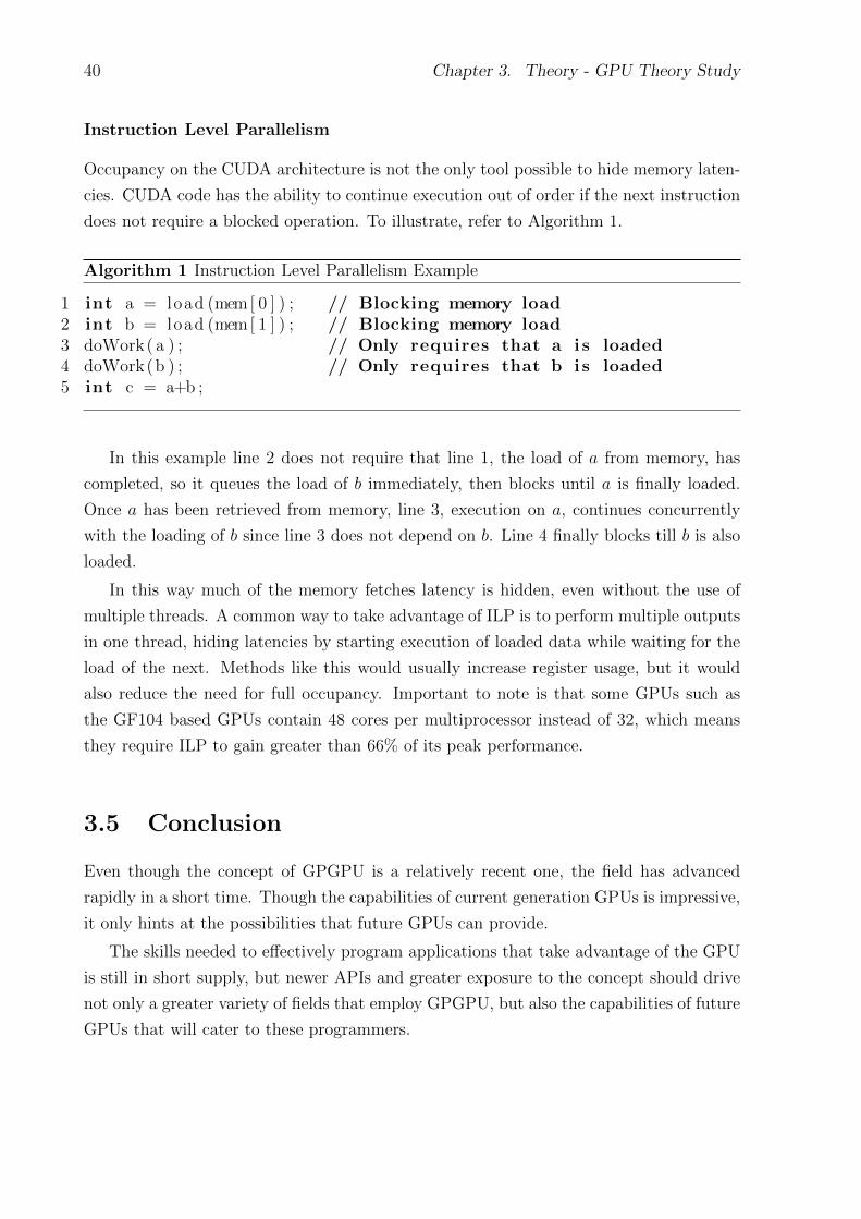
40 Chapter 3. Theory - GPU Theory Study
Instruction Level Parallelism
Occupancy on the CUDA architecture is not the only tool possible to hide memory laten-
cies. CUDA code has the ability to continue execution out of order if the next instruction
does not require a blocked operation. To illustrate, refer to Algorithm 1.
Algorithm 1 Instruction Level Parallelism Example
1 int a = load (mem[ 0 ] ) ; // Blocking memory load2 int b = load (mem[ 1 ] ) ; // Blocking memory load3 doWork( a ) ; // Only requires that a i s loaded4 doWork(b ) ; // Only requires that b i s loaded5 int c = a+b ;
In this example line 2 does not require that line 1, the load of a from memory, has
completed, so it queues the load of b immediately, then blocks until a is finally loaded.
Once a has been retrieved from memory, line 3, execution on a, continues concurrently
with the loading of b since line 3 does not depend on b. Line 4 finally blocks till b is also
loaded.
In this way much of the memory fetches latency is hidden, even without the use of
multiple threads. A common way to take advantage of ILP is to perform multiple outputs
in one thread, hiding latencies by starting execution of loaded data while waiting for the
load of the next. Methods like this would usually increase register usage, but it would
also reduce the need for full occupancy. Important to note is that some GPUs such as
the GF104 based GPUs contain 48 cores per multiprocessor instead of 32, which means
they require ILP to gain greater than 66% of its peak performance.
3.5 Conclusion
Even though the concept of GPGPU is a relatively recent one, the field has advanced
rapidly in a short time. Though the capabilities of current generation GPUs is impressive,
it only hints at the possibilities that future GPUs can provide.
The skills needed to effectively program applications that take advantage of the GPU
is still in short supply, but newer APIs and greater exposure to the concept should drive
not only a greater variety of fields that employ GPGPU, but also the capabilities of future
GPUs that will cater to these programmers.

3.5. Conclusion 41
In the next chapter, the experimentation design that will be used for the developed
application will be detailed, providing information on the metrics that is to be used and
the experiments that will be performed.

Chapter 4
Experimental Design
4.1 Introduction
“In theory, there is no difference between theory and practice. But, in practice, there is.”
– Yogi Berra
This thesis is concerned with the creation of a practical implementation of EST clus-
tering program utilizing the GPU. In order to gauge the success of such an attempt several
experiments are needed, identifying both the characteristics, strengths and weaknesses of
the created implementation as well as comparing this implementation to existing and
wide-spread used CPU implementations.
This chapter will describe experiments whose purpose is to measure and objectively
compare the performance of the algorithms that will be discussed and implemented in the
next chapters. It is important to plan the experiments in order to identify the criteria
necessary to be satisfied for any viable clustering algorithm.
This chapter will describe the terms and definitions of the various metrics that are
used for fair comparisons in these experiments. This includes not just performance mea-
surements, but also the correctness of the results and identifications of the shortcomings
of the chosen algorithms.
The chapter will begin with the listing of assumptions in the experiments due to the
non-conventional hardware platform used. Experimental concerns are listed as to provide
an introduction to the difficulty of a fair comparison across different hardware platforms.
The specifics of the experimental text platform is provided.
The theory and metrics section provides accurate definitions of the terms and measures
used in the experiments as well as indication of how experimental metrics are measured.
43
44 Chapter 4. Experimental Design
The experiments are listed. Each experiment will detail the aim of the experiment,
background information detailing its relevancy to the subject as a whole, as well as the
expected results from the experiment.
The final results provided by the experiments is provided in Chapter 7.
4.2 Assumptions and Experimental Framework
4.2.1 Common Assumptions
Scalability of CPU Cores
Modern CPU improvements have focussed largely on memory bandwidth optimizations
and increasing the number of cores, rather than increasing the speed of an individual
core. Testing of CPU implementations will for that reason only utilize a single core of
the CPU with the expectation that this will allow better comparison over a wider range
of hardware. This needs to be taken note of when making comparisons between the GPU
and CPU implementations, since in practice all the CPU cores will be used and their
running times will be much faster.
While a quad core CPU is unlikely to perform its computations in a quarter of the
time, they are expected to be faster by a significant factor. Comparisons between the
GPU, quad-core and dual-core setups should keep this in mind.
CPU speed has a negligible effect on GPU computation
One of the most significant assumptions in these experiments is that the CPU speed
performance has a negligible effect on the performance of GPU-only applications and
that only the GPU computational performance and memory access performance has an
effect on the final running times of the application.
For this reason only a single CPU core is sufficient to drive the application and theo-
retically should be enough to drive computation across multiple GPUs, though this ability
is not yet implemented.
Operating systems have a negligible effect on performance
Preliminary testing has also shown no difference between programs running on linux
versus programs running on windows if the hardware is identical. It is an assumption
that operating systems have little to no impact on performance.
4.2. Assumptions and Experimental Framework 45
4.2.2 Experimental Concerns
Fair Comparison
The goal of the experiment is to compare the created algorithm with those created by other
authors. Though speed and performance is the main considered attribute and advantages,
the many variations in clustering approaches all strive to solve different concerns and have
varying sensitivity to different experimental datasets.
In an attempt to be as fair as possible, many different datasets will be used in this
experiments, each different from differing sources and created by different sequencing
experiments.
While it is not possible to be exhaustive and be able to claim a single algorithm the
best at all possible datasets, testing with a large variety allows one to at least find the
most obvious strengths and shortcomings.
Sensitivity and Correctness
Some artificial datasets can provide a ‘correct’ reference clustering along with its data, but
this cannot be assumed for all datasets, especially not ones sequenced from real organisms.
In order to test datasets without provided reference clusterings, one is created from the
same dataset using a known high-quality algorithm that serves as a reference clustering.
It is important to note that the correct results where reference clusterings are not
provided are effectively unknown since varying quality of the ESTs have a great effect on
comparisons.
What is tested in this case is the similarity of the output between two algorithms,
not whether either output is correct. If the reference algorithm erroneously clusters two
sequences then the tested algorithm will in fact be penalized for a correct clustering.
This disadvantage is accepted however on the grounds that algorithms already ac-
cepted by the bioinformatics community would produce clusters of high enough quality
for professional use.
The developed algorithm is thus precluded from making any statements about the
correctness of its clustering, which is why the terms accuracy, similarity or sensitivity will
be used instead, denoting how well it matches the professional quality output from other
algorithms.
46 Chapter 4. Experimental Design
Differing Hardware
CPU and GPU technology is constantly improving, revealed by newer released GPU’s
greater performance and flexibility, but also by newer CPU’s increase in cores, speeds,
cache size and inter-core communication. Both platforms are moving towards greater
high performance computing capabilities and any experiments done in this project with
a specific generation of hardware is likely to be out of date before even the results are
released.
For this reason it is stressed that this experiment exists only as an indicator of future
direction and potential, and should not be used as an authoritative claim as to how specific
future generations of hardware will compare.
4.2.3 Experimental Setup
Test PC Platform
The computer that will be used to perform the experiments has the following specifica-
tions:
• CPU AMD Athlon(tm) 7750 2.7GHz Dual-Core Processor
• RAM 4GB DDR2-800 Memory
• Operating System Gentoo Linux
• GPU NVidia GTX480
In order to perform experimental repetition, a scripting language is needed to repeat-
edly execute the application on the same or differing datasets. The scripting language
PHP (PHP: Hypertext Preprocessor) was chosen for this task for no reason other than
author familiarity. Since it simply queues executions the choice of scripting language is
not expected to provide any detrimental or advantageous effect to the performance.
4.2.4 Theory and Metrics
Timing Methodology
In order to gain accurate performance results for comparison of gpucluster with other
tools, proper timing instuments are required. Two have been identified.
4.2. Assumptions and Experimental Framework 47
The first is the ‘time <command>’ command, available on all unix-based operating
systems and in MinGW on windows. This timer times execution to the returning of a
result, including the loading of libraries, loading the application to memory and clean-up
after the program has executed.
The chosen scripting language, PHP, contains the microtime() function, used to mea-
sure the performance results of repeated executions using the computer’s inbuilt high-
performance clock.
GFLOPS
Peak GFLOPS (Giga Floating Operations Per Second) is the theoretical maximum float-
ing point operations a computing device is possible.
Measured GFLOPS is a figure that is measured, typically via a loop computing a
large number of algorithmic operations in rapid succession with no memory access. These
measured figures offer a more realistic indication of what a computing device is capable
of, but can differ even between two devices of identical specifications.
While the measured GFLOPS is typically much lower than the peak GFLOPS, they
provide an indication of the performance of a device compared to another. Note though
that real-world performance is usually far more restrained by memory accesses and through-
put than GFLOPS.
Jaccard Index
In order to determine the accuracy of a clustering, a reference clustering is needed. This
reference clustering is created using an existing and proven cpu algorithm and is then
compared against the clustering created by GPU Cluster to provide a similarity score
that will be used to determine accuracy.
The metric chosen to compare the similarity of two different clusterings is the Jaccard
Index [108].
The Jaccard Index is a commonly used metric to compare sets or clusters and is the
ratio between the intersection and the union of two sets. It is defined as:
J(A,B) =|A
⋂B|
|A⋃B|
(4.1)
In order to apply this set theory to clustering, one has to consider a cluster as a set
48 Chapter 4. Experimental Design
of pairs. For example, for 4 possible elements, {1,2,3,4}, there exists two sets A and B:
A = {{1, 2, 3}, {4}}
B = {{1}, {2, 3, 4}}
these then need to be converted to unique pairs:
A = {{1, 2}, {2, 3}, {1, 3}}
B = {{2, 3}, {3, 4}, {2, 4}}
assuming clusterings A and B, this can then be implemented as:
J(A,B) =NAB
NAB +NA +NB
(4.2)
where
• NAB is the count of sequence pairs that are in both clustering A and B.
• NA is the count of sequence pairs that is in clustering A but not in clustering B.
• NB is the count of sequence pairs that is in clustering B but not in clustering A.
For the above example that would result in:
J(A,B) =NAB
NAB +NA +NB
=1
1 + 2 + 2
= 0.2
The Jaccard Index gives a value between 0.0 (none of the clusters overlap) and 1.0
(identical clusters).
Sensitivity Index
In the field of EST clustering, not clustering two related ESTs often have drastic effects in
the reassembly stage resulting in incorrectness or not combining two contigs that should
have been combined. On the other hand, clustering two unrelated ESTs have minimal
impact on the correctness of reassembly, only on the performance if there is an excessive
amount of over-clustering. This is because reassembly programs are already designed to
deal with chimeras and alternate splicing so they have the ability to deal with different
transcripts clustered together.
4.3. Dataset Descriptions 49
For this reason, an alternate index is also used in addition to the Jaccard Index, the
Sensitivity Index [59]. The benefit of this alternate Index is that it penalizes under-
clustering but not over-clustering, serving as a useful indicator of usefulness of the clus-
tering in terms of accuracy of final assembly, even if the exact clustering differs.
The Sensitivity Index is defined very similar to the Jaccard Index:
S(A,B) =NAB
NAB +NA
(4.3)
The sensitivity Index gives a value between 0.0 (clustering B contains none of clustering
A’s clusters) and 1.0 (clustering A is a subset of clustering B).
Due to its definition, the sensitivity will always be equal or greater than the Jaccard
Index.
While a high sensitivity is required for correct reassembly, a high sensitivity and a low
Jaccard Index is undesired due to the great performance deterioration that the reassembly
stage will experience.
Both the Jaccard Index and the Sensitivity Index will used to gauge accuracy.
CUDA Occupancy
Occupancy in terms of CUDA execution is a measure of the number of ’active’ CUDA cores
at any time [2]. While higher occupancy does not always indicate higher performance, it
does serve to assist in hiding of memory latencies in memory intensive applications.
Occupancy is discussed in more detail in Section 3.4.4, but in summary a larger oc-
cupation value results in less chance that multi-processors are left idle with all warps
blocking due to a pending memory read.
4.3 Dataset Descriptions
The following datasets were chosen mainly due to their availability and use in other
found benchmarks and comparisons. They consist of a wide range of differing species and
situations that should provide a fair test of the different datasets one should expect in
reality.
It is however only representative and not exhaustive, so datasets of unexpected length
or complexity might perform poorly compared to the datasets used in this experiment.
50 Chapter 4. Experimental Design
4.3.1 Arabidopsis
Arabidopsis is a popular and commonly used dataset to test and benchmark clustering
and assembly applications due to it being sourced from a well known and understood
model plant organism.
Two datasets are used from the ESTs downloaded from Genbank:
• A686904 - A dataset containing the full ESTs from Genbank; and
• A032 - A smaller random subset of the full dataset. It has the same number of
cDNA sources as the full dataset, but its coverage will be lower due to having much
less sequences.
4.3.2 SANBI 10000
This is a benchmark dataset popularised and provided by the South African Bioinformat-
ics Institute. The SANBI 10000 dataset contains 10k sequences and is provided so that
applications can perform comparative benchmarks.
4.3.3 Public Cotton
This is a set of Sanger-style ESTs from the public cotton data set.
4.3.4 C-Series
The C-Series is an artificial dataset created using ESTsim. As opposed to the A032
dataset, the C-series varies the cDNA sources with the size of the dataset, allowing the
same coverage of different amount of clusters with increasing or decreasing dataset size.
The C10 dataset is a full-size dataset, with C01 being 10% its size, the C02 being 20%
its size, and so on.
4.3.5 Mouse Curated
This is a curated dataset that was created from a limited selection of genes chosen from
chromosone 4 of the mouse. As a curated dataset, any clusterings derived from it should
contain few large clusters with very few orphaned ESTs.
4.4. Overview of Experiments 51
4.4 Overview of Experiments
This study will consist of 5 experiments. The first experiment will deal with purely theo-
retical performance while the second will gauge the practical sensitivity of the algorithm.
The rest of the experiments will deal with practical performance measurements of the
algorithm in question.
The following list provides a brief summary of the experiments:
1. Theoretical Performance and Cost Evaluation This experiment deals with
the comparison of theoretical ‘Peak GFLOPS’ between modern GPU and CPUs.
2. Sensitivity Comparison This experiment measures the sensitivity of the devel-
oped application in comparison to a known good benchmark.
3. Performance Benchmarking This experiment measures performance of the de-
veloped algorithm results for different datasets and compares against the perfor-
mance of a CPU implementation.
4. Dataset scaling tests This experiment tests the performance of the algorithm
when the dataset size is varied.
5. Profiling Analysis This experiment subjects the algorithm to a dynamic profiling
analysis in order to identify its inefficiencies and computational bottlenecks.
4.5 Investigation 1: Theoretical Performance and
Cost Evaluation
4.5.1 Aim
The aim of this experiment is to calculate and compare a theoretical FLOPS per rand
investment between GPU and classical computing.
4.5.2 Background
One of the main reasons for this project is due to the perceived cost savings of GPU hard-
ware compared to similar performing PC or server hardware. While a FLOPS measure-
ment is not guaranteed evidence of performance, this figure does serve as a performance
indicator.
52 Chapter 4. Experimental Design
4.5.3 Method
Various computing options will be found including GPU, personal computing solutions,
server solutions and large data server solutions. The ratio between their price and their
peak FLOPS will be compared.
Peak FLOPS is defined as the clock rate multiplied by the number of cores multiplied
by the number of floating point operations each core can theoretically perform every clock
cycle.
4.5.4 Expected Outcome
It is expected that GPU hardware will be shown to theoretically provide more performance
for the same price than classical computing alternatives.
It is not expected that this will reflect real-life performance, but it will indicate the
reason why GPUs are used in this project. Experiment 2 will show whether this translates
into real-world performance advantages.
4.6 Experiment 1: Sensitivity Comparison
4.6.1 Aim
In order to prove that sensitivity and accuracy is not lost with the transfer to new hardware
and algorithms, a test is needed to validate that the results given are of good quality when
compared to other tools.
4.6.2 Background
While a fully ‘correct’ clustering cannot be determined due to interdependancy between
the algorithms and the generation of the reference cluster, algorithms that are well-
documented to provide quality results can provide the reference that the developed algo-
rithm can be compared against.
Not all datasets are supplied with a reference clustering, so a comparison between
gpucluster and a known high quality algorithm is used instead. The wcdest tool is chosen
for this purpose.
4.7. Experiment 2: Performance Benchmarking 53
4.6.3 Method
1. A dataset is chosen and used as an input to wcdest to create the reference clustering.
2. The same dataset is used as an input to gpucluster to create the experimental
clustering.
3. The reference and experimental datasets are compared and the Jaccard and Sensi-
tivity Indexes are computed.
4. Steps 1-3 are repeated for all datasets.
5. Results are reported and tabulated.
4.6.4 Expected Outcome
While JI and SE scores of 1.00 are not expected due to the differences in distance algo-
rithms, it is still expected that gpucluster will show high sensitivity.
Gpucluster is expected to achieve senstivity and Jaccard scores of above 0.95. Any
values lower than this suggests a deviance that can negatively influence EST reassembly.
4.7 Experiment 2: Performance Benchmarking
4.7.1 Aim
The aim of this experiment is to obtain fair benchmarks comparing the performance of
gpucluster to that of wcdest.
4.7.2 Background
While one aim of this project is toward the relative cheapness of GPUs when compared
to classical computing hardware, it is important to provide a comparison as to any per-
formance benefit that may be gained.
The CPU used in this comparison is detailed above in Section 4.2.3. The reference
application is wcdest.
It is difficult to adequately measure the performance of two different algorithms on
two different sets of hardware fairly. Exact execution times will differ greatly with the
generation of hardware, the software implementation, the number of cores used and the
input dataset.
54 Chapter 4. Experimental Design
It is important to note that the CPU results are reported for only a single CPU Core
used. An upper bound of 4× faster execution exists when all cores on a quad-core CPU is
used, though in reality performance will not increase linearly with core numbers [109, 110].
Based on this it is important to assume a fairly large error on any exact results,
since it will differ depending on the exact hardware used. They serve mainly to provide
indications of suitability and for the identification of trends.
4.7.3 Method
1. Select a database.
2. Execute wcdest on the database and time its execution.
3. Execute gpucluster on the database and time its execution.
4. Repeat 2 and 3 for a total of 5 times and average the result.
5. Repeat 1-4 for all databases.
6. Results are reported and tabulated.
4.7.4 Expected Outcome
While gpucluster is not expected to be over an order of magnitude faster than wcdest, the
theoretical performance disparity between the CPU and GPU is still expected to provide
a significant performance advantage to gpucluster in this experiment.
4.8 Experiment 3: Dataset scaling tests
4.8.1 Aim
The aim of this experiment is to provide evidence that the GPU performance scales with
larger datasets.
4.8.2 Background
As sequencing technology becomes cheaper, so does the volume of data made available to
geneticists.
4.9. Experiment 4: Profiling Analysis 55
This experiment should show that the GPU scales well to larger datasets in terms of
performance. While an upper bound of memory use exists, so long as this limit is not
reached there is no reason that any performance advantages in the small scale would not
exist in the large scale.
4.8.3 Method
1. The A686904 is used, a very large database of ESTs.
2. Execute wcdest on a subset of the database and time its execution.
3. Execute gpucluster on the database and time its execution.
4. Repeat steps 2-3 with gradually increasing sized subsets.
5. Results are graphed and tabulated.
In our case the subset of sequences chosen was the first 5 000 ESTs of the A686904
database, then the first 10 000 sequences and so on.
4.8.4 Expected Outcome
Due to the higher overheads involved in GPU computation it is expected that performance
will be relatively low when small datasets are used, but that as dataset size increases the
overhead will become insignificant.
It is expected that this experiment will show that the GPU scales well compared to
the CPU. Since both the CPU and GPU will use similar algorithms, it is expected that
the execution time ratio between the two will remain somewhat constant even at higher
dataset sizes.
4.9 Experiment 4: Profiling Analysis
4.9.1 Aim
In this experiment we aim to evaluate the developed application for its efficiencies and
shortcomings. An analysis of its execution should both show the suitability of the GPU
for this algorithm and provide directions that future development can focus on.
56 Chapter 4. Experimental Design
4.9.2 Background
The computer science term profiling refers to the act of dynamically analysing a com-
puter program as it executes. Special software is needed for this process, but it provides
information on memory use, execution times, function calls and instruction executions,
all of which is valuable when optimizing a program.
NVidia provides software called the NVidia Compute Visual Profiler which serves this
purpose [111].
Profiling allows identification of the bottleneck that to the greatest degree limits the
performance. An application may be computationally bottlenecked, with several possi-
bilities discussied here:
1. Computational capacity limited
The majority of processing time is spent on instruction execution. Algorithm and
instruction optimizations can lead to increase in performance.
2. Data Transfer limited
The data transfer between the CPU and the GPU begins to take a non-trivial
amount of processing time. To optimize this streams should be utilized to concur-
rently process blocks and copy the data needed for the following block.
3. Memory throughput limited
Not enough data can be read fast enough for computation. Memory read optimiza-
tion can lead to an increase in performance. Random access reads lowers memory
throughput and would cause this bottleneck.
4. Memory latency limited
Computation is idle while long memory reads are performed. More concurrent
threads should be used and efforts made to increase occupancy. Low occupancy
or data dependence should be avoided and some values should be considered for
re-computation instead of memory storage.
4.9.3 Method
1. Initialize NVidia Visual Profiler.
2. Create a new project for GPUCluster.
4.10. Conclusion 57
3. Add arguments to point to the benchmark 10000 dataset.
4. Perform profiling.
5. Present results.
4.9.4 Expected Outcome
Optimally the application would prove to be computationally bottlenecked. This indicates
that the application execution speed is limited only by the speed of the GPU.
However, since this is a string manipulation problem it is very likely that the bottleneck
will be memory related. Random access read patterns is expected to be a primary negative
effect on performance.
4.10 Conclusion
In this chapter, the theory and concepts used for objective experimentation with the GPU
was listed and introduced. The assumptions used were introduced and described.
Any comparison of performance between a GPU and CPU application can draw the
criticism of comparing apples and oranges. It is attempted to make the comparison fair,
but any such results should be critically considered.
It should also be kept in mind, however, that GPU technology when applied to non-
graphics problems is still relatively in its infancy, even with expectations of it greatly
outpacing the performance improvements of the CPU.
The next chapter deals with the introduction of various algorithms that will be con-
sidered for porting to the GPU.

Chapter 5
Selection of Algorithms
5.1 Introduction
In Section 2.6 the basic classes of algorithms have been introduced. In this Chapter we
will offer specific implementations of each and evaluate their suitability to the GPGPU
platform.
The selection criteria used to judge the portability of a specific algorithm is first
discussed, based on the GPU platform and CUDA API’s strengths and limitations that
was presented in Chapter 2.
Various specific algorithms of interest are introduced and advantages and disadvan-
tages of each will be objectively discussed. The ones judged most suitable for GPU ac-
celeration will be ported to CUDA for use in an application to perform high performance
EST Clustering.
5.2 Selection Criteria
Several factors will need to be considered for the selection process of any algorithm that
is to be ported to the GPU.
Speed is one of the most important factors, but due to the platform differences this is
something that cannot be properly observed or guessed at until it is actually implemented.
Instead, factors that influence the suitability of the algorithm will be analysed instead,
with the assumption that a suitable algorithm will perform much faster than an unsuitable
one.
The identified criteria are described below.
59
60 Chapter 5. Selection of Algorithms
5.2.1 Large-scale Parallelizability
In order for an algorithm to be considered for porting to a GPU it needs to be inherently
parallelizable. That is to say, separate parts of its execution can run concurrently.
Unlike CPU parallelization however, the scale is much larger. Where a multi-core CPU
requires 2 to 8 separate threads in order to properly utilize all its cores a GPU requires
over a thousand per multiprocessor, with most GPUs having dozens of multiprocessors.
On the other hand however, every GPU thread is lightweight and can be assigned per
data point instead of per independent thread.
Any algorithm selected for porting to the GPU needs to be able to properly take
advantage of such a large amount of concurrent threads.
5.2.2 Data Independence
Ideally every thread will work independently, read in a piece of data, process, then output.
Realistically many algorithms require either data to be processed in sequence or require
the input of many separate pieces of data to form an output.
Shared memory on a GPU can be used as a limited way of inter-thread communication
to help deal with data dependence, but this is not always possible or implements a large
performance penalty.
For this reason algorithms will be selected for their data independence or suitability
for various techniques to overcome this limitation.
The data independence of an algorithm is often an indicator of its large-scale paral-
lelizability, though it sometimes happens that a data dependent algorithm can still be
scaled (such as n-body simulations where the results rely on computation with every
other body), or situations where high data independence does not result in large-scale
parallelizability such as applications with small sized datasets.
5.2.3 Random seeks
An algorithm that seeks to implement per-thread random seeks imposes great performance
penalties on the GPU. GPU memory is designed to read continuous memory with spatial
locality, able to in a single read operation read the data of multiple threads at once.
If there is no spatial locality to reads then these reads need to be performed sequen-
tially, negatively influencing the throughput of the memory.
5.2. Selection Criteria 61
5.2.4 Computation Size
Executing a GPU kernel causes an implicit delay as instructions and data are transmitted
to the GPU, the processing occurs, then the results are transmitted back to the CPU.
For large jobs this is a negligible impact, though if a large amount of very fast jobs
occur one after another this delay can become significant.
For this reason, large computation jobs are preferred over many small jobs.
5.2.5 Division into smaller tasks
It is an assumption that entire datasets as well as its indexing and structural overhead
will not be able to be loaded on the limited memory of a GPU at once. For this reason it
is a requirement that the algorithms should be able to operate on smaller self-contained
subsections of the full task. Algorithms that require random memory access on the full
dataset should therefore be rejected under this constraint.
5.2.6 Simplicity and Established algorithms
Rather than develop new algorithms or seek to port algorithms that have long established
histories with complex optimizations, simple algorithms will be preferred.
This is a new platform, so algorithms are unlikely to work perfectly first time. For
this reason simple and easy to understand and debug algorithms will be preferred.
5.2.7 Sensitivity
Where the other criteria focus mostly on performance-related concerns, sensitivity is based
on the accuracy and correctness of the algorithm. Bioinformatics applications dealing
with sequenced data is not a very binary science and results can be ’more correct’ or ’less
correct’ than others while not being incorrect. This is due to sequencing data having high
error rates owing to both individual genetic variation and sequencing errors.
This criteria serves as an indicator as to the algorithm’s performance in this regard.
It should not be used as an absolute judgement of an algorithm’s value, since even one
that is insensitive yet fast can prove to be very useful.
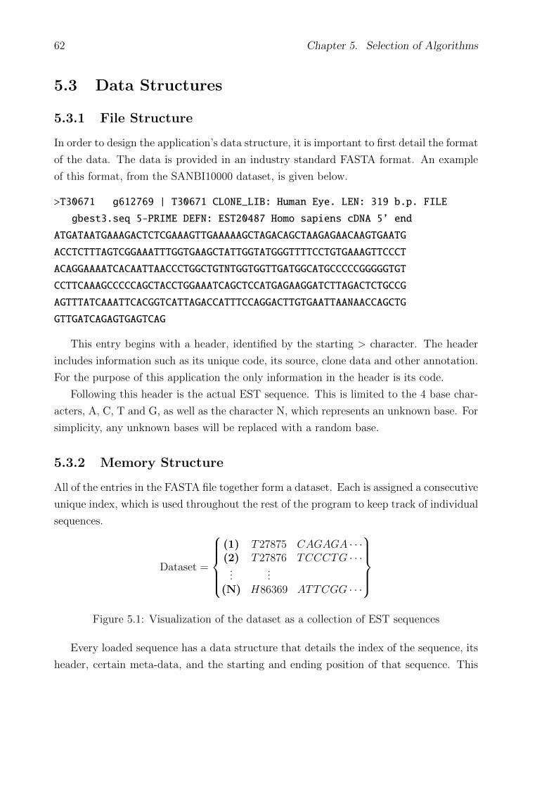
62 Chapter 5. Selection of Algorithms
5.3 Data Structures
5.3.1 File Structure
In order to design the application’s data structure, it is important to first detail the format
of the data. The data is provided in an industry standard FASTA format. An example
of this format, from the SANBI10000 dataset, is given below.
>T30671 g612769 | T30671 CLONE_LIB: Human Eye. LEN: 319 b.p. FILE
gbest3.seq 5-PRIME DEFN: EST20487 Homo sapiens cDNA 5’ end
ATGATAATGAAAGACTCTCGAAAGTTGAAAAAGCTAGACAGCTAAGAGAACAAGTGAATG
ACCTCTTTAGTCGGAAATTTGGTGAAGCTATTGGTATGGGTTTTCCTGTGAAAGTTCCCT
ACAGGAAAATCACAATTAACCCTGGCTGTNTGGTGGTTGATGGCATGCCCCCGGGGGTGT
CCTTCAAAGCCCCCAGCTACCTGGAAATCAGCTCCATGAGAAGGATCTTAGACTCTGCCG
AGTTTATCAAATTCACGGTCATTAGACCATTTCCAGGACTTGTGAATTAANAACCAGCTG
GTTGATCAGAGTGAGTCAG
This entry begins with a header, identified by the starting > character. The header
includes information such as its unique code, its source, clone data and other annotation.
For the purpose of this application the only information in the header is its code.
Following this header is the actual EST sequence. This is limited to the 4 base char-
acters, A, C, T and G, as well as the character N, which represents an unknown base. For
simplicity, any unknown bases will be replaced with a random base.
5.3.2 Memory Structure
All of the entries in the FASTA file together form a dataset. Each is assigned a consecutive
unique index, which is used throughout the rest of the program to keep track of individual
sequences.
Dataset =
(1) T27875 CAGAGA · · ·(2) T27876 TCCCTG · · ·
......
(N) H86369 ATTCGG · · ·
Figure 5.1: Visualization of the dataset as a collection of EST sequences
Every loaded sequence has a data structure that details the index of the sequence, its
header, certain meta-data, and the starting and ending position of that sequence. This
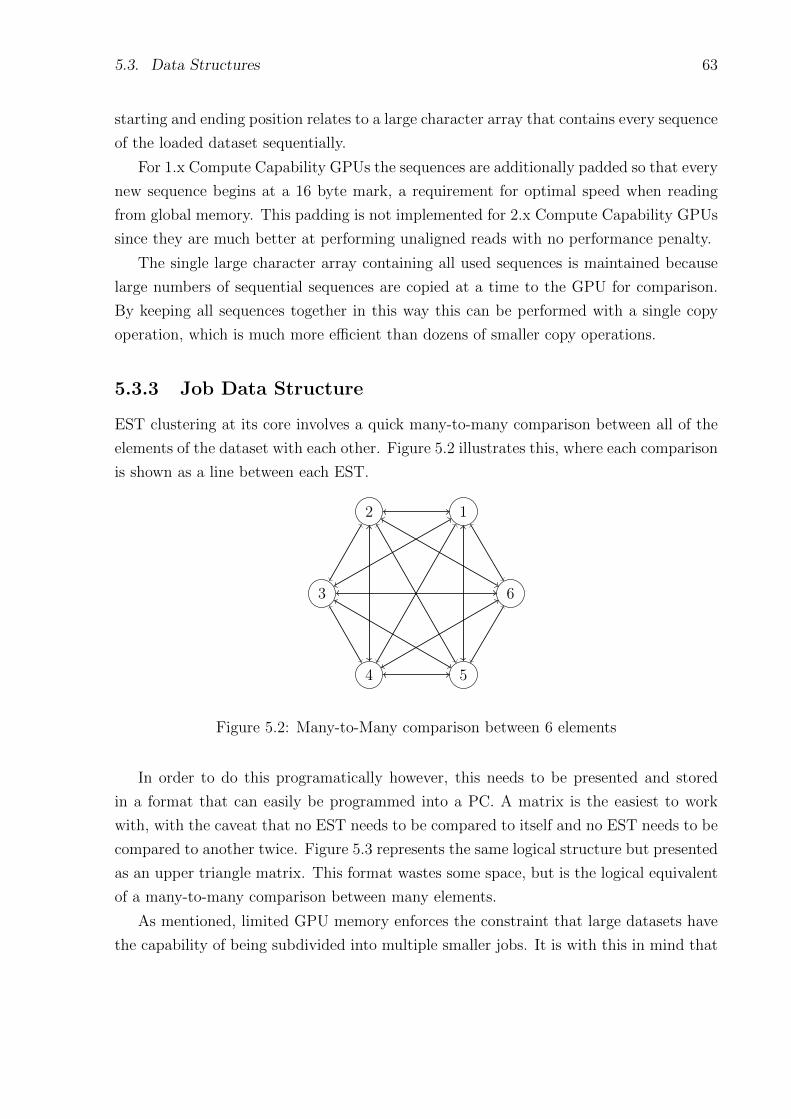
5.3. Data Structures 63
starting and ending position relates to a large character array that contains every sequence
of the loaded dataset sequentially.
For 1.x Compute Capability GPUs the sequences are additionally padded so that every
new sequence begins at a 16 byte mark, a requirement for optimal speed when reading
from global memory. This padding is not implemented for 2.x Compute Capability GPUs
since they are much better at performing unaligned reads with no performance penalty.
The single large character array containing all used sequences is maintained because
large numbers of sequential sequences are copied at a time to the GPU for comparison.
By keeping all sequences together in this way this can be performed with a single copy
operation, which is much more efficient than dozens of smaller copy operations.
5.3.3 Job Data Structure
EST clustering at its core involves a quick many-to-many comparison between all of the
elements of the dataset with each other. Figure 5.2 illustrates this, where each comparison
is shown as a line between each EST.
12
3
4 5
6
Figure 5.2: Many-to-Many comparison between 6 elements
In order to do this programatically however, this needs to be presented and stored
in a format that can easily be programmed into a PC. A matrix is the easiest to work
with, with the caveat that no EST needs to be compared to itself and no EST needs to be
compared to another twice. Figure 5.3 represents the same logical structure but presented
as an upper triangle matrix. This format wastes some space, but is the logical equivalent
of a many-to-many comparison between many elements.
As mentioned, limited GPU memory enforces the constraint that large datasets have
the capability of being subdivided into multiple smaller jobs. It is with this in mind that
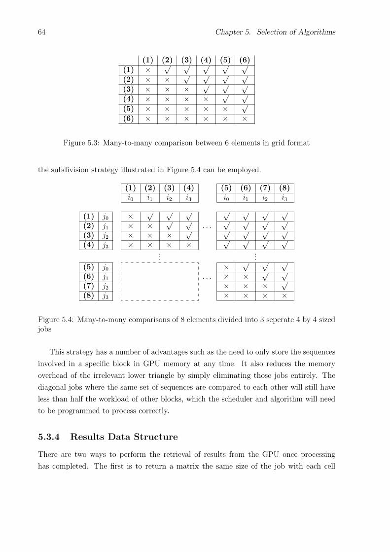
64 Chapter 5. Selection of Algorithms
(1) (2) (3) (4) (5) (6)(1) ×
√ √ √ √ √
(2) × ×√ √ √ √
(3) × × ×√ √ √
(4) × × × ×√ √
(5) × × × × ×√
(6) × × × × × ×
Figure 5.3: Many-to-many comparison between 6 elements in grid format
the subdivision strategy illustrated in Figure 5.4 can be employed.
(1) (2) (3) (4) (5) (6) (7) (8)i0 i1 i2 i3 i0 i1 i2 i3
(1) j0 ×√ √ √ √ √ √ √
(2) j1 × ×√ √
. . .√ √ √ √
(3) j2 × × ×√ √ √ √ √
(4) j3 × × × ×√ √ √ √
......
(5) j0 ×√ √ √
(6) j1 . . . × ×√ √
(7) j2 × × ×√
(8) j3 × × × ×
Figure 5.4: Many-to-many comparisons of 8 elements divided into 3 seperate 4 by 4 sizedjobs
This strategy has a number of advantages such as the need to only store the sequences
involved in a specific block in GPU memory at any time. It also reduces the memory
overhead of the irrelevant lower triangle by simply eliminating those jobs entirely. The
diagonal jobs where the same set of sequences are compared to each other will still have
less than half the workload of other blocks, which the scheduler and algorithm will need
to be programmed to process correctly.
5.3.4 Results Data Structure
There are two ways to perform the retrieval of results from the GPU once processing
has completed. The first is to return a matrix the same size of the job with each cell
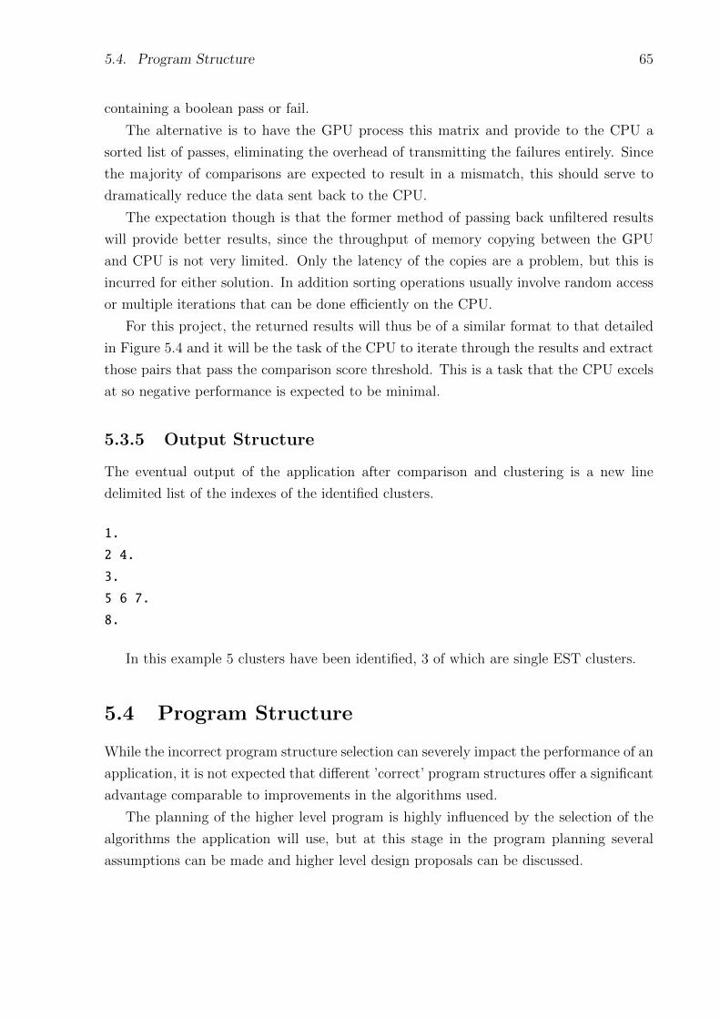
5.4. Program Structure 65
containing a boolean pass or fail.
The alternative is to have the GPU process this matrix and provide to the CPU a
sorted list of passes, eliminating the overhead of transmitting the failures entirely. Since
the majority of comparisons are expected to result in a mismatch, this should serve to
dramatically reduce the data sent back to the CPU.
The expectation though is that the former method of passing back unfiltered results
will provide better results, since the throughput of memory copying between the GPU
and CPU is not very limited. Only the latency of the copies are a problem, but this is
incurred for either solution. In addition sorting operations usually involve random access
or multiple iterations that can be done efficiently on the CPU.
For this project, the returned results will thus be of a similar format to that detailed
in Figure 5.4 and it will be the task of the CPU to iterate through the results and extract
those pairs that pass the comparison score threshold. This is a task that the CPU excels
at so negative performance is expected to be minimal.
5.3.5 Output Structure
The eventual output of the application after comparison and clustering is a new line
delimited list of the indexes of the identified clusters.
1.
2 4.
3.
5 6 7.
8.
In this example 5 clusters have been identified, 3 of which are single EST clusters.
5.4 Program Structure
While the incorrect program structure selection can severely impact the performance of an
application, it is not expected that different ’correct’ program structures offer a significant
advantage comparable to improvements in the algorithms used.
The planning of the higher level program is highly influenced by the selection of the
algorithms the application will use, but at this stage in the program planning several
assumptions can be made and higher level design proposals can be discussed.
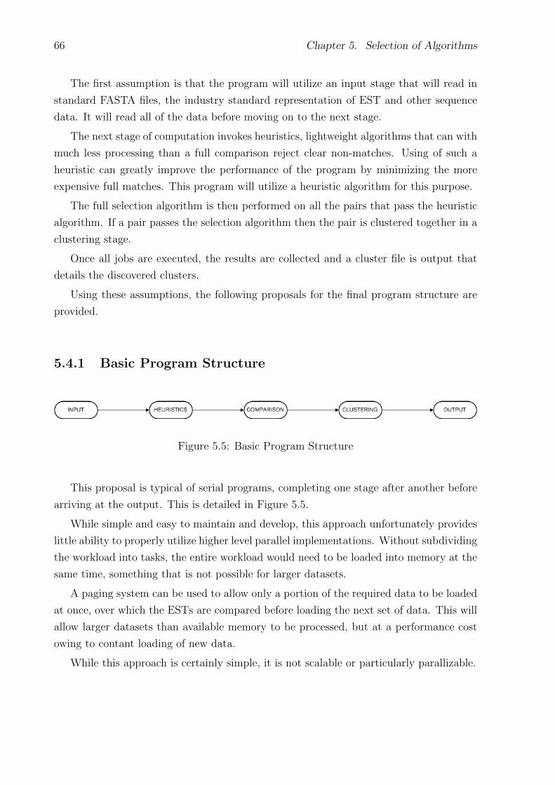
66 Chapter 5. Selection of Algorithms
The first assumption is that the program will utilize an input stage that will read in
standard FASTA files, the industry standard representation of EST and other sequence
data. It will read all of the data before moving on to the next stage.
The next stage of computation invokes heuristics, lightweight algorithms that can with
much less processing than a full comparison reject clear non-matches. Using of such a
heuristic can greatly improve the performance of the program by minimizing the more
expensive full matches. This program will utilize a heuristic algorithm for this purpose.
The full selection algorithm is then performed on all the pairs that pass the heuristic
algorithm. If a pair passes the selection algorithm then the pair is clustered together in a
clustering stage.
Once all jobs are executed, the results are collected and a cluster file is output that
details the discovered clusters.
Using these assumptions, the following proposals for the final program structure are
provided.
5.4.1 Basic Program Structure
Figure 5.5: Basic Program Structure
This proposal is typical of serial programs, completing one stage after another before
arriving at the output. This is detailed in Figure 5.5.
While simple and easy to maintain and develop, this approach unfortunately provides
little ability to properly utilize higher level parallel implementations. Without subdividing
the workload into tasks, the entire workload would need to be loaded into memory at the
same time, something that is not possible for larger datasets.
A paging system can be used to allow only a portion of the required data to be loaded
at once, over which the ESTs are compared before loading the next set of data. This will
allow larger datasets than available memory to be processed, but at a performance cost
owing to contant loading of new data.
While this approach is certainly simple, it is not scalable or particularly parallizable.
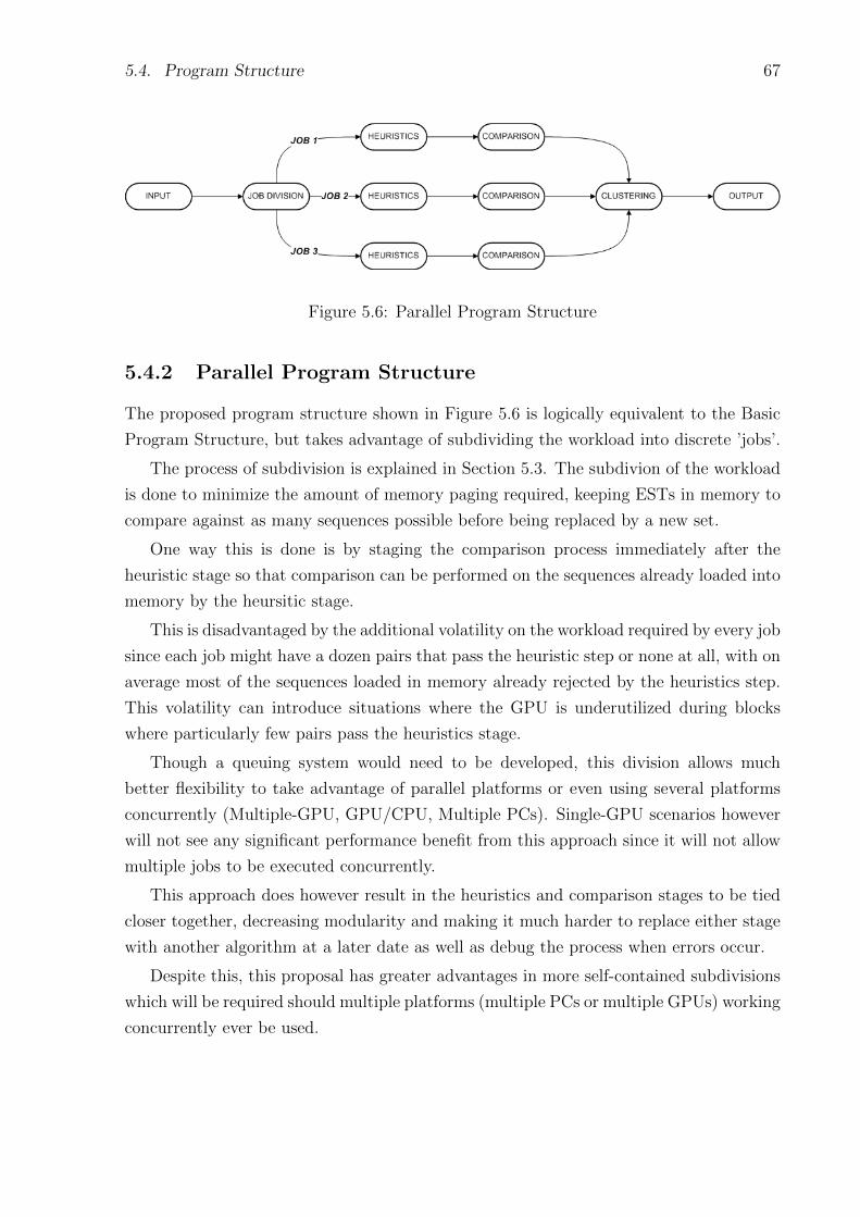
5.4. Program Structure 67
Figure 5.6: Parallel Program Structure
5.4.2 Parallel Program Structure
The proposed program structure shown in Figure 5.6 is logically equivalent to the Basic
Program Structure, but takes advantage of subdividing the workload into discrete ’jobs’.
The process of subdivision is explained in Section 5.3. The subdivion of the workload
is done to minimize the amount of memory paging required, keeping ESTs in memory to
compare against as many sequences possible before being replaced by a new set.
One way this is done is by staging the comparison process immediately after the
heuristic stage so that comparison can be performed on the sequences already loaded into
memory by the heursitic stage.
This is disadvantaged by the additional volatility on the workload required by every job
since each job might have a dozen pairs that pass the heuristic step or none at all, with on
average most of the sequences loaded in memory already rejected by the heuristics step.
This volatility can introduce situations where the GPU is underutilized during blocks
where particularly few pairs pass the heuristics stage.
Though a queuing system would need to be developed, this division allows much
better flexibility to take advantage of parallel platforms or even using several platforms
concurrently (Multiple-GPU, GPU/CPU, Multiple PCs). Single-GPU scenarios however
will not see any significant performance benefit from this approach since it will not allow
multiple jobs to be executed concurrently.
This approach does however result in the heuristics and comparison stages to be tied
closer together, decreasing modularity and making it much harder to replace either stage
with another algorithm at a later date as well as debug the process when errors occur.
Despite this, this proposal has greater advantages in more self-contained subdivisions
which will be required should multiple platforms (multiple PCs or multiple GPUs) working
concurrently ever be used.
68 Chapter 5. Selection of Algorithms
5.5 Heuristics Selection
A good heuristic algorithm is defined by both its speed and its ability to filter large
numbers of false negatives while more importantly having a minimum of impact on true
positives. In this project where the vast majority of comparisons are expected to be
mismatches, heuristics have a great ability to dramatically the reduce the computation
required by more expensive algorithms on rejecting obvious mismatches.
5.5.1 Common word heuristics
Common n-word Heuristic
This is a very simple heuristic, simply trying to confirm whether each sequence in a
pair contains a common number of n-length words. Since two sequences that are very
similar to each other can be almost guaranteed to share a large number of short common
sub-sequences, this algorithm matches the requirements of a heuristic algorithm.
Initially a word count table should be setup, but this can be done in a parallel manner.
For the actual matching every word in one sequence can be assigned its own thread with
little data dependence requirements. Searches in the word table does however use per-
thread random seeks, possibly negatively affecting memory throughput.
Since this algorithm operates in linear memory and is based around sub-sequences
debugging is simplified. Despite the concern about random seeks, this algorithm is a
potential for porting to the GPU, suiting the GPU architecture almost perfectly.
Yet despite its simplicity it is expected to be slow and not as sensitive as it can be.
Improvements on this base algorithm, such as the t/v-word and u/v-sample heuristics
should prove to be much more valuable for practical use.
t/v-word Heuristic
A concern of the common n-word heuristic is its insensitivity to locality of similarity. In
order to address this concern the t/v-word heuristic introduces the additional constraint
of using a 100-character wide window within which at least t of these v-words is required
to appear before passing, rather than allowing matches anywhere in the sequence.
This constraint introduces a challenge by reducing the data independence of the al-
gorithm, since each thread is now concerned with the results of other threads within a
locality.
5.5. Heuristics Selection 69
Though this heuristic is more difficult to implement and has the potential to cause
parallelisation problems, it does improve the sensitivity of the heuristic significantly.
u/v-sample Heuristic
Where the t/v-word heuristic trades performance for greater sensitivity, the u/v-sample
heuristic does the opposite, reducing sensitivity while greatly improving the performance.
Where the Common n-word heuristic would compare every word in a sequence with
the word table, the u/v-sample heuristic skips a number of words(usually skipping 8 or
16), testing only a fraction of the total words, requiring only that at least u v-words
appear in both the sequence and the word table.
This causes the heuristic to pass many algorithms that do not match, but more im-
portantly allows fast and easy rejection of the majority of the pairs that do not match,
which constitutes the overwhelming majority of the pairs.
Chained Heuristic
This is not a separate heuristic, but rather a combination of the t/v-word and u/v-sample
heuristics.
By chaining the two heuristics, first executing the u/v-sample Heuristic followed by
the t/v-word heuristic if the former passes, you can obtain the best of both heuristics.
The quick but insensitive sample heuristic rejects the majority of the EST pairs, while
the more expensive but more sensitive t/v-word heuristic confirms the pair’s candidacy for
a match. Once confirmed, the much more expensive and extensive comparison algorithm
can be used to accept or reject the clustering of the pair.
Through utilizing this combination of heuristics both high speed and high sensitivity
can be realised.
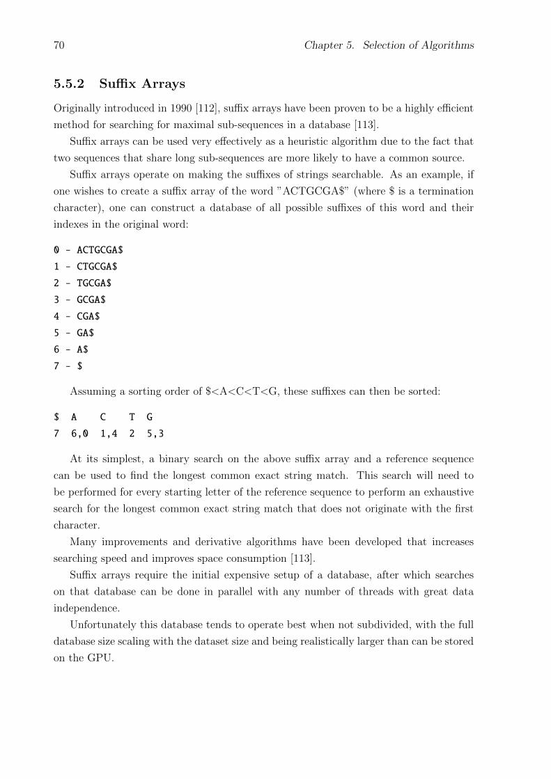
70 Chapter 5. Selection of Algorithms
5.5.2 Suffix Arrays
Originally introduced in 1990 [112], suffix arrays have been proven to be a highly efficient
method for searching for maximal sub-sequences in a database [113].
Suffix arrays can be used very effectively as a heuristic algorithm due to the fact that
two sequences that share long sub-sequences are more likely to have a common source.
Suffix arrays operate on making the suffixes of strings searchable. As an example, if
one wishes to create a suffix array of the word ”ACTGCGA$” (where $ is a termination
character), one can construct a database of all possible suffixes of this word and their
indexes in the original word:
0 - ACTGCGA$
1 - CTGCGA$
2 - TGCGA$
3 - GCGA$
4 - CGA$
5 - GA$
6 - A$
7 - $
Assuming a sorting order of $<A<C<T<G, these suffixes can then be sorted:
$ A C T G
7 6,0 1,4 2 5,3
At its simplest, a binary search on the above suffix array and a reference sequence
can be used to find the longest common exact string match. This search will need to
be performed for every starting letter of the reference sequence to perform an exhaustive
search for the longest common exact string match that does not originate with the first
character.
Many improvements and derivative algorithms have been developed that increases
searching speed and improves space consumption [113].
Suffix arrays require the initial expensive setup of a database, after which searches
on that database can be done in parallel with any number of threads with great data
independence.
Unfortunately this database tends to operate best when not subdivided, with the full
database size scaling with the dataset size and being realistically larger than can be stored
on the GPU.
5.6. Comparison Algorithm Selection 71
Even using the subdivided database on a GPU, this algorithm is based around random
searches, limiting the performance of a GPU. Additionally a suffix array database uses a
large amount of pointers and references, resulting in increased complexity and a difficulty
to debug in linear memory.
While this method can be considered a good possibility as a CPU side algorithm, it is
rejected as a candidate for GPU processing, though this assertion could be revisited and
proven incorrect in the future.
5.6 Comparison Algorithm Selection
Due to the implementation of heuristics, the selection algorithm can be far more expensive
than otherwise, since it will only be utilized for likely matches instead of for every pair.
The main criteria of the selection algorithm is its suitability on the GPU and the
expected quality of its results.
5.6.1 Simple Comparison
The simple comparison can be represented with the following formula:
d(k) =
|x|∑i=1
f(x(i), y(i+ k)) (5.1)
f(a, b) =
{1 if a = b
0 if a 6= b(5.2)
where |x| is the length of the string represented by x, x(i) is the ith character of the string
represented by x and y(i+ k) is the (i+ k)th character represented by the string y. This
function will return the count of all the matching characters at positional offset k.
When using the simple comparison the goal is to find a value of k where the greatest
number of characters in both sequences match.
The simple comparison has the advantage of its simplicity, but it is not widely used
in any but the most naive applications due to being slow and not taking into account
insertions and deletions.
The simple comparison is however a good candidate for GPU porting due to its par-
allelizability, high data independence and lack of random seeks. It does however suffer
from low accuracy due to above mentioned issues.
As such this comparison will not be considered for this project.
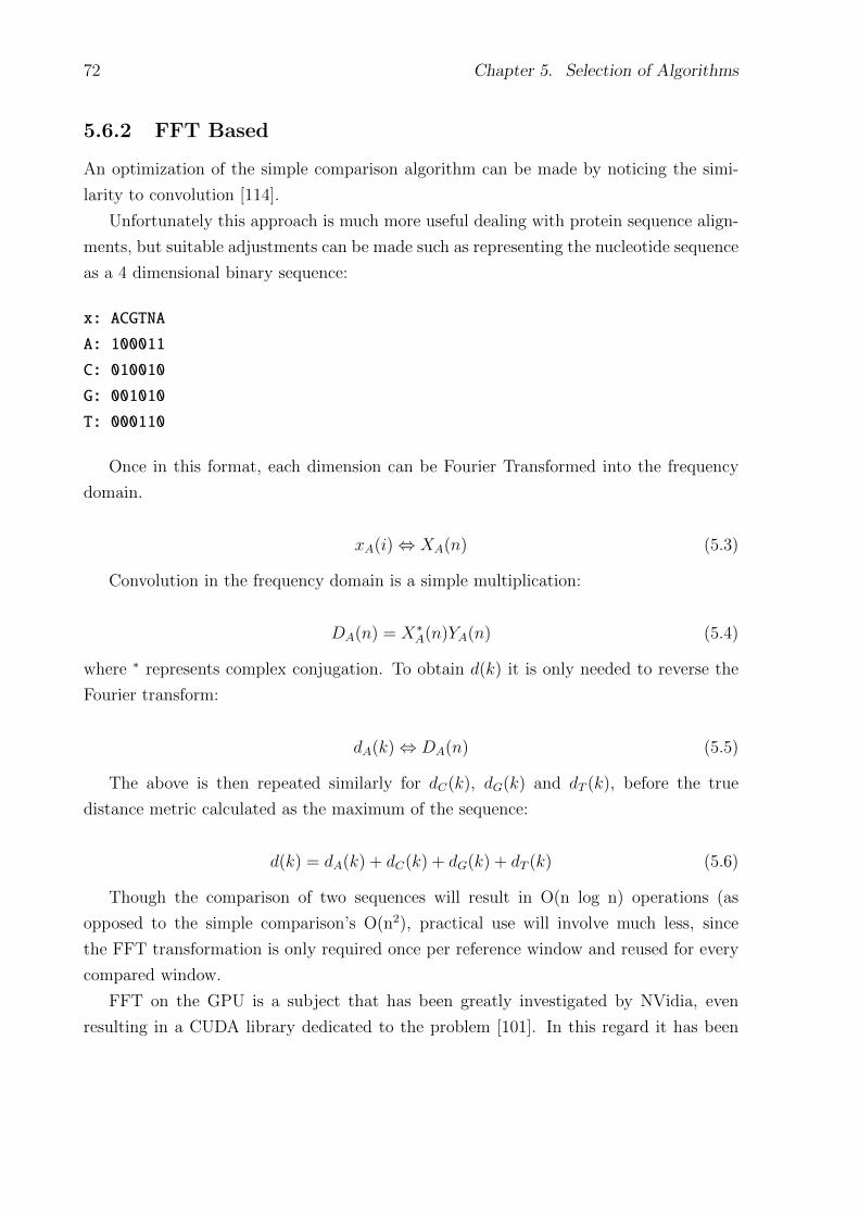
72 Chapter 5. Selection of Algorithms
5.6.2 FFT Based
An optimization of the simple comparison algorithm can be made by noticing the simi-
larity to convolution [114].
Unfortunately this approach is much more useful dealing with protein sequence align-
ments, but suitable adjustments can be made such as representing the nucleotide sequence
as a 4 dimensional binary sequence:
x: ACGTNA
A: 100011
C: 010010
G: 001010
T: 000110
Once in this format, each dimension can be Fourier Transformed into the frequency
domain.
xA(i)⇔ XA(n) (5.3)
Convolution in the frequency domain is a simple multiplication:
DA(n) = X∗A(n)YA(n) (5.4)
where ∗ represents complex conjugation. To obtain d(k) it is only needed to reverse the
Fourier transform:
dA(k)⇔ DA(n) (5.5)
The above is then repeated similarly for dC(k), dG(k) and dT (k), before the true
distance metric calculated as the maximum of the sequence:
d(k) = dA(k) + dC(k) + dG(k) + dT (k) (5.6)
Though the comparison of two sequences will result in O(n log n) operations (as
opposed to the simple comparison’s O(n2), practical use will involve much less, since
the FFT transformation is only required once per reference window and reused for every
compared window.
FFT on the GPU is a subject that has been greatly investigated by NVidia, even
resulting in a CUDA library dedicated to the problem [101]. In this regard it has been
5.6. Comparison Algorithm Selection 73
shown to be greatly suited to the GPU platform, showing great improvements over the
CPU for larger datasets [115].
Further research however revealed that while the FFT function is used extensively in
this algorithm, the actual FFT computation does not dominate the total computational
time of the algorithm. For this reason, even if the FFT portion can be improved greatly,
the limit to the improvement of the full algorithm will depend largely on the dynamic
programming portion, a domain that is typically much more difficult to parallelize on the
GPU.
While this algorithm features decent data independance and parallelism in the FFT
stage, this algorithm is not easily scalable due to the reduced returns of only parallelizing
a part of this algorithm.
5.6.3 d2 distance
The d2 clustering algorithm is a word based distance algorithm. When applied to pair-
wise comparisons it involves decomposing both sub-sequences into n-length words, then
comparing the two sequences word counts.
By example, the sequence x=ACGTATAT can be composed into 6 words each of length
3: ACG, CGT, GTA, TAT, ATA and TAT.
The function cx(w) is used to refer to the count of the occurrence of a particular word
in the sequence x. For the above example, cx(TAT) would be 2.
The definition of d2 as given by [116] is the following:
d2(x, y) =K∑k=1
4k∑i=1
ρ(wi)n(wi){cx(wi)− cy(wi)}2 (5.7)
where K is the maximum word length, ρ(wi) is the weighting of word wi and n(wi) is
the length of word wi.
A simplified version of the above formula can be created by fixing the value of k to a
single word length [117].
d2k(x, y) =4k∑i=1
(cx(wi)− cy(wi))2 (5.8)
A weighting term can also be added, possibly utilizing masking data to help minimize
the effects of repeats.
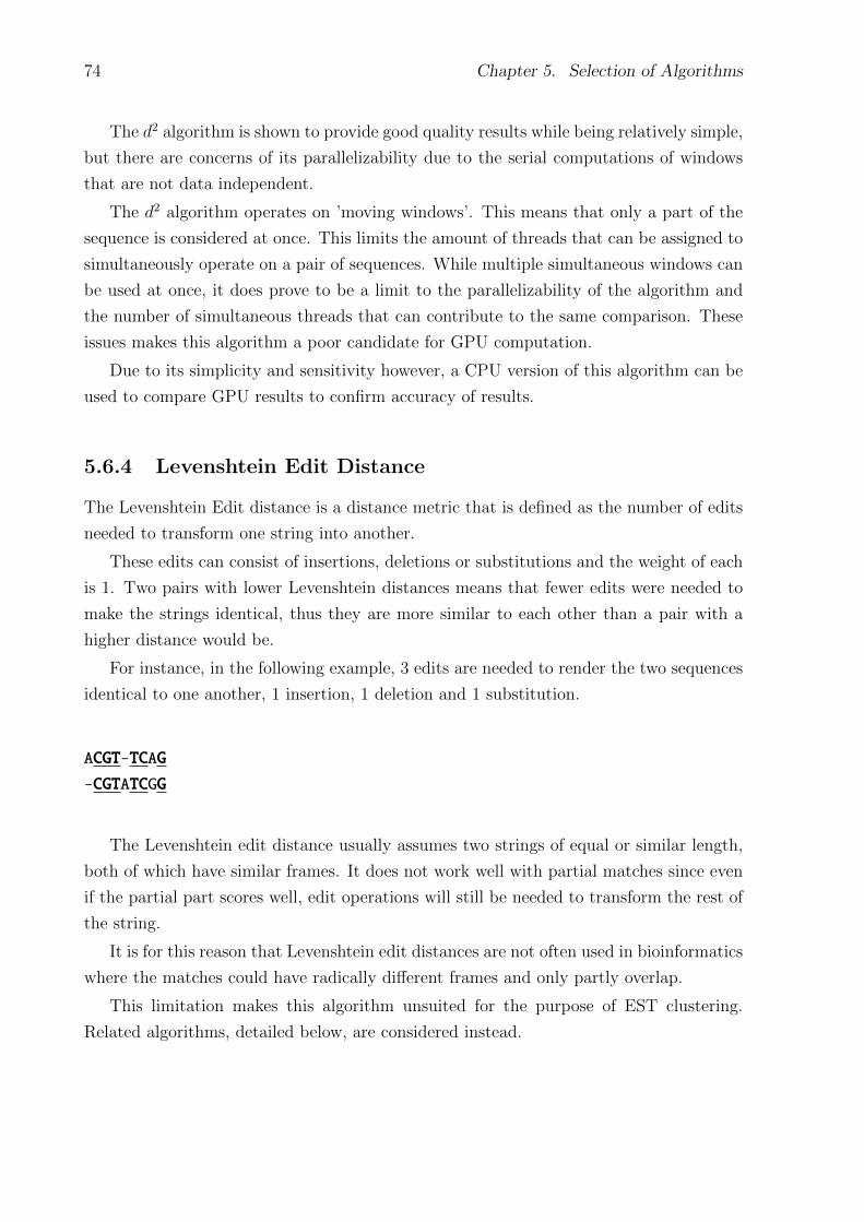
74 Chapter 5. Selection of Algorithms
The d2 algorithm is shown to provide good quality results while being relatively simple,
but there are concerns of its parallelizability due to the serial computations of windows
that are not data independent.
The d2 algorithm operates on ’moving windows’. This means that only a part of the
sequence is considered at once. This limits the amount of threads that can be assigned to
simultaneously operate on a pair of sequences. While multiple simultaneous windows can
be used at once, it does prove to be a limit to the parallelizability of the algorithm and
the number of simultaneous threads that can contribute to the same comparison. These
issues makes this algorithm a poor candidate for GPU computation.
Due to its simplicity and sensitivity however, a CPU version of this algorithm can be
used to compare GPU results to confirm accuracy of results.
5.6.4 Levenshtein Edit Distance
The Levenshtein Edit distance is a distance metric that is defined as the number of edits
needed to transform one string into another.
These edits can consist of insertions, deletions or substitutions and the weight of each
is 1. Two pairs with lower Levenshtein distances means that fewer edits were needed to
make the strings identical, thus they are more similar to each other than a pair with a
higher distance would be.
For instance, in the following example, 3 edits are needed to render the two sequences
identical to one another, 1 insertion, 1 deletion and 1 substitution.
ACGT-TCAG
-CGTATCGG
The Levenshtein edit distance usually assumes two strings of equal or similar length,
both of which have similar frames. It does not work well with partial matches since even
if the partial part scores well, edit operations will still be needed to transform the rest of
the string.
It is for this reason that Levenshtein edit distances are not often used in bioinformatics
where the matches could have radically different frames and only partly overlap.
This limitation makes this algorithm unsuited for the purpose of EST clustering.
Related algorithms, detailed below, are considered instead.
5.6. Comparison Algorithm Selection 75
5.6.5 Smith-Waterman
Smith-Waterman alignment is one of the most important algorithms in use in the bioin-
formatics field. It is used to obtain both a similarity score and an alignment for any pair
of sequences. The process of alignment is described in Section 2.6.2.
The Smith-Waterman algorithm is based on edit distances, but unlike the Levenshtein
edit distance it can obtain partial or overlapping matches, instead of attempting to match
the entirety of the two sequences. This is called local alignment and is a valuable quality
for EST comparisons where only part of the sequences need to match for the two sequences
to be clustered together.
To explain the algorithm, recall the example used in Section 2.6.2. The goal is to align
the following two sequences:
Sequence 1: GATTCGTTA
Sequence 2: GGATCGTA
To perform this alignment it is important to first create what is known as a Substi-
tution Matrix. Substitution matrices for protein comparisons are usually complex with
different weightings for every protein, dependent on the biological possibility of one pro-
tein randomly mutating or being read as a different protein. Thus this substitution matrix
accounts for both evolutionary divergence and experimental error.
When applied to this application though the substitution matrix tends to be simple,
due to fewer characters in an EST sequence than a whole genome, as well as the fact that
evolutionary divergence does not have to be accounted for due to all the ESTs all sourced
from the same individual. To account for experimental error only 2 variables are needed:
The match score and the mismatch score. These are chosen to provide the similarity
required. For instance, a match score of 1 and a mismatch of -1 will only pass pairs with
a 50% similarity, or where every second character matches.
For this algorithm to be more useful in this application however, higher similarity re-
quirements are needed, usually that of 95% or more. For this example though, a similarity
of 66% will be used, shown in Table 5.1.
This substitution matrix results in the requirement that for every 1 mismatch, the
region has at least 2 matches.
The data structure that Smith-Waterman operates on is best represented as a matrix
with the height of the matrix being equal to the length of one sequence and the width
being equal to the length of the other.
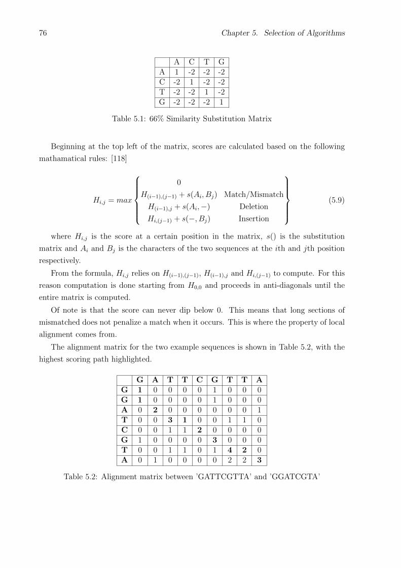
76 Chapter 5. Selection of Algorithms
A C T GA 1 -2 -2 -2C -2 1 -2 -2T -2 -2 1 -2G -2 -2 -2 1
Table 5.1: 66% Similarity Substitution Matrix
Beginning at the top left of the matrix, scores are calculated based on the following
mathamatical rules: [118]
Hi,j = max
0
H(i−1),(j−1) + s(Ai, Bj) Match/Mismatch
H(i−1),j + s(Ai,−) Deletion
Hi,(j−1) + s(−, Bj) Insertion
(5.9)
where Hi,j is the score at a certain position in the matrix, s() is the substitution
matrix and Ai and Bj is the characters of the two sequences at the ith and jth position
respectively.
From the formula, Hi,j relies on H(i−1),(j−1), H(i−1),j and Hi,(j−1) to compute. For this
reason computation is done starting from H0,0 and proceeds in anti-diagonals until the
entire matrix is computed.
Of note is that the score can never dip below 0. This means that long sections of
mismatched does not penalize a match when it occurs. This is where the property of local
alignment comes from.
The alignment matrix for the two example sequences is shown in Table 5.2, with the
highest scoring path highlighted.
G A T T C G T T AG 1 0 0 0 0 1 0 0 0G 1 0 0 0 0 1 0 0 0A 0 2 0 0 0 0 0 0 1T 0 0 3 1 0 0 1 1 0C 0 0 1 1 2 0 0 0 0G 1 0 0 0 0 3 0 0 0T 0 0 1 1 0 1 4 2 0A 0 1 0 0 0 0 2 2 3
Table 5.2: Alignment matrix between ’GATTCGTTA’ and ’GGATCGTA’
5.6. Comparison Algorithm Selection 77
The maximum value in the above matrix serves a dual purpose, namely that of being
an indicator of the similarity of the two sequences and providing a starting point for
tracking back along the highest values, from which the alignment can be obtained.
Sequence 1: -GATTCGTTA
Sequence 2: GGAT-CGT-A
where the ’−’ character represents gaps.
When adapting Smith-Waterman for the use of this application, it should be noted
that by using the Smith-Waterman algorithm as a distance metric and not an alignment
algorithm, the track-back stage of this algorithm is unnecessary and can be ignored.
The result of this adaption is that Smith-Waterman as written does not score pairs
that have long matching regions with few errors higher than short regions with no errors.
This score is dependent only on the ratio of errors versus matches and does not favor long
regions highly. Only after performing the back-tracking stage would the actual length of
the match become known. The next section deals with an attempt to compensate for this
shortcoming.
5.6.6 Modified Smith-Waterman
In order to address some of the shortcomings of the adapted Smith-Waterman algorithm,
the modified Smith-Waterman is proposed.
In this algorithm, in addition to the score variable another variable named the Cumu-
lative Score is used. This variable will increment with every match and not decrease with
mismatches, only resetting to 0 when the Smith-Waterman score is also set to 0.
The advantage of this alternate scoring is that it favors long matching sequences, even
if only barely above the needed similarity. The effect of this alternate scoring is shown
below in Figure 5.7.
In addition, several small modifications are made, such as gap penalties being equal
to mismatch penalties and the elimination of the track-back stage is done, intended to
simplify Smith-Waterman and use it as a more efficient distance metric.
This algorithm is not very data-dependent due to the matrix-format of the compu-
tation. Though the calculation can be parallelized using a diagonal method, this is not
optimal and often leaves processors idle. The maximum length of the sequences compared
is dependent on the registers and the threads utilized, making arbitrarily large sequences
difficult to compare. The algorithm is also not very simple.
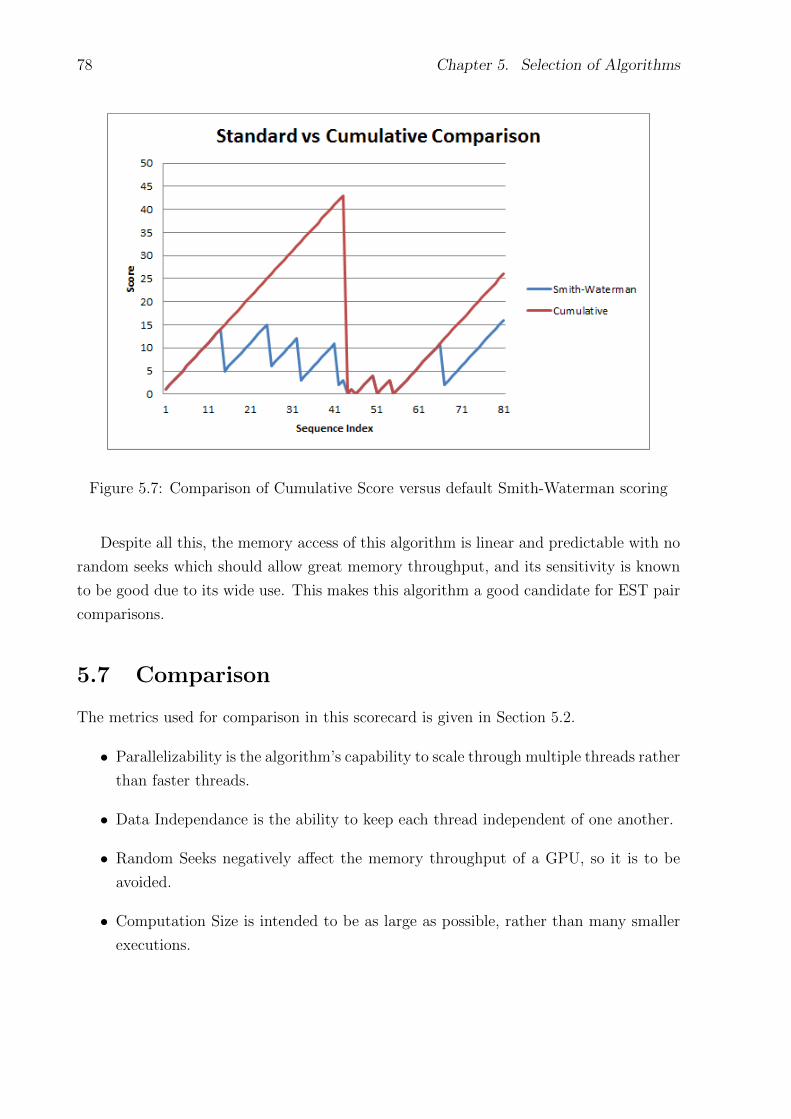
78 Chapter 5. Selection of Algorithms
Figure 5.7: Comparison of Cumulative Score versus default Smith-Waterman scoring
Despite all this, the memory access of this algorithm is linear and predictable with no
random seeks which should allow great memory throughput, and its sensitivity is known
to be good due to its wide use. This makes this algorithm a good candidate for EST pair
comparisons.
5.7 Comparison
The metrics used for comparison in this scorecard is given in Section 5.2.
• Parallelizability is the algorithm’s capability to scale through multiple threads rather
than faster threads.
• Data Independance is the ability to keep each thread independent of one another.
• Random Seeks negatively affect the memory throughput of a GPU, so it is to be
avoided.
• Computation Size is intended to be as large as possible, rather than many smaller
executions.
5.7. Comparison 79
• The ability to subdivide into smaller tasks is an important feature to allow the
computation size to be customized to the amount of available memory.
• Simplicity is important for finding errors and debugging.
The algorithms and options for this project are detailed above. Table 5.3 contains a
summary of these options’ score on various criteria.
Name Par
alle
l
Indep
enden
ce
Ran
dom
See
ks
Siz
e
Sub
div
ide
Sim
plici
ty
Sen
siti
vit
y
Ove
rall
Program Structure Options (Section 5.4)Basic Program Structure × − −
√× © − ×
Parallel Program Structure © − −√©
√− ©
Heuristics (Section 5.5 )Common n-word © ©
√© © © × ×
t/v-wordé
√ √© × ©
√
u/v-sample © ©√ √
©√ √
©Suffix Arrays © © × × × ×
√×
Comparison Algorithm (Section 5.6)Simple Comparison © © © ©
√© × ×
FFT Based√ √
© × ×√ √ √
d2 Distance ×√ √ √ √ √
©√
Edit Distance√
× © ×√ √ √
×Smith-Waterman
√× © ×
√× © ©
Table 5.3: Comparison of the various algorithms introduced in this chapter
The symbols used in the comparison chart are following:
• × This option does not meet this criteria particularly well.
•√
This option meets this criteria sufficiently well.
• © This option meets this criteria very well.
• − Meeting this criteria depends on implementation details, not the algorithm itself.
The criteria are judged in comparison relative expectations to other algorithms in the
same category.
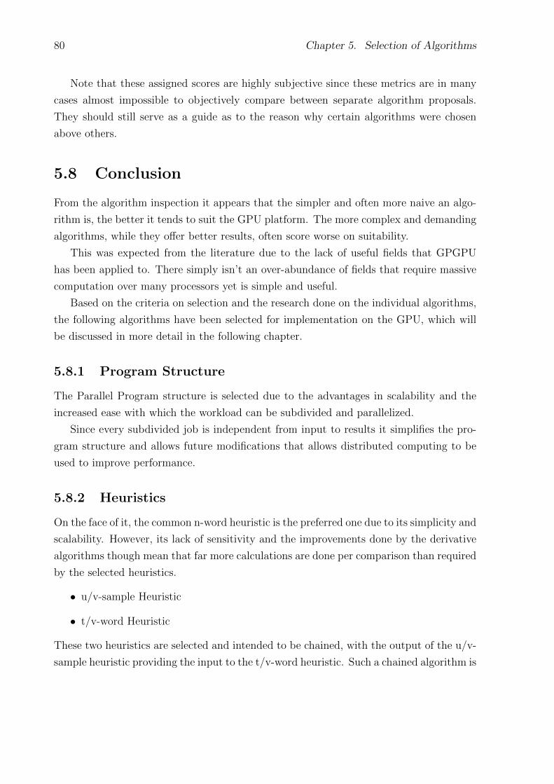
80 Chapter 5. Selection of Algorithms
Note that these assigned scores are highly subjective since these metrics are in many
cases almost impossible to objectively compare between separate algorithm proposals.
They should still serve as a guide as to the reason why certain algorithms were chosen
above others.
5.8 Conclusion
From the algorithm inspection it appears that the simpler and often more naive an algo-
rithm is, the better it tends to suit the GPU platform. The more complex and demanding
algorithms, while they offer better results, often score worse on suitability.
This was expected from the literature due to the lack of useful fields that GPGPU
has been applied to. There simply isn’t an over-abundance of fields that require massive
computation over many processors yet is simple and useful.
Based on the criteria on selection and the research done on the individual algorithms,
the following algorithms have been selected for implementation on the GPU, which will
be discussed in more detail in the following chapter.
5.8.1 Program Structure
The Parallel Program structure is selected due to the advantages in scalability and the
increased ease with which the workload can be subdivided and parallelized.
Since every subdivided job is independent from input to results it simplifies the pro-
gram structure and allows future modifications that allows distributed computing to be
used to improve performance.
5.8.2 Heuristics
On the face of it, the common n-word heuristic is the preferred one due to its simplicity and
scalability. However, its lack of sensitivity and the improvements done by the derivative
algorithms though mean that far more calculations are done per comparison than required
by the selected heuristics.
• u/v-sample Heuristic
• t/v-word Heuristic
These two heuristics are selected and intended to be chained, with the output of the u/v-
sample heuristic providing the input to the t/v-word heuristic. Such a chained algorithm is
5.8. Conclusion 81
expected to provide advantages that in accuracy and performance that cannot be realised
by either heuristic alone.
5.8.3 Comparison Algorithm
Two algorithms were selected for the comparison algorithm. Following is a list and an
explanation for each.
• d2 algorithm
While the d2 algorithm does not map very well to the GPU, it provides good accuracy
and is simple enough to create a CPU implementation. This implementation is to be used
for debugging as well as used to create a reference clustering to measure sensitivity issues.
• Modified Smith-Waterman
The Smith-Waterman algorithm is a well-known and respected workhorse for the bioinfor-
matics community. While the usual implementation does not serve our needs the modified
version detailed in Section 5.6.6 appears to match the sensitivity expected of the origi-
nal while having advantages in performance when ported to the GPU and used for the
purpose of identifying EST pairs to be clustered.

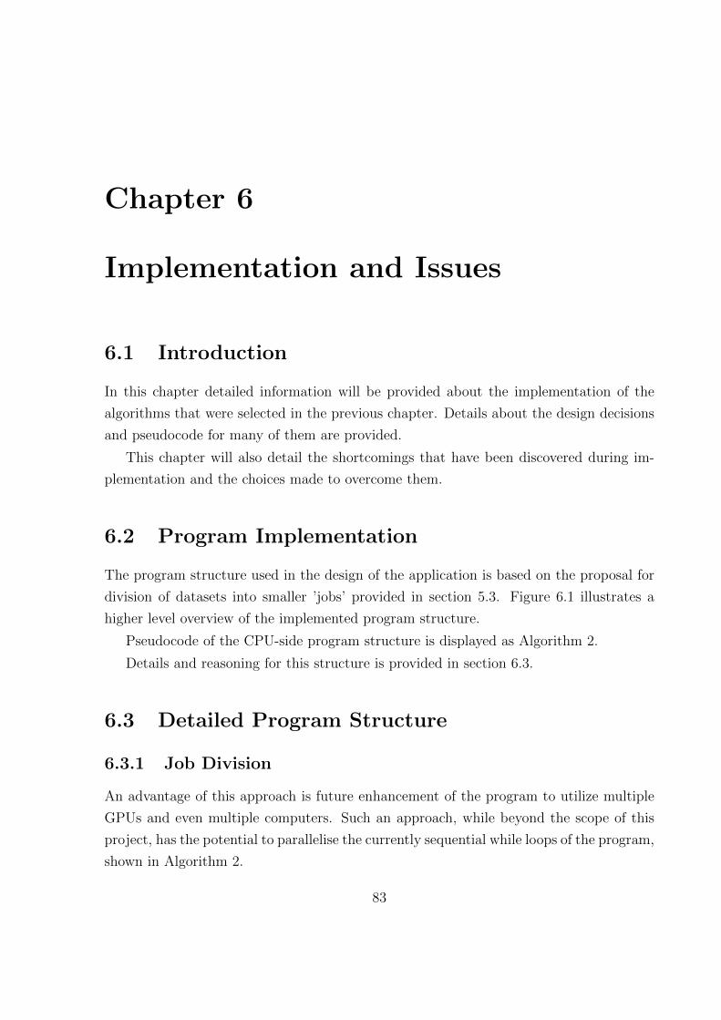
Chapter 6
Implementation and Issues
6.1 Introduction
In this chapter detailed information will be provided about the implementation of the
algorithms that were selected in the previous chapter. Details about the design decisions
and pseudocode for many of them are provided.
This chapter will also detail the shortcomings that have been discovered during im-
plementation and the choices made to overcome them.
6.2 Program Implementation
The program structure used in the design of the application is based on the proposal for
division of datasets into smaller ’jobs’ provided in section 5.3. Figure 6.1 illustrates a
higher level overview of the implemented program structure.
Pseudocode of the CPU-side program structure is displayed as Algorithm 2.
Details and reasoning for this structure is provided in section 6.3.
6.3 Detailed Program Structure
6.3.1 Job Division
An advantage of this approach is future enhancement of the program to utilize multiple
GPUs and even multiple computers. Such an approach, while beyond the scope of this
project, has the potential to parallelise the currently sequential while loops of the program,
shown in Algorithm 2.
83
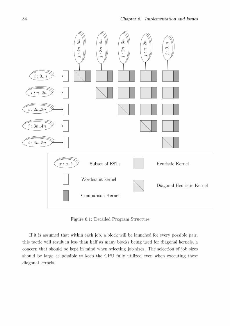
84 Chapter 6. Implementation and Issues
i : 0..n
i : n..2n
i : 2n..3n
i : 3n..4n
i : 4n..5n
j:
0..n
j:n..2n
j:
2n..3n
j:
3n..4n
j:
4n..5n
x : a..b Subset of ESTs
Wordcount kernel
Comparison Kernel
Heuristic Kernel
Diagonal Heuristic Kernel
Figure 6.1: Detailed Program Structure
If it is assumed that within each job, a block will be launched for every possible pair,
this tactic will result in less than half as many blocks being used for diagonal kernels, a
concern that should be kept in mind when selecting job sizes. The selection of job sizes
should be large as possible to keep the GPU fully utilized even when executing these
diagonal kernels.
6.3. Detailed Program Structure 85
Algorithm 2 CPU-side Program Structure
n← jobsize parameterCPU: Load Dataset D from file containing N ESTsi, j ← 0while i < N do
Load EST(i, ..., i+ n) to GPUGPU: WCi,...,i+n ← Kernel Word Count on EST(i, ..., i+ n)while j < N do
Load EST(j, ..., j + n) to GPUGPU: Run Heuristic between WCi,...,i+n and EST(j, ..., j + n)GPU: Run Comparison kernel on passing pairsCopy comparison results to CPUCPU: Cluster pairs that passes comparisonj ← j + n
end whilei, j ← i+ n
end while
Memory latency and CPU processing can be hidden by larger job sizes which result
in less overhead involving context switches. There is no significant advantage to smaller
job sizes. For this reason it is desirable to have a job size that is as large as possible.
A job size of 512 by 512 ESTs being compared at the same time was experimentally
determined to be the largest job size that can be selected without incurring memory or
addressing issues. Solutions to these issues might result in even larger jobs that can be
issued, but the benefits is not expected to be large beyond this point.
6.3.2 Memory management and paging
EST databases can be arbitrarily large, from a few megabytes to many gigabytes. The
memory available to GPUs however tend to be far more modest, ranging from half a
gigabyte for modern lower-level GPUs to a current maximum of 4 gigabytes on a NVidia
Tesla GPU. In addition, if a GPU is used to drive both a monitor and perform computation
at the same time, it is advised to reserve a few hundred megabytes of GPU memory for
the desktop to avoid graphical latency and errors and thus not use the available GPU
memory to its theoretical maximum.
This effectively limits the GPU memory size to a point generally lower than the ex-
pected database size. In order to circumvent this limitation, a strategy of paging memory
between RAM and GPU memory is employed. Only the ESTs currently involved in the
86 Chapter 6. Implementation and Issues
processing is required to be in GPU memory at any time.
When the application is initialized, memory is reserved for storing the ESTs, word
tables and results matrices. This storage is reserved when the application launches and
if properly implemented it should result in memory declarations being made only once
for the entire application runtime. This has advantages in eliminating costly memory
allocations and garbage collection as memory is freed mid-execution. However, since the
memory available will be static and not scaled to the needs of the application during
run-time, an upper bound must be found for reservation which will not be exceeded for
any expected dataset.
The maximum number of threads per block is 512 for 1.3 compute capability GPUs.
Though later GPUs support more threads per block, this would break backwards compat-
ibility. For this reason a maximum of 512 threads per block will be assumed for memory
use calculations.
Assuming a job size of 512 by 512 ESTs being compared on the GPU at once, this
means that enough space for 1024 ESTs should be reserved. Since each EST can differ
in length, an analysis of the experimental databases was performed. It was found that
all ESTs in these databases are under 2000 characters in length. For this reason 2kB of
memory is reserved per EST as an upper expected bound. Since the memory is pooled
for all ESTs, ESTs of longer length than this length are supported so long as the total
EST storage for the entire job does not exceed 2MB of space or approximately 2 million
characters. This is expected to serve the requirements for most standard datasets, though
the reserved memory can be increased if datasets are found for which this is not sufficient.
Every row of ESTs also requires the space for a word count table. If a word size of 6
is chosen and the word presence table detailed in Section 6.4.1 is used, this will total an
additional 512 B per EST. Multiplied by a job size of 512 ESTs this results in 256kB of
memory per job.
The results matrix that serves as a part of global memory that each block and inde-
pendently output to is sized as 512x512 bytes (1 byte for every pair). This totals another
256kB of memory per job.
If you include other memory requirements such as indexing and constant storage, the
total GPU memory used by gpucluster if paging is utilized will be less than 3MB per job,
compared to the 200 megabytes a database of only 100 000 ESTs will require. Many jobs
are launched simultaneously, each requiring approximately 3MB of storage, but even so
is unlikely to exceed the global memory available to even low-range GPUs.
An attempt was made to utilize the CUDA concept known as streams to optimize
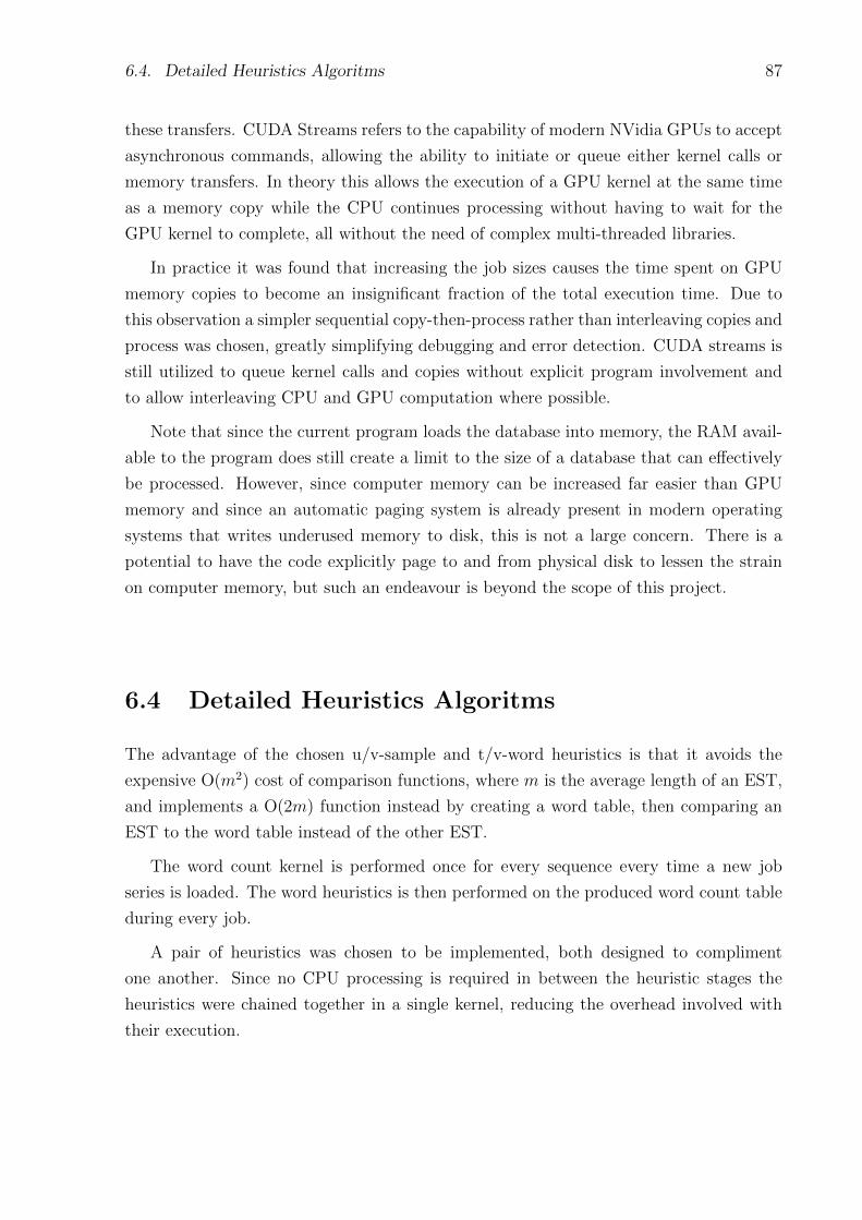
6.4. Detailed Heuristics Algoritms 87
these transfers. CUDA Streams refers to the capability of modern NVidia GPUs to accept
asynchronous commands, allowing the ability to initiate or queue either kernel calls or
memory transfers. In theory this allows the execution of a GPU kernel at the same time
as a memory copy while the CPU continues processing without having to wait for the
GPU kernel to complete, all without the need of complex multi-threaded libraries.
In practice it was found that increasing the job sizes causes the time spent on GPU
memory copies to become an insignificant fraction of the total execution time. Due to
this observation a simpler sequential copy-then-process rather than interleaving copies and
process was chosen, greatly simplifying debugging and error detection. CUDA streams is
still utilized to queue kernel calls and copies without explicit program involvement and
to allow interleaving CPU and GPU computation where possible.
Note that since the current program loads the database into memory, the RAM avail-
able to the program does still create a limit to the size of a database that can effectively
be processed. However, since computer memory can be increased far easier than GPU
memory and since an automatic paging system is already present in modern operating
systems that writes underused memory to disk, this is not a large concern. There is a
potential to have the code explicitly page to and from physical disk to lessen the strain
on computer memory, but such an endeavour is beyond the scope of this project.
6.4 Detailed Heuristics Algoritms
The advantage of the chosen u/v-sample and t/v-word heuristics is that it avoids the
expensive O(m2) cost of comparison functions, where m is the average length of an EST,
and implements a O(2m) function instead by creating a word table, then comparing an
EST to the word table instead of the other EST.
The word count kernel is performed once for every sequence every time a new job
series is loaded. The word heuristics is then performed on the produced word count table
during every job.
A pair of heuristics was chosen to be implemented, both designed to compliment
one another. Since no CPU processing is required in between the heuristic stages the
heuristics were chained together in a single kernel, reducing the overhead involved with
their execution.
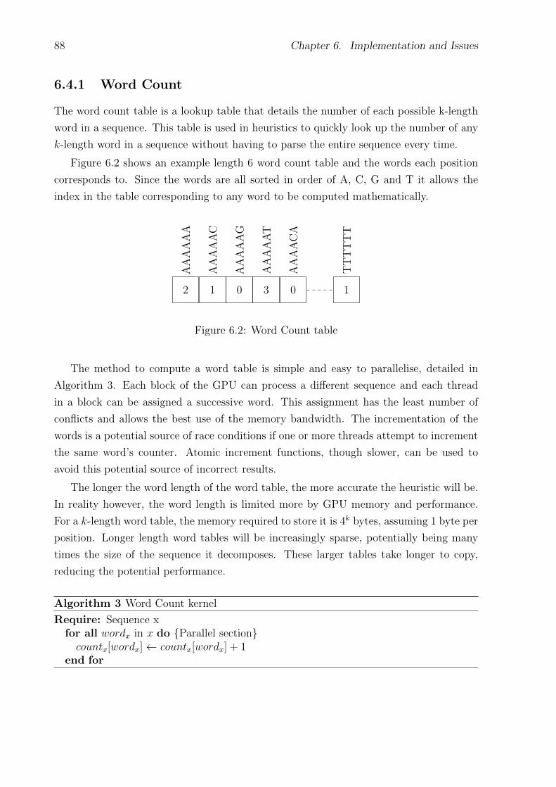
88 Chapter 6. Implementation and Issues
6.4.1 Word Count
The word count table is a lookup table that details the number of each possible k-length
word in a sequence. This table is used in heuristics to quickly look up the number of any
k-length word in a sequence without having to parse the entire sequence every time.
Figure 6.2 shows an example length 6 word count table and the words each position
corresponds to. Since the words are all sorted in order of A, C, G and T it allows the
index in the table corresponding to any word to be computed mathematically.
2 1 0 3 0 1
AA
AA
AA
AA
AA
AC
AA
AA
AG
AA
AA
AT
AA
AA
CA
TT
TT
TT
Figure 6.2: Word Count table
The method to compute a word table is simple and easy to parallelise, detailed in
Algorithm 3. Each block of the GPU can process a different sequence and each thread
in a block can be assigned a successive word. This assignment has the least number of
conflicts and allows the best use of the memory bandwidth. The incrementation of the
words is a potential source of race conditions if one or more threads attempt to increment
the same word’s counter. Atomic increment functions, though slower, can be used to
avoid this potential source of incorrect results.
The longer the word length of the word table, the more accurate the heuristic will be.
In reality however, the word length is limited more by GPU memory and performance.
For a k-length word table, the memory required to store it is 4k bytes, assuming 1 byte per
position. Longer length word tables will be increasingly sparse, potentially being many
times the size of the sequence it decomposes. These larger tables take longer to copy,
reducing the potential performance.
Algorithm 3 Word Count kernel
Require: Sequence xfor all wordx in x do {Parallel section}countx[wordx]← countx[wordx] + 1
end for
6.4. Detailed Heuristics Algoritms 89
Since memory constraints are likely to be the largest obstacle to larger word tables, it
becomes a goal to reduce the memory footprint of this table. An analysis of the heuristic
algorithms that utilize this word count table leads to the observation that the exact count
of a word is not as important as the recording of its presence or absence. This observation
leads to the subtly improved Algorithm 4. By recording the binary true or false value
instead of a count, it is possible to store every word table element as a bit rather than a
byte, reducing the memory requirements of the word table by 8.
Algorithm 4 Word Presence kernel
Require: Sequence xfor all wordx in x do {Parallel section}countx[wordx]← true
end for
This modification requires a little more processing since bit operations will be required
to retrieve the exact bit that represents a specific word, but the reduced memory use and
more compact data structure is expected to outweigh this concern, since more compact
data structures will lead to better utilization of the memory bandwidth which directly
impacts performance for memory intensive applications such as gpucluster.
The memory use for different k-lengths for both strategies is given in Table 6.1.
k-length 3 4 5 6 7 8 9 10Word Count 64 B 256 B 1024 B 4096 B 16 kB 65 kB 262 kB 1024 kBWord Presence 8 B 32 B 128 B 512 B 2 kB 8 kB 32 kB 131 kB
Table 6.1: Comparison of Word Count kernels memory use for different k-lengths
A k-value of 6 was initially chosen due to its use in the reference application, wcdest,
that will be used in the experiments. Practical testing with higher values shows that k-
values of up to 10 are easily supported before memory use becomes an obstacle, but this
also greatly reduces the performance of the application due to the additional memory op-
erations and computations required. Lower selections of k-values improved performance
but introduced undesirable divergence of clustering results from the reference applica-
tion. Though modifying the k-value is supported, the default of 6 will be used in the
experiments.
Every word count table will only have to be computed once for every sequence, while
every sequence will be compared multiple times to different sequences, the latter of which
is more likely to dominate the computational time. For this reason the significant saving
90 Chapter 6. Implementation and Issues
in memory is considered more valuable than the slightly increased computational cost. It
is for this reason that the word presence algorithm was chosen to be implemented.
6.4.2 u/v-sample Heuristic
The purpose of the u/v-sample Heuristic is high speed and throughput with a high rate
of rejection of true negatives. It is not meant to reject any possible true positives, so
its parameters are suggested to remain conservative, existing only to quickly reject the
obvious mismatches.
In this kernel, every 8th word is chosen from the comparison sequence to be checked
against the word table. If the word is present in the word table, a counter is incremented.
Algorithm 5 u/v - Sample Heuristic Kernel
Require: Sequence y and the wordcount array of xscore← 0for all wordy in y STEP 8 do {Parallel section}
if countx[wordy] > 0 thenscore← score+ 1
end ifend forif score > u then
result ← PASSelse
result ← FAILend if
A single block is assigned to every pair in the job while every thread within the block
operates on a different word in the sequence, each word’s starting character separated by
8 characters.
Shown below is a visualization of the way that words are sampled and threads and
blocks are assigned, assuming a word length of 6.
Words - [----] [----] [----] [----]
Index - 0123456789012345678901234567890...
Block1 - GGTGTTAAAACCCTGGATTGTCGAAACGTTT...
Block2 - GGAAAAAAGGAACTTTTCGTGACTTGGGACA...
Block3 - ACTTGGTGTTAAAACCCTGGATTGTCGAAAA...
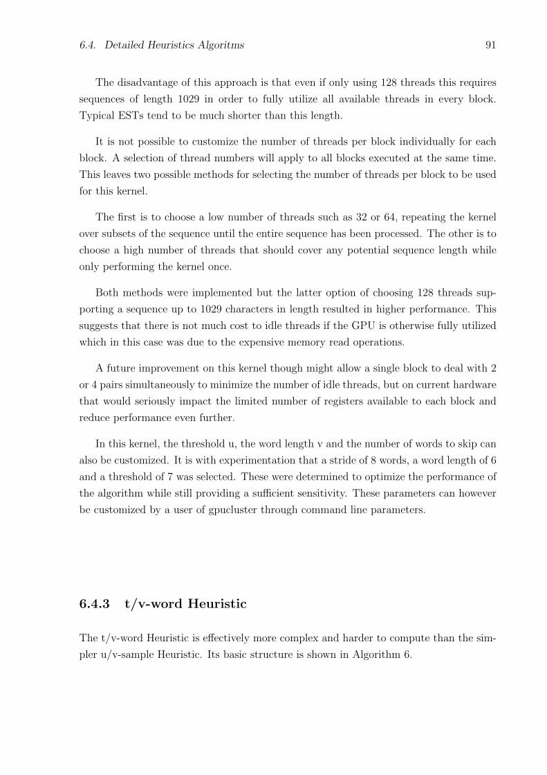
6.4. Detailed Heuristics Algoritms 91
The disadvantage of this approach is that even if only using 128 threads this requires
sequences of length 1029 in order to fully utilize all available threads in every block.
Typical ESTs tend to be much shorter than this length.
It is not possible to customize the number of threads per block individually for each
block. A selection of thread numbers will apply to all blocks executed at the same time.
This leaves two possible methods for selecting the number of threads per block to be used
for this kernel.
The first is to choose a low number of threads such as 32 or 64, repeating the kernel
over subsets of the sequence until the entire sequence has been processed. The other is to
choose a high number of threads that should cover any potential sequence length while
only performing the kernel once.
Both methods were implemented but the latter option of choosing 128 threads sup-
porting a sequence up to 1029 characters in length resulted in higher performance. This
suggests that there is not much cost to idle threads if the GPU is otherwise fully utilized
which in this case was due to the expensive memory read operations.
A future improvement on this kernel though might allow a single block to deal with 2
or 4 pairs simultaneously to minimize the number of idle threads, but on current hardware
that would seriously impact the limited number of registers available to each block and
reduce performance even further.
In this kernel, the threshold u, the word length v and the number of words to skip can
also be customized. It is with experimentation that a stride of 8 words, a word length of 6
and a threshold of 7 was selected. These were determined to optimize the performance of
the algorithm while still providing a sufficient sensitivity. These parameters can however
be customized by a user of gpucluster through command line parameters.
6.4.3 t/v-word Heuristic
The t/v-word Heuristic is effectively more complex and harder to compute than the sim-
pler u/v-sample Heuristic. Its basic structure is shown in Algorithm 6.
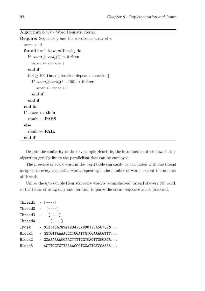
92 Chapter 6. Implementation and Issues
Algorithm 6 t/v - Word Heuristic Kernel
Require: Sequence y and the wordcount array of x
score← 0
for all i = 1 to numWordsy do
if countx[wordy(i)] > 0 then
score← score+ 1
end if
if i ≥ 100 then {Iteration dependent section}if countx[wordy(i− 100)] > 0 then
score← score+ 1
end if
end if
end for
if score > t then
result ← PASS
else
result ← FAIL
end if
Despite the similarity to the u/v-sample Heuristic, the introduction of windows in this
algorithm greatly limits the parallelism that can be employed.
The presence of every word in the word table can easily be calculated with one thread
assigned to every sequential word, repeating if the number of words exceed the number
of threads.
Unlike the u/v-sample Heuristic every word is being checked instead of every 8th word,
so the tactic of using only one iteration to parse the entire sequence is not practical.
Thread1 - [----]
Thread2 - [----]
Thread3 - [----]
Thread4 - [----]
Index - 0123456789012345678901234567890...
Block1 - GGTGTTAAAACCCTGGATTGTCGAAACGTTT...
Block2 - GGAAAAAAGGAACTTTTCGTGACTTGGGACA...
Block3 - ACTTGGTGTTAAAACCCTGGATTGTCGAAAA...
6.5. Detailed Comparison Algoritms 93
Once the presence of every word has been calculated, then a serial process to slide
the window of 100 characters across the entire EST is used to determine if there exists
enough matches within 100 characters to pass. The implementation of this serial process
on the GPU results in much of the GPU is being underutilized. Despite this, executing
this computation on the GPU is still faster than copying the results to the CPU and
testing every window.
The default parameters for this function ware experimentally determined to result in
the best performance and sensitivity if a threshold of 45 words within 100 characters
appear in the word table. More than this results in the rejection of a high number of
potential matches.
Since the t/v-word Heuristic operates directly on the results of the u/v-sample Heuris-
tic without the need for CPU processing, there exists two options for chaining the two
Heuristics together.
The first involves calling the two kernels directly after one another using the data pro-
vided from the first kernel while the other requires that the two kernels be combined into
a single kernel, the t/v-word Heuristic part of the kernel only executing if the u/v-sample
threshold is reached.
Since the entire block’s decision is determined by the threshold, concerns of divergent
branches, which occur when threads follow different branches, is eliminated.
Experimentation showed that a single kernel containing both Heuristics, though it
stresses the available per-thread memory, shared memory and registers, does have slight
performance advantages. It is considered that this advantage occurs due to the less
overhead required in launching two separate kernels.
6.5 Detailed Comparison Algoritms
A customized Smith-Waterman implementation was chosen to be used as the comparison
algorithm for this program. However, since Smith-Waterman is used more typically for
alignment and not for distance, a CPU version of the d2-Algorithm is used for correctness
analysis.
6.5.1 d2-Algorithm
The CPU implementation of the d2-Algorithm was taken and used with permission from
the wcdest tool [117]. Though some editing and customization was needed to use the
94 Chapter 6. Implementation and Issues
algorithm sucessfully in the gpucluster program, it was confirmed to have results identical
to that of the wcdest application. The algorithm performs slower than the original tool,
but this deemed acceptable since this implementation is required simply for correctness
analysis and not performance comparison. The wcdest tool will be used directly for the
purpose of computation of performance in the experiments.
6.5.2 Cumulative Smith-Waterman Distance
The Smith-Waterman algorithm has been implemented on the GPU various times in the
past. Rather than develop a novel implementation, it was decided to simply build up on
an existing implementation, namely that of CUDASW++ [85].
The chosen Cumulative Smith-Waterman Distance is a variation of the Smith-Waterman
algorithm with the addition of a cumulative score and the removal of the requirement to
actually compute the alignment. These customizations of the standard Smith-Waterman
algorithm implies that the exact code that CUDASW++ uses cannot be used, since its
larger scope includes various unneeded computations such as for alignment and support
for protein matching that impacts performance negatively and is not used for nucleotide
sequence clustering.
Instead, an original implementation was developed that uses the same structure as
CUDASW++’s anti-diagonal method, but with the addition of the required modifica-
tions: the removal of alignment support, addition of a cumulative scoring and removing
the algorithm’s support of protein sequences, limiting it to only nucleotide sequences as
detailed in Section 5.6.6. This original implementation additionally allowed much finer
control over the variables and execution which leads to greater optimization opportunities
in terms of memory manamgement, access, operation ordering and placing different parts
of execution in shared memory.
The performance of this implementation was deemed to be sufficient for our purposes,
even if the modifications in terms of scoring makes a direct comparison with the original
implementation impossible. A profile of the kernel revealed no significant bottlenecks.
Once the implementation of the distance algorithm was complete, it still needed to be
tuned to produce results that are similar to that of the d2-Algorithm. This process was
largely automated by executing the program multiple times for every possible variable
combination across a large selection of datasets. This experimentation revealed that a
match reward of 1, a mismatch and gap penalty of 20 and a threshold of a cumulative
score of 100 results in the best and most accurate similarity to the d2-Algorithm.
6.6. Conclusion and summary of concerns 95
The round numbers this experimentation provided is not completely unexpected, since
the threshold matches the default window length of the d2-Algorithm and the mismatch
and gap penalties correspond to a 95% similarity over that window length in order to
pass as a match. This observation increases the confidence that the Cumulative Smith-
Waterman Distance kernel and the d2-distance function will generate similar output over
any other dataset as well.
6.6 Conclusion and summary of concerns
It was found that the majority of processing time of these algorithms was in random access
read patterns. The GPU has great memory bandwidth, but it is optimized for either
sequential reads or in the case of texture memory, reads with 2D locality. Having a large
array such as the word count table randomly accessed stresses the memory capabilities
of the GPU more than intended, since for every byte read and used, at least 32-bytes are
actually fetched from the GPU global memory.
Storing the word table in faster memory such as the constant memory is not optimal
due to the size of the word count tables, which implies that either lower k-values should
be used, which degrades sensitivity, or smaller jobs used at once, which would result in a
higher level of idle multi-processors and thus lower performance.
Another concern is in the branching costs of control statements. It was surprisingly
found that optimizations to exit loops early often serve to slow down the algorithm, as
opposed to speeding it up in CPU equivalents. It is expected though that the ability to
deal with control branches will improve with successive GPUs, but it serves to illustrate
the differences in expectations between CPU and GPU optimization.It does underline the
importance to optimize iteratively and test assumptions under benchmark conditions.
Comparing the algorithm over various GPUs illustrate the clear advancements that
GPUs have made from capability 1.3 to 2.0. There are raw performance improvements,
but the true benefits are realised over the greater amount of instructions and the better
capability to deal with random reads and branching structures.
Lack of proper debugging tools under Linux and inability to expose the internal state
of GPUs contributed negatively to the development time of this project, though the recent
release of the NVIDIA Parallel Nsight Visual Studio plug-in offers to assist with these
concerns. This product is only available for Visual Studio 2008 or Visual Studio 2005
at the time of this writing and requires that the development machine have more than a
single GPU installed (one to debug on, one to continue driving the desktop).

96 Chapter 6. Implementation and Issues
Despite these concerns, the implementation can be considered a success with output
correct and comparable to the output of a CPU only implementation.
The next chapter will detail how this implementation performs in the experiments set
forth in Chapter 4.
Chapter 7
Results and Analysis
7.1 Introduction
With the implementation of our application complete, the experiments detailed in Chapter
4 can now be performed to measure the performance, sensitivity, scalability and short-
comings of the developed application.
The following experiments will be performed:
1. Theoretical Performance and Cost Evaluation This experiment deals with
the comparison of theoretical ‘Peak GFLOPS’ between modern GPU and CPUs.
2. Sensitivity Comparison This experiment measures the sensitivity of the devel-
oped application in comparison to a known good benchmark.
3. Performance Benchmarking This experiment measures performance of the de-
veloped algorithm for different datasets and compares against the performance of a
CPU implementation.
4. Dataset scaling tests This experiment tests the performance of the algorithm
when the dataset size is varied.
5. Profiling Analysis This experiment subjects the algorithm to a dynamic profiling
analysis in order to identify its inefficiencies and computational bottlenecks.
97
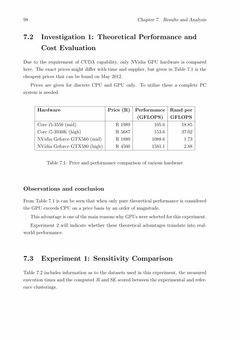
98 Chapter 7. Results and Analysis
7.2 Investigation 1: Theoretical Performance and
Cost Evaluation
Due to the requirement of CUDA capability, only NVidia GPU hardware is compared
here. The exact prices might differ with time and supplier, but given in Table 7.1 is the
cheapest prices that can be found on May 2012.
Prices are given for discrete CPU and GPU only. To utilize these a complete PC
system is needed.
Hardware Price (R) Performance Rand per
(GFLOPS) GFLOPS
Core i5-3550 (mid) R 1989 105.6 18.85
Core i7-3930K (high) R 5687 153.6 37.02
NVidia Geforce GTX560 (mid) R 1880 1088.6 1.73
NVidia Geforce GTX580 (high) R 4560 1581.1 2.88
Table 7.1: Price and performance comparison of various hardware
Observations and conclusion
From Table 7.1 is can be seen that when only pure theoretical performance is considered
the GPU exceeds CPU on a price basis by an order of magnitude.
This advantage is one of the main reasons why GPUs were selected for this experiment.
Experiment 2 will indicate whether these theoretical advantages translate into real-
world performance.
7.3 Experiment 1: Sensitivity Comparison
Table 7.2 includes information as to the datasets used in this experiment, the measured
execution times and the computed JI and SE scored between the experimental and refer-
ence clusterings.
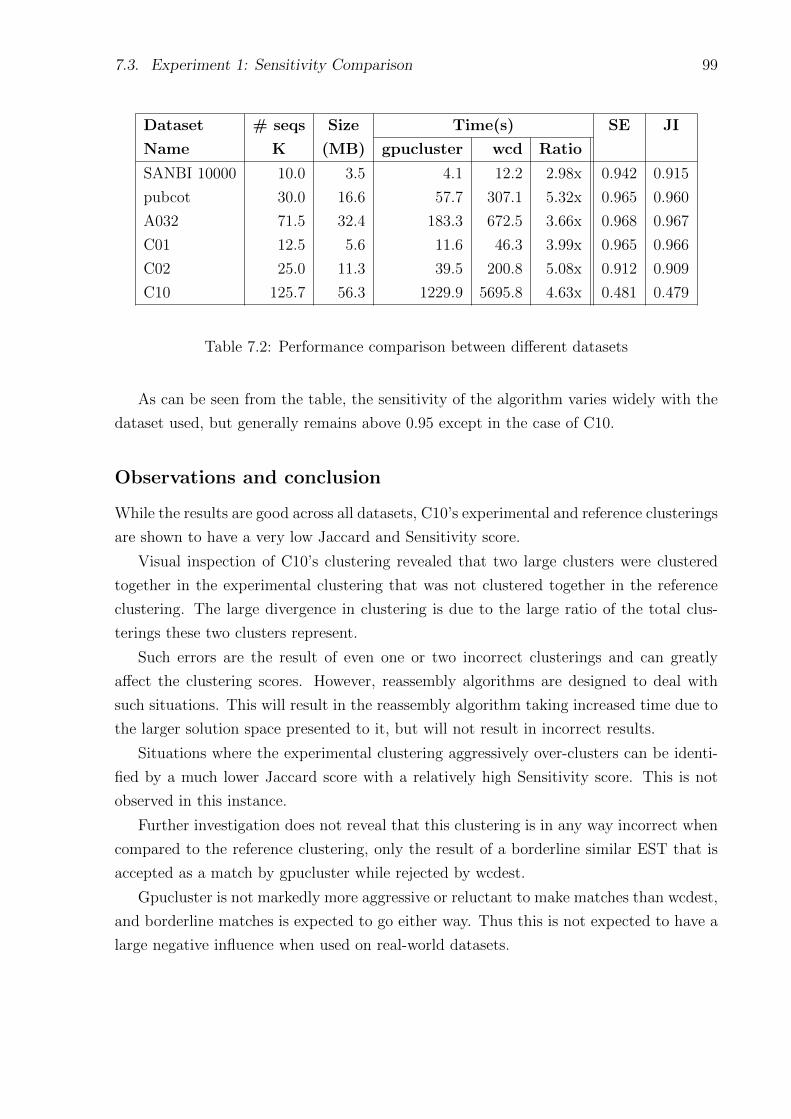
7.3. Experiment 1: Sensitivity Comparison 99
Dataset # seqs Size Time(s) SE JI
Name K (MB) gpucluster wcd Ratio
SANBI 10000 10.0 3.5 4.1 12.2 2.98x 0.942 0.915
pubcot 30.0 16.6 57.7 307.1 5.32x 0.965 0.960
A032 71.5 32.4 183.3 672.5 3.66x 0.968 0.967
C01 12.5 5.6 11.6 46.3 3.99x 0.965 0.966
C02 25.0 11.3 39.5 200.8 5.08x 0.912 0.909
C10 125.7 56.3 1229.9 5695.8 4.63x 0.481 0.479
Table 7.2: Performance comparison between different datasets
As can be seen from the table, the sensitivity of the algorithm varies widely with the
dataset used, but generally remains above 0.95 except in the case of C10.
Observations and conclusion
While the results are good across all datasets, C10’s experimental and reference clusterings
are shown to have a very low Jaccard and Sensitivity score.
Visual inspection of C10’s clustering revealed that two large clusters were clustered
together in the experimental clustering that was not clustered together in the reference
clustering. The large divergence in clustering is due to the large ratio of the total clus-
terings these two clusters represent.
Such errors are the result of even one or two incorrect clusterings and can greatly
affect the clustering scores. However, reassembly algorithms are designed to deal with
such situations. This will result in the reassembly algorithm taking increased time due to
the larger solution space presented to it, but will not result in incorrect results.
Situations where the experimental clustering aggressively over-clusters can be identi-
fied by a much lower Jaccard score with a relatively high Sensitivity score. This is not
observed in this instance.
Further investigation does not reveal that this clustering is in any way incorrect when
compared to the reference clustering, only the result of a borderline similar EST that is
accepted as a match by gpucluster while rejected by wcdest.
Gpucluster is not markedly more aggressive or reluctant to make matches than wcdest,
and borderline matches is expected to go either way. Thus this is not expected to have a
large negative influence when used on real-world datasets.
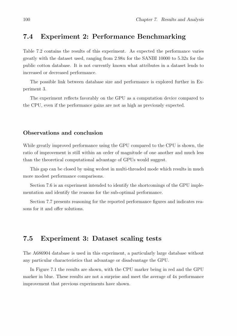
100 Chapter 7. Results and Analysis
7.4 Experiment 2: Performance Benchmarking
Table 7.2 contains the results of this experiment. As expected the performance varies
greatly with the dataset used, ranging from 2.98x for the SANBI 10000 to 5.32x for the
public cotton database. It is not currently known what attributes in a dataset lends to
increased or decreased performance.
The possible link between database size and performance is explored further in Ex-
periment 3.
The experiment reflects favorably on the GPU as a computation device compared to
the CPU, even if the performance gains are not as high as previously expected.
Observations and conclusion
While greatly improved performance using the GPU compared to the CPU is shown, the
ratio of improvement is still within an order of magnitude of one another and much less
than the theoretical computational advantage of GPUs would suggest.
This gap can be closed by using wcdest in multi-threaded mode which results in much
more modest performance comparisons.
Section 7.6 is an experiment intended to identify the shortcomings of the GPU imple-
mentation and identify the reasons for the sub-optimal performance.
Section 7.7 presents reasoning for the reported performance figures and indicates rea-
sons for it and offer solutions.
7.5 Experiment 3: Dataset scaling tests
The A686904 database is used in this experiment, a particularly large database without
any particular characteristics that advantage or disadvantage the GPU.
In Figure 7.1 the results are shown, with the CPU marker being in red and the GPU
marker in blue. These results are not a surprise and meet the average of 4x performance
improvement that previous experiments have shown.
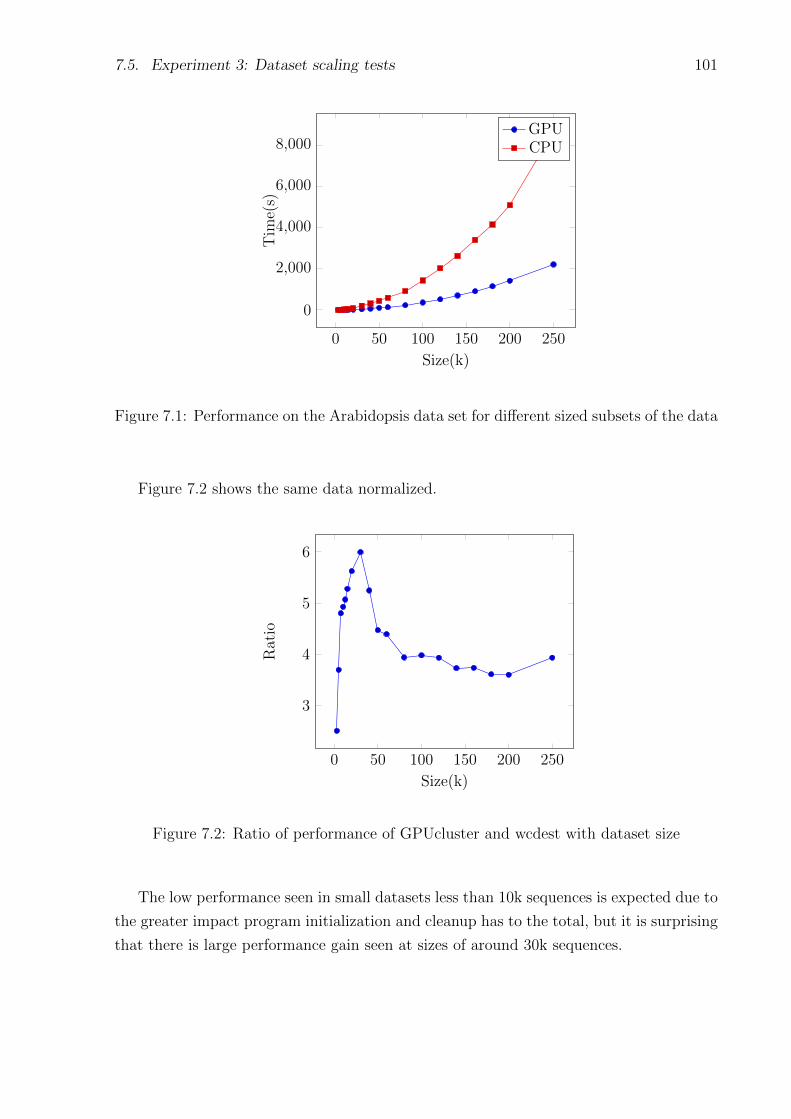
7.5. Experiment 3: Dataset scaling tests 101
0 50 100 150 200 250
0
2,000
4,000
6,000
8,000
Size(k)
Tim
e(s)
GPUCPU
Figure 7.1: Performance on the Arabidopsis data set for different sized subsets of the data
Figure 7.2 shows the same data normalized.
0 50 100 150 200 250
3
4
5
6
Size(k)
Rat
io
Figure 7.2: Ratio of performance of GPUcluster and wcdest with dataset size
The low performance seen in small datasets less than 10k sequences is expected due to
the greater impact program initialization and cleanup has to the total, but it is surprising
that there is large performance gain seen at sizes of around 30k sequences.
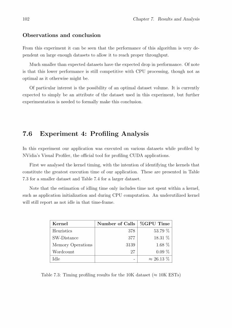
102 Chapter 7. Results and Analysis
Observations and conclusion
From this experiment it can be seen that the performance of this algorithm is very de-
pendent on large enough datasets to allow it to reach proper throughput.
Much smaller than expected datasets have the expected drop in performance. Of note
is that this lower performance is still competitive with CPU processing, though not as
optimal as it otherwise might be.
Of particular interest is the possibility of an optimal dataset volume. It is currently
expected to simply be an attribute of the dataset used in this experiment, but further
experimentation is needed to formally make this conclusion.
7.6 Experiment 4: Profiling Analysis
In this experiment our application was executed on various datasets while profiled by
NVidia’s Visual Profiler, the official tool for profiling CUDA applications.
First we analysed the kernel timing, with the intention of identifying the kernels that
constitute the greatest execution time of our application. These are presented in Table
7.3 for a smaller dataset and Table 7.4 for a larger dataset.
Note that the estimation of idling time only includes time not spent within a kernel,
such as application initialization and during CPU computation. An underutilized kernel
will still report as not idle in that time-frame.
Kernel Number of Calls %GPU Time
Heuristics 378 53.79 %
SW-Distance 377 18.31 %
Memory Operations 3139 1.68 %
Wordcount 27 0.09 %
Idle - ≈ 26.13 %
Table 7.3: Timing profiling results for the 10K dataset (≈ 10K ESTs)
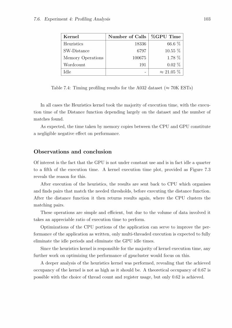
7.6. Experiment 4: Profiling Analysis 103
Kernel Number of Calls %GPU Time
Heuristics 18336 66.6 %
SW-Distance 6797 10.55 %
Memory Operations 100675 1.78 %
Wordcount 191 0.02 %
Idle - ≈ 21.05 %
Table 7.4: Timing profiling results for the A032 dataset (≈ 70K ESTs)
In all cases the Heuristics kernel took the majority of execution time, with the execu-
tion time of the Distance function depending largely on the dataset and the number of
matches found.
As expected, the time taken by memory copies between the CPU and GPU constitute
a negligible negative effect on performance.
Observations and conclusion
Of interest is the fact that the GPU is not under constant use and is in fact idle a quarter
to a fifth of the execution time. A kernel execution time plot, provided as Figure 7.3
reveals the reason for this.
After execution of the heuristics, the results are sent back to CPU which organises
and finds pairs that match the needed thresholds, before executing the distance function.
After the distance function it then returns results again, where the CPU clusters the
matching pairs.
These operations are simple and efficient, but due to the volume of data involved it
takes an appreciable ratio of execution time to perform.
Optimizations of the CPU portions of the application can serve to improve the per-
formance of the application as written, only multi-threaded execution is expected to fully
eliminate the idle periods and eliminate the GPU idle times.
Since the heuristics kernel is responsible for the majority of kernel execution time, any
further work on optimizing the performance of gpucluster would focus on this.
A deeper analysis of the heuristics kernel was performed, revealing that the achieved
occupancy of the kernel is not as high as it should be. A theoretical occupancy of 0.67 is
possible with the choice of thread count and register usage, but only 0.62 is achieved.
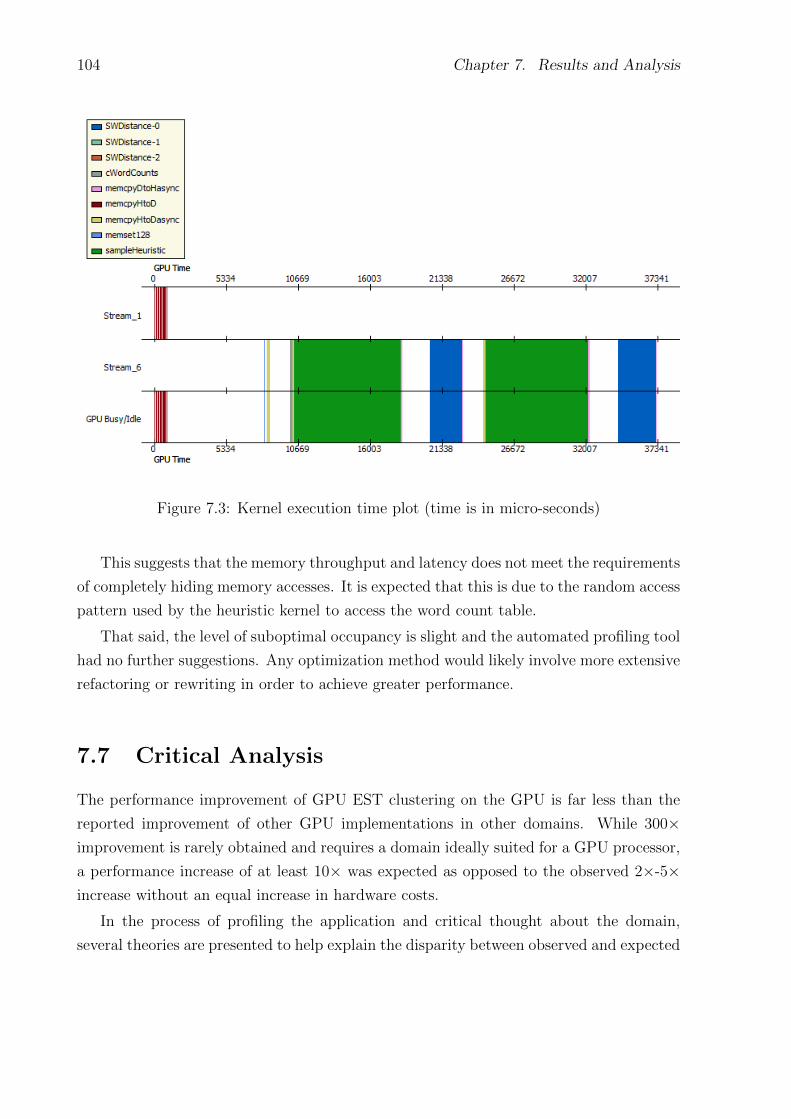
104 Chapter 7. Results and Analysis
Figure 7.3: Kernel execution time plot (time is in micro-seconds)
This suggests that the memory throughput and latency does not meet the requirements
of completely hiding memory accesses. It is expected that this is due to the random access
pattern used by the heuristic kernel to access the word count table.
That said, the level of suboptimal occupancy is slight and the automated profiling tool
had no further suggestions. Any optimization method would likely involve more extensive
refactoring or rewriting in order to achieve greater performance.
7.7 Critical Analysis
The performance improvement of GPU EST clustering on the GPU is far less than the
reported improvement of other GPU implementations in other domains. While 300×improvement is rarely obtained and requires a domain ideally suited for a GPU processor,
a performance increase of at least 10× was expected as opposed to the observed 2×-5×increase without an equal increase in hardware costs.
In the process of profiling the application and critical thought about the domain,
several theories are presented to help explain the disparity between observed and expected
7.7. Critical Analysis 105
performance results.
7.7.1 Multiple Threads
When this application was first designed and programmed, CUDA did not support multi-
ple CPU threads accessing the same GPU Context. Since that time though their support
for this scenario has increased. This offers the best opportunity for further work to im-
prove the performance of the application by eliminating GPU idle times, as well as add
support for multiple GPU operation.
7.7.2 Concurrent Execution
Many CUDA GPUs have the capability to ’hide’ memory latencies by performing copies
at the same time. While this is viable to employ in this application, Table 7.3 and
Table 7.4 indicates that this is unlikely to provide a large benefit, at best improving the
performance by 1%-2%. The negative effects of the increased complexity in application
structure suggests that this is not a worthwhile effort.
7.7.3 Sequences Data Size
In many GPU applications the application deals with data points or single or composite
numbers such as floating positions or color components. When dealing with biological
sequences however analysis is done on many bytes worth of data all of which needs to be
compared with all of the bytes of data of the comparison sequence.
This explosion in data read and memory requirements greatly increases the amount of
data needed to be read from memory and processed without greatly increasing the com-
putational requirements, leaving the GPU to be memory bandwidth limited and unable
to properly utilize its full computational ability.
7.7.4 Random Reads
Random reads of GPU memory is much much slower than reads of consecutive or spatially
related reads, possibly up to 16× slower if there is no spatial similarity. This is one of the
greatest negative effects when profiling the application, being one of the main causes of
memory bandwidth saturation.
This occurs especially often in the u/v-sample and t/v-word heuristics, which is per-
formed on each and every sequence comparison.
106 Chapter 7. Results and Analysis
7.7.5 Branching
Efforts have been made to minimize the amount of branching in the application to its
minimum, limiting it to block-level decisions as much as possible, but when profiling there
is still an apparent small negative effect of branching present.
7.8 Conclusion
The performance results of this experiment is disappointing, but it does serve to illustrate
why GPU computation has not spread to more domains than it already has.
While performance far greater than the CPU is certainly possible, there is additional
requirements on the type of data, its data dependencies, how it is streamed to the GPU
and how it is computed that limit the applications for which GPU computation is useful.
Many of these limits can be overcome as in this application, but not without a potentially
large performance decrease.
Regardless, this does show that if provided a PC with a powerful GPU, gpucluster
can greatly increase performance, though not by an order of magnitude. This advantage
can however be largely negated by a more powerful multi-core CPU operating across all
of its cores.
The quality results show however that the application is certainly useful for EST
clustering, providing correct results at good performance.
Chapter 8
Conclusion and Further Work
8.1 Summary
In this dissertation we had the aim of utilizing GPU technology in order to optimize and
improve on the problem of EST clustering.
Extensive research on this cross-disciplinary approach was required before even con-
sidering such an approach. It was found that though this line of research has not received
significant attention, there are significant gains that can be made through a project that
utilizes GPU computing for bioinformatics problems.
GPU programming differs from classical CPU programming in significant ways so a
familiarity with the CUDA API is needed in order to achieve the performance goals.
Understanding of the various types of parallelism and memory provided by GPUs is
essential to optimizing the execution of a CUDA application.
The metrics for performance and sensitivity measurement is important to consider for
fair comparison between different platforms. The details and goals for the project is de-
fined and expectations used for a measurement of success is defined before the application
is implemented.
EST clustering is a wide field with no single correct algorithm or implementation. For
this reason extensive research had to be done in order to identify potential algorithms
that this project will utilize. Each of the proposed algorithms are analysed for suitability
for the GPU platform with their weaknesses and strengths identified. Most had to be
discarded due to the limited scope of the project, but suitable algorithms for porting were
found.
Implementation involved a lot of learning, adapting, and a few surprises, but eventually
a program was completed that met the goals of the project.
107
108 Chapter 8. Conclusion and Further Work
Though the performance improvement was not as great as initially expected, the GPU
implementation shows promise as an alternative to the classical CPU computing approach
that is currently used. Though many shortcomings of the implementation was identified,
it still performed well and produced correct results.
It is the opinion of the author that this project has proven to be a success, not just in
its implementation, but more importantly it can serve as an example of GPU use in the
bioinformatics field. By identifying the many pitfalls and issues it is hoped that similar
problems can be avoided by other researchers working on similar problems.
8.2 Research Question Resolution
The objective of this research was to answer several questions posed in Section 1.3. The
scope of this project deals primarily with EST clustering, so the answers given may not
apply to the entire bioinformatics field. The insight provided may prove useful for any
future research.
1. Is GPGPU a practical computing platform for bioinformatics algorithms?
Section 2.4.4 in Chapter 2 lists various cases where GPGPU has been successfully
utilized in bioinformatics applications.
The positive results of the project leads to the conclusion that GPGPU can be a
practical computing platform for bioinformatics algorithms.
2. Can existing bioinformatics algorithms be practically ported to GPGPU?
Research listed in Section 2.4.4 provide examples of other ported algorithms that
was successfully used on the GPGPU platform. In addition, the positive results of
this project leads to the conclusion that bioinformatics algorithms can be ported
successfully to the GPGPU platform.
3. Is the cost of GPGPU competitive with classical CPU computing?
Yes, the costs have been shown to be competitive as per the cost evaluation in
Section 7.2.
4. Is the performance of GPGPU competitive with classical CPU comput-
ing?
Yes, the performance has been shown to be competitive as per the results of Exper-
iment 4 in Section 7.4.
8.3. Further Work 109
8.3 Further Work
Much of the work detailed in this thesis can be expanded on and improved through further
research and development. Though this project met its goals, various avenues of potential
further research and development has become apparent. This section will list the various
possible approaches that can allow further work to improve on the developed application.
8.3.1 Faster Heuristics
While the selected heuristics perform well on the CPU, this thesis has shown that they
port poorly to the GPU due to the great need for lookup tables utilizing random reads.
An alternate heuristic using fewer random reads and more linear reads can potentially
increase the performance of gpucluster significantly.
Another option is pre-sorting words before searching, potentially allowing the random
reads to occur much spatially closer to one another, decreasing their negative impact.
8.3.2 Multiple GPU
An obvious possible improvement would be to utilize the power of multiple GPUs on the
same PC. Using such a second GPU can potentially double the performance of gpucluster
for 2 GPUs.
Of note is the fact that many high end GPUs such as the Nvidia GTX 595 are two
separate GPUs located on the same board. Logistically and from the view of gpucluster
these remain separate GPUs and need to be managed separately, requiring the application
to implement multi-GPU support to properly utilize such a GPU.
8.3.3 CPU Concurrent Use
It is observed that the current gpucluster implementation largely leaves the CPU relatively
idle. A very possible performance improvement would be to use the CPU and GPU
concurrently on the same dataset, increasing utilization of all of a PC’s computational
assets.
110 Chapter 8. Conclusion and Further Work
8.4 Conclusion
GPU computation has great potential to be an invaluable tool in bioinformatics pro-
cessing. Though GPU computing is not dependent on overly expensive equipment, a
significant investment of time and effort on the part of developers is needed to make the
shift required for learning the programming paradigms involved in GPU programming.
This limits the pool of developers capable of fully taking advantage of GPGPU.
Despite this challenge, the advancing rate of GPU computing is promising for small
and large laboratories to enable much cheaper and more powerful computation of complex
data and interactions.

Bibliography
[1] Wikipedia, “Nucleotide — Wikipedia, The Free Encyclopedia,” 2011, [Online;
accessed 26-February-2011]. [Online]. Available: http://en.wikipedia.org/w/index.
php?title=Nucleotide&oldid=412067409
[2] NVidia Corporation. (2010, june) NVidia CUDA Programming Guide 3.1.
[Online]. Available: http://developer.download.nvidia.com/compute/cuda/3 1/
toolkit/docs/NVIDIA CUDA C ProgrammingGuide 3.1.pdf
[3] R. Schaller, “Moore’s law: past, present and future,” Spectrum, IEEE, vol. 34, no. 6,
pp. 52–59, 1997.
[4] Wikipedia, “FLOPS — Wikipedia, the free encyclopedia,” 2011, [Online; accessed
1-March-2011]. [Online]. Available: http://en.wikipedia.org/w/index.php?title=
FLOPS&oldid=416575050
[5] S. Ryoo, C. Rodrigues, S. Baghsorkhi, S. Stone, D. Kirk, and W. Hwu, “Optimiza-
tion principles and application performance evaluation of a multithreaded GPU us-
ing CUDA,” in Proceedings of the 13th ACM SIGPLAN Symposium on Principles
and practice of parallel programming. ACM, 2008, pp. 73–82.
[6] D. P. Anderson, “BOINC: A System for Public-Resource Computing and Storage,”
in Proceedings of the 5th IEEE/ACM International Workshop on Grid Computing,
ser. GRID ’04. Washington, DC, USA: IEEE Computer Society, 2004, pp. 4–10.
[Online]. Available: http://dx.doi.org/10.1109/GRID.2004.14
[7] C. van Deventer, W. Clarke, and S. Hazelhurst, “BOINC and CUDA: Distributed
High-Performance Computing for Bioinformatics String Matching Problems,” in
Proceedings of the Southern Africa Telecommunication Networks and Applications
Conference, Sept, 2010.
[8] E. Nordenskiold, “The history of biology.” 1928.
111
112 Bibliography
[9] H. Vickery, “The origin of the word protein,” The Yale journal of biology and
medicine, vol. 22, no. 5, p. 387, 1950.
[10] D. Davison, “The number of human genes and proteins,” Nanotech, vol. 2, pp. 6–11,
2002.
[11] G. Mendel, A. Corcos, and F. Monaghan, Gregor Mendel’s Experiments on plant
hybrids: a guided study. Rutgers Univ Pr, 1993.
[12] R. Henig, The monk in the garden: the lost and found genius of Gregor Mendel, the
father of genetics. Mariner Books, 2001.
[13] C. Darwin, “On the origin of species by means of natural selection. 1859,” Leipzig:
Verlag Philipp Reclam, 1859.
[14] T. Morgan et al., “Sex limited inheritance in Drosophila,” Science, vol. 32, no. 812,
pp. 120–122, 1910.
[15] R. Dahm, “Friedrich Miescher and the discovery of DNA,” Developmental Biology,
vol. 278, no. 2, pp. 274–288, 2005.
[16] P. Ceruzzi, A history of modern computing. The MIT press, 2003.
[17] J. Watson and F. Crick, “Molecular structure of nucleic acids,” Nature, vol. 171,
no. 4356, pp. 737–738, 1953.
[18] F. Crick and J. Watson, “A structure for deoxyribose nucleic acid,” Nature, vol.
171, no. 737-738, 1953.
[19] G. Gamow, A. Rich, and M. Ycas, “The problem of information transfer from the
nucleic acids to proteins.” Advances in biological and medical physics, vol. 4, p. 23,
1956.
[20] L. Gatlin, “The information content of DNA,” Journal of Theoretical Biology,
vol. 10, no. 2, pp. 281–300, 1966.
[21] C. Shannon, Mathematical theory of communication. University Illinois Press, 1963.
[22] A. Gibbs and G. Mcintyre, “The diagram, a method for comparing sequences,”
European Journal of Biochemistry, vol. 16, no. 1, pp. 1–11, 1970.
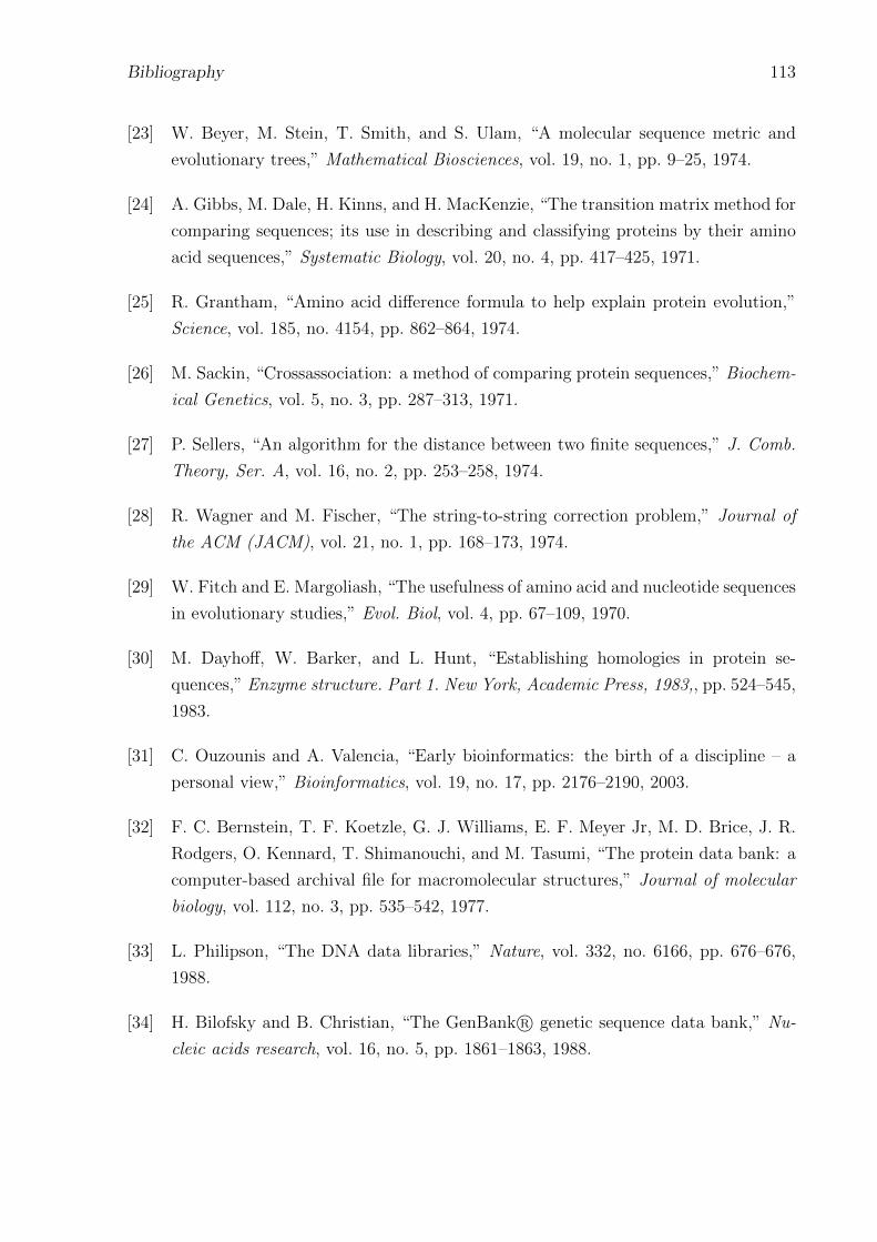
Bibliography 113
[23] W. Beyer, M. Stein, T. Smith, and S. Ulam, “A molecular sequence metric and
evolutionary trees,” Mathematical Biosciences, vol. 19, no. 1, pp. 9–25, 1974.
[24] A. Gibbs, M. Dale, H. Kinns, and H. MacKenzie, “The transition matrix method for
comparing sequences; its use in describing and classifying proteins by their amino
acid sequences,” Systematic Biology, vol. 20, no. 4, pp. 417–425, 1971.
[25] R. Grantham, “Amino acid difference formula to help explain protein evolution,”
Science, vol. 185, no. 4154, pp. 862–864, 1974.
[26] M. Sackin, “Crossassociation: a method of comparing protein sequences,” Biochem-
ical Genetics, vol. 5, no. 3, pp. 287–313, 1971.
[27] P. Sellers, “An algorithm for the distance between two finite sequences,” J. Comb.
Theory, Ser. A, vol. 16, no. 2, pp. 253–258, 1974.
[28] R. Wagner and M. Fischer, “The string-to-string correction problem,” Journal of
the ACM (JACM), vol. 21, no. 1, pp. 168–173, 1974.
[29] W. Fitch and E. Margoliash, “The usefulness of amino acid and nucleotide sequences
in evolutionary studies,” Evol. Biol, vol. 4, pp. 67–109, 1970.
[30] M. Dayhoff, W. Barker, and L. Hunt, “Establishing homologies in protein se-
quences,” Enzyme structure. Part 1. New York, Academic Press, 1983,, pp. 524–545,
1983.
[31] C. Ouzounis and A. Valencia, “Early bioinformatics: the birth of a discipline – a
personal view,” Bioinformatics, vol. 19, no. 17, pp. 2176–2190, 2003.
[32] F. C. Bernstein, T. F. Koetzle, G. J. Williams, E. F. Meyer Jr, M. D. Brice, J. R.
Rodgers, O. Kennard, T. Shimanouchi, and M. Tasumi, “The protein data bank: a
computer-based archival file for macromolecular structures,” Journal of molecular
biology, vol. 112, no. 3, pp. 535–542, 1977.
[33] L. Philipson, “The DNA data libraries,” Nature, vol. 332, no. 6166, pp. 676–676,
1988.
[34] H. Bilofsky and B. Christian, “The GenBank R© genetic sequence data bank,” Nu-
cleic acids research, vol. 16, no. 5, pp. 1861–1863, 1988.
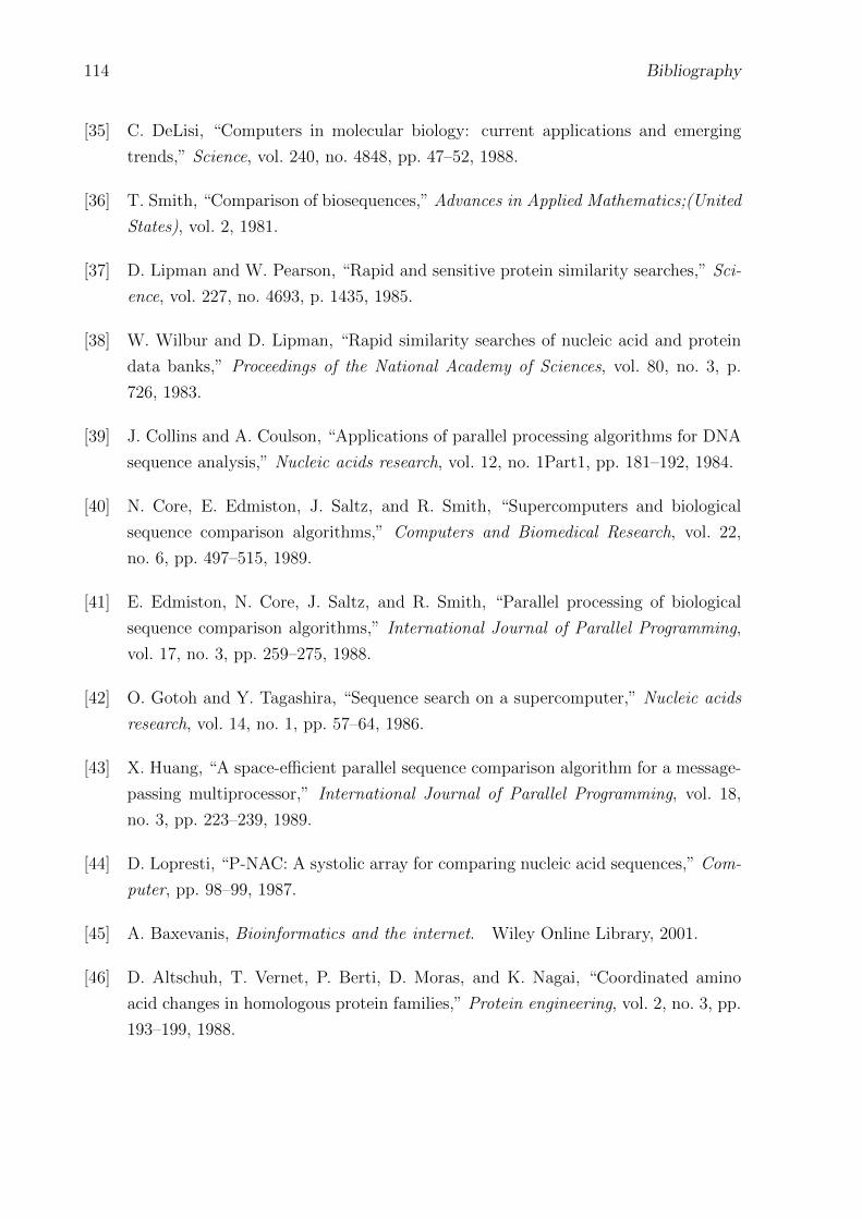
114 Bibliography
[35] C. DeLisi, “Computers in molecular biology: current applications and emerging
trends,” Science, vol. 240, no. 4848, pp. 47–52, 1988.
[36] T. Smith, “Comparison of biosequences,” Advances in Applied Mathematics;(United
States), vol. 2, 1981.
[37] D. Lipman and W. Pearson, “Rapid and sensitive protein similarity searches,” Sci-
ence, vol. 227, no. 4693, p. 1435, 1985.
[38] W. Wilbur and D. Lipman, “Rapid similarity searches of nucleic acid and protein
data banks,” Proceedings of the National Academy of Sciences, vol. 80, no. 3, p.
726, 1983.
[39] J. Collins and A. Coulson, “Applications of parallel processing algorithms for DNA
sequence analysis,” Nucleic acids research, vol. 12, no. 1Part1, pp. 181–192, 1984.
[40] N. Core, E. Edmiston, J. Saltz, and R. Smith, “Supercomputers and biological
sequence comparison algorithms,” Computers and Biomedical Research, vol. 22,
no. 6, pp. 497–515, 1989.
[41] E. Edmiston, N. Core, J. Saltz, and R. Smith, “Parallel processing of biological
sequence comparison algorithms,” International Journal of Parallel Programming,
vol. 17, no. 3, pp. 259–275, 1988.
[42] O. Gotoh and Y. Tagashira, “Sequence search on a supercomputer,” Nucleic acids
research, vol. 14, no. 1, pp. 57–64, 1986.
[43] X. Huang, “A space-efficient parallel sequence comparison algorithm for a message-
passing multiprocessor,” International Journal of Parallel Programming, vol. 18,
no. 3, pp. 223–239, 1989.
[44] D. Lopresti, “P-NAC: A systolic array for comparing nucleic acid sequences,” Com-
puter, pp. 98–99, 1987.
[45] A. Baxevanis, Bioinformatics and the internet. Wiley Online Library, 2001.
[46] D. Altschuh, T. Vernet, P. Berti, D. Moras, and K. Nagai, “Coordinated amino
acid changes in homologous protein families,” Protein engineering, vol. 2, no. 3, pp.
193–199, 1988.
Bibliography 115
[47] F. Collins, A. Patrinos, E. Jordan, A. Chakravarti, R. Gesteland, L. Walters et al.,
“New goals for the US human genome project: 1998-2003,” Science, vol. 282, no.
5389, pp. 682–689, 1998.
[48] E. Lander, L. Linton, B. Birren, C. Nusbaum, M. Zody, J. Baldwin, K. Devon,
K. Dewar, M. Doyle, W. FitzHugh et al., “Initial sequencing and analysis of the
human genome,” Nature, vol. 409, no. 6822, pp. 860–921, 2001.
[49] F. Collins, E. Lander, J. Rogers, R. Waterston, and I. Conso, “Finishing the eu-
chromatic sequence of the human genome,” Nature, vol. 431, no. 7011, pp. 931–945,
2004.
[50] F. Collins, M. Morgan, and A. Patrinos, “The Human Genome Project: lessons
from large-scale biology,” Science, vol. 300, no. 5617, pp. 286–290, 2003.
[51] M. Adams, J. Kelley, J. Gocayne, M. Dubnick, M. Polymeropoulos, H. Xiao, C. Mer-
ril, A. Wu, B. Olde, R. Moreno et al., “Complementary DNA sequencing: expressed
sequence tags and human genome project,” Science, vol. 252, no. 5013, pp. 1651–
1656, 1991.
[52] Y. Lee, J. Tsai, S. Sunkara, S. Karamycheva, G. Pertea, R. Sultana, V. Antonescu,
A. Chan, F. Cheung, and J. Quackenbush, “The TIGR Gene Indices: clustering
and assembling EST and known genes and integration with eukaryotic genomes,”
Nucleic acids research, vol. 33, no. suppl 1, p. D71, 2005.
[53] P. Green, “Phrap,” Unpublished, available for download at
http://www.genome.washington.edu/UWGC/analysistools/phrap.htm, 1994.
[54] F. Liang, I. Holt, G. Pertea, S. Karamycheva, S. Salzberg, and J. Quackenbush, “An
optimized protocol for analysis of EST sequences,” Nucleic acids research, vol. 28,
no. 18, p. 3657, 2000.
[55] X. Huang and A. Madan, “CAP3: A DNA Sequence Assembly Program,”
Genome Research, vol. 9, no. 9, pp. 868–877, 1999. [Online]. Available:
http://genome.cshlp.org/content/9/9/868.abstract
[56] G. Pertea, X. Huang, F. Liang, V. Antonescu, R. Sultana, S. Karamycheva, Y. Lee,
J. White, F. Cheung, B. Parvizi et al., “TIGR Gene Indices clustering tools (TG-
ICL): a software system for fast clustering of large EST datasets,” Bioinformatics,
vol. 19, no. 5, p. 651, 2003.
116 Bibliography
[57] A. Kalyanaraman, S. Aluru, S. Kothari, and V. Brendel, “Efficient clustering of
large EST data sets on parallel computers,” Nucleic Acids Research, vol. 31, no. 11,
p. 2963, 2003.
[58] J. Burke, D. Davison, and W. Hide, “d2 cluster: a validated method for clustering
EST and full-length cDNA sequences,” Genome Research, vol. 9, no. 11, p. 1135,
1999.
[59] S. Hazelhurst, W. Hide, Z. Liptak, R. Nogueira, and R. Starfield, “An
overview of the wcd EST clustering tool.” Bioinformatics (Oxford, England),
vol. 24, no. 13, pp. 1542–1546, July 2008. [Online]. Available: http:
//dx.doi.org/10.1093/bioinformatics/btn203
[60] J. Rhoades, G. Turk, A. Bell, U. Neumann, A. Varshney et al., “Real-time proce-
dural textures,” in Proceedings of the 1992 symposium on Interactive 3D graphics.
ACM, 1992, pp. 95–100.
[61] J. Eyles, S. Molnar, J. Poulton, T. Greer, A. Lastra, N. England, and L. West-
over, “PixelFlow: the realization,” in Proceedings of the ACM SIGGRAPH/EURO-
GRAPHICS workshop on Graphics hardware. ACM, 1997, pp. 57–68.
[62] B. Jobard, G. Erlebacher, and M. Hussaini, “Lagrangian-eulerian advection for
unsteady flow visualization,” in Proceedings of the conference on Visualization’01.
IEEE Computer Society, 2001, pp. 53–60.
[63] C. Bohn, “Kohonen feature mapping through graphics hardware,” in Proceedings of
the 3rd Int. Conference on Computational Intelligence and Neurosciences, 1998.
[64] N. Carr, J. Hall, and J. Hart, “The ray engine,” in Proceedings of the ACM SIG-
GRAPH/EUROGRAPHICS conference on Graphics hardware. Eurographics As-
sociation, 2002, pp. 37–46.
[65] T. Purcell, I. Buck, W. Mark, and P. Hanrahan, “Ray tracing on programmable
graphics hardware,” ACM Transactions on Graphics (TOG), vol. 21, no. 3, pp.
703–712, 2002.
[66] J. Tran, D. Jordan, and D. Luebke, “New challenges for cellular automata simulation
on the GPU,” 2003.
Bibliography 117
[67] M. Harris, G. Coombe, T. Scheuermann, and A. Lastra, “Physically-based visual
simulation on graphics hardware,” in Proceedings of the ACM SIGGRAPH/EURO-
GRAPHICS conference on Graphics hardware. Eurographics Association, 2002,
pp. 109–118.
[68] N. Govindaraju, J. Gray, R. Kumar, and D. Manocha, “GPUTeraSort: high perfor-
mance graphics co-processor sorting for large database management,” in Proceed-
ings of the 2006 ACM SIGMOD international conference on Management of data.
ACM, 2006, pp. 325–336.
[69] N. Govindaraju, D. Manocha, N. Raghuvanshi, and D. Tuft, “Gpusort: High per-
formance sorting using graphics processors,” 2006.
[70] E. Elsen, V. Vishal, M. Houston, V. Pande, P. Hanrahan, and E. Darve, “N-body
simulations on GPUs,” Arxiv preprint arXiv:0706.3060, 2007.
[71] M. Harris, “Fast fluid dynamics simulation on the GPU,” GPU gems, vol. 1, pp.
637–665, 2004.
[72] I. Buck, T. Foley, D. Horn, J. Sugerman, K. Fatahalian, M. Houston, and P. Hanra-
han, “Brook for GPUs: stream computing on graphics hardware,” in ACM Trans-
actions on Graphics (TOG), vol. 23, no. 3. ACM, 2004, pp. 777–786.
[73] I. Buck, “High level languages for GPUs,” in ACM SIGGRAPH, 2005.
[74] M. McCool, K. Wadleigh, B. Henderson, and H. Lin, “Performance evaluation of
GPUs using the RapidMind development platform,” in Proceedings of the 2006
ACM/IEEE conference on Supercomputing. ACM, 2006, p. 181.
[75] Berkeley University. (2010, Aug.) SETI@home Website. [Online]. Available:
http://setiathome.berkeley.edu/
[76] D. Anderson, J. Cobb, E. Korpela, M. Lebofsky, and D. Werthimer, “SETI@home:
an experiment in public-resource computing,” Communications of the ACM, vol. 45,
no. 11, pp. 56–61, 2002.
[77] Stanford University. (2010, Aug.) Folding@home Website. [Online]. Available:
http://folding.stanford.edu
118 Bibliography
[78] A. Beberg, D. Ensign, G. Jayachandran, S. Khaliq, and V. Pande, “Folding@home:
Lessons from eight years of volunteer distributed computing,” in Parallel & Dis-
tributed Processing, 2009. IPDPS 2009. IEEE International Symposium on. IEEE,
2009, pp. 1–8.
[79] W. Liu, B. Schmidt, G. Voss, A. Schroder, and W. Muller-Wittig, “Bio-sequence
database scanning on a GPU,” in Parallel and Distributed Processing Symposium,
2006. IPDPS 2006. 20th International. IEEE, 2006, pp. 8–pp.
[80] Y. Liu, W. Huang, J. Johnson, and S. Vaidya, “GPU accelerated smith-waterman,”
Computational Science–ICCS 2006, pp. 188–195, 2006.
[81] M. Charalambous, P. Trancoso, and A. Stamatakis, “Initial experiences porting a
bioinformatics application to a graphics processor,” Advances in Informatics, pp.
415–425, 2005.
[82] M. Schatz and C. Trapnell, “Fast exact string matching on the GPU,” Center for
Bioinformatics and Computational Biology, 2007.
[83] NVidia. (2011, Aug.) NVidia: Bio-Informatics and Life Sciences. [Online].
Available: http://www.nvidia.com/object/bio info life sciences.html
[84] S. Manavski and G. Valle, “CUDA compatible GPU cards as efficient hardware
accelerators for Smith-Waterman sequence alignment,” BMC bioinformatics, vol. 9,
no. Suppl 2, p. S10, 2008.
[85] Y. Liu, B. Schmidt, and D. Maskell, “CUDASW++ 2. 0: enhanced Smith-
Waterman protein database search on CUDA-enabled GPUs based on SIMT and
virtualized SIMD abstractions,” BMC Research Notes, vol. 3, no. 1, p. 93, 2010.
[86] Y. Munekawa, F. Ino, and K. Hagihara, “Design and implementation of the Smith-
Waterman algorithm on the CUDA-compatible GPU,” in BioInformatics and Bio-
Engineering, 2008. BIBE 2008. 8th IEEE International Conference on. IEEE,
2008, pp. 1–6.
[87] A. Akoglu and G. Striemer, “Scalable and highly parallel implementation of Smith-
Waterman on graphics processing unit using CUDA,” Cluster Computing, vol. 12,
no. 3, pp. 341–352, 2009.
[88] G. Striemer and A. Akoglu, “Sequence alignment with GPU: Performance and de-
sign challenges,” 2009.
Bibliography 119
[89] J. Walters, V. Balu, S. Kompalli, and V. Chaudhary, “Evaluating the use of GPUs in
liver image segmentation and HMMER database searches,” in Parallel & Distributed
Processing, 2009. IPDPS 2009. IEEE International Symposium on. IEEE, 2009,
pp. 1–12.
[90] M. Schatz, C. Trapnell, A. Delcher, and A. Varshney, “High-throughput sequence
alignment using Graphics Processing Units,” BMC bioinformatics, vol. 8, no. 1, p.
474, 2007.
[91] A. Eklund, M. Andersson, and H. Knutsson, “fMRI analysis on the GPU - possi-
bilities and challenges,” Computer Methods and Programs in Biomedicine, vol. 105,
no. 2, pp. 145–161, 2012.
[92] T. Sumanaweera and D. Liu, “Medical image reconstruction with the FFT,” GPU
gems, vol. 2, pp. 765–784, 2005.
[93] T. Kroes, F. Post, and C. Botha, “Exposure render: An interactive photo-realistic
volume rendering framework,” PloS one, vol. 7, no. 7, p. e38586, 2012.
[94] W. Liu, B. Schmidt, and W. Muller-Wittig, “CUDA-BLASTP: Accelerating
BLASTP on CUDA-Enabled Graphics Hardware,” IEEE/ACM Transactions on
Computational Biology and Bioinformatics (TCBB), vol. 8, no. 6, pp. 1678–1684,
2011.
[95] C. Trapnell and M. Schatz, “Optimizing data intensive GPGPU computations for
DNA sequence alignment,” Parallel computing, vol. 35, no. 8, pp. 429–440, 2009.
[96] K. Karimi, N. Dickson, and F. Hamze, “A performance comparison of CUDA and
OpenCL,” Arxiv preprint arXiv:1005.2581, 2010.
[97] K. Okonechnikov, O. Golosova, M. Fursov et al., “Unipro UGENE: a unified bioin-
formatics toolkit,” Bioinformatics, vol. 28, no. 8, pp. 1166–1167, 2012.
[98] U. o. M. Yang Zhang’s Research Group, “What is FASTA format?” 2011,
[Online; accessed 26-November-2011]. [Online]. Available: http://zhanglab.ccmb.
med.umich.edu/FASTA/
[99] P. Hanrahan, “Why is graphics hardware so fast?” in Proceedings of the tenth ACM
SIGPLAN symposium on Principles and practice of parallel programming. ACM,
2005, pp. 1–1.
120 Bibliography
[100] C. Gregg and K. Hazelwood, “Where is the data? Why you cannot debate CPU
vs. GPU performance without the answer,” in Performance Analysis of Systems
and Software (ISPASS), 2011 IEEE International Symposium on. IEEE, 2011, pp.
134–144.
[101] V. Podlozhnyuk, “FFT-based 2D convolution,” NVIDIA white paper, 2007.
[102] C. NVIDIA, “CUBLAS Library,” NVIDIA Corporation, Santa Clara, California,
vol. 15, 2008.
[103] M. Naumov, “CUSPARSE Library: A Set of Basic Linear Algebra Subroutines for
Sparse Matrices,” in GPU Technology Conference, vol. 2070.
[104] C. NVIDIA, “CURAND library,” NVIDIA Corporation, Santa Clara, California,
vol. 50, 2008.
[105] M. Harris, “Optimizing CUDA,” SC07: High Performance Computing With CUDA,
2007.
[106] V. Volkov, “Better performance at lower occupancy,” in Proceedings of the GPU
Technology Conference, GTC, vol. 10, 2010.
[107] NVidia Corporation. (2010, Aug.) CUDA Occupancy Calculator. [Online]. Avail-
able: http://developer.download.nvidia.com/compute/cuda/CUDA Occupancy
calculator.xls
[108] P. Jaccard, “The distribution of the flora in the alpine zone,” New Phytologist,
vol. 11, no. 2, pp. 37–50, 1912.
[109] G. Amdahl, “Validity of the single processor approach to achieving large scale com-
puting capabilities,” in Proceedings of the April 18-20, 1967, spring joint computer
conference. ACM, 1967, pp. 483–485.
[110] S. Hazelhurst, “Computational Performance Benchmarking of the wcd EST Clus-
tering System,” Technical Report TR-Wits-CS-2007-1, School of Computer Science,
University of the Witwatersrand, Tech. Rep., 2007.
[111] S. Mayanglambam, A. Malony, and M. Sottile, “Performance measurement of ap-
plications with GPU acceleration using CUDA,” in International Conference on
Parallel Computing (ParCo), 2009.
Bibliography 121
[112] U. Manber and G. Myers, “Suffix arrays: a new method for on-line
string searches,” in Proceedings of the first annual ACM-SIAM symposium
on Discrete algorithms, ser. SODA ’90. Philadelphia, PA, USA: Society for
Industrial and Applied Mathematics, 1990, pp. 319–327. [Online]. Available:
http://portal.acm.org/citation.cfm?id=320176.320218
[113] S. Puglisi, W. Smyth, and A. Turpin, “A taxonomy of suffix array construction
algorithms,” ACM Computing Surveys (CSUR), vol. 39, no. 2, p. 4, 2007.
[114] K. Katoh, K. Misawa, K.-i. Kuma, and T. Miyata, “MAFFT: a novel method
for rapid multiple sequence alignment based on fast Fourier transform.” Nucleic
acids research, vol. 30, no. 14, pp. 3059–3066, July 2002. [Online]. Available:
http://dx.doi.org/10.1093/nar/gkf436
[115] M. McGraw-Herdeg, D. Enright, and B. Michel, “Benchmarking the NVIDIA
8800GTX with the CUDA Development Platform,” in Proceedings of the 11th An-
nual High-Performance Embedded Computing Workshop (HPEC’07), 2007.
[116] W. Hide, J. Burke, and D. B. Davison, “Biological evaluation of d2, an
algorithm for high-performance sequence comparison.” J Comput Biol, vol. 1,
no. 3, pp. 199–215, 1994. [Online]. Available: http://www.biomedsearch.com/nih/
Biological-evaluation-d2-algorithm-high/8790465.html
[117] S. Hazelhurst, “Algorithms for clustering expressed sequence tags: the wcd tool,”
South African Comput. J, vol. 40, pp. 51–62, 2008.
[118] T. F. Smith and M. S. Waterman, “Identification of common molecular
subsequences,” Journal of Molecular Biology, vol. 147, no. 1, pp. 195 –
197, 1981. [Online]. Available: http://www.sciencedirect.com/science/article/
B6WK7-4DN3Y5S-24/2/b00036bf942b543981e4b5b7943b3f9a
