surface-source modeling and estimation using biomagnetic measurements

1872 IEEE TRANSACTIONS ON BIOMEDICAL ENGINEERING, VOL. 53, NO. 10, OCTOBER 2006

Surface-Source Modeling and Estimation UsingBiomagnetic Measurements

Imam Samil Yetik*, Arye Nehorai, Fellow, IEEE, Carlos H. Muravchik, Senior Member, IEEE, Jens Haueisen, andMichael Eiselt

Abstract—We propose a number of electric source models thatare spatially distributed on an unknown surface for biomagnetism.These can be useful to model, e.g., patches of electrical activityon the cortex. We use a realistic head (or another organ) modeland discuss the special case of a spherical head model with radialsensors resulting in more efficient computations of the estimatesfor magnetoencephalography. We derive forward solutions, max-imum likelihood (ML) estimates, and Cramér-Rao bound (CRB)expressions for the unknown source parameters. A model selec-tion method is applied to decide on the most appropriate model.We also present numerical examples to compare the performancesand computational costs of the different models and illustrate whenit is possible to distinguish between surface and focal sources or linesources. Finally, we apply our methods to real biomagnetic data ofphantom human torso and demonstrate the applicability of them.

Index Terms—Biomagnetic measurements, magnetoencephalo-graph, source localization, spatially extended sources, sur-face-source models.

I. INTRODUCTION

B IOMAGNETIC measurements allow for analyzing spatialand temporal electrical activities in the human body with

high temporal resolution. For example, locating electricalsources in the brain using magnetoencephalography/electroen-cephalography (MEG/EEG) has broad applications rangingfrom clinical [1], [2] (for instance finding the position of theabnormality before a surgery in epilepsy) to neuroscientific[3], [4] (such as locating parts of the brain that control certaincognitive functions). In neuroscience, typically a stimulus isapplied and MEG/EEG measurements are recorded duringthe course of activation, whereas in medicine, for instance inepilepsy, measurements of spontaneous activities are taken.These data are then used to infer certain properties of thesource.

Manuscript received May 17, 2005; revised February 5, 2006. The work ofI. S. Yetik and A. Nehorai was supported by the National Science Foundation(NSF) under Grant CCR-0105334 and Grant CCR-0330342. The work of C. H.Muravchik was supported by the CIC-PBA, UNLP, and ANPCTIP of Argentina.Asterisk indicates corresponding author.

*I. S. Yetik is with the Department of Biomedical Engineering, Universityof California at Davis, 451 East Health Sciences Drive, Davis, CA 95616 USA(e-mail: [email protected]).

A. Nehorai is with the Depatment of Electrical and Systems Engineering.,Washington University at St. Louis, St. Louis, MO 63130 USA (e-mail: [email protected]).

C. H. Muravchik is with the Universidad Nacional de La Plata, La Plata, Ar-gentina (e-mail: [email protected]).

J. Haueisen is with the Technical University Ilmenau, Ilmenau 98684 Ger-many (e-mail: [email protected]).

M. Eiselt is with the Friedrich-Schiller-University, Jena 07740 Germany(e-mail: [email protected]).

Digital Object Identifier 10.1109/TBME.2006.881799

For some applications, models with a single focal dipolesource [5]–[7] or multiple focal sources [8] are sufficient.Single focal source models are valid only when the electricalactivity is confined to a very small area relative to the source tosensor distances [9], and multiple focal sources may be usefulfor modeling individually concentrated and well separatedsources. However, the performance of estimating these focalmodels degrades when their actual regions of activity get larger[17], as a result there is a need to apply distributed sourcemodels. One method for studying distributed sources, oftenreferred as imaging, is to divide the brain into many smallvoxels using a discrete grid. Each of these voxels is assumedto potentially carry a dipole source as in [10]–[13], and thenthe parameters of these sources are estimated [14]. However,there are fundamental differences between these distributedsource models and the models proposed here. The number ofparameters that define the spatial distribution of the proposedsource models is much smaller compared with the existingdistributed source models. The existing distributed sourcemodels are useful for estimating the electrical activity in thewhole brain, and in general do not have spatial restrictions. Ourmodels have spatial restrictions making them more useful forelectrical sources concentrated in a certain area.

A different approach reduces the number of source parame-ters by presenting the distance between a sensor and the sourceas a function [15]–[18]. This function is then expressed usinga Taylor series expansion, and the third or higher order termsare truncated to decrease the number of unknown parameters.However, in [15] for example, the extent of the source is definedas the standard deviation of the support function of the sourcerather than its actual physical limits. In this paper, we directlyestimate the spatial limits of the source on a surface. Anothermethod to estimate extended sources is given in [19], where thedipoles are replaced by circular disks with fixed diameters, andother papers that discuss modeling extended source models are[20], [21]. In [22], we proposed line-source models to representextended sources for MEG. The models we propose in this paperare essentially two-dimensional generalizations. Surface sourcemodels are suitable for the electrical activity in the brain sinceit occurs on the cortex (2–4 mm thickness, practically a surface)[23] for many brain functions.

Estimating extended sources is generally a challengingproblem requiring a reasonably large field coverage. Therefore,all measurement sensors must be used during the estimationunlike dipole source estimation where a subset of the sensorarray may be utilized at the price of increased estimation error[24].

We propose three different surface-source dipole models formagnetic field measurements and investigate several aspects. In

0018-9294/$20.00 © 2006 IEEE

YETIK et al.: SURFACE-SOURCE MODELING AND ESTIMATION USING BIOMAGNETIC MEASUREMENTS 1873

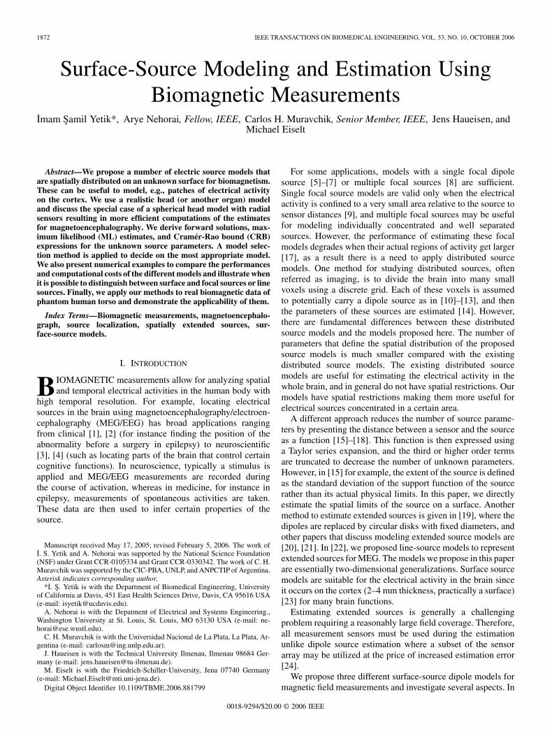
Fig. 1. Illustration of surface sources: (a) CRCM model where the source is apatch on a sphere with constant radius, and the surface moment density is fixed,(b) VPCM model, as in VPVM but the moment density is spatially constant, (c)VPVM model where the source position is presented by a parametric surfaceand the moment density varies over the surface.

Section II, we describe the proposed surface-source models, de-rive the forward solution, maximum likelihood (ML) estimatesand Cramér-Rao bounds (CRBs) on the unknown parameters,using a realistic head (or other organs) model. We also discusshow these models are inter-related. In Section III, we discuss thespecial case of spherical head model and radial sensors for MEGresulting in more efficient computations. Section IV presentsnumerical examples that demonstrate the usefulness of the sur-face-source models. This section also gives a closer look at theCRB and explains how we can select the most appropriate modelusing Akaike’s information criterion (AIC). Additionally, we in-vestigate when it is possible to distinguish between a focal and asurface source, as well as line and surface sources. In Section V,we apply the proposed models to the magnetic field measure-ments of the human phantom. We conclude and discuss futurework in Section VI.

II. FORWARD SOLUTIONS, PARAMETER ESTIMATES,AND BOUNDS

We describe the proposed three different surface-sourcemodels considering the human head and MEG, see Fig. 1 forthe illustration of the models. We use a realistic conductormodel and arbitrary sensor orientations in this section and con-sider the special case of spherical head model and radial sensorsfor MEG in Section III. All these models are identifiable aslong as a realistic head model is used with a number of basisfunctions that would not result in as many parameters as themeasurements. In practice, much less number of basis functionsshould be used for a practical numerical optimization.

A. Focal Source Model

In this section, we review the focal dipole source using a real-istic head model which has been studied extensively in the liter-ature, see, e.g., [37]. Consider a focal electrical source

, where is the current representing the source,the position variable, the time variable, the position, the

moment of the source, and represents the impulse func-tion. The solution to the magnetic field intensity induced by this

source using a realistic head model requires the calculation ofvolume currents. The magnetic field can be obtained by usingthe boundary element method (BEM). The surface of the bodyobtained from MRI scans is divided into small triangular ele-ments, and the equations yielding the induced magnetic fieldcan be discretized using these triangular elements. We refer thereader to [37] for a detailed discussion of BEM. Assumingbiomagnetic sensors oriented along , the measure-ment model can be written as

(2.1)

where is a vector of dimension of the measuredmagnetic fields, is additive noise, is thevector of source position parameters where denotes the az-imuth, the elevation, and distance from the origin, and(commonly called the lead field matrix in bioelectromagnetism)is a gain matrix of dimension which can be computedusing Maxwell’s equations. This equation is the basics of statis-tical modeling of MEG data that allows for a statistical frame-work for estimation. We assume that the noise is zero-mean,homoscedastic, normally distributed with variance , and alsospatially and temporally independent. The normally distributednoise assumption can be justified considering the central limittheorem and observing that there are many independent compo-nents contributing to the noise. It is possible to extend the resultsof this paper to more general correlated noise models [25], [26],but we do not consider them here since our main goal is to focuson the surface-source models.

Considering the model in (2.1) with independent trials(e.g., evoked responses) and temporal samples, the uncor-related noise, and assuming the source position is fixed in time,the ML estimate of is

(2.2)

where denotes themeasurement vector for the th trial, and

. The ML estimate ofcan be calculated using the Moore-Penrose pseudoinverse [25]

(2.3)

There are faster algorithms than ML methods for source lo-calization such as MUSIC [27], [28]. However, note that MLachieves the CRB asymptotically, and other methods may notbe as accurate.

The CRB is a lower bound on the covariance of any unbiasedestimator, and is asymptotically achieved by the ML estimator.It is an important performance measure that can be used to eval-uate the statistical efficiency of the estimation algorithms, to de-termine the main regions where good and poor estimates are ex-pected, and to optimize the sensor system design. We derive theCRB results assuming that the model is correct and hence theML estimate is unbiased. For the more general case where bias


is involved, results of [36] can be utilized. The unknown param-etersresult in a CRB matrix which is given bythe inverse of the Fisher information matrix (FIM) [37]

(2.4)

(2.5)

where the block matrices are

(2.6)

Here, is the identity matrix, “ ” denotes the Kro-necker product (see [29] for the definition and properties), and

(2.7)

where the “vec” operation converts a matrix into a vector bystacking the columns of the matrix on top of each other, and thederivative is a vector derivative resulting in of dimen-sion .

B. Surface-Source Models

We now describe the surface-source models that we propose.Constant-Radius Constant-Moment (CRCM) Model: The

source position has an azimuth and elevation varying incertain intervals with fixed distance from the center as isillustrated in Fig. 1(a); thus, the source can be seen as a patchon a sphere. The source current density is

(2.8)

where denotes the unit step function ( for ,and 1 otherwise), is the fixed radius of the source position,

and are the limit indices of the azimuth and eleva-tion extents of the source. In the present case, the unknown po-sition parameters are and unknownmoment parameters are . Note thatwe have only two extra location parameters compared with the

focal source model. The moment density is spatially constant;hence, we can write the measurement model as

(2.9)

where is of dimension

(2.10)

We approximate this integral by using a finite sum. Consideringthe model in (2.9) with independent trials, the ML estimatesof are given by (2.2), and of by (2.3) but using the gain ma-trix (2.10). For the present model, FIM is a matrix of dimension

which can be calculated using (2.4) and(2.6).

Variable-Position Constant-Moment (VPCM) Model: Thesource position consists of a parametric surface, and the surfacemoment density is assumed to be constant over this surface asis illustrated in Fig. 1(b). The source current density is

(2.11)

where and are the surface parameters, is the sur-face representing the source position, , and

are its coordinates, and are the the limitsof the surface parameters, and “ ” denotes the direct product.The moment density is spatially constant resulting in

(2.12)


(2.13)

(2.14)

In this case, the unknown position parameters are, and the unknown moment param-

eters are . The ML estimates forthe position parameters are given by (2.2) and dipole momentsby (2.3) but using the gain matrix (2.13) in both equations. TheFIM matrix is of dimensionand given by (2.4) and (2.6).


Variable-Position Variable-Moment (VPVM) Model: This isthe most general of the proposed models, see Fig. 1(c). It allowsboth the source position and the moments over the surface tovary. We present the source position as a parametric surface incartesian coordinates

(2.15)

The source position coordinates can be presented using basisfunctions (such as polynomials)

(2.16)

where is a matrix of unknown coefficients for basisfunctions, is a vector of known basis functions.The source current density is then

(2.17)

where denotes the moment of the source. We use basisfunctions for the spatial variation of the moment density as well

(2.18)

where is a time-varying matrix of dimension of un-known coefficients and isthe set of known basis functions.

Realizing that the source is a collection of delta functions(assuming certain regularity conditions for the basis functionsnamely being square integrable), we can calculate the inducedmagnetic field by integrating (2.1) over the surface

. The infinitesimal surface element that we integrate overis [40].

For VPVM, the unknown position parameters areand the unknown mo-

ment parameters are resulting in themodel

(2.19)


(2.20)

and is of dimension

(2.21)

with , and as defined in (2.14). We approximate thisintegral by using a double summation.

The ML estimates of the position and moment parameters aregoverned by (2.2) and (2.3) provided that we use the gain matrix(2.20). The FIM matrix here is of dimension

and have the same block formulae as in (2.4)and (2.6) but here

The basis functions for the VPCM and VPVM models can bechosen (independent from each other) depending on anatomicalinformation if available. Tissue shapes obtained from magneticresonance imaging (MRI) for example might give an idea aboutthe shape of the electrical activity. This shape can be more ac-curately represented using basis functions that better fit the ge-ometry of the brain tissue since inappropriate basis functionswill degrade the performance. Nevertheless, the details of thesource shape that we can obtain are limited by the spatial res-olution of biomagnetic techniques. Using polynomials is a nat-ural choice since enough number of polynomials can representany continuous function to a certain level of detail, and the de-tail which will be necessary is limited because of the limitedspatial resolution. Similar ideas are valid for the basis functionsfor the surface moment density in the VPVM model. We can se-lect basis functions other than polynomials, if a typical form ofa change in the surface moment density over the source area isexpected, and polynomials may not be the parsimonious choicein light of the prior knowledge. However, such better choices ofbasis functions may result in estimates which cannot be obtainedusing elliptic integrals and numerical integration methods maybe necessary.

C. Numerical Optimization

All parameter estimates require that we perform a non-linearoptimization for the source location parameters to reach themaximum of the likelihood function. The cost function and itsderivatives with respect to the unknown parameters can be cal-culated allowing us to use a conjugate gradient method, wherethe search direction is based on both the current gradient andone step history of the gradient, increasing convergence rate byavoiding zigzags. The update rule is

(2.22)

where denotes the iteration number, the search direction,the step size (obtained from a line search), and thederivative of the negative likelihood function with respect to

which can be calculated using the forward solutions in Sec-tion II-B.


III. SPHERICAL HEAD MODEL FOR MEG

We investigate the special case of a spherical head and radialsensors for MEG. These assumptions result in more compactforms of the induced magnetic field involving elliptic integrals[47] since the volume currents vanish. The magnetic field inten-sity measured by radial sensors outside a spherically symmetrichead is [23]

(3.1)

where is an arbitrary electrical source, the source po-sition, and the volume of this electrical activity. We now de-rive the gain matrices for the VPVM and CRCM surface-sourcemodels that are described in Section II-B. The derivation of thegain matrix of VPCM which we omit here follows the samesteps.

VPVM: Using (3.1) and (2.17) the intensity of the inducedmagnetic field is

(3.2)

where

(3.3)

and

(3.4)

The gain matrix has the same form as in (2.17), where the throw of the block column of dimensionis as shown in the equation at the bottom of the page, and

. We refer the reader to [30] regarding the solutions of theabove integrals. The special case of the spherical head model re-sulting in more elegant forms of gain matrices also yields easiercalculation of the CRB matrices.

A. Low-Rank Gain Matrices

Radial components of dipole sources do not produce mag-netic fields outside the spherical head as is evident from (3.1)resulting in a gain matrix with a rank equal to two. A similarsituation exists for the proposed surface-source models undercertain conditions. The physical meaning of low-rank matricesis that it is not possible to uniquely estimate certain parametersof a surface source in the brain when a spherical head model isused. We can choose the basis functions such that low-rank ma-trices are avoided, but this will result in insufficient or wrongpresentation of the surface source if it actually has parametersthat cannot be uniquely estimated. We should avoid basis func-tions that will result in low-rank gain matrices when the sur-face source actually does not have any parameters that cannotbe uniquely estimated so that we do not lose any informationduring the modeling of the source. In practice, the low-rank casecan be avoided by using a realistic head model. We derive theconditions under which the gain matrices for the three modelsare of low-rank .

Rank of the CRCM Gain Matrix: The gain matrix for thismodel is always full rank unless the start and end azimuth andelevation angles are the same with an infinitesimal source ex-tent (CRCM becomes the focal source model). Consider a sur-face moment density vector . Fora certain azimuth and elevation, will have a radial compo-nent which is silent but this component will not be radial for an-other azimuth or elevation angle. Therefore, there are no silentcomponents for a fixed in cartesian coordinates. The reasonis that fixed cartesian coordinates will result in different radialcomponents, and all components will affect the magnetic fieldoutside the head.

Rank of the VPCM Gain Matrix: In this model, the surfacemoment density is constant but the source position is paramet-rically variable. Therefore, certain source positions will resultin a constant angle between the position and moment vectors.This occurs only when the source is actually one-dimensional(a line source), this model is always full rank when the source isactually distributed in two dimensions. In this case, we need asingle parameter since the source is distributed in one-dimen-sion. We have a low rank when the line source (as a limiting


special case of the surface source) lies radially outwards withan arbitrary moment line density, i.e., , for arbitrary

. This is possible when a single basis function,, is used with .

Rank of the VPVM Gain Matrix: Here, we have more cases oflow-rank gain matrices since VPVM is the most general model.The general rule to have a low-rank gain matrix is

(3.5)

where and are arbitrary constants. These condi-tions simply describe a constant angle difference betweenthe position and moment vectors along the source. Any

satisfying (3.5) would result in a gainmatrix with a rank equal to two.

IV. NUMERICAL EXAMPLES

In the following numerical examples, we illustrate several as-pects of the proposed models using simulated MEG data.

A. Cramér-Rao Bound Results

We calculated the diagonal position components of theCRB matrix for the CRCM model. For VPCM and VPVM,the number of the position parameters is large, and it is noteasy to present the CRB components graphically. However,it is intuitive to expect that the estimation of the positionparameters is poor in regions similar to those of CRCM. Theresults characterize the regions of the parameter space thatresult in better estimates. In this way, we can use the boundsto determine certain requirements that will ensure reasonableestimates (estimates with sufficiently small variances). Theserequirements can be on the number of sensors, the location ofthe source, and the SNR.

We use MEG sensors which are positioned in rings of1, 6, 12, 18 sensors each separated by 12 to represent a realisticsystem following [31]. We employ a three-layer (scalp, skull,and brain) spherical head model with radii 9.8, 9.5, and 9.1 cmrespectively and radial sensors, and choose a noise variance suchthat the signal-to-noise ratio (SNR), which is defined as

, is equal to 10 dB (averaged over allsnapshots and trials), a typical value for MEG measurements(see [23]). For CRCM, we use dipole moments with equal x,y, z components in the simulations. The moment densities arechosen such that the total moment strength (integrated over thesurface of the source) is approximately equal to 10 nA m foreach of the three components. We used a noise variance

.The parameter values were chosen such that the center of

the source had approximately the same azimuth and elevationvalues so that the effect of the azimuth and elevation of the

Fig. 2. Diagonal position components of CRB with SNR �10 dB: for theCRCM model (a) as a function of ' with fixed � = 10 , � = 70 ,' = 70 , p = 8 cm, and fixed moment parameters. (b) As in (a), but for� = 35 , � = 40 . (c) As in (a), but as a function of � . (d) As in (b), butas a function of � . (e) As in (a) but as a function of p . (f) As in, (b) but as afunction of p .

source is minimized and the effect of the extent (azimuth or ele-vation extents) of the source can be observed more easily. Fig. 2shows the resulting CRBs.

We can infer from the CRB plots that the following hold.• Larger azimuth and elevation spreads result in smaller

values of the angle components of the CRB. This is ex-pected because the other angle (when one of them is fixed)is more difficult to estimate when the azimuth extent ofthe source is small due to the limited spatial resolution ofthe MEG.

• Deeper sources result in larger values of the radial compo-nent of the CRB. This is similar to the well-known MEGdifficulty of estimating deep focal sources. The CRB valueshere become very large for sources deeper than approxi-mately half the head radius.

• The diagonal CRB values for the elevation angle do notalways change monotonically. The reason is that certainelevation angles make the moment vectors closer to radial(more silent and hence larger CRB values), and other ele-vation angles make the moment vectors closer to tangential(smaller CRB values).

B. Comparisons of Different Models

Since our basic contribution is constructing new sourcemodels, it is important to justify the validity of our models.There are three important properties of a good model for anyphysical observation. First one is the ability of the proposedmodel to explain the observed data. Second one is the require-ment that the parameters of interest are a part of the model sothat they can be estimated. It is also important to have an appro-priate number of unknown parameters providing a well-posedestimation problem and a reasonable computation time.

The focal source model has the ability to explain most of theobserved data; hence satisfies the first requirement. However thespatial extent of the source is not a part of that model. Therefore,the focal source model does not satisfy the second requirementwhen the spatial extent is of interest. Our surface-source modelsboth explain the observed data (better than the focal source),


TABLE IESTIMATION PERFORMANCE RESULTS FOR A SIMULATED SURFACE SOURCE

WITH 37- AND 151-CHANNEL SYSTEMS. SEE SECTION IV-B FOR DETAILS

and incorporate the spatial extent of the source which is of in-terest (unlike the focal source model). The price is the increasednumber of parameters. The number of location parameters forthe focal source is 3, whereas it is 5 for CRCM, and forthe variable position moments where is the number of basisfunctions used.

We use AIC [32] as the measure of model fitness to be ableto evaluate our models considering all these aspects since it is acommonly used model validation technique and also accountsfor the number of parameters involved. It measures the good-ness of a model using the log-likelihood function with a penaltyterm for the number of parameters to account for the trade-offbetween model complexity and accuracy, see [32] for details.

We simulate the surface source using second order poly-nomials (basis functions ). The sourcehas an area of approximately 3.86 cm . The surfacemoment density vector is chosen to have equalcomponents with a strength varying along the source,

.For VPVM, the basis functions are used

for the source position resulting in 13 unknown position param-eters. Five basis functions are usedto model the moment variation of VPVM so that the number ofunknown moment parameters is 15. Note that, the basis func-tions used for simulating the source and estimating it are not thesame. For VPCM, polynomials are not used as basis functions,and for VPVM, the basis functions used for estimation are ofdifferent degree.

The mean-squared error (MSE) between the predicted andmeasured magnetic field intensity, number of unknown param-eters, and AIC values for the four models (the focal sourcemodel and three surface-source models) are given in Table I fora 37-channel and 151-channel system. We observe a certain im-provement in the performance when the surface-source modelsare used compared with the focal source. The model that fits thebest for 37-channel system is VPCM as is evident by the AICvalues, although the true source is VPVM. This is mainly be-cause of the high number of parameters that VPVM has. For the151-channel system, the improvement in the MSE is worth theincreased number of parameters making VPVM the best fit.

We conduct another simulation to observe the robustness ofthe estimates and also to observe the effect of the number of sen-sors. For this purpose, we use a realistic head model, 31-channelbiomagnetometer (Philips, Hamburg, Germany) and a whole-head 151-channel MEG system, and real brain noise recordedby these systems. We simulated a surface source and added sev-eral different real brain noise to the induced field and then esti-mated the source locations. The induced magnetic field by thesimulated source has a peak value of 100 fT, a typical value of

TABLE IICENTER COORDINATES (CM), AREAS OF THE TRUE AND ESTIMATED SOURCES

(CM ), AND THE STANDARD DEVIATIONS FOR THE ESTIMATES FOR 11DIFFERENT NOISE REALIZATIONS. RESULTS FOR BOTH 31 AND 151 CHANNELS

SYSTEMS ARE PRESENTED

neuromagnetic field induced by human brain [23]. The SNRhad eleven values varying between 15 and 25 dB. True sur-face source, and the estimated surface sources using eleven dif-ferent noise realizations are given in Table II using VPCM fora 31-channel and a 151-channel system. In this table, we showthe true area and estimated areas as well as true location andestimated locations (center of the patch). The standard devia-tions for the center and area estimates are given. We note thatthis table shows that we can obtain reasonably close estimatesfor different noise realizations, and a whole-head MEG systemimproves the performance as expected. The estimated sourcesusing the 31-channel system are shown in Fig. 3.

C. Distinguishing Between Line, Surface, and Focal Sources

We investigate when it is possible to distinguish between sur-face and focal sources; and surface and line sources (i.e., whenthe induced magnetic field intensities are sufficiently different).In [34], the authors suggest that there is little difference be-tween the induced potential fields, and it is difficult to distin-guish between focal and extended sources. The models used inthis paper are more general than the circular annuli used in [34],and it has been noted in [35] that the differences between the in-duced fields for extended and focal sources are larger when theextended sources differ from circular disc shapes which is thecase for the surface-source models we propose. We show thatthe focal, line-, and surface-source models are distinguishableusing the Neyman-Pearson hypothesis test although it is truethat magnetic field intensities are close for extended and focalsources.

We use the receiver operator characteristics (ROC) curvewhich is the parametric plot of the probability of detection asa function of false alarm probability with the parameter beingthe threshold [33]. We also plot this minimum spread requiredto make a distinction between focal and surface sources as afunction of the noise variance. The analysis is given for distin-guishing between focal and surface sources using the VPCMmodel; and a line and surface sources using the CRCM model.For a certain observation we estimate the parameters using


Fig. 3. Estimated surface sources using VPVM for a real brain (dots repre-senting the mesh plot of the brain surface) with 11 different sets of real brainnoise. Top left shows the simulated source. Reasonably close estimates are ob-tained for different noise realizations.

the focal, line, or surface source and use these estimates toconstruct the distributions that we use in the hypothesis testing.A collection of ROCs for different source extents is given inFig. 4.

We also plot the minimum source area which is distinguish-able from a focal source for different values of SNR in Fig. 4(d).We observe that minimum source area (which is distinguishablefrom a focal source) is more sensitive to noise variance for highnoise variance values compared with low values.

An SNR value of 10 dB is sufficient to estimate an extentof approximately 4 cm , which is a large patch, for equal az-imuth and elevation extents. The curve in Fig. 4(d) saturatesaround 4 cm , therefore very high SNR is required to estimatesources that are spread equally along two directions less than 4cm . However, we can obtain acceptable estimates (accordingto ROC curves) for sources smaller than 4 cm when the spreadis not uniform in two directions and the resulting source is elon-gating more in one direction (see Fig. 4(a) and (b) where sourceswith 3.2 and 3.88 cm result in detectable surface sources). Thisresult implies that detection and estimation of a surface sourcestrongly depend on the shape of the source, and sources withunisotropic elongation (different extent along two directions)are easier to estimate.

V. APPLICATION TO REAL MAGNETIC FIELD DATA OF

HUMAN PHANTOM

We have prepared a human phantom to apply and test ourmethods [41]. We applied the surface VPCM and focal sourcemodels to real magnetic field data measured around the heart ofthis human phantom. Although data we use is from a phantomhuman experiment, the proposed models are potenatially useful

Fig. 4 (a) Receiver operator characteristics for different source extents withequal azimuth and elevation extents for CRCM and focal source models, thecenter elevation is 20 and azimuth is 45 with p = 8 cm. (1) For �� = 10 ,�' = 55 , area = 3:66 cm (2) for �� = 15 , �' = 40 , area = 3:88

cm (3) for �� = 10 , �' = 40 , area = 2:66 cm (4) for �� = 5 ,�' = 40 , area = 1:76 cm (5) for �� = 15 , �' = 20 , area = 1:94

cm (6) for �� = 10 , �' = 20 , area = 1:33 cm (7) for �� = 5 ,�' = 20 area = 0:68 cm , (8) for�� = 0 ,�' = 0 , area = 0 cm . (b)Same as in (a), but for VPVM and (1) area = 3:8 cm (2) area = 3:2 cm (3)area = 2:6 cm (4) area = 2:0 cm (5) area = 1:6 cm (6) area = 1:2 cm(7) area = 0:8 cm (8) area = 0 cm . (c) Receiver operator characteristicsfor different source extents for CRCM and a line source. The line source has aconstant elevation and radius with an azimuth varying between 20 and 70 withp = 8 cm. (1) Elevation extent = 5 (2) 10 (3) 15 (4) 18 . (d) Minimumsurface source areas for CRCM and VPVM which are distinguishable from afocal source as a function of SNR.

in stroke [42], craniocerebral injury [43], migraine [44], [45],and intracranial bleedings [46].

Our torso phantom is based on a copy of the body surfaceof an adult male volunteer [41]. Epoxy resin, a non-magneticmaterial, is used to build the phantom. The phantom was filledwith a saline solution which gives the volume conductor a con-ductivity corresponding to a mean value for the human body(about 3.35 mS/cm). Current sources and optionally additionalcompartments (which represent the lungs as the main body inho-mogeneity) can be mounted in well-defined positions inside thephantom. A geometrical model of the whole volume conductorwas reconstructed from magnetic resonance images (MRI) ofthe phantom.

An extended source suitable for magnetic measurements wascreated by enlarging the dipole tips into rectangular electrodesresulting in a source dimension of 5 6 cm [41]. The sourcesignal emitted from this electrode was chosen to be sinusoidal.The magnetic field data were recorded with two sets of 31 chan-nels around the heart location [41] as shown in Fig. 5(a) and (b)providing 39 time samples. We have used one of the peak pointsduring the estimation. Please refer to [41] for more details on theexperiment setup.

We did not consider the spatial moment variation since thiswould decrease the performance of the estimation of the source


Fig. 5. (a) and (b) Sensor configurations and the tesselated phantom body withtwo views, and (c) and (d) the estimated focal and surface sources in the tessala-tions with two views.

position, and the source position is of more interest comparedwith the moment variation in this case. We used the basis func-tions set for the position.

We used one of the peak values of the response for estimation.The estimated surface and focal sources are shown in Fig. 5(c)and (d) with two different views. We observed that the estimateddipole source is very slightly closer to the surface than the esti-mated surface source of area 9.3 cm . The estimated source issmaller than the expected size obtained from the spread of theelectrodes, we can partly explain this fact by the the limited spa-tial resolution of biomagnetic techniques. We also observed thatthe source fits to the true source better in the right-left directionthan the top-down direction. The MSE for the focal source is1.296 fT , whereas it is 1.225 fT for the VPCM model resultingin a 5.5% improvement. Although the decrease in the MSE inthis experiment may not seem significant, it is a natural result ofthe fact that a single dipole can explain most of the biomagneticmeasurements especially for a relatively simple structure suchas the phantom when compared to the human body.

VI. CONCLUSION

We have proposed three different current surface-sourcemodels, derived the forward solutions, ML estimates, and CRBexpressions for these models. Numerical methods must beutilized when using a realistic head model. The special caseof spherical head model and radial sensors result in analyticalsolutions using elliptic and hyper-elliptic integrals and low-rankgain matrices for VPCM and VPVM under certain circum-stances. Relationships among the models, and the low-rankgain matrices were also investigated.

The main results of this paper can be summarized as follows.• The position components of the CRB matrix showed that

better estimates are expected when the surface source ismore spread for source shapes of the same type. Differentsource shapes may result in different results. For example,

comparing the CRBs on estimating surface versus linesources [22], we observe that the bounds are smaller forthe line source. That is, it is easier to estimate a line-sourcethan estimating a surface-source provided that their inte-grated moment strengths are similar. We also observedthat bounds on deeper sources are larger.

• Numerical examples showed that the surface-sourcemodels improve the mean-squared error performancecompared with the focal source model for extendedsources.

• It is possible to distinguish between line, surface, and focalsources when the activity is sufficiently spread.

• The proposed models were shown to be useful for real bio-magnetic data of human phantom we have prepared to testthe performances of extended source models.

When compared with other methods to estimate the spatialextent of the source such as multipolar expansion [15], [16],the main advantage of our method is the added flexibility ofthe source shape, and extent along different directions in 2-D,whereas the disadvantage is the increased number of parametersrestricting the estimation performance.

Future work will include extending the proposed sur-face-source models to unknown noise covariance [25], andvector electromagnetic sensors [38]. We are currently ex-tending our models to EEG considering also the estimationof conductivities [39], as well as imposing constraints on thesurface source. This constraint can potentially result in morerobust and stable surface-source estimates.

ACKNOWLEDGMENT

The authors are grateful to N. von Ellenrieder for sharing hissoftware on realistic head models.

REFERENCES

[1] H. Stefan and C. Hummel, “Magnetoencephalography,” in Handbookof Clinical Neurology, H. Meinardi, Ed. Amsterdam, The Nether-lands: Elsevier, 1999, pp. 319–336.

[2] J. S. Ebersole, “Magnetoencephalography/magnetic source imaging inthe assessment of patients with epilepsy,” Epilepsia, vol. 38, pp. 1–4,1997.

[3] S. Baillet, J. C. Mosher, and R. M. Leahy, “Electromagnetic brain map-ping,” IEEE Signal Process. Mag., vol. 18, no. 6, pp. 14–30, Nov. 2001.

[4] G. Pfurtscheller and F. H. L. da Silva, “Event-related EEG/MEG syn-chronization and desynchronization: Basic principles,” Clin. Neuro-physiol., vol. 110, pp. 1842–1857, 1999.

[5] R. Hari, K. Reinikainen, E. Kaukoranta, M. Hamalainen, R. Ilmoniemi,A. Penttinen, J. Salminen, and D. Teszner, “Somatosensory evokedcerebral magnetic fields from SI and SII in man,” Electroencephalogr.Clin. Neurophysiol., vol. 57, pp. 254–263, 1984.

[6] M. Scherg and D. Von Cramon, “Two bilateral sources of the late AEPas identified by a spatiotemporal dipole model,” Electroencephalogr.Clin. Neurophysiol., vol. 62, pp. 32–44, 1985.

[7] B. N. Cuffin, “A comparison of moving dipole inverse solutions usingEEG’s and MEG’s,” IEEE Trans. Biomed. Eng., vol. BME-32, pp.905–910, 1985.

[8] M. Scherg, M. R. Hari, and M. Hamalainen, “Frequency-specificsources of the auditory N19-P30-P50 response detected by a multiplesource analysis of evoked magnetic fields and potentials,” in Advancesin Biomagnetism, S. J. Williamson, M. Hoke, G. Stroink, and M.Kotani, Eds. New York: Plenum, 1989, pp. 97–100.

[9] A. Z. Snyder, “Dipole source localization in the study of EP genera-tors: A critique,” Electroencephalogr. Clin. Neurophysiol., vol. 80, pp.321–325, 1991.


[10] A. A. Ioannides, J. P. R. Bolton, R. Hasson, and C. J. S. Clarke,“Localized and distributed source solutions for the biomagneticinverse problem II,” in Advances in Biomagnetism, S. J. Williamson,M. Hoke, G. Stroink, and M. Kotani, Eds. New York: Plenum, 1989,pp. 591–594.

[11] J.-Z. Wang, S. J. Williamson, and L. Kaufman, “Magnetic source im-ages determined by a lead field analysis: The unique minimum normleast squares estimation,” IEEE Trans. Biomed. Eng., vol. 39, no. 7, pp.665–675, Jul. 1992.

[12] M. R. G. de Peralta and A. S. L. Gonzales, “Distributed source models:Standard solutions and new developments,” in Analysis of Neurophysi-logical Brain Functioning, C. Uhl, Ed. Berlin, Germany: Springer-Verlag, 1998, pp. 176–201.

[13] M. Fuchs, M. Wagner, T. Kohler, and H. A. Wischmann, “Linear andnon-linear current density reconstructions,” J. Clin. Neurophysiol., vol.16, pp. 267–295, 1999.

[14] J. Sarvas, “Basic mathematical and electromagnetic concepts of bio-magnetic inverse problem,” Phys. Med. Biol., vol. 32, pp. 11–22, 1987.

[15] G. Nolte and G. Curio, “Current multipole expansion to estimate lat-eral extent of neuronal activity: A theoretical analysis,” IEEE Trans.Biomed. Eng., vol. 47, no. 10, pp. 1347–1355, Oct. 2000.

[16] J. C. Mosher, S. Baillet, K. Jerbi, and R. M. Leahy, “MEG multipolarmodeling of distributed sources using RAP-MUSIC,” in Proc. 34thAsilomar Conf. Signals, Syst., Comput., Pacific Grove, CA, 2000, pp.318–322.

[17] K. Jerbi, J. C. Mosher, S. Baillet, and R. M. Leahy, “On MEG forwardmodelling using multipolar expansions,” Phys. Med. Biol., vol. 47, pp.523–555, 2002.

[18] J. Nenonen, T. Katila, and M. Leinio, “Magnetocardiographic func-tional localization using current multipole models,” IEEE Trans.Biomed. Eng., vol. 38, no. 7, pp. 648–657, Jul. 1991.

[19] M. Wagner, Th. Kohler, M. Fuchs, and J. Kastner, “Current densityreconstructions and deviation scans using extended sources,” in Proc.12th Int. Conf. Biomagn., Espoo, Finland, 2000, pp. 804–806.

[20] W. E. Kincses, C. Braun, S. Kaiser, and T. Elbert, “Modeling extendedsources of event-related potentials using anatomical and physiologicalconstraints,” Hum. Brain Mapp., vol. 8, pp. 182–193, 1999.

[21] B. Lutkenhoner, E. Menninghaus, O. Steinstrater, C. Wienbruch, H. M.Gissler, and T. Elbert, “Neuromagnetic source analysis using magneticresonance images for the construction of source and volume conductormodel,” Brain Topogr., vol. 7, pp. 291–299, 1995.

[22] I. S. Yetik, A. Nehorai, C. H. Muravchik, and J. Haueisen, “Line-sourcemodeling and estimation with magnetoencephalography,” IEEE Trans.Biomed. Eng., vol. 52, no. 5, pp. 839–851, May 2005.

[23] M. Hamalainen, R. Hari, R. J. Ilmoniemi, J. Knuutila, and O. V.Lounasmaa, “Magnetoencephalography-theory, instrumentation, andapplications to noninvasive studies of the working human brain,” Rev.Mod. Phys., vol. 65, pp. 413–497, 1993.

[24] J. Vrba, T. Cheung, D. Cheyne, S. E. Robinson, and A. Starr, “Errorsin ECD localization with partial sensor coverage,” in Recent Adv.Biomagn., T. Yoshimoto, M. Kotani, S. Kuriki, H. Karibe, and N.Nakasato, Eds. : , 1999, pp. 109–112.

[25] A. Dogandzic and A. Nehorai, “Estimating evoked dipole responsesin unknown spatially correlated noise with EEG/MEG arrays,” IEEETrans. Biomed. Eng., vol. 48, no. 1, pp. 13–25, Jan. 2000.

[26] H. M. Huizenga, J. C. de Munck, L. J. Waldorp, and R. P. P. P.Grasman, “Spatiotemporal EEG/MEG source analysis based on aparametric noise covariance model,” IEEE Trans. Biomed. Eng., vol.49, no. 6, pp. 533–539, Jun. 2002.

[27] P. Stoica, P. Handel, and A. Nehorai, “Improved sequential MUSIC,”IEEE Trans. Aerosp. Electron. Systems, vol. 31, no. 4, pp. 1230–1239,Oct. 1995.

[28] J. C. Mosher and R. M. Leahy, “Source localization using recursivelyapplied and projected (RAP) MUSIC,” IEEE Trans. Signal Process.,vol. 47, no. 2, pp. 332–340, Feb. 1999.

[29] J. W. Brewer, “Kronecker products and matrix calculus in systemtheory,” IEEE Trans. Circuits Syst., vol. 25, no. 9, pp. 772–781, Sep.1978.

[30] I. S. Yetik, “Extended-source estimation using magnetoencephalog-raphy and performance bounds on image registration,” Ph.D. thesis,University of Illinois at Chicago, , 2004.

[31] R. T. Johnson, W. C. Black, and D. S. Buchanan, “Source detectabilityfor multi-channel biomagnetic sensors,” in Proc. 10th Int. Conf. Bio-magnetism, Santa Fe, NM, 1996, pp. 804–807.

[32] H. Akaike, “Information and an extension of the likelihood principle,”in Proc. 2nd Int. Symp. Information Theory. Supplement to Problemsof Control and Information Theory, Budapest, Hungary, 1973, pp.267–281.

[33] H. V. Poor, An Introduction to Signal Detection and Estimation. NewYork: Springer, 1994.

[34] J. C. de Munck, B. W. van Dijk, and H. Spekreijse, “Mathematicaldipoles are adequate to describe realistic generators of human brainactivity,” IEEE Trans. Biomed. Eng., vol. 35, no. 11, pp. 960–966, Nov.1988.

[35] A. Hillebrand and G. R. Barnes, “A quantitative assessment of the sen-sitivity of whole-head MEG to activity in the adult human cortex,” Neu-roImage, vol. 16, pp. 638–650, 2002.

[36] K. Mahata and T. Soderstrom, “Large sample properties of separablenonlinear least squares estimators,” IEEE Trans. Signal Process., vol.52, no. 6, pp. 1650–1658, Jun. 2004.

[37] C. Muravchik and A. Nehorai, “EEG/MEG error bounds for a staticdipole source with a realistic head model,” IEEE Trans. Biomed. Eng.,vol. 49, no. 3, pp. 470–484, Mar. 2001.

[38] B. Hochwald and A. Nehorai, “Magnetoencephalography with di-versely oriented and multicomponent sensors,” IEEE Trans. Biomed.Eng., vol. 44, no. 1, pp. 40–50, Jan. 1997.

[39] D. Gutierrez, A. Nehorai, and C. Muravchik, “Estimating brain con-ductivities and dipole source signals with EEG arrays,” IEEE Trans.Biomed. Eng., vol. 51, no. 12, pp. 2113–2122, Dec. 2004.

[40] A. Gray, “The intuitive idea of area on a surface,” in Modern Dif-ferential Geometry of Curves and Surfaces With Mathematica, 2nded. Boca Raton, FL: CRC, 1997, pp. 351–353.

[41] H. Brauer, J. Haueisen, M. Ziolkowski, U. Tenner, and H. Nowak, “Re-construction of extended current sources in a human body phantomapplying biomagnetic measuring techniques,” IEEE Trans. Magn., vol.36, no. 4, pp. 1700–1705, Jul. 2000.

[42] T. P. Obrenovitch, “The ischaemic penumbra: Twenty years on,” Cere-brovasc. Brain Metabol. Rev., vol. 4, pp. 297–323, 1995.

[43] G. G. Rogatsky, A. Mayevsky, N. Zarchin, and A. Doron, “Continuousmultiparametric monitoring of brain activities following fluid-percus-sion injury in rats: Preliminary results,” J. Basic Clin. Physiol. Phar-macol., vol. 7, pp. 23–43, 1996.

[44] S. M. Bowyer, S. K. Aurora, J. E. Moran, N. Tepley, and K. M. Welsh,“MEG fields from patients with spontaneous and induced migraineaura,” Ann. Neurol., vol. 50, pp. 582–587, 2001.

[45] M. Lauritzen, “Cortical spreading depression in migraine,” Cepha-lalgia, vol. 21, pp. 757–760, 2001.

[46] S. Mun-Bryce, A. C. Wilkerson, N. Papuashvili, and Y. C. Okada, “Re-curring episodes of spreading depression are spontaneously elicitedby an intracerebral hemorrhage in the swine,” Brain Res., vol. 2, pp.248–255, 2001.

[47] P. F. Byrd and M. D. Friedman, Handbook of Elliptic Integrals forEngineers and Physicists. Berlin, Germany: Springer-Verlag, 1954.

Imam Samil Yetik was born in Istanbul, Turkey, in1978. He received the B.Sc. degree in electrical andelectronics engineering from Bogazici University, Is-tanbul, in 1998, the M.S. degree in electrical and elec-tronics engineering from Bilkent University, Ankara,Turkey, in 2000, and Ph.D. degree in electrical andcomputer engineering from the University of Illinoisat Chicago, in 2004.

He joined the Department of Electrical andComputer Engineering at the Illinois Institute ofTechnology as an Assistant Professor after his

postdoc positions at the University of Illinois at Chicago and University ofCalifornia at Davis. His research interests are in the areas of biomedical signaland image processing with emphasis on PET image reconstruction, imageregistration, and EEG/MEG.


Arye Nehorai (S’80–M’83–SM’90–F’94) receivedthe B.Sc. and M.Sc. degrees in electrical engineeringfrom the Technion, Haifa, Israel, and the Ph.D. de-gree in electrical engineering from Stanford Univer-sity,Stanford, CA.

From 1985 to 1995, he was a faculty member withthe Department of Electrical Engineering at YaleUniversity, New Haven, CT. In 1995, he joined theDepartment of Electrical Engineering and ComputerScience at The University of Illinois at Chicago(UIC) as Full Professor. From 2000 to 2001, he

was Chair of the department’s Electrical and Computer Engineering (ECE)Division, which then became a new department. In 2001, he was namedUniversity Scholar of the University of Illinois. In 2006, he assumed theChairman position of the Department of Electrical and Systems Engineering atWashington University, St. Louis, MO, where he is also the inaugural holder ofthe Eugene and Martha Lohman Professorship of Electrical Engineering. Heis the Principal Investigator of the new multidisciplinary university researchinitiative (MURI) project entitled Adaptive Waveform Diversity for FullSpectral Dominance.

Dr. Nehorai was Editor-in-Chief of the IEEE TRANSACTIONS ON SIGNAL

PROCESSING during the years 2000 to 2002. In 2003–2005, he was VicePresident (Publications) of the IEEE Signal Processing Society, Chair of thePublications Board, member of the Board of Governors, and member of theExecutive Committee of this Society. He is the founding editor of the specialcolumns on Leadership Reflections in the IEEE Signal Processing Magazine.He was co-recipient of the IEEE SPS 1989 Senior Award for Best Paperwith P. Stoica, co-author of the 2003 Young Author Best Paper Award andco-recipient of the 2004 Magazine Paper Award with A. Dogandzic. He waselected Distinguished Lecturer of the IEEE SPS for the term 2004 to 2005. Hehas been a Fellow of the Royal Statistical Society since 1996.

Carlos H. Muravchik (S’81–M’83–SM’99) wasborn in Argentina, June 11, 1951. He graduated as anElectronics Engineer from the National University ofLa Plata, La Plata, Argentina, in 1973. He receivedthe M.Sc. in statistics (1983) and the M.Sc. (1980)and Ph.D. (1983) degrees in electrical engineering,from Stanford University, Stanford, CA.

He is a Professor at the Department of the Elec-trical Engineering of the National University of LaPlata and a member of its Industrial Electronics, Con-trol and Instrumentation Laboratory (LEICI). He is

also a member of the Comision de Investigaciones Cientificas de la Pcia. deBuenos Aires. He was a Visiting Professor at Yale University in 1983 and 1994,and at the University of Illinois at Chicago in 1996, 1997, 1999, and 2003. Since1999, he is a member of the Advisory Board of the journal Latin American Ap-plied Research. His research interests are in the area of statistical signal andarray processing with biomedical, control and communications applications,and nonlinear control systems.

Dr. Muravchik was an Associate Editor of the IEEE TRANSACTIONS ON

SIGNAL PROCESSING (2003–2006).

Jens Haueisen received the M.S. and Ph.D. degreesin electrical engineering from the Technical Univer-sity Ilmenau, Ilmenau, Germany, in 1992 and 1996,respectively.

From 1996 to 1998 he worked as a Post-Doc andfrom 1998 to 2005 as the head of the BiomagneticCenter, Friedrich-Schiller-University, Jena, Ger-many. Since 2005, he is Professor of BiomedicalEngineering and directs the Institute of Biomed-ical Engineering and Informatics at the TechnicalUniversity Ilmenau. His research interests are in

the numerical computation of bioelectromagnetic fields and the analysis ofbioelectromagnetic signals.

Michael Eiselt was born in Gera, Germany, in 1956.He received the M.D. in 1983, the Ph.D. in 1987, andthe specialization in pathophysiology in 1987.

He is currently a Research Associate at theMedical Faculty of the Friedrich Schiller Univer-sity, Jena, Germany. His research interests includeclinical and experimental neuropathophysiologywith special regards to dysfunctions during earlyhuman development. Since 1991, he performed theinvestigations using MEG and EEG/ECoG.

surface-source modeling and estimation using biomagnetic measurements

Documents