arX

iv:m

ath/

0009

037v

2 [

mat

h.A

P] 2

8 N

ov 2

000 OPTIMAL ACOUSTIC MEASUREMENTS

Margaret Cheney ∗ David Isaacson † Matti Lassas ‡

February 1, 2008

Abstract

We consider the problem of obtaining information about an inaccessiblehalf-space from acoustic measurements made in the accessible half-space. Ifthe measurements are of limited precision, some scatterers will be undetectablebecause their scattered fields are below the precision of the measuring instru-ment. How can we make measurements that are optimal for detecting thepresence of an object? In other words, what incident fields should we applythat will result in the biggest measurements?

There are many ways to formulate this question, depending on the mea-suring instruments. In this paper we consider a formulation involving wave-splitting in the accessible half-space: what downgoing wave will result in anupgoing wave of greatest energy?

A closely related question arises in the case when we have a guess aboutthe configuration of the inaccessible half-space. What measurements should wemake to determine whether our guess is accurate? In this case we compare thescattered field to the field computed from the guessed configuration. Again welook for the incident field that results in the greatest energy difference.

We show that the optimal incident field can be found by an iterative pro-cess involving time reversal “mirrors”. For band-limited incident fields andcompactly supported scatterers, in the generic case this iterative process con-verges to a single time-harmonic field. In particular, the process automatically“tunes” to the best frequency. This analysis provides a theoretical foundationfor the frequency-shifting and pulse-broadening observed in certain computa-tions [3] and time-reversal experiments [14] [15].

∗Department of Mathematical Sciences, Rensselaer Polytechnic Institute, Troy, NY 12180†Department of Mathematical Sciences, Rensselaer Polytechnic Institute, Troy, NY 12180‡Rolf Nevanlinna Institute, P.O. Box 4, 00014 University of Helsinki, FINLAND

1

1 Introduction

This paper is motivated by the question “What is the best way to do acoustic imag-ing?” If we want to make the best possible images, we must begin with data thatcontain the most possible information. In particular, since all practical measurementsare of limited precision, some scatterers may be undetectable because their scatteredfields are below the precision of the measuring instrument: our data will contain noinformation about them. What incident fields are “best”, in the sense that theirscattered fields give the biggest measurements?

This paper considers only the problem of detecting the presence of an object (ordistinguishing it from a guess) and not the problem of making an image of thatobject. For imaging, there are other criteria for “best” that one could imagine using.A Bayesian criterion [9] [10], for example, would be to look for the measurementproducing the “narrowest” posterior distribution for the scatterer when an a prioridistribution for the scatterer is given.

The detection or distinguishability problem has been studied for fixed-frequencyproblems in electrical impedance tomography [6] and acoustic scattering [12]. Theconnection between optimal measurements and iterative time-reversal experimentswas pointed out in [12], [14], and [15]; in all these papers, the analysis was carriedout at a single fixed frequency. The issue of optimal time-dependent waveforms in aspecial 1 + 1 – dimensional case was studied in [3], where a time-harmonic waveformwas found to be optimal.

In this paper we study the question of optimal time-dependent waveforms in the3 + 1 – dimensional case. In particular, we consider the half-space geometry: weimagine that a plane divides space into accessible and inaccessible regions, and weassume that we can make measurements everywhere on the plane.

Section 2 contains a careful formulation of the idealized problem: the wave equa-tion, the measurements, the notion of “biggest”. Section 3 is devoted to the exampleof a one-dimensional medium, in which the problem can be solved explicitly. Section4 gives an iterative experimental method that can be used to find the optimal fieldeven if the scatterer is unknown. This method is precisely the iterative time-reversalprocedure of [14] and [15]. Section 5 discusses implications and open questions. Thepaper concludes with three appendices containing the technical details needed forthe proof of convergence of the time-reversal iterates. We show that in general theiterates converge to a time-harmonic field that is “tuned” to the best frequency.

2 Basic Concepts

2

2.1 Distinguishability

For any two operators A1 and A2, we say that A1 is distinguishable from A2 withmeasurement precision ǫ if the distinguishability δ(A1, A2), defined as

δ(A1, A2) = supf

||A1f − A2f ||

||f ||, (1)

is greater than ǫ. A field that is best for distinguishing A1 from A2 is an f for whichthe maximum is attained. We will determine below the norms that are appropriateto use.

2.2 Acoustic Wave Equation

We consider the constant-density acoustic wave equation

(∇2 − c−2(x)∂2t )U(t, x) = 0. (2)

in the case in which c = c0 everywhere in the upper half-space x3 > 0. This modelincludes neither dispersion nor dissipation.

We can formulate the scattering problem in a variety of ways [2]. In particular,we can use either a boundary map, sources, or a scattering operator defined in termsof wave splitting.

2.3 The Boundary Map

To define the boundary map, we specify that U = f on the surface x3 = 0. This condi-tion, together with an outgoing radiation condition at infinity [2], uniquely determinesa solution U in the lower half-space. We can then take the normal derivative ∂U/∂x3;this normal derivative, restricted to the surface x3 = 0, we denote by g. The mappingfrom f to g is the boundary map Λ. Thus, on the surface x3 = 0, ΛU = ∂U/∂x3.Note that Λ is an operator-valued function of time.

Acoustic distinguishability can be defined in terms of the boundary map as

δB(c, c0) = supf

‖(Λ − Λ0)f‖

‖f‖(3)

for appropriate norms. Here Λ0 denotes the boundary map for the reference soundspeed c0(x). This formulation, in terms of the boundary map, is not pursued in thispaper.

3

2.4 Sources

To formulate scattering in terms of sources, we consider the wave equation with asource:

(∇2 − c−2(x)∂2t )UJ(t, x) = J(t, x). (4)

Scattering data is then UJ(t, x) for x on the plane, where J is supported on or abovethe plane. Acoustic distinguishability in terms of sources would be

δS(c, c0) = supJ

‖UJ − U0J‖

‖J‖, (5)

where U0J denotes the field due to the reference sound speed c0(x) and source J . This

formulation is not pursued in this paper; instead we consider the scattering operator.

2.5 The Scattering Operator

We define the scattering operator in terms of upgoing and downgoing waves. Themotivation for this point of view is the existence of network analyzers, which can de-compose a time-harmonic signal in a waveguide into an upgoing one and a downgoingone, and measure the amplitude and phase of the upgoing wave. Stepped-frequencyradar, for example, is based on the ability of such instruments to transmit and receivesignals at the same time.

2.5.1 Upgoing and downgoing waves

To define upgoing and downgoing waves, we make use of two Fourier transforms, atemporal one and a spatial one. First we inverse-Fourier transform the solution U of(2) in t:

u(ω, x) = F−1U = (2π)−1∫

U(t, x)eiωtdt. (6)

This frequency-domain solution u satisfies the reduced wave equation

(∇2 + ω2c−2)u(ω, x) = 0. (7)

We write k = ω/c0 and with a small abuse of notation we write u(k, x) instead ofu(c0k, x). We then Fourier transform u again in x′ = (x1, x2), so that

u(k, η′, x3) = Fx3u =

∫

u(k, x)e−ikη′·x′

d2x′ (8)

where η′ = (η1, η2). (We note that Fx3depends also on k.) Then U is recovered as

U(t, x) =1

(2π)2

∫ ∫

u(k, η′, x3)eikη′·x′

e−ikc0tk2d2η′c0dk. (9)

4

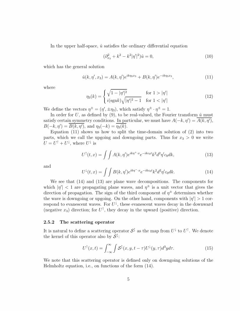
In the upper half-space, u satisfies the ordinary differential equation

(∂2x3

+ k2 − k2|η′|2)u = 0, (10)

which has the general solution

u(k, η′, x3) = A(k, η′)eikη3x3 +B(k, η′)e−ikη3x3, (11)

where

η3(k) =

√

1 − |η′|2 for 1 > |η′|

i(sgnk)√

|η′|2 − 1 for 1 < |η′|(12)

We define the vectors η± = (η′,±η3), which satisfy η± · η± = 1.In order for U , as defined by (9), to be real-valued, the Fourier transform u must

satisfy certain symmetry conditions. In particular, we must have A(−k, η′) = A(k, η′),B(−k, η′) = B(k, η′), and η3(−k) = η3(k).

Equation (11) shows us how to split the time-domain solution of (2) into twoparts, which we call the upgoing and downgoing parts. Thus for x3 > 0 we writeU = U↑ + U↓, where U↓ is

U↑(t, x) =∫ ∫

A(k, η′)eikη+·xe−ikc0tk2d2η′c0dk, (13)

andU↓(t, x) =

∫ ∫

B(k, η′)eikη−·xe−ikc0tk2d2η′c0dk. (14)

We see that (14) and (13) are plane wave decompositions. The components forwhich |η′| < 1 are propagating plane waves, and η± is a unit vector that gives thedirection of propagation. The sign of the third component of η± determines whetherthe wave is downgoing or upgoing. On the other hand, components with |η′| > 1 cor-respond to evanescent waves. For U↓, these evanescent waves decay in the downward(negative x3) direction; for U↑, they decay in the upward (positive) direction.

2.5.2 The scattering operator

It is natural to define a scattering operator Sl as the map from U↓ to U↑. We denotethe kernel of this operator also by Sl:

U↑(x, t) =∫ ∞

−∞

∫

Sl(x, y, t− τ)U↓(y, τ)d3ydτ. (15)

We note that this scattering operator is defined only on downgoing solutions of theHelmholtz equation, i.e., on functions of the form (14).

5

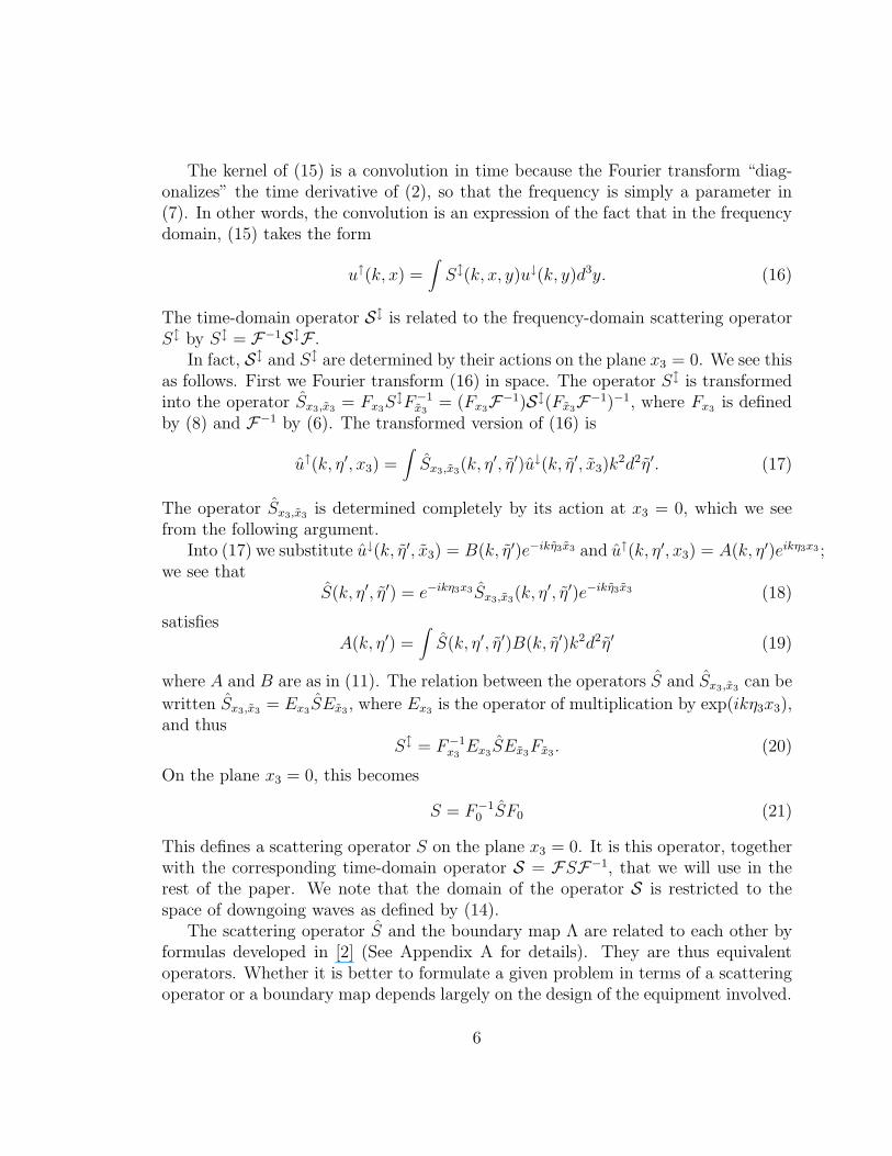
The kernel of (15) is a convolution in time because the Fourier transform “diag-onalizes” the time derivative of (2), so that the frequency is simply a parameter in(7). In other words, the convolution is an expression of the fact that in the frequencydomain, (15) takes the form

u↑(k, x) =∫

Sl(k, x, y)u↓(k, y)d3y. (16)

The time-domain operator Sl is related to the frequency-domain scattering operatorSl by Sl = F−1SlF .

In fact, Sl and Sl are determined by their actions on the plane x3 = 0. We see thisas follows. First we Fourier transform (16) in space. The operator Sl is transformedinto the operator Sx3,x3

= Fx3SlF−1

x3= (Fx3

F−1)Sl(Fx3F−1)−1, where Fx3

is definedby (8) and F−1 by (6). The transformed version of (16) is

u↑(k, η′, x3) =∫

Sx3,x3(k, η′, η′)u↓(k, η′, x3)k

2d2η′. (17)

The operator Sx3,x3is determined completely by its action at x3 = 0, which we see

from the following argument.Into (17) we substitute u↓(k, η′, x3) = B(k, η′)e−ikη3x3 and u↑(k, η′, x3) = A(k, η′)eikη3x3 ;

we see thatS(k, η′, η′) = e−ikη3x3Sx3,x3

(k, η′, η′)e−ikη3x3 (18)

satisfiesA(k, η′) =

∫

S(k, η′, η′)B(k, η′)k2d2η′ (19)

where A and B are as in (11). The relation between the operators S and Sx3,x3can be

written Sx3,x3= Ex3

SEx3, where Ex3

is the operator of multiplication by exp(ikη3x3),and thus

Sl = F−1x3Ex3

SEx3Fx3

. (20)

On the plane x3 = 0, this becomes

S = F−10 SF0 (21)

This defines a scattering operator S on the plane x3 = 0. It is this operator, togetherwith the corresponding time-domain operator S = FSF−1, that we will use in therest of the paper. We note that the domain of the operator S is restricted to thespace of downgoing waves as defined by (14).

The scattering operator S and the boundary map Λ are related to each other byformulas developed in [2] (See Appendix A for details). They are thus equivalentoperators. Whether it is better to formulate a given problem in terms of a scatteringoperator or a boundary map depends largely on the design of the equipment involved.

6

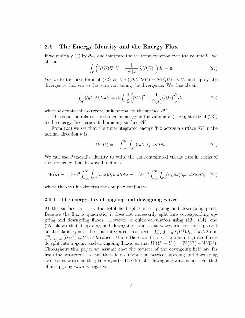
2.6 The Energy Identity and the Energy Flux

If we multiply (2) by ∂tU and integrate the resulting equation over the volume V , weobtain

∫

V

(

(∂tU)∇2U −1

2c2(x)∂t(∂tU)2

)

dx = 0. (22)

We write the first term of (22) as ∇ · ((∂tU)∇U) − ∇(∂tU) · ∇U , and apply thedivergence theorem to the term containing the divergence. We thus obtain

∫

∂V(∂tU)∂νUdS = ∂t

∫

V

1

2

(

|∇U |2 +1

c2(x)(∂tU)2

)

dx, (23)

where ν denotes the outward unit normal to the surface ∂V .This equation relates the change in energy in the volume V (the right side of (23))

to the energy flux across its boundary surface ∂V .From (23) we see that the time-integrated energy flux across a surface ∂V in the

normal direction ν is

W (U) = −∫ ∞

−∞

∫

∂V(∂tU)∂νUdSdt. (24)

We can use Parseval’s identity to write the time-integrated energy flux in terms ofthe frequency-domain wave functions:

W (u) = −(2π)3∫ ∞

−∞

∫

∂V(iωu)∂νu dSdω = −(2π)3

∫ ∞

−∞

∫

∂V(ic0ku)∂νu dSc0dk, (25)

where the overline denotes the complex conjugate.

2.6.1 The energy flux of upgoing and downgoing waves

At the surface x3 = 0, the total field splits into upgoing and downgoing parts.Because the flux is quadratic, it does not necessarily split into corresponding up-going and downgoing fluxes. However, a quick calculation using (13), (14), and(25) shows that if upgoing and downgoing evanescent waves are not both presenton the plane x3 = 0, the time-integrated cross terms

∫∞−∞

∫

x3=0(∂tU↓)∂x3

U↑dx′dt and∫∞−∞

∫

x3=0(∂tU↑)∂x3

U↓dx′dt cancel. Under these conditions, the time-integrated fluxesdo split into upgoing and downgoing fluxes, so that W (U↓ +U↑) = W (U↓) +W (U↑).Throughout this paper we assume that the sources of the downgoing field are farfrom the scatterers, so that there is no interaction between upgoing and downgoingevanescent waves on the plane x3 = 0. The flux of a downgoing wave is positive; thatof an upgoing wave is negative.

7

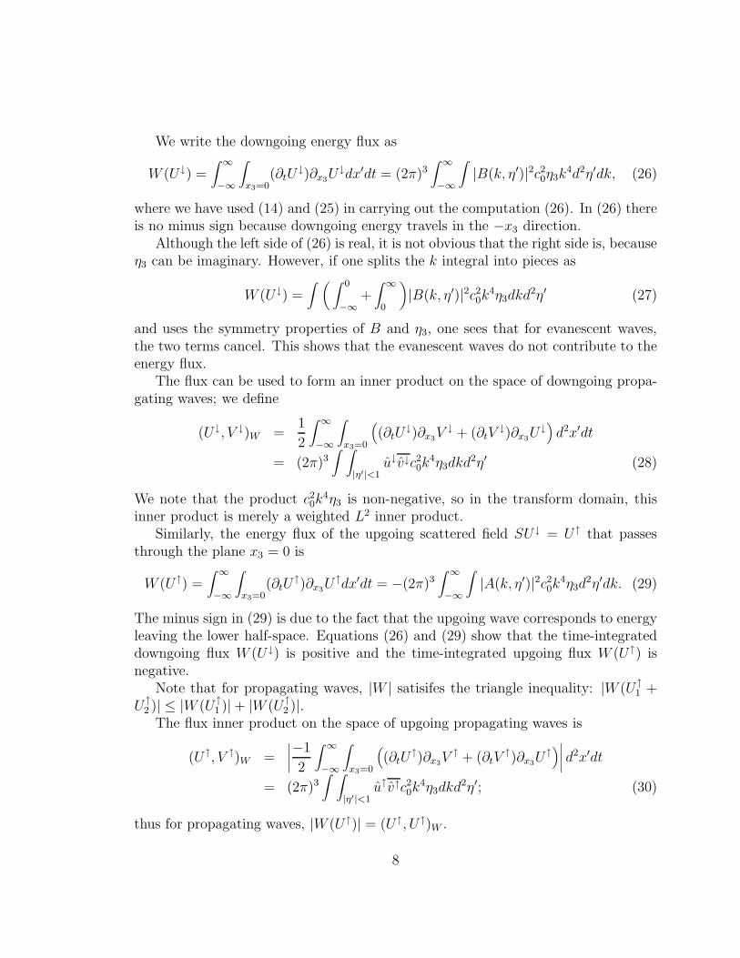
We write the downgoing energy flux as

W (U↓) =∫ ∞

−∞

∫

x3=0(∂tU

↓)∂x3U↓dx′dt = (2π)3

∫ ∞

−∞

∫

|B(k, η′)|2c20η3k4d2η′dk, (26)

where we have used (14) and (25) in carrying out the computation (26). In (26) thereis no minus sign because downgoing energy travels in the −x3 direction.

Although the left side of (26) is real, it is not obvious that the right side is, becauseη3 can be imaginary. However, if one splits the k integral into pieces as

W (U↓) =∫(∫ 0

−∞+∫ ∞

0

)

|B(k, η′)|2c20k4η3dkd

2η′ (27)

and uses the symmetry properties of B and η3, one sees that for evanescent waves,the two terms cancel. This shows that the evanescent waves do not contribute to theenergy flux.

The flux can be used to form an inner product on the space of downgoing propa-gating waves; we define

(U↓, V ↓)W =1

2

∫ ∞

−∞

∫

x3=0

(

(∂tU↓)∂x3

V ↓ + (∂tV↓)∂x3

U↓)

d2x′dt

= (2π)3∫ ∫

|η′|<1u↓v↓c20k

4η3dkd2η′ (28)

We note that the product c20k4η3 is non-negative, so in the transform domain, this

inner product is merely a weighted L2 inner product.Similarly, the energy flux of the upgoing scattered field SU↓ = U↑ that passes

through the plane x3 = 0 is

W (U↑) =∫ ∞

−∞

∫

x3=0(∂tU

↑)∂x3U↑dx′dt = −(2π)3

∫ ∞

−∞

∫

|A(k, η′)|2c20k4η3d

2η′dk. (29)

The minus sign in (29) is due to the fact that the upgoing wave corresponds to energyleaving the lower half-space. Equations (26) and (29) show that the time-integrateddowngoing flux W (U↓) is positive and the time-integrated upgoing flux W (U↑) isnegative.

Note that for propagating waves, |W | satisifes the triangle inequality: |W (U↑1 +

U↑2 )| ≤ |W (U↑

1 )| + |W (U↑2 )|.

The flux inner product on the space of upgoing propagating waves is

(U↑, V ↑)W =∣

∣

∣

∣

−1

2

∫ ∞

−∞

∫

x3=0

(

(∂tU↑)∂x3

V ↑ + (∂tV↑)∂x3

U↑)

∣

∣

∣

∣

d2x′dt

= (2π)3∫ ∫

|η′|<1u↑v↑c20k

4η3dkd2η′; (30)

thus for propagating waves, |W (U↑)| = (U↑, U↑)W .

8

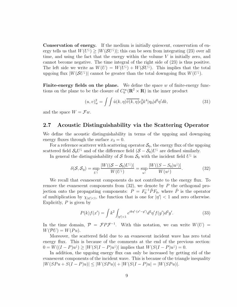
Conservation of energy. If the medium is initially quiescent, conservation of en-ergy tells us that W (U↓) ≥ |W (SU↓)|; this can be seen from integrating (23) over alltime, and using the fact that the energy within the volume V is initially zero, andcannot become negative. The time integral of the right side of (23) is thus positive.The left side we write as W (U) = W (U↓) + W (SU↓). This implies that the totalupgoing flux |W (SU↓)| cannot be greater than the total downgoing flux W (U↓).

Finite-energy fields on the plane. We define the space w of finite-energy func-tions on the plane to be the closure of C∞

0 (R2 × R) in the inner product

(u, v)2w =

∫ ∫

u(k, η)v(k, η)c20k4|η3|d

2η′dk, (31)

and the space W = Fw.

2.7 Acoustic Distinguishability via the Scattering Operator

We define the acoustic distinguishability in terms of the upgoing and downgoingenergy fluxes through the surface x3 = 0.

For a reference scatterer with scattering operator S0, the energy flux of the upgoingscattered field S0U

↓ and of the difference field (S − S0)U↓ are defined similarly.

In general the distinguishability of S from S0 with the incident field U↓ is

δ(S,S0) = supU↓

|W ((S − S0)U↓)|

W (U↓)= sup

u↓

|W ((S − S0)u↓)|

W (u↓). (32)

We recall that evanescent components do not contribute to the energy flux. Toremove the evanescent components from (32), we denote by P the orthogonal pro-jection onto the propagating components: P = F−1

0 PF0, where P is the operatorof multiplication by χ|η′|<1, the function that is one for |η′| < 1 and zero otherwise.Explicitly, P is given by

P (k)f(x′) =∫

k2∫

|η′|<1eikη′·(x′−y′)d2η′f(y′)d2y′. (33)

In the time domain, P = FPF−1. With this notation, we can write W (U) =W (PU) = W (Pu).

Moreover, the scattered field due to an evanescent incident wave has zero totalenergy flux. This is because of the comments at the end of the previous section:0 = W ((I − P )u↓) ≥ |W (S(I − P )u↓)| implies that W (S(I − P )u↓) = 0.

In addition, the upgoing energy flux can only be increased by getting rid of theevanescent components of the incident wave. This is because of the triangle inequality|W (SPu+ S(I − P )u)| ≤ |W (SPu)|+ |W (S(I − P )u| = |W (SPu)|.

9

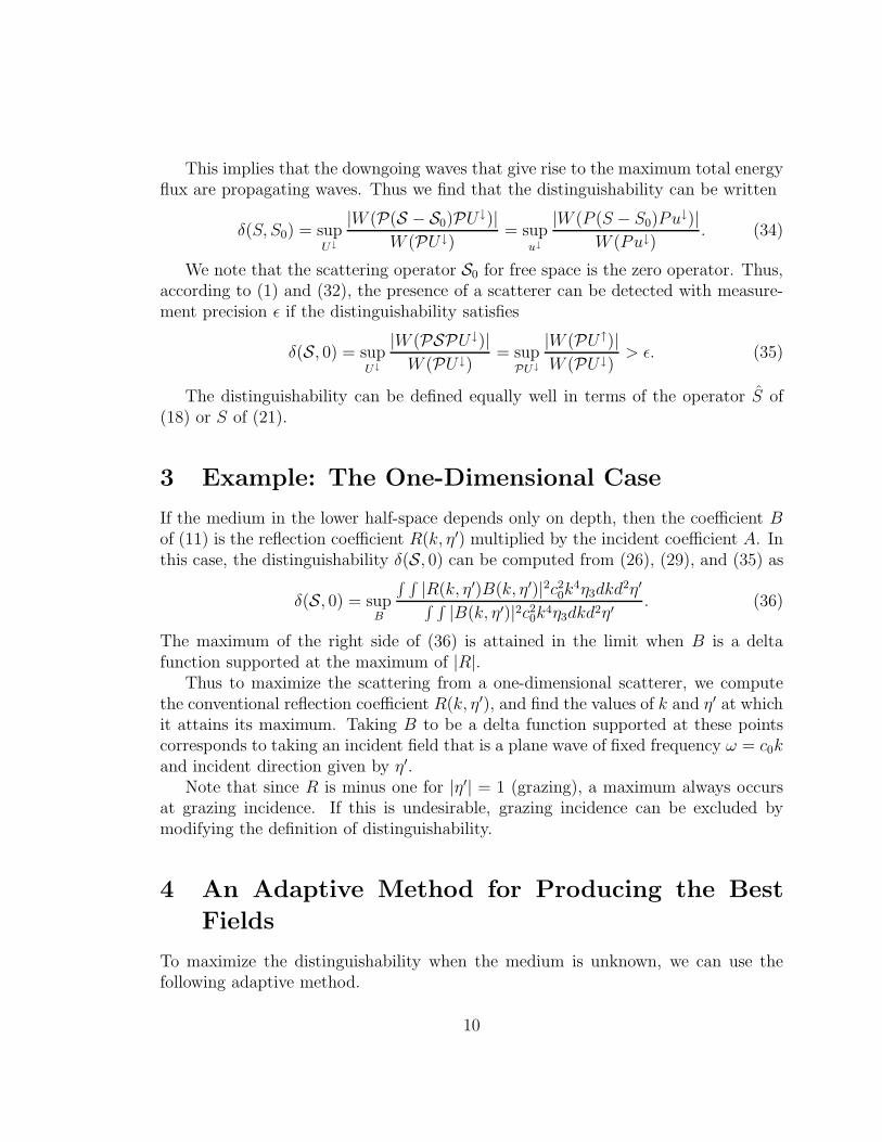
This implies that the downgoing waves that give rise to the maximum total energyflux are propagating waves. Thus we find that the distinguishability can be written

δ(S, S0) = supU↓

|W (P(S − S0)PU↓)|

W (PU↓)= sup

u↓

|W (P (S − S0)Pu↓)|

W (Pu↓). (34)

We note that the scattering operator S0 for free space is the zero operator. Thus,according to (1) and (32), the presence of a scatterer can be detected with measure-ment precision ǫ if the distinguishability satisfies

δ(S, 0) = supU↓

|W (PSPU↓)|

W (PU↓)= sup

PU↓

|W (PU↑)|

W (PU↓)> ǫ. (35)

The distinguishability can be defined equally well in terms of the operator S of(18) or S of (21).

3 Example: The One-Dimensional Case

If the medium in the lower half-space depends only on depth, then the coefficient Bof (11) is the reflection coefficient R(k, η′) multiplied by the incident coefficient A. Inthis case, the distinguishability δ(S, 0) can be computed from (26), (29), and (35) as

δ(S, 0) = supB

∫ ∫

|R(k, η′)B(k, η′)|2c20k4η3dkd

2η′∫ ∫

|B(k, η′)|2c20k4η3dkd2η′

. (36)

The maximum of the right side of (36) is attained in the limit when B is a deltafunction supported at the maximum of |R|.

Thus to maximize the scattering from a one-dimensional scatterer, we computethe conventional reflection coefficient R(k, η′), and find the values of k and η′ at whichit attains its maximum. Taking B to be a delta function supported at these pointscorresponds to taking an incident field that is a plane wave of fixed frequency ω = c0kand incident direction given by η′.

Note that since R is minus one for |η′| = 1 (grazing), a maximum always occursat grazing incidence. If this is undesirable, grazing incidence can be excluded bymodifying the definition of distinguishability.

4 An Adaptive Method for Producing the Best

Fields

To maximize the distinguishability when the medium is unknown, we can use thefollowing adaptive method.

10

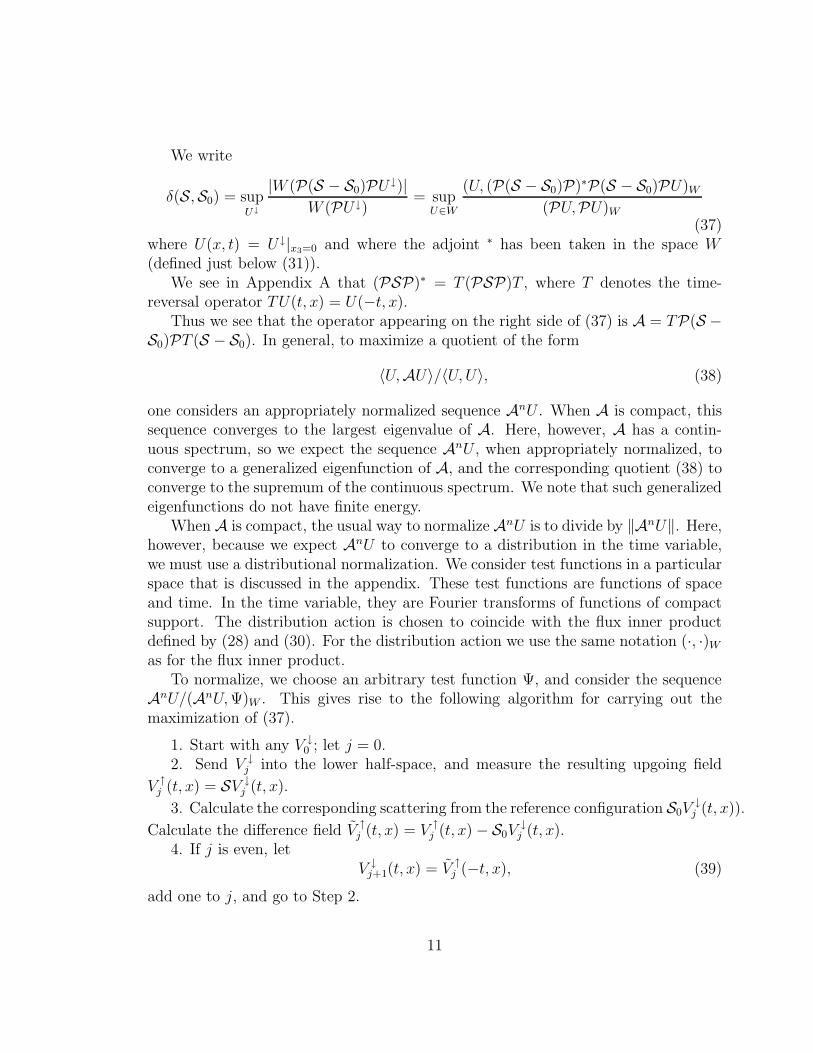
We write

δ(S,S0) = supU↓

|W (P(S − S0)PU↓)|

W (PU↓)= sup

U∈W

(U, (P(S − S0)P)∗P(S − S0)PU)W

(PU,PU)W

(37)where U(x, t) = U↓|x3=0 and where the adjoint ∗ has been taken in the space W(defined just below (31)).

We see in Appendix A that (PSP)∗ = T (PSP)T , where T denotes the time-reversal operator TU(t, x) = U(−t, x).

Thus we see that the operator appearing on the right side of (37) is A = TP(S −S0)PT (S − S0). In general, to maximize a quotient of the form

〈U,AU〉/〈U,U〉, (38)

one considers an appropriately normalized sequence AnU . When A is compact, thissequence converges to the largest eigenvalue of A. Here, however, A has a contin-uous spectrum, so we expect the sequence AnU , when appropriately normalized, toconverge to a generalized eigenfunction of A, and the corresponding quotient (38) toconverge to the supremum of the continuous spectrum. We note that such generalizedeigenfunctions do not have finite energy.

When A is compact, the usual way to normalize AnU is to divide by ‖AnU‖. Here,however, because we expect AnU to converge to a distribution in the time variable,we must use a distributional normalization. We consider test functions in a particularspace that is discussed in the appendix. These test functions are functions of spaceand time. In the time variable, they are Fourier transforms of functions of compactsupport. The distribution action is chosen to coincide with the flux inner productdefined by (28) and (30). For the distribution action we use the same notation (·, ·)W

as for the flux inner product.To normalize, we choose an arbitrary test function Ψ, and consider the sequence

AnU/(AnU,Ψ)W . This gives rise to the following algorithm for carrying out themaximization of (37).

1. Start with any V ↓0 ; let j = 0.

2. Send V ↓j into the lower half-space, and measure the resulting upgoing field

V ↑j (t, x) = SV ↓

j (t, x).

3. Calculate the corresponding scattering from the reference configuration S0V↓j (t, x)).

Calculate the difference field V ↑j (t, x) = V ↑

j (t, x) − S0V↓j (t, x).

4. If j is even, letV ↓

j+1(t, x) = V ↑j (−t, x), (39)

add one to j, and go to Step 2.

11

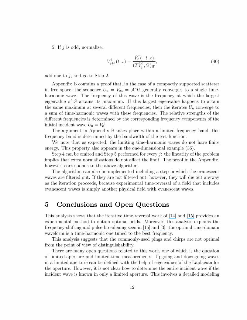
5. If j is odd, normalize:

V ↓j+1(t, x) =

V ↑j (−t, x)

(T V ↑j ,Ψ)W

, (40)

add one to j, and go to Step 2.

Appendix B contains a proof that, in the case of a compactly supported scattererin free space, the sequence Un = V2n = AnU generally converges to a single time-harmonic wave. The frequency of this wave is the frequency at which the largesteigenvalue of S attains its maximum. If this largest eigenvalue happens to attainthe same maximum at several different frequencies, then the iterates Un converge toa sum of time-harmonic waves with these frequencies. The relative strengths of thedifferent frequencies is determined by the corresponding frequency components of theinitial incident wave U0 = V ↓

0 .The argument in Appendix B takes place within a limited frequency band; this

frequency band is determined by the bandwidth of the test function.We note that as expected, the limiting time-harmonic waves do not have finite

energy. This property also appears in the one-dimensional example (36).Step 4 can be omited and Step 5 performed for every j: the linearity of the problem

implies that extra normalizations do not affect the limit. The proof in the Appendix,however, corresponds to the above algorithm.

The algorithm can also be implemented including a step in which the evanescentwaves are filtered out. If they are not filtered out, however, they will die out anywayas the iteration proceeds, because experimental time-reversal of a field that includesevanescent waves is simply another physical field with evanescent waves.

5 Conclusions and Open Questions

This analysis shows that the iterative time-reversal work of [14] and [15] provides anexperimental method to obtain optimal fields. Moreover, this analysis explains thefrequency-shifting and pulse-broadening seen in [15] and [3]: the optimal time-domainwaveform is a time-harmonic one tuned to the best frequency.

This analysis suggests that the commonly-used pings and chirps are not optimalfrom the point of view of distinguishability.

There are many open questions related to this work, one of which is the questionof limited-aperture and limited-time measurements. Upgoing and downgoing wavesin a limited aperture can be defined with the help of eigenvalues of the Laplacian forthe aperture. However, it is not clear how to determine the entire incident wave if theincident wave is known in only a limited aperture. This involves a detailed modeling

12

of the transducer or antenna. Perhaps a formulation in terms of sources will be moreuseful in this case.

We have not studied the question of whether the distinguishability, as a functionof the medium, is monotone in any sense. This is an important issue for the followingreason. Suppose we discover that a sphere of a certain radius is detectable witha certain measurement precision. Does this imply that a larger object will also bedetectable? For fixed-frequency measurements, the answer to this question is certainlyno, because of the phenomenon of resonance. A small sphere may happen to havea radius commensurate with the wavelength of the probing wave, and may thereforescatter much more strongly than a larger sphere. However, the use of time-dependentfields may give different results.

The simple wave equation studied in this paper does not include the importanteffects of variable density, dispersion, and dissipation.

Moreover, the question of distinguishability is only the first step in building anoptimal imaging system. How should we choose a full set of optimal fields that couldbe used to form an image?

6 Acknowledgments

This work was partially supported by the Office of Naval Research. M.C. would like tothank a number of people for helpful discussions: Gerhard Kristensson and his groupin Lund, Jim Rose, Claire Prada, and Isom Herron; M.L. thanks Lassi Paivarinta forinteresting discussions.

A Appendix: Properties of S.

A.1 Expression for Kernel

We can find an expression for the kernel S of (17) and (18) by taking u↓ to be adelta function. The kernel of S is then the corresponding upgoing wave u↑. Takingu↓ to be a delta function means that we take u↓ of the form exp(ikη− · x) for someη− = (η′,−η3). Here η3 can be complex. We write the corresponding frequency-domain field as ψ:

ψ(k, x, η−) =1

2π

∫

U(t, x, η−)eikc0tdt (41)

so thatu(k, η′, x3, η

−) =∫

ψ(k, x, η−)e−ikη′·x′

d2x′. (42)

13

In the case of scattering from a perturbation in free space, we can express thetotal frequency-domain field ψ as a solution of the Lippmann-Schwinger equation

ψ(k, x, η) = exp(ikη · x) − k2∫

g(k, x, y)V (y)ψ(k, y, η)d3y, (43)

where g is the usual outgoing Green’s function

g(k, x, y) =eik|x−y|

4π|x− y|(44)

and V (y) = 1 − c20/c2(y). The scattered field u↑ thus is represented by the integral

term of (43).The Green’s function can be written in terms of its two-dimensional Fourier trans-

form as [2]

g(k, x, y) =1

(2π)2

∫

i

2kη3eikη3|x3−y3|eikη′·(x′−y′)k2d2η′. (45)

To compute A and B of (11), we take the x1, x2 Fourier transform of (43) in theregion x3 > 0. We assume that the perturbation V is supported in the region y3 < 0,so that when we consider (43) we can remove the absolute values in (45). In thetransform domain, the scattered field is given by

u↑(k, η′, x3, η−) = −k2

∫

i

2kη3

∫

e−ikη+·yV (y)ψ(k, y, η−)d2y′dy3eikη3x3 . (46)

This shows that

S(k, η′, η′) = −ik

2η3A(k, η+, η−) (47)

whereA(k, η, η) =

∫

e−ikη·yV (y)ψ(k, y, η)d3y (48)

is a scalar multiple of the classical scattering amplitude [13]. (This A is not to beconfused with the A of (11)!) It satisfies the reciprocity relation

A(k, η, η) = A(k,−η,−η) (49)

and the symmetry relation (for real-valued perturbations V )

A(k, η, η) = A(−k, η, η). (50)

It is clear from (47) that S is an analytic function of k [13].An expression similar to (47) can be obtained for the field scattered from a per-

turbed half-space or layered medium; in this case the appropriate background Green’sfunction should be used instead of the free-space Green’s function in (43). Scatteringtheory in such cases is considered, for example, in [19], [20], and [7].

14

A.2 The Adjoint

For a scatterer in free space, the adjoint of PSP in the space W can be computedexplicitly as follows. From (30) we have

(PSPU, V )W = (2π)3∫ ∞

−∞

∫

|η′|<1

∫

|η′|<1S(k, η′, η′)u(k, η′)k2d2η′v(k, η′)c20k

4η3dkd2η′

= (2π)3∫ ∞

−∞

∫

|η′|<1u(k, η′)

∫

|η′|<1S(k, η′, η′)v(k, η′)η3d2η′c20k

6dkd2η′

(51)

From (47), (49), and (50), we have

(PSPU, V )W

(2π)3=

∫ ∞

−∞

∫

|η′|<1u(k, η′)

∫

|η′|<1−(ik/2)A(k,−η−,−η+)v(k, η′)d2η′c20k

6dkd2η′

=∫ ∞

−∞

∫

|η′|<1u(k, η′)

∫

|η′|<1(ik/2)A(−k,−η−,−η+)v(k, η′)d2η′c20k

6dkd2η′

=∫ ∞

−∞

∫

|η′|<1u(k, η′)

∫

|η′|<1S(−k,−η′,−η′)v(k, η′)d2η′η3(−k)c

20k

6dkd2η′,

(52)

where in the last equality we have used the fact that S(−k, η′, η′) = ik(2η3)−1A(−k, η+, η−).

We note that in the course of this computation, the η3 has disappeared and has beenreplaced by η3; this is because of the η3 in the denominator of (47).

We see that the action of the adjoint (PSP)∗ on V is given in the transformdomain by the η′ integral of (52):

FF−1(PSP)∗FF−1v(k, η′) =∫

|η′|<1S(−k,−η′,−η′)v(k, η′)k2d2η′. (53)

However, S(k, η′, η′) is defined by

δ(

c0(k − k))

S(k, η′, η′) =∫ ∞

−∞

∫ ∞

−∞

∫ ∫

e−ikη′·x′

eikc0tS(t−τ, x′, y′)e−ikc0τeikη′·y′

d2x′d2y′dτdt.

(54)From this, we see that

δ(

c0(k − k))

S(−k,−η′,−η′) =∫ ∞

−∞

∫ ∞

−∞

∫ ∫

e−ikη′·x′

e−ikc0tS(t−τ, x′, y′)eikc0τeikη′·y′

d2x′d2y′dτdt.

(55)Letting t→ −t and τ → −τ in (55) shows that the kernel of (53) corresponds to theoperator TPSPT , given by

(TPSPT )V (t, x′) =∫ ∞

−∞

∫ ∞

−∞S(τ − t, x′, y′)V (t, y′)dτd2y′. (56)

Thus (PSP)∗ = T (PSP)T .

15

A.3 Compactness

Theorem 1 Assume that the sound speed c(x) is bounded and differs from c0 only ina bounded subset of the half-space x3 ≤ −h < 0. Then the fixed-frequency scatteringoperator S is compact on the weighted space

L2g = {f : f(η′)|1 − |η′|2|1/4 ∈ L2}. (57)

Proof. We use (47) and (12) to compute the square of the Hilbert-Schmidt normof S in the space L2

g:

‖S‖2H.S. =

k4

4

∫ ∫∣

∣

∣

∣

∫

e−ikη·yV (y)ψ(k, y, η′)d3y

∣

∣

∣

∣

2∣

∣

∣

∣

∣

1 − |η′|2

1 − |η′|2

∣

∣

∣

∣

∣

1/2

d2η′d2η′. (58)

We use the fact that ψ can be split into an incident and scattered field via (43).This allows us to split the kernel (47) into two parts:

S(k, η, η′) = SB(k, η, η′) + Ssc(k, η, η′) (59)

where the “Born” term is

SB(k, η, η′) = −ik

2η3

∫

eik(η−η)·yV (y)d3y (60)

and

Ssc(k, η, η′) = −

ik3

2η3

∫

e−ikη·yV (y)∫

g(y − z)V (z)ψ(k, z, η′)d3zd3y. (61)

We compute the Hilbert-Schmidt norm of each part.The Hilbert-Schmidt norm of the Born term is

‖SB‖2H.S. =

k2

4

∫ ∫∣

∣

∣

∣

∫

eik(η−η)·yV (y)d3y∣

∣

∣

∣

2∣

∣

∣

∣

∣

1 − |η′|2

1 − |η′|2

∣

∣

∣

∣

∣

1/2

d2η′d2η′. (62)

The y integral of (62) can be written

∫

eik(η′−η′)·y′

e−ik(η3+η3)y3V (y)d3y. (63)

For |η′| < 1, for which η3 is real, this integral is bounded when V is integrable. For|η′| > 1, the integral decays exponentially because V is supported in the region wherey3 ≤ h < 0. The same comments apply to the behavior in η′. Thus this integral isbounded by c exp(−hk(|η′| + |η′|)). This estimate can easily be used to show that‖SB‖H.S. is finite.

16

The Hilbert-Schmidt norm of the scattered part is

‖Ssc‖2H.S. =

k6

4

∫ ∫∣

∣

∣

∣

∫

e−ikη·yV (y)∫

g(y − z)V (z)ψ(k, z, η′)d3zd3y

∣

∣

∣

∣

2∣

∣

∣

∣

∣

1 − |η′|2

1 − |η′|2

∣

∣

∣

∣

∣

1/2

d2η′d2η′.

(64)An application of the Cauchy-Schwarz inequality shows that the y integral of (64)

is bounded by

‖e−ikη·yV (y)|2‖L2(y)

∥

∥

∥

∥

|V (y)|1/2∫

g(y − z)V (z)ψ(k, z, η′)d3z∥

∥

∥

∥

L2(y)(65)

Direct computation shows that the first norm in (65) is bounded by c exp(−hk|η′|).Standard scattering theory arguments (See Appendix C) can be used to show thatthe second norm appearing in (65) is bounded by c exp(−hk|η′|); thus the y integralsatisfies the same bounds as in the Born term. QED

Remark. In [2], it was shown that on L2g, the operator P SP has norm less than

or equal to one.For future reference, we note that the operator a(k) = (PSP )∗(PSP ) is given

explicitly as

(Faf)(η′) =∫

|η′|<1

∫

|ζ′|<1S(−k,−η′,−ζ ′)S(k, ζ ′, η′)d2ζ ′f(η′)k4d2η′. (66)

B Appendix: Convergence of the Iterative Algo-

rithm

For simplicity of notation we consider only the case when S0 = 0. In this case, thenth iterate is

U↓n =

(T (PSP)T (PSP))nU↓0

((T (PSP)T (PSP))nU↓0 ,ΨB)W

=AnU↓

0

(AnU↓0 ,ΨB)W

, (67)

where A = (PSP)∗(PSP), where the star denotes the adjoint with respect tothe flux inner product (·, ·)W . We simplify the notation by dropping the arrowon U . Because we expect the limit to be a distribution, we consider the quantity(Un,Φ)W =

∫

(un, φ)x′c20k4dk, where Φ is a smooth test function, φ = FΦ, and ( , )x′

denotes the weighted inner product that for smooth functions is (f, φ)x′ = (f , φ)L2g

=∫

f(η′)φ(η′)|η3|d2η′.

Specifically, we consider test function that are functions of t and x′. When inverseFourier transformed in t and Fourier transformed in space, at each frequency they

17

must be in L2g, and in the frequency variable they must be integrable and (uniformly)

supported in the compact interval [−B,B]. We denote this space of test functions byX.

In the frequency domain, the nth iteration is F−1(AnU) = anu, where F−1 denotesthe inverse Fourier transform (6) and a = F−1AF = (PSP )∗(PSP ). From ournormalization of Un, we have

(Un,ΦB)W =(AnU,ΦB)W

(AnU,ΨB)W=

∫

〈anu, φB〉x′c20k4dk

∫

〈anu, ψB〉x′c20k4dk

. (68)

We note that A and a(k) are self-adjoint on the space W and on L2g, respectively.

Moreover, Theorem 1 shows that a(k) is compact on L2g, and it can therefore be

written a(k) =∑

l λl(k)Pl(k), where λl ≥ λl+1 and the Pl are orthogonal projections.Because A is non-negative, all the eigenvalues λl are non-negative. We see from (66)that a is analytic in k, and the λs are therefore piecewise analytic [8].

Suppose that λ0(k) attains its maximum in the set {|k| < B} at k0, and thatλ(k) = M . Then in a neighborhood of k0, λ(k) has a Taylor expansion whose firsttwo terms are M − b(k − k0)

p for some b and some integer p. We call p the order ofλ0.

We allow eigenvalues with different indices to coincide at a point; thus it is possiblethat a finite number of eigenvalues also attain the maximum M at k0. In this case,these eigenvalues have a Taylor expansion similar to that of λ0, possibly with differentbs and ps. In this case we also refer to the relevant p as the order of the eigenfunction.

We will need the following lemma.

Lemma 1 Assume that b is positive and that p is an integer. Then for large n,

I(n, p) =∫ h

0(1 − bkp)ndk ∼

C(p)

(bn)1/p, (69)

where C(p) is a nonzero constant independent of n. Thus the convergence to zero ofI(n, p) is slower for larger p and smaller b.

Proof. Let s = b1/pk. Then I = b−1/p∫ b1/ph0 (1− sp)nds. Replacing the upper limit

by 1 results in an error that is exponentially small in n. Denote by In the integral∫ 10 (1 − sp)nds. Then we can write

In+1 =∫ 1

0(1 − sp)(1 − sp)nds = In −

∫ 1

0sp(1 − sp)nds. (70)

In the integral of (70), we integrate by parts, differentiating s and integrating sp−1(1−sp)n. The boundary term vanishes, and (70) becomes

In+1 = In +1

p(n+ 1)In+1. (71)

18

Solving for In+1 gives the recursion

In+1 =p(n+ 1)

p(n + 1) + 1In. (72)

Since I0 = 1, we have

In =

(

p

p+ 1

)(

2p

2p+ 1

)

· · ·

(

np

np+ 1

)

. (73)

Taking reciprocals and logs and expanding, we find that

− log In =n∑

j=1

log(1 + 1/(jp))

=1

p

n∑

j=1

1

j−

∞∑

m=2

(−1)m

mpm

n∑

j=1

1

kjm(74)

Exponentiating and taking reciprocals again, we have

In = C(n, p) exp(−1

p

n∑

j=1

1

j), (75)

where C(n, p) has the large-n limit

limn→∞

C(n, p) = exp

(

−∞∑

m=2

(−1)m

mpmζ(m)

)

, (76)

where ζ(m) denotes the Riemann-zeta function ζ(m) =∑∞

k=1 k−m. Thus we see that

the large-n behavior of In is determined by the second factor of (75).We determine the large-n behavior of this second factor as follows. From approx-

imating the sum by a Riemann integral, we have the estimate

log n ≤ log(n+ 1) ≤n∑

j=1

1

j≤ 1 + log n (77)

We multiply by −1/p and exponentiate to obtain

e−1/pn−1/p ≤ exp(−1

p

n∑

j=1

1

j) ≤ n−1/p (78)

QED

19

Theorem 2 Assume that a is an analytic self-adjoint-compact-operator-valued func-tion of k having the representation a(k) =

∑

l λl(k)Pl(k), where λl ≥ λl+1 and the Pl

are orthogonal projections. Assume that λ0 is not a constant function of k. Then fortest functions φB(k, x′) and ψB(k, x′) in X whose support in the frequency domain isin the set {|k| ≤ B},

limn→∞

∫

(anu, φB)x′kdk∫

(anu, ψB)x′kdk=

∑

l,j βlj(Plu, φB)x′(kj)∑

l,j βlj(Plu, ψB)x′(kj)(79)

where the sums are over those indices j and l for which λl(kj) = M , where M is themaximum of λ0 in the set {k : |k| ≤ B}, and for which λl has maximal order at kj.

ProofThe representation for a allows us to write (68) as

(Un,ΦB)W =

∫∑

l λnl (Plu, φB)x′kdk

∫∑

l λnl (Plu, ψB)x′kdk

(80)

The λl and Pl are peicewise analytic functions of k [8]. In particular λ0(k) is piecewiseanalytic, and therefore attains its maximum M on a discrete subset of the set {|k| ≤B}. We cover the support of φ with open intervals Nj so that each Nj contains onlyone kj. We decompose the test function φB as φB =

∑

j φj [5], where the φj are inC∞

0 (Nj) and φj = φB in a neighborhood of kj . We carry out a similar decompositionfor ψB.

With the notation fl,j(k) = k(Plu, φj)x′ and gl,j(k) = k(Plu, ψj)x′, we can write(80) as

(Un,ΦB)W =

∑

l,j

∫

Njλn

l (k)fl,j(k)dk∑

l,j

∫

Njλn

l (k)gl,j(k)dk. (81)

We divide the numerator and denominator of (81) by Mn, and write rl(k) =λl(k)/M ; thus |r0| ≤ 1, and |rl| < 1 for all but a finite number of values of l. Then(81) can be written

(Un,ΦB)W =

∑

l,j

∫

Njrnl (k)fl,j(k)dk

∑

l,j

∫

Njrnl (k)gl,j(k)dk

. (82)

We writeInl,j =

∫

Nj

rnl (k)fl,j(k)dk. (83)

We multiply and divide Inl,j by

∫

Njrn0 (k)dk, and write ζn

l = rnl /∫

Njrn0dk.

For those l = 0, 1, . . . Lj for which λl attains the maximum M and thus rl attainsthe value 1, we add and subtract fl,j(kj) to the quotient, obtaining

Inl,j =

(

fl,j(kj) +∫

Nj

ζnl (k)(fl,j(k) − fl,j(kj))dk

)

∫

Nj

rn0 (k)dk (84)

20

We will show that the integral term within the parentheses on the right side of (84)vanishes as n goes to infinity. For this we use the two facts that 1) except at k = kj ,ζnl converges to zero pointwise as n goes to infinity; and 2)

∫

ζnl = 1 for all n.

Given ǫ > 0, we choose N ǫj so small that on N ǫ

j , |fl,j(k) − fl,j(kj)| < ǫ/2. Theintegral in parentheses on the right side of (84) we split into two integrals, namelyAn and Bn, where

An =∫

Nǫj

ζnl (k)(fl,j(k) − fl,j(kj))dk, (85)

andBn =

∫

Nj\Nǫj

ζnl (k)(fl,j(k) − fl,j(kj))dk. (86)

Then An < ǫ/2. Next, we choose N so large that for n greater than N , Bn < ǫ/2.This shows that the integral in parentheses on the right side of (84) vanishes as ngoes to infinity. Thus (84) is a product of a factor converging to fl,j(kj) and a factorconverging to zero.

For l = Lj + 1, Lj + 2, . . ., for which λl is strictly less than M , we write

Inl,j =

(∫

ζnl (k)fl,j(k)dk

)∫

Nj

rn0 (k)dk. (87)

In this case, ζnl converges to zero pointwise for all k. Thus the integral in parentheses

of Inl,j converges to zero by the Lebesgue Dominated Convergence Theorem.To estimate the tail of the sum over l in (82), we choose l0 so large that for l > l0,

ζl(k) < 1/2 for all k in Nj. This is possible because the the compactness of a impliesthat its eigenvalues decrease to zero. Thus for each j we have

∣

∣

∣

∣

∣

∣

∑

l>l0

Inl,j

∣

∣

∣

∣

∣

∣

=

∣

∣

∣

∣

∣

∣

∑

l>l0

∫

Nj

ζnl (k)(Plu, φj)x′kdk

∣

∣

∣

∣

∣

∣

≤1

2n

∫

Nj

∑

l>l0

|(u, ϕl)x′(ϕl, φj)x′k| dk, (88)

where the ϕl are the normalized eigenfunctions of a. Here it may be necessary toreindex the sum. Each of the sequences (u, ϕl)x′ and (ϕl, φj)x′ is in l2, and the innerproduct of two l2 sequences is in l1. We therefore find that the sum over l is boundedby ‖u‖k‖φj‖k, where ‖ · ‖k denotes the norm in the space L2

k. Thus we have∣

∣

∣

∣

∣

∣

∑

l>l0

Inl,j

∣

∣

∣

∣

∣

∣

≤1

2n

∫

Nj

‖u‖k‖φj‖kkdk (89)

which shows that the tail of the sum converges to zero as n goes to infinity.The same arguments, of course, apply to the denominator of (82). Thus we see

that the leading order behavior of (82) is given by the expression

(Un,ΦB)W ∼

∑

l,j fl,j(kj)∫

Njrn0 (k)dk

∑

l,j gl,j(kj)∫

Njrn0 (k)dk

, (90)

21

where the sum in l is over those values for which λl attains the maximum M at kj .The terms

∫

Njrn0 (k)dk, however, go to zero for large n. We must therefore consider

their behavior in more detail.As we have seen, in the neighborhood of k = kj, r0(k) has an expansion of the

form r0(k) = 1 − bj(k − kj)pj + . . ., where the positive integer pj is the order of the

eigenfunction at kj. The lemma shows that the order pj controls the speed with which∫

Njrn0 (k)dk goes to zero with n: the larger pj, the more slowly

∫

rN0 dk coverges to

zero. We divide the numerator and denominator of (82) by∫

Njrn0dk corresponding

to the slowest decay. Finally, we take the limit of the resulting quotient as n goes toinfinity. This shows that the quotient (82) converges to

(Un,ΦB)W ∼

∑

l,j βj(Plu, φ)x′(kj)∑

l,j βj(Plu, ψ)x′(kj)=∫ ∫

∑

l,j

βjPlu(kj, x

′)∑

l,i βi(Plu, ψ)x′(ki)δkj

(k)φ(k, x′)d2x′dk,

(91)

where the βj are proportional to βj = kjC(pj)/b1/pj

j , and where the sums are overthose indices j and l for which λl has maximal order at kj.

QED.

Corollary 1 Assume that the sound speed c(x) is bounded and differs from c0 onlyin a bounded subset of the half-space x3 ≤ −h < 0. Then for test functions ΨB,ΦB

in X whose Fourier transforms with respect to time are supported in −B ≤ k ≤ B,Un as defined by (67) converges to

1

2π∑

l,i βk(Plu, ψB)x′(ki)

∑

l,j

βjPlu(kj, x′)e−ikjc0t, (92)

where the sums are over those indices j and l for which λl(kj) attains the maximumM and has maximal order.

Proof. To apply Theorem 2, we need only check that a = F−1(PSP)∗(PSP)F isindeed an analytic compact-operator-valued function of k. Analyticity was shown insection A.1; compactness was shown in section A.3. The largest eigenvalue λ0 cannotbe constant: S is zero at k = 0, which implies that all the λj are zero there. Thus ifλ0 were constant it would be zero, and S itself would be zero.

We note that both the numerator and denominator in (92) can be zero, in whichcase (92) is not defined. However we do not study this case since the denominator isnon-zero for a generic test function ΨB. QED

22

C Appendix: Results from “Standard” Scattering

Theory

The solution of the equation

(∇2 + k2 − V (x))ψ(k, x) = 0 (93)

corresponding to an incident plane wave and a scattered field satisfying outgoingboundary conditions satisfies the Lippmann-Schwinger integral equation

ψ(k, x, η′) = exp(ikη · x) − k2∫

g(k, x, y)V (y)ψ(k, y, η′)d3y, (94)

where g is the usual outgoing Green’s function (44).The initial difficulty with the Lippmann-Schwinger equation is that the incident

field has infinite energy. This difficulty, however, can be circumvented by multiplyingthe whole equation by |V (x)|1/2 [18]. This converts (94) into

ζ(k, x, η′) = ζ0(k, x, η′) + k2

∫

K(k, x− y)ζ(k, y, η′)d3y, (95)

where

ζ(k, x, η′) = |V (x)|1/2ψ(k, x, η′), (96)

ζ0(k, x, η′) = |V (x)|1/2eikη·x, (97)

V1/2(y) = V (y)/|V (y)|1/2 (98)

K(x, y) = |V (x)|1/2g(k, x, y)V1/2(y) (99)

(100)

When V has compact support, (95) is an integral equation on a bounded region.The kernel K is an Hilbert-Schmidt-valued function that is analytic in the entirecomplex k-plane. By the analytic Fredholm theorem [16], the integral equation (95)is therefore uniquely solvable everywhere except at a discrete set of values of k, (the“exceptional points”) and moreover the solution ζ is a meromorphic function of kwith poles at these exceptional points. In addition, the arguments of [1] [17] showthat the only possible real exceptional point is k = 0. However, when k = 0, wealso have k = 0, and (95) reduces to the equation ζ = |V |1/2. Thus the operator(I − k2K)−1 is analytic in a neighborhood of the real k-axis.

This argument shows that for each k, ζ = |V |1/2ψ is in L2. Then the quantityneeded in section A.3, namely ‖|V |1/2

∫

gV ψ‖, can be rewritten as ‖Kζ‖ = ‖K(I −K)−1ζ0‖ ≤ ‖K‖‖(I − K)−1‖‖ζ0‖. Moreover, by explicit computation, we see that‖ζ0(k, ·, η

′)‖ ≤ ce−hk|η′|, where V is supported in the region y3 ≤ −h < 0.

23

References

[1] S. Agmon, “Spectral properties of Schrodinger operators and scattering theory”,Ann. Scuola Norm. Sup. Pisa Cl. Sci. II, 2 (1975), 151–218.

[2] M. Cheney and D. Isaacson, “Inverse Problems for a Perturbed Dissipative Half-Space”, Inverse Problems 11 (1995) 865–888.

[3] E. Cherkaeva and A.C. Tripp, “On optimal design of transient electromagneticwaveforms”, SEG97 Expanded Abstracts, 67th Annual Meeting of Soc. ExplorationGeophys. (1997) 438–441.

[4] J.W. Dettman, Applied Complex Variables, Dover, New York, 1965.

[5] L. Hormander, The Analysis of Linear Partial Differential Operators I, Springer,New York, 1983.

[6] D. Isaacson, “Distinguishability of conductivities by electric current computedtomography”, IEEE Trans. on Medical Imaging MI-5(2):92-95, 1986.

[7] G. Eskin and J. Ralston, “Inverse coefficient problems in perturbed half spaces”,Inverse Problems 15 (1999) 683–699.

[8] T. Kato, Perturbation Theory for Linear Operators, Springer-Verlag, Berlin, 1966.

[9] M.S. Lehtinen, On statistical inversion theory. Theory and applications of inverseproblems, Pitman Res. Notes Math. Ser. 167, 46–57, 1988.

[10] M.S. Lehtinen, L. Paivarinta, and E. Somersalo, “Linear inverse problems forgeneralised random variables”, Inverse Problems 5 (1989), no. 4, 599–612.

[11] M. Lassas, M. Cheney, and G. Uhlmann, ”Uniqueness for a wave propagationinverse problem in a half space”, Inverse Problems 14, 679-684 (1998) .

[12] T.D. Mast, A.I. Nachman, and R. C. Waag, “Focusing and imaging using eigen-functions of the scattering operator”, J. Acoust. Soc. Am. 102, Pt. 1 (1997) 715–725.

[13] R.G. Newton, Inverse Schrodinger Scattering in Three Dimensions, Springer,New York, 1989.

[14] C. Prada and M. Fink, “Eigenmodes of the time reversal operator: A solutionto selective focusing in multiple-target media”, Wave Motion 20 (1994), 151–163.

[15] C. Prada, J.-L. Thomas, and M. Fink, “The iterative time reversal process:Analysis of the convergence”, J. Acoust. Soc. Am. 97 (1995) 62–71.

24

[16] M. Reed and B. Simon, Methods of Modern Mathematical Physics. I. FunctionalAnalysis, Academic Press, New York, 1972.

[17] M. Reed and B. Simon, Methods of Modern Mathematical Physics. IV. Func-tional Anlaysis, Academic Press, New York, 1978.

[18] B. Simon, Quantum Mechanics for Hamiltonians Defined as Quadratic Forms,Princeton University Press, New Jersey, 1971.

[19] R. Weder, Spectral and Scattering Theory for Wave Propagation in PerturbedStratified Media”, Springer, New York, 1991.

[20] Y. Xu, “Reciprocity relations and completeness of far-field pattern vectors forobstacle scattering of acoustic wave in a stratified medium”, Math. Methods in theApplied Sciences 18 (1995) 41–66.

25