Efficient shape reconstruction of non-circular tubes using

broadband acoustic measurements

Loıc Le Marrec, Philippe Lasaygues, Thierry Scotti, Chrysoula Tsogka

January 24, 2006

Abstract

We propose an algorithm for reconstructing the boundaries of a non-circular cylindricaltube from broadband acoustic measurements. This algorithm is based on the minimization ofa cost function, which is the averaging over frequency of the absolute difference between theestimated and the measured scattered field. The estimated field is computed efficiently (veryfast) using ICBA, an analytic method that provides an approximated solution of the forwardproblem. Numerical results show that our algorithm is robust and provides an accuratereconstruction without any explicit regularization.

Key words: Acoustic; Non-linear inverse problem; Multi-frequency; Shape reconstruction

1 Introduction

In this paper we address the problem of reconstructing both the inner and outer section of al-most circular cylinders (i.e., for which the maximum deviation from the mean radius is small).The applications we have in mind are non-destructive evaluation (identification of pipe lines)and medical imaging (bones).To solve the inverse scattering problem, a cost function accounting for the discrepancy betweenthe measured and an estimated scattered field, is usually minimized [1]. To overcome the illposedness of such problems, a regularization term expressing some a priori information on thesolution is added to the cost function [2, 3]. The relative confidence on the regularization iscontrolled by a real positive parameter whose choice is delicate and depends on the consideredconfiguration.Our goal being to avoid such difficulties by increasing the amount of data (over-determine theproblem), we consider the insonification of the unknown scatterer by a broadband ultrasonicpulse that provides multi-frequency measurements. For this problem, linear imaging techniques[4, 5] are generally well adapted but their validity is restricted to low-frequency insonificationsor low-contrast objects. On the other hand, non-linear inversion methods [6, 7, 8], which use anexact forward solver to compute the estimated field, are computationally more intense and in-creasing the number of data becomes very expensive. Thus it appears as essential for non-linearinversion methods to employ a forward solver, which is fast and efficient in a large frequencyrange.To enhance the speed of computations in the proposed algorithm we use the Intercepting Canoni-cal Body Approximation (ICBA) as forward solver during the inversion. This consists in approx-imating the scattered field along the measurement direction of the real almost circular cylinderby the scattering due to a centred circular cylinder, which has locally (in the measured direction)the same radius as the object [9]. Our inversion algorithm is therefore computationally efficientas it uses an analytic expression for computing the scattered field.The ICBA approximation has proved its efficiency as forward solver in and beyond the resonanceregion [10] and has been successfully used for real time inversion of monochromatic data. The

1

hal-0

0440

680,

ver

sion

1 -

11 D

ec 2

009

Author manuscript, published in "Acta Acustica united with Acustica 92, 3 (2006) 355-361"

algorithm has been extended to the case of two or three frequencies where an unique solution isobtained by solving the inverse problem for each insonification and then choosing the “closest”common solution [11], the “closest” criterion depending on the user.The problem is here extended to broadband ultrasonic scattering and an algorithm adapted tomultiple frequencies is proposed. The method is first validated for the reconstruction of theshape of a plain cylinder. In a second step the method is extended to the reconstruction of boththe inner and outer sections of a tube with particular attention on the a priori information andon the inversion procedure.In comparison with the previously proposed algorithm it presents the advantage of requiring onlyone minimization (in contrast to two or as many as the frequencies available). Moreover, thesolution does not depend on the adjustment of any parameter. Although the forward problemis solved approximately during the inversion, the proposed method is efficient, and thus suitablefor systematic use in real time imaging.

2 Problem setup

2.1 Description of the scattering problem

Let a plane wave probing, normally to its generator, a cylindrical object defined by the domainΩ2 embedded in an infinite medium Ω1 (Fig.1). The generator of the cylinder is normal to the(x, y) plane and the origin O of the polar coordinate system lies in Ω2. Both materials occupyingdomains Ω1 and Ω2 are assumed to be non-absorbing, homogeneous, isotropic, acoustic materialsand thus the problem is reduced to a two-dimensional linear scalar acoustic scattering problem.The total acoustic fields Pj=1,2 in domains Ωj=1,2 are governed by the corresponding Helmholtzequation and satisfy the continuity conditions at the boundary. The object has penetrableboundary conditions. In Ω1, the scattered field P = P1 − P i satisfies the Sommerfeld radiationcondition at infinity.For a given frequency f , P i = A(f)eik1 cos(θi−θm) express the incident field along θm is expressedby , where θi is the incident angle, A(f) the complex amplitude, k1 = 2πf/c1 the wave number,and c1 the velocity of the surrounding medium. Note that the e−iωt is henceforth implicit.

2.2 Measurements

The measurements are synthetic data obtained by solving numerically the 2D acoustic waveequation. The method used is based on mixed finite elements for the space discretization andon a centered 2nd order finite difference scheme for the time discretization [12].The incident pulse is a normalized second derivative of a Gaussian with central frequency fc.The backscattered field P is recorded on a centered measurement circle of radius rm.In order to analyze the frequency dependence of the inversion, synthetic time-domain measure-ments for a given θm are converted to frequency-domain using a Fast Fourier Transform algo-rithm. This results to a set of backscattered data at L consecutive frequencies with a samplingfrequency δf .

2.3 Approximation

During the inversion, the (true) synthetic scattered field along the measurement direction isapproximated by P e, the scattered field due to a centered circular cylinder, which has the sameacoustical properties as the object and in the measured direction the same radius as the object.We denote here this radius by r1. Remark that for this approximation to be valid it is necessaryto assume that the center of the coordinate belongs to the body. At a single frequency, the

2

hal-0

0440

680,

ver

sion

1 -

11 D

ec 2

009

Table 1: Acoustical characteristics of the media.ρ1 [kg/m3] c1 [m/s] ρ2 [kg/m3] c2 [m/s]

1000 1500 1800 4000

Table 2: Characteristics of the simulations.Probing wave fc [kHz] k1a = 2πfcr1(θm)

c1N (for fc) δf [kHz] L rm [mm] θm

LFI 250.0 6.28 18 6.98 110 12.0 π/4

HFI 1000.0 25.13 41 33.33 92 12.0 π/4

estimated field, P e, is expressed via the following partial waves expansion,

P e(xm, f) = A(f)N∑

n=0

Bn(θm, f)inǫnH(1)n (k1rm) cos(n(θi−θm)) , N = Ent(4.05k1a

1/3+k1a+5)

(1)

where Ent is the entire part function, H(1)n is the first-kind Hankel function of order n, ǫn the

Neumann factor (ǫ0 = 1, ǫn≥1 = 2) and the scattering coefficient Bn is exactly evaluated usingRayleigh-Fourier method [13]. The final order N of the series is chosen according to the methodproposed in [14].

2.4 Numerical example

We first consider the cylinder, called clover, whose section is presented in Fig.2. The boundaryof the object is described by the following equation,

r1(θ) = 5.875 + 0.625 cos(3θ) ; 0 ≤ θ < 2π. (2)

The acoustical properties used in the simulations are given in Tab.1. These values correspondto a high contrast body with respect to the surrounding medium (bone, or pipe-line in water).Two probing pulses having respectively fc = 250 kHz (Low Frequency Insonification : LFI) andfc = 1 MHz (High Frequency Insonification : HFI) are simulated (Fig.3). According to themean radius of the body a and central frequency fc, the first insonification corresponds to anexcitation in the resonance region (k1a ≈ 6) while the second is beyond resonance (k1a ≈ 25).In Fig.4 and Fig.5, measured and approximated backscattered fields are presented for θm = π/4and rm = 12 mm (near field). The Tab.2 resumes all the numerical characteristics of the problemfor this configuration.

3 The local inversion method

Knowing that the center of the coordinate belongs to the body, the acoustical properties of eachdomain (density (ρj)j=1,2, velocity (cj)j=1,2), the incident P i and backscattered P numericallysimulated fields at xm = (rm, θm) ∈ Ω1, we seek to reconstruct the local radius r1(θm) of theboundary.According to ICBA, we seek solutions τ that minimize the cost function,

F(τ ;xm, f) = |P (xm, f) − P e(τ ;xm, f)|2. (3)

Here τ = r1, where r1 is the radius of the circular cylinder used to estimate the backscatteredfield P e(τ ;xm, f).

3

hal-0

0440

680,

ver

sion

1 -

11 D

ec 2

009

3.1 Single-frequency reconstruction

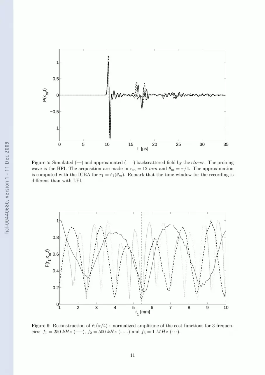
To analyze the role of each frequency in the inversion algorithm, the single frequency costfunction (3) is computed for several frequencies individually. We consider here the frequencydata corresponding to the scattered field at θm = π/4 and the unknown is the local radiusr1(π/4) = 5.433 mm of the clover.In Fig.6, cost functions for three frequencies, f1 = 250 kHz, f2 = 500 kHz and f3 = 1 MHz,illustrate the non-uniqueness of the solution of the inverse problem by a lot of local minima. Re-mark that all the cost functions have a minimum (not always global) close to the exact solution.However, there exist other estimations (e.g., r1 ≈ 2.5 mm) that are also close to minima for allthe three cost functions. Therefore, careful post-processing is needed when using this algorithmwith a small number of frequencies, in particularly when the data are noisy and/or the solutionof the forward problem is not exact.The main difficulty consists now in distinguishing the optimal solution. By plotting the localcost function for all the frequency-band of the HFI, between 100 kHz and 2 MHz (58 frequen-cies, 2 ≤ k1a ≤ 50) (Fig.7) we observe the following:(i) At fixed frequency the distribution of minima is periodic with the estimation. The period ofthis distribution is inversely proportional to the frequency and the number of admissible solu-tions increases with frequency.(ii) A line of local minima appears for which the estimated parameter is close to the solutionand varies weakly with frequency. This suggests that the reconstruction using the canonicalapproximation will not be perfect but a solution can be obtained with a good accuracy, for anyfrequency such that ka ≥ 1.When these multi-frequency data are treated independently the number of admissible solutionsincreases. Seeking the minima of all cost functions corresponding to the different frequenciesand then applying a post-processing algorithm to determine an unique solution requires as manyminimizations as frequencies. The same holds for a method based on an iterative frequency algo-rithm [7] (i.e., starting from the lower frequencies and then refining the solution by consideringthe higher available frequencies). Moreover the gain in precision for such algorithm is not en-sured.The broadband inversion method that we present in the following section is based on theseremarks.

3.2 Multi-frequency reconstruction

The proposed method is based on the minimization of a single cost function, the “Mean CostFunction”(MCF), defined by,

F(τ ;xm) =1

L

L∑

l=1

F(τ ;xm, fl). (4)

Figure 8 presents the mean cost function (4) corresponding to the reconstruction of the localradius r1(π/4) with HFI. The sum in (4) is made on three frequency domains (Dj ,j = 1, 2, 3)that cover respectively 33%, 66% and 99% of the energetic frequency-band of the probing wave(Fig.3).We observe in Fig.8 that as the frequency range increases, variations of the cost function de-crease and the minimum corresponding to the optimal solution becomes deeper with respectto the other minima, and thus easier to estimate. Averaging over frequency has a constructiveeffect on the minimum, which is frequency invariant and a destructive effect on the others.In Fig.9 the mean cost functions using the full frequency spectrum (domain D3) for HFI andLFI are compared. We remark that the number of local minima increases with fc. Thus, for agiven domain of estimation the number of initial guesses necessary for the reconstruction witha local inversion method, increases with the central frequency of the probing pulse.

4

hal-0

0440

680,

ver

sion

1 -

11 D

ec 2

009

In both cases, the deepest minimum is very close to the solution, thus we conclude that the cen-tral frequency does not affect the precision of the optimal estimation (absolute error : 0.019 mmfor LFI and 0.048 mm for HFI).

4 Numerical example

All around the body, the backscattered field is recorded at 16 points xm, with rm = 12 mmand θm = mπ/8, (m = 0, ...15). Each multi-frequency field P (θm) is used to reconstruct thelocal radius r1(θm) of the body. To examine the influence of the central frequency on thereconstruction we use both the LFI and HFI as probing waves.The MCF is defined on D3 (L = 110 for LFI and L = 92 for HFI). The minimization is realizedby a quasi-Newton algorithm [15]. Because a local minimization algorithm is used, 15 initialguesses, equally distributed on the estimation domain [3; 10] mm, are used.Both LFI and HFI provide satisfactory reconstructions (see Fig.10 and Fig.11). Note thatthe deepest minimum is obtained more than once for the lowest frequency insonification butgenerally only one time for the higher frequency insonification. This underlines the difficulty indistinguishing the optimal solution from all the admissible ones. The good results obtained herecan be explained by the low deviation of the section of the object from the mean radius, whichvalidates the circular approximation used for the forward problem.

5 Application to external and internal boundary reconstruction

We consider now the problem of reconstructing both the inner and outer sections of a tube.In this case, the body used to estimate the forward problem during the inversion is a centeredcircular tube with inner radius r2. The objective of the inversion is to reconstruct both theinner and outer sections of the body at several discrete angles θm. At each angle θm, the costfunction varies according to the radius r1 and r2 of the circular tube.This problem could be solved in the following two ways : (i) Reconstruction of both parametersat the same time. This needs a great amount of initial guesses in order to cover the wholeestimation domain, in particular for high central frequencies. (ii) Estimation of the parametersin two independent steps (using some a priori estimation for the second parameter during theinversion of the first). In this case one needs to ensure the robustness of the first estimatedparameter to the a priori on the second one.In the example considered here, the hollow cylinder is filled by an acoustic material (ρ3 =1200 kg/m3 and c3 = 1700 m/s) defining the domain Ω3. All material properties of the mediaare again exactly known. The outer and inner sections (Fig.14) are described by the followingpolar functions,

Outersection : r1(θ) = 5.875 − 0.875 cos(2θ) + 0.750 sin(3θ) ; 0 ≤ θ < 2πInnersection : r2(θ) = 3.0 − 0.45 cos(2θ) ; 0 ≤ θ < 2π.

(5)

All the other characteristics are the same: mean external radius, properties of the media andmeasurement configurations. This new body is distinguished from the previous ones by its con-cavity and a greater deviation of the outer section from the mean radius.In order to test the robustness of the reconstruction, the MCF for the estimation of each pa-rameter is plotted for two cases: in the first case the a priori on the second parameter is exactand in the second case the a priori is wrong.In Fig.12 and Fig.13, the MCF obtained for the estimation of each parameter is plotted foreach probing wave. The simulated measurements are the backscattered field at θm = 0, whichcorresponds to r1(0) = 5.000 mm and r2(0) = 2.550 mm. The unknowns r1 and r2 are estimatedin the domain [4; 8] mm and [2; 4] mm respectively. Numerical results are given in Tab.3.We remark that the estimation of the external radius is independent from the a priori on the

5

hal-0

0440

680,

ver

sion

1 -

11 D

ec 2

009

Table 3: Reconstruction of the inner and outer radius at θm = 0Reconstruction of r1(0) = 5.000 mm

Probing wave a priori on r2 [mm] estimation, r1 [mm] r1 − r1(0) [mm]

LFI 3.000 5.384 0.384r2(0) 5.356 0.356

HFI 3.000 5.390 0.390r2(0) 5.392 0.292

Reconstruction of r2(0) = 2.550 mm

Probing wave a priori on r1 [mm] estimation, r2 [mm] r2 − r2(0) [mm]

LFI 5.384 2.797 0.247r1(0) 2.727 0.177

HFI 5.390 2.604 0.054r1(0) 3.348 0.799

inner radius. The cost function and the admissible solution are of the same order, whatever thea priori information is.On the contrary for the inner radius, the estimation is more sensitive to the a priori on theouter radius. For the HFI the cost function obtained when the a priori is the exact solution isvery irregular. The minimization gives a solution that is far from the exact solution with anabsolute error that is of the order of half the wavelength (in the surrounding media). Whenthe a priori on the outer radius is the admissible solution obtained previously, the admissiblesolution is satisfactory. Remark that for the LFI, the solutions obtained with the two a prioriare of the same order.The above observations for θm = 0 also hold for other measurements directions. The recon-struction provides better (or equivalent) results when the a priori information on r1 is theradius estimated in the first step compared to the estimation obtained when the outer radius isthe true one. This is particularly surprising especially because there is only a small discrepancybetween the two a priori information (less than a quarter wavelength for both probing waves).This result suggests that the estimations of both parameters should be obtained with the samemethod: having the exact solution as a priori information seems not to be the best choice.We also observe that for both parameters the spectrum of the probing wave does not perturbthe estimation. The frequency domain used affects the width of the attraction domain of thesolution (and then the number of the admissible solutions) only for the external radius recon-struction.In order to recover the shape of the tube, 16 backscattered fields, recorded in the same configu-ration as in the previous section, are used. The proposed algorithm is the following:(i) for each angle of measurement independently, the outer local radius is first estimated withan arbitrary a priori on the inner local radius,(ii) in a second step, this estimation is used as a priori for the outer radius when the innerradius is estimated. This algorithm is faster and more robust than when the two unknowns areestimated simultaneously.The external boundary reconstruction is given in Fig.14.The presence of a hole seems not to disturb the reconstruction of the outer boundary. The con-cave part of the external boundary and the inner section are not as well reconstructed. However,the images obtained are satisfactory in and beyond the resonance region and the absolute erroris always negligible with respect to the wavelength.

6

hal-0

0440

680,

ver

sion

1 -

11 D

ec 2

009

6 Conclusion

An efficient method for reconstructing the external boundary of non-circular cylindrical objectsusing multi-frequency data has been presented. The proposed algorithm, using an analyticalsolution for the local forward problem and an iterative process to recover the unknowns, presentsthe advantage of being fast and thus able to provide real time images of the shape.This method is robust with respect to the geometry. Even when the deviation of the sectionfrom the mean radius is greater than the wavelength the method gives very attractive results.The frequency band of the probing wave does not play an essential role: the reconstruction isof the same order in and beyond the resonance region.Using ICBA as forward solver for the inversion is an efficient tool for reconstruction with broad-band acoustic measurements. The MCF does not need any regularization operator when the apriori are chosen properly.For such high contrast objects, reconstruction of the inner and outer shape is accurate when thematerial properties are exact.We are currently working on the extension of this method to the more general inverse problemwhere the acoustical or mechanical properties are also unknown. In this case, we need again tocheck the sensitivity of the estimation of the unknowns with respect to the a priori information.

7 Bibliography

References

[1] D. Colton, R. Kress, Inverse Acoustic and Electromagnetic Scattering Theory, 2nd ed.,Springer Verlag (1998).

[2] M.Y. Kokurin, Stable iteratively regularized gradient method for nonlinear irregular equa-tions under large noise, Inverse Problems 22, (2006), 197-207.

[3] M. Lambert, R. Bohbot, D. Lesselier, Caracterisation d’un sous-sol marin stratifie en situ-ation de petits fonds par une methode iterative, Proc., Publ. LMA 125, (1991), 133-143.

[4] K. Belkebir, A.G. Tijhuis, Modified gradient method and modified Born method for solvinga two-dimensional inverse scattering problem, Inverse Problems 17, (2001), 1671-1688.

[5] L. Crocco, M. D’Urso, T. Isernia, Testing the contrast source extended Born inversionmethod against real data: the TM case Inverse Problems 21, (2005), S33-S50.

[6] A. Abubakar, P.M. van den Berg, T.M. Habashy, Application of the multiplicative regular-ized contrast source inversion method on TM- and TE-polarized experimental Fresnel data,Inverse Problems 21, (2005), S5-S13.

[7] R. Marklein, K. Balasubramanian, A. Qing, K.J. Langenberg, Linear and nonlinear iterativescalar inversion of multi-frequency multi-bistatic experimental electromagnetic scatteringdata, Inverse Problems 17, (2001), 1597-1610.

[8] B. Duchene, Inversion of experimental data using linearized and binary specialized nonlinearinversion schemes, Inverse Problems 17, (2001), 1623-1634.

[9] T. Scotti, A. Wirgin, Shape reconstruction using diffracted waves and canonical solutions,Inverse Problems 11, (1995), 1097-1111.

[10] A. Wirgin, T. Scotti, Wide-band approximation of the sound field scattered by an impen-etrable body of arbitrary shape, J. Sound Vib. 194(4), (1996).

7

hal-0

0440

680,

ver

sion

1 -

11 D

ec 2

009

[11] E. Ogam, T. Scotti, A. Wirgin, Non-ambiguous boundary identification of a cylindricalobject by acoustic waves, C.R. Mecanique 329, (2001), 61-66.

[12] E. Becache, P. Joly, C. Tsogka, An analysis of new mixed finite elements for the approxi-mation of wave propagation problems, SIAM J. Num. Anal 37(4), (2000), 1053-1084.

[13] R.D. Doolittle, H. Uberall, Sound scattering by elastic cylindrical shells, J. Acoust. Soc.Am. 39(2), (1966).

[14] P.W. Barber, S.C. Hill, Light Scattering by Particles: Computational Methods, WorldScientific Publishing Co. Pte. Ltd, Advanced Series in Applied Physics 2, Chap 2, p.30,(1990).

[15] NAG Fortran Library Routine, E04JY F .

8

hal-0

0440

680,

ver

sion

1 -

11 D

ec 2

009

1

Ω2

x

x

m

Ω

oz θ

r

m

m

θ i

y

Figure 1: Problem setup.

−10 −5 0 5 10−10

−5

0

5

10

mm

mm

Figure 2: Clover geometry.

9

hal-0

0440

680,

ver

sion

1 -

11 D

ec 2

009

0 500 1000 1500 2000 2500 30000

0.2

0.4

0.6

0.8

1

f [kHz]

D1

D2

D3

Figure 3: Normalized spectrum of the probing wave for the LFI (- - -) and HFI (—). For theHFI each bandwidth used for the inversion in the section 3.2 is presented.

0 5 10 15 20 25 30 35

−1

−0.5

0

0.5

1

t [µs]

P(x

m,t)

Figure 4: Simulated (—) and approximated (- - -) backscattered field by the clover. The probingwave is the LFI. The acquisitions are made at rm = 12 mm and θm = π/4. The approximationis computed with the ICBA for r1 = r1(θm).

10

hal-0

0440

680,

ver

sion

1 -

11 D

ec 2

009

0 5 10 15 20 25 30 35

−1

−0.5

0

0.5

1

t [µs]

P(x

m,t)

Figure 5: Simulated (—) and approximated (- - -) backscattered field by the clover. The probingwave is the HFI. The acquisition are made in rm = 12 mm and θm = π/4. The approximationis computed with the ICBA for r1 = r1(θm). Remark that the time window for the recording isdifferent than with LFI.

1 2 3 4 5 6 7 8 9 100

0.2

0.4

0.6

0.8

1

F(r

1,xm

,f)

r1 [mm]

Figure 6: Reconstruction of r1(π/4) : normalized amplitude of the cost functions for 3 frequen-cies: f1 = 250 kHz (—–), f2 = 500 kHz (- - -) and f3 = 1 MHz (· · ·).

11

hal-0

0440

680,

ver

sion

1 -

11 D

ec 2

009

Figure 7: Reconstruction of r1(π/4) : the single frequency cost function (3) as a function offrequency and the estimation parameter.

1 2 3 4 5 6 7 8 9 100

0.5

1

1.5

2

2.5

r1 [mm]

F(r

1;xm

)

Figure 8: Reconstruction of r1(π/4) with the HFI (fc = 1 MHz). MCF (4) for 3 frequencybands: D1 (· · ·), D2 (- -), D3 (—). There is no normalization.

12

hal-0

0440

680,

ver

sion

1 -

11 D

ec 2

009

1 2 3 4 5 6 7 8 9 100

0.2

0.4

0.6

0.8

1

r1 [mm]

F(r

1;xm

)

Figure 9: Reconstruction of r1(π/4) using all the frequency bands for the each probing wave :LFI (- -) and HFI (—). There is no normalization.

−10 −5 0 5 10−10

−5

0

5

10

mm

mm

Figure 10: Reconstruction with LFI : admissible ∗ and optimal ⊛ estimation of the local radius.Actual sections : —–.

13

hal-0

0440

680,

ver

sion

1 -

11 D

ec 2

009

−10 −5 0 5 10−10

−5

0

5

10

mm

mm

Figure 11: Reconstruction with HFI : admissible ∗ and optimal ⊛ estimation of the local radius.Actual sections : —–.

4 4.5 5 5.5 6 6.5 7 7.5 80

0.5

1

r1 [mm]

F(r

1,xm

)

4 4.5 5 5.5 6 6.5 7 7.5 80

0.5

1

r1 [mm]

F(r

1,xm

)

Figure 12: Normalized MCF for the reconstruction of r1(0) with two a priori on r2 : r2 = r2(0)(—) and r2 = 3 mm (- -). Top : LFI, bottom : HFI.

14

hal-0

0440

680,

ver

sion

1 -

11 D

ec 2

009

2 2.2 2.4 2.6 2.8 3 3.2 3.4 3.6 3.8 40

0.5

1

r2 [mm]

F(r

2,xm

)

2 2.2 2.4 2.6 2.8 3 3.2 3.4 3.6 3.8 40

0.5

1

r2 [mm]

F(r

2,xm

)

Figure 13: Normalized MCF for the reconstruction of r2(0) with two a priori on r1 : r1 = r1(0)(—) and r1 = the optimal estimation obtained for the reconstruction of r1(0) (- -). Top : LFI,bottom : HFI.

−5 0 5

−5

0

5

mm

mm

Ω1

Ω2

Ω3

Figure 14: Actual section of the tube (bold) and corresponding domains. Optimal estimation ofeach local radius obtained with the LFI () and the HFI (+). 16 equally distributed syntheticmeasurements are made all around the body. The optimal estimation of r1(θ) is used as a priorifor the reconstruction of r2(θ).

15

hal-0

0440

680,

ver

sion

1 -

11 D

ec 2

009