‘bayesian source detection and parameter estimation of a plume model based on sensor network...

APPLIED STOCHASTIC MODELS IN BUSINESS AND INDUSTRYAppl. Stochastic Models Bus. Ind. 2010; 26:331–348Published online in Wiley Online Library (wileyonlinelibrary.com). DOI: 10.1002/asmb.859

Discussion

Bayesian source detection and parameter estimation of a plumemodel based on sensor network measurements‡

Chunfeng Huang1,∗†, Tailen Hsing2, Noel Cressie3, Auroop R. Ganguly4,Vladimir A. Protopopescu4 and Nageswara S. Rao4

1Department of Statistics, Indiana University, Bloomington, IN, U.S.A.2Department of Statistics, University of Michigan, Ann Arbor, MI, U.S.A.

3Department of Statistics, The Ohio State University, Columbus, OH, U.S.A.4Oak Ridge National Laboratory, Oak Ridge, TN, U.S.A.

SUMMARY

We consider a network of sensors that measure the intensities of a complex plume composed of multipleabsorption–diffusion source components. We address the problem of estimating the plume parameters,including the spatial and temporal source origins and the parameters of the diffusion model for eachsource, based on a sequence of sensor measurements. The approach not only leads to multiple-sourcedetection, but also the characterization and prediction of the combined plume in space and time. Theparameter estimation is formulated as a Bayesian inference problem, and the solution is obtained using aMarkov chain Monte Carlo algorithm. The approach is applied to a simulation study, which shows thatan accurate parameter estimation is achievable. Copyright q 2010 John Wiley & Sons, Ltd.

Received 15 February 2010; Revised 3 May 2010; Accepted 22 June 2010

KEY WORDS: Bayesian statistics; Markov chain Monte Carlo; partial differential equation; plume model;sensor networks

1. INTRODUCTION

Advances in monitoring and communication technologies have enabled environmental monitoringand security assessment using sensor networks, as evidenced by their deployments in a wide varietyof contexts [1, 2]. While the specific configuration of any particular sensor network depends on thecontext of the problem, sensor networks typically generate potentially complex and unstructured

∗Correspondence to: Chunfeng Huang, Department of Statistics, Indiana University, Bloomington, IN, U.S.A.†E-mail: [email protected]‡A preliminary version of this work was presented at 9th ONR/GTRI Workshop on Target Tracking in SensorFusion, 2006.

Copyright q 2010 John Wiley & Sons, Ltd.

332 C. HUANG ET AL.

data sets. These data sets are a crucial part of our understanding of the phenomena that the networksmonitor. Hence, our ability to analyze and extract useful information determines the effectivenessof the sensor networks.

After the initial explosion/release at a certain time and location, the results of a dirty bomb, achemical leak, or the release of biological agents take the form of an atmospheric plume that willundergo transport, advection, diffusion, adsorption, radioactive decay, and delayed re-emission. Todetect, study, identify, and/or track the plume, we must study its spatio-temporal evolution. In thispaper, we propose a Bayesian statistical approach that relies on both physical laws and statisticalmodels in space and time. That is, they are physical statistical models in the sense of [3].

Spatially disperse networks of sensors hold an enormous potential for the detection, identifi-cation, tracking, and prediction of these point-source phenomena. In particular, the problem ofdetecting and tracking sources was addressed using sensor networks for chemical dispersions in[4–6], and nuclear radiation in [7]. However, there has been limited effort in incorporating theanalytical and statistical nature of the plume and sensor models to analyze the measurementscollected by such networks. In [8], a linear array of detectors was employed to detect a moving radi-ation source against the background radiation. A sensor-network solution for detecting a movingradiological dispersion device was presented using a Bayesian formulation in [7]. Cost–benefitanalysis of using sensor networks for detecting the moving radiation sources was carried out in [9].These contributions mainly focus on detecting low-level radiation emitted by sources prior to theexplosion, and consequently they do not explicitly consider the dispersion dynamics. A recursivealgorithm was presented in [10] to locate a single source and track the plume intensity. It is notclear to us how this method can be extended to a multiple-source situation.

This paper is structured as follows. Section 2 gives a technical formulation of the problem,introduces a PDE plume model, and discusses the Bayesian inferential approach for this model.Section 3 contains a simulation study, and the discussion and conclusions are given in Section 4.

2. PDE PLUME MODEL AND ESTIMATION METHOD

2.1. Formulation of the problem

The objective of this paper is to introduce a statistical approach to systematically analyze andestimate the parameters of a plume resulting from a chemical leak (say), based on a sequenceof sensor-network measurements. The establishment of such networks is expected to accelerate,and the roles that they play in addressing significant issues will continue to expand in the nearfuture. We consider the following scenario of K pollution sources released into the environmentat different times t01, . . . , t0K and spatial locations s01, . . . ,s0K , respectively, for some K>1. Forsimplicity, we assume that the sensor locations are on the two-dimensional plane. Let

uk(x, y, t) ≡ true plume intensity at time t and location (x, y),

due to the kth source (1)

clearly uk(x, y, t)=0 if t<t0k . In most situations, such as dirty bombs and chemical leaks, theplume intensities are usually low and sources are not close to each other. We assume that plume

Copyright q 2010 John Wiley & Sons, Ltd. Appl. Stochastic Models Bus. Ind. 2010; 26:331–348DOI: 10.1002/asmb

BAYESIAN SOURCE DETECTION AND PARAMETER ESTIMATION 333

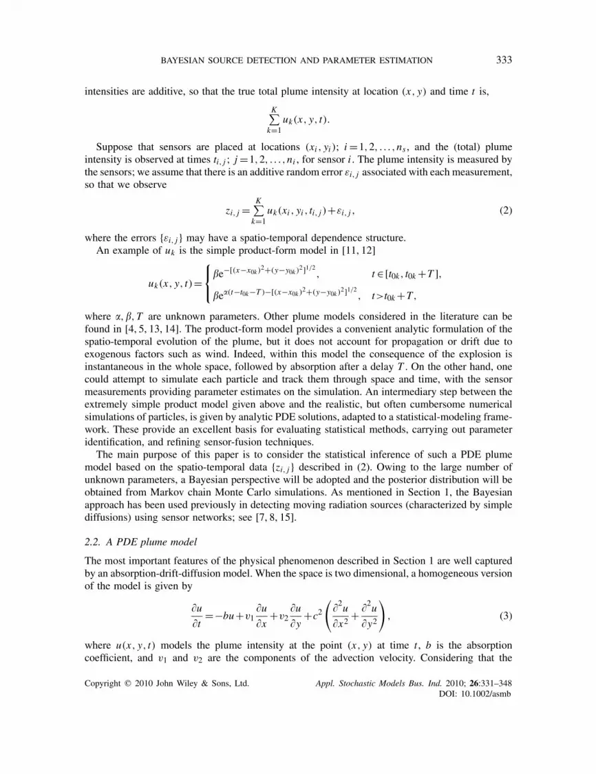
intensities are additive, so that the true total plume intensity at location (x, y) and time t is,

K∑k=1

uk(x, y, t).

Suppose that sensors are placed at locations (xi , yi ); i=1,2, . . . ,ns , and the (total) plumeintensity is observed at times ti, j ; j =1,2, . . . ,ni , for sensor i . The plume intensity is measured bythe sensors; we assume that there is an additive random error εi, j associated with each measurement,so that we observe

zi, j =K∑

k=1uk(xi , yi , ti, j )+εi, j , (2)

where the errors {εi, j } may have a spatio-temporal dependence structure.An example of uk is the simple product-form model in [11, 12]

uk(x, y, t)=⎧⎨⎩

�e−[(x−x0k)2+(y−y0k)2]1/2, t ∈[t0k, t0k+T ],�e�(t−t0k−T )−[(x−x0k)2+(y−y0k)2]1/2, t>t0k+T,

where �,�,T are unknown parameters. Other plume models considered in the literature can befound in [4, 5, 13, 14]. The product-form model provides a convenient analytic formulation of thespatio-temporal evolution of the plume, but it does not account for propagation or drift due toexogenous factors such as wind. Indeed, within this model the consequence of the explosion isinstantaneous in the whole space, followed by absorption after a delay T . On the other hand, onecould attempt to simulate each particle and track them through space and time, with the sensormeasurements providing parameter estimates on the simulation. An intermediary step between theextremely simple product model given above and the realistic, but often cumbersome numericalsimulations of particles, is given by analytic PDE solutions, adapted to a statistical-modeling frame-work. These provide an excellent basis for evaluating statistical methods, carrying out parameteridentification, and refining sensor-fusion techniques.

The main purpose of this paper is to consider the statistical inference of such a PDE plumemodel based on the spatio-temporal data {zi, j } described in (2). Owing to the large number ofunknown parameters, a Bayesian perspective will be adopted and the posterior distribution will beobtained from Markov chain Monte Carlo simulations. As mentioned in Section 1, the Bayesianapproach has been used previously in detecting moving radiation sources (characterized by simplediffusions) using sensor networks; see [7, 8, 15].2.2. A PDE plume model

The most important features of the physical phenomenon described in Section 1 are well capturedby an absorption-drift-diffusion model. When the space is two dimensional, a homogeneous versionof the model is given by

�u�t

=−bu+v1�u�x

+v2�u�y

+c2(

�2u�x2

+ �2u�y2

), (3)

where u(x, y, t) models the plume intensity at the point (x, y) at time t , b is the absorptioncoefficient, and v1 and v2 are the components of the advection velocity. Considering that the


334 C. HUANG ET AL.

propagation usually takes place within a relatively small field in the atmosphere, an isotropicmedium is assumed with a diffusion coefficient c. This model also assumes that the propagationtakes place essentially at the surface; accounting for the third dimension would be an importantnext step.

We assume that the medium is infinite and the initial condition is:

u(x, y, t= t0)=C�(x−x0)�(y− y0), (4)

where �(·) is the Dirac delta function, which corresponds to a very sharply localized release ofintensity C at time t= t0, at the point (x0, y0). Then the solution to (3) and (4) can be calculatedexactly as

u(x, y, t)= a

t− t0exp

{−b(t− t0)− (x−v1t−x0)2+(y−v2t− y0)2

4c2(t− t0)

}, (5)

where a is a normalization constant depending on the intensity of the initial source, C , and on thediffusion constant, c; for example, see [16]. Formula (5), which represents the Green’s functionof Equation (3) in an infinite medium, can be generalized to higher dimensions and variousanisotropic situations. Notice that it is not of product (time × space) form, and hence the modelis non-separable in space and time.

Propagation in inhomogeneous and/or non-stationary media (i.e. accounting for the presenceof buildings, mountains, forests, changing meteorological conditions, etc.) can be described byreplacing the constant coefficients with appropriate functions of time and position and/or supple-menting the equation with appropriate boundary conditions. While in general these situations donot lend themselves to simple analytical solutions (see [17]), numerical approaches are usuallypossible and have been pursued to a great extent (e.g. [18]). Note that (stochastic) PDE models forenvironmental and ecological processes have been used in the hierarchical Bayesian framework(e.g. [19, 20]), although their goal was not inference on the location of sources.

In the remainder of our paper, we rely on knowing the explicit solution (5). There are severalthings to note. Should the PDE be generalized to account for spatial or temporal inhomogeneity,our approach would need an analytical solution. A similar consideration holds if we generalizefrom two dimensions to three dimensions. Finally, the PDE plume model (3) has no uncertaintyassociated with it (often expressed in the form of a stochastic PDE).

The advantages of the class of models illustrated by Equation (3) include (i) their generalmathematical properties are very well understood [16, 17]; (ii) the evolution described by thecontinuous versions preserves the required physical properties, such as positivity and conservationlaws [16, 17]; (iii) due to the parabolic character of the equation, the discretized versions are stable.2.3. Methodology

From now on we shall focus on the PDE-based plume model (5). We assume here that the totalnumber of plume sources K is known; an approach to determine K from data will be discussedin Section 4. To simplify notation, write

u(x, y, t;sk)= I (t>t0k)ak

t− t0kexp

{−bk(t− t0k)− (x−v1k t−x0k)2+(y−v2k t− y0k)2

ck(t− t0k)

},

where sk =(ak,bk,ck,v1k,v2k, t0k, x0k, y0k)′ is the vector of parameter values for the kth plumesource. Let sk ≡(ak, bk, ck, v1k, v2k, t0k, x0k, y0k)′ denote the corresponding true parameter values.



Observe that the true intensity function uk(x, y, t) defined in (1) can be written in terms of themodel as u(x, y, t; sk).

Assume that the errors {εi, j } in (2) are independent and normally distributed with mean 0 andvariance �2; let the true variance be �2. We consider the robustness of this assumption below inSection 3. Thus, the combined parameter of the K plume sources is

h≡(s1,s2, . . . ,sK ,�2)′,

which is a vector of length 8K +1. In addition, denote by z the data {zi, j ,1� j�ni ,1�i�ns}defined by (2). Then the likelihood of h is

p(z|h)∝(�2)−N/2 exp

[− 1

2�2

ns∑i=1

ni∑j=1

{zi, j −

K∑k=1

u(xi , yi , ti, j ;sk)}2]

, (6)

where N =∑nsi=1 ni . The high dimensionality of h makes it attractive to regularize the likelihood

by putting a prior on h. Our approach in this paper is to put all the uncertainty about the PDE ontoits parameters s, and express that uncertainty through a prior distribution. Hence, the posteriordistribution can (in principle) be obtained, and inference carried out on such parameters as theplume’s source.

For prior distribution consideration, if the plume sources are dirty bombs, then highly populatedareas may be more likely to contain the bombs’ source locations than lowly populated areas,in which case it makes sense for the prior distribution to reflect this. In addition, certain valuesof ak,bk,ck may be more likely than others, as determined by the physical conditions of theenvironment. However, if no prior information is available or if one chooses to ignore it, then auniform distribution on the 6K -dimensional vector, (s′1, . . . ,s′K ), often called a non-informativeprior, could be used. One could also use a normal prior with large variances for the elements ofsk,k=1, . . . ,K .

Bayesian inference focuses on the properties of the posterior distribution, p(h|z), the conditionaldistribution of h given the data z. Once p(h|z) is available, inference based on it can be made withregard to the unknown model parameters. Furthermore, the overall plume intensity at any location(x, y) and any time t can be predicted using its posterior mean (say):

K∑k=1

∫h

u(x, y, t;sk)p(h|z)dh. (7)

The posterior distribution can sometimes be derived in a closed form but often has to be computednumerically. In this paper, the posterior distribution will be computed by Markov chain MonteCarlo (MCMC) simulations. MCMC methods are widely used in statistics, and there are manydifferent approaches. See [21] for an overview of MCMC and discussions of important issues.

3. NUMERICAL RESULTS

In this section, we present some numerical results for the statistical inference on h from the PDE-based plume model. We are not aware of any real-world data available, although there may be somethat are classified. Therefore, we illustrate our approach on the simulated data. For convenience,we shall make the simplification that, for the advection velocities, v1k =v and v2k =0, is the same


336 C. HUANG ET AL.

Figure 1. The upper-left/right panels give the source locations (×) and the 9/16 sensor locations (◦) forthe examples with two sources. The lower-left/right panels give the source locations (×) and the 16/25

sensor locations (◦) for the examples with three sources.

for all sensors, which reduces the number of parameters from 8K +1 to 6K +2. The assumptionmeans that the wind is blowing at more or less constant velocity in the direction of the x-axis inthe region containing the sensors. Note that this direction can be replaced by any other knowndirection, and we do not assume that the wind speed is known. The locations of the plume sources(unknown) and sensors (known) in our examples are given by the configurations in the upper-leftpanel of Figure 1, where sensor locations are denoted by ‘◦’ and source locations are denotedby ‘×’.

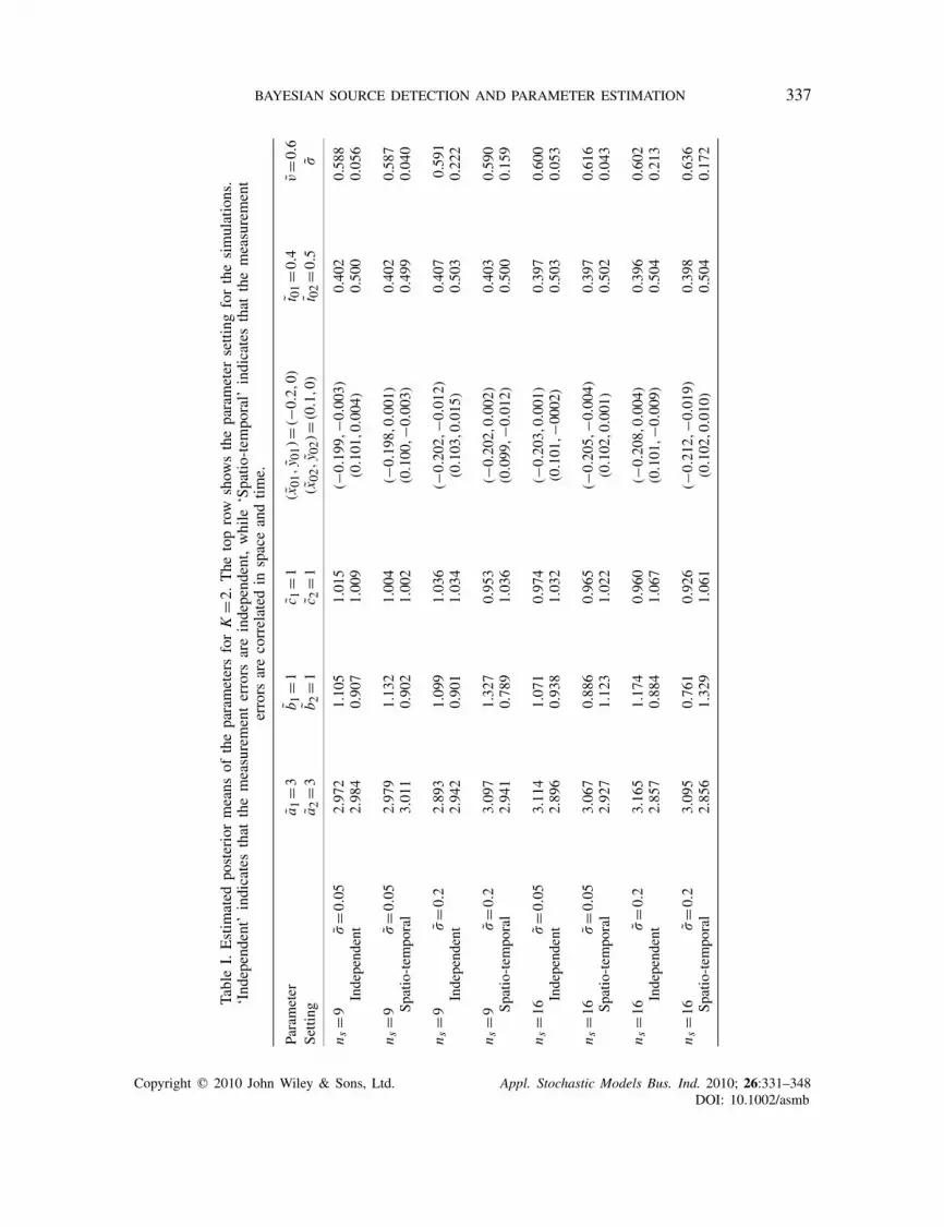
First, we consider an example for two sources (i.e. K =2) and ns =9 sensors. Assume that thetrue PDE plume model is specified by the parameters in the top row of Table I, and we simulatedata from the model (5) followed by (2). The data z={zi, j } are observed at 20 equally spaced timepoints from 0 to 2 at each of the 9 sensor locations shown in the top-left panel of Figure 1. In thissimulation, we assumed that the distribution of the measurement errors {εi, j } is independent andidentically distributed normal with mean 0 and standard deviation �=0.05. We first conducted asingle MCMC simulation run; see Figure 2, which shows the data zi, j observed at the 9 sensorsat 20 time points.

Based on the data, we conducted the statistical inference using the Bayesian approach describedin Section 2.3. We assumed that the prior distributions for each of the parameters were mutually



TableI.Estim

ated

posteriormeans

oftheparametersforK

=2.The

toprow

show

stheparameter

setting

forthesimulations.

‘Independent’indicatesthat

themeasurementerrors

areindependent,while

‘Spatio

-tem

poral’

indicatesthat

themeasurement

errors

arecorrelated

inspaceandtim

e.

Parameter

a 1=3

b 1=1

c 1=1

(x01

,y 0

1)=(

−0.2

,0)

t 01=0

.4v=0

.6Setting

a 2=3

b 2=1

c 2=1

(x02

,y 0

2)=(

0.1,0)

t 02=0

.5�

n s=9

�=0

.05

2.97

21.10

51.01

5(−

0.19

9,−0

.003

)0.40

20.58

8Independ

ent

2.98

40.90

71.00

9(0

.101

,0.004

)0.50

00.05

6

n s=9

�=0

.05

2.97

91.13

21.00

4(−

0.19

8,0.00

1)0.40

20.58

7Sp

atio-tem

poral

3.01

10.90

21.00

2(0

.100

,−0.00

3)0.49

90.04

0

n s=9

�=0

.22.89

31.09

91.03

6(−

0.20

2,−0

.012

)0.40

70.59

1Independ

ent

2.94

20.90

11.03

4(0

.103

,0.015

)0.50

30.22

2

n s=9

�=0

.23.09

71.32

70.95

3(−

0.20

2,0.00

2)0.40

30.59

0Sp

atio-tem

poral

2.94

10.78

91.03

6(0

.099

,−0.01

2)0.50

00.15

9

n s=1

6�

=0.05

3.11

41.07

10.97

4(−

0.20

3,0.00

1)0.39

70.60

0Independ

ent

2.89

60.93

81.03

2(0

.101

,−00

02)

0.50

30.05

3

n s=1

6�

=0.05

3.06

70.88

60.96

5(−

0.20

5,−0

.004

)0.39

70.61

6Sp

atio-tem

poral

2.92

71.12

31.02

2(0

.102

,0.001

)0.50

20.04

3

n s=1

6�

=0.2

3.16

51.17

40.96

0(−

0.20

8,0.00

4)0.39

60.60

2Independ

ent

2.85

70.88

41.06

7(0

.101

,−0.00

9)0.50

40.21

3

n s=1

6�

=0.2

3.09

50.76

10.92

6(−

0.21

2,−0

.019

)0.39

80.63

6Sp

atio-tem

poral

2.85

61.32

91.06

1(0

.102

,0.010

)0.50

40.17

2


338 C. HUANG ET AL.

Figure 2. The plots show the data collected by the nine sensors for one simulation.

independent. A scaled inverse-�2 distribution with scale parameter 0.01 and degrees of freedom 1was used for �2, while for x0i , y0i , v, ai , bi , ci , ti we used uniform priors with truncated ranges(−1,1), (−1,1), (−1,1), (1,3), (1,3), (1,3), and (0.2,0.8), respectively. Note that in practice, ifmore information is available, one may choose some more informative priors. While �2 was updateddirectly through a conjugate posterior distribution, all other parameters were updated using theMetropolis algorithm (see [21]). MCMC simulations were implemented with 100 000 iterations;after a burn-in of 50 000, the last 50 000 simulation results were used to compute the empiricalposterior distributions. The distributions obtained from a single MCMC run are summarized inthe plots in Figure 3, where the bar charts are relative-frequency histograms. The superimposedsmooth curves are the corresponding density estimates obtained by the kernel smoothing, whereSilverman’s bandwidth-selection rule-of-thumb (see [22]) is implemented. It can be observed thatthe estimated posterior distributions are fairly tight and include the true parameters in their ranges.The estimated posterior means are reported in Table I on the row that begins with ‘ns =9, �=0.05,Independent’. All the estimates are quite close to their corresponding true values.

We then used (7) to predict the true plume intensity at time t=2.5 and over the spatial region[−1,1]×[−1,1]. Note that this time point and a portion of the spatial region are beyond thecoverage of the sensors, as reflected by the data z. The predicted intensities are displayed in theleft panel of Figure 4, and the difference between the predicted and the true plume intensities isdisplayed in the right panel of Figure 4. Clearly, the plume levels are predicted extremely wellover the entire region at this time point.



Figure 3. Estimated posterior distributions of the parameters based on a single MCMC run for K =2. Thecurves denote kernel-smoothed densities. The true values are indicated by the vertical lines.

In practice, the sensor-network measurements may not be independent. For instance, one couldassume that the measurement errors have spatio-temporal covariance:

cov(�i1, j1,�i2, j2)=�2C1(s,/1)C2(t,/2), (8)

where s is the spatial distance between the sensor locations (xi1, yi1) and (xi2, yi2), and t is the timedifference between the observation times ti1, j1 and ti2, j2 . In (8), �

2 is the overall variance; C1(s,/1)is the spatial correlation function, where /1 indicates the spatial dependency; and C2(t,/2) is thetemporal correlation function with /2 representing the temporal dependency. In (6), let w denotethe vector whose elements are:

zi, j −K∑

k=1u(xi , yi , ti, j ;sk), 1�i�ns, 1� j�ni .


340 C. HUANG ET AL.

Figure 4. The left panel shows the predicted plume levels. The right panel shows the difference betweenthe predicted plume levels and the true plume levels.

Then, under the independent-measurement-error assumptions made earlier,

p(z|h)∝(�2)−N/2 exp

{− 1

2�2w′w

}. (9)

Now, if {εi, j } are dependent, having the covariance matrix � (e.g. obtained from (8)), then thelikelihood function becomes:

p(z|h)∝|�|−1/2 exp{− 12w

′�−1w} (10)

note that h is then augmented to include the parameters of �. In each iteration of the MCMCprocedure, an inversion of the matrix � needs to be computed. This can complicate the procedureand can be time consuming.

It is of great interest to investigate the robustness of our procedure in this situation. With thesame set up as above, we generated the random error terms according to the spatio-temporalstructure (8) with the spatial correlation function C1(s,/1)=e−s/�1 and the temporal correlationfunction C2(t,/2)=e−t/�2 , where �1=�2=0.4. The same MCMC procedure was conducted toobtain the (estimated) posterior distributions. We first present the estimated posterior means onthe row that begins with ‘ns =9, �=0.05, spatio-temporal’ in Table I. It can be observed thatthese values are very similar to their ‘independent’ counterparts and are close to the true values.To compare the estimated posterior distributions with those in Figure 3, Q–Q plots were drawnfor each parameter and are included in Figure 5. These plots show that the estimated posteriordistributions of each parameter for the two models are similar to each other. In conclusion, thislimited study demonstrates that an assumption of independent measurement errors in (2), evenwhen the measurement errors are correlated as in (8), can still result in valid inferences. Note thatthis approach can be viewed as a Bayesian procedure based on the quasi-likelihood [23]; we use (9)instead of the full likelihood (10), and the parameters (�1,�2) in the spatio-temporal correlationfunctions are not considered. Conducting inference based on quasi-likelihoods is common innon-Bayesian statistics; see [24] for a general discussion.

To investigate further the performance of the MCMC procedure for the case of two plumesources, we expanded the simulation study by considering all combinations of �=0.05 and 0.2;



Figure 5. Q–Q plots of the estimated posterior distributions of parameters when measurement errors arecorrelated in space and time versus those when measurement errors are independent; K =2.

ns =9 and 16; and independent and spatio-temporally correlated measurement errors. For example,the plume-source/sensor configuration for ns =16 is shown in the upper-right panel of Figure 1.The estimated posterior means are reported in Table I. For all the settings, the estimated posteriormeans estimate the true parameter values quite well, especially for estimating the spatial andtemporal origins (x0, y0) and t0, respectively, of the sources. The robustness of the procedure canbe observed by comparing the entries between the independent-measurement-error setting and thecorrelated-measurement-error setting. Note that the procedure performs slightly better for �=0.05than for �=0.2, as expected, while the results are similar when the number of sensors changes


342 C. HUANG ET AL.

from ns =9 to 16. A more complete simulation study would determine the value of � (expressedin terms of a signal-to-noise ratio) at which inferences deteriorate.

Next, we consider the situation when there are three sources (i.e. K =3). First assume that thetrue PDE plume model is specified by the parameters in the top row of Table II; the measurementerrors {εi, j } are assumed to be normally distributed with mean 0 and standard deviation �=0.05,and the data {zi, j } are observed at 20 equally spaced time points, as before. Consider the case of25 sensor locations shown in the lower-right panel of Figure 1, for which we obtained data froma single MCMC run. The estimated posterior means are presented in Table II, and the estimatedposterior distributions for the parameters are summarized in the plots in Figure 6. Some plotsseem to suggest that the procedure gives biased estimates; for example, the true value of t02 isnot in the range of the estimated posterior distribution. However, the true value of t02 is t02=0.6;considering the empirical posterior distribution ranges from 0.6002 to 0.6008 with an estimatedposterior mean of 0.601, the bias is actually quite small.

Similar to the case of two plume sources, we also studied the performance of the procedure undervarious settings. Specifically, we considered all combinations of �=0.05 and 0.2; ns =16 and 25;and independent and spatio-temporally correlated measurement errors. The plume-source/sensorconfiguration for ns =16 is shown in the lower-left panel of Figure 1, and recall that for ns =25is shown in the lower-right panel. The estimated posterior means using the MCMC procedure arepresented in Table II. Again, the MCMC procedure worked very well in all the settings.

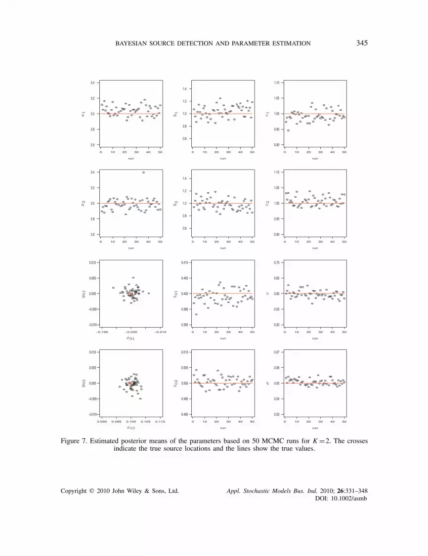
All the studies up to this point are based on a single MCMC run. One may wonder whetherthis approach would consistently perform well when multiple MCMC runs are conducted. In thispart of simulation, we conducted 50 MCMC runs for two examples: one with two sources (K =2)and one with three sources (K =3). Both examples have the same set up: ns =16, �=0.05 andmeasurement errors are independent. For each example, we simulated the data zi, j , 1�i�16,1� j�20, 50 independent times, and for each run we went through the MCMC simulation toobtain the (estimated) posterior distributions. For each parameter �, we computed the (estimated)posterior mean

∫� p(h|z)dh. Consequently, for each example, we obtained 50 posterior means,

one from each of the 50 simulations; these are presented in Figure 7 (K =2) and Figure 8 (K =3).It can be seen that they are all in a tight range and that they cover the corresponding true values.In particular, the spatial locations (x0, y0) and the temporal origins t0 of the sources are estimatedvery well for all 50 MCMC runs in both figures.

4. DISCUSSION

In this paper, we present a Bayesian statistical approach for identifying the parameters, particularlythe source locations, of a PDE-based plume model from sensor-network data. We showed thateven with a moderate amount of data, the model parameters can be estimated using an MCMCapproach. The approach can also be used for spatial and temporal prediction of plume levelsbeyond the sensor range.

In our analysis, we assumed that the true number of sources is known. In practice, the numbermay have to be determined from data. In the literature, the deviance information criterion (DIC)has been used (e.g. [21, 25]):

DIC= Dave+ pD,



TableII.Estim

ated

posteriormeans

oftheparametersforK

=3.The

toprow

show

stheparameter

setting

forthesimulation.

‘Independent’denotesthatthemeasurementerrorsareindependent,while‘Spatio

-tem

poral’indicatesthatthemeasurementerrors

arecorrelated

inspaceandtim

e.

Parameter

a 1=3

b 1=1

c 1=1

(x01

,y 0

1)=(

−0.2

,0.1

)t 01=0

.4v=0

.6Setting

a 2=3

b 2=1

c 2=1

(x02

,y 0

2)=(

−0.3

,0.0

)t 02=0

.6�

a 3=3

b 3=1

c 3=1

(x03

,y 0

3)=(

−0.1

,0.0

)t 03=0

.8

n s=1

6�

=0.05

2.92

50.95

81.01

6(−

0.19

8,0.10

1)0.40

10.60

1Independ

ent

3.02

20.99

10.98

8(−

0.30

1,0.00

3)0.60

00.05

43.01

91.05

30.99

8(−

0.10

0,0.00

1)0.80

0

n s=1

6�

=0.05

2.93

60.94

01.01

4(−

0.19

8,0.10

3)0.40

20.60

2Sp

atio-tem

poral

3.02

21.04

60.99

4(−

0.30

0,0.00

4)0.60

00.06

63.00

60.97

61.00

1(−

0.10

0,0.00

3)0.80

0

n s=1

6�

=0.2

2.82

21.23

21.09

3(−

0.20

3,0.11

2)0.41

30.64

8Independ

ent

2.78

60.68

31.11

9(−

0.29

7,−0

.002

)0.60

20.19

93.15

21.12

50.91

7(−

0.12

9,0.00

0)0.80

2

n s=1

6�

=0.2

2.82

70.82

21.04

1(−

0.19

5,0.11

2)0.40

80.61

1Sp

atio-tem

poral

2.95

01.04

51.00

4(−

0.29

7,0.01

9)0.60

40.13

83.10

41.01

80.98

3(−

0.10

2,0.01

2)0.79

7

n s=2

5�

=0.05

3.18

21.08

40.96

0(−

0.20

4,0.10

0)0.39

50.60

4Independ

ent

2.82

20.79

21.03

3(−

0.29

6,−0

.000

)0.60

10.06

03.11

31.15

70.97

2(−

0.10

3,0.00

0)0.79

8

n s=2

5�

=0.05

2.98

90.95

51.00

1(−

0.19

9,0.09

8)0.40

00.58

8Sp

atio-tem

poral

2.98

00.97

41.00

4(−

0.29

8,−0

.000

)0.60

00.04

83.07

91.07

80.98

8(−

0.10

0,0.00

0)0.79

8

n s=2

5�

=0.2

3.20

10.94

30.95

0(−

0.20

4,0.09

8)0.39

40.59

8Independ

ent

2.92

90.99

81.00

2(−

0.30

1,0.00

0)0.60

00.21

12.95

71.06

21.00

3(−

0.10

3,0.00

1)0.80

2

n s=2

5�

=0.2

3.24

61.15

30.95

5(−

0.20

4,0.10

0)0.39

40.61

2Sp

atio-tem

poral

3.06

90.97

70.98

7(−

0.30

4,−0

.005

)0.59

80.20

62.92

40.98

01.00

7(−

0.10

3,−0

.002

)0.80

1


344 C. HUANG ET AL.

Figure 6. Estimated posterior distributions of the parameters based on one MCMC run for K =3. Thecurves denote kernel-smoothed densities. The true values are indicated by the vertical lines.

where D is the deviance defined as −2 times the log-likelihood, and pD = Dave−Dhis a measure

of the effective number of parameters. The Dave is computed as the average of the deviancefunctions for all MCMC iterations, and D

his the deviance at the parameters’ posterior means.



Figure 7. Estimated posterior means of the parameters based on 50 MCMC runs for K =2. The crossesindicate the true source locations and the lines show the true values.


346 C. HUANG ET AL.

Figure 8. Estimated posterior means of the parameters based on 50 MCMC runs for K =3. The crossesindicate the true source locations and the lines show the true values.



Table III. The Dave, Dh, pD and DIC values for three models with K =1, 2, 3. Lowervalues of DIC indicate a better fit. The true model is K =2 with 14 parameters.

Model Dave Dh

pD DIC

K =1 155.0 156.7 1.7 158.3K =2 −873.2 −857.4 15.8 −841.6K =3 −875.3 −858.1 17.2 −840.9

Based on the data of the two-source example in Figure 2, the Dave, Dh, pD and DIC values arecomputed for K =1, 2, 3 and are shown in Table III. In this case, the true model has two sources,and it is clear from Table III that the model with K =2 is preferable than others, since it has thesmallest DIC. Note that the chosen model (K =2) has a pD that is closer to the true number ofparameters.

A number of important extensions would require further research:

(i) Various computational issues should be considered. The MCMC simulations that wepresented for the two-source example took about 90 seconds to implement on a Linuxworkstation (Dual Pentium 4 Xeon at 3GHz with 4GB RAM) using Fortran code. Thecomputational speed could be substantially improved using a more efficient computingplatform. The more interesting question is, how can the computations be performed inreal time? In other words, as new plume-evolution information becomes available, itis desirable to update the estimation/prediction based on the previous results withoutrestarting them from scratch. One possible way to achieve this goal is to use sequentialMonte Carlo algorithms as in [26].

(ii) In our simulations, we assumed that the sensors are placed on a grid. This is because ourtrial runs revealed that this scheme of sensor placement leads to the most satisfactorystatistical inference on average. An important question is if we have a fixed numberof sensors with limited query capabilities, how should we optimize the design of thenetwork? Spatial designs of this type are discussed in [27], and spatio-temporal designs(assuming mobile sensors) are discussed in [28, 29].

ACKNOWLEDGEMENTS

This work was supported by the SensorNet Program at the Oak Ridge National Laboratory under UT-Battelle LLC contract 4000042084, and the Office of Naval Research under contract number N00014-08-01-0464. The authors thank the editors and the referees for their helpful comments.

REFERENCES

1. Brooks RR, Iyengar SS. Frontiers of Distributed Sensor Networks. CRC Press: Boca Raton, FL, 2004.2. Culler D, Estrin D, Srivastava M. Overview of sensor networks. IEEE Computer 2004; 37:41–49.3. Berliner LM. Physical-statistical modeling in geophysics. Journal of Geophysical Research 2003; 108:D24, STS

3-1-STS 3-10.4. Chen Y, Moore K, Song Z. Diffusion boundary determination and zone control via mobile actuator-sensor networks

(mas-net): challenges and opportunities. Proceedings of SPIE: Intelligent Computing: Theory and Applications2004; 5421:102–113.


348 C. HUANG ET AL.

5. Ishida H, Nakamoto T, Moriizumi T, Kikas T, Janata J. Plume-tracking robots: a new application of chemicalsensors. Biological Bulletin 2001; 200:222–226.

6. Christopoulos VN, Roumeliotis S. Adaptive sensing for instantaneous gas release parameter estimation.Proceedings of the 2005 IEEE International Conference on Robotics and Automation (ICRA 2005), Barcelona,Spain, 18–22 April 2005.

7. Brennan SM, Mielke AM, Torney DC, Maccabe AB. Radiation detection with distributed sensor networks. IEEEComputer 2004; 37:57–59.

8. Nemzek RJ, Dreicer JS, Torney DC, Warnock TT. Distributed sensor networks for detection of mobile radioactivesources. IEEE Transactions on Nuclear Science 2004; 51:1693–1700.

9. Stephens DL, Peurrung AJ. Detection of moving radioactive sources using sensors networks. IEEE Transactionson Nuclear Science 2004; 51:2273–2278.

10. Ram SS, Veeravalli VV. Localization and intensity tracking of diffusing point sources using sensor networks.Proceedings of the IEEE Global Telecommunications Conference (IEEE GLOBECOM 2007), Washington, DC,26–30 November 2007.

11. Rao NSV. Identification of a class of simple product-form plumes using sensor networks. Innovations andCommercial Applications of Distributed Sensor Networks Symposium, Bethesda, MD, 2005.

12. Rao NSV. Identification of simple product-form plumes using networks of sensors with random errors. Proceedingsof the 9th International Conference on Information Fusion (Fusion 2006), Florence, Italy, 10–13 July 2006.

13. Li W, Farrell JA, Carde R. Tracking of fluid-advected odor plumes: strategies inspired by insect orientation topheromone. Adaptive Behavior 2001; 9:143–170.

14. Sykes RI, Lewellen WS, Parker SF. A Gaussian plume model of atmospheric dispersion based on second-orderclosure. Journal of Climate and Applied Meteorology 1986; 25:322–331.

15. Brennan SM, Mielke AM, Torney DC. Radiation source detection by sensor networks. IEEE Transactions onNuclear Science 2005; 52:813–819.

16. Greenberg W, van der Mee CVM, Protopopescu V. Boundary Value Problems in Abstract Kinetic Theory.Birkhauser: Boston, 1987.

17. Morse PM, Feshbach H. Methods of Mathematical Physics. McGraw-Hill: New York, 1953.18. Sykes RI. PC-Scipuff, Version 1.3 Technical Documentation. Titan Corporation, A.R.A.P. Report no. 725, 2000.19. Malmberg A, Arelleno A, Edwards DP, Flyer N, Nychka D, Wikle CK. Interpolating fields of carbon monoxide

data using a hybrid statistical-physical model. Annals of Applied Statistics 2008; 2:1231–1248.20. Wikle CK. Hierarchical Bayesian models for predicting the spread of ecological processes. Ecology 2003;

84:1382–1394.21. Gelman A, Karlin JB, Stern HS, Rubin DB. Bayesian Data Analysis (2nd edn). Chapman & Hall: Boca Raton,

FL, 2003.22. Silverman BW. Density Estimation. Chapman & Hall: Boca Raton, FL, 1986.23. White H. Maximum likelihood estimation of misspecified models. Econometrica 1982; 50:1–25.24. Cox DR, Reid N. A note on pseudolikelihood constructed from marginal densities. Biometrika 2004; 91:729–737.25. Spiegelhalter D, Best NG, Carlin BP, van der Linde A. Bayesian measures of model complexity and fit. Journal

of Royal Statistical Society B 2002; 64:583–639.26. Wikle CK, Berliner LM. A Bayesian tutorial for data assimilation. Physica D 2007; 230:1–16.27. Cressie N. Statistics for Spatial Data (Revised Edn). Wiley: New York, 1993.28. Wikle CK, Royle JA. Space-time dynamic design of environmental monitoring networks. Journal of Agriculture,

Biological, and Environmental Statistics 1999; 4:489–507.29. Royle JA, Wikle CK. Efficient statistical mapping of avian count data. Environmental and Ecological Statistics

2005; 12:225–243.


‘bayesian source detection and parameter estimation of a plume model based on sensor network...

Documents