delta ii explosion plume analysis report
TRANSCRIPT
NASA Contractor Report NASA/CR-2000-208582
Delta II Explosion Plume Analysis Report
Prepared by:
Applied Meteorology Unit
Prepared for:
Kennedy Space CenterUnder Contract NAS 10-96018
NASA
National Aeronautics and
Space Administration
Office of Management
Scientific and Technical
Information Program
2000
ATTRIBUTESANDACKNOWLEDGMENTS:
NASA/KSC POC:Dr. Francis J. Merceret
YA-D
Applied Meteorology Unit (AMU):
Randolph J. Evans
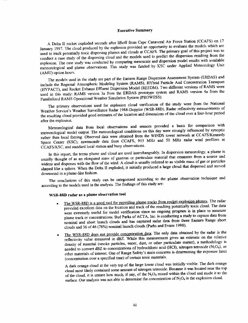
Executive Summary
A Delta II rocket exploded seconds after liftoff from Cape Canaveral Air Force Station (CCAFS) on 17
January 1997. The cloud produced by the explosion provided an opportunity to evaluate the models which are
used to track potentially toxic dispersing plumes and clouds at CCAFS. The primary goal of this project was toconduct a case study of the dispersing cloud and the models used to predict the dispersion resulting from the
explosion. The case study was conducted by comparing mesoscale and dispersion model results with available
meteorological and plume observations. This study was funded by KSC under Applied Meteorology Unit
(AMU) option hours.
The models used in the study are part of the Eastern Range Dispersion Assessment System (ERDAS) and
include the Regional Atmospheric Modeling System (RAMS), HYbrid Particle And Concentration Transport(HYPACT), and Rocket Exhaust Effluent Dispersion Model (REEDM). Two different versions of RAMS were
used in this study: RAMS version 3a from the ERDAS prototype system and RAMS version 4a from the
Parallelized RAMS Operational Weather Simulation System (PROWESS).
The primary observations used for explosion cloud verification of the study were from the NationalWeather Service's Weather Surveillance Radar 1988-Doppler (WSR-88D). Radar reflectivity measurements of
the resulting cloud provided good estimates of the location and dimensions of the cloud over a four-hour period
after the explosion.
Meteorological data from local observations and sensors provided a basis for comparison with
meteorological model output. The meteorological conditions on this day were strongly influenced by synopticrather than local forcing. Observed data were obtained from the WINDS tower network at CCAFS/Kennedy
Space Center (KSC), rawinsonde data from CCAFS, 915 MHz and 50 MHz radar wind profilers at
CCAFS/KSC, and standard local station and buoy observations.
In this report, the terms plume and cloud are used interchangeably. In dispersion meteorology, a plume is
usually thought of as an elongated mass of gaseous or particulate material that emanates from a source andwidens and disperses with the flow of the wind. A cloud is usually referred to as visible mass of gas or particles
shaped like a sphere. When the Delta II exploded, it initially produced a large cloud that dispersed and moved
downwind in a plume-like fashion.
The conclusions of this study can be categorized according to the plume observation technique and
according to the models used in the analysis. The findings of this study are:
WSR-88D radar as a plume observation tool
• The WSR-88D is a good tool for providing plume tracks from rocket explosion plumes. The radarprovided excellent data on the location and track of the resulting potentially toxic cloud. The data
were extremely useful for model verification since no ongoing program is in place to measure
plume track or concentrations. Bud Parks of ACTA, Inc. is conducting a study to capture data fromnominal and abort launch clouds and has captured radar data from three Eastern Range abort
clouds and 36 of 46 (78%) nominal launch clouds (Parks and Evans 1998).
* The WSR-88D does not provide concentration data. The only data obtained by the radar is thereflectivity value measured in dBZ. While this measurement gives an estimate on the relative
density of material (smoke particles, water, dust, or other particulate matter), a methodology isneeded to convert dBZ to concentrations of hydrochloric acid (HCI), nitrogen tetroxide (N204), or
other materials of interest. One of Range Safety's main concerns is determining the exposure limit
(concentration over a specified time) of certain toxic materials.
A dark orange cloud at the very top of the large lower cloud was initially visible. The dark orangecloud most likely contained some amount of nitrogen tetroxide. Because it was located near the top
of the cloud, it is unsure how much, if any, of the N204 mixed within the cloud and made it to the
surface. Our analysis was not able to determine the concentration of N204 in the explosion cloud.
nl
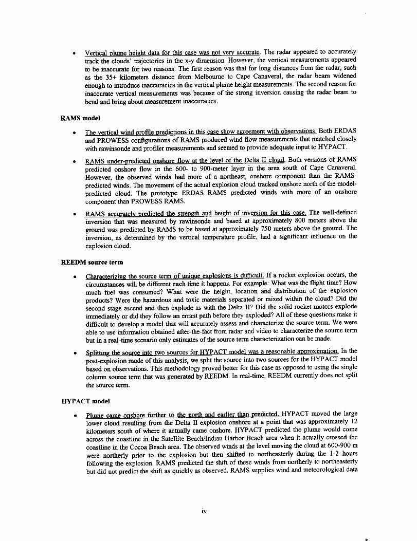
Vertical plume height data for this case was not very accurate. The radar appeared to accuratelytrack the clouds' trajectories in the x-y dimension. However, the vertical measurements appearedto be inaccurate for two reasons. The first reason was that for long distances from the radar, such
as the 35+ kilometers distance from Melbourne to Cape Canaveral, the radar beam widened
enough to introduce inaccuracies in the vertical plume height measurements. The second reason forinaccurate vertical measurements was because of the strong inversion causing the radar beam to
bend and bring about measurement inaccuracies.
RAMS model
• The vertical wind profile predictions in this case show agreement with observations. Both ERDAS
and PROWESS configurations of RAMS produced wind flow measurements that matched closelywith rawinsonde and profiler measurements and seemed to provide adequate input to HYPACT.
• RAMS under-predicted onshore flow at the level of the Delta II cloud. Both versions of RAMS
predicted onshore flow in the 600- to 900-meter layer in the area south of Cape Canaveral.However, the observed winds had more of a northeast, onshore component than the RAMS-
predicted winds. The movement of the actual explosion cloud tracked onshore north of the model-
predicted cloud. The prototype ERDAS RAMS predicted winds with more of an onshore
component than PROWESS RAMS.
• RAMS accurately predicted the strength and height of inversion for this case. The well-definedinversion that was measured by rawinsonde and based at approximately 800 meters above the
ground was predicted by RAMS to be based at approximately 750 meters above the ground. Theinversion, as determined by the vertical temperature profile, had a significant influence on the
explosion cloud.
REEDM source term
• Characterizing the source term of unique explosions is difficult. If a rocket explosion occurs, thecircumstances will be different each time it happens. For example: What was the flight time? How
much fuel was consumed? What were the height, location and distribution of the explosion
products? Were the hazardous and toxic materials separated or mixed within the cloud? Did thesecond stage ascend and then explode as with the Delta II? Did the solid rocket motors explode
immediately or did they follow an errant path before they exploded? All of these questions make itdifficult to develop a model that will accurately assess and characterize the source term. We wereable to use information obtained after-the-fact from radar and video to characterize the source term
but in a real-time scenario only estimates of the source term characterization can be made.
• Splitting the so_ce into two sources for HYPACT model was a reasonable approximation. In thepost-explosion mode of this analysis, we split the source into two sources for the HYPACT modelbased on observations. This methodology proved better for this case as opposed to using the single
column source term that was generated by REEDM. In real-time, REEDM currently does not split
the source term.
HYPACT model
Plume _ame onshore further to the north and earlier than predicted. HYPACT moved the largelower cloud resulting from the Delta II explosion onshore at a point that was approximately 12kilometers south of where it actually came onshore. HYPACT predicted the plume would comeacross the coastline in the Satellite Beach/Indian Harbor Beach area when it actually crossed the
coastline in the Cocoa Beach area. The observed winds at the level moving the cloud at 600-900 m
were northerly prior to the explosion but then shifted to northeasterly during the 1-2 hoursfollowing the explosion. RAMS predicted the shift of these winds from northerly to northeasterly
but did not predict the shift as quickly as observed. RAMS supplies wind and meteorological data
iv

to HYPACT. Because of RAMS' gradual response to shift the winds, HYPACT missed the
location and timing of the plume impact on the coastline.
Trajectory, diffusion and timing of HYPACT plumes showed similarities to observed plume.Except for the problem mentioned above, the trajectory, diffusion, and the timing of the HYPACT
plumes were similar to the plumes observed by radar. One favorable result was noted in the spread
and diffusion of the lower cloud as it moved south. The cloud spread in the crosswind direction ata rate and in distance similar to observed.
Range Safety's REEDM predicted the movement of plume to the south (176 degrees). REEDM
using the 1613 UTC rawinsonde from Cape Canaveral moved the plume to the south and kept itoffshore until it reached the Melboume Beach area. REEDM did not account for the winds with an
easterly component that existed at a height of 700-800 meters in the area over the ocean to the
south of Cape Canaveral.
Recommendations
Develop methodology to correlate concentrations with radar reflectivity measurements. The WSR-
88D proved to be a valuable tool in tracking nominal and abort rocket plumes. However, the radarprovides no information on the concentrations within the clouds. What is needed is measurement
of concentrations within the plumes using a sample collection method or another remote sensing
technique such as lidar. This data could then be correlated with radar measurements of reflectivityin dBZ.
Improvements are needed in HYPACT plume dynamics algorithms. HYPACT currently treats
plumes as non-buoyant, non-depositing entities. We recommend that future enhancements should
be made to HYPACT to improve its ability to handle buoyant plumes and particle deposition.These improvements would allow HYPACT to model rocket exhaust plumes better than thecurrent version of HYPACT.
Conduct other studies of rocket explosion plumes. Since the explosion of the Delta II, two otherrockets have exploded after launch from Cape Canaveral-Titan IV on 12 August 1998 and Delta
III on 26 August 1998. In both cases the explosion clouds were tracked by WSR-88D radar.
Detailed studies should be conducted to verify mesoscale models, diffusion models, and radar
tracking techniques.
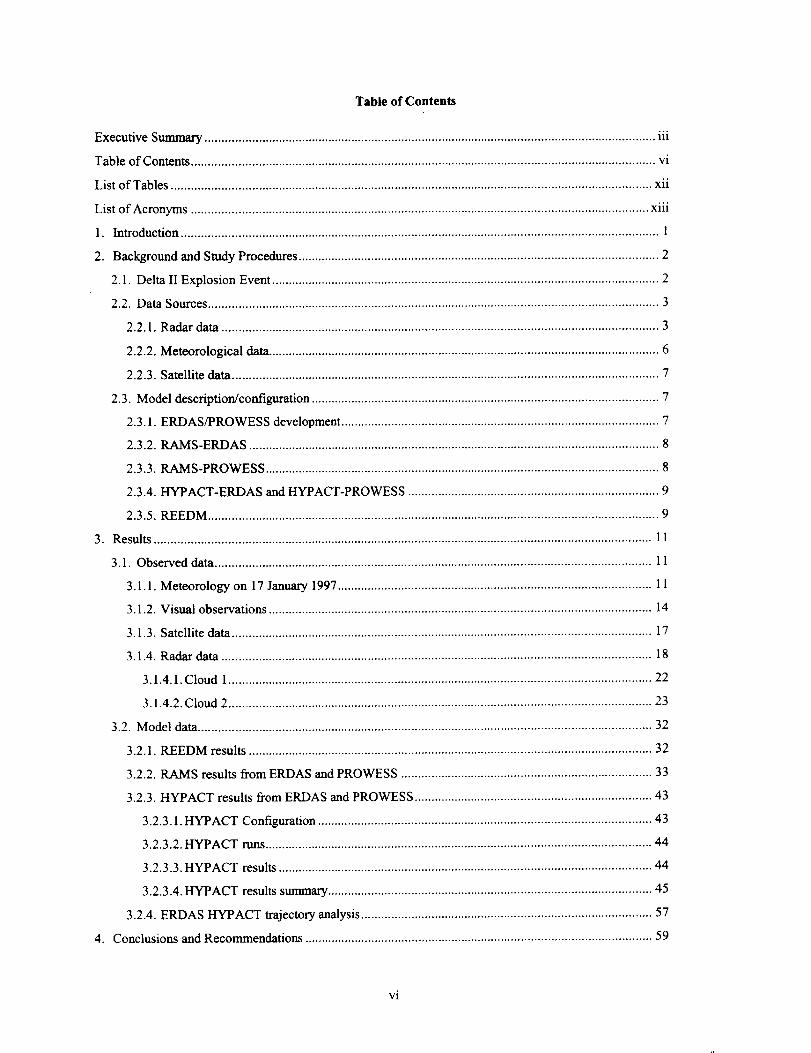
Table of Contents
Executive Summary ....................................................................................................................................... iii
Table of Contents ........................................................................................................................................... vi
List of Tables ................................................................................................................................................ xii
List of Acronyms ......................................................................................................................................... xiii
1. Introduction ............................................................................................................................................... 1
2. Background and Study Procedures ............................................................................................................ 2
2.1. Delta II Explosion Event .................................................................................................................... 2
2.2. Data Sources ....................................................................................................................................... 3
2.2.1. Radar data ................................................................................................................................... 3
2.2.2. Meteorological data ..................................................................................................................... 6
2.2.3. Satellite data ................................................................................................................................ 7
2.3. Model description/configuration ........................................................................................................ 7
2.3.1. ERDAS/PROWESS development ............................................................................................... 7
2.3.2. RAMS-ERDAS ........................................................................................................................... 8
2.3.3. RAMS-PROWESS ...................................................................................................................... 8
2.3.4. HYPACT-ERDAS and HYPACT-PROWESS ........................................................................... 9
2.3.5. REEDM ....................................................................................................................................... 9
3. Results ..................................................................................................................................................... 11
3.1. Observed data ................................................................................................................................... 11
3.1.1. Meteorology on 17 January 1997 .............................................................................................. 11
3.1.2. Visual observations ................................................................................................................... 14
3.1.3. Satellite data .............................................................................................................................. 17
3.1.4. Radar data ................................................................................................................................. 18
3.1.4.1. Cloud 1 ............................................................................................................................... 22
3.1.4.2. Cloud 2 ............................................................................................................................... 23
3.2. Model data ........................................................................................................................................ 32
3.2.1. REEDM results ......................................................................................................................... 32
3.2.2. RAMS results from ERDAS and PROWESS ........................................................................... 33
3.2.3. HYPACT results from ERDAS and PROWESS ....................................................................... 43
3.2.3.1. HYPACT Configuration .................................................................................................... 43
3.2.3.2. HYPACT runs .................................................................................................................... 44
3.2.3.3. HYPACT results ................................................................................................................ 44
3.2.3.4. HYPACT results summary ................................................................................................. 45
3.2.4. ERDAS HYPACT trajectory analysis ....................................................................................... 57
4. Conclusions and Recommendations ........................................................................................................ 59
vi
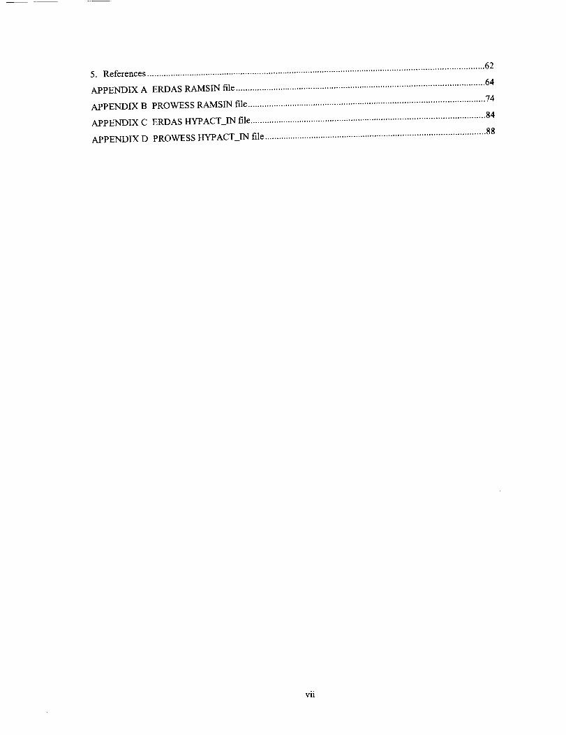
5. References................................................................................................................................................62
APPENDIXA ERDASRAMSINfile..........................................................................................................64APPENDIXB PROWESSRAMSINfile.....................................................................................................74
APPENDIXC ERDASHYPACTINfile....................................................................................................84
APPENDIXD PROWESSHYPACT_INfile..............................................................................................88
vii
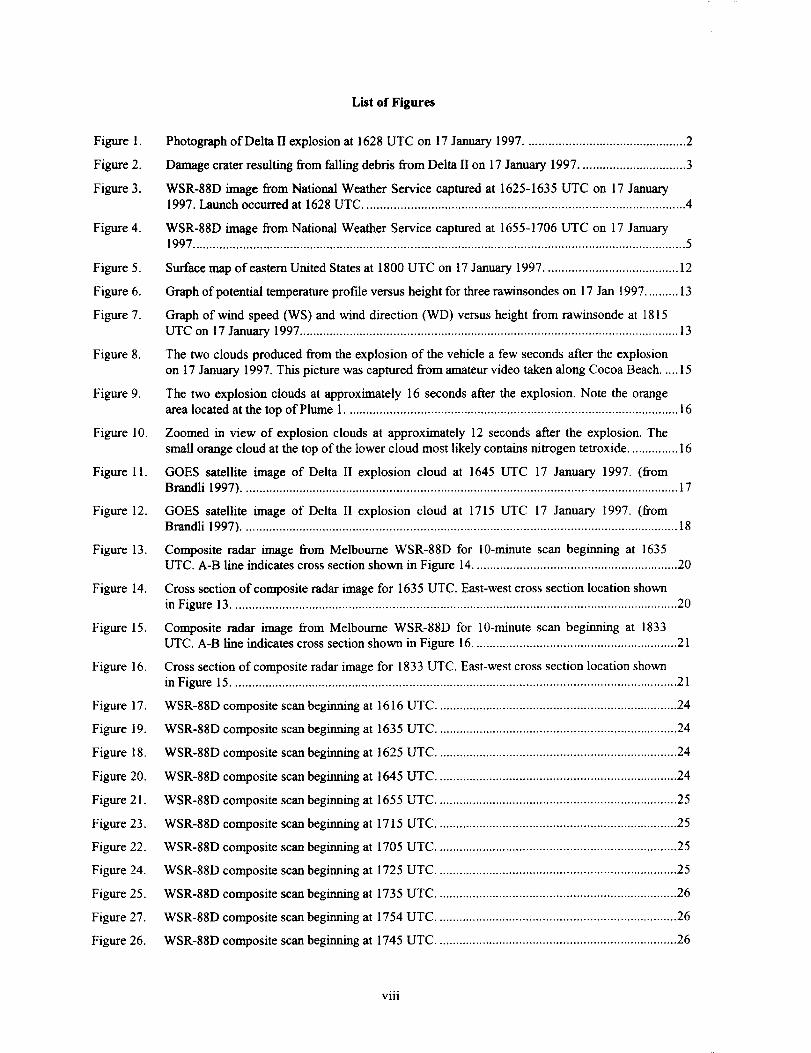
Figure1.
Figure2.Figure3.
Figure 4.
Figure 5.
Figure 6.
Figure 7.
Figure 8.
Figure 9.
Figure 10.
Figure 11.
Figure 12.
Figure 13.
Figure 14.
Figure 15.
Figure 16.
Figure 17.
Figure 19.
Figure 18.
Figure 20.
Figure 21.
Figure 23.
Figure 22.
Figure 24.
Figure 25.
Figure 27.
Figure 26.
List of Figures
Photograph of Delta II explosion at 1628 UTC on 17 January 1997 ................................................ 2
Damage crater resulting from falling debris from Delta II on 17 January 1997 ................................ 3
WSR-88D image from National Weather Service captured at 1625-1635 UTC on 17 January1997. Launch occurred at 1628 UTC ................................................................................................ 4
WSR-88D image from National Weather Service captured at 1655-1706 UTC on 17 January1997 ................................................................................................................................................... 5
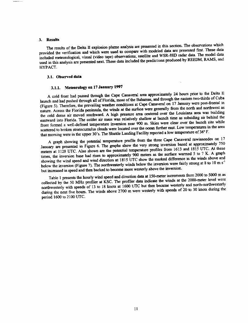
Surface map of eastern United States at 1800 UTC on 17 January 1997 ........................................ 12
Graph of potential temperature profile versus height for three rawinsondes on 17 Jan 1997 .......... 13
Graph of wind speed (WS) and wind direction (WD) versus height from rawinsonde at 1815
UTC on 17 January 1997 ................................................................................................................. 13
The two clouds produced from the explosion of the vehicle a few seconds after the explosion
on 17 January 1997. This picture was captured from amateur video taken along Cocoa Beach ..... 15
The two explosion clouds at approximately 16 seconds after the explosion. Note the orange
area located at the top of Plume 1................................................................................................... 16
Zoomed in view of explosion clouds at approximately 12 seconds after the explosion. The
small orange cloud at the top of the lower cloud most likely contains nitrogen tetroxide ............... 16
GOES satellite image of Delta II explosion cloud at 1645 UTC 17 January 1997. (fromBrandli 1997) .................................................................................................................................. 17
GOES satellite image of Delta II explosion cloud at 1715 UTC 17 January 1997. (fromBrandli 1997) .................................................................................................................................. 18
Composite radar image from Melbourne WSR-88D for 10-minute scan beginning at 1635UTC. A-B line indicates cross section shown in Figure 14 ............................................................. 20
Cross section of composite radar image for 1635 UTC. East-west cross section location shown
in Figure 13 ..................................................................................................................................... 20
Composite radar image from Melbourne WSR-88D for 10-minute scan beginning at 1833UTC. A-B line indicates cross section shown in Figure 16 ............................................................. 21
Cross section of composite radar image for 1833 UTC. East-west cross section location shown
in Figure 15 ..................................................................................................................................... 21
WSR-88D composite scan beginning at 1616
WSR-88D composite scan begmnmg at 1635
WSR-88D
WSR-88D
WSR-88D
WSR-88D
WSR-88D
WSR-88D
WSR-88D
WSR-88D
WSR-88D
composite scan beginning at 1625
composite scan beginning at 1645
composite scan begmmng at 1655
composite scan beginning at 1715
composite scan beginning at 1705
composite scan begmnmg at 1725
composite scan beginning at 1735
composite scan begmnmg at 1754
composite scan beginning at 1745
UTC ........................................................................ 24
UTC ........................................................................ 24
UTC ........................................................................ 24
UTC ........................................................................ 24
UTC ........................................................................ 25
UTC ........................................................................ 25
UTC ........................................................................ 25
UTC ........................................................................ 25
UTC ........................................................................ 26
UTC ........................................................................ 26
UTC ........................................................................ 26
Vlll
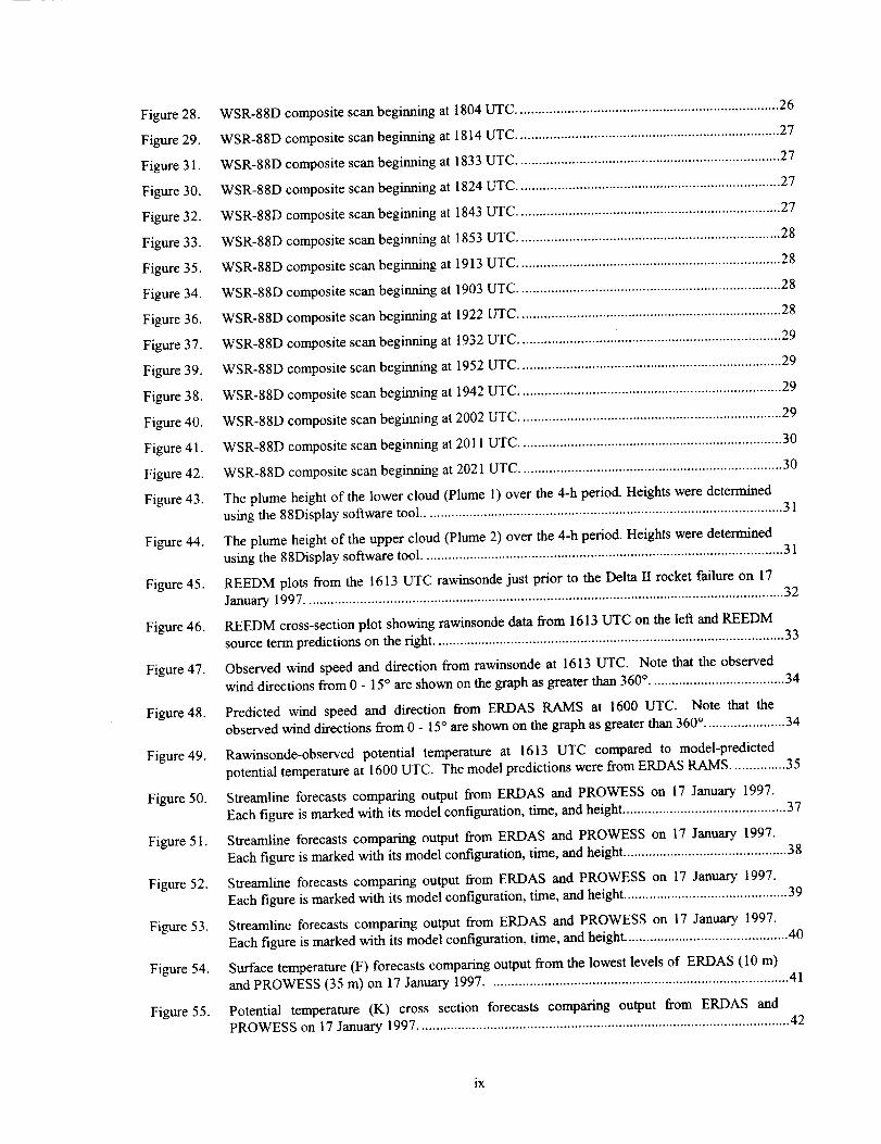
Figure 28.
Figure 29.
Figure 31.
Figure 30.
Figure 32.
Figure 33.
Figure 35.
Figure 34.
Figure 36.
Figure 37.
Figure 39.
Figure 38.
Figure 40.
Figure 41.
Figure 42.
Figure 43.
Figure 44.
Figure 45.
Figure 46.
Figure 47.
Figure 48.
Figure 49.
Figure 50.
Figure 5 I.
Figure 52.
Figure 53.
Figure 54.
Figure 55.
WSR-88D composite scan beginning at
WSR-88D composite scan begmmng at
WSR-88D composite scan begmmng at
WSR-88D composite scan beginning at
WSR-88D composite scan begmmng at
WSR-88D composite scan begmnlng at
WSR-88D composite scan begmmng at
WSR-88D composite scan begmmng at
WSR-88D composite
WSR-88D composite
WSR-88D composite
WSR-88D composite
WSR-88D composite
WSR-88D composite
WSR-88D composite
scan begmnmg at
scan begmmng at
scan beginning at
scan begmning at
scan beginning at
scan begmning at
scan beginning at
1804 UTC ........................................................................ 26
1814 UTC ........................................................................ 27
1833 UTC ........................................................................ 27
1824 UTC ........................................................................ 27
1843 UTC ........................................................................ 27
1853 UTC ........................................................................ 28
1913 UTC ........................................................................ 28
1903 UTC ........................................................................ 28
1922 UTC ........................................................................ 28
1932 UTC .......................... .............................................. 29
1952 UTC ........................................................................ 29
1942 UTC ........................................................................ 29
2002 UTC ........................................................................ 29
2011 UTC ........................................................................ 30
2021 UTC ........................................................................ 30
The plume height of the lower cloud (Plume 1) over the 4-h period. Heights were determined
using the 88Display software tool ................................................................................................... 31
The plume height of the upper cloud (Plume 2) over the 4-h period. Heights were determined
using the 88Display software tool ................................................................................................... 31
REEDM plots from the 1613 UTC rawinsonde just prior to the Delta II rocket failure on 17
January 1997 ................................................................................................................................... 32
REEDM cross-section plot showing raw/nsonde data from 1613 UTC on the left and REEDM
source term predictions on the right ................................................................................................ 33
Observed wind speed and direction from rawinsonde at 1613 UTC. Note that the observed
wind directions from 0 - 15 ° are shown on the graph as greater than 360 °..................................... 34
Predicted wind speed and direction from ERDAS RAMS at 1600 UTC. Note that the
observed wind directions from 0 - 15" are shown on the graph as greater than 360 °. ..................... 34
Rawinsonde-observed potential temperature at 1613 UTC compared to model-predicted
potential temperature at 1600 UTC. The model predictions were from ERDAS RAMS ............... 35
Streamline forecasts comparing output from ERDAS and PROWESS on 17 January 1997.Each figure is marked with its model configuration, time, and height ............................................. 37
Streamline forecasts comparing output from ERDAS and PROWESS on 17 January 1997.
Each figure is marked with its model configuration, time, and height ............................................. 38
Streamline forecasts comparing output from ERDAS and PROWESS on 17 January 1997.
Each figure is marked with its model configuration, time, and height ............................................. 39
Streamline forecasts comparing output from ERDAS and PROWESS on 17 January 1997.
Each figure is marked with its model configuration, time, and height ............................................. 40
Surface temperature (F) forecasts comparing output from the lowest levels of ERDAS (10 m)and PROWESS (35 m) on 17 January 1997 .................................................................................. 41
Potential temperature (K) cross section forecasts comparing output from ERDAS and
PROWESS on 17 January 1997 ...................................................................................................... 42
ix
Figure 56.
Figure 57.
Figure 58.
Figure 59.
Figure 60.
Figure 61.
Figure 62.
Figure 63.
Figure 64.
Figure 65.
Figure 66.
Figure 67.
Figure 68.
Figure 69.
Figure 70.
Figure 71.
Figure 72.
Figure 73.
Figure 74.
Figure 75.
Figure 76.
Figure 77.
Figure 78.
Figure 79.
Figure 80.
Figure 81.
Figure 82.
Figure 83.
Figure 84.
Figure 85.
Figure 86.
Figure 87.
Figure 88.
Figure 89.
Figure 90.
Figure 91.
ERDAS HYPACT, 1630 UTC, 17 Jan 1997 ................................................................................... 47
Same as Figure 56, vertical view from south ................................................................................... 47
ERDAS HYPACT, 1640 UTC, 17 Jan 1997 ................................................................................... 47
Same as Figure 58, vertical view from south ................................................................................... 47
ERDAS HYPACT, 1650 UTC, 17 Jan 1997 ................................................................................... 47
Same as Figure 60, vertical view from south ................................................................................... 47
ERDAS HYPACT, 1700 UTC, 17 Jan 1997 ................................................................................... 48
Same as Figure 62, vertical view from south ................................................................................... 48
ERDAS HYPACT. 1710 UTC, 17 Jan 1997 ................................................................................... 48
Same as Figure 64, vertical view from south ................................................................................... 48
ERDAS HYPACT, 1720 UTC, 17 Jan 1997 ................................................................................... 48
Same as Figure 66, vertical view from south ................................................................................... 48
ERDAS HYPACT, 1730 UTC, 17 Jan 1997 ................................................................................... 49
Same as Figure 68, vertical view from south ................................................................................... 49
ERDAS HYPACT, 1740 UTC, 17 Jan 1997 ................................................................................... 49
Same as Figure 70, vertical view from south ................................................................................... 49
ERDAS HYPACT, 1800 UTC, 17 Jan 1997 ................................................................................... 49
Same as Figure 72, vertical view from south ................................................................................... 49
ERDAS HYPACT 1820 UTC, 17 Jan 1997 ................................................................................... 50
Same as Figure 74, vertical view from south ................................................................................... 50
ERDAS HYPACT 1840 UTC, 17 Jan 1997 ................................................................................... 50
Same as Figure 76, vertical view from south ................................................................................... 50
ERDAS HYPACT 1900 UTC, 17 Jan 1997 ................................................................................... 50
Same as Figure 78, vertical view from south ................................................................................... 50
ERDAS HYPACT, 1930 UTC, 17 Jan 1997 ................................................................................... 51
Same as Figure 80, vertical view from south ................................................................................... 51
ERDAS HYPACT 2000 UTC, 17 Jan 1997 ................................................................................... 51
Same as Figure 82, vertical view from south ............................................. ...................................... 51
ERDAS HYPACT, 2030 UTC, 17 Jan 1997 ................................................................................... 51
Same as Figure 84, vertical view from south ................................................................................... 51
PROWESS HYPACT, 1630 UTC, 17 Jan 1997 ............................................................................ 52
Same as Figure 86, vertical view from south ................................................................................... 52
PROWESS HYPACT, 1640 UTC, 17 Jan 1997 ............................................................................ 52
Same as Figure 88, vertical view from south ................................................................................... 52
PROWESS HYPACT, 1650 UTC, 17 Jan 1997 ............................................................................ 52
Same as Figure 90, vertical view from south ................................................................................... 52
Figure
FigureFigure
Figure
Figure
Figure
FigureFigure
Figure
FigureFigure
Figure
Figure
Figure
FigureFigure
Figure
FigureFigure
Figure
Figure
FigureFigure
FigureFigure
92. PROWESSHYPACT,1700UTC,17Jan1997............................................................................53
93. SameasFigure92,verticalviewfromsouth...................................................................................5394. PROWESSHYPACT,1710UTC,17Jan1997............................................................................53
95. SameasFigure94,verticalviewfromsouth...................................................................................5396. PROWESSHYPACT,1720UTC,17Jan1997............................................................................53
97. SameasFigure96,verticalviewfromsouth...................................................................................5398. PROWESSHYPACT,1730UTC,17Jan1997............................................................................54
99. SameasFigure98,verticalviewfromsouth...................................................................................54100.PROWESSHYPACT,1740UTC,17Jan1997............................................................................54
101.SameasFigure100,verticalviewfromsouth.................................................................................54102.PROWESSHYPACT,1800UTC,17Jan1997............................................................................54
103.SameasFigure102,verticalviewfromsouth.................................................................................54104.PROWESSHYPACT,1820UTC,17Jan1997............................................................................55
105.SameasFigure104,verticalviewfromsouth.................................................................................55106.PROWESSHYPACT,1840UTC,17Jan1997............................................................................55
107.SameasFigure106,verticalviewfromsouth.................................................................................55
108.PROWESSHYPACT,1900UTC,17Jan1997............................................................................55
109.SameasFigure108,verticalviewfromsouth.................................................................................55110.PROWESSHYPACT,1930,UTC,17Jan1997...........................................................................56
111.SameasFigure110,verticalviewfromsouth.................................................................................56112.PROWESSHYPACT,2000UTC,17Jan97................................................................................56
113.SameasFigure112,verticalviewfromsouth.................................................................................56
114.PROWESSHYPACT,2030UTC,17Jan97................................................................................56
115.SameasFigure114,verticalviewfromsouth.................................................................................56116.DataOf observedvs.predictedplumelocationfor lowerplumeresultingfromDeltaII
explosionat1628UTCon17January1997...................................................................................58
xi
List of Tables
Table 1. Wind speed and direction from the 50-MHz profiler at KSC on 17 January 1997 ................................. 14
Table 2. Data obtained from WSR-88D Level II archive for 17 January 1997 using the 88Display software.
Data in this table show Plume 1 (lower cloud) information .................................................................... 19
Table 3. Data obtained from WSR-88D Level II archive for 17 January 1997 using the 88Display software.
Data in this table show Plume 2 (upper cloud) information .................................................................... 19
Table 4. Location and dimensions of plume determined by REEDM and modeled by HYPACT. These
plume dimensions were used in the ERDAS HYPACT simulation ........................................................ 43
Table 5. Location and dimensions of plume determined from visual and radar observations and modeled by
HYPACT. These plume dimensions were used in the PROWESS HYPACT simulation ...................... 43
xii

Term
45 WS
AMU
CCAFS
LC-17
DRWP
EHS
ERDAS
GOES
HC1
HYPACT
IRIS
KSC
LAN
MARSS
MARSS-REPL
MRC
MIDDS
MLB
N204
NCEP
NEXRAD
NGM
NWS
OBDG
PROWESS
REEDM
RAMS
ROCC
UDMH
VCP
WINDS
WSR-88D
List of Acronyms
Description
45th Weather Squadron
Applied Meteorology Unit
Cape Canaveral Air Force Station
Launch complex 17A
Doppler Radar Wind Profiler
Extremely Hazardous Substances
Eastern Range Dispersion Assessment System
Geostationary Operational Environmental Satellite
Hydrochloric acid
HYbrid Particle And Concentration Transport
Interactive Radar Information System
Kennedy Space Center
Local Area Network
Meteorological And Range Safety Support
MARSS Replacement
Mission Research Corporation
Meteorological Interactive Data Display System
Melbourne, Florida
Nitrogen tetroxide
National Centers for Environmental Prediction
NEXt generation RADar
Nested Grid Model
National Weather Service
Ocean Breeze/Dry Gulch
Parallelized RAMS Operational Weather Simulation System
Rocket Exhaust Effluent Dispersion Model
Regional Atmospheric Modeling System
Range Operations Control Center
Unsymmetrical dimethyl hydrazine
Volume Coverage Pattern
Weather Information Network Display System
Weather Surveillance Radar-1988 Doppler
xiii

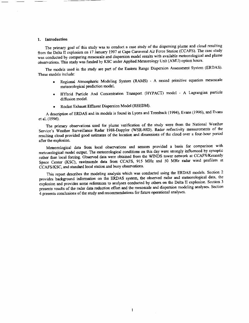
I. Introduction
The primary goal of this study was to conduct a case study of the dispersing plume and cloud resulting
from the Delta II explosion on 17 January 1997 at Cape Canaveral Air Force Station (CCAFS). The case study
was conducted by comparing mesoscale and dispersion model results with available meteorological and plumeobservations. This study was funded by KSC under Applied Meteorology Unit (AMU) option hours.
The models used in the study are part of the Eastern Range Dispersion Assessment System (ERDAS).These models include:
• Regional Atmospheric Modeling System (RAMS) - A nested primitive equation mesoscalemeteorological prediction model.
• HYbrid Particle And Concentration Transport (HYPACT) model - A Lagrangian particlediffusion model.
• Rocket Exhaust Effluent Dispersion Model (REEDM).
A description of ERDAS and its models is found in Lyons and Tremback (1994), Evans (1996), and Evans
et al. (1996).
The primary observations used for plume verification of the study were from the National WeatherService's Weather Surveillance Radar 1988-Doppler (WSR-88D). Radar reflectivity measurements of the
resulting cloud provided good estimates of the location and dimensions of the cloud over a four-hour period
after the explosion.
Meteorological data from local observations and sensors provided a basis for comparison with
meteorological model output. The meteorological conditions on this day were strongly influenced by synopticrather than local forcing. Observed data were obtained from the WINDS tower network at CCAFS/Kennedy
Space Center (KSC), rawinsonde data from CCAFS, 915 MHz and 50 MHz radar wind profilers at
CCAFS/KSC, and standard local station and buoy observations.
This report describes the modeling analysis which was conducted using the ERDAS models. Section 2
provides background information on the ERDAS system, the observed radar and meteorological data, the
explosion and provides some references to analyses conducted by others on the Delta II explosion. Section 3presents results of the radar data reduction effort and the mesoscale and dispersion modeling analyses. Section
4 presents conclusions of the study and recommendations for future operational analyses.
2. Background and Study Procedures
2.1. Delta II Explosion Event
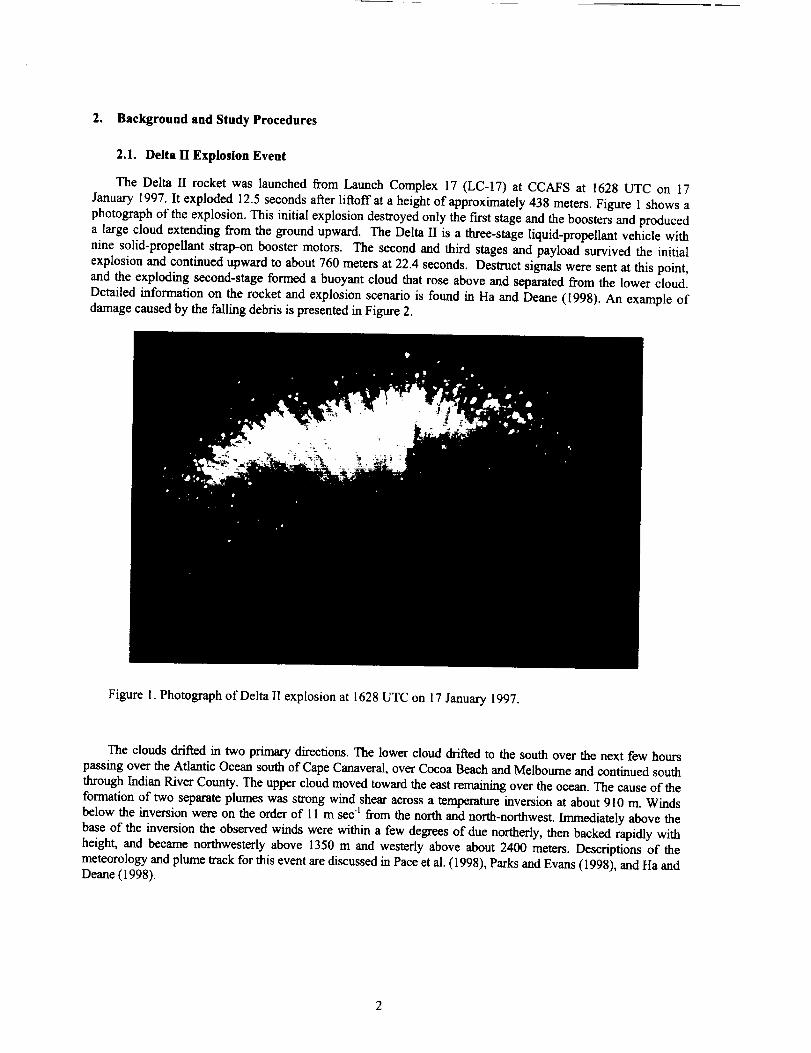
The Delta II rocket was launched from Launch Complex 17 (LC-17) at CCAFS at 1628 UTC on 17
January 1997. It exploded 12.5 seconds after liftoff at a height of approximately 438 meters. Figure 1 shows a
photograph of the explosion. This initial explosion destroyed only the fwst stage and the boosters and produceda large cloud extending from the ground upward. The Delta II is a three-stage liquid-propellant vehicle with
nine solid-propeUant strap-on booster motors. The second and third stages and payload survived the initial
explosion and continued upward to about 760 meters at 22.4 seconds. Destruct signals were sent at this point,
and the exploding second-stage formed a buoyant cloud that rose above and separated from the lower cloud.
Detailed information on the rocket and explosion scenario is found in Ha and Deane (1998). An example ofdamage caused by the falling debris is presented in Figure 2.
Figure 1. Photograph of Delta II explosion at 1628 UTC on 17 January 1997.
The cloudsdriftedintwo primarydirections.The lowerclouddriRedtothesouthoverthe nextfew hours
passingover theAtlanticOcean southofCape Canaveral,overCocoa Beach and Melbourne and continuedsouth
throughIndianRiverCounty.The upper cloudmoved towardtheeastremainingovertheocean.The causeofthe
formationof two separateplumes was strongwind shearacrossa temperatureinversionatabout 9I0 m. Winds
below theinversionwere on theorderof II m sec-tfrom thenorthand north-northwest.Immediatelyabove the
base of the inversionthe observedwinds were withina few degreesof due northerly,thenbacked rapidlywith
height,and became northwesterlyabove 1350 m and westerlyabove about 2400 meters.Descriptionsof the
meteorologyand plume trackforthiseventarediscussedinPaceetal.(1998),Parksand Evans (1998),and Ha and
Deane (I998).
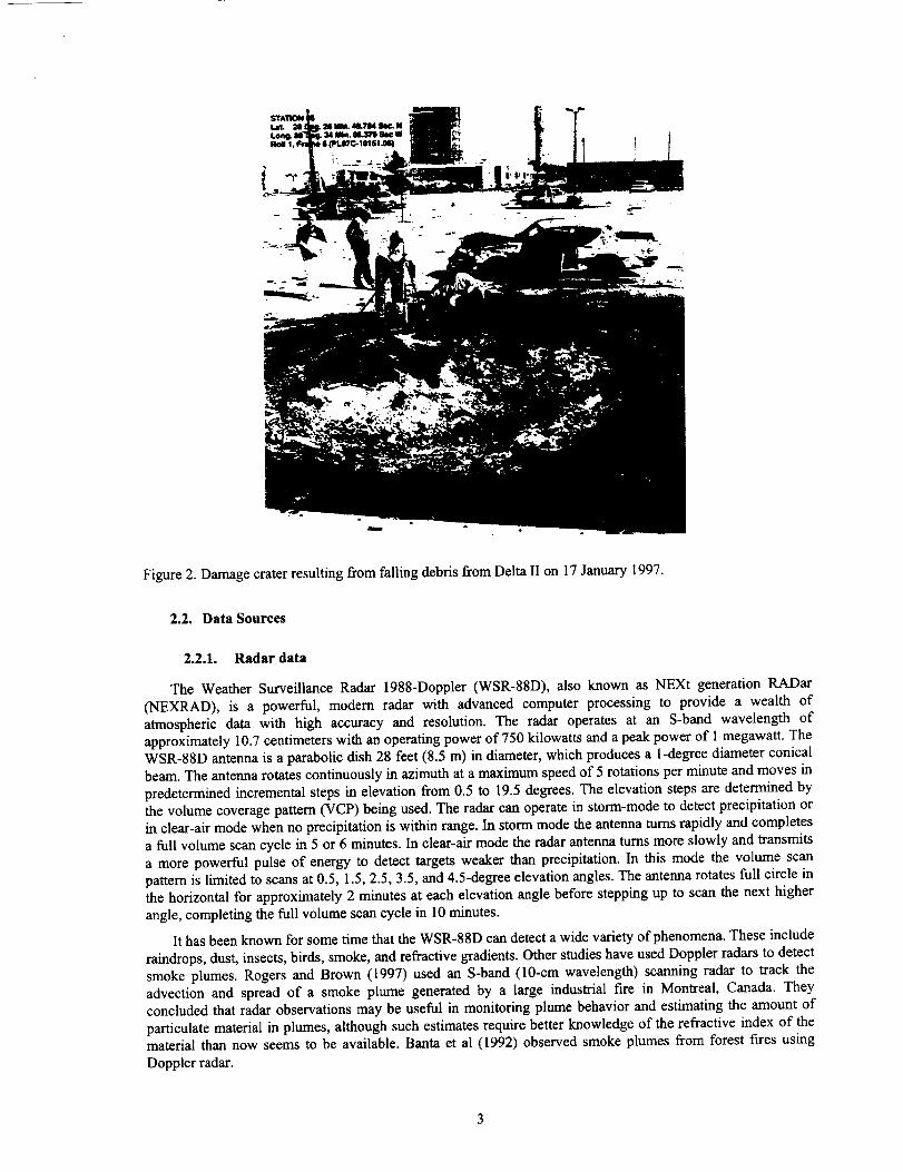
Figure 2. Damage crater resulting from falling debris from Delta II on 17 January 1997.
2.2. Data Sources
2.2.1. Radar data
The Weather Surveillance Radar 1988-Doppler (WSR-88D), also known as NEXt generation RADar
(NEXRAD), is a powerful, modern radar with advanced computer processing to provide a wealth of
atmospheric data with high accuracy and resolution. The radar operates at an S-band wavelength ofapproximately 10.7 centimeters with an operating power of 750 kilowatts and a peak power of I megawatt. The
WSR-88D antenna is a parabolic dish 28 feet (8.5 m) in diameter, which produces a 1-degree diameter conical
beam. The antenna rotates continuously in azimuth at a maximum speed of 5 rotations per minute and moves inpredetermined incremental steps in elevation from 0.5 to 19.5 degrees. The elevation steps are determined by
the volume coverage pattern (VCP) being used. The radar can operate in storm-mode to detect precipitation or
in clear-air mode when no precipitation is within range. In storm mode the antenna turns rapidly and completes
a full volume scan cycle in 5 or 6 minutes. In clear-air mode the radar antenna turns more slowly and transmits
a more powerful pulse of energy to detect targets weaker than precipitation. In this mode the volume scanpattern is limited to scans at 0.5, 1.5, 2.5, 3.5, and 4.5-degree elevation angles. The antenna rotates full circle in
the horizontal for approximately 2 minutes at each elevation angle before stepping up to scan the next higher
angle, completing the full volume scan cycle in 10 minutes.
It has been known for some time that the WSR-88D can detect a wide variety of phenomena. These include
raindrops, dust, insects, birds, smoke, and refractive gradients. Other studies have used Doppler radars to detect
smoke plumes. Rogers and Brown (1997) used an S-band (10-cm wavelength) scanning radar to track the
advection and spread of a smoke plume generated by a large industrial fire in Montreal, Canada. Theyconcluded that radar observations may be useful in monitoring plume behavior and estimating the amount of
particulate material in plumes, although such estimates require better knowledge of the refractive index of the
material than now seems to be available. Banta et al (1992) observed smoke plumes from forest fires using
Doppler radar.
It wasn'tknownhowwelltheradarcoulddetect the abort cloud from a launch vehicle failure until the
Delta II explosion at Cape Canaveral was observed on 17 January 1997. A detailed analysis of the Delta IIabort cloud will be described in Section 3.1.4.
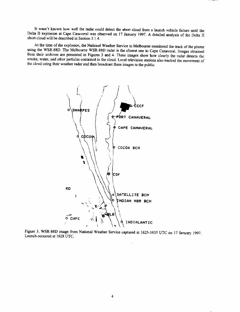
At the time of the explosion, the National Weather Service in Melbourne monitored the track of the plumeusing the WSR-88D. The Melbourne WSR-88D radar is the closest one to Cape Canaveral. Images obtained
from their archives are presented in Figures 3 and 4. These images show how clearly the radar detects the
smoke, water, and other particles contained in the cloud. Local television stations also tracked the movement of
the cloud using their weather radar and then broadcast these images to the public.
HAI_PES
'\
\
Figure 3. WSR-88D image from National Weather Service captured at 1625-1635 UTC on 17 January 1997.Launch occurred at 1628 UTC.
REVARD
i
,---- 0 CHFC._" /, .i _'_ \ _I INOIALANTIC2 "1 ' '_, '_
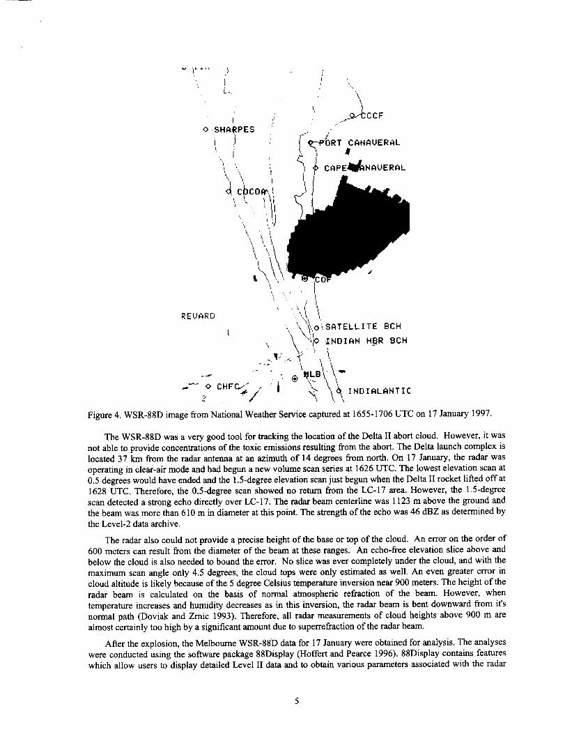
Figure4.WSR-88D image from NationalWeather Servicecapturedat1655-1706 UTC on 17January 1997.
The WSR-88D was a very good tool for tracking the location of the Delta II abort cloud. However, it wasnot able to provide concentrations of the toxic emissions resulting from the abort. The Delta launch complex is
located 37 km from the radar antenna at an azimuth of 14 degrees from north. On 17 January, the radar was
operating in clear-air mode and had begun a new volume scan series at 1626 UTC. The lowest elevation scan at
0.5 degrees would have ended and the 1.5-degree elevation scan just begun when the Delta II rocket lifted off at1628 UTC. Therefore, the 0.5-degree scan showed no return from the LC-17 area. However, the 1.5-degree
scan detected a strong echo directly over LC-17. The radar beam centerline was 1123 m above the ground andthe beam was more than 610 m in diameter at this point. The strength of the echo was 46 dBZ as determined by
the Level-2 data archive.
The radar also could not provide a precise height of the base or top of the cloud. An error on the order of600 meters can result from the diameter of the beam at these ranges. An echo-free elevation slice above and
below the cloud is also needed to bound the error. No slice was ever completely under the cloud, and with the
maximum scan angle only 4.5 degrees, the cloud tops were only estimated as well. An even greater error in
cloud altitude is likely because of the 5 degree Celsius temperature inversion near 900 meters. The height of theradar beam is calculated on the basis of normal atmospheric refraction of the beam. However, when
temperature increases and humidity decreases as in this inversion, the radar beam is bent downward from it'snormal path (Doviak and Zmic 1993). Therefore, all radar measurements of cloud heights above 900 m are
almost certainly too high by a significant amount due to superrefraction of the radar beam.
After the explosion, the Melbourne WSR-88D data for 17 January were obtained for analysis. The analyseswere conducted using the software package 88Display (Hoffert and Pearce 1996). 88Display contains features
which allow users to display detailed Level II data and to obtain various parameters associated with the radar
echoes.Level II data are base data which include base reflectivity, mean radial velocity, and spectrum width.
The features of 88Display include displaying composite reflectivity for all elevation angles, display basereflectivity for each elevation angle, building animated time loops, and also displaying vertical cross-sections.
The cross sections can be built using any two user-selected points from a map of the composite or basereflectivities. Another very useful feature of the software is the information query function. When a user clicks
the mouse on an echo feature on the map, the program returns data on elevation, azimuth, ground range(distance from radar), latitude, longitude, and height above ground. This information is based on elevationangle of the currently selected scan.
The data collected by the WSR-74C located at Patrick AFB were not available for these analyses (Herring1999). The tape containing the data was produced using the McGill processor and its associated software.
When the WSR-74C was upgraded to the Interactive Radar Information System (IRIS) SIGMET software in
1997, the new system would not read the tapes created on the older machine. Having no requirement to retainthese tapes, the contractor recycled them for other use.
2.2.2. Meteorological data
The meteorological data used for this study consisted of the data which are routinely available within theMeteorological Interactive Data Display System (MIDDS). The RAMS model runs which were made for 1200
UTC on 17 January 1997 were initialized with the following data:
• 1200 UTC Weather Information Network Display System (WINDS) tower data (39 stations)
• 1200 UTC surface and buoy observations (484 stations)
• 1200 UTC rawinsonde data (37 stations)
• NCEP Eta grids generated from the analysis at 1200 UTC 17 January 1998 for the followingforecast times:
• 1800 UTC 17 January,
• 0000 UTC 18 January,
• 0600 UTC 18 January,
• 1200 UTC 18 January,
The 12-hr forecast grid (0000 UTC 18 January) used for boundary conditions was found to contain bad
data that caused RAMS to stop running at the 7-h forecast time (1900 UTC). To t'LXthe problem, we substituted
the 24-h Eta forecast grid from the previous forecast cycle. RAMS ran to completion with these data.
Other meteorological data were available to characterize the weather conditions at the time of the accident.This data included the following:
• WINDS tower data (available at 5-minute intervals)
* Surface and buoy observations (available hourly)
• Rawinsonde data (available at 1128, 1243, 1453, 1548, 1613, and 1815 UTC)
• 50 MHz profiler data (available hourly)
• 915 MHz profiler data (including Radio Acoustic Sounding Systems virtual temperature data)
2.2.3. Satellite data
Satellite data from the GOES-8-east satellite data was available for 17 January 1997. The satellite photos
were used to show the clouds present on this day. The satellite data was also used to show the location of the
explosion clouds as they advected downwind.
2.3. Model description/configuration
2.3.1. ERDAS/PROWESS development
ERDAS was developed by Mission Research Corporation (MRC)/ASTER division for the Air Force as a
prototype system to provide emergency response guidance for operations at KSC/CCAFS in case of an
accidental hazardous material release or an aborted vehicle launch. The ERDAS development occurred during
the period 1989 to 1994 under Phase I and II Small Business Innovative Research contracts with the Air ForceSpace and Missile Systems Center, Los Angeles, CA. ERDAS was delivered to the Air Force's Range
Operations Control Center (ROCC) in March 1994. The AMId was tasked with keeping the prototype ERDAS
running and with evaluating ERDAS during the period March 1994 to December 1995. The AMId evaluation
report concluded that ERDAS provided significant improvement over current toxic dispersion modeling
capabilities but the system contained deficiencies which needed addressing before the ERDAS could becomeoperational (Evans 1996).
The Parallelized RAMS Operational Weather Simulation System (PROWESS) was developed by MRC
during the period 1993 to 1996 for NASA (Tremback et al. 1996). The goals of the PROWESS project were to
demonstrate capability of the parallelized RAMS code to run on a cluster of low-cost workstations. The modelwas configured to forecast the initiation, development, interaction and dissipation of sea breeze and river breeze-
generated thunderstorms during initially undisturbed conditions on scales as small as several kilometers. Thedifferences between PROWESS and ERDAS are described in Sections 2.3.2 and 2.3.3. PROWESS was installed
in the AMU and has run on a routine basis but was not evaluated by the AMId. PROWESS was not evaluated
because the AMU tasking committee selected other projects for the AMU at the time PROWESS was delivered.
The next generation of ERDAS was rehosted into the newly upgraded Meteorological And Range Safety
Support Replacement (MARSS-REPL) system. MARSS-REPL was installed in 1997 at CCAFS/KSC as the
primary toxic/hazard diffusion prediction system. An earlier version of MARSS and a prototype of the MARSS-
REPL, the Meteorological Monitoring System (MMS) are described in Lane and Evans (1989) and Evans et al.(1994). The MARSS-REPL consists of 13 Hewlett-Packard C100 and C110 workstations. The workstations are
connected by a Local Area Network (LAN) that allows users at CCAFS and KSC to run and display thediffusion model Ocean Breeze/Dry Gulch. Users can also display various meteorological displays.
Some of the primary features of the upgraded and certified system (called ERDAS-REPL), delivered in late1998, are:
* An upgraded LAN using a higher speed distribution mechanism known as Fiber Distributed Data
Interface to support the larger data transfers.
• A series of Hewlett-Packard K460 workstations used as dedicated RAMS processors utilizing a
Symmetric Multi-Processor architecture.
o RAMS with:
• Full microphysics activated,
• Four nested grids with the largest grid covering the southeast United States, and
• 1.25-km grid spacing on the fine grid covering approximately 100 km by 80 km centeredon CCAFS/KSC.
• Additional meteorological data sources now include 50 MHz Doppler radar wind profiler, 915
MHz radar wind profilers, rawinsondes, coastal buoys, surface stations, wind towers, and gridded
NationalCentersfor EnvironmentalPrediction(NCEP)ETAmodelgrids.Newdataqualitycontrolprocedureswereimplementedforobservationaldata.
• Thesystemwill nowrunRocketExhaustEffluentDiffusionModel(REEDM)andBLASTXmodels,alongwithOceanBreeze/DryGulch(OB/DG),HYPACT/RAMS.
2.3.2. RAMS-ERDAS
TheAMUconductedtheDeltaII modelinganalysisbyrunningRAMSfor17January1997andusingtheforecastmeteorologicaldatatodrivethediffusionmodelHYPACT.TheRAMS-ERDASconfigurationwasthesameastheconfigurationusedforthedailyoperationof RAMSin theprototypeERDAS.ThisconfigurationhasbeensetsincetheprototypeERDASwasinstalledin theROCCin 1994.Thekeypointsof thisconfigurationaxe:
• RAMSversion3a
• Microphysicsinactive(NLEVEL=I)
• 3nested grids
• Coarse grid: 60 km spacing, 2220 x 2100 km domain
• Medium grid: 15 km spacing, 495 x 555 km domain
• Fine grid: 3 km spacing, 108 x 108 km domain
• Vertical grid with 10-m lowest grid point on f'me grid and expanding m depth upward
• Twice-dally RAMS runs initialized at 0000 and 1200 UTC with hourly forecast output
• Input data used to initialize the model are obtained from MIDDS and include:
• NCEP ETA data
• rawinsondes
• surface and buoy data
• local CCAFS/KSC WINDS tower data
A complete listing of the file RAMSIN containing the input parameters for running RAMS is provided m
Appendix A.
2.3.3. RAMS-PROVgESS
The RAMS-PROWESS runs were made using the version of RAMS on the PROWESS workstations. ThePROWESS workstations consist of one IBM RS/6000-370 and seven IBM RS/6000-250 workstations which nan
the parallel version of RAMS. The key points of this configuration are:
RAMS version 4a
Microphysics active (NLEVEL=3)
4 nested grids
• Coarse grid:
• Medium grid:
• Fine grid:
• Finest grid:
72 km spacing, 2376 x 2088 km domain
18 km spacing, 594 x 666 km domain
6 km spacing, 222 x 222 km domain
1.5 km spacing, 61.5 x 85.5 km domain
• Vertical grid with 38-m lowest grid point
• Twice-daily RAMS runs initialized at 0000 and 1200 UTC with hourly forecast output

• Hourlyoutputbeginningatinitializationtimeof 1200UTC
• InputdatausedtoinitializethemodelisobtainedfromMIDDSandincludes• NCEPETAdata
• Rawinsondes
• Surfaceandbuoydata• LocalCCAFS/KSCWINDStowerdata
A completelistingof thefileRAMSINcontainingtheinputparametersforrunningRAMSisprovidedinAppendixB.
2.3.4. HYPACT-ERDAS and HYPACT-PROWESS
The primary model used for computing dispersion estimates in ERDAS is HYPACT. HYPACT is anadvanced Lagrangian particle dispersion model. Dispersion in the Lagrangian mode of HYPACT is simulated by
tracking a large set of particles. Subsequent positions of each particle are computed from the relation:
X[t +At] = X[t] + [u + u'] At
Y[t +At] = Y[t] + [v + v'] At
Z[t +At] = Z[t] + [w + w" + wp] At
where u, v and w are the resolvable scale wind components which are derived from the RAMS wind field,
and u', v', and w" are the random subgrid turbulent wind components deduced from RAMS. The wp term is theterminal velocity resulting from external forces such as gravitational settling.
REEDM predicts plume rise and downwind concentrations resulting from nominal or aborted launches. In
ERDAS, REEDM'produces the source term which is used by HYPACT to predict plume dispersion and
resulting downwind concentrations.
For modeling launch scenarios, HYPACT obtains the source term data (release rate) from the REEDM
launch plume data. HYPACT then diffuses the plume using the RAMS-predicted wind fields and potential
temperature fields to advect and disperse the particles vertically and horizontally downwind from the source.
HYPACT can model any number of sources which are specified anywhere in the domain and configured as
point, line, area, or volume sources. The emissions from these sources can be instantaneous, intermittent, or
continuous and the pollutants can be treated as gases or aerosols.
To simulate the Delta II explosion plume using HYPACT required that we modify the HYPACT input
configuration file produced within the ERDAS dispersion function. For launch plume dispersion scenarios,
ERDAS uses REEDM to produce a source term for a rocket exhaust plume. This source term, which is actuallya series of source terms in a vertical column, represents the mass of an emitted launch plume product. REEDM
computes the source term based on a number of factors such as:
• type of launch (e.g. nominal, abort conflagration, or abort deflagration)
• type of vehicle (e.g. Atlas, Delta II, Titan IV, Shuttle, etc.)
• vertical stability (i.e. stabilization height).
2.3.5. REEDM
Prior to each land-based launch, Range Safety, in conjunction with their support contractor, ACTA Inc.,
runs REEDM to predict the location and concentration of the toxic cloud arising from the normal launch or
abort plumes. REEDM is currently the model of choice and the only certified model which Range Safetypersonnel can use to evaluate launch cloud dispersion. At the time of the Delta II explosion, REEDM 7.07 was
the version of REEDM in use at the time. Range Safety has continued to upgrade REEDM and uses the latest
version available to evaluate launch cloud dispersion.
9
ToxicsubstancesareidentifiedontheEPAlistof ExtremelyHazardousSubstances(EHS).TheDeltaIIcontainedor producedthefollowingEHSchemicalsaspropellantsor productsof solidrocketpropellantcombustion.
• Hydrazine
• Unsymmetrical dimethyl hydrazine (UDMH)
• Nitrogen tetroxide
• Hydrogen chloride
Aerozine-50 is the Delta II second stage hypergolic fuel and is a 50-50 mixture of hydrazine and UDMH.Nitrogen tetroxide is the Delta II second stage hypergolic oxidizer. The reaction of the solid propellant involves
aluminum oxide as the oxidizer and ammonium perchlorate as the fuel to produce hydrogen chloride along with
other non-EHS reaction products.
REEDM models the toxic cloud formation process in four significant steps:
• cloud formation
• cloud rise (buoyant cloud rise)
• cloud stabilization (at neutral buoyancy after heat exchange with the atmosphere)
• cloud transport and dispersion
A single rawinsonde sounding provides the input meteorological data for REEDM, which incorporates verticalbut not horizontal wind shear. Thus the sounding is assumed to represent the flow across the entire area-wide modeldomain.
REEDM predicts the ground trace or net ground level concentration of hazardous material arising due to itsdispersion from the elevated cloud. This ground-level isopleth does not portray the cloud's passage in terms of
time, but lists range and bearing from the source, peak concentration at that range and bearing, and, cloud arrivaland departure times at that range and bearing. REEDM results for the Delta II scenario are presented in Section3.2.1.
10
3. Results
The results of the Delta 1] explosion plume analysis are presented in this section. The observations which
provided the verification and which were used to compare with modeled data are presented first. These dataincluded meteorological, visual (video tape) observations, satellite and WSR-88D radar data. The model data
used in this analysis are presented next. These data included the predictions produced by REEDM, RAMS, andHYPACT.
3.1. Observed data
3.1.1. Meteorology on 17 January 1997
A cold front had passed through the Cape Canaveral area approximately 24 hours prior to the Delta IIlaunch and had pushed through all of Florida, most of the Bahamas, and through the eastern two-thirds of Cuba
(Figure 5). Therefore, the prevailing weather conditions at Cape Canaveral on 17 January were post-frontal innature. Across the Florida peninsula, the winds at the surface were generally from the north and northwest as
the cold dense air moved southward. A high pressure area centered over the Louisiana area was building
eastward into Florida. The colder air mass was relatively shallow at launch time as subsiding air behind the
front formed a well-defined temperature inversion near 900 m. Skies were clear over the launch site whilescattered to broken stratocumulus clouds were located over the ocean further east. Low temperatures in the area
that morning were in the upper 30's. The Shuttle Landing Facility reported a low temperature of 36° F.
A graph showing the potential temperature profile from the three Cape Canaveral rawinsondes on 17
January are presented in Figure 6. The graphs show the very strong inversion based at approximately 750
meters at 1128 UTC. Also shown are the potential temperature profiles from 1613 and 1815 UTC. At thesetimes, the inversion base had risen to approximately 900 meters as the surface warmed 5 to 7 K. A graph
showing the wind speed and wind direction at 1815 UTC show the marked difference in the winds above andbelow the inversion (Figure 7). The northwesterly winds below the inversion were fairly slzong at 8 to 10 m s"_
but increased in speed and then backed to become more westerly above the inversion.
Table 1 presents the hourly wind speed anddirecti°n dam at 150-meter increments from 2000 to 5000 m as
collected by the 50 MHz profiler at KSC. The profiler data indicate the winds at the 2000-meter level were
northwesterly with speeds of 13 to 18 knots at 1600 UTC but then became westerly and north-northwesterlyduring the next five hours. The winds above 2700 m were westerly with speeds of 20 to 30 knots during the
period 1600 to 2100 UTC.
11
\\\
Figure 5. Surface map of eastern United States at 1800 UTC on 17 January 1997.
12

5000.
4500.--
4000.--
25OO.
3000.
Heig_ eel0.
-r
2000.
1500.
1000.
,50O,
O.
270
__L__lt615UTC !
1128 UTC, /:
1613 UTC j_
/
,-'.'.'.'.'.'.'.'.'_O 3,10 2_0
Potanhal Tam p_aluro (K)
Figure 6. Graph of potential temperature profile versus height for three rawinsondes on 17 Jan 1997.
Wind Speed (m-sec-t )
5 tO 15 20 25 30
?
"5 ,.,,
J
/ ,J
).
0
5000-
4500 -
4000-
3.500.
30130-
H_ig_l_0 •
1500.
tO00.
SO0.
O.
L..
-- WO 18t5 UTC
-- WS 181SUTC
f
33O 280210 240 270 300
Wind Direction (degree--)
Figure 7. Graph of wind speed (WS) and wind direction (WD) versus height from rawinsonde at 1815 UTC on
17 January 1997.
13
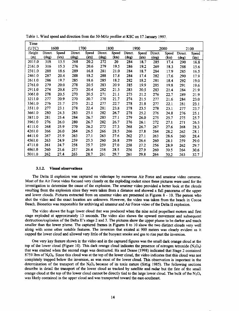
Table1.Windspeedand direction from the 50-MHz profiler at KSC on 17 January 1997.
Time
(UTC) 1600 1700 1800 1900 2000 2100
Height Direct. Speed Direct. Speed Direct. Speed Dkeet. Speed D_ect. Speed D_ect. Speed(m) (de_ (kts) (deg) (kts) (deg) (kts) (deg) (kts) (de_ (las) (deg) (kts)
2011.0 318 13.5 268 20.2 272 20 284 18.7 285 17.4 290 16.8
2161.0 316 15.3 276 20.6 279 19.5 286 19.2 269 18.3 288 15.6
2311.0 288 18.6 289 16.8 281 21.0 284 18.7 284 17.9 285 16.5
2461.0 287 20.4 288 18.2 288 17.8 284 17.4 282 17.6 290 17.9
2611.0 286 19.7 285 18.6 285 18.2 282 18.2 281 18.4 292 19.0
2761.0 279 20.0 278 20.5 283 20.9 285 19.9 285 19.8 291 19.62911.0 274 20.8 273 20.4 282 21.3 283 20.5 283 21.4 284 21.9
3061.0 278 20.5 270 20.5 271 21.1 275 21.2 276 22.7 289 21.9
3211.0 277 20.9 270 20.7 270 21.7 274 21.5 277 21.6 284 23.0
3361.0 276 21.7 275 21.2 277 22.7 278 21.8 277 22.1 281 23.1
3511.0 277 23.1 278 22.4 281 23.8 278 23.5 278 23.1 277 23.73661.0 280 24.3 283 25.1 282 26.7 278 25.2 276 24.8 276 25.1
3811.0 281 25.4 284 26.7 283 27.1 279 26.0 275 25.7 275 25.7
3961.0 276 26.0 280 26.7 282 26.7 276 26.1 272 27.1 271 26.5
4111.0 268 25.9 270 26.2 272 27.3 268 26.7 267 27.6 268 28.34261.0 266 26.0 264 26.5 266 28.5 266 27.8 264 28.2 262 28.1
4411.0 267 25.9 263 27.1 263 27.6 262 27.1 263 28.6 260 28.4
4561.0 263 24.9 259 25.3 260 26.8 259 26.6 260 28.1 259 29.04711.0 261 24.7 258 25.7 259 27.0 258 27.2 256 28.9 262 29.7
4861.0 260 25.6 257 26.4 258 28.5 256 27.9 260 30.5 264 30.6
5011.0 262 27.4 263 28.7 261 29.7 261 29.8 264 30.2 263 32.7
3.1.2. Visual observations
The Delta II explosion was captured on videotape by numerous Air Force and amateur video cameras.
Most of the Air Force video focused very closely on the exploding rocket since these pictures were used for theinvestigation to determine the cause of the explosion. The amateur video provided a better look at the clouds
resulting from the explosion since they were taken from a distance and showed a full panorama of the upper
and lower clouds. Pictures extracted from on amateur video are presented in Figures 8 - 10. The person whoshot the video and the exact location are unknown. However, the video was taken from the beach in Cocoa
Beach. Bionetics was responsible for archiving all amateur and Air Force video of the Delta H explosion.
The video shows the huge lower cloud that was produced when the nine solid propellant motors and ftrst
stage exploded at approximately 13 seconds. The video also shows the upward movement and subsequentdestruction/explosion of the Delta II's stage 2 and 3. The pictures show the upper plume to be darker and much
smaller than the lower plume. The captured frames in Figures 8 to 10 show the two distinct clouds very wellalong with some other notable features. The inversion that existed at 900 meters was clearly evident as it
capped the lower cloud and allowed very little of the buoyant smoke and gas to rise past the inversion.
One very key feature shown in the video and in the captured figures was the small dark orange cloud at the
top of the lower cloud (Figure 10). This dark orange cloud indicates the presence of nitrogen tetroxide (N204)
that was emitted when the second stage was destructed. Ha and Deane (1998) indicated that Stage 2 contained8759 Ibm of N204. Since this cloud was at the top of the lower cloud, the video indicates that this cloud was not
completely trapped below the inversion, as was most of the lower cloud. This observation is important in the
determination of the transport of the N204 because of its toxic nature (Sittig 1985). The following sectionsdescribe in detail the transport of the lower cloud as tracked by satellite and radar but the fate of the small
orange cloud at the top of the lower cloud cannot be directly tied to the large lower cloud. The bulk of the N204was likely contained in the upper cloud and was transported toward the east-southeast.
14
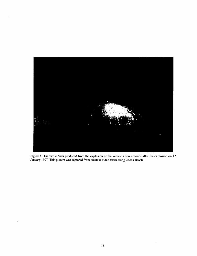
Figure 8. The two clouds produced from the explosion of the vehicle a few seconds after the explosion on 17January 1997. This picture was captured from amateur video taken along Cocoa Beach.
15
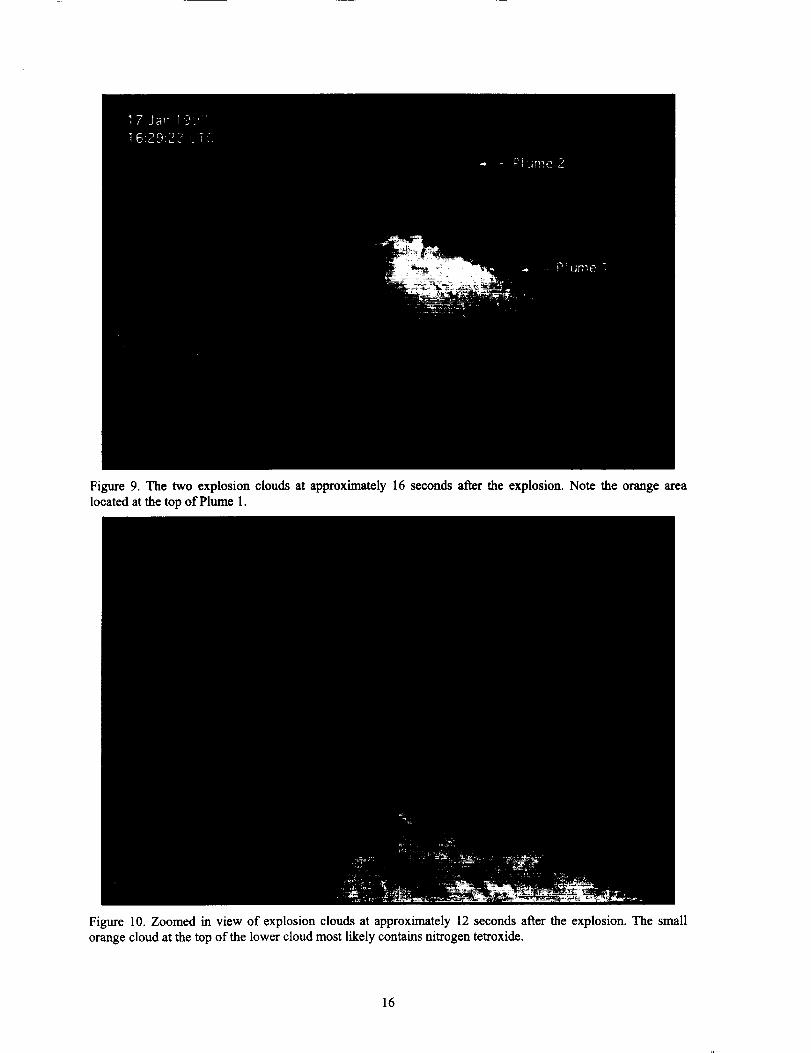
Figure9. The two explosion clouds at approximately 16 seconds after the explosion. Note the orange area
located at the top of Plume 1.
Figure 10. Zoomed in view of explosion clouds at approximately 12 seconds after the explosion. The smallorange cloud at the top of the lower cloud most likely contains nitrogen tetroxide.
16
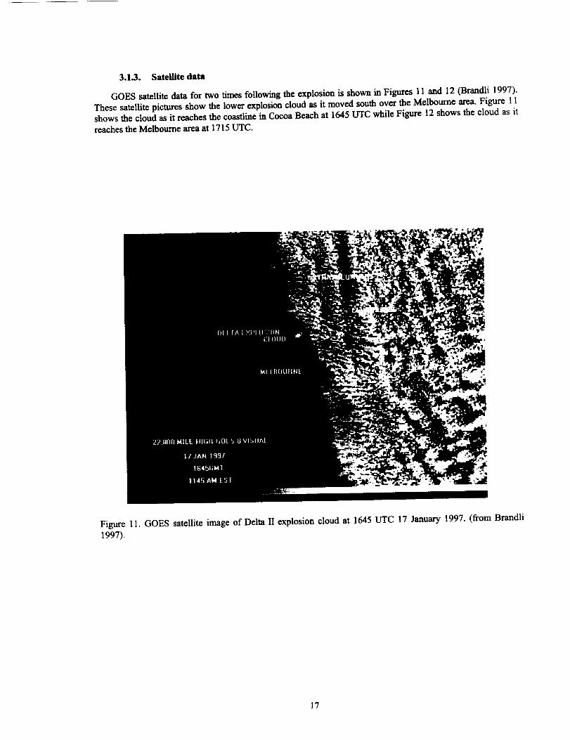
3.1.3. Satellite data
GOES satellite data for two times following the explosion is shown in Figures 11 and 12 (Brandli 1997).
These satellite pictures show the lower explosion cloud as it moved south over the Melbourne area. Figure 11shows the cloud as it reaches the coastline in Cocoa Beach at 1645 UTC while Figure 12 shows the cloud as it
reaches the Melbourne area at 1715 UTC.
Figure 11. GOES satellite image of Delta 11 explosion cloud at 1645 UTC 17 January 1997. (from Brandli
1997).
17

Figure 12.GOES satelliteimage of Delta H explosioncloud at 1715 UTC 17 January 1997.(from Brandli
1997).
3.1.4. Radar data
For the 17 January case, the WSR-88D clearly displayed the echoes resulting from the rocket explosion. Asdiscussed earlier, the display showed two distinctly separate plumes. Information on the two plumes was
obtained for each 10-minute scan by using the 88Display information query function. This information is
presented in Tables 2 and 3. Much of the data contained in the table was obtained by manually analyzing eachtime and ele_,ation scan using the information query function. The scan start time, stop time, and elevation
angle were displayed for each scan. We zoomed in on the area of interest to show the explosion clouds andfound the location of the maximum reflectivity using the color contouring. By selecting this point with the
mouse, we obtained the vital information such as location and height for that time and elevation. The actual
maximum reflectivity value was estimated from the color contours. The plume dimensions such as downwinddistance and alongwind and crosswind length were estimated using the cross-section tool of 88Display.
The plume top and bottom were found using the information query function for each elevation scan and
finding the highest and lowest point of the cloud of interest. It should be noted that the heights of the cloudsdetermined from this technique have a large uncertainty for reasons discussed earlier.
The Delta II abort cloud was first detected by the WSR-88D during the scan at 1635-1646 UTC. Figures
13 and 14 show the composite reflectivity and cross section of the radar image at that time. The cross sectionshows how the plume split into two distinct clouds with an upper cloud to the east and a lower cloud to the
south of LC-17. Figures 15 and 16 show the clouds two hours later at the scan ending at 1834 UTC. The upper
and lower clouds were still clearly detected by the radar. The lower cloud was more distinguishable, locatedsouth of the Melbourne area.
The composite reflectivity figures for each of the scans are shown in Figures 17 to 42.
18
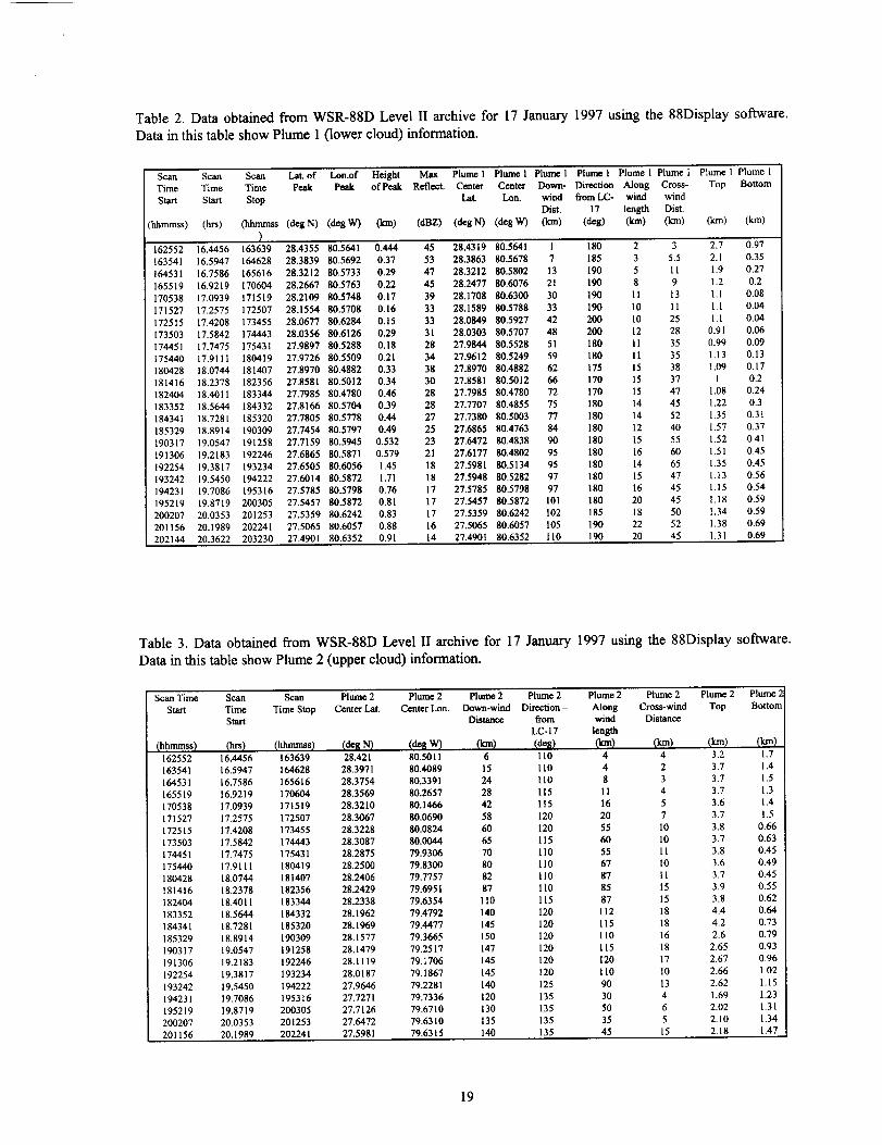
Table2. DataobtainedfromWSR-88DLevelII archivefor 17January1997usingthe88Displaysoftware.Datain thistableshowPlume1(lowercloud)information.
Scan Scan Scan Lat, of Ion.of Height Max Plvanc 1 Plume 1 Plume 1 Plume 1 Plume 1 Plume 1 Plume 1 Plume 1
Time Time Time Peak Peak of Peak Reflect. Center Center Down- Direction Along Cross- Top Bottom
Start Start Stop Lat. Ion. wind from LC- wind windDist. 17 length Dist.
ahmmss) (hrs) Othmmss (deg N) (deg W) (kin) (dBZ) (deg N) (deg W) (kin) (deg) (kin) (kin) (km) (kin)
)162552 16.4456 163639 28.4355 80.5641 0.444 45 28.4319 80.5641 1 180 2 3 2.7 0.97
163541 16.5947 164628 28.3839 80.5692 0.37 53 28.3863 80.5678 7 185 3 5.5 2.1 0.35
164531 16.7586 165616 28.3212 80.5733 0.29 47 28.3212 80.5802 13 190 5 11 1.9 0.27
165519 16.9219 170604 28.2667 80.5763 0.22 45 28.2477 80.6076 21 190 8 9 1.2 0.2
170538 17.0939 171519 28.2109 80.5748 0.17 39 28.1708 80.6300 30 190 11 13 1.1 0.08
171527 17.2575 172507 28.1554 80.5708 0.16 33 28.1589 80.5788 33 190 10 11 1.1 0.04
172515 17.4208 173455 28.0677 80.6284 0.15 33 28.0849 80.5927 42 200 10 25 1.l 0.04
173503 17.5842 174443 28.0356 80.6126 0.29 31 28.0303 80.5707 48 200 12 28 0.91 0.06
174451 17.7475 175431 27.9897 80.5288 0.18 28 27.9844 80.5528 51 180 11 35 0.99 0.09
175440 17.9111 180419 27.9726 80.5509 0.21 34 27.9612 80.5249 59 180 11 35 1.13 0.13
180428 18.0744 181407 27.8970 80.4882 0.33 38 27.8970 80.4882 62 175 15 38 1.09 0.17
181416 18.2378 182356 27.8581 80.5012 0.34 30 27.8581 80.5012 66 170 15 37 1 0.2
182404 18.4011 183344 27.7985 80.4780 0.46 28 27.7985 80.4780 72 170 15 47 1.08 0.24
183352 18.5644 184332 27.8166 80.5704 0.39 28 27.7707 80.4855 75 180 14 45 1.22 0.3
184341 18.7281 185320 27.7805 80.5778 0.44 27 27.7380 80.5003 77 180 14 52 1.35 0.31
185329 18.8914 190309 27.7454 80.5797 0.49 25 27.6865 80.4763 84 180 12 40 1.57 0.37
190317 19.0547 191258 27.7159 80.5945 0.532 23 27.6472 80.4838 90 180 15 55 1.52 0.41
191306 19.2183 192246 27.6865 80.5871 0.579 21 27.6177 80.4802 95 180 16 60 1.51 0.45
192254 19.3817 193234 27.6505 80.6056 1.45 18 27.5981 80.5134 95 180 14 65 1.35 0.45
193242 19.5450 194222 27.6014 80.5872 1.71 18 27.5948 80.5282 97 180 15 47 1.13 0.56
194231 19.7086 195316 27.5785 80.5798 0.76 17 27.5785 80.5798 97 180 16 45 1.15 0.54
195219 19.8719 200305 27.5457 80.5872 0.81 17 27.5457 80.5872 101 180 20 45 1.18 0.59
200207 20.0353 201253 27.5359 80.6242 0.83 17 27.5359 80.6242 102 185 18 50 1.34 0.59
201156 20.1989 202241 27.5065 80.6057 0.88 16 27.5065 80.6057 105 190 22 52 1.38 0.69
202144 20.3622 203230 27.4901 80.6352 0.91 14 27.4901 80.6352 110 190 20 45 1.31 0.69
Table 3. Data obtained from WSR-88D Level II archive for 17 January 1997 using the 88Display software.
Data in this table show Plume 2 (upper cloud) information.
Scan Time Scan Scan Plume 2 Plume 2 Plume 2 Plume 2 Plume 2 Plume 2 Plume 2 Plume 2
Start Time Time Stop Center Lat. Center Lon. Down-wind Direction - Along Cros_wind Top BoRom
Start Distance from wind Distance
LC- 17 length
(hhmmss) (h_) (hh.... ) (deg _ (de8 W) (kin) (des) 9m,) (kin) {kin) _krn)
162552 16.4456 163639 28.421 80.5011 6 110 4 4 3.2 1.7
163541 16.5947 164628 28.3971 80.4089 15 tl0 4 2 3.7 1.4
164531 16.7586 165616 28.3754 80.3391 24 110 8 3 3.7 1.5
165519 16.9219 170604 28.3569 80.2657 28 115 11 4 3.7 1.3
170538 17.0939 171519 28.3210 80.1466 42 115 16 5 3.6 1.4
171527 17.2575 172507 28.3067 80.0690 58 120 20 7 3.7 1.5
172515 17.4208 173455 28.3228 80.0824 60 120 55 10 3.8 0.66
173503 17.5842 174443 28.3087 80.0044 65 115 60 10 3.7 0.63
174451 17.7475 175431 28.2875 79.9306 70 110 55 II 3.8 0.45
175440 17.9111 180419 28.2500 79.8300 80 110 67 10 3.6 0.49
180428 [8.0744 181407 28.2406 79.7757 82 ll0 87 11 3.7 0.45
181416 18.2378 182356 28.2429 79.6951 87 110 85 15 3.9 0.55
182404 18.4011 183344 28.2338 79.6354 110 115 87 15 3.8 0.62
183352 18,5644 184332 28.1962 79.4792 140 120 112 18 4.4 0.64
184341 18.7281 185320 28.1969 79.4477 145 120 115 18 4.2 0.73
185329 18.8914 190309 28.1577 79.3665 150 120 ll0 16 2.6 0.79
190317 19.0547 191258 28.1479 79.2517 147 120 115 18 2.65 0.93
191306 19.2183 192246 28.1119 79.1706 145 120 120 17 2.67 0.96
192254 19.3817 193234 28.0187 79.1867 145 120 110 10 2.66 1.02
193242 19.5450 194222 27.9646 79.228l 140 125 90 13 2.62 1.15
194231 19.7086 195316 27.7271 79.7336 120 135 30 4 1.69 1.23
195219 19,8719 200305 27.7126 79.6710 130 135 50 6 2.02 1.31
200207 20.0353 201253 27.6472 79.6310 135 135 35 5 2.10 1.34
201156 20.1989 202241 27.5981 79.6315 140 135 45 15 2.18 1.47
19

I 202144 20.3622 203230 27.5883 79.6721 130 140 10 3 1.86 1.59 [
Figure 13. Composite radarimage from Melbourne WSR-88D for 10-minute scan beginning at 1635 UTC. A-B
line indicates cross section shown in Figure 14.
Figure 14. Cross section of composite radar image for 1635 UTC. East-west cross section location shown m
Figure 13.
20
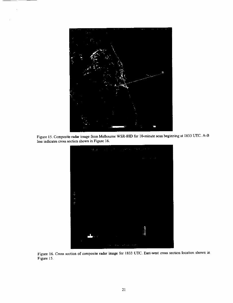
Figure15.CompositeradarimagefromMelbourneWSR-88Dfor10-minutescanbeginningat1833UTC.A-BlineindicatescrosssectionshowninFigure16.
Figure16.Crosssectionof compositeradarimagefor 1833UTC.East-westcrosssectionlocationshowninFigure15.
21
3.1.4.1. Cloud1
The lower cloud, designated Cloud 1, moved to the south over the next four hours after the explosion asthe WSR-88D radar clearly tracked the smoke and particles contained in the cloud. The reflectivity reached a
maximum of 53 dBZ in the 1635-1646 UTC scan (Figures 13 and 19) but then gradually decreased to
approximately 14 dBZ four hours later in the 2021-2032 UTC scan (Figure 42). The shape of the cloud asshown by radar appeared rounded initially but then became oval-shaped in the crosswind direction at
approximately one hour after the explosion. The cloud maintained this oval shape for the next three hours as it
became elongated in a northwest-southeast orientation. The analysis of the 1635 UTC scan (Figures 13 and 19)indicated the low-level cloud was approximately 3-kin long, 2-1an wide, at least 2-km thick and was located 1
km from LC-17. The cloud thickness is likely greatly exaggerated because of radar beam width and
superrefraction effects. The direction the cloud moved was initially south and it maintained this southerly
movement throughout the four hours. The cloud moved to intersect the coastline at approximately 1650 UTC(Figure 20) as it moved over the beaches between Cocoa Beach and Patrick AFB. It continued to move south
over the Melbourne area and was centered over the Melbourne airport at approximately 1735 UTC (Figure 25).
The cloud moved from Brevard County into Indian River County at approximately 1830 UTC (Figures 15 and30).
Ground fires produced smoke plumes which were detected by the WSR-88D on 17 January. These fires asobserved on the radar displays give a good indication of the surface level winds. The display at 1804 UTC(Figure 28) shows the smoke plume produced by the fires over Cape Canaveral that were started from the
falling solid rocket fuel. The low level winds affecting this plume were from the north-northwest. It isimportant to note that this low-level smoke plume stays offshore and does not move westward as did the Delta
II explosion cloud which was aloft. The plume from another fire (unrelated to the Delta II explosion) located inwestern Indian River County (southwest of the lower Delta II cloud) moves south and south-southwest. Thelow-level winds in this _,rea were from the north and north-northeast.
The height of the cloud top and bottom as determined by the 88Display program on the Level II data is
shown in Table 2. As discussed earlier these values are not very accurate because of errors caused by refraction
of the radar beam through a strong temperature inversion and because the cloud passed directly over the
Melbourne radar site. However, the cloud height data does provide some useful information. The plume topwas initially determined to be 2700 meters which is obviously too high as determined by the capping inversion
characteristics. The estimated plume top dropped to 1200 meters at 1655 UTC which more closely matches theother observations. The reason for the large initial discrepancy is probably due to the beam width and the beam
inversion problem. The cloud bottom was initially measured at 970 meters and dropped to a low of 40 meters at
1725 UTC as the cloud passed over the radar site and then rose to 690 meters at 2011 UTC. The change over
time of the height of the plume top and bottom most likely reflects the radar beam angle since the heights aredirectly proportional to the distance from the radar. A graph showing the plume height measurements ispresented in Figure 43.
22
3.1.4.2. C_ud2
The Delta II stages 2 and 3 along with the payload survived the initial explosion and drifted upward to just
over 750 meters where destruct signals were sent at 22.4 seconds. This formed a second cloud which broke
through the inversion. The upper cloud moved to the east and southeast over the four hours after the explosionat an average speed of approximately 13 m s"t. This cloud was detached from the lower cloud and moved at a
different speed and direction. The radar detected peak reflectivities of approximately 34 dBZ at 1645 UTC
(Figure 20). The reflectivities slowly decreased over time, then dropped below 30 dBZ at 1715 UTC (Figure 23)
and then below 20 dBZ at 1754 UTC (Figure 27). The cloud was moved by the strong westerly winds in thelayer above the inversion between 1200 and 2000 meters. The radar showed that the cloud had a somewhat
undulating shape as it was stretched from west to east.
The height of the cloud top and bottom as determined by the 88Display program on the Level II data is
shown in Table 3. The initial scan of the upper level cloud at 1625 UTC indicated the cloud was approximately4-km long, 4-km wide, 1.5-km thick and was located 6 km east of LC-17. The errors associated with the
refraction of the radar beam through the strong inversion that caused estimation errors for the height of the
lower cloud were more prominent in determining the height of the upper cloud. The radar indicated that the
initial vertical plume dimensions ranged from a cloud bottom of 1700 meters up to a cloud top of 3200 meters
(Figure 14). During the next three hours the radar detected that the cloud top rose to a height of 4400 meters at
1833 UTC while the cloud bottom lowered to a height of 450 meters at 1804 UTC (Table 3). Themeasurements indicate a maximum depth of the upper cloud of over 3700 meters at 1833 UTC. Visual
observations discussed in Section 3.1.2 did not support these radar depth determinations. Therefore, we
seriously question this cloud's radar height measurements which are shown in a graph in Figure 44.
23

Figure17.WSR-88Dcompositescanbeginning at1616 UTC.
Figure 18. WSR-88D composite scan beginning at1625 UTC.
Figure 19. WSR-88D composite scan beginning at1635 UTC.
Figure 20. WSR-88D composite scan beginning at1645 UTC.
24

Figure21.WSR-88Dcompositescanbeginningat1655UTC.
Figure22.WSR-88Dcompositescanbeginningat1705UTC.
Figure23.WSR-88Dcompositescanbeginningat1715UTC.
Figure24.WSR-88Dcompositescanbeginningat1725UTC.
25
Figure25.WSR-88Dcompositescanbeginningat1735UTC.
Figure26.WSR-88Dcompositescanbeginningat1745UTC.
Figure27.WSR-88Dcompositescanbeginningat1754UTC.
Figure28.WSR-88Dcompositescanbeginningat1804UTC.
26
Figure29.WSR-88Dcompositescanbeginningat1814UTC.
Figure30.WSR-88Dcompositescanbeginningat1824UTC.
Figure31. WSR-88D composite scan beginning at1833 UTC,
Figure 32. WSR-88D composite scan beginning at1843 UTC.
27
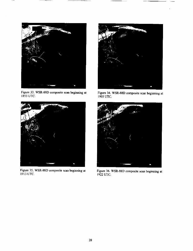
Figure33.WSR-88Dcomposite scan beginning at1853 UTC.
Figure 34. WSR-88D composite scan beginning at1903 UTC.
Figure 35. WSR-88D composite scan beginning at1913 UTC.
Figure 36. WSR-88D composite scan beginning at1922 UTC.
28

Figure37.WSR-88Dcompositescanbeginningat1932UTC.
Figure38.WSR-88Dcompositescanbeginningat1942 UTC.
Figure 39. WSR-88D composite scan beginning at1952 UTC.
Figure 40. WSR-88D composite scan beginning at2002 UTC.
29
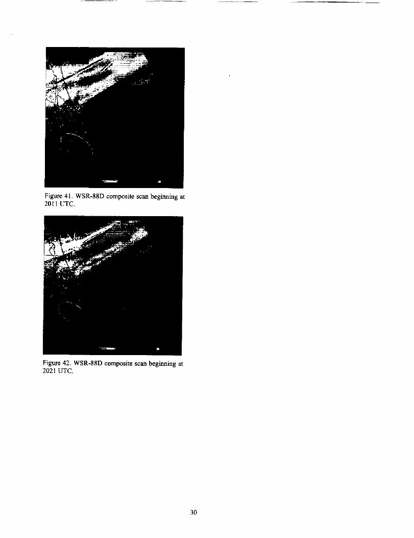
Figure41.WSR-88Dcompositescanbeginningat2011UTC.
Figure42.WSR-88Dcompositescanbeginningat2021UTC.
30
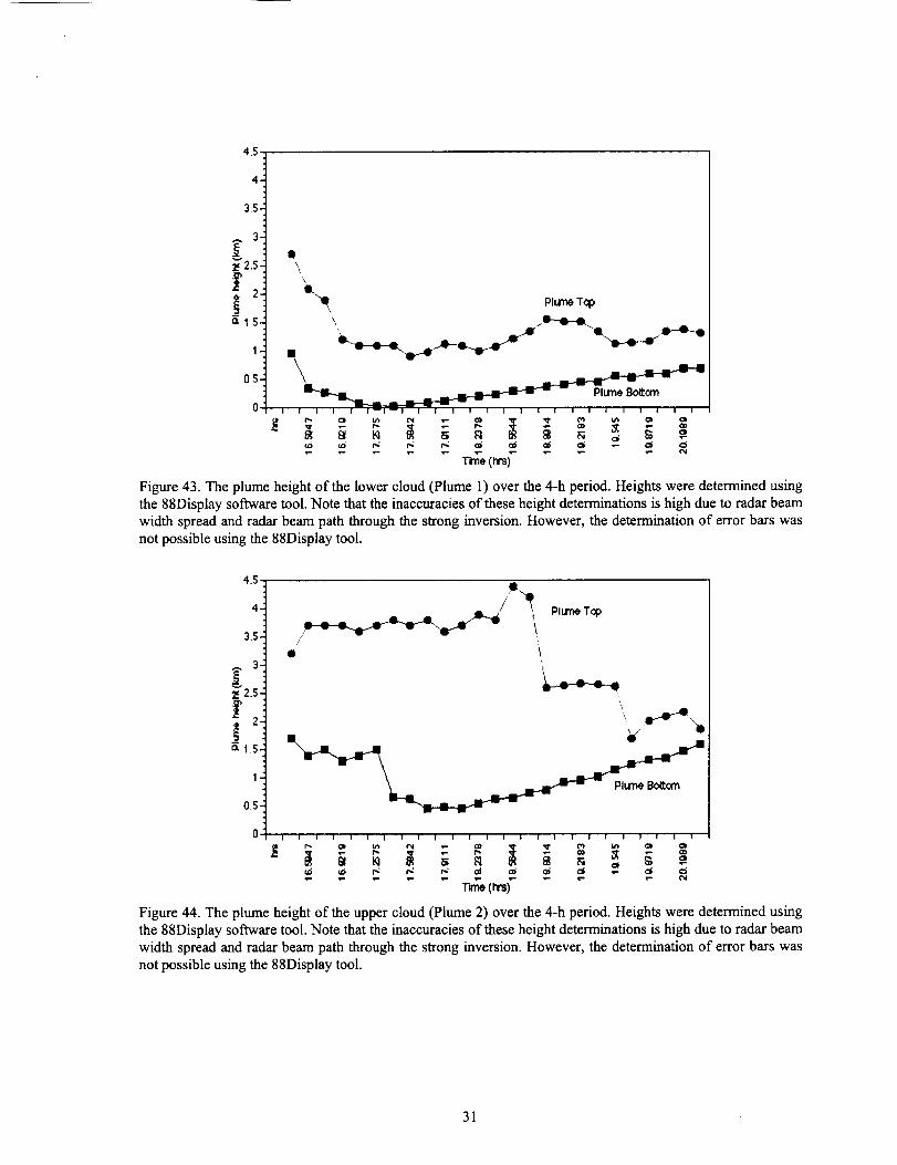
4.5
4-
35-
3-
2,5-
f, 2-§
I
it , PlumeT_p
"_' "lD--qH_t .l_4_--O
o,,0 I I I I I I--I--I I I I I I I I I I I 1 1 I I 1 I I
n,ne(_)
Figure 43. The plume height of the lower cloud (Plume 1) over the 4-h period. Heights were determined using
the 88Display software tool. Note that the inaccuracies of these height determinations is high due to radar beam
width spread and radar beam path through the strong inversion. However, the determination of error bars was
not possible using the 88Display tool.
1"2.5
°:1II I I I I I I I I I I I I I I I I I I I I I I
Figure 44. The plume height of the upper cloud (Plume 2) over the 4-h period. Heights were determined using
the 88Display software tool. Note that the inaccuracies of these height determinations is high due to radar beam
width spread and radar beam path through the strong inversion. However, the determination of error bars was
not possible using the 88Display tool.
31
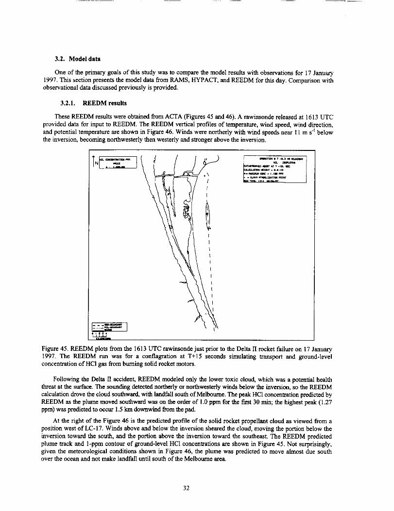
3.2. Model data
One of the primary goals of this study was to compare the model results with observations for 17 January
1997. This section presents the model data from RAMS, HYPACT, and REEDM for this day. Comparison withobservational data discussed previously is provided.
3.2.1. REEDM results
These REEDM results were obtained from ACTA (Figures 45 and 46). A rawinsonde released at 1613 UTC
provided data for input to REEDM. The REEDM vertical profiles of temperature, wind speed, wind direction,
and potential temperature are shown in Figure 46. Winds were northerly with wind speeds near 11 m s-_ belowthe inversion, becoming northwesterly then westerly and stronger above the inversion.
)
1IV, J_qtlltlt
Figure 45. REEDM plots from the 1613 UTC rawinsonde just prior to the Delta II rocket failure on 17 January1997. The REEDM run was for a conflagration at T+15 seconds simulating transport and ground-level
concentration of HCl gas from burning solid rocket motors.
Following the Delta II accident, REEDM modeled only the lower toxic cloud, which was a potential healththreat at the surface. The sounding detected northerly or northwesterly winds below the inversion, so the REEDM
calculation drove the cloud southward, with landfall south of Melbourne. The peak HC1 concentration predicted by
REEDM as the plume moved southward was on the order of 1.0 ppm for the first 30 rain; the highest peak (1.27ppm) was predicted to occur 1.5 km downwind from the pad.
At the right of the Figure 46 is the predicted profile of the solid rocket propellant cloud as viewed from a
position west of LC-17. Winds above and below the inversion sheared the cloud, moving the portion below the
inversion toward the south, and the portion above the inversion toward the southeast. The REEDM predicted
plume track and 1-ppm contour of ground-level HC1 concentrations are shown in Figure 45. Not surprisingly,given the meteorological conditions shown in Figure 46, the plume was predicted to move almost due southover the ocean and not make landfall until south of the Melbourne area.
32

TheresultspresentedherewerefromREEDM7.07whichwastheversioninuseatthetimeoftheDeltaIIexplosion.Newerversionsof REEDM(e.g.REEDM7.08andREEDM7.09)producedifferentresultsanddifferentgroundlevelconcentrations.RangeSafetyhascontinuedto upgradeREEDMastheresultof newscientificf'mdingsandusesthelatestversionavailabletoevaluatelaunchclouddispersion(Nyman1999).
_TIE- 17 IN_I 97 TZf'Eo1612 Z _ -_.3 HR _ _ 0 _ TYPIE-_TION
mJ_.2_EIIP.la_- 1_.7 N8 13_181_-1z63.40_f 3 _ST_ HT- 9_11.6 PI u.cJ_: _. 0.0 M
LAYER1 t._'n_2
SUm'_I[ _ 80T "rcP
O.O 878.7 876.7 2'g!2.9
8.4 0.6 8,6 4,6
7.2 8.0 O,O 33.4
6.7 le. EI 10,8 20.1
38Q.0 2.0 2.0 274.0
N.TI TUI_ (t_
ORY TEttP ( OE_ C)
POT TE/'P (QEG 0
HtND SPE]_ (rq/S)
UIND OIR (13E_
33M
A m
L. 27_
r 2_e
I211
T
lmmU
nlIc f_3
ole
/
/
I
I
/
PT
I kiD '/
/ /
/ /
/
/
/
I _....
I I L 961
/ I I '_7
' F-6 0 I_ 10 1E a 28 38 :38 40 4E Ee 0 2 4 6 0 _0
N..ONO tF.AN _JIND DIR ( [rOS_ZIXI'VlI_ 'rl_t_rirO 0 I I I I : : " : : : :27t • ge t88 278
MIND DIR (DEG)
Pq.O_ AT- ee. 1314, 26 flEP 1997 un,*
- 683
- 71_ p
- 736 R
- 763 [
S- 792
S
- 821U
- 882 R
- 884 E
- 917 (I_IB)
L.
Figure 46. REEDM cross-section plot showing rawinsonde data from 1613 UTC on the left and REEDM
source term predictions on the right.
3.2.2. RAMS results from ERDAS and PROWESS
The description and configuration of the two versions of RAMS used in this study were provided in
Section 2.3. Discussion and figures showing the results of those RAMS runs are presented here.
The RAMS runs were initialized at 1200 UTC, approximately 4.5 hours before the Delta II explosion. The
meteorology during this day did not change significantly because of the presence of the post-frontal regimewith the continued cold air advection. There were no sea breezes, river breezes, thunderstorms, or other
significant local-scale phenomena for RAMS to forecast for the Cape Canaveral area.
Graphs comparing ERDAS RAMS wind data with observed data are presented in Figures 47 and 48.These figures show the observed vertical wind profiles at 1613 UTC and the predicted vertical wind profiles at
1600 UTC. RAMS predicted the wind speed profile accurately through the mixing layer to the inversion at 900meters and then accurately predicted the gradual increase to 25 m s"] at 4500 meters. RAMS predicted the wind
direction more westerly than northwesterly in the layer from the surface to approximately 500 meters but then
accurately predicted the wind shear at the 900-meter inversion and the westerly winds aloft.
The potential temperature profile predicted by RAMS at 1600 UTC closely matched the observed profile at1613 UTC (Figure 49). The base of the predicted inversion was only slightly lower than the base of the
observed inversion.
Maps showing RAMS forecast data from ERDAS and PROWESS for the period 1500 UTC to 2000 UTC
are shown in Figures 50 - 56. Data are presented that represent wind flow in the different layers important in
33
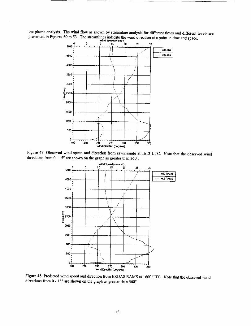
theplumeanalysis.Thewindflowasshown by streamline analysis for different times and different levels are
presented in Figures 50 to 53. The streamlines indicate the wind direction at a point in time and space._na speea (rn-s_:-l)
5 10 15 20 25 30i
4500 _ / WS-oL_s/
4o00 ,. Ji
,[3500 _ .¢
//3000 _ r-
\ /
2000 . ,,
J
soo
F
eo zlo 24o 27o 3o0 33o 3so_ ndOt_e<_n(ae_j_s)
Figure 4"7.Observed wind speed and d_ection from rawinsonde at 1613 UTC. Note that the observed wind
du'ections from 0 - 15° are shown on the graph as greater than 360 °.
S 10 15 Z0 25 305000 ................ !.,,,,
l -- WD-RAMS 1
I,," -- WS-RAMS4,500/
/
4000 I '"
/:ssoo //
3000 , ./'
_- \/
_p 25oo _
/"/
2000' /
,soo // \
iooo--,. )
soo |. _ .I
so 210 24o 270 300 33o 3sowind[_rq_on(Q_jrees)
Figure 48. Predicted wind speed and direction from ERDAS RAMS at 1600 UTC. Note that the observed wind
directions from 0 - 15 ° are shown on the graph as greater than 360 °.
34
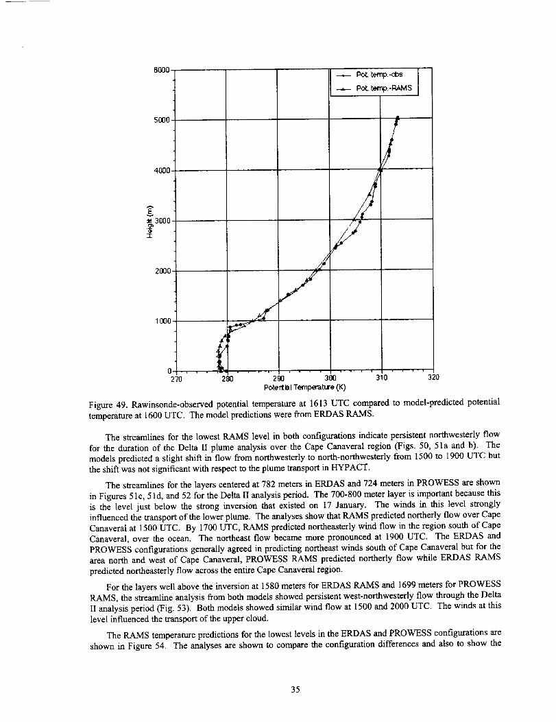
6000-
5000,
4000-
Z3000-
-r
2000.
1000"
0'
270
--.--Pot. temp.-cl_
Pot. temp.-RAMS
i
280 290 300 310 320Potential Temperature (K)
Figure 49. Rawinsonde-observed potential temperature at 1613 UTC compared to model-predicted potential
temperature at 1600 UTC. The model predictions were from ERDAS RAMS.
The streamlines for the lowest RAMS level in both configurations indicate persistent northwesterly flow
for the duration of the Delta II plume analysis over the Cape Canaveral region (Figs. 50, 51a and b). The
models predicted a slight shift in flow from northwesterly to north-northwesterly from 1500 to 1900 UTC but
the shift was not significant with respect to the plume transport in HYPACT.
The streamlines for the layers centered at 782 meters in ERDAS and 724 meters in PROWESS are shown
in Figures 51c, 51d, and 52 for the Delta II analysis period. The 700-800 meter layer is important because this
is the level just below the strong inversion that existed on 17 January. The winds in this level stronglyinfluenced the transport of the lower plume. The analyses show that RAMS predicted northerly flow over Cape
Canaveral at 1500 UTC. By 1700 UTC, RAMS predicted northeasterly wind flow in the region south of CapeCanaveral, over the ocean. The northeast flow became more pronounced at 1900 UTC. The ERDAS and
PROWESS configurations generally agreed in predicting northeast winds south of Cape Canaveral but for thearea north and west of Cape Canaveral, PROWESS RAMS predicted northerly flow while ERDAS RAMS
predicted northeasterly flow across the entire Cape Canaveral region.
For the layers well above the inversion at 1580 meters for ERDAS RAMS and 1699 meters for PROWESSRAMS, the streamline analysis from both models showed persistent west-northwesterly flow through the Delta
II analysis period (Fig. 53). Both models showed similar wind flow at 1500 and 2000 UTC. The winds at this
level influenced the transport of the upper cloud.
The RAMS temperature predictions for the lowest levels in the ERDAS and PROWESS configurations areshown in Figure 54. The analyses are shown to compare the configuration differences and also to show the
35
changeover time of the predicted low-level temperature structure. At 1500 UTC, both configurations show an
east-west temperature gradient with colder temperatures over the land and warmer temperatures to the east overthe ocean. It is difficult to compare the actual temperatures since the lowest level in ERDAS is centered at 10
meters and the lowest level in PROWESS is centered at 35 meters. By 2000 UTC, the temperature gradient hadshifted to north-south in both models and ERDAS RAMS, with its lowest level at 10 m, shows more influenceof the land-water interfaces associated with rivers and islands.
The vertical potential temperatttre structure of the atmosphere as predicted by RAMS is shown in Figure
55. These figures show an east-west cross section of the potential temperature as predicted by the two
configurations of RAMS at different times. The figures show that ERDAS RAMS predicted an elevatedinversion at approximately 750 meters at 1500 UTC while PROWESS RAMS predicted the inversion at
approximately 500 meters at 1500 UTC. By 2000 UTC the models lifted the inversion to approximately 1000meters for ERDAS RAMS and 750 meters for PROWESS RAMS. Rawinsonde data from 1613 UTC indicated
the base of the inversion was at approximately 900 meters (Figure 49).
36
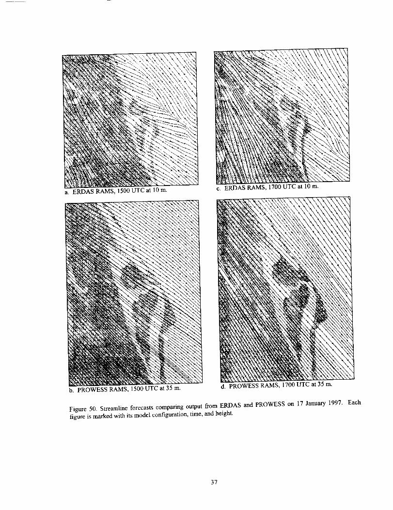
a. ERDAS RAMS, 1500 UTC at 10 m.
'{?,I_\_ \\,",\,',.I
c. ERDAS RAMS, 1700 UTC at 10 m.
b. PROWESS RAMS, 1500 UTC at 35 m. d. PROWESS RAMS, 1700 UTC at 35 m.
Figure 50. Streamline forecasts comparing output from ERDAS and PROWESS on 17 January 1997. Each
figure is marked with its model configuration, time, and height.
37
_'_\ _'\ _/_1_/_
a. ERDAS RAMS, 1900 UTC at 10 m. c. ERDAS RAMS, 1500 UTC at 782 m.
b. PROWESS RAMS, 1900 UTC at 35 m. d. PROWESS RAMS, 1500 UTC at 724 m.
Figure 51. Streamline forecasts comparing output from ERDAS and PROWESS on 17 January 1997. Each
figure is marked with its model configuration, time, and height.
38
a. ERDAS RAMS, 1700 UTC at 782 m.
l/1/1
!1I/t
I_ltl
c. ERDAS RAMS, 1900 UTC at 782 m.
d. PROWESS RAMS, 1900 UTC at 724 m.
Figure 52. Streamline forecasts comparing output from ERDAS and PROWESS on 17 January 1997.
figure is marked with its model configuration, time, and height
Each
39
c. ERDASRAMS,2000UTCat1580 m.
b. PROWESS RAMS, 1500 UTC at 1699 m. d. PROWESS RAMS, 2000 UTC at 1699 m.
Figure 53. Streamline forecasts comparing output from ERDAS and PROWESS on 17 January 1997. Each
figure is marked with its model configuration, time, and height.
4O

a,
r¸ J / i _ l_,
• . ,q
ERDAS RAMS, 1500 UTC at 10 m.
b. PROWESS RAMS, 1500 UTC at 35 m.
c. ERDAS RAMS, 2000 UTC at 10 m.
d. PROWESS RAMS, 2000 UTC at 35 m.
Figure 54. Surface temperature (F) forecasts comparing output from the lowest levels of ERDAS (10 m) andPROWESS (35 m) on 17 January 1997. Each figure is marked with its model configuration, time, and height.
The dark bold line in panels c and d shows the approximate location of the potential temperature cross sections
shown in Figure 55.
41
_0ol ¸_ :::-:_-; ..............__£7_--_............_5_2_ -u-_
30'30 ......... " .....................................
_500 -.......
, . _2ZI Z" ...... /iiiiZZI- _ ......
_.o_ ................._ -"r'_L-.C'I_;;.................. .0 " ' _ r'--:'rT";'T";, 7;-'-'" : ..... , ..... " ' ": _ ' '
I°0 _00. 220. 240 260
x (kin}
_,?,"_7,_, potenti_-A telrll, (K)
_Z_._ y = -173 kin 01/17"97 1500 UTC
a. ERDAS RAMS, 1500 UTC.
:,oo-_ ......h -- ..... .;..;Z77 ..._Z.C.ZZ2L.Z-LZT_L
._ooII; ...........180 200 2*_0. 240 260
X (kill)
_._. o p_Mential temp (,K)
•'7-./._,_ y - -'._0 kr-i 01/17,,'97 2000 UTC
b ERDAS RAMS, 2000 UTC.
2000-#
1_)oo-
1000 _- - ............... - --------
500 4.- ...... ----- ,t................... -T 7 : _i . 77_. . -- Z_
x (kni}
._.o poter,tlal Letup (K)
. . _ y = 17_. kill 01/'1T/97' 1500 UTC
c. PROWESS RAMS, 1500 UTC.
F ¸ .., • v. ............ _ ...........
,o_o_- - :t---_::?E:.-t 7 7-7_i;::%.::---
I
500 i
o[ " ;,.21 b ;J20 22u 230 _3o
X (kiilJ
_ potential temp (K)
_op: y = --:7_2. klIl 01/17,"97 0000 U_C
d. PROWESS RAMS, 2000 UTC.
Figure 55. Potential temperature (K) cross section forecasts comparing output from ERDAS and PROWESS on
17 January 1997. Each figure is marked with its model configuration and time. The cross-sections intersect the
Cape Canaveral Air Force Station along an east-west line as shown in Figure 54. The ERDAS cross-section isapproximately 110 kin wide and the PROWESS cross section is approximately 25 km wide.
42

3.2.3. HYPACT results from ERDAS and PROWESS
3.2.3.1. HYPACT Configuration
As discussed in Section 2.3.4, we modified the HYPACT input data configuration file to simulate the Delta
II explosion plume. When we first ran REEDM within ERDAS for the Delta II explosion, the source term was
characterized as 21 different sources extending from 300 to 2100 m above the ground. Table 4 presents the
source term data produced by REEDM for the 21 sources.
Table 4. Location and dimensions of plume determined by REEDM and modeled by HYPACT. These plumedimensions were used in the ERDAS HYPACT simulation.
Source
no.
latitude
28.42615
28.42622
28.42408
longitude
-80.55101
-80.55413
-80.55320
height
(m)349.9
449.9
508.3
x-size (m)
470.4
705.8
789.0
y-size (m)
470.4
705.8
789.0
z-size (m)
100.0
100.0
16.7
4 28.42531 -80.55086 524.9 808.2 808.2 16.7
5 28.42695 -80.54810 550.0 833.8 833.8 33.4
6 28.42695 -80.54810 583.5 862.0 862.0 33.5
7 28.42695 -80.54810 614.5 883.0 883.0 28.5
8 28.42695 -80.54810 643.0 898.0 898.0 28.6
9 28.42695 -80.54810 671.5 909.2 909.2 28.5
I0 28.42695 -80.54810 742.9 921.2 921.2 114.3
11 28.42695 -80.54810 856.3 894.6 894.6 112.5
12 28.42695 -80.54810 925.1 848.8 848.8 25.0
13
14
28.42695
28.42695
-80.54810
-80.54810
950.1
975.1
826.0799.4
826.0
799.4
25.0
25.0
15 28.42695 -80.54810 1000.9 767.4 767.4 26.7
16 28.42695 -80.54810 1028.6 727.6 727.6 28.6
17 28.42695 -80.54810 1057.2 679.4 679.4 28.6
18 28.42695" -80.54810 1085.8 622.2 622.2 28.5
19 28.42695 -80.54810 1200.0 399.8 399.8 200.0
20 28.42695 -80.54810 1450.1 399.8 399.8 300.2
21 28.42695 -80.54810 2050.1 399.8 399.8 899.8
shape
ellipse
ellipse
ellipse
ellipse
ellipse
ellipse
ellipse
ellipse
ellipse
ellipse
ellipse
ellipse
ellipse
ellipse
ellipse
ellipse
ellipse
ellipse
ellipse
ellipse
ellipse
The visual and radar observations of the plume indicated that the plume had obviously split into two distinct
clouds. To initialize more accurately HYPACT, we modified the source size and shape to more closely represent
the observed size and shape of the actual plume. Therefore, the plume was represented as two sources. The
plume's location and dimensions are presented in Table 5. A complete listing of the HYPACT configurationused to model the Delta II explosion is presented in Appendices C and D.
Table 5. Location and dimensions of plume determined from visual and radar observations and modeled byHYPACT. These flume dimensions were used in the PROWESS HYPACT simulation.
Source
no.latitude
28.448
28.448
longitude
-80.566
-80.566
height x-size y-size
(m) . (m) (m)
600. 600. 600.
1800. 600. 600.
z-size
(m)
400.
400.
shape
ellipse
ellipse
43

3.2.3.2. HYPACT runs
The HYPACT model was run for two scenarios. There were two reasons for the modeling exercise of
comparing the observed and predicted plumes. The principal of the two reasons was to determine how well themodeled plume trajectories compared with the observed plume trajectories. The secondary reason for the
exercise was to determine how the REEDM-predicted source term compared with the actual source term. To
reduce the number of runs and the number of figures we displayed, we combined the trajectory and source term
analysis in the ERDAS-HYPACT runs and we did not perform a source term analysis for the PROWESS-
HYPACT runs. Combining the runs did not hinder the results since we adequately assessed the trajectories of
both runs and we were able to assess how the REEDM-predicted source term compared with the actual sourceterm.
The figures presented in this report compare the predicted plume locations from ERDAS-HYPACT and
PROWESS-HYPACT with the observed plume locations from the WSR-88D radar. The comparisons presented
are for each 10-minute HYPACT model time during the four hours that the plume was tracked. The HYPACT
source terms were generated from the REEDM model using the REEDM function of ERDAS. REEDMgenerates the HYPACT source term for a rocket launch by creating a column that contains mass of the chemical
species of interest. The column is composed of separate sources (volumes) of mass, which are 75 meters in
thickness. We assessed the REEDM-predicted source term by observing how the modeled initial plume changed
during the simulation and comparing its shape with observed plume. The ERDAS-HYPACT run was made
leaving the mass in the entire column from the surface up to 2500 meters. We assessed the ERDAS-HYPACTtrajectories by tracking only the lower and upper part of the plume and comparing those with the trajectory of
the observed plume.
The source term for the PROWESS configuration was modified slightly to simulate the observed sourceterm since in our analysis we knew the initial shape of the plume. The plume was modified by removing the
initial mass in the layers between 925 and 1550 meters. We assessed the PROWESS-HYPACT trajectories by
tracking the two plumes and comparing those with the observed plume.
For the explosion time, both ERDAS-HYPACT and PROWESS-HYPACT transported the upper and lowerexplosion clouds in different directions. The split transport occurred because the upper cloud was at a height
where the winds were strong and from the west while the lower cloud was trapped below a strong inversion withwinds were from the north.
The primary purpose of analyzing the trajectory of the ERDAS-HYPACT and PROWESS-HYPACT
plumes was to determine how the model predictions compared with observations. Therefore, the part of the
HYPACT plumes which were compared and which are the focus of the discussion below are the lower plume
below 925 meters and the upper plume above 1550 meters. Even though, the ERDAS-HYPACT simulation wasrun with the entire plume, we were not concerned with the transport of the center of the plume between 925 and1550 meters.
3.2.3.3. HYPACT results
The HYPACT predictions of the ERDAS and PROWESS plumes are shown in Figures 56 to 115. The
figures show two-dimensional views of the plume from a horizontal map perspective and from a northward-facing vertical cross section. HYPACT output was produced every ten minutes.
HYPACT moved the lower cloud to the south where it reached the coast in the vicinity of Cocoa Beach at
approximately 30 minutes after the explosion. Figures 56 - 63 show the lowest part of the ERDAS cloud out
over the ocean and extending upward and westward to the coastline where it curves north and then east as itextends upward. The cross-section shows the slight shift to the east of the particles in the lowest part of the
plume. HYPACT begins spreading the lower cloud as shown by the diffusion of the lower plume particles
(Figures 62 and 63).
Figures 86 - 93 show the two PROWESS clouds (due to the initial source split) with the lower cloud to the
southwest of the upper cloud. The lower cloud extends upward and westward from over the ocean to thecoastline. The upper cloud extends eastward and upward from approximately 10 krn offshore out to
44
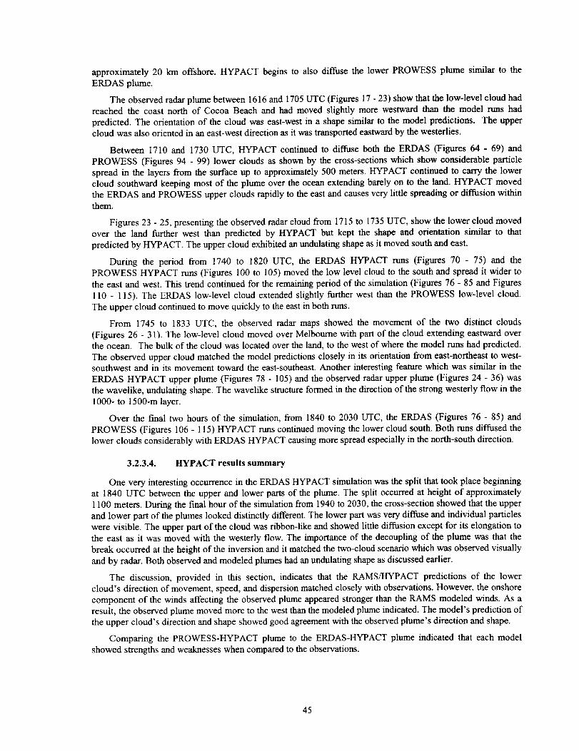
approximately20kmoffshore.HYPACTbeginsto alsodiffusethelowerPROWESSplumesimilarto the
ERDAS plume.
The observed radar plume between 1616 and 1705 UTC (Figures 17 - 23) show that the low-level cloud had
reached the coast north of Cocoa Beach and had moved slightly more westward than the model runs had
predicted. The orientation of the cloud was east-west in a shape similar to the model predictions. The uppercloud was also oriented in an east-west direction as it was transported eastward by the westerlies.
Between 1710 and 1730 UTC, HYPACT continued to diffuse both the ERDAS (Figures 64 - 69) and
PROWESS (Figures 94 - 99) lower clouds as shown by the cross-sections which show considerable particlespread in the layers from the surface up to approximately 500 meters. HYPACT continued to carry the lower
cloud southward keeping most of the plume over the ocean extending barely on to the land. HYPACT movedthe ERDAS and PROWESS upper clouds rapidly to the east and causes very little spreading or diffusion within
them.
Figures 23 - 25, presenting the observed radar cloud from 1715 to 1735 UTC, show the lower cloud movedover the land further west than predicted by HYPACT but kept the shape and orientation similar to that
predicted by HYPACT. The upper cloud exhibited an undulating shape as it moved south and east.
During the period from 1740 to 1820 UTC, the ERDAS HYPACT runs (Figures 70 - 75) and the
PROWESS HYPACT runs (Figures 100 to 105) moved the low level cloud to the south and spread it wider to
the east and west. This trend continued for the remaining period of the simulation (Figures 76 - 85 and Figures
110 - 115). The ERDAS low-level cloud extended slightly further west than the PROWESS low-level cloud.
The upper cloud continued to move quickly to the east in both runs.
From 1745 to 1833 UTC, the observed radar maps showed the movement of the two distinct clouds
(Figures 26 - 31). The low-level cloud moved over Melbourne with part of the cloud extending eastward overthe ocean. The bulk of the cloud was located over the land, to the west of where the model runs had predicted.
The observed upper cloud matched the model predictions closely in its orientation from east-northeast to west-southwest and in its movement toward the east-southeast. Another interesting feature which was similar in the
ERDAS HYPACT upper plume (Figures 78 - 105) and the observed radar upper plume (Figures 24 - 36) was
the wavelike, undulating shape. The wavelike structure formed in the direction of the strong westerly flow in the
1000- to 1500-m layer.
Over the f'mal two hours of the simulation, from 1840 to 2030 UTC, the ERDAS (Figures 76 - 85) and
PROWESS (Figures 106 - 115) HYPACT runs continued moving the lower cloud south. Both runs diffused the
lower clouds considerably with ERDAS HYPACT causing more spread especially in the north-south direction.
3.2.3.4. HYPACT results summary
One very interesting occurrence in the ERDAS HYPACT simulation was the split that took place beginningat 1840 UTC between the upper and lower parts of the plume. The split occurred at height of approximately
1100 meters. During the final hour of the simulation from 1940 to 2030, the cross-section showed that the upper
and lower part of the plumes looked distinctly different. The lower part was very diffuse and individual particles
were visible. The upper part of the cloud was ribbon-like and showed little diffusion except for its elongation tothe east as it was moved with the westerly flow. The importance of the decoupling of the plume was that the
break occurred at the height of the inversion and it matched the two-cloud scenario which was observed visuallyand by radar. Both observed and modeled plumes had an undulating shape as discussed earlier.
The discussion, provided in this section, indicates that the RAMS/HYPACT predictions of the lower
cloud's direction of movement, speed, and dispersion matched closely with observations. However, the onshore
component of the winds affecting the observed plume appeared stronger than the RAMS modeled winds. As aresult, the observed plume moved more to the west than the modeled plume indicated. The model's prediction of
the upper cloud's direction and shape showed good agreement with the observed plume's direction and shape.
Comparing the PROWESS-HYPACT plume to the ERDAS-HYPACT plume indicated that each modelshowed strengths and weaknesses when compared to the observations.
45
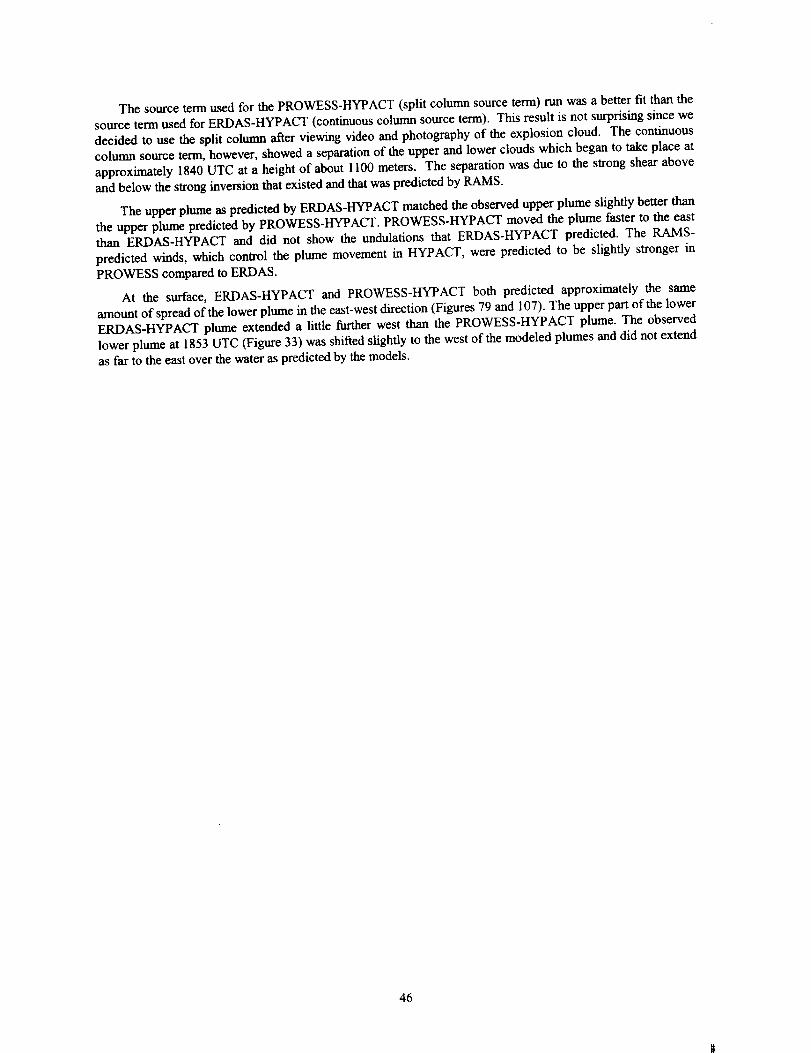
ThesourcetermusedforthePROWESS-HYPACT(splitcolumnsourceterm)runwasabetterfit thanthesourcetermusedforERDAS-HYPACT(continuouscolumnsourceterm).This result is not surprising since we
decided to use the split eoltunn after viewing video and photography of the explosion cloud. The continuous
column source term, however, showed a separation of the upper and lower clouds which began to take place at
approximately 1840 UTC at a height of about 1100 meters. The separation was due to the strong shear above
and below the strong inversion that existed and that was predicted by RAMS.
The upper plume as predicted by ERDAS-HYPACT matched the observed upper plume slightly better thanthe upper plume predicted by PROWESS-HYPACT. PROWESS-HYPACT moved the plume faster to the east
than ERDAS-HYPACT and did not show the undulations that ERDAS-HYPACT predicted. The RAMS-
predicted winds, which control the plume movement in HYPACT, were predicted to be slightly stronger in
PROWESS compared to ERDAS.
At the surface, ERDAS-HYPACT and PROWESS-HYPACT both predicted approximately the same
amount of spread of the lower plume in the east-west direction (Figures 79 and 107). The upper part of the lower
ERDAS-HYPACT plume extended a little further west than the PROWESS-HYPACT plume. The observed
lower plume at 1853 UTC (Figure 33) was shifted slightly to the west of the modeled plumes and did not extend
as far to the east over the water as predicted by the models.
46
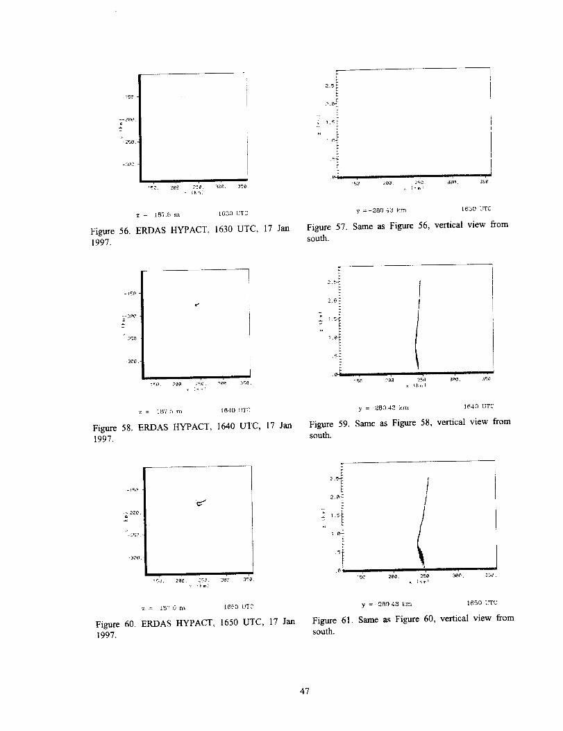
1 51D -
-->0_ ."g
"-25_ .-
-3f#d
I_'C. 2@'_ 25'e. 30'¢. 35_@.
2--'5 I
_ 1"'_ i
N E
, I , IIII iii• 5P 20'2. 25@ 3@@. 35 [_
. (_ml
z = 18,7.5 m 1630 UTC
Figure 56. ERDAS HYPACT, 1630 UTC, 17 Jan1997.
y =-2B043 krn 1630 UTC
Figure 57. Same as Figure 56, vertical view fromsouth.
z = 1B75 m L84D T,JTC
Figure 58. ERDAS HYPACT, 1640 UTC, 17 Jan1997.
ii I i ,
2P1_3. 25_* ( k m I
2. -_,t
C
F1.s 5
1 0 I
E
i_ Illl T
5(4 3_8. 35_.
y =-280 4,_ km 1640 UTC
Figure 59. Same as Figure 58, vertical view fromsouth.
-_ 2_
>- _?_
• IIT I
n _',J, 2@#. 250, 2_¢. 3'3@.
z = 1835 na 1650 UTC
Figure 60. ERDAS HYPACT, 1650 UTC, 17 Jan1997.
._!
,@r _ , i ,
! 50 200. 25¢
x Ibm I
i ,
3_, 35'0,
y = 2B9 43 krn 16t_0 IJTC
Figure 61. Same as Figure 60, vertical view fromsouth•
47
_- 200. -
-25@
- 3@0
,I15_. 2@@. 25e. 3_0. 358.
qkm_
z = 187.5 m 1700 UT["
Figure 62. ERDAS HYPACT, 1700 UTC, 17 Jan1997.
2.5 ¢
/
1.5 I,1. , ",_
_5'_ 280. 250
x IKmJ
i
31_)8, 35@.
y =-28043 krn 1700 UTC
Figure 63. Same as Figure 62, vertical view fromsouth.
15@ -
>'- 250
3@8
I
• Ikm_
Z = 187._ in 1710 UTC
Figure 64. ERDAS HYPACT, 1710 UTC, 17 Jan
1997.
[
7 _
._I
x lkm_
f
//
/
300. 35'0.
y =-280 43 ktn 1710 Lr['C
Figure 65. Same as Figure 64, vertical view fromsouth.
-15e -
-_ 20@.
3_
qhm)
I358.
z = 1875 m 1720 UTC
Figure 66. ERDAS HYPACT, 1720 UTC, 17 Jan1997.
[
2.5-! !.W /r
d ,'2. /
x ( Km I
y =_ _._I0 4Z km 1720 UTC
Figure 67. Same as Figure 66, vertical view fromsouth.
48
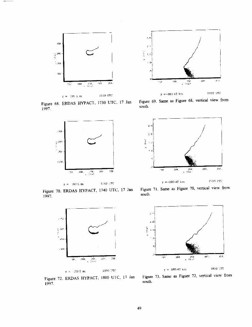
-150-
_z
_2250
i
IBT)
2._,±t
E
L
,5+
E
//
/
!:,W
x ( KJrl I
z = 187.5 m 1730 UTC
Figure 68. ERDAS HYPACT, 1730 UTC, 17 Jan] 997.
y =_BflO 43 k_Tl [730 U'TC
Figure 69. Same as Figure 68, vertical view fromsouth.
-15@
- 2r5_ .-
-sO_.
i , 1
f
2.0 i /
/
,5;
15'tt 2_'i]. _50 3_30. 35t_
z = 1B'?5 n'_ 174D UTC
Figure 70. ERDAS HYPACT, 1740 UTC, 17 Jan1997.
y =-2130 4._ krn 1740 I.WC
Figure 71. Same as Figure 70, vertical view fromsouth.
_ lr--d
- 3f_ra
i , i ,' me". 2.aO, 2¢_. 3_. ?Sg.
z _ 1B75 m lO00 UTC
Figure 72. ERDAS HYPACT, 1800 UTC, 17 Jan1997.
r
!7
2. _ //
s E
,0 _ . i i L
! 50 20_. _5_ ,303. 3.q0.t k,,.!
y = 2B0.4_ km I_00 UTC
Figure 73. Same as Figure 72, vertical view fromsouth.
49
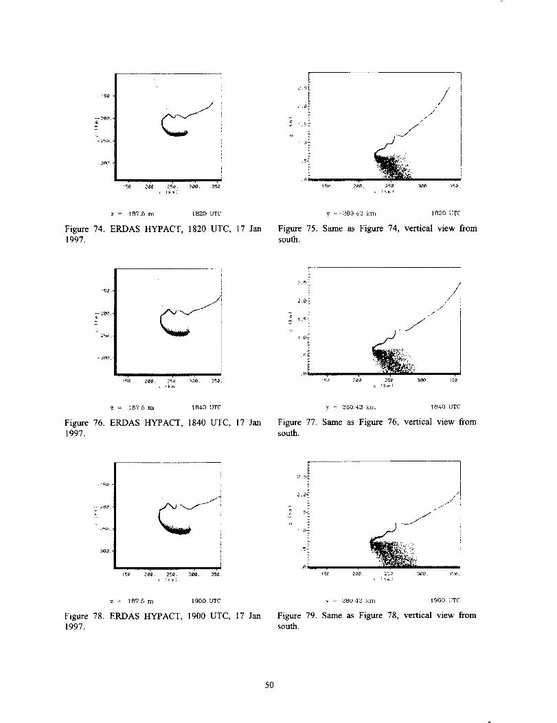
15_ ,-
_'-29P.-
>-250
- 380
"5g 2d'0.
I25'e. 3e_. 355.
z = 1B7,5 m 1820 UTC
Figure 74. ERDAS HYPACT, 1820 UTC, 17 Jan1997.
F%
2.5t /
/
/
F //
E /"
L
E ,._t ,
15; 28'0. _ 3ee.
x ikml
r r
350.
y =-28043 krn 1820 LnEC
Figure 75. Same as Figure 74, vertical view fromsouth.
- 150 -
-_- 200 .-
- 38O
I
qhmi
z = 187.5 m t840 UTC
Figure 76. ERDAS HYPACT, 1840 UTC, 17 Jan
1997.
c-
.@j-
15'_ 2e'0 25'f_ 3_,
x (L.,I
,/
,/
/i• i/
y =-280.43 Rift 1840 UTC
Figure 77. Same as Figure 76, vertical view fromsouth.
-_SZ -
-- 2@@.
25_.
3_rB.
E
I25'g. 30_. 35d.
z = 1B75 m 1900 UTC
Figure 78. ERDAS HYPACT, 1900 UTC, 17 Jan
1997.
F-
2.4 J1
E
1 5'@ 2 8' _ I 2 S _ ]_@I 35I_ .
x _Kml
y = _80.4_ km 1900 UTC
Figure 79. Same as Figure 78, vertical view from
south.
50
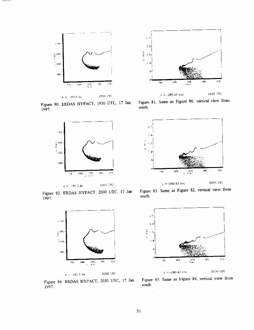
v
"-25_
-3oe
i
] ,_e,. 28,3 7!5'8. 30C. 35'0
= 1,_7 5 m 1930 I:TC
Figure 80. ERDAS HYPACT, 1930 UTC, 17 Jan1997.
c
.0 illl i
I%0 2oo
/t
. 1. --_
•_,_,_,___.'._/,,;'=,_ 300 3r_e
y =-280.43 km 1930 LTTC
Figure 81. Same as Figure 80, vertical view fromsouth.
-15t3 -
- 25_3
- 300
,, I2'._0. 25'0 3d_ ]'3£_.
z = i[_75 m 2,000 UTC
Figure 82. ERDAS HYPACT, 2000 UTC, 17 Jan1997.
t-
2.e+
I ._5_ _" //.,_ "
" _ _ i , , _'-_/_'_#ri r
50 200. 251_ 3_. 35_× [ F:rn !
7 =-28043 km 2000 LrTC
Figure 83. Same as Figure 82, vertical view fromsouth.
- _o -
-250
- 3(40
i
i
2@'0. 2-_'0. 306. 350.
Z = 3.8? 5 rn 2030 UTC
Figure 84. ERDAS HYPACT, 2030 UTC, 17 Jan1997.
'4 _,. _._.. ---'_/_"
x (Klnl
Figure 85. Same as Figure 84, vertical view fromsouth.
51
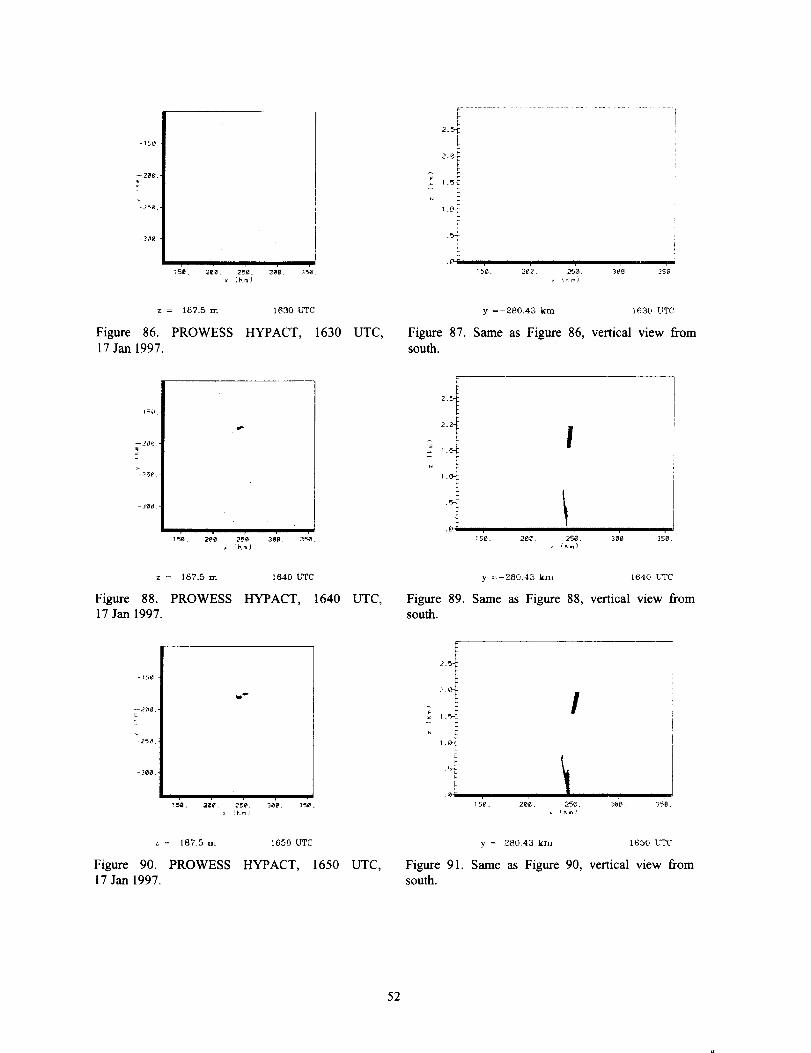
-150
_2@@.'
-25O.
3O0
15'fl. 2@'_1 25't_. 3@'fl. 35_
x [kmJ
z = 187.5
Figure 86. PROWESS17 Jan 1997.
1630 UTC
HYPACT, 1630
50-
--2fie -
-7_50
-3gd
lkm_
z = 187.5 m
Figure 88. PROWESS17 Jan 1997.
1640 UTC
HYPACT, 1640
t
25d,
-30_
x Ikm
= 18'?.5 nz
Figure 90. PROWESS17 Jan 1997.
1650 UTC
HYPACT, 1650
UTC,
UTC,
UTC,
2.5-
2.a3-
_ 1.5
.5-
C
.OP
35'_,
y =-280.43 km 1630 UTC
Figure 87. Same as Figure 86, vertical view fromsouth.
2._
E
150. 20'g . 2£,_. 30'0 35'1_
, ,7km)
y =-280.43 km t640 UTC
Figure 89. Same as Figure 88, vertical view fromsouth.
I
y = 280.43 km 1650 UTC
Figure 91. Same as Figure 90, verticalview fromsouth.
52
-3_
o
I I , iii , J
;5_ , 280 250. 3@_, _5J ,x (r, ml
2,5
2.@
,i
f_
/
........... J
z = 187,5 m 170'0 L%C
Figure 92. PROWESS HYPACT, 1700 UTC,
17 Jan 1997.
y =-280,43 knt 1700 UTC
Figure 93. Same as Figure 92, vertical view from
south.
! 5¢J -
--2_.
-2__0
-366
s
,J, r , ,
,< Ikm]
z = 1875 m 1710 UUC
Figure 94, PROWESS HYPACT, 1710 UTC,
17 Jan 1997.
2.5
2,3
".0.
,_. _
/
Jx (kin)
y =-28043 km 1710 UTC
Figure 95. Same as Figure 94, vertical view from
south.
-79_-
7_.-
2_ -
S
i i , I ,
15_. 2g_. 25@, 30_,< l_-ml
,L3B_,
Z = 187.5 _ 772_1 (T?C
Figure 96. PROWESS HYPACT, 1720 UTC,
17 Jan 1997.
2.%
2,£ _
.5-
._3 I-
_5_. _,-_. _e.
/
r r308 35e,
y =--28o 43 _ _7_o UTC
Figure 97. Same as Figure 96, vertical view from
south.
53
-15_.-
E
_-25e
-3ee
t5'd. 29'd. 25'9.
, ll_ =n )
I
39'9. 35_.
/
1 _£r_ 20e. 258. 3@_ 353.
Z = 187.5 m
Figure 98. PROWESS
17 Jan 1997.
;.730 UTC
HYPACT, 1730 UTC,
y =-28043 km 1730 UTC
Figure 99. Same as Figure 98, vertical view from
south.
-15e
3@e
159. 299 25_. 3dl6 35d
x D, ml
z = 187.5 m 1740 UTC
Figure I00. PROWESS HYPACT, 1740 UTC,
17 Jan 1997.
-156-
_-2Od .-
>
15_. 2_'e 2_'0 39'9 359.
x IKmJ
z = 18'7.5 m 1800 liT(;
Figure 102. PROWESS HYPACT, 1800 UTC,
17 Jan 1997.
2,@-
E1 . 5
/
y =-28043 km 1740 UTC
Figure 101. Same as Figure 100, vertical view from
south.
r
2 5 I
2.,_ff
E
lt I
rl
/
15'9. 29'0 , 25'C1 . 30'_ _:_5 re .
y = 28043 km 1800 UTC
Figure 103. Same as Figure 102, vertical view from
south.
54
--2_0g
_-250
-300
15_ 2_0 250.
× ILml
f [
I , i36'0. 35e.
Z = 187.5
Figure 104. PROWESS17 Jan 1997.
2820 UTC
HYPACT, 1820 UTC,
.,9
/L
I ] ]11 _ i I I1'"
y =-280.43 km 1820 UTC
Figure 105. Same as Figure 104, vertical view fromsouth.
.l r@
-250
-3_
J
I15_. 200 250. 30'£1. 35_,
z = 187.5 r'_ _._40 UTC
Figure 106. PROWESS HYPACT, 1840 UTC,17 Jan 1997.
7£
2.5
2._
1%-
2q_'0, 2r50.
/
i iii i T I
3_3¢l 352,
v =-28043 km 1840 UTC
Figure 107. Same as Figure 106, vertical view fromsouth.
15C
_2@t].
>
• 3_!fd
I
]5;_. 20_ 250, 30_ 'I . 350
. (:_m]
z = 187.5
Figure 108. PROWESS17 Jan 1997.
HYPACT, 1900 UTC,
.5-
200, 2_'_. _o _'_
y =-280.43 km 1900 UTC
Figure 109. Same as Figure 108, verticaI view fromsouth.
55

-15_
--28_.
"25_
-38_
Ikmi
z = 187.5 m ig30 U?C
Figure 110. PROWESS HYPACT, 1930, UTC,17 Jan 1997.
-159
_-2_@
" -25_
3ee
, [bmJ
z = 187.5 m 2000 UTC
Figure 112. PROWESS HYPACT, 2000 UTC,17 Jan 97.
t5g
T:ee.
>-2tt_.
z =
Figure 114.17 Jan 97.
x tkmJ
187.5 rn 2030 UTC
PROWESS HYPACT, 2030 UTC,
F
[
F
F
E,01-
15'8 2fd'O. 250, 3 f_'_
i35_'.
y =-28043 km 1930 UTC
Figure 111. Same as Figure 110, vertical view fromsouth.
2._
1 b J-
- E
15'8 . 2 e'_ . 25'0. 3010 35'el
y =-280.43 km 2000 UTC
Figure 113. Same as Figure 112, vertical view fromsouth.
E
.4b
or
't 5'0. 20'0 • 250. 30_ 356 •
/ ( k ,, ,:
y = 28043 k-q:n 2,330 UTC
Figure 115. Same as Figure 114, vertical view fromsouth.
56
3.2.4. ERDAS HYPACT trajectory analysis
We conducted an analysis to determine how well the model predicted the track of the plume when
compared to observations. We did not compare observed versus predicted concentrations because noconcentration measurements were available for this case. However, we used concentration predictions from
ERDAS HYPACT to help identify the model's prediction of plume location. HYPACT was configured to
output concentrations every 10 minutes and in layers with a thickness of 75 meters. HYPACT producedconcentrations on a 3-dimensional grid at 10-minute intervals from 1630 UTC until 2030 UTC. The location of
the observed plume was determined from the WSR-88D analysis. The location of the predicted plume was
determined by f'mding the maximum concentrations predicted by the ERDAS HYPACT model for each 10-
minute period in each vertical layer of interest. The latitude, longitude, and height of this maximumconcentration were then noted. By tracking this maximum at the 10-minute intervals we were able to determine
the trajectory of the HYPACT-predicted plume.
We had determined from the visual and radar observations of the initial explosion plume that its
dimensions were not precisely defined. However, the plume extended vertically from the ground up to a height
of approximately 900 meters. Because we did not know the height of maximum concentrations, we chose a
layer that was representative of the lower plume. We chose a layer centered at 412.5 meters since this layer was
near the midpoint of the lower plume.
The graph in Figure 116 shows the location of the maximum concentration of the layer centered on 412.5m. This layer is near the center of the ground-based layer which contained the lower plume resulting from the
explosion. The plume originated at Launch Complex 17 and then moved south over the following 4 hours. The
observed and predicted plume locations closely agreed for the first two hours except that the observed plume
was slightly west of the predicted plume. During the last two hours of the model simulation, the graph gives the
appearance of a widely spreading plume. This spread was not due to the plume shifting from the east to the westbut due to the shift in the location of the predicted maximum concentration within the plume from one 10-
minute period to the next.
57
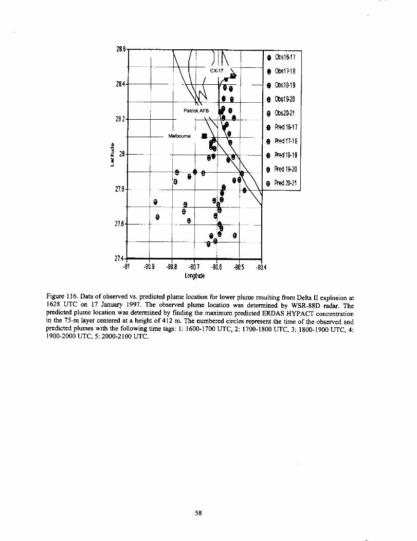
28.6
28.4-
282,
,,_J28.
.J
27.8.
27.6-0
x cx-t7_
Melbourne
PatrickAFB 8) 0
0 0 _ (t_0e e,ee i*
o2} ,,q
i
.807 -80.6 .80sLongtude
I27.4
-81 40.g .80,8 -80.4
0 CYc416-17
@ 0¢_17-18
0 0bs18.19
e 0_19,20
0 0bs20.2t
e Pred16-17
@ Pred17-18
e Pred18-1g
Pr_19-20
_21
Figure 116. Data of observed vs. predicted plume location for lower plume resulting from Delta II explosion at1628 UTC on 17 January 1997. The observed plume location was determined by WSR-88D radar. Thepredicted plume location was determined by f'mding the maximum predicted ERDAS HYPACT concentrationin the 75-m layer centered at a height of 412 m. The numbered circles represent the time of the observed andpredicted plumes with the following time tags: I: 1600-1700 UTC, 2:1700-1800 UTC, 3:1800-1900 UTC, 4:1900-2000 UTC, 5:2000-2100 UTC.
58

4. Conclusions and Recommendations
The primary goal of this study was to conduct a case study of _e dispersing cloud and the models used to
predict the dispersion resulting from the explosion of the Delta II on 17 January 1997 at Cape Canaveral Air
Force Station (CCAFS). The case study was conducted by comparing mesoscale and dispersion model results
with available meteorological and plume observations. The meteorological conditions on this day were strongly
influenced by synoptic rather than local forcing.
The conclusions of this study can be categorized according to the plume observation technique and
according to the models used in the analysis. The findings of this study are:
WSR-88D radar as a plume observation tool
* The WSR-88D is a good tool for providing plume tracks from rocket explosio.n plumes. The radar
provided excellent data on the location and track of the resulting potentially toxic cloud. The datawas extremely useful for model verification since no ongoing program is in place to measure
plume track or concentrations. Bud Parks of ACTA, Inc. is conducting a study to capture data from
nominal and abort launch clouds and has captured radar data from three Eastern Range abort
clouds and 36 of 46 (78%) nominal launch clouds (Parks and Evans 1998).
* The WSR-88D does not provide concentration data. The only data obtained by the radar is the
reflectivity value measured in dBZ. While this measurement gives an estimate on the relative
density of material (smoke particles, water, dust, or other particulate matter), a methodology isneeded to convert dBZ to concentrations of hydrochloric acid (HCI), nitrogen tetroxide 0N204), or
other materials of interest. One of Range Safety's main concerns is determining the exposure limit
(concentration over a specified time) of certain toxic materials.
A dark orange cloud at the very top of the large lower cloud was initially visible. The dark orange
cloud most likely contained some amount of nitrogen tetroxide. Because it was located near the top
of the cloud, it is unsure how much, if any, of the N204 mixed within the cloud and made it to thesurface. Our analysis was not able to determine the concentration of N204 in the explosion cloud.
• Vertical plume height data for this case was not very accurate. The radar appeared to accurately
track the clouds' trajectories in the x-y dimension. However, the vertical measurements appeared
to be inaccurate for two reasons. The fn'st reason was that for long distances from the radar, suchas the 35+ kilometers distance from Melbourne to Cape Canaveral, the radar beam widened
enough to introduce inaccuracies in the vertical plume height measurements. The second reason for
inaccurate vertical measurements was because of the strong inversion causing the radar beam to
bend and bring about measurement inaccuracies.
RAMS model
• The vertical wind profile predictions in this case show a_reemen.t wi.tb observations. Both ERDAS
and PROWESS configurations of RAMS produced wind flow measurements that matched closelywith rawinsonde and profiler measurements and seemed to provide adequate input to HYPACT.
• RAMS under-predicted onshore flow at the level of the Delta II cloud. Both versions of RAMS
predicted onshore flow in the 600- to 900-meter layer in the area south of Cape Canaveral.However, the observed winds had more of a northeast, onshore component than the RAMS-
predicted winds. The movement of the actual explosion cloud tracked onshore north of the model-predicted cloud. The prototype ERDAS RAMS predicted winds with more of an onshore
component than PROWESS RAMS.
• RAMS accurately predicted the strength and height of inversion for this case. The well-defined
inversion that was measured by rawinsonde and based at approximately 800 meters above the
ground was predicted by RAMS to be based at approximately 750 meters above the ground. The
59
inversion,asdeterminedby the vertical temperature profile, had a significant influence on the
explosion cloud.
REEDM source term
• Characterizing the source term of unique explosions is difficult. If a rocket explosion occurs, thecircumstances will be different each time it happens. For example: What was the flight time? How
much fuel was consumed? What were the height, location and distribution of the explosion
products? Were the hazardous and toxic materials separated or mixed within the cloud? Did the
second stage ascend and then explode as with the Delta II? Did the solid rocket motors explode
immediately or did they follow an errant path before they exploded? All of these questions make itdifficult to develop a model that will accurately assess and characterize the source term. We wereable to use information obtained after-the-fact from radar and video to characterize the source term
but in a real-time scenario only estimates of the source term characterization can be made.
• Splitting the source into two sources for HYPACT model was a reasonable approximation. In thepost-explosion mode of this analysis, we split the source into two sources for the HYPACT model
based on observations. This methodology proved better for this case as opposed to using the single
column source term that was generated by REEDM. In real-time, REEDM currently does not splitthe source term.
HYPACT model
• Plume came onshore further to the north and earlier than predicted. HYPACT moved the large
lower cloud resulting from the Delta II explosion onshore at a point that was approximately 12
kilometers south of where it actually came onshore. HYPACT predicted the plume would comeacross the coastline in the Satellite Beach/Indian Harbor Beach area when it actually crossed the
coastline in the Cocoa Beach area. The observed winds at the level moving the cloud at 600-900 m
were northerly prior to the explosion but then shifted to northeasterly during the 1-2 hours
following the explosion. RAMS predicted the shift of these winds fi'om northerly to northeasterlybut did not predict the shift as quickly as observed. RAMS supplies wind and meteorological data
to HYPACT. Because of RAMS' gradual response to shift the winds, HYPACT missed the
location and timing of the plume impact on the coastline.
• Trajectory, diffusion and timing of HYPACT plumes showed similarities to observed plume.
Except for the problem mentioned above, the trajectory, diffusion, and the timing of the HYPACTplumes were similar to the plumes observed by radar. One favorable result was noted in the spread
and diffusion of the lower cloud as it moved south. The cloud spread in the crosswind direction ata rate and in distance similar to observed.
• Range Safe ty's REEDM predicted the movement of plume to the south (176 degrees). REEDM
using the 1613 UTC rawinsonde from Cape Canaveral moved the plume to the south and kept itoffshore until it reached the Melbourne Beach area. REEDM did not account for the winds with an
easterly component that existed at a height of 700-800 meters in the area over the ocean to the
south of Cape Canaveral.
Recommendations
Develop methodology to correlate concentrations with radar reflectivity measurements. The WSR-
88D proved to be a valuable tool in tracking nominal and abort rocket plumes. However, the radarprovides no information on the concentrations within the clouds. What is needed is measurement
of concentrations within the plumes using a sample collection method or another remote sensing
technique such as lidar. This data could then be correlated with radar measurements of reflectivityin dBZ.
• Improvements are needed in HYPACT plume dynamics algorithms. HYPACT currently treats
plumes as non-buoyant, non-depositing entities. We recommend that future enhancements should
60

bemadeto HYPACTto improveits abilityto handlebuoyantplumesandparticledeposition.TheseimprovementswouldallowHYPACTto modelrocketexhaustplumesbetterthanthecurrentversionofHYPACT.
Conduct other studies of rocket explosion plumes. Since the explosion of the Delta II, two otherrockets have exploded after launch from Cape Canaveral-Titan IV on 12 August 1998 and Delta
III on 26 August 1998. In both cases the explosion clouds were tracked by WSR-88D radar.
Detailed studies should be conducted to verify mesoscale models, diffusion models, and radar
tracking techniques.
61
5. References
Banta, R.M., L.D. Oliver, E.T. Holloway, R.A. Kropfli, B.W. Bartram, R.E. Cupp, and M.J. Post, 1992: Smoke-
column observations from two forest fires using Doppler lidar and Doppler radar, d. Appl. Meteor., 31,1328-1349.
Bionetics Corp. film/video: Delta-II/GPS-II-R-i Composite Tape of File#'s 102-979, 102-980, 102-981, and102-982.
Brandli, H., 1997: GOES satellite photographs for 17 January 1997. Electronic mail received
([email protected]), Feb. 1997.
Doviak, R.J. and D.S. Zmic, 1993: Doppler Radar and Weather Observations. Academic Press, Inc., 562 pp.
Evans R. J. and C.J. Tremback, 1998: Operational implementation and continued evaluation of a mesoscale and
dispersion modeling system at Cape Canaveral Air Force Station/Kennedy Space Center, FL. Preprints,10th Joint Conf. of Air Pollution Meteorology with AWMA, Phoenix, AZ, Amer. Meteor. Soc., Boston,
6 pp. [Available from ENSCO, Inc, 445 Pineda Court, Melbourne, FL 32940]
Evans R. J., C.J. Tremback, and W.A. Lyons, 1996: The implementation and evaluation Emergency Response
Dose Assessment System (ERDAS) at Cape Canaveral Air Force Station/Kennedy Space Center, FL.
Preprints, 9th Joint Conf. of Air Pollution Meteorology with AWMA, Atlanta, GA, Amer. Meteor.Soc., Boston, 193-197.
Evans, R.J., 1996: Final report on the evaluation of the emergency response dose assessment system (ERDAS).
NASA CR-201353. Prepared by Applied Meteorology Unit, 184 pp.
Evans, R.J., A.V. Dianic, and L.N. Moore, 1994. The meteorological monitoring system (MMS). Preprints, 5th
Conf. on lIPS. Nashville, TN, Amer. Meteor. Soc., Boston, 362-367.
Ha, C.T. and N.A. Deane, 1998: Validation Analysis of the PUFF and SATRAP Codes and Cassini MethodsAgainst the 17Jan97 Delta II Accident Data. Lockheed Martin Astronautics Interoffice Memo, Cassini
Memo No. 579, 17 July 1998, 35 pp.
Herring, H., 1999: Electronic message, RE: 74-C data, 17Jan97. Electronic mail received
(HAROLD.HERR/[email protected]£mil), May, 1999.
Hoffert, S. and M. Pearce, 1996: 88Display software package, obtained by Applied Meteorology Unit from
Pennsylvania State University.
Lane, R.E. and R.J. Evans 1989: The meteorological and range safety support system (MARSS). Preprints, 5thConf. on lIPS, Anaheim, CA, Amer. Meteor. Soc., Boston, 226-231.
Lyons, W.A., and C.J. Tremback, 1994: Predicting 3-D wind flows at Cape Canaveral Air Force Station using a
mesoscale model. Contract No. F04701-91-C-0058. Prepared by ASTER/MRC for US Air Force Spaceand Missile Systems Center, SMC/CLNE, 30 June 1994.
National Weather Service, 1997: Delta rocket explosion 2.5 degree reflectivity loop.
(http://sunmlb.nws.fit.edu/17jan97b.gif).
Nyman, Randolph L., REEDM Version 7.09 Technical Description Manual, Technical Report No. 99-400/11.3-
02, ACTA Inc., Torrance, CA, 30 September 1999.
Overbeck K., 1997: Memorandum for Record to Safety Investigation Board: Delta GPS 2R-1 Toxic Support
Review, undated, 19 pp.
Pace, J.C., J.R. Albritton, R.L. Baskett, X.J. Zhang, M.C. Masonjones, N.A. Moussa, K. Overbeck, C.R. Parks,
R.J. Evans, 1998: Modeling the 17 January 1997 Delta-II Explosion by ARAC, ADORA, and REEDM.Preprints, 10th Joint Conf. of Air Pollution Meteorology with AWMA, Phoenix, AZ, Amer. Meteor.Soc., Boston, 294-301.
62
Parks,C.R.andR.J.Evans,1998,TrackingnominallaunchandabortrocketplumesusingWSR-88DDopplerradar.PresentedatJANNAFSEPSubcommitteemeeting,HoustonTX, May1998,10pp.
Rogers,R.R.andW.O.J.Brown,1997:Radarobservationsof majorindustrialfire.Bull.Amer.Meteor.Soc.,78,803-814.
Sittig,Marshall,1985:Handbookof ToxicandHazardousChemicalsandCarcinogens2nded.,NoyesPub.ParkRidge,NJ,659-660.
Tremback,C.J.,W.A.Lyons,W.P.Thorson,andR.L.Walko,1994:Anemergencyresponseandlocalweatherforecastingsoftwaresystem.Preprints,8thJointConf.of Air PollutionMeteorologywithAWMA,Nashville,TN,Amer.Meteor.Sot.,Boston,219-223.
Tremback,C.J., W.A. Lyons, I.T. Baker, M.J. Weissbluth, 1996: Enhanced Mesoscale Modeling for Kennedy
Space Center: Parallelized RAMS Operational Weather Simulation System: Final Report. MissionResearch Corp./ASTER Division, 184 pp. [Available from ENSCO, Inc, 1980 N. Atlantic Ave., Suite
230, Cocoa Beach, FL 32931 ]
63
APPENDIX A
ERDAS RAMSIN f'de
64
SMODEL_GRIDS
! Simulation title (64 chars)
EXPNME =
IOTYPE =
RUNTYPE = '
TIMEUNIT =
'CCAFS/KSC-Version 3a' ,
0,
INITIAL',
'h'
TIMMAX = 12.
! -]=diagnostic, 0=normal run
! type of run: INITIAL, HISTORY, or MAKEVFILE
! 'h','m','s' Time units of
! TIMMAX, TIMSTR0 VTIME
! Final time of simulation
NGRIDS = 3,
NNXP = 38, 34, 37,
NNYP = 36, 38, 37,
NNZP = 25, 25, 25,
NNZG = ii, II, Ii,
NXTNEST = 1, i, 2,
! Number of grids to run
! Number of x gridpoints
! Number of y gridpoints
! Number of z gridpoints
! Number of soil gridpoints
! Grid number which is the next
! coarser grid
J Coarse grid specifications
IHTRAN = i,
DELTAX = 60000.,
DELTAY = 60000.,
DELTAZ = 75.,
DZRAT = 1.25,
DZMAX = 1000.,
ZZ=0., 25., 75., 150.,
3250., 4000., 5000., 6000.,
DTLONG = 90.,
NRATIO = 3,
! 0-Cartesian, l-Polar stereo
! X and Y grid spacing
! Z grid spacing (set to 0. to use ZZ)
! vertical grid stretch ratio
! maximum delta Z for vertical stretch
250., 500., 750., I000., 1500., 2000., 2500.,
! Vertical levels if DELTAZ = 0
! Coarse grid long timestep
! Small timestep ratio
IMONTHI = 01, ! Month
IDATEI = 17, ! Day
IYEARI = 97, ! Year
STRTIM = 12.0,
NSTRATX = I, 4, 5,
NSTRATY = I, 4, 5,
NNDTRAT = i, 2, 2,
! GMT of model TIME = 0.
NESTZ = 3,
NSTRATZ=3,3,2,2,2,2,2,2,2,2,1,
! Nest ratios between this grid
! and the next coarser grid.
! x-direction
! y-direction
! time
! contort coarser grids if negative
POLELAT = 30.0,
POLELON = -83.0,
CENTLAT = 30.0,
CENTLON = -83.0,
NINEST = i, 17,
NJNEST = I, i0,
NKNE ST = 1, 1
NNSTTOP = i, 1
NNSTBOT = i, 1
GRIDU = 0., 0.
GRIDV = 0., 0.
20,
19,
I,
0,
i,
0.,
0. ,
! Latitude of pole point
! Longitude of pole point
! Grid point on the next coarser
! nest where the lower southwest
! corner of this nest will start.
! IF NINEST or NJNEST = 0, use CENTLAT/LON
! coarser grid
! i-point
! j-point
! k-point
Flag (0-no or l-yes) if this
nest goes the top or bottom of the
! coarsest nest.
u-component for moving grids
v-component for moving grids
! {still not working!)
65
SEND
SMODEL_FILEINFO
! History file input
TIMSTR= 0.,
HFILIN = 'ci.h0h',
! time of history start (see TIMEUNIT)
! input history file name
! History/analysis file output
IOUTPUT = I,
HFILOUT='hist/f.h',
AFILOUT='f.a',
HFUNITS='h', AFUNITS=,d , ,
FRQHIS =43200., FRQANL =3600.,
! 0-no files, l-save/dispose
! history file prefix
! analysis file prefix
! history/anal file units (M,m,H,h,S,s)
! history/anal file frequency
! Variable initialization input
INITIAL = 2,
VTIME = 0., 6., 12., 18.,
VARFIL(1)='isan/iv17-jan-97 -
VARFIL(2)='isan/iv17-jan-97-
VARFIL(3)='isan/iv17-jan-97-
VARFIL(4)='isan/iv17-jan-97 -
VARFIL(5)='isan/iv17-jan-97-
IVWIND = 0,
NUDLAT =
TNUDLAT =
TNUDCENT =
TNUDTOP =
ZNUDTOP =
5,
900.,
00.,
00.,
15000.,
! Initial fields - l=horiz.homogeneous,
24.,
2=variable
! model times for varfiles (See TIMEUNIT)
12', VTIME(1)=0.,
18', VTIME(2)=6.,
24 ° , VTIME(3)=I2.,
30', VTIME(4)=I8.,
36', VTIME(5)=24.,
! initial winds ( only 0 works)
! number of points in the lateral bnd region
! nudging time scale (s) at lateral boundary
! nudging time scale (s) in center of domain
! nudging time scale (s) at top of domain
! nudging at top of domain above this height (m)
! Printed output controls
FRQPRT = 21600.,
FRQIPR = 99930.,
FRQIST = 99900.,
ISTPFL = i,
INITFLD = I,
INPRTFL = I,
! Printout frequency
! Integral print frequency
! Integral store frequency
! Timestep message frequency flag
! Initial field print flag 0=no print, l=print
! Namelist print flag 0=no print, l=print
! Input topography variables
SFCFILES = '/ul/met/sfc/sfcb_jan',
characteristic
' File path and prefix for surface
ITOPTFLG = i,I,i,
IPCTLFLG = i,i,I,
ISSTFLG = 1,0,0,
IVEGTFLG = 1,1,1,
! 2 - Fill data in "ruser"
] 1 - Interp data from latlon dataset
! 0 - Interpolate from coarser grid
ITOPTFN =
IPCTLFN =
ISSTFN =
IVEGTFN =
!
! The following only apply for IxxxxFLG=l
/usr/geode/data/rams/topolOm/H',
/usr/geode/data/rams/topo3Os/U',
/usr/geode/data/rams/topo3Os/U',
/usr/geode/data/rams/pctllOm/L',
/usr/geode/data/rams/pctllOm/L',
/usr/geode/data/rams/pctllOm/L',
/usr/geode/data/rams/sst/SJUL',
'/usr/geode/data/rams/ndvi/V',
'/usr/geode/data/rams/ndvi/V',
'/usr/geode/data/rams/ndvi/V',
! Input topography file name
! Input topography file name
SILAVWT = 0.0, 0., 0., ! Weighting of topo silhouette averaging
66
TOPTWVL = 4.0, 4., 4.,
PCTLWVL = 2.0, 2., 2.,
SSTWVL = 2.0, 2., 2.,
$ END
! Topo wavelength cutoff in filter
! Land pct wavelength cutoff in filter
! Land pct wavelength cutoff in filter
$MODEL_OPTIONS
NADDSC = 0,0,0,
NTOPSMTH = 0, ! Number of passes for topography smoother
IZFLAT = 0, ! Width of flat margin around domain (in grid points)
! Numerical schemes
ITMDIFF = 3, ! l=forward, 2=leapfrog, 3=hybrid
NONHYD = i, ! nonhydrostatic=1, hydrostatic=O
SSPCT = 0., ! Sound speed fraction for the nonhydrostatic model
IMPL = i, [ Implicit flag for acoustic model 0=off, l=on
ICNTEQ = 2, ! Hyd - continuity equation - 1 -incomp, 2 -anelastic
WTKD = 0., ! Klemp/Durran - current timestep weighting
ICORFLG = I, ! Coriolis flag/2D v-component 0=off, l=on
IBCTOP = 0, ] top boundary condition
! 0-wall on top(nonhyd) 2-prognostic sfc prs(hyd)
! l-Klemp-Durran(nonhyd/hyd) 3-material surface(hyd)
IBND = l, ! Lateral boundary condition flags
JBND = I, l l-Klemp/Wilhelmson, 2-Klemp/Lilly, 3-Orlanski
! 4-cyclic
CPHAS = 20., ( Phase speed if IBND or JBND = l
LSFLG = 0, ! Large-scale gradient flag for variables other than
! normal velocity:
! 0 = zero gradient inflow and outflow
! i = zero gradient inflow, radiative b.c. outflow
! 2 = constant inflow, radiative b.c. outflow
! 3 = constant inflow and outflow
NFPT = 0, ! Rayleigh friction - number of points from the top
DISTIM = 0., ! dissipation time scale
TIMSCL = 0., ! Initial wind spin-up - time scale
KSPIN = 33, ! - below this level (velocity)
KMSPIN = i0, ! - below this level (momentum)
IPRSPLT = 0, ! precipitation time-split scheme - 0=off, l=on
IADVL = 2, ! Order of advection - Leapfrog - 2 or 4
IADVF = 2, ! Order of advection - Forward - 2 or 6
IPGRAD = i, ! Pressure gradient scheme for topo.: l-transform
! 2-interpolate
FILT4 = 000., ! Fourth order filter coefficient (0 - off)
! ( > 0 timestep at which 2 delta waves are
! totally removed)
FXLONG = 0.0000, ! Long filter coefficient 0=off
FYLONG = 0.0000, ! Long filter coefficient 0=off
! Radiation parameters
ISWRTYP = 2, ! Shortwave radiation type 0-none, 2-Mahrer/Pielke, l-Chen
ILWRTYP = 2, ! Longwave radiation type 0-none, 2-Mahrer/Pielke, l-Chen
RADFRQ = 1200., ! Frequency of radiation tendency update in seconds
LONRAD = i, ! Longitudinal variation of shortwave (0-no, 1-yes)
! Cumulus parameterization parameters
NNQPARM = 0, 0, 0, ! convective parameterization flag
! 0-off, l-on
CONFRQ = 1200., ! Frequency of conv param, updates in seconds
WCLDBS = .001, ! vertical motion needed at cloud base for convection
! Surface layer and soil parameterization
ISFCL = i, ! surface layer/soil/veg model
! 0-specified surface layer gradients
! 1-soil/vegetation model
NVGCON = 1, ! Vegetation type
! 1 -- Crop/mixed farming 2 -- Short grass
67
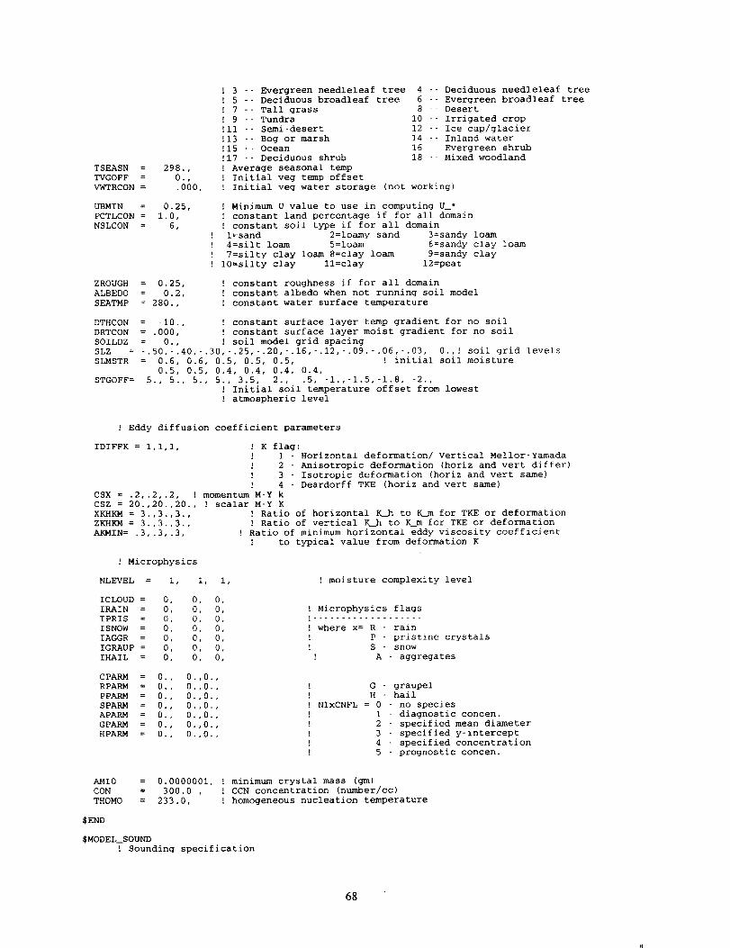
TSEASN = 298.,
TVGOFF = 0.,
VgFfRCON = .000,
! 3
' 5
! 7
9
!ii
!13
!15
!17
Evergreen needleleaf tree
Deciduous broadleaf tree
Tall grass
Tundra
Semi-desert
Bog or marsh
Ocean
Deciduous shrub
! Average seasonal temp
! Initial veg temp offset
4 -- Deciduous needleleaf tree
6 -- Evergreen broadleaf tree
8 -- Desert
i0 -- Irrigated crop
12 -- Ice cap/glacier
14 -- Inland water
16 -- Evergreen shrub
18 -- Mixed woodland
! Initial veg water storage (not working)
UBMIN = 0.25, ! Minimum U value to use in computing U_*
PCTLCON = 1.0, ! constant land percentage if for all domain
NSLCON = 6, ! constant soil type if for all domain
! l=sand 2=loamy sand 3=sandy loam
: 4=silt loam 5=loam 6=sandy clay loam
! 7=silty clay loam 8=clay loam 9=sandy clay
! 10=silty clay ll=clay 12=peat
ZROUGH = 0.25, ! constant roughness if for all domain
ALBED0 = 0.2, [ constant albedo when not running soil model
SEATMP = 280., ! constant water surface temperature
DTHCON = -10., ! constant surface layer temp gradient for no soil
DRTCON = .000, ! constant surface layer moist gradient for no soil
SOILDZ = 0., ! soil model grid spacing
SLZ = -.50,-.40,-.30,-.25,-.20,-.16,-.12,-.09,-.06,-.03, 0., ! soil grid levels
SLMSTR = 0.6, 0.6, 0.5, 0.5, 0.5, ! initial soil moisture
0.5, 0.5, 0.4, 0.4, 0.4, 0.4,
STGOFF= 5., 5., 5., 5., 3.5, 2., .5, -1.,-1.5,-1.8, -2.,
! Initial soil temperature offset from lowest
! atmospheric level
! Eddy diffusion coefficient parameters
IDIFFK = I,i,i, ! K flag:
! 1 - Horizontal deformation/ Vertical Mellor-Yamada
! 2 - Anisotropic deformation (horiz and vert differ)
! 3 - Isotropic deformation (horiz and vert same)
! 4 - Deardorff TKE (horiz and vert same)
CSX = .2,.2,.2, ! momentum M-Y k
CSZ = 20.,20.,20., ! scalar M-Y K
XKHKM = 3.,3.,3.,
ZKHKM = 3.,3.,3.,
AKMIN = .3, .3, .3,
! Microphysics
NLEVEL = 1, I, 1,
ICLOUD = 0, 0, 0,
IRAIN = 0, 0, 0,
IPRIS = 0, 0, 0,
ISNOW = 0, 0, 0,
IAGGR = 0, 0, 0,
IGRAUP = 0, 0, 0,
IHAIL = 0, 0, 0,
C PARM = 0.
R PARM = 0.
P PARM = 0.
S PARM = 0.
APARM = 0.
GPARM = 0.
HPARM = 0.
0.,0°
0.,0.
0.,0.
0.,0.
0.,0.
0.,0.
0.,0.
! Ratio of horizontal K_h to K_m for TKE or deformation
! Ratio of vertical K_ to K__m for TKE or deformation
! Ratio of minimum horizontal eddy viscosity coefficient
! to typical value from deformation K
! moisture complexity level
! Microphysics flags
! ...................
! where x = R - rain
! P - pristine crystals
! S - snow
! A - aggregates
[ G - graupel
! H - hail
[ NIxCNFL = 0 - no species
! 1 - diagnostic concen.
! 2 - specified mean diameter
! 3 - specified y-intercept
! 4 - specified concentration
! 5 - prognostic concen.
AMI0
CON
THOMO
= 0.0000001, ! minimum crystal mass (gm)
= 300.0 , ! CCN concentration (number/cc)
= 233.0, ! homogeneous nucleation temperature
SEND
$MODEL_SOUND
! Sounding specification
68

IPSFLG=0,
ITSFLG=2,
IRTSFLG=3,
IUSFLG=D,
IUSRC = 0,
! Flags for how sounding is specified
! specifies what is in PS array
! 0 - pressure (mb), 1 - heights (m), PS(1)=sfc press(mb)
[ specifies what is in TS array
! 0 - temp(C), 1 - temp(K), 2 - pot. temp(K)
! specifies what is in RTS array
! 0 - dew pnt. (C), 1 - dew pnt. (K), 2 - mix rat(g/kg)
! 3 - relative humidity on %, 4 - dew pnt depression(K)
! specifies what is in US and VS arrays
! 0 - u,v component(m/s), 1 - umoms-direction, vmoms-speed
! source of wind profile:
! 0 - umoms, vmoms, valid at sounding levels (PS)
! -i - usndg, vsndg, valid at model levels (Z)
PS=1012.00, 1000.00 ,
797.00, 700.00 ,
500.00, 498.00 ,
383.00, 328.00 ,
285.00, 250.00 ,
977.00 , 949.00 , 936.00 , 850.00 , 848.00 ,
662.00 , 595.00 , 579.00 , 565.00 , 560.00
461.00 , 443.00 , 406.00 , 400.00 , 387.00
325.00 , 316.00 , 309.00 , 307.00 , 300.00
200.00 , 150.00 , I00.00 , 80.00 , I0.0,
TS= 288.18, 288.36 , 288.88 , 293.11 , 294.27 , 298.93
304.48, 309.35 , 310.27 , 313.50 , 315.02 , 317.23
318.75, 318.88 , 320.88 , 322.03 , 326.27 , 327.02
328.73, 330.56 , 331.02 , 333.69 , 335.55 , 335.89
340.82, 343.42 , 347.35 , 364.39 , 379.82 , 398.66
298.92
317.80
328.41
336.99
480.,
RTS = 90.7, 95.5, 98.0,
99.3, 94.1, 75.8,
78.0, 71.1, 57.6,
09.7, 02.5, 06.1,
96.8, 96.1, 100.0, 100.0, 94.1,
49.3, 38.4, 55.8, 55.7, 85.1,
52.3, 74.9, 74.0, 39.6, 22.7,
15.8, 03.6, 02.1, 01.5, 01.5,
90.6,
80.6,
16.0,
US=4.,4.,4.,4.,4.,4.,4.,4.,4.,4.,4.,4.,4.,4.,4.,4.,4.,4.,4.,4.,4.,
4.,4.,4.,4.,4.,4.,4.,4.,4.,4.,4.,4.,4.,4.,4.,4.,4.,4.,4.,4.,4.,
VS=0.,0.,0.,0.,0.,0.,0.,0.,0.,0.,0.,0.,0.,0.,0.,0.,0.,0.,0.,0.,0.
0.,0.,0.,0.,0.,0.,0.,0.,0.,0.,0.,0.,0._0.,0.,0.,0.,0.,0.,0.,0.
! US = -i0., -i0., -ii., -12., -12., -5., 5.,
! 6.5, 8.7,11.0,14.0,16.0,17.0,18.0,
! 21.9, 22.0,24.0,26.0,30.0,30.0,32.0,
! 33.0, 34.0,35.0,36.0,37.0,39.0,40.6,
: 42.0, 50.7,46.6,35.0,30.0,30.0,30.,
! VS= 2.1, 2.1, 2.5,3.0,3.5,4.0,4.0,
! 3.5, 3.1, 3.3,3.5,3.7,4.2,4.5,
! 6.0, 6.0, 7.0,8.0,9.0,10.0,11.0,
! 12.0, 13.0,14.0,14.1,14.5,15.0,15.0,
! 14.8, 8.0,8.0,8.0,8.0,8.0,8.0,
US_G=0.,
VS_G=0.,
_i=0,
_2=0,
UMEAN = 0.0,
VMEAN = 0.0,
$ END
! Wind components if IUSRC = -I
!
] lower model level for calculation of (umean,vmean)
! upper model level for calculation of (umean,vmean)
! u-component for Galilean transformation
! v-component for Galilean transformation
SMODEL PRINT
! Specifies the fields to be printed during the simulation
NPLT = 6, ! Number of fields to be printed at each time
! for various cross-sections (limit of 50)
IPLFLD = 'UP,,'VP','WP','THETA','TKE','TVEG',
! Field names - see table below
! PLFMT(6) = '0PF7.2', ! Format specification if default is unacceptable
69
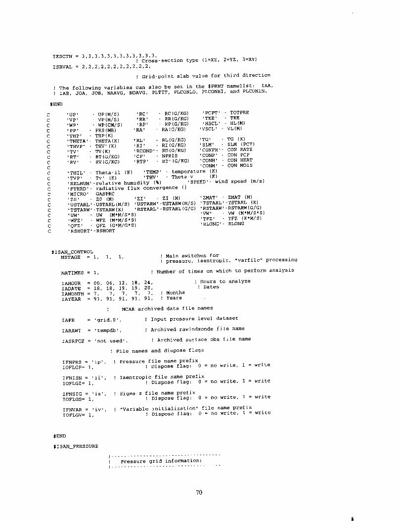
IXSCTN = 3,3,3,3,3,3,3,3,3,3,3,3,
! Cross-section t_e (I=XZ, 2=YZ, 3=XY)
ISBVAL = 2,2,2,2,2,2,2,2,2,2,2,
! Grid-point slab value for third direction
! The following variables can also be set in the SPRNT namelist: IAA,
!IAB, JOA, JOB, NAAVG, NOAVG, PLTIT, PLCONL0, PLCONHI, and PLCONIN.
SEND
'UP' UP(M/S)
'vP 0 VP(M/S)'WP' WP(CM/S)'PP' PRS(MB)
'THP' - THP(K)
'THETA'- THETA(K)
'THVP' - THV'(K)
'TV' - TV(K)
'RT' - RT(G/KG)
'RV' - RV(G/KG)
'THIL' - Theta-il (K)
'TVP' - Tv. (K)
'RC' RC(G/KG) 'PCPT' - TOTPRE
'RR' RR(G/KG) 'TKE' - TKE
'RP' RP(G/EG) 'HSCL' - HL(M)
'RA' RA(G/KG) 'VSCL' - VL(M)
'RL' RL(G/KG) 'TG'
'RI' RI(G/KG) 'SLM'
'RCOND'- RD(G/KG) 'CONPR'
'CP' NPRIS 'CONP'
'RTP' RT' (G/KG) 'CONH'
'CONM'
'TEMP' - temperature (K)
'THV' - Theta-v (K)
TG (K)
SLM (PCT)
CON RATE
CON PCP
CON HEAT
CON MOIS
'RELHUM'-relative humidity (%) 'SPEED'- wind speed (m/s)
'FTHRD'- radiative flux convergence (]
'MICRO'- GASPRC
'Z0' - Z0 (M) 'ZI' ZI (M) 'ZMAT' ZMAT (M)
'USTARL'-USTARL(M/S) 'USTARW'-USTARW(M/S) 'TSTARL'-TSTARL (K)
'TSTARW'-TSTARW(K) 'RSTARL'-RSTARL(G/G) 'RSTARW'-RSTARW(G/G)
'UW. - UW (M.M/S-S) .VW. VW (M'M/S'S)
'WFZ' - WFZ (M.M/S-S) 'TFZ' TFZ (K'M/S)
'QFZ' - QFZ (G.M/G'S) 'RLONG'- RLONG
'RSHORT'-RSHORT
$ISAN_CONTROL
MSTAGE = i, i, I, ! Main switches for
! pressure, isentropic0 "varfile" processing
NATIMIES = I, ! Number of times on which to perform analysis
IAHOUR = 00, 06, 12, 18, 24, ! Hours to analyze
IADATE = 18, 18, 19, 19, 20, ! Dates
IAMONTH = 7, 7, 7, 7, 7, ! Months
IAYEAR = 91, 91, 91, 91, 91, ! Years
! NCAR archived data file names
IAPR = 'grid.0' ! Input pressure level dataset
IARAWI = 'tempdb. _ Archived rawindsonde file name
IASRFCE = 'not-used' ! Archived surface obs file name
IFNPRS = 'ip'.
IOFLGP= i0
IFNISN = 'ii',
IOFLGI= I,
IFNSIG = °is',
IOFLGS = I,
IFNVAR = 'iv', [
IOFLGV= i,
! File names and dispose flags
! Pressure file name prefix
! Dispose flag: 0 = no write, i = write
! Isentropic file name prefix
! Dispose flag: 0 = no write, 1 = write
! Sigma-z file name prefix
! Dispose flag: 0 = no write, 1 = write
"Variable initialization" file name prefix
! Dispose flag: 0 = no write, i = write
SEND
$ISAN_PRESSURE
! ...................................
! Pressure grid information:
! ...................................
7O
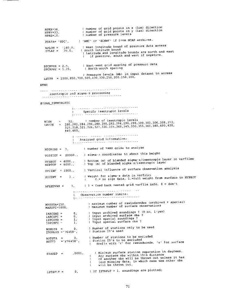
NPRX=36
NPRY=33
NPRZ=I0
PDATA = SPC'
WPLON = -140.0,
SPLAT = 20.0,
! number of grid points in x (lon) direction
! number of grid points in y (lat) direction
! number of pressure levels
! 'NMC' or 'ECMWF' if from NCAR archives.
! West longitude bound of pressure data access
! South latitude bound
! Latitude and longitude bounds are north and east
! if positive, south and west if negative.
SPCNPRX = 2.5,
SPCNPRY = 1.25,
, East-west grid spacing of pressure data
! North-south spacing
! Pressure levels (mb) in input dataset to access
LEVPR = 1000,850,700,500,400,300,250,200,150,100,
SEND
Isentropic and sigraa-z processing............................................
$1SAN_ISENTROPIC
...................................
! Specify isentropic levels
! ...................................
NISN = 32, ! number of isentropic levels
LEVTH = 280,282,284,286,288,290,292,294,296,298,300,303,306,309,312,
315,318,321,324,327,330,335,340,345,350,355,360,380,400,420,
440,460,
NIGRIDS = 3,
TOPSIGZ = 20000.,
HYBBOT = 4000.,
HYBTOP = 6000.,
SFCINF = 1000.,
SIGZWT = i.,
NFEEDVAR = I,
MAXSTA=I50,
MAXSFC=I000,
IARCSND = 0,
IARCSFC = 0,
ISPCSND = i,
ISPCSPC = i,
NONLYS = 0,
IDONLYS ='76458',
NOTSTA = 0,
NOTID ='r76458',
! ...................................
! Analyzed grid information:
! ...................................
! number of RAMS grids to analyze
! sigma-z coordinates to about this height
! Bottom (m) of blended sigma-z/isentropic layer in varfiles
! Top (m} of blended sigma-z/isentropic layer
! Vertical influence of surface observation analysis
! Weight for siqma-z data in varfile:
! 0. = no sigz data, l.=full weight from surface to HYBBOT
! 1 = feed back nested grid varfile info, 0 = don't
! ...................................
! Observation number limits:
! ...................................
! maximum number of rawindsondes (archived + special)
! maximum number of surface observations
! Input archived soundings ? (0-no, l-yes)
! Input archived surface obs ?
! Input special soundings ?
! Input special surface obs ?
! Number of stations only to be used
! Station ID's used
! Number of stations to be excluded
! Station ID's to be excluded
! Prefix with 'r' for rawindsonde, 's' for surface
STASEP = .0001,
ISTAPLT = 0,
! Minimum surface station separation in degrees.
! Any surface obs within this distance
! of another obs will be thrown out unless it has
! less missing data, in which case the other obs
! will be thrown out.
! If ISTAPLT = I, soundings are plotted;
71
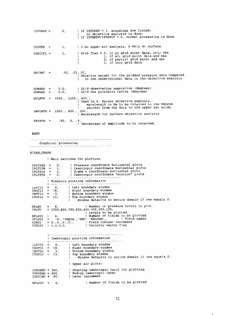
ISTAREP = 0, ! If ISTAREP = i, soundings are listed;
! no objective analysis is done.
! If ISTAREP/ISTAPLT = 0, normal processing is done
IUPPER =
IGRIDFL =
i,
I,
! l-Do upper air analysis, 0-Only do surface
! Grid flag = 0, if no grid point data, only obs
! I, if all grid point data and obs
! 2, if partial grid point and obs
] 3, if only grid data
GRIDWT .01, .01,.01,
! Relative weight for the gridded pressure data compared
! to the observational data in the objective analysis
GOBSEP = 5.0
GOBRAD = 5.0
WVLNTH = 1600.
SWVLNTH = i000.
RESPON = .90,
1200.
400..
.9,
! Grid-observation separation (degrees)
! Grid-obs proximity radius (degrees)
, 400.,
! Used in S. Barnes objective analysis.
! Wavelength in km to be retained to the RESPON
! percent from the data to the upper air grids.
i00.,
! Wavelength for surface objective analysis
.9,
! Percentage of amplitude to be retained.
SEND
Graphical processing
...........................................
SISAN_GRAPH
! Main switches for plotting
IPLTPRS = 0, ! Pressure coordinate horizontal plots
IPLTISN = i, ! Isentropic coordinate horizontal plots
IPLTSIG = i, ! Sigma-z coordinate horizontal plots
IPLTSTA = 0, ! Isentropic coordinate "station" plots
! ......................................
! Pressure plotting information
! ......................................
ILFTII = 0, ! Left boundary window
IRGTII = 18, ! Right boundary window
IBOTIJ = .3, ! Bottom boundary window
ITOPIJ = 13, ! Top boundary window
! Window defaults to entire domain if one equals 0.
NPLEV = 8, ! Number of pressure levels to plot
IPLEV = 1000,850,700,500,400,300,200,100,
! Levels to be plotted
NFLDUI = 4, ! Number of fields to be plotted
IFLDUI = 'U','THETA','GEO','RELHUM', ! Field names
CONUI = 0.,0.,0.,0., ! Field contour increment
IVELUI = 1,0,0,0, ! Velocity vector flag
ILFT3I
IRGT31
IBOT3J
ITOP3J
IUP3BEG = 340,
IUP3END = 400,
IUP3INC = 60,
! .......................................
! Isentropic plotting information
! .......................................
= 0, ! Left boundary window
= 18, ! Right boundary window
= 3, ! Bottom boundary window
= 13, ! Top boundary window! Window defaults to entire domain if one equals 0.
! Upper air plots:
! Starting isentropic level for plotting
! Ending isentropic level
! Level increment
NFLDU3 = 4, ! Number of fields to be plotted
72
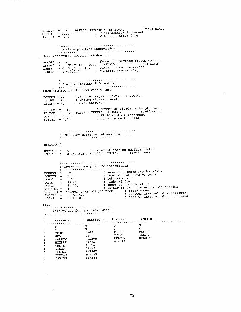
IFLDU3 = 'U','PRESS'
CONU3 = 0.,0.,
IVELU3 = 1,0,
,'MONTSTR','RELHUM', ! Field names
! Field contour increment
! Velocity vector flag
! .......................................
! Surface plotting information
! .......................................
Uses isentropic plotting window info
NFLDS3 = 4, ! Number of surface fields to plot
IFLDS3 = ,U,,,TEMP','PRESS','RELHUM', ! Field names
CONS3 = 0.,0.,0.,0.,0., ! Field contour increment
IVELS3 = 1,0,0,0,0, ! Velocity vector flag
! .......................................
! Sigma-z plotting information
! .......................................
! Uses isentropic plotting window info
ISZBEG = 2, [ Starting sigma-z level for plotting
ISZEND = 26, ! Ending sigma-z level
ISZINC = 6, ! Level increment
NFLDSZ = 4, ! Number of fields to be plotted
IFLDSZ = ,U,,,PRESS','THETA','RELHUM', ! Field names
CONSZ = 0.,0., ! Field contour increment
IVELSZ = 1,0, ! Velocity vector flag
! .......................................
! "Station" plotting information
.......................................
NPLTRAW=O,
NSTIS3 = 4, ! number of station surface plots
ISTIS3 = 'U',,PRESS','RELHUM','TEMP', ! field names
NCROSS3 =
ICRTYP3 =
ICRA3 =
ICRB3 =
ICRL3 =
NCRFLD3 =
ICRFLD3 =
THCON3 =
ACON3 =
! .......................................
! Cross-section plotting information
! .......................................
0, ! number of cross section slabs
2,1, ! type of slab: 1=E-W, 2=N-S
i,i, ! left window
35,43, ! right window
22,25, ! cross section location
3, ! number of plots on each cross section
'MIXRAT','RELHUM','THETAE', ! field names
5.,5.,5., ! contour interval of isentropes
0.,0.,0., ! contour interval of other field
SEND
! Field values for graphical stage
! ....................................
!
U U
V V
! TEMP PRESS
! GEO GEO
! RELHUM RELHUM
! MIXRAT MIXRAT
! THETA THETA
! SPEED SPEED
! ENERGY ENERGY
[ THETAE THETAE
! SPRESS SPRESS
!
U U
V V
PRESS PRESS
TEMP THETA
RELHUM RELHUM
MIXRAT
73

APPENDIX B
PROWESS RAMSIN f'de
74
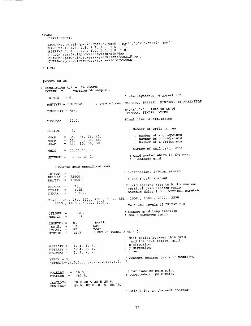
& PARA
I PARALLEL = 1,
NMACH=6, HOSTS ='par7' , 'par6', 'par5' , 'par4' , 'par3', 'par2', 'parl' ,
HPERF=I.I, 1.2, 1.3, 1.4, 1.5, 1.6, 1.7,
HPERF=I.0, 1.0, 1.0, 1.0, 1.0, 1.0, 1.0,
CPROG ='/parO/ul/prowess/system/bin/4an' ,
CNAME=,/parO/ul/prowess/system/fore/RAMSIN. op' ,
CVTAB= '/par0/ul/prowess/sys tem/fore/VTABLE'
/ SEND
SMODEL_GRIDS
! Simulation title (64 chars)
EXPNME = 'Version 3b sample',
IOTYPE = 0,
RUNTYPE = 'INITIAL',
TIMEUNiT = 'h',
TIMMAX-- 20.0,
! -l=diagnostic, 0=normal run
! type of run: MAKESFC, INITIAL, HISTORY, or MAKEVFILE
'h','m','s' - Time units of
! TIMMAX, TIMSTR, VTIME
! Final time of simulation
NGRIDS = 4,
NNXP = 34, 34, 38, 42,
NNYP = 30, 38, 38, 58,
NNZP = 30, 30, 30, 30,
NNZG = ii,ii,ii,II,
NXTNEST = i, i, 2, 3,
Coarse grid specifications
IHTRAN = I,
DELTAX = 72000.,
DELTAY = 72000.,
DELTAZ = 75.,
DZRAT = 1.25,
DZMAX = 1000.,
! Number of grids to run
!
! Number of x gridpoints
! Number of y gridpoints
! Number of z gridpoints
! Number of soil gridpoints
! Grid number which is the next
! coarser grid
O-Cartesian, l-Polar stereo
! X and Y grid spacing
! Z grid spacing (set to 0. to use ZZ)
! vertical grid stretch ratio
! maximum delta Z for vertical stretch
ZZ=0., 25., 75., 150., 250., 500., 750., 1000., 1500., 2000., 2500.,
3250., 4000., 5000., 6000.,
DTLONG = 90.,
NRATIO = 4,
IMONTH1 = D1,
IDATEI = i7,
IYEARI = 97,
STRTIM = 12.0,
NSTRATX = i, 4, 3, 4,
NSTRATY = I,' 4, 3, 4,
NNDTRAT = I, 2, 2, 2,
! Vertical levels if DELTAZ = 0
! Coarse grid long timestep
! Small timestep ratio
I Month
! Day
! Year
! GMT of model TIME = 0.
NESTZ = 0,
NSTRATZ=4,4,3,3,3,3,2,2,2,2,1,1,1,1,
! Nest ratios between this grid
! and the next coarser grid.
! x-direction
I y-direction
! time
contort coarser grids if negative
POLELAT = 30.0,
POLELON = -83.0,
CENTLAT =
CENTLON=
30.0,28.5,28.5,28.6,
-83.0,-82.0,-81.0,-80.75,
! Latitude of pole point
Longitude of pole point
! Grid point on the next coarser
75
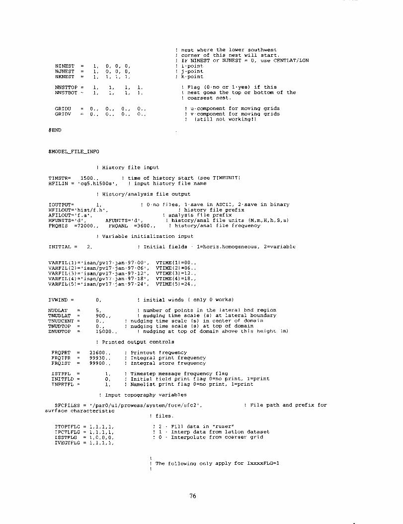
NINEST =
NJNEST =
NKNEST =
i, 0, 0, 0,
i, 0, 0, 0,
I, i, i, i,
NNSTTOP = i, I, i, i,
NNSTBOT = i, I, i, i,
GRIDU =
GRIDV =
SEND
0., 0., 0., 0.,
0., 0., 0., 0.,
[ nest where the lower southwest
! corner of this nest will start.
! IF NINEST or NJNEST = 0, use CENTLAT/LON
I i-point
! j-point
I k-point
! Flag (0-no or l-yes) if this
! nest goes the top or bottom of the
! coarsest nest.
! u-component for moving grids
! v-component for moving grids
! (still not working!)
SMODEL_FILE_INFO
! History file input
TIMSTR = 1500., ! time of history start (see TIMEUNIT)
HFILIN = 'cg5.h1500s' ! input history file name
! History/analysis file OUtput
IOUTPUT = I, ! 0-no files, l-save in ASCII, 2-save in binary
HFILOUT='hist/f.h', ' history file prefix
AFILOUT='f.a ', [ analysis file prefix
HFUNITS='d', AFUNITS='d', ! history/anal file units (M,m,H,h,S,s)
FRQHIS =72000., FRQANL =3600., ! history/anal file frequency
! Variable initialization input
INITIAL = 2, ! Initial fields - l=horiz.homogeneous, 2=variable
VARFIL(1)='isan/pv17-jan-97-00'
VARFIL(2)='isan/pv17-jan-97-06 '
VARFIL(3)='isan/pv17-jan-97-12'
VARFIL(4)='isan/pv17-jan-97-18 '
VARFIL(5)='isan/pv17-jan-97-24'
VTIME (I) =00.,
, VTIME (2) =06.,
, VTIME (3) =12.,
VTIME (4) =18.,
, VTIME (5) =24.,
IVWIND = 0,
NUDLAT = 5,
TNUDLAT = 900.,
TNUDCENT = 0.,
TNUDTO P = 0. ,
ZNUDTOP = 15000.,
! initial winds ( only 0 works)
! number of points in the lateral bnd region
! nudging time scale (s) at lateral boundary
! nudging time scale (s) in center of domain
l nudging time scale (s) at top of domain
! nudging at top of domain above this height (m)
! Printed output controls
FRQPRT = 21600., ! Printout frequency
FRQIPR = 99930., l Integral print frequency
FRQIST = 99900., l Integral store frequency
ISTPFL = i,
INITFLD = 0,
INPRTFL = i,
[ Input topography variables
SFCFILES = '/parO/ul/prowess/system/fore/sfc2',
surface characteristic
files.
ITOPTFLG = l,l,l,1, ! 2 - Fill data in "ruser"
IPCTLFLG = i,i,i,I,
ISSTFLG = 1,0,0,0,
IVEGTFLG = i,i,I,I,
! Timestep message frequency flag
l Initial field print flag 0=no print, l=print
I Namelist print flag 0=no print, l=print
! File path and prefix for
! 1 - Interp data from latlon dataset
! 0 - Interpolate from coarser grid
[
! The following only apply for IxxxxFLG=l
76
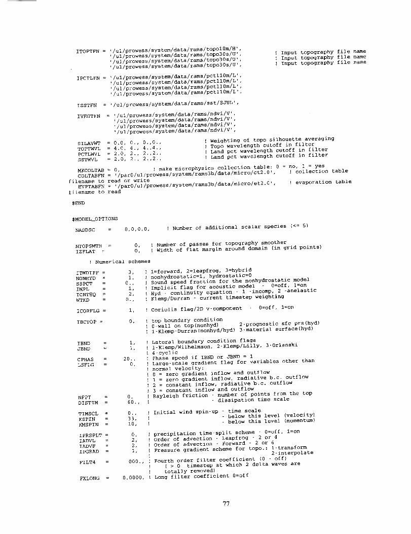
ITOPTFN = ,/ul/prowess/system/data/rams/topolOm/H',
'/ul/prowess/system/data/rams/topo3Os/U',
,/ul/prowess/system/data/rams/topo3Os/U',
,/ul/prowess/system/data/rams/topo3Os/U',
IPCTLFN = ,/ul/prowess/system/data/rams/pctllOm/L',
'/ul/prowess/system/data/rams/pctllOm/L',
,/ul/prowess/system/data/rams/pctllOm/L',
'/ul/prowess/system/data/rams/pctllOm/L',
ISSTFN
IVEGTFN
= '/ul/prowess/system/data/rams/sst/SJUL',
! Input topography file name
! Input topography file name
! Input topography file name
= '/ul/prowess/system/data/rams/ndvi/V',
'/ul/prowess/system/data/rams/ndvi/V',
'/ul/prowess/system/data/rams/ndvi/V',
'/ul/prowess/system/data/rams/ndvi/V',
SILAVWT = 0.0, 0., 0.,0.,
TOPTWVL = 4.0, 4., 4.,4.,
PCTLWVL = 2.0, 2., 2.,2.,
SSTWVL = 2.0, 2. , 2.,2.,
! Weighting of topo silhouette averaging
! Topo wavelength cutoff in filter
J Land pct wavelength cutoff in filter
! Land pct wavelength cutoff in filter
MKCOLTAB = 0, [ make microphysics collection table: 0 = no, 1 = yes
COLTABFN = '/parO/ul/prowess/system/rams3b/data/micro/ct2.0', ! collection table
filename to read or write
EVPTABFN = '/parO/ul/prowess/system/rams3b/data/micro/et2.0', ! evaporation table
filename to read
SEND
$MODEL OPTIONS
NADDSC = 0,0,0,0, l Number of additional scalar species (<= 5)
NTOPSMTH = 0,
IZFLAT = 0,
! Numerical schemes
ITMDIFF = 3,
NONHYD = I,
SSPCT = 0.,
IMPL = I,
ICNTEQ = 2,
WTKD = 0.,
ICORFLG = i,
IBCTOP = 0,
IBND = 1
JBND = 1
CPHAS = 20.
LSFLG = 0
NFPT = 0,
DISTIM = 60.,
TIMSCL = 0.,
KSPIN = 33,
KMSPIN = i0,
IPRSPLT = 0,
IADVL = 2,
IADVF = 2,
IPGRAD = i,
FILT4 = 000.,
FXLONG = 0.0000,
! Number of passes for topography smoother
! Width of flat margin around domain (in grid points)
! l=forward, 2=leapfrog, 3=hybrid
! nonhydrostatic=l, hydrostatic=0
! Sound speed fraction for the nonhydrostatic model
! Implicit flag for acoustic model 0=off, l=on
! Hyd - continuity equation - 1 -incomp, 2 -anelastic
! Klemp/Durran - current timestep weighting
! Coriolis flag/2D v-component 0=off, !=on
! top boundary condition
! 0-wall on top(nonhyd) 2-prognostic sfc prs(hyd)
! l-Klemp-Durran(nonhyd/hyd) 3-material surface(hyd)
! Lateral boundary condition flags
! l-Klemp/Wilhelmson, 2-Klemp/Lilly, 3-Orlanski
! 4-cyclic
! Phase speed if IBND or JBND = 1
! Large-scale gradient flag for variables other than
! normal velocity:
! 0 = zero gradient {nflow and outflow
[ 1 = zero gradient inflow, radiative b.c. outflow
! 2 = constant inflow, radiative b.c. outflow
! 3 = constant inflow and outflow
! Rayleigh friction - number of points from the top
! dissipation time scale
! Initial wind spin-up - time scale
! below this level (velocity)
! below this level (momentum)
! precipitation time-split scheme - 0=off, l=on
! Order of advection - Leapfrog - 2 or 4
! Order of advection - Forward - 2 or 6
! Pressure gradient scheme for topo.: l-transform
! 2-interpolate
! Fourth order filter coefficient (0 - off)
! ( > 0 timestep at which 2 delta waves are
! totally removed)
! Long filter coefficient 0=off
77
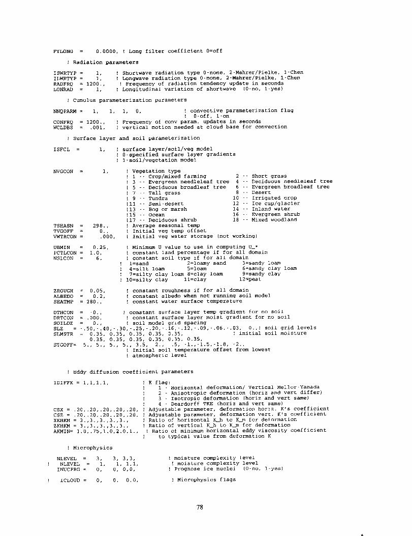
FYLONG = 0.0000, ! Long filter coefficient 0=off
! Radiation parameters
ISWRTYP = i, ! Shortwave radiation type 0-none, 2-Mahrer/Pielke, l-Chen
ILWRTYP = i, ! Longwave radiation type 0-none, 2-Mahrer/Pielke, l-Chen
RADFRQ = 1200., ! Frequency of radiation tendency update in seconds
LONRAD = i, ! Longitudinal variation of shortwave (0-no, l-yes)
! Cumulus parameterization parameters
NNQPARM = i, i, I, 0, ! convective parameterization flag
! 0-off, l-on
CONFRQ = 1200., ! Frequency of conv param, updates in seconds
WCLDBS = .001, ! vertical motion needed at cloud base for convection
! Surface layer and soil parameterization
ISFCL = i, ! surface layer/soil/veg model
! 0-specified surface layer gradients
! l-soil/vegetation model
NVGCON = i, ! Vegetation type
! 1
3
5
! 7
! 9
ill
!13
!15
!17
- Crop/mixed farming 2
Evergreen needleleaf tree 4
Deciduous broadleaf tree 6
Tall grass 8
Tundra 10
Semi-desert 12
Bog or marsh 14
Ocean 16
Deciduous shrub 18
Short grass
Deciduous needleleaf tree
Evergreen broadleaf tree
Desert
Irrigated crop
Ice cap/glacier
Inland water
Evergreen shrub
Mixed woodland
TSEASN = 298., ! Average seasonal temp
TVGOFF = 0., ! Initial veg temp offset
VWTRCON = .000, ] Initial veg water storage (not working)
UBMIN = 0.25, ! Minimum U value to use in computing U_*
PCTLCON = 1.0, ! constant land percentage if for all domain
NSLCON = 6, ! constant soil type if for all domain
! l=sand 2=loamy sand 3=sandy loam
! 4=silt loam 5=loam 6=sandy clay loam
! 7=silty clay loam 8=clay loam 9=sandy clay
! 10=silty clay 11=clay 12=peat
ZROUGH = 0.05, ! constant roughness if for all domain
ALBEDO = 0.2, ! constant albedo when not running soil model
SEATMP = 280., ! constant water surface temperature
DTHCON = -0., ! constant surface layer temp gradient for no soil
DRTCON = .000, ! constant surface layer moist gradient for no soil
SOILDZ = 0., ! soil model grid spacing
SLZ = -.50,-.40,-.30,-.25,-.20,-.16,-.12,-.09,-.06,-.03, 0.,! soil grid levels
SLMSTR = 0.35, 0.35, 0.35, 0.35, 0.35, ! initial soil moisture
0.35, 0.35, 0.35, 0.35, 0.35, 0.35,
STGOFF = 5., 5., 5., 5., 3.5, 2., .5, -1.,-1.5,-1.8, °2.,
! Initial soil temperature offset from lowest
! atmospheric level
! Eddy diffusion coefficient parameters
IDIFFK = l,l,l,l, ! K flag:
! I - Horizontal deformation/ Vertical Mellor-Yamada
! 2 - Anisotropic deformation (horiz and vert differ)
! 3 - Isotropic deformation (horiz and vert same)
! 4 - Deardorff TKE (horiz and vert same)
CSX = .20,.20,.20,.20,.20, ! Adjustable parameter, deformation horiz. K's coefficient
CSZ = .20,.20,.20,.20,.20, ! Adjustable parameter, deformation vert. K's coefficient
XKHKM = 3.,3.,3.,3.,3.,
ZKHKM = 3.,3.,3.,3.,3.,
AKMIN= 1.0,.75,1.0,2.0,1.,
! Microphysics
NLEVEL = 3, 3, 3,3,
NLEVEL = i, i, I,i,
INUCPRG = 0, 0, 0,0,
ICLOUD = 0, 0, 0,0,
! Ratio of horizontal K__h to K__m for deformation
! Ratio of vertical K_h to K__m for deformation
! Ratio of minimum horizontal eddy viscosity coefficient
! to typical value from deformation K
! moisture complexity level
! moisture complexity level
! Prognose ice nuclei (0-no, l-yes)
! Microphysics flags
78

! IRAIN = 0,
! IPRIS = 0,
! ISNOW = 0,
! IAGGR = 0,
: IGRAUP = 0,
! IHAIL = 0,
ICLOUD = 4,
IRAIN = 2,
IPRIS = 5,
I SNOW = 0,
IAGGR = 2,
IGRAUP = 0,
IHAIL = 2,
CPARM = .3e9,
0, 0 0,
0, 0 0,
0, 0 0,
0, 0 0,
0, 0 0,
0, 0 0,
4, 4,4,
2, 2,2,
5, 5,5,
O, 0,0,
2, 2,2,
0, 0,0,
2, 2,2,
.3e9, .3e9,
! ...................
] 0 - no species
! 1 - diagnostic concen.
! 2 - specified mean diameter
! 3 - specified y-intercept
! 4 - specified concentration
! Microphysics flags
! ...................
! 0 - no species
! 1 - diagnostic concen.
! 2 - specified mean diameter
! 3 - specified y-intercept
! 4 - specified concentration
! 5 - prognostic concentration
.3e9,
RPARM = .le-2, .le-2,.le-2, .le-2,
PPARM = 0., 0., 0., 0.,
SPARM = .le-2, .1e-2,.le-2, .le-2,
APARM = .le-2, .le-2,.le-2, .le-2,
GPARM = .le-2, .le-2,.le-2, .le-2,
HPARM = .3e-2, .3e-2,.3e-2, .3e-2,
! Microphysics parameters
! .........................
! Characteristic diameter,
! number concentration, or
! y-intercept
AMI0 = l.e-12, ! minimum crystal mass (kg)
! gnus for: cloud rain pris snow aggr graup hail
GNU : 2., 2., 2., 2., 2., 2., 2.,
SEND
SMODED_SOUND
! Sounding specification
IPSFLG=I,
ITSFLG=2,
IRTSFLG=3,
IUSFLG=0,
IUSRC = 0,
HS = 0.,
! gamma shape parms
' Flags for how sounding is specified
! specifies what is in PS array
! 0 - pressure (mb), 1 - heights (m), PS(1)=sfc press(mb)
! specifies what is in TS array
! 0 - temp(C), 1 - temp(K), 2 - pot. temp(K)
! specifies what is in RTS array
! 0 - dew pnt.(C), 1 - dew pnt. (K), 2 - mix rat(g/kg)
! 3 - relative humidity on %, 4 - dew pnt depression(K)
! specifies what is in US and VS arrays
I 0 - u,v component(m/s), I - umoms-direction, vmoms-speed
! source of wind profile:
! 0 umoms, vmoms, valid at sounding levels (PS)
! -i - usndg, vsndg, valid at model levels (Z)
PS = 1000.,1000.,2000.,3000.,3500.,4500.,?000.,I0000.,15000.,20000.,25000.,
TS = 300. ,302. ,304. ,306. ,308. ,310. ,314., 320. ,370. ,420. ,470.,
RTS = 60.,60.,60.,60.,I0.,10.,10.,i0.,i0.,i0.,I0.,
US = 3.,3.,3.,3.,3.,3.,3.,3.,3.,3.,3.,
VS = 0.,0.,0.,0.,0.,0.,0.,0.,0.,0.,0.,
USNDG = 0.,
VSNDG = 0.,
KMEANI = 0,
KMEAN2 = 0,
UMEAN = 0.0,
VMEAN = 0.0,
SEND
! Wind components if IUSRC = -i
!
! lower model level for calculation of (umean,vmean)
! upper model level for calculation of (umean,vmean)
! u-component for Galilean transformation
! v-component for Galilean transformation
SMODEL__PR_NT
! Specifies the fields to be printed during the simulation
NPLT = 6, ! Number of fields to be printed at each time
! for various cross-sections (limit of 50)
79
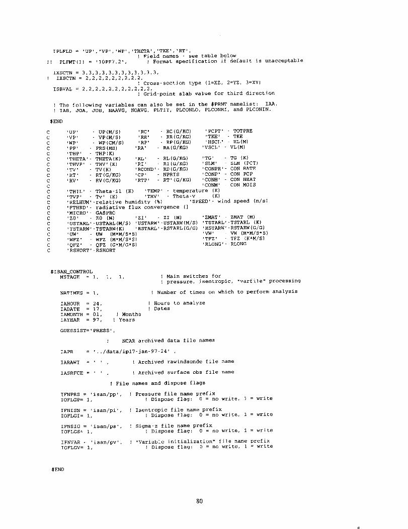
IPLFLD = 'UP' , 'VP', 'WP' , 'THETA', 'TKE', 'RT' ,
! Field names - see table below
! ! PLFMT(1) = '10PF7.2' , ! Format specification if default is unacceptable
IXSCTN = 3,3,3,3,3,3,3,3,3,3,3,3,
! IXSCTN = 2,2,2,2,2,2,2,2,2,
! Cross-section type (I=XZ, 2=YZ, 3=XY)
ISBVAL = 2,2,2,2,2,2,2,2,2,2,2,
! Grid-point slab value for third direction
! The following variables can also be set in the SPRNT namelist: IAA,
' IAB, JOA, JOB, NAAVG, NOAVG, PLTIT, PLCONLO, PLCONHI, and PLCONIN.
SEND
'UP' UP(M/S)
'VP' - VP(M/S)
'WP' WP(CM/S)
PP, PRS(MB)
THP' THP(K)
THETA'- THETA(K)
THVP' THV'(K)
TV' TV(K)
RT' RT(G/KG)
RV' RV(G/KG)
'THIL' Theta-il (K)
'TVP' - Tv' (K)
'RC' - RC(G/KG) 'PCPT
'RR' - RR(G/KG) 'TKE'
'RP' - RP(G/KG) 'HSCL
'RA' RA(G/KG) 'VSCL'
'RL' RL(G/KG) 'TG'
'RI' RI(G/KG) 'SLM'
'RCOND'- RD(G/KG) 'CONPR
'CP' NPRIS 'CONP'
'RTP' RT'(G/KG) 'CONH'
'CONM'
'TEMP' - temperature (K)
'THV' - Theta-v (K)
- TOTPRE
- TKE
HL(M)
- VL (M)
TG (K)
SLM (PCT)
CON RATE
CON PCP
CON HEAT
CON MOIS
'RELHUM'-relative humidity (%)
'FTHRD'- radiative flux convergence (]
'MICRO'- GASPRC
'Z0' - Z0 (M) 'Zl' ZI (M)
'USTARL'-USTARL(M/S) .USTARW'-USTARW(M/S)
'TSTARW'-TSTARW(K) ,RSTARL'-RSTARL(G/G)
'UW' - UW (M.M/S'S)
'WFZ' - WFZ (M.M/S'S)
'QFZ' - QFZ (G'M/G'S)
'RSHORT'-RSHORT
'SPEED'- wind speed (m/s)
'ZMAT' - ZMAT (M)
'TSTARL'-TSTARL (K)
'RSTARW'-RSTARW(G/G)
'VW' - VW (M'M/S'S)
'TFZ' - TFZ (K'M/S)
'RLONG'- RLONG
$ISAN CONTROL
MSTAGE = I, I, i,
NATIMES = I,
IAHOUR = 24,
IADATE = 17,
IAMONTH = 01, ! Months
IAYEAR = 97, ! Years
GUESSIST='PRESS'
! Main switches for
! pressure, isentropic, .varfile" processing
! Number of times on which to perform analysis
! Hours to analyze
! Dates
NCAR archived data file names
IAPR = ,../data/ip17-jan-97-24' ,
IARAWI = , , ! Archived rawindsonde file name
IASRFCE = ' ' , Archived surface obs file name, °
! File names and dispose flags
IFNPRS = 'isan/pp',
IOFLGP= i,
IFNISN = '!san/p!',
IOFLGI = i,
IFNSIG = 'isan/ps',
IOFLGS = I,
IFNVAR = 'isan/pv',
IOFLGV = I,
! Pressure file name prefix
! Dispose flag: 0 = no write, 1 = write
! Isentropic file name prefix
! Dispose flag: 0 = no write, 1 = write
! Sigma-z file name prefix
! Dispose flag: 0 = no write, 1 = write
! "Variable initialization" file name prefix
! Dispose flag: 0 = no write, 1 = write
SEND
8O

$ISAN_PRESSURE
NPRX=93,
NPRY=65,
NPRZ=I9,
! Pressure grid information:
] ...................................
! number of grid points in x (lon) direction
! number of grid points in y {lat) direction
! number of pressure levels
WPLON = -140.0,
SPLAT = 20.0,
! West longitude bound of pressure data access
! South latitude bound
! Latitude and longitude bounds are north and east
! if positive, south and west if negative.
SPCNPRX = 2.5, ! East-west grid spacing of pressure data
SPCNPRY = 1.25, ! North-south spacing
Pressure levels (mb) in input dataset to access
LEVPR = 1000,950,900,850,800,750,700,650,600,
550,500,450,400,350,300,250,200,150,100,
SEND
............................................
Isentropic and sigma-z processing............................................
SZSAN ISENTROPZC
! ...................................
! Specify isentropic levels
...................................
NISN = 32, ] number of isentropic levels
LEVTH = 280,282,284,286,288,290,292,294,296,298,300,303,306,309,312,
315,318,321,324,327,330,335,340,345,350,355,360,380,400,420,
440,460,
...................................
[ Analyzed grid information:
[ ...................................
NIGRIDS = 3, [ number of RAMS grids to analyze
TOPSIGZ = 20000., ! sigma-z coordinates to about this height
HYBBOT = 4000., , Bottom (m) of blended sigma-z/isentropic layer in varfiles
HYBTOP = 6000., ! TOp (m) of blended sigma-z/isentropic layer
SFCINF = 1000., ! Vertical influence of surface observation analysis
SIGZWT = 1., ! Weight for sigma-z data in varfile:
! 0. = no sigz data, l.=full weight from surface to HYBBOT
NFEEDVAR = l, ! ] = feed back nested grid varfile info, 0 = don't
! ...................................
! Observation number limits:
! ...................................
MAXSTA=I50, ] maximum number of rawindsondes (archived + special)
MAXSFC=I000, ! maximum number of surface observations
IARCSND = i, ! Input archived soundings ? (0-no, l-yes)
IARCSFC = i, _ Input archived surface obs ?
ISPCSND = 0, ! Input special soundings ?
ISPCSFC = 0, ! Input special surface obs ?
NONLYS = 0, ! Number of stations only to be used
IDONLYS ='76458', ! Station ID's used
NOTSTA = 0, ! Number of stations to be excluded
NOTID ='r76458' ! Station ID's to be excluded
! Prefix with 'r' for rawindsonde, 's' for surface
STASEP = .001, ! Minimum surface station separation in degrees.
! Any surface obs within this distance
81
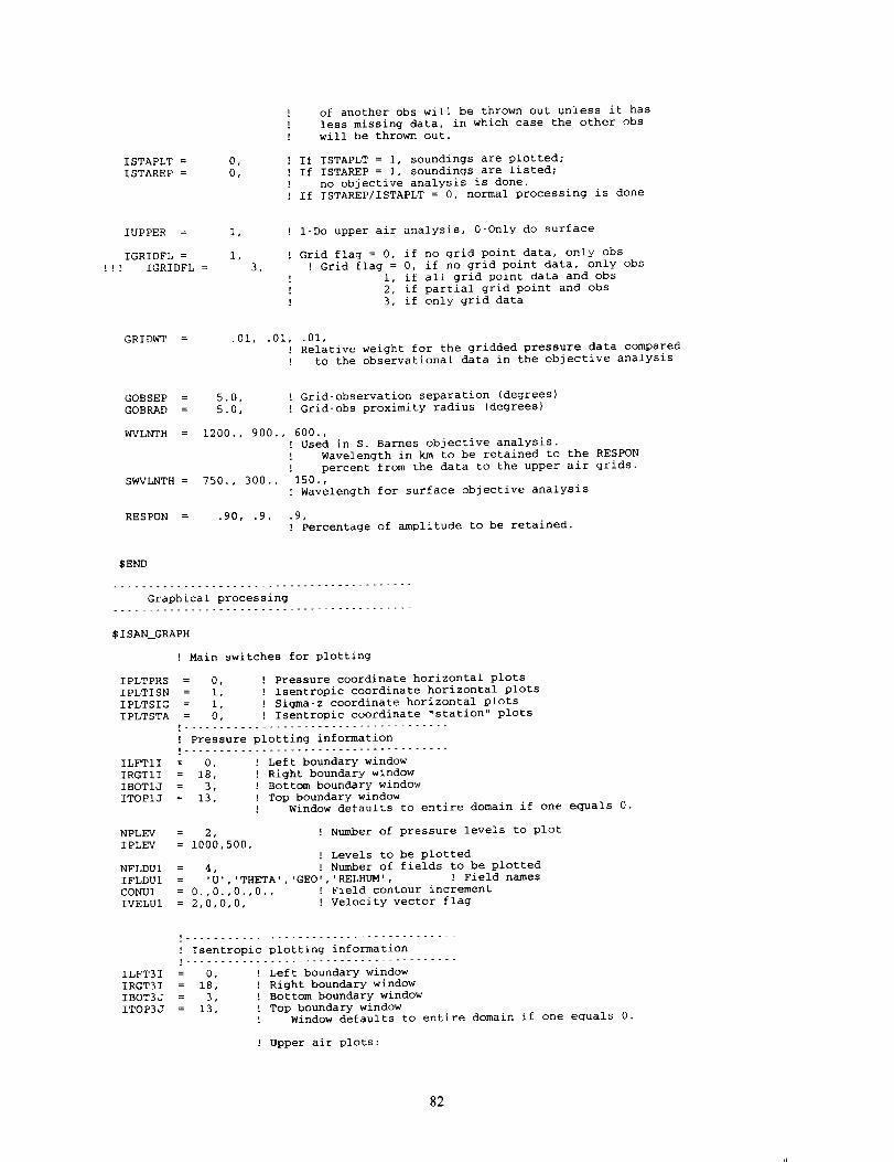
ISTAPLT = 0,
ISTAREP = 0,
of another obs will be thrown out unless it has
less missing data, in which case the other obs
will be thrown out.
! If ISTAPLT = I, soundings are plotted;
! If ISTAREP = i, soundings are listed;
! no objective analysis is done.
! If ISTAREP/ISTAPLT = 0, normal processing is done
IUPPER = I,
IGRIDFL = I,
IGRIDFL = 3,
[ l-Do upper air analysis, 0-Only do surface
! Grid flag = 0, if no grid point data, only obs
! Grid flag = 0, if no grid point data, only obs
i, if all grid point data and obs
[ 2, if partial grid point and obs
! 3, if only grid data
GRIDWT = .01, .01, .01,
! Relative weight for the gridded pressure data compared
! to the observational data in the objective analysis
GOBSEP = 5.0,
GOBRAD = 5.0,
WVLNTH = 1200., 900.,
SWVLNTH = 750., 300.,
RESPON = .90, .9,
! Grid-observation separation (degrees)
! Grid-obs proximity radius (degrees)
600.,
! Used in S. Barnes objective analysis.
! Wavelength in km to be retained to the RESPON
! percent from the data to the upper air grids.
150.,
! Wavelength for surface objective analysis
.9,
! Percentage of amplitude to be retained.
SEND
Graphical processing...........................................
SISAN GRAPH
IPLTPRS
IPLTISN
IPLTSIG
IPLTSTA
ILFTII
IRGTII
IBOTIJ
ITOPIJ
NPLEV
IPLEV
NFLDUI
IFLDUI
CONUI
IVELUI
! Main switches for plotting
= 0, ! Pressure coordinate horizontal plots
= I, ! Isentropic coordinate horizontal plots
= i, ! Sigma-z coordinate horizontal plots
= 0, ! Isentropic coordinate "station" plots
! ......................................
! Pressure plotting information
! ......................................
= 0, ! Left boundary window
= 18, ! Right boundary window
= 3, 2 Bottom boundary window
= 13, ! Top boundary window
! Window defaults to entire domain if one equals 0.
= 2, ! Nu_uber of pressure levels to plot
= 1000,500,
J Levels to be plotted
= 4, ! Number of fields to be plotted
= 'U','THETA','GEO','RELHUM', ! Field names
= 0.,0.,0.,0., ! Field contour increment
= 2,0,0,0, ! Velocity vector flag
ILFT3I
IRGT3I
IBOT3J
ITOP3J
! .......................................
! Isentropic plotting information
.......................................
= 0, ! Left boundary window
= 18, ! Right boundary window
= 3, ! Bottom boundary window
= 13, ! Top boundary window
! Window defaults to entire domain if one equals 0.
! Upper air plots:
82

IUP3BEG = 340,
IUP3END = 4000,
IUP3INC = 60,
! Starting isentropic level for plotting
! Ending isentropic level
! Level increment
NFLDU3 = 4,
IFLDU3 = 'U','PRESS'
CONU3 = 0.,0.,
IVELU3 = 1,0,
! Number of fields to be plotted
,,MONTSTR','RELHUM', ! Field names
2 Field contour increment
! Velocity vector flag
! .......................................
! Surface plotting information
! .......................................
! Uses isentropic plotting window info
NFLDS3 = 4, ! Number of surface fields to plot
IFLDS3 = ,U,,,TEMP','PRESS','RELHUM', ! Field names
CONS3 = 0.,0.,0.,0.,0., ! Field contour increment
IVELS3 = 1,0,0,0,0, ! Velocity vector flag
! .......................................
! Sigma-z plotting information
! .......................................
! Uses isentropic plotting window info
ISZBEG = 2, ! Starting sigma-z level for plotting
ISZEND = 26, ! Ending sigma-z level
ISZINC = 6, ! Level increment
NFLDSZ = 4, ! Number of fields to be plotted
IFLDSZ = ,U,,,PRESS', ,THETA','RELHUM', ! Field names
CONSZ = 0.,0., ! Field contour increment
IVELSZ = 1,0, ! Velocity vector flag
! .......................................
! "Station" plotting information
! .......................................
NPLTRAW = 9, _ Approximate number of raw rawinsonde plots per
! frame. 0 turns off plotting.
NSTIS3 = 3, ! number of station surface plots
ISTIS3 = ,PRESS,,,TEMP','RELHUM', ! field names
! .......................................
! Cross-section plotting information
! .......................................
NCROSS3 = 0,
ICRTYP3 = 2,1,
ICRA3 = i,I,
ICRB3 = 35,43,
ICRL3 = 22,25,
NCRFLD3 = 3,
ICRFLD3 = 'MIXRAT','RELHUM'
THCON3 = 5.,5.,5.,
ACON3 = 0.,0.,0.,
! number of cross section slabs
! type of slab: I=E-W, 2=N-S
! left window
! right window
! cross section location
! number of plots on each cross section
,'THETAE', ! field names
! contour interval of isentropes
! contour interval of other field
J U U
[ V v
! TEMP PRESS
! GEO GEO
] RELHUM RELHUM
! MIXRAT MIXRAT
! THETA THETA
! SPEED SPEED
! ENERGY ENERGY
! THETAE THETAE
! SPRESS SPRESS
U U
V V
PRESS PRESS
TEMP THETA
RELHUM RELHUM
MIXRAT
83
APPENDIX C
ERDAS HYPACT_IN f'de
84
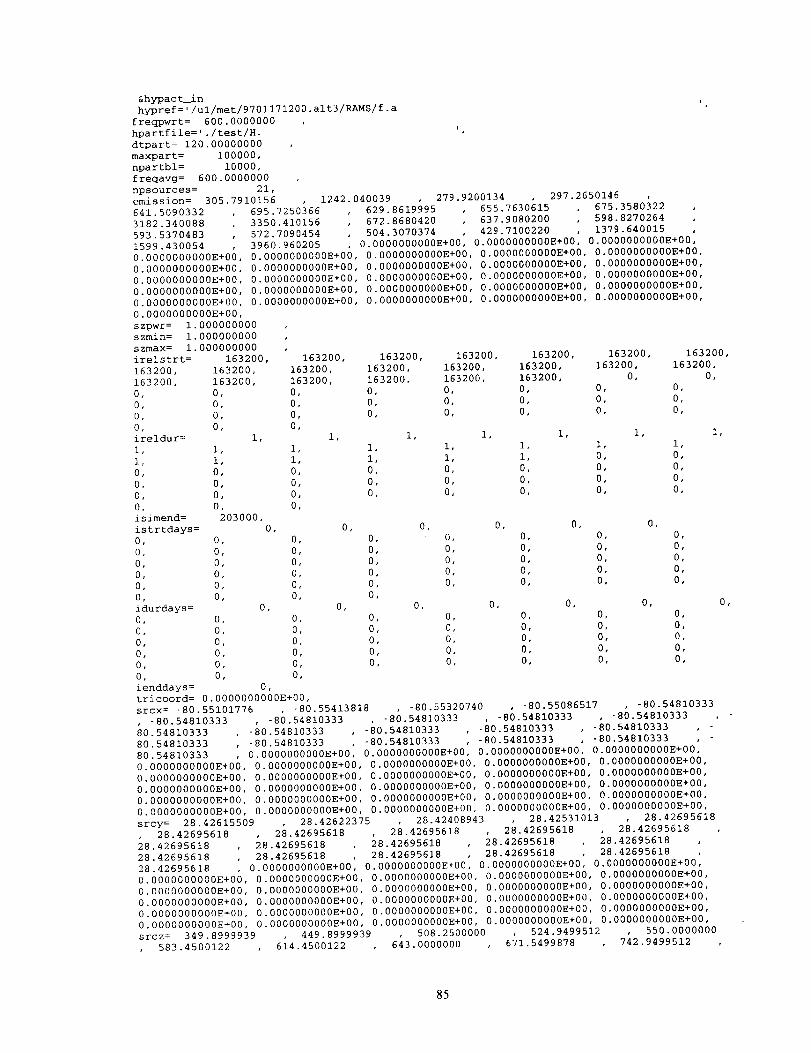
&hypactin
hypref='/ul/met/9701171200.alt3/RAMS/f.a
freqpwrt= 600.0000000 ,
hpartfile='./test/H. ',
dtpart = 120.00000000
maxpart = 100000,
npartbl= 10000,
freqavg= 600.0000000
npsources = 21,emission= 305.7910156 1242.040039 279.9200134 297.2650146
641.5090332 , 695.7250366 , 629.8619995 , 655.7630615 675.3580322
3182.340088 , 3350.410156 , 672.8680420 , 637.9080200 , 598.8270264 ,
593.5370483 , 572.7090454 , 504.3070374 429.7100220 , 1379.640015
1599.430054 , 3960.960205 , 0.0000000000E+001 0.0000000000E+00 0.0000000000E+001
0.0000000000E+00, 0.0000000000E+00, 0.0000000000E+00, 0.0000000000E+00, 0.0000000000E+00,
0.0000000000E+00, 0.00000000DOE+00, 0.0000000000E+00, 0.0000000000E+00, 0.0000000000E+00,
0.0000000000E+00, 0.0000000000E+00, 0.0000000000E+00, 0.0000000000E+00, 0.0000000000E+00,
0.0000000000E+00, 0.00000000O0E+00, 0.0000000000E+00, 0.0000000000E+00, 0.0000000000E+00,
0.0000000000E+00, 0.0000000000E+00, 0.0000000000E+00, 0.0000000000E+00, 0.0000000000E+00,
0.0000000000E+00,
szpwr = 1.000000000szmin= 1.000000000
szmax = 1.000000000
irelstrt=
163200,
163200,
0,
0,
0,
0,
ireldur=
i,
i,
0,
0,
0,
0,
isimend =
istrtdays =
0,
0,
0,
0,
0,
0,
idurdays =
0
0
0
0
0
0
ienddays =
163200,
163200,
163200,
0,
0,
0,
0,
i,
i,
i,
0,
0,
0,
0,
203000,
0,
0,
0,
0,
0,
0,
0,
0,
0
0
0
0
0
0
0,
163200, 163200,
163200, 163200,
163200, 163200,
0, 0,
0, 0,
0, 0,
0,
i, i,
i, I,
i, i,
0, 0,
0, 0,
0, 0,
0,
0, 0,
O, O, O,
O, O, O,O, O, O,
O, O, O,O, O, O,O, O,
O, O,O, O, O,
O, O, O,O, O, O,
O, O, O,
O, O, O,O,
tricoord= 0.0000000000E+00,
srcx = -80.55101776 -80.55413818 -80.55320740
e,
163200, 163200, 163200, 163200,
163200, 163200, 163200, 163200,
163200, 163200, 0, 0,
0, 0, 0, 0,
O, O, O, O,
O, O, O, O,
i, I, I, I,
i, i, i, i,
i, I, 0, 0,
O, O, O, 0,
O, O, O, O,
O, O, O, O,
O, O,
0, 0, 0,
0, 0, 0,
0, 0, 0,
0, 0, 0,
0, 0, 0,
0,
O, O, O, O,O, O, O,
O, O, O,O, O, O,
O, O, O,O, O, O,
, -80.55086517 , -80.54810333
-80.54810333 -80.54810333 -80.54810333 -80.54810333 , -80.54810333
80.54810333 , -80.54810333 , -80.54810333 , -80.54810333 , -80.54810333 ,
80.54810333 , -80.54810333 , -80.54810333 , -80.54810333 , -80.54810333 ,
80.54810333 , 0.0000000000E+00, 0.0000000000E+00, 0.0000000000E+00, 0.0000000000E+00,
0.0000000000E+00, 0.0000000000E+00, 0.0000000000E+00, 0.0000000000E+00, 0.0000000000E+00,
0.0000000000E+00, 0.0000000000E+00, 0.0000000000E+00, 0.0000000000E+00, 0.0000000000E+00,
0.0000000000E+00, 0.0000000000E+00, 0.0000000000E+00, 0.0000000000E+00, 0.0000000000E+00,
0.0000000000E+00, 0.0000000000E+00, 0.0000000000E+00, 0.0000000000E+00, 0.0000000000E+00,
0.0000000000E+00, 0.0000000000E+00, 0.0000000000E+00, 0.0000000000E+00, 0.0000000000E+00,
srcy= 28.42615509 28.42622375 28.42408943 , 28.42531013 28.4269561828.42695618 2_.42695618 2_.42695618 28.42695618 2_.42695618
18.42695618 _8.42695618 _8.42695618 18.42695618 , _8.4269561828.42695618 28.42695618 28.42695618 28.42695618 28.42695618
28.42695618 , 0.0000000000E+001 0.0000000000E+001 0.0000000000E+001 0.0000000000E+001
0.0000000000E+00, 0.0000000000E+00, 0.0000000000E+00, 0.0000000000E+00, 0.0000000000E+00,
0.0000000000E+00, 0.0000000000E+00, 0.0000000000E+00, 0.0000000000E+00, 0.0000000000E+00,
0.0000000000E+00, 0.0000000000E+00, 0.0000000000E+00, 0.0000000000E+00, 0.0000000000E+00,
0.0000000000E+00, 0.0000000000E+00, 0.0000000000E+00, 0.0000000000E+00, 0.0000000000E+00,
0.0000000000E+00, O.O000000000E+O0, O.O000000000E+O0, 0.0000000000E+00, 0.0000000000E+00,
srcz = 349.8999939 449.8999939 508.2500000 524.9499512 550.0000000
583.4500122 6{4.4500122 , 643.0000000 , 671.5499878 742.9499512
85
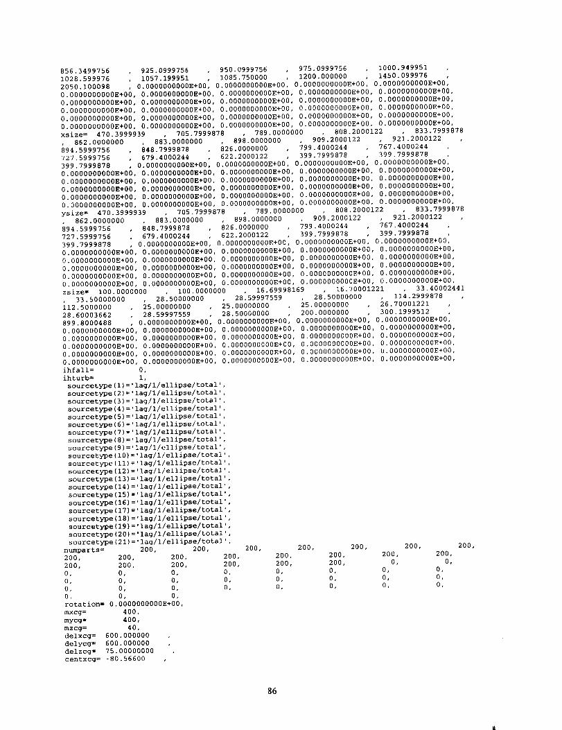
856.3499756 , 925.0999756 950.0999756 , 975.0999756 1000.949951
1028.599976 , 1057.199951 , 1085.750000 , 1200.000000 , 1450.099976 ,
2050.100098 , 0.0000000000E+00, 0.0000000000E+00, 0.0000000000E+00, 0.0000000000E+00
0.0000000000E+00, 0.0000000000E+00, 0.0000000000E+00, 0.0000000000E+00, 0.0000000000E+00,
0.0000000000E+00, 0.0000000000E+00, O.O000000000E+00, 0.0000000000E+00, 0.0000000000E+00,
0.0000000000E+00, 0.0000000000E+00, 0.0000000000E+00, 0.0000000000E+00, 0.0000000000E+00,
0.0000000000E+00, 0.0000000000E+00, 0.0000000000E+00, 0.0000000000E+00, 0.0000000000E+00,
0.0000000000E+00, 0.0000000000E+00, 0.0000000000E+00, 0.0000000000E+00, 0.0000000000E+00,
xsize= 470.3999939 705.7999878 789.0000000 808.2000122 833.7999878
862.0000000 883.0000000 898.0000000 909.2000122 92{.2000122
_94.5999756 , _48.7999878 , _26.0000000 , _99.4000244 %7.4000244727.5999756 , 679.4000244 622.2000122 399.7999870 399.7999078
399.7999878 , 0.0000000000E+001 0.0000000000E+001 0.0000000000E+001 O.O000000000E+O01
0.0000000000E+00, O.0000000000E+00, 0.0000000000E+00, 0.0000000000E+00, 0.0000000000E+00,
0.0000000000E+00, 0.0000000000E+00, 0.0000000000E+00, 0.0000000000E+00, 0.0000000000E+00,
0.0000000000E+00, 0.0000000000E+00, 0.0000000000E+00, 0.0000000000E+00, 0.0000000000E+00,
0.0000000000E+00, 0.0000000000E+00, 0.0000000000E+00, 0.0000000000E+00, 0.0000000000E+00,
0.0000000000E+00, 0.0000000000E+00, 0.0000000000E+00, 0.0000000000E+00, 0.0000000000E+00,
ysize= 470.3999939 705.7999878 789.0000000 808.2000122 833.7999878
862.0000000 88_.0000000 89_.0000000 90;.2000122 92i.2000122894.5999756 , 848.7999878 , 826.0000000 799.4000244 , 767.4000244 '
727.5999756 679.4000244 622.2000122 , 399.7999878 399.7999878399.3999838 , 0.0000000000E+001 0.0000000000E+00 0.0000000000E+001 0.0000000000E+001
0.0000000000E+00, 0.0000000000E+00, 0.0000000000E+00, 0.0000000000E+00, 0.0000000000E+00,
0.0000000000E+00, 0.0000000000E+00, 0.0000000000E+00, 0.0000000000E+00, 0.0000000000E+00,
0.0000000000E+00, 0.0000000000E+00, 0.0000000000E+00, 0.0000000000E+00, 0.0000000000E+00,
0.0000000000E+00, 0.0000000000E+00, 0.0000000000E+00, 0.0000000000E+00, 0.0000000000E+00,
0.0000000000E+000 0.0000000000E+00, 0.0000000000E+00, 0.0000000000E+00, 0.0000000000E+00,
zsize= i00.0000000 100.0000000 16.69998169 16.70001221 33.40002441
33.50000000 28[50000000 28[59997559 28[50000000 i14.2999878
112.5000000 25.00000000 25.00000000 25.00000000 , 26.70001221 ,
28.60003662 28.59997559 28.50000000 , 200.0000000 , 300.1999512899.8000488 , 0.0000000000N+001 0.0000000000E+00 0.0000000000E+00 0.0000000000E+001
0.0000000000E+00, 0.0000000000E+00, 0.0000000000E+00, 0.0000000000E+00, 0.0000000000E+00,
0.0000000000E+00, 0.0000000000E+00, 0.0000000000E+00, 0.0000000000E+00, 0.0000000000E+00,
0.0000000000E+00, 0.0000000000E+00, 0.0000000000E+00, 0.0000000000E+00, 0.0000000000E+00,
0.0000000000E+00, 0.0000000000E+00, 0.0000000000E+00, 0.0000000000E+00, 0.0000000000E+00,
0.0000000000E+00, 0.0000000000E+00, 0.0000000000E+00, 0.0000000000E+00, 0.0000000000E+00,
ihfall = 0,
ihturb = I,
sourcetype(1)='lag/i/ellipse/total
sourcetype(2)='lag/I/ellipse/total
sourcetype(3)='lag/I/ellipse/total
sourcetype(4)='lag/I/ellipse/total
sourcetype(5)='lag/I/ellipse/total
sourcetype(6)='lag/I/ellipse/total
sourcetype(7)='lag/I/ellipse/total
sourcetype(8)='lag/I/ellipse/total
sourcetype(9)='lag/i/ellipse/total
sourcetype(10)='lag/I/ellipse/total
sourcetype(ll)='lag/I/ellipse/total
sourcetype(12)='lag/i/ellipse/total
sourcetype(13)='lag/i/ellipse/total
sourcetype(14)='lag/i/ellipse/total
sourcetype(15)='lag/i/ellipse/total
sourcetype(16)='lag/I/ellipse/total
sourcetype(17)='lag/i/ellipse/total
sourcetype(18)='lag/i/ellipse/total
sourcetype(19)='lag/I/ellipse/total
sourcetype(20)='lag/I/ellipse/total
sourcetype(21)='lag/I/ellipse/total
numparts = 200, 200,
200, 200, 200,
200, 200, 200,
O, 0, O,
O, O, O,
O, O, O,
0, 0, 0,
rotation= 0.0000000000E+00,
mxcg= 400,
mycg = 400,
mzcg = 40,
delxcg = 600.000000
delycg = 600.000000
delzcg = 75.00000000 ,
centxcg = -80.56600
200, 200, 200, 200, 200,
200, 200, 200, 200, 200,
200, 200, 200, 0, 0,
0, 0, 0, 0, 0,
0, 0, 0, 0, 0,
0, 0, 0, 0, 0,
86

centycg = 28.00 ,
ixyslab = 4
ixzslab= i00,
iyzslab = O,
&end
87

APPENDIX D
PROWESS HYPACT_IN f'de
88
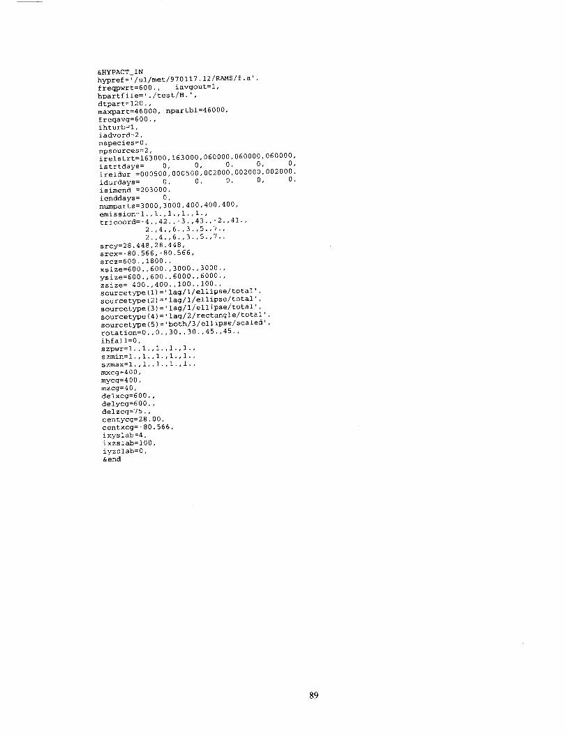
&HYPACT_IN
hypref='/ul/met/970117.12/RAMS/f.a '
freqpwrt=600., iavgout=l,
hpartfile='./test/H.',
dtpart=120.,
maxpart=46000, npartbl=46000,
freqavg=600.,
ihturb=l,
iadvord=2,
nspecies=0,
npsources=2,
irelstrt=163000,163000,060000,060000,060000,
istrtdays = 0, 0, 0, 0, 0,
ireldur =000500,000500,002000,002000,002000,
idurdays = 0, 0, 0, 0, 0,
isimend =203000,
ienddays= 0,
nuraparts=3000,3000,400,400,400,
emission=l.,l.,l.,l.,l.,
tricoord=-4.,42.,-3.,43.,-2.,41.,
2.,4.,6.,3.,5.,7.,
2.,4.,6.,3.,5.,7.,
srcy=28.448,28.448,
srcx=-80.566,-80.566,
srcz=600.,1800.,
xsize=600.,600.,3000.,3000.,
ysize=600.,600.,6000.,6000.,
zsize= 400.,400.,i00.,I00.,
sourcetype(1)='lag/i/ellipse/total ' ,
sourcetype(2)='lag/I/ellipse/total',
sourcetype(3)='lag/I/ellipse/total'
sourcetype(4)='lag/2/rectangle/total ' ,
sourcetype(5)='both/3/ellipse/scaled',
rotation=0.,0.,30.,30.,45.,45.,
ihfall=0,
szpwr=l.,l.,l.,l.,l.,
szmin=l.,l.,l.,l.,l.,
szmax=l. , 1. , 1. , 1. , 1. ,
mxcg=400,
mycg=400,
mzcg=40,
delxcg=600.,
delycq=600.,
delzcg=75.,
centycg=28.00,
centxcg=-80.566,
ixyslab=4,
ixzslab=100,
iyzslab=0,
&end
89

NOTICE
Mention of a copyrighted, trademarked or proprietary product, service, or document does not constitute
endorsement thereof by the author, ENSCO, Inc., the AMU, the National Aeronautics and Space
Administration, or the United States Government. Any such mention is solely to inform the reader of the
resources used to conduct the work reported herein.
90

REPORT DOCUMENTATION PAGEForm ApprovedOMB No. 0704-0188
Public te_orting burden for this coll_ion of information is estimated to avera=ge 1 hour per response, illcluditlg me lime for rev_ng ir61rgcliOrl$, searching existing data sources, Oatbedng
and maJnla_n_r_ _ data needed, an_ completing and rev_w_ng the collection of iofonl_atJon Send cornmenls reg_ng _ I_tde_ i_imate or any o_er aspect of _ collection ofinforrriation, including suggestions lot reduOn_g this i_rden Io Washington HeedquarletS Services, Directorate for information Ot0eratloqs and Reports, 1215 Jefferson Davis Highway, Suite
1204, Arlington, VA 22202-4302, and to the Office ot Managemant and Bu(:tget, PapenNo_ Reduction ProJec! (0704-0188), Wa_dlington, DC 20503
1. AGENCY USE ONLY (Leave blank) 2. REPORT DATE
July 20004, TITLE AND SUBTIITi_E
Delta II Explosion Plume Analysis Report6. AUTHOR(S)
Randolph J. Evans7. PERFORMINGORGANIZATIONNAME(S)ANDADDRESS(ES)
ENSCO, Inc., 1980 North Atlantic Avenue, Suite 230, CocoaBeach, FL 32931
9. SPONSORING/MONITORINGAGENCYNAME(S)ANDADDRESS(ES)
NASA, John F. Kennedy Space Center, Code AA-C-1, Kennedy
Space Center, FL 32899
3. REPORT TYPE AND DATES COVERED
Contractor Report5. FUNDING NUMBERS
C-NAS10-96018
PERFORMING ORGANIZATIONREPORT NUMBER
00-OO4
10. SPONSORING/MON ITORING
AGENCY REPORTNUMBER
CR-2000-208582
11.SUPPLEMENTARYNOTES
Subject Cat.: #47 (Meteorology and Climatolo_p/)12A.DISTRIBUTION/AVAILABILITYSTATEMENT
Unclassified - Unlimited
12B. D ISTRIBUTION CODE
13. ABSTRACT (Maximum 200 Words)
A Delta II rocket exploded seconds after liftoff from Cape Canaveral Air Force Station (CCAFS) on17 January 1997. The cloud produced by the explosion provided an opportunity to evaluate the modelswhich are used to track potentially toxic dispersing plumes and clouds at CCAFS. The primary goal of
this project was to conduct a case study of the dispersing cloud and the models used to predict thedispersion resulting from the explosion. The case study was conducted by comparing mesoscale anddispersion model results with available meteorological and plume observations.
The models used in the study are part of the Eastern Range Dispersion Assessment System (ERDAS)and include the Regional Atmospheric Modeling System (RAMS), HYbrid Particle And Concentration
Transport (HYPACT), and Rocket Exhaust Effluent Dispersion Model (REEDM).
The primary observations used for explosion cloud verification of the study were from the National
Weather Service's Weather Surveillance Radar 1988-Doppler (WSR-88D). Radar reflectivitymeasurements of the resulting cloud provided good estimates of the location and dimensions of the cloudover a four-hour period after the explosion.
The results indicated that RAMS and HYPACT models performed reasonably well, Future upgradesto ERDAS are recommended.
14.SUBJECTTERMS 15.NUMBEROFPAGES 104
Dispersion, Diffusion, Mesoscale Modeling, Launch Plume, 16.PRICECODE
Rocket Explosion, Weather Radar, RAMS, HYPACT, ERDAS,
REEDM, Hazardous Material, Toxic Cloud17. SECURITYCLASSIFICATION18. SECURITYCLASSIFICATION19. SECURITYCLASSIFICATION20. LIMITATIONOFABSTRACT
OFREPORT OFTHISPAGE OFABSTRACT
UNCLASSIFIED UNCLASSIFIED UNCLASSIFIED NONE