improving source reconstructions by combining bioelectric and biomagnetic data

Improving source reconstructions by combining bioelectricand biomagnetic data

Manfred Fuchsa,*, Michael Wagnera, Hans-Aloys Wischmanna, Thomas Ko¨hlera, Annette Theißena,Ralf Drenckhahna, Helmut Buchnerb

aPhilips Research Laboratories Hamburg, Ro¨ntgenstrasse 24, D-22335 Hamburg, GermanybDepartment of Neurology, RWTH, Pauwelsstrasse 30, D-52074 Aachen, Germany

Accepted for publication: 2 March 1998

Abstract

Objectives: A framework for combining bioelectric and biomagnetic data is presented. The data are transformed to signal-to-noise ratiosand reconstruction algorithms utilizing a new regularization approach are introduced.

Methods: Extensive simulations are carried out for 19 different EEG and MEG montages with radial and tangential test dipoles atdifferent eccentricities and noise levels. The methods are verified by real SEP/SEF measurements. A common realistic volume conductor isused and the less well known in vivo conductivies are matched by calibration to the magnetic data. Single equivalent dipole fits as well asspatio-temporal source models are presented for single and combined modality evaluations and overlaid to anatomic MR images.

Results: Normalized sensitivity and dipole resolution profiles of the different EEG/MEG acquisition systems are derived from thesimulated data. The methods and simulations are verified by simultaneously measured somatosensory data.

Conclusions: Superior spatial resolution of the combined data studies is revealed, which is due to the complementary nature of bothmodalities and the increased number of sensors. A better understanding of the underlying neuronal processes can be achieved, since animproved differentiation between quasi-tangential and quasi-radial sources is possible. 1998 Elsevier Science Ireland Ltd. All rightsreserved

Keywords:Electroencephalogram; Magnetoencephalogram; SEP; SEF; Source reconstruction; Regularization; Boundary element method

1. Introduction

Source reconstructions combining bioelectric and bio-magnetic data promise to benefit from the advantages ofboth modalities (Cohen and Cuffin, 1979, 1983, 1987,1991; Cohen et al., 1990; Lopes da Silva et al., 1991; Mau-guiere, 1992). Electroencephalographic (EEG) measure-ments can be carried out with an optimized electrodearrangement and provide nearly equal sensitivities for tan-gentially- and radially-oriented sources. Due to this unspe-cific sensitivity distribution EEG data often suffer from alimited signal-to-noise-ratio (SNR) and exhibit rather com-plex field structures. Magnetoencephalographic (MEG) gra-diometer systems have an increased sensitivity fortangential superficial sources, leading to an improved

SNR and a larger specificity for this class of generators.On the other hand this means that MEG sensor arrays aremore or less blind to (quasi-)radial neural current compo-nents and deep sources, leading to a reduced complexity ofthe measured field patterns. Therefore, a combination ofboth complementary methods should be able to reveal radialdipole components and stabilize the reconstruction of tan-gential sources by an increased information content and animproved overall SNR.

In order to combine both modalities in a unified frame-work, different problems have to be solved:

• The different measures have to be transformed to acommon basis. This is done by referencing eachsensor to its individual noise statistics (Greenblatt,1995; Pflieger et al., 1998). So every measurementchannel contributes with its statistical relevance tothe ensuing evaluation procedures. One method to

Electroencephalography and clinical Neurophysiology 107 (1998) 93–111

0013-4694/98/$19.00 1998 Elsevier Science Ireland Ltd. All rights reservedPII S0013-4694(98)00046-7 EEG 97820

* Corresponding author. Tel.: +49 40 50782691; fax: +49 40 50782887.

automatically determine the noise level of each sen-sor is to use the standard deviation of a fraction ofthe smallest signal levels of the total latency range,e.g. the smallest 20%. This method of courserequires about 20% signal-free (e.g. pre-trigger)samples in the measurement.

• For unified reconstruction algorithms, a commonvolume conductor model has to be used. EEGdata strongly depend on the head’s shape and itsconductivities (Cuffin, 1990). For example, involume conductor models with one compartmentonly, the measured signals are inversely propor-tional to the conductivity. MEG signals in the sphe-rical volume conductor approximation are not at allaffected by the conductivity. With more realisti-cally-shaped volume conductor models (e.g. bound-ary element method (BEM) models) the MEG datashow only a weak dependence on the electric prop-erties of the compartments. Furthermore the indivi-dual real (in-vivo) tissue conductivities are not wellknown (Geddes and Baker, 1963). We have thuschosen latencies where single dominantly tangentialdipoles can explain the measured data very well forboth modalities and used them for matching theconductivities of the volume conductor model.Thus the magnetic data are used for calibratingthe electric conductivities via a common scalingfactor that keeps the relative conductivities of themodel compartments (brain, skull, skin) constant.

• MEG reconstructions with realistic volume conduc-tor models tend to overemphasize quasi-radial cur-rent components due to their very small gain(Menninghaus and Lu¨tkenhoner, 1995). Therefore,dipole regularization techniques have to be intro-duced in order to limit or suppress these low-gaincomponents at least in single-modality MEG eva-luations. In EEG or combined EEG/MEG examina-tions, the electric data are expected to reduce theseeffects due to their nearly isotropic orientationalsensitivity distributions (Fuchs et al., 1998b).

For testing the methods described above in view of theirspatial resolution, simulations with different electrode andmagnetometer/gradiometer set-ups were used with a 3spherical shells volume conductor model. White noise,uncorrelated across sensors, was added to calculated fielddistributions to get statistically relevant results for differentdipole depths and signal-to-noise-ratios. Equivalent dipolarsources were then fitted with single and combined modalities.

Evoked somatosensory measurements from electric med-ianus nerve stimulation with simultaneously recorded 31electrodes EEG (SEP) and 31 channels MEG (SEF) (Buch-ner et al., 1994) were used to test combined evaluations withreal data. The volume conductor was modeled by a BEMconsisting of 3 compartments. The head/brain compart-ments for the BEM model were semi-automatically segmen-

ted, and triangulated from magnetic resonance (MR) images(Wagner et al., 1995). Single equivalent dipoles, corticallyconstrained deviation scans (Fuchs et al., 1994, 1998a), andspatiotemporal dipole models (Scherg and von Cramon,1985; Mosher et al., 1992) were used to compare singlemodality and merged evaluations.

2. Methods

2.1. Signal-to-noise-ratio transformation

In order to combine the different measures of electric andmagnetic data, both have to be converted to a commonbasis. Using their signal-to-noise-ratios (SNRs) (Greenblatt,1995; Pflieger et al., 1998) all sensor or sensor group signalsare processed in the ensuing reconstruction algorithmsaccording to their statistical significances. A channel-wiseSNR transformation can be utilized by determination of thenoise amplitudeni of each channel, i, from signal-free (e.g.pre-trigger) latency ranges. From these periods withtn time-points (samples) the noise amplitudes can be estimated fromthe standard deviations of the measured signalsmij = mi(tj):

ni =

��1

tn −1∑tn�mij −mi�

2 with mi = ∑tn

mij=tn

s(1)

Constant channel offsets are compensated by subtraction ofthe mean-valuesmi . Linear drifts of the signals can becompensated by subtracting linear best-fit functions,which are calculated per channel from continuous signal-free periods:

ni =��

1tn −2

∑tn

mij − ai tj +bi

ÿ �ÿ �2r

with ai =∑tn

mij tj − tnmi t

∑tn

t2j − tnt2, bi =mi −ai t, t = ∑

tntj=tn

(2)

The timepoints used for the noise estimation can also betaken from histographic analyses of the data (e.g.x% per-centile). Another possibility, assuming ‘white’ noise spec-tra, is to use the signal-free high-frequency part of the dataand extrapolate the spectral noise power for all frequenciesof the given measurement bandwidth. In multi-epoch datathe noise characteristics could also be estimated by moresophisticated techniques, e.g. by taking single trial statisticsinto account.

Finally the signal-to-noise-ratios are calculated by nor-malization of the measured signals to their individual noiseamplitudes, yielding unit-free measures for both electric andmagnetic modalities, that can be combined for mergedreconstructions:

mij =mij=ni (3)

94 M. Fuchs et al. / Electroencephalography and clinical Neurophysiology 107 (1998) 93–111

https://www.researchgate.net/publication/3033526_Effects_of_head_shape_on_EEGs_and_MEGs?el=1_x_8&enrichId=rgreq-eecc303e-0885-4f98-af97-8e7ea911f2ba&enrichSource=Y292ZXJQYWdlOzEzNTM1MjI4O0FTOjk5MjQ5OTQxMzg1MjIzQDE0MDA2NzQ0Mzk5Mzg=

https://www.researchgate.net/publication/13592821_An_improved_boundary_element_method_for_realistic_volume-conductor_modeling?el=1_x_8&enrichId=rgreq-eecc303e-0885-4f98-af97-8e7ea911f2ba&enrichSource=Y292ZXJQYWdlOzEzNTM1MjI4O0FTOjk5MjQ5OTQxMzg1MjIzQDE0MDA2NzQ0Mzk5Mzg=

In cases, where the channel-wise noise determination is notwell-suited, due to a low number of signal-free samples, agroup-wise noise normalization is possible. Here a commonmean noise levelng is used for all sensors of one modality(se, number of electrodes;sm, number of magnetometers):

ne = ∑se

nie=se andnm = ∑sm

nim=sm (4)

The forward calculation of the electromagnetic fields has,of course, to be modified accordingly (see below).

2.2. Forward models

To solve the inverse problem, that is reconstructing thegenerators of the measured data, appropriate models have tobe used. The neural sources are modeled by equivalent orelementary dipoles, for which analytical or numericalexpressions exist, that describe their electromagnetic fielddistributions. These formulas depend on the position andorientation of the dipolar source, the position (and orienta-tion, in the magnetic case) of the sensors, and the volumeconductor model and its conductivities. For example in infi-nite homogeneous volume conductors (conductivityj0, per-meabilitym0) there are very simple analytic expressions forthe electric potentialV0 and the magnetic fieldB0 (dipole atpositionr j, currentj, sensor at positionr):

V0 =1

4pj0j

r − r j

lr − r j l3 (5)

B0 =m0

4pj ×

r − r j

lr − r j l3 (6)

In the magnetic case, normally only one field component ismeasured by the sensor coils. The coil normal directiones

(weighted by the coil areaas) has to be multiplied to themagnetic field resulting in the calculated magnetic signalB:

B=asesB0 =asesm0

4pj ×

r − r j

lr − r j l3

!(7)

In both electric and magnetic cases, the fields depend lin-early on the current,j. This holds also for the more com-plicated spherical shell formulas (de Munck, 1988) or morerealistic volume conductor models.

The boundary element method (BEM) allows calculationof the electric potential,V and the magnetic field,B of acurrent source in an inhomogeneous conductor by the fol-lowing two integral equations, if the conducting object isdivided by closed surfacesSi(i = 1,...,ns) into ns compart-ments, each having a different enclosed isotropic conduc-tivity jin

i . The electric potential at positionr [ Sk is thengiven by the following formula (Geselowitz, 1967, 1970;Sarvas, 1987):

jkV(r) =j0V0(r) +1

4p∑ns

i =1Dji rr

Si

V(r ′)n(r ′) ⋅r ′ − r

lr ′ − rl3dSi ′ (8)

Given the solution of Eq. (8), the resulting magnetic fieldfor r Ó Sk is:

B(r) =B0(r) +m0

4p∑ns

i =1Dji rr

Si

V(r ′)n(r ′) ×r ′ − r

lr ′ − rl3dSi ′ (9)

with V0 andB0 representing the potential and the magneticfield of the source in an unlimited homogeneous mediumwith conductivity j0 (see above), the mean conductivityjk = jin

k +joutk

ÿ �=2 and the conductivity differences

Dji =jini −jout

i . To calculate the electromagnetic fields itis necessary to numerically approximate the two integralsover the closed surfacesSi of the conductor boundariesconsisting of differential surface elements(dSi ′) and withsurface normal orientations,n, at positionsr′. The surfacesare described by a large number of small triangles and theintegrals are replaced by summations over these triangleareas. Different assumptions about the variation of thepotential over the triangle area can be applied (van Oos-terom and Strackee, 1983; de Munck, 1992; Ferguson et al.,1994; Schlitt et al., 1995): averaged, regionally constant,linear, and quadratic dependencies. The potential values orthe coefficients of the basis functions, used to approximatethe potentials on the surface elements, form a vector ofunknowns which can be solved through the followingmatrix formulations:

j V =j0V0 +AV ⇒ V = (j −A) −1j0V0 (10)

B=B0 +C V ⇒ B=B0 +C j −A� �−1

j0V0 (11)

If one explicitly solves Eqs. (10) and (11) just for the fixednumber of measurement positions, a transfer matrix isobtained, that relates the sensor signals to the homogeneouspotentials/fields (e.g. Fletcher et al., 1995).

2.3. Lead-field formulation

Due to the linearity in the dipole components of allvolume conductor models, the so called lead-field formula-tion provides a more compact notation comprising alls = se + sm sensor signals in column vectors:

V =LV j andB=LBj (12)

The lead-field matricesLV(3*se) and LB(3*sm) contain allgeometric information, such as dipole and sensor positions,and volume conductor properties, whereas the linear dipolecomponentsj and thereby the dipole orientations are sepa-rated.

To combine both modalities, a common lead-field matrixhas to be set up after the transformation to common units(signal-to-noise-ratios) has been performed. For that pur-pose, each calculated sensor signal is normalized by itsindividual noise amplitude determined from the measureddata as described above (nie andnim, Eqs. (1)–(4)). Then thecolumns of magnetic lead-field matrix (sm sensors (rows))are appended to the corresponding columns of the electric

95M. Fuchs et al. / Electroencephalography and clinical Neurophysiology 107 (1998) 93–111

lead-field matrix (se sensors (rows)). The measured data,M,are treated similarly:

L j =LV

LB

24

35 j =

lV1x lV1y lV1z

… … …

lVsex lVsey lVsez

lB1x lB1y lB1z

… … …

lBsmx lBsmy lBsmz

2666666666664

3777777777775

jx

jy

jz

2664

3775

andM =MV

MB

" #=

m1e

…

msee

m1m

…

msmm

2666666666664

3777777777775

(13)

In a spatiotemporal formulation, the vector,M, containingthe measured data, has to be extended to a matrixM , whereeach column vector represents one sample. Accordingly thecurrent component vector,j, has to be extended. For keep-ing the expressions better readable, the vector and matrixunderlines are omitted in the following equations(j → j, L → L, M → M).

2.4. Conductivity matching

The combination of electric and magnetic data formerged reconstructions with real measured data may fail,since the exact in-vivo values of the electric conductivitiesare not well known (Geddes and Baker, 1963). The calcu-lated electric fields are inversely proportional to the con-ductivity of the source space for simple volume conductorgeometries (infinite homogeneous conductors or spheres)and depend on the conductivity ratios and differences formore complicated and more realistic models (sphericalshells and BEM). The magnetic fields of simple models(infinite homogeneous media, or spherically symmetric con-ductors) do not at all depend on the electric conductivitiesand for more realistic models there is only a weak depen-dency on the conductivity ratios of the BEM model com-partments used.

To overcome this problem, the absolute conductivityvalues can be scaled by a common factor, so that the con-ductivity ratios remain unchanged and the electric poten-tials are affected by this approach only. This factor canthen be fitted as an additional non-linear parameter duringthe minimization procedure that optimizes the dipole posi-tion(s) (see below). In order to obtain a reliable result forthe conductivity matching factor, latencies or latencyranges should be used, where good signal-to-noise-ratios

of both data modalities have been acquired, a single tan-gentially oriented dipolar source is dominant, and where alow residual fit variance can be achieved. The conductiv-ities are not assumed to depend on the source orientationsand the timepoint, so their fitted values will be usedthroughout the entire evaluation procedure and for anyreconstruction algorithms.

2.5. The inverse problem

The best-fit solution of the inverse problem is deter-mined by minimizing the residual varianceD2 (squareddeviation) between the measured data and the forwardcalculated fields using the Frobenius norm of an (m*n)matrix A:

lAl2 = ∑m

i =1∑n

k =1a2

ik (14)

D2 = lM −Ljl2 (15)

M is the spatiotemporal measured data matrix (s sen-sors*t samples), the lead-field matrixL (s*c currentdipole components) comprises the dipole positions, thevolume conductor characteristics, and the sensor geome-try, and j contains the (c* t) temporal loadings orstrengths of the (c = 3*d dipoles) dipole components.The best-fit currents,j, that minimize Eq. (15) in theoverdetermined case (more knowns than unknowns:s . c) are given by (Lawson and Hanson, 1974; Ben-Isreal and Greville, 1976):

j = LTLÿ �−1

LTM (16)

The best-fit dipole positions can be found by non-linearminimization algorithms (e.g. Nelder–Mead simplex(Nelder and Mead, 1965)). For each dipole position orconfiguration the lead-field matrix,L, has to be set upand the best-fit deviation (Eq. (15) withj = j) is calculatedby solving the linear problem for the dipole strengths (Eq.(16)). The minimizer changes the non-linear parameters(the dipole positions) and looks for the global minimumof the error hypersurface.

2.6. Generalized error function

A generalized formulation for the minimum norm solu-tion of the inverse problem can be written as follows:

D2 = lD(M −Lj)l2 +l2lCjl2 (17)

Here the varianceD2 consists of the weighted (byl2) sumof the data termlD(M −Lj)l2 and the minimum norm modelterm lCjl2. M, L, and j are defined as above (Eq. (15)). Aweighting of the sensors can be applied by the (s*s) matrixD, whereas a weighting of the current dipole components isdescribed by the (c*c) matrix, C. The best-fit solution,j,that minimizes Eq. (17) in the overdetermined case is givenby (Lawson and Hanson, 1974):


j =C−1 C−1TLTDTDLC−1 +l2ÿ �−1C−1TLTDTDM (18)

2.7. Singular value decomposition of the lead-field matrix

Analyzing the unweighted lead-field matrix,L, by per-forming a singular value decomposition (SVD) (Press et al.,1992) yields the principal dipole components, their gains,and their partial field-patterns. In the magnetic case for onedipole and a boundary element method (BEM) model of thehuman head the quasi-tangential and the low-gain quasi-radial dipole orientations can thus be determined (Fuchs etal., 1998b). Small gain dipole components have to be reg-ularized to avoid overemphasizing of the corresponding cur-rent strengths.

The solution of the linear problem (matrix inversion inEqs. (16) and (18)) can be found by performing an SVD ofthe (weighted) lead-field matrix,L =DLC−1, and the regu-larization can be applied:

L =USVT with UTU =1 andVTV =VVT =1 (19)

The orthonormal matrix,U(s*c), contains the principal nor-malized field-patterns, the diagonal matrix,∑(c*c), the cor-responding gains (gain of theith component:ji = jii ), andthe orthonormal rotation matrix,VT(c*c) the principaldipole orientations.

The generalized minimum norm solution is found byinserting Eq. (19) into Eq. (18):

j =C−1VS−1QUTDM (20)

with the diagonal regularization matrix

Q =1

1+l2=j2i

� �(21)

The bracketed term symbolizes a diagonal matrix (ith ele-ment) derived from theith element of the diagonal gainmatrix (ji) and the regularization parameter,l.

The termUTDM(c* t) comprises the projections of theweighted, normalized principal field patterns (generatedby the principal dipole components) onto the weighted,measured data. Regularization takes place in the uniqueprincipal coordinate system (rotated byVT). The (real-world) dipole current components are recovered by back-rotation into the original coordinate system (by matrix V inEq. (20)).

The best-fit variance in the generalized form follows byinsertion of Eq. (20) into Eq. (17):

D2 = ∑t

k =1MT

k DTDMk − ∑t

k =1MT

k DTUQUTDMk (22)

with the kth column of the spatiotemporal data matrixMdenoted asMk (so the summations are over allt samples).This formula shows that the minimum residual variance,D2, is the difference between the total data variance(squared, weighted measured data,DM) and the forwardcalculated, explainable variance, consisting of the squared,

regularized (byQ) projections (UTDM) of the field patterns(UT), that are generated by the principal dipole components,onto the weighted data,DM.

2.8. Standard minimum norm weights

From now on we will consider two special cases of thecurrent components weighting without any sensor weight-ing (D = 1). First the standard minimum norm case (C = 1)will be discussed. In this case the unweighted lead-fieldmatrix is decomposed (L =L =USVT), and the best-fit solu-tion of Eq. (17) is:

j =VS −1QUTM (23)

leading to

D2 = ∑t

k =1MT

k Mk − ∑t

k =1MT

k UQUTMk (24)

The remaining problem in this case is to find the correctvalue of the regularization parameterl. One possibility isto determinel by the so called L-curve method, i.e. byplotting data- against model-term on double logarithmicscales as a function ofl and choosingl from the pointof largest curvature (Hansen, 1992). The units ofl are gainfactors (nAm)−1, principal dipole components with gains ofji = l will be damped by a factor ofqi = 0.5 (Eq. (21), Fig.1).

Special care has to be taken for the tendency of minimumnorm solutions to overemphasize sources close to the sen-sors (Crowley et al., 1989; Gorodnitzky et al., 1992),because they can generate similar fields at lower loadingscompared to more distant sources. This leads to an increaseddata-term, but a decreased model-term in Eq. (17), so thatthe sum of both becomes minimal at more superficial sourcelocations. In order to compensate for this effect at leastpartially, an appropriate lead-field normalization should beintroduced (Lawson and Hanson, 1974; Ko¨hler et al., 1996).

2.9. A new measure for minimum norm weighting

A second method of current component weighting is touse the projections of their field patterns (UT) onto the mea-sured data and in that way their ability to explain these dataand minimize the rest varianceD2 (Eqs. (22) and (24)). Thisis done by choosing the model term matrix according to:

C =WVT andC−1 =VW−1 (25)

with the diagonal weighting matrix,W, that weights theprincipal current dipole components (which are determinedby an SVD of the weighted lead-field matrixDL = USVT)according to their projections (UTDM) and their gainsji:

wi =ji=

��∑t

k =1MT

k DTUiUTi DMk

s(26)

The ith diagonal element ofW (wi) is calculated from the


projections ofUi (the ith column ofU, containing the fieldpattern generated by theith principal dipole component(VTj i)) onto the weighted, measured dataDM. The denomi-nator of Eq. (26) represents the partial contribution of theith principal dipole component to the explainable totaldeviation. From Eq. (18) it follows for this special case:

j =VS −1QUTDM (27)

with the diagonal matrix

Q =1

1+l2w2i =j

2i

� �= 1+l2= ∑

t

k =1MT

k DTUiUTi DMk

�−1� ��(28)

and a residual variance expression similar to Eq. (24) withQ replaced by this regularization matrix. With this newmethod, the regularization parameter is now in the unitsof the measured data (SNRs). Principal dipole componentsthat explain a partial variance ofl2 (or a partial deviation ofl) will be damped by a factor ofqi = 0.5 (Eq. (28), Fig. 1).If the noise in the data is estimated correctly, a value ofl = 1 should be a good choice, since then those compo-nents are damped, that can produce statistically-insignifi-cant contributions to the measured data only. Thus a long-lasting search for the correct value of the regularizationparameter is avoided and a more practical measure isused instead of the abstract dipole gains of the standardmethod.

Furthermore, lead-field normalization is less critical com-pared to the standard minimum norm scheme, since the new,more indirect measure punishes insignificant contributionswithout using the component’s gains, instead of suppressinglow-gain components leading to large strengths in the modelterms. The applicability of this new regularization techniqueto underdetermined problems (minimum norm least

squares/current density reconstructions) will be the subjectof another publication (work in progress).

2.10. .Simulations

Simulations with tangentially- and radially-oriented testdipoles were carried out for 19 different EEG and MEGsensor configurations representing high-to-low numberelectrode montages as well as a full coverage whole headmagnetometer system to a low coverage first-order gradi-ometer system (Fig. 2). Three spherical shells fitted to theelectrodes have been used as volume conductor model(radii: 85, 92, 100 mm; conductivities: 0.33, 0.0042, 0.33(Qm)−1). Forward calculations were performed for radialand tangential test dipoles at 12 different heights (depthsin vertical direction) ranging from−30 to 80 mm (center ofthe volume conductor at 0 mm, stepsize 10 mm). Whitenoise was added to the calculated field distributions andaveraging was performed in order to get statistically-rele-vant results for mean SNRs and mean dipole mislocaliza-tions. From each test position, 200 field-patterns have beenderived by adding noise of a fixed variance. In order tosimulate different quality measurements, 5 noise classeswere generated by selecting different noise amplitudes. Atthe largest eccentricity (94%) the noise was adjusted toyield mean SNRs of about 100, 50, 20, 10, and 5 for thedifferent sensor configurations. Overall 460 000 field pat-terns were calculated and the same number of dipole fitswas performed.

The different sensor set-ups could thus be tested fortheir depth sensitivities and their equivalent dipole locali-zation accuracy in single as well as in combined modalityevaluations. Due to the spherical test volume conductorsymmetry in the magnetic case tangential dipoles couldbe used only. For the mixed EEG+ MEG studies alsotangential dipoles were used only, since the magneticdata would yield no additional information for radialsources (SNR= 0).

2.11. .Evoked somatosensory field examinations

In order to verify the simulation results with real mea-sured data, a standard SEP/SEF experiment was used. Theleft medianus nerve of a female, right-handed subject waselectrically stimulated at the wrist with an intensity of twicethe motor threshold. Rectangular current pulses of 0.2 msduration and a repetition frequency of 3.1 Hz were used(Buchner et al., 1994). The electric (31 electrodes) andmagnetic (31 first-order gradiometers (PHILIPS MEG)) sig-nals were sampled over periods of 128 ms pre- and 128 mspost-stimulus with a sampling rate of 1k Hz. The data werefiltered in a frequency range from 5 to 200 Hz. Four replica-tions of 1000 epochs each were averaged for SNR improve-ment.

The electrodes were unevenly distributed across the headto improve spatial sampling over the right somatosensory

Fig. 1. Regularization weightsqi (compare Eqs. (21) and (28)) as a func-tion of the reduced regularization parameterx = l/ji. For small reducedparameters no damping occurs, forx = 1 the weight is 0.5, and for largeparameter values strong attenuation takes place (≈ x−2).


areas corresponding to left medianus nerve stimulation(Figs. 3 and 10). The reference electrode was placed atFz, the measured data were finally rereferenced to a com-mon average reference and the same procedure was appliedto the calculated potentials.

The electrode positions as well as 4 additional landmarksfor registration of the MEG cryostat were marked with fatcapsules that produce a good contrast in magnetic resonance(MR) images. The landmarks were replaced by magneticcoilsets, that were localized before and after each sessionby the MEG system (Fuchs et al., 1995). For the anatomicaldata-set 128 sagittal MR slices (1.6 mm thick) with an

image matrix of 256× 256 pixels and a field of view of300 mm were taken with a 1.5 T system and a stronglyT1-weighted gradient echo pulse sequence.

2.11.1. BEM model setupThe evoked somatosensory measurements were analyzed

with both modalities combined, and compared to the corre-sponding single modality evaluations. In all cases a realis-tically-shaped volume conductor model (BEM) was used.The MR data were interpolated to an isotropic data cube andthe skin surface with the electrode markers was segmentedby radial raycasting from the outside (Fig. 3). The electrode

Fig. 2. Sensor set-ups used for the EEG and MEG simulations with 3 spherical shells volume conductor models. Left column: frontal views, right column:leftside views.


positions were read out by a mouse-controlled cursor in a 5-side-views presentation of this surface. The cortical surfacewas segmented by 3D region growing with a single intensitythreshold value representing the border layer between whiteand gray matter. The 3 BEM model compartments were alsosegmented from the MR data starting with the inside of theskull, which was approximated by a smoothed, dilatedenvelope of the gray matter layer. The outside of the skullwas then found by filling the first compartment with pass-markers (which are transparent for region growing), a dila-tion of about 7 mm and converting the outside to stop-mar-kers (which block the region growing) to avoid bleeding tothe lower parts of the head, followed finally by region grow-ing with a threshold value representing the border betweenbone and skin and a smoothing operation. The skin itselfwas segmented by filling the skull-compartment with pass-markers, further dilation of 14 mm, setting the outside tostop-markers, region growing with a threshold of the skin–air transition, and smoothing.

To get a triangular representation of the compartmentsurfaces needed for the BEM-meshes and visualization pur-poses, the surfaces were thinned with different radii (8 mmfor the liquor/brain-, 10 mm for the skull-, and 12 mm forthe skin-compartment, Fig. 3). This procedure yielded atotal of 2772 nodes (5532 triangles) for the BEM-modelwith 1212 nodes (2420 triangles) for the innermost compart-ment, that was treated separately, in an isolated problemapproach (IPA) (Ha¨malainen and Sarvas, 1989). The set-up time for both IPA-BEM matrices (27722 ⇒ 61.4 MBand 12122 ⇒ 11.8 MB storage requirement) with a linearpotential approximation (Schlitt et al., 1995) over virtuallyrefined triangles (Fuchs et al., 1998b) took about 9 min onan UltraSparc 1/170 workstation with 128 MB memory. TheLU-decomposition of the BEM matrices and the set-up ofthe transfer matrices containing all sensor positions (andorientations for the MEG) needed about 2 min altogether.

Fig. 3. Head and brain surfaces segmented from 3D MR data. Upper row: skin with electrodes and cortical gray matter layer. Lower row: 3 BEMcompartments: skin (12 mm mean triangle edge length, 755 nodes), outside skull (10 mm, 805 nodes), and inside skull (8 mm, 1212 nodes).


2.11.2. Source reconstruction methodsSingle moving dipole reconstructions representing the

centers of the (in this case overlapping) cortical activationsof the tangentially oriented N20 and the radially orientedP22 generators were overlaid onto the MR data of the sub-ject and the segmented cortical surface. In addition, corti-cally-constrained deviation scans (Fuchs et al., 1998a) wereperformed at different latencies for the single and mergedmodality cases and spatiotemporal methods (Scherg andvon Cramon, 1985; Mosher et al., 1992) were applied.The deviation scans were carried out on the segmentedgray matter layer surface with mean support point distancesof 2.3 mm for a patch containing the upper part of the righthemisphere only (3135 points). At each node of this corticalsurface representation the best-fit residual deviation (Eq.(22)) was calculated and 1-deviation was plotted in acolor-coded fashion (Fig. 9), so 1 corresponds to 0% relativedeviation (perfect fit) and 0 to 100% deviation (no fit pos-sible). The cortically constrained MUSIC scan was per-formed on all 18 681 nodes of the whole brain surface(mean node distance 3.3 mm). The surface normals, whichcould have been used to further constrain the reconstruc-tions in view of the dipole orientations, were not taken intoaccount.

The single equivalent dipole fits as well as the corticallyconstrained deviation scans were performed at latenciesbetween 18 and 24 ms, so the onset of the tangentially-oriented N20 and the transition to the radially orientedP22 was covered. The spatiotemporal approaches wereapplied for the whole interesting latency range of 10–60ms and up to 3 fixed dipole sources have been calculatedsequentially. In this approach, the dominating tangentialdipole patterns in the latency range of 18–21 ms were fittedfirst by a fixed dipole. Next, the mixed tangential/radialpatterns in the time-range from 22 to 26 ms were fittedwith a second fixed dipole, while keeping the first,already-fitted dipole, fixed in position and orientation.Finally, a third dipole was fitted in the range from 14 to17 ms, keeping both previously-fitted dipoles fixed in posi-tion and orientation. Then, with all 3 sources fixed, theirstrengths and residual variances were determined for allsamples from 10 to 60 ms. The results of this approachdepend on the order of the time-ranges chosen and theirextents, and were thus compared to the more objectiveMUSIC scan results. The source volume for all dipole fitswas restricted to the inside of the innermost boundary ele-ment compartment (inside of the skull).

3. Results

3.1. Simulations

First the mean SNRs were plotted against the depths ofthe dipoles. Thus the depth sensitivities of the differentsingle and combined modality set-ups can be studied by

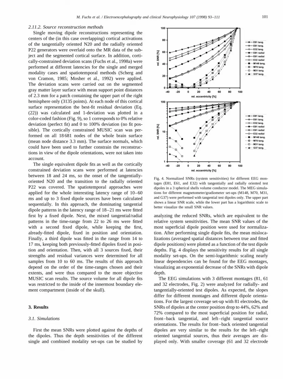
analyzing the reduced SNRs, which are equivalent to therelative system sensitivities. The mean SNR values of themost superficial dipole position were used for normaliza-tion. After performing single dipole fits, the mean misloca-lizations (averaged spatial distances between true and fitteddipole positions) were plotted as a function of the test dipoledepths. Fig. 4 displays the sensitivity results for all singlemodality set-ups. On the semi-logarithmic scaling nearlylinear dependencies can be found for the EEG montages,visualizing an exponential decrease of the SNRs with dipoledepth.

The EEG simulations with 3 different montages (81, 61and 32 electrodes, Fig. 2) were analyzed for radially- andtangentially-oriented test dipoles. As expected, the slopesdiffer for different montages and different dipole orienta-tions. For the largest coverage set-up with 81 electrodes, theSNRs of dipoles at the center position drop to 44%, 62% and72% compared to the most superficial position for radial,front–back tangential, and left–right tangential sourceorientations. The results for front–back oriented tangentialdipoles are very similar to the results for the left–rightoriented tangential sources, thus their averages are dis-played only. With smaller coverage (61 and 32 electrode

Fig. 4. Normalized SNRs (system sensitivities) for different EEG mon-tages (E81, E61, and E32) with tangentially and radially oriented testdipoles in a 3 spherical shells volume conductor model. The MEG simula-tions for different magnetometer/gradiometer set-ups (M148, M70, M31,and G37) were performed with tangential test dipoles only. The upper partshows a linear SNR scale, while the lower part has a logarithmic scale tobetter visualize the small SNR values.


montages), the mean sensor sensitivities drop slightly faster(to 27% for the radial and to about 58% for the tangentialdipole orientations). No significant dependency on the elec-trode density (spatial sampling) could be found when com-paring the 61 and 32 sensor set-ups. The differencesbetween the 81 electrodes montage and the lower sensornumber set-ups, especially for radial dipoles, has its reasonin the smaller coverage of those systems, so that the signalsof deeper radial sources cannot be detected as well as by thefull coverage system.

The results for the different MEG systems are shown fortangential source orientations only. The shielding effects ofthe volume conductor can clearly be seen in the sharplydecreasing SNRs with depth (approaching 0 at the centerof the sphere). This decrease is over-exponential for deepsources, which are consequently suppressed and cannot belocalized very well. The 1st order gradiometer system exhi-bits the steepest SNR versus depth slope and is thereforeworst for localizing deeper dipoles.

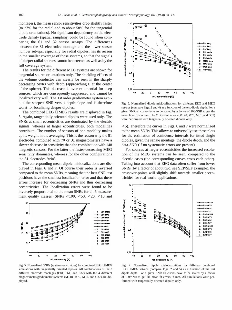
The combined EEG+ MEG results are displayed in Fig.5. Again, tangentially oriented dipoles were used only. TheSNRs at small eccentricities are dominated by the electricsignals, whereas at larger eccentricities, both modalitiescontribute. The number of sensors of one modality makesup its weight in the averaging. This is the reason why the 81electrodes combined with 70 or 31 magnetometers have aslower decrease in sensitivity than the combination with 148magnetic sensors. For the latter the faster-decreasing MEGsensitivity dominates, whereas for the other configurationsthe 81 electrodes ‘win’.

The corresponding mean dipole mislocalizations are dis-played in Figs. 6 and 7. Of course their order is reversedcompared to the mean SNRs, meaning that the best SNR testpositions have the smallest localization error and that theseerrors increase for decreasing SNRs and thus decreasingeccentricities. The localization errors were found to beinversely proportional to the mean SNRs for all 5 measure-ment quality classes (SNRs,100, ,50, ,20, ,10 and

,5). Therefore the curves in Figs. 6 and 7 were normalizedto the mean SNRs. This allows to universally use these plotsfor the estimation of confidence intervals for fitted singledipoles, given the sensor montage, the dipole depth, and thedata-SNR (if no systematic errors are present).

For sources at larger eccentricities the increased resolu-tion of the MEG systems can be seen, compared to theelectric cases (the corresponding curves cross each other).Taking into account that EEG data often suffer from lowerSNRs (by a factor of about two, see SEP/SEF example), thecrossover-points will slightly shift towards smaller eccen-tricities for real world applications.

Fig. 5. Normalized SNRs (system sensitivities) for combined EEG+ MEGsimulations with tangentially oriented dipoles. All combinations of the 3different electrode montages (E81, E61, and E32) with the 4 differentmagnetometer/gradiometer systems (M148, M70, M31, and G37) are dis-played.

Fig. 6. Normalized dipole mislocalizations for different EEG and MEGset-ups (compare Figs. 2 and 4) as a function of the test dipole depth. For agiven SNR all curves have to be scaled by a factor of 100/SNR to get themean fit errors in mm. The MEG simulations (M148, M70, M31, and G37)were performed with tangentially oriented dipoles only.

Fig. 7. Normalized dipole mislocalizations for different combinedEEG + MEG set-ups (compare Figs. 2 and 5) as a function of the testdipole depth. For a given SNR all curves have to be scaled by a factorof 100/SNR to get the mean fit errors in mm. All simulations were per-formed with tangentially oriented dipoles only.


In the MEG case a more prominent saturation of the mis-localizations for deep sources can be found, compared to theEEG case. This is due to the restriction of the sources to theinside of the spherical volume conductor. Theseartifacts have been omitted in Fig. 6, but the effect canbe estimated easily by comparing the sphere radius to thelarge mislocalizations of the MEG systems at low eccentri-

cities.The results of the combined EEG+ MEG evaluations can

be seen in Fig. 7. Due to the larger number of sensors andthe complementary field distributions, the combined resultsare always better than the corresponding single modalityevaluations. For superficial source positions the superiormagnetic localization power (compared to the EEG cases)

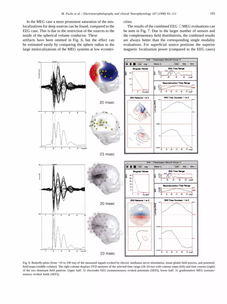
Fig. 8. Butterfly-plots (from−10 to 100 ms) of the measured signals evoked by electric medianus nerve stimulation, mean global field powers, and potential/field-maps (middle column). The right column displays SVD analyses of the selected time range (18–24 ms) with contour maps (left) and time courses (right)of the two dominant field patterns. Upper half: 31 electrodes EEG (somatosensory evoked potentials (SEP)), lower half: 31 gradiometers MEG (somato-sensory evoked fields (SEF)).


is further improved by the additional information content ofthe electric channels. The steep increase in localizationerrors of the MEG systems alone for deeper sources cannotbe found in the merged studies, where the electric data arecapable of localizing deep sources with smaller errors.

3.2. Evoked somatosensory field examinations

The measured EEG data are displayed in Fig. 8, togetherwith field-maps at two selected latencies (20 and 23 ms)

and singular value decomposition (SVD) analyses of thetime range, that was selected for source reconstructions(18–24 ms). For comparison, the corresponding MEGdata are analyzed and displayed in the same fashion inthe lower part of Fig. 8. The noise amplitudes were esti-mated in the pre-trigger periods of both data (from−120 to−10 ms). The EEG data are noisier (max. SNR: 25) thanthe MEG data (max. SNR: 52) and exhibit several struc-tures that cannot be found in the MEG traces. For example,the small peak at latencies around 15 ms and the shoulder

Fig. 9. Single moving dipole reconstructions (at 20, 23, and 18–24 ms) with an enlarged view of the right central sulcus (upper left to lower right). First row:EEG data only, middle row: MEG data only, lower row: EEG+ MEG used together. Left and middle columns: two single latency dipole reconstructionstogether with cortically constrained, color-coded deviation scans, right column: dipoles for all latencies overlaid with a rendering of the cortical gray matterlayer.


at the decreasing slope of the first large peak around 24 msare missing in the MEG signals. Furthermore, the differentamplitude ratios of the large peaks are obvious. All thesefeatures can be explained by the missing sensitivity of theMEG sensors to (quasi-) radially oriented source compo-nents.

3.2.1. Single equivalent dipoles and cortically constraineddeviation scans

The SVD analyses show, that in the selected latencyrange two EEG patterns (one apparently tangential, andone apparently radial) are present, which are comparablein amplitude (around 2:1), whereas in the MEG case onepattern is clearly dominating (amplitude ratio 10:1).

Before the dipole reconstructions and deviation scans wereperformed, a factor for matching the conductivities of theBEM volume conductor model was fitted at latencies around20 ms, where a tangential source clearly dominates both EEGand MEG data. Fig. 9 shows single moving dipole recon-structions at two selected latencies (20 and 23 ms), whentangential and radial patterns are pre-dominant in the EEGdata, and for the whole selected latency range (18–24 ms).

For visualization of the anatomical correlation an enlargedview of the cortical surface segmented from the MR data isoverlaid. The right central sulcus can clearly be identified(anterior: right, posterior: left, compare Fig. 3 field-maps).

In order to verify the dipole fit results and to show con-fidence regions (provided that there are no systematic errorslike sensor mislocalizations, oversimplified volume conduc-tor models or incorrect source models) for the single dipolesolutions, cortically constrained deviation scans are alsodisplayed as color-coded surfaces together with the singlelatency dipoles.

At all latencies the single dipole source model was able toexplain the measured data very well in both EEG and MEGcases (best fit at 21 ms: EEG: 11.8% relative deviation(normalized to the measured data)= 1.4% residual var-iance, MEG: 4.9% dev.= 0.2% res. var., EEG+ MEG:7.7% dev.= 0.6% res. var.). Details can be found in Table1, where source locations for single and combined modalityevaluations are compared to the results of EEG+ MEGwith regularization. At a latency of 20 ms all modalitieswithout and with regularization yield the same result forthe tangential source (largest distance 0.6 mm). The dipole

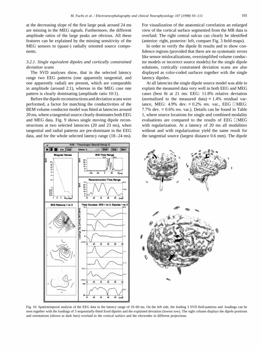
Fig. 10. Spatiotemporal analysis of the EEG data in the latency range of 10–60 ms. On the left side, the leading 3 SVD field-patterns and -loadings can beseen together with the loadings of 3 sequentially-fitted fixed dipoles and the explained deviation (lowest row). The right column displays the dipole positionsand orientations (shown as dark bars) overlaid to the cortical surface and the electrodes in different projections.


positions differ for the single modality results (compare Fig.9), especially at latencies with lower SNRs (e.g. MEG at 24ms). These results have larger confidence regions and arethus not well defined. Furthermore at the later timepoints theradial dipole develops in the EEG data, and therefore theEEG dipole positions differ as well from the MEG and thecombined results.

Regularization affects mainly the latencies with lowerSNRs at the beginning and the end of the analyzed peakby suppressing insignificant contributions to the residualvariance. Thus the explained variances are slightly smallerwith regularization (compare also Table 2) and the dipolepositions are shifted.

The EEG dipoles exhibit a transition from a tangentialsource at 20 ms located in the posterior wall of the centralsulcus to a radial source at a latency of 23 ms. The confi-dence regions of the reconstructions are larger and moreisotropic as compared to the MEG case. There the typicalellipsoidal shape with a narrow confidence range perpendi-cular to the dipole direction and smaller specificity along its

direction (and in the depth, which cannot be clearly seen inFig. 9) can be found. The MEG dipoles are all tangentiallyoriented and are rather stable in position (except for laten-cies with very small SNRs).

The combined evaluations (Fig. 9, lowest row) profitfrom both EEG and MEG properties. At latencies wherethe tangential component is dominating, an improved spa-tial resolution compared to both single modality evaluationscan be seen with a confidence area shape similar to the MEGcase (since the SNR of the MEG data is twice as large as inthe EEG data, the MEG data dominate at this latency). Atlater latencies, when the radial dipole comes up in the EEGdata and when in the MEG case only the decreasing tangen-tial dipole component can be reconstructed, the EEG datadominate and determine the dipole orientation and the moreisotropic confidence region. The remaining MEG signals ofthe decreasing tangential source force the radial dipole posi-tion towards lower locations, thus deteriorating the commonfit quality due to an inadequate source model (two differentsources are present with overlapping activation profiles).

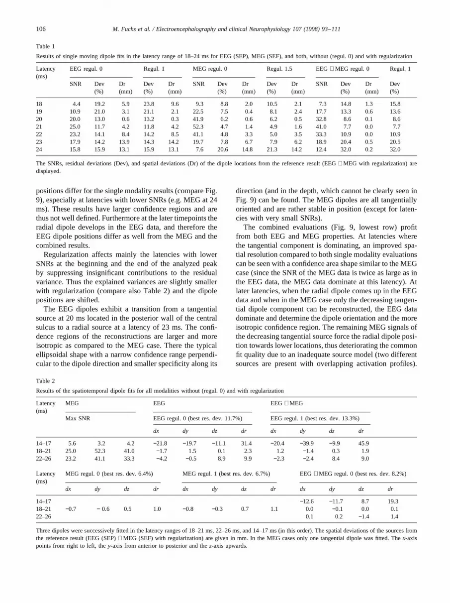
Table 1

Results of single moving dipole fits in the latency range of 18–24 ms for EEG (SEP), MEG (SEF), and both, without (regul. 0) and with regularization

Latency(ms)

EEG regul. 0 Regul. 1 MEG regul. 0 Regul. 1.5 EEG+ MEG regul. 0 Regul. 1

SNR Dev(%)

Dr(mm)

Dev(%)

Dr(mm)

SNR Dev(%)

Dr(mm)

Dev(%)

Dr(mm)

SNR Dev(%)

Dr(mm)

Dev(%)

18 4.4 19.2 5.9 23.8 9.6 9.3 8.8 2.0 10.5 2.1 7.3 14.8 1.3 15.819 10.9 21.0 3.1 21.1 2.1 22.5 7.5 0.4 8.1 2.4 17.7 13.3 0.6 13.620 20.0 13.0 0.6 13.2 0.3 41.9 6.2 0.6 6.2 0.5 32.8 8.6 0.1 8.621 25.0 11.7 4.2 11.8 4.2 52.3 4.7 1.4 4.9 1.6 41.0 7.7 0.0 7.722 23.2 14.1 8.4 14.2 8.5 41.1 4.8 3.3 5.0 3.5 33.3 10.9 0.0 10.923 17.9 14.2 13.9 14.3 14.2 19.7 7.8 6.7 7.9 6.2 18.9 20.4 0.5 20.524 15.8 15.9 13.1 15.9 13.1 7.6 20.6 14.8 21.3 14.2 12.4 32.0 0.2 32.0

The SNRs, residual deviations (Dev), and spatial deviations (Dr) of the dipole locations from the reference result (EEG+ MEG with regularization) aredisplayed.

Table 2

Results of the spatiotemporal dipole fits for all modalities without (regul. 0) and with regularization

Latency(ms)

MEG EEG EEG+ MEG

Max SNR EEG regul. 0 (best res. dev. 11.7%) EEG regul. 1 (best res. dev. 13.3%)

dx dy dz dr dx dy dz dr

14–17 5.6 3.2 4.2 −21.8 −19.7 −11.1 31.4 −20.4 −39.9 −9.9 45.918–21 25.0 52.3 41.0 −1.7 1.5 0.1 2.3 1.2 −1.4 0.3 1.922–26 23.2 41.1 33.3 −4.2 −0.5 8.9 9.9 −2.3 −2.4 8.4 9.0

Latency(ms)

MEG regul. 0 (best res. dev. 6.4%) MEG regul. 1 (best res. dev. 6.7%) EEG+ MEG regul. 0 (best res. dev. 8.2%)

dx dy dz dr dx dy dz dr dx dy dz dr

14–17 −12.6 −11.7 8.7 19.318–21 −0.7 − 0.6 0.5 1.0 −0.8 −0.3 0.7 1.1 0.0 −0.1 0.0 0.122–26 0.1 0.2 −1.4 1.4

Three dipoles were successively fitted in the latency ranges of 18–21 ms, 22–26 ms, and 14–17 ms (in this order). The spatial deviations of the sources fromthe reference result (EEG (SEP)+ MEG (SEF) with regularization) are given in mm. In the MEG cases only one tangential dipole was fitted. Thex-axispoints from right to left, they-axis from anterior to posterior and thez-axis upwards.


This motivates the use of spatiotemporal models.

3.2.2. Spatiotemporal dipole reconstructionsSpatiotemporal dipole modeling was performed for the

interesting latency range of 10–60 ms. SVD analyses ofthese time ranges revealed 3 significant field patterns inthe EEG and one dominating pattern in the MEG case(Figs. 10 and 11). Since the number of field patterns corre-sponds to the minimum number of fixed source configura-tions that might be able to generate the data, at least 3 fixeddipoles are needed to explain the EEG data. In the EEG andin the combined case (Fig. 12) the dipoles were sequentiallyfitted in the latency ranges of 18–21 ms (tangential N20dominating), 22–26 ms (radial P22 and decreasing N20),and the remaining small peak between 14 and 17 ms (deepsource close to the brainstem (Buchner et al., 1995)). Ascan be seen in Figs. 10 and 12 and Table 2, these 3 dipoleswere sufficient to explain the measured data reasonably well(best residual deviations about 10% (best explained var-iances about 99%). The deep source has its main loadingat very early latencies (P16, lowest loading trace), next the

tangentially-oriented source develops (N20, centered in theposterior wall of the central sulcus, upper loading trace),succeeded by the radial P22 (located in the postcentralgyrus (Buchner et al., 1996), middle loading trace).

The MEG data could be explained reasonably well withone single tangentially-oriented source in the posterior wallof the central sulcus, adding a second source did notimprove the overall fit accuracy (lowest trace in Fig. 11).The optimization was carried out with a regularization para-meter l ≈ 1, assuming that the SNRs are estimated cor-rectly. A value ofl = 1.5 was adequate to suppress quasi-radial components in single latency MEG results (Figs. 8and 9 and Table 1).

The results of the combined evaluation are displayed inFig. 12. Qualitatively, the dipole positions look similar tothe EEG localization results. The confidence intervals aresmaller in the combined case (compare Fig. 9), since thelarger number of sensors and the complementary nature ofboth modalities stabilize the results. Details about the dipolepositions can be found in Table 2. The tangential dipole islocalized equally well by all methods, whereas differences

Fig. 11. Spatiotemporal analysis of the MEG data in the latency range of 10–60 ms. On the left side, the leading 3 SVD field patterns and loadings can be seentogether with the loadings of one fitted fixed dipole and the explained deviation (lowest row). The right column displays the dipole position and orientation(shown as dark bar) overlaid to the cortical surface and the lower gradiometer pick-up coils in different projections.


can be found for radial source position and especially for thedeep (P16) dipole. The latter is most affected by regulariza-tion, due to the small SNR values (compared to the N20,P22 components) and the therefore rather large confidencevolume of the dipole fit result at these very early latencies.

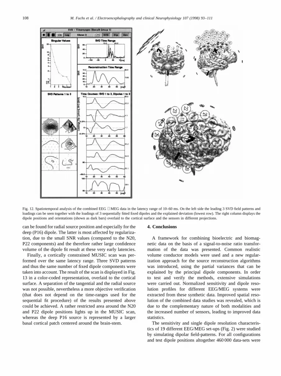
Finally, a cortically constrained MUSIC scan was per-formed over the same latency range. Three SVD patternsand thus the same number of fixed dipole components weretaken into account. The result of the scan is displayed in Fig.13 in a color-coded representation, overlaid to the corticalsurface. A separation of the tangential and the radial sourcewas not possible, nevertheless a more objective verification(that does not depend on the time-ranges used for thesequential fit procedure) of the results presented abovecould be achieved. A rather restricted area around the N20and P22 dipole positions lights up in the MUSIC scan,whereas the deep P16 source is represented by a largerbasal cortical patch centered around the brain-stem.

4. Conclusions

A framework for combining bioelectric and biomag-netic data on the basis of a signal-to-noise ratio transfor-mation of the data was presented. Common realisticvolume conductor models were used and a new regular-ization approach for the source reconstruction algorithmswas introduced, using the partial variances that can beexplained by the principal dipole components. In orderto test and verify the methods, extensive simulationswere carried out. Normalized sensitivity and dipole reso-lution profiles for different EEG/MEG systems wereextracted from these synthetic data. Improved spatial reso-lution of the combined data studies was revealed, which isdue to the complementary nature of both modalities andthe increased number of sensors, leading to improved datastatistics.

The sensitivity and single dipole resolution characteris-tics of 19 different EEG/MEG set-ups (Fig. 2) were studiedby simulating dipolar field-patterns. For all configurationsand test dipole positions altogether 460 000 data-sets were

Fig. 12. Spatiotemporal analysis of the combined EEG+ MEG data in the latency range of 10–60 ms. On the left side the leading 3 SVD field patterns andloadings can be seen together with the loadings of 3 sequentially fitted fixed dipoles and the explained deviation (lowest row). The right column displays thedipole positions and orientations (shown as dark bars) overlaid to the cortical surface and the sensors in different projections.


derived by adding white noise of 5 different levels to theforward calculated fields. For each field-pattern of thesesynthetic data a dipole fit was performed, followed by aver-aging of the corresponding results in order to get statisticallyrelevant conclusions.

Normalized mean SNR curves representing the systemsensitivities were calculated by averaging (5*) 200 data-sets per point (Figs. 4 and 5). The mean dipole mislocaliza-tions were found to be inversely proportional to the corre-sponding mean SNRs for all sensor montages, so anormalized representation could be extracted (Figs. 6 and7). This allows estimation of the confidence ranges of singledipole solutions, given the SNR of the data, the sensor set-up, and the depth of the fitted dipole. The shape of theconfidence region can be studied by high spatial resolutiondeviation scans around the dipole location, that has beendetermined by the preceding fit (Fig. 9).

The expected behavior of combined EEG and MEG datawas verified quantitatively by these simulations. Radialsources can by detected by EEG only. The sensitivity dif-ferences between radial and tangential dipoles are not asdramatic as in the magnetic case, but differ only by a factorof approximately 2 for deeper sources (Fig. 4). The depthdependency of the sensor gain is much weaker in the EEGcases, thus enabling still reasonable fit results for non-super-

ficial, deeper dipoles. The MEG systems exhibit animproved resolution for superficial, tangential sources(Fig. 6).

It can be seen from Fig. 5 that for radial source orienta-tions the SNRs drop faster than for tangential dipoles andthus the radial sources mislocalizations increase slightlyfaster with depth for all EEG montages. The larger the cov-erage, the better the localization accuracy for deepersources. By comparing the 61 and 32 electrode montages,which have the same coverage, but different electrode den-sities, we found that for tangential dipoles the coverage isthe most important factor (that determines the spatial reso-lution), whereas the set-up with the lower number of sensorsis not well suited for localizing superficial radial sources,due to a spatial under-sampling of the electric field-patterns.MEG systems have superior resolution power for superficialtangential sources, but the SNRs drop sharply and the loca-lization errors increase rapidly for deeper dipole positions.

The combination of both modalities gives overallimproved results at all eccentricities (Figs. 5 and 7), dueto the increased number of sensors and the complementaryfield distributions. For sources close to the center of thevolume conductor the electric data dominate, at mediumpositions both modalities contribute, and for superficialpositions an increasing influence of the magnetic data can

Fig. 13. Spatiotemporal MUSIC reconstruction of the combined EEG+ MEG data in the latency range of 10–60 ms. For the cortically constrained MUSICscan the leading 3 (combined) field patterns have been used. The result is shown as color-coded overlay onto the cortical surface together with the electrodesand the lower gradiometer pick-up coils.


be found.In order to verify the simulations with real measured data,

we have analyzed simultaneously acquired SEP/SEF data atvery early latencies with single dipole reconstructions, cor-tically constrained deviation scans, spatiotemporal, multipledipole models, and compared single and combined modalityresults. All approaches revealed dipolar sources in the rightcentral sulcus area, which should of course be expectedfrom left hand medianus nerve stimulation. The combinedEEG + MEG evaluations exhibit the best spatial resolutionwith a smooth transition between both tangential and radialdipole orientations, whereas the magnetic data alone containinformation of the tangential source only. The electric dataalone in this case suffer from smaller SNRs and less spatialresolution due to volume conductor effects and large inter-electrode distances.

Merged EEG/MEG evaluations thus indeed promiseincreased localization accuracy and a better understandingof the underlying neuronal processes, since also a betterdifferentiation between (quasi-) tangential and (quasi-)radial source components is possible.

References

Ben-Isreal, A. and Greville, T.N.E. Some topics in generalized inverses ofmatrices. In: M.Z. Nashed (Ed.), Generalized Inverses and Applications,Proc. of an Advanced Seminar Sponsored by the Mathematics ResearchCenter. Academic Press, New York, 1976, pp. 125–147.

Buchner, H., Fuchs, M., Wischmann, H.-A., Do¨ssel, O., Ludwig, I.,Knepper, A. and Berg, P. Source analysis of median nerve and fingerstimulated somato-sensory evoked potentials: multichannel simulta-neous recording of electric and magnetic fields combined with 3D-MR tomography. Brain Topogr., 1994, 6: 299–310.

Buchner, H., Waberski, T.D., Fuchs, M., Wischmann, H.-A., Beckmann,R. and Riena¨cker, A. Origin of P16 median nerve SEP componentidentified by dipole source analysis – subthalamic or within the tha-lamo-cortical radiation?. Exp. Brain. Res., 1995, 104 (3): 511–518.

Buchner, H., Waberski, T.D., Fuchs, M., Drenckhahn, R., Wagner, M. andWischmann, H.-A. Postcentral origin of P22: evidence from sourcereconstruction in a realistically shaped head model and from a patientwith a postcentral lesion. Electroenceph. clin. Neurophysiol., 1996, 100:332–342.

Cohen, D. and Cuffin, B.N. Comparison of the magnetoencephalogramand electroencephalogram. Electroenceph. clin. Neurophysiol., 1979,47: 132–146.

Cohen, D. and Cuffin, B.N. Demonstration of useful differences betweenmagnetoencephalogram and electroencephalogram. Electroenceph. clin.Neurophysiol., 1983, 56: 38–51.

Cohen, D. and Cuffin, B.N. A method for combining MEG and EEG todetermine the sources. Phys. Med. Biol., 1987, 32 (1): 85–89.

Cohen, D., Cuffin, B.N., Yunokuchi, K., Maniewski, R., Purcell, C.,Cosgrove, G.R., Ives, J., Kennedy, J.G. and Schomer, D.L. MEG versusEEG localization test using implanted sources in the human brain. Ann.Neurol., 1990, 28 (6): 811–817.

Cohen, D. and Cuffin, B.N. EEG versus MEG localization accuracy: the-ory and experiment. Brain Topogr., 1991, 4 (2): 95–103.

Crowley, C.W., Greenblatt, R.E. and Khalil, I. Minimum norm estimationof current distributions. In: S.J. Williamson, M. Hoke, G. Stroink andM. Kotani (Eds.), Advances in Biomagnetism. Plenum Press, NewYork, 1989, pp. 603–606.

Cuffin, B.N. Effects of head shape on EEGs and MEGs. IEEE Trans.Biomed. Eng., 1990, 37 (1): 44–52.

Ferguson, A.S., Zhang, X. and Stroink, G. A complete linear discretizationfor calculating the magnetic field using the boundary element method.IEEE Trans. Biomed. Eng., 1994, 41 (5): 455–460.

Fletcher, D.J., Amir, A., Jewett, D. L and Fein, G. Improved method forcomputation of potentials in a realistic head shape model. IEEE Trans.Biomed. Eng., 1995, 42 (11): 1094–1104.

Fuchs, M., Wagner, M., Wischmann, H.-A., Ottenberg, K. and Do¨ssel, O.Possibilities of functional brain imaging using a combination of MEGand MRT. In: C. Pantev (Ed.), Oscillatory Event-Related BrainDynamics. Plenum Press, New York, 1994, pp. 435–457.

Fuchs, M., Wischmann, H.-A., Wagner, M. and Kru¨ger, J. Coordinatesystem matching for neuromagnetic and morphological reconstructionoverlay. IEEE Biomed. Eng., 1995, 42 (4): 416–420.

Fuchs, M., Wischmann, H.-A., Wagner, M., Drenckhahn, R. and Ko¨hler,Th. Source reconstructions by spatial deviation scans. In: C. Aine, Y.Okada, G. Stroink, S. Swithenby and C. Wood (Eds.), Advances inBiomagnetism Research: Biomag96, Springer-Verlag, New York,1998a, in press.

Fuchs, M., Drenckhahn, R., Wischmann, H.-A. and Wagner, M. Animproved boundary element method for realistic volume conductormodeling. IEEE Trans. Biomed. Eng., 1998b, 45: in press.

Geddes, L.A. and Baker, L.E. The specific resistance of biological mate-rial, a compendium of data for the biomedical engineer andphysiologist. Med. Biol. Eng., 1963, 5: 271–293.

Geselowitz, D.B. On bioelectric potentials in an inhomogeneous volumeconductor. Biophys. J., 1967, 7: 1–17.

Geselowitz, D.B. On the magnetic field generated outside an inhomoge-neous volume conductor by internal current sources. IEEE Trans.Magn., 1970, MAG-6: 346–347.

Greenblatt, R.E. Combined EEG/MEG source estimation methods. In: C.Baumgartner, L. Deecke, G. Stroink and S.J. Williamson (Eds.), Bio-magnetism: Fundamental Research and Clinical Applications. Elsevier,Vienna, Austria, 1993, 1995, pp. 402–405.

Gorodnitzky, I, George, J.S, Schlitt, H.A. and Lewis, P.S. A weightediterative algorithm for neuromagnetic imaging. Proc. IEEE SatelliteSymposium on Neuroscience and Technology, Lyon, 1992, pp. 60–64.

Hamalainen, M.S. and Sarvas, J. Realistic conductivity geometry model ofthe human head for interpretation of neuromagnetic data. IEEE Trans.Biomed. Eng., 1989, 36 (2): 165–171.

Hansen, P.C. Analysis of discrete ill-posed problems by means of the L-curve. SIAM Rev., 1992, 34 (4): 561–580.

Kohler, T., Wagner, M., Fuchs, M., Wischmann, H.A., Drenckhahn, R.and Theißen, A. Depth normalization in MEG/EEG current densityimaging. In: H.B.K., Boom, C.J. Robinson and W.L.C. Rutten (Eds.),.Proc. IEEE Eng. Med. and Biol., Nijmegen, The Netherlands, 1996,paper 144.

Lawson, C.L. and Hanson, R.J. Solving Least Squares Problems. Prentice-Hall, Englewood Cliffs, NJ, 1974.

Lopes da Silva, F.H., Wieringa, H.J. and Peters, M.J. Source localizationof EEG and MEG: empirical comparison using visually evokedresponses and theoretical considerations. Brain Topogr., 1991, 4 (2):133–142.

Mauguiere, F. A consensus statement on relative merits of EEG and MEG.Electroenceph. clin. Neurophysiol., 1992, 82 (5): 317–319.

Menninghaus, E. and Lu¨tkenhoner, B. How silent are deep and radialsources in neuromagnetic measurements? In: C. Baumgartner, L.Deecke, G. Stroink and S.J Williamson (Eds.), Biomagnetism: Funda-mental Research and Clinical Applications. Elsevier, Vienna, Austria,1993, 1995, pp. 352–356.

Mosher, J.C., Lewis, P.S. and Leahy, R.M. Multiple dipole modeling andlocalization from spatio-temporal MEG data. IEEE Trans. Biomed.Eng., 1992, 39 (6): 541–557.

de Munck, J.C. The potential distribution in a layered anisotropic spher-oidal volume conductor. J. Appl. Phys., 1988, 64 (2): 464–470.

de Munck, J.C. A linear discretization of the volume conductor boundary


integral equation using analytically integrated elements. IEEE Trans.Biomed. Eng., 1992, 39 (9): 986–990.

Nelder, J.A. and Mead, R. A simplex method for function minimization.Comput. J., 1965, 7: 308–313.

Oostendorp, T.F. and van Oosterom, A. Source parameter estimation ininhomogeneous volume conductors of arbitrary shape. IEEE Trans.Biomed. Eng., 1989, 36 (3): 382–391.

van Oosterom, A. and Strackee, J. The solid angle of a plane triangle.IEEE Trans. Biomed. Eng., 1983, 30 (2): 125–126.

Pflieger, M.E., Simpson, G.V., Ahlfors, S.P. and Ilmoniemi, R.J. Super-

additive information from simultaneous MEG/EEG data. In: C.Aine, Y.Okada, G. Stroink, S. Swithenby and C. Wood (Eds.), Advances inBiomagnetism Research: Biomag96, Springer-Verlag, New York,1998, in press.

Press, W.H., Teukolsky, S.A., Vetterling, W.T. and Flannery, B.P. Numer-ical Recipies in C: The Art of Scientific Computing, 2nd edn. Cam-bridge University Press, New York, 1992.

Sarvas, J. Basic mathematical and electromagnetic concepts of the bio-magnetic inverse problem. Phs. Med. Biol., 1987, 32 (1): 11–22.

Scherg, M. and von Cramon, D. Two bilateral sources of the late AEP asidentified by a spatio-temporal dipole model. Electroenceph. clin.Neurophysiol., 1985, 65: 32–44.

Schlitt, H.A., Heller, L., Aaron, R., Best, E. and Ranken, D.M. Evaluationof boundary element methods for the EEG forward problem: effect oflinear interpolation. IEEE Trans. Biomed. Eng., 1995, 42 (1): 52–58.

Wagner, M., Fuchs, M., Wischmann, H.-A., Ottenberg, K. and Do¨ssel, O.Cortex segmentation from 3D MR images for MEG reconstructions. In:C. Baumgartner, L. Deecke, G. Stroink and S.J. Williamson (Eds.),Biomagnetism: Fundamental Research and Clinical Applications. Else-vier, Vienna, Austria, 1993, 1995, pp. 433–438.


improving source reconstructions by combining bioelectric and biomagnetic data

Documents