8-1

Chapter 8

Stormwater Storage-Treatment-Reuse Systems

James P. Heaney, Len Wright, and David Sample

IntroductionThe overall effectiveness of a variety of stormwater BMP’s was evaluated in Chapter 7.Two other aspects of control of stormwater: high-rate treatment and the potentialeffectiveness of using stormwater for supplemental irrigation are described in thischapter.

Stormwater TreatmentBecause of the dynamic nature of stormwater flows and water quality, most controlsystems are a hybrid of temporary storage and high-rate treatment. For a given level ofstormwater control, the engineer can accomplish this objective using variouscombinations of storage and treatment. Much has been written on this subject andmethods for finding the optimal combination of storage and treatment have beendeveloped. Heaney and Wright (1997) provide a summary of these methods. Severalunresolved issues remain with regard to evaluating the performance of these treatmentsystems.

Effect of Initial ConcentrationAs pointed out in Chapter 7, the effect of initial concentration on the performance of wet-weather controls should not be ignored. A high percent removal for a control will usuallyoccur if the initial concentration is high. Separate and combined stormwater flowsexhibit wide variability from storm to storm as well as within a given storm. The effect ofinitial concentration on performance can be evaluated directly by finding the order of thereaction as well as the rate constant (Heaney and Wright 1997).

Effect of Change of StorageAnother complication in dealing with treatment of wet-weather flows is that the controlunits are typically filling and emptying during and following the storm. Thus, it is vital toproperly measure the change in storage at short time intervals to incorporate thisimportant factor. The effect of changing storage is captured in the calculated detentiontime for each parcel of water.

Effect of Mixing RegimeAnother critical assumption is the type of mixing that takes place in the treatmentreactor. Two limiting cases are plug flow wherein the parcels simply queue through thereactor and complete mixing wherein the incoming parcel instantaneously mixes withthe water already in the reactor.

8-2

Effect of Nature of the Suspended SolidsThe nature of the suspended solids changes during the storm and can vary widely. Thesolids can range over several orders of magnitude from coarse solids to fine colloids.Pisano and Brombach (1996) present a summary of efforts to date to characterize wet-weather solids.

Essential Features of Future Wet-Weather Control FacilitiesGiven the large variability in the quantity and quality of wet-weather flows and the fillingand emptying of treatment reactors, direct monitoring of the wet-weather inflows and thestatus of the control units is of fundamental importance. Unfortunately, few suchsystems have been built in the United States. The Europeans are more advanced intrying to evaluate and optimize wet-weather control systems.

High-Rate Operation of Wastewater Treatment PlantsHigh-rate operation of WWTPs during and following wet-weather events is an importantoption to evaluate as part of the overall stormwater management program for combinedand for separate systems that are affected by I/I. It is possible to model the expectedperformance of these systems using the GPS-X WWTP software from Hydromantis,Inc., or similar programs, to do continuous simulation of the effect of wet-weather flowson DWF treatment plants. Mangeot (1996) performed a preliminary feasibility studyusing GPS-X to evaluate the Boulder WWTP during the 1995 high-flow year. High-rate operation of the WWTP during these wet periods and periods with high I/I due toseasonably high groundwater tables appears to be a very attractive option to consider.Not much research has been done on this problem and there are only a few literaturecitations on results of attempting to model the dynamics of WWTP operation during highflow periods. Some questions remain regarding the ability of GPS-X to properly handlethe hydraulics associated with wet-weather flows. However, it is possible to show withdirect measurements for the Boulder WWTP, that the plant is capable of operatingeffectively over a wide range of influent flows and concentrations. Because the influentis already so dilute, caution should be exercised in requiring a specified percent removalunder these wet-weather conditions.

Stormwater Reuse Systems

IntroductionAt present, there is much interest in local management of stormwater from smaller,more frequent events. The primary on-site option is to encourage infiltration ofstormwater from roofs, driveways, parking lots, and streets. This infiltrated waterincreases the moisture in the unsaturated zone and raises the groundwater table whichcan provide benefits in terms of increasing base flows in streams and providing stormwater to help meet the ET needs of the local vegetation. Higher groundwater levels canhave negative effects on basements and on sanitary and combined sewers. Thissection explores the possibility of the reuse of urban stormwater for irrigation waterwhich is a major component of urban water use.

8-3

Previous StudiesAs water supplies become more stressed, water conservation and reuse become moreattractive options. Wastewater disposal costs also encourage more water reuse.Asano and Levine (1996) provide a historical perspective and explore current issues inwastewater reclamation, recycling, and reuse, and outline requirements of a stormwaterand wastewater reuse feasibility study. Lejano et al. (1992) summarize the benefits ofwater reuse as the following:

1. Water supply related:a. Supplements regional water supply, eliminating need to develop additional

supplies.b. Provides more reliability than the usual supply and is less affected by

weather.c. Provides a locally controlled supply, reducing dependence on state or

regional politics.d. Avoids the operating costs of water treatment and delivery.e. Eliminates social and environmental impacts of diverting water from

natural drainageways.f. Eliminates impacts of constructing large-scale water storage and

transmission facilities.

2. Wastewater related:a. Avoids the capital and operating costs of disposal facilities.b. Avoids the costs of advanced treatment facilities needed to meet state and

federal discharge requirements.

Urban wet weather flow management needs to be viewed within the context of overallurban water management. Such an integrated framework was proposed in the late1960s and is regaining favor in the mid-1990s. Changes in urban water use areoccurring because of aggressive water conservation practices which will significantlyreduce indoor and outdoor water use.

As discussed in Chapter 3, per capita indoor residential water use is very stable at anaverage of 60 gpcd. Aggressive hardware changes such as low flush toilets shouldreduce this usage rate to 35-40 gpcd. Only a small proportion of this indoor waste isblack water. Most of it is graywater that could be reused on-site for lawn watering andother non-potable purposes. Peak water use in most cities is heavily influenced byurban lawn watering. This outdoor water use does not require potable quality. As thecost of water treatment continues to increase, dual water systems become more of apossibility, particularly with a decentralized infrastructure.

California has been a focal point of reuse activity for some time. Ashcraft and Hoover(1991) found that reclaimed water in southern California is selling at prices ranging from$303/ac-ft to $366/ac-ft, with costs of operation and maintenance of treatment facilitiesrunning from $10/ac-ft to $95/ac-ft. The authors argue that “avoided costs,” such as

8-4

those associated with wastewater disposal should be included in cost calculations.

Mallory and Boland (1970) developed a hydrologic and economic optimization model ofa stormwater reuse system in a new town in Maryland. Their system used a network ofsubdivision level detention ponds. Subpotable reuse required a dual distribution systemto deliver it to households. They found that the net capital cost of such a system(scaled up to 1998 dollars) was $560/dwelling unit for a potable reuse system, and$1175/dwelling unit for the subpotable system. This compares favorably with$950/dwelling unit for a conventional system, the differential of 23% premium forsubpotable reuse due mainly to the dual distribution system. When pollution controlcosts are included for stormwater quality, an additional cost of $640/dwelling unit wascalculated, making the investment in the subpotable system more attractive.

Requa et al. (1991) developed a wastewater reuse cost model for screening purposesin northern California. More recently, Tselentis and Alexopoulou (1996) describe afeasibility study of effluent reuse in the Athens, Greece metropolitan area. Usesconsidered were: crop irrigation, irrigation of forested areas, industrial water supply anddomestic non-potable use. The most cost-effective scenario was distribution for cropirrigation near the route of the current discharge point.

At the other extreme, Haarhoff and Van der Merwe (1996) describe direct potable reuseof reclaimed wastewater in Windhoek, Namibia. Law (1996) describes the Rouse Hillproject in Sydney, Australia, in which a dual non-potable distribution system wasinstalled in a new community in 1994. Oron (1996) developed an integrative economicmodel, arguing that the optimal cost of a reuse system is a function of treatmentmethod, cost of treatment, transportation and storage costs (pipelines and tanks),environmental costs, and the selling price of reused wastewater. New initiatives forreusing stormwater flows for urban residential and industrial water supply systems inAustralia were described by Anderson (1996a, 1996b).

Mitchell, Mein, and McMahon (1996) used a water budget approach to integrate storageand reuse of urban stormwater and treated wastewaters for two neighborhoods insuburban Melbourne, Australia. The authors developed an urban water balance modelto determine the impact of stormwater and wastewater reuse; and suggest itsapplication at a number of scales. They determined that water demand from reservoirsin Australia could be halved through the use of this resource.

Nelen, DeRidder, and Hartman (1996) described the planning of a new development forabout 10,000 people in Ede, Netherlands that considers a dual water supply system.Storing the treated wastewater on-site during wet weather periods can be moreattractive than only using black water for reuse (Pruel, 1996). Herrmann and Hase(1996) described rainwater utilization systems in Bavaria, Germany that save drinkingwater and reduce roof run-off to the sewerage system. The impact of urbanization onthe hydrological cycle of a new development near Tokyo, Japan was performed byImbe, Ohta, and Takano (1996).

8-5

Much of this work has focused upon using treated wastewater from a single effluentplant. The problem then becomes one of finding demand centers for the wastewaterthat are typically located quite some distance away. This becomes a nonlinear form ofthe transhipment problem, in which demand and distance are cost drivers in a nonlinearobjective function.

Many researchers have started to focus on less centralized systems, includingTchobanoglous and Angelakis (1996). Decentralized systems can take advantage of thesegregation between wet weather flow, graywater, and blackwater, and possibly utilizeless contaminated waters closer to their points or origin. Of the three, stormwater runoffis usually the least contaminated prior to central collection. This may avoid constructionof additional treatment systems, pipelines, and other infrastructure and presentsignificant cost savings.

From the wet weather flow quality management perspective, there is much interest inlocal management of wet weather flow from smaller, more frequent events, as theseevents tend to have more pollutants associated with them. The primary on-site option isto encourage infiltration of this stormwater flow from roofs, driveways, parking lots, andstreets.

Herrmann et al. (1996) found that rainwater utilization (using roof runoff water directedinto a storage tank) could provide from 30-50% of total water consumption of aresidence and reduce heavy metals (in stormwater runoff not reused) by 5-25%.Wanielista (1993) developed design curves in order to determine the storage retentionvolumes necessary to achieve given proportions of reuse. The design curves are basedon a daily water-balance model. The main objectives for this practice in the State ofFlorida are the costs avoided of using municipal or pumped groundwater for irrigationpurposes. From the regulatory viewpoint, the main objective is to discharge some of thestormwater onto the land and thereby get credit for 100% removal of this pollutantsource.

Field (1993) did a cost-effectiveness study of the reuse of urban stormwater to meet avariety of differing demands for a hypothetical urban area. The proposed uses variedin their water quality needs, as did the corresponding treatment system designated forthat use. Nowakowska-Blaszcyzyk and Zakrzewski (1996) project increases insuspended solids, nitrates, COD, BOD, and lead from rainfall routed through thefollowing sources: roofing, parking areas, streets, storm sewers, infiltration throughlawns, and infiltration through sand. The lowest values tended to be from roof runoff.Karpiscak, Foster, and Schmidt (1990) detail the application of stormwater andgraywater reuse techniques at a single residence in Tucson, AZ.

Harrison (1993) developed a spreadsheet model to estimate the amount of stormwatercaptured in a detention pond that could be reused for irrigation in Florida. His work isan application of earlier work by Harper (1991). The Southwest Florida Water

8-6

Management District is interested in stormwater reuse as a way of increasing thetreatment efficiency of detention systems. Their current design calls for storing the firstinch of runoff and draining the pond over a five-day period. They are considering goingto an average residence time of 14 days to improve performance from removal rates of50 to 70 % with a five-day drawdown time. Reusing stormwater would give them a100% treatment efficiency.

Harrison (1993) uses a daily water budget to estimate the amount of captured urbanrunoff that could be used for irrigation. The basic storage equation is:

dSdt

R P F RU D ET= + + − − − Equation 8.1

where

dSdt

= the change in storage.

R = runoff volume.P = direct precipitation onto the pond.F = water inflow through sides and bottom of the pond which can be negative.RU =reuse volume.D = pond outflow.ET = pond evapotranspiration.

Harrison assumes that there is no net subsurface flow into or out of the pond, i.e., F = 0.All values are converted into inches over the equivalent impervious drainage area. Adaily time step is used. A minimum precipitation volume of .04 inches is assumed to beneeded to produce runoff. This method is identical to the STORM-type calculationswith the exception that STORM uses an hourly time step and, in this case, outflowsoccur either by reuse or direct discharge of the excess water. Harrison does notindicate what he assumed for a pond drawdown rate in addition to the irrigation release.The final results are expressed as a production function showing the percent of theirrigation demand that is satisfied for various combinations of pond size and irrigationreuse rates. The primary purpose of the stormwater reuse study in Florida was tominimize the pond outflow and thereby achieve increased pollutant removal efficiencyby infiltrating the water locally. Lawn watering was more of a by-product.

Courtney (1997) explored the potential effectiveness of stormwater runon systems formeeting irrigation needs in Boulder, CO. She used an hourly simulation model thatmimicked the operating policy of the University of Colorado’s automatic irrigationsystem. The overall imperviousness of the campus is about 60% so there is ampleopportunity for infiltrating some of this storm water. The results of this study indicatethat, while much of the stormwater can be infiltrated, it is unclear how much of this waterwill ultimately be used to satisfy ET. During and immediately following the storm, the ET

8-7

needs have already been satisfied. Without detailed concurrent groundwater and soilmoisture monitoring data, it is not possible to estimate the longer term fate of thiscaptured stormwater. If this stormwater could be directed to local or regional storageponds, it could be reused later for irrigation. Some of this reuse already happens on theUniversity of Colorado at Boulder campus because some of the stormwater drains tothe local irrigation ponds.

Estimating the Demand for Urban Irrigation Water

Urban Water BudgetsOne of the most prevalent themes advanced in the recent literature in stormwatermanagement is to limit the generation of runoff from urban areas through the use ofBMPs and on-site control of stormwater particularly in frequent small storm events(Mitchell et al. 1996). This section evaluates residential on-site control.

Butler and Parkinson (1997) suggest that reuse of the stormwater resource provides fora more sustainable urban drainage infrastructure by minimizing available stormwaterthat could possibly be mixed with wastewater; as well as attempting to minimize the useof expensive drinking water for irrigation purposes. Pitt et al. (1996) suggests thatresidential stormwater (i.e. roofs and driveways, not streets) generally has the leastamount of contamination and advocates infiltration of residential stormwater as a meansof disposal with few environmental impacts.

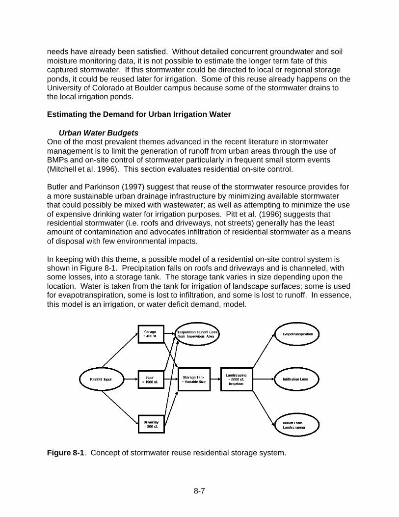
In keeping with this theme, a possible model of a residential on-site control system isshown in Figure 8-1. Precipitation falls on roofs and driveways and is channeled, withsome losses, into a storage tank. The storage tank varies in size depending upon thelocation. Water is taken from the tank for irrigation of landscape surfaces; some is usedfor evapotranspiration, some is lost to infiltration, and some is lost to runoff. In essence,this model is an irrigation, or water deficit demand, model.

Figure 8-1. Concept of stormwater reuse residential storage system.

8-8

Irrigation demand is determined mainly from ET requirements. In order to calculate ET, daily ormonthly water budgeting is performed. By examining the water balance of one residential parcelin differing climatic zones, the efficacy of the option of on site reuse of stormwater can beevaluated across the U.S. This section introduces the reader to climatic water balance models,and existing databases for use with these models, develops a parcel level storage/demandanalysis using the results from the climatic model and compares results regionally across theU.S.

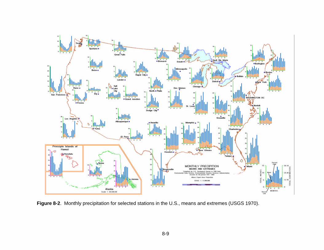
Water Budget ConceptsThe early efforts by Thornthwaite (1948) may have been the first work in climatology inwhich, by an analytical method, differing characteristics such as rainfall, temperature,and the number of daylight hours in a day were combined to yield regional climaticprojections. The number of daylight hours in a day are a function of the latitude of thelocation, whereas monthly precipitation and temperature are functions of the climate ofthe location. Average monthly precipitation in the U.S. varies widely with location, ascan be seen in Figure 8-2. For example, in comparing the rainfall signature of SanFrancisco, CA with Memphis, TN, San Francisco has dry summers and wet winters;whereas Memphis appears to have wet springs, with some precipitation falling in everymonth of the year. Extreme monthly precipitation is also shown in Figure 8-2. SanFrancisco appears to have much less variability than Memphis.

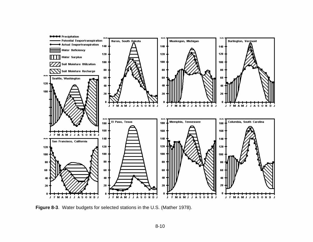
The Thornthwaite method keeps track of precipitation, calculated potentialevapotranspiration (PET), and calculated actual ET on a daily or monthly basis,calculating water deficit, water surplus, soil moisture recharge, and soil moistureutilization by integrating areas under the plotted curves. The graphical representation ofthis process is a water budget, examples of which are plotted in Figure 8-3, compiledfrom Mather (1978).

For example, for San Francisco, in January, the precipitation far exceeds the PET (andET, at this point they are equal). Up until mid February, the soil moisture is beingrecharged. This occurs until soil moisture capacity is reached, then the rest of therainfall exceeding PET is surplus (and available for runoff). For San Francisco, theannual surplus is about 4.3 inches. When PET exceeds rainfall (and is greater than ET)in April through October, there are two integrals of importance; the area between PETand ET is the water deficit, or 10.1 inches, and the area between ET and precipitation iswhat is being drawn from the soil moisture storage. Then, in October, whenprecipitation exceeds PET, the area between the precipitation curve and PET goes tosoil moisture recharge. The annual total PET for San Francisco is 26.6 inches, ET is16.6 inches, and precipitation is 20.8 inches. Memphis, also shown in Figure 8-3, hasan annual total PET of 39.2 inches, ET of 32.5 inches, precipitation of 45.8 inches, awater deficit of 6.7 inches, and a surplus of 13.2 inches. It is readily apparent that theclimate, and the subsequent irrigation needs for each location, are significantly different.

8-9

Figure 8-2. Monthly precipitation for selected stations in the U.S., means and extremes (USGS 1970).

8-10

Figure 8-3. Water budgets for selected stations in the U.S. (Mather 1978).

8-11

Methods of AnalysisThe Thornthwaite and Mather temperature based method (Thornthwaite 1948, Mather1957, and Willmott 1977) was used to calculate monthly PET, projected ET, waterdeficit, water surplus, and runoff (for undeveloped areas). Other methods, developedlater, require more information, such as net radiation measurements, wind speed, orhumidity. Such methods are usually found to be more accurate in arid areas (Yates1996). An even better approach to the daily water balance model is suggested byVorosmarty et al. (1996) and explained in detail in Vorosmarty et al. (1989, 1991). Thiswork is a continuation of the work of Mather and Thornthwaite at the University ofDelaware.

In the work in this section, the Thornthwaite (or other temperature or radiation basedPET model) is used as above, but the soil moisture term is actually modeled as well asthe PET. The result is a series of coupled differential equations that are solved by aRunge Kutta algorithm. The input data then reduced to soil and vegetation type. TheThornthwaite method was chosen for this analysis because of the simplicity of thealgorithm, as well as the availability of both monthly and daily precipitation andtemperature data. Daily data are available for most locations from the National ClimaticData Center.

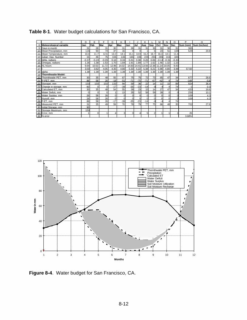
The water budget procedure is presented in Table 8-1 and graphically in Figure 8-4 forSan Francisco, CA. The reader may use the table to follow along the calculations stepby step. The mean precipitation, mean temperature, and mean PET (for comparativepurposes) are input parameters, and can be found in rows 10, 11, and 29, respectively.

The first step is the calculation of the Julian Day Number. This was done by startingwith the number 15 and adding 30 to each successive month in row 12. Next, thegeodesic variables are calculated by the following formula:

[ ] 360/2 Latitudeπφ = Equation 8.2and

δ π= −. sin ( / ) .4093 2 365 1 405J Equation 8.3

where φ=latitude in radians in Equation 8.2, δ also in radians, is the earth-sundeclination angle in Equation 8.3, and J is the Julian day number (e.g., December31=365). These formulas are used in rows 12 and 13. Next the following term iscalculated:

ω φ δs = −arccos tan tan Equation 8.4

using the terms calculated above. ωs is the sunset hour angle in radians (Equation 8.4).This is calculated for each month in row 15. Next, the total day length in hours iscalculated in Equation 8.5 as follows:

N i s= 24ω π/ Equation 8.5

8-12

Table 8-1. Water budget calculations for San Francisco, CA.

89

1011121315161718192021222324252627282930313233

C D E F G H I J K L M N O P QMeteorological variable Jan Feb Mar Apr May Jun Jul Aug Sep Oct Nov Dec Sum (mm) Sum (inches)Days in month 31 28 31 30 31 30 31 31 30 31 30 31 365Mean Precipitation, mm 116 93 74 37 16 4 0 1 6 23 51 108 529 20.8Mean Temperature, mm 10.4 11.7 12.6 13.2 14.1 15.1 14.9 15.2 16.7 16.3 14.1 11.4Julian_Day_Number 15 45 75 105 135 165 195 225 255 285 315 345delta, radians -0.37 -0.24 -0.05 0.16 0.33 0.41 0.38 0.26 0.06 -0.14 -0.31 -0.40Omegas, radians 1.26 1.38 1.53 1.70 1.84 1.91 1.89 1.77 1.62 1.46 1.32 1.23Ni, hours 9.64 10.53 11.72 12.96 14.02 14.60 14.41 13.56 12.38 11.14 10.05 9.43I 3.03 3.62 4.05 4.35 4.80 5.33 5.22 5.38 6.21 5.98 4.80 3.48 57.50alpha 1.39 1.39 1.39 1.39 1.39 1.39 1.39 1.39 1.39 1.39 1.39 1.39Thornthwaite Model:Thornthwaite PET, mm 30 35 48 55 67 75 75 72 73 65 47 34 677 26.6P-PET, mm 86 58 26 -18 -51 -71 -75 -71 -67 -42 4 74 -148 -5.8Storagei, mm 150 150 150 133 94 59 36 22 14 11 15 89 924 36.4Change in storage, mm 60 0 0 -17 -39 -35 -23 -14 -8 -4 4 74 -1 0.0Calculated ET, mm 30 35 48 54 55 39 23 15 14 27 47 34 420 16.6Water Deficit, mm 0 0 0 1 13 35 52 58 59 39 0 0 256 10.1Water Surplus, mm 26 58 26 0 0 0 0 0 0 0 0 0 109 4.3Runoff, mm 26 58 26 0 0 0 0 0 0 0 0 0 109 4.3P-ET, mm 86 58 26 -17 -39 -35 -23 -14 -8 -4 4 74Measured PET, mm 31 35 49 59 70 78 79 77 75 66 48 35 702 27.6Initial Storage, mm 90Storage Maximum, mm 150Error, mm 1 0 1 4 3 3 4 5 2 1 1 1 26% error 3.68%

0

20

40

60

80

100

120

1 2 3 4 5 6 7 8 9 10 11 12

Months

Wat

er in

mm

Thornthwaite PET, mmPrecipitationCalculated ETWater DeficitWater SurplusSoil Moisture UtilizationSoil Moisture Recharge

Figure 8-4. Water budget for San Francisco, CA.

8-13

and is shown in row 16. Then the following parameters are calculated in Equations 8.6and 8.7:

[ ]I Tii

n

==∑ .

.2

1 5

1

Equation 8.6

α = − + +− − −( . * ) ( . * ) ( . * ) .6 75 10 7 71 10 179 10 497 3 5 2 2I I Equation 8.7

where n= number of months (or days) in question. These are calculated in rows 17 and18, the sum of I is calculated by adding all the values of I for the previous 12 monthsshown in row 17 and is shown in cell P17 . Since Ti (temperature) can be negative, inthose cases, I and PET are set to zero. I represents an annual heat index for the areain question. Then, actual values for potential evapotranspiration, PET, storage, S,evapotranspiration, Et, and undeveloped runoff, R are calculated using the Equation8.8:

PET f fT

Iii=

1610

1 2

α

Equation 8.8

where f 1 = the fraction of the number of days in the month i divided by the average days

in a month, 30; and fN i

2 12= , the fraction of the number of hours in a day divided by the

base of 12 hours in a day. This is calculated in row 20. Next, the soil moisture storageis calculated. This is not to be confused with tank storage, which will be calculatedlater. The soil moisture storage is modeled as an offline reservoir that leaks when thesoil moisture field capacity is reached. Equations 8.9 and 8.10 compute storage inmonth i as follows:

S P PET S Si i i i= − + −min (( ) ), max1 if P PETi i> (surplus condition) Equation 8.9

S SPET P

Si ii i=−

−1 exp

(

max

if P PETi i≤ (deficit condition) Equation 8.10

in which Si is the soil moisture storage term for month i, Pi is precipitation term for monthi, and Smax is the maximum storage availability found in cell D31. The initial storageterm for month 0 is found in cell D30. The calculated Si for each month is found in row22. The change in storage, or ∆S S Si i= − −1 is calculated in row 23. Next, actual

evapotranspiration is calculated by Equations 8.11 and 8.12:

Et PETi i= if P PETi i> Equation 8.11

Et P S Si i i i= + −−1 if P PETi i≤ Equation 8.12

8-14

and can be found in row 24. Finally, runoff is computed by Equation 8.13,

R P Et Si i= − − ∆ Equation 8.13

and is shown in row 27. In cases in which R<0, runoff is then set to zero.

The parameters for which the least amount of information is usually available are theinitial storage term (when i=1) and the maximum soil moisture storage. In this case, anequal Smax of 150 mm was used and the initial storage term was determined by usingthe calculated Si for December (and iterating if necessary). Water deficit was calculatedby subtracting the estimated ET from the calculated PET in months in which PETexceeds rainfall (otherwise there is no deficit). This is shown in row 25. Water surpluswas calculated by Equation 8.14:

SU P PET Si i i i= − − ∆ if P PETi i> Equation 8.14

and is shown in row 26. The percent error is calculated by taking the absolute value ofthe difference between the calculated PET and measured PET, summing for the 12months, and dividing by the sum of the measured PET for 12 months, and is shown incell P33. For San Francisco, the error is 3.68%, indicating that there is a reasonablygood fit with the Thornthwaite model.

The tank calculations for San Francisco are shown in Table 8-2. Using a parcel size of10,000 sq. ft. (cell D36), and a 1500 sq. ft. house (cell D37), 400 sq. ft. garage(cellD38), an 800 sq. ft. driveway (cell D39), and an irrigated area of 5000 sq. ft. (cell D40),an irrigation demand model was developed in which 80% of the runoff from the house,garage, and driveway was recovered into a storage tank (unless spilled), converting mmof runoff into gallons by multiplying by the impervious areas and conversion factors.This is shown for each month in row 42. These criteria are approximately equal to thedimensions used in the “Casa Del Agua” house in Tucson, AZ (Foster, et al.,1988 andKarpiscak et al., 1990). For purposes of this exercise, runoff from the roof, garage, anddriveway are assumed to be channeled into the proposed cistern, which is assumed tobe 80% efficient at capturing rainfall (which is consistent with the “Casa Del Agua”case). An initial guess of 100 gallons was given for the storage tank to initiate thecalculations.

Water requirements of the landscaped vegetation were assumed to be similar to thatpredicted by the deficit calculations using the Thornthwaite procedure and losses due torunoff and infiltration were considered negligible. The cumulative volume was thencalculated, assuming that the tank initially is empty and that cumulative volume cannotexceed the size of the storage tank, subtracting actual use in the previous month fromthe storage volume. This is shown in row 43. Next, the potential use or demand for thewater was calculated by multiplying the deficit by the irrigated area and converting thenumber into gallons. This is shown in row 44. The actual use from the storage tank,

8-15

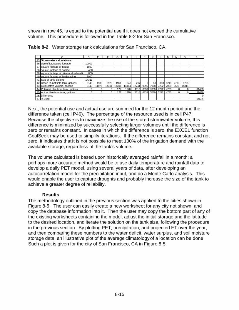
shown in row 45, is equal to the potential use if it does not exceed the cumulativevolume. This procedure is followed in the Table 8-2 for San Francisco.

Table 8-2. Water storage tank calculations for San Francisco, CA.

35363738394041424344454647

C D E F G H I J K L M N O PStormwater calculations:size of lot, square footage 10000square footage of house 1500square footage of garage 400square footage of drive and sidewalk 800square footage of landscaping 5000Size of tank, gallons 14311Urban Runoff into tank, gallons 6149 4930 3923 1961 848 212 0 53 318 1219 2703 5725Cumulative volume, gallons 6149 11079 14311 14311 14184 12741 9995 7978 7222 7089 9528 14311Potential Use from tank, gallons 0 0 0 127 1570 4316 6333 7089 7222 4783 0 0 31439Actual Use from tank, gallons 0 0 0 127 1570 4316 6333 7089 7222 4783 0 0 31439Difference 0% used 100%

Next, the potential use and actual use are summed for the 12 month period and thedifference taken (cell P46). The percentage of the resource used is in cell P47.Because the objective is to maximize the use of the stored stormwater volume, thisdifference is minimized by successfully selecting larger volumes until the difference iszero or remains constant. In cases in which the difference is zero, the EXCEL functionGoalSeek may be used to simplify iterations. If the difference remains constant and notzero, it indicates that it is not possible to meet 100% of the irrigation demand with theavailable storage, regardless of the tank’s volume.

The volume calculated is based upon historically averaged rainfall in a month; aperhaps more accurate method would be to use daily temperature and rainfall data todevelop a daily PET model, using several years of data, after developing anautocorrelation model for the precipitation input, and do a Monte Carlo analysis. Thiswould enable the user to capture droughts and probably increase the size of the tank toachieve a greater degree of reliability.

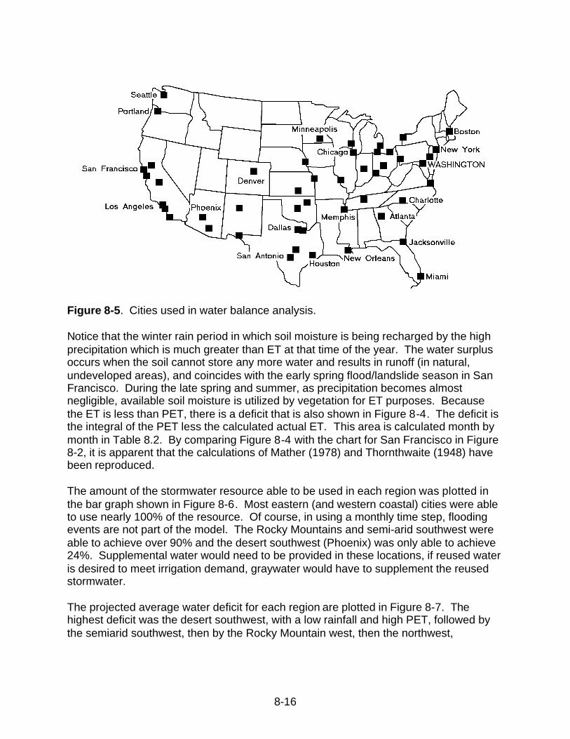
ResultsThe methodology outlined in the previous section was applied to the cities shown inFigure 8-5. The user can easily create a new worksheet for any city not shown, andcopy the database information into it. Then the user may copy the bottom part of any ofthe existing worksheets containing the model, adjust the initial storage and the latitudeto the desired location, and iterate the solution on the tank size, following the procedurein the previous section. By plotting PET, precipitation, and projected ET over the year,and then comparing these numbers to the water deficit, water surplus, and soil moisturestorage data, an illustrative plot of the average climatology of a location can be done.Such a plot is given for the city of San Francisco, CA in Figure 8-5.

8-16

Figure 8-5. Cities used in water balance analysis.

Notice that the winter rain period in which soil moisture is being recharged by the highprecipitation which is much greater than ET at that time of the year. The water surplusoccurs when the soil cannot store any more water and results in runoff (in natural,undeveloped areas), and coincides with the early spring flood/landslide season in SanFrancisco. During the late spring and summer, as precipitation becomes almostnegligible, available soil moisture is utilized by vegetation for ET purposes. Becausethe ET is less than PET, there is a deficit that is also shown in Figure 8-4. The deficit isthe integral of the PET less the calculated actual ET. This area is calculated month bymonth in Table 8.2. By comparing Figure 8-4 with the chart for San Francisco in Figure8-2, it is apparent that the calculations of Mather (1978) and Thornthwaite (1948) havebeen reproduced.

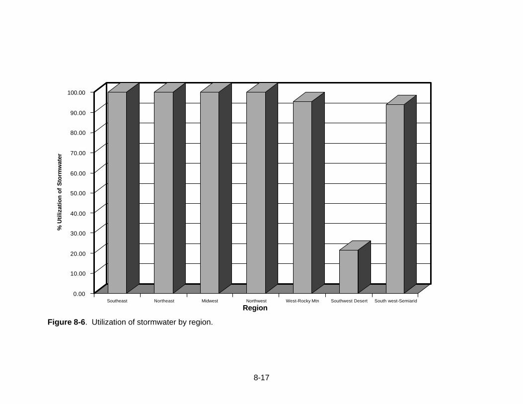
The amount of the stormwater resource able to be used in each region was plotted inthe bar graph shown in Figure 8-6. Most eastern (and western coastal) cities were ableto use nearly 100% of the resource. Of course, in using a monthly time step, floodingevents are not part of the model. The Rocky Mountains and semi-arid southwest wereable to achieve over 90% and the desert southwest (Phoenix) was only able to achieve24%. Supplemental water would need to be provided in these locations, if reused wateris desired to meet irrigation demand, graywater would have to supplement the reusedstormwater.

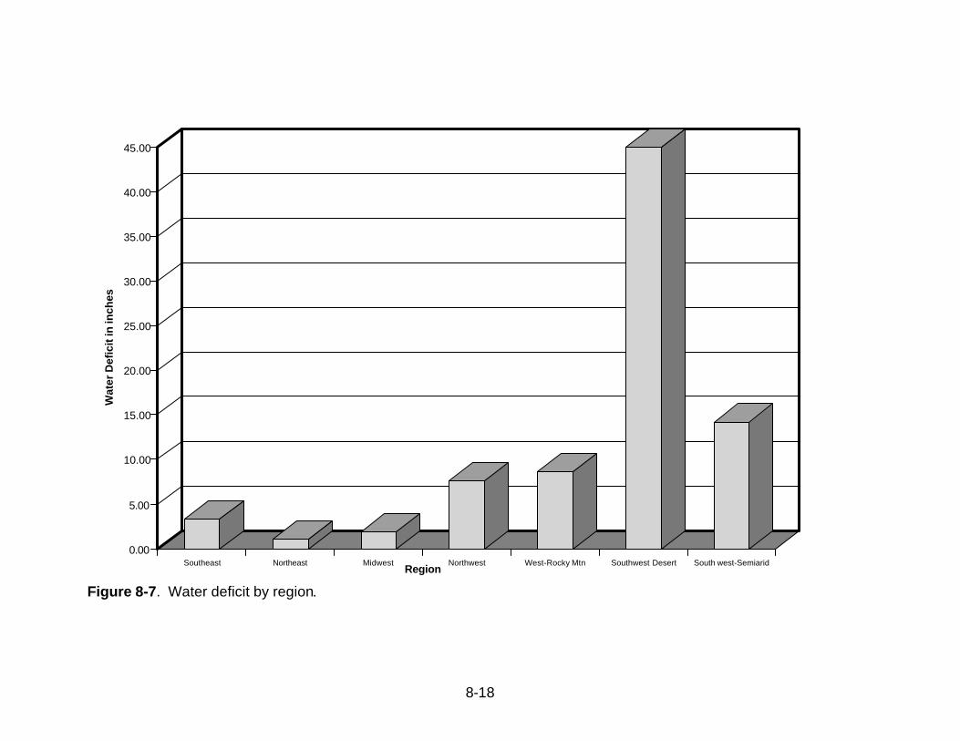
The projected average water deficit for each region are plotted in Figure 8-7. Thehighest deficit was the desert southwest, with a low rainfall and high PET, followed bythe semiarid southwest, then by the Rocky Mountain west, then the northwest,

8-17

0.00

10.00

20.00

30.00

40.00

50.00

60.00

70.00

80.00

90.00

100.00

% U

tiliz

atio

n o

f S

torm

wat

er

Southeast Northeast Midwest Northwest West-Rocky Mtn Southwest Desert South west-Semiarid

Region

Figure 8-6. Utilization of stormwater by region.

8-18

0.00

5.00

10.00

15.00

20.00

25.00

30.00

35.00

40.00

45.00

Wat

er D

efic

it in

inch

es

Southeast Northeast Midwest Northwest West-Rocky Mtn Southwest Desert South west-SemiaridRegion

Figure 8-7. Water deficit by region.

8-19

southeast, midwest, and northeast.

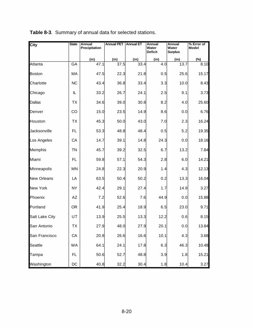
The annual precipitation, calculated PET, water deficit, and an estimate of the percenterror of the Thornthwaite model for each studied city is found in Table 8-3. There maybe some variation between these values and other published data depending upon thelocation of the measurement, as well as the length of the data record. This may affectthe error calculation as well. The Thornthwaite model, as stated previously, tends togive better results in non arid areas. The station chosen for Seattle, WA is probably at ahigher elevation than published data for the city of Seattle, as the value for precipitationin Table 8-3 is much higher than expected.

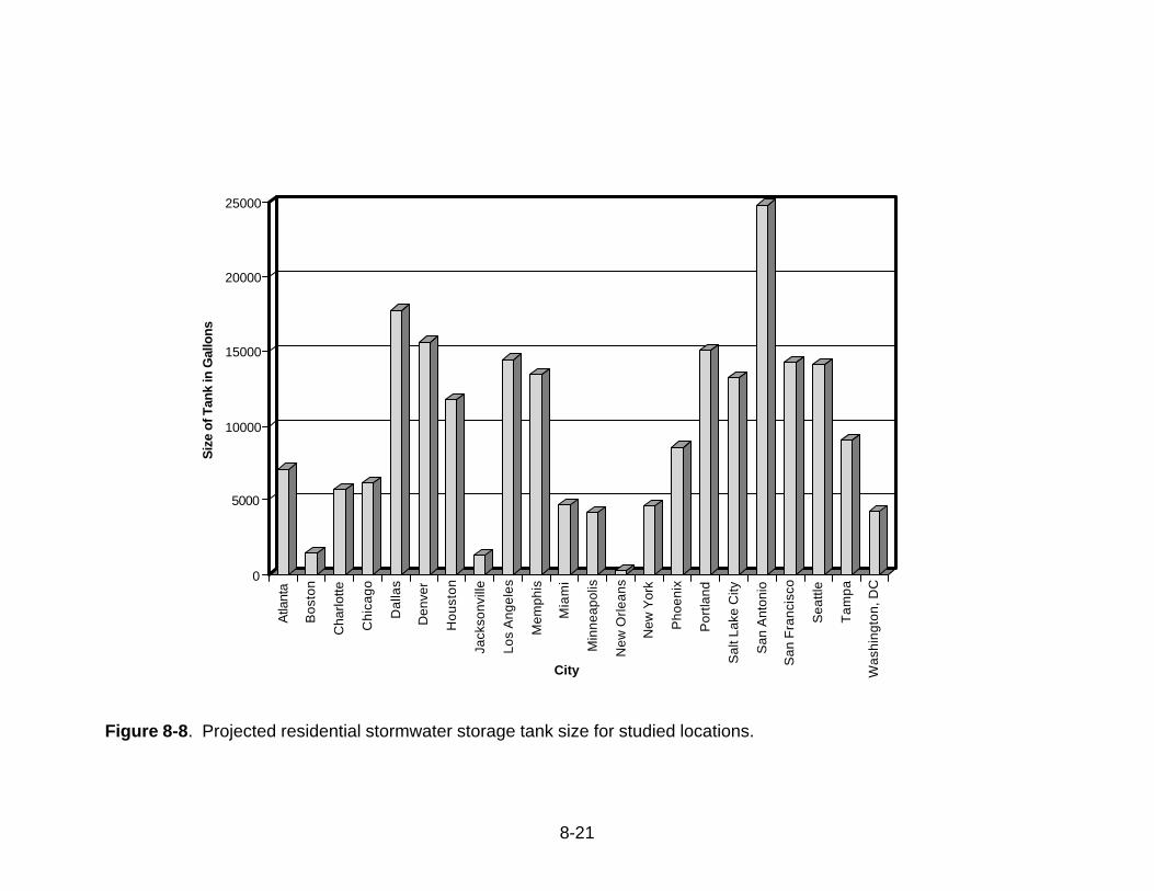
The projected storage tank size for each location is plotted in Figure 8-8. San Antonio,TX had the largest tank size, at 25,000 gallons, followed by Dallas, TX at about 17,500gallons, then Denver, CO at 15,500 gallons. Areas with very dry summers and wetwinters such as San Francisco, CA and Los Angeles, CA tended to be next, at around14,500 gallons. Most areas in the humid east were under 5,000 gallons, except inlocations where ET needs outstripped available precipitation, such as in Tampa, FL at9,000 gallons. The reason very high water deficit areas such as Phoenix, AZ did notresult in the largest tanks is that no available storage would have any benefit, that is, theET needs far exceed available rainfall.

This data compares favorably with Pazwash and Boswell (1997) who found the samenationwide trends when their results are scaled up to the same lot size. They found thatthe arid southwest tended to require smaller tanks than the rest of the country, due tothe lack of available rainfall. Average tank size for other areas ranged from 4320gallons in the northeast to 6750 in the southeast.

8-20

Table 8-3. Summary of annual data for selected stations.

City State AnnualPrecipitation

(in)

Annual PET

(in)

Annual ET

(in)

AnnualWaterDeficit

(in)

AnnualWaterSurplus

(in)

% Error ofModel

(%)

Atlanta GA 47.1 37.5 33.4 4.0 13.7 8.10

Boston MA 47.5 22.3 21.8 0.5 25.6 15.17

Charlotte NC 43.4 36.8 33.4 3.3 10.0 8.43

Chicago IL 33.2 26.7 24.1 2.5 9.1 3.73

Dallas TX 34.6 39.0 30.8 8.2 4.0 25.60

Denver CO 15.0 23.5 14.9 8.6 0.0 6.76

Houston TX 45.3 50.0 43.0 7.0 2.3 16.24

Jacksonville FL 53.3 48.8 48.4 0.5 5.2 19.35

Los Angeles CA 14.7 39.1 14.8 24.3 0.0 18.16

Memphis TN 45.7 39.2 32.5 6.7 13.2 7.84

Miami FL 59.8 57.1 54.3 2.8 6.0 14.21

Minneapolis MN 24.8 22.3 20.9 1.4 4.3 12.13

New Orleans LA 63.5 50.4 50.2 0.2 13.3 16.04

New York NY 42.4 29.1 27.4 1.7 14.9 3.27

Phoenix AZ 7.2 52.6 7.6 44.9 0.0 15.88

Portland OR 41.9 25.4 18.9 6.5 23.0 9.71

Salt Lake City UT 13.9 25.5 13.3 12.2 0.6 8.15

San Antonio TX 27.9 48.0 27.9 20.1 0.0 13.84

San Francisco CA 20.8 26.6 16.6 10.1 4.3 3.68

Seattle WA 64.1 24.1 17.8 6.3 46.3 10.48

Tampa FL 50.6 52.7 48.8 3.9 1.8 15.21

Washington DC 40.8 32.2 30.4 1.8 10.4 3.27

8-21

0

5000

10000

15000

20000

25000S

ize

of T

ank

in G

allo

ns

Atla

nta

Bo

sto

n

Cha

rlotte

Ch

ica

go

Da

llas

Den

ver

Ho

ust

on

Jack

son

ville

Lo

s A

ng

ele

s

Me

mp

his

Mia

mi

Min

ne

ap

olis

Ne

w O

rle

an

s

New

Yor

k

Ph

oe

nix

Po

rtla

nd

Sa

lt L

ake

City

Sa

n A

nto

nio

Sa

n F

ran

cisc

o

Se

att

le

Ta

mp

a

Wa

shin

gto

n, D

C

City

Figure 8-8. Projected residential stormwater storage tank size for studied locations.

8-22

ConclusionsIn summary, in many areas of the country, particularly in humid areas, enoughstormwater can be collected to satisfy average irrigation demands. If driveway areasare eliminated due to possible problems with water quality and ease of collection, theresult will be a larger tank size, however, irrigation demand may still be satisfied in amajority of cases. In arid areas, particularly those with high ET requirement, stormwaterreuse may not be justified by itself. In these cases, the option of combining storage withtreated graywater may be worth considering.

A possible enhancement in the technique could be to apply the model to a daily timeseries and developing an autoregessive time series model of the PET, ET, andprecipitation for each city. Next, a Monte Carlo analysis can be performed to determinethat, given the historical data series, a tank sized by this procedure will serve, say, 90%of the ET needs of the parcel. Such an analysis and computer model was developedfor rural regions of India by Vyas (1996). An extrapolation of this work tourban/suburban areas of the U.S. needs to be done. In addition, consideration of adaily time step model may be more realistic in this effort. The effect of using severalyears of data will be to enlarge the tank, as the tank size will increase in order to serveET needs during more extreme events, such as droughts.

8-23

References

Anderson, J.M. (1996a). Current water recycling initiatives in Australia: scenarios forthe 21st century. Water Science Technology. (G.B.), 33: 10-11, 37-43.

Anderson, J.M. (1996b). The potential for water recycling in Australia: expanding ourhorizons. Desalination, 106: 1-3, 151-156.

Asano, T., and A. D. Levine (1996). Wastewater reclamation, recycling and reuse:past, present, and future. Water Science Technology. (G.B.), 33: 10-11, 1-13.

Ashcraft, J. G., and M. G. Hoover (1991). Water reuse--implementation and costs insouthern California. In Water Supply and Water Reuse: 1991 and Beyond.Proceedings of the AWRA Conference. Denver, CO.

Butler, D. and J. Parkinson (1997). Towards sustainable urban drainage. WaterScience and Technology. 35 (9), 53-63.

Courtney, B.A. (1997). An Integrated Approach to Urban Irrigation: The Role ofShading, Scheduling, and Directly Connected Imperviousness. MS Thesis.Department of Civil, Environmental, and Architectural Engineering. University ofColorado. Boulder, CO.

Field, R. (1993). Reclamation of Urban Stormwater. Integrated StormwaterManagement. Field, R., M.L. O’Shea, and K.K. Chin (Ed.), p.307.

Foster, K. E., M. M. Karpiscak, and, R. G. Brittain (1988). Casa Del Agua: aresidential water conservation and reuse demonstration project in Tucson, AZ. WaterResources Bulletin. 24(6):1201-1206.

Grimmond, C. S. B. and T. R. Oke (1986). Urban water balance 2: Results from asuburb of Vancouver, British Columbia. Water Resources Research. 22(10):1404-1412.

Grimmond, C. S. B., T. R Oke, and D. G. Steyn (1986a). Urban water balance 1: amodel for daily totals. Water Resources Research. 22(10):1397-1403.

Haarhoff, J., and B. Van der Merwe (1996). Twenty-five years of wastewaterreclamation in Windhoek, Namibia. Water Science Technology. (G.B.), 33: 10-11, 25-35.

Harper, G. (1991). Reuse of Stormwater: Design Curves for Florida. MS Thesis.University of Central Florida. Orlando, FL.

8-24

Harrison, T.J. (1993). Stormwater Reuse Design Curves for Southwest Florida WaterManagement District. In SWFMD. Proceedings of 3rd Biennial Stormwater ResearchConference. Brooksville, FL.

Heaney, J.P. and L.T. Wright (1997). On Integrating Continuous Simulation andStatistical Methods for Evaluating Urban Stormwater Systems. Chapter 3 in James, W.(Editor). Advances in Modeling the Management of Stormwater Impacts. Vol. 5. CHI.Guelph, ON, Canada. P. 44-76.

Heaney, J.P., L.T. Wright, D. Sample, B. Urbonas, B. Mack, M. Schmidt, M. Solberg, J.Jones, J. Clary, and T. Brown (1998). Development of Methodologies for the Design ofIntegrated Wet-Weather Flow Collection/Control/Treatment Systems for NewlyUrbanizing Areas. Draft Rep. to U.S. EPA. Natl. Risk Manage. Res. Lab. Cincinnati,OH.

Herrmann, T., and K. Hase (1996). Way to get water rainwater utilization or long-distance water supply? A holistic assessment. In Proc. of the 7th Int. Conf. UrbanStorm Drainage. Hannover, Germany. IAHR/IAWQ Joint Committee Urban StormDrainage.

Herrmann, T., U. Schmida, U. Klaus, and V. Huhn (1996). Rainwater utilization ascomponent of urban drainage schemes: hydraulic aspects and pollutant retention. InProc. 7th Int. Conf. Urban Storm Drainage. Hannover, Germany. IAHR/IAWQ JointCommittee Urban Storm Drainage.

Imbe, M., T. Ohta, and N. Takano (1996). Quantitative assessment of improvement inhydrological water cycle in urbanized river basin. In Proc. of the 7th Int. Conf. UrbanStorm Drainage. Hannover, Germany. IAHR/IAWQ Joint Committee Urban StormDrainage.

Karpiscak, M. M., K. E. Foster, and N. Schmidt (1990). Residential water conservation:Casa Del Agua. Water Resources Research. 26: 6, 939-948.

Law, I. B. (1996). Rouse Hill—Australia’s first full scale domestic non-potable reuseapplication. Water Science Technology. (G.B.), 33: 10-11, 71-78.

Leemans, R. (1988). Dataset developed during the YSSP summary program 1988, atIIASA. Laxenburg, Austria for the BIOSPHERE.

Lejano, R. P., F. A. Grant, T. G. Richardson, B. M. Smith, and F. Farhang (1992).Assessing the benefits of water reuse: applying a cost-benefit allocation procedure.Water Environment & Technology. 4 (8), 44-50.

Mallory, C. W., and J. J. Boland (1970). A system study of storm runoff problems in anew town. Water Resources Bulletin. 6 (6), 980-989.

8-25

Mangeot, E.F. (1996). City of Boulder Wastewater Treatment Plant Model StormwaterSurge Analysis Using GPX-X. Independent Study for Professor Silverstein.Department of Civil, Environmental, and Architectural Engineering. University ofColorado. Boulder, CO.

Mather, J. R.(1978). The Climatic Water Budget in Environmental Analysis. D. C.Heath and Company. ISBN: 0-669-02087-7.

Mitchell, V.G., R.G. Mein, and T.A. McMahon (1996). Evaluating the resource potentialof stormwater and wastewater: an Australian perspective. In Proc. of the 7th Int. Conf.Urban Storm Drainage. Hannover, Germany. IAHR/IAWQ Joint Committee UrbanStorm Drainage.

Nelen, A.J.M., A.C. de Ridder, and E.C. Hartman (1996). Planning of a new urban areain a municipality of Ede using a new approach to environmental protection. In Proc. ofthe 7th Int. Conf. Urban Storm Drainage. Hannover, Germany. IAHR/IAWQ JointCommittee Urban Storm Drainage.

Nowakowska-Blaszczyk, A., and J. Zakrzewski (1996). The sources and phases ofincrease of pollution in runoff waters in route to receiving waters. In Proc. 7th Int. Conf.Urban Storm Drainage. Hannover, Germany. IAHR/IAWQ Joint Committee UrbanStorm Drainage.

Oron, G. (1996). Management modeling of integrative wastewater treatment and reusesystems, wastewater reclamation and reuse 1995. Water Science Technology. (G.B.),33: 10-11, 95-105.

Pazwash, H., and S. Boswell (1997). Management of roof runoff conservation andreuse. Proc. 24th ASCE Water Resources Planning and Management Annual Conf.,Aesthetics on the Constructed Environment. Houston, TX. 784.

Pisano, W.C. and H. Brombach (1997). Solids Settling Curves. Water EnvironmentTechnology. Vol. 8, No.4, P 27-33.

Pitt, R., R. Field, M. Lalor, and M. Brown (1996). Groundwater Contamination fromStormwater Infiltration. Chelsea, MI. Ann Arbor Press.

Pruel, H.C. (1996). Combined sewage prevention system (CSPS) for domesticwastewater source control. In Proc. of the 7th Int. Conf. Urban Storm Drainage.Hannover, Germany. IAHR/IAWQ Joint Committee Urban Storm Drainage.

8-26

Requa, A., J. M. Kelly, J. A. Burgh, and M. Manzione (1991). Successfulimplementation of an urban landscaping recycled water program. In Water Supply andWater Reuse: 1991 and Beyond. Proceedings of the Conference of the AWRA.Denver, CO.

Tchobanoglous, G., and A. Angelakis (1996). Technologies for wastewater treatmentappropriate for reuse potential for application in Greece. Water Science Technology.(G.B.), 33: 10-11, 15-24.

Thornthwaite, C. W. (1948). An approach toward a rational classification of climate.Geographical Review. volume 38 pp. 55-94.

Tselentis, Y., and S. Alexopoulou (1996). Effluent reuse options in Athens metropolitanarea: a case study. Water Science Technology. (G.B.), 33: 10-11, 127-137.

U.S. Geological Survey (1970). The National Atlas of the United States of America.Reston, VA.

Veldkamp. R. G., T. Hermann, V. Colandini, L. Terwel, and G. D. Geldof (1997). Adecision network for urban water management. Water Science Technology. (G.B.) 36:8-9, 111-115.

Vorosmarty, C. J. and B. Moore (1991). Modeling basin-scale hydrology in support ofphysical climate and global biogeochemical studies: an example using the ZambeziRiver. Surveys in Geophysics. volume 12, pp. 271-311.

Vorosmarty, C. J., C. J. Willmott, B. J. Choudhury, A. L. Schloss, T. K. Stearns, S. M.Robeson, and T. J. Dorman (1996). Analyzing the discharge regime of a large tropicalriver through remote sensing, ground-based climatic data and modeling. WaterResources Research. 32(10):3137-3150.

Vorsomarty, C. J., B. Moore, A. L. Grace, M. P. Gildea, J. M. Melillo, B. J. Peterson, E.B. Rastetter, and P. A. Steudler (1989). Continental scale models of water balance andfluvial transport: an application to South America. Global Biogeochemical Cycles.3(3):241-265.

Vyas, V. (1996). Monte-Carlo simulation of rainwater harvesting systems. Raindrop.December, 1996 and web pagehttp://www.geocities.com/RainForest/Canopy/4805/FAQ.html.

Wanielista, M. (1993). Stormwater Reuse: An Alternative Method of Infiltration. In Proc.National Conf. on Urban Runoff Management: Enhancing Urban WatershedManagement at the Local, County, and State Levels . U.S. EPA. Cincinnati, OH.

8-27

Willmott, C. J. (1977). WATBUG: A FORTRAN IV Algorithm for Calculating ClimaticWater Budget. Water Resources Center. Delaware University; Contribution Number23, Report Number 1. Publications in Climatology Vol. XXX, No. 2.

Yates, D. N. (1996). WatBal: an integrated water balance model for climate impactassessment of river basin runoff. Water Resources Development. 12(2):121-139.