stonex cube-a field software user manual - top-sys.de
TRANSCRIPT
www.stonex.it (December 2018)-Ver.4.2-Rev.0
Stonex Cube-a
Field Software
User Manual
4.2
Stonex Software Cube-a v.4.2 – User Manual 1
Contents 1 Software introduction .................................................................................................... 3
2 Cube-a installation and uninstallation ......................................................................... 4
2.1 Cube-a Installation ............................................................................................................................. 4
2.2 Cube-a First Run ................................................................................................................................. 5
2.3 Cube-a Uninstallation ....................................................................................................................... 7
3 Software Introduction - Project .................................................................................... 9
3.1 Project Manager .............................................................................................................................. 10
3.2 View Data ........................................................................................................................................... 12
3.3 File Manager ..................................................................................................................................... 15
3.4 Backup File Import .......................................................................................................................... 16
3.5 Export Data ........................................................................................................................................ 17
3.6 Import of Data .................................................................................................................................. 22
3.7 Import of Raster Images ............................................................................................................... 24
3.8 Project Details ................................................................................................................................... 26
3.9 Feature Codes ................................................................................................................................... 27
4 Software introduction - Device ................................................................................... 28
4.1 GPS Status .......................................................................................................................................... 29
4.2 Data Link Status ............................................................................................................................... 35
4.3 Communication Settings .............................................................................................................. 37
4.4 Working mode ................................................................................................................................. 41
4.4.1 Communication ....................................................................................................................... 42
4.4.2 Static Mode ............................................................................................................................... 43
4.4.3 Base Mode ................................................................................................................................. 47
4.4.4 Rover mode ............................................................................................................................... 50
4.4.5 Preset Configurations ............................................................................................................ 53
4.5 Data Link Settings ........................................................................................................................... 54
4.5.1 Internal Network ..................................................................................................................... 56
4.5.2 Internal Radio ........................................................................................................................... 59
4.5.3 External Radio .......................................................................................................................... 60
4.5.4 Phone Network ........................................................................................................................ 60
4.6 Information ........................................................................................................................................ 61
4.7 RTK Reset ........................................................................................................................................... 62
4.8 Register ............................................................................................................................................... 62
4.9 Distance meter ................................................................................................................................. 63
5 Software introduction – Survey .................................................................................. 65
5.1 Point Survey ...................................................................................................................................... 66
Stonex Software Cube-a v.4.2 – User Manual 2
5.2 Point Stakeout ................................................................................................................................ 103
5.2.1 Photo and Sketch .................................................................................................................. 111
5.3 Line Stakeout .................................................................................................................................. 113
5.4 Elevation Control ........................................................................................................................... 119
5.5 Geophysical Stakeout .................................................................................................................. 120
6 Software introduction – Configure ........................................................................... 121
6.1 Coordinate System ....................................................................................................................... 121
6.2 Record Settings .............................................................................................................................. 126
6.3 Display Settings ............................................................................................................................. 126
6.4 System Settings .............................................................................................................................. 127
6.5 Survey Settings ............................................................................................................................... 128
6.6 Layers Settings ............................................................................................................................... 129
6.7 Administration ................................................................................................................................ 130
7 Software introduction - Calibrate ............................................................................. 131
7.1 Site Calibration ............................................................................................................................... 131
7.2 Calibrate Point ................................................................................................................................ 137
7.3 Calibrate Sensor ............................................................................................................................. 142
8 Software introduction – Tools ................................................................................... 153
8.1 Points Library .................................................................................................................................. 154
8.2 Entities list ........................................................................................................................................ 157
8.3 Coordinates Converter ................................................................................................................ 158
8.4 Angles Converter ........................................................................................................................... 160
8.5 Perimeter and area ....................................................................................................................... 161
8.6 COGO Calculations ....................................................................................................................... 162
8.6.1 Azimuth and Range .............................................................................................................. 163
8.6.2 Angle offset ............................................................................................................................. 164
8.6.3 Distance .................................................................................................................................... 165
8.6.4 Two Lines Angle .................................................................................................................... 166
8.6.5 2 Alignments Intersection .................................................................................................. 167
8.6.6 2 Points 2 Distances ............................................................................................................. 168
8.6.7 2 Points 2 Angles .................................................................................................................. 169
8.6.8 2 points Distance and Angle ............................................................................................. 170
8.6.9 Polar from North ................................................................................................................... 171
8.7 Calculator ......................................................................................................................................... 171
8.8 Version and Update ...................................................................................................................... 172
Stonex Software Cube-a v.4.2 – User Manual 3
1 Software introduction
Cube-a is GNSS surveying and mapping software developed by Stonex Srl, designed and
implemented for the Android platform.
Thanks to the flexibility of the Android environment, it has been possible to create a simple
and intuitive user interface, which makes users ready to face any job, saving time and
increasing productivity.
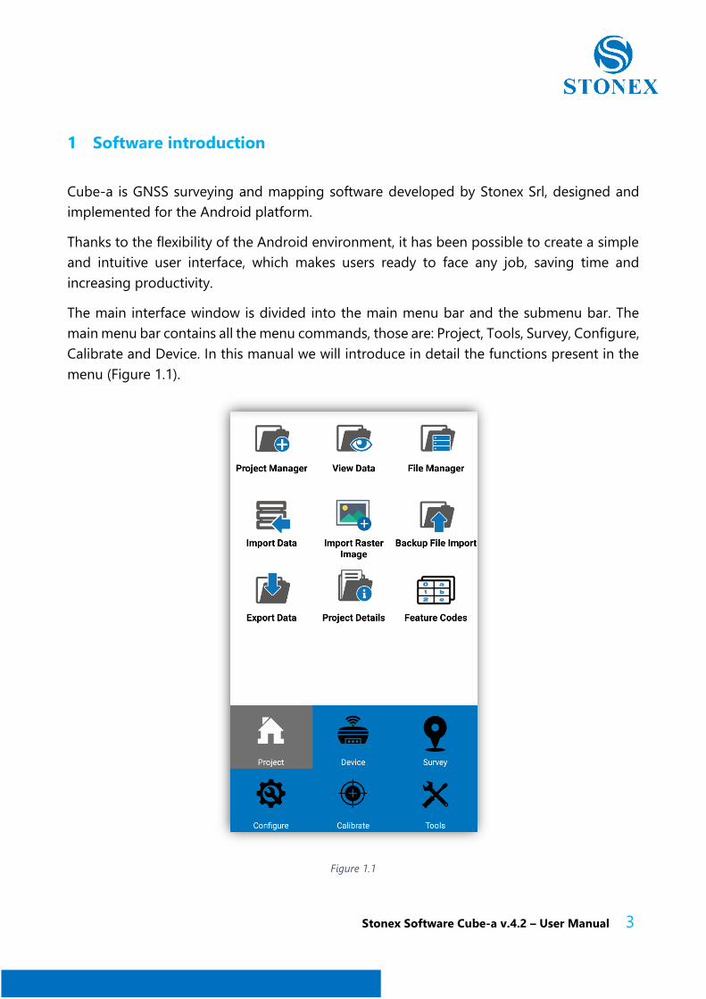
The main interface window is divided into the main menu bar and the submenu bar. The
main menu bar contains all the menu commands, those are: Project, Tools, Survey, Configure,
Calibrate and Device. In this manual we will introduce in detail the functions present in the
menu (Figure 1.1).
Figure 1.1
Stonex Software Cube-a v.4.2 – User Manual 4
2 Cube-a installation and uninstallation
This chapter describes the installation and uninstallation instructions for Cube-a Software.
2.1 Cube-a Installation
1. Please download the Android Cube-a installation package (*.apk) and copy the
installation package to your Android device.
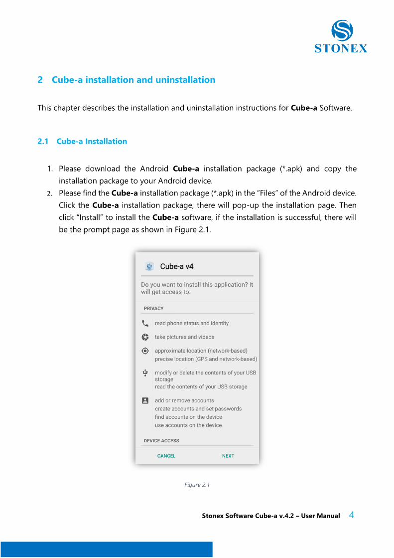
2. Please find the Cube-a installation package (*.apk) in the “Files” of the Android device.
Click the Cube-a installation package, there will pop-up the installation page. Then
click “Install” to install the Cube-a software, if the installation is successful, there will
be the prompt page as shown in Figure 2.1.
Figure 2.1
Stonex Software Cube-a v.4.2 – User Manual 5
2.2 Cube-a First Run
The software must be registered and unlocked at its first run. To unlock it, you need to know
which is your personal and unique Purchase Code ID.
The Purchase Code ID is in a form like STX000000000ABC and you should have got it by e-
mail or printed. The software cannot be unlocked without entering the correct Purchase
Code.
This operation must be done while your device (tablet or phone) has an active Internet
connection.
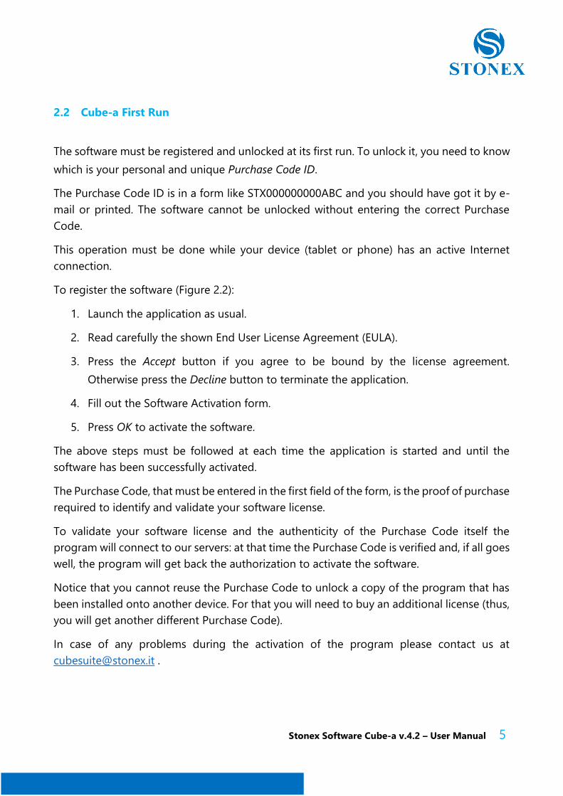
To register the software (Figure 2.2):
1. Launch the application as usual.
2. Read carefully the shown End User License Agreement (EULA).
3. Press the Accept button if you agree to be bound by the license agreement.
Otherwise press the Decline button to terminate the application.
4. Fill out the Software Activation form.
5. Press OK to activate the software.
The above steps must be followed at each time the application is started and until the
software has been successfully activated.
The Purchase Code, that must be entered in the first field of the form, is the proof of purchase
required to identify and validate your software license.
To validate your software license and the authenticity of the Purchase Code itself the
program will connect to our servers: at that time the Purchase Code is verified and, if all goes
well, the program will get back the authorization to activate the software.
Notice that you cannot reuse the Purchase Code to unlock a copy of the program that has
been installed onto another device. For that you will need to buy an additional license (thus,
you will get another different Purchase Code).
In case of any problems during the activation of the program please contact us at
Stonex Software Cube-a v.4.2 – User Manual 6
Figure 2.2
Stonex Software Cube-a v.4.2 – User Manual 7
2.3 Cube-a Uninstallation
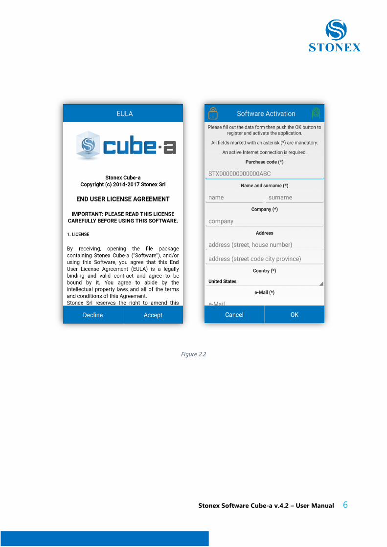
There are many ways to uninstall the software on the Android device. Here we mainly
introduce two methods: press the Cube-a icon on the desktop and drag it to the “uninstall”
option box, there will pop-up a dialog box “Uninstall Cube-a?” shown as the Figure 2.3. Then
click “uninstall” to uninstall the Cube-a software.
Figure 2.3
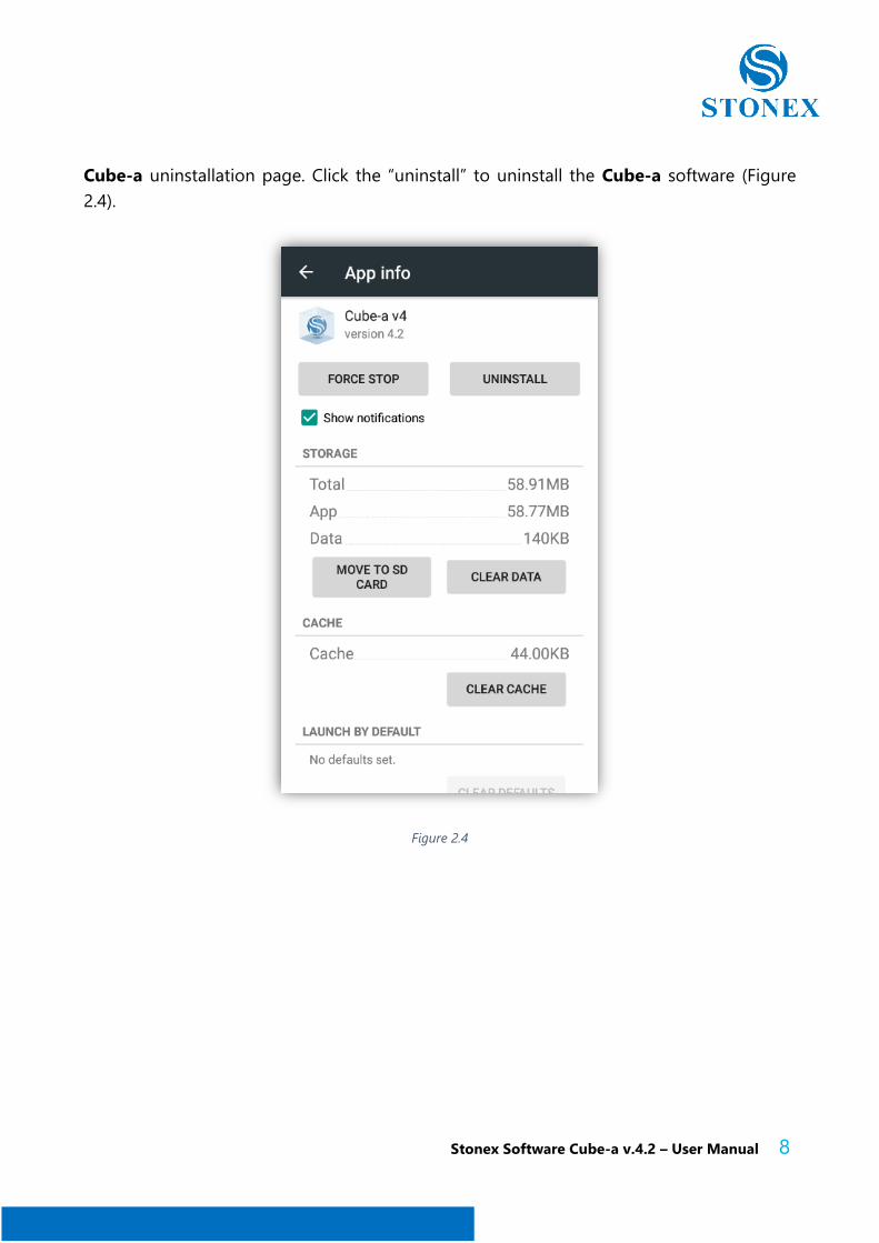
Click the “Settings” and then “Apps” to find the “Cube-a” in the submenu. Click the “Cube-
a”, the system will show the Cube-a information page. Then click the “uninstall” to enter the
Stonex Software Cube-a v.4.2 – User Manual 8
Cube-a uninstallation page. Click the “uninstall” to uninstall the Cube-a software (Figure
2.4).
Figure 2.4
Stonex Software Cube-a v.4.2 – User Manual 9
3 Software Introduction - Project
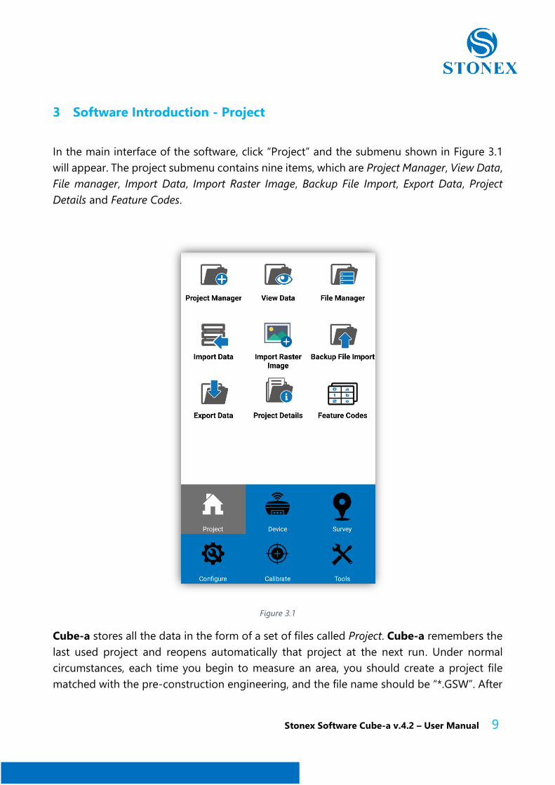
In the main interface of the software, click “Project” and the submenu shown in Figure 3.1
will appear. The project submenu contains nine items, which are Project Manager, View Data,
File manager, Import Data, Import Raster Image, Backup File Import, Export Data, Project
Details and Feature Codes.
Figure 3.1
Cube-a stores all the data in the form of a set of files called Project. Cube-a remembers the
last used project and reopens automatically that project at the next run. Under normal
circumstances, each time you begin to measure an area, you should create a project file
matched with the pre-construction engineering, and the file name should be “*.GSW”. After

Stonex Software Cube-a v.4.2 – User Manual 10
the project has been created, the software will create a file in the device storage disk and
the file name is same of the project, all data will be saved in this file.
3.1 Project Manager
Click “Project Manage” in the Project submenu: you will get to the page shown in Figure 3.2.
Figure 3.2
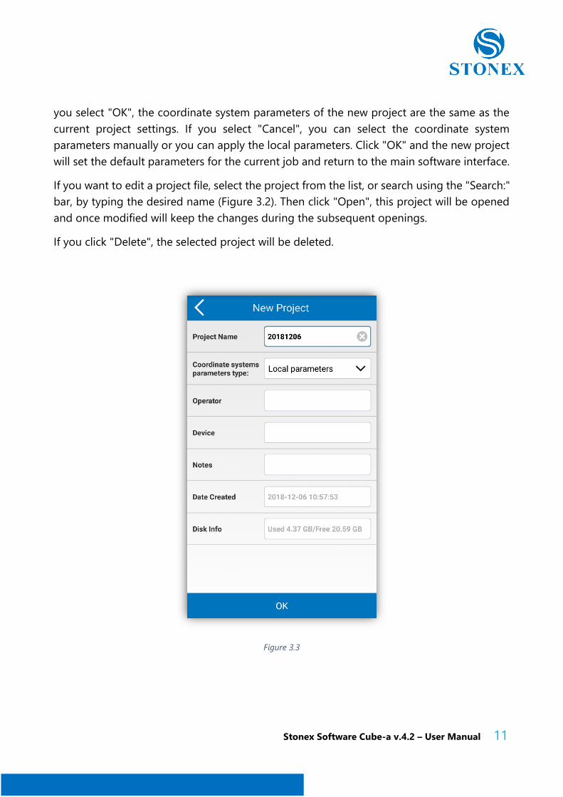
Click "New" at the bottom left to create a new project. It will open a page of a new project
as in Figure 3.3, click "ok" after entering the project name (mandatory), the device and the
notes (optional). Then you will see a request, "Keeping the current coordinate system?". If
Stonex Software Cube-a v.4.2 – User Manual 11
you select "OK", the coordinate system parameters of the new project are the same as the
current project settings. If you select "Cancel", you can select the coordinate system
parameters manually or you can apply the local parameters. Click "OK" and the new project
will set the default parameters for the current job and return to the main software interface.
If you want to edit a project file, select the project from the list, or search using the "Search:"
bar, by typing the desired name (Figure 3.2). Then click "Open", this project will be opened
and once modified will keep the changes during the subsequent openings.
If you click "Delete", the selected project will be deleted.
Figure 3.3
Stonex Software Cube-a v.4.2 – User Manual 12
3.2 View Data
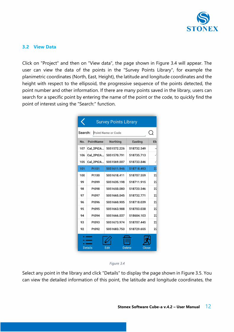
Click on "Project" and then on "View data", the page shown in Figure 3.4 will appear. The
user can view the data of the points in the "Survey Points Library", for example the
planimetric coordinates (North, East, Height), the latitude and longitude coordinates and the
height with respect to the ellipsoid, the progressive sequence of the points detected, the
point number and other information. If there are many points saved in the library, users can
search for a specific point by entering the name of the point or the code, to quickly find the
point of interest using the "Search:" function.
Figure 3.4
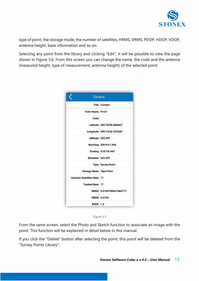
Select any point in the library and click "Details" to display the page shown in Figure 3.5. You
can view the detailed information of this point, the latitude and longitude coordinates, the
Stonex Software Cube-a v.4.2 – User Manual 13
type of point, the storage mode, the number of satellites, HRMS, VRMS, PDOP, HDOP, VDOP,
antenna height, base information and so on.
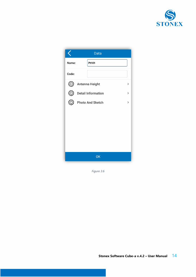
Selecting any point from the library and clicking "Edit", it will be possible to view the page
shown in Figure 3.6. From this screen you can change the name, the code and the antenna
(measured height, type of measurement, antenna height) of the selected point.
Figure 3.5
From the same screen, select the Photo and Sketch function to associate an image with the
point. This function will be explained in detail below in this manual.
If you click the "Delete" button after selecting the point, this point will be deleted from the
"Survey Points Library".
Stonex Software Cube-a v.4.2 – User Manual 14
Figure 3.6
Stonex Software Cube-a v.4.2 – User Manual 15
3.3 File Manager
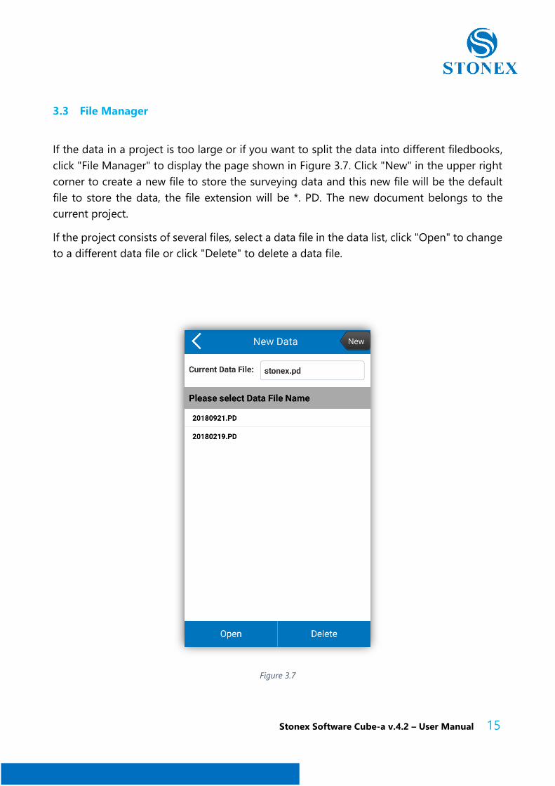
If the data in a project is too large or if you want to split the data into different filedbooks,
click "File Manager" to display the page shown in Figure 3.7. Click "New" in the upper right
corner to create a new file to store the surveying data and this new file will be the default
file to store the data, the file extension will be *. PD. The new document belongs to the
current project.
If the project consists of several files, select a data file in the data list, click "Open" to change
to a different data file or click "Delete" to delete a data file.
Figure 3.7
Stonex Software Cube-a v.4.2 – User Manual 16
3.4 Backup File Import
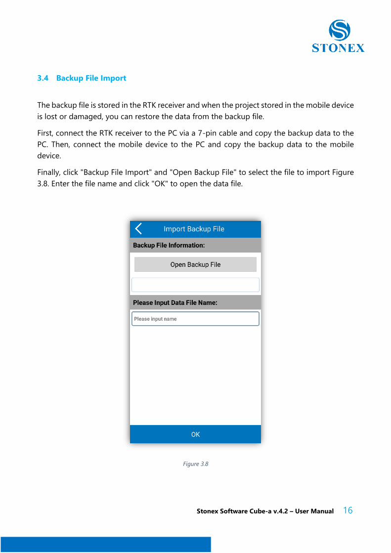
The backup file is stored in the RTK receiver and when the project stored in the mobile device
is lost or damaged, you can restore the data from the backup file.
First, connect the RTK receiver to the PC via a 7-pin cable and copy the backup data to the
PC. Then, connect the mobile device to the PC and copy the backup data to the mobile
device.
Finally, click "Backup File Import" and "Open Backup File" to select the file to import Figure
3.8. Enter the file name and click "OK" to open the data file.
Figure 3.8
Stonex Software Cube-a v.4.2 – User Manual 17
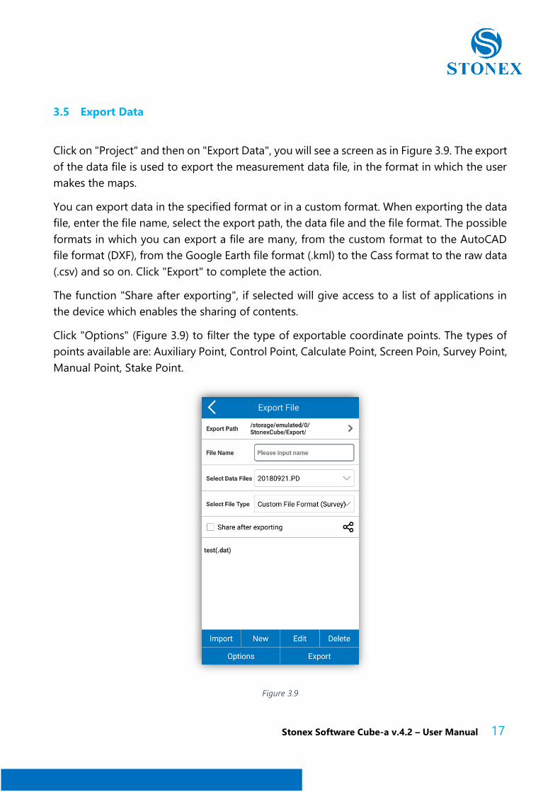
3.5 Export Data
Click on "Project" and then on "Export Data", you will see a screen as in Figure 3.9. The export
of the data file is used to export the measurement data file, in the format in which the user
makes the maps.
You can export data in the specified format or in a custom format. When exporting the data
file, enter the file name, select the export path, the data file and the file format. The possible
formats in which you can export a file are many, from the custom format to the AutoCAD
file format (DXF), from the Google Earth file format (.kml) to the Cass format to the raw data
(.csv) and so on. Click "Export" to complete the action.
The function "Share after exporting", if selected will give access to a list of applications in
the device which enables the sharing of contents.
Click "Options" (Figure 3.9) to filter the type of exportable coordinate points. The types of
points available are: Auxiliary Point, Control Point, Calculate Point, Screen Poin, Survey Point,
Manual Point, Stake Point.
Figure 3.9
Stonex Software Cube-a v.4.2 – User Manual 18
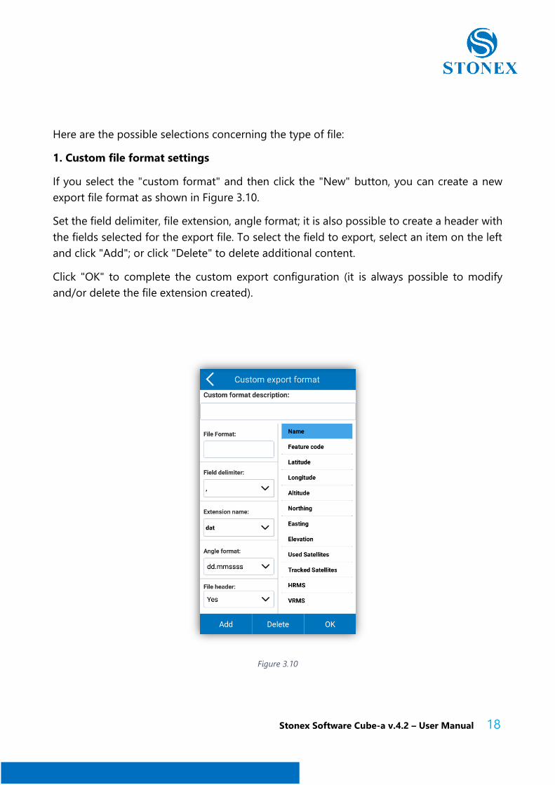
Here are the possible selections concerning the type of file:
1. Custom file format settings
If you select the "custom format" and then click the "New" button, you can create a new
export file format as shown in Figure 3.10.
Set the field delimiter, file extension, angle format; it is also possible to create a header with
the fields selected for the export file. To select the field to export, select an item on the left
and click "Add"; or click "Delete" to delete additional content.
Click "OK" to complete the custom export configuration (it is always possible to modify
and/or delete the file extension created).
Figure 3.10
Stonex Software Cube-a v.4.2 – User Manual 19
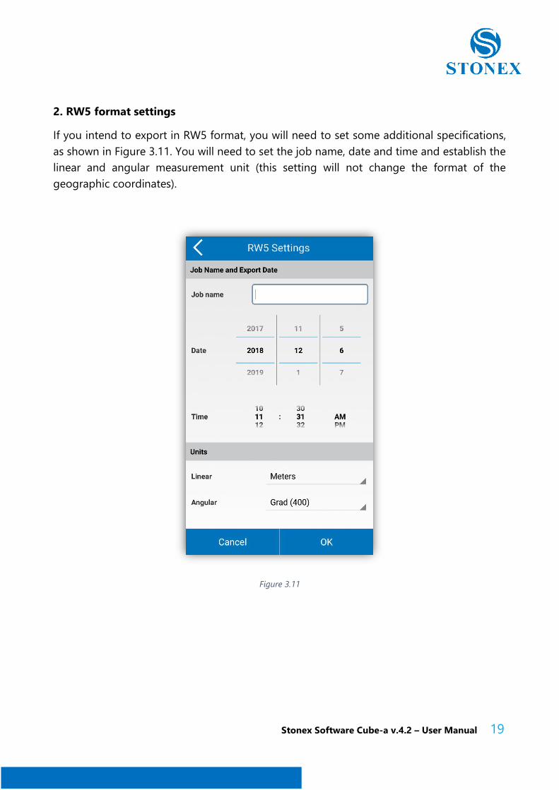
2. RW5 format settings
If you intend to export in RW5 format, you will need to set some additional specifications,
as shown in Figure 3.11. You will need to set the job name, date and time and establish the
linear and angular measurement unit (this setting will not change the format of the
geographic coordinates).
Figure 3.11
Stonex Software Cube-a v.4.2 – User Manual 20
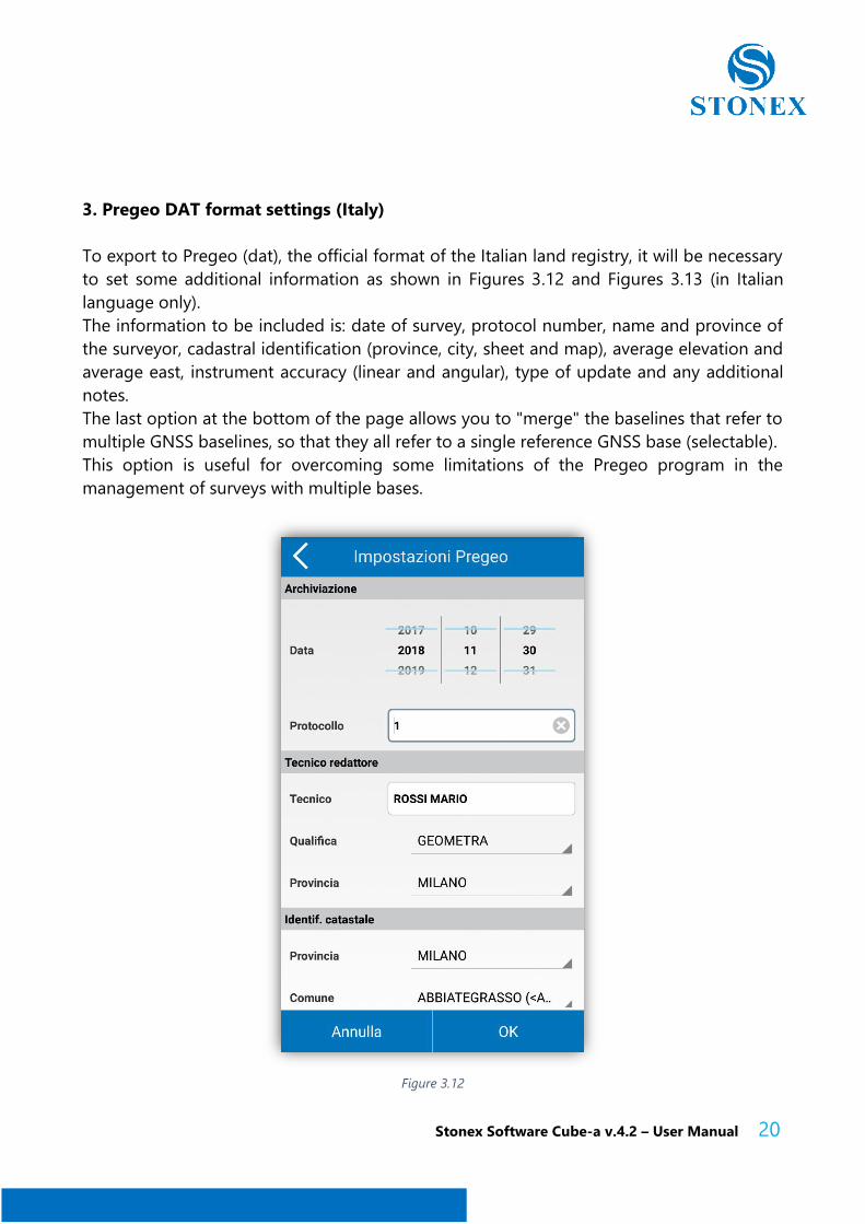
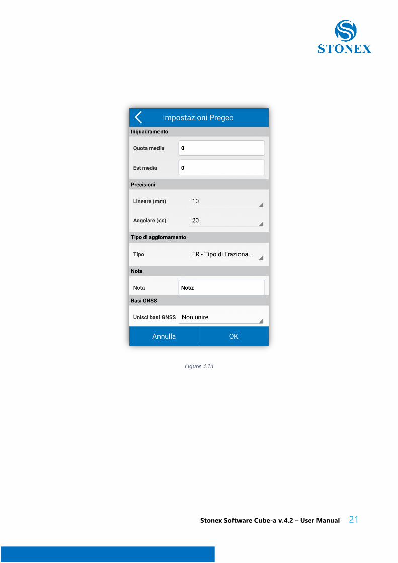
3. Pregeo DAT format settings (Italy)
To export to Pregeo (dat), the official format of the Italian land registry, it will be necessary
to set some additional information as shown in Figures 3.12 and Figures 3.13 (in Italian
language only).
The information to be included is: date of survey, protocol number, name and province of
the surveyor, cadastral identification (province, city, sheet and map), average elevation and
average east, instrument accuracy (linear and angular), type of update and any additional
notes.
The last option at the bottom of the page allows you to "merge" the baselines that refer to
multiple GNSS baselines, so that they all refer to a single reference GNSS base (selectable).
This option is useful for overcoming some limitations of the Pregeo program in the
management of surveys with multiple bases.
Figure 3.12
Stonex Software Cube-a v.4.2 – User Manual 21
Figure 3.13
Stonex Software Cube-a v.4.2 – User Manual 22
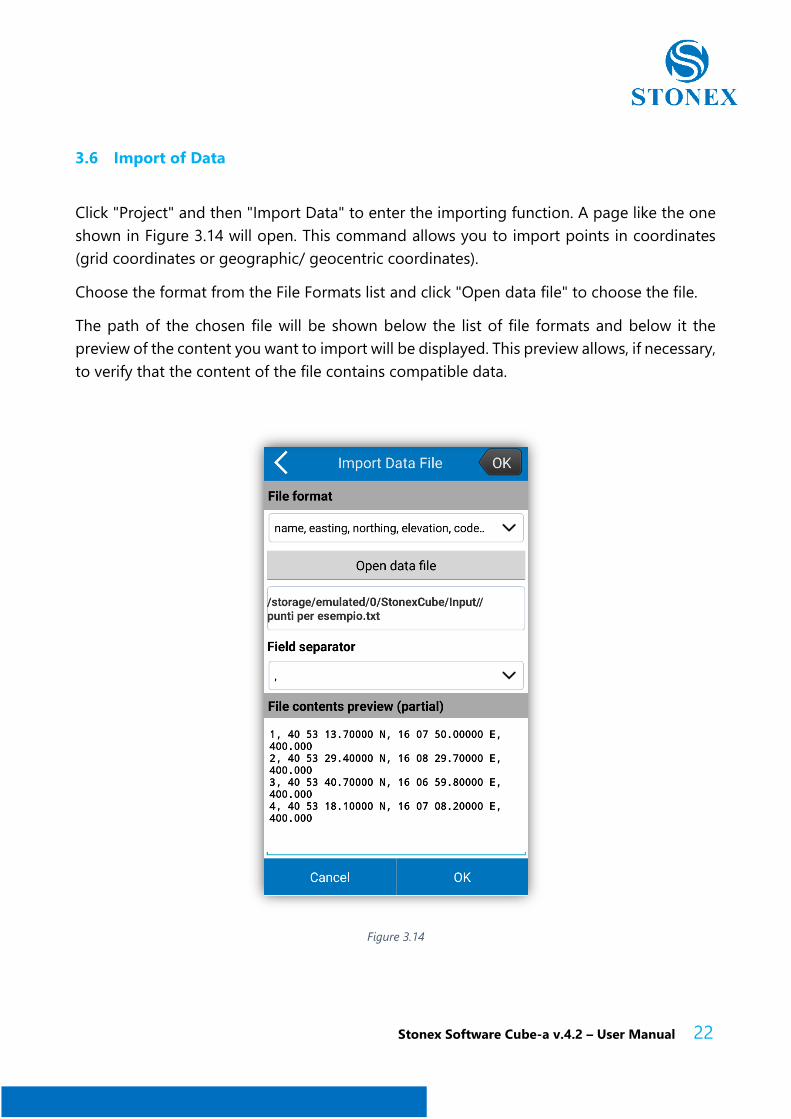
3.6 Import of Data
Click "Project" and then "Import Data" to enter the importing function. A page like the one
shown in Figure 3.14 will open. This command allows you to import points in coordinates
(grid coordinates or geographic/ geocentric coordinates).
Choose the format from the File Formats list and click "Open data file" to choose the file.
The path of the chosen file will be shown below the list of file formats and below it the
preview of the content you want to import will be displayed. This preview allows, if necessary,
to verify that the content of the file contains compatible data.
Figure 3.14

Stonex Software Cube-a v.4.2 – User Manual 23
Click "OK" to proceed with the import or click "Cancel" to cancel.
The imported points will be registered as "Imported Points", in this way they will not be
displayed in the list of surveyed points (i.e. in the list displayed by the "View data" command).
To access the imported points, open the "Point Library" (where both the imported points
and the surveyed points are collected) after clicking on "Tools" from the main menu. The
imported points will be shown and eventually used when the stakeout command is started.
Stonex Software Cube-a v.4.2 – User Manual 24
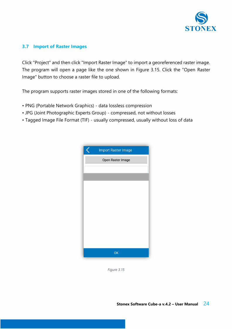
3.7 Import of Raster Images
Click "Project" and then click "Import Raster Image" to import a georeferenced raster image.
The program will open a page like the one shown in Figure 3.15. Click the "Open Raster
Image" button to choose a raster file to upload.
The program supports raster images stored in one of the following formats:
• PNG (Portable Network Graphics) - data lossless compression
• JPG (Joint Photographic Experts Group) - compressed, not without losses
• Tagged Image File Format (TIF) - usually compressed, usually without loss of data
Figure 3.15
Stonex Software Cube-a v.4.2 – User Manual 25
Having a raster image is not enough to have a georeferentiation: the raster image must have
a "twin" file that stores the georeferencing parameters. This file is called "World File" and
must be created on a PC using software that manages the image georeferencing. In short,
the following table shows which type of World file should be stored in the same folder that
contains the raster image to be imported:
Raster format World File
Format
*.PNG *.PGW
*.JPG *.JGW
*.TIF *.TFW
Limitations
Cube-a works on Android and must respect its limits on memory allocation. One of these
limitations is that any application does not have to allocate large blocks of memory and if
an application does so, it must release those blocks of memory as soon as possible.
From Android developer documents: "To allow multiple running processes, Android sets a
hard limit for the assigned heap size for each app. The exact limit of the heap size varies
between devices based on the amount of RAM available in the device If your app has reached
heap capacity and tries to allocate more memory, the system will generate an out of memory
error. "
All of this means that you need to be careful when trying to load raster images. Although a
raster image may look small (a few megabytes), the same may not be true for the data that
the image contains. Also remember that usually raster image files are compressed and that
Cube-a must decompress them before displaying them; this operation may require more
memory than the Android operating system can provide.
Typically, an image of W x H in pixels (width x height) requires a free amount of memory
equal to: W x H * 3 bytes. Example: a picture of 5 mega pixels (2560 x 1920) occupies, after
decompression, 14745600 bytes or 14 megabytes.
Stonex Software Cube-a v.4.2 – User Manual 26
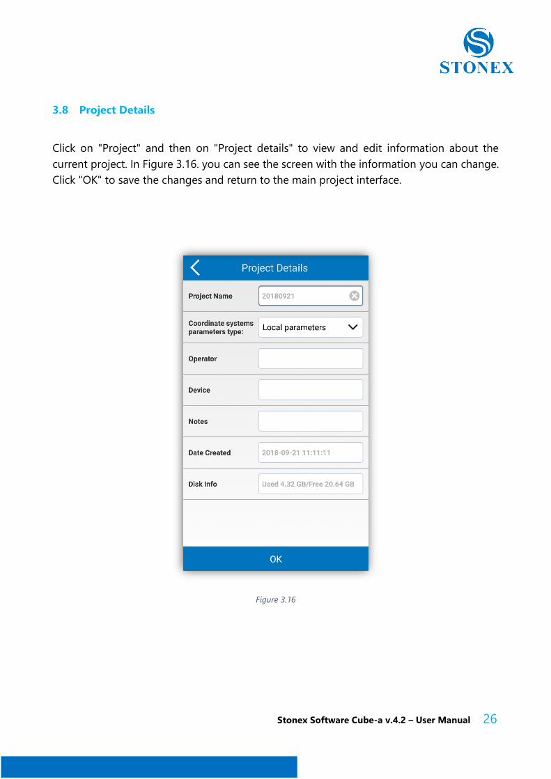
3.8 Project Details
Click on "Project" and then on "Project details" to view and edit information about the
current project. In Figure 3.16. you can see the screen with the information you can change.
Click "OK" to save the changes and return to the main project interface.
Figure 3.16
Stonex Software Cube-a v.4.2 – User Manual 27
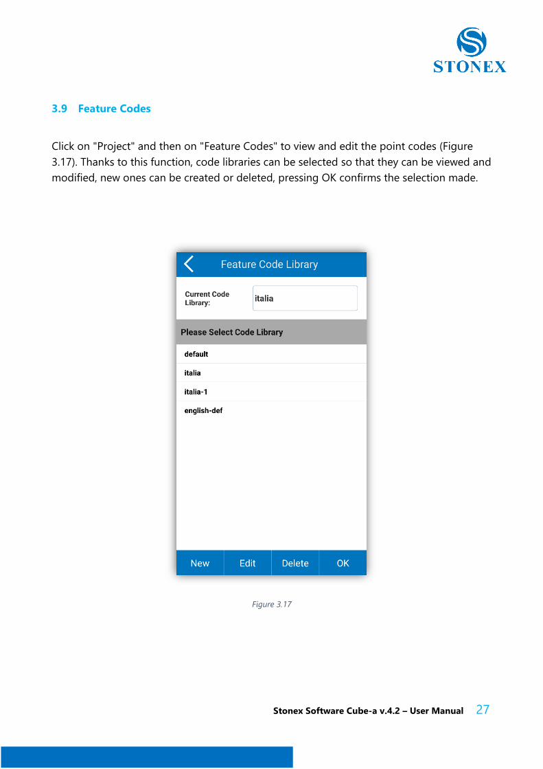
3.9 Feature Codes
Click on "Project" and then on "Feature Codes" to view and edit the point codes (Figure
3.17). Thanks to this function, code libraries can be selected so that they can be viewed and
modified, new ones can be created or deleted, pressing OK confirms the selection made.
Figure 3.17
Stonex Software Cube-a v.4.2 – User Manual 28
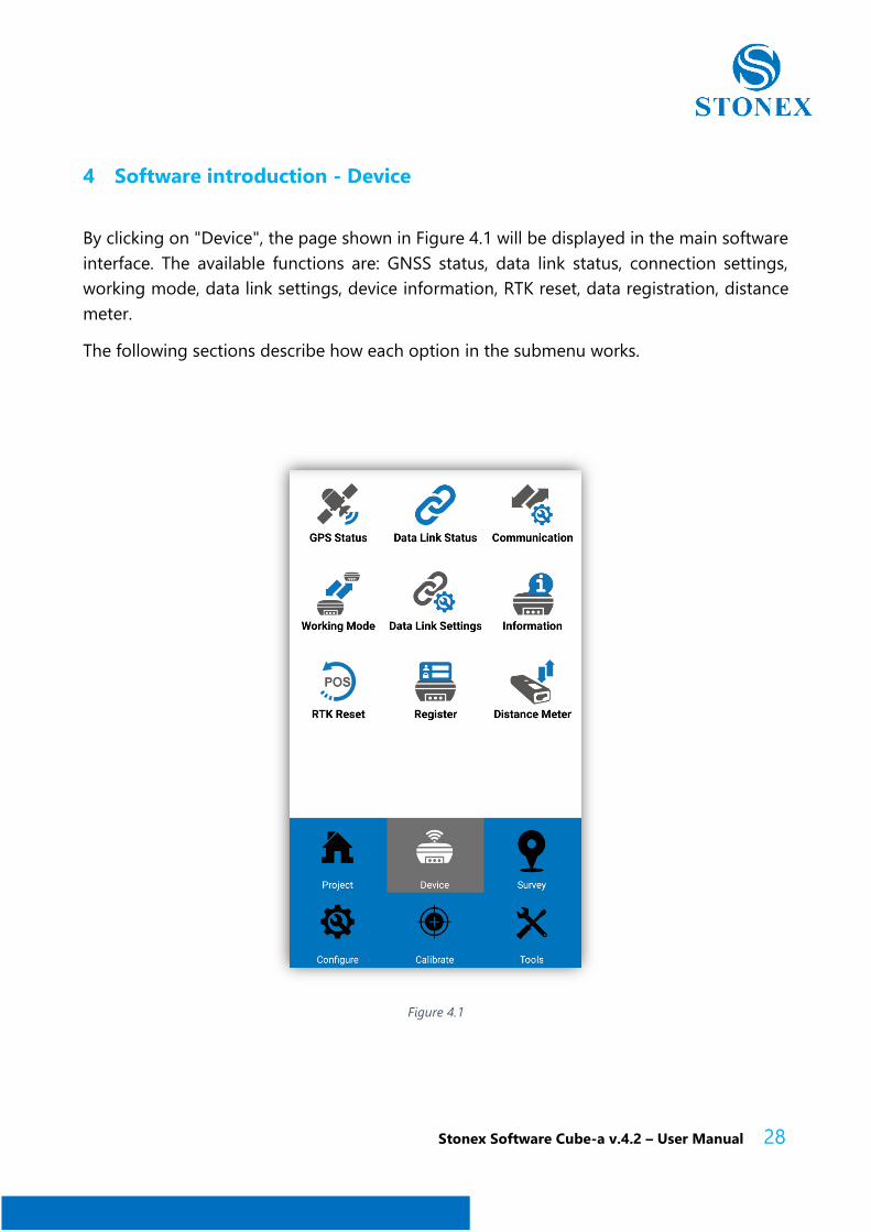
4 Software introduction - Device
By clicking on "Device", the page shown in Figure 4.1 will be displayed in the main software
interface. The available functions are: GNSS status, data link status, connection settings,
working mode, data link settings, device information, RTK reset, data registration, distance
meter.
The following sections describe how each option in the submenu works.
Figure 4.1
Stonex Software Cube-a v.4.2 – User Manual 29
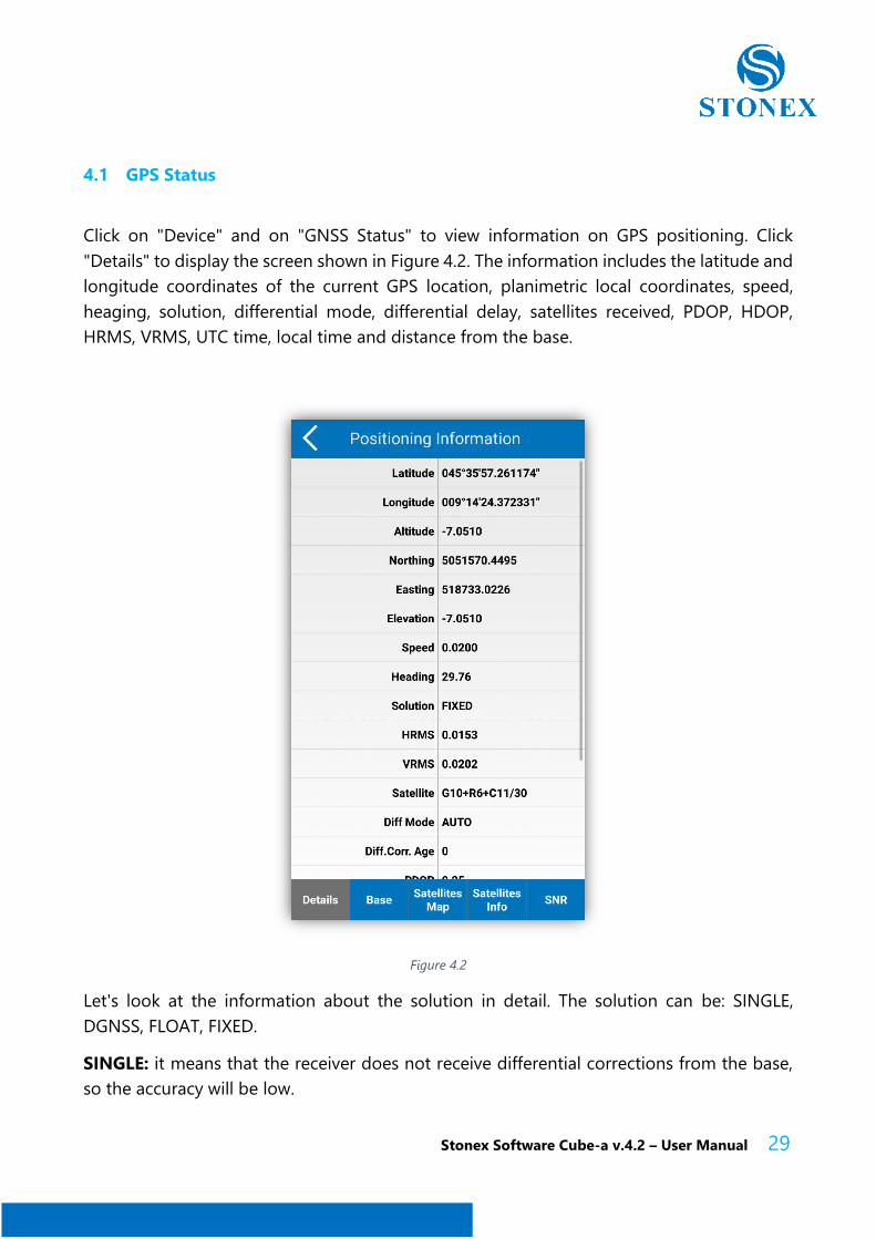
4.1 GPS Status
Click on "Device" and on "GNSS Status" to view information on GPS positioning. Click
"Details" to display the screen shown in Figure 4.2. The information includes the latitude and
longitude coordinates of the current GPS location, planimetric local coordinates, speed,
heaging, solution, differential mode, differential delay, satellites received, PDOP, HDOP,
HRMS, VRMS, UTC time, local time and distance from the base.
Figure 4.2
Let's look at the information about the solution in detail. The solution can be: SINGLE,
DGNSS, FLOAT, FIXED.
SINGLE: it means that the receiver does not receive differential corrections from the base,
so the accuracy will be low.
Stonex Software Cube-a v.4.2 – User Manual 30
DGNSS: it means that the receiver can receive the differential corrections from the base, but
the accuracy of the data is low for several reasons, such as, the position of the receiver does
not allow the device to receive many satellites.
FLOAT: it means that the receiver can receive the differential corrections from the base, the
accuracy is high, generally below the 0.5 meters.
FIXED: it means that the receiver can receive differential corrections from the base, it is the
final solution for transmitting the phase difference corrections of the vector with maximum
precision, usually within 2 cm. With high precision GPS measurement, you need to get a
fixed solution status to record data.
As for the differential mode it includes the CMR, a type of differential message format
defined by Trimble, and the RTCM, a general differential message format that includes X,
RTCM32, and so on.
The differential delay indicates the time when the Rover receives the corrections (for
example, a 10-second correction delay indicates that the base has sent a signal that will be
received by the Rovers after 10 seconds from sending), the unit of measure are the seconds.
When the RTK mode is running, the correction delay is low, so the result is better, generally
the delay is less than 10 seconds, usually 1 or 2 seconds.
PDOP: Dilution of position accuracy. When the PDOP value is less than 3, it represents the
ideal situation. The lower the PDOP value, the better the distribution of the satellites, this
facilitates the search for the FIXED solution of the instrument.
HDOP: Dilution of horizontal precision, it is the component of the horizontal direction in the
PDOP.
VDOP: Dilution of vertical precision, it represents the component of the vertical direction in
the PDOP.
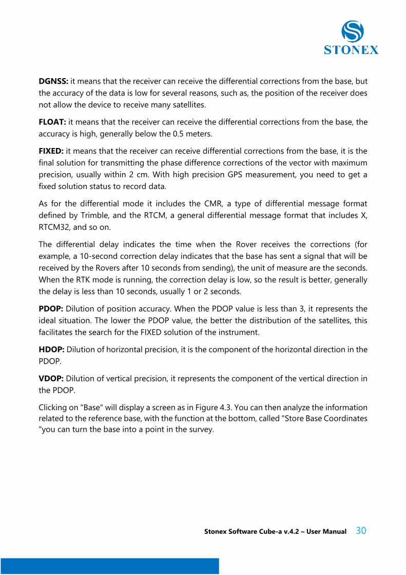
Clicking on "Base" will display a screen as in Figure 4.3. You can then analyze the information
related to the reference base, with the function at the bottom, called "Store Base Coordinates
"you can turn the base into a point in the survey.
Stonex Software Cube-a v.4.2 – User Manual 31
Figure 4.3
Stonex Software Cube-a v.4.2 – User Manual 32
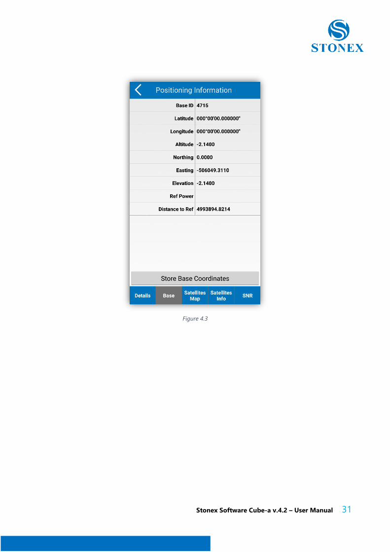
By clicking on "Satellites Map" you can view the sky plot (Figure 4.4), the map with the
position of the satellites detected by the receiver, positioned according to the azimuth (on
the circumference of the circle) and the elevation angle (on the radius), the center of the
circle represents the position of the receiver. Legend: GPS-blue (GPS); BD-light green
(BeiDou); GLN-red (GLONASS); GAL-magenta (Galileo); SBAS-dark green (SBAS); ATL-yellow
(ATLAS).
Figure 4.4
Stonex Software Cube-a v.4.2 – User Manual 33
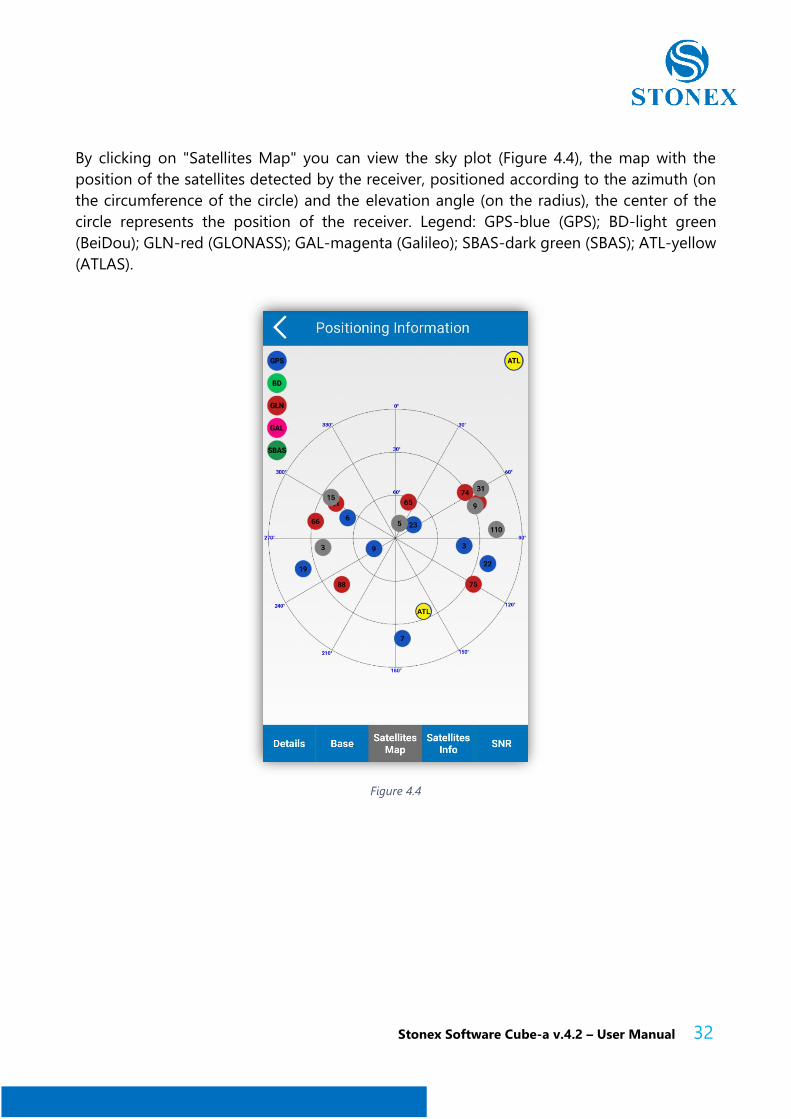
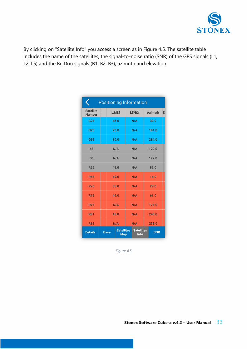
By clicking on "Satellite Info" you access a screen as in Figure 4.5. The satellite table
includes the name of the satellites, the signal-to-noise ratio (SNR) of the GPS signals (L1,
L2, L5) and the BeiDou signals (B1, B2, B3), azimuth and elevation.
Figure 4.5
Stonex Software Cube-a v.4.2 – User Manual 34
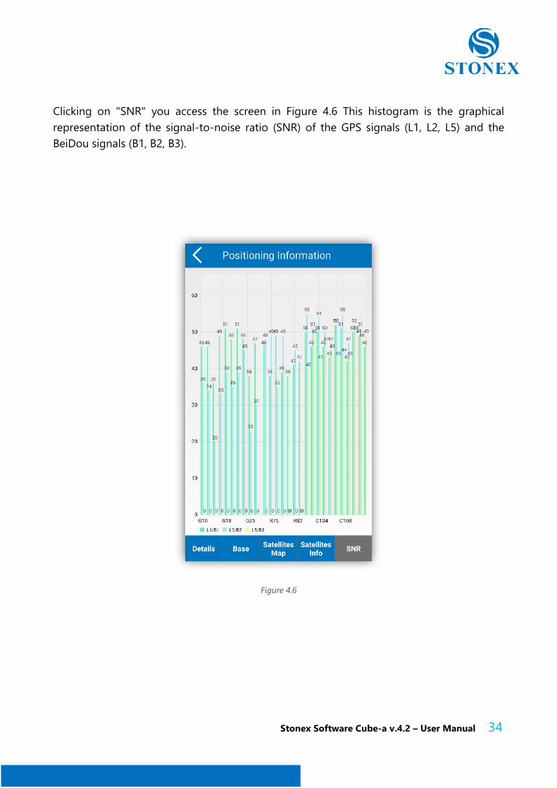
Clicking on "SNR" you access the screen in Figure 4.6 This histogram is the graphical
representation of the signal-to-noise ratio (SNR) of the GPS signals (L1, L2, L5) and the
BeiDou signals (B1, B2, B3).
Figure 4.6
Stonex Software Cube-a v.4.2 – User Manual 35
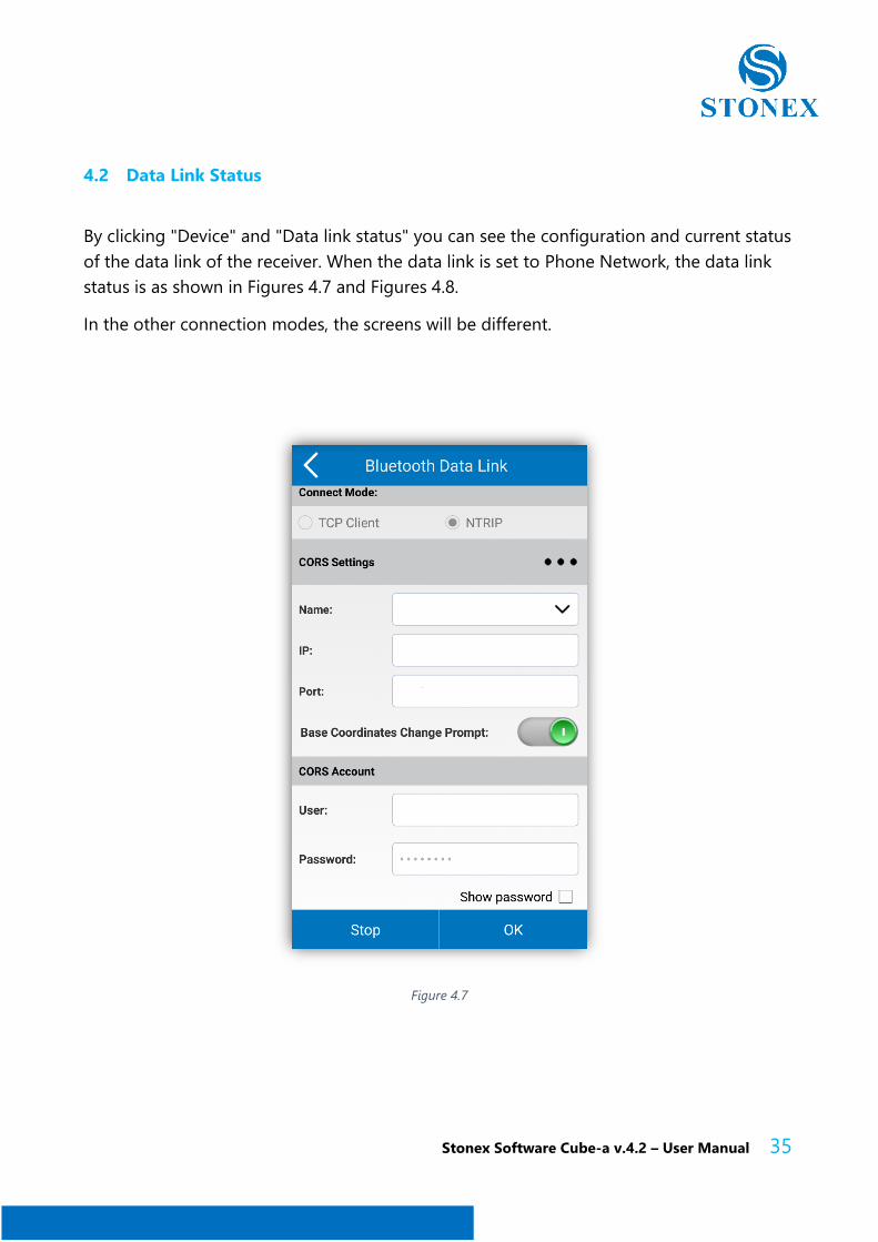
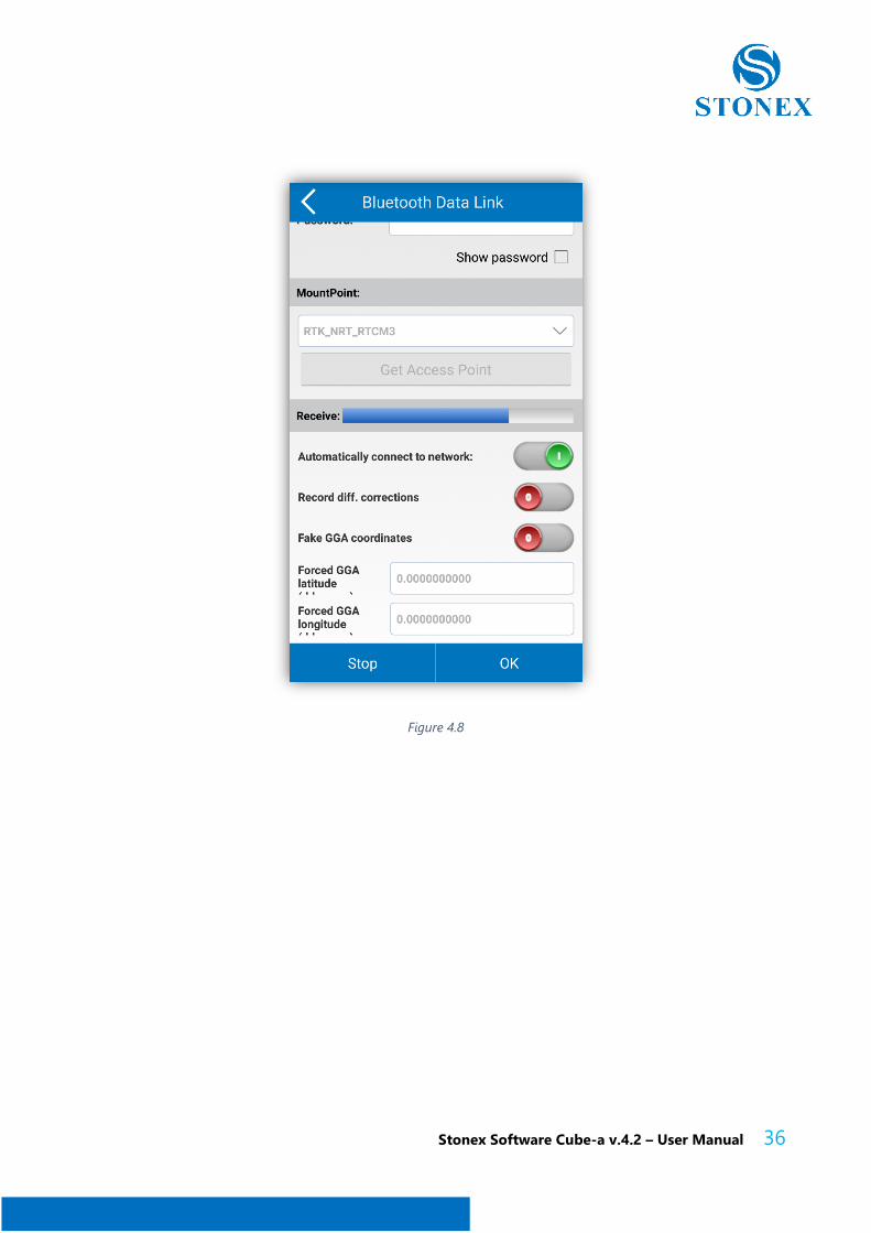
4.2 Data Link Status
By clicking "Device" and "Data link status" you can see the configuration and current status
of the data link of the receiver. When the data link is set to Phone Network, the data link
status is as shown in Figures 4.7 and Figures 4.8.
In the other connection modes, the screens will be different.
Figure 4.7
Stonex Software Cube-a v.4.2 – User Manual 36
Figure 4.8
Stonex Software Cube-a v.4.2 – User Manual 37
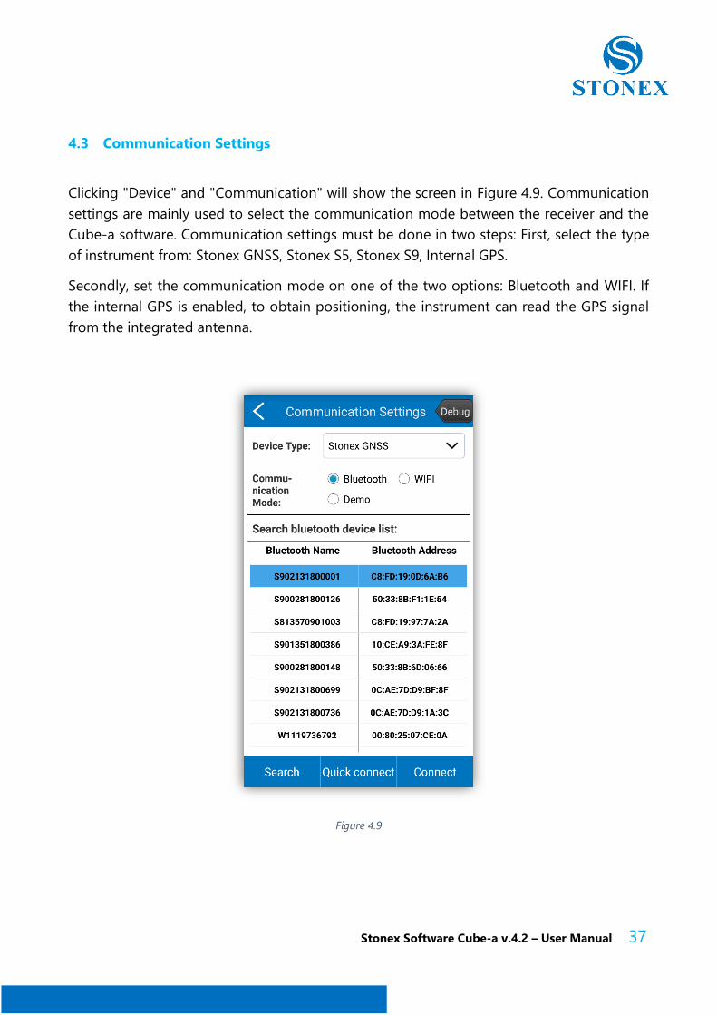
4.3 Communication Settings
Clicking "Device" and "Communication" will show the screen in Figure 4.9. Communication
settings are mainly used to select the communication mode between the receiver and the
Cube-a software. Communication settings must be done in two steps: First, select the type
of instrument from: Stonex GNSS, Stonex S5, Stonex S9, Internal GPS.
Secondly, set the communication mode on one of the two options: Bluetooth and WIFI. If
the internal GPS is enabled, to obtain positioning, the instrument can read the GPS signal
from the integrated antenna.
Figure 4.9
Stonex Software Cube-a v.4.2 – User Manual 38
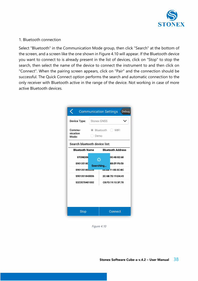
1. Bluetooth connection
Select "Bluetooth" in the Communication Mode group, then click "Search" at the bottom of
the screen, and a screen like the one shown in Figure 4.10 will appear. If the Bluetooth device
you want to connect to is already present in the list of devices, click on "Stop" to stop the
search, then select the name of the device to connect the instrument to and then click on
"Connect". When the pairing screen appears, click on "Pair" and the connection should be
successful. The Quick Connect option performs the search and automatic connection to the
only receiver with Bluetooth active in the range of the device. Not working in case of more
active Bluetooth devices.
Figure 4.10
Stonex Software Cube-a v.4.2 – User Manual 39
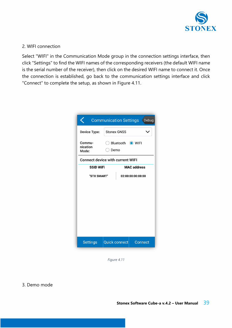
2. WIFI connection
Select "WIFI" in the Communication Mode group in the connection settings interface, then
click "Settings" to find the WIFI names of the corresponding receivers (the default WIFI name
is the serial number of the receiver), then click on the desired WIFI name to connect it. Once
the connection is established, go back to the communication settings interface and click
"Connect" to complete the setup, as shown in Figure 4.11.
Figure 4.11
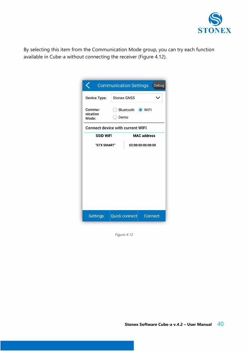
3. Demo mode
Stonex Software Cube-a v.4.2 – User Manual 40
By selecting this item from the Communication Mode group, you can try each function
available in Cube-a without connecting the receiver (Figure 4.12).
Figure 4.12
Stonex Software Cube-a v.4.2 – User Manual 41
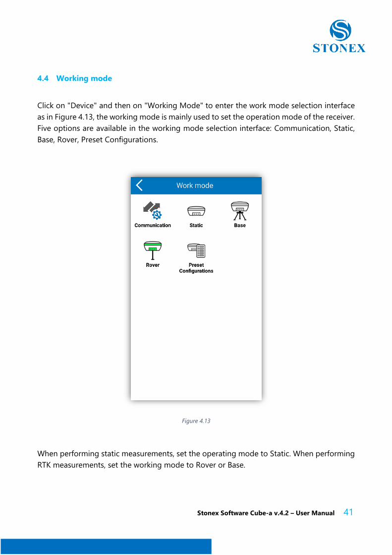
4.4 Working mode
Click on "Device" and then on "Working Mode" to enter the work mode selection interface
as in Figure 4.13, the working mode is mainly used to set the operation mode of the receiver.
Five options are available in the working mode selection interface: Communication, Static,
Base, Rover, Preset Configurations.
Figure 4.13
When performing static measurements, set the operating mode to Static. When performing
RTK measurements, set the working mode to Rover or Base.
Stonex Software Cube-a v.4.2 – User Manual 42
After connecting the device and the Cube-a software via the communication settings, you
can set the work mode and the data link. The following sections describe the settings in the
work mode menu.
4.4.1 Communication
Click "Device", then "Work Mode" and then "Communication", to enter the communication
settings such as those shown in section 4.3.
Stonex Software Cube-a v.4.2 – User Manual 43
4.4.2 Static Mode
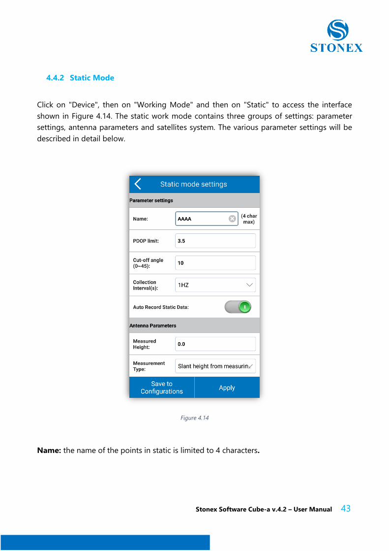
Click on "Device", then on "Working Mode" and then on "Static" to access the interface
shown in Figure 4.14. The static work mode contains three groups of settings: parameter
settings, antenna parameters and satellites system. The various parameter settings will be
described in detail below.
Figure 4.14
Name: the name of the points in static is limited to 4 characters.
Stonex Software Cube-a v.4.2 – User Manual 44
PDOP limit: the geometric factor that represents the quality of the satellite distribution. The
smaller the PDOP value, the better the satellite distribution. The PDOP value below 3
represents the ideal state.
Cut-off angle: the angle of the signal between satellite/receiver and horizon. The receiver
will not consider satellite signals received below the limit imposed by the cut-off angle.
Range of values: 0-45 °.
Collection interval (s): 1Hz indicates the acquisition of a data per second, 5HZ indicates the
acquisition of five data per second, 5s (0.2 Hz) indicates that the receiver collects data every
five seconds, and so on.
Auto recor of static data: if you enable this button, the receiver starts recording
automatically when it is switched on and receives satellite signals, otherwise you need to
manually record the static data after turning on the receiver.
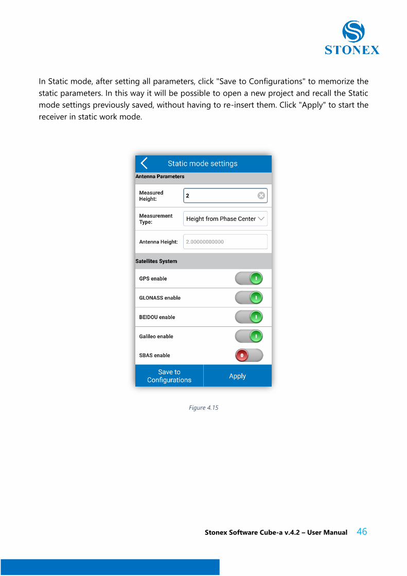
Antenna parameters: You can enter a value of the measured height and set the type of
measurement among the various options available such as Height from the phase center or
Slant height from measuring line. The value of the antenna height used in the surveys will
be calculated automatically by the program and visible as shown in Figure 4.15.
The known values that the receiver provides are as follows:
b: the height from the bottom of the device to the center of phase p.c.;
c: the height from the bottom of the device to the rubber ring;
R: The radius of the rubber ring of the device;
If the measured height is the vertical height (a) from the bottom of the device to the ground,
the measured height must be set to "Height from the phase center ". And the height of the
antenna: h = a + b.
If the measured height is the height of the inclination from the rubber ring to the ground,
the height measured is the "Slant height from measuring line". Antenna height h = √ (s² -
R²) - c + b

Stonex Software Cube-a v.4.2 – User Manual 45
Satellite constellations: the satellite system settings include five systems: GPS, GLONASS,
BeiDou, Galileo and SBAS. Depending on the job requirements, it is possible to choose
whether to receive the signal corresponding to a certain constellation of satellites, or to
disable it. The SBAS system is a large-scale differential correction system (improvement
system based on satellite signal reception quality). Navigation satellites are detected by
many different widely distributed stations and the raw data acquired is sent to the console.
Then from the console, through the calculation of the various satellite positioning correction
information and through the upload stations are sent to GEO satellites. Finally, GEO satellites
send corrections to users, helping to improve positioning accuracy.
Stonex Software Cube-a v.4.2 – User Manual 46
In Static mode, after setting all parameters, click "Save to Configurations" to memorize the
static parameters. In this way it will be possible to open a new project and recall the Static
mode settings previously saved, without having to re-insert them. Click "Apply" to start the
receiver in static work mode.
Figure 4.15

Stonex Software Cube-a v.4.2 – User Manual 47
4.4.3 Base Mode
Click on "Device", then on "Working Mode" and then on "Base" to access the "Basic mode
settings" screen shown in Figure 4.16. The base mode settings are divided into: Start Up
Mode, Options settings, Data Link, Satellites System.
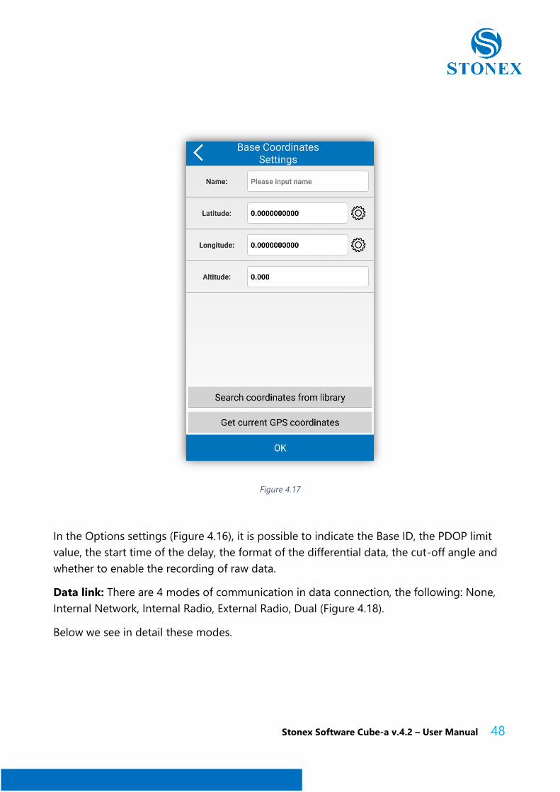
Start Up Mode: There modes, "Use Current Coordinates" and "Input Base Coordinates". Use
current point coordinates: The Base station takes the WGS-84 coordinates of the current
point and sets it as the base coordinates. Input base coordinates: allows you to manually
enter the coordinates to use for the base. The difference between the entered coordinates
and the precise WGS-84 coordinates of the current point on which the base is positioned,
must not be very large, otherwise the Base station will not work optimally. If you select "Input
Base Coordinates", click "Set Base Coordinates" to access the base coordinate settings as in
Figure 4.17. You have three possibilities to enter the coordinates: search for the coordinates
inside the library, acquire the GPS coordinates of the current point or enter the coordinates
manually. Then click "Set Base antenna height" to set the antenna parameters.
Figure 4.16
Stonex Software Cube-a v.4.2 – User Manual 48
Figure 4.17
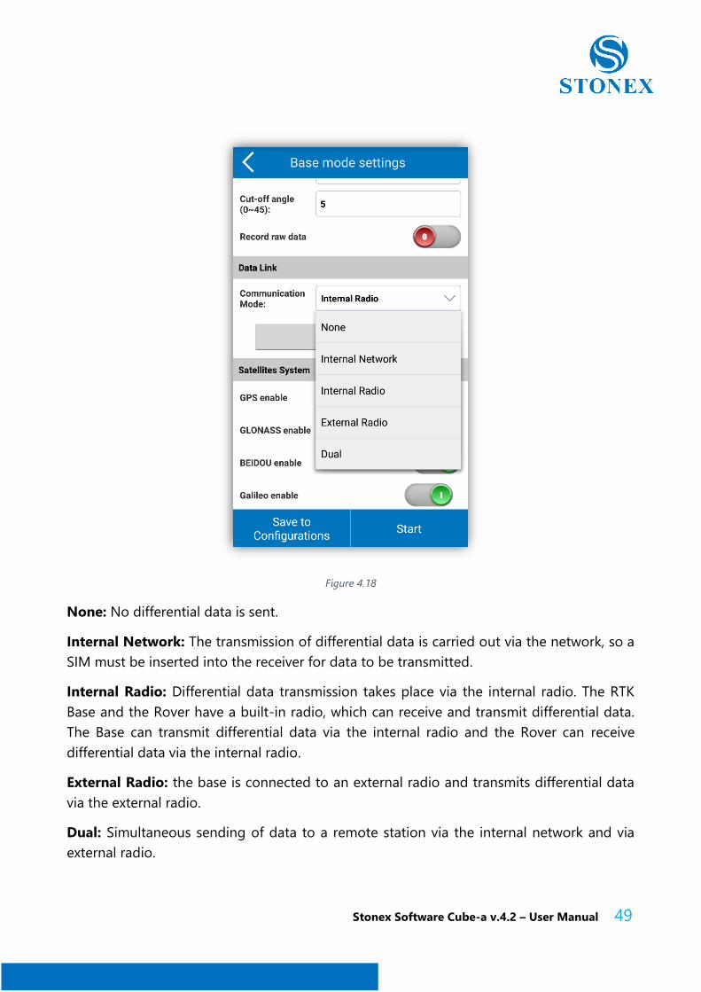
In the Options settings (Figure 4.16), it is possible to indicate the Base ID, the PDOP limit
value, the start time of the delay, the format of the differential data, the cut-off angle and
whether to enable the recording of raw data.
Data link: There are 4 modes of communication in data connection, the following: None,
Internal Network, Internal Radio, External Radio, Dual (Figure 4.18).
Below we see in detail these modes.
Stonex Software Cube-a v.4.2 – User Manual 49
Figure 4.18
None: No differential data is sent.
Internal Network: The transmission of differential data is carried out via the network, so a
SIM must be inserted into the receiver for data to be transmitted.
Internal Radio: Differential data transmission takes place via the internal radio. The RTK
Base and the Rover have a built-in radio, which can receive and transmit differential data.
The Base can transmit differential data via the internal radio and the Rover can receive
differential data via the internal radio.
External Radio: the base is connected to an external radio and transmits differential data
via the external radio.
Dual: Simultaneous sending of data to a remote station via the internal network and via
external radio.
Stonex Software Cube-a v.4.2 – User Manual 50
As a last setting for the Basic work mode, you can enable/disable the satellites to receive the
signal or not.
After all the parameters for the Base mode have been set, click on "Save to Configurations"
to save the parameters. The current parameters can be saved, so that you can recall the
configurations later without having to reinsert them.
After setting the parameters for the Base mode, click "Start" to start the Base work mode.
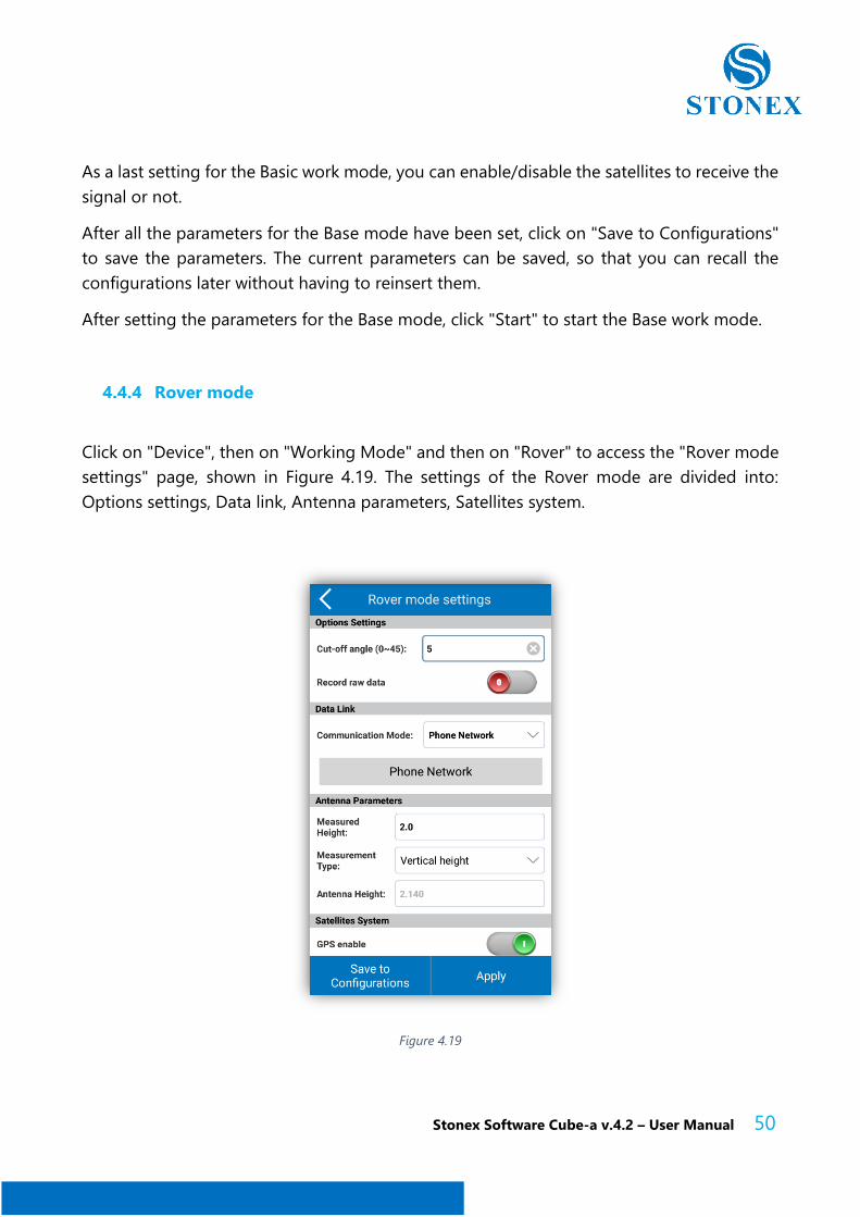
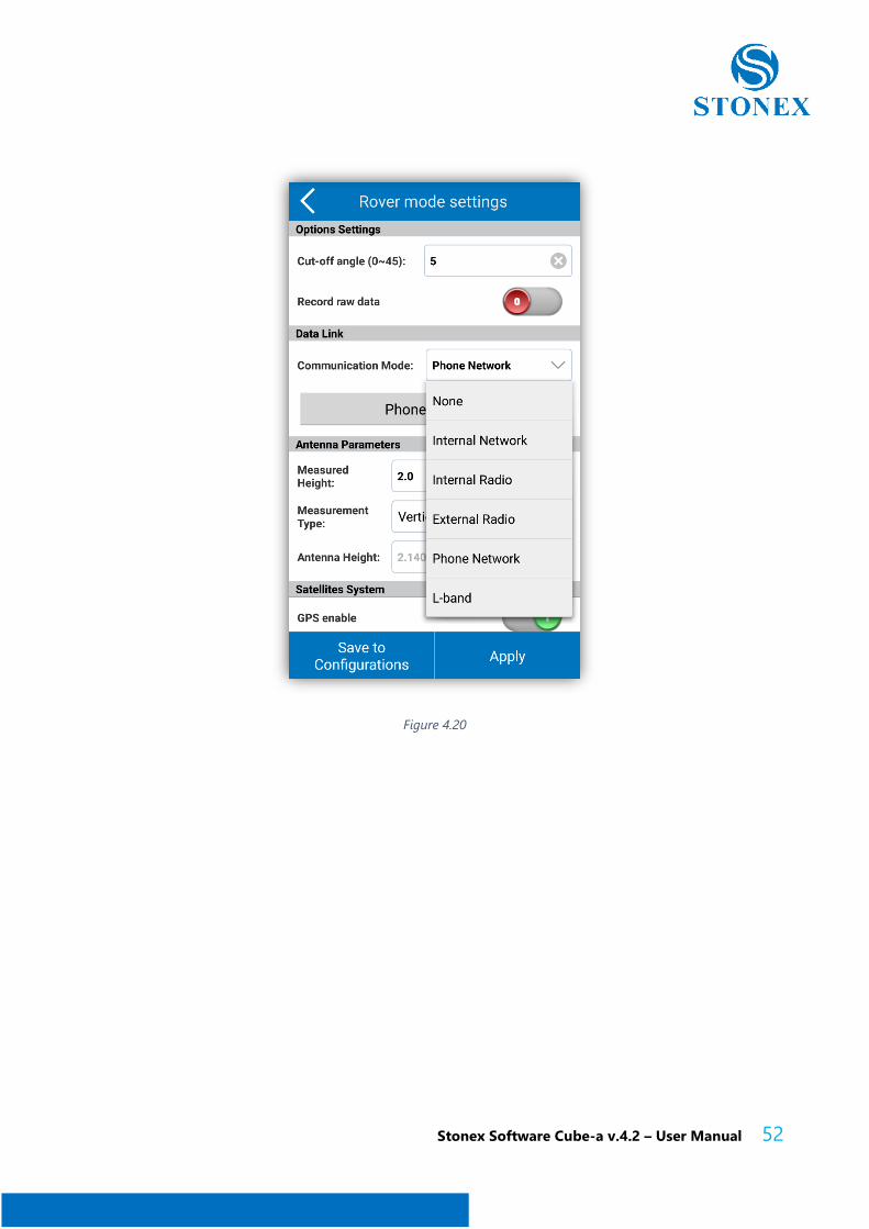
4.4.4 Rover mode
Click on "Device", then on "Working Mode" and then on "Rover" to access the "Rover mode
settings" page, shown in Figure 4.19. The settings of the Rover mode are divided into:
Options settings, Data link, Antenna parameters, Satellites system.
Figure 4.19
Stonex Software Cube-a v.4.2 – User Manual 51
Options: If you enable the "Register raw data" option, you can set the name of the recorded
raw data file. Then it will be possible to acquire points in "Stop and Go" mode on the survey
page.
Collegamento dati: There are 6 communication mode options in data link: None, Internal
Network, Internal Radio, External Radio, Phone Network and L-band. As shown in Figure
4.20.
The meaning of the first four modes of communication is the same as described previously
in the section concerning the Base.
Phone Network: The transmission of differential data is carried out through the mobile
device network. With this communication mode, a SIM must be inserted in your mobile
device or you must be connected to a Wi-Fi network.
L-band (Atlas): Using the precision system based on corrections sent by the satellites, it is
possible to receive the differential corrections and reach an accuracy level between 5 and 12
cm. This option allows you not to rely on base stations, CORS or network, in areas where the
differential signal could be absent such as deserts, oceans or mountains, you only need to
have the availability of receiving L-band satellites.
After setting the parameters, click on "Save to Configurations" to save the settings and click
"Apply" to change the working mode in Rover, the Rover will then receive the corrections
from the Base.
If the radio has been set as the connection between Base and Rover, then the frequency and
the protocol must be the same.
Stonex Software Cube-a v.4.2 – User Manual 52
Figure 4.20
Stonex Software Cube-a v.4.2 – User Manual 53
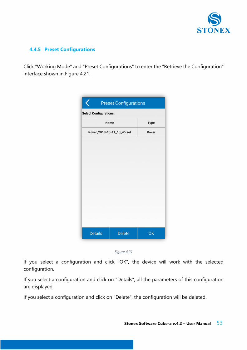
4.4.5 Preset Configurations
Click "Working Mode" and "Preset Configurations" to enter the "Retrieve the Configuration"
interface shown in Figure 4.21.
Figure 4.21
If you select a configuration and click "OK", the device will work with the selected
configuration.
If you select a configuration and click on "Details", all the parameters of this configuration
are displayed.
If you select a configuration and click on "Delete", the configuration will be deleted.
Stonex Software Cube-a v.4.2 – User Manual 54
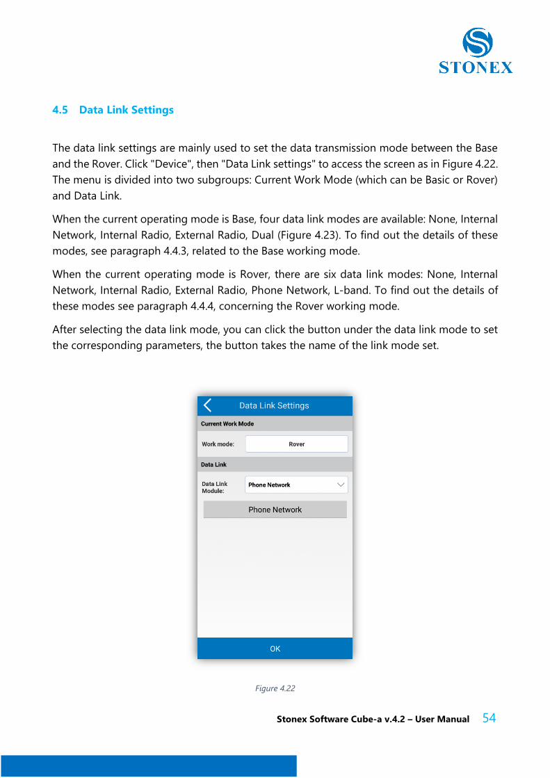
4.5 Data Link Settings
The data link settings are mainly used to set the data transmission mode between the Base
and the Rover. Click "Device", then "Data Link settings" to access the screen as in Figure 4.22.
The menu is divided into two subgroups: Current Work Mode (which can be Basic or Rover)
and Data Link.
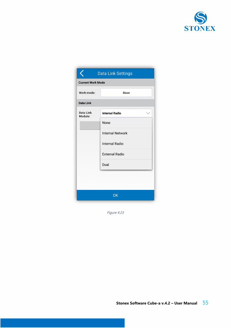
When the current operating mode is Base, four data link modes are available: None, Internal
Network, Internal Radio, External Radio, Dual (Figure 4.23). To find out the details of these
modes, see paragraph 4.4.3, related to the Base working mode.
When the current operating mode is Rover, there are six data link modes: None, Internal
Network, Internal Radio, External Radio, Phone Network, L-band. To find out the details of
these modes see paragraph 4.4.4, concerning the Rover working mode.
After selecting the data link mode, you can click the button under the data link mode to set
the corresponding parameters, the button takes the name of the link mode set.
Figure 4.22
Stonex Software Cube-a v.4.2 – User Manual 55
Figure 4.23
Stonex Software Cube-a v.4.2 – User Manual 56
4.5.1 Internal Network
There are 2 types of network: Internal network and phone network. When Cube-a is in Base
work mode, the network can only be an internal network. When the work mode is Rover, the
network can be an internal network and a phone network.
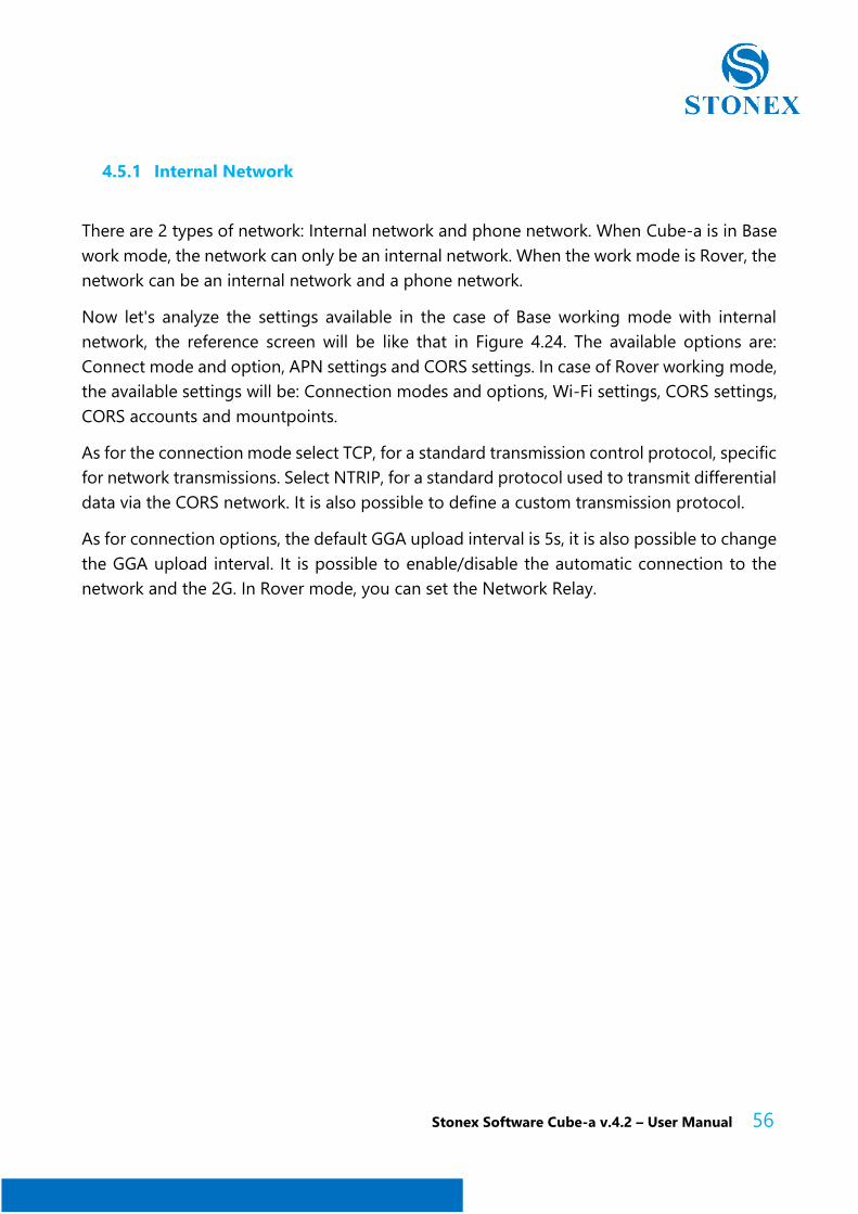
Now let's analyze the settings available in the case of Base working mode with internal
network, the reference screen will be like that in Figure 4.24. The available options are:
Connect mode and option, APN settings and CORS settings. In case of Rover working mode,
the available settings will be: Connection modes and options, Wi-Fi settings, CORS settings,
CORS accounts and mountpoints.
As for the connection mode select TCP, for a standard transmission control protocol, specific
for network transmissions. Select NTRIP, for a standard protocol used to transmit differential
data via the CORS network. It is also possible to define a custom transmission protocol.
As for connection options, the default GGA upload interval is 5s, it is also possible to change
the GGA upload interval. It is possible to enable/disable the automatic connection to the
network and the 2G. In Rover mode, you can set the Network Relay.
Stonex Software Cube-a v.4.2 – User Manual 57
Figure 4.24
In the APN settings you can search for an operator by clicking on the search button at the
top (with the three dots).
Base network settings: in the CORS settings, enter the IP, port, base mountpoint and
password. If you click on the search button on the right side, you can add or edit the CORS
server parameters.
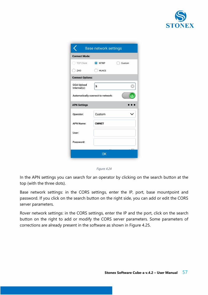
Rover network settings: in the CORS settings, enter the IP and the port, click on the search
button on the right to add or modify the CORS server parameters. Some parameters of
corrections are already present in the software as shown in Figure 4.25.
Stonex Software Cube-a v.4.2 – User Manual 58
Figure 4.25
Then set the mountpoint, you can use "RTK network" or "mobile phone network" to get the
mountpoints and select a mountpoint. Finally, set the user and password in the CORS
account. If the Base is set up independently, the user and password can be entered with any
character. If you use a CORS account, you must enter the corresponding user and password.
The IP in the Base and Rover settings must be the same.
Stonex Software Cube-a v.4.2 – User Manual 59
4.5.2 Internal Radio
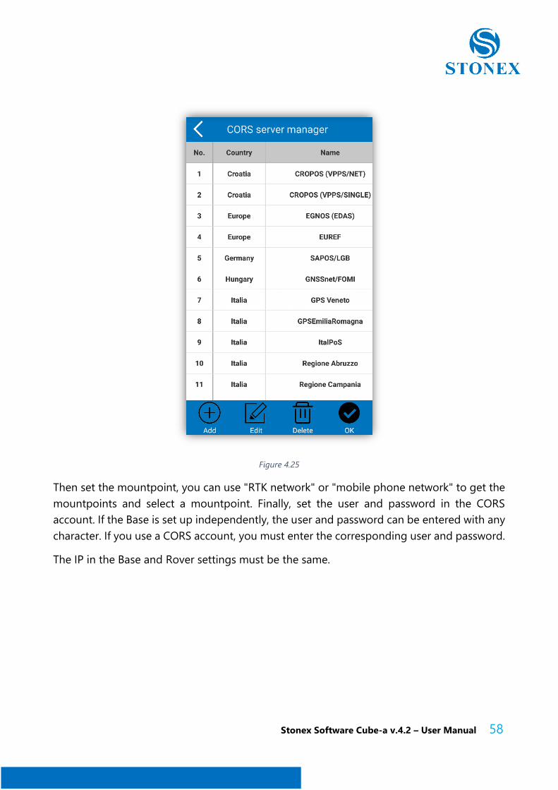
Select the "Internal Radio" data communication mode, click on the "Internal Radio" button
to access the screen where to set the parameters (Figure 4.26). The parameters in Base and
Rover modes are the same, including channel, frequency and protocol. Channels 1 to 7 are
fixed, the frequency can not be changed; channel 8 is the customizable channel, the
frequency could be set according to your needs. By clicking " Default radio settings", you
can set the frequency of channels 1-8.
If the data communication mode of Base and Rover is the internal radio, the frequency and
protocol of Base and Rover must be the same. In Base mode, the radio power will affect the
signal transmission distance. Low power, low power consumption, the signal transmission
distance is close; High power, high power consumption, the signal transmission distance is
far away.
Figure 4.26
Stonex Software Cube-a v.4.2 – User Manual 60
4.5.3 External Radio
Select the "External Radio" data communication mode and click on the "External Radio"
button to set the parameters. The parameters of the Base and Rover modes are the same,
only the baud rate must be set. The default speed value is 38400.
4.5.4 Phone Network
This mode of data communication is only available in Rover mode. Select this mode and
click on the phone network button to set the parameters (Figure 4.27), the parameters
include the CORS settings and the entry point. If the search button on the right side of the
CORS settings is on the CORS server, you can add or modify the CORS server parameters.
These settings are the same as those already illustrated for the internal network
communication mode, in this case, however, the network used in the telephone network
mode is that of the mobile device, which requires access to the Internet.

Stonex Software Cube-a v.4.2 – User Manual 61
Figure 4.27
4.6 Information
Contains detailed parameters and status of devices, antenna, network, radio and satellite
systems.
Stonex Software Cube-a v.4.2 – User Manual 62
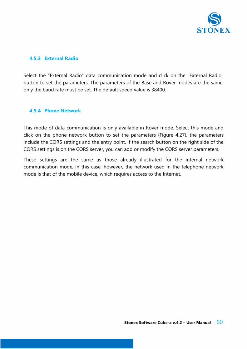
4.7 RTK Reset
Its function is to force the re-initialization of the OEM card, thus forcing a complete
recalculation of the position starting from new satellite signals. Click "Reset RTK", the dialog
box shown in Figure 4.28 will appear, then click "OK" and the receiver will restart positioning.
Figure 4.28
4.8 Register
With this command you can view the serial number of the device and the expiration date
of the license registration. In this screen you can enter any license codes and then register
the GNSS (in case of license expirying, for example), the device must of course be
connected to the Cube-a
Stonex Software Cube-a v.4.2 – User Manual 63
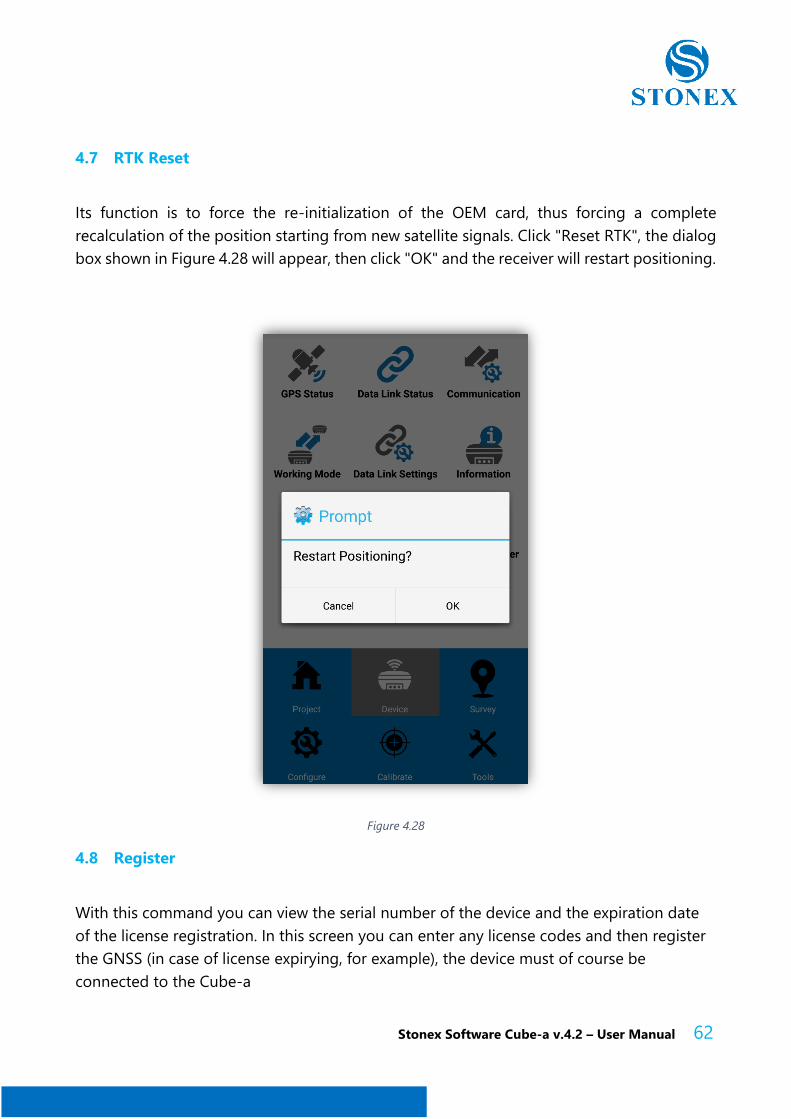
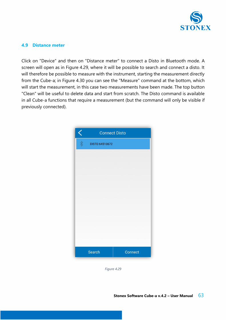
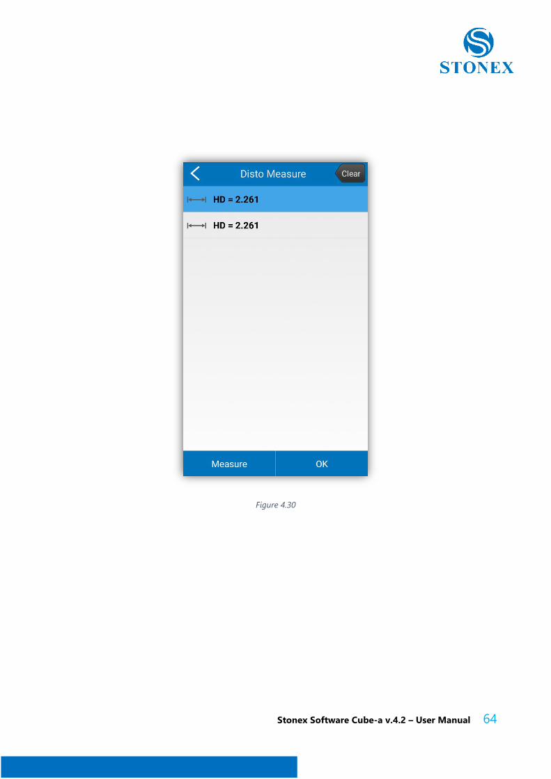
4.9 Distance meter
Click on "Device" and then on "Distance meter" to connect a Disto in Bluetooth mode. A
screen will open as in Figure 4.29, where it will be possible to search and connect a disto. It
will therefore be possible to measure with the instrument, starting the measurement directly
from the Cube-a; in Figure 4.30 you can see the "Measure" command at the bottom, which
will start the measurement, in this case two measurements have been made. The top button
"Clean" will be useful to delete data and start from scratch. The Disto command is available
in all Cube-a functions that require a measurement (but the command will only be visible if
previously connected).
Figure 4.29
Stonex Software Cube-a v.4.2 – User Manual 64
Figure 4.30
Stonex Software Cube-a v.4.2 – User Manual 65
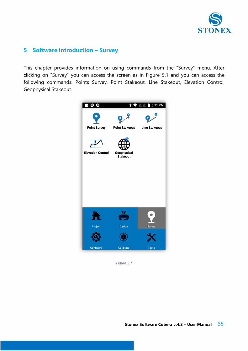
5 Software introduction – Survey
This chapter provides information on using commands from the "Survey" menu. After
clicking on "Survey" you can access the screen as in Figure 5.1 and you can access the
following commands: Points Survey, Point Stakeout, Line Stakeout, Elevation Control,
Geophysical Stakeout.
Figure 5.1
Stonex Software Cube-a v.4.2 – User Manual 66
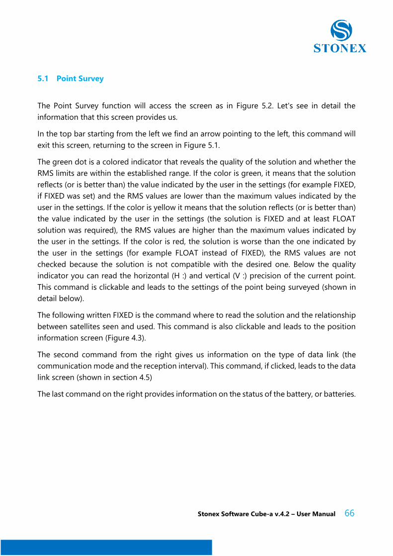
5.1 Point Survey
The Point Survey function will access the screen as in Figure 5.2. Let's see in detail the
information that this screen provides us.
In the top bar starting from the left we find an arrow pointing to the left, this command will
exit this screen, returning to the screen in Figure 5.1.
The green dot is a colored indicator that reveals the quality of the solution and whether the
RMS limits are within the established range. If the color is green, it means that the solution
reflects (or is better than) the value indicated by the user in the settings (for example FIXED,
if FIXED was set) and the RMS values are lower than the maximum values indicated by the
user in the settings. If the color is yellow it means that the solution reflects (or is better than)
the value indicated by the user in the settings (the solution is FIXED and at least FLOAT
solution was required), the RMS values are higher than the maximum values indicated by
the user in the settings. If the color is red, the solution is worse than the one indicated by
the user in the settings (for example FLOAT instead of FIXED), the RMS values are not
checked because the solution is not compatible with the desired one. Below the quality
indicator you can read the horizontal (H :) and vertical (V :) precision of the current point.
This command is clickable and leads to the settings of the point being surveyed (shown in
detail below).
The following written FIXED is the command where to read the solution and the relationship
between satellites seen and used. This command is also clickable and leads to the position
information screen (Figure 4.3).
The second command from the right gives us information on the type of data link (the
communication mode and the reception interval). This command, if clicked, leads to the data
link screen (shown in section 4.5)
The last command on the right provides information on the status of the battery, or batteries.
Stonex Software Cube-a v.4.2 – User Manual 67
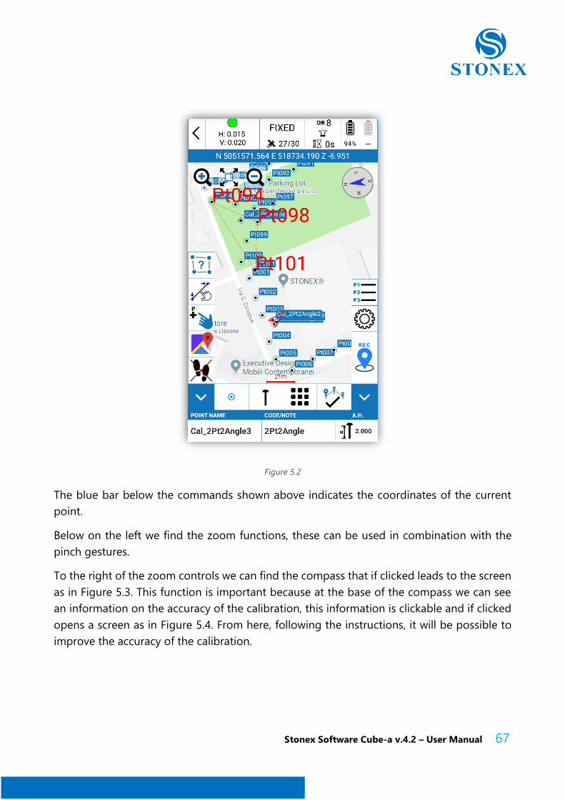
Figure 5.2
The blue bar below the commands shown above indicates the coordinates of the current
point.
Below on the left we find the zoom functions, these can be used in combination with the
pinch gestures.
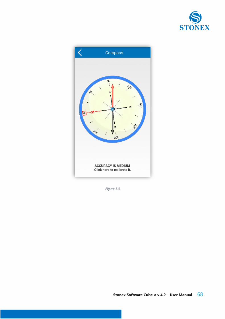
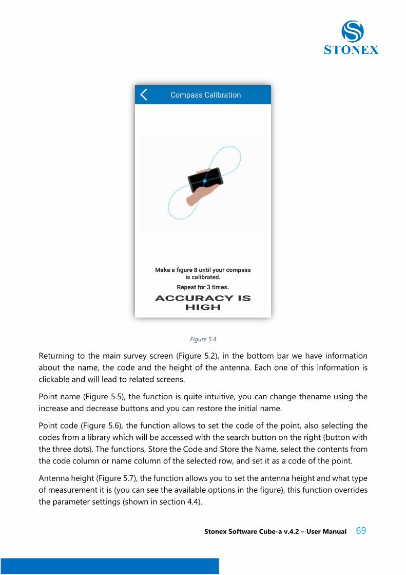
To the right of the zoom controls we can find the compass that if clicked leads to the screen
as in Figure 5.3. This function is important because at the base of the compass we can see
an information on the accuracy of the calibration, this information is clickable and if clicked
opens a screen as in Figure 5.4. From here, following the instructions, it will be possible to
improve the accuracy of the calibration.
Stonex Software Cube-a v.4.2 – User Manual 68
Figure 5.3
Stonex Software Cube-a v.4.2 – User Manual 69
Figure 5.4
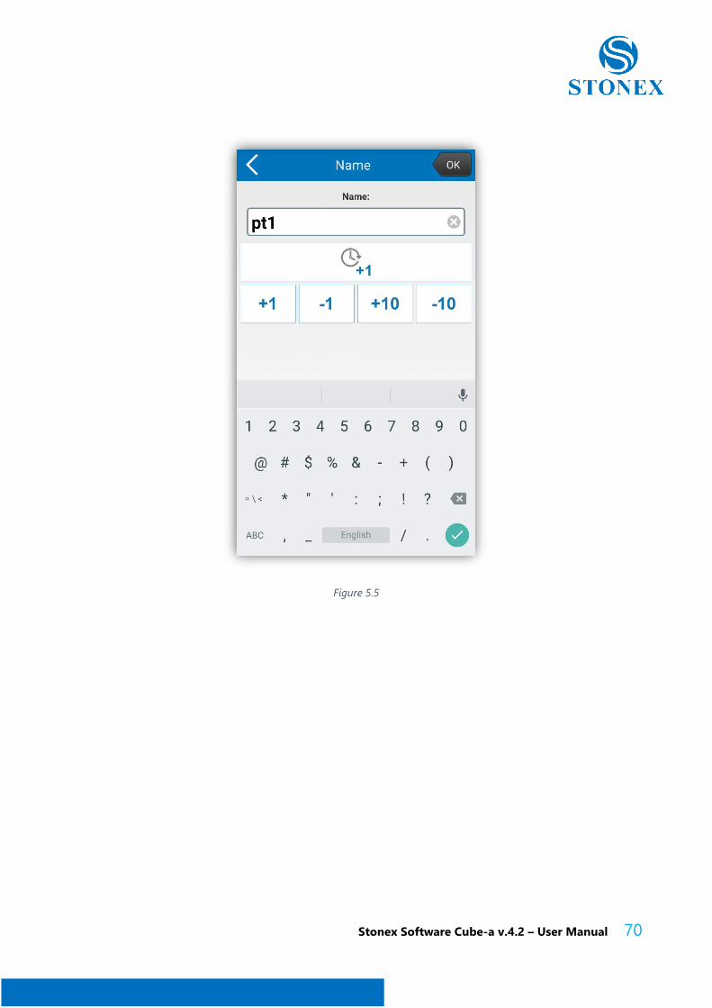
Returning to the main survey screen (Figure 5.2), in the bottom bar we have information
about the name, the code and the height of the antenna. Each one of this information is
clickable and will lead to related screens.
Point name (Figure 5.5), the function is quite intuitive, you can change thename using the
increase and decrease buttons and you can restore the initial name.
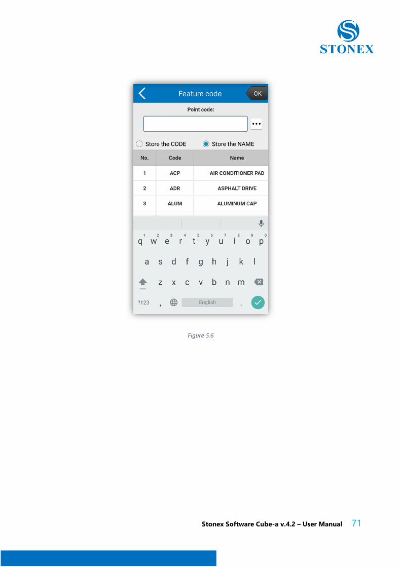
Point code (Figure 5.6), the function allows to set the code of the point, also selecting the
codes from a library which will be accessed with the search button on the right (button with
the three dots). The functions, Store the Code and Store the Name, select the contents from
the code column or name column of the selected row, and set it as a code of the point.
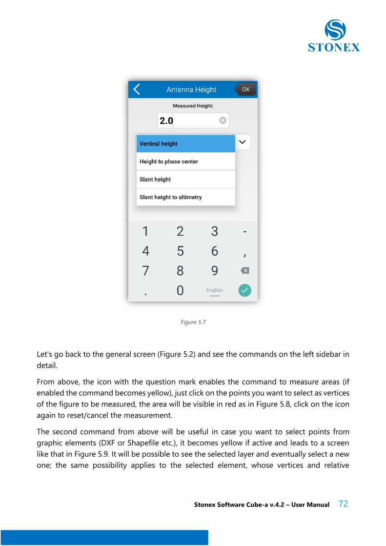
Antenna height (Figure 5.7), the function allows you to set the antenna height and what type
of measurement it is (you can see the available options in the figure), this function overrides
the parameter settings (shown in section 4.4).
Stonex Software Cube-a v.4.2 – User Manual 70
Figure 5.5
Stonex Software Cube-a v.4.2 – User Manual 71
Figure 5.6
Stonex Software Cube-a v.4.2 – User Manual 72
Figure 5.7
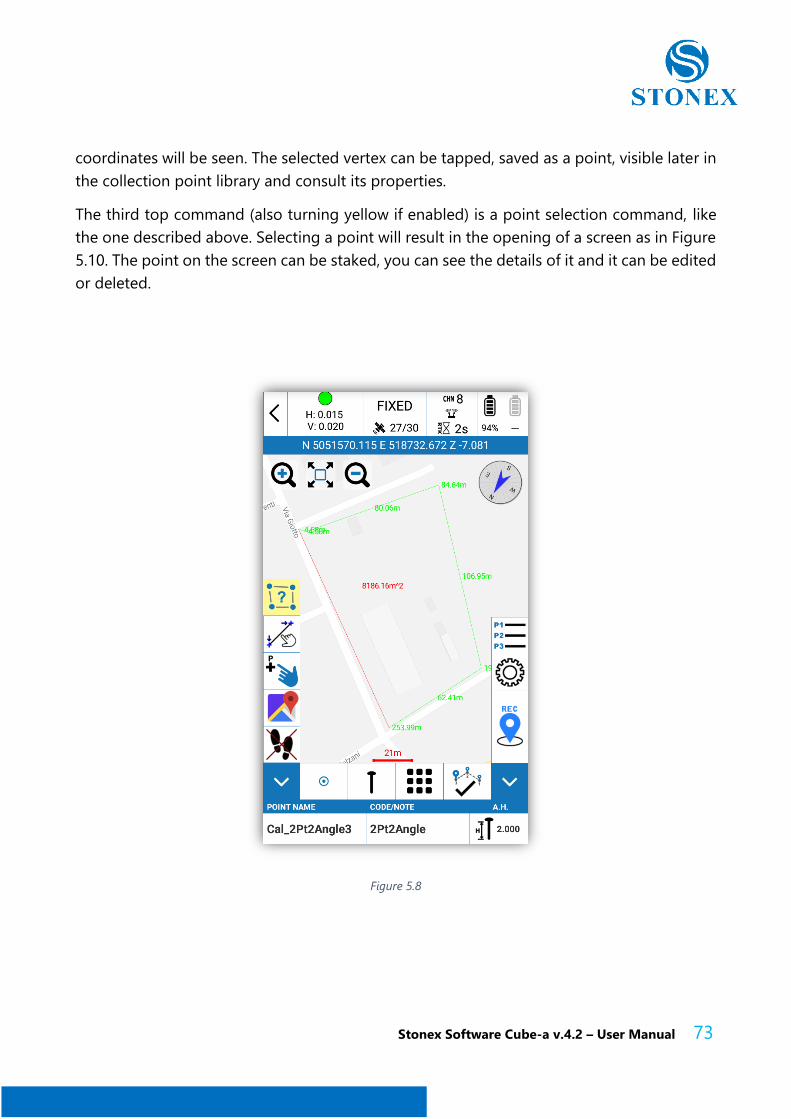
Let's go back to the general screen (Figure 5.2) and see the commands on the left sidebar in
detail.
From above, the icon with the question mark enables the command to measure areas (if
enabled the command becomes yellow), just click on the points you want to select as vertices
of the figure to be measured, the area will be visible in red as in Figure 5.8, click on the icon
again to reset/cancel the measurement.
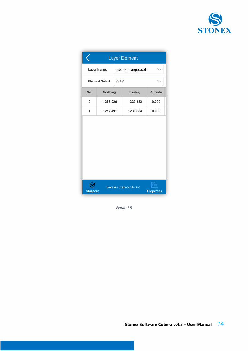
The second command from above will be useful in case you want to select points from
graphic elements (DXF or Shapefile etc.), it becomes yellow if active and leads to a screen
like that in Figure 5.9. It will be possible to see the selected layer and eventually select a new
one; the same possibility applies to the selected element, whose vertices and relative
Stonex Software Cube-a v.4.2 – User Manual 73
coordinates will be seen. The selected vertex can be tapped, saved as a point, visible later in
the collection point library and consult its properties.
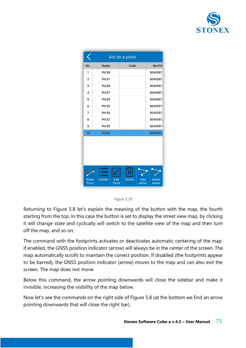
The third top command (also turning yellow if enabled) is a point selection command, like
the one described above. Selecting a point will result in the opening of a screen as in Figure
5.10. The point on the screen can be staked, you can see the details of it and it can be edited
or deleted.
Figure 5.8
Stonex Software Cube-a v.4.2 – User Manual 74
Figure 5.9
Stonex Software Cube-a v.4.2 – User Manual 75
Figure 5.10
Returning to Figure 5.8 let’s explain the meaning of the button with the map, the fourth
starting from the top. In this case the button is set to display the street view map, by clicking
it will change state and cyclically will switch to the satellite view of the map and then turn
off the map, and so on.
The command with the footprints activates or deactivates automatic centering of the map.
If enabled, the GNSS position indicator (arrow) will always be in the center of the screen. The
map automatically scrolls to maintain the correct position. If disabled (the footprints appear
to be barred), the GNSS position indicator (arrow) moves to the map and can also exit the
screen. The map does not move.
Below this command, the arrow pointing downwards will close the sidebar and make it
invisible, increasing the visibility of the map below.
Now let's see the commands on the right side of Figure 5.8 (at the bottom we find an arrow
pointing downwards that will close the right bar).
Stonex Software Cube-a v.4.2 – User Manual 76
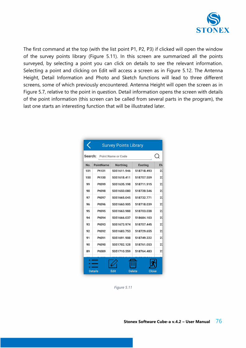
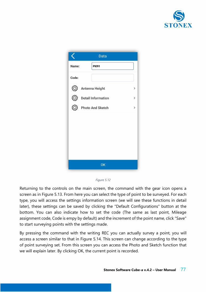
The first command at the top (with the list point P1, P2, P3) if clicked will open the window
of the survey points library (Figure 5.11). In this screen are summarized all the points
surveyed, by selecting a point you can click on details to see the relevant information.
Selecting a point and clicking on Edit will access a screen as in Figure 5.12. The Antenna
Height, Detail Information and Photo and Sketch functions will lead to three different
screens, some of which previously encountered. Antenna Height will open the screen as in
Figure 5.7, relative to the point in question. Detail information opens the screen with details
of the point information (this screen can be called from several parts in the program), the
last one starts an interesting function that will be illustrated later.
Figure 5.11
Stonex Software Cube-a v.4.2 – User Manual 77
Figure 5.12
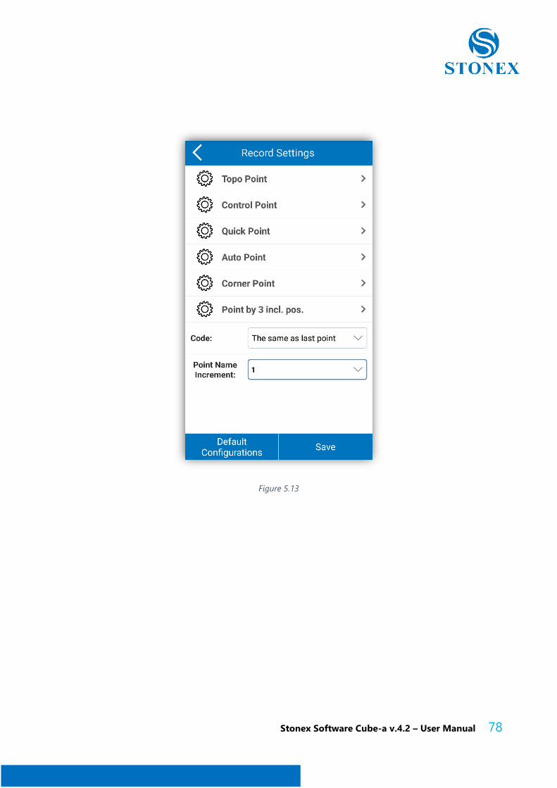
Returning to the controls on the main screen, the command with the gear icon opens a
screen as in Figure 5.13. From here you can select the type of point to be surveyed. For each
type, you will access the settings information screen (we will see these functions in detail
later), these settings can be saved by clicking the "Default Configurations" button at the
bottom. You can also indicate how to set the code (The same as last point, Mileage
assignment code, Code is empy by default) and the increment of the point name, click "Save"
to start surveying points with the settings made.
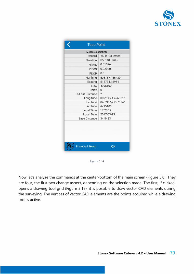
By pressing the command with the writing REC you can actually survey a point, you will
access a screen similar to that in Figure 5.14. This screen can change according to the type
of point surveying set. From this screen you can access the Photo and Sketch function that
we will explain later. By clicking OK, the current point is recorded.
Stonex Software Cube-a v.4.2 – User Manual 78
Figure 5.13
Stonex Software Cube-a v.4.2 – User Manual 79
Figure 5.14
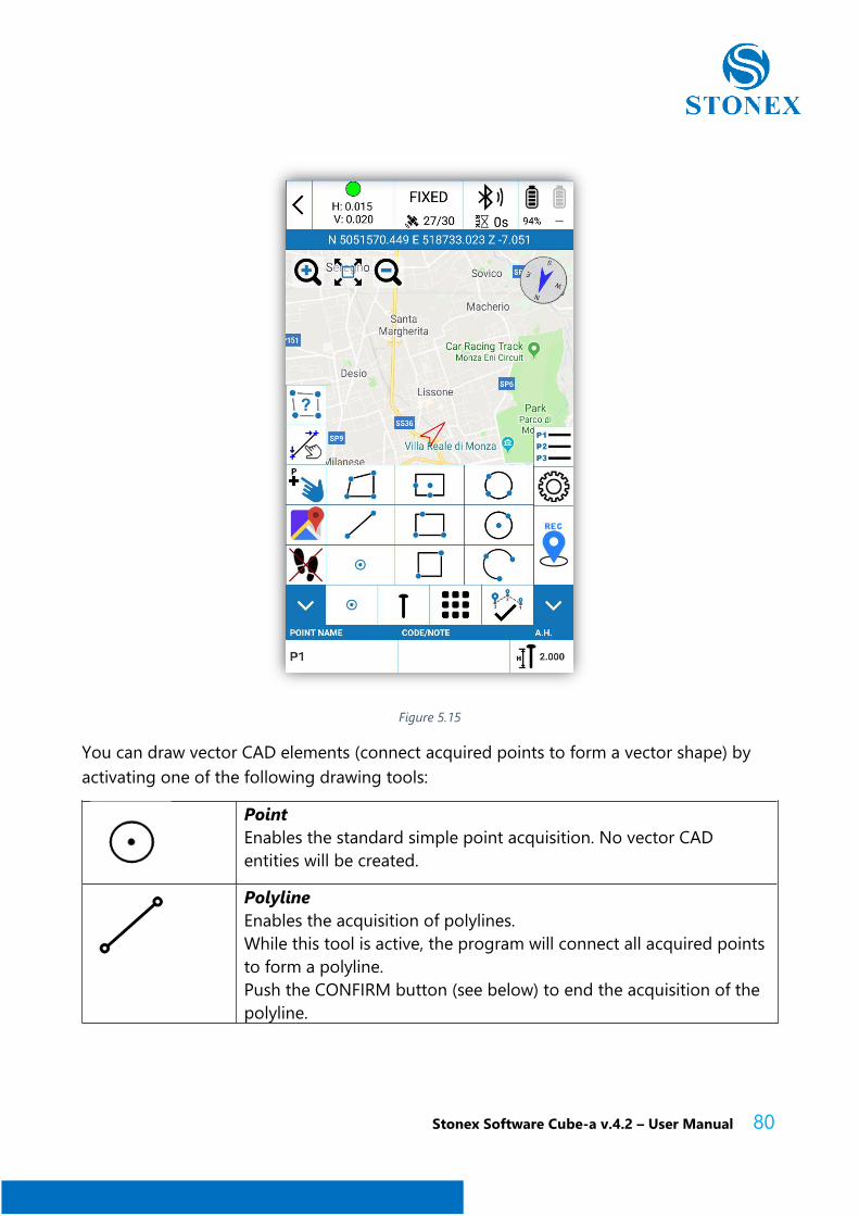
Now let's analyze the commands at the center-bottom of the main screen (Figure 5.8). They
are four, the first two change aspect, depending on the selection made. The first, if clicked,
opens a drawing tool grid (Figure 5.15), it is possible to draw vector CAD elements during
the surveying. The vertices of vector CAD elements are the points acquired while a drawing
tool is active.
Stonex Software Cube-a v.4.2 – User Manual 80
Figure 5.15
You can draw vector CAD elements (connect acquired points to form a vector shape) by
activating one of the following drawing tools:
Point
Enables the standard simple point acquisition. No vector CAD
entities will be created.
Polyline
Enables the acquisition of polylines.
While this tool is active, the program will connect all acquired points
to form a polyline.
Push the CONFIRM button (see below) to end the acquisition of the
polyline.
Stonex Software Cube-a v.4.2 – User Manual 81
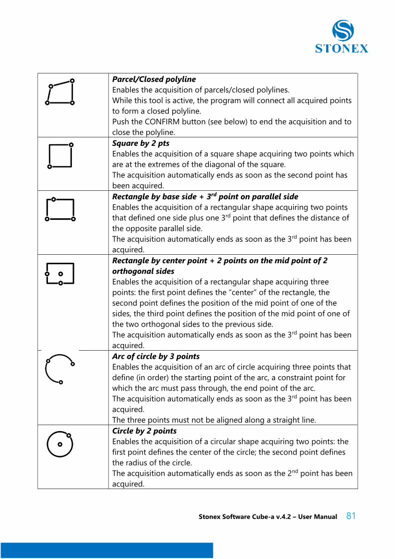
Parcel/Closed polyline
Enables the acquisition of parcels/closed polylines.
While this tool is active, the program will connect all acquired points
to form a closed polyline.
Push the CONFIRM button (see below) to end the acquisition and to
close the polyline.
Square by 2 pts
Enables the acquisition of a square shape acquiring two points which
are at the extremes of the diagonal of the square.
The acquisition automatically ends as soon as the second point has
been acquired.
Rectangle by base side + 3rd point on parallel side
Enables the acquisition of a rectangular shape acquiring two points
that defined one side plus one 3rd point that defines the distance of
the opposite parallel side.
The acquisition automatically ends as soon as the 3rd point has been
acquired.
Rectangle by center point + 2 points on the mid point of 2
orthogonal sides
Enables the acquisition of a rectangular shape acquiring three
points: the first point defines the “center” of the rectangle, the
second point defines the position of the mid point of one of the
sides, the third point defines the position of the mid point of one of
the two orthogonal sides to the previous side.
The acquisition automatically ends as soon as the 3rd point has been
acquired.
Arc of circle by 3 points
Enables the acquisition of an arc of circle acquiring three points that
define (in order) the starting point of the arc, a constraint point for
which the arc must pass through, the end point of the arc.
The acquisition automatically ends as soon as the 3rd point has been
acquired.
The three points must not be aligned along a straight line.
Circle by 2 points
Enables the acquisition of a circular shape acquiring two points: the
first point defines the center of the circle; the second point defines
the radius of the circle.
The acquisition automatically ends as soon as the 2nd point has been
acquired.
Stonex Software Cube-a v.4.2 – User Manual 82
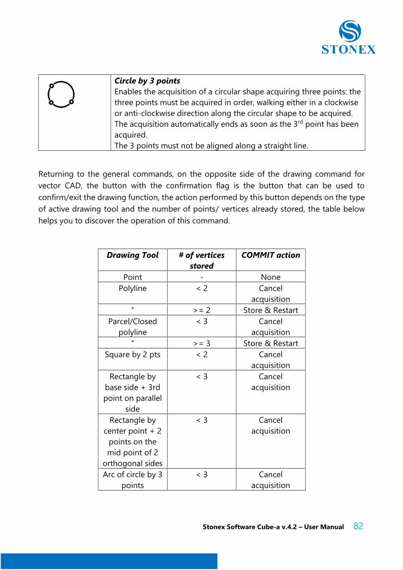
Circle by 3 points
Enables the acquisition of a circular shape acquiring three points: the
three points must be acquired in order, walking either in a clockwise
or anti-clockwise direction along the circular shape to be acquired.
The acquisition automatically ends as soon as the 3rd point has been
acquired.
The 3 points must not be aligned along a straight line.
Returning to the general commands, on the opposite side of the drawing command for
vector CAD, the button with the confirmation flag is the button that can be used to
confirm/exit the drawing function, the action performed by this button depends on the type
of active drawing tool and the number of points/ vertices already stored, the table below
helps you to discover the operation of this command.
Drawing Tool # of vertices
stored
COMMIT action
Point - None
Polyline < 2 Cancel
acquisition
“ >= 2 Store & Restart
Parcel/Closed
polyline
< 3 Cancel
acquisition
“ >= 3 Store & Restart
Square by 2 pts < 2 Cancel
acquisition
Rectangle by
base side + 3rd
point on parallel
side
< 3 Cancel
acquisition
Rectangle by
center point + 2
points on the
mid point of 2
orthogonal sides
< 3 Cancel
acquisition
Arc of circle by 3
points
< 3 Cancel
acquisition
Stonex Software Cube-a v.4.2 – User Manual 83
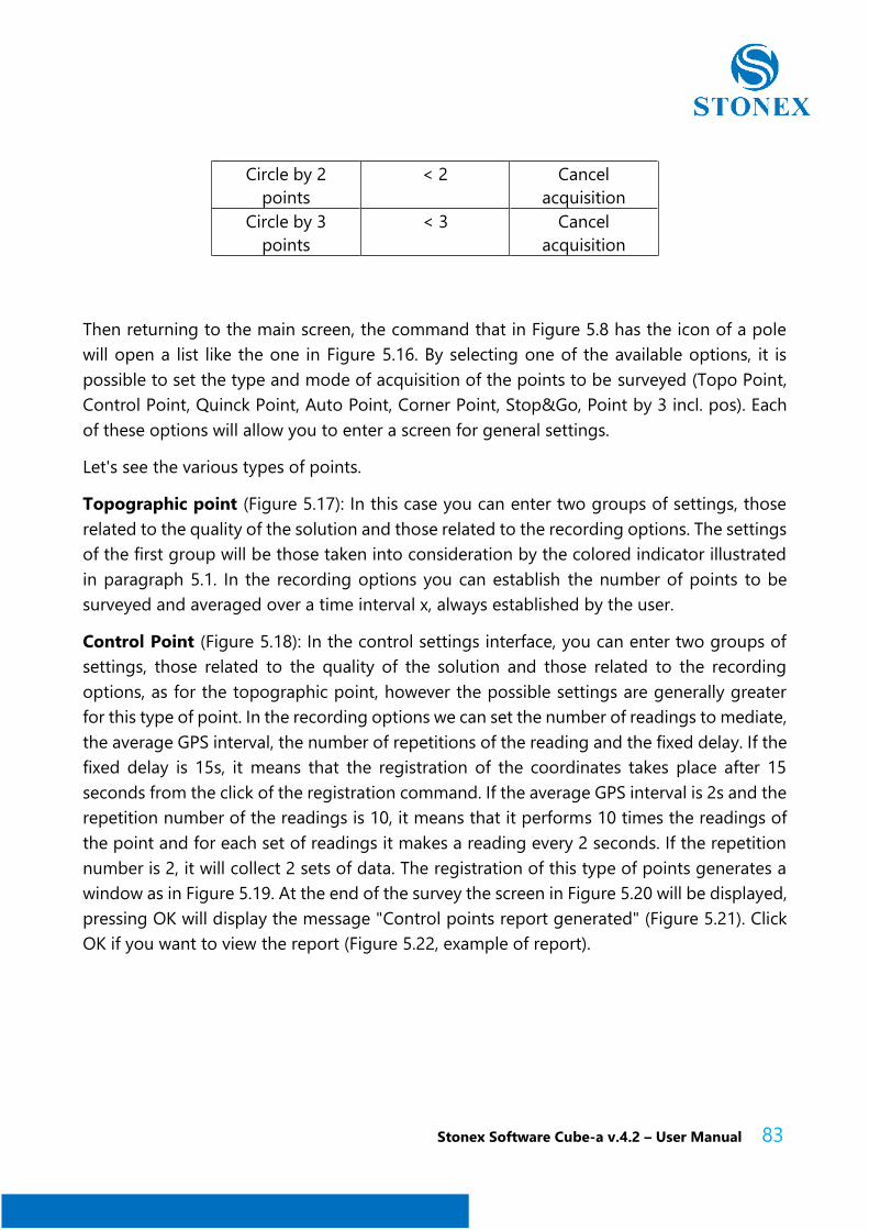
Circle by 2
points
< 2 Cancel
acquisition
Circle by 3
points
< 3 Cancel
acquisition
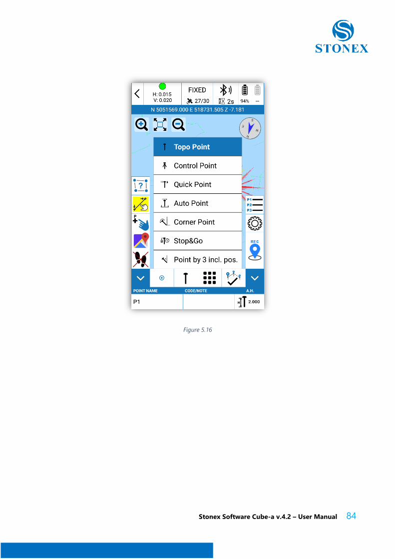
Then returning to the main screen, the command that in Figure 5.8 has the icon of a pole
will open a list like the one in Figure 5.16. By selecting one of the available options, it is
possible to set the type and mode of acquisition of the points to be surveyed (Topo Point,
Control Point, Quinck Point, Auto Point, Corner Point, Stop&Go, Point by 3 incl. pos). Each
of these options will allow you to enter a screen for general settings.
Let's see the various types of points.
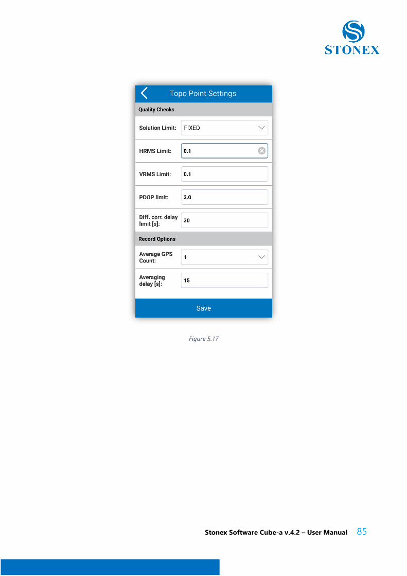
Topographic point (Figure 5.17): In this case you can enter two groups of settings, those
related to the quality of the solution and those related to the recording options. The settings
of the first group will be those taken into consideration by the colored indicator illustrated
in paragraph 5.1. In the recording options you can establish the number of points to be
surveyed and averaged over a time interval x, always established by the user.
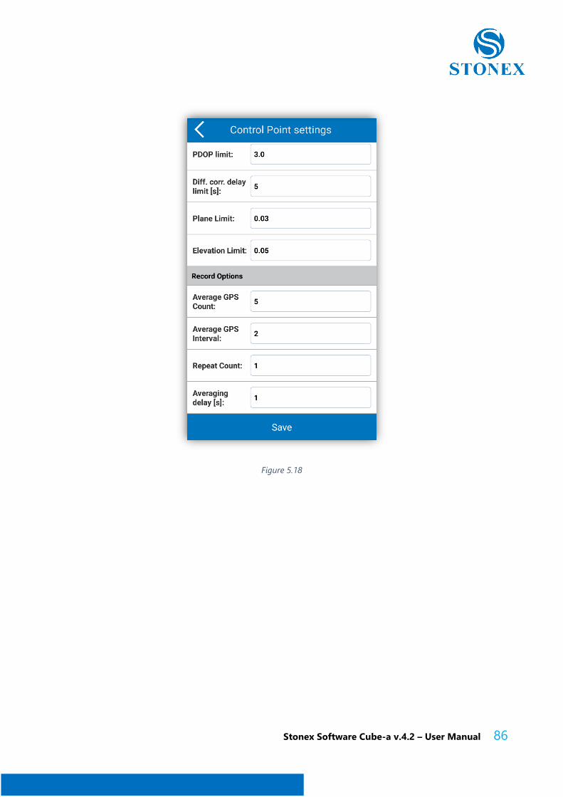
Control Point (Figure 5.18): In the control settings interface, you can enter two groups of
settings, those related to the quality of the solution and those related to the recording
options, as for the topographic point, however the possible settings are generally greater
for this type of point. In the recording options we can set the number of readings to mediate,
the average GPS interval, the number of repetitions of the reading and the fixed delay. If the
fixed delay is 15s, it means that the registration of the coordinates takes place after 15
seconds from the click of the registration command. If the average GPS interval is 2s and the
repetition number of the readings is 10, it means that it performs 10 times the readings of
the point and for each set of readings it makes a reading every 2 seconds. If the repetition
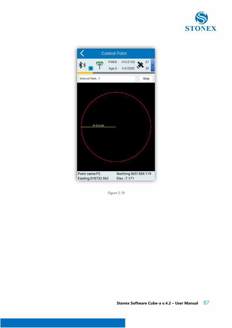
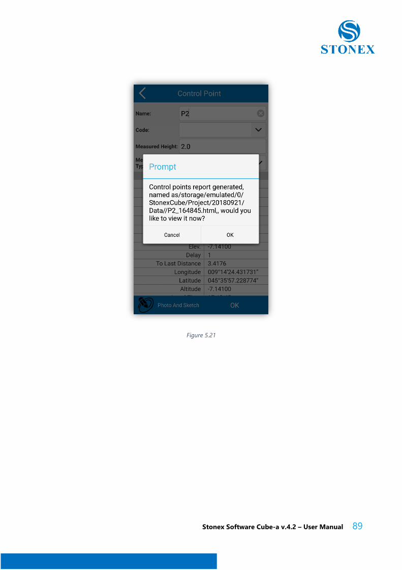
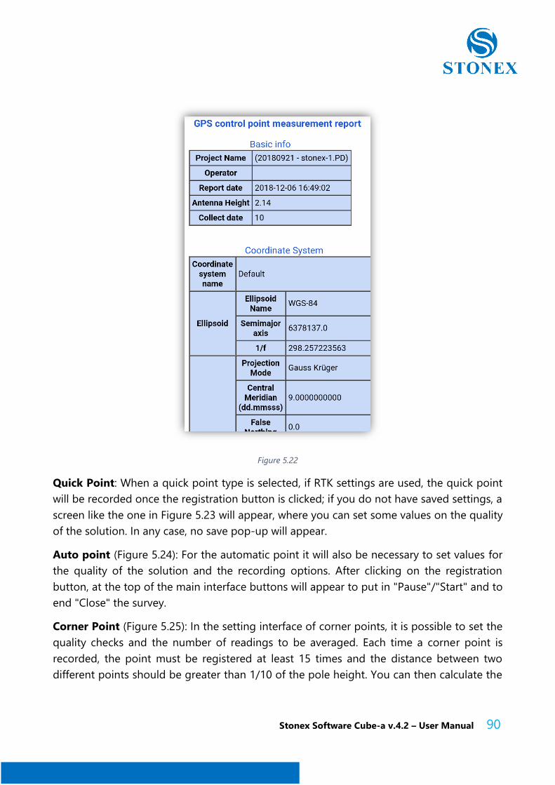
number is 2, it will collect 2 sets of data. The registration of this type of points generates a
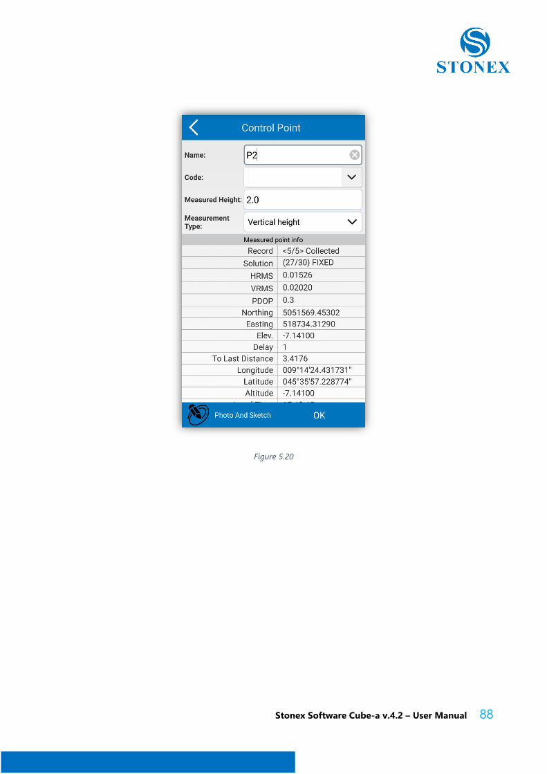
window as in Figure 5.19. At the end of the survey the screen in Figure 5.20 will be displayed,
pressing OK will display the message "Control points report generated" (Figure 5.21). Click
OK if you want to view the report (Figure 5.22, example of report).
Stonex Software Cube-a v.4.2 – User Manual 84
Figure 5.16
Stonex Software Cube-a v.4.2 – User Manual 85
Figure 5.17
Stonex Software Cube-a v.4.2 – User Manual 86
Figure 5.18
Stonex Software Cube-a v.4.2 – User Manual 87
Figure 5.19
Stonex Software Cube-a v.4.2 – User Manual 88
Figure 5.20
Stonex Software Cube-a v.4.2 – User Manual 89
Figure 5.21
Stonex Software Cube-a v.4.2 – User Manual 90
Figure 5.22
Quick Point: When a quick point type is selected, if RTK settings are used, the quick point
will be recorded once the registration button is clicked; if you do not have saved settings, a
screen like the one in Figure 5.23 will appear, where you can set some values on the quality
of the solution. In any case, no save pop-up will appear.
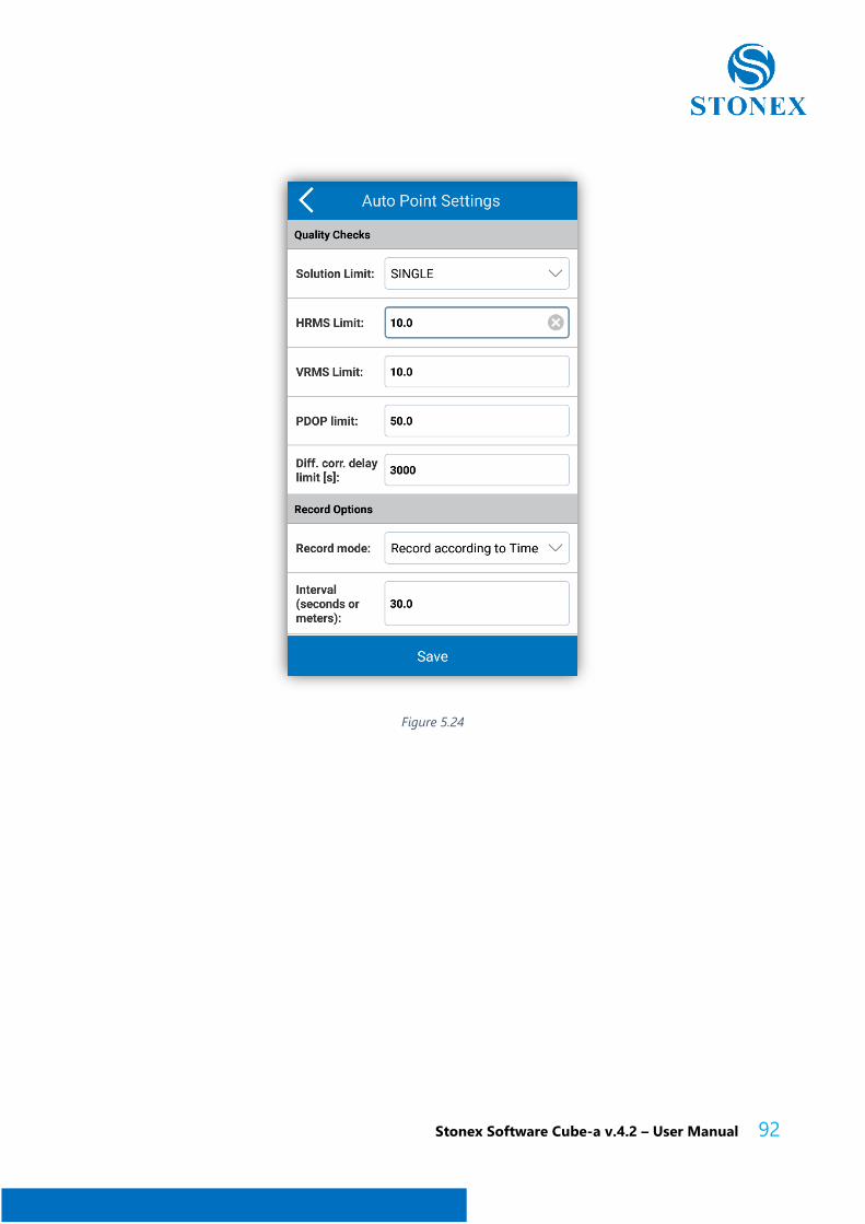
Auto point (Figure 5.24): For the automatic point it will also be necessary to set values for
the quality of the solution and the recording options. After clicking on the registration
button, at the top of the main interface buttons will appear to put in "Pause"/"Start" and to
end "Close" the survey.
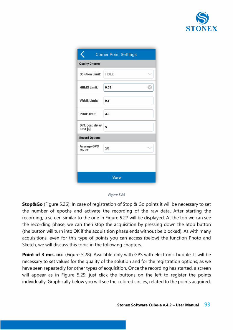
Corner Point (Figure 5.25): In the setting interface of corner points, it is possible to set the
quality checks and the number of readings to be averaged. Each time a corner point is
recorded, the point must be registered at least 15 times and the distance between two
different points should be greater than 1/10 of the pole height. You can then calculate the

Stonex Software Cube-a v.4.2 – User Manual 91
coordinates of the center of the corner through the coordinates of the corner points, the
coordinates of the center of the corner are the coordinates of the calculated corner point.
Figure 5.23
Stonex Software Cube-a v.4.2 – User Manual 92
Figure 5.24
Stonex Software Cube-a v.4.2 – User Manual 93
Figure 5.25
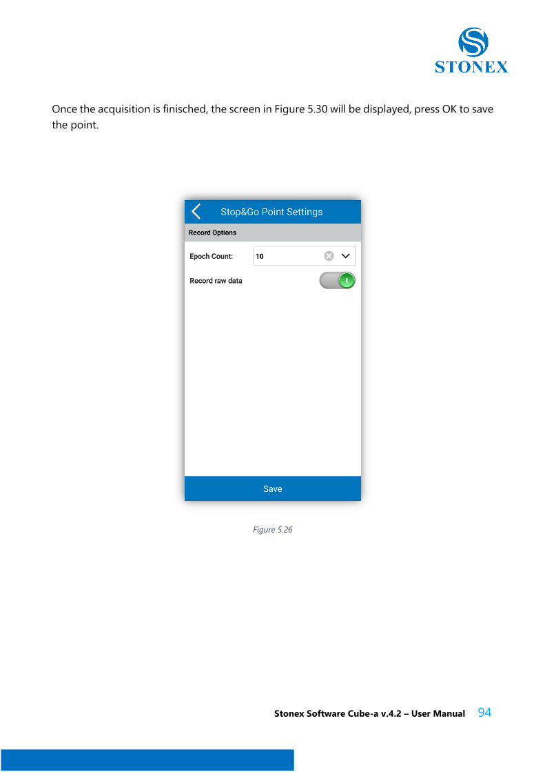
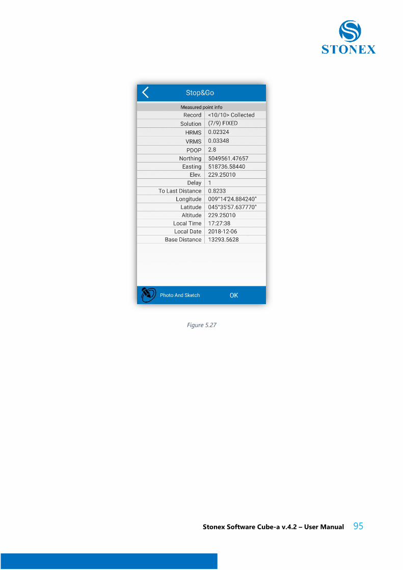
Stop&Go (Figure 5.26): In case of registration of Stop & Go points it will be necessary to set
the number of epochs and activate the recording of the raw data. After starting the
recording, a screen similar to the one in Figure 5.27 will be displayed. At the top we can see
the recording phase, we can then stop the acquisition by pressing down the Stop button
(the button will turn into OK if the acquisition phase ends without be blocked). As with many
acquisitions, even for this type of points you can access (below) the function Photo and
Sketch, we will discuss this topic in the following chapters.
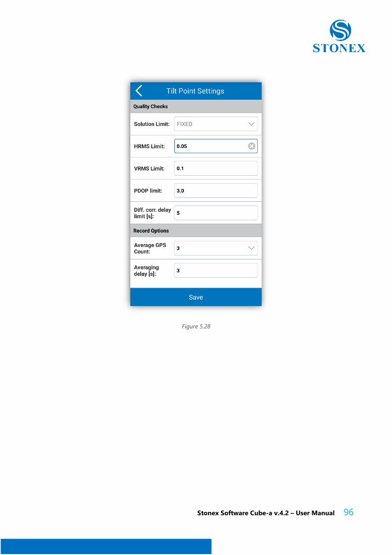
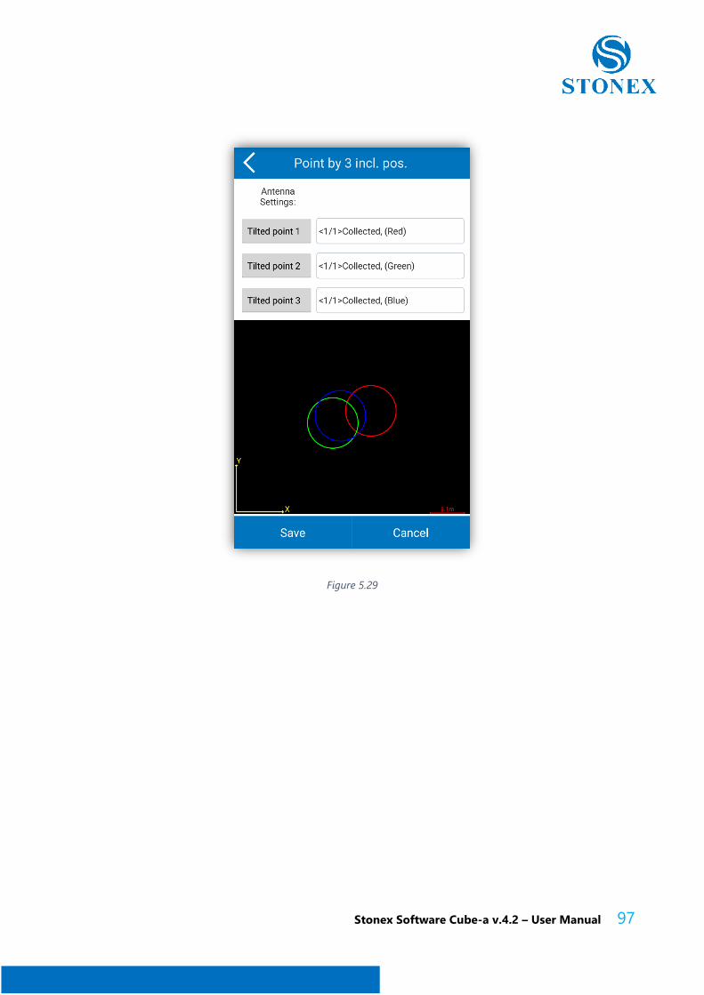
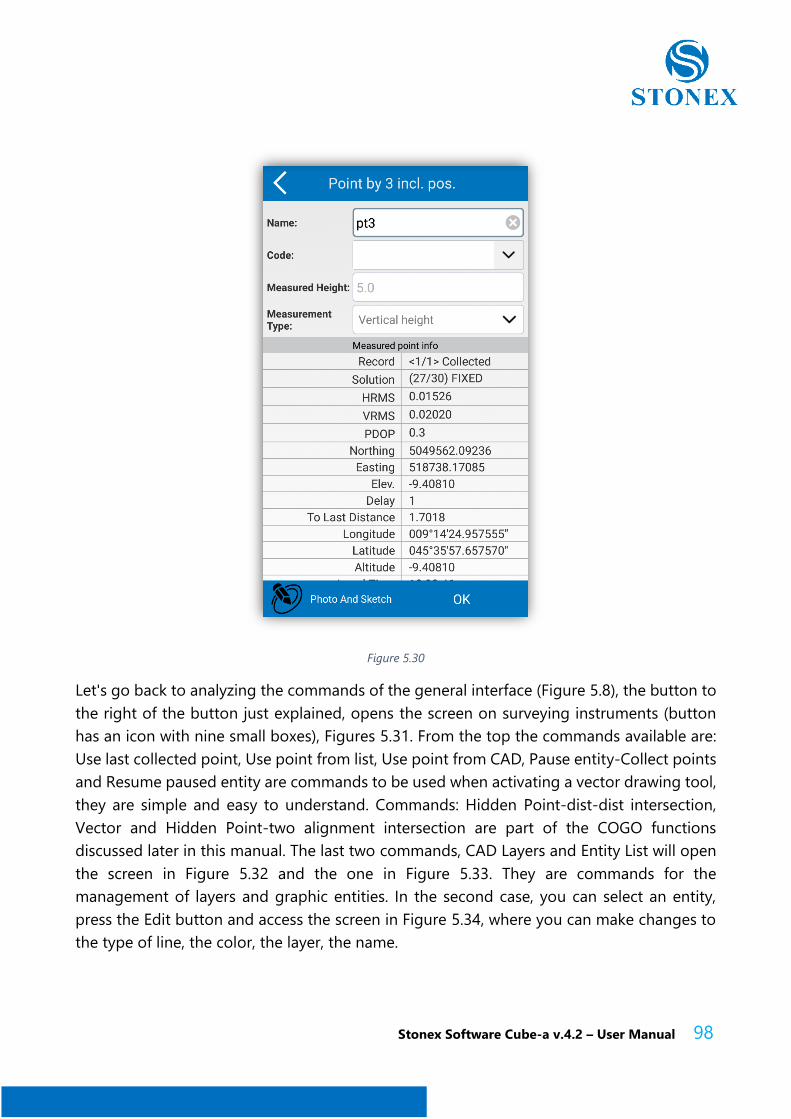
Point of 3 mis. inc. (Figure 5.28): Available only with GPS with electronic bubble. It will be
necessary to set values for the quality of the solution and for the registration options, as we
have seen repeatedly for other types of acquisition. Once the recording has started, a screen
will appear as in Figure 5.29, just click the buttons on the left to register the points
individually. Graphically below you will see the colored circles, related to the points acquired.
Stonex Software Cube-a v.4.2 – User Manual 94
Once the acquisition is finisched, the screen in Figure 5.30 will be displayed, press OK to save
the point.
Figure 5.26
Stonex Software Cube-a v.4.2 – User Manual 95
Figure 5.27
Stonex Software Cube-a v.4.2 – User Manual 96
Figure 5.28
Stonex Software Cube-a v.4.2 – User Manual 97
Figure 5.29
Stonex Software Cube-a v.4.2 – User Manual 98
Figure 5.30
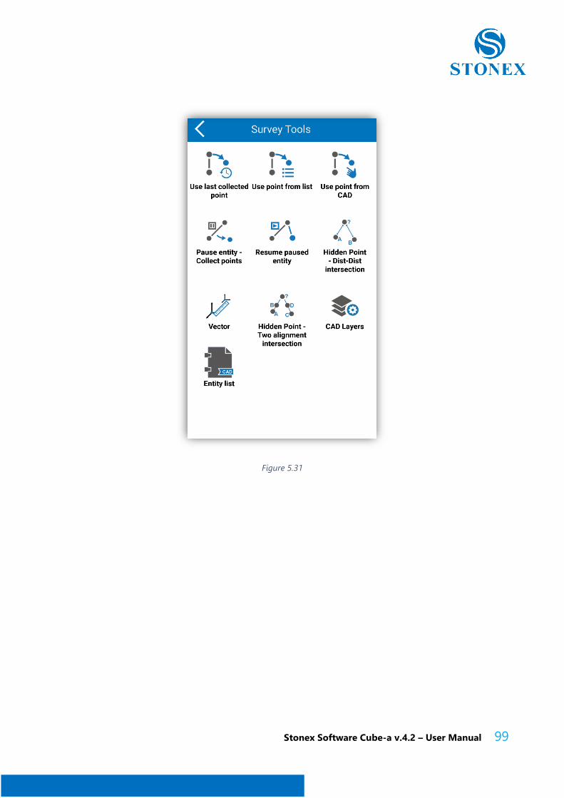
Let's go back to analyzing the commands of the general interface (Figure 5.8), the button to
the right of the button just explained, opens the screen on surveying instruments (button
has an icon with nine small boxes), Figures 5.31. From the top the commands available are:
Use last collected point, Use point from list, Use point from CAD, Pause entity-Collect points
and Resume paused entity are commands to be used when activating a vector drawing tool,
they are simple and easy to understand. Commands: Hidden Point-dist-dist intersection,
Vector and Hidden Point-two alignment intersection are part of the COGO functions
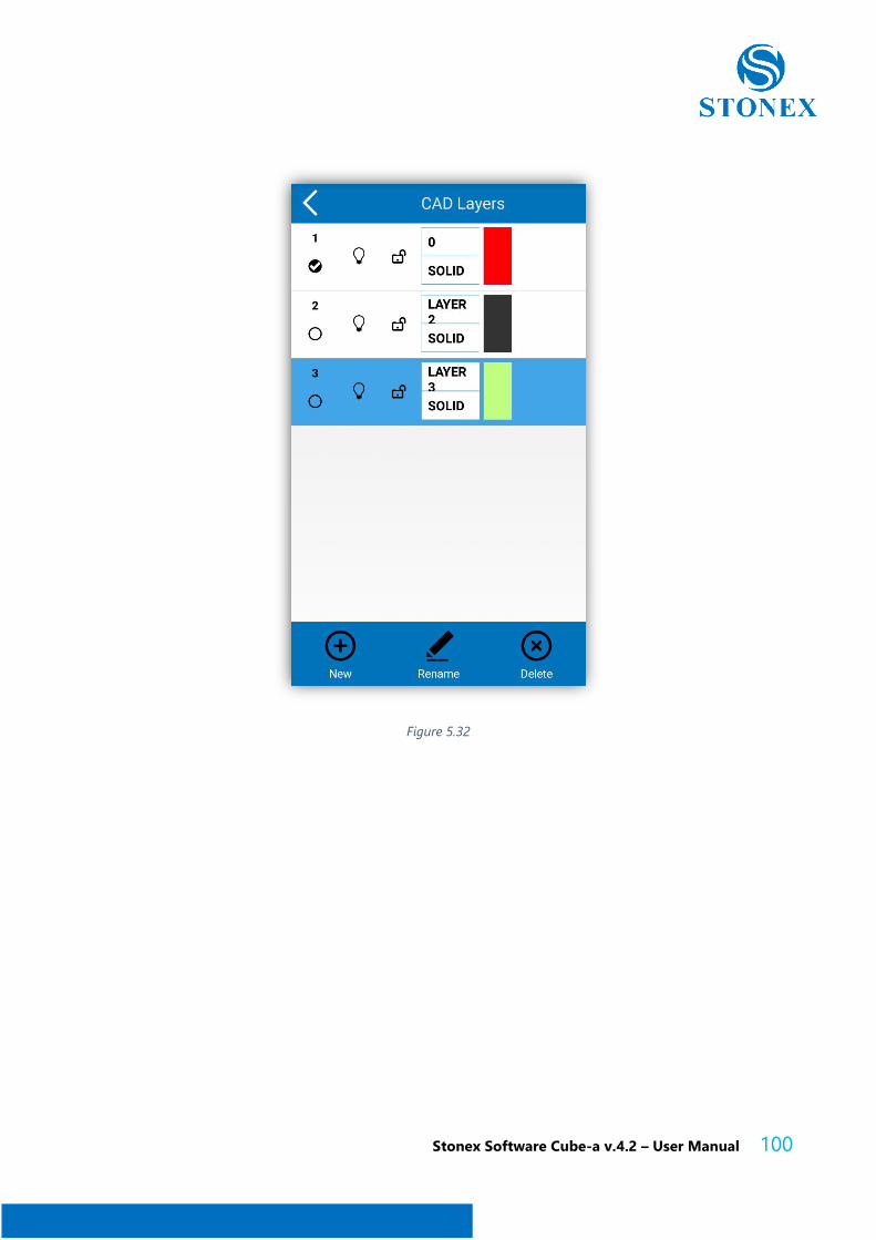
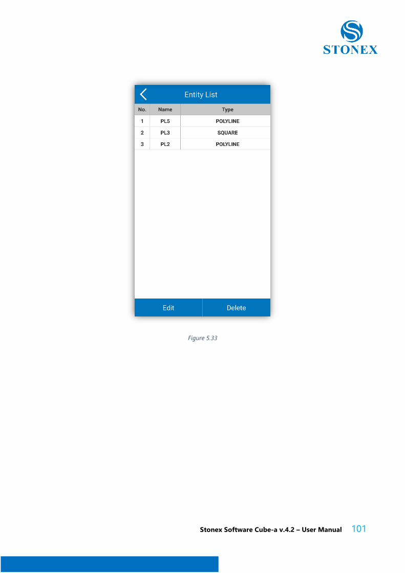
discussed later in this manual. The last two commands, CAD Layers and Entity List will open
the screen in Figure 5.32 and the one in Figure 5.33. They are commands for the
management of layers and graphic entities. In the second case, you can select an entity,
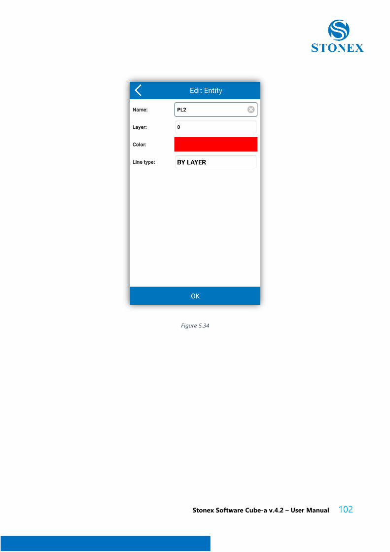
press the Edit button and access the screen in Figure 5.34, where you can make changes to
the type of line, the color, the layer, the name.
Stonex Software Cube-a v.4.2 – User Manual 99
Figure 5.31
Stonex Software Cube-a v.4.2 – User Manual 100
Figure 5.32
Stonex Software Cube-a v.4.2 – User Manual 101
Figure 5.33
Stonex Software Cube-a v.4.2 – User Manual 102
Figure 5.34
Stonex Software Cube-a v.4.2 – User Manual 103
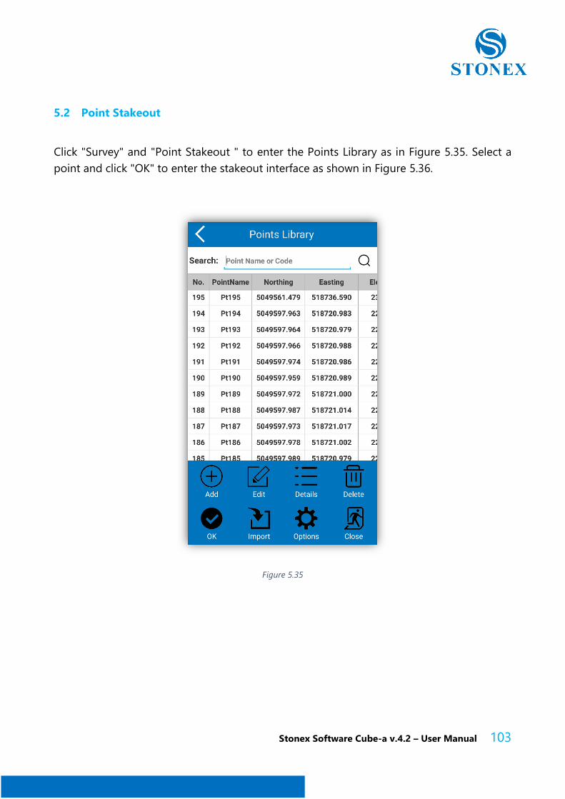
5.2 Point Stakeout
Click "Survey" and "Point Stakeout " to enter the Points Library as in Figure 5.35. Select a
point and click "OK" to enter the stakeout interface as shown in Figure 5.36.
Figure 5.35
Stonex Software Cube-a v.4.2 – User Manual 104
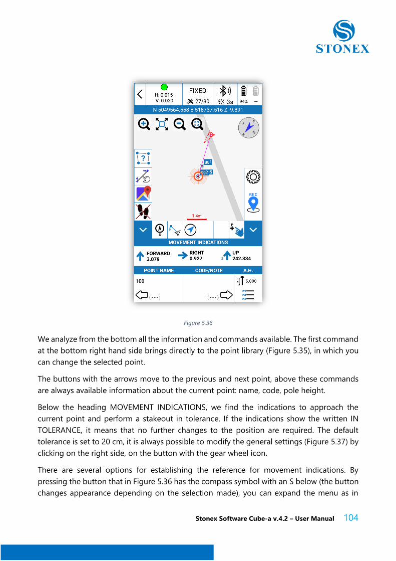
Figure 5.36
We analyze from the bottom all the information and commands available. The first command
at the bottom right hand side brings directly to the point library (Figure 5.35), in which you
can change the selected point.
The buttons with the arrows move to the previous and next point, above these commands
are always available information about the current point: name, code, pole height.
Below the heading MOVEMENT INDICATIONS, we find the indications to approach the
current point and perform a stakeout in tolerance. If the indications show the written IN
TOLERANCE, it means that no further changes to the position are required. The default
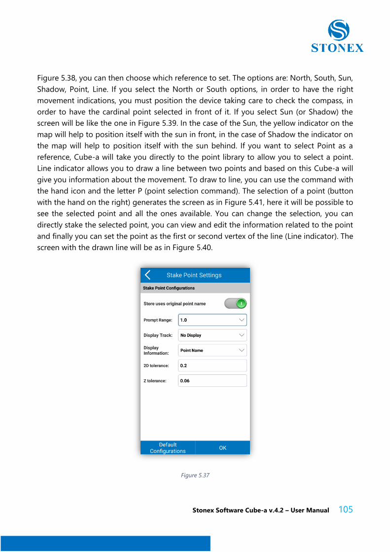
tolerance is set to 20 cm, it is always possible to modify the general settings (Figure 5.37) by
clicking on the right side, on the button with the gear wheel icon.
There are several options for establishing the reference for movement indications. By
pressing the button that in Figure 5.36 has the compass symbol with an S below (the button
changes appearance depending on the selection made), you can expand the menu as in
Stonex Software Cube-a v.4.2 – User Manual 105
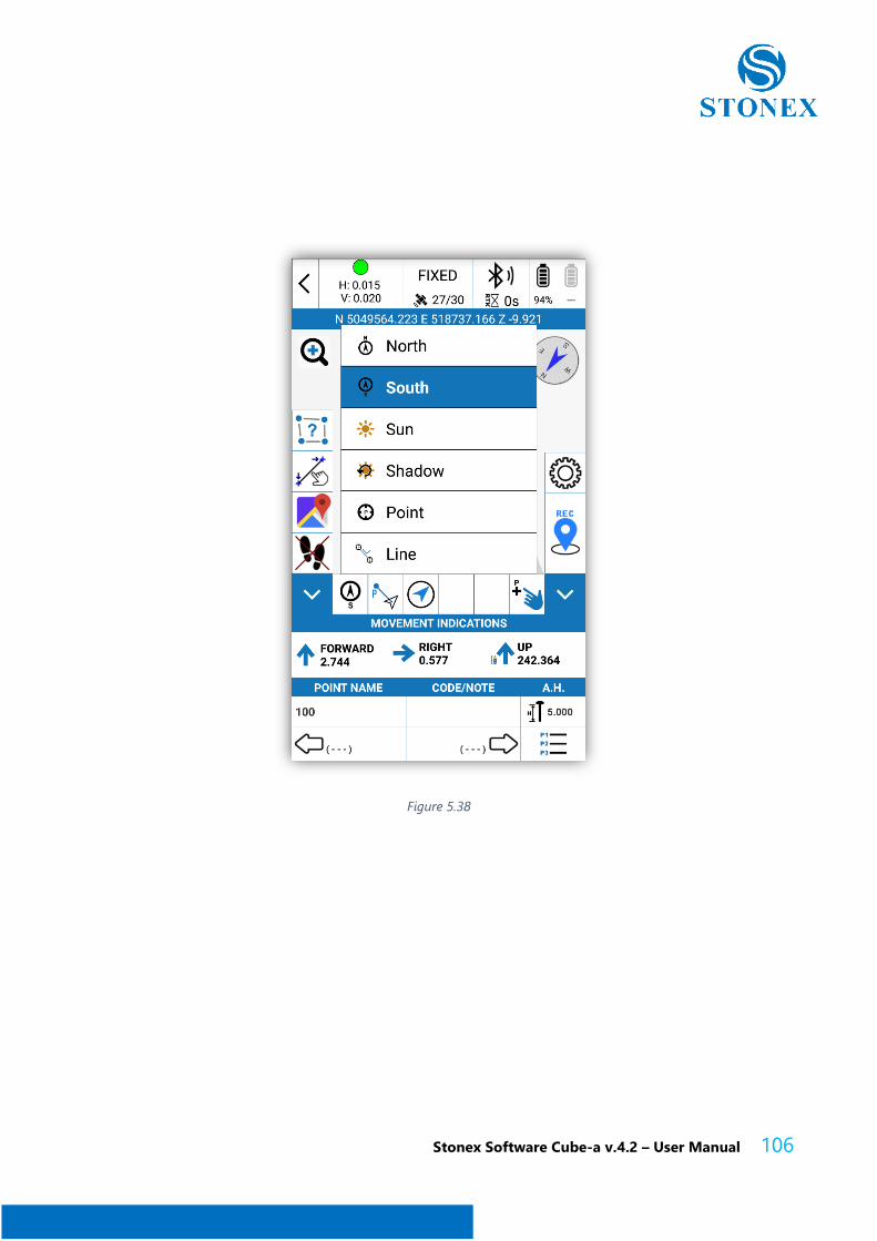
Figure 5.38, you can then choose which reference to set. The options are: North, South, Sun,
Shadow, Point, Line. If you select the North or South options, in order to have the right
movement indications, you must position the device taking care to check the compass, in
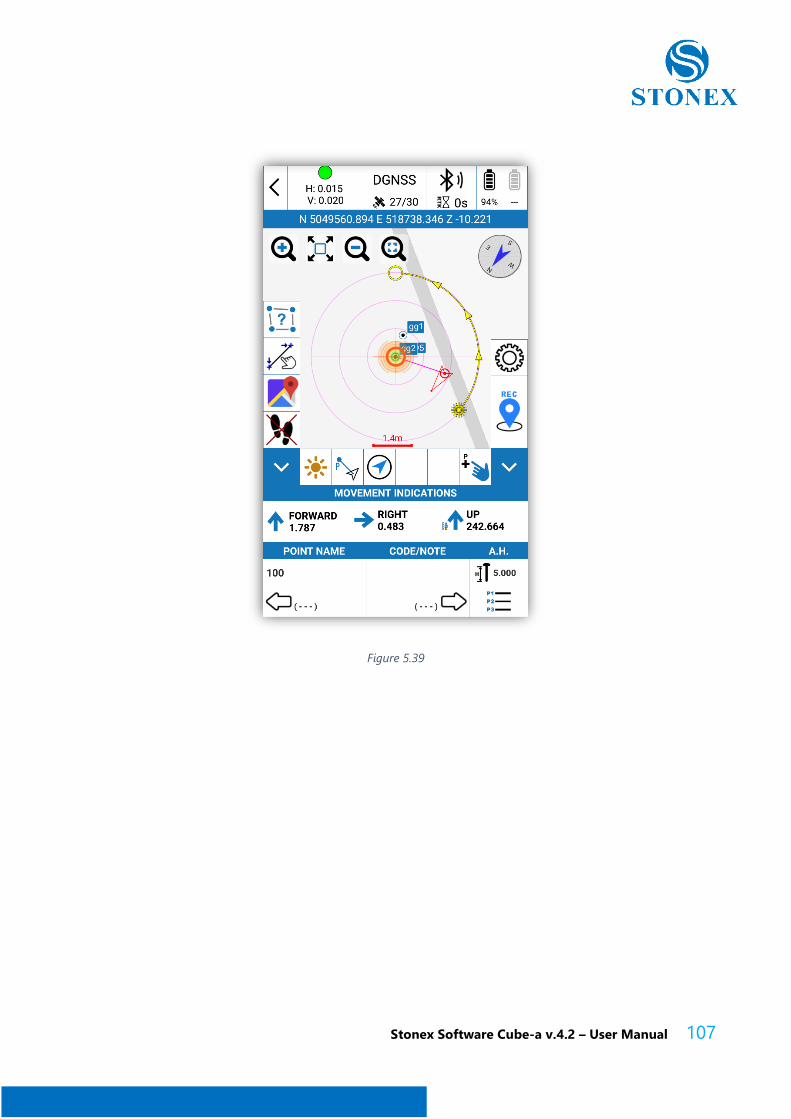
order to have the cardinal point selected in front of it. If you select Sun (or Shadow) the
screen will be like the one in Figure 5.39. In the case of the Sun, the yellow indicator on the
map will help to position itself with the sun in front, in the case of Shadow the indicator on
the map will help to position itself with the sun behind. If you want to select Point as a
reference, Cube-a will take you directly to the point library to allow you to select a point.
Line indicator allows you to draw a line between two points and based on this Cube-a will
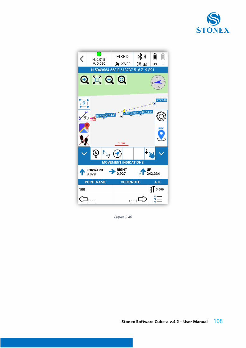
give you information about the movement. To draw to line, you can use the command with
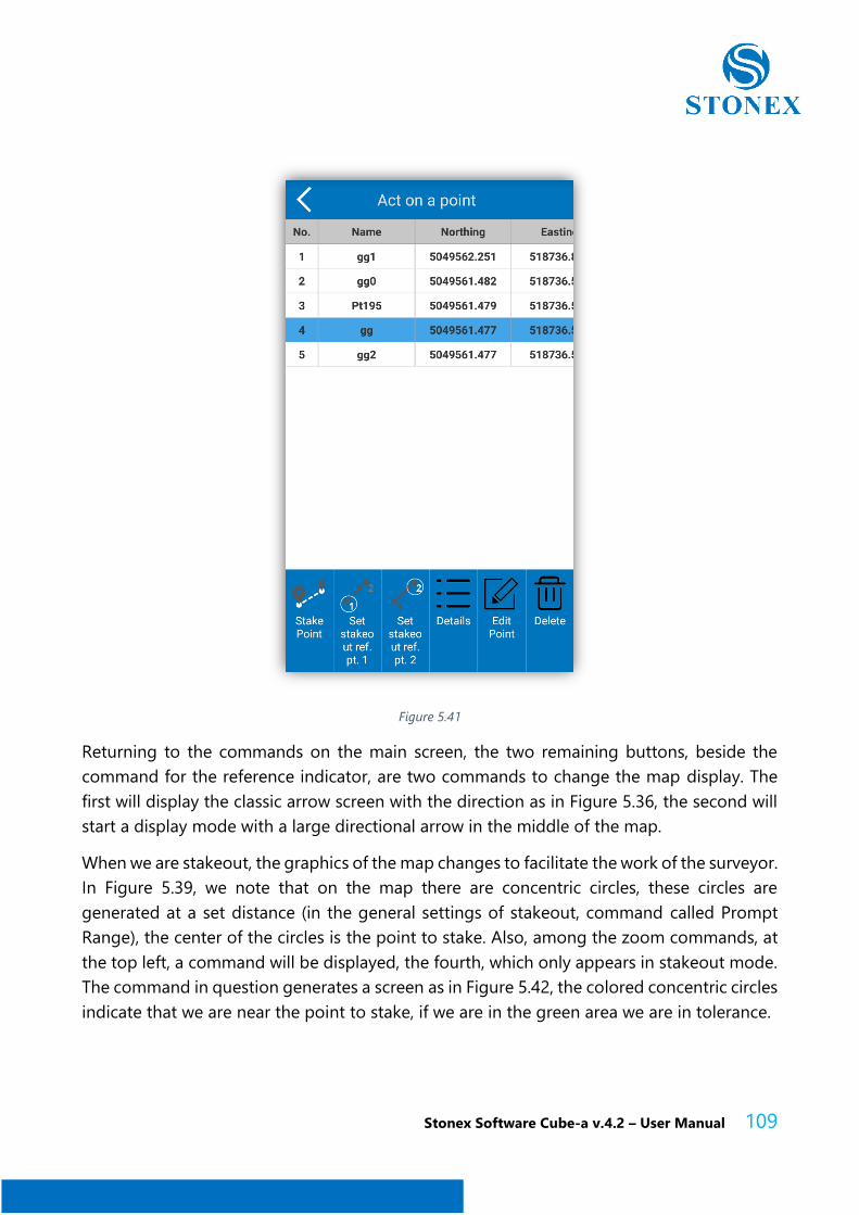
the hand icon and the letter P (point selection command). The selection of a point (button
with the hand on the right) generates the screen as in Figure 5.41, here it will be possible to
see the selected point and all the ones available. You can change the selection, you can
directly stake the selected point, you can view and edit the information related to the point
and finally you can set the point as the first or second vertex of the line (Line indicator). The
screen with the drawn line will be as in Figure 5.40.
Figure 5.37
Stonex Software Cube-a v.4.2 – User Manual 106
Figure 5.38
Stonex Software Cube-a v.4.2 – User Manual 107
Figure 5.39
Stonex Software Cube-a v.4.2 – User Manual 108
Figure 5.40
Stonex Software Cube-a v.4.2 – User Manual 109
Figure 5.41
Returning to the commands on the main screen, the two remaining buttons, beside the
command for the reference indicator, are two commands to change the map display. The
first will display the classic arrow screen with the direction as in Figure 5.36, the second will
start a display mode with a large directional arrow in the middle of the map.
When we are stakeout, the graphics of the map changes to facilitate the work of the surveyor.
In Figure 5.39, we note that on the map there are concentric circles, these circles are
generated at a set distance (in the general settings of stakeout, command called Prompt
Range), the center of the circles is the point to stake. Also, among the zoom commands, at
the top left, a command will be displayed, the fourth, which only appears in stakeout mode.
The command in question generates a screen as in Figure 5.42, the colored concentric circles
indicate that we are near the point to stake, if we are in the green area we are in tolerance.
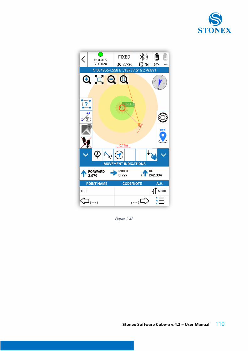
Stonex Software Cube-a v.4.2 – User Manual 110
Figure 5.42
Stonex Software Cube-a v.4.2 – User Manual 111
5.2.1 Photo and Sketch
The Photo and Sketch command (Figure 5.43) allows you to associate a photo with a
point. To start the Photo and Sketch function, you must press the relative button that can
be found at the bottom of the screen while you are:
- reviewing the details of the point just collected;
- modifying the data of a point from the library of survey points.
The photo will be taken using the built-in camera of your mobile device and will be stored
as a JPEG file in the Photos folder of the active project. The image file will have the same
name as the name of the collected point.
You can also draw on the image and insert:
- Text notes
- Information about the point (name, coordinates)
- Arrows
- Simple sketches (hand drawn polylines).
Each of the above elements can be moved and rotated freely. Images can also be deleted.
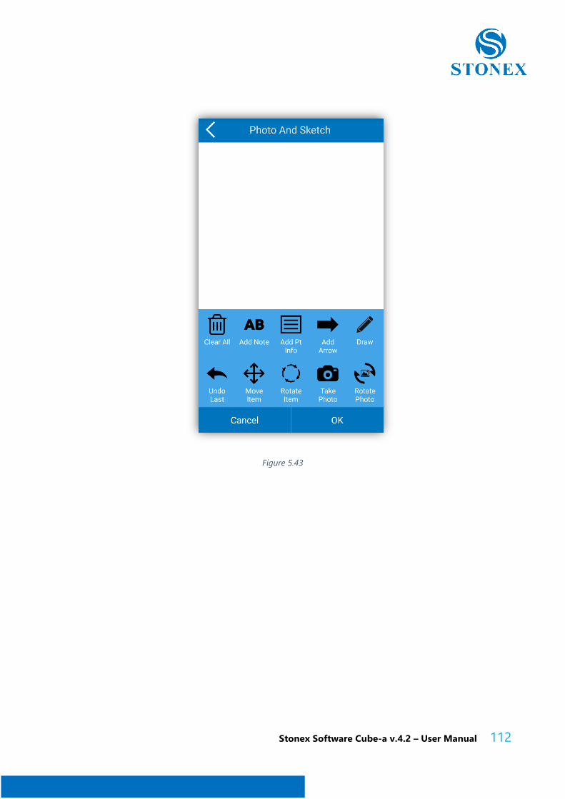
Stonex Software Cube-a v.4.2 – User Manual 112
Figure 5.43
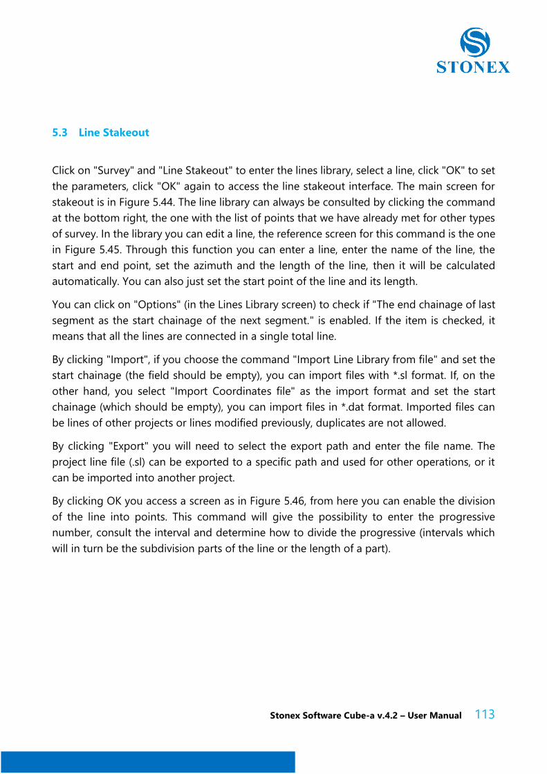
Stonex Software Cube-a v.4.2 – User Manual 113
5.3 Line Stakeout
Click on "Survey" and "Line Stakeout" to enter the lines library, select a line, click "OK" to set
the parameters, click "OK" again to access the line stakeout interface. The main screen for
stakeout is in Figure 5.44. The line library can always be consulted by clicking the command
at the bottom right, the one with the list of points that we have already met for other types
of survey. In the library you can edit a line, the reference screen for this command is the one
in Figure 5.45. Through this function you can enter a line, enter the name of the line, the
start and end point, set the azimuth and the length of the line, then it will be calculated
automatically. You can also just set the start point of the line and its length.
You can click on "Options" (in the Lines Library screen) to check if "The end chainage of last
segment as the start chainage of the next segment." is enabled. If the item is checked, it
means that all the lines are connected in a single total line.
By clicking "Import", if you choose the command "Import Line Library from file" and set the
start chainage (the field should be empty), you can import files with *.sl format. If, on the
other hand, you select "Import Coordinates file" as the import format and set the start
chainage (which should be empty), you can import files in *.dat format. Imported files can
be lines of other projects or lines modified previously, duplicates are not allowed.
By clicking "Export" you will need to select the export path and enter the file name. The
project line file (.sl) can be exported to a specific path and used for other operations, or it
can be imported into another project.
By clicking OK you access a screen as in Figure 5.46, from here you can enable the division
of the line into points. This command will give the possibility to enter the progressive
number, consult the interval and determine how to divide the progressive (intervals which
will in turn be the subdivision parts of the line or the length of a part).
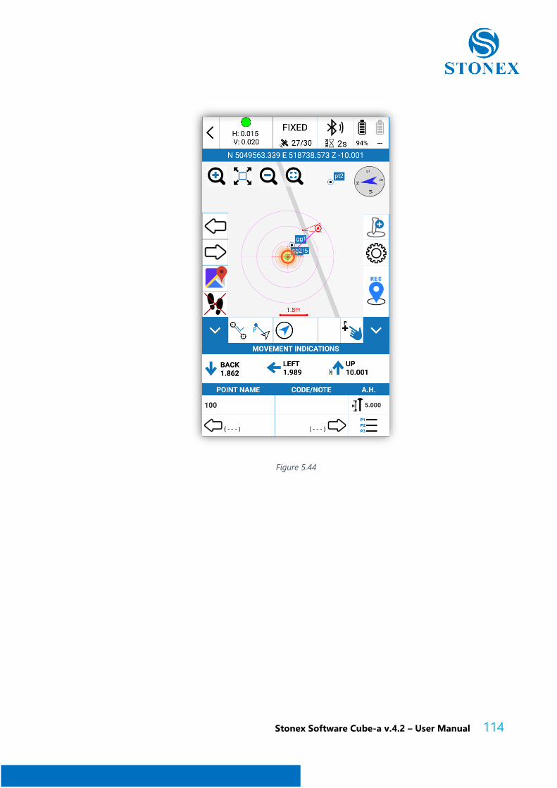
Stonex Software Cube-a v.4.2 – User Manual 114
Figure 5.44
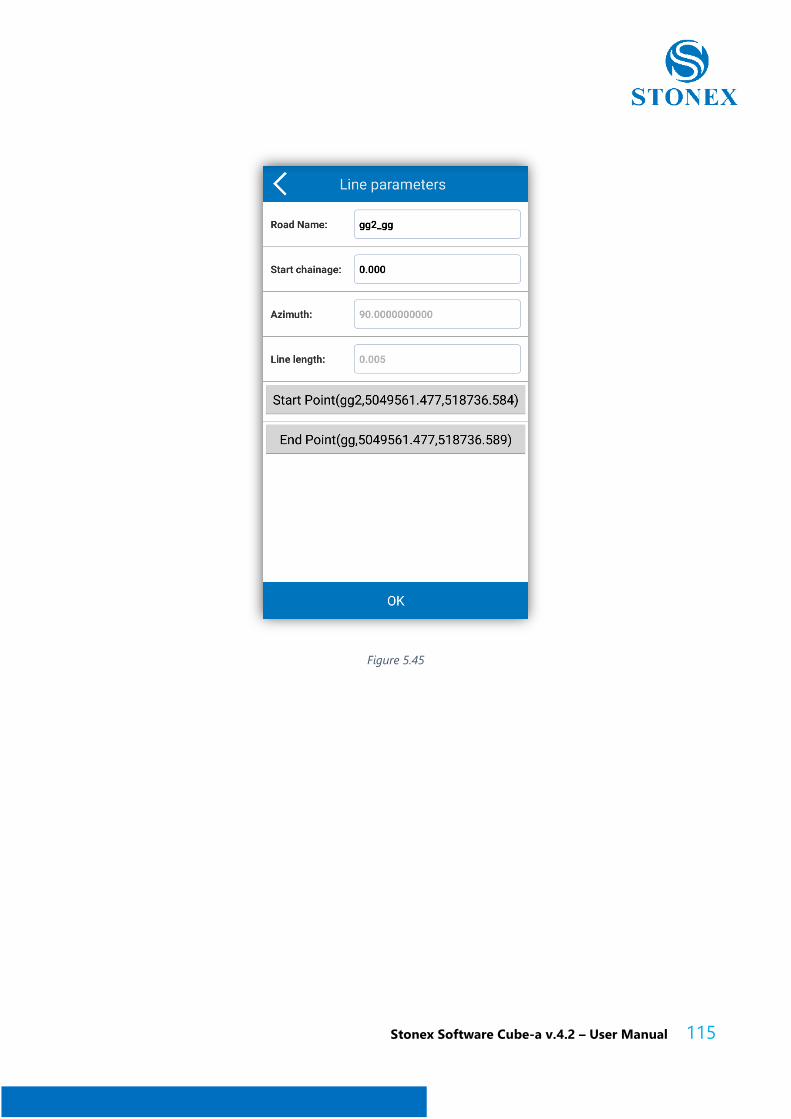
Stonex Software Cube-a v.4.2 – User Manual 115
Figure 5.45
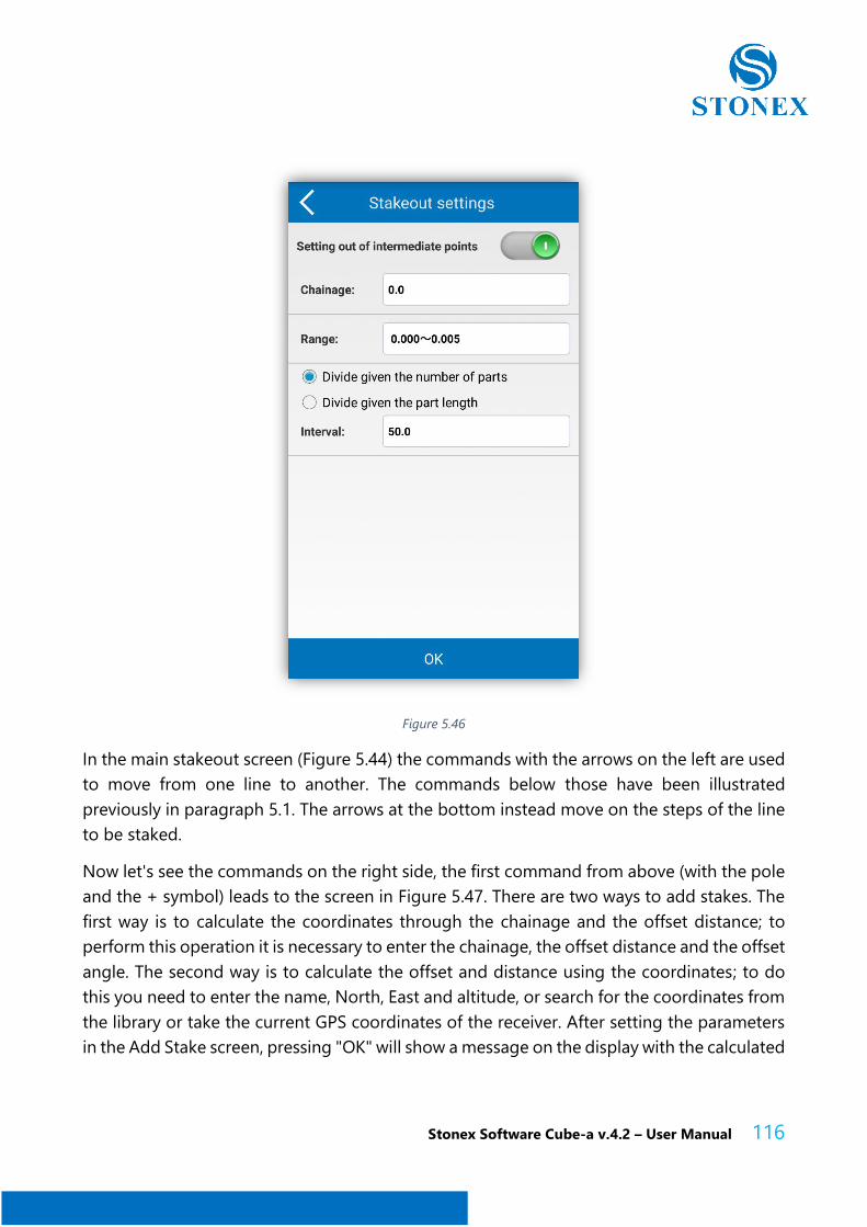
Stonex Software Cube-a v.4.2 – User Manual 116
Figure 5.46
In the main stakeout screen (Figure 5.44) the commands with the arrows on the left are used
to move from one line to another. The commands below those have been illustrated
previously in paragraph 5.1. The arrows at the bottom instead move on the steps of the line
to be staked.
Now let's see the commands on the right side, the first command from above (with the pole
and the + symbol) leads to the screen in Figure 5.47. There are two ways to add stakes. The
first way is to calculate the coordinates through the chainage and the offset distance; to
perform this operation it is necessary to enter the chainage, the offset distance and the offset
angle. The second way is to calculate the offset and distance using the coordinates; to do
this you need to enter the name, North, East and altitude, or search for the coordinates from
the library or take the current GPS coordinates of the receiver. After setting the parameters
in the Add Stake screen, pressing "OK" will show a message on the display with the calculated
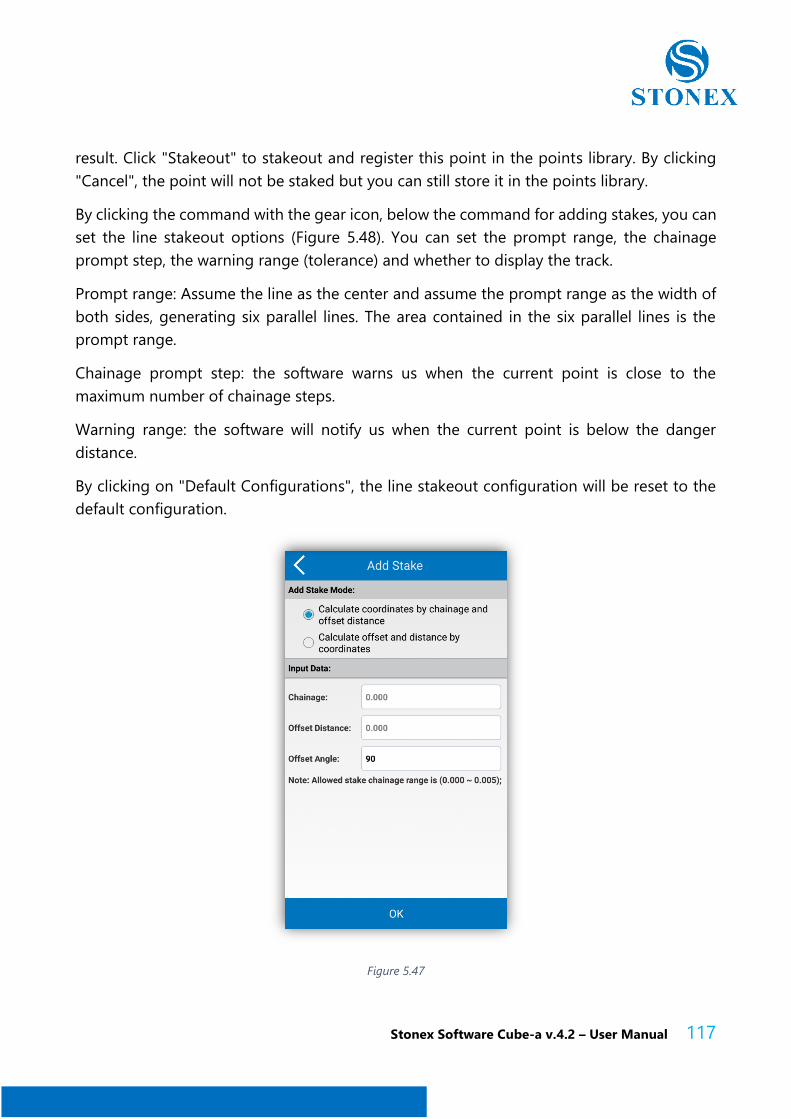
Stonex Software Cube-a v.4.2 – User Manual 117
result. Click "Stakeout" to stakeout and register this point in the points library. By clicking
"Cancel", the point will not be staked but you can still store it in the points library.
By clicking the command with the gear icon, below the command for adding stakes, you can
set the line stakeout options (Figure 5.48). You can set the prompt range, the chainage
prompt step, the warning range (tolerance) and whether to display the track.
Prompt range: Assume the line as the center and assume the prompt range as the width of
both sides, generating six parallel lines. The area contained in the six parallel lines is the
prompt range.
Chainage prompt step: the software warns us when the current point is close to the
maximum number of chainage steps.
Warning range: the software will notify us when the current point is below the danger
distance.
By clicking on "Default Configurations", the line stakeout configuration will be reset to the
default configuration.
Figure 5.47
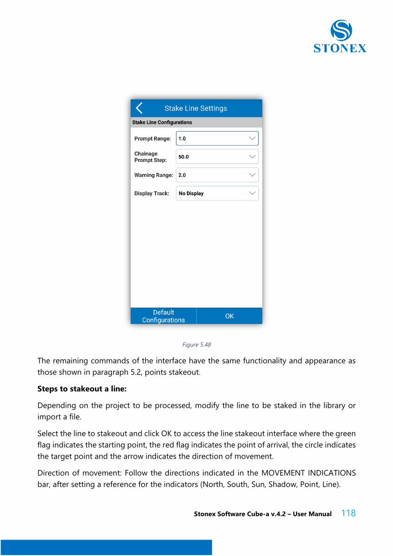
Stonex Software Cube-a v.4.2 – User Manual 118
Figure 5.48
The remaining commands of the interface have the same functionality and appearance as
those shown in paragraph 5.2, points stakeout.
Steps to stakeout a line:
Depending on the project to be processed, modify the line to be staked in the library or
import a file.
Select the line to stakeout and click OK to access the line stakeout interface where the green
flag indicates the starting point, the red flag indicates the point of arrival, the circle indicates
the target point and the arrow indicates the direction of movement.
Direction of movement: Follow the directions indicated in the MOVEMENT INDICATIONS
bar, after setting a reference for the indicators (North, South, Sun, Shadow, Point, Line).
Stonex Software Cube-a v.4.2 – User Manual 119
When the line offset on both sides is within the established range, parallel lines will be
generated on both sides of the line to be staked according to the "prompt range" settings.
If you need to add a stakeout point to the line during stakeout, click on the add stake button
(detailed in this section) to set it and define its position, then click OK to show the result
screen.
5.4 Elevation Control
Elevation Control tool lets you to “stakeout heights”.
The tool will display the difference between the current GPS height and a given reference
height.
If the height difference is positive then the program will show “cut” followed by the absolute
difference value: this means that to reach the reference height you must perform a “height
cut”, that is excavate the soil or just move down the GPS pole if it not yet touching the
ground.
If the height difference is negative then the program will show “fill” followed by the absolute
difference value: this means that to reach the reference height you must perform a “height
fill”, that is fill some soil or just move up the GPS pole if you are just going to mark level of
the reference height.
Reference height(s) can be defined in different ways:
- Import a Triangulated Irregular Network file (TIN or SJW file types)
- Add Triangles manually (by specifying the coordinates of its 3 vertices)
- Define a plane by 2 points (one 3D point plus one 2D point plus the slope in the
direction point 1 > point 2)
- Define a plane by 1 point (one 3D point plus north and east slopes).

Stonex Software Cube-a v.4.2 – User Manual 120
5.5 Geophysical Stakeout
Geophysical Stakeout tool is an expansion of the Line Stakeout tool.
While with the Line Stakeout tool you can define uncorrelated lines, with the Geophysical
Stakeout you can define sets of parallel lines to a previous defined line.
For example, you define an initial line A through two given points, then you define/add a set
of secondary lines, parallel to the line A, by specifying how many lines you want (at the right
and at the left sides of the given line A).
This tool is useful when you have to stakeout points which are all arranged along parallel
lines.
When staking out a line you have the same options of the standard Line Stakeout tool: you
can stakeout the line without splitting it in parts or you can stakeout specific points on the
line (split the line in equal parts or split it by part length).
Stonex Software Cube-a v.4.2 – User Manual 121
6 Software introduction – Configure
By clicking on "Configure", you can access a submenu with seven commands (Figure 6.1):
Coordinate System, Record Settings, Display Settings, System Settings, Survey Area Settings,
Layer Settings, Administration.
6.1 Coordinate System
By clicking on "Configure" and on "Coordinate system", you can access the screen in Figure
6.2. All options are editable.
By clicking on "Use existing" at the top, you can choose between three options. "Local Disk"
to import coordinate systems saved on the device (*.SP and *.EP files are supported). "QR
code" in order to scan the QR code to acquire the parameters of the coordinate system.
"Predefined Projections" allows access to the collection of projections divided by country
(Figure 6.3).
Ellipsoid: This command opens a screen where you can set the ellipsoid name, which
supports parameters already defined or customizable. To set a custom ellipsoid it is
necessary to set the value of the semimajor axis and the 1/f flattening ratio, which should be
consistent with the ellipsoid used for the calculation of the parameters.
Projection: Usually the most used projection is Gauss Krüger; after connecting the device,
the central meridian can be automatically calculated by clicking on the classic drop icon
(Figure 6.4, icon on the right side) or manually entered with the exact value. The common
parameters of the projections are set as follows: False Northing 0, False Easting 500000, Scale
Factor 1, Projection Height at low altitudes 0, Latitude of Origin 0.
ITRF Conversion: Enable/disable ITRF conversion. To enable ITRF conversion, choose the
type of conversion, enter the reference time (year of source coord.) and enable or disable
the speed input (velocity). If the speed is enabled, the parameters VX, Vy and Vz must be
entered.
The 7 parameters; 4 parameters/Horizontal Adjustment; Vertical Control Parameter; Vertical
Adjustment Plane; Geoid file; Local Offsets can be enabled or disabled and will generate
screens where it will be possible to set working values.
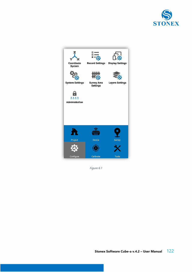
Stonex Software Cube-a v.4.2 – User Manual 122
Figure 6.1
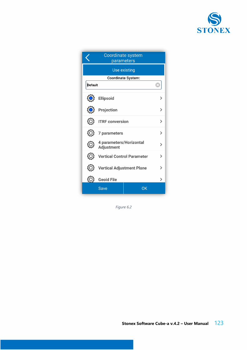
Stonex Software Cube-a v.4.2 – User Manual 123
Figure 6.2
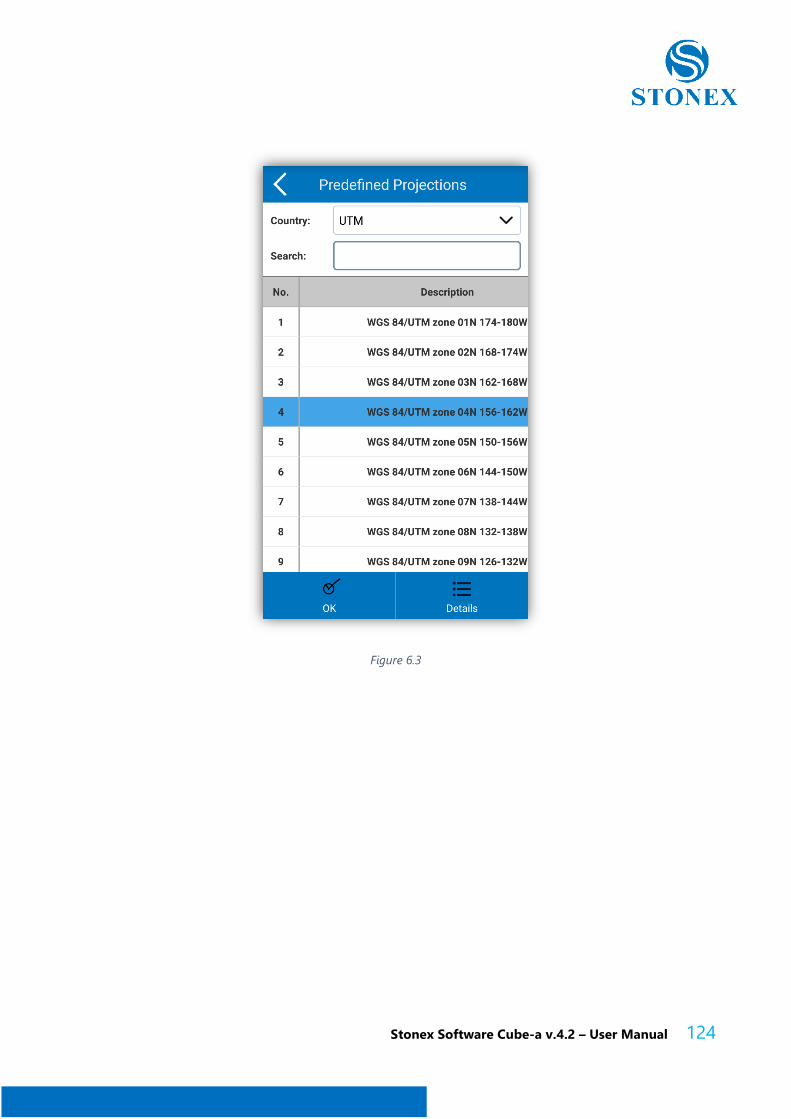
Stonex Software Cube-a v.4.2 – User Manual 124
Figure 6.3
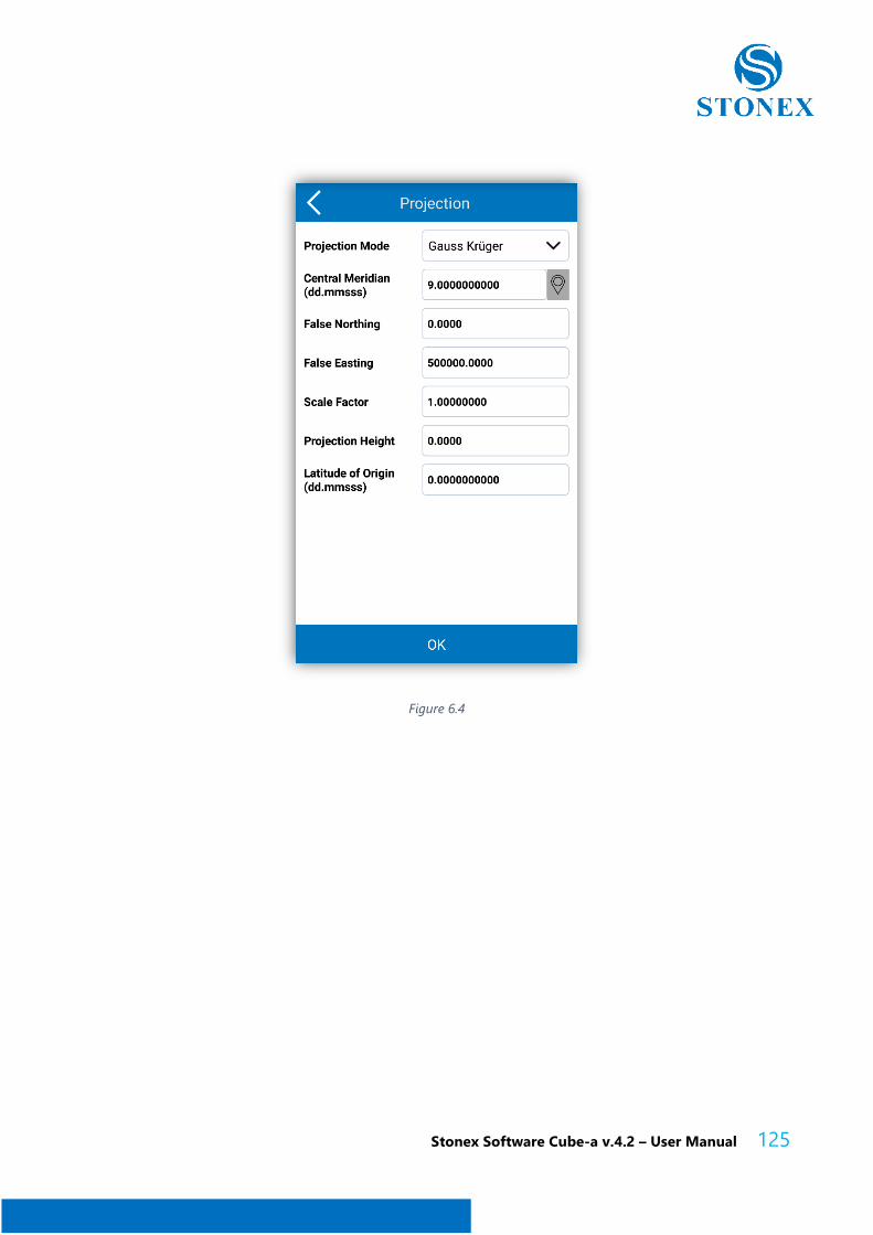
Stonex Software Cube-a v.4.2 – User Manual 125
Figure 6.4
Stonex Software Cube-a v.4.2 – User Manual 126
6.2 Record Settings
Click on "Configure" and then on "Record Settings" (this function has been explained in
detail also in paragraph 5.1, Figure 5.13), in this way it will be possible to set the settings for
saving topographic points, control points, quick points, automatic points, corner points and
points with tilt. You can set the code and choose how to increase the point names. The
default configuration is also supported.
Code: you can set it as same to the last point, as a mileage or leave it blank.
Point Name Increment: naming rule for saved points. For example, if the increment point
name is 2 and the default point name of the first saved point is pt1, the second will be pt3,
and so on.
6.3 Display Settings
Click on "Configure" and then on "Display Settings" to access the function. This function is
intended to set the information that will be shown in the survey interface. It is also possible
to filter the quantity of visible points.
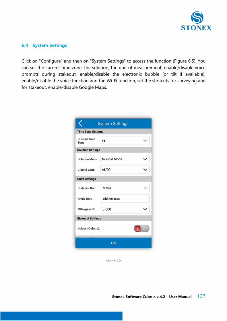
Stonex Software Cube-a v.4.2 – User Manual 127
6.4 System Settings
Click on "Configure" and then on "System Settings" to access the function (Figure 6.5). You
can set the current time zone, the solution, the unit of measurement, enable/disable voice
prompts during stakeout, enable/disable the electronic bubble (or tilt if available),
enable/disable the voice function and the Wi-Fi function, set the shotcuts for surveying and
for stakeout, enable/disable Google Maps.
Figure 6.5
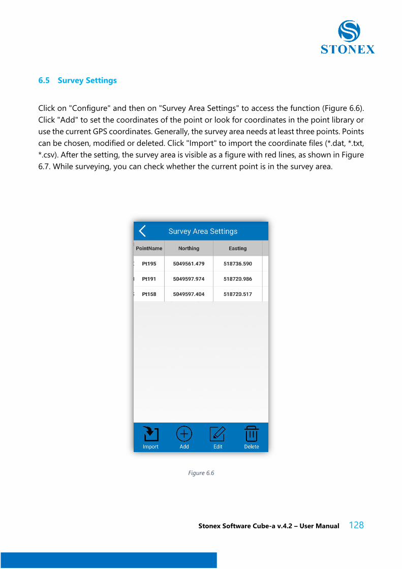
Stonex Software Cube-a v.4.2 – User Manual 128
6.5 Survey Settings
Click on "Configure" and then on "Survey Area Settings" to access the function (Figure 6.6).
Click "Add" to set the coordinates of the point or look for coordinates in the point library or
use the current GPS coordinates. Generally, the survey area needs at least three points. Points
can be chosen, modified or deleted. Click "Import" to import the coordinate files (*.dat, *.txt,
*.csv). After the setting, the survey area is visible as a figure with red lines, as shown in Figure
6.7. While surveying, you can check whether the current point is in the survey area.
Figure 6.6
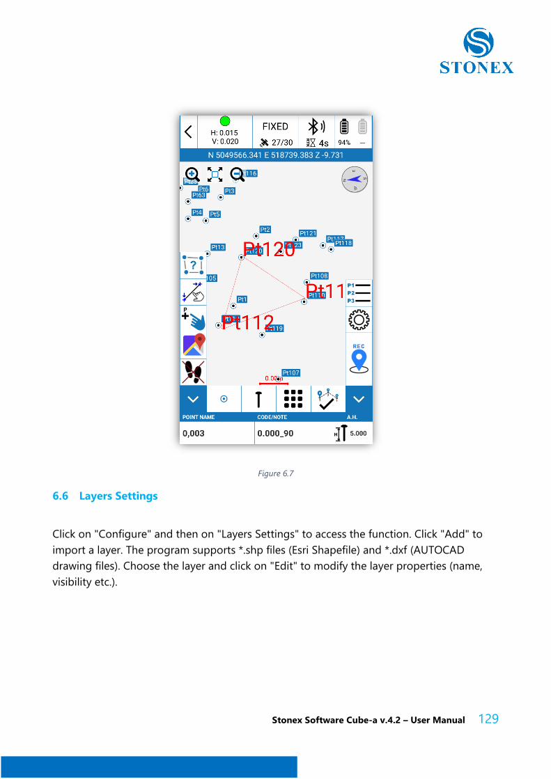
Stonex Software Cube-a v.4.2 – User Manual 129
Figure 6.7
6.6 Layers Settings
Click on "Configure" and then on "Layers Settings" to access the function. Click "Add" to
import a layer. The program supports *.shp files (Esri Shapefile) and *.dxf (AUTOCAD
drawing files). Choose the layer and click on "Edit" to modify the layer properties (name,
visibility etc.).
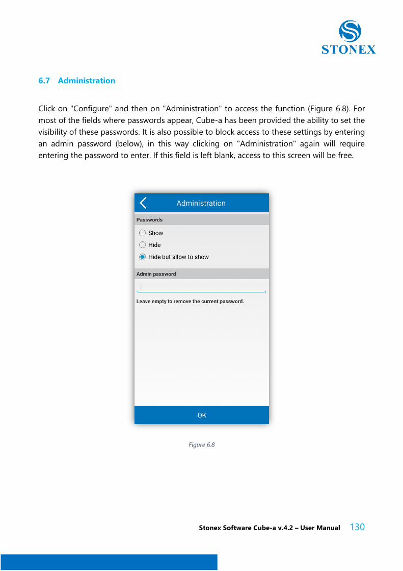
Stonex Software Cube-a v.4.2 – User Manual 130
6.7 Administration
Click on "Configure" and then on "Administration" to access the function (Figure 6.8). For
most of the fields where passwords appear, Cube-a has been provided the ability to set the
visibility of these passwords. It is also possible to block access to these settings by entering
an admin password (below), in this way clicking on "Administration" again will require
entering the password to enter. If this field is left blank, access to this screen will be free.
Figure 6.8
Stonex Software Cube-a v.4.2 – User Manual 131
7 Software introduction - Calibrate
This chapter provides useful information about the calibration function, click "Calibrate" to
access the screen in Figure 7.1. The commands available are Site Calibration; Calibrate Point;
Calibrate Sensor.
7.1 Site Calibration
In general, the GPS receiver's output data are WGS-84 coordinates, latitude and longitude.
The coordinates must be converted into a reference system based on the work to be
performed, this requires coordinate conversion parameters that are calculated and set by
the software.
There are three methods of coordinate conversion, including "four parameter + elev.
correction", "7 parameter + four parameter + elev. correction" and "seven parameters". Users
must evaluate which method should be used based on the known point.
4 parameters: At least two control points, must be known. This is the coordinate
transformation mode used to perform a conversion between different coordinate systems
within the same ellipsoid. The parameters include four values (North translation, East
translation, Rotation and Scale), the scale must be very close to 1.
In general, the distribution of control points directly determines the difference in height and
the four parameters to be controlled. The use of four parameters for the RTK measurement
method can be used in a reduced area (20-30 square kilometers).
Measure a point in grid coordinates and operate in the precision of a control network with
height coordinates of known points. The more known points selected the greater the
accuracy (2 or more than 2).
Note that in a very large distribution of points (for example ten kilometers) the
transformation parameters often do not help, in this case to have an increase of precision
both in the grid coordinates and on the height, we should use the 7-parameter
transformation.
First, you need to perform a static survey in the area where the contro points are, then select
a point A as a static reference station (in WGS84) that will be used to correct the point
network. Use a receiver in static mode to measure a single fixed point for more than 24 hours
Stonex Software Cube-a v.4.2 – User Manual 132
(this step, in the test areas can be performed in less time and in the case of low accuracy
required, this step can also be omitted) and then import into the software, as a single point
all the data acquired, the average of the readings will be the actual coordinates of point A
in WGS84 coordinates. The absolute precision should be below 2 meters, so about the
regulation of the 3D control network, it is necessary to assume the point A WGS84 as the
control point to calculate the 3D coordinates of other points.
The 4-parameter model, used to perform a 2D adjustment, can be either a barycentric roto-
translation (around the average point of the source coordinates, called “Horizontal
Adjustment”) or a non barycentric roto-translation (around the axes origin, called “Four
Parameter”).
When the 4-parameter model is used, the vertical correction will be automatically enabled.
The actual vertical correction parameters used depend on the number of points used. If less
than 3 points are used, then the heights are adjusted using the average of the corrections
about the given 3 points.
If 3 to 6 topographic points are used, then an inclined plane is calculated. If more than 7
points are used, then a paraboloid surface is used.
7 parameters: At least three control points, must be known. This is the coordinate
transformation mode used to perform a rectangular transformation of spatial coordinates
between different ellipsoids. The parameters include seven values: 3 translations, 3 rotations
and the scale factor (ΔX, ΔY, ΔZ, Δα, Δβ, Δγ, scale).
How to calculate the conversion parameters?
Generally, use 3 known points (A, B and C) to calculate the parameters, so first you need to
know the coordinates WGS84 and the local coordinates of the 3 known points (A, B and C).
There are 2 methods for obtaining the WGS84 coordinates of points A, B, C. The first method
is to set up the static control network and then obtain the WGS84 coordinates from the GPD
acquisition of the post-processing software. Second method, the Rover GPS records the
original WGS84 coordinates in fixed solution when the correction parameters are not active.
Click "Calibrate" and then "Site Calibration", to see the screen shown in Figure 7.2. The six
commands available are: add, edit, delete, options, calculate, import, export, close.
By clicking "Add" you can set the coordinates of the known points. There are 2 methods to
set the coordinates of the known points: the first, click on the search button (with the lens

Stonex Software Cube-a v.4.2 – User Manual 133
icon) to select a point from the point library, the second is to manually enter the coordinates,
name, north, east and height.
Then set the geodesic WGS84 coordinates and click OK to add the first group of coordinates.
The coordinates of the other points can be entered with the same procedure. Add
coordinates of the known points until you get the number of points needed to calculate the
parameters.
Select "Modify" to modify the parameters of the points and the geodesic WGS84
coordinates.
Select "Delete" to delete all data related to a point from thesite calibration interface.
Click "Options" to access the screen shown in Figure 7.3. You can select one of the three
conversion methods: four parameter + elev. correction, 7 parameter + four parameter + elev.
correction and seven parameters.
Click "Import" to import *.COT or *.loc files, (useful extensions to import coordinates).
Click "Export" to export and save coordinates, in a file with the *.COT extension. The
coordinates can be used in the future without having to reinsert them.
After entering all the coordinates click "Calculate" to perform the operation and a report will
appear containing the calculated GPS parameters. Click on "Return" to return to the previous
interface, then click on "Close" to exit the site calibration. Before closing, a message will
appear asking if you want to use the calculated parameters for the current project. You can
confirm or exit without saving the calculation.
After applying the conversion parameters, the original coordinates in WGS84 present in the
point library of the current project will be converted into the coordinate system based on
the calculated conversion parameters. To verify that the results are accurate, it is possible to
carry out a check by accessing another known point.
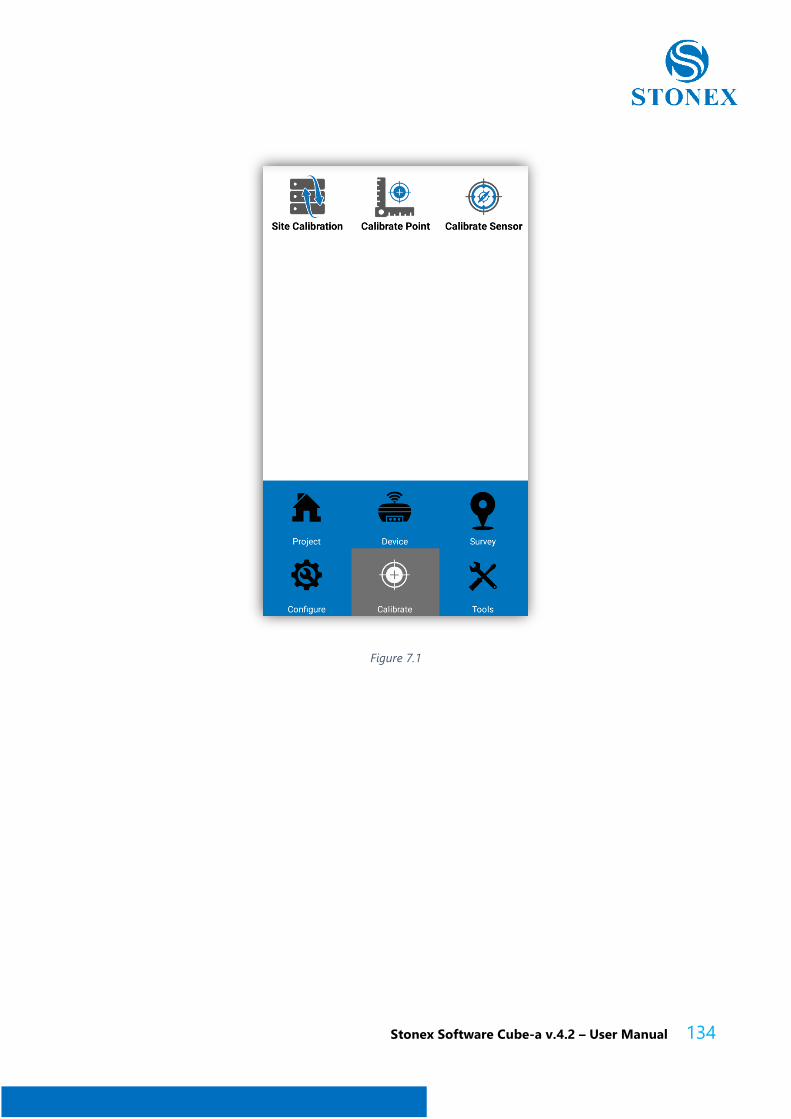
Stonex Software Cube-a v.4.2 – User Manual 134
Figure 7.1

Stonex Software Cube-a v.4.2 – User Manual 135
Figure 7.2
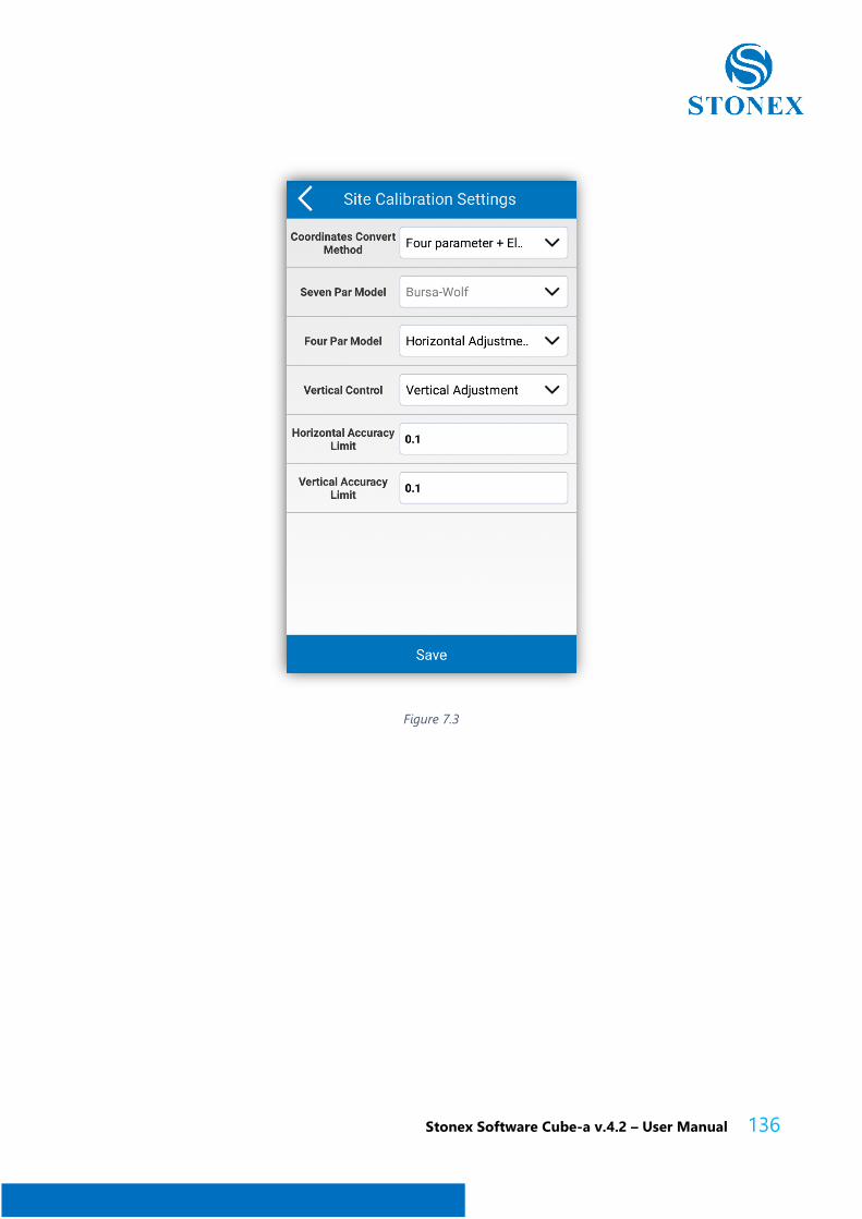
Stonex Software Cube-a v.4.2 – User Manual 136
Figure 7.3
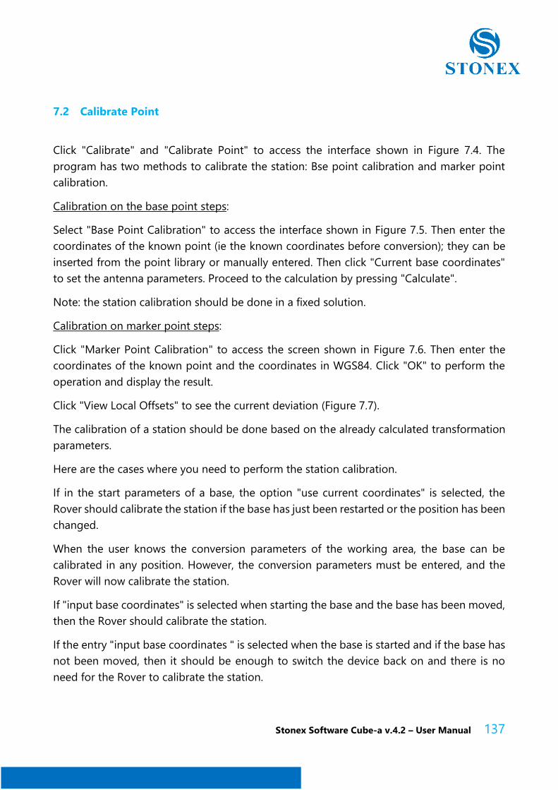
Stonex Software Cube-a v.4.2 – User Manual 137
7.2 Calibrate Point
Click "Calibrate" and "Calibrate Point" to access the interface shown in Figure 7.4. The
program has two methods to calibrate the station: Bse point calibration and marker point
calibration.
Calibration on the base point steps:
Select "Base Point Calibration" to access the interface shown in Figure 7.5. Then enter the
coordinates of the known point (ie the known coordinates before conversion); they can be
inserted from the point library or manually entered. Then click "Current base coordinates"
to set the antenna parameters. Proceed to the calculation by pressing "Calculate".
Note: the station calibration should be done in a fixed solution.
Calibration on marker point steps:
Click "Marker Point Calibration" to access the screen shown in Figure 7.6. Then enter the
coordinates of the known point and the coordinates in WGS84. Click "OK" to perform the
operation and display the result.
Click "View Local Offsets" to see the current deviation (Figure 7.7).
The calibration of a station should be done based on the already calculated transformation
parameters.
Here are the cases where you need to perform the station calibration.
If in the start parameters of a base, the option "use current coordinates" is selected, the
Rover should calibrate the station if the base has just been restarted or the position has been
changed.
When the user knows the conversion parameters of the working area, the base can be
calibrated in any position. However, the conversion parameters must be entered, and the
Rover will now calibrate the station.
If "input base coordinates" is selected when starting the base and the base has been moved,
then the Rover should calibrate the station.
If the entry "input base coordinates " is selected when the base is started and if the base has
not been moved, then it should be enough to switch the device back on and there is no
need for the Rover to calibrate the station.
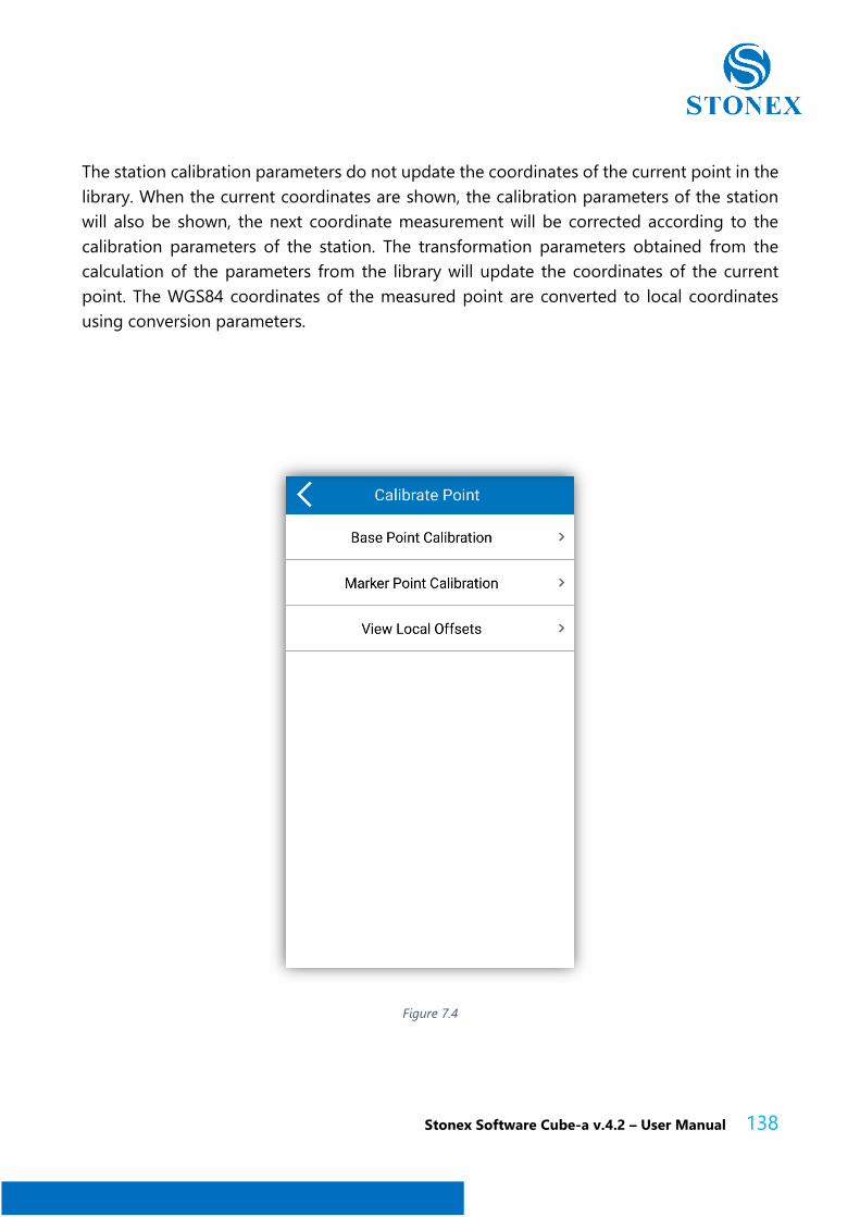
Stonex Software Cube-a v.4.2 – User Manual 138
The station calibration parameters do not update the coordinates of the current point in the
library. When the current coordinates are shown, the calibration parameters of the station
will also be shown, the next coordinate measurement will be corrected according to the
calibration parameters of the station. The transformation parameters obtained from the
calculation of the parameters from the library will update the coordinates of the current
point. The WGS84 coordinates of the measured point are converted to local coordinates
using conversion parameters.
Figure 7.4
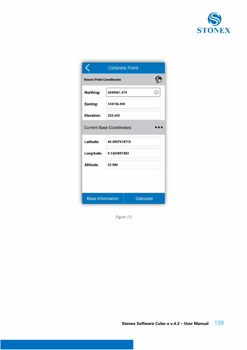
Stonex Software Cube-a v.4.2 – User Manual 139
Figure 7.5

Stonex Software Cube-a v.4.2 – User Manual 140
Figure 7.6
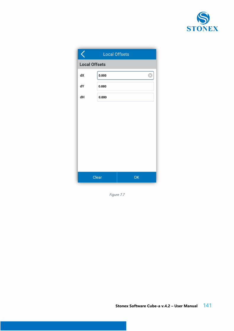
Stonex Software Cube-a v.4.2 – User Manual 141
Figure 7.7
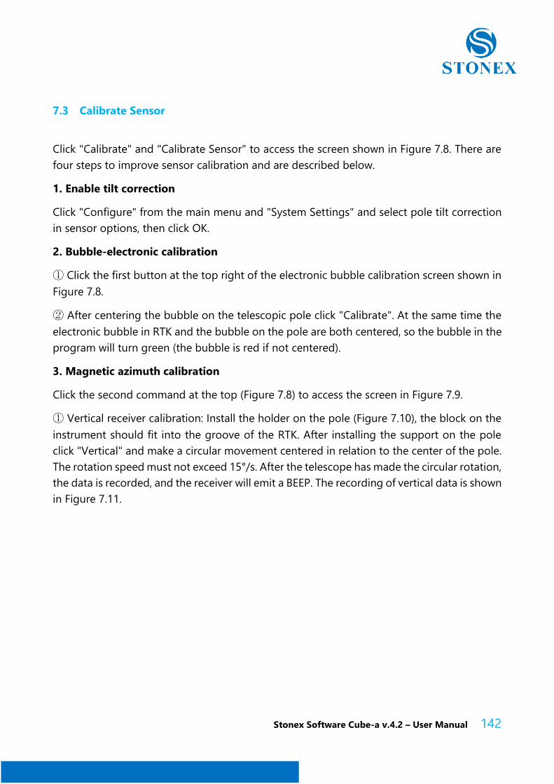
Stonex Software Cube-a v.4.2 – User Manual 142
7.3 Calibrate Sensor
Click "Calibrate" and "Calibrate Sensor" to access the screen shown in Figure 7.8. There are
four steps to improve sensor calibration and are described below.
1. Enable tilt correction
Click "Configure" from the main menu and "System Settings" and select pole tilt correction
in sensor options, then click OK.
2. Bubble-electronic calibration
① Click the first button at the top right of the electronic bubble calibration screen shown in
Figure 7.8.
② After centering the bubble on the telescopic pole click "Calibrate". At the same time the
electronic bubble in RTK and the bubble on the pole are both centered, so the bubble in the
program will turn green (the bubble is red if not centered).
3. Magnetic azimuth calibration
Click the second command at the top (Figure 7.8) to access the screen in Figure 7.9.
① Vertical receiver calibration: Install the holder on the pole (Figure 7.10), the block on the
instrument should fit into the groove of the RTK. After installing the support on the pole
click "Vertical" and make a circular movement centered in relation to the center of the pole.
The rotation speed must not exceed 15°/s. After the telescope has made the circular rotation,
the data is recorded, and the receiver will emit a BEEP. The recording of vertical data is shown
in Figure 7.11.
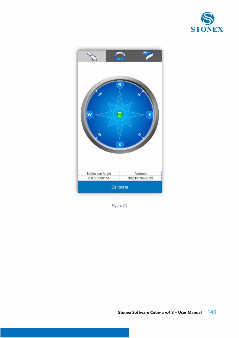
Stonex Software Cube-a v.4.2 – User Manual 143
Figure 7.8
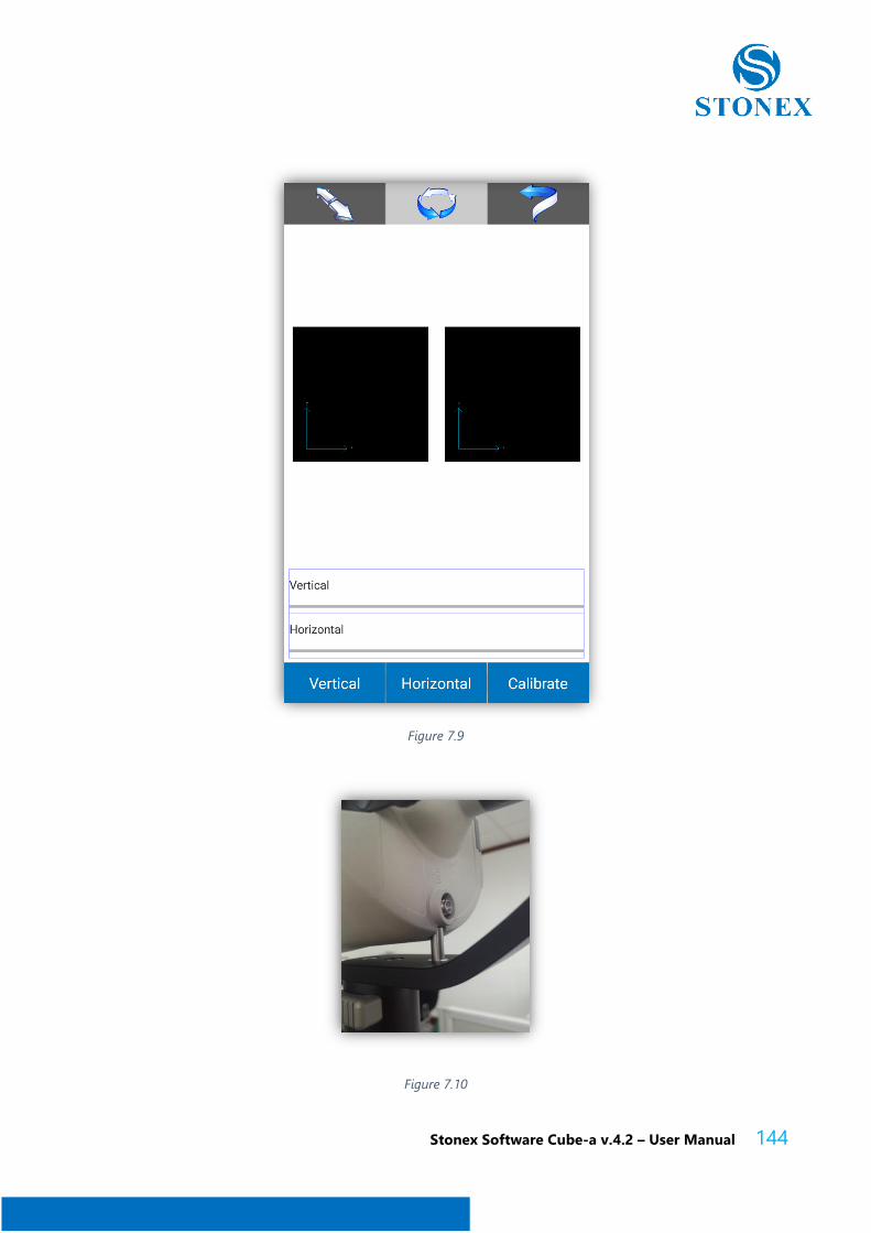
Stonex Software Cube-a v.4.2 – User Manual 144
Figure 7.9
Figure 7.10
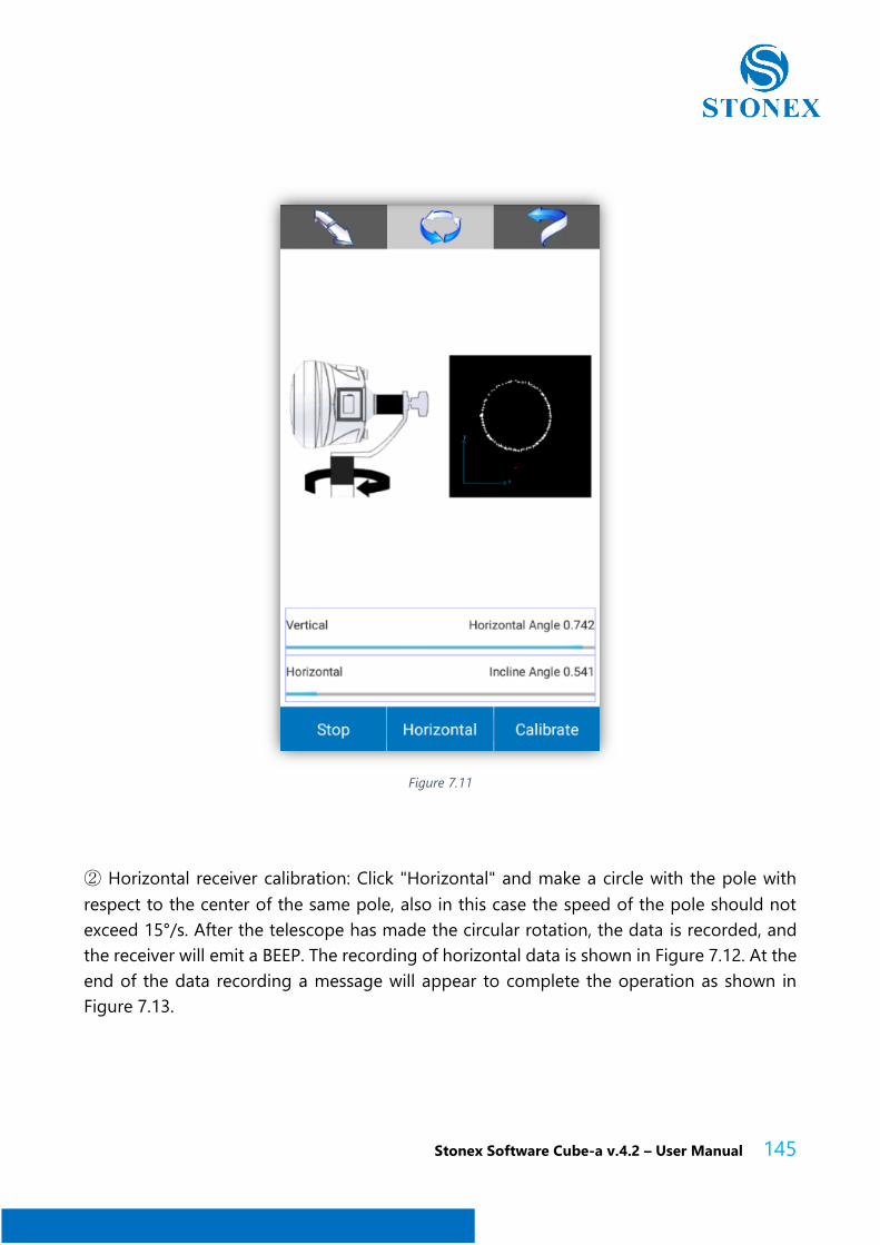
Stonex Software Cube-a v.4.2 – User Manual 145
Figure 7.11
② Horizontal receiver calibration: Click "Horizontal" and make a circle with the pole with
respect to the center of the same pole, also in this case the speed of the pole should not
exceed 15°/s. After the telescope has made the circular rotation, the data is recorded, and
the receiver will emit a BEEP. The recording of horizontal data is shown in Figure 7.12. At the
end of the data recording a message will appear to complete the operation as shown in
Figure 7.13.
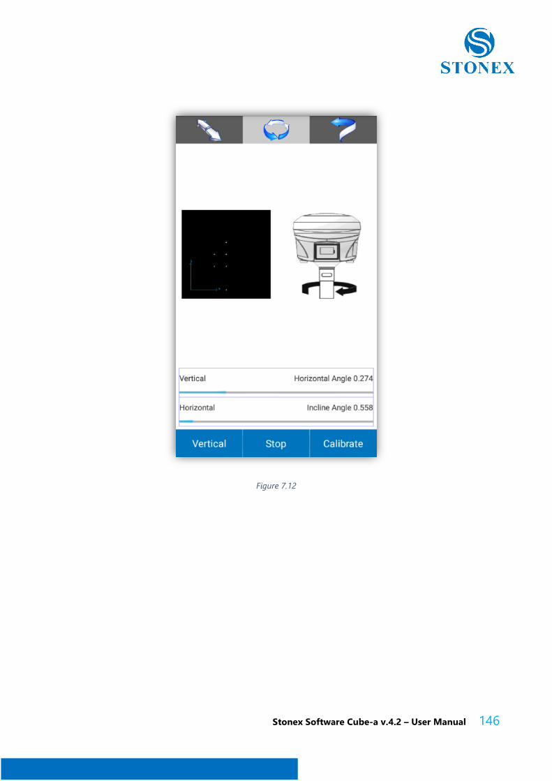
Stonex Software Cube-a v.4.2 – User Manual 146
Figure 7.12
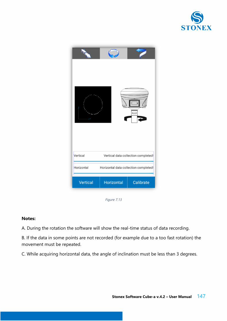
Stonex Software Cube-a v.4.2 – User Manual 147
Figure 7.13
Notes:
A. During the rotation the software will show the real-time status of data recording.
B. If the data in some points are not recorded (for example due to a too fast rotation) the
movement must be repeated.
C. While acquiring horizontal data, the angle of inclination must be less than 3 degrees.
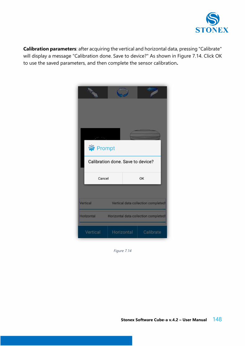
Stonex Software Cube-a v.4.2 – User Manual 148
Calibration parameters: after acquiring the vertical and horizontal data, pressing "Calibrate"
will display a message "Calibration done. Save to device?" As shown in Figure 7.14. Click OK
to use the saved parameters, and then complete the sensor calibration.
Figure 7.14
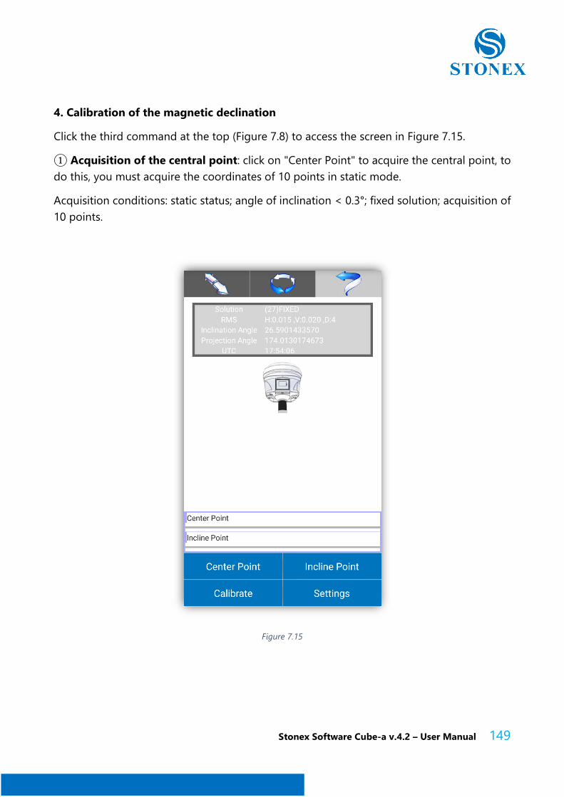
Stonex Software Cube-a v.4.2 – User Manual 149
4. Calibration of the magnetic declination
Click the third command at the top (Figure 7.8) to access the screen in Figure 7.15.
① Acquisition of the central point: click on "Center Point" to acquire the central point, to
do this, you must acquire the coordinates of 10 points in static mode.
Acquisition conditions: static status; angle of inclination < 0.3°; fixed solution; acquisition of
10 points.
Figure 7.15
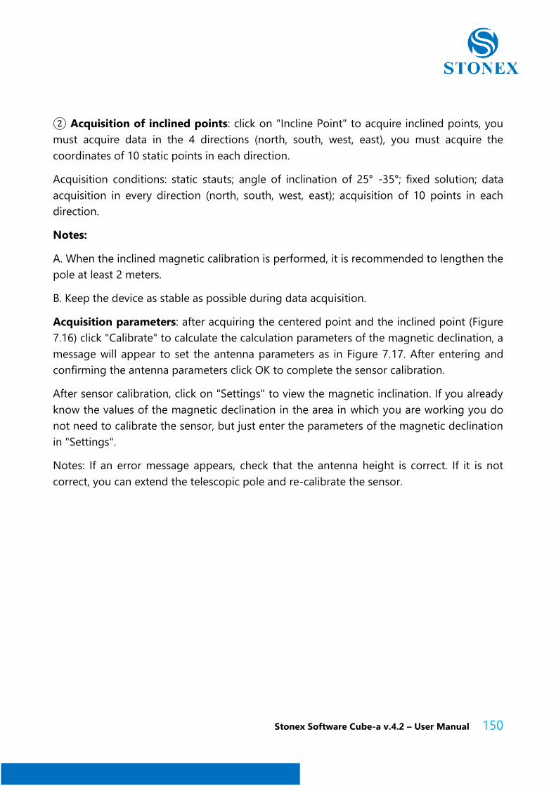
Stonex Software Cube-a v.4.2 – User Manual 150
② Acquisition of inclined points: click on "Incline Point" to acquire inclined points, you
must acquire data in the 4 directions (north, south, west, east), you must acquire the
coordinates of 10 static points in each direction.
Acquisition conditions: static stauts; angle of inclination of 25° -35°; fixed solution; data
acquisition in every direction (north, south, west, east); acquisition of 10 points in each
direction.
Notes:
A. When the inclined magnetic calibration is performed, it is recommended to lengthen the
pole at least 2 meters.
B. Keep the device as stable as possible during data acquisition.
Acquisition parameters: after acquiring the centered point and the inclined point (Figure
7.16) click "Calibrate" to calculate the calculation parameters of the magnetic declination, a
message will appear to set the antenna parameters as in Figure 7.17. After entering and
confirming the antenna parameters click OK to complete the sensor calibration.
After sensor calibration, click on "Settings" to view the magnetic inclination. If you already
know the values of the magnetic declination in the area in which you are working you do
not need to calibrate the sensor, but just enter the parameters of the magnetic declination
in "Settings".
Notes: If an error message appears, check that the antenna height is correct. If it is not
correct, you can extend the telescopic pole and re-calibrate the sensor.
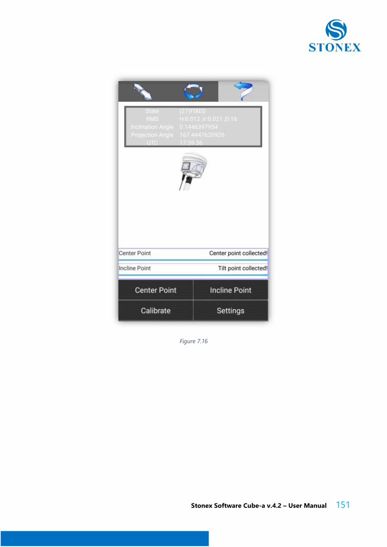
Stonex Software Cube-a v.4.2 – User Manual 151
Figure 7.16
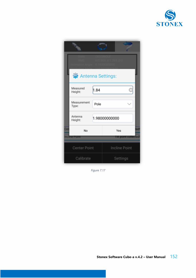
Stonex Software Cube-a v.4.2 – User Manual 152
Figure 7.17
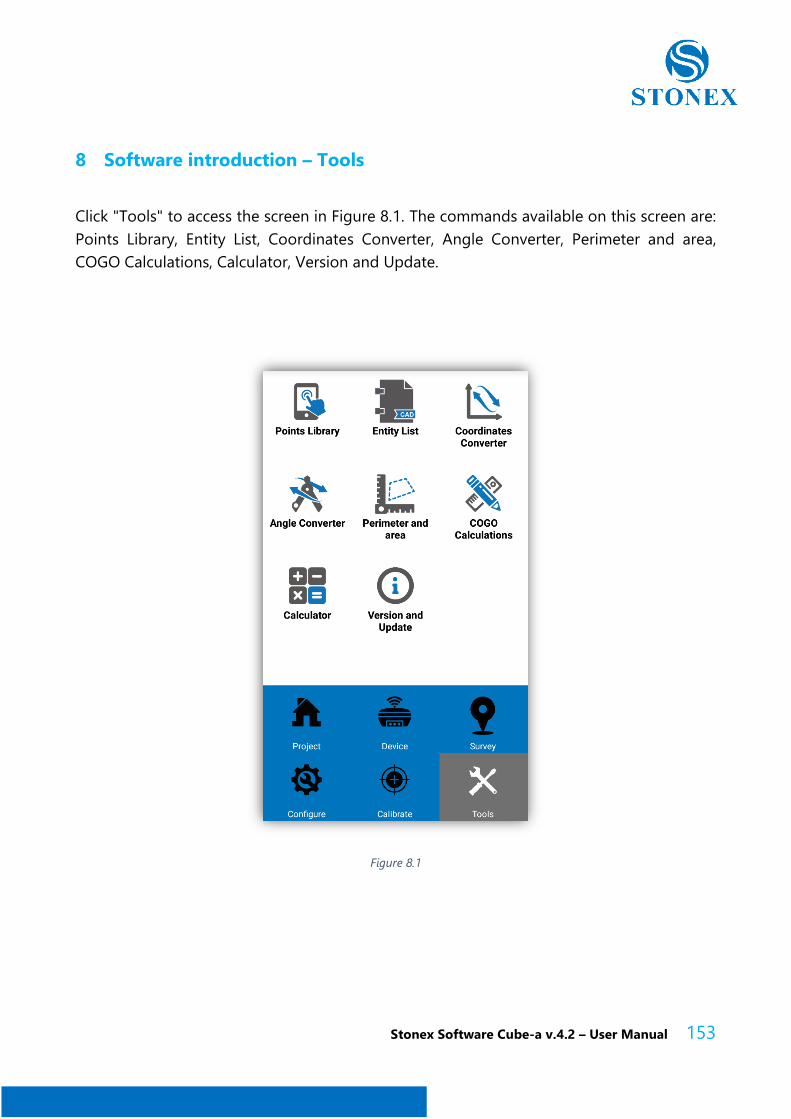
Stonex Software Cube-a v.4.2 – User Manual 153
8 Software introduction – Tools
Click "Tools" to access the screen in Figure 8.1. The commands available on this screen are:
Points Library, Entity List, Coordinates Converter, Angle Converter, Perimeter and area,
COGO Calculations, Calculator, Version and Update.
Figure 8.1
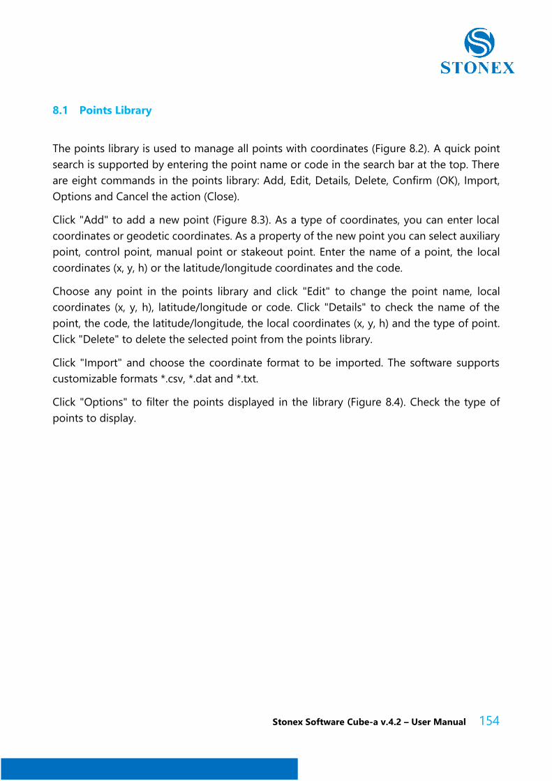
Stonex Software Cube-a v.4.2 – User Manual 154
8.1 Points Library
The points library is used to manage all points with coordinates (Figure 8.2). A quick point
search is supported by entering the point name or code in the search bar at the top. There
are eight commands in the points library: Add, Edit, Details, Delete, Confirm (OK), Import,
Options and Cancel the action (Close).
Click "Add" to add a new point (Figure 8.3). As a type of coordinates, you can enter local
coordinates or geodetic coordinates. As a property of the new point you can select auxiliary
point, control point, manual point or stakeout point. Enter the name of a point, the local
coordinates (x, y, h) or the latitude/longitude coordinates and the code.
Choose any point in the points library and click "Edit" to change the point name, local
coordinates (x, y, h), latitude/longitude or code. Click "Details" to check the name of the
point, the code, the latitude/longitude, the local coordinates (x, y, h) and the type of point.
Click "Delete" to delete the selected point from the points library.
Click "Import" and choose the coordinate format to be imported. The software supports
customizable formats *.csv, *.dat and *.txt.
Click "Options" to filter the points displayed in the library (Figure 8.4). Check the type of
points to display.
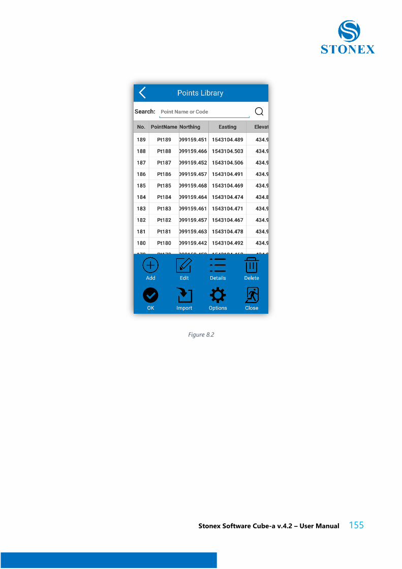
Stonex Software Cube-a v.4.2 – User Manual 155
Figure 8.2
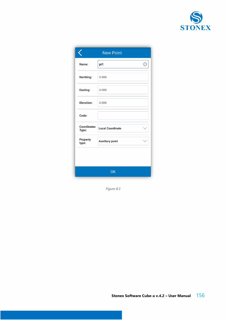
Stonex Software Cube-a v.4.2 – User Manual 156
Figure 8.3

Stonex Software Cube-a v.4.2 – User Manual 157
Figure 8.4
8.2 Entities list
Click on "Tools" and on "Entity List" to access the screen as in Figure 5.33, for more
information on this function refer to paragraph 5.1.
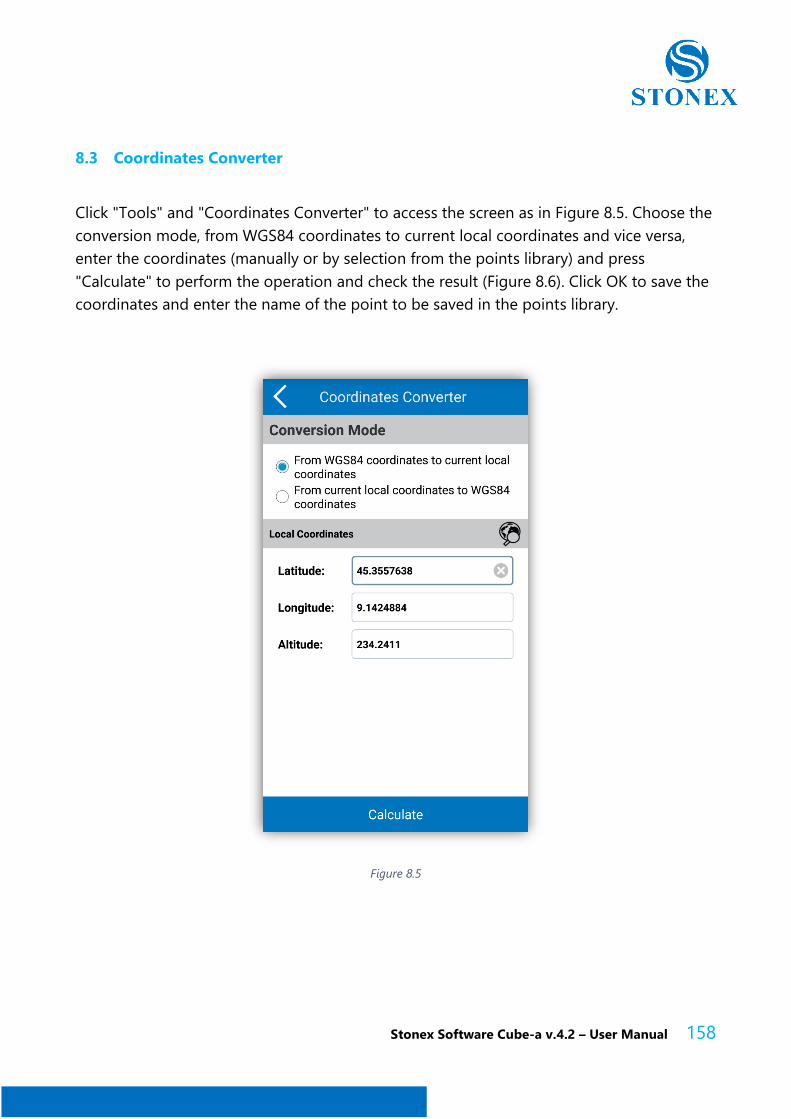
Stonex Software Cube-a v.4.2 – User Manual 158
8.3 Coordinates Converter
Click "Tools" and "Coordinates Converter" to access the screen as in Figure 8.5. Choose the
conversion mode, from WGS84 coordinates to current local coordinates and vice versa,
enter the coordinates (manually or by selection from the points library) and press
"Calculate" to perform the operation and check the result (Figure 8.6). Click OK to save the
coordinates and enter the name of the point to be saved in the points library.
Figure 8.5

Stonex Software Cube-a v.4.2 – User Manual 159
Figure 8.6
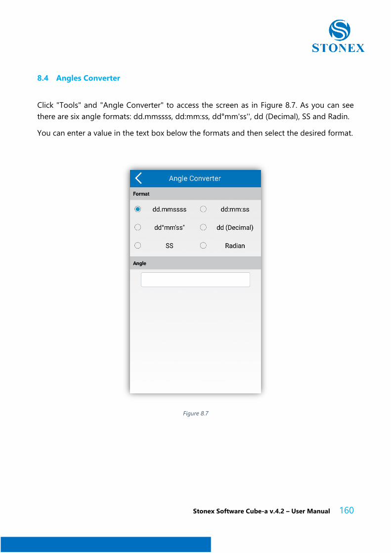
Stonex Software Cube-a v.4.2 – User Manual 160
8.4 Angles Converter
Click "Tools" and "Angle Converter" to access the screen as in Figure 8.7. As you can see
there are six angle formats: dd.mmssss, dd:mm:ss, dd°mm'ss'', dd (Decimal), SS and Radin.
You can enter a value in the text box below the formats and then select the desired format.
Figure 8.7
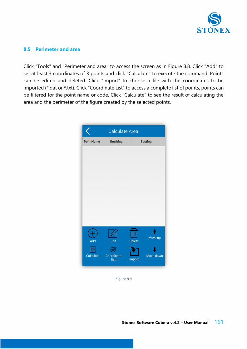
Stonex Software Cube-a v.4.2 – User Manual 161
8.5 Perimeter and area
Click "Tools" and "Perimeter and area" to access the screen as in Figure 8.8. Click "Add" to
set at least 3 coordinates of 3 points and click "Calculate" to execute the command. Points
can be edited and deleted. Click "Import" to choose a file with the coordinates to be
imported (*.dat or *.txt). Click "Coordinate List" to access a complete list of points, points can
be filtered for the point name or code. Click "Calculate" to see the result of calculating the
area and the perimeter of the figure created by the selected points.
Figure 8.8
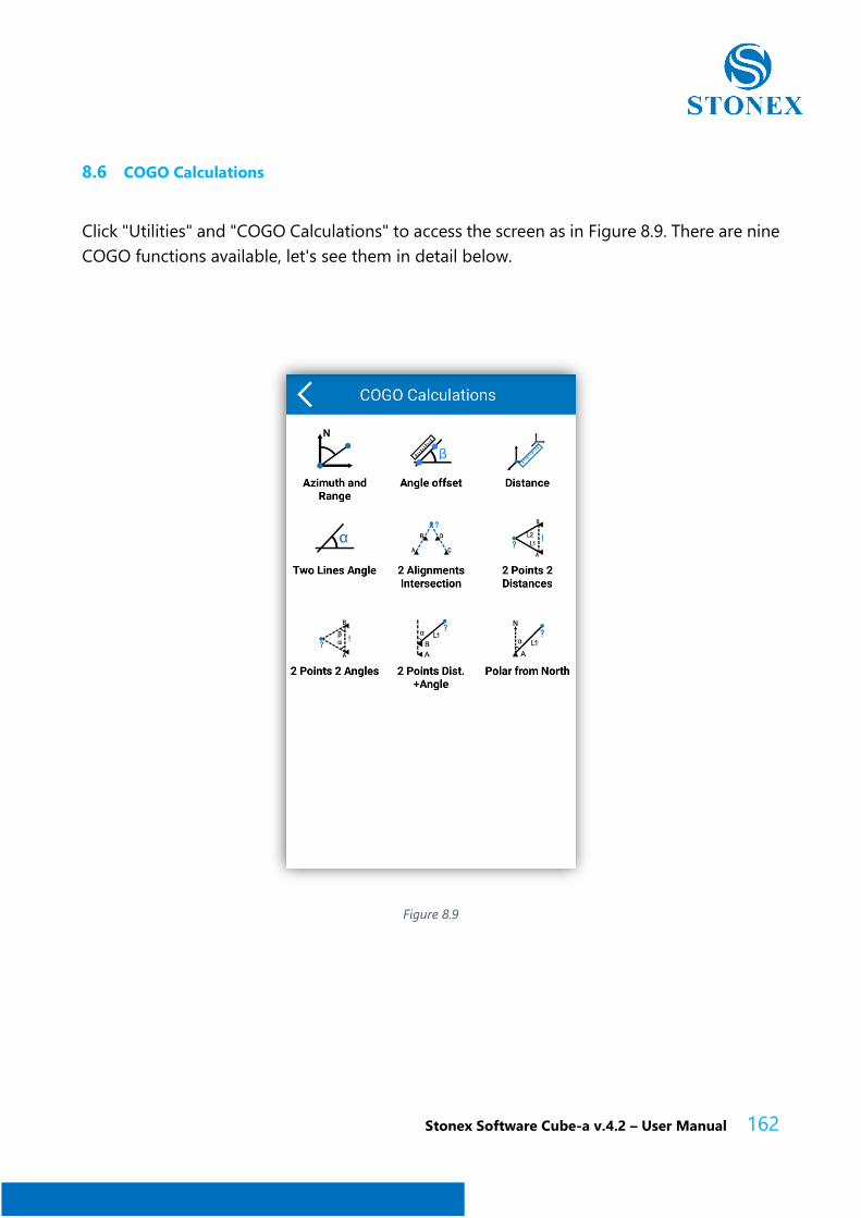
Stonex Software Cube-a v.4.2 – User Manual 162
8.6 COGO Calculations
Click "Utilities" and "COGO Calculations" to access the screen as in Figure 8.9. There are nine
COGO functions available, let's see them in detail below.
Figure 8.9
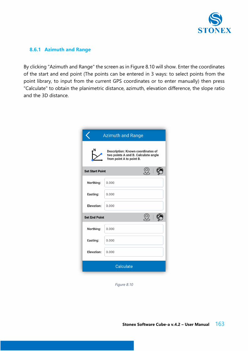
Stonex Software Cube-a v.4.2 – User Manual 163
8.6.1 Azimuth and Range
By clicking "Azimuth and Range" the screen as in Figure 8.10 will show. Enter the coordinates
of the start and end point (The points can be entered in 3 ways: to select points from the
point library, to input from the current GPS coordinates or to enter manually) then press
"Calculate" to obtain the planimetric distance, azimuth, elevation difference, the slope ratio
and the 3D distance.
Figure 8.10
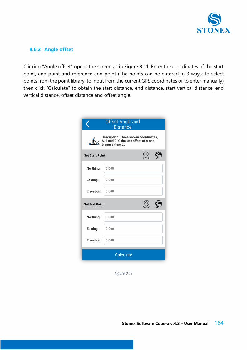
Stonex Software Cube-a v.4.2 – User Manual 164
8.6.2 Angle offset
Clicking "Angle offset" opens the screen as in Figure 8.11. Enter the coordinates of the start
point, end point and reference end point (The points can be entered in 3 ways: to select
points from the point library, to input from the current GPS coordinates or to enter manually)
then click "Calculate" to obtain the start distance, end distance, start vertical distance, end
vertical distance, offset distance and offset angle.
Figure 8.11
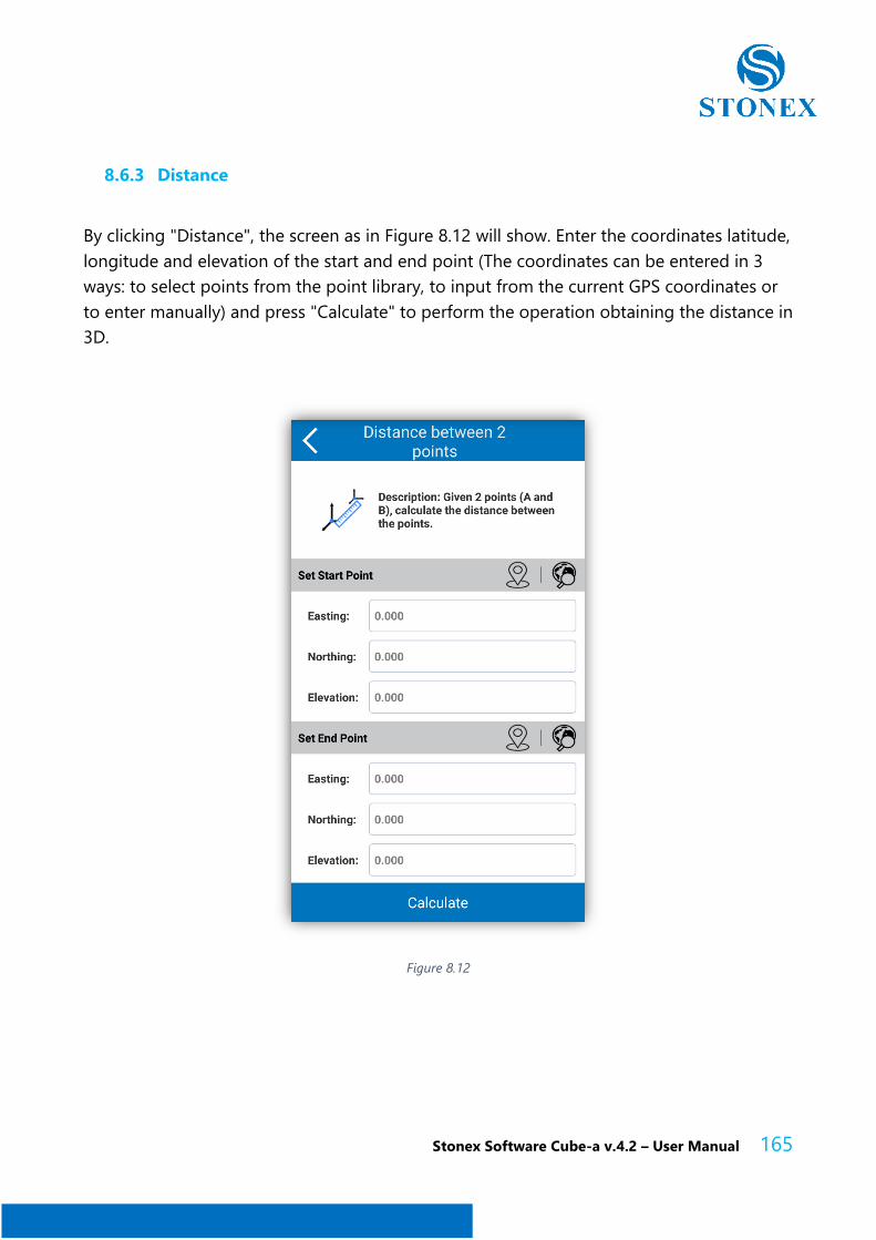
Stonex Software Cube-a v.4.2 – User Manual 165
8.6.3 Distance
By clicking "Distance", the screen as in Figure 8.12 will show. Enter the coordinates latitude,
longitude and elevation of the start and end point (The coordinates can be entered in 3
ways: to select points from the point library, to input from the current GPS coordinates or
to enter manually) and press "Calculate" to perform the operation obtaining the distance in
3D.
Figure 8.12
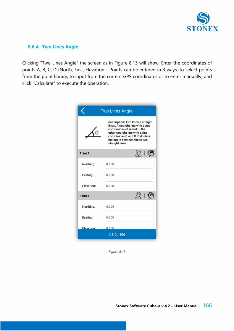
Stonex Software Cube-a v.4.2 – User Manual 166
8.6.4 Two Lines Angle
Clicking "Two Lines Angle" the screen as in Figure 8.13 will show. Enter the coordinates of
points A, B, C, D (North, East, Elevation - Points can be entered in 3 ways: to select points
from the point library, to input from the current GPS coordinates or to enter manually) and
click "Calculate" to execute the operation.
Figure 8.13
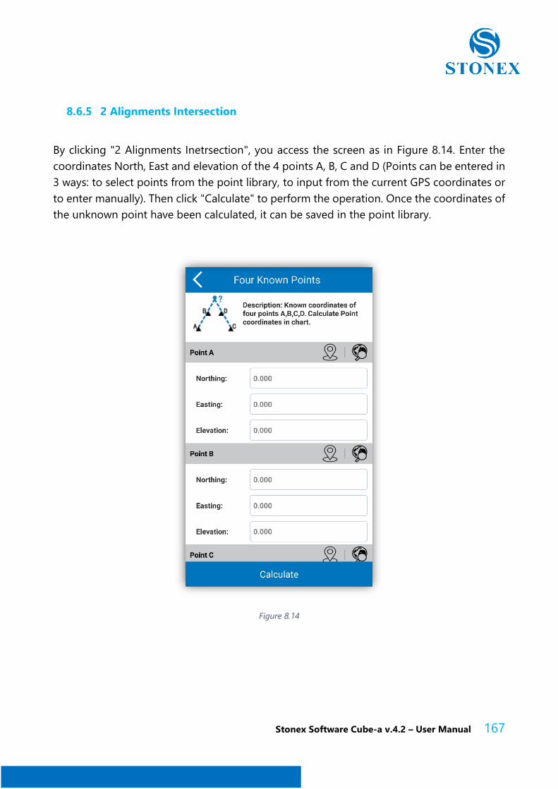
Stonex Software Cube-a v.4.2 – User Manual 167
8.6.5 2 Alignments Intersection
By clicking "2 Alignments Inetrsection", you access the screen as in Figure 8.14. Enter the
coordinates North, East and elevation of the 4 points A, B, C and D (Points can be entered in
3 ways: to select points from the point library, to input from the current GPS coordinates or
to enter manually). Then click "Calculate" to perform the operation. Once the coordinates of
the unknown point have been calculated, it can be saved in the point library.
Figure 8.14
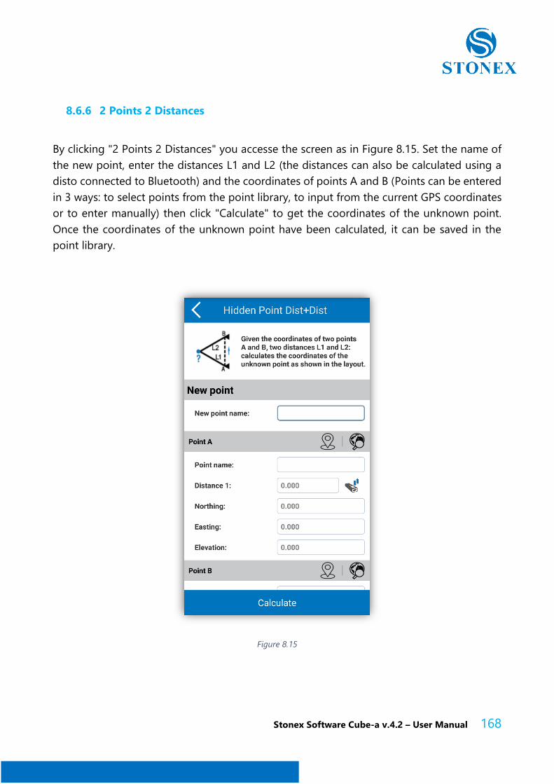
Stonex Software Cube-a v.4.2 – User Manual 168
8.6.6 2 Points 2 Distances
By clicking "2 Points 2 Distances" you accesse the screen as in Figure 8.15. Set the name of
the new point, enter the distances L1 and L2 (the distances can also be calculated using a
disto connected to Bluetooth) and the coordinates of points A and B (Points can be entered
in 3 ways: to select points from the point library, to input from the current GPS coordinates
or to enter manually) then click "Calculate" to get the coordinates of the unknown point.
Once the coordinates of the unknown point have been calculated, it can be saved in the
point library.
Figure 8.15
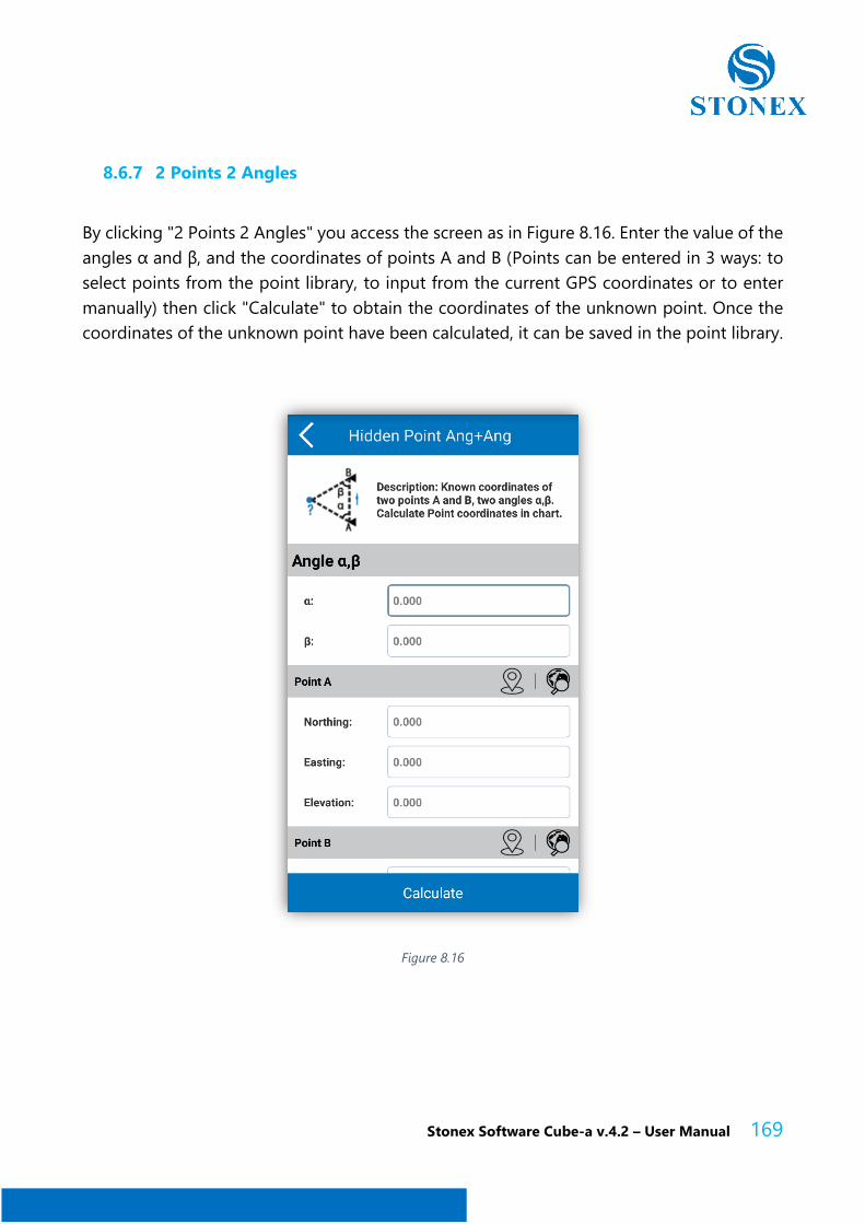
Stonex Software Cube-a v.4.2 – User Manual 169
8.6.7 2 Points 2 Angles
By clicking "2 Points 2 Angles" you access the screen as in Figure 8.16. Enter the value of the
angles α and β, and the coordinates of points A and B (Points can be entered in 3 ways: to
select points from the point library, to input from the current GPS coordinates or to enter
manually) then click "Calculate" to obtain the coordinates of the unknown point. Once the
coordinates of the unknown point have been calculated, it can be saved in the point library.
Figure 8.16
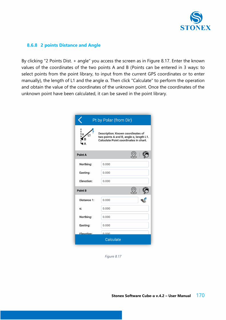
Stonex Software Cube-a v.4.2 – User Manual 170
8.6.8 2 points Distance and Angle
By clicking "2 Points Dist. + angle" you access the screen as in Figure 8.17. Enter the known
values of the coordinates of the two points A and B (Points can be entered in 3 ways: to
select points from the point library, to input from the current GPS coordinates or to enter
manually), the length of L1 and the angle α. Then click "Calculate" to perform the operation
and obtain the value of the coordinates of the unknown point. Once the coordinates of the
unknown point have been calculated, it can be saved in the point library.
Figure 8.17
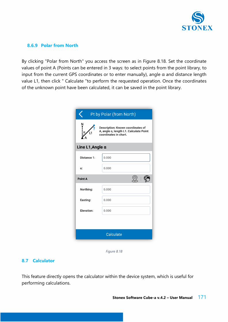
Stonex Software Cube-a v.4.2 – User Manual 171
8.6.9 Polar from North
By clicking "Polar from North" you access the screen as in Figure 8.18. Set the coordinate
values of point A (Points can be entered in 3 ways: to select points from the point library, to
input from the current GPS coordinates or to enter manually), angle α and distance length
value L1, then click " Calculate "to perform the requested operation. Once the coordinates
of the unknown point have been calculated, it can be saved in the point library.
Figure 8.18
8.7 Calculator
This feature directly opens the calculator within the device system, which is useful for
performing calculations.
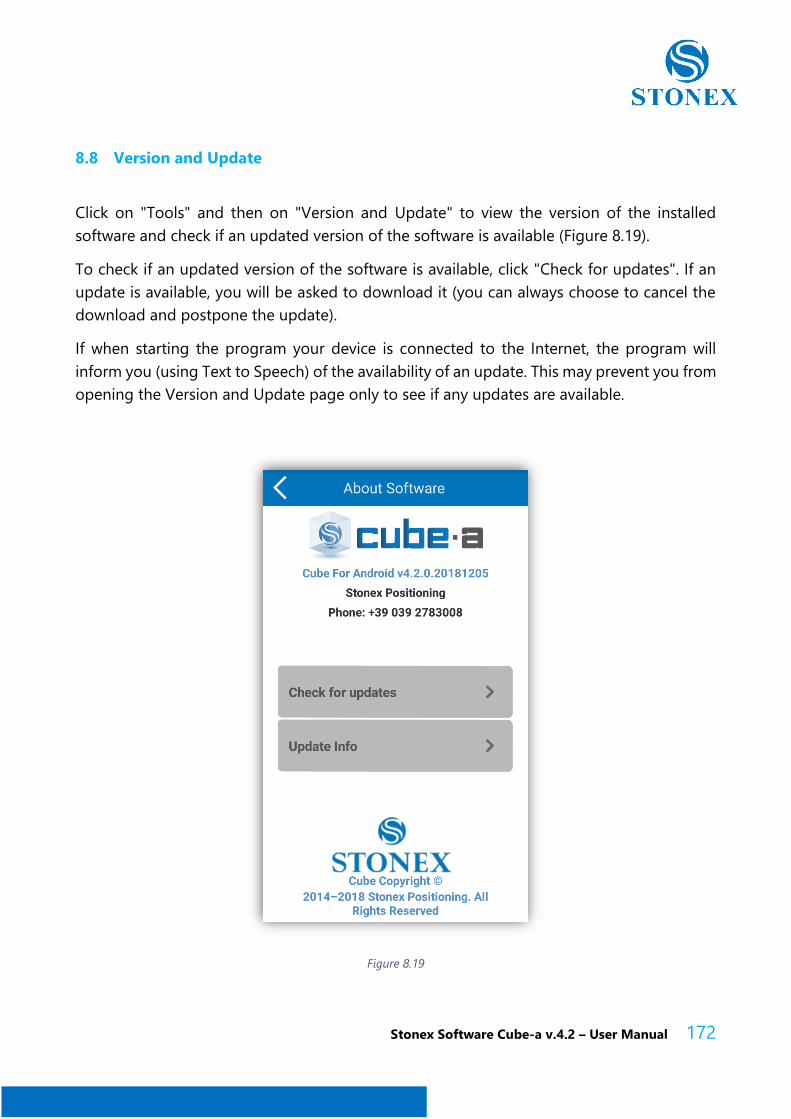
Stonex Software Cube-a v.4.2 – User Manual 172
8.8 Version and Update
Click on "Tools" and then on "Version and Update" to view the version of the installed
software and check if an updated version of the software is available (Figure 8.19).
To check if an updated version of the software is available, click "Check for updates". If an
update is available, you will be asked to download it (you can always choose to cancel the
download and postpone the update).
If when starting the program your device is connected to the Internet, the program will
inform you (using Text to Speech) of the availability of an update. This may prevent you from
opening the Version and Update page only to see if any updates are available.
Figure 8.19

Stonex Software Cube-a v.4.2 – User Manual 173
STONEX® SRL
Via Cimabue, 39 - 20851 Lissone (MB)
Tel: +390392783008 ; +390392785575 | Fax :+390392789576
www.stonex.it | [email protected]
0