Knowl Inf SystDOI 10.1007/s10115-014-0733-3

REGULAR PAPER

STenSr: Spatio-temporal tensor streams for anomalydetection and pattern discovery

Lei Shi · Aryya Gangopadhyay · Vandana P. Janeja

Received: 24 April 2012 / Revised: 16 November 2013 / Accepted: 24 January 2014© Springer-Verlag London 2014

Abstract The focus of this paper is anomaly detection and pattern discovery in spatio-temporal tensor streams. As an example, sensor networks comprising of multiple individualsensor streams generate spatio-temporal data, which can be captured in tensor streams. Anom-aly detection in such data is considered challenging because of the potential complexity andhigh order of the tensor data from spatio-temporal sources such as sensor networks. In thispaper, we propose an innovative approach for anomaly detection and pattern discovery in suchtensor streams. We model the tensor stream itself as a single incremental tensor, for examplerepresenting the entire sensor network, instead of dealing with each individual tensor in thestream separately. Such a model provides a global view of the tensor stream and enablessubsequent in-depth analysis of it. The proposed approach is designed for online analysis oftensor streams with fast runtime. We evaluate our approach for detecting anomalies underdifferent conditions and for identifying complex data patterns. We also compare the proposedapproach with the existing tensor stream analysis method (Sun et al. in ACM Trans KnowlDiscov Data 2, 2008). Our evaluation uses synthetic data as well as real-world data showingthe efficiency and effectiveness of the proposed approach.

Keywords Anomaly detection · Spatio-temporal · Tensor · High-order

1 Introduction

The rapid development of technologies is leading to the explosive growth of data in variouscomplex forms. For instance, data streams could be generated by video surveillance systems,sensor networks, transactions systems in financial market and retail industry, and monitoringsystems of various dynamic environments. There are more and more complex data streams ofhigh-order data being generated and collected from these sources. Our focus in this paper isthe discovery of anomalies and patterns in such complex data streams particularly in spatio-

L. Shi · A. Gangopadhyay · V. P. Janeja (B)Information Systems Department, University of Maryland, Baltimore County, MD, USAe-mail: vjaneja@umbc.edu

123

L. Shi et al.

temporal data. For example, in a sensor network, which is a distinct example of spatio-temporal data, advanced sensors are spatial objects, such as image sensors, video sensors,and bio-sensors. These sensors can measure certain properties by using higher-order complexdata like multivariate numeric data, images, video, and bio-signals rather than only a singlenumerical value. These data at a sensor are captured over a period of time bringing in thetemporal nature. This is just a single sensor measuring one property. Let us consider thewhole sensor network or neighborhoods of sensors [12] where there are numbers of sensorsmeasuring various distinct properties at different locations. One such application is thatof a traffic sensor network monitoring the state of traffic in terms of various propertiesincluding speed and volume of vehicles on a large road system [6]. In this scenario, the spatio-temporal data stream generated by such a sensor network could get to be complex and highorder.

However, there is a lack of methods for analyzing such complex streams of high-orderdata. Although mining time series data streams has been widely studied and explored, mostof the existing methods have been proposed to address problems on low-order univariate ormultivariate data streams [3,10,16]. For example, much of the work on anomaly detectionin data streams [1,2,17,18] is designed for handling multivariate data streams or multipleunivariate data streams specifically. Similarly in mining spatial-temporal data or sensor net-work data, the most recent methods focus on anomaly detection in low-order vector stream[5] or individual stream in the spatial neighborhoods [12].

Thus, there is a need for an approach for detecting anomalies, discovering patterns andtrends, and performing other data mining tasks in high-order data streams.

A tensor stream can be used to model such a high-order data stream. Tensor streams canbe considered as a generalization of the traditional univariate and multivariate data streams.A tensor stream uses tensors as an universal data structure enabling the modeling of differentforms of data in a consistent manner. Tensors extend the notion of the scalar, vector, andmatrix to higher orders. Scalar data can be modeled by a 0-mode tensor, vector data can bemodeled by a 1-mode tensor, and matrix data can be modeled by a 2-mode tensor. Tensorscan be further extended to k-mode for modeling data of even higher orders.

Tensors can be traced back to Tucker decomposition [22]. Since then, they have beenwidely used for representation, decomposition and interpretations of complex high-orderdata in many applications. Examples include, image representation [19], graph analysis (e.g.,[4,13]), computer vision (e.g., [23,24]), multilinear algebra and its applications (e.g., [14]),and data mining (e.g., [7,11,20]). To the best of our knowledge, our approach is the firstusing tensors to model complex spatio-temporal data. Such data are more and more commonin applications such as sensor networks monitoring traffic, water monitoring sensors to namea few.

An incremental tensor analysis framework was proposed in [21]. The framework usesreconstruction error of tensor for anomaly detection in a tensor stream. The assumption is thatthe higher its reconstruction error, the more abnormal the particular tensor is. The frameworkconstantly updates a tensor reconstruction model consisting of N projection matrices for astream of an N -mode tensor. It uses this model to compute reconstruction error for tensors.However, one vital problem [21] is that its reconstruction model is extremely susceptibleto anomalies. Another issue is that simply using reconstruction error is not sufficient foridentifying all kinds of anomalies.

In this paper, we propose a fast approach for anomaly detection and pattern discoveryin spatio-temporal tensor streams. Our method provides powerful anomaly detection thataddresses the above issues and enables subsequent easy pattern discovery from the tensorstream. Specifically, we make the following contributions:

123

Anomaly detection and pattern discovery

• We propose a generic, single incremental tensor model for modeling the entire tensorstream, and this provides a global view of the stream and enables subsequent in-depthanalysis of it;

• based on our model, we propose a simple and fast online anomaly detection technique thatenables efficient and accurate detection of abnormal tensors in the tensor stream, and thefurther location of deviant cells responsible for the abnormality in it;

• based on our model, we propose a uniform representation to capture, describe, and sum-marize the underlying pattern of the tensor stream online, which allows easy interpretationand utilization of it;

• we provide extensive experimental results with real-world traffic sensor data as well assynthetic data depicting the efficiency and effectiveness of our approach.

The rest of the paper is organized as follows: Sect. 2 introduces some key tensor basicsand HOSVD [15] preliminaries; Sect. 3 describes tensor stream and formalizes the problemthat we are solving in the paper; Sect. 4 discusses our approach in detail; Sect. 5 presents theexperimental evaluation of our approach; and lastly Sect. 6 concludes the paper and discussesfuture work.

2 Preliminaries

For better understanding of the paper, we begin with a brief introduction of some key tensorbasics in this section. We also discuss high-order singular value decomposition (HOSVD)[15]. For a detailed background on tensors and tensor operations, the reader is referred to[14,21].

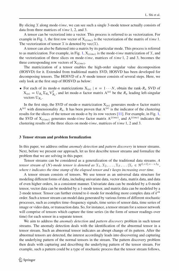
Tensor is defined as a multi-dimensional array of data. Its dimensions describe the ordersof the data and are referred to as modes or orders of the tensor (In the rest of the paper, weuse mode of the tensor to distinguish it from the dimension of the matrix). For example, asshown in Fig. 1, X is a 3-mode tensor ∈ �2×2×3 and its (i, j, k)th element is denoted by ai jk .

Fig. 1 Tensor slice, matricization, and decomposition

123

L. Shi et al.

By slicing X along mode-time, we can see such a single 3-mode tensor actually consists ofdata from three matrices of time 1, 2, and 3.

A tensor can be vectorized into a vector. This process is referred to as vectorization. Forexample in Fig. 1, the first row vector of X(time) is the vectorization of the matrix of time 1.The vectorization of tensor X is denoted by vec(X).

A tensor can also be flattened into a matrix by its particular mode. This process is referredto as matricization. For example, in Fig. 1, X(time) is the mode-time matricization of X, andthe vectorization of three slices on mode-time, matrices of time 1, 2 and 3, becomes thethree corresponding row vectors of X(time).

The matricization of a tensor enables the high-order singular value decomposition(HOSVD) for it. Extended from traditional matrix SVD, HOSVD has been developed fordecomposing tensors. The HOSVD of a N -mode tensor consists of several steps. Here, weonly look at the first step of HOSVD as below:

• For each of its mode-n matricizations X(n) | n = 1 · · · N , obtain the rank-Rn SVD ofX(n) = URn �Rn VT

Rn, and let mode-n factor matrix A(n) be the Rn leading left-singular

vectors URn .

In the first step, the SVD of mode-n matricization X(n) generates mode-n factor matrixA(n) with dimensionality Rn . It has been proven that A(n) is the indicator of the clusteringresults for the slices of the tensor on mode-n by its row vectors [11]. For example, in Fig. 1,the SVD of X(time) generates mode-time factor matrix A(time), and A(time) indicates theclustering results of the three slices on mode-time, matrices of time 1, 2 and 3.

3 Tensor stream and problem formalization

In this paper, we address online anomaly detection and pattern discovery in tensor streams.Next, before we present our approach, let us first describe tensor streams and formalize theproblem that we are solving in this paper.

Tensor streams can be considered as a generalization of the traditional data streams. Atensor stream of (N )-mode tensor is denoted as X1, X2, . . . , XT , . . . |Xt ∈ �I1×I2×···×IN ,where t indicates the time stamp of the elapsed tensor and t keeps increasing over time.

A tensor stream consists of tensors. We use tensor as an universal data structure formodeling different forms of data, including univariate data, vector data, matrix data, and dataof even higher orders, in a consistent manner. Univariate data can be modeled by a 0-modetensor, vector data can be modeled by a 1-mode tensor, and matrix data can be modeled by a2-mode tensor. Tensor can further extend to k-mode for modeling more complex data of kth

order. Such a tensor stream can model data generated by various forms of different stochasticprocesses, such as complex time–frequency signals, time series of sensor data, time series ofimage or video data, or transaction data. So, for instance, a tensor stream for a sensor networkwill comprise of tensors which capture the time series (in the form of sensor readings overtime) for each sensor in a separate tensor.

We aim to address the anomaly detection and pattern discovery problem in such tensorstreams. The anomaly detection deals with the identification of the abnormal tensor in atensor stream. Such an abnormal tensor indicates an abrupt change of its pattern. After theabnormal tensors are detected, the interest accordingly leads into discovering and capturingthe underlying pattern of the normal tensors in the stream. The pattern discovery problemthen deals with capturing and describing the underlying pattern of the tensor stream. Forexample, such a pattern could be a type of stochastic process that the tensor stream follows,

123

Anomaly detection and pattern discovery

such as stationary or cyclostationary process, or it could be the current and future trend ofthe tensor stream. We now describe these two problems in below.Anomaly detection in tensor stream: Given each newly incoming tensor Xt+1 in the stream,we must evaluate its abnormality in comparison with the previous tensors in the streamX1, X2, · · · , Xt . If Xt+1 is considered abnormal, the deviant cells responsible for the abnor-mality should be further located in it.Pattern discovery in tensor stream: We must identify the underlying pattern of the tensorstream. We need a uniform representation to capture, describe, and summarize such a patternfor the easy interpretation and utilization of it.

Single-scan, online data analysis methodology will be employed for addressing the twoproblems in tensor stream. Tensor stream is fast growing, of massive data volume due tothe high-order tensors, and is potentially infinite. It is impossible to store the entire tensorstream or to scan through it multiple times. We need to use single-scan, online approach fordetecting anomaly and discovering pattern in it.

There are several challenges for such a single-scan, online approach. It has particularlyhigh requirements on the time and space complexity of the algorithm. The algorithm shouldbe fast, efficient, and must have low memory cost. Each tensor can only be processed by thealgorithm once at the time when it arrives. Some of its statistics may be stored in the memoryfor future use, but not the tensor itself.

We next outline our approach to address these problems and challenges.

4 Approach

In the following, we propose a new perspective for approaching such a problem of onlineanomaly detection and pattern discovery. In our approach, instead of dealing with eachindividual tensor in the stream separately, we model the tensor stream itself as a large singleincremental tensor and perform global analysis on it. Consider, a tensor stream of (N − 1)-mode tensors X1, X2 · · · XT · · · |Xt ∈ �I1×I2×···×IN−1 , the stream itself can be modeled as asingle incremental N -mode tensor X ∈ �I1×I2×···×IN−1×Itime . The additional time mode ofX represents the time stamp of each individual tensor Xt in the tensor stream, such that Itime

increases with the incoming tensor. In this manner, our approach creates a generic modelof the tensor stream as a higher-order incremental tensor, which captures every individualtensor in the stream and their correlations. Such a model provides a global view of the streamand enables the subsequent in-depth analysis of its pattern and trend. We now explain ourapproach in more detail.

4.1 Approach overview

Based on the global model above, our approach consists of the following three distinct steps.When there is a newly incoming tensor Xt+1,

1. the first step is to update the mode-time factor matrix A(time) for the incremental tensormodel of the tensor stream. We update A(time) to account for new tensor Xt+1. As discussedin Sect. 2, the row vectors of mode-time factor matrix A(time) indicate the mode-timeslice of the tensor. As a result, one new row vector indicating Xt+1 will be included in theupdated factor matrix A′(time);

2. the second step is to evaluate the abnormality of Xt+1. Given the updated factor matrixA′(time), we identify whether there is an abrupt change in its new row vector. If the answer

123

L. Shi et al.

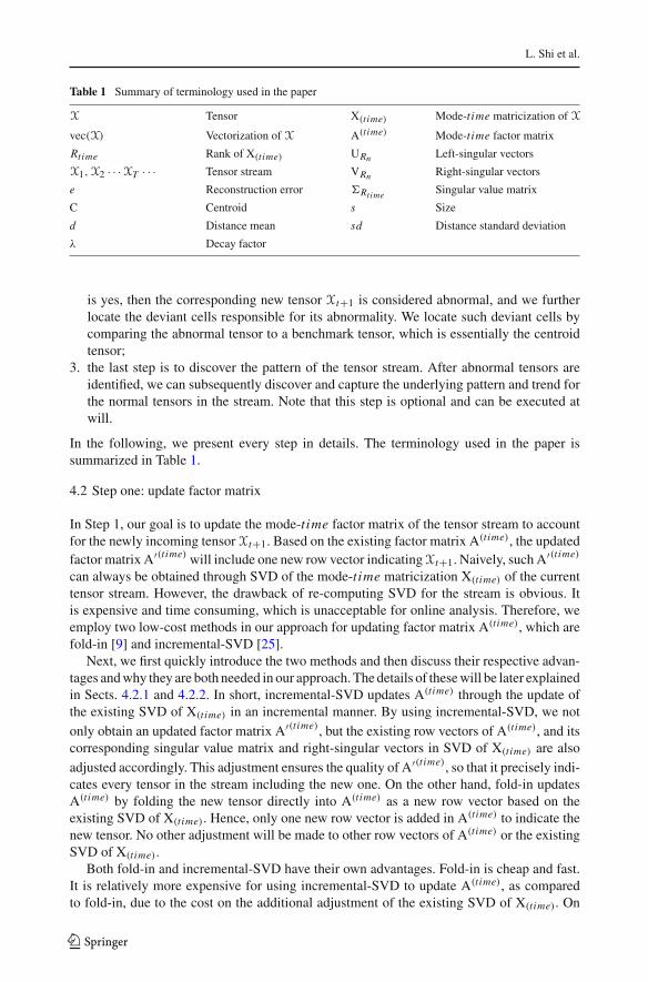
Table 1 Summary of terminology used in the paper

X Tensor X(time) Mode-time matricization of X

vec(X) Vectorization of X A(time) Mode-time factor matrix

Rtime Rank of X(time) URn Left-singular vectors

X1, X2 · · · XT · · · Tensor stream VRn Right-singular vectors

e Reconstruction error �Rtime Singular value matrix

C Centroid s Size

d Distance mean sd Distance standard deviation

λ Decay factor

is yes, then the corresponding new tensor Xt+1 is considered abnormal, and we furtherlocate the deviant cells responsible for its abnormality. We locate such deviant cells bycomparing the abnormal tensor to a benchmark tensor, which is essentially the centroidtensor;

3. the last step is to discover the pattern of the tensor stream. After abnormal tensors areidentified, we can subsequently discover and capture the underlying pattern and trend forthe normal tensors in the stream. Note that this step is optional and can be executed atwill.

In the following, we present every step in details. The terminology used in the paper issummarized in Table 1.

4.2 Step one: update factor matrix

In Step 1, our goal is to update the mode-time factor matrix of the tensor stream to accountfor the newly incoming tensor Xt+1. Based on the existing factor matrix A(time), the updatedfactor matrix A′(time) will include one new row vector indicating Xt+1. Naively, such A′(time)

can always be obtained through SVD of the mode-time matricization X(time) of the currenttensor stream. However, the drawback of re-computing SVD for the stream is obvious. Itis expensive and time consuming, which is unacceptable for online analysis. Therefore, weemploy two low-cost methods in our approach for updating factor matrix A(time), which arefold-in [9] and incremental-SVD [25].

Next, we first quickly introduce the two methods and then discuss their respective advan-tages and why they are both needed in our approach. The details of these will be later explainedin Sects. 4.2.1 and 4.2.2. In short, incremental-SVD updates A(time) through the update ofthe existing SVD of X(time) in an incremental manner. By using incremental-SVD, we notonly obtain an updated factor matrix A′(time), but the existing row vectors of A(time), and itscorresponding singular value matrix and right-singular vectors in SVD of X(time) are alsoadjusted accordingly. This adjustment ensures the quality of A′(time), so that it precisely indi-cates every tensor in the stream including the new one. On the other hand, fold-in updatesA(time) by folding the new tensor directly into A(time) as a new row vector based on theexisting SVD of X(time). Hence, only one new row vector is added in A(time) to indicate thenew tensor. No other adjustment will be made to other row vectors of A(time) or the existingSVD of X(time).

Both fold-in and incremental-SVD have their own advantages. Fold-in is cheap and fast.It is relatively more expensive for using incremental-SVD to update A(time), as comparedto fold-in, due to the cost on the additional adjustment of the existing SVD of X(time). On

123

Anomaly detection and pattern discovery

the other hand, such an adjustment made by incremental-SVD optimizes the decompositionof the tensor stream by taking into account the new tensor. This minimizes the informationloss in the updated factor matrix A′(time) and ensures it is of good quality. However, suchan adjustment can become redundant when the new tensor already fits well into the existingSVD of the stream. In such a case, incremental-SVD is not necessary. Thus, the issue is howcan we choose the most appropriate method of the two for updating A(time) depending onspecific situations?

In order to select the best method for updating A(time) at each time, we designed a testprocedure. The idea is to use fold-in whenever possible since it is fast and cheap, and useincremental-SVD only when necessary to update SVD. We propose a reconstruction error-based test to quickly quantify the potential information loss by using the existing SVD. Asshown in Eq. 1, given a newly incoming tensor Xt+1, we compare its vectorization vec(Xt+1)

to its reconstructed vectorization based on the existing right-singular vectors VRtime . Wemeasure the information loss in terms of the reconstruction error. Intuitively, if the erroris low, fold-in will be used since the new tensor fits well with the existing decomposition,otherwise incremental-SVD will be used to make necessary update of SVD. A correspondingreconstruction error threshold, in the form of a percentage measuring how much informationis lost, is used for this test

et+1 = ‖ vec(Xt+1)T − vec(Xt+1)

T VRtime VTRtime

‖2

‖ vec(Xt+1)T ‖2 (1)

In the following, we briefly explain the detailed process of updating A(time), by usingfold-in and incremental-SVD, respectively, in Sects. 4.2.1 and 4.2.2. Then, we summarizeStep 1 in Sect. 4.2.4.

4.2.1 Fold-in

Fold-in [9] is a fast and cheap method for updating the factor matrix. It updates A(time) bydirectly folding the new tensor into A(time) as its new row vector based on the existing SVDof X(time). Other row vectors of A(time) and existing SVD of X(time) remain the same afterthe update.

The detailed update process works in the following way. Given the existing factor matrixA(time), the updated factor matrix A′(time) can be obtained by Eq. 2. As we can see, A(time)

itself remains unchanged in A′(time), and a new row vector representing the new tensor Xt+1

is appended to A(time). This new row vector is computed by vec(Xt+1)T VRtime�

−1Rtime

, wherevec(Xt+1) is the vectorization of Xt+1, VRtime is the right-singular vectors, and �Rtime is thesingular value matrix of the existing SVD.

A′(time) =[

A(time)

vec(Xt+1)T VRtime�

−1Rtime

](2)

4.2.2 Incremental-SVD

Before we introduce incremental-SVD, we first explain how we convert the problem of updat-ing the factor matrix A(time) to the problem of incremental-SVD. Given a newly incomingtensor Xt+1, the mode-time matricization X′

(time) of the updated tensor stream is shown inEq. 3. In it, X(time) is the mode-time matricization of the tensor stream without the newtensor and vec(Xt+1) is the vectorization of the new tensor Xt+1. As we know, the updated

123

L. Shi et al.

factor matrix A′(time) is the left-singular vector of X′(time). Thus, by incrementally updating

SVD for X′(time) based on the existing SVD of X(time) in Eq. 3, we can accordingly obtain

the updated factor matrix A′(time).

X′(time) =

[X(time)

vec(Xt+1)T

], X(time) = A(time)�Rtime VT

Rtime(3)

The detailed incremental-SVD consists of the following three steps.

1. Obtain QL decomposition(I − VRtime VT

Rtime

)vec(Xt+1) = Q Rtime LT (4)

2. Obtain the rank-Rtime SVD[�Rtime 0

vec(Xt+1)T VRtime L

]= URtime �Rtime VT

Rtime(5)

3. Update SVD of X′(time) =

[A(time) 0

0 I

]URtime �Rtime

([VRtime Q Rtime

]VRtime

)T(6)

Accordingly, the updated factor matrix A′(time) is the left-singular vector of X′(time), as

shown in Eq. 7.

A′(time) =[

A(time) 00 I

]URtime (7)

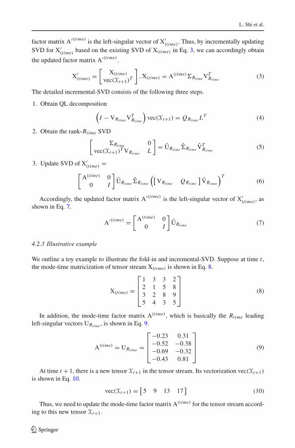
4.2.3 Illustrative example

We outline a toy example to illustrate the fold-in and incremental-SVD. Suppose at time t ,the mode-time matricization of tensor stream X(time) is shown in Eq. 8.

X(time) =

⎡⎢⎢⎣

1 3 3 22 1 5 83 2 8 95 4 3 5

⎤⎥⎥⎦ (8)

In addition, the mode-time factor matrix A(time), which is basically the Rtime leadingleft-singular vectors URtime , is shown in Eq. 9.

A(time) = URtime =

⎡⎢⎢⎣

−0.23 0.31−0.52 −0.38−0.69 −0.32−0.43 0.81

⎤⎥⎥⎦ (9)

At time t + 1, there is a new tensor Xt+1 in the tensor stream. Its vectorization vec(Xt+1)

is shown in Eq. 10.

vec(Xt+1) = [5 9 13 17

](10)

Thus, we need to update the mode-time factor matrix A(time) for the tensor stream accord-ing to this new tensor Xt+1.

123

Anomaly detection and pattern discovery

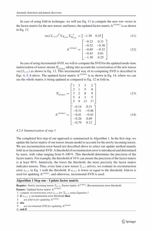
In case of using fold-in technique, we will use Eq. 11 to compute the new row vector inthe factor matrix for the new tensor, and hence, the updated factor matrix A′(time) is as shownin Eq. 12.

vec(Xt+1)T VRtime�

−1Rtime

= [−1.30 0.25]

(11)

A′(time) =

⎡⎢⎢⎢⎢⎣

−0.23 0.31−0.52 −0.38−0.69 −0.32−0.43 0.81−1.30 0.25

⎤⎥⎥⎥⎥⎦ (12)

In case of using incremental-SVD, we will re-compute the SVD for the updated mode-timematricization of tensor stream X′

(time) taking into account the vectorization of the new tensorvec(Xt+1) as shown in Eq. 13. This incremental way of re-computing SVD is described inEqs. 4, 5, 6 above. The updated factor matrix A′(time) is as shown in Eq. 14, where we cansee the whole matrix is being updated as compared to Eq. 12 in fold-in.

X′(time) =

⎡⎢⎢⎢⎢⎣

1 3 3 22 1 5 83 2 8 95 4 3 55 9 13 17

⎤⎥⎥⎥⎥⎦ (13)

A′(time) =

⎡⎢⎢⎢⎢⎣

−0.14 0.31−0.31 −0.46−0.41 −0.43−0.26 0.69−0.79 0.12

⎤⎥⎥⎥⎥⎦ (14)

4.2.4 Summarization of step 1

The completed first step of our approach is summarized in Algorithm 1. In the first step, weupdate the factor matrix of our tensor stream model to account for the newly incoming tensor.We use reconstruction error-based test described above to select our update method namelyfold-in or incremental-SVD. A threshold of reconstruction error is introduced and determinedby users, with value ranging from 0–100 %. This threshold determines the precision of thefactor matrix. For example, the threshold of 10 % can ensure the precision of the factor matrixis at least 90 %. Intuitively, the lower the threshold, the more precisely the factor matrixindicates tensors. Thus, every time a new tensor Xt+1 arrives, we evaluate its reconstructionerror et+1 in Eq. 1 with the threshold. If et+1 is lower or equal to the threshold, fold-in isused for updating A(time), and otherwise, incremental-SVD is used.

Algorithm 1 Step one - Update factor matrix

Require: Newly incoming tensor Xt+1, Factor matrix A(time), Reconstruction error threshold

Ensure: Updated factor matrix A′(time)

1: compute reconstruction error et+1 for Xt+1 using Equation 12: if et+1 ≤ reconstruction error threshold then3: use fold-in for updating A(time)

4: else5: use incremental-SVD for updating A(time)

6: end if

123

L. Shi et al.

4.3 Step two: anomaly detection

In Step 2, we evaluate the abnormality of the newly incoming tensor Xt+1. We considera tensor to be abnormal if there is an abrupt change of the stream being detected at thetime. Let us illustrate the idea by a simple example. Consider a univariate data stream[3, 2, 4, 3, 2, 47, 3, 2, · · · ]. The abrupt change in this stream is obviously located at 47,since 47 is significantly deviant from its previous numbers. Such an abrupt change in thecase of univariate data is easy to detect. However, when dealing with tensor stream andhigh-order data, the problem becomes much more complex. Fortunately, the factor matrixsimplifies the problem. The factor matrix consistently provides a simplified representationfor tensors in the stream. Each of its row vectors indicates a specific tensor in the stream.Hence, we can transform the problem of detecting the abrupt change of the stream to amuch easier problem of detecting the abrupt change of the factor matrix given its new rowvector.

The most noticeable sign of such an abrupt change in the factor matrix is the sudden andsignificant increase in the reconstruction error in Eq. 1. It indicates the newly incoming tensordoes not fit the existing SVD. We can use it to quickly filter out obvious anomalies. However,reconstruction error itself is not sufficient for capturing all such abrupt changes. Next, wepropose and describe a fast and simple Euclidean distance-based method for comprehensivedetection of such abrupt changes in Step two (a) in Sect. 4.3.1. In Step two (b) in Sect. 4.3.2,we further discuss how to locate deviant cells responsible for the abnormality in an identifiedabnormal tensor.

4.3.1 Step two (a): identify abnormal tensor

We propose a Euclidean distance-based procedure to detect the abrupt change in the new rowvector of the factor matrix. Our test is fast and simple. The underlying idea is to quantifythe level of change of the new row vector as compared to previous ones by using distancemeasurement. Let us consider that each row vector of factor matrix A′(time) can uniquelydefine a point in a Euclidean space. We quantify the distance from the new row vectorindicating the new tensor, denoted by A′(time)

(Xt+1), to the centroid of previous row vectors,denoted by C. We keep tracking this distance in terms of its mean d and standard deviationsd . We propose a test procedure to evaluate whether a significant change of this distanceoccurs for the new tensor.

The test formulation is shown in Eq. 15. d(C, A′(time)(Xt+1)) denotes the Euclidean

distance from centroid C to current A′(time)(Xt+1), such that d is the average of the pre-

vious distances and sd is the standard deviation of the previous distances. This formula-tion can be viewed as a generalized standard score test. It measures and checks the currentdistance A′(time)

(Xt+1) to centroid C is how many standard deviation sd away from theaverage distance d . Intuitively, if the current A′(time)

(Xt+1) is “too far” away from C ascompared to previous ones, it will be considered as a significant change and the corre-sponding new tensor will be considered abnormal. A threshold is imposed and determinedby users to set how many standard deviations away is considered “too far”. Generally, itcan be set to 3-4 standard deviations if we simply assume these distances are normallydistributed. ∣∣∣d (

C�Rtime , A′(time)(Xt+1)�Rtime

)− d

∣∣∣sd

(15)

123

Anomaly detection and pattern discovery

However, additional consideration needs to be given due to the potential use ofincremental-SVD in Step 1. The use of incremental-SVD in Step 1 can cause two prob-lems here namely the inconsistency of the centroid coordinates and the distance unitvalue. As discussed, incremental-SVD updates the whole SVD. The update of SVD canbe regarded as three space-related operations, which are a re-rotation by the new right-singular vectors VRtime , a re-scaling by the new singular value matrix �Rtime , and a re-projection onto Rtime new principal components. Such a re-rotation causes the first prob-lem, the inconsistency of the coordinates of the centroid C in the new space. Such a re-scaling causes the second problem, the inconsistency of the distance unit value in the newspace.

We now explain how to remedy this. The coordinates of centroid C in new space can beeasily obtained through a linear transformation by Eq. 16. While we first rotate the centroidC back to the original space by the old right-singular vectors VRtime before SVD update,we rotate it by the new right-singular vectors V′

Rtimeafter SVD update, to get the re-rotated

centroid Cre−rotated .

Cre−rotated = CVTRtime

V′Rtime

(16)

The inconsistency of the distance can be simply solved by using the multiplication offactor matrix and singular value matrix instead of using only the factor matrix. Since thesingular value matrix �Rtime is the scaling factor, Euclidean distance will be then consistent.For example, in Eq. 15, we use A′(time)

(Xt+1)�Rtime instead of A′(time)(Xt+1).

Next, if the new tensor were considered normal, the centroid C, and distance statistics dand sd then need to be updated to account for it. The average distance d is updated by Eq. 17.The distance standard deviation sd is updated by Eq. 18. The centroid C and the number ofrow vectors s are updated by Eq. 19. In these updates, we employ a decay factor to leveragethe time effect on data. We now explain the decay factor below.

d ′ =λs × d + d

(C, A′(time)

(Xt+1)�Rtime

)λs + 1

(17)

sd ′ =

√√√√λs × sd2 +(

d(

C, A′(time)(Xt+1)�Rtime

)− d ′

)2

λs + 1(18)

C′ = λs × C + A′(time)(Xt+1)�Rtime

λs + 1, s′ = λs + 1 (19)

In a time-varying environment, recency of the data is important. Intuitively, more recentthe data, the greater its importance. Hence, in the above three equations, a decay factor λ

(among 0 − 1) is introduced, so as to let the data with older time stamps gradually decay. λ

reduces the weights of older data each time when updating the centroid, size, distance mean,and distance standard deviation. As shown in Eqs. 17, 18, 19, values associated with the newtensor are given a 100 % weight, such as (d(C, A′(time)

(X)) and A′(time)(X). On the other

hand, existing centroid C, size s, distance mean d , and distance standard deviation sd are allassigned a less weight of the decay factor λ, in order to reduce the influence of older data.The value of λ can be determined by users based on how important they consider the recentdata to be. The less the value of λ is, the fast the old data decay and the more important therecent data is. The value of 1 means no decay at all.

123

L. Shi et al.

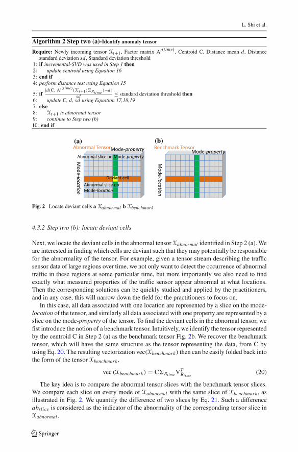
Algorithm 2 Step two (a)-Identify anomaly tensor

Require: Newly incoming tensor Xt+1, Factor matrix A′(time), Centroid C, Distance mean d, Distancestandard deviation sd, Standard deviation threshold

1: if incremental-SVD was used in Step 1 then2: update centroid using Equation 163: end if4: perform distance test using Equation 15

5: if|d(C, A′(time)

(Xt+1)�Rtime)−d|

sd ≤ standard deviation threshold then6: update C, d, sd using Equation 17,18,197: else8: Xt+1 is abnormal tensor9: continue to Step two (b)10: end if

(a) (b)

Fig. 2 Locate deviant cells a Xabnormal b Xbenchmark

4.3.2 Step two (b): locate deviant cells

Next, we locate the deviant cells in the abnormal tensor Xabnormal identified in Step 2 (a). Weare interested in finding which cells are deviant such that they may potentially be responsiblefor the abnormality of the tensor. For example, given a tensor stream describing the trafficsensor data of large regions over time, we not only want to detect the occurrence of abnormaltraffic in these regions at some particular time, but more importantly we also need to findexactly what measured properties of the traffic sensor appear abnormal at what locations.Then the corresponding solutions can be quickly studied and applied by the practitioners,and in any case, this will narrow down the field for the practitioners to focus on.

In this case, all data associated with one location are represented by a slice on the mode-location of the tensor, and similarly all data associated with one property are represented by aslice on the mode-property of the tensor. To find the deviant cells in the abnormal tensor, wefist introduce the notion of a benchmark tensor. Intuitively, we identify the tensor representedby the centroid C in Step 2 (a) as the benchmark tensor Fig. 2b. We recover the benchmarktensor, which will have the same structure as the tensor representing the data, from C byusing Eq. 20. The resulting vectorization vec(Xbenchmark) then can be easily folded back intothe form of the tensor Xbenchmark .

vec (Xbenchmark) = C�Rtime VTRtime

(20)

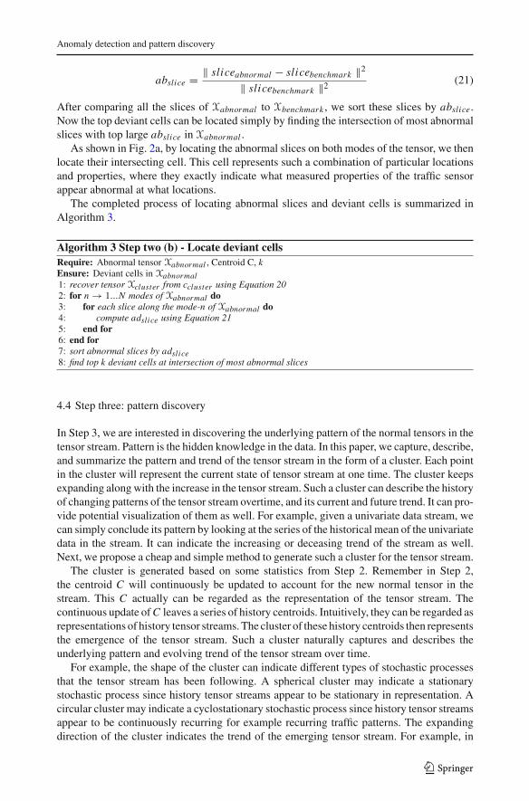
The key idea is to compare the abnormal tensor slices with the benchmark tensor slices.We compare each slice on every mode of Xabnormal with the same slice of Xbenchmark , asillustrated in Fig. 2. We quantify the difference of two slices by Eq. 21. Such a differenceabslice is considered as the indicator of the abnormality of the corresponding tensor slice inXabnormal .

123

Anomaly detection and pattern discovery

abslice = ‖ sliceabnormal − slicebenchmark ‖2

‖ slicebenchmark ‖2 (21)

After comparing all the slices of Xabnormal to Xbenchmark , we sort these slices by abslice.Now the top deviant cells can be located simply by finding the intersection of most abnormalslices with top large abslice in Xabnormal .

As shown in Fig. 2a, by locating the abnormal slices on both modes of the tensor, we thenlocate their intersecting cell. This cell represents such a combination of particular locationsand properties, where they exactly indicate what measured properties of the traffic sensorappear abnormal at what locations.

The completed process of locating abnormal slices and deviant cells is summarized inAlgorithm 3.

Algorithm 3 Step two (b) - Locate deviant cellsRequire: Abnormal tensor Xabnormal , Centroid C, kEnsure: Deviant cells in Xabnormal1: recover tensor Xcluster from ccluster using Equation 202: for n → 1...N modes of Xabnormal do3: for each slice along the mode-n of Xabnormal do4: compute adslice using Equation 215: end for6: end for7: sort abnormal slices by adslice8: find top k deviant cells at intersection of most abnormal slices

4.4 Step three: pattern discovery

In Step 3, we are interested in discovering the underlying pattern of the normal tensors in thetensor stream. Pattern is the hidden knowledge in the data. In this paper, we capture, describe,and summarize the pattern and trend of the tensor stream in the form of a cluster. Each pointin the cluster will represent the current state of tensor stream at one time. The cluster keepsexpanding along with the increase in the tensor stream. Such a cluster can describe the historyof changing patterns of the tensor stream overtime, and its current and future trend. It can pro-vide potential visualization of them as well. For example, given a univariate data stream, wecan simply conclude its pattern by looking at the series of the historical mean of the univariatedata in the stream. It can indicate the increasing or deceasing trend of the stream as well.Next, we propose a cheap and simple method to generate such a cluster for the tensor stream.

The cluster is generated based on some statistics from Step 2. Remember in Step 2,the centroid C will continuously be updated to account for the new normal tensor in thestream. This C actually can be regarded as the representation of the tensor stream. Thecontinuous update of C leaves a series of history centroids. Intuitively, they can be regarded asrepresentations of history tensor streams. The cluster of these history centroids then representsthe emergence of the tensor stream. Such a cluster naturally captures and describes theunderlying pattern and evolving trend of the tensor stream over time.

For example, the shape of the cluster can indicate different types of stochastic processesthat the tensor stream has been following. A spherical cluster may indicate a stationarystochastic process since history tensor streams appear to be stationary in representation. Acircular cluster may indicate a cyclostationary stochastic process since history tensor streamsappear to be continuously recurring for example recurring traffic patterns. The expandingdirection of the cluster indicates the trend of the emerging tensor stream. For example, in

123

L. Shi et al.

a univariate data stream, such a trend only increases or decreases since there are just twodirections in one axis frame. In high-order tensor stream, such a trend is more complicatedbut still can be classified and quantified by the direction that the cluster expands toward.

5 Experiments and results

5.1 Experiment overview

The experiments were conducted on a machine with CPU 3.00 GHZ, 3.25 GB RAM, andrunning Windows XP. All algorithms were implemented in Matlab.

The detailed experiments are divided into two parts:

• We evaluate our approach on synthetic data to identify different types of anomalies anddiscover the data pattern.

• We evaluate our approach on real-world traffic sensor data to identify the real traffic patternand other simulated highway shutdown, traffic jams.

At the same time, we compare the results of our approach to those of the dynamic tensoranalysis (DTA) [21] which is the closest to our approach for detecting anomalies in tensorstream. We only compare the results of the two approaches in comparable cases since DTAcannot handle all kinds of anomalies that our approach can.

Two main metrics, precision and recall, are used for the evaluation of the anomaly detectionresults. The running time is also presented for the evaluation of the performance. We useknown knowledge and ground truth to evaluate the pattern discovery results.

For our approach (referred to as STenSr in the following), reconstruction error thresholdin Step 1 was set to 10 given 90 % precision of factor matrix, standard deviation threshold inStep 2 was set to 3 as we simply assume a normal distribution of distance, and decay factorλ was set to 0.95. For DTA, its forgetting factor was set to 0.95 and its reconstruction errorthreshold was set to 2 standard deviation of all reconstruction errors.

5.2 Synthetic data

In the synthetic data generation, we take into account some important characteristics of thereal-life data. We generate the synthetic tensor as follows. We first generate a base tensor byassigning to each cell a random value drawn from an underlying normal distribution. Thisbase tensor is fixed. Then we create each normal tensor in the stream by building on thebase tensor with a random variation value drawn from another normal distribution, whichhas small mean as compared to the underlying normal distribution. We generate abnormaltensor from normal tensor by considerably increasing the original value of one of its randomcell. Abnormal tensor will be uniformly injected into the tensor stream.

The general experimental setting is as follows. Every tensor stream consists of 450 numberof 2-mode tensors. Each tensor is of size 90000 (300 × 300), which means it contains 90000cells. The first 50 tensors of the stream are all normal, in order for two methods to build somebasic statistics.

5.2.1 Single type of anomaly

We consider single type of anomaly to be anomalies with similar level of significance. Inother words, we generated these anomalies by increasing the original value of the cell by thesame coefficient. In the following experiments, we increase the original value to its tenfold.

123

Anomaly detection and pattern discovery

Table 2 Results for single type of anomaly

Anomalypercentage (%)

Method Average CPU time (s) Anomaly detection

Normal Anomaly Overall Recall (%) Precision (%)

10 STenSr 0.024425 0.024254 0.024407 100 99DTA 0.024387 0.024146 0.024362 97 78

20 STenSr 0.024636 0.024625 0.024633 98 97DTA 0.023685 0.024025 0.023753 95 83

25 STenSr 0.024406 0.024275 0.024373 99 98DTA 0.023394 0.023909 0.023525 68 80

33 STenSr 0.024657 0.024368 0.024560 97 98DTA 0.024243 0.023903 0.024129 23 79

(a) (b)

Fig. 3 Comparison of STenSr and DTA. a Recall rate b Precision rate

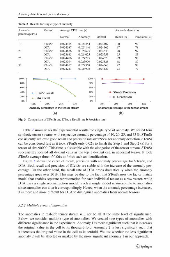
Table 2 summarizes the experimental results for single type of anomaly. We tested foursynthetic tensor streams with respective anomaly percentage of 10, 20, 25, and 33 %. STenSrconsistently achieved good recall and precision rate over 95 % for anomaly detection. STenSrcan be considered fast as it took STenSr only 0.02 s to finish the Step 1 and Step 2 (a) for atensor of size 90000. This time is also stable with the elongation of the tensor stream. STenSrsuccessfully located all deviant cells as the top 1 deviant cell in abnormal tensor. It tookSTenSr average time of 0.06 s to finish such an identification.

Figure 3 shows the curve of recall, precision with anomaly percentage for STenSr, andDTA. Both recall and precision of STenSr are stable with the increase of the anomaly per-centage. On the other hand, the recall rate of DTA drops dramatically when the anomalypercentage goes over 20 %. This may be due to the fact that STenSr uses the factor matrixmodel that enables separate representation for each individual tensor as a row vector, whileDTA uses a single reconstruction model. Such a single model is susceptible to anomaliessince anomalies can alter it correspondingly. Hence, when the anomaly percentage increases,it is more and more difficult for DTA to distinguish anomalies from normal tensors.

5.2.2 Multiple types of anomalies

The anomalies in real-life tensor stream will not be all at the same level of significance.Below, we consider multiple type of anomalies. We created two types of anomalies withdifferent significance in the experiment. Anomaly 1 is more significant such that it increasesthe original value in the cell to its thousand-fold. Anomaly 2 is less significant such thatit increases the original value in the cell to its tenfold. We test whether the less significantanomaly 2 will be affected or masked by the more significant anomaly 1 in our approach.

123

L. Shi et al.

Table 3 Results for multiple types of anomalies

Anomalypercentage (%)

Method Anomaly 1 Anomaly 2

Recall (%) Precision (%) Recall (%) Precision (%)

Anomaly 1: 1 STenSr 100 95 100 99

Anomaly 2: 9

Anomaly 1: 5 STenSr 95 100 100 97

Anomaly 2: 5

Table 4 Results for extreme anomalies

Anomalypercentage (%)

Method Average CPU time (s) Anomaly detection

Normal Abnormal Overall Recall (%) Precision (%)

10 STenSr 0.024908 0.023976 0.024814 100 96

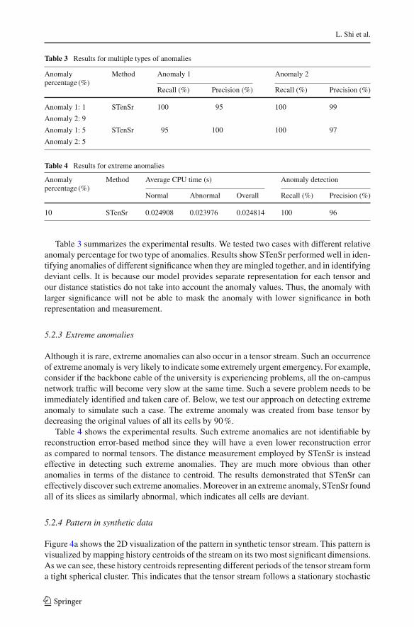
Table 3 summarizes the experimental results. We tested two cases with different relativeanomaly percentage for two type of anomalies. Results show STenSr performed well in iden-tifying anomalies of different significance when they are mingled together, and in identifyingdeviant cells. It is because our model provides separate representation for each tensor andour distance statistics do not take into account the anomaly values. Thus, the anomaly withlarger significance will not be able to mask the anomaly with lower significance in bothrepresentation and measurement.

5.2.3 Extreme anomalies

Although it is rare, extreme anomalies can also occur in a tensor stream. Such an occurrenceof extreme anomaly is very likely to indicate some extremely urgent emergency. For example,consider if the backbone cable of the university is experiencing problems, all the on-campusnetwork traffic will become very slow at the same time. Such a severe problem needs to beimmediately identified and taken care of. Below, we test our approach on detecting extremeanomaly to simulate such a case. The extreme anomaly was created from base tensor bydecreasing the original values of all its cells by 90 %.

Table 4 shows the experimental results. Such extreme anomalies are not identifiable byreconstruction error-based method since they will have a even lower reconstruction erroras compared to normal tensors. The distance measurement employed by STenSr is insteadeffective in detecting such extreme anomalies. They are much more obvious than otheranomalies in terms of the distance to centroid. The results demonstrated that STenSr caneffectively discover such extreme anomalies. Moreover in an extreme anomaly, STenSr foundall of its slices as similarly abnormal, which indicates all cells are deviant.

5.2.4 Pattern in synthetic data

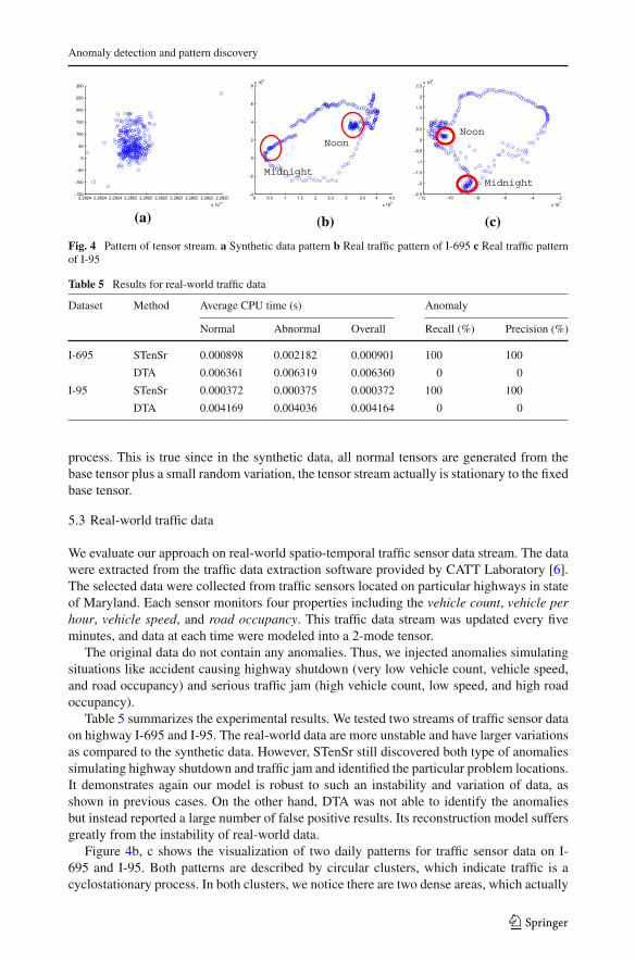
Figure 4a shows the 2D visualization of the pattern in synthetic tensor stream. This pattern isvisualized by mapping history centroids of the stream on its two most significant dimensions.As we can see, these history centroids representing different periods of the tensor stream forma tight spherical cluster. This indicates that the tensor stream follows a stationary stochastic

123

Anomaly detection and pattern discovery

(a) (b) (c)

Fig. 4 Pattern of tensor stream. a Synthetic data pattern b Real traffic pattern of I-695 c Real traffic patternof I-95

Table 5 Results for real-world traffic data

Dataset Method Average CPU time (s) Anomaly

Normal Abnormal Overall Recall (%) Precision (%)

I-695 STenSr 0.000898 0.002182 0.000901 100 100

DTA 0.006361 0.006319 0.006360 0 0

I-95 STenSr 0.000372 0.000375 0.000372 100 100

DTA 0.004169 0.004036 0.004164 0 0

process. This is true since in the synthetic data, all normal tensors are generated from thebase tensor plus a small random variation, the tensor stream actually is stationary to the fixedbase tensor.

5.3 Real-world traffic data

We evaluate our approach on real-world spatio-temporal traffic sensor data stream. The datawere extracted from the traffic data extraction software provided by CATT Laboratory [6].The selected data were collected from traffic sensors located on particular highways in stateof Maryland. Each sensor monitors four properties including the vehicle count, vehicle perhour, vehicle speed, and road occupancy. This traffic data stream was updated every fiveminutes, and data at each time were modeled into a 2-mode tensor.

The original data do not contain any anomalies. Thus, we injected anomalies simulatingsituations like accident causing highway shutdown (very low vehicle count, vehicle speed,and road occupancy) and serious traffic jam (high vehicle count, low speed, and high roadoccupancy).

Table 5 summarizes the experimental results. We tested two streams of traffic sensor dataon highway I-695 and I-95. The real-world data are more unstable and have larger variationsas compared to the synthetic data. However, STenSr still discovered both type of anomaliessimulating highway shutdown and traffic jam and identified the particular problem locations.It demonstrates again our model is robust to such an instability and variation of data, asshown in previous cases. On the other hand, DTA was not able to identify the anomaliesbut instead reported a large number of false positive results. Its reconstruction model suffersgreatly from the instability of real-world data.

Figure 4b, c shows the visualization of two daily patterns for traffic sensor data on I-695 and I-95. Both patterns are described by circular clusters, which indicate traffic is acyclostationary process. In both clusters, we notice there are two dense areas, which actually

123

L. Shi et al.

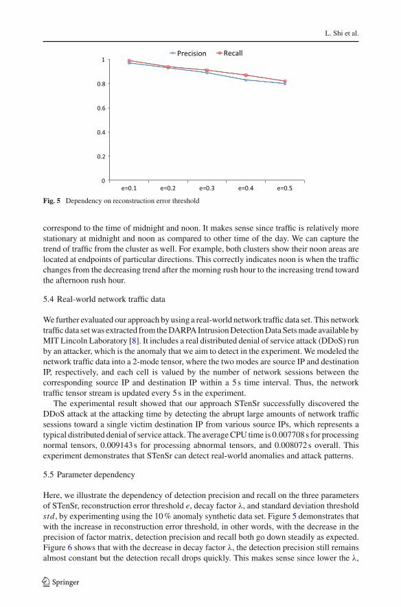
Fig. 5 Dependency on reconstruction error threshold

correspond to the time of midnight and noon. It makes sense since traffic is relatively morestationary at midnight and noon as compared to other time of the day. We can capture thetrend of traffic from the cluster as well. For example, both clusters show their noon areas arelocated at endpoints of particular directions. This correctly indicates noon is when the trafficchanges from the decreasing trend after the morning rush hour to the increasing trend towardthe afternoon rush hour.

5.4 Real-world network traffic data

We further evaluated our approach by using a real-world network traffic data set. This networktraffic data set was extracted from the DARPA Intrusion Detection Data Sets made available byMIT Lincoln Laboratory [8]. It includes a real distributed denial of service attack (DDoS) runby an attacker, which is the anomaly that we aim to detect in the experiment. We modeled thenetwork traffic data into a 2-mode tensor, where the two modes are source IP and destinationIP, respectively, and each cell is valued by the number of network sessions between thecorresponding source IP and destination IP within a 5 s time interval. Thus, the networktraffic tensor stream is updated every 5 s in the experiment.

The experimental result showed that our approach STenSr successfully discovered theDDoS attack at the attacking time by detecting the abrupt large amounts of network trafficsessions toward a single victim destination IP from various source IPs, which represents atypical distributed denial of service attack. The average CPU time is 0.007708 s for processingnormal tensors, 0.009143 s for processing abnormal tensors, and 0.008072 s overall. Thisexperiment demonstrates that STenSr can detect real-world anomalies and attack patterns.

5.5 Parameter dependency

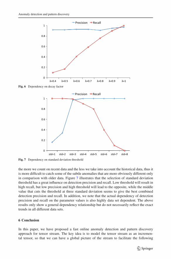
Here, we illustrate the dependency of detection precision and recall on the three parametersof STenSr, reconstruction error threshold e, decay factor λ, and standard deviation thresholdstd , by experimenting using the 10 % anomaly synthetic data set. Figure 5 demonstrates thatwith the increase in reconstruction error threshold, in other words, with the decrease in theprecision of factor matrix, detection precision and recall both go down steadily as expected.Figure 6 shows that with the decrease in decay factor λ, the detection precision still remainsalmost constant but the detection recall drops quickly. This makes sense since lower the λ,

123

Anomaly detection and pattern discovery

Fig. 6 Dependency on decay factor

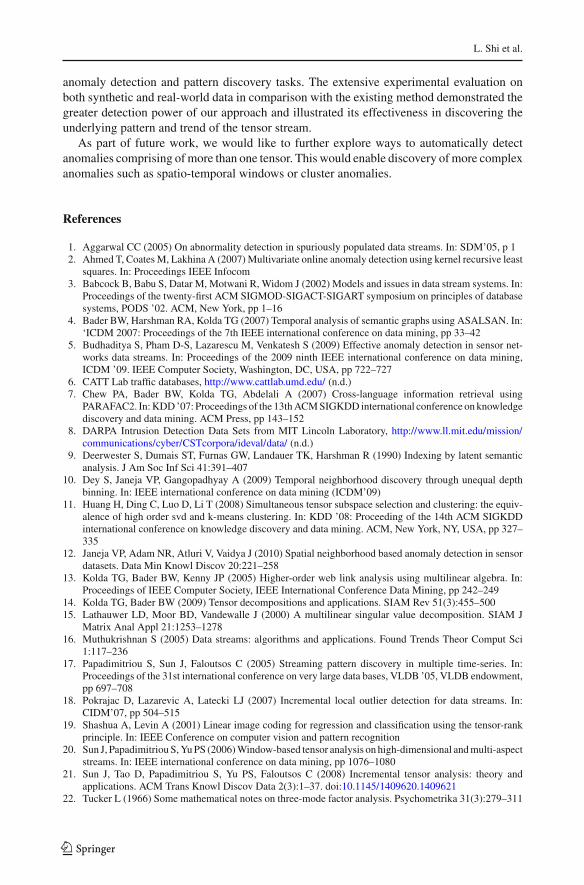
Fig. 7 Dependency on standard deviation threshold

the more we count on recent data and the less we take into account the historical data, thus itis more difficult to catch some of the subtle anomalies that are more obviously different onlyin comparison with older data. Figure 7 illustrates that the selection of standard deviationthreshold has a great influence on detection precision and recall. Low threshold will result inhigh recall, but low precision and high threshold will lead to the opposite, while the middlevalue that cuts the threshold at three standard deviation seems to give the best combineddetection precision and recall. In addition, we note that the actual dependency of detectionprecision and recall on the parameter values is also highly data set dependent. The aboveresults only show a general dependency relationship but do not necessarily reflect the exacttrends in all different data sets.

6 Conclusion

In this paper, we have proposed a fast online anomaly detection and pattern discoveryapproach for tensor stream. The key idea is to model the tensor stream as an incremen-tal tensor, so that we can have a global picture of the stream to facilitate the following

123

L. Shi et al.

anomaly detection and pattern discovery tasks. The extensive experimental evaluation onboth synthetic and real-world data in comparison with the existing method demonstrated thegreater detection power of our approach and illustrated its effectiveness in discovering theunderlying pattern and trend of the tensor stream.

As part of future work, we would like to further explore ways to automatically detectanomalies comprising of more than one tensor. This would enable discovery of more complexanomalies such as spatio-temporal windows or cluster anomalies.

References

1. Aggarwal CC (2005) On abnormality detection in spuriously populated data streams. In: SDM’05, p 12. Ahmed T, Coates M, Lakhina A (2007) Multivariate online anomaly detection using kernel recursive least

squares. In: Proceedings IEEE Infocom3. Babcock B, Babu S, Datar M, Motwani R, Widom J (2002) Models and issues in data stream systems. In:

Proceedings of the twenty-first ACM SIGMOD-SIGACT-SIGART symposium on principles of databasesystems, PODS ’02. ACM, New York, pp 1–16

4. Bader BW, Harshman RA, Kolda TG (2007) Temporal analysis of semantic graphs using ASALSAN. In:‘ICDM 2007: Proceedings of the 7th IEEE international conference on data mining, pp 33–42

5. Budhaditya S, Pham D-S, Lazarescu M, Venkatesh S (2009) Effective anomaly detection in sensor net-works data streams. In: Proceedings of the 2009 ninth IEEE international conference on data mining,ICDM ’09. IEEE Computer Society, Washington, DC, USA, pp 722–727

6. CATT Lab traffic databases, http://www.cattlab.umd.edu/ (n.d.)7. Chew PA, Bader BW, Kolda TG, Abdelali A (2007) Cross-language information retrieval using

PARAFAC2. In: KDD ’07: Proceedings of the 13th ACM SIGKDD international conference on knowledgediscovery and data mining. ACM Press, pp 143–152

8. DARPA Intrusion Detection Data Sets from MIT Lincoln Laboratory, http://www.ll.mit.edu/mission/communications/cyber/CSTcorpora/ideval/data/ (n.d.)

9. Deerwester S, Dumais ST, Furnas GW, Landauer TK, Harshman R (1990) Indexing by latent semanticanalysis. J Am Soc Inf Sci 41:391–407

10. Dey S, Janeja VP, Gangopadhyay A (2009) Temporal neighborhood discovery through unequal depthbinning. In: IEEE international conference on data mining (ICDM’09)

11. Huang H, Ding C, Luo D, Li T (2008) Simultaneous tensor subspace selection and clustering: the equiv-alence of high order svd and k-means clustering. In: KDD ’08: Proceeding of the 14th ACM SIGKDDinternational conference on knowledge discovery and data mining. ACM, New York, NY, USA, pp 327–335

12. Janeja VP, Adam NR, Atluri V, Vaidya J (2010) Spatial neighborhood based anomaly detection in sensordatasets. Data Min Knowl Discov 20:221–258

13. Kolda TG, Bader BW, Kenny JP (2005) Higher-order web link analysis using multilinear algebra. In:Proceedings of IEEE Computer Society, IEEE International Conference Data Mining, pp 242–249

14. Kolda TG, Bader BW (2009) Tensor decompositions and applications. SIAM Rev 51(3):455–50015. Lathauwer LD, Moor BD, Vandewalle J (2000) A multilinear singular value decomposition. SIAM J

Matrix Anal Appl 21:1253–127816. Muthukrishnan S (2005) Data streams: algorithms and applications. Found Trends Theor Comput Sci

1:117–23617. Papadimitriou S, Sun J, Faloutsos C (2005) Streaming pattern discovery in multiple time-series. In:

Proceedings of the 31st international conference on very large data bases, VLDB ’05, VLDB endowment,pp 697–708

18. Pokrajac D, Lazarevic A, Latecki LJ (2007) Incremental local outlier detection for data streams. In:CIDM’07, pp 504–515

19. Shashua A, Levin A (2001) Linear image coding for regression and classification using the tensor-rankprinciple. In: IEEE Conference on computer vision and pattern recognition

20. Sun J, Papadimitriou S, Yu PS (2006) Window-based tensor analysis on high-dimensional and multi-aspectstreams. In: IEEE international conference on data mining, pp 1076–1080

21. Sun J, Tao D, Papadimitriou S, Yu PS, Faloutsos C (2008) Incremental tensor analysis: theory andapplications. ACM Trans Knowl Discov Data 2(3):1–37. doi:10.1145/1409620.1409621

22. Tucker L (1966) Some mathematical notes on three-mode factor analysis. Psychometrika 31(3):279–311

123

Anomaly detection and pattern discovery

23. Vasilescu MAO, Terzopoulos D (2002) Multilinear image analysis for facial recognition. Int Conf PatternRecognit 2:20511

24. Wang H, Ahuja N (2003) Facial expression decomposition. In: ICCV, pp 958–96525. Zha H, Simon HD (1999) On updating problems in latent semantic indexing. SIAM J Sci Comput

21(2):782–791

Lei Shi received his B.E. degree in Computer Science and Technol-ogy from Zhejiang University, China, in 2006, and is currently pursuingthe Ph.D. degree at the department of Information Systems at the Uni-versity of Maryland Baltimore County (UMBC). His research interestsinclude spatio-temporal data mining, privacy preserving data mining,high-dimensional data mining, and anomaly detection.

Aryya Gangopadhyay is a professor and the chair of InformationSystems at the University of Maryland Baltimore County (UMBC).Dr. Gangopadhyay’s research interests are in the areas of databasesand data mining. Currently, he is focused on privacy preserving datamining, spatio-temporal data mining, and data mining for health infor-matics. His research has been funded by grants from NSF, NIST, USDepartment of Education, Maryland Department of Transportation, andother agencies. Dr. Gangopadhyay has published five books and nearly100 research articles. He holds a Ph.D. in Computer Information Sys-tems from Rutgers University.

Vandana P. Janeja received her Ph.D. and M.B.A in Informationtechnology from Rutgers Business School, Rutgers University, in 2007.She is currently an Assistant Professor at the Information Systemsdepartment at the University of Maryland Baltimore County (UMBC),USA. Her general area of research is Data Mining with a focus onanomaly detection in traditional and spatial data. She has published invarious refereed conferences such as ICDM, KDD, and SIAM and jour-nals such as TKDE and DMKD.

123