dimensional-reduction anomaly
TRANSCRIPT

arX
iv:h
ep-t
h/99
0908
6v3
9 O
ct 1
999
Alberta-Thy-15-99
The Dimensional-Reduction Anomaly
V. Frolov∗ and P. Sutton†
Theoretical Physics Institute, Department of Physics,
University of Alberta, Edmonton, Canada T6G 2J1
A. Zelnikov‡
Theoretical Physics Institute, Department of Physics,
University of Alberta, Edmonton, Canada T6G 2J1
and Lebedev Physics Institute, Leninsky Prospect 53,
Moscow 117924, Russia
Oct. 9, 1999
Abstract
In a wide class of D-dimensional spacetimes which are direct or semi-direct sumsof a (D−n)-dimensional space and an n-dimensional homogeneous “internal” space,a field can be decomposed into modes. As a result of this mode decomposition, themain objects which characterize the free quantum field, such as Green functions andheat kernels, can effectively be reduced to objects in a (D−n)-dimensional spacetimewith an external dilaton field. We study the problem of the dimensional reductionof the effective action for such spacetimes. While before renormalization the originalD-dimensional effective action can be presented as a “sum over modes” of (D −n)-dimensional effective actions, this property is violated after renormalization. Wecalculate the corresponding anomalous terms explicitly, illustrating the effect withsome simple examples.
∗e-mail: [email protected]†e-mail: [email protected]‡e-mail: [email protected]
1

1 Introduction
Simplifications connected with an assumption of symmetry play an important role inthe study of physical effects in a curved spacetime. In this paper we consider quantumfields propagating in a D-dimensional spacetime which is a semi-direct sum of a (D− n)-dimensional space and an n-dimensional homogeneous “internal” space. Such a field canbe decomposed into modes. As a result of this mode decomposition, the main objectswhich characterize the free quantum field, such as Green functions and heat kernels,can effectively be reduced to objects in a (D−n)-dimensional spacetime with an externaldilaton field. Our aim is to study the problem of the dimensional reduction of the effectiveaction for such spacetimes. We shall demonstrate that while before renormalization theoriginal D-dimensional effective action can be presented as a “sum over modes” of (D−n)-dimensional effective actions, this property is generically violated after renormalization.We call this effect the dimensional-reduction anomaly.
First of all, there is an evident general reason why D-dimensional renormalization isnot equivalent to renormalization of the (D−n)-dimensional effective theory. Namely, thenumber of divergent terms of the Schwinger-DeWitt series which is used to renormalizea given object depends on the number of dimensions. What is much more interesting isthat this is not the only reason for the presence of the dimensional-reduction anomaly.The aim of this paper is to discuss this problem and to derive explicit expressions forthe dimensional-reduction anomaly in a four-dimensional spacetime with special choicesof one- and two-dimensional homogeneous internal spaces.
In some aspects the problem we study is related to the study of the momentum-space representation of the ultraviolet divergences discussed by Bunch and Parker [1].Nevertheless, there exists a very important difference. Namely, Bunch and Parker used theFourier transform with respect to all D dimensions (D = 4 in their paper) in a spacetimewithout symmetries. We are making mode decompositions with respect to n internaldimensions only. Moreover, due to the symmetry we effectively rewrite the original D-dimensional theory in terms of a set of (D−n)-dimensional effective theories with a dilatonfield. This representation, which was absent in the paper by Bunch and Parker, allows usto make the comparison of renormalization in D- and (D − n)-dimensional theories.
The dimensional-reduction anomaly discussed in this paper might have interesting ap-plications. One of them is connected with black-hole physics. Recently there has beenmuch interest in the study of the Hawking radiation in two-dimensional dilaton gravitymodels of a black hole. This study was initiated by the paper [2]. In this and otherpapers on the subject (see e.g. [3]–[6]) it is either explicitly or implicitly assumed thattwo-dimensional calculations (at least for the special choice of the dilaton field correspond-ing to the spherical reduction of the four-dimensional Schwarzschild spacetime) correctlyreproduce the s-mode contribution to the stress-energy tensor of the four-dimensionaltheory. Generally speaking, in the presence of the dimensional-reduction anomaly this isnot true (see also the discussion in [7]).
It is interesting to note that in a numerical study of the vacuum polarization in blackholes where the mode decomposition was used, it has been demonstrated that one alwaysneeds to add extra contributions to the terms of the series in order to ensure convergenceof the series (see e.g. [8, 9, 10]). This fact, as we shall see, is a direct manifestation of thedimensional-reduction anomaly.
The paper is organized as follows. Section 2 contains a general discussion of the
2
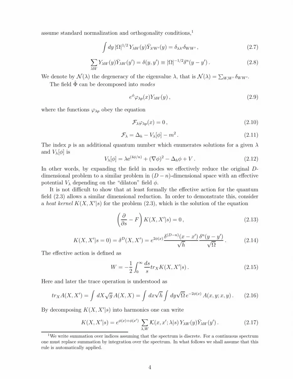
dimensional reduction of a free quantum field theory in a gravitational background. InSection 3 we discuss simple examples of the dimensional reduction of four-dimensional flatspacetime and illustrate the effect of the dimensional-reduction anomaly. In Sections 4and 5 we derive the dimensional-reduction anomaly for 〈Φ2〉ren and 〈T µ
ν 〉ren in a four-dimensional spacetime for (3 +1) and (2+ 2) reductions. We discuss the obtained resultsin the Conclusion. In our work we use dimensionless units where G = c = h = 1, and thesign conventions of [12] for the definition of the curvature.
2 Dimensional Reduction of the Heat Kernel and the
Effective Action
Consider a D-dimensional spacetime with a metric of the form
ds2 = gµν dXµ dXν = dh2 + e−(4φ/n)dΩ2 , Xµ = (xa, yi) , (2.1)
φ = φ(xc) , dh2 = hab(xc)dxadxb , dΩ2 = Ωij(y
k)dyidyj , (2.2)
where dΩ2 is the metric of an n-dimensional homogeneous space. In other words, themetric ds2 is a semi-direct sum of dh2 and dΩ2. We call the n-dimensional space withmetric dΩ2 the internal space, and the scalar field φ(xc) on the (D − n)-dimensionalmanifold with metric dh2 the dilaton field. Let us emphasize that the normalization ofthe dilaton field φ is a question of convenience. We fix this normalization by requiringthat
√g for the metric (2.1) be proportional to exp(−2φ) for any number of internal
dimensions n. Well-known examples of metrics of the form (2.1) are those of sphericalspacetimes, and metrics connected with a dimensional reduction in Kaluza-Klein theories.
Let Φ be a free scalar quantum field propagating in the spacetime (2.1) and obeyingthe equation
F Φ(X) = 0 , (2.3)
with field operatorF = 2 − V − m2 . (2.4)
Note that we explicitly separate the mass term m2 from the potential V . The latter maycontain an interaction with the curvature, ξR, for a non-minimally coupled field, but isnot fixed at the moment. We only assume that when calculated on the background (2.1)the potential V is independent of the ya coordinates.
Using the line element (2.1), the operator 2 becomes
2 = ∆h − 2∇φ · ∇ + e(4φ/n)∆Ω , (2.5)
where ∆h, ∆Ω are the d’Alembertians corresponding to the metrics hab, Ωij respectively,and ∇ is understood to denote the covariant derivative with respect to the metric hab.
Considerable simplification of the problem in spacetime (2.1) is connected with thefact that for a wide class of homogeneous metrics the eigenvalue problem
∆ΩY (y) = −λY (y) , (2.6)
is well-studied. We denote by YλW harmonics, that is eigenfunctions of (2.6), and use a(collective) index W to distinguish between different solutions of (2.6) for the same λ. We
3
assume standard normalization and orthogonality conditions,1
∫
dy |Ω|1/2 YλW (y)Yλ′W ′(y) = δλλ′δWW ′ , (2.7)
∑
λW
YλW (y)YλW (y′) = δ(y, y′) ≡ |Ω|−1/2δn(y − y′) . (2.8)
We denote by N (λ) the degeneracy of the eigenvalue λ, that is N (λ) =∑
W,W ′ δWW ′.
The field Φ can be decomposed into modes
eφϕλp(x)YλW (y) , (2.9)
where the functions ϕλp obey the equation
Fλϕλp(x) = 0 , (2.10)
Fλ = ∆h − Vλ[φ] − m2 . (2.11)
The index p is an additional quantum number which enumerates solutions for a given λand Vλ[φ] is
Vλ[φ] = λe(4φ/n) + (∇φ)2 − ∆hφ + V . (2.12)
In other words, by expanding the field in modes we effectively reduce the original D-dimensional problem to a similar problem in (D − n)-dimensional space with an effectivepotential Vλ depending on the “dilaton” field φ.
It is not difficult to show that at least formally the effective action for the quantumfield (2.3) allows a similar dimensional reduction. In order to demonstrate this, considera heat kernel K(X, X ′|s) for the problem (2.3), which is the solution of the equation
(
∂
∂s− F
)
K(X, X ′|s) = 0 , (2.13)
K(X, X ′|s = 0) = δD(X, X ′) = e2φ(x) δ(D−n)(x − x′)√
h
δn(y − y′)√Ω
. (2.14)
The effective action is defined as
W = −1
2
∫ ∞
0
ds
strXK(X, X ′|s) . (2.15)
Here and later the trace operation is understood as
trXA(X, X ′) =∫
dX√
g A(X, X) =∫
dx√
h∫
dy√
Ω e−2φ(x) A(x, y; x, y) . (2.16)
By decomposing K(X, X ′|s) into harmonics one can write
K(X, X ′|s) = eφ(x)+φ(x′)∑
λ,W
K(x, x′; λ|s) YλW (y)YλW (y′) . (2.17)
1We write summation over indices assuming that the spectrum is discrete. For a continuous spectrumone must replace summation by integration over the spectrum. In what follows we shall assume that thisrule is automatically applied.
4

Using relations (2.5)–(2.8), it is easy to verify that the reduced heat kernel K(x, x′; λ|s)obeys the relations
(
∂
∂s−Fλ
)
K(x, x′; λ|s) = 0 , (2.18)
K(x, x′; λ|s = 0) = δ(D−n)(x, x′) =δ(D−n)(x − x′)√
h. (2.19)
Here the operator Fλ is given by (2.10)–(2.11).Substituting representation (2.17) into the effective action (2.15), integrating over the
y-variables, and using (2.7), one gets
W =∑
λ
N (λ)Wλ , (2.20)
where
Wλ = −1
2
∫ ∞
0
ds
strxK(x, x′; λ|s) . (2.21)
HeretrxK(x, x′; λ|s) =
∫
dx√
hK(x, x; λ|s) , (2.22)
and N (λ) is the degeneracy factor of the eigenvalue λ. Relations (2.20)–(2.21) can beinterpreted as the mode decomposition of the effective action.
It should be emphasized that the above relations for the effective action are strictlyformal because of the presence of ultraviolet divergences. In order to obtain the renor-malized value of the effective action in D-dimensional spacetime one must subtract fromtrXK(X, X ′|s) the first ND terms of the Schwinger-DeWitt expansion of the heat kernel,where
ND =
D2
+ 1 for D even,
D+12
for D odd.(2.23)
Our main observation is that this procedure destroys the formal representation (2.20), sothat after renormalization one gets
W ren =∑
λ
N (λ) [W ren
λ + ∆Wλ] . (2.24)
In this expression W ren
λ is understood as the renormalized effective action of the (D − n)-dimensional theory with a dilaton field, (2.10), where the renormalization is performedby subtracting the first ND−n terms of the Schwinger-DeWitt expansion for the operatorFλ. We call the additional contribution ∆Wλ the dimensional-reduction anomaly. Arepresentation similar to (2.24) is also valid for 〈Φ2〉ren,
〈Φ2〉ren = e2φ∑
λ
N (λ)[
〈Φ2〉ren
λ + ∆〈Φ2〉λ]
. (2.25)
One might observe that there exists a relationship between the dimensional-reductionanomaly and the so-called multiplicative anomaly [13, 14]. Formally, we can write
F =∏
λ,W
Fλ , (2.26)
5

− 1
2log det F = −1
2
∑
λ
N(λ) log detFλ . (2.27)
The latter relation is nothing but (2.20). The violation of the formal relation (2.27) forproducts of operators after renormalization is known as the multiplicative anomaly.
The aim of this paper is to discuss special examples of the dimensional-reductionanomaly. In what follows, we restrict ourselves to the physically interesting case wherethe number of spacetime dimensions is 4, and the number of dimensions of the “inter-nal” homogeneous space is 1 or 2. We also restrict ourselves to manifolds of Euclideansignature. In each case the anomaly is found as the difference between the renormaliza-tion terms for the (D−n)-dimensional theory and the mode-decomposed renormalizationterms from D dimensions.
3 Flat Space Examples of the Dimensional-Reduction
Anomaly
The dimensional-reduction anomaly can occur in even the simple case of mode decom-position in a flat spacetime. In order to demonstrate this, let us consider a free massivescalar field Φ obeying the equation
F Φ = (2 − m2)Φ = 0 (3.1)
in four-dimensional flat Euclidean space. The Euclidean Green function for this equationis
G0(X, X ′) =m
4π2√
2σK1(m
√2σ) , (3.2)
where 2σ is the square of the geodesic distance from X to X ′, and K1 is a modified Besselfunction. If there exists a boundary Σ surrounding the region M under considerationand the field obeys a non-trivial boundary condition at Σ, or equation (3.1) includes anon-vanishing potential V which vanishes in M, then the Green function would differfrom G0. We denote this Green function by G(X, X ′). The renormalized Green functionin this case is defined as2
Gren(X, X ′) = G(X, X ′) − G0(X, X ′) . (3.3)
We also have〈Φ2(X)〉ren = lim
X′→XGren(X, X ′) . (3.4)
It is evident that 〈Φ2(X)〉ren = 0 in the absence of the external field V and boundaries.In this section we derive the dimensional-reduction anomaly in 〈Φ2〉ren for two examples
of mode decompositions in flat space. In each case, the anomaly is calculated as thedifference between the subtraction terms used to renormalize the Green function G of thedimensionally-reduced theory, and the G0 used to renormalize the four-dimensional Greenfunction G. These calculations are easily repeated for the heat kernel, allowing one toobtain the anomaly in the effective action in a similar manner.
2In a generic four-dimensional curved background, one has to subtract the first two terms in theSchwinger-DeWitt expansion for the heat kernel of the operator F .
6
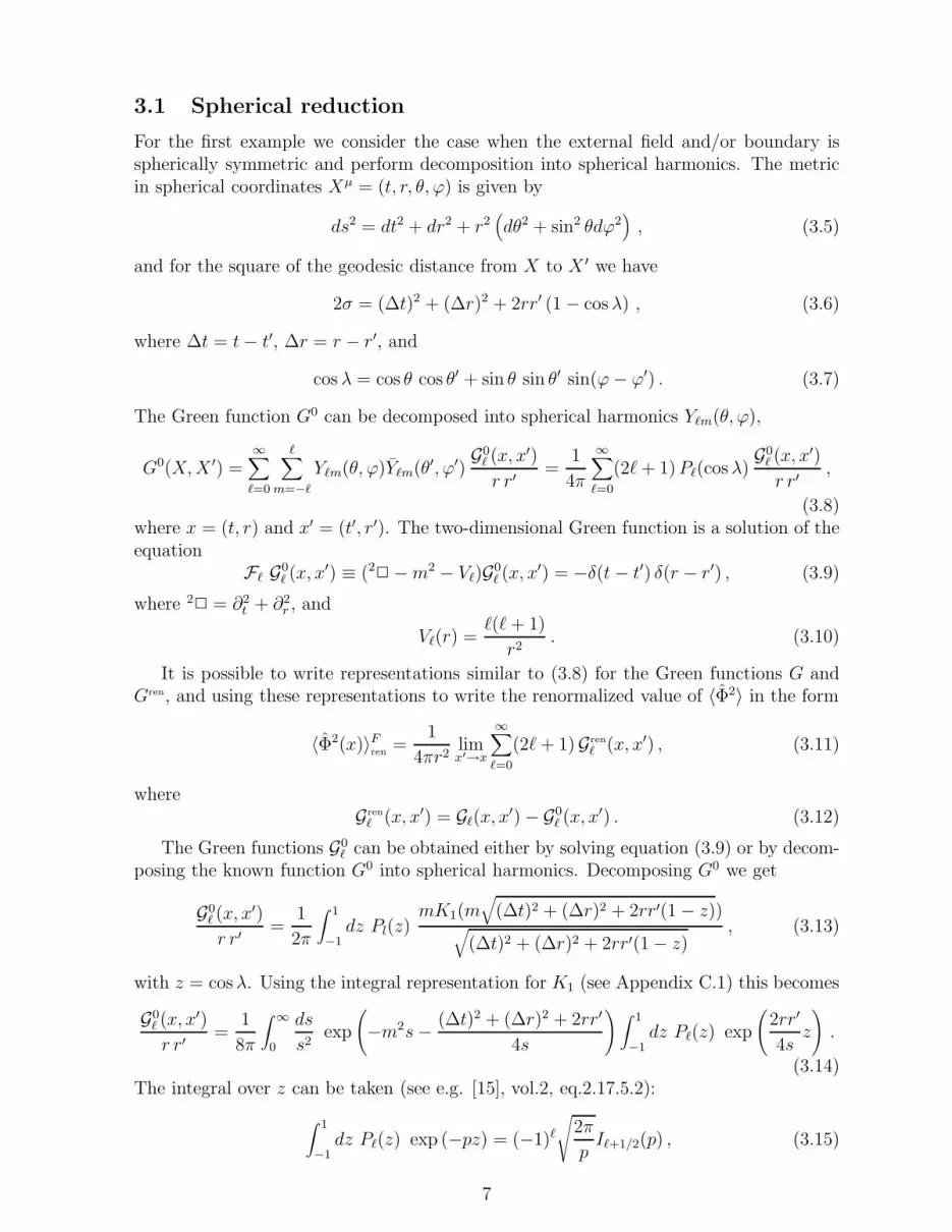
3.1 Spherical reduction
For the first example we consider the case when the external field and/or boundary isspherically symmetric and perform decomposition into spherical harmonics. The metricin spherical coordinates Xµ = (t, r, θ, ϕ) is given by
ds2 = dt2 + dr2 + r2(
dθ2 + sin2 θdϕ2)
, (3.5)
and for the square of the geodesic distance from X to X ′ we have
2σ = (∆t)2 + (∆r)2 + 2rr′ (1 − cos λ) , (3.6)
where ∆t = t − t′, ∆r = r − r′, and
cos λ = cos θ cos θ′ + sin θ sin θ′ sin(ϕ − ϕ′) . (3.7)
The Green function G0 can be decomposed into spherical harmonics Yℓm(θ, ϕ),
G0(X, X ′) =∞∑
ℓ=0
ℓ∑
m=−ℓ
Yℓm(θ, ϕ)Yℓm(θ′, ϕ′)G0
ℓ (x, x′)
r r′=
1
4π
∞∑
ℓ=0
(2ℓ + 1) Pℓ(cos λ)G0
ℓ (x, x′)
r r′,
(3.8)where x = (t, r) and x′ = (t′, r′). The two-dimensional Green function is a solution of theequation
Fℓ G0ℓ (x, x′) ≡ (2
2 − m2 − Vℓ)G0ℓ (x, x′) = −δ(t − t′) δ(r − r′) , (3.9)
where 22 = ∂2
t + ∂2r , and
Vℓ(r) =ℓ(ℓ + 1)
r2. (3.10)
It is possible to write representations similar to (3.8) for the Green functions G andGren, and using these representations to write the renormalized value of 〈Φ2〉 in the form
〈Φ2(x)〉Fren
=1
4πr2limx′→x
∞∑
ℓ=0
(2ℓ + 1)Gren
ℓ (x, x′) , (3.11)
whereGren
ℓ (x, x′) = Gℓ(x, x′) − G0ℓ (x, x′) . (3.12)
The Green functions G0ℓ can be obtained either by solving equation (3.9) or by decom-
posing the known function G0 into spherical harmonics. Decomposing G0 we get
G0ℓ (x, x′)
r r′=
1
2π
∫ 1
−1dz Pl(z)
mK1(m√
(∆t)2 + (∆r)2 + 2rr′(1 − z))√
(∆t)2 + (∆r)2 + 2rr′(1 − z), (3.13)
with z = cos λ. Using the integral representation for K1 (see Appendix C.1) this becomes
G0ℓ (x, x′)
r r′=
1
8π
∫ ∞
0
ds
s2exp
(
−m2s − (∆t)2 + (∆r)2 + 2rr′
4s
)
∫ 1
−1dz Pℓ(z) exp
(
2rr′
4sz
)
.
(3.14)The integral over z can be taken (see e.g. [15], vol.2, eq.2.17.5.2):
∫ 1
−1dz Pℓ(z) exp (−pz) = (−1)ℓ
√
2π
pIℓ+1/2(p) , (3.15)
7

where Iℓ+1/2 is a modified Bessel function. Since for ℓ ≥ 1 the expression in the right-handside of (3.15) vanishes at p = 0, one can easily show that the functions G0
ℓ (x, x′) vanishfor all ℓ when either r = 0 or r′ = 0. This property will be of some importance for theanomaly.
Using the following representation for the function Iℓ+1/2
Iℓ+1/2(p) =1√2πp
ℓ∑
k=0
(ℓ + k)!
k!(ℓ − k)!
1
(2p)k
[
(−1)kep − (−1)ℓe−p]
, (3.16)
(see, for example, 8.467 of [16]), we obtain for the reduced Green functions
G0ℓ (x, x′) =
1
2π
ℓ∑
k=0
(ℓ + k)!
k!(ℓ − k)!
[
(−1)k ((∆t)2 + (∆r)2)k/2
(2mrr′)kKk(m
√
(∆t)2 + (∆r)2)
− (−1)ℓ ((∆t)2 + (∆r)2 + 4rr′)k/2
(2mrr′)kKk(m
√
(∆t)2 + (∆r)2 + 4rr′)
]
.(3.17)
Until now we were working with the series representation for the four-dimensionalGreen function G0. On the other hand, one can start with the two-dimensional theorydefined by (3.9). In order to calculate the two-dimensional quantity 〈Φ2(X)〉Fℓ
renfor the
two-dimensional operator Fℓ, one subtracts from the Green function Gℓ(x, x′) the free-fieldGreen function3, and takes the coincidence limit:
〈Φ2(x)〉Fℓren
= limx′→x
[Gℓ(x, x′) − Gdiv
ℓ (x, x′)] , (3.18)
where the two-dimensional free-field Green function is
Gdiv
ℓ (x, x′) =1
2πK0(m
√
(∆t)2 + (∆r)2) . (3.19)
Note that Gdiv
ℓ is identical to the first term in the first sum for G0ℓ in (3.17).
By comparing (3.11)–(3.12) with (3.18) we get
〈Φ2(x)〉Fren
=1
4πr2
∞∑
ℓ=0
(2ℓ + 1)[
〈Φ2(x)〉Fℓren
+ ∆〈Φ2(r)〉ℓ]
, (3.20)
where the anomalous term ∆〈Φ2〉ℓ is given by
∆〈Φ2(r)〉ℓ = limx′→x
[
Gdiv
ℓ (x, x′) − G0ℓ (x, x′)
]
(3.21)
=1
4π
ℓ∑
k=1
(ℓ + k)!
(ℓ − k)!
1
k
(−1)k+1
(mr)2k+
(−1)ℓ
2π
ℓ∑
k=0
(ℓ + k)!
k!(ℓ − k)!
Kk(2mr)
(mr)k. (3.22)
For example,
∆〈Φ2(r)〉ℓ=0 =1
2πK0(2mr)
∆〈Φ2(r)〉ℓ=1 =1
2π
[
1
(mr)2− K0(2mr) − 2
(mr)K1(2mr)
]
(3.23)
∆〈Φ2(r)〉ℓ=2 =1
2π
[
3
(mr)2− 6
(mr)4+ K0(2mr) +
6
(mr)K1(2mr) +
12
(mr)2K2(2mr)
]
.
3 In two dimensions, renormalization consists of subtracting only the first term of the Schwinger-DeWitt expansion of the heat kernel for the operator Fℓ. In flat spacetime this is equivalent to thesubtraction of the free-field Green function, even in the presence of the dilaton field and a nontrivialpotential V .
8
Relation (3.20) explicitly demonstrates that 〈Φ2(x)〉Fren
can be expressed as a sum overmodes of 〈Φ2(x)〉Fℓ
renfrom the corresponding two-dimensional theory. However, to obtain
the correct result we see that each term in the decomposition must be modified by addingthe state-independent quantity ∆〈Φ2(r)〉ℓ of (3.21). Failure to account for these extrasterms would result, for example, in a nonzero value for 〈Φ2(x)〉F
renin the Minkowski state.
The violation of the expected mode decomposition for a physical observable in theprocess of dimensional reduction due to the renormalization procedure is called thedimensional-reduction anomaly. In this particular example the dimensional-reductionanomaly is given explicitly by (3.22). There are several reasons why this anomaly arises.First, the number of divergent terms which are to be subtracted in the renormalizationprocedure is different in 4 and 2 dimensions (see the footnotes on pages 6 and 8). How-ever, it is easily shown that even if we make an additional subtraction of the next termof the Schwinger-DeWitt expansion in two dimensions, for ℓ ≥ 2 there remains a non-vanishing “local” part of the dimensional-reduction anomaly which is given by the firstsum in (3.22), with k ≥ 2. Besides this local contribution, in our particular case thereis a “non-local” part to the anomaly given by the second sum. It is present because thetwo-dimensional (t, r) space is a half-plane and the two-dimensional field vanishes at theboundary r = 0. While the mode-decomposed subtraction term G0
ℓ from four dimensionsobeys this boundary condition, the two-dimensional subtraction term Gdiv
ℓ does not.
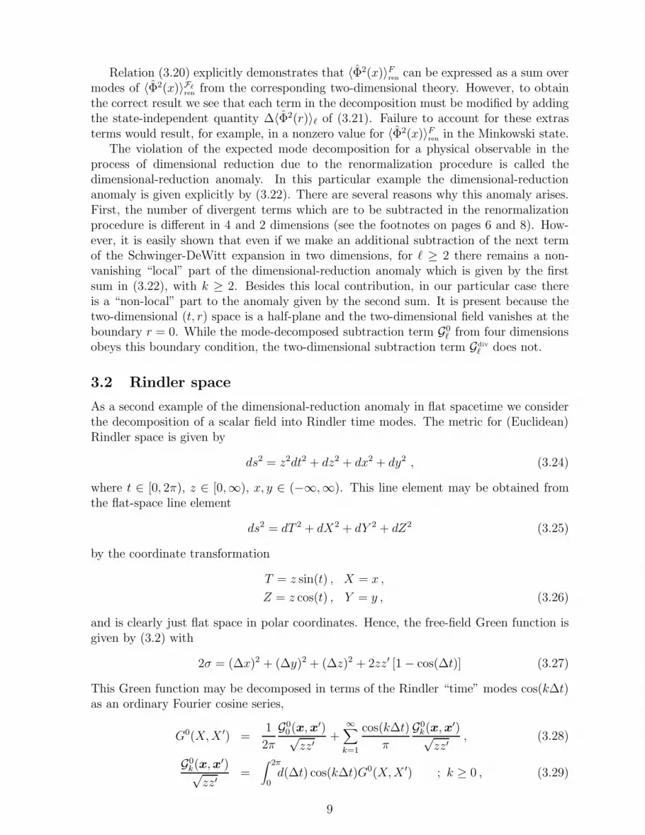
3.2 Rindler space
As a second example of the dimensional-reduction anomaly in flat spacetime we considerthe decomposition of a scalar field into Rindler time modes. The metric for (Euclidean)Rindler space is given by
ds2 = z2dt2 + dz2 + dx2 + dy2 , (3.24)
where t ∈ [0, 2π), z ∈ [0,∞), x, y ∈ (−∞,∞). This line element may be obtained fromthe flat-space line element
ds2 = dT 2 + dX2 + dY 2 + dZ2 (3.25)
by the coordinate transformation
T = z sin(t) , X = x ,
Z = z cos(t) , Y = y , (3.26)
and is clearly just flat space in polar coordinates. Hence, the free-field Green function isgiven by (3.2) with
2σ = (∆x)2 + (∆y)2 + (∆z)2 + 2zz′ [1 − cos(∆t)] (3.27)
This Green function may be decomposed in terms of the Rindler “time” modes cos(k∆t)as an ordinary Fourier cosine series,
G0(X, X ′) =1
2π
G00(x, x′)√
zz′+
∞∑
k=1
cos(k∆t)
π
G0k(x, x′)√
zz′, (3.28)
G0k(x, x′)√
zz′=
∫ 2π
0d(∆t) cos(k∆t)G0(X, X ′) ; k ≥ 0 , (3.29)
9

where x = (x, y, z). The three-dimensional Green function G0k(x, x′) is a solution of the
equation
Fk G0k(x, x′) ≡ (3
2 − m2 − Vk)G0k(x, x′) = −δ(x − x′) δ(y − y′) δ(z − z′) , (3.30)
where 32 = ∂2
x + ∂2y + ∂2
z , and
Vk(z) =4k2 − 1
4z2. (3.31)
As before, we may obtain an explicit expression for G0k(x, x′) by decomposing the four-
dimensional Green function, as in (3.29). Using the integral representation for K1 fromAppendix C.1, combined with the integrals
∫ 2π
0dx cos(kx) exp (p cos(x)) = 2πIk(|p|) (3.32)
and
∫ ∞
0dx
1
xexp (−ax − b
x)Ik(cx) = 2Ik(
√
b(a + c) −√
b(a − c))Kk(√
b(a + c) +√
b(a − c))
(3.33)(see, for example, 3.937.2 of [16] and 2.15.6.4 of [15] respectively), one can show that
G0k(x, x′)√
zz′= −m2
4π
[
(
Ik+1(α−) +k
α−Ik(α−)
)
Kk(α+)( 1
md+− 1
md−
)
− Ik(α−)(
Kk+1(α+) − k
α+
Kk(α+)) ( 1
md+
+1
md−
)
]
, (3.34)
where we have defined
α± =m
2(d+ ± d−) , d± =
√
(x − x′)2 + (y − y′)2 + (z ± z′)2 . (3.35)
The physical observable of interest, 〈Φ2〉Fren
, can be calculated from the Green functionG(X, X ′) in the presence of a t-independent boundary or potential using (3.3, 3.4). De-composing G in the same manner as G0 then allows us to write a decomposed form for〈Φ2〉F
renin analogy to (3.11, 3.12):
〈Φ2(x)〉Fren
=1
πzlim
x′→x
1
2[G0(x, x′) − G0
0(x, x′)] +∞∑
k=1
[Gk(x, x′) − G0k(x, x′)]
. (3.36)
On the other hand, the renormalized value of 〈Φ2〉 for the three-dimensional operatorFk in (3.30) is obtained by subtracting from the full three-dimensional Green functionGk(x, x′) not G0
k(x, x′), but rather the first term in the Schwinger-DeWitt expansion forFk, denoted Gdiv
k (x, x′). Specifically, for each k we have
〈Φ2(x)〉Fkren
= limx
′→x
[Gk(x, x′) − Gdiv
k (x, x′)] , (3.37)
where
Gdiv
k (x, x′) =
(
m
4π2√
2σ
)12
K 12(m
√2σ) . (3.38)
10
Comparing (3.36), (3.37), we find
〈Φ2(x)〉Fren
=1
πz
1
2[〈Φ2(x)〉F0
ren+ ∆〈Φ2(z)〉0] +
∞∑
k=1
[〈Φ2(x)〉Fkren
+ ∆〈Φ2(z)〉k]
, (3.39)
where for each k the anomaly is
∆〈Φ2(z)〉k = limx
′→x
[
Gdiv
k (x, x′) − G0k(x, x′)
]
(3.40)
=m
4π
[
−1 + mz(
Ik+1(mz)Kk+1(mz) + Ik(mz)Kk(mz))
+ k(
Ik(mz)Kk+1(mz) − Ik+1(mz)Kk(mz))]
. (3.41)
Once again, the anomaly is seen as the difference in the subtraction terms used to renor-malize the higher- and lower-dimensional theories. It is easily shown that (3.41) falls offas O(z−1) for large mz, and diverges as O(z−1) when mz → 0 for k 6= 0. For k = 0 theanomaly is finite as mz → 0.
These results are qualitatively very similar to those from the spherical decompositionof flat spacetime in the previous section. This should not be surprising, considering thatthe Euclidean Rindler space (3.24) is simply flat space in polar coordinates. As a result,the calculations of this section amount to a one-dimensional “spherical” decomposition offlat spacetime.
4 The Dimensional-Reduction Anomaly for 〈Φ2〉renIn the previous section we examined the dimensional-reduction anomaly for mode decom-positions in flat space. In the next two sections we extend these calculations to moregeneral, curved spaces. While our chief aim is the study of the dimensional-reductionanomaly in the effective action, in order to illustrate more clearly the effect of curvatureon local reduction anomalies we begin with the simpler case of the anomaly for 〈Φ2〉ren.
At this point some conventions on notation are in order. Henceforth the scalar field op-erator in four dimensions is denoted by F , and its Green function is GF . The calligraphicsymbols Fω and GFω represent the corresponding quantities in the dimensionally-reducedtheory. In both cases the subtraction terms for renormalization are identified by the sub-script ()div (rather than ()0 as in the previous section). Also, the mode decomposition ofGF
divwill be denoted by GF
div(ω) to distinguish it more clearly from GFω
div.
4.1 (1+3)-reduction
We begin with the case n = 1 and write the metric (2.1) in the form (a, b = 1, 2, 3)
ds2 = gµν dXµ dXν = e−4φ(x)dt2 + hab(x)dxadxb . (4.1)
We assume that t ∈ (−∞,∞), corresponding to a zero-temperature state. The scalarfield operator is taken to be F = 2 − V − m2, where the potential V is independent ofEuclidean “time” t. It is easy to see that the operator ∆Ω for the metric (4.1) is ∂2/∂t2.Hence, the mode decomposition in terms of its eigenvalues is simply the standard Fouriertransform with
Y (t) = exp(±iωt) . (4.2)
11

The bare 〈Φ2〉 is obtained from the coincidence limit of the Green function,
〈Φ2(X)〉F = limX′→X
GF (X, X ′) . (4.3)
For a general four-dimensional space, the divergences of the Green function in the coinci-dence limit come from the first two terms of the Schwinger-DeWitt expansion of the heatkernel,
GFdiv
(t, x; t′, x′) =∫ ∞
0ds
1
(4πs)2exp
−m2s − 2σ + ǫ2
4s
[
ℜ2−V0 + sℜ2−V
1
]
. (4.4)
Here σ = σ(X, X ′) is one-half of the square of the geodesic distance between pointsX = (t, xa) and X ′ = (t′, x′a), and
ℜ2−Vn = ∆
12 (X, X ′) a2−V
n (X, X ′) , (4.5)
where ∆(X, X ′) is the Van Vleck determinant,
∆(X, X ′) =1
√
g(X)√
g(X ′)det
[
∂
∂Xµ
∂
∂Xνσ(X, X ′)
]
, (4.6)
and the first few Schwinger-DeWitt coefficients in the coincidence limit X ′ → X are
a2−V0 = 1 ,
a2−V1 =
1
64R − V , (4.7)
a2−V2 =
1
180
[
4Rαβγδ4Rαβγδ − 4Rαβ
4Rαβ]
+1
2
( 1
64R − V
)2+
1
302
4R − 1
62V .
Expansions of σ and the ℜ2−Vn for the metric (4.1) with x = x′ and e−2φ(t− t′) small are
given in Appendix A.Clearly, the Green function and Schwinger-DeWitt coefficients depend on the form of
the field equation. We make this dependence explicit by providing such quantities witha corresponding superscript. The superscript for the an does not include the mass termfrom the operator F , as it is accounted for separately in (4.4). We also include a cut-offparameter ǫ in the exponent of the integrand in (4.4) which ensures convergence of theintegral for small s with σ vanishing.
Our purpose is to compare the divergences of four- and three-dimensional theoriesrelated by a Fourier time transform. Unfortunately, it is not possible to evaluate theFourier transform of (4.4) exactly for general hab. Our response is to make point splittingin the t-direction, expanding all t-dependent quantities in powers of the curvature, andtruncating all expressions at first order in the curvature (two derivatives of the dilaton ormetric). Denoting τ ≡ e−2φ(t − t′) and putting x = x′ we have up to first order in thecurvature
2σ(t, x; t′, x) = τ 2 − 1
3(∇φ)2τ 4 , (4.8)
ℜ2−V0 = 1 +
1
62φ τ 2 , (4.9)
ℜ2−V1 =
1
6R − V +
2
32φ . (4.10)
12

See Appendix A for details. Here R is understood to be the scalar curvature for thethree-metric h, and is related to the four-dimensional curvature 4R via
4R = R + 42φ . (4.11)
Substituting (4.8) into (4.4), expanding the exponent and keeping in the exponent onlyterms which are quadratic in τ , we get
GFdiv
(t, x; t′, x) =∫ ∞
0
ds
(4πs)2exp
−m2s − τ 2 + ǫ2
4s
[(
1 +(∇φ)2
12sτ 4
)
ℜ2−V0 + sℜ2−V
1
]
.
(4.12)The integral over the parameter s can be taken with the following result (see Appendix C.1):
GFdiv
(t, x; t′, x) =1
8π2
[
(
1
6R − V +
2
32φ
)
K0(z) + m2
(
1 +2φ
6τ 2
)
K1(z)
+ m4 (∇φ)2
12τ 4K2(z)
]
. (4.13)
Here z ≡ m√
τ 2 + ǫ2,
Kν(z) =(
2
z
)ν
Kν(z) , (4.14)
and the Kν are modified Bessel functions. Putting ǫ = 0 and expanding GFdiv
in a Laurentseries in τ we get
GFdiv
(t, x; t′, x) =1
4π2τ 2+
1
8π2
[
m2 −(
1
6R − V +
2
32φ
)]
γ +1
2ln
(
m2τ 2
4
)
− m2
16π2+
(∇φ)2
12π2+
2φ
24π2+ . . . . (4.15)
Here γ is the Euler constant, and the dots denote terms of higher order in τ . The termsdisplayed are just the usual DeWitt-Schwinger expansion for the divergent parts of GF
for the metric (4.1).The renormalized value of 〈Φ2〉F can be written in the form
〈Φ2(t, x)〉Fren
= limǫ→0
limt−t′→0
[
GF (t, x; t′, x) − GFdiv
(t, x; t′, x)]
. (4.16)
Taking the limit ǫ → 0 in this expression is a trivial operation since the difference in thesquare brackets is already a finite quantity.
Let us now analyze what happens when we mode decompose GFdiv
and compare tothe corresponding divergent terms from the three-dimensional theory. The Fourier time-transform pair is defined as
GFdiv
(x; x′|ω) = e−(φ+φ′)∫ ∞
−∞d(t − t′)eiω(t−t′)GF
div(t, x; t′, x′) , (4.17)
GFdiv
(t, x; t′, x′) = e(φ+φ′)∫ ∞
−∞
dω
2πe−iω(t−t′)GF
div(x; x′|ω) . (4.18)
Since GFdiv
(t, x; t′, x′) depends only on the difference t − t′, the function GFdiv
(x; x′|ω) doesnot depend on t and t′. Calculating the integral in (4.17) using (4.13) and (C.5) we obtain
GFdiv
(x; x|ω) =1
4π
[
1
ǫ− µ +
1
2µ
(
1
6R − V +
2
32φ
)
+m2
2φ
6µ3+
m4(∇φ)2
2µ5+ O(ǫ)
]
,
(4.19)
13
where µ ≡√
m2 + e4φω2. Meanwhile, the operator Fω which determines the reducedequation of motion (2.10) is
Fω = ∆h − Vω[φ] − m2 , (4.20)
whereVω[φ] = ω2e4φ + (∇φ)2 − ∆hφ + V . (4.21)
The divergent part of the Green function for the operator Fω in three dimensions isgenerated by the first term in the Schwinger-DeWitt expansion of the heat kernel and is
GFω
div(x; x) =
∫ ∞
0ds
1
(4πs)32
exp
−m2s − ǫ2
4s
=1
4π
[
1
ǫ− m + O(ǫ)
]
. (4.22)
Hence, if we start with a three-dimensional theory with the field equation
FωΦ(x) = 0 , (4.23)
we will obtain for the renormalized value of 〈Φ2〉Fω the representation
〈Φ2(x)〉Fω
ren= lim
ǫ→0
[
GFω(x; x) − GFω
div(x; x)
]
. (4.24)
By comparing (4.16) with (4.24) we can get the following relation between 〈Φ2〉 in thefour- and three-dimensional theories:
〈Φ2〉Fren
= e2φ∫ ∞
−∞
dω
2π
[
〈Φ2〉Fω
ren+ ∆〈Φ2〉ω
]
; (4.25)
where
∆〈Φ2〉ω = limǫ→0
[
GFω
div(x; x) − GF
div(x; x|ω)
]
(4.26)
=1
4π
[
µ − m − 1
2µ
(
1
6R − V +
2
32φ
)
− m22φ
6µ3− m4(∇φ)2
2µ5
]
(4.27)
(compare to (2.25)). Since ∆〈Φ2〉ω does not vanish we have another example of thedimensional-reduction anomaly.
The anomalous term ∆〈Φ2〉ω is finite and can be written in the form
∆〈Φ2〉ω = ∆〈Φ2〉♯ω + ∆〈Φ2〉ω , (4.28)
where
∆〈Φ2〉♯ω =1
4π
[
ω +m2
2ω− m − 1
2ω
(
1
6R − V +
2
32φ
)
]
, (4.29)
∆〈Φ2〉ω =1
4π
[
µ − ω − m2
2ω− 1
2
(
1
6R − V +
2
32φ
)
(
1
µ− 1
ω
)
− m22φ
6µ3− m4(∇φ)2
2µ5
]
.
(4.30)Here and later we use the notation ω = e2φω. The quantity ∆〈Φ2〉♯ω is that part ofthe anomaly which dominates at high frequency ω; it consists of all terms of O(ω−1)and higher in the large-ω expansion of ∆〈Φ2〉ω. These are the terms which diverge in theintegration over ω, and hence which lead to the divergences in the four-dimensional Greenfunction as t− t′ → 0. The part of the anomaly that remains when ∆〈Φ2〉♯ω is subtracted
14
off is denoted by ∆〈Φ2〉ω 4. It is of O(ω−1) for high frequencies, so the Fourier transformof ∆〈Φ2〉ω is finite as t − t′ → 0.
It should be emphasized that, generally speaking, the procedure of determining theFourier transform for the point-split divergent part of the Green function is not unique.The short distance Schwinger-DeWitt expansion guarantees us only the correct reproduc-tion of terms which are singular in the coincidence limit t − t′ → 0. For this reason,only the high-frequency part 〈Φ2〉♯ω which is responsible for the short distance behaviorof GF
div(t, x; t′, x) in four dimensions is a universal function. A particular form of the low
frequency part of the anomalous term, 〈Φ2〉ω, may depend on the concrete form of thecontinuation of GF
div(t, x; t′, x) for large separation of points t and t′. Our choice (4.13),
though not unique, possesses a number of pleasant properties. First of all, in a flat space-time it is identical to the Green function of the scalar field for both the massive andmassless cases. Moreover, the reduction anomaly obtained by using this prescription isdirectly related with a so-called analytic approximation for 〈Φ2〉F
renderived in [9]. In order
to demonstrate this let us take the inverse Fourier transform of 〈Φ2〉ω,
〈Φ2〉Fapprox
=∫ ∞
0
dω
π∆〈Φ2〉ω . (4.31)
Performing the integration (see Appendix C.2), we obtain
〈Φ2〉Fapprox
=m2
16π2+
1
16π2
(
1
64R − V − m2
)
lnm2e−4φ
4η2− 2φ
24π2− (∇φ)2
12π2. (4.32)
The parameter η is a low-frequency cut-off which is required to make the integral conver-gent. It corresponds to a well-known ambiguity in the renormalization prescription. Thisambiguity is absent for a conformally-invariant theory, when m = 0 and the parameter ofthe non-minimal coupling ξ takes its conformal value ξ = 1/6.
For the special case of a static spherically symmetric spacetime this reproduces exactlythe analytic approximation of Anderson [9]. Relation (4.32) also reproduces the zero-temperature Killing approximation [11] for a massless conformally-coupled field in a staticspacetime. Relation (4.32) can be considered in fact as an extension of these results to thegeneral case when the spacetime is static, but not necessary spherically symmetric, andthe field equation includes an arbitrary mass and potential V . We shall discuss the originof this approximation, its finite temperature generalization, and its properties elsewhere[17].
4.2 (2+2)-reduction
Let us discuss now the dimensional-reduction anomaly for 〈Φ2〉ren for the case when themetric of the internal space is flat and two-dimensional; that is, the spacetime metric isof the form (A, B = 2, 3)
ds2 = e−2φ(x)(dt20 + dt21) + hAB(x)dxAdxB . (4.33)
First of all, it should be noticed that this metric is a special case of the metric (4.1) whenthe dilaton field does not depend on one of the coordinates xa. Equation (4.33) can be
4The symbol ♯ (sharp) is borrowed from musical notation to denote the high-frequency part of theanomaly; the remainder is labelled with (flat).
15

obtained from (4.1) by rescaling the dilaton field φ → φ/2 and putting
habdxadxb = e−2φ(x) dt21 + hAB(x)dxAdxB . (4.34)
For the divergent part of the four-dimensional Green function expanded to first order inthe curvature we have an expression similar to (4.13),
GFdiv
(t, x; t′, x) =1
8π2
[
m2K1(z) +(∇φ)2
48m4τ 4K2(z) +
2φ
12m2τ 2K1(z)
+(
1
6R − V +
2
32φ +
1
3(∇φ)2
)
K0(z)
]
. (4.35)
See Appendix B. Here R refers to the curvature of the two-dimensional space with metrichAB, and we define
z = m√
τ 2 + ǫ2 , τ 2 = e−2φt2 ≡ e−2φ(t20 + t21) . (4.36)
To obtain the mode decomposition of the divergent part of the Green function wemake a Fourier transform similar to (4.17)
GFdiv
(x; x′|p) = e−(φ+φ′)∫ ∞
−∞d(t− t′)eip(t−t′)GF
div(t, x; t′, x′) , (4.37)
GFdiv
(t, x; t′, x′) = e(φ+φ′)∫ ∞
−∞
dp
(2π)2e−ip(t−t′)GF
div(x; x′|p) . (4.38)
Here we use the vector notations p = (p0, p1) and pt = p0t0+p1t1. We also denote p2 = p2.Since the function GF
divdepends only on the difference t−t′, its Fourier transform depends
only on p. Calculating the integrals we obtain
GFdiv
(x; x′|p) =1
2π
[
−
γ +1
2ln
(
µ2ǫ2
4
)
+1
2µ2
(
1
6R +
2
3∆φ − (∇φ)2 − V
)
+m2
6µ42φ +
m4
3µ6(∇φ)2
]
+ O(ǫ) , (4.39)
whereµ =
√
m2 + p2 , p = eφ p . (4.40)
The adopted mode expansion into plane waves exp(ipt) reduces the initial problemfor the four-dimensional operator F = 2 − V − m2 to two-dimensional problems with adilaton-dependent potential. The corresponding wave operator Fp is
Fp = ∆h − Vp[φ] − m2 , (4.41)
whereVp[φ] = p2 + (∇φ)2 − ∆hφ + V . (4.42)
The divergent part of the two-dimensional Green function for the operator Fp can beobtained by using the Schwinger-DeWitt expansion for this operator. In two dimensionsthis divergent part is generated by only the first term in the Schwinger-DeWitt expansionof the heat kernel and is
GFp
div (x; x) =∫ ∞
0ds
1
4πsexp
−m2s − ǫ2
4s
= − 1
2π
γ +1
2ln
(
m2ǫ2
4
)
+ O(ǫ) . (4.43)
16

We define the four- and two-dimensional renormalized values 〈Φ2(x)〉Fren
and 〈Φ2(x)〉Fpren
byexpressions similar to (4.16) and (4.24) respectively. By comparing these definitions, andusing relations (4.39) and (4.43) we obtain the representation
〈Φ2〉Fren
= e2φ∫
dp
(2π)2
[
〈Φ2〉Fp
ren+ ∆〈Φ2〉p
]
, (4.44)
where the dimensional-reduction anomaly ∆〈Φ2〉p is
∆〈Φ2〉p =1
4π
[
ln
(
µ2
m2
)
− 1
µ2
(
1
6R +
2
3∆φ − (∇φ)2 − V
)
− m2
3µ4
(
∆φ − 2(∇φ)2)
− 2m4
3µ6(∇φ)2
]
(4.45)
=1
4π
[
ln
(
µ2
m2
)
− 1
µ2
(
1
64R − V
)
− m2
3µ42φ − 2m4
3µ6(∇φ)2
]
. (4.46)
For convenience, we give here two different forms of the representation for ∆〈Φ2〉p. In thefirst equality, (4.45), all the quantities such as the curvature, covariant derivatives, andso on are two-dimensional objects calculated for two-metric hAB. In the second equality,(4.46), the same exression is written in terms of four-dimensional objects defined for thefour-metric (4.33).
The part of ∆〈Φ2〉p which dominates at large “momentum” p and which is responsiblefor the divergences of the four-dimensional Green function in the coincidence limit t−t′ →0 is
∆〈Φ2〉♯p =1
4π
[
lnp2
m2− 1
p2
(
1
64R − V − m2
)
]
. (4.47)
Defining the sub-leading part ∆〈Φ2〉p of the anomaly and 〈Φ2〉Fapprox
by relations similar
to (4.28) and (4.31), respectively, we obtain an expression for 〈Φ2〉Fapprox
which is identicalto (4.32). One can expect this result, since the (2 + 2) reduction may be considered as aspecial case of the (3 + 1) reduction.
5 The Dimensional-Reduction Anomaly for the Ef-
fective Action
5.1 (1+3)-reduction
For the static spacetime (4.1), the calculation of the anomaly in the effective action W F
W F [g] =∫
dX√
g LF (5.1)
proceeds analogously to the calculation of the anomaly in 〈Φ2〉. To analyse the divergentpart of the effective action we introduce first a point-split version of LF . Using theSchwinger-DeWitt expansion for the heat kernel, we have for the divergent part of LF
LFdiv
(t, x; t′, x) = −1
2
∫ ∞
0
ds
s
1
(4πs)2exp
−m2s − 2σ + ǫ2
4s
[
ℜ2−V0 + sℜ2−V
1 + s2ℜ2−V2
]
.
(5.2)
17

As earlier, the points are split in the t direction. Since the internal space is homogeneous,the point-split Lagrangian depends on t − t′.
Faced with the same problem as before, we expand σ and the ℜ2−Vn in terms of
τ ≡ e−2φ(t − t′) for x = x′, this time truncating at second order in the curvature (fourderivatives of the metric or dilaton). Writing
2σ(t, x; t′, x) = τ 2 + uτ 4 + vτ 6 + · · · ,
ℜ2−Vn (t, x; t′, x) = ℜ2−V
n(0) + ℜ2−Vn(2) τ 2 + ℜ2−V
n(4) τ 4 + · · · , (5.3)
we have ℜ2−V0(0) = 1, while u, v, and the other ℜ2−V
n(k) may be found in Appendix A. Inserting
and truncating at O(R2) gives
LFdiv
(t, x; t′, x) = − 1
(4π)2
[
m4K2(z) − 1
4(uτ 4 + vτ 6)m6K3(z) +
1
32u2τ 8m8K4(z)
+ ℜ2−V0(2) τ 2m4
(
K2(z) − 1
4uτ 4m2K3(z)
)
+ ℜ2−V0(4) τ 4m4K2(z)
+ ℜ2−V1(0) m2
(
K1(z) − 1
4uτ 4m2K2(z)
)
+ ℜ2−V1(2) τ 2m2K1(z)
+ ℜ2−V2(0) K0(z)
]
. (5.4)
The function Kν(z) is defined by (4.14).We define the Fourier transform of LF
divas in (4.17). Evaluating the transform as before
yields
LFdiv
(x|ω) = − 1
4π
1
ǫ3+
1
2ǫ
[
−3u + 2ℜ2−V0(2) + ℜ2−V
1(0) − µ2]
+1
3µ3 − 1
2µ(
−3u + 2ℜ2−V0(2) + ℜ2−V
1(0)
)
+5uω2
2µ+
m2uω2
2µ3− 15m6v
2µ7+
105m8u2
8µ9
+ ℜ2−V0(2)
[
− ω2
µ− 15m6u
2µ7
]
+ ℜ2−V0(4)
[
3m4
µ5
]
+ ℜ2−V1(0)
[
−3m4u
4µ5
]
+ ℜ2−V1(2)
[
m2
2µ3
]
+ ℜ2−V2(0)
[
1
4µ
]
+ O(ǫ)
.(5.5)
Meanwhile, for the three-dimensional theory with the field operator Fω given by (4.20)we have
LFω
div(x) = −1
2
∫ ∞
0
ds
s
1
(4πs)32
exp
−m2s − ǫ2
4s
[
ℜ∆h−Vω
0 + sℜ∆h−Vω
1
]
= − 1
4π
[
1
ǫ3+
1
2ǫ
(
1
6R − Vω − m2
)
+m3
3− m
2
(
1
6R − Vω
)
]
+ O(ǫ) . (5.6)
Here Vω is the effective potential of the three-dimensional system, and is given by (4.21).The renormalized effective actions in four and three dimensions are obtained by sub-
tracting from the exact effective action its divergent part, as given by (5.4) and (5.6)
18

respectively. By comparing these divergent parts using (4.17, 4.18) and (5.5) we canwrite
LFren
(x) = e2φ∫ ∞
−∞
dω
2π
[
LFω
ren(x) + ∆Lω(x)
]
, (5.7)
where ∆Lω is the term representing the dimensional-reduction anomaly of the renormal-ized effective action,
∆Lω =1
4π
1
3(µ3 − m3) − 1
2(µ − m)
(
1
6R − V − (∇φ)2 + ∆hφ
)
− 1
2mω2
+ µ(
5
2u − ℜ2−V
0(2)
)
+1
µ
(
−2m2u + m2ℜ2−V0(2) +
1
4ℜ2−V
2(0)
)
+m2
µ3
(
−m2
2u +
1
2ℜ2−V
1(2)
)
+m4
µ5
(
3ℜ2−V0(4) − 3
4uℜ2−V
1(0)
)
+m6
µ7
(
−15
2v − 15
2uℜ2−V
0(2)
)
+m8
µ9
(
105
8u2)
. (5.8)
As earlier, we write∆Lω = ∆L♯
ω + ∆Lω , (5.9)
where ∆L♯ω is the part of the anomaly which dominates at high frequencies (ω → ∞),
∆L♯ω =
1
4π
1
3ω3 − 1
2mω2 + ω
[
m2
2− 1
2
(
1
6R − V − (∇φ)2 + ∆hφ
)
+5u
2−ℜ2−V
0(2)
]
+
[
m
2
(
1
6R − V − (∇φ)2 + ∆hφ
)
− m3
3
]
(5.10)
+1
ω
[
3m4
8− m2
4
(
1
6R − V − (∇φ)2 + ∆hφ + 3u − 2ℜ2−V
0(2)
)
+1
4ℜ2−V
2(0)
]
.
By subtracting this large-ω limit from the anomaly (5.8) and making the inverse Fouriertransform, we can construct an approximate effective Lagrangian for the four-dimensionaltheory:
LFapprox
=∫ ∞
0
dω
π∆L
ω . (5.11)
Performing the ω-integration (see Appendix C.2) gives
LFapprox
=3m4
128π2+
m2
32π2
[
−1
6R + V + (∇φ)2 − ∆hφ + u − 2ℜ2−V
0(2)
]
+1
8π2
[
ℜ2−V1(2) + 4ℜ2−V
0(4) − uℜ2−V1(0) − 8uℜ2−V
0(2) − 8v + 12u2]
+1
32π2
[
− m4
2+ m2
(
1
6R − V − (∇φ)2 + ∆hφ + 3u − 2ℜ2−V
0(2)
)
− ℜ2−V2(0)
]
ln
(
m2e−4φ
4η2
)
. (5.12)
The effective action corresponding to this Lagrangian may be simplified considerablyusing integration by parts. Substituting for the u, v, and ℜ2−V
n(k) from Appendix A and
19
neglecting surface terms, one can show that the effective action for the important caseV = ξ 4R may be written as
W Fapprox
=∫
d4x√
g
− 1
64π2ln
(
m2e−4φ
4η2
)
[
m4 +1
90
(
4Rαβγδ4Rαβγδ − 4Rαβ
4Rαβ + 24R)
]
+3m4
128π2− m2(∇φ)2
24π2+
1
360π2
[
4Rαβφαφβ − 3
2(2φ)2 − 42φ(∇φ)2 − 4(∇φ)4
]
+
(
ξ − 16
)
32π2
∫
d4x√
g
m2 4R − 4
34R(∇φ)2 + ln
(
m2e−4φ
4η2
)
[
−m2 4R +1
62
4R]
−(
ξ − 16
)2
64π2
∫
d4x√
g
ln
(
m2e−4φ
4η2
)
(4R)2
(5.13)
Note that (5.13) has been written in terms of four-dimensional quantities. It may beshown [17] that the stress-energy tensor resulting from the variation of (5.13) in thespecial case of a static, spherically symmetric spacetime coincides with the analytic ap-proximation of Anderson et al [10] for the zero-temperature case. Furthermore, in themassless, conformally-coupled limit (5.13) coincides with the zero-temperature Killingapproximation [11].
5.2 (2+2)-reduction
As we already mentioned, the (2+2)-reduction is a special case of the “static”-spacetimereduction. The calculation of the dimensional-reduction anomaly is very similar to thecalculations of the previous subsection – straightforward but quite involved. We do notreproduce the details of these calculations here but simply give the final results.
The mode decomposition of the renormalized effective Lagrangian for the operatorF = 2 − V − m2 has the form
LFren
= e2φ∫
dp
(2π)2
[
LFp
ren+ ∆Lp
]
, (5.14)
where the dimensional-reduction anomaly ∆Lp is
∆Lp = =1
8π
[
−p2 +(
1
6R − V + ∆φ − (∇φ)2 − m2 − p2
)
ln
(
m2
µ2
)
+(
12u − 4ℜ2−V0(2)
)
+1
µ2
(
ℜ2−V2(0) − 8m2u + 4m2ℜ2−V
0(2)
)
+m2
µ4
(
−4m2u + 4ℜ2−V1(2)
)
+m4
µ6
(
−8uℜ2−V1(0) + 32ℜ2−V
0(4)
)
+m6
µ8
(
−96v − 96uℜ2−V0(2)
)
+m8
µ10
(
192u2)
]
. (5.15)
Recall that p and µ are given by relation (4.40). By subtracting the high-frequency partand taking the inverse Fourier transform we obtain a result for W F
approxwhich identically
coincides with (5.13).
20

6 Conclusion
In the presence of a continuous spacetime symmetry, when the field equation can besolved by decomposition of the field into harmonics, one can easily obtain similar mode-decomposed expressions for the field fluctuations and the effective action. Each of theterms in this decomposition coincides with the corresponding object (the fluctuations orthe effective action) of the lower-dimensional theory obtained by the reduction. We havedemonstrated that because of the ultraviolet divergences these decompositions have onlyformal meaning, as the renormalization violates the exact form of such representations.As a result, the expression for the renormalized expectation value of the object in the“physical” spacetime can be obtained by summing the contributions of correspondinglower-dimensional quantities only if additional anomalous terms are added to each of themodes. We call this effect the dimensional-reduction anomaly.
In the general case, there can be different origins of the dimensional-reduction anomaly.In particular, such an anomaly may arise when the lower-dimensional manifold whicharises as the result of the dimensional reduction has a non-trivial topology or has bound-aries. We demonstrated how this kind of situation arises in the simple examples of the re-duction of four-dimensional flat spacetime in spherical modes (Section 3.1) and in Rindlertime modes (Section 3.2). In addition to these “global” contributions to the dimensional-reduction anomaly, there also exist “local” contributions. The corresponding anomalousterms are local invariants constructed from the curvature, the dilaton field, and theircovariant derivatives. Our main objective was the study of such “local” dimensional-reduction anomalies. We derived the expressions for such anomalies for (3 + 1)- and(2 + 2)- spacetime reductions with a flat internal space. The remarkable fact that wasdiscovered in this analysis is that the calculated dimensional-reduction anomaly is closelyrelated to the analytical approximation in static spacetimes developed in [9, 10]. We shallinvestigate this intriguing relationship further in a future publication [17].
The dimensional-reduction anomaly discussed in the present paper might have manyinteresting applications. For example, it may be important for calculations of the contri-bution of individual modes with a fixed angular momentum to the stress-energy tensor andthe flux of Hawking radiation in the spacetime of a black hole. In order to obtain the con-tribution of each mode in the presence of the dimensional-reduction anomaly, the resultsof two-dimensional calculations must be modified by terms produced by the anomaly. Thecalculated dimensional-reduction anomaly for the effective action, or the correspondingresult for the spherical reduction, allows one to find directly the difference between thecontribution of a given mode to the stress-energy tensor, and the stress-energy tensor ofthe corresponding lower-dimensional reduced theory. This may also be important for thediscussion of self-consistent solutions which incorporate the back-reaction of the quantumfields. We hope to return to the discussion of this and other related topics in subsequentpublications.
Acknowledgments: This work was partly supported by the Natural Sciences andEngineering Research Council of Canada. Two of the authors (V.F. and A.Z.) are gratefulto the Killam Trust for its financial support.
21

A Small-Distance Expansions for the (1+3) Reduc-
tion of Static Space
The line element for a static space may be written in the form
ds2 = e−4φ(x)dt2 + hab(x)dxadxb . (A.1)
For this static metric, hab is an induced 3-metric, and nα = e2φ(x)δαt is a unit vector normal
to the surface t = const. The extrinsic curvature Kab on t = const surfaces vanishes. Thenonvanishing Christoffel symbols are
4Γabc[g] = Γa
bc[h] , 4Γa00 = 2e−4φφ;a , 4Γ0
0a = −2φ;a . (A.2)
Because we will be using some quantities defined in terms of the full four-dimensional met-ric g and others in terms of the three-dimensional metric h, some conventions on notationare in order. Henceforth four-dimensional curvatures and covariant derivatives will be de-noted by 4R··· and ();a respectively, while 2 is understood to represent the d’Alembertianwith respect to g. All other curvatures and covariant derivatives are understood to be cal-culated using the three-metric h. In particular, ∇ and ()|a are three-dimensional covariantderivatives, and ∆ = ∆h is the three-dimensional d’Alembertian. For the dilaton φ weshall understand φa, φab, etc. to denote multiple three-dimensional covariant derivativesof φ.
With these conventions we have, for example,
2φ = ∆φ − 2(∇φ)2 . (A.3)
It is convenient to define the following three-dimensional tensor which occurs naturallyin the 3 + 1 reduction:
Tab = 2 [φab − 2φaφb] , (A.4)
T = T aa = 2
[
∆φ − 2(∇φ)2]
= 22φ . (A.5)
In terms of Tab the only nonvanishing components of the four-dimensional curvatures are
4Rabcd = Rabcd , 4R0a0b = e−4φTab , (A.6)
4Rab = Rab + Tab , 4R00 = e−4φT , 4R = R + 2T . (A.7)
We shall also need the following expressions for 4Rαβ;γ ,4Rαβ;γδ,
4R;α, and 4R;αβ :
4Rab;c = (Rab + Tab)|c ,
4Ra0;0 = −2e−4φ[
(Rab + Tab)φb − Tφa
]
,
4R00;c = e−4φT|c , (A.8)
4Rab;cd = (Rab + Tab)|cd ,
4Rab;00 = −2e−4φ[
(Rab + Tab)|c φc − 4φaφbT + 2φa (Rbc + Tbc) φc + 2φb (Rac + Tac)φc]
,
4Ra0;c0 = −2e−4φ[
(Rab + Tab)|c φb + 2φb (Rab + Tab)φc − 2φaφcT − φaT|c
]
,
22

4Ra0;0d = −2e−4φ[
(Rab + Tab)φb − Tφa
]
|d,
4R00;cd = e−4φT|cd ,4R00;00 = 2e−8φ
[
4 (Rab + Tab)φaφb − 4Tφaφa − T|aφa]
, (A.9)
4R;a = (R + 2T )|a ,4R;ab = (R + 2T )|ab ,
4R;00 = −2e−4φ (R + 2T )|a φa . (A.10)
For the mode decomposition (Fourier time transform) we need to know the behaviourof the two-point functions σ and ∆1/2a2−V
n for points xα = (t, x) and x′α = (t′, x) whereτ ≡ e−2φ(t − t′) is small. For σ one can easily show that
2σ(t, x; t′, x) = τ 2 − 1
3φaφaτ
4 +1
45
[
8(φaφa)2 − 3φaφbφab
]
τ 6 + · · · ,
σa(t, x; t′, x) = − φaτ2 +
1
6
[
φbφbφa − φbφba
]
τ 4 + · · · , (A.11)
σt(t, x; t′, x) = e−2φτ[
1 − 2
3φaφaτ
2 +1
15
[
8(φaφa)2 − 3φaφbφab
]
τ 4 + · · ·]
.
Combining the above expressions with the results of [18, 19] for small-σα expansionsof the ∆1/2an, it is easily shown that for the operator 2−V , where the potential functionV is independent of t, the first three ∆1/2a2−V
n are5
∆1/2a2−V0 = 1 +
1
12Tτ 2 +
1
360
[
6 (Rab + Tab)φaφb − 16Tφaφa + 6T|aφa
+5
4T 2 + T abTab
]
τ 4 + O(τ 6) ,
∆1/2a2−V1 =
(
1
6R − V +
1
3T)
+
1
2
(
1
6R − V +
1
3T)
|aφa +
(
1
3V|aφ
a − 1
12V T
)
+1
360
[
3∆T + 6T 2 + 6T abTab + 5RT + 2RabTab + 24 (Rab + Tab) φaφb
−24Tφaφa − 18R|aφa − 42T|aφ
a]
τ 2 + O(τ 4) , (A.12)
∆1/2a2−V2 =
1
2
(
1
6R − V +
1
3T)2
+1
30
[
∆(R + 2T ) − 2(R + 2T )|aφa]
− 1
6
[
∆V − 2V|aφa]
+1
180
[
RabcdRabcd + 4T abTab −
(
Rab + T ab)
(Rab + Tab) − T 2]
+ O(τ 2) .
B Small-Distance Expansions for the (2+2) Reduc-
tion
Consider a spacetime with the line element (4.33). In this case we will be using somequantities defined in terms of the full four-dimensional metric gµν , and others in terms of
5 The Van Vleck determinant ∆ (4.6) is not to be confused with our notation for the three-dimensionalcovariant derivative.
23

the two-dimensional metric hAB (A, B = 2, 3). In analogy to the (3 + 1)-splitting case,four-dimensional curvatures and covariant derivatives will be denoted by 4R··· and ();a
respectively, while 2 is understood to represent the d’Alembertian with respect to gµν .All other curvatures and covariant derivatives are understood to be calculated using thetwo-metric hAB. In particular, ∇ and ()|A are two-dimensional covariant derivatives, and∆ = ∆h is the two-dimensional d’Alembertian. For the dilaton φ we shall understand φA,φAB, etc. to denote multiple two-dimensional covariant derivatives of φ. For example,with these conventions, the four-dimensional d’Alembertian of a y-independent scalar Sdecomposes to
2S = ∆S − 2∇φ · ∇S . (B.1)
In particular,
2φ = ∆φ − 2(∇φ)2 = −1
2e2φ∆e−2φ . (B.2)
For the given line element, the nonvanishing Christoffel symbols are (i, j = 0, 1)
ΓABC = gADΓDBC =
1
2hAD(hDB,C + hCD,B − hBC,D) ,
ΓAij = φAe−2φηij = φAgij ,
ΓijA = −φAδi
j = −φAgij ,
ΓAij = −ΓijA = φAe−2φηij = φAgij . (B.3)
Meanwhile, the only nonvanishing components of the four-dimensional curvatures are
4RABCD =1
2R(gACgBD − gADgBC) ,
4RAmBn = gmn[φAB − φAφB] ,4Rijkm = −φAφA(gikgjm − gimgjk) , (B.4)
4RAB =1
2RgAB + 2[φAB − φAφB] ,
4Rmn = gmn[φAA − 2φAφA] , (B.5)
4R = R + 4φAA − 6φAφA . (B.6)
For comparison, note that
2RABCD =1
2R(gACgBD − gADgBC) ,
2RAB =1
2RgAb , 2R = R . (B.7)
We shall also need the following components of 4Rαβ;γ ,4Rαβ;γδ,
4R;α, and 4R;αβ:
4RAB;C =1
2gABR,C + 2[φAB − φAφB]|C ,
4RAm;n = gmn[−1
2RφA + φA∆φ − 2φBφBA] ,
4Rmn;A = gmn[∆φ − 2(∇φ)2]|A , (B.8)
24

4Rmn;AB = gmn[∆φ − 2(∇φ)2]|AB ,
4Rij;km = (gikgjm + gimgjk)[
1
2R(∇φ)2 − (∇φ)2∆φ + 2φAφBφAB
]
− (gijgkm)[
∆φ − 2(∇φ)2]
|AφA , (B.9)
4R;A =[
R + 4∆φ − 6(∇φ)2]
,A, (B.10)
4R;AB =[
R + 4∆φ − 6(∇φ)2]
|AB,
4R;mn = −gmn
[
R + 4∆φ − 6(∇φ)2]
|AφA . (B.11)
Note again that operators and curvatures are with respect to the two-dimensional metrichAB unless explicitly labelled otherwise.
We now write out the expansions of σ(x, x; t−t′) and the ∆1/2an(x, x; t−t′) for smallseparations. Defining τ i ≡ e−φ(ti − t′i), we have
2σ(x, x; τ) = τ 2 − 1
12(∇φ)2τ 4 +
1
360
[
4(∇φ)4 − 3φAφBφAB
]
τ 6 + · · · ,
σi(x, x; τ) = eφτ i[
1 − 1
6φAφAτ 2 +
1
120
[
4(φAφA)2 − 3φAφBφAB
]
τ 4 + ...]
,
σa(x, x; τ) = −1
2φAτ 2 − 1
24φB
(
φBA − 2φBφA)
τ 4 (B.12)
+1
720
[
− 12(φBφB)2φA + 8φBφBφCφCA + 9φAφBφCφBC
− 3φBφBCφCA − 3
2φBφCφBCA
]
τ 6 + ... .
Combining these expressions with the results of [18, 19], it is easily shown that for theoperator 2 − V , where the potential function V is independent of ti, the first three∆1/2a2−V
n are
∆1/2a2−V0 = 1 +
1
12
[
∆φ − 2(∇φ)2]
τ 2 +1
1440
[
3R(∇φ)2 + 48(∇φ)4 − 36(∇φ)2∆φ
− 44φAφBφAB + 5(∆φ)2 + 4φABφAB + 12φA(∆φ)A
]
τ 4 + O(τ 6) ,
∆1/2a2−V1 =
[
1
6R − V +
2
3φA
A − φAφA
]
+1
2
[
−1
6VAφA − 1
6V [∆φ − 2(∇φ)2] +
1
30R,AφA + R[
1
30∆φ − 2
45(∇φ)2]
+1
180
(
60(∇φ)4 − 62(∇φ)2∆φ − 52φAφBφAB + 16(∆φ)2 − 4φABφAB
+ 18φA(∆φ)A − 12φA∆(φA) + 3∆2φ)]
τ 2 + O(τ 4) , (B.13)
∆1/2a2−V2 =
1
2
[
1
6R − V +
2
3φA
A − φAφA
]2
− 1
6∆V +
1
3V,AφA +
1
30∆R − 1
15R,AφA
+1
180
[
1
2R2 − 2R[∆φ − (∇φ)2] + 8(∇φ)2∆φ + 136φAφBφAB − 2(∆φ)2
25

− 68φABφAB − 72φA∆(φA) − 48φA(∆φ)A + 24∆2φ]
+ O(τ 2) .
C Useful Formulae
C.1 The Modified Bessel Function Kν
The modified Bessel functions Kν(z) may be defined via the integral
∫ ∞
0dxx−1−ν exp
−x − z2
4x
= 2(
2
z
)ν
Kν(z) (C.1)
It may be shown that K−ν(z) = Kν(z). Furthermore, for ν > 0 the Kν(z) obey thedifferential relation
(
−1
z
d
dz
)n
zνKν(z) = zν−nKν−n(z) (C.2)
In particular, for z = m√
τ 2 + ǫ2 one can easily show that
1
znKn(z) =
(
− 1
m2ǫ
d
dǫ
)n
K0(z) (C.3)
Combining (C.3) with integral (6.677) of [16],∫ ∞
−∞dτ cos(ωτ) K0(m
√ǫ2 + τ 2) =
π√m2 + ω2
exp(−ǫ√
m2 + ω2) , (C.4)
allows us to evaluate the (1+3)-splitting Fourier transforms of Sections 4.1, 5.1 as follows:∫ ∞
−∞dτ cos(ωτ) τ 2k 1
(m√
τ 2 + ǫ2)nKn(m
√ǫ2 + τ 2) =
= (−1)k d(2k)
dω(2k)
(
− 1
m2ǫ
d
dǫ
)nπ√
m2 + ω2exp(−ǫ
√m2 + ω2) (C.5)
For convenience, we have used the notation ω = e2φω introduced in Section 4.1.
C.2 Integrals of µn for the (1+3) Reduction
For µ =√
m2 + x2 it is easily shown that for large ω∫ ω
0dxµ3 =
1
4ω4 +
3
4m2ω2 +
9
32m4 +
3
8m4 ln
2ω
m,
∫ ω
0dxµ =
1
2ω2 +
1
4m2 +
1
2m2 ln
2ω
m, (C.6)
∫ ω
0dx
1
µ= ln
2ω
m.
In addition, for n ≥ 1,
∫ ∞
0dxµ−(2n+1) =
1
m2n
2n−1 (n − 1)!
(2n − 1)!!. (C.7)
See, for example, (2.271) of [16]. These results are sufficient to perform the sum overmodes in (4.31, 5.11).
26

C.3 Formulae for the (2+2) Reduction
The Fourier transforms of Sections 4.2, 5.2 were computed before performing the s-integration by expanding all z-dependent quantities for small curvatures and using
∫ ∞
−∞d2z exp
− 1
4sz2 + ipz
z2n = (4πs)e−p2s(4s)nIn , (C.8)
where p = eφp and
I0 = 1
I1 = 1 − p2s
I2 = 2 − 4p2s + p4s2 (C.9)
I3 = 6 − 18p2s + 9p4s2 − p6s3
I4 = 24 − 96p2s + 72p4s2 − 16p6s3 + p8s4 .
For the summation over modes referred to in Sections 4.2, 5.2 one may use the integrals
∫ p
0dx x ln
µ2
m2=
1
2(p2 + m2) ln
p2 + m2
m2− 1
2p2 ,
∫ p
0dx xµ−2 =
1
2ln
p2 + m2
m2, (C.10)
and for n > 1,∫ ∞
0dx xµ−2n =
1
2(n − 1)m2(n−1), (C.11)
where µ =√
m2 + x2.
References
[1] T. S. Bunch and L. Parker, Phys. Rev. D 20, 2499 (1979).
[2] V. Mukhanov, A. Wipf, and A. Zelnikov, Phys. Lett. B 332, 283 (1994).
[3] T. Chiba and M. Siino, Mod. Phys. Lett. A 12, 709 (1997).
[4] R. Bousso and S. Hawking, Phys. Rev. D 56, 7788 (1997).
[5] W. Kummer, H. Liebl and D. V. Vassilevich, Mod. Phys. Lett. A 12 2683 (1997).
[6] R. Balbinot and A. Fabbri, Phys. Rev. D 59, 044031 (1999) and Phys. Lett. B 459, 112(1999); W. Kummer, H. Liebl, D. V. Vassilevich, Phys. Rev. D 58, 108501 (1998); W.Kummer and D. V. Vassilevich, gr-qc/9907041 and Phys. Rev. D 60, 084021 (1999);S. Nojiri and S. D. Odintsov, Mod. Phys. Lett. A 12, 2083 (1997), and Phys. Rev. D57, 2363 (1998); A. Mikovic and V. Radovanovic, Class. Quant. Grav. 15, 827 (1998);F. C. Lombardo, F. D. Mazzitelli, and J. G. Russo, Phys. Rev. D 59, 064007 (1999).
[7] S. Nojiri and S. D. Odintsov, hep-th/9904146.
[8] P. Candelas, Phys. Rev. D 21, 2185 (1980).
27

[9] P. R. Anderson, Phys. Rev. D 41, 1152 (1990).
[10] P. R. Anderson, W. A. Hiscock, and D. A. Samuel, Phys. Rev. D 51, 4337 (1995).
[11] V. P. Frolov and A. I. Zel’nikov, Phys. Rev. D 35, 3031 (1987).
[12] C. W. Misner, K. S. Thorne, and J. A. Wheeler, Gravitation (W.H. Freeman, SanFrancisco, 1973).
[13] E. Elizalde, L. Vanzo, and S. Zerbini, Comm. Math. Phys. 194, 613 (1998).
[14] J. S. Dowker, hep-th/9803200.
[15] A. P. Prudnikov, Yu. A. Brychkov, and O. I. Marichev, Integrals and Series, v.1.Elementary Functions, and vol.2. Special Functions (Gordon and Breach, 1986).
[16] I. S. Gradshteyn and I. M. Ryzhik, Tables of Integrals, Series, and Products (Aca-demic Press, 1994).
[17] V. Frolov, P. Sutton, and A. Zelnikov, Vacuum Polarization and Thermal Effects in
a Static Spacetime: A New Generalized Approximation (1999).
[18] S. M. Christensen, Phys. Rev. D 14, 2490 (1976).
[19] S. M. Christensen, Phys. Rev. D 17, 946 (1978).
28