mikhail itskov tensor algebra and tensor analysis for engineers
TRANSCRIPT
Mikhail Itskov
Tensor Algebra and Tensor Analysis for Engineers

Mikhail Itskov
Tensor Algebraand Tensor Analysisfor Engineers
ith Applications to Continuum Mechanics
With 13 Figures and 3 Tables
123
W
Professor Dr.-Ing. Mikhail Itskov
Eilfschornsteinstr. 1852062 AachenGermany
ISBN 978-3-540-36046-9 Springer Berlin Heidelberg New York
This work is subject to copyright. All rights are reserved, whether the whole or part of the materialis concerned, specifically the rights of translation, reprinting, reuse of illustrations, recitation, broad-casting, reproduction on microfilm or in any other way, and storage in data banks. Duplication ofthis publication or parts thereof is permitted only under the provisions of the German Copyright Lawof September 9, 1965, in its current version, and permission for use must always be obtained fromSpringer. Violations are liable for prosecution under the German Copyright Law.
Springer is a part of Springer Science+Business Media
springer.com
© Springer-Verlag Berlin Heidelberg 2007
The use of general descriptive names, registered names, trademarks, etc. in this publication does notimply, even in the absence of a specific statement, that such names are exempt from the relevantprotective laws and regulations and therefore free for general use.
Typesetting: camera-ready by the AuthorProduction: LE-TEX Jelonek, Schmidt & Vöckler GbR, LeipzigCover: eStudio Calamar, Spain
Printed on acid-free paper /3100YL - 5 4 3 2 1 0
Library of Congress Control Number: 2007920572
Department of Continuum Mechanics
7
RWTH Aachen University

Moim roditel�m
Preface
Like many other textbooks the present one is based on a lecture course givenby the author for master students of the RWTH Aachen University. In spiteof a somewhat difficult matter those students were able to endure and, as faras I know, are still fine. I wish the same for the reader of the book.
Although the present book can be referred to as a textbook one finds onlylittle plain text inside. I tried to explain the matter in a brief way, neverthe-less going into detail where necessary. I also avoided tedious introductions andlengthy remarks about the significance of one topic or another. A reader in-terested in tensor algebra and tensor analysis but preferring, however, wordsinstead of equations can close this book immediately after having read thepreface.
The reader is assumed to be familiar with the basics of matrix algebraand continuum mechanics and is encouraged to solve at least some of numer-ous exercises accompanying every chapter. Having read many other texts onmathematics and mechanics I was always upset vainly looking for solutions tothe exercises which seemed to be most interesting for me. For this reason, allthe exercises here are supplied with solutions amounting a substantial part ofthe book. Without doubt, this part facilitates a deeper understanding of thesubject.
As a research work this book is open for discussion which will certainlycontribute to improving the text for further editions. In this sense, I am verygrateful for comments, suggestions and constructive criticism from the reader.I already expect such criticism for example with respect to the list of referenceswhich might be far from being complete. Indeed, throughout the book I onlyquote the sources indispensable to follow the exposition and notation. For thisreason, I apologize to colleagues whose valuable contributions to the matterare not cited.
Finally, a word of acknowledgment is appropriate. I would like to thankUwe Navrath for having prepared most of the figures for the book. Fur-ther, I am grateful to Alexander Ehret who taught me first steps as wellas some “dirty” tricks in LATEX, which were absolutely necessary to bring the

VIII Preface
manuscript to a printable form. He and Tran Dinh Tuyen are also acknowl-edged for careful proof reading and critical comments to an earlier versionof the book. My special thanks go to the Springer-Verlag and in particularto Eva Hestermann-Beyerle and Monika Lempe for their friendly support ingetting this book published.
Aachen, November 2006 Mikhail Itskov

Contents
1 Vectors and Tensors in a Finite-Dimensional Space . . . . . . . . 11.1 Notion of the Vector Space . . . . . . . . . . . . . . . . . . . . . . . . . . . . . . . 11.2 Basis and Dimension of the Vector Space . . . . . . . . . . . . . . . . . . . 31.3 Components of a Vector, Summation Convention . . . . . . . . . . . . 51.4 Scalar Product, Euclidean Space, Orthonormal Basis . . . . . . . . . 61.5 Dual Bases . . . . . . . . . . . . . . . . . . . . . . . . . . . . . . . . . . . . . . . . . . . . . 81.6 Second-Order Tensor as a Linear Mapping . . . . . . . . . . . . . . . . . . 121.7 Tensor Product, Representation of a Tensor with Respect to
a Basis . . . . . . . . . . . . . . . . . . . . . . . . . . . . . . . . . . . . . . . . . . . . . . . . . 161.8 Change of the Basis, Transformation Rules . . . . . . . . . . . . . . . . . 181.9 Special Operations with Second-Order Tensors . . . . . . . . . . . . . . 191.10 Scalar Product of Second-Order Tensors . . . . . . . . . . . . . . . . . . . . 251.11 Decompositions of Second-Order Tensors . . . . . . . . . . . . . . . . . . . 271.12 Tensors of Higher Orders . . . . . . . . . . . . . . . . . . . . . . . . . . . . . . . . . 28Exercises . . . . . . . . . . . . . . . . . . . . . . . . . . . . . . . . . . . . . . . . . . . . . . . . . . . 28
2 Vector and Tensor Analysis in Euclidean Space . . . . . . . . . . . . 332.1 Vector- and Tensor-Valued Functions, Differential Calculus . . . 332.2 Coordinates in Euclidean Space, Tangent Vectors . . . . . . . . . . . . 352.3 Coordinate Transformation. Co-, Contra- and Mixed Variant
Components . . . . . . . . . . . . . . . . . . . . . . . . . . . . . . . . . . . . . . . . . . . . 382.4 Gradient, Covariant and Contravariant Derivatives . . . . . . . . . . 402.5 Christoffel Symbols, Representation of the Covariant Derivative 442.6 Applications in Three-Dimensional Space: Divergence and Curl 47Exercises . . . . . . . . . . . . . . . . . . . . . . . . . . . . . . . . . . . . . . . . . . . . . . . . . . . 55
3 Curves and Surfaces in Three-Dimensional Euclidean Space 573.1 Curves in Three-Dimensional Euclidean Space . . . . . . . . . . . . . . . 573.2 Surfaces in Three-Dimensional Euclidean Space . . . . . . . . . . . . . 643.3 Application to Shell Theory . . . . . . . . . . . . . . . . . . . . . . . . . . . . . . . 71Exercises . . . . . . . . . . . . . . . . . . . . . . . . . . . . . . . . . . . . . . . . . . . . . . . . . . . 77
X Contents
4 Eigenvalue Problem and Spectral Decomposition ofSecond-Order Tensors . . . . . . . . . . . . . . . . . . . . . . . . . . . . . . . . . . . . . 794.1 Complexification . . . . . . . . . . . . . . . . . . . . . . . . . . . . . . . . . . . . . . . . 794.2 Eigenvalue Problem, Eigenvalues and Eigenvectors . . . . . . . . . . . 804.3 Characteristic Polynomial . . . . . . . . . . . . . . . . . . . . . . . . . . . . . . . . 834.4 Spectral Decomposition and Eigenprojections . . . . . . . . . . . . . . . 854.5 Spectral Decomposition of Symmetric Second-Order Tensors . . 904.6 Spectral Decomposition of Orthogonal
and Skew-Symmetric Second-Order Tensors . . . . . . . . . . . . . . . . . 924.7 Cayley-Hamilton Theorem . . . . . . . . . . . . . . . . . . . . . . . . . . . . . . . . 96Exercises . . . . . . . . . . . . . . . . . . . . . . . . . . . . . . . . . . . . . . . . . . . . . . . . . . . 97
5 Fourth-Order Tensors . . . . . . . . . . . . . . . . . . . . . . . . . . . . . . . . . . . . . . 995.1 Fourth-Order Tensors as a Linear Mapping . . . . . . . . . . . . . . . . . 995.2 Tensor Products, Representation of Fourth-Order Tensors
with Respect to a Basis . . . . . . . . . . . . . . . . . . . . . . . . . . . . . . . . . . 1005.3 Special Operations with Fourth-Order Tensors . . . . . . . . . . . . . . 1025.4 Super-Symmetric Fourth-Order Tensors . . . . . . . . . . . . . . . . . . . . 1055.5 Special Fourth-Order Tensors . . . . . . . . . . . . . . . . . . . . . . . . . . . . . 107Exercises . . . . . . . . . . . . . . . . . . . . . . . . . . . . . . . . . . . . . . . . . . . . . . . . . . . 109
6 Analysis of Tensor Functions . . . . . . . . . . . . . . . . . . . . . . . . . . . . . . 1116.1 Scalar-Valued Isotropic Tensor Functions . . . . . . . . . . . . . . . . . . . 1116.2 Scalar-Valued Anisotropic Tensor Functions . . . . . . . . . . . . . . . . . 1156.3 Derivatives of Scalar-Valued Tensor Functions . . . . . . . . . . . . . . . 1186.4 Tensor-Valued Isotropic and Anisotropic Tensor Functions . . . . 1246.5 Derivatives of Tensor-Valued Tensor Functions . . . . . . . . . . . . . . 1316.6 Generalized Rivlin’s Identities . . . . . . . . . . . . . . . . . . . . . . . . . . . . . 135Exercises . . . . . . . . . . . . . . . . . . . . . . . . . . . . . . . . . . . . . . . . . . . . . . . . . . . 137
7 Analytic Tensor Functions . . . . . . . . . . . . . . . . . . . . . . . . . . . . . . . . . 1417.1 Introduction . . . . . . . . . . . . . . . . . . . . . . . . . . . . . . . . . . . . . . . . . . . . 1417.2 Closed-Form Representation for Analytic Tensor Functions
and Their Derivatives . . . . . . . . . . . . . . . . . . . . . . . . . . . . . . . . . . . . 1457.3 Special Case: Diagonalizable Tensor Functions . . . . . . . . . . . . . . 1487.4 Special case: Three-Dimensional Space . . . . . . . . . . . . . . . . . . . . . 1507.5 Recurrent Calculation of Tensor Power Series and Their
Derivatives . . . . . . . . . . . . . . . . . . . . . . . . . . . . . . . . . . . . . . . . . . . . . 157Exercises . . . . . . . . . . . . . . . . . . . . . . . . . . . . . . . . . . . . . . . . . . . . . . . . . . . 159
8 Applications to Continuum Mechanics . . . . . . . . . . . . . . . . . . . . . 1618.1 Polar Decomposition of the Deformation Gradient . . . . . . . . . . . 1618.2 Basis-Free Representations for the Stretch and Rotation Tensor1628.3 The Derivative of the Stretch and Rotation Tensor
with Respect to the Deformation Gradient . . . . . . . . . . . . . . . . . . 165
Contents XI
8.4 Time Rate of Generalized Strains . . . . . . . . . . . . . . . . . . . . . . . . . . 1698.5 Stress Conjugate to a Generalized Strain . . . . . . . . . . . . . . . . . . . 1718.6 Finite Plasticity Based on the Additive
Decomposition of Generalized Strains . . . . . . . . . . . . . . . . . . . . . . 173Exercises . . . . . . . . . . . . . . . . . . . . . . . . . . . . . . . . . . . . . . . . . . . . . . . . . . . 178
Solutions . . . . . . . . . . . . . . . . . . . . . . . . . . . . . . . . . . . . . . . . . . . . . . . . . . . . . . 179
References . . . . . . . . . . . . . . . . . . . . . . . . . . . . . . . . . . . . . . . . . . . . . . . . . . . . . 231
Index . . . . . . . . . . . . . . . . . . . . . . . . . . . . . . . . . . . . . . . . . . . . . . . . . . . . . . . . . . 235
1
Vectors and Tensors in a Finite-DimensionalSpace
1.1 Notion of the Vector Space
We start with the definition of the vector space over the field of real numbersR.
Definition 1.1. A vector space is a set V of elements called vectors satisfyingthe following axioms.
A. To every pair, x and y of vectors in V there corresponds a vector x + y,called the sum of x and y, such that
(A.1) x + y = y + x (addition is commutative),
(A.2) (x + y) + z = x + (y + z) (addition is associative),
(A.3) there exists in V a unique vector zero 0 , such that 0 +x = x, ∀x ∈ V,
(A.4) to every vector x in V there corresponds a unique vector −x such thatx + (−x) = 0 .
B. To every pair α and x, where α is a scalar real number and x is a vector inV, there corresponds a vector αx, called the product of α and x, such that
(B.1) α (βx) = (αβ) x (multiplication by scalars is associative),
(B.2) 1x = x,
(B.3) α (x + y) = αx + αy (multiplication by scalars is distributive withrespect to vector addition),
(B.4) (α + β) x = αx + βx (multiplication by scalars is distributive withrespect to scalar addition),∀α, β ∈ R, ∀x, y ∈ V.
Examples of vector spaces.
1) The set of all real numbers R.
2 1 Vectors and Tensors in a Finite-Dimensional Space
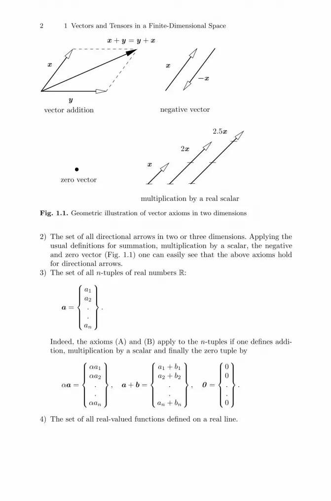
zero vector
vector addition
x
y
2.5x
2x
x
multiplication by a real scalar
−x
x
negative vector
x + y = y + x
Fig. 1.1. Geometric illustration of vector axioms in two dimensions
2) The set of all directional arrows in two or three dimensions. Applying theusual definitions for summation, multiplication by a scalar, the negativeand zero vector (Fig. 1.1) one can easily see that the above axioms holdfor directional arrows.
3) The set of all n-tuples of real numbers R:
a =
⎧⎪⎪⎪⎪⎨⎪⎪⎪⎪⎩a1
a2
.
.an
⎫⎪⎪⎪⎪⎬⎪⎪⎪⎪⎭ .
Indeed, the axioms (A) and (B) apply to the n-tuples if one defines addi-tion, multiplication by a scalar and finally the zero tuple by
αa =
⎧⎪⎪⎪⎪⎨⎪⎪⎪⎪⎩αa1
αa2
.
.αan
⎫⎪⎪⎪⎪⎬⎪⎪⎪⎪⎭ , a + b =
⎧⎪⎪⎪⎪⎨⎪⎪⎪⎪⎩a1 + b1
a2 + b2
.
.an + bn
⎫⎪⎪⎪⎪⎬⎪⎪⎪⎪⎭ , 0 =
⎧⎪⎪⎪⎪⎨⎪⎪⎪⎪⎩00..0
⎫⎪⎪⎪⎪⎬⎪⎪⎪⎪⎭ .
4) The set of all real-valued functions defined on a real line.
1.2 Basis and Dimension of the Vector Space 3
1.2 Basis and Dimension of the Vector Space
Definition 1.2. A set of vectors x1, x2, . . . ,xn is called linearly dependent ifthere exists a set of corresponding scalars α1, α2, . . . , αn ∈ R, not all zero,such that
n∑i=1
αixi = 0 . (1.1)
Otherwise, the vectors x1, x2, . . . ,xn are called linearly independent. In thiscase, none of the vectors xi is the zero vector (Exercise 1.2).
Definition 1.3. The vector
x =n∑
i=1
αixi (1.2)
is called linear combination of the vectors x1, x2, . . . ,xn, where αi ∈ R (i= 1, 2, . . . , n).
Theorem 1.1. The set of n non-zero vectors x1, x2, . . . ,xn is linearly depen-dent if and only if some vector xk (2 ≤ k ≤ n) is a linear combination of thepreceding ones xi (i = 1, . . . , k − 1).
Proof. If the vectors x1, x2, . . . ,xn are linearly dependent, then
n∑i=1
αixi = 0 ,
where not all αi are zero. Let αk (2 ≤ k ≤ n) be the last non-zero number, sothat αi = 0 (i = k + 1, . . . , n). Then,
k∑i=1
αixi = 0 ⇒ xk =k−1∑i=1
−αi
αkxi.
Thereby, the case k = 1 is avoided because α1x1 = 0 implies that x1 = 0(Exercise 1.1). Thus, the sufficiency is proved. The necessity is evident.
Definition 1.4. A basis of a vector space V is a set G of linearly independentvectors such that every vector in V is a linear combination of elements of G.A vector space V is finite-dimensional if it has a finite basis.
Within this book, we restrict our attention to finite-dimensional vector spaces.Although one can find for a finite-dimensional vector space an infinite numberof bases, they all have the same number of vectors.
4 1 Vectors and Tensors in a Finite-Dimensional Space
Theorem 1.2. All the bases of a finite-dimensional vector space V containthe same number of vectors.
Proof. Let G = {g1, g2, . . . , gn} and F = {f1, f2, . . . ,fm} be two arbitrarybases of V with different numbers of elements, say m > n. Then, every vectorin V is a linear combination of the following vectors:
f1, g1, g2, . . . , gn. (1.3)
These vectors are non-zero and linearly dependent. Thus, according to The-orem 1.1 we can find such a vector gk, which is a linear combination of thepreceding ones. Excluding this vector we obtain the set G′ by
f1, g1, g2, . . . , gk−1, gk+1, . . . , gn
again with the property that every vector in V is a linear combination of theelements of G′. Now, we consider the following vectors
f1, f2, g1, g2, . . . , gk−1, gk+1, . . . , gn
and repeat the excluding procedure just as before. We see that none of thevectors f i can be eliminated in this way because they are linearly independent.As soon as all gi (i = 1, 2, . . . , n) are exhausted we conclude that the vectors
f1, f2, . . . ,fn+1
are linearly dependent. This contradicts, however, the previous assumptionthat they belong to the basis F .
Definition 1.5. The dimension of a finite-dimensional vector space V is thenumber of elements in a basis of V.
Theorem 1.3. Every set F = {f1, f2, . . . ,fn} of linearly independent vec-tors in an n-dimensional vectors space V forms a basis of V. Every set ofmore than n vectors is linearly dependent.
Proof. The proof of this theorem is similar to the preceding one. Let G ={g1, g2, . . . , gn} be a basis of V. Then, the vectors (1.3) are linearly dependentand non-zero. Excluding a vector gk we obtain a set of vectors, say G′, withthe property that every vector in V is a linear combination of the elementsof G′. Repeating this procedure we finally end up with the set F with thesame property. Since the vectors f i (i = 1, 2, . . . , n) are linearly independentthey form a basis of V. Any further vectors in V, say fn+1, fn+2, . . . are thuslinear combinations of F . Hence, any set of more than n vectors is linearlydependent.
Theorem 1.4. Every set F = {f1, f2, . . . ,fm} of linearly independent vec-tors in an n-dimensional vector space V can be extended to a basis.
1.3 Components of a Vector, Summation Convention 5
Proof. If m = n, then F is already a basis according to Theorem 1.3. Ifm < n, then we try to find n − m vectors fm+1, fm+2, . . . ,fn, such that allthe vectors f i, that is, f1, f2, . . . ,fm, fm+1, . . . ,fn are linearly independentand consequently form a basis. Let us assume, on the contrary, that onlyk < n − m such vectors can be found. In this case, for all x ∈ V there existscalars α, α1, α2, . . . , αm+k, not all zero, such that
αx + α1f1 + α2f2 + . . . + αm+kfm+k = 0 ,
where α �= 0 since otherwise the vectors f i (i = 1, 2, . . . , m + k) would belinearly dependent. Thus, all the vectors x of V are linear combinations off i (i = 1, 2, . . . , m + k). Then, the dimension of V is m + k < n, which con-tradicts the assumption of this theorem.
1.3 Components of a Vector, Summation Convention
Let G = {g1, g2, . . . , gn} be a basis of an n-dimensional vector space V. Then,
x =n∑
i=1
xigi, ∀x ∈ V. (1.4)
Theorem 1.5. The representation (1.4) with respect to a given basis G isunique.
Proof. Let
x =n∑
i=1
xigi and x =n∑
i=1
yigi
be two different representations of a vector x, where not all scalar coefficientsxi and yi (i = 1, 2, . . . , n) are pairwise identical. Then,
0 = x + (−x) = x + (−1)x =n∑
i=1
xigi +n∑
i=1
(−yi)gi =
n∑i=1
(xi − yi
)gi,
where we use the identity −x = (−1) x (Exercise 1.1). Thus, either the num-bers xi and yi are pairwise equal xi = yi (i = 1, 2, . . . , n) or the vectors gi arelinearly dependent. The latter one is likewise impossible because these vectorsform a basis of V.
The scalar numbers xi (i = 1, 2, . . . , n) in the representation (1.4) are calledcomponents of the vector x with respect to the basis G = {g1, g2, . . . , gn}.
The summation of the form (1.4) is often used in tensor analysis. For thisreason it is usually represented without the summation symbol in a short formby
6 1 Vectors and Tensors in a Finite-Dimensional Space
x =n∑
i=1
xigi = xigi (1.5)
referred to as Einstein’s summation convention. Accordingly, the summation isimplied if an index appears twice in a multiplicative term, once as a superscriptand once as a subscript. Such a repeated index (called dummy index) takesthe values from 1 to n (the dimension of the vector space in consideration).The sense of the index changes (from superscript to subscript or vice versa)if it appears under the fraction bar.
1.4 Scalar Product, Euclidean Space, Orthonormal Basis
The scalar product plays an important role in vector and tensor algebra. Theproperties of the vector space essentially depend on whether and how thescalar product is defined in this space.
Definition 1.6. The scalar (inner) product is a real-valued function x · y oftwo vectors x and y in a vector space V, satisfying the following conditions.
C. (C.1) x · y = y · x (commutative rule),
(C.2) x · (y + z) = x · y + x · z (distributive rule),
(C.3) α (x · y) = (αx) · y = x · (αy) (associative rule for the multiplica-tion by a scalar), ∀α ∈ R, ∀x, y, z ∈ V,
(C.4) x · x ≥ 0 ∀x ∈ V, x · x = 0 if and only if x = 0 .
An n-dimensional vector space furnished by the scalar product with properties(C.1-C.4) is called Euclidean space En. On the basis of this scalar productone defines the Euclidean length (also called norm) of a vector x by
‖x‖ =√
x · x. (1.6)
A vector whose length is equal to 1 is referred to as unit vector.
Definition 1.7. Two vectors x and y are called orthogonal (perpendicular),denoted by x⊥y, if
x · y = 0. (1.7)
Of special interest is the so-called orthonormal basis of the Euclidean space.
Definition 1.8. A basis E = {e1, e2, . . . ,en} of an n-dimensional Euclideanspace En is called orthonormal if
ei · ej = δij , i, j = 1, 2, . . . , n, (1.8)
where
1.4 Scalar Product, Euclidean Space, Orthonormal Basis 7
δij = δij = δij =
{1 for i = j,
0 for i �= j(1.9)
denotes the Kronecker delta.
Thus, the elements of an orthonormal basis represent pairwise orthog-onal unit vectors. Of particular interest is the question of the existence ofan orthonormal basis. Now, we are going to demonstrate that every set ofm ≤ n linearly independent vectors in En can be orthogonalized and nor-malized by means of a linear transformation (Gram-Schmidt procedure).In other words, starting from linearly independent vectors x1, x2, . . . ,xm
one can always construct their linear combinations e1, e2, . . . ,em such thatei · ej = δij (i, j = 1, 2, . . . , m). Indeed, since the vectors xi (i = 1, 2, . . . , m)are linearly independent they are all non-zero (see Exercise 1.2). Thus, we candefine the first unit vector by
e1 =x1
‖x1‖ . (1.10)
Next, we consider the vector
e′2 = x2 − (x2 · e1)e1 (1.11)
orthogonal to e1. This holds for the unit vector e2 = e′2/‖e′
2‖ as well. Itis also seen that ‖e′
2‖ =√
e′2 · e′
2 �= 0 because otherwise e′2 = 0 and thus
x2 = (x2 · e1)e1 = (x2 · e1) ‖x1‖−1x1. However, the latter result contradicts
the fact that the vectors x1 and x2 are linearly independent.Further, we proceed to construct the vectors
e′3 = x3 − (x3 · e2)e2 − (x3 · e1)e1, e3 =
e′3
‖e′3‖
(1.12)
orthogonal to e1 and e2. Repeating this procedure we finally obtain the setof orthonormal vectors e1, e2, . . . ,em. Since these vectors are non-zero andmutually orthogonal, they are linearly independent (see Exercise 1.6). In thecase m = n, this set represents, according to Theorem 1.3, the orthonormalbasis (1.8) in En.
With respect to an orthonormal basis the scalar product of two vectorsx = xiei and y = yiei in En takes the form
x · y = x1y1 + x2y2 + . . . + xnyn. (1.13)
For the length of the vector x (1.6) we thus obtain the Pythagoras formula
‖x‖ =√
x1x1 + x2x2 + . . . + xnxn, x ∈ En. (1.14)

8 1 Vectors and Tensors in a Finite-Dimensional Space
1.5 Dual Bases
Definition 1.9. Let G = {g1, g2, . . . , gn} be a basis in the n-dimensional Eu-clidean space E
n. Then, a basis G′ ={g1, g2, . . . , gn
}of E
n is called dual toG, if
gi · gj = δji , i, j = 1, 2, . . . , n. (1.15)
In the following we show that a set of vectors G′ ={g1, g2, . . . , gn
}satisfying
the conditions (1.15) always exists, is unique and forms a basis in En.Let E = {e1, e2, . . . ,en} be an orthonormal basis in En. Since G also
represents a basis, we can write
ei = αjigj , gi = βj
i ej , i = 1, 2, . . . , n, (1.16)
where αji and βj
i (i = 1, 2, . . . , n) denote the components of ei and gi, respec-tively. Inserting the first relation (1.16) into the second one yields
gi = βji αk
j gk, ⇒ 0 =(βj
i αkj − δk
i
)gk, i = 1, 2, . . . , n. (1.17)
Since the vectors gi are linearly independent we obtain
βji α
kj = δk
i , i, k = 1, 2, . . . , n. (1.18)
Let further
gi = αije
j , i = 1, 2, . . . , n, (1.19)
where and henceforth we set ej = ej (j = 1, 2, . . . , n) in order to take theadvantage of Einstein’s summation convention. By virtue of (1.8), (1.16) and(1.18) one finally finds
gi ·gj =(βk
i ek
)·(αjl e
l)
= βki αj
l δlk = βk
i αjk = δj
i , i, j = 1, 2, . . . , n. (1.20)
Next, we show that the vectors gi (i = 1, 2, . . . , n) (1.19) are linearly indepen-dent and for this reason form a basis of En. Assume on the contrary that
aigi = 0 ,
where not all scalars ai (i = 1, 2, . . . , n) are zero. The scalar product of thisrelation with the vectors gj (j = 1, 2, . . . , n) leads to a contradiction. Indeed,we obtain in this case
0 = aigi · gj = aiδ
ij = aj , j = 1, 2, . . . , n.
The next important question is whether the dual basis is unique. Let G′ ={g1, g2, . . . , gn
}and H′ =
{h1, h2, . . . ,hn
}be two arbitrary non-coinciding
bases in En, both dual to G = {g1, g2, . . . , gn}. Then,
1.5 Dual Bases 9
hi = hijg
j , i = 1, 2, . . . , n.
Forming the scalar product with the vectors gj (j = 1, 2, . . . , n) we can con-clude that the bases G′ and H′ coincide:
δij = hi · gj =
(hi
kgk) · gj = hi
kδkj = hi
j ⇒ hi = gi, i = 1, 2, . . . , n.
Thus, we have proved the following theorem.
Theorem 1.6. To every basis in an Euclidean space En there exists a uniquedual basis.
Relation (1.19) enables to determine the dual basis. However, it can also beobtained without any orthonormal basis. Indeed, let gi be a basis dual togi (i = 1, 2, . . . , n). Then
gi = gijgj , gi = gijgj , i = 1, 2, . . . , n. (1.21)
Inserting the second relation (1.21) into the first one yields
gi = gijgjkgk, i = 1, 2, . . . , n. (1.22)
Multiplying scalarly with the vectors gl we have by virtue of (1.15)
δil = gijgjkδk
l = gijgjl, i, l = 1, 2, . . . , n. (1.23)
Thus, we see that the matrices [gkj ] and[gkj
]are inverse to each other such
that[gkj
]= [gkj ]
−1. (1.24)
Now, multiplying scalarly the first and second relation (1.21) by the vectorsgj and gj (j = 1, 2, . . . , n), respectively, we obtain with the aid of (1.15) thefollowing important identities:
gij = gji = gi · gj , gij = gji = gi · gj , i, j = 1, 2, . . . , n. (1.25)
By definition (1.8) the orthonormal basis in En is self-dual, so that
ei = ei, ei · ej = δji , i, j = 1, 2, . . . , n. (1.26)
With the aid of the dual bases one can represent an arbitrary vector in En by
x = xigi = xigi, ∀x ∈ E
n, (1.27)
where
xi = x · gi, xi = x · gi, i = 1, 2, . . . , n. (1.28)
Indeed, using (1.15) we can write
10 1 Vectors and Tensors in a Finite-Dimensional Space
x · gi =(xjgj
) · gi = xjδij = xi,
x · gi =(xjg
j) · gi = xjδ
ji = xi, i = 1, 2, . . . , n.
The components of a vector with respect to the dual bases are suitable forcalculating the scalar product. For example, for two arbitrary vectors x =xigi = xig
i and y = yigi = yigi we obtain
x · y = xiyjgij = xiyjgij = xiyi = xiy
i. (1.29)
The length of the vector x can thus be written by
‖x‖ =√
xixjgij =√
xixjgij =√
xixi. (1.30)
Example. Dual basis in E3. Let G = {g1, g2, g3} be a basis of thethree-dimensional Euclidean space and
g = [g1g2g3] , (1.31)
where [• • •] denotes the mixed product of vectors. It is defined by
[abc] = (a × b) · c = (b × c) · a = (c × a) · b, (1.32)
where “×” denotes the vector (also called cross or outer) product of vectors.Consider the following set of vectors:
g1 = g−1g2 × g3, g2 = g−1g3 × g1, g3 = g−1g1 × g2. (1.33)
It seen that the vectors (1.33) satisfy conditions (1.15), are linearly indepen-dent (Exercise 1.11) and consequently form the basis dual to gi (i = 1, 2, 3).Further, it can be shown that
g2 = |gij | , (1.34)
where |•| denotes the determinant of the matrix [•]. Indeed, with the aid of(1.16)2 we obtain
g = [g1g2g3] =[βi
1eiβj2ejβ
k3ek
]= βi
1βj2β
k3 [eiejek] = βi
1βj2β
k3 eijk =
∣∣βij
∣∣ , (1.35)
where eijk denotes the permutation symbol (also called Levi-Civita symbol).It is defined by
eijk = eijk = [eiejek]
=
⎧⎪⎨⎪⎩1 if ijk is an even permutation of 123,
−1 if ijk is an odd permutation of 123,0 otherwise,
(1.36)
1.5 Dual Bases 11
where the orthonormal vectors e1, e2 and e3 are numerated in such a waythat they form a right-handed system. In this case, [e1e2e3] = 1.
On the other hand, we can write again using (1.16)2
gij = gi · gj =3∑
k=1
βki βk
j .
The latter sum can be represented as a product of two matrices so that
[gij ] =[βj
i
] [βj
i
]T. (1.37)
Since the determinant of the matrix product is equal to the product of thematrix determinants we finally have
|gij | =∣∣∣βj
i
∣∣∣2 = g2. (1.38)
With the aid of the permutation symbol (1.36) one can represent the identities(1.33) by
gi × gj = eijk g gk, i, j = 1, 2, 3, (1.39)
which also delivers
[gigjgk] = eijk g, i, j, k = 1, 2, 3. (1.40)
Similarly to (1.34) one can also show that (see Exercise 1.12)[g1g2g3
]2=∣∣gij
∣∣ = g−2. (1.41)
Thus,
gi × gj =eijk
ggk, i, j = 1, 2, 3, (1.42)
which yields by analogy with (1.40)
[gigjgk
]=
eijk
g, i, j, k = 1, 2, 3. (1.43)
Relations (1.39) and (1.42) permit a useful representation of the vector prod-uct. Indeed, let a = aigi = aig
i and b = bjgj = bjgj be two arbitrary vectors
in E3. Then,
a × b =(aigi
)× (bjgj
)= aibjeijkggk = g
∣∣∣∣∣∣a1 a2 a3
b1 b2 b3
g1 g2 g3
∣∣∣∣∣∣ ,
12 1 Vectors and Tensors in a Finite-Dimensional Space
a × b =(aig
i)× (
bjgj)
= aibjeijkg−1gk =
1g
∣∣∣∣∣∣a1 a2 a3
b1 b2 b3
g1 g2 g3
∣∣∣∣∣∣ . (1.44)
For the orthonormal basis in E3 relations (1.39) and (1.42) reduce to
ei × ej = eijkek = eijkek, i, j = 1, 2, 3, (1.45)
so that the vector product (1.44) can be written by
a × b =
∣∣∣∣∣∣a1 a2 a3
b1 b2 b3
e1 e2 e3
∣∣∣∣∣∣ , (1.46)
where a = aiei and b = bje
j .
1.6 Second-Order Tensor as a Linear Mapping
Let us consider a set Linn of all linear mappings of one vector into anotherone within En. Such a mapping can be written as
y = Ax, y ∈ En, ∀x ∈ E
n, ∀A ∈ Linn. (1.47)
Elements of the set Linn are called second-order tensors or simply tensors.Linearity of the mapping (1.47) is expressed by the following relations:
A (x + y) = Ax + Ay, ∀x, y ∈ En, ∀A ∈ Linn, (1.48)
A (αx) = α (Ax) , ∀x ∈ En, ∀α ∈ R, ∀A ∈ Linn. (1.49)
Further, we define the product of a tensor by a scalar number α ∈ R as
(αA) x = α (Ax) = A (αx) , ∀x ∈ En (1.50)
and the sum of two tensors A and B as
(A + B)x = Ax + Bx, ∀x ∈ En. (1.51)
Thus, properties (A.1), (A.2) and (B.1-B.4) apply to the set Linn. Setting in(1.50) α = −1 we obtain the negative tensor by
−A = (−1)A. (1.52)
Further, we define a zero tensor 0 in the following manner
0x = 0 , ∀x ∈ En, (1.53)
so that the elements of the set Linn also fulfill conditions (A.3) and (A.4) andaccordingly form a vector space.
1.6 Second-Order Tensor as a Linear Mapping 13
The properties of second-order tensors can thus be summarized by
A + B = B + A, (addition is commutative), (1.54)
A + (B + C) = (A + B) + C, (addition is associative), (1.55)
0 + A = A, (1.56)
A + (−A) = 0, (1.57)
α (βA) = (αβ)A, (multiplication by scalars is associative), (1.58)
1A = A, (1.59)
α (A + B) = αA + αB, (multiplication by scalars is distributive
with respect to tensor addition), (1.60)
(α + β)A = αA + βA, (multiplication by scalars is distributive
with respect to scalar addition), ∀A,B,C ∈ Linn, ∀α, β ∈ R. (1.61)
Example. Vector product in E3. The vector product of two vectors inE3 represents again a vector in E3
z = w × x, z ∈ E3, ∀w, x ∈ E
3. (1.62)
According to (1.44) the mapping x → z is linear so that
w × (αx) = α (w × x) ,
w × (x + y) = w × x + w × y, ∀w, x, y ∈ E3, ∀α ∈ R. (1.63)
Thus, it can be described by means of a tensor of the second order by
w × x = Wx, W ∈ Lin3, ∀x ∈ E3. (1.64)
The tensor which forms the vector product by a vector w according to (1.64)will be denoted in the following by w. Thus, we write
w × x = wx. (1.65)
Example. Representation of a rotation by a second-order tensor.A rotation of a vector a in E3 about an axis yields another vector r in E3. Itcan be shown that the mapping a → r (a) is linear such that
r (αa) = αr (a) , r (a + b) = r (a) + r (b) , ∀α ∈ R, ∀a, b ∈ E3. (1.66)
Thus, it can again be described by a second-order tensor as
r (a) = Ra, ∀a ∈ E3, R ∈ Lin3. (1.67)
This tensor R is referred to as rotation tensor.
14 1 Vectors and Tensors in a Finite-Dimensional Space
a a
y
a∗
ωx
e
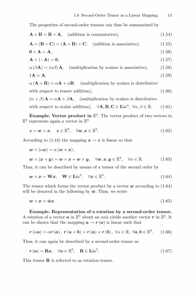
Fig. 1.2. Finite rotation of a vector in E3
Let us construct the rotation tensor which rotates an arbitrary vector a ∈E3 about an axis specified by a unit vector e ∈ E3 (see Fig. 1.2). Decomposingthe vector a by a = a∗ + x in two vectors along and perpendicular to therotation axis we can write
a = a∗ + x cosω + y sinω = a∗ + (a − a∗) cosω + y sin ω, (1.68)
where ω denotes the rotation angle. By virtue of the geometric identities
a∗ = (a · e)e = (e ⊗ e)a, y = e×x = e×(a − a∗) = e×a = ea, (1.69)
where “⊗” denotes the so-called tensor product (1.75) (see Sect. 1.7), weobtain
a = cosωa + sin ωea + (1 − cosω) (e ⊗ e)a. (1.70)
Thus the rotation tensor can be given by
R = cosωI + sin ωe + (1 − cosω)e ⊗ e, (1.71)
where I denotes the so-called identity tensor (1.84) (see Sect. 1.7).
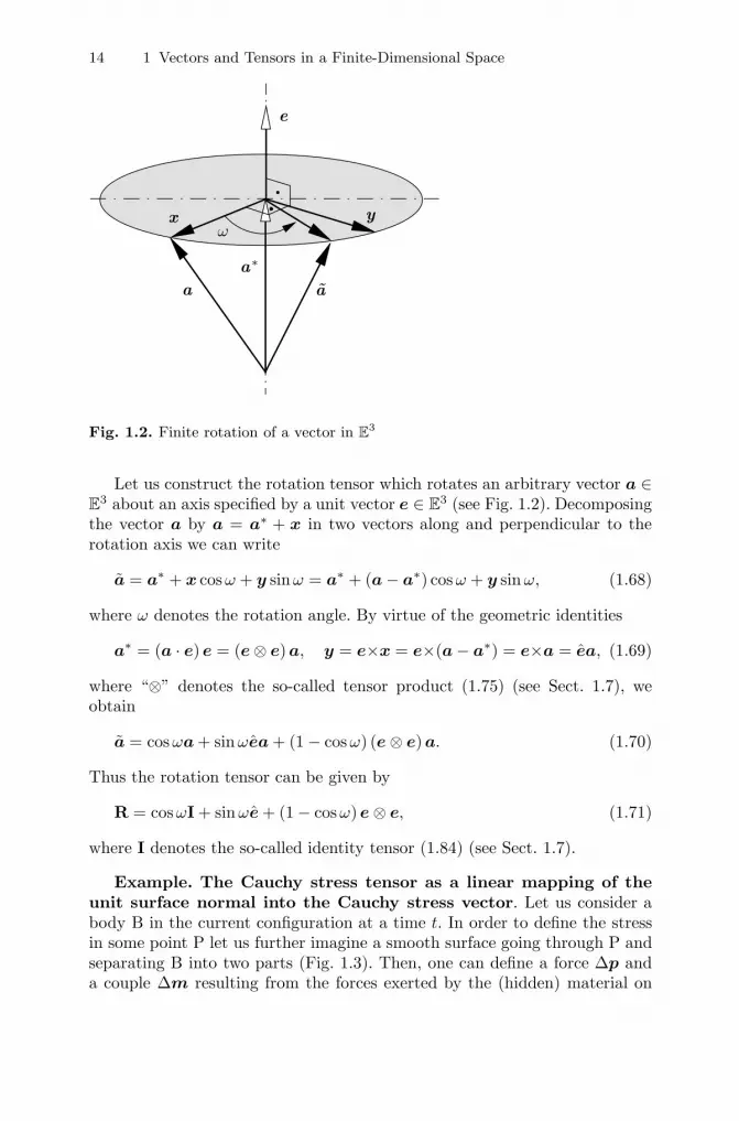
Example. The Cauchy stress tensor as a linear mapping of theunit surface normal into the Cauchy stress vector. Let us consider abody B in the current configuration at a time t. In order to define the stressin some point P let us further imagine a smooth surface going through P andseparating B into two parts (Fig. 1.3). Then, one can define a force Δp anda couple Δm resulting from the forces exerted by the (hidden) material on
1.6 Second-Order Tensor as a Linear Mapping 15
�
� � �
�
� � �
�
� � �
�
Fig. 1.3. Cauchy stress vector
one side of the surface ΔA and acting on the material on the other side ofthis surface. Let the area ΔA tend to zero keeping P as inner point. A basicpostulate of continuum mechanics is that the limit
t = limΔA→0
Δp
ΔA
exists and is final. The so-defined vector t is called Cauchy stress vector.Cauchy’s fundamental postulate states that the vector t depends on the sur-face only through the outward unit normal n. In other words, the Cauchystress vector is the same for all surfaces through P which have n as the nor-mal in P. Further, according to Cauchy’s theorem the mapping n → t is linearprovided t is a continuous function of the position vector x at P. Hence, thismapping can be described by a second-order tensor σ called the Cauchy stresstensor so that
t = σn. (1.72)
On the basis of the “right” mapping (1.47) we can also define the “left”one by the following condition
(yA) · x = y · (Ax) , ∀x ∈ En, A ∈ Linn. (1.73)
First, it should be shown that for all y ∈ En there exists a unique vector yA ∈En satisfying the condition (1.73) for all x ∈ En. Let G = {g1, g2, . . . , gn}and G′ =
{g1, g2, . . . , gn
}be dual bases in En. Then, we can represent two
arbitrary vectors x, y ∈ En, by x = xigi and y = yig
i. Now, consider thevector
yA = yi
[gi · (Agj
)]gj .
It holds: (yA) ·x = yixj
[gi · (Agj
)]. On the other hand, we obtain the same
result also by
16 1 Vectors and Tensors in a Finite-Dimensional Space
y · (Ax) = y · (xjAgj)
= yixj
[gi · (Agj
)].
Further, we show that the vector yA, satisfying condition (1.73) for all x ∈ En,is unique. Conversely, let a, b ∈ En be two such vectors. Then, we have
a · x = b · x ⇒ (a − b) · x = 0, ∀x ∈ En ⇒ (a − b) · (a − b) = 0,
which by axiom (C.4) implies that a = b.Since the order of mappings in (1.73) is irrelevant we can write them
without brackets and dots as follows
y · (Ax) = (yA) · x = yAx. (1.74)
1.7 Tensor Product, Representation of a Tensor withRespect to a Basis
The tensor product plays an important role since it enables to construct asecond-order tensor from two vectors. In order to define the tensor productwe consider two vectors a, b ∈ En. An arbitrary vector x ∈ En can be mappedinto another vector a (b · x) ∈ E
n. This mapping is denoted by symbol “⊗”as a ⊗ b. Thus,
(a ⊗ b)x = a (b · x) , a, b ∈ En, ∀x ∈ E
n. (1.75)
It can be shown that the mapping (1.75) fulfills the conditions (1.48-1.50) andfor this reason is linear. Indeed, by virtue of (B.1), (B.4), (C.2) and (C.3) wecan write
(a ⊗ b) (x + y) = a [b · (x + y)] = a (b · x + b · y)
= (a ⊗ b)x + (a ⊗ b)y, (1.76)
(a ⊗ b) (αx) = a [b · (αx)] = α (b · x)a
= α (a ⊗ b)x, a, b ∈ En, ∀x, y ∈ E
n, ∀α ∈ R. (1.77)
Thus, the tensor product of two vectors represents a second-order tensor.Further, it holds
c ⊗ (a + b) = c ⊗ a + c ⊗ b, (a + b) ⊗ c = a ⊗ c + b ⊗ c, (1.78)
(αa) ⊗ (βb) = αβ (a ⊗ b) , a, b, c ∈ En, ∀α, β ∈ R. (1.79)
Indeed, mapping an arbitrary vector x ∈ En by both sides of these relationsand using (1.51) and (1.75) we obtain
c ⊗ (a + b)x = c (a · x + b · x) = c (a · x) + c (b · x)
= (c ⊗ a)x + (c ⊗ b)x = (c ⊗ a + c ⊗ b)x,

1.7 Tensor Product, Representation of a Tensor with Respect to a Basis 17
[(a + b) ⊗ c]x = (a + b) (c · x) = a (c · x) + b (c · x)
= (a ⊗ c) x + (b ⊗ c) x = (a ⊗ c + b ⊗ c)x,
(αa) ⊗ (βb) x = (αa) (βb · x)
= αβa (b · x) = αβ (a ⊗ b)x, ∀x ∈ En.
For the “left” mapping by the tensor a⊗b we obtain from (1.73) (see Exercise1.19)
y (a ⊗ b) = (y · a) b, ∀y ∈ En. (1.80)
We have already seen that the set of all second-order tensors Linn repre-sents a vector space. In the following, we show that a basis of Linn can beconstructed with the aid of the tensor product (1.75).
Theorem 1.7. Let F = {f1, f2, . . . ,fn} and G = {g1, g2, . . . , gn} be twoarbitrary bases of En. Then, the tensors f i ⊗ gj (i, j = 1, 2, . . . , n) representa basis of Linn. The dimension of the vector space Linn is thus n2.
Proof. First, we prove that every tensor in Linn represents a linear combi-nation of the tensors f i ⊗ gj (i, j = 1, 2, . . . , n). Indeed, let A ∈ Linn be anarbitrary second-order tensor. Consider the following linear combination
A′ =(f iAgj
)f i ⊗ gj ,
where the vectors f i and gi (i = 1, 2, . . . , n) form the bases dual to F and G,respectively. The tensors A and A′ coincide if and only if
A′x = Ax, ∀x ∈ En. (1.81)
Let x = xjgj . Then
A′x =(f iAgj
)f i ⊗ gj
(xkgk
)=(f iAgj
)f ixkδk
j = xj
(f iAgj
)f i.
On the other hand, Ax = xjAgj . By virtue of (1.27-1.28) we can repre-sent the vectors Agj (j = 1, 2, . . . , n) with respect to the basis F by Agj =[f i · (Agj
)]f i =
(f iAgj
)f i (j = 1, 2, . . . , n). Hence,
Ax = xj
(f iAgj
)f i.
Thus, it is seen that condition (1.81) is satisfied for all x ∈ En. Finally,we show that the tensors f i ⊗ gj (i, j = 1, 2, . . . , n) are linearly independent.Otherwise, there would exist scalars αij (i, j = 1, 2, . . . , n), not all zero, suchthat
αijf i ⊗ gj = 0.
The right mapping of gk (k = 1, 2, . . . , n) by this tensor equality yields then:αikf i = 0 (k = 1, 2, . . . , n). This contradicts, however, the fact that the vec-tors fk (k = 1, 2, . . . , n) form a basis and are therefore linearly independent.
18 1 Vectors and Tensors in a Finite-Dimensional Space
For the representation of second-order tensors we will in the following useprimarily the bases gi⊗gj , gi⊗gj , gi⊗gj or gi⊗gj (i, j = 1, 2, . . . , n). Withrespect to these bases a tensor A ∈ Linn is written as
A = Aijgi ⊗ gj = Aijgi ⊗ gj = Ai
·jgi ⊗ gj = A ji·g
i ⊗ gj (1.82)
with the components (see Exercise 1.20)
Aij = giAgj , Aij = giAgj ,
Ai·j = giAgj , A j
i· = giAgj , i, j = 1, 2, . . . , n. (1.83)
Note, that the subscript dot indicates the position of the above index. Forexample, for the components Ai
·j , i is the first index while for the componentsA i
j·, i is the second index.Of special importance is the so-called identity tensor I. It is defined by
Ix = x, ∀x ∈ En. (1.84)
With the aid of (1.25), (1.82) and (1.83) the components of the identity tensorcan be expressed by
Iij = giIgj = gi · gj = gij , Iij = giIgj = gi · gj = gij ,
Ii·j = I ji· = Iij = giIgj = giIgj = gi · gj = gi · gj = δi
j , (1.85)
where i, j = 1, 2, . . . , n. Thus,
I = gijgi ⊗ gj = gijgi ⊗ gj = gi ⊗ gi = gi ⊗ gi. (1.86)
It is seen that the components (1.85)1,2 of the identity tensor are given byrelation (1.25). In view of (1.30) they characterize metric properties of theEuclidean space and are referred to as metric coefficients. For this reason, theidentity tensor is frequently called metric tensor. With respect to an orthonor-mal basis relation (1.86) reduces to
I =n∑
i=1
ei ⊗ ei. (1.87)
1.8 Change of the Basis, Transformation Rules
Now, we are going to clarify how the vector and tensor components transformwith the change of the basis. Let x be a vector and A a second-order tensor.According to (1.27) and (1.82)
x = xigi = xigi, (1.88)
1.9 Special Operations with Second-Order Tensors 19
A = Aijgi ⊗ gj = Aijgi ⊗ gj = Ai
·jgi ⊗ gj = A ji·g
i ⊗ gj . (1.89)
With the aid of (1.21) and (1.28) we can write
xi = x · gi = x · (gijgj
)= xjg
ji, xi = x · gi = x · (gijgj)
= xjgji, (1.90)
where i = 1, 2, . . . , n. Similarly we obtain by virtue of (1.83)
Aij = giAgj = giA(gjkgk
)=(gilgl
)A(gjkgk
)= Ai
·kgkj = gilAlkgkj , (1.91)
Aij = giAgj = giA(gjkgk
)=(gilg
l)A(gjkgk
)= A k
i· gkj = gilAlkgkj , (1.92)
where i, j = 1, 2, . . . , n. The transformation rules (1.90-1.92) hold not only fordual bases. Indeed, let gi and gi (i = 1, 2, . . . , n) be two arbitrary bases inEn, so that
x = xigi = xigi, (1.93)
A = Aijgi ⊗ gj = Aijgi ⊗ gj . (1.94)
By means of the relations
gi = aji gj , i = 1, 2, . . . , n (1.95)
one thus obtains
x = xigi = xiaji gj ⇒ xj = xiaj
i , j = 1, 2, . . . , n, (1.96)
A = Aijgi ⊗ gj = Aij(ak
i gk
)⊗ (al
j gl
)= Aijak
i alj gk ⊗ gl
⇒ Akl = Aijaki al
j , k, l = 1, 2, . . . , n. (1.97)
1.9 Special Operations with Second-Order Tensors
In Sect. 1.6 we have seen that the set Linn represents a finite-dimensionalvector space. Its elements are second-order tensors that can be treated asvectors in En2
with all the operations specific for vectors such as summation,multiplication by a scalar or a scalar product (the latter one will be definedfor second-order tensors in Sect. 1.10). However, in contrast to conventionalvectors in the Euclidean space, for second-order tensors one can additionallydefine some special operations as for example composition, transposition orinversion.
20 1 Vectors and Tensors in a Finite-Dimensional Space
Composition (simple contraction). Let A,B ∈ Linn be two second-order tensors. The tensor C = AB is called composition of A and B if
Cx = A (Bx) , ∀x ∈ En. (1.98)
For the left mapping (1.73) one can write
y (AB) = (yA)B, ∀y ∈ En. (1.99)
In order to prove the last relation we use again (1.73) and (1.98):
y (AB)x = y · [(AB)x] = y · [A (Bx)]
= (yA) · (Bx) = [(yA)B] · x, ∀x ∈ En.
The composition of tensors (1.98) is generally not commutative so that AB �=BA. Two tensors A and B are called commutative if on the contrary AB =BA. Besides, the composition of tensors is characterized by the followingproperties (see Exercise 1.24):
A0 = 0A = 0, AI = IA = A, (1.100)
A (B + C) = AB + AC, (B + C)A = BA + CA, (1.101)
A (BC) = (AB)C. (1.102)
For example, the distributive rule (1.101)1 can be proved as follows
[A (B + C)]x = A [(B + C)x] = A (Bx + Cx) = A (Bx) + A (Cx)
= (AB)x + (AC)x = (AB + AC)x, ∀x ∈ En.
For the tensor product (1.75) the composition (1.98) yields
(a ⊗ b) (c ⊗ d) = (b · c)a ⊗ d, a, b, c, d ∈ En. (1.103)
Indeed, by virtue of (1.75), (1.77) and (1.98)
(a ⊗ b) (c ⊗ d)x = (a ⊗ b) [(c ⊗ d)x] = (d · x) (a ⊗ b) c
= (d · x) (b · c)a = (b · c) (a ⊗ d)x
= [(b · c)a ⊗ d] x, ∀x ∈ En.
Thus, we can write
AB = AikB jk·gi ⊗ gj = AikBkjgi ⊗ gj
= Ai·kBk
·jgi ⊗ gj = A ki· Bkjg
i ⊗ gj , (1.104)
where A and B are given in the form (1.82).
Powers, polynomials and functions of second-order tensors. Onthe basis of the composition (1.98) one defines by

1.9 Special Operations with Second-Order Tensors 21
Am = AA . . .A︸ ︷︷ ︸m times
, m = 1, 2, 3 . . . , A0 = I (1.105)
powers (monomials) of second-order tensors characterized by the followingevident properties
AkAl = Ak+l,(Ak
)l= Akl, (1.106)
(αA)k = αkAk, k, l = 0, 1, 2 . . . (1.107)
With the aid of the tensor powers a polynomial of A can be defined by
g (A) = a0I + a1A + a2A2 + . . . + amAm =m∑
k=0
akAk. (1.108)
g (A): Linn →Linn represents a tensor function mapping one second-ordertensor into another one within Linn. By this means one can define varioustensor functions. Of special interest is the exponential one
exp (A) =∞∑
k=0
Ak
k!(1.109)
given by the infinite power series.
Transposition. The transposed tensor AT is defined by:
ATx = xA, ∀x ∈ En, (1.110)
so that one can also write
Ay = yAT, xAy = yATx, ∀x, y ∈ En. (1.111)
Indeed,
x · (Ay) = (xA) · y = y · (ATx)
= yATx = x · (yAT), ∀x, y ∈ E
n.
Consequently,(AT
)T= A. (1.112)
Transposition represents a linear operation over a second-order tensor since
(A + B)T = AT + BT (1.113)
and
(αA)T = αAT, ∀α ∈ R. (1.114)
The composition of second-order tensors is transposed by
22 1 Vectors and Tensors in a Finite-Dimensional Space
(AB)T = BTAT. (1.115)
Indeed, in view of (1.99) and (1.110)
(AB)T x = x (AB) = (xA)B = BT (xA) = BTATx, ∀x ∈ En.
For the tensor product of two vectors a, b ∈ En we further obtain by use of(1.75) and (1.80)
(a ⊗ b)T = b ⊗ a. (1.116)
This ensures the existence and uniqueness of the transposed tensor. Indeed,every tensor A in Linn can be represented with respect to the tensor productof the basis vectors in En in the form (1.82). Hence, considering (1.116) wehave
AT = Aijgj ⊗ gi = Aijgj ⊗ gi = Ai
·jgj ⊗ gi = A j
i·gj ⊗ gi, (1.117)
or
AT = Ajigi ⊗ gj = Ajigi ⊗ gj = Aj
·igi ⊗ gj = A i
j·gi ⊗ gj . (1.118)
Comparing the latter result with the original representation (1.82) one ob-serves that the components of the transposed tensor can be expressed by(
AT)ij
= Aji,(AT
)ij= Aji, (1.119)
(AT
) j
i· = Aj·i = gjkA l
k·gli,(AT
)i·j = A i
j· = gjkAk·lg
li. (1.120)
For example, the last relation results from (1.83) and (1.111) within the fol-lowing steps(
AT)i·j = giATgj = gjAgi = gj
(Ak
·lgk ⊗ gl)
gi = gjkAk·lg
li.
According to (1.119) the homogeneous (covariant or contravariant) compo-nents of the transposed tensor can simply be obtained by reflecting the matrixof the original components from the main diagonal. It does not, however, holdfor the mixed components (1.120).
The transposition operation (1.110) gives rise to the definition of symmet-ric MT = M and skew-symmetric second-order tensors WT = −W.
Obviously, the identity tensor is symmetric
IT = I. (1.121)
Indeed,
xIy = x · y = y · x = yIx = xITy, ∀x, y ∈ En.
1.9 Special Operations with Second-Order Tensors 23
Inversion. Let
y = Ax. (1.122)
A tensor A ∈ Linn is referred to as invertible if there exists a tensor A−1 ∈Linn satisfying the condition
x = A−1y, ∀x ∈ En. (1.123)
The tensor A−1 is called inverse of A. The set of all invertible tensors Invn ={A ∈ Linn : ∃A−1
}forms a subset of all second-order tensors Linn.
Inserting (1.122) into (1.123) yields
x = A−1y = A−1 (Ax) =(A−1A
)x, ∀x ∈ E
n
and consequently
A−1A = I. (1.124)
Theorem 1.8. A tensor A is invertible if and only if Ax = 0 implies thatx = 0 .
Proof. First we prove the sufficiency. To this end, we map the vector equationAx = 0 by A−1. According to (1.124) it yields: 0 = A−1Ax = Ix = x. Toprove the necessity we consider a basis G = {g1, g2, . . . , gn} in En. It can beshown that the vectors hi = Agi (i = 1, 2, . . . , n) form likewise a basis of En.Conversely, let these vectors be linearly dependent so that aihi = 0 , where notall scalars ai (i = 1, 2, . . . , n) are zero. Then, 0 = aihi = aiAgi = Aa, wherea = aigi �= 0 , which contradicts the assumption of the theorem. Now, considerthe tensor A′ = gi ⊗ hi, where the vectors hi are dual to hi (i = 1, 2, . . . , n).One can show that this tensor is inverse to A, such that A′ = A−1. Indeed,let x = xigi be an arbitrary vector in En. Then, y = Ax = xiAgi = xihi
and therefore A′y = gi ⊗ hi(xjhj
)= gix
jδij = xigi = x.
Conversely, it can be shown that an invertible tensor A is inverse to A−1 andconsequently
AA−1 = I. (1.125)
For the proof we again consider the bases gi and Agi (i = 1, 2, . . . , n). Lety = yiAgi be an arbitrary vector in En. Let further x = A−1y = yigi inview of (1.124). Then, Ax = yiAgi = y which implies that the tensor A isinverse to A−1.
Relation (1.125) implies the uniqueness of the inverse. Indeed, if A−1 andA−1 are two distinct tensors both inverse to A then there exists at least onevector y ∈ En such that A−1y �= A−1y. Mapping both sides of this vectorinequality by A and taking (1.125) into account we immediately come to thecontradiction.

24 1 Vectors and Tensors in a Finite-Dimensional Space
By means of (1.115), (1.121) and (1.125) we can write (see Exercise 1.37)(A−1
)T=(AT
)−1= A−T. (1.126)
The composition of two arbitrary invertible tensors A and B is inverted by
(AB)−1 = B−1A−1. (1.127)
Indeed, let
y = ABx.
Mapping both sides of this vector identity by A−1 and then by B−1, we obtainwith the aid of (1.124)
x = B−1A−1y, ∀x ∈ En.
On the basis of transposition and inversion one defines the so-called orthogonaltensors. They do not change after consecutive transposition and inversion andform the following subset of Linn:
Orthn ={Q ∈ Linn : Q = Q−T
}. (1.128)
For orthogonal tensors we can write in view of (1.124) and (1.125)
QQT = QTQ = I, ∀Q ∈ Orthn. (1.129)
For example, one can show that the rotation tensor (1.71) is orthogonal. Tothis end, we complete the vector e defining the rotation axis (Fig. 1.2) toan orthonormal basis {e, q, p} such that e = q × p. Then, using the vectoridentity (see Exercise 1.15)
p (q · x) − q (p · x) = (q × p) × x, ∀x ∈ E3 (1.130)
we can write
e = p ⊗ q − q ⊗ p. (1.131)
The rotation tensor (1.71) takes thus the form
R = cosωI + sin ω (p ⊗ q − q ⊗ p) + (1 − cosω) (e ⊗ e) . (1.132)
Hence,
RRT = [cosωI + sin ω (p ⊗ q − q ⊗ p) + (1 − cosω) (e ⊗ e)]
[cosωI− sin ω (p ⊗ q − q ⊗ p) + (1 − cosω) (e ⊗ e)]
= cos2 ωI + sin2 ω (e ⊗ e) + sin2 ω (p ⊗ p + q ⊗ q) = I.
1.10 Scalar Product of Second-Order Tensors 25
It is interesting that the exponential function (1.109) of a skew-symmetrictensors represents an orthogonal tensor. Indeed, keeping in mind that a skew-symmetric tensor W commutes with its transposed counterpart WT = −Wand using the identities exp (A + B) = exp (A) exp (B) for commutative ten-sors (Exercise 1.27) and
(Ak
)T =(AT
)k for integer k (Exercise 1.35) we canwrite
I = exp (0) = exp (W − W) = exp(W + WT
)= exp (W) exp
(WT
)= exp (W) [exp (W)]T , ∀W ∈ Skewn. (1.133)
1.10 Scalar Product of Second-Order Tensors
Consider two second-order tensors a⊗b and c⊗d given in terms of the tensorproduct (1.75). Their scalar product can be defined in the following manner:
(a ⊗ b) : (c ⊗ d) = (a · c) (b · d) , a, b, c, d ∈ En. (1.134)
It leads to the following identity (Exercise 1.39):
c ⊗ d : A = cAd = dATc. (1.135)
For two arbitrary tensors A and B given in the form (1.82) we thus obtain
A : B = AijBij = AijBij = Ai·jB
ji· = A j
i·Bi·j . (1.136)
Similar to vectors the scalar product of tensors is a real function characterizedby the following properties (see Exercise 1.40)
D. (D.1) A : B = B : A (commutative rule),
(D.2) A : (B + C) = A : B + A : C (distributive rule),
(D.3) α (A : B) = (αA) : B = A : (αB) (associative rule for multiplica-tion by a scalar), ∀A,B ∈ Linn, ∀α ∈ R,
(D.4) A : A ≥ 0 ∀A ∈ Linn, A : A = 0 if and only if A = 0.
We prove for example the property (D.4). To this end, we represent the tensorA with respect to an orthonormal basis (1.8) in En as: A = Aijei ⊗ ej =Aije
i ⊗ ej , where Aij = Aij , (i, j = 1, 2, . . . , n), since ei = ei (i = 1, 2, . . . , n).Keeping (1.136) in mind we then obtain:
A : A = AijAij =n∑
i,j=1
AijAij =n∑
i,j=1
(Aij
)2 ≥ 0.
Using this important property one can define the norm of a second-ordertensor by:
26 1 Vectors and Tensors in a Finite-Dimensional Space
‖A‖ = (A : A)1/2, A ∈ Linn. (1.137)
For the scalar product of tensors one of which is given by a composition wecan write
A : (BC) =(BTA
): C =
(ACT
): B. (1.138)
We prove this identity first for the tensor products:
(a ⊗ b) : [(c ⊗ d) (e ⊗ f )] = (d · e) [(a ⊗ b) : (c ⊗ f)]
= (d · e) (a · c) (b · f ) ,[(c ⊗ d)T (a ⊗ b)
]: (e ⊗ f ) = [(d ⊗ c) (a ⊗ b)] : (e ⊗ f)
= (a · c) [(d ⊗ b) : (e ⊗ f)]
= (d · e) (a · c) (b · f ) ,[(a ⊗ b) (e ⊗ f)T
]: (c ⊗ d) = [(a ⊗ b) (f ⊗ e)] : (c ⊗ d)
= (b · f) [(a ⊗ e) : (c ⊗ d)]
= (d · e) (a · c) (b · f ) .
For three arbitrary tensors A, B and C given in the form (1.82) we can writein view of (1.120) and (1.136)
Ai·j(B k
i· Cjk·)
=(B k
i· Ai·j)
C jk· =
[(BT
)k·i Ai
·j]C j
k·,
Ai·j(B k
i· Cjk·)
=(Ai
·jCjk·)
B ki· =
[Ai
·j(CT
)j·k]B k
i· . (1.139)
Similarly we can prove that
A : B = AT : BT. (1.140)
On the basis of the scalar product one defines the trace of second-order tensorsby:
trA = A : I. (1.141)
For the tensor product (1.75) the trace (1.141) yields in view of (1.135)
tr (a ⊗ b) = a · b. (1.142)
With the aid of the relation (1.138) we further write
tr (AB) = A : BT = AT : B. (1.143)
In view of (D.1) this also implies that
tr (AB) = tr (BA) . (1.144)
1.11 Decompositions of Second-Order Tensors 27
1.11 Decompositions of Second-Order Tensors
Additive decomposition into a symmetric and a skew-symmetricpart. Every second-order tensor can be decomposed additively into a sym-metric and a skew-symmetric part by
A = symA + skewA, (1.145)
where
symA =12(A + AT
), skewA =
12(A − AT
). (1.146)
Symmetric and skew-symmetric tensors form subsets of Linn defined by
Symn ={M ∈ Linn : M = MT
}, (1.147)
Skewn ={W ∈ Linn : W = −WT
}. (1.148)
One can easily show that these subsets represent vector spaces and can bereferred to as subspaces of Linn. Indeed, the axioms (A.1-A.4) and (B.1-B.4)including operations with the zero tensor are valid both for symmetric andskew-symmetric tensors. The zero tensor is the only linear mapping that isboth symmetric and skew-symmetric such that Symn∩ Skewn = 0.
For every symmetric tensor M = Mijgi ⊗ gj it follows from (1.119) thatMij = Mji (i �= j, i, j = 1, 2, . . . , n). Thus, we can write
M =n∑
i=1
Miigi ⊗ gi +n∑
i,j=1i>j
Mij (gi ⊗ gj + gj ⊗ gi) , M ∈ Symn. (1.149)
Similarly we can write for a skew-symmetric tensor
W =n∑
i,j=1i>j
Wij (gi ⊗ gj − gj ⊗ gi) , W ∈ Skewn (1.150)
taking into account that Wii = 0 and Wij = −Wji (i �= j, i, j = 1, 2, . . . , n).Therefore, the basis of Symn is formed by n tensors gi ⊗ gi and 1
2n (n − 1)tensors gi⊗gj +gj⊗gi, while the basis of Skewn consists of 1
2n (n − 1) tensorsgi ⊗ gj − gj ⊗ gi, where i > j = 1, 2, . . . , n. Thus, the dimensions of Symn
and Skewn are 12n (n + 1) and 1
2n (n − 1), respectively. It follows from (1.145)that any basis of Skewn complements any basis of Symn to a basis of Linn.
Obviously, symmetric and skew-symmetric tensors are mutually orthogo-nal such that (see Exercise 1.43)
M : W = 0, ∀M ∈ Symn, ∀W ∈ Skewn. (1.151)
Spaces characterized by this property are called orthogonal.
28 1 Vectors and Tensors in a Finite-Dimensional Space
Additive decomposition into a spherical and a deviatoric part.For every second-order tensor A we can write
A = sphA + devA, (1.152)
where
sphA =1n
tr (A) I, devA = A − 1n
tr (A) I (1.153)
denote its spherical and deviatoric part, respectively. Thus, every sphericaltensor S can be represented by S = αI, where α is a scalar number. In turn,every deviatoric tensor D is characterized by the condition trD = 0. Just likesymmetric and skew-symmetric tensors, spherical and deviatoric tensors formorthogonal subspaces of Linn.
1.12 Tensors of Higher Orders
Similarly to second-order tensors we can define tensors of higher orders. Forexample, a third-order tensor can be defined as a linear mapping from En toLinn. Thus, we can write
Y = Ax, Y ∈ Linn, ∀x ∈ En, ∀A ∈ Linn, (1.154)
where Linn denotes the set of all linear mappings of vectors in En into second-order tensors in Linn. The tensors of the third order can likewise be repre-sented with respect to a basis in Linn e.g. by
A = Aijkgi ⊗ gj ⊗ gk = Aijkgi ⊗ gj ⊗ gk
= Ai·jkgi ⊗ gj ⊗ gk = A j
i·kgi ⊗ gj ⊗ gk. (1.155)
For the components of the tensor A (1.155) we can thus write by analogy with(1.139)
Aijk = Aij··sg
sk = Ai·stg
sjgtk = Arstgrigsjgtk,
Aijk = Ar·jkgri = Ars
··kgrigsj = Arstgrigsjgtk. (1.156)
Exercises
1.1. Prove that if x ∈ V is a vector and α ∈ R is a scalar, then the followingidentities hold.(a) −0 = 0 , (b) α0 = 0 , (c) 0x = 0 , (d) −x = (−1)x, (e) if αx = 0 ,then either α = 0 or x = 0 or both.

1.12 Tensors of Higher Orders 29
1.2. Prove that xi �= 0 (i = 1, 2, . . . , n) for linearly independent vectorsx1, x2, . . . ,xn. In other words, linearly independent vectors are all non-zero.
1.3. Prove that any non-empty subset of linearly independent vectors x1, x2,. . . ,xn is also linearly independent.
1.4. Write out in full the following expressions for n = 3: (a) δija
j , (b) δijxixj ,
(c) δii , (d)
∂fi
∂xjdxj .
1.5. Prove that 0 · x = 0, ∀x ∈ En.
1.6. Prove that a set of mutually orthogonal non-zero vectors is always linearlyindependent.
1.7. Prove the so-called parallelogram law: ‖x + y‖2 = ‖x‖2 + 2x · y + ‖y‖2.
1.8. Let G = {g1, g2, . . . , gn} be a basis in En and a ∈ En be a vector. Provethat a · gi = 0 (i = 1, 2, . . . , n) if and only if a = 0 .
1.9. Prove that a = b if and only if a · x = b · x, ∀x ∈ En.
1.10. (a) Construct an orthonormal set of vectors orthogonalizing and nor-malizing (with the aid of the procedure described in Sect. 1.4) the followinglinearly independent vectors:
g1 =
⎧⎨⎩110
⎫⎬⎭ , g2 =
⎧⎨⎩ 21−2
⎫⎬⎭ , g3 =
⎧⎨⎩ 421
⎫⎬⎭ ,
where the components are given with respect to an orthonormal basis.(b) Construct a basis in E
3 dual to the given above by means of (1.21)1, (1.24)and (1.25)2.(c) Calculate again the vectors gi dual to gi (i = 1, 2, 3) by using relations(1.33) and (1.35). Compare the result with the solution of problem (b).
1.11. Verify that the vectors (1.33) are linearly independent.
1.12. Prove identity (1.41) by means of (1.18), (1.19) and (1.36).
1.13. Prove relations (1.39) and (1.42) using (1.33), (1.36) and (1.41).
1.14. Verify the following identities involving the permutation symbol (1.36)for n = 3: (a) δijeijk = 0, (b) eikmejkm = 2δi
j, (c) eijkeijk = 6, (d) eijmeklm =δikδj
l − δilδ
jk.
1.15. Prove the identity
(a × b) × c = (a · c) b − (b · c)a, ∀a, b, c ∈ E3. (1.157)
30 1 Vectors and Tensors in a Finite-Dimensional Space
1.16. Prove that A0 = 0A = 0 , ∀A ∈ Linn.
1.17. Prove that 0A = 0, ∀A ∈ Linn.
1.18. Prove formula (1.57), where the negative tensor −A is defined by (1.52).
1.19. Prove relation (1.80).
1.20. Prove (1.83) using (1.82) and (1.15).
1.21. Evaluate the tensor W = w = w×, where w = wigi.
1.22. Evaluate components of the tensor describing a rotation about the axise3 by the angle α.
1.23. Let A = Aijgi ⊗ gj , where
[Aij
]=
⎡⎣ 0 −1 00 0 01 0 0
⎤⎦and the vectors gi are given in Exercise 1.10. Evaluate the components Aij ,Ai
·j and A ji· .
1.24. Prove identities (1.100) and (1.102).
1.25. Let A = Ai·jgi⊗gj , B = Bi
·jgi⊗gj , C = Ci·jgi⊗gj and D = Di
·jgi⊗gj ,where
[Ai
·j]
=
⎡⎣ 0 2 00 0 00 0 0
⎤⎦ ,[Bi
·j]
=
⎡⎣0 0 00 0 00 0 1
⎤⎦ ,[Ci
·j]
=
⎡⎣ 1 2 30 0 00 1 0
⎤⎦ ,
[Di
·j]
=
⎡⎣1 0 00 1/2 00 0 10
⎤⎦ .
Find commutative pairs of tensors.
1.26. Let A and B be two commutative tensors. Write out in full (A + B)k,where k = 2, 3, . . .
1.27. Prove that
exp (A + B) = exp (A) exp (B) , (1.158)
where A and B commute.
1.28. Prove that exp (kA) = [exp (A)]k, where k = 2, 3, . . .
1.29. Evaluate exp (0) and exp (I).
1.12 Tensors of Higher Orders 31
1.30. Prove that exp (−A) exp (A) = exp (A) exp (−A) = I.
1.31. Prove that exp (A + B) = exp (A) + exp (B) if AB = BA = 0.
1.32. Prove that exp(QAQT
)= Q exp (A)QT, ∀Q ∈ Orthn.
1.33. Compute the exponential of the tensors D = Di·jgi⊗gj , E = Ei
·jgi⊗gj
and F = Fi·jgi ⊗ gj , where
[Di
·j]
=
⎡⎣2 0 00 3 00 0 1
⎤⎦ ,[Ei·j]
=
⎡⎣ 0 1 00 0 00 0 0
⎤⎦ ,[Fi·j]
=
⎡⎣ 0 2 00 0 00 0 1
⎤⎦ .
1.34. Prove that (ABCD)T = DTCTBTAT.
1.35. Verify that(Ak
)T =(AT
)k, where k = 1, 2, 3, . . .
1.36. Evaluate the components Bij , Bij , Bi·j and B j
i· of the tensor B = AT,where A is defined in Exercise 1.23.
1.37. Prove relation (1.126).
1.38. Verify that(A−1
)k =(Ak
)−1 = A−k, where k = 1, 2, 3, . . .
1.39. Prove identity (1.135) using (1.82) and (1.134).
1.40. Prove by means of (1.134-1.136) the properties of the scalar product(D.1-D.3).
1.41. Verify that [(a ⊗ b) (c ⊗ d)] : I = (a · d) (b · c).
1.42. Express trA in terms of the components Ai·j , Aij , Aij .
1.43. Prove that M : W = 0, where M is a symmetric tensor and W a skew-symmetric tensor.
1.44. Evaluate trWk, where W is a skew-symmetric tensor and k = 1, 3, 5, . . .
1.45. Verify that sym(skewA) = skew (symA) = 0, ∀A ∈ Linn.
1.46. Prove that sph (devA) = dev (sphA) = 0, ∀A ∈ Linn.

2
Vector and Tensor Analysis in Euclidean Space
2.1 Vector- and Tensor-Valued Functions, DifferentialCalculus
In the following we consider a vector-valued function x (t) and a tensor-valuedfunction A (t) of a real variable t. Henceforth, we assume that these functionsare continuous such that
limt→t0
[x (t) − x (t0)] = 0 , limt→t0
[A (t) − A (t0)] = 0 (2.1)
for all t0 within the definition domain. The functions x (t) and A (t) are calleddifferentiable if the following limits
dx
dt= lim
s→0
x (t + s) − x (t)s
,dAdt
= lims→0
A (t + s) − A (t)s
(2.2)
exist and are finite. They are referred to as the derivatives of the vector- andtensor-valued functions x (t) and A (t), respectively.
For differentiable vector- and tensor-valued functions the usual rules ofdifferentiation hold.
1) Product of a scalar function with a vector- or tensor-valued function:
ddt
[u (t) x (t)] =du
dtx (t) + u (t)
dx
dt, (2.3)
ddt
[u (t)A (t)] =du
dtA (t) + u (t)
dAdt
. (2.4)
2) Mapping of a vector-valued function by a tensor-valued function:
ddt
[A (t)x (t)] =dAdt
x (t) + A (t)dx
dt. (2.5)
34 2 Vector and Tensor Analysis in Euclidean Space
3) Scalar product of two vector- or tensor-valued functions:
ddt
[x (t) · y (t)] =dx
dt· y (t) + x (t) · dy
dt, (2.6)
ddt
[A (t) : B (t)] =dAdt
: B (t) + A (t) :dBdt
. (2.7)
4) Tensor product of two vector-valued functions:
ddt
[x (t) ⊗ y (t)] =dx
dt⊗ y (t) + x (t) ⊗ dy
dt. (2.8)
5) Composition of two tensor-valued functions:
ddt
[A (t)B (t)] =dAdt
B (t) + A (t)dBdt
. (2.9)
6) Chain rule:
ddt
x [u (t)] =dx
du
du
dt,
ddt
A [u (t)] =dAdu
du
dt. (2.10)
7) Chain rule for functions of several arguments:
ddt
x [u (t) ,v (t)] =∂x
∂u
du
dt+
∂x
∂v
dv
dt, (2.11)
ddt
A [u (t) ,v (t)] =∂A∂u
du
dt+
∂A∂v
dv
dt, (2.12)
where ∂/∂u denotes the partial derivative. It is defined for vector andtensor valued functions in the standard manner by
∂x (u,v)∂u
= lims→0
x (u + s,v) − x (u,v)s
, (2.13)
∂A (u,v)∂u
= lims→0
A (u + s,v) − A (u,v)s
. (2.14)
The above differentiation rules can be verified with the aid of elementarydifferential calculus. For example, for the derivative of the composition of twosecond-order tensors (2.9) we proceed as follows. Let us define two tensor-valued functions by
O1 (s) =A (t + s) − A (t)
s− dA
dt, O2 (s) =
B (t + s) − B (t)s
− dBdt
.
Bearing the definition of the derivative (2.2) in mind we have
lims→0
O1 (s) = 0, lims→0
O2 (s) = 0.

2.2 Coordinates in Euclidean Space, Tangent Vectors 35
Then,
ddt
[A (t)B (t)] = lims→0
A (t + s)B (t + s) − A (t)B (t)s
= lims→0
1s
{[A (t) + s
dAdt
+ sO1 (s)] [
B (t) + sdBdt
+ sO2 (s)]
− A (t)B (t)}
= lims→0
{[dAdt
+ O1 (s)]B (t) + A (t)
[dBdt
+ O2 (s)]}
+ lims→0
s
[dAdt
+ O1 (s)] [
dBdt
+ O2 (s)]
=dAdt
B (t) + A (t)dBdt
.
2.2 Coordinates in Euclidean Space, Tangent Vectors
Definition 2.1. A coordinate system is a one to one correspondence betweenvectors in the n-dimensional Euclidean space E
n and a set of n real numbers(x1, x2, . . . , xn). These numbers are called coordinates of the correspondingvectors.
Thus, we can write
xi = xi (r) ⇔ r = r(x1, x2, . . . , xn
), (2.15)
where r ∈ En and xi ∈ R (i = 1, 2, . . . , n). Henceforth, we assume that the
functions xi = xi (r) and r = r(x1, x2, . . . , xn
)are sufficiently differentiable.
Example. Cylindrical coordinates in E3. The cylindrical coordinates(Fig. 2.1) are defined by
r = r (ϕ, z, r) = r cosϕe1 + r sin ϕe2 + ze3 (2.16)
and
r =√
(r · e1)2 + (r · e2)
2, z = r · e3,
ϕ =
⎧⎨⎩arccosr · e1
rif r · e2 ≥ 0,
2π − arccosr · e1
rif r · e2 < 0,
(2.17)
where ei (i = 1, 2, 3) form an orthonormal basis in E3.

36 2 Vector and Tensor Analysis in Euclidean Space
ϕ
e1
r
x1
e2 x2
x3 = z
g3
g1
g2
e3
r
Fig. 2.1. Cylindrical coordinates in three-dimensional space
The vector components with respect to a fixed basis, say H = {h1, h2, . . . ,hn}, obviously represent its coordinates. Indeed, according to Theorem 1.5 ofthe previous chapter the following correspondence is one to one
r = xihi ⇔ xi = r · hi, i = 1, 2, . . . , n, (2.18)
where r ∈ En and H′ ={h1, h2, . . . ,hn
}is the basis dual to H. The compo-
nents xi (2.18)2 are referred to as the linear coordinates of the vector r.Let xi = xi (r) and yi = yi (r) (i = 1, 2, . . . , n) be two arbitrary coordinate
systems in En. Since their correspondences are one to one, the functions
xi = xi(y1, y2, . . . , yn
) ⇔ yi = yi(x1, x2, . . . , xn
), i = 1, 2, . . . , n (2.19)
are invertible. These functions describe the transformation of the coordinatesystems. Inserting one relation (2.19) into another one yields
yi = yi(x1(y1, y2, . . . , yn
),
x2(y1, y2, . . . , yn
), . . . , xn
(y1, y2, . . . , yn
)). (2.20)
2.2 Coordinates in Euclidean Space, Tangent Vectors 37
The further differentiation with respect to yj delivers with the aid of the chainrule
∂yi
∂yj= δij =
∂yi
∂xk
∂xk
∂yj, i, j = 1, 2, . . . , n. (2.21)
The determinant of the matrix (2.21) takes the form
|δij | = 1 =∣∣∣∣ ∂yi
∂xk
∂xk
∂yj
∣∣∣∣ =∣∣∣∣ ∂yi
∂xk
∣∣∣∣ ∣∣∣∣∂xk
∂yj
∣∣∣∣ . (2.22)
The determinant∣∣∂yi/∂xk
∣∣ on the right hand side of (2.22) is referred to as Ja-cobian determinant of the coordinate transformation yi = yi
(x1, x2, . . . , xn
)(i = 1, 2, . . . , n). Thus, we have proved the following theorem.
Theorem 2.1. If the transformation of the coordinates yi = yi(x1, x2, . . . , xn
)admits an inverse form xi = xi
(y1, y2, . . . , yn
)(i = 1, 2, . . . , n) and if J and
K are the Jacobians of these transformations then JK = 1.
One of the important consequences of this theorem is that
J =∣∣∣∣ ∂yi
∂xk
∣∣∣∣ �= 0. (2.23)
Now, we consider an arbitrary curvilinear coordinate system
θi = θi (r) ⇔ r = r(θ1, θ2, . . . , θn
), (2.24)
where r ∈ En and θi ∈ R (i = 1, 2, . . . , n). The equations
θi = const, i = 1, 2, . . . , k − 1, k + 1, . . . , n (2.25)
define a curve in En called θk-coordinate line. The vectors
gk =∂r
∂θk, k = 1, 2, . . . , n (2.26)
are called the tangent vectors to the corresponding θk-coordinate lines (2.25).One can verify that the tangent vectors are linearly independent and form thusa basis of E
n. Conversely, let the vectors (2.26) be linearly dependent. Then,there are scalars αi ∈ R (i = 1, 2, . . . , n), not all zero, such that αigi = 0 . Letfurther xi = xi (r) (i = 1, 2, . . . , n) be linear coordinates in En with respectto a basis H = {h1, h2, . . . ,hn}. Then,
0 = αigi = αi ∂r
∂θi= αi ∂r
∂xj
∂xj
∂θi= αi ∂xj
∂θihj .
Since the basis vectors hj (j = 1, 2, . . . , n) are linearly independent
αi ∂xj
∂θi= 0, j = 1, 2, . . . , n.
38 2 Vector and Tensor Analysis in Euclidean Space
This is a homogeneous linear equation system with a non-trivial solutionαi (i = 1, 2, . . . , n). Hence,
∣∣∂xj/∂θi∣∣ = 0, which obviously contradicts re-
lation (2.23).
Example. Tangent vectors and metric coefficients of cylindricalcoordinates in E3. By means of (2.16) and (2.26) we obtain
g1 =∂r
∂ϕ= −r sin ϕe1 + r cosϕe2,
g2 =∂r
∂z= e3,
g3 =∂r
∂r= cosϕe1 + sin ϕe2. (2.27)
The metric coefficients take by virtue of (1.24) and (1.25)2 the form
[gij ] = [gi · gj ] =
⎡⎣ r2 0 00 1 00 0 1
⎤⎦ ,[gij]
= [gij ]−1 =
⎡⎣ r−2 0 00 1 00 0 1
⎤⎦ . (2.28)
The dual basis results from (1.21)1 by
g1 =1r2
g1 = −1r
sinϕe1 +1r
cosϕe2,
g2 = g2 = e3,
g3 = g3 = cosϕe1 + sin ϕe2. (2.29)
2.3 Coordinate Transformation. Co-, Contra- and MixedVariant Components
Let θi = θi (r) and θi = θi (r) (i = 1, 2, . . . , n) be two arbitrary coordinatesystems in En. It holds
gi =∂r
∂θi=
∂r
∂θj
∂θj
∂θi= gj
∂θj
∂θi, i = 1, 2, . . . , n. (2.30)
If gi is the dual basis to gi (i = 1, 2, . . . , n), then we can write
gi = gj ∂θi
∂θj, i = 1, 2, . . . , n. (2.31)
Indeed,
gi · gj =(
gk ∂θi
∂θk
)·(
gl∂θl
∂θj
)= gk · gl
(∂θi
∂θk
∂θl
∂θj
)
= δkl
(∂θi
∂θk
∂θl
∂θj
)=
∂θi
∂θk
∂θk
∂θj=
∂θi
∂θj= δi
j , i, j = 1, 2, . . . , n. (2.32)
2.3 Co-, Contra- and Mixed Variant Components 39
One can observe the difference in the transformation of the dual vectors (2.30)and (2.31) which results from the change of the coordinate system. The trans-formation rules of the form (2.30) and (2.31) and the corresponding variablesare referred to as covariant and contravariant, respectively. Covariant andcontravariant variables are denoted by lower and upper indices, respectively.
The co- and contravariant rules can also be recognized in the transforma-tion of the components of vectors and tensors if they are related to tangentvectors. Indeed, let
x = xigi = xigi = xig
i = xigi, (2.33)
A = Aijgi ⊗ gj = Aijgi ⊗ gj = Ai
·jgi ⊗ gj
= Aij gi ⊗ gj = Aij
gi ⊗ gj = Ai·jgi ⊗ gj . (2.34)
Then, by means of (1.28), (1.83), (2.30) and (2.31) we obtain
xi = x · gi = x ·(
gj∂θj
∂θi
)= xj
∂θj
∂θi, (2.35)
xi = x · gi = x ·(
gj ∂θi
∂θj
)= xj ∂θi
∂θj, (2.36)
Aij = giAgj =(
gk∂θk
∂θi
)A(
gl∂θl
∂θj
)=
∂θk
∂θi
∂θl
∂θjAkl, (2.37)
Aij = giAgj =(
gk ∂θi
∂θk
)A(
gl ∂θj
∂θl
)=
∂θi
∂θk
∂θj
∂θlAkl, (2.38)
Ai·j = giAgj =
(gk ∂θi
∂θk
)A(
gl∂θl
∂θj
)=
∂θi
∂θk
∂θl
∂θjAk
·l. (2.39)
Accordingly, the vector and tensor components xi, Aij and xi, Aij are calledcovariant and contravariant, respectively. The tensor components Ai
·j are re-ferred to as mixed variant. The transformation rules (2.35-2.39) can similarlybe written for tensors of higher orders as well. For example, one obtains forthird-order tensors
Aijk =∂θr
∂θi
∂θs
∂θj
∂θt
∂θkArst, Aijk =
∂θi
∂θr
∂θj
∂θs
∂θk
∂θtArst, . . . (2.40)
From the very beginning we have supplied coordinates with upper indiceswhich imply the contravariant transformation rule. Indeed, let us considerthe transformation of a coordinate system θi = θi
(θ1, θ2, . . . , θn
)(i = 1, 2,
. . . , n). It holds:
dθi =∂θi
∂θkdθk, i = 1, 2, . . . , n. (2.41)
40 2 Vector and Tensor Analysis in Euclidean Space
Thus, the differentials of the coordinates really transform according to thecontravariant law (2.31).
Example. Transformation of linear coordinates into cylindricalones (2.16). Let xi = xi (r) be linear coordinates with respect to an or-thonormal basis ei (i = 1, 2, 3) in E3:
xi = r · ei ⇔ r = xiei. (2.42)
By means of (2.16) one can write
x1 = r cosϕ, x2 = r sin ϕ, x3 = z (2.43)
and consequently
∂x1
∂ϕ= −r sin ϕ = −x2,
∂x1
∂z= 0,
∂x1
∂r= cosϕ =
x1
r,
∂x2
∂ϕ= r cosϕ = x1,
∂x2
∂z= 0,
∂x2
∂r= sin ϕ =
x2
r,
∂x3
∂ϕ= 0,
∂x3
∂z= 1,
∂x3
∂r= 0.
(2.44)
The reciprocal derivatives can easily be obtained from (2.22) by inverting thematrix
[∂xi
∂ϕ∂xi
∂z∂xi
∂r
]according to Theorem 2.1. This yields:
∂ϕ
∂x1= −1
rsin ϕ = −x2
r2,
∂ϕ
∂x2=
1r
cosϕ =x1
r2,
∂ϕ
∂x3= 0,
∂z
∂x1= 0,
∂z
∂x2= 0,
∂z
∂x3= 1,
∂r
∂x1= cosϕ =
x1
r,
∂r
∂x2= sin ϕ =
x2
r,
∂r
∂x3= 0.
(2.45)
2.4 Gradient, Covariant and Contravariant Derivatives
Let Φ = Φ(θ1, θ2, . . . , θn
), x = x
(θ1, θ2, . . . , θn
)and A = A
(θ1, θ2, . . . , θn
)be, respectively, a scalar-, a vector- and a tensor-valued differentiable functionof the coordinates θi ∈ R (i = 1, 2, . . . , n). Such functions of coordinates aregenerally referred to as fields, as for example, the scalar field, the vector fieldor the tensor field. Due to the one to one correspondence (2.24) these fieldscan alternatively be represented by
Φ = Φ (r) , x = x (r) , A = A (r) . (2.46)
2.4 Gradient, Covariant and Contravariant Derivatives 41
In the following we assume that the so-called directional derivatives of thefunctions (2.46)
dds
Φ (r + sa)∣∣∣∣s=0
= lims→0
Φ (r + sa) − Φ (r)s
,
dds
x (r + sa)∣∣∣∣s=0
= lims→0
x (r + sa) − x (r)s
,
dds
A (r + sa)∣∣∣∣s=0
= lims→0
A (r + sa) − A (r)s
(2.47)
exist for all a ∈ En. Further, one can show that the mappings a →ddsΦ (r + sa)
∣∣s=0
, a → ddsx (r + sa)
∣∣s=0
and a → ddsA (r + sa)
∣∣s=0
are lin-ear with respect to the vector a. For example, we can write for the directionalderivative of the scalar function Φ = Φ (r)
dds
Φ [r + s (a + b)]∣∣∣∣s=0
=dds
Φ [r + s1a + s2b]∣∣∣∣s=0
, (2.48)
where s1 and s2 are assumed to be functions of s such that s1 = s and s2 = s.With the aid of the chain rule this delivers
dds
Φ [r + s1a + s2b]∣∣∣∣s=0
={
∂
∂s1Φ [r + s1a + s2b]
ds1
ds+
∂
∂s2Φ [r + s1a + s2b]
ds2
ds
}∣∣∣∣s=0
=∂
∂s1Φ (r + s1a + s2b)
∣∣∣∣s1=0,s2=0
+∂
∂s2Φ (r + s1a + s2b)
∣∣∣∣s1=0,s2=0
=dds
Φ (r + sa)∣∣∣∣s=0
+dds
Φ (r + sb)∣∣∣∣s=0
and finally
dds
Φ [r + s (a + b)]∣∣∣∣s=0
=dds
Φ (r + sa)∣∣∣∣s=0
+dds
Φ (r + sb)∣∣∣∣s=0
(2.49)
for all a, b ∈ En. In a similar fashion we can write
dds
Φ (r + sαa)∣∣∣∣s=0
=d
d (αs)Φ (r + sαa)
d (αs)ds
∣∣∣∣s=0
= αdds
Φ (r + sa)∣∣∣∣s=0
, ∀a ∈ En, ∀α ∈ R. (2.50)
Thus, comparing (2.49) and (2.50) with the properties of the scalar product(C.2) and (C.3) we can represent the directional derivative by
42 2 Vector and Tensor Analysis in Euclidean Space
dds
Φ (r + sa)∣∣∣∣s=0
= gradΦ · a, ∀a ∈ En, (2.51)
where the vector gradΦ ∈ En is referred to as gradient of the function Φ =
Φ (r).
Example. Gradient of the scalar function ‖r‖. Using the definitionof the directional derivative (2.47) we can write
dds
‖r + sa‖∣∣∣∣s=0
=dds
√(r + sa) · (r + sa)
∣∣∣∣s=0
=dds
√r · r + 2s (r · a) + s2 (a · a)
∣∣∣∣s=0
=12
2 (r · a) + 2s (a · a)√r · r + 2s (r · a) + s2 (a · a)
∣∣∣∣∣s=0
=r · a‖r‖ .
Comparing this result with (2.51) delivers
grad‖r‖ =r
‖r‖ . (2.52)
Similarly to (2.51) one defines the gradient of the vector function x = x (r)and the gradient of the tensor function A = A (r):
dds
x (r + sa)∣∣∣∣s=0
= (gradx)a, ∀a ∈ En, (2.53)
dds
A (r + sa)∣∣∣∣s=0
= (gradA) a, ∀a ∈ En. (2.54)
Herein, gradx and gradA represent tensors of second and third order, respec-tively.
In order to evaluate the above gradients (2.51), (2.53) and (2.54) we rep-resent the vectors r and a with respect to the linear coordinates (2.18) as
r = xihi, a = aihi. (2.55)
With the aid of the chain rule we can further write for the directional deriva-tive of the function Φ = Φ (r):
dds
Φ (r + sa)∣∣∣∣s=0
=dds
Φ[(
xi + sai)hi
]∣∣∣∣s=0
=∂Φ
∂ (xi + sai)d(xi + sai
)ds
∣∣∣∣∣s=0
=∂Φ
∂xiai
=(
∂Φ
∂xihi
)· (ajhj
)=(
∂Φ
∂xihi
)· a, ∀a ∈ E
n.

2.4 Gradient, Covariant and Contravariant Derivatives 43
Comparing this result with (2.51) and bearing in mind that it holds for allvectors a we obtain
gradΦ =∂Φ
∂xihi. (2.56)
The representation (2.56) can be rewritten in terms of arbitrary curvilinear co-ordinates r = r
(θ1, θ2, . . . , θn
)and the corresponding tangent vectors (2.26).
Indeed, in view of (2.31) and (2.56)
gradΦ =∂Φ
∂xihi =
∂Φ
∂θk
∂θk
∂xihi =
∂Φ
∂θigi. (2.57)
According to the definition (2.51) the gradient is independent of the choiceof the coordinate system. This can also be seen from relation (2.57). Indeed,taking (2.31) into account we can write for an arbitrary coordinate systemθi = θi
(θ1, θ2, . . . , θn
)(i = 1, 2, . . . , n):
gradΦ =∂Φ
∂θigi =
∂Φ
∂θj
∂θj
∂θigi =
∂Φ
∂θjgj . (2.58)
Similarly to relation (2.57) one can express the gradients of the vector-valuedfunction x = x (r) and the tensor-valued function A = A (r) by
gradx =∂x
∂θi⊗ gi, gradA =
∂A∂θi
⊗ gi. (2.59)
Henceforth, the derivatives of the functions Φ = Φ(θ1, θ2, . . . , θn
), x =
x(θ1, θ2, . . . , θn
)and A = A
(θ1, θ2, . . . , θn
)with respect to curvilinear coor-
dinates θi will be denoted shortly by
Φ,i =∂Φ
∂θi, x,i =
∂x
∂θi, A,i =
∂A∂θi
. (2.60)
They obey the covariant transformation rule (2.30) with respect to the indexi since
∂Φ
∂θi=
∂Φ
∂θk
∂θk
∂θi,
∂x
∂θi=
∂x
∂θk
∂θk
∂θi,
∂A∂θi
=∂A∂θk
∂θk
∂θi(2.61)
and represent again a scalar, a vector and a second-order tensor, respectively.The latter ones can be represented with respect to a basis as
x,i = xj |i gj = xj |i gj ,
A,i = Akl|i gk ⊗ gl = Akl|i gk ⊗ gl = Ak· l|i gk ⊗ gl, (2.62)
where (•)|i denotes some differential operator on the components of the vectorx or the tensor A. In view of (2.61) and (2.62) this operator transforms withrespect to the index i according to the covariant rule and is called covariant
44 2 Vector and Tensor Analysis in Euclidean Space
derivative. The covariant type of the derivative is accentuated by the lowerposition of the coordinate index.
On the basis of the covariant derivative we can also define the contravariantone. To this end, we formally apply the rule of component transformation(1.90)1 as (•)|i= gij (•)|j . Accordingly,
xj|i= gikxj |k, xj |i= gikxj|k,
Akl|i= gimAkl|m, Akl|i= gimAkl|m, Ak· l|i= gimAk
· l|m . (2.63)
For scalar functions the covariant and the contravariant derivatives identicallycoincide with the partial one:
Φ,i = Φ|i= Φ|i . (2.64)
In view of (2.58-2.60), (2.62) and (2.64) the gradients of the functions Φ =Φ(θ1, θ2, . . . , θn
), x = x
(θ1, θ2, . . . , θn
)and A = A
(θ1, θ2, . . . , θn
)take the
form
gradΦ = Φ|i gi = Φ|i gi,
gradx = xj |i gj ⊗ gi = xj |i gj ⊗ gi = xj |i gj ⊗ gi = xj |i gj ⊗ gi,
gradA = Akl|i gk ⊗ gl ⊗ gi = Akl|i gk ⊗ gl ⊗ gi = Ak· l|i gk ⊗ gl ⊗ gi
= Akl|i gk ⊗ gl ⊗ gi = Akl|i gk ⊗ gl ⊗ gi = Ak· l|i gk ⊗ gl ⊗ gi.
(2.65)
2.5 Christoffel Symbols, Representation of the CovariantDerivative
In the previous section we have introduced the notion of the covariant deriva-tive but have not so far discussed how it can be taken. Now, we are going toformulate a procedure constructing the differential operator of the covariantderivative. In other words, we would like to express the covariant derivative interms of the vector or tensor components. To this end, the partial derivativesof the tangent vectors (2.26) with respect to the coordinates are first needed.Since these derivatives again represent vectors in E
n, they can be expressedin terms of the tangent vectors gi or dual vectors gi (i = 1, 2, . . . , n) bothforming bases of E
n. Thus, one can write
gi,j = Γijkgk = Γkijgk, i, j = 1, 2, . . . , n, (2.66)
where the components Γijk and Γkij (i, j, k = 1, 2, . . . , n) are referred to as the
Christoffel symbols of the first and second kind, respectively. In view of the
2.5 Christoffel Symbols, Representation of the Covariant Derivative 45
relation gk = gklgl (k = 1, 2, . . . , n) (1.21) these symbols are connected witheach other by
Γkij = gklΓijl, i, j, k = 1, 2, . . . , n. (2.67)
Keeping the definition of tangent vectors (2.26) in mind we further obtain
gi,j = r,ij = r,ji = gj ,i , i, j = 1, 2, . . . , n. (2.68)
With the aid of (1.28) the Christoffel symbols can thus be expressed by
Γijk = Γjik = gi,j ·gk = gj ,i ·gk, (2.69)
Γkij = Γk
ji = gi,j ·gk = gj ,i ·gk, i, j, k = 1, 2, . . . , n. (2.70)
For the dual basis gi (i = 1, 2, . . . , n) one further gets by differentiating theidentities gi · gj = δi
j (1.15):
0 =(δij
),k =
(gi · gj
),k = gi,k ·gj + gi · gj ,k
= gi,k ·gj + gi · (Γljkgl
)= gi,k ·gj + Γi
jk, i, j, k = 1, 2, . . . , n.
Hence,
Γijk = Γi
kj = −gi,k ·gj = −gi,j ·gk, i, j, k = 1, 2, . . . , n (2.71)
and consequently
gi,k = −Γijkgj = −Γi
kjgj , i, k = 1, 2, . . . , n. (2.72)
By means of the identity
gij ,k = (gi · gj) ,k = gi,k ·gj + gi · gj ,k , i, j, k = 1, 2, . . . , n (2.73)
and in view of (2.67-2.69) we finally obtain
Γijk =12
(gki,j +gkj ,i −gij ,k ) , (2.74)
Γkij =
12gkl (gli,j +glj ,i −gij ,l ) , i, j, k = 1, 2, . . . , n. (2.75)
It is seen from (2.74) and (2.75) that all Christoffel symbols identically vanishin the Cartesian coordinates defined with respect to an orthonormal basis as
r = xiei. (2.76)
Indeed, in this case
gij = ei · ej = δij , i, j = 1, 2, . . . , n (2.77)
and hence
46 2 Vector and Tensor Analysis in Euclidean Space
Γijk = Γkij = 0, i, j, k = 1, 2, . . . , n. (2.78)
Example. Christoffel symbols for cylindrical coordinates in E3
(2.16). By virtue of relation (2.28)1 we realize that g11,3 = 2r, while all otherderivatives gik,j (i, j, k = 1, 2, 3) (2.73) are zero. Thus, eq. (2.74) delivers
Γ131 = Γ311 = r, Γ113 = −r, (2.79)
while all other Christoffel symbols of the first kind Γijk (i, j, k = 1, 2, 3) arelikewise zero. With the aid of (2.67) and (2.28)2 we further obtain
Γ1ij = g11Γij1 = r−2Γij1, Γ2
ij = g22Γij2 = Γij2,
Γ3ij = g33Γij3 = Γij3, i, j = 1, 2, 3. (2.80)
By virtue of (2.79) we can further write
Γ113 = Γ1
31 =1r, Γ3
11 = −r, (2.81)
while all remaining Christoffel symbols of the second kind Γkij (i, j, k = 1, 2, 3)
(2.75) vanish.
Now, we are in a position to express the covariant derivative in terms ofthe vector or tensor components by means of the Christoffel symbols. For thevector-valued function x = x
(θ1, θ2, . . . , θn
)we can write using (2.66)
x,j =(xigi
),j = xi,j gi + xigi,j
= xi,j gi + xiΓkijgk =
(xi,j +xkΓi
kj
)gi, (2.82)
or alternatively using (2.72)
x,j =(xig
i),j = xi,j gi + xig
i,j
= xi,j gi − xiΓikjg
k =(xi,j −xkΓk
ij
)gi. (2.83)
Comparing these results with (2.62) yields
xi|j= xi,j +xkΓikj , xi|j= xi,j −xkΓk
ij , i, j = 1, 2, . . . , n. (2.84)
Similarly, we treat the tensor-valued function A = A(θ1, θ2, . . . , θn
):
A,k =(Aijgi ⊗ gj
),k
= Aij ,k gi ⊗ gj + Aijgi,k ⊗gj + Aijgi ⊗ gj ,k
= Aij ,k gi ⊗ gj + Aij(Γl
ikgl
)⊗ gj + Aijgi ⊗(Γl
jkgl
)=(Aij ,k +AljΓi
lk + AilΓjlk
)gi ⊗ gj . (2.85)
2.6 Applications in Three-Dimensional Space: Divergence and Curl 47
Thus,
Aij |k= Aij ,k +AljΓilk + AilΓj
lk, i, j, k = 1, 2, . . . , n. (2.86)
By analogy, we further obtain
Aij |k= Aij ,k −AljΓlik − AilΓl
jk,
Ai·j|k= Ai
·j,k +Al·jΓ
ilk − Ai
·lΓljk, i, j, k = 1, 2, . . . , n. (2.87)
Similar expressions for the covariant derivative can also be formulated fortensors of higher orders.
From (2.78), (2.84), (2.86) and (2.87) it is seen that the covariant derivativetaken in Cartesian coordinates (2.76) coincides with the partial derivative:
xi|j= xi,j , xi|j= xi,j ,
Aij |k= Aij ,k , Aij |k= Aij ,k , Ai·j|k= Ai
·j ,k , i, j, k = 1, 2, . . . , n. (2.88)
Formal application of the covariant derivative (2.84) and (2.86-2.87) to thetangent vectors (2.26) and metric coefficients (1.85)1,2 yields by virtue of(2.66), (2.67), (2.72) and (2.74) the following identities referred to as Ricci’sTheorem:
gi|j= gi,j −glΓlij = 0 , gi|j= gi,j +glΓi
lj = 0 , (2.89)
gij|k= gij ,k −gljΓlik − gilΓl
jk = gij ,k −Γikj − Γjki = 0, (2.90)
gij|k= gij ,k +gljΓilk + gilΓj
lk = gilgjm (−glm,k +Γmkl + Γlkm) = 0, (2.91)
where i, j, k = 1, 2, . . . , n. The latter two identities can alternatively be provedby taking (1.25) into account and using the product rules of differentiationfor the covariant derivative which can be written as (Exercise 2.6)
Aij |k= ai|k bj + aibj|k for Aij = aibj , (2.92)
Aij |k= ai|k bj + aibj|k for Aij = aibj , (2.93)
Aij|k = ai|k bj + aibj|k for Ai
j = aibj , i, j, k = 1, 2, . . . , n. (2.94)
2.6 Applications in Three-Dimensional Space:Divergence and Curl
Divergence of a tensor field. One defines the divergence of a tensor fieldS (r) by
divS = limV →0
1V
∫A
SndA, (2.95)
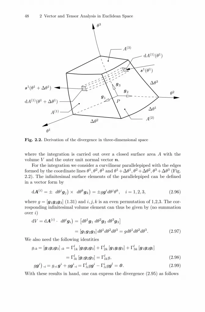
48 2 Vector and Tensor Analysis in Euclidean Space
P
A(1)
Δθ3
s1(θ1)
s1(θ1 + Δθ1)
A(2)
dA(1)(θ1)A(3)
θ3
g3
g2
g1
Δθ1
Δθ2
dA(1)(θ1 + Δθ1)
θ1
θ2
Fig. 2.2. Derivation of the divergence in three-dimensional space
where the integration is carried out over a closed surface area A with thevolume V and the outer unit normal vector n.
For the integration we consider a curvilinear parallelepiped with the edgesformed by the coordinate lines θ1, θ2, θ3 and θ1 +Δθ1, θ2 +Δθ2, θ3 +Δθ3 (Fig.2.2). The infinitesimal surface elements of the parallelepiped can be definedin a vector form by
dA(i) = ± (dθjgj
)× (dθkgk
)= ±ggidθjθk, i = 1, 2, 3, (2.96)
where g = [g1g2g3] (1.31) and i, j, k is an even permutation of 1,2,3. The cor-responding infinitesimal volume element can thus be given by (no summationover i)
dV = dA(i) · (dθigi
)=[dθ1g1 dθ2g2 dθ3g3
]= [g1g2g3] dθ1dθ2dθ3 = gdθ1dθ2dθ3. (2.97)
We also need the following identities
g,k = [g1g2g3] ,k = Γl1k [glg2g3] + Γl
2k [g1glg3] + Γl3k [g1g2gl]
= Γllk [g1g2g3] = Γl
lkg, (2.98)(ggi
),i = g,i gi + ggi,i = Γl
liggi − Γiliggl = 0 . (2.99)
With these results in hand, one can express the divergence (2.95) as follows

2.6 Applications in Three-Dimensional Space: Divergence and Curl 49
divS = limV →0
1V
∫A
SndA
= limV →0
1V
3∑i=1
∫A(i)
[S(θi + Δθi
)dA(i)
(θi + Δθi
)+ S
(θi)dA(i)
(θi)]
.
Using the abbreviation
si(θi)
= S(θi)g(θi)gi(θi), i = 1, 2, 3 (2.100)
we can thus write
divS = limV →0
1V
3∑i=1
θk+Δθk∫θk
θj+Δθj∫θj
[si(θi + Δθi
)− si(θi)]
dθjdθk
= limV →0
1V
3∑i=1
θk+Δθk∫θk
θj+Δθj∫θj
θi+Δθi∫θi
∂si
∂θidθidθjdθk
= limV →0
1V
3∑i=1
∫V
si,ig
dV, (2.101)
where i, j, k is again an even permutation of 1,2,3. Assuming continuity of theintegrand in (2.101) and applying (2.99) and (2.100) we obtain
divS =1gsi,i =
1g
[Sggi
],i =
1g
[S,i ggi + S
(ggi
),i]
= S,i gi, (2.102)
which finally yields by virtue of (2.62)2
divS = S,i gi = S ij·|i gj = Sji|i gj . (2.103)
Example. The momentum balance in Cartesian and cylindricalcoordinates. Let us consider a material body or a part of it with a massm, volume V and outer surface A. According to the Euler law of motion thevector sum of external volume forces fdV and surface tractions tdA results inthe vector sum of inertia forces xdm, where x stands for the position vectorof a material element dm and the superposed dot denotes the material timederivative. Hence,∫
m
xdm =∫A
tdA +∫V
fdV. (2.104)
Applying the Cauchy theorem (1.72) to the first integral on the right handside it further delivers
50 2 Vector and Tensor Analysis in Euclidean Space∫m
xdm =∫A
σndA +∫V
fdV. (2.105)
Dividing this equation by V and considering the limit case V → 0 we obtainby virtue of (2.95)
ρx = divσ + f , (2.106)
where ρ denotes the density of the material. This vector equation is referredto as the momentum balance.
Representing vector and tensor variables with respect to the tangent vec-tors gi (i = 1, 2, 3) of an arbitrary curvilinear coordinate system as
x = xigi, σ = σijgi ⊗ gj , f = f igi
and expressing the divergence of the Cauchy stress tensor by (2.103) we obtainthe component form of the momentum balance (2.106) by
ρxi = σij |j +f i, i = 1, 2, 3. (2.107)
With the aid of (2.86) the covariant derivative of the Cauchy stress tensor canfurther be written by
σij |k= σij ,k +σljΓilk + σilΓj
lk, i, j, k = 1, 2, 3 (2.108)
and thus,
σij |j= σij ,j +σljΓilj + σilΓj
lj , i = 1, 2, 3. (2.109)
By virtue of the expressions for the Christoffel symbols (2.81) and keeping inmind the symmetry of the Cauchy stress tensors σij = σji (i �= j = 1, 2, 3) wethus obtain for cylindrical coordinates:
σ1j |j = σ11,ϕ +σ12,z +σ13,r +3σ31
r,
σ2j |j = σ21,ϕ +σ22,z +σ23,r +σ32
r,
σ3j |j = σ31,ϕ +σ32,z +σ33,r −rσ11 +σ33
r. (2.110)
The balance equations finally take the form
ρx1 = σ11,ϕ +σ12,z +σ13,r +3σ31
r+ f1,
ρx2 = σ21,ϕ +σ22,z +σ23,r +σ32
r+ f2,
ρx3 = σ31,ϕ +σ32,z +σ33,r −rσ11 +σ33
r+ f3. (2.111)
2.6 Applications in Three-Dimensional Space: Divergence and Curl 51
In Cartesian coordinates, where gi = ei (i = 1, 2, 3), the covariant derivativecoincides with the partial one, so that
σij |j= σij ,j = σij ,j . (2.112)
Thus, the balance equations reduce to
ρx1 = σ11,1 +σ12,2 +σ13,3 +f1,
ρx2 = σ21,1 +σ22,2 +σ23,3 +f2,
ρx3 = σ31,1 +σ32,2 +σ33,3 +f3. (2.113)
Divergence and curl of a vector field. Now, we consider a differ-entiable vector field t
(θ1, θ2, θ3
). One defines the divergence and curl of
t(θ1, θ2, θ3
)respectively by
divt = limV →0
1V
∫A
(t · n) dA, (2.114)
curlt = limV →0
1V
∫A
(n × t) dA = − limV →0
1V
∫A
(t × n) dA, (2.115)
where the integration is again carried out over a closed surface area A withthe volume V and the outer unit normal vector n. Considering (1.65) and(2.95), the curl can also be represented by
curlt = − limV →0
1V
∫A
tndA = −divt. (2.116)
Treating the vector field in the same manner as the tensor field we can write
divt = t,i ·gi = ti|i (2.117)
and in view of (2.65)2
divt = tr (gradt) . (2.118)
The same procedure applied to the curl (2.115) leads to
curlt = gi × t,i . (2.119)
By virtue of (2.62) and (1.42) we further obtain (see also Exercise 2.7)
curlt = ti|j gj × gi = ejik 1gti|j gk. (2.120)
With respect to Cartesian coordinates with gi = ei (i = 1, 2, 3) the divergence(2.117) and curl (2.120) simplify to
52 2 Vector and Tensor Analysis in Euclidean Space
divt = ti,i = t1,1 +t2,2 +t3,3 = t1,1 +t2,2 +t3,3 , (2.121)
curlt = ejikti,j ek
= (t3,2 −t2,3 )e1 + (t1,3 −t3,1 )e2 + (t2,1 −t1,2 ) e3. (2.122)
Now, we are going to discuss some combined operations with a gradient, diver-gence, curl, tensor mapping and products of various types (see also Exercise2.11).
1) Curl of a gradient:
curl gradΦ = 0 . (2.123)
2) Divergence of a curl:
div curlt = 0. (2.124)
3) Divergence of a vector product:
div (u × v) = v · curlu − u · curlv. (2.125)
4) Gradient of a divergence:
graddivt = curl curlt + div gradt, (2.126)
graddivt = div (gradt)T . (2.127)
The combined operator div gradt appearing in (2.126) is known as theLaplacian and is also denoted by Δt.
5) Divergence of a (left) mapping
div (tA) = A : gradt + t · divA. (2.128)
6) Divergence of a product of a scalar-valued function and a vector-valuedfunction
div (Φt) = t · gradΦ + Φdivt. (2.129)
7) Divergence of a product of a scalar-valued function and a tensor-valuedfunction
div (ΦA) = AgradΦ + ΦdivA. (2.130)
We prove, for example, identity (2.123). To this end, we apply (2.65)1, (2.72)and (2.119). Thus, we write
curl gradΦ = gj × (Φ|i gi
),j = Φ,ij gj × gi + Φ,i gj × gi,j
= Φ,ij gj × gi − Φ,i Γikjg
j × gk = 0 (2.131)
2.6 Applications in Three-Dimensional Space: Divergence and Curl 53
taking into account that Φ,ij = Φ,ji, Γlij = Γl
ji and gi × gj = −gj × gi
(i �= j, i, j = 1, 2, 3).
Example. Balance of mechanical energy as an integral form ofthe momentum balance. Using the above identities we are now able toformulate the balance of mechanical energy on the basis of the momentumbalance (2.106). To this end, we multiply this vector relation scalarly by thevelocity vector v = x
v · (ρx) = v · divσ + v · f .
Using (2.128) we can further write
v · (ρx) + σ : gradv = div (vσ) + v · f .
Integrating this relation over the volume of the body V yields
ddt
∫m
(12v · v
)dm +
∫V
σ : gradvdV =∫V
div (vσ) dV +∫V
v · fdV,
where dm = ρdV and m denotes the mass of the body. Keeping in mind thedefinition of the divergence (2.95) and applying the Cauchy theorem (1.72)according to which the Cauchy stress vector is given by t = σn, we finallyobtain the relation
ddt
∫m
(12v · v
)dm +
∫V
σ : gradvdV =∫A
v · tdA +∫V
v · fdV (2.132)
expressing the balance of mechanical energy. Indeed, the first and the secondintegrals on the left hand side of (2.132) represent the time rate of the kineticenergy and the stress power, respectively. The right hand side of (2.132) ex-presses the power of external forces i.e. external tractions t on the boundaryof the body A and external volume forces f inside of it.
Example. Navier-Stokes equations for a linear-viscous fluid inCartesian and cylindrical coordinates. A linear-viscous fluid (also calledNewton fluid or Navier-Poisson fluid) is defined by a constitutive equation
σ = −pI + 2ηD + λ (trD) I, (2.133)
where
D =12
[gradv + (gradv)T
](2.134)
denotes the spatial strain rate tensor, p is the hydrostatic pressure while ηand λ represent material constants referred to as shear viscosity and secondviscosity coefficient, respectively. Inserting (2.134) into (2.133) and taking(2.118) into account delivers

54 2 Vector and Tensor Analysis in Euclidean Space
σ = −pI + η[gradv + (gradv)T
]+ λ (divv) I. (2.135)
Substituting this expression into the momentum balance (2.106) and using(2.127) and (2.130) we obtain the relation
ρv = −gradp + ηdiv gradv + (η + λ) graddivv + f (2.136)
referred to as the Navier-Stokes equation. By means of (2.126) it can be rewrit-ten as
ρv = −gradp + (2η + λ) graddivv − ηcurl curlv + f . (2.137)
For an incompressible fluid characterized by the kinematic condition trD =divv = 0, the latter two equations simplify to
ρv = −gradp + ηΔv + f , (2.138)
ρv = −gradp − ηcurl curlv + f . (2.139)
With the aid of the identity Δv = v,i|i (see Exercise 2.13) we thus can write
ρv = −gradp + ηv,i|i +f . (2.140)
In Cartesian coordinates this relation is thus written out as
ρvi = −p,i +η (vi,11 +vi,22 +vi,33 ) + fi, i = 1, 2, 3. (2.141)
For arbitrary curvilinear coordinates we use the following representation forthe vector Laplacian (see Exercise 2.15)
Δv = gij(vk,ij +2Γk
livl,j −Γm
ij vk,m +Γkli,j vl + Γk
mjΓmli vl − Γm
ij Γklmvl
)gk.
(2.142)
For the cylindrical coordinates it takes by virtue of (2.28) and (2.81) thefollowing form
Δv =(r−2v1,11 +v1,22 +v1,33 +3r−1v1,3 +2r−3v3,1
)g1
+(r−2v2,11 +v2,22 +v2,33 +r−1v2,3
)g2
+(r−2v3,11 +v3,22 +v3,33 −2r−1v1,1 +r−1v3,3 −r−2v3
)g3.
Inserting this result into (2.138) and using the representations v = vigi andf = f igi we finally obtain
ρv1 = f1 − ∂p
∂ϕ+ η
(1r2
∂2v1
∂ϕ2+
∂2v1
∂z2+
∂2v1
∂r2+
3r
∂v1
∂r+
2r3
∂v3
∂ϕ
),
ρv2 = f2 − ∂p
∂z+ η
(1r2
∂2v2
∂ϕ2+
∂2v2
∂z2+
∂2v2
∂r2+
1r
∂v2
∂r
),
ρv3 = f3 − ∂p
∂r+ η
(1r2
∂2v3
∂ϕ2+
∂2v3
∂z2+
∂2v3
∂r2− 2
r
∂v1
∂ϕ+
1r
∂v3
∂r− v3
r2
).
(2.143)
2.6 Applications in Three-Dimensional Space: Divergence and Curl 55
Exercises
2.1. Evaluate tangent vectors and metric coefficients of spherical coordinatesin E3 defined by
r (ϕ, φ, r) = r sin ϕ sin φe1 + r cosφe2 + r cosϕ sin φe3. (2.144)
2.2. Evaluate the coefficients∂θi
∂θk(2.41) for the transformation of linear co-
ordinates in the spherical ones and vice versa.
2.3. Evaluate gradients of the following functions of r:
(a)1
‖r‖ , (b) r · w, (c) rAr, (d) Ar, (e) w × r,
where w and A are some vector and tensor, respectively.
2.4. Evaluate the Christoffel symbols of the first and second kind for sphericalcoordinates (2.144).
2.5. Verify relations (2.87).
2.6. Prove the product rules of differentiation for the covariant derivative(2.92-2.94).
2.7. Verify relation (2.120) applying (2.103), (2.116) and using the results ofExercise 1.21.
2.8. Write out the balance equations (2.107) in spherical coordinates (2.144).
2.9. Evaluate tangent vectors, metric coefficients and Christoffel symbols forcylindrical surface coordinates defined by
r (r, s, z) = r coss
re1 + r sin
s
re2 + ze3. (2.145)
2.10. Write out the balance equations (2.107) in cylindrical surface coordi-nates (2.145).
2.11. Prove identities (2.124-2.130).
2.12. Write out the gradient, divergence and curl of a vector field t (r) incylindrical and spherical coordinates (2.16) and (2.144), respectively.
2.13. Prove that the Laplacian of a vector-valued function t (r) can be givenby Δt = t,i|i. Specify this identity for Cartesian coordinates.
2.14. Write out the Laplacian ΔΦ of a scalar field Φ (r) in cylindrical andspherical coordinates (2.16) and (2.144), respectively.
2.15. Write out the Laplacian of a vector field t (r) in component form inan arbitrary curvilinear coordinate system. Specify the result for sphericalcoordinates (2.144).
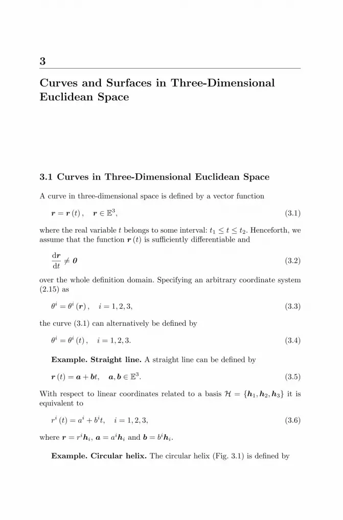
3
Curves and Surfaces in Three-DimensionalEuclidean Space
3.1 Curves in Three-Dimensional Euclidean Space
A curve in three-dimensional space is defined by a vector function
r = r (t) , r ∈ E3, (3.1)
where the real variable t belongs to some interval: t1 ≤ t ≤ t2. Henceforth, weassume that the function r (t) is sufficiently differentiable and
dr
dt�= 0 (3.2)
over the whole definition domain. Specifying an arbitrary coordinate system(2.15) as
θi = θi (r) , i = 1, 2, 3, (3.3)
the curve (3.1) can alternatively be defined by
θi = θi (t) , i = 1, 2, 3. (3.4)
Example. Straight line. A straight line can be defined by
r (t) = a + bt, a, b ∈ E3. (3.5)
With respect to linear coordinates related to a basis H = {h1, h2, h3} it isequivalent to
ri (t) = ai + bit, i = 1, 2, 3, (3.6)
where r = rihi, a = aihi and b = bihi.
Example. Circular helix. The circular helix (Fig. 3.1) is defined by
58 3 Curves and Surfaces in Three-Dimensional Euclidean Space
x3
2πc
e1
e2 x2
x1
r
t
e3
R
Fig. 3.1. Circular helix
r (t) = R cos (t)e1 + R sin (t)e2 + cte3, c �= 0, (3.7)
where ei (i = 1, 2, 3) form an orthonormal basis in E3. For the definition ofthe circular helix the cylindrical coordinates (2.16) appear to be very suitable.Indeed, alternatively to (3.7) we can write
r = R, ϕ = t, z = ct. (3.8)
In the previous chapter we defined tangent vectors to the coordinate lines. Byanalogy one can also define a vector tangent to the curve (3.1) as
gt =dr
dt. (3.9)
It is advantageous to parametrize the curve (3.1) in terms of the so-called arclength. To this end, we first calculate the length of a curve segment betweenthe points corresponding to parameters t1 and t as
s (t) =
r(t)∫r(t1)
√dr · dr. (3.10)
3.1 Curves in Three-Dimensional Euclidean Space 59
With the aid of (3.9) we can write dr = gtdt and consequently
s (t) =
t∫t1
√gt · gtdt =
t∫t1
‖gt‖ dt =
t∫t1
√gtt (t)dt. (3.11)
Using this equation and keeping in mind assumption (3.2) we have
ds
dt=√
gtt (t) �= 0. (3.12)
This implies that the function s = s (t) is invertible and
t (s) =
s∫s(t1)
‖gt‖−1 ds =
s∫s(t1)
ds√gtt (t)
. (3.13)
Thus, the curve (3.1) can be redefined in terms of the arc length s as
r = r (t (s)) = �r (s) . (3.14)
In analogy with (3.9) one defines the vector tangent to the curve �r (s) (3.14)
as
a1 =d�
r
ds=
dr
dt
dt
ds=
gt
‖gt‖ (3.15)
being a unit vector: ‖a1‖ = 1. Differentiation of this vector with respect to sfurther yields
a1,s =da1
ds=
d2 �r
ds2. (3.16)
It can be shown that the tangent vector a1 is orthogonal to a1,s providedthe latter one is not zero. Indeed, differentiating the identity a1 · a1 = 1 withrespect to s we have
a1 · a1,s = 0. (3.17)
The length of the vector a1,s
κ (s) = ‖a1,s ‖ (3.18)
plays an important role in the theory of curves and is called curvature. Theinverse value
ρ (s) =1
κ (s)(3.19)
60 3 Curves and Surfaces in Three-Dimensional Euclidean Space
is referred to as the radius of curvature of the curve at the point �r (s). Hence-
forth, we focus on curves with non-zero curvature. The case of zero curvaturecorresponds to a straight line (see Exercise 3.1) and is trivial.
Next, we define the unit vector in the direction of a1,s
a2 =a1,s
‖a1,s ‖ =a1,sκ (s)
(3.20)
called the principal normal vector to the curve. The orthogonal vectors a1
and a2 can further be completed to an orthonormal basis in E3 by the vector
a3 = a1 × a2 (3.21)
called the unit binormal vector. The triplet of vectors a1, a2 and a3 is referredto as the moving trihedron of the curve.
In order to study the rotation of the trihedron along the curve we againconsider the arc length s as a coordinate. In this case, we can write similarlyto (2.66)
ai,s = Γkisak, i = 1, 2, 3, (3.22)
where Γkis = ai,s ·ak (i, k = 1, 2, 3). From (3.17), (3.20) and (3.21) we imme-
diately observe that Γ21s = κ and Γ1
1s = Γ31s = 0. Further, differentiating the
identities
a3 · a3 = 1, a1 · a3 = 0 (3.23)
with respect to s yields
a3 · a3,s = 0, a1,s ·a3 + a1 · a3,s = 0. (3.24)
Taking into account (3.20) this results in the following identity
a1 · a3,s = −a1,s ·a3 = −κa2 · a3 = 0. (3.25)
Relations (3.24) and (3.25) suggest that
a3,s = −τ (s)a2, (3.26)
where the function
τ (s) = −a3,s ·a2 (3.27)
is called torsion of the curve at the point �r(s). Thus, Γ2
3s = −τ andΓ1
3s = Γ33s = 0. The sign of the torsion (3.27) has a geometric meaning and
remains unaffected by the change of the positive sense of the curve, i.e. bythe transformation s = −s′ (see Exercise 3.2). Accordingly, one distinguishesright-handed curves with a positive torsion and left-handed curves with a neg-ative torsion. In the case of zero torsion the curve is referred to as a planecurve.
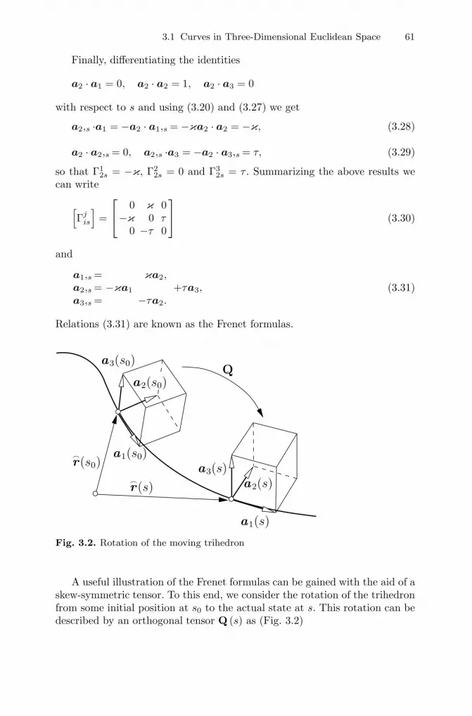
3.1 Curves in Three-Dimensional Euclidean Space 61
Finally, differentiating the identities
a2 · a1 = 0, a2 · a2 = 1, a2 · a3 = 0
with respect to s and using (3.20) and (3.27) we get
a2,s ·a1 = −a2 · a1,s = −κa2 · a2 = −κ, (3.28)
a2 · a2,s = 0, a2,s ·a3 = −a2 · a3,s = τ, (3.29)
so that Γ12s = −κ, Γ2
2s = 0 and Γ32s = τ . Summarizing the above results we
can write
[Γj
is
]=
⎡⎣ 0 κ 0−κ 0 τ
0 −τ 0
⎤⎦ (3.30)
and
a1,s =a2,s =a3,s =
κa2,−κa1 +τa3,
−τa2.(3.31)
Relations (3.31) are known as the Frenet formulas.
�r (s)
a1(s)
a1(s0)
a2(s)a3(s)
Qa2(s0)
�r(s0)
a3(s0)
Fig. 3.2. Rotation of the moving trihedron
A useful illustration of the Frenet formulas can be gained with the aid of askew-symmetric tensor. To this end, we consider the rotation of the trihedronfrom some initial position at s0 to the actual state at s. This rotation can bedescribed by an orthogonal tensor Q (s) as (Fig. 3.2)
62 3 Curves and Surfaces in Three-Dimensional Euclidean Space
ai (s) = Q (s)ai (s0) , i = 1, 2, 3. (3.32)
Differentiating this relation with respect to s yields
ai,s (s) = Q,s (s)ai (s0) , i = 1, 2, 3. (3.33)
Mapping both sides of (3.32) by QT (s) and inserting the result into (3.33)we further obtain
ai,s (s) = Q,s (s)QT (s)ai (s) , i = 1, 2, 3. (3.34)
Differentiating the identity (1.129) Q (s)QT (s) = I with respect to s we haveQ,s (s)QT (s) + Q (s)QT,s (s) = 0, which implies that the tensor W (s) =Q,s (s)QT (s) is skew-symmetric. Hence, eq. (3.34) can be rewritten as (seealso [3])
ai,s (s) = W (s) ai (s) , W ∈ Skew3, i = 1, 2, 3, (3.35)
where according to (3.31)
W (s) = τ (s) (a3 ⊗ a2 − a2 ⊗ a3) + κ (s) (a2 ⊗ a1 − a1 ⊗ a2) . (3.36)
By virtue of (1.130) and (1.131) we further obtain
W = τ a1 + κa3 (3.37)
and consequently
ai,s = d × ai = dai, i = 1, 2, 3, (3.38)
where
d = τa1 + κa3 (3.39)
is referred to as the Darboux vector.
Example. Curvature, torsion, moving trihedron and Darbouxvector for a circular helix. Inserting (3.7) into (3.9) delivers
gt =dr
dt= −R sin (t)e1 + R cos (t)e2 + ce3, (3.40)
so that
gtt = gt · gt = R2 + c2 = const. (3.41)
Thus, using (3.13) we may set
t (s) =s√
R2 + c2. (3.42)
3.1 Curves in Three-Dimensional Euclidean Space 63
Using this result, the circular helix (3.7) can be parametrized in terms of thearc length s by
�r(s) = R cos
(s√
R2 + c2
)e1 + R sin
(s√
R2 + c2
)e2 +
cs√R2 + c2
e3.
(3.43)
With the aid of (3.15) we further write
a1 =d�
r
ds=
1√R2 + c2
[−R sin
(s√
R2 + c2
)e1
+ R cos(
s√R2 + c2
)e2 + ce3
], (3.44)
a1,s = − R
R2 + c2
[cos
(s√
R2 + c2
)e1 + sin
(s√
R2 + c2
)e2
]. (3.45)
According to (3.18) the curvature of the helix is thus
κ =R
R2 + c2. (3.46)
By virtue of (3.20), (3.21) and (3.27) we have
a2 =a1,sκ
= − cos(
s√R2 + c2
)e1 − sin
(s√
R2 + c2
)e2, (3.47)
a3 = a1 × a2 =1√
R2 + c2
[c sin
(s√
R2 + c2
)e1
−c cos(
s√R2 + c2
)e2 + Re3
]. (3.48)
a3,s =c
R2 + c2
[cos
(s√
R2 + c2
)e1 + sin
(s√
R2 + c2
)e2
], (3.49)
τ =c
R2 + c2. (3.50)
It is seen that the circular helix is right-handed for c > 0, left-handed forc < 0 and becomes a circle for c = 0. For the Darboux vector (3.39) we finallyobtain
d = τa1 + κa3 =1√
R2 + c2e3. (3.51)

64 3 Curves and Surfaces in Three-Dimensional Euclidean Space
3.2 Surfaces in Three-Dimensional Euclidean Space
A surface in three-dimensional Euclidean space is defined by a vector function
r = r(t1, t2
), r ∈ E
3, (3.52)
of two real variables t1 and t2 referred to as Gauss coordinates. With the aidof the coordinate system (3.3) one can alternatively write
θi = θi(t1, t2
), i = 1, 2, 3. (3.53)
In the following, we assume that the function r(t1, t2
)is sufficiently differen-
tiable with respect to both arguments and
dr
dtα�= 0 , α = 1, 2 (3.54)
over the whole definition domain.
Example 1. Plane. Let us consider three linearly independent vectorsxi (i = 0, 1, 2) specifying three points in three-dimensional space. The planegoing through these points can be defined by
r(t1, t2
)= x0 + t1 (x1 − x0) + t2 (x2 − x0) . (3.55)
Example 2. Cylinder. A cylinder of radius R with the axis parallel toe3 is defined by
r(t1, t2
)= R cos t1e1 + R sin t1e2 + t2e3, (3.56)
where ei (i = 1, 2, 3) again form an orthonormal basis in E3. With the aid ofthe cylindrical coordinates (2.16) we can alternatively write
ϕ = t1, z = t2, r = R. (3.57)
Example 3. Sphere. A sphere of radius R with the center at r = 0 isdefined by
r(t1, t2
)= R sin t1 sin t2e1 + R cos t2e2 + R cos t1 sin t2e3, (3.58)
or by means of spherical coordinates (2.144) as
ϕ = t1, φ = t2, r = R. (3.59)
Using a parametric representation (see, e.g., [25])
t1 = t1 (t) , t2 = t2 (t) (3.60)
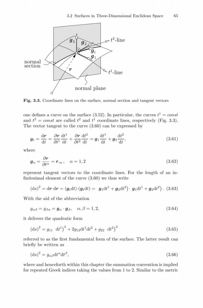
3.2 Surfaces in Three-Dimensional Euclidean Space 65
r
g 1
g3 g 2
g t
t2-line
t1-line
normal plane
normalsection
Fig. 3.3. Coordinate lines on the surface, normal section and tangent vectors
one defines a curve on the surface (3.52). In particular, the curves t1 = constand t2 = const are called t2 and t1 coordinate lines, respectively (Fig. 3.3).The vector tangent to the curve (3.60) can be expressed by
gt =dr
dt=
∂r
∂t1dt1
dt+
∂r
∂t2dt2
dt= g1
dt1
dt+ g2
dt2
dt, (3.61)
where
gα =∂r
∂tα= r,α , α = 1, 2 (3.62)
represent tangent vectors to the coordinate lines. For the length of an in-finitesimal element of the curve (3.60) we thus write
(ds)2 = dr·dr = (gtdt)·(gtdt) =(g1dt1 + g2dt2
)·(g1dt1 + g2dt2). (3.63)
With the aid of the abbreviation
gαβ = gβα = gα · gβ , α, β = 1, 2, (3.64)
it delivers the quadratic form
(ds)2 = g11
(dt1
)2+ 2g12dt1dt2 + g22
(dt2
)2(3.65)
referred to as the first fundamental form of the surface. The latter result canbriefly be written as
(ds)2 = gαβdtαdtβ , (3.66)
where and henceforth within this chapter the summation convention is impliedfor repeated Greek indices taking the values from 1 to 2. Similar to the metric
66 3 Curves and Surfaces in Three-Dimensional Euclidean Space
coefficients (1.85)1,2 in n-dimensional Euclidean space gαβ (3.64) describe themetric on a surface. Generally, the metric described by a differential quadraticform like (3.66) is referred to as Riemannian metric.
The tangent vectors (3.62) can be completed to a basis in E3 by the unitvector
g3 =g1 × g2
‖g1 × g2‖ (3.67)
called principal normal vector to the surface.In the following, we focus on a special class of surface curves called normal
sections. These are curves passing through a point of the surface r(t1, t2
)and
obtained by intersection of this surface with a plane involving the principalnormal vector. Such a plane is referred to as the normal plane.
In order to study curvature properties of normal sections we first expressthe derivatives of the basis vectors gi (i = 1, 2, 3) with respect to the surfacecoordinates. Using the formalism of Christoffel symbols we can write
gi,α =∂gi
∂tα= Γiαkgk = Γk
iαgk, i = 1, 2, 3, (3.68)
where
Γiαk = gi,α ·gk, Γkiα = gi,α ·gk, i = 1, 2, 3, α = 1, 2. (3.69)
Taking into account the identity g3 = g3 resulting from (3.67) we immediatelyobserve that
Γiα3 = Γ3iα, i = 1, 2, 3, α = 1, 2. (3.70)
Differentiating the relations
gα · g3 = 0, g3 · g3 = 1 (3.71)
with respect to the Gauss coordinates we further obtain
gα,β ·g3 = −gα · g3,β , g3,α ·g3 = 0, α, β = 1, 2 (3.72)
and consequently
Γ3αβ = −Γ3βα, Γ3
3α = 0, α, β = 1, 2. (3.73)
Using in (3.68) the abbreviation
bαβ = bβα = Γ3αβ = −Γ3αβ = gα,β ·g3, α, β = 1, 2, (3.74)
we arrive at the relations
gα,β = Γραβgρ + bαβg3, α, β = 1, 2 (3.75)
3.2 Surfaces in Three-Dimensional Euclidean Space 67
called the Gauss formulas.Similarly to a coordinate system one can notionally define the covariant
derivative also on the surface. To this end, relations (2.84), (2.86) and (2.87)are specified to the two-dimensional space in a straight forward manner as
fα|β= fα,β +fρΓαρβ , fα|β= fα,β −fρΓ
ραβ , (3.76)
Fαβ|γ= Fαβ ,γ +FρβΓαργ + FαρΓβ
ργ , Fαβ |γ= Fαβ ,γ −FρβΓραγ − FαρΓ
ρβγ ,
Fα·β|γ= Fα
·β,γ +Fρ·βΓα
ργ − Fα·ρΓ
ρβγ , α, β, γ = 1, 2. (3.77)
Thereby, with the aid of (3.76)2 the Gauss formulas (3.75) can alternativelybe given by (cf. (2.89))
gα|β= bαβg3, α, β = 1, 2. (3.78)
Further, we can write
bβα = bαρg
ρβ = −Γ3αρgρβ = −Γβ
3α, α, β = 1, 2. (3.79)
Inserting the latter relation into (3.68) and considering (3.73)2, this yields theidentities
g3,α = g3|α= −bραgρ, α = 1, 2 (3.80)
referred to as the Weingarten formulas.Now, we are in a position to express the curvature of a normal section. It
is called normal curvature and denoted in the following by κn. At first, weobserve that the principal normals of the surface and of the normal sectioncoincide in the sense that a2 = ±g3. Using (3.13), (3.28), (3.61), (3.72)1 and(3.74) and assuming for the moment that a2 = g3 we get
κn = −a2,s ·a1 = −g3,s · gt
‖gt‖ = −(
g3,tdt
ds
)· gt
‖gt‖ = −g3,t · gt
‖gt‖2
= −(
g3,αdtα
dt
)·(
gβdtβ
dt
)‖gt‖−2 = bαβ
dtα
dt
dtβ
dt‖gt‖−2
.
By virtue of (3.63) and (3.66) this leads to the following result
κn =bαβdtαdtβ
gαβdtαdtβ, (3.81)
where the quadratic form
bαβdtαdtβ = −dr · dg3 (3.82)
is referred to as the second fundamental form of the surface. In the casea2 = −g3 the sign of the expression for κn (3.81) must be changed. Instead of
68 3 Curves and Surfaces in Three-Dimensional Euclidean Space
that, we assume that the normal curvature can, in contrast to the curvatureof space curves (3.18), be negative. However, the sign of κn (3.81) has nogeometrical meaning. Indeed, it depends on the orientation of g3 with respectto a2 which is immaterial. For example, g3 changes the sign in coordinatetransformations like t1 = t2, t2 = t1.
Of special interest is the dependence of the normal curvature κn on thedirection of the normal section. For example, for the normal sections passingthrough the coordinate lines we have
κn|t2=const =b11
g11, κn|t1=const =
b22
g22. (3.83)
In the following, we are going to find the directions of the maximal and mini-mal curvature. Necessary conditions for the extremum of the normal curvature(3.81) are given by
∂κn
∂tα= 0, α = 1, 2. (3.84)
Rewriting (3.81) as
(bαβ − κngαβ) dtαdtβ = 0 (3.85)
and differentiating with respect to tα we obtain
(bαβ − κngαβ) dtβ = 0, α = 1, 2. (3.86)
Multiplying both sides of this equation system by gαρ and summing up overα we have with the aid of (3.79)(
bρβ − κnδρ
β
)dtβ = 0, ρ = 1, 2. (3.87)
A nontrivial solution of this homogeneous equation system exists if and onlyif ∣∣∣∣ b1
1 − κn b12
b21 b2
2 − κn
∣∣∣∣ = 0. (3.88)
Writing out the above determinant we can also write
κ2n − bα
ακn +∣∣bα
β
∣∣ = 0. (3.89)
The maximal and minimal curvatures κ1 and κ2 resulting from this quadraticequation are called the principal curvatures. One can show that directions ofprincipal curvatures are mutually orthogonal (see Theorem 4.5, Sect. 4). Thesedirections are called principal directions of normal curvature or curvaturedirections (see also [25]).
According to the Vieta theorem the product of principal curvatures canbe expressed by
3.2 Surfaces in Three-Dimensional Euclidean Space 69
K = κ1κ2 =∣∣bα
β
∣∣ =b
g2, (3.90)
where
b = |bαβ | =∣∣∣∣ b11 b12
b21 b22
∣∣∣∣ = b11b22 − (b12)2 , (3.91)
g2 = [g1g2g3]2 =
∣∣∣∣∣∣g11 g12 0g21 g22 00 0 1
∣∣∣∣∣∣ = g11g22 − (g12)2. (3.92)
For the arithmetic mean of the principal curvatures we further obtain
H =12
(κ1 + κ2) =12bαα. (3.93)
The values K (3.90) and H (3.93) do not depend on the direction of thenormal section and are called the Gaussian and mean curvatures, respectively.In terms of K and H the solutions of the quadratic equation (3.89) can simplybe given by
κ1,2 = H ±√
H2 − K. (3.94)
One recognizes that the sign of the Gaussian curvature K (3.90) is definedby the sign of b (3.91). For positive b both κ1 and κ2 are positive or negative sothat κn has the same sign for all directions of the normal sections at r
(t1, t2
).
In other words, the orientation of a2 with respect to g3 remains constant. Sucha point of the surface is called elliptic.
For b < 0, principal curvatures are of different signs so that different normalsections are characterized by different orientations of a2 with respect to g3.There are two directions of the normal sections with zero curvature. Suchnormal sections are referred to as asymptotic directions. The correspondingpoint of the surface is called hyperbolic or saddle point.
In the intermediate case b = 0, κn does not change sign. There is only oneasymptotic direction which coincides with one of the principal directions (ofκ1 or κ2). The corresponding point of the surface is called parabolic point.
Example. Torus. A torus is a surface obtained by rotating a circle abouta coplanar axis (see Fig. 3.4). Additionally we assume that the rotation axislies outside of the circle. Accordingly, the torus can be defined by
r(t1, t2
)=(R0 + R cos t2
)cos t1e1
+(R0 + R cos t2
)sin t1e2 + R sin t2e3, (3.95)
where R0 is the radius of the circle and R is the distance between its centerand the rotation axis. By means of (3.62) and (3.67) we obtain
g1 = − (R0 + R cos t2)sin t1e1 +
(R0 + R cos t2
)cos t1e2,

70 3 Curves and Surfaces in Three-Dimensional Euclidean Space
x3
x1
e2
e3
e1
R0
x2
t1
R t2
Fig. 3.4. Torus
g2 = −R cos t1 sin t2e1 − R sin t1 sin t2e2 + R cos t2e3,
g3 = cos t1 cos t2e1 + sin t1 cos t2e2 + sin t2e3. (3.96)
Thus, the coefficients (3.64) of the first fundamental form (3.65) are given by
g11 =(R0 + R cos t2
)2, g12 = 0, g22 = R2. (3.97)
In order to express coefficients (3.74) of the second fundamental form (3.82)we first calculate derivatives of the tangent vectors (3.96)1,2
g1,1 = − (R0 + R cos t2)cos t1e1 −
(R0 + R cos t2
)sin t1e2,
g1,2 = g2,1 = R sin t1 sin t2e1 − R cos t1 sin t2e2,
g2,2 = −R cos t1 cos t2e1 − R sin t1 cos t2e2 − R sin t2e3. (3.98)
Inserting these expressions as well as (3.96)3 into (3.74) we obtain
b11 = − (R0 + R cos t2)cos t2, b12 = b21 = 0, b22 = −R. (3.99)
In view of (3.79) and (3.97) b21 = b1
2 = 0. Thus, the solution of the equationsystem (3.88) delivers
κ1 = b11 =
b11
g11= − cos t2
R0 + R cos t2, κ2 = b2
2 =b22
g22= −R−1. (3.100)
Comparing this result with (3.83) we see that the coordinate lines of the torus(3.95) coincide with the principal directions of the normal curvature. Hence,by (3.90)
3.3 Application to Shell Theory 71
K = κ1κ2 =cos t2
R (R0 + R cos t2). (3.101)
Thus, points of the torus for which −π/2 < t2 < π/2 are elliptic while pointsfor which π/2 < t2 < 3π/2 are hyperbolic. Points of the coordinates linest2 = −π/2 and t2 = π/2 are parabolic.
3.3 Application to Shell Theory
Geometry of the shell continuum. Let us consider a surface in the three-dimensional Euclidean space defined by (3.52) as
r = r(t1, t2
), r ∈ E
3 (3.102)
and bounded by a closed curve C (Fig. 3.5). The shell continuum can then bedescribed by a vector function
r∗ = r∗ (t1, t2, t3) = r(t1, t2
)+ g3t
3, (3.103)
where the unit vector g3 is defined by (3.62) and (3.67) while −h/2 ≤ t3 ≤h/2. The surface (3.102) is referred to as the middle surface of the shell.The thickness of the shell h is assumed to be small in comparison to its otherdimensions as for example the minimal curvature radius of the middle surface.
Every fixed value of the thickness coordinate t3 defines a surface r∗ (t1, t2)whose geometrical variables are obtained according to (1.40), (3.62), (3.64),(3.79), (3.80), (3.90), (3.93) and (3.103) as follows.
g∗α = r∗,α = gα + t3g3,α =
(δρα − t3bρ
α
)gρ, α = 1, 2, (3.104)
g∗3 =
g∗1 × g∗
2
‖g∗1 × g∗
2‖= r∗,3 = g3, (3.105)
g∗αβ = g∗α · g∗
β = gαβ − 2t3bαβ +(t3)2
bαρbρβ, α, β = 1, 2, (3.106)
g∗ = [g∗1g
∗2g
∗3] =
[(δρ1 − t3bρ
1
)gρ
(δγ2 − t3bγ
2
)gγg3
]=(δρ1 − t3bρ
1
) (δγ2 − t3bγ
2
)geργ3 = g
∣∣δαβ − t3bα
β
∣∣= g
[1 − 2t3H +
(t3)2
K]. (3.107)
The factor in brackets in the latter expression
μ =g∗
g= 1 − 2t3H +
(t3)2
K (3.108)
is called the shell shifter.

72 3 Curves and Surfaces in Three-Dimensional Euclidean Space
g∗2
g ∗3 = g 3
g∗1
h/2
h/2
A(2)A(1)
r ∗(t1, t2, t3)
g3
t2-line
t3-line
t1-line
g 1
middle surface
boundarycurve C
r(t1, t2)
g2
Fig. 3.5. Geometry of the shell continuum
Internal force variables. Let us consider an element of the shell contin-uum (see Fig. 3.6) bounded by the coordinate lines tα and tα+Δtα (α = 1, 2).One defines the force vector fα and the couple vector mα relative to the mid-dle surface of the shell, respectively, by
fα =
h/2∫−h/2
μσg∗αdt3, mα =
h/2∫−h/2
μr∗ × (σg∗α) dt3, α = 1, 2, (3.109)
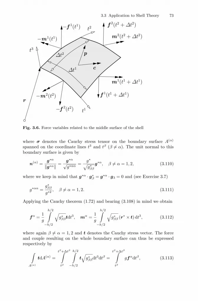
3.3 Application to Shell Theory 73
m1(t1 + Δt1)
p
c
−m2(t2)
−f 2(t2)
f 1(t1 + Δt1)
f 2(t2 + Δt2)
−m1(t1)
−f 1(t1)
t1
Δt1
Δt2
r
m2(t2 + Δt2)
t3
t2
Fig. 3.6. Force variables related to the middle surface of the shell
where σ denotes the Cauchy stress tensor on the boundary surface A(α)
spanned on the coordinate lines t3 and tβ (β �= α). The unit normal to thisboundary surface is given by
n(α) =g∗α
‖g∗α‖ =g∗α
√g∗αα
=g∗√g∗ββ
g∗α, β �= α = 1, 2, (3.110)
where we keep in mind that g∗α · g∗β = g∗α · g3 = 0 and (see Exercise 3.7)
g∗αα =g∗ββ
g∗2, β �= α = 1, 2. (3.111)
Applying the Cauchy theorem (1.72) and bearing (3.108) in mind we obtain
fα =1g
h/2∫−h/2
√g∗ββtdt3, mα =
1g
h/2∫−h/2
√g∗ββ (r∗ × t) dt3, (3.112)
where again β �= α = 1, 2 and t denotes the Cauchy stress vector. The forceand couple resulting on the whole boundary surface can thus be expressedrespectively by∫
A(α)
tdA(α) =
tβ+Δtβ∫tβ
h/2∫−h/2
t√
g∗ββdt3dtβ =
tβ+Δtβ∫tβ
gfαdtβ , (3.113)
74 3 Curves and Surfaces in Three-Dimensional Euclidean Space
∫A(α)
(r∗ × t) dA(α) =
tβ+Δtβ∫tβ
h/2∫−h/2
(r∗ × t)√
g∗ββdt3dtβ
=
tβ+Δtβ∫tβ
gmαdtβ , β �= α = 1, 2, (3.114)
where we make use of the relation
dA(α) = g∗√
g∗ααdtβdt3 =√
g∗ββdtβdt3, β �= α = 1, 2 (3.115)
following immediately from (2.96) and (3.111).The force and couple vectors (3.109) are usually represented with respect
to the basis related to the middle surface as (see also [1])
fα = fαβgβ + qαg3, mα = mαβg3 × gβ = g e3βρmαβgρ. (3.116)
In shell theory, their components are denoted as follows.
fαβ - components of the stress resultant tensor,
qα - components of the transverse shear stress vector,
mαβ - components of the moment tensor.
External force variables. One defines the load force vector and the loadmoment vector related to a unit area of the middle surface, respectively by
p = pigi, c = cρg3 × gρ. (3.117)
The load moment vector c is thus assumed to be tangential to the middlesurface. The resulting force and couple can be expressed respectively by
t2+Δt2∫t2
t1+Δt1∫t1
pgdt1dt2,
t2+Δt2∫t2
t1+Δt1∫t1
cgdt1dt2. (3.118)
Equilibrium conditions. Taking (3.113) and (3.118)1 into account theforce equilibrium condition of the shell element can be expressed as
2∑α,β=1α�=β
tβ+Δtβ∫tβ
[g (tα + Δtα)fα (tα + Δtα) − g (tα)fα (tα)] dtβ
3.3 Application to Shell Theory 75
+
t2+Δt2∫t2
t1+Δt1∫t1
pgdt1dt2 = 0 . (3.119)
Rewriting the first integral in (3.119) we further obtain
t2+Δt2∫t2
t1+Δt1∫t1
[(gfα) ,α +gp] dt1dt2 = 0 . (3.120)
Since the latter condition holds for all shell elements we infer that
(gfα) ,α +gp = 0 , (3.121)
which leads by virtue of (2.98) and (3.73)2 to
fα|α +p = 0 , (3.122)
where the covariant derivative is formally applied to the vectors fα accordingto (3.76)1.
In a similar fashion we can treat the moment equilibrium. In this case, weobtain instead of (3.121) the following condition
[g (mα + r × fα)] ,α +gr × p + gc = 0 . (3.123)
With the aid of (3.62) and keeping (3.122) in mind, it finally delivers
mα|α +gα × fα + c = 0 . (3.124)
In order to rewrite the equilibrium conditions (3.122) and (3.124) in compo-nent form we further utilize representations (3.116), (3.117) and apply theproduct rule of differentiation for the covariant derivative (see, e.g., (2.92-2.94)). By virtue of (3.78) and (3.80) it delivers
(fαρ|α −bραqα + pρ) gρ +
(fαβbαβ + qα|α +p3
)g3 = 0 , (3.125)
(mαρ|α −qρ + cρ) g3 × gρ + g eαβ3fαβg3 = 0 (3.126)
with a new variable
fαβ = fαβ + bβγmγα, α, β = 1, 2 (3.127)
called pseudo-stress resultant. Keeping in mind that the vectors gi (i = 1, 2, 3)are linearly independent we thus obtain the following scalar force equilibriumconditions
fαρ|α −bραqα + pρ = 0, ρ = 1, 2, (3.128)
bαβfαβ + qα|α +p3 = 0 (3.129)

76 3 Curves and Surfaces in Three-Dimensional Euclidean Space
and moment equilibrium conditions
mαρ|α −qρ + cρ = 0, ρ = 1, 2, (3.130)
fαβ = fβα, α, β = 1, 2, α �= β. (3.131)
With the aid of (3.127) one can finally eliminate the components of the stressresultant tensor fαβ from (3.128) and (3.129). This leads to the followingequation system
fαρ|α − (bργmγα
)|α −bραqα + pρ = 0, ρ = 1, 2, (3.132)
bαβ fαβ − bαβbβγmγα + qα|α +p3 = 0, (3.133)
mαρ|α −qρ + cρ = 0, ρ = 1, 2, (3.134)
where the latter relation is repeated from (3.130) for completeness.
Example. Equilibrium equations of plate theory. In this case, themiddle surface of the shell is a plane (3.55) for which
bαβ = bαβ = 0, α, β = 1, 2. (3.135)
Thus, the equilibrium equations (3.132-3.134) simplify to
fαρ,α +pρ = 0, ρ = 1, 2, (3.136)
qα,α +p3 = 0, (3.137)
mαρ,α −qρ + cρ = 0, ρ = 1, 2, (3.138)
where in view of (3.127) and (3.131) fαβ = fβα (α �= β = 1, 2).
Example. Equilibrium equations of membrane theory. The mem-brane theory assumes that the shell is moment free so that
mαβ = 0, cβ = 0, α, β = 1, 2. (3.139)
In this case, the equilibrium equations (3.132-3.134) reduce to
fαρ|α +pρ = 0, ρ = 1, 2, (3.140)
bαβfαβ + p3 = 0, (3.141)
qρ = 0, ρ = 1, 2, (3.142)
where again fαβ = fβα (α �= β = 1, 2).
3.3 Application to Shell Theory 77
Exercises
3.1. Show that a curve r (s) is a straight line if κ (s) ≡ 0 for any s .
3.2. Show that the curves r (s) and r′ (s) = r (−s) have the same curvatureand torsion.
3.3. Show that a curve r (s) characterized by zero torsion τ (s) ≡ 0 for any slies in a plane.
3.4. Evaluate the Christoffel symbols of the second kind, the coefficients ofthe first and second fundamental forms, the Gaussian and mean curvaturesfor the cylinder (3.56).
3.5. Evaluate the Christoffel symbols of the second kind, the coefficients ofthe first and second fundamental forms, the Gaussian and mean curvaturesfor the sphere (3.58).
3.6. For the so-called hyperbolic paraboloidal surface defined by
r(t1, t2
)= t1e1 + t2e2 +
t1t2
ce3, c > 0, (3.143)
evaluate the tangent vectors to the coordinate lines, the coefficients of thefirst and second fundamental forms, the Gaussian and mean curvatures.
3.7. Verify relation (3.111).
3.8. Write out equilibrium equations (3.140-3.141) of the membrane theoryfor a cylindrical shell and a spherical shell.
4
Eigenvalue Problem and SpectralDecomposition of Second-Order Tensors
4.1 Complexification
So far we have considered solely real vectors and real vector spaces. For thepurposes of this chapter an introduction of complex vectors is, however, nec-essary. Indeed, in the following we will see that the existence of a solution ofan eigenvalue problem even for real second-order tensors can be guaranteedonly within a complex vector space. In order to define the complex vectorspace let us consider ordered pairs 〈x, y〉 of real vectors x and y ∈ E
n. Thesum of two such pairs is defined by [14]
〈x1, y1〉 + 〈x2, y2〉 = 〈x1 + x2, y1 + y2〉 . (4.1)
Further, we define the product of a pair 〈x, y〉 by a complex number α + iβby
(α + iβ) 〈x, y〉 = 〈αx − βy, βx + αy〉 , (4.2)
where α, β ∈ R and i =√−1. These formulas can easily be recovered assuming
that
〈x, y〉 = x + iy. (4.3)
The definitions (4.1) and (4.2) enriched by the zero pair 〈0 ,0 〉 are sufficient toensure that the axioms (A.1-A.4) and (B.1-B.4) of Chap. 1 are valid. Thus, theset of all pairs z = 〈x, y〉 characterized by the above properties forms a vectorspace referred to as complex vector space. Every basis G = {g1, g2, . . . , gn}of the underlying Euclidean space En represents simultaneously a basis of thecorresponding complexified space. Indeed, for every complex vector withinthis space
z = x + iy, (4.4)
where x, y ∈ En and consequently
80 4 Eigenvalue Problem and Spectral Decomposition of Second-Order Tensors
x = xigi, y = yigi, (4.5)
we can write
z =(xi + iyi
)gi. (4.6)
Thus, the dimension of the complexified space coincides with the dimensionof the original real vector space. Using this fact we will denote the complexvector space based on En by Cn. Clearly, En represents a subset of Cn.
For every vector z ∈ Cn given by (4.4) one defines a complex conjugatecounterpart by
z = x − iy. (4.7)
Of special interest is the scalar product of two complex vectors, say z1 =x1 + iy1 and z2 = x2 + iy2, which we define by (see also [4])
(x1 + iy1) · (x2 + iy2) = x1 · x2 − y1 · y2 + i (x1 · y2 + y1 · x2) . (4.8)
This scalar product is commutative (C.1), distributive (C.2) and linear ineach factor (C.3). Thus, it differs from the classical scalar product of complexvectors given in terms of the complex conjugate (see, e.g., [14]). As a result,the axiom (C.4) does not generally hold. For instance, one can easily imagine anon-zero complex vector whose scalar product with itself is zero. For complexvectors with the scalar product (4.8) the notions of length, orthogonality orparallelity can hardly be interpreted geometrically.
However, for complex vectors the axiom (C.4) can be reformulated by
z · z ≥ 0, z · z = 0 if and only if z = 0 . (4.9)
Indeed, using (4.4), (4.7) and (4.8) we obtain z · z = x · x + y · y. Bearing inmind that the vectors x and y belong to the Euclidean space this immediatelyimplies (4.9).
As we learned in Chap. 1, the Euclidean space En is characterized by
the existence of an orthonormal basis (1.8). This can now be postulated forthe complex vector space Cn as well, because Cn includes En by the verydefinition. Also Theorem 1.6 remains valid since it has been proved withoutmaking use of the property (C.4). Thus, we may state that for every basis inC
n there exists a unique dual basis.The last step of the complexification is a generalization of a linear mapping
on complex vectors. This can be achieved by setting for every tensor A ∈ Linn
A (x + iy) = Ax + i (Ay) . (4.10)
4.2 Eigenvalue Problem, Eigenvalues and Eigenvectors
Let A ∈ Linn be a second-order tensor. The equation
4.2 Eigenvalue Problem, Eigenvalues and Eigenvectors 81
Aa = λa, a �= 0 (4.11)
is referred to as the eigenvalue problem of the tensor A. The non-zero vectora ∈ C
n satisfying this equation is called an eigenvector of A; λ is called aneigenvalue of A. It is clear that any product of an eigenvector with any (realor complex) scalar is again an eigenvector.
The eigenvalue problem (4.11) and the corresponding eigenvector a canbe regarded as the right eigenvalue problem and the right eigenvector, respec-tively. In contrast, one can define the left eigenvalue problem by
bA = λb, b �= 0 , (4.12)
where b ∈ Cn is the left eigenvector. In view of (1.110), every right eigenvectorof A represents the left eigenvector of AT and vice versa. In the following,unless indicated otherwise, we will mean the right eigenvalue problem and theright eigenvector.
Mapping (4.11) by A several times we obtain
Aka = λka, k = 1, 2, . . . (4.13)
This leads to the following (spectral mapping) theorem.
Theorem 4.1. Let λ be an eigenvalue of the tensor A and let g (A) =∑mk=0 akAk be a polynomial of A. Then g (λ) =
∑mk=0 akλk is the eigenvalue
of g (A).
Proof. Let a be an eigenvector of A associated with λ. Then, in view of (4.13)
g (A) a =m∑
k=0
akAka =m∑
k=0
akλka =
(m∑
k=0
akλk
)a = g (λ) a.
In order to find the eigenvalues of the tensor A we consider the followingrepresentations:
A = Ai·jgi ⊗ gj , a = aigi, b = big
i, (4.14)
where G = {g1, g2, . . . , gn} and G′ ={g1, g2, . . . , gn
}are two arbitrary mu-
tually dual bases in En and consequently also in Cn. Note that we prefer herethe mixed variant representation of the tensor A. Inserting (4.14) into (4.11)and (4.12) further yields
Ai·ja
jgi = λaigi, Ai·jbig
j = λbjgj ,
and therefore(Ai
·jaj − λai
)gi = 0 ,
(Ai
·jbi − λbj
)gj = 0 . (4.15)
82 4 Eigenvalue Problem and Spectral Decomposition of Second-Order Tensors
Since the vectors gi on the one side and gi (i = 1, 2, . . . , n) on the other sideare linearly independent the associated scalar coefficients in (4.15) must bezero. This results in the following two linear homogeneous equation systems(
Ai·j − λδi
j
)aj = 0,
(Aj
·i − λδji
)bj = 0, i = 1, 2, . . . , n (4.16)
with respect to the components of the right eigenvector a and the left eigen-vector b, respectively. A non-trivial solution of these equation systems existsif and only if∣∣Ai
·j − λδij
∣∣ = 0, (4.17)
where |•| denotes the determinant of a matrix. Eq. (4.17) is called the char-acteristic equation of the tensor A. Writing out the determinant on the lefthand side of this equation one obtains a polynomial of degree n with respectto the powers of λ
pA (λ) = λn − λn−1I(1)A + . . . + (−1)kλn−kI(k)
A + . . . + (−1)n I(n)A , (4.18)
referred to as the characteristic polynomial of the tensor A. Thereby, it caneasily be seen that
I(1)A = Ai·i = trA, I(n)
A =∣∣Ai
·j∣∣ . (4.19)
The characteristic equation (4.17) can briefly be written as
pA (λi) = 0. (4.20)
According to the fundamental theorem of algebra, a polynomial of degree nhas n complex roots which may be multiple. These roots are the eigenvaluesλi (i = 1, 2, . . . , n) of the tensor A.
Factorizing the characteristic polynomial (4.18) yields
pA (λ) =n∏
i=1
(λ − λi) . (4.21)
Collecting multiple eigenvalues the polynomial (4.21) can further be rewrittenas
pA (λ) =s∏
i=1
(λ − λi)ri , (4.22)
where s (1 ≤ s ≤ n) denotes the number of distinct eigenvalues, while ri isreferred to as an algebraic multiplicity of the eigenvalue λi (i = 1, 2, . . . , s). Itshould formally be distinguished from the so-called geometric multiplicity ti,which represents the number of linearly independent eigenvectors associatedwith this eigenvalue.
4.3 Characteristic Polynomial 83
Example. Eigenvalues and eigenvectors of the deformation gradi-ent in the case of simple shear. In simple shear, the deformation gradientcan be given by F = Fi
·jei ⊗ ej , where
[Fi·j]
=
⎡⎣ 1 γ 00 1 00 0 1
⎤⎦ (4.23)
and γ denotes the amount of shear. The characteristic equation (4.17) for thetensor F takes thus the form∣∣∣∣∣∣
1 − λ γ 00 1 − λ 00 0 1 − λ
∣∣∣∣∣∣ = 0.
Writing out this determinant we obtain
(1 − λ)3 = 0,
which yields one triple eigenvalue
λ1 = λ2 = λ3 = 1.
The associated (right) eigenvectors a = aiei can be obtained from the equa-tion system (4.16)1 i.e.(
Fi·j − λδi
j
)aj = 0, i = 1, 2, 3.
In view of (4.23) it reduces to the only non-trivial equation
a2γ = 0.
Hence, all eigenvectors of F can be given by a = a1e1 + a3e3. They are linearcombinations of the only two linearly independent eigenvectors e1 and e3.Accordingly, the geometric and algebraic multiplicities of the eigenvalue 1 aret1 = 2 and r1 = 3, respectively.
4.3 Characteristic Polynomial
By the very definition of the eigenvalue problem (4.11) the eigenvalues areindependent of the choice of the basis. This is also the case for the coeffi-cients I(i)A (i = 1, 2, . . . , n) of the characteristic polynomial (4.18) because theyuniquely define the eigenvalues and vice versa. These coefficients are calledprincipal invariants of A. Comparing (4.18) with (4.21) and applying the Vi-eta theorem we obtain the following relations between the principal invariantsand eigenvalues:
84 4 Eigenvalue Problem and Spectral Decomposition of Second-Order Tensors
I(1)A = λ1 + λ2 + . . . + λn,
I(2)A = λ1λ2 + λ1λ3 + . . . + λn−1λn,...
I(k)A =
n∑o1<o2<...<ok
λo1λo2 . . . λok,
...
I(n)A = λ1λ2 . . . λn. (4.24)
The principal invariants can also be expressed in terms of the so-called princi-pal traces trAk (k = 1, 2, . . . , n). Indeed, by use of (4.13), (4.19)1 and (4.24)1we first write
trAk = λk1 + λk
2 + . . . + λkn, k = 1, 2, . . . , n. (4.25)
Then, we apply Newton’s formula (see e.g. [9]) relating coefficients of a poly-nomial to its roots represented by the sum of the powers in the form of theright hand side of (4.25). Taking (4.25) into account, Newton’s formula canthus be written as
I(1)A = trA,
I(2)A =12
(I(1)A trA− trA2
),
I(3)A =13
(I(2)A trA− I(1)A trA2 + trA3
),
...
I(k)A =
1k
(I(k−1)A trA − I(k−2)
A trA2 + . . . + (−1)k−1 trAk)
=1k
k∑i=1
(−1)i−1 I(k−i)A trAi,
...
I(n)A = detA, (4.26)
where we set I(0)A = 1 and
detA =∣∣Ai
·j∣∣ =
∣∣A ij·∣∣ (4.27)
is called the determinant of the tensor A.
Example. Three-dimensional space. For illustration, we consider asecond-order tensor A in three-dimensional space. In this case, the character-istic polynomial (4.18) takes the form
pA (λ) = λ3 − IAλ2 + IIAλ − IIIA, (4.28)
4.4 Spectral Decomposition and Eigenprojections 85
where
IA = I(1)A = trA,
IIA = I(2)A =12
[(trA)2 − trA2
],
IIIA = I(3)A =13
[trA3 − 3
2trA2trA +
12
(trA)3]
= detA (4.29)
are the principal invariants (4.24) of the tensor A. They can alternatively beexpressed in terms of the eigenvalues as follows
IA = λ1 + λ2 + λ3, IIA = λ1λ2 + λ2λ3 + λ3λ1, IIIA = λ1λ2λ3. (4.30)
The roots of the cubic polynomial (4.28) can be obtained in a closed form bymeans of the Cardano formula (see, e.g. [5]) as
λk =13
{IA + 2
√I2A − 3IIA cos
13
[ϑ + 2π (k − 1)]}
, k = 1, 2, 3, (4.31)
where
ϑ = arccos
[2I3A − 9IAIIA + 27IIIA
2(I2A − 3IIA
)3/2
], I2A − 3IIA �= 0. (4.32)
In the case I2A − 3IIA = 0, the eigenvalues of A take another form
λk =13IA +
13(27IIIA − I3A
)1/3 [cos
(23πk
)+ i sin
(23πk
)], (4.33)
where k = 1, 2, 3.
4.4 Spectral Decomposition and Eigenprojections
The spectral decomposition is a powerful tool for the tensor analysis andtensor algebra. It enables to gain a deeper insight into the properties of second-order tensors and to represent various useful tensor operations in a relativelysimple form. In the spectral decomposition, eigenvectors represent one of themost important ingredients.
Theorem 4.2. The eigenvectors of a second-order tensor corresponding topairwise distinct eigenvalues are linearly independent.
Proof. Suppose that these eigenvectors are linearly dependent. Among all pos-sible nontrivial linear relations connecting them we can choose one involvingthe minimal number, say r, of eigenvectors ai �= 0 (i = 1, 2, . . . , r). Obviously,1 < r ≤ n. Thus,
86 4 Eigenvalue Problem and Spectral Decomposition of Second-Order Tensors
r∑i=1
αiai = 0 , (4.34)
where all αi (i = 1, 2, . . . , r) are non-zero. We can also write
Aai = λiai, i = 1, 2, . . . , r, (4.35)
where λi �= λj , (i �= j = 1, 2, . . . , r). Mapping both sides of (4.34) by A andtaking (4.35) into account we obtain
r∑i=1
αiAai =r∑
i=1
αiλiai = 0 . (4.36)
Multiplying (4.34) by λr and subtracting from (4.36) yield
0 =r∑
i=1
αi (λi − λr)ai =r−1∑i=1
αi (λi − λr)ai.
In the latter linear combination none of the coefficients is zero. Thus, we havea linear relation involving only r − 1 eigenvectors. This contradicts, however,the earlier assumption that r is the smallest number of eigenvectors satisfyingsuch a relation.
Theorem 4.3. Let bi be a left and aj a right eigenvector associated withdistinct eigenvalues λi �= λj of a tensor A. Then,
bi · aj = 0. (4.37)
Proof. With the aid of (1.73) and taking (4.11) into account we can write
biAaj = bi · (Aaj) = bi · (λjaj) = λjbi · aj.
On the other hand, in view of (4.12)
biAaj = (biA) · aj = (biλi) · aj = λibi · aj .
Subtracting one equation from another one we obtain
(λi − λj) bi · aj = 0.
Since λi �= λj this immediately implies (4.37).
Now, we proceed with the spectral decomposition of a second-order tensorA. First, we consider the case of n simple eigenvalues. Solving the equa-tion systems (4.16) one obtains for every simple eigenvalue λi the compo-nents of the right eigenvector ai and the components of the left eigenvectorbi (i = 1, 2, . . . , n). n right eigenvectors on the one hand and n left eigen-vectors on the other hand are linearly independent and form bases of Cn.
4.4 Spectral Decomposition and Eigenprojections 87
Obviously, bi · ai �= 0 (i = 1, 2, . . . , n) because otherwise it would contradict(4.37) (see Exercise 1.8). Normalizing the eigenvectors we can thus write
bi · aj = δij , i, j = 1, 2, . . . , n. (4.38)
Accordingly, the bases ai and bi are dual to each other such that ai = bi
and bi = ai (i = 1, 2, . . . , n). Now, representing A with respect to the basisai ⊗ bj (i, j = 1, 2, . . . , n) as A = Aijai ⊗ bj we obtain with the aid of (1.83),(4.11) and (4.38)
Aij = aiAbj = biAaj = bi · (Aaj) = bi · (λjaj) = λjδij ,
where i, j = 1, 2, . . . , n. Thus,
A =n∑
i=1
λiai ⊗ bi. (4.39)
Next, we consider second-order tensors with multiple eigenvalues. We assume,however, that the algebraic multiplicity ri of every eigenvalue λi coincides withits geometric multiplicity ti. In this case we again have n linearly independentright eigenvectors forming a basis of Cn (Exercise 4.3). We will denote theseeigenvectors by a
(k)i (i = 1, 2, . . . , s; k = 1, 2, . . . , ri) where s is the number of
pairwise distinct eigenvalues. Constructing the basis b(l)j dual to a
(k)i such
that
a(k)i · b(l)
j = δijδkl, i, j = 1, 2, . . . , s; k = 1, 2, . . . , ri; l = 1, 2, . . . , rj (4.40)
we can write similarly to (4.39)
A =s∑
i=1
λi
ri∑k=1
a(k)i ⊗ b
(k)i . (4.41)
The representations of the form (4.39) or (4.41) are called spectral decompo-sition in diagonal form or, briefly, spectral decomposition. Note that not everysecond-order tensor A ∈ Linn permits the spectral decomposition. The tensorswhich can be represented by (4.39) or (4.41) are referred to as diagonalizabletensors. For instance, we will show in the next sections that symmetric, skew-symmetric and orthogonal tensors are always diagonalizable. If, however, thealgebraic multiplicity of at least one eigenvalue exceeds its geometric multi-plicity, the spectral representation is not possible. Such eigenvalues (for whichri > ti) are called defective eigenvalues. A tensor that has one or more defec-tive eigenvalues is called defective tensor. In Sect. 4.2 we have seen, for ex-ample, that the deformation gradient F represents in the case of simple sheara defective tensor since its triple eigenvalue 1 is defective. Clearly, a simpleeigenvalue (ri = 1) cannot be defective. For this reason, a tensor whose alleigenvalues are simple is diagonalizable.

88 4 Eigenvalue Problem and Spectral Decomposition of Second-Order Tensors
Now, we look again at the spectral decompositions (4.39) and (4.41). Withthe aid of the abbreviation
Pi =ri∑
k=1
a(k)i ⊗ b
(k)i , i = 1, 2, . . . , s (4.42)
they can be given in a unified form by
A =s∑
i=1
λiPi. (4.43)
The generally complex tensors Pi (i = 1, 2, . . . , s) defined by (4.42) are calledeigenprojections. It follows from (4.40) and (4.42) that (Exercise 4.4)
PiPj = δijPi, i, j = 1, 2, . . . , s (4.44)
and consequently
PiA = APi = λiPi, i = 1, 2, . . . , s. (4.45)
Bearing in mind that the eigenvectors a(k)i (i = 1, 2, . . . , s; k = 1, 2, . . . , ri)
form a basis of Cn and taking (4.40) into account we also obtain (Exercise4.5)
s∑i=1
Pi = I. (4.46)
Due to these properties of eigenprojections (4.42) the spectral representation(4.43) is very suitable for calculating tensor powers, polynomials and othertensor functions defined in terms of power series. Indeed, in view of (4.44)powers of A can be expressed by
Ak =s∑
i=1
λki Pi, k = 0, 1, 2, . . . (4.47)
For a tensor polynomial it further yields
g (A) =s∑
i=1
g (λi)Pi. (4.48)
For example, the exponential tensor function (1.109) can thus be representedby
exp (A) =s∑
i=1
exp (λi)Pi. (4.49)
4.4 Spectral Decomposition and Eigenprojections 89
With the aid of (4.44) and (4.46) the eigenprojections can be obtained withoutsolving the eigenvalue problem in the general form (4.11). To this end, we firstconsider s polynomial functions pi (λ) (i = 1, 2, . . . , s) satisfying the followingconditions
pi (λj) = δij , i, j = 1, 2, . . . , s. (4.50)
Thus, by use of (4.48) we obtain
pi (A) =s∑
j=1
pi (λj)Pj =s∑
j=1
δijPj = Pi, i = 1, 2, . . . , s. (4.51)
Using Lagrange’s interpolation formula (see, e.g., [5]) and assuming that s �= 1one can represent the functions pi (λ) (4.50) by the following polynomials ofdegree s − 1:
pi (λ) =s∏
j=1j �=i
λ − λj
λi − λj, i = 1, 2, . . . , s > 1. (4.52)
Considering these expressions in (4.51) we obtain the so-called Sylvester for-mula as
Pi =s∏
j=1j �=i
A− λjIλi − λj
, i = 1, 2, . . . , s > 1. (4.53)
Note that according to (4.46), P1 = I in the the case of s = 1. With thisresult in hand the above representation can be generalized by
Pi = δ1sI +s∏
j=1j �=i
A − λjIλi − λj
, i = 1, 2, . . . , s. (4.54)
Writing out the product on the right hand side of (4.54) also delivers (see,e.g., [47])
Pi =1
Di
s−1∑p=0
ιi s−p−1Ap, i = 1, 2, . . . , s, (4.55)
where ιi0 = 1,
ιip = (−1)p∑
1≤o1≤···≤op≤s
λo1 · · ·λop (1 − δio1) · · ·(1 − δiop
),
Di = δ1s +s∏
j=1j �=i
(λi − λj) , p = 1, 2, . . . , s − 1, i = 1, 2, . . . , s. (4.56)
90 4 Eigenvalue Problem and Spectral Decomposition of Second-Order Tensors
4.5 Spectral Decomposition of Symmetric Second-OrderTensors
We begin with some useful theorems concerning eigenvalues and eigenvectorsof symmetric tensors.
Theorem 4.4. The eigenvalues of a symmetric second-order tensor M ∈Symn are real, the eigenvectors belong to En.
Proof. Let λ be an eigenvalue of M and a a corresponding eigenvector suchthat according to (4.11)
Ma = λa.
The complex conjugate counterpart of this equation is
M a = λ a.
Taking into account that M is real and symmetric such that M = M andMT = M we obtain in view of (1.110)
a M = λ a.
Hence, one can write
0 = aMa − aMa = a · (Ma) − (aM) · a= λ (a · a) − λ (a · a) =
(λ − λ
)(a · a) .
Bearing in mind that a �= 0 and taking (4.9) into account we conclude thata · a > 0. Hence, λ = λ. The components of a with respect to a basis G ={g1, g2, . . . , gn} in En are real since they represent a solution of the linearequation system (4.16)1 with real coefficients. Therefore, a ∈ En.
Theorem 4.5. Eigenvectors of a symmetric second-order tensor correspond-ing to distinct eigenvalues are mutually orthogonal.
Proof. According to Theorem 4.3 right and left eigenvectors associated withdistinct eigenvalues are mutually orthogonal. However, for a symmetric tensorevery right eigenvector represents the left eigenvector associated with the sameeigenvalue and vice versa. For this reason, right (left) eigenvectors associatedwith distinct eigenvalues are mutually orthogonal.
Theorem 4.6. Let λi be an eigenvalue of a symmetric second order tensorM. Then, the algebraic and geometric multiplicity of λi coincide.
Proof. Let ak ∈ En (k = 1, 2, . . . , ti) be all linearly independent eigenvectors
associated with λi, while ti and ri denote its geometric and algebraic multi-plicity, respectively. Every linear combination of ak is again an eigenvectorassociated with λi. Indeed,

4.5 Spectral Decomposition of Symmetric Second-Order Tensors 91
Mti∑
k=1
αkak =ti∑
k=1
αk (Mak) =ti∑
k=1
αkλiak = λi
ti∑k=1
αkak. (4.57)
According to Theorem 1.4 the set of vectors ak (k = 1, 2, . . . , ti) can becompleted to a basis of En. With the aid of the Gram-Schmidt proceduredescribed in Chap. 1 (Sect. 1.4) this basis can be transformed to an or-thonormal basis el (l = 1, 2, . . . , n). Since the vectors ej (j = 1, 2, . . . , ti) arelinear combinations of ak (k = 1, 2, . . . , ti) they likewise represent eigenvec-tors of M associated with λi. Further, we represent the tensor M withrespect to the basis el ⊗ em (l, m = 1, 2, . . . , n). In view of the identitiesMek = λiek (k = 1, 2, . . . , ti) and keeping in mind the symmetry of M wecan write:
M = λi
ti∑k=1
ek ⊗ ek +n∑
l,m=ti+1
M′lmel ⊗ em. (4.58)
Thus, the characteristic polynomial of M can be given as
pM (λ) =∣∣M′
lm − λδlm
∣∣ (λi − λ)ti , (4.59)
which implies that ri ≥ ti.Now, we consider the vector space En−ti of all linear combinations of the
vectors el (l = ti + 1, . . . , n). The tensor
M′ =n∑
l,m=ti+1
M′lmel ⊗ em
represents a linear mapping of this space into itself. The eigenvectors of M′
are linear combinations of el (l = ti + 1, . . . , n) and therefore are linearly in-dependent of ek (k = 1, 2, . . . , ti). Consequently, λi is not an eigenvalue ofM′. Otherwise, the eigenvector corresponding to this eigenvalue λi would belinearly independent of ek (k = 1, 2, . . . , ti) which contradicts the previous as-sumption. Thus, all the roots of the characteristic polynomial of this tensor
pM′ (λ) =∣∣M′
lm − λδlm
∣∣differ from λi. In view of (4.59) this implies that ri = ti .
As a result of this theorem, the spectral decomposition of a symmetric second-order tensor can be given by
M =s∑
i=1
λi
ri∑k=1
a(k)i ⊗ a
(k)i =
s∑i=1
λiPi, M ∈ Symn, (4.60)
in terms of the real symmetric eigenprojections
92 4 Eigenvalue Problem and Spectral Decomposition of Second-Order Tensors
Pi =ri∑
k=1
a(k)i ⊗ a
(k)i , (4.61)
where the eigenvectors a(k)i form an orthonormal basis in En so that
a(k)i · a(l)
j = δijδkl, (4.62)
where i, j = 1, 2, . . . , s; k = 1, 2, . . . , ri; l = 1, 2, . . . , rj .
4.6 Spectral Decomposition of Orthogonaland Skew-Symmetric Second-Order Tensors
We begin with the orthogonal tensors Q ∈ Orthn defined by the condition(1.129). For every eigenvector a and the corresponding eigenvalue λ we canwrite
Qa = λa, Qa = λ a, (4.63)
because Q is by definition a real tensor such that Q = Q. Mapping both sidesof these vector equations by QT and taking (1.110) into account we have
aQ = λ−1a, aQ = λ−1
a. (4.64)
Thus, every right eigenvector of an orthogonal tensor represents its left eigen-vector associated with the inverse eigenvalue. Hence, if λ �= λ−1 or, in otherwords, λ is neither +1 nor −1, Theorem 4.3 immediately implies the relations
a · a = 0, a · a = 0, λ �= λ−1 (4.65)
indicating that a and consequently a are complex (definitely not real) vectors.Using the representation
a =1√2
(p + iq) , p, q ∈ En (4.66)
and applying (4.8) one can write
‖p‖ = ‖q‖ = 1, p · q = 0. (4.67)
Now, we consider the product aQa. With the aid of (4.63)1 and (4.64)2 weobtain
aQa = λ (a · a) = λ−1
(a · a) . (4.68)
Since, however, a · a = 1/2 (p · p + q · q) = 1 we infer that

4.6 Spectral Decomposition of Orthogonal and Skew-Symmetric Tensors 93
λλ = 1. (4.69)
Thus, all eigenvalues of an orthogonal tensor have absolute value 1 so that wecan write
λ = eωi = cosω + i sin ω. (4.70)
By virtue of (4.69) one can further rewrite (4.64) as
aQ = λa, aQ = λa. (4.71)
Summarizing these results we conclude that every complex (definitely not real)eigenvalue λ of an orthogonal tensor comes in pair with its complex conjugatecounterpart λ = λ−1. If a is a right eigenvector associated with λ, then a isits left eigenvector. For λ, a is, vice versa, the left eigenvector and a the rightone.
Next, we show that the algebraic and geometric multiplicities of ev-ery eigenvalue of an orthogonal tensor Q coincide. Let ak (k = 1, 2, . . . , ti)be all linearly independent right eigenvectors associated with an eigenvalueλi. According to Theorem 1.4 these vectors can be completed to a basisof Cn. With the aid of the Gram-Schmidt procedure (see Exercise 4.11)a linear combination of this basis can be constructed in such a way thatak · al = δkl (k, l = 1, 2, . . . , n). Since the vectors ak (k = 1, 2, . . . , ti) arelinear combinations of ak (k = 1, 2, . . . , ti) they likewise represent eigenvec-tors of Q associated with λi. Thus, representing Q with respect to the basisak ⊗ al (k, l = 1, 2, . . . , n) we can write
Q = λi
ti∑k=1
ak ⊗ ak +n∑
l,m=ti+1
Q′lmal ⊗ am.
Comparing this representation with (4.58) and using the same reasoning asapplied for the proof of Theorem 4.6 we infer that λi cannot be an eigenvalue ofQ′ =
∑nl,m=ti+1 Q′
lmal ⊗am. This means that the algebraic multiplicity ri ofλi coincides with its geometric multiplicity ti. Thus, every orthogonal tensorQ ∈ Orthn is characterized by exactly n linearly independent eigenvectorsforming a basis of C
n. Using this fact the spectral decomposition of Q can begiven by
Q =r+1∑k=1
a(k)+1 ⊗ a
(k)+1 −
r−1∑l=1
a(l)−1 ⊗ a
(l)−1
+s∑
i=1
{λi
ri∑k=1
a(k)i ⊗ a
(k)i + λi
ri∑k=1
a(k)i ⊗ a
(k)i
}, (4.72)
where r+1 and r−1 denote the algebraic multiplicities of real eigenvalues +1and −1, respectively, while a
(k)+1 (k = 1, 2, . . . , r+1) and a
(l)−1 (l = 1, 2, . . . , r−1)
94 4 Eigenvalue Problem and Spectral Decomposition of Second-Order Tensors
are the corresponding orthonormal real eigenvectors. s is the number of com-plex conjugate pairs of eigenvalues λi = cosωi±i sinωi with distinct argumentsωi and the multiplicities ri. The associated eigenvectors a
(k)i and a
(k)i obey
the following relations (see also Exercise 4.12)
a(k)i ·a(o)
+1 = 0, a(k)i ·a(p)
−1 = 0, a(k)i ·a(l)
j = δijδkl, a
(k)i ·a(m)
i = 0, (4.73)
where i, j = 1, 2, . . . , s; k, m = 1, 2, . . . , ri; l = 1, 2, . . . , rj ; o = 1, 2, . . . , r+1;p = 1, 2, . . . , r−1. Using the representations (4.66) and (4.70) the spectraldecomposition (4.72) can alternatively be written as
Q =r+1∑k=1
a(k)+1 ⊗ a
(k)+1 +
s∑i=1
cosωi
ri∑k=1
(p
(k)i ⊗ p
(k)i + q
(k)i ⊗ q
(k)i
)−
r−1∑l=1
a(l)−1 ⊗ a
(l)−1 +
s∑i=1
sin ωi
ri∑k=1
(p
(k)i ⊗ q
(k)i − q
(k)i ⊗ p
(k)i
). (4.74)
Now, we turn our attention to skew-symmetric tensors W ∈ Skewn as definedin (1.148). Instead of (4.64) and (4.68) we have in this case
aW = −λa, aW = −λa, (4.75)
aWa = λ (a · a) = −λ (a · a) (4.76)
and consequently
λ = −λ. (4.77)
Thus, the eigenvalues of W are either zero or imaginary. The latter ones comein pairs with the complex conjugate like in the case of orthogonal tensors.Similarly to (4.72) and (4.74) we thus obtain
W =s∑
i=1
ωiiri∑
k=1
(a
(k)i ⊗ a
(k)i − a
(k)i ⊗ a
(k)i
)=
s∑i=1
ωi
ri∑k=1
(p
(k)i ⊗ q
(k)i − q
(k)i ⊗ p
(k)i
), (4.78)
where s denotes the number of pairwise distinct imaginary eigenvalues ωiiwhile the associated eigenvectors a
(k)i and a
(k)i are subject to the restrictions
(4.73)3,4.
Orthogonal tensors in three-dimensional space. In the three-dimen-sional case Q ∈ Orth3, at least one of the eigenvalues is real, since complexeigenvalues of orthogonal tensors appear in pairs with the complex conjugate.Hence, we can write
λ1 = ±1, λ2 = eiω = cosω + i sinω, λ3 = e−iω = cosω − i sinω. (4.79)
4.6 Spectral Decomposition of Orthogonal and Skew-Symmetric Tensors 95
In the case sin ω = 0 all three eigenvalues become real. The principal invariants(4.30) take thus the form
IQ = λ1 + 2 cosω = ±1 + 2 cosω,
IIQ = 2λ1 cosω + 1 = λ1IQ = ±IQ,
IIIQ = λ1 = ±1. (4.80)
The spectral representation (4.72) takes the form
Q = ±a1 ⊗ a1 + (cosω + i sin ω)a ⊗ a + (cosω − i sin ω)a ⊗ a, (4.81)
where a1 ∈ E3 and a ∈ C3 is given by (4.66) and (4.67). Taking into accountthat by (4.73)
a1 · a = a1 · p = a1 · q = 0 (4.82)
we can set
a1 = q × p. (4.83)
Substituting (4.66) into (4.81) we also obtain
Q = ±a1 ⊗ a1 + cosω (p ⊗ p + q ⊗ q) + sin ω (p ⊗ q − q ⊗ p) . (4.84)
By means of the vector identity (1.130) and considering (1.65) and (4.83) itfinally leads to
Q = cosωI + sin ωa1 + (±1 − cosω)a1 ⊗ a1. (4.85)
Comparing this representation with (1.71) we observe that any orthogonaltensor Q ∈ Orth3 describes a rotation in three-dimensional space if IIIQ =λ1 = 1. The eigenvector a1 corresponding to the eigenvalue 1 specifies therotation axis. In this case, Q is referred to as a proper orthogonal tensor.
Skew-symmetric tensors in three-dimensional space. For a skew-symmetric tensor W ∈ Skew3 we can write in view of (4.77)
λ1 = 0, λ2 = ωi, λ3 = −ωi. (4.86)
Similarly to (4.80) we further obtain (see Exercise 4.13)
IW = 0, IIW =12‖W‖2 = ω2, IIIW = 0. (4.87)
The spectral representation (4.78) takes the form
W = ωi (a ⊗ a − a ⊗ a) = ω (p ⊗ q − q ⊗ p) , (4.88)
where a, p and q are again related by (4.66) and (4.67). With the aid of theabbreviation
96 4 Eigenvalue Problem and Spectral Decomposition of Second-Order Tensors
w = ωa1 = ωq × p (4.89)
and bearing (1.130) in mind we finally arrive at the representation (1.64)
W = w. (4.90)
Thus, every skew-symmetric tensor in three-dimensional space describes across product by its eigenvector w (4.89) corresponding to the zero eigenvalue.The vector w is called in this case the axial vector of the skew-symmetrictensor W.
4.7 Cayley-Hamilton Theorem
Theorem 4.7. Let pA (λ) be the characteristic polynomial of a second-ordertensor A ∈ Linn. Then,
pA (A) =n∑
k=0
(−1)k I(k)A An−k = 0. (4.91)
Proof. As a proof (see, e.g., [11]) we show that
pA (A)x = 0 , ∀x ∈ En. (4.92)
For x = 0 it is trivial, so we suppose that x �= 0 . Consider the vectors
yi = Ai−1x, i = 1, 2, . . . . (4.93)
Obviously, there is an integer number k such that the vectors y1, y2, . . . ,yk
are linearly independent, but
a1y1 + a2y2 + . . . + akyk + Akx = 0 . (4.94)
Note that 1 ≤ k ≤ n. If k �= n we can complete the vectors yi (i = 1, 2, . . . , k)to a basis yi (i = 1, 2, . . . , n) of En. Let A = Ai
·jyi ⊗yj , where the vectors yi
form the basis dual to yi (i = 1, 2, . . . , n). By virtue of (4.93) and (4.94) wecan write
Ayi =
⎧⎪⎨⎪⎩yi+1 if i < k,
−k∑
j=1
ajyj if i = k.(4.95)
The components of A can thus be given by
[Ai
·j]
=[yiAyj
]=
⎡⎢⎢⎢⎢⎢⎣0 0 . . . 0 −a1
1 0 . . . 0 −a2
......
...... A′
0 0 . . . 1 −ak
0 A′′
⎤⎥⎥⎥⎥⎥⎦ , (4.96)
4.7 Cayley-Hamilton Theorem 97
where A′ and A′′ denote some submatrices. Therefore, the characteristic poly-nomial of A takes the form
pA (λ) = pA′′ (λ)
∣∣∣∣∣∣∣∣∣−λ 0 . . . 0 −a1
1 −λ . . . 0 −a2
......
......
0 0 . . . 1 −ak − λ
∣∣∣∣∣∣∣∣∣ , (4.97)
where pA′′ (λ) = det (A′′ − λI). By means of the Laplace expansion rule (see,e.g., [5]) we expand the determinant in (4.97) along the last column, whichyields
pA (λ) = pA′′ (λ) (−1)k (a1 + a2λ + . . . + akλk−1 + λk
). (4.98)
Bearing (4.93) and (4.94) in mind we finally prove (4.92) by
pA (A)x = (−1)k pA′′ (A)(a1I + a2A + . . . + akAk−1 + Ak
)x
= (−1)k pA′′ (A)(a1x + a2Ax + . . . + akAk−1x + Akx
)= (−1)k pA′′ (A) (a1y1 + a2y2 + . . . + akyk + yk+1) = 0 .
Exercises
4.1. Evaluate eigenvalues and eigenvectors of the right Cauchy-Green tensorC = FTF in the case of simple shear, where F is defined by (4.23).
4.2. Prove identity (4.29)3 using Newton’s formula (4.26).
4.3. Prove that eigenvectors a(k)i (i = 1, 2, . . . , s; k = 1, 2, . . . , ti) of a second
order tensor A ∈ Linn are linearly independent and form a basis of Cn if for
every eigenvalue the algebraic and geometric multiplicities coincide so thatri = ti (i = 1, 2, . . . , s).
4.4. Prove identity (4.44) using (4.40) and (4.42).
4.5. Prove identity (4.46) taking (4.40) and (4.42) into account and using theresults of Exercise 4.3.
4.6. Prove the identity det [exp (A)] = exp (trA).
4.7. Verify the Sylvester formula for s = 3 by inserting (4.43) and (4.46) into(4.54).

98 4 Eigenvalue Problem and Spectral Decomposition of Second-Order Tensors
4.8. Calculate eigenvalues and eigenprojections of the tensor A = Aijei ⊗ ej ,
where
[Ai
j
]=
⎡⎣−2 2 22 1 42 4 1
⎤⎦ .
Apply the Cardano formula (4.31) and Sylvester formula (4.54).
4.9. Calculate the exponential of the tensor A given in Exercise 4.8 using thespectral representation in terms of eigenprojections (4.43).
4.10. Calculate eigenvectors of the tensor A defined in Exercise 4.8. Expresseigenprojections by (4.42) and compare the results with those obtained by theSylvester formula (Exercise 4.8).
4.11. Let ci (i = 1, 2, . . . , m) ∈ Cn be a set of linearly independent complex
vectors. Using the (Gram-Schmidt) procedure described in Chap. 1 (Sect. 1.4),construct linear combinations of these vectors, say ai (i = 1, 2, . . . , m), againlinearly independent, in such a way that ai · aj = δij (i, j = 1, 2, . . . , m).
4.12. Let a(k)i (k = 1, 2, . . . , ti) be all linearly independent right eigenvectors
of an orthogonal tensor associated with a complex (definitely not real) eigen-value λi. Show that a
(k)i · a(l)
i = 0 (k, l = 1, 2, . . . , ti).
4.13. Evaluate principal invariants of a skew-symmetric tensor in three-dimensional space using (4.29).
4.14. Evaluate eigenvalues, eigenvectors and eigenprojections of the tensordescribing the rotation by the angle α about the axis e3 (see Exercise 1.22).
4.15. Verify the Cayley-Hamilton theorem for the tensor A defined in Exercise4.8.
4.16. Verify the Cayley-Hamilton theorem for the deformation gradient in thecase of simple shear (4.23).
5
Fourth-Order Tensors
5.1 Fourth-Order Tensors as a Linear Mapping
Fourth-order tensors play an important role in continuum mechanics wherethey appear as elasticity and compliance tensors. In this section we definefourth-order tensors and learn some basic operations with them. To this end,we consider a set Linn of all linear mappings of one second-order tensor intoanother one within Linn. Such mappings are denoted by a colon as
Y = A : X, A ∈ Linn, Y ∈ Linn, ∀X ∈ Linn. (5.1)
The elements of Linn are called fourth-order tensors.
Example. Elasticity and compliance tensors. A constitutive law of alinearly elastic material establishes a linear relationship between the Cauchystress tensor σ and Cauchy strain tensor ε. Since these tensors are of thesecond-order a linear relation between them can be expressed by fourth-ordertensors like
σ = C : ε or ε = H : σ. (5.2)
The fourth-order tensors C and H describe properties of the elastic materialand are called the elasticity and compliance tensor, respectively.
Linearity of the mapping (5.1) implies that
A : (X + Y) = A : X + A : Y, (5.3)
A : (αX) = α (A : X) , ∀X,Y ∈ Linn, ∀α ∈ R, A ∈ Linn. (5.4)
Similarly to second-order tensors one defines the product of a fourth-ordertensor with a scalar
(αA) : X = α (A : X) = A : (αX) (5.5)
100 5 Fourth-Order Tensors
and the sum of two fourth-order tensors by
(A + B) : X = A : X + B : X, ∀X ∈ Linn. (5.6)
Further, we define the zero-tensor O of the fourth-order by
O : X = 0, ∀X ∈ Linn. (5.7)
Thus, summarizing the properties of fourth-order tensors one can write simi-larly to second-order tensors
A + B = B + A, (addition is commutative), (5.8)
A + (B + C) = (A + B) + C, (addition is associative), (5.9)
O + A = A, (5.10)
A + (−A) = O, (5.11)
α (βA) = (αβ) A, (multiplication by scalars is associative), (5.12)
1A = A, (5.13)
α (A + B) = αA + αB, (multiplication by scalars is distributive
with respect to tensor addition), (5.14)
(α + β)A = αA + βA, (multiplication by scalars is distributive
with respect to scalar addition), ∀A, B, C ∈ Linn, ∀α, β ∈ R. (5.15)
Thus, the set of fourth-order tensors Linn forms a vector space.On the basis of the “right” mapping (5.1) and the scalar product of two
second-order tensors (1.136) we can also define the “left” mapping by
(Y : A) : X = Y : (A : X) , ∀X,Y ∈ Linn. (5.16)
5.2 Tensor Products, Representation of Fourth-OrderTensors with Respect to a Basis
For the construction of fourth-order tensors from second-order ones we intro-duce two tensor products as follows
A⊗B : X = AXB, A�B : X = A (B : X) , ∀A,B,X ∈ Linn. (5.17)
Note, that the tensor product “⊗” (5.17)1 applied to second-order tensorsdiffers from the tensor product of vectors (1.75). One can easily show that themappings described by (5.17) are linear and therefore represent fourth-ordertensors. Indeed, we have, for example, for the tensor product “⊗” (5.17)1

5.2 Tensor Products, Representation of Fourth-Order Tensors 101
A⊗ B : (X + Y) = A (X + Y)B
= AXB + AYB = A ⊗ B : X + A⊗ B : Y, (5.18)
A⊗ B : (αX) = A (αX)B = α (AXB)
= α (A ⊗ B : X) , ∀X,Y ∈ Linn, ∀α ∈ R. (5.19)
With definitions (5.17) in hand one can easily prove the following identities
A⊗ (B + C) = A⊗B+A⊗C, (B + C)⊗A = B⊗A+C⊗A, (5.20)
A� (B + C) = A�B+A�C, (B + C)�A = B�A+C�A. (5.21)
For the left mapping (5.16) the tensor products (5.17) yield
Y : A ⊗ B = ATYBT, Y : A� B = (Y : A)B. (5.22)
As fourth-order tensors represent vectors they can be given with respect to abasis in Linn.
Theorem 5.1. Let F = {F1,F2, . . . ,Fn2} and G = {G1,G2, . . . ,Gn2} be twoarbitrary (not necessarily distinct) bases of Linn. Then, fourth-order tensorsFi � Gj
(i, j = 1, 2, . . . , n2
)form a basis of Linn. The dimension of Linn is
thus n4.
Proof. See the proof of Theorem 1.6.
A basis in Linn can be represented in another way as by the tensorsFi � Gj
(i, j = 1, 2, . . . , n2
). To this end, we prove the following identity
(a ⊗ d) � (b ⊗ c) = a ⊗ b ⊗ c ⊗ d, (5.23)
where we set
(a ⊗ b) ⊗ (c ⊗ d) = a ⊗ b ⊗ c ⊗ d. (5.24)
Indeed, let X ∈ Linn be an arbitrary second-order tensor. Then, in view of(1.135) and (5.17)2
(a ⊗ d) � (b ⊗ c) : X = (bXc) (a ⊗ d) . (5.25)
For the right hand side of (5.23) we obtain the same result using (5.17)1 and(5.24)
a ⊗ b ⊗ c ⊗ d : X = (a ⊗ b) ⊗ (c ⊗ d) : X = (bXc) (a ⊗ d) . (5.26)
For the left mapping (5.16) it thus holds
Y : a ⊗ b ⊗ c ⊗ d = (aYd) (b ⊗ c) . (5.27)
Now, we are in a position to prove the following theorem.

102 5 Fourth-Order Tensors
Theorem 5.2. Let E = {e1, e2, . . . ,en}, F = {f1, f2, . . . ,fn}, G ={g1, g2, . . . , gn} and finally H = {h1, h2, . . . ,hn} be four arbitrary (not nec-essarily distinct) bases of E
n. Then, fourth-order tensors ei ⊗ f j ⊗ gk ⊗ hl
(i, j, k, l = 1, 2, . . . , n) represent a basis of Linn.
Proof. In view of (5.23)
ei ⊗ f j ⊗ gk ⊗ hl = (ei ⊗ hl) � (f j ⊗ gk) .
According to Theorem 1.6 the second-order tensors ei ⊗ hl (i, l = 1, 2, . . . , n)on the one hand and f j⊗gk (j, k = 1, 2, . . . , n) on the other hand form bases ofLinn. According to Theorem 5.1 the fourth-order tensors (ei ⊗ hl)�(f j ⊗ gk)and consequently ei⊗f j⊗gk⊗hl (i, j, k, l = 1, 2, . . . , n) represent thus a basisof Linn.
As a result of this Theorem any fourth-order tensor can be represented by
A = Aijklgi ⊗ gj ⊗ gk ⊗ gl = Aijklgi ⊗ gj ⊗ gk ⊗ gl
= Aij· ·klgi ⊗ gj ⊗ gk ⊗ gl = . . . (5.28)
The components of A appearing in (5.28) can be expressed by
Aijkl = gi ⊗ gl : A : gj ⊗ gk, Aijkl = gi ⊗ gl : A : gj ⊗ gk,
Aij· ·kl = gi ⊗ gl : A : gj ⊗ gk, i, j, k, l = 1, 2, . . . , n. (5.29)
By virtue of (1.104), (5.17)1 and (5.22)1 the right and left mappings with asecond-order tensor (5.1) and (5.16) can thus be represented by
A : X =(Aijklgi ⊗ gj ⊗ gk ⊗ gl
): (Xqpg
q ⊗ gp) = AijklXjkgi ⊗ gl,
X : A = (Xqpgq ⊗ gp) :
(Aijklgi ⊗ gj ⊗ gk ⊗ gl
)= AijklXilgj ⊗ gk.
(5.30)
We observe that the basis vectors of the second-order tensor are scalarly mul-tiplied either by the “inner” (right mapping) or “outer” (left mapping) basisvectors of the fourth-order tensor.
5.3 Special Operations with Fourth-Order Tensors
Similarly to second-order tensors one defines also for fourth-order tensors somespecific operations which are not generally applicable to conventional vectorsin the Euclidean space.
Composition. In analogy with second-order tensors we define the com-position of two fourth-order tensors A and B denoted by A : B as
5.3 Special Operations with Fourth-Order Tensors 103
(A : B) : X = A : (B : X) , ∀X ∈ Linn. (5.31)
For the left mapping (5.16) one can thus write
Y : (A : B) = (Y : A) : B, ∀Y ∈ Linn. (5.32)
For the tensor products (5.17) the composition (5.31) further yields
(A⊗ B) : (C ⊗ D) = (AC) ⊗ (DB) , (5.33)
(A⊗ B) : (C � D) = (ACB) � D, (5.34)
(A� B) : (C ⊗ D) = A� (CTBDT
), (5.35)
(A� B) : (C � D) = (B : C)A � D, A,B,C,D ∈ Linn. (5.36)
For example, the identity (5.33) can be proved within the following steps
(A⊗ B) : (C ⊗ D) : X = (A ⊗ B) : (CXD)
= ACXDB = (AC) ⊗ (DB) : X, ∀X ∈ Linn,
where we again take into account the definition of the tensor product (5.17).For the component representation (5.28) we further obtain
A : B =(Aijklgi ⊗ gj ⊗ gk ⊗ gl
):(Bpqrtg
p ⊗ gq ⊗ gr ⊗ gt)
= AijklBjqrkgi ⊗ gq ⊗ gr ⊗ gl. (5.37)
Note that the “inner” basis vectors of the left tensor A are scalarly multipliedwith the “outer” basis vectors of the right tensor B.
The composition of fourth-order tensors also gives rise to the definition ofpowers as
Ak = A : A : . . . : A︸ ︷︷ ︸k times
, k = 1, 2, . . . , A0 = I, (5.38)
where I stands for the fourth-order identity tensor to be defined in the nextsection. By means of (5.33) and (5.36) powers of tensor products (5.17) takethe following form
(A⊗ B)k = Ak⊗Bk, (A� B)k = (A : B)k−1 A�B, k = 1, 2, . . . (5.39)
Simple composition with second-order tensors. Let D be a fourth-order tensor and A, B two second-order tensors. One defines a fourth-ordertensor ADB by
(ADB) : X = A (D : X)B, ∀X ∈ Linn. (5.40)
Thus, we can also write
ADB = (A⊗ B) : D. (5.41)
104 5 Fourth-Order Tensors
This operation is very useful for the formulation of tensor differentiation rulesto be discussed in the next chapter.
For the tensor products (5.17) we further obtain
A (B⊗ C)D = (AB) ⊗ (CD) = (A ⊗ D) : (B⊗ C) , (5.42)
A (B� C)D = (ABD) � C = (A⊗ D) : (B � C) . (5.43)
With respect to a basis the simple composition can be given by
ADB = (Apqgp ⊗ gq)
(Dijklgi ⊗ gj ⊗ gk ⊗ gl
)(Brsg
r ⊗ gs)
= ApiDijklBlsg
p ⊗ gj ⊗ gk ⊗ gs. (5.44)
It is seen that expressed in component form the simple composition of second-order tensors with a fourth-order tensor represents the so-called simple con-traction of the classical tensor algebra (see, e.g., [41]).
Transposition. In contrast to second-order tensors allowing for theunique transposition operation one can define for fourth-order tensors varioustranspositions. We confine our attention here to the following two operations(•)T and (•)t defined by
AT : X = X : A, At : X = A : XT, ∀X ∈ Linn. (5.45)
Thus we can also write
Y : At = (Y : A)T . (5.46)
Indeed, a scalar product with an arbitrary second order tensor X yields inview of (1.140) and (5.16)(
Y : At)
: X = Y :(At : X
)= Y :
(A : XT
)= (Y : A) : XT = (Y : A)T : X, ∀X ∈ Linn.
Of special importance is also the following symmetrization operation resultingfrom the transposition (•)t:
Fs =12(F + Ft) . (5.47)
In view of (1.146)1, (5.45)2 and (5.46) we thus write
Fs : X = F : symX, Y : Fs = sym (Y : F) . (5.48)
Applying the transposition operations to the tensor products (5.17) we have
(A⊗ B)T = AT ⊗ BT, (A� B)T = B� A, (5.49)
(A� B)t = A� BT, A,B ∈ Linn. (5.50)
5.4 Super-Symmetric Fourth-Order Tensors 105
With the aid of (5.26) and (5.27) we further obtain
(a ⊗ b ⊗ c ⊗ d)T = b ⊗ a ⊗ d ⊗ c, (5.51)
(a ⊗ b ⊗ c ⊗ d)t = a ⊗ c ⊗ b ⊗ d. (5.52)
It can also easily be proved that
ATT = A, Att = A, ∀A ∈ Linn. (5.53)
Note, however, that the transposition operations (5.45) are not commutativewith each other so that generally DTt �= DtT.
Applied to the composition of fourth-order tensors these transposition op-erations yield (Exercise 5.6):
(A : B)T = BT : AT, (A : B)t = A : Bt. (5.54)
For the tensor products (5.17) we also obtain the following relations (seeExercise 5.7)
(A⊗ B)t : (C ⊗ D) =[(
ADT)⊗ (
CTB)]t
, (5.55)
(A⊗ B)t : (C � D) =(ACTB
)� D. (5.56)
Scalar product. Similarly to second-order tensors the scalar product offourth-order tensors can be defined in terms of the basis vectors or tensors.To this end, let us consider two fourth-order tensors A�B and C�D, whereA,B,C,D ∈ Linn. Then, we set
(A� B) :: (C � D) = (A : C) (B : D) . (5.57)
As a result of this definition we also obtain in view of (1.134) and (5.23)
(a ⊗ b ⊗ c ⊗ d) :: (e ⊗ f ⊗ g ⊗ h) = (a · e) (b · f) (c · g) (d · h) . (5.58)
For the component representation of fourth-order tensors it finally yields
A :: B =(Aijklgi ⊗ gj ⊗ gk ⊗ gl
)::(Bpqrtg
p ⊗ gq ⊗ gr ⊗ gt)
= AijklBijkl . (5.59)
Using the latter relation one can easily prove that the properties of the scalarproduct (D.1-D.4) hold for fourth-order tensors as well.
5.4 Super-Symmetric Fourth-Order Tensors
On the basis of the transposition operations one defines symmetric and super-symmetric fourth-order tensors. Accordingly, a fourth-order tensor C is saidto be symmetric if (major symmetry)
106 5 Fourth-Order Tensors
CT = C (5.60)
and super-symmetric if additionally (minor symmetry)
Ct = C. (5.61)
In this section we focus on the properties of super-symmetric fourth-order ten-sors. They constitute a subspace of Linn denoted in the following by Ssymn.First, we prove that every super-symmetric fourth-order tensor maps an ar-bitrary (not necessarily symmetric) second-order tensor into a symmetric oneso that
(C : X)T = C : X, ∀C ∈ Ssymn, ∀X ∈ Linn. (5.62)
Indeed, in view of (5.45), (5.46), (5.60) and (5.61) we have
(C : X)T =(X : CT
)T
= (X : C)T = X : Ct = X : C = X : CT = C : X.
Next, we deal with representations of super-symmetric fourth-order tensorsand study the properties of their components. Let F = {F1,F2, . . . ,Fn2} bean arbitrary basis of Linn and F ′ =
{F1,F2, . . . ,Fn2
}the corresponding
dual basis such that
Fp : Fq = δqp, p, q = 1, 2, . . . , n2. (5.63)
According to Theorem 5.1 we first write
C = CpqFp � Fq. (5.64)
Taking (5.60) into account and in view of (5.49)2 we infer that
Cpq = Cqp, p �= q; p, q = 1, 2, . . . , n2. (5.65)
Mapping (5.64) with the dual tensors Fr further yields
C : Fr = (CpqFp � Fq) : Fr = CprFp, r = 1, 2, . . . , n2. (5.66)
Let now Fp = Mp (p = 1, 2, . . . , m) and Fq = Wq−m
(q = m + 1, . . . , n2
)be
bases of Symn and Skewn (Sect. 1.9), respectively, where m = 12n (n + 1). In
view of (5.45)2, (5.61), (5.62) and (5.66) we conclude that
Cpr = Crp = 0, p = 1, 2, . . . , n2; r = m + 1, . . . , n2 (5.67)
and consequently
C =m∑
p,q=1
CpqMp � Mq, m =12n (n + 1) . (5.68)
5.5 Special Fourth-Order Tensors 107
Keeping (5.65) in mind we can also write by analogy with (1.149)
C =m∑
p=1
CppMp � Mp +m∑
p,q=1p>q
Cpq (Mp � Mq + Mq � Mp) . (5.69)
Therefore, every super-symmetric fourth-order tensor can be representedwith respect to the basis 1
2 (Mp � Mq + Mq � Mp), where Mq ∈ Symn andp ≥ q = 1, 2, . . . , 1
2n (n + 1). Thus, we infer that the dimension of Ssymn is12m (m + 1) = 1
8n2 (n + 1)2 + 14n (n + 1). We also observe that Ssymn can be
considered as the set of all linear mappings within Symn.Applying Theorem 5.2 we can also represent a super-symmetric tensor by
C = Cijklgi⊗gj⊗gk⊗gl. In this case, (5.51) and (5.52) require that (Exercise5.8)
Cijkl = Cjilk = Cikjl = Cljki = Cklij . (5.70)
Thus, we can also write
C = Cijkl (gi ⊗ gl) � (gj ⊗ gk)
=14Cijkl (gi ⊗ gl + gl ⊗ gi) � (gj ⊗ gk + gk ⊗ gj)
=14Cijkl (gj ⊗ gk + gk ⊗ gj) � (gi ⊗ gl + gl ⊗ gi) . (5.71)
Finally, we briefly consider the eigenvalue problem for super-symmetric fourth-order tensors. It is defined as
C : M = ΛM, C ∈ Ssymn, (5.72)
where Λ and M ∈ Symn denote the eigenvalue and the corresponding eigen-tensor, respectively. The spectral decomposition of C can be given similarlyto symmetric second-order tensors (4.60) by
C =m∑
p=1
ΛpMp � Mp, (5.73)
where again m = 12n (n + 1) and
Mp : Mq = δpq, p, q = 1, 2, . . . , m. (5.74)
5.5 Special Fourth-Order Tensors
Identity tensor. The fourth-order identity tensor I is defined by
I : X = X, ∀X ∈ Linn. (5.75)
108 5 Fourth-Order Tensors
It is seen that I is a symmetric (but not super-symmetric) fourth-order tensorsuch that IT = I. Indeed,
X : I = X, ∀X ∈ Linn. (5.76)
With the aid of (1.86), (5.17)1 or alternatively by using (5.29) the fourth-orderidentity tensor can be represented by
I = I ⊗ I = gi ⊗ gi ⊗ gj ⊗ gj . (5.77)
For the composition with other fourth-order tensors we can also write
I : A = A : I = A, ∀A ∈ Linn. (5.78)
Transposition tensor. The transposition of second-order tensors repre-sents a linear mapping and can therefore be expressed in terms of a fourth-order tensor. This tensor denoted by T is referred to as the transpositiontensor. Thus,
T : X = XT, ∀X ∈ Linn. (5.79)
One can easily show that (Exercise 5.9)
Y : T = YT, ∀Y ∈ Linn. (5.80)
Hence, the transposition tensor is symmetric such that T = TT. By virtue of(5.45)2 and (5.75), T can further be expressed in terms of the identity tensorby
T = It. (5.81)
Indeed,
It : X = I : XT = XT = T : X, ∀X ∈ Linn.
Considering (5.52) and (5.77) in (5.81) we thus obtain
T = (I ⊗ I)t = gi ⊗ gj ⊗ gi ⊗ gj . (5.82)
The transposition tensor can further be characterized by the following iden-tities (see Exercise 5.10)
A : T = At, T : A = ATtT, T : T = I, ∀A ∈ Linn. (5.83)
Super-symmetric identity tensor. The identity tensor (5.77) is sym-metric but not super-symmetric. For this reason, it is useful to define a specialidentity tensor within Ssymn. This super-symmetric tensor maps every sym-metric second-order tensor into itself like the identity tensor (5.77). It can beexpressed by
5.5 Special Fourth-Order Tensors 109
Is =12
(I + T) = (I ⊗ I)s . (5.84)
However, in contrast to the identity tensor I (5.77), the super-symmetric iden-tity tensor Is (5.84) maps any arbitrary (not necessarily symmetric) second-order tensor into its symmetric part so that in view of (5.48)
Is : X = X : Is = symX, ∀X ∈ Linn. (5.85)
Spherical, deviatoric and trace projection tensors. The sphericaland deviatoric part of a second-order tensor are defined as a linear mapping(1.153) and can thus be expressed by
sphA = Psph : A, devA = Pdev : A, (5.86)
where the fourth-order tensors Psph and Pdev are called the spherical anddeviatoric projection tensors, respectively. In view of (1.153) they are givenby
Psph =1nI� I, Pdev = I − 1
nI � I, (5.87)
where I � I represents the so-called trace projection tensor. Indeed,
I� I : X = ItrX, ∀X ∈ Linn. (5.88)
According to (5.49)2 and (5.50), the spherical and trace projection tensors aresuper-symmetric. The spherical and deviatoric projection tensors are further-more characterized by the properties:
Pdev : Pdev = Pdev, Psph : Psph = Psph,
Pdev : Psph = Psph : Pdev = O. (5.89)
Example. Elasticity tensor for the generalized Hooke’s law. Thegeneralized Hooke’s law is written as
σ = 2Gε + λtr (ε) I = 2Gdevε +(
λ +23G
)tr (ε) I, (5.90)
where G and λ denote the so-called Lame constants. The corresponding super-symmetric elasticity tensor takes the form
C = 2GIs + λI � I = 2GPsdev + (3λ + 2G)Psph. (5.91)
Exercises
5.1. Prove relations (5.20) and (5.21).
110 5 Fourth-Order Tensors
5.2. Prove relations (5.22).
5.3. Prove relations (5.42) and (5.43).
5.4. Prove relations (5.49-5.52).
5.5. Prove that ATt �= AtT for A = a ⊗ b ⊗ c ⊗ d.
5.6. Prove identities (5.54).
5.7. Verify relations (5.55) and (5.56).
5.8. Prove relations (5.70) for the components of a super-symmetric fourth-order tensor using (5.51) and (5.52).
5.9. Prove relation (5.80) using (5.16) and (5.79).
5.10. Verify the properties of the transposition tensor (5.83).
5.11. Prove that the fourth-order tensor of the form
C = (M1 ⊗ M2 + M2 ⊗ M1)s
is super-symmetric if M1,M2 ∈ Symn.
5.12. Calculate eigenvalues and eigentensors of the following super-symmetricfourth-order tensors for n = 3: (a) Is(5.84), (b) Psph (5.87)1, (c) Ps
dev (5.87)2,(d) C (5.91).
6
Analysis of Tensor Functions
6.1 Scalar-Valued Isotropic Tensor Functions
Let us consider a real scalar-valued function f (A1,A2, . . . ,Al) of second-order tensors Ak ∈ Linn (k = 1, 2, . . . , l). The function f is said to be isotropicif
f(QA1QT,QA2QT, . . . ,QAlQT
)= f (A1,A2, . . . ,Al) , ∀Q ∈ Orthn. (6.1)
Example. Consider the function f (A,B) = tr (AB). Since in view of(1.129) and (1.144)
f(QAQT,QBQT
)= tr
(QAQTQBQT
)= tr
(QABQT
)= tr
(ABQTQ
)= tr (AB) = f (A,B) , ∀Q ∈ Orthn,
this function is isotropic according to the definition (6.1). In contrast, the func-tion f (A) = tr (AL), where L denotes a second-order tensor, is not isotropic.Indeed,
f(QAQT
)= tr
(QAQTL
)�= tr (AL) .
Scalar-valued isotropic tensor functions are also called isotropic invariantsof the tensors Ak (k = 1, 2, . . . , l). For such a tensor system one can construct,in principle, an unlimited number of isotropic invariants. However, for everyfinite system of tensors one can find a finite number of isotropic invariantsin terms of which all other isotropic invariants can be expressed (Hilbert’stheorem). This system of invariants is called functional basis of the tensorsAk (k = 1, 2, . . . , l). For one and the same system of tensors there exist many
112 6 Analysis of Tensor Functions
functional bases. A functional basis is called irreducible if none of its elementscan be expressed in a unique form in terms of the remaining invariants.
First, we focus on isotropic functions of one second-order tensor
f(QAQT
)= f (A) , ∀Q ∈ Orthn, A ∈ Linn. (6.2)
One can show that the principal traces trAk, principal invariants I(k)A and
eigenvalues λk, (k = 1, 2, . . . , n) of the tensor A represent its isotropic tensorfunctions. Indeed, for the principal traces we can write by virtue of (1.144)
tr(QAQT
)k
= tr
⎛⎝QAQTQAQT . . .QAQT︸ ︷︷ ︸k times
⎞⎠ = tr(QAkQT
)= tr
(AkQTQ
)= trAk, ∀Q ∈ Orthn. (6.3)
The principal invariants are uniquely expressed in terms of the principal tracesby means of Newton’s formula (4.26), while the eigenvalues are, in turn, de-fined by the principal invariants as solutions of the characteristic equation(4.20) with the characteristic polynomial given by (4.18).
Further, we prove that both the eigenvalues λk, principal invariants I(k)M
and principal traces trMk (k = 1, 2, . . . , n) of one symmetric tensor M ∈Symn form its functional bases (see also [45]). To this end, we consider twoarbitrary symmetric second-order tensors M1,M2 ∈ Symn with the sameeigenvalues. Then, the spectral representation (4.60) takes the form
M1 =n∑
i=1
λini ⊗ ni, M2 =n∑
i=1
λimi ⊗ mi, (6.4)
where according to (4.62) both the eigenvectors ni and mi form orthonormalbases such that ni · nj = δij and mi · mj = δij (i, j = 1, 2, . . . , n). Now, weconsider the orthogonal tensor
Q =n∑
i=1
mi ⊗ ni. (6.5)
Indeed,
QQT =
(n∑
i=1
mi ⊗ ni
)⎛⎝ n∑j=1
nj ⊗ mj
⎞⎠=
n∑i,j=1
δijmi ⊗ mj =n∑
i=1
mi ⊗ mi = I.
By use of (1.116), (6.4) and (6.5) we further obtain
6.1 Scalar-Valued Isotropic Tensor Functions 113
QM1QT =
(n∑
i=1
mi ⊗ ni
)⎛⎝ n∑j=1
λjnj ⊗ nj
⎞⎠(n∑
k=1
nk ⊗ mk
)
=n∑
i,j,k=1
δijδjkλjmi ⊗ mk =n∑
i=1
λimi ⊗ mi = M2. (6.6)
Hence,
f (M1) = f(QM1Q
T)
= f (M2) . (6.7)
Thus, f takes the same value for all symmetric tensors with pairwise equaleigenvalues. This means that an isotropic tensor function of a symmetrictensor is uniquely defined in terms of its eigenvalues, principal invariants orprincipal traces because the latter ones are, in turn, uniquely defined by theeigenvalues according to (4.24) and (4.25). This implies the following repre-sentations
f (M) =�
f(I(1)M , I(2)M , . . . , I(n)
M
)= f (λ1, λ2, . . . , λn)
= f(trM, trM2, . . . , trMn
), M ∈ Symn. (6.8)
Example. Strain energy function of an isotropic hyperelastic ma-terial. A material is said to be hyperelastic if it is characterized by the ex-istence of a strain energy ψ defined as a function, for example, of the rightCauchy-Green tensor C. For isotropic materials this strain energy functionobeys the condition
ψ(QCQT
)= ψ (C) , ∀Q ∈ Orth3. (6.9)
By means of (6.8) this function can be expressed by
ψ (C) =�
ψ (IC, IIC, IIIC) = ψ (λ1, λ2, λ3) = ψ(trC, trC2, trC3
), (6.10)
where λi denote the so-called principal stretches. They are expressed interms of the eigenvalues Λi (i = 1, 2, 3) of the right Cauchy-Green tensorC =
∑3i=1 ΛiPi as λi =
√Λi. For example, the strain energy function of
the so-called Mooney-Rivlin material is given in terms of the first and secondprincipal invariants by
ψ (C) = c1 (IC − 3) + c2 (IIC − 3) , (6.11)
where c1 and c2 represent material constants. In contrast, the strain energyfunction of the Ogden material [29] is defined in terms of the principal stretchesby
ψ (C) =m∑
r=1
μr
αr(λαr
1 + λαr2 + λαr
3 − 3) , (6.12)

114 6 Analysis of Tensor Functions
where μr, αr (r = 1, 2, . . . , m) denote material constants.
For isotropic functions (6.1) of a finite number l of arbitrary second-ordertensors the functional basis is obtained only for three-dimensional space. In or-der to represent this basis, the tensor arguments are split according to (1.145)into a symmetric and a skew-symmetric part respectively as follows:
Mi = symAi =12(Ai + AT
i
), Wi = skewAi =
12(Ai − AT
i
). (6.13)
In this manner, every isotropic tensor function can be given in terms of afinite number of symmetric tensors Mi ∈ Sym3 (i = 1, 2, . . . , m) and skew-symmetric tensors Wi ∈ Skew3 (i = 1, 2, . . . , w) as
f = f (M1,M2, . . . ,Mm,W1,W2, . . . ,Ww) . (6.14)
An irreducible functional basis of such a system of tensors is proved to begiven by (see [2], [32], [40])
trMi, trM2i , trM3
i ,
tr (MiMj) , tr(M2
i Mj
), tr
(MiM2
j
), tr
(M2
i M2j
), tr (MiMjMk) ,
trW2p, tr (WpWq) , tr (WpWqWr) ,
tr(MiW2
p
), tr
(M2
i W2p
), tr
(M2
i W2pMiWp
), tr (MiWpWq) ,
tr(MiW2
pWq
), tr
(MiWpW2
q
), tr (MiMjWp) ,
tr(MiW2
pMjWp
), tr
(M2
i MjWp
), tr
(MiM2
jWp
),
i < j < k = 1, 2, . . . , m, p < q < r = 1, 2, . . . , w. (6.15)
For illustration of this result we consider some examples.
Example 1. Functional basis of one skew-symmetric second-order tensorW ∈ Skew3. With the aid of (6.15) and (4.87) we obtain the basis consistingof only one invariant
trW2 = −2IIW = −‖W‖2. (6.16)
Example 2. Functional basis of an arbitrary second-order tensor A ∈Lin3. By means of (6.15) one can write the following functional basis of A
trM, trM2, trM3,
trW2, tr(MW2
), tr
(M2W2
), tr
(M2W2MW
), (6.17)
where M = symA and W = skewA. Inserting representations (6.13) into(6.17) the functional basis of A can be rewritten as (see Exercise 6.2)

6.2 Scalar-Valued Anisotropic Tensor Functions 115
trA, trA2, trA3, tr(AAT
), tr
(AAT
)2, tr
(A2AT
),
tr[(
AT)2
A2ATA − A2(AT
)2AAT
]. (6.18)
Example 3. Functional basis of two symmetric second-order tensorsM1,M2 ∈ Sym3. According to (6.15) the functional basis includes in thiscase the following ten invariants
trM1, trM21, trM3
1, trM2, trM22, trM3
2,
tr (M1M2) , tr(M2
1M2
), tr
(M1M2
2
), tr
(M2
1M22
). (6.19)
6.2 Scalar-Valued Anisotropic Tensor Functions
A real scalar-valued function f (A1,A2, . . . ,Al) of second-order tensors Ak ∈Linn (k = 1, 2, . . . , l) is said to be anisotropic if it is invariant only with respectto a subset of all orthogonal transformations:
f(QA1QT,QA2QT, . . . ,QAlQT
)= f (A1,A2, . . . ,Al) , ∀Q ∈ Sorthn ⊂ Orthn. (6.20)
The subset Sorthn represents a group called symmetry group. In continuummechanics, anisotropic properties of materials are characterized by their sym-metry group. The largest symmetry group Orth3 (in three-dimensional space)includes all orthogonal transformations and is referred to as isotropic. In con-trast, the smallest symmetry group consists of only two elements I and −Iand is called triclinic.
Example. Transversely isotropic material symmetry. In this casethe material is characterized by symmetry with respect to one selected direc-tion referred to as principal material direction. Properties of a transverselyisotropic material remain unchanged by rotations about, and reflections fromthe planes orthogonal or parallel to, this direction. Introducing a unit vectorl in the principal direction we can write
Ql = ±l, ∀Q ∈ gt, (6.21)
where gt ⊂ Orth3 denotes the transversely isotropic symmetry group. Withthe aid of a special tensor
L = l ⊗ l, (6.22)
called structural tensor, condition (6.21) can be represented as
QLQT = L, ∀Q ∈ gt. (6.23)
116 6 Analysis of Tensor Functions
Hence, the transversely isotropic symmetry group can be defined by
gt ={Q ∈ Orth3 : QLQT = L
}. (6.24)
A strain energy function ψ of a transversely isotropic material is invariant withrespect to all orthogonal transformations within gt. Using a representation interms of the right Cauchy-Green tensor C this leads to the following condition:
ψ(QCQT
)= ψ (C) , ∀Q ∈ gt. (6.25)
It can be shown that this condition is a priori satisfied if the strain energyfunction can be represented as an isotropic function of both C and L so that
ψ(QCQT,QLQT
)= ψ (C,L) , ∀Q ∈ Orth3. (6.26)
Indeed,
ψ (C,L) = ψ(QCQT,QLQT
)= ψ
(QCQT,L
), ∀Q ∈ gt. (6.27)
With the aid of the functional basis (6.19) and taking into account the iden-tities
Lk = L, trLk = 1, k = 1, 2, . . . (6.28)
resulting from (6.22) we can thus represent the transversely isotropic functionin terms of the five invariants by (see also [42])
ψ = ψ (C,L) = ψ[trC, trC2, trC3, tr (CL) , tr
(C2L
)]. (6.29)
The above procedure can be generalized for an arbitrary anisotropic sym-metry group g. Let Li (i = 1, 2, . . . , m) be a set of second-order tensors whichuniquely define g by
g ={Q ∈ Orthn : QLiQT = Li, i = 1, 2, . . . , m
}. (6.30)
In continuum mechanics the tensors Li are called structural tensors since theylay down the material or structural symmetry.
It is seen that the isotropic tensor function
f(QAiQ
T,QLjQT)
= f (Ai,Lj) , ∀Q ∈ Orthn, (6.31)
where we use the abbreviated notation
f (Ai,Lj) = f (A1,A2, . . . ,Al,L1,L2, . . . ,Lm) , (6.32)
is anisotropic with respect to the arguments Ai (i = 1, 2, . . . , l) so that
6.2 Scalar-Valued Anisotropic Tensor Functions 117
f(QAiQ
T)
= f (Ai) , ∀Q ∈ g. (6.33)
Indeed, by virtue of (6.30) and (6.31) we have
f (Ai,Lj) = f(QAiQ
T,QLjQT)
= f(QAiQ
T,Lj
), ∀Q ∈ g. (6.34)
Thus, every isotropic invariant of the tensor system Ai (i = 1, 2, . . . , l), Lj
(j = 1, 2, . . . , m) represents an anisotropic invariant of the tensors Ai (i =1, 2, . . . , l) in the sense of definition (6.20). Conversely, one can show thatfor every anisotropic function (6.33) there exists an equivalent isotropic func-tion of the tensor system Ai (i = 1, 2, . . . , l) , Lj (j = 1, 2, . . . , m). In order toprove this statement we consider a new tensor function defined by
f (Ai,Xj) = f(Q′AiQ
′T)
, (6.35)
where the tensor Q′ ∈ Orthn results from the condition:
Q′XjQ′T = Lj , j = 1, 2, . . . , m. (6.36)
Thus, the function f is defined only over such tensors Xj that can be obtainedfrom the structural tensors Lj (j = 1, 2, . . . , m) by the transformation
Xj = Q′TLjQ′, j = 1, 2, . . . , m, (6.37)
where Q′ is an arbitrary orthogonal tensor.Further, one can show that the so-defined function (6.35) is isotropic.
Indeed,
f(QAiQ
T,QXjQT)
= f(Q′′QAiQ
TQ′′T) , ∀Q ∈ Orthn, (6.38)
where according to (6.36)
Q′′QXjQTQ′′T = Lj , Q′′ ∈ Orthn. (6.39)
Inserting (6.37) into (6.39) yields
Q′′QQ′TLjQ′QTQ′′T = Lj , (6.40)
so that
Q∗ = Q′′QQ′T ∈ g. (6.41)
Hence, we can write
f(Q′′QAiQ
TQ′′T) = f(Q∗Q′AiQ′TQ∗T)
= f(Q′AiQ′T) = f (Ai,Xj)
and consequently in view of (6.38)
f(QAiQ
T,QXjQT)
= f (Ai,Xj) , ∀Q ∈ Orthn. (6.42)
Thus, we have proved the following theorem [49].

118 6 Analysis of Tensor Functions
Theorem 6.1. A scalar-valued function f (Ai) is invariant within the sym-metry group g defined by (6.30) if and only if there exists an isotropic functionf (Ai,Lj) such that
f (Ai) = f (Ai,Lj) . (6.43)
6.3 Derivatives of Scalar-Valued Tensor Functions
Let us again consider a scalar-valued tensor function f (A) : Linn → R. Thisfunction is said to be differentiable in a neighborhood of A if there exists atensor f (A) ,A ∈ Linn, such that
ddt
f (A + tX)∣∣∣∣t=0
= f (A) ,A : X, ∀X ∈ Linn. (6.44)
This definition implies that the directional derivative (also called Gateaux
derivative)ddt
f (A + tX)∣∣∣∣t=0
exists and is continuous at A. The tensor
f (A) ,A is referred to as the derivative or the gradient of the tensor func-tion f (A).
In order to obtain a direct expression for f (A) ,A we represent thetensors A and X in (6.44) with respect to an arbitrary basis, say gi ⊗gj (i, j = 1, 2, . . . , n). Then, using the chain rule one can write
ddt
f (A + tX)∣∣∣∣t=0
=ddt
f[(
Ai·j + tXi
·j)gi ⊗ gj
]∣∣∣∣t=0
=∂f
∂Ai·j
Xi·j .
Comparing this result with (6.44) yields
f (A) ,A =∂f
∂Ai·j
gi⊗gj =∂f
∂Aijgi⊗gj =
∂f
∂Aij gi⊗gj =∂f
∂A ji·
gi⊗gj . (6.45)
If the function f (A) is defined not on all linear transformations but onlyon a subset Slinn ⊂ Linn, the directional derivative (6.44) does not, however,yield a unique result for f (A) ,A. In this context, let us consider for examplescalar-valued functions of symmetric tensors: f (M) : Symn → R. In this case,the directional derivative (6.44) defines f (M) ,M only up to an arbitrary skew-symmetric component W. Indeed,
f (M) ,M : X = [f (M) ,M +W] : X, ∀W ∈ Skewn, ∀X ∈ Symn. (6.46)
In this relation, X is restricted to symmetric tensors because the tensor M+tXappearing in the directional derivative (6.44) must belong to the definitiondomain of the function f for all real values of t.
6.3 Derivatives of Scalar-Valued Tensor Functions 119
To avoid this non-uniqueness we will assume that the derivative f (A) ,Abelongs to the same subset Slinn ⊂ Linn as its argument A ∈ Slinn. Inparticular, for symmetric tensor functions it implies that
f (M) ,M ∈ Symn for M ∈ Symn. (6.47)
In order to calculate the derivative of a symmetric tensor function satisfy-ing the condition (6.47) one can apply the following procedure. First, thedefinition domain of the function f is notionally extended to all linear trans-formations Linn. Applying then the directional derivative (6.44) one obtains aunique result for the tensor f,M which is finally symmetrized. For the deriva-tive with respect to a symmetric part (1.146) of a tensor argument this pro-cedure can be written by
f (A) ,symA = sym [f (A) ,A ] , A ∈ Linn. (6.48)
The problem with the non-uniqueness appears likewise by using the com-ponent representation (6.45) for the gradient of symmetric tensor functions.Indeed, in this case Mij = Mji (i �= j = 1, 2, . . . , n), so that only n (n + 1) /2among all n2 components of the tensor argument M ∈ Symn are independent.Thus, according to (1.149)
M =n∑
i=1
Miigi ⊗ gi +n∑
i,j=1j<i
Mij (gi ⊗ gj + gj ⊗ gi) , M ∈ Symn. (6.49)
Hence, instead of (6.45) we obtain
f (M) ,M =12
n∑i,j=1j≤i
∂f
∂Mij
(gi ⊗ gj + gj ⊗ gi
)
=12
n∑i,j=1j≤i
∂f
∂Mij(gi ⊗ gj + gj ⊗ gi) , M ∈ Symn. (6.50)
It is seen that the derivative is taken here only with respect to the independentcomponents of the symmetric tensor argument; the resulting tensor is thensymmetrized.
Example 1. Derivative of the quadratic norm ‖A‖ =√
A : A:
ddt
[(A + tX) : (A + tX)]1/2
∣∣∣∣t=0
=ddt
[A : A + 2tA : X + t2X : X
]1/2∣∣∣∣t=0
=2A : X + 2tX : X
2 [A : A + 2tA : X + t2X : X]1/2
∣∣∣∣∣t=0
=A
‖A‖ : X.
120 6 Analysis of Tensor Functions
Thus,
‖A‖ ,A =A‖A‖ . (6.51)
The same result can also be obtained using (6.45). Indeed, let A = Aijgi⊗gj .
Then,
‖A‖ =√
A : A =√
(Aijgi ⊗ gj) : (Aklgk ⊗ gl) =√
AijAklgikgjl.
Utilizing the identity
∂Aij
∂Apq= δp
i δqj , i, j, p, q = 1, 2, . . . , n
we further write
‖A‖ ,A =∂√
AijAklgikgjl
∂Apqgp ⊗ gq
=1
2 ‖A‖(Aklg
ikgjlgi ⊗ gj + Aijgikgjlgk ⊗ gl
)=
12 ‖A‖2Aklg
ikgjlgi ⊗ gj =1
‖A‖Aklgk ⊗ gl =
A‖A‖ .
Example 2. Derivatives of the principal traces trAk (k = 1, 2, . . .):
ddt
[tr (A + tX)k
]∣∣∣∣t=0
=ddt
[(A + tX)k : I
]∣∣∣∣t=0
=ddt
[(A + tX)k
]∣∣∣∣t=0
: I
=ddt
⎡⎣(A + tX) (A + tX) . . . (A + tX)︸ ︷︷ ︸k times
⎤⎦∣∣∣∣∣∣t=0
: I
=ddt
[Ak + t
k−1∑i=0
AiXAk−1−i + t2 . . .
]∣∣∣∣∣t=0
: I
=k−1∑i=0
AiXAk−1−i : I = k(Ak−1
)T: X.
Thus,(trAk
),A = k
(Ak−1
)T. (6.52)
In the special case k = 1 we obtain
(trA) ,A = I. (6.53)

6.3 Derivatives of Scalar-Valued Tensor Functions 121
Example 3. Derivatives of tr(AkL
)(k = 1, 2, . . .) with respect to A:
ddt
[(A + tX)k : LT
]∣∣∣∣t=0
=ddt
[(A + tX)k
]∣∣∣∣t=0
: LT
=k−1∑i=0
AiXAk−1−i : LT =k−1∑i=0
(AT
)iLT
(AT
)k−1−i: X.
Hence,
tr(AkL
),A =
k−1∑i=0
(AiLAk−1−i
)T
. (6.54)
In the special case k = 1 we have
tr (AL) ,A = LT. (6.55)
It is seen that the derivative of tr(AkL
)is not in general symmetric even if
the tensor argument A is. Applying (6.48) we can write in this case
tr(MkL
),M = sym
[k−1∑i=0
(MiLMk−1−i
)T]
=k−1∑i=0
Mi (symL)Mk−1−i,
(6.56)
where M ∈ Symn.
Example 4. Derivatives of the principal invariants I(k)A (k = 1, 2,
. . . , n) of a second-order tensor A ∈ Linn. By virtue of the representations(4.26) and using (6.52) we obtain
I(1)A ,A = (trA) ,A = I,
I(2)A ,A =12
(I(1)A trA − trA2
),A = I(1)A I− AT,
I(3)A ,A =13
(I(2)A trA − I(1)A trA2 + trA3
),A
=13
[trA
(I(1)A I− AT
)+ I(2)A I − (
trA2)I − 2I(1)A AT + 3
(AT
)2]=[A2 − I(1)A A + I(2)A I
]T, . . . (6.57)
Herein, one can observe the following regularity
I(k)A ,A =
k−1∑i=0
(−1)i I(k−1−i)A
(AT
)i= −I(k−1)
A ,A AT + I(k−1)A I, (6.58)

122 6 Analysis of Tensor Functions
where we again set I(0)A = 1. The above identity can be proved by mathematicalinduction (see also [7]). Indeed, according to (4.26) and (6.52)
I(k)A ,A =
1k
[k∑
i=1
(−1)i−1 I(k−i)A trAi
],A
=1k
k∑i=1
(−1)i−1iI(k−i)
A
(AT
)i−1+
1k
k−1∑i=1
(−1)i−1 I(k−i)A ,A trAi. (6.59)
Now, let
Yk+1 =k∑
i=0
(−1)i I(k−i)A
(AT
)i= −I(k)
A ,A AT + I(k)A I. (6.60)
Inserting (4.26) and (6.59) into the latter expression (6.60) delivers
Yk+1 = − 1k
k∑i=1
(−1)i−1iI(k−i)
A
(AT
)i −[
k−1∑i=1
(−1)i−1 I(k−i)A ,A trAi
]AT
k
+Ik
[k∑
i=1
(−1)i−1 I(k−i)A trAi
].
Adding Yk+1/k to both sides of this equality and using for Yk+1 the firstexpression in (6.60) we further obtain
k + 1k
Yk+1 =1k
k∑i=1
(−1)iiI(k−i)
A
(AT
)i+
1k
k∑i=0
(−1)i I(k−i)A
(AT
)i
+1k
[k∑
i=1
(−1)i−1(−I(k−i)
A ,A AT + I(k−i)A I
)trAi
].
Now, let us assume that representation (6.58) holds at least until the numberk. Then, taking (6.59) again into account we can write
k + 1k
Yk+1 =1k
k∑i=0
(−1)i (i + 1) I(k−i)A
(AT
)i
+1k
[k∑
i=1
(−1)i−1 I(k+1−i)A ,A trAi
]=
k + 1k
I(k+1)A ,A .
Hence,
Yk+1 = I(k+1)A ,A ,
which immediately implies that (6.58) holds for k +1 as well. Thereby, repre-sentation (6.58) is proved.
6.3 Derivatives of Scalar-Valued Tensor Functions 123
For invertible tensors one can get a simpler representation for the deriva-tive of the last invariant I(n)
A . This representation results from the Cayley-Hamilton theorem (4.91) as follows
I(n)A ,A AT =
[n−1∑i=0
(−1)i I(n−1−i)A
(AT
)i]AT =
n∑i=1
(−1)i−1 I(n−i)A
(AT
)i
=n∑
i=0
(−1)i−1 I(n−i)A
(AT
)i+ I(n)
A I = I(n)A I.
Thus,
I(n)A ,A = I(n)
A A−T, A ∈ Invn. (6.61)
Example 5. Derivatives of the eigenvalues λi. First, we show thatsimple eigenvalues of a second-order tensor A are differentiable. To this end,we consider the directional derivative (6.44) of an eigenvalue λ:
ddt
λ (A + tX)∣∣∣∣t=0
. (6.62)
Herein, λ (t) represents an implicit function defined through the characteristicequation
det (A + tX− λI) = p (λ, t) = 0. (6.63)
This equation can be written out in the polynomial form (4.18) with respectto powers of λ. The coefficients of this polynomial are principal invariants ofthe tensor A + tX. According to the results of the previous example theseinvariants are differentiable with respect to A + tX and therefore also withrespect to t. For this reason, the function p (λ, t) is differentiable both withrespect to λ and t. For a simple eigenvalue λ0 = λ (0) we can further write(see also [26])
p (λ0, 0) = 0,∂p (λ, 0)
∂λ
∣∣∣∣λ=λ0
�= 0. (6.64)
According to the implicit function theorem (see, e.g., [5]), the above conditionensures the differentiability of the function λ (t) at t = 0. Thus, the directionalderivative (6.62) exists and is continuous at A.
In order to represent the derivative λi,A we first consider the spectralrepresentation (4.43) of the tensor A with pairwise distinct eigenvalues
A =n∑
i=1
λiPi, (6.65)

124 6 Analysis of Tensor Functions
where Pi (i = 1, 2, . . . , n) denote the eigenprojections. They can uniquely bedetermined from the equation system
Ak =n∑
i=1
λki Pi, k = 0, 1, . . . , n − 1 (6.66)
resulting from (4.47). Applying the Vieta theorem to the tensor Al (l =1, 2, . . . , n) we further obtain relation (4.25) written as
trAl =n∑
i=1
λli, l = 1, 2, . . . , n. (6.67)
The derivative of (6.67) with respect to A further yields by virtue of (6.52)
l(AT
)l−1= l
n∑i=1
λl−1i λi,A , l = 1, 2, . . . , n
and consequently
Ak =n∑
i=1
λki (λi,A )T , k = 0, 1, . . . , n − 1. (6.68)
Comparing the linear equation systems (6.66) and (6.68) we notice that
λi,A = PTi . (6.69)
Finally, the Sylvester formula (4.54) results in the expression
λi,A = δ1nI +n∏
j=1j �=i
AT − λjIλi − λj
. (6.70)
It is seen that the solution (6.70) holds even if the remainder eigenvaluesλj (j = 1, 2, . . . , i − 1, i + 1, . . . , n) of the tensor A are not simple. In this case(6.70) transforms to
λi,A = δ1nI +s∏
j=1j �=i
AT − λjIλi − λj
, (6.71)
where s denotes the number of pairwise distinct eigenvalues λi (i = 1, 2, . . . , s).
6.4 Tensor-Valued Isotropic and Anisotropic TensorFunctions
A tensor-valued function g (A1,A2, . . . ,Al) ∈ Linn of a tensor system Ak ∈Linn (k = 1, 2, . . . , l) is called anisotropic if

6.4 Tensor-Valued Isotropic and Anisotropic Tensor Functions 125
g(QA1Q
T,QA2QT, . . . ,QAlQ
T)
= Qg (A1,A2, . . . ,Al)QT, ∀Q ∈ Sorthn ⊂ Orthn. (6.72)
For isotropic tensor-valued tensor functions the above identity holds for allorthogonal transformations so that Sorthn = Orthn.
As a starting point for the discussion of tensor-valued tensor functions weagain consider isotropic functions of one argument. In this case,
g(QAQT
)= Qg (A)QT, ∀Q ∈ Orthn. (6.73)
For example, one can easily show that the polynomial function (1.108) andthe exponential function (1.109) introduced in Chap. 1 are isotropic. Indeed,for a tensor polynomial g (A) =
∑mk=0 akAk we have (see also Exercise 1.32)
g(QAQT
)=
m∑k=0
ak
(QAQT
)k
=m∑
k=0
ak
⎛⎝QAQTQAQT . . .QAQT︸ ︷︷ ︸k times
⎞⎠=
m∑k=0
ak
(QAkQT
)= Q
(m∑
k=0
akAk
)QT
= Qg (A)QT, ∀Q ∈ Orthn. (6.74)
Of special interest are isotropic functions of a symmetric tensor. First, weprove that the tensors g (M) and M ∈ Symn are coaxial i.e. have the eigen-vectors in common. To this end, we represent M in the spectral form (4.60)by
M =n∑
i=1
λibi ⊗ bi, (6.75)
where bi · bj = δij (i, j = 1, 2, . . . , n). Further, we choose an arbitrary eigen-vector, say bk, and show that it simultaneously represents an eigenvector ofg (M). Indeed, let
Q = 2bk ⊗ bk − I = bk ⊗ bk +n∑
i=1i�=k
(−1)bi ⊗ bi (6.76)
bearing in mind that I =∑n
i=1 bi ⊗ bi in accordance with (1.87). The tensorQ (6.76) is orthogonal since
QQT = (2bk ⊗ bk − I) (2bk ⊗ bk − I) = 4bk⊗bk−2bk⊗bk−2bk⊗bk+I = I
and symmetric as well. One of its eigenvalues is equal to 1 while all the otherones are −1. Thus, we can write
126 6 Analysis of Tensor Functions
QM = (2bk ⊗ bk − I)M = 2λkbk ⊗ bk − M = M (2bk ⊗ bk − I) = MQ
and consequently
QMQT = M. (6.77)
Since the function g (M) is isotropic
g (M) = g(QMQT
)= Qg (M)QT
and therefore
Qg (M) = g (M)Q. (6.78)
Mapping the vector bk by both sides of this identity yields in view of (6.76)
Qg (M) bk = g (M) bk. (6.79)
It is seen that the vector g (M) bk is an eigenvector of Q (6.76) associatedwith the eigenvalue 1. Since it is the simple eigenvalue
g (M) bk = γkbk, (6.80)
where γk is some real number. Hence, bk represents the right eigenvector ofg (M). Forming the left mapping of bk by (6.78) one can similarly show thatbk is also the left eigenvector of g (M), which implies the symmetry of thetensor g (M).
Now, we are in a position to prove the following representation theorem[35], [45].
Theorem 6.2. A tensor-valued tensor function g (M), M ∈ Symn is isotropicif and only if it allows the following representation
g (M) = ϕ0I + ϕ1M + ϕ2M2 + . . . + ϕn−1Mn−1 =n−1∑i=0
ϕiMi, (6.81)
where ϕi are isotropic invariants (isotropic scalar functions) of M and cantherefore be expressed as functions of its principal invariants by
ϕi =�ϕi
(I(1)M , I(2)M , . . . , I(n)
M
), i = 0, 1, . . . , n − 1. (6.82)
Proof. We have already proved that the tensors g (M) and M have eigenvec-tors in common. Thus, according to (6.75)
g (M) =n∑
i=1
γibi ⊗ bi, (6.83)
6.4 Tensor-Valued Isotropic and Anisotropic Tensor Functions 127
where γi = γi (M). Hence (see Exercise 6.1(e)),
g(QMQT
)=
n∑i=1
γi
(QMQT
)Q (bi ⊗ bi)QT. (6.84)
Since the function g (M) is isotropic we have
g(QMQT
)= Qg (M)QT
=n∑
i=1
γi (M)Q (bi ⊗ bi)QT, ∀Q ∈ Orthn. (6.85)
Comparing (6.84) with (6.85) we conclude that
γi
(QMQT
)= γi (M) , i = 1, . . . , n, ∀Q ∈ Orthn. (6.86)
Thus, the eigenvalues of the tensor g (M) represent isotropic (scalar-valued)functions of M. Collecting repeated eigenvalues of g (M) we can furtherrewrite (6.83) in terms of the eigenprojections Pi (i = 1, 2, . . . , s) by
g (M) =s∑
i=1
γiPi, (6.87)
where s (1 ≤ s ≤ n) denotes the number of pairwise distinct eigenvalues ofg (M). Using the representation of the eigenprojections (4.55) based on theSylvester formula (4.54) we can write
Pi =s−1∑r=0
α(r)i (λ1, λ2, . . . , λs)Mr, i = 1, 2, . . . , s. (6.88)
Inserting this result into (6.87) yields the representation (sufficiency):
g (M) =s−1∑i=0
ϕiMi, (6.89)
where the functions ϕi (i = 0, 1, 2, . . . , s − 1) are given according to (6.8)and (6.86) by (6.82). The necessity is evident. Indeed, the function (6.81)is isotropic since in view of (6.74)
g(QMQT
)=
n−1∑i=0
ϕi
(QMQT
)QMiQT
= Q
[n−1∑i=0
ϕi (M)Mi
]QT = Qg (M)QT, ∀Q ∈ Orthn.(6.90)

128 6 Analysis of Tensor Functions
Example. Constitutive relations for isotropic materials. For iso-tropic materials the second Piola-Kirchhoff stress tensor S represents anisotropic function of the right Cauchy-Green tensor C so that
S(QCQT
)= QS (C)QT, ∀Q ∈ Orth3. (6.91)
Thus, according to the representation theorem
S (C) = α0I + α1C + α2C2, (6.92)
where αi = αi (C) (i = 0, 1, 2) are some scalar-valued isotropic functions of C.The same result can be obtained for isotropic hyperelastic materials by con-sidering the representation of the strain energy function (6.10) in the relation(see, e.g., [29])
S = 2∂ψ
∂C. (6.93)
Indeed, using the chain rule of differentiation and keeping in mind that thetensor C is symmetric we obtain by means of (6.52)
S = 23∑
k=1
∂ψ
∂trCk
∂trCk
∂C= 2
3∑k=1
k∂ψ
∂trCkCk−1, (6.94)
so that αi (C) = 2 (i + 1) ∂ψ/∂trCi+1 (i = 0, 1, 2).Let us further consider a linearly elastic material characterized by a linear
stress-strain response. In this case, the relation (6.92) reduces to
S (C) = ϕ (C) I + cC, (6.95)
where c is a material constant and ϕ (C) represents an isotropic scalar-valuedfunction linear in C. In view of (6.15) this function can be expressed by
ϕ (C) = a + btrC, (6.96)
where a and b are again material constants. Assuming that the reference con-figuration, in which C = I, is stress free, yields a+3b+c = 0 and consequently
S (C) = (−c − 3b + btrC) I + cC = b (trC− 3) I + c (C− I) .
Introducing further the so-called Green-Lagrange strain tensor defined by
E =12
(C− I) (6.97)
we finally obtain
S(E)
= 2b(trE
)I + 2cE. (6.98)

6.4 Tensor-Valued Isotropic and Anisotropic Tensor Functions 129
The material described by the linear constitutive relation (6.98) is referredto as St.Venant-Kirchhoff material. The corresponding material constants 2band 2c are called Lame constants. The strain energy function resulting in theconstitutive law (6.98) by (6.93) or equivalently by S = ∂ψ/∂E is of the form
ψ(E)
= btr2E + ctrE2. (6.99)
For isotropic functions of an arbitrary tensor system Ak ∈ Linn (k =1, 2, . . . , l) the representations are obtained only for the three-dimensionalspace. One again splits tensor arguments into symmetric Mi ∈ Sym3 (i =1, 2, . . . , m) and skew-symmetric tensors Wj ∈ Skew3 (j = 1, 2, . . . , w) ac-cording to (6.13). Then, all isotropic tensor-valued functions of these tensorscan be represented as linear combinations of the following terms (see [32],[40]), where the coefficients represent scalar-valued isotropic functions of thesame tensor arguments.Symmetric generators:
I,
Mi, M2i , MiMj + MjMi, M2
i Mj + MjM2i , MiM2
j + M2jMi,
W2p, WpWq + WqWp, W2
pWq − WqW2p, WpW2
q − W2qWp,
MiWp − WpMi, WpMiWp, M2i Wp − WpM2
i ,
WpMiW2p − W2
pMiWp. (6.100)
Skew-symmetric generators:
Wp, WpWq − WqWp,
MiMj − MjMi, M2i Mj − MjM2
i , MiM2j − M2
jMi,
MiMjM2i − M2
i MjMi, MjMiM2j − M2
jMiMj,
MiMjMk +MjMkMi+MkMiMj−MjMiMk−MkMjMi−MiMkMj ,
MiWp + WpMi, MiW2p − W2
pMi,
i < j = 1, 2, . . . , m, p < q = 1, 2, . . . , w. (6.101)
For anisotropic tensor-valued tensor functions one utilizes the procedureapplied for scalar-valued functions. It is based on the following theorem [49](cf. Theorem 6.1).
Theorem 6.3. (Rychlewski’s theorem) A tensor-valued function g (Ai) isanisotropic with the symmetry group Sorthn = g defined by (6.30) if andonly if there exists an isotropic tensor-valued function g (Ai,Lj) such that
g (Ai) = g (Ai,Lj) . (6.102)
130 6 Analysis of Tensor Functions
Proof. Let us define a new tensor-valued function by
g (Ai,Xj) = Q′Tg(Q′AiQ
′T)
Q′, (6.103)
where the tensor Q′ ∈ Orthn results from the condition (6.36). The furtherproof is similar to Theorem 6.1 (Exercise 6.12).
Example. Constitutive relations for a transversely isotropic elas-tic material. For illustration of the above results we construct a generalconstitutive equation for an elastic transversely isotropic material. The trans-versely isotropic material symmetry is defined by one structural tensor L(6.22) according to (6.24). The second Piola-Kirchhoff stress tensor S is atransversely isotropic function of the right Cauchy-Green tensor C. Accordingto Rychlewski’s theorem S can be represented as an isotropic tensor functionof C and L by
S = S (C,L) , (6.104)
such that
S(QCQT,QLQT
)= QS (C,L)QT, ∀Q ∈ Orth3. (6.105)
This ensures that the condition of the material symmetry is fulfilled a priorisince
S(QCQT,L
)= S
(QCQT,QLQT
)= QS (C,L)QT, ∀Q ∈ gt. (6.106)
Keeping in mind that S, C and L are symmetric tensors we can write byvirtue of (6.28)1 and (6.100)
S (C,L) = α0I + α1L + α2C
+ α3C2 + α4 (CL + LC) + α5
(C2L + LC2
). (6.107)
The coefficients αi (i = 0, 1, . . . , 5) represent scalar-valued isotropic tensorfunctions of C and L so that similar to (6.29)
αi (C,L) = αi
[trC, trC2, trC3, tr (CL) , tr
(C2L
)]. (6.108)
For comparison we derive the constitutive equations for a hyperelastic trans-versely isotropic material. To this end, we utilize the general representationfor the transversely isotropic strain energy function (6.29). By the chain ruleof differentiation and with the aid of (6.52) and (6.54) we obtain
S = 2∂ψ
∂trCI + 4
∂ψ
∂trC2C + 6
∂ψ
∂trC3C2
+2∂ψ
∂tr (CL)L + 2
∂ψ
∂tr (C2L)(CL + LC) (6.109)
6.5 Derivatives of Tensor-Valued Tensor Functions 131
and finally
S = α0I + α1L + α2C + α3C2 + α4 (CL + LC) . (6.110)
Comparing (6.107) and (6.110) we observe that the representation for thehyperelastic transversely isotropic material does not include the last term in(6.107) with C2L+LC2. Thus, the constitutive equations containing this termcorrespond to an elastic but not hyperelastic transversely isotropic material.The latter material cannot be described by a strain energy function.
6.5 Derivatives of Tensor-Valued Tensor Functions
The derivative of a tensor-valued tensor function can be defined in a similarfashion to (6.44). A function g (A) : Linn → Linn is said to be differentiablein a neighborhood of A if there exists a fourth-order tensor g (A) ,A ∈ Linn
(called the derivative), such that
ddt
g (A + tX)∣∣∣∣t=0
= g (A) ,A : X, ∀X ∈ Linn. (6.111)
The above definition implies that the directional derivativeddt
g (A + tX)∣∣∣∣t=0
exists and is continuous at A.Similarly to (6.45) we can obtain a direct relation for the fourth-order
tensor g (A) ,A. To this end, we represent the tensors A, X and G = g (A)with respect to an arbitrary basis in Linn, say gi ⊗ gj (i, j = 1, 2, . . . , n).Applying the chain rule of differentiation we can write
ddt
g (A + tX)∣∣∣∣t=0
=ddt
{Gi
·j[(
Ak·l + tXk
·l)
gk ⊗ gl]gi ⊗ gj
}∣∣∣∣t=0
=∂Gi
·j∂Ak
·lXk
·lgi ⊗ gj . (6.112)
In view of (5.30)1 and (6.111) this results in the following representations
g,A =∂Gi
·j∂Ak
·lgi ⊗ gk ⊗ gl ⊗ gj =
∂Gi·j
∂A lk·
gi ⊗ gk ⊗ gl ⊗ gj
=∂Gi
·j∂Akl
gi ⊗ gk ⊗ gl ⊗ gj =∂Gi
·j∂Akl
gi ⊗ gk ⊗ gl ⊗ gj . (6.113)
For functions defined only on a subset Slinn ⊂ Linn the directional deriva-tive (6.111) again does not deliver a unique result. Similarly to scalar-valuedfunctions this problem can be avoided defining the fourth-order tensor g (A) ,A
132 6 Analysis of Tensor Functions
as a linear mapping on Slinn. Of special interest in this context are symmet-ric tensor functions. In this case, using (5.47) and applying the proceduredescribed in Sect. 6.3 we can write
g (A) ,symA = [g (A) ,A ]s , A ∈ Linn. (6.114)
The component representation (6.113) can be given for symmetric tensor func-tions by
g (M) ,M =12
n∑k,l=1l≤k
∂Gi·j
∂Mklgi ⊗
(gk ⊗ gl + gl ⊗ gk
)⊗ gj
=12
n∑k,l=1l≤k
∂Gi·j
∂Mklgi ⊗ (gk ⊗ gl + gl ⊗ gk) ⊗ gj , (6.115)
where M ∈ Symn.
Example 1. Derivative of the power function Ak (k = 1, 2, . . .). The di-rectional derivative (6.111) of the power function yields
ddt
(A + tX)k
∣∣∣∣t=0
=ddt
(Ak + t
k−1∑i=0
AiXAk−1−i + t2 . . .
)∣∣∣∣∣t=0
=k−1∑i=0
AiXAk−1−i. (6.116)
Bearing (5.17)1 and (6.111) in mind we finally obtain
Ak,A =k−1∑i=0
Ai ⊗ Ak−1−i, A ∈ Linn. (6.117)
In the special case k = 1 it leads to the identity
A,A = I, A ∈ Linn. (6.118)
For power functions of symmetric tensors application of (6.114) yields
Mk,M =k−1∑i=0
(Mi ⊗ Mk−1−i
)s, M ∈ Symn (6.119)
and consequently
M,M = Is, M ∈ Symn. (6.120)
Example 2. Derivative of the transposed tensor AT. In this case, we can
6.5 Derivatives of Tensor-Valued Tensor Functions 133
write
ddt
(A + tX)T∣∣∣∣t=0
=ddt
(AT + tXT
)∣∣∣∣t=0
= XT.
On use of (5.79) this yields
AT,A = T. (6.121)
Example 3. Derivative of the inverse tensor A−1, where A ∈ Invn. Con-sider the directional derivative of the identity A−1A = I. It delivers:
ddt
(A + tX)−1 (A + tX)∣∣∣∣t=0
= 0.
Applying the product rule of differentiation (2.9) and using (6.116) we furtherwrite
ddt
(A + tX)−1
∣∣∣∣t=0
A + A−1X = 0
and finally
ddt
(A + tX)−1
∣∣∣∣t=0
= −A−1XA−1.
Hence, in view of (5.17)1
A−1,A = −A−1 ⊗ A−1. (6.122)
The calculation of the derivative of tensor functions can be simplified bymeans of differentiation rules. One of them is the following composition rule.Let G = g (A) and H = h (A) be two arbitrary differentiable tensor-valuedfunctions of A. Then,
(GH) ,A = G,A H + GH,A . (6.123)
For the proof we again apply the directional derivative (6.111) taking (2.9)and (5.40) into account
(GH) ,A : X =ddt
[g (A + tX)h (A + tX)]∣∣∣∣t=0
=ddt
g (A + tX)∣∣∣∣t=0
H + Gddt
h (A + tX)∣∣∣∣t=0
= (G,A : X)H + G (H,A : X)
= (G,A H + GH,A ) : X, ∀X ∈ Linn.
134 6 Analysis of Tensor Functions
Example 4. The right and left Cauchy-Green tensors are given in termsof the deformation gradient F respectively by
C = FTF, b = FFT. (6.124)
Of special interest in continuum mechanics is the derivative of these tensorswith respect to F. With the aid of the product rule (6.123) and using (5.42),(5.77), (5.82), (5.83)1, (6.118) and (6.121) we obtain
C,F = FT,F F + FTF,F = TF + FTI = (I ⊗ F)t + FT ⊗ I, (6.125)
b,F = F,F FT + FFT,F = IFT + FT = I ⊗ FT + (F⊗ I)t . (6.126)
Further product rules of differentiation of tensor functions can be writtenas
(fG) ,A = G� f,A +fG,A , (6.127)
(G : H) ,A = H : G,A +G : H,A , (6.128)
where f = f (A), G = g (A) and H = h (A) are again a scalar-valued and twotensor-valued differentiable tensor functions, respectively. The proof is similarto (6.123) (see Exercise 6.14).
Example 5. With the aid of the above differentiation rules we can eas-ily express the derivatives of the spherical and deviatoric parts (1.153) of asecond-order tensor by
sphA,A =[
1n
tr (A) I]
,A =1nI � I = Psph, (6.129)
devA,A =[A − 1
ntr (A) I
],A = I − 1
nI� I = Pdev. (6.130)
Example 6. Tangent moduli of hyperelastic isotropic and trans-versely isotropic materials. The tangent moduli are defined by (see, e.g.,[29])
C =∂S∂E
= 2∂S∂C
, (6.131)
where E denotes the Green-Lagrange strain tensor defined in (6.97). For hy-perelastic materials this definition implies in view of (6.93) the representation
C =∂2ψ
∂E∂E= 4
∂2ψ
∂C∂C. (6.132)
For a hyperelastic isotropic material we thus obtain by virtue of (6.119),(6.127), (6.10) or (6.94)
6.6 Generalized Rivlin’s Identities 135
C = 43∑
k,l=1
kl∂2ψ
∂trCk∂trClCk−1 � Cl−1
+8∂ψ
∂trC2Is + 12
∂ψ
∂trC3(C ⊗ I + I ⊗ C)s . (6.133)
For a hyperelastic transversely isotropic material the above procedure yieldswith the aid of (6.109)
C = 43∑
k,l=1
kl∂2ψ
∂trCk∂trClCk−1 � Cl−1 + 4
∂2ψ
∂tr (CL) ∂tr (CL)L � L
+ 4∂2ψ
∂tr (C2L) ∂tr (C2L)(CL + LC) � (CL + LC)
+ 43∑k
k∂2ψ
∂trCk∂tr (CL)(Ck−1 � L + L � Ck−1
)
+ 43∑k
k∂2ψ
∂trCk∂tr (C2L)[Ck−1 � (CL + LC) + (CL + LC) � Ck−1
]
+ 4∂2ψ
∂tr (CL) ∂tr (C2L)[L � (CL + LC) + (CL + LC) � L] + 8
∂ψ
∂trC2Is
+ 12∂ψ
∂trC3(C ⊗ I + I ⊗ C)s + 4
∂ψ
∂tr (C2L)(L ⊗ I + I⊗ L)s . (6.134)
6.6 Generalized Rivlin’s Identities
The Cayley-Hamilton equation (4.91)
An − I(1)A An−1 + I(2)A An−2 + . . . + (−1)n I(n)A I = 0 (6.135)
represents a universal relation connecting powers of a second-order tensorA with its principal invariants. Similar universal relations connecting severalsecond-order tensors might also be useful for example for the representation ofisotropic tensor functions or for the solution of tensor equations. Such relationsare generally called Rivlin’s identities.
In order to formulate the Rivlin identities we first differentiate the Cayley-Hamilton equation (6.135) with respect to A. With the aid of (6.58), (6.117)and (6.127) we can write
136 6 Analysis of Tensor Functions
O =
[n∑
k=0
(−1)k I(k)A An−k
],A
=n∑
k=1
(−1)k An−k �[
k∑i=1
(−1)i−1 I(k−i)A
(AT
)i−1
]
+n−1∑k=0
(−1)k I(k)A
[n−k∑i=1
An−k−i ⊗ Ai−1
].
Substituting in the last row the summation index k + i by k and using (5.42)and (5.43) we further obtain
n∑k=1
An−kk∑
i=1
(−1)k−i I(k−i)A
[I� (
AT)i−1 − I ⊗ Ai−1
]= O. (6.136)
Mapping an arbitrary second-order tensor B by both sides of this equationyields an identity written in terms of second-order tensors [10]
n∑k=1
An−kk∑
i=1
(−1)k−i I(k−i)A
[tr(Ai−1B
)I − BAi−1
]= 0. (6.137)
This relation is referred to as the generalized Rivlin’s identity. Indeed, in thespecial case of three-dimensional space (n = 3) it takes the form
ABA + A2B + BA2 − tr (A) (AB + BA) − tr (B)A2
− [tr (AB) − trAtrB]A +12[tr2A − trA2
]B
−{
tr(A2B
)− trAtr (AB) +12trB
[tr2A − trA2
]}I = 0, (6.138)
originally obtained by Rivlin [34] by means of matrix calculations.Differentiating (6.137) again with respect to A delivers
O =n−1∑k=1
n−k∑j=1
(An−k−j ⊗ Aj−1
) k∑i=1
(−1)k−i I(k−i)A
[tr(Ai−1B
)I − BAi−1
]
+n∑
k=2
k−1∑i=1
(−1)k−i An−k[tr(Ai−1B
)I − BAi−1
]�⎡⎣k−i∑
j=1
(−1)j−1 I(k−i−j)A
(AT
)j−1
⎤⎦

6.6 Generalized Rivlin’s Identities 137
+n∑
k=2
k∑i=2
(−1)k−i I(k−i)A An−k �
⎡⎣i−1∑j=1
(Aj−1BAi−1−j
)T⎤⎦
−n∑
k=2
k∑i=2
(−1)k−i I(k−i)A An−kB
⎡⎣i−1∑j=1
(Ai−j−1 ⊗ Aj−1
)⎤⎦ .
Changing the summation indices and summation order we obtainn−1∑i=1
n∑k=i+1
k−i∑j=1
(−1)k−i−j I(k−i−j)A An−k
{I⊗ [
tr(Aj−1B
)Ai−1
− Ai−1BAj−1]− [
tr(Ai−1B
)I − BAi−1
]� (AT
)j−1
+ I � (Ai−1BAj−1
)T − BAj−1 ⊗ Ai−1}
= O. (6.139)
The second-order counterpart of this relation can be obtained by mappinganother arbitrary second-order tensor C ∈ Linn as [10]
n−1∑i=1
n∑k=i+1
k−i∑j=1
(−1)k−i−j I(k−i−j)A An−k
{tr(Aj−1B
)CAi−1
−CAi−1BAj−1 − [tr(Ai−1B
)I− BAi−1
]tr(Aj−1C
)+tr
(Ai−1BAj−1C
)I − BAj−1CAi−1
}= 0. (6.140)
In the special case of three-dimensional space (n = 3) equation (6.140) leadsto the well-known identity (see [27], [34], [36])
ABC + ACB + BCA + BAC + CAB + CBA− tr (A) (BC + CB)
−tr (B) (CA + AC) − tr (C) (AB + BA) + [tr (B) tr (C) − tr (BC)]A
+ [tr (C) tr (A) − tr (CA)]B + [tr (A) tr (B) − tr (AB)]C
− [tr (A) tr (B) tr (C) − tr (A) tr (BC) − tr (B) tr (CA)
−tr (C) tr (AB) + tr (ABC) + tr (ACB)] I = 0. (6.141)
Exercises
6.1. Check isotropy of the following tensor functions:(a) f (A) = aAb, where a, b ∈ En,(b) f (A) = A11 + A22 + A33,(c) f (A) = A11 +A12 +A13, where Aij represent the components of A ∈ Lin3
138 6 Analysis of Tensor Functions
with respect to an orthonormal basis ei (i = 1, 2, 3), so that A = Aijei ⊗ ej ,(d) f (A) = detA,(e) f (A) = λmax, where λmax denotes the maximal (in the sense of the norm√
λλ) eigenvalue of A ∈ Linn.
6.2. Prove the alternative representation (6.18) for the functional basis of anarbitrary second-order tensor A.
6.3. An orthotropic symmetry group go is described in terms of three struc-tural tensors defined by Li = li ⊗ li, where li · lj = δij (i, j = 1, 2, 3) are unitvectors along mutually orthogonal principal material directions. Represent thegeneral orthotropic strain energy function
ψ(QCQT
)= ψ (C) , ∀Q ∈ go (6.142)
in terms of the orthotropic invariants.
6.4. Using the results of Exercise 6.3, derive the constitutive relation for thesecond Piola-Kirchhoff stress tensor S (6.93) and the tangent moduli C (6.131)for the general hyperelastic orthotropic material.
6.5. Represent the general constitutive relation for an orthotropic elastic ma-terial as a function S (C).
6.6. A symmetry group gf of a fiber reinforced material with an isotropicmatrix is described in terms of structural tensors defined by Li = li ⊗ li,where the unit vectors li (i = 1, 2, . . . , k) define the directions of fiber familiesand are not necessarily orthogonal to each other. Represent the strain energyfunction
ψ(QCQT
)= ψ (C) , ∀Q ∈ gf (6.143)
of a fiber reinforced material with two families of fibers (k = 2).
6.7. Derive the constitutive relation S = 2∂ψ/∂C + pC−1 and the tangentmoduli C = 2∂S/∂C for the Mooney-Rivlin material represented by the strainenergy function (6.11).
6.8. Derive the constitutive relation for the Ogden model (6.12) in terms ofthe second Piola-Kirchhoff stress tensor using expression (6.93).
6.9. Show that tr (CLiCLj), where Li (i = 1, 2, 3) are structural tensors de-fined in Exercise 6.3, represents an orthotropic tensor function (orthotropicinvariant) of C. Express this function in terms of the orthotropic functionalbasis obtained in Exercise 6.3.
6.6 Generalized Rivlin’s Identities 139
6.10. The strain energy function of the orthotropic St.Venant-Kirchhoff ma-terial is given by
ψ(E)
=12
3∑i,j=1
aijtr(ELi
)tr(ELj
)+
3∑i,j=1i�=j
Gijtr(ELiELj
), (6.144)
where E denotes the Green-Lagrange strain tensor (6.97) and Li (i = 1, 2, 3)are the structural tensors defined in Exercise 6.3. aij = aji (i, j = 1, 2, 3) andGij = Gji (i �= j = 1, 2, 3) represent material constants. Derive the consti-tutive relation for the second Piola-Kirchhoff stress tensor S (6.93) and thetangent moduli C (6.131).
6.11. Show that the function ψ(E) (6.144) becomes transversely isotropic if
a22 = a33, a12 = a13, G12 = G13, G23 =12
(a22 − a23) (6.145)
and isotropic of the form (6.99) if
a12 = a13 = a23 = λ, G12 = G13 = G23 = G,
a11 = a22 = a33 = λ + 2G. (6.146)
6.12. Complete the proof of Theorem 6.3.
6.13. Express A−k,A, where k = 1, 2, . . ..
6.14. Prove the product rules of differentiation (6.127) and (6.128).
6.15. Write out Rivlin’s identity (6.137) for n = 2.
7
Analytic Tensor Functions
7.1 Introduction
In the previous chapter we discussed isotropic and anisotropic tensor func-tions and their general representations. Of particular interest in continuummechanics are isotropic tensor-valued functions of one arbitrary (not neces-sarily symmetric) tensor. For example, the exponential function of the velocitygradient or other non-symmetric strain rates is very suitable for the formula-tion of evolution equations in large strain anisotropic plasticity. In this sectionwe focus on a special class of isotropic tensor-valued functions referred hereto as analytic tensor functions. In order to specify this class of functions wefirst deal with the general question how an isotropic tensor-valued functioncan be defined.
For isotropic functions of diagonalizable tensors the most natural way isthe spectral decomposition (4.43)
A =s∑
i=1
λiPi, (7.1)
so that we may write similarly to (4.48)
g (A) =s∑
i=1
g (λi)Pi, (7.2)
where g (λi) is an arbitrary (not necessarily polynomial) scalar function de-fined on the spectrum λi (i = 1, 2, . . . , s) of the tensor A. Obviously, the so-defined function g (A) is isotropic in the sense of the condition (6.73). Indeed,
g(QAQT
)=
s∑i=1
g (λi)QPiQT = Qg (A)QT, ∀Q ∈ Orthn, (7.3)
where we take into account that the spectral decomposition of the tensorQAQT is given by
142 7 Analytic Tensor Functions
QAQT =s∑
i=1
λiQPiQT. (7.4)
Example. Generalized strain measures. The so-called generalizedstrain measures E and e (also known as Hill’s strains, [15], [16]) play an im-portant role in kinematics of continuum. They are defined by (7.2) as isotropictensor-valued functions of the symmetric right and left stretch tensor U andv and are referred to as Lagrangian (material) and Eulerian (spatial) strains,respectively. The definition of the generalized strains is based on the spectralrepresentations by
U =s∑
i=1
λiPi, v =s∑
i=1
λipi, (7.5)
where λi > 0 are the eigenvalues (referred to as principal stretches) while Pi
and pi (i = 1, 2, . . . , s) denote the corresponding eigenprojections. Accord-ingly,
E =s∑
i=1
f (λi)Pi, e =s∑
i=1
f (λi)pi, (7.6)
where f is a strictly-increasing scalar function satisfying the conditions f (1) =0 and f ′ (1) = 1. A special class of generalized strain measures specified by
E(a) =
⎧⎪⎪⎨⎪⎪⎩s∑
i=1
1a
(λai − 1)Pi for a �= 0,
s∑i=1
ln (λi)Pi for a = 0,
(7.7)
e(a) =
⎧⎪⎪⎨⎪⎪⎩s∑
i=1
1a
(λai − 1)pi for a �= 0,
s∑i=1
ln (λi)pi for a = 0(7.8)
are referred to as Seth’s strains [39], where a is a real number. For example, theGreen-Lagrange strain tensor (6.97) introduced in Chap. 6 belongs to Seth’sstrains as E(2).
Since non-symmetric tensors do not generally admit the spectral decompo-sition in the diagonal form (7.1), it is necessary to search for other approachesfor the definition of the isotropic tensor function g (A) : Linn → Linn. One ofthese approaches is the tensor power series of the form
g (A) = a0I + a1A + a2A2 + . . . =∞∑
r=0
arAr. (7.9)
7.1 Introduction 143
Indeed, in view of (6.74)
g(QAQT
)=
∞∑r=0
ar
(QAQT
)r
=∞∑
r=0
arQArQT = Qg (A)QT, ∀Q ∈ Orthn. (7.10)
For example, the exponential tensor function can be defined in terms of theinfinite power series (7.9) by (1.109).
One can show that the power series (7.9), provided it converges, repre-sents a generalization of (7.2) to arbitrary (and not necessarily diagonalizable)second-order tensors. Conversely, the isotropic tensor function (7.2) with g (λ)analytic on the spectrum of A can be considered as an extension of infinitepower series (7.9) to its non-convergent domain if the latter exists. Indeed, fordiagonalizable tensor arguments within the convergence domain of the tensorpower series (7.9) both definitions coincide. For example, inserting (7.1) into(7.9) and taking (4.47) into account we have
g (A) =∞∑
r=0
ar
(s∑
i=1
λiPi
)r
=∞∑
r=0
ar
s∑i=1
λri Pi =
s∑i=1
g (λi)Pi (7.11)
with the abbreviation
g (λ) =∞∑
r=0
arλr, (7.12)
so that
ar =1r!
∂rg (λ)∂λr
∣∣∣∣λ=0
. (7.13)
The above mentioned convergence requirement vastly restricts the defini-tion domain of many isotropic tensor functions defined in terms of infiniteseries (7.9). For example, one can show that the power series for the logarith-mic tensor function
ln (A + I) =∞∑
r=1
(−1)r+1 Ar
r(7.14)
converges for |λi| < 1 (i = 1, 2, . . . , s) and diverges if |λk| > 1 at least for somek (1 ≤ k ≤ s) (see, e.g., [12]).
In order to avoid this convergence problem we consider a tensor functiondefined by the so-called Dunford-Taylor integral as (see, for example, [24])
g (A) =1
2πi
∮Γ
g (ζ) (ζI − A)−1 dζ (7.15)
144 7 Analytic Tensor Functions
taken on the complex plane over Γ , where Γ represents a closed curve orconsists of simple closed curves, the union interior of which includes all theeigenvalues λi ∈ C (i = 1, 2, . . . , s) of the tensor argument A. g (ζ) : C → C
is an arbitrary scalar function analytic within and on Γ .One can easily prove that the tensor function (7.15) is isotropic in the
sense of the definition (6.73). Indeed, with the aid of (1.127) and (1.128) weobtain (cf. [33])
g(QAQT
)=
12πi
∮Γ
g (ζ)(ζI − QAQT
)−1dζ
=1
2πi
∮Γ
g (ζ)[Q (ζI − A)QT
]−1dζ
=1
2πi
∮Γ
g (ζ)Q (ζI − A)−1 QTdζ
= Qg (A)QT, ∀Q ∈ Orthn. (7.16)
It can be verified that for diagonalizable tensors the Dunford-Taylor integral(7.15) reduces to the spectral decomposition (7.2) and represents therefore itsgeneralization. Indeed, inserting (7.1) into (7.15) delivers
g (A) =1
2πi
∮Γ
g (ζ)
(ζI −
s∑i=1
λiPi
)−1
dζ
=1
2πi
∮Γ
g (ζ)
[s∑
i=1
(ζ − λi)Pi
]−1
dζ
=1
2πi
∮Γ
g (ζ)s∑
i=1
(ζ − λi)−1 Pidζ
=s∑
i=1
[1
2πi
∮Γ
g (ζ) (ζ − λi)−1 dζ
]Pi =
s∑i=1
g (λi)Pi, (7.17)
where we keep (4.46) in mind and apply the the Cauchy integral formula (see,e.g. [5]). Using this result we can represent, for example, the generalized strainmeasures (7.6) by
E = f (U) , e = f (v) , (7.18)
where the tensor functions f (U) and f (v) are defined by (7.15).Further, one can show that the Dunford-Taylor integral (7.15) also repre-
sents a generalization of tensor power series (7.9). For this purpose, it sufficesto verify that (7.15) based on a scalar function g (ζ) = ζk (k = 0, 1, 2, . . .)results into the monomial g (A) = Ak. To this end, we consider in (7.15) thefollowing identity [24]

7.2 Closed-Form Representation for Analytic Tensor Functions 145
g (ζ) I = (ζI)k = (ζI − A + A)k = (ζI − A)k + . . . + Ak. (7.19)
Thereby, all terms except of the last one have no pole within Γ and vanishaccording to the Cauchy theorem (see, e.g., [5]), so that
g (A) =1
2πi
∮Γ
[(ζI − A)k−1 + . . . + Ak (ζI − A)−1
]dζ = Ak. (7.20)
Isotropic tensor functions defined by (7.15) will henceforth be referred toas analytic tensor functions. The above discussed properties of analytic tensorfunctions can be completed by the following relations (Exercise 7.3)
g (A) = αf (A) + βh (A) , if g (λ) = αf (λ) + βh (λ) ,
g (A) = f (A)h (A) , if g (λ) = f (λ)h (λ) ,
g (A) = f (h (A)) , if g (λ) = f (h (λ)) .
(7.21)
In the following we will deal with representations for analytic tensor functionsand their derivatives.
7.2 Closed-Form Representation for Analytic TensorFunctions and Their Derivatives
Our aim is to obtain the so-called closed form representation for analytictensor functions and their derivatives. This representation should be givenonly in terms of finite powers of the tensor argument and its eigenvalues andavoid any reference to the integral over the complex plane or to power series.
We start with the Cayley-Hamilton theorem (4.91) for the tensor ζI − A
n∑k=0
(−1)k I(k)ζI−A (ζI − A)n−k = 0. (7.22)
With the aid of the Vieta theorem (4.24) we can write
I(0)ζI−A = 1, I(k)ζI−A =
n∑i1<i2<...<ik
(ζ − λi1 ) (ζ − λi2) . . . (ζ − λik) , (7.23)
where k = 1, 2, . . . , n and the eigenvalues λi (i = 1, 2, . . . , n) of the tensor Aare counted with their multiplicity.
Composing (7.22) with the so-called resolvent of A
R (ζ) = (ζI − A)−1 (7.24)
yields

146 7 Analytic Tensor Functions
R (ζ) =1
I(n)ζI−A
n−1∑k=0
(−1)n−k−1 I(k)ζI−A (ζI − A)n−k−1
=1
I(n)ζI−A
n−1∑k=0
I(k)ζI−A (A − ζI)n−k−1
. (7.25)
Applying the binomial theorem (see, e.g., [5])
(A− ζI)l =l∑
p=0
(−1)l−p
(l
p
)ζl−pAp, l = 1, 2, . . . , (7.26)
where(l
p
)=
l!p! (l − p)!
, (7.27)
we obtain
R (ζ) =1
I(n)ζI−A
n−1∑k=0
I(k)ζI−A
n−k−1∑p=0
(−1)n−k−1−p
(n − k − 1
p
)ζn−k−1−pAp.
(7.28)
Rearranging this expression with respect to the powers of the tensor A delivers
R (ζ) =n−1∑p=0
αpAp (7.29)
with
αp =1
I(n)ζI−A
n−p−1∑k=0
(−1)n−k−p−1
(n − k − 1
p
)I(k)ζI−Aζn−k−p−1, (7.30)
where p = 0, 1, . . . , n − 1. Inserting this result into (7.15) we obtain the fol-lowing closed-form representation for the tensor function g (A) [20]
g (A) =n−1∑p=0
ϕpAp, (7.31)
where
ϕp =1
2πi
∮Γ
g (ζ)αpdζ, p = 0, 1, . . . , n − 1. (7.32)
The Cauchy integrals in (7.32) can be calculated with the aid of the residuetheorem (see, e.g.,[5]). To this end, we first represent the determinant of thetensor ζI − A in the form

7.2 Closed-Form Representation for Analytic Tensor Functions 147
I(n)ζI−A = det (ζI − A) =
s∏i=1
(ζ − λi)ri , (7.33)
where λi denote pairwise distinct eigenvalues with the algebraic multiplicitiesri (i = 1, 2, . . . , s) such that
s∑i=1
ri = n. (7.34)
Thus, inserting (7.30) and (7.33) into (7.32) we obtain
ϕp =s∑
i=1
1(ri − 1)!
limζ→λi
{dri−1
dζri−1[g (ζ) αp (ζ) (ζ − λi)
ri ]}
, (7.35)
where p = 1, 2, . . . , n − 1.The derivative of the tensor function g (A) can be obtained by direct
differentiation of the Dunfod-Taylor integral (7.15). Thus, by use of (6.122)we can write
g (A) ,A =1
2πi
∮Γ
g (ζ) (ζI − A)−1 ⊗ (ζI − A)−1 dζ (7.36)
and consequently
g (A) ,A =1
2πi
∮Γ
g (ζ)R (ζ) ⊗ R (ζ) dζ. (7.37)
Taking (7.29) into account further yields
g (A) ,A =n−1∑
p,q=0
ηpqAp ⊗ Aq, (7.38)
where
ηpq = ηqp =1
2πi
∮Γ
g (ζ)αp (ζ) αq (ζ) dζ, p, q = 0, 1, . . . , n − 1. (7.39)
The residue theorem finally delivers
ηpq =s∑
i=1
1(2ri − 1)!
limζ→λi
{d2ri−1
dζ2ri−1
[g (ζ)αp (ζ)αq (ζ) (ζ − λi)
2ri
]},
(7.40)
where p, q = 0, 1, . . . , n − 1.
148 7 Analytic Tensor Functions
7.3 Special Case: Diagonalizable Tensor Functions
For analytic functions of diagonalizable tensors the definitions in terms ofthe Dunford-Taylor integral (7.15) on the one side and eigenprojections (7.2)on the other side become equivalent. In this special case, one can obtainalternative closed-form representations for analytic tensor functions and theirderivatives. To this end, we first derive an alternative representation of theSylvester formula (4.54). In Sect. 4.4 we have shown that the eigenprojectionscan be given by (4.51)
Pi = pi (A) , i = 1, 2, . . . , s, (7.41)
where pi (i = 1, 2, . . . , s) are polynomials satisfying the requirements (4.50).Thus, the eigenprojections of a second-order tensor can be considered as itsanalytic (isotropic) tensor functions. Applying the Dunford-Taylor integral(7.15) we can thus write
Pi =1
2πi
∮Γ
pi (ζ) (ζI − A)−1 dζ, i = 1, 2, . . . , s. (7.42)
Similarly to (7.31) and (7.35) we further obtain
Pi =n−1∑p=0
ρipAp, i = 1, 2, . . . , s, (7.43)
where
ρip =s∑
k=1
1(rk − 1)!
limζ→λk
{drk−1
dζrk−1[pi (ζ) αp (ζ) (ζ − λk)rk ]
}(7.44)
and αp (p = 0, 1, . . . , n − 1) are given by (7.30). With the aid of polynomialfunctions pi (λ) satisfying in addition to (4.50) the following conditions
dr
dλrpi (λ)
∣∣∣∣λ=λj
= 0 i, j = 1, 2, . . . , s; r = 1, 2, . . . , ri − 1 (7.45)
we can simplify (7.44) by
ρip =1
(ri − 1)!lim
ζ→λi
{dri−1
dζri−1[αp (ζ) (ζ − λi)
ri ]}
. (7.46)
Now, inserting (7.43) into (7.2) delivers
g (A) =s∑
i=1
g (λi)n−1∑p=0
ρipAp. (7.47)
7.3 Special Case: Diagonalizable Tensor Functions 149
In order to obtain an alternative representation for g (A) ,A we again considerthe tensor power series (7.9). Direct differentiation of (7.9) with respect to Adelivers with the aid of (6.117)
g (A) ,A =∞∑
r=1
ar
r−1∑k=0
Ar−1−k ⊗ Ak. (7.48)
Applying the spectral representation (7.1) and taking (4.47) and (7.12) intoaccount we further obtain (see also [18], [48])
g (A) ,A =∞∑
r=1
ar
r−1∑k=0
s∑i,j=1
λr−1−ki λk
j Pi ⊗ Pj
=s∑
i=1
∞∑r=1
rarλr−1i Pi ⊗ Pi +
s∑i,j=1j �=i
∞∑r=1
ar
λri − λr
j
λi − λjPi ⊗ Pj
=s∑
i=1
g′ (λi)Pi ⊗ Pi +s∑
i,j=1j �=i
g (λi) − g (λj)λi − λj
Pi ⊗ Pj
=s∑
i,j=1
GijPi ⊗ Pj , (7.49)
where
Gij =
⎧⎪⎨⎪⎩g′ (λi) if i = j,
g (λi) − g (λj)λi − λj
if i �= j.(7.50)
Inserting into (7.49) the alternative representation for the eigenprojections(7.43) yields
g (A) ,A =s∑
i,j=1
Gij
n−1∑p,q=0
ρipρjqAp ⊗ Aq. (7.51)
Thus, we again end up with the representation (7.38)
g (A) ,A =n−1∑
p,q=0
ηpqAp ⊗ Aq, (7.52)
where
ηpq = ηqp =s∑
i,j=1
Gijρipρjq, p, q = 0, 1, . . . , n − 1. (7.53)
150 7 Analytic Tensor Functions
Finally, let us focus on the differentiability of eigenprojections. To this end,we represent them by [24] (Exercise 7.4)
Pi =1
2πi
∮Γi
(ζI − A)−1 dζ, i = 1, 2, . . . s, (7.54)
where the integral is taken on the complex plane over a closed curve Γi theinterior of which includes only the eigenvalue λi. All other eigenvalues of A lieoutside Γi. Γi does not depend on λi as far as this eigenvalue is simple and doesnot lie directly on Γi. Indeed, if λi is multiple, a perturbation of A by A+ tXcan lead to a split of eigenvalues within Γi. In this case, (7.54) yields a sum ofeigenprojections corresponding to these split eigenvalues which coalesce in λi
for t = 0. Thus, the eigenprojection Pi corresponding to a simple eigenvalueλi is differentiable according to (7.54). Direct differentiation of (7.54) deliversin this case
Pi,A =1
2πi
∮Γi
(ζI − A)−1 ⊗ (ζI − A)−1 dζ, ri = 1. (7.55)
By analogy with (7.38) we thus obtain
Pi,A =n−1∑
p,q=0
υipqAp ⊗ Aq, (7.56)
where
υipq = υiqp =1
2πi
∮Γi
αp (ζ) αq (ζ) dζ, p, q = 0, 1, . . . , n − 1. (7.57)
By the residue theorem we further write
υipq = limζ→λi
{ddζ
[αp (ζ)αq (ζ) (ζ − λi)
2]}
, p, q = 0, 1, . . . , n − 1. (7.58)
With the aid of (7.49) one can obtain an alternative representation for thederivative of the eigenprojections in terms of the eigenprojections themselves.Indeed, substituting the function g in (7.49) by pi and taking the propertiesof the latter function (4.50) and (7.45) into account we have
Pi,A =s∑
j=1j �=i
Pi ⊗ Pj + Pj ⊗ Pi
λi − λj. (7.59)
7.4 Special case: Three-Dimensional Space
First, we specify the closed-form solutions (7.31) and (7.38) for three-dimen-sional space (n = 3). In this case, the functions αk (ζ) (k = 0, 1, 2) (7.30) takethe form
7.4 Special case: Three-Dimensional Space 151
α0 (ζ) =ζ2 − ζIζI−A + IIζI−A
IIIζI−A
=ζ2 − ζ (λ1 + λ2 + λ3) + λ1λ2 + λ2λ3 + λ3λ1
(ζ − λ1) (ζ − λ2) (ζ − λ3),
α1 (ζ) =IζI−A − 2ζ
IIIζI−A=
ζ − λ1 − λ2 − λ3
(ζ − λ1) (ζ − λ2) (ζ − λ3),
α2 (ζ) =1
IIIζI−A=
1(ζ − λ1) (ζ − λ2) (ζ − λ3)
. (7.60)
Inserting these expressions into (7.35) and (7.40) and considering separatelycases of distinct and repeated eigenvalues, we obtain the following result [22].Distinct eigenvalues: λ1 �= λ2 �= λ3 �= λ1,
ϕ0 =3∑
i=1
g (λi)λjλk
Di,
ϕ1 = −3∑
i=1
g (λi) (λj + λk)Di
,
ϕ2 =3∑
i=1
g (λi)Di
, (7.61)
η00 =3∑
i=1
λ2jλ
2kg′ (λi)D2
i
−3∑
i,j=1i�=j
λiλjλ2k [g (λi) − g (λj)]
(λi − λj)3Dk
,
η01 = η10 = −3∑
i=1
(λj + λk)λjλkg′ (λi)D2
i
+3∑
i,j=1i�=j
(λj + λk)λiλk [g (λi) − g (λj)](λi − λj)
3 Dk
,
η02 = η20 =3∑
i=1
λjλkg′ (λi)D2
i
−3∑
i,j=1i�=j
λiλk [g (λi) − g (λj)]
(λi − λj)3Dk
,
η11 =3∑
i=1
(λj + λk)2 g′ (λi)D2
i
−3∑
i,j=1i�=j
(λj + λk) (λi + λk) [g (λi) − g (λj)](λi − λj)
3Dk
,
152 7 Analytic Tensor Functions
η12 = η21 = −3∑
i=1
(λj + λk) g′ (λi)D2
i
+3∑
i,j=1i�=j
(λi + λk) [g (λi) − g (λj)](λi − λj)
3Dk
,
η22 =3∑
i=1
g′ (λi)D2
i
−3∑
i,j=1i�=j
g (λi) − g (λj)(λi − λj)
3Dk
, i �= j �= k �= i, (7.62)
where
Di = (λi − λj) (λi − λk) , i �= j �= k �= i = 1, 2, 3. (7.63)
Double coalescence of eigenvalues: λi �= λj = λk = λ, j �= k,
ϕ0 = λλg (λi) − λig (λ)
(λi − λ)2+
λig (λ)(λi − λ)
− λλig′ (λ)
(λi − λ),
ϕ1 = −2λg (λi) − g (λ)
(λi − λ)2+
g′ (λ) (λi + λ)(λi − λ)
,
ϕ2 =g (λi) − g (λ)
(λi − λ)2− g′ (λ)
(λi − λ), (7.64)
η00 =
(2λ2λ2
i − 6λ3λi
)[g (λi) − g (λ)]
(λi − λ)5
+λ4g′ (λi) +
(2λ3λi + 4λ2λ2
i − 4λλ3i + λ4
i
)g′ (λ)
(λi − λ)4
+
(2λ2λ2
i − λ3i λ)g′′ (λ)
(λi − λ)3+
λ2λ2i g
′′′ (λ)
6 (λi − λ)2,
η01 = η10 =
(3λ3 + 7λiλ
2 − 2λ2i λ)[g (λi) − g (λ)]
(λi − λ)5
− 2λ3g′ (λi) +(λ3 + 7λiλ
2 − 2λ2i λ)g′ (λ)
(λi − λ)4
−(4λ2λi + λ2
i λ − λ3i
)g′′ (λ)
2 (λi − λ)3− λiλ (λi + λ) g′′′ (λ)
6 (λi − λ)2,
7.4 Special case: Three-Dimensional Space 153
η02 = η20 =
(λ2
i − 3λiλ − 2λ2)[g (λi) − g (λ)]
(λi − λ)5
+λ2g′ (λi) +
(λ2 + 3λiλ − λ2
i
)g′ (λ)
(λi − λ)4
+
(3λλi − λ2
i
)g′′ (λ)
2 (λi − λ)3+
λiλg′′′ (λ)6 (λi − λ)2
,
η11 = −4λ (λi + 3λ) [g (λi) − g (λ)]
(λi − λ)5+ 4
λ2g′ (λi) + λ (λi + 2λ) g′ (λ)(λi − λ)4
+2λ (λi + λ) g′′ (λ)
(λi − λ)3+
(λi + λ)2 g′′′ (λ)6 (λi − λ)2
,
η12 = η21 =(λi + 7λ) [g (λi) − g (λ)]
(λi − λ)5− 2λg′ (λi) + (λi + 5λ) g′ (λ)
(λi − λ)4
− (λi + 3λ) g′′ (λ)2 (λi − λ)3
− (λi + λ) g′′′ (λ)6 (λi − λ)2
,
η22 = −4g (λi) − g (λ)
(λi − λ)5+
g′ (λi) + 3g′ (λ)
(λi − λ)4+
g′′ (λ)
(λi − λ)3+
g′′′ (λ)
6 (λi − λ)2. (7.65)
Triple coalescence of eigenvalues: λ1 = λ2 = λ3 = λ,
ϕ0 = g (λ) − λg′ (λ) +12λ2g′′ (λ) ,
ϕ1 = g′ (λ) − λg′′ (λ) ,
ϕ2 =12g′′ (λ) , (7.66)
η00 = g′ (λ) − λg′′ (λ) +λ2g′′′ (λ)
2− λ3gIV (λ)
12+
λ4gV (λ)120
,
η01 = η10 =g′′ (λ)
2− λg′′′ (λ)
2+
λ2gIV (λ)8
− λ3gV (λ)60
,
η02 = η20 =g′′′ (λ)
6− λgIV (λ)
24+
λ2gV (λ)120
,
η11 =g′′′ (λ)
6− λgIV (λ)
6+
λ2gV (λ)30
,
η12 = η21 =gIV (λ)
24− λgV (λ)
60,

154 7 Analytic Tensor Functions
η22 =gV (λ)120
, (7.67)
where superposed Roman numerals denote the order of the derivative.
Example. To illustrate the application of the above closed-form solutionwe consider the exponential function of the velocity gradient under simpleshear. The velocity gradient is defined as the material time derivative of thedeformation gradient by L = F. Using the representation of F in the case ofsimple shear (4.23) we can write
L = Li·jei ⊗ ej , where
[Li·j]
=
⎡⎣ 0 γ 00 0 00 0 0
⎤⎦ . (7.68)
We observe that L has a triple (r1 = 3) zero eigenvalue
λ1 = λ2 = λ3 = λ = 0. (7.69)
This eigenvalue is, however, defect since it is associated with only two (t1 = 2)linearly independent (right) eigenvectors
a1 = e1, a2 = e3. (7.70)
Therefore, L (7.68) is not diagonalizable and admits no spectral decompositionin the form (7.1). For this reason, isotropic functions of L as well as theirderivative cannot be obtained on the basis of eigenprojections. Instead, weexploit the closed-form solution (7.31), (7.38) with the coefficients calculatedfor the case of triple coalescence of eigenvalues by (7.66) and (7.67). Thus, wecan write
exp (L) = exp (λ)[(
12λ2 − λ + 1
)I + (1 − λ)L +
12L2
], (7.71)
exp (L) ,L = exp (λ)[(
1 − λ +λ2
2− λ3
12+
λ4
120
)I
+(
12− λ
2+
λ2
8− λ3
60
)(L ⊗ I + I ⊗ L)
+(
16− λ
6+
λ2
30
)L ⊗ L
+(
16− λ
24+
λ2
120
)(L2 ⊗ I + I ⊗ L2
)+(
124
− λ
60
)(L2 ⊗ L + L ⊗ L2
)+
1120
L2 ⊗ L2
]. (7.72)
7.4 Special case: Three-Dimensional Space 155
On use of (7.69) this finally leads to the following expressions
exp (L) = I + L +12L2, (7.73)
exp (L) ,L = I +12
(L ⊗ I + I ⊗ L) +16L ⊗ L +
16(L2 ⊗ I + I ⊗ L2
)+
124(L2 ⊗ L + L ⊗ L2
)+
1120
L2 ⊗ L2. (7.74)
Taking into account a special property of L (7.68):
Lk = 0, k = 2, 3, . . . (7.75)
the same results can also be obtained directly from the power series (1.109)and its derivative. By virtue of (6.117) the latter one can be given by
exp (L) ,L =∞∑
r=1
1r!
r−1∑k=0
Lr−1−k ⊗ Lk. (7.76)
For diagonalizable tensor functions the representations (7.31) and (7.38)can be simplified in the cases of repeated eigenvalues where the coefficientsϕp and ηpq are given by (7.64-7.67). To this end, we use the identitiesA2 = (λi + λ)A − λiλI for the case of double coalescence of eigenvalues(λi �= λj = λk = λ) and A = λI, A2 = λ2I for the case of triple coalescenceof eigenvalues (λ1 = λ2 = λ3 = λ). Thus, we obtain the following result well-known for symmetric isotropic tensor functions [7].
Double coalescence of eigenvalues: λi �= λj = λk = λ, A2 = (λi + λ)A−λiλI,
ϕ0 =λig (λ) − λg (λi)
λi − λ, ϕ1 =
g (λi) − g (λ)λi − λ
, ϕ2 = 0, (7.77)
η00 = −2λiλg (λi) − g (λ)
(λi − λ)3+
λ2g′ (λi) + λ2i g
′ (λ)(λi − λ)2
,
η01 = η10 = (λi + λ)g (λi) − g (λ)
(λi − λ)3− λg′ (λi) + λig
′ (λ)(λi − λ)2
,
η11 = −2g (λi) − g (λ)
(λi − λ)3+
g′ (λi) + g′ (λ)(λi − λ)2
,
η02 = η20 = η12 = η21 = η22 = 0. (7.78)
Triple coalescence of eigenvalues: λ1 = λ2 = λ3 = λ, A = λI, A2 = λ2I,
ϕ0 = g (λ) , ϕ1 = ϕ2 = 0, (7.79)
156 7 Analytic Tensor Functions
η00 = g′ (λ) , η01 = η10 = η11 = η02 = η20 = η12 = η21 = η22 = 0. (7.80)
Finally, we specify the representations for eigenprojections (7.43) and theirderivative (7.56) for three-dimensional space. The expressions for the functionsρip (7.46) and υipq (7.58) can be obtained from the representations for ϕp
(7.61), (7.77), (7.79) and ηpq (7.62), (7.78), respectively. To this end, we setthere g (λi) = 1, g (λj) = g (λk) = g′ (λi) = g′ (λj) = g′ (λk) = 0. Accordingly,we obtain the following representations.
Distinct eigenvalues: λ1 �= λ2 �= λ3 �= λ1,
ρi0 =λjλk
Di, ρi1 = −λj + λk
Di, ρi2 =
1Di
, (7.81)
υi00 = −2λiλjλk
[λk
(λi − λj)3Dk
+λj
(λi − λk)3 Dj
],
υi01 = υi10 = λkλi (λj + λk) + λj (λi + λk)
(λi − λj)3Dk
+λjλi (λj + λk) + λk (λi + λj)
(λi − λk)3 Dj
,
υi02 = υi20 = −λkλi + λj
(λi − λj)3Dk
− λjλi + λk
(λi − λk)3 Dj
,
υi11 = −2 (λj + λk)
[λi + λk
(λi − λj)3Dk
+λi + λj
(λi − λk)3 Dj
],
υi12 = υi21 =λi + λj + 2λk
(λi − λj)3Dk
+λi + 2λj + λk
(λi − λk)3 Dj
,
υi22 = − 2(λi − λj)
3 Dk
− 2(λi − λk)3 Dj
, i �= j �= k �= i = 1, 2, 3. (7.82)
Double coalescence of eigenvalues: λi �= λj = λk = λ, j �= k,
ρi0 = − λ
λi − λ, ρi1 =
1λi − λ
, ρi2 = 0, (7.83)
υi00 = − 2λλi
(λi − λ)3, υi01 = υi10 =
λi + λ
(λi − λ)3, υi11 = − 2
(λi − λ)3,
υi02 = υi20 = υi12 = υi21 = υi22 = 0. (7.84)
Triple coalescence of eigenvalues: λ1 = λ2 = λ3 = λ,
ρ10 = 1, ρ11 = ρ12 = 0. (7.85)
The functions υ1pq (p, q = 0, 1, 2) are in this case undefined since the onlyeigenprojection P1 is not differentiable.

7.5 Recurrent Calculation of Tensor Power Series and Their Derivatives 157
7.5 Recurrent Calculation of Tensor Power Series andTheir Derivatives
In numerical calculations with a limited number of digits the above presentedclosed-form solutions especially those ones for the derivative of analytic tensorfunctions can lead to inexact results if at least two eigenvalues of the tensorargument are close to each other but do not coincide (see [19]). In this case,a numerical calculation of the derivative of an analytic tensor function onthe basis of the corresponding power series expansion might be advantageousprovided this series converges very fast so that only a relatively small numberof terms are sufficient in order to ensure a desired precision. This numericalcalculation can be carried out by means of a recurrent procedure presentedbelow.
The recurrent procedure is based on the sequential application of theCayley-Hamilton equation (4.91). Accordingly, we can write for an arbitrarysecond-order tensor A ∈ Linn
An =n−1∑k=0
(−1)n−k+1 I(n−k)A Ak. (7.86)
With the aid of this relation any non-negative integer power of A can berepresented by
Ar =n−1∑k=0
ω(r)k Ak, r = 0, 1, 2, . . . (7.87)
Indeed, for r ≤ n one obtains directly from (7.86)
ω(r)k = δrk, ω
(n)k = (−1)n−k+1 I(n−k)
A , r, k = 0, 1, . . . , n − 1. (7.88)
Further powers of A can be expressed by composing (7.87) with A and rep-resenting An by (7.86) as
Ar+1 =n−1∑k=0
ω(r)k Ak+1 =
n−1∑k=1
ω(r)k−1A
k + ω(r)n−1A
n
=n−1∑k=1
ω(r)k−1A
k + ω(r)n−1
n−1∑k=0
(−1)n−k−1 I(n−k)A Ak.
Comparing with (7.87) we obtain the following recurrent relations (see also[38])
ω(r+1)0 = ω
(r)n−1 (−1)n−1 I(n)
A ,
ω(r+1)k = ω
(r)k−1 + ω
(r)n−1 (−1)n−k−1 I(n−k)
A , k = 1, 2, . . . , n − 1. (7.89)

158 7 Analytic Tensor Functions
With the aid of representation (7.87) the infinite power series (7.9) can thusbe expressed by (7.31)
g (A) =n−1∑p=0
ϕpAp, (7.90)
where
ϕp =∞∑
r=0
arω(r)p . (7.91)
Thus, the infinite power series (7.9) with the coefficients (7.13) results inthe same representation as the corresponding analytic tensor function (7.15)provided the infinite series (7.91) converges.
Further, inserting (7.87) into (7.48) we obtain again the representation(7.38)
g (A) ,A =n−1∑
p,q=0
ηpqAp ⊗ Aq, (7.92)
where
ηpq = ηqp =∞∑
r=1
ar
r−1∑k=0
ω(r−1−k)p ω(k)
q , p, q = 0, 1, . . . , n − 1. (7.93)
The procedure computing the coefficients ηpq (7.93) can be simplified by meansof the following recurrent identity (see also [30])
r∑k=0
Ar−k ⊗ Ak = Ar ⊗ I +
[r−1∑k=0
Ar−1−k ⊗ Ak
]A
= A
[r−1∑k=0
Ar−1−k ⊗ Ak
]+ I⊗ Ar, r = 1, 2 . . . , (7.94)
where
r−1∑k=0
Ar−1−k ⊗ Ak =n−1∑
p,q=0
ξ(r)pq Ap ⊗ Aq, r = 1, 2 . . . (7.95)
Thus, we obtain
ηpq =∞∑
r=1
arξ(r)pq , (7.96)
where [19]

7.5 Recurrent Calculation of Tensor Power Series and Their Derivatives 159
ξ(1)pq = ξ(1)
qp = ω(0)p ω(0)
q = δ0pδ0q, p ≤ q; p, q = 0, 1, . . . , n − 1,
ξ(r)00 = ξ
(r−1)0 n−1ω
(n)0 + ω
(r−1)0 ,
ξ(r)0q = ξ
(r)q0 = ξ
(r−1)0 q−1 + ξ
(r−1)0 n−1ω
(n)q = ξ
(r−1)n−1 qω
(n)0 + ω(r−1)
q ,
ξ(r)pq = ξ(r)
qp = ξ(r−1)p q−1 + ξ
(r−1)p n−1ω
(n)q = ξ
(r−1)p−1 q + ξ
(r−1)n−1 qω(n)
p ,
p ≤ q; p, q = 1, 2, . . . , n − 1, r = 2, 3, . . . (7.97)
The calculation of coefficient series (7.89) and (7.97) can be finished as soonas for some r∣∣∣arω
(r)p
∣∣∣ ≤ ε
∣∣∣∣∣r∑
t=0
atω(t)p
∣∣∣∣∣ ,∣∣∣arξ
(r)pq
∣∣∣ ≤ ε
∣∣∣∣∣r∑
t=1
atξ(t)pq
∣∣∣∣∣ , p, q = 0, 1, . . . , n − 1, (7.98)
where ε > 0 denotes a precision parameter.
Example. To illustrate the application of the above recurrent procedurewe consider again the exponential function of the velocity gradient undersimple shear (7.68). In view of (7.69) we can write
I(1)L = I(2)L = I(3)L = 0. (7.99)
With this result in hand the coefficients ω(r)p and ξ
(r)pq (p, q = 0, 1, 2) appear-
ing in the representation of the analytic tensor function (7.90), (7.91) andits derivative (7.92), (7.96) can easily be calculated by means of the aboverecurrent formulas (7.88), (7.89) and (7.97). The results of the calculation aresummarized in Table 7.1.
Considering these results in (7.90), (7.91), (7.92) and (7.96) we obtain therepresentations (7.73) and (7.74). Note that the recurrent procedure deliversan exact result only in some special cases like this where the argument tensoris characterized by the property (7.75).
Exercises
7.1. Let R (ω) be a proper orthogonal tensor describing a rotation about someaxis e ∈ E3 by the angle ω. Prove that Ra (ω) = R (aω) for any real numbera.
7.2. Specify the right stretch tensor U (7.5)1 for simple shear utilizing theresults of Exercise 4.1.
7.3. Prove the properties of analytic tensor functions (7.21).
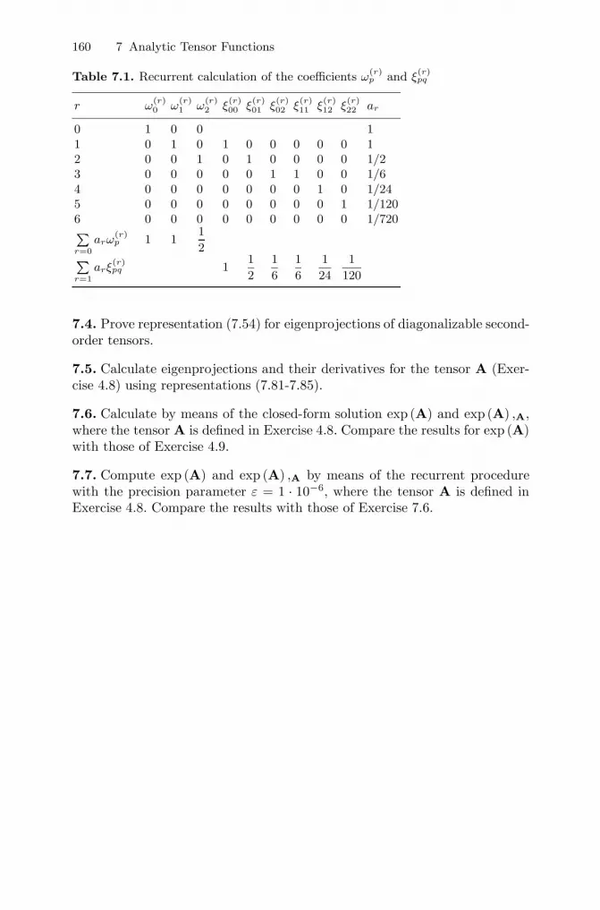
160 7 Analytic Tensor Functions
Table 7.1. Recurrent calculation of the coefficients ω(r)p and ξ
(r)pq
r ω(r)0 ω
(r)1 ω
(r)2 ξ
(r)00 ξ
(r)01 ξ
(r)02 ξ
(r)11 ξ
(r)12 ξ
(r)22 ar
0 1 0 0 11 0 1 0 1 0 0 0 0 0 12 0 0 1 0 1 0 0 0 0 1/23 0 0 0 0 0 1 1 0 0 1/64 0 0 0 0 0 0 0 1 0 1/245 0 0 0 0 0 0 0 0 1 1/1206 0 0 0 0 0 0 0 0 0 1/720
r=0
arω(r)p 1 1
1
2
r=1
arξ(r)pq 1
1
2
1
6
1
6
1
24
1
120
7.4. Prove representation (7.54) for eigenprojections of diagonalizable second-order tensors.
7.5. Calculate eigenprojections and their derivatives for the tensor A (Exer-cise 4.8) using representations (7.81-7.85).
7.6. Calculate by means of the closed-form solution exp (A) and exp (A) ,A,where the tensor A is defined in Exercise 4.8. Compare the results for exp (A)with those of Exercise 4.9.
7.7. Compute exp (A) and exp (A) ,A by means of the recurrent procedurewith the precision parameter ε = 1 · 10−6, where the tensor A is defined inExercise 4.8. Compare the results with those of Exercise 7.6.

8
Applications to Continuum Mechanics
8.1 Polar Decomposition of the Deformation Gradient
The deformation gradient F represents an invertible second-order tensor gen-erally permitting a unique polar decomposition by
F = RU = vR, (8.1)
where R is an orthogonal tensor while U and v are symmetric tensors. Incontinuum mechanics, R is called rotation tensor while U and v are referred toas the right and left stretch tensor, respectively. The latter ones have alreadybeen introduced in Sect. 7.1 in the context of generalized strain measures.
In order to show that the polar decomposition (8.1) always exists andis unique we first consider the so-called right and left Cauchy-Green tensorsrespectively by
C = FTF, b = FFT. (8.2)
These tensors are symmetric and have principal traces in common. Indeed, inview of (1.144)
tr(Ck)
= tr(FTF . . .FTF
)︸ ︷︷ ︸k times
= tr(FFT . . .FFT
)︸ ︷︷ ︸k times
= tr(bk). (8.3)
For this reason, all scalar-valued isotropic functions of C and b such as prin-cipal invariants or eigenvalues coincide. Thus, we can write
C =s∑
i=1
ΛiPi, b =s∑
i=1
Λipi, (8.4)
where eigenvalues Λi are positive. Indeed, let ai be a unit eigenvector asso-ciated with the eigenvalue Λi. Then, in view of (1.73), (1.99), (1.110) and byTheorem 1.8 one can write
162 8 Applications to Continuum Mechanics
Λi = ai · (Λiai) = ai · (Cai) = ai ·(FTFai
)=(aiFT
) · (Fai) = (Fai) · (Fai) > 0.
Thus, square roots of C and b are unique tensors defined by
U =√
C =s∑
i=1
√ΛiPi, v =
√b =
s∑i=1
√Λipi. (8.5)
Further, one can show that
R = FU−1 (8.6)
represents an orthogonal tensor. Indeed,
RRT = FU−1U−1FT = FU−2FT = FC−1FT
= F(FTF
)−1FT = FF−1F−TFT = I.
Thus, we can write taking (8.6) into account
F = RU =(RURT
)R. (8.7)
The tensor
RURT = FRT (8.8)
in (8.7) is symmetric due to symmetry of U (8.5)1. Thus, one can write(RURT
)2
=(RURT
)(RURT
)T
=(FRT
)(FRT
)T
= FRTRFT = FFT = b. (8.9)
In view of (8.5)2 there exists only one real symmetric tensor whose square isb. Hence,
RURT = v, (8.10)
which by virtue of (8.7) results in the polar decomposition (8.1).
8.2 Basis-Free Representations for the Stretch andRotation Tensor
With the aid of the closed-form representations for analytic tensor functionsdiscussed in Chap. 7 the stretch and rotation tensors can be expressed directlyin terms of the deformation gradient and Cauchy-Green tensors without anyreference to their eigenprojections. First, we deal with the stretch tensors
8.2 Basis-Free Representations for the Stretch and Rotation Tensor 163
(8.5). Inserting in (7.61) g (Λi) =√
Λi = λi and keeping in mind (7.31) wewrite
U = ϕ0I + ϕ1C + ϕ2C2, v = ϕ0I + ϕ1b + ϕ2b2, (8.11)
where [44]
ϕ0 =λ1λ2λ3 (λ1 + λ2 + λ3)
(λ1 + λ2) (λ2 + λ3) (λ3 + λ1),
ϕ1 =λ2
1 + λ22 + λ2
3 + λ1λ2 + λ2λ3 + λ3λ1
(λ1 + λ2) (λ2 + λ3) (λ3 + λ1),
ϕ2 = − 1(λ1 + λ2) (λ2 + λ3) (λ3 + λ1)
. (8.12)
These representations for ϕi are free of singularities and are therefore generallyvalid for the case of simple as well as repeated eigenvalues of C and b.
The rotation tensor results from (8.6) where we can again write
U−1 = ς0I + ς1C + ς2C2. (8.13)
The representations for ςp (p = 0, 1, 2) can be obtained either again by (7.61)where g (Λi) = Λ−1/2
i = λ−1i or by applying the Cayley-Hamilton equation
(4.91) leading to
U−1 = III−1U
(U2 − IUU + IIUI
)= III−1
U
[(IIU − ϕ0IU) I + (1 − ϕ1IU)C − ϕ2IUC2
], (8.14)
where
IU = λ1 + λ2 + λ3, IIU = λ1λ2 + λ2λ3 + λ3λ1, IIIU = λ1λ2λ3. (8.15)
Both procedures yield the same representation (8.13) where
ς0 =λ1λ2 + λ2λ3 + λ3λ1
λ1λ2λ3− (λ1 + λ2 + λ3)
2
(λ1 + λ2) (λ2 + λ3) (λ3 + λ1),
ς1 =1
λ1λ2λ3−(λ2
1 + λ22 + λ2
3 + λ1λ2 + λ2λ3 + λ3λ1
)(λ1 + λ2 + λ3)
λ1λ2λ3 (λ1 + λ2) (λ2 + λ3) (λ3 + λ1),
ς2 =λ1 + λ2 + λ3
λ1λ2λ3 (λ1 + λ2) (λ2 + λ3) (λ3 + λ1). (8.16)
Thus, the rotation tensor (8.6) can be given by
R = F(ς0I + ς1C + ς2C2
), (8.17)
where the functions ςi (i = 0, 1, 2) are given by (8.16) in terms of the principalstretches λi =
√Λi, while Λi (i = 1, 2, 3) denote the eigenvalues of the right
Cauchy-Green tensor C (8.2).
164 8 Applications to Continuum Mechanics
Example. Stretch and rotation tensor in the case of simple shear.In this loading case the right and left Cauchy-Green tensors take the form (seeExercise 4.1)
C = Cijei ⊗ ej ,
[Ci
j
]=
⎡⎣ 1 γ 0γ 1 + γ2 00 0 1
⎤⎦ , (8.18)
b = bijei ⊗ ej ,
[bi
j
]=
⎡⎣ 1 + γ2 γ 0γ 1 00 0 1
⎤⎦ (8.19)
with the eigenvalues
Λ1/2 = 1 +γ2 ±
√4γ2 + γ4
2=
(γ ±
√4 + γ2
2
)2
, Λ3 = 1. (8.20)
For the principal stretches we thus obtain
λ1/2 =√
Λ1/2 =
√4 + γ2 ± γ
2, λ3 =
√Λ3 = 1. (8.21)
The stretch tensors result from (8.11) where
ϕ0 =1 +
√γ2 + 4
2√
γ2 + 4 + γ2 + 4,
ϕ1 =1 +
√γ2 + 4
2 +√
γ2 + 4,
ϕ2 = − 12√
γ2 + 4 + γ2 + 4. (8.22)
This yields the following result (cf. Exercise 7.2)
U = Uijei ⊗ ej ,
[Ui
j
]=
⎡⎢⎢⎢⎢⎢⎢⎣
2√γ2 + 4
γ√γ2 + 4
0
γ√γ2 + 4
γ2 + 2√γ2 + 4
0
0 0 1
⎤⎥⎥⎥⎥⎥⎥⎦ , (8.23)
v = vijei ⊗ ej ,
[vi
j
]=
⎡⎢⎢⎢⎢⎢⎢⎣
γ2 + 2√γ2 + 4
γ√γ2 + 4
0
γ√γ2 + 4
2√γ2 + 4
0
0 0 1
⎤⎥⎥⎥⎥⎥⎥⎦ . (8.24)
8.3 The Derivative of the Stretch and Rotation Tensor 165
The rotation tensor can be calculated by (8.17) where
ς0 =√
γ2 + 4 − 12√
γ2 + 4 + γ2 + 4,
ς1 = −3 +√
γ2 + 4 + γ2
2 +√
γ2 + 4,
ς2 =1 +
√γ2 + 4
2√
γ2 + 4 + γ2 + 4. (8.25)
By this means we obtain
R = Ri·jei ⊗ ej ,
[Ri
·j]
=
⎡⎢⎢⎢⎢⎢⎢⎣
2√γ2 + 4
γ√γ2 + 4
0
− γ√γ2 + 4
2√γ2 + 4
0
0 0 1
⎤⎥⎥⎥⎥⎥⎥⎦ . (8.26)
8.3 The Derivative of the Stretch and Rotation Tensorwith Respect to the Deformation Gradient
In continuum mechanics these derivatives are used for the evaluation of therate of the stretch and rotation tensor. We begin with a very simple represen-tation in terms of eigenprojections of the right and left Cauchy-Green tensors(8.2). Applying the chain rule of differentiation and using (6.125) we first write
U,F = C1/2,C : C,F = C1/2,C :[(I ⊗ F)t + FT ⊗ I
]. (8.27)
Further, taking into account the spectral representation of C (8.4)1 and keep-ing its symmetry in mind we obtain by virtue of (7.49-7.50)
C1/2,C =s∑
i,j=1
(λi + λj)−1 (Pi ⊗ Pj)
s. (8.28)
Inserting this result into (8.27) delivers by means of (5.33), (5.47), (5.54)2 and(5.55)
U,F =s∑
i,j=1
(λi + λj)−1[(Pi ⊗ FPj)
t + PiFT ⊗ Pj
]. (8.29)
The same procedure applied to the left stretch tensor yields by virtue of(6.126)
166 8 Applications to Continuum Mechanics
v,F =s∑
i,j=1
(λi + λj)−1[pi ⊗ FTpj + (piF⊗ pj)
t]. (8.30)
Now, applying the product rule of differentiation (6.123) to (8.6) and taking(6.122) into account we write
R,F =(FU−1
),F = I ⊗ U−1 + FU−1,U : U,F
= I ⊗ U−1 − F(U−1 ⊗ U−1
)s: U,F . (8.31)
With the aid of (7.2) and (8.29) this finally leads to
R,F = I⊗(
s∑i=1
λ−1i Pi
)
− Fs∑
i,j=1
[(λi + λj)λiλj ]−1[(Pi ⊗ FPj)
t + PiFT ⊗ Pj
]. (8.32)
Note that the eigenprojections Pi and pi (i = 1, 2, . . . , s) are uniquely definedby the Sylvester formula (4.54) or its alternative form (7.43) in terms of C andb, respectively. The functions ρip appearing in (7.43) are, in turn, expressedin the unique form by (7.81), (7.83) and (7.85) in terms of the eigenvaluesΛi = λ2
i (i = 1, 2, . . . , s).In order to avoid the direct reference to the eigenprojections one can obtain
the so-called basis-free solutions for U,F, v,F and R,F (see, e.g., [8], [13],[17], [37], [46], [48]). As a rule, they are given in terms of the stretch androtation tensors themselves and require therefore either the explicit polardecomposition of the deformation gradient or a closed-form representation forU, v and R like (8.11) and (8.17). In the following we present the basis-freesolutions for U,F, v,F and R,F in terms of the Cauchy-Green tensors C andb (8.2) and the principal stretches λi =
√Λi (i = 1, 2, . . . , s). To this end, we
apply the representation (7.38) for the derivative of the square root. Thus, weobtain instead of (8.28)
C1/2,C =2∑
p,q=0
ηpq (Cp ⊗ Cq)s , b1/2,b =2∑
p,q=0
ηpq (bp ⊗ bq)s , (8.33)
where the functions ηpq result from (7.62) by setting again g (Λi) =√
Λi = λi.This leads to the following expressions (cf. [17])
η00 = Δ−1[I5UIII2U − I4UII2UIIIU + I3UII4U
−I2UIIIU(3II3U − 2III2U
)+ 3IUII2UIII2U − IIUIII3U
],
η01 = η10 = Δ−1[I6UIIIU − I5UII2U − I4UIIUIIIU
+2I3U(II3U + III2U
)− 4I2UII2UIIIU + 2IUIIUIII2U − III3U],
8.3 The Derivative of the Stretch and Rotation Tensor 167
η02 = η20 = Δ−1[−I4UIIIU + I3UII2U − I2UIIUIIIU − IUIII2U
],
η11 = Δ−1[I7U − 4I5UIIU + 3I4UIIIU
+4I3UII2U − 6I2UIIUIIIU + IUIII2U + II2UIIIU],
η12 = η21 = Δ−1[−I5U + 2I3UIIU − 2I2UIIIU + IIUIIIU
],
η22 = Δ−1[I3U + IIIU
], (8.34)
where
Δ = 2 (IUIIU − IIIU)3 IIIU (8.35)
and the principal invariants IU, IIU and IIIU are given by (8.15).Finally, substitution of (8.33) into (8.27) yields
U,F =2∑
p,q=0
ηpq
[(Cp ⊗ FCq)t + CpFT ⊗ Cq
]. (8.36)
Similar we can also write
v,F =2∑
p,q=0
ηpq
[bp ⊗ FTbq + (bpF⊗ bq)t
]. (8.37)
Inserting further (8.13) and (8.36) into (8.31) we get
R,F = I⊗2∑
p=0
ςpCp
− F2∑
p,q,r,t=0
ςrςtηpq
[(Cp+r ⊗ FCq+t
)t + Cp+rFT ⊗ Cq+t], (8.38)
where ςp and ηpq (p, q = 0, 1, 2) are given by (8.16) and (8.34), respectively.The third and fourth powers of C in (8.38) can be expressed by means of theCayley-Hamilton equation (4.91):
C3 − ICC2 + IICC− IIICI = 0. (8.39)
Composing both sides with C we can also write
C4 − ICC3 + IICC2 − IIICC = 0. (8.40)
Thus,
C3 = ICC2 − IICC + IIICI,
168 8 Applications to Continuum Mechanics
C4 =(I2C − IIC
)C2 + (IIIC − ICIIC)C + ICIIICI. (8.41)
Considering these expressions in (8.38) and taking into account that (see, e.g.,[43])
IC = I2U − 2IIU, IIC = II2U − 2IUIIIU, IIIC = III2U (8.42)
we finally obtain
R,F = I ⊗2∑
p=0
ςpCp + F2∑
p,q=0
μpq
[(Cp ⊗ FCq)t + CpFT ⊗ Cq
], (8.43)
where
μ00 = Υ−1[I6UIII3U + 2I5UII2UIII2U − 3I4UII4UIIIU − 7I4UIIUIII3U
+I3UII6U + 8I3UII3UIII2U + 6I3UIII4U − 3I2UII5UIIIU
−6I2UII2UIII3U + 3IUII4UIII2U − II3UIII3U + III5U],
μ01 = μ10 = Υ−1[I7UIII2U + I6UII2UIIIU − I5UII4U − 6I5UIIUIII2U + I4UII3UIIIU
+5I4UIII3U + 2I3UII5U + 4I3UII2UIII2U − 6I2UII4UIIIU
−6I2UIIUIII3U + 6IUII3UIII2U + IUIII4U − 2II2UIII3U],
μ02 = μ20 = −Υ−1[I5UIII2U + I4UII2UIIIU − I3UII4U − 4I3UIIUIII2U
+3I2UII3UIIIU + 4I2UIII3U − 3IUII2UIII2U + IIUIII3U],
μ11 = Υ−1[I8UIIIU + I7UII2U − 7I6UIIUIIIU − 4I5UII3U
+5I5UIII2U + 16I4UII2UIIIU + 4I3UII4U − 16I3UIIUIII2U
−12I2UII3UIIIU + 3I2UIII3U + 12IUII2UIII2U − 3IIUIII3U],
μ12 = μ21 = −Υ−1[I6UIIIU + I5UII2U − 5I4UIIUIIIU − 2I3UII3U
+4I3UIII2U + 6I2UII2UIIIU − 6IUIIUIII2U + III3U],
μ22 = Υ−1IU[I3UIIIU + I2UII2U − 3IUIIUIIIU + 3III2U
](8.44)
and
Υ = −2 (IUIIU − IIIU)3 III3U, (8.45)
while the principal invariants IU, IIU and IIIU are given by (8.15).The same result for R,F also follows from
R,F =(FU−1
),F = I ⊗ U−1 + FU−1,C : C,F (8.46)
8.4 Time Rate of Generalized Strains 169
by applying for U−1,C (7.38) and (7.62) where we set g (Λi) = (Λi)−1/2 = λ−1
i .Indeed, this yields
C−1/2,C = U−1,C =2∑
p,q=0
μpq (Cp ⊗ Cq)s , (8.47)
where μpq (p, q = 0, 1, 2) are given by (8.44).
8.4 Time Rate of Generalized Strains
Applying the chain rule of differentiation we first write
E = E,C : C, (8.48)
where the superposed dot denotes the material time derivative. The derivativeE,C can be expressed in a simple form in terms of the eigenprojections of Eand C. To this end, we apply (7.49-7.50) taking (7.18) and (8.5) into accountwhich yields
E,C =s∑
i,j=1
fij (Pi ⊗ Pj)s, (8.49)
where
fij =
⎧⎪⎪⎪⎨⎪⎪⎪⎩f ′ (λi)2λi
if i = j,
f (λi) − f (λj)λ2
i − λ2j
if i �= j.
(8.50)
A basis-free representation for E,C can be obtained either from (8.49) byexpressing the eigenprojections by (7.43) with (7.81), (7.83) and (7.85) ordirectly by using the closed-form solution (7.38) with (7.62), (7.78) and (7.80).Both procedures lead to the same result as follows (cf. [21], [47]).
E,C =2∑
p,q=0
ηpq (Cp ⊗ Cq)s . (8.51)
Distinct eigenvalues: λ1 �= λ2 �= λ3 �= λ1,
η00 =3∑
i=1
λ4jλ
4kf ′ (λi)
2λiΔ2i
−3∑
i,j=1i�=j
λ2i λ
2jλ
4k [f (λi) − f (λj)](λ2
i − λ2j
)3 Δk
,

170 8 Applications to Continuum Mechanics
η01 = η10 = −3∑
i=1
(λ2
j + λ2k
)λ2
jλ2kf ′ (λi)
2λiΔ2i
+3∑
i,j=1i�=j
(λ2
j + λ2k
)λ2
i λ2k [f (λi) − f (λj)](
λ2i − λ2
j
)3 Δk
,
η02 = η20 =3∑
i=1
λ2jλ
2kf ′ (λi)
2λiΔ2i
−3∑
i,j=1i�=j
λ2i λ
2k [f (λi) − f (λj)](λ2
i − λ2j
)3 Δk
,
η11 =3∑
i=1
(λ2
j + λ2k
)2f ′ (λi)
2λiΔ2i
−3∑
i,j=1i�=j
(λ2
j + λ2k
) (λ2
i + λ2k
)[f (λi) − f (λj)](
λ2i − λ2
j
)3 Δk
,
η12 = η21 = −3∑
i=1
(λ2
j + λ2k
)f ′ (λi)
2λiΔ2i
+3∑
i,j=1i�=j
(λ2
i + λ2k
)[f (λi) − f (λj)](
λ2i − λ2
j
)3 Δk
,
η22 =3∑
i=1
f ′ (λi)2λiΔ2
i
−3∑
i,j=1i�=j
f (λi) − f (λj)(λ2
i − λ2j
)3 Δk
, i �= j �= k �= i, (8.52)
with
Δi =(λ2
i − λ2j
) (λ2
i − λ2k
), i �= j �= k �= i = 1, 2, 3. (8.53)
Double coalescence of eigenvalues: λi �= λj = λk = λ,
η00 = −2λ2i λ
2 f (λi) − f (λ)
(λ2i − λ2)3
+λ5f ′ (λi) + λ5
i f′ (λ)
2λiλ (λ2i − λ2)2
,
η01 = η10 =(λ2
i + λ2) f (λi) − f (λ)
(λ2i − λ2)3
− λ3f ′ (λi) + λ3i f
′ (λ)
2λiλ (λ2i − λ2)2
,
η11 = −2f (λi) − f (λ)
(λ2i − λ2)3
+λf ′ (λi) + λif
′ (λ)
2λiλ (λ2i − λ2)2
,
η02 = η20 = η12 = η21 = η22 = 0. (8.54)
Triple coalescence of eigenvalues: λ1 = λ2 = λ3 = λ,
η00 =f ′ (λ)2λ
, η01 = η10 = η11 = η02 = η20 = η12 = η21 = η22 = 0. (8.55)
8.5 Stress Conjugate to a Generalized Strain 171
8.5 Stress Conjugate to a Generalized Strain
Let E be an arbitrary Lagrangian strain (7.6)1. Assume existence of the so-called strain energy function ψ (E) differentiable with respect to E. The sym-metric tensor
T = ψ (E) ,E (8.56)
is referred to as stress conjugate to E. With the aid of the chain rule it canbe represented by
T = ψ (E) ,C : C,E =12S : C,E , (8.57)
where S = 2ψ (E) ,C denotes the second Piola-Kirchhoff stress tensor. Thelatter one is defined in terms of the Cauchy stress σ by (see, e.g., [45])
S = det (F)F−1σF−T. (8.58)
Using (8.56) and (7.7) one can also write
ψ = T : E = S :12C = S : E(2). (8.59)
The fourth-order tensor C,E appearing in (8.57) can be expressed in terms ofthe right Cauchy-Green tensor C by means of the relation
Is = E,E = E,C : C,E , (8.60)
where the derivative E,C is given by (8.49-8.50). The basis tensors of the latterrepresentation are
Pij =
{(Pi ⊗ Pi)
s if i = j,
(Pi ⊗ Pj + Pj ⊗ Pi)s if i �= j.
(8.61)
In view of (4.44), (5.33) and (5.55) they are pairwise orthogonal (see Exercise8.2) such that (cf. [47])
Pij : Pkl =
{Pij if i = k and j = l or i = l and j = k,
O otherwise.(8.62)
By means of (4.46) and (5.84) we can also write
s∑i,j=1j≥i
Pij =
⎡⎣( s∑i=1
Pi
)⊗⎛⎝ s∑
j=1
Pj
⎞⎠⎤⎦s
= (I⊗ I)s = Is. (8.63)
Using these properties we thus obtain
172 8 Applications to Continuum Mechanics
C,E =s∑
i,j=1
f−1ij (Pi ⊗ Pj)
s , (8.64)
where fij (i, j = 1, 2, . . . , s) are given by (8.50). Substituting this result into(8.57) and taking (5.22)1, (5.46) and (5.47) into account yields [18]
T =12
s∑i,j=1
f−1ij PiSPj . (8.65)
In order to avoid any reference to eigenprojections we can again express themby (7.43) with (7.81), (7.83) and (7.85) or alternatively use the closed-formsolution (7.38) with (7.62), (7.78) and (7.80). Both procedures lead to thefollowing result (cf. [47]).
T =2∑
p,q=0
ηpqCpSCq. (8.66)
Distinct eigenvalues: λ1 �= λ2 �= λ3 �= λ1,
η00 =3∑
i=1
λ4jλ
4kλi
f ′ (λi)Δ2i
−3∑
i,j=1i�=j
λ2i λ
2jλ
4k
2(λ2
i − λ2j
)[f (λi) − f (λj)] Δk
,
η01 = η10 = −3∑
i=1
(λ2
j + λ2k
)λ2
jλ2kλi
f ′ (λi)Δ2i
+3∑
i,j=1i�=j
(λ2
j + λ2k
)λ2
i λ2k
2(λ2
i − λ2j
)[f (λi) − f (λj)] Δk
,
η02 = η20 =3∑
i=1
λ2jλ
2kλi
f ′ (λi)Δ2i
−3∑
i,j=1i�=j
λ2i λ
2k
2(λ2
i − λ2j
)[f (λi) − f (λj)] Δk
,
η11 =3∑
i=1
(λ2
j + λ2k
)2λi
f ′ (λi)Δ2i
−3∑
i,j=1i�=j
(λ2
j + λ2k
) (λ2
i + λ2k
)2(λ2
i − λ2j
)[f (λi) − f (λj)] Δk
,
η12 = η21 = −3∑
i=1
(λ2
j + λ2k
)λi
f ′ (λi)Δ2i
+3∑
i,j=1i�=j
λ2i + λ2
k
2(λ2
i − λ2j
)[f (λi) − f (λj)] Δk
,
η22 =3∑
i=1
λi
f ′ (λi)Δ2i
−3∑
i,j=1i�=j
12(λ2
i − λ2j
)[f (λi) − f (λj)] Δk
, (8.67)

8.6 Finite Plasticity Based on Generalized Strains 173
where i �= j �= k �= i and Δi are given by (8.53).
Double coalescence of eigenvalues: λi �= λj = λk = λ,
η00 = − λ2i λ
2
(λ2i − λ2) [f (λi) − f (λ)]
+λiλ
(λ2i − λ2)2
[λ3
f ′ (λi)+
λ3i
f ′ (λ)
],
η01 = η10 =λ2
i + λ2
2 (λ2i − λ2) [f (λi) − f (λ)]
− λiλ
(λ2i − λ2)2
[λ
f ′ (λi)+
λi
f ′ (λ)
],
η11 = − 1(λ2
i − λ2) [f (λi) − f (λ)]+
1
(λ2i − λ2)2
[λi
f ′ (λi)+
λ
f ′ (λ)
],
η02 = η20 = η12 = η21 = η22 = 0. (8.68)
Triple coalescence of eigenvalues: λ1 = λ2 = λ3 = λ,
η00 =λ
f ′ (λ), η01 = η10 = η11 = η02 = η20 = η12 = η21 = η22 = 0. (8.69)
8.6 Finite Plasticity Based on the AdditiveDecomposition of Generalized Strains
Keeping in mind the above results regarding generalized strains we are con-cerned in this section with a thermodynamically based plasticity theory. Thebasic kinematic assumption of this theory is the additive decomposition ofgeneralized strains (7.6) into an elastic part Ee and a plastic part Ep as
E = Ee + Ep. (8.70)
The derivation of evolution equations for the plastic strain is based on thesecond law of thermodynamics and the principle of maximum plastic dissipa-tion. The second law of thermodynamics can be written in the Clausius-Planckform as (see, e.g. [45])
D = T : E− ψ ≥ 0, (8.71)
where D denotes the dissipation and T is again the stress tensor work conju-gate to E. Inserting (8.70) into (8.71) we further write
D =(T − ∂ψ
∂Ee
): Ee + T : Ep ≥ 0, (8.72)
where the strain energy is assumed to be a function of the elastic strain asψ = ψ (Ee). The first term in the expression of the dissipation (8.72) dependssolely on the elastic strain rate Ee, while the second one on the plastic strain
174 8 Applications to Continuum Mechanics
rate Ep. Since the elastic and plastic strain rates are independent of each otherthe dissipation inequality (8.72) requires that
T =∂ψ
∂Ee. (8.73)
This leads to the so-called reduced dissipation inequality
D = T : Ep ≥ 0. (8.74)
Among all admissible processes the real one maximizes the dissipation (8.74).This statement is based on the postulate of maximum plastic dissipation (see,e.g., [28]). According to the converse Kuhn-Tucker theorem (see, e.g., [6]) thesufficient conditions of this maximum are written as
Ep = ζ∂Φ
∂T, ζ ≥ 0, ζΦ = 0, Φ ≤ 0, (8.75)
where Φ represents a convex yield function and ζ denotes a consistency pa-rameter. In the following, we will deal with an ideal-plastic isotropic materialdescribed by a von Mises-type yield criterion. Written in terms of the stresstensor T the von Mises yield function takes the form [31]
Φ = ‖devT‖ −√
23σY , (8.76)
where σY denotes the normal yield stress. With the aid of (6.51) and (6.130)the evolution equation (8.75)1 can thus be given by
Ep = ζ ‖devT‖ ,T
= ζ ‖devT‖ ,devT : devT,T = ζdevT
‖devT‖ : Pdev = ζdevT
‖devT‖ . (8.77)
Taking the quadratic norm on both the right and left hand side of this identitydelivers the consistency parameter as ζ = ||Ep||. In view of the yield conditionΦ = 0 we thus obtain
devT =
√23σY
Ep∥∥∥Ep
∥∥∥ , (8.78)
which immediately requires that (see Exercise 1.46)
trEp = 0. (8.79)
In the following, we assume small elastic but large plastic strains and spec-ify the above plasticity model for finite simple shear. In this case all threeprincipal stretches (8.21) are distinct so that we can write by virtue of (7.6)
8.6 Finite Plasticity Based on Generalized Strains 175
Ep = E =3∑
i=1
f ′ (λi) λiPi +3∑
i=1
f (λi) Pi. (8.80)
By means of the identities trPi = 1 and trPi = 0 following from (4.61) and(4.62) where ri = 1 (i = 1, 2, 3) the condition (8.79) requires that
3∑i=1
f ′ (λi) λi = 0. (8.81)
In view of (8.21) it leads to the equation
f ′ (λ) − f ′ (λ−1)λ−2 = 0, ∀λ > 0, (8.82)
where we set λ1 = λ and consequently λ2 = λ−1. Solutions of this equationscan be given by [21]
fa (λ) =
⎧⎪⎨⎪⎩12a
(λa − λ−a) for a �= 0,
lnλ for a = 0.
(8.83)
By means of (7.6)1 or (7.18)1 the functions fa (8.83) yield a set of new gen-eralized strain measures
E〈a〉 =
⎧⎪⎨⎪⎩12a
(Ua − U−a) =12a
(Ca/2 − C−a/2
)for a �= 0,
lnU =12
lnC for a = 0,
(8.84)
among which only the logarithmic one (a = 0) belongs to Seth’s family (7.7).Henceforth, we will deal only with the generalized strains (8.84) as able toprovide the traceless deformation rate (8.79). For these strains eq. (8.78) takesthe form
devT〈a〉 =
√23σY
E〈a〉∥∥∥E〈a〉∥∥∥ , (8.85)
where T〈a〉 denotes the stress tensor work conjugate to E〈a〉. T〈a〉 itself hasno physical meaning and should be transformed to the Cauchy stresses. Withthe aid of (8.57), (8.58) and (8.60) we can write
σ =1
detFFSFT =
1detF
F(T〈a〉 : Pa
)FT, (8.86)
where
Pa = 2E〈a〉,C (8.87)
176 8 Applications to Continuum Mechanics
can be expressed either by (8.49-8.50) or by (8.51-8.55). It is seen that thisfourth-order tensor is super-symmetric (see Exercise 5.11), so that T〈a〉 : Pa =Pa : T〈a〉. Thus, by virtue of (1.152) and (1.153) representation (8.86) can berewritten as
σ =1
detFF(Pa : T〈a〉
)FT
=1
detFF[Pa : devT〈a〉 +
13trT〈a〉 (Pa : I)
]FT. (8.88)
With the aid of the relation
Pa : I = 2ddt
E〈a〉 (C + tI)∣∣∣∣t=0
= 2ddt
3∑i=1
fa
(√λ2
i + t
)Pi
∣∣∣∣∣t=0
=3∑
i=1
f ′a (λi)λ−1
i Pi (8.89)
following from (6.111) and taking (8.83) into account one obtains
F (Pa : I)FT =12F(Ca/2−1 + C−a/2−1
)FT =
12
(ba/2 + b−a/2
).
Inserting this result into (8.88) yields
σ =1
detFF(Pa : devT〈a〉
)FT + σ (8.90)
with the abbreviation
σ =trT〈a〉
6 detF
(ba/2 + b−a/2
). (8.91)
Using the spectral decomposition of b by (8.4) and taking into account thatin the case of simple shear detF = 1 we can further write
σ =16trT〈a〉 [(λa + λ−a
)(p1 + p2) + 2p3
], (8.92)
where λ is given by (8.21). Thus, in the 1-2 shear plane the stress tensor σhas the double eigenvalue 1
6 trT〈a〉 (λa + λ−a) and causes equibiaxial tensionor compression. Hence, in this plane the component σ (8.91) is shear free anddoes not influence the shear stress response. Inserting (8.85) into (8.90) andtaking (8.18) and (8.48) into account we finally obtain
σ =
√23σY F
[Pa : Pa : A‖Pa : A‖
]FT + σ, (8.93)
where
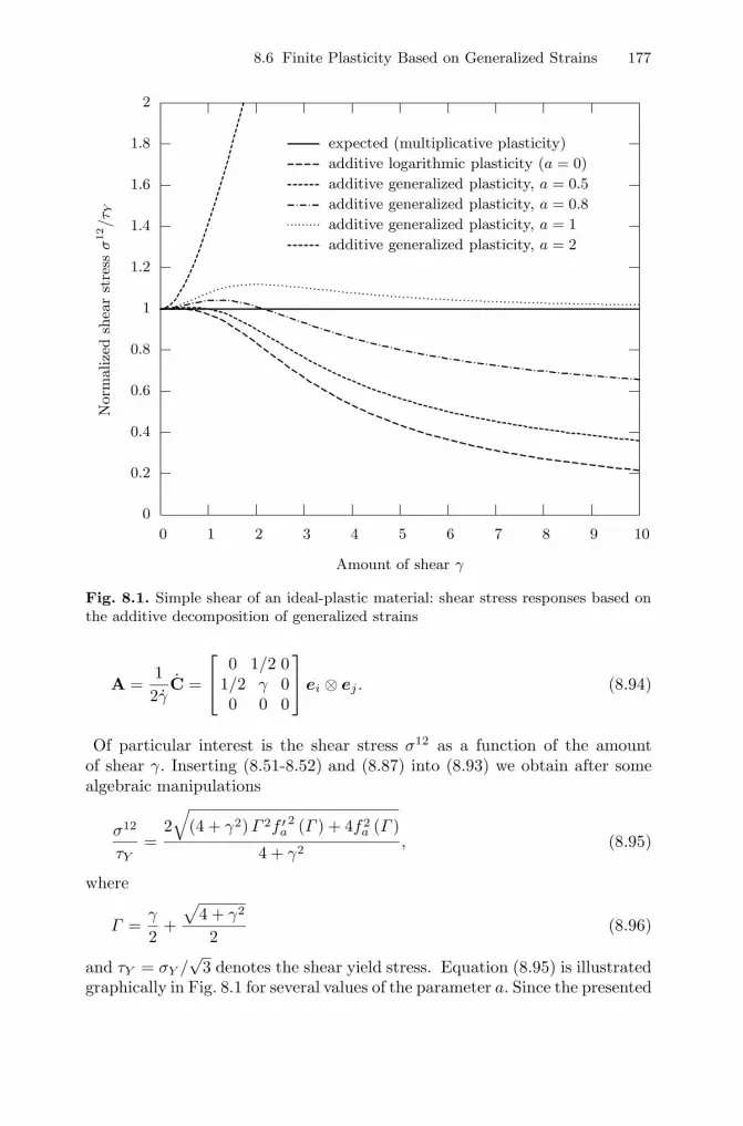
8.6 Finite Plasticity Based on Generalized Strains 177
0
0.2
0.4
0.6
0.8
1
1.2
1.4
1.6
1.8
2
0 1 2 3 4 5 6 7 8 9 10
Norm
alize
dsh
ear
stre
ssσ
12/τ Y
Amount of shear γ
expected (multiplicative plasticity)
additive logarithmic plasticity (a = 0)
additive generalized plasticity, a = 0.5
additive generalized plasticity, a = 0.8
additive generalized plasticity, a = 1
additive generalized plasticity, a = 2
Fig. 8.1. Simple shear of an ideal-plastic material: shear stress responses based onthe additive decomposition of generalized strains
A =12γ
C =
⎡⎣ 0 1/2 01/2 γ 00 0 0
⎤⎦ei ⊗ ej . (8.94)
Of particular interest is the shear stress σ12 as a function of the amountof shear γ. Inserting (8.51-8.52) and (8.87) into (8.93) we obtain after somealgebraic manipulations
σ12
τY=
2√
(4 + γ2)Γ 2f ′a2 (Γ ) + 4f2
a (Γ )
4 + γ2, (8.95)
where
Γ =γ
2+
√4 + γ2
2(8.96)
and τY = σY /√
3 denotes the shear yield stress. Equation (8.95) is illustratedgraphically in Fig. 8.1 for several values of the parameter a. Since the presented
178 8 Applications to Continuum Mechanics
plasticity model considers neither softening nor hardening and is restricted tosmall elastic strains a constant shear stress response even at large plasticdeformations is expected. It is also predicted by a plasticity model based onthe multiplicative decomposition of the deformation gradient (see, e.g., [21]for more details). The plasticity model based on the additive decompositionof generalized strains exhibits, however, a non-constant shear stress for allexamined values of a. This restricts the applicability of this model to moderateplastic shears. Indeed, in the vicinity of the point γ = 0 the power seriesexpansion of (8.95) takes the form
σ12
τY= 1 +
14a2γ2 +
(116
a4 − 34a2 − 1
)γ4 + O
(γ6). (8.97)
Thus, in the case of simple shear the amount of shear is limited for the log-arithmic strain (a = 0) by γ4 � 1 and for other generalized strain measuresby γ2 � 1.
Exercises
8.1. The deformation gradient is given by F = Fi·jei ⊗ ej , where
[Fi·j]
=
⎡⎣ 1 2 0−2 2 0
0 0 1
⎤⎦ .
Evaluate the stretch tensors U and v and the rotation tensor R using (8.11-8.12) and (8.16-8.17).
8.2. Prove the orthogonality (8.62) of the basis tensors (8.61) using (4.44),(5.33) and (5.55).
Solutions
Exercises of Chapter 1
1.1 (a) (A.4), (A.3):
0 = 0 + (−0 ) = −0 .
(b) (A.2-A.4), (B.3):
α0 = 0 + α0 = αx + (−αx) + α0
= α (0 + x) + (−αx) = αx + (−αx) = 0 .
(c) (A.2-A.4), (B.4):
0x = 0x + 0 = 0x + 0x + (−0x) = 0x + (−0x) = 0 , ∀x ∈ V.
(d) (A.2-A.4), (B.2), (B.4), (c):
(−1)x = (−1)x + 0 = (−1)x + x + (−x)= (−1 + 1)x + (−x) = 0x + (−x) = 0 + (−x) = −x, ∀x ∈ V.
(e) If, on the contrary, α �= 0 and x �= 0 , then according to (b), (B.1), (B.2):
0 = α−10 = α−1 (αx) = x.
1.2 Let, on the contrary, xk = 0 for some k. Then,∑n
i=1 αixi = 0 , whereαk = 1, αi = 0, i = 1, . . . , k − 1, k + 1, . . . , n.
1.3 If, on the contrary, for some k < n:∑k
i=1 αixi = 0 , where not allαi, (i = 1, 2, . . . , k) are zero, then we can also write:
∑ni=1 αixi = 0 , where
αi = 0, for i = k + 1, . . . , n.
1.4 (a) δija
j = δi1a
1 + δi2a
2 + δi3a
3 = ai,
(b) δijxixj = δ11x
1x1 + δ12x1x2 + . . . + δ33x
3x3 = x1x1 + x2x2 + x3x3,
(c) δii = δ1
1 + δ22 + δ3
3 = 3,
180 Solutions
(d)∂fi
∂xjdxj =
∂fi
∂x1dx1 +
∂fi
∂x2dx2 +
∂fi
∂x3dx3.
1.5 (A.4), (C.2), (C.3), Ex. 1.1 (d):
0 · x = [x + (−x)] · x = [x + (−1)x] · x = x · x − x · x = 0.
1.6 Let on the contrary∑m
i=1 αigi = 0 , where not all αi (i = 1, 2, . . . , m)are zero. Multiplying scalarly by gj we obtain: 0 = gj · (
∑mi=1 αigi). Since
gi · gj = 0 for i �= j, we can write: αjgj · gj = 0 (j = 1, 2, . . . , m). The factthat the vectors gj are non-zero leads in view of (C.4) to the conclusion thatαj = 0 (j = 1, 2, . . . , m) which contradicts the earlier assumption.
1.7 (1.6), (C.1), (C.2):
‖x + y‖2 = (x + y) · (x + y)
= x · x + x · y + y · x + y · y = ‖x‖2 + 2x · y + ‖y‖2 .
1.8 Since G = {g1, g2, . . . , gn} is a basis we can write a = aigi. Then,a · a = ai (gi · a). Thus, if a · gi = 0 (i = 1, 2, . . . , n), then a · a = 0 andaccording to (C.4) a = 0 (sufficiency). Conversely, if a = 0 , then (see Exercise1.5) a · gi = 0 (i = 1, 2, . . . , n) (necessity).
1.9 Necessity. (C.2): a ·x = b ·x ⇒ a ·x− b ·x = (a − b) ·x = 0, ∀x ∈ En.Let x = a − b, then (a − b) · (a − b) = 0 and according to (C.4) a − b = 0 .This implies that a = b. The sufficiency is evident.
1.10 (a) Orthonormal vectors e1, e2 and e3 can be calculated by means ofthe Gram-Schmidt procedure (1.10-1.12) as follows
e1 =g1
‖g1‖ =
⎧⎨⎩√
2/2√2/20
⎫⎬⎭ ,
e′2 = g2 − (g2 · e1)e1 =
⎧⎨⎩1/2−1/2−2
⎫⎬⎭ , e2 =e′
2
‖e′2‖
=
⎧⎨⎩√
2/6−√
2/6−2
√2/3
⎫⎬⎭ ,
e′3 = g3−(g3 · e2)e2−(g3 · e1)e1 =
⎧⎨⎩10/9−10/95/9
⎫⎬⎭ , e3 =e′
3
‖e′3‖
=
⎧⎨⎩2/3−2/31/3
⎫⎬⎭ .
(b) First, we calculate the matrices [gij ] and[gij]
by (1.25)2 and (1.24)
[gij ] = [gi · gj ] =
⎡⎣ 2 3 63 9 86 8 21
⎤⎦ ,[gij]
= [gij ]−1 =
⎡⎢⎢⎢⎢⎢⎣5 −3
5−6
5
−35
625
225
−65
225
925
⎤⎥⎥⎥⎥⎥⎦ ,
Solutions 181
With the aid of (1.21) we thus obtain
g1 = g11g1 + g12g2 + g13g3 =
⎧⎨⎩−120
⎫⎬⎭ ,
g2 = g21g1 + g22g2 + g23g3 =
⎧⎨⎩1/5−1/5−2/5
⎫⎬⎭ ,
g3 = g31g1 + g32g2 + g33g3 =
⎧⎨⎩2/5−2/51/5
⎫⎬⎭ .
(c) By virtue of (1.35) we write
g =∣∣βi
j
∣∣ =
∣∣∣∣∣∣1 1 02 1 −24 2 1
∣∣∣∣∣∣ = −5.
Applying (1.33) we further obtain with the aid of (1.46)
g1 = g−1g2 × g3 = −15
∣∣∣∣∣∣2 1 −24 2 1a1 a2 a3
∣∣∣∣∣∣ = −a1 + 2a2,
g2 = g−1g3 × g1 = −15
∣∣∣∣∣∣4 2 11 1 0a1 a2 a3
∣∣∣∣∣∣ =15
(a1 − a2 − 2a3) ,
g3 = g−1g1 × g2 = −15
∣∣∣∣∣∣1 1 02 1 −2a1 a2 a3
∣∣∣∣∣∣ =15
(2a1 − 2a2 + a3) ,
where ai denote the orthonormal basis the components of the original vectorsgi (i = 1, 2, 3) are related to.
1.11 Let on the contrary∑3
i=1 αigi = 0 , where not all αi are zero. Multi-
plying scalarly by gj we obtain by virtue of (1.15): 0 = gj ·(∑3
i=1 αigi)
=∑3i=1 αiδ
ij = αj (j = 1, 2, 3).
1.12 Similarly to (1.35) we write using also (1.18), (1.19) and (1.36)[g1g2g3
]=[α1
i eiα2
jejα3
kek]
= α1i α
2jα
3k
[eiejek
]= α1
i α2jα
3keijk =
∣∣αij
∣∣ =∣∣βi
j
∣∣−1= g−1.
1.13 In view of (1.33), (1.36) and (1.38) the left and right hand side of (1.39)yield for the case
182 Solutions
i = j:
gi × gi = 0 , eiikggk = 0 ,
∃k such that ijk is an even permutation of 123:
gi × gj = [g1g2g3] gk, eijlggl = [g1g2g3] gk,
∃k such that ijk is an odd permutation of 123:
gi × gj = −gj × gi = − [g1g2g3] gk, eijlggl = − [g1g2g3] gk.
Using the result of the previous exercise one proves in the same manner (1.42).
1.14 (a) δijeijk = δ11e11k + δ12e12k + . . . + δ33e33k = 0.
(b) Writing out the term eikmejkm we first obtain
eikmejkm = ei11ej11 + ei12ej12 + . . . + ei33ej33
= ei12ej12 + ei21ej21 + ei13ej13 + ei31ej31 + ei32ej32 + ei23ej23.
For i �= j each term in this sum is equal to zero. Let further i = j = 1.Then we obtain ei12ej12 + ei21ej21 + ei13ej13 + ei31ej31 + ei32ej32 + ei23ej23 =e132e132 + e123e123 = (−1) (−1) + 1 · 1 = 2. The same result also holds for thecases i = j = 2 and i = j = 3. Thus, we can write eikmejkm = 2δi
j .
(c) By means of the previous result (b) we can write: eijkeijk = 2δii = 2(δ1
1 +δ22 + δ3
3) = 6. This can also be shown directly by
eijkeijk = e123e123 + e132e132 + e213e213 + e231e231 + e312e312 + e321e321
= 1 · 1 + (−1) · (−1) + (−1) · (−1) + 1 · 1 + 1 · 1 + (−1) · (−1) = 6.
(d) eijmeklm = eij1ekl1 + eij2ekl2 + eij3ekl3. It is seen that in the case i = jor k = l this sum as well as the right hand side δi
kδjl − δi
lδjk are both zero. Let
further i �= j. Then, only one term in the above sum is non-zero if k = i andl = j or vice versa l = i and k = j. In the first case the left hand side is 1 andin the last case −1. The same holds also for the right side δi
kδjl − δi
lδjk. Indeed,
we obtain for k = i �= l = j: δikδj
l − δilδ
jk = 1 · 1 − 0 = 1 and for l = i �= k = j:
δikδj
l − δilδ
jk = 0 − 1 · 1 = −1.
1.15 Using the representations a = aigi, b = bjgj and c = clgl we can write
by virtue of (1.39) and (1.42)
(a × b) × c =[(
aigi
)× (bjgj
)]× c =(aibjeijkggk
)× (clg
l)
= aibjcleijkeklmgm = aibjcleijkelmkgm.
With the aid of the identity eijmeklm = δikδj
l − δilδ
jk (Exercise 1.14) we finally
obtain
Solutions 183
(a × b) × c = aibjcl
(δliδ
mj − δm
i δlj
)gm = aibjclδ
liδ
mj gm − aibjclδ
mi δl
jgm
= aibjcigj − aibjcjgi = (a · c) b − (b · c) a.
1.16 (A.2-A.4), (1.48):
0 = Ax + (−Ax) = A (x + 0 ) + (−Ax) = Ax + A0 + (−Ax) = A0 .
1.17 (1.49), Exercises 1.1(c), 1.16: (0A)x = A (0x) = A0 = 0 , ∀x ∈ En.
1.18 (1.61), Ex. 1.17: A + (−A) = A + (−1)A = (1 − 1)A = 0A = 0.
1.19 Indeed, a scalar product of the right-hand side of (1.80) with an arbitraryvector x yields [(y · a) b] ·x = (y · a) (b · x). The same result follows also fromy · [(a ⊗ b)x] = (y · a) (b · x) , ∀x, y ∈ E
n for the left-hand side. This impliesthat the identity (1.80) is true (see Exercise 1.9).
1.20 For (1.83)1 we have for example
giAgj = gi(Aklgk ⊗ gl
)gj = Akl
(gi · gk
) (gl · gj
)= Aklδi
kδjl = Aij .
1.21 For an arbitrary vector x = xigi ∈ E3 we can write using (1.28), (1.39)and (1.75)
Wx = w × x =(wigi
)× (xjgj
)= eijkgwixjgk = eijkgwi
(x · gj
)gk = eijkgwi
(gk ⊗ gj
)x.
Comparing the left and right hand side of this equality we obtain
W = eijkgwigk ⊗ gj , (S.1)
so that the components of W = Wkjgk ⊗ gj can be given by Wkj = eijkgwi
or in the matrix form as
[Wkj ] = g[eijkwi
]= g
⎡⎣ 0 −w3 w2
w3 0 −w1
−w2 w1 0
⎤⎦ .
This yields also an alternative representation for Wx as follows
Wx = g[(
w2x3 − w3x2)g1 +
(w3x1 − w1x3
)g2 +
(w1x2 − w2x1
)g3].
It is seen that the tensor W is skew-symmetric because WT = −W.
1.22 According to (1.71) we can write
R = cosαI + sin αe3 + (1 − cosα) (e3 ⊗ e3) .
Thus, an arbitrary vector a = aiei in E3 is rotated to Ra = cosα(aiei
)+
sin αe3 ×(aiei
)+ (1 − cosα) a3e3. By virtue of (1.45) we can further write
184 Solutions
Ra = cosα(aiei
)+ sin α
(a1e2 − a2e1
)+ (1 − cosα) a3e3
=(a1 cosα − a2 sin α
)e1 +
(a1 sin α + a2 cosα
)e2 + a3e3.
Thus, the rotation tensor can be given by R = Rijei ⊗ ej , where
[Rij
]=
⎡⎣ cosα − sinα 0sin α cosα 0
0 0 1
⎤⎦ .
1.23 With the aid of (1.83) and (1.92) we obtain
[Ai
·j]
=[Aikgkj
]=[Aik
][gkj ] =
⎡⎣ 0 −1 00 0 01 0 0
⎤⎦⎡⎣ 2 3 63 9 86 8 21
⎤⎦ =
⎡⎣−3 −9 −80 0 02 3 6
⎤⎦ ,
[A j
i·]
=[gikAkj
]= [gik]
[Akj
]=
⎡⎣ 2 3 63 9 86 8 21
⎤⎦⎡⎣0 −1 00 0 01 0 0
⎤⎦ =
⎡⎣ 6 −2 08 −3 0
21 −6 0
⎤⎦ ,
[Aij ] =[gikAk
·j]
= [gik][Ak
·j]
=[A k
i·gkj
]=[A k
i·][gkj ]
=
⎡⎣ 2 3 63 9 86 8 21
⎤⎦⎡⎣−3 −9 −80 0 02 3 6
⎤⎦ =
⎡⎣ 6 −2 08 −3 0
21 −6 0
⎤⎦⎡⎣ 2 3 63 9 86 8 21
⎤⎦ =
⎡⎣ 6 0 207 −3 24
24 9 78
⎤⎦ .
1.24 By means of (1.53), (1.84), (1.98), Exercise 1.16 we can write
(A0)x = A (0x) = A0 = 0 , (0A)x = 0 (Ax) = 0 ,
(AI)x = A (Ix) = Ax, (IA) x = I (Ax) = Ax,
A (BC)x = A [B (Cx)] = (AB) (Cx) = [(AB)C] x, ∀x ∈ En.
1.25 To check the commutativeness of the tensors A and B we compute thecomponents of the tensor AB − BA:[
(AB − BA)i·j]
=[Ai
·kBk·j − Bi
·kAk·j]
=[Ai
·k] [
Bk·j]− [
Bi·k] [
Ak·j]
=
⎡⎣ 0 2 00 0 00 0 0
⎤⎦⎡⎣ 0 0 00 0 00 0 1
⎤⎦−⎡⎣0 0 0
0 0 00 0 1
⎤⎦⎡⎣ 0 2 00 0 00 0 0
⎤⎦ =
⎡⎣ 0 0 00 0 00 0 0
⎤⎦ .
Similar we also obtain
[(AC − CA)i
·j]
=
⎡⎣ 0 −2 00 0 00 0 0
⎤⎦ ,[(AD − DA)i
·j]
=
⎡⎣ 0 −1 00 0 00 0 0
⎤⎦ ,
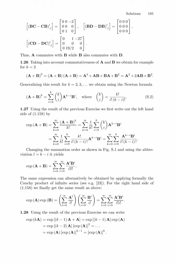
Solutions 185
[(BC− CB)i
·j]
=
⎡⎣ 0 0 −30 0 00 1 0
⎤⎦ ,[(BD − DB)i
·j]
=
⎡⎣0 0 00 0 00 0 0
⎤⎦ ,
[(CD − DC)i
·j]
=
⎡⎣ 0 1 −270 0 00 19/2 0
⎤⎦ .
Thus, A commutes with B while B also commutes with D.
1.26 Taking into account commutativeness of A and B we obtain for examplefor k = 2
(A + B)2 = (A + B) (A + B) = A2 +AB+BA+B2 = A2 +2AB+B2.
Generalizing this result for k = 2, 3, . . . we obtain using the Newton formula
(A + B)k =k∑
i=0
(k
i
)Ak−iBi, where
(k
i
)=
k!i! (k − i)!
. (S.2)
1.27 Using the result of the previous Exercise we first write out the left handside of (1.158) by
exp (A + B) =∞∑
k=0
(A + B)k
k!=
∞∑k=0
1k!
k∑i=0
(k
i
)Ak−iBi
=∞∑
k=0
1k!
k∑i=0
k!i! (k − i) !
Ak−iBi =∞∑
k=0
k∑i=0
Ak−iBi
i! (k − i) !.
Changing the summation order as shown in Fig. S.1 and using the abbre-viation l = k − i it yields
exp (A + B) =∞∑
l=0
∞∑i=0
AlBi
i!l!.
The same expression can alternatively be obtained by applying formally theCauchy product of infinite series (see e.g. [23]). For the right hand side of(1.158) we finally get the same result as above:
exp (A) exp (B) =
( ∞∑l=0
Al
l!
)( ∞∑i=0
Bi
i!
)=
∞∑l=0
∞∑i=0
AlBi
l!i!.
1.28 Using the result of the previous Exercise we can write
exp (kA) = exp [(k − 1)A + A] = exp [(k − 1)A] exp (A)
= exp [(k − 2)A] [exp (A)]2 = . . .
= exp (A) [exp (A)]k−1 = [exp (A)]k .
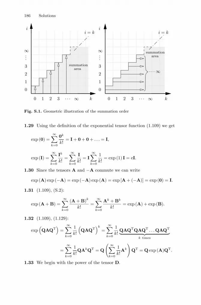
186 Solutions
0 1 2 3
0
1
2
3
· · · ∞
i = k
k
2
1
3
0
3210
i = k
· · · ∞
∞
k
ii
· · ·
∞ ∞...
...summation
summationarea
area
Fig. S.1. Geometric illustration of the summation order
1.29 Using the definition of the exponential tensor function (1.109) we get
exp (0) =∞∑
k=0
0k
k!= I + 0 + 0 + . . . = I,
exp (I) =∞∑
k=0
Ik
k!=
∞∑k=0
Ik!
= I∞∑
k=0
1k!
= exp (1) I = eI.
1.30 Since the tensors A and −A commute we can write
exp (A) exp (−A) = exp (−A) exp (A) = exp [A + (−A)] = exp (0) = I.
1.31 (1.109), (S.2):
exp (A + B) =∞∑
k=0
(A + B)k
k!=
∞∑k=0
Ak + Bk
k!= exp (A) + exp (B).
1.32 (1.109), (1.129):
exp(QAQT
)=
∞∑k=0
1k!
(QAQT
)k
=∞∑
k=0
1k!
QAQTQAQT . . .QAQT︸ ︷︷ ︸k times
=∞∑
k=0
1k!
QAkQT = Q
( ∞∑k=0
1k!
Ak
)QT = Q exp (A)QT.
1.33 We begin with the power of the tensor D.

Solutions 187
D2 = DD =(Di
·jgi ⊗ gj) (
Dk·lgk ⊗ gl
)= Di
·jDk·lδ
jkgi ⊗ gl = Di
·jDj·lgi ⊗ gl =
(D2)i·j gi ⊗ gj ,
where[(
D2)i·j]
=[Di
·j] [
Di·j]. Generalizing this results for an arbitrary integer
exponent yields
[(Dm)i
·j]
=[Di
·j]. . .
[Di
·j]︸ ︷︷ ︸
m times
=
⎡⎣ 2m 0 00 3m 00 0 1m
⎤⎦ .
We observe that the composition of tensors represented by mixed componentsrelated to the same mixed basis can be expressed in terms of the product ofthe component matrices. With this result in hand we thus obtain
exp (D) =∞∑
m=0
Dm
m!= exp (D)i
·j gi ⊗ gj ,
where
[exp (D)i
·j]
=
⎡⎢⎢⎢⎢⎢⎣∞∑
m=0
2m
m! 0 0
0∞∑
m=0
3m
m! 0
0 0∞∑
m=0
1m
m!
⎤⎥⎥⎥⎥⎥⎦ =
⎡⎣ e2 0 00 e3 00 0 e
⎤⎦ .
For the powers of the tensor E we further obtain
Ek = 0, k = 2, 3 . . .
Hence,
exp (E) =∞∑
m=0
Em
m!= I + E + 0 + 0 + . . . = I + E,
so that
[exp (E)i
·j]
=
⎡⎣ 1 1 00 1 00 0 1
⎤⎦ .
To express the exponential of the tensor F we first decompose it by F = X+Y,where
[Xi
·j]
=
⎡⎣ 0 0 00 0 00 0 1
⎤⎦ ,[Yi
·j]
=
⎡⎣ 0 2 00 0 00 0 0
⎤⎦ .
188 Solutions
X and Y are commutative since XY = YX = 0. Hence,
exp (F) = exp (X + Y) = exp (X) exp (Y) .
Noticing that X has the form of D and Y that of E we can write
[exp (X)i
·j]
=
⎡⎣ 1 0 00 1 00 0 e
⎤⎦ ,[exp (Y)i
·j]
=
⎡⎣ 1 2 00 1 00 0 1
⎤⎦ .
Finally, we obtain
[exp (F)i
·j]
=[exp (X)i
·j] [
exp (Y)i·j]
=
⎡⎣ 1 0 00 1 00 0 e
⎤⎦⎡⎣ 1 2 00 1 00 0 1
⎤⎦ =
⎡⎣ 1 2 00 1 00 0 e
⎤⎦ .
1.34 (1.115): (ABCD)T = (CD)T (AB)T = DTCTBTAT.
1.35 Using the result of the previous Exercise we can write
(AA . . .A︸ ︷︷ ︸k times
)T = ATAT . . .AT︸ ︷︷ ︸k times
=(AT
)k.
1.36 According to (1.119) and (1.120) Bij = Aji, Bij = Aji, B ji· = Aj
·i andBi
·j = A ij· so that (see Exercise 1.23)
[Bij
]=[Aij
]T=
⎡⎣ 0 0 1−1 0 0
0 0 0
⎤⎦ , [Bij ] = [Aij ]T =
⎡⎣ 6 7 240 −3 9
20 24 78
⎤⎦ ,
[B j
i·]
=[Ai
·j]T
=
⎡⎣−3 0 2−9 0 3−8 0 6
⎤⎦ ,[Bi·j]
=[A j
i·]T
=
⎡⎣ 6 8 21−2 −3 −6
0 0 0
⎤⎦ .
1.37 (1.115), (1.121), (1.125):
I = IT =(AA−1
)T=(A−1
)TAT.
1.38(Ak
)−1 is the tensor satisfying the identity(Ak
)−1Ak = I. On the
other hand,(A−1
)kAk = A−1A−1 . . .A−1︸ ︷︷ ︸
k times
AA . . .A︸ ︷︷ ︸k times
= I. Thus,(A−1
)k =(Ak
)−1.
1.39 An arbitrary tensor A ∈ Linn can be represented with respect to abasis for example by A = Aijgi ⊗ gj . Thus, by virtue of (1.134) we obtain:
c ⊗ d : A = c ⊗ d :(Aijgi ⊗ gj
)= Aij (c · gi) (gj · d)
= c(Aijgi ⊗ gj
)d = cAd = dATc.
Solutions 189
1.40 The properties (D.1) and (D.3) directly follow from (1.134) and (1.136).Further, for three arbitrary tensors A, B = Bijgi ⊗ gj and C = Cijgi ⊗ gj
we have with the aid of (1.135)
A : (B + C) = A :[(
Bij + Cij)(gi ⊗ gj)
]=(Bij + Cij
)(giAgj)
= Bij (giAgj) + Cij (giAgj)= A :
(Bijgi ⊗ gj
)+ A :
(Cijgi ⊗ gj
)= A : B + A : C,
which implies (D.2).
1.41 By virtue of (1.103), (1.84) and (1.135) we obtain
[(a ⊗ b) (c ⊗ d)] : I = [(b · c) (a ⊗ d)] : I= (b · c) (aId) = (a · d) (b · c) .
1.42 By virtue of (1.23), (1.82), (1.86), (1.91) and (1.134) we can write
trA = A : I =(Aijgi ⊗ gj
):(gk ⊗ gk
)= Aij (gi · gk)
(gj · gk
)= Aijgikδk
j = Aijgij = Ai·lg
ljgij = Ai·lδ
li = Ai
·i = Ajigji.
1.43 (1.140): M : W = MT : WT = M : (−W) = − (M : W) = 0.
1.44 Wk is skew-symmetric for odd k. Indeed,(Wk
)T =(WT
)k =(−W)k = (−1)k Wk = −Wk. Thus, using the result of the previous Exercisewe can write: trWk = Wk : I = 0.
1.45 By means of the definition (1.146) we obtain
sym(skewA) =12
[skewA + (skewA)T
]=
12
[12(A− AT
)+
12(A − AT
)T]=
12
[12A − 1
2AT +
12AT − 1
2A]
= 0.
The same procedure leads to the identity skew (symA) = 0.
1.46 On use of (1.153) we can write
sph (devA) = sph[A − 1
ntr (A) I
]=
1n
tr[A − 1
ntr (A) I
]I = 0,
where we take into account that trI = n. In the same way, one proves thatdev (sphA) = 0.
Exercises of Chapter 2
2.1 The tangent vectors take the form:
190 Solutions
g1 =∂r
∂ϕ= r cosϕ sin φe1 − r sin ϕ sin φe3,
g2 =∂r
∂φ= r sin ϕ cosφe1 − r sinφe2 + r cosϕ cosφe3,
g3 =∂r
∂r= sin ϕ sin φe1 + cosφe2 + cosϕ sin φe3. (S.3)
For the metrics coefficients we can further write:
g1 · g1 = (r cosϕ sin φe1 − r sinϕ sin φe3)· (r cosϕ sin φe1 − r sinϕ sin φe3) = r2 sin2 φ,
g1 · g2 = (r cosϕ sin φe1 − r sinϕ sin φe3)· (r sin ϕ cosφe1 − r sinφe2 + r cosϕ cosφe3)
= r2 (sin ϕ cosϕ sin φ cosφ − sin ϕ cosϕ sin φ cosφ) = 0,
g1 · g3 = (r cosϕ sin φe1 − r sinϕ sin φe3)· (sin ϕ sin φe1 + cosφe2 + cosϕ sin φe3)
= r(sin ϕ cosϕ sin2 φ − sin ϕ cosϕ sin2 φ
)= 0,
g2 · g2 = (r sin ϕ cosφe1 − r sinφe2 + r cosϕ cosφe3)· (r sin ϕ cosφe1 − r sinφe2 + r cosϕ cosφe3)
= r2(sin2 ϕ cos2 φ + sin2 φ + cos2 ϕ cos2 φ
)= r2,
g2 · g3 = (r sin ϕ cosφe1 − r sinφe2 + r cosϕ cosφe3)· (sin ϕ sin φe1 + cosφe2 + cosϕ sin φe3)
= r(sin2 ϕ sin φ cosφ − sin φ cosφ + cos2 ϕ sin φ cosφ
)= 0,
g3 · g3 = (sin ϕ sin φe1 + cosφe2 + cosϕ sin φe3)· (sin ϕ sin φe1 + cosφe2 + cosϕ sin φe3)
= sin2 ϕ sin2 φ + cos2 φ + cos2 ϕ sin2 φ = 1.
Thus,
[gij ] = [gi · gj ] =
⎡⎣ r2 sin2 φ 0 00 r2 00 0 1
⎤⎦and consequently
[gij]
= [gij ]−1 =
⎡⎢⎢⎢⎣1
r2 sin2 φ0 0
01r2
0
0 0 1
⎤⎥⎥⎥⎦ . (S.4)
Solutions 191
Finally, we calculate the dual basis by (1.21)1:
g1 =1
r2 sin2 φg1 = r−1 cosϕ
sin φe1 − r−1 sin ϕ
sin φe3,
g2 =1r2
g2 = r−1 sin ϕ cosφe1 − r−1 sinφe2 + r−1 cosϕ cosφe3,
g3 = g3 = sin ϕ sin φe1 + cosφe2 + cosϕ sin φe3.
2.2 The connection between the linear and spherical coordinates (2.144) canbe expressed by
x1 = r sinϕ sin φ, x2 = r cosφ, x3 = r cosϕ sin φ.
Thus, we obtain
∂x1
∂ϕ= r cosϕ sin φ,
∂x1
∂φ= r sin ϕ cosφ,
∂x1
∂r= sinϕ sin φ,
∂x2
∂ϕ= 0,
∂x2
∂φ= −r sinφ,
∂x2
∂r= cosφ,
∂x3
∂ϕ= −r sin ϕ sin φ,
∂x3
∂φ= r cosϕ cosφ,
∂x3
∂r= cosϕ sinφ.
Inverting the so-constructed matrix[
∂xi
∂ϕ
∂xi
∂φ
∂xi
∂r
]further yields
∂ϕ
∂x1=
cosϕ
r sinφ,
∂ϕ
∂x2= 0,
∂ϕ
∂x3= − sin ϕ
r sin φ,
∂φ
∂x1=
sin ϕ cosφ
r,
∂φ
∂x2= − sin φ
r,
∂φ
∂x3=
cosϕ cosφ
r,
∂r
∂x1= sin ϕ sin φ,
∂r
∂x2= cosφ,
∂r
∂x3= cosϕ sin φ.
2.3 Applying the directional derivative we have
(a) :dds
‖r + sa‖−1
∣∣∣∣s=0
=dds
[(r + sa) · (r + sa)]−1/2
∣∣∣∣s=0
=dds
[r · r + 2sr · a + s2a · a]−1/2
∣∣∣∣s=0
= −12
2r · a + 2sa · a[(r + sa) · (r + sa)]3/2
∣∣∣∣∣s=0
= − r · a‖r‖3 .
Comparing with (2.51) finally yields

192 Solutions
grad‖r‖−1 = − r
‖r‖3 .
(b) :dds
(r + sa) · w∣∣∣∣s=0
=dds
(r · w + sa · w)∣∣∣∣s=0
= a · w.
Hence, grad (r · w) = w.
(c) :dds
(r + sa)A (r + sa)∣∣∣∣s=0
=dds
(rAr + saAr + srAa + s2aAa
)∣∣∣∣s=0
= aAr + rAa = (Ar) · a + (rA) · a = (Ar + rA) · a,
Thus, applying (1.110) and (1.146)1 we can write
grad (rAr) = Ar + rA =(A + AT
)r = 2 (symA) r.
(d) :dds
A (r + sa)∣∣∣∣s=0
=dds
(Ar + sAa)∣∣∣∣s=0
= Aa.
Comparing with (2.53) we then have
grad (Ar) = A.
(e) : In view of (1.64) and using the results of (d) we obtain
grad (w × r) = grad (Wr) = W.
With the aid of the representation w = wigi we can further write (see Exercise1.21)
W = Wijgi ⊗ gj , [Wij ] = g
⎡⎣ 0 −w3 w2
w3 0 −w1
−w2 w1 0
⎤⎦ .
2.4 We begin with the derivative of the metrics coefficients obtained in Ex-ercise 2.1:
[gij ,1 ] =[∂gij
∂ϕ
]=
⎡⎣0 0 00 0 00 0 0
⎤⎦ , [gij ,2 ] =[∂gij
∂φ
]=
⎡⎣ 2r2 sin φ cosφ 0 00 0 00 0 0
⎤⎦ ,
[gij ,3 ] =[∂gij
∂r
]=
⎡⎣ 2r sin2 φ 0 00 2r 00 0 0
⎤⎦ .
Thus, according to (2.74)
Solutions 193
[Γij1] =[12
(g1i,j +g1j,i −gij ,1 )]
=
⎡⎣ 0 r2 sinφ cos φ r sin2 φr2 sin φ cosφ 0 0
r sin2 φ 0 0
⎤⎦ ,
[Γij2] =[12
(g2i,j +g2j ,i −gij ,2 )]
=
⎡⎣ −r2 sin φ cosφ 0 00 0 r0 r 0
⎤⎦ ,
[Γij3] =[12
(g3i,j +g3j ,i −gij ,3 )]
=
⎡⎣ −r sin2 φ 0 00 −r 00 0 0
⎤⎦ .
With the aid of (2.67) we further obtain
Γ1ij = g1lΓijl = g11Γij1 + g12Γij2 + g13Γij3 =
Γij1
r2 sin2 φ, i, j = 1, 2, 3,
[Γ1
ij
]=
⎡⎣ 0 cotφ r−1
cotφ 0 0r−1 0 0
⎤⎦ , (S.5)
Γ2ij = g2lΓijl = g21Γij1 + g22Γij2 + g23Γij3 =
Γij2
r2, i, j = 1, 2, 3,
[Γ2
ij
]=
⎡⎣ − sin φ cosφ 0 00 0 r−1
0 r−1 0
⎤⎦ , (S.6)
Γ3ij = g3lΓijl = g31Γij1 + g32Γij2 + g33Γij3 = Γij3, i, j = 1, 2, 3,
[Γ3
ij
]=
⎡⎣−r sin2 φ 0 00 −r 00 0 0
⎤⎦ . (S.7)
2.5 Relations (2.87) can be obtained in the same manner as (2.85). Indeed,using the representation A = Aijg
i ⊗ gj and by virtue of (2.72) we have forexample for (2.87)1:
A,k =(Aijg
i ⊗ gj),k
= Aij ,k gi ⊗ gj + Aijgi,k ⊗gj + Aijg
i ⊗ gj ,k
= Aij ,k gi ⊗ gj + Aij
(−Γilkgl
)⊗ gj + Aijgi ⊗
(−Γj
lkgl)
=(Aij ,k −AljΓl
ik − AilΓljk
)gi ⊗ gj .
194 Solutions
2.6 Using (2.87)1 we write for example for the left hand side of (2.92)
Aij |k= Aij ,k −AljΓlik − AilΓl
jk.
In view of (2.84)2 the same result holds for the right hand side of (2.92) aswell. Indeed,
ai|k bj + aibj|k =(ai,k −alΓl
ik
)bj + ai
(bj ,k −blΓl
jk
)= ai,k bj + aibj ,k −albjΓl
ik − aiblΓljk
= Aij ,k −AljΓlik − AilΓl
jk.
2.7 By analogy with (S.1)
t = eijkg−1tigk ⊗ gj .
Inserting this expression into (2.116) and taking (2.103) into account we fur-ther write
curlt = −divt = − (eijkg−1tigk ⊗ gj
),l g
l.
With the aid of the identities(g−1gj
),l ·gl = 0 (j = 1, 2, 3) following from
(2.66) and (2.98) and applying the product rule of differentiation we finallyobtain
curlt = −eijkg−1ti,j gk − eijkg−1tigk,j
= −eijkg−1ti,j gk = −eijkg−1ti|j gk = ejikg−1ti|j gk
keeping (1.36), (2.68) and (2.84)2 in mind.
2.8 We begin with the covariant derivative of the Cauchy stress components(2.109). Using the results of Exercise 2.4 concerning the Christoffel symbolsfor the spherical coordinates we get
σ1j |j= σ1j ,j +σljΓ1lj + σ1lΓj
lj = σ11,1 +σ12,2 +σ13,3 +3σ12 cotφ + 4σ13
r,
σ2j |j = σ2j ,j +σljΓ2lj + σ2lΓj
lj
= σ21,1 +σ22,2 +σ23,3 −σ11 sin φ cosφ + σ22 cotφ + 4σ23
r,
σ3j |j = σ3j ,j +σljΓ3lj + σ3lΓj
lj
= σ31,1 +σ32,2 +σ33,3 −σ11r sin2 φ − σ22r + σ32 cotφ + 2σ33
r.
The balance equations (2.107) take thus the form

Solutions 195
ρx1 = σ11,1 +σ12,2 +σ13,3 +3σ12 cotφ + 4σ13
r+ f1,
ρx2 = σ21,1 +σ22,2 +σ23,3 −σ11 sin φ cosφ + σ22 cotφ + 4σ23
r+ f2,
ρx3 = σ31,1 +σ32,2 +σ33,3 −σ11r sin2 φ − σ22r + σ32 cotφ + 2σ33
r+ f3.
2.9 The tangent vectors take the form:
g1 =∂r
∂r=(cos
s
r+
s
rsin
s
r
)e1 +
(sin
s
r− s
rcos
s
r
)e2,
g2 =∂r
∂s= − sin
s
re1 + cos
s
re2, g3 =
∂r
∂z= e3.
The metrics coefficients can further be written by
[gij ] = [gi · gj ] =
⎡⎢⎢⎢⎢⎣1 +
s2
r2−s
r0
−s
r1 0
0 0 1
⎤⎥⎥⎥⎥⎦ ,[gij]
= [gij ]−1 =
⎡⎢⎢⎢⎢⎣1
s
r0
s
r1 +
s2
r20
0 0 1
⎤⎥⎥⎥⎥⎦ .
For the dual basis we use (1.21)1:
g1 = g1 +s
rg2 = cos
s
re1 + sin
s
re2,
g2 =s
rg1 +
(1 +
s2
r2
)g2
=(− sin
s
r+
s
rcos
s
r
)e1 +
(cos
s
r+
s
rsin
s
r
)e2,
g3 = g3 = e3.
The derivatives of the metrics coefficients become
[gij ,1 ] =
⎡⎢⎢⎢⎢⎣−2
s2
r3
s
r20
s
r20 0
0 0 0
⎤⎥⎥⎥⎥⎦ , [gij ,2 ] =
⎡⎢⎢⎢⎢⎣2s
r2−1
r0
−1r
0 0
0 0 0
⎤⎥⎥⎥⎥⎦ , [gij ,3 ] =
⎡⎣ 0 0 00 0 00 0 0
⎤⎦ .
For the Christoffel symbols we thus obtain by means of (2.74) and (2.67):
[Γij1] =
⎡⎢⎢⎢⎢⎣−s2
r3
s
r20
s
r2−1
r0
0 0 0
⎤⎥⎥⎥⎥⎦ , [Γij2] =
⎡⎣ 0 0 00 0 00 0 0
⎤⎦ , [Γij3] =
⎡⎣ 0 0 00 0 00 0 0
⎤⎦ ,
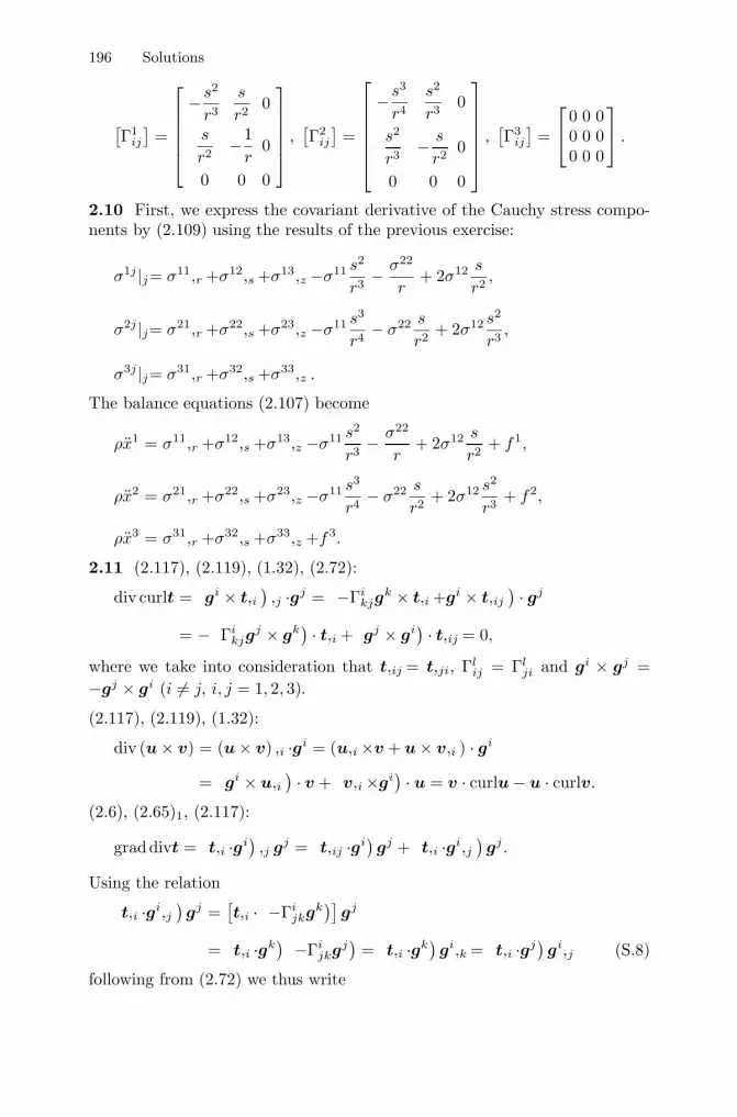
196 Solutions
[Γ1
ij
]=
⎡⎢⎢⎢⎢⎣−s2
r3
s
r20
s
r2−1
r0
0 0 0
⎤⎥⎥⎥⎥⎦ ,[Γ2
ij
]=
⎡⎢⎢⎢⎢⎢⎣−s3
r4
s2
r30
s2
r3− s
r20
0 0 0
⎤⎥⎥⎥⎥⎥⎦ ,[Γ3
ij
]=
⎡⎣ 0 0 00 0 00 0 0
⎤⎦ .
2.10 First, we express the covariant derivative of the Cauchy stress compo-nents by (2.109) using the results of the previous exercise:
σ1j |j= σ11,r +σ12,s +σ13,z −σ11 s2
r3− σ22
r+ 2σ12 s
r2,
σ2j |j= σ21,r +σ22,s +σ23,z −σ11 s3
r4− σ22 s
r2+ 2σ12 s2
r3,
σ3j |j= σ31,r +σ32,s +σ33,z .
The balance equations (2.107) become
ρx1 = σ11,r +σ12,s +σ13,z −σ11 s2
r3− σ22
r+ 2σ12 s
r2+ f1,
ρx2 = σ21,r +σ22,s +σ23,z −σ11 s3
r4− σ22 s
r2+ 2σ12 s2
r3+ f2,
ρx3 = σ31,r +σ32,s +σ33,z +f3.
2.11 (2.117), (2.119), (1.32), (2.72):
div curlt =(gi × t,i
),j ·gj =
(−Γikjg
k × t,i +gi × t,ij) · gj
= − (Γikjg
j × gk) · t,i +
(gj × gi
) · t,ij = 0,
where we take into consideration that t,ij = t,ji, Γlij = Γl
ji and gi × gj =−gj × gi (i �= j, i, j = 1, 2, 3).
(2.117), (2.119), (1.32):
div (u × v) = (u × v) ,i ·gi = (u,i ×v + u × v,i ) · gi
=(gi × u,i
) · v +(v,i ×gi
) · u = v · curlu − u · curlv.
(2.6), (2.65)1, (2.117):
graddivt =(t,i ·gi
),j gj =
(t,ij ·gi
)gj +
(t,i ·gi,j
)gj .
Using the relation(t,i ·gi,j
)gj =
[t,i ·
(−Γijkgk
)]gj
=(t,i ·gk
) (−Γijkgj
)=(t,i ·gk
)gi,k =
(t,i ·gj
)gi,j (S.8)
following from (2.72) we thus write
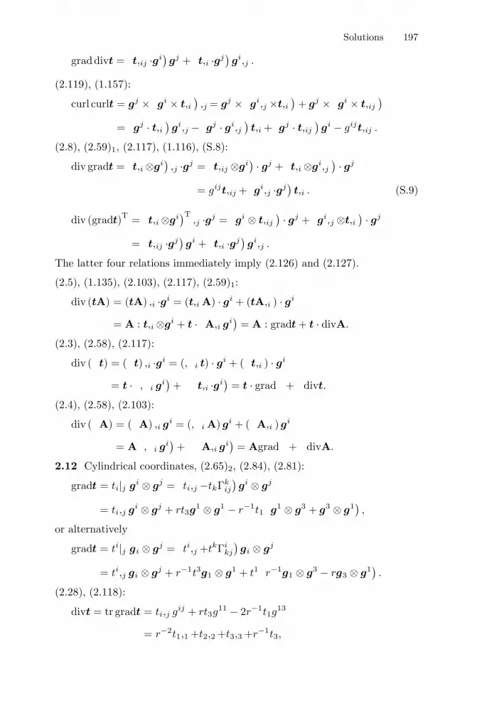
Solutions 197
graddivt =(t,ij ·gi
)gj +
(t,i ·gj
)gi,j .
(2.119), (1.157):
curl curlt = gj × (gi × t,i
),j = gj × (
gi,j ×t,i)
+ gj × (gi × t,ij
)=(gj · t,i
)gi,j −
(gj · gi,j
)t,i +
(gj · t,ij
)gi − gijt,ij .
(2.8), (2.59)1, (2.117), (1.116), (S.8):
div gradt =(t,i ⊗gi
),j ·gj =
(t,ij ⊗gi
) · gj +(t,i ⊗gi,j
) · gj
= gijt,ij +(gi,j ·gj
)t,i . (S.9)
div (gradt)T =(t,i ⊗gi
)T,j ·gj =
(gi ⊗ t,ij
) · gj +(gi,j ⊗t,i
) · gj
=(t,ij ·gj
)gi +
(t,i ·gj
)gi,j .
The latter four relations immediately imply (2.126) and (2.127).
(2.5), (1.135), (2.103), (2.117), (2.59)1:
div (tA) = (tA) ,i ·gi = (t,i A) · gi + (tA,i ) · gi
= A : t,i ⊗gi + t · (A,i gi)
= A : gradt + t · divA.
(2.3), (2.58), (2.117):
div (Φt) = (Φt) ,i ·gi = (Φ,i t) · gi + (Φt,i ) · gi
= t · (Φ,i gi)
+ Φ(t,i ·gi
)= t · gradΦ + Φdivt.
(2.4), (2.58), (2.103):
div (ΦA) = (ΦA) ,i gi = (Φ,i A) gi + (ΦA,i ) gi
= A(Φ,i gi
)+ Φ
(A,i gi
)= AgradΦ + ΦdivA.
2.12 Cylindrical coordinates, (2.65)2, (2.84), (2.81):
gradt = ti|j gi ⊗ gj =(ti,j −tkΓk
ij
)gi ⊗ gj
= ti,j gi ⊗ gj + rt3g1 ⊗ g1 − r−1t1
(g1 ⊗ g3 + g3 ⊗ g1
),
or alternatively
gradt = ti|j gi ⊗ gj =(ti,j +tkΓi
kj
)gi ⊗ gj
= ti,j gi ⊗ gj + r−1t3g1 ⊗ g1 + t1(r−1g1 ⊗ g3 − rg3 ⊗ g1
).
(2.28), (2.118):
divt = tr gradt = ti,j gij + rt3g11 − 2r−1t1g
13
= r−2t1,1 +t2,2 +t3,3 +r−1t3,
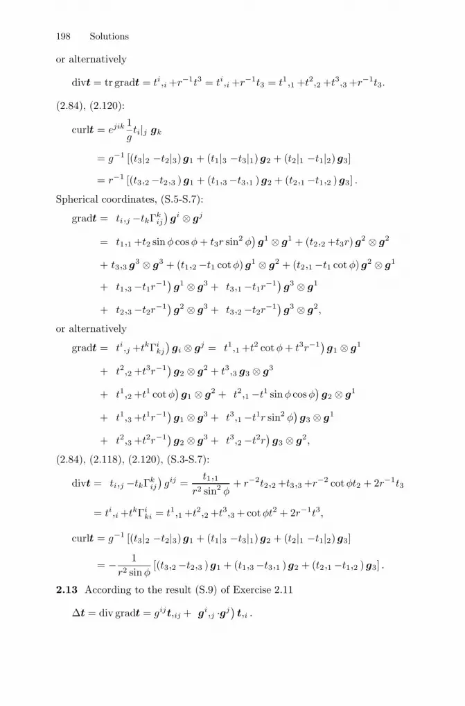
198 Solutions
or alternatively
divt = tr gradt = ti,i +r−1t3 = ti,i +r−1t3 = t1,1 +t2,2 +t3,3 +r−1t3.
(2.84), (2.120):
curlt = ejik 1gti|j gk
= g−1 [(t3|2 −t2|3) g1 + (t1|3 −t3|1) g2 + (t2|1 −t1|2) g3]
= r−1 [(t3,2 −t2,3 ) g1 + (t1,3 −t3,1 ) g2 + (t2,1 −t1,2 ) g3] .
Spherical coordinates, (S.5-S.7):
gradt =(ti,j −tkΓk
ij
)gi ⊗ gj
=(t1,1 +t2 sin φ cosφ + t3r sin2 φ
)g1 ⊗ g1 + (t2,2 +t3r) g2 ⊗ g2
+ t3,3 g3 ⊗ g3 + (t1,2 −t1 cotφ) g1 ⊗ g2 + (t2,1 −t1 cotφ) g2 ⊗ g1
+(t1,3 −t1r
−1)g1 ⊗ g3 +
(t3,1 −t1r
−1)g3 ⊗ g1
+(t2,3 −t2r
−1)g2 ⊗ g3 +
(t3,2 −t2r
−1)g3 ⊗ g2,
or alternatively
gradt =(ti,j +tkΓi
kj
)gi ⊗ gj =
(t1,1 +t2 cotφ + t3r−1
)g1 ⊗ g1
+(t2,2 +t3r−1
)g2 ⊗ g2 + t3,3 g3 ⊗ g3
+(t1,2 +t1 cotφ
)g1 ⊗ g2 +
(t2,1 −t1 sin φ cosφ
)g2 ⊗ g1
+(t1,3 +t1r−1
)g1 ⊗ g3 +
(t3,1 −t1r sin2 φ
)g3 ⊗ g1
+(t2,3 +t2r−1
)g2 ⊗ g3 +
(t3,2 −t2r
)g3 ⊗ g2,
(2.84), (2.118), (2.120), (S.3-S.7):
divt =(ti,j −tkΓk
ij
)gij =
t1,1
r2 sin2 φ+ r−2t2,2 +t3,3 +r−2 cotφt2 + 2r−1t3
= ti,i +tkΓiki = t1,1 +t2,2 +t3,3 + cotφt2 + 2r−1t3,
curlt = g−1 [(t3|2 −t2|3) g1 + (t1|3 −t3|1) g2 + (t2|1 −t1|2) g3]
= − 1r2 sin φ
[(t3,2 −t2,3 ) g1 + (t1,3 −t3,1 ) g2 + (t2,1 −t1,2 ) g3] .
2.13 According to the result (S.9) of Exercise 2.11
Δt = div gradt = gijt,ij +(gi,j ·gj
)t,i .
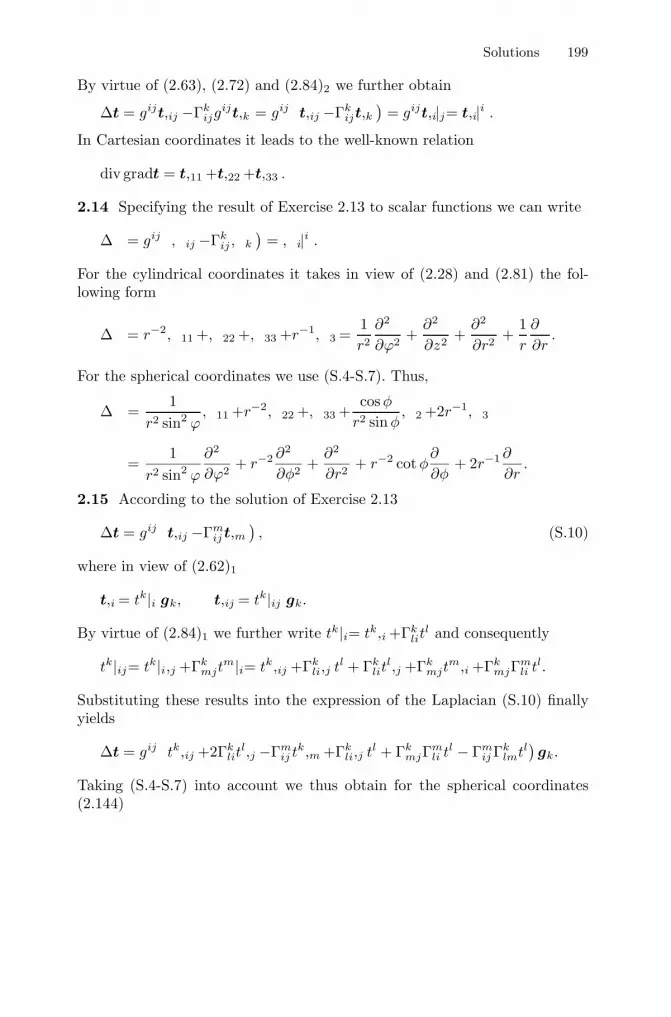
Solutions 199
By virtue of (2.63), (2.72) and (2.84)2 we further obtain
Δt = gijt,ij −Γkijg
ijt,k = gij(t,ij −Γk
ijt,k)
= gijt,i|j= t,i|i .
In Cartesian coordinates it leads to the well-known relation
div gradt = t,11 +t,22 +t,33 .
2.14 Specifying the result of Exercise 2.13 to scalar functions we can write
ΔΦ = gij(Φ,ij −Γk
ijΦ,k)
= Φ,i|i .
For the cylindrical coordinates it takes in view of (2.28) and (2.81) the fol-lowing form
ΔΦ = r−2Φ,11 +Φ,22 +Φ,33 +r−1Φ,3 =1r2
∂2Φ
∂ϕ2+
∂2Φ
∂z2+
∂2Φ
∂r2+
1r
∂Φ
∂r.
For the spherical coordinates we use (S.4-S.7). Thus,
ΔΦ =1
r2 sin2 ϕΦ,11 +r−2Φ,22 +Φ,33 +
cosφ
r2 sin φΦ,2 +2r−1Φ,3
=1
r2 sin2 ϕ
∂2Φ
∂ϕ2+ r−2 ∂2Φ
∂φ2+
∂2Φ
∂r2+ r−2 cotφ
∂Φ
∂φ+ 2r−1 ∂Φ
∂r.
2.15 According to the solution of Exercise 2.13
Δt = gij(t,ij −Γm
ij t,m), (S.10)
where in view of (2.62)1
t,i = tk|i gk, t,ij = tk|ij gk.
By virtue of (2.84)1 we further write tk|i= tk,i +Γklit
l and consequently
tk|ij= tk|i,j +Γkmjt
m|i= tk,ij +Γkli,j tl + Γk
litl,j +Γk
mjtm,i +Γk
mjΓmli tl.
Substituting these results into the expression of the Laplacian (S.10) finallyyields
Δt = gij(tk,ij +2Γk
litl,j −Γm
ij tk,m +Γkli,j tl + Γk
mjΓmli tl − Γm
ij Γklmtl
)gk.
Taking (S.4-S.7) into account we thus obtain for the spherical coordinates(2.144)

200 Solutions
Δt =(
t1,ϕϕ
r2 sin2 φ+
t1,φφ
r2+ t1,rr
+3 cotφ
r2t1,φ +
2 cosφ
r2 sin3 φt2,ϕ +
4t1,rr
+2t3,ϕ
r3 sin2 φ
)g1
+(
t2,ϕϕ
r2 sin2 φ+
t2,φφ
r2+ t2,rr
−2 cotφ
r2t1,ϕ +
cotφ
r2t2,φ +
4t2,rr
+2t3,φr3
+1 − cot2 φ
r2t2)
g2
+(
t3,ϕϕ
r2 sin2 φ+
t3,φφ
r2+ t3,rr
−2t1,ϕr
− 2t2,φr
+cotφ
r2t3,φ +
2t3,rr
− 2 cotφ
rt2 − 2t3
r2
)g3.
Exercises of Chapter 3
3.1 (C.4), (3.18): a1 = dr/ds = const. Hence, r (s) = b + sa1.
3.2 Using the fact that d/d (−s) = −d/ds we can write by means of (3.15),(3.18), (3.20), (3.21) and (3.27): a′
1 (s) = −a1 (s), a′2 (s) = a2 (s), a′
3 (s) =−a3 (s), κ′ (s) = κ (s) and τ ′ (s) = τ (s).
3.3 Let us show that the curve r (s) with the zero torsion τ (s) ≡ 0 belongs tothe plane p
(t1, t2
)= r (s0) + t1a1 (s0) + t2a2 (s0), where a1 (s0) and a2 (s0)
are, respectively, the unit tangent vector and the principal normal vector ata point s0. For any arbitrary point we can write using (3.15)
r (s) = r (s0) +
r(s)∫r(s0)
dr = r (s0) +
s∫s0
a1 (s) ds. (S.11)
The vector a1 (s) can further be represented with respect to the trihedron at s0
as a1 (s) = αi (s)ai (s0). Taking (3.26) into account we observe that a3,s = 0and consequently a3 (s) ≡ a3 (s0). In view of (3.23)2 it yields a1 (s) ·a3 (s0) =0, so that a1 (s) = α1 (s)a1 (s0) + α2 (s)a2 (s0). Inserting this result into(S.11) we have
r (s) = r (s0) + a1 (s0)
s∫s0
α1 (s) ds + a2 (s0)
s∫s0
α2 (s) ds
= r (s0) + t1a1 (s0) + t2a2 (s0) ,
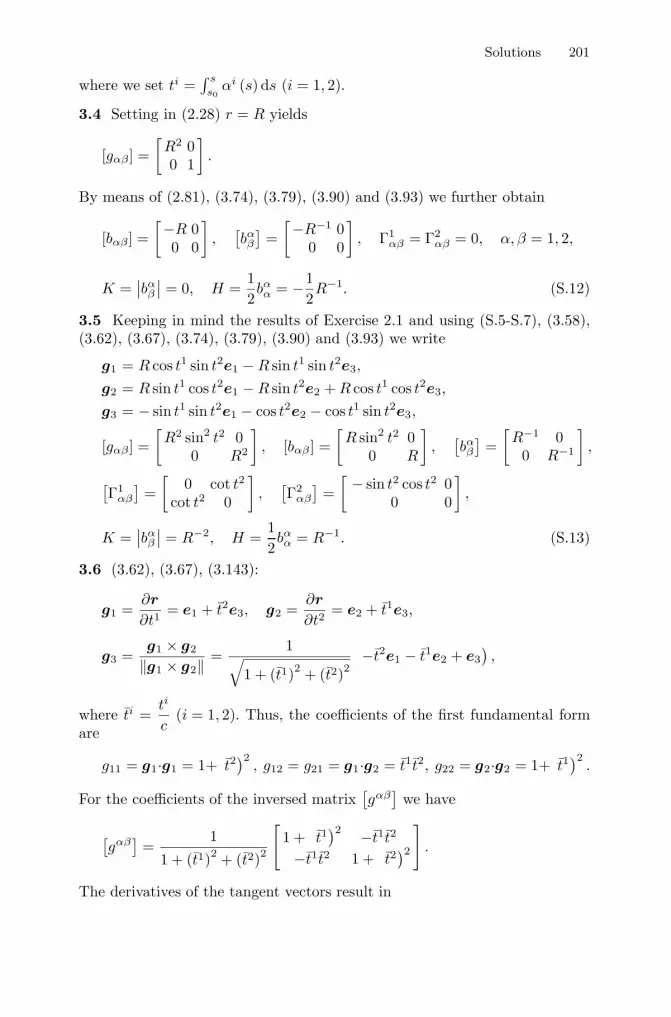
Solutions 201
where we set ti =∫ s
s0αi (s) ds (i = 1, 2).
3.4 Setting in (2.28) r = R yields
[gαβ] =[
R2 00 1
].
By means of (2.81), (3.74), (3.79), (3.90) and (3.93) we further obtain
[bαβ] =[−R 0
0 0
],
[bαβ
]=[−R−1 0
0 0
], Γ1
αβ = Γ2αβ = 0, α, β = 1, 2,
K =∣∣bα
β
∣∣ = 0, H =12bαα = −1
2R−1. (S.12)
3.5 Keeping in mind the results of Exercise 2.1 and using (S.5-S.7), (3.58),(3.62), (3.67), (3.74), (3.79), (3.90) and (3.93) we write
g1 = R cos t1 sin t2e1 − R sin t1 sin t2e3,
g2 = R sin t1 cos t2e1 − R sin t2e2 + R cos t1 cos t2e3,
g3 = − sin t1 sin t2e1 − cos t2e2 − cos t1 sin t2e3,
[gαβ] =[
R2 sin2 t2 00 R2
], [bαβ ] =
[R sin2 t2 0
0 R
],
[bαβ
]=[
R−1 00 R−1
],
[Γ1
αβ
]=[
0 cot t2
cot t2 0
],
[Γ2
αβ
]=[ − sin t2 cos t2 0
0 0
],
K =∣∣bα
β
∣∣ = R−2, H =12bαα = R−1. (S.13)
3.6 (3.62), (3.67), (3.143):
g1 =∂r
∂t1= e1 + t2e3, g2 =
∂r
∂t2= e2 + t1e3,
g3 =g1 × g2
‖g1 × g2‖ =1√
1 + (t1)2 + (t2)2
(−t2e1 − t1e2 + e3
),
where ti =ti
c(i = 1, 2). Thus, the coefficients of the first fundamental form
are
g11 = g1·g1 = 1+(t2)2
, g12 = g21 = g1·g2 = t1t2, g22 = g2·g2 = 1+(t1)2
.
For the coefficients of the inversed matrix[gαβ
]we have
[gαβ
]=
1
1 + (t1)2 + (t2)2
[1 +
(t1)2 −t1t2
−t1t2 1 +(t2)2]
.
The derivatives of the tangent vectors result in
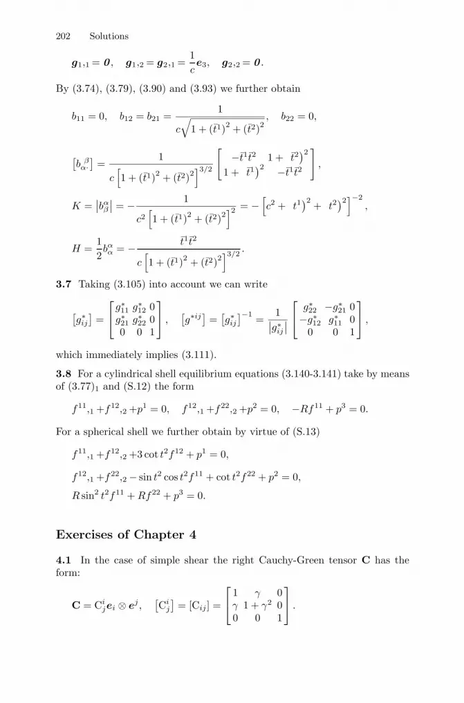
202 Solutions
g1,1 = 0 , g1,2 = g2,1 =1ce3, g2,2 = 0 .
By (3.74), (3.79), (3.90) and (3.93) we further obtain
b11 = 0, b12 = b21 =1
c
√1 + (t1)2 + (t2)2
, b22 = 0,
[b βα·]
=1
c[1 + (t1)2 + (t2)2
]3/2
[−t1t2 1 +
(t2)2
1 +(t1)2 −t1t2
],
K =∣∣bα
β
∣∣ = − 1
c2[1 + (t1)2 + (t2)2
]2 = −[c2 +
(t1)2
+(t2)2]−2
,
H =12bαα = − t1t2
c[1 + (t1)2 + (t2)2
]3/2.
3.7 Taking (3.105) into account we can write
[g∗ij]
=
⎡⎣g∗11 g∗12 0g∗21 g∗22 00 0 1
⎤⎦ ,[g∗ij
]=[g∗ij]−1 =
1∣∣g∗ij∣∣⎡⎣ g∗22 −g∗21 0−g∗12 g∗11 0
0 0 1
⎤⎦ ,
which immediately implies (3.111).
3.8 For a cylindrical shell equilibrium equations (3.140-3.141) take by meansof (3.77)1 and (S.12) the form
f11,1 +f12,2 +p1 = 0, f12,1 +f22,2 +p2 = 0, −Rf11 + p3 = 0.
For a spherical shell we further obtain by virtue of (S.13)
f11,1 +f12,2 +3 cot t2f12 + p1 = 0,
f12,1 +f22,2 − sin t2 cos t2f11 + cot t2f22 + p2 = 0,
R sin2 t2f11 + Rf22 + p3 = 0.
Exercises of Chapter 4
4.1 In the case of simple shear the right Cauchy-Green tensor C has theform:
C = Cijei ⊗ ej ,
[Ci
j
]= [Cij ] =
⎡⎣ 1 γ 0γ 1 + γ2 00 0 1
⎤⎦ .
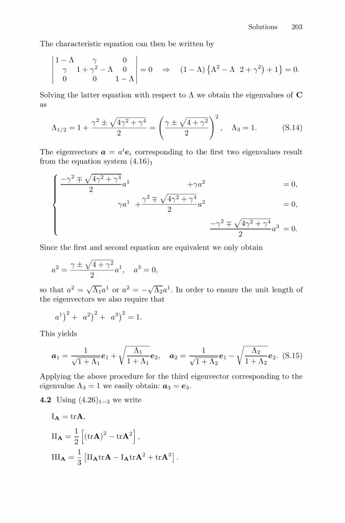
Solutions 203
The characteristic equation can then be written by∣∣∣∣∣∣1 − Λ γ 0
γ 1 + γ2 − Λ 00 0 1 − Λ
∣∣∣∣∣∣ = 0 ⇒ (1 − Λ){Λ2 − Λ
(2 + γ2
)+ 1
}= 0.
Solving the latter equation with respect to Λ we obtain the eigenvalues of Cas
Λ1/2 = 1 +γ2 ±
√4γ2 + γ4
2=
(γ ±
√4 + γ2
2
)2
, Λ3 = 1. (S.14)
The eigenvectors a = aiei corresponding to the first two eigenvalues resultfrom the equation system (4.16)1⎧⎪⎪⎪⎪⎪⎪⎪⎨⎪⎪⎪⎪⎪⎪⎪⎩
−γ2 ∓√
4γ2 + γ4
2a1 +γa2 = 0,
γa1 +γ2 ∓
√4γ2 + γ4
2a2 = 0,
−γ2 ∓√4γ2 + γ4
2a3 = 0.
Since the first and second equation are equivalent we only obtain
a2 =γ ±
√4 + γ2
2a1, a3 = 0,
so that a2 =√
Λ1a1 or a2 = −√
Λ2a1. In order to ensure the unit length of
the eigenvectors we also require that(a1)2
+(a2)2
+(a3)2
= 1.
This yields
a1 =1√
1 + Λ1
e1 +√
Λ1
1 + Λ1e2, a2 =
1√1 + Λ2
e1 −√
Λ2
1 + Λ2e2. (S.15)
Applying the above procedure for the third eigenvector corresponding to theeigenvalue Λ3 = 1 we easily obtain: a3 = e3.
4.2 Using (4.26)1−3 we write
IA = trA,
IIA =12
[(trA)2 − trA2
],
IIIA =13[IIAtrA− IAtrA2 + trA3
].
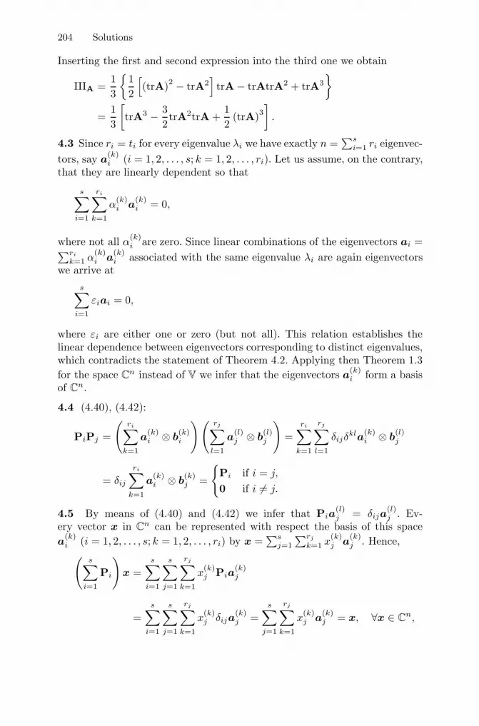
204 Solutions
Inserting the first and second expression into the third one we obtain
IIIA =13
{12
[(trA)2 − trA2
]trA − trAtrA2 + trA3
}=
13
[trA3 − 3
2trA2trA +
12
(trA)3]
.
4.3 Since ri = ti for every eigenvalue λi we have exactly n =∑s
i=1 ri eigenvec-tors, say a
(k)i (i = 1, 2, . . . , s; k = 1, 2, . . . , ri). Let us assume, on the contrary,
that they are linearly dependent so that
s∑i=1
ri∑k=1
α(k)i a
(k)i = 0,
where not all α(k)i are zero. Since linear combinations of the eigenvectors ai =∑ri
k=1 α(k)i a
(k)i associated with the same eigenvalue λi are again eigenvectors
we arrive ats∑
i=1
εiai = 0,
where εi are either one or zero (but not all). This relation establishes thelinear dependence between eigenvectors corresponding to distinct eigenvalues,which contradicts the statement of Theorem 4.2. Applying then Theorem 1.3for the space Cn instead of V we infer that the eigenvectors a
(k)i form a basis
of Cn.
4.4 (4.40), (4.42):
PiPj =
(ri∑
k=1
a(k)i ⊗ b
(k)i
)( rj∑l=1
a(l)j ⊗ b
(l)j
)=
ri∑k=1
rj∑l=1
δijδkla
(k)i ⊗ b
(l)j
= δij
ri∑k=1
a(k)i ⊗ b
(k)j =
{Pi if i = j,
0 if i �= j.
4.5 By means of (4.40) and (4.42) we infer that Pia(l)j = δija
(l)j . Ev-
ery vector x in Cn can be represented with respect the basis of this spacea
(k)i (i = 1, 2, . . . , s; k = 1, 2, . . . , ri) by x =
∑sj=1
∑rj
k=1 x(k)j a
(k)j . Hence,(
s∑i=1
Pi
)x =
s∑i=1
s∑j=1
rj∑k=1
x(k)j Pia
(k)j
=s∑
i=1
s∑j=1
rj∑k=1
x(k)j δija
(k)j =
s∑j=1
rj∑k=1
x(k)j a
(k)j = x, ∀x ∈ C
n,
Solutions 205
which immediately implies (4.46).
4.6 Let λ1, λ2, . . . , λn be eigenvalues of A ∈ Linn. By the spectral mappingtheorem (Theorem 4.1) we infer that exp (λi) (i = 1, 2, . . . , n) are eigenvaluesof expA. On use of (4.24) and (4.26) we can thus write: det [exp (A)] =n∏
i=1
exp λi = exp(
n∑i=1
λi
)= exp (trA).
4.7 Let us consider the right hand side of (4.54) for example for i = 1. Inthis case we have
3∏j=1j �=1
A − λjIλ1 − λj
=A − λ2Iλ1 − λ2
A− λ3Iλ1 − λ3
.
On use of (4.43), (4.44) and (4.46) we further obtain
A− λ2Iλ1 − λ2
A − λ3Iλ1 − λ3
=
3∑i=1
(λi − λ2)Pi
λ1 − λ2
3∑j=1
(λj − λ3)Pj
λ1 − λ3
=
3∑i,j=1
(λi − λ2) (λj − λ3) δijPi
(λ1 − λ2) (λ1 − λ3)=
3∑i=1
(λi − λ2) (λi − λ3)Pi
(λ1 − λ2) (λ1 − λ3)
=(λ1 − λ2) (λ1 − λ3)P1
(λ1 − λ2) (λ1 − λ3)= P1.
In a similar way, one verifies the Sylvester formula also for i = 2 and i = 3.
4.8 The characteristic equation of the tensor A takes the form:∣∣∣∣∣∣−2 − λ 2 2
2 1 − λ 42 4 1 − λ
∣∣∣∣∣∣ = 0.
Writing out this determinant we get after some algebraic manipulations
λ3 − 27λ − 54 = 0
Comparing this equation with (4.28) we see that
IA = 0, IIA = −27, IIIA = 54. (S.16)
Inserting this result into the Cardano formula (4.31) and (4.32) we obtain
ϑ = arccos
[2I3A − 9IAIIA + 27IIIA
2(I2A − 3IIA
)3/2
]
= arccos
[27 · 54
2 (3 · 27)3/2
]= arccos (1) = 0,
206 Solutions
λk =13
{IA + 2
√I2A − 3IIA cos
13
[ϑ + 2π (k − 1)]}
=23
√3 · 27 cos
(23π (k − 1)
)= 6 cos
(23π (k − 1)
), k = 1, 2, 3.
Thus, we obtain two pairwise distinct eigenvalues (s = 2):
λ1 = 6, λ2 = λ3 = −3. (S.17)
The Sylvester formula (4.54) further yields
P1 =2∏
j=1j �=1
A − λjIλi − λj
=A − λ2Iλ1 − λ2
=A + 3I
9=
19
⎡⎣ 1 2 22 4 42 4 4
⎤⎦ ei ⊗ ej ,
P2 =2∏
j=1j �=2
A − λjIλi − λj
=A − λ1Iλ2 − λ1
=A− 6I−9
=19
⎡⎣ 8 −2 −2−2 5 −4−2 −4 5
⎤⎦ei ⊗ ej .
4.9 The spectral representation of A takes the form
A =s∑
i=1
λiPi = λ1P1 + λ2P2 = 6P1 − 3P2.
Thus,
A =s∑
i=1
exp (λi)Pi
= exp (λ1)P1 + exp (λ2)P2 = exp (6)P1 + exp (−3)P2
=e6
9
⎡⎣ 1 2 22 4 42 4 4
⎤⎦ei ⊗ ej +e−3
9
⎡⎣ 8 −2 −2−2 5 −4−2 −4 5
⎤⎦ ei ⊗ ej
=19
⎡⎣ e6 + 8e−3 2e6 − 2e−3 2e6 − 2e−3
2e6 − 2e−3 4e6 + 5e−3 4e6 − 4e−3
2e6 − 2e−3 4e6 − 4e−3 4e6 + 5e−3
⎤⎦ei ⊗ ej .
4.10 Components of the eigenvectors a = aiei result from the equationsystem (4.16)(
Aij − δi
jλ)aj = 0, i = 1, 2, 3. (S.18)
Setting λ = 6 we obtain only two independent equations{−8a1 +2a2 +2a3 = 0,
2a1 −5a2 +4a3 = 0.

Solutions 207
Multiplying the first equation by two and subtracting from the second onewe get a2 = 2a1 and consequently a3 = 2a1. Additionally we require that theeigenvectors have unit length so that(
a1)2
+(a2)2
+(a3)2
= 1, (S.19)
which leads to
a1 =13e1 +
23e2 +
23e3.
Further, setting in the equation system (S.18) λ = −3 we obtain only oneindependent linear equation
a1 + 2a2 + 2a3 = 0 (S.20)
with respect to the components of the eigenvectors corresponding to this dou-ble eigenvalue. One of these eigenvectors can be obtained by setting for ex-ample a1 = 0. In this case, a2 = −a3 and in view of (S.19)
a(1)2 =
1√2e2 − 1√
2e3.
Requiring that the eigenvectors a(1)2 and a
(2)2 corresponding to the double
eigenvalue λ = −3 are orthogonal we get an additional condition a2 = a3 forthe components of a
(2)2 . Taking into account (S.19) and (S.20) this yields
a(2)2 = − 4
3√
2e1 +
13√
2e2 +
13√
2e3.
With the aid of the eigenvectors we can construct eigenprojections withoutthe Sylvester formula by (4.42):
P1 = a1 ⊗ a1
=(
13e1 +
23e2 +
23e3
)⊗(
13e1 +
23e2 +
23e3
)=
19
⎡⎣ 1 2 22 4 42 4 4
⎤⎦ei ⊗ ej ,
P2 = a(1)2 ⊗ a
(1)2 + a
(2)2 ⊗ a
(2)2 =
(1√2e2 − 1√
2e3
)⊗(
1√2e2 − 1√
2e3
)
+(− 4
3√
2e1 +
13√
2e2 +
13√
2e3
)⊗(− 4
3√
2e1 +
13√
2e2 +
13√
2e3
)
=19
⎡⎣ 8 −2 −2−2 5 −4−2 −4 5
⎤⎦ei ⊗ ej .

208 Solutions
4.11 Since linearly independent vectors are non-zero it follows from (4.9)that ci · ci �= 0 (i = 1, 2, . . . , m). Thus, the first vector can be given by
a1 =c1√
c1 · c1,
such that a1 · a1 = 1. Next, we set
a′2 = c2 − (c2 · a1)a1,
so that a′2 · a1 = 0. Further, a′
2 �= 0 because otherwise c2 = (c2 · a1)a1 =(c2 · a1) (c1 · c1)
−1/2c1 which implies a linear dependence between c1 and c2.
Thus, we can set a2 = a′2/√
a′2 · a′
2. The third vector can be given by
a3 =a′
3√a′
3 · a′3
, where a′3 = c3 − (c3 · a2)a2 − (c3 · a1)a1,
so that a3 · a1 = a3 · a2 = 0. Repeating this procedure we finally obtain theset of vectors ai satisfying the condition ai ·aj = δij , (i, j = 1, 2, . . . , m). Onecan easily show that these vectors are linearly independent. Indeed, otherwise∑m
i=1 αiai = 0 , where not all αi are zero. Multiplying this vector equationscalarly by aj (j = 1, 2, . . . , m) yields, however, αj = 0 (j = 1, 2, . . . , m).
4.12 Comparing (4.63)1 with (4.71)1 we infer that the right eigenvectorsa
(k)i (k = 1, 2, . . . , ti) associated with a complex eigenvalue λi are simulta-
neously the left eigenvalues associated with λi. Since λi �= λi Theorem 4.3implies that a
(k)i · a(l)
i = 0 (k, l = 1, 2, . . . , ti).
4.13 Taking into account the identities trWk = 0, where k = 1, 3, 5, . . . (seeExercise 1.46) we obtain from (4.29)
IW = trW = 0,
IIW =12
[(trW)2 − trW2
]= −1
2trW2 = −1
2(W : WT
)=
12
(W : W) =12‖W‖2
,
IIIW =13
[trW3 − 3
2trW2trW +
12
(trW)3]
= 0,
or in another way
IIIW = detW = detWT = −detWT = −IIIW = 0.
4.14 Eigenvalues of the rotation tensor (Exercise 1.22)
R = Ri·jei ⊗ ej , where
[Ri
·j]
=[Rij
]=
⎡⎣ cosα − sinα 0sin α cosα 0
0 0 1
⎤⎦

Solutions 209
result from the characteristic equation∣∣∣∣∣∣cosα − λ − sinα 0
sin α cosα − λ 00 0 1 − λ
∣∣∣∣∣∣ = 0.
Writing out this determinant we have
(1 − λ)(λ2 − 2λ cosα + 1
)= 0
and consequently
λ1 = 1, λ2/3 = cosα ± i sinα.
Components of the right eigenvectors a = aiei result from the equation system(4.16)(
Ri·j − δi
jλ)aj = 0, i = 1, 2, 3. (S.21)
Setting first λ = 1 we obtain a homogeneous equation system
a1 (cosα − 1) − a2 sin α = 0,
a1 sinα + a2 (cosα − 1) = 0,
leading to a1 = a2 = 0. Thus, a1 = a3e3, where a3 can be an arbitrary realnumber. The unit length condition requires further that
a1 = e3.
Next, inserting λ = cosα ± i sin α into (S.21) yields
a2 = ∓ia1, a3 = 0.
Thus, the right eigenvectors associated with the complex conjugate eigenvaluesλ2/3 are of the form a2/3 = a1 (e1 ∓ ie2). Bearing in mind that any rotationtensor is orthogonal we infer that a2/3 = a3/2 = a1 (e1 ± ie2) are the lefteigenvectors associated with λ2/3. Imposing the additional condition a2 ·a2 =a2 · a3 = 1 (4.38) we finally obtain
a2 =√
22
(e1 − ie2) , a3 =√
22
(e1 + ie2) .
The eigenprojections can further be expressed by (4.42) as
P1 = a1 ⊗ a1 = e3 ⊗ e3,
P2 = a2 ⊗ a2 =√
22
(e1 − ie2) ⊗√
22
(e1 + ie2)
=12
(e1 ⊗ e1 + e2 ⊗ e2) +12i (e1 ⊗ e2 − e2 ⊗ e1) ,
210 Solutions
P3 = a3 ⊗ a3 =√
22
(e1 + ie2) ⊗√
22
(e1 − ie2)
=12
(e1 ⊗ e1 + e2 ⊗ e2) − 12i (e1 ⊗ e2 − e2 ⊗ e1) .
4.15 First, we write
[(A2)ij
]=
⎡⎣−2 2 22 1 42 4 1
⎤⎦⎡⎣−2 2 22 1 42 4 1
⎤⎦ =
⎡⎣ 12 6 66 21 126 12 21
⎤⎦ ,
[(A3)ij
]=
⎡⎣ 12 6 66 21 126 12 21
⎤⎦⎡⎣−2 2 22 1 42 4 1
⎤⎦ =
⎡⎣ 0 54 5454 81 10854 108 81
⎤⎦ .
Then,
pA (A) = A3 − 27A− 54I =
⎡⎣ 0 54 5454 81 10854 108 81
⎤⎦ ei ⊗ ej
−27
⎡⎣−2 2 22 1 42 4 1
⎤⎦ei ⊗ ej − 54
⎡⎣1 0 00 1 00 0 1
⎤⎦ei ⊗ ej =
⎡⎣ 0 0 00 0 00 0 0
⎤⎦ei ⊗ ej .
4.16 The characteristic polynomial of F (4.23) can be represented bypA (λ) = (1 − λ)3. Hence,
pF (F) = (I − F)3 =
⎡⎣ 0 −γ 00 0 00 0 0
⎤⎦3
ei ⊗ ej =
⎡⎣ 0 0 00 0 00 0 0
⎤⎦ei ⊗ ej = 0.
Exercises of Chapter 5
5.1 By using (1.101)1, (D.2) and (5.17) one can verify for example (5.20)1and (5.21)1 within the following steps
A⊗(B + C) : X = AX (B + C) = AXB+AXC = (A⊗ B + A⊗ C) : X,
A� (B + C) : X = A [(B + C) : X] = A (B : X + C : X)= A (B : X) + A (C : X)= (A � B + A � C) : X, ∀X ∈ Linn.
The proof of (5.20)2 and (5.21)2 is similar.
5.2 With the aid of (5.16), (5.17) and (1.138) we can write
(Y : A⊗ B) : X = Y : (A⊗ B : X) = Y : AXB = ATYBT : X,
Solutions 211
(Y : A� B) : X = Y : (A � B : X) = Y : [A (B : X)]
= (Y : A) (B : X) = [(Y : A)B] : X, ∀X,Y ∈ Linn.
5.3 Using the definition of the simple composition (5.40) and taking (5.17)into account we obtain
A (B⊗ C)D : X = A (B⊗ C : X)D = A (BXC)D
= (AB)X (CD) = (AB) ⊗ (CD) : X,
A (B� C)D : X = A (B� C : X)D = A [B (C : X)]D
= ABD (C : X) = (ABD) � C : X, ∀X ∈ Linn.
5.4 By means of (1.140), (5.17), (5.22) and (5.45) we can write
(A⊗ B)T : X = X : (A ⊗ B) = ATXBT =(AT ⊗ BT
): X,
(A� B)T : X = X : (A � B) = (X : A)B = (B � A) : X,
(A� B)t : X = (A� B) : XT = A(B : XT
)= A
(BT : X
)=(A � BT
): X, ∀X ∈ Linn.
Identities (5.51) and (5.52) follow immediately from (1.116) (5.23), (5.24)(5.49)1 and (5.50) by setting A = a⊗ b, B = c⊗ d or A = a⊗ d, B = b⊗ c,respectively.
5.5 Using (5.51) and (5.52) we obtain for the left and right hand sides differentresults:
(a ⊗ b ⊗ c ⊗ d)tT = (a ⊗ c ⊗ b ⊗ d)T = c ⊗ a ⊗ d ⊗ b,
(a ⊗ b ⊗ c ⊗ d)Tt = (b ⊗ a ⊗ d ⊗ c)t = b ⊗ d ⊗ a ⊗ c.
5.6 (5.31), (5.32), (5.45):
(A : B)T : X = X : (A : B) = (X : A) : B
= BT : (X : A) = BT :(AT : X
)=(BT : AT
): X,
(A : B)t : X = (A : B) : XT = A :(B : XT
)= A :
(Bt : X
)=(A : Bt) : X, ∀X ∈ Linn.
5.7 In view of (1.115), (5.17) and (5.45) we write for an arbitrary tensorX ∈ Linn
(A⊗ B)t : (C ⊗ D) : X = (A⊗ B)t : (CXD) = (A⊗ B) : (CXD)T
= (A⊗ B) :(DTXTCT
)= ADTXTCTB
=[(
ADT)⊗ (
CTB)]
: XT =[(
ADT)⊗ (
CTB)]t
: X,
212 Solutions
(A⊗ B)t : (C� D) : X = (A ⊗ B)t : [(D : X)C]
= (A ⊗ B) :[(D : X)CT
]= (D : X)ACTB =
(ACTB
)� D : X.
5.8 By virtue of (5.51) and (5.52) we can write
CT =(Cijklgi ⊗ gj ⊗ gk ⊗ gl
)T= Cijklgj ⊗ gi ⊗ gl ⊗ gk
= Cjilkgi ⊗ gj ⊗ gk ⊗ gl,
Ct =(Cijklgi ⊗ gj ⊗ gk ⊗ gl
)t= Cijklgi ⊗ gk ⊗ gj ⊗ gl
= Cikjlgi ⊗ gj ⊗ gk ⊗ gl.
According to (5.60) and (5.61) CT = Ct = C. Taking also into account thatthe tensors gi ⊗ gj ⊗ gk ⊗ gl (i, j, k, l = 1, 2, . . . , n) are linearly independentwe thus write
Cijkl = Cjilk = Cikjl .
The remaining relations (5.70) are obtained in the same manner by applyingthe identities C = CTtT and C = CtTt.
5.9 With the aid of (1.140), (5.16) and (5.79) we get
(Y : T) : X = Y : (T : X) = Y : XT = YT : X, ∀X,Y ∈ Linn.
5.10 On use of (5.31), (5.45)2 and (5.79) we obtain
(A : T) : X = A : (T : X) = A : XT = At : X, ∀X ∈ Linn.
The second identity (5.83) can be derived by means of (5.54), (5.78) and (5.81)as follows
ATtT = (I : A)TtT =(AT : I
)tT
=(AT : It
)T
=(AT : T
)T
= T : A.
The last identity (5.83) can finally be proved by
(T : T) : X = T : (T : X) = T : XT = X = T : X, ∀X ∈ Linn.
5.11 C possesses the minor symmetry (5.61) by the very definition. In orderto prove the major symmetry (5.60) we show that C : X = X : C, ∀X ∈ Linn.Indeed, in view of (5.17)1, (5.22)1 and (5.48)
C : X = (M1 ⊗ M2 + M2 ⊗ M1)s : X = (M1 ⊗ M2 + M2 ⊗ M1) : symX
= M1 (symX)M2 + M2 (symX)M1,
X : C = X : (M1 ⊗ M2 + M2 ⊗ M1)s
= sym [X : (M1 ⊗ M2 + M2 ⊗ M1)]
= sym(M1XM2 + M2XM1) = M1 (symX)M2 + M2 (symX)M1.
Solutions 213
5.12 (a) Let ei (i = 1, 2, 3) be an orthonormal basis in E3. By virtue of (5.77),(5.82) and (5.84) we can write
Is =3∑
i,j=1
12ei ⊗ (ei ⊗ ej + ej ⊗ ei) ⊗ ej .
Using the notation
Mi = ei ⊗ ei, i = 1, 2, 3, M4 =e1 ⊗ e2 + e2 ⊗ e1√
2,
M5 =e1 ⊗ e3 + e3 ⊗ e1√
2, M6 =
e3 ⊗ e2 + e2 ⊗ e3√2
(S.22)
and taking (5.23) into account one thus obtains the spectral decomposition ofIs as
Is =6∑
p=1
Mp � Mp.
The only eigenvalue 1 is of multiplicity 6. Note that the corresponding eigen-tensors Mp (p = 1, 2, . . . , 6) form an orthonormal basis of Lin3.(b) Using the orthonormal basis (S.22) we can write
Psph =13
(M1 + M2 + M3) � (M1 + M2 + M3)
=6∑
p,q=1
PpqsphMp � Mq, where [Ppq
sph] =13
⎡⎢⎢⎢⎢⎢⎢⎣1 1 1 0 0 01 1 1 0 0 01 1 1 0 0 00 0 0 0 0 00 0 0 0 0 00 0 0 0 0 0
⎤⎥⎥⎥⎥⎥⎥⎦ .
Eigenvalues and eigenvectors of this matrix can be represented as
Λ1 = 1,
⎧⎪⎪⎪⎪⎪⎪⎨⎪⎪⎪⎪⎪⎪⎩
111000
⎫⎪⎪⎪⎪⎪⎪⎬⎪⎪⎪⎪⎪⎪⎭,
Λ2 = Λ3 = Λ4 = Λ5 = Λ6 = 0,
⎧⎪⎪⎪⎪⎪⎪⎨⎪⎪⎪⎪⎪⎪⎩
−110000
⎫⎪⎪⎪⎪⎪⎪⎬⎪⎪⎪⎪⎪⎪⎭,
⎧⎪⎪⎪⎪⎪⎪⎨⎪⎪⎪⎪⎪⎪⎩
−101000
⎫⎪⎪⎪⎪⎪⎪⎬⎪⎪⎪⎪⎪⎪⎭,
⎧⎪⎪⎪⎪⎪⎪⎨⎪⎪⎪⎪⎪⎪⎩
000100
⎫⎪⎪⎪⎪⎪⎪⎬⎪⎪⎪⎪⎪⎪⎭,
⎧⎪⎪⎪⎪⎪⎪⎨⎪⎪⎪⎪⎪⎪⎩
000010
⎫⎪⎪⎪⎪⎪⎪⎬⎪⎪⎪⎪⎪⎪⎭,
⎧⎪⎪⎪⎪⎪⎪⎨⎪⎪⎪⎪⎪⎪⎩
000001
⎫⎪⎪⎪⎪⎪⎪⎬⎪⎪⎪⎪⎪⎪⎭.

214 Solutions
Thus, the orthonormal eigentensors can be given by
M1 =1√3
(M1 + M2 + M3) =1√3I, M2 = −
√2
2M1 +
√2
2M2,
M3 = −√
66
M1 −√
66
M2 +√
63
M3, Mp = Mp, p = 4, 5, 6, (S.23)
where the tensors Mq, (q = 1, 2, . . . , 6) are defined by (S.22).(c) For the super-symmetric counterpart of the deviatoric projection tensor(5.87)2 (n = 3) we can write
Psdev =
6∑p,q=1
PpqdevMp � Mq, where [Ppq
dev] =
⎡⎢⎢⎢⎢⎢⎢⎢⎢⎢⎢⎢⎢⎣
23−1
3−1
30 0 0
−13
23−1
30 0 0
−13−1
323
0 0 0
0 0 0 1 0 00 0 0 0 1 00 0 0 0 0 1
⎤⎥⎥⎥⎥⎥⎥⎥⎥⎥⎥⎥⎥⎦.
Thus, the eigenvalues of Psdev are Λ1 = 0, Λq = 1 (q = 2, 3, . . . , 6). The cor-
responding eigentensors are again given by (S.23).(d) With respect to the orthonormal basis (S.22) the elasticity tensor (5.91)can be represented by
C =6∑
p,q=1
CpqMp � Mq,
where
[Cpq] =
⎡⎢⎢⎢⎢⎢⎢⎣2G + λ λ λ 0 0 0
λ 2G + λ λ 0 0 0λ λ 2G + λ 0 0 00 0 0 2G 0 00 0 0 0 2G 00 0 0 0 0 2G
⎤⎥⎥⎥⎥⎥⎥⎦ .
The eigentensors of C are the same as of Psph and Psdev and are given by (S.23).
The eigenvalues are as follows: Λ1 = 2G+3λ, Λq = 2G (q = 2, 3, . . . , 6). Theycan be obtained as linear combinations of those ones of Psph and Ps
dev.
Exercises of Chapter 6
6.1 (a) f(QAQT
)= aQAQTb �= aAb.
Solutions 215
(b) Since the components of A are related to an orthonormal basis we canwrite
f (A) = A11 + A22 + A33 = A1·1 + A2
·2 + A3·3 = Ai
·i = trA.
Trace of a tensor represents its isotropic function.(c) For an isotropic tensor function the condition (6.1) f(QAQT) = f (A)must hold on the whole definition domain of the arguments A and ∀Q ∈Orth3. Let us consider a special case where
A =
⎡⎣ 1 0 00 0 00 0 0
⎤⎦ei ⊗ ej , Q =
⎡⎣ 0 1 0−1 0 0
0 0 1
⎤⎦ei ⊗ ej .
Thus,
A′ = QAQT =
⎡⎣ 0 0 00 1 00 0 0
⎤⎦ei ⊗ ej
and consequently
f (A) = A11 + A12 + A13 = 1 �= 0 = A′11 + A′12 + A′13 = f(QAQT
),
which means that the function f (A) is not isotropic.(d) detA is the last principal invariant of A and represents thus its isotropictensor function. Isotropy of the determinant can, however, be shown directlyusing the relation det (BC) = detBdetC. Indeed,
det(QAQT
)= detQ detA detQT = detQ detQTdetA
= det(QQT
)detA = detIdetA = detA, ∀Q ∈ Orthn.
(e) Eigenvalues of a second-order tensor are uniquely defined by its principalinvariants and represent thus its isotropic functions. This can also be shownin a direct way considering the eigenvalue problem for the tensor QAQT as(
QAQT)
a = λa.
Mapping both sides of this vector equation by QT yields(QTQAQT
)a = λQTa.
Using the abbreviation a′ = QTa we finally obtain
Aa′ = λa′.
216 Solutions
Thus, every eigenvalue of QAQT is the eigenvalue of A and vice versa. Inother words, the eigenvalues of these tensors are pairwise equal which imme-diately implies that they are characterized by the same value of λmax. Thetensors obtained by the operation QAQT from the original one A are calledsimilar tensors.
6.2 Inserting
M =12(A + AT
), W =
12(A − AT
)into (6.17) we obtain
trM =12(trA + trAT
)= trA,
trM2 =14tr(A + AT
)2=
14
[trA2 + tr
(AAT
)+ tr
(ATA
)+ tr
(AT
)2]=
12[trA2 + tr
(AAT
)],
trM3 =18tr(A + AT
)3=
18
{trA3 + tr
(A2AT
)+ tr
(AATA
)+ tr
[A(AT
)2]+ tr
(ATA2
)+ tr
(ATAAT
)+ tr
[(AT
)2A]
+ tr(AT
)3}=
14[trA3 + 3tr
(A2AT
)],
trW2 =14tr(A − AT
)2=
14
[trA2 − tr
(AAT
)− tr(ATA
)+ tr
(AT
)2]=
12[trA2 − tr
(AAT
)],
tr(MW2
)=
18tr[(
A + AT) (
A − AT)2]
=18
{trA3 − tr
(A2AT
)− tr(AATA
)+ tr
[A(AT
)2]+ tr
(ATA2
)− tr(ATAAT
)− tr[(
AT)2
A]
+ tr(AT
)3}
Solutions 217
=14[trA3 − tr
(A2AT
)],
tr(M2W2
)=
116
tr[(
A + AT)2 (
A− AT)2]
=116
tr{[
A2 + AAT + ATA +(AT
)2] [A2 − AAT − ATA +
(AT
)2]}=
116
tr[A4 − A3AT − A2ATA + A2
(AT
)2+ AATA2 − AATAAT
− A(AT
)2A + A
(AT
)3+ ATA3 − ATA2AT − ATAATA
+ ATA(AT
)2+(AT
)2A2 − (
AT)2
AAT − (AT
)3A +
(AT
)4]=
18
[trA4 − tr
(AAT
)2],
tr(M2W2MW
)=
164
tr[A4 − A3AT − A2ATA + A2
(AT
)2+ AATA2 − AATAAT
− A(AT
)2A + A
(AT
)3+ ATA3 − ATA2AT − ATAATA
+ ATA(AT
)2+(AT
)2A2 − (
AT)2
AAT − (AT
)3A +
(AT
)4][A2 − AAT + ATA− (
AT)2]}
=116
tr[(
AT)2
A2ATA − A2(AT
)2AAT
].
Finally, trA4 should be expressed in terms of the principal traces trAi (i= 1, 2, 3) presented in the functional basis (6.18). To this end, we apply theCayley-Hamilton equation (4.91). Its composition with A yields
A4 − IAA3 + IIAA2 − IIIAA = 0,
so that
trA4 = IAtrA3 − IIAtrA2 + IIIAtrA,
where IA, IIA and IIIA are given by (4.29). Thus, all the invariants of thefunctional basis (6.17) are expressed in a unique form in terms of (6.18).
6.3 By Theorem 6.1 ψ is an isotropic function of C and Li (i = 1, 2, 3).Applying further (6.15) and taking into account the identities
LiLj = 0, Lki = Li, trLk
i = 1, i �= j, i, j = 1, 2, 3; k = 1, 2, . . . (S.24)
218 Solutions
we obtain the following orthotropic invariants
trC, trC2, trC3,
tr (CL1) = tr(CL2
1
), tr (CL2) = tr
(CL2
2
), tr (CL3) = tr
(CL2
3
),
tr(C2L1
)= tr
(C2L2
1
), tr
(C2L2
)= tr
(C2L2
2
), tr
(C2L3
)= tr
(C2L2
3
),
tr (LiCLj) = tr (CLjLi) = tr (LjLiC) = 0, i �= j = 1, 2, 3. (S.25)
Using the relation
3∑i=1
Li = I (S.26)
one can further write
tr (C) = C : I = C : (L1 + L2 + L3)= C : L1 + C : L2 + C : L3 = tr (CL1) + tr (CL2) + tr (CL3) .
In the same manner we also obtain
tr(C2)
= tr(C2L1
)+ tr
(C2L2
)+ tr
(C2L3
).
Thus, the invariants trC and trC2 are redundant and can be excluded fromthe functional basis (S.25). Finally, the orthotropic strain energy function canbe represented by
ψ = ψ [tr (CL1) , tr (CL2) , tr (CL3) ,
tr(C2L1
), tr
(C2L2
), tr
(C2L3
), trC3
]. (S.27)
Alternatively, a functional basis for the orthotropic material symmetry can beobtained in the component form. To this end, we represent the right Cauchy-Green tensor by C = Cijli ⊗ lj . Then,
tr (CLi) =(Ckllk ⊗ ll
): li ⊗ li = Cii, i = 1, 2, 3,
tr(C2Li
)=(Ci1
)2+(Ci2
)2+(Ci3
)2, i = 1, 2, 3,
tr(C3)
=(C11
)3+(C22
)3+(C33
)3+ 3
(C12
)2 (C11 + C22
)+ 3
(C13
)2 (C11 + C33
)+ 3
(C23
)2 (C22 + C33
)+ 6C12C13C23.
Thus, the orthotropic strain energy function (S.27) can be given in anotherform as
ψ = ψ[C11, C22, C33,
(C12
)2,(C13
)2,(C23
)2, C12C13C23
].
6.4 (6.52), (6.54), (6.93), (6.119), (6.123), (6.127) (6.131), (S.27):

Solutions 219
S = 6∂ψ
∂trC3C2 + 2
3∑i=1
∂ψ
∂tr (CLi)Li + 2
3∑i=1
∂ψ
∂tr (C2Li)(CLi + LiC) ,
C = 36∂2ψ
∂trC3∂trC3C2 � C2 + 4
3∑i,j=1
∂2ψ
∂tr (CLi) ∂tr (CLj)Li � Lj
+ 43∑
i,j=1
∂2ψ
∂tr (C2Li) ∂tr (C2Lj)(CLi + LiC) � (CLj + LjC)
+ 123∑
i=1
∂2ψ
∂tr (CLi) ∂trC3
(Li � C2 + C2 � Li
)
+ 123∑
i=1
∂2ψ
∂tr (C2Li) ∂trC3
[C2 � (CLi + LiC) + (CLi + LiC) � C2
]
+ 43∑
i,j=1
∂2ψ
∂tr (CLi) ∂tr (C2Lj)[Li � (CLj + LjC) + (CLj + LjC) � Li]
+ 12∂ψ
∂trC3(C ⊗ I + I ⊗ C)s + 4
3∑i=1
∂ψ
∂tr (C2Li)(Li ⊗ I + I⊗ Li)
s.
6.5 Any orthotropic function S (C) is an isotropic function of C andLi (i = 1, 2, 3). The latter function can be represented by (6.100). Taking(S.24) and (S.26) into account we thus obtain
S =3∑
i=1
[αiLi + βi (CLi + CLi) + γi
(C2Li + LiC2
)],
where αi, βi and γi (i = 1, 2, 3) are some scalar-valued orthotropic functionsof C (isotropic functions of C and Li (i = 1, 2, 3)).
6.6 Applying (6.15) and taking into account the identities Lmi = Li, trLm
i =1 (i = 1, 2; m = 1, 2, . . .) we obtain similarly to (S.25)
trC, trC2, trC3,
tr (CL1) = tr(CL2
1
), tr (CL2) = tr
(CL2
2
),
tr (L1L2) = tr(L1L2
2
)= tr
(L2
1L2
)= (l1 ⊗ l1) : (l2 ⊗ l2) = (l1 · l2)2 = cos2 φ,
tr(C2L1
)= tr
(C2L2
1
), tr
(C2L2
)= tr
(C2L2
2
), tr (L1CL2) ,
220 Solutions
where φ denotes the angle between the fiber directions l1 and l2. Thus, wecan write
ψ = ψ[trC, trC2, trC3, tr (CL1) , tr (CL2) ,
tr(C2L1
), tr
(C2L2
), tr (L1L2) , tr (L1CL2)
].
6.7 Using (6.57), (6.120), (6.122) and (6.127) we obtain
S = 2∂ψ
∂C+ pC−1 = 2c1IC,C +2c2IIC,C +pC−1
= 2c1I + 2c2 (ICI− C) + pC−1 = 2 (c1 + c2IC) I− 2c2C + pC−1,
C = 2∂S∂C
= 4c2 (I � I − Is) − 2p(C−1 ⊗ C−1
)s.
6.8 Using the abbreviation Λi = λ2i (i = 1, 2, 3) for the eigenvalues of C we
can write
ψ (C) =m∑
r=1
μr
αr
(Λαr/2
1 + Λαr/22 + Λαr/2
3 − 3)
.
Assuming further that Λ1 �= Λ2 �= Λ3 �= Λ1 and applying (6.69) we obtain
S = 2∂ψ
∂C=
m∑r=1
μr
(Λαr/2−1
1 Λ1,C +Λαr/2−12 Λ2,C +Λαr/2−1
3 Λ3,C
)
=m∑
r=1
μr
(Λαr/2−1
1 P1 + Λαr/2−12 P2 + Λαr/2−1
3 P3
)=
m∑r=1
μrCαr/2−1.
Note that the latter expression is obtained by means of (7.2).
6.9 Using the identities
QTLiQ = QLiQT = Li, ∀Q ∈ go
and taking (1.144) into account we can write
tr(QCQTLiQCQTLj
)= tr
(CQTLiQCQTLjQ
)= tr (CLiCLj) , ∀Q ∈ go.
Further, one can show that
tr (CLiCLi) = tr2 (CLi) , i = 1, 2, 3, (S.28)
where we use the abbreviation tr2 (•) = [tr (•)]2. Indeed, in view of the relationtr (CLi) = C : (li ⊗ li) = liCli we have
Solutions 221
tr (CLiCLi) = tr (Cli ⊗ liCli ⊗ li) = liClitr (Cli ⊗ li)
= liClitr (CLi) = tr2 (CLi) , i = 1, 2, 3.
Next, we obtain
tr(C2Li
)= tr (CICLi) = tr [C (L1 + L2 + L3)CLi] =
3∑j=1
tr (CLjCLi)
and consequently
tr (CL2CL1) + tr (CL3CL1) = tr(C2L1
)− tr2 (CL1) ,
tr (CL3CL2) + tr (CL1CL2) = tr(C2L2
)− tr2 (CL2) ,
tr (CL1CL3) + tr (CL2CL3) = tr(C2L3
)− tr2 (CL3) .
The latter relations can be given briefly by
tr (CLjCLi) + tr (CLkCLi)
= tr(C2Li
)− tr2 (CLi) , i �= j �= k �= i; i, j, k = 1, 2, 3.
Their linear combinations finally yield:
tr (CLiCLj) =12[tr(C2Li
)+ tr
(C2Lj
)− tr(C2Lk
)]− 1
2[tr2 (CLi) + tr2 (CLj) − tr2 (CLk)
],
where i �= j �= k �= i; i, j, k = 1, 2, 3.
6.10 We begin with the directional derivative of tr(ELiELj
):
ddt
tr[(
E + tX)
Li
(E + tX
)Lj
]∣∣∣∣t=0
=ddt
[ELiELj + t
(XLiELj + ELiXLj
)+ t2XLiXLj
]∣∣∣∣t=0
: I
=(XLiELj + ELiXLj
): I =
(XLiELj + LjELiX
): I
=(LiELj + LjELi
): XT =
(LiELj + LjELi
)T
: X.
Hence,
tr(ELiELj
),E = LiELj + LjELi.
For the second Piola-Kirchhoff stress tensor S we thus obtain
222 Solutions
S =∂ψ
∂E=
12
3∑i,j=1
aijLitr(ELj
)+
12
3∑i,j=1
aijtr(ELi
)Lj
+3∑
i,j=1j �=i
Gij
(LiELj + LjELi
)
=3∑
i,j=1
aijLitr(ELj
)+ 2
3∑i,j=1j �=i
GijLiELj .
By virtue of (5.42), (6.120), (6.123) and (6.127) the tangent moduli finallytake the form
C =∂S∂E
=3∑
i,j=1
aijLi � Lj + 23∑
i,j=1j �=i
Gij (Li ⊗ Lj)s .
6.11 Setting (6.145) in (6.144) yields
ψ(E)
=12a11tr2
(EL1
)+
12a22
[tr2
(EL2
)+ tr2
(EL3
)]+ a12
[tr(EL1
)tr(EL2
)+ tr
(EL1
)tr(EL3
)]+ a23tr
(EL2
)tr(EL3
)+ (a22 − a23) tr
(EL2EL3
)+ 2G12
[tr(EL1EL2
)+ tr
(EL1EL3
)].
Thus, we can write keeping in mind (S.28)
ψ(E)
=12a11tr2
(EL1
)+
12a23
[tr(EL2
)+ tr
(EL3
)]2+ a12tr
(EL1
) [tr(EL2
)+ tr
(EL3
)]+
12
(a22 − a23) tr(EL2 + EL3
)2
+ 2G12tr[EL1E (L2 + L3)
].
Using the abbreviation L = L1 and taking (S.26) into account one thus obtains
ψ(E)
=12a11tr2
(EL
)+
12a23
[trE− tr
(EL
)]2+ a12tr
(EL
) [trE− tr
(EL
)]+ 2G12
[tr(E2L
)− tr2
(EL
)]+
12
(a22 − a23)[trE2 − 2tr
(E2L
)+ tr2
(EL
)].

Solutions 223
Collecting the terms with the transversely isotropic invariants delivers
ψ(E)
=12a23tr2E +
12
(a22 − a23) trE2 + (a23 − a22 + 2G12) tr(E2L
)+(
12a11 +
12a22 − a12 − 2G12
)tr2
(EL
)+(a12 − a23) trEtr
(EL
).
It is seen that the function ψ(E) is transversely isotropic in the sense of therepresentation (6.29). Finally, considering (6.146) in the latter relation weobtain the isotropic strain energy function of the form (6.99) as
ψ(E)
=12λtr2E + GtrE2.
6.12 The tensor-valued function (6.103) can be shown to be isotropic. Indeed,
g(QAiQ
T,QXjQT)
= Q′′Tg(Q′′QAiQ
TQ′′T)Q′′, ∀Q ∈ Orthn,
where Q′′ is defined by (6.39). Further, we can write taking (6.41) into account
Q′′Tg(Q′′QAiQ
TQ′′T)Q′′ = Q′′Tg(Q∗Q′AiQ′TQ∗T)Q′′
= Q′′TQ∗g(Q′AiQ′T)Q∗TQ′′ = QQ′Tg
(Q′AiQ′T)Q′QT
= Qg (Ai,Xj)QT,
which finally yields
g(QAiQ
T,QXjQT)
= Qg (Ai,Xj)QT, ∀Q ∈ Orthn.
Thus, the sufficiency is proved. The necessity is evident.
6.13 Consider the directional derivative of the identity A−kAk = I. Takinginto account (2.9) and using (6.116) we can write
ddt
(A + tX)−k
∣∣∣∣t=0
Ak + A−k
(k−1∑i=0
AiXAk−1−i
)= 0
and consequently
ddt
(A + tX)−k
∣∣∣∣t=0
= −A−k
(k−1∑i=0
AiXAk−1−i
)A−k
= −k−1∑i=0
Ai−kXA−1−i.
Hence, in view of (5.17)1

224 Solutions
A−k,A = −k∑
j=1
Aj−k−1 ⊗ A−j . (S.29)
6.14 (2.4), (2.7), (5.16), (5.17)2, (6.111):
(fG) ,A : X =ddt
[f (A + tX) g (A + tX)
]∣∣∣∣t=0
=ddt
f (A + tX)∣∣∣∣t=0
G + fddt
g (A + tX)∣∣∣∣t=0
= (f,A : X)G + f (G,A : X)
= (G� f,A +fG,A ) : X,
(G : H) ,A : X =ddt
[g (A + tX) : h (A + tX)]∣∣∣∣t=0
=ddt
g (A + tX)∣∣∣∣t=0
: H + G :ddt
h (A + tX)∣∣∣∣t=0
= (G,A : X) : H + G : (H,A : X)
= (H : G,A +G : H,A ) : X, ∀X ∈ Linn,
where f = f (A), G = g (A) and H = h (A).
6.15 In the case n = 2 (6.137) takes the form
0 =2∑
k=1
A2−kk∑
i=1
(−1)k−i I(k−i)A
[tr(Ai−1B
)I − BAi−1
]= A [tr (B) I− B] − I(1)A [tr (B) I − B] + tr (AB) I − BA
and finally
AB + BA − tr (B)A− tr (A)B + [tr (A) tr (B) − tr (AB)] I = 0. (S.30)
Exercises of Chapter 7
7.1 By using (4.79) and (4.81) we can write
R (ω) = P1 + eiωP2 + e−iωP3.
Applying further (7.2) we get
Ra (ω) = 1aP1 +(eiω)a
P2 +(e−iω
)aP3
= P1 + eiaωP2 + e−iaωP3 = R (aω) .
Solutions 225
7.2 (7.5)1, (S.14), (S.15):
U =s∑
i=1
λiPi =s∑
i=1
√Λiai ⊗ ai = e3 ⊗ e3
+√
Λ1
(1√
1 + Λ1
e1 +√
Λ1
1 + Λ1e2
)⊗(
1√1 + Λ1
e1 +√
Λ1
1 + Λ1e2
)
+√
Λ2
(1√
1 + Λ2
e1 −√
Λ2
1 + Λ2e2
)⊗(
1√1 + Λ2
e1 −√
Λ2
1 + Λ2e2
)
=2√
γ2 + 4e1 ⊗ e1 +
γ√γ2 + 4
(e1 ⊗ e2 + e2 ⊗ e1) +γ2 + 2√γ2 + 4
e2 ⊗ e2
+ e3 ⊗ e3.
7.3 The proof of the first relation (7.21) directly results from the definitionof the analytic tensor function (7.15) and is obvious. In order to prove (7.21)2we first write
f (A) =1
2πi
∮Γ
f (ζ) (ζI − A)−1 dζ, h (A) =1
2πi
∮Γ ′
h (ζ′) (ζ′I − A)−1 dζ′,
where the closed curve Γ ′ of the second integral lies outside Γ which, in turn,includes all eigenvalues of A. Using the identity
(ζI − A)−1 (ζ′I − A)−1 = (ζ′ − ζ)−1[(ζI − A)−1 − (ζ′I − A)−1
]valid both on Γ and Γ ′ we thus obtain
f (A) h (A) =1
(2πi)2
∮Γ ′
∮Γ
f (ζ)h (ζ′) (ζI − A)−1 (ζ′I − A)−1 dζdζ′
=1
2πi
∮Γ
f (ζ)1
2πi
∮Γ ′
h (ζ′)ζ′ − ζ
dζ′ (ζI − A)−1 dζ
+1
2πi
∮Γ ′
h (ζ′)1
2πi
∮Γ
f (ζ)ζ − ζ′
dζ (ζ′I− A)−1 dζ′.
Since the function f (ζ) (ζ − ζ′)−1 is analytic in ζ inside Γ the Cauchy theorem(see, e.g. [5]) implies that
12πi
∮Γ
f (ζ)ζ − ζ′
dζ = 0.
Noticing further that
12πi
∮Γ ′
h (ζ′)ζ′ − ζ
dζ′ = h (ζ)
we obtain
226 Solutions
f (A) h (A) =1
2πi
∮Γ
f (ζ)1
2πi
∮Γ ′
h (ζ′)ζ′ − ζ
dζ′ (ζI − A)−1 dζ
=1
2πi
∮Γ
f (ζ) h (ζ) (ζI − A)−1 dζ
=1
2πi
∮Γ
g (ζ) (ζI − A)−1 dζ = g (A) .
Finally, we focus on the third relation (7.21). It implies that the functionsh and f are analytic on domains containing all the eigenvalues λi of A andh (λi) (i = 1, 2, . . . , n) of B = h (A), respectively. Hence (cf. [24]),
f (h (A)) = f (B) =1
2πi
∮Γ
f (ζ) (ζI − B)−1 dζ, (S.31)
where Γ encloses all the eigenvalues of B. Further, we write
(ζI − B)−1 = (ζI − h (A))−1 =1
2πi
∮Γ ′
(ζ − h (ζ′))−1 (ζ′I − A)−1 dζ′,
(S.32)
where Γ ′ includes all the eigenvalues λi of A so that the image of Γ ′ under hlies within Γ . Thus, inserting (S.32) into (S.31) delivers
f (h (A)) =1
(2πi)2
∮Γ
∮Γ ′
f (ζ) (ζ − h (ζ′))−1 (ζ′I− A)−1 dζ′dζ
=1
(2πi)2
∮Γ ′
∮Γ
f (ζ) (ζ − h (ζ′))−1 dζ (ζ′I − A)−1 dζ′
=1
2πi
∮Γ ′
f (h (ζ′)) (ζ′I− A)−1 dζ′
=1
2πi
∮Γ ′
g (ζ′) (ζ′I − A)−1 dζ′ = g (A) .
7.4 Inserting into the right hand side of (7.54) the spectral decomposition interms of eigenprojections (7.1) and taking (4.46) into account we can writesimilarly to (7.17)
12πi
∮Γi
(ζI − A)−1 dζ =1
2πi
∮Γi
⎛⎝ζI −s∑
j=1
λjPj
⎞⎠−1
dζ
=1
2πi
∮Γi
⎡⎣ s∑j=1
(ζ − λj)Pj
⎤⎦−1
dζ =1
2πi
∮Γi
s∑j=1
(ζ − λj)−1 Pjdζ
=s∑
j=1
[1
2πi
∮Γi
(ζ − λj)−1 dζ
]Pj .
Solutions 227
In the case i �= j the closed curve Γi does not include any pole so that
12πi
∮Γi
(ζ − λj)−1 dζ = δij , i, j = 1, 2, . . . s.
This immediately leads to (7.54).
7.5 By means of (7.43) and (7.83) and using the result for the eigenvalues ofA by (S.17), λi = 6, λ = −3 we write
P1 =2∑
p=0
ρ1pAp = − λ
(λi − λ)I +
1(λi − λ)
A =13I +
19A,
P2 = I− P1 =23I − 1
9A.
Taking symmetry of A into account we further obtain by virtue of (7.56) and(7.84)
P1,A =2∑
p,q=0
υ1pq (Ap ⊗ Aq)s
= − 2λλi
(λi − λ)3Is +
λi + λ
(λi − λ)3(I ⊗ A + A ⊗ I)s − 2
(λi − λ)3(A ⊗ A)s
=481
Is +1
243(I ⊗ A + A ⊗ I)s − 2
729(A ⊗ A)s .
The eigenprojection P2 corresponds to the double eigenvalue λ = −3 and forthis reason is not differentiable.
7.6 Since A is a symmetric tensor and it is diagonalizable. Thus, takingdouble coalescence of eigenvalues (S.17) into account we can apply the repre-sentations (7.77) and (7.78). Setting there λa = 6, λ = −3 delivers
exp (A) =e6 + 2e−3
3I +
e6 − e−3
9A,
exp (A) ,A =13e6 + 32e−3
81Is +
10e6 − 19e−3
243(A⊗ I + I ⊗ A)s
+7e6 + 11e−3
729(A ⊗ A)s .
Inserting
A =
⎡⎣−2 2 22 1 42 4 1
⎤⎦ei ⊗ ej

228 Solutions
into the expression for exp (A) we obtain
exp (A) =19
⎡⎣ e6 + 8e−3 2e6 − 2e−3 2e6 − 2e−3
2e6 − 2e−3 4e6 + 5e−3 4e6 − 4e−3
2e6 − 2e−3 4e6 − 4e−3 4e6 + 5e−3
⎤⎦ei ⊗ ej ,
which coincides with the result obtained in Exercise 4.9.
7.7 The computation of the coefficients series (7.89), (7.91) and (7.96), (7.97)with the precision parameter ε = 1 · 10−6 has required 23 iteration steps andhas been carried out by using MAPLE-program. The results of the compu-tation are summarized in Tables S.1 and S.2. On use of (7.90) and (7.92) wethus obtain
exp (A) = 44.96925I+ 29.89652A + 4.974456A2,
exp (A) ,A = 16.20582Is + 6.829754 (I ⊗ A + A⊗ I)s + 1.967368 (A ⊗ A)s
+1.039719(I⊗ A2 + A2 ⊗ I
)s+0.266328
(A ⊗ A2 + A2 ⊗ A
)s+0.034357
(A2 ⊗ A2
)s.
Taking into account double coalescence of eigenvalues of A we can furtherwrite
A2 = (λa + λ)A− λaλI = 3A + 18I.
Inserting this relation into the above representations for exp (A) and exp (A) ,Afinally yields
exp (A) = 134.50946I+ 44.81989A,
exp (A) ,A = 64.76737Is + 16.59809 (I⊗ A + A ⊗ I)s + 3.87638 (A ⊗ A)s .
Note that the relative error of this result in comparison to the closed-formsolution used in Exercise 7.6 lies within 0.044%.
Exercises of Chapter 8
8.1 By (8.2) we first calculate the right and left Cauchy-Green tensors as
C = FTF =
⎡⎣ 5 −2 0−2 8 0
0 0 1
⎤⎦ ei ⊗ ej , b = FFT =
⎡⎣5 2 02 8 00 0 1
⎤⎦ei ⊗ ej ,
with the following eigenvalues Λ1 = 1, Λ2 = 4, Λ3 = 9. Thus, λ1 =√
Λ1 = 1,λ2 =
√Λ2 = 2, λ3 =
√Λ3 = 3. By means of (8.11-8.12) we further obtain
ϕ0 = 35 , ϕ1 = 5
12 , ϕ2 = − 160 and
Solutions 229
Table S.1. Recurrent calculation of the coefficients ω(r)p
r arω(r)0 arω
(r)1 arω
(r)2
0 1 0 01 0 1 02 0 0 0.53 9.0 4.5 04 0 2.25 1.1255 12.15 6.075 0.456 4.05 4.05 1.0125. . . . . . . . . . . .23 ·10−6 3.394287 2.262832 0.377134ϕp 44.96925 29.89652 4.974456
Table S.2. Recurrent calculation of the coefficients ξ(r)pq
r arξ(r)00 arξ
(r)01 arξ
(r)02 arξ
(r)11 arξ
(r)12 arξ
(r)22
1 1 0 0 0 0 02 0 0.5 0 0 0 03 0 0 0.166666 0.166666 0 04 4.5 1.125 0 0 0.041666 05 0 0.9 0.225 0.45 0 0.0083336 4.05 1.0125 0.15 0.15 0.075 0. . . . . . . . . . . .23 ·10−6 2.284387 1.229329 0.197840 0.623937 0.099319 0.015781ηpq 16.20582 6.829754 1.039719 1.967368 0.266328 0.034357
U =35I +
512
C− 160
C2 =15
⎡⎣ 11 −2 0−2 14 0
0 0 5
⎤⎦ei ⊗ ej ,
v =35I +
512
b − 160
b2 =15
⎡⎣ 11 2 02 14 00 0 5
⎤⎦ei ⊗ ej .
Eqs. (8.16-8.17) further yield ς0 = 3730 , ς1 = − 1
4 , ς2 = 160 and
R = F(
3730
I − 14C +
160
C2
)=
15
⎡⎣ 3 4 0−4 3 0
0 0 5
⎤⎦ei ⊗ ej .
8.2 (4.44), (5.33), (5.47), (5.55), (5.83)1:
230 Solutions
Pij : Pkl = (Pi ⊗ Pj + Pj ⊗ Pi)s : (Pk ⊗ Pl + Pl ⊗ Pk)s
= [(Pi ⊗ Pj + Pj ⊗ Pi)s : (Pk ⊗ Pl + Pl ⊗ Pk)]s
=12
{[Pi ⊗ Pj + Pj ⊗ Pi + (Pi ⊗ Pj)
t + (Pj ⊗ Pi)t]
: (Pk ⊗ Pl + Pl ⊗ Pk)}s
= (δikδjl + δilδjk) (Pi ⊗ Pj + Pj ⊗ Pi)s, i �= j, k �= l.
In the case i = j or k = l the previous result should be divided by 2, whereasfor i = j and k = l by 4, which immediately leads to (8.62).
References
1. Basar Y, Kratzig WB (1985) Mechanik der Flachentragwerke. Vieweg Verlag,Braunschweig
2. Boehler JP (1977) Z Angew Math Mech 57: 323–3273. de Boer R (1982) Vektor- und Tensorrechnung fur Ingenieure. Springer, Berlin
Heidelberg New York4. Boulanger Ph, Hayes M (1993) Bivectors and Waves in Mechanics and Optics.
Chapman & Hall, London5. Bronstein IN, Semendyayev KA, Musiol G, Muehlig H (2004) Handbook of
Mathematics. Springer, Berlin Heidelberg New York6. Brousse P (1988) Optimization in Mechanics: Problems and Methods. Elsevier
Science, Amsterdam7. Carlson DE, Hoger A (1986) J Elasticity 16:221–2248. Chen Y, Wheeler L (1993) J Elasticity 32:175–1829. Chrystal G (1980) Algebra. An elementary text-book. Part I. Chelsea Publish-
ing Company, New York10. Dui G, Chen Y-C (2004) J Elasticity 76:107–11211. Friedberg SH, Insel AJ, Spence LE (2003) Linear Algebra. Pearson Education,
Upper Saddle River, New Jersey12. Gantmacher FR (1959) The theory of matrices. Chelsea Publishing Company,
New York13. Guo ZH (1984) J Elasticity 14:263–26714. Halmos PR (1958) Finite-Dimensional Vector Spaces. Van Nostrand, New York15. Hill R (1968) J Mech Phys Solids 16:229–24216. Hill R (1978) Adv Appl Mech 18:1–7517. Hoger A, Carlson DE (1984) J Elasticity 14:329–33618. Itskov M (2002) Z Angew Math Mech 82:535–54419. Itskov M (2003) Comput Meth Appl Mech Engrg 192:3985–399920. Itskov M (2003) Proc R Soc Lond A 459:1449–145721. Itskov M (2004) Mech Res Commun 31:507–51722. Itskov M, Aksel N (2002) Int J Solids Struct 39:5963–597823. Kaplan W (2003) Advanced calculus. Addison Wesley, Boston24. Kato T (1966) Perturbation theory for linear operators. Springer, New York25. Kreyszig E (1991) Differential geometry. Dover Publication, New York26. Lax PD (1997) Linear algebra. John Wiley & Sons, New York
232 References
27. Lew JS (1966) Z Angew Math Phys 17:650–65328. Lubliner J (1990) Plasticity theory. Macmillan Publishing Company, New York29. Ogden RW (1984) Non-Linear Elastic Deformations. Ellis Horwood, Chichester30. Ortiz M, Radovitzky RA, Repetto EA (2001) Int J Numer Meth Engrg 52:1431-
144131. Papadopoulos P, Lu J (2001) Comput Methods Appl Mech Engrg 190:4889–
491032. Pennisi S, Trovato M (1987) Int J Engng Sci 25:1059–106533. Rinehart RF (1955) Am Math Mon 62:395–41434. Rivlin RS (1955) J Rat Mech Anal 4:681–70235. Rivlin RS, Ericksen JL (1955) J Rat Mech Anal 4:323–42536. Rivlin RS, Smith GF (1975) Rendiconti di Matematica Serie VI 8:345–35337. Rosati L (1999) J Elasticity 56:213–23038. Sansour C, Kollmann FG (1998) Comput Mech 21:512–52539. Seth BR (1964) Generalized strain measures with applications to physical prob-
lems. In: Reiner M, Abir D (eds) Second-order effects in elasticity, plasticityand fluid dynamics. Academic Press, Jerusalem
40. Smith GF (1971) Int J Engng Sci 9:899–91641. Sokolnikoff IS (1964) Tensor analysis. Theory and applications to geometry and
mechanics of continua. John Wiley & Sons, New York42. Spencer AJM (1984) Constitutive theory for strongly anisotropic solids. In:
Spencer AJM(ed) Continuum theory of the mechanics of fibre-reinforced com-posites. Springer, Wien, New York
43. Steigmann DJ (2002) Math Mech Solids 7:393–40444. Ting TCT (1985) J Elasticity 15:319–32345. Truesdell C, Noll W (1965) The nonlinear field theories of mechanics. In: Flugge
S (ed) Handbuch der Physik, Vol. III/3. Springer, Berlin.46. Wheeler L (1990) J Elasticity 24:129–13347. Xiao H (1995) Int J Solids Struct 32:3327–334048. Xiao H, Bruhns OT, Meyers ATM (1998) J Elasticity 52:1–4149. Zhang JM, Rychlewski J (1990) Arch Mech 42:267–277
Further Reading
50. Abraham R, Marsden JE, Ratiu T (1988) Manifolds, Tensor Analysis and Ap-plications. Springer, Berlin Heidelberg New York
51. Akivis MA, Goldberg VV (2003) Tensor Calculus with Applications. WorldScientific Publishing, Singapore
52. Anton H, Rorres C (2000) Elementary linear algebra: application version. JohnWiley & Sons, New York
53. Basar Y, Weichert D (2000) Nonlinear Continuum Mechanics of Solids. Funda-mental Mathematical and Physical Concepts. Springer, Berlin Heidelberg NewYork
54. Bertram A (2005) Elasticity and Plasticity of Large Deformations. An Intro-duction. Springer, Berlin Heidelberg New York
55. Betten J (1987) Tensorrechnung fur Ingenieure. Teubner-Verlag, Stuttgart56. Bishop RL, Goldberg SI (1968) Tensor Analysis on Manifolds. The Macmillan
Company, New York
References 233
57. Borisenko AI, Tarapov IE (1968) Vector and Tensor Analysis with Applications.Prentice-Hall, Englewood Cliffs
58. Bowen RM, Wang C-C (1976) Introduction to vectors and tensors. PlenumPress, New York
59. Brillouin L (1964) Tensors in Mechanics and Elasticity. Academic Press, NewYork
60. Chadwick P (1976) Continuum Mechanics. Concise Theory and Problems.George Allen & Unwin, London
61. Dimitrienko Yu I (2002) Tensor Analysis and Nonlinear Tensor Functions.Kluwer Academic Publishers, Dordrecht
62. Flugge W (1972) Tensor Analysis and Continuum Mechanics. Springer, BerlinHeidelberg New York
63. Golub GH, van Loan CF (1996) Matrix computations. The Johns HopkinsUniversity Press, Baltimore
64. Gurtin ME (1981) An Introduction to Continuum Mechanics. Academic Press,New York
65. Lebedev LP, Cloud MJ (2003) Tensor Analysis. World Scientific Publishing,Singapore
66. Lutkepohl H (1996) Handbook of matrices. John Wiley & Sons, Chichester67. Narasimhan MNL (1993) Principles of Continuum Mechanics. John Wiley &
Sons, New York68. Noll W (1987) Finite-Dimensional Spaces. Martinus Nijhoff Publishers, Dor-
drecht69. Renton JD (2002) Applied Elasticity: Matrix and Tensor Analysis of Elastic
Continua. Horwood Publishing, Chichester70. Ruız-Tolosa JR, Castillo (2005) From Vectors to Tensors. Springer, Berlin Hei-
delberg New York71. Schade H (1997) Tensoranalysis. Walter der Gruyter, Berlin, New York72. Schey HM (2005) Div, grad, curl and all that: an informal text on vector cal-
culus. W.W.Norton & Company, New York73. Schouten JA (1990) Tensor analysis for physicists. Dover Publications, New
York74. Silhavy M (1997) The Mechanics and Thermodynamics of Continuous Media.
Springer, Berlin Heidelberg New York75. Simmonds JG (1997) A Brief on Tensor Analysis. Springer, Berlin Heidelberg
New York76. Talpaert YR (2002) Tensor Analysis and Continuum Mechanics. Kluwer Aca-
demic Publishers, Dordrecht
Index
algebraic multiplicity of an eigenvalue,82, 87, 90, 93
analytic tensor function, 145anisotropic tensor function, 115arc length, 58asymptotic direction, 69axial vector, 96
basis of a vector space, 3binomial theorem, 146binormal vector, 60
Cardano formula, 85Cartesian coordinates, 45, 47, 51, 54Cauchy
integral, 146integral formula, 144strain tensor, 99stress tensor, 14, 73, 99, 175stress vector, 15, 53, 73theorem, 15, 53
Cayley-Hamilton equation, 157, 163,167
Cayley-Hamilton theorem, 96, 145characteristic
equation, 82polynomial, 82
Christoffel symbols, 44–46, 50, 55, 66,77
coaxial tensors, 125commutative tensors, 20complex
conjugate vector, 80number, 79
vector space, 79complexification, 79compliance tensor, 99
componentscontravariant, 39
covariant, 39mixed variant, 39of a vector, 5
composition of tensors, 20contravariant
components, 39derivative, 44
coordinate
line, 37, 65system, 35
transformation, 37coordinates
Cartesian, 45, 47, 51, 54
cylindrical, 35, 38, 40, 46, 50, 54linear, 36, 40, 42, 55
spherical, 55covariant
components, 39
derivative, 44on a surface, 67
curl of a vector field, 51curvature
directions, 68
Gaussian, 69mean, 69
normal, 67of the curve, 59radius of, 60

236 Index
curve, 57left-handed, 60on a surface, 64plane, 60right-handed, 60torsion of, 60
cylinder, 64cylindrical coordinates, 35, 38, 40, 46,
50, 54
Darboux vector, 62defective
eigenvalue, 87tensor, 87
deformation gradient, 134, 154, 161derivative
contravariant, 44covariant, 44directional, 118, 131Gateaux, 118, 131
determinant of a tensor, 84deviatoric
projection tensor, 109tensor, 28
diagonalizable tensor, 87, 144, 148dimension of a vector space, 3, 4directional derivative, 118, 131divergence, 47dual basis, 8dummy index, 6Dunford-Taylor integral, 143, 148
eigenprojection, 88eigentensor, 107eigenvalue, 81
defective, 87problem, 81, 107
left, 81right, 81
eigenvector, 81left, 81right, 81
Einstein’s summation convention, 6elasticity tensor, 99elliptic point, 69Euclidean space, 6, 79, 80Eulerian strains, 142exponential tensor function, 21, 88, 125,
154, 159
fourth-order tensor, 99deviatoric projection, 109spherical projection, 109super-symmetric, 105trace projection, 109transposition, 108
Frenet formulas, 61functional basis, 111fundamental form of the surface
first, 65second, 67
Gateaux derivative, 118, 131Gauss
coordinates, 64, 66formulas, 67
Gaussian curvature, 69generalized
Hooke’s law, 109Rivlin’s identity, 136strain measures, 142
geometric multiplicity of an eigenvalue,82, 87, 90, 93
gradient, 42Gram-Schmidt procedure, 7, 91, 93, 98Green-Lagrange strain tensor, 128, 134,
142
Hill’s strains, 142Hooke’s law, 109hyperbolic
paraboloidal surface, 77point, 69
hyperelastic material, 113, 128, 134
identity tensor, 18invariant
isotropic, 111principal, 83
inverse of the tensor, 23inversion, 23invertible tensor, 23irreducible functional basis, 112isotropic
invariant, 111material, 113, 128, 134symmetry, 115tensor function, 111
Jacobian determinant, 37

Index 237
Kronecker delta, 7
Lagrangian strains, 142Lame constants, 109, 129Laplace expansion rule, 97Laplacian, 52left
Cauchy-Green tensor, 134, 161eigenvalue problem, 81eigenvector, 81mapping, 15, 17, 20, 100–103stretch tensor, 142, 161
left-handed curve, 60length of a vector, 6Levi-Civita symbol, 10linear
combination, 3coordinates, 36, 40, 42, 55mapping, 12, 27, 28, 99, 108, 109
linear-viscous fluid, 53linearly elastic material, 99, 128logarithmic tensor function, 143
major symmetry, 105mapping
left, 15, 17, 20, 100–103right, 15, 100, 102
materialhyperelastic, 113, 128, 134isotropic, 113, 128, 134linearly elastic, 99, 128Mooney-Rivlin, 113Ogden, 113orthotropic, 138St.Venant-Kirchhoff, 129transversely isotropic, 115, 130, 134
mean curvature, 69mechanical energy, 53membrane theory, 76metric coefficients, 18, 66middle surface of the shell, 71minor symmetry, 106mixed product of vectors, 10mixed variant components, 39moment tensor, 74momentum balance, 50Mooney-Rivlin material, 113moving trihedron of the curve, 60multiplicity of an eigenvalue
algebraic, 82, 87, 90, 93geometric, 82, 87, 90, 93
Navier-Stokes equation, 54Newton’s formula, 84normal
curvature, 67plane, 66section of the surface, 66yield stress, 174
Ogden material, 113orthogonal
spaces, 27tensor, 24, 92, 94vectors, 6
orthonormal basis, 6orthotropic material, 138
parabolic point, 69permutation symbol, 10plane, 64plane curve, 60plate theory, 76point
elliptic, 69hyperbolic, 69parabolic, 69saddle, 69
polar decomposition, 161principal
curvature, 68invariants, 83material direction, 115, 138normal vector, 60, 66stretches, 142, 163, 164, 166traces, 84
proper orthogonal tensor, 95Pythagoras formula, 7
radius of curvature, 60representation theorem, 126, 128residue theorem, 146, 147Ricci’s Theorem, 47Riemannian metric, 66right
Cauchy-Green tensor, 113, 116, 128,134, 161
eigenvalue problem, 81
238 Index
eigenvector, 81mapping, 15, 100, 102stretch tensor, 142, 159, 161
right-handed curve, 60Rivlin’s identities, 135rotation, 13
tensor, 13, 161Rychlewski’s theorem, 129
saddle point, 69scalar
field, 40product, 6
of tensors, 25second Piola-Kirchhoff stress tensor,
128, 138, 171second-order tensor, 12Seth’s strains, 142shear yield stress, 177shell
continuum, 71shifter, 71
similar tensors, 216simple shear, 83, 154, 159, 164skew-symmetric
generator, 129tensor, 22, 94, 95
spectraldecomposition, 87, 107mapping theorem, 81
sphere, 64spherical
coordinates, 55projection tensor, 109tensor, 28
St.Venant-Kirchhoff material, 129straight line, 57strain energy function, 113strain tensor
Cauchy, 99Green-Lagrange, 128, 134, 142
strainsEulerian, 142Hill’s, 142Lagrangian, 142Seth’s, 142
stress resultant tensor, 74stress tensor
Cauchy, 14, 73, 99
second Piola-Kirchhoff, 128stretch tensors, 142, 161structural tensor, 115summation convention, 6super-symmetric fourth-order tensor,
105surface, 64
hyperbolic paraboloidal, 77Sylvester formula, 89, 148symmetric
generator, 129tensor, 22, 90, 91
symmetrymajor, 105minor, 106
symmetry group, 115anisotropic, 116isotropic, 115of fiber reinforced material, 138orthotropic, 138transversely isotropic, 115, 130triclinic, 115
tangentmoduli, 134vectors, 37
tensordefective, 87deviatoric, 28diagonalizable, 87, 144, 148field, 40function, 33
analytic, 145anisotropic, 115exponential, 21, 88, 125, 154, 159isotropic, 111logarithmic, 143
identity, 18invertible, 23left Cauchy-Green, 134, 161left stretch, 142, 161monomial, 21, 144of the fourth order, 99of the second order, 12of the third order, 28orthogonal, 24, 92, 94polynomial, 21, 88, 125power series, 21, 142product, 16
Index 239
proper orthogonal, 95right Cauchy-Green, 113, 116, 128,
134, 161right stretch, 142, 161rotation, 13, 161skew-symmetric, 22, 94, 95spherical, 28structural, 115symmetric, 22, 90, 91
tensorscoaxial, 125commutative, 20composition of, 20scalar product of, 25
third-order tensor, 28torsion of the curve, 60torus, 69trace, 26trace projection tensor, 109transposition, 21transposition tensor, 108transverse shear stress vector, 74transversely isotropic material, 115,
130, 134triclinic symmetry, 115
unit vector, 6
vectoraxial, 96
binormal, 60complex conjugate, 80components, 5Darboux, 62field, 40function, 33length, 6product of vectors, 10, 13space, 1
basis of, 3complex, 79dimension of, 3, 4Euclidean, 6
zero, 1vectors
mixed product of, 10orthogonal, 6tangent, 37
velocity gradient, 141, 154, 159Vieta theorem, 68, 83, 145von Mises yield function, 174
Weingarten formulas, 67
yield stressnormal, 174shear, 177
zero tensor, 12zero vector, 1