error propagation framework for diffusion tensor imaging via diffusion tensor representations

IEEE TRANSACTIONS ON MEDICAL IMAGING, VOL. 26, NO. 8, AUGUST 2007 1017

Error Propagation Framework for Diffusion TensorImaging via Diffusion Tensor Representations

Cheng Guan Koay*, Lin-Ching Chang, Carlo Pierpaoli, and Peter J. Basser

Abstract—An analytical framework of error propagation fordiffusion tensor imaging (DTI) is presented. Using this framework,any uncertainty of interest related to the diffusion tensor elementsor to the tensor-derived quantities such as eigenvalues, eigenvec-tors, trace, fractional anisotropy (FA), and relative anisotropy(RA) can be analytically expressed and derived from the noisydiffusion-weighted signals. The proposed framework elucidatesthe underlying geometric relationship between the variabilityof a tensor-derived quantity and the variability of the diffusionweighted signals through the nonlinear least squares objectivefunction of DTI. Monte Carlo simulations are carried out to vali-date and investigate the basic statistical properties of the proposedframework.

Index Terms—Cone of uncertainty, covariance structures, diffu-sion tensor imaging, diffusion tensor representations, error prop-agation, invariant Hessian.

I. INTRODUCTION

DIFFUSION tensor imaging (DTI) is a unique noninvasivemagnetic resonance imaging technique capable of probing

tissue microstructure in the brain [1]–[7]. DTI is a well-estab-lished diagnostic technique and has provided fresh impetusin monitoring human brain morphology and development[6]–[12]. Therefore, an accurate quantification of uncertaintiesin tensor elements as well as in tensor derived quantities, suchas the eigenvalues, eigenvectors, trace, fractional anisotropy(FA), and relative anisotropy (RA), is needed so that statisticalinferences can inform clinical decision making.

Accurate characterization of variability in tensor-derivedquantities is of great relevance in various stages of DTI dataanalysis—from exploratory and diagnostic testing to hypoth-esis testing, experimental design and tensor classification. Todate, many studies have been conducted on optimal designand the effects of noise in DTI [13]–[24]. In the context ofvariability studies on tensor-derived quantities in DTI, thereare currently two different methods—perturbation and errorpropagation—which have been studied in the work of Anderson

Manuscript received December 21, 2006; revised February 27, 2007. Thiswork was supported by the Intramural Research Program of the National In-stitute of Child Health and Human Development, National Institutes of Health,Bethesda, MD. Asterisk indicates corresponding author.

*C. G. Koay is with the National Institute of Child Health and Human De-velopment, National Institutes of Health, Bethesda, MD 20892 USA (e-mail:[email protected]).

L.-C. Chang, C. Pierpaoli, and P. J. Basser are with the National Institute ofChild Health and Human Development, National Institutes of Health, Bethesda,MD 20892 USA.

Digital Object Identifier 10.1109/TMI.2007.897415

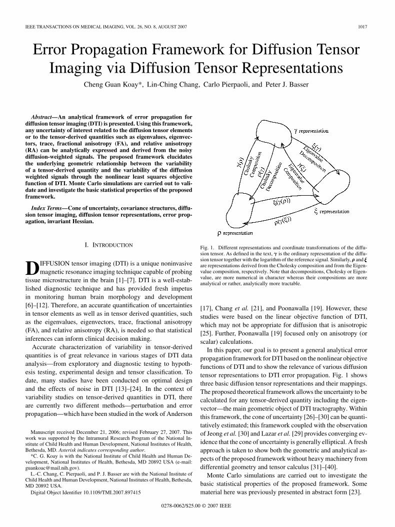
Fig. 1. Different representations and coordinate transformations of the diffu-sion tensor. As defined in the text, is the ordinary representation of the diffu-sion tensor together with the logarithm of the reference signal. Similarly,�� and ��are representations derived from the Cholesky composition and from the Eigen-value composition, respectively. Note that decompositions, Cholesky or Eigen-value, are more numerical in character whereas their compositions are moreanalytical or rather, analytically more tractable.

[17], Chang et al. [21], and Poonawalla [19]. However, thesestudies were based on the linear objective function of DTI,which may not be appropriate for diffusion that is anisotropic[25]. Further, Poonawalla [19] focused only on anisotropy (orscalar) calculations.

In this paper, our goal is to present a general analytical errorpropagation framework for DTI based on the nonlinear objectivefunctions of DTI and to show the relevance of various diffusiontensor representations to DTI error propagation. Fig. 1 showsthree basic diffusion tensor representations and their mappings.The proposed theoretical framework allows the uncertainty to becalculated for any tensor-derived quantity including the eigen-vector—the main geometric object of DTI tractography. Withinthis framework, the cone of uncertainty [26]–[30] can be quanti-tatively estimated; this framework coupled with the observationof Jeong et al. [30] and Lazar et al. [29] provides converging ev-idence that the cone of uncertainty is generally elliptical. A freshapproach is taken to show both the geometric and analytical as-pects of the proposed framework without heavy machinery fromdifferential geometry and tensor calculus [31]–[40].

Monte Carlo simulations are carried out to investigate thebasic statistical properties of the proposed framework. Somematerial here was previously presented in abstract form [23].

0278-0062/$25.00 © 2007 IEEE

1018 IEEE TRANSACTIONS ON MEDICAL IMAGING, VOL. 26, NO. 8, AUGUST 2007

II. METHODS

A. Nonlinear DTI Estimation in Different Diffusion TensorRepresentations

In a typical DTI experiment, the measured signal in a singlevoxel has the following form [1], [4], [41]:

(1)

where the measured signal depends on the diffusion encodinggradient vector of unit length, the diffusion weight , the ref-erence signal , and the diffusion tensor . The symbol “ ”denotes the matrix or vector transpose. Given sampledsignals based on at least six noncollinear gradient directions andat least one sampled reference signal, the diffusion tensor esti-mate can be found by minimizing various objective functionswith respect to different representations of the diffusion tensorin (1). Different representations of the diffusion tensor providedifferent insights and information about the diffusion tensor it-self. We will use three distinct diffusion tensor representationsthat have applications to DTI and show how they can be used inDTI error propagation.

In general, the objective functions for the nonlinear leastsquares problem in different diffusion tensor representationscan be expressed as follows:

(2)

(3)

(4)

where is the measured diffusion weighted signal with noise;is the diffusion weighted func-

tion evaluated at ;

is the diffusion weighted function evaluated at ;

is the diffusion weighted

function evaluated at ; and see the equations at the bottomof the page.

The three representations of the diffusion tensor are

(5)

(6)

(7)

where is the parameter for the nondiffusion weighted signal.We shall denote , , and as the ordinary, the Cholesky,

and the Euler representations, respectively. The meaning of eachterm mentioned here will be obvious in the following discus-sion. Fig. 1 shows the mappings between different spaces orrepresentations.

To construct the mappings and , we use the mainideas from the Cholesky decomposition of a symmetric posi-tive definite matrix and the eigenvalue decomposition of a sym-metric matrix [42] in reverse. The connections between (5) and(6) and between (5) and (7) can then be established based on thefollowing equations:

(8)

and

(9)

where is an upper triangular matrix with nonzero diagonalelements and are the column vectors of which depend onthe Euler angles. Without loss of generality, we shall assume theeigenvalues are arranged in decreasing order, i.e.,

......

......

......

...

KOAY et al.: ERROR PROPAGATION FRAMEWORK FOR DIFFUSION TENSOR IMAGING 1019

. Each column vector of is also an eigenvector of .Particularly, we have

(10)

(11)

(12)

(13)

and

(14)

where , , and are the eigenvalues of . If ispositive definite then its eigenvalues are positive. Finally, therotation matrices, , , and represent rota-tions through angle around the , , and axes, respectively,and are defined in Appendix I.

Given (8) and (9), the mappings, and , can be ex-pressed as

(15)

(16)

Since the expressions for (16) are lengthy but easy to com-pute, we have collected them in Appendix II.

It is important to note that the inverse mapping of , ,which can be constructed analytically, is well defined only whenthe diffusion tensor contained within is positive definite, oth-erwise the modified Cholesky decomposition is needed to forcethe diffusion tensor to be sufficiently positive definite [43].However, the solution obtained from the modified Choleskydecomposition is generally not a minimizer of .The solution is, nevertheless, useful as an initial guess of theminimization of . A specific algorithm of this typeof minimization, where the resultant diffusion tensor estimateis both positive definite and a minimizer of , canbe found in [25]. Finally, the analytical expression ofbased on the Cholesky decomposition is shown in Appendix II.

Another mapping of interest is . The construction of, which requires the eigenvalue decomposition of a sym-

metric matrix, e.g., using the Jacobi method (34), has twomain advantages. First, it is numerically more stable and moreaccurate than the analytical approach of [44]. Second, it canbe used even when the diffusion tensor within is not positivedefinite—an additional advantage over the analytical approachof [44]. Once the orthogonal matrix is obtained by diagonal-ization, we still need to solve for the Euler angles, , , and .The solution to this problem is simple but, for completeness,we have collected these results in Appendix I. The Euler rep-resentation is more useful than the representation proposed byHext [45], a special case of which was used by Anderson [17]and Chang et al. [21] in computing the covariance betweeneigenvalues, because the covariance matrix of the major eigen-vector of the diffusion tensor can be constructed in the Eulerrepresentation. Appendix III contains further comments on therepresentation by Hext.

The first two objective functions, (2) and (3), have been usedin many studies [25], [46]–[50], and the theoretical and algo-rithmic framework for these objective functions was investi-gated by Koay et al. [25]. To date, the third objective function,(4), has not been used for DTI estimation because the direct es-timation of the eigenvalues and eigenvectors by (4) is imprac-tical due to the cost of computation, particularly for the initialsolution and for those trigonometric functions occurring in therotation matrix. Nonetheless, (4) as expressed in the Euler rep-resentation does provide a foundation for DTI error propagationthat is conceptually elegant and algorithmically practical.

We introduce the proposed framework with respect first to theordinary representation for a scalar function in Section II-B andthen for a vector function in Section II-C. In Section II-D, wediscuss commonly used scalar and vector tensor-derived quanti-ties and their corresponding gradient vectors, while Section II-Ecovers the diffusion tensor representation and analytical for-mulas for the invariant Hessian structures, a new concept to bedefined later, with respect to different diffusion tensor represen-tations. Section II-F discusses selected applications of the pro-posed framework. Fig. 7 shows the schematic diagram of thenecessary steps needed to obtain appropriate covariance struc-tures. The segment above the dotted line in Fig. 7 deals withdiffusion tensor estimations; these techniques can be found in[25], while the segment below the dotted line pertains to theproposed framework.


Fig. 2. (A) Hyper-surface of the nonlinear objective function, f , with respect to the coordinate system with a minimum value of f ( ̂ ) at ̂ . A newcoordinate system centered at f ( ̂ ) is also shown here and will be denoted as the ��-coordinate system. (B) Typical hyper-surface of a tensor-derived quantitywith respect to a -coordinate system. The contours of f are projected vertically onto the tangent plane of g. This tangent plane of g at g( ̂ ) shows the intersectionbetween the contours of f and those of g. (C) The magnified image of the region centered at f ( ̂ ) with respect to the ��-coordinate system. (D) Themagnified image of the tangent plane of g at g( ̂ ). The gradient vector of g( ̂ ) shows the direction of greatest ascent with respect to the landscape of g aroundg( ̂ ). (E) New look of the hyper-surface of f with respect to the transformed ��-coordinate system as defined in both (20) and (21) where the change in flooks uniform in all directions of any unit vector. (F) Tangent plane of g( ̂ ) with respect to the ��-coordinate system.

B. Error Propagation Framework For Scalar Functions

Let bethe NLS objective function in the ordinary representation. Let

be any smooth function (tensor-derived quantity) of andlet be the NLS estimate, i.e., is a minimizer of . Theconnection between the uncertainty of and of can berepresented geometrically.

To examine the effect of the variability of on the vari-ability of , we first focus on the region around (theblue contour) and its relation to the function by projectingthe contour around to the tangent plane of at[Fig. 2(A) and (B)].

By second-order Taylor expansion, the change in is

(17)where and is the Hessian matrix of

. Here, we can safely assume that becauseminimizes [Fig. 2(C)]. In the same vein, the first-order

change in is

(18)

where is defined later. If minimizes then the Hessianmatrix is positive definite at and can be written as

(19)

where is an orthogonal matrix and is a diagonal matrix withpositive elements. Therefore, we can express the change inas

(20)

such that

(21)

In the -coordinate system, the change in looks uniformin all directions of since (20) is the equation of a hyper-sphere[Fig. 2(E)]. To measure or capture the change in in a consistentmanner, has to satisfy (20) and be parallel to ; the theo-retical reason behind the latter condition is related to anothercondition, which we shall refer to as the consistency condition.This condition is best explained using a geometric figure and isdiscussed in the caption of Fig. 3. These conditions then leadnaturally to the following formula:

(22)

where is a unit vector along . Therefore, (18)can be written as

(23)


Fig. 3. The consistency condition. As in Fig. 2(F), suppose the contours of g areprojected onto the tangent plane of g, depicted here as a circle. The contours ofg on the tangent plane provide a means of measuring change or variation but thistype of change is 1-D, that is perpendicular to the contours, i.e., parallel tor g.Without loss of generality, we will assume that both �� andr g are normalizedto unit length and suppose that �� is not parallel to the gradient of g. This impliesthe projections of �� ontor g and ofr g onto �� no longer fall onto the samecontours. Therefore, the change in g cannot be measured consistently if �� is notparallel to r g. If �� is perpendicular to r g then the change in g is alwayszero by (18). Therefore, �� must be parallel to r g.

[Fig. 2(F)]. By changing the variables from the -coordinatesystem back to the -coordinate system and squaring (23)[Fig. 2(D)–(F)], we arrive at the error propagation equation forDTI [51]

(24)

The derivation of (24) is provided in Appendix IV.Note that there is freedom in setting the magnitude of the

change in , . However, it is more meaningful touse the following definitionwhere is the number of degrees-of-freedom. Here,for DTI, i.e., the number of tensor elements and one referencesignal. This definition is meaningful becauseis an unbiased estimate of the variance of the diffusion weighted(DW) signals [25], so that can serve as an estimate ofthe variance of . More importantly, if the change in wereto be taken as some multiple of the DW signal variance insteadof one unit of the DW signal variance, then would nolonger be in agreement with the familiar notion of variance instatistics.

In subsequent discussion, we will denote for. As an example, the variance of

can be calculated by setting in (24), which yields. Similarly, for

, .We can also work with the objective functions

and instead of so that the variances ofinterest with respect to a particular representation can be com-puted without elaborate computation. However, it is importantto realize that the Hessian matrix of the ordinary representa-tion is fundamentally different from the Hessian matrices of theEuler and the Cholesky representations because the latter ma-trices do not transform like a tensor. Although a detailed discus-sion on tensor transformation laws is beyond the scope of thispaper, we shall pursue along a different line by constructing co-variance matrices of the Euler and the Cholesky representations

based on the technique explicated in Section II-C. We will showthat fundamental geometric objects in error propagation fromwhich the covariance matrices are derived are the invariant Hes-sian matrices, and not the Hessian matrices. Briefly, an invariantHessian matrix is defined to be the term in the Hessian matrixthat is invariant with respect to coordinate transformations.

One of the goals in this paper is to show that with one condi-tion—which is that the tensor estimate has to be positive definite[25], [47], [50]—separate minimizations of each objective func-tion are unnecessary and the variances computed from one rep-resentation can also be obtained rather easily from another rep-resentation by a continuous coordinate transformation betweenthe representations. Before we discuss the technique of coordi-nate transformation between representations, we will work onerror propagation for vector functions and on practical varianceor covariance computations of commonly used tensor-derivedquantities in Sections II-C and II-D.

C. Error Propagation Framework for Vector Functions

The discussion thus far has focused mainly on the proposedframework for any scalar function of . Here, we will extendthe framework to include vector functions so that quantitiesof interest such as the variance-covariance matrix of or ofthe major eigenvector of the diffusion tensor can be obtained.Without loss of generality, we will assume the vector function

consists of three scalar functions. By thefirst-order Taylor expansion of at , we have

... (25)

The variance-covariance matrix of can be defined as(26)–(28), shown at the bottom of the page.

Under the consistency condition, there are three pos-sibilities in choosing : ,

, and . But thecorrect choice of in each element of the matrix in (28) isagain determined by the same consistency condition. Thiscondition also ensures that the matrix in (28) is symmetric. Asan example, let us consider the case of two distinct tangentplanes, say of and of . In this case, , which appears inthe off-diagonal term, , of (28), can betaken to be either or .It is important to note here that either one will yield the sameresult, which is . In other words, the projection of

onto the tangent plane of or the projection ofonto the tangent plane of will yield the same covariation.Taking the consistency condition into account, the final expres-sion of (28) can be written as

��g(��) =�2

DW

rT�� g1 � r��g1 r

T�� g1 � r��g2 r

T�� g1 � r��g3

rT�� g2 � r��g1 r

T�� g2 � r��g2 r

T�� g2 � r��g3

rT�� g3 � r��g1 r

T�� g3 � r��g2 r

T�� g3 � r��g3

:

(29)


or, equivalently

(30)

where andis the correlation coefficient. Note that

is a unit vector parallel to . Finally, thevariance-covariance matrix in the coordinate system hasthe following expression:

(31)

or

(32)

where

(33)

and (34), shown at the bottom of the page, is the corre-lation coefficient. As an example, it can be shown thatthe variance-covariance matrix of can be expressed as

; see Appendix V for variousHessian structures and Appendix VI for the derivation of

.The reader should be cautious not to be misled into thinking

that the covariance matrix of the Euler representation, ,is simply . These two quantities areclosely related but they are not equivalent. As mentionedearlier, the Hessian matrix of the Euler representation is nota tensor. This means that its inverse will not be invariant withrespect to coordinate transformations. In Appendix VI, it isshown that the covariance matrix of the Euler representation,

, is equal to , wheredenotes the invariant Hessian matrix of , which is the part ofthe Hessian matrix that is invariant with respect to coordinatetransformations. It is noteworthy that we can discover these

invariant Hessian structures within the proposed frameworkusing the technique discussed in this section, see Appendix VI.

D. Scalar and Vector Functions of the Diffusion Tensor

As mentioned earlier, variance computation for certaintensor-derived quantities can be greatly simplified by usingthe appropriate diffusion tensor representation. The most com-monly used tensor-derived quantities are listed below [2], [5]

1) Trace:

(35)

2) Fractional Anisotropy:

or

(36)

3) Relative Anisotropy:

or

(37)

4) Eigenvalues of :

(38)

as defined in (9) and (14).5) Eigenvalues of :

and as defined in (9), and (11) -(13) (39)

(26)

......

...... (27)

(28)

(34)


It should be noted here that the first component in each represen-tation, , , and , is and, therefore, the partial derivativeof any tensor-derived quantity with respect to is 0.

Since and , it is clearthat the variance computation for (35)–(37) is equally tractablein both the ordinary and the Euler representations. However,the variance-covariance computation of (38) and (39) is mostconvenient in the Euler representation.

The formulas listed below are the gradients of the most com-monly used tensor-derived quantities; the first three formulas areexpressed with respect to both the ordinary representation andthe Euler representation, while the last two are expressed withrespect to the Euler representation only.

1) Gradient of Trace:

or

(40)

2) Gradient FA: Letand then

. The gradient of FA with re-spect to the Euler representation is

,where

and

The gradient of FA with respect to the ordinary represen-tation has the following components:

(41)

3) Gradient of RA: Let , the gradient ofRA with respect to the Euler representation is

,where

and

The gradient of RA with respect to the ordinary represen-tation has the following components:

(42)

4) Gradients of the eigenvalues are

(43)

5) Gradients of a component of an eigenvector: i.e.,. Since the expressions are more in-

volved, we have collected these formulas in Appendix VII.Some of the preliminary formulas used to derive (40)–(42)

are collected in Appendix VIII.

E. Coordinate Transformation Between Different TensorRepresentations

As discussed in Section II-C and Appendix VI, invariantHessian structures are very important to variance-covariancecomputation. Particularly, we have used the technique expli-cated in Section II-C to derive the invariant Hessian structuresof the ordinary and Euler representations in Appendix VI. Forconvenience, these structures are explicitly given here

(44)

(45)

(46)

where the invariant Hessian matrix of is denoted by .Please refer to Appendix V for the terms defined above.

We have previously mentioned why the expression,, should not be taken as the defi-

nition of the covariance matrix of the Euler representation. Onintuitive ground, variance or covariance of a quantity shouldbe invariant with respect to coordinate transformations, orequivalently, it can be said that variance or covariance of aquantity should transform like a tensor. Here, we will show howthe invariance property of the covariance matrix is violated ifone insists on using as the covariancematrix of the Euler representation. According to (31), we needto construct so thator

(47)

Since the covariance structure should be invariant withrespect to coordinate transformation, one expects in(47) to be equal to . However, theinvariance property is violated if one substitutes the followingexpression:


into (47)

(48)

Comparing (48) and , we see thatthe additional error introduced in the estimation of vio-lates the invariance property of the covariance matrix.

In brief, the covariance matrices in various tensor representa-tions are derived from the invariant Hessian structures and theirexpressions are given below

(49)

(50)

and

(51)

F. Applications

1) Average Variance-Covariance Matrix: The average vari-ance-covariance matrix for a given diffusion tensor is a veryuseful quantity to compute in a simulation study; it is directlyrelated to average DW signals where the estimated signals areassumed to be fitted perfectly to the observed signals, i.e., theresiduals are zero. One can see then that the average variance-covariance matrices can be easily derived from (49)–(51), andare given by

(52)

(53)

(54)

The symbol, , represents the average quantity of . Themethod of averaging and the derivations of (52)–(54) are dis-cussed in Appendix IX.

It should be noted here that has to be defined differ-ently from the previous definition, which was based on the esti-mated DW signal variance, because the residual sum of squaresis now assumed to be zero. Therefore, has to be taken froma known variance with respect to the Rician-distributed DW sig-nals. The technique on transforming the variance with respect tothe Gaussian-distributed complex signals to the variance withrespect to Rician-distributed magnitude signals at a prescribedlevel of signal-to-noise ratio (SNR) can be found in Koay et al.[25], [52]. For , is an acceptable approximationto ; represents the standard deviation of theGaussian-distributed complex signals.

Once the average covariance matrices with respect to var-ious tensor representations are known, the mean variance ofany tensor-derived quantity or the mean variance-covariance be-tween any two tensor-derived quantities can then be computedbased on the techniques explained in the preceding sections. Asan example, the mean variance of can be expressed as

Here, we use this approach to show the rotational variance of Trof a prolate tensor based on the variance-covariance matrix in(52), Fig. 4. This framework will also be useful in analyzing theeffect of gradient sampling schemes on tensor-derived quanti-ties without the need for a computationally intensive bootstrapto quantify uncertainty, see Jones [53]. It is clear that the vari-ance of trace exhibits rotational asymmetry, Fig. 4. Increasingthe number of gradient directions will not reduce the systematicvariation, Fig. 4. The theoretical reason for this phenomenon isthat the experimental design for DTI is not rotationally invariant[54].

2) Elliptical Cones of Uncertainty of the Principal Eigen-vectors: Based on the technique expounded in Sections II-Cand D, the variance-covariance matrix of the components of aneigenvector can be computed quite easily. This particular vari-ance-covariance matrix is useful in constructing the ellipticalcone of uncertainty about that eigenvector.

Without loss of generality, we shall take the major vector of adiffusion tensor to illustrate the method in this section. By (11),

, and (31), we have

(55)

According to the perturbation method proposed by Hext [45],is normal to the plane of the elliptical cone of uncertainty. In

other words, the eigenvector that is associated with the smallesteigenvalue of is parallel to , therefore, the other twoeigenvectors are perpendicular to . The same observation canbe made within the proposed framework. That is, the equationof a sphere , will force to be a matrixof rank 2, therefore, the smallest eigenvalue of is essen-tially zero. Another argument for this observation is based onthe dyadics formulation; it is presented in Appendix X. We shalloutline the basic idea with an example. If we have , as shown


Fig. 4. Rotational Asymmetry in the variance of Trace for a prolate tensor. Generally, the rotation of a typical tensor requires three parameters, i.e., Euler angles.But, analysis of rotational asymmetry of any tensor-derived quantity can be studied using a prolate tensor where only two parameters are sufficient, i.e., the majoreigenvector of the prolate tensor can be parametrized by [ sin(�) cos(') sin(�) sin(') cos(�) ] with 0 � � < � and 0 � ' < 2�. The plots above arecomputed with a prolate tensor having FA of 0.586 and eigenvalues of � = 1:24� 10 mm =s and � = � = 4:30� 10 mm =s at SNR = 25. ImagesA–C were computed with different numbers of gradient directions: 23, 85, and 382, respectively. In each plot, the final design matrixW was constructed fromfour spherical shells having b values of 0, 500, 1000, and 1500 s=mm . The color-coded variation is specific to each plot but the numerical scale, which has beennormalized to the unit interval, [0; 1], from b0;2:0� 10 mm =s c, is common to all.

in the equation at the bottom of the page, then the major eigen-vector is and the majoreigenvalue is 0.00114 .

We shall denote the lower right 3 3 submatrix of asand

based on the SNR level of 50 and on a design matrix, , thatwas constructed from a 35 gradient direction set with four spher-ical shells having values of 0, 500, 1000, and 1500 .

Similarly, we shall denote the lower 3 3 submatrix ofas ,

particularly, we have

for our example.The variance-covariance matrix can then be computed as

follows:

which has the following numerical values

The eigenvalue–eigenvector pairs of this matrix are

and

It is quite clear then that is parallel to the minor eigenvector of. Note that the other two eigenvectors of are not gener-

ally equal to the medium and minor eigenvectors of the diffusiontensor. Once the eigenvalue–eigenvector pairs of and arecomputed, the elliptical confidence cone can beconstructed quite easily. We shall mention here a simple but im-portant method for visualizing the confidence cone. We prefer touse the approach proposed by Hext [45] in which the confidencecone is projected onto the unit sphere, thus avoiding an impor-tant visual ambiguity: if the height of a confidence cone were tobe scaled proportional to some function of the major eigenvalue,then the spread of the cone would be a function not only of thetwo nonzero eigenvalues of but also of the major eigenvalueof the diffusion tensor. It would then be harder to compare twoneighboring confidence cones visually. Fig. 5 shows an exampleof the elliptical confidence cones constructed from the humanbrain data.

III. RESULTS

A variance-covariance estimate can be obtained from a set ofDW measurements. Therefore, repeated DW measurements can


Fig. 5. Elliptical confidence cones. (A) FA map. (B) Magnified image of the region bounded by a red square on the FA map. (C) Corresponding elliptical 95%confidence cones on that region at SNR level of 15.

be carried out to measure the uncertainty of the variance-co-variance estimate by a graphical method based on histogramanalysis. This approach will provide a reasonable measure ofthe distributional properties of these estimates. Further, the clas-sical sample variance-covariance formulas can be employed tocompare with the analytically derived value of these estimates.Monte Carlo simulations similar to those of Pierpaoli and Basser[5] were carried out to validate the proposed method.

For simplicity, we shall use the simulation condition (in-cluding the parameter vector, ) similar to that of Section II-F2except at a single SNR level of 15. Further, 50 000 re-peated measurements were generated to facilitate statis-tical comparison. Briefly, this parameter vector has Tr of0.0021 and FA of 0.5278. Further, its major eigen-vector is .

The sample statistics, and the results from the proposedframework with respect to two different covariance matrices,

and are listed in Table I. The sample statistics, listed as(I) in Table I, are computed based on classical statistical ex-pressions for sample mean and sample variance. Similarly, thesample covariance matrix of the major eigenvector is based onclassical statistics but the sample eigenvectors,for , 2, 3, have to be properly oriented so that theirdirections are on the same hemisphere as the estimated meanmajor eigenvector. The estimated mean major eigenvectoris computed based on the dyadic product formulation [27]where the major eigenvector ofcorresponds to the mean major eigenvector. An importantobservation about this dyadic product is that the medium andthe minor eigenvectors of can be used to construct thecovariance matrix of the major eigenvector. The argument forthis observation is presented in Appendix X. The results on(II) and (III) are obtained from the average covariance matrixdiscussed in Section II-F1. The results on (IV) and (V) are ob-tained by averaging the 50 000 variance estimates of Tr and FA;these variance estimates, (IV) and (V), are obtained from the

TABLE ISIMULATION RESULTS BASED ON VARIOUS METHODS

DISCUSSED IN THIS PAPER

proposed framework with respect to the ordinary and the Eulerrepresentations, respectively. Further, the DW signal varianceswere estimated from each nonlinear fit using the modified fullNewton method described in [25]. To complement the resultsin Table I, we also show the distributional property of thesevariance estimates in Fig. 6.

Before presenting the results on the covariance matrix of themajor eigenvector, we will show some results on the dyadicsformalism for later comparison. The average dyadics from the50 000 samples of eigenvectors turns out to be

and the corresponding eigenvalue–eigenvector pairs are


Fig. 6. Histograms of the variance estimates of (A) trace and of (B) FA based on three different covariance matrices: �� (red), �� (blue), and �� (green). Theconstruction of �� is discussed in Appendix III and it is related to the Hext representation. Note that on Fig. 6(A) and (B), the lines are superimposed. Samplevariance of trace (FA), which is computed from the 50 000 trace (FA) estimates, is shown in Fig. 6(A) and (B) as a vertical line.

and

The average vector before and after normalization is, and

, respectively, with a vectornorm of and ;

is an approximation to the minor eigenvalue ofthe covariance matrix of the major eigenvector of the diffusiontensor, see Appendix X.

Here, we present the results on the covariance matrices of themajor eigenvector

and

which are obtained, respectively, by methods, (I), (III), and (V)listed in Table I. Their corresponding eigenvalue–eigenvectorpairs are shown in the equation at the bottom of the page

Clearly, , a result from theaverage dyadics, is a good approximation to the minor eigen-value of the sample covariance matrix of the major eigenvector,

. Further, the medium and minor eigenvalue–eigenvectorpairs from the average dyadics respectively are very close to thelargest and medium eigenvalue–eigenvector pairs of the samplecovariance matrix of the major eigenvector. This result validatesthe analysis represented in Appendix X.

IV. DISCUSSION

In this work, our main objective is to present as simply aspossible both the geometric and analytical ideas that underlie theproposed framework of error propagation so that the translationof this work into practice is clear to interested readers.

Here, we outline the main findings of this work. As a tech-nique of error propagation, the proposed framework has severaldesirable features—namely, that the uncertainty of any tensor-derived quantity, scalar or vector, can be estimated by using theappropriate diffusion tensor representation; that the covariancematrices with respect to different diffusion tensor representa-tions can be analytically expressed; and that covariance estima-tion is very accurate and is a natural by-product of the modifiedfull Newton method of tensor estimation, a description of whichcan be found in [25]. Fig. 7 shows schematically the necessarysteps needed to obtain the covariance matrices of interest. Thesample statistics and the simulation results obtained from theproposed framework agreed reasonably well, see Fig. 6.

The concept of the average covariance matrix is introducedand applied to the issue of rotational asymmetry of the varianceof the trace. This particular approach circumvents the need forbootstrap methods [18], [53] in this type of investigation. It isnot hard to see that a covariance matrix with respect to a diffu-sion tensor representation corresponding to a particular tensorcan be generated with great ease and efficiency. This techniqueof generating covariance matrices will be very useful in simu-lation studies but we should emphasize here that it is based onthe limiting case of zero-residual. Therefore, readers who areinterested in analyzing experimental DTI data should use thecovariance matrices in (49)–(51) of Section II-E rather than theaverage covariance matrices discussed in Section II-F1. A sim-ilar idea related to the average covariance matrix is that of theaverage Hessian matrix of the ordinary representation, whichis also known as the precision matrix [55]. The precision ma-trix is very useful in DTI experimental design [54], [55], and itcan also be used in constructing the Hotelling’s -statistic fortesting group differences or the Mahalanobis distance for tensorclassification. However, we expect the invariant Hessian matrixof the Euler representation to be more useful than its regularcounterpart, Hessian matrix, for tensor classification. These are


Fig. 7. Overview of the proposed error propagation framework for diffusion tensor imaging. The segment above the dotted line deals with tensor estimations;(these techniques can be found in [25]); while the segment below the dotted line pertains to the proposed framework.

areas of our current interest and we shall present them in futurework.

The confidence cone, or the cone of uncertainty, of the majoreigenvector in DTI—a concept introduced by Basser [26] andexpounded upon by Basser and Pajevic [27], was brought tobear in fiber tract visualization by Jones [28]. But, the shape ofthe confidence cone discussed in these work has always beensimplified or reduced to being circular. The observation ofJeong et al. [30] and Lazar et al. [29] provided clear evidencethat the cone of uncertainty is generally elliptical in cross sec-tion. In this work, we have presented several analytical tools,based on the proposed framework, the perturbation method,and dyadic formalism, for constructing the elliptical cone ofuncertainty. According to the result derived in Appendix X, itis noteworthy that the length and direction of the major andminor axes of the ellipse of the confidence cone are just themedium and minor eigenvalue–eigenvector pairs of the averagedyadics of the particular eigenvector—a fact that had escapednotice for sometime.

The proposed framework can also be used to analyze DTIdata retrospectively to investigate the reproducibility of a DTIparameter of interest or of the fiber orientation. For example,if there is an insufficient number of diffusion-weighted imagesto perform a bootstrap analysis, at least the uncertainty in the

tensor elements and tensor-derived quantities can still be esti-mated within the proposed framework.

Although we have presented some cogent reasons—the uni-fying principles of diffusion tensor representations, of Taylorapproximations of scalar and vector functions and, more impor-tantly, of invariant Hessian and covariance structures of the non-linear least squares objective function of DTI—for preferringthe proposed framework to the perturbation method, the pertur-bation method is nevertheless a useful technique [17]. The diffu-sion tensor representations studied here are logically equivalentbut they are not equally useful or significant. It is the variety ofapplications that made one diffusion tensor representation to bepreferable to another.

We have shown that invariant Hessian matrices are more im-portant than the Hessian matrices in DTI error propagation be-cause covariance matrices are directly linked to them. Further,we also showed how these invariant Hessian matrices can beobtained from the proposed framework without employing thetechnique of covariant derivatives in tensor calculus and differ-ential geometry.

V. CONCLUSION

We have developed an analytical and geometrically intuitiveerror propagation framework for diffusion tensor imaging.


We have presented the nuts and bolts of various aspects ofdiffusion representations for understanding variability in anytensor derived quantity, vector, or scalar. This frameworkprovides an analytical and efficient method for understandingthe dependence of variance of a tensor-derived quantity onorientation or gradient schemes. Furthermore, it provides anapproach for computing the necessary parameters in order toconstruct the elliptical confidence cone of an eigenvector. Thisparticular technique will be very useful in fiber tractography,group analysis of diffusion tensor data and tensor classification.It is also clear that the proposed framework can be adapted toother nonlinear least squares problems.

APPENDIX IROTATION MATRICES AND A METHOD

FOR FINDING EULER ANGLES

The rotation matrices, , , and representrotations through angle around the , , and axes, respec-tively, and are defined as follows:

and

The following discussion is on obtaining the Euler anglesfrom the proper rotation matrix, , which can be expressedcolumnwise as

and

By proper rotation, we mean that the determinant of shouldbe positive one. If negative one is encountered, we can alwayschange to its additive inverse, . Once this step is checked,the Euler angles can then be found as follows:

1)2) If , then

a)b)

The function is defined in many programming lan-guages such as C and Java.

In the case where , the rotation matrix can be shownto reduce to

It is clear that and can not be uniquely determinedand we can set one of them to zero. Let , then

.

APPENDIX IIMAPPINGS BETWEEN VARIOUS REPRESENTATIONS

The components of are defined below

where the components of are functions of , , and .


For completeness, we will show analytical formulas for eachcomponent of by the Cholesky decomposition with the as-sumption that the diffusion tensor within is positive definiteotherwise, as mentioned in the text, the modified Cholesky de-composition is to be used for constructing [25], [50]. Be-fore presenting the formulas, we shall define the following termsto simplify the expression of :

, , , and is

the matrix determinant.can be expressed as follows:

APPENDIX IIIREPRESENTATION BY HEXT

The representation proposed by Hext [45] is the mapping re-lating the components of to those of

(C1)

where , but the off-diagonal elements of are notnecessarily zero. A special case of (C1) with being a diagonalmatrix was used by Anderson [17] to compute the covariancebetween two eigenvalues.

Adapting (C1) to the convention used in this paper, we canshow that the linear relation in vector form can be expressed asshown in the equation at the bottom of the page.

We shall denote the above equation as , the first-orderdifferential can be written as so that we can identifythe elements of as or . If the

covariance matrix is given then it can be shown that. See Section II-E and Appendix VI

for the technique for transforming covariance matrices from onerepresentation to another.

It is evident that this representation has a simpler expres-sion than that of the proposed Euler representation, . However,this representation cannot answer questions regarding the uncer-tainties in the eigenvectors, i.e., the elliptical cone of uncertaintyof the major eigenvector, without resorting to the perturbationmethod.

APPENDIX IVDERIVATION OF A KEY EQUATION ON ERROR PROPAGATION

As defined in the main text, we haveand where

is an orthogonal matrix and is a diagonal matrix withpositive elements. Therefore, we can write . Thisis equivalent to the following expressions in component form:

(D1)

and

(D2)

and


(D3)

From the above derivation, we also see thatand .

APPENDIX VHESSIAN STRUCTURES IN DIFFERENT REPRESENTATIONS

Here, we provide explicit Hessian expressions with respect tovarious representations studied in this paper

(E1)

(E2)

(E3)

where and are diagonal matrices whose diagonal elementsare the observed and the estimated diffusion weighted signals,respectively, i.e.,

. . .. . .

Further, we have , ,, ,

and . Equations (E1) and(E2) have been previously derived and studied by Koay et al.[25].

APPENDIX VICOVARIANCE STRUCTURES IN DIFFERENT REPRESENTATIONS

In (31), we have the following equation:

To construct the covariance matrix with respect to the ordi-nary representation, we write

or

where and denotes the identity matrix.To construct the covariance matrix with respect to the Euler

representation, we write

or

(F1)

Two identities: andwere used in the derivation of (F1).

Equation (F1) is very important because we have discoveredthe part of the Hessian matrix that is invariant with respect totransformation without using the concept of covariant derivativein tensor calculus. Interestingly, the invariant Hessian matrix ofthe Euler representation is exactly the first term of the Hessianmatrix in (E2).

APPENDIX VIIGRADIENT COMPUTATION: EIGENVECTORS

The gradient of the first, second, and third components ofcan be written as


and

Similarly, the gradient of the components of and canbe computed quite easily.

APPENDIX VIIIGRADIENT COMPUTATION: TENSOR-DERIVED QUANTITIES

A few notations and conventions are introduced here to keepthe formulas shown in (38)–(40) in a compact form.

1) The indices , 2, 3 denote , , , respectively.2) is the Kronecker delta function, i.e., for

and for .3) The formulas for the partial derivatives with respect to

the off-diagonal elements of is symmetrized, i.e.,for .

For convenience, the formulas that are frequently used arelisted here

(H1)

(H2)

and

(H3)

(H4)

APPENDIX IX

AVERAGE COVARIANCE MATRIX

In the zero-residual case, which is very useful in simulationstudies where the ground truth is known, the invariant Hessianexpressions in (49)–(51) reduce to

(I1)

(I2)

and

(I3)

Further, we have , whereis known. As an example, the average invariant Hessian matrixof (I1) can be expressed as follows:

(I4)

Therefore, the average covariance matrix is

(I5)In other words, we expect the arithmetic mean of to ap-

proach as the number of samples of in-creases. Note that the arithmetic mean and the method of av-eraging used in obtaining (I5) are different but we expect thedifference between these two quantities to be negligible for alarge sample.

APPENDIX X

CONNECTION BETWEEN THE ELLIPTICAL CONE OF

UNCERTAINTY AND THE AVERAGE DYADICS

Let be the collection of properly orientedmajor eigenvectors with respect to the mean major eigenvectorand let be the average dyadics[27]. Further, let the eigenvalue decomposition of the averagedyadics be where .

According to [56], the maximum likelihood estimate of themean of is . We shall now show that theseeigenvalue–eigenvector pairs, and , are re-lated to the length and direction of the major and the minor axesof the confidence cone of the major eigenvector, . In otherwords, these two eigenvalue–eigenvector pairs are related to thecovariance matrix of . The argument goes as fol-lows. Let the sample covariance of be definedas

(J1)


Let , then . If we assume that, which is not unreasonable because is an estimate of

the mean major eigenvector, then we have

When is large we have and , so that. The sample covariance is then reduced to

(J2)

Essentially, the dyadic product formulation suggested in [27]is sufficient to construct the elliptical confidence cone withouthaving to use (J1). In retrospect, the construction of the confi-dence cone using (J2) bypasses the need to reorient the sampleeigenvectors such that they are pointing on the same hemisphereas the mean major eigenvector.

ACKNOWLEDGMENT

C. G. Koay dedicates this work to the memory ofDr. M. C. Toh. The authors would like to thank L. Salakfor editing this paper and thank the anonymous reviewers fortheir helpful comments.

REFERENCES

[1] P. J. Basser, J. Mattiello, and D. LeBihan, “MR diffusion tensor spec-troscopy and imaging,” Biophys. J., vol. 66, pp. 259–267, 1994.

[2] P. J. Basser, “Inferring microstructural features and the physiologicalstate of tissues from diffusion-weighted images,” NMR Biomed., vol.8, pp. 333–344, 1995.

[3] P. J. Basser and C. Pierpaoli, “Microstructural and physiological fea-tures of tissues elucidated by quantitative-diffusion-tensor MRI,” J.Magn. Reson. B, vol. 111, pp. 209–219, 1996.

[4] P. J. Basser, J. Mattiello, and D. LeBihan, “Estimation of the effectiveself-diffusion tensor from the NMR spin echo,” J. Magn. Reson. B, vol.103, pp. 247–254, 1994.

[5] C. Pierpaoli and P. J. Basser, “Toward a quantitative assessment ofdiffusion anisotropy,” Magn. Reson. Med., vol. 36, pp. 893–906, 1996.

[6] C. Pierpaoli, P. Jezzard, P. J. Basser, A. Barnett, and G. D. Chiro, “Dif-fusion tensor MR imaging of the human brain,” Radiology, vol. 201, pp.637–648, 1996.

[7] J. J. Neil, S. I. Shiran, R. C. McKinstry, G. L. Schefft, A. Z. Snyder,C. R. Almli, E. Akbudak, J. A. Aronovitz, J. P. Miller, B. C. Lee, andT. E. Conturo, “Normal brain in human newborns: Apparent diffusioncoefficient and diffusion anisotropy measured by using diffusion tensorMR imaging,” Radiology, vol. 209, pp. 57–66, 1998.

[8] A. M. Ulug, N. Beauchamp, Jr, R. N. Bryan, and P. C. van Zijl, “Abso-lute quantitation of diffusion constants in human stroke,” Stroke, vol.28, pp. 483–490, 1997.

[9] J. S. Shimony, R. C. McKinstry, E. Akbudak, J. A. Aronovitz, A. Z.Snyder, N. F. Lori, T. S. Cull, and T. E. Conturo, “Quantitative diffu-sion-tensor anisotropy brain MR imaging: Normative human data andanatomic analysis,” Radiology, vol. 212, pp. 770–784, 1999.

[10] P. J. Basser, S. Pajevic, C. Pierpaoli, J. Duda, and A. Aldroubi, “In vivofiber tractography using DT-MRI data,” Magn. Reson. Med., vol. 44,pp. 625–632, 2000.

[11] M. Lazar, D. M. Weinstein, J. S. Tsuruda, K. M. Hasan, K. Arfanakis,M. E. Meyerand, B. Badie, H. A. Rowley, V. Haughton, A. Field, andA. L. Alexander, “White matter tractography using diffusion tensor de-flection,” Hum. Brain Mapp., vol. 18, pp. 306–321, 2003.

[12] D. K. Jones, A. R. Travis, G. Eden, C. Pierpaoli, and P. J. Basser,“PASTA: Pointwise assessment of streamline tractography attributes,”Magn. Reson. Med., vol. 53, pp. 1462–1467, 2005.

[13] D. K. Jones, M. A. Horsfield, and A. Simmons, “Optimal strategiesfor measuring diffusion in anisotropic systems by magnetic resonanceimaging,” Magn. Reson. Med., vol. 42, pp. 515–525, 1999.

[14] K. M. Hasan, D. L. Parker, and A. L. Alexander, “Comparison of gra-dient encoding schemes for diffusion-tensor MRI,” J Magn. Reson.Imag., vol. 13, pp. 769–780, 2001.

[15] P. G. Batchelor, D. Atkinson, D. L. Hill, F. Calamante, and A. Con-nelly, “Anisotropic noise propagation in diffusion tensor MRI samplingschemes,” Magn. Reson. Med., vol. 49, pp. 1143–1151, 2003.

[16] S. Skare, T. Li, B. Nordell, and M. Ingvar, “Noise considerations inthe determination of diffusion tensor anisotropy,” Magn. Reson. Imag.,vol. 18, pp. 659–669, 2000.

[17] A. W. Anderson, “Theoretical analysis of the effects of noise on dif-fusion tensor imaging,” Magn. Reson. Med., vol. 46, pp. 1174–1188,2001.

[18] S. Pajevic and P. J. Basser, “Parametric and non-parametric statisticalanalysis of DT-MRI data,” J. Magn. Reson., vol. 161, pp. 1–14, 2003.

[19] A. H. Poonawalla and X. J. Zhou, “Analytical error propagation in dif-fusion anisotropy calculations,” J. Magn. Reson. Imag., vol. 19, pp.489–498, 2004.

[20] Y. C. Wu, A. S. Field, M. K. Chung, B. Badie, and A. L. Alexander,“Quantitative analysis of diffusion tensor orientation: Theoreticalframework,” Magn. Reson. Med., vol. 52, pp. 1146–1155, 2004.

[21] L. C. Chang, C. G. Koay, C. Pierpaoli, and P. J. Basser, “Variance of es-timated DTI-derived parameters via first-order perturbation methods,”Magn. Reson. Med., vol. 57, pp. 141–149, 2007.

[22] J. D. Carew, C. G. Koay, G. Wahba, A. L. Alexander, P. J. Basser, andM. E. Meyerand, “The asymptotic distribution of diffusion tensor andfractional anisotropy estimates,” Proc. Int. Soc. Magn. Reson. Med.,2006.

[23] C. G. Koay, L. C. Chang, C. Pierpaoli, and P. J. Basser, “Error propa-gation framework for diffusion tensor imaging,” Proc. Int. Soc. Magn.Reson. Med., 2006.

[24] Y. Shen, I. Pu, and C. Clark, “Analytical expressions for noise propa-gation in diffusion tensor imaging,” Proc. Int. So. Magn. Reson. Med.,2006.

[25] C. G. Koay, L. C. Chang, J. D. Carew, C. Pierpaoli, and P. J. Basser,“A unifying theoretical and algorithmic framework for least squaresmethods of estimation in diffusion tensor imaging,” J. Magn. Reson.,vol. 182, pp. 115–125, 2006.

[26] P. J. Basser, “Quantifying errors in fiber-tract direction and diffusiontensor field maps resulting from MR noise,” Proc. Int. Soc. Magn.Reson. Med., 1997.

[27] P. J. Basser and S. Pajevic, “Statistical artifacts in diffusion tensor MRI(DT-MRI) caused by background noise,” Magn. Reson. Med., vol. 44,pp. 41–50, 2000.

[28] D. K. Jones, “Determining and visualizing uncertainty in estimates offiber orientation from diffusion tensor MRI,” Magn. Reson. Med., vol.49, pp. 7–12, 2003.

[29] M. Lazar and A. L. Alexander, “Bootstrap white matter tractography(BOOT-TRAC),” NeuroImage, vol. 24, pp. 524–532, 2005.

[30] H. K. Jeong, Y. Lu, Z. Ding, and A. W. Anderson, “Characterizing coneof uncertainty in diffusion tensor MRI,” Proc. Int. Soc. Magn. Reson.Med., 2005.

[31] S. I. Amari, Differential Geometrical Methods in Statistics. NewYork: Springer-Verlag, 1985, vol. 28.

[32] S. I. Amari and H. Nagaoka, Methods of Information Geometry.Providence, RI: Amer. Math. Soc., 2000, vol. 191.

[33] M. P. d. Carmo, Riemannian Geometry. Boston, MA: Birkhäuser,1992.

[34] E. Cartan, Leçons sur la Géométrie des Espaces de Riemann. Paris,France: Gauthier-Villars, 1946.

[35] A. S. Eddington, The Mathematical Theory of Relativity, 2nd ed.New York: Cambridge Univ. Press, 1924.

[36] L. P. Eisenhart, Riemannian Geometry. Princeton, NJ: PrincetonUniv. Press, 1950.

[37] D. Laugwitz, Differential Geometry and Riemannian Geometry. NewYork: Academic, 1965.

[38] M. K. Murray and J. W. Rice, Differential Geometry and Statistics.Roca Raton: CRC Press, 1993, vol. 48.


[39] E. Schrödinger, Space-Time Structure. New York: Cambridge Univ.Press, 1950.

[40] P. Marriott and M. Salmon, “An introduction to differential geometryin econometrics,” in Applications of Differential Geometry to Econo-metrics, P. Marriott and M. Salmon, Eds. Cambridge, U.K.: Cam-bridge Univ. Press, 2000, pp. 7–63.

[41] E. O. Stejskal and J. E. Tanner, “Spin diffusion measurements: Spinechoes in the presence of a time-dependent field gradient,” J. Chem.Phys., vol. 42, pp. 288–292, 1965.

[42] G. H. Golub and C. F. Van Loan, Matrix Computation, 3rd ed. Bal-timore, MD: Johns Hopkins Univ. Press, 1996.

[43] P. Gill, W. Murray, and M. H. Wright, Practical Optimization. NewYork: Academic, 1981.

[44] K. M. Hasan, P. J. Basser, D. L. Parker, and A. L. Alexander, “Analyt-ical computation of the eigenvalues and eigenvectors in DT-MRI,” J.Magn. Reson., vol. 152, pp. 41–47, 2001.

[45] G. R. Hext, “The estimation of second-order tensors, with related testsand designs,” Biometrika, vol. 50, pp. 353–373, 1963.

[46] L. C. Chang, D. K. Jones, and C. Pierpaoli, “RESTORE: Robust esti-mation of tensors by outlier rejection,” Magn. Reson. Med., vol. 53, pp.1088–1095, 2005.

[47] Z. Wang, B. C. Vemuri, Y. Chen, and T. H. Mareci, “A constrainedvariational principle for direct estimation and smoothing of the diffu-sion tensor field from complex DWI,” IEEE Trans. Med. Imag., vol. 23,no. 8, pp. 930–939, Aug. 2004.

[48] J. F. Mangin, C. Poupon, C. Clark, D. LeBihan, and I. Bloch, “Distor-tion correction and robust tensor estimation for MR diffusion imaging,”Med. Image Anal., vol. 6, pp. 191–198, 2002.

[49] D. K. Jones and P. J. Basser, “Squashing peanuts and smashing pump-kins: How noise distorts diffusion-weighted MR data,” Magn. Reson.Med., vol. 52, pp. 979–993, 2004.

[50] C. G. Koay, J. D. Carew, A. L. Alexander, P. J. Basser, and M. E.Meyerand, “Investigation of anomalous estimates of tensor-derivedquantities in diffusion tensor imaging,” Magn. Reson. Med., vol. 55,pp. 930–936, 2006.

[51] P. R. Bevington and D. K. Robinson, Data Reduction and Error Anal-ysis for the Physical Sciences, 2nd ed. New York: McGraw-Hill,1992.

[52] C. G. Koay and P. J. Basser, “Analytically exact correction scheme forsignal extraction from noisy magnitude MR signals,” J. Magn. Reson.,vol. 179, pp. 317–322, 2006.

[53] D. K. Jones, “The effect of gradient sampling schemes on measuresderived from diffusion tensor MRI: A Monte Carlo study,” Mag. Reson.Med., vol. 51, pp. 807–815, 2004.

[54] D. K. Jones, C. G. Koay, and P. J. Basser, “It is not possible to designa rotationally invariant sampling scheme for DT-MRI,” Proc. Int. Soc.Magn. Reson. Med., 2007.

[55] P. J. Basser and S. Pajevic, “A normal distribution for tensor-valuedrandom variables: Applications to diffusion tensor MRI,” IEEE Trans.Med. Imag., vol. 22, no. 7, pp. 785–794, Jul. 2003.

[56] C. Bingham, “An antipodally symmetric distribution on the sphere,”Ann. Stat., vol. 2, pp. 1201–1225, 1974.

error propagation framework for diffusion tensor imaging via diffusion tensor representations

Documents